Measuring the Chirp and the Linewidth Enhancement Factor of ...

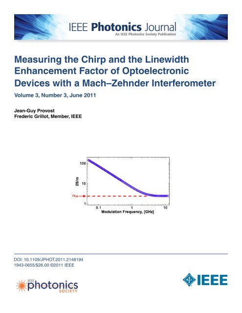
IEEE Photonics JournalChirp and Linewidth Enhancement FactorMeasuring the Chirp and the LinewidthEnhancement Factor of OptoelectronicDevices with a Mach–ZehnderInterferometerJean-Guy Provost 1 and Frederic Grillot, 2;3 Member, IEEE1 III-V Lab, a joint lab of Alcatel-Lucent Bell Labs France, Thales Research and Technology,and CEA Leti, 91460 Marcoussis, France2 Université Européenne de Bretagne, CNRS FOTON, Institut National des SciencesAppliquées, 35043 Rennes Cedex, France3 Institut TELECOM/Telecom Paristech, CNRS LTCI, 75634 Paris Cedex, FranceDOI: 10.1109/JPHOT.2011.21481941943-0655/$26.00 Ó2011 IEEEManuscript received April 20, 2011; accepted April 21, 2011. Date of publication April 29, 2011; dateof current version May 20, 2011. Corresponding author: J.-G. Provost (e-mail: jean-guy.provost@3-5lab.fr).Abstract: In this paper, a technique based on the use of a Mach–Zehnder (MZ) interferometeris proposed to evaluate chirp properties, as well as the linewidth enhancement factor( H -factor) of optoelectronic devices. When the device is modulated, this experimental setupallows the extraction of the component’s response of amplitude modulation (AM) and frequencymodulation (FM) that can be used to obtain the value of the H -factor. As comparedwith other techniques, the proposed method gives also the sign of the H -factor withoutrequiring any fitting parameters and, thus, is a reliable tool, which can be used for thecharacterization of high-speed properties of semiconductor diode lasers and electroabsorptionmodulators. A comparison with the widely accepted fiber transfer function method isalso performed with very good agreement.Index Terms: Chirp, electroabsorption modulators, linewidth enhancement factor, opticalmodulation, semiconductor lasers.1. IntroductionThe linewidth enhancement factor ( H -factor) is used to distinguish the behavior of semiconductorlasers (SLs) with respect to other types of lasers [1] and influences several fundamental aspects,such as the linewidth [1], [2], the chirp under modulation [3], the laser’s behavior under opticalfeedback [4], [5], as well as the occurrence of the filamentation in broad-area lasers [6]. The H -factor is usually defined as the coupling between the phase and the amplitude of the electric fieldsuch as [1] H ¼4 dn=dNdg=dN ¼4 dn=dNdG net =dNwhere is the lasing wavelength, N is the carrier density, g is the material gain, is the opticalconfinement factor, and G net ¼ g i is the net modal gain with i the internal loss coefficient. The H -factor depends on the ratio of the evolution of the refractive index n with the carrier density N tothat of the differential gain dg=dN. As reported in [7], several different techniques have beenproposed to measure the H -factor, with no rigorous comparison between the results achieved, as(1)Vol. 3, No. 3, June 2011 Page 476

IEEE Photonics JournalChirp and Linewidth Enhancement Factorrewritten such assðtÞs ðtÞ¼ P 02 mcos f mcos 2f m tFSRT 1 þT 22þ "P 0 sinf mcos 2f m tFSRT 1 þ T 22 þ ’ : (7)As shown in Fig. 1, the network analyzer giving two results associated with the A and B operatingpoints, respectively, the normalized measured signals can be expressed as follows:M ¼ P 02 m cos f mexpð j2f m ÞP 0 sin f mexp jð 2f m þ ’ Þ (8)FSRFSRwhere M þ is the result in A and M in B, respectively, while ¼ðT 1 þ T 2 Þ=2 is the transit time withinthe interferometer. On one hand, the first term in (8) only depends on the AM (i.e., -independent),while the term cosðf m =FSRÞ corresponds to the AM transfer function of the interferometer [33]. Onthe other hand, the second term in (8) is purely related to the modulation frequency (m independent)and can be expressed as a function of the interferometer FM transfer function, such asP 0 ðF =FSRÞsincðf m = FSRÞ with sincðxÞ ¼sinðxÞ=x.From (8), following expressions can be deduced:2m ¼ 1tan f M þm FSR’ ¼ arg M þ MM þ þ MMM þ þ M (9a): (9b)Using the definitions of parameters m and , (9a) allows extraction of the CPR [34], such asFP ¼ f m 12P 0 tan f M þ Mm M FSR þ þ M : (10)The value of the H -factor is then determined through the so-called relationship [21]sffiffiffiffiffiffiffiffiffiffiffiffiffiffiffiffiffiffiffiffiffiffiffi2m ¼ H 1 þ f 2c:f m(11)In (11), f c is defined as the corner frequency [35]f c ¼ 12 v @gg@P P (12)with v g the group velocity, P the output power, and @g=@P a nonzero parameter because of thephenomenon of nonlinear gain related to nonzero intraband relaxation times, as well as carrierheating. Parameter @g=@P can be expanded as a function of the gain compression factor " Pfollowing the relationship [36]:@g@P ¼ " Pg1 þ " P P : (13)For typical numbers, the corner frequency can be in the hundreds of Megahertz to the fewGigahertz range, depending on the output power level. On one hand, for modulation frequenciessuch as f m f c , which is the case in the experiment since the maximum modulation frequency f m isVol. 3, No. 3, June 2011 Page 480

IEEE Photonics JournalChirp and Linewidth Enhancement FactorFig. 2. Amplitude (solid line) and Phase (dotted line) of the CPR as a function of the modulationfrequency for the QW DFB laser under study.about in the 20-GHz range, the factor 2=m directly equals the laser’s H -factor. On the other hand,for lower modulation frequencies, the ratio 2=m becomes inversely proportional to the modulationfrequency. Let us note that the measurement of 2=m with frequency and at different output powerlevels could serve for the determination of the corner frequency and, consequently, the gaincompression factor.2.3. Theoretical Description of an External Modulator (AM and PM)In case of an external modulator the phase variation is given by [37]dðtÞdt¼ H21 dPðtÞPðtÞ dt(14)with ðtÞ the instantaneous phase of the optical signal and PðtÞ the related power. Under a smallsignal analysis condition, the optical power PðtÞ can be expressed such asPðtÞ ¼P 0 ð1 þ mcosð2f m tÞÞ: (15)Then, it can be shown that the signal at the output of the modulator can be written following therelationship:peðtÞ ¼ffiffiffiffiffiP 0 ð 1 þ mcosð2fm tÞÞ 1=2 expj 2f 0 t þ H2 mcosð2f mtÞ : (16)Based on a similar calculation as the one conducted in Section 2.2, the H -factor can be expressedas H ¼ 1 j1tan f mFSR3. Experimental Results and Discussion3.1. Case of a DFB LaserM þ MM þ þ M: (17)The device under study is a DFB laser having a high reflection (HR) coating on the rear facet andan antireflection (AR) coating on the front facet to allow for high efficiency. The device is 350 mlong with an active layer made with quantum wells nanostructures. The threshold current is about7.5 mA at room temperature (25 C). In Fig. 2, the ratio F =P in amplitude and in phase isdepicted for a DFB laser operating under direct modulation in the range from 10 kHz to 15 GHz. TheVol. 3, No. 3, June 2011 Page 481

IEEE Photonics JournalChirp and Linewidth Enhancement FactorFig. 3. 2=m as a function of the modulation frequency for the QW DFB laser under study.amplitude term of F =P is obtained through (10), considering a 5-mW optical output power (thisvalue is obtained for a DC bias current equal to 2.6 times the threshold current) for the laser understudy, while the FSR equals 47.6 GHz (see the Appendix). With regard to the phase term ofF =P, it is obtained from (9b). At low frequencies ðf m G 10 MHzÞ, thermal effects are predominant[3], [36]. When the modulation frequency decreases, the continuous wave regime getscloser, and the phase difference between the FM and AM responses tends to 180 [3], [36]. Suchbehavior is similar to the static operation case in which an increase in the laser’s emittingwavelength (a decrease in the laser’s optical frequency, respectively) is observed both with theinjected current and with the output power. When 10 MHz G f m G 2 GHz, thermal effects are nolonger significant, and the CPR is relatively constant. This regime corresponds to the adiabaticregime dominated by the gain compression effects and in which the AM and FM modulations are inphase[3], [36]. Then, for larger frequencies ðf m 9 2 GHzÞ, relaxation oscillations between thecarrier and photon numbers take place. The CPR gets proportional to f m and the FM and AMresponses are in quadrature with each other, leading to a 90 phase difference. In Fig. 3, themeasured 2=m ratio is plotted via (9a) starting from 50 MHz (beyond the thermal effects). Aspredicted by (11), the function 2=m tends asymptotically to the H -factor, which is estimated to beabout 2.4 for the laser under study.3.2. Case of an EAMIn Fig. 4, the EAM’s H -factor, as well as the corresponding phase, is evaluated through (17) for amonochromatic incident optical signal. On one hand, in Fig. 4(a), the H -factor is measured for a2.0 V reverse voltage. This figure shows that the phase term remains constant and equal to zeroso that the H -factor is positive (þ1.32 in that case). On the other hand, Fig. 4(b) shows that whenthe reverse voltage decreases down to 3.2 V, the phase term drops to 180 so that themeasured H -factor gets negative ( 1.20 in that case). Those results demonstrate that phasevariations can be used to obtain the sign of the H -factor.Let us note that for EAM-based devices, the H -factor remaining frequency-independent,measurements could be conducted at one frequency only, which is much quicker by comparisonwith the fiber transfer function method [24]. Indeed, to reach a good resolution on the minima oftransmission, the fiber transfer method typically requires a wider span up to 15 or 20 GHz, as wellas a lot of data points (400). Considering the same component as well as the same wavelength,Fig. 5 shows a comparison between the two methods as a function of the bias voltage. As it can beshown, a very good agreement is demonstrated; in particular, the bifurcation point from which the H -factor switches from positive to negative values occurs at 2.6 V for both methods. However,when the bias voltage equals 4 V, which corresponds to H 10, the discrepancy between thetwo methods starts increasing. This discrepancy is due to the lower experimental accuracy whichtypically arises when the H -factors gets larger ðj H j10Þ, as pointed out in [24] for the fibertransfer function method and in Section 3.4 (see below) for the method under study.Vol. 3, No. 3, June 2011 Page 482

IEEE Photonics JournalChirp and Linewidth Enhancement FactorFig. 4. Measured H -factor and phase as a function of the modulation frequency for the EAM.(a) V ¼ 2:0 V. (b) V ¼ 3:2 V.Fig. 5. Comparison of the H -factor measurements by the fiber method (blue line) and MZ method (redline) as a function of the reverse voltage for the EAM ðf m ¼ 10 GHzÞ.3.3. Case of an ILMTheoretically speaking, the chirp of an ILM should be similar to the one obtained for an isolatedmodulator, meaning that it should not be frequency-dependent, as already pointed out inSection 3.2. However, in an actual situation, a perturbation whose origin comes from an electricalor optical feedback is usually observed in the amplitude response [38], [39]. This unwantedfeedback leads to either a positive or a negative dip arising close to the relaxation frequency of thelaser section, as well as impacting the chirp behavior. Fig. 6(a) shows an example of the ILM’s H -factor measured for a bias current of 100 mA (for the laser section) and for a 1 V bias voltage(for the EAM section). As shown, a dip occurring close to 7.7 GHz and with a full bandwidth of 3 GHzis observed. Based on relative intensity noise (RIN) measurements, the laser’s relaxation frequencyis confirmed to occur at 7.7 GHz for the same bias current condition. In Fig. 6(a), the phase beingdisturbed in the dip area, the H -factor is estimated to be about þ0.17 outside this region. Such aVol. 3, No. 3, June 2011 Page 483

IEEE Photonics JournalChirp and Linewidth Enhancement FactorFig. 6. (a) Measured H -factor amplitude (solid line) and phase (squared line) as a function of themodulation frequency for the ILM. (b) Corresponding AM response.perturbation appears more pronounced on the chirp characteristic, as compared with the AMresponse on which this phenomenon could be less perceptible, as shown in Fig. 6(b).3.4. Evaluation of the H -Factor’s Experimental AccuracyThis section aims to evaluate the experimental accuracy related to the measurement of the H -factor (or to the 2=m ratio) in the case of f m ¼ 10 GHz. This last value is considered because itcorresponds to a realistic value used for the determination of the chirp parameter (see Section 3.1).Typically, the two main sources of uncertainties occurring in the determination of the H -factor arethose related to the accuracy of the FSR of the MZ interferometer, as well as to the linearity of theelectrooptics network analyzer. All other contributions can be neglected and have minor effects, ascompared with the overall accuracy. For instance, the electrical frequency modulation f m is knownwith an accuracy of 10 5 , while we can demonstrate that the locations around the points A and Bhave no effect, at the first order, on the signal measured by the network analyzer.• Accuracy on the FSRIn the Appendix, it is shown that the FSR is equal to 47.6 0.2 GHz.Consequently, for f m ¼ 10 GHz, accuracy of the term tanðf m =FSRÞ occurring in (9a) and (17)does not exceed 0.7%.• Nonlinearity of the electrooptics network analyzerFirst, let us note that in the case of the CPR and H -factor measurements, the networkanalyzer’s calibration is not required since the correction factor vanishes through the ratiojðM þ M Þ=ðM þ þ M Þj, which occurs in the set of (9a), (10), and (17). Consequently, only thenonlinear behavior of the network analyzer has to be taken into account for the estimation ofthe experimental accuracy. Thus, by using a referenced optical attenuator, the deviation of theanalyzer’s linearity at 10 GHz and, in the optical power operating range at the input of thephoto-detector, is found to be at most equal to 0.15 dB, which can lead to an error of 1.7% onthe ratio jM þ =M j. In Table 1, the experimental accuracy of the H -factor (or of the 2=m ratio)has been evaluated, taking into account both the nonlinearity of the analyzer, as well as theadditional contribution of the FSR. Calculations are done for different values of the H -factorVol. 3, No. 3, June 2011 Page 484

IEEE Photonics JournalChirp and Linewidth Enhancement FactorTABLE 1Experimental accuracy on the H -factor taking into account both the nonlinearity of the analyzer as wellthe additional contribution of the FSR. Calculations are done for different values of the H -factor and atf m ¼ 10 GHzand at f m ¼ 10 GHz. Let us note that regarding the CPR [see (10)], the output power precision(2% in the best case [40]) has to be included in the accuracy calculations.We also have to consider the assumption made in (7) J 1 2sin f mFSR sinf m:FSRFor instance, for m ¼ 10% and H ¼ 2, the calculated deviation is 0.2% for f m ¼ 10 GHz butincreases to 1.2% for H ¼ 5. However, let us stress that such a deviation remains negligible aslong as m 5%.4. ConclusionIn this paper, an optical discriminator based on a tunable MZ interferometer has been used toextract FM/AM ratio, as well as the H -factor for both laser diodes and EAM-based devices. Assuch a method allows the determination of both modulus and phase over a wide frequency span,more relevant information on the chirp can be extracted, as compared with the traditionaltechniques like the fiber transfer method, which only holds under the assumption that the chirp isnot frequency-dependent. In case of DFB lasers, the proposed method also allows evaluation of theadiabatic chirp and the thermal effects. With regard to the EAM, the experimental results have beenfound to be in a very good agreement with those obtained from the fiber transfer. As discussed, theproposed technique is also much quicker, as compared with the fiber transfer one and can also beused to evaluate the influence of the optical feedback on the EAM’s laser section. Finally, let usstress that the proposed experimental setup can also cover a wide range of operating wavelengthssince only the couplers and the optical fibers are wavelength-sensitive and can easily be convertedto a large-signal analysis configuration [31], leading to complementary results from those presentedin this paper. As compared with other techniques, this method based on a tunable MZinterferometer requires no fitting parameters and, thus, is a reliable tool, which can be used forthe characterization of high-speed properties of semiconductor diode lasers and EAMs.AppendixDetermination of the Optimum Value of the FSR of theMZ InterferometerRelationships obtained in Section 2 allow determination of the optimum value of the FSR. Indeed,the term tanðf m =FSRÞ occurring in (9a), (10), and (17) can be a source of uncertainty especiallyVol. 3, No. 3, June 2011 Page 485

IEEE Photonics JournalChirp and Linewidth Enhancement FactorFig. 7. Measurement of the transfer function of the MZ interferometer.when the modulation frequency gets closer to half of the FSR (see Section 3.4). In our case,measurements are conducted up to 20 GHz (corresponding to the network analyzer bandwidthlimit) so that the FSR of the interferometer has to be a bit greater than 40 GHz. As demonstrated inSection 2.2 for the laser case, the signals measured by the network analyzer can be expressed asfollows (8):M ¼ P 02 m cos f mexpðFSRFj2f m ÞP 0 sin f mexp jð 2f m þ ’Þ (A1)f m FSRin which the parameter has been replaced by its definition.To simplify (A1), let us consider the case FSR f m . In that case, the following approximationscan be made cosðf m =FSRÞ 1 and sinðf m =FSRÞ f m =FSR such that (A1) becomesM ¼ P 02 m expð j2f mÞP 0 FFSR exp jð 2f m þ ’Þ: (A2)When the FSR is too large, the second part of the right-hand side of (A2) becomes muchweaker compared with the first part. Consequently, this situation could enhance the sensitivity tonoise and to experimental evolution between measurements in M þ and M (small decouplingeffect, ...).As a conclusion, to overcome such a problem, a 50-GHz value was targeted at the time that theinterferometer was built. The interferometer transfer function is measured with a broadband opticalsource and an optical spectrum analyzer (OSA) to obtain the value of the FSR. In Fig. 7, theobtained value between the two vertical solid lines is equal to ¼ 3:818 nm (ten times the FSR).A result as accurate as 47.6 0.2 GHz is deduced for the FSR where 0.2 GHz takes into accountboth the accuracy of the OSA as well as the experimental resolution related to the position of theminima on the interferometer’s characteristic.AcknowledgmentThe authors would like to thank D. Leclerc, who proposed to work on this subject, and J.-L. Beylat,H. Bissessur, T. Ducelier, J. Jacquet, C. Kazmierski, C. Smith, and B. Thedrez for fruitful discussionsand encouragements.Vol. 3, No. 3, June 2011 Page 486

IEEE Photonics JournalChirp and Linewidth Enhancement FactorReferences[1] C. H. Henry, BTheory of the linewidth of semiconductor lasers,[ IEEE J. Quantum Electron., vol. QE-18, no. 2, pp. 259–264, Feb. 1982.[2] H. Su, L. Zhang, A. L. Gray, R. Wang, T. C. Newell, K. J. Malloy, and L. F. Lester, BLinewidth study of InAs-InGaAsquantum dot distributed feedback lasers,[ IEEE Photon. Technol. Lett., vol. 16, no. 10, pp. 2206–2208, Oct. 2004.[3] K. Petermann, Laser Diode Modulation and Noise. Norwell, MA: Kluwer, 1991.[4] D. M. Kane and K. A. Shore, Unlocking Dynamical Diversity. Hoboken, NJ: Wiley, 2005.[5] F. Grillot, N. A. Naderi, M. Pochet, C.-Y. Lin, and L. F. Lester, BVariation of the feedback sensitivity in a 1.55-m InAs/InP quantum-dash Fabry–Perot semiconductor laser,[ Appl. Phys. Lett., vol. 93, no. 19, p. 191 108, Nov. 2008.[6] J. Marciante and G. P. Agrawal, BNonlinear mechanisms of filamentation in broad-area semiconductor lasers,[ IEEE J.Quantum Electron., vol. 32, no. 4, pp. 590–596, Apr. 1996.[7] M. Osinski and J. Buus, BLinewidth broadening factor in semiconductor lasersVAn overview,[ IEEE J. QuantumElectron., vol. QE-23, no. 1, pp. 9–29, Jan. 1987.[8] G. Giuliani, S. Donati, A. Villafranca, J. Lasobras, I. Garces, M. Chacinski, R. Schatz, C. Kouloumentas, D. Klonidis,I. Tomkos, P. Landais, R. Escorihuela, J. Rorison, J. Pozo, A. Fiore, P. Moreno, M. Rossetti, W. Elsiisser, J. Von Staden,G. Huyet, M. Saarinen, M. Pessa, P. Leinonen, V. Vilokkinen, M. Sciamanna, J. Danckaert, K. Panajotov, T. Fordell,A. Lindberg, J.-F. Hayau, J. Poette, P. Besnard, F. Grillot, M. Pereira, R. Nelander, A. Wacker, A. Tredicucci, andR. Green, BRound-robin measurements of linewidth enhancement factor of semiconductor lasers in COST 288 action,[presented at the Conf. Lasers Electro-Optics (CLEO) Europe/Int. Quantum Electronics Conf. (IQEC), Munich, Germany,2007, Paper CB9-2-WED.[9] F. Grillot, B. Dagens, J. G. Provost, H. Su, and L. F. Lester, BGain compression and above threshold linewidthenhancement factor in 1.3-m InAs-GaAs quantum-dot lasers,[ IEEE J. Quantum Electron., vol. 44, no. 10, pp. 946–951, Oct. 2008.[10] B. W. Hakki and T. L. Paoli, BGain spectra in GaAs double-heterostructure injection laser,[ J. Appl. Phys., vol. 46, no. 3,pp. 1299–1306, Mar. 1975.[11] I. D. Henning and J. V. Collins, BMeasurements of the semiconductor laser linewidth broadening factor,[ Electron. Lett.,vol. 19, no. 22, pp. 927–929, Oct. 1983.[12] G. P. Agrawal, BEffect of gain and index nonlinearities on single-mode dynamics in semiconductor lasers,[ IEEE J.Quantum Electron., vol. 26, no. 11, pp. 1901–1909, Nov. 1990.[13] Z. Toffano, A. Destrez, C. Birocheau, and L. Hassine, BNew linewidth enhancement determination method insemiconductor lasers based on spectrum analysis above and below threshold,[ Electron. Lett., vol. 28, no. 1, pp. 9–11,Jan. 1992.[14] A. Villafranca, J. A. Lázaro, I. Salinas, and I. Garcés, BMeasurement of the linewidth enhancement factor in DFB lasersusing a high-resolution optical spectrum analyzer,[ IEEE Photon. Technol. Lett., vol. 17, no. 11, pp. 2268–2270,Nov. 2005.[15] A. Villafranca, A. Villafranca, G. Giuliani, and I. Garces, BMode-resolved measurements of the linewidth enhancementfactor of a Fabry–Perot laser,[ IEEE Photon. Technol. Lett., vol. 21, no. 17, pp. 1256–1258, Sep. 2009.[16] R. Hui, A. Mecozzi, A. D’Ottavi, and P. Spano, BNovel measurement technique of -factor in DFB semiconductor lasersby injection locking,[ Electron. Lett., vol. 26, no. 14, pp. 997–998, Jul. 1990.[17] G. Liu, X. Jin, and S. L. Chuang, BMeasurement of linewidth enhancement factor of semiconductor lasers using aninjection-locking technique,[ IEEE Photon. Technol. Lett., vol. 13, no. 5, pp. 430–432, May 2001.[18] Y. Yu, G. Giuliani, and S. Donati, BMeasurement of the linewidth enhancement factor of semiconductor lasers based onthe optical feedback self-mixing effect,[ IEEE Photon. Technol. Lett., vol. 16, no. 4, pp. 990–992, Apr. 2004.[19] C. Palavicini, G. Campuzano, B. Thedrez, Y. Jaouen, and P. Gallion, BAnalysis of optical-injected distributed feedbacklasers using complex optical low-coherence reflectometry,[ IEEE Photon. Technol. Lett., vol. 15, no. 12, pp. 1683–1685, Dec. 2003.[20] C. Harder, K. Vahala, and A. Yariv, BMeasurement of the linewidth enhancement factor of semiconductor lasers,[Appl. Phys. Lett., vol. 42, no. 4, pp. 328–330, Feb. 1983.[21] R. Schimpe, J. E. Bowers, and T. L. Koch, BCharacterization of frequency response of 1.5-m InGaAsP DFB laserdiode and InGaAs PIN photodiode by heterodyne measurement technique,[ Electron. Lett., vol. 22, no. 9, pp. 453–454,Apr. 1986.[22] U. Kruger and K. Kruger, BSimultaneous measurement of the linewidth enhancement factor, and FM and AM responseof a semiconductor laser,[ J. Lightw. Technol., vol. 13, no. 4, pp. 592–597, Apr. 1995.[23] T. Zhang, N. H. Zhu, B. H. Zhang, and X. Zhang, BMeasurement of chirp parameter and modulation index of a semiconductorlaser based on optical spectrum analysis,[ IEEE Photon. Technol. Lett., vol. 19, no. 4, pp. 227–229, Feb. 2007.[24] F. Devaux, Y. Sorel, and J. F. Kerdiles, BSimple measurement of fiber dispersion and of chirp parameter of intensitymodulated light emitter,[ J. Lightw. Technol., vol. 11, no. 12, pp. 1937–1940, Dec. 1993.[25] A. Royset, L. Bjerkan, D. Myhre, and L. Hafskjaer, BUse of dispersive optical fibre for characterisation of chirp insemiconductor lasers,[ Electron. Lett., vol. 30, no. 9, pp. 710–712, Apr. 1994.[26] R. C. Srinivasan and J. C. Cartledge, BOn using fiber transfer functions to characterize laser chirp and fiber dispersion,[IEEE Photon. Technol. Lett., vol. 7, no. 11, pp. 1327–1329, Nov. 1995.[27] H. Olesen and G. Jacobsen, BPhase delay between intensity and frequency modulation of a semiconductor laser(including a new measurement method),[ in Proc. ECOC, 1982, pp. 291–295, Paper BIV-4.[28] D. Welford and S. B. Alexander, BMagnitude and phase characteristics of frequency modulation in directly modulatedGaAlAs semiconductor diode lasers,[ J. Lightw. Technol., vol. LT-3, no. 5, pp. 1092–1099, Oct. 1985.[29] E. Goobar, L. Gillner, R. Schatz, B. Broberg, S. Nilsson, and T. Tanbun-ek, BMeasurement of a VPE-transported DFBlaser with blue-shifted frequency modulation response from DC to 2 GHz,[ Electron. Lett., vol. 24, no. 12, pp. 746–747,Jun. 1988.Vol. 3, No. 3, June 2011 Page 487

IEEE Photonics JournalChirp and Linewidth Enhancement Factor[30] R. S. Vodhanel and S. Tsuji, B12 GHz FM bandwidth for a 1530 nm DFB laser,[ Electron. Lett., vol. 24, no. 22,pp. 1359–1361, Oct. 1988.[31] R. A. Saunders, J. P. King, and I. Hardcastle, BWideband chirp measurement technique for high bit rate sources,[Electron. Lett., vol. 30, no. 16, pp. 1336–1338, Aug. 1994.[32] R. Brenot, M. D. Manzanedo, J.-G. Provost, O. Legouezigou, F. Pommereau, F. Poingt, L. Legouezigou, E. Derouin,O. Drisse, B. Rousseau, F. Martin, F. Lelarge, and G. H. Duan, BChirp reduction in quantum dot-like semiconductoroptical amplifiers,[ presented at the Eur. Conf. Exh. Opt. Commun., Berlin, Germany, 2007, Paper we.08.6.6.[33] W. V. Sorin, K. W. Chang, G. A. Conrad, and P. R. Hernday, BFrequency domain analysis of an optical FMdiscriminator,[ J. Lightw. Technol., vol. 10, no. 6, pp. 787–793, Jun. 1992.[34] T. L. Koch and J. E. Bowers, BNature of wavelength chirping in directly modulated semiconductor lasers,[ Electron. Lett.,vol. 20, no. 25, pp. 1038–1040, Dec. 1984.[35] L. Olofsson and T. G. Brown, BFrequency dependence of the chirp factor in 1.55 m distributed feedback semiconductorlasers,[ IEEE Photon. Technol. Lett., vol. 4, no. 7, pp. 688–691, Jul. 1992.[36] L. A. Coldren and S. W. Corzine, Diode Lasers and Photonic Integrated Circuits. Hoboken, NJ: Wiley, 1995.[37] F. Koyama and K. Iga, BFrequency chirping in external modulators,[ J. Lightw. Technol., vol. 6, no. 1, pp. 87–93,Jan. 1988.[38] P. Brosson and H. Bissessur, BAnalytical expressions for the FM and AM responses of an integrated laser-modulator,[IEEE J. Sel. Topics Quantum Electron., vol. 2, no. 2, pp. 336–340, Jun. 1996.[39] N. H. Zhu, G. H. Hou, H. P. Huang, G. Z. Xu, T. Zhang, Y. Liu, H. L. Zhu, L. J. Zhao, and W. Wang, BElectrical andoptical coupling in an electroabsorption modulator integrated with a DFB laser,[ IEEE J. Quantum Electron., vol. 43,no. 7, pp. 535–544, Jul. 2007.[40] D. Derickson, Fiber Optic Test and Measurement. Englewood Cliffs, NJ: Prentice-Hall, 1998.Vol. 3, No. 3, June 2011 Page 488