Probability density function for frequency response function - Vrije ...

2where Uk () and Yk () are the input/output Discrete Fourier transform (DFT) spectra ofthe input/output samples u( nT s ) and ynT ( s ), n = 01… , , , N – 1 , with T s the samplingperiod. The measured input/output DFT spectra U(), k Yk () are related to the truevalues U 0 (), k Y 0 () k byYk () = Y 0 () k + N Y () kUk () = U 0 () k + N U () k(2)with Y 0 () k = G 0 ( jω k )U 0 () k and N U (), k N Y () k the disturbing input/output errors. Notethat the input/output errors in (2) may be correlated due to generator noise, and/orprocess noise in feedback, and/or common disturbances picked up by both acquisitionchannels of the measurement device [3].In [3] the expected value of the FRF estimate (1) has been calculated for the generalcase of correlated input/output errors N U (), k N Y (). k It has also been shown in [3] thatthe variance of (1) is infinitely large, but that it is still possible to construct confidenceregions with a given confidence level for Ĝ( jω k ). These confidence regions are validonly if the input signal-to-noise (SNR) ratio is larger than or equal to 20 dB . Note thatinput SNRs lower than 20 dB are typically encountered at the resonance frequency oflightly damped vibrating mechanical structures. The main contribution of this paper isto calculate exact confidence regions for Ĝ( jω k ) which are valid FOR ANY input SNR.These confidence bounds are calculated via an analytic expression of the probabilitydensity function (pdf) of Ĝ( jω k ). Using the pdf of Ĝ( jω k ) it is also possible to verifyfor which input SNR the FRF Ĝ( jω k ) is circular complex normally distributed.Summarized, the contributions of the paper are: (i) calculation of the exact pdf of (1);(ii) calculation of confidence regions for (1) for any input/output SNR; (iii) verificationfor which input SNR (1) is circular complex normally distributed; (iv) illustration of thetheory on a real measurement example. Note that the results are valid for open- andclosed-loop FRF measurements.II. PROBABILITY DENSITY FUNCTION FRF ESTIMATEA. Main resultThe probability density function (pdf) of the FRF estimate (1) is calculated, assumingthat the input/output errors N Z () k = [ N Y () k N U () k ] T of the DFT spectra (2) are zeromean, jointly correlated, circular complex normally distributed random variables (tosimplify the notations the frequency index k is dropped)

5normally distributed (the equi-pdf lines are not ellipses with centre E{ Ĝ} ), while forSNR U = 40 dB (7) seems to be indistinguishable from a circular complex normaldistribution (the equi-pdf lines are circles with centre E{ Ĝ} ). To quantify moreprecisely how close (7) matches a circular complex normal pdf, (7) is approximated inleast squares sense byin a disc with centre E{ z} and radius rf n () z = exp( – z – µ 2 0 ⁄ σ20 ) ⁄ ( πσ20 )(14)E{ z} = 1–exp( – 1 ⁄ σ2u )( 1 – ρσ y ⁄ σ u )r = σ 1 – ln( 1 – p)(15)σ2 1 = σ2 y + σ2 u – 2σ u σ y Re( ρ)(see [3] for the calculation of E{ z} ). The value of p ∈ [ 01 , ] corresponds to the p %confidence level of the disc with centre E{ z} and radius r for the pdfexp( – z – E{ z} 2 ⁄ σ21 ) ⁄ ( πσ21 )(16)Since f z () z converges for σ u → 0 to (16) (see [3]), E{ z} and σ2 1 are used as startingvalues for µ 0 and σ 02 in the nonlinear minimization problem. The approximation errorfor the bottom left pdf of Figure 2 is shown in Figure 3. Table 1 gives the upper boundon the approximation error as a function of the input SNR, SNR U , and the radius of thedisc r (the results are valid for any σ y and ρ ). Taking into account (i) the dynamicrange of the pdf (16) for the different radii r (see Table 1), and (ii) the fact that theworst case approximation error occurs at the border of the disc (see Figure 3), it followsfrom Table 1 that in the neighborhood of the expected value E{ z} , (7) can beapproximated very well by a circular complex normal distribution (14) forSNR U≥ 40 dB .D. Circular complex approximationA random variable is circular complex distributed ifE{ ( z –E{ z} ) 2 } = 0 and E{ z – E{ z} 2 } < ∞(17)The difficulty here is that the second order moments of z (6) do not exist. Therefore, asis done in practise when calculating the sample variance of FRF measurements [7], theoutliers in z (6) are removed. Outliers are, for example, those values of z such thatz – E{ z} > r with Prob( z – E{ z} ≤ r) = 0.9999 (see Appendix D for the calculation ofr ). The second order moments of the truncated variable z (= z without outliers) exist,and the ratio

6γσ ( y , σ u , ρ)E{ ( z –E{ z} ) 2 }= -----------------------------------E{ z – E{ z} 2 =}∫( z –E{ z} ) 2 f z () z dzz– E{ z} ≤ r-----------------------------------------------------------------------z – E{ z} 2 , (18)∫f z () z dzz – E{ z} ≤ ris then a measure of how well z is circular complex distributed. Note that E{ z} in (18)can be approximated very well by E{ z} (15). Numerical calculation of (18) over adense grid of ρ - and σ y -values, with ρ ≤ 1 and σ y ≥ 1 , shows that the ratioγσ ( y , σ u , ρ) is maximal for ρ = – 1 , and that the maximal value γ max is independent ofσ y . Note that the fact that γ is maximal for ρ = – 1 is consistent with the observationthat the pdf (7) has the largest asymmetry for ρ = – 1 (see Figure 2). Figure 4 showsγ max as a function of the input signal-to-noise ratio. It follows that the truncatedvariable z can be approximated very well by a circular complex distributed randomvariable for SNR U≥ 20 dB .Via a perturbation analysis of (4)III. CONFIDENCE REGIONS OF THE FRF ESTIMATEĜ( jω k ) ≈ G 0 ()1 k ( + yk ()–uk ())(19)circular p % confidence regions with center E{ Ĝ} and radius R = r G 0 wereconstructed in [3]Prob( Ĝ – E{ Ĝ} ≤ R) = Prob( z – E{ z} ≤ r) = p(20)with E{ z} and r defined in (15), and where the probability Prob( ) is calculated using(16). Eq. (20) is accurate only if the input SNR is larger than 20 dB (see [3]). The exactconfidence level of the circular confidence region Ĝ – E{ Ĝ} ≤ R is calculated throughnumerical integration of2π rProb( z – E{ z} ≤ r) =∫ ∫f z ( E{ z} + r 1 e jθ )r 1 dr 1 dθ(21)0 0with f z () z defined in (7). Figure 5 compares the calculated confidence level (21) to the5one obtained from 5×10 FRF estimates Ĝ( jω k ) (1). It follows that both coincide.Note that (20) and (21) define an equation of the formgr () = p(22)where gr () is a monotonic increasing function of r . Hence, (22) has exactly onesolution r = g – 1 () p , which can be calculated using an iterative root finding algorithm(see Appendix D). Solving (22) for r allows to draw uncertainty bounds with a givenconfidence level for FRF measurements Ĝ . Figure 6 compares the true value of r(solution (22)) with the value (15) predicted by the Gaussian approximation (16), forthree different values of the confidence level p . For large input SNRs (SNR U≥ 20 dB )

7both radii coincide for any p . For small input SNRs and p = 0.95 the true solution islarger than the Gaussian approximation (15), while the reverse is true for p = 0.50 .These observations are consistent with the results of Figure 5: for p = 0.95 the truefraction outside the p % confidence region is larger than that predicted by the Gaussianapproximation, while the converse is true for p = 0.50 . Note also that the differencebetween the true solution and the Gaussian approximation becomes very large forconfidence levels close to one. This is explained by the fact that the Gaussianapproximation (16) decreases exponentially while (7) decreases as 1 ⁄ z 4 for zsufficiently large.IV. MEASUREMENT EXAMPLEAn iron beam (length 39.4 cm, width 2.4 cm, thickness 0.4 cm, and weight 354 g) isexcited in its point of gravity by a mini shaker (B&K 4810). The force applied to thebeam and the acceleration of the beam are measured with an impedance head (B&K8001). The force and acceleration signals of the impedance head are amplified (chargeamplifier B&K 2635) and buffered (buffers with a 50 Ω output impedance) before beingapplied to the acquisition unit (HP E1437A). An arbitrary waveform generator (HPE1445A) creates the excitation current of the mini shaker.The beam is excited with a multisine consisting of F = 556 frequencies equallydistributed in the band [ 1.2 kHz,2.6 kHz] . The multisine has a random phase spectrum(uniformly distributed in [0, 2π)) and a flat amplitude spectrum (the RMS value of themeasured acceleration is 36.6 mV). Four hundred consecutive periods of the steadystate response are measured at the sampling frequency f s = 20 MHz ⁄ 2 11 , which gives400 × 4096 data points per measured signal. From the M = 400 sets of F input/outputFourier coefficients, U[ m ]k , Y [ m]k with m = 12… , , , M and k = 12… , , , F , one cancalculate the force over acceleration frequency response function (see Figure 7)Ĝ( jω k )1Ŷ k M---- MY [ m ]∑m = 1 k = ----- = ------------------------------------ , (23)Û1 kM---- MU [ m ]∑m = 1 kthe input/output SNRs corresponding to one measured period (see Figure 8.a and 8.b),and the correlation coefficient (see Figure 8.c)SNR U () kÛ= ------------- k, SNRσˆ U () k Y () kŶ= ------------ k, ρσˆ Y () kσˆ 2YU () k=σˆ --------------------------exp (–Y ()σˆ k U () kj ∠ Ĝ ( jω ))(24)kwith σˆ (), k σˆ () k and σˆ 2 U2 Y2 YU () k the sample (co-)variances

8σˆ () k U2σˆ () k Y2σˆ 2YU () k1M ------------- M– 1U [ m ] 2= ∑ – Û k km = 11M ------------- M– 1Y [ m ] 2= ∑ – Ŷ k km = 11 M= ------------- ( Y[ m] M – 1k – Ŷ k ) U[ m] ∑( k – Û k )m = 1(25)Note that the input and output SNRs are minimal at, respectively, the resonance (1.7kHz) and anti-resonance (2.1 kHz) frequency of the FRF, and that the input/outputdisturbances are highly correlated around 1.95 kHz (see Figure 8.c).From the M = 400 sets of F = 556 FRF residualsG [ m]( jω k )1M---- M– ∑ G[ m]( jω k ) with G [ m]( jωm = 1k ) = Y [ m ] U [ m ]k ⁄(26)kone can calculate any p % percentile. It allows to verify experimentally the exact p %confidence bound (22). Since the difference between the exact (22) and the Gaussian(15) confidence bounds is apparent for low input SNRs (see Figure 5) and largeconfidence levels (see Figure 6) only, the p = 99% confidence bounds are comparedin the neighborhood of the resonance frequency of the FRF. The results are shown inFigure 9.a. It follows that the p = 99% percentile of the FRF residuals (26) and theexact p = 99% confidence bound coincide, while a significant difference with theGaussian approximation can be observed for low input SNRs (SNR U < 10 dB ). Thefraction of the residuals (26) outside the exact and the Gaussian p = 99% confidencebounds is shown in Figure 9.b. Note the good fraction prediction of the exact bound(mean value fraction = 0.997%) and the large deviation of the Gaussian approximation(mean fraction = 3.98%).V. CONCLUSIONBased on an analytic expression for the pdf of FRF measurements, exact uncertaintybounds for FRF measurements have been derived. For input SNRs larger than 40 dB thepdf can be approximated very well by a circular complex normal pdf. For input SNRslarger than 20 dB the uncertainty bounds (fraction, uncertainty levels, …) of the FRFand the second order moments of the truncated FRF (= FRF without outliers) arepredicted very well by the Gaussian approximation (16). The obtained results wereverified using real world measurements.APPENDIX APROOF OF THE THEOREMThe calculation the pdf of z = ( 1 + y) ⁄ ( 1 + u)(6), is facilitated by introducing anauxiliary variable v = u (see [5], Chapter 7). The joint pdf f zv ( zv , ) of z and v is

9related to the joint pdf f yu ( yu , ) of y and u byf zv ( zv , ) = f yu ( z( 1 + v) – 1,v) J(27)with J the determinant of the Jacobian of the transformation from( Re()Im z , ()Re z , ()Im v , () v ) to ( Re()Im y , ()Re y , ()Im u , () u ) (see [5]). Using∂y⁄ ∂Re()z = 1 + v , ∂y⁄ ∂Im()z = j( 1 + v), ∂y⁄ ∂Re()v = z , ∂y⁄ ∂Im()v = jz ,Re( j( 1 + v)) = – Im( 1 + v), and Im( j( 1 + v)) = Re( 1 + v), we findJ= ∂( ---------------------------------------------------------------------- Re()Im y , ()Re y , ()Im u , () u ) =∂( Re()Im z , ()Re z , ()Im v , () v )1 + v 2(28)The pdf of z is found by integrating the joint pdf f zv ( zv , ) (27) over v+∞ +∞f z () z = f zv ( zv , ) 1 + v 2 dRe()v dIm()v(29)∫∫–∞ –∞Since y = N Y ⁄ Y 0 and u = N U ⁄ U 0 are by assumption (3) circular complex normallydistributed, we havewheref yu ( z( 1 + v) – 1,v)HC 1– z( 1 + v) – 1 – z( 1 + v)– 11vv= ---------------------eπ 2 (30)det( C)Cσ 2y σ2= yu(31)σ 2 yu σ2uCollecting (27) to (31) gives, after some calculations,f z () zσ2+∞ +∞= ------------------e v – z – 1 2 ⁄ az () fπdet( C)∫ ∫ v ()1 v + v 2 dRe()v dIm()v(32)–∞ –∞where f v () v is the pdf of a circular complex normally distributed random variable vwith mean µ v and variance σ2vf v () v1 –---------e v – µ v2 ⁄ σ2bz ()= v , µπσ2v = -------- , σ2 det( C)az () v = --------------(33)az ()vand where a(), z b() z are defined in (8). Note that the double integral in (32) is nothingelse than E{ 1 + v 2 } . Collecting E{ 1 + v 2 } = σ2 v + µ v + 1 2 , (32), and (33) gives (7).Let yAPPENDIX BPROOF OF EQ. (9)= ax with y , x complex random variables and a a complex number. The pdf

10f y () yof y is related to the pdf f x () x of x by f y () y = f x ( y⁄a) J with J thedeterminant of the Jacobian of the transformation from ( Re()Im y , () y ) to ( Re()Im x , () x )(see [5]). Using∂xIm( j⁄a) = Re( 1 ⁄ a)we find⁄ ∂Re()y = 1 ⁄ a , ∂x⁄ ∂Im()y = j⁄a , Re( j⁄a) = – Im( 1 ⁄ a), andwhich concludes the proof.J∂Re()x ∂Re()x--------------- --------------- Re( 1 ∂Re()y ∂Im()y ā - ) Re( j ā - )= =∂Im()x ∂Im()x--------------- --------------- Im( 1 ∂Re()y ∂Im()y ā - ) Im( j =ā - )1-------a 2(34)APPENDIX CPROOF OF EQ. (13)For the closed-loop measurement set up shown in Figure 1, (2) becomesRGU 0 = ---------------------- Y 0 RN1 + G 0 C 0 = ---------------------- N P C 0N, ,0 1 + G 0 C U = –---------------------- , N P0 1 + G 0 C Y = ---------------------- (35)0 1 + G 0 C 0Hence, u = – N P C 0 ⁄ R , y = N P ⁄ ( G 0 R), andσσ22 P C 20 σ2u = -------------------R 2 σ2P Cy = ----------------G 0 R 2 ρ -------- G 0 0, , = – ---------(36)C 0 G 0Collecting (9), (12), (36) andgives (13).2σ 2= var( Y⁄R)=Ĝ – G----------------------------------------------------- 0=( 1 + ĜC 0 )( 1 + G 0 C 0 )σ2-------------------------------------- PR 2 1 + G 0 C 20Ĝ G-------------------- – ---------------------- 01 + ĜC1 + G 0 C 00(37)APPENDIX DROOT FINDING ALGORITHM FOR (22)The i th step of the iterative Newton-Raphson root finding algorithm for (22) isr ( i + 1)= r () i – ( gr ( () i )–p) ⁄ g' ( r () i )(38)with g' () r the derivative of g() r w.r.t. r (see [8]). The Gaussian approximation (15) istaken as starting value, r ( 0)= σ 1 – ln( 1 – p), and the functions g(), r g' (), r2π rgr () f z ( E{ z} + r 1 e jθ2π=∫ ∫)r 1 dr 1 dθ, g' () r = r f z ( E{ z} + re jθ ) dθ0 0∫(39)0with f z () z and E{ z} defined in (7) and (15) respectively, are calculated via numerical

11integration (see, for example, [8]).REFERENCES[1] K. Godfrey (ed.), Perturbation Signals for System Identification, Prentice Hall,Hempstead (UK), 1993.[2] R. Pintelon and J. Schoukens, System Identification: A Frequency Domain Approach,IEEE Press, Piscataway (USA), 2001.[3] R. Pintelon and J. Schoukens, “Measurement of frequency response functions usingperiodic excitations, corrupted by correlated input/output errors,” IEEE Trans.Instrum. Meas., vol. 50, no. 6, pp. ?-?, 2001.[4] D. R. Brillinger, Time Series: Data Analysis and Theory, McGraw-Hill, New York,1981.[5] A. Papoulis, Probability, Random Variables, and Stochastic Processes. McGraw-Hill,New York, 1981.[6] W. P. Heath, “Probability density function of indirect non-parametric transferfunction estimates for plants in closed loop,” Preprints of the 12th IFAC Symposiumon System Identification, Santa Barbara (USA), June 21-23, 2000.[7] Guillaume P., I. Kollar and R. Pintelon (1996). Statistical analysis of nonparametrictransfer function estimates, IEEE Trans. Instrum. Meas., vol. IM-45, no. 2, pp. 594-600.[8] A. Ralston and P. Rabinowitz, A First Course in Numerical Analysis, McGraw-Hill,New York (USA), 1984.

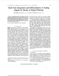
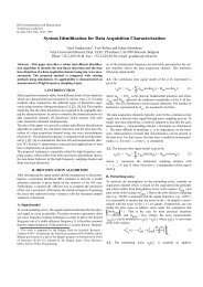
12Figure and Table captionsFigure 1: Frequency response function (FRF) measurement in closed-loop. G 0 and C 0are the true device under test and controller FRFs respectively, R is the referencesignal, N P is the process noise, and the input U and noisy output Y are observedwithout measurement errors.Figure 2: Probability density function (pdf) of z = ( 1 + y) ⁄ ( 1 + u)(eq. (7)) in decibelsfor σ y = 1 (SNR Y = 0 dB ) and ρ = – 1 . Top figures: σ u = 0.4 (SNR U = 8 dB ),bottom figures: σ u = 0.01 (SNR U = 40 dB ), left figures: pdfs, right figures: equi-pdflines (contour plot pdfs). The ‘+’ symbol in the contour plots indicates the expectedvalue of z .Figure 3: Difference between the true pdf f z () z (7) in dB and the Gaussianapproximation f n () z (14) in dB for σ y = 1 (SNR Y = 0 dB ), ρ = – 1 , and σ u = 0.01(SNR U = 40 dB ). The true pdf is shown in Figure 2 (bottom left figure).Figure 4: Maximum over σ y and ρ of the ratio γ( σ y , σ u , ρ) (18) as a function of theinput signal-to-noise ratio SNR U = 1 ⁄ σ u .Figure 5: Fraction of Ĝ outside the confidence region Ĝ – E{ Ĝ} ≤ rG 0 with radius r(15) and σ y = 1 as a function of the input signal-to-noise ratio SNR U : p = 50% (1),p = 60% (2), p = 70% (3), p = 80% (4), p = 90% (5), and p = 95% (6). Solid5lines: fractions calculated via eq. (21), symbols +: fractions calculated using 5×10 FRFestimates Ĝ (eq. (1)). (a) ρ = – 1 , (b) ρ = 0 , and (c) ρ = 0.5exp( jπ ⁄ 8).Figure 6: Radius r of the circular confidence region for z (6) as a function of the inputsignal-to-noise ratio SNR U , with σ y = 1 , and p = 50% (I), p = 95% (II) andp = 99% (III). Solid line: true value of r (solution of (22)); and dashed line: value of r(15) predicted by the Gaussian approximation (16). (a) ρ = – 1 , (b) ρ = 0 , and (c)ρ = 0.5exp( jπ ⁄ 8).Figure 7: Magnitude (a) and phase (b) of the FRF (force/acceleration) of the iron beam.Figure 8: Uncertainty of the FRF measurement. (a) input SNR, (b) output SNR, and (c)magnitude of the correlation coefficient.Figure 9: Analysis of the FRF residuals (26) in the neighborhood of the resonancefrequency. (a) Comparison of the p = 99% percentile (+) of the residuals, with theexact (black line) and the Gaussian (gray line) p = 99% uncertainty bounds. (b)Fraction of the residuals outside the exact (black line) and the Gaussian (gray line)p = 99% confidence bound.Table 1: Upper bound on the difference between f z () z (7) in dB and f n () z (14) in dB

13as a function of the input signal-to-noise ratio SNR U and the radius r (15). The 4 radiicorrespond to a dynamic range of the pdf (16) of 78 dB, 26 dB, 9.9 dB, and 6 dBrespectively. The corresponding p % confidence level is that of the normal pdf (16).

14Figure 1: Frequency response function (FRF) measurement in closed-loop. G 0 and C 0are the true device under test and controller FRFs respectively, R is the referencesignal, N P is the process noise, and the input U and noisy output Y are observedwithout measurement errors.controllerC 0 ( jω)N PR+-Udeviceunder testG 0 ( jω)Y

15Figure 2: Probability density function (pdf) of z = ( 1 + y) ⁄ ( 1 + u)(eq. (7)) in decibelsfor σ y = 1 (SNR Y = 0 dB ) and ρ = – 1 . Top figures: σ u = 0.4 (SNR U = 8 dB ),bottom figures: σ u = 0.01 (SNR U = 40 dB ), left figures: pdfs, right figures: equi-pdflines (contour plot pdfs). The ‘+’ symbol in the contour plots indicates the expectedvalue of z .pdf z = (1+y)/(1+u)2SNR U=8 dB0-50-100-150-200-25020imag(z)-2-20real(z)24imag(z)1.510.50-0.5-1-1.5-2-1 0 1 2 3real(z)pdf z = (1+y)/(1+u)21.5SNR U = 40 dB0-20-40-60-80-10020imag(z)-2-20real(z)24imag(z)10.50-0.5-1-1.5-2-1 0 1 2 3real(z)

16Figure 3: Difference between the true pdf f z () z (7) in dB and the Gaussianapproximation f n () z (14) in dB for σ y = 1 (SNR Y = 0 dB ), ρ = – 1 , and σ u = 0.01(SNR U= 40 dB ). The true pdf is shown in Figure 2 (bottom left figure).pdf z = (1+y)/(1+u)db210-1-220imag(z)-2-20real(z)24

17Figure 4: Maximum over σ y and ρ of the ratio γ( σ y , σ u , ρ) (18) as a function of theinput signal-to-noise ratio SNR U= 1 ⁄ σ u .-20maximal ratio (dB)-30-40-50-60-700 5 10 15 20 25SNR U (dB)

18Figure 5: Fraction of Ĝ outside the confidence region Ĝ – E{ Ĝ} ≤ rG 0 with radius r(15) and σ y = 1 as a function of the input signal-to-noise ratio SNR U : p = 50% (1),p = 60% (2), p = 70% (3), p = 80% (4), p = 90% (5), and p = 95% (6). Solid5lines: fractions calculated via eq. (21), symbols +: fractions calculated using 5×10 FRFestimates Ĝ (eq. (1)). (a) ρ = – 1 , (b) ρ = 0 , and (c) ρ = 0.5exp( jπ ⁄ 8).fraction% outside p% conf. region fraction% outside p% conf. region fraction% outside p% conf. region50D D D D D D 50D DD D D D D D D 50D D D D DD(1)D(1)D D DDD(1)DD40D D D D D D D D 40 DD DDD D D D D D 40D D D D D D D(2)D(2)DD(2)D DD DD D30 D D DDD D D D D D 30D D D D D DDDDD 30D DD D D D D D D D(3) D D(3)D(3)DD DDD20D DDDDDDDDD DDD D DD D D20D D D 20D D D D D DD(4) D(4) DD(4)DDDDD DDD D DD DDDDD D10DDDD DD D D D D D10DD DDDD D D D D D10DDD D D DD D(5)DD D DD(5)DD DD DD(5)D D DD D D D D(6)(6)(6)0000 5 10 15 20 25 0 5 10 15 20 25 0 5 10 15 20 25SNR U (dB)SNR U (dB)SNR U (dB)(a) (b) (c)

19Figure 6: Radius r of the circular confidence region for z (6) as a function of the inputsignal-to-noise ratio SNR U , with σ y = 1 , and p = 50% (I), p = 95% (II) andp = 99% (III). Solid line: true value of r (solution of (22)); and dashed line: value of r(15) predicted by the Gaussian approximation (16). (a) ρ = – 1 , (b) ρ = 0 , and (c)ρ = 0.5exp( jπ ⁄ 8).12radius p% confidence region(III)12radius p% confidence region12radius p% confidence region8(II)8(III)8(III)44(II)4(II)(I)00 5 10 15 20 25SNR U (dB)(I)00 5 10 15 20 25SNR U (dB)(I)00 5 10 15 20 25SNR U (dB)(a) (b) (c)

20Figure 7: Magnitude (a) and phase (b) of the FRF (force/acceleration) of the iron beam.40200Amplitude (dB)200-20Phase (°)1000-100-401000 1500 2000 2500 3000f (Hz)(a)-2001000 1500 2000 2500 3000f (Hz)(b)

23Table 1: Upper bound on the difference between f z () z (7) in dB and f n () z (14) in dBas a function of the input signal-to-noise ratio SNR U and the radius r (15). The 4 radiicorrespond to a dynamic range of the pdf (16) of 78 dB, 26 dB, 9.9 dB, and 6 dBrespectively. The corresponding p % confidence level is that of the normal pdf (16).max f z () z – f n () zdB dBr(p %)3σ 1(99.988% )1.73σ 1(95% )1.07σ 1(68% )0.83σ 1(50% )20 dB 20 5 1 0.5SNR U (dB)40 dB 2 0.5 0.1 0.0560 dB 0.2 0.05 0.01 0.00580 dB 0.02 0.005 0.001 0.0005