Applications of Transmission Line Matrix Method For NDT

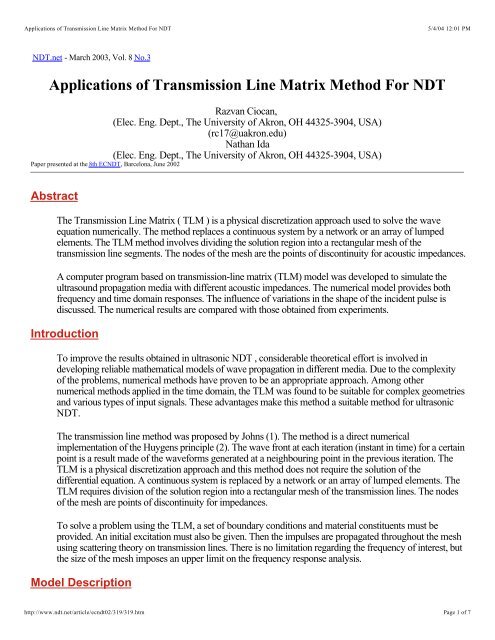
Applications of Transmission Line Matrix Method For NDT5/4/04 12:01 PMNDT.net - March 2003, Vol. 8 No.3Applications of Transmission Line Matrix Method For NDTPaper presented at the 8th ECNDT, Barcelona, June 2002Razvan Ciocan,(Elec. Eng. Dept., The University of Akron, OH 44325-3904, USA)(rc17@uakron.edu)Nathan Ida(Elec. Eng. Dept., The University of Akron, OH 44325-3904, USA)AbstractThe Transmission Line Matrix ( TLM ) is a physical discretization approach used to solve the waveequation numerically. The method replaces a continuous system by a network or an array of lumpedelements. The TLM method involves dividing the solution region into a rectangular mesh of thetransmission line segments. The nodes of the mesh are the points of discontinuity for acoustic impedances.A computer program based on transmission-line matrix (TLM) model was developed to simulate theultrasound propagation media with different acoustic impedances. The numerical model provides bothfrequency and time domain responses. The influence of variations in the shape of the incident pulse isdiscussed. The numerical results are compared with those obtained from experiments.IntroductionTo improve the results obtained in ultrasonic NDT , considerable theoretical effort is involved indeveloping reliable mathematical models of wave propagation in different media. Due to the complexityof the problems, numerical methods have proven to be an appropriate approach. Among othernumerical methods applied in the time domain, the TLM was found to be suitable for complex geometriesand various types of input signals. These advantages make this method a suitable method for ultrasonicNDT.The transmission line method was proposed by Johns (1). The method is a direct numericalimplementation of the Huygens principle (2). The wave front at each iteration (instant in time) for a certainpoint is a result made of the waveforms generated at a neighbouring point in the previous iteration. TheTLM is a physical discretization approach and this method does not require the solution of thedifferential equation. A continuous system is replaced by a network or an array of lumped elements. TheTLM requires division of the solution region into a rectangular mesh of the transmission lines. The nodesof the mesh are points of discontinuity for impedances.To solve a problem using the TLM, a set of boundary conditions and material constituents must beprovided. An initial excitation must also be given. Then the impulses are propagated throughout the meshusing scattering theory on transmission lines. There is no limitation regarding the frequency of interest, butthe size of the mesh imposes an upper limit on the frequency response analysis.Model Descriptionhttp://www.ndt.net/article/ecndt02/319/319.htmPage 1 of 7

Applications of Transmission Line Matrix Method For NDT5/4/04 12:01 PMTLM algorithmConsidering Kirchhoff’s laws for a shunt transmission the wave equation for the voltage can be written(3):(1)Assuming that the transmission line is lossless and nondispersive. The elements of the circuit (L and C)are chosen to model the propagation in a homogenous infinite space with acoustic impedance Z m:Bycombining the continuity equation and the equation of motion for a medium with a uniform density ρ andcompressibility κ , the acoustic wave equation written for pressure p has the form (4):(2)Equations (1) and (2) show that the following equivalencies can be enforced:The equivalencies between the current components ( I x, I y) and velocity components ( u xand u y) can bedetermined in the same way. Based on the equivalence between the wave equation written for acousticwaves and the wave equation for an ideal transmission line, the scattering matrix theory (SMT) is appliedto study the equivalent microwave network system as seen at its ports. The SMT determines the outputat all ports for a given input. In a general form this can be written as:(4)(3)where [ ] and [ ] are matrices of reflected and incident pulses, respectively. The scattering parametersS jiare determined by considering that a signal is injected at port “i” ( P i i 1 0 ) whereas at the rest of thep rp iports the signal is zero – they are match-terminated ( P i j= 0 for i1j). Since the system is equivalencedwith a microwave network, the scattering matrix elements become the voltage reflection and transmissioncoefficients, respectively. The voltage reflected at any port “s" at time ( k+1) ∆twill be (2):(5)The positive integer variable k is the number of iterations and represents the number of time steps ∆t thathave passed since the beginning of the computation.The presence of a medium l is modelled in two ways. The first method is modelled by modifying thereflection coefficients at the boundary between the two media. The second way to model the presence ofdifferent media in a TLM mesh is to modify the scattering matrix. The discontinuity in impedances thatexists at the interface between two media is modelled by incorporating an open circuit stub of length ∆l/2http://www.ndt.net/article/ecndt02/319/319.htmPage 2 of 7

Applications of Transmission Line Matrix Method For NDT5/4/04 12:01 PM(5). This implies introducing a supplementary leg that will match impedances of two different layers. Forthis case equation (5) becomes:(6)The pressure at node (i,j) at iteration k is found as:(7)Equation (7) shows that the method discussed above is equivalent to the finite difference time domain(FD-TD) method with respect to the final result, but the TLM does not require explicitly finding thesolution for the wave equation (2). The equivalence between admittances Y land Y oand mediacompressibilities κ mand κ ois expressed by(6):(8)Attenuation of the ultrasonic pulse in medium l is modelled by assuming that the losses are distributedcontinuously. Therefore the amplitude of the reflected wave is attenuated by the attenuation factor αalong the mesh lines. This was implemented in the TLM code using the relation:Wave propagation is modelled by the so called connection process. In this process, the reflected pulsefor a certain node at time (k+1) ∆tbecomes the incident pulse for neighbouring nodes at the same time(k+1) ∆t.ExcitationsEquations (6) - (9) describe the wave propagation at any coordinate (x,y) at any instant k∆t. To initiatethe process an input energy needs to be provided. This energy is called excitation. Due to the equivalencewith a microwave network the initial conditions of the problem are modelled by voltage sources that canbe placed at any node. A TLM structure can be excited at any location with practically any kind ofexcitation. The physical problem determines the locations and the type of excitation. It is possible for acontinuous waveform to be excited at appropriate input nodes. This excitation is implemented bykeeping, for all iterations, the voltages for input points at pre-set values. When the characteristics of astructure have to be investigated over a wide frequency range a single localised pulse is used. Initially,the voltage amplitudes at all nodes are set to zero except at the selected input point. An impulse is thenapplied there. The minimum time interval for a pulse is where v is the phase velocity in the mesh. Tominimise the effect of dispersion the minimum distance between the nodes, ∆l, is related to the smallestwavelength of interest by the following relationship (7):λ min(9)http://www.ndt.net/article/ecndt02/319/319.htmPage 3 of 7

Applications of Transmission Line Matrix Method For NDT5/4/04 12:01 PM(10)For the purpose of the present discussion a sinusoidal Gauss-modulated pulse is considered:(11)Frequency responseThe output impulse function at a particular point is obtained by summing the total node voltage at k for alliteration. Mathematically this is written as a sum over the total number of iterations Nit:(12)Similarly, the excitation function can be written as:(13)For example, for a sinusoidal excitation at frequency f, such as that given in equation (11), the coefficientsa(i,j) at iteration k are:(14)The frequency response, H ( j ω)= H ( j2πf), is obtained as the Fourier Transform of the time responsefunction given by equation. (14):(15)ResultsThe concepts of the TLM algorithm presented in previous section are demonstrated in figure 1. AGaussian pulse was launched in a 101 by 101 mesh modelling free space. The interaction of this wavewith a perfect reflecting square is shown for two iterations. The first iteration is when the wave fronttouches the square ( iteration 39). The second iteration was chosen when the wave front reaches theboundary of mesh ( iteration 60).http://www.ndt.net/article/ecndt02/319/319.htmPage 4 of 7

Applications of Transmission Line Matrix Method For NDT5/4/04 12:01 PMFig 1: The simulated waveforms for a Gaussian pulsepropagating in 101x 101 mesh, containning a perfectreflecting square. Two instances are shown: a) iteration39 ( when the waveform touches the corner placed inposition (70,70); b) iteration 60.The ultrasonic images for this work were obtained in two different experimental arrangements in thesame structure (8) : a data acquisition board with a high sampling rate : 80 MHz (128 MHz ) maximumamplitude of 400V and 9ns rise time; a mechanical system based on a computer controlled steppermotor allowing achievement of ± 0.05mm resolution.A multilayered structure made of two plastic sheets ( 0.5mm thickness) with a water gap between themwas investigated. The ultrasonic image of the structure is shown in figure 2. The same experiment wasreproduced numerically. A sinusoidal Gaussian pulse was injected in the TLM mesh according toequation (11). The parameters that were used to generate this pulse are: A= 400V; σ = 6.7; t o= 0.3µs;f =3.5MHz.Fig 2: The ultrasonic image of the water-plastic-water-plasticwaterstructure investigated.http://www.ndt.net/article/ecndt02/319/319.htmPage 5 of 7

Applications of Transmission Line Matrix Method For NDT5/4/04 12:01 PMThe comparaison between the numerically generated signal ( continue line) and the reflected pulse(dashed line) obtained from structure under investigation is shown in figure 3. As shown in figure 3 TLMmodel reproduced the real pulse all boundaries have been solved corectly.Fig 3: TLM reflected pulse from a multilayer structure: water-plasticwater-plastic-water.A metallic multilayer bearing containing a disbound was considered next. This structure is made of a steelbase and an antifriction layer ( 6 mm thickness) . The ultrasonic image was obtained in immersion usingand emitter-receiver transducer ( 5MHz). The TLM model consisted of a 1000 by 1000 mesh in whicha Gaussian pulse with the following parameters was used for excitation: A= 400V; σ = 7.7; t o= 0.2µs;f =5MHz. The sampling frequency for this simulation was 128 MHz. A comparison between thefrequency response obtained for the real case and TLM case is shown in figure 4. The main frequencycomponents have been correctly identified.http://www.ndt.net/article/ecndt02/319/319.htmPage 6 of 7

Applications of Transmission Line Matrix Method For NDT5/4/04 12:01 PMFig 4: Comaparison between frequency response obtained from experimentand the numerically generated response. The structure under investigationwas a metallic multilayer bearing containing a disbound.ConclusionA numerical model for ultrasonic wave propagation in layered media is proposed. The model is based onthe TLM algorithm. The model proposed was implemented in a FORTRAN program. The results shownin this paper demonstrate that the model can be applied to characterisation of the flaw in multilayeredstructure. Samples with different acoustic impedance profiles have been investigated. Comparisonbetween numerically generated signals and real ultrasonic signals validate the proposed model.References1. P. B. Johns, R. L. Beurle, “ Numerical solution of Two-Dimensional Scattering Problems Using aTransmission-Line Matrix”, Proc. IEEE, vol 118, pp. 1203-1209, 1971.2. Y. Kagawa, T. Tsuchiya, B. Fujii, and K. Fujioka, “ Discrete Huygens ‘ model approach to sound wavepropagation”, Journal of sound and vibration 218(3), pp. 419-444, 1998.3. N. Ida, Engineering Electromagnetics , Springer , pp.890-892, 2000.4. P.M. Morse, K.U. Ingard, Theoretical acoustics, McGraw-Hill, pp. 242-243, 1968.5. C. Christopoulos, The Transmission-Line Modeling Method, IEEE Press, 1995.6. A.H.M. Saleh, P. Blanchfield, “Analysis of acoustic radiation patterns of array transducers using theTLM Method” Int. Journ.Numer. Model. , . 3,pp. 39-56 1990.7. W.J.R. Hoefer, P.M. So, The electromagnetic wave simulator, John Wiley & Sons, pp. 87-99 1993.8. R. Ciocan, M. Soare, V. Revenco, “The quality evaluation of the end-plate welds and brazed joints forCANDU nuclear fuel by an ultrasonic imaging method”, Insight-Non-Destructive Testing and ConditionMonitoring, vol. 39. vol.39. no.9 pp. 622-625, 1997© NDT.net - info@ndt.net | Top|http://www.ndt.net/article/ecndt02/319/319.htmPage 7 of 7