Introduction to Molecular Dynamics with GROMACS

Introduction toMolecular Dynamicswith GROMACSMolecular Modeling Course 2007Simulation of Lysozyme in WaterErik Lindahl (lindahl@cbr.su.se)

SummaryMolecular simulation is a very powerful toolbox in modern molecular modeling, and enables us tofollow and understand structure and dynamics with extreme detail – literally on scales where motion ofindividual atoms can be tracked. This task will focus on the two most commonly used methods, namelyenergy minimization and molecular dynamics that respectively optimize structure and simulate thenatural motion of biological macromolecules. we are first going to set up your Gromacs environments,have a look at the structure, prepare the input files necessary for simulation, solvate the structure in water,minimize & equilibrate it, and finally perform a short production simulation. After this we’ll testsome simple analysis programs that are part of Gromacs.You should write a brief report about your work and describe your findings. In particular, try tothink about why you are using particular algorithms/choices, and whether there are alternatives.Molecular motions occur over a wide range of scales in both time and space, and the choice of approachto study them depends on the question asked. Molecular simulation is far from the only availablemethod, and when the aim e.g. is to predict the structure of a protein it is often more efficient touse bioinformatics instead of spending thousands or millions of CPU hours. Ideally, the timedependentSchrödinger equation should be able to predict all properties of any molecule with arbitraryprecision ab initio. However, as soon as more than a handful of particles are involved it is necessary tointroduce approximations. For most biomolecular systems we therefore choose to work with empiricalparameterizations of models instead, for instance classical Coulomb interactions between pointlikeatomic charges rather than a quantum description of the electrons. These models are not only orders ofmagnitude faster, but since they have been parameterized from experiments they also perform betterwhen it comes to reproducing observations on microsecond scale (Fig. 1), rather than extrapolatingquantum models 10 orders of magnitude. The first molecular dynamics simulation was performed aslate as 1957, although it was not until the 1970’s that it was possible to simulate water and biomolecules.Background & TheoryMacroscopic properties measured in an experiment are not direct observations, but averages over billionsof molecules representing a statistical mechanics ensemble. This has deep theoretical implicationsthat are covered in great detail in the literature, but even from a practical point of view there are importantconsequences: (i) It is not sufficient to work with individual structures, but systems have to be expandedto generate a representative ensemble of structures at the given experimental conditions, e.g.temperature and pressure. (ii) Thermodynamic equilibrium properties related to free energy, such asbinding constant, solubilities, and relative stability cannot be calculated directly from individual simulations,but require more elaborate techniques. (iii) For equilibrium properties (in contrast to kinetic) theaim is to examine structure ensembles, and not necessarily to reproduce individual atomic trajectories!The two most common ways to generate statistically faithful equilibrium ensembles are Monte Carloand Molecular Dynamics simulations. Monte Carlo simulations rely on designing intelligent moves togenerate new conformations, but since these are fairly difficult to invent most simulations tend to doclassical dynamics with Newton’s equations of motion since this also has the advantage of accuratelyreproducing kinetics of non-equilibrium properties such as diffusion or folding times. When a startingconfiguration is very far from equilibrium, large forces can cause the simulation to crash or distort thesystem, and for this reason it is usually necessary to start with an Energy Minimization of the systemprior to the molecular dynamics simulation. In addition, energy minimizations are commonly used torefine low-resolution experimental structures.All classical simulation methods rely on more or less empirical approximations called Force fields tocalculate interactions and evaluate the potential energy of the system as a function of point-like atomiccoordinates. A force field consists of both the set of equations used to calculate the potential energy andforces from particle coordinates, as well as a collection of parameters used in the equations.

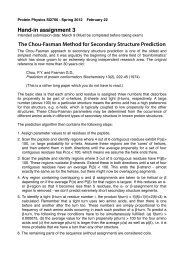
3. Install Gromacs from a package, or compileit the same way as FFTW.4 . I n s t a l l P y M o l f r o m t h e w e b s i t ehttp://www.pymol.org, or alternatively VMD.Initial input data:Interaction function V(r) - "force field"coordinates r, velocities v5. Install the 2D plotting program Grace/xmgrace. Depending on your platform youmight have to install the Lesstif (clone of Motif)libraries first (www.lesstif.org), and then getthe Grace program source code from the sitehttp://plasma-gate.weizmann.ac.il/Grace/.6. To create beautiful secondary structureanalysis plots, you can use the program “DSSP”from http://swift.cmbi.ru.nl/gv/dssp/. This isfreely available for academic use but requires alicense, so we will use the Gromacs built-in alternative“my_dssp” for this tutorial.If you are following this exercise as part of a labcourse, the installation might already have beendone for you.Compute potential V(r) andforces F i=iV(r) on atomsUpdate coordinates &velocities according toequations of motionCollect statistics and writeenergy/coordinates totrajectory filesMore steps?YesRepeat for millions of stepsThe PDB Structure - thinkbefore you simulate!The first thing you will need is a structure ofthe protein you want to simulate. Go to theProtein Data Bank at http://www.pdb.org, andDone!search for “Lysozyme”. You should get lots of hits, many of which were determined with bound ligands,mutations, etc. One possible alternative is the PDB entry 1LYD, but feel free to test some other alternativetoo.It is a VERY good idea to look carefully at the structure before you start any simulations. Is the resolutionhigh enough? Are there any missing residues? Are there any strange ligands? Check both the PDBweb page and the header in the actual file. Finally, try to open it in a viewer like PyMOL, VMD, orRasMol and see what it looks like. In PyMOL you have some menus on the right where you can show(“S”) e.g. cartoon representations of the backbone!Creating a Gromacs topology from the PDB fileWhen you believe you have a good starting structure the next step is to prepare it for simulation.What do we need to prepare? Well, for instance the choice of force fields, water model, charge states oftitratable residues, termini, add in the missing hydrogens, etc. You will fairly quickly realize that most ofthis stuff is static and independent of the protein coordinates, so it makes sense to put it in a separatefile called a “topology” for the system. The good news is that Gromacs can create topologies automaticallyfor you with the tool pdb2gmx.There are several places where you can find documentation for the Gromacs commands. You shouldalways get some help with “pdb2gmx -h”, which first includes a brief description of what the programNoFig. 3: Simplified flowchart of a standard moleculardynamics simulation, e.g. as implemented in Gromacs.

does, then a list of (optional) input/output files, and finally a list of available flags. The same informationis present with “man pdb2gmx” (if it was properly installed), and you can also use thewww.gromacs.org website: Choose “documentation” in the top menu, and then “manuals” in the leftsidemenu. There is both an extensive book describing everything and a shorter online reference to thecommands and file formats.For the first command we’ll help you. pdb2gmx should read its input from a coordinate file, and justfor fun we’ll pick a specific water model and force field. Typepdb2gmx -f 1LYD.pdb -water tip3pThe program will ask you for a force field - for this tutorial I suggest that you use “OPLS-AA/L”, andthen write out lots of information. The important thing to look for is if there were any errors or warnings(it will say at the end). Otherwise you are probably fine. Read the help text of pdb2gmx (-h) andtry to find out what the different files it just created do, and what options are available for pdb2gmx!The important output files are (find out yourself what they do)conf.gro topol.top posre.itpIf you issue the command several times, Gromacs will back up old files so their names start with ahash mark (#) - you can safely ignore (or erase) these for now.Adding solvent water around the proteinIf you started a simulation now it would be in vacuo. This was actually the norm 25-30 years ago,since it is much faster, but since we want this simulation to be accurate you are going to add solvent.However, before adding solvent we have to determine how big the simulation box should be, andwhat shape to use for it. There should be at least half a cutoff between the molecule and the box side,and preferably more. Due to the limited time you be cheap here and only use 0.5nm margin betweenthe protein and box. To further reduce the volume of the box you could explore the box type optionsand for instance test a “rhombic dodecahedron” box instead of a cubic one. The program you should useto alter the box is “editconf”. This time you will have to figure out the exact command(s) yourself,but the primary options to look at in the documentation are “–f”, “–d”, “–o”, and “–bt”.As an exercise, you could try a couple of different box sizes (the volume is written on the output!)and also other box shapes like “cubic” or “octahedron”. What effect does it have on the volume?The last step before the simulation is to add water in the box to solvate the protein. This is done byusing a small pre-equilibrated system of water coordinates that is repeated over the box, and overlappingwater molecules removed. The Lysozyme system will require roughly 6000 water molecules with 0.5nmto the box side, which increases the number of atoms significantly (from 2900 to over 20,000).GROMACS does not use a special pre-equilibrated system for TIP3P water since water coordinates canbe used with any model – the actual parameters are stored in the topology and force field. For this reasonthe program only provides pre-equilibrated coordinates for a small 216-water system using a watermodel called “SPC” (simple point charge). The best program to add solvent water is “genbox”, i.e.you will generate a box of solvent. You can select the SPC water coordinates to add with the flag “–csspc216.gro”, and for the rest of the choices you can use the documentation. Remember that yourtopology needs to be updated with the new water molecules! The easiest way to do that is to supply thetopology to the genbox command.Before you continue it is once more a good idea to look at this system in PyMOL. However, Py-MOL and most other programs cannot read the Gromacs gro file directly. There are two simple ways tocreate a PDB file for PyMOL:

1. Use the ability of all Gromacs programs to write output in alternative formats, e.g.:genbox –cp box.gro –cs spc216.gro –p topol.top –o solvated.pdb2. Use the Gromacs editconf program to convert it (use -h to get help on the options):editconf -f solvated.gro -o solvated.pdbIf you just use the commands like this, the resulting structure might look a bit strange, with water ina rectangular box even if the system is triclinic/octahedron/dodecahedron. This is actually fine, and dependson the algorithms used to add the water combined with periodic boundary conditions. However,to get a beautiful-looking unit cell you can try the commands (backslash means the entire commandshould be on a single line):trjconv -s solvated.gro -f solvated.gro -o solv_triclinic.pdb \-pbc inbox -ur trictrjconv -s solvated.gro -f solvated.gro -o solv_compact.pdb \-pbc inbox -ur compactWe’re not going to tell you what they do - play around and use the -h option to learn more :-)Running energy minimizationThe added hydrogens and broken hydrogen bond network in water would lead to quite large forcesand structure distortion if molecular dynamics was started immediately. To remove these forces it is necessaryto first run a short energy minimization. The aim is not to reach any local energy minimum, soe.g. 200 to 500 steps of steepest descent works very well as a stable rather than maximally efficient minimization.Nonbonded interactions and other settings are specified in a parameter file (em.mdp); it isonly necessary to specify parameters where we deviate from the default value, for example:------em.mdp------integrator = steepnsteps = 200nstlist = 10rlist = 1.0coulombtype = pmercoulomb = 1.0vdw-type = cut-offrvdw = 1.0nstenergy = 10------------------Comments on the parameters used:We choose a standard cut-off of 1.0 nm, both for the neighborlist generation and the coulomb andLennard-Jones interactions. nstlist=10 means it is updated at least every 10 steps, but for energy minimizationit will usually be every step. Energies and other statistical data are stored every 10 steps (nstenergy),and we have chosen the more expensive Particle-Mesh-Ewald summation for electrostatic interactions. Thetreatment of nonbonded interactions is frequently bordering to religion. One camp advocates standardcutoffs are fine, another swears by switched-off interactions, while the third wouldn’t even consider anythingbut PME. One argument in this context is that ‘true’ interactions should conserve energy, which isviolated by sharp cut-offs since the force is no longer the exact derivative of the potential. On the otherhand, just because an interaction conserves energy doesn’t mean it describes nature accurately. In practice,the difference is most pronounced for systems that are very small or with large charges, but the key lesson is

eally that it is a trade-off. PME is great, but also clearly slower than cut-offs. Longer cut-offs are alwaysbetter than short ones (but slower), and while switched interactions improve energy conservation they introduceartificially large forces. Using PME is the safe option, but if that’s not fast enough it is worth investigatingreaction-field or cut-off interactions. It is also a good idea to check and follow the recommendedsettings for the force field used.GROMACS uses a separate preprocessing program grompp to collect parameters, topology, andcoordinates into a single run input file (e.g. em.tpr) from which the simulation is then started (thismakes it easier to prepare a run on your workstation but run it on a separate supercomputer).As we just said, the command grompp prepares run input files. You will need to provide it withthe parameter file above, the topology, a set of coordinates, and give the run input file some name (otherwiseit will get the default topol.tpr name). The program to actually run the energy minimization ismdrun - this is the very heart of Gromacs. mdrun has a really smart shortcut flag called “-deffnm” to use a string you provide (e.g. “em”) as the default name for all options. If you want toget some status update during the run it is also smart to turn on the verbosity flag (guess the letter,or consult the documentation). The minimization should finish in a couple of minutes.Carefully equilibrating the water around the proteinTo avoid unnecessary distortion of the protein when the molecular dynamics simulation is started,we first perform an equilibration run where all heavy protein atoms are restrained to their starting positions(using the file posre.itp generated earlier) while the water is relaxing around the structure. Thisshould really be 50-100ps, but if that appears to be too slow you can make do with 10ps (5000 steps)here. Bonds will be constrained to enable 2 fs time steps. Other settings are identical to energy minimization,but for molecular dynamics we also control the temperature and pressure with the Berendsenweak coupling algorithm. This is mostly done by extending the parameter file used above:------pr.mdp------integrator = mdnsteps = 5000dt = 0.002nstlist = 10rlist = 1.0coulombtype = pmercoulomb = 1.0vdw-type = cut-offrvdw = 1.0tcoupl= Berendsentc-grps= protein non-proteintau-t = 0.1 0.1ref-t = 298 298Pcoupl= Berendsentau-p = 1.0compressibility = 5e-5 5e-5 5e-5 0 0 0ref-p = 1.0nstenergy = 100define= -DPOSRES

------------------For a small protein like Lysozyme it should be more than enough with 100 ps (50,000 steps) for thewater to fully equilibrate around it, but in a large membrane system the slow lipid motions can requireseveral nanoseconds of relaxation. The only way to know for certain is to watch the potential energy,and extend the equilibration until it has converged. To run this equilibration in GROMACS youshould once more use the programs grompp and mdrun, but (i) apply the new parameters, and (ii)start from the final coordinates of the energy minimization.Running the production simulationThe difference between equilibration and production run will be minimal: the position restraints andpressure coupling are turned off, we decide how often to write output coordinates to analyze (say, every100 steps), and start a significantly longer simulation. How long depends on what you are studying, andthat should be decided before starting any simulations! For decent sampling the simulation should be atleast 10 times longer than the phenomena you are studying, which unfortunately sometimes conflictswith reality and available computer resources. This will depend a lot on the performance of your computer,but one option is to first run a very short simulation so you have something to work with whilelearning the analysis tools, and in the meantime you can run a longer simulation in the background.Select the number of steps and output frequencies yourself, but for reasons you’ll see later it is recommendedto write coordinates at least every picosecond, i.e. 500 steps.------run.mdp------integrator = mdnsteps = < select yourself! >dt = 0.002nstlist = 10rlist = 1.0coulombtype = pmercoulomb = 1.0vdw-type = cut-offrvdw = 1.0tcoupl= Berendsentc-grps= protein non-proteintau-t = 0.1 0.1ref-t = 298 298nstxout = < select yourself! >nstvout = < select yourself! >nstxtcout = < select yourself! >nstenergy = < select yourself! >------------------Storing full precision coordinates/velocities (nstxout/nstvout) enables restart if runs crash (poweroutage, full disk, etc.). The analysis normally only uses the compressed coordinates (nstxtcout). Use thedocumentation to figure out the names of the corresponding files. Perform the production run with thecommands grompp and mdrun (remember the verbosity flag to see how the run is progressing).Analysis of the simulation

You don’t have to do exactly these analyses, but try one or a couple of them that sound interestingand then use the documentation website or Google to see what else you can do if you prefer that. Atleast for the longer ones you will get clearer results with a longer trajectory.Deviation from X-ray structureOne of the most important fundamental properties to analyze is whether the protein is stable andclose to the experimental structure. The standard way to measure this is the root-mean-square displacement(RMSD) of all heavy atoms with respect to the X-ray structure. GROMACS has a finished programto do this, called g_rms that takes a run input file and a trajectory to produce RMSD output.It is usually a good idea to use a reference structure (the tpr file) from the input before energy minimization,since that is the experimental one. The program will prompt both for a fit group, and thegroup to calculate RMSD for – choose “Protein-H” (protein except hydrogens) for both. The outputwill be written to rmsd.xvg, and if you installed the Grace program you will directly get a finished graphthat you can display with xmgrace rmsd.xvg.The RMSD increases pretty rapidly in the first part of the simulation, but stabilizes around 0.l9 nm,roughly the resolution of the X-ray structure. The difference is partly caused by limitations in the forcefield, but also because atoms in the simulation are moving and vibrating around an equilibrium structure.A better measure can be obtained by first creating a running average structure from the simulationand comparing the running average to the X-ray structure, which would give a more realistic RMSDaround 0.16 nm.Comparing fluctuations with temperature factorsVibrations around the equilibrium are not random, but depend on local structure flexibility. Theroot-mean-square-fluctuation (RMSF) of each residue is straightforward to calculate over the trajectory,but more important they can be converted to temperature factors that are also present for each atom in aPDB file. Once again there is a program that will do the entire job - g_rmsf. The output can be writtento an xvg file you can view with xmgrace, but also as temperature factors directly in a PDB file(check the output file options for the program). When prompted, you can use the group “C-alpha” toget one value per residue. The overall agreement should be quite good (check the temperature factorfield in this and the input PDB file), which hopefully lends further credibility to the accuracy and stabilityof the simulation - your fluctuations are similar to those seen in the X-ray experiment.Secondary structure (Requires DSSP)Another measure of stability is the protein secondary structure. This can be calculated for each framewith a program such as DSSP. If the DSSP program is installed and the environment variable DSSPpoints to the binary (do_dssp -h will give you help on that), the GROMACS program do_dsspcan create time-resolved secondary structure plots. Since the program writes output in a special xpm (Xpixmap) format you probably also need the GROMACS program xpm2ps to convert it to postscript.Both commands are reasonably well documented, and the end result will be an eps file that you canview e.g. with ghostview or some other standard previewer application.Use the group “protein” for the secondary structure calculation. The DSSP secondary structure definitionis pretty tight, so it is quite normal for residues to fluctuate around the well-defined state, in particularat the ends of helices or sheets. For a (long) protein folding simulation, a DSSP plot would showhow the secondary structures form during the simulation. If you do not have DSSP installed, you cancompile the Gromacs built-in replacement “my_dssp” from the src/contrib directory, or hope thatyour system administrator already did so for you.

Distance and hydrogen bondsWith basic properties accurately reproduced, we can use the simulation to analyze more specific details.As an example, Lysozyme appears to be stabilized by hydrogen bonds between the residues GLU22and ARG137 (the numbers might be slightly different for structures other than 1LYD), so how muchdoes this fluctuate in the simulation, and are the hydrogen bonds intact? Gromacs has some very powerfultools to analyze distances and hydrogen bonds, but to specify what to analyze you need an “indexfile” with the groups of atoms in question. To create such a file, use the commandmake_ndx –f run.groAt the prompt, create a group for GLU22 with “r 22”, ARG137 with “r 137” (for residue 22 and137), and then “q” to save an index file as index.ndx. The distance and number of hydrogen bonds cannow be calculated with the commands g_dist and g_hbond. Both use more or less the same input(including the index file you just created). For the first program you might e.g. want the distance as afunction of time as output, and for the second the total number of hydrogen bonds vs. time. In bothcases you should select the two groups you just created. Two hydrogen bonds should be present almostthroughout the simulation, at least for 1LYD.Making a movieA normal movie uses roughly 30 frames/second, so a 10-second movie requires 300 simulation trajectoryframes. To make a smooth movie the frames should not be more 1-2 ps apart, or it will just appearto shake nervously. To create a PDB-format trajectory (which can be read by PyMOL and VMD)with roughly 300 frames you can use the command trjconv. The option -e will set an end time (toget fewer frames), or you can use -skip e.g. to only use every fifth frame. Write the output in PDBformat by using .pdb as extension, e.g. movie.pdb.Choose the protein group for output rather than the entire system (water move too fast). If you openthis trajectory in PyMOL you can immediately play it using the VCR-style controls on the bottomright, adjust visual settings in the menus, and even use photorealistic ray-tracing for all images in themovie. With MacPyMOL you can directly save the movie as a quicktime file, and on Linux you cansave it as a sequence of PNG images for assembly in another program. Rendering a movie only takes afew minutes, and if that doesn’t work you can still export PNG files. PyMOL can also create (rendered)PNG files with transparent background if you do: set ray_opaque_background, offConclusions & ReportThe main point of this exercise was to get your feet wet, and at least an idea of how to use MD inpractice. There are more advanced analysis tools available, not to mention a wealth of simulation options.Write a brief report about your work and describe your findings. In particular, try to think aboutwhy you are using particular algorithms/choices, and whether there are alternatives!If you want to continue we’d like to recommend the Gromacs manual which is available from thewebsite: It goes quite a bit beyond just being a program manual, and explains many of the algorithmsand equations in detail! There are also a few videos & slides available online - Google is your friend!