

Inverse Kinematics With Constraints - iCandy.dk by Morten Bonding ...
Inverse Kinematics With Constraints - iCandy.dk by Morten Bonding ...
Inverse Kinematics With Constraints - iCandy.dk by Morten Bonding ...

You also want an ePaper? Increase the reach of your titles
YUMPU automatically turns print PDFs into web optimized ePapers that Google loves.
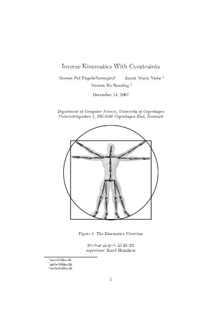
<strong>Inverse</strong> <strong>Kinematics</strong> <strong>With</strong> <strong>Constraints</strong><strong>Morten</strong> Pol Engell-Nørregård ∗ Sarah Maria Niebe †<strong>Morten</strong> Bo <strong>Bonding</strong> ‡December 14, 2007Department of Computer Science, University of CopenhagenUniversitetsparken 1, DK-2100 Copenhagen East, DenmarkFigure 1: The <strong>Kinematics</strong> VitruvianStudent project, 15 ECTSsupervisor: Knud Henriksen∗ mort@diku.<strong>dk</strong>† niebe@diku.<strong>dk</strong>‡ mobo@diku.<strong>dk</strong>1
Contents1 Introduction 51.1 Motivation . . . . . . . . . . . . . . . . . . . . . . . . . . . . . 51.2 Goals and requirements . . . . . . . . . . . . . . . . . . . . . 61.2.1 Main goals for an inverse kinematics solver . . . . . . 71.3 Section Overview . . . . . . . . . . . . . . . . . . . . . . . . . 81.4 Dividing the work . . . . . . . . . . . . . . . . . . . . . . . . . 82 Background 103 A data set for testing 123.1 Making the models . . . . . . . . . . . . . . . . . . . . . . . . 123.2 Making the video . . . . . . . . . . . . . . . . . . . . . . . . . 133.3 2d to 3d . . . . . . . . . . . . . . . . . . . . . . . . . . . . . . 143.4 From graphics to data structures . . . . . . . . . . . . . . . . 153.5 Conclusion on the Data set . . . . . . . . . . . . . . . . . . . 154 <strong>Inverse</strong> <strong>Kinematics</strong> 164.1 Uses of IK . . . . . . . . . . . . . . . . . . . . . . . . . . . . . 164.2 Introducing Concepts . . . . . . . . . . . . . . . . . . . . . . . 164.2.1 Quaternions . . . . . . . . . . . . . . . . . . . . . . . . 164.2.2 Spherical Coordinates . . . . . . . . . . . . . . . . . . 174.3 Articulated Figures . . . . . . . . . . . . . . . . . . . . . . . . 194.4 Joint Representation . . . . . . . . . . . . . . . . . . . . . . . 194.5 Joint Chain . . . . . . . . . . . . . . . . . . . . . . . . . . . . 204.6 Joint Parameters . . . . . . . . . . . . . . . . . . . . . . . . . 214.7 Increasing realism . . . . . . . . . . . . . . . . . . . . . . . . . 235 Optimization 245.1 Introducing concepts . . . . . . . . . . . . . . . . . . . . . . . 245.1.1 Wolfe conditions . . . . . . . . . . . . . . . . . . . . . 245.1.2 The Jacobian Matrix . . . . . . . . . . . . . . . . . . . 265.1.3 The Hessian Matrix . . . . . . . . . . . . . . . . . . . 275.2 Newton's method . . . . . . . . . . . . . . . . . . . . . . . . . 285.3 The Jacobian inverse method . . . . . . . . . . . . . . . . . . 295.3.1 The Jacobian transpose method . . . . . . . . . . . . . 305.3.2 The Pseudo inverse . . . . . . . . . . . . . . . . . . . . 305.4 Quasi Newton methods . . . . . . . . . . . . . . . . . . . . . . 305.5 The BFGS algorithm . . . . . . . . . . . . . . . . . . . . . . . 315.6 Constraining the problem . . . . . . . . . . . . . . . . . . . . 325.6.1 Lagrange Multipliers . . . . . . . . . . . . . . . . . . . 335.6.2 Karush-Kuhn-Tucker conditions . . . . . . . . . . . . . 352
5.6.3 The simple approach . . . . . . . . . . . . . . . . . . . 365.6.4 Active Set Methods . . . . . . . . . . . . . . . . . . . 365.6.5 The gradient projection method . . . . . . . . . . . . . 376 Implementation 396.1 Overview of the program . . . . . . . . . . . . . . . . . . . . . 396.2 The Editor . . . . . . . . . . . . . . . . . . . . . . . . . . . . 396.3 The solvers . . . . . . . . . . . . . . . . . . . . . . . . . . . . 406.4 data structures . . . . . . . . . . . . . . . . . . . . . . . . . . 416.5 constraints . . . . . . . . . . . . . . . . . . . . . . . . . . . . . 416.6 optimizing . . . . . . . . . . . . . . . . . . . . . . . . . . . . . 427 Evaluation 437.1 Implementation requirements . . . . . . . . . . . . . . . . . . 437.2 Evaluation <strong>by</strong> comparison . . . . . . . . . . . . . . . . . . . . 437.2.1 <strong>Constraints</strong> . . . . . . . . . . . . . . . . . . . . . . . . 447.2.2 Dening constraints . . . . . . . . . . . . . . . . . . . 447.3 Evaluating esthetic quality and realism . . . . . . . . . . . . . 457.3.1 Obtaining motion capture data . . . . . . . . . . . . . 458 Results 468.1 Test results . . . . . . . . . . . . . . . . . . . . . . . . . . . . 468.2 Comparing the methods . . . . . . . . . . . . . . . . . . . . . 478.2.1 <strong>Constraints</strong> . . . . . . . . . . . . . . . . . . . . . . . . 488.3 Evaluating esthetic quality and realism . . . . . . . . . . . . . 498.4 Concluding remarks . . . . . . . . . . . . . . . . . . . . . . . 509 Conclusion 5110 Future work 5310.1 incorporating global constraints . . . . . . . . . . . . . . . . . 5310.2 Experiments with alternative optimization methods . . . . . . 5310.3 Making the code fully OpenTissue compliant . . . . . . . . . 5410.4 Evaluating the Quaternion representation . . . . . . . . . . . 54A Images 573
AbstractIn the eld of computer animation, there is a variety of animationtechniques that an animator can utilize when animating articulatedgures. Each technique has its benets and draw-backs. Therefore thechoice of technique often depends on the task at hand. An animatorworking on a main character of an animated feature may wish to handmodel every frame of motion, gaining maximum level of detail control.When control is of less importance and ease of modeling becomes apriority, inverse kinematics proves to be a powerful tool.This report is a study of two dierent methods for solving the inversekinematics problem, posed as an unconstrained as well as constrainedoptimization problems.We describe the theory behind the methods and have implementedboth methods in their unconstrained version. We have also incorporatedjoint limit constraints, <strong>by</strong> projection of the solution unto afeasible region dened <strong>by</strong> these constraints.We evaluate the two methods, assessing the qualitative gains comparedto the computational complexities. The resulting implementation is tobe integrated with the existing open source meta library OpenTissue.A small set of 3D models and motion capture data has been composedto be used for an evaluation of the system once it is nished. A webpage has been constructed for the project comprising the full text pluspictures and video clips to document the process. The web page canbe found at http://kinematics.icandy.<strong>dk</strong>/ [3].Figure 2: The two gures modeled for the motion capture data set4
1 INTRODUCTION1 IntroductionIn the following section we give a brief introduction to our project. Wedescribe the motivation for the project as well as what we hope to accomplish.We go on to describing the document as a whole, and give a short descriptionof our individual focus.1.1 Motivation<strong>Inverse</strong> kinematics rst found its use in the eld of robot technology, whereit was used to compute the poses of the robots. Since then it has beenintegrated in the world of animation, where it is used in a similar fashioncomputing poses of articulated animated gures.The reason for this new found use, was the prospects of easing the processFigure 3: Example of a gure posed <strong>by</strong> skeletal deformation to resemple thefamous statue le penseur <strong>by</strong> Auguste Rodin.of animation, eliminating the need for animating every single joint of the articulatedgure. <strong>With</strong> inverse kinematics, an animator only needs to positionthe end eectors of a gure, leaving the positioning of intermediate joints tothe inverse kinematics solver. For this to result in a pose that seems natural,it is necessary to impose constraints on the joints of the gure, whichmeans that the solver will have to solve a constrained optimization problem.This is <strong>by</strong> no means uncharted territory, however we still feel that the work5
1.2 Goals and requirements 1 INTRODUCTIONbehind this report is justied since we combine well-known techniques withnew approaches. Furthermore the code will contribute to OpenTissue.1.2 Goals and requirementsOur main goal is to create and document an inverse kinematics based animationsystem for the OpenTissue[4] meta library, using quaternions as internalrepresentation of the joints. Since there is currently no implementation ofkinematics, we nd that our work is a needed and valuable contribution toOpenTissue.We must adhere to certain programming guidelines and rules when aimingat integrating, which can make implementation a somewhat tedious task.Also we are obligated to thoroughly document our implementation to makeit accessible to others, being that OpenTissue is an open source library.The methods we intend to use are based on previous work within the eld.For the purpose of comparison, we will implement two numerical optimizationmethods for solving the inverse kinematics problem: A rst order Newtonmethod and a second order Quasi-Newton based method.The core of the Newton method is the calculation of the inverse of a matrix.Actually, since the matrix in question is typically non-square, we need the tocalculate either an approximation, i.e. the transpose, or the pseudo-inverse.We plan to implement both of these methods and test which way of matrixinversion is the most ecient and which produce the most visually appealingresults.The Quasi-Newton based method (called BFGS) approximates second orderderivatives, i.e. the Hessian matrix, which is a quite expensive calculation.It should, however, enable this method to converge much faster than theJacobian. We will perform tests hoping to shed light on whether the addedcomputational complexity is aordable compared to the Newton method.In order to create realistic movement, constraining our skeleton is crucial.Therefore it is our goal to implement methods of constraining. As a minimum,our implementation should be able to explicitly enforce constraints onthe skeleton. This could be done <strong>by</strong> projection of the solution unto the feasibleregion. This will change the skeleton pose with no regards to a potentialsolver working on the skeleton, in eect wasting resources on computing nonvalidsolutions. More optimal, yet still not quite satisfactory, is the use ofgradient constraints which eectively set limits on the search direction forthe optimization methods. If time allows it, we will enable the implementationof the BFGS to solve the constrained IK problem. This allows forthe most general type of constraint, but is a very complex technique bothregarding implementation and time complexity. Also it scales rather badly,which we will need to exam in detail, if we implement it.In our experience there is a need for a graphical user interface whendeveloping OpenTissue based software. Especially when testing end debug-6
1.2 Goals and requirements 1 INTRODUCTIONging these high dimensional non-linear methods and constrained IK, we willneed to ease interaction with the program. Therefore we have decided tointegrate a graphical user interface allowing runtime variable manipulation.In addition we will use utilities for enhancing interaction and give runtimefeedback.In this report we seek to present methods and theory in such a way thatit will be possible for the reader to implement an inverse kinematics solveron her own. Also this is an aid to those wanting to work on or improve ourimplementation.1.2.1 Main goals for an inverse kinematics solverThe main goals when making a solver for inverse kinematics are user-controland a high degree of automation. What does that mean? User control meansthat the solver must not impede the work of an artist <strong>by</strong> constraining his orher possibilities. High degree of automation means that it must be possible toobtain a plausible result with as few parameters as possible. As an examplerelated to our project it would be desirable to only have to position the endeectors and then the rest of the gure is posed in a realistic way accordingto the constraints.These two goals are to some degree opposed to each other, the more controlyou want the more parameters you need to be able to tweak and hence theless automatic the process is. One way to tackle this dilemma is to let thesystem be automatic but to also to make it possible to change the automaticsettings afterwards, again an example from character animation would beto make it possible for an animator to reposition the links between the rootand the end eector after the IK solver has calculated their position.For this to be feasible the poses computed <strong>by</strong> the IK-solver would have tobe usable in most cases. If the animator has to ne tune the poses each andevery time, IK would be no help. What we want then, is poses that could becalled generic and realistic, so that in most cases the animator could leavethe poses as they were, and only had to tweak them in some special cases.It is not possible for a automatic IK system to produce life-like animationsfor living creatures, they will always be sti and puppet-like, unless somekind of post-processing is administered. This could be in the form of themethod proposed in [9] or could be done <strong>by</strong> an artist.The reason for this is that even with a constrained IK there are innitelymany viable solutions and only a few are the ones that a real person wouldchoose. Therefore we need something more. One obvious lack of the modelis gravity and muscle-actions. <strong>Kinematics</strong> are <strong>by</strong> denition not aected <strong>by</strong>Newtonian forces and so can never hope to give a realistic solution. It is nothowever impossible to incorporate gravity etc. into IK but that is beyondthe scope of this project, and might be the subject of later work as describedin section 10.7
1.3 Section Overview 1 INTRODUCTION1.3 Section OverviewEach chapter of this report begins with a short introduction of the contentof the given chapter. This section is a brief summary of these introductionsand is meant as a reading guide.Section 1 on page 5 This rst section is of a practical nature, presentingformalities pertaining to the project at hand. There is no theoreticalinformation in this section, so readers that are only interested inimplementing an IK solver may skip this chapter.Section 2 on page 10 is a background study, trying to recap previous researchin the eld of IK.Section 3 on page 12 Is a documentation of the process of acquiring aproper data set for testing our solution.Section 4 on page 16 is a walk trough of the most basic concepts of IK.This is where we describe the articulated gure, on which we will performIK. As such, in can be perceived as a prerequisite for understandingnot only the section on optimization theory, but only the hows andwhys of our implementation.Section 5 on page 24 is on the theory of optimization. When optimizationis given a separate section, it is an acknowledgment of the importanceof the optimizing unit of an IK solver.Section 6 on page 39 is a brief description of the developed program, andits key parts.Section 7 on page 43 describes which qualitative measures we wish totest our system against, and how we mean to execute these tests.Section 8 on page 46 is a followup on chapter 7. This is were we presentthe results of our evaluation tests.Section 9 on page 51 is the conclusion where we compare our results withthe goals we hoped to achieve and conclude on the project.Section 10 on page 53 is concerned with describing possible ways to extentour work.1.4 Dividing the workAll members of the group have partaken in all parts of the project, howeverthere are subjects where we each have had slightly more focus than others.The following is a list of the areas each of us have concentrated upon. Wehave each written our own description of the areas we have focused on in theproject.8
1.4 Dividing the work 1 INTRODUCTION<strong>Morten</strong> Bo <strong>Bonding</strong> This project is going to be a part of the OpenTissuemeta library, which is why my main focus has been code designand implementation evaluation, verication and testing. This includesdevelopment of a range of utilities e.g. for importing constraints, datahandling, constraint manipulation as well as utilities for runtime logging,feedback and interaction.Sarah Maria Niebe I have placed my focus on the theoretical part of thisproject, trying to get an all-round knowledge of the optimization algorithmsand optimality conditions. The BFGS method as [16] describesit, has been the main focus of this theoretical study, as it is one of thetwo methods we have chosen to implement.<strong>Morten</strong> Pol Engell-Nørregård My focus has been the development ofthe inverse kinematics solvers, both theoretically and practically. Ihave mostly concentrated on the unconstrained version.Project management have also been one of my key areas, I have takencare of trying to get some structure on the way we where working,and making an overview of the current state of aairs available to allmembers of the group.I have also been the graphics artist on the project having made all themotion capture data. This is not strictly a part of the project per sebut I mention it because it has been a prerequisite for the entire project.9
2 BACKGROUND2 BackgroundThis section is a description of the background for our project, as well as adescription of the literature that has formed the basis for our project.In robot technology, inverse kinematics (IK) has long been used for computingthe positioning of intermediate joints on the path from root joint to endeector joint. Must robotic systems consist of a single chain of joints, e.g.a car factory migth have a robotic arm placing parts on a car chassis. Thismeans that an IK solver for such a system only has to handle a small numberof degrees of freedom (DOF), combined with the advantage of havinga specic underlying architecture, one can implement a highly specialized -maybe even hardware accelerated - IK solver.So when IK was discovered <strong>by</strong> the graphics community, as a new way ofanimating articulated gures, the need for more general methods was born.The challenge was generalizing the methods while at the same time handlinga higher number of DOF. An often used articulated gure in animation isthe human body, if this is to be simulated somewhat accurately the gurewill have to have many DOF, some of which will be redundant. E.g. thehuman arm, this is considered to have seven DOF 1 , but only 3 DOF wouldbe necessary for reaching any point reached using the seven DOF. The redundantDOF are what enables the arm to grasp at the same object fromdierent angles and directions.According to Martin F¥dor [8], most IK systems use the Jacobian inverse/-transpose method even though these methods suers from singularity problems.The most common approach seems to be using some kind of pseudoinverse [12] to invert the Jacobian, the problem with singularity is not solved<strong>by</strong> this though [13].Another approach is the Cyclic coordinate descent (CCD) described in [8,15], it uses the greedy paradigm to solve for each joint in turn, and repeatsthis process until a satisfactory solution is found. Although this method isboth simple and fast, it suers from several drawbacks when it comes toprecision. This text does not address CCD in any detail.In 1994 Jianmin Zhao and Norman I. Badler [16] presented another methodfor solving the IK problem using a nonlinear system of equations, that madeit possible to solve large systems with many redundant DOF. Most literatureon this subject use Euler angles when representing the joints, this report willhowever be representing the joints with quaternions. The reason for this approachis the - to our knowledge - lack of literature that combines the theoryof such a solver with the actual implementation of it. The work of KennyErleben and Knud Henriksen [11] serves as a basis for this approach.Many dierent methods for solving the IK problem has been proposed, but1 A shoulder gives pitch, yaw and roll, an elbow allows for pitch, and a wrist allows forpitch, yaw and roll10
2 BACKGROUNDrecent research seems to favor numerical optimisation approaches. Most ofthese methods are described in [13], where a both recent and thorough descriptionof numerical optimization techniques can be found.Much of the resent research in the eld such as [9, 7] is not really concernedwith solving the IK problem but rather with elaborating on the periferals ofthe method, such as easing interaction[7], or combining dierent animationscalculated with IK [9].11
3 A DATA SET FOR TESTING3 A data set for testingSince we work with <strong>Inverse</strong> <strong>Kinematics</strong> in a graphics context we needed somekind of data set to test our system on. A typical test set would consist of amodel consisting of a skinned skeleton, and possibly some Motion capturedanimations.After having tried out dierent possibilities we decided on making our owntest data set. The Set should consist of two models each with a number ofanimations.Motion capture is a broad term covering a lot of dierent techniques fromadvanced machines that capture directly to 3D data, to simple version wheredata is taken from 2d movies of persons from dierent angles and transformedinto 3d data <strong>by</strong> hand. Since we do not have access to expensive equipment,it was fairly obvious that we had to make do with less than that. Fortunatelywe had a member in our group with some experience in 3d graphics.3.1 Making the modelsThe most important part of the dataset are the models themselves. theseshould be realistic with regard to proportions and visually pleasing, so asto not disturb the communication of the results. The Models used for ourprogram are 3d models of humans. One male, E.R.I.K. (which is short forExperimental Rig for <strong>Inverse</strong> <strong>Kinematics</strong>) and on female, E.R.I.K.A. (whichis a feminine form of E.R.I.K.). The models have approximately 32 jointseach with up to 6 degrees of freedom (although no more than 3 are used inthis context).Both models have been build in Blender[1] using pictures of humans asFigure 4: The Male model E.R.I.K. as it looks in our editor window12
3.2 Making the video 3 A DATA SET FOR TESTINGreference in much the same way as described below for the animations. Thereason we chose human models are rst and foremost that it is the mostobvious choice since animations using motion-capture are usually (but farfrom always) human. The second reason is that it was far easier for us tomake human motion capture since we could then use friends and family asmodels.Figure 5: the female model E.R.I.K.A as it looks in our editor window3.2 Making the videothe easiest part was getting the videos it was a simple matter of taking somevideos of people walking around or doing motions. There are however someproblems involved, since these videos where to be used as the basis for 3dmodels they would have to have the same orientation and position, relativeto the camera in every frame of the video. This is an almost impossible taskto accomplish using a small hand held camera, so we did something else.The orientation isn't so big a problem, when you want to have a side shot.You make people go around the camera in a circle. This can be marked onthe ground so as to make sure the distance is the same all the time.Keeping a walking person centered is a more dicult problem. This wassolved again as simple as possible <strong>by</strong> simply translating the individual framesof the video so the person was in the same position in each of them.As easy as this may sound it is not a simple problem, since a body deformswhen the person walks, arms sway, legs move, head and shoulders sink andrise. Had it not been so, it would have been a simple task, best solved <strong>by</strong> a13
3.3 2d to 3d 3 A DATA SET FOR TESTINGcomputer. as it is developing such a solution would be a project in its ownright.Now it must be done <strong>by</strong> hand using the pelvis as the reference in the X-axisand the foot currently touching the ground as the reference in the Y-axis.Another problem arise when you lm people from the front. Since they aremoving towards the camera they will get bigger as they move closer. this issolved <strong>by</strong> scaling the frames until the person walking is the same size as theother frames.The nal problem and one that is not easily solved unless one has an orthographiccamera, is the perspective in the frame. as a person walks towardsthe camera, his front most foot will be closer to the camera than the otherthis is quite obvious when compared to the 3dmodel that must be tted to thepicture. There is no easy solution to this , however the necessary informationcan be interpolated from the other views (where the perspective is dierent).3.3 2d to 3dWhen the movie are nished they are between 20-40 frames long these areimported in Blender [1] and used as background in the modeling window.Figure 6: illustration of the steps in transferring the pose from the pictureto the modelArtistic freedomSome degree of artistic freedom is inevitable when using the method wehave used here. The important notion here however is that we have realisticlooking animation as the basis for our analysis, and that great care has been14
3.4 From graphics to data structures 3 A DATA SET FOR TESTINGtaken, not to modify the original data more than absolutely necessary. Allpeople have slightly dierent motions anyway so as long as our models keepwell within these limits, there is really no reason to be concerned about therealism.Most motion capture is used in graphics where we are not really interestedin realism anyway. We want what is commonly known as cinematic realitymeaning that we want something that we think look realistic, not somethingthat really is realistic. As we have thrived to make our animations realisticand have not taken the artistic freedom too far (actually we have tried notto take it anywhere) our animations are very close to the way humans reallymoves which can also be seen from the accompanying video material.foundat [3].3.4 From graphics to data structuresConverting the graphics les to OpenTissue data structures has been a fairlystraight forward process. Blender has an export option to the cal3d format[2]and OpenTissue has import code from this format to Opentissue data structures.3.5 Conclusion on the Data setAs we have shown we have succeeded in making realistic and usable 3D modelsfor use with our project, a motion capture data set consisting of walking,standing, and saluting has also been made. It has been a time consumingprocess but since this dataset will be made available for other students atDIKU and otherwise who want to work with character-animation,we believeit has been worth the eort. Examples of the data set can be found athttp://kinematics.icandy.<strong>dk</strong>/ [3].15
4 INVERSE KINEMATICS4 <strong>Inverse</strong> <strong>Kinematics</strong>This chapter is a short introduction to inverse kinematics, and the systemwe wish to apply it to. It is not a chapter on solving the inverse kinematicsproblem, but rather a walk through of the system we wish to perform inversekinematics on.4.1 Uses of IKIK can be used in several dierent applications, each of which places dierentrequirements on the solver. The two most widely applications are:1. Real time solving for robots or simulation. In this context it is necessaryfor the solver to be able to solve the problem at rates that makesit possible for the simulation/robot to move in real time. This is similarto collision detection in simulation, which should be computableat rates of approximately 50 - 100 times per second or more. Solvinga kinematics problem this fast is nigh on impossible unless we eitherplace some restrictions on the number of iterations we allow the solverto take or we work on a very restricted model with regard to DOF.2. Interactive solving for modeling and animation. In this case we canallow ourselves a little more time since we only need to compute 15-25poses per second. This means that we can handle more DOF and canachieve greater precision since we do not have to enforce a hard limiton the number of iterations.Which of these applications that are the most interesting depends on theproblem at hand.4.2 Introducing ConceptsThere are some mathematical and theoretical concepts that we need to explain,in order for the following to be easily understood.4.2.1 QuaternionsQuaternions are a non-commutative extension of the complex numbers. Theyare dened as the mathematical ring:H = {a + bi + cj + <strong>dk</strong> | a, b, c, d ∈ R} (1)where i 2 = j 2 = k 2 = ijk = −1. This means that a quaternion can berepresented <strong>by</strong> just 4 real numbers. Quaternions are widely used for 3Drotations, having the advantages over normal rotation matrices that:16
4.2 Introducing Concepts 4 INVERSE KINEMATICS• representing a quaternion is compact, 4 numbers compared to the 9needed for a rotation matrix• rotation <strong>by</strong> quaternions eliminates gimbal lock (for an explanation ofgimbal lock see [12])The common mathematical operations - addition, multiplication, inversionand so fourth - are also dened for quaternions, but since we use quaternionsfor 3D rotations we will only show the rules for multiplication and inversion.Given two quaternions a = (a 1 +b 1 i+c 1 j+d 1 k) and b = (a 2 +b 2 i+c 2 j+d 2 k),the product ab is dened as:ab = (a 1 + b 1 i + c 1 j + d 1 k)(a 2 + b 2 i + c 2 j + d 2 k)= (a 1 a 2 − b 1 b 2 − c 1 c 2 − d 1 d 2 ) + (2)(a 1 b 2 + b 1 a 1 + c 1 d 2 − d 1 c 2 )i +(a 1 c 2 − b 1 d 2 + c 1 a 2 + d 1 b 2 )j +(a 1 d 2 + b 1 c 2 − c 1 b 2 + d 1 a 2 )kThe inverse quaternion is dened as a −1 = ā where ā = (a − bi − cj − <strong>dk</strong>)aāis the conjugate of a. This gives us:a −1 = ā(3)aāa − bi − cj − <strong>dk</strong>=a 2 + b 2 + c 2 + d 2 (4)Knowing how to invert and multiply quaternions enables us to use them forrotations. A θ degree rotation around axis n = (n 1 , n 2 , n 3 ) T of the vector vis given <strong>by</strong>:v ′ = qvq −1 (5)where q = (cos( θ 2 ) + n 1 sin( θ 2 )i + n 2 sin( θ 2 )j + n 3 sin( θ 2)k). When the rotationquaternion is of unit length, the inversion is equal to the conjugate of q.This is seen in equation (4), where the denominator is in fact the length ofquaternion a, which in the case of a unit quaternion is 1.For more on quaternions, see [6].4.2.2 Spherical CoordinatesUsing quaternions for rotation and orientation dictates the use of sphericalcoordinates, which might not be familiar to the reader. Therefore we willrecap the theory of spherical coordinates here.Spherical coordinates, like the well known Cartesian coordinates, are a wayof representing position in 3D. In our particular case, where we wish to describeorientation, we use the model slightly dierent. Where the parameter17
4.2 Introducing Concepts 4 INVERSE KINEMATICSθ usually denotes the distance from origo (and is usually named ρ), we let itdenote twist as explained below. The math however, is identical.A given orientation is represented <strong>by</strong> the three angles azimuth φ, elevationψ, and twist θ. Throughout the literature, there is great ambiguity as towhich parameter is denoted <strong>by</strong> what symbol, we have adopted our use ofnotation from [11].The relationship between quaternions and spherical coordinates are de-Figure 7: Spherical coordinates: the gure shows an orientation version,modeling azimuth φ, elevation ψ, and twist θ. Twist could be exchangedfor length giving an arbitrary position. Note that the gure is only a halfsphere, this is for visual simplicity.scribed in details in 4.6 on page 21.Quaternions describe a rotation around an arbitrary axis in 3D space. Sphericalcoordinates are very close to this representation since the two rst parametersazimuth and elevation describe an arbitrary vector in 3D space,and the last parameter twist describes a rotation around this axis.There is a one to one mapping from the Cartesian coordinates to the sphericalcoordinates, given <strong>by</strong>:θ = √ x 2 + y 2 + z 2 (6)(√ )xφ = arctan22 + y 2(7)z( yψ = arctan2(8)x)And the reverse from spherical to Cartesian coordinates is given <strong>by</strong>:x = θ sin φ sin ψ (9)y = θ sin φ cos ψ (10)z = θ cos φ (11)18
4.3 Articulated Figures 4 INVERSE KINEMATICS4.3 Articulated FiguresThere seems to be two dominating ways of working with articulated gures• constructing a skeleton unto which a skin is rigged, there<strong>by</strong> deninghow the movement of the skeleton should deform the skin• working directly on the skin, skipping the time consuming rigging ofskinRecent study shows that it is possible to do impressive deformations directlyon the mesh, [7], so why bother with skin rigging and making a skeleton?First of all because of generality, animations on a skeleton can be tted todierent skins with little or no modications. Second, the methods developedfor direct mesh deformation requires the construction of a number ofexample poses from which other deformations are deduced. This makes thismethod at least as time consuming as the rigging process, since most meshesare very detailed. Third, since the process of making the example poses andgenerating the deformable mesh is fully automated, based only on the examplemeshes, explicit control on the part of the modeler is lost. When this iscompared to the fact that, what the process does, is in fact a sort of rigging,based on grouping the vertices of the mesh into rigid groups, old fashionedrigging is still a fully acceptable a competitive method.Based on this argumentation, we have chosen to work with the skeleton representationwhich means we will have to dene a skeletal structure. Similarto the human skeleton, the articulated gures we have worked on during thisproject, consist of bones connected <strong>by</strong> joints. The literature on this subjectspeaks of prismatic and revolute joints, but since the human body doesn'thave prismatic joints we will only use the latter type.A skeleton can be thought of as a graph tree, it typically has one root bone,but can have several end eectors 2 . The joints on the path from root toend eector make a joint chain, see chapter 4.5, and it is on these chains weperform the inverse kinematics.4.4 Joint RepresentationIf we assume a one to one correspondence of bones and joints, we can mergethe information of the length of the bone and the orientation of the joint,see gure 8. From this point on, the denition of a joint is its rotation andtranslation, relative to the parent joint. This can be represented as a rotationquaternion q and a translation vector t. Given a parameter vector you cancompute the pose of joint i <strong>by</strong> performing a series of relative rotations andtranslations, this is called forward kinematics. From section 4.2.1 we know2 A bone with no child bones, or in graph theory a leaf19
4.5 Joint Chain 4 INVERSE KINEMATICSFigure 8: A single joint consisting of translation and orientation. The conerepresents the translation, while the sphere with the small coordinate systemattached is the orientationthat a rotation quaternion has the form:( ( ( ( θ θ θ θq = (cos + n 1 sin i + n 2 sin j + n 3 sin k) (12)2)2)2)2)in vector notation:( ( θ θq = [cos , n sin ] (13)2)2)However, the revolute joints we wish to rotate are spherical and to modelthis we have to introduce two more parameters φ and ψ, also known as theazimuth- and elevation angles. These new parameters are used to parameterizethe axis of rotation:( ( θ θq(θ, φ, ψ) = [cos , n(φ, ψ) sin ] (14)2)2)where⎡n(φ, ψ) = ⎣cosφsinψsinφsinψcosψ⎤⎦ (15)4.5 Joint ChainA joint chain is a number of connected joints, where the translation and rotationof the i'th joint aects the translation and rotation of any joint placedlater in the chain, which means we are operating with relative transformationsas opposed to absolute transformations. Figure 9 illustrates a simplejoint chain, constructed <strong>by</strong> three joints.The chains are build under the assumption that all bones have at most oneparent but can have any number of children. This assumption is not a verystrong constraint on the generality since almost any conguration that we20
4.6 Joint Parameters 4 INVERSE KINEMATICSFigure 9: A joint chain consisting of 3 joints. The cones represent thetranslation of the joint and the spheres represent the rotation. Notice thatthe order of transformations is translation,rotation.can think of from real life is like this. Even those that might not be, could bemade to work as if they were, <strong>by</strong> careful placement of the root. Furthermorethis restriction is one that very often is placed upon the skeleton anyway.This assumption makes it possible to build all the chains in a skeleton verysimply. We just run through the entire skeleton and mark all bones withno children as end eectors. Then we build a chain for each end eectors<strong>by</strong> moving back through the skeleton, going from parent to parent until wereach the root. Figure 10 illustrates a branched skeleton, and how it is traversedto build to joint chains.By doing so we have a robust and simple way to construct the chains andwe are thus ready to start performing inverse kinematics on each of these,or all simultaneously if we so please.4.6 Joint ParametersGiven a quaternion q i , representing the relative orientation of the i'th bone,we may wish to extract the three angles θ, φ and ψ. Since they are not explicitlyrepresented, we have to derive a way of computing the angles. Equation(14) gave us the quaternion that describes the rotation around axis n(φ, ψ),combined with equation (15) we have all the information needed to isolatethe three unknown angles. First we dene the vector n ∗ = (n(φ, ψ) sin( 1 2 θ))and a rotation quaternion q = [s, n ∗ ] where:( θs = cos(16)2)( θn ∗ 0 = cosφsinψsin(17)2)21
4.6 Joint Parameters 4 INVERSE KINEMATICSFigure 10: A simple branched skeleton. Two chains are build consisting ofthe joints {0, 3, 4} and {0, 1, 2}( θn ∗ 1 = sinφsinψsin2)( θn ∗ 2 = cosψsin2)We can now isolate the angle φ sincen ∗ 1n ∗ = sinφsinψsin ( )θ20 cosφsinψsin ( ) = sinφθ cosφ2and φ is given <strong>by</strong>φ = arctan( ) sinφcosφ(18)(19)(20)(21)To be sure to compute the correct angle, no matter which quadrant it liesin, we recommend using the slightly modied version of arctan, arctan2 see[12].Now that we know the value of φ we can use this knowledge to computethe other two parameters.By using the relationn ∗ ( )0θcosφ = sinψsin (22)2andn ∗ 0cosφn ∗ 2= sinψcosψ22(23)
4.7 Increasing realism 4 INVERSE KINEMATICSwe can use the arctan2 function again to compute ψ as⎛ ⎞ψ = arctan2 ⎝nally we can nd the value of θ <strong>by</strong>( )n ∗ 0cosφsinψsθ can then be determined asθ2⎛= arctan2 ⎝⎛⎛θ = 2 ⎝arctan2 ⎝n ∗ 0cosφn ∗ 2⎠ (24)= sin ( )θ2cos ( ) (25)θ2(n ∗ )0cosφ i sinψ is(n ∗ )0cosφ i sinψ is⎞⎠ ⇔ (26)⎞⎞⎠⎠ (27)4.7 Increasing realismThere exists several ways of increasing the realism of the animation. Thesimplest yet surprisingly eective method, is weighting the individual jointswillingness to move. This can be done quite simply <strong>by</strong> weighting the distanceeach link is moved each iteration. Given an update vector p and a weightmatrix W , where W = w T I and w is a vector of weights on the individualjoints, the weighted update p u is given <strong>by</strong>:p u = W p (28)This simple weighting method can be applied to any or all joints in this wayand can be used to model the willingness to move.In practice this weighting is performed on the update vector. See section 5.3on page 29 and section 5.5 on page 31 for a detailed description of the updatevector.23
5 OPTIMIZATIONFigure 11: An example of the inuence of dierent weights on the nishedpose. This illustration is produced with our program, using low weights onthe two outermost joint in the left case and low weights on the innermostjoint in the right case.5 OptimizationWhen solving optimization problems, the choice of solver is not a straightforwardright or wrong choice. Dierent solvers pose dierent benets anddrawbacks, some of which can be dicult to foresee theoretically, based onthe optimization problem at hand. Appreciating this, we have chosen to implementtwo dierent types of solvers with the intent of comparing the resultsthey produce. This chapter is meant as a brief introduction to the Jacobianinverse method and the BFGS method, for a more in depth description ofthe two, the reader is referred to [13, 16, 14].5.1 Introducing conceptsBefore we start deriving the two methods, we rst need to introduce a coupleof mathematical concepts used in a wide selection of optimization solvers.The following subsections attempt to give an explanation of the concepts ina manner that doesn't require a complete understanding of the underlyingmath.5.1.1 Wolfe conditionsA large part of optimization is determining the search direction, p k , for thenext iteration. This could be the negated gradient of the object function,the negated product of the inverted Hessian and the gradient, or some other24
5.1 Introducing concepts 5 OPTIMIZATIONupdate paradigm. But common to them all is that they only represent thedirection of search, not where along this direction the local optimum lies.To determine the step size, α k , there exist a variety of line search methodsthat tries to minimize φ(α) = f(x k + αp k ), where α > 0. A common set ofconditions for many line search methods is the Wolfe conditions:f(x k + α k p k ) ≤ f(x k ) + c 1 α k ∇f T k p k (29)∇f(x k + α k p k ) T p k ≥ c 2 ∇f T k p k (30)with 0 < c 1 < c 2 < 1The rst condition, (29), is also known as the Armijo condition. The Armijocondition is a sucient decrease condition, as it demands a sucient reductionin f at point x k+1 = x k + α k p k . Figure 12 illustrates the intervalsFigure 12: The Armijo conditionthat will satisfy the Armijo condition, but it also illustrates the shortcomingof using only the Armijo condition as in this case the condition is satisedfor very small α k values, impeding the rate of convergence. To correct thisbehaviour, the Wolfe conditions incorporates information of the functionscurvature with inequality (30). The curvature condition requires an increasein the slope, since a strongly negative slope at x k+1 implies that f is decreasingafter x k+1 , meaning that α k is not a minimizer of φ.We are still not guaranteed that the step size found using the Wolfe conditionsis a step that brings us to a global minimum of φ. To amend this,the strong Wolfe conditions force α k to lie close to a minimizer of φ <strong>by</strong> notallowing a positive derivative at φ(α):f(x k + α k p k ) ≤ f(x k ) + c 1 α k ∇f T k p k (31)|∇f(x k + α k p k ) T p k | ≤ c 2 |∇f T k p k| (32)with 0 < c 1 < c 2 < 1The setting of variables c 1 and c 2 depends on how the search direction is25
5.1 Introducing concepts 5 OPTIMIZATIONfound, however the two methods of this report - Newton and Quasi-Newtonmethods - often use the values c 1 = 10 −4 and c 2 = 0.9, [13].5.1.2 The Jacobian MatrixThe Jacobian J f (x) is the matrix of rst-order partial derivatives of f(x).J f (x) is a n × m matrix, where n is the size of the goal vector and m is thenumber of parameters. For f(x 1 , x 2 , . . . , x m ) = (y 1 , y 2 , . . . , y n ), this is theJacobian:⎡⎤J f (x) =⎢⎣∂y 1 ∂y 1∂x 1∂y 2 ∂y 2∂x 1.∂y n∂x 1∂y 1∂x m∂y 2∂x m∂x 2. . .∂x 2. . ... .. .∂y n∂x 2. . .∂y n∂x m⎥⎦(33)The Jacobian can be viewed as a multi-dimensional gradient, that is it denesthe direction of travel in a multi-dimensional space much like a tangentdenes the direction of travel in a one-dimensional space. To get a moretangible explanation of the Jacobian, consider this example:Example in 2 dimensions The situation is this, we have a simple chainof two joints each with one DOF. Assuming that the movement of the endeector is conned to a plane, we can model this in a two-dimensional space,see gure 13. The Jacobian of this problem is a 2 × 2 matrix, since the jointshave one DOF and is therefore parameterized with one parameter each andthe goal vector is two-dimensional. Figure 14 shows a plot of the objectiveFigure 13: A conguration with to joints each with 1 DOF, the unconnectedcircle, at {1.2 , 0.6} is the goal positionfunction for a chain with two joints, each of which is of unit length. Both26
5.1 Introducing concepts 5 OPTIMIZATIONjoints have one rotational DOF. The root of the chain is situated in origo andthe goal position have the coordinates x = 1.2 y = 0.6 Since the distanceFigure 14: A plot of the objective function for a joint chain of two joints,each with two DOF. Notice the two global minima seen as bulges on theunderside of the functionfrom the root is less than the maximum reach of the chain there is morethan one minimum in the objective function. In this simple example thereare only two possible optimal solutions, however with more joints or moreDOF the number of solutions will go towards innity.The Jacobian can be used to minimize this function, see section 5.2 on thenext page and 5.3 on page 29.5.1.3 The Hessian MatrixSince the methods we have implemented don't use the actual Hessian matrix,but just an approximation of it, we will only briey describe it here.Assuming that the function f(x) is twice dierentiable, the Hessian matrixH f (x) is a square matrix, consisting of the second-order partial derivativesof f(x). The Hessian is equivalent to the Jacobian of the gradient of f.⎡⎤∂ 2 f(x) ∂ 2 f(x) ∂∂x 1 ∂x 2. . .2 f(x)H f (x) =⎢⎣∂x 2 1∂ 2 f(x)∂x 2 ∂x 1.∂ 2 f(x)∂x n∂x 1∂ 2 f(x)∂x 2 2.∂ 2 f(x)∂x n∂x 2. . .∂x 1 ∂x n∂ 2 f(x)∂x 2 ∂x n. . .. .. .∂ 2 f(x)∂x 2 n⎥⎦(34)The Hessian contains information of the curvature of function f at point x.The properties of the Hessian can be used to test for optimality of a given27
5.2 Newton's method 5 OPTIMIZATIONpoint. If we have ∇f(x ∗ ) = 0, and H f (x) is:• Positive denite: then x ∗ is a minimum of f• Negative denite: then x ∗ is a maximum of f• Indenite: then x ∗ is a saddle point of f• Singular: udeneable behaviour of fTesting a symmetric matrix for positive deniteness - which is of interest ofthis project since we are trying to minimize our problem - can be done in acouple of ways. Some methods use factorization of the matrix, analyzing theresulting sub matrices. By computing the eigenvalues of H f (x) and checkingthat they are all positive, is an alternative and very expensive way of testingfor positive deniteness.5.2 Newton's methodNewton's method is based on a second order Taylor series expansion of theobject function f(x):f(x + σ) ≈ f(x) + ∇f(x) T σ + 1 2 σT H f (x)σ (35)The minimizer of (35) is found when ∇f(x + σ) = 0, which <strong>by</strong> a rst-orderTaylor series expansion is∇f(x + σ) ≈ ∇f(x) + H f (x)σ (36)recalling from 5.1.3, the Hessian is equivalent to the Jacobian of the gradient.Solving the systemH f (x)σ = ∇f(x) (37)thus solves ∇f(x + σ) = 0 and is the minimizer of equation (35). Since thisis just approximations of f(x) we are not guaranteed that solving (37) willgive us the exact solution to min f(x). This is why the Newton method is aniterative method, updating x in each iteration <strong>by</strong> adding the σ computed in(37), till it converges towards a solution. The Newton method has, in mostproblems, a quadratic convergence rate, when given a good initial point x 0 .When presented with a bad choice of x 0 , there is no guarantee that theNewton method will converge at all. When given good starting points, theNewton method won't need a line search method as the newton update givesnot only the direction but also the size of the step. To improve the methodsrobustness towards bad starting points, one can alter the newton updateso that the update vector σ is weighted <strong>by</strong> a scalar α. This scalar is oftenreferred to as a step length, and it can be computed <strong>by</strong> a line search methodsuch as the back-tracking algorithm. The altered newton update would thenbe x k+1 = x k + α k σ k . This is known as a damped Newton method.28
5.3 The Jacobian inverse method 5 OPTIMIZATIONx k = initial guesswhile(not done)x k = x k − J f (x k ) −1 f(x k )check if doneendFigure 15: Pseudo code for the Jacobian inverse algorithm5.3 The Jacobian inverse methodThe Jacobian inverse method, also known as Newton-Raphson, is a simpli-ed version of the general Newton method without the second order Taylorexpansion, thus disregarding the Hessian matrix.When solving a unconstrained linear system:f i (x) = 0 (38)for i = 1, 2, . . . , m one has to solve m simultaneous equations. Performing arst order Taylor series expansion gives us:f i (x) ≈ f i (x k ) + f ′ i(x k )(x − x k ) (39)so instead of solving f i (x) = 0 which would require determining the inversefunction fi−1 (x), we can solve:where the solution x can be isolated:f i (x k ) + f ′ i(x k )(x − x k ) = 0 (40)x = x k + f i(x k )f ′ i (x k)(41)Since we have reformulated the original problem the x in equation (41) cannot be expected to be the exact solution to equation (38). Instead equation(41) is used as an update step in an iterative method of the form illustratedin gure 15, where f(x) is expanded to include all m equations and J f (x)is a matrix of the rst partial derivates of f at x, this matrix is called theJacobian of f.The termination criteria can be a variety of termination , e.g. a xed numberof iterations, an absolute e.g. the distance from end eector to the goal ora relative measuring the rate of change. One drawback of this method isthat a bad choice of initial value of x k might cause the algorithm to divergerather than converge. However no method is known to guarantee a goodinitial value, which brings us back to the termination condition. When wellchosen, the termination condition can ensure that the algorithm won't loop29
5.4 Quasi Newton methods 5 OPTIMIZATIONindenitely.Inverting a matrix is an expensive operation so alternatives has been suggested,one is to solve the system J f (x k )(x − x k ) = −f(x k ) but for largesystems this is still expensive. A second alternative is using the transposedJacobian J f (x) T instead of the inverse, this is yet another approximation ofthe original problem which is so widely used that it will be described shortlyin its own section5.3.1 The Jacobian transpose methodSince the Jacobian matrix is usually not square, inversion is often not possible,one simple and widely used alternative is transposing the matrix instead.This has led to a variant of the Jacobian method called the Jacobian transpose.the greatest advantage of this method, is the fact that no singularityissues arise, since no inversion takes place. This and the fact that transposinga matrix is both faster and simpler than inversion, has led to manyimplementation of the Jacobian transpose method. The method is similarto the original Jacobian inverse in all respects apart from the approximationof the inverted Jacobian, which is why it would be folly not to implement aversion of this method when we have the Jacobian inverse.5.3.2 The Pseudo inverseA much better approximation of the inverse of the Jacobian is the pseudoinverse J + dened in one of three ways depending on whether the systemis over determined ,under determined or regular. In the regular case theinverse is taken directly in the over determined case the pseudo inverse takesthe following form:J + = (J T J) −1 J T (42)in the under determined case it takes the form:J + = J T (JJ T ) −1 (43)it can be shown that the pseudo inverse is a least squares approximation tothe inversion, this is beyond the scope of this text though. Finally it shouldbe noted that the pseudo inverse does not solve the problem of singularity.since if the matrix J T J or JJ T is singular, the inverse is still undened.5.4 Quasi Newton methodsThe main concern when constructing a real time inverse kinematics solver, iscomputational complexity. In order to label a solver real time it has to supplyat least 25 fps, not just when running on a supercomputer but also on most30
5.5 The BFGS algorithm 5 OPTIMIZATIONcommercial PC's. For this to be accomplished, we need to choose the bestalgorithm for the main component of the solver, the optimization algorithm.A Quasi-Newton algorithm is based on Newton methods, in that it alsosearches for a stationary point, a local minima. In Newton methods thesestationary point are found using line search algorithms and <strong>by</strong> computing theHessian matrix for each point along the search direction. The computation ofthe Hessian matrix is a computationally heavy operation, as is the inversionof the Hessian needed in the Newton update step. Enter the Quasi-Newtonmethods, these methods excel in never computing the exact Hessian, onlyapproximations of the Hessian. Some methods extends this to approximatingthe inverse Hessian thus removing the expensive matrix inversion in theupdate step.The Quasi-Newton method we've chosen to implement for this project is theBFGS algorithm as it is presented in [13], however an important referencehas been the version described in [16], a slight alteration of the originalalgorithm presented i 1970 <strong>by</strong> Broyden, Fletcher, Goldfarb and Shanno.5.5 The BFGS algorithmAs mentioned earlier, the Quasi-Newton methods mainly dier from ordinaryNewton methods in the use of an approximated Hessian matrix as opposedto a computed Hessian. How the Hessian is approximated, is therefore oneof the main dierences between the various Quasi-Newton methods.The BFGS method updates the inverse Hessian <strong>by</strong> applying the followingformula:((H k+1 = H k + 1 + yT k H ))ky kσk T y σ k σk T − σ kyk T H k − H k y k σkT /σk T y i (44)iIt maintains existing information of the objective function, while also addingrecent acquired knowledge about the development of the objective function.The latter is <strong>by</strong> incorporating σ k and y i , which is the step taken and thechange of gradients during the k'th iteration. The formula is derived <strong>by</strong>imposing three conditions on the updated inverse Hessian H k+1 :1. The updated matrix must remain symmetric and positive denite2. The updated matrix must satisfy the secant equation3. The updated matrix must be close to the previous updateWe assume that within a close neighborhood of x ∗ , f(x ∗ ) is twice continuouslydierentiable which means that the Hessian of f(x ∗ ) is symmetric 3 ,therefore we will require that the approximated inverse Hessian also is symmetric.The Hessian is constructed of the second partial derivatives of the3 For further elaboration on Hessians see [10]31
5.6 Constraining the problem 5 OPTIMIZATIONobject function, this means that the Hessian contains information about thecurvature of the object function at a given point x ∗ . When the Hessian ispositive denite it means that in a small neighborhood of x ∗ , the object functionwill increase meaning that x ∗ is a local minimum of the object function.Since the inverse of a positive denite matrix is also positive denite, we willrequire that the approximated inverse Hessian also is positive denite.By second order Taylor expansion of f, rearranging and short handing thenotation one ends up with the secant equation, see [13]:B k+1 ρ k = y k (45)B k+1 is the approximated Hessian, however we are approximating the inverseHessian and therefore we need to enforce the following:H k+1 y k = ρ k (46)Compliance with all three conditions can be achieved <strong>by</strong> minimizing ‖H −H k ‖ subject to H = H T and the secant equation (46). When using theweighted Frobenius form 4 , the unique solution to this minimization problemis (44).5.6 Constraining the problemUp until now we have described how to solve the unconstrained optimizationproblem. However since we are dealing with IK, whose nature demandsconstraints on joints, we will have to address this problem too.There are two major groups of constraints that invariably presents itselfwhen dealing with IK. The rst is joint limits which work on the individualDOF of a joint, the second group is global constraints, imposed <strong>by</strong> externalobjects in the scene, or <strong>by</strong> the user to add realism.Joint limits take the form of inequality constraints where a given variable x iis constrained <strong>by</strong> a lower and an upper bound.l i ≤ x i ≤ u i (47)where l i and u i are lower and upper bound respectively. An example of ajoint limit is shown in gure 17.Global constraints are a more diverse lot. Global constraints can be equalityconstraints on e.g. position, they could also be inequality constraints constraininga given bone to lie on one side of a plane, or orientation constraintsforcing a bone to have a certain range of orientations.The knowledge about the dierent types of constraints makes it possible touse tailored approaches to their solution.4 See [13]32
5.6 Constraining the problem 5 OPTIMIZATION01:Init Hessian02:Check if initial point is a Kuhn-Tucker point03: While point is not a Kuch-Tucker point04: if q'th constraints is obsolete05: Drop q'th constraint06: Update the Hessian07: else08: Use line search to find next feasible point09: if most tight constraint becomes active10: Add constraint11: Update the Hessian12: else13: Update the Hessian <strong>by</strong> either BFGS or DFP method14: Check if current point is a Kuhn-Tucker point15:Return when Kuhn-Tucker point is foundFigure 16: Outline of the BFGS algorithm as presented in [16]5.6.1 Lagrange MultipliersSolving a constrained optimization problem is often far more complicatedthan solving an unconstrained problem, so if we can turn the former into thelatter and solve this, we should be better of.First we dene the problem to be minimized:min f(x, s) (48)subject to c i (x) ≥ 0, i = 1, 2, . . . , m (49)where m is the number of constraints. Inequality constraints is turned intoequality constraints <strong>by</strong> adding a slack variable s 2 i ≥ 0min f(x) (50)subject to c i (x) + s 2 i= 0 i = 1, 2, . . . , m (51)Dening c = (c 1 , c 2 , . . . , c m ) T , s 2 = (s 2 1 , s2 2 , . . . , s2 m) T , λ = (λ 1 , λ 2 , . . . , λ m ) Tand the Lagrangean functionL(x, s, λ) = f(x) − λ[c(x) + s 2 ] (52)the claim is that minimizing (52) is equivalent to solving (50). Acceptingthis claim for now, we rst will look at what happens when minimizing (52).33
5.6 Constraining the problem 5 OPTIMIZATIONFigure 17: The joint limit of an elbows single DOFThe optimality condition states that at an optimal point x ∗ the gradient∇f(x ∗ ) = 0, so let us analyse the gradient of L(x, s, λ)( ∂L∇L(x, s, λ) =∂x , ∂L∂s , ∂L )(53)∂λfor ∇L(x, s, λ) = 0 to hold the following must hold∂L∂x= ∇f(x) − λ∇c(x) = 0 (54)∂L∂s i= −2λ i s i = 0, i = 1, 2, . . . , m (55)∂L∂λ = −(c(x) + s2 ) = 0 (56)An interpretation of λ is extracted from (54), where λ can be isolatedλ = ∂f∂cλ is thus a measure of the rate of variation of f with respect to c.Returning to the claim thatmin L(x, s, λ) = min f(x). let us rst show that min f(x) ⇒ min L(x, s, λ):If x ∗ is a minimizer of f(x) constrained <strong>by</strong> (51), thengiving(57)c(x ∗ ) + s 2 = 0 (58)L(x ∗ , s, λ) = f(x ∗ ) − λ[c(x ∗ ) + s 2 ] (59)= f(x ∗ ) − λ(0) (60)= f(x ∗ ) (61)34
5.6 Constraining the problem 5 OPTIMIZATIONThe reverse min f(x) ⇐ min L(x, s, λ) is shown <strong>by</strong> looking at the partialderivative of L(x, s, λ) with regards to λ, ∂L∂λ. Optimality conditions requirethe partial derivatives of L(x, s, λ) are equal to zero, see equation (56). Since∂L∂λ = −(c(x) + s2 ) = 0 (62)then we know that (58) holds at x ∗ and that once againL(x ∗ , s, λ) = f(x ∗ ) − λ[c(x ∗ ) + s 2 ] = f(x ∗ ) − λ(0) = f(x ∗ )given that the minimizer of L(x ∗ , s, λ) is also the minimizer of f(x ∗ ) subjectto c(x ∗ ) + s 2 = 0.The benet of solving an unconstrained problem versus the original problem,must be compared with the cost of expanding the number of variables <strong>by</strong>2 × m, since we're no longer minimizing over x but also over s and λ.For more on Lagrange multipliers see [14].5.6.2 Karush-Kuhn-Tucker conditionsWhen searching for an optimal solution to a constrained optimization problem,one needs to be able to tell whether a given point is a (local) optimalsolution(hereafter solution). The Karush-Kuhn-Tucker conditions (hereafterKKT) are a set of necessary conditions, which need to be satised at a solution.Since they are only necessary conditions we can not be sure that apoint which satises the conditions is an optimal solution, but any point notsatisfying them we can discard as being not optimal solutions. The KKTconditions are also known as rst-order condition, since they only take therst-derivative into account when checking for optimality.The KKT conditions are an application of the Lagrangean method, see 5.6.1on page 33, exploiting the properties of the Lagrange multipliers and thebehaviour of the gradient ∇L(x, s, λ), equation (53), at a stationary point.For convenience, we will restate the partial derivatives of the Lagrangeanfunction.∂L∂x= ∇f(x) − λ∇c(x) = 0 (63)∂L∂s i= −2λ i s i = 0, i = 1, 2, . . . , m (64)∂L∂λ = −(c(x) + s2 ) = 0 (65)Deriving the necessary conditions starts with equation (64).The set of equations of (64) describes the relationship between s i and λ i• if λ i ≠ 0 then s i = s 2 i = 0, meaning that inequality constraint c i of theoriginal problem f(x) at this point would be an equality constraint35
5.6 Constraining the problem 5 OPTIMIZATION• if s 2 i > 0 then λ i = 0, this means that inequality constraint c i of theoriginal problem has not yet reached its limit, c i is not aecting thevalue of f(x)Combining equations (64) and (65), we getλ i c i (x) = 0, i = 1, 2, . . . , m (66)since we know that when λ ≠ 0 then s 2 i = 0 and <strong>by</strong> (65) so is c i(x, on theother hand when s 2 i > 0 then λ i = 0. Equation (66) combines the check ofthese two conditions in one (or conceptually m) equation(s). The Lagrangemultipliers, as λ is known as, must all be nonpositive at an optimal solutionwhen the problem is a minimizing problem.Uniting these observations gives the following four conditionsλ ≤ 0 (67)∇f(x) − λ∇c(x) = 0 (68)λ i c i (x) = 0 (69)c(x) ≤ 0 (70)Any optimal solution to f(x) will satisfy the KKT necessary conditions,but the reverse is not necessarily true, any x satisfying the KKT necessarycondition is not guaranteed to be anything more than a stationary point. Inorder to these conditions to be sucient as well, both the objective functionand the solution space has to be convex (when minimizing). Since convexityof functions and solution spaces is beyond the scope of this report, we willrefer to [14] for more on this subject.5.6.3 The simple approachThe simplest approach to imposing constraints on a problem is a projectionof the solution unto the feasible region. Welman [15] actually favors thisapproach even though he admits it is discouraged in most optimization literature.The inherent problem in the simple projection method is that since we solvethe problem as if it is unconstrained, and then afterwards projects the solutionunto the feasible region, we cannot know whether or not the projectedsolution is a minimum of the constrained feasible region. It is however a verysimple solution to a complicated problem, and even though no theoreticalfoundation is supporting this, it seems to work adequately as long as theconstraints are of a certain type e.g. joint limits.5.6.4 Active Set MethodsActive set methods are based on the idea that if we know all the active constraintsi.e. those that are constraining the solution at the optimal solution,36
5.6 Constraining the problem 5 OPTIMIZATIONwe can use only these constraints in our calculation of a solution. Considerthe minimization problemmin f(x) (71)subject to c i (x) = b i i ∈ E (72)c i (x) ≥ b i i ∈ I (73)where E is the set of equality constraints and I is the set of inequality constraints.The i'th constraint is said to be active at x ∗ if c i (x ∗ ) = b 1 , equalityconstraints are thus always active. The problem with this approach is todetermine which constraints are active at the optimal solution. Inequalityconstraints will have to be iteratively added to and removed from the activeset as the solution moves around the feasible region towards a solution.The core of an active set method is the building of a working set, based on anumber of "educated guesses" on the active constraints, followed <strong>by</strong> iterativeadding and subtracting constraints, until a solution is found.For a formal description we refer to [13].5.6.5 The gradient projection methodOne of the problems with active set methods, is that the active set changesslowly, typically adding only one constraint to the set per iteration. Whenthe problem is structured assubject tomin f(x) (74)l i ≤ x i ≤ u iwhere l i is the i'th lower limit, u i is the i'th upper limit and x i is the i'thvariable. Then there is a simple and eective method, which will update theactive set rapidly.The approach is based on the fact that the type of constraints described in(74) denes what can be thought of as a box enclosing the feasible region.Figure 18 shows this, extending the example from section 5.1.2 on page 26The constraints in (74) are exactly the constraints imposed <strong>by</strong> joint limitssince these only work on one DOF and typically sets an upper and a lowerlimit on these.If we stopped here, this approach would be little more than an elaborateversion of the simple approach mentioned in section 5.6.3. The method goeson to nd a Cauchy point in the constrained feasible region. A Cauchy pointis an intersection of two constraints or one constraint and the objective function,thus ensuring that a (local) minimum of the constrained feasible regionis found. A formal description of Cauchy points is beyond the scope of thisbrief description. (se below).37
5.6 Constraining the problem 5 OPTIMIZATIONFigure 18: Plot of the objective function for a 2 DOF kinematic chain. Thejoint variables are plotted along the horizontal axis. Notice the box shapedfeasible region dened <strong>by</strong> the constraints.Given a problem where all constraints are joint limits we could solve it eectivelyusing this approach. For a more in depth description of the method,and of Cauchy points, the reader is referred to chapter 16.7 of [13], on whichthis section is based.38
6 IMPLEMENTATION6 ImplementationIn this section we describe the developed program, and try to explain some ofthe issues that may arise for someone implementing a similar program. Thesource code can be found in the IK branch of the OpenTissue svn repository[5], and includes the les inside the path $OpenTissue$/OpenTissue/kinematics/.The walk through will be quite brief, and we direct the interested reader tothe source code for a more in depth understanding of the internal workings.This is meant to give a general overview, not an implementation cookbook.On a general note, we have implemented the system using the meta libraryOpenTissue [4]. Where possible and practical, we have tried to comply withthe coding paradigms of OpenTissue to ease future integration of our codewith OpenTissue.However since the focus of our project have been IK and not coding style,there are several areas where a signicant clean up has to be carried out,before the code could be included in OpenTissue. OpenTissue is a crossplatformlibrary. Our solution however has only been tested on the MicrosoftWindows XP platform using Visual Studio 2005 SP1. Whether the sourcecode compiles and runs on other platforms is untested.6.1 Overview of the programThe program consists of the following parts:The Editor The details of implementation as well as a short guide of use,is described in details in section 6.2.The solvers The solvers are the core of the program, and the most theoreticallychallenging. For a thorough explanation of the theory seesection 5 on page 24. Section 6.3 on the following page will give amore practical explanation, pertaining to the implementation of suchsolvers.Data structures We make use of a couple of specialized data structures,section 6.4 on page 41 lists these structures.6.2 The EditorWe have constructed an editor based on the OpenTissue GLUI applicationtemplate. The editor allows us to manipulate constraints in a seamless manner.For the purpose of easing testing and debugging we also added controlsfor changing various visualization related settings, including toggling skin,bones and end eector visibility. By utilizing the OpenTissue On Screen Display(OSD), we can supply runtime data feedback and program information39
6.3 The solvers 6 IMPLEMENTATIONFigure 19: Our user interface for manipulating constraints and changingvisualization optionssuch as frame rate, currently selected bone and which method of optimizationis currently active. An example of the GUI is shown in gure 19. Theembedded display is a perspective view of the 3D world used for visualization.In the display we show the results of our IK computations, charactermodel, skeleton and bones, coordinate systems, plane grid for orientationreference as well as On Screen Displays.We visualize the skeleton <strong>by</strong> iteratively drawing the individual bones usingthe DrawBone and DrawFancyBone utilities from OpenTissue. For a realisticlooking character visualization we use the built in skinning feature, whichdraws the surface (i.e. the skin) of the character. Examples are shown ingure 20. When manipulating the constraints and bone weighting activebone can be selected using either the so called "spinner" GUI control, or <strong>by</strong>iterating through the bones using the keyboard. Since the bone selection ismerely an index for the internal skeleton bone array, the user has no meansof determining which bone is actually being controlled. As a result we applya very clear distinctive visual style to the bone being manipulated <strong>by</strong> scalingup and changing the color of an OpenTissue bone draw procedure. In theskeleton to the left in gure 20, the active bone is the rightmost thighbone.6.3 The solversAt present two solvers are implemented. The object structure is simpleinheritance. A base solver implements the basic functionality, such as ini-40
6.4 data structures 6 IMPLEMENTATIONFigure 20: Visualization of 1. Skeleton, 2. skinned character, 3. both.Notice the thick black visualization of the active bone in the leftmost image.tialization of the chains, see 6.4. The specialized solvers implement oneoptimization algorithm each, i.e. Jacobian inverse and BFGS. Both solversare presently implemented as classes which hold information of the currentskeleton on which it works. This is not a very generic approach, but it hasthe advantage of making the solvers more simple. it should be noted thatwe have implemented the Jacobian transpose as a variation of the Jacobianinverse. this has mainly been done out of curiosity, and because it is such asimple modication of the inverse method.6.4 data structuresThe following data structures are implemented in the system.• Chain holds one IK chain, and implements the dierent functions necessaryto access chains, such as iterators.• Constrained bone is an extension of the bone structure, found in Open-Tissue [4]. It incorporates the ability to constrain the bone directly aswell as containing information on lower and upper bounds, accessible<strong>by</strong> e.g. the solvers.6.5 constraintsOnly one constraint method has been implemented. This is the simple projectionmethod described in section 5.6.3 on page 36. the reader should referto this section for an explanation of the method.41
6.6 optimizing 6 IMPLEMENTATION6.6 optimizingThe code should be seen as a proof of concept code, meaning that we havenot used any of our resources on optimizing the code. It could be arguedthat since our project concerns itself explicitly with real-time execution, itshould also be optimized accordingly. However the resources spent on suchan activity was, we felt, better used on making the method work.42
7 EVALUATION7 EvaluationThis section describes how we wish to verify that our implementation iscorrect and functional. We will evaluate our implementation with regardsto both accuracy, resource usage, benchmark speed and esthetic quality(i.e.realism). In section 8 on page 46 we discuss the results we have obtained.The evaluation falls in three parts. First we test whether our solution meetsthe goals we have dened for it. Second we test the performance of oursolvers. This is done through a variety of benchmarks and <strong>by</strong> measuring theresource usage. By doing so, we seek to give an overview of the speed andthe level of interactivity at dierent congurations. Also, we will comparethe accuracy and resource usage of the BFGS and the Jacobian <strong>Inverse</strong> toanalyze the performance of our implementation in greater detail. Finally wewill evaluate the level of realism obtained <strong>by</strong> our implementation.7.1 Implementation requirementsThe system should be interactive in the sense that it spends less than 115 ofa second on computing a pose for a given number of DOF and constraints.Obviously this is hardware-dependent so we will test it on dierent platforms.The BFGS method, as well as the Jacobian <strong>Inverse</strong>, is meant to minimizethe distance from the end eector to the goal position. Over time, the distanceshould be monotonously decreasing. However, in the case that thesolver exceeds the maximum number of iterations, the distance might notbe minimal. We wish to see if this happens, and if so, how often. Since weaim at producing realistic results, we do not want sudden large variationsin movement. As a result the dierence in parameter vector from one timestep/iteration/solution to another should be as small as possible. We calculatethe 2-norm of the distance vector, which in eect, should be as smallas possible. Since the size should be dependent on the step size, we need toverify that it is.As we mention in section 1.2, the Jacobian <strong>Inverse</strong> is implemented in twoways: the transpose and the pseudo-inverse. Since both of these methodshas been implemented we need to test which is the most ecient and whichproduce the most visually appealing results.7.2 Evaluation <strong>by</strong> comparisonEven though the BFGS method has a higher CPU and memory usage thanthe Jacobian <strong>Inverse</strong>, it should be faster as it should have superior convergencedue to its second order nature. Additionally, the BFGS should bemore accurate due to its global solutions. Also, the high level of freedomin constraint manipulation allowed in the BFGS, should help provide the43
7.2 Evaluation <strong>by</strong> comparison 7 EVALUATIONmost esthetically pleasing solutions of the methods in question. We intendto evaluate the esthetic properties of the BFGS <strong>by</strong> comparing it to animationdone with the Jacobian <strong>Inverse</strong> as well as motion capture based characteranimations (see section 7.3).7.2.1 <strong>Constraints</strong>When doing explicit constraint enforcing, the limitations to the solutionsdone <strong>by</strong> our solvers should be visible. Since the solutions does not actuallyincorporate the constraints, this method should be slower than the gradientconstraints. If we are able to apply gradient constraints, the method shouldset limits on the search direction, eectively reducing the sample space. Providedthat we have an implementation of the constrained BFGS method atthe time of testing, there are some things we wish to evaluate. We expectthe number of active constraints to have signicant impact on the speed ofupdating the approximated inverted Hessian matrix. By enforcing a series ofequality constraints, on a simple skeleton chain, we can xate the number ofactive constraints per bone. Increasing the number of bones in the skeletonshould result in an noticeable decrease in speed. We obtain a measure of theper-constraint resource usage which is essential for predicting the resourceusage for a specic conguration. This allows us to dene limitations on thenumber of constraints feasible, still enabling the implementation to operateat interactive speeds.7.2.2 Dening constraintsFor constraining our skeleton we need to either manually dene the constraints,calculate them in some way or import existing data. Manuallydening would involve setting 1-6 DOF per bone for more than 30 dierentbones. This would require a lot of time and testing and since it is quite unlikelyto result in realistic animations it is not a feasible solution. If we wantto create realistic movements we need realistic constraints. Therefore wewill obtain constraints <strong>by</strong> reading character animation movement thresholdsand calculate the constraints based on these values. This allows for simpleextraction of hopefully usable constraint values for our skeleton, and can bebased on the actual animations we wish to use for comparison. Whether ornot these constraints will result in life-like movement is hard to say but willbe put to the test. In addition to import routines we have constructed aGUI for manipulating our constraints allowing us to do manipulation of theconstraints interactively at runtime (see section 6.2).44
7.3 Evaluating esthetic quality and realism 7 EVALUATION7.3 Evaluating esthetic quality and realismOur implementation needs to comply with a set of technical requirementsbut also has to be visually realistic. Since we aim at producing result of highesthetic quality our implementation needs to produce realistic or at leastplausible looking animations. The most intuitive way of evaluating the qualityin terms of realism is to make a comparison with something known to becorrect. For that we need real world data such as motion capture data. Wecould use hand modelled animations, however there are several importantproperties of such animations which makes them unsuitable. First o, theworld of animation is littered with what is commonly known as cinematicreality. As a result, hand modelled animations may not be particularly realisticor even possible in real life. Furthermore, animators do not necessarilyagree on what is realistic and no general rules exists for hand modelled animations.In eect, subjective realism is not very useful since our evaluationmight dier signicantly when comparing the work of various animators.Most motion capture on the other hand is <strong>by</strong> denition realistic since it isin essence a sampling of real human motion. We want to present a workingbasis for a modeller and so we nd that the realistic motion of a human is asuitable starting point.7.3.1 Obtaining motion capture dataWe have chosen to make our own motion capture dataset since this wouldfree us from any considerations regarding property rights. The data set hasbeen made in the simplest possible way <strong>by</strong> recording a series of video clipsof humans moving and then transforming this into 3D using Blender [1].While not the easiest or most precise way it is <strong>by</strong> far the least complicatedwhen it comes to specialized equipment. Furthermore, since the IK and themotion capture animations are performed on the same models and hencethe same skeletons, this gives us an optimal foundation for comparing theresults. Although not an inherent part of the project a documentation ofthe process of creating the motion capture dataset has been included. Itmay be of interest to the reader to see this process described as a means ofevaluating the correctness of our work. The detailed description of how themotion capture dataset was made is included in section 3 on page 12.We use two hand modeled skeletons, a human male and a human female.These models have a number of associated animations based on motion capturedata acquired as described in Appendix 3. We will try to reconstructthe motions of the models as precisely as possible with only the positions ofthe end eectors and the constraints on the skeletons.45
8 RESULTSComputer BFGS JI1 24-30 15-202 36-40 20-253 36-43 19-244 28-36 18-22Table 1: Frames Per Second(FPS) for four dierent computers8 ResultsIn this section we describe the results we have obtained when carrying outthe evaluative tests. In some cases we were unable to perform the test wewanted, since time limitations did not allow us to implement every detail describedin 1.2 on page 6. Unfortunately we did not have time to implementthe constrained BFGS nor the gradient projection method. This means thatour intension of testing these functionalities will not be realized. Also weprobably will not obtain the visual results we hoped for <strong>by</strong> using the constrainedsolvers. We did however implement the simple projection methodallowing us to constrain the resulting poses.8.1 Test resultsFirst we test if the system runs interactively. For all the computers we ranboth the BFGS method and the Jacobian <strong>Inverse</strong>. We congured the terminationcriteria to make sure that they would not converge. We manuallyread the frame rate from the On Screen Display. We have tested our implementationon four computers with the following hardware congurations:Computer 1 Intel PM740 1.73GHz, 2GB RAM, GeForce GO6200 64MBComputer 2 AMD Athlon 64 3400+, 1GB RAM, Radeon X800 256MBComputer 3 Intel Dual Core TM2 T5500 1.66GHz, 1GB RAM, RadeonX1600 256MBComputer 4 Intel Dual Core T2400 1.83GHz, 1GB RAM, GeFOrce Go7400128MBThese machines range in frame rate from 24 to 43 fps for the BFGS and 15to 25 for the Jacobian inverse. See table 1.In table 2 is an example of time usage on machine 1 when running 1.000iterations of the Jacobian <strong>Inverse</strong>, Jacobian Transpose and the BFGS. TheJacobian Transpose is roughly 6 times faster than the Jacobian <strong>Inverse</strong>. TheJacobian <strong>Inverse</strong> is 10 times faster than the BFGS.46
8.2 Comparing the methods 8 RESULTSJacobian <strong>Inverse</strong> 1.3Jacobian Transpose 0.23BFGS12.9 secondsTable 2: Time spent for each method solving for 1000 iterations, which isalso the number of milliseconds per iteration.This was to be expected since what we measure here merely is the averagetime usage of the methods.8.2 Comparing the methodsOur results show that the BFGS is faster the Jacobian inverse in spite of beingmuch more complex. However, these two methods are inherently dierentand not directly comparable with respect to convergence speed and framerate. If we allowed the BFGS a mere 5 additional iterations the frame ratewould decrease signicantly, making the Jacobian inverse the faster method.Also the line search step-size computation aects the number of iterationsused <strong>by</strong> the BFGS since the rate of convergence is much faster for the BFGS.In the following we will present example gures which has been created inmatlab from unmodied output data, taken directly from our implementation,using the OpenTissue logging facility. The tests are done <strong>by</strong> positioningthe goal position 100 unit away from the end eector of the chain, and solvingthe IK problem only once. As a measure of quality, we plot the squareddistance from the goal position to the end eector. .Figure 21: Nicely decreasing Jacobian <strong>Inverse</strong>47
8.2 Comparing the methods 8 RESULTSFigure 22: Chaotic Jacobian Transpose convergence/divergence exampleWe have tested the convergence properties of the BFGS and the Jacobian<strong>Inverse</strong> <strong>by</strong> forcing them to run 1.000 iterations in a single solve. Bothmethods does in fact minimize the distance at some point. The Jacobian <strong>Inverse</strong>does however diverge after reaching a local minima. The BFGS on theother hand does the job remarkably well, even though it has a slight spike indistance. See an example of the results in gures 23 and 24. In this test wehad no relative stop criteria in the Jacobian <strong>Inverse</strong> method, which is quiteobvious, since the method clearly diverges after 400 iterations. When addinga rst order nite dierence threshold check, the Jacobian <strong>Inverse</strong> does decreasemonotonously as can be seen in gure 21. Though the change inparameter vector is rather small from one iteration to another the Jacobian<strong>Inverse</strong> presents some key problems. First the solutions does not visuallycomply with our needs, second the end eector is typically pretty far fromthe goal position. Figure 22 shows an example of the Jacobian Transpose,the use of which is particularly troublesome. Notice how the distance isickering which would suggest that the resulting poses might neither be veryreliable nor visually appealing. In our experience this is in fact the case,and we mention this test for completeness only. The use of the JacobianTranspose is not a viable solution for us. However, of the methods we haveimplemented it is <strong>by</strong> far the fastest way of solving the IK problem.8.2.1 <strong>Constraints</strong>We have tested the simple constraints <strong>by</strong> making a number of poses whereone or more bones have been constrained, with our method.In Figure 28 on page 54 an example of testing our constraints are shown.What we can derive from this is that the constraints although simple, makes48
8.3 Evaluating esthetic quality and realism 8 RESULTSFigure 23: Jacobian <strong>Inverse</strong> convergence over 1.000 iterations. Nonmonotonouslydecreasing.This conguration had the goal out of range whichprevented the absolute stopping criteria from being metit possible to constraint the pose of a gure. more examples of poses areshown in appendix A on page 57. All the constrained poses are made with acombination of constraining and weighting the joints. Since the editor is nota nished commercial product, but rather a tool for testing , it is possible tomake complicated poses only with some diculty. Nonetheless interactionwith both constraints and weight are possible and not too complicated.8.3 Evaluating esthetic quality and realismSince we aim at producing realistic results, we will now compare the BFGSto the Jacobian <strong>Inverse</strong> with regards to visual quality. This part of the testingwill not be as elaborate as we had initially planned, this is due to thefact mentioned in 8.2.1 on the preceding page.Figure 26 on page 52 and 27 on page 53 shows how the two methods solve aconguration with the end eector situated in the head and the goal placedin front of and slightly to the side of the head. The expected pose would bea slight bend forward of the spine. Much as the one shown in 30 on page 58.however since no constraints or weight are applied both methods come upwith much dierent poses. The Bfgs method gives a pretty fair pose, apartfrom the legs which has been ung backwards. This is the result of not xingthe pelvis, and as the legs are calculated with forward kinematics relativeto the pelvis joint, the look of the gure diers much from the desired pose.49
8.4 Concluding remarks 8 RESULTSFigure 24: BFGS convergence. Again the goal is out of range preventingthe absolute stopping criteria from being met. The method actually ndsan optimal (local) solutionNo constraints are necessary to solve this. It could be solved with weightsalone just <strong>by</strong> setting the pelvis joint weight close to zero.The Jacobian method suers from graver problems though, and this couldnot be xed without applying constraints to the spine links, to prevent themfrom moving to far to the sides. The behavior in this simple test is symptomaticof the overall behavior of the methods, in all the (informal) teststhat we have run.Several dierent poses has been made and some of these can be seen in appendixA on page 57. The results from these informal tests are that it isindeed possible to pose the gures in complicated yet realistically possibleposes.8.4 Concluding remarksOur results, even when applying our simple constraining, are not really comparableto the animations. As for realism, it is hard to say whether thecharacter does in fact behave realistically in some ways. It seems that forvery specic congurations we can obtain some level of plausibility, thoughonly for a subset of the skeleton. Presumably, since we do not incorporatesuciently general constraining, our methods does not produce quite theresults we had hoped for.50
9 CONCLUSIONFigure 25: Jacobian Transpose character solve example9 ConclusionThese concluding remarks are meant as an overview of the goals fullled orunfullled, and a description of what we have learned.Where this project at rst was meant as a study of the inverse kinematicsproblem, it has undergone a seamless transformation and is now in largeparts a study on optimization algorithms. This change of focus means thatnot only have we gained a great amount of knowledge on where, why andhow inverse kinematics is applied, we are now also familiar with a wide rangeof optimality solvers. Since the only course on optimization, the three of ushas attended was an introductory course. The attempts on understandingthe theory has therefore at times felt like an uphill climb. In spite of this,we have been able to implement two dierent optimization algorithms 5 , aswell as feel prepared to take on further work on optimization problems.Combining this lack of theoretic foundations upon entering this project, withthe fact that our only previous acquaintance with inverse kinematic is basedon a minor project 6 , one might argue that our original goals were somewhatambitious.Even though we feel that we have accomplished much, there are still some5 Three if counting the slight alterations resulting in the Jacobian Transposed6 An inverse kinematics solver using the Jacobian <strong>Inverse</strong> method and Denavit-Hartenberg joints51
9 CONCLUSIONFigure 26: Jacobian <strong>Inverse</strong> character solve exampleof our original goals that we have not reached. Evaluating the quaternionrepresentation versus the Euler representation, comparing our inverse kinematicswith motion capture data and implementing general constraining ofthe system, this is the three goals unfullled.When comparing the three goals not met, to the vast amount of work putin both implementation and theory, we feel that this project as a whole is asuccess.The nal result is a system that can handle simple joint limit constraints,solving inverse kinematics for an articulated gure of 33 joints each with 6DOF (even if we still have to do it one chain at a time). As extra featureswe have implemented a GUI for the solver, which have eased the testing ofthe system considerably. We have modeled two skins rigged to skeletons andwe have provided 3D animations obtained <strong>by</strong> means of motion capture. Thelast two features are going to be made available for free to be used i futureanimation courses or projects at DIKU, thus contributing to other studentsfuture work.52
10 FUTURE WORKFigure 27: BFGS character solve example10 Future workHaving worked both with IK and the numerical optimization techniquesused to solve IK, has opened a Pandora's box of possibilities for future work.This section is a short introduction to some of the possible projects we couldchoose to take on. Some of them are already being made real <strong>by</strong> membersof this group, some are merely ideas.10.1 incorporating global constraintsSince we have only implemented a simple method for imposing constraintson joint limits, it would seem natural to try and incorporate more generalconstraints in the system. This was one of our original intentions, and onethat has not been forgotten.10.2 Experiments with alternative optimization methodsHaving worked hard on understanding the enormous wealth of methods availableto solve optimization problems, and having seen how the IK problemseems solvable <strong>by</strong> many dierent approaches, it is tempting to followup someof these alternative methods.Some of the possibilities has been briey mentioned in section 5. Any one ofthese methods could be an obvious choice for future study.53
10.3 Making the code fully OpenTissue compliant 10 FUTURE WORKFigure 28: A pose obtained <strong>by</strong> constraining the shoulder joints in their initialposition, while moving both the hands. While the pose might not look veryrelaxed, it is certainly possible.This could also take the form of a comparison between two or more methods,regarding their eciency, precision and so forth.10.3 Making the code fully OpenTissue compliantSince this project has been focused on the IK problem, there is a lot of workto be done before the code is acceptable for inclusion in OpenTissue.Some of the auxiliary parts of the program such as the GUI could probablyturn into a project in its own right.10.4 Evaluating the Quaternion representationIt would be interesting to make a comparison on the eciency of the quaternionrepresentation with the classical Euler representation.The fact that OpenTissue did not include an rotation matrix based skeletondata structure, made it infeasible to make that kind of comparison part ofthis project.The problem remains an interesting one and could quite easily be turnedinto a stand alone project.54
REFERENCESREFERENCESReferences[1] Blender, http://www.blender.org, 2007. The Blender Foundation. 12,14, 45[2] Cal3d, https://gna.org/projects/cal3d/, 2007. Open source project. 15[3] icandy, http://kinematics.icandy.<strong>dk</strong>/, 2007. icandy.<strong>dk</strong>. 4, 15[4] OpenTissue, http://www.opentissue.org/, 2007. OpenTissue Library. 6,39, 41[5] Source code, http://www.opentissue.org/websvn/, 2007. OpenTissueLibrary IK branch. 39[6] Erik B. Dam, Martin Koch, and Martin Lillholm. Quaternions, interpolationand animation. Technical report, Department of ComputerScience, University of Copenhagen, 1998. 17[7] Kevin G. Der, Robert W. Sumner, and Jovan Popović. <strong>Inverse</strong>kinematics for reduced deformable models. In SIGGRAPH '06: ACMSIGGRAPH 2006 Papers, pages 11741179, New York, NY, USA, 2006.ACM Press. 11, 19[8] Martin F¥dor. Application of inverse kinematics for skeleton manipulationin real-time. In SCCG '03: Proceedings of the 19th spring conferenceon Computer graphics, pages 203212, New York, NY, USA, 2003.ACM Press. 10[9] Keith Grochow, Steven L. Martin, Aaron Hertzmann, and ZoranPopovic;. Style-based inverse kinematics. In SIGGRAPH '04: ACMSIGGRAPH 2004 Papers, pages 522531, New York, NY, USA, 2004.ACM Press. 7, 11[10] Michael T. Heath. Scientic Computing, An Introductory Survey.McGraw-Hill, second edition, 2002. 31[11] Knud Henriksen and Kenny Erleben. <strong>Inverse</strong> kinematics using quaternions.Technical report, Department of Computer Science, Universityof Copenhagen, 2007. 10, 18[12] Kenny Erleben, Jon Sporring, Knud Henriksen and Henrik Dohlmann.Physics based animation. Charles River Media, 2005. 10, 17, 22[13] Nocedal, J. and Wright, S.J. Numerical Optimization. Springer, 1999.10, 11, 24, 26, 31, 32, 37, 38[14] H.A. Taha. Operations research: an introduction. Pearson Education,Inc., seventh edition, 2003. 24, 35, 3655
REFERENCESREFERENCES[15] C. Welman. <strong>Inverse</strong> <strong>Kinematics</strong> and geometric constraints for articulatedgure manipulation. Master's thesis, SIMON FRASER UNIVER-SITY, 1993. 10, 36[16] Jianmin Zhao and Norman I. Badler. <strong>Inverse</strong> kinematics positioningusing nonlinear programming for highly articulated gures. ACM Trans.Graph., 13(4):313336, 1994. 9, 10, 24, 31, 3356
AIMAGESAImagesThis section is a collection of images of poses computed <strong>by</strong> our Ik solver. Itis stated <strong>by</strong> each picture, which solver has been used and whether some oral bones are constrained.Figure 29: A skeleton of a walking pose seen from the front and both sides.The pose has been obtained <strong>by</strong>, constraining the knee joints and placing thefeet.57
AIMAGESFigure 30: An arm reaching for an end eector. the Bfgs solver was used.the spine has been weighted so that the lowest weight are nearest the pelvis.the shoulder has been constrained to prevent unrealistic behaviour. Noticethat only the chain going from the pelvis to the left hand has been posedthe rest of the joints are in their bind pose.58