Modeling of Vibrating Atomic Force Microscope's ... - COMSOL.com

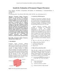
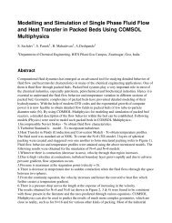
Fig. 1: CAD Model of the geometry objects.The dimensions are given in millimeters.Throughout this paper a cantilever of dimensionslength L = 450µm, width W =50µm and thickness T = 2µm was investigated,which was built from crystalline silicon.In the experimental setup correspondingto the models the cantilever was excitedby a 0.5 mm thick piezo plate of the ceramicPIC255 produced by PI (Physik InstrumenteGmbH & Co. KG, Karlsruhe/Palmbach,Germany). Piezo material data for PIC255were unavailable from PI, however, and wefollowed the recommendation of PI to usethe data of PIC155 in simulations instead,which was said to show up a very similarbehavior. The computing system used forsimulations comprised as hardware an AMDAthlon 64 X2 Dual Core 3800+ processor operatedat 2 GHz and 3.25 GB RAM. The systemwas operated by Microsoft Windows XPProfessional, Version 2002, SP2 (32-bit version),and the software COMSOL 3.4.0.250together with MatLab 7.1.0.246 (R14), SP3was installed.3 Models3.1 Model 1With the aim of realizing a numerical procedurefor solving the continuum mechanicsof all the components described in Fig. 1,all their physical and dynamical aspects hadto be considered and duly described. Thissubsection gives an insight of the major aspectsthat were crucial in development ofthe first model, which involved two differentCOMSOL modules, the structural mechanicsmodule and the MEMS module.Options of both modules were combinedin a single multiphysics model such that asolid, stress-strain domain from COMSOL’sstructural mechanics package and a piezosolid domain from the MEMS package wasbuilt. The geometrical components weredesigned using Autodesk Inventor and importedinto the COMSOL environment usingthe CAD import tool. A set of boundaryconditions was introduced in order tocorrectly couple the different compounds ofthe model. These consisted of two mechanicaland one electrical boundary conditions.One of the former conditions consisted in thefixation of the chip-holder to the piezo element.The other mechanical boundary conditionspecified the fixation of the lower surfaceof the piezo element. The piezo’s axis ofpolarization was defined to be along the z-axis. The electrodes were defined such thatthe electric field across the element had onlya z-component. Due to these conditions thepiezo was excited mainly to vibrations in z-direction. The uppermost face for the piezowas defined as the ground potential therebyrealizing the electrical boundary condition.The load versus response behavior is crucialin any FEM model. This mainly dependson the material properties of all componentswithin the system. The matrices

containing material property data of the mechanicalcomponents were imported fromCOMSOL’s material library. Data matricesof the PIC 155 piezo element used inthis model are presented in (1), (2) and (3),where c E is the elasticity matrix, e the couplingmatrix and ɛ S the relative permittivity.c E =e =⎡⎢⎣10.1 6.33 6.33 0 0 06.33 10.1 6.33 0 0 06.33 6.33 1.01 0 0 00 0 0 1.91 0 00 0 0 0 1.91 00 0 0 0 0 2.38×10 10 P a(1)[ 0 0 0 0 10.3] 00 0 0 10.3 0 0−5.6 −5.6 12.8 0 0 0× C m 2 (2)ɛ S =3.2 Model 2[ 873 0 00 873 00 0 680](3)The design of the second model aims at asimplification of the simulation process. Forthis purpose a frame of reference is chosensuch that the sinusoidally excited contactarea of the piezo and the cantilever chipstays at rest within this frame (Fig. 1(b)).The multiphysics model in this case was setusing only the solid, stress-strain option.The fix position of the contact area pointsrepresents the only boundary condition to beconsidered within this model. Since the simulationno longer takes place in an inertialsystem but in an accelerated frame of reference,fictitious forces F f have to be takeninto account.Figure 1: Schematic representation of theinertial system (a) and the accelated frame ofreference system (b) as defined for model 1 and2 respectively. Blue rectangle: Chip pluscantilever.⎤⎥⎦The vertical coordinates z, z ∗ within thetwo different frames of reference are relatedviaz = z ∗ + Asin(ωt) (4)The vertical dynamics of a mass element min the inertial system (Fig. 1(a)) is describedby Newtons second lawF z = m¨z (5)where F z denotes the vertical component ofthe sum of all forces acting on the mass. Ingeneral F z can be categorized into internalforces (elastically transmitted through thematerial) and external forces (electric, magnetic,frictional, viscous, gravitational). Forthe treatment in this paper we neglect allexternal forces besides those acting on theboundary between the chip and piezo dueto excitation. Insertion of equation (4) intoequation (5) leads toF z = m ¨ z ∗ − mAω 2 sin(ωt),which can be converted toF ∗ z := F z + mA 2 sin(ωt) = m ¨ z ∗ . (6)Equation (6) represents Newtons second lawin the accelerated frame of reference. Hereone has to take into account a fictitious forceF f = mAω 2 sin(ωt) in addition to the forcesF z present in the inertial system. Insteadof forces F one considers loads L z := F z /Vin continuum mechanics, where V denotes avolume element. Hence Newtons second lawreads in terms of loadsL ∗ := L z + L f = ρ ¨ z ∗ (7)with the load L z := F z /V , the fictitious loadL f := ρAω 2 sin(ωt) and the material densityρ := m/V . It is worthwhile to note that thefictitious load depends on the excitation frequencyω.During the simulation the fictitious loadwas calculated and updated after each stepin excitation frequency. The excitation amplitudewas kept constant at a value A, definedas the average value of the vibrationamplitudes of the contact points on the interfacebetween the holder and the chip inmodel 1.

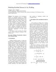
These displacements were used to determinethe cantilever displacement amplitudes andits resonance frequency. To arrive at thisinformation, calculations were made for anumber of frequencies using the frequencyresponse option.Essentially the electro-mechanical FEMequations representing piezoelectric materialsare summarized into a couple of equationsand are grouped into two categories.These are the stress-charge form and thestrain-charge form. The former is definedwithin COMSOL asFigure 2: Geometry of the meshed single-siliconcantilever beam with a pyramidal tip.T = c E S − eE (9)4 MethodsThe relation between displacement andstrain is essential in the formulation of FEMelements [6]. Strain can be defined as the geometricalexpression of displacements causedby the action of stress on a physical body.Nodal displacements (u, v and w) were theprimary unknowns in this work. The stressfield in both, model 1 and 2, originated fromthe vibration of the piezo element. The shearand normal strain present on the chip andthe cantilever were therefore known. Theywere determined through the calculation ofinternal stresses within the piezo element.From the strain-displacement relations thedisplacements sought could be determined.These relations can be stated in matrixoperatorform according to [6] as⎧⎪⎨ɛ xɛ y⎫⎪ ⎬ɛ z=γ xyγ yz ⎪ ⎭γ zx⎡∂∂x0 0∂0∂y0∂0 0∂z∂ ∂⎢∂y ∂x0⎣⎤⎧⎨⎩⎥⎦uvw⎫⎬⎭ ,∂ ∂0 ⎪⎩∂z ∂y∂∂∂z0∂x(8)where ɛ and γ represent normal and shearstrain respectively. Within COMSOL’sstructural mechanics package there are welldefined and highly optimized tools for solvingsuch systems. After a thorough definitionof the model and the boundary conditionswithin the COMSOL environment asdiscussed in the previous sections a solverroutine was run to compute the solution.Nodal displacements along the z-axis of thecantilever beam were of special interest.D = e + ɛ S E, (10)where T is the stress vector, S the strain vector,E the electric field vector, D the electricflux density vector, c E the elasticity matrix,e the piezoelectric coupling matrix in stresschargeform and ɛ S the matrix of relativepermittivity. The stress-charge form is usedthroughout this work. Material characteristicsare stored in the matrices c E , e and ɛ S ,which are presented in (1), (2) and (3).In model 2, since the fictitious force dependson the excitation frequency, the fictitiousload L f had to be calculated iterativelyfor each calculation step. The frequency responsewas therefore implemented in Mat-Lab. Values of L f were calculated at initializationand then passed on to an automaticallygenerated COMSOL script in vectorform. In the calculation a loop was implementedusing frequency as the loop variable.For each frequency step the respectivevalue of L f was read, the solution was calculatedand the results were saved in a matrix.At the end of the for loop the results wereassigned to the fem.sol structure for postprocessingpurposes.5 Results and DiscussionBy analytical methods the flexural naturalfrequencies of a cantilever can be calculated[5]. Using the cantilever geometry describedin Section 2 and the silicon material propertiesdensity ρ = 2.33g/cm 3 and Young’smodulus E = 169GP a we arrived at a frequencyf (1)theo = 13.586kHz

for the first vertical flexural natural mode.This calculated value is located in theresonance frequency specification rangef (1)manuf= (13 ± 4)kHz stated by the manufacturerof the cantilever. In the neighborhoodof this value simulations were performedwithin the frequency response optionof COMSOL. Fig. 1 shows the simulated amplitudeof a point at the end of the cantileverin dependence on frequency. Clearlya peak at f (1)model1= (13600±5)Hz is visible.The simulation time for the 40 data pointsamounted to t model1 = 54min. Furthermorethe displacement amplitudes of points on thecantilever surface at the frequency f (1)model1are shown in Fig. 2. The figure clearly indicatesthat the cantilever vibrates in the firstvertical flexural natural mode.this value into the simulations according tomodel 2. We observed that the piezo amplitudedelicately depends on the boundaryconditions, describing how the piezo is embeddedwithin its environment. A freely oscillatingpiezo plate of the material PIC155is ideally expected to vibrate with an amplitudeA theo = d 33 · 0.5V = 3.07 × 10 −10 m/V ·0.5V = 0.1535nm. However, in a systemwhere the piezo plate is fixed with its surfacesto other components the vibration amplitudeis substantially decreased. Furthermoredeformations of other parts of the system,e.g. the aluminum holder plate, alsohave to be taken into account. Fig. 3 showsthat as well the piezo plate as the aluminumholder deform in directions parallelto the piezo plate surfaces. In our simulatedsystem the vibration amplitude at 0.5V excitation voltage and 13.6 kHz excitationfrequency amounted to A sim,piezo =0.0395nm measured at the upper piezo surfaceand A sim,holder = 0.0430nm measuredat the fixation points between the holderplate and the cantilever chip. Further thevalue A sim,holder was used as basis withinmodel 2.Figure 1: Amplitude of the end of thecantilever vs. excitation frequency. Solidcircles: model 1. Open circles: model 2. Solidlines just serve as a guide to the eye.Figure 2: Displacement amplitudes of thecantilever vibrating at 13600Hz. Simulationbased on model 1. (Deformation exaggerateddue to specification of the deformed shapeoption.)The results within model 1 were comparedto simulations based on model 2. Inorder to match the simulations within the2 models, one has to determine the amplitudeA of oscillation in model 1 and feedFigure 3: Displacement amplitude inz-direction of piezo plate and aluminumcantilever holder. (Deformation exaggerateddue to specification of deformed shape option.)The total system was simulated according tomodel 1 at 13.6 kHz, cantilever and chipcomponents are suppressed within the figure.Results of simulations according tomodel 2 are included in Fig. 1. They matchwell the results based on model 1 and showup a similar resonance frequency peak at= (13600 ± 5)Hz. Simulation timeamounted to t model2 = 16min. In conclusionthe ratio of processing times of simulationsfollowing the 2 models is determinedas t model1 /t model2 = 3.375 ≈ 3.f (1)model2

The amplitude values obtained by bothmodels near the resonance frequency showdifferences. At the resonance frequencyof 13600Hz a relative deviation (250 −200)/250 = 20% occurs and at 13605Hz thedeviation is even more than a factor 2, butreversed. Based on the definition of the coordinatesystem in model 2 the amplitudesderived within this model are expected tobe by A = 0.0430nm smaller than the onesderived by model 1. Compared to amplitudevalues of more than 100 nm obtainedby simulation near the resonance frequency,however, this correction can be neglected.We rather expect that numerical inaccuraciessum up differently within the two modelsespecially near the resonance. As dampingof the cantilever was neglected in bothmodels amplitudes diverging to infinity areexpected for frequencies near the resonance.A proper treatment of the system should includedamping, however, damping was neglected,as it exceeded the capacity of thecomputer system in the used configuration.Resonance frequencies determined bysimulations according to the 2 models agreewell with the analytically derived frequencyf (1)(1) (1)theo. The difference fmodel1−ftheo = 14Hzof 0.1% can mainly be attributed to numericalinaccuracies due to the usage of finiteelements.6 ConclusionsDue to surging interests in operating anAFM in atmospheric or aqueous environment,complex simulation models are becomingmore and more crucial. The complexityhowever considerably increases thecomputational burden. Therefore a methodof diminishing processing load in simulationsby choosing a suitable accelerated coordinatesystem was developed in the work presentedin this article. The first vertical flexuralresonance of a cantilever was simulatedwithin different frames of reference. Withinboth models the estimated resonance frequenciesf (1)model1 = f (1)model2= (13600 ± 5)Hzexcellently agree with each other. They alsoagree well with the analytically derived resonancefrequency f (1)theo= 13586Hz calculatedby the formula for a clamped-free rectangularbeam. The amplitudes derived by thetwo models, however, largely disagree nearthe resonance frequency. We attribute thedifferences mainly to the missing implementationof damping within the simulations.Processing time of simulations in an acceleratedcoordinate system according to model2 was more than a factor 3 shorter thanfor simulations in model 1. Combined withother known solutions, which help to easecalculation load, the presented method canaid in decreasing the computing load andprocessing time in simulations of AFM cantilevervibrations.References[1] A. Raman, J. Melcher, and R. Tung,Cantilever dynamics in atomic forcemicroscopy, Nanotoday, Vol. 3, 20(2008)[2] W. W. Clegg, D. F. L. Jenkins, andM. J. Cunningham, The preparationof piezoceramicpolymer thick films andtheir application as micromechanicalactuators, Sensors and Actuators, Vol.58, 173 (1997)[3] U. Rabe, K. Janser, and W. Arnold,Vibrations of free and surface-coupledatomic force microscope cantilevers:Theory and experiment, Rev. Sci. Instrum.,Vol. 67, 3281 (1996)[4] C. C. Chou, et al., Simulation of anatomic force microscopy’s Probe consideringdamping effect, Proceedingsexcerpt, COMSOL users conferenceTaipei (2007)[5] U. Rabe, S. Hirsekorn, M. Reinsteadtler,T. Sulzbach, Ch. Lehrer andW. Arnold, Influence of the cantileverholder on the vibrations of AFM cantilevers,Nanotechnology., Vol. 18, 1(2007)[6] R. D. Cook, Concepts and Applicationsof Finite Element Analysis,3rded., John Wiley and Sons, New York(1989)[7] COMSOL 3.4, Multiphysics UsersGuide, COMSOL Version 3.4 (2007)[8] G. Scheerschmidt, K. J. Kirk, andG. McRobbie Finite Element Analysisof Resonant Frequencies in Sur-

face Acoustic Wave Devices, COMSOLUsers Conference, Birmingham (2006)AcknowledgementsThis work was supported by theDeutsche Forschungsgemeinschaft in projectNanoLatVib (FA 347/24-1).