Polynomial Regression Using Excel

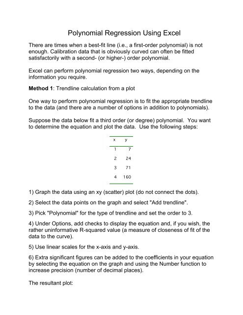
Polynomial Regression Using ExcelThere are times when a best-fit line (i.e., a first-order polynomial) is notenough. Calibration data that is obviously curved can often be fittedsatisfactorily with a second- (or higher-) order polynomial.Excel can perform polynomial regression two ways, depending on theinformation you require.Method 1: Trendline calculation from a plotOne way to perform polynomial regression is to fit the appropriate trendlineto the data (and there are a number of options in addition to polynomials).Suppose the data below fit a third order (or degree) polynomial. You wantto determine the equation and plot the data. Use the following steps:xy1 72 243 714 1601) Graph the data using an xy (scatter) plot (do not connect the dots).2) Select the data points on the graph and select "Add trendline".3) Pick "Polynomial" for the type of trendline and set the order to 3.4) Under Options, add checks to display the equation and, if you wish, therather uninformative R-squared value (a measure of closeness of fit of thedata to the curve).5) Use linear scales for the x-axis and y-axis.6) Extra significant figures can be added to the coefficients in your equationby selecting the equation on the graph and using the Number function toincrease precision (number of decimal places).The resultant plot:

yPolynomialRegression,yversusx180160140120100806040200y=2x 3 +3x 2 ‐6x+80 0.5 1 1.5 2 2.5 3 3.5 4 4.5xMethod 2: Using the Regression Function in the Data Analysis ToolpakWhile Method 1 is useful in providing basic information about a polynomialcurve, there is some information missing (such as the standard error in theestimates or the standard deviation in the residuals * ). It is possible to applythe Data Analysis ToolPak add-in to obtain this information.Suppose you want to analyze the Pb concentration in tap water usinggraphite furnace AAS. The following data (next page) were collected.Assuming the data fit a second-order polynomial, report theconcentration of lead in the tap water and its uncertainty.* The residual (or error) represents unexplained variation after fitting a regressionmodel. It is the difference between the observed value of the variable and the valuesuggested by the regression model.

1) First the data must be entered into an Excel worksheet.2) Since you want to generate a second order polynomial, you must theninsert another column after the Pb concentration column whose cellscontain the squared concentration values. (If you had wanted a thirdorder polynomial, you would insert another column containing the cubeof the concentration value. Etc.)

3) Select the Data Analysis ToolPak add-in Regression. When choosingthe X range, highlight the block that contains both concentrations andtheir squared values. (You would highlight additional x n columns forhigher order polynomials.) If you include headings in your selection, besure to check the Labels box. Also select the Confidence Level (95%)and the Residuals boxes.4) The data, a Method 1-generated calibration curve, and the output of theRegression add-in are posted on the course website (separate tabs inthe “Method 2 Output” Excel file). There is a lot of information that isextraneous. Here are the four things researchers most commonly lookfor; the last two will be of most interest to us:• R 2 and Adjusted R 2 : the R 2 value gives the percent variance of y thatis explained by the variance of the x value(s). Adjusted R 2 is moreconservative and therefore more likely to be quoted. The higherthese values (closer to 1), the better the data fit the curve.• Regression Significance F: This is the probability that the outputresults by chance rather than from a real correlation betweenindependent and dependent variables. The smaller the value, thegreater the probability that the results have not arisen by chance.• Coefficients for the intercept, x, x 2 , etc. (or their labels, if you hadused them) and their standard errors: These are the actualcoefficients for the equation of your polynomial curve. As withSignificance F, the smaller the P-values, the greater the probabilitythat the results have not arisen by chance.• Residuals: These have been previously defined qualitatively in afootnote. You want to see no pattern in these values and that theyare distributed around 0. You can do a quick scatter plot of thesedata to see if this is the case. If the residuals follow a pattern, thenthere is another factor that is affecting the correlation between yourindependent and dependent variables, possibly a systematic error inthe experiment or a physical phenomenon whose influence on thedata has not been taken into consideration.

5) As noted above, you now have the equation of your curve and you canuse it to calculate the Pb concentration (and its uncertainty, using thestandard errors given for your error propagation) in the tap watersample.Answer: Pb concentration is 44.3 ± 1.0 ppb, or 44 ± 1 ppb.