MODELING OF LOW SALINITY EFFECTS IN SANDSTONE OIL ...

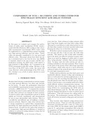
18 OMEKEH, EVJE, AND FRIISx 10 −4BetaMgx 10 −34.5BetaCa12 x 10−3BetaNa14121043.532.5108Initial0.133days0.3330.6671.3332.0004.0006.00082661.51440.520 0.5 1Dimensionless distance00 0.5 1Dimensionless distance0 0.5 1Dimensionless distanceFigure 5. Plots showing the behavior of the various β-functions along the coreat different times during a time period of 6 days, for the case with LSW as theinvading low salinity brine. Note that there is no desorption of the divalent ions(calcium and magnesium), only adsorption. Left: β mg . Middle: β ca . Right:β na .represented by relative permeability curves (15) versus oil recovery for the low salinity conditionsrepresented by relative permeability curves (16). See also Appendix B for specific data used forthe relative permeability functions. Results are shown in Fig. 4. This information is useful tohave in mind when we in the remaining part of this section consider brine-dependent oil recoverycurves.6.4. Example 1: Water flooding using different brines and fixed formation water. Herewe present simulations of corefloods. The core is composed of clay and other minerals that areassumed to be relatively chemically nonreactive typical of sandstone cores. The clay content/massof the core is given by M c (Kg/Liter of core) and clay capacity by CEC (moles/kg of clay), seeAppendix A for values. Initially the core is at equilibrium with formation water at initial watersaturation, S wi = 0.15, and oil. Subsequently, we flood the core with an invading brine at aflow velocity v T = 0.01 (meters/day) for a sufficiently long time, t days, till no appreciable oil isobtained from the core. The runs made in Example 1 are grouped into two groups: Case 1 inwhich we inject with a low salinity water and other brines modified from low salinity water (seeTable 1 in Appendix A) and Case 2 in which we inject seawater and other seawater based brines(see Table 2 in Appendix A).6.4.1. Case 1: Injecting low salinity water and low salinity modified brines. For thedifferent runs in this section, we inject with low salinity brine, LSW and modified low salinitybrines LSW1, LSW2 and LSW3. LSW is obtained by a 100 times dilution of formation water.LSW1 by 10 times dilution of formation water. LSW2 by reducing the magnesium component inLSW1 and LSW3 by reducing both divalent ions in LSW1. The brine compositions are given inTable 1 and all other parameters used in the runs are listed in appendix A and B.Fig. 5 shows the β-functions, which describe the amount of Mg 2+ , Ca 2+ , and Na + -ions bondedto the core, for injection of LSW brine. Initially, the formation brine is at equilibrium with therock, hence, there is a fixed amount of each ion bonded to the surface of the rock. This is denotedby the red curve in Fig. 5. On flooding the core with LSW, this equilibrium is disturbed and a newone is reached after some time. From the figure it is seen that there is no desorption of any of thedivalent ions (calcium and magnesium) but rather adsorption of the divalent ions and desorptionof the monovalent ion (sodium). Consequently, the H-function, which is the weighting factor forflow function alteration, remains equal to 1 at all times as shown in Fig. 7. We also show in Fig 6various ion concentrations C ca , C mg , C na , and C cl .