MODELING OF LOW SALINITY EFFECTS IN SANDSTONE OIL ...

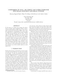
MODELING OF LOW SALINITY EFFECTS IN SANDSTONE OIL ROCKS 171Water Saturation0.940cells120cells0.80.70.6Sw0.50.40.30.20.100 0.1 0.2 0.3 0.4 0.5 0.6 0.7 0.8 0.9 1Dimensionless distanceFigure 3. Saturation profiles computed with 40 and 120 grid cells, respectively.The comparison is taken from SW flooding (Example 1, case 2).0.9Recovery0.80.70.6oil recovery0.50.4LSHS0.30.20.100 1 2 3 4 5 6Time (days)Figure 4. Plot showing the recoveries for HS and LS relative permeability curvesgiven in Fig. 2.6.2. Various data needed for the water flooding simulations. A range of input parametersmust be specified for the above model, and are given in Appendix A and B. We emphasize thatwe will use a fixed set of parameters for all simulations, unless anything else is clearly stated.The only change from one simulation to another is the brine composition and/or formation watercomposition (initial condition).6.3. A remark on the numerical resolution in the simulations. As stated earlier, theequation systems are solved explicitly. We think that the solutions provided by the explicit methodin this paper are sufficient for our present purpose, since we are interested in investigating thefundamental behavior of our one dimensional model. We first present a simulation case wherewe demonstrate convergence of the numerical solution. We have considered formation water FWand flooding water SW with ion concentrations as described in Table 2 in Appendix A. We havecomputed solutions on a grid of 40 cells and 120 cells, respectively. Result for the water saturationat different times is shown in Fig. 3. We conclude that it is sufficient to compute solutions on agrid of 40 cells. This will be done in the remaining part of the work.Before we start exploring how oil recovery can be sensitive for the brine composition of thewater that is used for flooding, we show two extremes: Oil recovery for the high salinity conditions