MODELING OF LOW SALINITY EFFECTS IN SANDSTONE OIL ...

INTERNATIONAL JOURNAL OFNUMERICAL ANALYSIS AND MODELINGVolume 1, Number 1, Pages 1–18c⃝ 2004 Institute for ScientificComputing and InformationMODELING OF LOW SALINITY EFFECTSIN SANDSTONE OIL ROCKSARUOTURE VOKE OMEKEH, STEINAR EVJE, AND HELMER ANDRÉ FRIISAbstract. Low salinity water has been reported as being capable of improving oil recovery in sandstone coresunder certain conditions. The objective of this paper is the development and examination of a one-dimensionalmathematical model for the study of water flooding lab experiments with special focus on the effect of low salinitytype of brines for sandstone cores. The main mechanism that is built into the model is a multiple ion exchange (MIE)process, which due to the presence of clay, will have an impact on the water-oil flow functions (relative permeabilitycurves). The chemical water-rock system (MIE process) we consider takes into account desorption and adsorptionof calcium, magnesium, and sodium. More precisely, the model is formulated such that the total release of divalentcations (calcium and magnesium) from the rock surface will give rise to a change of the relative permeabilityfunctions such that more oil is mobilized. The release of cations depend on several factors like (i) connate watercomposition; (ii) brine composition for the flooding water; (iii) clay content/capacity. Consequently, the modeldemonstrates that the oil recovery also, in a nontrivial manner, is sensitive to these factors. An appropriatenumerical discretization is employed to solve the resulting system of conservation laws and characteristic featuresof the model is explored in order to gain more insight into the role played by low salinity flooding waters, and itspossible impact on oil recovery.Key words. low salinity, multiple ion exchange, porous media, two-phase flow, convection-diffusion equations andwettability alteration1. IntroductionIn recent years, brine-rock-oil chemistry has generated a lot of interest in relation to improvingoil production from reservoirs. In carbonate reservoirs, the brine constituents have been foundto be important for oil recovery [37]. In sandstone reservoirs, the salinity and components of thebrine have shown a lot of promise to improve recovery [34, 42, 44]. A number of requirementshave been listed as being necessary for low salinity improved recovery. These include:- Presence of clay [40] or some negatively charged rock surfaces;- Polar components in the oil phase [35, 40];- Presence of formation water [40];- Presence of divalent ion/multicomponent ions in the formation water [24].Despite meeting the above criteria, some experiments carried out have not shown positive lowsalinity effect [36, 48]. We also refer to [33] for experimental observations indicating that lowsalinity water injection as an EOR method appears very sensitive to a combination of severalparameters.1.1. Different mechanisms that have been proposed. Quite a number of different low salinitymechanisms have been put forward in the literature. Some of these mechanisms include:• Multicomponent ion exchange (MIE) process [24]: This mechanism describes the releaseof oil component previously bonded to the rock surface by divalent ion bridging. Lowsalinity is said to result in a double layer expansion that makes the desorption of the oilbearing divalent ions from the rock surface possible.• pH increase: The authors of [40] describes a model, in which pH increase as a resultof mineral dissolution, is the underlying mechanisms for low salinity induced improvedReceived by the editors June 25, 2012 and, in revised form, November 23, 2012.2000 Mathematics Subject Classification. 35R35, 49J40, 60G40.This research has been supported by the Norwegian Research Council, Statoil, Dong Energy, and GDF Suez,through the project Low Salinity Waterflooding of North Sea Sandstone Reservoirs. The second author is alsosupported by A/S Norske Shell.1

2 OMEKEH, EVJE, AND FRIISrecovery. Austad et al.[6] describe a model of local pH increase as a result of a chemicalprocess involving the release of divalent ions from the rock surface.• Clay dispersion[40]: This mechanism describes a model in which oil-wetted clays aredispersed from the rock surface in low salinity environment. The desorption of divalentions can only aid such mechanism since divalent ions promotes clay flocculation.1.2. Main objective of this work. As an attempt to develop some basic understanding of howsuch mechanisms possibly will have an impact on core flooding experiments in the context of lowsalinity studies, we will in this work formulate a Buckley-Leverett two-phase flow model where thewetting state, as represented by the relative permeability functions, has been coupled to a multipleion exchange (MIE) process. In other words, in this work we have singled out MIE as the onlymechanisms for taking into consideration possible low salinity effects. More precisely, according tothe proposed MIE mechanism, we chose to link desorption of the divalent ions bonded to the rocksurface to a change of relative permeability functions such that more oil can be mobilized. Thiswill allow us to do some systematic investigations how different brine compositions can possiblyhave an impact on the oil recovery.Hence, the purpose of this work is to, motivated by laboratory experiments with flooding ofvarious seawater like brines, formulate a concrete water-rock chemical system relevant for sandstoneflooding experiments with focus on low salinity effects. Main components in the proposedmodel are:• Consider modeling of sandstone core plugs with a certain amount of clay attached to itthat is responsible for the ion exchange process;• Include a multiple ion exchange process that involve Ca 2+ , Mg 2+ , and Na + ions;• Implement a coupling between release of divalent ions (calcium and magnesium) from therock surface and a corresponding change of water-oil flow functions (relative permeabilitycurves) such that more oil can be mobilized.The resulting model takes the form of a system of convection-diffusion equations:(1)s t + f(s, β ca , β mg ) x = 0,(sC na + M c β na ) t + (C na f(s, β ca , β mg )) x = (D(s, ϕ)C na,x ) x ,(sC cl ) t + (C cl f(s, β ca , β mg )) x = (D(s, ϕ)C cl,x ) x ,(sC ca + M c β ca ) t + (C ca f(s, β ca , β mg )) x = (D(s, ϕ)C ca,x ) x ,(sC so ) t + (C so f(s, β ca , β mg )) x = (D(s, ϕ)C so,x ) x ,(sC mg + M c β mg ) t + (C mg f(s, β ca , β mg )) x = (D(s, ϕ)C mg,x ) x .For completeness, since we are interested in flooding of seawater like brines (high salinity andlow salinity), we have included chloride C cl and sulphate C so , despite that these will act onlyas tracers in our system. In other words, these ions are not directly involved in the water-rockchemistry model in terms of the MIE process. The unknown variables we solve for are watersaturation s (dimensionless), and concentrations C na , C cl , C ca , C so , C mg (in terms of mole perliter water). β na , β ca , and β mg are the concentrations of sodium, calcium, and magnesium bondedto the rock surface. Note that β i = β i (C na , C ca , C mg ), for i = na, ca, mg. Moreover, f(s, β ca , β mg )is the fractional flow function. The dependence on β ca and β mg is due to the proposed couplingbetween wettability alteration and desorption of the divalent cations Ca 2+ and Mg 2+ from therock surface. The quantity M c represents the mass of clay whereas D = D(ϕ, s) is the diffusioncoefficient which accounts for both molecular diffusion and mechanical dispersion. More detailsleading to this model are given in the subsequent sections. In the model (1), a characteristic timeτ = ϕLv Tand length scale L have been introduced.Such a model can potentially be a helpful tool for visualizing in a systematic manner therelatively complicated interplay between (i) change in injecting brine compositions; (ii) change information water compositions; (iii) clay content/capacity. This can also serve as a help to designnew laboratory experiments. In particular, we observe a number of different scenarios:

MODELING OF LOW SALINITY EFFECTS IN SANDSTONE OIL ROCKS 3• Certain low salinity brines can give rise to adsorption of both Ca 2+ and Mg 2+ ions. Thiswill give no additional oil recovery due to the fact that the model predicts no change inthe wetting state.• Other low salinity brines give rise to desorption of both Ca 2+ and Mg 2+ ions. This willgive favorable results as far as the oil recovery is concerned.• Seawater type of brines may show adsorption of Mg 2+ ions and desorption of Ca 2+ ions.This will in turn give oil recovery curves that sometimes are different from those obtainedby using the low salinity brines.• Whether desorption or adsorption of divalent ions will take place is also a result of theformation brine composition relative to the injecting brine composition.We remark that capillary pressure is being neglected in this paper. Depending on the flow velocityand the particular capillary pressure curves, capillary pressure effects might be significant on thecore scale. In addition the so-called capillary end effect will always be present when laboratorycoreflood experiments are performed. We also mention that the capillary pressure might be affectedby wettability changes as studied in this work. However, as emphasized above our main intentionis to obtain a basic understanding of the proposed flow model with the MIE process as a lowsalinity mechanism. For that purpose it is preferable to keep the mathematical model as simple aspossible, in order to avoid unnecessary complications in the interpretation of the model behavior.Moreover, capillary pressure is not expected to influence the ion exchange to a large extent. Thisprocess is affected mainly by the ion concentrations, clay content and selectivity. Our results willthus essentially cover laboratory behavior that is relevant for a larger scale where capillary pressureoften plays a minor role. Effects of including capillary pressure as well as mineral solubility in thepresent mathematical model will be explored in a future paper.1.3. Other works. A lot of work on low salinity have been published in the literature. Wegroup them under experimental and modeling works. While a lot of experimental work havebeen published, relatively few modeling works can be found. The authors of [21] and [44] carriedout standard waterflood with Moutray crude oil and Berea sandstone to show the effect of brinecomposition on oil recovery. Their work showed that ageing and flooding with CaCl 2 based brinegave more recovery than NaCl brine. Sharma and Filoco [35] studied the effect of salinity onrecovery of Berea sandstone cores with crude oil and NaCl brines. Beneficial low salinity effectwas reported when both the connate and the invading brine was of the same salinity, but no effectwas seen when the invading brine was of lower salinity than the connate brine or when refinedcrude was used.The authors of [5],[39] and [48] performed secondary waterflood experiments (i.e., injected brinedifferent from connate brine) with Berea sandstone. Tang and Morrow [39] reported beneficialeffect with injection of low salinity water independent of the valency of the invading brine. Zhangand Morrow [48] used three groups of Berea sandstone (60md, 500md and 1100md ) and reportedno tangible low salinity effect in the 60md and 1100md cores. Ashraf et. al [5] studied the lowsalinity effect at different wetting conditions by using different oil with different wetting conditionswith the Berea sandstone and connate brine. Ashraf et. al [5] reported different degrees of lowsalinity success with each wetting condition; a water wetting state was reported to perform best.Alotaibi et al. [3],Boussour et al. [33], Cissokho et al.[13], Pu et al. [31] and Skrettinglandet al. [36] carried out tertiary waterflood experiments. This involves injecting with the connatebrine before changing to a different invading brine at a high water cut after breakthrough, usuallywhen no more oil is produced with the connate brine. Alotaibi et al. [3] flooded with Berea coreand reported mixed result with low salinity injection, depending on the water-rock interaction.Cissokho et al. [13] used an outcrop sandstone core with another clay type apart from kaoliniteand reported improved low salinity recovery. Skrettingland et al. [36] used north-sea reservoircores and reported very minor response to low salinity at both high pressure and low pressurefloods. Pu et al. [31] used a reservoir core with almost no clay content but with substantialamount of dolomite crystal and reported low salinity response in spite of the near absence of clay.Finally, Webb et al. [43] determined the water-oil relative permeability curves of high andlow salinity water using cores from different sandstone reservoirs and performed the experiments

4 OMEKEH, EVJE, AND FRIISunder full reservoir conditions. In particular, different water-oil relative permeability curves forhigh and low salinity water was reported. Berg et al. [9] devised an experiment where they wereable to film the release of oil droplets bonded to clay layers when the clay layers were exposed tolow salinity water in a flow cell. The authors attributed this release of oil droplets to either doublelayer expansion or cation exchange.The above review deals with experimental related works. We now mention some of the modelingrelated work we are aware of which seems relevant for low salinity flooding experiments.The authors of [22], [41] and [47] modeled beneficial low salinity effects by directly linking thebrine salinity to the flow conditions (relative permeability and/or capillary pressure). Using thisprinciple, Tripathi et al. [41] studied flow instability at the saturation fronts. Jerauld et al. [22]studied the dispersion at the saturation front. Yu-shu and Baojun [47] included the possible adsorption/desorptionof salt but did not link the adsorbed salt to improved flow functions. Twohighly interesting works, in view of the proposed model (1), are represented by [38] and [29]. Theystudied a general system of the form(2)s t + f(s, c) x = 0,(cs + a(c)) t + (cf(s, c)) x = 0,for n components c = (c 1 , . . . , c n ). If diffusion effects are ignored in model (1), it can be consideredas a special case of (2). The authors of [38] and [29] introduced a reformulation of themodel by employing a coordinate transformation which decouples the hydrodynamic part fromthe thermodynamic. Hence, they could produce analytical solutions for various problems. Suchtechniques could most likely be used for our model to allow for fast calculations. However, it isbeyond the scope of this work since the main objective here is to obtain a model which can beused to test various hypothesis for how low salinity effects may impact the oil recovery. We wouldalso mention that the model (1) is a generalization of the one studied in [45, 46] in the sense thatin those works only adsorption of a single component is considered, not a multiple ion exchangeprocess involving several components.Finally, the model we are presenting in this paper has been used in [28] to explain the behaviorobserved in some low salinity waterflood experiments where expected low salinity improvedrecovery were not seen.1.4. Structure of paper. The rest of this paper is organized as follows: In Section 2 we mathematicallydescribe the multiple ion exchange process built into the flow model. In Section 3 weexplain how the MIE process is linked to a change of the wetting state as represented by two setsof relative permeability functions referred to as high salinity and low salinity conditions. Section4 gives a presentation of the flow equations where the two-phase flow and ion concentration flowdynamics are accounted for. In Section 5 some details are given of the numerical approach usedto solve the coupled system (1). Finally, Section 6 presents a number of different flow cases whosepurpose is to illustrate basic features of the model as a tool to explore the relation between thebehavior of the MIE process and oil recovery curves.2. Modeling of the multiple ion exchange (MIE) processIn this section we describe the multiple ion exchange process we shall rely on in this work.2.1. Generally. We distinguish between concentration C and chemical activity a noting thatthey are related by(3) a = γC,where γ is the activity coefficient. According to the extended Debuye-Hückel equation, see forexample [4, 25] and [27] (page 25), the activity coefficient γ i is given by√I0(4) log 10 (γ i ) = −AZ2 i1 + a 0 i B√ + bI 0 ,I 0where the index i refers to the different species involved in the system which is studied. Moreover,Z i refers to the ionic charges, b is an extended term parameter, A(T ) and B(T ) are temperature

MODELING OF LOW SALINITY EFFECTS IN SANDSTONE OIL ROCKS 5dependent given functions [4, 19], similarly for the constants a 0 i , whereas I 0 refers to the ionicstrength defined by(5) I 0 = 1 ∑C i Zi 2 .2For the numerical calculations, we calculate I 0 in each grid block based on the ion concentrationsfor the previous time step. Consequently, I 0 is always updated throughout the flooding process.Hence the activity coefficients are updated as well, according to equation (4).2.2. Cation exchange. The cation exchange model include the following ions: Na + , Ca 2+ andMg 2+ . Though the proton (H + ) ion has a stronger displacing power, its concentration in oilreservoirs is considered to be low in comparison to the other ions in reservoir condition. Typicallythe pH of oil reservoirs fall in the range between 5-7 fixing the H + concentrations at between 10 −5to 10 −7 which is low compared to the other cation concentrations (see Tables 1, 2, 3 and 4). Forthis reason we expect that the H + concentration on the clay surface to be negligible compared tothe other cations and we have chosen not to include it in the ion exchange reactions.We model the cation exchange using the Gapon model.12 Ca2+ + Na-X ⇋ Ca 1 -X + Na+ ,2(6)12 Mg2+ + Na-X ⇋ Mg 1 -X + Na+ .2This model has been used in the modeling of cation exchange in chemical flooding [30]. TheGapon model is based on a single monovalent exchange site and as such makes no difference onthe choice of unit for the activity of the absorbed ion [4]. The model can also be expressed as anequivalent of the Langmuir multicomponent isotherm as done in equations (11), (12) and (13).There have been concerns about the performance of the model when several heterovalent ionsare present. However it is popular among soil scientists and has been used extensively to modelirrigation systems containing Na + , Ca 2+ and Mg 2+ [4].Other popular ion exchange models make use of the number of exchangeable cations conventionand the reaction written thus12 Ca2+ + Na-X ⇋ 1 2 Ca-X 2 + Na + ,(7)12 Mg2+ + Na-X ⇋ 1 2 Mg-X 2 + Na + .Expressing the exchange reactions as done in (7) makes the choice of the unit for the activity of theabsorbed specie important. The Gaines–Thomas model uses equivalents as units of the absorbedspecie. The use of molar units for the absorbed species follows the Kerr or Vanslow convention.The exchange reactions are supposed to take place at a fast rate. Constant selectivity factorsK cana and K mgna are assumed, and using the Gapon model (6) they are expressed as(8) K cana = β caγ na C naβ na√γca C ca,(9) K mgna = β mgγ na C naβ na√γmg C mg,and(10) β na + 2β mg + 2β ca = CEC,where β na , β mg and β ca are the number of moles of Na + , Mg 2+ and Ca 2+ ions attached to a unitmass of clay. The CEC as used here is the Cation Exchange Capacity in equivalent/Kg. Theequation system (8), (9) and (10) is linear in the variables β na , β mg and β ca , and a solution caneasily be obtained. We find that(11) β na (C na , C ca , C mg ) =iγ na C na CEC2K cana√γca C ca + 2K mgna√γmg C mg + γ na C na,

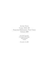
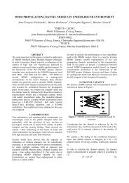
6 OMEKEH, EVJE, AND FRIISBeta Cabeta Cax 10 −34.543.532.521.510.50.10.20.30.40.5Mg2+ (mole/liter)0.60.70.20.410.80.6Ca2+ (mole/liter)1.21.4Figure 1. Plot showing β ca as a function of varying C ca and C mg concentrations,and with C na = 0.15 (moles per liter). Other parameters in (12) like K cana ,K mgna , and CEC, are listed in Appendix A.(12) β ca (C na , C ca , C mg ) =and(13) β mg (C na , C ca , C mg ) =K cana√γca C ca CEC2K cana√γca C ca + 2K mgna√γmg C mg + γ na C na,K mgna√γmg C mg CEC2K cana√γca C ca + 2K mgna√γmg C mg + γ na C na.We note that the equations (11), (12) and (13) are equivalent to a Langmuir-type adsorptionisotherm. Fig. 1 illustrates how the β ca function depends on the concentrations C na , C ca , C mg .At high magnesium concentration, the amount of calcium ion adsorbed on the rock, β ca , becomesquite low.3. Coupling of wettability alteration to changes on the rock surfaceThis section discusses aspects concerning the flow functions. Since we only consider flows withoutcapillary pressure in Section 6, we limit the discussion to the relative permeability functions.The following ideas are also employed in [14, 15], however, in the context of spontaneous imbibitionon chalk cores where capillary forces are the driving forces in oil recovery. It also partially followsideas employed in previous works in [22, 41, 45].3.1. Relative permeability functions. As a basic model for relative permeability functionsthe well-known Corey type correlations are used [12]. They are given in the form (dimensionlessfunctions)(14)k(s) = k ∗( s − s)wrNk,swr ≤ s ≤ 1 − s or ,1 − s or − s wr( 1 −k o (s) = ko∗ sor − s) Nko,swr ≤ s ≤ 1 − s or ,1 − s or − s wrwhere s wr and s or represent critical saturation values and Nk and Nk o are the Corey exponentsthat must be specified. In addition, k ∗ and k ∗ o are the end point relative permeability values thatalso must be given. Now, we define two extreme relative permeability functions corresponding tothe wetting state of the rock for high salinity and low salinity conditions.

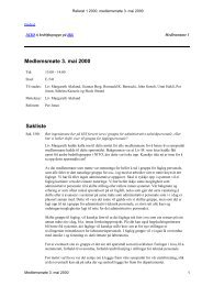
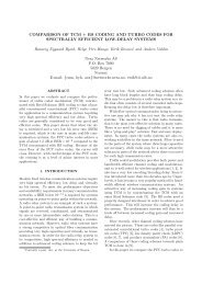
MODELING OF LOW SALINITY EFFECTS IN SANDSTONE OIL ROCKS 7Relative permeability0.90.80.70.60.50.40.30.2krw−HSkro−HSkrw−LSkro−LSfractional flow10.80.60.40.2HSLS0.100 0.1 0.2 0.3 0.4 0.5 0.6 0.7 0.8 0.9 1Water Saturation00 0.2 0.4 0.6 0.8 1Water SaturationFigure 2. Left: Example of relative permeability curves corresponding to highsalinity(HS) and low-salinity (LS) conditions. Right: Corresponding fractionalflow functions.3.1.1. High salinity conditions. This is assumed to be the initial state of the core. The valuesfor generating the functions are listed in Appendix B. Applying the values of the high salinitycondition in (14) the following two relative permeability curves are obtained(15) k HS (s; s HSwr , s HSor ),koHS (s; s HSwr , s HSor ),We refer to Fig. 2 for a plot of these curves (red line).for s HSwr≤ s ≤ 1 − s HSor .3.1.2. Low salinity conditions. This wetting condition is assumed to be attained only whenthere is complete desorption of Ca 2+ and Mg 2+ ions from the rock surface. The values for generatingthe functions are listed in Appendix B. Applying the values of the low salinity condition in(14) gives corresponding relative permeability curves(16) k LS (s; s LSwr , s LSor ),koLS (s; s LSwr , s LSor ),for s LSwr ≤ s ≤ 1 − s LSor .We refer to Fig. 2 for a plot of these curves (blue line). The motivation for the choice of the valueswas to match the form of the relative permeability measured for a variety of high salinity and lowsalinity brines in [43].3.2. Cation exchange as a mechanism for wettability alteration. We let β ca0 and β mg0be the amount of calcium and magnesium, respectively, initially bounded to the clay surface. Wethen define the quantity(17) m(β ca , β mg ) := max(β ca0 − β ca , 0) + max(β mg0 − β mg , 0),as a measure for the desorption of cations from the clay. Moreover, we define(18) H(β ca , β mg ) :=11 + rm(β ca , β mg ) ,where r > 0 is a specified constant. Note that the choice of r determines the extent in which thedivalent ion desorbed leads to a certain change of the wetting state.The function H(β ca , β mg ) is a weighting function, and works such that H = 1, when there is nodesorption of calcium and magnesium from the rock, whereas 0 < H < 1 in case of desorption ofat least one of these cations. How fast H(β ca , β mg ) is approaching 0 as m(β ca , β mg ) is increasing,depends on the choice of r. Now, the weighting function H(β ca , β mg ) can be used to represent thewetting state in the core plug; H(β ca , β mg ) = 1 corresponds to the initial oil-wet state, whereasH(β ca , β mg ) ≈ 0 represents the water-wet state. By defining relative permeability curves by meansof the weighting function H(β ca , β mg ) as described in the next subsection, the model can account

8 OMEKEH, EVJE, AND FRIISfor a dynamic change from an initial high salinity state towards a low salinity state controlled bythe degree of desorption of calcium and magnesium from the core.3.3. Modeling of transition from high salinity to low salinity conditions. In this work, wefollow along the lines of [14, 15], and model wettability alteration by defining relative permeabilitycurves through an interpolation between the high salinity and low salinity curves given by (14),combined with the data specified in Appendix B as given by (97) and (98).More precisely, motivated by the proposed hypothesis that transition from a high salinity wettingstate towards low salinity conditions depends on the desorption of calcium and magnesiumcaused by the cation exchange process, the following interpolation is proposed:(19) k(s, β ca , β mg ) = H(β ca , β mg )k HS (s) + [1 − H(β ca , β mg )]k LS (s),where H(β ca , β mg ) is defined by (18). Hence, when no desorption of divalent cations from the claysurface takes place it follows that H(β ca , β mg ) = 1, implying that k(β ca , β mg ) = k HS (s). Thisreflects the initial high salinity wetting state. Then, as desorption of divalent cations takes place,it follows that m(β ca , β mg ) increases. In particular, if the desorption effects becomes large enough,it follows from the above discussion (see equation (18)) that H(β ca , β mg ) ≈ 0, which means thatk(s, β ca , β mg ) ≈ k LS (s), reflecting that a wettability alteration has taken place which results in alow salinity wetting state.4. The coupled model for water-oil flow and multiple ion exchangeWe now want to take into account convective and diffusive forces associated with the brine aswell as the oil phase. In order to include such effects we must consider the following equations forthe total concentrations ρ o , ρ l , ρ ca , ρ so , ρ mg , ρ na , ρ cl (mol per liter core):(20)∂ t ρ o + ∇ · (ρ o v o ) = 0,∂ t ρ l + ∇ · (ρ l v l ) = 0,∂ t ρ na + ∂ t (M c β na ) + ∇ · (ρ na v g ) = 0,∂ t ρ cl + ∇ · (ρ cl v g ) = 0,∂ t ρ ca + ∂ t (M c β ca ) + ∇ · (ρ ca v g ) = 0,∂ t ρ so + ∇ · (ρ so v g ) = 0,∂ t ρ mg + ∂ t (M c β mg ) + ∇ · (ρ mg v g ) = 0,(oil flowing through the pore space)(water flowing through the pore space)(Na + -ions in water)(Cl − -ions in water)(Ca 2+ -ions in water)(SO 2−4 -ions in water)(Mg 2+ -ions in water).Here v o , v l and v g are, respectively, the oil, water and species ”fluid” velocities, whereas M crepresents the mass of the clay. The subsequent derivation of the model closely follows the work[14, 15], however, the water-rock chemistry in our current model is given in terms of a multipleion exchange process (MIE), not dissolution/precipitation as in [14, 15].Let s o denote the oil saturation, i.e. the fraction of volume of the pore space represented byporosity ϕ that is occupied by the oil phase, and s the corresponding water saturation. Thetwo saturations are related by the basic relation s o + s = 1. Furthermore, we define the porousconcentration C o associated with the oil component as the concentration taken with respect to thevolume of the pore space occupied by oil and represented by ϕs o . Hence, C o and ρ o are related by(21) ρ o = ϕs o C o .Similarly, the porous concentrations of the various components in the water phase are defined as theconcentration taken with respect to the volume of the pores occupied by water ϕs. Consequently,the porous concentrations C l , C na , C cl , C ca , C mg , and C so are related to the total concentrationsbyρ l = ϕsC l , ρ na = ϕsC na , ρ cl = ϕsC cl , ρ ca = ϕsC ca , ρ mg = ϕsC mg , ρ so = ϕsC so .Following, for example, [1, 2], we argue that since oil, water, and the ions in water Na + , Cl − ,Ca 2+ , Mg 2+ , and SO 2−4 flow only through the pores of the calcite specimen, the ”interstitial”velocity v o associated with the oil, v l associated with the water, and v g associated with theions, have to be defined with respect to the concentrations inside the pores, and differ from the

MODELING OF LOW SALINITY EFFECTS IN SANDSTONE OIL ROCKS 9respective seepage velocities V o , V l and V g . The velocities are related by the Dupuit-Forchheimerrelations, see [1] and references therein,(22) V o = ϕs o v o , V l = ϕsv l , V g = ϕsv g .Consequently, the balance equations (20) can be written in the form(23)∂ t (ϕs o C o ) + ∇ · (C o V o ) = 0,∂ t (ϕsC l ) + ∇ · (C l V l ) = 0,∂ t (ϕsC na ) + ∂ t (M c β na ) + ∇ · (C na V g ) = 0,∂ t (ϕsC cl ) + ∇ · (C cl V g ) = 0,∂ t (ϕsC ca ) + ∂ t (M c β ca ) + ∇ · (C ca V g ) = 0,∂ t (ϕsC so ) + ∇ · (C so V g ) = 0,∂ t (ϕsC mg ) + ∂ t (M c β mg ) + ∇ · (C mg V g ) = 0.In order to close the system we must determine the seepage velocities V o , V l and V g . For thatpurpose we consider the concentration of the water phase (brine) C that occupies the pore spaceas a mixture of water C l and the various species Na + , Cl − , Ca 2+ , Mg 2+ , and SO 2−4 representedby C g . In other words,(24) C g = C na + C cl + C ca + C mg + C so , C = C g + C l .Then, we define the seepage velocity V associated with C by(25) CV := C g V g + C l V l .Now we are in a position to rewrite the model in terms of V and the diffusive velocity U g givenby(26) U g = V g − V.Then the model (23) takes the form(27)∂ t (ϕs o C o ) + ∇ · (C o V o ) = 0,∂ t (ϕsC l ) + ∇ · (C l V l ) = 0,∂ t (ϕsC na ) + ∂ t (M c β na ) + ∇ · (C na U g ) = −∇ · (C na V),∂ t (ϕsC cl ) + ∇ · (C cl U g ) = −∇ · (C cl V),∂ t (ϕsC ca ) + ∂ t (M c β ca ) + ∇ · (C ca U g ) = −∇ · (C ca V),∂ t (ϕsC so ) + ∇ · (C so U g ) = −∇ · (C so V),∂ t (ϕsC mg ) + ∂ t (M c β mg ) + ∇ · (C mg U g ) = −∇ · (C mg V).Furthermore, we can assume that the seepage velocity V associated with the water phase representedby C, is given by Darcy’s law [1, 7, 26](28) V = −κλ(∇p − ρg∇d), λ = k µ ,where κ is absolute permeability, k is water relative permeability, and µ is viscosity, and p pressurein water phase. Similarly, for the oil phase(29) V o = −κλ o (∇p o − ρ o g∇d), λ o = k oµ o.The diffusive velocity U g is expressed by Fick’s law by(30) C i U g = −D∇C i , i = na, cl, ca, so, mg,where D is the diffusion coefficient. In view of (24) and (30), it follows that(31) C g U g = −D∇C g .Note that we assume that the diffusion coefficient D is the same for all species i = na, cl, ca, so, mg.This is a reasonable assumption as long as the concentration is not too high. D is the diffusion

10 OMEKEH, EVJE, AND FRIIScoefficient (longitudinal and transversal dispersion lengths are here taken to be equal), which issplit into molecular diffusion contribution and the so called mechanical/advective contribution. Awidely quoted formulation by Sahimi [32] is of the form(32)DD m= ϕ p s q + aP e + bP δ e + cP 2 e ,where D m is the free molecular diffusion coefficient, p, q, a, b, c, and δ are experimentally determinedconstants and P e is the Péclet number given by(33) P e = α|V|D m,where α is the characteristic dispersion length which varies from millimeters (in laboratory scale)to metres(field scale). Several authors [8, 32] have experimentally determined that the diffusionco-efficient is determined by only the first term of equation(32) when P e is less than 0.3, and atransition zone between 0.3 and 5 where D is not clearly defined. The other terms of the equationbecomes significant at higher Péclet numbers. For our application of the model, the Péclet numberfalls below 0.3, hence subsequently we use only the first term of equation (32). In (32) the coefficientp is referred to as the cementation exponent, q as the saturation exponent. The cementationexponent is often close to 2 whereas the saturation exponent is also often fixed at a value in thesame range, see for example [8, 10, 11]. Using (30) in (27) yields(34)∂ t (ϕs o C o ) + ∇ · (C o V o ) = 0,∂ t (ϕsC l ) + ∇ · (C l V l ) = 0,∂ t (ϕsC na ) + ∂ t (M c β na ) − ∇ · (D∇C na ) = −∇ · (C na V),∂ t (ϕsC cl ) − ∇ · (D∇C cl ) = −∇ · (C cl V),∂ t (ϕsC ca ) + ∂ t (M c β ca ) − ∇ · (D∇C ca ) = −∇ · (C ca V),∂ t (ϕsC so ) − ∇ · (D∇C so ) = −∇ · (C so V),∂ t (ϕsC mg ) + ∂ t (M c β mg ) − ∇ · (D∇C mg ) = −∇ · (C mg V).In particular, summing the equations corresponding to C na , C cl , C ca , C so , and C mg , we obtain anequation for C g in the form(35) ∂ t (ϕsC g ) + ∂ t (M c [β na + β ca + β mg ]) − ∇ · (D∇C g ) = −∇ · (C g V).In a similar manner, using C l V l = C l V − C g U g (obtained from (25), (26), and (24)) in the secondequation of (34), the following equation is obtained(36)∂ t (ϕsC l ) + ∇ · (C l V) = ∇ · (C g U g ).Summing (36) and (35), we get the following equation for the concentration of the water phasewith its different chemical components, represented by C = C g + C l ,(37) ∂ t (ϕsC) + ∂ t (M c [β na + β ca + β mg ]) + ∇ · (CV) = 0.To sum up, we have a model in the form(38)∂ t (ϕs o C o ) + ∇ · (C o V o ) = 0,∂ t (ϕsC) + ∂ t (M c [β na + β ca + β mg ]) + ∇ · (CV) = 0,where D = D(ϕ, s) as given by (32).∂ t (ϕsC na ) + ∂ t (M c β na ) + ∇ · (C na V) = ∇ · (D∇C na ),∂ t (ϕsC cl ) + ∇ · (C cl V) = ∇ · (D∇C cl ),∂ t (ϕsC ca ) + ∂ t (M c β ca ) + ∇ · (C ca V) = ∇ · (D∇C ca ),∂ t (ϕsC so ) + ∇ · (C so V) = ∇ · (D∇C so ),∂ t (ϕsC mg ) + ∂ t (M c β mg ) + ∇ · (C mg V) = ∇ · (D∇C mg ),

MODELING OF LOW SALINITY EFFECTS IN SANDSTONE OIL ROCKS 114.1. Simplifying assumptions. Before we proceed some simplifying assumptions are made:• The oil and water component densities C o and C are assumed to be constant, i.e., incompressiblefluids;• The effect from the water-rock chemistry in the water phase equation (second equation of(38)) is neglected which is reasonable since the concentration of the water phase C is muchlarger than the concentrations of the ion exchange involved in the chemical reactions;• Constant porosity ϕ, absolute permeability κ, viscosities µ, µ o ;• One dimensional flow in a horizontal domain.• Capillary pressure is currently neglected as discussed in the introduction (Section 1.2).This results in the following simplified model:(39)∂ t (ϕs o ) + ∂ x (V o ) = 0,∂ t (ϕs) + ∂ x (V ) = 0,∂ t (ϕsC na ) + ∂ t (M c β na ) + ∂ x (C na V ) = ∂ x (D(ϕ, s)∂ x C na ),∂ t (ϕsC cl ) + ∂ x (C cl V ) = ∂ x (D(ϕ, s)∂ x C cl ),∂ t (ϕsC ca ) + ∂ t (M c β ca ) + ∂ x (C ca V ) = ∂ x (D(ϕ, s)∂ x C ca ),∂ t (ϕsC so ) + ∂ x (C so V ) = ∂ x (D(ϕ, s)∂ x C so ),∂ t (ϕsC mg ) + ∂ t (M c β mg ) + ∂ x (C mg V ) = ∂ x (D(ϕ, s)∂ x C mg ).In view of (28) and (29) in a 1D domain, we get(40)(41)V = − κλp x , λ(β ca , β mg ) = k(β ca, β mg )µV o = − κλ o p o,x , λ o (β ca , β mg ) = k o(β ca , β mg ),µ oMoreover, capillary pressure P c is defined as the difference between oil and water pressure(42) P c = p o − p,and is assumed to be zero in the following. Total velocity v T is given by(43)where total mobility λ Tv T := V + V o = −κ(λp x + λ o p o,x ) = −κλ T p x ,(44) λ T = λ + λ o ,has been introduced. Summing the two first equations of (39) and using that 1 = s+s o , implies that(v T ) x = 0, i.e., v T =constant and is determined, for example, from the boundary conditions. Fromthe continuity equation for s given by the second equation of (39) it follows (since V = −κλp x )(45) (ϕs) t + (−κλp x ) x = 0,where, in view of (43),Thus,(46)−κp x = v Tλ T.(ϕs) t + (v Tλλ T) x = 0.The fractional flow functions f(β ca , β mg ) and f o (β ca , β mg ) are defined as follows(47) f(s, β ca , β mg ) :=def(48)f o (s, β ca , β mg ) :=defUsing this in (46) implies thatλ(s, β ca , β mg )λ(s, β ca , β mg ) + λ o (β ca , β mg ) ,λ o (s, β ca , β mg )λ(s, β ca , β mg ) + λ o (β ca , β mg ) = 1 − f(β ca, β mg ).(49) (ϕs) t + v T f(s, β ca , β mg ) x = 0.

12 OMEKEH, EVJE, AND FRIISThe same procedure can be applied for the continuity equation for the different ions in water in(39). This gives the following equation for i = na, cl, ca, so, mg:(50)(ϕsC i ) t + (M c β i ) t + v T (C i f(s, β ca , β mg ) x = (D(ϕ, s)C i,x ) x ,i = na, cl, ca, so, mg.Thus, in view of (49) and (50), a model has been obtained of the form(51)∂ t (ϕs) + v T ∂ x f(s, β ca , β mg ) = 0,∂ t (ϕsC na + M c β na ) + v T ∂ x (C na f(s, β ca , β mg )) = ∂ x (D(ϕ, s)∂ x C na ),∂ t (ϕsC cl ) + v T ∂ x (C cl f(s, β ca , β mg )) = ∂ x (D(ϕ, s)∂ x C cl ),∂ t (ϕsC ca + M c β ca ) + v T ∂ x (C ca f(s, β ca , β mg )) = ∂ x (D(ϕ, s)∂ x C ca )∂ t (ϕsC so ) + v T ∂ x (C so f(s, β ca , β mg )) = ∂ x (D(ϕ, s)∂ x C so ),∂ t (ϕsC mg + M c β mg ) + v T ∂ x (C mg f(s, β ca , β mg )) = ∂ x (D(ϕ, s)∂ x C mg ).4.2. Scaled version of the model. First, we introduce the variables(52)c 1 := ϕsC na , c 2 := ϕsC cl , c 3 := ϕsC ca , c 4 := ϕsC so , c 5 := ϕsC mg .We also introduce the variables(53)B 1 = M c β na (C na , C ca , C mg ), B 3 = M c β ca (C na , C ca , C mg ), B 5 = M c β mg (C na , C ca , C mg ).Now let L be the the reference length, which here is chosen to be the length of the core. As timescale of the problem τ (sec) we use(54) τ = ϕLv T.We then define dimensionless space x ′ and time t ′ variables as follows(55) x ′ = x L , t′ = t τ .We introduce reference viscosity µ (Pa s), and reference diffusion coefficient D m (m 2 /s). Then wedefine dimensionless coefficients(56) D ′ m = D mD m, µ ′ = µ µ .Rewriting (51) in terms of the dimensionless space and time variables (55) and using (56), thefollowing form of the system is obtained (skipping the prime notation)(57)(58)∂ t (ϕs) + ∂ x (ϕf(s, β ca , β mg )) = 0,∂ t (c 1 + B 1 (c 1 , c 3 , c 5 )) + ∂ x (C na ϕf(s, β ca , β mg )) = δ∂ x (D m ϕ p s q ∂ x C na ),∂ t (c 2 ) + ∂ x (C cl ϕf(s, β ca , β mg )) = δ∂ x (D m ϕ p s q ∂ x C cl ),∂ t (c 3 + B 2 (c 1 , c 3 , c 5 )) + ∂ x (C ca ϕf(s, β ca , β mg )) = δ∂ x (D m ϕ p s q ∂ x C ca ),∂ t (c 4 ) + ∂ x (C so ϕf(s, β ca , β mg )) = δ∂ x (D m ϕ p s q ∂ x C so ),∂ t (c 5 + B 3 (c 1 , c 3 , c 5 )) + ∂ x (C mg ϕf(s, β ca , β mg )) = δ∂ x (D m ϕ p s q ∂ x C mg ),where the dimensionless characteristic number δ, is given by(59) δ = ϕD mLv T.We choose D m = Lv T in (56) such that δ = ϕ.4.3. Boundary and initial conditions. In order to have a well defined system to solve we mustspecify appropriate initial and boundary conditions.

MODELING OF LOW SALINITY EFFECTS IN SANDSTONE OIL ROCKS 134.3.1. Boundary conditions. At the inlet, the following Dirichlet boundary conditions areemployed(60) s(0 − , t) = s(1 + , t) = 1.0, C i (0 − , t) = C i (1 + , t) = C ∗ i ,for the species i = na, cl, ca, so, mg where Ci∗ is the specified ion concentrations of the brine thatis used. At the outlet extrapolation is employed both for s and the C i ’s.4.3.2. Initial data. Initially, the plug is filled with oil and 15.0% formation water. Thus, initialdata are given by(61) s| t=0 (x) = s init = 0.15, x ∈ [0, 1],and for i = na, cl, ca, so, mg,(62) C i | t=0 (x) = C i,0 , x ∈ [0, 1],for given initial concentration of the species C i,0 in the water phase (formation water).5. Numerical discretizationThe numerical discretization of the resulting nonlinear convection-diffusion system is based onthe same approach as that used in [45, 46], and we refer to these works for more details. However,for completeness we briefly sketch the discretization of the nonlinear convective term. The diffusionterm is discretized by using a standard central discretization.5.1. Discretization of convective flux. Consider now a system of conservation laws in onespace variable(63)∂ t w + ∂ x F (w) = 0,where F (w) ∈ R n is a smooth vector-valued function. The discretization of the nonlinear convective(advective) flux is based on the relaxed scheme by Jin and Xin [23]. The relaxed scheme canbe written in the following ”viscous” form(64)⎧⎪⎨⎪⎩w n+1j = w n j − λ( ˆF n j+1/2 − ˆF n j−1/2), λ =∆t∆xwhere()ˆF j+1/2 = 1 2F (w j ) + F (w j+1 ) − 1 2 A1/2 (w j+1 − w j ),where A 1/2 plays the role as the “viscosity matrix” which determines the numerical dissipation ofthe scheme. Here we must require that the well known subcharacteristic condition holds given by(65)A − F ′ (w) 2 ≥ 0, for all w.In our case it suffices to choose that A has the special form(66)A = aI, a > 0where I is the identity matrix. In the case of one space variable (as we consider) and where weassume (66), the dissipative condition (65) is satisfied if(67)λ 2 < a,where λ = max 1≤i≤n |λ i (w)| where λ i are the genuine eigenvalues of F ′ (w).The relaxed scheme (64) can also be viewed as a flux splitting scheme. To see this we write thesystem as(68)⎧⎪⎨where we have (for the first order scheme) that⎪⎩w n+1j = w n j − λ( ˆF n j+1/2 − ˆF n j−1/2 )whereˆF j+1/2 = F + j+1/2,− + F − j+1/2,+ ,F + j+1/2,− = F + (w j ), F − j+1/2,+ = F − (w j+1 ),

14 OMEKEH, EVJE, AND FRIISand where we have used the Lax-Friedrichs flux splitting(69)F ± (w) = 1 2 (F (w) ± A1/2 w).Note that the condition (65) ensures that the Jacobian of F ± (w) has nonnegative eigenvalues onlyor nonpositive eigenvalues only.The second order relaxed scheme can be obtained by using van Leer’s MUSCL scheme. Insteadof using the piecewise constant interpolation, MUSCL uses the piecewise linear interpolation which,when it is applied to the p-th components of F + (w j ) approximated at x j , yields:(70)and(F + ) (p)j (x) = (F + ) (p) (w j ) + (S + ) (p)j (x − x j ), x ∈ (x j−1/2 , x j+1/2 )where(S + ) (p)j = S((s + l )(p) , (s + r ) (p) )(s + l )p = (F + ) (p) (w j ) − (F + ) (p) (w j−1 )∆x, (s + r ) p = (F + ) (p) (w j+1 ) − (F + ) (p) (w j ).∆xHere S(u, v) represents the slope limiter function. Similarly, the piecewise linear interpolationapplied to the p-th components of the negative flux part F − (w j+1 ) approximated at x j+1 yields:(71)and(F − ) (p)j+1 (x) = (F − ) (p) (w j+1 ) + (S − ) (p)j+1 (x − x j+1), x ∈ (x j+1/2 , x j+3/2 )where(S − ) (p)j+1 = S((s− l )(p) , (s − r ) (p) )(s − l )p = (F − ) (p) (w j+1 ) − (F − ) (p) (w j ), (s − r ) p = (F − ) (p) (w j+2 ) − (F − ) (p) (w j+1 ).∆x∆xThe van Leer limiter corresponds to the choice(72)S(u, v) = s(u, v) 2|u||v||u| + |v| ,where s(u, v) = 1/2(sgn(u) + sgn(v)). The numerical flux F (p)j+1/2is then computed in a split form,(73)ˆF (p)j+1/2 = (F + ) (p)j (x)| xj+1/2 + (F − ) (p)j+1 (x)| x j+1/2.Second order accuracy in time can be obtained by using a two-stage Runge-Kutta discretization.We chose to employ a standard forward Euler since this required less time and main purpose ofsimulations was to evaluate impact from the ion exchange process on the two-phase flow behavior.5.2. Generally. A main difference between the current model and the one discussed in [45] isthat a more complicated nonlinear system of algebraic equations must be solved due to the multipleion exchange process. In contrast, [45, 46] considered only a single adsorption isotherm. In orderto describe this more precisely, let us introduce the vector(74) E = (c 1 + B 1 (c 1 , c 3 , c 5 , ϕs), c 2 , c 3 + B 3 (c 1 , c 3 , c 5 , ϕs), c 4 , c 5 + B 5 (c 1 , c 3 , c 5 , ϕs)) T ,and(75) C = (c 1 , c 2 , c 3 , c 4 , c 5 ) T .We assume that we have approximate solutions (s n , C n )(·) ≈ (s, C)(·, t n ). Now, we want tocalculate an approximation at the next time level (s n+1 , C n+1 )(·) ≈ (s, C)(·, t n+1 ). The systemof parabolic PDEs given by equations (57) and (58), which we solve for t ∈ (0, ∆t], is in the form(76)∂ t s + ∂ x f(s, C) = 0, s(·, 0) = s n (·),∂ t E + ∂ x F(s, C) = ∂ x (D(s)∂ x (C/s)), C(·, 0) = C n (·),

MODELING OF LOW SALINITY EFFECTS IN SANDSTONE OIL ROCKS 15for suitable choices of F and D. Then we find (s n+1 , E n+1 ). Finally, in order to proceed to thenext time step, we must compute C n+1 = H(E n+1 ), where the latter equation is a nonlinearalgebraic equation, which can be written as(77) (c 1 +B 1 (c 1 , c 3 , c 5 , ϕs n+1 ), c 2 , c 3 +B 3 (c 1 , c 3 , c 5 , ϕs n+1 ), c 4 , c 5 +B 5 (c 1 , c 3 , c 5 , ϕs n+1 )) T = E n+1 .Note that the above equations are nonlinear in the variables c 1 , c 3 and c 5 , but is a straightforwardidentity for c 2 and c 4 . By solving equation (77) numerically, we obtain C n+1 . We describethe procedure in the next subsection. However, we should also note that the chemical activitycoefficients γ i = γ i (I 0 ) for species i, are updated before every new time step in our numericalprocedure by using the concentrations C na , C cl , C ca , C so , C mg obtained from C, in equations (4)and (5), as explained in Section 2.1.5.3. Solving the nonlinear system. It is seen by looking at the equations (11), (12) and (13),and using the definition (53) that(78) B 1 = ˜C 1c 1√c3B 3 ,and(79) B 5 = ˜C 3√c5√c3B 3 ,where(80) ˜C1 =and(81) ˜C3 =γ na√ϕsn+1γ ca K cana,√γmg K mgna√γca K cana.Now using (78) as well as the first and third equations in (77), it is easily found that√ xEn+11(82) c 1 = √ x + ˜C1 (E3 n+1 − x) ,where we have set x := c 3 . Likewise, (79) can be used in combination with the third and fifthequations in (77) to establish the equation√(83) c 5 x + ˜C3 (E3 n+1 − x) √ c 5 = E5n+1 √ x.We note from (83) that if x is equal to zero then c 5 = 0. If x > 0 then let(84) ˜B =˜C3 (E n+13 − x)√ x,and(85) w = √ c 5 , (c 5 = w 2 ),in order to obtain the second order equation(86) w 2 + ˜Bw − E n+15 = 0,which has the physical solution√(87) w = w(x) = − ˜B(x) +Finally, using the third equation in (77) i.e.˜B(x) 2 + 4E5n+1.2(88) x + B 3 (c 1 (x), x, c 5 (x), ϕs n+1 ) = E n+13 ,

16 OMEKEH, EVJE, AND FRIISand substituting the expressions for c 1 (x) and c 5 (x), found from the equations (82), (85), and (87)above, in B 3 , we arrive at the following nonlinear equation in the variable x (in light of (12) and(52)):(89) x + g(x)h(x) − En+1 3 = 0,where(90) g(x) = M c CEC √ γ ca K cana√ x,and(91)h(x) = 2K cana√γca√ x +γ na√ϕsn+1+ K mgna√γmg(( √ xEn+11√ x + ˜C1 (E n+1√− ˜C 3 (E3 n+1 − x)√ + x3 − x))( ˜C 3 (E3 n+1 − x)) 2+ 4E5n+1xCurrently, we solve the nonlinear equation (89) by using the matlab routine fzero.5.4. Numerical treatment of the selectivity factors. A number of authors have shown thatthe selectivity factors may vary with brine salinity and concentrations in a complex way. See [4, 20]for examples of such relations. For the MIE model represented by (6) we see that the selectivityfactors we have to deal with are K cana and K mgna .linearly between two extreme values of selectivity factors Kmgna LS and K HSsalinity brine concentrations B LSs(92)K mgna (B s ) =K cana (B s ) =where Brine salinity B s is given by).For ease of computations we interpolatemgna, corresponding to lowrespectively:and high salinity brine concentrations B HSs( BHSsBsHS( BHSsB HS s− B s− B LSs− B s− BsLS) (Kmgna LS Bs − BsLS+B HS − B LS)K LScana +ss( Bs − B LSsB HS s− B LS s)K HSmgna)K HScana,(93) B s = ∑ iC i Z i .Note that the selectivity factors are updated at each grid block for every new time step by usingvalues of the brine salinity from the previous time step. We refer to Appendix A for specific choicesof BsLS and BsHS as well as Kmgna, LS Kmgna HS and Kcana, LS Kcana.HS6. Numerical investigations6.1. Generally. The core plug under consideration is initially filled with formation water whichis in equilibrium with the ions on the rock surface. Initially, the core plug has a given wettingstate, termed here as high salinity wetting state, which is completely described by its relativepermeability functions, see Section 3.1. However, when flooding is done with a brine with ionconcentrations different from the formation water, the invading brine creates concentration frontsthat move with a certain speed. At these fronts, as well as behind them, chemical interactionsin terms of a multiple ion exchange process will take place. It is expected that the water-rockinteraction then can lead to a change of the wetting state such that more oil can be mobilized.Main focus of this paper has been, motivated by previous experimental research as described inSection 1, to build into the model a mechanism that relates wettability alteration (towards a lowsalinity wetting state) to desorption of divalent cations from the rock surface. The purpose ofthis computational section is to gain some general insight into the behavior of this model, whenperforming water flooding with different brines. Obviously, we are particularly interested to seewhether we can discover any ”low salinity effects” on the oil recovery curves produced by thenumerical model.

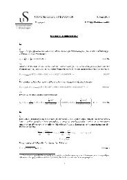
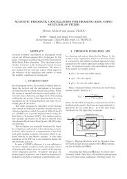
MODELING OF LOW SALINITY EFFECTS IN SANDSTONE OIL ROCKS 171Water Saturation0.940cells120cells0.80.70.6Sw0.50.40.30.20.100 0.1 0.2 0.3 0.4 0.5 0.6 0.7 0.8 0.9 1Dimensionless distanceFigure 3. Saturation profiles computed with 40 and 120 grid cells, respectively.The comparison is taken from SW flooding (Example 1, case 2).0.9Recovery0.80.70.6oil recovery0.50.4LSHS0.30.20.100 1 2 3 4 5 6Time (days)Figure 4. Plot showing the recoveries for HS and LS relative permeability curvesgiven in Fig. 2.6.2. Various data needed for the water flooding simulations. A range of input parametersmust be specified for the above model, and are given in Appendix A and B. We emphasize thatwe will use a fixed set of parameters for all simulations, unless anything else is clearly stated.The only change from one simulation to another is the brine composition and/or formation watercomposition (initial condition).6.3. A remark on the numerical resolution in the simulations. As stated earlier, theequation systems are solved explicitly. We think that the solutions provided by the explicit methodin this paper are sufficient for our present purpose, since we are interested in investigating thefundamental behavior of our one dimensional model. We first present a simulation case wherewe demonstrate convergence of the numerical solution. We have considered formation water FWand flooding water SW with ion concentrations as described in Table 2 in Appendix A. We havecomputed solutions on a grid of 40 cells and 120 cells, respectively. Result for the water saturationat different times is shown in Fig. 3. We conclude that it is sufficient to compute solutions on agrid of 40 cells. This will be done in the remaining part of the work.Before we start exploring how oil recovery can be sensitive for the brine composition of thewater that is used for flooding, we show two extremes: Oil recovery for the high salinity conditions

18 OMEKEH, EVJE, AND FRIISx 10 −4BetaMgx 10 −34.5BetaCa12 x 10−3BetaNa14121043.532.5108Initial0.133days0.3330.6671.3332.0004.0006.00082661.51440.520 0.5 1Dimensionless distance00 0.5 1Dimensionless distance0 0.5 1Dimensionless distanceFigure 5. Plots showing the behavior of the various β-functions along the coreat different times during a time period of 6 days, for the case with LSW as theinvading low salinity brine. Note that there is no desorption of the divalent ions(calcium and magnesium), only adsorption. Left: β mg . Middle: β ca . Right:β na .represented by relative permeability curves (15) versus oil recovery for the low salinity conditionsrepresented by relative permeability curves (16). See also Appendix B for specific data used forthe relative permeability functions. Results are shown in Fig. 4. This information is useful tohave in mind when we in the remaining part of this section consider brine-dependent oil recoverycurves.6.4. Example 1: Water flooding using different brines and fixed formation water. Herewe present simulations of corefloods. The core is composed of clay and other minerals that areassumed to be relatively chemically nonreactive typical of sandstone cores. The clay content/massof the core is given by M c (Kg/Liter of core) and clay capacity by CEC (moles/kg of clay), seeAppendix A for values. Initially the core is at equilibrium with formation water at initial watersaturation, S wi = 0.15, and oil. Subsequently, we flood the core with an invading brine at aflow velocity v T = 0.01 (meters/day) for a sufficiently long time, t days, till no appreciable oil isobtained from the core. The runs made in Example 1 are grouped into two groups: Case 1 inwhich we inject with a low salinity water and other brines modified from low salinity water (seeTable 1 in Appendix A) and Case 2 in which we inject seawater and other seawater based brines(see Table 2 in Appendix A).6.4.1. Case 1: Injecting low salinity water and low salinity modified brines. For thedifferent runs in this section, we inject with low salinity brine, LSW and modified low salinitybrines LSW1, LSW2 and LSW3. LSW is obtained by a 100 times dilution of formation water.LSW1 by 10 times dilution of formation water. LSW2 by reducing the magnesium component inLSW1 and LSW3 by reducing both divalent ions in LSW1. The brine compositions are given inTable 1 and all other parameters used in the runs are listed in appendix A and B.Fig. 5 shows the β-functions, which describe the amount of Mg 2+ , Ca 2+ , and Na + -ions bondedto the core, for injection of LSW brine. Initially, the formation brine is at equilibrium with therock, hence, there is a fixed amount of each ion bonded to the surface of the rock. This is denotedby the red curve in Fig. 5. On flooding the core with LSW, this equilibrium is disturbed and a newone is reached after some time. From the figure it is seen that there is no desorption of any of thedivalent ions (calcium and magnesium) but rather adsorption of the divalent ions and desorptionof the monovalent ion (sodium). Consequently, the H-function, which is the weighting factor forflow function alteration, remains equal to 1 at all times as shown in Fig. 7. We also show in Fig 6various ion concentrations C ca , C mg , C na , and C cl .

MODELING OF LOW SALINITY EFFECTS IN SANDSTONE OIL ROCKS 190.02Mg Concentration0.2Ca ConcentrationConcentration mol/L0.0150.010.005Concentration mol/L0.150.10.0500 0.2 0.4 0.6 0.8 1Dimensionless distance00 0.2 0.4 0.6 0.8 1Dimensionless distance1.5Na Concentration2Cl ConcentrationConcentration mol/L10.5Concentration mol/L1.510.500 0.2 0.4 0.6 0.8 1Dimensionless distance00 0.2 0.4 0.6 0.8 1Dimensionless distanceFigure 6. Concentrations for different ions for the case with LSW as the invadinglow salinity brine. Top Left: Mg 2+ concentration. Top Right: Ca 2+concentration. Bottom Left: Na 2+ concentration. Bottom Right: Cl − concentration.10.90.80.70.60.50.40.30.20.1H function0.133days0.333days0.6671.3332.0004.0006.00000 0.2 0.4 0.6 0.8 1Dimensionless distanceFigure 7. The H-function, see equation 18, corresponding to the β-functions forLSW injection.There is no change in H because there is no desorption of divalentions in Fig. 5.

20 OMEKEH, EVJE, AND FRIIS0.8Recovery0.70.6oil recovery0.50.40.30.2LSWLSW1LSW2LSW30.100 1 2 3 4 5 6Time (days)Figure 8. Oil recovery for different invading low salinity brines. LSW showingthe least recovery since there was no change in H-function in Fig. 7.x 10 −4BetaMgx 10 −34.5BetaCa12 x 10−3BetaNa14410123.538102.5826640 0.5 1Dimensionless distance1.510.500 0.5 1Dimensionless distance420 0.5 1Dimensionless distanceInitial0.1333days0.33330.66671.33332.00004.00006.0000Figure 9. Plots showing the various β-functions along the core at different timesduring a time period of 6 days, for the case with LSW3 as the invading low salinitybrine. Note that there is desorption of both divalent ions. Left: β mg . Middle:β ca . Right: β na .Clearly, when LSW brine is injected there is no positive low salinity effect in terms of improvedoil recovery, see Fig. 8. However, the injection of the modified low salinity brines, LSW1, LSW2,and LSW3 led to different degrees of desorption of the divalent ions. Fig. 9 shows desorption ofmagnesium and calcium ions during LSW3 flooding. Fig. 10 shows the corresponding change inthe H-function which moves from 1 towards a lower value as a result of the desorption of calciumand magnesium ions originally attached to the rock. This leads to an almost immediate improvedflow of oil behind the water front. See Fig. 11 for a comparison of the water front behavior forLSW3 versus LSW.The main difference between the low salinity brines LSW1, LSW2, and LSW3, is that LSW2leads to a desorption of calcium ions only, LSW1 leads to a greater desorption of calcium ions,whereas LSW3 leads to desorption of both magnesium and calcium ions. This is the explanationfor the various recoveries seen in Fig. 8.

MODELING OF LOW SALINITY EFFECTS IN SANDSTONE OIL ROCKS 211H function0.90.80.70.60.50.40.30.20.10.133days0.3330.6671.3332.0004.0006.00000 0.1 0.2 0.3 0.4 0.5 0.6 0.7 0.8 0.9 1Dimensionless distanceFigure 10. The H-function for LSW3 injection corresponding to the β-functionsgiven in Fig. 9. The change from 1 is as a result of desorption of both divalentions Ca 2+ and Mg 2+ during LSW3 injection.10.90.80.7water saturation10.90.80.7water saturation0.133days0.3330.6671.3332.0004.0006.0000.60.60.50.50.40.30.20.10.133days0.3330.6671.3332.0004.0006.00000 0.1 0.2 0.3 0.4 0.5 0.6 0.7 0.8 0.9 1Dimensionless distance0.40.30.20.100 0.1 0.2 0.3 0.4 0.5 0.6 0.7 0.8 0.9 1Dimensionless distanceFigure 11. Plots showing the water saturation s along the core, for differentinvading low salinity brines, at different times during a time period of 6 days.The remobilization of oil behind the water front is seen in LSW3. Left: LSW3.Right: LSW.6.4.2. Case 2: Injecting seawater and seawater modified brines. Similar runs as in Example1, case 1, were made but this time injecting with the sea water brine SW and modified seawater brines SW1 and SW2, see Table 2. SW1 is obtained by a 10 times dilution of sea water andSW2 by reducing the calcium component in SW1. The brine compositions are given in table 3.Flooding with seawater, SW, and the seawater modified brines, SW1 and SW2, the model predictsdifferent degrees of desorption of calcium and adsorption of magnesium ions. Figs. 12 and13 show the desorption/adsorption on the rock surface for SW and SW2 injection, respectively.It can be seen from the plots that the desorption of calcium is stronger for SW2 injection. Thisstronger calcium stripping is responsible for the stronger response to favorable wettability alterationtypified by a lower H-function in SW2 injection (Fig. 15) than in SW injection (Fig. 14),and consequently a better recovery of SW2 (Fig. 17). SW1 gives the lowest desorption of calciumions, hence it also gives the lowest recovery. Note that according to equations (17) and (18), only

22 OMEKEH, EVJE, AND FRIISx 10 −3BetaMg3.5 x 10−3BetaCa5.5 x 10−3BetaNa5354.542.54.53.52432.521.51.510.53.532.5initial0.133days0.3330.6671.3332.0004.0006.00010 0.5 1Dimensionless distance00 0.5 1Dimensionless distance20 0.5 1Dimensionless distanceFigure 12. Plots showing the behavior of the various β-functions along the coreat different times during a time period of 6 days, for the case with SW as theinvading sea water brine. Calcium ion is the only desorbed divalent ion. Left:β mg . Middle: β ca . Right: β na .5.5 x 10−3BetaMg3.5 x 10−3BetaCa5.5 x 10−3BetaNa5354.542.54.53.52432.521.51.510.53.532.5Initial0.133days0.3330.6671.3332.0004.0006.00010 0.5 1Dimensionless distance00 0.5 1Dimensionless distance20 0.5 1Dimensionless distanceFigure 13. Plots showing the behavior of the various β-functions along the coreat different times during a time period of 6 days, for the case with SW2 as theinvading sea water brine.A stronger calcium desorption is seen here than in Fig. 12.Left: β mg . Middle: β ca . Right: β na .calcium desorption contributed to the change in the H-function since there was no desorption ofmagnesium ions in these floods.Another significant difference in the SW and SW2 injection is the rate of the calcium strippingand subsequently the rate of the wettability alteration. It can be seen in Figs. 12 and 13 that thecalcium stripping is faster with SW injection than in SW2 injection. The effect of the above isclearly seen in Fig. 17 where SW recovery is better than SW2 recovery in the early stages and inFig. 16, where there is no immediate improved oil flow behind the water front in SW2 injection.6.5. Example 2: Water flooding using different formation waters and a fixed invadingbrine. For the runs made in this section, we vary the initial formation water FW, FW1 and FW2and flood with a fixed low salinity water LSW in order to demonstrate the effect that the initialformation water may have in low salinity recovery. FW and LSW are the formation water andlow salinity brines used in Example 1. FW1 is derived from FW by increasing the magnesium and

MODELING OF LOW SALINITY EFFECTS IN SANDSTONE OIL ROCKS 231H function0.90.80.70.6H c0.50.40.30.20.10.133days0.3330.6671.3332.0004.0006.00000 0.1 0.2 0.3 0.4 0.5 0.6 0.7 0.8 0.9 1Dimensionless distanceFigure 14. The H-function for SW injection corresponding to the β-functionsgiven in Fig. 12.1H function0.90.80.70.6H c0.50.40.30.20.10.133days0.3330.6671.3332.0004.0006.00000 0.1 0.2 0.3 0.4 0.5 0.6 0.7 0.8 0.9 1Dimensionless distanceFigure 15. The H-function for SW2 corresponding to the β-functions given inFig. 13. The improved H-function is as a result of the stronger calcium desorptionin Fig. 13.chloride concentration. FW2 is a seawater-like brine. Full description of the brines that are usedare given in Table 3. The results show that the initial formation water can play an importantrole in the recovery that it is obtained. Using FW1 as the formation water clearly gives a higherrecovery than FW and FW2 when low salinity water LSW is injected (Fig. 18). This is becausethe initial state of the core with FW1 brine, promotes more divalent ions on the core surfacethan either with FW or FW2. Hence subsequent flooding with LSW brine desorbs more of thesedivalent ions when FW1 is used as the initial brine.6.6. Example 3: Water flooding showing the effect of clay content and capacity on theconcentration profiles. Here we present an example to illustrate the effect of the clay contentM c and cation exchange capacity of the clay, CEC, on the concentration profiles generated alongthe core. To demonstrate this effect, a CEC of 1.3 eq/Kg of clay and M c of 0.088 Kg/Litre of corewere used. The initial formation water and invading brines are FW and IB, respectively. Theircompositions are given in Table 4. It can be seen in Fig. 19 that there is adsorption of calciumand magnesium ions and desorption of sodium ions. The increased adsorption and desorptionseen in Fig. 19 is as a result of the high CEC and M c values used in this example. Note that a

24 OMEKEH, EVJE, AND FRIIS1Water Saturation1Water Saturation0.90.90.80.80.70.70.60.6Sw0.5Sw0.50.40.30.20.10.133days0.3330.6671.3332.0004.0006.0000.40.30.20.10.133days0.3330.6671.3332.0004.0006.00000 0.1 0.2 0.3 0.4 0.5 0.6 0.7 0.8 0.9 1Dimensionless distance00 0.1 0.2 0.3 0.4 0.5 0.6 0.7 0.8 0.9 1Dimensionless distanceFigure 16. Plots showing the water saturation s along the core, for differentinvading sea water brines, at different times during a time period of 6 days. Left:SW2. Right: SW.0.8Oil Recovery0.70.6oil recovery0.50.40.3SwSW1SW20.20.100 1 2 3 4 5 6Time (days)Figure 17. Oil recovery for different invading sea water brines. SW showingbetter recovery at early time after which SW2 performs better, due to a strongerrelease of Ca 2+ ions from the rock, which in turn contributes to a change ofwetting state.steady state of the β ca , β mg and β na is not reached for the duration of the example. Fig. 20 showsthe concentrations of the different ions along the core at various times. As a consequence of thelarge adsorption of Ca 2+ and Mg 2+ ions on the rock surface, there exists certain regions along thecore where the Ca 2+ and Mg 2+ concentrations are below the injected and initial concentrations.The Na + ions are desorbed from the rock surface and this desorption is responsible for the Na +concentration profile seen in Fig. 20. The Cl − acts as a tracer and is neither desorbed or adsorbed.

MODELING OF LOW SALINITY EFFECTS IN SANDSTONE OIL ROCKS 250.8Recoveryoil recovery0.60.40.2FWFW1FW200 1 2 3 4 5 6Time (days)Figure 18. Oil recovery for different formation brines and LSW as the invading brine.0.155BetaMg0.48BetaCa0.6BetaNa0.150.460.550.1450.440.50.140.420.450.1350.40.40.130.1250.120.1150.110.1050 0.5 1Dimensionless distance0.380.360.340.320.30 0.5 1Dimensionless distance0.350.30.250.20.150.10 0.5 1Dimensionless distanceInitial0.133days0.3330.6671.2002.0004.0006.000Figure 19. β-functions along the core for Example 3. Left: β mg . Middle: β ca .Right: β na .

26 OMEKEH, EVJE, AND FRIIS0.02Mg2+ concentration0.2Ca2+ concentration0.0150.15mole/Litre0.010.005mole/Litre0.10.0500 0.2 0.4 0.6 0.8 1Dimensionless distance00 0.2 0.4 0.6 0.8 1Dimensionless distance1.5Na+ concentration2Cl− concentrationmole/Litre10.5mole/Litre1.510.500 0.2 0.4 0.6 0.8 1Dimensionless distance00 0.2 0.4 0.6 0.8 1Dimensionless distanceFigure 20. Concentrations along the core for Example 3. Top Left: Mg 2+concentration. Top Right: Ca 2+ concentration. Bottom Left: Na + concentration.Bottom Right: Cl − concentration. Since the changes in the β mg and β caconcentrations seen in Fig. 19 now are of the same order as the concentrations ofC mg and C ca , the interaction between them can clearly be observed. I.e., there isa ”new” dip in the C mg concentration front due to the strong adsorption of theseions to the rock as seen from the behavior of β mg . Similarly for C ca and C na .7. Concluding remarksThe proposed model which couples a standard Buckley-Leverett two-phase model to a multipleion exchange process relevant for sandstone, and where desorption of divalent ions has been attributeda change of the wetting state such that more oil is mobilized, demonstrates how a rangeof different flow scenarios can occur. In particular, some main observations in view of the modelbehavior are:• Different low salinity brines can give different degree of desorption of divalent ions (calciumand magnesium) from the rock surface, ranging from no desorption, partial desorption(either calcium or magnesium), or full desorption (both calcium and magnesium). Thisgives rise to different oil recovery curves ranging from no additional oil recovery effect toa more or less strong additional effect.• Flooding with a seawater like brine and diluted variants of this gave rise to different degreesof calcium desorption, but no desorption of magnesium. It was observed that the speed ofthese desorption fronts were quite sensitive for the brine composition, leading to a range

MODELING OF LOW SALINITY EFFECTS IN SANDSTONE OIL ROCKS 27of different oil recovery behavior in the initial stage (first 2 days) of the simulated floodingexperiments.• The model demonstrates that the oil recovery is quite sensitive to the composition of theformation water relative to the injected water composition.In the future we will focus on expanding the model by including effects of e.g. capaillary pressureand mineral solubility, as well as evaluating the model by carrying out systematic comparisonstudies between predicted model behavior and different experimental works, as mentioned in theintroduction part.AcknowledgmentsThis research has been supported by the Norwegian Research Council, Statoil, Dong Energy,and GDF Suez, through the project Low Salinity Waterflooding of North Sea Sandstone Reservoirs.The second author is also supported by A/S Norske Shell

28 OMEKEH, EVJE, AND FRIISReferences1. G. Ali, V. Furuholt, R. Natalini, and I. Torcicollo, A mathematical model of sulphite chemicalaggression of limestones with high permeability. part i. modeling and qualitative analysis,Transport Porous Med 69 (2007), 109–122.2. , A mathematical model of sulphite chemical aggression of limestones with high permeability.part ii. numerical approximation, Transport Porous Med 69 (2007), 175–188.3. M. Alotaibi, R. Azmy, and H. Nasr-El-Din, A comprehensive EOR study using low salinitywater in sandstone reservoirs, 17th Symposium on Improved Oil Recovery (Tulsa, Oklahoma,USA), SPE 129976, April 2010.4. C.A.J. Appelo and D. Postma, Geochemistry, groundwater and polution, 2nd edition ed., CRCPress, 2005.5. A. Ashraf, N. Hadia, and O. Torsæter, Laboratory investigation of low salinity waterfloodingas secondary recovery process: effect of wettability, SPE Oil and Gas India Conference andExhibition (Mumbai, India), SPE 129012, January 2010.6. T. Austad, A. Rezaeidoust, and T. Puntervold, Chemical mechanism of low salinity waterflooding in sandstone reservoirs, 17th Symposium on Improved Oil Recovery (Tulsa, Oklahoma,USA), SPE 129767, April 2010.7. G.I. Barenblatt, V.M. Entov, and V.M. Ryzhik, Theory of fluid flows through natural rocks,Kluwer Academic Publisher, 1990.8. J. Bear, Dynamics of fluids in porous media, Elsevier, Amsterdam, 1972.9. S. Berg, A. Cense, E. Jansen, and K. Bakker, Direct experimental evidence of wettability modificationby low salinity, International Symposium of the Society of Core Analyst (Noordwijk,The Netherlands), September 2009.10. D. Boyd and K. Al Nayadi, Validating laboratory measured archie saturation exponents usingnon-resistivity based methods, International Symposium of the Society of Core Analyst (AbuDhabi, UAE), October 2004.11. Jui-Sheng Chen and Chen-Wuing Liu, Numerical simulation of the evolution of aquifer porosityand species concentrations during reactive transport, Computers & Geosciences 28 (2002),no. 4, 485 – 499.12. Z. Chen, G. Huan, and Y. Ma, Computational methods for multiphase flows in porous media,Computational Science And Engineering, Society for Industrial and Applied Mathematics,2006.13. M. Cissokho, S. Boussour, P. Cordier, H. Bertin, and G. Hamon, Low salinity oil recovery onclayey sandstone: experimental study, International Symposium of the Society of Core Analyst(Noordwijk, The Netherlands), September 2009.14. S. Evje and A. Hiorth, A mathematical model for dynamic wettability alteration controlled bywater-rock chemistry, Networks and Heterogeneous Media 5 (2010), 217–256.15. , A model for interpretation of brine-dependent spontaneous imbibition experiments,Advances in Water Resources 34 (2011), 1627–1642.16. S. Evje, A. Hiorth, M.V. Madland, and R.Korsnes, A mathematical model relevant for weakeningof chalk reservoirs due to chemical reactions, Networks and Heterogeneous Media 4(2009), 755–788.17. H. Helgeson, D. Kirkham, and G. Flowers, Theoretical prediction of the thermodynamic behaviourof aqueous electrolytes by high pressure and temperatures; ii, American Journal ofScience 274 (1974), 1199–1261.18. H. Helgeson, D. Kirkham, and G Flowers, Theoretical prediction of the thermodynamic behaviourof aqueous electrolytes by high pressure and temperatures; iv, American Journal ofScience 281 (1981), 1249–1516.19. A. Hiorth, L.M. Cathles, J. Kolnes, O. Vikane, A. Lohne, and Madland M.V., A chemicalmodel for the seawater-CO 2 -carbonate system – aqueous and surface chemistry, WettabilityConference (Abu Dhabi, UAE), October 2008.20. G. Hirasaki, Ion exchange with clays in the presence of surfactants, SPE J. 22 (1982), 181–192.

REFERENCES 2921. P.P. Jadhunandan and N.R. Morrow, Effect of wettability on waterflood recovery for crudeoil/brine/rock systems., SPE Reservoir Engineering 12 (1995), 40–46.22. G.R. Jerauld, C.Y. Lin, K.J. Webb, and J.C. Seccombe, Modeling low-salinity waterflooding,SPE Reservoir Evaluation & Engineering 11 (2008), 1000–1012.23. S. Jin, Z. Xin, Shi Jin, and Zhouping Xin, The relaxation schemes for systems of conservationlaws in arbitrary space dimensions, Comm. Pure Appl. Math 48 (1995), 235–277.24. A. Lager, K. Webb, C. Black, M. Singleton, and K. Sorbie, Low salinity oil recovery: An experimentalinvestigation, International Symposium of the Society of Core Analyst (Trondhiem,Norway), September 2006.25. A.C. Lasaga, Kinetic theory in the earth sciences, Princeton series in geochemistry, PrincetonUniversity Press, 1998.26. D.A. Nield and A. Bejan, Convection in porous media, Springer, 2006.27. E.H. Oelkers and J. Schott, Thermodynamics and kinetics of water-rock interaction, Reviewsin Mineralogy and Geochemistry, no. v. 70, Mineralogical Society of America, 2009.28. A. Omekeh, S. Evje, I. Fjelde, and H.A. Friis, Experimental and modeling investigation of ionexchange during low salinity waterflooding, International Symposium of the Society of CoreAnalyst (Austin, Texas, USA), September 2011.29. Adolfo P. Pires, Pavel G. Bedrikovetsky, and Alexander A. Shapiro, A splitting technique foranalytical modelling of two-phase multicomponent flow in porous media, Journal of PetroleumScience and Engineering 51 (2006), no. 1 - 2, 54 – 67.30. G.A. Pope, L.W. Lake, and F.G. Helfferich, Cation exchange in chemical flooding: Part 1–basictheory without dispersion, Society of Petroleum Engineers Journal 18 (1978), 418–434.31. H. Pu, X. Xie, P. Yin, and N. Morrow, Application of coalbed methane water to oil recovery bylow salinity waterflooding, SPE Improved Oil Recovery Symposium (Tulsa, Oklahoma, USA),SPE 113410, April 2008.32. M. Sahimi, Flow and transport in porous media and fractured rock: From classical methods tomodern approaches, John Wiley & Sons, 2011.33. S.Boussour, M. Cissokho, P. Cordier, H. Bertin, and G. Hamon, Oil recovery by low salinitybrine injection: laboratory results outcrop and reservoir cores, SPE Annual Technical Conferenceand Exhibition (New Orleans, USA), SPE 124277, October 2009.34. J. Seccombe, A. Lager, K. Webb, G. Jerauld, and E. Fueg, Improving waterflood recovery:LoSal EOR field evaluation, SPE/DOE Symposium on Improved Oil Recovery (Tulsa, Oklahoma,USA), SPE 113480, April 2008.35. M. Sharma and P. Filoco, Effect of brine salinity and crude oil properties on oil recovery andresidual saturations, SPE Journal 5 (2000), 293–300.36. K. Skrettingland, K. Holt, M. Tweheyo, and I. Skjevrak, Snorre low salinity water injection- core flooding experiments and single well field pilot, Symposium on Improved Oil Recovery(Tulsa, Oklahoma, USA), SPE 129877, April 2010.37. Skule Strand, Eli J. Hagnesen, and Tor Austad, Wettability alteration of carbonates- effectsof potential determining ions (Ca 2+ and SO 2−4 ) and temperature, Colloids and Surfaces A:Physicochemical and Engineering Aspects 275 (2006), no. 1-3, 1 – 10.38. T.A.Dutra, A.P.Pires, and P.G.Bedrikovetsky, A new splitting scheme and existence of ellipticregion for gasflood modeling, SPE J. 14 (2009), no. 1, 101–111.39. G. Tang and N. Morrow, Oil recovery by waterflooding and imbibition - invading brine cationvalency and salinity, International Symposium of the Society of Core Analysts (Golden, CO),August 1999.40. Guo Qing Tang and Norman R Morrow, Influence of brine composition and fines migrationon crude oil/brine/rock interactions and oil recovery, Journal of Petroleum Science and Engineering24 (1999), no. 2-4, 99 – 111.41. I. Tripathi and K.K. Mohanty, Instability due to wettability alteration in displacements throughporous media, Chemical Engineering Science 63 (2008), no. 21, 5366 – 5374.42. K. Webb, C. Black, and H. Al-Jeel, Low salinity oil recovery - log inject log, SPE/DOESymposium on Improved Oil Recovery (Tulsa, Oklahoma, USA), SPE 89379, April 2004.

30 REFERENCES43. K. Webb, A. Lager, and C. Black, Comparison of high/low salinity water/oil relative permeability,International Symposium of the Society of Core Analysts (Abu Dhabi, UAE), November2008.44. Hasan O. Yildiz and Norman R. Morrow, Effect of brine composition on recovery of moutraycrude oil by waterflooding, Journal of Petroleum Science and Engineering 14 (1996), no. 3-4,159 – 168.45. L. Yu, S. Evje, H. Kleppe, T. Kaarstad, I. Fjelde, and S.M. Skjaeveland, Modelling of wettabilityalteration processes in carbonate oil reservoirs, Networks and Heterogeneous Media 3(2008), 149–183.46. , Spontaneous imbibition of seawater into preferentially oil-wet chalk cores : Experimentsand simulations, Journal of Petroleum Science and Engineering 66 (2009), no. 3-4, 171– 179.47. W. Yu-shu and B. Baojun, Efficient simulstion for low salinity waterflooding in porous andfractured reservoirs, SPE Reservoir Simulation Symposium (The Woodlands, Texas, USA),SPE 118830, February 2009.48. Y. Zhang and N. Morrow, Comparison of secondary and tertiary recovery with change ininjection brine composition for crude oil/sandstone combinations, SPE/DOE Symposium onImproved Oil Recovery (Tulsa, Oklahoma, USA), SPE 99757, April 2006.8. APPENDIX A: DATA FOR WATER-ROCK CHEMISTRYActivity coefficients. Along the line of the previous work [16] the following values, taken from[4], are used for the constants a 0 i :(94)and for b 0 i(95)we use:a 0 ca = 5, a 0 na = 4, a 0 cl = 3.5, a 0 mg = 5.5, a 0 so = 5.b 0 ca = 0.165, b 0 na = 0.075, b 0 cl = 0.015, b 0 mg = 0.2, b 0 so = −0.04.Moreover, we shall use the following values for A(T ) and B(T ) taken from [18, 17]:(96) A(T = 80) = 0.5706, B(T = 80) = 0.3381.Core properties. The following core properties are assumed for the model example studiedbelow.• Length: L = 0.04 m• Porosity: ϕ = 0.274• Mass of clay: M c = 0.088 Kg/Litre of core• Permeability: κ = 500 mD = 500 · 0.987 · 10 −15 m 2 .Oil and brine properties.• Oil viscosity: µ o = 0.6 cp (1 cp = 10 −3 Pa s)• Water viscosity: µ = 0.3 cpProperties connected to the cation exchange process.• Cation exchange capacity: CEC = 0.013 eq/Kg of clay• Selectivity factor : Kcana HS = 5.1; Kcana LS = 1.7• Selectivity factor: Kmgna HS = 4.8; Kmgna LS = 1.6• Corresponding brine salinity : BsHS = 4.5; BsLS = 10 −8• r constant r = 400.Other quantities.• Total velocity v T = 0.01 m/day= 1.1574 · 10 −7 m/s.• Reference diffusion coefficient: D m = Lv T = 4.6296 · 10 −9 m 2 /s ≈ 5 · 10 −9 m 2 /s.• Reference viscosity: µ = 10 −3 Pa s.

REFERENCES 31The molecular diffusion coefficient D m is set equal to reference diffusion D m . Since the totalvelocity v T is low and the dispersion length α of the order of millimeters, the Peclet number (33)becomes small (< 1), and the first term of (32) only is used. In addition, for all simulations wehave used the choice p = q = 1.9 in the expression for molecular diffusion given by equation (32).Oil recovery is defined as∫ 10Oil Recovery :=[s(x, t) − s init(x)] dx∫ 10 [1 − s ,init(x)] dxwhere s init (x) is initial water saturation in the core.Ions FW LSW LSW1 LSW2 LSW3[mol/l] [mol/l] [mol/l] [mol/l] [mol/l]Na + 1.3262 0.013262 0.13262 0.13262 0.13262Cl − 1.6569 0.016570 0.17050 0.13907 0.13266Ca 2+ 0.1479 0.001479 0.00148 0.00148 0.00001Mg 2+ 0.0175 0.000175 0.01746 0.00175 0.00001SO 2−4 0.0000 0.000000 0.00000 0.00000 0.00000Ion Strength I 0 1.8224 0.018224 0.18944 0.17373 0.13616Table 1. Composition of the formation water and the different brines used forExample 1, Case 1.Ions FW SW SW1 SW2[mol/l] [mol/l] [mol/l] [mol/l]Na + 1.3262 0.45014 0.045014 0.045014Cl − 1.6569 0.51912 0.051912 0.049316Ca 2+ 0.1479 0.01299 0.001299 0.000001Mg 2+ 0.0175 0.04551 0.004551 0.004551SO 2−4 0.0000 0.02401 0.002401 0.002401Ion Strength I 0 1.8224 0.64965 0.064965 0.061071Table 2. Composition of the formation water and the different brines used forExample 1, Case 2.Ions LSW FW FW1 FW2[mol/l] [mol/l] [mol/l] [mol/l]Na + 0.013262 1.3262 1.3262 0.45014Cl − 0.016570 1.6569 1.9712 0.51912Ca 2+ 0.001479 0.1479 0.1479 0.01299Mg 2+ 0.000175 0.0175 0.1746 0.04551SO 2−4 0.000000 0.0000 0.0000 0.02401Ion Strength I 0 0.018224 1.8224 2.2937 0.64965Table 3. Composition of the brine and the different formation waters used forExample 2.

32 REFERENCESIons FW IW[mol/l] [mol/l]Na + 1.3262 1.0610Cl − 1.6569 1.3255Ca 2+ 0.1479 0.1183Mg 2+ 0.0175 0.0140SO 2−4 0.0000 0.0000Ion Strength I 0 1.8224 1.4578Table 4. Composition of the formation water and the different brines used forExample 3.APPENDIX B: DATA FOR WATER-OIL FLOW FUNCTIONSHigh salinity conditions. The following set of values for oil-wet conditions is used:(97)k ∗,ow = 0.3, k ∗,owo= 0.75, s owwr = 0.15, s owor = 0.3, Nk ow = 3, Nk owo = 2.Applying these values in (14) the following two relative permeability curves are obtainedk ow (s; s owwr, s owor ),koow (s; s owwr, s owor ),for s owwr ≤ s ≤ 1 − s owor .Low salinity conditions. The following set of values for water-wet conditions is used:(98)k ∗,ww = 0.4, k ∗,wwo=0.9, s wwwr= 0.15, s wworThese choices give corresponding relative permeability curvesk ww (s; s wwwr , s wwor ),koww (s; s wwwr , s wwor ),= 0.15, Nk ww = 3, Nk wwo = 2.for s wwwr≤ s ≤ 1 − s wwor .International Research Institute of Stavanger, P.O.Box 8046, 4068 Stavanger, Norway.E-mail: Aruoture.Voke.Omekeh@iris.noUniversity of Stavanger (UiS), 4036 Stavanger, Norway.E-mail: Steinar.Evje@uis.noInternational Research Institute of Stavanger, P.O.Box 8046, 4068 Stavanger, Norway.E-mail: HelmerAndre.Friis@iris.no