Chapter 8

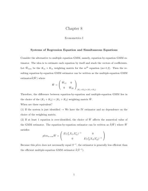
Chapter 8Econometrics ISystems of Regression Equation and Simultaneous EquationsConsider the alternative to multiple equation GMM, namely, equation-by-equation GMM estimator.The idea is to estimate each equation by itself and stack the vectors of coefficients.Let Ŵmm be the K m × K m weighting matrix for the m th equation (m=1,2). Then the resultingequation-by-equation GMM estimator can be written as the multiple-equation GMMestimatorˆδ(Ŵ ) where ⎛⎞Ŵ = ⎝ Ŵ11 0⎠0 Ŵ 22(K 1 +K 2 )×(K 1 +K 2 )Therefore, the difference between equation-by-equation and multiple-equation GMM lies inthe choice of the (K 1 + K 2 ) × (K 1 + K 2 ) weighting matrix Ŵ .When are these equivalent?(1) If the system is just identified → We have the IV estimator and no dependence on thechoice of the weighting matrix.(2) If at least 1 equation is over-identified, the choice of Ŵ affects the numerical value ofthe GMM estimator. The equation-by-equation estimator can be written asˆδ(Ŵ ) where Ŵsatisfies⎛⎞plim n→∞ Ŵ = ⎝ E(ε2 i1 X i1X i1 ′ )−1 0⎠0 E(ε 2 i2 X i2X i2 ′ )−1Because this plim does not necessarily equal S −1 , the estimator is generally less efficient thanthe efficient multiple-equation GMM estimator ˆδ(Ŝ−1 ).1

However, if the equations are unrelated in the sense thatE[ε i1 ε i2 X i1 X ′ i2] =0E[ε i2 ε i1 X i2 X ′ i1] =0Then S becomes a block diagonal matrix and plim n→∞ Ŵ = S −1 .Since Ŵ − S−1 → p 0 then √ nˆδ(Ŵ ) − √ nˆδ(Ŝ−1 ) → p 0.So under the above conditions the equation-by-equation GMM estimator is asymptoticallyequivalent to the multiple-equation GMM estimator.Some caveats:(1) Small sample properties might be better without joint estimation.(2) The asymptotic result presumes the model is correctly specified.If the model is misspecified, neither the single-equation GMM nor the multiple-equation GMMis guaranteed to be consistent.Chances of misspecification increase as we add equations.Consider our current example:(1) ln W i = φ 1 + β 1 S i + γ 1 IQ i + ΠEXP i + ε i1(2) KW W i = φ 2 + β 2 S i + γ 2 IQ i + ε i2⎛X i1 = X i2 =⎜⎝⎞1S iEXP i ⎟⎠MED iAssume that E[S i · ε i1 ] ≠ 0.Schooling is correlated with the error term in the log wageequation.We know this implies that estimating equation ♯1 by GMM will result in asymptotically biasedestimates, but equation ♯2 would yield consistent estimates.What about joint estimation?2

Remember the sampling error is given by:⎛plim n→∞ˆδ( Ŵ ) − δ = (Σ ′ xzŴ Σ xz) −1 Σ ′ xzŴ ⎝ E[X i1 · ε i1 ]0⎞⎠ (1)In efficient multiple equation-GMM, W is not block diagonal so any element of plim n→∞ˆδ( Ŵ )−δ can be non-zero when the orthogonality conditions of any equation is violated. Joint estimation:Biases due to a local misspecification contaminate the rest of the system.This problem does not arise in equation-by-equation GMM which constrains Ŵ to be blockdiagonal.Next, consider the conditional homoskedasticity assumption.E(ε im ε ih |X im , X ih ) = σ mh ∀m, h = 1.2This gives us a very simplified version of the matrix of cross moments S = E(g i g ′ i ).Consider the (1, 1) blockE(ε i1 ε i1 X i1 X ′ i1) = E [ E(ε i1 ε i1 X i1 X ′ i1|X i1 , X i2 ) ]S =An estimator exploiting the structure of S is= E [ E(ε i1 ε i1 |X i1 , X i2 )X i1 X i1′ ]= E[σ 11 X i1 X ′ i1]= σ 11 E(X i1 X ′ i1)⎛⎞⎝ σ 11E(X i1 X i1 ′ ) σ 12E(X i1 X i2 ′ ) ⎠σ 21 E(X i2 X i1 ′ ) σ 22E(X i2 X i2 ′ )⎛Ŝ = ⎝ ˆσ 11( 1 ∑n Xi1 X i1 ′ ) ˆσ 12( 1 ∑⎞n Xi1 X i2 ′ ) ⎠ˆσ 21 ( 1 ∑n Xi2 X i1 ′ ) ˆσ 22( 1 ∑n Xi2 X i2 ′ )3

where for some consistent estimator ˆδ mˆσ mh = 1 n∑ˆεimˆε ihˆε im = y im − Z ′ imˆδ m m = 1, 2; h = 1, 2.The Full-Information Instrumental Variables Estimator (FIVE)exploits this structure such thatˆδ F IV E = ˆδ(Ŝ−1 )with Ŝ coming from the structure on the previous page.Usually the initial estimator of ˆδ m , m = 1, 2, to calculate Ŝ is the 2SLS estimator.Now, if the set of instruments is the same across equations such that X i1 = X i2 = X i = K × 1vector , we can simplify the estimators even more. Let⎛ ⎞ε i = ⎝ ε i1⎠ε i22×1Then let Σ denote the 2 × 2 matrix of cross moment of ε i s.t.Σ =⎛⎞⎝ σ 11 σ 12⎠σ 21 σ 222×2= E(ε i ε ′ i)To estimate Σ consistently we need an initial consistent estimator of ˆδ 1 and ˆδ 2 to calculate ε i1and ε i2 . The term 3SLS comes from the fact that the 2SLS estimator of δ 1 and δ 2 are usedas the initial estimator.Then,ˆΣ =⎛ ⎞⎝ ˆσ 11 ˆσ 12⎠ = 1ˆσ 21 ˆσn22∑ˆεiˆε ′ i4

With the common instruments assumption we can write⎛ ⎞ ⎛ ⎞g i = ⎝ X i · ε i1⎠ = ⎝ ε i1⎠ ⊗ X i = ε i ⊗ X iX i · ε i2 ε i22K×1where ⊗ indicates Kronecker product.Some brief facts (see Greene for details)(1) A M×N ⊗ B K×L = C MK×LN ⇒ ε i ⊗ X i = g i(2)⎛A ⊗ B = ⎜⎝a 11 B · · · a 1n B.. .. .a m1 B · · · a mn B⎞⎛ ⎞⎟⎠ ⇒ ε i ⊗ X i = ⎝ ε i1X i⎠ε i2 X iIn addition, we can write S asS =⎛⎞⎝ σ 11E(X i1 X i1 ′ ) σ 12E(X i1 X i2 ′ ) ⎠ =σ 21 E(X i2 X i1 ′ ) σ 22E(X i2 X i2 ′ )⎛⎞⎝ σ 11E(X i X i ′) σ 12E(X i X i ′)σ 21 E(X i X i ′)σ 22E(X i X i ′) ⎠ = Σ ⊗ E(X i X ′ i)⇒ S −1 = Σ −1 ⊗ E(X i X i) ′ −1and Ŝ−1 = ˆΣ −1 ⊗ ( 1 ∑Xi X ′ni) −1⇒ Ŵmh = ˆσ mh · ( 1 ∑Xi X ′ni) −1 m, h = 1, 2.where ˆσ mh is the (m, h) element of ˆΣ −1 .Substituting into the expression in the last lecture(expanded GMM estimator), we getˆδ 3SLS =⎛⎞⎝ ˆσ 11Â11 ˆσ 12  12⎠ˆσ 21  21 ˆσ 22  22−1 ⎛⎞⎝ ˆσ 11Ĉ11 + ˆσ 12 Ĉ 12⎠ˆσ 21 Ĉ 21 + ˆσ 22 Ĉ 22where mh = ( 1 ∑Zim X ′ni)( 1 ∑Xi X ′ni) −1 ( 1 ∑Xi Z ih ′ n)Ĉ mh = ( 1 ∑Zim X ′ni)( 1 ∑Xi X ′ni) −1 ( 1 ∑Xi · y ih )n5

Similarly, we can write the asymptotic variance (and its estimator) asAvar(ˆδ 3SLS ) =⎛⎞⎝ σ 11A 11 σ 12 A 12⎠σ 21 A 21 σ 22 A 22−1whereA mh = E(Z im X ′ i)[E(X i X ′ i)] −1 E(X i Z ′ ih )σ mh = (m, h) element of Σ −1Andˆ Avar(ˆδ 3SLS ) =⎛⎝ ˆσ 11Â11 ˆσ 12 Â 12ˆσ 21 Â 21⎞⎠ˆσ 22 Â 22−1Most textbooks give formula in terms of the data matrices X,Z, and y. Deriving these expressionswill be a question on the next problem set.The final simplification follows from the assumption (really a fact from the set of instrumentsand regressors) ofX i = union(Z i1 , Z i2 )Instruments include regressors from both equations.This condition is equivalent toE(Z im · ε ih ) = 0 m, h = 1, 2That is, the predetermined regressors satisfy ”cross” orthogonalities: not only are they predeterminedin each equation (E(Z im·ε im ) = 0) but also in the other equations (E(Z im·ε ih ) = 0).The simplified formula is called the SUR estimator, ˆδ SUR .SUR=Seemingly Unrelated Regressions.6