Molecular Simulation Methods with Gromacs
Molecular Simulation Methods with Gromacs
Molecular Simulation Methods with Gromacs

You also want an ePaper? Increase the reach of your titles
YUMPU automatically turns print PDFs into web optimized ePapers that Google loves.
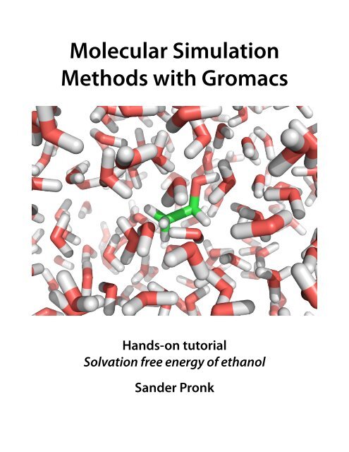
<strong>Molecular</strong> <strong>Simulation</strong><strong>Methods</strong> <strong>with</strong> <strong>Gromacs</strong>Hands-on tutorialSolvation free energy of ethanolSander Pronk
BackgroundIn this tutorial, we’ll calculate the free energy of solvation of a small molecule:ethanol. This type of calculation can either be done on its own, or can be part of abinding free energy calculation. Such calculations can be important, because the freeenergy is the most important static quantity in a thermal system: its sign determines thewhether of a molecule will be soluble, or whether it will bind to another molecule.We will start this tutorial <strong>with</strong> some background on how to calculate free energies,and how a free energy of solvation relates to a free energy of binding calculation. Then,we will focus on the practicalities of doing such a calculation in <strong>Gromacs</strong>. You will need<strong>Gromacs</strong> 4.6 (or later) for this tutorial.Calculating a free energy of bindingCalculating free energies can usually only be done using small steps and a full pathbetween one end state and the other. For example, to calculate the binding free energyof the ligand to a protein, we ultimately need to compare the situation of the ligandbeing bound to the protein, to the situation where both the ligand and the protein areseparately in solution:LPGLPThis could be calculated directly, for example by dragging the ligand away from theprotein and integrating the potential of mean force (averaging the force, and integratingit). Forces have very large fluctuations, however, and this turns out to be much moreexpensive than using free energy perturbation methods such as the Bennett AcceptanceRatio (BAR) we’ll use in the tutorial.Remember that a free energy difference between two states A and B determines theirrelative probability p A and p B ,p A= exp F B F Ap B k B Twhere k B is Boltzmann’s constant relating thermal energy to the temperature (1.38·10 -23J/K), and T which is the temperature. We could, in principle, calculate a free energydifference by waiting long enough, and measuring how often the system is in which1
state. The free energy differences, however, are often of the order of tens of kJ/mol: forexample, the free energy of solvation of ethanol at 298K is -20.1 kJ/mol, which isequivalent to -8.1 k B T: a relative probability of 3·10 -4 . One would need to wait a longtime for that transition to occur spontaneously, and even longer to get good statistics onit.Because of this probability issue, free energy methods rely on one basic idea: to forcethe system to where it doesn’t want to be, and then measure by how much it doesn’twant to be there. In free energy perturbation methods, we force the system by couplingthe interaction strength between a molecule of interest and the rest of the system to avariable !:E total = E ligand ligand + E rest rest + E ligand restand we slowly turn ! from 1 to 0. This means we can effectively turn off a molecule, andpretend that it is in vacuum (at !=0): we force the system to where it doesn’t want to be(either in the solvated or in the vacuum state, depending on what the sign of the freeenergy difference is). We’ll then use the BAR method of calculating by how much itdoesn’t want to be there.Coupling and de-coupling in this way helps us <strong>with</strong> calculating the free energy ofbinding, because we can now create a two-step path:2
LPG 1LPLPG 2LPwhere we first de-couple the ligand from the solvent, and then re-solvate the ligand inthe presence of the protein. The free energy of binding is thusG binding = G 1 + G 2 ,and the simulation is split into two parts: one calculating the de-solvation free energy,and one involving the free energy of coupling of a molecule into the system <strong>with</strong> aprotein. That last simulation couples the ligand from ! =0 where it doesn’t interact <strong>with</strong>the system, to the situation at !=1, where the protein is bound to the ligand. The firstsimulation is the inverse of a free energy of solvation. This is the one we’ll concentrateon in this tutorial - partly for computational performance reasons: because there is noprotein involved, the simulation box size can be small and the simulations will be fast.Free energy of solvationTo calculate a free energy of solvation, we calculate -!G 1 in the picture above, or,equivalently, !G solv in this picture:LG solvL
We’ll do this coupling our molecule to a variable ! (see Eq. 1) and Bennett AcceptanceRatio (BAR) calculations, as built into <strong>Gromacs</strong> 4.6.The BAR method relies on the output of pairs of simulations, say at state ! A and ! B .The free energy difference can be calculated directly if ! A and ! B are close enough (seeBennett’s original article: Bennett, J. Comp. Phys, (1976) vol. 22 p. 245 for details), bycalculating the Monte Carlo acceptance rates of transitions from ! A to ! B and vice versa,mapping states from ! A to ! B . The term ‘close enough’ here means that switchingbetween the two states should be possible in both directions: some of the sameconfigurations should be allowed in both end points (i.e. they should share some partsof phase space).The most obvious points for ! A and ! B would be ! A =0 and ! B =1. These end points,however, usually have very few states in common: they share very little phase space.Because of this, the free energy would never converge to a usable value. That’s whywe’ll split up the problem:G L G L G L!=0 !=0.4!=0.6!=1<strong>with</strong> as many ! points as are needed. We will therefore effectively ‘slowly’ turn on (oroff) the interactions between our ligand and the solvent. This means that we need to runas many simulations as there are ! points, that we need to tell each simulation whichneighboring ! points there are, and that we will post-process the results combining theresults of many simulations (we will use 7 ! points: 0, 0.2, 0.4, 0.6, 0.8, 0.9 and 1). As anexample, we will run one simulation at !=0.4, and that simulation will calculate theenergy differences between its ! point and the neighboring points !=0.2 and !=0.6.We will take one shortcut: we will turn off both the electrostatic (Coulomb)interactions and the Van der Waals (Lennard-Jones) interactions at the same time. Forhigh-quality results, these stages are normally separated, but here we will do them bothat the same time for expediency. <strong>Gromacs</strong> uses ‘soft-core’ interactions to make sure thatwhile the normal (Lennard-Jones and Coulomb) interactions are being turned off, therewill never be two point charges sitting on top of each other: this is achieved by turningon an interaction that effectively repels particles at intermediate ! points (in such a waythat it cancels out from the free energy difference).
Preparing the systemWe will start <strong>with</strong> a topology that can be downloaded from http://www.gromacs.org/Documentation/Tutorials/Free_energy_of_solvation_tutorial: getthe archive file fe-tutorial-4.6.tar.gz from the bottom of the page, or dowget http://www.gromacs.org/@api/deki/files/194/=fe-tutorial-4.6.tar.gzThen extract the archive <strong>with</strong>tar xzvf fe-tutorial-4.6.tar.gzand look for a file named topol.top, and a very basic coordinate file namedethanol.gro. This topology uses the OPLS force field and defines a methanemolecule, and includes the definitions for SPC/E water.Question: Take a look at the topology file topol.top. For the ethanol moleculedefinition, can you find which atoms are there, and how they are connected?We will first prepare the simulation box: the original configuration file has a dummysimulation box associated <strong>with</strong> it (you can see that by looking at the file ethanol.gro).We do this <strong>with</strong>:editconf -f ethanol.gro -o box.gro -bt dodecahedron -d 1which sets up the simulation box. In this case, it will make the simulation box a rhombicdodecahedron <strong>with</strong> a minimum distance between the solute (the ethanol molecule) andthe box edge of 1nm. The box is a rhombic dodecahedron because it provides a moreeffective packing of periodic images than rectangular boxes: we can use fewer watersfor the same distance between periodic images of the ethanol molecule. See the<strong>Gromacs</strong> manual for illustrations of this box shape and how its periodic images arearranged.Next, we solvate the system in watergenbox -cp box.gro -cs -o solvated.gro -p topol.topThis should generate a system <strong>with</strong> 310 water molecules taken from the default filename of the -cs option: a box of equilibrated water molecules.To make the configuration suitable for simulation, we will first minimize its energy,twice: once <strong>with</strong> flexible bonds, and once <strong>with</strong> constrained bonds. For the flexible-bondminimization we will use the following settings (see the included fileem_flexible.mdp)integrator = steep ; steepest-descent minimizationnsteps = 500 ; max. number of steps
emtol = 10 ; stop if forces reach this valueemstep = 0.01 ; minimization step sizenstxout = 1 ; compressed traj. output every stepnstenergy = 1 ; energy output every steprlist = 1.0 ; calculate interactions up to 1nmcoulombtype = pme ; use PME for electrostaticsvdw-type = cut-off ; simply cut off the LJ interactionsrvdw = 1.0 ; cut-off range for LJ interactionsconstraints = none ; we use flexible bondsdefine= -DFLEXIBLEThese settings are for a steepest-descent minimization for 500 steps, or until forces of10 kJ mol -1 nm -1 (the standard <strong>Gromacs</strong> force units). The configuration and systemenergies will be output every step, and the cut-offs will be at 1nm. PME will be used forelectrostatics. The flexible bonds are turned on by disabling constraints, and defining anpreprocessor directive ‘-DFLEXIBLE’ to ensure that the force field included in thetopology gives flexible bonds.Run the equilibration by preprocessing the input files into a run file <strong>with</strong>grompp -f em_flexible.mdp -c solvated.gro -o em_flexible.tprwhich generates the run file em_flexible.tpr. Run this file <strong>with</strong>mdrun -v -deffnm em_flexibleand do the next step, minimization <strong>with</strong> constrained (held at fixed distance) bonds. Forthis we use em.mdp:integrator = steepnsteps = 500emtol = 10emstep = 0.01nstxout = 1nstenergy = 1rlist = 1.0coulombtype = pmevdw-type = cut-offrvdw = 1.0constraints = all-bonds ; all chem. bonds are constrainedwhich differs only from em_flexible.mdp in the last two lines. We run in a similarway:grompp -f em.mdp -c em_flexible.gro -o em.tpr
lambda_02lambda_03lambda_04lambda_05lambda_06which each have contents:conf.grogrompp.mdptopol.topVerify that the substitution worked correctly <strong>with</strong>grep init-lambda lambda_*/grompp.mdpwhich should show something likelambda_0.2/grompp.mdp:init-lambda = 0.2lambda_0.4/grompp.mdp:init-lambda = 0.4etc. for each ! point. We now need to pre-process each run <strong>with</strong>cd lambda_00gromppcd ../lambda_01grompp....Check the output for whether these are successful, just to be sure. At this point we areready to run. The total run time will be about 5 minutes on 4 cores on a modern x86(AMD/Intel) CPU per ! point. This means that we can run the jobs sequentially, butthen we’ll have to wait 35 minutes and we’re wasting a big opportunity forparallelization.Instead, we’re going to try to run them in parallel and assume that we have somekind of batch system that we can submit jobs to. Because the system only has 1000particles, scaling beyond 4 cores makes no real gains. Typically, a modern computecluster has 8 core or more cores per node. We will therefore trick our to submit our jobs.Because we use fewer cores than there are in a node, we can use the threaded versionof <strong>Gromacs</strong> - which doesn’t need MPI (a library and run environment for runningparallel high-performance computing jobs over a network) to run in parallel. In manylocations, <strong>Gromacs</strong> is installed such that mdrun runs the threaded version, andmdrun_mpi the MPI version, though this may vary.
To run, we’ll create a set of batch-submittable run scripts. The exact settings to use inthe batch system settings (usually #PBS or #SBATCH depending on the batch system inuse) fields depends strongly on the system you’re running on, so the example hereprobably won’t work.#!/bin/sh#SBATCH -J fe#SBATCH -e run1.stderr#SBATCH -o run1.stdout#SBATCH --mem-per-cpu=1000#SBATCH -t 00:10:00# One node of 12 cores per job:#SBATCH -N 1#SBATCH -n 12module load gromacs( cd lambda_0; mdrun -nt 4 >& run.log ) &( cd lambda_01; mdrun -nt 4 >& run.log ) &( cd lambda_02; mdrun -nt 4 >& run.log ) &wait # wait for all background tasks to finishwhich will run three 4-threaded (set <strong>with</strong> -nt 4) versions of mdrun, each in their owndirectory, for a maximum of 10 minutes. Make as many of these scripts as needed for allthe different !-values (i.e. 3), and submit them to the queue.Post-processing: extracting the free energyAfter the simulations are done, we can extract the full free energy difference from theoutput data. Check your directories lambda_00 to lambda_06 for files calleddhdl.xvg. These contain the energy differences that are going to be used to calculatethe free energy difference. Combine them into a free energy <strong>with</strong> the <strong>Gromacs</strong> BAR toolg_bar:g_bar -b 100 -f lambda_*/dhdl.xvgWhere the -b 100 means that the first 100 ps should be disregarded: they serve asanother equilibration, this time at the conditions of the simulation. You should get a freeenergy difference of approximately -17.8 +/- 3.3 kJ/mol (this may be different if you runon different hardware: this answer is from a standard x86_64 cluster). This should becompared to an experimental value of -20.9 kJ/mol.Question: Longer runs will bring the free energy closer to -19.1 +/- 0.3 kJ/mol.Why is there a significant (i.e. bigger than the estimated error) differencebetween the experimental result and the simulation result? How could this beimproved?
Question: Look at the error bars for the individual ! points: they vary a lotbetween individual point pairs. What does this mean for the efficiency for theoverall calculation? How could it be improved?Where to go from hereAfter calculating the free energy of solvation, we’ve solved the first part of the freeenergy of binding of Eq. 2. The second part involves coupling a molecule into (or out of)a situation where it is bound to a protein. This introduces one additional complexity: weend up <strong>with</strong> a situation where a weakly coupled ligand wanders through our system:LPLPPLwhich is bad because this is a poorly reversible situation: there are suddenly very fewstates that map from a weakly coupled to a more strongly coupled molecule, which willdrastically reduce the accuracy of the free energy calculation.This situation can be remedied by forcing the ligand to stay at a specific positionrelative to the protein. This can be done <strong>with</strong> the <strong>Gromacs</strong> ‘pull code’, which allows thespecification of arbitrary forces or constraints onto <strong>with</strong> respect to centers of mass of anychosen set of atoms onto any other group of atoms. With a pull type of ‘umbrella’, wecan specify that we want a quadratic potential to this specified location, forcing theligand to stay at its native position even when it has been fully de-coupled.One way find out where to put the center of the force is by choosing a group of atomsin the protein close to the ligand, and doing a simulation <strong>with</strong> full ligand coupling,where the pull code is enabled, but <strong>with</strong> zero force. The pull code will then frequentlyoutput the coordinates of the ligand, from which an average position and an expecteddeviation can be calculated. This can then serve as a reference point for the location ofthe center of force for the pull code during the production runs, and the force constantof the pull code.Once the free energy has been calculated, care must be taken to correct for the factthat we have trapped our molecule. This can easily be done analytically.Optional Question: Given a measured standard deviation in the location of thecenter of mass of our ligand, how do we choose the force constant for the pullcode?
Optional Question: How do we correct for using the pull code: what is thecontribution to the free energy of applying a quadratic potential to a molecule?