Vehicle Dynamics

VEHICLE DYNAMICSFACHHOCHSCHULE REGENSBURGUNIVERSITY OF APPLIED SCIENCESHOCHSCHULE FÜRTECHNIKWIRTSCHAFTSOZIALESLECTURE NOTESProf. Dr. Georg Rill© October 2004download: http://homepages.fh-regensburg.de/%7Erig39165/

ContentsContentsI1 Introduction 11.1 Terminology . . . . . . . . . . . . . . . . . . . . . . . . . . . . . . . . . . . . 11.1.1 Vehicle Dynamics . . . . . . . . . . . . . . . . . . . . . . . . . . . . 11.1.2 Driver . . . . . . . . . . . . . . . . . . . . . . . . . . . . . . . . . . . 21.1.3 Vehicle . . . . . . . . . . . . . . . . . . . . . . . . . . . . . . . . . . 21.1.4 Load . . . . . . . . . . . . . . . . . . . . . . . . . . . . . . . . . . . 31.1.5 Environment . . . . . . . . . . . . . . . . . . . . . . . . . . . . . . . 31.2 Wheel/Axle Suspension Systems . . . . . . . . . . . . . . . . . . . . . . . . . 41.2.1 General Remarks . . . . . . . . . . . . . . . . . . . . . . . . . . . . . 41.2.2 Multi Purpose Suspension Systems . . . . . . . . . . . . . . . . . . . 41.2.3 Specific Suspension Systems . . . . . . . . . . . . . . . . . . . . . . . 51.3 Steering Systems . . . . . . . . . . . . . . . . . . . . . . . . . . . . . . . . . 51.3.1 Requirements . . . . . . . . . . . . . . . . . . . . . . . . . . . . . . . 51.3.2 Rack and Pinion Steering . . . . . . . . . . . . . . . . . . . . . . . . . 61.3.3 Lever Arm Steering System . . . . . . . . . . . . . . . . . . . . . . . 61.3.4 Drag Link Steering System . . . . . . . . . . . . . . . . . . . . . . . . 71.3.5 Bus Steer System . . . . . . . . . . . . . . . . . . . . . . . . . . . . . 71.4 Definitions . . . . . . . . . . . . . . . . . . . . . . . . . . . . . . . . . . . . . 81.4.1 Coordinate Systems . . . . . . . . . . . . . . . . . . . . . . . . . . . 81.4.2 Toe and Camber Angle . . . . . . . . . . . . . . . . . . . . . . . . . . 91.4.2.1 Definitions according to DIN 70 000 . . . . . . . . . . . . . 91.4.2.2 Calculation . . . . . . . . . . . . . . . . . . . . . . . . . . . 91.4.3 Steering Geometry . . . . . . . . . . . . . . . . . . . . . . . . . . . . 101.4.3.1 Kingpin . . . . . . . . . . . . . . . . . . . . . . . . . . . . 101.4.3.2 Caster and Kingpin Angle . . . . . . . . . . . . . . . . . . . 111.4.3.3 Disturbing Force Lever, Caster and Kingpin Offset . . . . . . 122 The Tire 132.1 Introduction . . . . . . . . . . . . . . . . . . . . . . . . . . . . . . . . . . . . 132.1.1 Tire Development . . . . . . . . . . . . . . . . . . . . . . . . . . . . . 132.1.2 Tire Composites . . . . . . . . . . . . . . . . . . . . . . . . . . . . . 132.1.3 Forces and Torques in the Tire Contact Area . . . . . . . . . . . . . . . 14I

2.2 Contact Geometry . . . . . . . . . . . . . . . . . . . . . . . . . . . . . . . . . 152.2.1 Contact Point . . . . . . . . . . . . . . . . . . . . . . . . . . . . . . . 152.2.2 Local Track Plane . . . . . . . . . . . . . . . . . . . . . . . . . . . . 172.3 Wheel Load . . . . . . . . . . . . . . . . . . . . . . . . . . . . . . . . . . . . 172.3.1 Dynamic Rolling Radius . . . . . . . . . . . . . . . . . . . . . . . . . 182.3.2 Contact Point Velocity . . . . . . . . . . . . . . . . . . . . . . . . . . 202.4 Longitudinal Force and Longitudinal Slip . . . . . . . . . . . . . . . . . . . . 212.5 Lateral Slip, Lateral Force and Self Aligning Torque . . . . . . . . . . . . . . 242.6 Camber Influence . . . . . . . . . . . . . . . . . . . . . . . . . . . . . . . . . 252.7 Bore Torque . . . . . . . . . . . . . . . . . . . . . . . . . . . . . . . . . . . . 272.8 Typical Tire Characteristics . . . . . . . . . . . . . . . . . . . . . . . . . . . . 293 Vertical Dynamics 313.1 Goals . . . . . . . . . . . . . . . . . . . . . . . . . . . . . . . . . . . . . . . 313.2 Basic Tuning . . . . . . . . . . . . . . . . . . . . . . . . . . . . . . . . . . . 313.2.1 Simple Models . . . . . . . . . . . . . . . . . . . . . . . . . . . . . . 313.2.2 Track . . . . . . . . . . . . . . . . . . . . . . . . . . . . . . . . . . . 323.2.3 Spring Preload . . . . . . . . . . . . . . . . . . . . . . . . . . . . . . 323.2.4 Eigenvalues . . . . . . . . . . . . . . . . . . . . . . . . . . . . . . . . 333.2.5 Free Vibrations . . . . . . . . . . . . . . . . . . . . . . . . . . . . . . 343.3 Sky Hook Damper . . . . . . . . . . . . . . . . . . . . . . . . . . . . . . . . 363.3.1 Modelling Aspects . . . . . . . . . . . . . . . . . . . . . . . . . . . . 363.3.2 System Performance . . . . . . . . . . . . . . . . . . . . . . . . . . . 373.4 Nonlinear Force Elements . . . . . . . . . . . . . . . . . . . . . . . . . . . . 393.4.1 Quarter Car Model . . . . . . . . . . . . . . . . . . . . . . . . . . . . 393.4.2 Random Road Profile . . . . . . . . . . . . . . . . . . . . . . . . . . . 403.4.3 Vehicle Data . . . . . . . . . . . . . . . . . . . . . . . . . . . . . . . 413.4.4 Merit Function . . . . . . . . . . . . . . . . . . . . . . . . . . . . . . 413.4.5 Optimal Parameter . . . . . . . . . . . . . . . . . . . . . . . . . . . . 423.4.5.1 Linear Characteristics . . . . . . . . . . . . . . . . . . . . . 423.4.5.2 Nonlinear Characteristics . . . . . . . . . . . . . . . . . . . 423.4.5.3 Limited Spring Travel . . . . . . . . . . . . . . . . . . . . . 443.5 Dynamic Force Elements . . . . . . . . . . . . . . . . . . . . . . . . . . . . . 453.5.1 System Response in the Frequency Domain . . . . . . . . . . . . . . . 453.5.1.1 First Harmonic Oscillation . . . . . . . . . . . . . . . . . . 453.5.1.2 Sweep-Sine Excitation . . . . . . . . . . . . . . . . . . . . . 473.5.2 Hydro-Mount . . . . . . . . . . . . . . . . . . . . . . . . . . . . . . . 483.5.2.1 Principle and Model . . . . . . . . . . . . . . . . . . . . . . 483.5.2.2 Dynamic Force Characteristics . . . . . . . . . . . . . . . . 504 Longitudinal Dynamics 514.1 Dynamic Wheel Loads . . . . . . . . . . . . . . . . . . . . . . . . . . . . . . 514.1.1 Simple Vehicle Model . . . . . . . . . . . . . . . . . . . . . . . . . . 514.1.2 Influence of Grade . . . . . . . . . . . . . . . . . . . . . . . . . . . . 52II

4.1.3 Aerodynamic Forces . . . . . . . . . . . . . . . . . . . . . . . . . . . 534.2 Maximum Acceleration . . . . . . . . . . . . . . . . . . . . . . . . . . . . . . 544.2.1 Tilting Limits . . . . . . . . . . . . . . . . . . . . . . . . . . . . . . . 544.2.2 Friction Limits . . . . . . . . . . . . . . . . . . . . . . . . . . . . . . 544.3 Driving and Braking . . . . . . . . . . . . . . . . . . . . . . . . . . . . . . . 554.3.1 Single Axle Drive . . . . . . . . . . . . . . . . . . . . . . . . . . . . . 554.3.2 Braking at Single Axle . . . . . . . . . . . . . . . . . . . . . . . . . . 564.3.3 Optimal Distribution of Drive and Brake Forces . . . . . . . . . . . . . 574.3.4 Different Distributions of Brake Forces . . . . . . . . . . . . . . . . . 594.3.5 Anti-Lock-Systems . . . . . . . . . . . . . . . . . . . . . . . . . . . . 594.4 Drive and Brake Pitch . . . . . . . . . . . . . . . . . . . . . . . . . . . . . . . 604.4.1 Vehicle Model . . . . . . . . . . . . . . . . . . . . . . . . . . . . . . 604.4.2 Equations of Motion . . . . . . . . . . . . . . . . . . . . . . . . . . . 624.4.3 Equilibrium . . . . . . . . . . . . . . . . . . . . . . . . . . . . . . . . 634.4.4 Driving and Braking . . . . . . . . . . . . . . . . . . . . . . . . . . . 644.4.5 Brake Pitch Pole . . . . . . . . . . . . . . . . . . . . . . . . . . . . . 655 Lateral Dynamics 665.1 Kinematic Approach . . . . . . . . . . . . . . . . . . . . . . . . . . . . . . . 665.1.1 Kinematic Tire Model . . . . . . . . . . . . . . . . . . . . . . . . . . 665.1.2 Ackermann Geometry . . . . . . . . . . . . . . . . . . . . . . . . . . 665.1.3 Space Requirement . . . . . . . . . . . . . . . . . . . . . . . . . . . . 675.1.4 Vehicle Model with Trailer . . . . . . . . . . . . . . . . . . . . . . . . 695.1.4.1 Position . . . . . . . . . . . . . . . . . . . . . . . . . . . . 695.1.4.2 Vehicle . . . . . . . . . . . . . . . . . . . . . . . . . . . . . 705.1.4.3 Entering a Curve . . . . . . . . . . . . . . . . . . . . . . . . 725.1.4.4 Trailer . . . . . . . . . . . . . . . . . . . . . . . . . . . . . 725.1.4.5 Course Calculations . . . . . . . . . . . . . . . . . . . . . . 735.2 Steady State Cornering . . . . . . . . . . . . . . . . . . . . . . . . . . . . . . 745.2.1 Cornering Resistance . . . . . . . . . . . . . . . . . . . . . . . . . . . 745.2.2 Overturning Limit . . . . . . . . . . . . . . . . . . . . . . . . . . . . 765.2.3 Roll Support and Camber Compensation . . . . . . . . . . . . . . . . 795.2.4 Roll Center and Roll Axis . . . . . . . . . . . . . . . . . . . . . . . . 815.2.5 Wheel Loads . . . . . . . . . . . . . . . . . . . . . . . . . . . . . . . 825.3 Simple Handling Model . . . . . . . . . . . . . . . . . . . . . . . . . . . . . . 835.3.1 Modelling Concept . . . . . . . . . . . . . . . . . . . . . . . . . . . . 835.3.2 Kinematics . . . . . . . . . . . . . . . . . . . . . . . . . . . . . . . . 835.3.3 Tire Forces . . . . . . . . . . . . . . . . . . . . . . . . . . . . . . . . 845.3.4 Lateral Slips . . . . . . . . . . . . . . . . . . . . . . . . . . . . . . . 855.3.5 Equations of Motion . . . . . . . . . . . . . . . . . . . . . . . . . . . 855.3.6 Stability . . . . . . . . . . . . . . . . . . . . . . . . . . . . . . . . . . 875.3.6.1 Eigenvalues . . . . . . . . . . . . . . . . . . . . . . . . . . 875.3.6.2 Low Speed Approximation . . . . . . . . . . . . . . . . . . 875.3.6.3 High Speed Approximation . . . . . . . . . . . . . . . . . . 87III

5.3.7 Steady State Solution . . . . . . . . . . . . . . . . . . . . . . . . . . . 885.3.7.1 Side Slip Angle and Yaw Velocity . . . . . . . . . . . . . . . 885.3.7.2 Steering Tendency . . . . . . . . . . . . . . . . . . . . . . . 905.3.7.3 Slip Angles . . . . . . . . . . . . . . . . . . . . . . . . . . 915.3.8 Influence of Wheel Load on Cornering Stiffness . . . . . . . . . . . . . 926 Driving Behavior of Single Vehicles 946.1 Standard Driving Maneuvers . . . . . . . . . . . . . . . . . . . . . . . . . . . 946.1.1 Steady State Cornering . . . . . . . . . . . . . . . . . . . . . . . . . . 946.1.2 Step Steer Input . . . . . . . . . . . . . . . . . . . . . . . . . . . . . . 956.1.3 Driving Straight Ahead . . . . . . . . . . . . . . . . . . . . . . . . . . 966.1.3.1 Random Road Profile . . . . . . . . . . . . . . . . . . . . . 966.1.3.2 Steering Activity . . . . . . . . . . . . . . . . . . . . . . . . 986.2 Coach with different Loading Conditions . . . . . . . . . . . . . . . . . . . . 986.2.1 Data . . . . . . . . . . . . . . . . . . . . . . . . . . . . . . . . . . . . 986.2.2 Roll Steer Behavior . . . . . . . . . . . . . . . . . . . . . . . . . . . . 996.2.3 Steady State Cornering . . . . . . . . . . . . . . . . . . . . . . . . . . 996.2.4 Step Steer Input . . . . . . . . . . . . . . . . . . . . . . . . . . . . . . 1006.3 Different Rear Axle Concepts for a Passenger Car . . . . . . . . . . . . . . . . 1006.4 Different Influences on Comfort and Safety . . . . . . . . . . . . . . . . . . . 1026.4.1 Vehicle Model . . . . . . . . . . . . . . . . . . . . . . . . . . . . . . 1026.4.2 Simulation Results . . . . . . . . . . . . . . . . . . . . . . . . . . . . 103IV

1 Introduction1.1 Terminology1.1.1 Vehicle DynamicsThe Expression ’Vehicle Dynamics’ encompasses the interaction of• driver,• vehicle• load and• environmentVehicle dynamics mainly deals with• the improvement of active safety and driving comfort as well as• the reduction of road destruction.In vehicle dynamics• computer calculations• test rig measurements and• field testsare employed.The interactions between the single systems and the problems with computer calculations and/ormeasurements shall be discussed in the following.1

Vehicle DynamicsFH Regensburg, University of Applied Sciences1.1.2 DriverBy various means of interference the driver can interfere with the vehicle:⎧⎫steering wheel ⎫ lateral dynamics⎪⎨ gas pedal⎪⎬⎪⎬driver brake pedal−→ vehiclelongitudinal dynamicsclutch ⎪⎩⎪⎭⎪⎭gear shiftThe vehicle provides the driver with some information:⎧⎫⎨ vibrations: longitudinal, lateral, vertical ⎬vehicle sound: motor, aerodynamics, tires −→ driver⎩⎭instruments: velocity, external temperature, ...The environment also influences the driver:⎧⎨environment⎩climatetraffic densitytrack⎫⎬−→ driver⎭A driver’s reaction is very complex. To achieve objective results, an ”ideal” driver is used incomputer simulations and in driving experiments automated drivers (e.g. steering machines)are employed.Transferring results to normal drivers is often difficult, if field tests are made with test drivers.Field tests with normal drivers have to be evaluated statistically. In all tests, the driver’s securitymust have absolute priority.Driving simulators provide an excellent means of analyzing the behavior of drivers even in limitsituations without danger.For some years it has been tried to analyze the interaction between driver and vehicle withcomplex driver models.1.1.3 VehicleThe following vehicles are listed in the ISO 3833 directive:• Motorcycles,• Passenger Cars,• Busses,• Trucks2

FH Regensburg, University of Applied Sciences© Prof. Dr.-Ing. G. Rill• Agricultural Tractors,• Passenger Cars with Trailer• Truck Trailer / Semitrailer,• Road Trains.For computer calculations these vehicles have to be depicted in mathematically describablesubstitute systems. The generation of the equations of motions and the numeric solution as wellas the acquisition of data require great expenses.In times of PCs and workstations computing costs hardly matter anymore.At an early stage of development often only prototypes are available for field and/or laboratorytests.Results can be falsified by safety devices, e.g. jockey wheels on trucks.1.1.4 LoadTrucks are conceived for taking up load. Thus their driving behavior changes.{ mass, inertia, center of gravityLoaddynamic behaviour (liquid load)In computer calculations problems occur with the determination of the inertias and the modellingof liquid loads.Even the loading and unloading process of experimental vehicles takes some effort. When makingexperiments with tank trucks, flammable liquids have to be substituted with water. Theresults thus achieved cannot be simply transferred to real loads.1.1.5 EnvironmentThe Environment influences primarily the vehicle:{ }Road: irregularities, coefficient of frictionEnvironment−→ vehicleAir: resistance, cross windbut also influences the driverEnvironment{ climatevisibility}−→ driverThrough the interactions between vehicle and road, roads can quickly be destroyed.The greatest problem in field test and laboratory experiments is the virtual impossibility ofreproducing environmental influences.The main problems in computer simulation are the description of random road irregularities andthe interaction of tires and road as well as the calculation of aerodynamic forces and torques.3

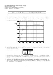
Vehicle DynamicsFH Regensburg, University of Applied Sciences1.2 Wheel/Axle Suspension Systems1.2.1 General RemarksThe Automotive Industry uses different kinds of wheel/axle suspension systems. Important criteriaare costs, space requirements, kinematic properties and compliance attributes.1.2.2 Multi Purpose Suspension SystemsThe Double Wishbone Suspension, the McPherson Suspension and the Multi-Link Suspensionare multi purpose wheel suspension systems, Fig. 1.1.Ez REGOz RGyRDRSN1ON 23xRO1GPQϕ 2ϕ 1FU 2U 1yBzBMδ SxByRz RFQRBASUλPxRDCyBzBMδ SxByRD FZXRSQVBAxRYWPUFigure 1.1: Double Wishbone, McPherson and Multi-Link SuspensionThey are used as steered front or non steered rear axle suspension systems. These suspensionsystems are also suitable for driven axles.In a McPherson suspension the spring is mounted with an inclination to the strut axis. Thusbending torques at the strut which cause high friction forces can be reduced.Z 2Y 2Z 1X 2Y 1z Az Ax xA AX 1y A y AFigure 1.2: Solid AxlesAt pickups, trucks and busses often solid axles are used. Solid axles are guided either by leafsprings or by rigid links, Fig. 1.2. Solid axles tend to tramp on rough road.4

FH Regensburg, University of Applied Sciences© Prof. Dr.-Ing. G. RillLeaf spring guided solid axle suspension systems are very robust. Dry friction between the leafsleads to locking effects in the suspension. Although the leaf springs provide axle guidance onsome solid axle suspension systems additional links in longitudinal and lateral direction areused. Thus the typical wind up effect on braking can be avoided.Solid axles suspended by air springs need at least four links for guidance. In addition to a gooddriving comfort air springs allow level control too.1.2.3 Specific Suspension SystemsThe Semi-Trailing Arm, the SLA and the Twist Beam axle suspension are suitable only for nonsteered axles, Fig. 1.3.z Rz Ay Rx Ay Ax RϕFigure 1.3: Specific Wheel/Axles Suspension SystemsThe semi-trailing arm is a simple and cheap design which requires only few space. It is mostlyused for driven rear axles.The SLA axle design allows a nearly independent layout of longitudinal and lateral axle motions.It is similar to the Central Control Arm axle suspension, where the trailing arm is completelyrigid and hence only two lateral links are needed.The twist beam axle suspension exhibits either a trailing arm or a semi-trailing arm characteristic.It is used for non driven rear axles only. The twist beam axle provides enough space forspare tire and fuel tank.1.3 Steering Systems1.3.1 RequirementsThe steering system must guarantee easy and safe steering of the vehicle. The entirety of themechanical transmission devices must be able to cope with all loads and stresses occurring inoperation.In order to achieve a good maneuverability a maximum steer angle of approx. 30 ◦ must beprovided at the front wheels of passenger cars. Depending on the wheel base busses and trucksneed maximum steer angles up to 55 ◦ at the front wheels.5

Vehicle DynamicsFH Regensburg, University of Applied SciencesRecently some companies have started investigations on ’steer by wire’ techniques.1.3.2 Rack and Pinion SteeringRack and pinion is the most common steering system on passenger cars, Fig. 1.4. The rack maybe located either in front of or behind the axle. The rotations of the steering wheel δ L are firstlywheelandwheelbodyQLdrag linkPu δZ Lpinionrack steerδ box1δ 2Figure 1.4: Rack and Pinion Steeringtransformed by the steering box to the rack travel u Z = u Z (δ L ) and then via the drag linkstransmitted to the wheel rotations δ 1 = δ 1 (u Z ), δ 2 = δ 2 (u Z ). Hence the overall steering ratiodepends on the ratio of the steer box and on the kinematics of the steer linkage.1.3.3 Lever Arm Steering Systemsteer lever 1drag link 1steer boxδ GQ 1 Q 2P 1P 2δ L 1wheel andwheel bodysteer lever 2drag link 2δ 2Figure 1.5: Lever Arm Steering SystemUsing a lever arm steering system Fig. 1.5, large steer angles at the wheels are possible. Thissteering system is used on trucks with large wheel bases and independent wheel suspension atthe front axle. Here the steering box can be placed outside of the axle center.6

FH Regensburg, University of Applied Sciences© Prof. Dr.-Ing. G. RillThe rotations of the steering wheel δ L are firstly transformed by the steering box to the rotationof the steer levers δ G = δ G (δ L ). The drag links transmit this rotation to the wheelδ 1 = δ 1 (δ G ), δ 2 = δ 2 (δ G ). Hence, again the overall steering ratio depends on the ratio ofthe steer box and on the kinematics of the steer linkage.1.3.4 Drag Link Steering SystemAt solid axles the drag link steering system is used, Fig. 1.6.δ Hsteer leverHOsteer box(90 o rotated)wheelandwheelbodysteer linkLIδ 1 δ 2Kdrag linkFigure 1.6: Drag Link Steering SystemThe rotations of the steering wheel δ L are transformed by the steering box to the rotation of thesteer lever arm δ H = δ H (δ L ) and further on to the rotation of the left wheel, δ 1 = δ 1 (δ H ). Thedrag link transmits the rotation of the left wheel to the right wheel, δ 2 = δ 2 (δ 1 ). The steeringratio is defined by the ratio of the steer box and the kinematics of the steer link. Here the ratioδ 2 = δ 2 (δ 1 ) given by the kinematics of the drag link can be changed separately.1.3.5 Bus Steer SystemIn busses the driver sits more than 2m in front of the front axle. Here, sophisticated steer systemsare needed, Fig. 1.7.The rotations of the steering wheel δ L are transformed by the steering box to the rotation of thesteer lever arm δ H = δ H (δ L ). Via the steer link the left lever arm is moved, δ H = δ H (δ G ). Thismotion is transferred by a coupling link to the right lever arm. Via the drag links the left andright wheel are rotated, δ 1 = δ 1 (δ H ) and δ 2 = δ 2 (δ H ).7

Vehicle DynamicsFH Regensburg, University of Applied Sciencessteer leverHδ Gsteer boxsteer linkδ 1QLIdrag linkwheel andwheel bodyleftleverarmδ HJPKcoupl.linkδ 2Figure 1.7: Bus Steer System1.4 Definitions1.4.1 Coordinate SystemsIn vehicle dynamics several different coordinate systems are used, Fig 1.8. The inertial systemxFzFyFx0z0y0e xe ne ye yRFigure 1.8: Coordinate Systemswith the axes x 0 , y 0 , z 0 is fixed to the track. Within the vehicle fixed system the x F -axis is8

FH Regensburg, University of Applied Sciences© Prof. Dr.-Ing. G. Rillpointing forward, the y F -axis left and the z F -axis upward. The orientation of the wheel is givenby the unit vector e yR in direction of the wheel rotation axis.The unit vectors in the directions of circumferential and lateral forces e x and e y as well as thetrack normal e n follow from the contact geometry.1.4.2 Toe and Camber Angle1.4.2.1 Definitions according to DIN 70 000The angle between the vehicle center plane in longitudinal direction and the intersection line ofthe tire center plane with the track plane is named toe angle. It is positive, if the front part of theδfrontδx Flefty FrearrightFigure 1.9: Positive Toe Anglewheel is oriented towards the vehicle center plane, Fig. 1.9.The camber angle is the angle between the wheel center plane and the track normal. It is positive,γleftγtopy Fz FrightbottomFigure 1.10: Positive Camber Angleif the upper part of the wheel is inclined outwards, Fig. 1.10.1.4.2.2 CalculationThe calculation of the toe angle is done for the left wheel. The unit vector e yR in direction ofthe wheel rotation axis is described in the vehicle fixed coordinate system F , Fig. 1.11e yR,F =[e (1)yR,Fe (2)yR,Fe (3)yR,F] T, (1.1)9

Vehicle DynamicsFH Regensburg, University of Applied Sciencese yRy Fz Fx F(2)eδ (3)V e yR,FyR,F(1)e yR,FFigure 1.11: Toe Anglewhere the axis x F and z F span the vehicle center plane. The x F -axis points forward and thez F -axis points upward. The toe angle δ can then be calculated fromtan δ = e(1) yR,Fe (2)yR,F. (1.2)The real camber angle γ follows from the scalar product between the unit vectors in the directionof the wheel rotation axis e yR and in the direction of the track normal e n ,The wheel camber angle can be calculated byOn a flat horizontal road both definitions are equal.sin γ = −e T n e yR . (1.3)sin γ = −e (3)yR,F . (1.4)1.4.3 Steering Geometry1.4.3.1 KingpinAt the steered front axle the McPherson-damper strut axis, the double wishbone axis and multilinkwheel suspension or dissolved double wishbone axis are frequently employed in passengercars, Fig. 1.12 and Fig. 1.13.The wheel body rotates around the kingpin at steering movements.At the double wishbone axis, the ball joints A and B, which determine the kingpin, are fixed tothe wheel body.The ball joint point A is also fixed to the wheel body at the classic McPherson wheel suspension,but the point B is fixed to the vehicle body.At a multi-link axle, the kingpin is no longer defined by real link points. Here, as well as withthe McPherson wheel suspension, the kingpin changes its position against the wheel body atwheel travel and steer motions.10

FH Regensburg, University of Applied Sciences© Prof. Dr.-Ing. G. Rillz RyRBMxRAkingpin axis A-BFigure 1.12: Double Wishbone Wheel SuspensionBz Rz RyRMAxRyRMxRkingpin axis A-Brotation axisFigure 1.13: McPherson and Multi-Link Wheel Suspensions1.4.3.2 Caster and Kingpin AngleThe current direction of the kingpin can be defined by two angles within the vehicle fixedcoordinate system, Fig. 1.14.If the kingpin is projected into the y F -, z F -plane, the kingpin inclination angle σ can be readas the angle between the z F -axis and the projection of the kingpin. The projection of the kingpininto the x F -, z F -plane delivers the caster angle ν with the angle between the z F -axis andthe projection of the kingpin. With many axles the kingpin and caster angle can no longer bedetermined directly. The current rotation axis at steering movements, that can be taken fromkinematic calculations here delivers a virtual kingpin. The current values of the caster angle νand the kingpin inclination angle σ can be calculated from the components of the unit vector in11

Vehicle DynamicsFH Regensburg, University of Applied Sciencesz Fz Fe Sσνy Fx FFigure 1.14: Kingpin and Caster Anglethe direction of the kingpin, described in the vehicle fixed coordinate systemtan ν = −e(1) S,Fe (3)S,Fandtan σ = −e(2) S,Fe (3)S,Fwith e S,F =[e (1)S,Fe (2)S,Fe (3)S,F] T. (1.5)1.4.3.3 Disturbing Force Lever, Caster and Kingpin OffsetThe distance d between the wheel center and the king pin axis is called disturbing force lever.It is an important quantity in evaluating the overall steer behavior. In general, the point S whereCde yPe xSr Sn KFigure 1.15: Caster and Kingpin Offsetthe kingpin runs through the track plane does not coincide with the contact point P , Fig. 1.15.If the kingpin penetrates the track plane before the contact point, the kinematic kingpin offsetis positive, n K > 0.The caster offset is positive, r S > 0, if the contact point P lies outwards of S.12

2 The Tire2.1 Introduction2.1.1 Tire DevelopmentThe following table shows some important mile stones in the development of tires.1839 Charles Goodyear: vulcanization1845 Robert William Thompson: first pneumatic tire(several thin inflated tubes inside a leather cover)1888 John Boyd Dunlop: patent for bicycle (pneumatic) tires1893 The Dunlop Pneumatic and Tyre Co. GmbH, Hanau, Germany1895 André and Edouard Michelin: pneumatic tires for PeugeotParis-Bordeaux-Paris (720 Miles): 50 tire deflations,22 complete inner tube changes1899 Continental: longer life tires (approx. 500 Kilometer)1904 Carbon added: black tires.1908 Frank Seiberling: grooved tires with improved road traction1922 Dunlop: steel cord thread in the tire bead1943 Continental: patent for tubeless tires1946 Radial Tire.Table 2.1: Mile Stones in the Development of Tires2.1.2 Tire CompositesA modern tire is a mixture of steel, fabric, and rubber.13

¡¢Vehicle DynamicsFH Regensburg, University of Applied SciencesReinforcements: steel, rayon, nylon 16%Rubber: natural/synthetic 38%Compounds: carbon, silica, chalk, ... 30%Softener: oil, resin 10%Vulcanization: sulfur, zinc oxide, ... 4%Miscellaneous 2%Tire Mass8.5 kgTable 2.2: Tire Composites: 195/65 R 15 ContiEcoContact, Data from www.felge.de2.1.3 Forces and Torques in the Tire Contact AreaIn any point of contact between tire and track normal and friction forces are delivered. Accordingto the tire’s profile design the contact area forms a not necessarily coherent area.The effect of the contact forces can be fully described by a vector of force and a torque in referenceto a point in the contact patch. The vectors are described in a track-fixed coordinate system.The z-axis is normal to the track, the x-axis is perpendicular to the z-axis and perpendicular tothe wheel rotation axis e yR . The demand for a right-handed coordinate system then also fixesthe y-axis.F xF yF zM xM yM zlongitudinal or circumferential forcelateral forcevertical force or wheel loadtilting torquerolling resistance torqueself aligning and bore torqueM xMzF x F z ¡MF y¢yFigure 2.1: Contact Forces and TorquesThe components of the contact force are named according to the direction of the axes, Fig. 2.1.Non symmetric distributions of force in the contact patch cause torques around the x and y axes.The tilting torque M x occurs when the tire is cambered. M y also contains the rolling resistanceof the tire. In particular the torque around the z-axis is relevant in vehicle dynamics. It consistsof two parts,M z = M B + M S . (2.1)Rotation of the tire around the z-axis causes the bore torque M B . The self aligning torque M Srespects the fact that in general the resulting lateral force is not applied in the center of thecontact patch.14

FH Regensburg, University of Applied Sciences© Prof. Dr.-Ing. G. Rill2.2 Contact Geometry2.2.1 Contact PointThe current position of a wheel in relation to the fixed x 0 -, y 0 - z 0 -system is given by the wheelcenter M and the unit vector e yR in the direction of the wheel rotation axis, Fig. 2.2.γtirerim centre planee yRMe yRe zRr SMe ne nP0P *road: z = z ( x , y )y 0x 0z 00e xP 0e ybaPlocal road planeFigure 2.2: Contact GeometryThe irregularities of the track can be described by an arbitrary function of two spatial coordinatesz = z(x, y). (2.2)At an uneven track the contact point P can not be calculated directly. One can firstly get anestimated value with the vectorr MP ∗ = −r 0 e zB , (2.3)where r 0 is the undeformed tire radius and e zB is the unit vector in the z-direction of the bodyfixed reference frame.The position of P ∗ with respect to the fixed system x 0 , y 0 , z 0 is determined byr 0P ∗ = r 0M + r MP ∗, (2.4)where the vector r 0M states the position of the rim center M. Usually the point P ∗ lies not onthe track. The corresponding track point P 0 follows from⎡⎤r (1)0P ∗ ,0r 0P0 ,0 = ⎢⎣r (2)⎥( 0P ∗ ,0 ) ⎦ . (2.5)z r (1)0P ∗ ,0 , r(2) 0P ∗ ,015

Vehicle DynamicsFH Regensburg, University of Applied SciencesIn the point P 0 now the track normal e n is calculated. Then the unit vectors in the tire’s circumferentialdirection and lateral direction can be calculatede x = e yR×e n| e yR ×e n | , and e y = e n ×e x . (2.6)Calculating e x demands a normalization, for the unit vector in the direction of the wheel rotationaxis e yR is not always perpendicular to the track. The tire camber angleγ = arcsin ( e T yR e n)(2.7)describes the inclination of the wheel rotation axis against the track normal.The vector from the rim center M to the track point P 0 is now split into three partsr MP0 = −r S e zR + a e x + b e y , (2.8)where r S names the loaded or static tire radius and a, b are displacements in circumferentialand lateral direction.The unit vectore zR = e x×e yR| e x ×e yR | . (2.9)is perpendicular to e x and e yR . Because the unit vectors e x and e y are perpendicular to e n , thescalar multiplication of (2.8) with e n results ine T n r MP0 = −r S e T n e zR or r S = − eT n r MP0e T n e zR. (2.10)Now also the tire deflection can be calculatedwith r 0 marking the undeformed tire radius.The point P given by the vector△r = r 0 − r S , (2.11)r MP = −r S e zR (2.12)lies within the rim center plane. The transition from P 0 to P takes place according to (2.8) byterms a e x and b e y , standing perpendicular to the track normal. The track normal however wascalculated in the point P 0 . Therefore with an uneven track P no longer lies on the track.With the newly estimated value P ∗ = P now the equations (2.5) to (2.12) can be recurred untilthe difference between P and P 0 is sufficiently small.Tire models which can be simulated within acceptable time assume that the contact patch iseven. At an ordinary passenger-car tire, the contact patch has at normal load about the size ofapproximately 20×20 cm. There is obviously little sense in calculating a fictitious contact pointto fractions of millimeters, when later the real track is approximated in the range of centimetersby a plane.If the track in the contact patch is replaced by a plane, no further iterative improvement isnecessary at the hereby used initial value.16

FH Regensburg, University of Applied Sciences© Prof. Dr.-Ing. G. Rill2.2.2 Local Track PlaneA plane is given by three points. With the tire width b, the undeformed tire radius r 0 and thelength of the contact area L N at given wheel load, estimated values for three track points can begiven in analogy to (2.4)r ML ∗ =b2 yR − r 0 e zB ,r MR ∗ = − b e 2 yR − r 0 e zB ,r MF ∗ = L N2e xB −r 0 e zB .(2.13)The points lie left, resp. right and to the front of a point below the rim center. The unit vectorse xB and e zB point in the longitudinal and vertical direction of the vehicle. The wheel rotationaxis is given by e yR . According to (2.5) the corresponding points on the track L, R and F canbe calculated.The vectorsr RF = r 0F − r 0R and r RL = r 0L − r 0R (2.14)lie within the track plane. The unit vector calculated bye n = r RF ×r RL| r RF ×r RL | . (2.15)is perpendicular to the plane defined by the points L, R, and F and gives an average tracknormal over the contact area. Discontinuities which occur at step- or ramp-sized obstacles aresmoothed that way.Of course it would be obvious to replace L N in (2.13) by the actual length L of the contactarea and the unit vector e zB by the unit vector e zR which points upwards in the wheel centerplane. The values however, can only be calculated from the current track normal. Here also aniterative solution would be possible. Despite higher computing effort the model quality cannotbe improved by this, because approximations in the contact calculation and in the tire modellimit the exactness of the tire model.2.3 Wheel LoadThe vertical tire force F z can be calculated as a function of the normal tire deflection △z =e T n △r and the deflection velocity △ż = e T n △ṙF z = F z (△z, △ż) . (2.16)Because the tire can only deliver pressure forces to the road, the restriction F z ≥ 0 holds.In a first approximation F z is separated into a static and a dynamic partF z = F S z + F D z . (2.17)17

Vehicle DynamicsFH Regensburg, University of Applied SciencesThe static part is described as a nonlinear function of the normal tire deflectionF S z = c 0 △z + κ (△z) 2 . (2.18)The constants c 0 and κ may be calculated from the radial stiffness at nominal payload and atdouble the payload. Results for a passenger car and a truck tire are shown in Fig. 2.3. Theparabolic approximation Eq. (2.18) fits very well to the measurements.10Passenger Car Tire: 205/50 R15100Truck Tire: X31580 R22.5880F z [kN]64F z [kN]604022000 10 20 30 40 50∆z [mm]00 20 40 60 80∆z [mm]Figure 2.3: Tire Radial Stiffness: ◦ Measurements, — ApproximationThe radial tire stiffness of the passenger car tire at the payload of F z = 3 200 N can be specifiedwith c 0 = 190 000N/m. The Payload F z = 35 000 N and the stiffness c 0 = 1 250 000N/m of atruck tire are significantly larger.The dynamic part is roughly approximated bywhere d R is a constant describing the radial tire damping.F D z = d R △ż , (2.19)2.3.1 Dynamic Rolling RadiusAt an angular rotation of △ϕ, assuming the tread particles stick to the track, the deflected tiremoves on a distance of x, Fig. 2.4.With r 0 as unloaded and r S = r 0 − △r as loaded or static tire radiusandhold.r 0 sin △ϕ = x (2.20)r 0 cos △ϕ = r S . (2.21)If the movement of a tire is compared to the rolling of a rigid wheel, its radius r D then has to bechosen so, that at an angular rotation of △ϕ the tire moves the distancer 0 sin △ϕ = x = r D △ϕ . (2.22)18

FH Regensburg, University of Applied Sciences© Prof. Dr.-Ing. G. Rilldeflected tireΩrigid wheelΩr 0∆ϕxr Sv trD∆ϕxFigure 2.4: Dynamic Rolling RadiusHence, the dynamic tire radius is given byr D= r 0 sin △ϕ△ϕ. (2.23)For △ϕ → 0 one gets the trivial solution r D = r 0 .At small, yet finite angular rotations the sine-function can be approximated by the first terms ofits Taylor-Expansion. Then, (2.23) reads asr D= r 0△ϕ − 1 6 △ϕ3△ϕ= r 0(1 − 1 6 △ϕ2 ). (2.24)With the according approximation for the cosine-functionr Sr 0= cos △ϕ = 1 − 1 2 △ϕ2 or △ϕ 2 = 2(1 − r Sr 0)(2.25)one finally getsremains.(r D = r 0 1 − 1 (1 − r ))S3 r 0= 2 3 r 0 + 1 3 r S (2.26)The radius r D depends on the wheel load F z because of r S = r S (F z ) and thus is named dynamictire radius. With this first approximation it can be calculated from the undeformed radius r 0 andthe steady state radius r S .Byv t = r D Ω (2.27)the average velocity is given with which tread particles are transported through the contact area.19

Vehicle DynamicsFH Regensburg, University of Applied Sciences2.3.2 Contact Point VelocityThe absolute velocity of the contact point one gets from the derivation of the position vectorv 0P,0 = ṙ 0P,0 = ṙ 0M,0 + ṙ MP,0 . (2.28)Here ṙ 0M,0 = v 0M,0 is the absolute velocity of the wheel center and r MP,0 the vector from thewheel center M to the contact point P , expressed in the inertial frame 0. With (2.12) one getsDue to r 0 = const.follows from (2.11).ṙ MP,0 = d dt (−r S e zR,0 ) = −ṙ S e zR,0 − r S ė zR,0 . (2.29)− ṙ S = △ṙ (2.30)The unit vector e zR moves with the rim but does not perform rotations around the wheel rotationaxis. Its time derivative is then given byė zR,0 = ω ∗ 0R,0×e zR,0 (2.31)where ω0R ∗ is the angular velocity of the wheel rim without components in the direction of thewheel rotation axis. Now (2.29) reads asand the contact point velocity can be written asṙ MP,0 = △ṙ e zR,0 − r S ω ∗ 0R,0×e ZR,0 (2.32)v 0P,0 = v 0M,0 + △ṙ e zR,0 − r S ω ∗ 0R,0×e ZR,0 . (2.33)Because the point P lies on the track, v 0P,0 must not contain a component normal to the trackThe tire deformation velocity is defined by this demande T n v 0P = 0 . (2.34)△ṙ = −eT n (v 0M + r S ω ∗ 0R ×e ZR)e T n e zR. (2.35)Now, the contact point velocity v 0P and its components in longitudinal and lateral directionv x = e T x v 0P (2.36)andcan be calculated.v y = e T y v 0P (2.37)20

FH Regensburg, University of Applied Sciences© Prof. Dr.-Ing. G. Rill2.4 Longitudinal Force and Longitudinal SlipTo get some insight into the mechanism generating tire forces in longitudinal direction weconsider a tire on a flat test rig. The rim is rotating with the angular speed Ω and the flat trackruns with speed v x . The distance between the rim center an the flat track is controlled to theloaded tire radius corresponding to the wheel load F z , Fig. 2.5.A tread particle enters at time t = 0 the contact area. If we assume adhesion between the particleand the track then the top of the particle runs with the track speed v x and the bottom with theaverage transport velocity v t = r D Ω. Depending on the speed difference △v = r D Ω − v x thetread particle is deflected in longitudinal directionu = (r D Ω − v x ) t . (2.38)r Dv xΩv xΩr DLuu maxFigure 2.5: Tire on Flat Track Test RigThe time a particle spends in the contact area can be calculated byT =Lr D |Ω| , (2.39)where L denotes the contact length, and T > 0 is assured by |Ω|.The maximum deflection occurs when the tread particle leaves at t = T the contact areau max = (r D Ω − v x ) T = (r D Ω − v x )Lr D |Ω| . (2.40)The deflected tread particle applies a force to the tire. In a first approximation we getF t x = c t x u , (2.41)21

Vehicle DynamicsFH Regensburg, University of Applied Scienceswhere c t x is the stiffness of one tread particle in longitudinal direction.On normal wheel loads more than one tread particle is in contact with the track, Fig. 2.6a. Thenumber p of the tread particles can be estimated byp =Ls + a . (2.42)where s is the length of one particle and a denotes the distance between the particles.a) b)c)LLr 0satx*c utcu * umaxL/2∇rFigure 2.6: a) Particles, b) Force Distribution, c) Tire DeformationParticles entering the contact area are undeformed on exit the have the maximum deflection.According to (2.41) this results in a linear force distribution versus the contact length, Fig. 2.6b.For p particles the resulting force in longitudinal direction is given byWith (2.42) and (2.40) this results inF x = 1 2A first approximation of the contact length L is given byF x = 1 2 p ct x u max . (2.43)LLs + a ct x (r D Ω − v x )r D |Ω| . (2.44)(L/2) 2 = r 2 0 − (r 0 − △r) 2 , (2.45)where r 0 is the undeformed tire radius, and △r denotes the tire deflection, Fig. 2.6c. With△r ≪ r 0 one getsL 2 ≈ 8 r 0 △r . (2.46)The tire deflection can be approximated by△r = F z /c R . (2.47)where F z is the wheel load, and c R denotes the radial tire stiffness. Now, (2.43) can be writtenasF x = 4 r 0 c t x r D Ω − v xF z . (2.48)s + a c R r D |Ω|22

FH Regensburg, University of Applied Sciences© Prof. Dr.-Ing. G. RillThe non-dimensional relation between the sliding velocity of the tread particles in longitudinaldirection v S x = v x − r D Ω and the average transport velocity r D |Ω| forms the longitudinal slips x = −(v x − r D Ω)r D |Ω|. (2.49)In this first approximation the longitudinal force F x is proportional to the wheel load F z andthe longitudinal slip s xF x = k F z s x , (2.50)where the constant k collects the tire properties r 0 , s, a, c t x and c R .The relation (2.50) holds only as long as all particles stick to the track. At average slip valuesthe particles at the end of the contact area start sliding, and at high slip values only the parts atthe beginning of the contact area still stick to the road, Fig. . 2.7.small slip values moderate slip values large slip valuesF x = k * F z*sx F x = F z * f ( s x)F = FLLxLGadhesionF xt

Vehicle DynamicsFH Regensburg, University of Applied Sciences2.5 Lateral Slip, Lateral Force and Self Aligning TorqueSimilar to the longitudinal slip s x , given by (2.49), the lateral slip can be defined bywhere the sliding velocity in lateral direction is given bys y = −vS yr D |Ω| , (2.51)v S y = v y (2.52)and the lateral component of the contact point velocity v y follows from (2.37).As long as the tread particles stick to the road (small amounts of slip), an almost linear distributionof the forces along the length L of the contact area appears. At moderate slip valuesthe particles at the end of the contact area start sliding, and at high slip values only the partsat the beginning of the contact area stick to the road, Fig. 2.9. The nonlinear characteristicssmall slip values moderate slip values large slip valuesF y = k * F z*sy F y = F z * f ( s y)F = FyGFyslidingadhesionnLadhesionFyLslidingF yLFigure 2.9: Lateral Force Distribution over Contact Areaof the lateral force versus the lateral slip can be described by the initial inclination (corneringstiffness) dFy 0 , location s M y and magnitude Fy M of the maximum and start of full sliding s G y andmagnitude FyG of the sliding force.The distribution of the lateral forces over the contact area length also defines the acting point ofthe resulting lateral force. At small slip values the working point lies behind the center of thecontact area (contact point P). With rising slip values, it moves forward, sometimes even beforethe center of the contact area. At extreme slip values, when practically all particles are sliding,the resulting force is applied at the center of the contact area.The resulting lateral force F y with the dynamic tire offset or pneumatic trail n as a lever generatesthe self aligning torqueM S = −n F y . (2.53)The lateral force F y as well as the dynamic tire offset are functions of the lateral slip s y . Typicalplots of these quantities are shown in Fig. 2.10. Characteristic parameters for the lateral24

FH Regensburg, University of Applied Sciences© Prof. Dr.-Ing. G. Rilln/L(n/L)0adhesionadhesion/slidingF yMyFGF 0 dFyyadhesion adhesion/slidingfull slidingMSadhesions y0full slidingGs s y yadhesion/slidingfull slidings yMsGys ys y0s yGs yFigure 2.10: Typical Plot of Lateral Force, Tire Offset and Self Aligning Torqueforce graph are initial inclination (cornering stiffness) dFy 0 , location s M ymaximum Fy M , begin of full sliding s G y , and the sliding force Fy G .and magnitude of theThe dynamic tire offset has been normalized by the length of the contact area L. The initialvalue (n/L) 0 as well as the slip values s 0 y and s G y characterize the graph sufficiently.2.6 Camber InfluenceAt a cambered tire, Fig. 2.11, the angular velocity of the wheel Ω has a component normal tothe roadΩ n = Ω sin γ . (2.54)Now, the tread particles in the contact area possess a lateral velocity which depends on theirposition ξ and is given byv γ (ξ) = −Ω nL2ξ, = −Ω sin γ ξ , −L/2 ≤ ξ ≤ L/2 . (2.55)L/2At the center of the contact area (contact point) it vanishes and at the end of the contact area itis of the same value but opposite to the value at the beginning of the contact area.Assuming that the tread particles stick to the track, the deflection profile is defined byThe time derivative can be transformed to a space derivativeẏ γ (ξ) = d y γ(ξ)d ξẏ γ (ξ) = v γ (ξ) . (2.56)d ξd t = d y γ(ξ)r D |Ω| (2.57)d ξ25

Vehicle DynamicsFH Regensburg, University of Applied Sciencese nrimF y = Fcentre4000plane30002000Ω nΩ10000-1000e x r D |Ω|-2000-3000vγ(ξ)ξe yyγ(ξ)e yRγy (s y): Parameter γγ-4000-0.5 0 0.5Figure 2.11: Cambered Tire F y (γ) at F z = 3.2 kN and γ = 0 ◦ , 2 ◦ , 4 ◦ , 6 ◦ , 8 ◦where r D |Ω| denotes the average transport velocity. Now (2.56) reads asd y γ (ξ)d ξwhich results in the parabolic deflection profiley γ (ξ) = 1 2r D |Ω| = −Ω sin γ ξ , (2.58)Ω sin γr D |Ω|( L2) 2[1 −( ) ] 2 ξL/2Similar to the lateral slip s y which is by (2.51) we now can define a camber slip. (2.59)s γ=−Ω sin γr D |Ω|L2 . (2.60)The lateral deflection of the tread particles generates a lateral forcewhere c y denotes the lateral stiffness of the tread particles andF yγ = −c y ȳ γ , (2.61)ȳ γ = 1 2 (−s γ) L 21L∫L/2−L/2[1 −( ) ] 2 xdξ = − 1 L/26 s γ L (2.62)is the average value of the parabolic deflection profile.26

FH Regensburg, University of Applied Sciences© Prof. Dr.-Ing. G. RillA purely lateral tire movement without camber results in a linear deflexion profile with theaverage deflexionA comparison of (2.62) to (2.63) shows, that withȳ y = − 1 2 s y L . (2.63)s γ y = 1 3 s γ (2.64)the lateral camber slip s γ can be converted to an equivalent lateral slip s γ y.In normal driving operation, the camber angle and thus the lateral camber slip are limited tosmall values. So the lateral camber force can be approximated byF γ y ≈ dF 0 y s γ y . (2.65)If the “global” inclination dF y = F y /s y is used instead of the initial inclination dF 0 y , one getsthe camber influence on the lateral force as shown in Fig. 2.11.The camber angle influences the distribution of pressure in the lateral direction of the contactarea, and changes the shape of the contact area from rectangular to trapezoidal. It is thus extremelydifficult if not impossible to quantify the camber influence with the aid of such simplemodels. But this approach turns out to be a quit good approximation.2.7 Bore TorqueIf the angular velocity of the wheelhas a component in direction of the track normal e nω 0W = ω ∗ 0R + Ω e yR (2.66)ω n = e T n ω 0W ≠ 0 . (2.67)a very complicated deflection profile of the tread particles in the contact area occurs. By a simpleapproach the resulting bore torque can be approximated by the parameter of the longitudinalforce characteristics.Fig. 2.12 shows the contact area at zero camber, γ = 0 and small slip values, s x ≈ 0, s y ≈ 0.The contact area is separated into small stripes of width dy. The longitudinal slip in a stripe atposition y is then given bys x (y) = − (−ω n y). (2.68)r D |Ω|For small slip values the nonlinear tire force characteristics can be linearized. The longitudinalforce in the stripe can then be approximated byF x (y) = d F xd s x∣ ∣∣∣sx=0d s xd y y . (2.69)27

Vehicle DynamicsFH Regensburg, University of Applied SciencesdyxdyxyU(y)Qω nPcontactareaLyUGω nPcontactarea-U GLBBFigure 2.12: Bore Torque generated by Longitudinal ForcesWith (2.68) one getsF x (y) = d F xd s x∣ ∣∣∣sx=0The forces F x (y) generate a bore torque in the contact point Pω nr D |Ω| y . (2.70)M B = − 1 B+∫B 2− B 2= 1 12 B2 d F xd s x∣ ∣∣∣sx=0y F x (y) dy = − 1 B−ω nr D |Ω|+∫B 2− B 2y d F xd s x∣ ∣∣∣sx=0= 1 12 B d F xd s x∣ ∣∣∣sx=0Br Dω nr D |Ω| y dy−ω n| Ω |,(2.71)wheres B = −ω n| Ω |(2.72)can be considered as bore slip. Via dF x /ds x the bore torque takes into account the actualfriction and slip conditions.The bore torque calculated by (2.71) is only a first approximation. At large bore slips the longitudinalforces in the stripes are limited by the sliding values. Hence, the bore torque is limitedbywhere F G x| M B | ≤ M maxB= 2 1 Bdenotes the longitudinal sliding force.+∫B 20y F G x dy = 1 4 B F G x , (2.73)28

FH Regensburg, University of Applied Sciences© Prof. Dr.-Ing. G. Rill2.8 Typical Tire CharacteristicsThe tire model TMeasy 1 which is based on this simple approach can be used for passenger cartires as well as for truck tires. It approximates the characteristic curves F x = F x (s x ), F y =F y (α) and M z = M z (α) quite well even for different wheel loads F z , Fig. 2.13.F x[kN]6420-2-41.8 kN3.2 kN4.6 kN5.4 kN-6-40 -20 0 20 40s [%] xF x[kN]40200-20-4010 kN20 kN30 kN40 kN50 kN-40 -20 0 20 40s [%] xF y[kN]6420-2-4-61501.8 kN3.2 kN4.6 kN6.0 kNF y[kN]40200-20-40150010 kN20 kN30 kN40 kN1001000M z[Nm]500-50-100-1501.8 kN3.2 kN4.6 kN6.0 kN-20 -10 0 10 20α [o]M z[Nm]5000-500-1000-150018.4 kN36.8 kN55.2 kN-20 -10 0 10 20α [o]Figure 2.13: Longitudinal Force, Lateral Force and Self Aligning Torque: ◦ Meas., − TMeasy1 Hirschberg, W; Rill, G. Weinfurter, H.: User-Appropriate Tyre-Modelling for Vehicle Dynamics in Standardand Limit Situations. Vehicle System Dynamics 2002, Vol. 38, No. 2, pp. 103-125. Lisse: Swets & Zeitlinger.29

Vehicle DynamicsFH Regensburg, University of Applied SciencesWithin TMeasy the one-dimensional characteristics are automatically converted to a twodimensionalcombination characteristics, Fig. 2.14.F y[kN]3210-1-2-3-4 -2 0 2 4F [kN] xF y[kN]3020100-10-20-30-20 0 20F [kN] x|s x | = 1, 2, 4, 6, 10, 15 %; |α| = 1, 2, 4, 6, 10, 14 ◦Figure 2.14: Two-dimensional Tire Characteristics at F z = 3.2 kN / F z = 35 kN30

3 Vertical Dynamics3.1 GoalsThe aim of vertical dynamics is the tuning of body suspension and damping to guarantee gooddriving comfort, resp. a minimal stress of the load at sufficient safety.The stress of the load can be judged fairly well by maximal or integral values of the bodyaccelerations.The wheel load F z is linked to the longitudinal F x and lateral force F y by the coefficient offriction. The digressive influence of F z on F x and F y as well as instationary processes at theincrease of F x and F y in the average lead to lower longitudinal and lateral forces at wheel loadvariations.Maximal driving safety can therefore be achieved with minimal variations of wheel load. Smallvariations of wheel load also reduce the stress on the track.The comfort of a vehicle is subjectively judged by the driver. In literature, different approachesof describing the human sense of vibrations by different metrics can be found.Transferred to vehicle vertical dynamics, the driver primarily registers the amplitudes and accelerationsof the body vibrations. These values are thus used as objective criteria in practice.3.2 Basic Tuning3.2.1 Simple ModelsFig. 3.1 shows simple quarter car models, that are suitable for basic investigations of body andaxle vibrations.At normal vehicles the wheel mass m is in relation to the respective body mass M much smallerm ≪ M. The coupling of wheel and body movement can thus be neglected for basic investigations.In describing the vertical movements of the body, the wheel movements remain unrespected. Ifthe wheel movements are in the foreground, then body movements can be neglected.The equations of motion for the models read asM ¨z B + d S ż B + c S z B = d S ż R + c S z R (3.1)31

Vehicle DynamicsFH Regensburg, University of Applied SciencesM✻z B❵✥c ❵✥✥❵S ❵✥✥❵ d✥❵S❵✥c S ❵✥✥❵❵✥✥❵✥❵❝d S✻z Rm❵✥❵✥✥❵❵✥✥❵ c T✥❵❝✻z W✻z RandFigure 3.1: Simple Vehicle and Suspension Modelm ¨z W + d S ż W + (c S + c T ) z W = c T z R , (3.2)where z B and z W label the vertical movements of the body and the wheel mass out of theequilibrium position. The constants c S , d S describe the body suspension and damping, and c Tthe vertical stiffness of the tire. The tire damping is hereby neglected against the body damping.3.2.2 TrackThe track is given as function in the space domainz R = z R (x) . (3.3)In (3.1) also the time gradient of the track irregularities is necessary. From (3.3) firstly followsż R = d z R dxdx dt . (3.4)At the simple model the speed, with which the track irregularities are probed equals the vehiclespeed dx/dt = v. If the vehicle speed is given as time function v = v(t), the covered distance xcan be calculated by simple integration.3.2.3 Spring PreloadThe suspension spring is loaded with the respective vehicle load. At linear spring characteristicsthe steady state spring deflection is calculated fromf 0= M gc S. (3.5)At a conventional suspension without niveau regulation a load variation M → M + △M leadsto changed spring deflections f 0 → f 0 + △f. In analogy to (3.5) the additional deflectionfollows from△f = △M g . (3.6)c S32

FH Regensburg, University of Applied Sciences© Prof. Dr.-Ing. G. RillIf for the maximum load variation △M max the additional spring deflection is limited to △f maxthe suspension spring rate can be estimated by a lower boundc S≥ △M max g△f max . (3.7)3.2.4 EigenvaluesAt an ideally even track the right side of the equations of motion (3.1), (3.2) vanishes becauseof z R = 0 and ż R = 0. The remaining homogeneous second order differential equations can bewritten as¨z + 2 δ ż + ω 2 0 z = 0 . (3.8)The respective attenuation constants δ and the undamped natural circular frequency ω 0 for themodels in Fig. 3.1 can be determined from a comparison of (3.8) with (3.1) and (3.2). Theresults are arranged in table 3.1.MotionsDifferential EquationattenuationconstantundampedEigenfrequencyBody M ¨z B + d S ż B + c S z B = 0 δ B = d S2 Mω 2 B 0= c SMWheel m ¨z W + d S ż W + (c S + c T ) z W = 0 δ R = d S2 m ω2 W 0= c S + c TmTable 3.1: Attenuation Constants and undamped natural FrequenciesWiththe equationfollows from (3.8). Forz = z 0 e λt (3.9)(λ 2 + 2 δ λ + ω 2 0) z 0 e λt = 0 . (3.10)λ 2 + 2 δ λ + ω 2 0 = 0 (3.11)also non-trivial solutions are possible. The characteristical equation (3.11) has got the solutions√λ 1,2 = −δ ± δ 2 − ω0 2 (3.12)For δ 2 ≥ ω 2 0 the eigenvalues λ 1,2 are real and, because of δ ≥ 0 not positive, λ 1,2 ≤ 0. Disturbancesz(t=0) = z 0 with ż(t=0) = 0 then subside exponentially.33

Vehicle DynamicsFH Regensburg, University of Applied SciencesWith δ 2 < ω0 2 the eigenvalues become complex√λ 1,2 = −δ ± i ω0 2 − δ 2 . (3.13)The system now executes damped oscillations.The caseδ 2 = ω 2 0 , bzw. δ = ω 0 (3.14)describes, in the sense of stability, an optimal system behavior.Wheel and body mass, as well as tire stiffness are fixed. The body spring rate can be calculatedvia load variations, cf. section 3.2.3. With the abbreviations from table 3.1 now dampingparameters can be calculated from (3.14) which provide with√cS(d S ) opt1= 2 MM = 2 √ c S M (3.15)optimal body vibrations and with(d S ) opt2= 2 moptimal wheel vibrations.√cS + c Tm= 2 √ (c S + c T ) m (3.16)3.2.5 Free VibrationsFig. 3.2 shows the time response of a damped single-mass oscillator to an initial disturbanceas results from the solution of the differential equation (3.8). The system here has been startedwithout initial speed ż(t=0) = 0 but with the initial disturbance z(t=0) = z 0 . If the attenuationconstant δ is increased at first the system approaches the steady state position z G = 0 faster andfaster, but then, a slow asymptotic behavior occurs.z 0z(t)tFigure 3.2: Damped Vibration34

FH Regensburg, University of Applied Sciences© Prof. Dr.-Ing. G. RillCounting differences from the steady state positions as errors ɛ(t) = z(t) − z G , allows judgingthe quality of the vibration. The overall error is calculated byɛ 2 G =∫t=t Ez(t) 2 dt , (3.17)t=0where the time t E have to be chosen appropriately. If the overall error becomes a Minimumthe system approaches the steady state position as fast as possible.ɛ 2 G → Minimum (3.18)To judge driving comfort and safety the deflections z B and accelerations ¨z B of the body and thedynamic wheel load variations are used.The system behavior is optimal if the parameters M, m, c S , d S , c T result from the demands forcomfortt=t ∫ E{ (ɛ 2 ) 2 ( ) }2G C= g1 ¨z B + g2 z B dt → Minimum (3.19)and safetyt=0ɛ 2 G S=∫t=t E(cT z W) 2dt → Minimum . (3.20)t=0With the factors g 1 and g 2 accelerations and deflections can be weighted differently. In theequations of motion for the body (3.1) the terms M ¨z B and c S z B are added. With g 1 = M andg 2 = c S or g 1 = 1 and g 2 = c S /M one gets system-fitted weighting factors.At the damped single-mass oscillator, the integrals in (3.19) can, for t E → ∞, still be solvedanalytically. One gets[ɛ 2 G C= zB 2 c S 1 dS0M 2 M + 2 c ]S(3.21)d Sandɛ 2 G S= z 2 W 0c 2 T12[d S+ m ]c S + c T d S. (3.22)Small body suspension stiffnesses c S → 0 or large body masses M → ∞ make the comfortcriteria (3.21) small ɛ 2 G C→ 0 and so guarantee a high driving comfort.A great body mass however is uneconomic. The body suspension stiffness cannot be reducedarbitrary low values, because then load variations would lead to too great changes in staticdeflection. At fixed values for c S and M the damper can be designed in a way that minimizesthe comfort criteria (3.21). From the necessary condition for a minimum∂ɛ 2 G C∂d S= z 2 B 0c SM12[ 1M − 2 c Sd 2 S]= 0 (3.23)35

Vehicle DynamicsFH Regensburg, University of Applied Sciencesthe optimal damper parameterthat guarantees optimal comfort follows.(d S ) opt3= √ 2 c S M , (3.24)Small tire spring stiffnesses c T → 0 make the safety criteria (3.22) small ɛ 2 G S→ 0 and thusreduce dynamic wheel load variations. The tire spring stiffness can however not be reduced toarbitrary low values, because this would cause too great tire deformation. Small wheel massesm → 0 and/or a hard body suspension c S → ∞ also reduce the safety criteria (3.22). The useof light metal rims increases, because of wheel weight reduction, the driving safety of a car.Hard body suspensions contradict driving comfort.With fixed values for c S , c T and m here the damper can also be designed to minimize the safetycriteria (3.22). From the necessary condition of a minimum∂ɛ 2 G S∂d Sthe optimal damper parameter= z 2 W 0c 2 Tfollows, which guarantees optimal safety.12[1c S + c T− m d 2 S]= 0 (3.25)(d S ) opt4= √ (c S + c T ) m , (3.26)3.3 Sky Hook Damper3.3.1 Modelling AspectsIn standard vehicle suspension systems the damper is mounted between the wheel and the body.Hence, the damper affects body and wheel/axle motions simultaneously.To take this situation into account the simple quarter car models of section 3.2.1 must be combinedto a more enhanced model, Fig. 3.3a.Assuming a linear characteristics the suspension damper force is given byF D = −d S (ż B − ż W ) , (3.27)where d S denotes the damping constant, and ż B , ż W are the time derivatives of the absolutevertical body and wheel displacements.The sky hook damping concept starts with two independent dampers for the body and thewheel/axle mass, Fig. 3.3b. A practical realization in form of a controllable damper will thenprovide the damping forceF D = −d B ż B + d W ż W , (3.28)where instead of the single damping constant d S now two design parameter d B and d W areavailable.36

FH Regensburg, University of Applied Sciences© Prof. Dr.-Ing. G. Rillskyz Bc Sc TMd Sz Bc Sc TMF Dd Bd Wz Wmz Wmz Rz Ra) Standard Damper b) Sky Hook DamperFigure 3.3: Quarter Car Model with Standard and Sky Hook DamperThe equations of motion for the quarter car model are given byM ¨z B = F S + F D − M g ,m ¨z W = F T − F S − F D − m g ,(3.29)where M, m are the sprung and unsprung mass, z B , z W denote their vertical displacements, andg is the constant of gravity.The suspension spring force is modelled byF S = F 0 S − c S (z B − z W ) , (3.30)where F 0 S = m B g is the spring preload, and c S is the spring stiffness.Finally, the vertical tire force is given byF T = F 0 T − c S (z W − z R ) , (3.31)where FT0 = (M + m) g is the tire preload, c S the vertical tire stiffness, and z R describes theroad roughness. The condition F T ≥ 0 takes the tire lift off into account.3.3.2 System PerformanceTo perform an optimization the merit functions (3.19) and (3.20) were combined to one meritfunctionɛ 2 G C=∫t=t Et=0{( ¨zBg) 2+( cS z BM g) 2+(cT z WF 0 T) 2}dt → Minimum , (3.32)37

Vehicle DynamicsFH Regensburg, University of Applied Scienceswhere the constant of gravity g and the tire preload FT 0 were used to weight the comfort andsafety parts.The optimization was done numerically. The masses M = 300kg and m = 50kg, the suspensionstiffness c S = 18 000 N/m and the vertical tire stiffness c T = 220 000 N/m correspond to apassenger car. This parameter were kept unchanged.Using the simple model approach the standard damper can be designed according to the comfort(3.24) or to the safety criteria (3.26). One gets(d S ) C opt= √ 2 c S M = √ 2 18 000 300 = 3286.3 N/(m/s) ,(d S ) S opt= √ (c S + c T ) m = √ (18 000 + 220 000) 50 = 3449.6 N/(m/s) ,(3.33)An optimization with the quarter car model results in(d S ) qcmopt= 2927 N/(m/s) , (3.34)where, according to the merit function (3.32) a weighted compromise between comfort andsafety was demanded. This ”optimal” damper value is 10% smaller than the one calculated withthe simple model approach.dynamic wheel load [N]body accelerations [m/s^2]10Standard Damper8Sky Hook Damper6420-25000Standard Damper4000Sky Hook Damper3000200010000-10000 0.2 0.4 0.6 0.8 1time [s]displacements [m] suspension travel [m]0.020-0.02-0.04-0.06-0.080.020-0.02-0.04-0.06wheelbodyStandard DamperSky Hook DamperStandard DamperSky Hook Damper-0.080 0.2 0.4 0.6 0.8 1time [s]Figure 3.4: Standard and Sky Hook Damper Performance38

FH Regensburg, University of Applied Sciences© Prof. Dr.-Ing. G. RillThe optimization of the sky hook damper results in results in(d C ) qcmopt= 3580 N/(m/s) (d W ) qcmopt= 1732 N/(m/s) . (3.35)In Fig. 3.4 the simulation results of a quarter car model with optimized standard and sky hookdamper are plotted. The free vibration manoeuver was performed with the initial displacementsz B (t = 0) = −0.08 m, z W (t = 0) = −0.02 m and vanishing initial velocities ż B (t = 0) =0.0 m/s, ż W (t = 0) = 0.0 m/s.The sky hook damper provides an larger potential to optimize vehicle vibrations. The improvementin the merit function amounts to 7%. Here, especially the part evaluating the body accelerationchanged significantly.3.4 Nonlinear Force Elements3.4.1 Quarter Car ModelThe principal influence of nonlinear characteristics on driving comfort and safety can alreadybe displayed on a quarter car model Fig. 3.5.progressive springF FMz Bdegressive damperF Dx RF Rvxc Tmz Wz RFigure 3.5: Quarter Car Model with nonlinear CharacteristicsThe equations of motion are given byM ¨z B = F − M gm ¨z W = F z − F − m g ,(3.36)where g = 9.81m/s 2 labels the constant of gravity and M, m are the masses of body and wheel.The coordinates z B and z W are measured from the equilibrium position.Thus, the wheel load F z is calculated from the tire deflection z W − z R via the tire stiffness c TF z = (M + m) g + c T (z R − z W ) . (3.37)39

Vehicle DynamicsFH Regensburg, University of Applied SciencesThe first term in (3.37) describes the static part. The condition F z ≥ 0 takes the wheel lift offinto consideration.Body suspension and damping are described with nonlinear functions of the spring traveland the spring velocitywhere x > 0 and v > 0 marks the spring and damper compression.x = z W − z B (3.38)v = ż W − ż B , (3.39)The damper characteristics are modelled as digressive functions with the parameters p i ≥ 0,i = 1(1)4⎧1⎪⎨ p 1 vv ≥ 0 (Druck)1 + p 2 vF D (v) =. (3.40)1⎪⎩ p 3 vv < 0 (Zug)1 − p 4 vA linear damper with the constant d is described by p 1 = p 3 = d and p 2 = p 4 = 0.For the spring characteristics the approachF F (x) = M g + F Rx Rx 1 − p 51 − p 5|x|x R(3.41)is used, where M g marks the spring preload. With parameters within the range 0 ≤ p 5 < 1,one gets differently progressive characteristics. The special case p 5 = 0 describes a linear springwith the constant c = F R /x R . All spring characteristics run through the operating point x R , F R .Thus, at a real vehicle, one gets the same roll angle, independent from the chosen progressionat a certain lateral acceleration.3.4.2 Random Road ProfileThe vehicle moves with the constant speed v F = const. When starting at t = 0 at the pointx F = 0, the current position of the car is given byx F (t) = v F ∗ t . (3.42)The irregularities of the track can thus be written as time function z R = z R (x F (t))The calculation of optimal characteristics, i.e. the determination of the parameters p 1 to p 5 ,is done for three different tracks. Each track consists of a number of single obstacles, whichlengths and heights are distributed randomly. Fig. 3.6 shows the first track profile z S1 (x). Profilesnumber two and three are generated from the first by multiplication with the factors 3 and5, z S2 (x) = 3 ∗ z S1 (x), z S3 (x) = 5 ∗ z S1 (x).40

FH Regensburg, University of Applied Sciences© Prof. Dr.-Ing. G. Rill0.1road profil [m]0.050-0.05-0.10 20 40 60[m]80 1003.4.3 Vehicle DataFigure 3.6: Track profile 1The values, arranged in table 3.2, describe the respective body mass of a fully loaded and anempty bus over the rear axle, the mass of the rear axle and the sum of tire stiffnesses at the twintire rear axle.vehicle data M [kg] m [kg] F R [N] x R [m] c T [N/m]fully loaded 11 000 800 40 000 0.100 3 200 000unloaded 6 000 800 22 500 0.100 3 200 000Table 3.2: Vehicle DataThe vehicle possesses niveau-regulation. Therefore also the force F R at the reference deflectionx R has been fitted to the load.The vehicle drives at the constant speed v F = 20 m/s.The five parameters, p i , i = 1(1)5, which describe the nonlinear spring-damper characteristics,are calculated by minimizing merit functions.3.4.4 Merit FunctionIn a first merit function, driving comfort and safety are to be judged by body accelerations andwheel load variations∫1tE{ ( ¨zB) 2 ( FD ) 2}G K1 =+ z. (3.43)t E − t 0 t 0g F} {{ }z} {{ S }comfort safetyThe body acceleration ¨z B has been normalized to the constant of gravity g. The dynamic shareof the normal force FzD = c T (z R − z W ) follows from (3.37) with the static normal forceFz S = (M + m) g.41

Vehicle DynamicsFH Regensburg, University of Applied SciencesAt real cars the spring travel is limited. The merit function is therefore extended accordingly∫1tE{ ( ¨zB) 2 ( PD) 2 ( x) 2}G K2 =+ +, (3.44)t E − t 0 t 0g P} {{ } } {{ S x} } {{ R}comfort safety spring travelwhere the spring travel x, defined by (3.38), has been related to the reference travel x r .According to the covered distance and chosen driving speed, the times used in (3.43) and (3.44)have been set to t 0 = 0 s and t E = 8 s3.4.5 Optimal Parameter3.4.5.1 Linear CharacteristicsJudging the driving comfort and safety after the criteria G K1 and restricting to linear characteristics,with p 1 = p 3 and p 2 = p 4 = p 5 = 0, one gets the results arrayed in table3.3. The springoptimal parameter parts in merit functionroad load p 1 p 2 p 3 p 4 p 5 comfort safety1 + 35766 0 35766 0 0 0.002886 0.0026692 + 35763 0 35763 0 0 0.025972 0.0240133 + 35762 0 35762 0 0 0.072143 0.0667011 − 20298 0 20298 0 0 0.003321 0.0039612 − 20300 0 20300 0 0 0.029889 0.0356413 − 19974 0 19974 0 0 0.083040 0.098385Table 3.3: Linear Spring and Damper Parameter optimized via G K1constants c = F R /x r for the fully loaded and the empty vehicle are defined by the numericalvalues in table 3.2. One gets:c empty = 225 000N/m and c loaded = 400 000N/m.As expected the results are almost independent from the track. The optimal value of the dampingparameter d=p 1 =p 3 however is strongly dependent on the load state. The optimizing quasi fitsthe damper constant to the changed spring rate.The loaded vehicle is more comfortable and safer.3.4.5.2 Nonlinear CharacteristicsThe results of the optimization with nonlinear characteristics are arrayed in the table 3.4.The optimizing has been started with the linear parameters from table 3.3. Only at the extremetrack irregularities of profile 3, linear spring characteristics, with p 5 = 0, appear, Fig. 3.8. Atmoderate track irregularities, one gets strongly progressive springs.42

FH Regensburg, University of Applied Sciences© Prof. Dr.-Ing. G. Rilloptimal parameter parts in merit functionroad load p 1 p 2 p 3 p 4 p 5 comfort safety1 + 16182 0.000 20028 1.316 0.9671 0.000265 0.0011042 + 52170 2.689 57892 1.175 0.6983 0.009060 0.0127643 + 1875 3.048 311773 4.295 0.0000 0.040813 0.0500691 − 13961 0.000 17255 0.337 0.9203 0.000819 0.0034142 − 16081 0.808 27703 0.454 0.6567 0.012947 0.0312853 − 9942 0.227 64345 0.714 0.0000 0.060992 0.090250Table 3.4: Nonlinear Spring and Damper Characteristics optimized via G K1The dampers are digressive and differ in jounce and rebound.In comparison to the linear model a significant improvement can be noted, especially in comfort.While driving over profile 2 with the loaded vehicle, the body accelerations are displayed inFig. 3.7.10body accelerations [m/s 2 ]50-5-100 2 4 [s] 6 8Figure 3.7: Body Accelerations optimized via G K1(· · · linear, — nonlinear)40spring force [kN]200-20-40-0.1 -0.05 0 0.05 0.1spring travel [m]Figure 3.8: Optimal Spring Characteristics for fully loaded Vehicle; Criteria: G K143

Vehicle DynamicsFH Regensburg, University of Applied SciencesThe extremely progressive spring characteristics, optimal at smooth tracks (profile 1), cannot berealize practically in that way. Due to the small spring stiffness around the equilibrium position,small disturbances cause only small aligning forces. Therefore it would take long to reach theequilibrium position again. Additionally, friction forces in the body suspension would cause alarge deviation of the equilibrium position.3.4.5.3 Limited Spring TravelPractically relevant results can only be achieved, if additionally the spring travels are judged.Firstly, linear characteristics are assumed again, table 3.5.optimal parameter parts in merit functionroad load p 1 p 2 p 3 p 4 p 5 comfort safety s. travel1 + 68727 0 68727 0 0 0.003854 0.003673 0.0063392 + 68666 0 68666 0 0 0.034657 0.033025 0.0570973 + 72882 0 72882 0 0 0.098961 0.094431 0.1487571 − 35332 0 35332 0 0 0.004417 0.004701 0.0066382 − 35656 0 35656 0 0 0.040049 0.042507 0.0591623 − 37480 0 37480 0 0 0.112143 0.116722 0.155290Table 3.5: Linear Spring and Damper Characteristics optimized via G K2The judging numbers for comfort and safety have worsened by limiting the spring travel incomparison to the values from table 3.3.In order to receive realistic spring characteristics, now the parameter p 5 has been limited upwardsto p 5 ≤ 0.6. Starting with the linear parameters from table 3.5, an optimization via criteriaoptimal parameterparts in merit functionroad load p 1 p 2 p 3 p 4 p 5 comfort safety s. travel1 + 175530 12.89 102997 3.437 0.4722 0.001747 0.002044 0.0057692 + 204674 5.505 107498 1.234 0.6000 0.015877 0.018500 0.0500733 + 327864 4.844 152732 1.165 0.5140 0.064980 0.068329 0.1165551 − 66391 5.244 50353 2.082 0.5841 0.002380 0.003943 0.0055972 − 37246 0.601 37392 0.101 0.5459 0.024524 0.033156 0.0597173 − 89007 1.668 68917 0.643 0.3614 0.085001 0.102876 0.125042Table 3.6: Nonlinear Spring and Damper Characteristics optimized via G K2G K2 delivers the results arranged in table 3.6.A vehicle with G K2 -optimized characteristics manages the travel over uneven tracks with significantlyless spring travel than a vehicle with G K1 -optimized characteristics, Fig. 3.9.44

FH Regensburg, University of Applied Sciences© Prof. Dr.-Ing. G. Rill0.1spring travel [m]0.050-0.05-0.10 2 4 [s] 6 8Figure 3.9: Spring Travels on Profile 2 (- - - G K1 , — G K2 )The reduced spring travel however reduces comfort and safety.Still, in most cases, the according part of the merit function in table 3.6 lie even below the valuesof the linear model from table 3.3, where the spring travels have not been evaluated.By the use of nonlinear characteristics, the comfort and safety of a vehicle can so be improved,despite limitation of the spring travel.The optimal damper characteristics strongly depend on the roughness of the track, Fig. 3.10.100500rebounddamper force [kN]-50compression-100-1 -0.5 0 [m/s] 0.5 1Figure 3.10: Optimal Damper Characteristics according to Table 3.6Optimal comfort and safety are only guaranteed if the dampers are fitted to the load as well asto the roughness of the track.3.5 Dynamic Force Elements3.5.1 System Response in the Frequency Domain3.5.1.1 First Harmonic OscillationThe effect of dynamic force elements is usually judged in the frequency domain. For this, ontest rigs or in simulation, the force element is periodically excited with different frequencies45

Vehicle DynamicsFH Regensburg, University of Applied Sciencesf 0 ≤ f i ≤ f E and amplitudes A min ≤ A j ≤ A maxx e (t) = A j sin(2π f i t) . (3.45)Starting at t = 0 at t = T 0 with T 0 = 1/f 0 the system usually is in a steady state condition.Due to the nonlinear system behavior the system response is periodic, yet not harmonic. For theevaluation thus the answer, e.g. the measured or calculated force F , each within the intervalst Si ≤ t ≤ t Si +T i , is approximated by harmonic functions as good as possibleF (t)}{{}measuredorcalculated≈ α i sin(2π f i t) + β i cos(2π f i t)} {{ }first harmonic approximation. (3.46)The coefficients α i and β i can be calculated from the demand for a minimal overall error12t Si +T∫ i(2α i sin(2π f i t)+β i cos(2π f i t) − F (t))dt −→ Minimum . (3.47)t SiThe differentiation of (3.47) with respect to α i and β i delivers two linear equations as necessaryconditionst Si +T∫ i(2α i sin(2π f i t)+β i cos(2π f i t) − F (t))sin(2π fi t) dt = 0t Sit Si +T∫ i2α i sin(2π f i t)+β i cos(2π f i t) − F (t))cos(2π fi t) dt = 0t Si(with the solutionsα i =β i =∫F sin dt∫cos 2 dt − ∫ F cos dt ∫ sin cos dt∫sin 2 dt ∫ cos 2 dt − 2 ∫ sin cos dt∫F cos dt∫sin 2 dt − ∫ F sin dt ∫ sin cos dt∫sin 2 dt ∫ cos 2 dt − 2 ∫ sin cos dt(3.48), (3.49)where the integral limits and arguments of sine and cosine have no longer been written.Because it is integrated exactly over one period t Si ≤ t ≤ t Si +T i , for the integrals in (3.49)∫ ∫sin cos dt = 0 ; sin 2 dt = T i2 ; ∫cos 2 dt = T i2(3.50)holds, and as solutionα i = 2 ∫T iF sin dt , β i = 2 ∫T iF cos dt . (3.51)remains. These however are exactly the first two coefficients of a Fourier–Approximation.In practice, the frequency response of a system is not determined punctual, but continuous. Forthis, the system is excited by a sweep-sine.46

FH Regensburg, University of Applied Sciences© Prof. Dr.-Ing. G. Rill3.5.1.2 Sweep-Sine ExcitationIn analogy to the simple sine-functionx e (t) = A sin(2π f t) , (3.52)where the period duration T = 1/f appears as pre-factor at differentiationẋ e (t) = A 2π f cos(2π f t) = 2πTnow a generalized sine-function can be constructed. Starting withthe time derivative results inA cos(2π f t) , (3.53)x e (t) = A sin(2π h(t)) (3.54)ẋ e (t) = A 2π ḣ(t) cos(2π h(t)) . (3.55)Now we demand, that the function h(t) delivers a period, that fades linear in time, i.e:ḣ(t) = 1T (t) = 1p − q t , (3.56)where p > 0 and q > 0 are constants yet to determine. From (3.56)h(t) = − 1 ln(p − q t) + C (3.57)qfollows. The initial condition h(t = 0) = 0 fixes the integration constantC = 1 ln p . (3.58)qInserting (3.58) in (3.57), a sine-like function follows from (3.54)( 2πx e (t) = A sinq ln p), (3.59)p − q tdelivering linear fading period durations.The important zero values for determining the period duration lie atand1q ln p= 0, 1, 2, orp − q t npp − q t n= e n q , mit n = 0, 1, 2, (3.60)t n = p q (1 − e−n q ) , n = 0, 1, 2, . (3.61)The time difference between two zero points determines the periodT n = t n+1 − t n = p q (1−e−(n+1) q − 1+e −n q )T n = p q e−n q (1 − e −q ), n = 0, 1, 2, . (3.62)47

Vehicle DynamicsFH Regensburg, University of Applied SciencesFor the first (n = 0) and last (n = N) period one findsT 0 = p q (1 − e−q )T N = p q (1 − e−q ) e −N q = T 0 e −N q . (3.63)With the frequency range to investigate given by the initial f 0 and final f E frequency, the parametersq and the relation q/p can be calculated from (3.63)q =1 N ln f Ef 0,q{ [p = f fE] 1 }N0 1 − , (3.64)f 0with N fixing the number of frequency intervals. The passing of the whole frequency range thentakest N+1 = 1 − e−(N+1) q(3.65)q/pseconds.3.5.2 Hydro-Mount3.5.2.1 Principle and ModelFor elastic suspension of engines in vehicles very often specially developed hydro-mounts areused. The dynamic nonlinear behavior of these components guarantees a good acoustic decoupling,but simultaneously provides sufficient damping.main springx echamber 1membrane__ cT2u Fc__T2c FM Fring channelchamber 2__ dF2__ dF2Figure 3.11: Hydro-MountFig. 3.11 shows the principle and mathematical model of a hydro-mount.48

FH Regensburg, University of Applied Sciences© Prof. Dr.-Ing. G. RillAt small deformations the change of volume in chamber 1 is compensated by displacements ofthe membrane. When the membrane reaches the stop, the liquid in chamber 1 is pressed througha ring channel into chamber 2. The relation of the chamber cross section to ring channel crosssection is very large. Thus the fluid is moved through the ring channel at very high speed. Fromthis remarkable inertia and resistance forces (damping forces) result.The force effect of a hydro-mount is combined from the elasticity of the main spring and thevolume change in chamber 1.With u F labelling the displacement of the generalized fluid mass M F ,F H = c T x e + F F (x e − u F ) (3.66)holds, where the force effect of the main spring has been approximated by a linear spring withthe constant c T .With M F R as actual mass in the ring channel and the cross sections A K , A R of chamber andring channel the generalized fluid mass is given byM F =( AKA R) 2MF R . (3.67)The fluid in chamber 1 is not being compressed, unless the membrane can evade no longer. Withthe fluid stiffness c F and the membrane clearance s F one getsF F (x e − u F ) =⎧⎪⎨⎪⎩c F((x e − u F ) + s F)(x e − u F ) < −s F0 for |x e − u f | ≤ s F (3.68)()c F (x e − u F ) − s F (x e − u f ) > +s FThe hard transition from clearance F F = 0 and fluid compression, resp. chamber deformationwith F F ≠ 0 is not realistic and leads to problems, even with the numeric solution. The function(3.68) is therefore smoothed by a parable in the range |x e − u f | ≤ 2 ∗ s F .The motions of the fluid mass cause friction losses in the ring channel, which are, at first approximation,proportional to the speed,The equation of motion for the fluid mass then reads asF D = d F ˙u F . (3.69)M F ü F = − F F − F D . (3.70)The membrane clearing makes (3.70) nonlinear, and only solvable by numerical integration.The nonlinearity also affects the overall force (3.66) in the hydro-mount.49

Vehicle DynamicsFH Regensburg, University of Applied Sciences400Dynamic Stiffness [N/m] at Excitation Amplitudes A = 2.5/0.5/0.1 mm300200100060Dissipation Angle [deg] at Excitation Amplitudes A = 2.5/0.5/0.1 mm5040302010010 0 10 1Excitation Frequency [Hz]Figure 3.12: Dynamic Stiffness [N/mm] and Dissipation Angle [deg] for a Hydro-Mount3.5.2.2 Dynamic Force CharacteristicsThe dynamic stiffness and the dissipation angle of a hydro bearing are displayed in Fig. 3.12over the frequency. The dissipation angle is a measurement for the damping.The simulation is based on the following system parametersm F = 25 kg generalized fluid massc T = 125 000 N/m stiffness of main springd F = 750 N/(m/s) damping constantc F = 100 000 N/m fluid stiffnesss F = 0.0002 mm clearance in membrane bearingBy the nonlinear and dynamic behavior a very good compromise between noise isolation andvibration damping can be achieved.50

4 Longitudinal Dynamics4.1 Dynamic Wheel Loads4.1.1 Simple Vehicle ModelThe vehicle is considered as one rigid body which moves along an ideally even and horizontalroad. At each axle the forces in the wheel contact points are combined into one normal and onelongitudinal force.vShmgF z1F x1a a12F z2F x2Figure 4.1: Simple Vehicle ModelIf aerodynamic forces (drag, positive and negative lift) are neglected at first, then the equationsof motions in the x-, z-plane read asm ˙v = F x1 + F x2 , (4.1)0 = F z1 + F z2 − m g , (4.2)0 = F z1 a 1 − F z2 a 2 + (F x1 + F x2 ) h , (4.3)where ˙v indicates the vehicle’s acceleration, m is the mass of the vehicle, a 1 +a 2 is the wheelbase, and h is the height of the center of gravity.This are only three equations for the four unknown forces F x1 , F x2 , F z1 , F z2 . But, if we insert(4.1) in (4.3) we can eliminate two unknowns by one stroke0 = F z1 a 1 − F z2 a 2 + m ˙v h . (4.4)51

Vehicle DynamicsFH Regensburg, University of Applied SciencesThe equations (4.2) and (4.4) can now be resolved for the axle loadsF z1a 2= m ga 1 + a 2−ha 1 + a 2m ˙v , (4.5)The static partsF z2= m gFz1 st a 2= m g ,a 1 + a 2a 1a 1 + a 2+ha 1 + a 2m ˙v . (4.6)Fz2 st a 1= m g(4.7)a 1 + a 2describe the weight distribution according to the horizontal position of the center of gravity. Theheight of the center of gravity has influence only on the dynamic part of the axle loads,F dynz1h= −m ga 1 + a 2˙vg ,F dynz2h= +m ga 1 + a 2˙vg . (4.8)When accelerating ˙v >0, the front axle is relieved, as is the rear when decelerating ˙v

FH Regensburg, University of Applied Sciences© Prof. Dr.-Ing. G. Rillwhere α denotes the grade angle. Now, the axle loads are given byF z1= m g cos α a 2 − h tan αa 1 + a 2−ha 1 + a 2m ˙v , (4.10)F z2 = m g cos α a 1 + h tan α h+ m ˙v , (4.11)a 1 + a 2 a 1 + a 2where the dynamic parts remain unchanged, and the static parts also depend on the grade angleand the height of the center of gravity.4.1.3 Aerodynamic ForcesThe shape of most vehicles or specific wings mounted at the vehicle produce aerodynamicforces and torques. The effect of this aerodynamic forces and torques can be represented by aresistant force applied at the center of gravity and ”down forces” acting at the front and rearaxle, Fig. 4.3.F D1F ARF D2F x1mghF x2F z1a 1a 2Fz2Figure 4.3: Vehicle with Aerodynamic ForcesIf we assume a positive driving speed, v >, then the equations of motion read asm ˙v = F x1 + F x2 − F AR ,0 = F z1 −F D1 + F z2 −F D2 − m g ,0 = (F z1 −F D1 ) a 1 − (F z2 −F D2 ) a 2 + (F x1 + F x2 ) h ,(4.12)where F AR and F D1 , F D2 describe the air resistance and the down forces. For the dynamic axleloads we geta 2 hF z1 = F D1 + m g − (m ˙v + F AR ) , (4.13)a 1 + a 2 a 1 + a 2a 1 hF z2 = F D2 + m g + (m ˙v + F AR ) . (4.14)a 1 + a 2 a 1 + a 2The down forces F D1 , F D2 increase the static axle loads, and the air resistance F AR generatesan additional dynamic term.53

Vehicle DynamicsFH Regensburg, University of Applied Sciences4.2 Maximum Acceleration4.2.1 Tilting LimitsOrdinary automotive vehicles can only deliver pressure forces to the road. If we apply the demandsF z1 ≥ 0 and F z2 ≥ 0 to (4.10) and (4.11) we getwhich can be combined to˙vg ≤ a 2h cos α − sin α and ˙vg ≥ −a 1cos α − sin α , (4.15)h− a 1h cos α ≤ ˙v g + sin α ≤ a 2hcos α . (4.16)Hence, the maximum achievable accelerations ( ˙v > 0) and decelerations ( ˙v > 0) are limited bythe grade angle and the position of the center of gravity. For ˙v → 0 the tilting condition (4.16)results in− a 1h ≤ tan α ≤ a 2(4.17)hwhich describes the climbing and downhill capacity of a vehicle.The presence of aerodynamic forces complicates the tilting condition. Aerodynamic forces becomeimportant only at high speeds. Here the vehicle acceleration normally is limited by theengine power.4.2.2 Friction LimitsThe maximum acceleration is also limited by the friction conditions|F x1 | ≤ µ F z1 and |F x2 | ≤ µ F z2 (4.18)where the same friction coefficient µ has been assumed at front and rear axle.In the limit casethe first equation in (4.9) can be written asUsing (4.10) and (4.11) one gets( ˙vg)F x1 = ± µ F z1 and F x2 = ± µ F z2 (4.19)m ˙v max = ± µ (F z1 + F z2 ) − m g sin α . (4.20)max= ± µ cos α − sin α . (4.21)That means climbing ( ˙v > 0, α > 0) or downhill stopping ( ˙v < 0, α < 0) requires at least afriction coefficient µ ≥ tan α.54

FH Regensburg, University of Applied Sciences© Prof. Dr.-Ing. G. RillAccording to the vehicle dimensions and the friction values the maximal acceleration or decelerationis restricted either by (4.16) or by (4.21).If we take aerodynamic forces into account the maximum acceleration on a horizontal road islimited by(− µ 1 + F D1mg + F )D2− F AR≤ ˙v (≤ µ 1 + F D1mg mg gmg + F )D2− F ARmg mg . (4.22)In particular the aerodynamic forces enhance the braking performance of the vehicle.4.3 Driving and Braking4.3.1 Single Axle DriveWith the rear axle driven in limit situations F x1 =0 and F x2 =µ F z2 holds. Then, using (4.6) thelinear momentum (4.1) results in[]a 1 h ˙v R WDm ˙v R WD = µ m g +, (4.23)a 1 + a 2 a 1 + a 2 gwhere the subscript R WD indicates the rear wheel drive. Hence, the maximum acceleration fora rear wheel driven vehicle is given by˙v R WDg=µ a 1. (4.24)h a1 − µ1 + a 2a 1 + a 2By setting F x1 = µ F z1 and F x2 = 0 the maximum acceleration for a front wheel driven vehiclecan be calculated in a similar way. One gets˙v F WDg=µ a 2, (4.25)h a1 + µ1 + a 2a 1 + a 2where the subscript F WD denotes front wheel drive. Depending on the parameter µ, a 1 , a 2 andh the accelerations may be limited by the tilting condition ˙v g ≤ a 2h.The maximum accelerations of a single axle driven vehicle are plotted in Fig. 4.4.For rear wheel driven passenger cars the parameter a 2 /(a 1 +a 2 ) which describes the static axleload distribution is in the range of 0.4 ≤ a 2 /(a 1 +a 2 ) ≤ 0.5. For µ = 1 and h = 0.55 this resultsin maximum accelerations in between 0.77 ≥ ˙v/g ≥ 0.64. Front wheel driven passenger carsusually cover the range 0.55 ≤ a 2 /(a 1 +a 2 ) ≤ 0.60 which produces accelerations in the rangeof 0.45 ≤ ˙v/g ≥ 0.49. Hence, rear wheel driven vehicles can accelerate much faster than frontwheel driven vehicles.55

Vehicle DynamicsFH Regensburg, University of Applied Sciencesv / g.10.80.6range of load distributionRWDFWDFWD0.40.2RWD00 0.2 0.4 0.6 0.8 1a 2 / (a 1 +a 2 )Figure 4.4: Single Axle Driven Passenger Car: µ = 1, h = 0.55 m, a 1 +a 2 = 2.5 m4.3.2 Braking at Single AxleIf only the front axle is braked then in the limit case F x1 =−µ F z1 and F x2 =0 holds. With (4.5)one gets from (4.1)[a 2m ˙v F WB = −µ m g −h ]˙v F WB(4.26)a 1 + a 2 a 1 + a 2 gwhere the subscript F WB indicates front wheel braking. The maximum deceleration is thengiven by˙v F WBµ a 2= −. (4.27)gh a1 − µ1 + a 2a 1 + a 2If only the rear axle is braked (F x1 =0, F x2 =−µ F z2 ) one gets the maximal deceleration˙v R WBg= −µ a 1, (4.28)h a1 + µ1 + a 2a 1 + a 2where the subscript R WB indicates a braked rear axle. Depending on the parameter µ, a 1 , a 2 andh the decelerations may be limited by the tilting condition ˙v g ≥ − a 1h.The maximum decelerations of a single axle braked vehicle are plotted in Fig. 4.5.For passenger cars the load distribution parameter a 2 /(a 1 +a 2 ) usually covers the range from0.4 to 0.6. If only the front axle is braked then decelerations from ˙v/g = −0.51 to ˙v/g = −0.77can be achieved. This is pretty much compared to the deceleration range of a braked rear axlewhich is in the range from ˙v/g = −0.49 to ˙v/g = −0.33.That is why the braking system at the front axle has a redundant design.56

FH Regensburg, University of Applied Sciences© Prof. Dr.-Ing. G. Rillv / g.0-0.2-0.4FWBrange ofloaddistribution-0.6-0.8RWB-10 0.2 0.4 0.6 0.8 1a 2 / (a 1 +a 2 )Figure 4.5: Single Axle Braked Passenger Car: µ = 1, h = 0.55 m, a 1 +a 2 = 2.5 m4.3.3 Optimal Distribution of Drive and Brake ForcesThe sum of the longitudinal forces accelerates or decelerates the vehicle. In dimensionless style(4.1) reads˙vg = F x1m g + F x2m g . (4.29)A certain acceleration or deceleration can only be achieved by different combinations of thelongitudinal forces F x1 and F x2 . According to (4.19) the longitudinal forces are limited bywheel load and friction.The optimal combination of F x1 and F x2 is achieved, when front and rear axle have the sameskid resistance.F x1 = ± ν µ F z1 and F x2 = ± ν µ F z2 . (4.30)With (4.5) and (4.6) one getsand(F x1m g = ± ν µ a2h − ˙v )g(F x2m g = ± ν µ a1h + ˙v )gWith (4.31) and (4.32) one gets from (4.29)where it has been assumed that F x1 and F x2 have the same sign.With (4.33 inserted in (4.31) and (4.32) one getsF x1m g = ˙v gha 1 + a 2(4.31)ha 1 + a 2. (4.32)˙vg = ± ν µ , (4.33)(a2h − ˙v )gha 1 + a 2(4.34)57

Vehicle DynamicsFH Regensburg, University of Applied Sciencesandremain.F x2m g = ˙v g(a1h + ˙v )gha 1 + a 2. (4.35)Depending on the desired acceleration ˙v > 0 or deceleration ˙v < 0 the longitudinal forces thatgrant the same skid resistance at both axles can now be calculated.Fig.4.6 shows the curve of optimal drive and brake forces for typical passenger car values. AtB 2 /mgbrakingF x1 /mg-a 1 /hdF x2dF x1 00-1-2B 1 /mga 1=1.15driving1a =1.35 2h=0.55µ=1.20tilting limits2a 2 /hF x2 /mgFigure 4.6: Optimal Distribution of Drive and Brake Forcesthe tilting limits ˙v/g = −a 1 /h and ˙v/g = +a 2 /h no longitudinal forces can be delivered at thelifting axle.The initial gradient only depends on the steady state distribution of wheel loads. From (4.34)and (4.35) it followsd F x1m gd ˙v g=(a2h − 2 ˙v )gha 1 + a 2(4.36)58

FH Regensburg, University of Applied Sciences© Prof. Dr.-Ing. G. Rillandd F x2m gd ˙v g=(a1h + 2 ˙v )gha 1 + a 2. (4.37)For ˙v/g = 0 the initial gradient remains asd F x2d F x1∣ ∣∣∣0= a 1a 2. (4.38)4.3.4 Different Distributions of Brake ForcesIn practice it is tried to approximate the optimal distribution of brake forces by constant distribution,limitation or reduction of brake forces as good as possible. Fig. 4.7.F x1 /mgF x1 /mgF x1 /mgF x2 /mgconstantdistributionF x2 /mglimitationFx2/mgreductionFigure 4.7: Different Distributions of Brake ForcesWhen braking, the vehicle’s stability is dependent on the potential of lateral force (corneringstiffness) at the rear axle. In practice, a greater skid (locking) resistance is thus realized atthe rear axle than at the front axle. Because of this, the brake force balances in the physicallyrelevant area are all below the optimal curve. This restricts the achievable deceleration, speciallyat low friction values.Because the optimal curve is dependent on the vehicle’s center of gravity additional safetieshave to be installed when designing real distributions of brake forces.Often the distribution of brake forces is fitted to the axle loads. There the influence of the heightof the center of gravity, which may also vary much on trucks, remains unrespected and has tobe compensated by a safety distance from the optimal curve.Only the control of brake pressure in anti-lock-systems provides an optimal distribution of brakeforces independent from loading conditions.4.3.5 Anti-Lock-SystemsLateral forces can only be scarcely transmitted, if high values of longitudinal slip occur whendecelerating a vehicle. Stability and/or steerability is then no longer given.By controlling the brake torque, respectively brake pressure, the longitudinal slip can be restrictedto values that allow considerable lateral forces.59

Vehicle DynamicsFH Regensburg, University of Applied SciencesThe angular wheel acceleration ˙Ω is used here as control variable. Angular wheel accelerationsare derived from the measured angular wheel speeds by differentiation. With a longitudinal slipof s L = 0 the rolling condition is fulfilled. Thenr D ˙Ω = ẍ (4.39)holds, where r D labels the dynamic tyre radius and ẍ is the vehicle’s acceleration. Accordingto (4.21), the maximum acceleration/deceleration of a vehicle is dependent on the friction coefficient,|ẍ| = µ g. With a known friction coefficient µ a simple control law can be realized forevery wheel| ˙Ω| ≤ 1r D|ẍ| . (4.40)Because until today no reliable possibility to determine the local friction coefficient betweentyre and road has been found, useful information can only be gained from (4.40) at optimalconditions on dry road. Therefore the longitudinal slip is used as a second control variable.In order to calculate longitudinal slips, a reference speed is estimated from all measured wheelspeeds which is then used for the calculation of slip at all wheels. This method is too impreciseat low speeds. Below a limit velocity no control occurs therefore. Problems also occur when forexample all wheels lock simultaneously which may happen on icy roads.The control of the brake torque is done via the brake pressure which can be increased, held ordecreased by a three-way valve. To prevent vibrations, the decrement is usually made slowerthan the increment.To prevent a strong yaw reaction, the select low principle is often used with µ-split brakingat the rear axle. The break pressure at both wheels is controlled the wheel running on lowerfriction. Thus the brake forces at the rear axle cause no yaw torque. The maximally achievabledeceleration however is reduced by this.4.4 Drive and Brake Pitch4.4.1 Vehicle ModelThe vehicle model drawn in Fig. 4.8 consists of five rigid bodies. The body has three degreesof freedom: Longitudinal motion x A , vertical motion z A and pitch β A . The coordinates z 1 andz 2 describe the vertical motions of wheel and axle bodies relative to the body. The longitudinaland rotational motions of the wheel bodies relative to the body can be described via suspensionkinematics as functions of the vertical wheel motion:x 1 = x 1 (z 1 ) , β 1 = β 1 (z 1 ) ;x 2 = x 2 (z 2 ) , β 2 = β 2 (z 2 ) .(4.41)The rotation angles ϕ R1 and ϕ R2 describe the wheel rotations relative to the wheel bodies.The forces between wheel body and vehicle body are labelled F F 1 and F F 2 . At the wheels drivetorques M A1 , M A2 and brake torques M B1 , M B2 , longitudinal forces F x1 , F x2 and the wheel60

FH Regensburg, University of Applied Sciences© Prof. Dr.-Ing. G. Rillz AF F1x AM A1M A2z 2z 1β AM A1M B1h RF F2ϕ R1M B1F z1 F x1F z2 F x2M A2M B2a 1Rϕ R2M B2a 2Figure 4.8: Plane Vehicle Modelloads F z1 , F z2 apply. The brake torques are supported directly by the wheel bodies, the drivetorques are transmitted by the drive shafts to the vehicle body. The forces and torques that applyto the single bodies are listed in the last column of the tables 4.1 and 4.2.The velocity of the vehicle body and its angular velocity is given by⎡ ⎤ ⎡ ⎤⎡ẋ A 0v 0A,0 = ⎣ 0 ⎦ + ⎣ 0 ⎦ ; ω 0A,0 = ⎣0 ż A0˙β A0⎤⎦ . (4.42)At small rotational motions of the body one gets for the speed of the wheel bodies and wheels⎡ ⎤ ⎡ ⎤ ⎡ ⎤ ⎡∂xẋ A 0 −h 1⎤R ˙βA∂z 1ż 1v 0RK1 ,0 = v 0R1 ,0 = ⎣ 0 ⎦ + ⎣ 0 ⎦ + ⎣ 0 ⎦ + ⎣ 0 ⎦ ; (4.43)0 ż A −a 1 ˙βA ż 1v 0RK2 ,0 = v 0R2 ,0 =⎡⎣ẋ A00⎤⎦ +⎡⎣⎤00 ⎦ +ż A⎡⎣⎤−h R ˙βA0 ⎦ ++a 2 ˙βAThe angular velocities of the wheel bodies and wheels are given by⎡ ⎤ ⎡ ⎤⎡ ⎤0 00ω 0RK1 ,0 = ⎣ ˙β A⎦ + ⎣ ˙β 1⎦ and ω 0R1 ,0 = ⎣ ˙β A⎦ +0 00⎡⎣⎡⎣∂x 2∂z 2ż 20ż 20˙β 10⎤⎦ +⎤⎦ . (4.44)⎡⎣0˙ϕ R10⎤⎦(4.45)61

Vehicle DynamicsFH Regensburg, University of Applied Sciencesas well asω 0RK2 ,0 =⎡⎣0˙β A0⎤⎦ +⎡⎣0˙β 20⎤⎦ and ω 0R2 ,0 =⎡⎣0˙β A0⎤⎦ +⎡⎣0˙β 20⎤⎦ +⎡⎣0˙ϕ R20⎤⎦(4.46)Introducing a vector of generalized velocitiesz = [ ẋ A ż A˙βA ˙β1 ˙ϕ R1˙β2 ˙ϕ R2] T(4.47)the velocities and angular velocities (4.42), (4.43), (4.44), (4.45), (4.46) can be written asv 0i =7∑j=1∂v 0i∂z jz j and ω 0i =7∑j=1∂ω 0i∂z jz j (4.48)4.4.2 Equations of MotionThe partial velocities ∂v 0i∂z jand partial angular velocities ∂ω 0i∂z jfor the five bodies i=1(1)5 and forthe seven generalized speeds j = 1(1)7 are arranged in the tables 4.1 and 4.2. With the aid ofpartial velocities ∂v 0i /∂z jbodies ẋ A ż A˙βA ż 1 ˙ϕ R1 ż 2 ˙ϕ R2 Fie1chassism0A0wheel body 1front 0m RK10wheel 1front 0m R1 0wheel body 1rear 0m RK2 0wheel 1rear 0m R2 0001001001001001000−h R0000∂x 1∂z 10−a 1−h R01∂x 1∂z 10−a 11−h R 00 0a 2 0−h R 00 0a 2 0000000000000000000000000∂x 2∂z 201∂x 2∂z 201000000000000000applied forces00F F 1 +F F 2 −m A g00−F F 1 −m RK1 gF x10F z1 −m R1 g00−F F 2 −m RK2 gF x20F z2 −m R2 gTable 4.1: Partial Velocities and Applied Forcesthe partial velocities and partial angular velocities the elements of the mass matrix M and thecomponents of the vector of generalized forces and torques Q can be calculated.M(i, j) =5∑k=1(∂v0k∂z i) Tm k∂v 0k∂z j+5∑k=1(∂ω0k∂z i) TΘ k∂ω 0k∂z j; i, j = 1(1)7 ; (4.49)62

FH Regensburg, University of Applied Sciencespartial angular velocities ∂ω 0i /∂z j© Prof. Dr.-Ing. G. Rillapplied torquesbodies ẋ A ż A˙βA ż 1 ˙ϕ R1 ż 2 ˙ϕ R2 Mie0 0 0 0 0 0 00chassisΘ0 0 1 0 0 0 0 −M A1 −M A2 −a 1 F F 1 +a 2 F F 2A0 0 0 0 0 0 00wheel body 0 0 0 0 0 0 00∂βfront 0 0 1 1∂zΘ10 0 0M B1RK1 0 0 0 0 0 0 00wheel 0 0 0 0 0 0 00∂βfront 0 0 1 1∂zΘ11 0 0 M A1 −M B1 −R F x1R1 0 0 0 0 0 0 00wheel body 0 0 0 0 0 0 00∂βrear 0 0 1 0 0 2∂zΘ20M B2RK2 0 0 0 0 0 0 00wheel 0 0 0 0 0 0 00∂βrear 0 0 1 0 0 2∂zΘ21 M A2 −M B2 −R F x2R2 0 0 0 0 0 0 00Table 4.2: Partial Angular Velocities and Applied TorquesQ(i) =5∑k=1(∂v0k∂z i) TF e k +The equations of motion for the plane vehicle model are then given by5∑k=1(∂ω0k∂z i) TM e k ; i = 1(1)7 . (4.50)M ż = Q . (4.51)4.4.3 EquilibriumWith the abbreviationsm 1 = m RK1 + m R1 ; m 2 = m RK2 + m R2 ; m G = m A + m 1 + m 2 (4.52)andh = h R + R (4.53)The components of the vector of generalized forces and torques read asQ(1) = F x1 + F x2 ;Q(2) = F z1 + F z2 − m G g ;Q(3) = −a 1 F z1 + a 2 F z2 − h(F x1 + F x2 ) + a 1 m 1 g − a 2 m 2 g ;Q(4) = F z1 − F F 1 + ∂x 1∂z 1F x1 − m 1 g + ∂β 1∂z 1(M A1 − R F x1 ) ;Q(5) = M A1 − M B1 − R F x1 ;(4.54)(4.55)63

Vehicle DynamicsFH Regensburg, University of Applied SciencesQ(6) = F z2 − F F 2 + ∂x 2∂z 2F x2 − m 2 g + ∂β 2∂z 2(M A2 − R F x2 ) ;Q(7) = M A2 − M B2 − R F x2 .(4.56)Without drive and brake forcesM A1 = 0 ; M A2 = 0 ; M B1 = 0 ; M B2 = 0 (4.57)from (4.54), (4.55) and (4.56) one gets the steady state longitudinal forces, the spring preloadsand the wheel loadsF 0 x1 = 0 ; F 0 x2 = 0 ;FF 0 1 = b m a+b A g ; FF 0 2 = a m a+b A g ;Fz1 0 = m 1 g + b m a+b A g ; Fz2 0 = m 2 g + a m a+b A g .(4.58)4.4.4 Driving and BrakingAssuming that on accelerating or decelerating the vehicle ẍ A ≠ 0 the wheels neither slip norlock,R ˙ϕ R1 = ẋ A − h R ˙βA + ∂x 1∂z 1ż 1 ;(4.59)R ˙ϕ R2 = ẋ A − h R ˙βA + ∂x 2∂z 2ż 2 .holds. In steady state the pitch motion of the body and the vertical motion of the wheels reachconstant valuesand (4.59) simplifies toβ A = β stA = const. ;z 1 = z st1 = const. ; z 2 = z st2 = const. (4.60)R ˙ϕ R1 = ẋ A ; R ˙ϕ R2 = ẋ A . (4.61)With(4.60), (4.61) and (4.53) the equation of motion (4.51) results inm G ẍ A = F a x1 + F a x2 ;0 = F a z1 + F a z2 ;ẍ−h R (m 1 +m 2 ) ẍ A + Θ AR ẍR1 + Θ AR R2 = −a Fz1 a + b Fz2 a − (h R + R)(Fx1 a + Fx2) a ;(4.62)∂x 1∂z 1m 1 ẍ A + ∂β 1∂z 1Θ R1ẍ AR= F a z1 − F a F 1 + ∂x 1∂z 1F a x1 + ∂β 1∂z 1(M A1 − R F a x1) ;Θ R1ẍ AR= M A1 − M B1 − R F a x1 ;∂x 2∂z 2m 2 ẍ A + ∂β 2∂z 2Θ R2ẍ AR= F a z2 − F a F 2 + ∂x 2∂z 2F a x2 + ∂β 2∂z 2(M A2 − R F a x2) ;Θ R2ẍ AR= M A2 − M B2 − R F a x2 ;(4.63)(4.64)where the steady state spring forces, longitudinal forces and wheel loads have been separatedinto initial and acceleration-dependent termsF stxi = F 0 xi + F a xi ; F stzi = F 0 zi + F a zi ; F stF i = F 0 F i + F a F i ; i=1, 2 . (4.65)64

FH Regensburg, University of Applied Sciences© Prof. Dr.-Ing. G. RillWith given torques of drive and brake the vehicle acceleration ẍ A , the wheel forces Fx1, a Fx2,aFz1, a Fz2 a and the spring forces FF a 1 , F F a 2 can be calculated from (4.62), (4.63) and (4.64)Via the spring characteristics which have been assumed as linear the acceleration-dependentforces also cause a vertical displacement and pitch motion of the bodyF a F 1 = c A1 z a 1 ,F a F 2 = c A2 z a 2 ,besides the vertical motions of the wheels.F a z1 = −c R1 (z a A − a βa A + za 1) ,F a z2 = −c R2 (z a A + b βa A + za 2) .(4.66)Especially the pitch of the vehicle βA a ≠ 0, caused by drive or brake is, if too distinct, felt asannoying.By an axle kinematics with ’anti dive’ and/or ’anti squat’ properties the drive and/or brake pitchangle can be reduced by rotating the wheel body and moving the wheel center in longitudinaldirection during jounce and rebound.4.4.5 Brake Pitch PoleFor real suspension systems the brake pitch pole can be calculated from the motions of thewheel contact points in the x-, z-plane, Fig. 4.9.pitch polex-, z- motion of the contact pointsduring compression and reboundFigure 4.9: Brake Pitch PoleIncreasing the pitch pole height above the track level means a decrease in the brake pitch angle.65

5 Lateral Dynamics5.1 Kinematic Approach5.1.1 Kinematic Tire ModelWhen a vehicle drives through the curve at low lateral acceleration, low lateral forces are neededfor course holding. At the wheels then hardly lateral slip occurs. In the ideal case, with vanishinglateral slip, the wheels only move in circumferential direction. The speed component of thecontact point in the tire’s lateral direction then vanishesv y = e T y v 0P = 0 . (5.1)This kinematic constraint equation can be used for course calculation of slowly moving vehicles.5.1.2 Ackermann GeometryWithin the validity limits of the kinematic tire model the necessary steering angle of the frontwheels can be constructed via given momentary turning center M, Fig. 5.1.At slowly moving vehicles the lay out of the steering linkage is usually done according to theAckermann geometry. Then, it holdstan δ 1= a Rand tan δ 2 =aR + s , (5.2)where s the track width and a denotes the wheel base. Eliminating the curve radius R we gettan δ 2 =aa+ stan δ 1or tan δ 2 =a tan δ 1a + s tan δ 1. (5.3)The deviations △δ 2 = δ2 a − δ2A of the actual steering angle δ2 a from the Ackermann steeringangle δ2 A , which follows from (5.3), are used to judge a steering system.At a rotation around the momentary pole M the direction of the velocity is fixed for every pointof the vehicle. The angle β between the velocity vector v and the vehicle’s longitudinal axis iscalled side slip angle. The side slip angle at point P is given bytan β P= x Ror tan β P = x a tan δ 1 , (5.4)where x denotes the distance of P to the to the inner rear wheel.66

FH Regensburg, University of Applied Sciences© Prof. Dr.-Ing. G. Rillδ 1δ 2vβ PPaxMβ Pδ 2δ 1RsFigure 5.1: Ackermann Steering Geometry at a two-axled Vehicle5.1.3 Space RequirementThe Ackermann approach can also be used to calculate the space requirement of a vehicle duringcornering, Fig. 5.2.If the front wheels of a two-axled vehicle are steered according to the Ackermann geometry theouter point of the vehicle front runs on the maximum radius R max and a point on the inner sideof the vehicle at the location of the rear axle runs on the minimum radius R min . We getR 2 max = (R min + b) 2 + (a + f) 2 , (5.5)where a, b are the wheel base and the width of the vehicle, and f specifies the distance of thevehicle front to the front axle. Hence, the space requirement√△R = R max − R min = (R min + b) 2 + (a + f) 2 − R min , (5.6)can be calculated as a function of the cornering radius R min .The space requirement △R of a typical passenger car and a bus is plotted in Fig. 5.3 versus theminimum cornering radius.In narrow curves R min = 5.0 m a bus requires a space of 2.5 the width, whereas a passengercar needs only 1.5 the width.67

R maxVehicle DynamicsFH Regensburg, University of Applied SciencesafR minMbFigure 5.2: Space Requirement76bus: a=6.25 m, b=2.50 m, f=2.25 mcar: a=2.50 m, b=1.60 m, f=1.00 m5∆ R [m]432100 10 20 30 40 50R min [m]Figure 5.3: Space Requirement of typical Passenger Car and Bus68

FH Regensburg, University of Applied Sciences© Prof. Dr.-Ing. G. Rill5.1.4 Vehicle Model with Trailer5.1.4.1 PositionFig. 5.4 shows a simple lateral dynamics model for a two-axled vehicle with a single-axledtrailer. Vehicle and trailer move on a horizontal track. The position and the orientation of they 1x 1δaA 1bKy 2A 2x 2γy 3cx 3κy 0A 3x 0Figure 5.4: Kinematic Model with Trailervehicle relative to the track fixed frame x 0 , y 0 , z 0 is defined by the position vector to the rearaxle center⎡ ⎤r 02,0 =⎢⎣x Fy FR⎥⎦ (5.7)and the rotation matrixA 02 =⎡⎣cos γ − sin γ 0sin γ cos γ 00 0 1⎤⎦ . (5.8)Here, the tire radius R is considered to be constant, and x F , y F as well as γ are generalizedcoordinates.69

Vehicle DynamicsThe position vectorr 01,0 = r 02,0 + A 02 r 21,2 mit r 21,2 = ⎣FH Regensburg, University of Applied Sciences⎡a00⎤⎦ (5.9)and the rotation matrixA 01 = A 02 A 21 mit A 21 =⎡⎣cos δ − sin δ 0sin δ cos δ 00 0 1⎤⎦ (5.10)describe the position and the orientation of the front axle, where a = const labels the wheelbase and δ the steering angle.The position vectorwithand the rotation matrixr 03,0 = r 02,0 + A 02(r2K,2 + A 23 r K3,3)⎡−br 2K,2 = ⎣ 00⎤A 03 = A 02 A 23 mit A 23 =⎡⎦ and r K3,2 = ⎣⎡⎣−c00⎤cos κ − sin κ 0sin κ cos κ 00 0 1(5.11)⎦ (5.12)⎤⎦ (5.13)define the position and the orientation of the trailer axis, with κ labelling the bend angle betweenvehicle and trailer and b, c marking the distances from the rear axle 2 to the coupling point Kand from the coupling point K to the trailer axis 3.5.1.4.2 VehicleAccording to the kinematic tire model, cf. section 5.1.1, the velocity at the rear axle can onlyhave a component in the vehicle’s longitudinal direction⎡v x2⎤v 02,2 = ⎣ 00⎦ . (5.14)The time derivative of (5.7) results inv 02,0 = ṙ 02,0 =⎡⎣ẋ Fẏ F0⎤⎦ . (5.15)70

FH Regensburg, University of Applied Sciences© Prof. Dr.-Ing. G. RillWith the transformation of (5.14) into the system 0⎡v x2v 02,0 = A 02 v 02,2 = A 02⎣ 00⎤⎦ =⎡⎣cos γ v x2sin γ v x20⎤⎦ (5.16)one gets by equalizing with (5.15) two first order differential equations for the position coordinatesx F and y Fẋ F = cos γ v x2 ,ẏ F = sin γ v x2 .The velocity at the front axis follows from (5.9)(5.17)v 01,0 = ṙ 01,0 = ṙ 02,0 + ω 02,0 × A 02 r 21,2 . (5.18)Transformed into the vehicle fixed system x 2 , y 2 , z 2⎡ ⎤ ⎡ ⎤ ⎡ ⎤v x2 0 av 01,2 = ⎣ 0 ⎦ + ⎣ 0 ⎦ × ⎣ 0 ⎦ =0 ˙γ 0} {{ } } {{ } } {{ }v 02,2 ω 02,2 r 21,2⎡⎣v x2a ˙γ0⎤⎦ . (5.19)remains. The unit vectorse x1,2 =⎡⎣cos δsin δ0⎤⎦ and e y1,2 =⎡⎣− sin δcos δ0⎤⎦ (5.20)define the longitudinal and lateral direction at the front axle.According to (5.1) the velocity component lateral to the wheel must vanish,In longitudinal direction thenremains.e T y1,2 v 01,2 = − sin δ v x2 + cos δ a ˙γ = 0 . (5.21)e T x1,2 v 01,2 = cos δ v x2 + sin δ a ˙γ = v x1 (5.22)From (5.21) a first order differential equation follows for the yaw angle˙γ = v x2a tan δ . (5.23)71

Vehicle DynamicsFH Regensburg, University of Applied Sciences5.1.4.3 Entering a CurveIn analogy to (5.2) the steering angle δ can be related to the current track radius R or withk = 1/R to the current track curvatureThe differential equation for the yaw angle then reads astan δ = a R = a k . (5.24)˙γ = v x2 k . (5.25)With the curvature gradienttk = k(t) = k C(5.26)TThe entering of a curve is described as a continuous transition from a line with the curvaturek = 0 into a circle with the curvature k = k C .The yaw angle of the vehicle can now be calculated by simple integrationγ(t) = v x2 k CTt 2 2 , (5.27)where at time t = 0 a vanishing yaw angle, γ(t=0) = 0, has been assumed.The vehicle’s position then follows with (5.27) from the differential equations (5.17)x F∫t=T= v x2t=0(vx2 k CcosTt 2 2)∫t=Tdt , y F = v x2t=0(vx2 k CsinT)t 2 dt . (5.28)2At constant vehicle speed v x2 = const. (5.28) is the parameterized form of a clothoide.From (5.24) the necessary steering angle can be calculated, too. If only small steering angles arenecessary for driving through the curve, the tan-function can be approximated by its argument,andtδ = δ(t) ≈ a k = a k C(5.29)Tholds, i.e. the driving through a clothoide is manageable by continuous steer motion.5.1.4.4 TrailerThe velocity of the trailer axis can be received by differentiation of the position vector (5.11)v 03,0 = ṙ 03,0 = ṙ 02,0 + ω 02,0 × A 02 r 23,2 + A 02 ṙ 23,2 . (5.30)Withr 23,2 = r 2K,2 + A 23 r K3,3 =⎡⎣−b − c cos κ−c sin κ0⎤⎦ (5.31)72

FH Regensburg, University of Applied Sciences© Prof. Dr.-Ing. G. Rillandṙ 23,2 =⎡ ⎤ ⎡ ⎤0 −c cos κ⎣ 0 ⎦ × ⎣ −c sin κ ⎦ =˙κ0} {{ } } {{ }ω 23,2 A 23 r K3,3⎡⎣c sin κ ˙κ−c cos κ ˙κ0⎤⎦ (5.32)it remains, if (5.30) is transformed into the vehicle fixed frame x 2 , y 2 , z 2⎡ ⎤ ⎡ ⎤ ⎡⎤ ⎡ ⎤ ⎡⎤v x2 0 −b − c cos κ c sin κ ˙κ v x2 + c sin κ ( ˙κ+ ˙γ)v 03,2 = ⎣ 0 ⎦ + ⎣ 0 ⎦×⎣ −c sin κ ⎦ + ⎣−c cos κ ˙κ ⎦ = ⎣−b ˙γ − c cos κ ( ˙κ+ ˙γ) ⎦ .0 ˙γ000} {{ } } {{ } } {{ } } {{ }v 02,2 ω 02,2 r 23,2 ṙ 23,2(5.33)The longitudinal and lateral direction at the trailer axis are defined by the unit vectors⎡ ⎤cos κ⎡ ⎤− sin κe x3,2 = ⎣ sin κ ⎦ and e y3,2 = ⎣ cos κ ⎦ . (5.34)00At the trailer axis the lateral velocity must also vanishe T y3,2 v 03,2 = − sin κ ( v x2 + c sin κ ( ˙κ+ ˙γ) ) + cos κ ( −b ˙γ − c cos κ ( ˙κ+ ˙γ) ) = 0 . (5.35)In longitudinal directione T x3,2 v 03,2 = cos κ ( v x2 + c sin κ ( ˙κ+ ˙γ) ) + sin κ ( −b ˙γ − c cos κ ( ˙κ+ ˙γ) ) = v x3 (5.36)remains.When (5.23) is inserted into (5.35), one gets a differential equation of first order for the bendangle˙κ = − v ( ( ) )x2 a ba c sin κ + c cos κ + 1 tan δ . (5.37)The differential equations (5.17) and (5.23) describe position and orientation within the x 0 , y 0plane. The position of the trailer relative to the vehicle follows from (5.37).5.1.4.5 Course CalculationsFor a given set of vehicle parameters a, b, c, and predefined time functions of the vehicle speed,v x2 = v x2 (t) and the steering angle, δ = δ(t) the course of vehicle and trailer can be calculatedby numerical integration of the differential equations (5.17), (5.23) and (5.37).If the steering angle is slowly increased at constant driving speed, then the vehicle drives figurewhich is similar to a clothoide, Fig. 5.5.73

Vehicle DynamicsFH Regensburg, University of Applied Sciences[m]2010front axlerear axletrailer axle[Grad]0302010-30 -20 -10 0 10 20 30 40 50 60[m]front axle steer angle δ00 5 10 15 20 25 30[s]5.2 Steady State Cornering5.2.1 Cornering ResistanceFigure 5.5: Entering a CurveIn a body fixed reference frame B, Fig. 5.6, the velocity state of the vehicle can be described by⎡ ⎤v cos β⎡ ⎤0v 0C,B = ⎣ v sin β ⎦ und ω 0F,F = ⎣ 0 ⎦ . (5.38)0ωwhere β denotes the side slip angle of the vehicle at the center of gravity.The angular velocity of a vehicle cornering with constant velocity v on an flat horizontal roadis given byω = v R , (5.39)where R denotes the radius of curvature.In the body fixed reference frame linear and angular momentum result in)m(− v2R sin β = F x1 cos δ − F y1 sin δ + F x2 , (5.40)( ) v2mR cos β = F x1 sin δ + F y1 cos δ + F y2 , (5.41)0 = a 1 (F x1 sin δ + F y1 cos δ) − a 2 F y2 , (5.42)74

FH Regensburg, University of Applied Sciences© Prof. Dr.-Ing. G. Rilla 2F x2F y2aC1 ωRβ y Bvx BF x1 Fy1δFigure 5.6: Cornering Resistancewhere m denotes the mass of the vehicle, F x1 , F x2 , F y1 , F y2 are the resulting forces in longitudinaland vertical direction applied at the front and rear axle, and δ specifies the average steerangle at the front axle.The engine torque is distributed by the center differential to the front and rear axle. Then, insteady state condition it holdsF x1 = k F D und F x2 = (1 − k) F D , (5.43)where F D is the driving force and by k different driving conditions can be modelled:k = 0 Rear Wheel Drive F x1 = 0, F x2 = F D0 < k < 1 All Wheel DriveF x1=kF x2 1 − kk = 1 Front Wheel Drive F x1 = F D , F x2 = 075

Vehicle DynamicsFH Regensburg, University of Applied SciencesIf we insert (5.43) into (5.40) we get()k cos δ + (1−k) F D − sin δ F y1 = − mv2R sin β ,k sin δ F D + cos δ F y1 + F y2 = mv2R cos β ,a 1 k sin δ F D + a 1 cos δ F y1 − a 2 F y2 = 0 .(5.44)This equations can be resolved for the drive forceThe drive force vanishes, ifF D =a 2a 1 + a 2cosβ sin δ − sin β cosδk + (1 − k) cos δmv 2R . (5.45)a 2a 1 + a 2cosβ sin δ = sin β cosδholds. This corresponds with the Ackermann geometry.ora 2a 1 + a 2tan δ = tan β (5.46)But the Ackermann geometry holds only for small lateral accelerations. In real driving situationsthe side slip angle of a vehicle at the center of gravity is always smaller then the Ackermannside slip angle. Then, due to tan β < a 2a 1 +a 2tan δ a drive force F D > 0 is needed to overcomethe ’cornering resistance’ of the vehicle.5.2.2 Overturning LimitThe overturning hazard of a vehicle is primarily determined by the track width and the heightof the center of gravity. With trucks however, also the tire deflection and the body roll have tobe respected., Fig. 5.7.The balance of torques at the already inclined vehicle delivers for small angles α 1 ≪1, α 2 ≪1(F zL − F zR ) s 2 = m a y (h 1 + h 2 ) + m g [(h 1 + h 2 )α 1 + h 2 α 2 ] , (5.47)where a y indicates the lateral acceleration and m is the sprung mass.On a left-hand tilt, the right tire raisesand the left tire carries all the vehicle weightUsing (5.48) and (5.49) one gets from (5.47)a K yg=F K zR = 0 (5.48)F K zL = m g . (5.49)s2h 1 + h 2− α1 K −h 2h 1 + h 2α K 2 . (5.50)76

FH Regensburg, University of Applied Sciences© Prof. Dr.-Ing. G. Rillα α 1 2m a yh 2h 1m gF yLF yRF zLs/2s/2F zRFigure 5.7: Overturning Hazard on TrucksThe vehicle turns over, when the lateral acceleration a y rises above the limit a K yRoll of axle and body reduce the overturning limit. The angles α K 1 and α K 2 can be calculatedfrom the tire stiffness c R and the body’s roll stiffness.On a straight-ahead drive, the vehicle weight is equally distributed to both tiresF statzR= F statzL = 1 2 m g . (5.51)WithF K zL= F statzL + △F z (5.52)and the relations (5.49), (5.51) one gets for the increase of the wheel load at the overturninglimit△F z = 1 2 m g . (5.53)The resulting tire deflection then follows fromwhere c R is the radial tire stiffness.△F z = c R △r , (5.54)77

Vehicle DynamicsFH Regensburg, University of Applied SciencesBecause the right tire simultaneously rebounds for the same amount, for the roll angle of theaxleholds.2 △r = s α K 1 or α K 1 = 2 △rsIn analogy to (5.47) the balance of torques at the body delivers= m gs c R. (5.55)c W ∗ α 2 = m a y h 2 + m g h 2 (α 1 + α 2 ) , (5.56)where c W names the roll stiffness of the body suspension.Accordingly, at the overturning limit a y = a K yα K 2= aK ygmgh 2c W − mgh 2+mgh 2c W − mgh 2α K 1 (5.57)holds. Not allowing the vehicle to overturn already at a K y = 0 demands a minimum of rollstiffness c W > c minW = mgh 2.With (5.55) and (5.57) the overturning condition (5.50) reads as(h 1 + h 2 ) aK yg= s 2 − (h 1 + h 2 ) 1c ∗ R− h 2a K yg1c ∗ W − 1 − h 1 12c ∗ W − 1 c R ∗ , (5.58)where, for abbreviation purposes, the dimensionless stiffnesseshave been used.c ∗ R = c Rm gsResolved for the normalized lateral accelerationremains.a K yg=and c ∗ W = c Wm g h 2(5.59)s2h 1 + h 2 + h − 12c ∗ W − 1c ∗ R(5.60)At heavy trucks, a twin tire axle can be loaded with m = 13 000 kg. The radial stiffness of onetire is c R = 800 000 N/m and the track with can be set to s = 2 m. The values h 1 = 0.8 m andh 2 = 1.0 m hold at maximal load. This values deliver the results shown in Fig. 5.8 Even at arigid body suspension c ∗ W → ∞ the vehicle turns over at a lateral acceleration of a y ≈ 0.5 g.The roll angle of the vehicle then solely results from the tire deflection.At a normalized roll stiffness of c ∗ W = 5 the overturning limit lies at a y ≈ 0.45 g and so reachesalready 90% of the maximum. The vehicle will then turn over at a roll angle of α ≈ 10 ◦ .78

FH Regensburg, University of Applied Sciences© Prof. Dr.-Ing. G. Rilloverturning limit a y /groll angle α=α 1 K +α 2K0.6200.50.4150.3100.20.1500 10 20normalized roll stiffness c W*00 10 20normalized roll stiffness c W*Figure 5.8: Tilting Limit for a Truck at Steady State Cornering5.2.3 Roll Support and Camber CompensationWhen a vehicle drives through a curve with the lateral acceleration a y , centrifugal forces aredelivered to the single masses. At the even roll model in Fig. 5.9 these are the forces m A a y andm R a y , where m A names the body mass and m R the wheel mass.Through the centrifugal force m A a y applied to the body at the center of gravity, a roll torque isgenerated, that rolls the body with the angle α A and leads to a opposite deflection of the tiresz 1 = −z 2 .b/2 b/2z Aα Ar 0m A a y S Ah 0z 2 α 2F F2y AF F1z 1α1m R a yS 2Q 2Fy2F y2y 2m R a yS 1Q 1Fz1y 1F y1Figure 5.9: Plane Roll Model79

Vehicle DynamicsFH Regensburg, University of Applied SciencesAt steady state cornering, the vehicle is balanced. With the principle of virtual workthe equilibrium position can be calculated.δW = 0 (5.61)At the plane vehicle model in Fig. 5.9 the suspension forces F F 1 , F F 2 and tire forces F y1 , F z1 ,F y2 , F z2 , are approximated by linear spring elements with the constants c A and c Q , c R . The workW of these forces can be calculated directly or using W = −V via the potential V . At smalldeflections with linearized kinematics one getsW = −m A a y y A−m R a y (y A + h R α A + y 1 ) 2 − m R a y (y A + h R α A + y 2 ) 2− 1 2 c A z 2 1 − 1 2 c A z 2 2− 1 2 c S (z 1 − z 2 ) 2− 1 c 2 Q (y A + h 0 α A + y 1 + r 0 α 1 ) 2 − 1 c 2 Q (y A + h 0 α A + y 2 + r 0 α 2 ) 2− 1 c (2 R zA + b α ) 22 A + z 1 −1c 2 R(zA − b 2 α A + z 2) 2,(5.62)where the abbreviation h R = h 0 − r 0 has been used and c S describes the spring constant of theanti roll bar, converted to the vertical displacement of the wheel centers.The kinematics of the wheel suspension are symmetrical. With the linear approachesy 1 = ∂y∂z z 1 , α 1 = ∂α∂z α 1 and y 2 = − ∂y∂z z 2 , α 2 = − ∂α∂z α 2 (5.63)the work W can be described as function of the position vectorDue toprinciple of virtual work (5.61) leads toy = [ y A , z A , α A , z 1 , z 2 ] T . (5.64)W = W (y) (5.65)δW = ∂W δy = 0 . (5.66)∂yBecause of δy ≠ 0 a system of linear equations in the form ofK y = b (5.67)results from (5.66). The matrix K and the vector b are given by⎡⎤∂y2 c Q 0 2 c Q h Q0 c ∂z Q − ∂yQ c ∂z Q0 2 c R 0 c R c RK =b2 c Q h 0 0 c α c ∂y2 R+h Q0 c ∂z Q − b c ∂y2 R−h Q0 c ∂z Q∂y⎢Q∂z⎣c bQ c R c ∂y2 R+h Q0 c ∂z Q c ∗ A + c S + c R −c S ⎥⎦− ∂yQ c ∂z Q c R − b c ∂y2 R−h Q0 c ∂z Q −c S c ∗ A + c S + c R(5.68)80

FH Regensburg, University of Applied Sciences© Prof. Dr.-Ing. G. Rillandb = −⎡⎢⎣The following abbreviations have been used:m A + 2 m R0(m 1 + m 2 ) h Rm R ∂y/∂z−m R ∂y/∂z⎤⎥⎦a y . (5.69)∂y Q∂z= ∂y( ) 2 ( ) 2∂z + r ∂α∂yb0∂z , c∗ A = c A + c Q , c α = 2 c Q h 2 0 + 2 c R . (5.70)∂z 2The system of linear equations (5.67) can be solved numerically, e.g. with MATLAB. Thusthe influence of axle suspension and axle kinematics on the roll behavior of the vehicle can beinvestigated.a)α Ab)α Aγ 21roll centerγγ roll center21 0γ0Figure 5.10: Roll Behavior at Cornering: a) without and b) with Camber CompensationIf the wheels only move vertically to the body at bound and rebound, then, at fast cornering thewheels are no longer perpendicular to the track Fig. 5.10 a.The camber angles γ 1 > 0 and γ 2 > 0 result in an unfavorable pressure distribution in thecontact area, which leads to a reduction of the maximally transmittable lateral forces.At more sportive vehicles thus axle kinematics are employed, where the wheels are rotatedaround the longitudinal axis at bound and rebound, α 1 = α 1 (z 1 ) and α 2 = α 2 (z 2 ). With this, a”camber compensation” can be achieved with γ 1 ≈ 0 and γ 2 ≈ 0. Fig. 5.10 b. By the rotation ofthe wheels around the longitudinal axis on jounce, the wheel contact points are moved outwards,i.e against the lateral force. By this a ’roll support’ is achieved, that reduces the body roll.5.2.4 Roll Center and Roll AxisThe ’roll center’ can be constructed from the lateral motion of the wheel contact points Q 1 andQ 2 , Fig. 5.10.The line through the roll center at the front and rear axle is called ’roll axis’, Fig. 5.11.81

Vehicle DynamicsFH Regensburg, University of Applied Sciencesroll axisroll center frontroll center rearFigure 5.11: Roll Axis5.2.5 Wheel LoadsThe roll angle of a vehicle during cornering depends on the roll stiffness of the axle and on theposition of the roll center.Different axle layouts at the front and rear axle may result in different roll angles of the frontand rear part of the chassis, Fig. 5.12.+T T-T TP F0+∆PP F0-∆PP R0+∆PP R0-∆PP F0+∆P FP F0-∆P FP R0+∆P RP R0-∆P RFigure 5.12: Wheel Loads for a flexible and a rigid ChassisOn most passenger cars the chassis is rather stiff. Hence, front an rear part of the chassis areforced via an internal torque to an overall chassis roll angle. This torque affects the wheel loadsand generates different wheel load differences at the front and rear axle.Due to the digressive influence of the wheel load to longitudinal and lateral tire forces thesteering tendency of a vehicle can be affected.82

FH Regensburg, University of Applied Sciences© Prof. Dr.-Ing. G. Rill5.3 Simple Handling Model5.3.1 Modelling ConceptThe main vehicle motions take place in a horizontal plane defined by the earth-fixed axis x 0 andy 0 , Fig. 5.13. The tire forces at the wheels of one axle are combined to one resulting force. Tirex 0y 0a 1a 2F y2x 2y 2x 1Cβγx BF y1y By 1δFigure 5.13: Simple Handling Modeltorques, the rolling resistance and aerodynamic forces and torques applied at the vehicle are leftout of account.5.3.2 Kinematicsv C,B =The vehicle velocity at the center of gravity can easily be expressed in the body fixed frame x B ,y B , z B ⎡ ⎤v cos β⎣ v sin β0⎦ , (5.71)where β denotes the side slip angle, and v is the magnitude of the velocity.83

Vehicle DynamicsFH Regensburg, University of Applied SciencesFor the calculation of the lateral slips, the velocity vectors and the unit vectors in longitudinaland lateral direction of the axles are needed. One gets⎡ ⎤cos δ⎡ ⎤− sin δ⎡v cos β⎤e x1 ,B = ⎣ sin δ ⎦ , e y1 ,B = ⎣ cos δ ⎦ , v 01,B = ⎣ v sin β + a 1 ˙γ ⎦ (5.72)000and⎡e x2 ,B = ⎣100⎤⎡⎦ , e y2 ,B = ⎣010⎤⎡⎦ , v 02,B = ⎣v cos βv sin β − a 2 ˙γ0⎤⎦ , (5.73)where a 1 and a 2 are the distances from the center of gravity to the front and rear axle, and ˙γdenotes the yaw angular velocity of the vehicle.5.3.3 Tire ForcesUnlike with the kinematic tire model, now small lateral motions in the contact points are permitted.At small lateral slips, the lateral force can be approximated by a linear approachF y = c S s y (5.74)where c S is a constant depending on the wheel load F z and the lateral slip s y is defined by(2.51).Because the vehicle is neither accelerated nor decelerated, the rolling condition is fulfilled atevery wheelr D Ω = e T x v 0P . (5.75)Here r D is the dynamic tire radius, v 0P the contact point velocity and e x the unit vector inlongitudinal direction.With the lateral tire velocityv y = e T y v 0P (5.76)and the rolling condition (5.75) the lateral slip can be calculated froms y= −eT y v 0P| e T x v 0P | , (5.77)with e y labelling the unit vector in the tire’s lateral direction.So, the lateral forces can be calculated fromF y1 = c S1 s y1 ; F y2 = c S2 s y2 . (5.78)84

FH Regensburg, University of Applied Sciences© Prof. Dr.-Ing. G. Rill5.3.4 Lateral SlipsWith (5.73), the lateral slip at the front axle follows from (5.77):s y1= + sin δ (v cos β) − cos δ (v sin β + a 1 ˙γ)| cos δ (v cos β) + sin δ (v sin β + a 1 ˙γ) | . (5.79)The lateral slip at the rear axle is given bys y2= − v sin β − a 2 ˙γ| v cos β |. (5.80)The yaw velocity of the vehicle ˙γ, the side slip angle β and the steering angle δ are consideredto be small| a 1 ˙γ | ≪ |v| ; | a 2 ˙γ | ≪ |v| (5.81)| β | ≪ 1 and | δ | ≪ 1 . (5.82)Because the side slip angle always labels the smaller angle between speed vector and vehiclelongitudinal axis, instead of v sin β ≈ v β the approximationhas to be used.v sin β ≈ |v| β (5.83)Respecting (5.81), (5.82) and (5.83), from (5.79) and (5.80) then follows y1 = −β − a 1|v| ˙γ +v|v| δ (5.84)ands y2 = −β + a 2|v|˙γ . (5.85)5.3.5 Equations of MotionTo derive the equations of motion, the velocities, angular velocities and the accelerations areneeded.For small side slip angles β ≪ 1, (5.71) can be approximated by⎡ ⎤vv C,B = ⎣ |v| β ⎦ . (5.86)0The angular velocity is given byω 0F,B =⎡⎣00˙γ⎤⎦ . (5.87)85

Vehicle DynamicsFH Regensburg, University of Applied SciencesIf the vehicle accelerations are also expressed in the vehicle fixed frame x F , y F , z F , one findsat constant vehicle speed v = const and with neglecting small higher order terms⎡0⎤a C,B = ω 0F,B × v C,B + ˙v C,B = ⎣ v ˙γ + |v| ˙β ⎦ . (5.88)0The angular acceleration is given by˙ω 0F,B =⎡⎣00˙ω⎤⎦ (5.89)where the substitution˙γ = ω (5.90)was used. The linear momentum in the vehicle’s lateral direction reads asm (v ω + |v| ˙β) = F y1 + F y2 , (5.91)where, due to the small steering angle, the term F y1 cos δ has been approximated by F y1 and mdescribes the vehicle mass.With (5.90) the angular momentum deliverswhere Θ names the inertia of vehicle around the vertical axis.Θ ˙ω = a 1 F y1 − a 2 F y2 , (5.92)With the linear description of the lateral forces (5.78) and the lateral slips (5.84), (5.85) one getsfrom (5.91) and (5.92) two coupled, but linear first order differential equations˙β = c (S1−β − a 1m |v| |v| ω + v )|v| δ + c (S2−β + a )2m |v| |v| ω −v|v| ω (5.93)˙ω = a 1 c S1Θ(−β − a 1|v| ω + v|v| δ )which can be written in the form of a state equation⎡[ ]− c S1 + c S2˙βm |v|=˙ω ⎢} {{ } ⎣ a 2 c S2 − a 1 c S1ẋΘa 2 c S2 − a 1 c S1m |v||v|−− a 2 c S2Θv|v|− a2 1 c S1 + a 2 2 c S2Θ |v|} {{ }A⎤(−β + a 2|v| ω )⎡, (5.94)⎤[ ]v c S1β |v| m |v|[ ]+δ⎥ ω ⎢ ⎥}{{}⎦} {{ } ⎣ v a 1 c S1 ⎦ ux|v| Θ} {{ }B. (5.95)If a system can be, at least approximatively, described by a linear state equation, then, stability,steady state solutions, transient response, and optimal controlling can be calculated with classicmethods of system dynamics.86

FH Regensburg, University of Applied Sciences© Prof. Dr.-Ing. G. Rill5.3.6 Stability5.3.6.1 EigenvaluesThe homogeneous state equationẋ = A x (5.96)describes the eigen-dynamics. If the approachx h (t) = x 0 e λt (5.97)is inserted into (5.96), then the homogeneous equation remains(λ E − A) x 0 = 0 . (5.98)Non-trivial solutions x 0 ≠ 0 one gets fordet |λ E − A| = 0 . (5.99)The eigenvalues λ provide information about the stability of the system.5.3.6.2 Low Speed ApproximationThe state matrixA v→0 =⎡⎢⎣− c S1 + c S2m |v|a 2 c S2 − a 1 c S1m |v||v|−0 − a2 1 c S1 + a 2 2 c S2Θ |v|approximates at v → 0 the eigen-dynamics of vehicles at low speeds.The matrix (5.100) has the eigenvaluesv|v|⎤⎥⎦(5.100)λ 1v→0= − c S1 + c S2m |v|and λ 2v→0 = − a2 1 c S1 + a 2 2 c S2Θ |v|. (5.101)The eigenvalues are real and, independent from the driving direction, always negative.Thus, vehicles at low speed possess an asymptotically stable driving behavior!5.3.6.3 High Speed ApproximationAt highest driving velocities v → ∞, the state matrix can be approximated by⎡0 − v⎤A v→∞ = ⎢|v|⎥⎣a 2 c S2 − a 1 c⎦ . (5.102)S10Θ87

Vehicle DynamicsFH Regensburg, University of Applied SciencesUsing (5.102) one receives from (5.99) the relationλ 2 v→∞ +v a 2 c S2 − a 1 c S1|v| Θ= 0 (5.103)with the solutions√λ 1,2v→∞ = ± − v a 2 c S2 − a 1 c S1|v| Θ. (5.104)When driving forward with v > 0, the root argument is positive, ifa 2 c S2 − a 1 c S1 < 0 (5.105)holds. Then however, one eigenvalue is positive and the system is unstable.Two zero-eigenvalues λ 1 = 0 and λ 2 = 0 one gets fora 1 c S1 = a 2 c S2 . (5.106)The driving behavior is then indifferent. Slight parameter variations however can lead to anunstable behavior.Witha 2 c S2 − a 1 c S1 > 0 or a 1 c S1 < a 2 c S2 (5.107)and v > 0 the root argument in (5.104) becomes negative. The eigenvalues are then imaginary,and disturbances lead to undamped vibrations.To avoid instability, high-speed vehicles have to satisfy the condition (5.107).The root argument in (5.104) changes at backward driving its sign. A vehicle showing stabledriving behavior at forward driving becomes unstable at fast backward driving!5.3.7 Steady State Solution5.3.7.1 Side Slip Angle and Yaw VelocityWith a given steering angle δ = δ 0 , after a certain time, a stable system reaches steady state.With x st =const. or ẋ st =0, the state equation (5.95) is reduced to a linear system of equationsA x st = −B u . (5.108)With the elements from the state matrix A and the vector B one gets from (5.108) two equationsto determine the steady state side slip angle β st and the steady state angular velocity ω st at aconstant given steering angle δ =δ 0|v| (c S1 + c S2 ) β st + (m v |v| + a 1 c S1 −a 2 c S2 ) ω st = v c S1 δ 0 , (5.109)|v| (a 1 c S1 − a 2 c S2 ) β st + (a 2 1 c S1 + a 2 2 c S2 ) ω st = v a 1 c S1 δ 0 , (5.110)88

FH Regensburg, University of Applied Sciences© Prof. Dr.-Ing. G. Rillwhere the first equation has been multiplied by −m |v| |v| and the second with −Θ |v|. Thesolution can be derived fromv c S1 δ 0m v |v| + a 1 c S1 −a 2 c S2β st =v a 1 c S1 δ 0 a 2 1 c S1 + a 2 2 c S2(5.111)|v| (a 1 c S1 − a 2 c S2 ) a 2 1 c S1 + a 2 2 c S2|v| (c S1 + c S2 ) m v |v| + a 1 c S1 −a 2 c S2and|v| (c S1 + c S2 ) v c S1 δ 0ω st =The denominator results in(5.112)|v| (a 1 c S1 − a 2 c S2 ) v a 1 c S1 δ 0|v| (a 1 c S1 − a 2 c S2 ) a 2 1 c S1 + a 2 2 c S2|v| (c S1 + c S2 ) m v |v| + a 1 c S1 −a 2 c S2det D = |v| ( c S1 c S2 (a 1 + a 2 ) 2 + m v |v| (a 2 c S2 − a 1 c S1 ) ) . (5.113)For a non vanishing denominator det D ≠0 steady state solutions existβ st = v|v|ω st =a 1a 2 − m v |v|c S2 (a 1 + a 2 )a 2 c S2 − a 1 cδ 0 , (5.114)S1a 1 + a 2 + m v |v|c S1 c S2 (a 1 + a 2 )va 1 + a 2 + m v |v|a 2 c S2 − a 1 c S1c S1 c S2 (a 1 + a 2 )δ 0 . (5.115)At forward driving vehicles v > 0 the steady state side slip angle, starts with the kinematicvalueβst v→0 = v a 2δ 0 and ω v→0 vst = δ 0 (5.116)|v| a 1 + a 2 a 1 + a 2and decreases with increasing speed. At speeds larger then√a 2 c S2 (a 1 + a 2 )v βst=0 =a 1 mthe side slip angle changes the sign.Using the kinematic value of the yaw velocity equation (5.115) can be written asω st =v1a 1 + a 21 + |v|v(5.117)( vv ch) 2δ 0 , (5.118)89

Vehicle DynamicsFH Regensburg, University of Applied Scienceswherev ch =is called the ’characteristic’ speed of the vehicle.√c S1 c S2 (a 1 + a 2 ) 2m (a 2 c S2 − a 1 c S1 )(5.119)Because the rear wheels are not steered, higher slip angles at the rear axle can only be reachedby slanting the car.2steady state side slip angle200radius of curvrature0-2150β [deg]-4-6-8a 1 *c S1 /a 2 *c S2 = 0.66667a 1 *c S1 /a 2 *c S2 = 1a 1 *c S1 /a 2 *c S2 = 1.3333-100 10 20 30 40v [m/s]m=700 kg;Θ=1000 kg m 2 ;a 1 =1.2 m;a 2 =1.3 m;r [m]10050a 1 * c S1 /a 2*c S2= 0.66667a 1 *c S1/a 2 *c S2= 1a 1 * c S1 /a 2*c S2= 1.333300 10 20 30 40v [m/s]c S1 = 80 000 Nm; c S2 =110 770 Nm73 846 Nm55 385 NmFigure 5.14: Steady State CorneringIn Fig. 5.14 the side slip angle β, and the driven curve radius R are plotted versus the drivingspeed v. The steering angle has been set to δ 0 = 1.4321 ◦ , in order to let the vehicle drive a circlewith the radius R 0 = 100 m at v → 0. The actually driven circle radius R has been calculatedviaω st = v R . (5.120)Some concepts for an additional steering of the rear axle were trying to keep the vehicle’sside slip angle to zero by an appropriate steering or controlling. Due to numerous problemsproduction stage could not yet be reached.5.3.7.2 Steering TendencyAfter reaching the steady state solution, the vehicle moves in a circle. When inserting (5.120)into (5.115) and resolving for the steering angle, one getsδ 0 = a 1 + a 2R+ m v2Rv|v|a 2 c S2 − a 1 c S1c S1 c S2 (a 1 + a 2 ) . (5.121)90

FH Regensburg, University of Applied Sciences© Prof. Dr.-Ing. G. RillThe first term is the Ackermann steering angle, which follows from (5.2) with the wheel basea = a 1 + a 2 and the approximation for small steering angles tan δ 0 ≈δ 0 .The Ackermann-steering angle provides a good approximation for slowly moving vehicles,because at v → 0 the second expression in (5.121) becomes neglectably small.At higher speeds, depending on the value of a 2 c S2 − a 1 c S1 and the driving direction (forward:v > 0, backward: v < 0), the necessary steering angle differs from the Ackermann-steeringangle. The difference is proportional to the lateral accelerationa y= v2R . (5.122)At v > 0 the steering tendency of a vehicle is defined by the position of the center of gravity a 1 ,a 2 and the cornering stiffnesses at the axles c S1 , c S2 .The various steering tendencies are arranged in the table 5.1.• understeer δ 0 > δ A 0 or a 1 c S1 < a 2 c S2 or• neutral δ 0 = δ A 0 or a 1 c S1 = a 2 c S2 ora 1 c S1a 2 c S2< 1a 1 c S1a 2 c S2= 1• oversteer δ 0 < δ A 0 or a 1 c S1 > a 2 c S2 ora 1 c S1a 2 c S2> 1Table 5.1: Steering Tendency of a Vehicle at Forward Driving5.3.7.3 Slip AnglesWith the conditions for a steady state solution ˙β st = 0, ˙ω st = 0 and the relation (5.120), theequations of motion (5.91) and (5.92) can be dissolved for the lateral forcesF y1st =F y2st =a 2a 1 + a 2a 1a 1 + a 2m v2R ,m v2Rora 1a 2= F y2 stF y1st. (5.123)With the linear tire model (5.74) one getswhere s sty A1now followsF sty1= c S1 s sty1 and F sty2= c S2 s sty2 , (5.124)and s sty A2label the steady state lateral slips at the axles. From (5.123) and (5.124)a 1a 2= F sty2F sty1= c S2 s sty2c S1 s sty1ora 1 c S1a 2 c S2= sst y2s st . (5.125)y191

Vehicle DynamicsFH Regensburg, University of Applied SciencesThat means, at a vehicle with understeer tendency (a 1 c S1 < a 2 c S2 ) during steady state corneringthe slip angles at the front axle are larger then the slip angles at the rear axle, s sty1 > s sty2.So, the steering tendency can also be determined from the slip angle at the axles.5.3.8 Influence of Wheel Load on Cornering StiffnessWith identical tires at the front and rear axle, given a linear influence of wheel load on the raiseof the lateral force over the lateral slip,c linS1 = c S F z1 and c linS2 = c S F z2 . (5.126)holds. The weight of the vehicle G = m g is distributed over the axles according to the positionof the center of gravityF z1 =With (5.126) and (5.127) one getsa 2a 1 + a 2G and .F z2 =a 1a 1 + a 2G (5.127)a 1 c linS1 = a 1 c Sa 2a 1 + a 2G (5.128)anda 2 c lina 1S2 = a 2 c S G . (5.129)a 1 + a 2A vehicle with identical tires would thus be steering neutrally at a linear influence of wheel loadon the slip stiffness, because ofa 1 c linS1 = a 2 c linS2 (5.130)The fact that the lateral force is applied behind the center of the contact area at the caster offsetdistance, leads, because of a 1 → a 1 − v n |v| L 1and a 2 → a 2 + v n |v| L 1to a stabilization of thedriving behavior, independent from the driving direction.At a real tire, a digressive influence of wheel load on the tire forces is observed, Fig. 5.15.According to (5.92) the rotation of the vehicle is stable, if the torque from the lateral forces F y1and F y2 is aligning, i.e.a 1 F y1 − a 2 F y2 < 0 (5.131)holds.At a vehicle with the wheel base a = 2.45 m the axle loads F z1 = 4000 N and F z2 = 3000 Ndeliver the position of the center of gravity a 1 = 1.05 m and a 2 = 1.40 m. At equal slip on frontand rear axle one receives from the table in 5.15 F y1 = 2576 N and F y2 = 2043 N. With this,the condition (5.131) delivers 1.05 ∗ 2576 − 1.45 ∗ 2043 = −257.55 . The value is significantlynegative and thus stabilizing.Vehicles with a 1 < a 2 have a stable, i.e. understeering driving behavior.If the axle load at the rear axle is larger than at the front axle (a 1 > a 2 ), a stable driving behaviorcan generally only be achieved with different tires.92

FH Regensburg, University of Applied Sciences© Prof. Dr.-Ing. G. Rill6F y [kN]5432100 1 2 3 4 5 6 7 8F z [kN]αF z [N] F y [N]0 01000 7582000 14383000 20434000 25765000 30396000 34347000 37628000 4025Figure 5.15: Lateral Force F y over Wheel Load F z at different Slip AnglesAt increasing lateral acceleration the vehicle is more and more supported by the outer wheels.At a sufficiently rigid vehicle body the wheel load differences can differ, because of differentkinematics (roll support) or different roll stiffnessesDue to the digressive influence of wheel load, the deliverable lateral force at an axle decreaseswith increasing wheel load difference.If the wheel load is split more strongly at the front axle than at the rear axle, the lateral forcepotential at the front axle decreases more than at the rear axle and the vehicle becomes morestable with increasing lateral force, i.e. more understeering.93

6 Driving Behavior of Single Vehicles6.1 Standard Driving Maneuvers6.1.1 Steady State CorneringThe steering tendency of a real vehicle is determined by the driving maneuver called steadystate cornering. The maneuver is performed quasi-static. The driver tries to keep the vehicle ona circle with the given radius R. He slowly increases the driving speed v and, with this, becauseof a y = v2 , the lateral acceleration, until reaching the limit. Typical results are displayed inRFig. 6.1.804steer angle [deg]roll angle [deg]60402004321side slip angle [deg]wheel loads [kN]20-2-465432100 0.2 0.4 0.6 0.8lateral acceleration [g]00 0.2 0.4 0.6 0.8lateral acceleration [g]Figure 6.1: Steady State Cornering: Rear-Wheel-Driven Car on R = 100 mThe vehicle is under-steering and thus stable. The inclination in the diagram steering angleover lateral velocity decides, according to (5.121) with (5.122), about the steering tendency andstability behavior.94

FH Regensburg, University of Applied Sciences© Prof. Dr.-Ing. G. RillThe nonlinear influence of the wheel load on the tire performance is here used to design a vehiclethat is weakly stable, but sensitive to steer input in the lower range of lateral acceleration, andis very stable but less sensitive to steer input in limit conditions.With the increase of the lateral acceleration the roll angle becomes larger. The overturningtorque is intercepted by according wheel load differences between the outer and inner wheels.With a sufficiently rigid frame the use of a anti roll bar at the front axle allows to increase thewheel load difference there and to decrease it at the rear axle accordingly.The digressive influence of the wheel load on the tire properties, cornering stiffness and maximallypossible lateral force is thus stressed more strongly at the front axle and the vehiclebecomes more under-steering and stable at increasing lateral acceleration, until, in the limitsituation, it drifts out of the curve over the front axle.Problems occur at front driven vehicles, because, due to the traction, the front axle cannot berelieved at will.Having a sufficiently large test site, the steady state cornering maneuver can also be carried outat constant speed. There the steering wheel is slowly turned until the vehicle reaches the limitrange. That way also weakly motorized vehicles can be tested at high lateral accelerations.6.1.2 Step Steer InputThe dynamic response of a vehicle is often tested with a step steer input. Methods for thecalculation and evaluation of an ideal response, as used in system theory or control technics,can not be used with a real car, for a step input at the steering wheel is not possible in practice.In Fig. 6.2 a real steering angle gradient is displayed.40steering angle [deg]30201000 0.2 0.4 0.6 0.8 1time [s]Figure 6.2: Step Steer InputNot the angle at the steering wheel is the decisive factor for the driving behavior, but the steerangle at the wheels, which can differ from the steering wheel angle because of elasticities,friction influences and a servo-support. At very fast steering movements also the dynamic raiseof tire forces plays an important role.In practice, a step steer input is usually only used to judge vehicles subjectively. Exceeds in yawvelocity, roll angle and especially sideslip angle are felt as annoying.95

Vehicle DynamicsFH Regensburg, University of Applied Scienceslateral acceleration [g]0.60.50.40.30.20.1032.5yaw velocity [deg/s]12108642010.5roll angle [deg]21.510.5side slip angle [deg]0-0.5-1-1.500 2 4-20 2 [t] 4Figure 6.3: Step Steer: Passenger Car at v = 100 km/hThe vehicle behaves dynamically very well, Fig. 6.3. Almost no exceeds at roll angle and lateralacceleration. Small exceeds at yaw velocity and sideslip angle.6.1.3 Driving Straight Ahead6.1.3.1 Random Road ProfileThe irregularities of a track are of stochastic nature. Fig. 6.4 shows a country road profile indifferent scalings. To limit the effort at the stochastic description of a track, one usually employssimplifying models.Instead of a fully two-dimensional description either two parallel tracks are evaluatedz = z(x, y) → z 1 = z 1 (s 1 ) , and z 2 = z 2 (s 2 ) (6.1)or one uses an isotropic track. At an isotropic track the statistic properties are directionindependent.Then a two-dimensional track with its stochastic properties can be described by asingle random processz = z(x, y) → z = z(s) ; (6.2)96

FH Regensburg, University of Applied Sciences© Prof. Dr.-Ing. G. Rill0.050.040.030.020.010-0.01-0.02-0.03-0.04-0.050 10 20 30 40 50 60 70 80 90 1000 1 2 3 4 5Figure 6.4: Track IrregularitiesA normally distributed, stationary and ergodic random process z = z(s) is completely characterizedby the first two expectation values, mean valueand correlating functionm z1= lims→∞ 2s1R zz (δ) = lims→∞ 2s∫ s−s∫ s−sz(s) ds (6.3)z(s) z(s − δ) ds (6.4). A vanishing mean value m z = 0 can always be achieved by an appropriate coordinate transformation.The correlation function is symmetric,anddescribes the squared average of z s .R zz (δ) = R zz (−δ) (6.5)1R zz (0) = lims→∞ 2s∫ s−s(z(s)) 2ds (6.6)Stochastic track irregularities are mostly described by power spectral densities (abbreviated bypsd). Correlating function and the one-sided power spectral density are linked by the FouriertransformationR zz (δ) =∫ ∞0S zz (Ω) cos(Ωδ) dΩ (6.7)where Ω denotes the space circular frequency. With (6.7) follows from (6.6)R zz (0) =∫ ∞0S zz (Ω) dΩ . (6.8)97

Vehicle DynamicsFH Regensburg, University of Applied SciencesThe psd thus gives information, how the square average is compiled from the single frequencyshares.The power spectral densities of real tracks can be approximated by the relation 1S zz (Ω) = S 0[ ΩΩ 0] −w(6.9)Where the reference frequency is fixed to Ω 0 = 1 m −1 . The reference psd S 0 = S zz (Ω 0 ) actsas a measurement for unevennes and the waviness w indicates, whether the track has notableirregularities in the short or long wave spectrum.At real tracks reference-psd and waviness lie within the range1 ∗ 10 −6 m 3 ≤ S 0 ≤ 100 ∗ 10 −6 m 3 and6.1.3.2 Steering ActivityA straightforward drive upon an uneven track makes continuous steering corrections necessary.The histograms of the steering angle at a driving speed of v = 90km/h are displayed in Fig. 6.5.1000highway: S 0 =1*10 -6 m 3 ; w=21000country road: S 0 =2*10 -5 m 3 ; w=25005000-2 0 [deg] 20-2 0 [deg] 2Figure 6.5: Steering Activity on different RoadsThe track quality is reflected in the amount of steering actions. The steering activity is oftenused to judge a vehicle in practice.6.2 Coach with different Loading Conditions6.2.1 DataAt trucks and coaches the difference between empty and laden is sometimes very large. In thetable 6.1 all relevant data of a travel coach in fully laden and empty condition are arrayed.1 cf.: M. Mitschke: Dynamik der Kraftfahrzeuge (Band B), Springer-Verlag, Berlin 1984, S. 29.98

FH Regensburg, University of Applied Sciences© Prof. Dr.-Ing. G. Rillvehicle mass [kg] center of gravity [m] inertias [kg m 2 ]empty 12 500 −3.800 | 0.000 | 1.500fully laden 18 000 −3.860 | 0.000 | 1.60012 500 0 00 155 000 00 0 155 00015 400 0 2500 200 550 0250 0 202 160Table 6.1: Data for a Laden and Empty CoachThe coach has a wheel base of a = 6.25 m. The front axle with the track width s v = 2.046 mhas a double wishbone single wheel suspension. The twin-tire rear axle with the track widthss o h = 2.152 m and si h = 1.492 m is guided by two longitudinal links and an a-arm. The airspringsare fitted to load variations via a niveau-control.6.2.2 Roll Steer Behaviorsuspension travel [cm]1050-5-10-1 0 1steer angle [deg]Figure 6.6: Roll Steer: - - front, — rearWhile the kinematics at the front axle hardly cause steering movements at roll motions, thekinematics at the rear axle are tuned in a way to cause a notable roll steer effect, Fig. 6.6.6.2.3 Steady State CorneringFig. 6.7 shows the results of a steady state cornering on a 100 m-Radius.The fully occupied vehicle is slightly more understeering than the empty one. The higher wheelloads cause greater tire aligning torques and increase the digressive wheel load influence on theincrease of the lateral forces. Additionally roll steering at the rear axle occurs.In the limit range both vehicles can not be kept on the given radius. Due to the high position ofthe center of gravity the maximal lateral acceleration is limited by the overturning hazard. At99

Vehicle DynamicsFH Regensburg, University of Applied Sciences250steer angle δ LW[deg]200vehicle course200150150100500 0.1 0.2 0.3 0.4lateral acceleration a y [g][m]100500-100 0 100[m]100wheel loads [kN]100wheel loads [kN]505000 0.1 0.2 0.3 0.4lateral acceleration a y [g]00 0.1 0.2 0.3 0.4lateral acceleration a y [g]Figure 6.7: Steady State Cornering: Coach - - empty, — fully occupiedthe empty vehicle, the inner front wheel lift off at a lateral acceleration of a y ≈ 0.4 g . If thevehicle is fully occupied, this effect occurs already at a y ≈ 0.35 g.6.2.4 Step Steer InputThe results of a step steer input at the driving speed of v = 80 km/h can be seen in Fig. 6.8.To achieve comparable acceleration values in steady state condition, the step steer input wasdone at the empty vehicle with δ = 90 Grad and at the fully occupied one with δ = 135 Grad.The steady state roll angle is at the fully occupied bus 50% larger than at the empty one.By the niveau-control the air spring stiffness increases with the load. Because the damper effectremains unchange, the fully laden vehicle is not damped as well as the empty one. The resultsare higher exceeds in the lateral acceleration, the yaw speed and sideslip angle.6.3 Different Rear Axle Concepts for a Passenger CarA medium-sized passenger car is equipped in standard design with a semi-trailing rear axle.By accordingly changed data this axle can easily be transformed into a trailing arm or a singlewishbone axis.100

FH Regensburg, University of Applied Sciences© Prof. Dr.-Ing. G. Rilllateral acceleration a y [g]yaw velocity ω Z[deg/s]0.4100.380.20.164200 2 4 6 800 2 4 6 886roll angle α [deg]21side slip angle β [deg]40200 2 4 [s] 6 8-1-20 2 4 [s] 6 8Figure 6.8: Step Steer: - - Coach empty, — Coach fully occupiedvertical motion [cm]1050-5-10-5 0 5lateral motion [cm]Figure 6.9: Rear Axle Kinematics: — Semi-Trailing Arm, - - Single Wishbone, · · · TrailingArmThe semi-trailing axle realized in serial production represents, according to the roll support,Fig. 6.9, a compromise between the trailing arm and the single wishbone.The influences on the driving behavior at steady state cornering on a 100 m radius are shown inFig. 6.10.Substituting the semi-trailing arm at the standard car by a single wishbone, one gets, withoutadaption of the other system parameters, a vehicle, which oversteers in the limit range.The single wishbone causes, compared to the semi-trailing arm a notably higher roll support.This increases the wheel load difference at the rear axle, Fig. 6.10. Because the wheel loaddifference is simultaneously reduced at the front axle, the understeer tendency is reduced. In thelimit range, this even leads to oversteer behavior.101

Vehicle DynamicsFH Regensburg, University of Applied Sciences10050steer angle δ LW[deg]00 0.2 0.4 0.6 0.854321roll angle α [Grad]00 0.2 0.4 0.6 0.86wheel loads front [kN]6wheel loads rear [kN]442200 0.2 0.4 0.6 0.8lateral acceleration a y [g]00 0.2 0.4 0.6 0.8lateral acceleration a y [g]Figure 6.10: Steady State Cornering, — Semi-Trailing Arm, - - Single Wishbone, · · · TrailingArmThe vehicle with a trailing arm rear axle is, compared to the serial car, more understeering. Thelack of roll support at the rear axle also causes a larger roll angle.6.4 Different Influences on Comfort and Safety6.4.1 Vehicle ModelFord motor company uses the vehicle dynamics program VeDynA (Vehicle Dynamic Analysis)for comfort calculations.The theoretical basics of the program – modelling, generating the equations of motion, andnumeric solution – have been published in the book ”G.Rill: Simulation von Kraftfahrzeugen,Vieweg 1994”Through program extensions, adaption to different operating systems, installation of interfacesto other programs and a menu-controlled in- and output, VeDynA has been subsequently developedto marketability by the company TESIS GmbH in Munich.At the tire model tmeasy(tire model easy to use), as integrated in VeDynA, the tire forces arecalculated dynamically with respect to the tire deformation. For every tire a contact calculation102

FH Ford Regensburg, University of Applied Sciences© Prof. Dr.-Ing. G. Rillis made. The local inclination of the track is determined from three track points. From thestatistic characteristics of a track, spectral density and waviness, two-dimensional, irregulartracks are calculated.Time = 0.000000ZXYFigure 6.11: Car ModelThe vehicle model is specially distinguished by the following details:Thilo Seibert Ext. 37598Vehicle Dynamics, Ford Research Center Aachen/export/ford/dffa089/u/tseiber1/vedyna/work/results/mview.mvw 07/02/98AA/FFA• nonlinear elastic kinematics of the wheel suspensions,• friction-affected and elastically suspended dampers,• fully elastic motor suspension by static and dynamic force elements(rubber elements and/or hydro-mounts,• integrated passenger-seat models.Beyond this, interfaces to external tire- and force element models are provided. A speciallydeveloped integration procedure allows real-time simulation on a PC.6.4.2 Simulation ResultsThe vehicle, a Ford Mondeo, occupied by two persons, drives with v = 80 km/h over a countryroad. The thereby occurring accelerations at the driver’s seat rail and the wheel load variationsare displayed in Fig. 6.12.The peak values of the accelerations and the maximal wheel load variations are arranged in thetables 6.2 and 6.3 for the standard car and several modifications.It can be seen, that the damper friction, the passengers, the engine suspension and the complianceof the wheel suspensions, (here:represented by comfort bushings) influence especially theaccelerations and with this the driving comfort.At fine tuning thus all these influences must be respected.103

Vehicle DynamicsFH Regensburg, University of Applied Sciencesacceleration standard – friction – seat model – engine mounts – comfort bushingsẍ min -0.7192 -0.7133 -0.7403 -0.5086 -0.7328ẍ max +0.6543 +0.6100 +0.6695 +0.5092 +0.6886ÿ min -1.4199 -1.2873 -1.4344 -0.7331 -1.5660ÿ max +1.3991 +1.2529 +1.3247 +0.8721 +1.2564¨z min -4.1864 -3.9986 -4.1788 -3.6950 -4.2593¨z max +3.0623 2.7769 +3.1176 +2.8114 +3.1449Table 6.2: Peak Acceleration Values△F zstandard – friction – seat model – engine mounts – comfort bushingsfront left 2.3830 2.4507 2.4124 2.3891 2.2394front right 2.4208 2.3856 2.4436 2.3891 2.4148rear left 2.1450 2.2616 2.1600 2.1113 2.1018rear right 2.3355 2.2726 2.3730 2.2997 2.1608Table 6.3: Wheel Load Variations △F z = F maxz− F minz104

FH Regensburg, University of Applied Sciences© Prof. Dr.-Ing. G. Rill0.1road profil [m]5body longitudinal acceleration [m/s 2 ]0.0500-0.05-0.10 500 1000[m]-50 500 1000[m]5body vertical acceleration [m/s 2 ]5body lateral acceleration [m/s 2 ]00-50 500 1000[m]-50 500 1000[m]6wheel load front left [kN]6wheel load front right [kN]554433221100 500 1000[m]654321wheel load rear left [kN]00 500 1000[m]00 500 1000[m]654321wheel load rear right [kN]00 500 1000[m]Figure 6.12: Road Profile, Accelerations and Wheel Loads105

IndexAckermann Geometry, 66Ackermann Steering Angle, 66, 91Aerodynamic Forces, 53Air Resistance, 53All Wheel Drive, 75Angular Wheel Velocity, 27Anti Dive, 65Anti Roll Bar, 80Anti Squat, 65Anti-Lock-Systems, 59Axle Kinematics, 65Double Wishbone, 10McPherson, 10Multi-Link, 10Axle Load, 52Axle SuspensionRigid Axle, 4Twist Beam, 5Bend Angle, 73Brake Pitch Angle, 60Brake Pitch Pole, 65Camber Angle, 9, 16Camber Compensation, 79, 81Camber Slip, 26Caster Angle, 11Caster Offset, 12Characteristic Speed, 90Climbing Capacity, 54Comfort, 31Contact Geometry, 15Contact Point, 16Contact Point Velocity, 20Cornering Resistance, 74, 76Cornering Stiffness, 24, 91Damper Characteristic, 40Disturbing Force Lever, 12Down Forces, 53Downhill Capacity, 54Drag Link, 6, 7Drive Pitch Angle, 60Driver, 2DrivingMaximum Acceleration, 55Driving Comfort, 35Driving Safety, 31Dynamic Axle Load, 52Dynamic Force Elements, 45Dynamic Wheel Loads, 51Eigenvalues, 33, 87Environment, 3First Harmonic Oscillation, 45Fourier–Approximation, 46Free Vibrations, 34Frequency Domain, 45Friction, 54Front Wheel Drive, 55, 75Generalized Fluid Mass, 49Grade, 52Hydro-Mount, 48Kingpin, 10Kingpin Angle, 11Kingpin Inclination, 11Kingpin Offset, 12i

Vehicle DynamicsLateral Acceleration, 78, 91Lateral Force, 84Lateral Slip, 84, 85Load, 3Maximum Acceleration, 54, 55Maximum Deceleration, 54, 56Merit Function, 37, 41Optimal Brake Force Distribution, 57Optimal Damper, 42Optimal Damping, 34, 36Optimal Drive Force Distribution, 57Optimal Parameter, 42Optimal Spring, 42Optimization, 38Oversteer, 91Overturning Limit, 76Parallel Tracks, 96Pinion, 6Power Spectral Density, 97Preload, 32Quarter Car Model, 36, 39Rack, 6Random Road Profile, 40, 96Rear Wheel Drive, 55, 75ReferenciesHirschberg, W., 29Rill, G., 29Weinfurter, H., 29Road, 15Roll Axis, 81Roll Center, 81Roll Steer, 99Roll Stiffness, 78Roll Support, 79, 81Rolling Condition, 84Safety, 31Side Slip Angle, 66Sky Hook Damper, 36Space Requirement, 67Spring Characteristic, 40FH Regensburg, University of Applied SciencesSpring Rate, 33Stability, 87State Equation, 86Steady State Cornering, 74, 94, 99Steer Box, 6, 7Steer Lever, 7Steering Activity, 98Steering Angle, 72Steering SystemDrag Link Steering, 7Lever Arm, 6Rack and Pinion, 6Steering Tendency, 82, 90Step Steer Input, 95, 100Suspension Model, 31Suspension Spring Rate, 33Sweep-Sine, 47System Response, 45Tilting Condition, 54TireBore Slip, 28Bore Torque, 14, 27, 28Camber Angle, 16Camber Influence, 25Characteristics, 29Circumferential Direction, 16Contact Area, 14Contact Forces, 14Contact Length, 22Contact Point, 15Contact Torques, 14Cornering Stiffness, 25Deflection, 16, 22Deformation Velocity, 20Dynamic Offset, 24Dynamic Radius, 19Lateral Direction, 16Lateral Force, 14Lateral Force Distribution, 24Lateral Slip, 24Lateral Velocity, 20Linear Model, 84Loaded Radius, 16, 19ii

FH Regensburg, University of Applied SciencesLongitudinal Force, 14, 22, 23Longitudinal Force Characteristics, 23Longitudinal Force Distribution, 23Longitudinal Slip, 23Longitudinal Velocity, 20Normal Force, 14Pneumatic Trail, 24Radial Damping, 18Radial Direction, 16Radial Stiffness, 78Rolling Resistance, 14Self Aligning Torque, 14, 24Sliding Velocity, 24Static Radius, 16, 19Tilting Torque, 14Transport Velocity, 19Tread Deflection, 21Tread Particles, 21Undeformed Radius, 19Vertical Force, 17tire composites, 13Tire Development, 13Tire ModelKinematic, 66Linear, 91TMeasy, 29Toe Angle, 9Track, 32Track Curvature, 72Track Normal, 16, 17Track Radius, 72Track Width, 66, 78Trailer, 69, 72Turning Center, 66Waviness, 98Wheel Base, 66Wheel Load, 14Wheel Loads, 51Wheel SuspensionCentral Control Arm, 5Double Wishbone, 4McPherson, 4Multi-Link, 4Semi-Trailing Arm, 5, 100Single Wishbone, 100SLA, 5Trailing Arm, 100Yaw Angle, 72Yaw Velocity, 84© Prof. Dr.-Ing. G. RillUndersteer, 91Vehicle, 2Vehicle Comfort, 31Vehicle Data, 41Vehicle Dynamics, 1Vehicle Model, 31, 39, 51, 60, 69, 79, 83,102Virtual Work, 80iii