Kriging and Radial Basis Functions

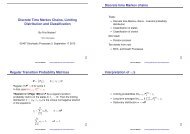
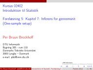
SIAM OP05 Kriging and RBFs 1Kriging and Radial Basis FunctionsHans Bruun Nielsen & Kristine Frisenfeldt ThuesenDTU, IMM, Scientific Computing Section◦ Introduction, definitions◦ Kriging◦ General RBFs◦ Unified approach◦ Examples◦ Plans for future workSIAM OP05 Kriging and RBFs 2• IntroductionY : R d ↦→ R given by design points {(x i ,y i =Y(x i ))} m i=1Surrogate model:s(x) = α T φ(θ,x)+β T f(x)Regression (polynomial) part: f(x) = (f 1 (x),...,f q (x)) T , f j : R d ↦→ RCorrelation (radial) part:φ(θ,x) = (φ 1 (θ,x),...,φ m (θ,x)) Twhere φ i (θ,x) = φ(‖Θ(x − x i )‖ 2 ), φ : R + ↦→ R . scaling Θ = diag(θ 1 ,...,θ d )ExamplesName φ(r), r ≥ 0Gaussiane −r2inverse multiquadric (r 2 +1) −1/221Gaussianthin plate splinemultiquadric (r 2 +1) 1/2thin plate spliner 2 log r0−2 −1.5 −1 −0.5 0 0.5 1 1.5 2

SIAM OP05 Kriging and RBFs 3InterpolationΦα + Fβ = y , Φ ij = φ j (θ,x i ), F i,: = f(x i ) Tm equations with m+q unknowns.Both in Kriging and general RBF approach: supply with F T α =0( )( ) ( )Φ F α y=(∗)F ⊤ 0 β 0Φ∈R m×mis symmetric. Full rank if the x i are distinct.F ∈ R m×q ,q

SIAM OP05 Kriging and RBFs 5• General RBFsΦ is not necessarily definite, but Powell 1 shows thata number of popular RBFs satisfysign ( v T Φ v ) = (−1) µfor all v ∈ V µ ,v≠0V µ = {v∈R m ∑: mi=1 v ip(x i )=0for any p ∈ Π µ−1 }We assume that {f j } comprises a basis of Π µ−1 .Then V µ ⊆N(F T ), the nullspace of F T . An orthonormalbasis of N can be found as N in the completeQR factorization of F ,( ) ( )RF = Q N = QR0Name φ(r), r ≥ 0 µGaussian e −r2 0inverse multiquadric (r 2 +1) −1/2 0linear r 1multiquadric (r 2 +1) 1/2 1thin plate spline r 2 log r 2cubic r 3 21M.J.D. Powell: 5 lectures on radial basis functions. Report IMM-REP-2005-03, IMM, DTU, 2005.SIAM OP05 Kriging and RBFs 6s(x) = α T φ(θ,x)+β T f(x).Φα+Fβ = ySeek α ∈ V µ ⊆N(F T ):α=Nα NN T ΦNα N +N T Fβ = N T y, (−1) µ ˜Φ αN = y NThe matrix ˜Φ =(−1) µ N T Φ N is symmetric and positive definite.The regression coefficients are found fromRβ = Q ( )T y−ΦNα N

SIAM OP05 Kriging and RBFs 7• Unified approacha ∈ R m . a = Qa R + Na N , a R = Q T a, a N = N T aAssume that y = Fβ +z, z = Nz NE [ z z T] = σ 2 NAN T , A = D˜ΦD, D = diag(˜Φ −1/2ii )A is symmetric, positive definite, and A ii =1. Valid correlation matrix.A = DC T CDBLUE:min ‖v‖ 2 2 s.t. Fβ +NDC T v = y Solution: C T v =(−1) µ D −1 N T yv,gbv ∈ R m−q has variance σ 2 I. Estimate: σ 2 = ‖v‖ 2 2/(m − q)}Assume Gaussian process: θ ∗ = argmin θ{Γ(θ) ≡ det A(θ) · σ 2(m−q) (θ)SIAM OP05 Kriging and RBFs 8Theorem: For φ(r) ∈{r, r 3 ,r 2 log r}, ω∈R + :s(ωθ,x) = s(θ,x),Γ(ωθ) = Γ(θ)Remarks:“Scalar” θ has no effect.“Full” θ : Finding θ ∗ reduces to a problem in R d−1+ instead of R d +

SIAM OP05 Kriging and RBFs 9• ExamplesY (x) =d∏e kx kcos(2kx k )k=1Educated guess: θ ∗ =(1,2,...,d) T2Test regions T of sizes 2 2 , 2 3 , 0.5 40−2Successively insert new designpoint atargmax x∈T|s(x) − Y (x)|−4−60−0.5−1−1.50.511.52SIAM OP05 Kriging and RBFs 1010 0 No scaling: θ = (1, 1)10 0 With scaling10 −210 −4Thin plate splineMultiquadricGaussian0 10 20 30 40 50 60 70 80 90 1002-D10 −210 −40 10 20 30 40 50 60 70 80 90 10010 0 No scaling: θ = (1, 1, 1)10 0 With scaling10 −1Thin plate splineMultiquadricGaussian10 −20 10 20 30 40 50 60 70 80 90 1003-D10 −110 −20 10 20 30 40 50 60 70 80 90 10010 0 No scaling: θ = (1, 1, 1, 1)10 0 With scaling10 −1Thin plate splineMultiquadricGaussian10 −210 20 30 40 50 60 70 80 90 1004-D10 −110 −210 20 30 40 50 60 70 80 90 100

SIAM OP05 Kriging and RBFs 11Data: First 25 points from Gaussian example.Use thin plate spline. θ ∗ = (1,θ ∗ 2) T10 10 Γ10 510 010 −5MSE10 −1 10 0 10 1θ ∗ = (1, 2) T (as expected)SIAM OP05 Kriging and RBFs 12MSE:under progress.Assume φ(0) ∈{0,1}.Ω 2 (x) = (−1) µ σ 2 { φ(0) + γ(x) T [ Φγ(x) − 2φ(θ,x) ]} (?)0.2Ω(x)0.2|s(x) − Y(x)|00−0.2−0.2−0.4−0.4−0.6−0.6−0.8−0.8−1−1−1.2−1.2−1.40.5 1 1.5 2−1.40.5 1 1.5 2

SIAM OP05 Kriging and RBFs 13• Plans for future work• Verifying (improving ?) the expression for Ω 2 (x)• Large scale: can explicit computation of N be avoided ?• Update the Matlab DACE package 2 to allow for general RBFs2See http://www2.imm.dtu.dk/∼hbn/dace/