Chapter 5 Inviscid Flows and Irrotational Flows

122 CHAPTER 5. INVISCID FLOWS AND IRROTATIONAL FLOWS5.2 Bernoulli’s equationThere are several forms of Bernoulli’s equations, relying on more or lessrestrictive assumptions. The student should make a clear distinction betweenthem. In all cases, we start from the Navier-Stokes equations:where∂ t u + ω × u = −∇B − ν∇ × ω, (5.3)B = p ρ + u22+ gz, (5.4)and look for ways to isolate the gradient in the r.h.s. (The Bernoulli termB is a scalar and cannot be confused with the body force per unit volume,which is a vector.)5.2.1 The strong formThe simplest way is to assume that the flow is irrotational. A necessary andsufficient condition for this to hold is thatu = ∇ϕ ↔ ω = 0 (5.5)(see Helmholtz decomposition). Then, the Magnus and viscous terms vanish,and the time derivative can be brought inside the gradient, to give∇(∂ t ϕ + p ρ + u22+ gz) = 0 (5.6)implying that∂ t ϕ + B = C(t) (5.7)has a (possibly time-dependent) uniform value in the entire field. The assumptionsmade here seem to hold in simple wave motion, where the timedependentpotential is needed (see Ch. 11 for simple examples).If, furthermore, the flow is steady, there is also a useful relation knownas Euler’s normal equation. The normal pressure gradient is only balancedby the centripetal acceleration. So,1ρ ∂ np = u2R(5.8)where R is the local radius of curvature of the streamline.

5.2. BERNOULLI’S EQUATION 1235.2.2 The weaker formA separate version of Bernoulli’s equation is not as restrictive: allowing vorticity,the initial assumption is that viscous effects can be neglected. Thus,we work with Euler’s equation∂ t u + ω × u = −∇B. (5.9)Then, project the equation on the direction of the velocity vector itself, i.e.along the streamlines. This cancels out the Magnus term, and we have∂ tu 22= −u · ∇B (5.10)In words, the local rate of change of kinetic energy (per unit mass) comesat the expense of the convective (directional) derivative of the Bernoulli expression.If we restrict ourselves to steady flows, we see thatB = p ρ + u22+ gz (5.11)is constant along any streamline. This does not preclude B from havingdifferent values along different streamlines. This is the form of the equationgenerally presented in undergraduate texts; streamline independence isusually achieved through reservoirs where static conditions prevail.At this point, we see that the undergraduate version of Bernoulli’s equation(along streamlines) is only part of the picture. Incompressible inviscidflows remain as strong conditions, but unsteadiness can be accommodated(Fig. 5.1), and the streamline restriction disappears in irrotational flow. Wesaw in Ch. 3 how viscous effects can be handled as losses along streamlines.Furthermore, if there is vorticity in steady flow, not only is B constant alongstreamlines, but is is also constant along vortex lines since5.2.3 Bernoulli and energyω · ∇B = 0. (5.12)Equation (5.10) is derived directly from the momentum equation. But it canalso be read as a scalar equation for kinetic energy, covered in Ch.3. Thisis not a new idea: in elementary frictionless dynamics, the energy equation

124 CHAPTER 5. INVISCID FLOWS AND IRROTATIONAL FLOWSFigure 5.1: Bernoulli’s equation and assumptions

5.2. BERNOULLI’S EQUATION 125Figure 5.2: Bernoulli and energy balance

126 CHAPTER 5. INVISCID FLOWS AND IRROTATIONAL FLOWS(kinetic and potential) is derived from F=ma by projecting Newton’s secondlaw on the trajectory. In Bernoulli’s equation, we recognize the kineticand potential energies easily; the pressure term can be interpreted as themechanical part of internal energy for an incompressible fluid, missing inthe case of point particles. If these mechanical contributions are subtractedfrom the first law of thermodynamics, all that is left is the thermal part ofinternal energy: so, after mechanical terms are accounted for in agreementwith Navier-Stokes, the (total) energy equation reduces to an equation fortemperature only, with friction as an exchange term with the mechanicalworld.We also recover the hydrostatic equation (when V = 0).5.2.4 Simplified Crocco’s equationRather than asking about the conditions for B to be constant Bernoulli’squestion), we can also wonder what makes B change. We already touchedon these topics in Ch. 3, with the viscous losses, and above with the shearlayer. Consider steady inviscid (incompressible) isothermal flow. Thenω × u = −∇B (5.13)Bernoulli’s equation states that B is constant along streamlines and alongvortex lines. If vorticity is aligned with the streamlines (helicity is maximum),B is constant again. Crocco’s theorem states how B changes from streamlineto streamline according to the equation above: the Lamb vector gives themagnitude and direction of ∇B. In 2D flows, where vorticity is perpendicularto the plane of the flow (and therefore to the streamlines), the gradient of B isnormal to the streamlines and to the vortex lines. See Batchelor Section 3.5p.156-160 (where H is enthalpy) for the compressible flow version. See alsoCurrie Section 3.3 p.57. Compare the derivation with viscous losses alongstreamlines in Ch. 3.This helps us understand what happens to B at the base of a manometertube (Fig. 5.4) mounted on the wall normal to some flow. While Bernoulli’sequation, or its variant ‘with losses’, may be applied in the flow (alongstreamlines), and is certainly applicable in the hydrostatic conditions of themanometer, it is definitely not applicable across the shear layer that separatesthe flow from the manometer (Fig. 5.4). According to Crocco’s equation, thevalue of B changes across the shear layer. A similar situation is encounteredin boundary layers (Ch 8).

5.2. BERNOULLI’S EQUATION 127Figure 5.3: Crocco’s theorem for 2-D inviscid flows.Figure 5.4: The shear layer at the base of a manometer resets the value ofthe Bernoulli term.

128 CHAPTER 5. INVISCID FLOWS AND IRROTATIONAL FLOWS5.2.5 Applications of Bernoulli’s equationStudents should fill in this information from suitable undegraduate texts:1/2 page of text and a figure for each topic, maybe a simple mind-map withrelevant topics, would do. Every student at this level should know aboutthese phenomena.VenturiPitot tubeFree surfaceSiphonsNozzlesCavitationAerodynamic lift5.2.6 Lagrange’s theoremBefore Navier and Stokes reintroduced Newton’s viscosity in the momentumbalance, the theory of inviscid flow progressed rapidly, and an early theoremby Lagrange is worth mentioning. The theorem states that inviscid irrotationalflow remains irrotational forever.The proof is easy. Starting from Euler’s equation, cancel the Magnusterm, and take the curl to get the evolution of vorticity.∇ × ∂ t u = ∂ t ω = ∇ × ∇B = 0 (5.14)This is the Eulerian equivalent of Kelvin’s theorem (Lagrangian, below);it applies only to irrotational flows, whereas Kelvin’s theorem has no suchrestriction.5.2.7 Creation of vorticityUnder the Boussinesq approximation, it is possible to have density variationsin the flow while preserving the simple form the continuity equation. Then∂ t u + ω × u = − 1 ρ ∇( p + ρu2 2+ ρgz) (5.15)

5.2. BERNOULLI’S EQUATION 129Figure 5.5: Creation of vorticity from density gradientsand the vorticity equation takes the form∂ t ω + ∇ × (ω × u) = −∇ 1 × ∇(ρB) (5.16)ρFrom Shapiro’s movie, if density gradient is not parallel to pressure gradient,creation of vorticity in the flow is possible. This remark underscores theimportance of the conditions attached to Lagrange’s and Kelvin’s theorem(next).We will see other mechanisms of vorticity creation in relation to boundarylayers, flow separation and rotating flows.5.2.8 Kelvin’s theoremIn Ch. 2 we introduced the circulation Γ and its relation to vorticity∮ ∫Γ = u · dr = ω · dA (5.17)An exact equation was derived by Kelvin under the assumption of inviscidflow of uniform density, also assuming that the contour of integration is amaterial line moving with the fluid. Let us write the Euler equation in termsof the material derivatived t u i = −gδ i3 − 1 ρ ∂ ip (5.18)

130 CHAPTER 5. INVISCID FLOWS AND IRROTATIONAL FLOWSFigure 5.6: About Kelvin’s theoremand multiply by dx i taken along a material line. Then, simple manipulationsyielddx i d t u i = d t (u i dx i ) − u i d t dx i = d t (u i dx i ) − d( u22 )1−gdx i δ i3 − dx iρ ∂ ip = −gdx 3 − 1 dp, (5.19)ρwhere the differentials of u 2 , x 3 and p are along the contour. Under thestandard assumption that all functions are smooth enough, the integral ofthese differentials along the contour must vanish, since we come back to thestarting value at the end of integration. Henced t Γ = 0 (5.20)We can read the surface integral of vorticity as equivalent to an averagevorticity normal to the surface multiplied by the area of this surface. If theproduct of the two is constant for an arbitrary material line moving withthe flow, it means that a reduction in area is associated with an increase inaverage vorticity, and conversely. This mechanism is very important in anumber of applications covered later in this course. Perhaps more importantly,if the material contour initiates its travel in a region where there is

5.2. BERNOULLI’S EQUATION 131Figure 5.7: Vortex stretchingno vorticity, the associated particles will remain in irrotational motion aslong as viscous effects are negligible. (Note the interesting exception in Ch.10 where the addition of a weak rotational force (Coriolis) and stretchingamplifies the creation of weak vorticity).Vortex stretchingA different formulation of the same idea can be obtained from the vorticityequation. For inviscid flow, the material derivative of vorticity isd t ω i = ω j ∂ j u i (5.21)The square vorticity (enstrophy) then obeys the equationd tω 22 = ω j∂ j u i ω i = ω j s ij ω i (5.22)because the symmetry of ω i ω j cancels the non-symmetric part of the velocityderivative (see linear algebra). In particular, we can select the local axes tocoincide with the principal axes of the local rate of strain. Then for eachdirectiond tω 2 (i)2 = (s (i)ω 2 (i)) (no sum). (5.23)Therefore, following a material point (Lagrangian description), the squaredvorticity in each direction (no sum) varies exponentially in timeω 2 (i) ∼ e s (i)t . (5.24)

132 CHAPTER 5. INVISCID FLOWS AND IRROTATIONAL FLOWSFor the component of vorticity long the primary extensional axis, we havean exponential increase; along the compression axis, exponential decreaseof square vorticity. Because the latter approaches zero while the formerincreases very rapidly, vorticity tends to align itself with the extensional axisand increases in magnitude. The idea here is the same as in Kelvin’s theorem,the presentation quite different, the result equivalent.5.2.9 Helmholtz’s vortex theoremsRecall (Ch. 2) Helmholtz’s theorems1. vortex lines cannot end in the fluid, they can only end at a boundary.2. in inviscid incompressible flow, fluid elements that lie on a vortex lineremain on vortex line (this means that vorticity is a marker just asdye).3. circulation is the same for all sections of a vortex tube.Theorems 1 and 3 were proved and explained in Ch. 2; theorem 2 invokesinviscid dynamics and can finally be addressed.Consider the vorticity field, with vorticity vectors distributed throughspace; consider the associated vortex lines; and finally select the vortex linessupported by some smooth line so as to make a vortex sheet. Then, draw amaterial contour within this vortex sheet. Since the vorticity is in the sheet,the normal to the sheet is normal to vorticity, and therefore∫Γ = ω n dA = 0 (5.25)for any such contour. By Kelvin’s theorem, it will remain zero. This impliesthat, as the arbitrary material contour deforms in the flow, it remains withinthe vortex sheet. Now, take some support line intersecting the first one, andthe corresponding vortex sheet, and arbitrary contours within the sheet, andreach the same conclusion: the material points remain on the vortex sheet.Finally, since a vortex line is the intersection of two vortex sheets, itsmaterial points remain within each of the sheets, therefore remain on thesame vortex line.See Panton Section 13.8 p.338, Acheson Section 5.3 p.162-3 for moreinformation.

5.3. IRROTATIONAL FLOW 133Figure 5.8: Helmholtz’ second theoremThis theorem is very important: as long as effects of viscosity (diffusion)and density changes change be neglected, vortex lines act as flow markers,and conversely dye injected along a vortex line will continue to show thevortex line as it moves downstream.This is a good point to view Shapiro’s movie again (Fig. 5.9) is repeatedhere from Ch. 2.5.3 Irrotational flowIrrotational means that there is no vorticity. Kelvin’s theorem provides agood understanding for the conditions under which this could happen. Now,let us explore the consequences.We start fromω = 0, (5.26)which in turn implies (and conversely)u = ∇ϕ. (5.27)

134 CHAPTER 5. INVISCID FLOWS AND IRROTATIONAL FLOWSA.H. Shapiro’s movie: Vorticity• Kinematics– Definition, vorticity meter– Potential vortex– Vorticity and circulation: Stokes’ theorem• Dynamics∗ Start-up vortex– Bernoulli’s equation: conditions for B = p + 1 2 ρV 2 + ρg z tobe constant– Crocco’s equation: how B changes– Kelvin’s theorem: inviscid, Lagrangian, vortex stretching• Potential flow, singular vortices– Model (ν = 0)– Motion of vortex pair, induced velocity• Helmholtz’s theorems (material lines, vortex tubes, vortex linesend only at boundary)• How to introduce vorticity– Singularities– ∇p × ∇ρ and interface– unsteadiness– rotational forces– pressure gradient along boundary (viscous effect)– See Ch. 9Figure 5.9: Kinematics and dynamics of vorticity and circulation, A.Shapiro’s movie.

5.3. IRROTATIONAL FLOW 135Figure 5.10: About ∇ 2 = 0Then, incompressibility leads to∇ 2 ϕ = 0 (5.28)at every instant. Laplace’s equation admits unique solutions if either thefield value (ϕ: Dirichlet condition) or its normal derivative (∂ n ϕ = u n : Neumancondition) is given at every point on the boundary. In the presence ofimpermeable boundaries, the normal velocity must be equal to that of theboundary (which can be in motion), and the entire field responds instantaneouslyto the current conditions. The no-slip condition would require thepresence of viscous effects, themselves associated with vorticity. The no-slipcondition is incompatible with the Laplace equation for potential flow.A similar picture emerges if we satisfy mass balance first. Then the vectorpotential∇ × A = u (5.29)must be such that∇ × u = ω = 0 = −∇ 2 A. (5.30)The Laplace equation now applies to the vector potential instead of the scalarvelocity potential. The picture is consistent: irrotational flow is characterizedby unique solutions that reflect the boundary conditions throughout the fieldat each instant.

136 CHAPTER 5. INVISCID FLOWS AND IRROTATIONAL FLOWSFigure 5.11: Potential lines and streamfunctions.5.3.1 2D potential lines and streamlinesIn 2-D flows, it is easy to show that lines of constant ϕ and lines of constantψ are perpendicular to each other. Indeed, we can writedϕ = ∂ x ϕ dx + ∂ y ϕ dy = u dx + v dy = 0 (5.31)so thatFor the streamlinesdydx | ϕ= − u v . (5.32)dψ = ∂ x ψ dx + ∂ y ψ dy = −v dx + u dy = 0 (5.33)soHencewhich proves the result.dydx | ψ= v u . (5.34)dydx | ·dyψdx | ϕ= −1, (5.35)

5.3. IRROTATIONAL FLOW 137In 2D, it is also convenient to use polar coordinates when the symmetry ofthe flow makes this representation simpler. For the velocity potential ϕ(r, θ),we need the components of the gradient:u r = ∂ r ϕ and u θ = 1 r ∂ θϕ (5.36)Similarly, with A = (0, 0, ψ), the expression of the curl givesu r = 1 r ∂ θψ and u θ = −∂ r ψ (5.37)5.3.2 Superposition of 2D potentialsThis material may have been covered at the undergraduate level. This subsectionis a list of elementary flow types and a brief discussion of how to usethem. The key is to realize that the Laplace equation (for ϕ and ψ) is linear,so that elementary solutions can be added to each other.Uniform flowWe take the flow to be uniform with velocity U in the x direction: changesof coordinates can accommodate different directions easily.u = U and v = 0. (5.38)Then, the potential and streamfunctions are easily obtained by integration.(Note that the arbitrary constant of integration can be ignored without lossof generality: addition of the constant does not modify the velocity field.)Stagnation flowFor this caseϕ = Ux and ψ = Uy. (5.39)ϕ = x 2 − y 2 and ψ = Cxy, (5.40)for which the streamlines are branches of hyperbola.For other flows, polar coordinates capture the symmetries more effectively;but of course the choice of coordinates is yours, for most effectivesolution of the problem at hand.

138 CHAPTER 5. INVISCID FLOWS AND IRROTATIONAL FLOWS3Potential flow at a stagnation point2.52y1.510.50−3 −2 −1 0 1 2 3xFigure 5.12: Potential lines (dashed lines) and streamlines (solid lines) of astagnation flowPoint source or sinkSign reversal gives a point sink, obviously. Let q be the flow rate coming outof the source, where we place the origin of coordinates. Thenϕ = q2π ln(r) = q √2π ln( x 2 + y 2 ) and ψ = q2π θ = − q2π atan( y√x2 + y ). 2Then, the velocity components areu r = q 12π r(5.41)and u θ = 0. (5.42)Point vortexDual of the source: swap ϕ and ψ above and getϕ = − Γ 2π θ = − Γ 2π atan( y√x2 + y ) and ψ = Γ 2 2π ln(r) = Γ √x2π ln( 2 + y 2 ).Then, the velocity components are(5.43)u r = 0 and u θ = Γ2πr . (5.44)

5.3. IRROTATIONAL FLOW 1393Potential flow around a source21y0−1−2−3−3 −2 −1 0 1 2 3xFigure 5.13: Potential lines and streamlines of a point source3Potential flow around a source21y0−1−2−3−3 −2 −1 0 1 2 3xFigure 5.14: Potential lines and streamlines of a point vortex

140 CHAPTER 5. INVISCID FLOWS AND IRROTATIONAL FLOWS2Potential flow around a doublet1.510.5y0−0.5−1−1.5−2−2 −1.5 −1 −0.5 0 0.5 1 1.5 2xFigure 5.15: Potential lines and streamlines of a doubletSource-sink doubletPlace a source of strength q at x = a, a sink of equal strength at x = −a,and superpose the flows (add the potentials); then take the limit of a → 0 atfixed value of Λ = aq. The result is a doublet aligned with the x-axis.ϕ = Λ cos θrThen, the velocity components areandψ = −Λ sin θr . (5.45)u r = −Λ cos θr 2 and u θ = −Λ sin θr 2 . (5.46)It can be checked that streamlines and potential lines are circles.Rankine half-bodySuperposition of a uniform flow and a sourceϕ = Ur cos θ + qqln(r) and ψ = Ur sin θ + θ. (5.47)2π 2πThen, the velocity components areu r = U cos θ +q2πrand u θ = −Ur sin θ. (5.48)

5.3. IRROTATIONAL FLOW 1413Potential flow around a Rankine half−body21y0−1−2−3−3 −2 −1 0 1 2 3xFigure 5.16: Potential lines and streamlines of a Rankine half-bodyCylinderSuperposition of a doublet and a uniform flowϕ = Ur cos θ + Λ cos θrThen, the velocity components areandψ = Ur sin θ − Λ sin θr . (5.49)u r = U cos θ − Λ cos θr 2 and u θ = −U sin θ − Λ sin θr 2 . (5.50)Cylinder with circulationSuperposition of a doublet, a vortex and a uniform flow This to be filled in.5.3.3 F=ma!?The previous subsections show that, for suitable boundary conditions, onedoes obtain unique solutions for the velocity field by satisfying mass balanceand the kinematic constraint of irrotational flow. How about F = ma? Canwe have a solution without momentum balance? Answer in class, after youthink it through!

142 CHAPTER 5. INVISCID FLOWS AND IRROTATIONAL FLOWS3Potential flow around a cylinder21y0−1−2−3−3 −2 −1 0 1 2 3xFigure 5.17: Potential lines and streamlines of the flow around a cylinder3Potential flow around a cylinder21y0−1−2−3−3 −2 −1 0 1 2 3xFigure 5.18: Potential lines and streamlines for a cylinder with circulation

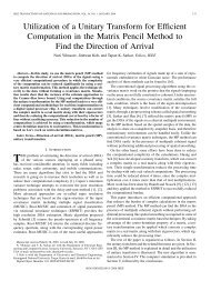
5.3. IRROTATIONAL FLOW 1431Pressure distribution on cylinder in potential flow0.50Pressure coefficient−0.5−1−1.5−2−2.5−30 20 40 60 80 100 120 140 160 180Angle (degrees)Figure 5.19: Pressure force on the cylinder5.3.4 D’Alembert’s paradoxIt is √easy to see that the streamline ψ = 0 corresponds to a circle of radiusR = Λ/U. Applying Bernoulli’s equation between infinity and the cylindersurface, we haveρU 22 + p ∞ = ρ(u2 r + u 2 θ)+ p | R (5.51)2Taking p ∞ = 0 as reference pressure (why is this OK?) we get the surfacepressure (Fig. 5.19) asp | R = ρU 2(cos 2θ − 1) (5.52)2This is maximum at the front and back stagnation points θ = 0 and π, andminimum at θ = ±π/2.Then it is easy to see that, for a surface element of area Rdθ, the componentsof force aredF x = Rdθ cos θp R (5.53)anddF y = Rdθ sin θp R . (5.54)

144 CHAPTER 5. INVISCID FLOWS AND IRROTATIONAL FLOWSBy integration, the drag D and lift L are∫D = dF x = 0 (5.55)and∫L =dF y = 0. (5.56)Vanishing lift is clearly the result of symmetry, broken by adding circulation.But the vanishing drag has much deeper roots. In fact, the absence of dragwas proved by D’Alembert for bodies of any shape whatsoever: the mismatchbetween this elegant result (and the vindication of potential external flows asvalid models within the accuracy achievable then) and the common experienceof drag was called D’Alembert’s paradox. It started a profound schismin the fluids community, lasting for much of the nineteenth century, betweenthe aerodynamicists (who, with Joukovky and others, took potential flowsinto higher mathematics) and hydraulics practitioners (who relied more onempirical data). The paradox was finally solved by Prandtl, with the discoveryof the boundary layer and its effect on the flow (skin friction, boundarylayer separation, wake formation...)5.4 Viscous potential flowsWe will see in Ch. 9 the role played by viscosity to introduce vorticityfrom solid boundaries into many flows. This ubiquitous complication blindedthe fluid mechanics community to the interest of viscous potential flows.Combining potential flow with incompressibility gives∇ 2 u = 0 (5.57)so that, although the viscous stress does not vanish, the viscous force does.For additional information, see the recent work of D.D. Joseph.5.5 Advanced topics and ideas for further readingBatchelor’s entire Ch.6 is devoted to inviscid flows with vorticity: good reading!In his Ch.5, Batchelor also covers the effect of viscosity on Kelvin’s

5.5. ADVANCED TOPICS AND IDEAS FOR FURTHER READING 145theorem. In relation of Helmholtz’s interpretation of vortex lines with materiallines in inviscid flow, the effect of viscosity on vortex line topology(break-up and reconnections) has also been studied extensively.Complex coordinates, conformal mapping for 2D flows: see Acheson for agood overview, Panton or Currie for more details. Currie’s Ch. 5 is devotedto 3D potential flows.Kelvin’s theorem is a particular of the Poincaré-Cartan invariant in Hamiltoniandynamics. There are many points of overlap between irrotational flowsand Hamiltonian dynamics.Finally, Onsager pointed out the possibility of having energy dissipationin inviscid flows: this requires that singularities (infinite derivatives) developas a result of vortex stretching. This cannot happen in 2D, but the issue isstill unresolved in 3D.Problems1. Categorize the ideas in this chapter as being for inviscid flow, irrotationalflow, or both. Explain relations between these ideas.2. Discuss (on the basis of equations) the following proposition: any flowthat is irrotational is also inviscid (the converse is clearly not true).3. Derive the equation of the free surface associated with a potential vortex(next: add a sink at the origin); discuss in what respects this is oris not a good model for the bathtub vortex.4. Work out the pressure distribution eq. (5.52) for the potential flowaround a cylinder, and integrate it to get drag and lift; repeat with thecylinder with circulation (add a vortex).

146 CHAPTER 5. INVISCID FLOWS AND IRROTATIONAL FLOWS