Multivariate Analysis of Ecological Communities in R: vegan tutorial

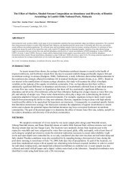
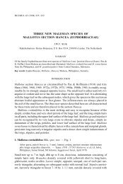
2.1 Non-metric Multidimensional scaling 2 ORDINATION: BASIC METHODDim2−0.4 −0.2 0.0 0.2 0.45147131661822 1542025112332419122272810921−0.6 −0.4 −0.2 0.0 0.2 0.4Dim1Functions scores and ordiplot in vegan can be used to handle theresults of nmds:> ordiplot(vare.mds0, type = "t")Only site scores were shown, because dissimilarities did not have informationabout species.The iterative search is very difficult in nmds, because of nonlinear relationshipbetween ordination and original dissimilarities. The iterationeasily gets trapped into local optimum instead of finding the global optimum.Therefore it is recommended to use several random starts, andselect among similar solutions with smallest stresses. This may be tedious,but vegan has function metaMDS which does this, and many morethings. The tracing output is long, and we suppress it with trace = 0,but normally we want to see that something happens, since the analysiscan take a long time:> vare.mds vare.mdsNMDS2−0.5 0.0 0.5Cla.phyDic.polCet.isl 24Cla.ste112Cla.chlPin.sylBar.lyc12Cla.cer10 Poh.nut Pti.cil 21Cla.bot9Dic.spEmp.nig Vac.vit19234 Cla.ran Cla.uncPel.aphCla.cri Cla.graBet.pubPol.pilPle.sch6 13 2028Cet.nivCet.eri Cal.vul Cla.cor Cla.defCla.fimVac.myr15Led.pal3 18 Cla.sp 16Cla.arb Cla.coc22277Pol.junHyl.spl14Pol.comSte.spDes.fle5 Dip.monDic.fusVac.uli25Cla.amaIch.eriNep.arc−0.5 0.0 0.5 1.0NMDS1Call:metaMDS(comm = varespec, trace = FALSE)Nonmetric Multidimensional Scaling using isoMDS (MASS package)Data: wisconsin(sqrt(varespec))Distance: brayDimensions: 2Stress: 18.26Two convergent solutions found after 8 triesScaling: centring, PC rotation, halfchange scalingSpecies: expanded scores based on ‘wisconsin(sqrt(varespec))’> plot(vare.mds, type = "t")We did not calculate dissimilarities in a separate step, but we gave theoriginal data matrix as input. The result is more complicated than previously,and has quite a few components in addition to those in isoMDS results:points, dims, stress, data, distance, converged, tries,species, call. The function wraps recommended procedures into onecommand. So what happened here?1. The range of data values was so large that the data were square roottransformed, and then submitted to Wisconsin double standardization,or species divided by their maxima, and stands standardizedto equal totals. These two standardizations often improve the qualityof ordinations, but we forgot to think about them in the initialanalysis.2. Function used Bray–Curtis dissimilarities.3. Function run isoMDS with several random starts, and stopped eitherafter a certain number of tries, or after finding two similarconfigurations with minimum stress. In any case, it returned thebest solution.4

2 ORDINATION: BASIC METHOD 2.2 Community dissimilarities4. Function rotated the solution so that the largest variance of sitescores will be on the first axis.5. Function scaled the solution so that one unit corresponds to halvingof community similarity from the replicate similarity.6. Function found species scores as weighted averages of site scores,but expanded them so that species and site scores have equal variances.This expansion can be undone using shrink = TRUE in displaycommands.The help page for metaMDS will give more details, and point to explanationof functions used in the function.2.2 Community dissimilaritiesNon-metric multidimensional scaling is a good ordination method becauseit can use ecologically meaningful ways of measuring communitydissimilarities. A good dissimilarity measure has a good rank order relationto distance along environmental gradients. Because nmds only usesrank information and maps ranks non-linearly onto ordination space, itcan handle non-linear species responses of any shape and effectively androbustly find the underlying gradients.The most natural dissimilarity measure is Euclidean distance which isinherently used by eigenvector methods of ordination. It is the distance inspecies space. Species space means that each species is an axis orthogonalto all other species, and sites are points in this multidimensional hyperspace.However, Euclidean distance is based on squared differences andstrongly dominated by single large differences. Most ecologically meaningfuldissimilarities are of Manhattan type, and use differences instead ofsquared differences. Another feature in good dissimilarity indices is thatthey are proportional: if two communities share no species, they have amaximum dissimilarity = 1. Euclidean and Manhattan dissimilaritieswill vary according to total abundances even though there are no sharedspecies.Package vegan has function vegdist with Bray–Curtis, Jaccard andKulczyński indices. All these are of the Manhattan type and useonly first order terms (sums and differences), and all are relativized bysite total and reach their maximum value (1) when there are no sharedspecies between two compared communities. Function vegdist is a dropinreplacement for standard R function dist, and either of these functionscan be used in analyses of dissimilarities.There are many confusing aspects in dissimilarity indices. One is thatsame indices can be written with very different looking equations: twoalternative formulations of Manhattan dissimilarities in the margin serveas an example. Another complication is naming. Function vegdist usescolloquial names which may not be strictly correct. The default index invegan is called Bray (or Bray–Curtis), but it probably should be calledSteinhaus index. On the other hand, its correct name was supposed to beCzekanowski index some years ago (but now this is regarded as anotherindex), and it is also known as Sørensen index (but usually misspelt).5∑d jk = √ N (x ij − x ik ) 2 Euclideand jk =i=1N∑|x ij − x ik | Manhattani=1N∑N∑A = x ij B =J =i=1N∑min(x ij , x ik )i=1d jk = A + B − 2Jd jk = A + B − 2JA + Bd jk = A + B − 2JA + B − Jd jk = 1 − 1 ( J2 A + J )Bi=1x ikManhattanBrayJaccardKulczyński

2.2 Community dissimilarities 2 ORDINATION: BASIC METHODfor A = B d AB = 0for A ≠ B d AB > 0d AB = d BAd AB ≤ d Ax + d xBStrictly speaking, Jaccard index is binary, and the quantitative variantin vegan should be called Ružička index. However, vegan finds eitherquantitative or binary variant of any index under the same name.These three basic indices are regarded as good in detecting gradients.In addition, vegdist function has indices that should satisfy othercriteria. Morisita, Horn–Morisita, Raup–Cric, Binomial and Mountfordindices should be able to compare sampling units of different sizes. Euclidean,Canberra and Gower indices should have better theoretical properties.Function metaMDS used Bray-Curtis dissimilarity as default, whichusually is a good choice. Jaccard (Ružička) index has identical rankorder, but has better metric properties, and probably should be preferred.Function rankindex in vegan can be used to study which of the indicesbest separates communities along known gradients using rank correlationas default. The following example uses all environmental variables in dataset varechem, but standardizes these to unit variance:> data(varechem)> rankindex(scale(varechem), varespec, c("euc", "man",+ "bray", "jac", "kul"))euc man bray jac kul0.2396 0.2735 0.2838 0.2838 0.2840are non-linearly related, but they have identical rank orders, and theirrank correlations are identical. In general, the three recommended indicesare fairly equal.I took a very practical approach on indices emphasizing their abilityto recover underlying environmental gradients. Many textbooks emphasizemetric properties of indices. These are important in some methods,but not in nmds which only uses rank order information. The metricproperties simply say that1. if two sites are identical, their distance is zero,2. if two sites are different, their distance is larger than zero,3. distances are symmetric, and4. the shortest distance between two sites is a line, and you cannotimprove by going through other sites.These all sound very natural conditions, but they are not fulfilled by alldissimilarities. Actually, only Euclidean distances – and probably Jaccardindex – fulfill all conditions among the dissimilarities discussed here, andare metrics. Many other dissimilarities fulfill three first conditions andare semimetrics.There is a school that says that we should use metric indices, andmost naturally, Euclidean distances. One of their drawbacks was thatthey have no fixed limit, but two sites with no shared species can varyin dissimilarities, and even look more similar than two sites sharing somespecies. This can be cured by standardizing data. Since Euclidean distancesare based on squared differences, a natural transformation is tostandardize sites to equal sum of squares, or to their vector norm usingfunction decostand:6

2 ORDINATION: BASIC METHOD 2.3 Comparing ordinations: Procrustes rotation> dis dis d d d

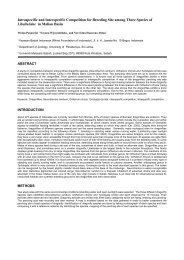
2 ORDINATION: BASIC METHOD 2.4 Eigenvector methodsInertia is varianceEigenvalues for unconstrained axes:PC1 PC2 PC3 PC4 PC5 PC6 PC7 PC8983.0 464.3 132.3 73.9 48.4 37.0 25.7 19.7(Showed only 8 of all 23 unconstrained eigenvalues)> plot(vare.pca)The output tells that the total inertia is 1826, and the inertia is variance.The sum of all 23 (rank) eigenvalues would be equal to the totalinertia. In other words, the solution decomposes the total variance intolinear components. We can easily see that the variance equals inertia:> sum(apply(varespec, 2, var))PC2−6 −4 −2 0 2 4 6576Cla.ranCla.arb1318414Cal.vul Vac.uliSte.sp112016 Cla.unc Nep.arc Cla.ama Led.pal Dip.mon Pol.com Pol.jun Des.fle Cla.def Bet.pub Pel.aph Poh.nut Cla.coc Cla.gra Cla.phy Cla.cor Cla.bot Cla.cer Dic.pol Cla.fim Bar.lyc Cla.cri Cet.eri Cla.chl Cla.sp Pin.syl Ich.eri Cet.isl Pol.pil Cet.niv Pti.cil23Dic.fusDic.sp Hyl.spl 21 Emp.nigVac.myr Vac.vit15 22192524Ple.sch 27283122109Cla.ste[1] 1826Function apply applies function var or variance to dimension 2 or columns(species), and then sum takes the sum of these values. Inertia is the sumof all species variances. The eigenvalues sum up to total inertia. In otherwords, they each “explain” a certain proportion of total variance. Thefirst axis “explains” 983/ 1826 = 53.8˜% of total variance.The standard ordination plot command uses points or labels forspecies and sites. Some people prefer to use biplot arrows for speciesin pca and possibly also for sites. There is a special biplot function forthis purpose:> biplot(vare.pca, scaling = -1)For this graph we specified scaling = -1. The results are scaled onlywhen they are accessed, and we can flexibly change the scaling in plot,biplot and other commands. The negative values mean that speciesscores are divided by the species standard deviations so that abundantand scarce species will be approximately as far away from the origin.The species ordination looks somewhat unsatisfactory: only reindeerlichens (Cladina) and Pleurozium schreberi are visible, and all otherspecies are crowded at the origin. This happens because inertia was variance,and only abundant species with high variances are worth explaining(but we could hide this in plot by setting negative scaling). Standardizingall species to unit variance, or using correlation coefficients insteadof covariances will give a more balanced ordination:PC2−4 −2 0 2 4−4 −2 0 2 4 6 8 10PC1Cla.arb Cla.ranIch.eri 7Ste.sp56Vac.uliCla.ama Pol.pil Cla.cocCla.gra 1813 Dip.monCal.vulCet.niv4Cet.eriCla.fim314Cla.unc Cla.cerCla.def 201116 Cla.cri23Cla.cor Pel.aph Bet.pub Bar.lycCla.bot Pti.cil 212Pol.jun Nep.arc15 Dic.fus Dic.pol 19 Cla.spPin.syl1222 24 25Dic.spCet.isl Cla.chl Cla.phy Cla.ste10Led.pal Pol.comEmp.nig9Vac.vit Poh.nut27 Des.fleVac.myr28Hyl.splPle.sch−4 −2 0 2 4 6PC1> vare.pca vare.pcaCall: rda(X = varespec, scale = TRUE)Inertia RankTotal 44Unconstrained 44 23Inertia is correlationsEigenvalues for unconstrained axes:PC1 PC2 PC3 PC4 PC5 PC6 PC7 PC88.90 4.76 4.26 3.73 2.96 2.88 2.73 2.18(Showed only 8 of all 23 unconstrained eigenvalues)> plot(vare.pca, scaling = 3)9

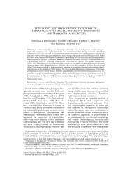
2.4 Eigenvector methods 2 ORDINATION: BASIC METHODPC2CA2−2 −1 0 1−2.0 −1.5 −1.0 −0.5 0.0 0.5 1.0 1.511Cla.phy10Cla.cocCla.ste Pin.sylCla.sp Cla.graPol.pil Cet.eri Cla.cri Cla.fim 23 12Cla.ran 1418Cla.def5 Cla.arb Ste.sp6 Dip.mon Cla.uncCla.ama Cla.corPel.aph13 24Ich.eri Cal.vul3Cet.niv7 1516 20Dic.sp4 Vac.uliCla.cer Dic.fusPol.jun2Nep.arc192225 Des.flePle.sch Hyl.spl289Poh.nutCla.chlCet.isl27Vac.vitEmp.nigPol.com Led.palVac.myrDic.polPti.cilBet.pub Bar.lycCla.bot−1 0 1 2 39102312Cla.phyCla.steCet.niv4Cet.islCla.chlPin.sylCla.spCla.cer11Dip.mon Cla.ranPol.pilCla.ama56Ste.sp 13719Cla.arb 18Vac.uli Cal.vulPC1Poh.nutEmp.nigVac.vitCla.cocPti.cil Vac.myrLed.palDic.polPol.com27Des.fleCla.bot−1 0 1 2CA121Bar.lycBet.pubPel.aphCla.fim Cla.cor 23Cla.graIch.eriCla.cri Cla.def 20Cet.eriPle.schDic.sp 2425Nep.arcPol.junCla.unc1415Dic.fus1622Hyl.spl2821Now inertia is correlation, and the correlation of a variable with itself isone. Thus the total inertia is equal to the number of variables (species).The rank or the total number of eigenvectors is the same as previously.The maximum possible rank is defined by the dimensions of the data: itis one less than smaller of number of species or number of sites:> dim(varespec)[1] 24 44If there are species or sites similar to each other, rank will be reducedeven from this.The percentage explained by the first axis decreased from the previouspca. This is natural, since previously we needed to “explain” only theabundant species with high variances, but now we have to explain allspecies equally. We should not look blindly at percentages, but the resultwe get.Correspondence analysis is very similar to pca:> vare.ca vare.caCall: cca(X = varespec)Inertia RankTotal 2.08Unconstrained 2.08 23Inertia is mean squared contingency coefficientEigenvalues for unconstrained axes:CA1 CA2 CA3 CA4 CA5 CA6 CA7 CA80.525 0.357 0.234 0.195 0.178 0.122 0.115 0.089(Showed only 8 of all 23 unconstrained eigenvalues)> plot(vare.ca)Now the inertia is called mean squared contingency coefficient. Correspondenceanalysis is based on Chi-squared distance, and the inertia isthe Chi-squared statistic of a data matrix standardized to unit total:> chisq.test(varespec/sum(varespec))CA2−2 −1 0 1 2Cla.phyCla.steCet.nivCet.islCla.chlDip.monCla.ran 7Pol.pil 5Cla.arbVac.uli Cal.vulPti.cil Vac.myrLed.palDic.polPol.comDes.fleCla.bot−2 −1 0 1 2 3CA1Bar.lycBet.pub9212810Pin.syl Poh.nutPle.sch2Cla.sp1227Emp.nig 19Vac.vitDic.spNep.arc3Pol.jun 24 25Cla.cer 11 Pel.aph 23Cla.fim Cla.cor 15 22204Cla.gra 16Cla.cri Cla.defCla.coc 18Dic.fusCet.eri146 13Cla.amaSte.spIch.eriCla.uncHyl.splPearson's Chi-squared testdata: varespec/sum(varespec)X-squared = 2.083, df = 989, p-value = 1You should not pay any attention to P -values which are certainly misleading,but notice that the reported X-squared is equal to the inertiaabove.Correspondence analysis is a weighted averaging method. In the graphabove species scores were weighted averages of site scores. With differentscaling of results, we could display the site scores as weighted averages ofspecies scores:> plot(vare.ca, scaling = 1)We already saw an example of scaling = 3 or symmetric scaling in pca.The other two integers mean that either species are weighted averages ofsites (2) or sites are weighted averages of species (1). When we take10

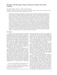
2 ORDINATION: BASIC METHOD 2.5 Detrended correspondence analysisweighted averages, the range of averages shrinks from the original values.The shrinkage factor is equal to the eigenvalue of ca, which has atheoretical maximum of 1.2.5 Detrended correspondence analysisCorrespondence analysis is a much better and more robust method forcommunity ordination than principal components analysis. However,with long ecological gradients it suffers from some drawbacks or “faults”which were corrected in detrended correspondence analysis (dca):• Single long gradients appear as curves or arcs in ordination (arceffect): the solution is to detrend the later axes by making theirmeans equal along segments of previous axes.• Sites are packed more closely at gradient extremes than at the centre:the solution is to rescale the axes to equal variances of speciesscores.• Rare species seem to have an unduly high influence on the results:the solution iss to downweight rare species.All these three separate tricks are incorporated in function decoranawhich is a faithful port of Mark Hill’s original programme with the samename. The usage is simple:> vare.dca vare.dca21Call:decorana(veg = varespec)Detrended correspondence analysis with 26 segments.Rescaling of axes with 4 iterations.DCA1 DCA2 DCA3 DCA4Eigenvalues 0.524 0.325 0.2001 0.1918Decorana values 0.525 0.157 0.0967 0.0608Axis lengths 2.816 2.205 1.5465 1.6486> plot(vare.dca, display = "sites")DCA2−1.0 −0.5 0.0 0.5 1.01092 12282719311231824202515224616137514−1.0 −0.5 0.0 0.5 1.0 1.5DCA1Function decorana finds only four axes. Eigenvalues are defined as shrinkagevalues in weighted averages, similarly as in cca above. The “Decoranavalues” are the numbers that the original programme returns as “eigenvalues”— I have no idea of their possible meaning, and they should notbe used. Most often people comment on axis lengths, which sometimesare called “gradient lengths”. The etymology is obscure: these are notgradients, but ordination axes. It is often said that if the axis length isshorter than two units, the data are linear, and pca should be used. Thisis only folklore and not based on research which shows that ca is at leastas good as pca with short gradients, and usually better.The current data set is homogeneous, and the effects of dca are notvery large. In heterogeneous data with a clear arc effect the changes often11

2.6 Ordination graphics 2 ORDINATION: BASIC METHODare more dramatic. Rescaling may have larger influence than detrendingin many cases.The default analysis is without downweighting of rare species: see helppages for the needed arguments. Actually, downweight is an independentfunction that can be used with cca as well.There is a school of thought that regards dca as the method of choicein unconstrained ordination. However, it seems to be a fragile and vagueback of tricks that is better avoided.2.6 Ordination graphicsWe have already seen many ordination diagrams in this tutorial with onefeature in common: they are cluttered and labels are difficult to read.Ordination diagrams are difficult to draw cleanly because we must put alarge number of labels in a small plot, and often it is impossible to drawclean plots with all items labelled. In this chapter we look at producingcleaner plots. For this we must look at the anatomy of plotting functionsin vegan and see how to gain a better control of default functions.Ordination functions in vegan have their dedicated plot functionswhich provides a simple plot. For instance, the result of decorana isdisplayed by function plot.decorana which behind the scenes is calledby our plot function. Alternatively, we can use function ordiplot whichalso works with many non-vegan ordination functions, but uses pointsinstead of text as default. The plot.decorana function (or ordiplot)actually works in three stages:1. It draws an empty plot with labelled axes, but with no symbols forsites or species.2. It uses functions text or points to add species to the empty frame.If the user does not ask specifically, the function will use text insmall data sets and points in large data sets.3. It adds the sites similarly.DCA2−4 −2 0 2 4++++ + + + ++ ++++ +++++++ + ++ ++++● ●● ●●+ ++ ++● + + + +●●●●+ ++ +●●●● ●●● ●● ● ● ●+++ ++ ++ ++ +●● ●●●+ + +●●++++ ++ +++ +++ +++++++++++++ ++++++ + +++++ ++++++ + +++ +++ ++++For better control of the plots we must repeat these stages by hand: drawan empty plot and then add sites and/or species as desired.In this chapter we study a difficult case: plotting the Barro ColoradoIsland ordinations.> data(BCI)This is a difficult data set for plotting: it has 225 species and there is noway of labelling them all cleanly – unless we use very large plotting areawith small text. We must show only a selection of the species or smallparts of the plot. First an ordination with decorana and its default plot:−6 −4 −2 0 2 4 6DCA1> mod plot(mod)There is an additional problem in plotting species ordination with thesedata:> names(BCI)[1:5]12

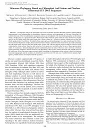
3 ENVIRONMENTAL INTERPRETATIONgraphics files. Moreover, the ordipointlabel ouput can be edited usingorditkplot.Functions identify, orditorp, ordilabel and ordipointlabel mayprovide a quick and easy way to inspect ordination results. Often we needa better control of graphics, and judicuously select the labelled species.In that case we can first draw an empty plot (with type = "n"), andthen use select argument in ordination text and points functions. Theselect argument can be a numeric vector that lists the indices of selecteditems. Such indices are displayed from identify functions which can beused to help in selecting the items. Alternatively, select can be a logicalvector which is TRUE to selected items. Such a list was produced invisiblyfrom orditorp. You cannot see invisible results directly from the method,but you can catch the result like we did above in the first orditorp call,and use this vector as a basis for fully controlled graphics. In this casethe first items were:> sel[1:14]Abarmacr Acacmela Acaldive Acalmacr Adeltril Aegipana AlchcostFALSE FALSE FALSE FALSE FALSE FALSE FALSEAlchlati Alibedul Allopsil Alseblac Amaicory Anacexce AndiinerTRUE FALSE FALSE FALSE TRUE TRUE FALSE3 Environmental interpretationIt is often possible to “explain” ordination using ecological knowledge onstudied sites, or knowledge on the ecological characteristics of species.Usually it is preferable to use external environmental variables to interpretthe ordination. There are many ways of overlaying environmentalinformation onto ordination diagrams. One of the simplest is to changethe size of plotting characters according to an environmental variables(argument cex in plot functions). The vegan package has some usefulfunctions for fitting environmental variables.3.1 Vector fittingThe most commonly used method of interpretation is to fit environmentalvectors onto ordination. The fitted vectors are arrows with the interpretation:• The arrow points to the direction of most rapid change in the theenvironmental variable. Often this is called the direction of thegradient.• The length of the arrow is proportional to the correlation betweenordination and environmental variable. Often this is called thestrength of the gradient.Fitting environmental vectors is easy using function envfit. Theexample uses the previous nmds result and environmental variables inthe data set varechem:> data(varechem)> ef ef14

3 ENVIRONMENTAL INTERPRETATION 3.2 Surface fitting***VECTORSNMDS1 NMDS2 r2 Pr(>r)N -0.0573 -0.9984 0.25 0.041 *P 0.6197 0.7848 0.19 0.092 .K 0.7665 0.6423 0.18 0.109Ca 0.6852 0.7284 0.41 0.003 **Mg 0.6325 0.7745 0.43 0.003 **S 0.1914 0.9815 0.18 0.137Al -0.8716 0.4902 0.53 0.002 **Fe -0.9360 0.3519 0.45 0.004 **Mn 0.7987 -0.6017 0.52 0.001 ***Zn 0.6175 0.7865 0.19 0.104Mo -0.9031 0.4294 0.06 0.504Baresoil 0.9249 -0.3802 0.25 0.041 *Humdepth 0.9328 -0.3603 0.52 0.003 **pH -0.6480 0.7616 0.23 0.070 .---Signif. codes: 0 ‘***’ 0.001 ‘**’ 0.01 ‘*’ 0.05 ‘.’ 0.1 ‘ ’ 1P values based on 999 permutations.The first two columns give direction cosines of the vectors, and r2 givesthe squared correlation coefficient. For plotting, the axes should be scaledby the square root of r2. The plot function does this automatically, andyou can extract the scaled values with scores(ef, "vectors"). Thesignificances (Pr>r), or P -values are based on random permutations ofthe data: if you often get as good or better R 2 with randomly permuteddata, your values are insignificant.You can add the fitted vectors to an ordination using plot command.You can limit plotting to most significant variables with argument p.max.As usual, more options can be found in the help pages.NMDS2−0.4 −0.2 0.0 0.2 0.4●●AlFe●●●pH●●●●●●●N●●●●●●P●●●MgCaBaresoilHumdepthMn●●●> plot(vare.mds, display = "sites")> plot(ef, p.max = 0.1)−0.4 −0.2 0.0 0.2 0.4 0.6NMDS13.2 Surface fittingVector fitting is popular, and it provides a compact way of simultaneouslydisplaying a large number of environmental variables. However, it impliesa linear relationship between ordination and environment: direction andstrength are all you need to know. This may not always be appropriate.Function ordisurf fits surfaces of environmental variables to ordinations.It uses generalized additive models in function gam of packagemgcv. Function gam uses thinplate splines in two dimensions, and automaticallyselects the degree of smoothing by generalized cross-validation.If the response really is linear and vectors are appropriate, the fitted surfaceis a plane whose gradient is parallel to the arrow, and the fittedcontours are equally spaced parallel lines perpendicular to the arrow.In the following example I introduce two new R features:• Function envfit can be called with formula interface. Formulahas a special character tilde (∼), and the left-hand side gives theordination results, and the right-hand side lists the environmental15

3.3 Factors 3 ENVIRONMENTAL INTERPRETATIONvariables. In addition, we must define the name of the data containingthe fitted variables.• The variables in data frames are not visible to R session unless thedata frame is attached to the session. We may not want to make allvariables visible to the session, because there may be synonymousnames, and we may use wrong variables with the same name insome analyses. We can use function with which makes the givendata frame visible only to the following command.Now we are ready for the example. We make vector fitting for selectedvariables and add fitted surfaces in the same plot.> ef plot(vare.mds, display = "sites")> plot(ef)> tmp

3 ENVIRONMENTAL INTERPRETATION 3.3 FactorsA1 0.9982 0.0606 0.31 0.043 *---Signif. codes: 0 ‘***’ 0.001 ‘**’ 0.01 ‘*’ 0.05 ‘.’ 0.1 ‘ ’ 1P values based on 999 permutations.***FACTORS:Centroids:CA1 CA2Moisture1 -0.75 -0.14Moisture2 -0.47 -0.22Moisture4 0.18 -0.73Moisture5 1.11 0.57ManagementBF -0.73 -0.14ManagementHF -0.39 -0.30ManagementNM 0.65 1.44ManagementSF 0.34 -0.68UseHayfield -0.29 0.65UseHaypastu -0.07 -0.56UsePasture 0.52 0.05Manure0 0.65 1.44Manure1 -0.46 -0.17Manure2 -0.59 -0.36Manure3 0.52 -0.32Manure4 -0.21 -0.8819Goodness of fit:r2 Pr(>r)Moisture 0.41 0.006 **Management 0.44 0.003 **Use 0.18 0.085 .Manure 0.46 0.005 **---Signif. codes: 0 ‘***’ 0.001 ‘**’ 0.01 ‘*’ 0.05 ‘.’ 0.1 ‘ ’ 1P values based on 999 permutations.CA2−1 0 1 2 317ManagementNMManure0UseHayfield 18Moisture51110 6 UsePastureManagementBFMoisture157Moisture2Manure1ManagementHF 8Manure2 Manure3UseHaypastu2 ManagementSF12Moisture44 9Manure4 13312015 1416A1> plot(dune.ca, display = "sites")> plot(ef)−2 −1 0 1 2CA1The names of factor centroids are formed by combining the name ofthe factor and the name of the level. Now the axes show the centroidsfor the level, and the R 2 values are for the whole factor, just like thesignificance test. The plot looks congested, and we may use tricks of §2.6(p. 12) to make cleaner plots, but obviously not all factors are necessaryin interpretation.Package vegan has several functions for graphical display of factors.Function ordihull draws an enclosing convex hull for the items in aclass, ordispider combines items to their (weighted) class centroid, andordiellipse draws ellipses for class standard deviations, standard errorsor confidence areas. The example displays all these for Management typein the previous ordination:> plot(dune.ca, display = "sites", type = "p")> with(dune.env, ordiellipse(dune.ca, Management,+ kind = "se", conf = 0.95))17

4 CONSTRAINED ORDINATION●> with(dune.env, ordispider(dune.ca, Management, col = "blue"))> with(dune.env, ordihull(dune.ca, Management, col = "blue",+ lty = 2))CA2−1 0 1 2 3●●●●●●●●●●●●● ●●●●−2 −1 0 1 2CA1Correspondence analysis is a weighted ordination method, and veganfunctions envfit and ordisurf will do weighted fitting, unless the userspecifies equal weights.4 Constrained ordinationIn unconstrained ordination we first find the major compositional variation,and then relate this variation to observed environmental variation.In constrained ordination we do not want to display all or even most ofthe compositional variation, but only the variation that can be explainedby the used environmental variables, or constraints. Constrained ordinationis often known as “canonical” ordination, but this name is misleading:there is nothing particularly canonical in these methods (see your favoriteDictionary for the term). The name was taken into use, because thereis one special statistical method, canonical correlations, but these indeedare canonical: they are correlations between two matrices regarded to besymmetrically dependent on each other. The constrained ordination isnon-symmetric: we have “independent” variables or constraints and wehave “dependent” variables or the community. Constrained ordinationrather is related to multivariate linear models.The vegan package has three constrained ordination methods whichall are constrained versions of basic ordination methods:• Constrained analysis of proximities (cap) in function capscale isrelated to metric scaling (cmdscale). It can handle any dissimilaritymeasures and performs a linear mapping.• Redundancy analysis (rda) in function rda is related to principalcomponents analysis. It is based on Euclidean distances and performslinear mapping.• Constrained correspondence analysis (cca) in function cca is relatedto correspondence analysis. It is based on Chi-squared distancesand performs weighted linear mapping.We have already used functions rda and cca for unconstrained ordination:they will perform the basic unconstrained method as a special case ifconstraints are not used.All these three vegan functions are very similar. The following examplesmainly use cca, but other methods can be used similarly. Actually,the results are similarly structured, and they inherit properties from eachother. For historical reasons, cca is the basic method, and rda inheritsproperties from it. Function capscale inherits directly from rda, andthrough this from cca. Many functions, are common with all these methods,and there are specific functions only if the method deviates from itsancestor. In vegan version 1.17-2 the following class functions are definedfor these methods:18

4 CONSTRAINED ORDINATION 4.1 Model specification• cca: add1, alias, anova, as.mlm, bstick, calibrate, coef, deviance,drop1, eigenvals, extractAIC, fitted, goodness, model.frame, model.matrix,permutest, plot, points, predict, print, residuals, RsquareAdj,scores, screeplot, simulate, summary, text, weights• rda: as.mlm, biplot, coef, deviance, fitted, goodness, predict,RsquareAdj, scores, simulate, weights• capscale: fitted, print, simulate.Many of these methods are internal functions that users rarely need.4.1 Model specificationThe recommended way of defining a constrained model is to use modelformula. Formula has a special character ∼, and on its left-hand sidegives the name of the community data, and right-hand gives the equationfor constraints. In addition, you should give the name of the data setwhere to find the constraints. This fits a cca for varespec constrainedby soil Al, K and P:> vare.cca vare.ccaCall: cca(formula = varespec ~ Al + P + K, data =varechem)Inertia RankTotal 2.083Constrained 0.644 3Unconstrained 1.439 20Inertia is mean squared contingency coefficientEigenvalues for constrained axes:CCA1 CCA2 CCA30.362 0.170 0.113Eigenvalues for unconstrained axes:CA1 CA2 CA3 CA4 CA5 CA6 CA7 CA80.3500 0.2201 0.1851 0.1551 0.1351 0.1003 0.0773 0.0537(Showed only 8 of all 20 unconstrained eigenvalues)The output is similar as in unconstrained ordination. Now the totalinertia is decomposed into constrained and unconstrained components.There were three constraints, and the rank of constrained componentis three. The rank of unconstrained component is 20, when it used tobe 23 in the previous analysis. The rank is the same as the number ofaxes: you have 3 constrained axes and 20 unconstrained axes. In somecases, the ranks may be lower than the number of constraints: some ofthe constraints are dependent on each other, and they are aliased in theanalysis, and an informative message is printed with the result.It is very common to calculate the proportion of constrained inertiafrom the total inertia. However, total inertia does not have a clear meaningin cca, and the meaning of this proportion is just as obscure. In rdathis would be the proportion of variance (or correlation). This may havea clearer meaning, but even in this case most of the total inertia may be19

4.1 Model specification 4 CONSTRAINED ORDINATION13random noise. It may be better to concentrate on results instead of theseproportions.Basic plotting works just like earlier:CCA2−2 −1 0 1 2221614 Cal.vul7Bar.lycBet.pub5216Led.palDic.fus Cla.bot Pti.cil Ich.eri 1815 Pol.com23Cla.arbCla.cri Ste.sp Vac.uliVac.myrCla.fim20 Cla.def Emp.nig Cla.ranPin.syl Dip.monDes.fleDic.pol Cla.unc Cla.graCet.islCla.ama Cla.cocVac.vitPol.pilPle.schCla.corPol.jun Poh.nut Cet.eriCla.spCla.chl 11KNep.arcPel.aphCla.steAl27193Hyl.splCla.phy42528Dic.sp12 Cla.cer210 Cet.nivP924−3 −2 −1 0 1 2CCA1−1 0 1> plot(vare.cca)have similar interpretation as fitted vectors: the arrow points to the directionof the gradient, and its length indicates the strength of the variablein this dimensionality of solution. The vectors will be of unit length infull rank solution, but they are projected to the plane used in the plot.There is also a primitive 3D plotting function ordiplot3d (which needsuser interaction for final graphs) that shows all arrows in full length:> ordiplot3d(vare.cca, type = "h")With function ordirgl you can also inspect 3D dynamic plots that canbe spinned or zoomed into with your mouse.The formula interface works with factor variables as well:> dune.cca plot(dune.cca)> dune.cca●Call: cca(formula = dune ~ Management, data = dune.env)CCA2CCA3−3 −2 −1 0 1 2 3 4−2 −1 0 1 2●● ●●●●●● ● ●●●●●●●●●●●●3●210−1−2−3 −2 −1 0 1 2CCA11710675ManagementBF 1118Viclat2AchmilManagementHFTripra BrohorPlalan191AntodoRumaceTrirepLolper LeoautHypradPoapraBelperBrarut JunartManagementNMEmpnig Salrep Potpal AirpraElyrep PoatriElepal RanflaJunbufSagproCalcus9AlogenAgrsto3814154ManagementSFChealb Cirarv20121316−2 −1 0 1 2 3CCA1CCA2Inertia RankTotal 2.115Constrained 0.604 3Unconstrained 1.511 16Inertia is mean squared contingency coefficientEigenvalues for constrained axes:CCA1 CCA2 CCA30.319 0.182 0.103Eigenvalues for unconstrained axes:CA1 CA2 CA3 CA4 CA5 CA6 CA70.44737 0.20300 0.16301 0.13457 0.12940 0.09494 0.07904CA8 CA9 CA10 CA11 CA12 CA13 CA140.06526 0.05004 0.04321 0.03870 0.02385 0.01773 0.00917CA15 CA160.00796 0.00416Factor variable Management had four levels (BF, HF, NM, SF). InternallyR expressed these four levels as three contrasts (sometimes called“dummyvariables”). The applied contrasts look like this:ManagementHF ManagementNM ManagementSFBF 0 0 0SF 0 0 1HF 1 0 0NM 0 1 0We do not need but three variables to express four levels: if there isnumber one in a column, the observation belongs to that level, and ifthere is a whole line of zeros, the observation must belong to the omittedlevel, or the first. The basic plot function displays class centroids insteadof vectors for factors.20

4 CONSTRAINED ORDINATION 4.2 Permutation testsIn addition to these ordinary factors, R also knows ordered factors.Variable Moisture in dune.env is defined as an ordered four-level factor.In this case the contrasts look different:Moisture.L Moisture.Q Moisture.C1 -0.6708 0.5 -0.22362 -0.2236 -0.5 0.67084 0.2236 -0.5 -0.67085 0.6708 0.5 0.2236R uses polynomial contrasts: the linear term L is equal to treatingMoisture as a continuous variable, and the quadratic Q and cubic C termsshow nonlinear features. There were four distinct levels, and the numberof contrasts is one less, just like with ordinary contrasts. The ordinationconfiguration, eigenvalues or rank do not change if the factor is unorderedor ordered, but the presentation of the factor in the results may change:> vare.cca plot(vare.cca)Now plot shows both the centroids of factor levels and the contrasts.If we could change the ordered factor to a continuous vector, only thelinear effect arrow would be important. If the response to the variable isnonlinear, the quadratic (and cubic) arrows would be long as well.I have explained only the simplest usage of the formula interface. Theformula is very powerful in model specification: you can transform yourcontrasts within the formula, you can define interactions, you can usepolynomial contrasts etc. However, models with interactions or polynomialsmay be difficult to interpret.CCA2−3 −2 −1 0 1 21017186 1116Empnig Ranfla Potpal ElepalTripraSalrep Chealb CalcusMoisture1Moisture55 PlalanHypradViclat7AchmilAirpraBrohor Belper LolperAntodoLeoautPoapra2BrarutCirarv TrirepPoatri Agrsto1 Moisture2RumaceJunart8Moisture.LElyrepSagpro Alogen43Moisture.Q19Moisture.C9Junbuf12−2 −1 0 1 2 313Moisture4CCA1141520−1 04.2 Permutation testsThe significance of all terms together can be assessed using permutationtests: the dat are permuted randomly and the model is refitted. Whenconstrained inertia in permutations is nearly always lower than observedconstrained inertia, we say that constraints are significant.The easiest way of running permutation tests is to use the mock anovafunction in vegan:> anova(vare.cca)Permutation test for cca under reduced modelModel: cca(formula = dune ~ Moisture, data = dune.env)Df Chisq F N.Perm Pr(>F)Model 3 0.63 2.25 199 0.005 **Residual 16 1.49---Signif. codes: 0 ‘***’ 0.001 ‘**’ 0.01 ‘*’ 0.05 ‘.’ 0.1 ‘ ’ 1The Model refers to the constrained component, and Residual to theunconstrained component of the ordination, Chisq is the correspondinginertia, and Df the corresponding rank. The test statistic F, or morecorrectly “pseudo-F ” is defined as their ratio. You should not pay anyattention to its numeric values or to the numbers of degrees of freedom,since this “pseudo-F ” has nothing to do with the real F , and the only wayF = 0.628/31.487/16 = 2.25421

4.2 Permutation tests 4 CONSTRAINED ORDINATIONto assess its “significance” is permutation. In simple models like the onestudied here we could directly use inertia in testing, but the “pseudo-F ”is needed in more complicated model including “partialled” terms.The number of permutations was not specified in the mock anovafunction. The function tries to be lazy: it continues permutations only aslong as it is uncertain whether the final P -value will be below or abovethe critical value (usually P = 0.05). If the observed inertia is neverreached in permutations, the function may stop after 200 permutations,and if it is very often exceeded, it may stop after 100 permutations.When we are close to the critical level, the permutations may continue tothousands. In this way the calculations are fast when this is possible, butthey are continued longer in uncertain cases. If you want to have a fixednumber of iterations, you must specify that in anova call or directly usethe underlying function permutest.ccaIn addition to the overall test for all constraints together, we canalso analyse single terms or axes by setting argument by. The followingcommand analyses all terms separately in a sequential (“Type I”) test:> mod anova(mod, by = "term", step = 200)Permutation test for cca under reduced modelTerms added sequentially (first to last)Model: cca(formula = varespec ~ Al + P + K, data = varechem)Df Chisq F N.Perm Pr(>F)Al 1 0.30 4.14 199 0.005 **P 1 0.19 2.64 199 0.005 **K 1 0.16 2.17 199 0.020 *Residual 20 1.44---Signif. codes: 0 ‘***’ 0.001 ‘**’ 0.01 ‘*’ 0.05 ‘.’ 0.1 ‘ ’ 1All terms are compared against the same residuals, and there is no heuristicfor the number permutations. The test is sequential, and the orderof terms will influence the results, unless the terms are uncorrelated. Inthis case the same number of permutations will be used for all terms.The sum of test statistics (Chisq) for terms is the same as the Model teststatistic in the overall test.“Type III” tests analyse the marginal effects when each term is eliminatedfrom the model containing all other terms:> anova(mod, by = "margin", perm = 500)Permutation test for cca under reduced modelMarginal effects of termsModel: cca(formula = varespec ~ Al + P + K, data = varechem)Df Chisq F N.Perm Pr(>F)Al 1 0.31 4.33 199 0.005 **P 1 0.17 2.34 199 0.015 *K 1 0.16 2.17 399 0.025 *Residual 20 1.44---Signif. codes: 0 ‘***’ 0.001 ‘**’ 0.01 ‘*’ 0.05 ‘.’ 0.1 ‘ ’ 122

4 CONSTRAINED ORDINATION 4.3 Model buildingThe marginal effects are independent of the order of the terms, but correlatedterms will get higher (“worse”) P -values. Now the the sum of teststatistics is not equal to the Model test statistic in the overall test, unlessthe terms are uncorrelated.We can also ask for a test of individual axes:> anova(mod, by = "axis", perm = 1000)Permutation test for cca under reduced modelModel: cca(formula = varespec ~ Al + P + K, data = varechem)Df Chisq F N.Perm Pr(>F)CCA1 1 0.36 5.02 199 0.005 **CCA2 1 0.17 2.36 999 0.042 *CCA3 1 0.11 1.57 99 0.140Residual 20 1.44---Signif. codes: 0 ‘***’ 0.001 ‘**’ 0.01 ‘*’ 0.05 ‘.’ 0.1 ‘ ’ 14.3 Model buildingIt is very popular to perform constrained ordination using all availableconstraints simultaneously. Increasing the number of constraints actuallymeans relaxing constraints: the ordination becomes more similar to theunconstrained one. When the rank of unconstrained component reducestowards zero, there are absolutely no constraints. However, the relaxationof constraints often happens much earlier in first ordination axes. If wedo not have strict constraints, it may be better to use unconstrainedordination with vector fitting (or surface fitting), which allows detectionof compositional variation for which we have not observed environmentalvariables. In constrained ordination it is best to reduce the number ofconstraints to just a few, say three to five.I do not want to encourage using all possible environmental variablestogether as constraints. However, there still is a shortcut for that purposein formula interface:> mod1 mod1Call: cca(formula = varespec ~ N + P + K + Ca + Mg + S+ Al + Fe + Mn + Zn + Mo + Baresoil + Humdepth + pH,data = varechem)Inertia RankTotal 2.083Constrained 1.441 14Unconstrained 0.642 9Inertia is mean squared contingency coefficientEigenvalues for constrained axes:CCA1 CCA2 CCA3 CCA4 CCA5 CCA6 CCA70.43887 0.29178 0.16285 0.14213 0.11795 0.08903 0.07029CCA8 CCA9 CCA10 CCA11 CCA12 CCA13 CCA140.05836 0.03114 0.01329 0.00836 0.00654 0.00616 0.0047323

4.3 Model building 4 CONSTRAINED ORDINATIONDimension 2−2.0 −1.5 −1.0 −0.5 0.0 0.5 1.0 1.5●●●●Procrustes errors●●●●●●●●● ●●●●●●●●●●●−1 0 1 2Dimension 1Eigenvalues for unconstrained axes:CA1 CA2 CA3 CA4 CA5 CA6 CA70.19776 0.14193 0.10117 0.07079 0.05330 0.03330 0.01887CA8 CA90.01510 0.00949This result probably is very similar to unconstrained ordination:> plot(procrustes(cca(varespec), mod1))For heuristic purposes we should reduce the number of constraints tofind important environmental variables. In principle, constrained ordinationonly should be used with designed a priori constraints. All kind ofautomatic tools of model selection are dangerous: There may be severalalternative models which are nearly equally good; Small changes in datacan cause large changes in selected models; There may be no route to thebest model with the adapted strategy; The model building has a history:one different step in the beginning may lead into wildly different finalmodels; Significance tests are biased, because the model is selected forthe best test performance.After all these warnings, I show how vegan can be used to automaticallyselect constraints into model using standard R function step. Thestep uses Akaike’s information criterion (aic) as the selection criterion.Aic is a penalized goodness-of-fit measure: the goodness-of-fit is basicallyderived from the residual (unconstrained) inertia penalized by therank of the constraints. In principle aic is based on log-Likelihood thatordination does not have. However, a deviance function changes theunconstrained inertia to Chi-squared in cca or sum of squares in rdaand capscale. This deviance is treated like sum of squares in Gaussianmodels. If we have only continuous (or 1 d.f.) terms, this is the same asselecting variables by their contributions to constrained eigenvalues (inertia).With factors the situation is more tricky, because factors must bepenalized by their degrees of freedom, and there is no way of knowing themagnitude of penalty. The step function may still be useful in helpingto gain insight into the data, but it should not be trusted blindly (or atall), but only regarded as an aid in model building.After this longish introduction the example: using step is much simplerthan explaining how it works. We need to give the model we startwith, and the scope of possible models inspected. For this we need anotherformula trick: formula with only 1 as the constraint defines anunconstrained model. We must define it like this so that we can add newterms to initially unconstrained model. The aic used in model buildingis not based on a firm theory, and therefore we also ask for permutationtests at each step. In ideal case, all included terms should be significantand all excluded terms insignificant in the final model. The scope mustbe given as a list a formula, but we can extract this from fitted modelsusing function formula. The model building should The following examplebegins with an unconstrained model mod0 and steps towards thepreviously fitted maximum model mod1:> mod0 mod

4 CONSTRAINED ORDINATION 4.3 Model buildingDf AIC F N.Perm Pr(>F)+ Al 1 128.61 3.6749 199 0.005 **+ Mn 1 128.95 3.3115 199 0.005 **+ Humdepth 1 129.24 3.0072 199 0.010 **+ Baresoil 1 129.77 2.4574 199 0.020 *+ Fe 1 129.79 2.4360 199 0.005 **+ P 1 130.03 2.1926 199 0.035 *+ Zn 1 130.30 1.9278 199 0.020 * 130.31+ Mg 1 130.35 1.8749 199 0.040 *+ K 1 130.37 1.8609 199 0.065 .+ Ca 1 130.43 1.7959 199 0.065 .+ pH 1 130.57 1.6560 199 0.090 .+ S 1 130.72 1.5114 199 0.090 .+ N 1 130.77 1.4644 199 0.135+ Mo 1 131.19 1.0561 99 0.490---Signif. codes: 0 ‘***’ 0.001 ‘**’ 0.01 ‘*’ 0.05 ‘.’ 0.1 ‘ ’ 1Step: AIC=128.61varespec ~ AlDf AIC F N.Perm Pr(>F)+ P 1 127.91 2.5001 199 0.010 **+ K 1 128.09 2.3240 199 0.005 **+ S 1 128.26 2.1596 199 0.005 **+ Zn 1 128.44 1.9851 199 0.035 *+ Mn 1 128.53 1.8945 199 0.040 * 128.61+ Mg 1 128.70 1.7379 199 0.125+ N 1 128.85 1.5900 199 0.080 .+ Baresoil 1 128.88 1.5670 199 0.095 .+ Ca 1 129.04 1.4180 99 0.140+ Humdepth 1 129.08 1.3814 99 0.250+ Mo 1 129.50 0.9884 99 0.460+ pH 1 129.63 0.8753 99 0.520+ Fe 1 130.02 0.5222 99 0.850- Al 1 130.31 3.6749 199 0.005 **---Signif. codes: 0 ‘***’ 0.001 ‘**’ 0.01 ‘*’ 0.05 ‘.’ 0.1 ‘ ’ 1Step: AIC=127.91varespec ~ Al + PDf AIC F N.Perm Pr(>F)+ K 1 127.44 2.1688 199 0.040 * 127.91+ Baresoil 1 127.99 1.6606 199 0.065 .+ N 1 128.11 1.5543 99 0.140+ S 1 128.36 1.3351 99 0.230+ Mn 1 128.44 1.2641 99 0.180+ Zn 1 128.51 1.2002 99 0.300+ Humdepth 1 128.56 1.1536 99 0.39025

4.3 Model building 4 CONSTRAINED ORDINATION- P 1 128.61 2.5001 199 0.010 **+ Mo 1 128.75 0.9837 99 0.400+ Mg 1 128.79 0.9555 99 0.470+ pH 1 128.82 0.9247 99 0.510+ Fe 1 129.28 0.5253 99 0.850+ Ca 1 129.36 0.4648 99 0.890- Al 1 130.03 3.9401 199 0.005 **---Signif. codes: 0 ‘***’ 0.001 ‘**’ 0.01 ‘*’ 0.05 ‘.’ 0.1 ‘ ’ 1Step: AIC=127.44varespec ~ Al + P + KDf AIC F N.Perm Pr(>F) 127.44+ N 1 127.59 1.5148 99 0.140+ Baresoil 1 127.67 1.4544 99 0.180+ Zn 1 127.84 1.3067 99 0.200+ S 1 127.89 1.2604 99 0.250- K 1 127.91 2.1688 199 0.050 *+ Mo 1 127.92 1.2350 99 0.280- P 1 128.09 2.3362 199 0.010 **+ Mg 1 128.17 1.0300 99 0.390+ Mn 1 128.34 0.8879 99 0.460+ Humdepth 1 128.44 0.8056 99 0.600+ Fe 1 128.79 0.5215 99 0.930+ pH 1 128.81 0.5067 99 0.830+ Ca 1 128.89 0.4358 99 0.920- Al 1 130.14 4.3340 199 0.005 **---Signif. codes: 0 ‘***’ 0.001 ‘**’ 0.01 ‘*’ 0.05 ‘.’ 0.1 ‘ ’ 1> modCall: cca(formula = varespec ~ Al + P + K, data =varechem)Inertia RankTotal 2.083Constrained 0.644 3Unconstrained 1.439 20Inertia is mean squared contingency coefficientEigenvalues for constrained axes:CCA1 CCA2 CCA30.362 0.170 0.113Eigenvalues for unconstrained axes:CA1 CA2 CA3 CA4 CA5 CA6 CA7 CA80.3500 0.2201 0.1851 0.1551 0.1351 0.1003 0.0773 0.0537(Showed only 8 of all 20 unconstrained eigenvalues)We ended up with the same familiar model we have been using all the time(and now you know the reason why this model was used in the first place).The aic was based on deviance, and penalty for each added parameter26

4 CONSTRAINED ORDINATION 4.3 Model buildingwas 2 per degree of freedom. At every step the aic was evaluated for allpossible additions (+) and removals (-), and the variables are listed inthe order of aic. The stepping stops when or the current modelis at the top.Model building with step is fragile, and the strategy of model buildingcan change the final model. If we start with the largest model (mod1),the final model will be different:> modb modbCall: cca(formula = varespec ~ P + K + Mg + S + Mn + Mo+ Baresoil + Humdepth, data = varechem)Inertia RankTotal 2.083Constrained 1.117 8Unconstrained 0.967 15Inertia is mean squared contingency coefficientEigenvalues for constrained axes:CCA1 CCA2 CCA3 CCA4 CCA5 CCA6 CCA7 CCA80.4007 0.2488 0.1488 0.1266 0.0875 0.0661 0.0250 0.0130Eigenvalues for unconstrained axes:CA1 CA2 CA3 CA4 CA5 CA6 CA70.25821 0.18813 0.11927 0.10204 0.08791 0.06085 0.04461CA8 CA9 CA10 CA11 CA12 CA13 CA140.02782 0.02691 0.01646 0.01364 0.00823 0.00655 0.00365CA150.00238The aic of this model is 127.89 which is higher (worse) than reachedin forward selection (127.44). We supressed tracing to save some pagesof output, but step adds its history in the result:> modb$anovaStep Df Deviance Resid. Df Resid. Dev AIC1 NA NA -15 1551 130.12 - Fe 1 115.2 -14 1667 129.83 - Al 1 106.0 -13 1773 129.34 - N 1 117.5 -12 1890 128.85 - pH 1 140.4 -11 2031 128.56 - Ca 1 141.2 -10 2172 128.17 - Zn 1 165.3 -9 2337 127.9Variable Al was the first to be selected in the model in forward selection,but it was the second to be removed in backward elimination.Variable Al is strongly correlated with many other explanatory variables.This is obvious when looking at the variance inflation factors (vif) in thefull model mod1:> vif.cca(mod1)N P K Ca Mg S Al1.982 6.029 12.009 9.926 9.811 18.379 21.19327

4.4 Linear combinations and weighted averages 4 CONSTRAINED ORDINATIONFe Mn Zn Mo Baresoil Humdepth pH9.128 5.380 7.740 4.320 2.254 6.013 7.389A common rule of thumb is that vif > 10 indicates that a variable isstrongly dependent on others and does not have independent information.On the other hand, it may not be the variable that should be removed,but alternatively some other variables may be removed. The vifs wereall modest in model found by forward selection, including Al:> vif.cca(mod)Al P K1.012 2.365 2.3794.4 Linear combinations and weighted averagesThere are two kind of site scores in constrained ordinations:1. Linear combination scores lc which are linear combinations of constrainingvariables.2. Weighted averages scores wa which are weighted averages of speciesscores.These two scores are as similar as possible, and their (weighted) correlationis called the species–environment correlation:> spenvcor(mod)CCA1 CCA2 CCA30.8555 0.8133 0.8793Correlation coefficient is very sensitive to single extreme values, like seemsto happen in the example above where axis 3 has the “best” correlationsimply because it has some extreme points, and eigenvalue is a moreappropriate measure of similarity between lc and wa socres.The opinions are divided on using lc or wa as primary results in ordinationgraphics. The vegan package prefers wa scores, whereas the majorcommercial programme for cca prefers lc scores. The vegan packagecomes with a separate document (“vegan FAQ”) which studies the issuein more detail, but I will briefly discuss the subject here also, and showhow you can circumvent my decisions.The practical reason to prefer wa scores is that they are more robustagainst random error in environmental variables. All ecological observationshave random error, and therefore it is better to use scores thatare resistant to this variation. Another point is that I see lc scores asconstraints: the scores are dependent only on environmental variables,and community composition does not influence them. The wa scoresare based on community composition, but so that they are as similar aspossible to the constraints. This duality is particularly clear when usinga single factor variable as constraint: the lc scores are constant withineach level of the factor and fall in the same point. The wa scores showhow well we can predict the factor level from community composition.The vegan package has a graphical function ordispider which (amongother alternatives) will combine wa scores to the corresponding lc score.With a single factor constraint:28

4 CONSTRAINED ORDINATION 4.5 Biplot arrows and environmental calibration> dune.cca plot(dune.cca, display = c("lc", "wa"), type = "p")> ordispider(dune.cca, col = "blue")The interpretation is similar as in discriminant analysis: lc scores givethe predicted class centroids, and wa scores give the predicted values.For distinct classes, there is no overlap among groups. In general, thelength of ordispider segments is a visual image of species–environmentcorrelation.4.5 Biplot arrows and environmental calibrationBiplot arrows are an essential part of constrained ordination plots. Thearrows are based on (weighted) correlation of lc scores and environmentalvariables. They are scaled to unit length in the constrained ordination offull rank. When these arrows are projected onto 2D ordination plot, theylook shorter if they go off the plane.In vegan the biplot arrows are always scaled similarly irrespective ofscaling of sites or species. With default scaling = 2, the biplot arrowshave optimal relation to sites, but with scaling = 1 they rather arerelated to species.The standard interpretation of biplot arrows is that a site should beperpendicularly projected onto the arrow to predict the value of the variable.The arrow starts from the (weighted) mean of the environmentalvariable, and the values increase towards the arrow head, and decrease tothe opposite direction. Then we still should figure out the unit of change.Function calibrate.cca performs this automatically in vegan. Let usinspect the result of the step function with three constraints:CCA2−2 −1 0 1 2●●●●●●●●●●●●●●●●●●●●−2 −1 0 1 2 3CCA1> pred head(pred)Al P K18 103.219 25.64 80.5715 30.661 47.25 190.9024 32.105 72.80 208.3427 7.178 64.44 241.8923 14.321 38.50 125.7319 136.568 54.39 182.60Actually, this is not based on biplot arrows, but on regression coefficientsused internally in constrained ordination. Biplot arrows should only beseen as a visual approximation. The fitting is done in full constrained rankas default and for all constraints simultaneously. The example draws aresidual plot of predictions:> with(varechem, plot(Al, pred[, "Al"] - Al, ylab = "Prediction Error"))> abline(h = 0, col = "grey")The vegan package provides function ordisurf which is based ongam in the mgcv package, and can automatically detect the degree ofsmoothness needed, and can be used to check the linearity hypothesis ofthe biplot method. Function performs weighted fitting, and the modelshould be consistent with the one used in arrow fitting. Aluminium wasthe most important of three constraints in our example. Now we shouldfit the model to the lc scores, just like the arrows:Prediction Error−150 −100 −50 0 50 100 150●●●●●●●●●●●●●●●●●●●●●0 100 200 300 400Al●29

4.6 Conditioned or partial models 4 CONSTRAINED ORDINATION1313> plot(mod, display = c("bp", "wa", "lc"))> ef dune.cca plot(dune.cca)> dune.ccaCall: cca(formula = dune ~ Management +Condition(Moisture), data = dune.env)CCA2−2 −1 0 1 265ManagementHFTripra7RumaceAntodoJunart Plalan 915810AirpraCirarv1916 Poatri ElyrepJunbufPoapraAchmil20Agrsto Lolper Elepal Ranfla BrarutTrirep Leoaut ManagementNMEmpnig PotpalAlogen Sagpro BrohorBelper Calcus Hyprad Salrep13ManagementSF34 12Chealb14Viclat1 ManagementBF21811−2 −1 0 1 2 3CCA117Inertia RankTotal 2.115Conditional 0.628 3Constrained 0.374 3Unconstrained 1.113 13Inertia is mean squared contingency coefficientEigenvalues for constrained axes:CCA1 CCA2 CCA30.2278 0.0849 0.0614Eigenvalues for unconstrained axes:CA1 CA2 CA3 CA4 CA5 CA6 CA70.35040 0.15206 0.12508 0.10984 0.09221 0.07711 0.05944CA8 CA9 CA10 CA11 CA12 CA130.04776 0.03696 0.02227 0.02070 0.01083 0.00825Now the total inertia is decomposed into three components: inertia explainedby conditions, inertia explained by constraints and the remaining30

4 CONSTRAINED ORDINATION 4.6 Conditioned or partial modelsunconstrained inertia. We previously fitted a model with Managementas the only constraint, and in that case constrained inertia was clearlyhigher than now. It seems that different Management was practised indifferent natural conditions, and the variation we previously attributedto Management may be due to Moisture.We can perform permutation tests for Management in conditionedmodel, and Management alone:> anova(dune.cca, perm.max = 2000)Permutation test for cca under reduced modelModel: cca(formula = dune ~ Management + Condition(Moisture), data = dune.env)Df Chisq F N.Perm Pr(>F)Model 3 0.37 1.46 1799 0.037 *Residual 13 1.11---Signif. codes: 0 ‘***’ 0.001 ‘**’ 0.01 ‘*’ 0.05 ‘.’ 0.1 ‘ ’ 1> anova(cca(dune ~ Management, dune.env))Permutation test for cca under reduced modelModel: cca(formula = dune ~ Management, data = dune.env)Df Chisq F N.Perm Pr(>F)Model 3 0.60 2.13 199 0.01 **Residual 16 1.51---Signif. codes: 0 ‘***’ 0.001 ‘**’ 0.01 ‘*’ 0.05 ‘.’ 0.1 ‘ ’ 1Inspected alone, Management seemed to be very significant, but the situationis much less clear after removing the variation due to Moisture.The anova function (like any permutation test in vegan) can be restrictedso that permutation are made only within strata or within alevel of a factor variable:> with(dune.env, anova(dune.cca, strata = Moisture))Permutation test for cca under reduced modelPermutations stratified within 'Moisture'Model: cca(formula = dune ~ Management + Condition(Moisture), data = dune.env)Df Chisq F N.Perm Pr(>F)Model 3 0.37 1.46 199 0.01 **Residual 13 1.11---Signif. codes: 0 ‘***’ 0.001 ‘**’ 0.01 ‘*’ 0.05 ‘.’ 0.1 ‘ ’ 1Conditioned or partial models are sometimes used for decompositionof inertia into various components attributed to different sets of environmentalvariables. In some cases this gives meaningful results, but thegroups of environmental variables should be non-linearly independent forunbiased decomposition. If the groups of environmental variables havepolynomial dependencies, some of the components of inertia may evenbecome negative (that should be impossible). That kind of higher-orderdependencies are almost certain to appear with high number of variablesand high number of groups. However, varpart performs decompositionof rda models among two to four components.31

5 DISSIMILARITIES AND ENVIRONMENT5 Dissimilarities and environmentWe already discussed environmental interpretation of ordination and environmentallyconstrained ordination. These both reduce the variation intoan ordination space, and mainly inspect the first dimensions. Sometimeswe may wish to analyse vegetation–environment relationships without ordination,or in full space. Typically these methods use the dissimilaritymatrix in analysis. The recommended method in vegan is adonis whichimplements a multivariate analysis of variances using distance matrices.Function adonis can handle both continuous and factor predictors. Othermethods in vegan include multiresponse permutation procedure (mrpp)and analysis of similarities (anosim). Both of these handle only classpredictors, and they are less robust than adonis.5.1 adonis: Multivariate ANOVA based on dissimilaritiesS =kX zz =[log(2) − log(2a + b + c)+ log(a + b + c)]/ log(2)Function adonis partitions dissimilarities for the sources of variation, anduses permutation tests to inspect the significances of those partitions.With Euclidean distances the results are similar as in rda and its anovapermutation tests, but adonis can handle any dissimilarity objects.The example uses adonis to study beta diversity between Managementclasses in the dune meadow data. We define beta diversity as theslope of species-area curve, or the exponent z of the Arrhenius modelwhere the number of species S is dependent on the size X of the studyarea. For pairwise comparison of sites the slope z can be found from thenumber of species shared between two sites (a) and the number of speciesunique to each sites (b and c). It is commonly regarded that z ≈ 0.3implies random sampling variability, and only higher values mean realsystematic differences. The Arrhenius z can be directly found with functionbetadiver that also provided many other indices of pairwise betadiversity.> betad adonis(betad ~ Management, dune.env, perm = 200)Call:adonis(formula = betad ~ Management, data = dune.env, permutations = 200)Df SumsOfSqs MeanSqs F.Model R2 Pr(>F)Management 3.000 1.236 0.412 2.362 0.31 0.01 **Residuals 16.000 2.790 0.174 0.69Total 19.000 4.026 1.00---Signif. codes: 0 ‘***’ 0.001 ‘**’ 0.01 ‘*’ 0.05 ‘.’ 0.1 ‘ ’ 1The models can be more complicated, and sequential test of permutationalANOVA is performed if there are several parameters:> adonis(betad ~ A1 * Management, dune.env, perm = 200)32

5 DISSIMILARITIES AND ENVIRONMENT 5.2 Homogeneity of groups and beta diversityCall:adonis(formula = betad ~ A1 * Management, data = dune.env, permutations = 200)Df SumsOfSqs MeanSqs F.Model R2 Pr(>F)A1 1.000 0.655 0.655 4.134 0.16 0.005 **Management 3.000 1.001 0.334 2.107 0.25 0.045 *A1:Management 3.000 0.469 0.156 0.987 0.12 0.438Residuals 12.000 1.901 0.158 0.47Total 19.000 4.026 1.00---Signif. codes: 0 ‘***’ 0.001 ‘**’ 0.01 ‘*’ 0.05 ‘.’ 0.1 ‘ ’ 15.2 Homogeneity of groups and beta diversityFunction adonis studied the differences in the group means, but functionbetadisper studies the differences in group homogeneities. Functionadonis was analogous to multivariate analysis of variance, and betadisperis analogous to Levene’s test of the equality of variances.The example continues the analysis of the previous section and inspectsthe beta diversity. The function can only use one factor as anindependent variable, and it does not know the formula interface, so thatwe need to attach the data frame or use with to make the factor visibleto the function:> mod modHomogeneity of multivariate dispersionsCall: betadisper(d = betad, group = Management)No. of Positive Eigenvalues: 12No. of Negative Eigenvalues: 7Average distance to centroid:BF HF NM SF0.260 0.257 0.442 0.367Eigenvalues for PCoA axes:PCoA1 PCoA2 PCoA3 PCoA4 PCoA5 PCoA6 PCoA7 PCoA8 PCoA91.655 0.887 0.533 0.374 0.287 0.224 0.161 0.081 0.065PCoA10 PCoA11 PCoA12 PCoA13 PCoA14 PCoA15 PCoA16 PCoA17 PCoA180.035 0.018 0.004 -0.004 -0.019 -0.037 -0.043 -0.054 -0.060PCoA19-0.083The function has plot and boxplot methods for graphical display.PCoA 2−0.2 0.0 0.2 0.4●●●●●mod●●> plot(mod)> boxplot(mod)The significance of the fitted model can be analysed either using standardparametric anova or permutation tests (permutest):−0.2 0.0 0.2 0.4PCoA 1method = "beta.z"> anova(mod)Analysis of Variance Table33Distance to centroid0.1 0.2 0.3 0.4 0.5 0.6BF HF NM SF

5.3 Mantel test 5 DISSIMILARITIES AND ENVIRONMENTResponse: DistancesDf Sum Sq Mean Sq F value Pr(>F)Groups 3 0.120 0.0399 1.7 0.21Residuals 16 0.374 0.0234> permutest(mod)Permutation test for homogeneity of multivariatedispersionsNo. of permutations: 999Permutation type: freePermutations are unstratifiedMirrored permutations?: NoUse same permutation within strata?: NoResponse: DistancesDf Sum Sq Mean Sq F N.Perm Pr(>F)Groups 3 0.120 0.0399 1.7 999 0.20Residuals 16 0.374 0.0234Moreover, it is possible to analyse pairwise differences between groupsusing parametric Tukey’s HSD test:> TukeyHSD(mod)Tukey multiple comparisons of means95% family-wise confidence levelFit: aov(formula = distances ~ group, data = df)$groupdiff lwr upr p adjHF-BF -0.003039 -0.32253 0.3165 1.0000NM-BF 0.181909 -0.12744 0.4913 0.3643SF-BF 0.106716 -0.20263 0.4161 0.7588NM-HF 0.184948 -0.07996 0.4499 0.2298SF-HF 0.109755 -0.15515 0.3747 0.6443SF-NM -0.075193 -0.32777 0.1774 0.82915.3 Mantel testMantel test compares two sets of dissimilarities. Basically, it is the correlationbetween dissimilarity entries. As there are N(N − 1)/2 dissimilaritiesamong N objects, normal significance tests are not applicable.Mantel developed asymptotic test statistics, but vegan function manteluses permutation tests.In this example we study how well the lichen pastures (varespec) correspondto the environment. We have already used vector fitting after ordination.However, the ordination and environment may be non-linearlyrelated, and we try now with function mantel. We first perform a pca ofenvironmental variables, and then compute dissimilarities for first principalcomponents. We use standard R function prcomp, but princomp orrda will work as well. Function scores in vegan will work with all thesemethods. The following uses the same standardizations for communitydissimilarities as previously used in metaMDS.34

5 DISSIMILARITIES AND ENVIRONMENT 5.4 Protest: Procrustes test> pc pc edis vare.dis mantel(vare.dis, edis)Mantel statistic based on Pearson's product-moment correlationCall:mantel(xdis = vare.dis, ydis = edis)Mantel statistic r: 0.381Significance: 0.001Empirical upper confidence limits of r:90% 95% 97.5% 99%0.150 0.185 0.221 0.261Based on 999 permutationsWe could use a selection of environmental variables in pca, or we coulduse standardized environmental variables directly without pca — tastesvary. Function bioenv gives an intriguing alternative for selecting optimalsubsets for comparing ordination and environment. There also is a partialMantel test where we can remove the influence of third set dissimilaritiesfrom the analysis, but its results often are difficult to interpret.Function mantel does not have diagnostic plot functions, but you candirectly plot two dissimilarity matrices against each other:> plot(vare.dis, edis)Everything is O.K. if the relationship is more or less monotonous, or evenlinear and positive. In spatial models we even may observe a hump whichindicates spatial aggregation.edis2 4 6 8●●●●●●●●●●●●●●●●●●●●●●●●●● ●●●● ●●●●●● ● ●●●●●● ●●●●●●●● ● ● ●●●● ●● ●●● ● ●●● ●●●●●●●●●●●●●●●●●●●●●●●●●●●●● ●●● ●●●●●●●●●●●●●●●●●● ●●● ● ● ●●● ●●●●●●●●●●●●● ●●●●●●●●● ●●●● ●●●●●● ●● ●●●●●●● ●●●●●●● ●●●●●●●●●●●●● ●●●● ●●●●●●●●●●0.2 0.3 0.4 0.5 0.6 0.7vare.dis●●●●●●●●●●●●●●●5.4 Protest: Procrustes testProcrustes test or protest compares two ordinations using symmetricProcrustes analysis. It is an alternative to Mantel tests, but uses reducedspace instead of complete dissimilarity matrices. We can repeat the previousanalysis, but now with the solution of metaMDS and two first principalcomponents of the environmental analysis:> pc pro plot(pro)> proCall:protest(X = vare.mds, Y = pc)Correlation in a symmetric Procrustes rotation: 0.683Significance: 0.001Based on 1000 permutations.Dimension 2−0.2 −0.1 0.0 0.1 0.2●●●●●Procrustes errors●●●●●●●●●●●●●●●●●●The significance is assessed by permutation tests. The statistic is nowProcrustes correlation r derived from the symmetric Procrustes residualm 2 . The correlation is clearly higher than the Mantel correlation−0.2 −0.1 0.0 0.1 0.2 0.3Dimension 135r = √ 1 − m 2

6 CLASSIFICATIONfor the corresponding dissimilarities. In lower number of dimensions weremove noise from the data which may explain higher correlations (aswell as different methods of calculating the correlation). However, bothmethods are about as significant. Significance often is not a significantconcept: even small deviations from randomness may be highly significantin large data sets. Function protest provides graphical presentations(“Procrustes superimposition plot”) which may be more useful inevaluating the congruence between configurations.Protest (as ordinary Procrustes analysis) is often used in assessingsimilarities between different community ordinations. This is known asanalysis of congruence.6 ClassificationThe vegan mainly is a package for ordination and diversity analysis, andthere is only a scanty support to classification. There are several other Rpackages with more extensive classification functions. Among communityecological packages, labdsv package by Dave Roberts is particularly strongin classification functions.This chapter describes performing simple classification tasks in communityecology that are sufficient to many community ecologists.Cluster DendrogramHeightHeight0.20 0.25 0.30 0.35 0.40 0.45 0.50 0.550.2 0.4 0.6 0.8 1.0171917191141118161152021011181312210dishclust (*, "single")Cluster Dendrogram513126743567148916431520896.1 Cluster analysisHierarchic clustering can be perfomed using standard R function hclust.In addition, there are several other clustering packages, some of whichmay be compatible with hclust. Function hclust needs a dissimilaritiesas input.Function hclust provides several alternative clustering strategies. Incommunity ecology, most popular are single linkage a.k.a. nearest neighbour,complete linkage a.k.a. furthest neighbour, and various brands ofaverage linkage methods. These are best illustrated with examples:> dis clus plot(clus)Some people prefer single linkage, because it is conceptually related tominimum spanning tree which nicely can be represented in ordinations,and it is able to find discontinuities in the data. However, single linkageis prone to chain data so that single sites are joined to large clusters.> cluc plot(cluc)Some people prefer complete linkage because it makes compact clusters.However, this is in part an artefact of the method: the clusters are notallowed to grow, because the complete linkage criterion would be violated.> clua plot(clua)dishclust (*, "complete")36

6 CLASSIFICATION 6.2 Display and interpretation of classesSome people (I included) prefer average linkage clustering, because itseems to be a compromise between the previous two extremes, and moreneutral in grouping. There are several alternative methods loosely connectedto “average linkage” family. Ward’s method seems to be popular inpublications. It approaches complete linkage in its attempt to minimizevariances in agglomeration. The default "average" method is the oneoften known as upgma which was popular in old-time genetics.All these clustering methods are agglomerative. They start with combiningtwo most similar sites to each other. Then they proceed by combiningpoints to points or to groups, or groups to groups. The fusion criteriavary. The vertical axis in all graphs shows the level of fusion. The numbersvary among methods, but all are based on the same dissimilaritieswith range:> range(dis)[1] 0.2273 1.0000The first fusion is between the same two most similar sites in all examples,and at the same minimum dissimilarity. In complete linkage the lastfusion combines the two most dissimilar sites, and it is at the maximumdissimilarity. In single linkage the fusion level always is at the smallestgap between groups, and the reported levels are much lower than withcomplete linkage. Average linkage makes fusions between group centrepoints, and its fusion levels are between the previous two trees. Theestimated dissimilarity between two points is the level where they arefused in a tree. Function cophenetic finds this estimated dissimilarityfrom a tree for evey pair of points – the name of the function reflectsthe history of clustering in numerical taxonomy. Cophenetic correlationmeasures the similarity between original dissimilarities and dissimilaritiesestimated from the tree. For our three example methods:> cor(dis, cophenetic(clus))Height0.2 0.3 0.4 0.5 0.6 0.7 0.8141615201719Cluster Dendrogram113128dishclust (*, "average")4391118521067[1] 0.6602> cor(dis, cophenetic(cluc))[1] 0.6707> cor(dis, cophenetic(clua))[1] 0.8169Approximating dissimilarities is the same task that ordinations perform,and average linkage is the best performer.6.2 Display and interpretation of classesCluster analysis performs a hierarchic clustering, and its results can beinspected at as many levels as there are points: the extremes are thatevery point is in its private cluster, or that all points belong to the samecluster. We commonly want to inspect clustering at a certain level, as anon-hierarchic system of certain number of clusters. The flattening of theclustering happens by cutting the tree at some fusion level so that we geta desired number of clusters.Base R provides function rect.hclust to visualize the cutting, andfunction cutree to make a classification vector with certain number ofclasses:37

6.2 Display and interpretation of classes 6 CLASSIFICATIONHeight0.2 0.4 0.6 0.8 1.0171911181210Cluster Dendrogram5131267dishclust (*, "complete")431489161520> plot(cluc)> rect.hclust(cluc, 3)> grp boxplot(A1 ~ grp, data = dune.env, notch = TRUE)If we wish, we may use all normal statistical methods with factors, suchas functions lm or aov for formal testing of “significance” of clusters.Classification can be compared against external factor variables as well.However, vegan does not provide any tools for this. It may be best tosee the labdsv package and its tutorial for this purpose.The clustering results can be displayed in ordination diagrams. Allusual vegan functions for factors can be used: ordihull, ordispider,and ordiellipse. We shall see only the first as an example:4 6 8 10●●1 2 3> ord plot(ord, display = "sites")> ordihull(ord, grp, lty = 2, col = "red")It is said sometimes that overlaying classification in ordination can beused as a cross-check: if the clusters look distinct in the ordination diagram,(both) analyses probably were adequate. However, the classes canoverlap and the analyses can still be good. It may be that you need threeor more axes to display the multivariate class structure. In addition, ordinationand classification may use different criteria. In our example, causes weighted Chi-squared criteria, and the clustering uses Bray–Curtisdissimilarities which may be quite different. Function ordirgl with itssupport function orglspider can be used to inspect classification usingdynamic 3D graphics.The vegan package has function ordicluster to overlay hclust treein an ordination:CA2−1 0 1 2 31710 6571191121843−2 −1 0 1 291213CA182015 1416> plot(ord, display = "sites")> ordicluster(ord, cluc, col = "blue")The function combines points and cluster midpoints similarly as in theoriginal cluster dendrogram.Single linkage clustering is the method most often used with with ordinationdiagrams. Single linkage clustering is special among the clusteringalgorithms, because it always combines points to points: it is only thenearest point that is recognized and no information on its cluster membershipis used. The dendrogram, however, hides this information: itonly shows the fusions between clusters, but does not show which werethe actual points that were joined. The tree connecting individual pointsis called a minimum spanning tree (mst). In graph theory, ‘tree’ is aconnected graph with no loops, ‘spanning tree’ is tree that connects allpoints, and minimum spanning tree is the one where the total length ofconnecting segments is shortest. Function spantree in vegan find thistree, and it has a lines function to overlay the tree onto ordination:CA2−1 0 1 2 31710 65711911218439121382015 1416> mst plot(mst, ord = ord, pch = 21, col = "red", bg = "yellow")38−2 −1 0 1 2

6 CLASSIFICATION 6.3 Classified community tablesIn our dissimilarity index, distance = 1 means that there is nothing incommon with two sample plots. Function spantree regards these maximumdissimilarities as missing data, and does not use them in buildingthe tree. If all points cannot be connected because of these missing values,the result will consist of disconnected spanning trees. In graph theory thisis known as a ‘forest’. Mst is used sometimes to cross-check ordination:if the tree is linear, the ordination might be good. A curved tree mayindicate arc or horseshoe artefacts, and a messy tree a bad ordination, ora need of higher number of dimensions. However, the results often aredifficult to interpret.6.3 Classified community tablesThe aim of classification often is to make a classified community table.For this purpose, both sites and species should be arranged so that thetable looks structured. The original clustering may not be ideally structured,because the ordering of sites is not strictly defined in the clusterdendrogram. You can take any branch and rotate it around its base, andthe clustering is the same. The tree drawing algorithms use heuristicrules to make the tree look aesthetically pleasing, but this ordering maynot be the best one for a structured community table.Base R has a general tree class called dendrogram which is intended asa common base for any tree-like presentations. This class has a functionto reorder a tree according to some external variable. The hclust resultcan be changed into dendrogram with function as.dendrogram, and thiscan be reorderd with function reorder. The only continuous variablein the Dune data is the thickness of A1 horizon, and this could be usedto arrange the tree. However, for a nicely structured community tablewe use another trick: ca is an ordination method that structures tableoptimally into a diagonal structure, and we can use its first axis to reorderthe tree:> wa den oden op plot(den)> plot(oden)> par(op)Function vegemite in vegan produces compact vegetation tables. Itcan take an argument use to arrange the sites (and species, if possible).This argument can be a vector used to arrange sites, or it can be anordination result, or it can be an hclust result or a dendrogram object.CA2−1 0 1 2 30.0 0.2 0.4 0.6 0.80.0 0.2 0.4 0.6 0.8●●●●●●●●●●●−2 −1 0 1 214161520171917191610157●13122●●CA11118●91118438349●●●2108121314152016567> vegemite(dune, use = oden, zero = "-")11 1 11 11112179157602183498234506Airpra 23------------------39

6.3 Classified community tables 6 CLASSIFICATIONEmpnig -2------------------Hyprad 25------2-----------Antodo 44-4234-------------Tripra ---225--------------Achmil 2-122243------------Plalan 2--5553-33----------Rumace ---536------2-2-----Brohor ---22-44---3--------Lolper --726665726524------Belper ---2--23-222--------Viclat ------1-21----------Elyrep --44---4--446-------Poapra 1-424344435444-2----Leoaut 26-3333555222322222-Trirep -2-225653221323261--Poatri --265447--655449---2Brarut -3-2262-4622224--444Sagpro -3------2--52242----Salrep -3-------3--------5-Cirarv -----------2--------Junbuf ----2-------4-43----Alogen -------2--723585---4Agrsto ----------4834454457Chealb ---------------1----Junart ------------44---343Potpal ----------------22--Ranfla -------------2-22242Elepal -------------4--4548Calcus ----------------4-33sites species20 30The dendrogram had no information on species, but it uses weigthedaverages to arrange them similarly as sites. This may not be optimal fora clustering results, but if the clusters are reorderd nicely, the results maybe very satisfactory with a nicely structured community table.The vegemite output is very compact (hence the name), and it usesonly one column for sites. In this case this was automatic, since Dunemeadow data uses class scales. Percent cover scale can be transformed totraditional class scales, such as Braun-Blanquet, Domin or Hult–Sernander–Du˜Rietz.Session Info• R version 2.10.1 (2009-12-14), i686-pc-linux-gnu• Locale: LC_CTYPE=en_GB.UTF-8, LC_NUMERIC=C, LC_TIME=en_GB.UTF-8,LC_COLLATE=en_GB.UTF-8, LC_MONETARY=C, LC_MESSAGES=en_GB.UTF-8,LC_PAPER=en_GB.UTF-8, LC_NAME=C, LC_ADDRESS=C, LC_TELEPHONE=C,LC_MEASUREMENT=en_GB.UTF-8, LC_IDENTIFICATION=C• Base packages: base, datasets, graphics, grDevices, methods, stats, utils• Other packages: MASS˜7.3-5, mgcv˜1.6-1, scatterplot3d˜0.3-30,vegan˜1.17-240

6 CLASSIFICATION 6.3 Classified community tables• Loaded via a namespace (and not attached): grid˜2.10.1, lattice˜0.18-3,Matrix˜0.999375-37, nlme˜3.1-96, tools˜2.10.141

Indexadonis, 32, 33AIC, 24, 26, 27anosim, 32anova, 21, 22, 31–33aov, 38apply, 9arc effect, 11as.dendrogram, 39attach, 16, 33beta diversity, 7, 32, 33betadisper, 33betadiver, 7, 32bioenv, 35biplot, 9calibrate.cca, 29capscale, 18, 24cca, 8, 11, 12, 18, 24clustering, 36–38cmdscale, 3, 18constrained analysis of proximities,18constrained correspondence analysis,18, 19constrained ordination, 18, 19, 21,23, 28contrasts, 20, 21cophenetic, 37correspondence analysis, 8, 10, 11,18, 39cutree, 37daisy, 7decorana, 11, 12decostand, 6dendrogram, 39, 40designdist, 7detrended correspondence analysis,11, 12deviance, 24dissimilarityArrhenius, 32binomial, 6Bray-Curtis, 3–6Canberra, 6Chi-square, 8, 10, 18chord, 7Czekanowski, 5Euclidean, 5–8, 18, 32Gower, 6Hellinger, 7Horn-Morisita, 6Jaccard, 5, 6Kulczyński, 5Manhattan, 5metric properties, 6Morisita, 6Mountford, 6Raup-Crick, 6Ružička, 6semimetric, 6Steinhaus, 3, 5Sørensen, 5, 7dist, 5, 7distance, 7downweight, 12downweighting, 11, 12dsvdis, 7envfit, 14–16, 18factor fitting, 16formula, 15, 19, 21, 23, 24gam, 15, 16, 29half-change scaling, 5hclust, 36, 38, 39identify, 8, 13, 14inertia, 9, 10, 19, 21, 24isoMDS, 3, 4, 8LC scores, 28, 29Levene’s test, 33lm, 38local optimum, 4make.cepnames, 13mantel, 34, 35Mantel test, 34, 35partial, 35metaMDS, 4–8, 35metric scaling, 3, 8, 1842

INDEXINDEXminimum spanning tree, 38mrpp, 32non-metric multidimensional scaling,3–8, 14ordered factors, 21ordicluster, 38ordiellipse, 17, 38ordihull, 17, 38ordilabel, 13, 14ordiplot, 4, 12, 13ordiplot3d, 20ordipointlabel, 13, 14ordirgl, 20, 38ordispider, 17, 28, 38ordisurf, 15, 16, 18, 29orditkplot, 13, 14orditorp, 13, 14orglspider, 38packageanalogue, 7cluster, 7labdsv, 7, 36, 38MASS, 3mgcv, 15, 29partial ordination, 30permutation tests, 21, 32–35permutest, 33permutest.cca, 22points, 12, 14prcomp, 8, 34principal components analysis, 8, 11,34principal coordinates analysis, 8princomp, 8, 34procrustes, 7Procrustes analysis, 35Procrustes rotation, 7, 8protest, 35, 36rankindex, 6rda, 8, 18, 24, 31, 32, 34rect.hclust, 37redundancy analysis, 18, 19reorder, 39scores, 4Shepard, 3spantree, 38, 39species space, 5species–environment correlation, 28,29splines, 15standardizationHellinger, 7norm, 6Wisconsin, 4, 7step, 24, 27, 29stress, 3stressplot, 3surface fitting, 15Tcl/Tk, 13text, 12, 14transformationsquare root, 4, 7Tukey’s HSD, 34var, 9variance inflation factor, 27varpart, 31vector fitting, 14vegdist, 3, 5–7, 32vegemite, 39, 40WA scores, 28, 29weighted averages, 5, 10, 11, 28wisconsin, 7with, 16, 3343