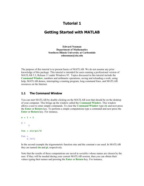
Tutorial 1 Getting Started with MATLAB

3xi = 10xi =10However, the following numberxr = 10.01xr =10.0100is saved as the real number. It is not our intention to discuss here machine representation ofnumbers. This topic is usually included in the numerical analysis courses.Variables realmin and realmax denote the smallest and the largest positive real numbers inMATLAB. For instance,realminans =2.2251e-308Complex numbers in MATLAB are represented in rectangular form. The imaginary unit − 1 isdenoted either by i or jians =0 + 1.0000iIn addition to classes of numbers mentioned above, MATLAB has three variables representingthe nonnumbers:• -Inf• Inf• NaNThe –Inf and Inf are the IEEE representations for the negative and positive infinity, respectively.Infinity is generated by overflow or by the operation of dividing by zero. The NaN stands for thenot-a-number and is obtained as a result of the mathematically undefined operations such as0.0/0.0 or ∞ − ∞ .List of basic arithmetic operations in MATLAB include six operations

4Operation Symboladdition +subtraction -multiplication *division / or \exponentiation ^MATLAB has two division operators / - the right division and \ - the left division. They do notproduce the same resultsrd = 47/3rd =15.6667ld = 47\3ld =0.0638!" # $All variables used in the current MATLAB session are saved in the Workspace. You can viewthe content of the Workspace by clicking on File in the toolbar and next selecting ShowWorkspace from the pull-down menu. You can also check contents of the Workspace typingwhos in the Command Window. For instance,whosName Size Bytes Classans 1x1 16 double array (complex)fun 1x1 8 double arrayld 1x1 8 double arrayrd 1x1 8 double arrays 1x1 8 double arrayxi 1x1 8 double arrayxr 1x1 8 double arrayGrand total is 7 elements using 64 bytesshows all variables used in current session. You can also use command who to generate a list ofvariables used in current sessionwho

5Your variables are:ans ld s xrfun rd xiTo save your current workspace select Save Workspace as… from the File menu. Chose a namefor your file, e.g. filename.mat and next click on Save. Remember that the file you just createdmust be located in MATLAB's search path. Another way of saving your workspace is to typesave filename in the Command Window. The following command save filename s saves onlythe variable s.Another way to save your workspace is to type the command diary filename in the CommandWindow. All commands and variables created from now will be saved in your file. The followingcommand: diary off will close the file and save it as the text file. You can open this file in a texteditor, by double clicking on the name of your file, and modify its contents if you wish to do so.To load contents of the file named filename into MATLAB's workspace type load filename inthe Command Window.More advanced computations often require execution of several lines of computer code. Ratherthan typing those commands in the Command Window you should create a file. Each time youwill need to repeat computations just invoke your file. Another advantage of using files is theease to modify its contents. To learn more about files, see [1], pp. 67-75 and also Section 2.2 ofTutorial 2.%&One of the nice features of MATLAB is its help system. To learn more about a function you areto use, say rref, type in the Command Windowhelp svdSVD Singular value decomposition.[U,S,V] = SVD(X) produces a diagonal matrix S, of the samedimension as X and with nonnegative diagonal elements indecreasing order, and unitary matrices U and V so thatX = U*S*V'.S = SVD(X) returns a vector containing the singular values.[U,S,V] = SVD(X,0) produces the "economy size"decomposition. If X is m-by-n with m > n, then only thefirst n columns of U are computed and S is n-by-n.See also SVDS, GSVD.Overloaded methodshelp sym/svd.mIf you do not remember the exact name of a function you want to learn more about use commandlookfor followed by the incomplete name of a function in the Command Window. In thefollowing example we use a "word" sv

6lookfor svISVMS True for the VMS version of MATLAB.HSV2RGB Convert hue-saturation-value colors to red-green-blue.RGB2HSV Convert red-green-blue colors to hue-saturation-value.GSVD Generalized Singular Value Decomposition.SVD Singular value decomposition.SVDS Find a few singular values and vectors.HSV Hue-saturation-value color map.JET Variant of HSV.CSVREAD Read a comma separated value file.CSVWRITE Write a comma separated value file.ISVARNAME Check for a valid variable name.RANDSVD Random matrix with pre-assigned singular values.Trusvibs.m: % Example: trusvibsSVD Symbolic singular value decomposition.RANDSVD Random matrix with pre-assigned singular values.The helpwin command, invoked without arguments, opens a new window on the screen. To findan information you need double click on the name of the subdirectory and next double click on afunction to see the help text for that function. You can go directly to the help text of your functioninvoking helpwin command followed by an argument. For instance, executing the followingcommandhelpwin zerosZEROS Zeros array.ZEROS(N) is an N-by-N matrix of zeros.ZEROS(M,N) or ZEROS([M,N]) is an M-by-N matrix of zeros.ZEROS(M,N,P,...) or ZEROS([M N P ...]) is an M-by-N-by-P-by-...array of zeros.ZEROS(SIZE(A)) is the same size as A and all zeros.See also ONES.generates an information about MATLAB's function zeros.MATLAB also provides the browser-based help. In order to access these help files click on Helpand next select Help Desk (HTML). This will launch your Web browser. To access aninformation you need click on a highlighted link or type a name of a function in the text box. Inorder for the Help Desk to work properly on your computer the appropriate help files, in theHTML or PDF format, must be installed on your computer. You should be aware that these filesrequire a significant amount of the disk space.'(To learn more about MATLAB capabilities you can execute the demo command in theCommand Window or click on Help and next select Examples and Demos from the pull-downmenu. Some of the MATLAB demos use both the Command and the Figure windows.

7To learn about matrices in MATLAB open the demo window using one of the methods describedabove. In the left pane select Matrices and in the right pane select Basic matrix operations thenclick on Run Basic matrix … . Click on the Start >> button to begin the show.If you are familiar with functions of a complex variable I recommend another demo. SelectVisualization and next 3-D Plots of complex functions. You can generate graphs of simplepower functions by selecting an appropriate button in the current window.)* To interrupt a running program press simultaneously the Ctrl-c keys. Sometimes you have torepeat pressing these keys a couple of times to halt execution of your program. This is not arecommended way to exit a program, however, in certain circumstances it is a necessity. Forinstance, a poorly written computer code can put MATLAB in the infinite loop and this would bethe only option you will have left.+ To enter a statement that is too long to be typed in one line, use three periods, … , followed byEnter or Return. For instance,x = sin(1) - sin(2) + sin(3) - sin(4) + sin(5) -...sin(6) + sin(7) - sin(8) + sin(9) - sin(10)x =0.7744You can suppress output to the screen by adding a semicolon after the statementu = 2 + 3;, *If your computer has an access to the Internet you can learn more about MATLAB and alsodownload user supplied files posted in the public domain. We provide below some pointers toinformation related to MATLAB.• The MathWorks Web site: http://www.mathworks.com/The MathWorks, the makers of MATLAB, maintains an important Web site. Here you canfind information about new products, MATLAB related books, user supplied files and muchmore.• The MATLAB newsgroup: news://saluki-news.siu.edu/comp.soft-sys.matlab/If you have an access to the Internet News, you can read messages posted in this newsgroup.Also, you can post your own messages. The link shown above would work only for thosewho have access to the news server in Southern Illinois University at Carbondale.

8• http://dir.yahoo.com/science/mathematics/software/matlab/A useful source of information about MATLAB and good starting point to other Web sites.• http://www.cse.uiuc.edu/cse301/matlab.htmlThus Web site, maintained by the University of Illinois at Champaign-Urbana, providesseveral links to MATLAB resources on the Internet.• The Mastering Matlab Web site: http://www.eece.maine.edu/mmRecommended link for those who are familiar with the book Mastering Matlab 5.A Comprehensive Tutorial and Reference, by D. Hanselman and B. Littlefield (see [2].)

9-.[1] Getting Started with MATLAB, Version 5, The MathWorks, Inc., 1996.[2] D. Hanselman and B. Littlefield, Mastering MATLAB 5. A Comprehensive Tutorial andReference, Prentice Hall, Upper Saddle River, NJ, 1998.[3] K. Sigmon, MATLAB Primer, Fifth edition, CRC Press, Boca Raton, 1998.[4] Using MATLAB, Version 5, The MathWorks, Inc., 1996.

Edward NeumanDepartment of MathematicsSouthern Illinois University at Carbondaleedneuman@siu.eduThis tutorial is intended for those who want to learn basics of MATLAB programming language.Even with a limited knowledge of this language a beginning programmer can write his/her owncomputer code for solving problems that are complex enough to be solved by other means.Numerous examples included in this text should help a reader to learn quickly basic programmingtools of this language. Topics discussed include the m-files, inline functions, control flow,relational and logical operators, strings, cell arrays, rounding numbers to integers and MATLABgraphics. Files that contain a computer code are called the m-files. There are two kinds of m-files: the scriptfiles and the function files. Script files do not take the input arguments or return the outputarguments. The function files may take input arguments or return output arguments.To make the m-file click on File next select New and click on M-File from the pull-down menu.You will be presented with the MATLAB Editor/Debugger screen. Here you will type yourcode, can make changes, etc. Once you are done with typing, click on File, in the MATLABEditor/Debugger screen and select Save As… . Chose a name for your file, e.g., firstgraph.mand click on Save. Make sure that your file is saved in the directory that is in MATLAB's searchpath.If you have at least two files with duplicated names, then the one that occurs first in MATLAB'ssearch path will be executed.To open the m-file from within the Command Window type edit firstgraph and then pressEnter or Return key.Here is an example of a small script file% Script file firstgraph.x = pi/100:pi/100:10*pi;y = sin(x)./x;plot(x,y)grid

2Let us analyze contents of this file. First line begins with the percentage sign %. This is acomment. All comments are ignored by MATLAB. They are added to improve readability of thecode. In the next two lines arrays x and y are created. Note that the semicolon follows bothcommands. This suppresses display of the content of both vectors to the screen (see Tutorial 1,page 5 for more details). Array x holds 1000 evenly spaced numbers in the interval [/100 10]while the array y holds the values of the sinc function y = sin(x)/x at these points. Note use of thedot operator . before the right division operator /. This tells MATLAB to perform thecomponentwise division of two arrays sin(x) and x. Special operators in MATLAB and operationson one- and two dimensional arrays are discussed in detail in Tutorial 3, Section 3.2. Thecommand plot creates the graph of the sinc function using the points generated in two previouslines. For more details about command plot see Section 2.8.1 of this tutorial. Finally, thecommand grid is executed. This adds a grid to the graph. We invoke this file by typing its namein the Command Window and next pressing the Enter or Return keyfirstgraph10.80.60.40.20-0.2-0.40 5 10 15 20 25 30 35Here is an example of the function filefunction [b, j] = descsort(a)% Function descsort sorts, in the descending order, a real array a.% Second output parameter j holds a permutation used to obtain% array b from the array a.

3[b ,j] = sort(-a);b = -b;This function takes one input argument, the array of real numbers, and returns a sorted arraytogether with a permutation used to obtain array b from the array a. MATLAB built-in functionsort is used here. Recall that this function sort numbers in the ascending order. A simple trickused here allows us to sort an array of numbers in the descending order.To demonstrate functionality of the function under discussion leta = [pi –10 35 0.15];[b, j] = descsort(a)b =35.0000 3.1416 0.1500 -10.0000j =3 1 4 2You can execute function descsort without output arguments. In this case an information about apermutation used will be lostdescsort(a)ans =35.0000 3.1416 0.1500 -10.0000Since no output argument was used in the call to function descorder a sorted array a is assignedto the default variable ans. Sometimes it is handy to define a function that will be used during the current MATLAB sessiononly. MATLAB has a command inline used to define the so-called inline functions in theCommand Window.Letf = inline('sqrt(x.^2+y.^2)','x','y')f =Inline function:f(x,y) = sqrt(x.^2+y.^2)You can evaluate this function in a usual wayf(3,4)ans =5

4Note that this function also works with arrays. LetA = [1 2;3 4]A =1 23 4andB = ones(2)B =1 11 1ThenC = f(A, B)C =1.4142 2.23613.1623 4.1231For the later use let us mention briefly a concept of the string in MATLAB. The character stringis a text surrounded by single quotes. For instance,str = 'programming in MATLAB is fun'str =programming in MATLAB is funis an example of the string. Strings are discussed in Section 2.5 of this tutorial.In the previous section you have learned how to create the function files. Some functions take asthe input argument a name of another function, which is specified as a string. In order to executefunction specified by string you should use the command feval as shown belowfeval('functname', input parameters of function functname)Consider the problem of computing the least common multiple of two integers. MATLAB has abuilt-in function lcm that computes the number in question. Recall that the least commonmultiple and the greatest common divisor (gcd) satisfy the following equationab = lcm(a, b)gcd(a, b)MATLAB has its own function, named gcd, for computing the greatest common divisor.

5To illustrate the use of the command feval let us take a closer look at the code in the m-filemylcmfunction c = mylcm(a, b)% The least common multiple c of two integers a and b.if feval('isint',a) & feval('isint',b)c = a.*b./gcd(a,b);elseerror('Input arguments must be integral numbers')endCommand feval is used twice in line two (I do do not count the comment lines and the blanklines). It checks whether or not both input arguments are integers. The logical and operator &used here is discussed in Section 2.4. If this condition is satisfied, then the least common multipleis computed using the formula mentioned earlier, otherwise the error message is generated. Noteuse of the command error, which takes as the argument a string. The conditional if - else - endused here is discussed in Section 2.4 of this tutorial. Function that is executed twice in the body ofthe function mylcm is named isintfunction k = isint(x);% Check whether or not x is an integer number.% If it is, function isint returns 1 otherwise it returns 0.if abs(x - round(x)) < realmink = 1;elsek = 0;endNew functions used here are the absolute value function (abs) and the round function (round).The former is the classical math function while the latter takes a number and rounds it to theclosest integer. Other functions used to round real numbers to integers are discussed in Section2.7. Finally, realmin is the smallest positive real number on your computerformat longrealminans =2.225073858507201e-308format shortThe Trapezoidal Rule with the correction term is often used to numerical integration of functionsthat are differentiable on the interval of integration

6baf ( x)dx h[2f ( a)2hf ( b)] [ f ' ( a)12f ' ( b)]where h = b – a. This formula is easy to implement in MATLABfunction y = corrtrap(fname, fpname, a, b)% Corrected trapezoidal rule y.% fname - the m-file used to evaluate the integrand,% fpname - the m-file used to evaluate the first derivative% of the integrand,% a,b - endpoinds of the interval of integration.h = b - a;y = (h/2).*(feval(fname,a) + feval(fname,b))+ (h.^2)/12.*( ...feval(fpname,a) - feval(fpname,b));The input parameters a and b can be arrays of the same dimension. This is possible because thedot operator proceeds certain arithmetic operations in the command that defines the variable y.In this example we will integrate the sine function over two intervals whose end points are storedin the arrays a and b, wherea = [0 0.1];b = [pi/2 pi/2 + 0.1];y = corrtrap('sin', 'cos', a, b)y =0.9910 1.0850Since the integrand and its first order derivative are both the built-in functions, there is no need todefine these functions in the m-files. To control the flow of commands, the makers of MATLAB supplied four devices a programmercan use while writing his/her computer codethe for loopsthe while loopsthe if-else-end constructionsthe switch-case constructions

7 Syntax of the for loop is shown belowfor k = arraycommandsendThe commands between the for and end statements are executed for all values stored in thearray.Suppose that one-need values of the sine function at eleven evenly spaced points n/10, forn = 0, 1, …, 10. To generate the numbers in question one can use the for loopfor n=0:10x(n+1) = sin(pi*n/10);endxx =Columns 1 through 70 0.3090 0.5878 0.8090 0.9511 1.0000 0.9511Columns 8 through 110.8090 0.5878 0.3090 0.0000The for loops can be nestedH = zeros(5);for k=1:5for l=1:5H(k,l) = 1/(k+l-1);endendHH =1.0000 0.5000 0.3333 0.2500 0.20000.5000 0.3333 0.2500 0.2000 0.16670.3333 0.2500 0.2000 0.1667 0.14290.2500 0.2000 0.1667 0.1429 0.12500.2000 0.1667 0.1429 0.1250 0.1111Matrix H created here is called the Hilbert matrix. First command assigns a space in computer'smemory for the matrix to be generated. This is added here to reduce the overhead that is requiredby loops in MATLAB.The for loop should be used only when other methods cannot be applied. Consider the followingproblem. Generate a 10-by-10 matrix A = [a kl ], where a kl = sin(k)cos(l). Using nested loops onecan compute entries of the matrix A using the following code

8A = zeros(10);for k=1:10for l=1:10A(k,l) = sin(k)*cos(l);endendA loop free version might look like thisk = 1:10;A = sin(k)'*cos(k);First command generates a row array k consisting of integers 1, 2, … , 10. The command sin(k)'creates a column vector while cos(k) is the row vector. Components of both vectors are the valuesof the two trig functions evaluated at k. Code presented above illustrates a powerful feature ofMATLAB called vectorization. This technique should be used whenever it is possible. Syntax of the while loop iswhile expressionstatementsendThis loop is used when the programmer does not know the number of repetitions a priori.Here is an almost trivial problem that requires a use of this loop. Suppose that the number isdivided by 2. The resulting quotient is divided by 2 again. This process is continued till thecurrent quotient is less than or equal to 0.01. What is the largest quotient that is greater than 0.01?To answer this question we write a few lines of codeq = pi;while q > 0.01q = q/2;endqq =0.0061 Syntax of the simplest form of the construction under discussion isif expressioncommandsend

9This construction is used if there is one alternative only. Two alternatives require the constructionif expressioncommands (evaluated if expression is true)elsecommands (evaluated if expression is false)endConstruction of this form is used in functions mylcm and isint (see Section 2.3).If there are several alternatives one should use the following constructionif expression1commands (evaluated if expression 1 is true)elseif expression 2commands (evaluated if expression 2 is true)elseif …...elsecommands (executed if all previous expressions evaluate to false)endChebyshev polynomials T n (x), n = 0, 1, … of the first kind are of great importance in numericalanalysis. They are defined recursively as followsT n (x) = 2xT n – 1 (x) – T n – 2 (x), n = 2, 3, … , T 0 (x) = 1, T 1 (x) = x.Implementation of this definition is easyfunction T = ChebT(n)% Coefficients T of the nth Chebyshev polynomial of the first kind.% They are stored in the descending order of powers.t0 = 1;t1 = [1 0];if n == 0T = t0;elseif n == 1;T = t1;elsefor k=2:nT = [2*t1 0] - [0 0 t0];t0 = t1;t1 = T;endend

10Coefficients of the cubic Chebyshev polynomial of the first kind arecoeff = ChebT(3)coeff =4 0 -3 0Thus T 3 (x) = 4x 3 – 3x. Syntax of the switch-case construction isswitch expression (scalar or string)case value1 (executes if expression evaluates to value1)commandscase value2 (executes if expression evaluates to value2)commands...otherwisestatementsendSwitch compares the input expression to each case value. Once the match is found it executes theassociated commands.In the following example a random integer number x from the set {1, 2, … , 10} is generated. Ifx = 1 or x = 2, then the message Probability = 20% is displayed to the screen. If x = 3 or 4 or 5,then the message Probability = 30% is displayed, otherwise the message Probability = 50% isgenerated. The script file fswitch utilizes a switch as a tool for handling all cases mentionedabove% Script file fswitch.x = ceil(10*rand); % Generate a random integer in {1, 2, ... , 10}switch xcase {1,2}disp('Probability = 20%');case {3,4,5}disp('Probability = 30%');otherwisedisp('Probability = 50%');endNote use of the curly braces after the word case. This creates the so-called cell array rather thanthe one-dimensional array, which requires use of the square brackets.

11Here are new MATLAB functions that are used in file fswitchrand – uniformly distributed random numbers in the interval (0, 1)ceil – round towards plus infinity infinity (see Section 2.5 for more details)disp – display string/array to the screenLet us test this code ten timesfor k = 1:10fswitchendProbability = 50%Probability = 30%Probability = 50%Probability = 50%Probability = 50%Probability = 30%Probability = 20%Probability = 50%Probability = 30%Probability = 50%!" #Comparisons in MATLAB are performed with the aid of the following operatorsOperator Description< Less than Greater>= Greater or equal to== Equal to~= Not equal toOperator == compares two variables and returns ones when they are equal and zeros otherwise.Leta = [1 1 3 4 1]a =1 1 3 4 1Then

12ind = (a == 1)ind =1 1 0 0 1You can extract all entries in the array a that are equal to 1 usingb = a(ind)b =1 1 1This is an example of so-called logical addressing in MATLAB. You can obtain the same resultusing function findind = find(a == 1)ind =1 2 5Variable ind now holds indices of those entries that satisfy the imposed condition. To extract allones from the array a useb = a(ind)b =1 1 1There are three logical operators available in MATLABLogical operator Description| And&Or~ NotSuppose that one wants to select all entries x that satisfy the inequalities x 1 or x < -0.2 wherex = randn(1,7)x =-0.4326 -1.6656 0.1253 0.2877 -1.1465 1.1909 1.1892is the array of normally distributed random numbers. We can solve easily this problem usingoperators discussed in this sectionind = (x >= 1) | (x < -0.2)ind =1 1 0 0 1 1 1y = x(ind)

13y =-0.4326 -1.6656 -1.1465 1.1909 1.1892Solve the last problem without using the logical addressing.In addition to relational and logical operators MATLAB has several logical functions designedfor performing similar tasks. These functions return 1 (true) if a specific condition is satisfied and0 (false) otherwise. A list of these functions is too long to be included here. The interested readeris referred to [1], pp. 85-86 and [4], Chapter 10, pp. 26-27. Names of the most of these functionsbegin with the prefix is. For instance, the following commandisempty(y)ans =0returns 0 because the array y of the last example is not empty. However, this commandisempty([ ])ans =1returns 1 because the argument of the function used is the empty array [ ].Here is another example that requires use of the isempty commandfunction dp = derp(p)% Derivative dp of an algebraic polynomial that is% represented by its coefficients p. They must be stored% in the descending order of powers.n = length(p) - 1;p = p(:)';dp = p(1:n).*(n:-1:1);k = find(dp ~= 0);if ~isempty(k)dp = dp(k(1):end);elsedp = 0;end% Make sure p is a row array.% Apply the Power Rule.% Delete leading zeros if any.In this example p(x) = x 3 + 2x 2 + 4. Using a convention for representing polynomials inMATLAB as the array of their coefficients that are stored in the descending order of powers, weobtaindp = derp([1 2 0 4])dp =3 4 0

14$%String is an array of characters. Each character is represented internally by its ASCII value.This is an example of a stringstr = 'I am learning MATLAB this semester.'str =I am learning MATLAB this semester.To see its ASCII representation use function doublestr1 = double(str)str1 =Columns 1 through 1273 32 97 109 32 108 101 97 114 110 105110Columns 13 through 24103 32 77 65 84 76 65 66 32 116 104105Columns 25 through 35115 32 115 101 109 101 115 116 101 114 46You can convert array str1 to its character form using function charstr2 = char(str1)str2 =I am learning MATLAB this semester.Application of the string conversion is used in Tutorial 3, Section 3.11 to uncode and decodemessages.To compare two strings for equality use function strcmpiseq = strcmp(str, str2)iseq =1Two strings can be concatenated using function ctrcatstrcat(str,str2)ans =I am learning MATLAB this semester.I am learning MATLAB this semester.Note that the concatenated strings are not separated by the blank space.

15You can create two-dimensional array of strings. To this aim the cell array rather than the twodimensionalarray must be used. This is due to the fact that numeric array must have the samenumber of columns in each row.This is an example of the cell arraycarr = {'first name'; 'last name'; 'hometown'}carr ='first name''last name''hometown'Note use of the curly braces instead of the square brackets. Cell arrays are discussed in detail inthe next section of this tutorial.MATLAB has two functions to categorize characters: isletter and isspace. We will run bothfunctions on the string strisletter(str)ans =Columns 1 through 121 0 1 1 0 1 1 1 1 1 11Columns 13 through 241 0 1 1 1 1 1 1 0 1 11Columns 25 through 351 0 1 1 1 1 1 1 1 1 0isspace(str)ans =Columns 1 through 120 1 0 0 1 0 0 0 0 0 00Columns 13 through 240 1 0 0 0 0 0 0 1 0 00Columns 25 through 350 1 0 0 0 0 0 0 0 0 0The former function returns 1 if a character is a letter and 0 otherwise while the latter returns 1 ifa character is whitespace (blank, tab, or new line) and 0 otherwise.We close this section with two important functions that are intended for conversion of numbers tostrings. Functions in question are named int2str and num2str. Function int2str rounds itsargument (matrix) to integers and converts the result into a string matrix.

16LetA = randn(3)A =-0.4326 0.2877 1.1892-1.6656 -1.1465 -0.03760.1253 1.1909 0.3273ThenB = int2str(A)B =0 0 1-2 -1 00 1 0Function num2str takes an array and converts it to the array string. Running this function on thematrix A defined earlier, we obtainC = num2str(A)C =-0.43256 0.28768 1.1892-1.6656 -1.1465 -0.0376330.12533 1.1909 0.32729Function under discussion takes a second optional argument - a number of decimal digits. Thisfeature allows a user to display digits that are far to the right of the decimal point. Using matrix Aagain, we getD = num2str(A, 18)D =-0.43256481152822068 0.28767642035854885 1.1891642016521031-1.665584378238097 -1.1464713506814637 -0.0376332765933176450.12533230647483068 1.1909154656429988 0.32729236140865414For comparison, changing format to long, we obtainformat longAA =-0.43256481152822 0.28767642035855 1.18916420165210-1.66558437823810 -1.14647135068146 -0.037633276593320.12533230647483 1.19091546564300 0.32729236140865format short

17Function num2str his is often used for labeling plots with the title, xlabel, ylabel, and textcommands.& 'Two data types the cell arrays and structures make MATLAB a powerful tool for applications.They hold other MATLAB arrays. In this section we discuss the cell arrays only. To learn aboutstructures the interested reader is referred to [4], Chapter 13 and [1], Chapter 12.To create the cell array one can use one of the two techniques called the cell indexing and thecontent indexing. The following example reveals differences between these two techniques.Suppose one want to save the string 'John Brown' and his SSN 123-45-6789 (without dashes) inthe cell array.1. Cell indexingA(1,1) = {'John Brown'};A(1,2) = {[1 2 3 4 5 6 7 8 9]};2. Content indexingB{1,1} = 'John Brown';B{1,2} = [1 2 3 4 5 6 7 8 9];A condensed form of the cell array A isAA ='John Brown'[1x9 double]To display its full form use function celldispcelldisp(A)A{1} =John BrownA{2} =1 2 3 4 5 6 7 8 9To access data in a particular cell use content indexing on the right-hand side. For instance,B{1,1}ans =John BrownTo delete a cell use the empty matrix operator [ ]. For instance, this operation

18B(1) = []B =[1x9 double]deletes cell B(1, 1) of the cell array B.This commandC = {A B}C ={1x2 cell} {1x1 cell}creates a new cell arraycelldisp(C)C{1}{1} =John BrownC{1}{2} =1 2 3 4 5 6 7 8 9C{2}{1} =1 2 3 4 5 6 7 8 9How would you delete cell C(2,1)?(" ) * * + We have already used two MATLAB functions round and ceil to round real numbers to integers.They are briefly described in the previous sections of this tutorial. A full list of functionsdesigned for rounding numbers is provided belowFunctionfloorceilfixroundDescriptionRound towards minus infinityRound towards plus infinityRound towards zeroRound towards nearest integerTo illustrate differences between these functions let us create first a two-dimensional array ofrandom numbers that are normally distributed (mean = 0, variance = 1) using another MATLABfunction randnrandn('seed', 0)% This sets the seed of the random numbers generator to zeroT = randn(5)

19T =1.1650 1.6961 -1.4462 -0.3600 -0.04490.6268 0.0591 -0.7012 -0.1356 -0.79890.0751 1.7971 1.2460 -1.3493 -0.76520.3516 0.2641 -0.6390 -1.2704 0.8617-0.6965 0.8717 0.5774 0.9846 -0.0562A = floor(T)A =1 1 -2 -1 -10 0 -1 -1 -10 1 1 -2 -10 0 -1 -2 0-1 0 0 0 -1B = ceil(T)B =2 2 -1 0 01 1 0 0 01 2 2 -1 01 1 0 -1 10 1 1 1 0C = fix(T)C =1 1 -1 0 00 0 0 0 00 1 1 -1 00 0 0 -1 00 0 0 0 0D = round(T)D =1 2 -1 0 01 0 -1 0 -10 2 1 -1 -10 0 -1 -1 1-1 1 1 1 0It is worth mentioning that the following identitiesandfloor(x) = fix(x) for x 0ceil(x) = fix(x) for x 0

20hold true.In the following m-file functions floor and ceil are used to obtain a certain representation of anonnegative real numberfunction [m, r] = rep4(x)% Given a nonnegative number x, function rep4 computes an integer m% and a real number r, where 0.25

21Before we begin discussion of graphical tools that are available in MATLAB I recommend thatyou will run a couple of demos that come with MATLAB. In the Command Window click onHelp and next select Examples and Demos. ChoseVisualization, and next select 2-D Plots. Youwill be presented with several buttons. Select Line and examine the m-file below the graph. Itshould give you some idea about computer code needed for creating a simple graph. It isrecommended that you examine carefully contents of all m-files that generate the graphs in thisdemo. Basic function used to create 2-D graphs is the plot function. This function takes a variablenumber of input arguments. For the full definition of this function type help plot in theCommand Window.xIn this example the graph of the rational function f ( x)21xusing a variable number of points on the graph of f(x), -2 x 2, will be plotted% Script file graph1.% Graph of the rational function y = x/(1+x^2).for n=1:2:5n10 = 10*n;x = linspace(-2,2,n10);y = x./(1+x.^2);plot(x,y,'r')title(sprintf('Graph %g. Plot based upon n = %g points.' ..., (n+1)/2, n10))axis([-2,2,-.8,.8])xlabel('x')ylabel('y')gridpause(3)endLet us analyze contents of this file. The loop for is executed three times. Therefore, three graphsof the same function will be displayed in the Figure Window. A MATLAB functionlinspace(a, b, n) generates a one-dimensional array of n evenly spaced numbers in the interval[a b]. The y-ordinates of the points to be plotted are stored in the array y. Command plot iscalled with three arguments: two arrays holding the x- and the y-coordinates and the string 'r',which describes the color (red) to be used to paint a plotted curve. You should notice a differencebetween three graphs created by this file. There is a significant difference between smoothness ofgraphs 1 and 3. Based on your visual observation you should be able to reach the followingconclusion: "more points you supply the smoother graph is generated by the function plot".Function title adds a descriptive information to the graphs generated by this m-file and isfollowed by the command sprintf. Note that sprintf takes here three arguments: the string andnames of two variables printed in the title of each graph. To specify format of printed numbers weuse here the construction %g, which is recommended for printing integers. The command axistells MATLAB what the dimensions of the box holding the plot are. To add more information to

22the graphs created here, we label the x- and the y-axes using commands xlabel and the ylabel,respectively. Each of these commands takes a string as the input argument. Function grid addsthe grid lines to the graph. The last command used before the closing end is the pause command.The command pause(n) holds on the current graph for n seconds before continuing, where n canalso be a fraction. If pause is called without the input argument, then the computer waits to userresponse. For instance, pressing the Enter key will resume execution of a program.Function subplot is used to plot of several graphs in the same Figure Window. Here is a slightmodification of the m-file graph1% Script file graph2.% Several plots of the rational function y = x/(1+x^2)% in the same window.k = 0;for n=1:3:10n10 = 10*n;x = linspace(-2,2,n10);y = x./(1+x.^2);k = k+1;subplot(2,2,k)plot(x,y,'r')title(sprintf('Graph %g. Plot based upon n = %g points.' ..., k, n10))xlabel('x')ylabel('y')axis([-2,2,-.8,.8])gridpause(3);endThe command subplot is called here with three arguments. The first two tell MATLAB that a2-by-2 array consisting of four plots will be created. The third parameter is the running indextelling MATLAB which subplot is currently generated.graph2

23Graph 1. Plot based upon n = 10 points.Graph 2. Plot based upon n = 40 points.0.50.5y0y0-0.5-2 -1 0 1 2xGraph 3. Plot based upon n = 70 points.-0.5-2 -1 0 1 2xGraph 4. Plot based upon n = 100 points.0.50.5y0y0-0.5-2 -1 0 1 2x-0.5-2 -1 0 1 2xUsing command plot you can display several curves in the same Figure Window.We will plot two ellipses2( x 3) ( y 2)36 812 122( x 7) ( y 8)and 14 36using command plot% Script file graph3.% Graphs of two ellipses% x(t) = 3 + 6cos(t), y(t) = -2 + 9sin(t)% and% x(t) = 7 + 2cos(t), y(t) = 8 + 6sin(t).t = 0:pi/100:2*pi;x1 = 3 + 6*cos(t);y1 = -2 + 9*sin(t);x2 = 7 + 2*cos(t);y2 = 8 + 6*sin(t);h1 = plot(x1,y1,'r',x2,y2,'b');set(h1,'LineWidth',1.25)axis('square')xlabel('x')

24h = get(gca,'xlabel');set(h,'FontSize',12)set(gca,'XTick',-4:10)ylabel('y')h = get(gca,'ylabel');set(h,'FontSize',12)set(gca,'YTick',-12:2:14)title('Graphs of (x-3)^2/36+(y+2)^2/81 = 1 and (x-7)^2/4+(y-8)^2/36 =1.')h = get(gca,'Title');set(h,'FontSize',12)gridIn this file we use several new MATLAB commands. They are used here to enhance thereadability of the graph. Let us now analyze the computer code contained in the m-file graph3.First of all, the equations of ellipses in rectangular coordinates are transformed to parametricequations. This is a convenient way to plot graphs of equations in the implicit form. The points tobe plotted, and smoothed by function plot, are defined in the first five lines of the file. I do notcount here the comment lines and the blank lines. You can plot both curves using a single plotcommand. Moreover, you can select colors of the curves. They are specified as strings(see line 6). MATLAB has several colors you can use to plot graphs:y yellowm magentac cyanr redg greenb bluew whitek blackNote that the command in line 6 begins with h1 = plot… Variable h1 holds an information aboutthe graph you generate and is called the handle graphics. Command set used in the next lineallows a user to manipulate a plot. Note that this command takes as the input parameter thevariable h1. We change thickness of the plotted curves from the default value to a width of ourchoice, namely 1.25. In the next line we use command axis to customize plot. We chose option'square' to force axes to have square dimensions. Other available options are:'equal', 'normal', 'ij', 'xy', and 'tight'. To learn more about these options use MATLAB's help.If function axis is not used, then the circular curves are not necessarily circular. To justify this letus plot a graph of the unit circle of radius 1 with center at the origint = 0:pi/100:2*pi;x = cos(t);y = sin(t);plot(x,y)

2510.80.60.40.20-0.2-0.4-0.6-0.8-1-1 -0.5 0 0.5 1Another important MATLAB function used in the file under discussion is named get(see line 10). It takes as the first input parameter a variable named gca = get current axis. Itshould be obvious to you, that the axis targeted by this function is the x-axis. Variableh = get(gca, … ) is the graphics handle of this axis. With the information stored in variable h,we change the font size associated with the x-axis using the 'FontSize' string followed by a sizeof the font we wish to use. Invoking function set in line 12, we will change the tick marks alongthe x-axis using the 'XTick' string followed by the array describing distribution of marks. Youcan comment out temporarily line 12 by adding the percent sign % before the word set to see thedifference between the default tick marks and the marks generated by the command in line 12.When you are done delete the percent sign you typed in line 12 and click on Save from the Filemenu in the MATLAB Editor/Debugger. Finally, you can also make changes in the title of yourplot. For instance, you can choose the font size used in the title. This is accomplished here byusing function set. It should be obvious from the short discussion presented here that twoMATLAB functions get and set are of great importance in manipulating graphs.Graphs of the ellipses in question are shown on the next pagegraph3

26Graphs of (x-3) 2 /36+(y+2) 2 /81 = 1 and (x-7) 2 /4+(y-8) 2 /36 = 1.y14121086420-2-4-6-8-10-12-4 -3 -2 -1 0 1 2 3 4 5 6 7 8 9 10xMATLAB has several functions designed for plotting specialized 2-D graphs. A partial list ofthese functions is included here fill, polar, bar, barh, pie, hist, compass, errorbar, stem, andfeather.In this example function fill is used to create a well-known objectn = -6:6;x = sin(n*pi/6);y = cos(n*pi/6);fill(x, y, 'r')axis('square')title('Graph of the n-gone')text(-0.45,0,'What is a name of this object?')Function in question takes three input parameters - two arrays, named here x and y. They hold thex- and y-coordinates of vertices of the polygon to be filled. Third parameter is the user-selectedcolor to be used to paint the object. A new command that appears in this short code is the textcommand. It is used to annotate a text. First two input parameters specify text location. Thirdinput parameter is a text, which will be added to the plot.Graph of the filled object that is generated by this code is displayed below

271Graph of the n-gone0.80.60.40.20What is a name of this object?-0.2-0.4-0.6-0.8-1-1 -0.5 0 0.5 1 MATLAB has several built-in functions for plotting three-dimensional objects. In this subsectionwe will deal mostly with functions used to plot curves in space (plot3), mesh surfaces (mesh),surfaces (surf) and contour plots (contour). Also, two functions for plotting special surfaces,sphere and cylinder will be discussed briefly. I recommend that any time you need help with the3-D graphics you should type help graph3d in the Command Window to learn more aboutvarious functions that are available for plotting three-dimensional objects.Let r(t) = < t cos(t), t sin(t), t >, -10 t 10, be the space curve. We plot its graph over theindicated interval using function plot3% Script file graph4.% Curve r(t) = < t*cos(t), t*sin(t), t >.t = -10*pi:pi/100:10*pi;x = t.*cos(t);y = t.*sin(t);h = plot3(x,y,t);set(h,'LineWidth',1.25)title('Curve u(t) = < t*cos(t), t*sin(t), t >')h = get(gca,'Title');set(h,'FontSize',12)xlabel('x')h = get(gca,'xlabel');set(h,'FontSize',12)ylabel('y')h = get(gca,'ylabel');

28set(h,'FontSize',12)zlabel('z')h = get(gca,'zlabel');set(h,'FontSize',12)gridFunction plot3 is used in line 4. It takes three input parameters – arrays holding coordinates ofpoints on the curve to be plotted. Another new command in this code is the zlabel command(see line 4 from the bottom). Its meaning is self-explanatory.graph4Curve u(t) = < t*cos(t), t*sin(t), t >4020z0-20-4040200y-20-40-40-20x02040Function mesh is intended for plotting graphs of the 3-D mesh surfaces. Before we begin to workwith this function, another function meshgrid should be introduced. This function generates twotwo-dimensional arrays for 3-D plots. Suppose that one wants to plot a mesh surface over the gridthat is defined as the Cartesian product of two setsx = [0 1 2];y = [10 12 14];The meshgrid command applied to the arrays x and y creates two matrices[xi, yi] = meshgrid(x,y)

29xi =0 1 20 1 20 1 2yi =10 10 1012 12 1214 14 14Note that the matrix xi contains replicated rows of the array x while yi contains replicatedcolumns of y. The z-values of a function to be plotted are computed from arrays xi and yi.In this example we will plot the hyperbolic paraboloid z = y 2 – x 2 over the square –1 x 1,-1 y 1x = -1:0.05:1;y = x;[xi, yi] = meshgrid(x,y);zi = yi.^2 – xi.^2;mesh(xi, yi, zi)axis offTo plot the graph of the mesh surface together with the contour plot beneath the plotted surfaceuse function meshcmeshc(xi, yi, zi)axis off

30Function surf is used to visualize data as a shaded surface.Computer code in the m-file graph5 should help you to learn some finer points of the 3-Dgraphics in MATLAB% Script file graph5.% Surface plot of the hyperbolic paraboloid z = y^2 - x^2% and its level curves.x = -1:.05:1;y = x;[xi,yi] = meshgrid(x,y);zi = yi.^2 - xi.^2;surfc(xi,yi,zi)colormap coppershading interpview([25,15,20])grid offtitle('Hyperbolic paraboloid z = y^2 – x^2')h = get(gca,'Title');set(h,'FontSize',12)xlabel('x')h = get(gca,'xlabel');set(h,'FontSize',12)ylabel('y')h = get(gca,'ylabel');set(h,'FontSize',12)zlabel('z')h = get(gca,'zlabel');set(h,'FontSize',12)pause(5)figurecontourf(zi), hold on, shading flat[c,h] = contour(zi,'k-'); clabel(c,h)title('The level curves of z = y^2 - x^2.')h = get(gca,'Title');set(h,'FontSize',12)

31xlabel('x')h = get(gca,'xlabel');set(h,'FontSize',12)ylabel('y')h = get(gca,'ylabel');set(h,'FontSize',12)graph5A second graph is shown on the next page.

-0.432The level curves of z = y 2 - x 2 .4035-0.4-0.200.40.20.80.60.40.80.60.40.20-0.4-0.230-0.60.22500-0.2-0.6y20-0.4-0.8-0.2-0.815105-0.4-0.60-0.20.20.400.60.80.20.45 10 15 20 25 30 35 40x0.600.80.2-0.20.40-0.6-0.4There are several new commands used in this file. On line 5 (again, I do not count the blank linesand the comment lines) a command surfc is used. It plots a surface together with the level linesbeneath. Unlike the command surfc the command surf plots a surface only without the levelcurves. Command colormap is used in line 6 to paint the surface using a user-supplied colors. Ifthe command colormap is not added, MATLAB uses default colors. Here is a list of color mapsthat are available in MATLABhsv - hue-saturation-value color maphot - black-red-yellow-white color mapgray - linear gray-scale color mapbone - gray-scale with tinge of blue color mapcopper - linear copper-tone color mappink - pastel shades of pink color mapwhite - all white color mapflag - alternating red, white, blue, and black color maplines - color map with the line colorscolorcube - enhanced color-cube color mapvga - windows colormap for 16 colorsjet - variant of HSVprism - prism color mapcool - shades of cyan and magenta color mapautumn - shades of red and yellow color mapspring - shades of magenta and yellow color mapwinter - shades of blue and green color mapsummer - shades of green and yellow color mapCommand shading (see line 7) controls the color shading used to paint the surface. Command inquestion takes one argument. The following

33shading flat sets the shading of the current graph to flatshading interp sets the shading to interpolatedshading faceted sets the shading to faceted, which is the default.are the shading options that are available in MATLAB.Command view (see line 8) is the 3-D graph viewpoint specification. It takes a three-dimensionalvector, which sets the view angle in Cartesian coordinates.We will now focus attention on commands on lines 23 through 25. Command figure promptsMATLAB to create a new Figure Window in which the level lines will be plotted. In order toenhance the graph, we use command contourf instead of contour. The former plots filled contourlines while the latter doesn't. On the same line we use command hold on to hold the current plotand all axis properties so that subsequent graphing commands add to the existing graph. Firstcommand on line 25 returns matrix c and graphics handle h that are used as the input parametersfor the function clabel, which adds height labels to the current contour plot.Due to the space limitation we cannot address here other issues that are of interest forprogrammers dealing with the 3-D graphics in MATLAB. To learn more on this subject theinterested reader is referred to [1-3] and [5]. In addition to static graphs discussed so far one can put a sequence of graphs in motion. In otherwords, you can make a movie using MATLAB graphics tools. To learn how to create a movie, letus analyze the m-file firstmovie% Script file firstmovie.% Graphs of y = sin(kx) over the interval [0, pi],% where k = 1, 2, 3, 4, 5.m = moviein(5);x = 0:pi/100:pi;for i=1:5h1_line = plot(x,sin(i*x));set(h1_line,'LineWidth',1.5,'Color','m')gridtitle('Sine functions sin(kx), k = 1, 2, 3, 4, 5')h = get(gca,'Title');set(h,'FontSize',12)xlabel('x')k = num2str(i);if i > 1s = strcat('sin(',k,'x)');elses = 'sin(x)';endylabel(s)h = get(gca,'ylabel');set(h,'FontSize',12)m(:,i) = getframe;pause(2)

34endmovie(m)I suggest that you will play this movie first. To this aim type firstmovie in the CommandWindow and press the Enter or Return key. You should notice that five frames are displayedand at the end of the "show" frames are played again at a different speed.There are very few new commands one has to learn in order to animate graphics in MATLAB.We will use the m-file firstmovie as a starting point to our discussion. Command moviein, online 1, with an integral parameter, tells MATLAB that a movie consisting of five frames iscreated in the body of this file. Consecutive frames are generated inside the loop for. Almost allof the commands used there should be familiar to you. The only new one inside the loop isgetframe command. Each frame of the movie is stored in the column of the matrix m. With thisremark a role of this command should be clear. The last command in this file is movie(m). Thistells MATLAB to play the movie just created and saved in columns of the matrix m.Warning. File firstmovie cannot be used with the Student Edition of MATLAB, version 4.2.This is due to the matrix size limitation in this edition of MATLAB. Future release of the StudentEdition of MATLAB, version 5.3 will allow large size matrices. According to MathWorks, Inc.,the makers of MATLAB, this product will be released in September 1999. MATLAB has some functions for generating special surfaces. We will be concerned mostly withtwo functions- sphere and cylinder.The command sphere(n) generates a unit sphere with center at the origin using (n+1) 2 points. Iffunction sphere is called without the input parameter, MATLAB uses the default value n = 20.You can translate the center of the sphere easily. In the following example we will plot graph ofthe unit sphere with center at (2, -1, 1)[x,y,z] = sphere(30);surf(x+2, y-1, z+1)Function sphere together with function surf or mesh can be used to plot graphs of spheres ofarbitrary radii. Also, they can be used to plot graphs of ellipsoids. See Problems 25 and 26.

35Function cylinder is used for plotting a surface of revolution. It takes two (optional) inputparameters. In the following command cylinder(r, n) parameter r stands for the vector thatdefines the radius of cylinder along the z-axis and n specifies a number of points used to definecircumference of the cylinder. Default values of these parameters are r = [1 1] and n = 20. Agenerated cylinder has a unit height.The following commandcylinder([1 0])title('Unit cone')Unit cone10.80.60.40.2010.50-0.5-1-1-0.500.51plots a cone with the base radius equal to one and the unit height.In this example we will plot a graph of the surface of revolution obtained by rotating the curver(t) = < sin(t), t >, 0 t about the y-axis. Graphs of the generating curve and the surface ofrevolution are created using a few lines of the computer codet = 0:pi/100:pi;r = sin(t);plot(r,t)

363.532.521.510.500 0.2 0.4 0.6 0.8 1cylinder(r,15)shading interp!" #$% In this section we deal with printing MATLAB graphics. To send a current graph to the printerclick on File and next select Print from the pull down menu. Once this menu is open you may

37wish to preview a graph to be printed be selecting the option PrintPreview… first. You can alsosend your graph to the printer using the print command as shown belowx = 0:0.01:1;plot(x, x.^2)printYou can print your graphics to an m- file using built-in device drivers. A fairly incomplete list ofthese drivers is included here:-depsc Level 1 color Encapsulated PostScript-deps2 Level 2 black and white Encapsulated PostScript-depsc2 Level 2 color Encapsulated PostScriptFor a complete list of available device drivers see [5], Chapter 7, pp. 8-9.Suppose that one wants to print a current graph to the m-file Figure1 using level 2 colorEncapsulated PostScript. This can be accomplished by executing the following commandprint –depsc2 Figure1You can put this command either inside your m-file or execute it from within the CommandWindow.

38"[1] D. Hanselman and B. Littlefield, Mastering MATLAB 5. A Comprehensive Tutorial andReference, Prentice Hall, Upper Saddle River, NJ, 1998.[2] P. Marchand, Graphics and GUIs with MATLAB, Second edition, CRC Press, Boca Raton,1999.[3] K. Sigmon, MATLAB Primer, Fifth edition, CRC Press, Boca Raton, 1998.[4] Using MATLAB, Version 5, The MathWorks, Inc., 1996.[5] Using MATLAB Graphics, Version 5, The MathWorks, Inc., 1996.

39-In Problems 1- 4 you cannot use loops for or while.1. Write MATLAB function sigma = ascsum(x) that takes a one-dimensional array x of realnumbers and computes their sum sigma in the ascending order of magnitudes.Hint: You may wish to use MATLAB functions sort, sum, and abs.2. In this exercise you are to write MATLAB function d = dsc(c) that takes a one-dimensionalarray of numbers c and returns an array d consisting of all numbers in the array c with allneighboring duplicated numbers being removed. For instance, if c = [1 2 2 2 3 1], thend = [1 2 3 1].3. Write MATLAB function p = fact(n) that takes a nonnegative integer n and returns value ofthe factorial function n! = 1*2* … *n. Add an error message to your code that will beexecuted when the input parameter is a negative number.4. Write MATLAB function [in, fr] = infr(x) that takes an array x of real numbers and returnsarrays in and fr holding the integral and fractional parts, respectively, of all numbers in thearray x.5. Given an array b and a positive integer m create an array d whose entries are those in thearray b each replicated m-times. Write MATLAB function d = repel(b, m) that generatesarray d as described in this problem.6. In this exercise you are to write MATLAB function d = rep(b, m) that has morefunctionality than the function repel of Problem 5. It takes an array of numbers b and thearray m of positive integers and returns an array d whose each entry is taken from the array band is duplicated according to the corresponding value in the array m. For instance, ifb = [ 1 2] and m = [2 3], then d = [1 1 2 2 2].7. A checkerboard matrix is a square block diagonal matrix, i.e., the only nonzero entries are inthe square blocks along the main diagonal. In this exercise you are to write MATLABfunction A = mysparse(n) that takes an odd number n and returns a checkerboard matrixas shown belowA = mysparse(3)A =1 0 00 1 20 3 4A = mysparse(5)

40A =1 0 0 0 00 1 2 0 00 3 4 0 00 0 0 2 30 0 0 4 5A = mysparse(7)A =1 0 0 0 0 0 00 1 2 0 0 0 00 3 4 0 0 0 00 0 0 2 3 0 00 0 0 4 5 0 00 0 0 0 0 3 40 0 0 0 0 5 6First block in the upper-left corner is the 1-by-1 matrix while the remaining blocks are all2-by-2.8. The Legendre polynomials P n (x), n = 0, 1, … are defined recursively as followsnP n (x) = (2n-1)xP n -1 – (n-1)P n-2 (x), n = 2, 3, … , P 0 (x) = 1, P 1 (x) = x.Write MATLAB function P = LegendP(n) that takes an integer n – the degree of P n (x) andreturns its coefficient stored in the descending order of powers.9. In this exercise you are to implement Euclid's Algorithm for computing the greatest commondivisor (gcd) of two integer numbers a and b:gcd(a, 0) = a, gcd(a, b) = gcd(b, rem(a, b)).Here rem(a, b) stands for the remainder in dividing a by b. MATLAB has function rem.Write MATLAB function gcd = mygcd(a,b) that implements Euclid's Algorithm.10. The Pascale triangle holds coefficients in the series exapansion of (1 + x) n , wheren = 0, 1, 2, … . The top of this triangle, for n = 0, 1, 2, is shown here11 11 2 1Write MATLAB function t = pasctri(n) that generates the Pascal triangle t up to the level n.Remark. Two-dimensional arrays in MATLAB must have the same number of columns ineach row. In order to aviod error messages you have to add a certain number of zero entriesto the right of last nonzero entry in each row of t but one. Thist = pasctri(2)

41t =1 0 01 1 01 2 1is an example of the array t for n = 2.11. This is a continuation of Problem 10. Write MATLAB function t = binexp(n) thatcomputes an array t with row k+1 holding coefficients in the series expansion of (1-x)^k,k = 0, 1, ... , n, in the ascending order of powers. You may wish to make a call from withinyour function to the function pasctri of Problem 10. Your output sholud look like this (casen = 3)t = binexp(3)t =1 0 0 01 -1 0 01 -2 1 01 -3 3 -112. MATLAB come with the built-in function mean for computing the unweighted arithmeticmean of real numbers. Let x = {x 1 , x 2 , … , x n } be an array of n real numbers. Thenmean(x)1nn x nk 1In some problems that arise in mathematical statistics one has to compute the weightedarithmetic mean of numbers in the array x. The latter, abbreviated here as wam, is defined asfollowswam(x,w)nk 1nwk 1kwxkkHere w = {w 1 , w 2 , … , w n } is the array of weights associated with variables x. The weightsare all nonnegative with w 1 + w 2 + … + w n > 0.In this exercise you are to write MATLAB function y = wam(x, w) that takes the arrays ofvariables and weights and returns the weighted arithmetic mean as defined above. Add threeerror messages to terminate prematurely execution of this file in the case when: arrays x and w are of different lengths at least one number in the array w is negative sum of all weights is equal to zero.

4213. Let w = {w 1 , w 2 , … , w n } be an array of positive numbers. The weighted geometric mean,abbreviated as wgm, of the nonnegative variables x = {x 1 , x 2 , … , x n } is defined as followsw1w2( x,w) x1x2wgm ... xw nnHere we assume that the weights w sum up to one.Write MATLAB function y = wgm(x, w) that takes arrays x and w and returns the weightedgeometric mean y of x with weights stored in the array w. Add three error messages toterminate prematurely execution of this file in the case when: arrays x and w are of different lengths at least one variable in the array x is negative at least one weight in the array w is less than or equal to zeroAlso, normalize the weights w, if necessary, so that they will sum up to one.14. Write MATLAB function [nonz, mns] = matstat(A) that takes as the input argument a realmatrix A and returns all nonzero entries of A in the column vector nonz. Second outputparameter mns holds values of the unweighted arithmetic means of all columns of A.15. Solving triangles requires a bit of knowledge of trigonometry. In this exerciseyou are to write MATLAB function [a, B, C] = sas(b, A, c) that is intended for solvingtriangles given two sides b and c and the angle A between these sides. Your function shoulddetermine remaining two angels and the third side of the triangle to be solved. All anglesshould be expressed in the degree measure.16. Write MATLAB function [A, B, C] = sss(a, b, c) that takes three positive numbers a, b, andc. If they are sides of a triangle, then your function should return its angles A, B, and C, inthe degree measure, otherwise an error message should be displayed to the screen.17. In this exercise you are to write MATLAB function dms(x) that takes a nonnegative numberx that represents an angle in the degree measure and converts it to the formx deg. y min. z sec.. Display a result to the screen using commands disp and sprintf.Example:dms(10.2345)Angle = 10 deg. 14 min. 4 sec.18. Complete elliptic integral of the first kind in the Legendre form K(k 2 ), 0 < k 2 < 1,K(k2) / 201kdt2sin2( t)cannot be evaluated in terms of the elementary functions. The following algorithm, due toC. F. Gauss, generates a sequence of the arithmetic means {a n } and a sequence of thegeometric means {b n }, where

43a 0 = 1, b 0 =21ka n = (a n-1 + b n-1 )/2, b n = a b1n = 1, 2, … .n1 nIt is known that both sequences have a common limit g and that a n b n , for all n.Moreover,K(k 2 ) =2gWrite MATLAB function K = compK(k2) which implements this algorithm. The inputparameter k2 stands for k 2 . Use the loop while to generate consecutive members of bothsequences, but do not save all numbers generated in the course of computations. Continueexecution of the while loop as long as a n – b n eps, where eps is the machine epsilonepsans =2.2204e-016Add more functionality to your code by allowing the input parameter k2 to be an array. Testyour m-file and compare your results with those included hereformat longcompK([.1 .2 .3 .7 .8 .9])ans =1.612441348720221.659623598610531.713889448178792.075363135292472.257205326820852.57809211334794format short19. In this exercise you are to model one of the games in the Illinois State Lottery. Threenumbers, with duplicates allowed, are selected randomly from the set {0,1,2,3,4,5,6,7,8,9}in the game Pick3 and four numbers are selected in the Pick4 game. Write MATLABfunction winnumbs = lotto(n) that takes an integer n as its input parameter and returns anarray winnumbs consisting of n numbers from the set of integers described in thisproblem. Use MATLAB function rand together with other functions to generate a set ofwinning numbers. Add an error message that is displayed to the screen when the inputparameter is out of range.

4420. Write MATLAB function t = isodd(A) that takes an array A of nonzero integers and returns1 if all entries in the array A are odd numbers and 0 otherwise. You may wish to useMATLAB function rem in your file.21. Given two one-dimensional arrays a and b, not necessarily of the same length. WriteMATLAB function c = interleave(a, b) which takes arrays a and b and returns an array cobtained by interleaving entries in the input arrays. For instance, if a = [1, 3, 5, 7] andb = [-2, –4], then c = [1, –2, 3, –4, 5, 7]. Your program should work for empty arrays too.You cannot use loops for or while.22. Write a script file Problem22 to plot, in the same window, graphs of two parabolas y = x 2and x = y 2 , where –1 x 1. Label the axes, add a title to your graph and use commandgrid. To improve readability of the graphs plotted add a legend. MATLAB has a commandlegend. To learn more about this command type help legend in the Command Window andpress Enter or Return key.23. Write MATLAB function eqtri(a, b) that plots the graph of the equilateral triangle with twovertices at (a,a) and (b,a). Third vertex lies above the line segment that connects points (a, a)and (b, a). Use function fill to paint the triangle using a color of your choice.24. In this exercise you are to plot graphs of the Chebyshev polynomial T n (x) and its first orderderivative over the interval [-1, 1]. Write MATLAB function plotChT(n) that takes as theinput parameter the degree n of the Chebyshev polynomial. Use functions ChebT and derp,included in Tutorial 2, to compute coefficients of T n (x) and T' n (x), respectively. Evaluateboth, the polynomial and its first order derivative at x = linspace(-1, 1) using MATLABfunction polyval. Add a meaningful title to your graph. In order to improve readability ofyour graph you may wish to add a descriptive legend. Here is a sample outputplotChT(5)2520Chebyshev polynomial T 5(x) and its first order derivativepolynomialderivative1510y50-5-10-1 -0.5 0 0.5 1x

4525. Use function sphere to plot the graph of a sphere of radius r with center at (a, b, c). UseMATLAB function axis with an option 'equal'. Add a title to your graph and save yourcomputer code as the MATLAB function sph(r, a, b, c).26. Write MATLAB function ellipsoid(x0, y0, z0, a, b, c) that takes coordinates (x0, y0, z0) ofthe center of the ellipsoid with semiaxes (a, b, c) and plots its graph. Use MATLABfunctions sphere and surf. Add a meaningful title to your graph and use functionaxis('equal').27. In this exercise you are to plot a graph of the two-sided cone, with vertex at the origin, andthe-axis as the axis of symmetry. Write MATLAB function cone(a, b), where the inputparameters a and b stand for the radius of the lower and upper base, respectively. UseMATLAB functions cylinder and surf to plot a cone in question. Add a title to your graphand use function shading with an argument of your choice. A sample output is shown belowcone(1, 2)Two-sided cone with the radii of the bases equal to1 and20.5z0-0.5210y-1-2-2-1x01228. The space curve r(t) = < cos(t)sin(4t), sin(t)sin(4t), cos(4t) >, 0 t 2, lies on the surfaceof the unit sphere x 2 + y 2 + z 2 = 1. Write MATLAB script file curvsph that plots both thecurve and the sphere in the same window. Add a meaningful title to your graph. UseMATLAB functions colormap and shading with arguments of your choice. Add theview([150 125 50]) command.29. This problem requires that the professional version 5.x of MATLAB is installed.In this exercise you are to write the m-file secondmovie that crates five frames of the surfacez = sin(kx)cos(ky), where 0 x, y and k = 1, 2, 3, 4, 5. Make a movie consisting of the

frames you generated in your file. Use MATLAB functions colormap and shading witharguments of your choice. Add a title, which might look like thisGraphs of z = sin(kx)*cos(ky), 0

Edward NeumanDepartment of MathematicsSouthern Illinois University at Carbondaleedneuman@siu.eduOne of the nice features of MATLAB is its ease of computations with vectors and matrices. Inthis tutorial the following topics are discussed: vectors and matrices in MATLAB, solvingsystems of linear equations, the inverse of a matrix, determinants, vectors in n-dimensionalEuclidean space, linear transformations, real vector spaces and the matrix eigenvalue problem.Applications of linear algebra to the curve fitting, message coding and computer graphics are alsoincluded. For the reader's convenience we include lists of special characters and MATLAB functions thatare used in this tutorial.Special characters; Semicolon operator' Conjugated transpose.'Transpose* Times. Dot operator^ Power operator[ ] Emty vector operator: Colon operator= Assignment== Equality\ Backslash or left division/ Right divisioni, j Imaginary unit~ Logical not~= Logical not equal& Logical and| Logical or{ } Cell

2Functionacosaxischarcholcoscrossdetdiagdoubleeigeyefillfixfliplrflopsgridhadamardhilbholdinvisemptylegendlengthlinspacelogicalmagicmaxminnormnullnum2cellnum2stronespascalplotpolypolyvalrandrandnrankreffremreshaperootssinsizesortDescriptionInverse cosineControl axis scaling and appearanceCreate character arrayCholesky factorizationCosine functionVector cross productDeterminantDiagonal matrices and diagonals of a matrixConvert to double precisionEigenvalues and eigenvectorsIdentity matrixFilled 2-D polygonsRound towards zeroFlip matrix in left/right directionFloating point operation countGrid linesHadamard matrixHilbert matrixHold current graphMatrix inverseTrue for empty matrixGraph legendLength of vectorLinearly spaced vectorConvert numerical values to logicalMagic squareLargest componentSmallest componentMatrix or vector normNull spaceConvert numeric array into cell arrayConvert number to stringOnes arrayPascal matrixLinear plotConvert roots to polynomialEvaluate polynomialUniformly distributed random numbersNormally distributed random numbersMatrix rankReduced row echelon formRemainder after divisionChange sizeFind polynomial rootsSine functionSize of matrixSort in ascending order

3subssymtictitletoctoeplitztriltriuvandervararginzerosSymbolic substitutionConstruct symbolic bumbers and variablesStart a stopwatch timerGraph titleRead the stopwatch timerTioeplitz matrixExtract lower triangular partExtract upper triangular partVandermonde matrixVariable length input argument listZeros array The purpose of this section is to demonstrate how to create and transform vectors and matrices inMATLAB.This command creates a row vectora = [1 2 3]a =1 2 3Column vectors are inputted in a similar way, however, semicolons must separate the componentsof a vectorb = [1;2;3]b =123The quote operator ' is used to create the conjugate transpose of a vector (matrix) while the dotquoteoperator .' creates the transpose vector (matrix). To illustrate this let us form a complexvector a + i*b' and next apply these operations to the resulting vector to obtain(a+i*b')'ans =1.0000 - 1.0000i2.0000 - 2.0000i3.0000 - 3.0000iwhile

4(a+i*b').'ans =1.0000 + 1.0000i2.0000 + 2.0000i3.0000 + 3.0000iCommand length returns the number of components of a vectorlength(a)ans =3The dot operator. plays a specific role in MATLAB. It is used for the componentwise applicationof the operator that follows the dot operatora.*aans =1 4 9The same result is obtained by applying the power operator ^ to the vector aa.^2ans =1 4 9Componentwise division of vectors a and b can be accomplished by using the backslash operator\ together with the dot operator .a.\b'ans =1 1 1For the purpose of the next example let us change vector a to the column vectora = a'a =123The dot product and the outer product of vectors a and b are calculated as followsdotprod = a'*b

5dotprod =14outprod = a*b'outprod =1 2 32 4 63 6 9The cross product of two three-dimensional vectors is calculated using command cross. Let thevector a be the same as above and letb = [-2 1 2];Note that the semicolon after a command avoids display of the result. The cross product of a andb iscp = cross(a,b)cp =1 -8 5The cross product vector cp is perpendicular to both a and b[cp*a cp*b']ans =0 0We will now deal with operations on matrices. Addition, subtraction, and scalar multiplication aredefined in the same way as for the vectors.This creates a 3-by-3 matrixA = [1 2 3;4 5 6;7 8 10]A =1 2 34 5 67 8 10Note that the semicolon operator ; separates the rows. To extract a submatrix B consisting ofrows 1 and 3 and columns 1 and 2 of the matrix A do the followingB = A([1 3], [1 2])B =1 27 8To interchange rows 1 and 3 of A use the vector of row indices together with the colon operatorC = A([3 2 1],:)

6C =7 8 104 5 61 2 3The colon operator : stands for all columns or all rows. For the matrix A from the last examplethe following commandA(:)ans =1472583610creates a vector version of the matrix A. We will use this operator on several occasions.To delete a row (column) use the empty vector operator [ ]A(:, 2) = []A =1 34 67 10Second column of the matrix A is now deleted. To insert a row (column) we use the technique forcreating matrices and vectorsA = [A(:,1) [2 5 8]' A(:,2)]A =1 2 34 5 67 8 10Matrix A is now restored to its original form.Using MATLAB commands one can easily extract those entries of a matrix that satisfy an impsedcondition. Suppose that one wants to extract all entries of that are greater than one. First, wedefine a new matrix AA = [-1 2 3;0 5 1]A =-1 2 30 5 1

7Command A > 1 creates a matrix of zeros and onesA > 1ans =0 1 10 1 0with ones on these positions where the entries of A satisfy the imposed condition and zeroseverywhere else. This illustrates logical addressing in MATLAB. To extract those entries of thematrix A that are greater than one we execute the following commandA(A > 1)ans =253The dot operator . works for matrices too. Let nowA = [1 2 3; 3 2 1] ;The following commandA.*Aans =1 4 99 4 1computes the entry-by-entry product of A with A. However, the following commandA*A¨??? Error using ==> *Inner matrix dimensions must agree.generates an error message.Function diag will be used on several occasions. This creates a diagonal matrix with the diagonalentries stored in the vector dd = [1 2 3];D = diag(d)D =1 0 00 2 00 0 3

8To extract the main diagonal of the matrix D we use function diag again to obtaind = diag(D)d =123What is the result of executing of the following command?diag(diag(d));In some problems that arise in linear algebra one needs to calculate a linear combination ofseveral matrices of the same dimension. In order to obtain the desired combination both thecoefficients and the matrices must be stored in cells. In MATLAB a cell is inputted using curlybraces{ }. Thisc = {1,-2,3}c =[1] [-2] [3]is an example of the cell. Function lincomb will be used later on in this tutorial.function M = lincomb(v,A)% Linear combination M of several matrices of the same size.% Coefficients v = {v1,v2,…,vm} of the linear combination and the% matrices A = {A1,A2,...,Am} must be inputted as cells.m = length(v);[k, l] = size(A{1});M = zeros(k, l);for i = 1:mM = M + v{i}*A{i};end ! "MATLAB has several tool needed for computing a solution of the system of linear equations.Let A be an m-by-n matrix and let b be an m-dimensional (column) vector. To solvethe linear system Ax = b one can use the backslash operator \ , which is also called the leftdivision.

91. Case m = nIn this case MATLAB calculates the exact solution (modulo the roundoff errors) to the system inquestion.LetA = [1 2 3;4 5 6;7 8 10]A =1 2 34 5 67 8 10and letb = ones(3,1);Thenx = A\bx =-1.00001.00000.0000In order to verify correctness of the computed solution let us compute the residual vector rr = b - A*xr =1.0e-015 *0.11100.66610.2220Entries of the computed residual r theoretically should all be equal to zero. This exampleillustrates an effect of the roundoff erros on the computed solution.2. Case m > nIf m > n, then the system Ax = b is overdetermined and in most cases system is inconsistent. Asolution to the system Ax = b, obtained with the aid of the backslash operator \ , is the leastsquaressolution.Let nowA = [2 –1; 1 10; 1 2];and let the vector of the right-hand sides will be the same as the one in the last example. Then

10x = A\bx =0.58490.0491The residual r of the computed solution is equal tor = b - A*xr =-0.1208-0.07550.3170Theoretically the residual r is orthogonal to the column space of A. We haver'*Aans =1.0e-014 *0.11100.69943. Case m < nIf the number of unknowns exceeds the number of equations, then the linear system isunderdetermined. In this case MATLAB computes a particular solution provided the system isconsistent. Let nowA = [1 2 3; 4 5 6];b = ones(2,1);Thenx = A\bx =-0.500000.5000A general solution to the given system is obtained by forming a linear combination of x with thecolumns of the null space of A. The latter is computed using MATLAB function nullz = null(A)z =0.4082-0.81650.4082

11Suppose that one wants to compute a solution being a linear combination of x and z, withcoefficients 1 and –1. Using function lincomb we obtainw = lincomb({1,-1},{x,z})w =-0.90820.81650.0918The residual r is calculated in a usual wayr = b - A*wr =1.0e-015 *-0.44410.1110# $ The built-in function rref allows a user to solve several problems of linear algebra. In this sectionwe shall employ this function to compute a solution to the system of linear equations and also tofind the rank of a matrix. Other applications are discussed in the subsequent sections of thistutorial.Function rref takes a matrix and returns the reduced row echelon form of its argument. Syntax ofthe rref command isB = rref(A) or[B, pivot] = rref(A)The second output parameter pivot holds the indices of the pivot columns.LetA = magic(3); b = ones(3,1);A solution x to the linear system Ax = b is obtained in two steps. First the augmented matrix ofthe system is transformed to the reduced echelon form and next its last column is extracted[x, pivot] = rref([A b])x =1.0000 0 0 0.06670 1.0000 0 0.06670 0 1.0000 0.0667pivot =1 2 3

12x = x(:,4)x =0.06670.06670.0667The residual of the computed solution isb - A*xans =000Information stored in the output parameter pivot can be used to compute the rank of the matrix Alength(pivot)ans =3% &MATLAB function inv is used to compute the inverse matrix.Let the matrix A be defined as followsA = [1 2 3;4 5 6;7 8 10]A =1 2 34 5 67 8 10ThenB = inv(A)B =-0.6667 -1.3333 1.0000-0.6667 3.6667 -2.00001.0000 -2.0000 1.0000In order to verify that B is the inverse matrix of A it sufficies to show that A*B = I andB*A = I, where I is the 3-by-3 identity matrix. We have

13A*Bans =1.0000 0 -0.00000 1.0000 00 0 1.0000In a similar way one can check that B*A = I.The Pascal matrix, named in MATLAB pascal, has several interesting properties. LetA = pascal(3)A =1 1 11 2 31 3 6Its inverse BB = inv(A)B =3 -3 1-3 5 -21 -2 1is the matrix of integers. The Cholesky triangle of the matrix A isS = chol(A)S =1 1 10 1 20 0 1Note that the upper triangular part of S holds the binomial coefficients. One can verify easily thatA = S'*S.Function rref can also be used to compute the inverse matrix. Let A is the same as above. Wecreate first the augmented matrix B with A being followed by the identity matrix of the same sizeas A. Running function rref on the augmented matrix and next extracting columns four throughsix of the resulting matrix, we obtainB = rref([A eye(size(A))]);B = B(:, 4:6)B =3 -3 1-3 5 -21 -2 1

14To verify this result, we compute first the product A *BA*Bans =1 0 00 1 00 0 1and next B*AB*Aans =1 0 00 1 00 0 1This shows that B is indeed the inverse matrix of A.'(In some applications of linear algebra knowledge of the determinant of a matrix is required.MATLAB built-in function det is designed for computing determinants.LetA = magic(3);Determinant of A is equal todet(A)ans =-360One of the classical methods for computing determinants utilizes a cofactor expansion. For moredetails, see e.g., [2], pp. 103-114.Function ckl = cofact(A, k, l) computes the cofactor ckl of the a kl entry of the matrix Afunction ckl = cofact(A,k,l)% Cofactor ckl of the a_kl entry of the matrix A.[m,n] = size(A);if m ~= nerror('Matrix must be square')

15endB = A([1:k-1,k+1:n],[1:l-1,l+1:n]);ckl = (-1)^(k+l)*det(B);Function d = mydet(A) implements the method of cofactor expansion for computingdeterminantsfunction d = mydet(A)% Determinant d of the matrix A. Function cofact must be% in MATLAB's search path.[m,n] = size(A);if m ~= nerror('Matrix must be square')enda = A(1,:);c = [];for l=1:nc1l = cofact(A,1,l);c = [c;c1l];endd = a*c;Let us note that function mydet uses the cofactor expansion along the row 1 of the matrix A.Method of cofactors has a high computational complexity. Therefore it is not recommended forcomputations with large matrices. Its is included here for pedagogical reasons only. To measure acomputational complexity of two functions det and mydet we will use MATLAB built-infunction flops. It counts the number of floating-point operations (additions, subtractions,multiplications and divisions). LetA = rand(25);be a 25-by-25 matrix of uniformly distributed random numbers in the interval ( 0, 1 ). Usingfunction det we obtainflops(0)det(A)ans =-0.1867flopsans =10100For comparison, a number of flops used by function mydet isflops(0)

16mydet(A)ans =-0.1867flopsans =223350The adjoint matrix adj(A) of the matrix A is also of interest in linear algebra (see, e.g., [2],p.108).function B = adj(A)% Adjoint matrix B of the square matrix A.[m,n] = size(A);if m ~= nerror('Matrix must be square')endB = [];for k = 1:nfor l=1:nB = [B;cofact(A,k,l)];endendB = reshape(B,n,n);The adjoint matrix and the inverse matrix satisfy the equationA -1 = adj(A)/det(A)(see [2], p.110 ). Due to the high computational complexity this formula is not recommended forcomputing the inverse matrix.) The 2-norm (Euclidean norm) of a vector is computed in MATLAB using function norm.Leta = -2:2a =-2 -1 0 1 2The 2-norm of a is equal totwon = norm(a)

17twon =3.1623With each nonzero vector one can associate a unit vector that is parallel to the given vector. Forinstance, for the vector a in the last example its unit vector isunitv = a /twonunitv =-0.6325 -0.3162 0 0.3162 0.6325The angle θ between two vectors a and b of the same dimension is computed using the formula = arccos(a.b/||a|| ||b||),where a.b stands for the dot product of a and b, ||a|| is the norm of the vector a and arccos is theinverse cosine function.Let the vector a be the same as defined above and letb = (1:5)'b =12345Thenangle = acos((a*b)/(norm(a)*norm(b)))angle =1.1303Concept of the cross product can be generalized easily to the set consisting of n -1 vectors in then-dimensional Euclidean space n . Function crossprod provides a generalization of theMATLAB function cross.function cp = crossprod(A)% Cross product cp of a set of vectors that are stored in columns of A.[n, m] = size(A);if n ~= m+1error('Number of columns of A must be one less than the number ofrows')

18endif rank(A) < min(m,n)cp = zeros(n,1);elseC = [ones(n,1) A]';cp = zeros(n,1);for j=1:ncp(j) = cofact(C,1,j);endendLetA = [1 -2 3; 4 5 6; 7 8 9; 1 0 1]A =1 -2 34 5 67 8 91 0 1The cross product of column vectors of A iscp = crossprod(A)cp =-620-1424Vector cp is orthogonal to the column space of the matrix A. One can easily verify this bycomputing the vector-matrix productcp'*Aans =0 0 0* Let L: n m be a linear transformation. It is well known that any linear transformation inquestion is represented by an m-by-n matrix A, i.e., L(x) = Ax holds true for any x n .Matrices of some linear transformations including those of reflections and rotations are discussedin detail in Tutorial 4, Section 4.3.With each matrix one can associate four subspaces called the four fundamental subspaces. Thesubspaces in question are called the column space, the nullspace, the row space, and the left

19nullspace. First two subspaces are tied closely to the linear transformations on the finitedimensionalspaces.Throughout the sequel the symbols (L) and (L) will stand for the range and the kernel of thelinear transformation L, respectively. Bases of these subspaces can be computed easily. Recallthat (L) = column space of A and (L) = nullspace of A. Thus the problem of computing thebases of the range and the kernel of a linear transformation L is equivalent to the problem offinding bases of the column space and the nullspace of a matrix that represents transformation L.Function fourb uses two MATLAB functions rref and null to campute bases of four fundamentalsubspaces associated with a matrix A.function [cs, ns, rs, lns] = fourb(A)% Bases of four fundamental vector spaces associated% with the matrix A.% cs- basis of the column space of A% ns- basis of the nullspace of A% rs- basis of the row space of A% lns- basis of the left nullspace of A[V, pivot] = rref(A);r = length(pivot);cs = A(:,pivot);ns = null(A,'r');rs = V(1:r,:)';lns = null(A','r');In this example we will find bases of four fundamental subspaces associated with the randommatrix of zeros and ones.This set up the seed of the randn function to 0randn('seed',0)Recall that this function generates normally distributed random numbers. Next a 3-by-5 randommatrix is generated using function randnA = randn(3,5)A =1.1650 0.3516 0.0591 0.8717 1.24600.6268 -0.6965 1.7971 -1.4462 -0.63900.0751 1.6961 0.2641 -0.7012 0.5774The following trick creates a matrix of zeros and ones from the random matrix AA = A >= 0A =1 1 1 1 11 0 1 0 01 1 1 0 1

20Bases of four fundamental subspaces of matrix A are now computed using function fourb[cs, ns, rs, lns] = fourb(A)cs =1 1 11 0 01 1 0ns =-1 00 -11 00 00 1rs =1 0 00 1 01 0 00 0 10 1 0lns =Empty matrix: 3-by-0Vectors that form bases of the subspaces under discussion are saved as the column vectors.The Fundamental Theorem of Linear Algebra states that the row space of A is orthogonal to thenullspace of A and also that the column space of A is orthogonal to the left nullspace of A(see [6] ). For the bases of the subspaces in this example we havers'*nsans =0 00 00 0cs'*lnsans =Empty matrix: 3-by-0+, In this section we discuss some computational tools that can be used in studies of real vectorspaces. Focus is on linear span, linear independence, transition matrices and the Gram-Schmidtorthogonalization.

21Linear spanConcept of the linear span of a set of vectors in a vector space is one of the most important onesin linear algebra. Using MATLAB one can determine easily whether or not given vector is in thespan of a set of vectors. Function span takes a vector, say v, and an unspecified numbers ofvectors that form a span. All inputted vectors must be of the same size. On the output a messageis displayed to the screen. It says that either v is in the span or that v is not in the span.function span(v, varargin)% Test whether or not vector v is in the span of a set% of vectors.A = [];n = length(varargin);for i=1:nu = varargin{i};u = u';A = [A u(:)];endv = v';v = v(:);if rank(A) == rank([A v])disp(' Given vector is in the span.')elsedisp(' Given vector is not in the span.')endThe key fact used in this function is a well-known result regarding existence of a solution to thesystem of linear equations. Recall that the system of linear equations Ax = b possesses a solutioniff rank(A) = rank( [A b] ). MATLAB function varargin used here allows a user to enter avariable number of vectors of the span.To test function span we will run this function on matrices. Letv = ones(3);and choose matricesA = pascal(3);andB = rand(3);to determine whether or not v belongs to the span of A and B. Executing function span we obtainspan(v, A, B)Given vector is not in the span.

22Linear independenceSuppose that one wants to check whether or not a given set of vectors is linearly independent.Utilizing some ideas used in function span one can write his/her function that will take anuspecified number of vectors and return a message regarding linear independence/dependence ofthe given set of vectors. We leave this task to the reader (see Problem 32).Transition matrixProblem of finding the transition matrix from one vector space to another vector space is interestin linear algebra. We assume that the ordered bases of these spaces are stored in columns ofmatrices T and S, respectively. Function transmat implements a well-known method for findingthe transition matrix.function V = transmat(T, S)% Transition matrix V from a vector space having the ordered% basis T to another vector space having the ordered basis S.% Bases of the vector spaces are stored in columns of the% matrices T and S.[m, n] = size(T);[p, q] = size(S);if (m ~= p) | (n ~= q)error('Matrices must be of the same dimension')endV = rref([S T]);V = V(:,(m + 1):(m + n));LetT = [1 2;3 4]; S = [0 1;1 0];be the ordered bases of two vector spaces. The transition matrix V form a vector space having theordered basis T to a vector space whose ordered basis is stored in columns of the matrix S isV = transmat(T, S)V =3 41 2We will use the transition matrix V to compute a coordinate vector in the basis S. Let⎡1⎤[x] T = ⎢ ⎥⎦⎣1be the coordinate vector in the basis T. Then the coordinate vector [x] S , isxs = V*[1;1]

23xs =73Gram-Schmidt orthogonalizationProblem discussed in this subsection is formulated as follows. Given a basis A = {u 1 , u 2 , … , u m }of a nonzero subspace W of n . Find an orthonormal basis V = {v 1 , v 2 , … , v m } for W.Assume that the basis S of the subspace W is stored in columns of the matrix A, i.e.,A = [u 1 ; u 2 ; … ; u m ], where each u k is a column vector. Function gs(A) computes an orthonormalbasis V for W using a classical method of Gram and Schmidt.function V = gs(A)% Gram-Schmidt orthogonalization of vectors stored in% columns of the matrix A. Orthonormalized vectors are% stored in columns of the matrix V.[m,n] = size(A);for k=1:nV(:,k) = A(:,k);for j=1:k-1R(j,k) = V(:,j)'*A(:,k);V(:,k) = V(:,k) - R(j,k)*V(:,j);endR(k,k) = norm(V(:,k));V(:,k) = V(:,k)/R(k,k);endLet W be a subspace of 3 and let the columns of the matrix A, where⎡1A =⎢⎢2⎢⎣31⎤1⎥⎥1⎥⎦form a basis for W. An orthonormal basis V for W is computed using function gsV = gs([1 1;2 1;3 1])V =0.2673 0.87290.5345 0.21820.8018 -0.4364To verify that the columns of V form an orthonormal set it sufficies to check that V T V = I. Wehave

24V'*Vans =1.0000 0.00000.0000 1.0000We will now use matrix V to compute the coordinate vector [v] V , wherev = [1 0 1];We havev*Vans =1.0690 0.4364- & MATLAB function eig is designed for computing the eigenvalues and the eigenvectors of thematrix A. Its syntax is shown below[V, D] = eig(A)The eigenvalues of A are stored as the diagonal entries of the diagonal matrix D and theassociated eigenvectors are stored in columns of the matrix V.LetA = pascal(3);Then[V, D] = eig(A)V =0.5438 -0.8165 0.1938-0.7812 -0.4082 0.47220.3065 0.4082 0.8599D =0.1270 0 00 1.0000 00 0 7.8730Clearly, matrix A is diagonalizable. The eigenvalue-eigenvector decomposition A = VDV -1 of Ais calculated as followsV*D/V

25ans =1.0000 1.0000 1.00001.0000 2.0000 3.00001.0000 3.0000 6.0000Note the use of the right division operator / instead of using the inverse matrix function inv. Thisis motivated by the fact that computation of the inverse matrix takes longer than the execution ofthe right division operation.The characteristic polynomial of a matrix is obtained by invoking the function poly.LetA = magic(3);be the magic square. In this example the vector chpol holds the coefficients of the characteristicpolynomial of the matrix A. Recall that a polynomial is represented in MATLAB by itscoefficients that are ordered by descending powerschpol = poly(A)chpol =1.0000 -15.0000 -24.0000 360.0000The eigenvalues of A can be computed using function rootseigenvals = roots(chpol)eigenvals =15.00004.8990-4.8990This method, however, is not recommended for numerical computing the eigenvalues of a matrix.There are several reasons for which this approach is not used in numerical linear algebra. Aninterested reader is referred to Tutorial 4.The Caley-Hamilton Theorem states that each matrix satisfies its characteristic equation, i.e.,chpol(A) = 0, where the last zero stands for the matrix of zeros of the appropriate dimension. Weuse function lincomb to verify this resultQ = lincomb(num2cell(chpol), {A^3, A^2, A, eye(size(A))})Q =1.0e-012 *-0.5684 -0.5542 -0.4832-0.5258 -0.6253 -0.4547-0.5116 -0.4547 -0.6821

26 List of applications of methods of linear algebra is long and impressive. Areas that relay heavilyon the methods of linear algebra include the data fitting, mathematical statistics, linearprogramming, computer graphics, cryptography, and economics, to mention the most importantones. Applications discussed in this section include the data fitting, coding messages, andcomputer graphics. In many problems that arise in science and engineering one wants to fit a discrete set of points inthe plane by a smooth curve or function. A typical choice of a smoothing function is a polynomialof a certain degree. If the smoothing criterion requires minimization of the 2-norm, then one hasto solve the least-squares approximation problem. Function fit takes three arguments, the degreeof the approximating polynomial, and two vectors holding the x- and the y- coordinates of pointsto be approximated. On the output, the coefficients of the least-squares polynomials are returned.Also, its graph and the plot of the data points are generated.function c = fit(n, t, y)% The least-squares approximating polynomial of degree n (n>=0).% Coordinates of points to be fitted are stored in the column vectors% t and y. Coefficients of the approximating polynomial are stored in% the vector c. Graphs of the data points and the least-squares% approximating polynomial are also generated.if ( n >= length(t))error('Degree is too big')endv = fliplr(vander(t));v = v(:,1:(n+1));c = v\y;c = fliplr(c');x = linspace(min(t),max(t));w = polyval(c, x);plot(t,y,'ro',x,w);title(sprintf('The least-squares polynomial of degree n = %2.0f',n))legend('data points','fitting polynomial')To demonstrate functionality of this code we generate first a set of points in the plane. Our goal isto fit ten evenly spaced points with the y-ordinates being the values of the function y = sin(2t) atthese pointst = linspace(0, pi/2, 10); t = t';y = sin(2*t);We will fit the data by a polynomial of degree at most threec = fit(3, t, y)c =-0.0000 -1.6156 2.5377 -0.0234

271.21Fitting polynomial of degree at most 3data pointsfitting polynomial0.80.60.40.20-0.20 0.2 0.4 0.6 0.8 1 1.2 1.4 1.6 Some elementary tools of linear algebra can be used to code and decode messages. A typicalmessage can be represented as a string. The following 'coded message' is an example of thestring in MATLAB. Strings in turn can be converted to a sequence of positive integers usingMATLAB's function double. To code a transformed message multiplication by a nonsingularmatrix is used. Process of decoding messages can be viewed as the inverse process to the onedescribed earlier. This time multiplication by the inverse of the coding matrix is applied and nextMATLAB's function char is applied to the resulting sequence to recover the original message.Functions code and decode implement these steps.function B = code(s, A)% String s is coded using a nonsingular matrix A.% A coded message is stored in the vector B.p = length(s);[n,n] = size(A);b = double(s);r = rem(p,n);if r ~= 0b = [b zeros(1,n-r)]';endb = reshape(b,n,length(b)/n);B = A*b;B = B(:)';

28function s = dcode(B, A)% Coded message, stored in the vector B, is% decoded with the aid of the nonsingular matrix A% and is stored in the string s.[n,n]= size(A);p = length(B);B = reshape(B,n,p/n);d = A\B;s = char(d(:)');A message to be coded iss = 'Linear algebra is fun';As a coding matrix we use the Pascal matrixA = pascal(4);This codes the message sB = code(s,A)B =Columns 1 through 6392 1020 2061 3616 340809Columns 7 through 121601 2813 410 1009 20033490Columns 13 through 18348 824 1647 2922 366953Columns 19 through 241993 3603 110 110 110110To decode this message we have to work with the same coding matrix Adcode(B,A)ans =Linear algebra is fun Linear algebra provides many tools that are of interest for computer programmers especially forthose who deal with the computer graphics. Once the graphical object is created one has totransform it to another object. Certain plane and/or space transformations are linear. Thereforethey can be realized as the matrix-vector multiplication. For instance, the reflections, translations,

29rotations all belong to this class of transformations. A computer code provided below deals withthe plane rotations in the counterclockwise direction. Function rot2d takes a planar objectrepresented by two vectors x and y and returns its image. The angle of rotation is supplied in thedegree measure.function [xt, yt] = rot2d(t, x, y)% Rotation of a two-dimensional object that is represented by two% vectors x and y. The angle of rotation t is in the degree measure.% Transformed vectors x and y are saved in xt and yt, respectively.t1 = t*pi/180;r = [cos(t1) -sin(t1);sin(t1) cos(t1)];x = [x x(1)];y = [y y(1)];hold ongrid onaxis equalfill(x, y,'b')z = r*[x;y];xt = z(1,:);yt = z(2,:);fill(xt, yt,'r');title(sprintf('Plane rotation through the angle of %3.2f degrees',t))hold offVectors x and yx = [1 2 3 2]; y = [3 1 2 4];are the vertices of the parallelogram. We will test function rot2d on these vectors using as theangle of rotation t = 75.[xt, yt] = rot2d(75, x, y)xt =-2.6390 -0.4483 -1.1554 -3.3461 -2.6390yt =1.7424 2.1907 3.4154 2.9671 1.7424

305Plane rotation through the angle of 75.00 degrees4.543.532.521.510.50-3 -2 -1 0 1 2 3The right object is the original parallelogram while the left one is its image.

31,[1] B.D. Hahn, Essential MATLAB for Scientists and Engineers, John Wiley & Sons, NewYork, NY, 1997.[2] D.R. Hill and D.E. Zitarelli, Linear Algebra Labs with MATLAB, Second edition, PrenticeHall, Upper Saddle River, NJ, 1996.[3] B. Kolman, Introductory Linear Algebra with Applications, Sixth edition, Prentice Hall,Upper Saddle River, NJ, 1997.[4] R.E. Larson and B.H. Edwards, Elementary Linear Algebra, Third edition, D.C. Heath andCompany, Lexington, MA, 1996.[5] S.J. Leon, Linear Algebra with Applications, Fifth edition, Prentice Hall, Upper SaddleRiver, NJ, 1998.[6] G. Strang, Linear Algebra and Its Applications, Second edition, Academic Press, Orlando,FL, 1980.

32.In Problems 1 – 12 you cannot use loops for and/or while.Problems 40 - 42 involve symbolic computations. In order to do these problems you have to usethe Symbolic Math Toolbox.1. Create a ten-dimensional row vector whose all components are equal 2. You cannot enternumber 2 more than once.2. Given a row vector a = [1 2 3 4 5]. Create a column vector b that has the same components asthe vector a but they must bestored in the reversed order.3. MATLAB built-in function sort(a) sorts components of the vector a in the ascending order.Use function sort to sort components of the vector a in the descending order.4. To find the largest (smallest) entry of a vector you can use function max (min). Suppose thatthese functions are not available. How would you calculate(a) the largest entry of a vector ?(b) the smallest entry of a vector?5. Suppose that one wants to create a vector a of ones and zeros whose length is equal to 2n( n = 1, 2, … ). For instance, when n = 3, then a = [1 0 1 0 1 0]. Given value of n create avector a with the desired property.6. Let a be a vector of integers.(a) Create a vector b whose all components are the even entries of the vector a.(b) Repeat part (a) where now b consists of all odd entries of the vector a.Hint: Function logical is often used to logical tests. Another useful function you mayconsider to use is rem(x, y) - the remainder after division of x by y.7. Given two nonempty row vectors a and b and two vectors ind1and ind2 with length(a) =length(ind1) and length(b) = length(ind2). Components of ind1 and ind2 are positiveintegers. Create a vector c whose components are those of vectors a and b. Their indices aredetermined by vectors ind1 and ind2, respectively.8. Using function rand, generate a vector of random integers that are uniformly distributed inthe interval (2, 10). In order to insure that the resulting vector is not empty begin with avector that has a sufficient number of components.Hint: Function fix might be helpful. Type help fix in the Command Window to learn moreabout this function.9. Let A be a square matrix. Create a matrix B whose entries are the same as those of A exceptthe entries along the main diagonal. The main diagonal of the matrix B should consist entierlyof ones.

3310. Let A be a square matrix. Create a tridiagonal matrix T whose subdiagonal, main diagonal,and the superdiagonal are taken from the matrix A.Hint: You may wish to use MATLAB functions triu and tril. These functions take a secondoptional argument. To learn more about these functions use MATLAB's help.11. In this exercise you are to test a square matrix A for symmetry. Write MATLAB functions = issymm(A) that takes a matrix A and returns a number s. If A is symmetric, then s = 1,otherwise s = 0.12. Let A be an m-by-n and let B be an n-by-p matrices. Computing the product C = ABrequires mnp multiplications. If either A or B has a special structure, then the number ofmultiplications can be reduced drastically. Let A be a full matrix of dimension m-by-n and letB be an upper triangular matrix of dimension n-by-n whose all nonzero entries are equal toone. The product AB can be calculated without using a single multiplicationa. Write analgorithm for computing the matrix product C = A*B that does not require multiplications.Test your code with the following matrices A = pascal(3) and B = triu(ones(3)).13. Given square invertible matrices A and B and the column vector b. Assume that the matricesA and B and the vector b have the same number of rows. Suppose that one wants to solve alinear system of equations ABx = b. Without computing the matrix-matrix product A*B, finda solution x to to this system using the backslash operator \.14. Find all solutions to the linear system Ax = b, where the matrix A consists of rows onethrough three of the 5-by-5 magic squareA = magic(5);A = A(1:3,: )A =17 24 1 8 1523 5 7 14 164 6 13 20 22and b = ones(3; 1).15. Determine whether or not the system of linear equations Ax = b, whereA = ones(3, 2); b = [1; 2; 3];possesses an exact solution x.16. The purpose of this exercise is to demonstrate that for some matrices the computed solutionto Ax = b can be poor. DefineA = hilb(50);b = rand(50,1);Find the 2-norm of the residual r = A*x – b. How would you explain a fact that the computednorm is essentially bigger than zero?

3417. In this exercise you are to compare computational complexity of two methods for finding asolution to the linear system Ax = b where A is a square matrix. First method utilizes thebackslash operator \ while the second method requires a use of the function rref. UseMATLAB function flops to compare both methods for various linear systems of your choice.Which of these methods require, in general, a smaller number of flops?18. Repeat an experiment described in Problem 17 using as a measure of efficiency a time neededto compute the solution vector. MATLAB has a pair of functions tic and toc that can be usedin this experiment. This illustrates use of the above mentioned functionstic; x = A\b; toc. Using linear systems of your choice compare both methods for speed.Which method is a faster one? Experiment with linear systems having at least ten equations.19. Let A be a real matrix. Use MATLAB function rref to extract all(a) columns of A that are linearly independent(b) rows of A that are linearly independent20. In this exercise you are to use MATLAB function rref to compute the rank of the followingmatrices:(a) A = magic(3)(b) A = magic(4)(c) A = magic(5)(d) A = magic(6)Based on the results of your computations what hypotheses would you formulate aboutthe rank(magic(n)), when n is odd, when n is even?21. Use MATLAB to demonstrate that det(A + B) det(A) + det(B) for matrices of your choice.22. Let A = hilb(5). Hilbert matrix is often used to test computer algorithms for reliability. In thisexercise you will use MATLAB function num2str that converts numbers to strings, to seethat contrary to the well-known theorem of Linear Algebra the computed determinantdet(A*A') is not necessarily the same as det(A)*det(A'). You can notice a difference incomputed quantities by executing the following commands: num2str(det(A*A'), 16) andnum2str(det(A)*det(A'), 16).23. The inverse matrix of a symmetric nonsingular matrix is a symmetric matrix. Check thisproperty using function inv and a symmetric nonsingular matrix of your choice.24. The following matrixA = ones(5) + eye(5)A =2 1 1 1 11 2 1 1 11 1 2 1 11 1 1 2 11 1 1 1 2

35is a special case of the Pei matrix. Normalize columns of the matrix A so that all columns ofthe resulting matrix, say B, have the Euclidean norm (2-norm) equal to one.25. Find the angles between consecutive columns of the matrix B of Problem 24.26. Find the cross product vector cp that is perpendicular to columns one through four of the Peimatrix of Problem 24.27. Let L be a linear transformation from 5 to 5 that is represented by the Pei matrix ofProblem 24. Use MATLAB to determine the range and the kernel of this transformation.28. Let n denote a space of algebraic polynomials of degree at most n. Transformation Lfrom n to 3 is defined as followsL(p) =⎡⎢⎢⎢⎢⎢⎢⎣1∫0⎤p(t)dt⎥⎥p(0) ⎥⎥0 ⎥⎥⎦(a) Show that L is a linear transformation.(b) Find a matrix that represents transformation L with respect to the ordered basis{t n , t n –1 , … 1}.(c) Use MATLAB to compute bases of the range and the kernel of L. Perform yourexperiment for the following values of n = 2, 3, 4.29. Transformation L from n to n –1 is defined as follows L(p) = p'(t). Symbol n , isintroduced in Problem 28. Answer questions (a) through (c) of Problem 28 for thetransformation L of this problem.30. Given vectors a = [1; 2; 3] and b = [-3; 0; 2]. Determine whether or not vector c = [4; 1;1] isin the span of vectors a and b.31. Determine whether or not the Toeplitz matrixA = toeplitz( [1 0 1 1 1] )A =1 0 1 1 10 1 0 1 11 0 1 0 11 1 0 1 01 1 1 0 1is in the span of matrices B = ones(5) and C = magic(5).

3632. Write MATLAB function linind(varargin) that takes an arbitrary number of vectors(matrices) of the same dimension and determines whether or not the inputted vectors(matrices) are linearly independent. You may wish to reuse some lines of code that arecontained in the function span presented in Section 3.9 of this tutorial.33. Use function linind of Problem 32 to show that the columns of the matrix A of Problem31 are linearly independent.34. Let [a] A = ones(5,1) be the coordinate vector with respect to the basis A – columns of thematrix A of Problem 31. Find the coordinate vector [a] P , where P is the basis of the vectorspace spanned by the columns of the matrix pascal(5).35. Let A be a real symmetric matrix. Use the well-known fact from linear algebra to determinethe interval containing all the eigenvalues of A. Write MATLAB function[a, b] = interval(A) that takes a symmetric matrix A and returns the endpoints a and b of theinterval that contains all the eigenvalues of A.36. Without solving the matrix eigenvalue problem find the sum and the product of alleigenvalues of the following matrices:(a)(b)(c)(d)P = pascal(30)M= magic(40)H = hilb(50)H = hadamard(64)37. Find a matrix B that is similar to A = magic(3).38. In this exercise you are to compute a power of the diagonalizable matrix A. LetA = pascal(5). Use the eigenvalue decomposition of A to calculate the ninthpower of A. You cannot apply the power operator ^ to the matrix A.39. Let A be a square matrix. A matrix B is said to be the square root of A if B^2 = A.In MATLAB the square root of a matrix can be found using the power operator ^. In thisexercise you are to use the eigenvalue-eigenvector decomposition of a matrix find the squareroot of A = [3 3;-2 -2].40. Declare a variable k to be a symbolic variable typing syms k in the Command Window.Find a value of k for which the following symbolic matrixA = sym( [1 k^2 2; 1 k -1; 2 –1 0] ) is not invertible.41. Let the matrix A be the same as in Problem 40.(a) Without solving the matrix eigenvalue problem, determine a value of k for which all theeigenvalues of A are real.(b) Let v be a number you found in part (a). Convert the symbolic matrix A to a numericmatrix B using the substitution command subs, i.e., B = subs(A, k, v).(c) Determine whether or not the matrix B is diagonalizable. If so, find a diagonal matrix Dthat is similar to B.

37(d) If matrix B is diagonalizable use the results of part (c) to compute all the eigenvectors ofthe matrix B. Do not use MATLAB's function eig.42. Given a symbolic matrix A = sym( [1 0 k; 2 2 0; 3 3 3]).(a) Find a nonzero value of k for which all the eigenvalues of A are real.(b) For what value of k two eigenvalues of A are complex and the remaining one is real?

MATLAB has many tools that make this package well suited for numerical computations. Thistutorial deals with the rootfinding, interpolation, numerical differentiation and integration andnumerical solutions of the ordinary differential equations. Numerical methods of linear algebraare discussed in Tutorial 4. Functionabsdblquaderffevalfzerogammainlineinterp1interp2linspacemeshgridnormode23ode45ode113ode15sode23spolypolyvalppvalquadquad8rcondrootssplinesurfunmkppDescriptionAbsolute valueNumerically evaluate double integralError functionExecute function specified by stringScalar nonlinear zero findingGamma functionConstruct INLINE objectOne-dimensional interpolationTwo-dimensional interpolationEvenly spaced vectorX and Y arrays for 3-D plotsMatrix or vector normSolve non-stiff differential equationsSolve non-stiff differential equationsSolve non-stiff differential equationsSolve stiff differential equationsSolve stiff differential equationsConvert roots to polynomialEvaluate polynomialEvaluate piecewise polynomialNumerically evaluate integral, low order methodNumerically evaluate integral, higher order methodReciprocal condition estimatorFind polynomial rootsCubic spline data interpolation3-D colored surfaceSupply details about piecewise polynomial

2!" #A central problem discussed in this section is formulated as follows. Given a real-valued functionf: n n , n 1, find a vector r so that f(r) = 0. Vector r is called the root or zero of f.5.2.1 Computing roots of the univariate polynomialsPolynomials are represented in MATLAB by their coefficients in the descending order of powers.For instance, the cubic polynomial p(x) = 3x 3 + 2x 2 - 1 is represented asp = [3 2 0 1];Its roots can be found using function rootsformat longr = roots(p)r =-1.000000000000000.16666666666667 + 0.55277079839257i0.16666666666667 - 0.55277079839257iTo check correctness of this result we evaluate p(x) at r using function polyvalerr = polyval(p, r)err =1.0e-014 *0.222044604925030 + 0.01110223024625i0 - 0.01110223024625iTo reconstruct a polynomial from its roots one can use function poly. Using the roots r computedearlier we obtainpoly(r)ans =1.00000000000000 0.66666666666667 0.000000000000000.33333333333333Let us note that these are the coefficients of p(x) all divided by 3. The coefficients of p(x) can berecovered easily3*ansans =3.00000000000000 2.00000000000000 0.000000000000001.00000000000000

3Numerical computation of roots of a polynomial is the ill-conditioned problem. Consider the fifthdegree polynomial p(x) = x 5 – 10x 4 + 40x 3 – 80x 2 + 80x – 32. Let us note that p(x) = (x –2) 5 .Using function roots we findformat shortp = [1 –10 40 –80 80 –32];x = roots(p)x =2.00172.0005 + 0.0016i2.0005 - 0.0016i1.9987 + 0.0010i1.9987 - 0.0010iThese results are not satisfactory. We will return to the problem of finding the roots of p(x) in thenext section.5.2.2 Finding zeros of the univariate functions using MATLAB function fzeroLet now f be a transcendental function from to . MATLAB function fzero computes a zero ofthe function f using user supplied initial guess of a zero sought.In the following example let f(x) = cos(x) – x. First we define a function y = f1(x)function y = f1(x)% A univariate function with a simple zero.y = cos(x) - x;To compute its zero we use MATLAB function fzeror = fzero('f1', 0.5)r =0.73908513321516Name of the function whose zero is computed is entered as a string. Second argument of functionfzero is the initial approximation of r. One can check last result using function fevalerr = feval('f1', r)err =0In the case when a zero of function is bracketed a user can enter a two-element vector thatdesignates a starting interval. In our example we choose [ 0 1] as a starting interval to obtain

4r = fzero('f1', [0 1])r =0.73908513321516However, this choice of the designated intervalfzero('f1', [1 2])¨??? Error using ==> fzeroThe function values at the interval endpoints must differ in sign.generates the error message.By adding the third input parameter tol you can force MATLAB to compute the zero of afunction with the relative error tolerance tol. In our example we let tol = 10 -3 to obtainrt = fzero('f1', .5, 1e-3)rt =0.73886572291538A relative error in the computed zero rt isrel_err = abs(rt-r)/rrel_err =2.969162630892787e-004Function fzero takes fourth optional parameter. If it is set up to 1, then the iteration information isdisplayed. Using function f1, with x0 = 0.5, we obtainformat shortrt = fzero('f1', .5, eps, 1)Func evals x f(x) Procedure1 0.5 0.377583 initial2 0.485858 0.398417 search3 0.514142 0.356573 search4 0.48 0.406995 search5 0.52 0.347819 search6 0.471716 0.419074 search7 0.528284 0.335389 search8 0.46 0.436052 search9 0.54 0.317709 search10 0.443431 0.459853 search11 0.556569 0.292504 search12 0.42 0.493089 search13 0.58 0.256463 search14 0.386863 0.539234 search15 0.613137 0.20471 search16 0.34 0.602755 search17 0.66 0.129992 search18 0.273726 0.689045 search

519 0.726274 0.0213797 search20 0.18 0.803844 search21 0.82 -0.137779 searchLooking for a zero in the interval [0.18, 0.82]22 0.726355 0.0212455 interpolation23 0.738866 0.00036719 interpolation24 0.739085 -6.04288e-008 interpolation25 0.739085 2.92788e-012 interpolation26 0.739085 0 interpolationrt =0.7391We have already seen that MATLAB function roots had faild to produce satisfactory resultswhen computing roots of the polynomial p(x) = (x – 2) 5 . This time we will use function fzero tofind a multiple root of p(x). We define a new function named f2function y = f2(x)y = (x - 2)^5;and next change format toformat longRunning function fzero we obtainrt = fzero('f2', 1.5)rt =2.00000000000000This time the result is as expected.Finally, we will apply function fzero to compute the multiple root of p(x) using an expandedform of the polynomial p(x)function y = f3(x)y = x^5 - 10*x^4 + 40*x^3 -80*x^2 + 80*x - 32;rt = fzero('f3', 1.5)rt =1.99845515925755Again, the computed approximation of the root of p(x) has a few correct digits only.

65.2.3 The Newton-Raphson method for systems of nonlinear equationsThis section deals with the problem of computing zeros of the vector-valued functionf : n n , n 1. Assume that the first order partial derivatives of f are continuous on an opendomain holding all zeros of f. A method discussed below is called the Newton-Raphson method.To present details of this method let us introduce more notation. Using MATLAB's conventionfor representing vectors we write f as a column vector f = [f 1 ; …;f n ], where each f k is a functionfrom n to . Given an initial approximation x (0) n of r this method generates a sequence ofvectors {x (k) } using the iterationx (k+1) = x (k) – J f (x (k) ) -1 f(x (k) ), k = 0, 1, … .Here J f stands for the Jacobian matrix of f, i.e., J f (x) = [f i (x)/x j ], 1 i, j n. For more detailsthe reader is referred to [6] and [9].Function NR computes a zero of the system of nonlinear equations.function [r, niter] = NR(f, J, x0, tol, rerror, maxiter)% Zero r of the nonlinear system of equations f(x) = 0.% Here J is the Jacobian matrix of f and x0 is the initial% approximation of the zero r.% Computations are interrupted either if the norm of% f at current approximation is less (in magnitude)% than the number tol,or if the relative error of two% consecutive approximations is smaller than the prescribed% accuracy rerror, or if the number of allowed iterations% maxiter is attained.% The second output parameter niter stands for the number% of performed iterations.Jc = rcond(feval(J,x0));if Jc < 1e-10error('Try a new initial approximation x0')endxold = x0(:);xnew = xold - feval(J,xold)\feval(f,xold);for k=1:maxiterxold = xnew;niter = k;xnew = xold - feval(J,xold)\feval(f,xold);if (norm(feval(f,xnew)) < tol) |...norm(xold-xnew,'inf')/norm(xnew,'inf') < tol|...(niter == maxiter)breakendendr = xnew;The following nonlinear systemf 1 (x) = x 1 + 2x 2 – 2,f 2 (x) = x 1 2 + 4x 2 2 – 4

7has the exact zeros r = [0 1] T and r = [2 0] T (see [6], p. 166). Functions fun1 and J1 define thesystem of equations and its Jacobian, respectivelyfunction z = fun1(x)z = zeros(2,1);z(1) = x(1) + 2*x(2) - 2;z(2) = x(1)^2 + 4*x(2)^2 - 4;function s = J1(x)s = [1 2;2*x(1) 8*x(2)];Letx0 = [0 0];Then[r, iter] = NR('fun1', 'J1', x0, eps, eps, 10)¨??? Error using ==> nrTry a new initial approximation x0For x0 as chosen above the associated Jacobian is singular. Let's try another initial guess for rx0 = [1 0];[r, niter] = NR('fun1', 'J1', x0, eps, eps, 10)r =2.00000000000000-0.00000000000000niter =5Consider another nonlinear systemf 1 (x) = x 1 + x 2 –1f 2 (x) = sin(x 1 2 + x 2 2 ) – x 1 .The m-files needed for computing its zeros are named fun2 and J2function w = fun2(x);w(1) = x(1) + x(2) - 1;w(2) = sin(x(1)^2 + x(2)^2) - x(1);w = w(:);

8function s = J2(x)s = [1 1;2*x(1)*cos(x(1)^2 + x(2)^2)-1 2*x(2)*cos(x(1)^2 + x(2)^2)];With the initial guessx0 = [0 1];the zero r is found to be[r, niter] = NR('fun2', 'J2', x0, eps, eps, 10)r =0.480119116898390.51988088310161niter =5while the initial guessx0 = [1 1];[r, iter] = NR('fun2', 'J2', x0, eps, eps, 10)r =-0.853595456002071.85359545600207iter =10gives another solution. The value of function fun2 at the computed zero r isfeval('fun2', r)ans =1.0e-015 *0-0.11102230246252Implementation of other classical methods for computing the zeros of scalar equations, includingthe fixed-point iteration, the secant method and the Schroder method are left to the reader (seeProblems 3, 6, and 12 at the end of this tutorial).$% & '(Interpolation of functions is one of the classical problems in numerical analysis. A onedimensional interpolation problem is formulated as follows.Given set of n+1 points x k , y k , 0 k n, with x 0 < x 1 < … < x n , find a function f(x) whosegraph interpolates the data points, i.e., f(x k ) = y k , for k = 0, 1, …, n.

9In this section we will use as the interpolating functions algebraic polynomials and splinefunctions.5.3.1 MATLAB function interp1The general form of the function interp1 is yi = interp1(x, y, xi, method), where the vectors xand y are the vectors holding the x- and the y- coordinates of points to be interpolated,respectively, xi is a vector holding points of evaluation, i.e., yi = f(xi) and method is an optionalstring specifying an interpolation method. The following methods work with the function interp1• Nearest neighbor interpolation, method = 'nearest'. Produces a locally piecewise constantinterpolant.• Linear interpolation method = 'linear'. Produces a piecewise linear interpolant.• Cubic spline interpolation, method = 'spline'. Produces a cubic spline interpolant.• Cubic interpolation, method = 'cubic'. Produces a piecewise cubic polynomial.In this example, the following points (x k , y k ) = (k/5, sin(2x k )), k = 0, 1, … , 5,x = 0:pi/5:pi;y = sin(2.*x);are interpolated using two methods of interpolation 'nearest' and 'cubic' . The interpolant isevaluated at the following pointsxi = 0:pi/100:pi;yi = interp1(x, y, xi, 'nearest');Points of interpolation together with the resulting interpolant are displayed belowplot(x, y, 'o', xi, yi), title('Piecewise constant interpolant of y =sin(2x)')

101Piecewise constant interpolant of y = sin(2x)0.80.60.40.20-0.2-0.4-0.6-0.8-10 0.5 1 1.5 2 2.5 3 3.5yi = interp1(x, y, xi, 'cubic');plot(x, y, 'o', xi, yi), title('Cubic interpolant of y = sin(2x)')1Cubic interpolant of y = sin(2x)0.80.60.40.20-0.2-0.4-0.6-0.8-10 0.5 1 1.5 2 2.5 3 3.5

115.3.2 Interpolation by algebraic polynomialsAssume now that the interpolating function is an algebraic polynomial p n (x) of degree at most n,where n = number of points of interpolation – 1. It is well known that the interpolatingpolynomial p n always exists and is unique (see e.g., [6], [9]). To determine the polynomialinterpolant one can use either the Vandermonde's method or Lagrange form or Newton's form orAitken's method. We shall describe briefly the Newton's method.We begin writing p(x) as(5.3.1) p n (x) = a 0 + a 1 (x – x 0 ) + a 2 (x – x 0 )(x – x 1 ) + … + a n (x – x 0 )(x – x 1 ) … (x – x n-1 )Coefficients a 0 , a 1 , … , a n are called the divided differences and they can be computedrecursively. Representation (5.3.1) of p n (x) is called the Newton's form of the interpolatingpolynomial. The k-th order divided difference based on points x 0 , … x k , denoted by [x 0 , … , x k ],is defined recursively as[x m ] = y m if k = 0[x 0 , … , x k ] = ([x 1 , … , x k ] – [x 0 , … , x k-1 ])/(x k – x 0 ) if k > 0.Coefficients {a k } in representation (5.3.1) and the divided differences are related in the followingwaya k = [x 0 , … , x k ].Function Newtonpol evaluates an interpolating polynomial at the user supplied points.function [yi, a] = Newtonpol(x, y, xi)% Values yi of the interpolating polynomial at the points xi.% Coordinates of the points of interpolation are stored in% vectors x and y. Horner's method is used to evaluate% a polynomial. Second output parameter a holds coeeficients% of the interpolating polynomial in Newton's form.a = divdiff(x, y);n = length(a);val = a(n);for m = n-1:-1:1val = (xi - x(m)).*val + a(m);endyi = val(:);function a = divdiff(x, y)% Divided differences based on points stored in arrays x and y.n = length(x);for k=1:n-1

12y(k+1:n) = (y(k+1:n) - y(k))./(x(k+1:n) - x(k));enda = y(:);For the data of the last example, we will evaluate Newton's interpolating polynomial of degree atmost five, using function Newtonpol. Also its graph together with the points of interpolation willbe plotted.[yi, a] = Newtonpol(x, y, xi);plot(x, y, 'o', xi, yi), title('Quintic interpolant of y = sin(2x)')1.5Quintic interpolant of y = sin(2x)10.50-0.5-1-1.50 0.5 1 1.5 2 2.5 3 3.5Interpolation process not always produces a sequence of polynomials that converge uniformly tothe interpolated function as degree of the interpolating polynomial tends to infinity. A famousexample of divergence, due to Runge, illustrates this phenomenon. Let g(x) = 1/(1 + x 2 ),-5 x 5, be the function that is interpolated at n + 1 evenly spaced points x k = -5 + 10k/n,k = 0, 1, … , n.Script file showint creates graphs of both, the function g(x) ant its interpolating polynomial p n (x).% Script showint.m% Plot of the function 1/(1 + x^2) and its% interpolating polynomial of degree n.m = input('Enter number of interpolating polynomials ');

13for k=1:mn = input('Enter degree of the interpolating polynomial ');hold onx = linspace(-5,5,n+1);y = 1./(1 + x.*x);z = linspace(-5.5,5.5);t = 1./(1 + z.^2);h1_line = plot(z,t,'-.');set(h1_line, 'LineWidth',1.25)t = Newtonpol(x,y,z);h2_line = plot(z,t,'r');set(h2_line,'LineWidth',1.3,'Color',[0 0 0])axis([-5.5 5.5 -.5 1])title(sprintf('Example of divergence (n = %2.0f)',n))xlabel('x')ylabel('y')legend('y = 1/(1+x^2)','interpolant')hold offendTyping showint in the Command Window you will be prompted to enter value for the parameterm = number of interpolating polynomials you wish to generate and also you have to entervalue(s) of the degree of the interpolating polynomial(s). In the following example m = 1 andn = 9Divergence occurs at points that are close enough to the endpoints of the interval of interpolation[-5, 5].We close this section with the two-point Hermite interpolaion problem by cubic polynomials.Assume that a function y= g(x) is differentiable on the interval [ a, b]. We seek a cubicpolynomial p 3 (x) that satisfies the following interpolatory conditions

14(5.3.2) p 3 (a) = g(a), p 3 (b) = g(b), p 3 '(a) = g'(a), p ' 3 (b) = g'(b)Interpolating polynomial p 3 (x) always exists and is represented as follows(5.3.3) p 3 (x) = (1 + 2t)(1 - t) 2 g(a) + (3 - 2t)t 2 g(b) + h[t(1 - t) 2 g'(a) + t 2 (t - 1)g'(b)] ,where t = (x - a)/(b - a) and h = b – a.Function Hermpol evaluates the Hermite interpolant at the points stored in the vector xi.function yi = Hermpol(ga, gb, dga, dgb, a, b, xi)% Two-point cubic Hermite interpolant. Points of interpolation% are a and b. Values of the interpolant and its first order% derivatives at a and b are equal to ga, gb, dga and dgb,% respectively.% Vector yi holds values of the interpolant at the points xi.h = b – a;t = (xi - a)./h;t1 = 1 - t;t2 = t1.*t1;yi = (1 + 2*t).*t2*ga + (3 - 2*t).*(t.*t)*gb +…h.*(t.*t2*dga + t.^2.**(t - 1)*dgb);In this example we will interpolate function g(x) = sin(x) using a two-point cubic Hermiteinterpolant with a = 0 and b = /2xi = linspace(0, pi/2);yi = Hermpol(0, 1, 1, 0, 0, pi/2, xi);zi = yi – sin(xi);plot(xi, zi), title('Error in interpolation of sin(x) by a two-pointcubic Hermite polynomial')

150Error in interpolation of sin(x) by a two-point cubic Hermite polynomial-0.002-0.004-0.006-0.008-0.01-0.0120 0.2 0.4 0.6 0.8 1 1.2 1.4 1.65.3.3 Interpolation by splinesIn this section we will deal with interpolation by polynomial splines. In recent decades splineshave attracted attention of both researchers and users who need a versatile approximation tools.We begin with the definition of the polynomial spline functions and the spline space.Given an interval [a, b]. A partition of the interval [a, b] with the breakpoints {x l } 1 m is definedas = {a = x 1 < x 2 < … < x m = b}, where m > 1. Further, let k and n, k < n, be nonnegativeintegers. Function s(x) is said to be a spline function of degree n with smoothness k if thefollowing conditions are satisfied:(i) On each subinterval [x l , x l+1 ] s(x) coincides with an algebraic polynomial of degree atmost n.(ii) s(x) and its derivatives up to order k are all continuous on the interval [a, b]Throughout the sequel the symbol Sp(n, k, ) will stand for the space of the polynomial splinesof degree n with smoothness k , and the breakpoints . It is well known that Sp(n, k, ) is alinear subspace of dimension (n + 1)(m – 1) – (k + 1)(m – 2). In the case when k = n – 1, we willwrite Sp(n, ) instead of Sp(n, n – 1, ).MATLAB function spline is designed for computations with the cubic splines (n = 3) that aretwice continuously differentiable (k = 2) on the interval [x 1 , x m ]. Clearlydim Sp(3, ) = m + 2. The spline interpolant s(x) is determined uniquely by the interpolatoryconditions s(x l ) = y l , l = 1, 2, … , m and two additional boundary conditions, namely that s'''(x)is continuous at x = x 2 and x = x m-1 . These conditions are commonly referred to as the not-a-knotend conditions.

16MATLAB's command yi = spline(x, y, xi) evaluates cubic spline s(x) at points stored in the arrayxi. Vectors x and y hold coordinates of the points to be interpolated. To obtain the piecewisepolynomial representation of the spline interpolant one can execute the commandpp = spline(x, y). Command zi = ppval(pp, xi) evaluates the piecewise polynomial form of thespline interpolant. Points of evaluation are stored in the array xi. If a spline interpolant has to beevaluated for several vectors xi, then the use of function ppval is strongly recommended.In this example we will interpolate Runge's function g(x) = 1/(1 + x 2 ) on the interval [0, 5] usingsix evenly spaced breakpointsx = 0:5;y = 1./(1 + x.^2);xi = linspace(0, 5);yi = spline(x, y, xi);plot(x, y, 'o', xi, yi), title('Cubic spline interpolant')1Cubic spline interpolant0.90.80.70.60.50.40.30.20.100 1 2 3 4 5The maximum error on the set xi in approximating Runge's function by the cubic spline we foundis

17err = norm(abs(yi-1./(1+xi.^2)),'inf')err =0.0859Detailed information about the piecewise polynomial representation of the spline interpolant canbe obtained running function spline with two input parameters x and ypp = spline(x, y);and next executing command unmkpp[brpts, coeffs, npol, ncoeff] = unmkpp(pp)brpts =0 1 2 3 4 5coeffs =0.0074 0.0777 -0.5852 1.00000.0074 0.1000 -0.4074 0.5000-0.0371 0.1223 -0.1852 0.2000-0.0002 0.0110 -0.0519 0.1000-0.0002 0.0104 -0.0306 0.0588npol =5ncoeff =4The output parameters brpts, coeffs, npol, and ncoeff represent the breakpoints of the splineinterpolant, coefficients of s(x) on successive subintervals, number of polynomial pieces thatconstitute spline function and number of coefficients that represent each polynomial piece,respectively. On the subinterval [x l , x l+1 ] the spline interpolant is represented ass(x) = c l1 (x – x l ) 3 + c l2 (x – x l ) 2 + c l3 (x – x l ) + c l4where [c l1 c l2 c l3 c l4 ] is the lth row of the matrix coeffs. This form is called the piecewisepolynomial form (pp–form) of the spline function.Differentiation of the spline function s(x) can be accomplished running function splder. In orderfor this function to work properly another function pold (see Problem 19) must be in MATLAB'ssearch path.function p = splder(k, pp, x)% Piecewise polynomial representation of the derivative% of order k (0

18p = pp(1:lx4);p(lx4) = n - k;p = [p b];The third order derivative of the spline function of the last example is shown belowp = splder(3, pp, x);yi = ppval(p, xi);plot(xi, yi), title('Third order derivative of s(x)')0.1Third order derivative of s(x)0.050-0.05-0.1-0.15-0.2-0.250 1 2 3 4 5Note that s'''(x) is continuous at the breakpoints x 2 = 1 and x 5 = 4. This is due to the fact that thenot-a-knot boundary conditions were imposed on the spline interpolant.Function evalppf is the utility tool for evaluating the piecewise polynomial function s(x) at thepoints stored in the vector xi. The breakpoints x = {x 1 < x 2 < … < x m } of s(x) and the points ofevaluation xi must be such that x 1 = xi 1 and x m = xi p , where p is the index of the largest number inxi. Coefficients of the polynomial pieces of s(x) are stored in rows of the matrix A in thedescending order of powers.function [pts, yi] = evalppf(x, xi, A)% Values yi of the piecewise polynomial function (pp-function)% evaluated at the points xi. Vector x holds the breakpoints% of the pp-function and matrix A holds the coefficients of the% pp-function. They are stored in the consecutive rows in

19% the descending order of powers.The output parameter pts holds% the points of the union of two sets x and xi.n = length(x);[p, q] = size(A);if n-1 ~= perror('Vector t and matrix A must be "compatible"')endyi = [];pts = union(x, xi);for m=1:pl = find(pts == x(m));r = find(pts == x(m+1));if m < n-1yi = [yi polyval(A(m,:), pts(l:r-1))];elseyi = [yi polyval(A(m,:), pts(l:r))];endendIn this example we will evaluate and plot the graph of the piecewise linear function s(x) that isdefined as followss(x) = 0, if |x| 1s(x) = 1 + x, if -1 x 0s(x) = 1 – x, if 0 x 1Letx = -2:2;xi = linspace(-2, 2);A = [0 0;1 1;1 –1;0 0];[pts, yi] = evalppf(x, xi, A);plot(pts, yi), title('Graph of s(x)'), axis([-2 2 -.25 1.25])

20Graph of s(x)1.210.80.60.40.20-0.2-2 -1.5 -1 -0.5 0 0.5 1 1.5 2$ & '(The interpolation problem discussed in this section is formulated as follows.Given a rectangular grid {x k , y l } and the associated set of numbers z kl , 1 k m, 1 l n, finda bivariate function z = f(x, y) that interpolates the data, i.e., f(x k . y l ) = z kl for all values of k and l.The grid points must be sorted monotonically, i.e. x 1 < x 2 < … < x m with a similar ordering of they-ordinates.MATLAB's built-in function zi = interp2(x, y, z, xi, yi, 'method') generates a bivariateinterpolant on the rectangular grids and evaluates it in the points specified in the arrays xi and yi.Sixth input parameter 'method' is optional and specifies a method of interpolation. Availablemethods are:• 'nearest' - nearest neighbor interpolation• 'linear' - bilinear interpolation• 'cubic' - bicubic interpolation• 'spline' - spline interpolationIn the following example a bivariate function z = sin(x 2 + y 2 ) is interpolated on the square–1 x 1, -1 y 1 using the 'linear' and the 'cubic' methods.[x, y] = meshgrid(-1:.25:1);z = sin(x.^2 + y.^2);[xi, yi] = meshgrid(-1:.05:1);

21zi = interp2(x, y, z, xi, yi, 'linear');surf(xi, yi, zi), title('Bilinear interpolant to sin(x^2 + y^2)')The bicubic interpolant is obtained in a similar fashionzi = interp2(x, y, z, xi, yi, 'cubic');

22 '# &A classical problem of the numerical integration is formulated as follows.Given a continuous function f(x), a x b, find the coefficients {w k } and the nodes {x k },1 k n, so that the quadrature formula(5.4.1) f(x)dx≈ w f(x )is exact for polynomials of a highest possible degree.b∫aFor the evenly spaced nodes {x k } the resulting family of the quadrature formulas is called theNewton-Cotes formulas. If the coefficients {w k } are assumed to be all equal, then the quadratureformulas are called the Chebyshev quadrature formulas. If both, the coefficients {w k } and thenodes {x k } are determined by requiring that the formula (5.4.1) is exact for polynomials of thehighest possible degree, then the resulting formulas are called the Gauss quadrature formulas.n∑k = 1kk

235.4.1 Numerical integration using MATLAB functions quad and quad8Two MATLAB functions quad('f ', a, b, tol, trace, p1, p2, …) andquad8('f ', a, b, tol, trace, p1, p2, …) are designed for numerical integration of the univariatefunctions. The input parameter 'f' is a string containing the name of the function to be integratedfrom a to b. The fourth input parameter tol is optional and specifies user's chosen relative error inthe computed integral. Parameter tol can hold both the relative and the absolute errors supplied bythe user. In this case a two-dimensional vector tol = [rel_tol, abs_tol] must be included.Parameter trace is optional and traces the function evaluations with a point plot of the integrand.To use default values for tol or trace one may pass in the empty matrix [ ]. Parameters p1, p2, …are also optional and they are supplied only if the integrand depends on p1, p2, … .In this example a simple rational functiona + bxf(x) =21 + cxfunction y = rfun(x, a, b, c)% A simple rational function that depends on three% parameters a, b and c.y = (a + b.*x)./(1 + c.*x.^2);y = y';is integrated numerically from 0 to 1 using both functions quad and quad8. The assumed relativeand absolute errors are stored in the vector toltol = [1e-5 1e-3];format long[q, nfev] = quad('rfun', 0, 1, tol, [], 1, 2, 1)q =1.47856630183943nfev =9Using function quad8 we obtain[q8,nfev] = quad8('rfun', 0, 1, tol, [], 1, 2, 1)q8 =1.47854534395683nfev =33Second output parameter nfev gives an information about the number of function evaluationsneeded in the course of computation of the integral.

24The exact value of the integral in question isexact = log(2) + pi/4exact =1.47854534395739The relative errors in the computed approximations q and q8 arerel_errors = [abs(q – exact)/exact; abs(q8 – exact)/exact]rel_errors =1.0e-004 *0.141746630360020.000000003804005.4.2 Newton – Cotes quadrature formulasOne of the oldest method for computing the approximate value of the definite integral over theinterval [a, b] was proposed by Newton and Cotes. The nodes of the Newton – Cotes formulasare chosen to be evenly spaced in the interval of integration. There are two types of the Newton –Cotes formulas the closed and the open formulas. In the first case the endpoints of the interval ofintegration are included in the sets of nodes whereas in the open formulas they are not. Theweights {w k } are determined by requiring that the quadrature formula is exact for polynomials ofa highest possible degree.Let us discuss briefly the Newton – Cotes formulas of the closed type. The nodes of the n – pointformula are defined as follows x k = a + (k – 1)h, k = 1, 2, … , n, where h = (b – a)/(n – 1),n > 1. The weights of the quadrature formula are determined from the conditions that thefollowing equations are satisfied for the monomials f(x) = 1, x, … x n - 1b∫af(x)dx=n∑k = 1wkf(xk)function [s, w, x] = cNCqf(fun, a, b, n, varargin)% Numerical approximation s of the definite integral of% f(x). fun is a string containing the name of the integrand f(x).% Integration is over the interval [a, b].% Method used:% n-point closed Newton-Cotes quadrature formula.% The weights and the nodes of the quadrature formula% are stored in vectors w and x, respectively.if n < 2error(' Number of nodes must be greater than 1')endx = (0:n-1)/(n-1);

25f = 1./(1:n);V = Vander(x);V = rot90(V);w = V\f';w = (b-a)*w;x = a + (b-a)*x;x = x';s = feval(fun,x,varargin{:});s = w'*s;In this example the error function Erf(x) , whereErf(x) =2 x ∫ −t2π0e dtwill be approximated at x = 1 using the closed Newton – Cotes quadrature formulas wit n = 2(Trapezoidal Rule), n = 3 (Simpson's Rule), and n = 4 (Boole's Rule). The integrand of the lastintegral is evaluated using function exp2function w = exp2(x)% The weight function w of the Gauss-Hermite quadrarure formula.w = exp(-x.^2);approx_v = [];for n =2:4approx_v = [approx_v; (2/sqrt(pi))*cNCqf('exp2', 0, 1, n)];endapprox_vapprox_v =0.771743332258050.843102830042980.84289057143172For comparison, using MATLAB's built - in function erf we obtain the following approximatevalue of the error function at x = 1exact_v = erf(1)exact_v =0.84270079294971

265.4.3 Gauss quadature formulasThis class of numerical integration formulas is constructed by requiring that the formulas areexact for polynomials of the highest possible degree. The Gauss formulas are of the typeb∫ap(x)f(x)dx≈where p(x) denotes the weight function. Typical choices of the weight functions together with theassociated intervals of integration are listed belown∑k = 1wkf(xk)Weight p(x) Interval [a, b] Quadrature name1 [-1, 1] Gauss-Legendre1/21 − x[-1, 1] Gauss-Chebyshevxe − [ 0, ∞)Gauss-Laguerrexe − 2 ( −∞,∞)Gauss-HermiteIt is well known that the weights of the Gauss formulas are all positive and the nodes are the rootsof the class of polynomials that are orthogonal, with respect to the given weight function p(x), onthe associated interval.Two functions included below, Gquad1 and Gquad2 are designed for numerical computation ofthe definite integrals using Gauss quadrature formulas. A method used here is described in [3],pp. 93 – 94.function [s, w, x] = Gquad1(fun, a, b, n, type, varargin)% Numerical integration using either the Gauss-Legendre (type = 'L')% or the Gauss-Chebyshev (type = 'C') quadrature with n (n > 0) nodes.% fun is a string representing the name of the function that is% integrated from a to b. For the Gauss - Chebyshev quadrature% it is assumed that a = -1 and b = 1.% The output parameters s, w, and x hold the computed approximation% of the integral, list of weights, and the list of nodes,% respectively.d = zeros(1,n-1);if type == 'L'k = 1:n-1;d = k./(2*k - 1).*sqrt((2*k - 1)./(2*k + 1));fc = 2;J = diag(d,-1) + diag(d,1);[u,v] = eig(J);[x,j] = sort(diag(v));w = (fc*u(1,:).^2)';w = w(j)';

27w = 0.5*(b - a)*w;x = 0.5*((b - a)*x + a + b);elsex = cos((2*(1:n) - (2*n + 1))*pi/(2*n))';w(1:n) = pi/n;endf = feval(fun,x,varargin{:});s = w*f(:);w = w';In this example we will approximate the error function Erf(1) using Gauss-Legendre formulaswith n = 2, 3, … , 8.approx_v = [];for n=2:8approx_v = [approx_v; (2/sqrt(pi))*Gquad1('exp2', 0, 1, n, 'L')];endapprox_vapprox_v =0.842441892522550.842690018484510.842701171316200.842700786127330.842700793037420.842700792948820.84270079294972Recall that using MATLAB's function erf we have already found thatexact_v = erf(1)exact_v =0.84270079294971If the interval of integration is either semi-infinite or bi-infinite then one may use functionGquad2. Details of a method used in this function are discussed in [3], pp. 93 – 94.function [s, w, x] = Gquad2(fun, n, type, varargin)% Numerical integration using either the Gauss-Laguerre% (type = 'L') or the Gauss-Hermite (type = 'H') with n (n > 0) nodes.% fun is a string containing the name of the function that is% integrated.% The output parameters s, w, and x hold the computed approximation% of the integral, list of weights, and the list of nodes,% respectively.if type == 'L'd = -(1:n-1);

28f = 1:2:2*n-1;fc = 1;elsed = sqrt(.5*(1:n-1));f = zeros(1,n);fc = sqrt(pi);endJ = diag(d,-1) + diag (f) + diag(d,1);[u,v] = eig(J);[x,j] = sort(diag(v));w = (fc*u(1,:).^2)';w = w(j);f = feval(fun,x,varargin{:});s = w'*f(:);The Euler's gamma function∞∫−xt−1Γ (t) = e x dx ( t > -1)0can be approximated using function Gquad2 with type being set to 'L' (Gauss-Laguerrequadratures). Let us recall that Γ (n) = (n - 1)! for n = 1, 2, … . Function mygamma is designedfor computing numerical approximation of the gamma function using Gauss-Laguerrequadratures.function y = mygamma(t)% Value(s) y of the Euler's gamma function evaluated at t (t > -1).td = t - fix(t);if td == 0n = ceil(t/2);elsen = ceil(abs(t)) + 10;endy = Gquad2('pow',n,'L',t-1);The following functionfunction z = pow(x, e)% Power function z = x^ez = x.^e;is called from within function mygamma.In this example we will approximate the gamma function for t = 1, 1.1, … , 2 and compare theresults with those obtained by using MATLAB's function gamma. A script file testmygcomputes approximate values of the gamma function using two functions mygamma and gamma

29% Script testmyg.mformat longdisp(' t mygamma gamma')disp(sprintf('\n_____________________________________________________'))for t=1:.1:2s1 = mygamma(t);s2 = gamma(t);disp(sprintf('%1.14f %1.14f %1.14f',t,s1,s2))endtestmygt mygamma gamma_____________________________________________________1.00000000000000 1.00000000000000 1.000000000000001.10000000000000 0.95470549811706 0.951350769866871.20000000000000 0.92244757458893 0.918168742399761.30000000000000 0.90150911731168 0.897470696306281.40000000000000 0.89058495940663 0.887263817503081.50000000000000 0.88871435840715 0.886226925452761.60000000000000 0.89522845323377 0.893515349287691.70000000000000 0.90971011289336 0.908638732853291.80000000000000 0.93196414951082 0.931383770980241.90000000000000 0.96199632935381 0.961765831907392.00000000000000 1.00000000000000 1.000000000000005.4.4 Romberg's methodTwo functions, namely quad and qauad8, discussed earlier in this tutorial are based on theadaptive methods. Romberg (see, e.g., [2] ), proposed another method, which does not belong tothis class of methods. This method is the two-phase method. Phase one generates a sequence ofapproximations using the composite trapezoidal rule. Phase two improves approximations foundin phase one using Richardson's extrapolation. This process is a recursive one and the number ofperformed iterations depends on the value of the integral parameter n. In many cases a modestvalue for n suffices to obtain a satisfactory approximation.Function Romberg(fun, a, b, n, varargin) implements Romberg's algorithmfunction [rn, r1] = Romberg(fun, a, b, n, varargin)% Numerical approximation rn of the definite integral from a to b% that is obtained with the aid of Romberg's method with n rows% and n columns. fun is a string that names the integrand.% If integrand depends on parameters, say p1, p2, ... , then

30% they should be supplied just after the parameter n.% Second output parameter r1 holds approximate values of the% computed integral obtained with the aid of the composite% trapezoidal rule using 1, 2, ... ,n subintervals.h = b - a;d = 1;r = zeros(n,1);r(1) = .5*h*sum(feval(fun,[a b],varargin{:}));for i=2:nh = .5*h;d = 2*d;t = a + h*(1:2:d);s = feval(fun, t, varargin{:});r(i) = .5*r(i-1) + h*sum(s);endr1 = r;d = 4;for j=2:ns = zeros(n-j+1,1);s = r(j:n) + diff(r(j-1:n))/(d - 1);r(j:n) = s;d = 4*d;endrn = r(n);We will test function Romberg integrating the rational function introduced earlier in this tutorial(see the m-file rfun). The interval of integration is [a, b] = [0, 1], n= 10, and the values of theparameters a, b, and c are set to 1, 2, and 1, respectively.[rn, r1] = Romberg('rfun', 0 , 1, 10, 1, 2, 1)rn =1.47854534395739r1 =1.250000000000001.425000000000001.465441176470591.475285020497221.477731223537301.478341873561411.478494480085311.478532628222231.478542165038161.47854454922849The absolute and relative errors in rn are[abs(exact - rn); abs(rn - exact)/exact]ans =0

315.4.4 Numerical integration of the bivariate functions using MATLAB functiondblquadFunction dblquad computes a numerical approximation of the double integral∫∫Df(x, y)dxdywhere D = {(x, y): a x b, c y d} is the domain of integration. Syntax of the functiondblquad is dblquad (fun, a, b, c, d, tol), where the parameter tol has the same meaning as in thefunction quad.e − xyLet f(x, y) = sin(xy), -1 x 1, 0 y 1. The m-file esin is used to evaluate function ffunction z = esin(x,y);z = exp(-x*y).*sin(x*y);Integrating function f , with the aid of the function dblquad, over the indicated domain we obtainresult = dblquad('esin', -1, 1, 0, 1)result =-0.221766461832455.4.5 Numerical differentiationProblem discussed in this section is formulated as follows. Given a univariate function f(x) findan approximate value of f '(x). The algorithm presented below computes a sequence of theapproximate values to derivative in question using the following finite difference approximationof f '(x)f '(x)≈f(x+ h) − f(x − h)2hwhere h is the initial stepsize. Phase one of this method computes a sequence of approximationsto f'(x) using several values of h. When the next approximation is sought the previous value of his halved. Phase two utilizes Richardson's extrapolation. For more details the reader is referred to[2], pp. 171 – 180.Function numder implements the method introduced in this section.

32function der = numder(fun, x, h, n, varargin)% Approximation der of the first order derivative, at the point x,% of a function named by the string fun. Parameters h and n% are user supplied values of the initial stepsize and the number% of performed iterations in the Richardson extrapolation.% For fuctions that depend on parameters their values must follow% the parameter n.d = [];for i=1:ns = (feval(fun,x+h,varargin{:})-feval(fun,x-h,varargin{:}))/(2*h);d = [d;s];h = .5*h;endl = 4;for j=2:ns = zeros(n-j+1,1);s = d(j:n) + diff(d(j-1:n))/(l - 1);d(j:n) = s;l = 4*l;endder = d(n);In this example numerical approximations of the first order derivative of the function2−xf(x) = e are computed using function numder and they are compared against the exact valuesof f '(x) at x = 0.1, 0.2, … , 1.0. The values of the input parameters h and n are 0.01 and 10,respectively.function testnder(h, n)% Test file for the function numder. The initial stepsize is h and% the number of iterations is n. Function to be tested is% f(x) = exp(-x^2).format longdisp(' x numder exact')disp(sprintf('\n_____________________________________________________'))for x=.1:.1:1s1 = numder('exp2', x, h, n);s2 = derexp2(x);disp(sprintf('%1.14f %1.14f %1.14f',x,s1,s2))endfunction y = derexp2(x)% First order derivative of f(x) = exp(-x^2).y = -2*x.*exp(-x.^2);

33The following results are obtained with the aid of function testndrtestnder(0.01, 10)x numder exact_____________________________________________________0.10000000000000 -0.19800996675001 -0.198009966749830.20000000000000 -0.38431577566308 -0.384315775660930.30000000000000 -0.54835871116311 -0.548358711162740.40000000000000 -0.68171503117430 -0.681715031172970.50000000000000 -0.77880078306967 -0.778800783071400.60000000000000 -0.83721159128436 -0.837211591285240.70000000000000 -0.85767695185699 -0.857676951858180.80000000000000 -0.84366787846708 -0.843667878468880.90000000000000 -0.80074451919839 -0.80074451920129 % & )*Many problems that arise in science and engineering require a knowledge of a function y = y(t)that satisfies the first order differential equation y' = f(t, y) and the initial condition y(a) = y 0 ,where a and y 0 are given real numbers and f is a bivariate function that satisfies certainsmoothness conditions. A more general problem is formulated as follows. Given function f of nvariables, find a function y = y(t) that satisfies the nth order ordinary differential equationy ( n ) = f(t, y, y', … , y (n – 1) ) together with the initial conditions y(a) = y 0 , y'(a) = y 0 ' , … ,y ( n – 1) (a) = y 0( n – 1) . The latter problem is often transformed into the problem of solving a systemof the first order differential equations. To this end a term "ordinary differential equations" willbe abbreviated as ODEs.5.5.1 Solving the initial value problems using MATLAB built-in functionsMATLAB has several functions for computing a numerical solution of the initial value problemsfor the ODEs. They are listed in the following tableFunction Application Method usedode23 Nonstiff ODEs Explicit Runge-Kutta (2, 3) formulaode45 Nonstiff ODEs Explicit Runge-Kutta (4, 5) formulaode113 Nonstiff ODEs Adams-Bashforth-Moulton solverode15s Stiff ODEs Solver based on the numerical differentiationformulasode23s Stiff ODEs Solver based on a modified Rosenbrockformula of order 2A simplest form of the syntax for the MATLAB ODE solvers is

34[t, y] = solver(fun, tspan, y0], where fun is a string containing name of the ODE m-file thatdescribes the differential equation, tspan is the interval of integration, and y0 is the vectorholding the initial value(s). If tspan has more than two elements, then solver returns computedvalues of y at these points. The output parameters t and y are the vectors holding the points ofevaluation and the computed values of y at these points.In the following example we will seek a numerical solution y at t = 0, .25, .5, .75, 1 to thefollowing initial value problem y' = -2ty 2 , with the initial condition y(0) = 1. We will use both theode23 and the ode45 solvers. The exact solution to this problem is y(t) = 1/(1 + t 2 ) (see, e.g., [6],p.289). The ODE m-file needed in these computations is named eq1function dy = eq1(t,y)% The m-file for the ODE y' = -2ty^2.dy = -2*t.*y(1).^2;format longtspan = [0 .25 .5 .75 1]; y0 = 1;[t1 y1] = ode23('eq1', tspan, y0);[t2 y2] = ode45('eq1', tspan, y0);To compare obtained results let us create a three-column table holding the points of evaluationand the y-values obtained with the aid of the ode23 and the ode45 solvers[t1 y1 y2]ans =0 1.00000000000000 1.000000000000000.25000000000000 0.94118221525751 0.941176467656500.50000000000000 0.80002280597122 0.799999996783800.75000000000000 0.64001788410487 0.639999987757361.00000000000000 0.49999658522366 0.50000000471194Next example deals with the system of the first order ODEsy 1 '(t) = y 1 (t) – 4y 2 (t), y 2 '(t) = -y 1 (t) + y 2 (t),y 1 (0) = 1; y 2 (0) = 0.Instead of writing the ODE m – file for this system, we will use MATLAB inline functiondy = inline('[1 –4;-1 1]*y', 't', 'y')dy =Inline function:dy(t,y) = [1 –4;-1 1]*y

35The inline functions are created in the Command Window. Interval over wich numerical solution iscomputed and the initial values are stored in the vectors tspan and y0, respectivelytspan = [0 1]; y0 = [1 0];Numerical solution to this system is obtained using the ode23 function[t,y] = ode23(dy, tspan, y0);Graphs of y 1 (t) (solid line) and y 2 (t) (dashed line) are shown belowplot(t,y(:,1),t,y(:,2),'--'), legend('y1','y2'), xlabel('t'),ylabel('y(t)'), title('Numerical solutions y_1(t) and y_2(t)')1210Numerical solutions y 1(t) and y 2(t)y1y2864y(t)20-2-4-60 0.2 0.4 0.6 0.8 1tThe exact solution (y 1 (t), y 2 (t)) to this system isy1, y2y1 =1/2*exp(-t)+1/2*exp(3*t)y2 =-1/4*exp(3*t)+1/4*exp(-t)Functions y1 and y2 were found using command dsolve which is available in the Symbolic MathToolbox.Last example in this section deals with the stiff ODE. Consider

36y'(t) = -1000(y – log(1 + t)) +y(0) = 1.11 + t,dy = inline('-1000*(y – log(1 + t)) + 1/(1 + t)', 't', 'y')dy =Inline function:dy(t,y) = -1000*(y – log(1 + t)) + 1/(1 + t)Using the ode23s function on the intervaltspan = [0 0.5];we obtain[t, y] = ode23s(dy, tspan, 1);To illustrate the effect of stiffness of the differential equation in question, let us plot the graph ofthe computed solutionplot(t, y), axis([-.05 .55 -.05 1] ), xlabel('t'), ylabel('y(t)'),title('Solution to the stiff ODE')1Solution to the stiff ODEy(t)0.90.80.70.60.50.40.30.20.100 0.1 0.2 0.3 0.4 0.5tThe exact solution to this problem is y(t) = log(1+t) + exp(-1000*t). Try to plot this function onthe interval [-0.05, 0.5].

375.5.2 The two – point boundary value problem for the second order ODE'sThe purpose of this section is to discuss a numerical method for the two – point boundary valueproblem for the second order ODEy''(t) = f(t, y, y')y(a) = ya, y(b) = yb.A method in question is the finite difference method. Let us assume that the function f is of theform f(t, y, y') = g 0 (t) + g 1 (t)y + g 2 (t)y'. Thus the function f is linear in both y and y'. Usingstandard second order approximations for y' and y'' one can easily construct a linear system ofequations for computing approximate values of the function y on the set of evenly spaced points.Function bvp2ode implements this methodfunction [t, y] = bvp2ode(g0, g1, g2, tspan, bc, n)% Numerical solution y of the boundary value problem% y'' = g0(t) + g1(t)*y + g2(t)*y', y(a) = ya, y(b) = yb,% at n+2 evenly spaced points t in the interval tspan = [a b].% g0, g1, and g2 are strings representing functions g0(t),% g1(t), and g2(t), respectively. The boundary values% ya and yb are stored in the vector bc = [ya yb].a = tspan(1);b = tspan(2);t = linspace(a,b,n+2);t1 = t(2:n+1);u = feval(g0, t1);v = feval(g1, t1);w = feval(g2, t1);h = (b-a)/(n+1);d1 = 1+.5*h*w(1:n-1);d2 = -(2+v(1:n)*h^2);d3 = 1-.5*h*w(2:n);A = diag(d1,-1) + diag(d2) + diag(d3,1);f = zeros(n,1);f(1) = h^2*u(1) - (1+.5*h*w(1))*bc(1);f(n) = h^2*u(n) - (1-.5*h*w(n))*bc(2);f(2:n-1) = h^2*u(2:n-1)';s = A\f;y = [bc(1);s;bc(2)];t = t';In this example we will deal with the two-point boundary value problemWe define three inline functionsy''(t) = 1 +sin(t)y + cos(t)y'y(0) = y(1) = 1.

38g0 = inline('ones(1, length(t))', 't'), g1 = inline('sin(t)', 't'), g2= inline('cos(t)', 't')g0 =g1 =g2 =Inline function:g0(t) = ones(1, length(t))Inline function:g1(t) = sin(t)Inline function:g2(t) = cos(t)and next run function bvp2ode to obtain[t, y] = bvp2ode(g0, g1, g2, [0 1],[1 1],100);Graph of a function generated by bvp2ode is shown belowplot(t, y), axis([0 1 0.85 1]), title('Solution to the boundary valueproblem'), xlabel('t'), ylabel('y(t)')1Solution to the boundary value problem0.95y(t)0.90.850 0.2 0.4 0.6 0.8 1t

39"[1] B.C. Carlson, Special Functions of Applied Mathematics, Academic Press, New York, 1977.[2] W. Cheney and D. Kincaid, Numerical Mathematics and Computing, Fourth edition,Brooks/Cole Publishing Company, Pacific Grove, 1999.[3] P.J. Davis and P. Rabinowitz, Methods of Numerical Integration, Academic Press, NewYork, 1975.[4] L.V. Fausett, Applied Numerical Analysis Using MATLAB, Prentice Hall, Upper SaddleRiver, NJ, 1999.[4] D. Hanselman and B. Littlefield, Mastering MATLAB 5. A ComprehensiveTutorial and Reference, Prentice Hall, Upper Saddle River, NJ, 1998.[6] M.T. Heath, Scientific Computing: An Introductory Survey, McGraw-Hill, Boston,MA, 1997.[7] N.J. Higham, Accuracy and Stability of Numerical Algorithms, SIAM,Philadelphia, PA, 1996.[8] G. Lindfield and J. Penny, Numerical Methods Using MATLAB, Ellis Horwood,New York, 1995.[9] J.H. Mathews and K.D. Fink, Numerical Methods Using MATLAB, Third edition,Prentice Hall, Upper Saddle River, NJ, 1999.[10] MATLAB, The Language of Technical Computing. Using MATLAB, Version 5,The MathWorks, Inc., 1997.[11] J.C. Polking, Ordinary Differential Equations using MATLAB, Prentice Hall,Upper Saddle River, NJ, 1995.[12] Ch.F. Van Loan, Introduction to Scientific Computing. A Matrix-Vector ApproachUsing MATLAB, Prentice Hall, Upper Saddle River, NJ, 1997.[13] H.B. Wilson and L.H. Turcotte, Advanced Mathematics and Mechanics Applications UsingMATLAB, Second edition, CRC Press, Boca Raton, 1997.

40+,1. Give an example of a polynomial of degree n 3 with real roots only for which functionroots fails to compute a correct type of its roots.2. All roots of the polynomial p(x) = a 0 + a 1 x + … + a n-1 x n-1 + x n , with real coefficientsa k ( k = 0, 1, … n - 1), are the eigenvalues of the companion matrixA =⎡⎢⎢⎢⎢⎣−00.a10.− a...1.− a...−0 1 2 ... an−1Write MATLAB function r = polroots(a) that takes a one-dimensional array a of thecoefficients of the polynomial p(x) in the descending order of powers and returns its roots inthe array r.Organize your work as follows:(i) Create a matrix A. You may wish to use MATLAB's built-in function diag to avoidusing loops. Function diag takes a second argument that can be used to put asuperdiagonal in the desired position.(ii) Use MATLAB's function eig to compute all eigenvalues of the companion matrix A.See Tutorial 4 for more details about the matrix eigenvalue problem.3. Write MATLAB function [r, niter] = fpiter(g, x0, maxiter) that computes a zero r ofx = g(x) using the fixed-point iteration x n + 1 = g(x n ), n = 0, 1, … with a given initialapproximation x0 of r. The input parameter maxiter is the maximum number ofallowed iterations while the output parameter niter stands for the number of iterationsperformed. Use an appropriate stopping criterion to interrupt computations whencurrent approximation satisfies the exit condition of your choice.4. In this exercise you are to test function fpiter of Problem 3.Recall that a convergent sequence {x (k) }, with the limit r, has the order ofconvergence ifIf = 1, then C < 1.0.00.⎤⎥⎥⎥⎥⎦|x (k+1) – r| C|x (k) – r| , for some C > 0.(i)(ii)Construct at least one equation of the form x = g(x), with at least one real zero, forwhich function fpiter computes a sequence of approximations {x n } that convergesto the zero of your function. Print out consecutive approximations of the zero r anddetermine the order of convergence.Repeat previous part where this time a sequence of approximations generated bythe function fpiter does not converge to the zero r. Explain why a computedsequence diverges.

415. Derive Newton's iteration for a problem of computing the reciprocal of a nonzeronumber a.(i) Does your iteration always converge for any value of the initial guess x 0 ?(ii) Write MATLAB function r = recp(a, x0) that computes the reciprocal of a usingNewton's method with the initial guess x0.(iii) Run function recp for the following following values of (a, x 0 ) : (2, 0.3) and(10, 0.15) and print out consecutive approximations generated by the function recpand determine the order of convergence.6. In this exercise you are to write MATLAB function[r, niter] = Sch(f, derf, x0, m, tol) to compute a multiple root r of the function f(x).Recall that r is a root of multiplicity m of f(x) if f(x) = (x – r) m g(x), for somefunction g(x). Schroder (see [8]) has proposed the following iterative scheme forcomputing a multiple root r of f(x)x k+1 = x k – mf(x k )/f '(x k ), k = 0, 1, … .When m = 1, this method becomes the Newton – Raphson method.The input parameters: f is the function with a multiple root r, derf is the firstderivative of f, x0 is the initial guess, m stands for the multiplicity of r and tol is theassumed tolerance for the computed root.The output parameters: r is the computed root and niter is the number of performediterations.7. In this exercise you are to test function Sch of Problem 6.(i)(ii)(iii)Use function f2 defined in Section 5.2 and write function derf2 to compute the firstorder derivative of a function in file f2.Use unexpanded form for the derivative. Run function Sch with m = 5 then repeatthis experiment letting m = 1. In each case choose x 0 = 0. Compare number ofiterations performed in each case.Repeat the above experiment using function f3. You will need a function derf3 toevaluate the first derivative in the expanded form.8. Let p(x) be a cubic polynomial with three distinct real roots r k , k = 1, 2, 3. Supposethat the exact values of r 1 and r 2 are available. To compute the root r 3 one wants to usefunction Sch of Problem 6 with m = 1 and x 0 = (r 1 + r 2 )/2. How many iterations are neededto compute r 3 ?9. Based on your observations made during the numerical experiments performed whensolving Problem 8 prove that only one step of the Newton-Raphson method is needed tocompute the third root of p(x).10. Given a system of nonlinear equationsx 2 /16 + y 2 /4 = 1x 2 – y 2 = 1Use function NR to compute all the zeros of this system. Compare your results with the exactvalues x = 2 and y = 3. Evaluate function f at the computed zeros and print your resultsusing format long.

4211. Using function NR find all the zeros of the system of nonlinear equationsx 2 /16 + y 2 /4 = 1x 2 – x – y – 8 = 0The following graph should help you to choose the initial approximations to thezeros of this system15Graphs of x 2 /16 + y 2 /4 = 1 and y = x 2 - x - 8105y0-5-10-4 -3 -2 -1 0 1 2 3 4xEvaluate function f at the computed zeros and print out your results using format long.12. Another method for computing zeros of the scalar equation f(x) = 0 is the secantmethod. Given two initial approximations x 0 and x 1 of the zero r this method generates asequence {x k } using the iterative schemexkx k+1 = x k – f(x k )f(x )k−−xk−f(x1k−1, k = 1, 2, … .)Write MATLAB function [r, niter] = secm(f, x0, x1, tol, maxiter) that computes the zero rof f(x) = 0. The input parameters: f is the name of a function whose zero is computed, x0 andx1 are the initial approximations of r, tol is the prescribed tolerance and maxiter is themaximum number of the allowed iterations. The output parameters: r is the computed zero off(x) and niter is the number of the performed iterations.13. Use the function secm of Problem 12 to find the smallest positive zero of f(x).(i) f(x) = sin(tan(x)) – x(ii) f(x) = sin(x) + 1/(1 + e -x ) – 1(iii) f(x) = cos(x) – e -sin(x)

43Evaluate each function f at the computed zero and print out results using format long.14. Another form of the interpolating polynomial is due to Lagrange and uses as the basisfunction the so–called fundamental polynomials L k (x), 0 k n. The kth fundamentalpolynomial L k is defined as follows: L k (x k ) = 1, L k (x m ) = 0 for k m, and deg(L k ) n.Write MATLAB function yi = fundpol(k, x, xi) which evaluates the kth Lagrangefundamental polynomial at points stored in the array xi.15. The Lagrange form of the interpolating polynomial p n (x) of degree at most n whichinterpolates the data (x k , y k ), 0 k n, isp n (x) = y 0 L 0 (x) + y 1 L 1 (x) + … + y n L n (x)Write MATLAB function yi = Lagrpol(x, y, xi) that evaluates polynomial p n at points storedin the array xi. You may wish to use function fundpol of Problem 14.16. In this exercise you are to interpolate function g(x), a x b, using functions Newtonpol(see Section 5.3) and Lagrpol (see Problem 15). Arrays x, y, and xi are defined as followsx k = a + k(b - a)/10, y k = g(x k ), k = 0, 1, … , 10, and xi = linspace(a, b). Run bothfunctions using the following functions g(x) and the associated intervals [a, b](i) g(x) = sin(4x), [a, b] = [0, 1](ii) g(x) = J 0 (x), [a, b] = [2, 3],where J 0 stands for the Bessel function of the first kind of order zero. In MATLAB Besselfunction J 0 (x) can be evaluated using command besselj(0, x).In each case find the values yi of the interpolating polynomial at xi and compute the errormaximum err = norm(abs(yi - g(xi)), 'inf '). Compare efficiency of two methods used tointerpolate function g(x). Which method is more efficient? Explain why.17. Continuation of Problem 16. Using MATLAB's function interp1, with options 'cubic' and'spline', interpolate both functions g(x) of Problem 16 and answer the same questions asstated in this problem. Among four method if interpolation you have used to interpolatefunctions g(x) which method is the the best one as long as(i)(ii)efficiency is considered?accuracy is considered?18. The Lebesgue function (x) of the interpolating operator is defined as follows(x) = |L o (x)| + |L 1 (x)| + … +|L n (x)|,where L k stands for the kth fundamental polynomial introduced in Problem 14. This functionwas investigated in depth by numerous researchers. It's global maximum over the interval ofinterpolation provides a useful information about the error of interpolation.In this exercise you are to graph function (x) for various sets of the interpolating abscissa{x k }. We will assume that the points of interpolation are symmetric with respect to theorigin, i.e., -x k = x n - k , for k = 0, 1, … , n. Without loss of generality, we may also assume

44that -x 0 = x n = 1. Plot the graph of the Lebesgue function (x) for the following choices ofthe points x k(i)x k = -1 +2k/n, k = 0, 1, … , n(ii) x k = -cos(k/n), k = 0, 1, … , nIn each case put n = 1, 2, 3 and estimate the global maximum of (x). Which setof the interpolating abscissa provides a smaller value of Max{(x) : x 0 x x n }?19. MATLAB's function polyder computes the first order derivative of an algebraic polynomialthat is represented by its coefficients in the descending order of powers. In this exercise youare to write MATLAB function B = pold(A, k) that computes the kth order derivative ofseveral polynomials of the same degree whose coefficients are stored in the consecutive rowsof the matrix A. This utility function is useful in manipulations with splines that arerepresented as the piecewise polynomial functions.Hint: You may wish to use function polyder.20. The Hermite cubic spline interpolant s(x) with the breakpoints = {x x < x 2 < … < x m } is amember of Sp(3, 1, ) that is uniquely determined by the interpolatory conditions(i)(ii)s(x l ) = y l , l = 1, 2, … , ms'(x l ) = p l , l = 1, 2, … , mOn the subinterval [x l , x l+1 ] , l = 1, 2, … , m – 1, s(x) is represented as followss(x) = (1 + 2t)(1 – t) 2 y l + (3 – 2t)t 2 y l+1 + h l [t(1 – t) 2 p l + t 2 (t – 1)p l+1 ],where t = (x – x l )/(x l+1 – x l ) and h l = x l+1 – x l .Prove that the Hermite cubic spline interpolant s(x) is convex on the interval [x 1 , x m ] if andonly if the following inequalitiesare satisfied for all l = 1, 2, … , m - 1.2pl + p l+ 1 s l+1 − s l p l + 2p l+1≤ ≤3 h 321. Write MATLAB function [pts, yi] = Hermspl(x, y, p) that computes coefficients of theHermite cubic spline interpolant s(x) described in Problem 20 and evaluates spline interpolantat points stored in the array xi. Parameters x, y, and p stand for the breakpoints, values ofs(x), and values of s'(x) at the breakpoints of s(x), respectively. The output parameter yi is thearray of values of s(x) at points stored in the array pts which is defined as the union of thearrays linspace(x(k), x(k+1)), k = 1, 2, … , n – 1, where n = length(x).Hint: You may wish to use function Hermpol discussed in Section 5.3.l22. The nodes {x k } of the Newton – Cotes formulas of the open type are defined as followsx k = a + (k – 1/2)h, k = 1, 2, … , n – 1, where h = (b – a)/(n – 1). Write MATLABfunction [s, w, x] = oNCqf(fun, a, b, n, varargin) that computes an approximate value s of

45the integral of the function that is represented by the string fun. Interval of integration is[a, b] and the method used is the n-point open formula whose weights and nodes areare stored in the arrays w and x, respectively.23. The Fresnel integralf(x) =xiπt∫ exp(20is of interest in several areas of applied mathematics. Write MATLAB function [fr1, fr2] =Fresnel(x, tol, n) which takes a real array x, a two dimensional vector tol holding the relativeand absolute tolerance for the error of the computed integral (see MATLAB help file for thefunction quad8), and a positive integer n used in the function Romberg and returns numericalapproximations fr1 and fr2 of the Fresnel integral using each of the following methods(i) quad8 with tolerance tol = [1e-8 1e-8](ii) Romberg with n = 10Compute Fresnel integrals for the following values of x = 0: 0.1:1.To compare theapproximations fr1 and fr2 calculate the number of decimal places of accuracydpa = –log10(norm(fr1 – fr2, 'inf ')). For what choices of the input parameters tol and n thenumber dpa is greater than or equal to 13? The last inequality must be satisfied for all valuesx as defined earlier.2) dt24. Let us assume that the real-valued function f(x) has a convergent integral∞∫0f (x)dx .Explain how would you compute an approximate value of this integral using functionGquad2 developed earlier in this chapter? Extend your idea to convergent integrals of theform∞∫ f(x)dx.−∞25. The following integral is discussed in [3], p. 3171J = ∫xdx4 2+ x +− 1.0.9To compute an approximate value of the integral J use(i) MATLAB functions quad and quad8 with tolerance tol = [1e-8 1e-8](ii) functions Romberg and Gquad1 with n = 8.Print out numerical results using format long. Which method should be recommended fornumerical integration of the integral J? Justify your answer.

4626. The arc length s of the ellipsexa22y+b22= 1from (a, 0) to (x, y) in quadrant one is equal tos = bθ∫021 − k sin tdt2where k 2 = 1 – (a/b) 2 , a ≤ b, and θ = arccos( x / a) = arcsin(y / b).In this exercise you are to write MATLAB function [sR, sq8] = arcell(a, b, x, n, tol) thattakes as the input parameters the semiaxes a and b and the x – coordinate of the point on theellipse in quadrant one and returns an approximate value of the arc of ellipse from (a, 0) to(x, y) using functions Romberg, described in this chapter, and the MATLAB functionquad8. The fourth input parameter n will be used by the function Romberg. The fifth inputparameter tol is optional and it holds the user supplied tolerances for the relative and absoluteerrors in the computed approximation sq8. If tol is not supplied, the default values fortolerances should be assigned. For more details about using this parameter, type help quad8in the Command Window. Your program should also work for ellipses whose semiaxes arenot restricted to those in the definition of the parameter k 2 . Test your function for thefollowing values of the input parameters(i) a = 1, b = 2, x = 1: -0.1: 0, n = 10, tol = [ ](ii) a = 2, b = 1, x = 2: -0.2: 0, n = 10, tol = [ ](iii) a = 2, b = 1, x = 0: -0.2: -2, n = 10, tol = [ ]Note that the terminal points (x, y) of the third ellipse lie in quadrant two.27. Many of the most important special functions can be represented as the Dirichlet average Fof a continuous function f (see [1] )11 b −1b −1F(b 1 , b 2 ; a, b) = t1 2(1 − t) f[ta + (1 t)b]dt,B(b ,b )−12∫0where B(b 1 , b 2 ), (b 1 , b 2 > 0) stands for the beta function. Of special interest are the Dirichletaverages of elementary functions f(t) = t -c and f(t) = e t . Former gives raise to thehypergeometric functions such as a celebrated Gauss hypergeometric function 2 F 1 while thelatter is used to represent the confluent hypergeometric functions.In this exercise you are to implement a method for approximating the Dirichlet integraldefined above using f(t) = t -c . Write MATLAB function y = dav(c, b1, b2, a, b) whichcomputes a numerical approximation of the Dirichlet average of f. Use a method of yourchoice to integrate numerically the Dirichlet integral. MATLAB has a function named betadesigned for evaluating the beta function. Test your function for the following values of theparameter c:c = 0 (exact value of the Dirichlet average F is equal to 1)

47c = b 1 + b 2 (exact value of the Dirichlet average is equal to 1/(a b 1 b b 2).28. Gauss hypergeometric function 2 F 1 (a, b; c; x) is defined by the infinite power series asfollows2F 1 (a, b; c; x) =∑ ∞n=0(a,n)(b,n)x(c,n)n!n, |x| ≤ 1,where (a, n) = a(a + 1) … (a + n – 1) is the Appel symbol. Gauss hypergeometric functioncan be represented as the Dirichlet average of the power function f(t) = t -a2F 1 (a, b; c; x) = F(b, c – b; 1 – x, 1) (c > b > 0, |x| < 1).Many of the important elementary functions are special cases of this function. Forinstance for |x| < 1, the following formulasarcsin x = 2 F 1 (0.5, 0.5; 1.5; x 2 )ln(1 + x) = x 2 F 1 (1, 1; 1.5; x 2 )arctanh x = x 2 F 1 (0.5, 1; 1.5; x 2 )hold true. In this exercise you are to use function dav of Problem 27 to evaluate threefunctions listed above for x = -0.9 : 0.1 : 0.9. Compare obtained approximate values withthose obtained by using MATLAB functions asin, log, and atanh.29 Let a and b be positive numbers. In this exercise you will deal with the four formulas forcomputing the mean value of a and b. Among the well – known means the arithmetic meanA(a, b) = (a + b)/2 and the geometric mean G(a, b) = ab are the most frequently usedones. Two less known means are the logarithmic mean L and the identric mean IL(a, b) =a − blna − lnbI(a, b) = e -1 (a a /b b 1/(a – b))The logarithmic and identric means are of interest in some problems that arise ineconomics, electrostatics, to mention a few areas only. All four means described in thisproblem can be represented as the Dirichlet averages of some elementary functions. For themeans under discussion their b – parameters are both equal to one. Let M(a, b) stand for anyof these means. ThenM(a, b) = f -1 ( F(1, 1; a, b) )where f -1 stands for the inverse function of f and F is the Dirichlet average of f.In this exercise you will deal with the means described earlier in this problem.

48(i)(ii)Prove that the arithmetic, geometric, logarithmic and identric means can berepresented as the inverse function of the Dirichlet average of the followingfunctions f(t) = t, f(t) = t -2 , f(t) = t -1 and f(t) = ln t, respectively.The logarithmic mean can also be represented asL(a,b) =1∫0ta b1−tdt.(iii)Establish this formula.Use the integral representations you found in the previous part together with themidpoint and the trapezoidal quadrature formulas (with the error terms) to establishthe following inequalities: G ≤ L ≤ A and G ≤ I ≤ A. For the sake of brevity thearguments a and b are omitted in these inequalities.30. A second order approximation of the second derivative of the function f(x) isf(x+ h) − 2f(x) + f(x − h) 2f ''(x) = + O(h ) .2hWrite MATLAB function der2 = numder2(fun, x, h, n, varargin) that computes anapproximate value of the second order derivative of a function named by the string fun at thepoint x. Parameters h and n are user-supplied values of the initial step size and the numberof performed iterations in the Richardson extrapolation. For functions that depend onparameters their values must follow the parameter n.Test your function for f(x) = tan x with x = /4 and h = 0.01. Experiment with differentvalues for n and compare your results with the exact value f ''(/4) = 4.31. Consider the following initial – value problemy 1 '''(t) = - y 1 (t)y 1 ''(t), y 1 (0) = 1, y 1 '(0) = -1, y 1 ''(0) = 1.(i)(ii)(iii)(iv)Replace the differential equation by the system of three differential equations oforder one.Write a MATLAB function dy = order3(t, y) that evaluates the right – hand sides ofthe equations you found in the previous part.Write a script file Problem31 to solve the resulting initial – value problem usingMATLAB solver ode45 on the interval [0 1].Plot in the same window graphs of function y 1 (t) together with its derivatives up toorder two. Add a legend to your graph that clearly describes curves you are plotting.32. In this exercise you are to deal with the following initial – value problemx '(t) = -x(t) – y(t), y '(t) = -20x(t) – 2y(t), x(0) = 2, y(0) = 0.(i)(ii)(iii)Determine whether or not this system is stiff.If it is, use an appropriate MATLAB solver to find a numerical solution on theinterval [0 1].Plot the graphs of functions x(t) and y(t) in the same window.

4933. The Lotka – Volterra equations describe populations of two speciesy 1 '(t) = y 1 (t) – y 1 (t)y 2 (t), y 2 '(t) = -15y 2 (t) + y 1 (t)y 2 (t).Write MATLAB function LV(y10, y20, tspan) that takes the initial values y10 = y 1 (0)and y20 = y 2 (0) and plots graphs of the numerical solutions y1 and y2 over the intervaltspan.34. Numerical evaluation of a definite integralb∫ f(t)dtacan be accomplished by solving the ODE y'(t) = f(t) with the initial condition y(a) = 0. Thenthe integral in question is equal to y(b). Write MATLAB function yb = integral(a, b, fun)which implements this method. The input parameter fun is the string holding the name of theintegrand f(t) and a and b are the limits of integration. To find a numerical solution of theODE use the MATLAB solver ode45. Test your function on integrals of your choice.35. Given the two – point boundary value problemy'' = -t + t 2 + e t – ty + ty' , y(0) = 1, y(1) = 1 + e.(i)(ii)Use function bvp2ode included in this tutorial to find the approximate values of thefunction y for the following values of n = 8, 18.Plot, in the same window, graphs of functions you found in the previous part of theproblem. Also, plot the graph of function y(t) = t + e t which is the exact solution tothe boundary value problem in question.36. Another method for solving the two – point boundary value problem is the collocationmethod. Lety'' = f(t, y, y') , y(a) = ya, y(b) = yb.This method computes a polynomial p(t) that approximates a solution y(t) using thefollowing conditionsp(a) = ya, p(b) = yb, p'' (t k ) = f(t k , p(t k ), p'(t k ))where k = 2, 3, … , n – 1 and a = t 1 < t 2 < … < t n = b are the collocation points that areevenly spaced in the given interval.In this exercise function f is assumed to be of the form f(t, y, y') = g 0 (t) + g 1 (t)y + g 2 (t)y'.(i)(ii)Set up a system of linear equations that follows from the collocation conditions.Write MATLAB function p = colloc(g0, g1, g2, a, b, ya, yb, n) which computescoefficients p of the approximating polynomial. They should be stored in the array pin the descending order of powers. Note that the approximating polynomial is ofdegree n – 1 or less.37. Test the function colloc of Problem 36 using the two – point boundary value problem ofProblem 35 and plot the graph of the approximating polynomial.