Do Large-Firm Bargaining Models Amplify and Propagate ...

to productivity shocks to that in the present model. 7 Thus, the assumption on entry is key for theadjustment of the economy to aggregate shocks, a point that goes back at least to Lucas (1967).The structure of the remainder of the paper is as follows. In Section 2 I study the version of themodel with balanced growth preferences and a time-intensive vacancy-posting technology; in thisversion productivity shocks do not induce fluctuations in unemployment. Section 3 modifies thebenchmark model to introduce linear preferences over consumption and goods-intensive vacancyposting.In Section 4 I undertake a quantitative analysis of the model in Section 3, and relate itsfindings to those of the MP model. Section 5 relates the model and the results of the paper to theliterature, and discusses possible extensions. Section 6 concludes.2 Model with Balanced Growth PreferencesIn this section I introduce the benchmark model and prove that there is an equilibrium in whichconsumption and wages are proportional to current productivity and unemployment is constant. Ithen provide an algorithm for computing this equilibrium.Time is discrete, t = 0, 1, 2, . . .. There are four types of agents in the economy, a representativehousehold containing a continuum of measure 1 of workers and continua of three types of firms,production firms, recruitment firms, and construction firms. Only some production firms are activeat any time. For the sake of brevity, the term ‘firm’ in the sequel refers to production firms unlessotherwise specified. Each period, the following events occur.• Nature draws aggregate productivity and, for each active production firm, idiosyncratic productivity.These values are publicly observable.• Incumbent production firms choose how many of their existing workers to fire.• Entry of new production firms occurs and their idiosyncratic productivity is realized.• Incumbent and new entrant production firms engage recruitment firms in order to hire unemployedworkers; meetings between recruitment firms and unemployed workers occur.• Production occurs and wages are paid.• Some firms are exogenously destroyed.I now discuss the economic agents and each of the listed events in more detail.2.1 Productivity and Production FirmsThere is a large continuum of production firms. Production firms are ultimately owned by therepresentative household, via a mutual fund which holds a diversified portfolio of all productionfirms. Any profits earned by the production firms are rebated to the household as dividends.7 The model studied in this paper is closely related to that of Elsby and Michaels in other respects.4

At the beginning of each period, active production firms learn the new realizations of the aggregateand idiosyncratic productivity shocks. I therefore commence by describing the assumptionson the productivity shock process. Productivity shocks affect production firms only. I assume thatwhen the aggregate productivity shock is p and its own idiosyncratic productivity shock is π, aproduction firm with n employees produces output per period of y(n; p, π) = pπy(n), where y(n)is strictly increasing, strictly concave, and satisfies the usual Inada conditions.To simplify notation and to enable me to provide a constructive algorithm to calculate equilibrium,I assume that the aggregate productivity shock p takes only finitely many possible values,z 1 < z 2 < . . . < z mp . Denote by p t = (p 0 , p 1 , . . . , p t ) the history of aggregate productivity shocks. Iassume complete markets for claims on the consumption good contingent on aggregate variables, soit is helpful to denote by s t = (s 0 , s 1 , . . . , s t ) the history of the economy, and by P (s t ) the period-0probability of history s t being realized through period t. In addition to the aggregate productivityshock p t , s t incorporates all payoff-relevant variables such as the distribution of employment acrossfirms, prices and wages, and the consumption, asset holdings and labor supply of households. Infact I will study an equilibrium in which the history of aggregate productivity (along with period-0initial conditions) is a sufficient statistic for the state of the economy, but I do not wish to assumethis structure from the outset and therefore keep track of s t and not merely p t .Denote by π t l = (π 0l, π 1l , . . . , π tl ) the history of idiosyncratic productivity shocks for an arbitraryproduction firm (indexed by l). I assume that the idiosyncratic productivity shock process is iidacross firms (conditional on the history of idiosyncratic productivity shocks), orthogonal to theaggregate productivity shock, and the same for entrants and incumbents. 8If a firm becomesactive during period τ ≥ 0 after history s τ , I write π tl = 0 for t < τ, and ˜Π(π t ; s τ ) for theprobability, before the realization of the period-τ value of the idiosyncratic productivity shock, ofthe history π t through date t. Note that by assumption ˜Π(π t ; s τ ) = 0 if π σ > 0 for any σ < τ.The distribution of idiosyncratic productivity shocks that can be drawn by new entrants (that is,the set of probabilities ˜Π((0, . . . , 0, ζ j ); s τ ) for j = 1, 2, . . . , m π ) could potentially be different thanthe marginal distribution of the new idiosyncratic shock in period t for earlier entrants or for firmsalready active at period 0. I denote this distribution by F e π(π), and assume that it is independentof the period τ and history s τ . 9The idiosyncratic shock takes only finitely many values, ζ 1 < ζ 2 < . . . < ζ mπ , and follows8 Nothing material is altered by relaxing any of these assumptions except for the notational burden. For example,if entrants have a different productivity process to incumbents after the period of entry, then this may act like anaggregate productivity shock, but it is inconvenient to analyze because I then have to write separate notation forinitially-active firms and for entrants even after the period of entry.I do not assume that the idiosyncratic shock has a unique ergodic distribution. In the numerical implementationin Section 4 I assume that it takes the form of a firm fixed effect multiplied by a purely transitory component.9 One possible assumption on Fπ(·), e following Mortensen and Pissarides (1994), is that potential entrants knowtheir productivity before entering, so that only firms with the maximum productivity π mπ will enter in equilibrium.An alternative assumption is that potential entrants face the same distribution of idiosyncratic shocks as incumbents.A third possibility, used in the quantitative implementation of the model in Section 4, is that Fπe is concentratedon low values of π, so that entrants increase in expected productivity over time. This is consistent with evidencereported by Lee and Mukoyama (2011) from the Annual Survey of Manufactures of the U.S. Census Bureau that newentrant plants have only 60% as many employees as continuing plants.5

a first-order Markov process which is identical across firms (including for initially inactive firmsonce they become active). 10 Write Π(π t ) for the probability, before the realization of the period-0idiosyncratic productivity shocks, of the history π t through date t for any initially-active firm,independently across firms. The first-order Markov assumption implies that there is a functionµ(·, ·) such thatΠ((π t−1 , π t , π t+1 ))Π((π t−1 , π t ))= ˜Π((π t−1 , π t , π t+1 ), s τ )˜Π((π t−1 , π t ), s τ )= µ(π t , π t+1 ). (1)Note that I allow for arbitrary history dependence in the aggregate productivity process, althoughin the calibrated model I will assume that the aggregate productivity shock processes, likethat for idiosyncratic shocks, is first-order Markov.The first choice firms face each period is whether to lay off workers. There is no firing cost. 11Next, each inactive firm has the option of becoming active by buying a factory.Factoriesare sold by construction firms (described in Section 2.2 below) for a price of k f (s t ) units of thehistory-s t consumption good. After buying a factory, a newly-active firm observes its idiosyncraticproductivity shock. (Inactive production firms who do not enter simply wait for the next period.)After factories have been purchased, incumbent and new entrant production firms alike payrecruitment firms in order to hire unemployed workers. The opportunity to match with an unemployedworker can be purchased from recruitment firms (to be described in Section 2.3 below) for aprice of k r (s t ) units of the history-s t consumption good. Next, bargaining (described in Section 2.5below) commences between the firm and its employees, incumbent and newly-recruited. Denote byw(s t , a(s t ); π t , n) the bargained wage (in units of the history-s t consumption good). Following this,production occurs and wages are paid.The last event in each period is that a fraction δ of active production firms are destroyed atthe end of each period. These firms are removed from the economy (there is no scrap value) andreplaced by new inactive firms. Their employees begin the following period unemployed. 12In summary, the objective of a firm that begins period 0 active and with n −1 employees, whenthe history of the economy is s 0 and that of its own idiosyncratic shock is π 0 , is to maximize∞∑ ∑ ∑[J(n −1 ; s 0 , π 0 ) =q 0 (s t )(1 − δ) t Π(π t ) − h t (n −1 , s t , π t )k r (s t ) + p t π t y(n(n −1 , s t , π t ))t=0 s t π t ]− n(n −1 , s t , π t )w(s t , a(s t ); π t , n(n −1 , s t , π t )) .(2)Here q 0 (s t ) denotes the Arrow-Debreu price of goods in period t after history s t (the numeraire is10 This assumption simplifies notation by allowing for a unified treatment of all firms, regardless of age.11 A per-worker firing cost τ > 0 can be incorporated in the model; however, the bargaining equation (27) needsto be replaced by η [ J n(w(n; s t , π t ), n; s t , π t ) + τ ] = (1 − η)S(w(n; s t , π t ), n; s t , π t )c(s t ) so that the firing cost isincorporated in the firm’s outside option in bargaining. The main results of the paper are unchanged in this case.12 Because there is no operating cost beyond wage payments, if all the realizations of aggregate and idiosyncraticproductivity are nonnegative then no firm ever wishes to exit endogenously. Allowing for a period-by-period operatingcost and therefore for endogenous exit is possible at the cost of increasing the notational burden; the main results ofthe paper carry over unchanged.6

the date-0, history s 0 good). The law of motion for the firm’s employment can be writtenn(n −1 , s t , π t ) = n(n −1 , s t−1 , π t−1 ) − f(n −1 , s t , π t ) + h t (n −1 , s t , π t ), (3)where f(n −1 , s t , π t ) ≥ 0 denotes the firm’s choice of how many workers to fire in period t after history(s t , π t ) and h t (n −1 , s t , π t ) ≥ 0 denotes the corresponding hiring choice. (Since no informationis revealed between the decision on firing and that on recruitment, it is immediate that at mostone of these two variables will be non-zero at any time for any production firm.)It is convenient to write the firm’s problem in recursive notation. To do so, denote by Ĵ(n 0; s t , π t )the value of a firm which arrives with n 0 workers at the beginning of period t, before firing andrecruitment occur but after the aggregate and idiosyncratic productivity shocks are revealed, andby J(n; s t , π t ) the value of a firm which has n workers after the recruitment season is over in periodt. These values are to be measured in terms of date t, history s t goods. ThenandĴ(n; s t , π t [) = max −k r (s t )h + J(n − f + h; s t , π t ) ] (4)f,h≥0J(n; s t , π t ) = p t π t y(n) − nw(n; s t , π t ) + (1 − δ) ∑s t+1 |s t q t (s t+1 ) ∑ π t+1 µ(π t , π t+1 )Ĵ(n; st+1 , π t+1 ). (5)Here q t (s t+1 ) denotes the period-t price of a unit of consumption goods at date t + 1.f(n; s t , π t ) and h(n; s t , π t ) for the optimal firing and recruitment policies of the firm, andI writen ′ (n; s t , π t ) = n − f(n; s t , π t ) + h(n; s t , π t ) (6)for the law of motion for the firm’s employment.The objective of a firm that begins period 0 inactive but becomes active after history s τ is verysimilar to that just described for active firms. I describe it in the recursive formulation directly.The firm first pays k f (s τ ) units of the history-s τ good to buy its factory. After this but beforeit has learned its idiosyncratic shock, its value J e (s τ ) is given by ∑ j F e (π j )Ĵ(0; st , (0, . . . , 0, π j )).There is free entry for production firms, which requires thatJ e (s t ) = ∑ jF e (π j )Ĵ(0; st , (0, . . . , 0, π j ) ≤ k f (p t ) (7)with equality if a positive amount of entry occurs.Last, since it will be needed below, introduce the notation G(n; s t , π t ) for the cumulative distribution(conditional on history s t and current idiosyncratic productivity shock π t ) of the numberof firms with employment less than or equal to n during the production phase of period t.7

2.2 Construction FirmsAn inactive production firm needs to purchase a factory from a construction firm in order to enter.The construction firm sector consists of many firms each of which operates a linear technology whichuses κ units of labor services to produce a single factory. These firms are not subject to searchfrictions, and rent their labor each period in a competitive market. Because the construction offactories is finished before the labor market operates, any worker in the economy is able to work inthe construction sector during any period in addition to any other activities that she may be engagedin (such as work in the production sector). Denote by w f (s t ) the wage paid by a construction firm;then the assumption of perfect competition ensures that the price of a factory satisfiesk f (s t ) = κw f (s t ). (8)2.3 Recruitment FirmsProduction firms need to purchase the opportunity to meet with new workers from recruitmentfirms. The recruitment firm sector consists of many firms, each of which operates a technologythat produces 1 γvm(θ) recruitment opportunities if it employs v recruiters and if the aggregateratio of recruiters to unemployed workers looking for jobs is θ. The probability that a particularunemployed worker is matched to a particular recruiting firm is proportional to the number of recruitersemployed by that recruiting firm. As in Shimer (2010), this matching technology representsa matching function that exhibits constant returns to scale in recruiters and unemployed workersjointly. I assume that m is continuous and nonincreasing, with lim θ→0 m(θ) = +∞. Denote byf(θ) = θm(θ) the probability that an unemployed worker successfully meets a recruitment firm. Iassume that a law of large numbers applies, so that although matching is stochastic from the perspectiveof an unemployed worker, it is deterministic from the point of view of recruitment firms.I assume that lim θ→0 f(θ) = 0 and that f(·) is continuous and strictly increasing.As in the construction sector, the workers employed as recruiters by recruitment firms arerented each period in a competitive labor market which is not affected by search frictions. Denoteby w r (s t ) the wage paid by a recruitment firm. I assume that the recruitment sector is perfectlycompetitive, so that the price of a recruitment opportunity isk r (s t ) = γw r (s t )/m(θ(s t )). (9)Because the recruitment sector operates after the construction sector is closed and before theproduction sector operates, any worker in the economy can work in the recruitment sector independentlyof other activities she may undertake.The unemployment pool able to be hired in the current period includes those exogenouslyseparated at the end of the previous period, as well as those fired from their firms at the beginningof the current period. Thus, some unemployment spells have a length of zero.8

2.4 HouseholdsThere is a representative household which contains a continuum of measure 1 of members. Eachindividual member of the household maximizes expected utility and lives for ever. Each member ofthe household has time-separable preferences over histories of consumption and labor supply, withthe period felicity function given byHere e flog c − e f φ f − e r φ r − e y φ y . (10)and e r are the worker’s labor supply respectively in the construction and recruitmentsectors. e f and e r take nonnegative real values. e y , on the other hand, takes the value 1 if theworker works in the production sector and 0 otherwise. 13The discount factor for future felicity is β. Following Merz (1995), there is complete insurancewithin the household: because of the separability in (10), the household allocates consumptionamong its members equally, so as to equalize the marginal utility of consumption across them.The household also instructs its members on whether to work in the recruitment sector or theconstruction sector. However, it cannot influence the number of its workers that are employed inthe production sector, which is determined from last period’s employment in the production sectoraccording to the choices of production firms for firing, entry, and recruitment. In summary, thehousehold acts as if it maximizes the utility function∞∑t=0[]β t P (s t ) log c(s t ) − φ f e f (s t ) − φ r e r (s t ) − φ y e y (s t ) ,where e f (s t ), e r (s t ), and e y (s t ) are the average labor supply of household members respectively tothe construction, recruitment, and production sectors during period t after history s t . e y (s t ) canbe interpreted as the fraction of household members working in the production sector.The household faces the budget constraint that the expected present discounted value of consumptionless labor income and dividends must equal initial assets:a 0 =∞∑ ∑t=0s t β t q 0 (s t )()c(s t ) − e f (s t )w f (s t ) − e r (s t )w r (s t ) − e y (s t )Ew(s t ) − d(s t ) .Here Ew(s t ) denotes the average wage earned by each member of the household in the productionsector after history s t . The household takes the evolution of Ew(s t ) and e y (s t ) as given. 1413 That is, there is an intensive margin of labor supply for the individual worker in the construction and recruitmentsectors, but only an extensive margin in the production sector. Note that because these activities are not mutuallyexclusive, there are no additional restrictions on the values of e f , e r , and e y .14 To define Ew(s t ) more precisely, I need to assume that wages depend only on a firm’s employment n and currentidiosyncratic productivity shock π t and on the history s t . This will be established in Lemma 1 below. In this casethe total wages earned by the household’s members employed in the production sector satisfye y (s t )Ew(s t ) = ∑ s t∑π t∫ ∞0nw(n; z i, ζ j) dG(n; s t , ζ j).The9

household owns, via a mutual fund, shares in the market portfolio of firms; d(s t ) denotes thedividends received from this portfolio.The household’s problem can be written in recursive notation. Denote by V (s t , a) the household’sutility after history s t if its assets are a. During period t the household chooses employmentin the construction and recruitment sectors along with state-contingent asset holdings for periodt + 1, so that its value can be represented byV (s t , a) =⎡⎤max ⎣log c − φ f e f − φ r e r − φ y e y (s t ) + β ∑ P (s t+1 )a(s t+1 ),e c ,e r P (s t ) V (st+1 ), a(s t+1 ) ⎦ (11)s t+1 |s tsubject to the constraints that e c , e r ∈ [0, 1], to the intertemporal budget constraintc = a + e f w f (s t ) + e r w r (s t ) + e y (s t )Ew(s t ) − ∑and taking the evolution of e y (·) and Ew(·) as given.s t+1 |s t q t (s t+1 )a(s t+1 ), (12)Assume that parameters are such that there is a positive amount of entry and recruiting inevery period. Because of the linear disutility, the household’s labor supply to these sectors can takea positive finite value only ifφ f = wf (s t )c(s t )and φ r = wr (s t )c(s t ) . (13)where c(s t ) = c(s t , a(s t )) is the equilibrium value of the representative household’s consumptionafter history s t .As is standard, combining the envelope condition for current assets and the first-order conditionfor next period’s assets yields the asset pricing equationq t (s t+1 ) = β P (st+1 )c(s t )P (s t )c(s t+1 ) ; (14)the particular functional form of the pricing kernel arises because of the assumption of logarithmicutility of consumption. Suppressed in the notation for the household’s value function is the fact thatthe household’s labor income in the production sector depends on the distribution of employmentacross firms and on the wages paid by each firm.2.5 Wage determinationI assume that wages are set by the appropriate version of the bargaining protocol of Stole andZwiebel (1996a,b). In order to set up the equation which characterizes the bargained wage, I needto write expressions for the marginal benefit to the firm of employing a marginal worker and to thehousehold of having a marginal member employed at a firm.10

2.5.1 Marginal value of employment for the firmFirst, consider the firm. Denote by Ĵn(n; s t , π t ) and J n (n; s t , π t ) the marginal benefit to the firm ofemploying a worker respectively at the beginning of period t (after learning the new aggregate andidiosyncratic productivity shocks but before firing and recruitment occur) and at the beginningof the production phase of period t (before production and wage payments occur, but after therecruitment phase is closed). This notation and timing is consistent with that introduced in (4)and (5). Accordingly, I can differentiate equation (5) to obtain thatJ n (n; s t , π t ) = ∂ [pt π t y(n) − nw(n; s t , π t ) ] + (1 − δ) ∑q t (s t+1 ) ∑ µ(π t , π t+1 )Ĵn(n; s t+1 , π t+1 ).∂ns t+1 |s t π t+1Next, note that if Ĵ(n; st , π t ) is strictly concave in n, then the optimal hiring and firing behaviorof the firm takes a particularly simple form because of the constant marginal costs of recruitmentand of firing workers (in fact, the latter cost is zero). There exist two values n ∗ (s t , π t ) < ¯n(s t , π t ),respectively the firm’s hiring target and firing target.(15)Any firm which entered the period withemployment n > n(s t , π t ) will fire n − ¯n(s t , π t ) workers after learning (s t , π t ) and reduce its employmentto ¯n(s t , π t ). Such a firm will not recruit. On the other hand, if n < n ∗ (s t , π t ), the firmdoes not fire workers and instead immediately recruits n ∗ (s t , π t ) − n workers. I will assume for nowthat the firm’s hiring and firing policies take this form, and will verify in Lemma 2 that indeed thevalue function is strictly concave in the relevant range.The firing target is characterized by the condition that the marginal value to the firm duringthe production phase of having an additional worker equal zero. Because excess workers can befired at zero cost, for any n ≥ ¯n(s t , π t ),Ĵ n (n; s t , π t ) = Ĵn(¯n(s t , π t ); s t , π t ) = J n (¯n(s t , π t ); s t , π t ) = 0. (16)Analogously, the hiring target is characterized by the condition that the marginal value to the firmduring the production phase equal the cost of recruiting an additional worker, k r (s t ).workers can be recruited at constant marginal cost, for any n ≤ n ∗ (s t , π t ),BecauseĴ n (n; s t , π t ) = Ĵn(n ∗ (s t , π t ); s t , π t ) = J n (¯n ∗ (s t , π t ); s t , π t ) = k r (s t ). (17)Finally, any firm whose initial employment lies strictly between the hiring and firing target neitherhires nor fires. It immediately follows that for such a firm,Ĵ n (n; s t , π t ) = J n (n; s t , π t ). (18)(16), (17), and (18) imply that the marginal benefit to the firm from employing a worker is always11

the same at the beginning of period t and during the hiring phase. Substitute into (15) to see thatJ n (n; s t , π t ) = ∂ [pt π t y(n) − nw(n; s t , π t ) ] + (1 − δ) ∑q t (s t+1 ) ∑ µ(π t , π t+1 )J n (n; s t+1 , π t+1 ).∂ns t+1 |s t π t+1Finally, define ˜J n (w, n; s t , π t ) to be the marginal value to the firm during the production phaseof period t of a worker who will be paid during period t only an arbitrary wage w rather than theregular bargained wage w(n; s t , π t ) to be described below. That is,(19)˜J n (w, n; s t , π t ) = −(w − w(n; s t , π t )) + J n (n; s t , π t ), (20)since the worker is the same as any other worker except for her different period-t wage.2.5.2 Marginal value of employment for the householdNow consider the marginal value to the household of having a worker employed. 15Analogouslyto the notation used for the firm, denote by ˆV n (n; s t , π t ) the marginal value to the household ofhaving a worker employed in a firm with idiosyncratic shock history π t and employment n at thebeginning of period t, after the aggregate and idiosyncratic productivity shocks have been realizedbut before firing, recruitment, or production have occurred. Denote by V n (n; s t , π t ) the marginalvalue to the household of having a worker employed in such a firm after firing and recruitment butbefore production and wage payments occur. Denote by ˆV u (s t ) the marginal value to the householdof an unemployed worker before the labor market closes in period t. Finally, definex(s t ) = ˆV u (s t ) − β ∑ P (s t+1 )P (s t ) ˆV u (s t+1 ). (21)s t+1 |s tx(s t ) can be interpreted as the ‘rental value’ of an unemployed worker for a single period. If ˆV u (·)is independent of the aggregate history, then x(·) = (1 − β) ˆV u (·). More generally (21) accounts forchanges over time in the value of an unemployed worker due to changes in job-finding probabilitiesand in wages of employed workers.Observe that ˆV n (n; s t , π t ) = V n (n; s t , π t ). This is obvious if the firm does not fire workers. Ifthe firm enters period t with more workers than its firing target then, although some workers arefired, it follows from the condition characterizing the firing target (16), together with the bargainingequation (26) below, that these workers were generating zero surplus in any case.I can then write the following recursive expression for the marginal value for the household ofhaving a worker employed at a firm in state (s t , π t ) and which has n employees after recruitment15 The measure of workers in the household is fixed, so more formally, the values defined in this paragraph areLagrange multipliers on the appropriate constraints in the household’s problem.12

is completed and before the production stage has commenced. 16V n (n; s t , π t ) = w(n; st , π t )c(s t − φ y + βδ ∑ P (s t+1 ))P (s t ) ˆV u (s t+1 )s t+1 |s t+ β(1 − δ) ∑ P (s t+1 ) ∑P (s t µ(π t , π t+1 )V n (n ′ (n; s t+1 , π t+1 ); s t+1 , π t+1 ).)s t+1 |s t π t+1(22)The period-t wage w(n; s t , π t ) is valued at the household’s marginal utility of consumption; φ yis the disutility of labor. Recall from (6) that n ′ (n; s t+1 , π t+1 ) denotes the firm’s policy for thestate-contingent evolution of its employment.Next, subtract ˆV u (s t ) from both sides of (22) and rearrange to see that the net surplus to thehousehold from having an employed worker in period t relative to an unemployed worker,satisfiesS(n; s t , π t ) = V n (n; s t , π t ) − ˆV u (s t ), (23)S(n; s t , π t ) = w(n; st , π t )c(s t − φ y − x(s t ))+ β(1 − δ) ∑ P (s t+1 ) ∑P (s t µ(π t , π t+1 )S(n ′ (n; s t+1 , π t+1 ); s t+1 , π t+1 ))s t+1 |s t π t+1(24)Finally, define ˜S(w, n; s t , π t ) to be the surplus relative to unemployment for the household ofhaving a worker employed at a firm with idiosyncratic shock history π t and employment n if thewage during period t only is equal to w and not to the wage w(n; s t , π t ) that would be selected bythe wage bargaining mechanism to be described below. (In periods after period t, it is assumedthat the wage returns to the bargained value.) That is,˜S(w, n; s t , π t ) = w − w(n; st , π t )c(s t )+ S(n; s t , π t ), (25)since the household values the alteration in wage during period t according to its marginal utility ofconsumption; after period t, the wage returns to the bargained level, so that all other componentsof the value to the household of such a worker are given by (22).16 A reader familiar with the analysis of Shimer (2010)—see his equation 2.39—might wonder why equation (22)does not incorporate any terms relating to the probability that an unemployed worker finds a job except implicitlythrough ˆV u (·). This is because of a difference of timing assumptions; he assumes that a worker unemployed atthe beginning of a period cannot work in the production sector until the following period, whereas I assume thatemployment starts during the current period. My assumption generates a simple formula for the bargained wage.13

2.5.3 Bargaining Equation and WagesI assume that firms bargain with all their workers following Stole and Zwiebel (1996a,b). The wagew to be paid by a firm with n workers in period t after history (s t , π t ) isw(n; s t , π t ) = arg maxw˜S(w, n; s t , π t ) η ˜Jn (w, n; s t , π t ) 1−η . (26)Here η ∈ (0, 1), the bargaining power of workers, is a structural parameter of the model. Intuitively,firms and workers bargain over the marginal surplus generated by an employment relationship. Thefirm’s outside option is to produce with one fewer worker, while the worker’s outside option is unemployment.The firm bargains individually with its entire workforce, treating each as marginal. 17From (20), ˜Jn (w(n; s t , π t ), n; s t , π t ) = J n (n; s t , π t ) and ∂w n (w(n; s t , π t ), n; s t , π t ) = −1. From(25), ˜S(w(n; s t , π t ), n; s t , π t ) = S(n; s t , π t ) and ∂ ˜S(w(n; ∂ws t , π t ), n; s t , π t ) = 1c(s t ). It follows thatthe solution to (26) satisfies 18ηJ n (w(n; s t , π t ), n; s t , π t ) = (1 − η)S(w(n; s t , π t ), n; s t , π t )c(s t ). (27)Equation (27) holds for all (n, s t , π t ). Substituting into (19) and (22) and using the asset pricingequation (14) establishes immediately that(1 − η) [ w(n; s t , π t ) − (φ y + x(s t ))c(s t ) ] = η ∂ [pt π t y(n) − nw(n; s t , π t ) ] . (28)∂nThe power of equation (28) is that it establishes that wages depend on aggregate conditions onlyvia the consumption of the representative household, c(s t ), the value of an unemployed worker,x(s t ), and the current aggregate productivity shock, p t . Equation (28) can be solved through theuse of the appropriate integrating factor; the general solution isw(n; s t , π t ) = (1 − η)(φ y + x(s t ))c(s t ) + n − 1 η∂[C + p t π t∫ n0]ν 1−ηη y ′ (ν) dνwhere C is a constant of integration. However, for the total wage bill of a firm to remain finite asits employment level n becomes small requires that C = 0. This proves the following Lemma.17 Notice that interpreting (23) as a surplus over an outside option in the bargaining equation (26) involves aproblematic timing assumption. Should a worker reject the firm’s offer, her outside option is ˆV u (s t ), which isavailable only if the labor market remains open for her to look for another job. For incumbent workers alreadyemployed by the firm the previous period, this is plausible if bargaining takes place before the recruitment phase ofthe period. For workers newly hired in the current period, the timing assumption is more problematic: it must bethat, although hired in this period’s labor market, the worker can return to that labor market and search again fora job this period should bargaining fail. This artificial assumption is necessary to generate a convenient solution forthe bargained wage in the discrete-time environment considered here and would not be an issue in continuous time.18 Because a worker’s assets affect her marginal utility of consumption, (27) suggests there should be an incentivefor a household to increase its saving so as to increase bargained wages. I implicitly assume here that this is notthe case: firms bargain as if facing a worker whose household has the same wealth as the representative household.This can be justified if the worker’s wealth is not observable to the firm. An alternative justification is that the firmemploys workers from many different households, but bargains simultaneously with all its workers. In either case asingle household cannot change the wage its workers receive by saving more.14

Lemma 1. The wage paid by a production firm with n workers and idiosyncratic shock history π tin period t after history s t is given byw(n; s t , π t ) = (1 − η)(φ y + x(s t ))c(s t ) + p t π t n − 1 η∫ n0ν 1−ηη y ′ (ν) dν. (29)I assume henceforth that the value of η and the form of the production function are such thatthe integral on the right side of (29) is finite, withlim n η−1ηn→0 +∫ n0ν 1−ηη y ′ (ν) dν = 0. (30)In the case that y(n; p, π) = pπn α is Cobb-Douglas, a necessary and sufficient condition to ensurethis is that 1 1−ηη+α > 1, so that ν η y ′ (ν) = Aν 1 η +α−2 is integrable near ν = 0. Since η < 1 and α > 0,the condition is always satisfied in this case, which will be the case used in the calibrated model.In this case the integral on the right side of (29) can be calculated in closed form, establishing thatw(n; s t , π t ) = (1 − η)(φ y + x(s t ))c(s t ) +More generally, (29) can be rewritten asw(n; s t , π t ) = (1 − η)(φ y + x(s t ))c(s t ) + ηαηαη + 1 − η p tπ t n α−1 . (31)∫ n0 ν 1−ηηp t π t y ′ (ν) dν.∫ n0 ν 1−ηη dνWages are a weighted average of two terms. The first term is the disutility of labor (measuredin terms of the consumption good by adjusting using the marginal utility of consumption). Thesecond term is itself a weighted average of the inframarginal products of workers at smaller firmsthan n. Stole and Zwiebel (1996a) explain how such a term arises in a static model; intuitively,inframarginal products are relevant for the firm’s outside option, which is that it bargains with asmaller workforce if the marginal worker were to refuse its wage offer.The functional form for wages given by (29) guarantees that the the firm’s flow profit function,y(n; p, π) − nw(n; s t , π t ) has the standard properties of a neoclassical production function, whichjustifies assumptions made above in deriving the nature of optimal firing and recruitment policies.Lemma 2. The functionỹ(n) = y(n) − n η−1η∫ n0ν 1−ηη y ′ (ν) dν (32)is always nonnegative, strictly increasing, strictly concave and satisfies the Inada conditions lim n→0 ỹ ′ (n) =+∞ and lim n→+∞ ỹ ′ (n) = 0.The proof of Lemma 2 is in the Appendix.The bargaining equation provides a particularly simple characterization of x(s t ), the rental15

value of an unemployed worker. The Bellman equation for an unemployed worker isˆV u (s t ) = f(¯θ)EV n (n; s t , π t ) + (1 − f(¯θ))β ˆV u (s t+1 ) (33)where the expectation is taken over all hiring firms in proportion to their recruitment purchases.However, at any firm which recruits a nonzero number of workers, equation (27) and the characterizationof optimal hiring in Section 2.5.1 imply thatV n (n; s t , π t ) = ˆV u (s t ) +η J n (n; s t , π t )1 − η c(s t =)ˆV u (s t ) + η k r (s t )1 − η c(s t ) .(9) and (13) imply that k r (s t ) = γφ r c(s t )/m(θ(s t )). Substitute into (33) and use the relationf(θ) = θm(θ) to deduce that2.6 Market Clearingx(s t ) = ˆV u (s t ) − βE ˆV u (s t+1 ) =θ(s t )ηγφ r(1 − f(θ(s t )))(1 − η) . (34)Closing the model requires imposing market clearing conditions. Two of these have already beenmentioned: interior solutions for labor supply in the construction and recruiting sectors requirethat the wages in those sectors satisfy (13). In addition to this, the market for the consumptiongood must clears, so that the representative household’s consumption equals production by firms:c(s t ) = ∑ s t∑∫ ∞π t 0p t π t y(n) dG(n; s t , π t ), (35)I need to impose several consistency conditions. First, the evolution of the firm size distributionmust be consistent with the firing and recruitment decisions of firms, so that for incumbent firms∫G(n; s t , π t ) = (1 − δ) dG(ν; s t−1 , π t−1 ) (36)T (n;s t ,π t )where T (n; s t , π t ) = {ν | n ≥ ν − f(ν; s t , π t ) + h(ν; s t , π t )} is the set of employment values at thebeginning of period t which lead the firm to have employment at most n during the productionstage of period t when the realized productivity shocks are s t and π t . For entrants,⎧⎨G(n; s t 0 n < n ′ (0; s t , (0, . . . , 0, ζ j )), (0, . . . , 0, ζ j )) =⎩n e (s t )Fπ(ζ e j ) otherwise.Here n e (s t ) is the measure of entrant firms following history s t .Second, the ratio of recruiters to unemployed workers must equal θ(s t ); that is,(37)θ(s t ) = er (s t )u(s t ) , (38)16

where u(s t ), the number of unemployed workers after the firing stage of period t, satisfiesu(s t ) = u(s t−1 )(1 − f(θ(s t−1 ))) + δ(1 − u(s t−1 )(1 − f(θ(s t−1 ))))+ (1 − δ) ∑ π t ∫f(n; s t , π t )µ(π t−1 , π t ) dG(n; s t−1 , π t−1 ).(39)The explanation of this equation is that unemployed workers arise from three sources, those whowere unemployed in the previous period and failed to find a job in the production sector (whichoccurred with probability 1 − f(θ(s t−1 )), those who were employed in the production sector duringthe previous period but whose firm was exogenously destroyed (with probability δ), and those whowere fired from the production sector at the beginning of the current period.Last, employment in the construction sector must be consistent with construction firms’ outputof factories, which in turn must equal entrant firms’ demand,e f (s t ) = κn e (s t ); (40)employment in the recruitment sector must be consistent with recruitment firms’ production ofrecruitment opportunities, which in turn must be consistent with production firms’ hiring policies,1γ er (s t )m(θ(s t )) = (1 − δ) ∑ ∫h(n; s t , π t )π tdG(n; s t−1 , π t−1 ); (41)and labor supply to the production sector must be consistent with employment at active firms,e y (s t ) = ∑ s t∑∫ ∞π t 0n dG(n; s t , π t ). (42)2.7 EquilibriumI am now ready to define equilibrium.Definition 1. An equilibrium is a set of (aggregate history-dependent) sequences for consumptionc(s t ), asset holding a(s t ), labor supply in the construction, recruitment, and production sectorse f (s t ), e r (s t ), and e y (s t ), unemployment u(s t ), the recruiter-unemployment ratio θ(s t ), entry bynew production firms n e (s t ), wages in the construction and recruitment sectors w f (s t ) and w r (s t ),prices of factories and of recruitment opportunities k f (s t ) and k r (s t ), and date-0 prices of history-s tconsumption goods q 0 (s t ) together with a set of (aggregate and idiosyncratic history-dependent) sequencesfor firing, recruitment, and target employment by production firms f(n; s t , π t ), h(n; s t , π t ),and n ′ (n; s t , π t ), wages paid by production firms w(n; s t , π), and the distribution of productionfirms by employment level G(n; s t , π t ), such that• the household chooses consumption, savings, and labor supply to the construction and recruitmentsectors to maximize the right side of (11), so that (13) and (14) hold;17

• the household’s budget constraint (12) holds;• construction firms choose factory production and recruitment firms choose recruitment opportunityproduction optimally subject to perfect competition, so that (8) and (9) hold;• wages in the production sector are determined by (29), and firing and recruitment are chosento maximize profits, so that f(n; s t , π t ) and h(n; s t , π t ) maximize the right side of (4);• the free entry condition (7) holds, and entry is always non-negative, and strictly positive onlyif (7) holds with equality;• markets clear for consumption goods, factories, and recruitment opportunities, so that (35),(40), and (41) hold;• labor supply by the household to the production sector is consistent with labor demand byproduction firms, so that (42) holds;• unemployment evolves according to (39);• individual production firm sizes evolve according to (3) and the firm size distribution evolvesaccording to (36) and (37); and• θ(s t ) is consistent with the recruitment activities of firms and the number of unemployedworkers, according to (38)The definition of equilibrium looks unwieldy, since the interaction between aggregate variablesand the idiosyncratic shock process appears intractable. Fortunately, because of the balancedgrowth preferences of households, an equilibrium with a very simple structure exists. In this equilibrium,unemployment, labor supply to the construction and recruitment sectors and employmentin the production sector, the entry of production firms, and the distribution of production firm sizesare constant over time and independent of the history of aggregate productivity p t . Consumption,wages, and prices all move proportionally to current aggregate productivity p t .Definition 2. A stationary equilibrium is an equilibrium with the property that there exist constantvalues ¯c, ā, ē f , ē r , ē y , ū, ¯n e , ¯w f , ¯w r , ¯k f , ¯k r , and functions ¯f, ¯h, ¯n ′ , ¯w, Ḡ : [0, ∞) × {ζ 1, . . . , ζ mπ } →[0, ∞), with G(·, ζ j ) nondecreasing for 1 ≤ j ≤ m π , such that for all t, s t , n, and π t ,• e f (s t ) = ē f , e r (s t ) = ē r , e y (s t ) = ē y , u(s t ) = ū, n e (s t ) = ¯n e , f(n; s t , π t ) = ¯f(n, π t ),h(n; s t , π t ) = ¯h(n, π t ), n ′ (n; s t , π t ) = ¯n ′ (n, π t ), and G(n; s t , π t ) = Ḡ(n, π t);• c(s t ) = p t¯c, a(s t ) = p t ā, w f (s t ) = p t ¯w f , w r (s t ) = p t ¯w r , k f (s t ) = p t¯kf , k r (s t ) = p t¯kr , andw(n; s t , π t ) = p t ¯w(n, π t ).Proposition 1. A stationary equilibrium exists.18

The proof of Proposition 1 is in the Appendix. The structure of the proof is as follows. First,normalize the value function for firms by dividing through by current aggregate productivity. Underthe assumption that the equilibrium is stationary, the functional form of wages given by (29) showsthat the firm’s normalized value depends only on current idiosyncratic productivity and currentemployment. Market clearing shows that the cost of a factory and of recruiting a worker dependonly on the level of consumption, ¯c, and on the recruiter-unemployment ratio ¯θ. Given ¯c, there is aunique ¯θ consistent with free entry; then by continuity I can also find a value for ¯c that is consistentwith goods market clearing. Walras’ law then ensures the asset market clears.A stationary equilibrium exists for the same reasons as in Shimer (2010). I assumed balancedgrowth preferences such that income and substitution effects cancel, as well as that that the entryand recruiting sectors are labor-intensive. When aggregate productivity is temporarily high, allelse equal, active production firms would increase recruitment and inactive production firms wouldincrease entry.However, the representative household is made richer by the positive aggregateshock, which it benefits from via an increase in wages in all three sectors of the economy. 19increases its desire to consume and enjoy leisure today, which, in general equilibrium, must leadto an increase in the interest rate. Under the assumed preferences, these two effects exactly canceleach other.In generating the exact neutrality result, it is important not only that the utility function of therepresentative household takes the particular form it does (with logarithmic utility of consumptionand additive separability), but also that the construction and recruitment sectors use only laborto generate new factories and new matching opportunities. This allows for a stationary allocationto be an equilibrium, since when consumption is proportional to aggregate productivity, the costof creating a factory or a match is constant in terms of marginal utility. This would not be true ifthese sectors used the consumption good as an input. This is again analogous to Shimer (2010).Finally, note that a stationary equilibrium only exists if the initial conditions of the economy aresuitably chosen. In particular, the measure of production firms and the distribution of employmentacross them must take specific values; if there are too few production firms, intuitively, more shouldenter over time as the economy converges towards stationarity. A formal proof of the stability ofthe stationary equilibrium is beyond the scope of the current paper.The most noteworthy implication of Proposition 1 is that a stationary equilibrium exists independentlyof the shock process for idiosyncratic productivity. Essentially any observations onthe firm size distribution and on the stochastic process for the size of an individual firm can berationalized by the model using an appropriate choice for the stochastic process for idiosyncraticproductivity, µ. 20 Such data only have implications for the dynamics of aggregate variables if either19 One might think that the household would also benefit from higher dividend payments, but in a stationaryequilibrium, the dividend payment d(s t ) ≡ 0 as payment of entry costs for new firms always exactly offsets profitsfrom active firms.20 Intuitively, suppose that idiosyncratic productivity includes both a permanent and a transitory component. Thevariance of the transitory component can be chosen to match the cross-sectional dispersion in firm employment growth,and then conditionally on this, the variance of the permanent component can be chosen to match the cross-sectionaldispersion in firm employment levels. In the quantitative analysis in Section 4 I perform such a calibration.This19

preferences are not consistent with balanced growth (so that income and substitution effects donot cancel), or if the entry and recruitment technologies do not use only labor as an input. Toinvestigate the effect of such assumptions, in Section 3 I modify the model in two ways that arecommon in the search literature. There, I assume that workers are risk-neutral, so that the generalequilibrium effect of productivity on interest rates is absent, so that an increase in productivity nolonger drives up the disutility of labor, measured terms of consumption goods. I assume also thatthe entry and recruitment technologies use the consumption good as an input.2.8 Constructive Solution AlgorithmThe proof of Proposition 1 is not constructive, so it is useful to provide an algorithm for constructingthe equilibrium allocation. In the proof of the Proposition, I show that the normalized Bellmanequation for a firm in a stationary allocation (defined as ˆK(n; s t , π t ) =depends only on π t and so can be writtenĴ(n; st , π t )/p t ) in fact[ˆK(n, π) = max −¯k r max(n ′ − n, 0) + πỹ(n ′ ) − n ′ (1 − η)(φ y + ¯x)¯c + β(1 − δ) ∑ ]µ(π t , π t+1 ) ˆK(n ′ , π t+1 ) ,n ′ π t+1where ¯k r = γφ r¯c/m(¯θ), ¯x = x(s t ) is defined in (21) and is constant in a stationary allocation, andỹ(·) is defined in (32). The hiring and firing targets characterized by the first-order conditions (16)and (17) also depend only on p t :ˆK n (n ∗ (π), π) = K n (n ∗ (π), π) = ¯k r and ˆKn (¯n(π), π) = K n (¯n(π), π) = 0. (44)(43)In addition, for n < n ∗ (π),ˆK(n, π) = −(n ∗ (π) − n)¯k r + K(n ∗ (π), π) and ˆKn (n, π) = ¯k r , (45)and for n > ¯n(π),ˆK(n, π) = K(¯n(π), π) and ˆKn (n, π) = 0. (46)Finally, for n ∈ [n ∗ (π), ¯n(π)], of course, ˆK(n, π) = K(n, π), since neither firing nor recruitmentoccurs. Thus in all cases, ˆKn (n, π) = K n (n, π). This allows (43) to be rewritten as⎧−(n ⎪⎨∗ (π) − n)¯k r + K(n ∗ (π), π)n ≤ n ∗ (π)K(n, π) = ỹ(n) − n(1 − η)(φ y + ¯x)¯c + β(1 − δ) ∑ π ′ µ(π, π′ )K(n, π ′ ) n ∗ (p) ≤ n ≤ ¯n(π) (47)⎪⎩ K(¯n(π), π)n ≥ ¯n(π).20

Differentiate (47) with respect to n and use this fact to observe that for n ∈ [n ∗ (π), ¯n(π)],⎧¯k ⎪⎨rn ≤ n ∗ (π)K n (n, π) = ỹ ′ (n) − (1 − η)(φ y + ¯x)¯c + β(1 − δ) ∑ π ′ µ(π, π′ )K n (n, π ′ ) n ∗ (p) ≤ n ≤ ¯n(π)⎪⎩ 0 n ≥ ¯n(π).(48)Now write K j ′(n∗ l ) = K n(n ∗ (ζ l ), ζ j ) and K j ′(¯n l) = K n (¯n(ζ l ), ζ j ). Substituting repeatedly into{ }(48) gives 2m 2 π + 2m π linear equations in the 2m 2 π + 2m π variables{K j ′(n∗ l}jl ) ∪ K j ′(¯n l){ỹ ′ (n ∗ l )} l ∪{ỹ′ (¯n l )} l. 21 Given the value of the key endogenous variables ¯c and ¯θ (which enter the valueof ¯k r ), this system of linear equations depends only on the ordering of the set L ≡ {n ∗ l } jl ∪ {¯n l} jl,since this ordering determines which of the three cases applies in (48). If I knew the ordering ofL, I could solve the equations and determine {ỹ ′ (n ∗ l )} l ∪ {ỹ′ (¯n l )} l. Since ỹ ′ is strictly decreasingaccording to Lemma 2, this would determine {n ∗ l } l ∪ {¯n l} l. Conveniently, the solution to (47) and(48) for {n ∗ l } l ∪ {¯n l} lis unique conditional on the rank order of the elements of L and the value of¯c. 22 Next, substitute the resulting solution for the elements of L into (43) to obtain another systemof 2m 2 π linear equations in {K j (n ∗ l )} jl ∪ {K j(¯n l )} jl. These must be consistent with the free entrycondition, which takes the formjl ∪∑m πFπ(ζ e j ) ˆK(0, ζ j ) = ¯k f . (49)This suggests the following algorithm for constructing a solution.1. Guess values for ¯c and ¯θ.j=12. Guess the rank order of the elements of L.3. Solve the 2m 2 π + 2m π linear equations given by (48) for{ỹ ′ (¯n l )} l.{ }{K j ′(n∗ l}jl ) ∪ K j ′(¯n l)jl ∪{ỹ′ (n ∗ l )} l ∪4. Solve for {n ∗ l } l ∪ {¯n l} l. Verify whether the order of the solution is consistent with the guessedorder from step 2. If not, guess a new order and return to step 3.5. Solve the 2m 2 π equations given by (43) for {K j (n ∗ l )} jl ∪ {K j(¯n l )} jl.6. Verify whether the free entry condition (49) holds with equality for every i. If not, adjust theguess for ¯θ and return to step 2.7. Verify whether the goods market clears; if not, adjust the guess for ¯c and return to step 1.The only part of the algorithm that is not fully specified above is how to guess the rank orderof the set L at step 2. Brute-force checking of all possibilities is not feasible: L has 2m π elements,21 The ‘additional’ 2m π equations come because for every j, both the first and second cases in (48) hold whenn = n ∗ (ζ j), and both the second and third cases hold when n = ¯n(ζ j).22 I prove this statement as Lemma 4 in the Appendix.21

so the number of possible orderings is (2m π )!, which already exceeds 3.6 × 10 6 if m π = 5. Someorderings can be ruled out a priori since necessarily n ∗ j < ¯n j for each j, and, if the distribution of afirm’s future idiosyncratic productivity is increasing in the sense of first-order stochastic dominancein today’s productivity, also n ∗ j 1< n ∗ j 2and ¯n j1 < ¯n j2 whenever j 1 < j 2 . However, this still leavesa large set of possible orderings for L. I use the following procedure to generate the correct order.The first time I reach step 2, I use an arbitrary ordering. Next, each time I need to make a newguess for the ordering at step 4, I use the ordering implied by the solution for {n ∗ l } l ∪ {¯n l} ljustgenerated using the old guess. In practice this process quickly converges. The dependence on ¯c and¯θ is smooth, so that standard numerical algorithms for solution-finding work well in steps 6 and 7.3 Model with Linear UtilityThe equilibrium of the model described in the previous section does not generate aggregate fluctuations.In this, it matches the findings of Shimer (2010) for an environment in which firms wishto hire only a single worker. However, in the search literature, it is more common to assume thatworkers have linear preferences over consumption and that the technologies for creating new firmsand recruiting workers use the consumption good as inputs, rather than labor. In this section Iincorporate these features into the model. This allows for aggregate fluctuations in employment,unemployment, and vacancy creation, but these fluctuations need not be any more persistent thanin the standard MP model. In fact, if aggregate shocks are small, then I can use a modification ofthe algorithm described in Section 2.8 to construct an equilibrium in which labor market tightnessis a jump variable, as in the usual equilibrium of the benchmark MP model. 233.1 Model DescriptionSince the economic environment is similar to that described in Section 2, for the sake of brevity Ihere indicate only what is different. Anything not mentioned is unchanged from the earlier model.First, construction firms now use κ units of the consumption good to produce a factory. Sincethe construction sector is perfectly competitive, this will also be the price of a factory.Second, the inputs to the matching technology operated by recruitment firms are now vacancyadvertising and unemployed workers. A recruitment firm which uses v units of advertising generatesvm(θ) matches with unemployed workers, where the assumptions on m(θ) remain as in Section 2.3.A unit of advertising is generated at a cost of γ units of the consumption good. Because therecruitment sector is perfectly competitive, the price to a production firm to recruit a worker isk r = γ/m(θ) units of the consumption good.Workers have linear utility over consumption, so that (39) is replaced by the felicity functionc − e y φ y . (50)23 In the MP model, this equilibrium is unique in the continuous-time version of the model, although other equilibriacan exist in discrete time (Pissarides, 2000; Shimer, 2005).22

(Terms for labor supply in the construction and recruitment sectors are now absent since there isno demand for labor in these sectors.) Since the worker is risk-neutral, there is now no role forconsumption insurance within the household; therefore it is sufficient to assume that the workeralways consumes her income. Under this assumption, households make no economic decisions, sinceemployment in the production sector is determined by the recruitment activities of production firmsand not by the decisions of workers. This is just as in the MP model.The asset pricing equation for the price at date t of history-s t+1 consumption goods is therisk-neutral equivalent to (14), that is,q t (s t+1 ) = β P (st+1 )P (s t ) . (51)Wage bargaining is still determined by (26), but the resulting form of the wage equation isslightly different. Routine manipulations establish thatLemma 3. The wage paid by a production firm in the linear utility model with n workers andidiosyncratic shock history π t in period t after history s t is given byw(n; s t , π t ) = (1 − η)(φ y + x(s t )) + p t π t n − 1 η∫ n0ν 1−ηη y ′ (ν) dν. (52)Wages depend on aggregate conditions only through x(s t ), the rental value of an unemployedworker, and p t , the current aggregate productivity shock.This is simpler than under balancedgrowth preferences, since the consumption of the representative household no longer matters.3.2 EquilibriumThe definition of an equilibrium in this environment is the same as Definition 1 modified as suggestedby Section 3.1. (Specifically, (50), (51), and (52) replace their respective counterparts (39), (14),and (29) from the model with balanced growth preferences.) I therefore omit it.Since income and substitution effects no longer cancel in the setting of the current section,no stationary equilibrium can now exist. A natural alternative conjecture for the structure of anequilibrium is that, analogously to results of Pissarides (2000) and Shimer (2005) for the MP model,labor market tightness θ t may be a jump variable whose value depends only on the current value ofaggregate productivity, p t . In this section I investigate whether an equilibrium of this form exists.Assume that the stochastic process for the aggregate productivity shock is a first-order Markovprocess with support on the m p values z 1 , . . . , z mp . Write λ(p t , p t+1 ) for the probability that theperiod-t + 1 aggregate productivity shock is p t+1 , conditional on the value of the period-t shockp t . By assumption, θ depends only on p, so for each i = 1, . . . , m p I can write θ i for the value of θassociated with the productivity shock ζ i .If market tightness depends only on the aggregate productivity shock, then (34) shows thatx(s t ) depends only on the aggregate productivity shock also; I can therefore write x i for the valueof x(s t ) when p t = z i . Also k r = γ/m(θ), so I can likewise write ki r for the value of k r when p t = z i .23

(52) now shows that wages depend only on a firm’s current employment, current idiosyncraticproductivity shock, and on the current aggregate shock. Denote by J ij (n) the Bellman value ofa firm with n employees when aggregate productivity is p = z i and idiosyncratic productivity isπ = ζ j . The Bellman equation for a firm can be written analogously to (43), as[J ij (n) = max −k rn ′ i max(n ′ −n, 0)+z i ζ j ỹ(n ′ )−n ′ (1−η)(φ y +x i )+β(1−δ)m p∑∑m πi ′ =1 j ′ =1λ(z i , z i ′)µ(ζ j , ζ j ′)J i ′ j ′(n′ )The associated Bellman operator is a contraction, so that there is a unique solution (conditionalon the values of (θ 1 , . . . , θ mp )) for J·(·).(53)Arguing as in Section 2.8, the firm’s hiring and firingbehavior are characterized by hiring targets n ∗ ij and firing targets ¯n ij that depend only on thecurrent aggregate and idiosyncratic productivity states. I can write the analog of (47), that⎧−(n ⎪⎨∗ ij − n)kr i + J ij(n ∗ ij )n ≤ n∗ ijJ ij (n) = z i ζ j ỹ(n) − n(1 − η)(φ y + ¯x i ) + β(1 − δ) ∑ m p∑ mπi ′ =1 j ′ =1 λ(z i, z i ′)µ(ζ j , ζ j ′)J i ′ j ′(n) n∗ ij ≤ n ≤ ¯n ij⎪⎩ J ij (¯n ij ) n ≥ ¯n ij .Differentiation produces the analog of (48),⎧k ⎪⎨ ir n ≤ n ∗ ijJ ij(n) ′ = z i ζ j ỹ ′ (n) − (1 − η)(φ y + ¯x i ) + β(1 − δ) ∑ m p∑ mπi ′ =1 j ′ =1 λ(z i, z i ′)µ(ζ j , ζ j ′)Ji ′ ′ j(n) n ∗ ′ ij ≤ n ≤ ¯n ij⎪⎩ 0 n ≥ ¯n ij .Arguing as in the proof of Proposition 1, I can readily establish that a solution to (54) and (55),together with the free-entry condition (7), exists. This solution will be an equilibrium provided onlythat the stochastic process for entry of new production firms that is implied takes only nonnegativevalues. This can be guaranteed provided the stochastic process for aggregate productivity is nottoo volatile. More formally, I can state the following Proposition.Proposition 2. If the volatility of aggregate productivity is not too large and if the transition matrixλ(p t , p t+1 ) is strictly diagonally dominant, then there exists an equilibrium in the model with linearutility in which market tightness depends only on contemporaneous aggregate productivity.I can proceed analogously to the argument in Section 2.8 to provide a constructive algorithmto calculate the equilibrium. Suppose that the values of market tightness, θ i are known for eachi. Using the matching function, I can calculate the marginal recruiting cost k r i = γ/m(θ i ). Fori, k ∈ {1, 2, . . . , m p } and j, l ∈ {1, 2, . . . , m π }, substitute n = n ∗ kl and n = ¯n kl into equations (54)and (55). This generates a system of 2m 2 pm 2 π + 2m p m π linear equations in the 2m 2 pm 2 π + 2m p m π(54)(55)].24

search and matching literature.I assume that the matching function takes the Cobb-Douglasform m(θ) = Zθ −ζ , and set ζ = 0.6, following Petrongolo and Pissarides (2001) and EM. I thenchoose Z so the worker’s probability of finding a job within a month, f(θ) = θm(θ), takes the value0.45 when the vacancy-unemployment ratio θ equals 0.72. 25 This requires setting Z = 0.515.I set the cost of vacancy posting, following Silva and Toledo (2009) and EM, so that the costof a recruitment opportunity, γ/m(θ), is 42% of the average monthly wage.I then choose thebargaining power of workers to be η = 0.5. Intuitively, η maps monotonically to the replacementratio (that is, the ratio of the disutility of labor, φ h —or equivalently, the value of leisure—to theaverage wage of employed workers). To see the intuition, imagine that all workers earned the samewage w and that the separation rate s was constant across workers. In that case, the two steadystateBellman equations for a worker unemployed at the beginning of the labor market phase in aparticular period and for an employed worker would respectively be given byV u = f(θ)V e + (1 − f(θ))βV u (56)V e = w − φ h + βsV u + β(1 − s)V e . (57)The version of (34) appropriate for linear utility implies in steady state that(1 − β)V u = η1 − η ·θ1 − f(θ) ·Equations (56), (57), and (58) can be rearranged to yield thatφ hw = 1 −η1 − η1 − β(1 − f(θ))(1 − s) γ/m(θ)1 − f(θ) w .γm(θ) . (58)Since f(θ), s, and (γ/m(θ))/w are all calibration targets, it follows that η is montonically relatedto the replacement ratio. In this simplified model, η = 0.5 corresponds to a replacement ratio of0.640. In the full model, dispersion in wages and separation rates makes this calculation not exactlycorrect; the actual replacement ratio turns out to be 0.629.Because the choice of η = 0.5 is arbitrary, and because the replacement ratio is a crucial parameterin the benchmark MP model, I also investigate the effect of choosing η = 0.25, correspondingto a high replacement ratio of 0.880.Following EM, I assume that idiosyncratic productivity π takes the form π = π f π x where π f is afixed effect drawn at entry and π x is a mean-reverting transitory component. In this representation,the process for π x governs the distribution of employment growth; for this π f is irrelevant. 26 I follow25 This value follows Pissarides (2009) and EM, but since I do not use data on vacancies as a calibration target,it is simply a normalization. To see this, observe that for x > 0, multiplying the scale parameter in the matchingfunction, Z, by x ζ−1 and dividing the vacancy-posting cost parameter γ by x leads to an equilibrium which differsonly in that the equilibrium value of θ is multiplied by x and the equilibrium value of m(θ) is divided by x. Thisγleaves the matching rate for workers, f(θ) = θm(θ), the cost of hiring for firms unchanged.26 m(θ)To see that π f is irrelevant for the distribution of employment growth, suppose that two firms are born at thesame time, one with permanent shock x > 1 times the other, and both draw the same sequence of realizations ofπ x . Let the optimal sequence of employment choices by the firm with the lower value of π f by ˆn t. Then it is easy26

EM again by assuming that the stochastic process for π x is such that with probability λ, π x t+1 = πx t ,while with probability 1−λ, π x t+1 is drawn independently of πx t (as well as of the aggregate state andof the productivity of other firms) from a Pareto(m x , k x ) distribution. 27 I choose m x to normalizethe expected value of π x to one. Finally, I assume that the initial draw for the transitory componentof idiosyncratic productivity takes the lowest possible value. This ensures that young firms are notunrealistically large, and that expected employment growth is positive for young firms, consistentwith evidence from Haltiwanger, Jarmin, and Miranda (2010).Because the distribution of π f is irrelevant for the cross-sectional distribution of log employmentgrowth and for the cyclical properties of aggregate variables, it can be chosen so as to matchproperties of the cross-sectional distribution of employment. I follow EM in assuming the distributionof π f is Pareto(m f , k f ). I choose m f to match a minimum firm size of 1 worker, and setk f= (1 − α) so that the upper tail of the employment distribution satisfies a power law withexponent k f /(1 − α) = 1, consistent with Zipf’s law (Axtell, 2001). 28I assume that exogenous firm destruction occurs with a monthly probability of 1 percent, butonly for those firms in the bottom 9.4 percent of the transitory idiosyncratic productivity distribution.29 This implies that around 1.05 percent of firms are destroyed annually, a value that is on thelow end of the range suggested by the results in Haltiwanger, Jarmin, and Miranda (2010). Notethat because all entrant firms begin with the lowest possible value of π x , this ensures that firm exitfalls with firm age.A key parameter value is α, the returns-to-scale parameter in the production function. Theappropriate value depends on the source of decreasing returns in the model. It is standard to takeα = 0.67, the labor share, but this is not an appropriate motivation when wages are bargained ratherthan determined competitively and in addition implausible since even if wages were competitive,this parameterization would logically require capital to be fixed for the entire life of the firm.Thinking of decreasing returns as arising from Lucas (1978) span-of-control suggests a much highervalue for α. I consider an intermediate value of α = 0.8.I choose the entry cost K so that entering firms make zero profits in the steady state.There are two parameters remaining to calibrate, namely k x and λ, respectively governingthe dispersion of the transitory idiosyncratic productivity shock and the probability with whichthis shock changes its value. I use these moments to match two moments reported by EM fromthe Longitudinal Business Database for 1992-2005, namely that each year 37.2% of firms do notchange their employment, while the standard deviation of (log) employment growth is 0.416. As anoveridentifying test of the model, I also target by choice of these two parameters a total monthlyto verify that second firm always optimally sets its employment equal to x 1−α 1ˆn t. It follows that changes in logemployment are identical across the two firms. Note also that both firms will pay the same wages, according to (31).This property is also present in EM but their solution method using approximate aggregation obscures it.27 The density of a Pareto(m x, k x) distribution is G(π) = k xm kxx π kx+1 on [m x, ∞) and zero elsewhere.28 Under Zipf’s law the moments of firm-level employment are not finite. Truncating the distribution at an arbitraryupper limit resolves this problem and does not affect any of the results I report below.29 Since I discretize the probability distribution for π x using a 31-point grid, this corresponds to the lowest six gridpoints.27

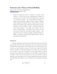
separation rate (due to both the endogenous firing by firms receiving adverse productivity shocksand the exogenous job destruction at closing firms) of 3.12%, consistent with Shimer (2005) as wellas EM.Moving to the stochastic model, I need to parameterize the stochastic process for aggregateproductivity, p t .I use the method suggested by Stokey (2009, Section 2.8) to approximate anOrnstein-Uhlenbeck process. Specifically, I allow for log p t to take 2M + 1 possible values, on theequally-spaced grid (−Md, −(M − 1)d, . . . , Md) for d > 0. If log p t = κd for κ ∈ {−M, −M −1, . . . , M}, then log p t+1 takes the value log p t with probability 1 − 2Mµ, log p t − d with probability(M + κ)µ, and log p t + d with probability (M − κ)µ; here µ ∈ (0, (2M) −1 ) is a parameter. I setM = 2, and choose d and µ so that in a long time series, model-generated GDP (aggregated toquarterly frequency and considered as a log deviation from the sample mean) matches the empiricalvolatility and autocorrelation of US GDP per capita from 1947Q1 through 2010Q4 (log deviationfrom an HP trend with smoothing parameter 1600).Finally, I also target the volatility of establishment openings. I obtain seasonally-adjusted dataon establishment openings between 1992Q3 and 2010Q2 from the Business Employment Dynamicsdatabase of the Bureau of Labor Statistics (BLS), detrend, and regress on detrended GDP percapita. The point estimate for the elasticity of establishment openings with respect to GDP percapita is 1.03, and is statistically significant. 30To match this, I need to assume that the cost ofentry varies with aggregate productivity, with elasticity ξ = 0.0294. (If ξ = 0, then entry is toovolatile in the model).The resulting parameter values are reported in Table 1. The model is nonlinear and the productivitydistribution is discrete, so not all of the calibration targets can be fit precisely. Table 2shows the fit of the benchmark model.4.2 Results4.2.1 Cross-Sectional PropertiesI first discuss some properties of the behavior of the model without aggregate productivity shocks.To do this, I fix the aggregate component of productivity at its steady-state value.Figure 1 shows a representative example of the hiring and firing behavior of a single firm. Theblue line indicates the time path of the firm’s number of employees, n(t). The green and red linesrespectively indicate the hiring target, n ∗ j , and the firing target, ¯n j, corresponding to the currentidiosyncratic productivity state ζ j at time t. As can be seen, whenever the hiring target increases30 Data on establishment openings predating 1992Q3 at sub-annual frequency is not publicly available. I use GDPper capita as a cyclical measure, rather than output per worker, because, as is well known, the detrended outputper worker is much less highly correlated with detrended GDP per capita and much less highly negatively correlatedwith unemployment after 1990 than before 1990. If I use detrended output per worker as the cyclical indicator,establishment openings are countercyclical but the point estimate is small and not statistically significant. It isbeyond the scope of the current paper to speculate on why the cyclical relationship between labor productivity andGDP per capita appears to have changed after 1990. This is a problem for the vast majority of the labor searchliterature using US data, but is usually hidden because in longer time series the period from 1948 to 1990 in whichoutput per worker was highly positively correlated with GDP per capita drives the results.28

3.53Employment, n(t)Hiring targetFiring target0.70.62.50.5Number of workers21.5Frequency0.40.310.20.50.100 20 40 60 80 100Time, t0−2 −1.5 −1 −0.5 0 0.5 1 1.5 2Firm employment growthFigure 1. Left panel: Example firm size dynamics. Right panel: Histogram of firm employment growth.distribution of firm size. Because this distribution obeys Zipf’s law in the tail, I plot the log offirm size against the logarithm of one minus the cumulative distribution function. In the left partof the distribution, the distribution does not obey a power law because very small firms must haveboth a low value for the transitory component of idiosyncratic productivity as well as a low valuefor the permanent component, so that transitory fluctuations in firm size are more important here.The model is consistent with a positive cross-sectional correlation between firm size and wages,as Oi and Idson (1999) report for US data. After controlling for the permanent component ofproductivity, in data generated by the model I regress log wages (log w it ) on log employment(log n it ) and a constant; the resulting regression relationship islog w it = 0.385 + 0.062 log n it + ε itwith R 2 = 0.357 and Var(ε it ) = 0.00177. 33 The correlation arises entirely from a positive relationshipbetween wages and employment conditional on the permanent component of the idiosyncraticproductivity shock; as already mentioned, a firm with higher permanent productivity hires moreworkers than, but pays the same wages as, a firm with lower permanent productivity. 34The model is also consistent with the empirical positive relationship between wages and firmgrowth rates. In model-generated data, I regress log wages on firm growth, g it =n it−n i,t−1, and12 (n it−n i,t−1 )obtain thatlog w it = 0.435 + 0.042g it + ε itwith R 2 = 0.137 and Var(ε it ) = 0.00238. This positive correlation between wages and firm growth33 I do not report standard errors because there is no sampling error: the firm size distribution is calculated exactly.The positive relationship is robust to the inclusion of higher moments of log employment.34 Accordingly, if I do not control for permanent productivity, the relationship is much weaker:with R 2 = 0.090 and Var(ε it) = 0.00257.log w it = 0.408 + 0.015 log n it + ε it,30

100.90.8−0.50.7CDF0.60.50.4log(1−CDF)−1−1.50.30.20.1Conditional CDF of firm size00 0.5 1 1.5 2 2.5 3 3.5 4Log firm size, log(n)−2Unconditional distribution of firm size−2.50 0.5 1 1.5 2 2.5 3Log firm size, log(n)Figure 2. Left panel:CDF of firm size conditional on permanent component of idiosyncratic productivity.Right panel: log(1 − Unconditional CDF) of firm size.might seem to be counterintuitive, since the wage-setting assumption implies that conditional onproductivity, firms with higher employment pay lower wages because the marginal product of thelast worker is lower. However, this observation ignores the endogeneity of employment. If therewere no labor market friction, all firms would hire and fire up to the point that the bargained wagewas equated across firms (and in fact equal to the worker’s outside option, as in Stole and Zwiebel,1996a,b). In the presence of costly recruiting, firms that receive a positive productivity shock donot hire enough workers to drive the wage so far down, so that such firms pay higher wages, atleast conditional on employment. 35Finally, the model is also consistent with a further stylized feature of the employment growthdistribution. Haltiwanger, Jarmin, and Miranda (2010) report that young businesses and startupscreate a disproportionate fraction of jobs in the US economy. Figure 3 shows the model’s predictionsfor employment growth by firm age. As is apparent, the model replicates this stylized factsuccessfully: young firms hire many employees at entry as they grow to their target size. Moreover,a firm that initially draws a low value of the transitory component of idiosyncratic productivityexpects to increase in size in the future as it draws higher values. As the firm ages, its employmentlevel is more likely to lie in the inaction region, and its growth rate declines. In addition, the differencebetween employment growth at continuing firms and employment growth at all firms fallswith the age of the cohort of firms; this is because firm exit rates fall with firm age, as mentionedabove. In addition, because firm size is largely driven by the permanent component of idiosyncraticproductivity, the model is also consistent with the finding that there is no systematic relationshipbetween firm sizes and growth rates, also reported by Haltiwanger, Jarmin, and Miranda.35 Because I assume that entrant firms draw from the same transitory productivity distribution as incumbents,this mechanism renders the model inconsistent with the fact that younger firms on average pay lower wages (Davisand Haltiwanger, 1991). This could easily be rectified by assuming that the productivity distribution for entrants isdominated (in the sense of first-order stochastic dominance) by that for incumbents.31

0.30.25Continuing firmsAll firms0.2Employment growth0.150.10.050−0.050 5 10 15AgeFigure 3. The relationship between net employment growth and firm age.0.060.04v−u ratioGDP per capitaUnemployment0.50.40.30.2Change in v−u ratioEntryLog deviation0.020−0.02Log deviation0.10−0.1−0.2−0.3−0.04−0.4−0.060 20 40 60 80 100Time, t−0.5−0.60 20 40 60 80 100Time, tFigure 4. Benchmark calibration.Left panel: dynamics of market tightness, GDP per capita, and unemployment.Right panel: dynamics of first-differenced market tightness and entry.4.2.2 Business Cycle PropertiesI now turn to describing the business-cycle features of the model. The left panel of Figure 4 showsa sample path for the dynamics of market tightness, GDP per capita, and unemployment. The firstfeature to note is that, as established theoretically, the vacancy-unemployment ratio θ is a jumpvariable whose value is affected only by contemporaneous productivity. Although unemployment isnot a jump variable—it exhibits transitional dynamics following changes in aggregate productivity—it is extremely highly correlated with the v-u ratio, with a negative correlation with absolute value0.951 in the benchmark parameterization. GDP per capita in theory exhibits slightly more complexdynamics, which arise not only from movements of workers between unemployment and employmentbut also from movement of workers across firms; however, in practice this variable is extremelyhighly correlated with labor market tightness (correlation greater than 0.999).32

U.S. Data u v v/u e p yStandard deviation 0.136 0.140 0.268 0.035 0.011 0.013Quarterly autocorrelation 0.923 0.873 0.888 0.037 0.771 0.885u 1 -0.925 -0.960 -0.460 0.494 -0.911v 1 0.990 0.433 -0.365 0.882Correlation v/u 1 0.433 -0.435 0.893matrix e 1 -0.097 0.494p 1 -0.136y 1Notes: The (seasonally adjusted) unemployment rate u is reported by the BLS using Current Population Survey(CPS) data. Vacancies in the non-farm business sector, v, are obtained from the BLS’ Job Openings and LaborTurnover Survey. Entry e is seasonally-adjusted number of opening establishments for the total private sector fromthe BED. Labor productivity p is measured as seasonally adjusted output per hour in the non-farm business sector,constructed by the BLS from the National Income and Product Accounts (NIPA). GDP per capita y comes fromNIPA Table 7.1. All variables are reported as log deviations from an HP trend with smoothing parameters 1600.Table 3. Business cycle statistics: U.S. data, 2000Q1-2010Q3The right panel of Figure 4 exhibits the behavior of firm entry. For comparison, also shown isthe first difference of the logarithm of the v-u ratio. The very high correlation of these two series isimmediately apparent: firm entry spikes upwards on the arrival of a positive aggregate productivityshock, and downwards on the arrival of a negative shock. Following a positive shock, vacancieshave to jump so that the vacancy-unemployment ratio jumps to its new value while unemploymentdoes not immediately change. The fraction of this increase in vacancies that arises on the extensivemargin (vacancies posted by new entrant firms) as opposed to the intensive margin (vacanciesposted by incumbents) is governed by the parameter ξ, the elasticity of the entry cost with respectto aggregate productivity. Raising ξ would reduce the magnitude of the spikes in entry, and wouldreduce the volatility of entry (in the model, the standard deviation of log entry is 0.101, while inthe Business Employment Dynamics database for 1992Q3-2010Q2, the analogous value is 0.034).However, this would come at the cost of worsening the model’s fit to the target used to calibrate ξ,namely the elasticity of entry with respect to changes in GDP per capita. Improving the empiricalperformance of the model along this dimension could be accomplished by introducing a ‘time-tobuild’feature along the lines of Fujita and Ramey (2007); this might also help with making thevacancy-unemployment ratio respond with a lag to productivity shocks, as in their paper, althoughthe implication is not clear since in my model incumbent firms can also respond to a shock byposting more vacancies. A further examination of this modification is beyond the scope of thecurrent paper.Table 3 reports standard business cycle statistics for the U.S. economy for the period 2000Q1through 2010Q3. The short time period is because JOLTS data on vacancies are only availablecommencing in 2000. In this period, labor productivity is positively correlated with unemploymentand negatively correlated with GDP per capita, vacancies and the v-u ratio, so that some termsof the correlation matrix have signs that are unexpected to those more familiar with statistics for33

longer sample periods. 36To investigate the model’s ability to match these patterns, I simulate data from the calibratedmodel. I assume that initially the economy begins with the non-stochastic steady-state joint distributionof firms over employment and idiosyncratic productivity, and with aggregate productivityequal to its mean. I then simulate a time series of 123000 months of data. Each month I draw anew aggregate productivity shock p t , and allow the sizes of existing firms to evolve according tothe optimal hiring and firing policies associated with p t and with their new draws of idiosyncraticproductivity. I then solve for entry so that total vacancies are consistent with the (known) valueof the v-u ratio θ t consistent with aggregate productivity p t . I aggregate to quarterly frequency,and discard the first 2000 quarters of data to alleviate any dependence on initial conditions. Eachsubsequent 39 quarters gives me a single sample from the model. For each such sample, I calculatethe log deviation from its sample mean for each variable of interest. I then calculate the samestatistics as reported in Table 3. 37 Finally, I repeat this procedure for each of the resulting 1000samples. In Table 4 I then report the mean and standard deviation for each business cycle statisticof interest for the 1000 data points so generated. 38The results reported in Table 4 show that the model matches the data very well in some dimensions.There is a clear Beveridge curve, indicated by the strong negative correlation betweenunemployment and vacancies, although the negative correlation in the data is stronger still. Vacanciesand establishment entry are positively correlated, and while all other business cycle variablesare quite positively autocorrelated, entry is almost serially uncorrelated. Entry is more volatilethan GDP per capita.However, there are three dimensions in which the model does not do a particularly job ofreplicating the data, and all of these are revealing. The first is the excess volatility of entry in themodel, discussed above. The second, which is the main focus of the current paper, is that the modeldoes not generate volatile unemployment and vacancies. The moment most readers will probablyfocus on most is the ratio of the standard deviation of the v-u ratio to that of productivity. This ratiois around 1.75 in Shimer’s model, and around 1.87 in mine. However, recall that I calibrated thereplacement ratio to around 0.63, higher than Shimer’s value of 0.4. Using the back-of-the-envelopeelasticity formulae provided on page 36 of Shimer’s paper, one can see that this change alone wouldtend to increase the elasticity of unemployment with respect to productivity shocks in the MPmodel by a factor of around (1 − 0.4)/(1 − 0.63) ≈ 1.62. Observe that 1.62 × 1.75 ≈ 2.84 > 1.87,so that when this difference is controlled for, my model actually generates less volatility in thev-u ratio than the benchmark MP model! (Of course, there is no distinction between average and36 Note also that during this period, which mostly consists of years from the Great Moderation, GDP per capitawas slightly less volatile and more strongly autocorrelated than over the period from 1947Q1 through 2010Q4 usedto generate the calibration targets reported in Table 2.37 Note that I do not remove an HP trend from the (stationary) model-generated data to avoid introducing spuriousautocorrelation arising from the introduction of a time trend arising from the filtering process. Statistics calculatedusing HP filtering are available on request, and do not differ significantly.38 Because Table 4 reports statistics for short time series of model-generated data, the volatilities of business-cyclevariables are slightly lower than those that would obtain in longer samples, and therefore in particular the volatilityof GDP per capita does not exactly match the correlation target reported in Table 2.34

Model u v v/u e p yStandard deviation 0.012 0.015 0.026 0.098 0.014 0.015(0.003) (0.003) (0.005) (0.014) (0.003) (0.003)Quarterly autocorrelation 0.791 0.607 0.731 0.036 0.731 0.736(0.075) (0.133) (0.097) (0.141) (0.097) (0.096)u 1 -0.838 -0.948 0.161 -0.948 -0.952(0.060) (0.023) (0.063) (0.023) (0.021)v 1 0.968 0.345 0.968 0.965(0.011) (0.113) (0.010) (0.012)Correlation v/u 1 0.126 1.000 1.000matrix (0.093) (0.000) (0.000)e 1 0.126 0.115(0.093) (0.091)p 1 1.000(0.000)y 1Table 4. Business cycle statistics: modelmarginal product in Shimer’s model, so there is no reason to expect the two models to producesimilar results here; still, the complete absence of amplification is striking.)The other main class of differences between the model and the data arise because during thesample period I consider, starting in 2000, empirical labor productivity is weakly negatively correlatedwith GDP per capita. Since labor productivity is the only driving force in the model, onthe other hand, there it is almost perfectly positively correlated with GDP per capita. In addition,labor productivity is empirically positively correlated with unemployment and negatively correlatedwith vacancies and the v-u ratio, while the opposite is true in the model. If the results forlabor productivity are ignored and GDP per capita is taken as the cyclical indicator in both thedata and the model, the results correspond much more closely: GDP per capita in both cases isstrongly positively correlated with vacancies and the v-u ratio and strongly negatively correlatedwith unemployment. This shortcoming of the model is shared with almost all models in the laborsearch literature which take labor productivity as the driving force of business cycles. (For example,comparing Table 4 with Table 3 of Shimer (2005) shows that my model behaves very similarlyto the benchmark MP model along these dimensions, and is therefore much more consistent withU.S. data in the period from 1951 to 2003 reported in Shimer’s Table 1.) It is beyond the scope ofthe paper to account for the change in the empirical behavior of labor productivity after the mid-1980s (Galí and Gambetti, 2009; Stiroh, 2009; Galí and van Rens, 2010; Hagedorn and Manovskii,2011). 3939 One possible reason for the negative correlation of labor productivity with GDP per capita is compositionbias (low-marginal product workers may move from employment to non-employment during recessions). Another isfinancial frictions, which drive a wedge between the marginal benefit to a firm of employing an additional worker andthe only component of this present in the model, namely the value of the marginal output.35

u v v/u e p yBenchmark 0.014 0.016 0.029 0.236 0.016 0.017α = 0.80 0.015 0.015 0.029 0.146 0.016 0.017η = 0.25 0.033 0.040 0.072 0.187 0.014 0.017Table 5. Standard deviations of endogenous variables under alternative parameterizationsFinally, note that I essentially imposed the values of the returns-to-scale parameter in theproduction function and of the bargaining power of workers arbitrarily. Therefore, as a robustnesscheck, I separately consider the effects of reparameterizing the model with less decreasing returnsto scale (α = 0.80), or with a lower value of workers’ bargaining power (η = 0.25, corresponding toa replacement ratio of 0.840). In each case I recalibrate four parameters that relate to the crosssection(δ, γ, k x , and λ) and three relating to the time-series behavior of the model (µ, d, and ξ)so as to match the same targets listed in Table 2. Table 5 reports the results of this exercise.Neither parameterization changes the behavior of the model substantially. When η = 0.25,unemployment, vacancies, and the vacancy-unemployment ratio are slightly more volatile than inthe benchmark model, while if α = 0.80, the standard deviation of unemployment, vacancies, andthe v-u ratio are almost unchanged from the benchmark although the volatility of entry falls slightly.Autocorrelations and cross-correlations (not reported) are barely changed from Table 4.Again, thesechanges in volatility are no more than would be suggested by Shimer’s (2005) back-of-the-envelopecalculation given the replacement ratio.5 DiscussionAs noted in the Introduction, the question of whether a firm-size distribution that responds sluggishlyto shocks provides a channel for propagating or amplifying aggregate shocks has not beenunanimously resolved in the literature to date. The current paper therefore casts in starker reliefwhat features of the models of Acemoglu and Hawkins (2011), Elsby and Michaels (2011), Fujitaand Nakajima (2009) and Kaas and Kircher (2011) are important for generating propagation andamplification. (I hereafter refer to these papers as AH, EM, FN, and KK respectively.)The first important difference among the five papers is the nature of returns to scale in therecruiting technology. AH and KK both assume that a firm that wishes to recruit progressivelymore workers in a given period faces a convex cost schedule for doing so, while the current paper,along with EM and FN, assumes a constant returns vacancy-posting technology. The propagationfound by AH and by KK, but not by the current paper, appears to arise from this feature of themodel. In response to an aggregate shock, incumbent firms may change their size target. However,arriving at the new size target instantaneously is very costly, so that at the level of the individualfirm, there are slow adjustment dynamics. This generates sluggish aggregate dynamics for thevacancy-unemployment ratio. By contrast, in the model of the current paper, there is no suchsluggishness at the level of the individual firm. Moreover, the changing composition of hiring at the36

intensive and extensive margin over the cycle provides a margin by which the desire of incumbentfirms to hire en masse in response to a shock can be accommodated. The resulting aggregatedynamics therefore display no persistence in the vacancy-unemployment ratio.Propagation arises in EM and in FN for a different reason. There, the vacancy-posting technologydoes exhibit constant returns, but the crucial difference with the current paper is that thenumber of firms is fixed. Consider the response to a negative productivity shock. In the modelof the current paper, entry falls sharply on the arrival of the shock, with vacancy-posting by incumbentsrising to take up some of the slack. Wages fall as incumbent firms increase in size, sotheir marginal product decreases. Once wages have fallen, entry by new firms returns nearly to itspre-shock level. In the absence of an entry margin, the response is different, however. Suppose thatthe vacancy-unemployment ratio were to fall instantly to the post-shock quasi-steady state level.Then, because unemployment rises during the transition to the new quasi-steady state, vacancieswould also have to fall on impact and then rise thereafter. However, on impact of the shock, wagesfall as the outside option of being unemployed falls with the job-finding rate and with the fall inaggregate productivity, so that incumbent firms instead wish to increase vacancy posting at thearrival of the shock. This inconsistency means that the fall in vacancy-posting on impact must bemore gradual, and this leads to persistence.The crucial role of how precisely the entry process is modeled for the cyclical properties ofmodels with frictional labor markets applies also beyond the context of multi-worker firms. Colesand Moghaddasi (2011) study a model in which entrepreneurs can only post vacancies after atime-consuming construction period has elapsed. They show that this allows for larger and morepersistent fluctuations in unemployment and in market tightness than in the benchmark Mortensen-Pissarides model. This is consistent with the relatively volatile and persistent fluctuations inemployment and market tightness in EM and FJ relative to the current paper, to AH, and to KK.Another difference between EM and FN and the three other papers mentioned is that thoseauthors find substantial amplification of productivity shocks. Of course, some of the difference inthis respect arises because of the surplus of average labor productivity over the opportunity cost ofemployment in these two papers. (The replacement ratio in EM is around 0.85, and around 0.83in the benchmark calibration of FN.) However, as the sensitivity analysis in this paper made clear,such a replacement ratio is not sufficient to generate large fluctuations in employment by itself.The more important assumption that drives the results of those two papers is the absence of anextensive margin of adjustment. This works to generate increased amplification, due to the role ofthe wage bargaining assumption. Following a positive productivity shock, not only do firms wishto hire more workers simply because of the direct increase in profitability due to the shock, butalso because the rise in wages for all workers is offset as larger firms pay lower wages conditional onproductivity. As the average size of firms increases following the shock, the rise in wages due to theproductivity shock is partially offset. This dampening effect on the elasticity of wages due to theproductivity shock acts as would an exogenously sticky wage, increasing the response of employmentto the shock. By contrast, in the current model, the adjustment to a positive productivity shock37

occurs largely on the extensive margin: more establishments enter, and the size of incumbent firmsbarely changes. Thus, this second feedback channel is absent.6 ConclusionThe key contributions of this paper are twofold. The first is theoretical. I solve, nearly in closedform, a large-firm bargaining model in the presence of a rich structure of cross-sectional heterogeneity.The second is more quantitative. I show that in this class of models, the ability to matchcross-sectional features of the employment and employment growth distribution has no implicationsfor the response of the model to aggregate shocks. Indeed, if preferences take a balanced-growthform and recruiting is time-intensive, then no matter what the cross-sectional features of the modelin steady state, there will be no fluctuations in unemployment in response to an aggregate productivityshock! In the more familiar case with linear preferences and goods-intensive recruiting, theresponses of the key aggregate variables described by the MP model are not significantly different inmy model. The presence of large firms and of a rich structure of cross-sectional heterogeneity neednot amplify or propagate business-cycle shocks. To propagate shocks, it appears that either convexcosts of recruiting or shutting down the extensive margin of adjustment to shocks is required. Toamplify shocks seems to require that the surplus from employment be small, something which isunsurprising since the work of Shimer (2005) and Hagedorn and Manovskii (2008).A significant success not just of the current paper, but also of the quantitatively-oriented contributionsof Elsby and Michaels (2011) and Kaas and Kircher (2011) is to match the empiricalcross-sectional patterns of employment and employment growth well. However, a concern about allthree papers is that the calibrational strategy that underlies this success is not well-disciplined: inthe calibration, the productivity distribution is essentially a residual. A natural direction for futureresearch in theoretical modeling is to determine to what extent the results of the three papers aredependent on the adjustment cost structure (what would happen in the presence of a fixed costof adjusting the labor force?) A natural direction for empirical research is to attempt to groundthe productivity distribution more directly in the data. Finally, since the key contribution of thecurrent paper is to underline the crucial role of the processes for the entry of new firms and for vacancycreation for the aggregate cyclical properties of multi-worker search models, it would also bevery useful to understand more about the empirical properties of these processes. All are necessaryfor a better understanding of the role of heterogeneous firms in the aggregate labor market.AOmitted ProofsThis Appendix contains statements of some definitions and results that are not formalized in thetext, together with all technical proofs. Some proofs are not yet complete in this preliminary versionof the paper.38

Proof of Lemma 2. DefineT (n) = 1 η n− 1 η∫ n0∫ nν 1−ηη y ′ 0(ν) dν =ν 1−ηη y ′ (ν) dν∫ . (59)n0 ν 1−ηη dνFrom the definition of ỹ(·) in (32), it is apparent that ỹ(n) = y(n) − nT (n). Differentiatingestablishes also that ỹ ′ (n) = (1 − η)T (n) and ỹ ′′ (n) = 1−ηηn [y′ (n) − T (n)]. Thus, to establish thedesired claims about ỹ(·), it is sufficient to show that y ′ (n) < T (n) < y(n)nfor all n. This establishesdirectly that ỹ(n) is strictly positive and that ỹ ′′ (·) is strictly negative. That ỹ ′ (n) > 0 follows afortiori because y ′ (n) > 0. The two Inada conditions also follow: as n → 0 + , T (n) > y ′ (n) → +∞,and as n → +∞, 0 < T (n) < y(n)n → 0.To see that T (n) > y ′ (n), note that the last expression in (59) shows that T (n) is a weightedaverage of inframarginal products y ′ (ν) for ν ∈ (0, n). Since y(·) is strictly concave, y ′ (ν) strictlyexceeds y ′ (n) whenever 0 ≤ ν < n since y ′ (·) is a strictly decreasing function; that is, T (n) > y ′ (n)for all n.To see that T (n) < y(n)/n, writey(n)/n =∫ n0 y′ (ν) dν∫ n0 dν . (60)Comparing the last expression in (59) with (60), it is apparent that both y(n)/n and T (n) areweighted averages of y(ν) for ν ∈ (0, n). However, the weighting function ν ↦→ ν (1−η)/η in (59) isstrictly increasing in ν, while that in (60) is a constant function. Because the integrand y ′ (ν) isstrictly decreasing in ν, the weighting function that puts relatively higher weights on lower valuesof ν, that is, the constant function, yields a higher weighted average. This completes the proof.Proof of Proposition 1. I show that amongst the allocations which satisfy the hypotheses of Proposition1 (that is, stationary allocations), I can find one which is an equilibrium. The proof consistsof several parts. First, I normalize the problem of a production firm in a stationary allocation tomake it independent of aggregate productivity. Second, I construct values of the key endogenousvariable ¯c and ¯θ that are consistent with equilibrium in the labor market, equilibrium in the goodsmarket, and free entry for production firms. Finally, I show that there are values for the remainingendogenous variables consistent with equilibrium.Therefore, consider an arbitrary stationary allocation. Observe first that x(s t ) is constant sinceθ(s t ) ≡ ¯θ, so that from (34) it follows that in a stationary allocation,x(s t ) ≡ ¯x =¯θηγφ r(1 − f(¯θ))(1 − η)(61)is a function only of ¯θ and parameters. Note that ¯x is strictly increasing in ¯θ.Next, define normalized value functions for firms by dividing equations (4) and (5) by currentaggregate productivity p t , so that the normalized value of a firm after learning the realizations ofproductivity but before firing or recruitment is[ˆK(n; s t , π t ) = max − kr (s t ])h + K(n − f + h; s t , π t )(62)f,h≥0 p t39

and the value after firing and recruitment but before production or wage payments isK(n; s t , π t ) = π t y(n) − n w(n; st , π t )p tBy assumption of stationarity, k r (s t ) = ¯k r p t . Also, from (29),w(n; s t , π t )p t+ (1 − δ) ∑q t (s t+1 ) p ∑t+1µ(π t , π t+1 )p ˆK(n; s t+1 , π t+1 ).ts t+1 |s t π t+1= (1 − η)(φ y + ¯x)¯c + n − 1 η∫ n0(63)ν 1−ηη π j y ′ (ν) dν. (64)That is, the ratio of wages to aggregate productivity depends only on current employment andidiosyncratic productivity at the firm. Denote this quantity (the right side of (64)) as ¯w(n, π t )hereafter. Finally, (14), together with stationarity, implies thatq t (s t+1 ) p t+1= β P (st+1 )c(s t )p t P (s t )c(s t+1 )p t+1p t= β P (st+1 )P (s t ) .Substituting all these observations into (62) and (63) establishes thatˆK(n; s t , π t [) = max −¯kr h + K(n − f + h; s t , π t ) ] (65)f,h≥0andK(n; s t , π t ) = π t y(n) − n ¯w(n, π t ) + β(1 − δ) ∑ P (s t+1 ) ∑P (s t µ(π t , π t+1 ))ˆK(n; s t+1 , π t+1 ). (66)s t+1 |s t π t+1Now, suppose the solution for ˆK and for K is in fact independent of the history s t . In this case theonly terms involving s t are the weights P (st+1 )P (s t )on the right side of (66); however, these weights andthe entire summation are superfluous since the summand is constant with respect to s t+1 . That is,ˆK and K are a history-independent solution to (65) and (66) if and only if they satisfy[ˆK(n, π t ) = max −¯kr h + K(n − f + h, π t ) ] (67)f,h≥0andK(n, π t ) = π t y(n) − n ¯w(n, π t ) + β(1 − δ) ∑ π t+1µ(π t , π t+1 ) ˆK(n, π t+1 ). (68)(Here I abuse notation and drop redundant arguments of the two value functions.) (67) and (68)can be combined as the single equation[ˆK(n, π) = max −¯k r max(n ′ − n, 0) + πỹ(n ′ ) − n ′ (1 − η)(φ y + ¯x)¯c + β(1 − δ) ∑ ]µ(π t , π t+1 ) ˆK(n ′ , π t+1 )n ′ π t+1(69)where ỹ(n) was defined in (32). The discussion there established the strict concavity of ỹ(·). Also,Blackwell’s sufficient conditions apply, so that there is a unique solution to (69) (and therefore to(67) and (68). This solution then solves (65) and (66), and therefore generates a solution to (4)and (5). (It is unique under weak assumptions on the stationarity of the aggregate productivityprocess, but formalizing this is unnecessary for the current argument.)Because ỹ(·) is a neoclassical production function, (69) can be viewed as characterizing the40

problem of a firm with this production function that, in a competitive labor market, maximizes itsvalue subject to paying all its employees a wage of (1 − η)(φ y + ¯x)¯c and subject to a hiring cost of¯k r . The free entry condition in this modified economy is∑m πFπ(ζ e j ) ˆK(0, ζ j ) = ¯k f . (70)j=1In a stationary allocation, (8), (9), and (13) imply that ¯k f = κφ f ¯c and ¯k r = γφ r¯c/m(¯θ).I now show that there are values of ¯c and ¯θ consistent with market clearing in the labor andgoods markets and with free entry.The problem of a neoclassical firm solving (69) is well-understood. The value of such a firm iscontinuously decreasing in ¯θ and in ¯c. (To prove the first of these claims more formally, parameterizethe solution for different candidate values of ¯θ by ˆK(n, π; ¯θ), and note that if ¯θ 1 > ¯θ 2 , then ¯k r (¯θ 1 ) >¯k r (¯θ 2 ) (it is more expensive to recruit when the recruiter to unemployment ratio is high) and¯x(¯θ 1 ) > ¯x(¯θ 2 ) (wages are higher). A production firm in an economy with ¯θ = ¯θ 1 can always followthe policy that is optimal in an economy with ¯θ = ¯θ 2 . This will achieve a higher value since the costof the recruiting the firm does is reduced, as are wages. Further optimizing recruitment strategiescan only increase the firm’s value. Moreover, this increase in the value occurs continuously, in thesense that there is no ¯θ 1 at which the value of an entrant, which is given by ∑ m πj=1 F π(ζ e j ) ˆK(0, ζ j ),increases discretely. This is because if ¯θ 2 → ¯θ 1 , a firm in the economy with ¯θ = ¯θ 2 could also followthe firing and recruitment policies that are optimal in the ¯θ = ¯θ 1 economy. A similar argumentestablishes the other claim.)Next, the largest value of ¯c that is consistent with the free entry condition is obtained when¯θ → 0, so that m(¯θ) → +∞ and ¯k r → 0. In this case, recruitment has zero cost from the perspectiveof the firm, so that there are no costs of adjusting the firm’s labor force, and it sets employmentduring the production phase of the economy always at the static optimum, which satisfiesỹ ′ (n) = (1 − η)φ y¯c (71)since ¯x → 0 in this case. Because ỹ(·) is a neoclassical production function by Lemma 2, it followsthere is an finite upper bound ¯c 1 which is the largest value consistent with the free entry conditionfor the firm, and then only if ¯θ = 0. On the other hand, as ¯c → 0 + , in order to be consistent with thefree entry condition, we must have ¯θ → +∞ so that recruiting becomes expensive, since if ¯θ remainsbounded, so does ¯x, so that the firm faces no other costs of operation as wages (1 − η)(φ y + ¯x)¯cvanish. Therefore if I write ψ(¯c) for the value of ¯θ consistent with (70), then ψ : (0, ¯c 1 ) → [0, ∞) isa strictly decreasing continuous function with lim¯c→0 + ψ(¯c) = +∞ and ψ(¯c 1 ) = 0.Next, define a function ξ : (0, ¯c 1 ] → [0, ∞) as the level of output consistent with firm behaviorand labor market clearing in an economy where consumption is ¯c and the recruiter-unemploymentratio is ψ(¯c). To define this more precisely, first denote by Ḡ(n, ζ j) ∈ [0, 1] the probability a firmhas employment n and idiosyncratic shock ζ j during the production phase of a period. Denote byg(¯c) the measure of active firms (after entry and before exogenous destruction within any period)that is consistent with labor market clearing in this environment. g(¯c) is uniquely determined bythe job-finding probability of workers, f(¯θ) = f(ψ(¯c)), together with the firing behavior of firms,determined as part of the solution to the firm’s problem, and the distribution Ḡ(·).40 Then total40 More precisely, after the recruitment phase of a period, total employment is∑m πē f = g(¯c)j=1∫ ∞0n dF (n; ζ j).41

ˆK j ′(n∗ l) assuming no hiring and firing with the correct equation arising from (48). This equationis of the form ˆK j ′(n∗ l) = s for some constant s, and so adducing it does not affect the full rankof the coefficient matrix, nor the property that S j ′(n ∗ l ) is strictly decreasing in n∗ lfor any j ′ suchthat n ∗ l∈ [n ∗ j, ¯n ′ j ′]. Repeating this step as many times as necessary establishes that there is a{ }unique solution for ˆKj (n ∗ l ) , with the same comparative static property in j n∗ ljust mentioned.In particular, note that the value of ˆK l ′(n∗ l ) is decreasing in n∗ l. Also, note that this solution dependsonly on the rank order of L and the value of n ∗ l. One can then proceed to use (48) to obtain theadditional equation, so far unused, that Kl ′(n∗ l ) = (1−η)(φy + ¯x)¯c, which is independent of n ∗ l ; thusit follows that there is also a unique solution{for n ∗ l. A similar argument then applies to establishthat there is also a unique solution for ˆK′ j (¯n l )}and for ¯n l. Repeating this argument for all ljestablishes the claimed uniqueness property.Proof of Lemma 3. The firm’s problem is unchanged, so that its marginal surplus J n (n; s t , π t ) fromemploying a worker at the equilibrium wage w(n; s t , π t ) still satisfies (15), and the marginal valuefrom employing a worker whose current-period wage is w and not w(n; s t , π t ) still satisfies (20).However, the marginal surplus over unemployment of employment at the equilibrium wage to thehousehold is now given by a version of (24) modified to account for the linear utility of consumption,S(n; s t , π t ) = w(n; s t , π t ) − φ y − x(s t )+ β(1 − δ) ∑ P (s t+1 ) ∑P (s t µ(π t , π t+1 )S(n ′ (n; s t+1 , π t+1 ); s t+1 , π t+1 ))s t+1 |s t π t+1(73)and the marginal value of employment at an arbitrary wage w is the analogous modification of(25), namely˜S(w, n; s t , π t ) = w − w(n; s t , π t ) + S(n; s t , π t ). (74)The first-order condition for the solution to (26) therefore takes the form thatηJ n (w(n; s t , π t ), n; s t , π t ) = (1 − η)S(w(n; s t , π t ), n; s t , π t ), (75)or(1 − η) [ w(n; s t , π t ) − φ y − x(s t ) ] = η ∂ [pt π t y(n) − nw(n; s t , π t ) ] . (76)∂nAs in the proof, integrating and setting the constant of integration to zero so that wages remainbounded in small firms completes the proof.Proof of Proposition 2. The argument is analogous to that given in the proof of Proposition 1. Theonly difficulty is to show that values {θ i } i can be found so that the free-entry condition (7) holdsfor all aggregate states. To see this, first consider the simpler case where aggregate productivityis non-stochastic, so that p t ≡ ¯p is constant. In this case I seek to show that there exists anθηγφequilibrium in which θ is constant also. According to (34), this requires that x =r(1−f(θ))(1−η) andk r = γ/m(θ) are also constant. Specializing (53) to this case and dropping superfluous notationfor aggregate productivity shows that[]∑m πJ j (n) = max −k r max(n ′ −n, 0)+pπ j ỹ(n ′ )−n ′ (1−η)(φ y +x)+β(1−δ) µ(π j , π j ′)J j ′(n ′ ) . (77)n ′j ′ =143

The right side of (77) is strictly decreasing and continuous in θ, since both x and k r are continuousand strictly increasing in θ while the other terms do not depend on θ. Moreover, as θ → 0 + , so thatx, k r → 0 + , it follows that ∑ m πj=1 F e π(ζ j )J j (0) > k f . On the other hand, if θ → +∞, then wagesbecome arbitrarily large so that the optimal policy for the firm is to fire its entire workforce. ThusJ j (n) → 0 for all j and all n, so that ∑ m πj=1 F π(ζ e j )J j (0) → 0 < k f . The intermediate value theoremthen implies that there exists a θ such that (7) holds, and from the monotonicity in θ of the rightside of (77) it follows that this solution is unique.When aggregate productivity is again stochastic, existence of a solution for {θ i } i follows as in theproof of Proposition 5 of Kaas and Kircher (2011), since the transition matrix λ(p t , p t+1 ) is strictlydiagonally dominant, J ij (n) is differentiable in θ, and all elements of the Jacobian dJ ij (n)/dθ i ′ arenon-positive. Existence (and uniqueness) of a solution to (54), (55), and (7) then follows fromthe implicit function theorem in a neighborhood of the non-stochastic solution calculated in theprevious paragraph. The only other condition that needs to be checked to ensure that the resultingsolution is an equilibrium is that entry should never be negative; however, in the non-stochasticsteady state, entry must be constant and strictly positive so as to keep employment constant.Entry after any sequence of realized productivity shocks depends continuously on {z 1 , . . . , z mp }, soit follows by continuity that entry is also always positive provided the aggregate shocks are not toolarge.ReferencesAcemoglu, D., P. Antràs, and E. Helpman (2007): “Contracts and Technology Adoption,”American Economic Review, 97(3), 916–943.Acemoglu, D., and W. B. Hawkins (2011): “Wages and Employment Persistence with MultiworkerFirms,” unpublished.Axtell, R. L. (2001): “Zipf Distribution of U.S. Firm Sizes,” Science, 293(5356), 1818–1820.Bertola, G., and R. J. Caballero (1994): “Cross-Sectional Efficiency and Labor Hoarding ina Matching Model of Unemployment,” Review of Economic Studies, 61(3), 435–456.Coles, M. G., and A. Moghaddasi (2011): “Persistent and Volatile Unemployment/VacancyDynamics with Diamond (Coconut) Entry and Time-to-Build Constraints,” unpublished.Cooper, R., J. Haltiwanger, and J. L. Willis (2007): “Search frictions: Matching aggregateand establishment observations,” Journal of Monetary Economics, 54(Supplement 1), 56–78.Coşar, A. K., N. Guner, and J. Tybout (2010): “Firm Dynamics, Job Turnover, and WageDistributions in an Open Economy,” Working Paper 16326, National Bureau of Economic Research,Cambridge, MA.Costain, J. S., and M. Reiter (2008): “Business Cycles, Unemployment Insurance, and theCalibration of Matching Models,” Journal of Economic Dynamics and Control, 32(4), 1120–1155.Davis, S. J., and J. C. Haltiwanger (1990): “Gross Job Creation and Destruction: MicroeconomicEvidence and Macroeconomic Implications,” NBER Macroeconomics Annual, 5, 123–168.44

(1991): “Wage Dispersion between and within U.S. Manufacturing Plants, 1963–86,”Brookings Papers on Economic Activity: Microeconomics, pp. 115–200.(1992): “Gross Job Creation, Gross Job Destruction, and Employment Reallocation,”Quarterly Journal of Economics, 107(3), 819–863.Davis, S. J., J. C. Haltiwanger, R. Jarmin, and J. Miranda (2006): “Volatility and Dispersionin Business Growth Rates: Publicly Traded versus Privately Held Firms,” NBER MacroeconomicsAnnual, 21, 107–179.Delacroix, A., and R. M. Samaniego (2009): “Joint Determination of Product and LaborMarket Policies in a Model of Rent Creation and Division,” unpublished.Ebell, M., and C. Haefke (2009): “Product Market Deregulation and the U.S. EmploymentMiracle,” Review of Economic Dynamics, 12(3), 479–504.Elsby, M., and R. Michaels (2011): “Marginal Jobs, Heterogeneous Firms, and UnemploymentFlows,” unpublished.Felbermayr, G., and J. Prat (2007): “Product Market Regulation, Firm Selection and Unemployment,”Discussion Paper 2754, Institute for the Study of Labor (IZA).Fujita, S. (2011): “Dynamics of Worker Flows and Vacancies: Evidence from the Sign RestrictionApproach,” Journal of Applied Econometrics, 26(1), 89–121.Fujita, S., and M. Nakajima (2009): “Worker Flows and Job Flows: A Quantitative Investigation,”Working Paper 09-33, Federal Reserve Bank of Philadelphia.Fujita, S., and G. Ramey (2007): “Job matching and propagation,” Journal of Economic Dynamicsand Control, 31(11), 3671–3698.Galí, J., and L. Gambetti (2009): “On the Sources of the Great Moderation,” American EconomicJournal: Macroeconomics, 1(1), 26–57.Galí, J., and T. van Rens (2010): “The Vanishing Procyclicality of Labor Productivity,” unpublished.Hagedorn, M., and I. Manovskii (2008): “The Cyclical Behavior of Unemployment and VacanciesRevisited,” American Economic Review, 98(4), 1692–1706.(2011): “Productivity and the Labor Market: Comovement Over the Business Cycle,”International Economic Review, 52(3), 603–620.Haltiwanger, J. C., R. S. Jarmin, and J. Miranda (2010): “Who Creates Jobs? Small vs.Large vs. Young,” Working Paper 16300, National Bureau of Economic Research, Cambridge,MA.Hawkins, W. B. (2011):Firms,” unpublished.“Identifying the Nature of Bargaining between Workers and LargeHelpman, E., and O. Itskhoki (2010): “Labour Market Rigidities, Trade and Unemployment,”Review of Economic Studies, 77(3), 1100–1137.45

Hopenhayn, H., and R. Rogerson (1993): “Job Turnover and Policy Evaluation: A GeneralEquilibrium Analysis,” Journal of Political Economy, 101(5), 915–938.Kaas, L., and P. Kircher (2011): “Efficient Firm Dynamics in a Frictional Labor Market,”unpublished.Krusell, P., and A. A. Smith, Jr. (1998): “Income and Wealth Heterogeneity in the Macroeconomy,”Journal of Political Economy, 106(5), 867–896.Lee, Y., and T. Mukoyama (2011): “Entry, Exit, and Plant-level Dynamics over the BusinessCycle,” unpublished.Lucas, Jr., R. E. (1967): “Adjustment Costs and the Theory of Supply,” Journal of PoliticalEconomy, 75(4), 321–334.(1978): “On the Size Distribution of Business Firms,” Bell Journal of Economics, 9(2),508–523.Merz, M. (1995): “Search in the labor market and the real business cycle,” Journal of MonetaryEconomics, 36(2), 269–300.Mortensen, D. T. (1982): “Property Rights and Efficiency in Mating, Racing, and RelatedGames,” American Economic Review, 72(5), 968–79.Mortensen, D. T., and C. A. Pissarides (1994): “Job Creation and Job Destruction in theTheory of Unemployment,” Review of Economic Studies, 61(3), 397–415.Moscarini, G., and F. Postel-Vinay (2009): “Large Employers are More Cyclically Sensitive,”Working Paper 14740, National Bureau of Economic Research, Cambridge, MA.Oi, W. Y., and T. L. Idson (1999): “Firm size and wages,” in Handbook of Labor Economics,ed. by O. C. Ashenfelter, and D. Card, vol. 3A, chap. 33, pp. 2165–2214. Elsevier, Amsterdam.Petrongolo, B., and C. A. Pissarides (2001): “Looking into the Black Box: A Survey of theMatching Function,” Journal of Economic Literature, 39(2), 390–431.Pissarides, C. A. (2000): Equilibrium Unemployment Theory. MIT Press, Cambridge, MA, secondedn.(2009): “The Unemployment Volatility Puzzle: Is Wage Stickiness the Answer?,” Econometrica,77(5), 1339–1369.Roys, N. (2010): “Estimating Labor Market Rigidities with Heterogeneous Firms,” unpublished,Paris School of Economics and CEMMAP.Schaal, E. (2012): “Uncertainty, Productivity and Unemployment during the Great Recession,”unpublished.Shimer, R. (2005): “The Cyclical Behavior of Equilibrium Unemployment and Vacancies,” AmericanEconomic Review, 95(1), 25–49.(2010): Labor Markets and Business Cycles, CREI Lectures in Macroeconomics. PrincetonUniversity Press, Princeton, NJ.46

Silva, J. I., and M. Toledo (2009): “Labor Turnover Costs and the Cyclical Behavior of Vacanciesand Unemployment,” Macroeconomic Dynamics, 13(S1), 76–96.Smith, E. (1999): “Search, Concave Production and Optimal Firm Size,” Review of EconomicDynamics, 2(2), 456–471.Stiroh, K. J. (2009): “Volatility Accounting: A Production Perspective on Increased EconomicStability,” Journal of the European Economic Association, 7(4), 671–696.Stokey, N. L. (2009): The Economics of Inaction. Princeton University Press, Princeton, NJ.Stole, L. A., and J. Zwiebel (1996a): “Intra-firm Bargaining under Non-binding Contracts,”Review of Economic Studies, 63(3), 375–410.(1996b): “Organizational Design and Technology Choice under Intrafirm Bargaining,”American Economic Review, 86(1), 195–222.Veracierto, M. (2008): “Firing Costs and Business Cycle Fluctuations,” International EconomicReview, 49(1), 1–39.(2009): “Establishments Dynamics, Vacancies and Unemployment: A Neoclassical Synthesis,”Working Paper 2009-14, Federal Reserve Bank of Chicago, Chicago, IL.Yashiv, E. (2006): “Evaluating the performance of the search and matching model,” EuropeanEconomic Review, 50(4), 909–936.47