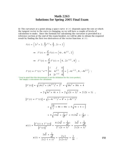
Math 2263 Solutions for Spring 2005 Final Exam

z = f ( x, y ) over a closed region D in the xy-plane , S = 1 + ∂ f2⎛⎛ ⎞⎞⎜⎜ ⎟⎟ + ∂ f2⎛⎛ ⎞⎞∫∫ ⎜⎜ ⎟⎟ dA⎝⎝ ∂ x ⎠⎠ ⎝⎝ ∂ y.⎠⎠Dfindf xThe three-dimensional surface in question is given by z = 2 √xy , for which we= 2 ∂∂ x(x y )1/2=€2 ⋅ 1 2 ⋅ ( x y )−1/ 2 ∂⋅∂ x (x y ) =yxy,€f y= 2 ∂∂ y( xy )1/2=2 ⋅ 1 2 ⋅ ( x y )−1/ 2 ⋅ ∂∂ y ( xy ) =xxy€⎛⎛⇒ 1 + ∂ f ⎞⎞⎜⎜ ⎟⎟⎝⎝ ∂ x ⎠⎠2⎛⎛+ ∂ f ⎞⎞⎜⎜ ⎟⎟⎝⎝ ∂ y ⎠⎠2= 1 +⎛⎛⎜⎜⎝⎝yx y⎞⎞⎟⎟⎠⎠2+⎛⎛⎜⎜⎝⎝xx y⎞⎞⎟⎟⎠⎠2=x y + x 2 + y 2x y. The region D in the xy-plane is a triangle with vertices ( 0, 0 ) , ( 2, 0 ) , and ( 0, 1 ) ,so it lies in the first quadrant and is bounded by the x- and y-axes and the line€ y = 1 − ½ x . So we wish to integrate in the y-direction from the x-axis ( y = 0 ) upto the line we have identified, and we will integrate in the x-direction from the y-axis( x = 0 ) to the x-intercept of the oblique line, at x = 2 . Bringing all of these resultstogether, our surface area integral is then given by.S =2∫01 − x 2∫0x 2 + y 2 + xyx ydy dx(B)€€9) We can take on this line integral in one € of two ways. The direct approach is to makean integration from A( -1, 0 ) to B( 1, 0 ) along the x-axis, with y = 0 and dy = 0 ,followed by an integration from point B back to point A along the semi-circular path,using polar coordinates. The two segments tracing the closed curve C thus yield∫C(12x + 4 y ) dx + (7x − 2y ) dy =∫ (12x + 4 y ) dx + (7x − 2y ) dy + ∫ (12x + 4 y ) dx + (7x − 2y ) dy A → B1∫= (12x + 4 ⋅ 0) dx + (7x − 2y ) ⋅ 0−1B→ Aπ∫+ (12 ⋅ cos θ + 4 ⋅ sin θ ) ( −sin θ dθ ) + (7 ⋅ cos θ − 2 ⋅ sin θ ) ( cos θ dθ )€0using x = cos θ , dx = −sin θ dθ ; y = sin θ , dy = cos θ dθand integrating from the positive ( θ = 0 ) to the negative x-direction ( θ = π )€

1= ∫ 12x dx + ∫ (7 cos 2 θ − 4 sin 2 θ − 14 sin θ cos θ ) dθ −1π0€1= (6x 2 )−1π∫+ (7 ⋅ 1 2 [1 + cos 2θ ] − 4 ⋅ 1 [1 − cos 2θ ] − 7 ⋅ sin 2θ ) dθ2 0€= (6 ⋅ 1 2 − 6 ⋅[ −1] 2 ) + ( 3 2 + 11 2π∫0cos 2θ − 7 ⋅ sin 2θ ) dθ π€€= 0 + ( 3 2 θ − 11 4 sin 2θ + 7 2 cos 2θ ) 0= ( 3 2 ⋅ π − 11 4 sin 2π + 7 2 cos 2π ) − ( 3 2 ⋅ 0 − 114 sin 0 + 7 2 cos 0) €€= 3 2 π − 0 + 7 2 − 0 + 0 − 7 2 = 3π 2. (C) This first is the approach we would take using the “tools” of Calculus II. However,we are now also familiar with Green’s Theorem, which states that for a region Dbounded by a simple closed curve C which is piecewise-continuous and positiveoriented(that is, we trace it in the “counter-clockwise” direction), if P ( x , y ) and Q ( x ,y ) are functions with continuous partial derivatives in an open region containing D ,then∫ P( x, y ) dx + Q( x, y ) dy =C∫∫D⎛⎛⎜⎜⎝⎝∂ Q∂ x− ∂ P∂ y⎞⎞⎟⎟ dA .⎠⎠€Using this method, our line integral becomes∫C(12x € + 4 y ) dx + (7x − 2y ) dy=⎛⎛ ∂⎜⎜ [ 7x − 2y ] −∂⎝⎝ ∂ x ∂ y [12x + 4 y ] ⎞⎞∫∫ ⎟⎟ dA = (7 − 4 ) dA⎠⎠∫∫ = 3 dADThe integrand in the Green’s Function integral reduces to a constant, so the line integralis simply equal to 3 times the area of the enclosed semicircle. Since this semi-circle has€1a radius of 1 , we obtain ∫ (12x + 4 y ) dx + (7x − 2y ) dy = 3 ⋅2 π ⋅ 12 = 3π .2CD∫∫ .D€

10) This Problem only requires a straightforward calculation of the curl of the vectorfunction (the function which describes the vector field)F = < 6x + 3y 2 z − yz 2 , 3xy − 3y 2 z , yz 2 − 4xz > .The 3 × 3 determinant used here is not the definition of this vector operation, butserves as a convenience for remembering the order of differentiations:r∇ × F r"="i j k∂∂ x∂∂ y∂∂z6x + 3y 2 z − yz 2 3x y − 3y 2 z yz 2 − 4 xz€€= (z 2 − 0) − (0 − 3y 2 ) , − (0 − 4z ) + (0 + 3y 2 − 2yz ) , (3y − 0) − (0 + 6yz − z 2 )= 3y 2 + z 2 , 3y 2 − 2yz + 4z , 3y − 6yz + z 2 . (D)€11) A vector field F is said to be conservative when its line integral around a simpleclosed curve is zero (€∫rF ⋅ dr= 0 ) ; this is equivalent to saying that its lineCintegral between two points is “path-independent”, and that the curl of the vector fieldis zero (the vector field is then also called “irrotational” or “curl-free”). For the vectorfield F = < αxy + βy 2 + 3x 2 , 6x 2 + 2xy − y 2 > , which is only two-dimensional,the analogue of the curl calculation is" r∇ × rF " = ∂Q∂ x − ∂P∂ y , with F = < P , Q >having components which are functions of x and y . Thus, our vector field isconservative if∂€∂ x (6x2 + 2x y − y 2 ) −∂∂ y (α x y + β y 2 + 3x 2 ) = 0⇒ (12x + 2y ) − (α x + 2β y ) = 0 .€ This will hold true if we can match x- and y-terms, giving us 12x = αx and 2y = 2βy. Hence, this vector field is conservative in the case where α = 12 and β = 1 .(E) €12) The integration in this Problem can also be taken on in one of two ways. Thevector field involved is F = < y , −x , xy > ; in the double integral ( ∇ r× F r) ⋅ d SrSthe surface to be integrated over is the section of z = g ( x, y ) = xy which “liesabove” the square with vertices O( 0, 0, 0 ) , P( 0, 1, 0 ) , Q( 1, 1, 0 ) , and R( 1, 0, 0 )€∫∫ ,

1= ∫ − x dy + ∫ y dx + ∫ − x dy + ∫ y dx01011x = 0 here y = 1 here x = 1 here y = 0 here00€101= 0 + ∫ 1 dx + ∫ −1 dy + 0 = x 001− y 10= 1 − (−1) = 2 .13) This Problem revisits a topic we discussed in Calculus II. The infinitesimal€arclength element in the plane isds = dx 2 + dy 2 , which is always what we areintegrating in order to find the distance between two points measured along a curve.When the curve is described by y = f ( x ) and we will be integrating along thex-direction from x = a to x = b , then we can factor dx out of the radical to calculatethe arclength as €B b⎛⎛s = ∫ ds = 1 + ⎜⎜dy ⎞⎞∫ ⎟⎟ 2dx .⎝⎝ dx ⎠⎠For our function, we haveAay = € 1 4 x 2 − 1 2ln x ⇒dydx = 1 2 x − 1 2 ⋅ 1 x€⇒⎛⎛ dy ⎞⎞⎜⎜ ⎟⎟⎝⎝ dx ⎠⎠2=⎛⎛⎜⎜⎝⎝12 x − 1 2 ⋅ 1 x⎞⎞⎟⎟ 2 = 1 ⎠⎠ 4 x 2 − 1 2 + 14 x 2 €⎛⎛⇒ 1 + dy ⎞⎞⎜⎜ ⎟⎟⎝⎝ dx ⎠⎠2= 1 4 x 2 +↑12 + 14 x 2 =⎛⎛⎜⎜⎝⎝12 x + 12x⎞⎞⎟⎟ 2⎠⎠€s =e⎛⎛ 12 x + 1 ⎞⎞∫ ⎜⎜ ⎟⎟ dx =⎝⎝ 2x ⎠⎠12e∫112 x + 1 2xdx€⎛⎛= ⎜⎜1 4 x 2 + 1 ⎝⎝ 2 ln x ⎞⎞⎟⎟⎠⎠e1⎛⎛= ⎜⎜1 4 e2 + 1 ⎝⎝ 2 ln e ⎞⎞⎠⎠⎟⎟ − ⎛⎛⎜⎜1 4 ⋅12 + 1 ⎝⎝ 2 ln 1 ⎞⎞⎟⎟⎠⎠€= 1 4 e2 + 1 2 − 1 4 − 0 = 1 4 e2 + 1 4 or 14 (e2 + 1) .14) We have a function of two variables z = F ( x , y ) , for which x and y arethemselves € functions of two variables, x = g ( r , θ ) and y = h ( r , θ ) . In order to∂zcalculate first partial derivatives such as∂rChain Rule. So we will be working with, we need the multi-variate version of the€

∂z∂r = ∂z∂ x ⋅ ∂ x∂r + ∂z ∂ y∂ y ∂rand∂z∂θ = ∂z∂ x ⋅ ∂ x∂θ + ∂z ∂ y∂ y ∂θ.For this Problem, we findz = €⎛⎛ln x + x 2 + y 2 ⎞⎞⎜⎜⎟⎟ ,⎝⎝⎠⎠x = r cos θ , y = r sin θ€⇒∂z∂ x =∂ ⎡⎡∂ x ln ⎛⎛⎜⎜ x + x 2 + y 2 ⎞⎞ ⎤⎤⎟⎟⎣⎣ ⎢⎢ ⎝⎝⎠⎠ ⎦⎦ ⎥⎥ = 1⋅x + x 2 + y 2∂ ⎛⎛∂ x x + x 2 + y 2 ⎞⎞⎜⎜⎟⎟⎝⎝⎠⎠€=1 ⎛⎛⋅ ⎜⎜ 1 + 1x + x 2 + y 2 2 x 2 + y 2⎝⎝[ ] −1/ 2 ⋅ 2x⎞⎞⎟⎟⎠⎠€=⎛⎛1⋅ ⎜⎜ 1 +x + x 2 + y 2 ⎜⎜⎝⎝⎞⎞x ⎟⎟x 2 + y 2 ⎟⎟⎠⎠,∂z∂ y =€∂ ⎡⎡∂ y ln ⎛⎛⎜⎜ x + x 2 + y 2 ⎞⎞ ⎤⎤⎟⎟⎣⎣ ⎢⎢ ⎝⎝⎠⎠ ⎦⎦ ⎥⎥ = 1⋅x + x 2 + y 2∂ ⎛⎛∂ y x + x 2 + y 2 ⎞⎞⎜⎜⎟⎟⎝⎝⎠⎠€=1⋅x + x 2 + y 2[ ] −1/ 2 ⋅ 2y⎛⎛ 1⎜⎜2 x 2 + y 2⎝⎝⎞⎞⎟⎟ =⎠⎠1x + x 2 + y 2 ⋅⎛⎛⎜⎜⎜⎜⎝⎝⎞⎞y ⎟⎟x 2 + y 2 ⎟⎟⎠⎠;∂ x€ ∂r = cos θ , ∂ y∂r = sin θ , ∂ x∂θ = − r sin θ , ∂ y∂θ = r cos θ .Thus, the extended version of the Chain Rule gives us€ ⎡⎡⎛⎛∂z∂r = ⎢⎢ 1⋅ ⎜⎜ 1 +⎢⎢x + x 2 + y 2 ⎜⎜⎣⎣⎝⎝⎞⎞ ⎤⎤ ⎡⎡x ⎟⎟ ⎥⎥x 2 + y 2 ⎟⎟ ⎥⎥ cos θ + ⎢⎢ 1⋅⎢⎢⎠⎠ ⎦⎦ ⎣⎣ x + x 2 + y 2⎛⎛⎜⎜⎜⎜⎝⎝⎞⎞ ⎤⎤y ⎟⎟ ⎥⎥x 2 + y 2 ⎟⎟ ⎥⎥ sin θ⎠⎠ ⎦⎦€=⎡⎡ 1⎢⎢⎣⎣ r cos θ + r ⋅⎛⎛1 + r cos θ ⎞⎞ ⎤⎤⎜⎜⎟⎟ ⎥⎥ cos θ +⎝⎝ r ⎠⎠ ⎦⎦⎡⎡ 1⎢⎢⎣⎣ r cos θ + r ⋅using rectangular to polar transformations⎛⎛ r sin θ ⎞⎞ ⎤⎤⎜⎜ ⎟⎟ ⎥⎥ sin θ⎝⎝ r ⎠⎠ ⎦⎦€=⎛⎛ 1 + cos θ ⎞⎞⎜⎜⎟⎟ cos θ +⎝⎝ r cos θ + r ⎠⎠⎛⎛ sin θ ⎞⎞⎜⎜⎟⎟ sin θ⎝⎝ r cos θ + r ⎠⎠€= cos θ + cos2 θ + sin 2 θr cos θ + r=cos θ + 1r (cos θ + 1) = 1 rand€

€€⎡⎡⎛⎛⎞⎞ ⎤⎤⎡⎡∂z∂θ = ⎢⎢ 1⋅ ⎜⎜ x1 + ⎟⎟ ⎥⎥⎢⎢x + x 2 + y 2 ⎜⎜⎝⎝ x 2 + y 2 ⎟⎟ ⎥⎥ (− r sin θ ) + ⎢⎢ 1⋅⎢⎢⎣⎣⎠⎠ ⎦⎦⎣⎣ x + x 2 + y 2⎛⎛ 1 + cos θ ⎞⎞⎛⎛ sin θ ⎞⎞= ⎜⎜⎟⎟ (− r sin θ ) + ⎜⎜⎟⎟ (r cos θ )⎝⎝ r [ cos θ + 1] ⎠⎠⎝⎝ r [ cos θ + 1] ⎠⎠=−sin θ − sin θ cos θcos θ + 1+sin θ cos θcos θ + 1 = −sin θcos θ + 1 .⎛⎛⎜⎜⎜⎜⎝⎝⎞⎞ ⎤⎤y ⎟⎟ ⎥⎥ (r cos θ )x 2 + y 2 ⎟⎟ ⎥⎥⎠⎠ ⎦⎦15) The method of Lagrange multipliers is an extension of the approach we take in€ finding local extrema of a function of a single variable. Rather than simply find thelocations (if any) of horizontal tangents to a curve y = f ( x ) , we look for places onthe surface of a multivariate function f ( x 1, … , x n) where the normal vector is alignedwith the normal vector of a constraint function g ( x 1, … , x n) . Since these normalvectors are given by the gradients of each function, we can attempt to solve the vectorequation ∇f = λ ∇g , where λ is a constant real number (hence, one gradient is justa scalar multiple of the other one). Each component of the gradient vectors gives usone of n equations to be solved simultaneously (if possible) for the coordinates ofcritical points.We are seeking in this Problem the maximal value of the functionf ( x , y , z ) = xy 2 z 3 , subject to the requirements that g ( x , y , z ) = x + y + z = 12and that x , y , and z all be positive. (This last condition is rather important: thefunction f can still be positive if x and z are both negative, but then y could becomeincreasing positive as the other variables become increasingly negative, all without limit,which would allow f to grow without limit. With all three variables being positive, weare also guaranteed that we will have found the maximum value for f in that octant.)The two gradients we will work with are∇ f =∂∂x x y 2 z 3 ,∂∂ y x y 2 z 3 ,∂∂z x y 2 z 3 = y 2 z 3 , 2x yz 3 , 3x y 2 z 2 and€∇g =∂∂x [ x + y + z ] ,∂∂ y [ x + y + z ] , ∂∂z [ x + y + z ] = 1 , 1 , 1 .Applying the Lagrange multiplier equation, we obtain the three component equations€y 2 z 3 = λ ⋅ 1 , 2x yz 3 = λ ⋅ 1 , 3x y 2 z 2 = λ ⋅ 1 . In this case, all three components of ∇f are equal to λ and thus to each other atcritical points*, so we can “pair up” the expressions for these components in threeseparate equations:€y 2 z 3 = 2x yz 3 ⇒ y = 2x , y 2 z 3 = 3x y 2 z 2 ⇒ z = 3x , €2x yz 3 = 3x y 2 z 2 ⇒ 2 z = 3y . €

* we end up eliminating λ in this situation; in other Lagrange multiplier calculations,we may need to determine its valueThis last result is redundant (it follows from the first two), so we will not give it furtherattention. The first two equations we’ve derived can be inserted into the constraintequation to yield x + y + z = x + 2x + 3x = 12 ⇒ 6x = 12 ⇒ x = 2 . Hence,we have y = 4 , z = 6 , and the maximal value of f in the first octant isf ( 2 , 4 , 6 ) = 2 · 4 2 · 6 3 = 6912 .16) We are asked to evaluate∫∫D11 + x 2 + y 2dA , with the region D beingdescribed by x 2 + y 2 ≤ 1 (referred to as the “closed unit disk centered on theorigin”). The appearance of the terms x 2 + y 2 and the region of integration being acircle suggest that polar coordinates might be of value here, and indeed they are. Uponwriting x 2 + y 2 as r€ 2 and using the infinitesimal area element in polar coordinates,dA = r dr dθ , we have1∫∫1 + x 2 + y 2 dA →D2π 12π∫1∫1 + r 2 r dr dθ = ∫ dθ0001∫0r1 + r 2 dr€→12π 2∫ dθ2∫du 2π 1u= θ 0 ⋅2 ln u0 1using u = 1 + r 2 , du = 2r dr( )12= 2π ⋅1( ln 2 − ln 1) = π ln 2 .2€17) This is a Problem similar to Problem 6 above. We again have a paraboloidz = x 2 + y 2 opening upward from the origin and also the oblique plane z = 2x .Since the paraboloid extends upward without limit, it must be the case that the volumeenclosed by these two surfaces has the paraboloid for its “floor” and the plane as its“roof”. If we set the two surface equations equal to one another, we obtainx 2 + y 2 = 2x ⇒ x 2 − 2x + y 2 = 0 ⇒ ( x 2 − 2x + 1 ) ⇒ y 2 = 0 + 1“completing the square”⇒ ( x − 1 ) 2 + y 2 = 1 ,which is a circle of radius 1 centered at ( 1, 0 ) . This will serve as the “base figure” inthe xy-plane over which we carry out our volume integration (shown in the graphbelow). Since this circle and the enclosed volume are symmetrical about the x-axis, wecan integrate the half of the volume for which x ≥ 0 , and then double the result. Thelimits of integration in the y-direction run from the x-axis ( y = 0 ) to the “upper”semi-circley = 1 − ( x − 1) 2 , with the limits in the x-direction extending from€

x = 0 to x = 2 . The height of the enclosed volume reaches from the paraboloidupward to the oblique plane, so we can write the volume integral in Cartesiancoordinates asV = 221 − ( x −1) 2∫ ∫ (2x ) − ( x 2 + y 2 ) dy dx .00€That radical in the limits of integration makes this integral a bit daunting toperform, so we may wish to look for a more convenient form in which to express it. Wemay recall from Calculus II that the circle above can also be described by the polarequation r = 2 cos θ ; the x 2 + y 2 terms in the integrand also suggest the possibilityof working with polar coordinates. The limits of integration for the “upper semi-circle”would then run in the radial direction from r = 0 to r = 2 cos θ and in angle fromθ = 0 to θ = π/2 . With the usual formulas for transformation from rectangular topolar coordinates and the infinitesimal area element being dA = r dr dθ , this makesour volume integral into€π / 22 cosθ→ V = 2 ∫ ∫ [ (2r cos θ ) − (r 2 ) ] r dr dθ = 2 ∫ ∫ [ (2r 2 cos θ ) − (r 3 ) ] dr dθ 00π / 2∫= 2 ( 2 3 r 3 cos θ − 1 4 r 4 )02 cosθ0π / 20dθ 2 cosθ0€π / 2∫= 2 ( 2 3 [ 23 cos 3 θ ]cos θ − 1 4 [ 24 cos 4 θ ] − 0 + 0) dθ 0€π / 2= 2 ∫ ( 2 3 ⋅ 8 − 1 4 ⋅16) cos4 θ dθ = 8 30π / 2∫0cos 4 θ dθ; it will be helpful here to write cos 4 θ as a sum of terms with multiplied angles, hence,€

cos 4 θ = (cos 2 θ ) 2 = ( 1 2 [1 + cos 2θ ])2 = 1 4 (1 + 2 cos 2θ + cos2 2θ )€€€V = 8 3= 1 4 (1 + 2 cos 2θ + { 1 2 [1 + cos 4θ ]}) = 1 4 + 2 4 cos 2θ + 1 8 + 1 8 cos 4θ = 3 8 + 1 2 cos 2θ + 1 8 cos 4θ ; and so our volume integral is at lastπ / 2∫0( 3 8 + 1 2 cos 2θ + 1 cos 4θ ) dθ8 €= (θ + 4 3 ⋅ 1 2 sin 2θ + 1 3 ⋅ 1 4 sin 4θ ) 0π / 2€€€= ( π 2 + 2 3 sin π + 112 sin 2π ) − (0 + 2 3 sin 0 + 112 sin 0) = π 2 + 0 + 0 − 0 − 0 − 0 = π 218) Because of the mixture of the variables x and y in the ratio in the exponent of thex−yx+yintegrand function of ∫∫ e dA , this is a difficult integral to approach directly, allDthe more so as the region of integration D is a quadrilateral with two non-parallelsides, being bounded by the x- and y-axes and the oblique lines x + y = 2 andx + y = 4 . When we encountered such challenges with integration of functions of onevariable, we € could start by making a variable transformation that might make theintegration more tractable..€Here, we will need to transform two variables, so we will use the numerator anddenominator of the exponent ratio as a guide and propose x = u + v and y = u – v .Just as we need to determine how to alter the differential dx in the one-variableintegral into du , we must work out an analogous change for dA = dx dy here. Weaccomplish this by computing the “Jacobian determinant”J = x u x vy u y v, which allowsus to write dA = | J | du dv . We observe that x + y = 2u and x − y = 2v and thatJ = 1 11 −1 = − 2 ; the boundaries of our region of integration become u + v = 0€⇒ v = −u ( x = 0 , the y-axis) , u – v = 0 ⇒ v = u ( y = 0 , the x-axis) ,2u = 2 ⇒ u = 1 (the line x + y = 2 ), and 2u = 4 ⇒ u = 2 (the line x + y = 4).Graphs of the region in the xy- and uv-planes are shown below. [Notice that thedirection around the trapezium of the vertices A , B , C , and D is reversed in theuv-plane: this is the significance of the Jacobian determinant being negative.]

the region D in the xy-plane (left) and the uv-plane (right)The transformed double integral will now have limits of v = −u to v = u inthe v-direction and u = 1 to u = 2 in the u-direction, making our calculation→2 ue 2v2 u∫ ∫2u ⋅ − 2 dv du = 2 e v u∫1 −u1 −u∫ dv du = 22∫1⎡⎡ ⎛⎛ 1 ⎞⎞⎜⎜ ⎟⎟ e v ⎤⎤u⎣⎣⎢⎢ ⎝⎝ 1/u ⎠⎠ ⎦⎦⎥⎥u−udu€2⎡⎡= 2 u e v ⎤⎤u∫⎣⎣⎢⎢⎦⎦⎥⎥1u−u2⎡⎡du = 2 u e u u− u e −u ⎤⎤u∫⎣⎣⎢⎢⎦⎦⎥⎥ du = 2 ∫ u (e 1 − e −1 )121[ ]du €2= 2 (e − e −1 ) ∫ u du = 2 (e − e −1 ) ⋅ ( 1 2 u 2 )12= (e − e −1 ) ⋅ (2 2 − 1 2 ) 1€€€= 3 (e − e −1 ) .19) In evaluating the integral of a function over a surface which is not flat and parallelto one of the coordinate planes, we cannot simply compute, say,∫∫ f ( x, y ) dA = ∫∫ f ( x, y ) dx dy , because we must take into account theSSinclination of tangent planes at each point on the surface with respect, in this example,⎛⎛to the xy-plane. Just as we introduce a differential 1 + ⎜⎜dy ⎞⎞dx when integrating⎝⎝ dx ⎠⎠arclength along the x-direction, we must include an analogous “inclination factor” fortwo dimensions,⎛⎛1 + ∂z ⎞⎞⎜⎜ ⎟⎟⎝⎝ ∂ x ⎠⎠2⎛⎛+ ∂z ⎞⎞⎜⎜ ⎟⎟⎝⎝ ∂ y ⎠⎠2⎟⎟ 2, in the surface integral.€In this Problem, the surface S is the portion of the cone, x 2 + y 2 = z 2 , fromz = 0 to z = 1 . Implicit differentiation of the equation for the cone gives us€

∂∂ x z 2 = ∂∂ x x 2 + ∂∂ x y 2 ⇒ 2 z ∂z∂ x= 2x + 0 ⇒∂z∂ x = x z,€and similarly,€∂z∂ y = y z. So the inclination factor for the cone is1 + ( x z ) 2 + ( y z ) 2 ⎛⎛= 1 + x 2 + y⎜⎜2⎝⎝z 2⎞⎞ ⎛⎛⎟⎟ = 1 + z 2 ⎞⎞⎜⎜ ⎟⎟ = 2⎠⎠ ⎝⎝ ⎠⎠(which makes sense, since the surface of the cone makes a constant 45º inclination tothe xy-plane), and our surface integral becomes ∫∫ z 2 dS → ∫∫ z 2 ⋅ 2 dA , with€SDthe region of integration D being the area in the xy-plane which is the projection of thecone. Since our surface extends “upward” to z = 1 , this projection will be the circlex 2 + y 2 = 1 2 .€While we could go on to complete the integration in Cartesian coordinates, wemay also note that the cone and its projection onto the xy-plane are symmetrical aboutthe z-axis. This suggests that we could use polar coordinates instead. We havez 2 = x 2 + y 2 = r 2 ; since the infinitesimal area element in polar coordinates isdA = r dr dθ , this integral can now be written as2π 12 ∫∫ z 2 dA = 2 ∫∫ r 2 ⋅ r dr dθ = 2 ∫ dθ ∫ r 3 dr DD0 0z 2€2π 1= 2 ⋅ θ 0 ⋅ ( 4 r 4 1)0= 2π 24= π 22.€20) In the previous Problem, we calculated a surface integral for a scalar function; nowwe are determining the surface integral for a vector function. We can writerF ⋅ d r r∫∫ S € = ∫∫ F ⋅ n ˆ d S , with dS being the so-called “areal vector” which pointsSSin a direction normal to the surface at each point, and n ˆ is the unit vector in thatnormal direction. If we follow the approach described in Section 16.7 of Stewart (6 thrF ⋅ n d Aedition) for vector surface integrals, we can transform this into , with DDbeing the projection of the surface onto, say, € the xy-plane, and n being the normalvector to the surface (not adjusted to unit length).∫∫The surface we are working with is the “downward-opening”€paraboloid,z = 1 − x 2 − y 2 ; using implicit differentiation in the same manner as we did above,we find€∂z∂ x = − xz,∂z∂ y = − yzparaboloid’s surface is given by€, so the normal vector pointing “outward” from then =− ∂z∂ x , − ∂z∂ y , 1 = − −xz( ) , − ( −yz ) , 1 . The

projection of our paraboloid onto the xy-plane is the circle x 2 + y 2 = 1 2 , which willserve as our region of integration D , making the surface integralSrF ⋅ n d A∫∫ = ∫∫ x 3 , y 3 , 1 + z 3 ⋅Sxz , yz , 1dA€=∫∫S⎛⎛⎜⎜⎝⎝x 4z⎞⎞ ⎛⎛⎟⎟ + y 4 ⎞⎞⎜⎜⎠⎠ ⎝⎝ z ⎟⎟ + 1 + z 3⎠⎠( ) dA. Unfortunately, given the form of the function z , this integral is not very convenient towork out in either Cartesian or polar coordinates.€However, for vector surface integrals, we have an alternative approach availableto us by applying the Divergence Theorem: if E is a simply-connected volume and S isits boundary surface with positive (“outward”) orientation, then for a vector field Fwith components possessing continuous partial derivatives in an open volumercontaining E , ∫∫ F ⋅ d Sr= ∫∫∫ ( ∇ r⋅ F r) dV . The divergence of our vector fieldSEF = < x 3 , y 3 , 1 + z 3 > is given by€r∇ ⋅ F r= ∂F x∂ x+ ∂F y∂ y+ ∂F z∂zsubscripts here are being usedto indicate components of F= ∂∂ x x 3 + ∂∂ y y 3 + ∂ ∂z (1 + z 3 ) €= 3 x 2 + 3 y 2 + 3z 2 = 3 x 2 + 3 y 2 + 3 (1 − x 2 − y 2 ) 2 .€This is the function upon which we will perform a volume integration, with the volume Ebeing the portion of our “downward-opening” paraboloid above the xy-plane.€This paraboloid, like the cone in the previous Problem, is symmetrical about thez-axis, so it will be straightforward to apply cylindrical coordinates. We will integrate“upward” in the z-direction from the xy-plane ( z = 0 ) to the apex of the paraboloid’ssurface at z = 1 . In the radial direction, we integrate from the z-axis ( r = 0 ) to theparaboloid’s surface at z = 1 − ( x 2 + y 2 ) = 1 − r 2 ⇒ r = 1 − z . Since none ofthis depends upon the azimuthal angle θ , we can separately integrate in azimuth oncearound the z-axis. Applying polar coordinates here also, we can writer∇ ⋅ F r= 3 ( x 2 + y 2 ) + 3 (1 − [ x 2 + y 2 ]) 2 = 3[ r 2 + (1 − r 2 ) 2 ] = 3 (1 − r 2 + r 4 ) .€With the infinitesimal volume element in cylindrical coordinates being dV = r dr dθ dz ,our necessary integration becomesSrF ⋅ d Sr∫∫ = ∫∫∫ 3 (1 − r 2 + r 4 ) r d r dθ d z = 3 dθ ∫ ∫ ( r − r 3 + r 5 ) dr dzE2π∫0101 − z0€

1∫2π 1= 3 ⋅ θ 0 ⋅ (2 r 2 − 1 4 r 4 + 1 6 r 6 )001 − zd z€1∫= 3 ⋅ 2π ( 1 2 [ 1 − z ]2 − 1 4 [ 1 − z ]4 + 1 6 [ 1 − z ]6 − 0 + 0 − 0) d z01= 6π ∫ 2 (1 − z ) − 1 4 (1 − z )2 + 1 6 (1 − z )3 d z ;€€10at this point, we could multiply out the binomials and collect terms to produce a singlecubic polynomial to integrate, but it will be less trouble to work out if we make thesubstitution w = 1 − z , dw = −dz :→ 6π0∫12 w − 1 4 w2 + 1 6 w3 (− d w ) = 6π ( 1 4 w2 − 112 w3 + 124 w4 )110€€= 6π ( 1 4 − 112 + 1246 − 2 + 1 5− 0 + 0 − 0) = 6π ( ) = 6π ⋅2424 = 5π 4The integration of the divergence of F over the volume of the paraboloid canalso be handled by “slicing up” the volume along the z-axis to integrate the divergencein infinitesimal “discs” of volume dV = π [ r ( z ) ] 2 dz , thusly:SrF ⋅ d Sr∫∫ = ∫∫∫ 3 (1 − r 2 + r 4 ) r d r dθ d z → 3 (1 − r 2 + r 4 ) ⋅ π r 2 dzE1∫ ,0.withr(z ) =1 − z€€1= 3π ∫ ( r 2 − r 4 + r 6 ) dz = 3π ∫ ([1 − z ] − [1 − z ] 2 + [1 − z ] 3 ) dz010€0→ 3π ∫ w − w 2 + w 3 (− d w ) = 3π ( 1 2 w2 − 1 3 w3 + 1 4 w4 )110€= 3π ( 1 2 − 1 3 + 1 4− 0 + 0 − 0) = 3π (6 − 4 + 3125) = 3π ⋅12 = 5π 4.€G. Ruffa – 8/11