Misner - Gravitation (Freeman, 1973)

GRAVITATIONCharles W. M!S.NER Kip S. THORNE John Archibald WHEELERUNIVERSITY OF MARYLAND CALIFORNIA INSTITUTE OF TECHNOLOGY PRINCETON UNIVERSITYrn w. H. FREEMAN AND COMPANYSan Francisco

Library of Congress Cataloging in Publication DataMisner, Charles W. 1932-Gravitation.Bibliography: p.I. Gravitation. 2. Astrophysics. 3. Generalrelativity (Physics) I. Thome, Kip S., 1940- joint author.II. Wheeler, John Archibald, 1911- joint author.Ill. Title.QC178.M57 531'.14 78-156043ISBN 0-7167-0334-3ISBN 0-7167-0344-0 (pbk)Copyright © 1970 and 1971 by Charles W. Misner,Kip S. Thorne, and John Archibald Wheeler.Copyright © 1973 by W. H. Freeman and Company.No part of this book may be reproducedby any mechanical, photographic, or electronic process,or in the form of a phonographic recording,nor may it be stored in a retrieval system, transmitted,or otherwise copied for public or private usewithout the written permission of the publisher.Printed in the United States of America10 11 12 13 14 15 16 17 18 19 20 KP 8 9 8 7 6 5 4 3 2 1

SIGN CONVENTIONSThis book follows the "Landau-Lifshitz Spacelike Convention" (LLSC). Arrowsbelow mark signs that are "+" in it. The facing table shows signs that other authorsuse.+9 ::= _(WO)2 + (W 1 )2 + (w 2 ? + (w 3 ?~9 sign(col. 2)r--+t'l?(u, v) ::= V u V v - V v V u - 'Vru.v/+RlJ. p"'/3 ::= a",rlJ."/3 - a/3rlJ. p", + rlJ. a ",ro p /3 - rlJ.o/3ro p",Riemann sign(col. 3)Iquotient of Einsteinand Riemann signsEinstein ::=I+87TTGil" ::= R w - Igw R ::= +87TT w--------~Einstein sign(col. 4)all authors agreeon this "positiveenergy density" signToo ::= T(eo, eo) > 0----~/The above sign choice for Riemann is convenient for coordinate-free methods, asin the curvature operator M(u, v) above, in the curvature 2-forms (equation 14.19),and for matrix computations (exercise 14.9), The definitions of Ricci and Einsteinwith the signs adopted above are those that make their eigenvalues (and R RIJ.IJ.)positive for standard spheres with positive definite metrics.T

TABLE OF SIGN CONVENTIONSReference~~ Spacetime~II:il'~f'four-dimensionale,' '0~.~~~~ ~~~indicesLandau, Lifshitz (1962) "spacelike convention" + + + latinLandau, Lifshitz (1971) "timelike convention" + + latinMisner, Thorne. Wheeler (1973; thi" text) + + + greekAdler, Bazin, Schiffer (1965)greekAnderson (1967)greekBergmann (1942)agreekCartan (1946)Davis (1970) + latinEddington (1922) + greekEhlers (1971) + + + latinEinstein (1950) + greekEisenhart (1926) +Fock (1959)a greekFokker (1965) + latinHawking and Ellis (1973) + + + latinHicks (1965) + +In feld, Plebanski (1960) + greekLichnerowicz (1955) + + greekMcVittie (1956) + greekMisner (1969a) + + + greekMoller (1952) + latinPauli (1958) + latinPenrose (1968)latinPirani (1965)Robertson, Noonan (1968) + + latinSachs ( 1964) ± + + latinSchild (1967) + latinSchouten (1954) +Schroedinger (1950) + latinSynge (l960b) + + latinThorne (1967) + + greekTolman (l934a) + greekTrautman (\965)Weber (1961) + + + greekWeinberg (1972) + greekWeyl (1922) + + latinWheeler (1964a) + + + greeka Unusual index positioning on Riemann components gives a different sign for R",'.{3'bNote: his K < 0 is the negative of the gravitational constant.latinlatin

We dedicate this bookTo our fel/ow citizensWho, for love of truth,Take from their own wantsBy taxes and gifts,And now and then send forthOne of themselvesAs dedicated servant,To forward the searchInto the mysteries and marvelous simplicitiesOf this strange and beautiful Universe,Our home.

This is a textbook on gravitation physics (Einstein's "general relativity" or "geometrodynamics").It supplies two tracks through the subject. The first track is focusedon the key physical ideas. It assumes, as mathematical prerequisite, only vectoranalysis and simple partial-differential equations. It is suitable for a one-semestercourse at the junior or senior level or in graduate school; and it constitutes-in theopinion of the authors-the indispensable core of gravitation theory that everyadvanced student of physics should learn. The Track-l material is contained in thosepages of the book that have a 1 outlined in gray in the upper outside corner, bywhich the eye of the reader can quickly pick out the Track-l sections. In the contents,the same purpose is served by a gray bar beside the section, box, or figurenumber.The rest of the text builds up Track 1 into Track 2. Readers and teachers areinvited to select, as enrichment material, those portions of Track 2 that interest themmost. With a few exceptions, any Track-2 chapter can be understood by readerswho have studied only the earlier Track-l material. The exceptions are spelled outexplicitly in "dependency statements" located at the beginning of each Track-2chapter, or at each transition within a chapter from Track 1 to Track 2.The entire book (all of Track 1 plus all of Track 2) is designed for a rigorous,full-year course at the graduate level, though many teachers of a full-year coursemay prefer a more leisurely pace that omits some of the Track-2 material. The fullbook is intended to give a competence in gravitation physics comparable to thatwhich the average Ph.D. has in electromagnetism. When the student achieves thiscompetence, he knows the laws of physics in flat spacetime (Chapters 1-7). He canpredict orders ofmagnitude. He can also calculate using the principal tools ofmoderndifferential geometry (Chapters 8-15), and he can predict at all relevant levels ofprecision. He understands Einstein's geometric framework for physics (ChaptersPREFACE

VIIIGRAVITATION16-22). He knows the applications of greatest present-day interest: pulsars andneutron stars (Chapters 23-26); cosmology (Chapters 27-30); the Schwarzschildgeometry and gravitational collapse (Chapters 31-34); and gravitational waves(Chapters 35-37). He has probed the experimental tests of Einstein's theory (Chapters38-40). He will be able to read the modern mathematical literature on differentialgeometry, and also the latest papers in the physics and astrophysics journals aboutgeometrodynamics and its applications. Ifhe wishes to go beyond the field equations,the four major applications, and the tests, he will find at the end of the book(Chapters 41-44) a brief survey of several advanced topics in general relativity.Among the topics touched on here, superspace and quantum geometrodynamicsreceive special attention. These chapters identify some of the outstanding physicalissues and lines of investigation being pursued today.Whether the department is physics or astrophysics or mathematics, more studentsthan ever ask for more about general relativity than mere conversation. They wantto hear its principal theses clearly stated. They want to know how to "work thehandles of its information pump" themselves. More universities than ever respondwith a serious course in Einstein's standard 1915 geometrodynamics. What a contrastto Maxwell's standard 1864 electrodynamics! In 1897, when Einstein was a studentat Zurich, this subject was not on the instructional calendar of even half theuniversities of Europe. 1 "We waited in vain for an exposition of Maxwell's theory,"says one ofEinstein's classmates. "Above all it was Einstein who was disappointed," 2for he rated electrodynamics as "the most fascinating subject at the time" 3_as manystudents rate Einstein's theory today!Maxwell's theory recalls Einstein's theory in the time it took to win acceptance.Even as.late as 1904 a book could appear by so great an investigator as WilliamThomson, Lord Kelvin, with the words, "The so-called 'electromagnetic theory oflight' has not helped us hitherto ... it seems to me that it is rather a backwardstep ... the one thing about it that seems intelligible to me, I do not think isadmissible ... that there should be an electric displacement perpendicular to theline of propagation." 4 Did the pioneer of the Atlantic cable in the end contributeso richly to Maxwell electrodynamics-from units, and principles of measurement,to the theory of waves guided by wires-because of his own early difficulties withthe subject? Then there is hope for many who study Einstein's geometrodynamicstoday! By the 1920's the weight of developments, from Kelvin's cable to Marconi'swireless, from the atom of Rutherford and Bohr to the new technology of highfrequencycircuits, had produced general conviction that Maxwell was right. Doubtdwindled. Confidence led to applications, and applications led to confidence.Many were slow to take up general relativity in the beginning because it seemedto be poor in applications. Einstein's theory attracts the interest of many todaybecause it is rich in applications. No longer is attention confined to three famousbut meager tests: the gravitational red shift, the bending of light by the sun, and1G. Holton (1965). 3 A. Einstein (l949a).2L. Kolbros (1956). 4W. Thomson (1904).Citations for references will be found in the bibliography.

PREFACEixthe precession of the perihelion of Mercury around the sun. The combination ofradar ranging and general relativity is, step by step, transforming the solar-systemcelestial mechanics of an older generation to a new subject, with a new level ofprecision, new kinds of effects, and a new outlook. Pulsars, discovered in 1968, findno acceptable explanation except as the neutron stars predicted in 1934, objects witha central density so high (~1014g/cm 3 ) that the Einstein predictions of mass differfrom the Newtonian predictions by 10 to 100 per cent. About further density increaseand a final continued gravitational collapse, Newtonian theory is silent. In contrast,Einstein's standard 1915 geometrodynamics predicted in 1939 the properties of acompletely collapsed object, a "frozen star" or "black hole." By 1966 detailed digitalcalculations were available describing the formation ofsuch an object in the collapseof a star with a white-dwarf core. Today hope to discover the first black hole isnot least among the forces propelling more than one research: How does rotationinfluence the properties ofa black hole? What kind ofpulse ofgravitational radiationcomes off when such an object is formed? What spectrum of x-rays emerges whengas from a companion star piles up on its way into a black hole? 5 All such investigationsand more base themselves on Schwarzschild's standard 1916 static andspherically symmetric solution of Einstein's field equations, first really understoodin the modern sense in 1960, and in 1963 generalized to a black hole endowed withangular momentum.Beyond solar-system tests and applications of relativity, beyond pulsars, neutronstars, and black holes, beyond geometrostatics (compare electrostatics!) and stationarygeometries (compare the magnetic field set up by a steady current!) lies geometrodynamicsin the full sense of the word (compare electrodynamics!). Nowheredoes Einstein's great conception stand out more clearly than here, that the geometryof space is a new physical entity, with degrees of freedom and a dynamics of itsown. Deformations in the geometry of space, he predicted in 1918, can transportenergy from place to place. Today, thanks to the initiative ofJoseph Weber, detectorsof such gravitational radiation have been constructed and exploited to give upperlimits to the flux of energy streaming past the earth at selected frequencies. Neverbefore has one realized from how many kinds of processes significant gravitationalradiation can be anticipated. Never before has there been more interest in pickingup this new kind of signal and using it to diagnose faraway events. Never beforehas there been such a drive in more than one laboratory to raise instrumentalsensitivity until gravitational radiation becomes a workaday new window on theuniverse.The expansion of the universe is the greatest of all tests of Einstein's geometrodynamics,and cosmology the greatest of all applications. Making a prediction toofantastic for its author to credit, the theory forecast the expansion years before itwas observed (1929). Violating the short time-scale that Hubble gave for the expansion,and in the face of "theories" ("steady state"; "continuous creation") manufacturedto welcome and utilize this short time-scale, standard general relativityresolutely persisted in the prediction of a long time-scale, decades before the astro-5 As of April 1973, there are significant indications that Cygnus X-I and other compact x-ray sourcesmay be black holes.

xGRAVITATIONphysical discovery (1952) that the Hubble scale of distances and times was wrong,and had to be stretched by a factor of more than five. Disagreeing by a factor ofthe order of thirty with the average density of mass-energy in the universe deducedfrom astrophysical evidence as recently as 1958, Einstein's theory now as in the pastargues for the higher density, proclaims "the mystery of the missing matter," andencourages astrophysics in a continuing search that year by year turns up newindications of matter in the space between the galaxies. General relativity forecastthe primordial cosmic fireball radiation, and even an approximate value for itspresent temperature, seventeen years before the radiation was discovered. Thisradiation brings information about the universe when it had a thousand times smallerlinear dimensions, and a billion times smaller volume, than it does today. Quasistellarobjects, discovered in 1963, supply more detailed information from a more recentera, when the universe had a quarter to half its present linear dimensions. Tellingabout a stage in the evolution of galaxies and the universe reachable in no otherway, these objects are more than beacons to light up the far away and long ago.They put out energy at a rate unparalleled anywhere else in the universe. They ejectmatter with a surprising directivity. They show a puzzling variation with time,different between the microwave and the visible part of the spectrum. Quasistellarobjects on a great scale, and galactic nuclei nearer at hand on a smaller scale, voicea challenge to general relativity: help clear up these mysteries!If its wealth of applications attracts many young astrophysicists to the study ofEinstein's geometrodynamics, the same attraction draws those in the world ofphysicswho are concerned with physical cosmology, experimental general relativity, gravitationalradiation, and the properties of objects made out of superdense matter. Ofquite another motive for study of the subject, to contemplate Einstein's inspiringvision of geometry as the machinery of physics, we shall say nothing here becauseit speaks out, we hope, in every chapter of this book.Why a new book? The new applications of general relativity, with their extraordinaryphysical interest, outdate excellent textbooks of an earlier era, among themeven that great treatise on the subject written by Wolfgang Pauli at the age oftwenty-one. In addition, differential geometry has undergone a transformation ofoutlook that isolates the student who is confined in his training to the traditionaltensor calculus of the earlier texts. For him it is difficult or impossible either to readthe writings ofhis up-to-date mathematical colleague or to explain the mathematicalcontent of his physical problem to that friendly source of help. We have not seenany way to meet our responsibilities to our students at our three institutions exceptby a new exposition, aimed at establishing a solid competence in the subject, contemporaryin its mathematics, oriented to the physical and astrophysical applicationsof greatest present-day interest, and animated by belief in the beauty and simplicityof nature.High IslandSouth Bristol, MaineSeptember 4, 1972Charles W MisnerKip S. ThorneJohn Archibald Wheeler

CONTENTSBOXESFIGURESxxixxivACKNOWLEDGMENTSxxviiPart ISPACETIME PHYSICS1. Geometrodynamics in Brief 31. The Parable of the Apple 32. Spacetime With and Without Coordinates 53. Weightlessness 134. Local Lorentz Geometry, With and Without Coordinates 195. Time 236. Curvature 297. Effect of Matter on Geometry 37Part II PHYSICS IN FLAT SPACETIME 452. Foundations of Special Relativity 471. Overview 472. Geometric Objects 483. Vectors 494. The Metric Tensor 515. Differential Forms 536. Gradients and Directional Derivatives 597. Coordinate Representation of Geometric Objects 608. The Centrifuge and the Photon 639. Lorentz Transformations 6610. Collisions 69

XIIGRAVITATION3.4.The Electromagnetic Field 711'1 The Lorentz Force and the Electromagnetic Field Tensor2. Tensors in All Generality 743. Three-Plus-One View Versus Geometric View 784. Maxwell"s Equations 795. Working with Tensors 81Electromagnetism and Differential Forms 901. Exterior Calculus 902. Electromagnetic 2-Form and Lorentz Force 993. Forms Illuminate Electromagnetism and ElectromagnetismForms 1054. Radiation Fields 1105. Maxwell"s Equations 1126. Exterior Derivative and Closed Forms 1147. Distant Action from Local Law 1205. Stress-Energy Tensor and Conservation Laws 1301.• Track-1 Overview 1302. Three-Dimensional Volumes and Definition of the Stress-EnergyTensor 1303. Components of Stress-Energy Tensor 1374. Stress-Energy Tensor for a Swarm of Particles 1385. Stress-Energy Tensor for a Perfect Fluid 1396. Electromagnetic Stress-Energy 1407. Symmetry of the Stress-Energy Tensor 1418. Conservation of 4-Momentum: Integral Formulation 1429. Conservation of 4-Momentum: Differential Formulation 14610. Sample Application of V· T = 0 15211. Angular Momentum 1566. Accelerated Observers 16371Illuminates1.1 Accelerated Observers Can Be Analyzed Using Special Relativity 1632. Hyperbolic Motion 1663. Constraints on Size of an Accelerated Frame 1684. The Tetrad Carried by a Uniformly Accelerated Observer 1695. The Tetrad Fermi-Walker Transported by an Observer with ArbitraryAcceleration 1706. The Local Coordinate System of an Accelerated Observer 1727. Incompatibility of Gravity and Special Relativity 1771. Attempts to Incorporate Gravity into Special Relativity 1772. Gravitational Redshift Derived from Energy Conservation 1873. Gravitational Redshift Implies Spacetime Is Curved 1874. Gravitational Redshift as Evidence for the Principle of Equivalence 1895. Local Flatness, Global Curvature 190Part III THE MATHEMATICS OF CURVED SPACETIME 1938. Differential Geometry: An Overview 1951. An Overview of Part III 1952. Track 1 Versus Track 2: Difference in Outlook and Power 1973. Three Aspects of Geometry: Pictorial, Abstract, Component 1984. Tensor Algebra in Curved Spacetime 2015. Parallel Transport, Covariant Derivative, Connection Coefficients,Geodesics 2076. Local Lorentz Frames: Mathematical Discussion 21 77. Geodesic Deviation and the Riemann Curvature Tensor 218

CONTENTSXIII9. Differential Topology 2251. Geometric Objects in Metric-Free, Geodesic-Free Spacetime 2252. "Vector" and "Directional Derivative" Refined into Tangent Vector 2263. Bases, Components, and Transformation Laws for Vectors 2304. 1-Forms 2315. Tensors 2336. Commutators and Pictorial Techniques 2357. Manifolds and Differential Topology 24010. Affine Geometry: Geodesics, Parallel Transport and Covariant Derivative 2441. Geodesics and the Equivalence Principle 2442. Parallel Transport and Covariant Derivative: Pictorial Approach 2453. Parallel Transport and Covariant Derivative: Abstract Approach 2474. Parallel Transport and Covariant Derivative: Component Approach 2585. Geodesic Equation 26211. Geodesic Deviation and Spacetime Curvature 2651. Curvature. At Last! 2652. The Relative Acceleration of Neighboring Geodesics 2653. Tidal Gravitational Forces and Riemann Curvature Tensor 2704. Parallel Transport Around a Closed Curve 2775. Flatness is Equivalent to Zero Riemann Curvature 2836. Riemann Normal Coordinates 28512. Newtonian Gravity in the Language of Curved Spacetime 2891. Newtonian Gravity in Brief 2892. Stratification of Newtonian Spacetime 2913. Galilean Coordinate Systems 2924. Geometric, Coordinate-Free Formulation of Newtonian Gravity 2985. The Geometric View of Physics: A Critique 30213. Riemannian Geometry: Metric as Foundation of All 3041. New Features Imposed on Geometry by Local Validity of SpecialRelativity 3042. Metric 3053. Concord Between Geodesics of Curved Spacetime Geometry and StraightLines of Local Lorentz Geometry 3124. Geodesics as World Lines of Extremal Proper Time 3155. Metric-Induced Properties of Riemann 3246. The Proper Reference Frame of an Accelerated Observer 32714. Calculation of Curvature 3331. Curvature as a Tool for Understanding Physics 3332. Forming the Einstein Tensor 3433. More Efficient Computation 3444. The Geodesic Lagrangian Method 3445. Curvature 2-Forms 3486. Computation of Curvature Using Exterior Differential Forms 35415. Bianchi Identities and the Boundary of a Boundary 3641. Bianchi Identities in Brief 3642. Bianchi Identity dM = 0 as a Manifestation of "Boundary ofBoundary = 0" 3723. Moment of Rotation: Key to Contracted Bianchi Identity 3734. Calculation of the Moment of Rotation 3755. Conservation of Moment of Rotation Seen from" Boundary of a Boundary isZero" 3776. Conservation of Moment of Rotation Expressed in Differential Form 3787. From Conservation of Moment of Rotation to Einstein's Geometrodynamics: APreview 379

xivGRAVITATIONPart IV EINSTEIN'S GEOMETRIC THEORY OF GRAVITY 38316. Equivalence Principle and Measurement of the "Gravitational Field" 3851'1 Overview 3852. The Laws of Physics in Curved Spacetime 3853. Factor-Ordering Problems in the Equivalence Principle 3884. The Rods and Clocks Used to Measure Space and Time Intervals 3935. The Measurement of the Gravitational Field 39917. How Mass-Energy Generates Curvature 4041'1 Automatic Conservation of the Source as the Central Idea in the Formulationof the Field Equation 4042. Automatic Conservation of the Source: A Dynamic Necessity 4083. Cosmological Constant 4094. The Newtonian Limit 4125. Axiomatize Einstein's Theory? 4166. "No Prior Geometry": A Feature Distinguishing Einstein's Theory from OtherTheories of Gravity 4297. A Taste of the History of Einstein's Equation 43118. Weak Gravitational Fields 4351.1 The Linearized Theory of Gravity 4352. Gravitational Waves 4423. Effect of Gravity on Matter 4424. Nearly Newtonian Gravitational Fields 44519. Mass and Angular Momentum of a Gravitating System 4481'1 External Field of a Weakly Gravitating Source 4482. Measurement of the Mass and Angular Momentum 4503. Mass and Angular Momentum of Fully Relativistic Sources 4514. Mass and Angular Momentum of a Closed Universe 45720. Conservation Laws for 4-Momentum and Angular Momentum 4601. Overview 4602. Gaussian Flux Integrals for 4-Momentum and Angular Momentum 4613. Volume Integrals for 4-Momentum and Angular Momentum 4644. Why the Energy of the Gravitational Field Cannot be Localized 4665. Conservation Laws for Total 4-Momentum and Angular Momentum 4686. Equation of Motion Derived from the Field Equation 47121. Variational Principle and Initial-Value Data 4841. Dynamics Requires Initial-Value Data 4842. The Hilbert Action Principle and the Palatini Method of Variation 4913. Matter Lagrangian and Stress-Energy Tensor 5044. Splitting Spacetime into Space and Time 5055. Intrinsic and Extrinsic Curvature 5096. The Hilbert Action Principle and the Arnowitt-Deser-Misner ModificationThereof in the Space-plus-Time Split 5197. The Arnowitt-Deser-M isner Formulation of the Dynamics of Geometry 5208. Integrating Forward in Time 5269. The Initial-Value Problem in the Thin-Sandwich Formulation 52810. The Time-Symmetric and Time-Antisymmetric Initial-Value Problem 53511. York's "Handles" to Specify a 4-Geometry 53912. Mach's Principle and the Origin of Inertia 54313. Junction Conditions 551

...CONTENTSxv22. Thermodynamics, Hydrodynamics, Electrodynamics, Geometric Optics,and Kinetic Theory 5571. The Why of this Chapter 5572. Thermodynamics in Curved Spacetime 5573. Hydrodynamics in Curved Spacetime 5624. Electrodynamics in Curved Spacetime 5685. Geometric Optics in Curved Spacetime 5706. Kinetic Theory in Curved Spacetime 583Part V RELATIVISTIC STARS 59123.Spherical Stars 5931 . Prolog 5932. Coordinates and Metric for a Static, Spherical System 5943. Physical Interpretation of Schwarzschild coordinates 5954. Description of the Matter Inside a Star 5975. Equations of Structure 6006. External Gravitational Field 6077. How to Construct a Stellar Model 6088. The Spacetime Geometry for a Static Star 61224. Pulsars and Neutron Stars; Quasars and Supermassive Stars 6181. Overview 6 182. The Endpoint of Stellar Evolution 6213. Pulsars 6274. Supermassive Stars and Stellar Instabilities 6305. Quasars and Explosions In Galactic Nuclei 6346. Relativistic Star Clusters 63425. The" Pit in the Potential" as the Central New Feature of Motion inSchwarzschild Geometry 6361'1 From Kepler's Laws to the Effective Potential for Motion in SchwarzschildGeometry 6362. Symmetries and Conservation Laws 6503. Conserved Quantities for Motion in Schwarzschild Geometry 6554. Gravitational Redshift 6595. Orbits of Particles 6596. Orbit of a Photon, Neutrino, or Graviton in Schwarzschild Geometry 6727. Spherical Star Clusters 67926. Stellar Pulsations 6881. Motivation 6882. Setting Up the Problem 6893. Eulerian versus Lagrangian Perturbations 6904. Initial-Value Equations 6915. Dynamic Equation and Boundary Conditions 6936. Summary of Results 694Part VI THE UNIVERSE 70127. Idealized Cosmologies 7031.• The Homogeneity and Isotropy of the Universe 7032. Stress-Energy Content of the Universe-the Fluid Idealization 7113. Geometric Implications of Homogeneity and Isotropy 713

xviGRAVITATION4. Co moving, Synchronous Coordinate Systems for the Universe 7155. The Expansion Factor 7186. Possible 3-Geometries for a Hypersurface of Homogeneity 7207. Equations of Motion for the Fluid 7268. The Einstein Field Equations 7289. Time Parameters and the Hubble Constant 73010. The Elementary Friedmann Cosmology of a Closed Universe 73311. Homogeneous Isotropic Model Universes that Violate Einstein's Conception ofCosmology 74228. Evolution of the Universe into Its Present State 7631./ The "Standard Model" of the Universe 7632. Standard Model Modified for Primordial Chaos 7693. What "Preceded" the Initial Singularity? 7694. Other Cosmological Theories 77029. Present State and Future Evolution of the Universe 7711. Parameters that Determine the Fate of the Universe 7712. Cosmological Redshift 7723. The Distance-Redshift Relation: Measurement of the Hubble Constant 7804. The Magnitude-Redshift Relation: Measurement of the DecelerationParameter 7825. Search for "Lens Effect" of the Universe 7956. Density of the Universe Today 7967. Summary of Present Knowledge About Cosmological Parameters 79730. Anisotropic and Inhomogeneous Cosmologies 8001. Why Is the Universe So Homogeneous and Isotropic? 8002. The Kasner Model for an Anisotropic Universe 8013. Adiabatic Cooling of Anisotropy 8024. Viscous Dissipation of Anisotropy 8025. Particle Creation in an Anisotropic Universe 8036. Inhomogeneous Cosmologies 8047, The Mixmaster Universe 8058. Horizons and the Isotropy of the Microwave Background 815Part VII GRAVITATIONAL COLLAPSE AND BLACK HOLES- 81731. Schwarzschild Geometry 8191. Inevitability of Collapse for Massive Stars 8192. The Nonsingularity of the Gravitational Radius 8203. Behavior of Schwarzschild Coordinates at r = 2M 8234. Several Well-Behaved Coordinate Systems 8265. Relationship Between Kruskal-Szekeres Coordinates and SchwarzschildCoordinates 8336. Dynamics of the Schwarzschild Geometry 83632. Gravitational Collapse 8421'1 Relevance of Schwarzschild Geometry 8422. Birkhoff's Theorem 8433. Exterior Geometry of a Collapsing Star 8464. Collapse of a Star with Uniform Density and Zero Pressure 8515. Spherically Symmetric Collapse with Internal Pressure Forces 8576. The Fate of a Man Who Falls into the Singularity at r = 0 8607. Realistic Gravitational Collapse-An Overview 862

XVIIIGRAVITATION4. Vibrating, Mechanical Detectors: Introductory Remarks 10195. Idealized Wave-Dominated Detector, Excited by Steady Flux of MonochromaticWaves 10226. Idealized, Wave-Dominated Detector, Excited by Arbitrary Flux ofRadiation 10267. General Wave-Dominated Detector, Excited by Arbitrary Flux ofRadiation 10288. Noisy Detectors 10369. Nonmechanical Detectors 104010. Looking Toward the Future 1040Part IX. EXPERIMENTAL TESTS OF GENERAL RELATIVITY 104538. Testing the Foundations of Relativity 10471.1 Testing is Easier in the Solar System than in Remote Space 10472. Theoretical Frameworks for Analyzing Tests of General Relativity 10483. Tests of the Principle of the Uniqueness of Free Fall: Eotvos-DickeExperiment 10504. Tests for the Existence of a Metric Governing Length and TimeMeasurements 10545. Tests of Geodesic Motion: Gravitational Redshift Experiments 10556. Tests of the Equivalence Principle 10607. Tests for the Existence of Unknown Long-Range Fields 106339. Other Theories of Gravity and the Post-Newtonian Approximation 10661'1 Other Theories 10662. Metric Theories of Gravity 10673. Post-Newtonian Limit and PPN Formalism 10684. PPN Coordinate System 10735. Description of the Matter in the Solar System 10746. Nature of the Post-Newtonian Expansion 10757. Newtonian Approximation 10778. PPN Metric Coefficients 10809. Velocity of PPN Coordinates Relative to "Universal Rest Frame" 108310. PPN Stress-Energy Tensor 108611. PPN Equations of Motion 108712. Relation of PPN Coordinates to Surrounding Universe 109113. Summary of PPN Formalism 109140. Solar-System Experiments 10961'1 Many Experiments Open to Distinguish General Relativity fro~ ProposedMetric Theories of Gravity 10962. The Use of Light Rays and Radio Waves to Test Gravity 10993. "Light" Deflection 11014. Time-Delay in Radar Propagation 11035. Perihelion Shift and Periodic Perturbations in Geodesic Orbits 11106. Three-Body Effects in the Lunar Orbit 11167. The Dragging of Inertial Frames 11178. Is the Gravitational Constant Constant? 11219. Do Planets and the Sun Move on Geodesics? 112610. Summary of Experimental Tests of General Relativity 1131Part X. FRONTIERS 113341. Spinors 11351. Reflections, Rotations, and the Combination of Rotations 11352. Infinitesimal Rotations 1 j 40

CONTENTSxix3. Lorentz Transformation via Spinor Algebra 11424. Thomas Precession via Spinor Algebra 11455. Spinors 11486. Correspondence Between Vectors and Spinors 11507. Spinor Algebra 11518. Spin Space and Its Basis Spinors 11569. Spinor Viewed as Flagpole Plus Flag Plus Orientation-EntanglementRelation 115710. Appearance of the Night Sky: An Application of Spinors 116011. Spinors as a Powerful Tool in Gravitation Theory 116442. Regge Calculus 11661. Why the Regge Calculus? 11662. Regge Calculus in Brief 11663. Simplexes and Deficit Angles 11674. Skeleton Form of Field Equations 11695. The Choice of Lattice Structure 11736. The Choice of Edge Lengths 11777. Past Applications of Regge Calculus 11788. The Future of Regge Calculus 117943. Superspace: Arena for the Dynamics of Geometry 11801. Space, Superspace, and Spacetime Distinguished 11802. The Dynamics of Geometry Described in the Language of the Superspace ofthe (3)Hs 11843. The Einstein-Hamilton-Jacobi Equation 11854. Fluctuations in Geometry 119044. Beyond the End of Time 11961. Gravitational Collapse as the Greatest Crisis in Physics of All Time 11962. Assessment of the Theory that Predicts Collapse 11983. Vacuum Fluctuations: Their Prevalence and Final Dominance 12024. Not Geometry, but Pregeometry, as the Magic Building Material 12035. Pregeometry as the Calculus of Propositions 12086. The Black Box: The Reprocessing of the Universe 1209Bibliography and Index of Names 1221Subject Index 1255

BOXES1.1.1.2.1.3.1.4.1.5.1.6.1. 7.1.8.1.9.1.101.11.2.1'1 2.2.2.3.2.4.3·1.13.2.3.3.Mathematical notation for events, coordinates,and vectors. 9Acceleration independent of composition. 16Local Lorentz and local Euclidean geometry. 20Time today. 28Test for flatness. 30Curvature of what? 32Lorentz force equation and geodesic deviationequation compared. 35Geometrized units 36Galileo Galilei. 38Isaac Newton. 40Albert Einstein. 42Farewell to "ict." 51Worked exercises using the metric. 54Differentials 63Lorentz transformations 67Lorentz force law defines fields, predicts motions.72Metric in different languages. 77Techniques of index gymnastics. 854.1. Differential forms and exterior calculus inbrief. 914.2. From honeycomb to abstract 2-form. 1024.3. Duality of 2-forms. 1084.4. Progression of forms and exterior derivatives.1154.5. Metric structure versus Hamiltonian or symplecticstructure. 1264.6. Birth of Stokes' Theorem. 1275.1.1 Stress-energy summarized. 1315.2. Three-dimensional volumes. 1355.3. Volume integrals, surface integrals, and Gauss'stheorem in component notation. 1475.4. Integrals and Gauss's theorem in the languageof forms. 1505.5. Newtonian hydrodynamics reviewed. 1535.6. Angular momentum. 1576.1'16.2.7.1.8.1.8.2.8.3.8.4.8.5.8.6.9.1.9.2.10.1.10.2.10.3.11.1.11.2.11.3.11.4.11.5.11.6.11. 7.12.1.12.2.12.3.General relativity built on special relativity. 164Accelerated observers in brief. 164An attempt to describe gravity as a symmetrictensor field in flat spacetime. 181Books on differential geometry. 196Elie Cartan. 198Pictorial, abstract, and component treatments ofdifferential geometry. 199Local tensor algebra in an arbitrary basis. 202George Friedrich Bernhard Riemann. 220Fundamental equations for covariant derivativeand curvature. 223Tangent vectors and tangent space. 227Commutator as closer of quadrilaterals. 236Geodesics. 246Parallel transport and covariant differentiation interms of Schild's ladder. 248Covariant derivative: the machine and its components.254Geodesic deviation and curvature in brief. 266Geodesic deviation represented as anarrow 268Arrow correlated with second derivative. 270Newtonian and geometric analyses of relativeacceleration. 272Definition of Riemann curvature tensor. 273Geodesic deviation and parallel transport arounda closed curve as two aspects of same construction.279The law for parallel transport around a closedcurve. 281Geodesic deviation in Newtonian spacetime.293Spacetimes. of Newton, Minkowski, and Einstein.296Treatments of gravity of Newton a la Cartan andof Einstein. 297

xxiiGRAVITATION12.4.13.1.13.2.13.3.14.1.14.214.3.14.4.14.5.15.1.15.2.153.Geometric versus standard formulation of Newtoniangravity. 300Metric distilled from distances. 306"Geodesic" versus"extremal world line." 322"Dynamic" variational principle for geodesics.322Perspectives on curvature. 335Straightforward curvature computation. 340Analytical calculations on a computer. 342Geodesic Lagrangian method shortens some curvaturecomputations. 346Curvature computed using exterior differentialforms (metric for Friedmann cosmology). 35516.1. Factor ordering and coupling to curvature in applicationsof the equivalence principle. 39016.2 Pendulum clock analyzed. 39416.3. Response of clocks to acceleration. 39616.4. Ideal rods and clocks built from geodesic worldlines. 39716.5. Gravity gradiometer for measuring Riemann curvature.40117.1.1 Correspondence principles. 41217.2. Six routes to Einstein's geometrodynamic law.41717.3. An experiment on prior geometry. 43018. 1'1 Derivations of general relativity from geometricviewpoint and from theory of field of spintwo. 43718.2 Gauge transformations and coordinate transformationsin linearized theory. 43919.1'1192.20.1.20.2.The boundary of a boundary is zero. 365Mathematical representations for the moment ofrotation and the source of gravitation. 379Other identities satisfied by the curvature. 381Mass-energy, 4-momentum, and angular momentumof an isolated system. 454Metric correction term near selected heavenlybodies. 459Proper Lorentz transformation and duality rotation.482Transformation of generic electromagnetic fieldtensor in local inertial frame. 48322.3.22.4.22.5.22.6.Geometry of an electromagnetic wavetrain.574Geometric optics in curved spacetime. 578Volume in phase space. 585Conservation of volume in phase space. 58623.1'1 Mass-energy inside radius r. 60323.2. Model star of uniform density. 60923.3. Rigorous derivation of the spherically symmetricline element. 61624.1'1 Stellar configurations where relativistic effects areimportant. 61924.2. Oscillation of a Newtonian star. 63025.1. Mass from mean angular frequency and semimajoraxis. 63825.2. Motion in Schwarzschild geometry as point ofdeparture for major applications of Einstein's theory.64025.3. Hamilton-Jacobi description of motion: naturalbecause ratified by quantum principle. 64125.4. Motion in Schwarzschild geometry analyzed byHamilton-Jacobi method. 64425.5. Killing vectors and isometries. 65225.6'1 Motion of a particle in Schwarzschild geometry.66025.7. Motion of a photon in Schwarzschild geometry.67425.8. Equations of structure for a spherical star cluster.68325.9. Isothermal star clusters. 68526.1. Eigenvalue problem and variational principle fornormal-mode pulsations. 69526.2. Critical adiabatic index for nearly Newtonianstars. 69727.1. 1 Cosmology in brief. 70427.2. The 3-geometry of hypersurfaces of ho mogeneity.72327.3. Friedmann cosmology for matter-dominated andradiation-dominated model universes. 73427.4'1 A typical cosmological model that agrees withastronomical observations. 73827.5. Effect of choice of A and choice of closed or openon the predicted course of cosmology. 74627.6. Alexander Alexandrovitch Friedmann. 75127.7. A short history of cosmology. 75221.1.21.2.22.1.22.2.Hamiltonian as dispersion relation. 493Counting the degrees of freedom of the electromagneticfield. 530Alternative thermodynamic potentials. 561Thermodynamics and hydrodynamics of a perfectfluid in curved spacetime. 56428.1.1 Evolution of the quasar population. 76729.1.29.2.29.3.Observational parameters compared to relativityparameters. 773Redshift of the primordial radiation. 779Use of redshift to characterize distance andtime. 779

BOXESxxiii29.4.29.5.30.1.32.1.32.2.32.3.33.2. 33·1.133.3.33.4.33.5.34.1.34.2.34.3.Measurement of Hubble constant and decelerationparameter. 785Edwin Powell Hubble. 792The mixmaster universe. 80631.1'1The Schwarzschild singularity: historical remarks.82231.2. Motivation for Kruskal-Szerekes coordinates.828Collapsing star with Friedmann interior and Schwarschildexterior. 854Collapse with nonspherical perturbations. 864Collapse in one and two dimensions. 867A black hole has no hair. 876Kerr-Newman geometry and electromagneticfield. 878Astrophysics of black holes. 883The laws of black-hole dynamics. 887Orbits in "equatorial plane" of Kerr-Newmanblack hole. 911Horizons are generated by nonterminating nullgeodesics. 926Roger Penrose. 936Stephen W. Hawking. 93837.5.37.6.38·1.138.2.38.3.39.1./39.2.39.3.39.4.39.5.40'1'140.2.40.3.40.4.41.1.Detectability of hammer-blow waves from astrophysicalsources. 1041.Nonmechanical detector. 1043Technology of the 1970's confronted with relativisticphenomena. 1048Baron Lorand von Eotvos. 1051Robert Henry Dicke. 1053The theories of Dicke-Brans-Jordan and ofNi. 1070Heuristic description of the tenpost-Newtonian parameters. 1072Post-Newtonian expansion of the metric coefficients.1077Summary of the PPN formalism. 1092PPN parameters used in the literature: a translator'sguide. 1093Experimental results on deflection of light andradio waves. 1104Experimental results on radar time-delay. 1109Experimental results on perihelion precession.1112Catalog of experiments. 1129Spinor representation of simple tensors. 115435.1.136·1.136.2.36.3.37.1./37.2.37.3.37.4.Transverse-traceless part of a wave. 948Gravitational waves from pulsating neutron stars.984Analysis of burst of radiation from impulse event.987Radiation from several binary star systems. 990Derivation of equations of motion of detector.1007Lines of force for gravitational-wave accelerations.1011Use of cross-section for wave-dominated detector.1020Vibrating, resonant detector of arbitraryshape. 103142.1.42.2.42.3.43.1.44.1.44.2.44.3.44.4.44.5.The hinges where "angle of rattle" is concentratedin two, three, and four dimensions. 1169Flow diagrams for Regge calculus. 11 71Synthesis of higher-dimensional skeleton geometriesout of lower-dimensional ones. 1176Geometrodynamics compared with particle dynamics.1181Collapse of universe compared and contrastedwith collapse of atom. 1197Three levels of gravitational collapse. 1201Relation of spin ~ to geometrodynamics. 1204Bucket-of-dust concept of pregeometry. 1205Pregeometry as the calculus of propositions.1211

FIGURES1.1.1.2.1.3.1.4.1.5.1.6.1.7.1.8.1.9.1.10.1.11.1.12.2.1.2.2.2.3.2.4.2.5.2.6.2.7.2.8.2.9.Spacetime compared with the surface of anapple. 4World-line crossings mark events. 6Two systems of coordinates for same events. 7Mere coordinate singularities. 11Singularities in the coordinates on a 2-sphere.12The Roll-Krotkov-Dicke experiment. 14Testing for a local inertial frame. 18Path of totality of an ancient eclipse. 25Good clock versus bad clock. 27"Acceleration of the separation" of nearby geodesics.31Separation of geodesics in a 3-manifold. 31Satellite period and Earth density. 39From bilocal vector to tangent vector. 49Different curves, same tangent vector. 50Velocity 4-vector resolved into components. 52A l-form pierced by a vector. 55Gradient as l-form. 56Addition of l-forms. 57Vectors and their corresponding l-forms. 58Lorentz basis. 60The centrifuge and the photon. 636.3.6.4.7.1.8.1.8.2.8.3.8.4.9.1.9.2.9.3.10.1.10.2.11. 1.11.2.Hyperplanes orthogonal to curved worldline. 172Local coordinates for observer in hyperbolic motion.173Congruence of world lines of successive lightpulses. 188Basis vectors for Kepler orbit. 200Covariant derivation. 209Connection coefficients as aviator's turning coefficients.212Selector parameter and affine parameter for afamily of geodesics. 219Basis vectors induced bytem. 231Basis vectors and dual basisThree representations of 5".a coordinate sysl-forms.232241Straight-on parallel transport. 245Nearby tangent spaces linked by parallel transport.252One-parameter family of geodesics. 267Parallel transport around a closed curve. 2784.1.4.2.4.3.4.4.4.5.4.6.4.7.5.1.5.2.5.3.Faraday 2-form. 100Faraday form creates a l-form out of 4-velocity.104Spacelike slices through Faraday. 106Faraday and its dual, Maxwell. 107Maxwell 2-form for charge at rest. 109Mechanism of radiation. 111Simple types of l-form. 123River of 4-momentum sensed by different 3­volumes. 133Aluminum ring lifted by Faraday stresses. 141Integral conservation laws for energy-momentum.14312.1.13.1.13.2.13.3.13.4.Coordinates carried by an Earth satellite. 298Distances determine geometry. 309Two events connected by more than one geodesic.318Coordinates in the truncated space of all histories.320Proper reference frame of an accelerated observer.32815.1. The rotations associated with all six faces add tozero. 37218.1. I Primitive detector for gravitational waves. 4456.1.6.2.Hyperbolic motion. 167World line of accelerated observer. 16920.1.20.2."World tube.""Buffer zone."473477

FIGURESxxv21.1.21.2.21.3.21.4.21.5.21.6.22.1.22.2.Momentum and energy as rate of change of "dynamicphase," 487Building a thin-sandwich 4-geometry. 506Extrinsic curvature. 511Spacelike slices through Schwarzschild geometry.528Einstein thanks Mach. 544Gaussian normal coordinates. 552Geometric optics for a bundle of rays. 581N um ber density of photons and specific intensity.58923.1. I Geometry within and around a star. 61424.1.24.2.24.3.25.1.25.2'125.3.25.4.25.5.25.6.•25.7.27.1.27.2.27.3.27.4.27.5.28.1'1 Temperature and density versus time for thestandard big-bang model. 76429.1.29.2.31'1'131.2.31.3.First publications on black holes and neutronstars. 622Harrison-Wheeler equation of state for cold catalyzedmatter and Harrison-Wakano-Wheeler stellarmodels. 625Collapse, pursuit. and plunge scenario. 629Jupiter's satellites followed from night tonight. 637Effective potential for motion in Schwarzschildgeometry. 639Cycloid relation between rand t for straight-infall. 664Effective potential as a function of the tortoisecoordinate. 666Fall toward a black hole as described by a comovingobserver versus a far-away observer. 667Photon orbits in Schwarzschild geometry. 677Deflection of a photon as a function of im pactparameter. 678Comoving, synchronous coordinate system forthe universe. 716Expanding balloon models an expanding universe.719Schwarzschild zones fitted together to make aclosed universe. 739Friedmann cosmology in terms of arc parametertime and hyperpolar angle. 741Effective potential for Friedmann dynamics.748Redshift as an effect of standing waves.Angle-effective distance versus redshift.776796Radial geodesics charted in Schwarzschild coordinates.825Novikov coordinates for Schwarzschild geometry.827Transformation from Schwarzschild to Kruskal­Szekeres coordinates. 83431.4. Varieties of radial geodesic presented in Schwarzschildand Kruskal-Szekeres coordinates.83531.5. Embedding diagram for Schwarzschild geometryat a moment of time symmetry. 83731.6. Dynamics of the Schwarzschild throat. 83932.1.1 Free-fall collapse of a star. 84833.1. I33.2.33.3.34.1.34.2.34.3.34.434.5.34.6.34.7.34.8.37'1'137.2.37.3.37.4.37.5.38.1.38.2.38.3.Surface of last influence for collapsing star. 873Black hole as garbage dump and energysource. 908Energy of particle near a Kerr black hole. 910Future null infinity and the energy radiated in asupernova explosion. 918M inkowski spacetime depicted in coordinates thatare finite at infinity. 919Schwarzschild spacetime. 920Reissner-Nordstr.0m spacetime depicted in coordinatesthat are finite at infinity. 921Spacetime diagrams for selected causal relationships.922Black holes in an asymptotically flat spacetime.924The horizon produced by spherical collapse of astar. 925Spacetime diagram used to prove the second lawof black-hole dynamics. 93235.1.1 Plane electromagnetic waves. 95235.2. Plane gravitational waves. 95335.3. Exact plane-wave solution. 95936.1'1 Why gravitational radiation is ordinarily weak.97636.2. Spectrum given off in head-on plunge into aSchwarzschild black hole. 98336.3. Slow-motion source. 997Reference frame for vibrating bar detector.1005Types of detectors. 1013Separation between geodesics responds to agravitational wave. 1014Vibrator responding to linearly polarized radiation.1022Hammer blow of a gravitational wave on a noisydetector. 1037The Pound-Rebka-Snider measurement of gravitationalredshift on the Earth. 1057Brault's determination of the redshift of the 0 1line of sodium from the sun. 1059The Turner-Hill search for a dependence of properclock rate on velocity relative to distant matter.106540.1.1 Bending of trajectory near the sun. 110040.2. Coordinates used in calculating the deflection oflight. 1101

XXVIGRAVITATION40.3'1 Coordinates for calculating the relativistic timedelay.110640.4. Laser measurement of Earth-moon separation.113042.1. A 2-geometry approximated by a polyhedron.116842.2. Cycle of building blocks associated with a singlehinge. 117041.1.41.2.41.3.41.4.41.5.41.6.41.7.41.8.Com bination of rotations of 90° about axes thatdiverge by 90°. 1136Rotation depicted as two reflections. 1137Composition of two rotations seen in terms ofreflections. 1138Law of composition of rotations epitomized in aspherical triangle. 1139"Orientation-entanglement relation" between acube and its surroundings. 1148A 720° rotation is equivalent to no rotation.1149Spinor as flagpole plus flag. 1157Direction in space represented on the complexplane. 116143.1.43.2.43.3.44.1.44.2.44.3.44.4.44.5.Superspace in the simplicial approximation.1182Space, spacetime, and superspace. 1183Electron motion affected by field fluctuations.1190Wormhole picture of electric charge. 1200Gravitation as the metric elasticity of space.1207What pregeometry is not. 1210Black-box model for reprocessing of universe.1213A mind full of geometrodynamics. 1219

ACKNOWLEDGMENTSDeep appreciation goes to all who made this book possible. A colleague gives usa special lecture so that we may adapt it into one ofthe chapters ofthis book. Anotherinvestigator clears up for us the tangled history of the production of matter out ofthe vacuum by strong tidal gravitational forces. A distant colleague telephones inreferences on the absence of any change in physical constants with time. One studentprovides a problem on the energy density of a null electromagnetic field. Anothersupplies curves for effective potential as a function of distance. A librarian writesabroad to get us an article in an obscure publication. A secretary who cares typesthe third revision of a chapter. Editor and illustrator imaginatively solve a puzzlingproblem of presentation. Repeat in imagination such instances of warm helpfulnessand happy good colleagueship times beyond count. Then one has some impressionof the immense debt we owe to over a hundred-fifty colleagues. Each face is etchedin our mind, and to each our gratitude is heartfelt. Warm thanks we give also tothe California Institute of Technology, the Dublin Institute for Advanced Studies,the Institute for Advanced Study at Princeton, Kyoto University, the University ofMaryland, Princeton University, and the University ofTexas at Austin for hospitalityduring the writing of this book. We are grateful to the Academy of Sciences ofthe U.S.S.R., to Moscow University, and to our Soviet colleagues for their hospitalityand the opportunity to become better acquainted in June-July 1971 with Soviet workin gravitation physics. For assistance in the research that went into this book wethank the National Science Foundation for grants (GP27304 and 28027 to Caltech;GPl7673 and GP8560 to Maryland; and GP3974 and GP7669 to Princeton); theU.S. Air Force Office of Scientific Research (grant AF49-638-1545 to Princeton);the U.S. National Aeronautics and Space Agency (grant NGR 05-002-256 to Caltech,NSG 210-002-010 to Maryland); the Alfred P. Sloan Foundation for a fellowshipawarded to one of us (K.S.T.); and the John Simon Guggenheim Memorial Foundationand All Souls College, Oxford, England, for fellowships awarded to anotherof us (C.W.M.).

GRAVITATION

PARTISPACETIME PHYSICSWherein the reader is led, once quickly (§ 1.1),then again more slowly, down the highways anda few byways of Einstein's geometrodynamicswithoutbenefit of a good mathematkal CQmpass.

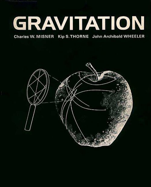
CHAPTER 1GEOMETRODYNAMICS IN BRIEF§1.1. THE PARABLE OF THE APPLEOne day in the year 1666 Newton had gone to the country,and seeing the fall of an apple, as his niece told me, let himselfbe led into a deep meditation on the cause which thusdraws every object along a line whose extension would passalmost through the center of the Earth.VOLTAIRE (1738)Once upon a time a student lay in a garden under an apple tree reflecting on thedifference between Einstein's and Newton's views about gravity. He was startledby the fall of an apple neiirby. As he looked at the apple, he noticed ants beginningto run along its surface (Figure l.l). His curiosity aroused, he thought to investigatethe principles of navigation followed by an ant. With his magnifying glass, he notedone track carefully, and, taking his knife, made a cut in the apple skin one mmabove the track and another cut one mm below it. He peeled off the resulting littlehighway of skin and laid it out on the face of his book. The track ran as straightas a laser beam along this highway. No more economical path could the ant havefound to cover the ten cm from start to end of that strip of skin. Any zigs andzags or even any smooth bend in the path on its way along the apple peel fromstarting point to end point would have increased its length."What a beautiful geodesic." the student commented.His eye fell on two ants starting off from a common point P in slightly differentdirections. Their routes happened to carry them through the region of the dimpleat the top of the apple. one on each side of it. Each ant conscientiously pursued

41. GEOMETRODYNAMICS IN BRIEF---Figure 1.1.The Riemannian geometry of the spacetime of general relativity is here symbolized by the two-dimensionalgeometry of the surface of an apple. The geodesic tracks followed by the ants on the apple'ssurface symbolize the world line followed through spacetime by a free particle. In any sufficiently localizedregion of spacetime, the geometry can be idealized as flat, as symbolized on the apple's two-dimensionalsurface' by the straight-line course of the tracks viewed in the magnifying glass ("local Lorentz character"of geometry of spacetime). In a region of greater extension, the curvature of the manifold (four-dimensionalspacetime in the case of the real physical world; curved two-dimensional geometry in the caseof the apple) makes itself felt. Two tracks (J and (fl, originally diverging from a commOn point

§1.2. SPACETIME WITH AND WITHOUT COORDINATES 5the world line that a satellite follows [in spacetime, around the Earth) is alreadyas straight as any world line can be. Forget all this talk about 'deflection' and 'forceof gravitation.' I'm inside a spaceship. Or I'm floating outside and near it. Do Ifeel any 'force of gravitation'? Not at all. Does the spaceship 'feel' such a force?No. Then why talk about it? Recognize that the spaceship and I traverse a regionof spacetime free of all force. Acknowledge that the motion through that regionis already ideally straight."The dinner bell was ringing, but still the student sat, musing to himself. "Let mesee if I can summarize Einstein's geometric theory of gravity in three ideas: (I)locally, geodesics appear straight: (2) over more extended regions ofspace and time,geodesics originally receding from each other begin to approach at a rate governedby the curvature of spacetime, and this effect of geometry on matter is what wemean today by that old word 'gravitation': (3) matter in turn warps geometry. Thedimple arises in the apple because the stem is there. I think I see how to put thewhole story even more briefly: Space acts on matter, telling it how to move. In turn,matter reacts back on space, telling it how to curve. In other words, matter here,"he said, rising and picking up the apple by its stem, "curves space here. To producea curvature in space here is to force a curvature in space there," he went on, ashe watched a lingering ant busily following its geodesic a finger's breadth away fromthe apple's stem. "Thus matter here influences matter there. That is Einstein'sexplanation for 'gravi tation.'''Then the dinner bell was quiet. and he was gone, with book, magnifying glass-andapple.Space tells matter how tomoveMatter tells space how tocurve§1.2. SPACETIME WITH AND WITHOUT COORDINATESNow it came to me: ... the independence of thegravitational acceleration from the nature of the fallingsubstance, may be expressed as follows: In agravitational field (of small spatial extension) thingsbehave as they do in a space free of gravitation. ... Thishappened in 1908. Why were another seven years requiredfor the construction of the general theory of relativity?The main reason lies in the fact that it is not so easy tofree oneself from the idea that coordinates must have animmediate metrical meaning.ALBERT EINSTEIN [in Schilpp (1949), pp. 65-67.]Nothing is more distressing on first contact with the idea of "curved spacetime" thanthe fear that every simple means of measurement has lost its power in this unfamiliarcontext. One thinks of oneself as confronted with the task of measuring the shapeof a gigantic and fantastically sculptured iceberg as one stands \vith a meter stickin a tossing rowboat on the surface of a hea\'ing ocean. Were it the rowboat itselfwhose shape were to be measured. the procedure would be simple enough. Onewould draw it up on shore. turn it upside down. and drive tacks in lightly at strategicpoints here and there on the surface. The measurement of distances from tack toProblem: how to measure incurved spacetime

6 1. GEOMETRODYNAMICS IN BRIEFFigure 1.2.The crossing of straws in a barn full of hay is a symbol for the world lines that fill up spacetime. Bytheir crossings and bends. these world lines mark events with a uniqueness beyond all need of coordinatesystems or coordinates. Typical events symbolized in the diagram, from left to right (black dots). are:absorption of a photon; reemission of a photon; collision between a particle and a particle: collisionbetween a photon and a particle; another collision between a photon and a particle; explosion of afirecracker; and collision of a particle from outside with one of the fragments of that firecracker.Resolution: characterizeevents by what happenstheretack would record and reveal the shape of the surface. The precision could be madearbitrarily great by making the number oftacks arbitrarily large. It takes more daringto think of driving several score pitons into the towering iceberg. But with all thedaring in the world, how is one to drive a nail into spacetime to mark a point?Happily, nature provides its own way to localize a point in spacetime, as Einsteinwas the first to emphasize. Characterize the point by what happens there! Give apoint in spacetime the name "event." Where the event lies is defined as clearly andsharply as where two straws cross each other in a barn full of hay (Figure 1.2). Tosay that the event marks a collision of such and such a photon with such and sucha particle is identification enough. The world lines of that photon and that particleare rooted in the past and stretch out into the future. They have a rich texture ofconnections with nearby world lines. These nearby world lines in turn are linkedin a hundred ways with world lines more remote. How then does One tell the locationof an event? Tell first what world lines participate in the event. Next follow each#'

7q\'lI,).r'-'t,'t,'t,b't,1>.'t,1-0?....S\'l"Isv' v' ,-" '....J;> C' cPII~-\l ::::. 30:-:2?J2624222018..,. ..,.'-

.8 1. GEOMETRODYNAMICS IN BRIEFThe name of an event caneven be arbitraryCoordinates provide aconvenient naming systemof these world lines. Name the additional events that they encounter. These eventspick out further world lines. Eventually the whole barn of hay is catalogued. Eachevent is named. One can find one's way as surely to a given intersection as the citydweller can pick his path to the meeting of St. James Street and_Piccadilly. Nonumbers. No coordinate s\'stem. No coordinates.That most streets in Japan have no names, and most houses no numbers, illustratesone's ability to do without coordinates. One can abandon the names of two worldlines as a means to identify the event where they intersect. Just as one could namea Japanese house after its senior occupant, so one can and often does attach arbitrarynames to specific events in spacetime. as in Box 1.1.Coordinates. however, are convenient. How else from the great thick catalog ofevents, randomly listed, can one easily discover that along a certain world line onewill first encounter event Trinity. then Baker, then Mike, then Argus-but not thesame events in some permuted order?To order events, introduce coordinates! (See Figure 1.3.) Coordinates are fourindexed numbers per event in spacetime; on a sheet of paper, only two. Trinityacquires coordinatesCoordinates generally do notmeasure lengthSeveral coordinate systemscan be used at onceVectorsIn christening events with coordinates, one demands smoothness but foregoes everythought ofmensuration. The four numbers for an eventare nothing but an elaboratekind of telephone number. Compare their "telephone" numbers to discover whethertwo events are neighbors. But do not expect to learn how many meters separatethem from the difference in their telephone numbers!Nothing prevents a subscriber from being served by competing telephone systems,nor an event from being catalogued by alternative coordinate systems (Figure 1.3).Box 1.1 illustrates the relationships between one coordinate system and another, aswell as the notation used to denote coordinates and their transformations.Choose two events, known to be neighbors by the nearness of their coordinatevalues in a smooth coordinate system. Draw a little arrow from one~,,:ent to theother. Such an arrow is called a vector. (It is a well-defined concept in fiilt spacetime,or in curved spacetime in the limit of vanishingly small length; for finite lengthsin curved spacetime, it must be refined and made precise, under the new name"tangent vector," on which see Chapter 9.) This vector, like events, can be givena name. But whether named "John" or "Charles" or "Kip," it is a unique, welldefinedgeometrical object. The name is a convenience, but the vector exists evenwithout it.Just as a quadruple of coordinatesis a particularly useful name for the event "Trinity" (it can be used to identify whatother events are nearby), so a quadruple of "components"

Box 1.1MATHEMATICAL NOTATION FOR EVENTS, COORDINATES, AND VECTORSEvents are denoted by capital script, one-letter Latin names such asSometimes subscripts are used:Coordinates of an event ~1' are denoted byor byor more abstractly bywhere it is understood that Greek indices can take on any value 0, 1,2. or 3.'!J', ;2, d, ~.1i.'!F0' ~:i", ~1'6'tU'). x(:1'). y(:1'), :('!F),XO(~11), x'(::I'). x 2 (:1').x 3 et'),x!L(~P) or x"(:1'),Time coordinate (when one of the four is picked to play this role)Space coordinates areand are sometimes denoted byIt is to be understood that Latin indices take on values I, 2. or 3.x'(~:I'), X2(~1'), X3(~1')xi(:·P) or Xk(~1') or ....Shorthand notation: One soon tires of writing explicitly the functional dependenceof the coordinates, x il (:1'); so one adopts the shorthand notationfor the coordinates of the event ~'P, andfor the space coordinates. One even begins to think of x il as representingthe event :1' itself, but must remind oneself that the values of xo, x', x 2 ,x 3 depend not only on the choice of ~P but also on the arbitrary choiceof coordinates!Other coordinates for the same event :1' may be denotedEXA~IPLE: In Figure 1.3 (XO, Xl) = (77 .2.22.6) and (xo. Xl) = (18.5.51.4)refer to the same event. The bars, priines, and hats distinguish onecoordinate system from another: by putting them on the indices ratherthan on the x·s. we simplify later notation.Transformation from one coordinate system to another is achieved by the fourfunctionswhich are denoted more succinctlySeparation vector* (little arrow) reaching from one event i! to neighboring event~.p can be denoted abstractly byIt can also be characterized by the coordinate-value ditferencest between:'1' and i! (called "components" of the vector).\a(~.p) or just x a ,X';'(:1') or just x a '.x"(:'p) or just x,i.XO(X O , Xl, x 2 • x 3 ).X 1 (Xo. xl, x 2 . x 3 ),x 2 (X O • x', x 2 • x 3 ),X 3 (X O • x', x 2 • x 3 ).xa(x B ).u or v or (. or :'1' -~" == .\"Ul) - x"(:':').~;\ == Xli(~.i') - .\"(i(.~2).i!.Transformation of components of a vector from one coordinate system to anotheris achieved by partial derivatives of transformation equationssince ~" = x"U'p) - X"(~') = (2x"i'x ll )[X il (:·P) - XIJ(:.:')).tEinstein summation com'ention is used here:any index that is repeated in a product is automatically slimmed on*This ddiniti,)n ,)1' a vector i, valid onl~ in tlat spacetime, The refined detinirion (.. tangcnt vcctor") ill cur\cd spacetimei, n,)t 'pdkd out here (see Chapkr 91. hut tlat-geomctr~ idea, apply with g,)od appnl:\illlati"n c\en in a curved geometr~.when the tl\O p,)ints are sut1i

10 1. GEOMETRODYNAMICS IN BRIEFis a convenient name for the vector "John" that reaches fromto(XO, xl, X 2 , X 3 ) = (78.2,22.1,64.0,13.1).Coordinate singularitiesnormally unavoidableContinuity of spacetimeThe mathematics ofmanifolds applied to thephysics of spacetimeDimensionality of spacetimeHow to work with the components of a vector is explored in Box 1.1.There are many ways in which a coordinate system can be imperfect. Figure 1.4illustrates a coordinate singularity. For another example of a coordinate singularity,run the eye over the surface of a globe to the North Pole. Note the many meridiansthat meet there ("coIlapse ofceIls ofegg crates to zero content"). Can't one do better?Find a single coordinate system that will cover the globe without singularity? Atheorem says no. Two is the minimum number of "coordinate patches" requiredto cover the two-sphere without singularity (Figure 1.5). This circumstance emphasizesanew that points and events are primary, whereas coordinates are a merebookkeeping device.Figures 1.2 and 1.3 show only a few world lines and events. A more detaileddiagram would show a maze of world lines and of light rays and the intersectionsbetween them. From such a picture, one can in imagination step to the idealizedlimit: an infinitely dense coIlection of light rays and of world lines of infinitesimaltest particles. With this idealized physical limit, the mathematical concept of acontinuous four-dimensional "manifold" (four-dimensional space with certainsmoothness properties) has a one-to-one correspondence; and in this limit continuous,differentiable (i.e., smooth) coordinate systems operate. The mathematics thensupplies a tool to reason about the physics.A simple countdown reveals the dimensionality of the manifold. Take a point ,:,7'in an n-dimensional manifold. Its neighborhood is an n-dimensional ball (i.e., theinterior of a sphere whose surface has n - I dimensions). Choose this ball so thatits boundary is a smooth manifold. The dimensionality of this manifold is (n - 1).In this (n - 1)-dimensional manifold, pick a point 2. Its neighborhood is an(n - I)-dimensional ball. Choose this baIl so that ... , and so on. Eventually onecomes by this construction to a manifold that is two-dimensional but is not yet knownto be two-dimensional (two-sphere). In this two-dimensional manifold, pick a point'3ll. Its neighborhood is a two-dimensional baIl ("disc"). Choose this disc so thatits boundary is a smooth manifold (circle). In this manifold, pick a point 9l. Itsneighborhood is a one-dimensional ball, but is not yet known to be one-dimensional("line segment"). The boundaries of this object are two points. This circumstancetells that the intervening manifold is one-dimensional; therefore the previous manifoldwas two-dimensional; and so on. The dimensionality of the original manifoldis equal to the number of points employed in the construction. For spacetime, thedimensionality is 4.This kind of mathematical reasoning about dimensionality makes good sense atthe everyday scale of distances, at atomic distances (10- 8 cm), at nuclear dimensions(10- 13 cm), and even at lengths smaller by several powers of ten, if one judges bythe concord between prediction and observation in quantum electrodynamics at high

= 1.8mr::: 111--r-----1r----t---t----+-------= _ mtr = 2.2m 2.4m 2.6m 2.8m 3.0mFigure 1.4.Howa mere coordinare singulariry arises. Above: A coordinare sysrem becomes singular when rhe "cellsin rhe egg crare" are squashed ro zero volume. Below: An example showing such a singulariry in rheSchwarzschild coordinares r, t offen used ro describe rhe geomerry around a black hole (Chaprer 31).For simpliciry rhe angular coordinares 0, ¢ have been suppressed. The singulanry shows itself in twoways. Firsr, all rhe poinrs along rhe doffed line. while quire disrincr one from anorher, are designaredby rhe same pair of(r. t) values: namely. r = 2m. t = 00. The coordinares provide no way ro disringuishrhese points. Second. rhe "cells in rhe egg crare." of which one is shown grey in rhe diagram. collapsero zero conrenr ar rhe doffed line. In summary, rhere is norhing srrange abour rhe geomerry ar rhe doffedline: all rhe singulariry lies in rhe coordinare sysrem ("poor sysrem ofrelephone numbers"). No confusionshould be permiffed ro arise from rhe accidenral circumsrance rhar rhe t coordinare affains an infinirevalue on rhe doffed line. No such infiniry would occur if I were replaced by rhe new coordinare t. definedby(t/2m) = ran(i/2m).When t = x. rhe new coordinare t is t = ':Tn!. The r, t coordinares srill provide no way ro disringuishrhe poinrs along rhe dorred line. They sriIl give "cells in rhe egg crare" collapsed ro zero conrenr alongrhe dOffed line.

Figure 1.5.Singularities in familiar coordinates on the two-sphere can be eliminated by covering the sphere withtwo overlapping coordinate patches. A. Spherical polar coordinate~, singular at the North and SouthPoles, and discontinuous at the international date line. B. Projection of the Euclidean coordinates ofthe Euclidean two-plane, tangent at the North Pole, onto the sphere via a line running to the SouthPole; coordinate singularity at the South Pole. C. Coverage of two-sphere by two overlapping coordinatepatches. One, constructed as in B, covers without singularity the northern hemisphere and also thesouthern tropics down to the Tropic of Capricorn. The other (grey) also covers without singularity allof the tropics and the southern hemisphere besides.Breakdown in smoothness ofspacetime at Planck lengthenergies (corresponding de Broglie wavelength 10- 16 em). Moreover, classical generalrelativity thinks of the spacetime manifold as a deterministic structure, completelywell-defined down to arbitrarily small distances. Not so quantum general relativityor "quantum geometrodynamics." It predicts violent fluctuations in the geometryat distances on the order of the Planck length,L * = (fiGj C 3 )1/2= [(1.054 X 10- 27 g cm 2 jsec)(6.670 X 10- 8 cm 3 jg sec 2 )j1/2 X= 1.616 X 10- 33 em.X (2.998 X 10 10 cmjsect 3 / 2 (1.1)No one has found any way to escape this prediction. As nearly as one can estimate,these fluctuations give space at small distances a "multiply connected" or "foamlike"character. This lack ofsmoothness may well deprive even the concept of dimensionalityitself of any meaning at the Planck scale of distances. The further explorationof this issue takes one to the frontiers of Einstein's theory (Chapter 44).Ifspacetime at small distances is far from the mathematical model ofa continuousmanifold, is there not also at larger distances a wide gap between the mathematical

§1.3. WEIGHTLESSNESS 13idealization and the physical reality? The infinitely dense collection of light raysand of world lines of infinitesimal test particles that are to define all the points ofthe manifold: they surely are beyond practical realization. Nobody has ever founda particle that moves on timelike world lines (finite rest mass) lighter than an electron.A collection of electrons, even if endowed with zero density of charge (e+ and e­world lines present in equal numbers) will have a density of mass. This density willcurve the very manifold under study. Investigation in infinite detail means unlimiteddensity, and unlimited disturbance of the geometry.However, to demand investigatability in infinite detail in the sense just describedis as out of place in general relativity as it would be in electrodynamics or gasdynamics. Electrodynamics speaks of the strength of the electric and magnetic fieldat each point in space and at each moment of time. To measure those fields, it iswilling to contemplate infinitesimal test particles scattered everywhere as denselyas one pleases. However, the test particles do not have to be there at all to givethe field reality. The field has everywhere a clear-cut value and goes about itsdeterministic dynamic evolution willy-nilly and continuously, infinitesimal testparticles or no infinitesimal test particles. Similarly with the geometry of space.In conclusion, when one deals with spacetime in the context of classical physics,one accepts (I) the notion of "infinitesimal test particle" and (2) the idealizationthat the totality ofidentifiable events forms a four-dimensional continuous manifold.Only at the end of this book will a look be taken at some of the limitations placedby the quantum principle on one's way of speaking about and analyzing spacetime.Difficulty in defininggeometry even at classicaldistances?No; one must acceptgeometry at classicaldistances as meaningful§1.3. WEIGHTLESSNESS"Gravity is a great mystery. Drop a stone. See it fall. Hear it hit. No one understandswhy." What a misleading statement! Mystery about fall? What else should the stonedo except fall? To fall is normal. The abnormality is an object standing in the wayof the stone. If one wishes to pursue a "mystery," do not follow the track of thefalling stone. Look instead at the impact, and ask what was the force that pushedthe stone away from its natural "world line," (Le., its natural track through spacetime).That could lead to an interesting issue of solid-state physics, but that is notthe topic of concern here. Fall is. Free fall is synonymous with weightlessness:absence of any force to drive the object away from its normal track through spacetime.Travel aboard a freely falling elevator to experience weightlessness. Or travelaboard a spaceship also falling straight toward the Earth. Or, more happily, travelaboard a spaceship in that state of steady fall toward the Earth that marks a circularorbit. In each case one is following a natural track through spacetime.The traveler has one chemical composition, the spaceship another; yet they traveltogether, the traveler weightless in his moving home. Objects ofsuch different nuclearconstitution as aluminum and gold fall with accelerations that agree to better thanone part in lOll, according to Roll, Krotkov, and Dicke (1964), one of the mostimportant null experiments in all physics (see Figure 1.6). Individual molecules fallin step, too, with macroscopic objects [Estermann, Simpson, and Stern (1938»): andso do individual neutrons [Dabbs, Harvey, Paya, and Horstmann (1965»). individual(coJllillued all page 16)Free fall is the natural stateof motionAll objects fall with the sameacceleration

14 1. GEOMETRODYNAMICS IN BRIEFFigure 1.6.Principle of the Roll-Krotkov-Dicke experiment. which showed that the grm'itational accelerations ofgold and aluminum are equal to I part in 1011 or better (Princeton, 1964). In the upper lefthand corner,equal masses of gold and aluminum hang from a supporting bar. This bar in turn is supported at itsmidpoint. If both objects fall toward the sun with the same acceleration of g = 0.59 cm/sec 2 • the bardoes not turn. If the Au mass receives a higher acceleration. g + 8g. then the gold end of the bar startsto turn toward the sun in the Earth-fixed frame. Twoelve hours laler the sun is on the other side. pullingthe other way. The ahernating torque lends itself to recognition against a background of noise becauseof its precise 24-hour period. Unhappily. any substamial mass nearby, such as an experimenter, locatedat M. will produce a torque that swamps the effect sought. Therefore the actual arrangement was asshown in the body of the figure. One gold weight and two aluminum weights were supported at thethree corners of a horizontal equilateral triangle. 6 cm on a side (three-fold axis of symmetry. givingzero response to all the simplest nonuniformities in the gravitational field). Also. the observers performedall operations remotely to eliminate their own gravitational effects". To detect a rotation of the torsionbalance as small as -10-" rad without disturbing the balance. Roll. Krotkov, and Dicke reflected avery weak light beam from the optically flat back face of the quartz triangle. The image of the sourceslit fell on a wire of about the same size as the slit image. The light transmitted past the wire fell ona photomultiplier. A separate oscillator circuit drove the wire back and forth across the image at 3,000hertz. When the image was centered perfectly, only even harmonics of the oscillation frequency appearedin the light intensity. However, when the image was displaced slightly to one side. the fundamentalfrequency appeared in the light intensity. The electrical output of the photomultiplier then containeda 3,OOO-hertz component. The magnitude and sign of this component were determined automatically.Equally automatically a proportional D.C. voltage was applied to the electrodes shown in the diagram.It restored the torsion balance to its zero position. The D.C. voltage required to restore the balance toits zero position was recorded as a measure of the torque acting on the pendulum. This torque wasFourier-analyzed over a period of many days. The magnitude of the Fourier component of 24-hourperiod indicated a ratio 8g/g = (0.96 ± 1.04) X 10- 11 • Aluminum and gold thus fall with the sameacceleration, despite their important differences summarized in the table.Ratios AI AuNumber of neutronsNumber of prolonsMass of kinetic energy of K-electronRest mass of eleclronEleetroslatic mass-energy of nucleusMass of atom1.08 1.50.005 0.160.001 0.004The theoretical implications of this experiment will be discussed in greater detail in Chapters 16 and 38.Braginsky and Panov (1971) at Moscow University performed an experiment identical in principleto that of Dicke-Roll-Krotkov, but with a modified experimental set-up. Comparing the accelerationsof platinum and aluminum rather than of gold and aluminum, they say that8g/g ~I X 10- 12 •"Other perturbations had to be, and were, guarded against. (I) A bit of iron on the torsion balanceas big as 10- 3 cm on a side would have contributed, in the Earth's magnetic field, a torque a hundredtimes greater than the measured torque. (2) The unequal pressure of radiation on the two sides of amass would have produced an unacceptably large perturbation if the temperature difference betweenthese two sides had exceeded 10- 4 OK. (3) Gas evolution from one side ofa mass would have propelledit like a rocket. If the rate of evolution were as great as 10- 8 g/day, the calculated force would havebeen - 10- 7 g cm/sec 2 , enough to affect the measurements. (4) The rotation was measured with respectto the pier that supported the equipment. As a guarantee that this pier did not itself rotate, it was anchoredto bed rock. (5) Electrostatic forces were eliminated; otherwise they would have perturbed the balance.

15AuEarth0• MAI'\ ...0.59 em! sec~0.59 cm!se c2}~0.59 cm/ secl I/' ---\ \Fused quartz fiber coaled with athin aluminum film to eliminatee1ecrrostat"rc fieldsLightemer!!esfro;nfixedslitSun alo .\.H.

16 1. GEOMETRODYNAMICS IN BRIEFelectrons [Witteborn and Fairbank (1967») and individual mu mesons [Beall (1970»).What is more, not one of these objects has to see out into space to know how tomove.Contemplate the interior ofa spaceship, and a key, penny, nut, and pea by accidentor design set free inside. Shielded from all view of the world outside by the wallsof the vessel, each object stays at rest relative to the vessel. Or it moves throughthe room in a straight line with uniform velocity. That is the lesson which experienceshouts out.Forego talk of acceleration! That, paradoxically, is the lesson of the circumstancethat "all objects fall with the same acceleration." Whose fault were those accelerations,after all? They came from allowing a groundbased observer into the act. TheBox 1.2MATERIALS OF THE MOST DIVERSE COMPOSITION FALL WITHTHE SAME ACCELERATION ("STANDARD WORLD LINE")Aristotle: "the downward movement of a mass ofgold or lead, or of any other body endowed withweight, is quicker in proportion to its size."Pre-Galilean literature: metal and wood weightsfall at the same rate.Galileo: (I) "the variation of speed in air betweenballs of gold, lead, copper, porphyry, and otherheavy materials is so slight that in a fall of 100cubits [about 46 meters] a ball ofgold would surelynot outstrip one of copper by as much as fourfingers. Having observed this, I came to the conclusionthat in a medium totally void of resistanceall bodies would fall with the same speed." (2)later experiments of greater precision "dilutinggravity" and finding same time of descent fordifferent objects along an inclined plane.Newton: inclined plane replaced by arc of pendulumbob; "time of fall" for bodies of differentcomposition determined by comparing time ofoscillation of pendulum bobs of the two materials.Ultimate limit of precision in such experimentslimited by problem ofdetermining effective lengthof each pendulum: (acceleration) = (2'7T/period)2(length).Lorand von Eotvos, Budapest, 1889 and 1922:compared on the rotating earth the vertical definedby a plumb bob of one material with the verticaldefined by a plumb bob of other material. Thetwo hanging masses, by the two unbroken threadsthat support them, were drawn along identicalworld lines through spacetime (middle of the laboratoryof Eotvos!). If cut free, would they alsofollow identical tracks through spacetime ("normalworld line of test mass")? If so, the accelerationthat draws the actual world line from the normalfree-fall world line will have a standard value, a.The experiment of Eotvos did not try to test agreementon the magnitude of a between the twomasses. Doing so would have required (1) cuttingthe threads and (2) following the fall of the twomasses. Eotvos renounced this approach in favorof a static observation that he could make withgreater precision, comparing the direction of a forthe two masses. The direction of the supportingthread, so his argument ran, reveals the directionin which the mass is being dragged away from itsnormal world line of "free fall" or "weightlessness."This acceleration is the vectorial resultantof (I) an acceleration of magnitude g, directedoutward against so-called gravity, and (2) an accelerationdirected toward the axis of rotation ofthe earth, of magnitude w 2 R sin 8 (w, angular ve-

§ 1.3. WEIGHTLESSNESS 17push of the ground under his feet was driving him away from a natural world line.Through that flaw in his arrangements, he became responsible for all those accelerations.Put him in space and strap rockets to his legs. No difference!* Again theresponsibility for what he sees is his. Once more he notes that "all objects fall with'''No difference" spelled out amounts to Einstein's (1911) principle of the local equivalence between a"gravitational field" and an acceleration: "We arrive at a very satisfactory Interpretation of this law ofexperience, if we assume that the systems K and K' are physically exactly equivalent, that is, if we assumethat we may just as well regard the system K as being in a space free from gravitational fields, if we thenregard K as uniformly accelerated. This assumption of exact physical equivalence makes it impossible forus to speak of the absolute acceleration of the system of reference, just as the usual theory of relativityforbids us to talk of the absolute velocity of a system; and it makes the equal falling of all bodies in agravitational field seem a matter of course."locity; R, radius of earth; 8, polar angle measuredfrom North Pole to location of experiment). Thiscentripetal acceleration has a vertical component_w 2 R sin 2 8 too small to come into discussion.The important component is w 2 R sin 8 cos 8, directednorthward and parallel to the surface of theearth. It deflects the thread by the anglehorizontal accelerationvertical accelerationw 2 R sin 8 cos 8=g= 3.4 em!sec 2 sin 8 cos 8980 cm!sec 2= 1.7 X 10- 3 radian at 8 = 45 °from the straight line connecting the center of theearth to the point of support. A difference, og, ofone part in 10 8 between g for the two hangingsubstances would produce a difference in angle ofhang of plumb bobs equal to 1.7 X 10- 11 radianat Budapest (8 = 42.5°). Eotvos reported og!g lessthan a few parts in 10 9 .Roll, Krotkov, and Dicke, Princeton, 1964: employedas fiducial acceleration, not the 1.7 cm!sec 2steady horizontal acceleration, produced by theearth's rotation at 8 = 45 0, but the daily alternating0.59 cm!sec 2 produced by the sun's attraction.Reported Ig(Au) - g(Al)l!g less than 1 X 10- 11 .See Figure 1.6.Braginsky and Panov, Moscow, 1971: like Roll,Krotkov, and Dicke, employed Sun's attraction asfiducial acceleration. Reported Ig(Pt) - g(Al)I!gless than 1 X 10- 12 .Beall, 1970: particles that are deflected less by theEarth's or the sun's gravitational field than a photonwould be, effectively travel faster than light.If they are charged or have other electromagneticstructure, they would then emit Cerenkov radiation,and reduce their velocity below threshold inless than a micron of travel. The threshold is atenergies around 10 3 mc 2 . Ultrarelativistic particlesin cosmic-ray showers are not easily identified, butobservations of 10 13 eV muons show that muonsare not "too light" by as much as 5 X 10- 5 . Conversely,a particle P bound more strongly thanphotons by gravity will transfer the momentumneeded to make pair production y ~ P + Poccurwithin a submicron decay length. The existence ofphotons with energies above 10 13 eV shows thate± are not "too heavy" by 5 parts in 10 9 , IJ.± notby 2 in 10\ A, ;:-, g- not by a few per cent.

181. GEOMETRODYNAMICS IN BRIEFLJJlLFigure 1.7."Weightlessness" as test for a local inertial frame of reference ("Lorentz frame"). Each spring-drivencannon succeeds in driving its projectile, a steel ball bearing, through the aligned holes in the sheetsof lucite, and into the woven-mesh pocket, when the frame of reference is free of rotation and in freefall ("normal world line through spacetime"). A cannon would fail (curved and ricocheting trajectoryat bottom of drawing) if the frame were hanging as indicated when the cannon went off ("frame drawnaway by pull of rope from its normal world line through spacetime"). Harold Waage at Princeton hasconstructed such a model for an inertial reference frame with lucite sheets about I m square. The "fuses"symbolizing time delay were replaced by electric relays. Penetration fails if the frame (1) rotates, (2)accelerates, or (3) does any combination of the two. It is difficult to cite any easily realizable devicethat more fully illustrates the meaning of the term "local Lorentz frame."Eliminate the acceleration byuse of a local inertial framethe same acceleration." Physics looks as complicated to the jet-driven observer asit does to the man on the ground. Rule out both observers to make physics looksimple. Instead, travel aboard the freely moving spaceship. Nothing could be morenatural than what one sees: every free object moves in a straight line with uniformvelocity. This is the way to do physics! Work in a very special coordinate system:a coordinate frame in which one is weightless; a local inertial frame of reference.Or calculate how things look in such a frame. Or-if one is constrained to a groundbasedframe ofreference-use a particle moving so fast, and a path length so limited,that the ideal, freely falling frame of reference and the actual ground-based frameget out of alignment by an amount negligible on the scale ofthe experiment. [Givena 1,500-m linear accelerator, and a I GeV electron, time of flight ~ (1.5 X 10 5 cm)/

§1.4. GEOMETRY IS LOCALLY LORENTZIAN 19(3 X 10 10 em/sec) = 0.5 X 10- 5 sec; fall in this time _~gt2 = (490 cm/sec 2 )(0.5 X10- 5 sec)2 ~ 10- 8 em.]In analyzing physics in a local inertial frame of reference, or following an anton his little section of apple skin, one wins simplicity by foregoing every referenceto what is far away. Physics is simple only when viewed locally: that is Einstein'sgreat lesson.Newton spoke differently: "Absolute space, in its own nature, without relationto anything external, remains always similar and immovable." But how does onegive meaning to Newton's absolute space, find its cornerstones, mark out its straightlines? In the real world of gravitation, no particle ever follows one of Newton'sstraight lines. His ideal geometry is beyond observation. "A comet going past thesun is deviated from an ideal straight line." No. There is no pavement on whichto mark out that line. The "ideal straight line" is a myth. It never happened, andit never will."It required a severe struggle [for Newton) to arrive at the concept of independentand absolute space, indispensible for the development of theory.... Newton's decisionwas, in the contemporary state of science, the only possible one, and particularly theonly fruitful one. But the subsequent development of the problems, proceeding in aroundabout way which no one could then possibly foresee, has shown that the resistanceof Leibniz and Huygens, intuitively well-founded but supported by inadequate arguments,was actuallyjustified.... It has required no less strenuous exertions subsequentlyto overcome this concept [of absolute space)"[A. EINSTEIN (1954»).What is direct and simple and meaningful, according to Einstein, is the geometryin every local inertial reference frame. There every particle moves in a straight linewith uniform velocity. Define the local inertial frame so that this simplicity occursfor the first few particles (Figure 1.7). In the frame thus defined, every other freeparticle is observed also to move in a straight line with uniform velocity. Collisionand disintegration processes follow the laws of conservation of momentum andenergy of special relativity. That all these miracles come about, as attested by tensof thousands of observations in elementary particle physics, is witness to the innerworkings of the machinery of the world. The message is easy to summarize: (l)physics is always and everywhere locally Lorentzian; i.e., locally the laws of specialrelativity are valid; (2) this simplicity shows most clearly in a local Lorentz frameof reference ("inertial frame of reference"; Figure 1.7); and (3) to test for a localLorentz frame, test for weightlessness!Newton's absolute space isunobservable, nonexistentBut Einstein's loca,l inertialframes exist, are simpleIn local inertial frames,physics is Lorentzian§1.4. LOCAL LORENTZ GEOMETRY,WITH AND WITHOUT COORDINATESOn the surface of an apple within the space of a thumbprint, the geometry isEuclidean (Figure 1.1; the view in the magnifying glass). In spacetime, within alimited region, the geometry is Lorentzian. On the apple the distances between pointand point accord with the theorems of Euclid. In spacetime the intervals ("properdistance," "proper time") between event and event satisfy the corresponding theoremsof Lorentz-Minkowski geometry (Box 1.3). These theorems lend themselves(continued 011 page 23)Local Lorentz geometry is thespacetime analog of localEuclidean geometry.

20 1. GEOMETRODYNAMICS IN BRIEFBox 1.3LOCAL LORENTZ GEOMETRY AND LOCAL EUCLIDEAN GEOMETRY:WITH AND WITHOUT COORDINATES1. Local Euclidean GeometryWhat does it mean to say that the geometry ofa tiny thumbprint on the apple is Euclidean?A. Coordinatejree language (Euclid):Given a line de. Extend it by an equaldistance e:z. Let ~t3 be a point not on d:;:":but equidistant from d and :=. Then(Theorem of Pythagoras; also other theoremsof Euclidean geometry.)B. Language of coordinates (Descartes):From any point d to any other point ~13there is a distance s given in suitable (Euclidean)coordinates bystl,,l = [x 1 Ut3) - x 1 (d)j2 + [x 2 (:t3) - x 2 (d)j2.If one succeeds in finding any coordinatesystem where this is true for all points dand ~13 in the thumbprint, then one is guaranteedthat (i) this coordinate system islocally Euclidean, and (ii) the geometry ofthe apple's surface is locally Euclidean.tI---~{/x 2 = 12t'J1/JII{//"N ("fj ..::t V')IIII-~ -~ -~ -~•",'II.Local Lorentz GeometryWhat does it mean to say that the geometry ofa sufficiently limited region of spacetime in thereal physical world is Lorentzian?A. Coordinatejree language (Robb 1936):Let d:z be the world line of a free particle.Let ~B be an event not on this world line.Let a light ray from ~3 strike d:z at theevent f2. Let a light ray take off from suchan earlier event

§1.4. GEOMETRY IS LOCALLY LORENTZIAN21:E1 + x !2Proof of above criterion for local Lorentzgeometry, using coordinate methods in thelocal Lorentz frame where particle remainsat rest:1(nl = t 2 - X 2 = (t - X)(t + x)= 1 (/'}'1(/Z.1- X '3'o(/xB. Language ofcoordinates (Lorentz, Poincare,Minkowski, Einstein):From any event d to any other nearbyevent ~i3, there is a proper distance Sd

Box 1.3 (continued)IV.Local Geometry in the Language ofModern Mathematics -A. The metric for any manifold:At each point on the apple, at each eventof spacetime, indeed, at each point of any"Riemannian manifold." there exists a geometricalobject called the metric tensor g.lt is a machine with two input slots for theinsertion of two vectors:slot 1 slot 2+ +g(Ifone insertsthe same vectoru intobothslots,one gets out the square of the length of u:g(u, u) = u 2 •If one inserts two different vectors, u and v(it matters not in which order!), one gets outa number called the "scalar product ofu onv" and denoted u· v:g(u, v) = g(v, u) = u· v = v· u.The metric is a linear machine:g(2u + 3w, v) = 2g(u, v) + 3g(w, v),g(u, av + bw) = ag(u, v) + bg(u, w).Consequently, in a given (arbitrary) coordinatesystem, its operation on two vectors canbe written in terms of their components as abilinear expression:g(u, v) = ga(3u a v(3(implied summation on 0:, 13)= gnu1v1 + g12u1v2 + g21 u2v1 + ....The quantities ga(3 = g(3a (0: and 13 runningfrom 0 to 3 in spacetime, from 1 to 2 on theapple) are called the "components ofgin thegiven coordinate system."B. Components ofthe metric in local Lorentz andlocal Euclidea~ frames:To connect the metric with our previous descriptionsof the local geometry, introduce).local Euclidean coordinates (on apple) orlocal Lorentz coordinates (in spacetime).v7 ,,' .'Let ( be the separation vector reaching fromd to ~jj. lts components in the local Euclidean(Lorentz) coordinates are~a = xa(~13) - xa(d)(cf. Box 1.1). Then the squared length ofUd,';'which is the same as the squared distancefrom d tO~1j, must be (cf. LB. and 11.B. above)(. ( = g«(, () = ga(3~a~(3= sdi = (~1)2 + (e)2 on apple= _ (~O)2 + (~1f + (~2)2 + (e)2in spacetime.Consequently, the components of the metricaregu = g22 = 1, g12 = g21 = 0;i.e., gfr(3 = 0a(3 on apple, inlocal Euclideancoordinates;goo = -I, gOk = 0, gjk = 0jkin spacetime, inlocal Lorentzcoordinates.These special components of the metric inlocal Lorentz coordinates are written hereand hereafter as g,,{3 or 1/a(3' by analogywith the Kronecker delta 0a(3' In matrixnotation:- f3---+o1 2 3o -1 0 0 01 0 1 0 02 0 0 1 03 0 0 0 1,-------------------------~

§1.5. TIME 23to empirical test in the appropriate, very special coordinate systems: Euclideancoordinates in Euclidean geometry; the natural generalization of Euclidean coordinates(local Lorentz coordinates; local inertial frame) in the local Lorentz geometryof physics. However, the theorems rise above all coordinate systems in their content.They refer to intervals or distances. Those distances no more call on coordinatesfor their definition in our day than they did in the time of Euclid. Points in thegreat pile of hay that is spacetime; and distances between these points: that isgeometry! State them in the coordinate-free language or in the language of coordinates:they are the same (Box 1.3).§ 1.5. TIMETime is defined so that motion looks simple.Time is awake when all things sleep.Time stands straight when all things fall.Time shuts in all and will not be shut.Is, was, and shall be are Time's children.a Reasoning, be witness, be stable.VYASA, the Mahabarata (ca. A.D. 400)Relative to a local Lorentz frame, a free particle "moves in a straight line withuniform velocity." What "straight" means is clear enough in the model inertialreference frame illustrated in Figure 1.7. But where does the "uniform velocity" comein? Or where does "velocity" show itself? There is not even one clock in the drawing!A more fully developed model of a Lorentz reference frame will have not onlyholes, as in Fig. 1.7, but also clock-activated shutters over each hole. The projectilecan reach its target only if it (l) travels through the correct region in space and(2) gets through that hole in the correct interval of time ("window in time"). Howthen is time defined? Time is defined so that motion looks simple!No standard of time is more widely used than the day, the time from one highnoon to the next. Take that as standard, however, and one will find every good clockor watch clashing with it, for a simple reason. The Earth spins on its axis and alsorevolves in orbit about the sun. The motion of the sun across the sky arises fromneither effect alone, but from the two in combination, different in magnitude thoughthey are. The fast angular velocity of the Earth on its axis (roughly 366.25 completeturns per year) is wonderfully uniform. Not so the apparent angular velocity of thesun about the center of the Earth (one turn per year). It is greater than averageby 2 per cent when the Earth in its orbit (eccentricity 0.017) has come 1 per centcloser than average to the sun (Kepler's law) and lower by 2 per cent when theEarth is 1 per cent further than average from the sun. In the first case, the momentaryrate ofrotation ofthe sun across the sky, expressed in turns per year, is approximatelyThe time coordinate of alocal Lorentz frame is sodefined that motion lookssimple366.25 - (l + 0.02);

241. GEOMETRODYNAMICS IN BRIEFin the other,366.25 - (1 - 0.02).Taking the "mean solar day" to contain 24 X 3.600 = 86,400 standard seconds, onesees that, when the Earth is 1per cent closer to (or further from) the sun than average,then the number of standard seconds from one high noon to the next is greater(or less) than normal by0.02 (drop in turns per year) 86400 _ 47, sec . sec.365.25 (turns per year on average)This is the bookkeeping on time from noon to noon. No standard of time that variesso much from one month to another is acceptable. If adopted, it would make thespeed of light vary from month to month!This lack of uniformity, once recognized (and it was already recognized by theancients), forces one to abandon the solar day as the standard of time; that daydoes not make motion look simple. Turn to a new standard that eliminates the motionof the Earth around the sun and concentrates on the spin of the Earth about itsaxis: the sidereal day, the time between one arrival of a star at the zenith and thenext arrival of that star at the zenith. Good! Or good, so long as one's precisionof measurement does not allow one to see changes in the intrinsic angular velocityof the Earth. What clock was so bold as first to challenge the spin of the Earth foraccuracy? The machinery of the heavens.Halley (1693) and later others, including Kant (1754), suspected something wasamiss from apparent discrepancies between the paths of totality in eclipses of thesun, as predicted by Newtonian gravitation theory using the standard of time thencurrent, and the location of the sites where ancient Greeks and Romans actuallyrecorded an eclipse on the day in question. The moon casts a moving shadow inspace. On the day of a solar eclipse, that shadow paints onto the disk of the spinningEarth a black brush stroke, often thousands of kilometers in length, but of widthgenerally much less than a hundred kilometers. He who spins the globe upon thetable and wants to make the shadow fall rightly on it must calculate back meticulouslyto determine two key items: (1) where the moon is relative to Earth and sunat each moment on the ancient day in question; and (2) how much angle the Earthhas turned through from then until now. Take the eclipse of Jan. 14, A.D. 484, asan example (Figure 1.8), and assume the same angular velocity for the Earth inthe intervening fifteen centuries as the Earth had in 1900 (astronomical referencepoint). One comes out wrong. The Earth has to be set back by 30° (or the moonmoved from its computed position, or some combination of the two effects) to makethe Athens observer fall under the black brush. To catch up those 30° (or less, ifpart of the effect is due to a slow change in the angular momentum of the moon),the Earth had to tum faster in the past than it does today. Assigning most of thediscrepancy to terrestrial spin-down (rate of spin-down compatible with modernatomic-clock evidence), and assuming a uniform rate of slowing from then to now

25I I I I Io 200 400 km.A: 'Observed' track.. B: Computed track iflength of day constantWE20 0 EFigure 1.8.Calculated path of totality for the eclipse of January 14, A.D. 484 (left; calculation based on no spin-downof Earth relative to its 1900 angular velocity) contrasted with the same path as set ahead enough toput the center of totality (at sunrise) at Athens [displacement very close to 30°; actual figure of decelerationadopted in calculations, 32.75 arc sec/(century)2). This is "undoubtedly the most reliable of all ancientEuropean eclipses," according to Dr. F. R. Stephenson, of the Department of Geophysics and PlanetaryPhysics of the University of Newcastle upon Tyne, who most kindly prepared this diagram especiallyfor this book. He has also sent a passage from the original Greek biography of Proclus of Athens (diedat Athens A.D. 485) by Marinus of Naples, reading, "Nor were there portents wanting in the year whichpreceded his death; for example, such a great eclipse of the Sun that night seemed to fall by day. Fora profound darkness arose so that stars even appeared in the sky. This happened in the eastern skywhen the Sun dwelt in Capricorn" [from Westermann and Boissonade (1878»).Does this 30° for this eclipse, IOgether with corresponding amounts for other eclipses, represent the"right" correction? "Right" is no easy word. From one total eclipse of the sun in the Mediterraneanarea to another is normally many years. The various provinces of the Greek and Roman worlds werefar from having a uniform level of peace and settled life, and even farther from having a uniform standardof what it is to observe an eclipse and put it down for posterity. If the scores of records of the pastare unhappily fragmentary, even more unhappy has been the willingness of a few uncritical "investigators"in recent times to rush in and identify this and that historical event with this and that calculated eclipse.Fortunately, by now a great literature is available on the secular deceleration of the Earth's rotation,in the highest tradition of critical scholarship, both astronomical and historical. In addition to the booksof o. Neugebauer (1959) and Munk and MacDonald (1960). the paper of Curott (1966), and items citedby these workers, the following are key items. (For direction to them, we thank Professor Otto Neugebauer-norelation to the other Neugebauer cited below!) For the ancient records, and for calculationsof the tracks of ancient eclipses, F. K. Ginzel (1882, 1883, 1884): for an atlas of calculated eclipse tracks,Oppolzer (1887) and Ginzel (1899); and for a critical analysis of the e\idence. P. V. Neugebauer (1927,1929, and 1930). This particular eclipse was chosen rather than any other because of the great reliabilityof the historical record of it.

26 1. GEOMETRODYNAMICS IN BRIEF(angular velocity correction proportional to first power of elapsed time: angle correctionitself proportional to square ofelapsed time), one estimates from a correctionof30° or 2 hours 1,500 years agothe following corrections for intermediate times:30° /10 2 , or 1.2 min30° /10'\ or 0.8 sec150 years ago,15 years ago.Good clocks make spacetimetrajectories of free particleslook straightThus one sees the downfall of the Earth as a standard of time and its replacementby the orbital motions of the heavenly bodies as a better standard: a standard thatdoes more to "make motion look simple." Astronomical time is itself in turn todaybeing supplanted by atomic time as a standard of reference (see Box lA, "TimeToday").Look at a bad clock for a good view of how time is defined. Let t be time ona "good" clock (time coordinate of a local inertial frame); it makes the tracks offree particles through the local region of spacetime look straight. Let T(t) be thereading of the "bad" clock; it makes the world lines of free particles through thelocal region of spacetime look curved (Figure 1.9). The old value of the acceleration,translated into the new ("bad") time, becomes0= d 2 x = .!J....(dT dX) = d 2 T dx + (dT)2 d 2 x.dt 2 dt dt dT dt 2 dT dt dT2To explain the apparent accelerations of the particles, the user of the new timeintroduces a force that one knows to be fictitious:(l.2)Our choice of unit formeasuring time: thegeometrodynamic centimeter.It is clear from this example of a "bad" time that Newton thought of a "good" timewhen he set up the principle that "Time flows uniformly" (d 2 T/dt 2 = 0). Time isdefined to make motion look simple!The principle of uniformity, taken by itself, leaves free the scale of the timevariable. The quantity T = at + b satisfies the requirement as well as t itself. Thehistory of timekeeping discloses many choices of the unit and origin of time. Eachone required some human action to give it sanction, from the fiat of a Pharaoh tothe communique of a committee. In this book the amount of time it takes light totravel one centimeter is decreed to be the unit of time. Spacelike intervals andtimelike intervals are measured in terms of one and the same geometric unit: thecentimeter. Any other decision would complicate in analysis what is simple in nature.No other choice would live up to Minkowski's words, "Henceforth space by itself,and time by itself, are doomed to fade away into mere shadows, and only a kindof union of the two will preserve an independent reality."

§1.5. TIME 27t(ItTI-x~-x~Figure 1.9.Good clock (left) vs. bad clock (right) as seen in the maps they give of the same free particles movingthrough the same region of spacetime. The world lines as depicted at the right give the impression thata force is at work. The good definition of time eliminates such fictitious forces. The dashed lines connectcorresponding instants on the two time scales.One can measure time more accurately today than distance. Is that an argumentagainst taking the elementary unit to be the centimeter? No, provided that thisdefinition of the centimeter is accepted: the geometrodynamic standard centimeteris the fraction1/(9.460546 X 10 17 ) (1.3)of the interval between the two "effective equinoxes" that bound the tropical year1900.0. The tropical year 1900.0 has already been recognized internationally as thefiducial interval by reason ofits definiteness and the precision with which it is known.Standards committees have defined the ephemeris second so that 31,556,925.974 secmake up that standard interval. Were the speed oflight known with perfect precision,the standards committees could have given in the same breath the number ofcentimeters in the standard interval. But it isn't; it is known to only six decimals.Moreover, the international centimeter is defined in terms of the orange-red wavelengthof Kr 86 to only nine decimals (16,507.6373 wavelengths). Yet the standardsecond is given to 11 decimals. We match the standard second by arbitrarily definingthe geometrodynamic standard centimeter so that9.4605460000 X 10 17such centimeters are contained in the standard tropical year 1900.0. The speed oflight then becomes exactly9.4605460000 X 10 17 •31,556,925.974 geometrodynamlc cm/sec. (1.4)This is compatible with the speed oflight, as known in 1967, in units of"internationalcm/sec":29,979,300,000 ± 30,000 international cm/sec.

~----------...Box 1.4TIME TODAYPrior to 1956 the second was defined as the fraction1/86,400 of the mean solar day.From 1956 to 1967 the· "second" meant theephemeris second, defined as the fraction1/(31,556,925.9747) of the tropical yearOOhOOmOOs December 31, 1899.Since 1967 the standard second has been theSI (Systeme International) second, defined as9,192,631,770 periods of the unperturbed microwavetransition between the two hyperfine levelsof the ground state of CS133.Like the foregoing evolution of the unit for thetime interval, the evolution of a time coordinatehas been marked by several stages.Universal time, UTO, is based on the count ofdays as they actually occurred historically; in otherwords, on the actual spin of the earth on its axis;historically, on mean solar time (solar position ascorrected by the "equation of time"; i.e., the fastertravel of the earth when near the sun than whenfar from the sun) as determined at GreenwichObservatory.UTI, the "navigator's time scale," is the sametime as corrected for the wobble of the earth onits axis (..1t - 0.05 sec).UT2 is UTI as corrected for the periodic fluctuationsof unknown origin with periods of onehalfyear and Qne year (..1t - 0.05 sec; measuredto 3 ms in one day).Ephemeris Time, ET (as defined by the theoryof gravitation and by astronomical observationsand calculations), is essentially determined by theorbital motion of the earth around the sun."Measurement uncertainties limit the realizationof accurate ephemeris time to about 0.05 sec fora nine-year average."Coordinated Universal Time (UTC) is broadcaston stations such as V,rWV. It was adopted internationallyin February 1971 to become effective January1,1972. The clock rate is controlled by atomicclocks to be as uniform as possible for one year(atomic time is measured to -0.1 microsec in 1min, with diffusion rates of 0.1 microsec per dayfor ensembles of clocks), but is changed by theinfrequent addition or deletion ofa second-calleda "leap second"-so that UTC never differs morethan 0.7 sec from the navigator's time scale, UTI.THE TIMESWednesdayJune 21 1972The foregoing account is abstracted from J. A.Barnes (1971). The following is extracted from atable (not official at time of receipt), kindly suppliedby the Time and Frequency Division of theU.S. National Bureau of Standards in Boulder,Colorado.Timekeeping capabilities ofsome familiar clocksare as follows:Tuning fork wrist watch (1960),1 min/mo.Quartz crystal clock (1921-1930),1 fLsec/day,1 sec/yr.Quartz crystal wrist watch (1971),0.2 sec/2 mos.,1 sec/yr.Cesium beam (atomic resonance, CS133), (1952­1955),0.1 fLsec/day,0.5 fLsec/mo.Rubidium gas cell (Rb 8i resonance), (1957),0.1 fLsec/ day,1-5 fLsec/mo.Hydrogen maser (1960),0.Q1 fLsec/2 hr,0.1 fLsec/day.Time suspendedfor a second ~Time will stand still throughoutthe world for one ~ccond at midnight.June 30. All radio timesignal~ will insert a .. leap !iecond ..to bring Greenwich Mean Time intoline with the earth's los~ of threethousandths of a second a day.The signal from the Royal GreenwichOhservatory to BroadcastingHouse at midnight GMT (I amBST July I) wH1 be six short pipsmarking the seconds 55 to 60 inclusive,followed by a lengthened signalat the following second to marktho new minute.Methane stabilized laser (1969),0.Q1 fLsec/IOO sec.

§1.6. CURVATURE 29Recent measurements [Evenson et at. (1972)] change the details of the foregoing1967 argument, but not the principles.§1.6. CURVATUREGravitation seems to have disappeared. Everywhere the geometry of spacetime islocally Lorentzian. And in Lorentz geometry, particles move in a straight line withconstant velocity. Where is any gravitational deflection to be seen in that? Foranswer, turn back to the apple (Figure 1.1). Inspect again the geodesic tracks ofthe ants on the surface of the apple. Note the reconvergence of two nearby geodesicsthat originally diverged from a common point. What is the analog in the real worldof physics? What analogous concept fits Einstein's injunction that physics is onlysimple when analyzed locally? Don't look at the distance from the spaceship to theEarth. Look at the distance from the spaceship to a nearby spaceship! Or, to avoidany possible concern about attraction between the two ships, look at two nearbytest particles in orbit about the Earth. To avoid distraction by the nonlocal element(the Earth) in the situation, conduct the study in the interior of a spaceship, alsoin orbit about the Earth. But this region has already been counted as a local inertialframe! What gravitational physics is to be seen there? None. Relative to the spaceshipand therefore relative to each other, the two test particles move in a straight linewith uniform velocity, to the precision of measurement that is contemplated (seeBox 1.5, "Test for Flatness"). Now the key point begins to appear: precision ofmeasurement. Increase it until one begins to discern the gradual acceleration of thetest particles away from each other, if they lie along a common radius through thecenter of the Earth; or toward each other, if their separation lies perpendicular tothat line. In Newtonian language, the source of these accelerations is the tide-producingaction of the Earth. To the observer in the spaceship, however, no Earthis to be seen. And following Einstein, he knows it is important to analyze motionlocally. He represents the separation of the new test particle from the fiducial testparticle by the vector ~k(k = 1,2,3; components measured in a local Lorentz frame).For the acceleration of this separation, one knows from Newtonian physics whathe will find: if the Cartesian z-axis is in the radial direction, thenGravitation is manifest inrelative acceleration ofneighboring test particles(1.5)Proof: In Newtonian physics the acceleration of a single particle toward the centerof the Earth in conventional units of time is Gmconv/r2, where G is the Newtonianconstant of gravitation, 6.670 X 10- 8 cm 3 /g sec 2 and m conv is the mass of the Earthin conventional units of grams. In geometric units of time (cm of light-travel time).

301. GEOMETRODYNAMICS IN BRIEFRelative acceleration iscaused by curvaturethe acceleration is Gl11 eonv/ c 2 r 2 • When the two particles are separated by a distance~ perpendicular to r, the one downward acceleration vector is out of line with theother by the angle ~/r. Consequently one particle accelerates toward the other bythe stated amount. When the separation is parallel to r, the relative accelerationis given by evaluating the Newtonian acceleration at r and at r + ~, and taking thedifference (~times d/dr) Q.E.D. In conclusion, the "local tide-producing acceleration"of Newtonian gravitation theory provides the local description of gravitation thatEinstein bids one to seek.What has this tide-producing acceleration to do with curvature? (See Box 1.6.)Look again at the apple or, better, at a sphere of radius a (Figure 1.10). Theseparation of nearby geodesics satisfies the "equation of geodesic deviation,"d2~/ds 2 + R~ = O.(1.6)Here R = l/a 2 is the so-called Gaussian curvature of the surface. For the surfaceof the apple, the same equation applies, with the one difference that the curvatureR varies from place to place.Box 1.5TEST FOR FLATNESS1. Specify the extension in space L (cm or m)and extension in time T (cm or m of light traveltime) of the region under study.2. Specify the precision o~ with which one canmeasure the separation of test particles in thisregion.3. Follow the motion of test particles movingalong initially parallel world lines through thisregion of spacetime.4. When the world lines remain parallel to theprecision o~ for all directions of travel, then onesays that "in a region so limited and to a precisionso specified, spacetime is flat."EXAMPLE:Region just above the surface of theearth, 100 m X 100 m X 100 m (space extension),followed for 10 9 m of light-travel time (T eonv ­3 sec). Mass of Earth, m eonv= 5.98 X 10 2 ; g,m = (0.742 X 10- 28 cm/g) X (5.98 X 10 2 ; g) =0.444 cm [see eq. (1.12)]. Tide-producing accelerationR Z OzO (relative acceleration in z-direction oftwo test particles initially at rest and separatedfrom each other by 1 cm of vertical elevation) is(d/dr)(m/r 2 ) = -2m/r 3= -0.888 cm/(6.37 X 10 8 cm)3= -3.44 X 10- 2 ; cm- 2("cm of relative displacement per cm of lighttraveltime per cm of light-travel time per cm ofvertical separation"). Two test particles with a verticalseparation ~z = 10 4 cm acquire in the timet = 1011 cm (difference between time and propertime negligible for such slowly moving test particles)a relative displacemento~z= -~Rzozot2~Z= 1.72 X 10- 2 ; cm- 2 (lOll cm)2 10 4 cm= 1.72 mm.(Change in relative separation less for other directionsof motion). When the minimum uncertaintyo~ attainable in a measurement over a 100 mspacing is "worse" than this figure (exceeds 1.72mm), then to this level of precision the region ofspacetime under consideration can be treated asflat. When the uncertainty in measurement is"better" (less) than 1.72 mm, then one must limitattention to a smaller region of space or a shorterinterval of time or both, to find a region of spacetimethat can be regarded as flat to that precision.

§ 1.6. CURVATURE31Figure 1.10.Curvature as manifested in the "acceleration of the separation" of twonearby geodesics. Two geodesics, originally parallel, and separated by thedistance ("geodesic deviation") ~o, are no longer parallel when followeda distance s. The separation is ~ := ~o cos

~-------Box 1.6CURVATURE OF WHAT?Nothing seems more attractive at first glance thanthe idea that gravitation is a manifestation of thecurvature of space (A)-, and nothing more ridiculousat a second glance (B). How can the tracksof a ball and of a bullet be curved so differentlyif that curvature arises from the geometry ofspace? No wonder that great Riemann did not givethe world a geometric theory of gravity. Yes, atthe age of 28 (June 10, 1854) he gave the worldthe mathematical machinery to define and calculatecurvature (metric and Riemannian geometry).Yes, he spent his dying days at 40 working to finda unified account ofelectricity and gravitation. Butif there was one reason more than any other whyhe failed to make the decisive connection betweengravitation and curvature, it was this, that hethought of space and the curvature of space, notof spacetime and the curvature of spacetime. Tomake that forward step took the forty years tospecial relativity (1905: time on the same footingas space) and then another ten years (1915: generalrelativity). Depicted in spacetime (C), thetracks of ball and bullet appear to have comparablecurvature. In fact, however, neither track hasany curvature at all. They both look curved in (C)only because one has forgotten that the spacetimethey reside in is itself curved-curved preciselyenough to make these tracks the straightest linesin existence ("geodesics").If it is at first satisfying to see curvature, andcurvature of spacetime at that, coming to the forein so direct a way, then a little more reflectionproduces a renewed sense of concern. Curvaturewith respect to what? Not with respect to the labo-Photograph of starswhen sun (eclipsedbv moon) lies "a~ indicated ..."Photograph of starswhen sun swimselsewheretIIIIl' IIIIA. Bending of light by the sun depicted as a consequenceof the curvature of space near the sun. Ray oflight pursues geodesic, but geometry in which it travelsis curved (actual travel takes place in spacetime ratherthan space; correct deflection is twice that given byabove elementary picture). Deflection inversely proportionalto angular separation between star and center ofsun. See Box 40.1 for actual deflections observed at timeof an eclipse.[32]

atory. The earth-bound laboratory has no simplestatus whatsoever in a proper discussion. First, itis no Lorentz frame. Second, even to mention theearth makes one think of an action-at-a-distanceversion of gravity (distance from center of earthto ball or bullet). In contrast, it was the wholepoint of Einstein that physics looks simple onlywhen analyzed locally. To look at local physics,however, means to compare one geodesic of onetest particle with geodesics of other test particlestraveling (1) nearby with (2) nearly the same directionsand (3) nearly the same speeds. Then onecan "look at the separations between these nearbytest particles and from the second time-rate ofchange of these separations and the 'equation ofgeodesic deviation' (equation 1.8) read out thecurvature of spacetime."1------10 m -----~..I.....,5 mlsec ","- \\500 mlsec \ 5 X 10- 4 m_______ \ -l5mB. Tracks of ball and bullet through space as seen inlaboratory have very different curvatures.TzBallvel timerlight-trameters 0C. Tracks of ball and bullet through spacetime, as recordedin laboratory, have comparable curvatures.Track compared to arc of circle: (radius) = (horizontaldistance)2/8 (rise).[33]

34 1. GEOMETRODYNAMICS IN BRIEFthe higher-dimensional analog of the Gaussian curvature R of our apple's surface.Riemann is the mathematical embodiment of the bends and warps in spacetime.And Riemann is the agent by which those bends and warps (curvature ofspacetime)produce the relative acceleration of geodesics.Riemann, like the metric tensor 9 of Box 1.3, can be thought of as a family ofmachines, one machine residing at each event in spacetime. Each machine has threeslots for the insertion of three vectors:slot slot 2 slot 3+ + +Riemann ( ).Choose a fiducial geodesic (free-particle world line) passing through an event 2,and denote its unit tangent vector (particle 4-velocity) there byu = dx/dr; components, ua = dx"/dr. (1.7)Choose another, neighboring geodesic, and denote by ( its perpendicular separationfrom the fiducial geodesic. Then insert u into the first slot of Riemann at 2, ( intothe second slot, and u into the third. Riemann will grind for awhile; then out willpop a new vector,Riemann (u, (, u).Riemann tensor, throughequation of geodesicdeviation, produces relativeaccelerationsThe equation of geodesic deviation states that this new vector is the negative ofthe relative acceleration of the two geodesics:D2(/dr 2 + Riemann (u, (, u) = O. (1.8)The Riemann tensor, like the metric tensor (Box 1.3), and like all other tensors,is a linear machine. The vector it puts out is a linear function of each vector insertedinto a slot:Riemann (2u, aw + bv, 3,)= 2 X a X 3 Riemann (u, w,') + 2 X b X 3 Riemann (u, v, ,). (1.9)Consequently, in any coordinate system the components of the vector put out canbe written as a "trilinear function" of the components of the vectors put in:r = Riemann (u, v, w) r" = R"/3Y3 u(3 v y w 3 . (1.10)(Here there is an implied summation on the indices {3, y, 8; cf. Box 1.1.) The4 X 4 X 4 X 4 = 256 numbers R"(3Y3 are called the "components of the Riemanntensor in the given coordinate system." In terms of components, the equation ofgeodesic deviation states(1.8')

§1.6. CURVATURE 35In Einstein's geometric theory of gravity, this equation of geodesic deviationsummarizes the entire effect of geometry on matter. It does for gravitation physicswhat the Lorentz force equation,Equation of geodesicdeviation is analog of Lorentzforce law(Lll)does for electromagnetism. See Box 1.7.The units of measurement of the curvature are cm- 2 just as well in spacetimeas on the surface of the apple. Nothing does so much to make these units standout clearly as to express mass in "geometrized units":Geometrized unitsm(cm) = (G/c2)mconv(g)= (0.742 X 10- 28 cm/g)mconv(g). (1.12)Box 1.7EQUATION OF MOTION UNDER THE INFLUENCE OF A GRAVITATIONAL FIELDAND AN ELECTROMAGNETIC FIELD, COMPARED AND CONTRASTEDAcceleration is defined forone particle?Acceleration defined how?Acceleration depends on allfour components of the4-velocity of the particle?Universal acceleration for alltest particles in samelocations with same4-velocity?Driving fieldOstensible number of distinctcomponents of drivingfieldActual number when allowanceis made for symmetries oftensorNames for more familiar ofthese componentsElectromagnetism[Lorentz force, equation (1.11)]YesActual world line compared toworld line of uncharged"fiducial" test particlepassing through same pointwith same 4-velocity.YesNo: is proportional to elmElectromagnetic field4 X 4 = 1663 electric3 magneticNoGravitation [Equation ofgeodesic deviation (1.8,)]Already an uncharged testparticle, which can'taccelerate relative toitself! Accelerationmeasured relative to anearby test particle asfiduciary standard.YesYesRiemann curvature tensor4' = 256206 components of localNewtonian tide-producingacceleration

36 1. GEOMETRODYNAMICS IN BRIEFThis conversion from grams to centimeters by means of the ratioG/c 2 = 0.742 X 10- 28 cm/gis completely analogous to converting from seconds to centimeters by means of theratio9.4605460000 X 10 17 cmc = ..:.....:...:....:.:-:~-::-:-::-=-:=--'='::-:-:..-..;:.:..c.;..31,556,925.974 secComponents of Riemanntensor evaluated from relativeaccelerations of slowlymoving particles(see end of § 1.5). The sun, which in conventional units has m eonv = 1.989 X 10 33 g,has in geometrized units a mass m = 1.477 km. Box 1.8 gives further discussion.Using geometrized units, and using the Newtonian theory of gravity, one canreadily evaluate nine of the most interesting components of the Riemann curvaturetensor near the Earth or the sun. The method is the gravitational analog of determiningthe electric field strength by measuring the acceleration of a slowly movingtest particle. Consider the separation between the geodesics of two nearby and slowlymoving (v ~c) particles at a distance r from the Earth or sun. In the standard, nearlyinertial coordinates of celestial mechanics, all components of the 4-velocity of theBox 1.8GEOMETRIZED UNITSThroughout this book, we use "geometrized units,"in which the speed of light c, Newton's gravitationalconstarit G, and Boltzman's constant k areall equal to unity. The following alternative waysto express the number l.0 are of great value:1.0 = c = 2.997930 ... X 10 10 cm/sec1.0 = G/c 2 = 0.7425 X 10- 28 cm/g;1.0 = G/c 4 = 0.826 X 10- 49 cm/erg;l.0 = Gk/c 4 = 1.140 X 10- 65 cm/K;1.0 = C 2 /GI/2 = 3.48 X 10 24 cm/gauss- I •One can multiply a factor of unity, expressed inanyone of these ways, into any term in any equationwithout affecting the validity of the equation.Thereby one can convert one's units of measurefrom grams to centimeters to seconds to ergs to.... For example:Mass of sun = Me:>= 1.989 X 10 33 g= (1.989 X 10 33 g) X (G/c 2 )= 1.477 X 10 5 cm= (1.989 X 10 33 g) X (c 2 )= 1.788 X 10 54 ergs.The standard unit, in terms of which everythingis measured in this book, is centimeters. However,occasionally conventional units are used; in suchcases a subscript "conv" is sometimes, but notalways, appended to the quantity measured:M 0conv = 1.989 X 10 33 g.

§1.7. EFFECT OF MATTER ON GEOMETRY 37fiducial test particle can be neglected except dxoldT = 1. The space components ofthe equation of geodesic deviation read(1.13)Comparing with the conclusions of Newtonian theory, equations (1.5), we arrive atthe following information about the curvature of spacetime near a center of mass:RZ••• RYozo RZ•••= mlr3 0 00",0 0",0RZ o" RII OYORZ•••= 0 mlr 3 0 (1.14)110 OyORZ··o OzRY ozo RZ o "zO = 0 0 -2mlr 3(units cm- 2 ). Here and henceforth the caret or "hat" is used to indicate the componentsof a vector or tensor in a local Lorentz frame of reference ("physical components,"as distinguished from components in a general coordinate system). Einstein'stheory will determine the values of the other components of curvature (e.g.,RZ zzz = -mlr 3 ); but these nine terms are the ones of principal relevance formany applications of gravitation theory. They are analogous to the componentsof the electric field in the Lorentz equation of motion. Many of the terms notevaluated are analogous to magnetic field components-ordinarily weak unless thesource is in rapid motion.This ends the survey of the effect of geometry on matter ("effect of curvatureof apple in causing geodesics to cross"-especially great near the dimple at the top,just as the curvature of spacetime is especially large near a center of gravitationalattraction). Now for the effect of matter on geometry ("effect of stem of apple incausing dimple")!§1.7. EFFECT OF MAnER ON GEOMETRYThe weight of any heavy body of known weight at a particulardistance from the center of the world varies according to thevariation of its distance therefrom; so that as often as it isremoved from the center, it becomes heavier, and when broughtnear to it, is lighter. On this account, the relation of gravity togravity is as the relation of distance to distance from the center.AL KHAZINi (Merv, A.D.1115), Book of the Balance of WisdomFigure 1.12 shows a sphere of the same density, p == 5.52 g/cm 3 , as the averagedensity of the Earth. A hole is bored through this sphere. Two test particles, A andE, execute simple harmonic motion in this hole, with an 84-minute period. Thereforetheir geodesic separation (, however it may be oriented, undergoes a simple periodicmotion with the same 84-minute period:j = x or y or z.(I.I5)

38 1. GEOMETRODYNAMICS IN BRIEFBox 1.9GAll LEO GAll LEIPisa, February 15, 1564-Arcetri, Florence, January 8, 1642"In questions of science the authorityof a thousand is not worth the humblereasoning of a single individual. "GAll LEO GALILEI (1632)UfflZI Gallery, Florence"The spaces described by a body falling from restwith a uniformly accelerated motion are to each otheras the squares of the time intervals employed intraversing these distances. "GAll LEO GAll LEI (1638)"Everything that has been said before and imagined bV other people [about thetides] is in my opinion completely invalid. But among the great men who havephilosophised about this marvellous effect of nature the one who surprised me themost is Kepler. More than other people he was a person of independent genius,sharp, and had in his hands the motion of the earth. He later pricked up his earsand became interested in the action of the moon on the water, and in other occultphenomena, and similar childishness. "GALILEO GAll LEI (1632)"It is a most beautiful and delightful sight to behold [with the new telescope] thebody of the Moon.. the Moon certainly does not possess a smooth and polishedsurface, but one rough and uneven . .. full of vast protuberances, deep chasmsand sinuosities . .. stars in myriads, which have never been seen before andwhich surpass the old, previously known, stars in number more than ten times. Ihave discovered four planets, neither known nor observed by anyone of theastronomers before my time . .. got rid of disputes about the Galaxy or MilkyWay, and made its nature clear to the very senses, not to say to theunderstanding . .. the galaxy is nothing else than a mass of luminous starsplanted together in clusters . .. the number of small ones is quite beyonddetermination-the stars which have been called by everyone of the astronomersup to this day nebulous are groups of small stars set thick together in a wonderfulway. "GALILEO GAll LEI IN SIDEREUS NUNCIUS (1610)"So the principles which are set forth in this treatise will, when taken up bythoughtful minds, lead to many another more remarkable result; and it is to bebelieved that it will be so on account of the nobility of the subiect, which issuperior to any other in nature. "GAll LEO GAll LEI (1638)

§1.7. EFFECT OF MATTER ON GEOMETRY 39tIIFigure 1.12.Test particles A and B move up and down a hole bored throughthe Earth, idealized as of uniform density. At radius r, a particlefeels Newtonian accelerationd·, -rd r- ·,tFrc 2 dl conv2G (mass inside radius r)= - c2 r2_ (G )(4\7 3)- - r2c2 3 pconvrAConsequently, each particle oscillates in simple harmonic motionwith precisely the same angular frequency as a satellite,grazing the model Earth, traverses its circular orbit:5.52 g/cm 3.,( 2 4\7 ( .,w- cm- ) == - p cm--).3" _" 4\7G (/ 3w-eonv(sec -) == -3- Peony g, em' ).Comparing this actual motion with the equation of geodesic deviation (1.13) forslowly moving particles in a nearly inertial frame, we can read off some of thecurvature components for the interior of this model Earth.The Riemann tensor insidethe EarthRX.. , RY oxo RZo;'fl I 0 00",0R"'oiJo RY RZ ... oiJo OyO = (4'iTpj3) 0 I 0 (1.16)RX... RY...OzO OzO R"fl.ifl 0 0 IThis example illustrates how the curvature ofspacetime is connected to the distributionofmatter.Let a gravitational wave from a supernova pass through the Earth. Idealize theEarth's matter as so nearly incompressible that its density remains practically unchanged,The wave is characterized by ripples in the curvature of spacetime. propagatingwith the speed of light. The ripples will show up in the components Ri okOof the Riemann tensor. and in the relative acceleration of our two test particles.The left side of equation (1.16) will ripple: but the right side will not. Equation(1.16) will break down. No longer will the Riemann curvature be generated directlyand solely by the Earth's matter.Nevertheless. Einstein tells us. a part of equation (1.16) is undisturbed by theEffect of gravitational waveon Riemann tensor

401. GEOMETRODYNAMICS IN BRIEFwaves: its trace(1.1 7)Einstein tensor introducedEven in the vacuum outside the Earth this is valid; there both sides vanish rcf. (1.14)].More generally, a certain piece of the Riemann tensor, called the Einstein tensorand denoted Einstein or G, is always generated directly by the local distributionof matter. Einstein is the geometric object that generalizes Roo, the lefthand sideBox 1.10ISAAC NEWTONWoolsthorpe, Lincolnshire, England, December 25, 1642­Kensington, London, March 20, 1726"The description of right lines and circles, upon which geometryis founded, belongs to mechanics. Geometry does not teachus to draw these lines, but requires them to be drawn. "[FROM P. 1 OF NEWTON'S PREFACE TOTHE FIRST (1687) EDITION OF THE PRINCIPIA)"Absolute space, in its own nature,without relation to anything external, remainsalways similar and immovable"Absolute, true, and mathematical time,of itself, and from its own nature, flowsequably without relation to anything external. "[FROM THE SCHOLIUM IN THE PRINCIPIA)"I have not been able to discover the cause of those properties of gravity fromphenomena, and I frame no hypotheses; for whatever is not reduced from thephenomena is to be called an hypothesis; and hypotheses . .. have no place inexperimental philosophy. ... And to us it is enough that gravity does really exist,and act according to the laws which we have explained, and abundantly serves toaccount for all the motions of the celestial bodies, and of our sea. "[FROM THE GENERAL SCHOLIUM ADDED AT THE END OF THE THIRD BOOK OF THE PRINCIPIA INTHE SECOND EDITION OF 1713; ESPECIALLY FAMOUS FOR THE PHRASE OFTEN QUOTED FROMNEWTON'S ORIGINAL LATIN. "HYPOTHESES NON FINGO.")"And the same year [1665 or 1666] I began to think of gravity extending to theorb of the Moon, and having found out. ... All this was in the two plague yearsof 1665 and 1666, for in those days I was in the prime of my age for invention,and minded Mathematicks and Philosophy more than at any time since."[FROM MEMORANDUM IN NEWTON'S HANDWRITING ABOUT HIS DISCOVERIES ON FLUXIONS, THEBINOMIAL THEOREM, OPTICS, DYNAMICS. AND GRAVITY, BELIEVED TO HAVE BEEN WRITTENABOUT 1714. AND FOUND BY ADAMS ABOUT 1887 IN THE "PORTSMOUTH COLLECTION" OFNEWTON PAPERS)

§ 1.7, EFFECT OF MATTER ON GEOMETRY 41of equation (1.17). Like Roo, Einstein is a sort of average of Riemann over alldirections. Generating Einstein and generalizing the righthand side of (1.16) is ageometric object called the stress-energy tensor of the matter. It is denoted T. Nocoordinates are need to define Einstein, and none to define T; like the Riemanntensor, Riemann, and the metric tensor, g, they exist in the complete absence ofcoordinates. Moreover, in natu're they are always equal, aside from a factor of 8'77:St ress-energy tensorintroducedEinstein = G = 8'77T. (1.18)"For hypotheses ought, , , to explain the properties of things and not attempt topredetermine them except in so far as they can be an aid to experiments,"[FROM LETIER OF NEWTON TO I, M, PARDIES. 1672. AS QUOTED IN THE CAJORI NOTES AT THEEND OF NEWTON (1687). P. 673)"That one body may act upon another at a distance through a vacuum, withoutthe mediation of any thing else, by and through which their action and force maybe conveyed from one to another, is to me so great an absurdity, that I believe noman, who has in philosophical matters a competent faculty of thinking, can everfall into it. "[PASSAGE OFTEN QUOTED BY MICHAEL FARADAY FROM LETTERS OF NEWTON TO RICHARDBENTLY, 1692-1693, AS QUOTED IN THE NOTES OF THE CAJORI EDITION OF NEWTON (1687), P.643)"The attractions of gravity, magnetism, and electricity, reach to very sensibledistances, and so have been observed . . , ; and there may be others which reachto so small distances as hitherto escape observation; , , , some force, which inimmediate contract is exceeding strong, at small distances performs the chemicaloperations above-mentioned, and reaches not far from the particles with anysensible effect. "[FROM QUERY 31 AT THE END OF NEWTON'S OPTICKS (1730))"What is there in places almost empty of matter, and whence is it that the sunand planets gravitate towards one another, without dense matter between them?Whence is it that nature doth nothing in vain; and whence arises all that order andbeauty which we see in the world? To what end are comets, and whence is it thatplanets move all one and the same way in orbs concentrick, while comets move allmanner of ways in orbs very excentrick; and what hinders the fixed stars fromfalling upon one another?"[FROM QUERY 28)"He is not eternity or infinity, but eternal and infinite; He is not duration or space,but He endures and is present. He endures forever, and is everywhere present; andby existing always and everywhere, He constitutes duration and space, , , , Andthus much concerning God; to discourse of whom from the appearances of things,does certainly belong to natural philosophy, "[FROM THE GENERAL SCHOLIUM AT THE END OF THE PRINCIPIA (1687))

42 1. GEOMETRODYNAM ICS IN BRIEFEinstein field equation: howmatter generates curvatureConsequences of Einsteinfield equationThis Einstein field equation, rewritten in terms of components in an arbitrary coordinatesystem. readsGaf! = 8r.-Tap · (1.19)The Einstein field equation is elegant and rich. No equation of physics can bewritten more simply. And none contains such a treasure of applications and consequences.The field equation shows how the stress-energy of matter generates an averagecurvature (Einstein = G) in its neighborhood. Simultaneously, the field equationis a propagation equation for the remaining, anisotropic part of the curvature: itgoverns the external spacetime curvature of a static source (Earth); it governs thegeneration ofgravitational waves (ripples in curvature ofspacetime) by stress-energyin motion; and it governs the propagation of those waves through the universe. Thefield equation even contains within itself the equations of motion ("Force =Box 1.11ALBERT EINSTEINUlm, Germany. :March 14. 1879- iPrinceton. New Jersey.April 18. 1955LIbrary of E. T. Hochschule. Zunch AcademIa des SCIences. Pans ArchIves of Cahfornla Instttute of TechnologySEAL: Courtesy of the LewIs and Rosa Strauss FoundatIon and Pnnceton UnIversIty Press

§1.7. EFFECT OF MATTER ON GEOMETRY 43mass X acceleration") for the matter whose stress-energy generates the curvature.Those were some consequences of G = 8'7TT. Now for some applications.The field equation governs the motion ofthe planets in the solar system; it governsthe deflection of light by the sun; it governs the collapse of a star to form a blackhole; it determines uniquely the external spacetime geometry of a black hole ("ablack hole has no hair"); it governs the evolution of spacetime singularities at theend point of collapse; it governs the expansion and recontraction of the universe.And more; much more.In order to understand how the simple equation G = 8'7TT can be so all powerful,it is desirable to backtrack, and spend a few chapters rebuilding the entire pictureof spacetime, of its curvature, and of its laws, this time with greater care, detail,and mathematics.Thus ends this survey of the effect of geometry on matter, and the reaction ofmatter back on geometry, rounding out the parable of the apple.Applications of Einstein fieldequation"What really interests me is whether God had any choice in the creation of theworld"EINSTEIN TO AN ASSISTANT. AS QUOTED BY G. HOLTON (1971). P. 20"But the years of anxious searching in the dark, with their intense longing, theiralternations of confidence and exhaustion, and the final emergence into thelight-only those who have experienced it can understand that"EINSTEIN. AS QUOTED BY M. KLEIN (1971). P. 1315"Of all the communities available to us there is not one I would want to devotemyself to, except for the society of the true searchers, which has very few livingmembers at any time. .. "EINSTEIN LETTER TO BORN. QUOTED BY BORN (1971). P. 82"I am studying your great works and-when I get stuck anywhere-now have thepleasure of seeing your friendly young face before me smiling and explaining"EINSTEIN. LETTER OF MAY 2. 1920. AFTER MEETING NIELS BOHR"As far as the laws of mathematics refer to reality, they are not certain; and as faras they are certain, they do not refer to reality. "EINSTEIN (1921). P. 28'The most incomprehensible thing about the world is that it is comprehensible. "EINSTEIN. IN SCHILPP (1949). P, 112

44 1. GEOMETRODYNAMICS IN BRIEFEXERCISES Exercise 1.1. CURVATURE OF A CYLINDERShow that the Gaussian curvature R of the surface of a cylinder is zero by showing thatgeodesics on that surface (unroll!) suffer no geodesic deviation. Give an independent argumentfor the same conclusion by employing the formula R = l/PIPZ' where PI and Pz arethe principal radii of curvature at the point in question with respect to the envelopingEuclidean three-dimensional space.Exercise 1.2.SPRING TIDE VS. NEAP TIDEEvaluate (1) in conventional units and (2) in geometrized units the magnitude ofthe Newtoniantide-producing acceleration RmOno(m, n = 1,2,3) generated at the Earth by (1) themoon (m eODV= 7.35 X 10 25 g, r = 3.84 X 10 10 cm) and (2) the sun (m eODV= 1.989 X 10 33 g,r = 1.496 X 10 13 cm). By what factor do you expect spring tides to exceed neap tides?Exercise 1.3.KEPLER ENCAPSULATEDA small satellite has a circular frequency w(cm- 1 ) in an orbit of radius r about a centralobject of mass m(cm). From the known value of w, show that it is possible to determineneither r nor m individually, but only the effective "Kepler density" ofthe object as averagedover a sphere of the same radius as the orbit. Give the formula for w Z in terms of this Keplerdensity.It is a reminder of the continuity of history that Kepler and Galileo (Box 1.9) wrote backand forth, and that the year that witnessed the death of Galileo saw the birth of Newton(Box 1.10). After Newton the first dramatically new synthesis of the laws of gravitation camefrom Einstein (Box 1.11).And what the dead had no speech for, when living,They can tell you, being dead; the communicationOf the dead is tongued with fire beyondthe language of the living.T. S. ELIOT. in LITTLE GIDDING (1942)I measured the skiesNow the shadows I measureSkybound was the mindEarthbound the body restsJOHANN ES KEPLER. d. November 15, 1630.He wrote his epitaph in Latin;it is translated by Coleman (1967). p. 109.Ubi materia, ibi geometria.JOHANNES KEPLER

PARTIIPHYSICS IN FLATSPACETIMEWherein the reader meets an old friend, Special Relativity,outfitted in new, mod attire, and becomes moreintimately acquainted with her charms.

CHAPTER 2FOUNDATIONS OFSPECIAL RELATIVITYIn geometric and physical applications, it always turns out that aquantity is characterized not only by its tensor order,but also by symmetry.HERMAN WEYL (1925)Undoubtedly the most striking development of geometry duringthe last 2,000 years is the continual expansion of the concept"geometric object." This concept began by comprising only thefew curves and surfaces of Greek synthetic geometry; it wasstretched, during the Renaissance, to cover the whole domain ofthose objects defined by analytic geometry; more recently, it hasbeen extended to cover the boundless universe treated bypoint-set theory.KARL MENGER. IN SCHILPP (1949), P 466.§2.1. OVERVIEWCurvature in geometry manifests itself as gravitation. Gravitation works on theseparation of nearby particle world lines. In turn, particles and other sources ofmass-energy cause curvature in the geometry. How does one break into this closedloop of the action of geometry on matter and the reaction of matter on geometry?One can begin no better than by analyzing the motion ofparticles and the dynamicsof fields in a region of spacetime so limited that it can be regarded as flat. (See"Test for Flatness," Box 1.5).Chapters 2-6 develop this flat-spacetime viewpoint (special relativity). The reader,it is assumed. is already somewhat familiar with special relativity:* 4-vectors ingeneral: the energy-momentum 4-vector; elementary Lorentz transformations: theLorentz law for the force on a charged particle; at least one look at one equationBackground assumed ofreader• For example, see Goldstein (1959). Leighton (1959), Jackson (1962). or. for the physical perspectivepresented geometrically. Taylor and Wheeler (1966),

48 2. FOUNDATIONS OF SPECIAL RELATIVITYin one book that refers to the electromagnetic field tensor Fp. •. ; and the qualitativefeatures of spacetime diagrams, including such points as (I) future and past lightcones, (2) causal relationships ("past of," "future 0[," "neutral," or "in a spacelikerelationship to"), (3) Loren~tz contraction. (4) time dilation, (5) absence ofa universalconcept of simultaneity, and (6) the fact that the rand z axes in Box 2.4 areorthogonal even though they do not look so. If the reader finds anything new inthese chapters, it will be: (i) a new viewpoint on special relativity, one emphasizingcoordinate-free concepts and notation that generalize readily to curved spacetime("geometric objects," tensors viewed as machines-treated in Chapters 2-4); or Oi)unfamiliar topics in special relativity, topics crucial to the later exposition of gravitationtheory ("stress-energy tensor and conservation laws," Chapter 5; "acceleratedobservers," Chapter 6).§2.2. GEOMETRIC OBJECTSEvery physical quantity canbe described by a geometricobjectAll laws of physics can beexpressed geometricallyEverything that goes on in spacetime has its geometric deSCription, and almost everyone of these descriptions lends itself to ready generalization from flat spacetime tocurved spacetime. The greatest of the differences between one geometric object andanother is its scope: the individual object (vector) for the momentum of a certainparticle at a certain phase in its history, as contrasted to the extended geometricobject that describes an electromagnetic field defined throughout space and time("antisymmetric second-rank tensor field" or, more briefly, "field of 2-forms"). Theidea that every physical quantity must be describable by a geometric object, andthat the laws of physics must all be expressible as geometric relationships betweenthese geometric objects, had its intellectual beginnings in the Erlanger program ofFelix Klein (1872), came closer to physics in Einstein's "principle of general covariance"and in the writings of Hermann Weyl (1925), seems to have first been formulatedclearly by Veblen and Whitehead (1932), and today pervades relativity theory,both special and general.A. Nijenhuis (1952) and S.-S. Chern (1960, 1966, 1971)have expounded the mathematicaltheory of geometric objects. But to understand or do research in geometrodynamics,one need not master this elegant and beautiful subject. One need onlyknow that geometric objects in spacetime are entities that exist independently ofcoordinate systems or reference frames. A point in spacetime ("event") is a geometricobject. The arrow linking two neighboring events ("vector") is a geometric objectin flat spacetime, and its generalization, the "tangent vector," is a geometric objecteven when spacetime is curved. The "metric" (machine for producing the squaredlength of any vector; see Box 1.3) is a geometric object. No coordinates are neededto define any of these concepts.The next few sections will introduce several geometric objects, and show the rolesthey playas representatives of physical quantities in flat spacetime.

§2.3. VECTORSA.~C/,\=l9('\ = 0.7)49Two eventsVector Vd~conceived asarrow Cl~ or ~ - Cl(not valid incurved space)Parametrizedline,\ = 0 9(,\) = Cl + ,\(~ - Cl)D/Vector Vd~conceived as(valid in c!ed space)Figure 2.1.From vector as connector of two points to vector as derivative("tangent vector"; a local rather than a bilocal concept).§2.3. VECTORSBegin with the simplest idea of a vector (Figure 2.1 B): an arrow extending fromone spacetime event Cl ("tail") to another event ?iJ ("tip"). Write this vector asWays of defining vector:As arrowv(/qj = ?iJ - Cl (or Cl~B).For many purposes (including later generalization to curved spacetime) other completelyequivalent ways to think of this vector are more convenient. Represent thearrow by the parametrized straight line 9(;\) = Cl + ;\(?iJ - Cl), with ;\ = 0 the tail As parametrized straightHineof the arrow, and;\ = I its tip. Form the derivative of this simple linear expressionfor 9(;\):(d/d;\)[Cl + ;\(~B - Cl)] = ?iJ - Cl = 9(1) - 9(0) (tip) - (tail) V{/!ff'This result allows one to replace the idea of a vector as a 2-point object ("bilocal")by the concept of a vector as a I-point object ("tangent vector"; local):(2,1) As derivative of point alongcurveExample: if 9(T) is the straight world line of a free particle, parametrized by itsproper time, then the displacement that occurs in a proper time interval ofone secondgives an arrow u = 9( I) - 9(0). This arrow is easily drawn on a spacetime diagram.It accurately shows the 4-velocity of the particle. However, the derivative formulau = d9/dT for computing the same displacement (I) is more suggestive of thevelocity concept and (2) lends itself to the case of accelerated motion. Thus, givena world line 9(T) that is not straight, as in Figure 2.2, one must first form d9/dT,and only thereafter draw the straight line 9(0) + ;\(d':P /dT)O of the arrow u = d9/dTto display the 4-velocity u.

50 2. FOUNDATIONS OF SPECIAL RELATIVITY37 \,=6--------2A=IFigure 2.2.Same tangent vector derived from two very different curves. That parametrizedstraight line is also drawn which best fits the two curves at ';'i'o' Thetangent vector reaches from 0 to I on this straight line.Components of a vectorThe reader may be unfamiliar with this viewpoint. More familiar may be thecomponents of the 4-velocity in a specific Lorentz reference frame:Uo =.!!!.... =dTI~'. dxi vidT ~'u'=-=-===(2.2)whereVi = dx i jdt = components of "ordinary velocity,"1'2 = (V.1')2 + (V Y)2 + (V Z )2.Basis vectorsEven the components (2.2) of4-velocity may seem slightly unfamiliar if the readeris accustomed to having the fourth component of a vector be multiplied by a factori = v=T If so, he must adjust himself to new notation. (See "Farewell to 'ict,'"Box 2.1.)More fundamental than the components of a vector is the vector itself. It is ageometric object with a meaning independent of all coordinates. Thus a particlehas a world line 9(T), and a 4-velocity u = d9/dT, that have nothing to do withany coordinates. Coordinates enter the picture when analysis on a computer isrequired (rejects vectors; accepts numbers). For this purpose one adopts a Lorentzframe with orthonormal basis vectors (Figure 2.3) eo, e l, e2' and ea' Relative tothe origin e of this frame, the world line has a coordinate descriptionExpressed relative to the same Lorentz frame, the 4-velocity of the particle is

§2.4. METRIC TENSOR51Box 2.1FAREWELL TO "iet"One sometime participant in special relativity willhave to be put to the sword: "x 4 = ict." Thisimaginary coordinate was invented to make thegeometry of spacetime look formally as littledifferent as possible from the geometry of Euclideanspace; to make a Lorentz transformationlook on paper like a rotation; and to spare onethe distinction that one otherwise is forced to makebetween quantities with upper indices (such as thecomponents piJ. of the energy-momentum vector)and quantities with lower indices (such as thecomponents PiJ. of the energy-momentum I-form).However, it is no kindness to be spared this latterdistinction. Without it, one cannot know whethera vector (§2.3) is meant or the very different geometricobject that is a I-form (§2.5). Moreover,there is a significant difference between an angleon which everything depends periodically (a rotation)and a parameter the increase of which givesrise to ever-growing momentum differences (the"velocity parameter" of a Lorentz transformation;Box 2.4). If the imaginary time-coordinate hidesfrom view the character of the geometric objectbeing dealt with and the nature of the parameterin a transformation, it also does something evenmore serious: it hides the completely differentmetric structure (§2.4) of +++ geometry and- +++ geometry. In Euclidean geometry, whenthe distance between two points is zero, the twopoints must be the same point. In Lorentz-Minkowskigeometry, when the interval between twoevents is zero, one event may be on Earth and theother on a supernova in the galaxy M3l, but theirseparation must be a null ray (piece of a lightcone). The backward-pointing light cone at a givenevent contains all the events by which that eventcan be influenced. The forward-pointing light conecontains all events that it can influence. The multitudeof double light cones taking off from all theevents of spacetime forms an interlocking causalstructure. This structure makes the machinery ofthe physical world function as it does (furthercomments on this structure in Wheeler and Feynman1945 and 1949 and in Zeeman 1964). If ina region where spacetime is flat, one can hide thisstructure from view by writingwith x 4 = ict, no one has discovered a way tomake an imaginary coordinate work in the generalcurved spacetime manifold. If "x 4 = ict" cannotbe used there, it will not be used here. In thischapter and hereafter, as throughout the literatureofgeneral relativity, a real time coordinate is used,XO = t = ct conv (superscript 0 rather than 4 toavoid any possibility of confusion with the imaginarytime coordinate).The components w" of any other vector w in this frame are similarly defined asthe coefficients in such an expansion,Expansion of vector in termsof basisw = w"e".(2.4)Notice: the subscript a on e" tells which vector, not which component!§2.4. THE METRIC TENSORThe metric tensor, one recalls from part IV of Box 1.3, is a machine for calculatingthe squared length of a single vector, or the scalar product of two different vectors.

52 2. FOUNDATIONS OF SPECIAL RELATIVITY32• y3x 32Figure 2.3.The 4-velocity of a particle in flat spacetime. The 4-velocity u is the unit vector(arrow) tangent to the particle's world line-one tangent vector for each event onthe world line. In a specific Lorentz coordinate system, there are basis vectors ofunit length, which point along the four coordinate axes: eo, ej,e Z ' e 3 . The 4-velocity,like any vector, can be expressed as a sum of components along the basis vectors:u = uOe o + u1e j+ uZe z + u 3 e 3 = uae a .Metric defined as machine More precisely, the metric tensor 9 is a machine with two slots for inserting vectorsfor computing scalarproducts of vectors slot I slot 2g(+ +Upon insertion, the machine spews out a real number:). (2.5)g(u, v) = "scalar product of u and v," also denoted u· v. (2.6)g(u, u) = "squared length of u," also denoted u 2 •Moreover, this number is independent ofthe order in which the vectors are inserted("symmetry of metric tensor"),g(u, v) = g(v, u);(2.7)and it is linear in the vectors insertedg(au + bv, w) =g(w, au + bv) =ag(u, w) + bg(v, w). (2.8)Because the metric "machine" is linear, one can calculate its output, for any input,

§2.5. DIFFERENTIAL FORMS 53as follows, if one kriows only what it does to the basis vectors e aof a Lorentz frame.(l) Define the symbols ("metric coefficients") 'r/ap byMetric coefficients(2) Calculate their numerical values from the known squared length ofthe separationvector ( = ..:1x a e a between two events:(L1s)2 = - (,jxO)2 + (..:1x 1 )2 + (..:1x 2 f + (..:1x3f=g(.axaea, ,jxPep) = ..:1xa,jxPg (e a , ep)= ..:1x a ,jxP'r/aP for every choice of ,jxa-1ooo000100010001(2.9)in any Lorentz frame. (2.10)(3) Calculate the scalar product of any two vectors u and v fromu· v = g(u, v) = g(uae a , vPep) = uavPg(e a , e p);u· v = uavP'r/aP = -uovo + U1V 1 + U 2 V 2 + U 3 V 3 . (2.11) Scalar products computedfrom components of vectorsThat one can classify directions and vectors in spacetime into "timelike" (negativesquared length), "spacelike" (positive squared length), and "null" or "lightlike" (zerosquared length) is made possible by the negative sign on the metric coefficient 'r/oo'Box 2.2 shows applications of the above ideas and notation to two elementaryproblems in special relativity theory.§2.5. DIFFERENTIAL FORMSVectors and the metric tensor are geometric objects that are already familiar fromChapter I and from elementary courses in special relativity. Not so familiar, yetequally important, is a third geometric object: the "differential form" or "] form."Consider the 4-momentum p of a particle, an electron, for example. To spell outone concept of momentum, start with the 4-velocity, u = d?i'/dT, of this electron("spacetime displacement per unit ofproper time along a straightline approximationof the world line"). This is a vector of unit length. Multiply by the mass m of theparticle to obtain the momentum vectorp =mu.But physics gives also quite another idea of momentum. It associates a de Brogliewave with each particle. Moreover, this wave has the most direct possible physicalsignificance. Diffract this wave from a crystal lattice. From the pattern ofdiffraction,one can determine not merely the length ofthe de Broglie waves, but also the patternin space made by surfaces of equal, integral phase ep = 7, ep = 8, ep = 9, .... ThisThe 1-form illustrated by deBroglie waves

54 2. FOUNDATIONS OF SPECIAL RELATIVITYBox 2.2WORKED EXERCISES USING THE METRICExercise: Show that the squared length of a test particle's 4-velocity u is -1.Soilition: In any Lorentz frame. using the components (2.2), one calculates as followsu 2 = g(u, u) = U"l1/31/o./3 = _(11°)2 + (u 1 )2 + (u 2 f + (11 3 )2I 1,2= ----ry +---) =-1.I - 1'- I - I'~Exercise: Show that the rest mass ofa particle is related to its energy and momentumby the famous equationor, equivalently (geometrized units!),First Solution: The 4-momentum is defined by p = mu, where u is the 4-velocityand m is the rest mass. Consequently, its squared length isSecond Solution: In the frame of the observer, where E and p are measured, the4-momentum splits into time and space parts aspO = E,hence, its squared length isBut in the particle's rest frame, p splits ashence, its squared length is p2 = _m 2 • But the squared length is a geometric objectdefined independently of any coordinate system; so it must be the same by whatevermeans one calculates it:

§2.5. DIFFERENTIAL FORMS55Figure 2.4.The vector separation v = '1' - '1'0 between two neighboring events'1'0 and '1'; a I-form 0"; and the piercing of 0" by v to give the number(0", v) = (number of surfaces pierced) = 4.4(4.4 "bongs of bell"). When 0" is made of surfaces of constant phase, = 17, = 18, = 19, ... of the de Broglie wave for an electron,then (0", v) is the phase difference between the events '1'0 and '1'. Notethat 0" is not fully specified by its surfaces; an orientation is alsonecessary. Which direction from surface to surface is "positive"; i.e.,in which direction does increase?pattern of surfaces, given a name "ii.," provides the simplest illustration one caneasily find for a I-form.The pattern of surfaces in spacetime made by such a I-form: what is it good for?Take two nearby points in spacetime, 9 and 9 0, Run an arrow v = 9 - 9 0 from9 0to 9. It will pierce a certain number of the de Broglie wave's surfaces of integral Vector pierces 1-formphase, with a bong of an imaginary bell at each piercing. The number of surfacespierced (number of "bongs of bell") is denoted(ii., v);I-form pierced ~ [vector that piercesin this example it equals the phase difference between tail (90) and tip (9) of v,See Figure 2.4.Normally neither 9 0 nor 9 will lie at a point of integral phase. Therefore onecan and will imagine, as uniformly interpolated between the surfaces of integralphase, an infinitude of surfaces with all the intermediate phase values. With theiraid, the precise value of (ii., v) = ep(9) - ep(9 0) can be determined.To make the mathematics simple, regard ii. not as the global pattern ofde Brogliewavesurfaces, but as a local pattern near a specific point in spacetime. Just as thevector u = d9/dT represents the local behavior of a particle's world line (linearapproximation to curved line in general), so the I-form ii. represents the local formThe 1-form viewed as familyof flat equally spacedsurfaces

56 2. FOUNDATIONS OF SPECIAL RELATIVITYIi = dc>, with three extra -----"......,.---

§2.5. DIFFERENTIAL FORMS57aPositive sense-----.uPositivesense+ IluIII+tIIPositivei senseIFigure 2.6.The addition of two I·forms, a and P, to produce the I-form u. Required is a pictorial constructionthat starts from the surfaces of a and P, e.g., (a, 'Y - 'Yo) = ... -1,0, 1,2, ... , and constructs thoseof u = a + p. Such a construction, based on linearity (2.I2b) of the addition process, is as follows.(I) Pick several vectors u, v, ... that lie parallel to the surfaces of P (no piercing!), but pierce precisely3 surfaces of a; each of these must then pierce precisely 3 surfaces of u:(u, u) = (a + P, u) = (a, u) = 3.(2) Pick several other vectors w, ... that lie parallel to the surfaces of a but pierce precisely 3 surfacesof P; these will also pierce precisely 3 surfaces of u. (3) Construct that unique family of equally spacedsurfaces in which u, v, ... , w, ... all have their tails on one surface and their tips on the third succeedingsurface.Sometimes I-forms are denoted by boldface, sans-serif Latin letters with tildesover them, e.g., k; but more often by boldface Greek letters, e.g., a, P, CT. The outputof a I-form CT, when a vector u is inserted, is called "the value of CT on u" or "thecontraction of CT with u."Also, I-forms, like any other kind of function, can be added. The I-form aa + bPis that machine (family of surfaces) which puts out the following number when avector u is put in:Addition of 1-forms(aa + bP,u) = a(a,u) + b(P,u).(2.12b)Figure 2.6 depicts this addition in terms of surfaces.One can verify that the set of all I-forms at a given event is a "vector space"in the abstract, algebraic sense of the term.Return to a particle and its de Broglie wave. Just as the arrow p = md?Y/dTrepresents the best linear approximation to the particle's actual world line near ?Yo'so the flat surfaces of the I-form k provide the best linear approximation to thecurved surfaces of the particle's de Broglie wave, and k itself is the linear functionthat best approximates the de Broglie phase ep near ?Yo:epW) = epWo) + (k,?Y - 9 0 )+ terms of higher order in (9 - 9 0),(2.13)

58 2, FOUNDATIONS OF SPECIAL RELATIVITY4B, jA, Ax4323 / ' 7 ~ \P",;'h·,\ sensePositive \ -~fJ'2 /FIJI sense ~ ,0fBCIJt of A.c+-72 3 4GBB~E'E?jibp",;/}i+1sense ----------Positivesenseof i of 0Positi\'e~ "sense~' -~Figure 2.7.Several vectors, A, B, C, D, E, and corresponding l-forms,4, S, C, 0, E. The process of drawing Dcorresponding to a given vector U is quite simple. (I) Orient the surfaces of D orthogonal to the vectorU. (Why? Because any vector V that is perpendicular to U must pierce no surfaces of D(0 = U· V = (D, V» and must therefore lie in a surface of D.) (2) Space the surfaces of D so thatthe number of surfaces pierced by some arbitrary vector Y (e.g., Y = U) is equal to y. U.Note that in the figure the surfaces ofS are, indeed, orthogonal to B; those of Care, indeed, orthogonalto C, etc. If they do not look so, that is because the reader is attributing Euclidean geometry, not Lorentzgeometry, to the spacetime diagram. He should recall, for example, that because C is a null vector, itis orthogonal to itself (C' C = 0), so it must itself lie in a surface of the I-form C. Confused readersmay review spacetime diagrams in a more elementary text, e.g., Taylor and Wheeler (1966).Physical correspondencebetween 1-forms and vectorsActually, the de Broglie I-form ii: and the momentum vector p contain preciselythe same information, both physically (via quantum theory) and mathematically.To see their relationship. relabel the surfaces of ii: by n X phase, thereby obtainingthe "momentum Iform"p. Pierce this I-form with any vector v, and find the result(exercise 2.1) thatp'v = (p, v). (2.14)Mathematical correspondencebetween 1-forms and vectorsIn words: the projection of v on the 4-momentum vector p equals the number of'surfaces it pierces in the 4-momentum I-form p. Examples: Vectors v lying in asurface of p (no piercing) are perpendicular to p (no projection); p itself piercesp2 = _ m 2 surfaces ofp.Corresponding to any vector p there exists a unique I-form (linear function ofvectors) p defined by equation (2.14). And corresponding to any I-form p, thereexists a unique vector p defined by its projections on all other vectors, by equation(2.14), Figure 2.7 shows several vectors and their corresponding I-forms.

§2.6. GRADIENTS AND DIRECTIONAL DERIVATIVES 59A single physical quantity can be described equally well by a vector p or by thecorresponding I-form p. Sometimes the vector description is the simplest and mostnatural; sometimes the I-form description is nicer. Example: Consider a I-formrepresenting the march of Lorentz coordinate time toward the future-surfacesX o = ... ,7,8, 9, .... The corresponding vector points toward the past [see Figure2.7 or equation (2.14)]; its description of the forward march of time is not so nice!One often omits the tilde from the I-form p corresponding to a vector p, anduses the same symbol p for both. Such practice is justified by the unique correspondence(both mathematical and physical) between p and p.Exercise 2.1.Show that equation (2.14) is in accord with the quantum-mechanical properties ofa de Brogliewave,1J! = e1q, = exp [i(k: x - wt)].EXERCISE§2.6. GRADIENTS AND DIRECTIONAL DERIVATIVESThere is no simpIer I-form than the gradient, "df," ofa functionf Gradient a I-form?How so? Hasn't one always known the gradient as a vector? Yes, indeed, but onlybecause one was not familiar with the more appropriate I-form concept. The morefamiliar gradient is the vector corresponding, via equation (2.14), to the I-formgradient. The hyperplanes-representing dJ at a point rjJo are just the level surfacesofJitself, except for flattening and adjustment to equal spacing (Figure 2.5; identifyJhere with ep there). More precisely, they are the level surfaces of the linear functionthat approximates J in an infinitesimal neighborhood of fjlo.Why the name "gradient"? Because dJ describes the first order changes in J inthe neighborhood of '!l0:Gradient of a function as a1-formJ('!l) = JW o ) + (df, fjl - 9 0 >+ (nonlinear terms). (2.15)[Compare the fundamental idea of "derivative" of something as "best linear approximationto that something at a point"-an idea that works even for functionswhose values and arguments are infinite dimensional vectors! See, e.g., Dieudonne(1960).]Take any vector v; construct the curve ~)(A) defined by '!leA) - '!Po ~ AV; anddifferentiate the function J along this curve:The "differential operator,"(2.16a)(2.16b)

60 2. FOUNDATIONS OF SPECIAL RELATIVITYDirectional derivativeoperator definedwhich does this differentiating, is called the "directional derivative operator alongthe vector v." The directional derivative ovf and the gradient df are intimatelyrelated, as one sees by applying Ov to equation (2.15) and evaluating the result atthe point rjJ0:ov/= (df,dCJ'/dA) = (df,v). (2.17)This result, expressed in words, is: df is a linear machine for computing the rateof change off along any desired vector v. Insert v into df, the output ("numberof surfaces pierced; number of bongs of bell") is ovf-which, for sufficiently smallv, is simply the difference inf between tip and tail of v.§2.7. COORDINATE REPRESENTATION OFGEOMETRIC OBJECTSBasis 1-formsIn flat spacetime, special attention focuses on Lorentz frames. The coordinates XO(CJ'),x 1 (9), x 2 (CJ'), x 3 (CJ') of a Lorentz frame are functions; so their gradients can becalculated. Each of the resulting "basis I-forms,"(2.18)has as its hyperplanes the coordinate surfaces x a = const; see Figure 2.8. Consequentlythe basis vector e apierces precisely one surface of the basis I-form w a ,IPositive •:sense I~~2PositivesenseFigure 2.8.The basis vectors and I-forms of a particular Lorentzcoordinate frame. The basis I-forms are so laidout that

§2.7. COORDINATE REPRESENTATION OF GEOMETRIC OBJECTS 61while the other three basis vectors lie parallel to the surfaces of wa and thus piercenone:(2.19)(One says that the set of basis I-forms {w a } and the set of basis vectors {e,8} arethe "duals" of each other if they have this property.)Just as arbitrary vectors cim be expanded in terms of the basis e a , v = vae a , soarbitrary I-forms can be expanded in terms of w,8:(2.20)The expansion coefficients (J,8 are called "the components of CT on the basis w,8."These definitions produce an elegant computational formalism, thus: Calculatehow many surfaces of CT are pierced by the basis vector e a; equations (2.19) and(2.20) give the answer:Expansion of 1-form in termsof basisCalculation and manipulationof vector and 1-formcomponentsi.e.,(2.21a)Similarly, calculate (w a , v) for any vector v = e,8v,8; the result is(2.21 b)Multiply equation (2.21 a) by va and sum, or multiply (2.21b) by (Ja and sum; theresult in either case is(2.22)This provides a way, using components, to calculate the coordinate-independentvalue of (CT, v).Each Lorentz frame gives a coordinate-dependent representation ofany geometricobject or relation: v is represented by its components va; CT, by its components (Ja;a point '3', by its coordinates x a ; the relation (CT, v) = 17.3 by (Java = 17.3.To find the coordinate representation of the directional derivative operator 0v'rewrite equation (2.16b) using elementary calculusthe result is°v = C;D~o = ~~t~OalOng~(h)-~O= h~C:a);va; see equation (2.3)In particular, the directional derivative along a basis vector e a[eal,B = (w,B,ea) = 8,Ba) is0a = oe o= %x a .This should also be obvious from Figure 2.8.(components(2.23) Directional derivative in termsof coordinates(2.24)

62 2. FOUNDATIONS OF SPECIAL RELATIVITYComponents of gradientThe components of the gradient I-form df which are denoted fa(2.25a)are calculated -easily using the above formulas:fa = (df, eo.) [standard way to calculate components; equation (2.2Ia)]=Caf [by relation (2.17) between directional derivative and gradient]= of/ox a [by equation (2.24 )].Thus, in agreement with the elementary calculus idea of gradient, the componentsof df are just the partial derivatives along the coordinate axes:fa = if/cx a ; i.e., df = CiJf/oxQ) dx Q . (2.25b)(Recall: w a = dx a .) The formula df = (of/ox Q ) dx a suggests, correctly, that df isa rigorous version of the "differential" of elementary calculus; see Box 2.3.Other important coordinate representations for geometric relations are exploredin the following exercises.EXERCISESDerive the following computationally useful formulas:Exercise 2.2.LOWERING INDEX TO GET THE 1-FORMCORRESPONDING TO A VECTORThe components Uo. of the I-form Ii that corresponds to a vector u can be obtained by"lowering an index" with the metric coefficients 1jo.fJ:(2.26a)Exercise 2.3. RAISING INDEX TO RECOVER THE VECTOROne can return to the components of u by raising indices.(2.26b)the matrix lI1jo.fJlI is defined as the inverse of lI1jo.fJlI, and happens to equal lI1jo.fJlI:1jo.fJ = 1jafJ for all a, (3. (2.27)Exercise 2.4. VARIED ROUTES TO THE SCALAR PRODUCTThe scalar product of u with v can be calculated in any of the following ways:(2.28)

§2.8. CENTRIFUGE AND THE PHOTON63Box 2.3DIFFERENTIALSThe "exterior derivative" or "gradient" df of afunction f is a more rigorous version of the elementaryconcept of "differential."In elementary textbooks, one is presented withthe differential dfas representing "an infinitesimalchange in the functionf(9)" associated with someinfinitesimal displacement of the point '3'; but onewill recall that the displacement of '3' is left arbitrary,albeit infinitesimal. Thus df represents achange in f in some unspecified direction.But this is precisely what the exterior derivativedf represents. Choose a particular, infinitesimallylong displacement v of the point '3'. Let the dis-placement vector v pierce df to give the number(df, v) = avi That number is the change off ingoing from the tail of v to its tip. Thus df, beforeit has been pierced to give a number, representsthe change off in an unspecified direction. Theact of piercing df with v is the act of makingexplicit the direction in which the change is to bemeasured. The only failing of the textbook presentation,then, was its suggestion that dfwas a scalaror a number; the explicit recognition of the needfor specifying a direction v to reduce df to a number(df, v) shows that in fact df is a I-form, thegradient ofI§2.8. THE CENTRIFUGE AND THE PHOTONVectors, metric, I-forms, functions, gradients, directional derivatives: all these geometricobjects and more are used in flat spacetime to represent physical quantities;and all the laws of physics must be expressible in terms of such geometric objects.As an example, consider a high-precision redshift experiment that uses the Mossbauereffect (Figure 2.9). The emitter and the absorber of photons are attached toGeometric objects ~n action:example of centrifuge andphotonAbsorber attime of emissionEmitter at timeof emissionwAbsorber at timeof absorptionFigure 2.9.The centrifuge and the photon.the rim of a centrifuge at points separated by an angle a, as measured in the inertiallaboratory. The emitter and absorber are at radius r as measured in the laboratory,and the centrifuge rotates with angular velocity w. PROBLEM: What is the redshiftmeasured,in terms of w. r, and a?

64 2. FOUNDATIONS OF SPECIAL RELATIVITYSOLUTION: Let u e be the 4-velocity of the emitter at the event of emission of agiven photon; let U a be the 4-velocity of the absorber at the event of absorption;and letp be the 4-momentum of the photon. All three quantities are vectors definedwithout reference to coordinates. Equally coordinate-free are the photoIL energiesE e and E a measured by emitter and absorber. No coordinates are needed to describethe fact that a specific emitter emitting a specific photon attribute~ to it the energyE e ; and no coordinates are required in the geometric formula(2.29)for E e . [That this formula works can be readily verified by recalling that, in theemitter's frame, u eo = I and u/ = 0; soin accordance with the identification "(time component of 4-momentum) = (energy."]Analogous to equation (2.29) is the purely geometric formulafor the absorbed energy.The ratio of absorbed wavelength to emitted wavelength is the inverse of theenergy ratio (since E = hv = he/A):This ratio is most readily calculated in the inertial laboratory frame(2.30)(Here and throughout we use boldface Latin letters for three-dimensional vectorsin a given Lorentz frame; and we use the usual notation and formalism of threedimensional,Euclidean vector analysis to manipulate them.) Because the magnitudeof the ordinary velocity of the rim of the centrifuge, v = wr, is unchanging in time,u e0and U a0are equal, and the magnitudes-but not the directions-of u e and u aare equal:From the geometry of Figure 2.9, one sees that u e makes the same angle with pas does U a • Consequently, p. u e =p. u a ' and Aabsorbed/Aemitted = 1. There is noredshift!Notice that this solution made no reference whatsoever to Lorentz transformations-theyhave not even been discussed yet in this book! The power ofthe geometric,coordinate-free viewpoint is evident!

_§_2._8_._C_E_N_T_R_IF_U_G_E_A_N_D_T_H_E_P_H_O_T_O_N 6_5 ~One must have a variety of coordinate-free contacts between theory and experiment in orderto use the geometric viewpoint. One such contact is the equation E = -p' u for the energyof a photon with 4-momentum p, as measured by an observer with 4-velocity u. Verify thefollowing other points of contact.EXERCISESExercise 2.5.ENERGY AND VELOCITY FROM 4-MOMENTUMA particle of rest mass m and 4-momentum p is examined by an observer with 4-velocityu. Show that just as (a) the energy he measures isE=-p'u;(2.31)so (b) the rest mass he attributes to the particle is(2.32)(c) the momentum he measures has magnitude!PI = [(p' U)2 + (p' p)]1/2;(2.33)(d) the ordinary velocity v he measures has magnitude(2.34)where !PI and E are as given above; and (e) the 4-vector v, whose components in theobserver's Lorentz frame areVO = 0,Vi = (dx i / dt)ror particle = ordinary velocity,is given byp + (p' u)uv = -=----"--"---.-p'U(2.35)Exercise 2.6. TEMPERATURE GRADIENTTo each event f2 inside the sun one attributes a temperature T(f2), the temperature measuredby a thermometer at rest in the hot gas there. Then T(f2) is a function; no coordinates arerequired for its definition and discussion. A cosmic ray from outer space flies through thesun with 4-velocity u. Show that, as measured by the cosmic ray's clock, the time derivativeof temperature in its vicinity isIn a local Lorentz frame inside the sun, this equation can be written(2.36)(2.37)Why is this result reasonable?

66 2. FOUNDATIONS OF SPECIAL RELATIVITY§2.9. LORENTZ TRANSFORMATIONSLorentz transformations: ofcoordinatesTo simplify computations, one often works with the components of vectors andI-forms, rather than with coordinate-free language. Such component manipulationssometimes involve transformations from one Lorentz frame to another. The readeris already familiar with such Lorentz transformations; but the short review in Box2.4 will refresh his memory and acquaint him with the notation used in this book.The key entities in the Lorentz transformation are the matrices IIAQ',s1l and IIA,sa,ll;the first transforms coordinates from an unprimed frame to a primed frame, whilethe second goes from primed to unprimedX a' Aa' x,s- ,e-' (2.38)Since they go in opposite directions, each of the two matrices must be the inverseof the other:Aa' A,s ~a' .,s y' - u y" A ,s Aa' -~,sa' y - U y. (2.39)From the coordinate-independent nature of4-velocity, u = (dxajdT)e a , one readilyderives the expressionsOf basis vectors (2.40)for the basis vectors of one frame in terms of those of the other; and from othergeoinetric equations, such asv = eav a = e,s'v.B',(CT, v) = 0ava = 0,s,v,s',CT= 0awa = 0,B'w,s',one derives transformation lawsOf basis 1-formsOf componentsw a' - Aa' ,s w,s, (2.41 )(2.42)(2.43)One need never memorize the index positions in these transformation laws. Oneneed only line the indices up so that (1) free indices on each side of the equationare in the same position; and (2) summed indices appear once up and oncedown. Then all will be correct! (Note: the indices on A always run "northwest tosoutheast.")

Box 2.4LORENTZ TRANSFORMATIONSRotation of Frame of Reference by Angle 6 in x-y PlaneSlope s = tan ();. () SSID = 1 2)1/2 :( + sy1cos () = 1 2)1/2( + st = [x = X COS () - y sin ()~:T+JCOS61,0;;;;;;'-'.... x[== tx == x cos () + Y sin ()y = - x sin () + Y cos ()z==zAll signs follow from sign of this term. Positive by inspection of point '3'.Combination of Two Such RotationsorBoost of Frame of Reference by Velocity Parameter a in z-t PlaneVelocity {3 = tanh a;cosh a = (l _ {32)1/2 == "y"Ī~-_-Io.._ztan () == velocity {3= tanh ax.xt = [cosh a + zsinh ax=xy=yz = fsinh a + zcosh a'----I"""'[== t cosh a - z sinh ax==xJ==Yz == - t sinh a + z cosh aAll signs follow from sign of this term. Positive because object at rest at z == 0in rocket frame moves in direction of increasing z in lab frame.Matrix notation: x IL =AILvx v , XV == AV xILILIIAIL.II ==cosh a 0 0 sinh a: cosh a 0 0 -sinh a0 1 0 00 1 0 0,IIAvILII ==0 0 1 0 0 0 1 0sinh a 0 0 cosh a: -shih a 0 0 cosh a

Box 2.4 (continued)Energy-momentum 4-vectorE = {cosh a + pi sinh apZ =pzpll =pllpZ = Esinh a + pi cosh aCharge density-current 4-vectorp = p cosh a +l sinh aF =j:j1I =jllf = Psinh a +ii cosh aAberration, incoming photon:p (1 - /32)1/2 sin 8sin () = --=-..J:. = -'--~'----_E I - /3 cos 8pz. cos 8 - /3cos () =--=-----=--E I - /3 cos 8tan (()12) = e a tan (812)sin if = - P.1.. = (1 - /32) 1/2 sin ()E I + /3 cos ()- - pi cos () + /3cos () =--=-----E I + /3 cos ()tan (fiI2) = e- a tan (()12)Combination of Two Boosts in Same DirectionorGeneral Combinations of Boosts and RotationsSpinor formalism of Chapter 41Poincare TransformationCondition on the Lorentz part of this transformation:or ATl1 A = 11dS'2 = l1a'p' dx a ' dxP' = ds 2 = 11 1L,AILa'A'P' dxa'dx p '(matrix equation, with Tindicating "transposed," or rows and columnsinterchanged).Effect of transformation on other quantities:u lL = AlLa,u a 'plL = AlLa,pa'FIL' = AILa'A'p,Fa'P'ea' = elLAlLa,w a' = Aa' WILILU = ea'u a ' = elLu lL = u(4-velocity)(4-momentum)(electromagnetic field)(basis vectors);(basis I-forms);(the 4-velocity vector).ua' = uILAlL a ,;Pa' = PILAlLa,;Fa,p' = FIL,AILa'A'P';

§2.10. COLLISIONS69Exercise 2.7. BOOST IN AN ARBITRARY DIRECTIONAn especially useful Lorentz transformation has the matrix componentsEXERCISEA o'- - 1 o-y=~,AO'j = Ar o = -f3yni,Ark = Ak'i = (y - I)nin k + {ji k ,AlL v , = (same as AV'IL but with 13 replaced by -13),(2.44)where 13, n l , n 2 , and n 3 are parameters, and n 2 =(n l )2 + (n 2 )2 + (n 3 )2 = 1. Show (a) thatthis does satisfy the condition AT1jA = 1j required of a Lorentz transformation (see Box 2.4);(b) that the primed frame moves with ordinary velocity f3n as seen in the unprimed frame;(c) that the unprimed frame moves with ordinary velocity - f3n (i.e., VI' = - f3n l , v 2 ' = - f3n 2 ,v 3 '= -f3n 3 ) as seen in the primed frame; and (d) that for motion in the z direction, thetransformation matrices reduce to the familiar formyoo-f3yo 0I 0o 1o 0-f3yoo'yy 0 0 f3yo 1 0 0o 0 I 0f3y 0 0 y(2.45)§2.10. COLLISIONSWhatever the physical entity, whether it is an individual mass in motion, or a torrentof fluid, or a field of force, or t~e geometry of space itself, it is described in classicalgeneral relativity as a geometric object ofits own characteristic kind. Each such objectis built directly or by abstraction from identifiable points, and needs no coordinatesfor its representation. It has been seen how this coordinate-free description translatesinto, and how it can be translated out of, the language of coordinates and components,and how components in a local Lorentz frame transform under a Lorentztransformation. Turn now to two elementary applications of this mathematicalmachinery to a mass in motion. One has to do with short-range forces (collisions,this section); the other, with the long-range electromagnetic force (Lorentz force law,next chapter).In a collision, all the change in momentum is concentrated in a time that is shortcompared to the time of observation. Moreover, the target is typically so small, andquantum mechanics so dominating, that a probabilistic description is the right one.A quantityScattering of particlesdo = (~) d!2d!2 8(2.46)gives the cross section (cm 2 ) for scattering into the element of solid angle d!2 atthe deflection angle 8; a more complicated expression gives the probability that the

70 2. FOUNDATIONS OF SPECIAL RELATIVITYConservation ofenergy-momentum in acollisionoriginal particle will enter the aperture d!2 at a given polar angle () and azimuthep and with energy E to E + dE, while simultaneously products of reaction alsoemerge into specified energy intervals and into specified angular apertures. It wouldbe out of place here to enter into the calculation of such cross sections, though itis a fascinating branch of atomic physics. It IS enough to note that the cross sectionis an area oriented perpendicular to the line of travel of the incident particle.Therefore it is unaffected by any boost of the observer in that direction, providedof course that energies and angles of emergence of the particles are transformedin accordance with the magnitude of that boost ("same events seen in an alteredreference system").Over and above any such detailed account of the encounter as follows from thelocal dynamic analysis, there stands the law of conservation of energy-momentum:originalparticles, Jfinalparticles, K(2.47)Out of this relation, one wins without further analysis such simple results as thefollowing. (1) A photon traveling as a plane wave through empty space cannot split(not true for a focused photon!). (2) When a high-energy electron strikes an electronat rest in an elastic encounter, and the two happen to come off sharing the energyequally, then the angle between their directions of travel is less than the Newtonianvalue of 90 0 , and the deficit gives a sim pIe measure of the energy of the primary.(3) When an electron makes a head-on elastic encounter with a proton, the formulafor the fraction ofkinetic energy transferred has three rather different limiting forms,according to whether the energy of the electron is nonrelativistic, relativistic, orextreme-relativistic. (4) The threshold for the production of an (e+, e-) pair by aphoton in the field of force of a massive nucleus is 2m e . (5) The threshold for theproduction of an (e+, e-) pair by a photon in an encounter with an electron at rest •is 4m e (or 4m e - f when account is taken of the binding of the e+e-e- system ina very light "molecule"). All these results (topics for independent projects!) and morecan be read out of the law of conservation of energy-momentum. For more on thistopic, see Blaton (1950), Hagedorn (1964), and Chapter 4 and the last part ofChapter5 of Sard (1970).

CHAPTER 3THE ELECTROMAGNETICFIELDThe rotating armatures of every generator and every motor in thisage of electricity are steadily proclaiming the truth of therelativity theory to al/ who have ears to hear.LEIGH PAGE (1941)§3.1. THE LORENTZ FORCE ANDTHE ELECTROMAGNETIC FIELD TENSORAt the opposite extreme from an impulsive change of momentum in a collision (thelast topic ofChapter 2) is the gradual change in the momentum ofa charged particleunder the action of electric and magnetic forces (the topic treated here).Let electric and magnetic fields act on a system of charged particles. The accelerationsof the particles reveal the electric and magnetic field strengths. In other words,the Lorentz force law, plus measurements on the components of acceleration of testparticles, can be viewed as defining the components of the electric and magneticfields. Once the field components are known from the accelerations of a few testparticles, they can be used to predict the accelerations of other test particles (Box3.1). Thus the Lorentz force law does double service (1) as definer of fields and (2)as predicter of motions.Here and elsewhere in science, as stressed not least by Henri Poincare, that viewis out ofdate which used to say, "Define your terms before you proceed. " All the lawsand theories of physics, including the Lorent= force law, have this deep and subtlecharacter, that they both define the concepts they use (here B and E) and makestatements about these concepts. Contrariwise, the absence of some body of theory,law, andprinciple deprives one ofthe means properly to define or even to use concepts.Any forward step in human knowledge is truly creative in this sense: that theory,concept, law, and method of measurement-forever inseparable-are born into theworld in union.Lorentz force as definer offields and predicter ofmotions

72 3. THE ELECTROMAGNETIC FIELDBox 3.1LORENTZ FORCE LAW AS BOTH DEFINER OF FIELDS ANDPREDICTER OF MOTIONSHow one goes about determining the componentsof the field from measurements of accelerations isnot different in principle for electromagnetism andfor gravitation. Compare the equations in the twocases:andD2~ae-d2 =- Faf3uf3 in a Lorentz frame, (1)T md 2 xa--?- = -Ra"Y8Uf3f!u8 in any coordinate system.dT- ,...(2)To make explicit the simpler procedure for electromagnetismwill indicate in broad outline howone similarly determines all the components ofRaf3y8 for gravity. Begin by asking how many testparticles one needs to determine the three componentsof B and the three components of E in theneighborhood under study. For one particle, threecomponents of acceleration are measurable; for asecond particle, three more. Enough? No! Theinformation from the one duplicates in part theinformation from the other. The proof? Whateverthe state of motion of the first test particle, pickone's Lorentz frame to be moving the same way.Having zero velocity in this frame, the particle hasa zero response to any magnetic field. The electricfield alone acts on the particle. The three componentsof its acceleration give directly the threecomponents E z ' Ell' E z of the electric field. Thesecond test particle cannot be at rest if it is to domore than duplicate the information provided bythe first test particle. Orient the x-axis of the frameof reference parallel to the direction of motion ofthis second particle, which will then respond toand measure the components B IIand B z of themagnetic field. Not so B z ! The acceleration in thex-direction merely remeasures the already oncemeasured E z . To evaluate B z ' a third test particleis required, but it then gives duplicate informationabout the other field components. The alternative?Use all N particles simultaneously and on the samedemocratic footing, both in the evaluation of thesix F af3and in the testing of the Lorentz force, byapplying the method of least squares. Thus, writethe discrepancy between predicted and observedacceleration of the Kth particle in the formU K _ ..!!- F Uf3,K = Sa K (3)a m af3 a'Take the squared magnitude of this discrepancyand sum over all the particless = 2: 1jaf3 SaaKSaK f3'k(4)In this expression, everything is regarded as knownexcept the six F af3. Minimize with respect to thesesix unknowns. In this way, arrive at six equationsfor the components of Band E. These equationsonce solved, one goes back to (3) to test the Lorentzforce law.The 6 X 6 determinant of the coefficients in theequation for the F af3automatically vanishes whenthere are only two test particles. The same line ofreasoning permits one to determine the minimumnumber of test particles required to determine allthe components of the Riemann curvature tensor.

§3.1. LORENTZ FORCE AND ELECTROMAGNETIC FIELD TENSOR 73. The Lorentz force law, written in familiar three-dimensional notation,withE = electric field, B = magnetic field, v = ordinary velocity of particle, p =momentum of particle, e = charge of particle, readsThe three-dimensional versionof the Lorentz force law(dpjdt) = e(E + v x B). (3.1)Useful though this version of the equation may be, it is far from the geometric spiritof Einstein. A fully geometric equation will involve the test particle's energy-momentum4-vector, p, not just the spatial part p as measured in a specific Lorentzframe; and it will ask for the rate of change of momentum not as measured bya specific Lorentz observer (djdt), but as measured by the only clock present aprioriin the problem: the test particle's own clock (djdT). Thus, the lefthand side of afully geometric equation will readdpjdT = .The righthand side, the Lorentz 4-force, must also be a frame-independent object.It will be linear in the particle's 4-velocity u, since the frame-dependent expressiondpdTe_~ (E + vxB) = e(uOE + uxB)v I - v 2 (3.2a)is linear in the components of u. Consequently, there must be a linear machinenamed Faraday, or F, or "electromagnetic field tensor," with a slot into which oneinserts the 4-velocity of a test particle. The output of this machine, multiplied bythe particle's charge, must be the electromagnetic 4-force that it feels:dpjdT = eF(u). (3.3)Electromagnetic field tensordefinedGeometrical version ofLorentz force law·By comparing this geometric equation with the original Lorentz force law (equation3.2a), and with the companion energy-change law=IdEvT=V2 dtI-==__ eE· v = eE· u,vT=V2(3.2b)one can read off the components of F in a specific Lorentz frame. The componentsof dpjdT are dpajdT, and the components of eF(u) can be written (definition of Pf3!)eFaf3u f3 . Consequently(3.4)must reduce to equations (3.2a,b). Indeed it does if one makes the identification/3=0 (3=1 (3=2 (3=3 Components of0:=0 0 E r Ell E zelectromagnetic field tensor0:=1 E r 0 B r-BIIFaIIII =f3 0:=2 Ell -B z 0 B r (3.5)0:=3 E z B II-B r 0

74 3. THE ELECTROMAGNETIC FIELDMore often seen in the literature are the "covariant components," obtained bylowering an index with the metric components:F"f3 = l1ayF 'Yf3;(3.6)0 -Ex -Ell -Ezil11F"f3 11 = Er 0 B z -BEll -B (3.7)z 0£z B II-B x~x IIThis matrix equation demonstrates the unity of the electric and magnetic fields.Neither one by itself, E or B, is a frame-independent, geometric entity. But mergedtogether into a single entity, F = Faraday, they acquire a meaning and significancethat transcends coordinates and reference frames.EXERCISEExercise 3.1.Derive equations (3.5) and (3.7) for the components of Faraday by comparing (3.4) with(3.2a,b), and by using definition (3.6).§3.2. TENSORS IN ALL GENERALITYExamples of tensorsA digression is in order. Now on the scene are several different tensors: the metrictensor 9 (§2.4), the Riemann curvature tensor Riemann (§ 1.6), the electromagneticfield tensor Faraday (§3.l). Each has been defined as a linear machine with inputslots for vectors, and with an output that is either a real number, e.g., g(u, v), ora vector, e.g., Riemann (u, v, w) and Faraday (u).Should one make a distinction between tensors whose outputs are scalars, andtensors whose outputs are vectors? No! A tensor whose output is a vector can bereinterpreted trivially as one whose output is a scalar. Take, for example, Faraday= F. Add a new slot for the insertion of an arbitrary I-form u, and gears andwheels that guarantee the outputF(u, u) = (u, F(u) = real number. (3.8)Then permit the user to choose whether he inserts only a vector, and gets out thevector F(. .. , u) = F(u), or whether he inserts a 'form and a vector, and gets outthe number F(u, u). The same machine will do both jobs. Moreover, in terms ofcomponents in a given Lorentz frame, both jobs are achieved very simply:F(.. . , u) is a vector with components F"-f3uf3;F(u, u) is the number (u, F(... , u) = o,,Fa f3uf3 .(3.9)

\ .-§3.2. TENSORS75By analogy, one defines the most general tensor H and its rank (~ as 'follows:H is a linear machine with n input slots for n I-forms, and m input slots for m vectors;given the requested input, it puts out a real number denotedH(CT,..4, ... , p, u, v, ... , w).,n I-forms m vectors(3.10)Definition of tensor as linearmachine that convertsvectors and 1-forms intonumbersFor most tensors the output changes when two input vectors are interchanged,Riemann(CT, U, v, w) ::j:. Riemann(CT, v, U, w), (3.11 )or when two input I-forms are interchanged.Choose a specific tensor S, of rank cD for explicitness. Into the slots of S, insertthe basis vectors and I-forms of a specific Lorentz coordinate frame. The outputis a "component of S in that frame":This defines components. Knowing the components in a specific frame, one can easilycalculate the output produced from' any input forms and vectors:S(CT, p, v) = S(IJaW a , Pf3wf3, uYey) = IJaPf3uYS(wa, w f3 , ey)= saf3 yIJaPf3U Y .And knowing the components of S in one Lorentz frame (unprimed), plus theLorentz transformation matrices IIAa'f311 and IIAf3 a' II which link that frame withanother (primed), one can calculate the components in the new (primed) frame. Asshown in exercise 3.2, one need only apply a matrix to each index of S, lining upthe matrix indices in the logical manner(3.12) Components of a tensor(3.13) Tensor"s machine actionexpressed in terms ofcomponentsSIl'v' - saf3 All' Av' AY"h' - Y a f3 "h"(3.14) Lorentz transformation ofcomponentsA slight change of the internal gears and wheels inside the tensor enables oneof its I-form slots to accept a vector. All that is necessary is a mechanism to convertan input vector n into its corresponding I-form ii and then to put that I-form intothe old machinery. Thus, denoting the modified tensor by the same symbol S aswas used for the original tensor, one demandsor, in component notationS(CT, n, v)= S(CT, ii, v);sa IJ n f3 uY = S a f3 a n u yf3y a Y a f3 .(3.15) Modifying a tensor to accepteither a vector or a 1-forminto each slot(3.15')This is achieved if one raises and lowers the indices of S using the components ofthe metric:Sap. - ."p.f3SaY - " f3y' (3.16) Raising and lowering indices(See exercise 3.3 below.) By using the same symbol S for the original tensor and

76 3. THE ELECTROMAGNETIC FIELDthe modified tensor, one allows each slot to accept either a I-form or a vector, soone loses sight of whether S is a CD tensor, or a CD tensor, or a @ tensor, or a mtensor; one only distinguishes its total rank, 3. Terminology: an "upstairs index" iscalled "contravariant"; a "downstairs" index is called "covariant." Thus in sa.{jy'"a" is a contravariant index, while "{3" and "y" are covariant indices.Because tensors are nothing but functions, they can be added (if they have thesame rank!) and multiplied by numbers in the usual way: the output of the rank-3tensor as + bO, when vectors u, v, ware put in, is(as + bO)(u, v, w) as(u, v, w) + bO(u, v, w). (3.17)Several other important operations on tensors are explored in the following exercises.They and the results of the exercises will be used freely in the material that follows.EXERCISESExercise 3.2.TRANSFORMATION LAW FOR COMPONENTS OF A TENSORFrom the transformation laws for components of vectors and I-forms, derive the transformationlaw (3.14).Exercise 3.3.RAISING AND LOWERING INDICESDerive equations (3.16) from equation (3.15') plus the law n a = Tfa/3n/3 for getting thecomponents of the I-form Ii from the components of its corresponding vector n.Exercise 3.4.TENSOR PRODUCTGiven any two vectors u and v, one defines the second-rank tensor u I8l v ("tensor productof u with v") to be a machine, with two input slots, whose output is the number(u I8l v)(O", A) = (0", u)(A, v) (3.18)when I-forms 0" and A are inserted. Show that the components of T = u I8l v are the productsof the components of u and v:Extend the definition to several vectors and forms,(3.19)(u I8l v I8l P I8l w)(O", A, n, 0 = (0", u)(A, v)(P, n)(C w), (3.20)and show that the product rule for components still holds:s = u I8l v I8l P I8l w has componentssPo\r = uPou"f3).wr.(3.21 )Exercise 3.5. BASIS TENSORSShow that a tensor M with components Ma/3-/ in a given Lorentz frame can be reconstructedfrom its components and from the basis I-forms and vectors of that frame as follows:(3.22)(For a special case of this, see Box 3.2.)

Box 3.2THE METRIC IN DIFFERENT LANGUAGESA. Geometric Language9 is a linear, symmetric machine with two slots for insertion ofvectors. When vectorsu and v are inserted, the output of 9 is their scalar product:g(u, v) = u' v.B. Component Language'T/p." are the metric components. They are used to calculate the scalar product of twovectors from components in a specific Lorentz frame:C. Coordinate-Based Geometric LanguageThe metric 9 can be written, in terms of basis I-forms of a specific Lorentz frame,as[see equations (2.18) and (3.22)].D. Connection to the Elementary Concept of Line ElementBox 2.3 demonstrated the correspondence between the gradient df of a function,and the elementary concept df of a differential change of f in some unspecifieddirection. There is a similar correspondence between the metric, written as 'T/p." dxP.® dx", and the elementary concept of "line element," written as ds 2 = 'T/p." dxp. dx".This elementary line element, as expounded in many special relativity texts, representsthe squared length of the displacement "dxp." in an unspecified direction. Themetric'T/p." dxP. ® dx" does the same. Pick a specificinfinitesimal displacement vector(', and insert it into the slots of 'T//l" dx/l ® dx". The output will be e = 'T/p."~/l~",the squared length of the displacement. Before (' is inserted, 'T/p." dxP. ® dx" has thepotential to tell the squared length of any vector; the insertion of(' converts potentialityinto actuality: the numerical value of (2.Because the metric 'T/p." dx/l ® dx" and the line element ds 2 = 'T/p." dxp. dx" performthis same function of representing the squared length of an unspecified infinitesimaldisplacement, there is no conceptual distinction between them. One sometimes usesthe symbols ds 2 to denote the metric; one sometimes gets pressed and writes it asds 2 = 'T/p." dX/l dx", omitting the "®"; and one sometimes even gets so pressed asto use nonbold characters, so that no notational distinction remains at all betweenmetric and elementary line element:9 = ds 2 = ds 2 = 'T//l" dxP. dx".

78 3. THE ELECTROMAGNETIC FIELDExercise 3.6.Faraday MACHINERY AT WORKAn observer with 4-velocity u picks out three directions in spacetime that are orthogonaland purely spatial (no time part) as seen in his frame. Let 8j, 8 2 ,8 3 be unit vectors in thosedirections and let them be oriented in a righthanded way (8j • 8 2 X 8 3 = + I in three-dimensionallanguage). Why do the following relations hold?8J' U = 0,What vectors are to be inserted in the two slots of the electromagnetic field tensor Faradayif one wants to get out the electric field along 8J as measured by this observer? What vectorsmust be inserted to get the magnetic field he measures along 8j?§3.3. THREE-PLUS-ONE VIEW VERSUS GEOMETRIC VIEWThe power of the geometricview of physicsExample of electromagnetismGreat computational and conceptual power resides in Einstein's geometric view ofphysics. Ideas that seem complex when viewed in the everyday "space-plus-time"or "3 + I" manner become elegant and simple when viewed as relations betweengeometric objects in four-dimensional spacetime. Derivations that are difficult in3 + I language simplify in geometric language.The electromagnetic field is a good example. In geometric language, it is describedby a second-rank, antisymmetric tensor ("2-form") F, which requires no coordinatesfor its definition. This tensor produces a 4-force on any charged particle given bydpjdT = eF(u).It is all so simple!By contrast, consider the "3 + I" viewpoint. In a given Lorentz frame, there isan electric field E and a magnetic field B. They push on a particle in accordancewithdpjdt = e(E + v x B).Transformation law forelectric and magnetic fieldsBut the values ofp, E, l', and B all change when one passes from the given Lorentzframe to a new one. For example, the electric and magnetic fields viewed from arocket ship ("barred" frame) are related to those viewed in the laboratory ("unbarred"frame) by(3.23)(Here "II" means component along direction ofrocket's motion; "1." means perpendicularcomponent; and {3; = dxirocketjdt is the rocket's ordinary velocity.) Theanalogous transformation laws for the particle's momentum p and ordinary velocity

§3.4. MAXWELL'S EQUATIONS 79v, and for the coordinate time t, all conspire-as if by magic, it seems, froni the3 + 1 viewpoint-to maintain the validity of the Lorentz force law in all frames.Not only is the geometric view far simpler than the 3 + 1 view, it can even derivethe 3 + 1 equations with greater ease than can the 3 + 1 view itself. Consider, forexample, the transformation law (3.23) for the electric and magnetic fields. Thegeometric view derives it as follows: (l) Orient the axes of the two frames so theirrelative motion is in the z-direction. (2) Perform a simple Lorentz transformation(equation 2.45) on the components of the electromagnetic field tensor:Ell = Ex = F3fj = A"3A.8oF".8 = y2F 30 + f32 y2F o3= (1 - f32)y2 F 30 = F 30 = Ex = Eil'Ex = FlO = A"rA.8oF".8 = yF lO + f3yF 13 = y(Ex -etc.f3B y),(3.24)By contrast, the 3 + I view shows much more work. A standard approach is basedon the Lorentz force law and energy-change law (3.2a,b), written in the slightlymodified formd 2 'X (- dt d'X - dJ - dZ)m-=e E-+O-+B--B-,dT 2 x dT dT x dT Y dT(3.25)... (three additional equations) ....It proceeds as follows (details omitted because of their great length!):(1) Substitute for the d2'XjdT 2 , etc., the expression for these quantities in termsof the d 2 xjdT 2 , •• • (Lorentz transformation).(2) Substitute for the d 2 xjdT 2 , ••• the expression for these accelerations in termsof the laboratory E and B (Lorentz force law).(3) In these expressions, wherever the components dxjdT of the 4-velocity in thelaboratory frame appear, substitute expressions in terms of the 4-velocitiesin the rocket frame (inverse Lorentz transformation).(4) In (3.25) as thus transformed, demand equality of left and right sides for allvalues of the d'Xj dT, etc. (validity for all test particles).(5) In this way arrive at the expressions (3.23) for the E and jj in terms of theE and B.The contrast in difficulty is obvious!§3.4. MAXWELL'S EQUATIONSTurn now from the action of the field on a charge, and ask about the action of acharge on the field, or, more generally, ask about the dynamics ofthe electromagnetic

80 3. THE ELECTROMAGNETIC FIELDMagnetodynamics derivedfrom magnetostaticsfield, charge or no charge. Begin with the simplest of Maxwell's equations in a specificLorentz frame, the one that says there are no free magnetic poles:V' B d· lvB=--+-+-=.oB" oB" oB" 0ax oy oz(3.26)This statement has to be true in all Lorentz frames. It is therefore true in the rocketframe:(3.27)For an infinitesimal Lorentz transformation in the x-direction (nonrelativistic velocity13), one has (see Box 2.4 and equations 3.23)li" = B", B" = B II + f3E",a a a a aax = ax + f3 ai , oj! - oy'a = ozaoz(3.28)(3.29)Substitute into the condition of zero divergence in the rocket frame. Recover theoriginal condition of zero divergence in the laboratory frame, plus the followingadditional information (requirement for the vanishing of the coefficient of thearbitrary small velocity 13):(3.30)Had the velocity of transformation been directed in the y- or z-directions, a similarequation would have been obtained for aBu/at or oBz/ot. In the language of threedimensionalvectors, these three equations reduce to the one equationoBatoBat- + V X E - + curl E = O.(3.31 )Magnetodynamics andmagnetostatics unified in onegeometric lawHow beautiful that (l) the principle of covariance (laws of physics are the samein every Lorentz reference system, which is equivalent to the geometric view ofphysics) plus (2) the principle that magnetic tubes of force never end, gives(3) Maxwell's dynamic law for the time-rate of change of the magnetic field!This suggests that the magnetostatic law V • B = 0 and the magnetodynamic lawoB/ot + V X E = 0 must be wrapped up together in a single frame-independent,geometric law. In terms of components of the field tensor F, that geometric lawmust read(3.32)since this reduces to V • B = 0 when one takes a = 1,13= 2, y = 3; and it reducesto oB/ot + V X E = 0 when one sets any index, e.g., a, equal to zero (see exercise3.7 below). In frame-independent geometric language, this law is written (see §3.5,exercise 3.14, and Chapter 4 for notation)

§3.5. WORKING WITH TENSORSdF = 0, or, equivalently, V· *F = 0;81(3.33)and it says, "Take the electromagnetic 2-form F (a geometric object defined evenin absence of coordinates); from it construct a new geometric object dF (called the"exterior derivative of F"); dF must vanish. The details of this coordinate-freeprocess will be spelled out in exercise 3.15 and in §4.5 (track 2).Two of Maxwell's equations remain: the electrostatic equationV·E= 4'7Tp,(3.34)and the electrodynamic equationaEjat -V X B = -4'7TJ.(3.35)They, like the magnetostatic and magnetodynarnic equations, are actually twodifferent parts of a single geometric law. Written in terms of field components, thatlaw saysFa./3 - 4'7TJa.(3.36)./3 - ,Electrodynamics andelectrostatics unified in onegeometric lawwhere the 'components of the "4-current" J areJO = p = charge density,(J\ P, J3) = components of current density.(3.37)Written in coordinate-free, geometric language, this electrodynamic law says-d*F = 4'7T *J or, equivalently, V . F = 4'7TJ.(For full discussion, see exercise 3.15 and §4.5, which is on Track 2.)(3.38)Exercise 3.7.MAXWELL'S EQUATIONSShow, by explicit examination of components, that the geometric lawsEXERCISEdo reduce to Maxwell's equations (3.26), (3.31), (3.34), (3.35), as claimed above.§3.5 WORKING WITH TENSORSAnother mathematical digression is needed. Given an arbitrary tensor field, S, ofarbitrary rank (choose rank = 3 for concreteness), one can construct new tensorfields by a variety of operations.One operation is the gradient V. (The symbol d is reserved for gradients ofscalars,in which case Vf df, and for "exterior derivatives of differential forms;" a Track-2Ways to produce new tensorsfrom old:Gradient

82 3. THE ELECTROMAGNETIC FIELDconcept, on which see §4.5.) Like 5, V5 is a machine. It has four slots, whereas5 has three. It describes how 5 changes from point to point. Specifically, if onedesires to know how the number 5(u, v, w) for fixed u, v, w changes under adisplacement (', one inserts u, v, w, (' into the four slots of V5:V5(u, v, w, no(5(u, v, w) with u, v, w fixed~ + [value of 5(u, v, w) at tip of (]- [value of 5(u, v, w) at tail of nIn component notation in a Lorentz frame, this says(3.39)- S uetv13Wl"t8- etl3y.8 ...ContractionThus, the Lorentz-frame components of V5 are nothing but the partial derivativesof the components of 5. Notice that the gradient raises the rank of a tensor by 1(from 3 to 4 for 5).Contraction is another process that produces a new tensor from an old one. Itseals off ("contracts") two of the old tensor's slots, thereby reducing the rank bytwo. Specifically, if R is a fourth-rank tensor and M is obtained by contracting thefirst and third slots of R, then the output of M is given by (definition!)3M(u, v) = L R(eet' u, wet, v).et=O(3.40)Here eet and wet are the basis vectors and I-forms ofa specific but arbitrary Lorentzcoordinate frame. It makes no difference which frame is chosen; the result will alwaysbe the same (exercise 3.8 below). In terms of components in any Lorentz frame,equation (3.40) says (exercise 3.8)so that(3.41 )DivergenceThus, in terms of components, contraction amounts to putting one index up andthe other down, and then summing on them.Divergence is a third process for creating new tensors from old. It is accomplishedby taking the gradient, then contracting the gradient's slot with one of the originalslots:(divergence of 5 on first slot) V . 5 is a machine such thati.e. V' 5 has components SetP'I. et'V' 5(u, v) =V5(w et , U, v, eet) = Set13'1.etu13v'l; (3.42)

§3.5. WORKING WITH TENSORS 83Transpose is a fourth, rather trivial process for creating'new tensors. It merelyinterchanges two slots:N obtained by transposing second and third slots of S=N(u, v, w) = S(u, w, v). (3.43)Symmetrization and antisymmetrization are fifth and sixth processes for producingnew tensors from old. A tensor is completely symmetric if its output is unaffectedby an interchange of two input vectors or I-forms:S(u, v, w) = S(v, u, w) = S(v, w, u) =(3.44a)TransposeSymmetrization andantisymmetrizationIt is completely antisymmetric if it reverses sign on each interchange of inputS(u, v, w) = -S(v, u, w) = +S(v, w, u) = ....(3.44b)Any tensor can be symmetrized or antisymmetrized by constructing an appropriatelinear combination of it and its transposes; see exercise 3.12.Wedge product is a seventh process for producing new tensors from old. It is merelyan antisymmetrized tensor product: given two vectors u and v, their wedge product,the "bivector" u /\ v, is defined byu /\ v u ® v - v ® u; (3.45a)similarly, the "2jorm" a /\ p constructed from two I-forms isWedge productBivector2-forma /\ P a ® p - P ® a.(3.45b)From three vectors u, v, w one constructs the "trivector"Trivectoru /\ v /\ w (u /\ v) /\ w _ u /\ (v /\ w)=u ® v ® w + terms that guarantee complete antisymmetry=u ® v ® w + v ® w ® u + w ® u ® v (3.45c)-v®u®w-u®w®v-w®v®u.From I-forms a, p, y one similarly constructs the "3-forms" a /\ p /\ y. The wedgeproduct gives a simple way to test for coplanarity (linear dependence) of vectors:if u and v are collinear, so u = av, thenu /\ v = av /\ v = 0(by antisymmetry of"/\").If w is coplanar with u and v so w = au + bv ("collapsed box"), thenw /\ u /\ v = au /\ u /\ v + bv /\ u /\ v = O.The symbol"/\" is called a "hat" or "wedge" or "exterior product sign." Its propertiesare investigated in Chapter 4.Taking the dual is an eighth process for constructing new tensors. It plays afundamental role in Track 2 of this book, but since it is not needed for Track 1,its definition and properties are treated only in the exercises (3.14 and 3.15).Dual

84 3. THE ELECTROMAGNETIC FIELDBecause the frame-independent geometric notation is somewhat ambiguous (whichslots are being contracted? on which slot is the divergence taken? which slots arebeing transposed?), one often uses component notation to express coordinate-independent,geometric relations between geometric objects. For example,J/3Y = sa./3y.a.means "J is a tensor obtained by taking the divergence on the first slot of the tensorS". Also,vY = (F FiJ.P).Y = (F FiJ.P) TJ/3YiJ.P - iJ.P ./3Index gymnasticsmeans "v is a vector obtained by (1) constructing the tensor product F ® F of Fwith itself, (2) contracting F ® F on its first and third slots, and also on its secondand fourth, (3) taking the gradient of the resultant scalar function, (4) convertingthat gradient, which is a I-form, into the corresponding vector.""Index gymnastics," the technique of extracting the content from geometricequations by working in component notation and rearranging indices as required,must be mastered if one wishes to do difficult calculations in relativity, special orgeneral. Box 3.3 expounds some ofthe short cuts in index gymnastics, and exercises3.8-3.18 offer practice.EXERCISESExercise 3.8.CONTRACTION IS FRAME-INDEPENDENTShow that contraction, as defined in equation (3.40), does not depend on which Lorentzframe eO. and wo. are taken from. Also show that equation (3.40) impliesExercise 3.9.(a) Justify the formulaDIFFERENTIATIONby considering the special case J.L = 0, v = I.(b) Explain whyExercise 3.10. MORE DIFFERENTIATION(a) Justify the formula,by writing out the summation u/Lu/L - l1/LpU/LUP explicitly.(b) Let aindicate a variation or small change, and justify the formula

§3.5. WORKING WITH TENSORS85Box 3.3TECHNIQUES OF INDEX GYMNASTICSEquationName and DiscussionComputing components.Computing other components.Reconstructing the rank-@ version of S.Reconstructing the rank-a) version of S. [Recall: one doesnot usually distinguish between the various versions; see equation(3.15) and associated discussion.]Raising an index.Lowering an index.Contraction of S to form a new tensor M.Tensor product of S with M to form a new tensor T.Squared length ofvector A produced by forming tensor productA ® A and then contracting, which is the same as forming thecorresponding I-formA and thenpiercing:A2 = (A, A) = AaA a .The matrix formed from the metric's "covariant components,"II1Ja/lIl, is the inverse of that formed from its "contravariantcomponents," lI1Ja/l11. Equivalently, raising one index of themetric 1J a /l produces the Kronecker delta.Gradient of N to form a new tensor S.Divergence of N to form a new tensor R.Taking gradients and raising or lowering indices are operationsthat commute.Contravariant index on a gradient is obtained by raising covariantindex.Gradient of a tensor product; says V(R ® M) =Transpose (VR ® M) + R ® VM.Antisymmetrizing a tensor F to produce a new tensor G.Symmetrizing a tensor F to produce a new tensor H.Forming the rank-3 tensor that is dual to a vector (exercise3.14).Forming the antisymmetric rank-2 tensor that is dual to a givenantisymmetric rank-2 tensor (exercise 3.14).Forming the I-form that is dual to an antisymmetric rank-3tensor (exercise 3.14).

86 3. THE ELECTROMAGNETIC FIELDExercise 3.11.SYMMETRIESLet AIL" be an antisymmetric tensor so that AIL' = -A"IL; and let SIL" be a symmetric tensorso that SIL' = S··IL.(a) Justify the equations AIL •.SIL' = 0 in two ways: first, by writing out the sum explicitly(all sixteen terms) and showing how"the terms in the sum cancel in pairs; second, by givingan argument to justify each equals sign in the following string:(b) Establish the following two identities for any arbitrary tensor V IL •. :Exercise 3.12.SYMMETRIZATION AND ANTISYMMETRIZATIONTo "symmetrize" a tensor, one averages it with all of its transposes. The components of thenew, symmetrized tensor are distinguished by round brackets:(3.46)One "antisymmetrizes" a tensor (square brackets) similarly:(3.47)(a) Show that such symmetrized and antisymmetrized tensors are, indeed, symmetric andantisymmetric under interchange of the vectors inserted into their slots:V(a.By)uav.B w Y = + V(a.By)vau.BwY = "',V[a.BYluav.BwY = - V[a.BYlvau.BwY = ....(b) Show that a second-rank tensor can be reconstructed from its symmetric and antisymmetricparts,(3.48)but that a third-rank tensor cannot; V(a.BY) and V[a.BYl contain together "less information"than Va.BY' "Young diagrams" (see, e.g., Messiah [1961], appendix D) describe other symmetries,more subtle than these two, which contain the missing information.(c) Show that the electromagnetic field tensor satisfiesF(aP) = 0,(3.49a)(d) Show that Maxwell's "magnetic" equationscan be rewritten in the formF[a.B,Yl = O.(3.49b)

§3.5. WORKING WITH TENSORS87Exercise 3.13.LEVI-CIVITA TENSORThe "Levi-Civita tensor" & in spacetime is a fourth-rank, completely antisymmetric tensor:&(n, u, v, w) changes sign when any two of thevectors are interchanged.(3.50a)Choose an arbitrary but specific Lorentz frame, with 8 0pointing toward the future and with8 1 , 8 2 , 83 a righthanded set of spatial basis vectors. The covariant components of & in thisframe are(3.50b)[Note: In an n-dimensional space, & is the analogous completely antisymmetric rank-n tensor.Its components arewhen computed on a "positively oriented," orthonormal basis 8 1 , ... ,8 nol(a) Use the antisymmetry to show that(3.50c)f"j3Y8 = 0 unless a, {3, y, S are all different,_(+ I for even permutations of 0, I, 2, 3, andf.".0""'.".2""3 - _ I for odd permutations.(3.50d)(3.50e)(b) Show thatf'7TO'1Tl'iT2'iTJ= - f'1TO'1Tl '1T2'1T3'(3.50f)(c) By means of a Lorentz transformation show that eC i1J yr, and f;;1Jyr, have these same valuesin any other Lorentz frame with eo pointing toward the future and with 8y, ez, 8 3 arighthanded set. Hint: show that(3.50g)from ATl1 A = 11, show that detIA;;.1 = ± I; and verify that the determinant is + I for transformationsbetween frames with 8 0and 8ij future-pointing, and with 8 1 , 8 2 , 8 3 and 8y, 8 2 ,8} righthanded.(d) What are the components of & in a Lorentz frame with past-pointing 8ij? withlefthanded 8y, 8 2 • 8"3?(e) From the Levi-Civita tensor, one can construct several "permutation tensors." In indexnotation:S"j3y It'~=-f"j3YPflt'~p;S"j3 = .!. S"j3~ = - ~"j3~Pf .It' - 2 Itl'~ 2 1t'~P'(3.50h)(3.50i)(3.50j)Show that:+ I if a{3y is an even permutation of J.LvA.S"j3yIt.~ = - I if a{3y is an odd permutation of J.LvA,[o otherwise;(3.50k)

883. THE ELECTROMAGNETIC FIELDsaj3"p = sa"Sj3., -Sa pSj3"+ I if af3 is an even permutation of j.LV,=[- I if af3 is an odd permutation of j.LV,o otherwise;- -Sa _ { + I if a = j.L," - 0 otherwise.(3.501)(3.50m)Exercise 3.14.DUALSFrom any vector J, any second-rank antisymmetric tensor F(Faj3 = F[aj3])' and any third-rankantisymmetric tensor B(Baj3y = B[aj3yj), one can construct new tensors defined by(3.5 I)One calls *J the "dual" of J, *F the dual of F, and *B the dual of B. [A previous andentirely distinct use of the word "dual" (§2.7) called a set of basis one-forms {w a } dualto a set of basis vectors {ea} if (w a , ej3) = saw Fortunately there are no grounds forconfusion between the two types of duality. One relates sets of vectors to sets of I-forms.The other relates antisymmetric tensors of rank p to antisymmetric tensors of rank 4 - p.](a) Show that**J = J, **F = -F, **B = B. (3.52)so (aside from sign) one can recover any completely antisymmetric tensor H from its dual*H by taking the dual once again, **H. This shows that Hand *H contain precisely thesame information.(b) Make explicit this fact of same-information-content by writing out the components*Aaj3y in terms of Aa, also *Faj3 in terms of Faj3, also *Ba in terms of Baj3y.Exercise 3.15.GEOMETRIC VERSIONS OF MAXWELL EQUATIONSShow that, if F is the electromagnetic field tensor, then V' *F = 0 is a geometric frame-independentversion of the Maxwell equationsSimilarly show that V' F = 4r.J (divergence on second slot of F) is a geometric versionof Faj3,j3 = 4r.Ja.Exercise 3.16.CHARGE CONSERVATIONFrom Maxwell's equations Faj3,j3 = 4r.Ja, derive the "equation of charge conservation"Ja = O.,a (3.53)Show that this equation does, indeed, correspond to conservation of charge. It will be studiedfurther in Chapter 5.Exercise 3.17.VECTOR POTENTIALThe vector potential A of electromagnetic theory generates the electromagnetic field tensorvia the geometric equationF = - (antisymmetric part of VA), (3.54)i.e.,(3.54')

§3.5. WORKING WITH TENSORS89(a) Show that the electric and magnetic fields in a specific Lorentz frame are given byB= V XA, E = -CiA/Cit - VAo.(3.55)(b) Show that F will satisfy Maxwell's equations if and only if A satisfies(3.56)(c) Show that "gauge transformations"ANEW = A OLD + dc[>, c[>'= arbitrary function, (3.57)leave F unaffected.(d) Show that one can adjust the gauge so thatV'A =0 ("Lorentz gauge"), (3.58a)DA = -4r.J.Here 0 is the wave operator ("d'Alembertian"):Exercise 3.18.DIVERGENCE OF ELECTROMAGNETICSTRESS-ENERGY TENSOR(3.58b)(3.59)From an electromagnetic field tensor F, one constructs a second-rank, symmetric tensor T("stress-energy tensor," to be studied in Chapter 5) as follows:Tit" = -L(Fp.aF" -ll1lt"F Fa f3 )4r. a 4 af3 .(3.60)As an exercise in index gymnastics:(a) Show that V' T has components(3.61)(b) Manipulate this expression into the formT " - -L [-F Fa" _ 1 Fa f3 (F F F)] :It ." - 4r. p.a." 2 af3.1t + lta.f3 + f31t. a '(3.62)note that the first term of (3.62) arises directly from the second term of (3.6 I).(c) Use Maxwell's equations to conclude that(3.63)

yCHAPTER 4ELECTROMAGNETISM ANDDIFFERENTIAL FORMSThe ether trembled at his agitationsIn a manner so familiar that I only need to say,In accordance with Clerk Maxwell's six equationsIt tickled peoples' optics far away.You can feel the way it's done,You may trace them as they rundyby dy less df3 by dz is equal KdX/dt. ..While the curl of (X, Y, Z) is theminus d/dt of the vector (a, b, c):From The Revolution of the Corpuscle,written by A. A. Robb(to the tune of The Interfering Parrott)for a dinner of the research studentsof the Cavendish Laboratoryin the days of the old mathematics."'" §4.1. EXTERIOR CALCULUSThis chapter is all Track 2. It isneeded as preparation for§§ 14.5 and 14.6 (computationof curvature using differentialforms) and for Chapter 15(Bianchi identities andboundary of a boundary), but isnot needed for the rest of thebook.Stacks ofsurfaces, individually or intersecting to make "honeycombs," "egg crates,"and other such structures ("differential forms"), give unique insight into the geometryof electromagnetism and gravitation. However, such insight comes at some cost intime. Therefore, most readers should skip this chapter and later material that dependson it during a first reading of this book.Analytically speaking, differential forms are completely antisymmetric tensors;pictorially speaking, they are intersecting stacks of surfaces. The mathematicalformalism for manipulating differential forms with ease, called "exterior calculus,"is summarized concisely in Box 4.1; its basic features are illustrated in the rest ofthis chapter by rewriting electromagnetic theory in its language. An effective wayto tackle this chapter might be to (1) scan Box 4.1 to get the flavor ofthe formalism;(2) read the rest ofthe chapter in detail; (3) restudy Box 4.1 carefully; (4) get practicein manipulating the formalism by working the exercises.*(continued on page 99)• Exterior calculus is. treated in greater detail than here by: E. Cartan (1945); de Rham (1955);Nickerson, Spencer, and Steenrod (1959); Hauser (1970); Israel (1979); especially Flanders (1963,relatively easy, with many applications); Spivak (1965, sophomore or junior level, but fully in tune withmodem mathematics); H. Cartan (1970); and Choquet-Bruhat (l968a).

§4.1. EXTERIOR CALCULUS91Box 4.1DIFFERENTIAL FORMS ANDEXTERIOR CALCULUS IN BRIEFThe fundamental definitions and formulas of exterior calculus are summarized herefor ready reference. Each item consists of a general statement (at left of page) plusa leading application (at right of page). This formalism is applicable not only tospacetime, but also to more general geometrical systems (see heading ofeach section).No attempt is made here to demonstrate the internal consistency of the formalism,nor to derive it from any set of definitions and axioms. For a systematic treatmentthat does so, see, e.g., Spivak (1965), or Misner and Wheeler (1957).A. Algebra I (applicable to any vector space)1. Basis 1jorms.a. Coordinate basis wi = dx i(j tells which I-form, not which component).b. General basis wi = Li k, dx k '.An applicationSimple basis I-forms for analyzing Schwarzschild geometryaround static spherically symmetric center ofattraction:WO = (1 - 2m/r)I/2 dt;WI = (1 - 2m/r)-l/2 dr;w 2 = rdB;w 3 = rsinO dq,.2. General pjorm (or p-vector) is a completely antisymmetrictensor of rank (~) [or (8)]. It can beexpanded in terms ofwedge products (see §3.5 andexercise 4.12):I ., .. w" /\ W'2 /\ ... /\ w'pp! "'2...'pa = - a··a l..1.t1.2•••1.p I. ,wit /\ W i2 /\ ••• /\ w iP •(Note: Vertical bars around the indices mean summationextends only over i 1< i 2 < .,. < i p')Two applicationsEnergy-momentum I-form is of type a = aiw i orp = -E dt + P;r dx + Py dy + pz d::.Faraday is a 2-form of type P = f3 1J.L PIWJ.L /\ w P or inflat spacetimeF=-~~/\~-~~/\~-~~/\~+ B;r dy /\ d:: + By d:: /\ dx + Bz dx /\ dy

924. ELECTROMAGNETISM AND DIFFERENTIAL FORMSBox 4.1 (continued)3. Wedge product.All familiar rules of addition and multiplicationhold, such as(aa + bP) /\ y = aa /\ y + bP /\ y,(a /\ P) /\ Y = a /\ (P /\ y) a /\ p /\ y,except for a modified commutation law betweena p-form a and a q-form p:a /\ Il = (-l)pqll /\ a.p q q p4. Contraction of pform on p-vector.Applications to 1forms a, p:a /\P = -p /\a, a /\a =0;a /\ p = (ajw j ) /\ (f3 k W k ) = a;f3 k w ; /\ w kI . k= "2 (ajf3k - f3,oO.k)W' /\ w .(a,A)p p= a l· . IAI;1''';'!(w i1 /\ '" /\ Wi. e. /\ '" /\ e. )1.1 •••11' , 11 Jp\ ,[ 6~,.,,!, (see exercises 3.13 and 4.12)]It·..'.a Ait...i •- lit...i.1 .Four applicationsa. Contraction of a particle's energy-momentum I-formp = Pawa with 4-velocity u = uae a of observer (aI-vector):-(p, u) = -Paua = energy of particle.b. Contraction of Faraday 2-form F with bivectorMy /\ Jq> [where 6q> = (d&' j dA1),JA land Jq> =(d&' jdA 2 )JA 2 are two infinitesimal vectors in a 2-surfaceq>(A l , A 2 ), and the bivector represents the surfaceelement they span] is the magnetic flux /\ Jq» through that surface element.c. More generally, a p-dimensional parallelepiped withvectors a v a 2 , ••• , a p for legs has an oriented volumedescribed by the "simple"p-vector a /\ la /\ .,. 2a p(oriented because interchange of two legs changes itssign). An egg-crate type of structure with walls madefrom the hyperplanes of p different I-forms 0'1,

§4.1. EXTERIOR CALCULUS 93q2, ... ,qP is described by the "simple" p-form q1/\ q2 /\ '" /\ qP. The number of cells of q1 /\q2 /\ '" /\ qP sliced through by the infinitesimalp-volume a 1/\ a 2/\ •.• /\ a pis(q1 /\ q2 /\ ... /\ qP, a 1/\ a 2/\ ... /\ a p)'d. The Jacobian determinant of a set of p functionsfk(xl, ... ,x n ) with respect to p of their argumentsis(dp /\ dj2 /\ ... /\ djP, a'!J /\ a'!J /\ ... /\ a'!J)ax 1 ax 2 ax p_ d II( afk )11 = a(jl,j2, .. ,fP)- et . - 1 2 •ax' . a(x , x , ... , xP)5. Simple forms.a. A simple p-form is one that can be written asa wedge product ofpI-forms:q = a /\ p /\ '" /\ y.P , ,p factors.b. A simple p-form a /\ p /\ '" /\ Y is representedby the intersecting families of surfacesof a, p, ... ,y (egg-crate structure) plus a senseof circulation (orientation).Applications:a. In four dimensions (e.g., spacetime) all O-forms, 1­forms, 3-forms, and 4-forms are simple. A 2-form Fis generally a sum of two simple forms, e.g., F =- e dt /\ dx + h dy /\ dz; it is simple if and only ifF /\ F = O.b. A set of I-forms a, p, ... , y is linearly dependent(one a linear combination of the others) if andonly ifa/\p/\···/\y=O(egg crate collapsed).B. Exterior Derivative (applicable to any "differentiable manifold,"with or without metric)1. d produces a (p + 1)-form dq from a p-form q.2. Effect of d is defined by induction using the

944. ELECTROMAGNETISM AND DIFFERENTIAL FORMSBox 4.1 (continued)(Chapter 2) definition of df, and f a function (0­form), plusd(a /\ f!) = da /\ p + (-I)Pa /\ dp,P qd 2 = dd = O.Two applicationsFor the p-form cp, withd(a /\ dP) = da /\ dp.cp = li,...i.1 dx it /\ ... /\ dx i .,one has (alternative and equivalent definition of dcp)C. Integration (applicable to any "differentiable manifold," with orwithout metric)I. Pictorial interpretation.Text and pictures of Chapter 4 interpret fa (integralof specified I-form a along specified curvefrom specified starting point to specified end point)as "number of a-surfaces pierced on that route";similarly, they interpret fcp (integral of specified2-form cp over specified bit of surface on whichthere is an assigned sense of circulation or "orientation")as "number ofcells ofthe honeycomb-likestructure cp cut through by that surface"; similarlyfor the egg-crate-like structures that represent 3­forms; etc.2. Computational rules for integration.To evaluate fa, the integral of a p-forma = (Xlit ...i.l(xl, ... , x n ) dx it /\ ... /\ dx i .,over a p-dimensional surface, proceed in two steps.a. Substitute a parameterization of the surface,X k (Al, . .. , AP)into a, and collect terms in the forma = alAi) dA 1 /\ '"/\ dAP(this is a viewed as a p-form in the p-dimensionalsurface);

§4.1. EXTERIOR CALCULUS95b. Integratef a =f a(AJ) clA l clA 2 ... clAPusing elementary definition of integration.Example: See equations (4.12) to (4.14).3. The differential geometry of integration.Calculate fa for a p-form a as follows.a. Choose the p-dimensional surface S over whichto integrate.b. Represent S by a parametrization giving thegeneric point of the surface as a function of theparameters, &'(;\1, ;\2, ... ;\P). This fixes the orientation.The same function with ;\1 ~ ;\2,&,(;\2,;\1, ... ,;\P), describes a different (i.e., oppositelyoriented) surface, - S.c. The infinitesimal parallelepipedis tangent to the surface. The number of cellsof a it slices is/a o'!P /\ ... /\ o&') A~ 1 A~ P\. '0;\1 0;\ P 411~ •• • "-11\ •This number changes sign if two of the vectorso&'10;\ k are interchanged, as for an oppositelyoriented surface.d. The above provides an interpretation motivatingthe definitionfa=ff ... f (a.2J!.../\ o&' /\ ... /\ o&')- , 0;\1 0;\2 o;\Pd;\1 d;\2 ... clAp.This definition is identified with the computationalrule of the preceding section (C.2) inexercise 4.9.An applicationIntegrate a gradient df along a curve, '!P(;\) from 91(0)to '!P(1):1 If df=f

964. ELECTROMAGNETISM AND DIFFERENTIAL FORMSBox 4.1 (continued)dlda, or dflda, or d9Ida; neither numerator nordenominator alone has any meaning, but onlythe full string of symbols. Second, lightface dinside an integral sign; e.g., Ifda. This is aninstruction to perform integration, and has nomeaning whatsoever without an integral sign;"I ... d . .." lives as an indivisible unit. Third,sans-serif d; e.g., d alone, or df, or da. This isan exterior derivative, which converts a p-forminto a (p + I)-form. Sometimes lightface d isused for the same purpose. Hence, d alone, ordf, or dx, is always an exterior derivative unlesscoupled to an I sign (second use), or coupledto a I sign (first use).4. The generalized Stokes theorem (see Box 4.6).a. Let a'Y be the closed p-dimensional boundaryof a (p + I)-dimensional surface 'Y. Let q bea p-form defined throughout 'Y.Then[integral ofp-form qover boundary a'Y equalsintegral of (p + I)-form dq over interior 'Y].b. For the sign to come out right, orientations of'Y and a'Y must agree in this sense: choosecoordinates yO, yl, ... ,yP on a portion of 'Y,with yO specialized so yO ::; 0 in 'Y, and yO = 0at the boundary a'Y; then the orientationa'!J /\ a'!J /\ ... /\ a'!Jayo ayl aypfor 'Y demands the orientationfor a'Y.c. Note: For a nonorientable surface, such as aMobius strip, where a consistent and continuouschoice of orientation is impossible, more intricatemathematics is required to give a definitionof "a" for which the Stokes theorem holds.Applications: Includes as special cases all integral theoremsfor surfaces of arbitrary dimension in spaces ofarbitrary dimension, with or without metric, generaliz-

§4.1. EXTERIOR CALCULUS 97ing all versions of theorems of Stokes and Gauss. Examples:a. 'V a curve, o'V its endpoints, C1 =f a O-form (function):1f df= f (df/d"A)dA =f f=f(l) -f(O).'V 0 3'Vb. 'Va 2-surface in 3-space, o'V its closed-curve boundary,val-form; translated into Euclidean vectornotation, the two integrals aref dv =f (V X v)· dS; f v = f v· dl.'V 'V cl'V 3'Vc. Other applications in §§5.8, 20.2, 20.3, 20.5, andexercises 4.10, 4.11, 5.2, and below.D. Algebra II (applicable to any vector space with metric)1. Norm ofa pjorm.lIall 2 = 0:. . o:it ...i p •- ['too.'p[Two applications: Norm of a I-form equals its squaredlength, lIall 2 = a • a. Norm of electromagnetic 2-formor Faraday: IIFII2 = B2 _ £2.2. Dual of a pjorm.a. In an n-dimensional space, the dual of a p-forma is the (n - p)-form *a, with components( *0:) - o:litoo.ipl Ekt ...k n _ p - il...i p kt ...kn-p·b. Properties of duals:**a = (-I)P-1a in spacetime;a /\ *a = lIall 2 e in general.c. Note: the definition of e (exercise 3.13) entailschoosing an orientation of the space, i.e., decidingwhich orthonormal bases (l) are "righthanded"and thus (2) have e(e 1 , ... ,en) = + 1.Applicationsa. For f a O-form, *f= fe, and ffd(volume) = f*fb. Dual of charge-current I-form J is charge-current3-form *J. The total charge Q in a 3-dimensionalhypersurface region S isQ(S) = f *J.s

984. ELECTROMAGNETISM AND DIFFERENTIAL FORMSBox 4.1 (continued)Conservation of charge is stated locally by d*J = O.Stokes' Theorem goes from this differential conservationlaw to the Integral conservation law,o=f d*J::=f *J.'V aTThis law is of most interest when a'Tf" = 52 - 51 consistsof the future 52 and past 51 boundaries of aspacetime region, in which case it states Q(5 2) =Q(5 1 ); see exercise 5.2.c. Dual of electromagnetic field tensor F = Faraday is*F = Maxwell. From the d*F = 417 *J Maxwellequation, find 417Q = 417fs *J = fs d*F = fas *F.3. Simple forms revisited.a. The dual of a simple form is simple.b. Egg crate of *(1 is perpendicular to egg crateof (1 = a /\ p /\ ... /\ P in this sense:(1) pick any vector V lying in intersection ofsurfaces of (1«a, V) = (P, V) = ... = (P, V) = 0);(2) pick any vector W lying in intersection ofsurfaces of *(1;(3) then V and Ware necessarily perpendicular:V· W = O.Example: (1 = 3 dt is a simple I-form in spacetime.a. *(1 = -3 dx /\ dy /\ dz is a simple 3-form.b. General vector in surfaces of (1 isV = VZe z + Vlle ll + VZe z·c. General vector in intersection of surfaces of *(1 isd. W· V=O.

§4.2. ELECTROMAGNETIC 2-FORM AND LORENTZ FORCE99§4.2. ELECTROMAGNETIC 2-FORM AND LORENTZ FORCEThe electromagnetic field tensor, Faraday = F, is an antisymmetric second-ranktensor (i.e., 2-form). Instead of expanding it in terms of the tensor products of basisI-forms,the exterior calculus prefers to expand in terms of antisymmetrized tensor products("exterior products," exercise 4.1):F = i F a /3 dx a/\ dx/3,(4.1)Electromagnetic 2-formexpressed in terms of exteriorproductsdx a /\ dx/3 =dx a ® dx/3 - dx/3 ® dx a •(4.2)Any 2-form (antisymmetric, second-rank tensor) can be so expanded. The symbol" /\" is variously called a "wedge," a "hat," or an "exterior product sign"; anddx a /\ dx/3 are the "basis 2-forms" of a given Lorentz frame (see §3.5, exercise 3.12,and Box 4.1).There is no simpler way to illustrate this 2-form representation of the electromagneticfield than to consider a magnetic field in the x-direction:FyZ = -F"y = Bx'F = B x dy /\ dz.(4.3)The I-form dy = grad y is the set of surfaces (actually hypersurfaces) y = 18 (allt, x, z),y = 19 (all t, x, z),y= 20 (all t, x, z), etc.; and surfaces uniformly interpolatedbetween them. Similarly for the I-form dz. The intersection between these two setsofsurfaces produces a honeycomb-like structure. That structure becomes a "2-form"when it is supplemented by instructions (see arrows in Figure 4.1) that give a "senseof circulation" to each tube of the honeycomb (order of factors in the "wedgeproduct" of equation 4.2; dy /\ dz = -dz /\ dy). The 2-form F in the examplediffers from this "basis 2-form" dy /\ dz only in this respect, that where dy /\ dzhad one tube, the field 2-form has B x tubes.When one considers a tubular structure that twists and turns on its way throughspacetime. one must have more components to describe it. The 2-form for the generalelectromagnetic field can be written asA 2-form as a honeycomb oftubes with a sense ofcirculationF=~~/\~+~~/\~+~~/\~+~~/\~+ By dz /\ dx + B z dx /\ dv (4.4)(6 components. 6 basis 2-forms).A I-form is a machine to produce a number out of a vector (bongs of a bell asthe vector pierces successive surfaces). A 2-form is a machine to produce a numberout of an oriented surface (surface with a sense of circulation indicated on it: Figure4.1, lower right). The meaning is as clear here as it is in elementary magnetism:A 2-form as a machine toproduce a number out of anoriented surface

100zzyr--------.L-~~yxdyxdzz-t~ul\v/u ~1yvxdy 1\ dzxFigure 4.1.Construction of the 2-form for the electromagnetic field F = B z dy 1\ dz out of the I-forms dy anddz by "wedge multiplication" (formation of honeycomb-like structure with sense of circulation indicatedby arrows). A 2-form is a "machine to construct a number out of an oriented surface" (illustrated bysample surface enclosed by arrows at lower right; number of tubes intersected by this surface isf F= 18;(this surface)Faraday's concept of "magnetic flux"). This idea of 2-form machinery can be connected to the "tensoras-machine"idea of Chapter 3 as follows. The shape of the oriented surface over which one integratesF does not matter, for small surfaces. All that affects JF is the area of the surface, and its orientation.Choose two vectors, u and v, that lie in the surface. They form two legs of a parallelogram, whoseorientation (u followed by v) and area are embodied in the exterior product u 1\ v. Adjust the lengthsof u and v so their parallelogram, u 1\ v, has the same area as the surface of integration. Thenf F =f F = F(u, v).. surface u 1\ v I '---'machinery idei1 t t-machinery ideaof. this chapter]-----J ~ of Chapter 3Exercise: derive this result, for an infinitesimal surface u 1\ v and for general F, using the formalismof Box 4.1.

·"'\ §4.2,ELECTROMAGNETIC 2·FORM AND LORENTZ FORCE101the number of Faraday tubes cu't by that surface. The electromagnetic 2-form For Faraday described by such a "tubular structure" (suitably abstracted; Box 4.2)has a reality and a location in space that is independent of all coordinate systemsand all artificial distinctions between "electric" and "magnetic" fields. Moreover,those tubes provide the most direct geometric representation that anyone has everbeen able to give for the machinery by which the electromagnetic field acts on acharged particle. Take a particle of charge e and 4-velocity(4.5)Let this particle go through a region where the electromagnetic field is describedby the 2-formF = Bz dy /\ dz(4.6)of Figure 4.1. Then the force exerted on the particle (regarded as a I-form) is thecontraction of this 2-form with the 4-velocity (and the charge);p = dp/dT = eF(u) = e(F, u),(4.7)Lorentz force as contractionof electromagnetic 2-formwith particle's 4-velocityas one sees by direct evaluation, letting the two factors in the 2-form act in turnon the tangent vector u:orp := eBz(dy /\ dz, u):= eBz{dy(dz,u) - dZ(dy,u)}:= eBx{dy(dz,uZe z ) - dZ(dy,uVe v )}(4.8)Comparing coefficients of the separate basis I-forms on the two sides of this equation,one sees reproduced all the detail of the Lorentz force exerted by the magneticfield B z :. dpv dzPv := dT := eBx dT '(4.9)By simple extension of this line of reasoning to the general electromagnetic field,one concludes that the time-rate ofchange ofmomentum (ljorm) is equal to the chargemultiplied by the contraction ofthe Faraday with the 4.velocity. Figure 4.2 illustratespictorially how the 2-form, F, serves as a machine to produce the I-form, p, outof the tangent vector, eu.(continued on page 105)

102 4. ELECTROMAGNETISM AND DIFFERENTIAL FORMSBox 4.2ABSTRACTING A 2-FORM FROM THE CONCEPT OF "HONEYCOMB­LIKE STRUCTURE," IN 3-SPACE AND IN SPACETIMEOpen up a cardboard carton containing a dozenbottles, and observe the honeycomb structure ofintersecting north-south and east-west cardboardseparators between the bottles. That honeycombstructure of "tubes" ("channels for bottles") is afairly apt illustration of a 2-form in the contextof everyday 3-space. It yields a number (numberof tubes cut) for each choice of smooth elementof2-surface slicing through the three-dimensionalstructure. However, the intersecting cardboardseparators are rather too specific. All that a true2-form can ever give is the number of tubes slicedthrough, not the "shape" of the tubes. Slew thecarton around on the floor by 45 0 • Then half theseparators run NW-SE and the other half runNE-SW, but through a given bit of 2-surface fixedin 3-space the count oftubes is unchanged. Therefore,one should be careful to make the conceptof tubes in the mind's eye abstract enough thatone envisages direction of tubes (vertical in theexample) and density oftubes, but not any specificlocation or orientation for the tube walls. Thus allthe following representations give one and thesame 2-form, CT:CT= B dx /\ dy;CT = B(2 dx) /\ (~ dY)(NS cardboards spaced twice as close as before:EW cardboards spaced twice as wide as before);CT= Bd(X0) /\ d(X;I)(cardboards rotated through 45 0 );a dx + f3 dy /\ Y dx + 0 dyCT-B----=- (ao - f3y)1/2 (ao - f3y)1/2(both orientation and spacing of "cardboards"changing from point to point, with all fourfunctions, 0:, /1, y, and 8, depending onposition).What has physical reality, and constitutes the realgeometric object, is not anyone of the I-forms justencountered individually, but only the 2-form CTitself. This circumstance helps to explain why inthe physical literature one sometimes refers to"tubes of force" and sometimes to "lines of force."The two terms for the same structure have this incommon, that each yields a number when slicedby a bit of surface. The line-of-force picture hasthe advantage of not imposing on the mind anyspecific structure of "sheets of cardboard"; that is,any specific decomposition of the 2-form into theproduct of I-forms. However, that very feature isalso a disadvantage, for in a calculation one oftenfinds it useful to have a well-defined representationof the 2-form as the wedge product of I-forms.Moreover, the tube picture, abstract though itmust be if it is to be truthful, also has this advantage,that the orientation of the elementary tubes(sense of circulation as indicated by arrows inFigures 4.1 and 4.5, for example) lends itself toready visualization. Let the "walls" of the tubestherefore remain in all pictures drawn in this bookas a reminder that 2-forms can be built out ofI-forms; but let it be understood here and hereafterhow manyfold are the options for the individualI-forms!Turn now from three dimensions to four, andfind that the concept of "honeycomb-like structure"must be made still more abstract. In threedimensions the arbitrariness of the decompositionof the 2-form into I-forms showed in the slant andpacking of the "cardboards," but had no effect onthe verticality ,of the "channels for the bottles"("direction of Faraday lines of force or tubes of

.~§4.2. ELECTROMAGNETIC 2·FORM AND LORENTZ FORCE 103--------------------------------------.force"); not so in four dimensions, or at least notin the generic case in four dimensions.In special cases, the story is almost as simplein four dimensions as in three. An example of aspecial case is once again the 2-form C1 = B dx/\ dy, with all the options for decomposition intoI-forms that have already been mentioned, butwith every option giving the same "direction" forthe tubes. If the word "direction" now rises instatus from "tube walls unpierced by motion inthe direction of increasing z" to "tube walls unpiercedeither by motion in the direction of increasingz, or by motion in the direction of increasingt, or by any linear combination of suchmotions," that is a natural enough consequence ofadding the new dimension. Moreover, the samesimplicity prevails for an electromagnetic planewave. For example, let the wave be advancing inthe z-direction, and let the electric polarizationpoint in the x-direction; then for a monochromaticwave, one hasand all components distinct from these equal zero.Faraday isF = F Ol dt /\ dx + F 31 dz /\ dx= Eo cos w(z - t) d(z - t) /\ dx,which is again representable as a single wedgeproduct of two I-forms.Not so in general! The general 2-form in fourdimensions consists of six distinct wedge products,F = F Oldt /\ dx + F 02 dt /\ dy + '"+ F 23 dy /\ dz.It is too much to hope that this expression willreduce in the generic case to a single wedge productof two I-forms ("simple"2-form). It is not eventrue that it will. It is only remarkable that it canbe reduced from six exterior products to two (detailsin exercise 4.1); thus,Each product n i /\ (i individually can be visualizedas a honeycomb-like structure like those depictedin Figures 4.1, 4.2, 4.4, and 4.5. Each suchstructure individually can be pictured as built outof intersecting sheets (I-forms), but with such detailsas the tilt and packing of these I-forms abstractedaway. Each such structure individuallygives a number when sliced by an element ofsurface. What counts for the 2-form F, however,is neither the number of tubes of n 1 /\ (l cut bythe surface, nor the number of tubes of n 2 /\ (2cut by the surface, but only the sum of the two.This sum is what is referred to in the text as the"number of tubes of F" cut by the surface. Thecontribution of either wedge product individua~yis not well-defined, for a simple reason: the decompositionof a six-wedge-product object intotwo wedge products, miraculous though it seems,is actually far from unique (details in exercise 4.2).In keeping with the need to have two productsof I-forms to represent the general 2-form notethat the vanishing of dF ("no magnetic charges")does not automatically imply that d(n 1 /\ (1) ord(n 2 /\ (2) separately vanish. Note also that anyspacelike slice through the general 2-form F (reductionfrom four dimensions to three) can alwaysbe represented in terms of a honeycomb-likestructure ("simple" 2-form in three dimensions;Faraday's picture of magnetic tubes of force).Despite the abstraction that has gone on in seeingin all generality what a 2-form is, there is nobar to continuing to use the term "honeycomb-likestructure" in a broadened sense to describe thisobject; and that is the practice here and hereafter.

yFContract eu ~with ----------....-~n206'82-- 36J~:4-t]1j p+2Pp+1n- +t]P+12Figure 4.2.The Faraday or 2-form F of the electromagnetic field is a machine to produce a I-form (the time-rateof change of momentum p of a charged particle) out of a tangent vector (product of charge e of theparticle and its 4-velocity u). In spacetime the general 2-form is the "superposition" (see Box 4.2) oftwo structures like that illustrated at the top of this diagram, the tubes ofthe first being tilted and packedas indicated, the tubes of the second being tilted in another direction and having a different packingdensity.

§4.3. ELECTROMAGNETISM IN TERMS OF FORMS105§4.3. FORMS ILLUMINATE ELECTROMAGNETISM, ANDELECTROMAGNETISM ILLUMINATES FORMSAll electromagnetism allows itself to be summarized in the language of 2-forrns,honeycomb-like "structures" (again in the abstract sense of "structure" of Box 4.2)of tubes filling all spacetime, as well when spacetime is curved as when it is flat.In brief, there are two such structures, one Faraday = F, the other Maxwell = *F,each dual ("perpendicular," the only place where metric need enter the discussion)to the other, each satisfying an elementary equation:dF = 0(4.10)("no tubes of Faraday ever end") andd*F = 417 *J(4.11 )("the number of tubes of Maxwell that end in an elementary volume is equal tothe amount of electric charge in that volume"). To see in more detail how thismachinery shows up in action, look in turn at: (1) the definition of a 2-forrn; (2)the appearance of a given electromagnetic field as Faraday and as Maxwell; (3)the Maxwell structure for a point-charge at rest; (4) the same for a point-chargein motion; (5) the nature ofthe field of a charge that moves uniformly except duringa briefinstant ofacceleration; (6) the Faraday structure for the field ofan oscillatingdipole; (7) the concept ofexterior derivative; (8) Maxwell's equations in the languageofforms; and (9) the solution ofMaxwell's equations in flat spacetime, using a I-formA from which the Lienard-Wiechert 2-forrn F can be calculated via F = dA.A 2-forrn, as illustrated in Figure 4.1, is a machine to construct a number ("netnumber of tubes cut") out of any "oriented 2-surface" (2-surface with "sense ofcirculation" marked on it):Preview of key points inelectromagnetismA 2-form as machine fornumber of tubes cutnUmber)of tubes = f F( cutsurface(4.12)For example, let the 2-forrn be the one illustrated in Figure 4.1Number of tubes cutcalculated in one exampleand let the surface of integration be the portion of the surface of the 2-spherex 2 + y2 + Z2 = a 2 , t = constant, bounded between () = 70° and () = 110° andbetween cp = 0° and cp = 90° ("Atlantic region of the tropics"). Writey = a sin () sin cp,z = a cos (),dy = a (cos () sin cp cJ() + sin () cos cp dcp),dz = -a sin () cJ(),dy /\ dz = a 2 sin 2 () cos cp cJ() /\ dcp. (4.13)

106. 4. ELECTROMAGNETISM AND DIFFERENTIAL FORMSBFigure 4.3.Spacelike slices through Faraday, the electromagnetic 2-form, a geometric object, a honeycomb of tubesthat pervades all spacetime ("honeycomb" in the abstract sense spelled out more precisely in Box 42).The surfaces in the drawing do not look like a 2-form (honeycomb), because the second family of surfacesmaking up the honeycomb extends in the spatial direction that is suppressed from the drawing. DiagramA shows one spacelike slice through the 2-form (time increases upwards in the diagram). In diagramB, a projection of the 2-form on this spacelike hypersurface gives the Faraday tubes of magnetic force. in this three-dimensional geometry (if the suppressed dimension were restored, the tubes would be tubes,not channels between lines). Diagram C shows another spacelike slice (hypersurface of simultaneity foran observer in a different Lorentz frame). Diagram D shows the very different pattern of magnetic tubesin this reference system. The demand that magnetic tubes of force shall not end (V. B = 0), repeatedover and over for every spacelike slice through Faraday, gives everywhere the result OB/Of = - V X E.Thus (magnetostatics) + (covariance) -+ (magnetodynamics). Similarly-see Chapters 17 and 21­(geometrostatics) + (covariance) -+ (geometrodynamics).The structure d() /\ d() looks like a "collapsed egg-crate" (Figure 1.4, upper right)and has zero content, a fact formally evident from the vanishing of a /\ p =- P /\ a when a and p are identical. The result ofthe integration, assuming constantB z ' is110· 90·f F = a 2 B z i sin 2 () d()f COS cp dcpsurface 70· O·(4.14)It is not so easy to visualize a pure electric field by means of its 2-form F (Figure4.4, left) as it is to visualize a pure magnetic field by means of its 2-form F (Figures4.1,4.2,4.3). Is there not some way to treat the two fields on more nearly the samefooting? Yes, construct the 2-form *F (Figure 4.4, right) that is dual ("perpendicular";Box 4.3; exercise 3.14) to F

§4.3. ELECTROMAGNETISM IN TERMS OF FORMS 107OFf7r-__ y,zyFigure 4.4.The Faraday structurexI I IF = 2" F~. dx~ 1\ dx' = 2" F OI dt 1\ dx + 2" FlO dx 1\ dt = E z dx 1\ dtassociated with an electric field in the x-direction, and the dual ("perpendicular") Maxwell honeycomblike2-formI*F = 2" * F~. dx~ 1\ dx' = *F 23 dx 2 1\ dx 3 = FOI dx 2 1\ dx 3 = FlO dx 2 1\ dx 3 = E z dy 1\ dz.Represent in geometric form the field of a point-charge of strength e at rest atthe origin. Operate in flat space with spherical polar coordinates:(4.15)The electric field in the r-direction being E ror Faraday is= ejr Z , it follows that the 2-form FF =IF dxlJ. /\ dx' = -Erdt /\ dr = - e zdt /\ dr.2 IJ.V rIts dual, according to the prescription in exercise 3.14, is Maxwell:Maxwell = *F = e sin B dB /\ dfP,(4.16)Pattern of tubes in dualstructure Mexwel/ for(4.17) point-charge at restas illustrated in Figure 4.5.Take a tour in the positive sense around a region of the surface of the sphereillustrated in Figure 4.5. The number of tubes of *F encompassed in the route willbe preciselynUmber) (SOlid)( of tubes = e angle .The whole number of tubes of *F emergent Over the entire sphere will be 47Te, inconformity with Faraday's picture of tubes of force.

108 4. ELECTROMAGNETISM AND DIFFERENTIAL FORMSBox 4.3DUALITY OF 2-FORMS IN SPACETIMEGiven a general 2:.form (containing six exterior or wedge products)F = Exdx /\ dt + E"dy /\ dt + ... + Bzdx /\ dy,one gets to its dual ("perpendicular") by the prescription*F = -Bxdx /\ dt - ... + E"dz /\ dx + Ezdx /\ dy.Duality RotationsNote that the dual of the dual is the negative of the original 2-form; thus**F = -Exdx /\ dt -... -Bzdx /\ dy = -F.In this sense * has the same property as the imaginary number i: ** = ii = -1.Thus one can writee*'" = cos a + *sin a.This operation, applied to F, carries attention from the generic 2-form in its simplestrepresentation (see exercise 4.1)F = Exdx /\ dt + Bxdy /\ dzto another "duality rotated electromagnetic field"e*"'F = (Ex cos a -B x sin a) dx /\ dt + (B x cos a + Ex sin a) dy /\ dz.If the original field satisfied Maxwell's empty-space field equations, so does the newfield. With suitable choice of the "complexion" a, one can annul one of the twowedge products at any chosen point in spacetime and have for the otherField of a point-charge inmotionHow can one determine the structure of tubes associated with a charged particlemoving at a uniform velocity? First express *F in rectangular coordinates movingwith the particle (barred coordinates in this comoving "rocket" frame of reference;unbarred coordinates will be used later for a laboratory frame of reference). Therelevant steps can be listed:(a)*F = e sin BdB /\ dip = -e(d cos B) /\ dip;

§4.3. ELECTROMAGNETISM IN TERMS OF FORMS109Figure 4.5.The field of 2-fonns Maxwell = of = e sin (J dO 1\ d

110 4. ELECTROMAGNETISM AND DIFFERENTIAL FORMS(d) compare with the general dual 2-form,~=~~A~+~~A~+~~A~+ B z dt A dx + B v dt A dy + B z dt Adz;and get the desired individual field components(e)E r = (e/r 3 )(x cosh a -E( v = (e/r 3 )y cosh cr,E z = (e/r 3 )z cosh a,t sinh a),B r = 0,By = -(e/r 3 )z sinh cr,B z = (e/r 3 )y sinh 0:.(420)One can verify that the invariantsB2 _ E2 = 1 F px/32 a/3 '1 .E· B =-F *Fa/34 a/3(4.21 )(4.22)have the same value in the laboratory frame as in the rocket frame, as required.Note that the honeycomb structure of the differential form is not changed whenone goes from the rocket frame to the laboratory frame. What changes is only themathematical formula that describes it.§4.4. RADIATION FIELDSHow an acceleration causesradiationThe Maxwell structure oftubes associated with a charge in uniform motion is moreremarkable than it may seem at first sight, and not only because of the Lorentzcontraction of the tubes in the direction of motion. The tubes arbitrarily far awaymove on in military step with the charge on which they center, despite the fact thatthere is no time for information "emitted" from the charge "right now" to get tothe faraway tube "right now." The structure of the faraway tubes "right now" musttherefore derive from the charge at an earlier moment on its uniform-motion,straight-line trajectory. This circumstance shows up nowhere more clearly than inwhat happens to the field in consequence of a sudden change, in a short time ,,'h,from one uniform velocity to another uniform velocity (Figure 4.6). The tubes havethe standard patterns for the two states of motion, one pattern within a sphere ofradius r, the other outside that sphere, where r is equal to the lapse of time ("cmof light-travel time") since the acceleration took place. The necessity for the twopatterns to fit together in the intervening zone, of thickness ..dr = ..dr, forces the fieldthere to be multiplied up by a "stretching factor," proportional to r. This factor isresponsible for the well-known fact that radiative forces fall off inversely only asthe first power of the distance (Figure 4.6).When the charge continuously changes its state of motion, the structure of theelectromagnetic field, though based on the same simple principles as those illustratedin Figure 4.6, nevertheless looks more complex. The following is the Faraday 2-form

§4.4. RADIATION FIELDS 1 1 1+/3~------------------~:~~ -----..----/3Figure 4.6.Mechanism ofradiation. J. J. Thomson's way to understand why the strength of an electromagnetic wavefalls only as the inverse first power of distance r and why the amplitude of the wave varies (for lowvelocities) as sin (J (maximum in the plane perpendicular to the line of acceleration). The charge wasmoving to the left at uniform velocity. Far away from it, the lines of force continue to move as if thisuniform velocity were going to continue forever (Coulomb field of point.charge in slow motion). However,closer up the field is that of a point-change moving to the right with uniform velocity (1/r 2 dependenceof strength upon distance). The change from the one field pattern to another is confined to a shell ofthickness .17 located at a distance r from the point of acceleration (amplification of field by "stretchingfactor" r sin (J J/3/JT; see text). We thank C. Teitelboim for the construction of this diagram.for the field of an electric dipole of magnitude PI oscillating up and down parallelto the z-axis:Field of an oscillating dipoleF = Ex dx /\ dl + ... + B x d)' /\ dz + ... = real part of {PIeiwr-iwt[2 cos () (-:-1 1 -? iw ) dr /\ dt + SIn . () ( -3 1 - ? iw - - w2 )r cJ() /\ dt,.. r- r r- r, ;' ,gives E rgives E 9(4.23)+ sin () (-~w _~) dr /\ r cJ()]}r- rgives B¢

112 4. ELECTROMAGNETISM AND DIFFERENTIAL FORMSand the dual 2-form Maxwell = *F is*F = -B x dx /\ dt - ... + Ex dy /\ d= + ... = real part of {Pleiwr-iwt[sin 0 ( - ~w - ~) dt /\ rsin 0 de>r- rgives B¢+ 2 cos 0 C~ - ~~)r dO /\ r sin 0 dep, Igives E r+ sin 0(-1_ iw - ~)r sin 0 d /\ dr]).r 3 r 2 r(4.24)gives Eo§4.5. MAXWELL'S EQUATIONSThe general 2-form F is written as a superposition of wedge products with afactor ~,F = 1- Fdx/l /\ dx'2 JlP '(4.25)because the typical term appears twice, once as Fz" dx /\ dy and the second timeas F"x dy /\ dx, with F"x = - Fz" and dy /\ dx = - dx /\ dy.If differentiation ("taking the gradient"; the operator d) produced out of a scalara I-form, it is also true that differentiation (again the operator d, but now generallyknown under Cartan's name of "exterior differentiation") produces a 2-form 'outof the general I-form; and applied to a 2-form produces a 3-form; and applied toa 3-form produces a 4-form, the form of the highest order that spacetime willaccommodate. Write the general.fform as(4.26)Taking exterior derivativewhere the coefficient ep"I"Z"'''f' like the wedge product that follows it, is antisymmetricunder interchange of any two indices. Then the exterior derivative of t/J is(4.27)Take the exterior derivative of Faraday according to this rule and find that itvanishes, not only for the special case of the dipole oscillator, but also for a generalelectromagnetic field. Thus, in the coordinates appropriate for a local Lorentz frame,one has

§4.5. MAXWELL'S EQUATIONS113dF = d(Ezdx /\ dt + ... + Bzdy /\ dz + ...)= __z dt + __z dx + __z dy + __z dz /\ dx /\ dtaE aE aE aE)(at ax ay az+ ... (5 more such sets of 4 terms each) ....(4.28)Note that such a term as dy /\ dy /\ dz is automatically zero ("collapse of egg-cratecell when stamped on"). Collect the terms that do not vanish and findaB aB aB )(dx /\ dy /\ dzax ay azdF = __z + __" + __zaBz aEz aE,,)(at ay az+ - + - - - dt /\ dy /\ dzaB" aEz aEz )(at az ax+ - + - - - dt /\ dz /\ dxaB aE aE )(at ax ay+ __z + __" z dt /\ dx /\ dy.(4.29)Each term in this expression is familiar from Maxwell's equationsdiv B = V· B = 0andcurlE = V xE=-B.Each vanishes, and with their vanishing Faraday itself is seen to have zero exteriorderivative:dF=O. (4.30)In other words, "Faraday is a closed 2-form"; "the tubes of F nowhere come toan end."A similar calculation gives for the exterior derivative of the dual2-form Maxwellthe resultd*F = d(-Bzdx /\ dt - '" + Ezdy /\ dz + ...)aE aE aE)(ax ay az= __x + __" + __z dx /\ dy /\ dzaEz aBz aB,,)(at ay az+ - - - + - dt /\ dy /\ dz+ .. ,= 417(p dx /\ dy /\ dz- J x dt /\ dy /\ dz- J" dt /\ dz /\ dx- Jz dt /\ dx /\ dy) = 4'ii *J;d*F = 417 *J.Faraday structure: tubesnowhere endMaxwell structure: densityof tube endings given by(4.31) charge-current 3-form

114 4. ELECTROMAGNETISM AND DIFFERENTIAL FORMSIn empty space this exterior derivative, too, vanishes; there Maxwell is a closed2-form; the tubes of *F, like the tubes of F, nowhere come to an end.In a region where charge is present, the situation changes. Tubes of Maxwelltake their origin in such a region. The density of endings is described by the 3-form*J = charge, a "collection of eggcrate cells" collected along bundles ofworld lines.The two equationsanddF= 0d*F=4'iT*JDuality: the only place inelectromagnetism wheremetric must entersummarize the entire content of Maxwell's equations in geometric language. Theforms F = Faraday, and *F = Maxwell, can be described in any coordinates onepleases-or in a language (honeycomb and egg-crate structures) free ofany referencewhatsoever to coordinates. Remarkably, neither equation makes any referencewhatsoever to metric. As Hermann Weyl was one of the most emphatic in stressing(see also Chapters 8 and 9), the concepts of form and exterior derivative are metricfree.Metric made an appearance only in one place, in the concept of duality("perpendicularity") that carried attention from F to the dual structure *F§4.6. EXTERIOR DERIVATIVE AND CLOSED FORMSClosed 2-form contrastedwith general 2-formThe words "honeycomb" and "egg crate" may have given some feeling for thegeometry that goes with electrodynamics. Now to spell out these concepts moreclearly and illustrate in geometric terms, with electrodynamics as subject matter,what it means to speak of "exterior differentiation." Marching around a boundary,yes; but how and why and with what consequences? It is helpful to return to functionsand I-forms, and see them and the 2-forms Faraday and Maxwell and the 3-formcharge as part of an ordered progression (see Box 4.4). Two-forms are seen in thisbox to be of two kinds: (I) a special 2-form, known as a "closed" 2-form, whichhas the property that as many tubes enter a closed 2-surface as emerge from it(exterior derivative of2-form zero; no 3-form derivable from it other than the trivialzero 3-form!); and (2) a general 2-form, which sends across a closed 2-surface anon-zero net number oftubes, and therefore permits one to define a nontrivial3-form("exterior derivative of the 2-form"), which has precisely as many egg-crate cellsin any closed 2-surface as the net number of tubes of the 2-form emerging fromthat same closed 2-surface (generalization of Faraday's concept of tubes of forceto the world of spacetime, curved as well as flat).(continued on page 120)

§4.6. EXTERIOR DERIVATIVE AND CLOSED FORMS 115Box 4.4THE PROGRESSION OF FORMS AND EXTERIOR DERIVATIVESO-Form or Scalar, fAn example in the context of 3-space and Newtonianphysics is temperature, T(x,y, z), and in thecontext of spacetime, a scalar potential, ep(t, x,y, z).From Scalar to 1-FormTake the gradient or "exterior derivative" of ascalar fto obtain a special I-form, y = df Comments:(a) Any additive constant included inf iserased in the process of differentiation; the quantityn in the diagram at the left is unknown andirrelevant. (b) The I-form y is special in the sensethat surfaces in one region "mesh" with surfacesin a neighboring region ("closed I-form"). (c) Lineintegral f~ dfis independent of path for any classof paths equivalent to one another under continuousdeformation. (d) The I-form is a machine toproduce a number ("bongs of bell" as each successiveintegral surface is crossed) out of a displacement(approximation to concept of a tangentvector).General 1-Form f3 = f3 a dx aThis is a pattern of surfaces, as illustrated in thediagram at the right; i.e., a machine to producea number ("bongs ofbell";

1164. ELECTROMAGNETISM AND DIFFERENTIAL FORMSBox 4.4 (continued)that the number ofcells encompassed in the dottedclosed path is identical to the net contribution(excess of bongs over antibongs) for the same pathin the diagram of P above. The "exterior derivative"is defined so this shall be so; the generalizedStokes theorem codifies it. The word· "exterior"comes from the fact that the path goes around theperiphery of the region under analysis. Thus the2-form is a machine to get a number (number oftubes, «, u /\ v» out of a bit of surface (u /\ v)that has a sense of circulation indicated uponit. The 2-form thus defined is special in this sense:a rubber sheet "supported around its edges" bythe dotted curve or any other closed curve iscrossed by the same number of tubes when; (a)it bulges up in the middle; (b) it is pushed downin the middle; (c) it experiences any other continuousdeformation. The Faraday or 2-form F ofelectromagnetism, always expressible as F = dA(A = 4-potential, a I-form), also has always thisspecial property ("conservation of tubes").O-Form to 1-Form to 2-Form? No!Go from scalarf to I-form y = df The next stepto a 2-form a is vacuous. The net contribution ofthe line integral fy around the dotted closed pathis automatically zero. To reproduce that zero resultrequires a zero 2-form. Thus a = dy = ddf hasto be the zero 2-form. This result is a special instanceof the general result dd = O.Again, this is a honeycomb-like structure, andagain a machine to get a number (number oftubes,

§4.6. EXTERIOR DERIVATIVE AND CLOSED FORMS117in a neighboring region. In consequence, a closed2-surface, such as the box-like surface indicatedby dotted lines at the right, is ordinarily crossedby a non-zero net number of tubes. The net numberof tubes emerging from such a closed surfaceis, however, exactly zero when the 2-forrn is theexterior derivative of a I-form./f --/~// ... t'\: II \rC-- • -- •.. --I I\ tfji ::I 'J.•••.••...; I II::., I II .' I II :' I II . I II-i----/I /I ,/ I /1,/ . 1/L_ .. 1/-----JFrom 2-Form to 3-Form JJ = dq = oO'la,81 dxY 1\ dxa 1\ dx,8,oxYwhere dxY 1\ dx a 1\ dx,8=3! dx[Y ® dx a ® dx,8lThis egg-crate type of structure is a machine toget a number (number of cells (p, U 1\ v 1\ w»from a volume (volume U 1\ v 1\ w within whichone counts the cells). A more complete diagramwould provide each cell and the volume of integrationitself with an indicator of orientation(analogous to the arrow of circulation shown forcells of the 2-form). The contribution of a givencell to the count of cells is + I or -I, accordingas the orientation indicators have same sense oropposite sense. The number of egg-crate cells ofp = dq in any given volume (such as the volumeindicated by the dotted lines) is tailored to giveprecisely the same number as the net number oftubes ofthe 2-form q (diagram above) that emergefrom that volume (generalized Stokes theorem).For electromagnetism, the exterior derivative ofFaraday or 2-form F gives a null 3-form, but theexterior derivative ofMaxwell or 2-form *F gives4'1T times the 3-form *J of charge:*J = p dx 1\ dy 1\ dz - J z dt 1\ dy 1\ dz- J v dt 1\ dz 1\ dx - J z dt 1\ dx 1\ dy.

y1184. ELECTROMAGNETISM AND DIFFERENTIAL FORMSBox 4.4 (continued)From 1-Form to 2-Form to 3-Form? No!Starting with a I-form (electromagnetic 4-potential), construct its exterior derivative.the 2-form F = dA (Faraday). The tubes in this honeycomb-like structure neverend. So the number of tube endings in any elementary volume, and with it the 3-formdF = ddA, is automatically zero. This is another example of the general result thatdd =0.From 2-Form to 3-Form to 4-Form? No!Starting with 2-form *F (Maxwell), construct its exterior derivative, the 3-form4'17 *J. The cells in this egg-crate type of structure extend in a fourth dimension("hypertube"). The number of these hypertubes that end in any elementary 4-volume,and with it the 4-formd(4'17 *J) = dd*F,is automatically zero, still another example of the general result that dd = O. Thisresult says thatap aJ aJ aJ )(at ax ay azd *J = - + _z + _/I + _z dt 1\ dx 1\ dy 1\ dz = 0("law of conservation of charge"). Note:This implies dt 1\ dx 1\ dy 1\ dz = c.From 3-Form to 4-Form T = dJJ = oV 1a ,8YI dx~OX~/\ dx a /\ dx,8 /\ dxYThis four-dimensional "super-egg-crate" type structure is a machine to get a number(number of cells, (7, n 1\ u 1\ v 1\ w» from a 4-volume n 1\ u 1\ v 1\ w.

§4.6. EXTERIOR DERIVATIVE AND CLOSED FORMS119From 4-Form to 5-Form? No!Spacetime, being four-dimensional, cannot accommodate five-dimensional egg-cratestructures. At least two of the dxll's indx" 1\ dx/3 1\ dx Y 1\ dx 8 1\ dx'must be the same; so, by antisymmetry of"1\," this "basis 5-form" must vanish.Results of Exterior Differentiation, SummarizedO-formI-form2-form3-form4-form5-form?fdfddf=ONo!AF= dAdF = ddA =0*F4'17 *J = d*Fd(4'17 *J) = dd*F=0"T = dtIdT=OPdp =0New Forms from Old by Taking Dual (see exercise 3.14)Dual of scalar f is 4-form: *f=f dxo 1\ dx 1 1\ dx 2 1\ dx 3 =fe.Dual of I-form J is 3-form: *J = JO dx 1 1\ dx 2 1\ dx 3 - jl dx 2 1\ dx 3 1\ dxo+ j2 dx 3 1\ dxo 1\ dx 1 - J3 dx o 1\ dx 1 1\ dx 2 .Dual of 2-form F is 2-form: *F = FI"/3lf dxll 1\ dx V where"/3lll v l'F"/3 = l)"Al)/3 8 F A8•Dual of 3-form K is I-form: *K = K012 dx 3 - K123 dx o + K230 dx 1 - K301 dx 2 ,where K,,/3Y = l)"~/3vl)YAKIlVA'Dual of 4-form L is a scalar: L = L 0123 dxo 1\ dx 1 1\ dx 2 1\ dx 3 ;*L = L0123 = -L 0123'Note I: This concept of duality between one form and another is to be distinguishedfrom the concept of duality between the vector basis e" and the Ijorm basis w"of a given frame. The two types of duality have nothing whatsoever to do with eachother!

1204. ELECTROMAGNETISM AND DIFFERENTIAL FORMSBox 4.4 (continued)Note 2: In spacetime, the operation of taking the dual, applied twice, leads backto the original form for forms of odd order, and to the negative thereof for formsof even order. In Euclidean 3-space the operation reproduces the original form,regardless of its order.Duality Plus Exterior DifferentiationStart with scalar cf;. Its gradient dcf; is a I-form. Take its dual, to get the 3-forrn *dcf;.Take its exterior derivative, to get the 4-form d *dcf;. Take its dual, to get the scalarDcf; = -*d*dcf;. Verify by index manipulations that D as defined here is thewave operator; i.e., in any Lorentz frame, Dcf; = cf;,'= -(a 2 cf;/at 2 ) + V 2 cf;.Start with 110rm A. Get 2-form F = dA. Take its dual *F = *dA, also a 2-form.Take its exterior derivative, obtaining the 3-form d*F (has value 4'17 *J in electromagnetism).Take its dual, obtaining the I-form *d*F = *d*dA = 4'17J ("Waveequation for electromagnetic 4-potential"). Reduce in index notation toF ,v = A ,v - A ,v = 4'17J .JI." ",JI. JI.," JI.[More in Flanders (1963) or Misner and Wheeler (1957); see also exercise 3.17.]§4.7. DISTANT ACTION FROM LOCAL LAWDifferential forms are a powerful tool in electromagnetic theory, but full powerrequires mastery of other tools as well. Action-at-a-distance techniques ("Green'sfunctions," "propagators") are of special importance. Moreover, the passage fromMaxwell field equations to electromagnetic action at a distance provides a previewof how Einstein's local equations will reproduce (approximately) Newton's l/r 2 law.In flat spacetime and in a Lorentz coordinate system, express the coordinates ofparticle A as a function of its proper time a, thus:d 2 a ll _ "Il( )da 2 - a a. (4.32)Dirac found it helpful to express the distribution of charge and current for a particleof charge e following such a motion as a superposition of charges that momentarily

§4.7. DISTANT ACTION FROM LOCAL LAW 121flash into existence and then flash out ofexistence. Any such flash has a localizationin space and time that can be written as the product of four Dirac delta functions[see, for example, Schwartz (1950-1951), Lighthill (1958)]:World line of chargeregarded as succession offlash-on, flash-off charges8 4 (X Il - all) = 8[x O - dl(a)] 8[x 1 - a1(a)] 8[x 2 - a 2 (a)] 8[x 3 - a3(a)]. (4.33)Here any single Dirac function 8(x) ("symbolic function"; "distribution"; "limit ofa Gauss error function" as width is made indefinitely narrow and peak indefinitelyhigh, with integrated value always unity) both (1) vanishes for x f:. 0, and (2) hasthe integral J:: 8(x) dx = 1. Described in these terms, the density-current vectorfor the particle has the value ("superposition of flashes")Jil = ef 8 4 [x" -a"(a)]all(a) da.(4.34)The density-current (4.34) drives the electromagnetic field, F. Write F = dA tosatisfy automatically half of Maxwell's equations (dF = ddA =0):(4.35)In flat space, the remainder of Maxwell's equations (d*F = 4'1T *J) becomeor(4.36)Make use of the freedom that exists in the choice of 4-potentials A" to demandaA"-=0ax"(4.37)(Lorentz gauge condition; see exercise 3.17). Thus get(4.38) The electromagnetic waveequationThe density-current being the superposition of "flashes," the effect (A) of thisdensity-current can be expressed as the superposition of the effects E of elementaryflashes; thusAIl(X) =f E[x - a(a)]all(a) da, (4.39) The solution of the waveequationwhere the "elementary effect" E ("kernel"; "Green's function") satisfies the equationDE(x) = -4'1T 8 4 (x).(4.40)One solution is the "half-advanced-plus-half-retarded potential,"(4.41)

122 4. ELECTROMAGNETISM AND DIFFERENTIAL FORMSIt vanishes everywhere except on the backward and forward light cones, where ithas equal strength. Normally more useful is the retarded solution,R(x) = {~E(X)if XO > 0,if XO < 0,(4.42)which is obtained by doubling (4.41) in the region of the forward light cone andnullifying it in the region of the backward light cone. All electrodynamics (Coulombforces, Ampere's law, electromagnetic induction, radiation) follows from the simpleexpression (4.39) for the vector potential [see, e.g., Wheeler and Feynman (1945)and (1949), also Rohrlich (1965)].EXERCISESExercise 4.1.GENERIC LOCAL ELECTROMAGNETIC FIELDEXPRESSED IN SIMPLEST FORMIn the laboratory Lorentz frame, the electric field is E, the magnetic field B. Special casesare: (I) pure electric field (B = 0); (2) pure magnetic field (E = 0); and (3) "radiation field"or "null field" (E and B equal in magnitude and perpendicular in direction). All cases otherthan (I), (2), and (3) are "generic." In the generic case, calculate the Poynting density offlow of energy E X B/4" and the density of energy (E2 + B2)/S". Define the direction ofa unit vector n and the magnitude of a velocity parameter a by the ratio of energy flowto energy density:2E X Bn tanh 2a = E2 + B2 .View the same electromagnetic field in a rocket frame moving in the direction of n withthe velocity parameter a (not 2a; factor 2 comes in because energy flow and energy densityare components, not of a vector, but of a tensor). By employing the formulas for a Lorentztransformation (equation 3.23), or otherwise, show that the energy flux vanishes in the rocketframe, with the consequence that E and B are parallel. No one can prevent the z-axis frombeing put in the direction common to E and B. Show that with this choice of direction,Faraday becomes(only two wedge products needed to represent the generic local field; "canonical representation";valid in one frame, valid in any frame).Exercise 4.2. FREEDOM OF CHOICE OF 1-FORMS IN CANONICALREPRESENTATION OF GENERIC LOCAL FIELDDeal with a region so small that the variation of the field from place to place can be neglected.Write Faraday in canonical representation in the formwhere PA (A = I or II) and qA are scalar functions of position in spacetime. Define a"canonical transformation" to new scalar functions of position PA and qA by way of the"equation of transformation"

§4.7. DISTANT ACTION FROM LOCAL LAW 123v=df("curl-free")v= hdf("rotation-free")(has rotation)Figure 4.7.Some simple types of I-forms compared and contrasted.where the "generating function" S of the transformation is an arbitrary function of the qAand the qA:(a) Derive expressions for the two PA'S and the two p;r's in terms of S by equatingcoefficients of dqI, dqIl, dqT. dqlT individually on the two sides of the equation of transformation.(b) Use these expressions for the PA's and pis to show that F = dPA /\ dqA and F=dpA. /\ dqA, ostensibly different, are actually expressions for one and the same 2-form interms of alternative sets of I-forms.Exercise 4.3.A CLOSED OR CURL-FREE 1-FORM IS A GRADIENTGiven a I-form u such that du = 0, show that u can be expressed in the form u = df,wherefis some scalar. The I-form u is said to be "curl-free," a narrower category of I-formthan the "rotation-free" I-form of the next exercise (expressible as u = h df), and it in turnis narrower (see Figure 4.7) than the category of "I-forms with rotation" (not expressiblein the form u = h df). When the I-form u is expressed in terms of basis I-forms dx a ,multiplied by corresponding components G a , show that "curl-free" implies G[a,13l = O.Exercise 4.4.CANONICAL EXPRESSION FOR A ROTATION-FREE 1-FORMIn three dimensions a rigid body turning with angular velocity w about the z-axis hascomponents of velocity vy= wx, and v r = -wy. The quantity curl v = V X v has z-componentequal to 2w, and all other components equal to zero. Thus the scalar product of vand curl I' vanishes:The same concept generalizes to four dimensions,and lends itself to expression in coordinate-free language, as the requirement that a certain3-form must vanish:dv /\ v = O.

124 4. ELECTROMAGNETISM AND DIFFERENTIAL FORMSAny I-form v satisfying this condition is said to be "rotation-free." Show that a I-form isrotation-free if and only if it can be written in the formv = h df,where handf are scalar functions of position (the "Frobenius theorem").Exercise 4.5.FORMS ENDOWED WITH POLAR SINGULARITIESList the principal results on how such forms are representable, such asand the conditions under which each applies [for the meaning and answer to this exercise,see Lascoux (1968)].Exercise 4.6.THE FIELD OF THE OSCILLATING DIPOLEVerify that the expressions given for the electromagnetic field of an oscillating dipole inequations (4.23) and (4.24) satisfy dF = 0 everywhere and d*F = 0 everywhere except atthe origin.Exercise 4.7.THE 2-FORM MACHINERY TRANSLATEDINTO TENSOR MACHINERYThis exercise is stated at the end of the legend caption of Figure 4.1.Exercise 4.8.PANCAKING THE COULOMB FIELDFigure 4.5 shows a spacelike slice, t = const, through the Maxwell of a point-charge at rest.By the following pictorial steps, verify that the electric-field lines get compressed into thetransverse direction when viewed from a moving Lorentz frame: (I) Draw a picture of anequatorial slice (8 = ?T/2; t, r, cf> variable) through Maxwell = *F. (2) Draw various spacelikeslices, corresponding to constant time in various Lorentz frames, through the resultantgeometric structure. (3) Interpret the intersection of Maxwell = *F with each Lorentzslice in the manner of Figure 4.3.Exercise 4.9. COMPUTATION OF SURFACE INTEGRALSIn Box 4.1 the definitionfa =f···f (a, ;0 A ... A ;~) d'A1 ... d'A Pis given for the integral ofa p-form a over a p-surface P('A 1, ••• ,'A P) in n-dimensional space.From this show that the following computational rule (also given in Box 4.1) works: (I)substitute the equation for the surface,into a and collect terms in the form(2) integratefa =f··.f a('A1, ... ,'AP)d'A1 ... d'A Pusing the elementary definition of integration.

§4.7. DISTANT ACTION FROM LOCAL LAW 125Exercise 4.10.WHITAKER'S CALUMOID, OR, THE LIFE OF A LOOPTake a closed loop, bounding a 2-dimensional surface S. It entraps a certain flux of FaradaytP F :::: IsF ("magnetic tubes") and a certain flux of Maxwell tP M:::: Is*F ("electric tubes").(a) Show that the fluxes tP Fand tP Mdepend only on the choice of loop, and not on thechoice of the surface S bounded by the loop, if and only if dF :::: d*F :::: 0 (no magneticcharge; no electric charge). Hint: use generalized Stokes theorem, Boxes 4.1 and 4.6.(b) Move the loop in space and time so that it continues to entrap the same two fluxes.Move it forward a little more here, a little less there, so that it continues to do so. In thisway trace out a 2-dimensional surface ("calumoid"; see E. T. Whitaker 1904) '3' :::: '3'(a, b);xIJ. :::: xIJ.(a, b). Show that the elementary bivector in this surface, E :::: 0'3'loa /\ 0'3'lobsatisfies (F, E) :::: 0 and (*F, E) :::: O.(c) Show that these differential equations for xIJ.(a, b) can possess a solution, with giveninitial condition xIJ. :::: xIJ.(a,O) for the initial location of the loop, if dF :::: 0 and d*F :::: 0(no magnetic charge, no electric charge).(d) Consider a static, uniform electric field F:::: -Ex dt /\ dx. Solve the equations,(F, E) :::: 0 and (*F, E) :::: 0 to find the equation '3'(a, b) for the most general calumoid.[Answer: y :::: y(a), z:::: z(a), x:::: x(b), t:::: t(b).] Exhibit two special cases: (i) a calumoidthat lies entirely in a hypersurface ofconstant time [loop moves at infinite velocity; analogousto super-light velocity of point of crossing for two blades of a pair ofscissors]; (ii) a calumoidwhose loop remains forever at rest in the t, x, y, z Lorentz frame.Exercise 4.11.DIFFERENTIAL FORMS AND HAMILTONIAN MECHANICSConsider a dynamic system endowed with two degrees of freedom. For the definition ofthis system as a Hamiltonian system (special case: here the Hamiltonian is independent oftime), one needs (I) a definition of canonical variables (see Box 4.5) and (2) a knowledgeof the Hamiltonian H as a function of the coordinates ql, q2 and the canonically conjugatemomenta Pl' P2' To derive the laws of mechanics, consider the five-dimensional space ofPl, P2' ql, q2, and t, and a curve in this space leading from starting values of the fivecoordinates (subscript A) to final values (subscript B), and the valueB1:::: f Pl dql + P2 d q 2 - H(p, q) dt :::: f WAAof the integral 1 taken along this path. The difference of the integral for two "neighboring"paths enclosing a two-dimensional region S, according to the theorem of Stokes(Boxes 4.1 and 4.6), isB81:::: ¢.w :::: f dw.sThe principle of least action (principle of "extremal history") states that the representativepoint of the system must travel along a route in the five-dimensional manifold (route withtangent vector d'3' Idt) such that the variation vanishes for this path: i.e.,dW(. .. ,d'3'Idt) :::: 0(2-form dw with a single vector argument supplied, and other slot left unfilled, gives theI-form in 5-space that must vanish). This fixes only the direction of d!i'ldt; its magnitudecan be normalized by requiring (dt, ti':Pjdt) :::: 1.(a) Evaluate dw from the expression w :::: Pi dqi - H dt.(b) Set ti'.i'/dt:::: qJ(o'3'loqi) + N0'3'loPi) + l(o':Plot), and expand dw(... ,d'3'ldt):::: 0 interms of the basis {dpi' dqk, dt}.

126 4. ELECTROMAGNETISM AND DIFFERENTIAL FORMSBox 4.5METRIC STRUCTURE AND HAMILTONIAN OR "SYMPLECTIC STRUCTURE"COMPARED AND CONTRASTEDI. Physical applicationMetric structureGeometry of spacetimeSymplecticstructureHamiltonian mechanics2. Canonical structure (... ' ...) = '"ds 2 " = -dt ® dt e = dpl 1\ dql + dP2 1\ dq2+dx®dx+dv®dl'+ dz ® d: • .3. Nature of "metric"4. Name for given coordinatesystem and any other set offour coordinates in whichmetric has same form5. Field equation for this metric6. The four-dimensional manifold7. Coordinate-free description ofthe structure of this manifold8. Canonical coordinatesdistinguished from othercoordinates (allowable butless simple)SymmetricLorentz coordinate systemR~,a{J = 0 (zero Riemanncurvature; flat spacetime)SpacetimeRiemann = 0Make metric take above form(item 2)AntisymmetricSystem of "canonically" (or"dynamically") conjugatecoordinatesde = 0 ('"closed 2-form";condition automaticallysatisfied by expression above).Phase spaceMake metric take above form(item 2)(c) Show that this five-dimensional equation can be written in the 4-dimensional phasespace of {qi,pd ase(. .. , d'3' j dt) = dH,where e is the 2-form defined in Box 4.5.(d) Show that the components of'e(. .. , d'3' jdt) = dH in the {qi,Pk} coordinate systemare the familiar Hamilton equations. Note that this conclusion depends only on the formassumed for e, so that one also obtains the standard Hamilton equations in any otherphase-space coordinates {iii, jid ("canonical variables") for whichExercise 4.12. SYMMETRY OPERATIONS AS TENSORSWe define the meaning of square and round brackets enclosing a set of indices as follows:

§4.7. DISTANT ACTION FROM LOCAL LAW127Box 4.6BIRTH OF STOKES' THEOREMCentral to the mathematical formulation of electromagnetism are the theorems ofGauss (taken up in Chapter 5) and Stokes. Both today appear together as one unitywhen expressed in the language of forms. In earlier times the unity was not evident.Everitt (1970) recalls the history of Stokes' theorem: "The Smith's Prize paper setby [G. C.] Stokes [Lucasian Professor of Mathematics] and taken by Maxwell in[February] 1854 ...5. Given the centre and two points of an ellipse, and the length of the major axis,find its direction by a geometrical construction.6. Integrate the differential equation(a 2 _ x 2 ) dy 2 + 2xydydx + (a2 _ y2) dx2 = O.Has it a singular solution?7. In a double system of curves of double curvature, a tangent is always drawn atthe variable point P; shew that, as P moves away from an arbitrary fixed point Q,it must begin to move along a generating line of an elliptic cone having Q for vertexin order that consecutive tangents may ultimately intersect, but that the conditionsof the problem may be impossible.8. If X, Y, Z be functions of the rectangular co-ordinates x, y, z, dS an elementof any limited surface, I, m, n the cosines of the inclinations of the normal at dS tothe axes, dsan element of the bounding line, shew that/(dZ _ dY)f.J{+ m(dX _ dZ) + n(dY _ dX)}dSdy dz dz dx dx dyf(dx dy dZ)= X ds + Y ds + Z ds ds,the differential coefficients of X, Y, Z being partial, and the single integral being takenall round the perimeter of the surfacemarks the first appearance in print of the formula connecting line and surfaceintegrals now known as Stokes' theorem. This was of great importance to Maxwell'sdevelopment of electromagnetic theory. The earliest explicit proof of the theoremappears to be that given in a letter from Thomson to Stokes dated July 2, 1850."[Quoted in Campbell and Garnett (1882), pp. 186-187.]

128 4. ELECTROMAGNETISM AND DIFFERENTIAL FORMSHere the sum is taken over all permutations 'IT of the numbers I, 2, ... , p, and (- I)"" is+ I or - I depending on whether the permutation is even or odd. The quantity V may haveother indices, not shown here, besides the set of p indices aI' a 2 , ... ,a p ' but only this setof indices is affected by the operations described here. The numbers "I' 'lT 2 , . •. , 'lT p are thenumbers 1,2, ... ,p rearranged according to the permutation ". (Casesp = 2,3 were treatedin exercise 3.12.) We therefore have machinery to convert any rank-p tensor with componentsV a1 .•. a • into a new tensor with componentsSince this machinery Alt is linear, it can be viewed as a tensor which, given suitable argumentsu, v, ... , w, a, {J, ... , y produces a number(a) Show that the components of this tensor arewhere1(Note: indices of {) arealmost never raised orlowered, so this notationleads to no confusion.)+ I ~f (a l , ,ap) !s an even permuta~ion of ({31' , {3p),-I If (a l , , ap) IS an odd perrnutatlOn of ({31> , {3p),{)K·:.p~ = 0 if (i) any two of the a's are the same,oif (ii) any two of the {3's are the same,oif (iii) the a's and {3's are different sets of integers.Note that the demonstration, and therefore these component values, are correct in anyframe.(b) Show for any "alternating" (Le., "completely antisymmetric") tensor Aa,...a. = A[al...ap]that='" A {)a, ...a.p,...PqL..J Q't'··Q'p y1···-········· Y p+ qQ't

§4. 7. DISTANT ACTION FROM LOCAL LAW129Show that this implies equation (3.45b). Establish the associative law for this product ruleby showing that[(a /\ (J) /\ Y]I1,... l1o+ o+'- 8A, A"Jl,..·/LOV''''V-a f3 Y- 11, 110+0+' IA,,,.A.I I/L,·.. /Lol Iv,,,.v,1=[a /\ ({J /\ Y)]I1, ... l1o+q+,;and show that this reduces to the 3-form version of Equation (3.45c) when a, (J, and yareall I-forms.(d) Derive the following formula for the components of the exterior product ofp vectors(U 1 /\ u 2 /\ ... /\ up)Q',,·Q, = 8~~.:;Q'(U1)/L (up)"=p!U 1 [Q'U 2Q2 u pQ •1= 8 Q 'Q2...Q, det [(u,y].1 2 ". P ~

STRESS-ENERGY TENSORAND CONSERVATION LAWS§5.1. TRACK-1 OVERVIEW"Geometry tells matter how to move, and matter tells geometry how to curve."However, it will do no good to look into curvature (Part III) and Einstein's lawfor the production of curvature by mass-energy (Part IV) until a tool can be foundto determine how much mass-energy there is in a unit- volume. That tool is thestress-energy tensor. It is the focus of attention in this chapter.The essential features of the stress-energy tensor are summarized in Box 5.1 forthe benefit of readers who want to rush on into gravitation physics as quickly aspossible. Such readers can proceed directly from Box 5.1 into Chapter 6-thoughby doing so, they close the door on several later portions of track two, which leanheavily on material treated in this chapter.r\..The rest of this chapter isTrack 2.It depends on no precedingTrack-2 material.It is needed as preparationfor Chapter 20 (conservationlaws for mass and angularmomentum).It will be extremely helpful inall applications of gravitationtheory (Chapters 18-40).§5.2. THREE-DIMENSIONAL VOLUMES AND DEFINITIONOF THE STRESS-ENERGY TENSORSpacetime contains a flowing "river" of 4-momentum. Each particle carries its4-momentum vector with itself along its world line. Many particles, on many worldlines, viewed in a smeared-out manner (continuum approximation), produce acontinuum flow-a river of 4-momentum. Electromagnetic fields, neutrino fields,me&on fields: they too contribute to the river.How can the flow of the river be quantified? By means of a linear machine: thestress-energy tensor T.Choose a small, three-dimensional parallelepiped in spacetime with vectors A,B, C for edges (Figure 5.1). Ask how much 4-momentum crosses that volume in

§5.1. TRACK-1 OVERVIEW131Box 5.1CHAPTER 5 SUMMARIZEDA. STRESS-ENERGY TENSOR AS A MACHINEAt each event in spacetime, there exists a stress-energy tensor. It is a machine thatcontains a knowledge of the energy density, momentum density, and stress asmeasured by any and all observers at that event. Included are energy, momentum,and stress associated with all forms of matter and all nongravitational fields.The stress-energy tensor is a linear, symmetric machine with two slots for theinsertion of two vectors: T(. .. , ...). Its output, for given input, can be summarizedas follows.(1) Insert the 4-ve1ocity u of an observer into one of the slots; leave the other slotempty. The output isT(u, ...) = T(. .. ,u) = -density of 4-momentum,"dpjdV," i.e., 4-momentumper unit of three-dimensional volume,as measured in observer'sLorentz frame at event whereT is choseni.e., T"/3u/3 = Tp"u/3 = -(dpjdV) for observer with 4-velocity U.(2) Insert 4-velocity of observer into one slot; insert an arbitrary unit vector n intothe other slot. The output iscomponent, "n' dpjdV", of ). 4-momentum density along the .Tun=Tnu=-( ,) (,) n directIOn,. .as measured.,In(observer's Lorentz framei.e., T/3un/3 = T/3nu/3 = -n/Ldp/LjdV(3) Insert 4-ve1ocity of observer into both slots. The output is the density of massenergythat he measures in his Lorentz frame:T(u, u) = (mass-en~rgy per u~it volume .as measured).In frame with 4-ve1oclty u(4) Pick an observer and choose two space1ike basis vectors, ej and e k, of his Lorentzframe. Insert e jand ek into the slots of T The output is the i,k component ofthe stress as measured by that observer:1jk = T(e i , e k ) = T ki = T(e k , e j )i-component of force acting ) k-COmponent of force acting )from side x k - E to side x k + E, from side x j - E to side xi + E,-(across a unit surface area with =(across a unit surface area with .perpendicular direction e k perpendicular direction e i

1325. STRESS-ENERGY TENSOR AND CONSERVATION LAWSBox 5.1 (continued)B. STRESS-ENERGY TENSOR FOR A PERFECT FLUIDOne type of matter studied extensively later in this book is a "perfectfluid." A perfectfluid is a fluid or gas that (1) moves through spacetime with a 4-velocity u whichmay vary from event to event, and (2) exhibits a density of mass-energy p and anisotropic pressure p in the rest frame ofeach fluid element. Shear stresses, anisotropicpressures, and viscosity must be absent, or the fluid is not perfect. The stress-energytensor for a perfect fluid at a given event can be constructed from the metric tensor,g, the 4-ve1ocity, u, and the rest-frame density and pressure, p and p:T = (p + p)u ® u + pg,In the fluid's rest frame, the components of this stress-energy tensor have theexpected form (insert into a slot of T, as 4-velocity of observer, just the fluid's4-velocity):I.e.,alsoT"/3u/3 = [(p + p)u"u/3 + p8"/3]u/3 = -(p + p)u" + pu" = -pu";TO/3u/3 = -p = -(mass-energy density) = -dpo/dV,Tj/3u/3 = 0 = -(momentum density) = -dpiJdV;T;k = T(ej' ek) = p8jk = stress-tensor components.C. CONSERVATION OF ENERGY-MOMENTUMIn electrodynamics the conservation of charge can be expressed by the differentialequationa(charge density)/at + V' (current density) = 0;i.e., JO,o + V' J = 0; i.e. J"." = 0; i.e., V' J = O. Similarly, conservation ofenergy-momentum can be expressed by the fundamental geometric lawV·T=O.(Because T is symmetric, it does not matter on which slot the divergence is taken.)This law plays an important role in gravitation theory.

§5.2. THREE-VOLUMES AND STRESS-ENERGY TENSOR133x~yFigure 5.1.The "river" of 4-momentum flowing through spacetime, and three different 3-volumes across which itflows. (One dimension is suppressed from the picture; so the 3-volumes look like 2-volumes.) The first3-volume is the interior of a cubical soap box momentarily at rest in the depicted Lorentz frame. Itsedges are Le z 'Ley, Le.: and its volume I-form, with "positive" sense toward future ("standardorientation"), is E = L3 dl = - Vu( V = L3 = volume as measured in rest frame; u = - dl = 4-velocityof box). The second 3-volume is the "world sheet" swept out in time LiT by the top of a second cubicalbox. The box top's edges are Le zand Le.: and its volume I-form, with "positive" sense away fromthe box's interior, in direction of increasing y, is E = U LiT ely = (f LiTO" «f = U = area of box top;0" = dy = unit I-form containing world tUbe). The third 3-volume is an arbitrary one, with edges A,B, C and volume I-form I~ = ("" lJy AaBIJCY.its positive sense (i.e., from its "negative side" toward its "positive side"). To calculatethe answer: (1) Construct the "volume I-form"(5.1)the parallelepiped lies in one of the I-form surfaces, and the positive sense acrossthe parallelepiped is defined to be the positive sense of the I-form E. (2) Insertthis volume I-form into the second slot of the stress-energy tensor T. The result isemp~slotT( . .. , E) = p =(momentum crossing from )negative side toward positive side .(5.2)Mathematical representationof 3-volumesMomentum crossing a3-volume calculated, usingstress-energy tensor(3) To get the projection of the 4-momentum along a vector w or I-form a, insertthe volume I-form E into the second slot and w or a into the first:T(w,E) = w'p,T(a, E) = (a,p). (5.3)This defines the stress-energy tensor.

134 5. STRESS-ENERGY TENSOR AND CONSERVATION LAWSThe key features of 3-volumes and the stress-energy tensor are encapsulated bythe above three-step procedure. But encapsulation is not sufficient; deep understandingis also required. To gain it, one must study special cases, both of 3-volumesand of the operation of the stress-energy machinery.A Special CaseInterior of a soap box:A soap box moves through spacetime. A man at an event tj'0 on the box's worldline peers inside it, and examines all the soap, air, and electromagnetic fields it€ontains. He adds up all their 4-momenta to get a grand total Pboxat90' How muchis this grand total? One can calculate it by noting that the 4-momentum inside thebox at ~Po is precisely the 4-momentum crossing the box from past toward futurethere (Figure 5.1). Hence, the 4-momentum the man measures isPboxat90 = T(. .. , E), (5.4)Its volume l-formwhere E is the box's volume I-form at ?l o ' But for such a soap box, E has amagnitude equal to the box's volume Vas measured by a man in its momentaryrest frame, and the box itself lies in one of the hyperplanes of E; equivalently,E = -Vu, (5.5)Its 4-momentum contentwhere u is the soap box's 4-velocity at ?l o (minus sign because u, regarded as aI-form, has positive sense toward the past, Uo < 0); see Box 5.2. Hence, the total4-momentum inside the box isPboxat90 = T(... , - Vu) = - VT(... , u),(5.6)or, in component notation,(5.6')The energy in the box, as measured in its rest frame, is minus the projection ofthe 4-momentum on the box's 4-velocity:E = -U' Pbox at ?o = + VTc

Box 5.2THREE-DIMENSIONAL VOLUMESA. General Parallelepiped1. Edges of parallelepiped are three vectors A,B, C. One must order the edges; e.g., "Ais followed by B is followed by C."B(One dimension, that orthogonalto the parallelepiped, issuppressed here.)2. Volume trivector is defined to be A 1\ B 1\ C. It enters into the sophisticatedtheory of volumes (Chapter 4), but is not used much in the elementary theory.3. Volume I-form is defined by ~/l = f.p.a!3yAaB!3CY. (A, B, C must appear herein standard order as chosen in step 1.) Note that the vector "corresponding"to X and the volume trivector are related by X = - *(A 1\ B 1\ C).4. Orientation of the volume is defined to agreewith the orientation of its I-form X. Morespecifically: the edges A, B, C lie in a hyperplaneof X«X, A) = (X, B) = (X, C) = 0;no "bongs of bell"). Thus, the volume itselfis one of X's hyperplanes! The positive sensemoving away from the volume is defined tobe the positive sense of X. Note: reversingthe order of A, B, C reverses the positivesense!(One dimension, that along which Cextends, is suppressed here.)5. The "standard orientation" for a spacelike 3-volume has the positive sense ofthe I-form X toward the future, corresponding toA, B, C forming a righthandedtriad of vectors.B. 3-Volumes of Arbitrary ShapeCan be analyzed by being broken up into union of parallelepipeds.C. Interior of a Soap Box (Example)1. Analysis in soap box's rest frame. Pick an event on the box's world line. Thebox's three edges there are three specific vectors A, B, C. In the box's rest framethey are purely spatial: AD = BO = Co = O. Hence, the volume I-form hascomponents ~i = 0 and

Box 5.2 (continued)Al A2 A31~ 0 = (OiikAiBiCk = det BI B 2 B3CI C2 C3\=A • (B X C), in the standard notation of 3-dimensional vector analysis;= + V (V = volume of box) if (A, B, C) are righthand ordered (positivesense of E toward future; standard orientation);= - V (V = volume ofbox) if(A, B, C) are lefthand ordered (positive senseof E toward past).2. This result reexpressed in geometric language: Let u be the box's 4-velocityand V be its volume, as measured in its rest frame. Then eitherE = - Vu, in which case the "positive side" of the box's 3-surface is the future side,and its edges are ordered in a righthanded manner-the standard orientation;or elseE = + Vu, in which case the "positive side" is the past side, and the box's edgesare ordered in a lefthanded manner.D. 3-Volume Swept Out in Time LiT by Two-Dimensional Topof a Soap Box (Example)1. Analysis in box's rest frame: Pick an event onbox's world line. There the two edges of thebox top are vectors A and B. In the box'srest frame, orient the space axes so that Aand B lie in the y,z-plane. During the lapseof a proper time .1T, the box top sweeps outa 3-volume whose third edge is u .1T (u =4-velocity of box). In the box's rest-frame,with ordering "A followed by B followed byu .1T," the volume I-form has componentsB~ 0 = ~ 2 = ~ 3 = 0, and~ 1 = (likoA i B k .1TU O = -(01i0 i Bk .1T= -tl .1T (tl = area of box top) if (e z ' A, B) are righthand ordered= +tl .1T (tl = area of box top) if (e z ' A, B) are lefthand ordered.(Note: No standard orientation can be defined in this case, because E can becarried continuously into - E by purely spatial rotations.)2. This result reexpressed in geometric language: Let tl be the area of the boxtop as measured in its rest frame; and let u be a unit I-form, one of whosesurfaces contains the box top and its 4-velocity (i.e., contains the box top's"world sheet"). Orient the positive sense of u with the (arbitrarily chosen)positive sense of the box-top 3-volume. ThenE = tl .1TU.

§5.3. COMPONENTS OF STRESS-ENERGY TENSOR137To answer this question, consider the three-dimensional volume swept out duringLiT by the box's opened two-dimensional top ("world sheet of top"). The 4-momentumasked for is the 4-momentum that crosses this world sheet in the positive sense(see Figure 5.1); hence, it isThe top of a soap box:Pflowsout = .T(. .. ,E),(5.8)where E is the world sheet's volume I-form. Let tl be the area of the box top, and . Its volume 1-formu be the outward-oriented unit I-form, whose surfaces contain the world sheet (i.e.,contain the box top and its momentary 4-velocity vector). ThenE = tl LiTU(see Box 5.2); so the 4-momentum that flows out during LiT isPflowsout = tl LiT T(. .. , u).(5.9)(5.10)Its 4-momentum that flowsacross§5.3. COMPONENTS OF STRESS-ENERGY TENSORLike all other tensors, the stress-energy tensor is a machine whose definition andsignificance transcend coordinate systems and reference frames. But anyone observer,locked as he is into some one Lorentz frame, pays more attention to thecomponents of T than to T itself. To each component he ascribes a specific physicalsignificance. Of greatest interest, perhaps, is the "time-time" component. It is thetotal density of mass-energy as measured in the observer's Lorentz frame:Physical interpretation ofstress-energy tensor'scomponents:Too = - To 0 ~ TOo = T(eo, eo) = density of mass-energy (5.11) roo: energy density(cr. equation 5.7, with the observer's 4-velocity u replaced by the basis vector eo = u).The "spacetime" components Ti O can be interpreted by considering the interiorof a soap box at rest in the observer's frame. If its volume is V, then its volumeI-form is E = - Vu = + V dt; and the JL-component of 4-momentum inside it ispiJ. = (dxiJ.,p) = T(dxiJ., E) = VT(dxiJ., dt) = Vpo.Thus, the 4-momentum per unit volume isor, equivalently:(5.12a)TOo = density of mass-energy(units: g/cm 3 , or erg/cm 3 , or cm- 2 );Ti O = density of j-component of momentum(units: g (em/sec) cm- 3 , or cm- 2 ).(5.13a)(5.13b)rio: momentum densityThe components TiJ. k can be interpreted using a two-dimensional surface of areatl, at rest in the observer's frame with positive normal pointing in the k-direction.

y 1385. STRESS-ENERGY TENSOR AND CONSERVATION LAWSDuring the lapse of time Lit, this 2-surface sweeps out a 3-volume with volume I-formE = {/ Lit dx k (see Box 5.2). The JI.-component of 4-momentum that crosses the2-surface in time Lit isThus, the flux of 4-momentum (4-momentum crossing a unit surface orientedperpendicular to e k , in unit time) isor, equivalently:(5.12b)TOk: energy fluxTi k : stress'['Ok = k-component of energy flux(units: erg/cm 2 sec, or cm- 2 );Ti k = i, k component of "stress"_ k-component of flux ofi-component of momentum=i-component of force produced by fields and matter at x k - E: actingon fields and matter at x k + E: across a unit surface, the perpendicularto which is e k(units: dynes/cm 2 , or cm- 2 ).(5.13c)(5.13d)(Recall that "momentum transfer per second" is the same as "force.")The stress-energy tensor is necessarily symmetric, Ta/3 = T/3 a ; but the proof ofthis will be delayed until several illustrations have been examined.§5.4. STRESS-ENERGY TENSOR FOR A SWARMOF PARTICLESConsider a swarm of particles. Choose some event'!! inside the swarm. Divide theparticles near'!! into categories, A = 1, 2, ... , in such a way that all particles inthe same categof'j have the same properties:rest mass;4-velocity;4-momentum.Number-flux vector forswarm of particles definedLet N(A) be the number of category-A particles per unit volume, as measured in theparticles' own rest frame. Then the "number-flux vector" S(A), defined by(5.14)has components with simple physical meanings. In a frame where category-A particleshave ordinary velocity vw, the meanings are:

§5.5. STRESS-ENERGY TENSOR FOR A PERFECT FLUID139S~) = N(A)u~) = N(A) [l - V(A) 2 t 1 / 2 = number density;Number density inparticles' rest frame~~S(A) = N(A)u(A) = S~)v(A)Lorentz contractionfactor for volume= flux of particles.(5.l5a)(5.l5b)Consequently, the 4-momentum density has componentsTl1) pLi)S~) = m(A)uLi)N(A)U~)= m(A)N(A)uLi)u~);and the flux of JI.-component of momentum across a surface with perpendiculardirection e j isT(1) = pLi)Sk) = m(A)uLi)N(A)ulA)= m(A)N(A)uLi)ulA)·These equations are precisely the JI., 0 and JI.,j components of the geometric, frameindependentequation(5.16)The total number-flux vector and stress-energy tensor for all particles in the swarmnear?l are obtained by summing over all categories:Stress-energy tensor forswarm of particles(5.17)T = ~ m(A)N(A)u(A) ® u(A) = ~ P(A) ® S(A).AA(5.18)§5.5. STRESS-ENERGY TENSOR FOR A PERFECT FLUIDThere is no simpler example of a fluid than a gas of noninteracting particles ("idealgas") in which the velocities of the particles are distributed isotropically. In theLorentz frame where isotropy obtains, symmetry argues equality of the diagonalspace-space components of the stress-energy tensor,Ideal gas defined(5.19)and vanishing of all the Off-diagonal components. Moreover, (5.19) represents aproduct: the number of particles per unit volume, multiplied by velocity in thex-direction (giving flux in the x-direction) and by momentum in the x-direction,

140 5. STRESS-ENERGY TENSOR AND CONSERVATION LAWSgiving the standard kinetic-theory expression for the pressure, p. Therefore, thestress-energy tensor takes the formp 0 0 0o p 0 0o 0 p 0o 0 0 p(5.20)in this special Lorentz frame-the "rest frame" of the gas. Here the quantity p hasnothing directly to do with the rest-masses of the constituent particles. It measuresthe density of rest-pius-kinetic energy of these particles.Rewrite (5.20) in terms of the 4-velocity u a = (1, 0,0,0) of the fluid in the gas'srest frame, and findp 0 0 0 0 0 0 00 0 0 0 0 p 0 0TaP = 0 0 0 0 + 0 0 0 p0 0 0 0 0 0 0 p=puaup + p(YJaP + uaup),or, in frame-independent, geometric languageStress-energy tensor for idealgas or perfect fluidPerfect fluid definedT =pg + (p + p)u ® u. (5.21 )Expression (5.21) has general application. It is exact for the "ideal gas" just considered.It is also exact for any fluid that is "perfect" in the sense that it is free ofsuch transport processes as heat conduction and viscosity, and therefore (in the restframe) free of shear stress (diagonal stress tensor; diagonal components identical,because if they were not identical, a rotation of the frame of reference would revealpresence of shear stress). However, for a general perfect fluid, density p ofmass-energy as measured in the fluid's rest frame includes not only rest mass pluskinetic energy ofparticles, but also energy ofcompression, energy ofnuclear binding,and all other sources of mass-energy [total density of mass-energy as it might bedetermined by an idealized experiment, such as that depicted in Figure 1.12, withthe sample mass at the center ofthe sphere, and the test particle executing oscillationsof small amplitude about that location, with w 2 = (4'IT/3)p].§5.6. ELECTROMAGNETIC STRESS-ENERGYFaraday, with his picture oftensions along lines offorce and pressures at right anglesto them (Figure 5.2), won insight into new features of electromagnetism. In additionto the tension E2/8'IT (or B2/8'IT) along lines of force, and an equal pressure at rightangles, one has the Poynting flux (E X B)/4'IT and the Maxwell expression for the

§5.7. SYMMETRY OF THE STRESS-ENERGY TENSOR 141Figure 5.2.Faraday stresses at work. When the electromagnet is connectedto an alternating current, the aluminum ring flies into the air.energy density, (£2 + B2)/87T. All these quantities find their places in the Maxwellstress-energy tensor, defined by(5.22)Stress-energy tensor forelectromagnetic fieldExercise 5.1.Show that expression (5.22), evaluated in a Lorentz coordinate frame, givesEXERCISEroo = (£2.-t- B2)/87T,TOi = Ti O = (£ X B)i/47T,Ti k =J... [_(£i£k + BiBk) + .!. (£2 + B2) 8ik].47T 2(5.23)Show that the stress tensor does describe a tension (£2 + B2)/87T along the field lines anda pressure (£2 + B2)/87T perpendicular to the field lines, as stated in the text.§5.7. SYMMETRY OF THE STRESS-ENERGY TENSORAll the stress-energy tensors explored above were symmetric. That they could nothave been otherwise one sees as follows.Calculate in a specific Lorentz frame. Consider first the momentum density(components Ti O ) and the energy flux (components TOi). They must be equal becauseenergy = mass ("E = Mc 2 = M"):Proof that stress-energytensor is symmetricTOi = (energy flux)= (energy density) X (mean velocity of energy flow)i= (mass density) X (mean velocity of mass flow)i= (momentum density) = Ti o .(5.24)Only the stress tensor Ti k remains. For it, one uses the same standard argumentas in Newtonian theory. Consider a very small cube, of side L, mass-energy TOOL3,

142 5. STRESS-ENERGY TENSOR AND CONSERVATION LAWSand moment of inertia _7"loL5. With the space coordinates centered at the cube,the expression for the z-component of torque exerted on the cube by its surroundingsis((L/2) + (pz[2)'----"" '-..-'y~~o;:~~n::t)(a~:e~o) (y~~of~~~n::tVa~:e~o )+x face +x face - x face A- x face(-FYL2) (L/2) (FY[2) (-L/2), I~ ~X~~of~~~n::t)f a~e;e~o) (X~~of:~n::tV a~:e~o )(+y face ~y face - y face A-y faceSince the torque decreases only as L3 with decreasing L, while the moment of inertiadecreases as L5, the torque will set an arbitrarily small cube into arbitrarily greatangular acceleration-which is absurd. To avoid this, the stresses distribute themselvesso the torque vanishes:Put differently, if the stresses were not so distributed, the resultant infinite angularaccelerations would instantaneously redistribute them back to equilibrium. Thiscondition of torque balance, repeated for all other pairs of directions, is equivalentto symmetry of the stresses:(5.25)§5.8. CONSERVATION OF 4-MOMENTUM:INTEGRAL FORMULATIONIntegral conservation law for4-momentum:f T· d 3 E = 0C'1Energy-momentum conservation has been a cornerstone of physics for more thana century. Nowhere does its essence shine forth so clearly as in Einstein's geometricformulation of it (Figure 5.3,a). There one examines a four-dimensional region ofspacetime 'V bounded by a closed, three-dimensional surface a'V. As particles andfields flow into 'V and later out, they carry 4-momentum. Inside 'V the particlescollide, break up, radiate; radiation propagates, jiggles particles, produces pairs. Butat each stage in this complex maze of physical processes, total energy-momentumis conserved. The energy-momentum lost by particles goes into fields; the energymomentumlost by fields goes into particles. So finally, when the "river" of 4-momentumexits from 'V, it carries out precisely the same energy-momentum as itcarried in.Restate this equality by asking for the total flux of 4-momentum outward acrossa'V. Count inflowing 4-momentum negatively. Then "inflow equals outflow" means"total outflow vanishes":

a'Y \ -d s... ;;:;-\0 0 ~x / /J/f//III '~~~~,,(a)/•II 52.....I '",I -1' \,,51 I/... ...Xa'r = 52 - 51(b)'\r-­./.......-----"7'iI£----,----''-/"ll-l- ---::"i""""'---+---4---X\ t \ 1 I\a-r = a('l- 2 - -1'1) = 5 - 5(c)_-rI """--__-"T"-'..."'VI///,\I------~-----II\\___+-+XI•IIta-Y = 5 - 5 +~"1~II/----l-----t---- X(d)(e)Figure 5.3.(a) A four-dimensional region of spacetime '1' bounded by a closed three-dimensional surface a-r. Thepositive sense of a'r is defined to be everywhere outward (away from -1'). Conservation of energymomentumdemands that every bit of 4-momentum which flows into -1' through c-r must somewh~reflow back out; none can g~t lost inside; the interior contains no ·-sinks." Equivalently. the total fluxof 4-momentum across c-l - in the positive (outward) sense must be zero:1 P"'d:lJ:u=O.a,..Figures (b). (c). (d). and (e) depict examples to which the text applies this law of conservation of4-momentum. All symbols -1' (or S) in these figures mean spacetime volumes (or spacelike 3-volumes)with standard orientations. The dotted arrows indicate the positive sense of the closed surface cor usedin the text's discussion of 4-momentum conservation. How cor is construct~d from the surfaces 5 and:"1 is indicated by formulas below the figures. For example. in case (b). cT = 52 - 51 m~ans that c-T'is mad~ by joining together S~ with its stand:trd orientation and 51 with reversed orientation.

144 5. STRESS-ENERGY TENSOR AND CONSERVATION LAWSTotal flux of 4-momentum outward across a closedthree-dimensional surface must vanish.(5.26)To calculate the total outward flux in the most elementary of fashions, approximatethe closed 3-surface a'Y by a large number of flat 3-volumes ("boiler plates") withpositive direction oriented outward (away from 'V). ThenPtotalout =boiler plates A(5.27)where E wnotationIS the volume I-form of boiler plate A. Equivalently, III componentp,utotalout = ~ T,ua2:Wa'A(5.27')To be slightly more sophisticated about the calculation, take the limit as the numberof boiler plates goes to infinity and their sizes go to zero. The result is an integral(Box 5.3, at the end of this section),p,utotalout =f T,ua d 3 2:a = O.aT(5.28)Think of this (like all component equations) as a convenient way to express acoordinate-independent statement:Special cases of integralconservation law:Ptotalout =f T' d 3 E = O.a'V(5.29)To be more sophisticated yet (not recommended on first reading of this book) andto simplify the computations in practical cases, interpret the integrands as exteriordifferential forms (Box 5.4, at the end of this section).But however one calculates it, and however one interprets the integrands, thestatement of the result is simple: the total flux of 4-momentum outward across aclosed 3-surface must vanish.Several special cases of this "integral conservation law," shown in Figure 5.3, areinstructive. There shown, in addition to the general case (a), are:Case (b)The closed 3-surface a'Y is made \lP of two slices taken at constant time t ofa specificLorentz frame, plus timelike surfaces at "infinity" that join the two slices together.The surfaces at infinity do not contribute to ~a" Tf.W- d 3 2:a if the stress-energy tensordies out rapidly enough there. The boundary a'Y of the standard-oriented 4-volume'Y, by definition, has its positive sense away from 'Y. This demands nonstandard

§5.8. CONSERVATION LAWS: INTEGRAL FORMULATION 145orientation of 3 1(positive sense toward past), as is indicated by writing 0'V =3 2- 3 1; and it produces a sign flip in the evaluation of the hypersurface integral0=f p:p. d 3 Ip. = -f POdxdydz +f P:odxdydz.Clo/ SI S2Because p.0 is the density of 4-momentum, this equation says(total 4-momentum in )all of space at time t1=f p:o dxdydzSItotal 4-momentum in) f(= all of space at time t 2= S2P.0 dxdy dz.(5.30)Total 4·momentum conservedin timeCase (c)Here one wants to compare hypersurface integrals over 3 and S, which are slicesof constant time, t = const and l = const in two different Lorentz frames. To forma closed surface, one adds time-like hypersurfaces at infinity and assumes they donot contribute to the integral. The orientations fit together smoothly and give a closedsurfacea'V = S - 3 + (surfaces at infinity)only if one takes 'V = 'V 2- 'VI-i.e., only if one uses the nonstandard 4-volumeorientation in 'Vl' (See part A.I of Box 5.3 for "standard" versus "non-standard"orientation.) The integral conservation law then giveso= LT' d 3 E - iT' d 3 E,SSor, equivalently,L T· d 3 E = (totaI4-momentum p on S)S=f T' d 3 E = (totaI4-momentum p on 3).S(5.31 )This says that observers in different Lorentz frames measure the same total 4-momentump. It does not mean that they measure the same components (pa t:. p'Y.);rather, it means they measure the same geometric vectorTotal 4-momentum the samein all Lorentz framesa vector whose components are connected by the usual Lorentz transformation lawpa = Aa iiplJ • (5.32)

y1465. STRESS-ENERGY TENSOR AND CONSERVATION LAWSCase (d)Total 4-momentumindependent of hypersurfacewhere measuredHere the contribution to the integral comes entirely from two arbitrary spacelikehypersurfaces, SA and SB' cutting all the way across spacetime. As in cases (a) and(b), the integral form of the conservation law says(5.33)i.e., the total 4-momentum on a spacelike slice through spacetime is independent ofthe specific slice chosen-so long as the energy-momentum flux across the "hypersurfaceat infinity" connecting SA and SB is zero.Case (e)Change with time of4-momentum in a box equalsflux of 4-momentum acrossits facesThis case concerns a box whose walls oscillate and accelerate as time passes. Thethree-dimensional boundary a'Y is made up of (1) the interior S of the box, at aninitial moment of time t = constant in the box's initial Lorentz frame, taken withnonstandard orientation; (2) the interior S of the box, at t = constant in its finalLorentz frame, with standard orientation; (3) the 3-volume '!j swept out by the box'stwo-dimensional faces between the initial and final states, with positive sense orientedoutward. The integral conservation law f (J'jf"T' d 3 E = 0 saystotal 4-mOEJentum) _ (total 4-momentum)( in box at Sin box at S= (total 4-momentum that enters ~ox through).its faces between states Sand S(5.34)§5.9. CONSERVATION OF 4-MOMENTUM:DIFFERENTIAL FORMULATIONComplementary to any "integral conservation law in flat spacetime" is a "differentialconservation law" with identical information content. To pass back and forth betweenthem, one can use Gauss's theorem.Gauss's theorem in four dimensions, applied to the law of4-momentum conservation,converts the surface integral of Tf.W- into a volume integral of p.a,a:0=f p a d 3 I a = f Tf.W-,adtdxdydz.(J'jf"'"-(5.35)Differential conservation lawfor 4-momentum: V' T = 0(See Box 5.3 for elementary discussion; Box 5.4 for sophisticated discussion.) If theintegral of Tf.W-,a is to vanish, as demanded, for any and every 4-volume 'Y, thenTf.W-,a must itself vanish everywhere in spacetime:Tf.W-,a = 0; i.e., V' T = 0 everywhere.(5.36)(continued on page 152)

§5.9. CONSERVATION LAWS: DIFFERENTIAL FORMULATION147Box 5.3VOLUME INTEGRALS. SURFACE INTEGRALS. ANDGAUSS'S THEOREM IN COMPONENT NOTATIONA. Volume Integrals in Spacetime1. By analogy with three-dimensional space, the volume of a "hyperparallelepiped"with vector edges A, S, C, 0 is4-volume[J = £O:/3yaAO:B/3 CYD a = det= *(A /\ S /\ C /\ D).Here, as for 3-volumes, orientation matters; interchange of any two edgesreverses the sign of [J. The standard orientation for any 4-volume is the onewhich makec; [J positive; thus, 8 0 /\ 8 1 /\ 8 2/\ 8 3has standard orientation if8 0 points toward the future and 8 1 , 8 2, 8 3are a righthanded triad.2. The "volume element" whose edges in a specific, standard-oriented Lorentzframe areAO: = (Lit, 0, 0, 0), Bo: = (0, Llx, 0, 0), CO: = (0,0, Lly, 0), Do: = (0,0,0, Liz)has a 4-volume, according to the above definition, given byLl4[J = £0123 Lit Llx Lly Liz = Lit Llx Lly Liz.3. Thus, the volume integral of a tensor S over a four-dimensional region 'V ofspacetime, defined asLimnumber Of) (elementarv)elementary vol~e.s it( volumes In',->00Satcenterofil (volume of (/),can be calculated in a Lorentz frame by

1485. STRESS-ENERGY TENSOR AND CONSERVATION LAWSBox 5.3 (continued)B. Integrals over 3-Surfaces in Spacetime1. Introduce arbitrary coordinates a, b, c on thethree-dimensional surface. The elementaryvolume bounded by coordinate surfacesao < a < ao + Lla,Co < c < Co + Llcbo < b < bo + Lib,has edgesA" = ax" Lla BP = ax P Lib CY = ax Y Llc'aa' ab' ac'so its volume I-form is2. The integral of a tensor S over the 3-surface S thus has componentsAn equivalent formula involving a Jacobian is often used (see exercise 5.5):fI a(xl-' x· x~)N"p = S"p Y -3 1f.YI-"~ (' b' da db dc.s . aa, ,c)C. Gauss's Theorem StatedI. Consider a bounded four-dimensional regionof spacetime 'Y with closed boundary a'Y.Orient the volume I-forms on a'Y so that the"positive sense" is away from 'Y.2. Choose a tensor field S. Integrate its divergenceover 'Y, and integrate it itself over a'Y.The results must be the same (Gauss'stheorem):'Zositive sense",: PositiveI sense

§5.9. CONSERVATION LAWS: DIFFERENTIAL FORMULATION149D. Proof of Gauss's Theorem1. The indices a and {3 of SO'.!3Y"go along for a free ride," so one can suppressthem from the proof. Then the equation to be derived isf SY,y dt dx dydz =f SY d 3 I y •0/ ao/2. Since the integral ofa derivative is just the original function, the volume integralof SO,O isfSo°dt dx dy dz0/ •= " So dx dy dz - fdown" SO dx dy dz.fup\ , , ,-/.............. --'~Down" -_ ......,;3. The surface integral fao/ So d 3 I o can be reduced to the same set of terms:a. Use x, y, z as coordinates on a'Y. On the "up" side, d 3 I o must be positiveto achieve a "positive" sense pointing away from 'Y, so (see part B above)3 axO'. ax!3 axYd Io = £oO'.!3Y------dx dy dz = £0123 dx dy dz = dx dy dz.ax ay azb. On the "down" side, d 3 I o must be negative, soc. Hence,d 3 I o = -dxdydz.{, So d 3 I °=f .. So dx dy dz - f So dx dy dz.updown"4. Equality is proved for the other components in the same manner. Addingcomponents produces the result desired:f SY.y d 4 {] =f SY d 3 I y .0/ a'v

FOR THE READER WHO HAS STUDIED CHAPTER 4Box 5.4I. EVERY INTEGRAL IS THE INTEGRAL OF A FORM.II. THE THEOREM OF GAUSS IN THE LANGUAGE OF FORMS.I. Every integral encountered in Chapter 5 can be interpreted as ,he integr,l! of anexterior differential form. This circumstance shows up in fOlllli\ld .Ind thr~·~·t',\ldintegrals, for example, in the fact thatd 4 {] = & = *1 = f 0123 dt /\ dx /\ dy /\ dzandd 3 Ip. = fp.laPYI dx a/\ dx P /\ dx Yare basis 4- and 3-forms. (Recall: the indices i\[3y between vertical bars are to besummed only over 0 S a < [3 < y S 3.) A more extensive glossary of notations isfound in C below.II. Gauss's Theorem for a tensor integral in flat space readsf. (V' S) d 4 {] =f S· dE0/ 00/for any tensor, such as S = sapYea ® w P ® e y (see Box 5.3 for component form).It is an application of the generalized Stokes Theorem (Box 4.1), and depends onthe fact that the basis vectors e aand w P of a global Lorentz frame are constants,i.e., are independent of x. The definitions follow in A; the proof is in B.A. Tensor-valued integrals can be defined in flat spaces because one uses constantbasis vectors. Thus one definesf S· d 3 E = e a ® w P f sapY d 3 I yfor a tensor ofthe indicated rank. One justifies pulling basis vectors and forms outsidethe integral sign because they are constants, independent of location in spacetime.Each of the numbers fsaPY d 3 I Y (for a, [3 = 0, 1,2,3) is then evaluated by substitutingany properly oriented parametrization of the hypersurface into the 3-formsa/ d 3 I Y as described in Box 4.1 (arbitrary curvilinear parametrization in the partof the calculation not involving the "free indices" a and [3). In other words,S· d 3 E = e a ® w P ® sapY d 3 I Y is considered a "tensor-valued 3-form." Underan integral sign, it is contracted with the hyperplane element tangent to the 3-surface!Y'(A1, A 2 , A3) of integration to form the integralf S'd3 E =f (S'd 3 E O!Y' /\ O!Y' /\ o!Y') dA 1 dA 2 dA 3, OA 1 OA2 OA 3_ to. P fay o(x\ xp., XV) d'l d 2 d' 3- ea 'CI W S P fYI~p.vl 1 A 2 A 3 ) 1\ A 1\.,O(A, , .JacobiandeterminantAlthough constant basis vectors ea' wP derived from rectangular coordinates areessential here, a completely general parametrization ofthe hypersurface may be used.B. The proofof Gauss's Theorem is a computation:

f s· d 3 E - e ® w{3 f Sa Y d3~Clo/ ClO/'- 0'. {3 Y= eO'. ® w{3f d(SO'.{3Y d3~y)0/= e ® w{3 f SO'. Y *10'. {3 .Y0/=f (V . S) d 4 {].0/The missing computational step above is(eO'., w{3 are constant)(Stokes Theorem)(see below)(merely notation)d(SO'./ d3~y) = (asO'.{3YlaxP) dxP /\ d 3 2:y= (aSO'./lax Y ) *1.Here the first step uses d(d3~y) = 0 (which follows from fp.a{3y = const ill flatspacetime). The second step usesdxP/\ d3~y = 8~ *1.[Write the lefthand side of this identity as fYI/Lv~1 dxP /\ dx/L /\ dx V /\ dx~. The onlypossible non-zero term in the sum over }LVA is the one with }L < v < A all differentfrom p. The righthand side is the value of this term.]C. Glossary of notations.Charge density 3-form:*J=J!Ld3~Maxwell and Faraday 2-forms:=J·d 3 E/L= J~fw,{3y dxO'. /\ dx{3 /\ dx Y13\~ ~(*J)O'.{3Y d 3 ~ /L*F = IF/LV d 2 S .2 /LV'1F =-2 F/LV dx/L /\ dx V .Basis 2-forms:dxO'. /\ dx{3;d 2 S/LV = f/LvIO'.{31 dxO'. /\ dx{3.(one way to label)(dual way to label)Energy-momentum density 3-form:Angular momentum density 3-form:'dual on last index, (*T)/La{3Y = T/LI'f v O'.{3Y.'(* d)/LV - d/LV~f,I O'.{3y - ,I ~0'.{3Y'

152 5. STRESS-ENERGY TENSOR AND CONSERVATION LAWS(In the frame-independent equation V' T = 0, one need not worry about whichslot of T to take the divergence on; the slots are symmetric, so either can be used.)The equation V . T = 0 is the differential formulation of the law of 4-momentumconservation. It is also called the equation ofmotionfor stress-energy, because it placesconstraints on the dynamic evolution of the stress-energy tensor. To examine theseconstraints for simple systems is to realize the beauty and power of the equationV·T=O.§5.10. SAMPLE APPLICATIONS OF V' T = 0Newtonian fluid characterizedby Ivii ~ 1. P ~ PThe equation of motion V' T = 0 makes contact with the classical (Newtonian)equations of hydrodynamics, when applied to a nearly Newtonian fluid. Such a fluidhas low velocities relative to the Lorentz frame used, Ivii

§5.10. APPLICATIONS OF •• T = 0153Box 5.5NEWTONIAN HYDRODYNAMICS REVIEWEDConsider a classical, nonrelativistic, perfect fluid. Apply Newton's law F = rna toa "fluid particle"; that is, to a small fixed mass of fluid followed in its progressthrough space:.!!...- (momentum per unit mass) = (force per unit mass)dt(force per unit volume)= =(density)- (gradient of pressure)(density)ordv 1-= --Vp.dt p(1)Translate from time-rate of change following the fluid to time-rate of change asmeasured at a fixed location, findingrate . of h Change) . (rate. h of. Change) vel' OCIty rate f h0 c angeWIt tIme = Wit tIme at + .'. . .( r 11 . fl'd fi dl' (Of flUId) (WIth pOSItIOn)10 owmg UI xe ocatlOnor(2)or(Latin indices run from 1 to 3; summation convention; upper and lower indices usedindifferently for space dimensions in flat space!) This is Euler'sfundamenral equationfor the hydrodynamics of a perfect fluid.Two further equations are needed to complete the description of a perfect fluid.One states the absence of heat transfer by requiring that the specific entropy (entropyper unit mass) be constant for each fluid "particle":ds _ 0asdt - , or- + (v'V)sat= o.The final equation expresses the conservation of mass:(3)ap- + V' (pv) = 0ct'(4)or

p : pv i (11)1545. STRESS-ENERGY TENSOR AND CONSERVATION LAWSBox 5.5 (continued)it is analagous in every way to the equation that expresses conservation of chargein electrodynamics and that bears the same name, "equation of continuity."The Newtonian stress-energy tensor, like its relativistic counterpart, is linked toconservation of momentum and mass. Therefore examine the time-rate of changeof the density of fluid momentum, PV i' contained in a unit volume; thus,Momentum flows into the little volume element on the left ("force equals time-rateofchange ofmomentum") and out on the right; similarly at the other faces. Thereforethe righthand side of (5) must represent the divergence of this momentum flux:(5)a(pVi)/ot = - Tik,k'(6)Consequently, we take for the momentum flux itselfT ik = Tik = PViVk + 8ikP"convection"'--..--'"push"(7)For the momentum density, the Newtonian value is'J'Oi = Tio = pv i •(8)With this notation, the equation for the time-rate of change of momentum becomesaTiIJ./axIJ. = 0;(9)and with TOo = p, the equation of continuity readsIn conclusion, these Newtonian considerations give a reasonable approximation tothe relativistic stress-energy tensor:(10)

§5.10. APPLICATIONS OF ..,. T = 0155The 4~momentum of neither block nor field is conserved; neither V' 1(block) norV' 1(emfieldl vanishes. But total 4-momentum must be conserved, soV' (1(block) + 1(emfieldl) must vanish.(5.39)For a general electromagnetic field interacting with any source, V' 1(emfieldl has theformTr:mfieldl,v = -FILO'.JO'.. (5.40)(This was derived in exercise 3.18 by combining TILv,v = 0 with expression 5.22 forthe electromagnetic stress-energy tensor, and with Maxwell's equations.) For ourbeaded block, J is the 4-current associated with the vibrating, charged beads, andF is the electromagnetic field tensor. The time component of equation (5.40) reads11:m fieldl v = - FOkJk = - E •J__(rate at which electric field E does WOrk)- on a unit volume of charged beads .(5.41 )For comparison, 11b°lock),O is the rate at which the block's energy density changeswith time, - 11~lOCk),i is the contribution of the block's energy flux to this rate ofchange ofenergy density, and consequently their difference 11WOCk),v has the meaningrate at which mass-energy of block per)= unit volum: increases due t.o actions(block), v( other than mternal mechamcal forces .between one part of block and anothern v(5.42)Hence, the conservation lawsays that the mass-energy of the block increases at precisely the same rate as theelectric field does work on the beads. A similar result holds for momentum:Tt:mfieldl,vek = -FkvJvek = -(JOE + J X B)__(LOrentz force per unit VOlUme)- acting on beads 'rate at which momentum per unit VOlUme)TtwoCk),vek = of block increases due to actions ;(other than its OWn stresses(5.43)(5.44)so the conservation lawsays that the rate of change of the momentum of the block equals the force of theelectromagnetic field on its beads.

156 5. STRESS-ENERGY TENSOR AND CONSERVATION LAWS§5.11. ANGULAR MOMENTUMAngular momentum definedand its integral conservationlaw derivedThe symmetry, TIL' = T"IL, of the stress-energy tensor enables one to define aconserved angular momentum lO'./3, analogous to the linear momentum pO'.. Theangular momentum is defined relative to a specific but arbitrary origin-an eventtl with coordinates, in a particular Lorentz frame,xO'.(tl) = aO'..(5.45)The angular momentum about d is defined using the tensor(5.46)(Note that xO'. - aO'. is the vector separation of the "field point" xO'. from the "origin"tl; TO'.Y is here evaluated at the "field point".) Because of the symmetry of T, jO'./3Yhas vanishing divergence:= T/3O'. _ TO'./3 = O.(5.47)Consequently, its integral over any closed 3-surface vanishesf jO'./3Y d 3 I y = 0a·v("integral form of the law ofconservation of angular momentum").The integral over a spacelike surface of constant time t is(5.48)lO'./3 =f jO'./30 dx dy dz =f [(xO'. - aO'.)T/3 0 - (x/3 - a/3)TO'.O] dx dy dz. (5.49)Recalling that T/30 is momentum density, one sees that (5.49) has the same formas the equation "i = r X p" of Newtonian theory. Hence the name "total angularmomentum" for lO'./3. Various aspects ofthis conserved angular momentum, includingthe tie to its Newtonian cousin, are explored in Box 5.6.EXERCISESExercise 5.2. CHARGE CONSERVATIONExercise 3.16 revealed that the charge-current 4-vector J satisfies the differential conservationlaw'" . J = O. Write down the corresponding integral conservation law, and interpret it forthe four closed surfaces of Fig. 5.3.Exercise 5.3. PARTICLE PRODUCTIONInside highly evolved, massive stars, the temperature is so high that electron-positron pairsare continually produced and destroyed. Let S be the number-flux vector for electrons andpositrons, and denote its divergence by€ =..,. S. (5.50)

...----------~Box 5.6ANGULAR MOMENTUMA. Definition of Angular Momentum(a) Pick an arbitrary spacelike hypersurface S and an arbitrary event tl withcoordinates xa(tl) _ aa. (Use globally inertial coordinates throughout.)(b) Define "total angular momentum on S about tl" to beJILVf jlL Va d3~a'S--+----------.x(c) If S is a hypersurface of constant time t, this becomesJILV =f jlL vO dx dydz.B. Conservation of Angular Momentum(a) TILv,v = 0 implies pva,a = O.(b) This means thatJILv is independent ofthe hypersurface S on which it is calculated(Gauss's theorem):JlLV(SA) -JlLV(SB)=f pvad3~a00/=f jILVa,a d 4 x = O.0/(Note: ao/ (boundary of 0/) includes SA' SB' and timelike surfaces at spatialinfinity; contribution of latter dropped-localized source.)C. Change of Point About Which Angular Momentum is CalculatedJlLV(about tl 1) - JILV(about tl o )=-blLf pa d3~a + b v f TlLa d3~aSS--+-----------.xswhere plL is total 4-momentum.

yBox 5.6 (continued)D. Intrinsic Angular Momentum(a) Work, for a moment, in the system's rest frame, wherepO=M, pi = 0, XcJ = ~f xiTOo d 3 x = location of center of mass.Intrinsic angular momentum is defined as angular momentum about any event(aO, x CMi ) on center of mass's world line. Its components are denoted Sill' and workout to bewheres f (x - X CM ) X (momentum density) d 3 x"intrinsic angular momentum vector."(b) Define "intrinsic angular momentum 4-vector" Sil to be that 4-vector whosecomponents in the rest frame are (0, S); then the above equations saySIlV = U aS{3f. a {3W,U{3 P{31M = 4-velocity of center of mass,U{3S{3 = O.E. Decomposition of Angular Momentum into Intrinsicand Orbital Parts(a) Pick an arbitrary event tl, whose perpendicular displacement from centerof-massworld line is - ya, soU{3y{3 =0.x

§5.11. ANGULAR MOMENTUM159(b) Then, by Part C, the angular momentum about tl isjp.v = VaS f.a{3p.v + yp.pv _yvpp.., {3 , , ,sp.v (intrinsic)UV (orbital)(c) Knowing the angular momentum about tl, and the 4-momentum (and hence4-ve!ocity), one can calculate the vector from tl to the center-of-mass world line,and the intrinsic angular momentumUse Gauss's theorem to show that f. is the number of particles created (minus the numberdestroyed) in a unit four-dimensional volume of spacetime.Exercise 5.4.INERTIAL MASS PER UNIT VOLUMEConsider a stressed medium in motion with ordinary velocity Ivl < I with respect to a specificLorentz frame.(a) Show by Lorentz transformations that the spatial components ofthe momentum densityare(5.51)wheremik = TOO {Jik + Tlk(5.52)and TP-v are the components of the stress-energy tensor in the rest frame of the medium.Throughout the solar system too ~ Itiki (see, e.g., discussion of hurricane in §5.1O), so oneis accustomed to write roi = Toou i , i.e., "(momentum density) = (rest-mass density) X (velocity)".But inside a neutron star TOO may be of the same order of magnitude as Tl k , soone must replace "(momentum density) = (rest-mass density) X (velocity)" by equations(5.51) and (5.52), at low velocities.(b) Derive equations (5.51) and (5.52) from Newtonian considerations plus the equivalenceof mass and energy. (Hint: the total mass-energy carried past the observer by a volume Vof the medium includes both the rest mass roo V and the work done by forces acting acrossthe volume's faces as they "push" the volume through a distance.)(c) As a result of relation (5.51), the force per unit volume required to produce anacceleration du k / dt in a stressed medium, which is at rest with respect to the man who appliesthe force. isFi = dToi/dt = L m ik duk/dt.k(5.53)

y1605. STRESS·ENERGY TENSOR AND CONSERVATION LAWSThis equation suggests that one call m ik the "inertial mass per unit volume" of a stressedmedium at rest. In general m ik is a symmetric 3-tensor. What does it become for the specialcase of a perfect fluid?(d) Consider an isolated, stressed body at rest and in equilibrium (Ta f3 ,o = 0) in the. laboratory frame. Show that its total inertial mass, defined byMii =f m li dx dy dz,stressedbody(5.54)is isotropic and equals the rest mass of the bodyMii = {Jlif roo dx dy dz.(5.55)Exercise 5.5. DETERMINANTS AND JACOBIANS(a) Write out explicitly the sum defining d 2 S 01 inThereby establish the formula2 _ o(x a , x (3 ) _ ~ o(x a , x (3 ) dd Sp.v - €p.vlaf31 o(a, b) da db - 2! €p.vaf3 o(a, b) a db.(Expressions such as these should occur only under integral signs. In this exercise one mayeither supply an f ... wherever necessary. or else interpret the differentials in terms of theexterior calculus, da db -+ da I\. db; see Box 5.4.) The notation used here for Jacobiandeterminants isof ofo(f, g)o(a, b)oaob~~oa ob(b) By a similar inspection of a specific case, show that_ ox a ox f3 ox Y I o(x a , x f3 , x Y )d 3 :E p. = € p.af3y - -;-b -,,- da db de = -3' € p.af3y a b da db de.oa u ue . (a, , e)(c) Cite a precise definition of the value of a determinant as a sum of terms (with suitablyalternating signs), with each term a product containing one factor from each row andsimultaneously one factor from each column. Show that this definition can be stated (in the4 X 4 case, with the p X P case an obvious extension) as(d) Show thatdet A =1. {Jp.'CP0" At> Af3 ,jy ,j84! afJy8 p. ,P 1'" 0"(for a definition of {J~1f;8' see exercises 3.13 and 4.12).

§5.11. ANGULAR MOMENTUM 161(e) Use properties of the 8-symbol to show that the matrix A-l inverse to A has entries(A-l)!,a given by(A-l)!' (det A) = 1- 8!'vpu A/3 ,lY .4 8a 3! a/3y8 ,p 1'" u'(f) By an "index-mechanics" computation, from the formula for det A in part (d) derivethe following expression for the derivative of the logarithm of the determinantdlnldetAI = trace(A-l dA).Here dA is the matrix IIdAa)1 whose entries are I-forms.Exercise 5.6. CENTROIDS AND SIZESConsider an isolated system with stress-energy tensor T!'v, total4-momentum pa, magnitudeof 4-momentum M = (-p. P)1/2, intrinsic angular momentum tensor sa/3, and intrinsicangular momentum vector sa. (See Box 5.6.) An observer with 4-velocity u a defines thecentroid of the system, at his Lorentz time XO = t and in his own Lorentz frame, byXW) = (IIPO)fxo= txiTOo d 3 xin Lorentz frame where u = 0'1'loxo. (5.56)This centroid depends on (i) the particular system being studied, (ii) the 4-velocity u ofthe observer, and (iii) the time t at which the system is observed.(a) Show that the centroid moves with a uniform velocitycorresponding to the 4-velocity(5.57)U = P/M.(5.57')Note that this "4-velocity of centroid" is independent of the 4-velocity u used in definingthe centroid.(b) The centroid associated with the rest frame of the system (i.e., the centroid definedwith u = U) is called the center of mass; see Box 5.6. Let (u be a vector reaChing fromany event on the center-of-mass world line to any event on the world line of the centroidassociated with 4-velocity u; thus the components of (u in any coordinate system areShow that (u satisfies the equation~~ = X~ - Xu' (5.58)(5.59)[Hint: perform the calculation in a Lorentz frame where u = 2'1'/oxo.)(c) Show that, as seen in the rest-frame of the system at any given moment of time. theabove equation reduces to the three-dimensional Euclidean equation~u = -(v X S)/M, (5.59')where v = u/uo is the ordinary velocity of the frame associated with the centroid.(d) Assume that the energy density measured by any observer anywhere in spacetime is

162 5. STRESS-ENERGY TENSOR AND CONSERVATION LAWSnon-negative (u' T' u :2: 0 for all timelike u). In the rest frame of the system, constructthe smallest possible cylinder that is parallel to 8 and that contains the entire system (Tap = 0everywhere outside the cylinder). Show that the radius '0 of this cylinder is limited by'0:2: 18 1/M. (5.60)Thus, a system with given intrinsic angular momentum 8 and given mass M has a minimumpossible size 'Omin = 181/M as measured in its rest frame.

---------~CHAPTER 6ACCELERATED OBSERVERSThe objective world simply is; it does not happen. Only tothe gaze of my consciousness, crawling upward along the lifeline [world line] of my body, does a section of this worldcome to life as a fleeting image in spacewhich continuously changes in time.HERMAN WEYL (1949. p. 116)§6.1. ACCELERATED OBSERVERS CAN BE ANALYZEDUSING SPECIAL RELATIVITYIt helps in analyzing gravitation to consider a situation where gravity is mockedup by acceleration. Focus attention on a region so far from any attracting matter,and so free of disturbance, that (to some proposed degree of precision) spacetimethere can be considered to be flat and to have Lorentz geometry. Let the observeracquire the feeling that he is subject to gravity, either because ofjet rockets strappedto his legs or because he is in a rocket-driven spaceship. How does physics lookto him?Dare one answer this question? At this early stage in the book, is one not tooignorant of gravitation physics to predict what physical effects will be measured byan observer who thinks he is in a gravitational field, although he is really in anaccelerated spaceship? Quite the contrary; special relativity was developed preciselyto predict the physics of accelerated objects-e.g., the radiation from an acceleratedcharge. Even the fantastic accelerationsanuclear __ v 2 /r __ 10 31 cm/sec 2 -- 10 28 "earth gravities"Accelerated motion andaccelerated observers can beanalyzed using specialrelativitysuffered by a neutron bound in a nucleus. and the even greater accelerations metin high-energy particle-scattering events, are routinely and accurately treated within

Box 6.1GENERAL RELATIVITY IS BUILT ON SPECIAL RELATIVITYA tourist in a powered interplanetary rocket feels"gravity." Can a physicist by local effects convincehim that this "gravity" is bogus? Never, says Einstein'sprinciple of the local equivalence of gravityand accelerations. But then the physicist will makeno errors if he deludes himself into treating truegravity as a local illusion caused by acceleration.Under this delusion, he barges ahead and solvesgravitational problems by using special relativity:if he is clever enough to divide every problem intoa network of local questions, each solvable undersuch a delusion, then he can work out all influencesof any gravitational field. Only three basicprinciples are invoked: special-relativity physics,the equivalence principle, and the local nature ofphysics. They are simple and clear. To apply them,however, imposes a double task: (I) take spacetimeapart into locally flat pieces (where the principlesare valid), and (2) put these pieces togetheragain into a comprehensible picture. To undertakethis dissection and reconstitution, to see curveddynamic spacetime inescapably take form, and tosee the consequences for physics: that is generalrelativity.the framework of special relativity. The theoretician who confidently applies specialrelativity to antiproton annihilations and strange-particle resonances is not aboutto be frightened off by the mere illusions ofa rocket passenger who gullibly believedthe travel brochures advertising "earth gravity all the way." When spacetime is flat,move however one will, special relativity can handle the job. (It can handle biggerjobs too; see Box 6.1.) The essential features of how special relativity handles thejob are summarized in Box 6.2 for the benefit of the Track-l reader, who can skipthe rest of the chapter, and also for the benefit of the Track-2 reader, who will findit useful background for the rest of the chapter.Box 6.2ACCELERATED OBSERVERS IN BRIEFAn accelerated observer can carry clocks and measuring rods with him, and canuse them to set up a reference frame (coordinate system) in his neighborhood.His clocks, if carefully chosen so their structures are affected negligibly by acceleration(e.g., atomic clocks), will tick at the same rate as unaccelerated clocks movingmomentarily along with him:time interval ticked off )L1 = by observer's clocks as he _ _ 1/2T - moves a vector displacement - [ g«(, ()] .(( along his world lineAnd his rods, if chosen to be sufficiently rigid, will measure the same lengths as

§6.1. ACCELERATED OBSERVERS VIA SPECIAL RELATIVITY 165momentarily comoving, unaccelerated rods do. (For further discussion, see §16.4,and Boxes 16.2 to 16.4.)Let the observer's coordinate system be a Cartesian latticework ofrods and clocks,with the origin of the lattice always on his world line. He must keep his latticeworksmall:)-1 --l.I=(spatial dim.ensions) «( the acceleration measure~of lattlCe by accelerometers he carnes gAt distances I away from his world line, strange things of dimensionless magnitudegl happen to his lattice-e.g., the acceleration measured by accelerometers differsfrom g by a fractional amount -gl (exercise 6.7); also, clocks initially synchronizedwith the clock on his world line get out ofstep (tick at different rates) by a fractionalamount -gl (exercise 6.6). (Note that an acceleration of one "earth gravity" correspondstog-1 _ 10- 3 sec 2 /cm _ 10 18 cm - 1 light-year,so the restriction 1« l/g is normally not severe.)To deduce the results ofexperiments and observations performed byan acceleratedobserver, one can analyze them in coordinate-independent, geometric terms, andthen project the results onto the basis vectors of his accelerated frame. Alternatively,one can analyze the experiments and observations in a Lorentz frame, and thentransform to the accelerated frame.As deduced in this manner, the results of experiments performed locally (at1« l/g) by an accelerated observer differ from the results of the same experimentsperformed in a Lorentz frame in only three ways:(1) There are complicated fractional differences oforder gl « 1 mentioned above,that can be made negligible by making the accelerated frame small enough.(2) There are Coriolis forces of precisely the same type as are encountered inNewtonian theory (exercise 6.8). These the observer can get rid ofby carefullypreventing his latticework from rotating-e.g., by tying it to gyroscopes thathe accelerates with himself by means of forces applied to their centers ofmass (no torque!). Such a nonrotating latticework has "Fermi-Walker transported"basis vectors (§6.5),(1)where u = 4-velocity, and a = duldT = 4-acceleration.(3) There are inertial forces of precisely the same type as are encountered inNewtonian theory (exercise 6.8). These are due to the observer's acceleration,and he cannot get rid of them except by stopping his accelerating.

1666. ACCELERATED OBSERVERS§6.2. HYPERBOLIC MOTIONStudy a rocket passenger who feels "gravity" because he is being accelerated in flatspacetime. Begin by describing his motion relative to an inertial reference frame.His 4-velocity satisfies the condition u 2 = - I. To say that it is fixed in magnitudeis to say that the 4-acceleration,The rest of this chapter isTrack 2.It depends on no precedingTrack-2 material.It is needed as preparationfor(1) the mathematicalanalysis of gyroscopesin curved spacetime(exercise 19.2, §40.7),and(2) the mathematicaltheory of the properreference frame of anaccelerated observer(§13.6).It will be helpful in manyapplications of gravitationtheory (Chapters 1B-40).is orthogonal to the 4-velocity:a = du/dT,(6.1)0= (d/dT)(-1/2) = (d/dT)(~ u.u) = a·u. (6.2)This equation implies that a O = 0 in the rest frame of the passenger (that Lorentzframe, where, at the instant in question, u = eo); in this frame the space componentsof aIL reduce to the ordinary definition of acceleration, a i = d 2 x i /dt 2 • From thecomponents aIL = (0; a i ) in the rest frame, then, one sees that the magnitude of theacceleration in the rest frame can be computed as the simple invariantConsider, for simplicity, an observer who feels always a constant acceleration g.Take the acceleration to be in the Xl direction of some inertial frame, and takex 2 = x 3 = O. The equations for the motion of the observer in that inertial framebecomedt ° -=u,dT(6.3)Write out the three algebraic equationsUILU IL= -1,andulLa lL= -uoao + ula l = 0,Solve for the acceleration, finding(6.4)These linear differential equations can be solved immediately. The solution, witha suitable choice of the origin, reads(= g-l sinh p, (6.5)Uniformly acceleratedobserver moves on hyperbolain spacetime diagramNote that x 2 - (2 = g-2. The world line is a hyperbola in a spacetime diagram("hyperbolic motion"; Figure 6.1). Several interesting aspects of this motion are

§6.2. HYPERBOLIC MOTION 167"- "- "- "- "-"-"-"-"-" "///UII///////--III----lIE-- -rt-....---x//////// IV////// IFigure 6.1.Hyperbolic motion. World line of an object that (or an observerwho) experiences always a fixed acceleration g withrespect to an inertial frame that is instantaneously comoving(different inertial frames at different instants!). The 4-acceleraliona is everywhere orthogonal (Lorentz geometry!) to the4-velocity u.treated in the exercises. Let the magnitude of the constant acceleration g be theacceleration of gravity, g = 980 cm/sec 2 experienced on earth: g ~ (l03 cm/sec 2 )/(3 X 10 10 cm/sec)2 = (3 X 10 7 sec· 3 X 10 10 cm/sec)-l = (llight-year)-l. Thus theobserver will attain relativistic velocities after maintaining this acceleration forsomething like one year of his own proper time. He can outrun a photon if he hasa head start on it of one light-year or more.Exercise 6.1. A TRIP TO THE GALACTIC NUCLEUS EXERCISESCompute the proper time required for the occupants of a rocket ship to travel the -30,000light-years from the Earth to the center of the Galaxy. Assume that they maintain anacceleration of one "earth gravity" (10 3 cm/sec 2 ) for half the trip, and then decelerate atone earth gravity for the remaining half.Exercise 6.2.ROCKET PAYLOADWhat fraction of the initial mass of the rocket can be payload for the journey consideredin exercise 6.l? Assume an ideal rocket that converts rest mass into radiation and ejects allthe radiation out the back of the rocket with 100 per cent efficiency and perfect collimation.Exercise 6.3.TWIN PARADOX(a) Show that. of all timelike world lines connecting two events {/ and ~IJ, the one with thelongest lapse of proper time is the unaccelerated one. (Hint: perform the calculation in theinertial frame of the unaccelerated world line.)(b) One twin chooses to move from {/ to ~lJ along the unaccelerated world .line. Show thatthe other twin, by an appropriate choice of accelerations, can get from (/ to ~IJ in arbitrarilysmall proper time.(c) If the second twin prefers to ride in comfort. with the acceleration he feels neverexceeding one earth gravity, g, what is the shortest proper time-lapse he can achieve between{/ and ~iJ? Express the answer in terms of g and the proper time-lapse .1T measured by theunaccelerated twin.(d) Evaluate the answer numerically for several interesting trips.

168 6. ACCELERATED OBSERVERSExercise 6.4.RADAR SPEED INDICATORA radar set measures velocity by emitting a signal at a standard frequency and comparingit with the frequency ofthe signal reflected back by another object. This redshift measurementis then converted, using. the standard special-relativistic formula, into the correspondingvelocity, and the radar reads out this velocity. How useful is this radar set as a velocity-measuringinstrument for a uniformly_ accelerated observer?(a) Consider this problem first for the special case where the object and the radar set areat rest with respect to each other at the instant the radar pulse is reflected. Compute theredshift I + Z = we/w o that the radar set measures in this case, and the resulting (incorrect)velocity it infers. Simplify by making use of the symmetries of the situation.(b) Now consider the situation where the object has a non-zero velocity in the momentaryrest frame of the observer at the instant it reflects the radar pulse. Compute the ratio ofthe actual relative velocity to the velocity read out by the radar set.Exercise 6.5.RADAR DISTANCE INDICATORUse radar as a distance-measuring device. The radar set measures its proper time T betweenthe instant at which it emits a pulse and the later instant when it receives the reflected pulse.It then performs the simple computation Lo = T/2 and supplies as output the "distance"L o . How accurate is the output reading of the radar set for measuring the actual distanceL to the object, when used by a uniformly accelerated observer? (L is defined as the distancein the momentary rest frame of the observer at the instant the pulse is reflected, which isat the observer's proper time halfway between emitting and receiving the pulse.) Give acorrect formula relating L o=T/2 to the actual distance L. Show that the reading L o becomesinfinite as L approaches g-l, where g is the observer's acceleration, as measured by an·accelerometer he carries.§6.3. CONSTRAINTS ON SIZE OF AN ACCELERATED FRAMEDifficulties in constructing"the coordinate system of anaccelerated observer":Breakdown in communicationbetween observer and eventsat distanceI > (acceleration)-lIt is very easy to put together the words "the coordinate system of an acceleratedobserver," but it is much harder to find a concept these words might refer to. Themost useful first remark one can make about these words is that, if taken seriously,they are self-contradictory. The definite article "the" in this phrase suggests thatone is thinking of some unique coordinate system naturally associated with somespecified accelerated observer, such as one whose world line is given in equation(6.5). If the coordinate system is indeed natural, one would expect that the coordinatesofany event could be determined by a sufficiently ingenious observer by sendingand receiving light signals. But from Figure 6.1 it is clear that the events composingone quarter of all spacetime (Zone III) can neither send light signals to, nor receivelight signals from, the specified observer. Another half of spacetime suffers lesserdisabilities in this respect: Zone II cannot send to the observer, Zone IV cannotreceive from him. It is hard to see how the observer could define in any naturalway a coordinate system covering events with which he has no causal relationship,which he cannot see, and from which he cannot be seen!Difficulties also occur when one considers an observer who begins at rest in oneframe, is accelerated for a time, and maintains thereafter a constant velocity, at restin some other inertial coordinate system. Do his motions define in any natural way

§6.4. UNIFORMLY ACCELERATED OBSERVER 169Figure 6.2.World line of an observer who has undergone a brief period ofacceleration. In each phase of motion at constant velocity, an inertialcoordinate system can be set up. However, there is no way to reconcilethese discordant coordinates in the region of overlap (beginning atdistance g-l to the left of the region of acceleration).a coordinate system? Then this coordinate system (1) should be the inertial framex/L in which he was at rest for times X o less than O. and (2) should be the otherinertial frame x/L' for times x o ' > T in which he was at rest in that other frame.Evidently some further thinking would be required to decide how to define thecoordinates in the regions not determined by these two conditions (Figure 6.2). Moreserious, however, is the fact that these two conditions are inconsistent for a regionof spacetime that satisfies simultaneously X o < 0 and x o ' > T. In both examplesof accelerated motion (Figures 6.1 and 6.2), the serious difficulties about defininga coordinate system begin only at a finite distance g-1 from the world line of theaccelerated observer. The problem evidently has no solution for distances from theworld line greater than g-l. It does possess a natural solution in the immediatevicinity of the observer. This solution goes under the name of "Fermi-Walkertransported orthonormal tetrad." The essential idea lends itself to simple illustrationfor hyperbolic motion, as follows.Natural coordinatesinconsistent at distanceI > (acceleration)-l§6.4. THE TETRAD CARRIED BY A UNIFORMLYACCELERATED OBSERVERAn infinitesimal version ofa coordinate system is supplied by a "tetrad," or "movingframe" (Cartan's "repere mobile"), or set of basis vectors eo" e l" e 2" e 3, (subscripttells which vector, not which component of one vector!) Let the time axis be thetime axis of a comoving inertial frame in which the observer is momentarily at rest.Thus the zeroth basis vector is identical with his 4-velocity: eo' = u. The space axese 2and e 3are not affected by Lorentz transformations in the I-direction. Thereforetake e 2, and e3' to be the unit basis vectors of the all-encompassing Lorentz framerelative to which the hyperbolic motion of the observer has already been describedin equations (6.5): e 2 , = e 2 ; e3' = e 3• The remaining basis vector, e 1 " orthogonalto the other three, is parallel to the acceleration vector, e 1, = g-Ia [see equation(6.4)]. There is a more satisfactory way to characterize this moving frame: the timeaxis eo' is the observer's 4-velocity, so he is always at rest in this frame; and theOrthonormal tetrad of basisvectors carried by uniformlyaccelerated observer

y 1706. ACCELERATED OBSERVERSother three vectors e l, are chosen in such a way as to be (l) orthogonal and (2)nonrotating. These basis vectors are:(eoY' = (cosh gr; sinh gr, 0, 0);(el,)1' = (sinh g7; cosh gr, 0, 0);(e 2 ,)1' = (0; 0, 1, 0);(e 3 .)1l = (0; 0, 0, 1). (6.6)There is a simple prescription to obtain these four basis vectors. Take the four basisvectors eo, e 1 , e 2 , e 3 of the original global Lorentz reference frame, and apply tothem a simple boost in the I-direction, of such a magnitude that eO' comes intocoincidence with the 4-velocity of the observer. The fact that these vectors are allorthogonal to each other and of unit magnitude is formally stated by the equation(6.7)§6.5. THE TETRAD FERMI-WALKER TRANSPORTED BYAN OBSERVER WITH ARBITRARY ACCELERATIONOrthonormal tetrad ofarbitrarily acceleratedobserver: should be"nonrotating""Nonrotating" meansrotation only in timelikeplane of 4-velocity and4-accelerationMathematics of rotation in3-spaceTurn now from an observer, or an object, in hyperbolic motion to one whoseacceleration, always finite, varies arbitrarily with time. Here also we impose threecriteria on the moving, infinitesimal reference frame, or tetrad: (1) the basis vectorsel" ofthe tetrad must remain orthonormal [equation (6.7)]~ (2) the basis vectors mustform a rest frame for the observer at each instant (eo' = u); and (3) the tetrad shouldbe "nonrotating."This last criterion requires discussion. The basis vectors ofthe tetrad at any propertime 7 must be related to the basis vectors eo, e 1 , e 2 , e 3ofsome given inertial frameby a Lorentz transformation el',(7) = Ap1"(7)ep. Therefore the basis vectors at twosuccessive instants must also be related to each other by a Lorentz transformation.But a Lorentz transformation can be thought of as a "rotation" in spacetime. The4-velocity u, always of unit magnitude, changes in direction. The very concept ofacceleration therefore implies "rotation" of velocity 4-vector. How then is the requirementof "no rotation" to be interpreted? Demand that the tetrad el',(7) changefrom instant to instant by precisely that amount implied by the rate of change ofu = eO', and by no additional arbitrary rotation. In other words, (1) accept theinevitable pseudorotation in the timelike plane defined by the velocity 4-vector andthe acceleration, but (2) rule out any ordinary rotation of the three space vectors.Nonrelativistic physics describes the rotation of a vector (components Vi) by aninstantaneous angular velocity vector (components Wi)' This angular velocity appearsin the formula for the rate of change of v,(6.8)For the extension to four-dimensional spacetime, it is helpful to think ofthe rotation

§6.5. FERMI-WALKER TRANSPORT 171as occurring in the plane perpendicular to the angular velocity vector "'. Thus rewrite(6.8) aswhere(6.9)(6.10)has non-zero components only in the plane of the rotation. In other words, to speakof "a rotation in the (1, 2)-plane" is more useful than to speak of a rotation aboutthe 3-axis. The concept of "plane ofrotation" carries over to four dimensions. Therea rotation in the (1,2)-plane will leave constant not only the va but also the Vocomponent of the velocity. The four-dimensional definition of a rotation isMathematics of rotation inspacetimewith (6.11 )To test the appropriateness ofthis definition ofa generalized rotation or infinitesimalLorentz transformation, verify that it leaves invariant the length of the 4-vector:(6.12)The last expression vanishes because gllv is antisymmetric, whereas vllV Vis symmetric.Note also that the antisymmetric tensor gllv ("rotation matrix"; "infinitesimalLorentz transformation") has 4 X 3/2 = 6 independent components. This numberagrees with the number of components in a finite Lorentz transformation (threeparameters for rotations, plus three parameters for the components of a boost). The"infinitesimal Lorentz transformation" here must (1) generate the appropriate Lorentztransformation in the timelike plane spanned by the 4-velocity and the 4-acceleration,and (2) exclude a rotation in any other plane, in particular, in any spacelikeplane. The unique answer to these requirements isi.e., a = a /\ u. (6.13)Apply this rotation to a spacelike vector w orthogonal to u and a, (u· w = 0 anda· w = 0). Immediately compute gllvwv = O. Thus verify the absence of any spacerotation. Now check the over-all normalization of gllv in equation (6.13). Apply theinfinitesimal Lorentz transformation to the velocity 4-vector u of the observer. Thusinsert Vil = u ll in (6.11). It then readsThis result is an identity, since u· u = -1 and u· a = O.A vector v that undergoes the indicated infinitesimal Lorentz transformation,(6.14)is said to experience "Fermi-Walker transport" along the world line of the observer.Fermi-Walker law of transportOOfor oononrotating tetrad ofbasis vectors carried by anaccelerated observer

1726. ACCELERATED OBSERVERS./----~-+---t_/./Figure 6.3.Construction of spacelike hyperplanes (dashed) orthogonal tothe world line (heavy line) of an accelerated particle at selectedmoments along that world line. Note crossing of hyperplanesat distance g-I(T) (time-dependent acceleration!) from theworld line.The natural moving frame associated with an accelerated observer consists offourorthonormal vectors, each of which is Fermi- Walker transported along the world lineand one ofwhich is 80' = u (the 4-velocity of the observer). Fermi-Walker transportof the space basis vectors 8j' can be achieved in practice by attaching them togyroscopes (see Box 6.2 and exercise 6.9).§6.6. THE LOCAL COORDINATE SYSTEM OFAN ACCELERATED OBSERVERTetrad used to construct"local coordinate system ofaccelerated observer"Extend this moving frame or "infinitesimal coordinate system" to a "local coordinatesystem" covering a finite domain. Such local coordinates can escape none of theproblems encountered in "hyperbolic motion" (Figure 6.1) and "briefly acceleratedmotion" (Figure 6.2). Therefore the local coordinate system has to be restricted toa region within a distance g-1 of the observer, where these problems do not arise.Figure 6.3 illustrates the construction ofthe local coordinates ~p.'. At any given propertime T the observer sits at a specific event :1'(T) along his world line. Let the displacementvector, from the origin of the original inertial frame to his position :1'(T), beZ(T). At :1'(T) the observer has three spacelike basis vectors 8 1 '(T), 8 2 '(T), 83'(T). Thepoint :1'(T) plus those basis vectors define a spacelike hyperplane. The typical pointof this hyperplane can be represented in the formx = ~1'81'(T) + e 82'(T) + ~3'83'(T)+ Z(T)= (separation vector from origin of original inertial frame).(6.15)Here the three numbers ~k' play the role ofEuclidean coordinates in the hyperplane.This hyperplane advances as proper time unrolls. Eventually the hyperplane cutsthrough the event :1'0 to which it is desired to assign coordinates. Assign to this eventas coordinates the numbers ~' = T, ~k' given by (6.15). Call these four numbers

§6,6. LOCAL COORDINATES FOR ACCELERATED OBSERVER173"coordinates relative to the accelerated observer." In detail, the prescription for thedetermination of these four coordinates consists of the four equations(6.16)in which the xll- are considered as known, and the coordinates T, ~k' are consideredunknowns.At a certain distance from the accelerated world line, successive spacelike hyperplanes,instead ofadvancing with increasing T, will be retrogressing. At this distance,and at greater distances, the concept of "coordinates relative to the acceleratedobserver" becomes ambiguous and has to be abandoned. To evaluate this distance,note that any sufficiently short section of the world line can be approximated bya hyperbola ("hyperbolic motion with acceleration g"), where the time-dependentacceleration g(T) is given by the equation g2 = all-all-'Apply the above general prescription to hyperbolic motion, arriving at the equationsX O = (g-l + ~l')sinh(g~'),Local coordinate system foruniformly acceleratedobserverXl = (g-l + ~l')cosh(g~'),x2 = ~2',x3 = ~3'.(6.17)The surfaces of constant ~' are the hyperplanes with XO/ Xl = tanh g~' sketched inFigure 6.4. Substitute expressions (6.17) into the Minkowski formula for the lineelement to find(6.18)---jll':::-+=:--t----+:::::--I-7--*:--~()' = 0 Figure 6.4.Local coordinate system associated with an observerin hyperbolic motion (heavy black worldline). The local coordinate system fails for e' lessthan _g-I.

y1746. ACCELERATED OBSERVERSThe coefficients of d~Il' de' in this expansion are not the standard Lorentz metriccomponents. The reason is clear. The ~Il' do not form an inertial coordinate system.However, at the position of the observer, ~l' = 0, the coefficients reduce to thestandard form: Therefore these "local coordinates" approximate a Lorentz coordinatesystem in the immediate neighborhood of the observer.EXERCISESExercise 6.6.CLOCK RATES VERSUS COORDINATE TIMEIN ACCELERATED COORDINATESLet a clock be attached to each grid point, (~l', ~~', ~3') = constant, of the local coordinatesystem of an accelerated observer. Assume for simplicity that the observer is in hyperbolicmotion. Use equation (6.18) to show that proper time as measured by a lattice clock differsfrom coordinate time at its lattice point:(Of course, very near the observer, at F < g-l, the discrepancy is negligible.)Exercise 6.7.ACCELERATION OF LATTICE POINTSIN ACCELERATED COORDINATESLet an accelerometer be attached to each grid point of the local coordinates of an observerin hyperbolic motion. Calculate the magnitude of the acceleration measured by the accelerometerat (~l', e', ~3)Exercise 6.8.OBSERVER WITH ROTATING TETRADAn observer moving along an arbitrarily accelerated world line chooses not to Fermi-Walkertransport his orthonormal tetrad. Instead, he allows it to rotate. The antisymmetric rotationtensor ° that enters into his transport lawsplits into a Fermi-Walker part plus a spatial rotation part:(6.19)illl V =,allu V -aVull, + ,UaWp(aPIl",(6.20)ilrFW)ilrSB)w = a vector orthogonal to 4-velocity u.(a) The observer chooses his time basis vector to be eo' = u. Show that this choice ispermitted by his transport law (6.19), (6.20).(b) Show that ilrSR) produces a rotation in the plane perpendicular to u and w-i.e., thatO(SB)"U = 0, O(SR)"W = O. (6.21 )(c) Suppose the accelerated observer Fermi-Walker transports a second orthonormal tetrade a ". Show that the space vectors of his first tetrad rotate relative to those of his second tetradwith angular velocity vector equal to w. Hint: At a moment when the tetrads coincide, showthat (in three-dimensional notation, referring to the 3-space orthogonal to the observer's worldline):d(e,_ - e,.,)/dT = '" X e,.. (6.22)

§6.6. LOCAL COORDINATES FOR ACCELERATED OBSERVER 175(d) The observer uses the same prescription [equation (6.16)] to set up local coordinatesbased on his rotating tetrad as for his Fermi-Walker tetrad. Pick an event 2 on the observer'sworld line, set T =°there, and choose the original inertial frame of prescription (6.16) so(1) it comoves with the accelerated observer at 2, (2) its origin is at 2, and (3) its axescoincide with the accelerated axes at 2. Show that these conditions translate intoZfl(O) = 0, ea,(O) = ea' (6.23)(e) Show that near 2, equations (6.16) for the rotating, accelerated coordinates reduceto:X O = ~o' + ak,~k'~O' + o([~a'j3);xi = e + -.L ai~O'2 + (iklWk~I'~O' + O(W'j3).2(6.24)(f) A freely moving particle passes through the event 2 with ordinary velocity ~. asmeasured in the inertial frame. By transforming its straight world line xi = uix o to theaccelerated, rotating coordinates, show that its coordinate velocity and acceleration there are:(d2~i' /d~O'2)at~ = -ai - 2€ikIwkul + 2via k u k .-.- "'---..--" --..-(6.25)Exercise 6.9.inertial ~ coriots relLivisitcacceleration acceleration correction toinertial accelerationTHOMAS PRECESSIONConsider a spinning body (gyroscope, electron, ...) that accelerates because forces act at itscenter of mass. Such forces produce no torque; so they leave the body's intrinsic angularmomentumvector S unchanged, except for the unique rotation in the u 1\ a plane requiredto keep S orthogonal to the 4-velocity u. Mathematically speaking, the body Fermi-Walkertransports its angular momentum (no rotation in planes other than u 1\ a):dS/dT = (u 1\ a)· S. (6.26 )This transport law applies to a spinning electron that moves in a circular orbit of radiusr around an atomic nucleus. As seen in the laboratory frame, the electron moves in the x,y-plane with constant angular velocity, w. At time t = 0, the electron is at x = r, y = 0;and its spin (as treated classically) has componentsso = 0,s" =_I_ nVi'SY = 0,sz = -.Ln.2Calculate the subsequent behavior of the spin as a function oflaboratory time. SIl(t). Answer:S" = ~fJ (cos wt cos wyt + y sin wt sin wyt);SY = ~ n (sin wt cos wyt -sz = 1. n;2u = wr;so = - ~ fJy = (I - U 2 )-1/2.y cos wt sin wyt);uy sin wyt;(6.27)

y 176Rewrite the time-dependent spatial part of this as6. ACCELERATED OBSERVERSS" + iSY = ....!!..- [e-;(Y-llw/ + i(l - y)sin(wyt)e iw /].v'2The first term rotates steadily in a retrograde direction with angular velocity(6.28)WTbomas = (y -I)w(6.29)It is called the Thomas precession. The second term rotates in a righthanded manner forpart of an orbit (0 < wyt < 17) and in a lefthanded manner for the rest (17 < wyt < 217).Averaged in time, it does nothing. Moreover, in an atom it is very small (y -must be present, superimposed on the Thomas precession, in order to keepandI < I). Its· u = S· u - SOu o = 0, (6.30)(6.31 )It comes into play with righthanded rotation when S· u is negative; it goes out of play whenS· u = 0; and it returns with lefthanded rotation when S· u turns positive.The Thomas precession can be understood, alternatively, as a spatial rotation that resultsfrom the combination of successive boosts in slightly different directions. [See, e.g., exercise103 of Taylor and Wheeler (1966).] For an alternative derivation of the Thomas precession(6.29) from "spinor formalism," see §41.4.

~--------------------------------~CHAPTER 7INCOMPATIBILITY OF GRAVITYAND SPECIAL RELATIVITY§7.1. ATTEMPTS TO INCORPORATE GRAVITYINTO SPECIAL RELATIVITYThe discussion of special relativity so far has consistently assumed an absence ofgravitational fields. Why must gravity be ignored in special relativity? This chapterdescribes the difficulties that gravitational fields cause in the foundations of specialrelativity. After meeting these difficulties, one can appreciate fully the curved-spacetimemethods that Einstein introduced to overcome them.Start, then, with what one already knows about gravity, Newton's formulationof its laws:d 2 x i /dt 2 = -af/J/ax i ,V 2 f/J = 4'17Gp.(7.1 )(7.2)These equations cannot be incorporated as they stand into special relativity. Theequation of motion (7.1) for a particle is in three-dimensional rather than four-dimensionalform; it requires modification into a four-dimensional vector equationfor d 2 xlJ./dT 2 • Likewise, the field equation (7.2) is not Lorentz-invariant, since theappearance ofa three-dimensional Laplacian operator instead ofa four-dimensionald'Alembertian operator means that the potential f/J responds instantaneously tochanges in the density p at arbitrarily large distances away. In brief, Newtoniangravitational fields propagate with infinite velocity.One's first reaction to these problems might be to think that they are relativelystraightforward to correct. Exercises at the end of this section study some relativelystraightforward generalizations of these equations, in which the gravitational potentialf/J is taken to be first a scalar, then a vector, and finally a symmetric tensor field.Each of these theories has significant shortcomings. and all fail to agree with observations.The best of them is the tensor theory (exercise 7.3, Box 7.1). which, however,\.This chapter is entirelyTrack 2.It depends on no precedingTrack-2 material.It is not needed aspreparation for arw laterchapter, but will behelpful in Chapter 18 (weakgravitational fields). and inChapters 38 and 39(experimental tests and othertheories of gravity).Newton's gravitational lawsmust be modified intofour-dimensional, geometricformAll straightforwardmodifications areunsatisfactory

y 178Best modification (tensortheory in flat spacetime) isinternally inconsistent; whenrepaired, it becomes generalrelativity.7. INCOMPATIBILITY OF GRAVITY AND SPECIAL RELATIVITYis internally inconsistent and admits no exact solutions. This difficulty has beenattacked in recent times by Gupta (1954, 1957, 1962), Kraichnan (1955), Thirring(1961), Feynman (1963), Weinberg (1965), Deser (1970). They show how the flatspacetensor theory may be modified within the spirit of present-day relativistic fieldtheory to overcome these inconsistencies. By this field-theory route (part 5 of Box17.2), they arrive uniquely at standard 1915 general relativity. Only at this end pointdoes one finally recognize, from the mathematical form of the equations, that whatostensibly started out as a flat-space theory of gravity is really Einstein's theory,with gravitation being a manifestation of the curvature of spacetime. This bookfollows Einstein's line of reasoning because it keeps the physics to the fore.EXERCISESEXERCISES ON FLAT·SPACETIME THEORIES OF GRAVITYThe following three exercises provide a solid challenge. Happily, all three require similartechniques, and a solution to the most difficult one (exercise 7.3) is presented in Box 7.1.Therefore, it is reasonable to proceed as follows. (a) Work either exercise 7.1 (scalar theoryof gravity) or 7.2 (vector theory of gravity), skimming exercise 7.3 and Box 7.1 (tensor theoryof gravity) for outline and method, not for detail, whenever difficulties arise. (b) Becomefamiliar with the results of the other exercise (7.2 or 7.1) by discussing it with someone whohas worked it in detail. (c) Read in detail the solution to exercise 7.3 as presented in Box7.1, and compare with the computed results for the other two theories. (d) Develop computationalpower by checking some detailed computations from Box 7.1.Exercise 7.1. SCALAR GRAVITATIONAL FIELD. f/JA. Consider the variational principle 81 = 0, wheredz'" dz/3 )1121 = -mf e ( tfJ -11"'/3 dt.. dt.. dt.., (7.3)Here m = (rest mass) and z"'(t..) = (parametrized world line) for a test particle in the scalargravitational field f/J. By varying the particle's world line, derive differential equationsgoverning the particle's motion. Write them using the particle's proper time as the pathparameter,so that u'" = dz"'/dr satisfies u a u/311"'/3 = -I.B. Obtain the field equation for f/J(x) implied by the variational principle 81 = 0, where1 = JE d 4 x and(7.4)Show that the second term here gives the same integral as that studied in part A (equation7.3).Discussion: The field equations obtained describe how a Single particle of mass m generatesthe scalar field. If many particles are present, one includes in 13 a term - Jme tfJ 8 4 [x - Z(T)] dTfor each particle.C. Solve the field equation of part B, assuming a single source particle at rest. Also assumethat e = tfJ I is an adequate approximation in the neighborhood of the particle. Then checkthis assumption from your solution; i.e., what value does it assign to e tfJat the surface ofthe earth? (Units with c = I are used throughout; one may also set G = I, if one wishes.)

§7.1. GRAVITY BURSTS OUT OF SPECIAL RELATIVITY 179D. Now treat the static, spherically symmetric field rp from part C as the field of the sunacting as a given external field in the variational principle of part A, and study the motionof a planet determined by this variational principle. Constants of motion are available fromthe spherical symmetry and time-independence of the integrand. Use spherical coordinatesand assume motion in a plane. Derive a formula for the perihelion precession of a planet.E. Pass to the limit of a zero rest-mass particle in the equations of motion of part A.Do this by using a parameter A different from proper time, so chosen that kP. = dxP./ dAis the energy-momentum vector, and by taking the limit m -+°with kO = ym = E remainingfinite (so UO =Y-+ 00). Use these equations to show that the quantities qp. = kP.e tfJ areconstants of motion, and from this deduce that there is no bending of light by the sun inthis scalar theory.Exercise 7.2. VECTOR GRAVITATIONAL FIELD, rp p.A. Verify that the variational principle 8I =°gives Maxwell's equations by varying Ap.' andthe Lorentz force law by varying ZP.(T), when(7.5)Here Fp.. is an abbreviation for A.,p. - Ap.••. Hint: to vary Ap.(x), rewrite the last term asa spacetime integral by introducing a delta function 8 4 [x - Z(T)] as in exercise 7.1, partsA and B.B. Define, by analogy to the above, a vector gravitational field rp p. with GIJ."=rp '.p. - rp p..'using a variational principle withI f I dzP. dz f dzP.1 = +-- G Gp.· d 4 x + -mf--=.1!:. dT + m rpP.-d dT.167iG p.. 2 dT dT T(7.6)(Note: ifmany particles are present, one must augment 1 by terms ~mJ(dzP./dT)(dzp./dT) dT +mJrpp.(dzP./dT) dT for each particle.) Find the "Coulomb" law in this theory, and verify thatthe coefficients of the terms in the variational principle have been chosen reasonably.C. Compute the perihelion precession in this theory.D. Compute the bending of light in this theory (i.e., scattering of a highly relativisticparticle UO = Y-+ 00), as it passes by the sun, because of the sun's rp p. field.E. Obtain a formula for the total field energy corresponding to the Lagrangian implicitin part B. Use the standard method of Hamiltonian mechanics, withf is the Lagrangian density and L =Jf d 3 x is the Lagrangian. The corresponding Hamiltoniandensity (= energy density) isShow that vector gravitational waves carry negative energy.Exercise 7.3.SYMMETRIC TENSOR GRAVITATIONAL FIELD, hp.,. = h.p.Here the action principle is, as for the vector field, 81 = 0, with 1 = l tie1d + 1particle +linteraction' 1particle is the same as for the vector field:If dziJ. dzIparticle = '2 m dT 7: dT. (7.7)

180 7. INCOMPATIBILITY OF GRAVITY AND SPECIAL RELATIVITYHowever, ltield and linteraction are different:withh - - h I hU 'p.. = p.. - 2"11p.. u'I . -Ifl TP.· d 4interaction - 2 Ip.. X.Gote that J?ne h her~ ,s not an h(7.8a)(7.8b)(7.8c)(7.9)Here TP.· is the stress-energy tensor for all nongravitational fields and matter present. Fora system of point particles (used throughout this exercise),(7.10)A. Obtain the equations of motion of a particle by varying ZP.(T) in 8(lparticle +linteraction) = O. Express your result in terms of the "gravitational force field"(7.11)derived from the tensor gravitational potentials hp.. = h. wB. Obtain the field equations from 8(lfield + linteraction) = 0; express them in terms of(7.12)Discuss gauge invariance, and the condition hp.

Box 7.1AN ATTEMPT TO DESCRIBE GRAVITY BY A SYMMETRICTENSOR FIELD IN FLAT SPACETIME [Solution to exercise 7.3]Attempts to describe gravity within the framework of special relativity would naturallybegin by considering the gravitational field to be a scalar (exercise 7.1) as itis in Newtonian theory, or a vector (exercise 7.2) by analogy to electromagnetism.Only after these are found to be deficient (e.g., no bending of light in either theory;negative-energy waves in the vector theory) would one face the computationalcomplexities ofa symmetric tensor gravitational potential, h llv = hv!l' which has moreindices.The foundations of the most satisfactory of all tensor theories of gravity in flatspacetime are laid out at the beginning ofexercise 7.3. The choice ofthe Lagrangianmade there (equations 7.8) is dictated by the demand that h llv be a "Lorentz covariant,massless, spin-two field." The meaning of this demand, and the techniques ofspecial relativity required to translate it into a set offield equations, are customarilyfound in books on elementary particle physics or quantum field theory; see, e.g.,Wentzel (1949), Feynman (1963), or Gasiorowicz (1966). Fierz and Pauli (1939)were the first to write down this Lagrangian and investigate the resulting theory.The conclusions ofthe theory are spelled out here in the form ofa solution to exercise7.3.A. Equation of Motion for a Test Particle (exercise 7.3A)Carry out the integration in equation (7.9), using the particle stress-energy tensorof equation (7.10), to findwhere1 =1 I -1 I( h )'Il'vdp+i - particle + interaction - 2 m l1 w + IlV Z Z T,(1)Then compute M p + i. and find that the coefficient of the arbitrary variation in path8z Il vanishes if and only ifRewrite this equation of motion in the form( h ) ··v r +0I'(3 1101l ,. + Il" Z + !-"x{3- Z - •(2)where r lla{3 is defined in equation (7.11).B 1.Field Equations (exercise 7.3B)Use l fie1d and linteraction in the forms given in equations (7.8) and (7.9); but for thequickest and least messy derivation. do not use the standard Euler-Lagrangeequations. Instead. compute directly the first-order change 8t~r produced by a small

182 7. INCOMPATIBILITY OF GRAVITY AND SPECIAL RELATIVITYBox 7.1 (continued)variation 8h a {3 ofthe field. For the second term oft'(, it is clear (by relabeling dummyindices as needed) that varying each factor gives the same result, so the two termsfrom the product rule combine:8(h ,ah/l{3{3) = 2h/l{3{38h ,1.1'.JL{X, , JLaA similar result holds for the first term oft'(, in view ofthe identity all); /ll' = G/lpb/l V ,which holds for the "bar" operation of equations (7.8); each side here is just a/lpb/l V- ~a/l/lbP". Consequently,(3)Next use this expression in Mfjeld;derivatives from 8h w' givingand, by an integration by parts, remove theM fie1d = (32.".GrIf[h p{3,a,a 8h P {3 - 2h/l{3,{3'1.I' 8h/l a l d 4 x.To find the coefficient of 8h w in this expression, write (from equation 7.8c)and then rearrange and relabel dummy (summation) indices to obtainM fie1d = (32.".G)-1f [h/l{3,a,a 8h v{3 - iii/l{3,{3,a 8h/l al d 4 x.By combining this with Minteraetion = ~T/lP 8h/l pd 4 x, and by using the symmetry8hjJ.P = 8h pIl' obtainThe definition made in equation (7.12) allows this to be rewritten as(4)(4')B 2 ·Gauge Invariance (exercise 7.3B, continued)The symmetries,of H/lll'P{3 imply an identityanalogous to F/lP,p/l 0 in electromagnetism.Thus T/lP,p = 0 is required of the sources, just as is J/l'/l = 0 in electromagnetism(exercise 3.16). These identities make the field equations (4') too weak to fix h w

§7.1. GRAVITY BURSTS OUT OF SPECIAL RELATIVITY 183completely. In particular, by direct substitution in equations (4), one verifies thatto any solution one can add a gauge fieldh (gauge) = I:.+ I:.~" ~~,,, ~"'~'h (gauge) - I:. + I:. 1:.01~" - ~~,,, ~"'~ - 1J~,,'i) ,a'without changing PP.Let ~/.L vanish outside some finite spacetime volume, but be otherwise arbitrary.Then h/.Lp and h/.Lp = h/.Lp + h/.L}gauge) both satisfy the source equation (4) for the samesource T/.LP and the same boundary conditions at infinity. We therefore expect themto be physically equivalent.Bya specialization ofthe gauge analogous to the "Lorentz" specializationAOI. a= 0of electromagnetism (equation 3.58a; exercise 3.17), one imposes the conditionh/.La = o.,a(6)This reduces the field equations (4) to the simple d'Alembertian form(see exercise 18.2). Here and henceforth we set G = 1 ("geometrized units").C. Field of a Point Mass (exercise 7.3C)For a static source, the wave equation (7) reduces to a Laplace equationV 2 h/.Lp = -16'17T w 'The stress-energy tensor for a static point mass (equation 7.10) is TJo = M8 3 (x) andpk = O. Put this into the Laplace equation, solve for h/.Lp, and use equation (7.8c)to obtain h/.Lp' The result is:(5)(7)h OO= 2M/r;(8)(see equation l8.15a).D. Perihelion Precession (exercise 7.30)Direct substitution of the potential (8) into the equations of motion (2) is tediousand not very instructive. Variational principles are popular in mechanics becausethey simplify such calculations. Return to the basic variational principle 8l p+ i = 0(equation 1), and insert the potential (8) for the sun. Convert to spherical coordinatesso oriented that the orb'it lies in the equatorial (8 = '17/2) plane:IV+i =f L dT; (9)L = ~ m[ -(1 - 2Mr- l )i:!. + (1 + 2Mr- I )(;2 + r 2 2)]. (10)

184 7. INCOMPATIBILITY OF GRAVITY AND SPECIAL RELATIVITYBox 7.1 (continued)From the absence of explicit t-, ¢-, and ,,-dependence in L, infer three constantsof motion: the canonical momenta(this defines y) andP t = -my = aL/ai(this defines 0:); and the HamiltonianH = xlL(a L/axJ1.) - L,which can be set equal to -~m by appropriate normalization of the path parameterT. From these constants of the motion, derive an orbit equation as follows: (I)calculate H = -!m in terms of r, f, 4>, and i; (2) eliminate i and ~ in favor of theconstants y and 0:; (3) as in Newtonian orbit problems, define u = M/r, and writedu it Mf M .- = "7" = - -. = - - (I + 2u)r;d¢ ep r 2 ep 0:(4) in H, eliminate f in favor of du/d¢ via the above equation, and eliminate r infavor of u; (5) solve for du/dep. The result isdU)2 M2 [I + 2u](- + u 2 = (y2 - I + 2u)- .d¢ 0: 2 I - 2u(II)Neglecting cubic and higher powers of u = GM/c 2 r -- (I -y2) in this equation,derive the perihelion shift. (For details of method, see exercise 40.4, with the y and0: of this box renamed E and r, and with the y and f3 of that exercise set equalto I and 0.) The resulting shift per orbit isL1ep = 8'17M/ro + O([M/roF). (12)This is 1the prediction of general relativity; and it disagrees with the observationson Mercury (see Box 40.3).E. Bending of Light (exercise 7.3E)The deflection angle for light passing the sun is, on dimensional grounds, a smallquantity, L1ep -- MdR 0 -- 10- 6 ; from the outset, one makes approximations basedon this smallness. A diagram of the photon trajectory, set in the x, z-plane, showsthat, for initial motion parallel to the z-axis, the deflection angle can be expressedin terms of the final momentum as L1ep = P./pz- Compute the finalp., by an integralalong the trajectory,+""p., =f (dp.,/dz) dz,-""

§7.1. GRAVITY BURSTS OUT OF SPECIAL RELATIVITY185xPinitial1---.I--t----zMpztreating pz as essentially constant. This computation requires generalization of theequation of motion (2) to the case of zero rest mass. To handle the limit m ---+- 0,introduce a new parameter A.= T/m; then p,. = m(dz"/dT) = dz"/dA.. Also defineP,. = (11,." + h,.")p", since this quantity appears simply in equation (2) and agreeswith P,. in the limit r ---+- 00, where one will need to evaluate it. Then equation (2)reads, for any m, including m = 0,dP,. _ ~ a {3dA. - 2 ha{3,,.p P .On the righthand side here, since h a {3,,. is small, a crude approximation to p,. suffices;p 1 = p2 = 0, pO = p3 = dz/dA. = w = constant. Thus,anddP 1 _ 1 2dA. -"2 (hoo + 2h03 + h33),1 wFor the sun, hoo := h 33 = 2M/r, and h 03 = 0 (equation 8), so= 4M 0 / R 0 radians = 1".75, whichFor light grazing the sun, 1 = R 0, this gives L1is also the prediction of general relativity, and is consistent with the observations(see Box 40.1).F. Gravitational Waves (exercise 7.3F)The field equations (4) and gauge properties (5) of the present flat-spacetime theoryare identical to those of Einstein's "linearized theory." Thus, the treatment ofgravitational waves using linearized theory, which is presented in §§ 18.2,35.3, and35.4, applies here.G. Positive Energy of the Waves (exercise 7.3G)Computing a general formula for :7( from equation (7.17) is tedious, but it is sufficientto consider only the special case of a plane wave (equation 7.13)-or better still,

Box 7.1 (continued)a plane wave with only h 12= h 21=fez - t). Any gravitational wave can be constructedas a superposition ofsuch plane waves. First compute the Langrangian forthis case. According to equation (7.8), it readsNow the full content of the formula (7.17) defining J( is precisely the following:start from the Lagrangian; keep all terms that are quadratic in time derivatives;omit all terms that are linear in time derivatives; and reverse the sign of terms thatcontain no time derivatives. The result iswhich is positive.(14)H. Self-Inconsistency of the Theory (exercise 7.3H)From equation (7.10), findBut i)4(X - z) depends only on the difference x ll - Zll, so - alaz" can replace alax"when acting on the i)-function. Noting thatrewrite Til"," asP"," = -mf ill(dldT) i)4[X - Z(T)] dT = +mf ill i)4[X - Z(T)] dT.(The last step is obtained by an integration by parts.) Thus P" " =°holds if andonly If ill = 0. But ill =°means that the gravitational fields ha~e no effect on themotion ofthe particle. But this contradicts the equation of motion (2), which followsfrom the theory's variational principle. Thus, this tensor theory of gravity is inconsistent.[Stated briefly, equation (4) requires P" " = 0, while equation (2) excludesit.] ,The fact that, in this theory, gravitating bodies cannot be affected by gravity, alsoholds for bodies made of arbitrary stress-energy (e.g., rubber balls or the Earth).Since all bodies gravitate, since the field equations imply P"," = 0, and since this"equation of motion for stress-energy" implies conservation of a body's totaI4-momentumpll = fTllo d 3 x, no body can be accelerated by gravity. The Earth cannotbe attracted by the sun; it must fly off into interstellar space!Straightforward steps to repair this inconsistency in the theory lead inexorablyto general relativity (see Box 17.2 part 5). Having adopted general relativity asthe theory of gravity, one can then use the present flat-spacetime theory as anapproximation to it ("Linearized general relativity"; treated in Chapters 18, 19, and35; see especially discussion at end of§18.3).

§7.2. RED SHIFT FROM ENERGY CONSERVATION187§7.2. GRAVITATIONAL RED SHIFT DERIVEDFROM ENERGY CONSERVATIONEinstein argued against the existence ofany ideal, straight-line reference system suchas is assumed in Newtonian theory. He emphasized that nothing in a natural stateof motion, not even a photon, could ever give evidence for the existence or locationof such ideal straight lines.That a photon must be affected by a gravitational field Einstein (1911) showedfrom the law ofconservation ofenergy, applied in the context of Newtonian gravitationtheory. Let a particle of rest mass m start from rest in a gravitational field gat point d and fall freely for a distance h to point qJ. It gains kinetic energy mgh.Its total energy, including rest mass, becomesGravitational redshift derivedfrom energy considerationsm + mgh. (7.18)Now let the particle undergo an annihilation at qJ, converting its total rest massplus kinetic energy into a photon of the same total energy. Let this photon travelupward in the gravitational field to d. If it does not interact with gravity, it willhave its original energy on arrival at d. At this point it could be converted by asuitable apparatus into another particle of rest mass m (which could then repeatthe whole process) plus an eXCess energy mgh that costs nothing to produce. To avoidthis contradiction ofthe principal ofconservation ofenergy, which can also be statedin purely classical terms, Einstein saw that the photon must suffer a red shift. Theenergy of the photon must decrease just as that of a particle does when it climbsout of the gravitational field. The photon energy at the top and the bottom of itspath through the gravitational field must therefore be related by(7.19)The drop in energy because of work done against gravitation implies a drop infrequency and an increase in wavelength (red shift; traditionally stated in terms ofa red shift parameter, Z = &/A); thus,1 + Z =~ = hVbottom = Ebottom = 1 + gh.Abottom hv top E top(7.20)The redshift predicted by this formula has been verified to 1 percent by Pound andSnider (1964, 1965), refining an experiment by Pound and Rebka (1960).§7.3. GRAVITATIONAL REDSHIFT IMPLIESSPACETIME IS CURVEDAn argument by Schild (1960, 1962, 1967) yields an important conclusion: theexistence ofthe gravitational redshift shows that a consistent theory ofgravity cannotbe constructed within the framework of special relativity.

188 7. INCOMPATIBILITY OF GRAVITY AND SPECIAL RELATIVITYA-r-..B-r-..Figure 7.1.Successive pulses of light rising from height "._ to height "2 = '" + h against the gravitational field ofthe earth. The paths y" and Y2 must be exactly congruent, whether sloped at 45° (left) or having variableslope (right).Assume gravity is describedby an (unspecified) field inflat spacetime ...Whereas Einstein's argument (last section) was formulated in Newtonian theory,Schild's is formulated in special relativity. It analyzes gravitational redshift experimentsin the field of the Earth, using a global Lorentz frame tied to the Earth'scenter. It makes no demand that free particles initially at rest remain at rest in thisglobal Lorentz frame (except far from the Earth, where gravity is negligible). Onthe contrary, it demands that free particles be accelerated relative to the Lorentzframe by the Earth's gravitational field. It is indifferent to the mathematical natureof that field (scalar, vector, tensor, ...), but it does insist that the gravitationalaccelerations agree with experiment. And, ofcourse, it de!Jlands that proper lengthsand times be governed by the metric of special relativity.Schild's argument proceeds as follows. Consider one observer at rest on the Earth'ssurface at height Zl' and a second above the Earth's surface at height Z2 = Zl + h(Figure 7.1). The observers may verify that they are at rest relative to each otherand relative to the Earth's Lorentz frame by, for instance, radar ranging to freeparticles that are at rest in the Earth's frame far outside its gravitational field. Thebottom experimenter then emits an electromagnetic signal of a fixed standardfrequency W bwhich is received by the observer on top. For definiteness, let the signalbe a pulse exactly N cycles long. Then the interval of time* 8T botrequired for theemission of the pulse is given by 2'T1N = W b8T bot• The observer at the top is thento receive these same N cycles of the electromagnetic wave pulse and measure thetime interval* 8T toprequired. By the definition of "frequency," it satisfies 2'T1N =W t 8T top' The redshift effect, established by experiment (for us) or by energy conservation(for Einstein), shows W t< w b; consequently the time intervals are different,8T top> 8T bot• Transfer this information to the special-relativity spacetime diagram ofthe experiment (Figure 7.1). The waves are light rays; so one might show them astraveling along 45 0null lines in the spacetime diagram (Figure 7.1 ,A). In this*Proper time equals Lorentz coordinate time for both observers, since they are at rest in the Earth'sLorentz frame.

§7.4. RED SHIFT AS EVIDENCE FOR EQUIVALENCE PRINCIPLE 189simplified but slightly inadequate form ofthe argument, one reaches a contradictionby noticing that here one has drawn a parallelogram in Minkowski spacetime inwhich two of the sides are unequal, T top> Tbat> whereas a parallelogram in flatMinkowski spacetime cannot have opposite sides unequal. One concludes that specialrelativity cannot be valid over any sufficiently extended region. Globally, spacetime,as probed by the tracks oflight rays and test particles, departs from flatness ("curvature";Parts III and IV of this book), despite the fine fit that Lorentz-Minkowskiflatness gives to physics locally.Figure 7.1 ,B, repairs an oversimplification in this argument by recognizing thatthe propagation of light will be influenced by the gravitational field. Thereforephotons might not follow straight lines in the diagram. Consequently, the world lines11 and 12 of successive pulses are curves. However, the gravitational field is staticand the experimenters do not move. Therefore nothing in the experimental setupchanges with time. Whatever the path 11' the path 12 must be a congruent pathofexactly the same shape, merely translated in time. On the basis ofthis congruenceand the fact that the observers are moving on parallel world lines, one would againconclude, if flat Minkowski geometry were valid, that T bot = T top ' thus contradictingthe observed redshift experiment. The experimenters do not need to understand thepropagation oflight in a gravitational field. They need only use their radar apparatusto verify the fact that they are at rest relative to each other and relative to the sourceofthe gravitational field. They know that, whatever influence the gravitational fieldhas on their radar apparatus, it will not be a time-dependent influence. Moreover,they do not have to know how to compute their separation in order to verify thatthe separation remains constant. They only need to verify that the round-trip timerequired for radar pulses to go out to each other and back is the same every timethey measure it.Schild's redshift argument does not reveal what kind of curvature must exist, orwhether the curvature exists in the neighborhood of the observational equipmentor some distance away from it. It does say, however, quite unambigously, that theflat spacetime of special relativity is inadequate to describe the situation, and itshould therefore motivate one to undertake the mathematical analysis of curvaturein Part III.This assumption isincompatible withgravitational redshiftConclusion: spacetime iscurved§7.4. GRAVITATIONAL REDSHIFT AS EVIDENCE FORTHE PRINCIPLE OF EQUIVALENCEEinstein (1908, 1911) elevated the idea ofthe universality ofgravitational interactionsto the status of a fundamental principle ofeqUivalence, that all effects ofa uniformgravitationalfield are identical to the effects ofa uniform acceleration ofthe coordinatesystem. This principle generalized a result of Newtonian gravitation theory, in whicha uniform acceleration of the coordinate system in equation (7.1) gives rises to aPrinciple of equivalence: auniform gravitational field isindistinguishable from auniform acceleration of areference frame

190 7. INCOMPATIBILITY OF GRAVITY AND SPECIAL RELATIVITYGravitational redshift derivedfrom equivalence principlesupplementary uniform gravitational field. However, the Newtonian theory onlygives this result for particle mechanics. Einstein's principle of equivalence assertsthat a similar correspondence will hold for all the laws of physics, including Maxwell'sequations for the electromagnetic field.The rules ofthe game-the "scientific method"-require that experimental supportbe sought for any new theory or principle, and Einstein could treat the gravitationalredshift as the equivalent of experimental confirmation of his principle of equivalence.There are two steps in such a confirmation: first, the theory or principle mustpredict an effect (the next paragraph describes how the equivalence principle impliesthe redshift); second, the predicted effect must be observed. With the Pound-Rebka­Snider experiments, one is in much better shape today than Einstein was for thissecond step. Einstein himself had to rely on the experiments supporting the generalconcept of energy conservation, plus the necessity of a redshift to preserve energyconservation, as a substitute for direct experimental confirmation.The existence of the gravitational redshift can be deduced from the equivalenceprinciple by considering two experimenters in a rocket ship that maintains a constantacceleration g. Let the distance between the two observers be h in the direction ofthe acceleration. Suppose for definiteness that the rocket ship was at rest in someinertial coordinate system when the bottom observer sent off a photon. It will requiretime t = h for the photon to reach the upper observer. In that time the top observeracquires a velocity v = gt = gh. He will therefore detect the photon and observea Doppler redshift z = v = gh. The results here are therefore identical to equation(7.20). The principle ofequivalence ofcourse requires that, ifthis redshift is observedin an experiment performed under conditions ofuniform acceleration in the absenceof gravitational fields, then the same redshift must be observed by an experimentperformed under conditions where there is a uniform gravitational field, but noacceleration. Consequently, by the principle ofequivalence, one can derive equation(7.20) as applied to the gravitational situation.§7.5. LOCAL FLATNESS, GLOBAL CURVATUREEquivalence principle impliesnonmeshing of local Lorentzframes near Earth (spacetimecurvature!)The equivalence principle helps one to discern the nature ofthe spacetime curvature,whose existence was inferred from Schild's argument. Physics is the same in anaccelerated frame as it is in a laboratory tied to the Earth's surface. Thus, anEarth-bound lab can be regarded as accelerating upward, with acceleration g, relativeto the Lorentz frames in its neighborhood.* Equivalently, relative to the lab andthe Earth's surface, all Lorentz frames must accelerate downward. But the downward(radial) direction is different at different latitudes and longitudes. Hence, localLorentz frames, initially at rest with respect to each other but on opposite sides ofthe Earth, subsequently fall toward the center and go flying through each other.Clearly they cannot be meshed to form the single global Lorentz frame, tied to the*This upward acceleration of the laboratory, plus equation (6.18) for the line element in an acceleratedcoordinate system, explains the nonequality of the bottom and top edges of the parallelograms in Figure7.1.'

§7.5. LOCAL FLATNESS, GLOBAL CURVATURE 191Earth, that was assumed in Schild's argument. This nonmeshing of local Lorentzframes, like the nonmeshing of local Cartesian coordinates on a curved 2-surface,is a clear manifestation of spacetime curvature.Geographers have similar problems when mapping the surface of the earth. Oversmall areas, a township or a county, it is easy to use a standard rectangular coordinatesystem. However, when two fairly large regions are mapped, each with one coordinateaxis pointing north, then one finds that the edges of the maps overlap eachother best if placed at a slight angle (spacetime analog: relative velocity of two localLorentz frames meeting at center of Earth). It is much easier to start from a pictureof a spherical globe, and then talk about how small flat maps might be used asgood approximations to parts of it, than to start with a huge collection of smallmaps and try to piece them together to build up a picture ofthe globe. The expositionof the geometry of spacetime in this book will therefore take the first approach.Now that one recognizes that the problem is to fit together local, flat spacetimedescriptions of physics into an over-all view of the universe, one should be happyto jump, in the next chapter, into a broadscale study of geometry. From this moreadvantageous viewpoint, one can then face the problem ofdiscussing the relationshipbetween the local inertial coordinate systems appropriate to two nearby regions thathave slightly different gravitational fields.There are actually two distinguishable ways in which geometry enters the theoryof general relativity. One is the geometry of lengths and angles in four-dimensionalspacetime, which is inherited from the metric structure ds 2 of special relativity.Schild's argument already shows (without a direct appeal to the equivalence principle)that the special-relativistic ideas of length and angle must be modified. Themodified ideas of metric structure lead to Riemannian geometry, which will betreated in Chapters 8 and 13. However, geometry also enters general relativitybecause ofthe equivalence principle. An equivalence principle can already be statedwithin Newtonian gravitational theory, in which no concepts of a spacetime metricenter, but only the Euclidean metric structure of three-dimensional space. Theequivalence-principle view of Newtonian theory again insists that the local standardof reference be the freely falling particles. This requirement leads to the study ofa spacetime geometry in which the curved world lines of freely falling particles aredefined to be locally straight. They play the role in a curved spacetime geometrythat straight lines play in flat spacetime. This "affine geometry" will be studied inChapters 10-12. It leads to a quantitative formulation of the ideas of "covariantderivative" and "curvature" and even "curvature of Newtonian spacetime"!Nonmeshing of local Lorentzframes motivates study ofgeometryTwo types of geometryrelevant to spacetime:Riemannian geometry(lengthS and angles)Affine geometry ("straightlines" and curvature)

PARTIIITHE MATHEMATICS OFCURVED SPACETIMEWherein the reader is exposed to the charms of a new temptress­Modern Differential Geometry-and makes a decision:to embrace her for eight full chapters; or,having drunk his fill, to escape after one.

CHAPTER 8DIFFERENTIAL GEOMETRY:AN OVERVIEWI am coming more and more to the conviction that the necessityof our geometry cannot be demonstrated, at least neither by, norfor, the human intellect. ... geometry should be ranked, notwith arithmetic, which is purely aprioristic, but with mechanics.(1817)We must confess in all humility that while number is a productof our mind alone, space has a reality beyond the mind whoserules we cannot completely prescribe. (1830)CARL FRIEDRICH GAUSS§8.1. AN OVERVIEW OF PART IIIGravitation is a manifestation of spacetime curvature, and that curvature shows upin the deviation of one geodesic from a nearby geodesic ("relative acceleration oftest particles"). The central issue of this part of the book is clear: How can onequantify the "separation," and the "rate ofchange" of"separation, "oftwo "geodesics"in "curved" spacetime? A clear, precise answer requires new concepts."Separation" between geodesics will mean "vector." But the concept of vector asemployed in flat Lorentz spacetime (a bilocal object: point for head and point fortail) must be sharpened up into the local concept of tangent vector, when one passesto curved spacetime. Chapter 9 does the sharpening. It also reveals how the passageto curved spacetime affects I-forms and' tensors.It takes one tool (vectors in curved geometry, Chapter 9) to define "separation"clearly as a vector; it takes another tool (parallel transport in curved spacetime,Chapter 10) to compare separation vectors at neighboring points and to define the"rate of change of separation." No transport, no comparison; no comparison, nomeaning to the term "rate ofchange"! The notion of parallel transport founds itselfConcepts to be developed inPart III:Tangent vector

196 B. DIFFERENTIAL GEOMETRY: AN OVERVIEWGeodesicCovariant derivativeGeodesic deviationSpacetime curvatureThis cha pter: a Track-1overview of differentialgeometryon the idea of "geodesic," the world line of a freely falling particle. The specialmathematical properties ofa geodesic are explored in Chapter 10. That chapter usesgeodesics to define parallel transport, uses parallel transport to define covariantderivative, and-completing the circle~uses covariant derivative to describe geodesics.Chapter 11 faces up to the central issue: geodesic deviation ("rate of change ofseparation vector between two geodesics"), and its use in defining the curvature ofspacetime.But to define curvature is not enough. The man who would understand gravitydeeply must also see curvature at work, producing relative accelerations of particlesin_ Newtonian spacetime (Chapter 12); he must learn how, in Einstein spacetime,distances (metric) determine completely the curvature and the law of parallel transport(Chapter 13); he must be the master of powerful tools for computing curvature(Chapter 14); and he must grasp the geometric significance of the algebraic anddifferential symmetries of curvature (Chapter 15).Unfortunately, such deep understanding requires time-far more time than onecan afford in a ten-week or fifteen-week course, far more than a lone reader maywish to spend on first passage through the book. For the man who must rush onrapidly, this chapter contains a "Track-I" overview of the essential mathematicaltools (§§8.4-8.7). From it one can gain an adequate, but not deep, understandingofspacetime curvature, oftidal gravitational forces, and ofthe mathematics ofcurvedspacetime. This overview is also intended for the Track-2 reader; it will give hima taste of what is to come. The ambitious reader may also wish to consult otherintroductions to differential geometry (see Box 8.1).Box 8.1 BOOKS ON DIFFERENTIAL GEOMETRYThere are several mathematics texts that may beconsulted for a more detailed and extensive discussionof modern differential geometry along theline taken here. Bishop and Goldberg (1968) is theno. 1 reference. Hicks (1965) could be chosen asa current standard graduate-level text, withO'Neill (1966) at the undergraduate level introducingmany ofthe same topics without presumingthat the reader finds easy and obvious the currentstyle in which pure mathematicians think andwrite. Auslander and MacKenzie (1963) at asomewhat more advanced level also allow for thereader to whom differential equations are morefamiliar than homomorphisms. Willmore (1959) iseasy to read but presents no challenge, and leadsto little progress in adapting to the style of currentmathematics. Trautman (1965) and Misner (1964a,1969a) are introductions somewhat similar to ours,except for deemphasis of pictures; like ours, theyare aimed at the student of relativity. Flanders(1963) is easy and useful as an introduction toexterior differential forms; it also gives examplesof their application to a wide variety of topics inphysics and engineering.

§8.2. TRACK 1 VERSUS TRACK 2197§8.2. TRACK 1 VERSUS TRACK 2:DIFFERENCE IN OUTLOOK AND POWERNothing is more wonderful about the relation between Einstein's theory of gravityand Newton's theory than this, as discovered by Elie Cartan (1923,1924): that boththeories lend themselves to des0iption in terms of curvature; that in both thiscurvature is governed by the density of mass-energy; and that this curvature allowsitself to be defined and measured without any use of or reference to any conceptof metric. The difference between the two theories shows itself up in this: Einstein'stheory in the end (or in the beginning, depending upon how one presents it!) doesdefine an interval between every event and every nearby event; Newton's theorynot only does not, but even says that any attempt to talk of spacetime intervalsviolates Newton's laws. This being the case, Track 2 will forego for a time (Chapters9-12) any use of a spacetime metric ("Einstein interval"). It will extract everythingpossible from a metric-free description of spacetime curvature (all of Newton'stheory; important parts of Einstein's theory).Geodesic deviation is a measurer and definer of curvature, but the onlooker isforbidden to reduce a vector description of separation to a numerical measure ofdistance (no metric at this stage of the analysis): what an impossible situation!Nevertheless, that is exactly the situation with which Chapters 9-12 will concernthemselves: how to do geometry without a metric. Speaking physically, one willoverlook at this stage the fact that the geometry of the physical world is alwaysand everywhere locally Lorentz, and endowed with a light cone, but one will exploitto the fullest the Galileo-Einstein principle of equivalence: in any given locality onecan find a frame of reference in which every neutral test particle, whatever itsvelocity, is free of acceleration. The tracks of these neutral test particles define thegeodesics of the geometry. These geodesics provide tools with which one can domuch: define parallel transport (Chapter 10), define covariant derivative (Chapter10), quantify geodesic deviation (Chapter 11), define spacetime curvature (Chapter11), and explore Newtonian gravity (Chapter 12). Only after this full exploitationof metric-free geodesics will Track 2 admit the Einstein metric back into the scene(Chapters 13-15).But to forego use of the metric is a luxury which Track 1 can ill afford; too littletime would be left for relativistic stars, cosmology, black holes, gravitational waves,experimental tests, and the dynamics of geometry. Therefore, the Track-l overviewin this chapter keeps the Einstein metric throughout. But in doing so, it pays a heavyprice: (1) no possibility ofseeing curvature at work in Newtonian spacetime (Chapter12); (2) no possibility of comparing and contrasting the geometric structures ofNewtonian spacetime (Chapter 12) and Einstein spacetime (Chapter 13), and henceno possibility ofgrasping fully the Newtonian-based motivation for the Einstein fieldequations (Chapter 17); (3) no possibility of understanding fulry the mathematicalinterrelationships of "geodesic," "parallel transport," "covariant derivative," "curvature,"and "metric" (Chapters 9,10,11,13); (4) no possibility of introducing themathematical subjects "differential topology" (geometry without metric or covariantPreview of Track-2differential geometryWhat the Track-l reader willmiss

198 8. DIFFERENTIAL GEOMETRY: AN OVERVIEWderivative, Chapter 9) and "affine geometry" (geometry with covariant derivativebut no metric, Chapters 10 and 11), subjects which find major application in modernanalytical mechanics [see, e.g., Arnold and Avez (1968); also exercise 4.11 of thisbook],in Lie group theory with its deep implications for elementary particle physics[see, e.g., Hermann (1966); also exercises 9.12, 9.13, 10.16, and 11.12 of this book],in the theory and solution ofpartial differential equations [see, e.g., Sternberg (1969)],and, of course, in gravitation theory.§8.3. THREE ASPECTS OF GEOMETRY:PICTORIAL, ABSTRACT, COMPONENTGeometry from threeviewpoints: pictorial, abstract,componentGain the power in §8,4 and Chapter 9 to discuss tangent vectors, I-forms, tensorsin curved spacetime; gain the power in §8.5 and Chapter 10 to parallel-transportvectors, to differentiate them, to discuss geodesics; use this power in §8.7 and Chapter11 to discuss geodesic deviation, to define curvature; .... But full power this willbe only if it can be exercised in three ways: in pictures, in abstract notation, andin component notation (Box 8.3). Elie Cartan (Box 8.2) gave new insight into bothBox 8.2 ELIE CARTAN, 1869-1951Elie Cartan is a most remarkable figure in recentmathematical history. One learns from his obituary[Chern and Chevalley (1952)] that he was borna blacksmith's son in southern France, and provedthe value of government scholarship aid by risingthrough the system to a professorship at the Sorbonnein 1912 when he was 43. At the age of32he invented the exterior derivative [Cartan (1901)],which he used then mostly in differential equationsand the theory of Lie groups, where he had alreadymade significant contributions. He wasabout fifty when he began applying it to geometry,and sixty before Riemannian geometry specificallywas the object of this research, including his text[Cartan (1928)], which is still reprinted and worthstudying. Although universally recognized, hiswork did not find responsive readers until heneared retirement around 1940, when the "Bourbaki"generation of French mathematicians beganto provide a conceptual framework for (amongother things) Cartan's insights and methods. Thismade Cartan communicable and teachable as hisown writings never were, so that by the time ofhis death at 82 in 1951 his influence was obviouslydominating the revolutions then in full swing inall the fields (Lie groups, differential equations,and differential geometry) in which he had primarilyworked.The modern, abstract, coordinate-free approachto geometry, which is used extensively in this book,is due largely to Elie Cartan. He also discoveredthe geometric approach to Newtonian gravity thatis developed and exploited in Chapter 12.

§8...._3_._T_H_R_E_E_A_S_P_E_CT_S_O_F_G_E_O_M_E_T_R_y 1_9_9 ~..... · .. - :Box 8.3THREE LEVELS OF DIFFERENTIAL GEOMETRY(1) Purely pictorial treatment of geometry:tangent vector is conceived in terms of theseparation oftwo points in the limit in whichthe points are indefinitely close;vectors are added and subtracted locally as inflat space;vectors at distinct points are compared by paralleltransport from one point to another;this parallel transport is accomplished by a"Schild's ladder construction" of geodesics(Box 10.2);diagrams, yes; algebra, no;it is tied conceptually as closely as possible tothe world of test particles and measurements.(2) Abstract differential geometry:treats a tangent vector as existing in its Ownright, without necessity to give its breakdowninto components,A = AOe o + Ale l + A2ez + A3e3,just as one is accustomed nowadays in electromagnetismto treat the electric vector E,without having to write out its components;uses a similar approach to differentiation(compare gradienfoperator V ofelementaryvector analysis, as distinguished from coordinate-dependentpieces of such an operator,such as a/ax, a/ay, etc.);is the quickest, simplest mathematical schemeone knows to derive general results in differentialgeometry.(3) Differential geometry as expressed in the languageof components:is indispensible in programming large parts ofgeneral relativity for a computer;is convenient or necessary or both when oneis dealing even at the level of elementaryalgebra with the most simple applications ofrelativity, from the expansion of the Friedmannuniverse to the curvature around astatic center of attraction.Newtonian gravity (Chapter 12) and the central geometric simplicity of Einstein'sfield equations (Chapter 15), because he had full command of all three methodsof doing differential geometry. Today, nO One has full power to communicate withothers about the subject who cannot express himself in all three languages. Hencethe interplay between the three forms of expression in what follows.It is not new to go back and forth between the three languages, as witnesses thetextbook treatment of the velocity and acceleration of a planet in Kepler motionaround the sun. The velocity is writtenPlanetary orbit as example ofthree viewpoints(8.1)(The hats '"." On ei- and eJ, signify that these are unit vectors.) The accelerationisdl' dV T dv¢ . de' . de'T+ dt dt v¢=.£..T dt ¢ dt dta =- =-e' + --e' + V T _(8.2)

200 8. DIFFERENTIAL GEOMETRY: AN OVERVIEWr1=17Sun ~-..1 _Figure 8.1.A Keplerian orbit in the sun's gravitational field, as treated using the standard Euclidean-space versionofNewtonian gravity. The basis vectors themselves change from point to point along the orbit [equations(8.3)J. This figure illustrates the pictorial aspect ofdifferential geometry. Later(exercise 8.5) it will illustratethe concepts of "covariant derivative" and "connection coefficients."The unit vectors are turning (Figure 8.1) with the angular velocity w = dcp/dt; sode;.dq;- = we- =-edt dt 'de-dcp:::;;:- = -we;. = - -;It e;..(8.3)Thus the components of the acceleration have the valuesa;' = dv;' _ v¢ dcp = d 2 r _ r(dCP)2dt . dt dt 2 dt(8.4a)and(8.4b)Here is the acceleration in the language of components; a was the accelerationin abstract language; and Figure 8.1 shows the acceleration as an arrow. Each ofthese three languages will receive its natural generalization in the coming sectionsand chapters from two-dimensional flat space (with curvilinear coordinates) tofour-dimensional curved spacetime, and from spacetime to more general manifolds(see §9.7 on manifolds).Turn now to the Track-l overview of differential geometry.

§8.4. TENSOR ALGEBRA IN CURVED SPACETIME201§8.4. TENSOR ALGEBRA IN CURVED SPACETIMETo see spacetime curvature at work, examine tidal gravitational forces (geodesicdeviation); and to probe these forces, make measurements in a finite-sized laboratory.Squeeze the laboratory to infinitesimal size; all effects ofspacetime curvature becomeinfinitesimal~ the physicist cannot tell whether he is in flat spacetime or curvedspacetime. Neither can the mathematician, in the limit as his domain of attentionsqueezes down to a single event, ':fo'At the event ':fo (in the infinitesimal laboratory) both physicist and mathematiciancan talk of vectors, of I-forms, of tensors~ and no amount of spacetime curvaturecan force the discussion to change from its flat-space form. A particle at ':f0 has a4-momentum p, with squared lengthTensor algebra:(1) occurs in infinitesimalneighborhood of an event(2) is same in curvedspacetime as in flatp2 = P' P = g(p,p) = _m 2 .The squared length, as always, is calculated by inserting p into both slots of a linearmachine, the metric g at ':fo. The particle also has a 4-acceleration a at ':fo; and,if the particle is charged and freely moving, then a is produced by the electromagneticfield tensor F:ma = eF(. .. , u).In no way can curvature affect such local, coordinate-free, geometric relations. Andin no way can it prevent one from introducing a local Lorentz frame at ':fo' andfrom performing standard, flat-space index manipulations in it:pa p p 1J_ papP 2 _ - .- ap - a'But local Lorentz frames are not enough for the man who would calculate incurved spacetime. Non-Lorentz frames (nonorthonormal basis vectors {e a}) oftensimplify calculations. Fortunately, no effort at all is required to master the rulesof"index mechanics" in an arbitrary basis at a fixed event ':fo' The rules are identicalto those in flat spacetime, except that (1) the covariant Lorentz components 1Jap ofthe metric are replaced bygap ea' ep g(ea, ep);(8.5)(3) rules for componentmanipulation change slightlywhen .using nonorthonormalbasisComponents of metric(2) the contravariant components 1Jap are replaced by gaP, whereLe.,g gPy 8 y.ap - a'(8.6)(8.6')(3) the Lorentz transformation matrix IIAa'pll and its inverse IIAP a' II are replacedby an arbitrary but nonsingular transformation matrix 1IL""pll and its inverse IILP""II:(8.7) Transformation of basis(8.8)

202 8. DIFFERENTIAL GEOMETRY: AN OVERVIEW(4) in the special case of "coordinate bases," e a = a9/ax a , e{J' = a9/ax fJ ',(8.9)Components of Levi-Civita - ­tensorana (5) the Levi-Civita tensor &, like the metric tensor, has components that depend--- ­on how nonorthonormal the basis vectors are (see exercise 8.3): if eo points towardthe future and e l, e 2, e 3are righthanded, thenf afJys= (-g)1/2[0:,8y8],f afJYS = g-lf afJys= - (- g)-1/2[a,8y8],(8.10a)where [0:,8y8] is the completely antisymmetric symbol+ 1 if 0:,8y8 Is' an even permutation of 0123,[0:,8y8]_ -1 if 0:,8y8 is an odd permutation of 0123,oif 0:,8y8 are not all different,1and where g is the determinant of the matrix Ig afJ "(8.10b)(8.11)Read Box 8.4 for full discussion and proofs; work exercise 8.1 below for fullerunderstanding and mastery.Several dangers are glossed over in this discussion. In flat spacetime one oftendoes not bother to say where a vector, I-form, or tensor is located. One freely movesgeometric objects from event to event without even thinking. Ofcourse, the unwrittenrule of transport is: hold all lengths and directions fix~d while moving; i.e., holdall Lorentz-frame components fixed; i.e., "parallel-transport" the object. But inBox 8.4TENSOR ALGEBRA Al A FIXED EVENT IN AN ARBITRARY BASISA. BasesTangent-vector basis: Pick eo' e l , e 2 , e 3 at 9 0 arbitrarily-but insist they be ­linearly independent."Dual basis" for I-forms: The basis {e a} determines a I-form basis {w a } (its "dualbasis") by[see equation (2.19)].Geometric interpretation (Figure 9.2): e 2 , e 3 , eo lie parallel to surfaces of w l ;e l pierces precisely one surface of w l .Function interpretation: ( wa, e fJ>= 801.fJ determines the value ofwa on any vectoru = ufJe fJ(number of "bongs of bell" as u pierces wa):

§8.4. TENSOR ALGEBRA IN CURVED SPACETIME 203(wa, u) = (wa, ufJe fJ ) = UfJ(wa, efJ) = ufJf/"fJ = u"'.Special case: coordinate bases. Choose an arbitrary coordinate system {x"'(~)}.At ~0 choose e", = a~lax'" as basis vectors. Then the dual basis is wa = dx"'.Proof" the general coordinate-free relation (df, v) = avf[equation (2.17)], withf = x'" and v = a~lax fJ , readsB. Algebra of Tangent Vectors and 1-FormsThe Lorentz-frame discussion ofequations (2.19) to (2.22) is completely unchangedwhen one switches to an arbitrary basis. Its conclusions:expansion, u = e",u"', (7 =

2048. DIFFERENTIAL GEOMETRY: AN OVERVIEWBox 8.4 (continued)D. Algebra of TensorsThe discussions of tensor algebra given in §3.2 [equations (3.8) to (3.22)] and in§3.5 (excluding gradient and divergence) are unchanged, except thatA a' p ~ La' p,and the components of the Levi-Civita tensor are changed from (3.50) to (8.10)[see exercise 8.3[.Chief conclusions:expansion, S = sapye a ® w P ® w Y;components, sapy = S(w a , ep, e y);raising and lowering indices, SIJ./ = gp.agPysapy;change of basis, Sh'IJ.'p' = Lh'aLPIJ.LYp,sapy;machine operation, Seq, u, v) = sapy(JauPvY;tensor product, T = U ® v -- Tap = uav p ;contraction, "M = contraction of R on slots I and 3" --- MlJ.p = Ra/J.

§8.4. TENSOR ALGEBRA IN CURVED SPACETIME 205curved spacetime there is no global Lorentz coordinate system in which to holdcomponents fixed; and objects initially parallel, after "parallel transport" alongdifferent curves cease to be parallel ("geodesic deviation"; Earth's meridians, parallelat equator, cross at north and south poles). Thus, in curved spacetime one mustnot blithely move a geometric object from point to point, without carefully specifyinghow it is to be moved and by what route. Each local geometric object has its ownofficial place of residence (event ':fo); it can interact with other 05jects residing there(tensor algebra); but it cannot interact with any object at another event 2, untilit has been carefully transported from ':fo to 2.This line of reasoning, pursued further, leads one to speak of the "tangent space"at each event, in which that event's vectors (arrows) and I-forms (families ofsurfaces)lie, and in which its tensors (linear machines) operate. One even draws heuristicpictures of the tangent space, as in Figure 9.1 (p. 231).Another danger in curved spacetime is the temptation to regard vectors as arrowslinking two events ("point for head and point for tail")-Le., to regard the tangentspace ofFigure 9.1 as lying in spacetime itself. This practice can be useful for heuristicpurposes, but it is incompatible with complete mathematical precision. (How is thetangent space to be molded into a warped surface?) Four definitions of a vectorwere given in Figure 2.1 (page 49): three definitions relying on "point for headand point for tail"; one, "d':f/ d"A.", purely local. Only the local definition is whollyviable in curved spacetime, and even it can be improved upon, in the eyes ofmathematicians, as follows.There is a one-to-one correspondence (complete "isomorphism") between vectorsu and directional derivative operators au' The concept of vector is a bit fuzzy, but"directional derivative" is perfectly well-defined. To get rid of all fuzziness, exploitthe isomorphism to the full: define the tangent vector u to be equal to the correspondingdirectional derivative(8.12)Vectors and tensors must notbe moved blithely from pointto pointTangent space definedDefinitions of vector incurved spacetime:(1) as d'!i'/dA(2) as directional derivative(This practice, unfamiliar as it may be to a physicist at first, has mathematical power;so this book will use it frequently. For a fuller discussion, see §9.2.)Exercise 8.1.PRACTICE WITH TENSOR ALGEBRALet t, x, y, z be Lorentz coordinates in flat spacetime, and letEXERCISESbe the corresponding spherical coordinates. Theno= cos- 1 (z/r), ep = tan- 1 (y/x)eo = o'.i'lot, e T= o'.i'for, e 9 = o'.i'/00,is a coordinate basis, ando'!i'e6 =at'is a noncoordinate basis.o'.i'e;.=--;;;:-,Ie-=---o'.i'if> r sin 0 oep

206 8. DIFFERENTIAL GEOMETRY: AN OVERVIEW(a) Draw a picture of e9' e¢, e9' and e ¢ at several different points on a sphere of constantt, r. [Answer for e9' eo should resemble Figure 9.1.](b) What are the I-form bases {w"} and {we.} dual to these tangent-vector bases? [Answer:= dr. we = dO. w o = d9; wi! = dt. wi = dr, we = rdO, w¢ = r sin 0 d9.]WO = dt. w T(c) What is the transformation matrix linking the original Lorentz frame to the spherical_coordinate frame {e,,}? [Answer: nonzero components areLZ r = sin 0 cos 9,= sin 0 sin cp,U TLZra-= -=- = cosO.arL Z 9 = rcosOcoS9,LV 9 = r cos 0 sin 9,Z _ oz - . 0L 9 - an - -r SIn ,L Z ¢= -r sin 0 sin cp,U¢ = rsinOcos9.](d) Use this transformation matrix to calculate the metric components g"p in the sphericalcoordinate basis. and invert the resulting matrix to get g"p. [Answer:goo = -I,gOO = -I,gTT = I,gTT = I,g99 = r 2 ,g99 = r-2,g¢¢ = r 2 sin 2 0,g¢¢ = r- 2 sin- 2 0,all other g"p = O.all other g"p = 0.](e) Show that the noncoordinate basis {e a } is orthonormal everywhere; i.e., that gaP =1)"13; i.e. that9 = -wo ® Wo+ wi ® w T + w 9 ® w 9 + w¢ ® w¢.(f) Write the gradient of a functionf in terms of the spherical coordinate and noncoordinatebases. [Answer:df= afdt + of dr + af dO + of dcpat ar ao acpalf· alf· I alf· I ~ .=-w O + -w + __ T w 9 + -.--w¢.]at or r 00 r SIn 0 acp(g) What are the components of the Levi-Civita tensor in the spherical coordinate andnoncoordinate bases? [Answer for coordinate basis:. Exercise 8.2. COMMUTATORS€OT9¢ = -€r09¢ = +€T90¢ = '" = r 2 sin 0,€Or9¢ = _€T09¢ = +€T9¢O = ... = _r-2 sin-t 0.]Take the mathematician's viewpoint that tangent vectors and directional derivatives are thesame thing, u =au. Let u and v be two vector fields, and define their commutator in themanner familiar from quantum mechanics(a) Derive the following expression for [u, v], valid in any coordinate basis,(8.13a)(8.13b)Thus, despite the fact that it looks like a second-order differential operator, [u, v] is actuallyof first order-i.e., it is a tangent vector.(b) For any basis {e,,}, one defines the "commutation coefficients" cpy'" and cpY" byShow that cpr" = cpY" = 0 for any coordinate basis.(8.14)

§8.5. PARALLEL TRANSPORT AND COVARIANT DERIVATIVE 207(c) Calculate cpr" for the spherical noncoordinate basis of exercise 8.1. [Answer: All vanishexceptcri/ i = -ce/ l = -I/r,cr/I> = -c;il> = -I/r,ceil> = -cif,/I> = -cotO/r.]Exercise 8.3.COMPONENTS OF LEVI-CIVITA TENSOR INNONORTHONORMAL FRAME(a) Show that expressions (8.10) are the components of I: in an arbitrary basis, with 8 0pointing toward the future and 8 1 , 82,83 right-handed. [Hints: (I) Review the discussionof I: in Lorentz frames, given in exercise 3.13. (2) Calculate e a {3ya and e a {3ya by transformingfrom a local Lorentz frame {8it}, e.g.,(3) Show that these expressions reduce toe - Lit LP L~ LP eO',·a{3ya - a {3 y a P.PAp·(4) Show, from the transformation law for the metric components, that(detIUit")2 detllg a {311= -I.(5) Combine these results to obtain expressions (8.10).](b) Show that the components of the permutation tensors [defined by equations (3.50h)­(3.50j)] have the same values [equations (3.50k)-(3.50m)] in arbitrary frames as in Lorentzframes.Additional exercises on tensor algebra: exercises 9.3 and 9.4 (page 234).§8.5. PARALLEL TRANSPORT, COVARIANT DERIVATIVE,CONNECTION COEFFICIENTS, GEODESICSThe vehicle that carries One from classical mechanics to quantum mechanics is thecorrespondence principle. Similarly, the vehicle between flat spacetime and curvedspacetime is the equivalence principle: "The laws of physics are the same in anylocal Lorentz frame of curved spacetime as in a global Lorentz frame of flat spacetime."But to apply the equiv~lence principle, one must first have a mathematicalrepresentation of a local Lorentz frame. The obvious choice is this: A local Lorentzframe at a given event Cf o is the closest thing there is to a global LOrentz frame atthat event; i.e., it is a coordinate system in whichEquivalence principle asvehicle between flatspacetime and curvedLocal Lorentz frame:mathematical representationand in which gp.p holds as tightly as possible to 1Jp.p in the neighborhood of

208 8. DIFFERENTIAL GEOMETRY: AN OVERVIEWParallel transport definedCovariant derivative definedAn observer in a local Lorentz frame in curved spacetime can compare vectorsand tensors at neighboring events, just as he would in flat spacetime. But to makethe comparison, he must parallel-transport them to a common event. For him theact of parallel transport is simple: he keeps all Lorentz-frame components fixed,just as if he were in flat spacetime. But for a man without a local Lorentz frameperhapswith no coordinate system or basis vectors at all-parallel transport is lesstrivial. He must either ask his Lorentz-based friend the result, or he must use a moresophisticated technique. One technique he can use-a "Schild's ladder" constructionthat requires no coordinates or basis vectors whatsoever-is described in §1O.2 andBox 10.2. But the Track-l reader need not master Schild's ladder. He can alwaysask a local Lorentz observer what the result of any given parallel transport iS,orhe can use general formulas worked out below.Comparison by parallel transport is the foundation on which rests the gradientof a tensor field, VT. No mention of parallel transport was made in §3.5, wherethe gradient was first defined, but parallel transport occurred implicitly: one definedVTin such a way that its components were T"'p,y = aT"'plaxY [for Ta CD tensor];i.e., one asked VT to measure how much the Lorentz-frame components of Tchangefrom point to point. But "no change in Lorentz components" would have meant"parallel transport," so one was implicitly asking for the change in T relative towhat T would have been after pure parallel transport.To codify in abstract notation this concept pf differentiation, proceed as follows.First define the "covariant derivative" V uT of T along a curve 9(;\'), whose tangentvector is u = d9Id;\.:(V T) - Lim {T[9(e)]parallel-transportedto§'(01 - T[9(O)]}u at§'(OI - ......0 e(8.16)Gradient defined(See Figure 8.2 for the special case where T is a vector field v.) Then define VTto be the linear machine, that gives V uT when u is inserted into its last slot:(8.17)The result is the same animal ("gradient") as was defined in §3.5 (for proof seeexercise 8.8). But this alternative definition makes clear the relationship to paralleltransport, including the fact thatV u T = 0 --- T is parallel-transported along u = d9I d;\,. (8.18)Connection coefficientsdefinedIn a local Lorentz frame, the components of VT are directional derivatives ofthe components of T: TP"',r Not so in a general basis. If {e p (9)} is a basis thatvaries arbitrarily but smoothly from point to point, and {w"'(9)} is its dual basis,then VT = V(TP",ep ® w"') will contain contributions from Ve p and VW"', as wellas from VTP", dTP", = TP""ywY.To quantify the contributions from Ve p and Vw"', i.e., to quantify the twisting,turning, expansion, and contraction of the basis vectors and I-forms, one defines"connection coefficients":

§8.5. PARALLEL TRANSPORT AND COVARIANT DERIVATIVE209'\=3Figure 8.2.Definition of the covariant derivative ""uv" of a vector field v along a curve

210 8. DIFFERENTIAL GEOMETRY: AN OVERVIEWKnowing the components (8.21) ofthe gradient, one can calculate the componentsofthe covariant derivative V uT by a simple contraction into uY [see equation (8.17)]:(8.22)Components of covariantderivativeWhen u is the tangent vector to a curve ~y.,(;\), u = d

§8.5. PARALLEL TRANSPORT AND COVARIANT DERIVATIVE 211are simple enough to be learned easily. By contrast, the abstract notation (VT, V u T,etc.) is poorly suited to complex calculations; but it possesses great conceptual power.This contrast shows clearly in the way the two notations handle the concept ofgeodesic. A geodesic of spacetime is a curve that is straight and uniformly parametrized,as measured in each local Lorentz frame along its way. If the geodesic istimelike, then it is a possible world line for a freely falling particle, and its uniformlyticking parameter "A. (called «affine parameter") is a multiple of the particle's propertime;"A. = aT + b. (Principle of equivalence: test particles move on straight lines inlocal Lorentz frames, and each particle's clock ticks at a uniform rate as measuredby any Lorentz observer.) This definition of geodesic is readily translated intoabstract, coordinate-free language: a geodesic is a curve 9("A.) that parallel-transportsits tangent vector u = d9ld"A. along itself-Geodesic and affineparameter defined(8.25)(See Figure 10.1.) What could be simpler conceptually? But to compute the geodesic,given an initial event 9 0and initial tangent vector u(9o) there, one must use thecomponent formalism. Introduce a coordinate system x"'(9), in which u'" = dx'"I d"A.,and write the component version of equation (8.25) as_ D(dx"'ld"A.) _ d(dx"'ld"A.)('" dXIJ.) dx Yo- d"A. - d"A. + r IJ.Y d"A. d"A.[see equation (8.23), with one less index on Tl; i.e.,(8.26) Geodesic equatio.nThis geodesic equation can be solved (in principle) for the coordinates ofthe geodesic,x"'("A.), when initial data [x'" and dx'" Id"A. at "A. = "A.ol have been specified.The geodesics of the Earth's surface (great circles) are a foil against which onecan visualize connection coefficients; see Figure 8.3.The material of this section is presented more deeply and from a different viewpointin Chapters 10 and 13. The Track-2 reader who plans to study those chaptersis advised to ignore the following exercises. The Track-l reader who intends to skipChapters 9-15 will gain necessary experience with the component formalism byworking exercises 8.4-8.7. Less important to him, but valuable nonetheless, areexercises 8.8-8.15, which develop the formalism of covariant derivatives and connectioncoefficients in a systematic manner. The most important results of theseexercises will be summarized in Box 8.6 (pages 223 and 224).Exercise 8.4. PRACTICE IN WRITING COMPONENTS OF GRADIENT EXERCISESRewrite the following quantities in terms of ordinary derivatives

212pv-~-----,.--Figure 8.3.The why of connection coefficients, schematically portrayed. The aviator pursuing his great circle routefrom Peking to vancouver finds himself early going north, but later going south, although he is navigatingthe straightest route iliat is at all open to him (geodesic). The apparent change in direction indicatesa turning. not in his route, but in the system of coordinates with respect to which his route is described.The vector v of his velocity (a vector defined not on spacetime but rather on the Earth's two-dimensionalsurface), carried forward by parallel transport from an earlier moment to a later moment, finds itselfin agreement with the velocity that he is then pursuing; or. in the abstract language of coordinate-freedifferential geometry. the covariant derivative"vV vanishes along the route ("equation of a geodesic").Though v is in this sense constant, the individual pieces of which the navigator considers this vectorto be built, v = u 8 e B + V¢e¢. are not constant.In the language of components, the quantities u B and u'" are changing along the route at a rate thatannuls the covariant derivative of v; thusor"vv = a = a4'e¢ + aBeB= 0,In this sense the connection coefficients r i mn serve as "turning coefficients" to tell how fast to "turn"the components of a vector in order to keep that vector constant (against the turning influence of thebase vectors).Alternatively, the navigator can use an "automatic pilot system" which parallel-transports its own basevectors along the plane's route:"VeB' = "ve"" = 0;solid vectors at (! become dotted vectors at !ii. Then the components of v must be kept fixed to achievea great-circle route.dUB' dV¢'--=--=0;dt dtand the turning coefficients are used to describe the turning of the lines of latitude and longitude relativeto this parallel-transported basis:"VeB = emr m enUn,""s", = emr m ",,,v n .The same turning coefficients enter into both viewpoints. The only difference is in how these coefficientsare used.

§8.5. PARALLEL TRANSPORT AND COVARIANT DERIVATIVE 213Exercise 8.5.A SHEET OF PAPER IN POLAR COORDINATESThe two-dimensional metric for a flat sheet of paper in polar coordinates (r, B) is ds 2 = dr 2+ r 2 dep2-or, in modern notation, 9 = dr ® dr + r 2 dep ® dep.(a) Calculate the connection coefficients using equations (8.24). [Answer: r T ¢¢ = -r;r¢T¢ = r¢¢T = l/r; all others vanish.](b) Write down the geodesic equation in (r, ep) .coordinates. [Answer: d 2 rldA 2 ­r(depldA)2 = 0; d 2 epldA 2 + (2/r)(drldA)(depldA) = 0.](c) Solve this geodesic equation for r(A) and ep(A), and show that the solution is a uniformlyparametrized straight line (x=r cos ep = aA + b for some a and b; y=r sin ep =jA + k forsome j and k).(d) Verifx. that the noncoordinate basis e, - e T= a'!'lor, e ¢ = r-Ie¢ r- 1 o

214 8. DIFFERENTIAL GEOMETRY: AN OVERVIEWof the commutation coefficients. show that: r o1f3y ] = 0 (last two indices are symmetric) ina coordinate basis: r(aJj)y = 0 (first two indices are antisymmetric) in a globally orthonormalbasis. gail = 1)0/3·SYSTEMATIC DERIVATION OF RESULTS IN §8.5Exercise 8.8.NEW DEFINITION OF VT COMPARED WITHOLD DEFINITIONThe new definition of VT is given by equations (8.16) and (8.17). Use the fact that paralleltransport keeps local-Lorentz components fixed to derive, from (8.16), the Lorentz-frameequation VuT = T/3o,yuYe/3 0 W O • From this and equation (8.17), infer that the Lorentzframecomponents of V Tare T/30,y-which accords with the old definition of V T.Exercise 8.9.CHAIN RULE FOR VuT(a) Use calculations in' a local Lorentz frame to show that "V u " obeys the standard chainrule for derivatives:Here A and B are arbitrary vectors, I-forms, or tensors; andfis an arbitrary function. [Hint:assume for concreteness that A is a (I) tensor and B is a vector. Then this equation reads,in Lorentz-frame component notation,(8.27')(b) Rewrite equation (8.27) in component notation in an arbitrary basis. [Answer: sameas (8.27'), except "," is replaced everywhere by";". But note that/;aua =faua, because thefunction f "has no components to correct".] .Exercise 8.10.COVARIANT DERIVATIVE COMMUTES WITHCONTRACTION(a) Let S be a mtensor, Using components in a local Lorentz frame show thatV u (contraction on slots I and 2 of S) = (contraction on slots I and 2 ofVuS). (8.28)[Hint: in a local Lorentz frame this equation makes the trivial statementExercise 8.11.(2: SOo(3) u Y = 2: ( so o/3,y uY ).]a ,Y aALGEBRAIC PROPERTIES OF VUse calculations in a local Lorentz frame to show thatfor all tangent vectors u, v and numbers G, b; also thatfor any two tensor fields Sand M of the same rank; also that(8.29)(8.30)

§8.5. PARALLEL TRANSPORT AND COVARIANT DERIVATIVE215VuW -Vwu = [u, w],---..'(8.31 )for any two vector fields u and w.t ,ommutato, of U ,od w;]4 discussed in exercise 8.2Exercise 8.12.CONNECTION COEFFICIENTS FOR 1-FORM BASISShow that the same connection coefficients r a py that describe the changes in {e p } frompoint to point [definition (8.19a)] also describe the changes in twa}, except for a changein sign [equation (8.19b)]. {Answer: (I) (wa,e p ) = sap is a constant function (0 or I, dependingon whether ex = {3). (2) Thus, Vy(w a , e p) = 0e (w a , e p ) = o. (3) But (w a , e p) isthe contraction of w a ® e p ' so equation (8.28) implie; 0 = Vy(contraction of w a ® e p )= contraction of [Vy(w a ® e p )]. (4) Apply the chain rule (8.27) to conclude 0 = contractionof [(Vyw a ) ® e p + w a ® (Vye p )] = (Vyw a , e p ) + (w a , Vye p ). (5) Finally, use definition(8.l9a) to arrive at the desired result, (8.19b).}Exercise 8,13."rT" CORRECTION TERMS FOR TPa;yDerive equation (8.21) for TPa;y in an arbitrary basis by first calculating the componentsof VuT for arbitrary u, and by then using equation (8.17) to infer the components of VT,[Answer: (I) Use the chain rule (8.27) to getVuT = Vu(TPaep ® w a )= (VuTPa)ep ® w a + TPa(Vuep) ® w a + T 13 aep ® (Vuw a ).(2) Write u in terms of its components, u = uYe y; use linearity of V uin u from equation(8.29), to get V u = UyVy; and use this in V u T:VuT = u 1 { TPa,yep ® w a + TPa(Vyep) ® w a + TPaep ® (Vyw a )}.(3) Use equations (8.19a,b), rewritten asto put V u T in the formVuT = uY{TPa,yep ® w a + rfJpyTPaefJ ® w a - rafJyTPaep ® w fJ }.(4) Rename dummy indices so that the basis tensor e p ® w a can be factored out:(8.32)(5) By comparison withV u T = V T( . .. , ... , u) = (TI3a;yuY)ep ® w a ,read off the value of TPa;r]Exercise 8.14. METRIC IS COVARIANTLY CONSTANTShow on physical grounds (using properties of local Lorentz frames) thatVg = 0 (8.33)

216 8. DIFFERENTIAL GEOMETRY: AN OVERVIEWor, equivalently, that Vug = 0 for any vector u. Then deduce as a mathematical consequencethe obviously desirable product rule[Answer: (I) As discussed following equation (8.18), the components ofVg in a local Lorentzframe are gp.I',a' Just use 9 for T in that discussion. But these components all vanish by equation(8.15b). Therefore equation (8.33) holds in this frame, and-as a tensor equation-in allframes. (2) The product rule is also a tensor equation, true immediately via componentsin a local Lorentz frame. (3) Prove the product rule also the hard way, to see where equation(8.33) enters. Use the chain rule of exercise 8.9 to writeVu(g 0 A ® B) = (Vug) 0 A ® B + 9 ® (V~) ® B+ 9 ® A ® (VuB).Use tquation (8.33) to drop one term, then contract, formingA • B = contraction (g ® A ® B)and the other inner products. Exercise 8.10 is used to justify commuting the contractionwith V uon the lefthand side.]Exercise 8.15.CONNECTION COEFFICIENTSIN TERMS OF METRICUse the fact that the metric is covariantly constant [equation (8.33)] to derive equation (8.24b)for the connection coefficients. Treat equation (8.24c) as a definition of Tp. py in terms ofTapy• [Answer: (I) Calculate the components of Vg in an arbitrary frame:gap;y = 0 = gap,y - TP.aygp.P - TP.pygp.ix= gap,y - T pay - T apy;thereby conclude that gap,y = 2T(a{3)y' (Round brackets denote symmetric part.) (2) Constructthe metric terms in the claimed answer for T p.py:I'2 (gp.p,y + gp.y,p - gpy,p.) = T(p.{3)y + T(P.YlP - T(PYlp.I= '2 [Tp. py + Tpp.y + Tp.yp + Typ. p - Tpyp. - Typp.]= Tp. py + (-Tp.[pYI + Tp[p.yl + Ty[p.PI)·(3) Infer from equation (8.31), with u and w chosen as two basis vectors (u =e"" w = e v )thati.e.,. ITp - __ cPo[p.vl - 2 p.v, (8.34)(4) This, combined with step (2) yields the desired formula for Tp. py.]

§8.6. LOCAL LORENTZ FRAMES: MATHEMATICAL DISCUSSION217§8.6: LOCAL LORENTZ FRAMES:MATHEMATICAL DISCUSSIONAn observer falling freely in curved spacetime makes measurements in his localLorentz frame. What he discovers has been discussed extensively in Parts I and IIof this book. Try now to derive his basic discoveries from the formalism of the lastsection.Pick an event '3'0 on the observer's world line. His local Lorentz frame there isa coordinate system x a ('3') in whichLocal Lorentz frame:(8.35a)(Lorentz metric at '3'0)' and in which(8.35b)(metric as Lorentz as possible near '3'0). [See equation (8.15).] In addition, by virtueof equations (8.24),(8.36)(no "correction terms" in covariant derivatives). Of course, the observer must beat rest in his local Lorentz frame; i.e., his world line must beXo varying. (8.37)Query: Equations (8.35) to (8.37) guarantee that the observer is at rest in a localLorentz frame. Do they imply that he is freely falling? (They should!) Answer:Calculate the observer's 4-acceleration 8 = dujdr (notation of chapter 6) = Vuu(notation of this chapter). His 4-velocity, calculated from equation (8.37) isOrigin falls freely along ageodesicso his 4-acceleration isu = (dxajdr)e a = (dxOjdr)e o = eo;[rbecause u and eo both1thave unit length8 = Vuu = Voeo = raooea= 0 at '3'0.(8.38)(8.39)Thus, he is indeed freely falling (8 = 0); and he moves along a geodesic (Vuu = 0).Query: Do freely falling particles move along straight lines (d 2 x a jdr 2 = 0) in theobserver's local Lorentz frame at '3'0? (They should!) Answer: A freely falling particleexperiences zero 4-accelerationFreely falling particles moveon straight lines8 ti I = V U ti I = 0;par c e Uparticle par c ei.e., it parallel-transports its 4-velocity; i.e., it moves along a geodesic of spacetime

218 8. DIFFERENTIAL GEOMETRY; AN OVERVIEWwith affine parameter equal to its proper time. The geodesic equation for its worldline, in local Lorentz coordinates, says--=d 2 x a_ra ----dxIJ. dx pdr 2 IJ.P dr dr·= 0 at '!fa.Basis vectors at origin areFermi-Walker transportedThe particle's world line is, indeed, straight at '3'0'Query: Does the freely falling observer Fermi-Walker-transport his spatial basisvectors e;; i.e., can he attach them to gyroscopes that he carries? (He should beable to!) Answer: Fermi-Walker transport (Box 6.2) would sayde jdrtoldnotationtnewnotationBut u = eo, eo' e j = 0, and a = 0 for the observer; so Fermi-Walker transport inthis case reduces to parallel transport along eo: thus "'oe; = O. This is, indeed, howe; is transported through 0/0' because"'oe; = rajOea = 0 at '3'0'§8.7. GEODESIC DEVIATION ANDTHE RIEMANN CURVATURE TENSOR"Gravitation is a manifestation of spacetime curvature, and that curvature showsup in the deviation of one geodesic from a nearby geodesic (relative accelerationof test particles)." To make this statement precise, first quantify the "deviation" or"relative acceleration" of neighboring geodesics.Focus attention on a family of geodesics '3'(>-.., n); see Figure 804. The smoothlyvarying parameter n ("selector parameter") distinguishes one geodesic from the next.For fixed n, '3'(>-.., n) is a geodesic with affine parameter>-.. and with tangent vectoru = 0'3'jo>-..;(8040)thus "'uu = 0 (geodesic equation). The vectorn = 0'3'jon(8041 )measures the separation between points with the same value of>-.. on neighboringgeodesics.An observer falling freely along the "fiducial geodesic" n = 0 watches a testparticle fall along the "test geodesic" n = I. The velocity of the test particle relative

§8.7. GEODESIC DEVIATION AND RIEMANN CURVATURE TENSOR219/I""")..1\rI/////n:::: OFigure 8.4.A family of geodesics ~(A, n). The selector parameter n tells "which" geodesic; the affine parameterA tells "where" on a given geodesic. The separation vector n =a~ jan at a point !1'(A, 0) along thefiducial geodesic, n = 0, reaches (approximately) to the point ~(A, I) with the same value of Aon thetest geodesic, n = I.to him he quantifies by ""un. This relative velocity, like the separation vector n,is an arbitrary "initial condition," Not arbitrary, however, is the "relative acceleration,"""u ""un of the test particle relative to the observer (see Boxes 11.2 and 11.3).It would be zero in flat spacetime. In curved spacetime, it is given byor, in component notation,""u ""un + Riemann (... , u, n, u) = 0,Riemann curvature tensor(8.42) defined by relativeacceleration of geodesics(8.43)This equation serves as a definition of the "Riemann curvature tensor;" and it canalso be used to derive the following expressions for the components of Riemannin a coordinate basis:Components of Riemann(8.44)

220 8. DIFFERENTIAL GEOMETRY: AN OVERVIEWEffects of curvature(For proof, read Box 1104, Box 11.5. and exercise 11.3, in that order.) For a glimpseof the man who first analyzed the curvature of spaces with three and more dimensions,see Box 8.5.Spacetime curvature causes not only geodesic devi~tion, but als? route dependencein parallel transport (parallel transport around a closed curve changes a vector ortensor-Box 11.7); it causes covariant derivatives to fail to commute [equation(8044)]; and it prevents the existence of a global Lorentz coordinate system (§11.5).At first sight one might think Riemann has 4 X 4 X 4 X 4 = 256 independentcomponents. But closer examination (§ 13.5) reveals a variety of symmetriesSymmetries of Riemann (8045)Box 8.5GEORG FRIEDRICH BERNHARD RIEMANNSeptember 17, 1826, Breselenz, Hanover-July 20, 1866,Selasca, Lake MaggioreWith his famous doctoral thesis of 1851, "Foundationsfor a general theory of functions of a singlecomplex variable," Riemann founded one branchof modem mathematics (the theory of Riemannsurfaces); and with his famous lecture of threeyears later founded another (Riemannian geom­.etry). These and other writings will be found inhis collected works, edited by H. Weber (1953)."The properties which distinguish space fromother conceivable triply-extended magnitudes areonly to be deduced from experience.... At everypoint the three-directional measure of curvaturecan have an arbitrary value if only the effectivecurvature of every measurable region of spacedoes not differ noticeably from zero." [G. F. B.Riemann, "On the hypotheses that lie at the foundationsof geometry," Habilitationsvorlesung ofJune 10, 1854, on entry into the philosophicalfaculty of the University of Gottingen.]Dying of tuberculosis twelve years later, occu-

§8.7. GEODESIC DEVIATION AND RIEMANN CURVATURE TENSOR 221(antisymmetry on first two indices; antisymmetry on last two; symmetry underexchange of first pair with last pair; vanishing of completely antisymmetric parts).These reduce Riemann (in four dimensions) from 256 to 20 independent components.Besides these algebraic symmetries, Riemann possesses differential symmetriescalled "Bianchi identities,"which have deep geometric significance (Chapter 15).From Riemann one can form several other curvature tensors by contraction. Theeasiest to form are the "Ricci curvature tensor,"(8.46) Bianchi identities\pied with an attempt at a unified explanation ofgravity and electromagnetism, Riemann communicatedto Betti his system of characterization ofmultiply-connected topologies (which opened thedoor to the view ofelectric charge as "lines offorcetrapped in the topology of space"), making use ofnumbers that today are named after Betti but thatare identified with a symbol, Rrl' that honors Riemann."A more detailed scrutiny of a surface mightdisclose that what we had considered an elemen-·tary piece in reality has tiny handles attached toit which change the connectivity character of thepiece, and that a microscope of ever greater magnificationwould reveal ever new topological complicationsof this type, ad infinitum. The Riemannpoint of view allows, also for real space, topologicalconditions entirely different from those realizedby Euclidean space. I believe that only on the basisof the freer and more general conception of geometrywhich had been brought out by the developmentof mathematics during the last century, andwith an open mind for the imaginative possibilitieswhich it has revealed, can a philosophically fruitfulattack upon the space problem be undertaken."H. Weyl (1949, p. 91)."But ... physicists were still far removed fromsuch a way of thinking; space was still, for them,a rigid, homogeneous something, susceptible of nochange or conditions. Only the genius of Riemann,solitary and uncomprehended, had already won itsway by the middle of the last century to a newconception of space, in which space was deprivedof its rigidity, and in which its power to take partin physical events was recognized as possible."A. Einstein (1934, p. 68).Riemann formulated the first known model forsuperspace (for which see Chapter 43), a superspacebuilt, however, not of the totality of all 3­geometries with positive definite Riemannian metric(the dynamic arena of Einstein's generalrelativity), but·of all conformally equivalent closedRiemannian 2-geometries of the same topology, atype of superspace known today as Teichmiillerspace, for more on Riemann's contributions towhich and the subsequent development of which,see the chapters by L. Bers and 1. A. Wheeler inGilbert and Newton (1970).

222 8. DIFFERENTIAL GEOMETRY: AN OVERVIEWRicci curvature tensor R = Ra r a r a + r a r /3 r a r/3jJ..J' - jJ..D:JI - jJ..J',o: - jJ..o:,J' po- jJ..J' - f3v jJ..Q'~in a coordinate frame](8.47)and the "scalar curvature,"Scalar curvature (8.48)But of much greater geometric significance is the "Einstein curvature tensor"Einstein curvature tensor G il =1 ll a /3YR p(Jl - RIl _loll R.' - 2 E /3Y 2 Evap(J - v 2 v· (8.49)Of all second-rank curvature tensors one can form by contracting Riemann, onlyEinstein = G retains part of the Bianchi identities (8.46): it satisfiesContracted Bianchi identities (8.50)For the beautiful geometric meaning of these "contracted Bianchi identities" ("theboundary of a boundary is zero"), see Chapter 15.Box 8.6 summarizes the above equations describing curvature, as well as thefundamental equations for covariant derivatives.EXERCISE[The following exercises from Track 2 are appropriate for the Track-l reader who wishesto solidfy his understanding of curvature: 11.6, 11.9, 11.10, 13.7-11, and 14.3.]Exercise 8.16. SOME USEFUL FORMULAS IN COORDINATE FRAMESIn any coordinate frame, define g to be the determinant of the matrix gaB [equation 8.11].Derive the following relations, valid in any coordinate frame.(a) Contraction of connection coefficients:[Hint: Use the results of exercise 5.5.](b) Components of Ricci tensor:(8.51a)(8.51b)(c) Divergence of a vector Aa or antisymmetric tensor Fa/3:(8.51 c)(d) Integral of a scalar field'!' over the proper volume of a 4-dimensional region '"V:1'!' d(proper volume) = r '!' v=g dt dx dy dz.0/ ~(8.51d)

§8.7. GEODESIC DEVIATION AND RIEMANN CURVATURE TENSOR 223[Hint: In a local Lorentz frame, d(proper volume) = df dx df dE. Use a Jacobian to transformthis volume element to the given coordinate frame, and prove from the transformation lawthat the Jacobian is equal to v=g.]Box 8.6COVARIANT DERIVATIVE AND CURVATURE: FUNDAMENTAL EQUATIONSEntityCovariantDerivativeAbstract notationVuT=VT(... , ... ,u)Component notationTfJa;yuY = DTfJa/dA (u = d

2248. DIFFERENTIAL GEOMETRY: AN OVERVIEWBox 8.6 (continued)EntityAbstract notationComponent nOiationGeodesicEquationRiemannCurvatureTensorRicci CurvatureTensor" CurvatureScalar"EinsteinCurvatureTensorV,.u = 0Riemann (0-. C, A. B) == (0-. (~'(A. BlC)!1I(A. B) == [VA' VB] -VlA,Bj(not track-one formulas: seeChapter II)Ricci = contraction on slotsI and 3 of RiemannR = (contraction of Ricci)G = Ricci-1 gR,[2x a /dA 2 + ra",. (dx"/dA)(dx'/dA) = 0in a coordinate basisa _ ar a /3' ar a /3yR /3yS - --2y - -2-S-X .x+ r a "yr"/3S - r a "sr"/3Yin coordinate frame[see equation (11.13) for formula in noncoordinateframe]R",. = R a """ = ra",.,a - r a "",." + ra/3ar/3",in coordinate frameIGa/3 = R a/3 - "2 ga/3R- r a /3,r/3""Useful formulas for computing Ga. 8 (derived in § 14.2):GOo = _(RI2'2 + R23 23 + R3\,),GO I = R02 l2 + R0 3 '3'"Symmetries ofCurvatureTensorsBianchiIdentities"ContractedBianchiIdentitiesGeodesicDeviationParallelTransportaround closedcurve (§IIA)V u v~ + Riemann (... , u. n, u) = 0SA + Riemann (... A, u, v) = 0if u, v are edges of curveR a/3Ys = R 1a/311yS] = RlySlla/3j, R 1a/3ySI = 0, R al /3ys] = 0R a /3 = R(af3)' Ga/3 = G(af3)"If metric is absent, these starred formulas cannot be formulated. All other formulas are valid in absence of metric.

------------...~CHAPTER 9DIFFERENTIAL TOPOLOGYIn analytic geometry. many relations which are independent ofany frame must be expressed with respect to some particularframe. It is therefore preferable to devise new methodsmethodswhich lead directly to intrinsic properties without anymention of coordinates. The development of the topology ofgeneral spaces and of the objects which occur in them. as wellas the development of the geometry of general metric spaces.are steps in this direction.KARL MENGER, in Schilpp (1949), p. 467.§9.1. GEOMETRIC OBJECTS IN METRIC-FREE,GEODESIC-FREE SPACETIMECurved spacetime without metric or geodesics or parallel transport, i.e., "differentialtopology," is the subject of this easy chapter. It is easy because all the necessarygeometric objects (event, curve, vector, I-form, tensor) are already familiar fromflat spacetime. Yet it is also necessary, because one's viewpoint must be refined whenone abandons the Lorentz metric of flat spacetime.EventsThis chapter is entirely Track 2.It depends on no precedingTrack-2 material.It is needed as preparationfor(1) Chapters 10-13(differential geometry;Newtonian gravity).and(2) Box 30.1 (mixmastercosmology).It will be helpful in(1) Chapter 14 (calculationof curvature) and in(2) Chapter 15 (Bianchiidentities).The primitive concept of an event '3' (Figure 1.2) needs no refinement. The essentialproperty here is identifiability, which is not dependent on the Lorentz metric structureof spacetime.

y2269. DIFFERENTIAL TOPOLOGYMetric is abandonedGeometric concepts must berefinedCurvesAgain no refinement. A "curve" 9(A.) is also too primitive to care whether spacetimehas a metric-except that, with metric gone, there is no concept of "proper length"along the curve. This is in accord with Newton's theory of gravity, where one talksof the lengths of curves in "space," but never in "spacetime."VectorsHere refinement is needed. In special relativity one could dress primitive ("identifiable")events in enough algebraic plumage to talk of vectors as differences '3' - 2between "algebraic" events. Now the plumage is gone, and the old bilocal ("pointfor head and point for tail") version of a vector must be replaced by a purely localversion (§9.2). Also vectors cannot be moved around; each vector must be attachedto a specific event (§§9.2 and 9.3).1-FormsAlmost no refinement needed, except that, with metric gone, there is no way to tellwhich I-form corresponds to a given vector (no way to raise and lower indices),and each I-form must be attached to a specific event (§9.4).TensorsAgain almost no refinement, except that each slot of a tensor is specific: if it acceptsvectors, then it cannot accommodate I-forms, and conversely (no raising and loweringof indices); also, each tensor must be attached to a specific event (§9.5).§9.2. "VECTOR" AND "DIRECTIONAL DERIVATIVE"REFINED INTO TANGENT VECTOROld definitions of vectorbreak down when metric isabandonedFlat spacetime can accommodate several equivalent definitions of a vector (§2.3):a vector is an arrow reaching from an event '3'0 to an event 2 0 ; it is the parameterizedstraight line, '3'(A.) = '3'0 + A.(20 - '3'0) extending from '3'0 at A. = 0 to 2 0 at A. = I;it is the rate of change of the point '3'(A.) with increasing A., d'3'/ dA..With Lorentz metric gone, the "arrow" definition and the "parametrized-straightline" definition must break down. By what route is the arrow or line to be laid outbetween '3'0 and 2 0 1 There is no concept ofstraightness; all routes are equally straightor bent.Such fuzziness forces one to focus on the "rate-of-change-of-point-along-curve"

§9.2. TANGENT VECTOR AND DIRECTIONAL DERIVATIVE227Box 9.1TANGEl'lT VECTORS AND TANGENT SPACE~(P)~~"n~(T/)A tangent vector d'3'I d"A. is defined to be "the limit,when N ----+ 00, of N times the displacement of'3' as "A. ranges from 0 to liN." One cannot thinkof this final displacement d'3'Id"A. as lying in spacetime;fuzziness forbids (no concept ofstraightness).Instead, one visualizes d'3'I d"A. as lying in a "tangentplane" or "tangent space," which makes contactwith spacetime only at '3'(0), the event whered'3'I d"A. is evaluated. All other tangent vectors at'3'(O)-e.g., d'3'ldp, d'3'ldri, d'3'ld~-lie in this sametangent space.To make precise these concepts of tangent spaceand tangent vector,one may regard spacetime asembedded in a flat space of more than four dimensions.One can then perform the limitingprocess that leads to d'3'I d"A., using straight arrowsin the flat embedding space. The result is a higherdimensionalanalog of the figure shown above.But such a treatment is dangerous. It suggests,falsely, that the tangent vector d'3'Id"A. and thetangent space at '3'0 depend on how the embeddingis done, or depend for their existence on the embeddingprocess. They do not. And to make clearthat they do not is one motivation for defining thedirectional derivative operator "dldA." to be thetangent vector, rather than using Cartan's morepictorial concept "d'3'I d"A.".definition, d'3'I d"A.. It, under the new name "tangent vector," is explored briefly inBox 9.1, and in greater depth in the following paragraphs.Even "d'3'I d"A." is a fuzzy definition of tangent vector, most mathematicians wouldargue. More acceptable, they suggest, is this definition: the tangent vector u to acurve '3'("A.) is the directional derivative operator along that curveu = au = (dld"A.)a!ongcurve. (9.1)Best new definition: "tangentvector equals directionalderivative operator"u = d/d"ATangent vector equals directional derivative operator? Preposterous! A vectorstarted out as a happy, irresponsible trip from '3'0 to 20- It ended up loaded withthe social responsibility to tell how something else changes at '3'0. At what pointdid the vector get saddled with this unexpected load? And did it really change itscharacter all that much, as it seems to have done? For an answer, go back and try

228 9. DIFFERENTIAL TOPOLOGYto redo the "rate-of-change-of-point" definition, d'3'I d"A., in the form of a limitingprocess:O. Choose a curve g>("A.) whose tangent vector dg>Id"A. at "A. = 0 is desired.1. Take the displacement of g> as "A. ranges from 0 to I; that is not d'j'I d"A..2. Take twice the displacement of g> as "A. ranges from 0 to !; that is not dg>I d"A..N. Take N times the displacement of '3' as "A. ranges from 0 to 1IN; that is notd'3'Id"A..00. Take the limit of such displacements as N ----+ 00; that is dg>Id"A..Alternative definition.u = d':f'/d"A. requiresembedding in flat space ofhigher dimensio nalityRefinement of d'J'/ d"A intod/d"AThis definition has the virtue that d'3'I d"A. describes the properties of the curve '3'( "A.),not over the huge range from "A. = 0 to "A. = 1, where the curve might be doing wildthings, but only in an infinitesimal neighborhood of the point g>0 = g>(0).The deficiency in this definition is that no meaning is assigned to steps I, 2, ... ,N, ... , so there is nothing, yet, to take the limit of. To make each "displacementof '3''' a definite mathematical object in a space where "limit" has a meaning, onecan imagine the original manifold to be a low-dimensional surface in some muchhigher-dimensional flat space. Then '3'(11N) - '3'(0) is just a straight arrow connectingtwo points, i.e. a segment of a straight line, which, in general, will not lie inthe surface itself-see Box 9.1. The resulting mental picture ofa tangent vector makesits essential properties beautifully clear, but at the cost ofsome artifacts. The picturerelies on a specific but arbitrary way of embedding the manifold of interest (metricfreespacetime) in an extraneous flat space. In using this picture, one must ignoreeverything that depends on the peculiarities of the embedding. One must think likethe chemist, who uses tinkertoy molecular models to visualize many essential propertiesof a molecule clearly, but easily ignores artifacts of the model (colors of theatoms, diameters of the pegs, its tendency to collapse) that do not mimic quantummechanicalreality.Elie Cartan's approach to differential geometry, including the d'3'I d"A. idea of atangent vector, suggests that he always thought of manifolds as embedded in flatspaces this way, and relied on insights that he did not always formalize to separatethe essential geometry of these pictures from their embedding-dependent details.Acceptance of his methods ofcalculation came late. Mathematicians, who mistrustedtheir own ability to distinguish fact from artifact, exacted this price for acceptance:stop talking about the movement of the point itself, and start dealing only withconcrete measurable changes that take place within the manifold, changes in anyor all scalar functions f as the point moves. The limiting process then reads:O. Choose a curve '3'("A.) whose tangent vector at "A. = 0 is desired.1. Compute the number f['3'(1)] - f['3'(O)], which measures the change inf asthe point '3'("A.) moves from '3'0 = '3'(0) to 2 0 = '3'(1).2. Compute 2{f['3'(!)] - f['3'(O)]} , which is twice the change inf as the pointgoes from '3'(0) to '3'(!).N. Compute N{f['3'(1/N)]- f['3'(O)]} , which is N times the change infas thepoint goes from '3'(0) to '3'(1 IN).

§9.2. TANGENT VECTOR AND DIRECTIONAL DERIVATIVE 22900. Same in the limit as N ----+ 00: (change in f) = dfldA.O. The vector is not itself the change inf It is instead the operation dldA, which,when applied to f, gives the change dfldA. Thus[cf. definition (9.1)].tangent vector = dldAThe operation dldA clearly involves nothing but the last steps N ----+ 00 in thislimiting process, and only those aspects of these steps that are independent offBut this means it involves the infinitesimal displacements of the point '3' and nothingmore.One who wishes both to stay in touch with the present and to not abandon Cartan'sdeep geometric insight (Box 9.1) can seek to keep alive a distinction between:(A) the tangent vector itself in the sense of Cartan, the displacement d'3'IdA ofa point; and(B) the "tangent vector operator," or "directional derivative operator," tellingwhat happens to a function in this displacement: (tangent vector operator)=dldA.However, pres~nt practice drops (or, if one will, "slurs") the word "operator" in (B),and uses the phrase "tangent vector" itself for the operator, as will be the practicehere from now on. The ideas (A) and (B) should also slur or coalesce in one's mind,so that when one visualizes an embedding diagram with arrows drawn tangent tothe surface, one always realizes that the arrow characterizes an infinitesimal motionof a point d'3'IdA that takes place purely within the surface, and when one thinksof a derivative operator dldA, one always visualizes this same infinitesimal motionof a point in the manifold, a motion that must occur in constructing any derivativedf('3')ldA. In this sense, one should regard a vector d'3'IdA dldA as both "adisplacement that carries attention from one point to another" and "a purely geometricobject built on points and nothing but points."The hard-nosed physicist may still be inclined to say "Tangent vector equalsdirectional derivative operator? Preposterous!" Perhaps he will be put at ease byanother argument. He is asked to pick an event '3'0' At that event he chooses anyset of four noncoplanar vectors (vectors defined in whatever way seems reasonableto him); he names them eo, e 1, e 2, e 3; and he uses them as a basis on which toexpand all other vectors at '3'0:(9.2)He is asked to construct the four directional derivative operators 0a oSo along hisfour basis vectors. As in flat spacetime, so also here; the same expansion coefficientsthat appear in u = uae a also appear in the expansion for the directional derivative:(9.3)Isomorphism betweendirectional derivatives andvectors

230 9. DIFFERENTIAL TOPOLOGYHence, every relation between specific vectors at ~i'° induces an identical relationbetween their differential operators:u = aw + bv ~ u Q = awQ + bu Q~ Ou = a Ow + b ov'(9.4)Tangent space definedThere is a complete "isomorphism" between the vectors and the correspondingdirectional derivatives. So how can the hard-nosed physicist deny the hard-nosedmathematician the right to identify completely each tangent vector with its directionalderivative? No harm is done; no answer to any computation can be affected.This isomorphism extends to the concept "tangent space." Because linear relations(such as Ou = a Ow + b ov) among directional derivatives evaluated at one and thesame point Po are meaningful and obey the usual addition and multiplication rules,these derivative operators form an abstract (but finite-dimensional) vector spacecalled the tangent space at '3'0' In an embedding picture (Box 9.1) one uses thesederivatives (as operators in the flat embedding space) to construct tangent vectorsu = ou'!!' v = o.;f, in the form ofstraight arrows. Thereby one identifies the abstracttangent space with the geometrically visualized tangent space.§9.3. BASES, COMPONENTS, ANDTRANSFORMATION LAWS FOR VECTORSCoordi nate-induced basisdefinedAn especially useful basis in the tangent space at an event '3'0 is induced by anycoordinate system [four functions, x°('3'), x l ('3'), x 2 ('3'), x 3 ('3')]:directional derivative along the)ox 1 2 3 • '0()(x ,x ,x and wIth parameter {\ = X at &'0' (9.5)80 _ ~ = curve with constant (Xl, x 2 , x 3 )8 2 = --2'ox °Changes of basis:transformation matricesdefined(See Figure 9.1.)A transformation from one basis to another in the tangent space at '3'0' like anychange of basis in any vector space, is produced by a nonsingular matrix,(9.6)and, as always (including the Lorentz frames of flat spacetime), the components ofa vector must transform by the inverse matrix(9.7)(9.8)

§9.4. '-FORMS 231Figure 9.1.The basis vectors induced, by a coordinate system,into the tangent space at each event. Herea truncated, two-dimensional spacetime is shown(two other dimensions suppressed), with coordinatesX(P) and "'(P), and with correspondingbasis vectors a/aX and a/a",.This "inverse" transformation law guarantees compatibility between the expansionsu = ea,u a ' and u = e f3u f3 :u = ea,u a ' = (eyLYa,)(La'f3uf3) = e/>Yf3uf3= e f3 uf3 .In the special case of transformations between coordinate-induced bases, thetransformation matrix has a simple form:soa ax 13 a-;--;- = -;--;- --13 (by usual rules of calculus),ux aux a axLf3 - (a 1310 a')a' - X X at event Po where tangent spacelies' (9.9)(Note: this generalizes the Lorentz-transformation law x f3 = Af3a,x a ', which has thedifferential form Af3a' = ax f3lax a '; also, it provides a good way to remember thesigns in the A matrices.)§9.4. 1-FORMSWhen the Lorentz metric is removed from spacetime, one must sharpen up theconcept of a I-form u by insisting that it, like any tangent vector u, be attachedto a specific event '3'0 in spacetime. The family of surfaces representing u residesin the tangent space at '3'0' not in spacetime itself. The piercing of surfaces of uby an arrow u to produce the number (u, u) ("bongs of bell") occurs entirely inthe tangent space.

232 9. DIFFERENTIAL TOPOLOGY~----------Positive senseFigure 9.2.The basis vectors e aand dual basis I-forms wf3 in the tangent space of an event '1 7 0 , The condition(w f3 ,e a >= of3 adictates that the vectors e2 and e 3 lie parallel to the surfaces of wI, and that eI extend from one surfaceof WI to the next (precisely 1.00 surfaces pierced).Notice that this picture could fit perfectly well into a book on X-rays and crystallography. There thevectors e1' e 2, e3 would be the edges of a unit cell of the crystal; and the surfaces of wI, w 2 , w 3 wouldbe the surfaces of unit cells. Also, for an X-ray diffraction experiment, with wavelength of radiationand orientation of crystal appropriately adjusted, the successive surfaces of WI would produce Braggreflection. For other choices of wavelength and orientation, the surfaces of w 2 or w 3 would produceBragg reflection.Dual basis of 1-forms definedGiven any set of basis vectors {eo, e 1 , e 2 , e 3 } at an event '3'0' one constructs the"dual basis" of I-forms {WO, wI, w 2 , w 3 } by choosing the surfaces of w/3 such thatthat(9.10)See Figure 9.2. A marvelously simple formalism for calculating and manipulatingcomponents of tangent vectors and I-forms then results:Component-manipulationformulas0" == (J/3w/3u a == (w a , u)(definition of components of u),(definition of components of 0"),(way to calculate components of u),(way to calculate components of 0"),(way to calculate (0", u) usingcomponents),(transformation law for I-formbasis, corresponding to equation 9.6),(transformation law for I-formcomponents).(9.1Ia)(9.11 b)(9.11c)(9.1Id)(9.11 e)(9.11 f)(9.1Ig)(Exercise 9.1 below justifies these equations.)

§9.5. TENSORS233In the absence of a metric, there is no way to pick a specific I-form ii at an eventCJ'0 and say that it corresponds to a specific tangent vector u at CJ'0' The correspondenceset up in flat spacetime,Correspondence betweenvectors and 1-forms rubbedout(ii, v) = u' v for all v,was rubbed out when"·" was rubbed out. Restated in component language: theraising ofan index, u a = 1/af3 uf3 , is i!Jlpossible because the 1/af3 do not exist; similarly,lowering of an index, uf3 = 1/f3aua, is impossible.The I-form gradient dfwas introduced in §2.6 with absolutely no reference tometric. Consequently, it and its mathematical formalism are the same here, withoutmetric, as there with metric, except that, like all other I-forms, df now resides inthe tangent space rather than in spacetime itself. For example, there is no changein the fundamental equation relating the projection ofthe gradient to the directionalderivative:(df, u) = ouf= u[f].r old notation fOIl t t rnew notation;]Ldirectional derivativeJ '-lrecall u = ou.(9.12)Gradient of a functionSimilarly, there are no changes in the component equations,(expansion of df in arbitrarybasis),(way to calculate componentsof dj),if {e a}is a coordinate basis,(9.13a)(9.13b)except that they work in arbitrary bases, not just in Lorentz bases. And, as in Lorentzframes, so also in general: the one-form basis {dx a } and the tangent-vector basis{oloxa}, which are induced into a tangent space by the same coordinate system,are the duals of each other,(9.14)(See exercise 9.2 for proofs.) Also, most aspects ofCartan's "Exterior Calculus" (partsA, B, C of Box 4.1) are left unaffected by the removal of metric.§9.5. TENSORSA tensor S, in the absence of Lorentz metric, differs from the tensors offlat, Lorentzspacetime in two ways. (l) S must reside at a specific event

234 9. DIFFERENTIAL TOPOLOGYvector" u as it sends u through its linear machinery. Thus, if 5 is a Wtensor5(... , ' .. , ...),insert I-form hereJ r linsert vector hereinsert vector here(9.15 )then it cannoT be converted alternatively to a (i) tensor, or a @ tensor, or a (~) tensorby the procedure of§3.2. In component language, the indices of 5 cannot be raisedand lowered.Except for these two restrictions (attachment to a specific event; specificity ofslots),a tensor 5 is the same linear machine as ever. And the algebra of componentmanipulations is the same:saf3y = 5(w a , e , f3e y) (5, w a , ef3 must all reside at same event)5 = S a f3y e a @ w f3 @ wy,5(0', U, v) = saf3y(Jauf3vY.(9.16)(9.17)(9.18)EXERCISES Exercise 9.1. COMPONENT MANIPULATIONSDerive equations (9.11c) through (9.llg) from (9.10), (9.1 la, b), (9.6), (9.7), and (9.8).Exercise 9.2. COMPONENTS OF GRADIENT, AND DUALITY OF. COORDINATE BASESIn an arbitrary basis, define!a by the expansion (9.13a). Then combine equations (9.lld)and (9.12) to obtain the meth~d (9.13b) of computing!,a' Finally, combine equations (9.12)and (9.13b) to show that the bases {dx a } and {%x/3} are the duals of each other.Exercise 9.3. PRACTICE MANIPULATING TANGENT VECTORSLet 'f0and define three curves through '3'0 bybe the point with coordinates (x = 0, y = I, z =0) in a three-dimensional space;'3'(11.) = (A, I, A),'3'm = (sin~,#cos~, no'3'(p) = (sinh p, cosh p, p + p3).(a) Compute (d/dA)f, (d/dnf, and (d/dp)f for the function f = x 2 - y2 + Z2 at the point'3'o' (b) Calculate the components of the tangent vectors d/dA, d/d~, and d/dp at '3'0' usingthe basis {a/ox, %y, %z}.Exercise 9.4. MORE PRACTICE WITH TANGENT VECTORSIn a three-dimensional space with coordinates (x,y, z), introduce the vector field v =y2a/ox - x a/oz, and the functions f = xy, g = Z3. Compute(a) v[f](b) v[g](c) v[fg](d) fv[g] -gv[f](e) v[j2 + g2](j) v{v[f]}

§9.6. COMMUTATORS AND PICTORIAL TECHNIQUES 235Exercise 9.5.PICTURE OF BASIS 1-FORMS INDUCED BY COORDINATESIn the tangent space of Figure 9.1, draw the basis I-forms do/ and dX induced by the1f;, X-coordinate system.Exercise 9.6.PRACTICE WITH DUAL BASESIn a three-dimensional space with spherical coordinates r, 0, cp, one often likes to use, insteadof the basis a/or, 0/00, %cp, the basisaei = or'aIe-----¢> - rsinO ocp'(a) What is the I-form basis {wi, wi!, w¢} dual to this tangent-vector basis? (b) On thesphere r= I, draw pictures of the bases {%r,%O,%cp}. {ei,ei!,e¢}, {dr,dO,dC>},and {wi, wi!, w¢}.§9.6. COMMUTATORS AND PICTORIAL TECHNIQUESA vector U o given only at one point '3'0 suffices to compute the derivative uo[/louo!, which is simply a number associated with the point

y236Commutator of two vectorfields is a vector fieldCommutator as a "closer ofcurves"9. DIFFERENTIAL TOPOLOGYNotice however, that the commutator [u, v], like u and v themselves, is a vectorfield, i.e., a linear differential operator at each event:o 0[u, v] = (u[v,B]- v[u,BJ)- = (uav,B - vau,B )-.ox,B ,a ,a ox,B(9.20)lSuch results should be familiar from quantum theory's formalism for angular momentumoperators (exercise 9.8).The three levels of geometry-pictorial, abstract, and component-yield threedifferent insights into the commutator. (1) The abstract expression [u, v] suggeststhe close connection to quantum theory, and brings to mind the many tools developedthere for handling operators. But recall that the operators of q~antum theoryneed not be first-order differential operators. The kinetic energy is second order andthe potential is zeroth order in the familiar Schrodinger equation. Only first-orderoperators are vectors. (2) The component expression uav,B,a - vau,B,a' valid in anycoordinate basis, brings the commutator into the reaches of the powerful tools ofindex mechanics. (3) The pictorial representation of [u, v] (Box 9.2) reveals itsfundamental role as a "closer of curves"-a role that will be important in ChapterII's analysis of curvature.Commutators find application in the distinction between a coordinate-inducedbasis, {e a } = {o jox a }, and a noncoordinate basis. Because partial derivatives alwayscommute,lea' e,B] = [ojoxa, ojox,B] = 0 in any coordinate basis.(9.21 )Box 9.2THE COMMUTATOR AS A CLOSER OF QUADRILATERALSA. Pictorial Representation in Flat Spacetime1. For ease of visualization, consider flat spacetime,so the two vector fields uW) and v{g»can be laid out in spacetime itself.2. Choose an event ~1~0 where the commutator[u, v] is to be calculated.3. Give the names g>1' g>2' g>3' g>4 to the eventspictured in the diagram.4. Then the vector g>4 - g>3' which measureshow much the four-legged curve fails to close, ':Jocan be expressed in a coordinate basis asturns out tobe [u, vI,.)

§9.6. COMMUTATORS AND PICTORIAL TECHNIQUES237'3'4 - '3'3 = [u('3'O) + v('3'l)] - [U('3'2) + v('3'O)]= [v('3'1) - v('3'O)] - [U('3'2) - u('3'O)](V f3 uae,,)

2389. DIFFERENTIAL TOPOLOGYBox 9.2 (continued)f(~1\) - f(?P 3) = Jf(~'P4) - f(~1~ 1)] + [j(~1\) - fer0)](.r."V a + ; f.af3 V"Vf3t (.r."U" + ; f.af3 U"Uf3t. 1 • 0-Jf(~f2) - f(~1~O)] [j(?P3) - f( 2 )](.r."V"+ ;f."f3V"Vf3),(.r."U"+ ;f."f3U"Uf3)"0 9 2= [(f."Va),f3Uf3 - (f.aUa),f3Vf3]~,O + "cubic errors"= [(Uf3 V",f3 - Vf3U",f3)Of/OX"]90 + "cubic errors"= {[U, V][f]},r + "cubic errors."oHere "cubic errors" are cut down by a factor of 8, while [U, v]f is cut downby one of 4, whenever u and v are cut in half.3. The resultsays that [u, v] is a tangent vector at tj'0 that describes the separation betweenthe points '3'3 and !1~4' Its description gets arbitrarily accurate when u and vget arbitrarily short. Thus, [u, v] closes the quadrilateral whose edges are theprojections of u and v into spacetime. -C. Philosophy of Pictures1. Pictures are no substitute for computation. Rather, they are useful for (a)suggesting geometric relationships that were previously unsuspected and thatone verifies subsequently by computation; (b) interpreting newly learnedgeometric results. .2. This usual noncomputational role of pictures permits one to be sloppy indrawing them. No essential new insight was gained in part B over part A, whenone carefully moved the tangent vectors into their respective tangent spaces,and permitted only curves to lie in spacetime. Moreover, the original picture(part A) was clearer because of its greater simplicity.3. This motivates one to draw "sloppy" pictures, with tangent vectors lying inspacetime itself-so long as one keeps those tangent vectors short and occasionallychecks the scaling of errors when the lengths ofthe vectors are halved.

§9.6. COMMUTATORS AND PICTORIAL TECHNIQUES 239Conversely, if one is given a field of basis vectors ("frame field") {eaW)}, but onedoes not know whether a coordinate system {xaW)} exists in which {e a } = {a /ox a },one can find out by a simple test: calculate all (4 X 3)/2 = 6 commutators rea' e.e];if they all vanish, then there exists such a coordinate system. If not, there doesn't.Stated more briefly, {eaW)} is a coordinate-induced basis ifand only If[ea, e.e] = 0lor all e a and e p' (See exercise 9.9 for proof; see §11.5 for an important application.)Coordinate-induced bases are sometimes called "holonomic." In an "anholonomicbasis" (noncoordinate basis), one defines the commutation coefficients cp. pa by(9.22)Vanishing commutator: a testfor coordinate basesCommutation coefficientsdefinedThey enter into the component formula for the commutator ofarbitrary vector fieldsu and v:(9.23)(see exercise 9.10).[Warning! In notation for functions and fields, mathematicians and physicists oftenuse the same symbols to mean contradictory things. The physicist may write 1 whenconsidering the length of some critical component in an instrument he is designing,then switch to leT) when he begins to analyze its response to temperature changes.Thus 1 is a number, whereas leT) is a function. The mathematician, in contrast,will write I for a function that he may be considering as an element in someinfinite-dimensional function space. Once the function is supplied with an argument,he then contemplates I(x), which is merely a number: the value ofI at the pointx. Caught between these antithetical rituals of the physics and mathematics sects,the authors have adopted a clear policy: vacillation. Usually physics-sect statements,like "On a curve g'(A) ... ," are used; and the reader can translate them himselfinto mathematically precise language: "Consider a curve 8 on which a typical pointis g' = 8(A); on this curve ...." But on occasion the reader will encounter a pedantic-soundingparagraph written in mathematics-sect jargon (Example: Box 23.3).Such paragraphs deal with concepts and relationships so complex that standardphysics usage would lead to extreme confusion. They also should prevent the readerfrom becoming so conditioned to physics usage that he is allergic to the mathematicalliterature, where great advantages of clarity and economy of thought are achievedby consistent reliance on wholly unambiguous notation.]Physicists' notation vs.mathematicians' notationExercise 9.7.PRACTICE WITH COMMUTATORSCompute the commutator [e~. e cd of the vector fieldsEXERCISESI 17e·=---¢ r sin e 179'Express your result as a linear combination of e 8 and e ¢.

240 9. DIFFERENTIAL TOPOLOGYExercise 9.8.ANGULAR MOMENTUM OPERATORSIn Cartesian coordinates qf three-dimensional Euclidean space, one defines three "angularmome11lumoperators" (vector fields) L j byDraw a picture of these three vector fields. Calculate their commutators both pictorially andanalytically.Exercise 9.9.COMMUTATORS AND COORDINATE-INDUCED BASESLet u and v be vector fields in spacetime. Show that in some neighborhood of any givenpoint there exists a coordinate system for whichu = %.xl,if and only if u and v are linearly independent and commute:[u,v] = O.First make this result plausible from the second figure in Box 9.2; then prove it mathematically.Note: this result can be generalized to four arbitrary vector fields eo, e 1, e 2, e 3•There exists a coordinate system in which e" = a/ox" ifand only ifeo, e 1,e2' e 3 are linearlyindependent and [eI" e p] = 0 for all pairs e 1" e I"Exercise 9.10.Derive equation (9.23).Exercise 9.11.COMPONENTS OF COMMUTATOR IN NON-COORDINATE BASISLIE DERIVATIVEThe "Lie derivative" of a vector field vW) along a vector field uW) is defined by~uv= [u, v]. (9.24)Draw a space-filling family of curves (a "congruence'') on a sheet ofpaper. Draw an arbitraryvector vat an arbitrary point 'J' 0 on the sheet. Transport that vector along the curve through'!Po by means of the "Lie transport law" ~uv = 0, where u = d/dt is the tangent to the curve.Draw the resulting vector v at various points 'J'(t) along the curve.Exercise 9.12.(a) Prove the Jacobi identityA CHIP OFF THE OLD BLOCK[u, [v, w]] + [v, [w, u]] + [w, [u, v]] =0 (9.25)by picking out all terms of the form au avow, showing that they add to zero, and arguingfrom symmetry that all other terms, e.g., Ow au Ov terms, must similarly cancel.(b) State this identity in index form.(c) Draw a picture corresponding to this identity (see Box 9.2).§9.7. MANIFOLDS AND DIFFERENTIAL TOPOLOGYSpacetime is not the only arena in which the ideas of this chapter can be applied.Points, curves, vectors, I-forms, and tensors exist in any "differentiable manifold."

§9.7. MANIFOLDS AND DIFFERENTIAL TOPOLOGY 241Their use to study differentiable manifolds constitutes a branch ofmathematics called"differential topology"-hence the title of this chapter.The mathematician usually begins his development of differential topology byintroducing some very primitive concepts, such as sets and topologies of sets, bybuilding a fairly elaborate framework out ofthem, and by then using that frameworkto define the concept of a differentiable manifold. But most physicists are satisfiedwith a more fuzzy, intuitive definition of manifold: roughly speaking, an n-dimensionaldifferentiable manifold is a set of "points" tied together continuously anddifferentiably, so that the points in any sufficiently small region can be put into aone-to-one correspondence with an open set ofpoints ofR". [Rn is the number spaceof n dimensions, i.e., the space of ordered n-tuples (xl, x 2 , ••• ,x n ).] That correspondencefurnishes a coordinate system for the neighborhood..A few examples will convey the concept better than this definition. Elementaryexamples (Euclidean 3-spaces, the surface of a sphere) bring to mind too manygeometric ideas from richer levels of geometry; so one is forced to contemplatesomething more complicated. Let R3 be a three-dimensional number space with theusual advanced-calculus ideas of continuity and differentiability. Points €of R3 aretriples, € = (~1' ~2' ~3)' of real numbers. Let a ray '3' in R3 be any half-line from theorigin consisting ofall €ofthe form €= A7J for some fixed 7J i' 0 and for all positivereal numbers A > O. (See Figure 9.3.) A good example of a differentiable manifoldthen is the set S2 of all distinct rays. If1 is a real-valued function with a specificvalue 1('3') for any ray '3' [so one writes f S2 ----+ R: '3' ----+ 1('3')], it should beintuitively (or even demonstrably) clear that we can define what we mean by saying1 is continuous or differentiable. In this sense S2 itself is continuous and differentiable.Thus S2 is a manifold, and the rays '3' are the points of S2. There are manyother manifolds that differential topology finds indistinguishable from S2. Thesimplest is the two-dimensional spherical surface (2-sphere), which is the standardrepresentation ofS2; it is the set ofpoints €ofR3 satisfying (~1)2 + (~2)2 + (~3)2 = 1.Clearly a different point '3' ofS2 (one ray in R3) intersects each point ofthis standard2-sphere surface, and the correspondence is continuous and differentiable in eitherdirection (ray to point; point to ray). The same is true for

242 9. DIFFERENTIAL TOPOLOGYThe manifold PThe manifold 80(3) (rotationgroup)Affine geometry andRiemannian geometry defineda different ray through each point of itself. They each embody the same globalcontinuity and differentiability concepts. and represent the same abstract differentiablemanifold S2, the 2-sphere. They, and the bundle of rays we started with,all have the same geometric properties at this rudimentary level of geometry. Atwo-dimensional manifold that has a different geometric structure at this level (adifferent "differentiable structure") is the torus T2, the surface of a donut. Thereis no way to imbed this surface smoothly in R3 so that a distinct ray tjJ E S2 intersectseach of its points; there is no invertible and differentiable correspondence betweenT2 and S2.Another example of a manifold is the rotation group SO(3), whose points ':P areall the 3 X 3 orthogonal matrices of unit determinant, so ,:P = IIP;jll with '!JT'!J = Iand det ~1~ = I. This is a three-dimensional space (one often uses the three Eulerangleparameters in computations), where differential ideas (e.g., angular velocity)are employed; hence, it is a manifold. So is the Lorentz group.The differentiability of a manifold (i.e., the possibility of defining differentiablefunctions on it) permits one to introduce coordinate systems locally, if not globally,and also curves, tangent spaces, tangent vectors, I-forms, and tensors, just as is donefor spacetime. But the mere fact that a manifold is differentiable does not meanthat such concepts as geodesics, parallel transport, curvature, metric, or length existin it. These are additional layers of structure possessed by some manifolds, but notby all. Roughly speaking, every manifold has smoothness properties and topology,but without additional structure it is shapeless and sizeless.That branch of mathematics which adds geodesics, parallel transport, and curvature(shape) to a manifold is called affine geometry; that branch which adds a metricis called Riemannian geometry. They will be studied in the next few chapters.EXERCISESEXERCISES ON THE ROTATION GROUPAs the exposition of differential geometry becomes more and more sophisticated in thefollowing chapters, the exercises will return time and again to the rotation group as anexample of a manifold. Then, in Box 30.1, the results developed in these exercises willbe used to analyze the "Mixmaster universe," which is a particularly important cosmologicalsolution to Einstein's field equation.Before working these exercises, the reader may wish to review the EUler-angie parametrizationfor rotation matrices, as treated, e.g., on pp. 107-109 of Goldstein (1959).Exercise 9.13.ROTATION GROUP: GENERATORSLet :l{t be three 3 X 3 matrices whose components are (Kt)mn = ltmn'(a) Display the matrices .'l{l' (.'h""1) 2, (.'l{ 1)3, and (.X1)4.(b) Sum the series(9.26)Show that (';lz(O) is a rotation matrix and that it produces a rotation through an angleo about the x-axis.

§9.7. MANIFOLDS AND DIFFERENTIAL TOPOLOGY 243(c) Show similarly that qilz(cf» = exp(X' 3 cf» and qilu(X) = exp(X'2X) are roiation matrices,and that they produce rotations through angles cf>and X about the z- and y-axes,respectively.(d) Explain why 'J' = qilz(l[;)qilz(O)~'ilz(cf» defines the Euler-angle coordinates, l[;, 0, cf> forthe generic element 'J' E SO(3) of the rotation group.(e) Let e be the curve 'J' = qilz(t) through the identity matrix, e(O) = .'! E SO(3). Showthat its tangent, (de/dt)(O) =6'(0) does not vanish by computing (:(0)/12' where /12is the function /12('3') = P12' whose value is the 12 matrix element of 'J'.(f) Define a vector field 8 3 on SO(3) by letting 8 3('3') be the tangent (at t = 0) to thecurve e(t) = !'ilz(t)'J' through 'J'. Show that 8 3 ('3') is nowhere zero. Note: 8 3 ('3') is calledthe "generator of rotations about the z-axis," because it points from 'J' toward neighboringrotations, !'ilz8 1 and 8 2 are the "generators of rotations about the x- and y-axes."Exercise 9.14. ROTATION G"OUP: STRUCTURE CONSTANTSUse the three vector fields constructed in the last exercise,o . ( 00 I 0)8 = cosl[;- - SIOl[; cot - - -.-- ,1 00 ol[; smO ocf>8 2 = sinl[;~o + cosl[;(cotO~ - ~O+), (9.27)o ol[; SIO ucf>as basis vectors for the manifold of the rotation group. The above equations express this"basis ofgenerators" in terms ofthe Euler-angle basis. Show that the commutation coefficientsfor this basis are(9.28)independently of location ':'J in the rotation group. These coefficients are also called thestructure constants of the rotation group.

CHAPTER 10AFFINE GEOMETRY:GEODESICS, PARALLEL TRANSPORT,AND COVARIANT DERIVATIVEGalilei's Principle of Inertia is sufficient in itself to proveconclusively that the world is affine in character.HERMANN WEYL§10.1. GEODESICS AND THE EQUIVALENCE PRINCIPLEThis chapter is entirely Track 2.Chapter 9 is necessarypreparation for it.It will be needed aspreparation for(11 Chapters 11-1 3(differential geometry;Newtonian gravitYl,(21 the second half ofChapter 14 (calculationof curvaturel, and(31 the details, but not themessage, of Chapter 15(Bianchi identitiesl.Freely falling particles andtheir clocksFree fall is the "natural state of motion," so natural, in fact, that the path throughspacetime of a freely falling, neutral test body is independent of its structure andcomposition (the "weak equivalence principle" of Einstein, Eotvos, Dicke; seeBox 1.2 and §38.3).Picture spacetime as filled with free-fall trajectories. Pick an event. Pick a velocitythere. They determine a unique trajectory.Be more precise. Ask for the maximum amount of information tied up in eachtrajectory. Is it merely the sequence of points along which the test body falls? No;there is more. Each test body can carry a clock with itself (same kind ofclock-"good" clock in sense ofFigure 1.9-regardless of structure or compositionoftest body). The clock ticks as the body moves, labeling each event on its trajectorywith a number: the time A the body was there. Result: the free-fall trajectory isnot just a sequence of points; it is a parametrized sequence, a "curve" !7'(A).But is the parametrization unique? Not entirely. Quite arbitrary are (1) the choiceof time origin, !7'(O); and (2) the units (centimeters, seconds, furlongs, ...) in whichclock time A is measured. Hence, A is unique only up to linear transformationsAnew = aA 01d + b; (10.1)

§10.2. PICTORIAL APPROACH245A = 1A=OA==4A=3A=2A==5Figure 10.1. .A geodesic viewed as a rule for "straight-on parallel transport." Pick an event Po' and a tangent vectoru == d/dA there. Construct the unique geodesic P(A) that (I) passes through Po: P(O) = Po; and (2)has u as its tangent vector there: (dP/dAh.=o = u. This geodesic can be viewed as a rule for pickingup u from P(O) and laying it down again at its tip, P(I), in as straight a manner as possible,U.=l = (dP/dA h.=l;and for then picking it up and laying it down as straight as possible again at P(2),U.=2 = (dP/dAh.:2;etc. This sequence of "straight as possible," "taiI-on-tip" transports gives meaning to the idea that(dP/dAh.=17 and u = (dP/dAh.=o are "the same vector" at different points along the geodesic; or,equivalently. that one has been obtained from the other by "straight-on parallel transport."b ("new origin of clock time") is a number independent of location on this specificfree-fall trajectory, and a ("ratio of new units to old") is also.In the curved spacetime of Einstein (and in that of Cartan-Newton, Chapter 12),these parametrized free-fall trajectories are the straightest of all possible curves.Consequently, one gives these trajectories the same name, "geodesics," that mathematiciansuse for the straight lines ofa,curved manifold; and like the mathematicians,one uses the name "afftrze parameter" for the parameter Aalong a free-fall geodesic.Equation (10.1) then says "the affine parameter of a geodesic is unique up to lineartransformations."The affine parameter ("clock time") along a geodesic has nothing to do, it priori,with any pletric. It exists even in the absence of metric (e.g., in Cartan-Newtonianspacetime). It gives one a method for comparing the separation between events ona geodesic (~ and (J are "twice as far apart" as ~ and !?2 if[A r ;; - Ad1= 2[A qz - A;:? D.But the affine parameter measures relative separations only along its own geodesic.It has no means of reaching off the geodesic.The above features of geodesics, and others, are summarized in Figure 10.1 andBox 10.1.Geodesic defined as afree-fall trajectoryAffine parameter defined asclock time along free-falltrajectory§10.2. PARALLEL TRANSPORT AND COVARIANTDERIVATIVE: PICTORIAL APPROACHTwo test bodies, initially falling through spacetime on parallel, neighboring geodesics,get pushed toward each other or apart by tidal gravitational forces (spacetimecurvature). To quantify this statement, one must quantify the concepts of "parallel"and "rate of acceleration away from each other." Begin with parallelism.

246 10. GEODESICS, PARALLEL TRANSPORT. AND COVARIANT DERIVATIVEBox 10.1GEODESICSGeodesic in briefGeodesic: in context ofgravitation physicsGive point, give tangent vector; get unique, affine-parametrized curve("geodesic").World line of a neutral test particle ("Einstein's geometric theory ofgravity"; also "Cartan's translation into geometric terms of Newton'stheory of gravity"):(I) "given point": some event on this world line;(2) "given vector": vector ("displacement per unit increase ofparameter")tangent to world line at instant defined by that event;(3) "unique curve": every neutral test particle with a specified initialposition and a specified initial velocity follows the same world line,regardless of its composition and regardless of its mass (small; testmass!; "weak equivalence principle of Einstein-Eotvos-Dicke");(4) "affine parameter": in Cartan-Newton theory, Newton's "universaltime" (which is measured by "good" clocks); in the real physicalworld, "proper time" (as measured by a "good" clock) along a timelikegeodesic;(5) "parametrized curve": (a) affine parameter unique up to a transformationof the form A~ ciA + b, where a and b are constants (noarbitrariness along a given geodesic other than zero ofparameter andunit of parameter); or equivalently (b) given any three events (1, &3,e on the geodesic, one can find by well-determined physical construction("clocking") a unique fourth event 6j) on the geodesic suchthat (Aq) - A e ) is equal to (\11 - A a ); or equivalently (c) [differentialversion] given a tangent vector with components (dx"/dA)a atpoint (1, one can find by physical construction (again "clocking")"the same tangent vector" at point e with uniquely determinedcomponents (dx"/dA)e (vector "equal"; components ordinarily notequal because of twisting and turning of arbitrary base vectors between(1 and e).Comparison of vectors atdifferent events by paralleltransportConsider two neighboring events (1 and &3 connected by a curve g'(A). A vectorva lies in the tangent space at (1, and a vector V,il lies in the tangent space at &3.How can one say whether va and V!il are parallel, and how can one compare theirlengths? The equivalence principle gives an answer: an observer travels (using rocketpower as necessary) through spacetime along the world line g'(A). He carries thevector va with himself as he moves, and he uses flat-space Newtonian or Minkowskianstandards to keep it always unchanging (flat-space physics is valid locally

§ 10.2, PICTORIAL APPROACH 247according to the equivalence principle!). On reaching event ~ the observer compareshis "parallel-transported vector" v(/ with the vector v ll . If they are identical, thenthe original vector vd was (by definition) parallel to v~ll' and they had the same length.(No metric means no way to quantify length; nevertheless, parallel transport givesa way to compare length!)The equivalence principle entered this discussion in a perhaps unfamiliar way,applied to an observer who may be accelerated, rather than to one who is freelyfalling. But one cannot evade a basic principle by merely confronting it with anintricate application. (Ingenious perpetual-motion machines are as impossible assimpleminded ones!) The equivalence principle states that no local measurementthat is insensitive to gravitational tidal forces can detect any difference whatsoeverbetween flat and curved spacetime. The spaceship navigator has an inertial guidancesystem (accelerometers, gyroscopes, computers) capable of preserving an inertialreference frame in flat spacetime; and in flat spacetime it can compute the attitudeand velocity of any object in the spaceship relative to a given inertial frame. Thepurchaser may specify whether he wants a guidance computer programmed withthe laws of zero-gravity Newtonian mechanics, or with those of special-relativityphysics. Use this same guidance system-including the same computer program-incurved spacetime. A vector is being parallel transported if the guidance system'scomputer says it is not changing.Will the result of transport in this way be independent of the curve used to link(J and ~i3? Clearly yes, in gravity-free spacetime, since this is a principal performancecriterion that the purchaser of an inertial guidance system can demand of themanufacturer. But in a curved spacetime, the answer is "NO!" If v dagrees withV"l after parallel transport along one curve, it need not agree with v~ after paralleltransport along another. Spacetime curvature produces discrepancies. But one is notready to study and quantify those discrepancies (Chapter 11), until one has developedthe mathematical formalism of parallel transport, which, in turn, cannot be doneuntil one has made precise the "flat-space standards for keeping the vector Vii alwaysunchanging" as it is transported along a curve.The flat-space standards are made precise in Box 10.2. They lead to (1) a "Schild'sladder" construction for performing parallel transport; (2) the concept "covariantderivative," Vuv, of a vector field v along a curve with tangent u; (3) the "equationofmotion" Vuu = 0 for a geodesic, which states that "a geodesic parallel transportsits own tangent vector along itself;" and (4) a link between the tangent spaces atadjacent events (Figure 10.2).Parallel transport definedusing inertial guidancesystems and equivalenceprincipleResult of parallel transportdepends on routeSchild's ladder for performingparallel transport; itsconsequences§10.3. PARALLEL TRANSPORT AND COVARIANTDERIVATIVE: ABSTRACT APPROACHFrom the "Schild's ladder" construction of Box 10.2, one learns the followingproperties of spacetime's covariant derivative:(continued on page 252)

248 10. GEODESICS. PARALLEL TRANSPORT. AND COVARIANT DERIVATIVEBox 10.2FROM GEODESICS TO PARALLEL TRANSPORT TO COVARIANTDIFFERENTIATION TO GEODESICS TO . .."Parallel transport" asdefined by geodesicsA. Transport any sufficiently short stretch of acurve 11~:r (Le., any tangent vector) parallel toitself along curve 11('i3 to point !t, as follows:{////////////'~tJI. Take some point i)/l along 11!'iJ close to 11.Take geodesic Xi)/l through X and i)/l. Takeany affine parametrization A of Xi)/l anddefine a unique point ~ by the conditionA~ = !(A~t + A~'l/l) ("equal stretches of timein X~ and ~i)/l").:~ll\/ 9l/I{/ ...-- .':r/I/////I '!i'I ~j/ I Ado --///~2. Take geodesic that starts at 11 and passesthrough ~, and extend it by an equal parameterincrement to point '3'.3. Curve i)/l'3' gives vector I1X as propagatedparallel to itself from 11 to i)/l (for sufficientlyshort I1X and 11i)/l). This constructioncertainly yields parallel transport in flatspacetime (Newtonian or Einsteinian).Moreover, it is local (vectors tlX, 11i)/l, etc.,very short). Therefore, it must work even incurved spacetime. (It embodies the equivalenceprinciple.)

§ 10.2. PICTORIAL APPROACH~b249 ..... ~4. Repeat process over and over, and eventuallyend up with (JX propagated parallel toitself from (J to ~. Call this construction"Schild's Ladder," from Schild's (1970) similarconstruction. [See also Ehlers, Pirani,and Schild (1972).] Note that curve (JtJ3 neednot be a geodesic. There is no requirementthat iJ1l2 be the straight-on continuation of(JiJ1l similar to the geodesic requirement inthe "cross-brace" that q}lq> be the straight-oncontinuation of (Jq}l.5. Result of propagating (JX parallel to itselffrom (J to tJ3 depends on choice ofworld line(JtJ3 ("evidence of curvature of spacetime").B. Ask how rapidly a vector field v is changingalong a curve with tangent vector u = d/dA.The answer, dv/dA Vuv "rate of changeof v with respect to A" "covariant derivativeof v along u," is constructed by the followingobvious procedure: (1) Take v at A = A O + e.(2) Parallel transport it back to A = A O' (3)Calculate how much it differs from v there. (4)Divide bye (and take limit as e ~ 0):"Covariant differentiation" asdefined by parallel transportV - L' {[v(Ao-+ e)]paralleltransportedtoh o - v(AO)}uV - 1m .f ~ 0 eIfu = d/dA is short compared to scale ofinhomogeneitiesin the vector field v, then V u v canbe read directly off drawing I, or, equally well,off drawing II.

y250 10. GEODESICS. PARALLEL TRANSPORT. AND COVARIANT DERIVATIVEBox 10.2 (continued)"Symmetry" of covariantdifferentiationC. Take two vector fields. Combine into one thetwo diagrams for V u v and Vvu. Thereby discoverthat Vuv - Vvu is the vector by which~v - v..u = [u. v] the v-u-v-u quadrilateral fails to close-i.e.(see Box 9.2), it is the commutator [u, v]:Vuv - Vvu = [u, v].// I/ I",,// I// " / " I/ "I/ " I/ "Chain rule for covariantdifferentiationTerminology: V is said to be a "symmetric" or"torsion-free" covariant derivative when Vuv- Vvu = [u, v]. Other types of covariant derivatives,as studied by mathematicians, haveno relevance for any gravitation theory basedon the equivalence principle.D. The "take-the-difference" and "take-the-limit"process used to define Vult guarantees that itobeys the usual rule for differentiating products:Vu(fv) = IVuv + ~LDv'",adt ',,~o""dorivL" offalong,field, ,fiel,d I u," denoted Quf in firstpart of book; actuallyequal to dfld'A if u = dld'A;,also sometimes denoted V,J,Additivity for covariantdifferentiation/~_ C/ :~/ B ...-/////////~-~I ...-B(for proof, see exercise 10.2.)E. In the real physical world, be it Newtonian orrelativistic, parallel transport of a triangle cannotbreak its legs apart: (l) A, S, C initiallysuch that A + S = C; (2) A, S, Ceach paralleltransported with himself by freely falling(inertial) observer; (3) then A + S = Calways. Any other result would violate theequivalence principle!

§ 10.2. PICTORIAL APPROACH2511. Consequence of this (as seen by followingthrough definition of covariant derivative,and by noting that any vector u can beregarded as the tangent vector to a freelyfalling world line):for any vector u and vector fields v and w.2. Consequence of this, combined with symmetryof covariant derivative, and withadditivity of the "closer of quadrilaterals"[u, v]:(See exercise 10.1.) This can be inferred,alternatively, from the equivalence principle:in a local inertial frame, as in specialrelativity or Newtonian theory, the changein v along u + n should equal the sum ofthe changes along u and along n.3. Consequence of above: choose n to be amultiple of u; thereby concludeF. The "Schild's ladder" construction process forparallel transport (beginning of this box), appliedto the tangent vector of a geodesic (exercise10.6) guarantees: a geodesic parallel transportsits own tangent vector along itself.Translated into covariant-derivative language:Geodesics as defined byparallel transport or covariantdifferentiationu = d/d"A is a tangent) (the curve is)vector to a curve, and = a geodesic .(Vuu =0Thus closes the circle: geodesic to paralleltransport to covariant derivative to geodesic.

252 10. GEODESICS, PARALLEL TRANSPORT, AND COVARIANT DERIVATIVECovariant derivative: ba~cpropertiesSymmetry: Vuv - Vvu = [u, v] for any vector fields u and v;Chain rule:Additivity:Vu(jv) =/Vuv + v au/for any functionJ,vector field v, and vector u;Vu(v + w) = Vuv + Vuw for any vectorfields v and w, and vector u;(lO.2a)(lO.2b)(lO.2c)V au + bn V = a V u v + b V n v for any vector (lO.2d)field v, vectors or vector fields u and n,and numbers or functions a and b.Figure 10.2.The link between the tangent spaces at neighboring points, made possible by a parallel-transport law.Choose basis vectors e 1 and e 2 at the event d. Parallel transport them to a neighboring event !iJ. (Schild'sladder for transport of e 1is shown in the Ilgure.) Then any other vector v that is parallel transportedfrom d to !i' will have the same components at the two events (parallel transport cannot break the legsof a triangle; see Box 10.2):nme numerically as at d]v = v l e 1 + v 2 e 2 at d = v = v l e 1 + v 2 e 2 at !Xl.~el transported from d to !Xl]Thus, parallel transport provides a unique and complete link between the tangent space at d and thetangent space at !Xl. It identifies a unique vector at !Xl with each vector at d in a way that preservesall algebraic relations. Similarly (see §1O.3), it identifies a unique I-form at !Xl with each I-form at d,and a unique tensor at !Xl with each tensor at d, preserving all algebraic relations such as (0', v) = 19.9and $(0', v, w) = 37 I.Actually, all this is true only in the limit when d and !Xl are arbitrarily close to each other. Whend and !Xl are close but not arbitrarily close, the result of parallel transport is slightly different for differentpaths; so the link between the tangent spaces is slightly nonunique. But the differences decrease by afactor of 4 each time the affine-parameter distance between d and !Xl is cut in half; see Chapter II.

§ 10.3. ABSTRACT APPROACH253Any "rule" V, for producing new vector fields from old, that satisfies these fourconditions, is called by differential geometers a "symmetric covariant derivative."Such a rule is not inherent in the more primitive concepts (Chapter 9) of curves,vectors, tensors, etc. In the arena of a spacetime laboratory, there are as many waysof defining a covariant derivative rule V as there are of rearranging sources of thegravitational field. Different free-fall trajectories (geodesics) result from differentdistributions of masses.Given the geodesics of spacetime, or of any other manifold, one can constructa unique corresponding covariant derivative by the Schild's ladder procedure ofBox10.2. Given any covariant derivative, one can discuss parallel transport via theequationdvld>"Vuv = 0 -- the vector field v is parallel transportedalong the vector u = did>..;(10.3) Equation for parallel transportand one can test whether any curve is a geodesic viaVuu = 0 -- the curve g'(>") with tangent vector u = did>"parallel transports its own tangent vector u-- g'(>") is a geodesic.(10.4)Thus a knowledge of all geodesics is completely equivalent to a knowledge of thecovariant derivative.The covariant derivative V generalizes to curved spacetime the flat-space gradientV. Like its flat-space cousin, it can be viewed as a machine for producing a number(q, Vuv) out of a I-form q, a vector u, and a vector field v. This machine viewpointis explored in Box 10.3. Note there an important fact: despite its machine nature,V is not a tensor; it is a nontensorial geometric object.In curved as in flat spacetime, V can be applied not only to vector fields, butalso to functions, I-form fields, and tensor fields. Its action on functions is definedin the obvious manner:Knowledge of all geodesics isequivalent to knowledge ofcovariant derivativeCova riant derivativegeneralizes flat-space gradientAction of covariant derivativeon functions. l-forms. andtensorsVI df; (10.5)Its action on I-form fields and tensor fields is defined by the curved-space generalizationofequation (3.39): VS is a linear machine for calculating the change in outputof S, from point to point, when "constant" (i.e., parallel transported) vectors areinserted into its slots. Example: the gradient of a (?) tensor, i.e., of a I-form fieldq. Pick an event g'0; pick two vectors u and v in the tangent space at g'0; constructfrom v a "constant" vector field v(g') by parallel transport along the direction ofu, Vuv = O. Then Vq is a (g) tensor, and Vuq is a mtensor defined at '!J~o by(10.6)where u = did>... This defines V qand Vuq, because it states their output for any(continued on page 257)

254 10. GEODESICS. PARALLEL TRANSPORT. AND COVARIANT DERIVATIVEBox 10.3COVARIANT DERIVATIVE VIEWED AS A MACHINE;CONNECTION COEFFICIENTS AS ITS COMPONENTSA. The Machine View1. The covariant derivative operator V, like most other geometric objects, canbe regarded as a machine with slots. There is one such machine at each event ':l'oin spacetime. In brief, the machine interpretation of V at ':'J~o saysV( q. v(~1~), u) _ (q, Vuv) ...... ... ... ~iF' I '-1'---'S--d---Jtled I :Th' d I It--- ---.,Irst sot: Insert econ sot; IOsert Ir sot: IOsert 1Ā new vector:a I-form 0" that a vector field v(~:P) a vector u that "the covariant deresidesin the tan- defined on a neigh- resides in the rivative of the vec-_ent space at ~'1'0 I borhood of '!Po tangent space at (oj'0 tor field v wi tht: _ I I I{espect to u."[Note: this slot notation for V serves no useful purpose except to emphasize the"machine"-nature of V. This box is the only place it will be used.]2. Geometrically, the output of the machine, (q, Vuv), is obtained as follows:(a) Calculate the rate of change of v, Vuv, along the vector u; when u and vare infinitesimally small, the calculation can be represented pictorially:vat tailof u(\~ _ vattipofuVuv. a vector that residesin the tangent space at '.'f0vat tip of u, afterparallel transport back to tail(b) Count how many surfaces of the I-form q(piercing occurs in tangent space at ':'J'o)are pierced by the vector Vuv

§ 10.3. ABSTRACT APPROACH 255This number is the output ~f the machine V, when q, v(!7') and u are inserted intoits slots.3. Another, equivalent, statement ofcovariant derivative as a machine. Leave firstslot empty (no mention ofany I-form q); get a new vector field from original vectorfield v:V( , v(!7'), u) Vuv~empty= "covariant derivative of vector field v along vector u."4. A third machine operation. Leave first and third slots empty (no mention ofany I-form q; no mention of any vector u along which to differentiate); get a mtensor field from original vector field v;V( , v(!7'), ) Vv.:...:-;.- .:...:-;.-emptyempty= "covariant derivative" or "gradient" of vector field v.This tensor field, Vv, is the curved-space generalization ofthe flat-space Vv studiedin §3.5. It has two slots (the two left empty in its definition). Its output for giveninput isemptyVv(q, u) = (q, Vuv).5. Summary of the quantities defined above:(a) V is a covariant derivative operator; to get a number from it, insert q, v(~),and u; the result is (q, Vuv).(b) Vv is the gradient ofv; to get a number from it, insert q and u; the resultis (q, Vuv) [same as in (a)].(c) Vuv is the covariant derivative ofv along u; to get a number from it, insertq; the result is (q, Vuv) [same as in (a) and (b)].B. How V Differs from a TensorThe machine V differs from a tensor in two ways. (1) The middle slot of V willnot accept a vector; it demands a vector field-the vector field that is to be differentiated.(2) V is not a linear machine (whereas a tensor must be linear!):

25610. GEODESICS. PARALLEL TRANSPORT. AN D COVARIANT DERIVATIVEBox 10.3 (continued)V (a(j.j(':f)v(tJ'), bu) _ (aq, Vbufv)=abf

§ 10.3. ABSTRACT APPROACH 257given input vectors v and u. If v(&') is not constrained to be "constant" alongu = dld"A., then (did>...) (C1, v) has contributions from both the change in v and thechange in C1:(l0.7)(see exercise 103).Similarly, ifS is a mtensor field, then its gradient V S is a (}) tensor field definedas follows. Pick an event &'0; pick three vectors u, v, W, and a I-form C1 in the tangentspace at &'0; tum v, W, and C1 into "constant" vector fields and a "constant" I-formfield near &'0 by means of parallel transport (Vuv = Vuw = VuC1 = 0 at &'0); thendefineVS(C1, v, w, u) (V u S)(C1, v, w) V u[S(C1, v, w)]= 0u[S(C1, v, w)].(l0.8)Exercise 10.1.ADDITIVITY OF COVARIANT DIFFERENTIATIONShow that the commutator ("closer of quadrilaterals") is additive:EXERCISES[u, v + w) = [u, v) + [u, w);[u + n, v) = [u, v) + [n, v).Use this result, the additivity condition Vu(v + w) = Vuv + Vuw, and symmetry of thecovariant derivative, Vuv - Vvu = [u, v), to prove thatExercise 10.2.CHAIN RULE FOR COVARIANT DIFFERENTIATIONUse pictures. and the "take-the-difference-and-take-the-limit" definition of Vuv (Box 10.2)to show thatExercise 10.3.ANOTHER CHAIN RULE(10.9)Derive equation (10.7), using the "take-the-difference-and-take-the-limit" definitions ofderivatives. Hint: Before taking the differences, parallel transport CT[~j'(.\.») and v[':i'(.\.») backfrom :7'(.\.) to :7'(0).Exercise 10.4.STILL ANOTHER CHAIN RULEShow that, as in flat spacetime, so also in curved spacetime,(10.10)Write down the more familiar component version of this equation in flat spacetime.Solution to first part of exercise: Choose I-forms CT and p at the event ':i'0 in question,and extend them along the vector u = did.\. by parallel transport, VuP = VuCT = O. Then

258 10. GEODESICS, PARALLEL TRANSPORT, AND COVARIANT DERIVATIVE[Vu(v Q9 w»)(p. a) = it.. [(v Q9 w)(p, al)(def of V u on a tensor)Exercise 10.5.d= d>" [(p, v>(a. w» (def of tensor product "Q9")d(p,v>d(a,w>= d>" (a, w> + (p, v> d>" (chain rule for derivatives)=(p, Vuv>(a, w> + (p, v>(a, Vuw>(by equation 10.7 with p, a const)= [(Vuv) Q9 w)(p, a) + [v Q9 (Vuw»)(p, a)(def of tensor product"Q9").ONE MORE CHAIN RULEShow, using techniques similar to those in exercise lOA, thatExercise 10.6. GEODESIC EQUATIONUse the "Schild's ladder" construction process for parallel transport (beginning of Box 10.2)to show that a geodesic parallel transports its own tangent vector along itself (end of Box10.2).§10.4. PARALLEL TRANSPORT AND COVARIANTDERIVATIVE: COMPONENT APPROACHThe pictorial approach motivates the mathematics; the abstract approach makes thepictorial ideas precise; but usually one must use the component approach in orderto actually do complex calculations.To work with components, one needs a set of basis vectors {e a } and the dualset of basis I-forms {w a }. In flat spacetime a single such basis suffices; all eventscan use the same Lorentz basis. Not so in curved spacetime! There each event hasits own tangent space, and each tangent space requires a basis of its own. As onetravels from event to event, comparing their bases via parallel transport, one seesthe bases twist and turn. They must do so. In no other way can they accommodatethemselves to the curvature of spacetime. Bases at points '3'0 and '3'1' which are thesame when compared by parallel transport along one curve, must differ whencompared along another curve (see "Curvature"; Chapter 11).To quantify the twisting and turning of a "field" of basis vectors {e a ('3')} andforms {w a ('3')}, use the covariant derivative. Examine the changes in vector fieldsalong a basis vector e/3' abbreviating(def of V/3); (10.12)and especially examine the rate of change of some basis vector: V /3e a • This rateof change is itself a vector, so it can be expanded in terms of the basis:

§ 10.4. COMPONENT APPROACH259V/3e a = eJJ.rJJ.a/3 (def of rJJ.a/3);"---"' '-"-'note reversal of order of it and {3!(10.13) Connection coefficientsdefinedand the resultant "connection coefficients" r JJ.a/3 can be calculated by projection onthe basis I-forms:(10.14)(See exercise 10.7; also Box IOJ.) Because the basis I-forms are "locked into" thebasis vectors «W V , e a ) = oVa)' these same connection coefficients r V at3 tell how theI-form basis changes from point to point:V/3W V = -Fv a /3w a ,(V/3w v , e a) = -Fva/3'(10.15)(10.16)(See exercise 10.8.)The connection coefficients do even more. They allow one to calculate the componentsof the gradient of an arbitrary tensor S. In a Lorentz frame of flat spacetime,the components of V S are obtained by letting the basis vectors e a = 0'3'jox a =ojox a act on the components of S. Thus for a mtensor field S one finds thatVS has components sa/3y,8 = O~8[sa/3Y]'Not so in curved spacetime, or even in a non-Lorentz basis in flat spacetime. Therethe basis vectors tum, twist, expand, and contract, so even if S were constant(VS = 0), its components on the twisting basis vectors would vary. The connectioncoefficients, properly applied, will compensate for this twisting and turning. As onelearns in exercise 10.10, the components of VS, called sa/3Y;8 so that(10.17)Components of the gradientof a tensor fieldcan be calculated from those of S by the usual flat-space method, plus a correctionapplied to each index (i.e., to each basis vector):["+" when correcting "up" indicf Gnterchange and sum JLon index being correctedArdifferentiating index]sa/3Y;8 = sa/3y,8 + SJJ./3yFaJJ.8 - sa JJ.yFJJ./38 - sa/3JJ.FJJ.y8'["-" when correcting "down" indices~~ ~pnterchange and sumdifferentiatinglLon index being corrected index J(10.18)Here(10.19)

260 10. GEODESICS, PARALLEL TRANSPORT, AND COVARIANT DERIVATIVEComponents of the covariantderivative of a tensor fieldEquation (10.18) looks complicated; but it is really very simple, once the patternhas been grasped.Just as one uses special notation, sa/3y;8' for the components of VS, so oneintroduces special notation, Dsa/3y!d"A., for components of the covariant derivativeVuS along u = dld"A.:(10.20)Since for any fthis reduces toChain rule for gradientThe power ofthe component approach shows up clearly when one discusses chainrules for covariant derivatives. The multitude of abstract-approach chain rules(equations lO.2b, 10.7, 10.10, 10.11) all boil down into a single rule for components:The gradient operation ";" obeys the standard partial-differentiation chain rule ofordinary calculus. Example:(fva);/L =!/Lv a + fva;/LY =f,/Lbecause f has no indices to correct](contract this with u/L to get chain rule 1O.2b). Another example:(O'ava);/L = O'a;/Lv a + O'ava;/L~ = (O'ava)./L because O'ava has no free indices to correct](contract this with u/L to get chain rule 10.7). Another example:(1O.22a)(1O.22b)(1O.22c)(contract this with u/L to get chain rule 10.11). Another example: see Exercise (10.12)below.EXERCISESExercise 10.7. COMPUTATION OF CONNECTION COEFFICIENTSDerive equation (10.14) for F/L afJ from equation (10.13).Exercise 10.8. CONNECTION FOR 1-FORM BASISDerive equations (10.15) and (10.16), which relate V 13 w P to FP afJ, from equation (10.14).Hint: use equation (10.7).

§10.4. COMPONENT APPROACH261Exercise 10.9.SYMMETRY OF CONNECTION COEFFICIENTSShow that the symmetry of spacetime's covariant derivative (equation 1O.2a) is equivalentto the following symmetry condition on the connection coefficients:(antisymmetric part of Fl'a(3) =t(Fl'a/3 -FI'/3a)=F/L - -l(WI' [ l>- I I'- [a(3) - - 2 ' ~~ = - "2 ca/3 .(10.23)I,ommutoto, of b,,;, vomo"JAs a special case, F I'a/3 is symmetric in a and f3 when a coordinate basis (e a = %x a ) is used.Show that in a coordinate basis this symmetry reduces the number ofindependent connectioncoefficients at each event from 4 X 4 X 4 = 64 to 4 X 10 = 40.Exercise 10.10.COMPONENTS OF GRADIENTDerive equation (10.18) for the components of the gradient, sa/3Y;~' Hint: Expand S in termsof the given basis, and then evaluate the righthand side offor an arbitrary vector u. Use the chain rules (1O.2b) and (10.11). By comparing the resultwithread off the components sa/3Y;~'Exercise 10.11.DIVERGENCEVuS = sa/3y;~u~ea Q9 w/3 Q9 w Y•Let T be a @ tensor field, and define the divergence on its second slot by the same processas in flat spacetime: V . T = contraction of VT; i.e.,(V . T)a = rafl ;/3' ( 10.24)Write the components Ta/3;/3 in terms of Ta/3,/3 plus correction terms for each of the twoindices of T.[Answer:Exercise 10.12.VERIFICATION OF CHAIN RULELet sa/3 y be components of a mtensor field, and M/ be components of a mtensor field.By contracting these tensor fields, one obtains a vector field sa/3 yM/3Y' The chain rule forthe divergence of this vector field readsVerify the validity of this chain rule by expressing both sides of the equation in terms ofdirectional derivatives (, e) plus connection-coefficient corrections. Hint: the left side becomes( S"/3 M Y) - (sa/3 M Y) + Fa (SI'/3 M Y)Y /3 ;a - , Y /3 .Ct, I'a Y /3 .t ""sa/3 y,a M flY + S"/3y M/3Y,a 1L{~y chain rule for directional derivativ':.J

y26210. GEODESICS. PARALLEL TRANSPORT. AND COVARIANT DERIVATIVEThe right side has many more correction terms (three on S"1l y;,,: two on M{3 Y;,,), but theymust cancel against each other, leaving only one.Exercise 10.13.TRANSFORMATION LAW FOR CONNECTION COEFFICIENTSLet {e,,} and {el"} be two different fields of basis vectors related by the transformation lawShow that the corresponding connection coefficients are related by(10.25)F"'{3'y' = ,L"'pLI'{3,L"y, FP I"; + L"'I'LI'{3',y'standard transformation lawfor components of a tensor(10.26)Exercise 10.14.POLAR COORDINATES IN FLAT 2-DIMENSIONAL SPACEOn a sheet of paper draw an (r, ep) polar coordinate system. At neighboring points, drawthe basis vectors e T = a/or and e", - r- 1 a/aep. (a) Use this picture, and Euclid's versionof parallel transport, to justify the relationsVTeT = 0, VTe", = 0,(b) From these relations write down the connection coefficients. (c) Let A = ATeT + A"'e",be a vector field. Show that its divergence, V' A = A'\., = ACe,a + riri

§ 10.5. GEODESIC EQUATION263(2) then components of Vuu = 0 are0= ua;l3u13 = (u a ,13 + raYl3uY)ul3a I dx a ) dx 13 a dx Y dx 13= a;e\ dA. dA. + r YI3 dA. dA.'which reduces to the differential equation(10.27) Component versionThis component version of the geodesic equation gives an analytic method("translation" of Schild's ladder) for constructing the parallel transport law froma knowledge of the geodesics. Pick an event '3'0 and set up a coordinate system inits neighborhood. Watch many clock-carrying particles pass through (or arbitrarilyclose to) '3'0' For each particle read off the values of d 2 x a / dA. 2 and dx a / dA. at '3'0'Insert all the data for many particles into equation (10.27), and solve for the connectioncoefficients. Do not be disturbed that only the symmetric part ofr a YI3 is obtainedthereby; the antisymmetric part, r a [YI31' vanishes identically in any coordinate frame!(See exercise 10.9.) Knowing r a YI3' use them to parallel transport any desired vectoralong any desired curve through '3'0:How to construct paralleltransport law fromknowledge of geodesicsdv a ra Y dx 13 - 0dA. + Yl3 v dA. - .(10.28)Exercise 10.15. COMPONENTS OF PARALLEL-TRANSPORT LAW EXERCISESShow that equation (10.28) is the component version of the law for parallel transportinga vector v along the curve P(.\.) with tangent vector u = dPjd.\..Exercise 10.16.GEODESICS IN POLAR COORDINATESIn rectangular coordinates on a flat sheet of paper, Euclid's straight lines (geodesics) satisfyd 2 xjd.\.2 = d 2 yjd.\.2 = O. Transform this geodesic equation into polar coordinates (x =r cos cp, y = r sin cp); and read off the resulting connection coefficients by comparisonwith equation (10.27). These are the connection coefficients for the coordinate basis (ajar,ajacp). From them calculate the connection coefficients for the basisae; = ar'I 2e· ---¢ - r a¢'The answer should agree with the answer to part (b) of Exercise 10.14. Hint: Use suchrelations as

y26410. GEODESICS, PARALLEL TRANSPORT, AND COVARIANT DERIVATIVEExercise 10.17.ROTATION GROUP: GEODESICS AND CONNECTIONCOEFFICIENTS[Continuation of exercises 9.13 and 9.14.] In discussing the rotation group, one must makea clear distinction between the Euclidean space (coordin_ates x,y, z; basis vectors a/ax, a/ay,a/az) in which the rotation matrices act. and the group manifold 50(3) (coordinates l/;, 0,ep; coordinate basis a/al/;, 0/00, 2/a¢; basis of "generators" e 1 , e 2 , e 3 ), whose points Parerotation matrices.(a) Pick a vectorn = n" a/ax + n Y a/ay + n Z a/azin Euclidean space. Show thatis a rotation matrix that rotates the axes of Euclidean space by an angle(10.29)about the direction n. (::r j are matrices defined in exercise 9.13.)(b) In the group manifold 50(3), pick a point (rotation matrix) P, and pick a tangentvector u = u"e" at P. Let u be a vector in Euclidean space with the same components asu has in 50(3):Show that u is the tangent vector (at t = 0) to the curveu = u 1 a/ax + u 2 a/ay + u 3 a/oz. (10.30)(10.31)The curve e(t) through the arbitrary point P with arbitrary tangent vector u = (de/dt)t =0is a very special curve: every point on it differs from P by a -rotation tJlu(t) about one andthe same direction u. No other curve in 50(3) with "starting conditions" {P, u} has suchbeautiful simplicity. Hence it is natural to decree that each such e(t) is a geodesic of thegroup manifold 50(3). This decree adds new geometric structure to 50(3); it converts 50(3)from a differentiable manifold into something more special: an affine manifold.One has no guarantee that an arbitrarily chosen family of curves in an arbitrary manifoldcan be decreed to be geodesics. Most families of curves simply do not possess the rightgeometric properties to function as geodesics. Most will lead to covariant derivatives thatviolate one or more of the fundamental conditions (10.2). To learn whether a given choiceof geodesics is possible, one can try to derive connection coefficients r"/3Y (for some givenbasis) corresponding to the chosen geodesics. If the derivation is successful, the choice ofgeodesics was a possible one. If the derivation produces inconsistencies, the chosen familyof curves have the wrong geometric properties to function as geodesics.(c) For the basis of generators {e,,} derive connection coefficients corresponding to thechosen geodesics, 2(t) =

.~----------------------------.....;...""..CHAPTER 11GEODESIC DEVIATION ANDSPACETIME CURVATURE§11.1. CURVATURE, AT LAST!Spacetime curvature manifests itself as gravitation, by means of the deviation ofone geodesic from a nearby geodesic (relative acceleration of test particles).Let the geodesics of spacetime be known. Then the covariant derivative V andits connection coefficients r a /3y are also known. How, from this information, doesone define, calculate, and understand geodesic deviation and spacetime curvature?The answer unfolds in this chapter, and is summarized in Box 11.1. To disclose theanswer one must (l) define the "relative acceleration vector" V uVun, which measuresthe deviation of one geodesic from another (§ 11.2); (2) derive an expressionin terms of V or r a /3Y for the "Riemann curvature tensor," which produces thegeodesic deviation (§ 11.3); (3) see Riemann curvature at work, producing changesin vectors that are parallel transported around closed circuits (§ 11.4); (4) see Riemanncurvature test whether spacetime is flat (§ 11.5); and (5) construct a special coordinatesystem, "Riemann normal coordinates," which is tied in a special way to the Riemanncurvature tensor (§ 11.6).This chapter is entirelyTrack 2. Chapters, 9 and 10 arenecessary preparation for it.It will be needed aspreparation for(1) Chapters 12 and 13(Newtonian gravity;Riemannian geometry).(2) the second half ofChapter 14 (calculationof curvature). and(3) the details, but not themessage, of Chapter 15(Bianchi identities).Overview of chapter§11.2. THE RELATIVE ACCELERATION OFNEIGHBORING GEODESICSFocus attention on a family of geodesics (Figure 11.1). Let one geodesic be distinguishedfrom another by the value of a "selector parameter" n. The family includesnot only geodesics n = 0, 1, 2, ... but also geodesics for all intervening values ofGeometry of a family ofgeodesics:Selector parameter

266 11. GEODESIC DEVIATION AND SPACETIME CURVATUREBox 11.1GEODESIC DEVIATION AND RIEMANN CURVATURE IN BRIEF"Geodesic separation" n is displacement (tangentvector) from point on fiducial geodesic to point onnearby geodesic characterized by same value ofaffine parameter .\.Geodesic separation changes with respect to .\(i.e., changes along the tangent vector u = djd.\)at a rate given by the equation ofgeodesic deviationV u Vun + Riemann (... , u, n, u) = ° (1)(second-order equation; see §§ 1.6 and 1.7; Figures1.10, 1.11, 1.12).In terms of components of the Riemann tensorthe driving force ("tidal graviational force") isRiemann (... , u, n, u) = eaRa/3Y8u/3nYu8. (2)The components of the Riemann curvature tensorin a coordinate frame are given in terms ofthe connection coefficients by the formulaa _ ar a /38 ar a /3YR -----/3y8 - axY ax8+ r a /Ly r /L/38 - r a /L8 r /L/3Y'(3)This curvature tensor not only quantifies theconcept of "tidal gravitational force," but alsoenters into Einstein's law, by which "matter tellsspacetime how to curve." That law, to be studiedin later chapters, takes the following operationalcomputationalform in a given coordinate system:(a) Write down trial formula for dynamic evolutionof metric coefficients gJLP with time.(b) Calculate the connection coefficients fromr a - ga/3r· (4)/LV - /3/L'"r = ~(ag/3v + ag/3/L _ ag/Lv) (5)/3/LV 2 axIL axV ax/3(derived in Chapter 13).(c) Calculate Riemann curvature tensor fromequation (3).(d) Calculate Einstein curvature tensor from(6)(geometric significance in Chapter 15).(e) Insert into Einstein's equations (Chapter17):G/LV = ° (empty space),G/LV = 87rT/Lv (whenmass-energy is. present).(f) Test whether the trial formula for the dynamicevolution of the geometry was correct,and, if not, change it so it is.Affine parametern. The typical point '3' on the typical geodesic will be a continuous, doubly differentiablefunction of the selector parameter n and the affine parameter .\; thus'3' = '3'(.\, n).(11.1 )Tangent vectorThe tangent vectoror(Cartan notation)(notation of this book)(11.2)is constant along any given geodesic in this sense: the vector U at any point, trans-

§ 11.2. RELATIVE ACCELERATION OF NEIGHBORING GEODESICS267Figure 11.1.One-parameter family of geodesics. The "selector parameter" n tellswhich geodesic. 1 he affine parameter A tells where on a givengeodesic. The two tangent vectors indicated in the diagram are u =alaA (Cartan: agolaA) and n = alan (Cartan: 2&'Ian).ported parallel to itself along the geodesic, arrives at a second point coincident indirection and length with the u already existing at that point.The "separation vector"Separation vectororan=an(Cartan notation)(notation of this book) (11.3)measures the separation between the geodesic n, regarded as the fiducial geodesic,and the typical nearby geodesic, n + LIn (for small LIn), in the sense thatJLIn a~1'" 1 jposition1LI on measures the( n)n =lLIn ~ J change in an~anfunction(1104)brought about by transfer of attention from the one geodesic to the other at a fixedvalue of the affine parameter A. This vector is represented by the arrow ~'Jll!:2 in thefirst diagram in Box 11.2.(continued on page 270)

268 11. GEODESIC DEVIATION AND SPACETIME CURVATUREBox 11.2GEODESIC DEVIATION REPRESENTED AS AN ARROW"Fiducial geodesic" n. Separation vector n LIn ='31lf2 leads from point ~")/l on it, to point f! withsame value of affine parameter .\ (timelike quantity)on neighboring "test geodesic" n + LIn.n + .:innParallel transport of '31lf2 by "Schild's ladder construction"(Box 10.2) to ~~ and Ed. If the testgeodesic n + LIn had kept a constant separationfrom the fiducial geodesic n, its tracer point wouldhave arrived at d at the value (.\ - .1.\) of theaffine parameter, and at ~ at (.\ + .1.\).Actual location of tracer point of test geodesic atvalues of the timelike affine parameter (.\ - .1.\),.\, and (.\ + .1.\).Confrontation between actual course of tracerpoint on test geodesic and "canonical course":course it would have had to take to keep constantseparation from the tracer point moving along thefiducial geodesic.

§ 11.2. RELATIVE ACCELERATION OF NEIGHBORING GEODESICS 269Test geodesic same as before, except for uniformstretchout in scale of affine parameter. Any measureof departure of the actual course of geodesicfrom the canonical course (Cl2~),to be useful,should be independent of this stretchout. Hence,take as measure of geodesic deviation, not thevector ~'!il alone, nor the vector Cl'3', but thestretch-independent combination 6 2 = (~'!il) +(Cl'3'). Here the sign of addition implies that thetwo vectors have been transported parallel tothemselves, before addition, to a common point(2 in the diagram; '31l in the differential calculuslimit L1n -+ 0, Lt\ -+ 0).Alternative courses that the test geodesic of Dcould have taken through 2 (families of geodesicscharacterized by different degrees of divergencefrom the left or convergence towards the right).Tilt changes values of Cl

270 11. GEODESIC DEVIATION AND SPACETIME CURVATURERelative-acceleration vectorBox 11.2 illustrates what it means to speak of geodesic deviation. One transportsthe separation n L1n = VIl!!! parallel to itself along the fiducial geodesic. The tip ofthis vector traces out the canonical course that the nearby tracer point would haveto pursue if it were to maintain constant separation from the fiducial tracer point.The actual course of the test geodesic deviates from this "canonical" course. Thedeviation, a vector (Cl'!! of Box 11.2), changes with the affine parameter CCl'!! at Cl,Oat 2, :'i3('il at :13). The first derivative ofthis vector with respect to the affine parameteris sensitive to the scale of parameterization along the test geodesic, and to its slope(Box 11.2, F). Not so the second derivative. It depends only on the tangent vectoru of the fiducial geodesic, and on the separation vector n L1n. Divide this secondderivative of the deviation by L1n and give it a name: the "relative-accelerationvector". Discover (Box 11.3) a simple formula for it(relative-acceleration vector) = V uVun.(11.5)§11.3. TIDAL GRAVITATIONAL FORCES ANDRIEMANN CURVATURE TENSORWith "relative acceleration" now defined, tum to the "tidal gravitational force" (i.e.,"spacetime curvature") that produces it. Use a Newtonian analysis of tidal forcesBox 11.3GEODESIC DEVIATION: ARROW CORRELATED WITHSECOND COVARIANT DERIVATIVEThe arrow 6 2in Box 11.2 measures, not the rate of change of the separation ofthe test geodesic n + L1n from the "canonical course" Cl2ri3 as baseline, but the secondderivative:( first derivative at .\ + 21 .1.\) = Vun = 'J{/!il - 'Jl:13 =~..1.\ L1n .1.\ L1n '( first derivative at .\ _1.1.\) = V n = £Cl - £'!! = -Cl'!!2 u .1.\ L1n .1.\ L1n .Transpose to common location .\, take difference, and divide it by L1.\ to obtain thesecond covariant derivative with respect to the vector u; thusv V = (Vunh,+!.::Ix - (Vunh,_! .::IXu un .1.\(:13&l + Cl'!!)vectorstransportedtocommon location 6 2=(.1.\)2 L1n=(.1.\)2 L1n= "relative acceleration vector" for neighboring geodesics.

§ 11.3. TIDAL FORCES AND RIEMANN TENSOR 271(left half of Box llA) to motivate the geometric analysis (right half of same box).Thereby arrive at the remarkable equation"relativeI acceleration","tide-producing ,wavitational forces",This equation is remarkable, because at first sight it seems crazy. The term[V n, Vu]u involves second derivatives of u, and a first derivative of V n :Tide-producing gravitational(11.6) forces expressed in terms ofa commutator(11.7)It thus must depend on how u and n vary from point to point. But the relativeacceleration it produces, V uVun, is known to depend only on the values of u andn at the fiducial point, not on how u and n vary (see Box 11.2, F). How is thispossible?Somehow all derivatives must drop out ofthe tidal-force quantity [V n, Vu]u. Onemust be able to regard ['V..., 'V...]... as a purely local, algebraic machine withthree slots, whose output is a vector. If it is purely local and not differential, thenit is even linear (as one sees from the additivity properties of V), so it must be atensor. Give this tensor the name Riemann, and give it a fourth slot for inputtinga I-form:Riemann (. .. , C,A, B)Riemann «(1, C,A, B)[VA' VB ]C;«(1, [VA, VB ]C).This is only a tentative definition of Riemann. Before accepting it, one shouldverify that it is, indeed, a tensor. Does it really depend on only the values of A,B, C at the point ofevaluation, and not on how they are changing there? The answer(derived in Box 11.5) is "almost." It fails the test, but with a slight modificationit will pass. The modification is to replace the commutator [VA, VB] by the "curvatureoperator"Curvature operator defined(11.8)where V[A,Bl is the derivative along the vector [A, B] (commutator of A and B).(!1l(A, B) [VA,V B ] for the fields A = nand B = u of the geodesic-deviationproblem, because [n, u] = 0.) Then the modified and acceptable definition of theRiemann curvature tensor isRiemann curvature tensordefinedRiemann (... , C, A, B)!Yi'(A, B)C;Riemann «(1, C,A, B) _ «(1, !:ii'(A, B)C).(11.9)To define Riemann thus, and to verify its tensorial character (exercise 11.2), doesnot by any means teach one what curvature is all about. To understand curvature,one must scrutinize Riemann from all viewpoints. That is the task of the rest ofthis chapter.(continlled all page 275)

272 11. GEODESIC DEVIATION AND SPACETIME CURVATUREBox 11.4RELATIVE ACCELERATION OF TEST PARTICLES-GEOMETRIC ANALYSIS PATTERNED ON NEWTONIAN ANALYSISNewtonian Analysis1. Consider a family of test-particle trajectoriesxi(t, n) in ordinary, three-dimensional space:"t" is time measured by particle's clock, or anyclock; "n" is "selector parameter."Geometric Analysis1. Consider a family of test-particle trajectories(geodesics), g'(A, n), in spacetime: "A" is affineparameter,i.e., time measured by particle'sclock; "n" is "selector parameter."2. Equation of motion for each trajectory:( aZx i ) + al/J. = 0at Z n ax' 'where l/J is Newtonian potential.2. Geodesic equation for each trajectory:Vuu = O.[Looks like first-order equation; is actuallysecond-order because the "u" being differentiatedis itself a derivative, u = (a&'/aA)n']3. Take difference between equations of motionfor neighboring trajectories, nand n + LIn, andtake limit as LIn -+ O-i.e., take derivative( ~) [( aZx i ) +~] _0an t atZ n ax; - .3. Take difference between geodesic equations forneighboring geodesics nand n + LIn, and takelimit as LIn -+ O-i.e., take covariant derivative4. When a/an acts on second term, rewrite it as(Thereby obtaina) ( ax k ) a k aa;; t = a;;- t axk = n axk ;4. There is no second term, so leave equation inform( ~) (~) (ax i ) + aZl/J n k - 0an t at n at n ax; ax k -.

5. To obtain equation for relative acceleration,move (a/an)t through both of the (a/at)n terms(permissible because partial derivatives commute!):[( ~) (~) (ax J ) + a 2 lP n k = o.at n at n an taX; ax kThis is equivalent to( a2 n J ) a 2 lP-- + n k = 0at2 ax J axk .1 gravitational forces]'relative 11 tr'tide-producing 1acceleration"J5. To obtain equation for relative acceleration,V u Vun, move V n through V u and through theafaA. of U= a'3'/aA.:a. First step: In V n Vuu = 0, move V n throughV u. The result:(V u V n + [V n , Vuj}u = o.r--t---:--~Icommutator; must be included Ias protection against possibility,that V u V ni- V nV u.b. Second step: Move V n through a/aA. ofU = a'3'/aA.; i.e., writea'3'a'3'Vn af = Vnu = Vun = V u -~def ::nJWhy? Because symmetry of covariantderivative says Vnu - Vun = [n, u]c. Result:~ef. u~ of[ a a] 02 a 2= a;;'aI =~-~=o;V u Vun + [V m Vu]u = 0t~~----lt--,I "relative I I"tide-producingacceleration"lgravitational forces";Le.. "spacetime curvature" IBox 11.5RIEMANN CURVATURE TENSORA. Definition of Riemann Motivated byTidal Gravitational Forces:1. Tidal forces (spacetime curvature) produce relative acceleration of test particles(geod~sics) given by(1)

27411. GEODESIC DEVIATION AND SPACETIME CURVATUREBox 11.5 (continued)2. This motivates the definitionRiemann (... , C,A, B) = [VA' Vs]C.4empty slot for inserting a one-form](2)B. Failure of this Definition1. Definition acceptable only if Riemann (... , C, A, B) is a linear machine, independentof how A, B, C vary from point to point.2. Check, in part: change variations of C, but not C itself, at event

§11.3. TIDAL FORCES AND RIEMANN TENSOR275('ff(n, u) = [Vn, Vul- V[n,ul = [Vn , Vul·t 1= 0 because n = (a/anh. and]LU = (a/a.\)n commuteGeodesic deviation and tidal forces cannot tell the difference between ('ff(n, u)and [Vno Vul, nor consequently between old and new definitions of Riemann.E. Is Modified Definition Acceptable?I.e., is Riemann (... , C, A, B) ('ff(A, B)C a linear machine with output independentof how A, B, C vary near point of evaluation? YES! (See exercise 11.2.)Take stock, first, of what one knows already about the Riemann curvature tensor.(1) Riemann is a tensor; despite the appearance of V in its definition (11.9), noderivatives actually act on the input vectors A, B, and C. (2) Riemann is a mtensor;its first slot accepts a I-form; the others, vectors. (3) Riemann is determined entirelyby V, or equivalently by the geodesics of spacetime, or equivalently by spacetime'sparallel transport law; nothing but V and the input vectors and I-form are requiredto fix Riemann's output. (4) Riemann produces the tidal gravitational forces thatpry geodesics (test-particle trajectories) apart or push them together; i.e., it characterizesthe "curvature of spacetime":Tide-producing gravitationalforces expressed i'n terms ofRiemannV u Vun + Riemann (... , u, n, u) = O. (11.10)(This "equation of geodesic deviation" follows from equations 11.6, 11.8, and 11.9,and the relation [n, ul = 0.)All these facets of Riemann are pictorial (e.g., geodesic deviation; see Boxes 11.2and 11.3) or abstract (e.g., equations 11.8 and 11.9 for Riemann in terms of V).Riemann's component facet,(11.11)Components of Riemannexpressed in terms ofconnection coefficientsis related to the component facet of V by the following equation, valid in anycoordinate basis {e a } = {a/ax a }:(11.12)(See exercise 11.3 for derivation, and exercise 11.4 for the extension to noncoordinatebases,) These components of Riemann, with no sign of any derivative operatoranywhere, may leave one with a better feeling in one's stomach than the definition(11.8) with its nondifferentiating derivatives!

276 11. GEODESIC DEVIATION AND SPACETIME CURVATUREEXERCISES Exercise 11.1. [VA' VslC DEPENDS ON DERIVATIVES OF C(Based on Box 11.5.) Let C:-;EW and COLD be vector fields related byShow thatCNEW(~Y~)=f(~1')COLDU1~).~arbitrary function, exceptf(:ro) = I)Exercise 11.2.PROOF THAT Riemann IS A TENSORShow from its definition (11.8, 11.9) that Riemann is a tensor. Hint: Use the followingprocedure.(a) Iff(P) is an arbitrary function, show that(b) Similarly show that~-H(A,B)fC =fij/(A,B)C.~'Il(jA, B)C =j!'ll(A, B)C(c) Show that ~(A, B)C is linear; Le.,and;'Il(A,jB)C =fM(A, B)C.~(A+ a,B)C = ?il(A,B)C + (1l(a,B)C;?ileA, B + b)C = ?ileA, B)C + !Yl(A, b)C;?ileA, B)(C + c) = !ileA, B)C + ?ileA, B)c.(d) Now use the above properties to prove the most crucial feature ofij/(A, B)C: Modifythe variations (gradients) ofA. B, and C in an arbitrary manner, but leave A, B, C unchangedat Po:A --+ A + a"e"B --+ B + bae"C --+ C + cae a1a"W), b"W), c"W) arbitrary exceptthey all vanish at ,:,P = Po.Show that this modification leaves ?ileA, B)C unchanged at '!Po.(e) From these facts, conclude that Riemann is a tensor.Exercise 11.3.COMPONENTS OF Riemann IN COORDINATE BASISDerive equation (11.12) for the components of the Riemann tensor in a coordinate basis.[Solution:R"I3Y8 = Riemann (w", e 13 , e y, e8)standard way to ][ calculate components= (w a , ij/(e y , e 8 )e 13) [by definition (11.9»)by definition (11.8) plus ]=(w a , (Vy V 8 - V 8 V y )e 13) [ . .ley, e 8 ) = 0 In coord. basIs=(w a , eP.Fp.13 8 ,y + (e v FVp.y)FP.138 - eP.Fp.l3y,8 - (e v FVp.8)Fp.I3Y)= (FP.13 8,y - FP.l3y,8)(W a , ep.) + (FVp.yFP.138 - FVp.8FP.l3y)(wa, e v),which reduces (upon using (w a , ep.) = 0\) to (11.12).)

§ 11.4. PARALLEL TRANSPORT AROUND A CLOSED CURVE 277Exercise 11.4.COM PONENTS 0 F RIEMANNIN NONCOORDINATE BASISIn a noncoordinate basis with commutation coefficients cap Y defined by equation (9.22), derivethe following equation for the components of Riemann:(11.13)§11.4. PARALLEL TRANSPORT AROUND A CLOSED CURVEWhat are the effects of spacetime curvature, and how can one quantify them? Oneeffect is geodesic deviation (relative acceleration of test bodies), quantified by equation(11.10). Another effect, almost as important, is the change in a vector causedby parallel transport around a closed curve. This effect shows up most clearly inthe same problem, geodesic deviation, that motivated curvature in the first place.The relative acceleration vector V uVun is also the change 8u in the vector u causedby parallel transport around the curve whose legs are the vectors nand u:Change in a vector due toparallel transport around aclosed curve:Related to geodesic deviation(See Box 11.6 for proof.) Hence, in this special case one can write8u + Riemann (... , u, n, u) = O.The expected generalization is obvious: pick a closed quadrilateral with legs u ..1aand v..1b (Figure 11.2; ..1a and ..1b are small parameters, to go to zero at end ofdiscussion). Parallel transport the vector A around this quadrilateral. The resultantchange in A should satisfy the equationor, equivalently,8A + Riemann (... ,A, u ..1a, v ..1b) = 0; (11.14) Equation for change8A + ..1a..1b tJl(u, v)A = 0;(11.14')or, more precisely,Lim ( 8A b) + Riemann (... ,A, u, v) = O..1a_O.1b-O..1a..1(11.14")The proof is enlightening, for it reveals the geometric origin ofthe correction termV[u.vl in the curvature operator.The circuit of transport (Figure 11.2) is to be made from two arbitrary vectorfields u ..1a and v ..1b. However, a circuit made only of these fields has a gap in it,for a simple reason. The magnitude of u varies the wrong way from place to place.The displacement u ..1a that reaches. across at the bottom of the quadrilateral fromDerivation of equation forchange

y[v. u]Ja.1bv.1buJaA b~forf' transportFigure 11.2.The change SA in a vector A as a result of parallel transport arounda closed curve. The edges of the curve are the vector fields u .Ja andv Jb. plus the "c1oser of the quadrilateral" [v .Jb, u .Ja] == [v, u] .JaJb (see Box 9.2).one line of v's to another cannot make the connection at the top ofthe quadrilateral.Similarly the v's vary the wrong way from place to place to connect the u's. Toclose the gap and complete the circuit, insert the "closer of quadrilaterals" [v Lib,u Lla] = [v, u]Lla Lib. (See Box 9.2 for why this vector closes the gap.)With the route now specified, the vector A is to be transported around it. Oneway to do this, "geometrical construction" by the method of Schild's ladder appliedover and over, is the foundation for planning a possible experiment. For planningan abstract and coordinate-free calculation (the present line of action), introducea "fiducial field," only to take it away at the end of the calculation. Plan: ConceiveofA, not as a localized vector defined solely at the start of the trip, but as a vectorfield (defined throughout the trip). Purpose: To provide a standard of reference(comparison of A transported from the origin with A at the place in question).Principle: The standard of reference will cancel out in the end. Procedure:(Net change made in taking the vector A, originally localized at the)start of the circuit, and transporting it parallel to itself ("mobile A")-8A = - around the closed circuit. This quantity cannot be evaluated untilcompletion of circuit because there is no preexisting standard ofreference along the way.A quantity subject to analysis for each leg ofcircuit individually. Thisnew quantity is defined by introducing throughout the whole region= + a vector field A (field), smoothly varying, and in agreement at startingpoint with the original localized A, but otherwise arbitrary. This newquantity is then given by A (field) at starting point (same as A (localized)at starting point) minus A(mobile) at finish point (after transit).Change in A (field) relative to A (mobile) in the course oftransport along)specified leg. Value for anyone leg depends on the arbitrary choice= 2: ofA (field), but this arbitrariness cancels out in end because ofclosure(~frcu~~ of circuit.

§ 11.4. PARALLEL TRANSPORT AROUN D A CLOS ED CU RVE 279Change in A (field) relative to the parallel-transported A (mobile) as standardof reference, made up of contributions along following legs of Figure11.2:v Lib, giving V vA (field) Lib (on line displaced u Lla from start)- v Lib, giving - VvA (field) Lib (on line through starting point)- u Lla, giving - VuA(field) Lla (on line displaced v Lib from start)+u Lla, giving VuA(field) Lla (on line through starting point)+ [v, uJLla Lib, giving V[v.ujA(field) Lla Lib= {V u V v - V vV u + V[v.uj} A (field) Lla Lib= Riemann (... ,A(field),u,v)LlaLib == 0'l(u,v)A(field)LlaLib. (IU5)Profit: The curvature operatorRiemann (... , ... , u, v) == '!il(u, v) = [V", VvJ- V[u,vj'Box 11.6GEODESIC DEVIATION AND PARALLEL TRANSPORT AROUNDCLOSED CURVE: TWO ASPECTS OF SAME CONSTRUCTIONGeodesic DeviationVV n = Lim {Clfj' + ~''!il}.u u &.._0 (Lli\)2 Lin.:In _ 0(See Boxes 11.2 and 11.3)Geodesic DeviationSame result;different construction. Tosimplify the connection with closed-curvetransport, change the tilt and dilate theparametrization of geodesic '!i:2ijl in A.The result: B, where (j and Cl coincide.From F of Box 11.2 one knows Cl~y~ +~'B:il = Cl9 + ~·B~-i.e. V u Vun is the

Box 11.6 (continued)same for this family of geodesics as for the original familyv V n = Lim { !f!(.i }u u .:3,\ _ 0 ( ..::I"W..::In ..In _ 0Also, to simplify discussion set ..::In = ..::Ii\ = 1, and assume nand u are small enoughthat one can evaluate V u Vun without taking the limit:Parallel Transport Around Closed Curve, Performed bySame ConstructionPlan: Parallel transport the vector u ..::Ii\ = 2(.i counterclockwise around the curve!2 ---+ &> ---+ E ---+ ':.~ ---+ 2. Execution: (1) Call transported vector u(m) ("m"for "mobile"). (2) At f2, u(m) = 2(.i. (3) At &>, u(m) = &>2 because &>2(.i is a geodesicand u(m) is its tangent vector. (4) At E, u(m) = E'!JlZ according to Schild's ladder ofthe picture. (5) At '!JlZ, u(m) = '!JlZ'!Jl because E'!JlZ'!Jl is a geodesic and u(m) is now itstangent vector. (6) At 2, u(m) = 2q] according to Schild's ladder. Result: The changein u(m) is -q](.i. Had the curve been circuited in opposite direction (E ---+ &> ---+2 ---+ '!JlZ ---+ E), the change would have been +q](.i:(8U)duetoparalleltransportupn, outu, down-n, and = q](.i = V u Vun.back a1ong-uto startingpointapplied to the vector field A (field), gives the negative of the change in the localizedvector A (localized) (called A (mobile) during the phase of travel) on parallel transportaround the closed circuit. It does not give the change in A (field) on traversal of thatcircuit, for A (field) has the same value at the end of the journey as at the beginning.Equation (11.14') expresses that change in terms of the conveniently calculateddifferential operator, &leu, v) = [Vu' V.,] - V[u,.,j' Paradox: Neither wanted norevaluated is the change in the quantity A (field) acted on by this operato~. Payoff:Ostensibly differential in the character of its action on A, the operator Riemann(•.• , ... , u, v) = &leu, v) is actually local. Thus, replace the proposed smoothlyvarying vector field A (field) by a quite different but also smoothly varying vector fieldA (field, new). Then the two fields need agree only at the one point in question for themto give the same output Riemann (... ,A, u, v) = &leu, v)A at that point. This one

§ 11.4. PARALLEL TRANSPORT AROUND A CLOSED CURVE 281knows from the fact that

Box 11.7 (continued)event along a given direction." Two vectors at the same event lie on the sameline if they are multiples of each other; their relative length in that case is theirratio. Similarly, two small closed curves at the same event lie in the same planeif their bivectors are multiples of each other (exercise 11.5); their relative areain that case is the ratio of their bivectors.]B. General CaseArbitrary but small closed curve.1. Break the curve down into a numberof quadrilaterals, all lying in the sameplane as the curve.2. Traverse each quadrilateral once in thesame sense as the curve is to be traversed.Result: all interior edges gettraversed twice in opposite directions(no net traversal); the outer edge (thecurve itself) gets traversed once.3. Thus,8A due to traversing curve is the sum of the 8A's from traversal of eachquadrilateral:8Aa = 2 2: Ra!3Y8A!3( U /\ Vfor given qUadrilateral)Y8.quadrilateralsDefine the bivector f for the curve as the sum of the bivectors for its componentquadrilaterals:(add "areas"; keep plane the same).4. Thenf 2: (u /\ V)qUadrilateralquadrilaterals8Aa + 1. Ra A!3I'Y8 = 8Aa + Ra A!31'Y8 - 02 !3y8 J - !3ly81 J -.C. WarningThis is valid only for closed curves of small compass: 8A doubles when the areadoubles; but the error increases by a factor _23/2 [SA ex: Lla Lib in calculation of§11.4; but error ex: (Lla)2Lib or Lla(Llb)2].

§ 11.5. FLATNESS MEANS ZERO RIEMANN CURVATURE283§11.5. FLATNESS IS EQUIVALENT TOZERO RIEMANN CURVATURETo say that space or spacetime or any other manifold is fiat is to say that thereexists a coordinate system {xa(g')} in which all geodesics appear straight:Flatness of a manifolddefinedxa(i\) == fiX + bai\. (11.16)(Example: Lorentz spacetime of special relativity, where test bodies move on suchstraight lines.) They can appear sO if and only if the connection coefficients in thegeodesic equationd 2 x f3 r f3 dx JL dx v _di\2 + JLV di\ di\ - 0,(11.17)expressed in the same coordinate system, all vanish:r f3 JLV == o.(11.18)From the vanishing of these connection coefficients, it follows immediately (equation11.12) that all the components of the curvature tensor are zero:Flatness impliesRiemann = 0R f3 - 0 .YJLV - •(11.19)[Geometric restatement of (I 1.16) ---+ (11.18) ---+ (11.19): For all geodesics to bestraight in a given coordinate system means that initially parallel geodesics preservetheir separation; the geodesic deviation is zero; and therefore the curvature vanishes.]Is the converse true? Does zero Riemann curvature imply the existence of acoordinate system in which all geodesics appear straight? Yes, as one sees by thefollowing construction.Transport a vector parallel to itself from ?f0 to !!!., and then back from !!!. to ?f 0 Proof that Riemann = 0along a slightly different route. It returns to its starting point with no alteration in implies flatnessmagnitude or direction, because Riemann everywhere vanishes. Therefore paralleltransport of a base vector e JL from q'0 to !!!. yields at !!!. a base vector e JL that isindependent, both in magnitude and in direction, of the route of transportation (forroutes obtainable one from the other by any contiimous sequence of deformations).As for !!!., so for all points of the manifold; and as for the one base vector e , JLsofor a complete set of base vectors (p. == 0, 1,2,3): Parallel transport of a basis{ea(g'o)} yields everywhere a field of frames ("frame field"), each base vector ofwhich suffers zero change (relative to the frame field) on parallel transport fromany point to any nearby point: thus,orVep' == 0; (11.20)(11.21)With the vanishing of these individual derivatives, there also vanishes the commutatorof any two basis-vector fields:(11.22)

284 11. GEODESIC DEVIATION AND SPACETIME CURVATUREThe gap in the quadrilateral of Figure 11.2 (there read "e,/' for "u," "e." for "v")closes up completely. Thereupon one can introduce coordinates xl-', each of whichincreases with a motion in the direction of the corresponding vector field; and withappropriate scaling of these coordinates, one can writeae =--I-'axl-'(11.23)(see exercise 9.9). With this coordinate basis in hand, one can employ the formula(11.24)Lorentz coordinates exist ifand only if Riemann = 0Flatness does not implyEuclidean topologyto calculate the connection coefficients. From the vanishing of the quantities on theleft, one concludes that all the connection coefficients on the right ("bending ofgeodesics") must be zero; so spacetime is indeed flat.Summary: Spacetime is flat-i.e., there exist "flat coordinates" in which r I-'a/3 = 0everywhere and geodesics are straight lines, xa(i\) = an + bai\-if and only ifRiemann = O.Note: In the spacetime of Einstein, which has a metric, one can choose {el-'Wo)}in the above argument to be orthonormal, el-' • e v = 1/I-'V at ?fo. The resulting fieldof frames will then be orthonormal everywhere, and the resulting coordinate systemwill be Lorentz. Thus, in Einsteinian gravity the above summary can be rewritten:spacetime isflat (there exists a Lorentz coordinate system) ifand only ifRiemann = O.Warning: Flatness does not necessarily imply Euclidean topology. Take a sheetof paper. It is flat. Roll it up into a cylinder. It is still flat, intrinsically. The tracksof geodesics over it have not changed. Distances between neighboring points havenot changed. Only the topology has changed, so far as an observer confined foreverto the sheet is concerned. (The "extrinsic geometry"-the way the sheet is embeddedin the surrounding three-dimensional space-has also changed; but an observer onthe sheet knows nothing of this, and it is not the subject of the present chapter.See, instead §21.5.)Take this cylinder. Bend it around and glue its two ends together, without changingits flat intrinsic geometry. Doing so is impossible if the cylinder remains embeddedin flat, three-dimensional Euclidean space; perfectly possible if it is embedded ina Euclidean space of4 dimensions. However, embedding is unimportant to observersconfined to the cylinder, since all they ever measure is intrinsic geometry; so allthat matters to them is the topological identification of the two ends of the cylinderwith each other. The result is topologically a torus; but the tracks of geodesics arestill unchanged; the intrinsic geometry is flat; Riemann vanishes.By analogy, take flat Minkowskii spacetime. Pick some'Lorentz frame, and in itpick a cube 10 10 light years on each side (0 < x < 10 10 light years; similarly fory and z). Identify opposite faces of the cube so that a geodesic exiting across oneface enters across the other. The result is topologically a three-torus: a "closeduniverse" with finite volume, with flat, Minkowskii geometry, and with a form thatchanges not at all as Lorentz time t passes (no expansion, no contraction).

§ 11.6. RIEMANN NORMAL COORDINATES285§11.6. RIEMANN NORMAL COORDINATESIn curved spacetime one can never find a coordinate system with r a /3y = 0 everywhere.But one can always construct local inertial frames at a given event ?f0; andas viewed in such frames, free particles must move along straight lines, at leastlocally-which means r a /3y must vanish, at least locally.A very special and useful realization of such a local inertial frame is a Riemannnormalcoordinate system. Pick an event ?f0 and a set of basis vectors {ea(?fo)} tobe used there by an inertial observer. Fill spacetime, near?f0' with geodesics radiatingout from ?f0 like the quills of a hedgehog or porcupine. Each geodesic is determinedby its tangent vector v at ?f0; and the general point on it can be denoted•Riemann normal coordinates:a realization of local inertialframesGeometric construction ofRiemann normal coordinates[?f = §(i\; v).affine parameter; 1 t tr tangent vector at ?f0; }tells "where" on geodesicr Ltells "which geodesic"(11.25)Actually, this gives more geodesics than are needed. One reaches the same pointafter parameter length ~i\ if the initial tangent vector is 2v, as one reaches afteri\ if the tangent vector is v:Thus, by fixing i\ = 1 and varying v in all possible ways, one can reach every pointin some neighborhood of?fo' This is the foundation for constructing Riemann normalcoordinates. Choose an event ?f. Find that tangent vector v at ?f0 for which ?f =§ (1; v). Expand that v in terms of the chosen basis and give its components thenames x a :?f = r:] (1; xae a ). (11.26)The point ?f determines x a uniquely (if ?f is near enough to ?f0 that spacetimecurvature has not caused geodesics to cross each other). Similarly, x a determines?f uniquely. Hence, x a can be chosen as the coordinates ofg'-its "Riemann-normalcoordinates, based on the event ?f0 and basis {eaWo)}."Equation (11.26) summarizes Riemann-normal coordinates concisely. Otherequations, derived in exercise 11.9, summarize their powerful properties:Mathematical properties ofRiemann normal coordinateseaWo) = (a /axa);i'o;r a /3y(?fo) = 0;r a /3Y,Il('.f'o) = - ~(Ra/3YIl + R\/3,,),(11.27)(11.28)(11.29)If spacetime has a metric (as it does in actuality), and if the observer's frame at?f0 has been chosen orthonormal (ea' e /3 = 7Ia/3)' then

286 11. GEODESIC DEVIATION AND SPACETIME CURVATUREgalA?f~0) = 1/a/3'ga/3,/J.(':J~o) = 0,Ig,,/3,/J.v(?fo) = - "3 (Ra/l/3,' + R"v/3/J.)(11.30)(11.31)(11.32)2= - 3" Ja/3/lV'(11.32')Other mathematicalrealizations of a local inertialframeHere J a /3/lV are components of the Jacobi curvature tensor (see exercise 11.7).Is this the only coordinate system that is locally inertial at. '!?0 (Le., has r a /3y = 0there) and is tied to the basis vectors e a there (Le., has a/ax a = e a there)? No. Butall such coordinate systems (called "normal coordinates") will be the same to secondorder:Moreover, only those the same to third order,XNEw(?f) = xgLD(?f) + corrections of order (x(lLD)4,will preserve the beautiful ties (11.29) and (11.32) to the Riemann curvature tensor.EXERCISESExercise 11.6. SYMMETRIES OF Riemann(To be discussed in Chapter 13). Show that Riemann has the following symmetries:R"/3Y8 = R"/3ly81R"I/3y81 = 0(antisymmetric on last 2 indices)(vanishing of completely antisymmetric part)(11.33a)(11.33b)Exercise 11.7. GEODESIC DEVIATION MEASURES ALLCURVATURE COMPONENTSThe equation of geodesic deviation, written up to now in the formorT uTun + Riemann (... , u, n, u) = 0also lets itself be written in the Jacobi form T uTun + j(u, u)n = O. Here j (u, v), the "Jacobicurvature operator," is defined byj(u, v)n =t [&len, u)v + &len, v)u],(11.34)and is related to the "Jacobi curvature tensor" byJacobi (... , n, u, v) =feu, v)n,(11.35)

§ 11.6, RIEMANN NORMAL COORDINATES287which implies(11.36)(a) Show that j!J.CapYl = 0 follows from RIJ.apy = RIJ.a[py]'(b) Show that by studying geodesic deviation (allowing arbitrary u and n in T u Tun +j(u, u)n = 0) one can measure all components of Jacobi.(c) Show that Jacobi contains precisely the same information as Riemann, [Hint: showthatIJ. -1. IJ. _ IJ. 'R avp - 3 (J vap J pav), (11.37)this plus equation (11.36) for jIJ.vap proves "same information content",) Hence, by studyinggeodesic deviation one can also measure all the components of Riemann.(d) Show that the symmetry of RIJ.[vaP] = 0 is essential in the equivalence between Jacobiand Riemann by exhibiting proposed values for RlJ. vap = -RlJ. vPa for which RIJ.[vap] :j:. 0,and from which one would find jIJ.vap = 0,Exercise 11,8,GEODESIC DEVIATION IN GORY DETAILWrite out the equation of geodesic deviatio.n in component form in a coordinate system,Expand all covariant derivatives (semicolon notation) in terms of ordinary (comma) derivativesand in terms of F's to show all r and a terms explicitly,Exercise 11 ,g,RIEMANN NORMAL COORQINATES IN GENERALDerive properties (11.27), (11.28), (11.29), (11.31), (11.32), and (11.32') of Riemann normalcoordinates, Hint: Proceed as follows,(a) From definition (11.26), derive (ap/aX a )9 o= e a,(b) Similarly, from definition (11.26), show that each of the curves x a = val.. (where theva are constants) is a geodesic through Po, with affine parameter A.(c) Show that rapy(po) = 0 by SUbstituting x a = val.. into the geodesic equation.(d) Since the curves x a = val.. are geodesics for every choice of the parameters va, theyprovide not only a geodesic tangent u =(a/aA)V"' but also several deviation vectorsN Cal =(a/avah, Compute the components of these vectors in the Riemann normal coordinatesystem, and substitute into the geodesic deviation equation as written in exercise 1l,8.(e) Equate to zero the coefficients of the zeroth and first powers of A in the geodesicdeviation equation of part (d), usingrapYI,.=,.,=AvlJ.rapyjPo) + 0(1.. 2 ),which is a Taylor series for r, In this way arrive at equation (11.29) for rapy,lJ. in termsof the Riemann tensor,(f) From equations (l1.28), (11.29), and (8,24) for the connection coefficients in termsof the metric, derive equations (l1.31), (l1.32), and (11.32'),Exercise 11,10,BIANCHI IDENTITIESShow that the Riemann curvature tensor satisfies the following "Bianchi identities"Rap[y8;

y 28811. GEODESIC DEVIATION AND SPACETIME CURVATUREExercise 11.11.CURVATURE OPERATOR ACTS ON 1-FORMSLet ~il(u. v) be the operator ~il(u, v) = [Vu. V v ) - V[u. vI when acting on I-forms 0' (or othertensors) as well as on tangent vectors. Show that(tJl(u, v)O', w) = -(0', M(u, v)w).Exercise 11.12. ROTATION GROUP: RIEMANN CURVATURE[Continuation of exercises 9.13,9.14, and 10.17.) Calculate the components of the Riemanncurvature tensor for the rotation group's manifold SO(3); use the basis of generators {e,,}.[Answer:R " Py8 -_ "2 I ."p UY8 (l1.39)'where 8~~ is the permutation symbol defined in equation (3.501):8~~ =(8"y8 P 8 - 8"88Py).Note that this answer is independent of location tJ' in the group manifold.)

CHAPTER 12NEWTONIAN GRAVITY IN THELANGUAGE OF CURVED SPACETIMEThe longest period of time for which a modern painting has hungupside down in a public gallery unnoticed is 47 days. Thisoccurred to Le Bateau by Matisse in the Museum of Modern ArtNew York City. In this time 116,000 peoplehad passed through the gallery.McWHIRTER AND McWHIRTER (1971)§12.1. NEWTONIAN GRAVITY IN BRIEFThe equivalence principle is not unique to Einstein's description of the facts ofgravity. What is unique to Einstein is the combination of the equivalence principleand local Lorentz geometry. To return to the world of Newton, forget everythingdiscovered in the last century about special relativity, light cones, the limiting speedof light, and proper time. Return to the "universal time" t of earlier centuries. Interms of that universal time, and of rectangular, "Galilean" space coordinates,Newtonian theory gives for the trajectories of neutral test particles(l2.l)This chapter is entirelyTrack 2. Chapters 9-11 arenecessary preparation for it.It is not needed for anylater chapter, but it will behelpful in(1) Chapter 17 (Einstein fieldequations) and(2) Chapters 38 and 39(experimental tests andother theories of gravity).l/J (sometimes denoted - U) = Newtonian potential.(12.2)Newtonian gravity: originalformulationCustomarily one interprets these equations as describing the "curved paths" xi(t)along which test particles fall in Euclidean space (not spacetime). These curved pathsinclude circular orbits about the Earth and the parabolic trajectory of a baseball.Cartan (1923, 1924) asks one to abandon this viewpoint. Instead, he says, regardthese trajectories as geodesics [t(i\), xi(i\)] in curved spacetime. (This change ofviewpoint was embodied in Figures Band C of Box 1.6.) Since the "affinely ticking"Newtonian gravity:translation into language ofcurved spacetime

290 12. NEWTONIAN GRAVITY IN LANGUAGE OF CURVED SPACETIMENewtonian clocks carried by test particles read universal time (or some multiple,'A = at + b, thereof), the equation of motion (12.1) can be rewritten(12.3)By comparing with the geodesic equationone can read off the values of the connection coefficients:all other r a /3y vanish. (12.4)And by inserting these into the standard equation (11.12) for the components ofthe Riemann tensor, one learns (exercise 12.1). . a2l/JR' - R' - .OkO - - OOk - axi axk 'all other Ra/3ya vanish. (12.5)Finally, the source equation for the Newtonian potentialV 2 l/J2: l/J,ii = 47TPione can rewrite with the help of the "Ricci curvature tensor"(12.6)R a /3R /la/l/3 (contraction of Riemann)(12.7)in the geometric form (exercise 12.2)Roo = 47TP; all other R a /3 vanish. (12.8)Equation (12.4) for r a /3y' equation (12.5) for Ra/3ya, equation (12.8) for R a /3' plusthe law of geodesic motion are the full content of Newtonian gravity, rewritten ingeometric language.It is one thing to pass quickly through these component manipulations. It is quiteanother to understand fully, in abstract and pictorial terms, the meanings of theseequations and the structure ofNewtonian spacetime. To produce such understanding,and to compare Newtonian spacetime with Einsteinian spacetime, are the goals ofthis chapter, which is based on the work of Cartan (1923, 1924), Trautman (1965),and Misner (1969a).EXERCISESExercise 12.1.RIEMANN CURVATURE OF NEWTONIAN SPACETIMEDerive equation (12.5) for R"py8 from equation (12.4) for r"py.Exercise 12.2.NEWTONIAN FIELD EQUATIONDerive the geometric form (12.8) of the Newtonian field equation from (12.5) through (12.7).

§ 12.2. STRATIFICATION OF NEWTONIAN SPACETIME291§ 12.2. STRATIFICATION OF NEWTONIAN SPACETIMEGalileo and Newton spoke ofa fiat, Euclidean "absolute space" and ofan "absolutetime," two concepts distinct and unlinked. In absolute space Newtonian physics tookplace; and as it took place, absolute time marched on. No hint was there that spaceand time might be two aspects ofa single entity, a curved "spacetime"-until Einsteinmade the unification in relativity physics, and Cartan (1923) followed suit in Newtonianphysics in order to provide clearer insight into Einstein's ideas.How do the absolute space of Galileo and Newton, and their absolute time, fitinto Cartan's "Newtonian spacetime"? The key to the fit is stratification; stratificationproduced by the universal time coordinate t.Regard t as a function (scalar field) defined once and for all in Newtonian spacetimet = t(!7'). (12.9)Without it, spacetime could not be Newtonian, for "t" is every bit as intrinsic toNewtonian spacetime as the metric "g" is to Lorentz spaceJime. The layers ofspacetime are the slices of constant t-the "space slices"-each of which has anidentical geometric structure: the old "absolute space."Adopting Cartan's viewpoint, ask what kind of geometry is induced onto eachspace slice by the surrounding geometry ofspacetime. A given space slice is endowed,by the Galilean coordinates of§12.l, with basis vectors e i= a/ax i ; and this basishas vanishing connection coefficients, r 4 ki = 0 [cf. equation (12.4)]. Consequently,the geometry of each space slice is completely flat."Absolute space" is Euclidean in its geometry, according to the old viewpoint,and the Galilean coordinates are Cartesian. Translated into Cartan's language, thissays: not only is each space slice (t = constant) fiat, and not only do its Galileancoordinates have vanishing connection coefficients, but also each space slice is endowedwith a three-dimensional metric, andits Galilean coordinate basis is orthonormal,The geometry of Newtonianspacetime:"Universal time" as a scalarfieldSpace slices with Euclideangeometry(l2.l0)If the space slices are really so fiat, where do curvature and geodesic deviationenter in? They are properties ofspacetime. Parallel transport a vector around a closedcurve lying entirely in a space slice; it will return to its starting point unchanged.But transport it forward in time by ..1t, northerly in space by ..1x k , back in time by- ..1t, and southerly by - ..1x k to its starting point; it will return changed byCurvature acts in spacetime,not in space slices8A = -fJl.(..1tl.-..1x k _ a _. )A'at' ax" 'i.e.,(12.11)Geodesics of a space slice (Euclid's straight lines) that are initially parallel remain

y 29212. NEWTONIAN GRAVITY IN LANGUAGE OF CURVED SPACETIMEalways parallel. But geodesics of spacetime (trajectories of freely falling particles)initially parallel get pried apart or pushed together by spacetime curvature,or equivalently in Galilean coordinates:nO = dno/dt = 0 initially =- nO = 0 always;d 2 n idt 2a 2 l/Jax} ax k-- + . n k = 0(12.l2a)(l2.l2b)(see Box 12.1 and exercise 12.3).EXERCISEExercise 12.3.GEODESIC DEVIATION DERIVEDProduce a third column for Box 11.4, one that carries out the "geometric analysis" incomponent notation using the Galilean connection coefficients (12.4) ofNewtonian spacetime.Thereby achieve a deeper understanding of how the geometric analysis parallels the oldNewtonian analysis.§12.3. GALILEAN COORDINATE SYSTEMSThe Lorentz spacetime ofspecial relativity has an existence and structure completelyindependent of any coordinate system. But a special property of its geometry (zerocurvature) allows the introduction of a special class of coordinates (Lorentz coordinates),which cling to spacetime in a special way(o/ax") . (a /ax/3) = 1/,,/3 everywhere.Galilean coordinates definedBy studying these special coordinate systems and the relationships between them(Lorentz transformations), one learns much about the structure of spacetime itself(breakdown in simultaneity; Lorentz contraction; time dilatation; ...).Similarly for Newtonian spacetime. Special properties of its geometry (exploredin abstract later; Box 12.4) permit the introduction of special coordinates (Galileancoordinates), which cling to spacetime in a special wayXO(?f) = t(?f);(a/ax i ). (a/ax k ) = 8 jk ;r i oo = l/J,i for some scalar field P, and all other r"/3Y vanish.To understand Newtonian spacetime more deeply, study the relations between theseGalilean coordinate systems.

Box 12.1GEODESIC DEVIATION IN NEWTONIAN SPACETIMECoordinate system for calculation: Galilean spacecoordinates xi and universal time coordinate t.General component form of equation:D 2 a d!3 d 8__n_ + Ra ~ nY ---.:!- = 0cfA2 !3y8 d"A. d"A. .Special conditions for this calculation: let the particles'clocks (affine parameters) all be normalizedto read universal time, "A. = t. This means that theseparation vectorn a = (ox a jon).;..between geodesics has zero time component,nO = 0; Le., in abstract language,X)--y1= 15 min.(dt, n) = t,ana = nO = 0;i.e., in geometric language, n lies in a space slice(surface of constant t).Evaluation of covariant derivative:Evaluation of tidal accelerations:since Ri okO and Ri oOk are only nonzero components.Ri dx!3 nY dx 8 _ Ri .!!!...- nk .!!i. - Ri nk _ o2l/J nk~ d"A. t d"A. - OkO d"A. d"A. - OkO - oxi oxkl40 unless y is space index]for y a space index: 0 unless f3 = /) = 0)Resultant equation of geodesic deviation:agrees with result nO = 0 always, which )( followed from choice "A. = t for all particles(agrees with Newton-type calculatiOn)in Box 11.4; see also exercise 12.3 .

294 12. NEWTONIAN GRAVITY IN LANGUAGE OF CURVED SPACETIMEPoint of principle: how can one write down the laws of gravity and propertiesof spacetime in Galilean coordinates first (§12.1), and only afterward (here) cometo grip with the nature of the coordinate system and its nonuniqueness? Answer:(a quotation from §3.1, slightly modified): "Here and elsewhere in science, asemphasized not least by Henri Poincare, that view is out of date which used to say'Define your terms before you proceed.' All the laws and theories of physics, includingNewton's laws of gravity, have this deep and subtle character, that they bothdefine the concepts they use (here Galilean coordinates) and make statements aboutthese concepts."The Newtonian laws of gravity, written in a Galilean coordinate systemmake the statement "Fi oo = lP,i and all other Fapy = 0" about the geometry ofspacetime. This statement in turn gives information about the relationships betweendifferent Galilean systems. Let one Galilean system {xa(g')} be given, and seek themost general coordinate transformation leading to another, {xa'(g')}. The followingconstraints exist: (1) xO' = XO = t (both time coordinates must be universal time);(2) at fixed t (i.e., in a fixed space slice) both sets of space coordinates must beEuclidean, so they must be related by a rotation and a translation:x f = Aj'k Xk + atL ~translatiOn]rotation matrix, i.e., AflAk'l =

§ 12.3. GALILEAN COORDINATE SYSTEMS 295These results can be restated in words: any two Galilean coordinate systems arerelated by (1) a time-independent rotation of the space grid (same rotation on eachspace slice), and (2) a time-dependent translation of the space grid (translationpossibly different on different slices)Transformations .IinkingGalilean coordinate systemsx f = AfkX k + a f (t).[constant] t Wtime-dependent](12.16)The Newtonian potential is not a function defined in spacetime with existenceindependent of all coordinate systems. (There is no coordinate-free way to measureit.) Rather, it depends for its existence on a particular choice ofGalilean coordinates;and if the choice is changed via equation (12.16), then l/J is changed:Newtonian potential dependson choice of Galileancoordinate system(12.17)(By contrast, an existence independent of all coordinates is granted to the universaltime tW) and the covariant derivative V.)Were all the matter in the universe concentrated' in a finite region of space andsurrounded by emptiness ("island universe"), then one could impose the globalboundary condition•Absolute Galilean coordinatesdefined(12.18)This would single out a subclass of Galilean coordinates ("absolute" Galilean coordinates),with a unique, common Newtonian potential. The transformation from oneabsolute Galilean coordinate system to any other would beTransformations linkingabsolute Galilean coordinatesystemsrcon'ta::~~ ti~kXk~otatlOnJ+ at +4vrtconstantIdisplacemenqcon'tant]velocity(12.19)("Galilean transformation"). But, (1) by no local measurements could one everdistinguish these absolute Galilean coordinate systems from the broader class ofGalilean systems (to distinguish, one must integrate the locally measurable quantityl/J,i = r i oo out to infinity); and (2) astronomical data deny that the real universeis an island of matter surrounded by emptiness.It is instructive to compare Galilean coordinates and Newtonian spacetime asdescribed above with Lorentz coordinates and the Minkowskii spacetime of specialrelativity, and with the general coordinates and Einstein spacetime of general relativity;see Boxes 12.2 and 12.3.(continued on page 298)

~Box 12.2NEWTONIAN SPACETIME, MINKOWSKIIAN SPACETIME, AND EINSTEINIAN SPACETIME:COMPARISON AND CONTRASTQueryNewtonian spacetimeMinkowskiian spacetime(special relativity)Einsteinian spacetime(general relativity)What a priori geometric structuresdoes spacetime possess?(I) Universal time function t(2) Covariant derivative V(3) Spatial metric "'''; but spacetimemetric can not be defined(exercise 12.10)A spacetime metric that is flat(vanishing Riemann curv,lture)A spacetime metricWhat preferred coordinate systemsare present?(I) Galilean coordinates in general(2) Absolute Galilean coordinates inan island universe (this case notconsidered here)Lorentz coordinatesIn general, every coordinate systcmis equally preferred (t~ough inspecial cases with symmetry thereare special preferred coordinates)What is required to select OUt aparticular preferred coordinatesystem?(I) A single spatial orientation, thesame throughout all spacetime(three Euler angles)(2) The arbitrary world line of theorigin of space coordinates(three functions of time)(I) A single spatial orientation, thesame throughout all spacetime(three Euler angles)(2) The loclltion of the origin ofcoordinates (four numbers)(3) The velocity of the origin ofspace coordinates (thrce numbers)All four functions of position x n (!l')Under what conditions is "~1' and 2are simullaneous" well-defined?In general; it is a coordinate-freegeometric conceptOnly after a choice of Lorentz framehas been made; "simultaneity" dependson the frame's velocityOnly after arbitrary choice of limccoordinate has been madcUnder what conditions is "

§ 12.3. GALILEAN COORDINATE SYSTEMS 297Box 12.3NEWTONIAN GRAVITY A LA CARTAN. AND EINSTEINIAN GRAVITY:COMPARISON AND CONTRASTPropertyIdea in brief (formulations ofthe equivalence principle ofvery different scope)Idea even more briefly statedConsequence (tested to onepart in lO" by Roll-Krotkov­Dicke experiment)Another consequenceConsequence of way light raystravel in real physical world?Summary of spacetime structureThis structure expressed inmathematical languageNewton-CartanLaws of motion of free particlesin a local, freelyfalling, nonrotating frame areidentical to Newton's laws ofmotion as expressed in agravity-free Galilean framePoint mechanics simple in alocal inertial frameTest particles of diversecomposition started with sameinitial position and sameinitial velocity follow thesame world line ("definitionof geodesic") .In every local region, thereexists a local frame ("freelyfaIling frame") in which allgeodesics appear straight (allr a #> = 0)Disregarded or evaded. Alllight rays have same velocity?Speed depend on motion ofsource? Speed depend on motionof observer? possible to movefast enough to catch up witha light ray? No satisfactoryposition on any of theseissuesStratified into spacelikeslices; geometry in each sliceEuclidean; each slice characterizedby value of universaltime (geodesic parameter):displacement of one slice withrespect to another not specified;no such thing as aspacetime intervalr a .,.'s. yes: spacetime metricgu," no:r i 00---. - 21' ('-123)' 1_ t ••2x'all other r a #,. vanishEinsteinLaws of physics in a local,freely falling, nonrotatingframe are identical with thelaws of physics as formulatedin special relativity in aLorentz frameEverything simple in a localinertial frameTest particles of diversecomposition started with sameinitial position and sameinitial velocity follow thesame world line ("definitionof geodesic")In every local region thereexists a local frame ("freelyfalling frame") in which allgeodesics appear straight(all r a #> = 0)Spacetime always and everywherehas local LorentzcharacterNo stratification. Welldefinedinterval between everyevent and every nearby event;spacetime has everywhere localLorentz character, with onelocal frame (specific spaceand time axes) as good asanother (other space and timeaxes); "homogeneous" ratherthan stratifiedr a u,.'s have no independentexistence; all derived fromra = gaP ~ (. 2gB >#> 2 ax#+ agB# _ 2g #»ax" 2x P("metric theory of gravity")

298 12. NEWTONIAN GRAVITY IN LANGUAGE OF CURVED SPACETIMEEXERCISESx' ________y'1= 1 0 1 = I" + ';; '2",Figure 12.1.The coordinate system carried by an orbital laboratoryas it moves in a circular orbit about the Earth.Exercise 12.4.CONNECTION COEFFICIENTS FOR ROTATING,ACCELERATING COORDINATESBeginning with equation (12.4) for the connection coefficients ofa Galilean coordinate system(xa(P)}, derive the connection coefficients (12.14) of the coordinate system (xa'(P)} ofequations (12.13). From this, verify that (12.15) are necessary and sufficient for (xa'(P)} tobe Galilean.Exercise 12.5. EINSTEIN'S ELEVATORUse the formalism of this chapter to discuss "Einstein's elevator"-i.e., the equivalence of"gravity" to an acceleration of one's reference frame. Which aspects of "gravity" are equivalentto an acceleration, and which are not?Exercise 12.6.GEODESIC DEVIATION ABOVE THE EARTHA manned orbital laboratory is put into a circular orbit about the Earth [radius of orbit = ro,angular velocity = w = (M/r o3 )1!2-why?]. An astronaut jetisons a bag of garbage andwatches it move along its geodesic path. He observes its motion relative to (non-Galilean)space coordinates (xf'(p)} which-see Figure 12.1-(1) are Euclidean at each moment ofuniversal time [(a/ax!') •(a/ax k ') = B!k), (2) have origin at the laboratory's center, (3) havea/ax' pointing away from the Earth, (4) have a/ax' and a/ay' in the plane of orbit. Usethe equation of geodesic deviation to calculate tile motion of the garbage bag in this coordinatesystem. Verify the answer by examining the Keplerian orbits of laboratory and garbage.Hints: (I) Calculate Ra'/3'Y'8' in this coordinate system by a trivial transformation of tensorialcomponents. (2) Use equation (12.14) to calculate r a '/3'y' at the center of the laboratory (i.e.,on the fiducial geodesic).§12.4. GEOMETRIC, COORDINATE-FREE FORMULATIONOF NEWTONIAN GRAVITYTo restate Newton's theory ofgravity in coordinate-independent, geometric languageis the principal goal of this chapter. It has been achieved, thus far, with extensiveassistance from a special class of coordinate systems, the Galilean coordinates. To

§12.4. COORDINATE-FREE FORMULATION OF NEWTONIAN GRAVITY 299climb out of Galilean coordinates and into completely coordinate-free language isstraightforward in principle. One merely passes from index notation to abstractnotation.Example: Restate in coordinate-free language the condition rO a/3 = 0 of Galileancoordinates.Solution: Write rO a/3 = -(V/3 dt, e a>; the vanishing of this for all a meansV/3 dt = 0 for all /3, which in turn means V u dt = 0 for all u. In words: the gradientof universal time is covariantly constant.By this process_ one can construct a set of coordinate-free statements about Newtonianspacetime (Box 12.4) that are completely equivalent to the standard, nongeometricversion of Newton's gravitation theory. From standard Newtonian theory,one can deduce these geometric statements (exercise 12.7); from these geometricstatements, regarded as axioms, one can deduce standard Newtonian theory (exercise12.8).Coordinate-free. geometricaxioms for Newton's theoryof gravityExercise 12.7.FROM NEWTON TO CARTAN•From the standard axioms of Newtonian theory (last part of Box 12.4) derive the geometricaxioms (first part of Box 12.4). Suggested procedure: Verify each of the geometric axiomsby a calculation in the Galilean coordinate system. Make free use of the calculations andresults in § 12.1.EXERCISESExercise 12.8.FROM CARTAN TO NEWTONFrom the geometric axioms of Newtonian theory (first part of Box 12.4) derive the standardaxioms (last part of Box 12.4). Suggested procedure: (I) Pick three orthonormal, spatial basisvectors (ej with e j ' e k = B jk ) at some event Po' Parallel transport each of them by arbitraryroutes to all other events in spacetime.(2) Use the condition '!il(u, n)ej =0 for all u and n [axiom (3)) and an argument likethat in § 11.5 to conclude: (a) the resultant vector fields e j are independent of the arbitrarytransport routes. (b) Vel = 0 for the resultant fields, and (c) [ej, e k ) = O.(3) Pick an arbitrary "time line", which passes through each space slice (slice of constantt) once and only once. Parametrize it by t and select its tangent vector as the basis vectoreo at each event along it. Parallel transport each of these eo's throughout its respective spaceslice by arbitrary routes.(4) From axiom (4) conclude that the resultant field is independent of the transport routes;also show that the above construction process guarantees ~eo = VOej = O.(5) Show that [e a , ep) = 0 for all pairs of the four basis-vector fields, and conclude fromthis that there exists a coordinate system ("Galilean coordinates") in which e a= (J/(Jx a (see§11.5 and exercise 9.9).(6) Show that in this coordinate system e j ' e k= B ik ~verywhere (space coordinates areEuclidean). and the only nonzero components of the connection coefficient are r joo: hereaxioms (6) and (2) will be helpful.(7) From the self-adjoint property of the Jacobi curvature operator (axiom 7) show thatRjOkO = R\Jjo= show that in terms of the connection coefficients this reads r j oO • k = r k oo • j :and from this conclude that there exists a potential r/J such that r j on = r/J.i"(8) Show that the geometric field equation (axiom 5) reduces to Poisson's equationV 2 r/J = 4rrp.(9) Show that the geodesic equation for free fall (axiom 8) reduces to the Newtonianequation of motion d 2 x j /dt 2 + r/J j = O.(continued on page 302)

300 12. NEWTONIAN GRAVITY IN LANGUAGE OF CURVED SPACETIMEBox 12.4NEWTONIAN GRAVITY: GEOMETRIC FORMULATIONCONTRASTED WITH STANDARD FORMULATIONGeometric FormulationNewton's theory ofgravity and the properties ofNewtonian spacetime can be derivedfrom the following axioms. (For derivation see exercise 12.8.)(l) There exists a function t called "universal time", and a symmetric covariantderivative V (with associated geodesics, parallel transport law, curvature operator,etc.).(2) The I-form dt is covariantly constant; i.e.,V u dt = 0 for all u.[Consequence: if w is a spatial vector field (Le., w lies everywhere in a surface ofconstant t; i.e. (dt, w) = 0 everywhere), then Vuw is also spatial for every u,(dt, Vuw) = Vu (dt, w) - (Vu dt, w) = 0.]'-.-.' '-.-.'[0 alWay,J to always](3) Spatial vectors are unchanged by parallel transport around infinitesimal closedcurves; i.e.,&/(u, n)w = 0 if w is spatial, for every u and n.(4) All vectors are unchanged by parallel transport around infinitesimal, spatial,closed curves; i.e.,&l(v, w) = 0 for every spatial v and w.(5) The Ricci curvature tensor, R a{3 RP.ap.{3' has the formRicci = 4'lTp dt ® dt,where p is the density of mass.(6) There exists a metric"·" defined on spatial vectors only, which is compatiblewith the covariant derivative in this sense: for any spatial w and v, and forany u whatsoever,Vu(w· v) = (Vuw)· v + w· (Vuv).[Note: axioms (1), (2), and (3) guarantee that such a spatial metric can exist;see exercise 12.9.]

§ 12.4. COORDINATE-FREE FORMULATION OF NEWTONIAN GRAVITY301(7) The Jacobi curvature operator j(u, n), defined for any vectors u, n, p by1$(u,n)p =2[~(p,n)u+ ~(p,u)n],is "self-adjoint" when operating on spatial vectors; i.e.,v' [$ (u, n)w] = w· [$ (u, n)v] for all spatial v, w;and for any u, n.(8) "Ideal rods" measure the lengths that are calculated with the spatial metric;"ideal clocks" measure universal time t (or some multiple thereof); and "freelyfalling particles" move along geodesics of V. [Note: this can be regarded as adefinition of "ideal rods," "ideal clocks," and "freely falling particles." A morecomplete theory (e.g., general relativity; see § 16.4) would predict in advancewhether a given physical rod or clock is ideal, and whether a given real particleis freely falling.]Note: For an alternative but equivalent set ofaxioms, see pp. 106-107 ofTrautman(1965).Standard FormulationThe following standard axioms are equivalent to the above.(1) There exist a universal time t, a set of Cartesian space coordinates xi (called"Galilean coordinates"), and a Newtonian gravitational potential t/J.(2) The density of mass p generates the Newtonian potential by Poisson's equation,(3) The equation of motion for a freely falling particle isd?x iat/Jdt?' + ox i = O.(4) "Ideal rods" mea~ure the Galilean coordinate lengths; "ideal clocks" measureuniversal time.

302 12. NEWTONIAN GRAVITY IN LANGUAGE OF CURVED SPACETIMEExercise 12.9.SPATIAL METRIC ALLOWED BY OTHER AXIOMSShow that the geometric axioms (I), (2), and (3) of Box 12.4 permit one to introduce a spatialmetric satisfying axiom (6). Hint: Pick an arbitrary spatial basis {e;} at some event. Defineit to be orthonormal. e;' el:=Bjk" Extend this basis through all spacetime by the methodused in (I) of exercise 12.8. Define e j • e k=B jkeverywhere in spacetime for this basis. Thenprove that the resulting metric satisfies the compatibility condition of axiom (6).Exercise 12.10.SPACETIME METRIC FORBIDDEN BY OTHER AXIOMSShow that in Newtonian spacetime it is impossible to construct a nondegenerate spacetimemetric g. defined on all vectors, that is compatible with the covariant derivative in the sensethat(12.20)Note: to prove this requires mastery of the material in Chapter 8 or 13; so study either 8or 13 before tackling it. Hint: Assume that such a 9 exists. Show, by the methods of exercise12.8, that in a Galilean coordinate system the spatial components gil: are independent ofposition in spacetime. Then use this and the form of RQ/3-;8 in Galilean coordinates to proveR iOkO and - RO;kO are not identical, a result that conflicts with the symmetries of the Riemanntensor [eq. (8.45)) in a manifold with compatible metric and covariant derivative.§12.5. THE GEOMETRIC VIEW OF PHYSICS:A CRITIQUEThe principle of generalcovariance has no forciblecontentTwentieth-century viewpointjudges a theory by simplicityof its geometric formulationEinstein's theory of gravity issimple; Newton's is complexAn important digression is in order."Every physical quantity must be describable by a (coordinate-free) geometricobject, and the laws of physics must all be expressible as geometric relationshipsbetween these geometric objects." This view of physics, sometimes known as the"principle of general covariance," pervades twentieth-century thinking. But does ithave any forcible content? No, not at all, according to one viewpoint that dates backto Kretschmann (1917). Any physical theory originally written in a special coordinatesystem can be recast in geometric, coordinate-free language. Newtonian theory isa good example, with its equivalent geometric and standard formulations (Box 12.4).Hence, as a sieve for separating viable theories from nonviable theories, the principleof general covariance is useless.But another viewpoint is cogent. It constructs a powerful sieve in the form of aslightly altered and slightly more nebulous principle: "Nature likes theories that aresimple when stated in coordinate-free, geometric language."* According to thisprinciple, Nature must love general relativity, and it must hate Newtonian theory.Of all theories ever conceived by physicists, general relativity has the simplest, mostelegant geometric foundation [three axioms: (1) there is a metric; (2) the metric isgoverned by the Einstein field equation G = 8'lTT; (3) all special relativistic lawsof physics are valid in local Lorentz frames of metric]. By contrast, what diabolically*Admittedly, this principle is anthropomorphic: twentieth-century physicists like such theories andeven find them effective in correlating observational data. Therefore, Nature must like them too!

§ 12.5. GEOMETRIC VIEW OF PHYSICS: A CRITIQUE 303clever physicist would ever foist on man a theory with such-a complicated geometricfoundation as Newtonian theory?Ofcourse, from the nineteenth-century viewpoint, the roles are reversed. Itjudgedsimplicity of theories by examining their coordinate formulations. In Galileancoordinates, Newtonian theory is beautifully simple. Expressed as differential equationsfor the metric coefficients in a specific coordinate system, Einstein's fieldequations (ten of them now!) are horrendously complex.The geometric, twentieth-century view prevails because it accords best with experimentaldata (see Chapters 38-40). In Chapter 17 it will be applied ruthlessly tomake Einstein's field equation seem compelling.

CHAPTER 13RIEMANNIAN GEOMETRY:METRIC AS FOUNDATION OF ALLPhilosophy is written in this great book (by which I mean theuniverse) which stands always open to our view. but it cannotbe understood unless one first learns how to comprehend thelanguage and interpret the symbols in which it is written, and itssymbols are triangles, circlas, and other geometric figures,without which it is not humanly possible to comprehend evenone word of it; without these one wanders in a dark labyrinth.GAll LEO GAll LEI (1623)§13.1. NEW FEATURES IMPOSED ON GEOMETRY BYLOCAL VALIDITY OF SPECIAL RELATIVITYThis chapter is entirely Track 2.Chapters 9-11 are necessarypreparation for it. It will beneeded as preparation for(11 the second half ofChapter 14 (calculationof curvaturel. and(21 the details. but not themessage, of Chapter 15(Bianchi identitiesl.§ 13.6 (proper referenceframel will be usefulthroughout the applications ofgravitation theory (Chapters18-401·Constraints imposed onspacetime by special relativityFreely falling particles (geodesics) define and probe the structure of spacetime. Thisspacetime is curved. Gravitation is a manifestation of its curvature. So far, so good,in terms of Newton's theory of gravity as translated into geometric language byCartan. What is absolutely unacceptable, however, is the further consequence ofthe Cartan-Newton viewpoint (Chapter 12): stratification of spacetime into slidableslices, with no meaning for the spacetime separation between an event in one sliceand an event in another.Of all the foundations of physics, none is more firmly established than specialrelativity; and of all the lessons of special relativity none stand out with greaterforce than these. (I) Spacetime, far from being stratified, is homogeneous andisotropic throughout any region small enough ("local region") that gravitationaltide-producing effects ("spacetime curvatures") are negligible. (2) No local experimentwhatsoever can distinguish one local inertial frame from another. (3) The speedof light is the same in every local inertial frame. (4) It is not possible to giveframe-independent meaning to the separation in time ("no Newtonian stratifica-

§ 13.2. METRIC 305tion"). (5) Between every event and every nearby event there exists a frameindependent,coordinate-independent spacetime interval ("Riemannian geometry").(6) Spacetime is always and everywhere locally Lorentz in character ("local Lorentzcharacter of this Riemannian geometry").What mathematics gives all these physical properties? A metric: a metric that islocally Lorentz (§§ 13.2 and 13.6). All else then follows. In particular, the metricdestroys the stratified structure of Newtonian spacetime, as well as its gravitationalpotential and universal time coordinate. But not destroyed are the deepest featuresof Newtonian gravity: (1) the equivalence principle (as embodied in geodesic descriptionof free-fall motion, §§13.3 and 13.4); and (2) spacetime curvature (asmeasured by tidal effects, § 13.5).The skyscraper ofvectors, forms, tensors (Chapter 9), geodesics, parallel transport,covariant derivative (Chapter 10), and curvature (Chapter 11) has rested on crumblingfoundations-Newtonian physics and a geodesic law based on Newtonianphysics. But with metric now on the scene, the whole skyscraper can be transferredto new foundations without a crack appearing. Only one change is necessary: thegeodesic law must be selected in a new, relativistic way; a way based on metric(§§ 13.3 and 13.4). Resting on metric foundations, spacetime curvature acquiresadditional and stronger properties (the skyscraper is redecorated and extended),which are studied in §13.5 and in Chapters 14 and 15, and which lead almostinexorably to Einstein's field equation.Metric: the instrument whichimposes the constraints§13.2. METRICA spacetime metric: a curved spacetime metric; a locally Lorentz, curved spacetimemetric. This is the foundation of spacetime geometry in the real, physical world.Therefore take a moment to recall what "metric" is in three contrasting languages.In the language of elementary geometry, "metric" is a table giving the intervalbetween every event and every other event (Box 13.1 and Figure 13.1). In thelanguage of coordinates, "metric" is a set of ten functions of position, g/lv(x"'), suchthat the expression(13.1 )Metric described in threelanguagesgives the interval between any event x'" and any nearby event x'" + Llx"'. In thelanguage of abstract differential geometry, metric is a bilinear machine,9 =-( ). to produce anumber ["scalar product g(u, v) (u' v)"] out of twotangent vectors. u and v.The link between the abstract. machine viewpoint and the concrete coordinateviewpoint is readily exhibited. Let the tangent vectorrepresent the displacement between two neighboring events. The abstract viewpointgives(, olllilll/

y30613. RIEMANNIAN GEOMETRY: METRIC AS FOUNDATION OF ALLBox 13.1METRIC DISTILLED FROM DISTANCESRaw Data on DistancesLet the shape of the earth be described as in Figure 13.1, by giving distances betweensome of the principal identifiable points: buoys. ships, icebergs, lighthouses, peaks,and flags: points to a total of n = 2 X 10 7 • The total number of distances to begiven is l1(n - 1)/2 = 2 X 10 14 . With 200 distances per page of printout, this meansFirsl Second Distance First Seco'point point (Nautical miles) point p"9,316,434 14.117,103 1410.316 9.316,4349.316,434 14.117.104 1812.717 9,316,4169,316,434 14,117,105 1629.291 9.~ ,9' I r A"A10 12 pages weighing 6 g each, or 6 X 10 6 metric tons of data. With 6 tons per truckthis means 10 6 truckloads of data; or with one truck passing by every 5 seconds,.~ ~ CidS;:;fnight and day t,.!lie to get in the data.~~~~cFirst Distillation: Distances to Nearby Points OnlyGet distances between faraway points by adding distances covered on the elementaryshort legs of the trip. Boil down the table of distances to give only the distancebetween each point and the hundred nearest points. Now have 100 n = 2 X 10 9distances, or 2 X 10 9 /200 = 10 7 pages ofdata, or 60 tons of records, or 10 truckloads.Second Distillation: Distances Between NearbyPoints in Terms of MetricIdealize the surface of the earth as smooth. Then in any sufficiently limited regionthe geometry is Euclidean. This circumstance has a happy consequence. It is.enoughto know a few distances between the nearby points to be able to determine all the

§ 13.2. METRIC307(10)2distances between the nearby points. Locate point 2 so that (102) is a right triangle;thus, (12)2 = (10)2 + (20)2. Consider a point 3 close to O. Defineandx(3) = (13) - (10)y(3) = (23) - (20).Then the distance (03) does not have to be supplied independently; it can becalculated from the formula*(03)2 = [x(3)]2 + [y(3)]2.Similarly for a point 4 and its distance (04) from the local origin O. Similarly forthe distance (mn) between any two points m and n that are close to 0:(mn)2 = [x(m) -x(n)j2 + [y(m) - y(n)j2.Thus it is only needful to have the distance (1m) (from point 1) and (2m) (frompoint 2) for each point m close to 0 (m = 3,4, ... , N + 2) to be able to work out'If the distance (03) is given arbitrarily, the resulting four-vertex figure will burst out of the plane.Regarded as a tetrahedron in a three-dimensional Euclidean space. it has a volume given by the formulaof Niccolo Fontana Tartaglia (1500-1557). generalized today (Blumenthal 1953) to('""m"" )0 I I I II/:!II.-dimensional (-I)n+ 1 1/~ I I 0 (O1)~ (02f (Oll)~simplex = ( ) _ I (10)~ 0 (12 )'z (In)~ .spanned by 2 n n! . . . . . . . . . .(II + I) point> (1I0)~ (n I)~ (n2)~ 0which reduces for three points to the standard textbook formula of Hero of Alexandria (A.D. 62 toA.D. 150).area = {sIs - (01)][5 - (02)][5 - (12)])1'~.2s = (01) + (02) + (12).fl)r the area of a triangle. Conversely. if the four point> are to remain in two-dimensional Euclideanspace. the tetrahedron must collapse to zero volume. This reyuirement supplies one condition on theone distance (03). It simplifies the discw,sion of this condition to take (03) small and (102) to he a righttriangle. as above. However. the general principle is independent of such approximation,. and followsdirectly from the extended Heru-Tartaglia formula. It is enough in 'I I,)cally Euclidean or Lorentz spaceof II dimensions to have laid dO\\I1 (n + I) fiducial points O. 1. 2..... II. and to know the distance ofe\'ery other point j. k • ... from these fiducial pl)ints. in order to be able to calculate the distance ofthese pointsj. k . ... fn)m one another ("distances between nearby points in terms of coordinates": metricas distillation of distance data).

30813. RIEMANNIAN GEOMETRY: METRIC AS FOUNDATION OF ALLBox 13.1 (continued)its distance from every point n close to O. The prescription to determine theN(N - 1)/2 distances between these N nearby points can be reexpressed to advantagein these words: (1) each point has two coordinates, x andy; and (2) the distanceis given in terms of these coordinates by the standard Euclidean metric; thusHaving gone this far on the basis of "distance geometry" (for more on which, seeRobb 1914 and 1936), one can generalize from a small region (Euclidean) to a largeregion (not Euclidean). Introduce any arbitrary smooth pair of everywhere-independentcurvilinear coordinates x k , and express distance, not only in theimmediate neighborhood of the point 0, but also in the immediate neighborhoodofevery point ofthe surface (except places where one has to go to another coordinatepatch; at least two patches needed for 2-sphere) in terms of the formulaThus out of the table of distances between nearby points one has distilled now fivenumbers per point (two coordinates, x!, x 2 , and three metric coefficients, gw gl2 =g21' and g22)' down by a factor of 100/5 = 20 from what one had before (now 3tons of data, or half a truckload).Third Distillation: Metric Coefficients Expressed as AnalyticalFunctions of CoordinatesInstead of giving the three metric coefficients at each of the 2 X 10 7 points of thesurface, give them as functions of the two coordinates Xl, x 2 , in terms of a powerseries or an expansion in spherical harmonics or otherwise with some modest number,say 100, of adjustable coefficients. Then the information about the geometry itself(as distinct from the coordinates of the 2 X 10 7 points located on that geometry)is caught up in these three hundred coefficients, a single page of printout. Goodbyeto any truck! In brief, metric provides a shorthand way ofgiving the distance betweenevery point and every other point-but its role, its justification and its meaning liesin these distances and only in these many distances.

309BrusselsRejkjavikCairoBrusselsBrusselsKashgarKyoto_RioAucklandCapetownFigure 13.1.Distances determine geometry. Upper left: Sufficiently great tidal forces, applied to the earth with tailoredtiming, have deformed it to the shape of a tear drop. Lower left: This tear drop is approximated bya polyhedron built out of triangles ("skeleton geometry"). The approximation can be made arbitrarily- -good by makfrig- the number of triangles sufficiently great and the size of each sufficiently small. Upperright: The geometry in each triangle is Euclidean: giving the three edge lengths fixes all the featuresof the figure, including the indicated angle. Lower right: The triangles that belong to a given vertex,laid out on a flat surface, fail to meet. The deficit angle measures the amount of curvature concentratedat that vertex on the tear-drop earth. The sum of these deficit angles for all vertices of the tear dropequals 4'1T. This "Gauss-Bonnet theorem" is valid for any figure with the topology of the 2-sphere; forthe simplest figure of all, a tetrahedron, four vertices with a deficit angle at each of 180' are needed-3triangles X 60' per triangle available = 180' deficit. In brief. the shape of the tear drop, in the givenskeleton-geometry approximation, is determined by its 50 visible edge lengths plus. say, 32 more edgelengths hidden behind the figure, or a total of82 edge lengths, and by nothing more ("distances determinegeom

v310Covariant components ofmetric"Line element" comparedwith "metric as bilinearmachine"13. RIEMANNIAN GEOMETRY: METRIC AS FOUNDATION OF ALLfor the interval between those events; comparison with the coordinate viewpoint[equation (13.1)] reveals(standard equation for calculating components of a tensor).Just as modern differential geometry replaces the old style "differential" df bythe "differential form" df (Box 2.3, page 63), so it also replaces the old-style "lineelement"ds 2 = gil' dx ll dx' = ("interval between x'" and x'" + dx"''')(13.2)(13.3)by the bilinear machine ("metric tensor")-d 2 - dll!O.d'·9 = s = gil' X '01 X.(13.4)Metric produces acorrespondence between'-forms and tangent vectorsThe output g«(, () of this machine, for given displacement-vector input, is identicalto the old-style interval. Hence, ds 2 = gil' dxll I8l dx' represents the interval of anunspecified displacement; and the act of inserting ( into the slots of ds 2 is the actof making explicit the interval g«(, () = gil" .::lx ll .::lx'· of an explicit displacement.In curved spacetime with metric, just as in flat spacetime with metric (§2.5), aparticular I-form ii corresponds to any given tangent vector u:ii is defined by "(ii, v) = g(u, v) for all v"(13.5)("representation of the same physical quantity in the two alternative versions ofvector and I-form"; "corresponding representations" as (A)-tensor and as (~)-tensor).Example: the I-form ii corresponding to a basis vector u = e", has componentsthus[ to compute upJUp = (ii, ep) =g(u, ep) = g(e"" ep) = g",P;standard way ~- t J t- ~equation (13.2)][definition (13.5)'--iby u = e",]g",pwP is the I-form e", corresponding to e",. (13.6)Also as in flat spacetime (§3.2), a tensor can accept either a vector or a I-form intoany given slotS(ii, G, v) = S(u, G, v). (13.7)Lowering indicesEquivalently, in component language, the indices of a tensor can be lowered withthe covariant components of the metricS/y = S(e"" w P , e y) = S(e"" w P , e y) = S(g"'llwlJ., w P , e y) = g"'IlSIJ.Py- (13.8)l[definition of S/y] l[by equation (13.6)]

§ 13.2. METRIC 311The basis vectors {e a } can be chosen arbitrarily at each event. Therefore thecorresponding components gap of the metric are quite arbitrary (though symmetric:gaP = gpa)' But the mixed components gap are not arbitrary. In particular, equations(13.5) and (13.7) implyg(ii, v)=g(u, v)=(ii, v). (13.9)Therefore one concludes that the metric tensor in mixed representation is identicalwith the unit matrix:Mixed and contravariantcomponents of metric(13.10)This feature of the metric in tum fixes the contravariant components of the metric:a~g _ ga _ ~a .g ~p - 13 - u 13'l["lowering an index" of gall](13.11)l.e.,IlgaPl1 is the matrix inverse of Ilgapii.(13.12)This reciprocity enables one to undo the lowering of tensor indices (i.e., raise indices)with gap:s~P - 81l sap - gllV g sap - gllVS 13y- a y- va y- v yo(13.13)Raising indicesThe last two paragraphs may be summarized in brief:(1) gap = 8 a p;(2) IlgaPl1 = Ilg ap il-l;(3) tensor indices are lowered with gap;(4) tensor indices are raised with gap.In this formalism of metric and index shuffling, a big question demands attention:how can one tell whether the metric is locally Lorentz rather than locally Euclideanor locally something else? Of course, one criterion (necessary; not sufficient!) isdimensionality-a locally Lorentz spacetime must have four dimensions. (Recall themethod of §1.2 to determine dimensionality.) Confine attention, then, to fourdimensionalmanifolds. What else must one demand? One must demand that atevery event tj' there exist an orthonormal frame (orthonormal set of basis vectors{eli}) in which the components of the metric have their flat-spacetime formMetric must be locallyLorentzgliP =eli' ep = 'TIap = diagonal (-1,1,1,1). (13.14)To test for this is straightforward (exercise 13.1). (1) Search for a timelike vectoru (u' u < 0). If none exist, spacetime is not locally Lorentz. If one is found, then(2) examine all non-zero vectors v perpendicular to u. If they are all spacelike(v' v > 0), then spacetime is locally Lorentz. Otherwise it is not.

y31213. RIEMANNIAN GEOMETRY: METRIC AS FOUNDATION OF ALLEXERCISES Exercise 13.1. TEST WHETHER SPACETIME IS LOCAL LORENTZProve that the above two-step procedure for testing whether spacetime is locally Lorentzis valid: i.e.. prove that if the procedure says "yes," then there exists an orthonormal basiswith gap = 1)all at the event in question; if it says "no." then no such basis exists.Exercise 13.2.PRACTICE WITH METRICA four-dimensional manifold with coordinates v, r, O. ep has line element (old-style notation)corresponding to metric (new-style notation)ds 2 = -(I -2M/r) dv I8i dv + dv I8i dr + dr I8i dv + r 2 (dO I8i dO + sin 2 0 dep I8i d¢),where M is a constant.(a) Find the "covariant" components gall and "contravariant" components gall of the metricin this coordinate system. [Answer: gvv = -(I - 2M/r), gVT = grv = I, gee = r 2 , gc/>e:> = r 2sin 2 0; all other gall vanish; gVT = gTV = I, gTT = (I - 2M/r), gee = r- 2 , gc/>c/> = r- 2 sin- 2 0,all other gall vanish.](b) Define a scalar field t byt= v - r - 2Mln[(r/2M) - I].What are the covariant and contravariant components (u a and u a ) of the I-form Ii=dt?What is the squared length u 2 =u· u, of the corresponding vector? Show that u is timelikein the region r > 2M. [Answer: U v = I, uT= -1/(1 - 2M/r), ue = Uc/> = 0; U V = -1/(1 ­2M/r), u T = 0, u e = uc/> = 0; u 2 = -1/(1 - 2M/r).](c) Find the most general non-zero vector worthogonal to II in the region r > 2M. andshow that it is spacelike. Thereby conclude that spacetime is locally Lorentz in the regionr> 2M. [Answer: Since w' u = wau a = -wv/(I - 2M/r), Wv must vanish, but wT' we' we:>are arbitrary, and w 2 = (I - 2M/r)w/ + r- 2 w/ + r- 2 sin- 2 0w/ > 0.](d) Let t, r, 0, ep be new coordinates for spacetime. Find the line element in this coordinatesystem. [Answer: This is the "Schwarzschild" line element(e) Find an orthonormal basis, for which gaP = 1)all in the region r > 2M. [Answer:eo=(I - 2M/r)-1/2 a/at, e;=(I - 2M/r)1/2 a/or, eiJ = r- 1 0/00, e¢ = (r sin 0)-1 a/oep.]§13.3. CONCORD BETWEEN GEODESICS OFCURVED SPACETIME GEOMETRY AND STRAIGHTLINES OF LOCAL LORENTZ GEOMETRYMore could be said about the mathematical machinery and physical implicationsof "metric," but an issue of greater urgency presses for attention. What has metric(or spacetime interval) to do with geodesic (or world line of test particle)1 Answer:

§ 13.3 GEODESIC AS STRAIGHT LINE OF LOCAL LORENTZ GEOMETRY 313Two mathematical objects ("straight line iii a local Lorentz frame" and "geodesicof the over-all global curved spacetime geometry") equal to the same physical object("world line of test particle") must be equal to each other ("condition of consistency").As a first method to spell out this consistency requirement,examine the twomathematical representations of the world line ofa test particle in the neighborhoodof a given event tJ'0. The local-Lorentz representation says:"Pick a local Lorentz frame at tJ'o. [As spelled out in exercise 13.3, such a localLorentz frame is the closest thing there is to a global Lorentz frame at tJ'0; i.e.,it is a coordinate system in whichLocal-Lorentz description ofstraight linesgaP(tJ'0) = 1Iap (flat-spacetime metric),gaP,y(tJ'O) = 0,gap,ya(tJ'o) ¥= 0 except in special cases, such as flat space.](13.15a)(13.15b)(13.15c)The world line in that frame has zero acceleration,d 2 x a / dr 2 = 0 at tJ'0 ("straight-line equation"),(13.16)where 7' is proper time as measured by the particle's clock."The geodesic representation says"In the local Lorentz frame, as in any coordinate frame, the world line satisfiesthe geodesic equationGeodesic description ofstraight lines(13.17)(7' is an affine parameter because it is time as measured by the test particle's clock)."Consistency of the two representations for any and every choice of test particle (anyand every choice of dx a / d7' at tJ'0) demandsrapy{tJ'o) = 0 in any local Lorentz frame [coordinatesystem satisfying equations (13.15) at tJ'0];(13.18)i.e., it demands that everyJocal Lorentz frame is a local inertial frame. (On localinertial frames see §11.6.) In such a frame, all local effects of"gravitation" disappear.That is the physical shorthand for (13.18).One does not have to speak in the language of a specific coordinate system whenone demands identity between the geodesic (derived from the r a py) and the straightline of the local Lorentz geometry (gp..)' The local Lorentz specialization of coordinatesmay be the most immediate way to see the physics ("no local effects ofgravitation"), but it is not the right way to formulate the basic mathematical requirementin its full generality and power. The right way is to demandVg = 0 ("compatibility of 9 and V"). (13.19)Condition of consistency:r a py = 0 in local LorentzframeConsistency reformulated:Vg = O.Stated in the language of an arbitrary coordinate system, this requirement reads(13.19')

y31413. RIEMANNIAN GEOMETRY: METRIC AS FOUNDATION OF ALLThat this covariant requirement is fulfilled in every coordinate system follows fromits validity in one coordinate system: a local Lorentz frame. (The first term in thisequation, and the last two terms, are separately required to vanish in the localLorentz frame at point &'o-and required to vanish by the physics.) From Vg = 0,one can derive both the abstract chain rule(13.20)r a f3"y expressed in terms ofmetric(Exercise 13.4) and the following equations for the connection coefficients in anyframe in terms of (1) the metric coefficients, ga{3 = 8 a ' 8{3' and (2) the covariantcommutation coefficients(13.21)of that frame:r a {3y = gap. rp.{3y(definition of rp.{3Y)'1rp.{3y = "2 (gp.{3,y + cp.{3y + gp.y,{3 + cp.y{3 - g{3Y,p. - c{3yp.)=±(gp.{3,y + gp.y,{3 -g{3Y,p.) in any coordinate frame.(13.22)(13.23)(See Exercise 13.4).Equations (13.23) are the connection coefficients required to make the geodesics ofcurved spacetime coincide with the straight lines of the local Lorentz geometry. Andthey are fixed uniquely; no other choice of connection coefficients will do the job!Summary: in curved spacetime with a local Lorentz metric, the following seeminglydifferent statements are actually equivalent: (1) the geodesics of curved spacetimecoincide with the straight lines of the local Lorentz geometry; (2) every local Lorentzframe [coordinates with ga{3('3'o) = 1I a {3' ga{3,r

§ 13.4. GEODESICS AS WORLD LINES OF EXTREMAL PROPER TIME 315with origins at '!i'o' Expand the coordinate transformation between the two in powers of xp.and use the transformation matrix La' p.=ox a '/oxp. to get gp.v('!i'0)' gp.vj'!i'0), and gp.v,pCl ('!i'0)in terms of ga'/3' and its derivatives and the constants Ma Po' Na p.v' pap.vp' Show that whateverga'(j' may be (so long as it is nonsingular, so ga'f3' exists!), one can choose the 16 constantsMap. to make gp.v = TJp.v(ten conditions); one can choose the 4 X 10 = 40 constants NYp.vto make the 10 X 4 = 40 gp.v,p('!i'0) vanish; but one cannot in general choose the 4 X 20 =80 pap.vp to make the lOX 10 = 100 gp.v,pCl vanish.]Exercise 13.4.CONSEQUENCES OF COMPATIBILITY BETWEEN 9 AND V(a) From the condition of compatibility V9 = 0, derive the chain rule (13.20).(b) From the condition ofcompatibility Vg = 0 and definitions (13.21) a.nd (13.22), deriveequation (13.23) for the connection coefficients. [Answer: See exercise 8.15, p. 216.]§13.4. GEODESICS AS WORLD LINES OFEXTREMAL PROPER TIMEIn a local Lorentz frame, it is easy to distinguish a world line that is straight fromone that is not. Position the Lorentz frame and so orient it that the starting pointof the world line, {f, lies at the origin and the end point, ~E, lies at x = 0, y = 0,z = 0, t = T As an example ofa nonstraight world line, consider passage at uniformvelocity from {f to point tj' with coordinates (~T; 0, 0, ~R) and from there again withuniform velocity to point qa. The lapse of proper time from start to finish ("lengthof world line") isThus the lapse of proper time is diminished from its straight-line value, and diminishedmoreover for any choice of R whatsoever, except for the zero or straight-linevalue R = 0. As for this simple nonstraight curve, so also for any other nonstraightcurve: the lapse of proper time between {f and £13 is less than the straight-line lapse(Exercise 6.3). Thus, in flat spacetime, extremal length of world line is an indicatorof straightness.Any local region of the curved spacetime of the real, physical world is Lorentzin character. In this local Lorentz geometry, it is easy to set up Lorentz coordinatesand carry out the extremal-length analysis just sketched to distinguish between astraight line and a nonstraight line:In flat spacetime. straightlines have extremal lengthExtremal length in curvedspacetime'N'N7' = f d7' = f' (-'I)p.v dxp. dx v )1/2{/ {/a maximurn for straight line )= as compared to any variant of .(the straight line(13.24)

y31613. RIEMANNIAN GEOMETRY: METRIC AS FOUNDATION OF ALLSuch a test for straightness can be carried out separately in each local Lorentz regionalong the world line, or, with greater efficiency, it can be carried out over manylocal Lorentz regions simultaneously, i.e., over a region with endpoints {f and ~1jso widely separated that no single Lorentz frame can possibly contain them both.To carry out the analysis, one must abandon local Lorentz coordinates. Thereforeintroduce a general curvilinear coordinate system and find'N '117' = J d7' = J (- gill' dx ll dX V )I/2{/ {/(an extremum for timelike world line that )is straight in each local Lorentz framealong its path, as compared to any "nearby" .variant of this world line(13.25)Proof that curves of extremallength are geodesicsIn the real world, the path ofextremal 7', being straight in every local Lorentz frame,must be a geodesic of spacetime.Notice that the word "maximum" in equation (13.24) has been replaced by"extremum" in the statement (13.25). When {f and ('8 are widely separated, theymay be connected by several different geodesics with differing lapses of propertime (Figure 13.2). Each timelike geodesic extremizes 7' with respect to nearby deformationsof itself, but the extremum need not be a maximum. When severaldistinct geodesics connect two events, the typical one is not a local maximum ("mountainpeak") but a saddle point ("mountain pass") in such a diagram as Figure 13.2or 13.3.Concord between locally straight lines (lines ofextremal 7') and geodesics ofcurvedspacetime demands that timelike geodesics have extremal proper length. If so, thenany curve x ll (;\) between {f (where ;\ = 0) and qa (where ;\ = 1) that extremizes 7'should satisfy the geodesic equation. To test for an extremal by comparing times,pick a curve suspected to be a geodesic, and deform it slightly but arbitrarily:original curve, xlJ. = alJ.(;\);deformed curve, xlJ. = alJ.(;\) + SalJ.(;\).Along either curve the lapse of proper time is-J!'il _r 1 (_ dxlJ. dX V )1/2 ;\7' - d7' - L glJ.v d;\ d;\ d .d 0(13.26)(13.27)At fixed ;\ the metric coefficient glJ.v[x"'(;\)] differs from one curve to the other by(13.28)and the components dx v Id;\ of the tangent vector differ by( dXV ) = d(a V + SaV) _ da v _..:!..... S vS d;\ - d;\ d;\ - d;\ ( a ).(13.29)

§ 13.4. GEODESICS AS WORLD LINES OF EXTREMAL PROPER TIME 317These changes in gp.v and dx v IdA, at fixed A, produce corresponding changes in thelapse of proper time in equation (1327):1 -gp.v(daP.ldA)d(8a V )/dA - ~ (gp.v,u8aU)(daP.ldA)(daVldA)8T = ~ { [_ gYB(daYIdA)(daBIdA)P/2 _} dA..Integrate the first term by parts. Strike out the end-point terms, because both pathsmust pass through {f and qa (8ap. = 0 at A = 0 and A = 1). Thus findIA=1[ daY daB ]1128T = A= 0 fu(A) 8a U - gYB dA di: dA. (13.30)Here thefu ("force terms") in the integrand are abbreviations for the four expressions(13.31)An extremum is achieved, and the first-order change 8T vanishes for every first-orderdeformation 8a U (A) from an optimal path XU = aU(A), when the four quantities.fathat multiply the 80u all vanish. Thus one arrives at the four conditions(13.32)for the determination of an extremal world line. (An alternative viewpoint on theextremization is spelled out in Figure 13.3.)Sufficient these four equations are, but independent they are not, by reason of a"bead argument" (automatic vanishing of 8T for any set ofchanges that merely slidepoints, like beads, along an existing world line). The operation of mere "sliding ofbeads" implies the trivial change(13.33)where h(A) is an arbitrary function of position along the world line ("more slidinghere than there"). Already knowing that this operation cannot change T, one isguaranteed that the integrand in (13.30) must vanish when one inserts (13.33) for8a u ; and must vanish, moreover, whatever choice is made for the arbitrary "magnitudeof slide" factor h(A). This requirement implies and demands that the scalarproduct fu da u I dA must automatically vanish; or, otherwise stated,(13.34)The argument applies, and this equation holds, whether one is or is not dealingwith an optimal world line. An equation of this type, valid whether or not the world

y31813. RIEMANNIAN GEOMETRY; METRIC AS FOUNDATION OF ALLtime), is known as an identity. Equation (13.34), an important identity in the realmof spacetime geodesics, is an appropriate forerunner for the Bianchi identities ofChapter 15: the most important identities in the realm of spacetime curvature.The freedom that exists to "slide A.-values along the world line" can be exploitedto replace the arbitrary parameter A. by the physically more interesting parameterof proper time itself,(13.35)Figure 13.2.Star oscillating back and forth through the plane of a disc galaxy, as an example of a situation wheretwo events {/ and ~ll can be connected by more than one geodesic. Upper left: The galaxy seen edge-on.showing (dashed line) the path of the star in question. referred to a local frame partaking of and comovingwith the general revolution of the nearby "disc stars." Upper right: The effective potential sensed bythe star, according to Newtonian gravitation theory, is like that experienced by a ball which rolls downone inclined plane and up another ("free fall toward galactic plane" with acceleration g == ~ in the unitsused here). The three central frames: Possible and impossible world lines for the star connecting twogiven events {/ (plane of galaxy at I = 0) and ~ (plane of galaxy at I = 2). Right: Throw star up fromthe galactic plane with enough velocity so that it just gets back to the plane at I = 2. Left: Throw itup with half the velocity and it will come back in half the time (very contrary to behavior of a simpleharmonic oscillation, but in accord with galaxy's v-shaped potentia!!), thus being able to make twoexcursions in the allotted time between {/ and til. Center: A conceivable world line (conceivable withrocket propulsion!) but not a geodesic. Bottom: Comparison of these and any other paths that allowthemselves to be approximated in the formZ = a 1 sin (wI/2) + az sin (2wI/2).Here the two adjustable parameters, a 1and a z ' provide the coordinate~ in a two-dimensional "functionspace" (approximation to the infinite-dimensional function space re"quired to depict all conceivable worldlines connecting {/ and ~jJ; note comparison in right center frame between one-term Fourier approximationand exact, parabolic law of free fall; similarly in left center frame, where the two curves agree too closelyto be shown separate on the diagram). Details: In the context of general relativity, take an arbitraryworld line that connects {/ and !ti, evaluate lapse of proper time, repeat for other world lines, and saythat a given world line represents a possible motion ("geodesic") when for it the proper time is anextremum with respect to all nearby world lines. In the Newtonian approximation, the difference betweenthe lapse of proper time and the lapse (tqj - til) of coordinate time is all that comes to attention, in theform of the "action integral" (on a "per-unit-mass basis")f = f?il [(kinetic) _ (potential)] denergy energy td= fH(~r - IZI]dl(maximum, or other extremum, in the proper time implies minimum, or corresponding other extremum,in the action f). The integration givesf = (w Z ai;8) - (4IalI/17) + (wZa~/2)for lazl < ~ la 1 1 (one-excursion motions), and for lazl > ~ lall (two-excursion motions),f = (w Z ai;8) + (wZa~/2) - (4Iazl/w) - (ar;wlazl).The one-excursion motion minimizes the action (maximizes the lapse of proper time). The two-excursionmotion extremizes the action but does not minimize it ("saddle point"; "mountain pass" in the topography).Choquard (1955) gives other examples of problems of mechanics where there is more than oneextremum. Morse (1934) and Morse and Cairns (1969) give a theorem connecting the number of saddlesof various types with the numbers of maxima and minima ("critical-point theorem of the calculus ofvariations in the large").

Stari + Galaxy ..,.".:.:. '.'.:,....\ ..:;.:.'.:.... ~ .::.~..~:..:\;...:..;::;;.: :·..:.:.~t·;::t~!I~t!:i:("::~;;;';'::.:,:: :ii";':''':;",;::::':'.;'{.:.::::':":::::.::::";':';':'."•••~!--01, t0- 2 2 rt1I"""'-=::::-=:::: -...:::-...:::z = 0.516 SIn-21= -0.328. "'1/"-...::::: .........."'"ttI. 7ft•-1.c _ 1.c 20- 221= ':"'0.0833. 20;71Z = 0.129 Sin2Z = 0.129 Sin -2. 20;7C+ 0129sm- . 21 00- • - t - -c­21=-0.3331= -0.0821{/o 0.1-z~•- 0.328

320 13. RIEMANNIAN GEOMETRY: METRIC AS FOUNDATION OF All..,..---"/ .. ://" // //;1/ / -1/ / /:1/D / //!// E / li// / .I;: }/ /' F / / \!/I/ G / if/ / H AI / / / J....II / / // /././\1 / /

§ 13.4. GEODESICS AS WORLD LINES OF EXTREMAL PROPER TIME 321As an aside, note that the identity (13.34) now follows by one differentiation (withrespect to 'T) of the equation(13.37)Thus the identity is to be interpreted as saying that 4-velocity and 4-accelerationare orthogonal for any world line, extremal or not. Now return to (13.36), raise anindex with gf3 C1 , and thereby bring the equation for a straight line of local Lorentzgeometry into the form(13.38)Compare with the standard form of the equation for a geodesic in "premetricgeometry,"(13.39)Conclude that the geodesics of the premetric geometry will agree with the straight. lines of the local Lorentz geometry if and only if two conditions are satisfied: (1)the 40 connection coefficients Ff3p.> that define geodesics, covariant derivatives, andparallel transport must be given in terms of the 10 metric coefficients gp.> ("Einsteingravitation potentials") by the equations (13.22) and (13.23) previously derived; and(2) the geodesic parameter ;\ must agree with the proper time 'T up to an arbitrarynormalization of zero point and an arbitrary but constant scale factor; thus;\ = a'T + b.(Nothing in the formalism has any resemblance whatsoever to the universal timet ofNewton "flowing everywhere uniformly"; rather, there is a separate proper time'T for each geodesic). See Box 13.3 for another variational principle, which gives inone step both the extremal world line and the right parametrization on that line.With this step, one has completed the transfer of the ideas of curved-spacegeometry from a foundation based on geodesics to a foundation based on metric.The resulting geometry always and everywhere anchors itselfto the principle of"localLorentz character," as the geometry of Newton-Cartan never did and never could.Exercise 13.5.ONCE TIMELIKE. ALWAYS T1MELIKEShow that a geodesic of spacetime which is timelike at one event is everywhere timelike.Similarly, show that a geodesic initially spacelike is everywhere spacelike, and a geodesicinitially null is everywhere nulL [Hint: This is the easiest exercise in the book!](cominued on page 324)EXERCISES

322 13. RIEMANNIAN GEOMETRY: METRIC AS FOUNDATION OF AllBox 13.2"GEODESIC" VERSUS "EXTREMAL WORLD LINE"Once the connection coefficients rap.I' have beenexpressed in terms of Einstein's gravitational potentialsgp.I' by the equations (13.22) and (13.23),as they are now and hereafter will be in this book("Riemannian or metric geometry"), it is permissibleand appropriate to subsume under the oneword "geodesic" two previously distinct ideas: (1)a parametrized world line that satisfies the geodesicequationd 2 x a dxp. dx vd"A.2 + rap.v d"A. d"A. = 0;and (2) a world line that extremizes the propertime (or, if spacelike, a curve that extremizes theproper distance) between two events {f and qa. Theone possible source of confusion is this, that (1)presupposes a properly parametrized curve (as wasessential, for example, in the Schild's ladder constructionemployed for parallel transport in Chapter10), whereas (2) cares only about the courseof the world line through spacetime, being indifferentto what parametrization is used orwhether any parametrization at all is introduced.This is not to deny the possibility of "marking inafterward" along the extremal curve the most naturaland easily evaluated of all parameters, theproper time itself, whereupon the extremal curveof (2) satisfies the geodesic equation of (1). Ambiguityis avoided by insisting on proper parametrization:henceforth the word "curve" meansa parametrized curve, the word "geodesic" meansa properly parametrized geodesic.Box 13.3"DYNAMIC" VARIATIONAL PRINCIPLE FOR GEODESICSIf the principle of extremal lengthf'll[ dxp. dx v J 1 / 2T = d - gp.v d"A. d"A. d"A. = extremum (1 )is indifferent to choice of parametrization ["d"A." canceling out in (1)] and if thegeodesic equation finds the proper parametrization a matter of concern, it is appropriateto search for another extremal principle that yields in one package both theright curve and the right parameter. By analogy with elementary mechanics, oneexpects that an equation of motion [the geodesic equationwhose leading term has the form "x" can be derived from a Lagrangian with leadingterm "~X2" ("kinetic energy"; "dynamic" term). The simplest coordinate invariantgeneralization of ~X2 is

§ 13.4. GEODESICS AS WORLD LINES OF EXTREMAL PROPER TIME 323Thus one is led to try, in place of the "geometric" principle of extremal length, anew "dynamic" extremal principle:dxlJ. dx'. I ="2 d glJ.' dl\. dA. dl\.I f!1J= f !1J ( dX CT )d L x CT , dl\. dl\. = extremum(2)(replacement of square root in previous variational principle by first power). Thecondition for an extremum, here as before [equations (13.30) to (13.32)] is annulmentof the so-called Euler-Lagrange "functional derivative"o=~ = (coefficient of ox CT in)ox CT - the integrand of OJoL d oL= ox CT - dl\. o(~;);(3)or, written out in full detail,d 2 x' +1 (ogCT' og CTIJ. og) dxlJ. dx'IJ.' o.gCT. dA.2 "2 oxlJ. + ax' - ox CT dl\. dA. = ,(4)or, after multiplication by the reciprocal metric,(5)which translates into the geodesic equation(6)Thus, the new "dynamic" expression (2) is indeed extremal for geodesic curvesand,by contrast with proper length, (1), it is extremal when and only when thegeodesic is affinely parametrized. [Its "Euler-Lagrange equations" (6) remain satisfiedonly under parameter changes l\.new = al\.Old + b, which keep the parameter affine;by contrast, the Euler-Lagrange equations (13.31) and (13.32) for the "principle ofextremal length" (1) remain satisfied for any change of parameter whatsoever.]

324 13. RIEMANNIAN GEOMETRY: METRIC AS FOUNDATION OF AllExercise 13.6.SPACELIKE GEODESICS HAVE EXTREMAL LENGTHShow that any spacelike curve linking two events (/ and q) is a geodesic if and only if itextremizes the proper length[Hint: This is almost as easy as exercise 13.5 ifone has already proved the analogous theoremfor timelike geodesics.]Exercise 13.7.METRIC TENSOR MEASURED BY LIGHT SIGNALS ANDFREE PARTICLES [Kuchar](a) Instead of parametrizing a timelike geodesic by the proper time T, parametrize it by anarbitrary parameter IL,T = F(IL).Write the geodesic equation in the IL-parametrization.(b) Use now the coordinate time t as a parameter. Throw out a cloud of free particleswith different "velocities" Vi = dx i /dt and observe their "accelerations" a i = d 2 x i /dt 2 •Discuss what combinations of the components ofthe affine connection r'K). one can measurein this way. (Assume that no standard clocks measuring 'T are available!)(c) Show that one can measure the conformal metric g"" i.e., the ratios of the componentsof the metric tensor g'K to a given component (say, goo)using only the light signals moving along the null geodesics g'K dx' dx K = O.(d) Combine now the results of (b) and (c). Assume that r'K). is generated by the metrictensor by (13.22), (13.23), in the coordinate frame x'. Show that one can determine Aeverywhere, if one prescribes it at one event (equivalent to fixing the unit of time).§13.5. METRIC-INDUCED PROPERTIES OF RIEMANNSymmetries of Riemann inabsence of metricIn Newtonian spacetime, in the real, physical spacetime of Einstein-indeed, in anymanifold with covariant derivative-the Riemann curvature tensor has these symmetries(exercise 11.6):Ra{3ya=Ra{3[yalRa[{3yal =0(antisymmetry on last two indices) (13.40)(vanishing of completely antisymmetric part). (13.41)In addition, it satisfies a differential identity (exercise 11.10):("Bianchi identity") (13.42)New symmetries imposed bymetric(see Chapter 15 for geometric significance).When metric is brought onto the scene, whether in Einstein spacetime or elsewhere,it impresses on Riemann the additional symmetry (exercise 13.8)

§ 13.5. METRIC-INDUCED PROPERTIES OF RIEMANN .R af3ya =R[af3lya (antisymmetry o~ first tWo indices).325(13.43)This, together with (13.40) and (13.41), forms a complete set of symmetries forRiemann; other symmetries that follow from these (exercise 13.10) areand(symmetry under pair exchange), (13.44)(vanishing of completely antisymmetric part). (13.45)These symmetries reduce the number ofindependent components ofRiemann from4 X 4 X 4 X 4 = 256 to 20 (exercise 13.9).With metric present, one can construct a variety of new curvature tensors fromRiemann. Some that will play important roles later are as follows.(1) The double dual of Riemann, 6 *Riemann* (analog of Maxwell The curvature tensor 6*Faraday), which has componentsL'af3 = 1- af3p. PR pCl 1- - _ 1-saf3p.pR pClU ya - 2 f p.p 2 fpClya - 4 pClya p.y(13.46)(exercise 13.11).(2) The Einstein curvature tensor, which is symmetric (exercise 13.11)Einstein tensor(13.47)(3) The Ricci curvature tensor, which is symmetric, and the curvature scalarR =Rf3 .- f3'which are related to the Einstein tensor by (exercise 13.12)(13.48)Ricci tensorCurvature scalar(13.49)(4) The Weyl conformal tensor (exercise 13.13)Weyl conformal tensorC af3 R af3 2~[a Rf31 + 1- ~[a ~f31 Rya - ya - U [y al 3 U [yU al .(13.50)The Bianchi identity (13.42) takes a particularly simple form when rewritten interms of the double dual 6:Bianchi identities(exercise 13.11); and it has the obvious consequence("Bianchi identity") (13.51)("contracted Bianchi identity"). (13.52)Chapter 15 will be devoted to the deep geometric significance of these Bianchiidentities.

326 13. RIEMANNIAN GEOMETRY: METRIC AS FOUNDATION OF AllEXERCISES Exercise 13.8. RIEMANN ANTISYMMETRIC IN FIRSTTWO INDICES(a) Derive the antisymmetry condition (13.43). [Hint: Prove by abstract calculations that anyvector fields s, u, v, w satisfy 0 = '.il(u, v)(s' w) =s' [:~(u, v)w] + w· Uff(U, v)s]. Thenfrom this infer (13.43).](b) Explain in geometric terms the meaning of this antisymmetry.Exercise 13.9.NUMBER OF INDEPENDENT COMPONENTSOF RIEMANN(a) In the absence of metric, a complete set ofsymmetry conditions for Riemann is Ra(3yS =Ra{3[ysJ and Ra[{3ysJ = O. Show that in four-dimensional spacetime these reduce the numberof independent components from 4 X 4 X 4 X 4 = 256 to 4 X 4 X 6 - 4 X 4 = 96 ­16 = 80.(b) Show that in a manifold of n dimensions without metric, the number of independentcomponents isn 2 (n - I)(n - 2)6(13.53)(c) In the presence of metric, a complete set of symmetries is R a {3Ys = R[a{3HYSJ' andR a [{3YSJ = O. Show that in four-dimensional spacetime, these reduce the number of independentcomponents to 6 X 6 - 4 X 4 = 36 - 16 = 20.(d) Show that in a manifold of n dimensions with metric, the number of independentcomponents is[n(n - 1)]2 _ n 2 (n - I)(n - 2) _ n 2 (n 2 - I)2 6 - ·12 .(13.54)Exercise 13.10.RIEMANN SYMMETRIC IN EXCHANGE OF PAIRS;COMPLETELY ANTISYMMETRIC PART VANISHESFrom the complete set of symmetries in the presence of a metric, R a {3YS = R[a{3HySJ andR a [{3YSJ = 0, derive: (a) symmetry under pair exchange, R a {3YS = R ysa {3' and (b) vanishingof completely antisymmetric part, R[a{3YSJ = O. Then (c) show that the following form acomplete set of symmetries:Exercise 13.11.DOUBLE DUAL OF RIEMANN; EINSTEIN(13.55)(a) Show that 6 = *Riemann* contains precisely the same amount of information asRiemann, and satisfies precisely the same set of symmetries [(13.40), (13.41), (13.43) to(13.45)].(b) From the symmetries of 6, show that Einstein [defined in (13.47)] is symmetric(G[{3SJ = 0).(c) Show that the Bianchi identities (13.42), when written in terms of 6, take the form(13.51) ("vanishing divergence," V • 6 = 0).(d) By contracting the Bianchi identities V· 6 = 0, show that G=Einstein has vanishingdivergence [equation (13.52)].Exercise 13.12.RICCI AND EINSTEIN RELATED(a) From the symmetries of Riemann, show that Ricci is symmetric (R[{3sJ = 0).(b) Show that Ricci is related to Einstein by equation (13.49).

§ 13.6. PROPER REFERENCE FRAME OF AN ACCELERATED OBSERVER 327Exercise 13.13.THE WEYL CONFORMAL TENSOR(a) Show that the Weyl conformal tensor (13.50) possesses the same symmetries [(13.40),(13.41), (13.43) to (13.45)] as the Riemann tensor.(b) Show that the Weyl tensor is completely "trace-free"; i.e., thatcontraction of Caf3Y~ on any pair of slots vanishes. (13.56)Thus, Caf3Y~ can be regarded as the trace-free part of Riemann, and R af3 can be regardedas the trace of Riemann. Riemann is determined entirely by its trace-free part Caf3Y~ andits trace R af3 [see equation (13.50), and recall R = Raa]'(c) Show that in spacetime the Weyl tensor has 10 independent components.(d) Show that in an n-dimensional manifold the number of independent components ofWeyl [defined by a modification of (13.50) that maintains (13.56)] isn 2 (n 2 - I) n(n + I) fi > 312 - 2 or n - ,ofor n :::; 3.(13.57)Thus, in manifolds of I, 2, or 3 dimensions, the Weyl tensor is identically zero, and theRicci tensor completely determines the Riemann tensor.§13.6. THE PROPER REFERENCE FRAME OFAN ACCELERATED OBSERVERA physicist performing an experiment in a jet airplane (e.g., an infrared astronomyexperiment) may use several different coordinate systems at once. But a coordinatesystem of special utility is one at rest relative to all the apparatus bolted into thefloor and walls ofthe airplane cabin. This "proper reference frame" has a rectangular"i, y, j" grid attached to the walls of the cabin, and one or more clocks at restin the grid. That this proper reference frame is accelerated relative to the localLorentz frames, the physicist knows from his own failure to float freely in the cabin,or, with greater precision, from accelerometer measurements. That his proper referenceframe is rotating relative to local Lorentz frames he knows from the Coriolisforces he feels, or, with greater precision, from the rotation of inertial-guidancegyroscopes relative to the cabin walls.Exercise 6.8 gave a mathematical treatment of such an accelerated, rotating, butlocally orthonormal reference frame in flat spacetime. This section does the samein curved spacetime. In the immediate vicinity of the spatial grid's origin xi = 0(region of spatial extent so small that curvature effects are negligible), no aspectof the coordinate system can possibly reveal whether spacetime is curved or flat.Hence, all the details of exercise 6.8 must remain valid in curved spacetime. Nevertheless,it is instructive to rediscuss those details, and some new ones, using thepowerful mathematics of the last few chapters.Begin by making more precise the coordinate grid to be used. The following isperhaps the most natural way to set up the grid.(1) Let T be proper time as measured by the accelerated observer's clock (clock atcenter ofairplane cabin in above example). Let '3' ::: '3'O(T) be the observer's worldline, as shown in Figure 13.4,a.Proper reference framedescribed physicallySix-step construction ofcoordinate grid for properframe

328 13. RIEMANNIAN GEOMETRY: METRIC AS FOUNDATION OF AllGeodesics = 1__~~~-=--"""-s=2./ ....-_,/ -..------/ /'i/ .s=1'- -_s=3. / I I \,'- '-,- --.............../ I / .s=2" ........s = 4 / II / '\ ""I / .s=3 "/ I / \""-/ I .s=4 '"/ I \I I ~t \ Geodesic9' [4, ~ (el + e~), SJ(a)(b)Figure 1 3~4.The proper reference frame of an accelerated observer. Diagram (a) shows the observer's orthonormaltetrad {e u } being transported along his world line POC'T) [transport law (13.60)]. Diagram (b) showsgeodesics bristling out perpendicularly from an arbitrary event ~o(4) on the observer's world line. Eachgeodesic is specified uniquely by (I) the proper time 'T at which it originates, and (2) the direction (unittangent vector n = d(ds = n;e; along which it emanates). A given event on the geodesic is specifiedby 'T, n, and proper distance s from the geodesic's emanation point; hence the notationP = .'i'['T, n, s]for the given event. The observer's proper reference frame attributes to this given event the coordinatesXO(.'i'['T, n, s]) = 'T,x;(.'i'['T, n, s]) = sn;.(2) The observer carries with himself an orthonormal tetrad {eoJ (Figure 13.4,a),witheo =u = dtJ'o/d-r = (4-velocity of observer) (13.58)(eo points along observer's "time direction"), and with(orthonormality).ea' efj = Y/a/3 (13.59)

§ 13.6. PROPER REFERENCE FRAME OF AN ACCELERATED OBSERVER 329(3) The tetrad changes from point to point along the observer's world line, relativeto parallel transport:Transport law for observer'stetradVuea= -0' e a,[]IJ.' = alJ.u' - ulJ.a' + u a W/3f. a /3IJ.'= "generator of infinitesimal Lorentz transformation."(13.60)(13.61)This transport law has the same form in curved spacetime as in flat (§6.5 andexercise 6.8) because curvature can only be felt over finite distances, not overthe infinitesimal distance involved in the "first time-rate of change of a vector"(equivalence principle). As in exercise 6.8,a = Vuu = (4-acceleration of observer),angular velocity of rotation of spatial )w = basis vectors ej relative to Fermi- ,(Walker-transported vectors, i.e.,relative to inertial-guidance gyroscopesu'a =u'w = o.(13.62)If w were zero, the observer would be Fermi-Walker-transporting his tetrad(gyroscope-type transport). Ifboth a and w were zero, he would be freely falling(geodesic motion) and would be parallel-transporting his tetrad, Vuea = O.(4) The observer constructs his proper reference frame (local coordinate system) ina manner analogous to the Riemann-nomal construction of§11.6. From eachevent 9 0 (T) on his world line, he sends out purely spatial geodesics (geodesicsorthogonal to u = d9 0 /dT), with affine parameter equal to proper length.[proper time; tells"starting point" ofgeodesicI9 = 9'[T, n, s].t---,tangent vector togeodesic at startingpoint; tells "which",geodesicproper length along ~geodesic from startingpoint; tells "where". on geodesic(13.63)(See Figure 13.4,b.) The tangent vector has unit length, because the chosen affineparameter is proper length:n = (o§/os).=o;n' n = glJ.' ( d;) ( d:s') = ~~ = 1.nlJ. = (dxlJ./ds) along geodesic,(13.64)(5) Each event near the observer's world line is intersected by precisely one of thegeodesics §[T, n, s]. [Far away, this is not true; the geodesics may cross, eitherbecause of the observer's acceleration, as in Figure 6.3, or because of the curvatureof spacetime ("geodesic deviation").]

y 33013. RIEMANNIAN GEOMETRY: METRIC AS FOUNDATION OF All(6) Pick an event ,:P near the observer's world line. The geodesic through it originatedon the observer's world line at a specific time T, had original direction n = njej,and needed to extend a distance s before reaching ':P. Hence, the four numbers(13.65)are a natural way of identifying the event 9. These are the coordinates of ,:Pin the observer's proper reference frame.(7) Restated more abstractly,XO(9'[T, n, s]) = T,Xj(9'[T, n, s]) = Sl1 j = snj = sn' ej'(13.65')In flat spacetime this construction process and the resulting coordinates x"(~") areidentical to the process and resulting coordinates ~a'(9) of exercise 6.8.For use in calculations one wants not only the coordinate system, but also its metriccoefficients and connection coefficients. Fortunately, g"/3 and F"/3y are needed onlyalong the observer's world line, where they are especially simple. Only a foolishobserver would try to use his own proper reference frame far from his world line,where its grid ceases to be orthonormal and its geodesic grid lines may even cross!(See §6.3.)All along the observer's world line 9 0 (T), the basis vectors of his coordinate gridare identical (by construction) to his orthonormal tetradand therefore its metric coefficients are(13.66)(13.67)Connection coefficients alongobserver's world lineSome of the connection coefficients are determined by the transport law (13.60)for the observer's orthonormal tetrad:ThusV e' = Vre' = eIJF/3··u a 0 a p aO= -0' e", = -e/3 []/3",.(13.68)Since 0 has the form (13.61) and the observer's 4-velocity and 4-acceleration havecomponents U o = -1, Uj = 0, 00 =°in the observer's own proper frame, theseconnection coefficients are(13.69a)

§ 13.6. PROPER REFERENCE FRAME OF AN ACCELERATED OBSERVER 331The remaining connection coefficients can be read from the geodesic equation forthe geodesics .9'[T, n, s] that emanate from the observer's world line. According toequation (13.65), the coordinate representation of each such geodesic isXO(s) = T = constant,hence, d 2 x"'jds 2 = 0 all along the geodesic, and the geodesic equation readsd 2 x'" . dx4 dxY ., •0=-- + rafj. = ra,·n'n"ds 2 py ds ds ,k·This equation is satisfied on the observer's world line for all spatial geodesics (alln;) if and only if(13.69b)r"';" = r",;" = 0 all along 9 0(T).The values (13.69) of the connection coefficients determine uniquely the partialderivatives of the metric coefficients [see equation (13.19')]:ga4,O = 0,goo,; = -2a;,(13.70)and these, plus the orthonormality condition g"'4[tJ'0(T)] = 'YIa/3' imply that the lineelement near the observer's world line isds 2 = - (1 + 2a;x;) dx 02 -2(f;/dX"wI) dx° dx;+ O;k dx; dx" + O(lx J I2) dx'" dx4.(13.71)Metric of proper referenceframe, and its physicalinterpretationSeveral features of this line element deserve notice, as follows.(1) On the observer's world line 9 0 (T)-i.e., x; = 0-ds 2 = 'YI a /3 dx'" dx 4 .(2) The observer's acceleration shows up in a correction term to goo,ogoo = -2a-x,(13.72a)which is proportional to distance along the acceleration direction. For the flat-spacetimederivation of this correction term, see §6.6.(3) The observer's rotation relative to inertial-guidance gyroscopes shows up ina correction term to go;, which can be rewritten in 3-vector notation(13.72b)(4) These first-order corrections to the line element are unaffected by spacetimecurvature and contain no information about curvature. Only at second order,O(lxJ I2), will curvature begin to show up.(5) In the special case of zero acceleration and zero rotation (a = w = 0), theobserver's proper reference frame reduces to a local Lorentz frame (gaS = 'YI a /3'r a4r = 0) all along his geodesic world line! By contrast, the local Lorentz coordinate

332 13. RIEMANNIAN GEOMETRY: METRIC AS FOUNDATION OF ALLsystems constructed earlier in the book ("general" local Lorentz coordinates of§8.6,"Riemann normal coordinates" of111.6) are local Lorentz only at a single event.In the case of zero rotation and zero acceleration, one can derive the followingexpression for the metric, accurate to seoood order in Ixil:ds 2 = (- 1 - Ro~x!x.) dJZ - (: RoII-'x1x.)dt dx'+ (at; - ~ RW.x1x.)dx e dx l + O(lx J I3) dx d dx P (13.73)[see, e.g., Manasse and Misner (1963»), Here RaMl are the components of theRiemann tensor along the world line xl = O. Such coordinates are called "FermiNormal Coordinates."EXERCISESEx.rci•• 13.14. INERTIAL AND CO.UOLII fORCEIAn accelerated observer studies the path of a freely falling particle as it passes through theorigin of his proper reference frame. If(13.74)is the particle's ordinary velocity, show that its ordinary acceleration relative to the observer'sproper reference frame isd2 1-:!... e; =-a - 2Iol X II + 2(a' II)'. (13.75)[inertial accel~:ion~ i L relativistic correction 1[Coriolis acceleration] L~o inertial accelerationJHere a is the observer's own 4-acceleration, and ~ is the angular velocity with which hisspatial basis vectors el are rotating [see equations (13.62)]. [Hint: Use the geodesic equationat the point xI = 0 of the particle's trajectory. Note; This result was derived in fiat spacetimein exercise 6.8 using a different method.].'Exerci•• 13.15. ROTATION GROUP: METRIC(Continuation of exercises 9.13, 9.14, 10.17 and 11.l2). Show that for the manifold SO(3)of the rotation group, there exists a metric. that is compatible with the covariant derivativeT. Prove existence by exhibiting the metric components explicitly in the noncoordinate basisof generators {e a}. [Answer;(13.76)Restated in words: If one postulates that: (I) the manifold of the rotation group is locallyEuclidean; (2) the generators ofinfinitesimal rotations {eo} are orthonormal, eo' elJ =8 olJ ;and (3) {eo} obey the standard rotation-group commutation relations(13.77)then the resulting geodesics of S0(3) agree with the geodesics chosen in exercise 10.17.J

~--------------------------------.......CHAPTER 14CALCULATION OF CURVATURE§14.1. CURVATURE AS A TOOL FORUNDERSTANDING PHYSICSElementary physics sometimes allows one to shortcircuit any systematized calculationof curvature (frequency of oscillation of test particle; tide-producing accelerationnear a center of attraction; curvature of a closed 3-sphere model universe; effectof parallel transport on gyroscope or vector; see Figures 1.1, 1.10, and 1.12, andBoxes 1.6 and 1.7); but on other occasions a calculation of curvature is the quickestway into the physics. This chapter is designed for such occasions. It describes threeways to calculate curvature and gives the components ofthe Einstein curvature tensorfor a plane gravitational wave (Box 14.4, equation 5), for the Friedmann geometry. . of the unIverse (Box 14.5), and for Schwarzschild geometry, both static (exerciseThis chapter is entirely Track 2.Chapter 4 (differential forms)and Chapter 10, 11, and 13(differential geometry) arenecessary preparation for§§14.5-14.6.This chapter is needed aspreparation for Chapter 15(Bianchi identities).It will be helpful in manyapplications of gravitationtheory (Chapters 23-40).14.13) and dynamic (exercise 14.16). These and other calculations of curvature '" ,elsewhere are indexed under "curvature tensors."It is enough to look at an expression for a 4-geometry as complicated as----"-- -(14.1)

334 14. CALCULATION OF CURVATURESituations in which one mustcompute curvature"Standard procedure"computing curvatureMethods of displayingcurvature formulasforComputation of curvatureusing a computer[Harrison (1959)] to realize that one might understand the physical situation betterif one knew what the curvature is; similarly with any other complicated expressionsfor metrics that arise from solving Einstein's equations or that appear undigestedin the literature. In any such case, the appropriate method often is: curvature first,understanding second.Curvature is the simplest local measure of geometric properties (see Box 14.1).Curvature is therefore a good first step toward a more comprehensive picture ofthe spacetime in question.One sometimes has an expression for a spacetime metric first, and then makescalculations of curvature to understand it. But more often one makes calculationsof curvature, subject to specified conditions of symmetry in space and time, as anaid in arriving at an expression for a physically interesting metric (stars, Chapters23 to 26; model cosmologies, Chapters 27 to 30; collapse and black holes, Chapters31 to 34; and gravitational waves, Chapters 35 to 37).The basic "standard procedure for computing curvature" is illustrated in Box 14.2.Two formulas in Box 14.2, derived previously, are used in succession. The first(equations 1 and 2) has the form r -.. gog and provides the rlJ. a {3' The other(equation 3) has the form R -.. or + r 2 and gives the curvature components RlJ. va {3'After the curvature components have been computed, there are helpful ways topresent the results. (1) Form the Ricci tensor RlJ.v = RalJ.av and the scalar curvatureR = RIJ.IJ.' (2) Form other invariants such as RIJ.V a {3 Ra{3 IJ.V' (3) Form components R~j,ajjin a judiciously chosen orthonormal frame w a = La{3 dx{3, and (4) display R[~j,l[ajjlas a 6 X 6 matrix (in four dimensions; a 3 X 3 matrix in three dimensions) where[J!v] = [Of], [02], [03], [23], [31], [12] labels the rows and [a,8] labels the Columns(exercises 14.14 and 14.15). (5) Last, but by far the most important for generalrelativity, form the Einstein tensor G~j, as described in §14.2.The method of computation outlined above and described in more detail in Box14.2 is used wherever it is quicker to employ a standard method than to learn orinvent a better method. The standard method is always preferable for the studentin a short course where physical insight has higher priority than technical facility.It is, however, a dull method, better suited to computers than to people. E"~thealgebra can be handled by a computer (see Box 14.3).EXERCISESExercise 14.1. CURVATURE OF A TWO-DIMENSIONAL HYPERBOLOIDCompute the curvature of the hyperboloid 1 2 - x 2 - y2 == jZ == const in 2 + 1 Minkowskispacetime with dS 2 3 == _d1 2 + dx 2 + dy 2. First show that intervals within this two-dimensionalsurface can be expressed in.the form ds 2 == P(da 2 + sinh 2 a dcp2) by a suitable choiceof coordinates a, cp, on the hyperboloid. -~-Exercise 14.2. RIEMANNIAN CURVATURE EXPRESSIBLE IN TERMS OFRICCI CURVATURE IN TWO AND THREE DIMENSIONSIn two dimensions, there is only one independent curvature component, R 1212 . Evidentlythe single scalar quantity R must carry the same information. The two-dimensional identityRp.vap == ~R(gp.agvp - gp.pgva) is established by noting that it is the only tensor formula giving(continued on page 343)

§ 14.1. CURVATURE AS A TOOL FOR UNDERSTANDING PHYSICSBox 14.1PERSPECTIVES ON CURVATURE1. Historical point of departure: a curved line ona plane. There is no way to define the curvatureof a line by measurements confined to ("intrinsicto") the line itself. One needs, for example, theazimuthal bearing 0 of the tangent vector relativeto a fixed direction in the plane, as a function ofproper distance s measured along the curve; thus,o= O(s). Then curvature K and its reciprocal, theradius of curvature p, are given by K(S) =l/p(s) = dO(s)/ds. Alternatively, one can examinedeparture, y, measured normally off from the tangentline as a function of distance x measuredalong that tangent line; then K = 1/p = dZy/dx z .• \\\p\\335Reference»» •azimuth2. This concept was later extended to a curved surface embedded in flat (Euclidean)3-space. Departure, z, of the smooth curved surface from the flat surface tangentto it at a given point is described in the neighborhood of that point by the quadraticexpressionRotation of the axes by an appropriate angle a,x = ~ cos a + 1/ sin a,y = - ~ sin a + 1/ cos a,reduces this expression towithandK Z = l/pzrepresenting the two "principal curvatures" of the surface.3. Gauss (1827) conceived the idea ofdefining curvature by measurements confinedentirely to the surface ("society of ants"). From a given point '1' on the surface,proceed on a geodesic on the surface for a proper distance f measured entirely withinthe surface. Repeat, starting at the original point but proceeding in other directions.

336 14. CAlCULATION OF CURVATUREBox 14.1 (continued)Obtain an infinity of points. They define a "circle". Determine its proper circumference,again by measurements confined entirely to the surface. Using the metriccorresponding to the embedding viewpointds Z = dz z + ~z + dq2(Euclidean 3-space)metric intrinSiC)= [(KI~ d~ + "z1/ dr,)Z + (~Z + dr,Z)] to the curved ,(2-geometryone can calculate the result of such an "intrinsic measurement." One calculates thatthe circumference differs from the Euclidean value, 2!T(, by a fractional correctionthat is proportional to the square of t; specifically,. 6 ( circumferenCe) I d (0 be)'Lim - 1 - = K 1 "z =-- = et.....0 (z 2!T( PIPZ bNote especially the first equality sign. Gauss did not conceal the elation he felt ondiscovering that something defined by measurements entirely within the surfaceagrees with the product of two quantities, K I and "2' that individually demand fortheir definition measurements extrinsic to the surface.4. The contrast between "extrinsic" and "intrinsic"curvature is summarized in the terms,(extrinsic curvature) =" = ("1 + "z)(cm- 1 ),intrinsic or GaUSSian) -2( curvature = "1"Z(cm )(the latter being identical with half the scalar curvatureinvariant, R, of the 2-geometry). Draw a3 :4 :5 triangle on a fiat piece of paper; then curlup the paper. The Euclidean 2-geometry intrinsicto the piece of paper is preserved by this bending.The Gaussian curvature intrinsic to the surfaceremains unaltered; it keeps the Euclidean valueof zero ("2' non-zero; "1' zero; product, "1"Z =zero). However, the extrinsic curvature is changedfrom "1 + "z = 0 to a non-zero value, ,,} +"2 :j:. O.5. The curvature dealt with in this chapter is curvature intrinsic to spacetime; thatis, curvature defined without any use of, and repelling every thought of, any embeddingin any hypothetical bigher-dimensional fiat manifold (concept ofRiemann,

§14.1. CURVATURE AS A TOOL FOR UNDERSTANDING PHYSICS 337Clifford, and Einstein that geometry is a dynamic participant in physics, not someGod-given perfection above the battles of matter and energy).6. The curvature of the geometry ofspacetime imposes curvature on any spacelikeslice(3-geometry; "initial-value hypersurface") through that spacetime(see "relationsof Gauss and Codazzj" in Chapter 21, on the initial-value problem of geometrodynamics).7. Rotation of a vector transported parallel toitself around a closed loop provides it definitionof curvature as useful in four and three as in twodimensions. (In a curved two-dimensional geometry,at a point there is only one plane. Consequentlyonly one number is required to describethe Gaussian curvature there. In three and fourdimensions, there are more independent planesthrough a point and therefore more numbers arerequired to describe the curvature.) In the diagram,start with a vector at position I (North Pole).Transport it parallel to itself (position 2,3, ...)around a 90°_90°_90° spherical triangle. It arrivesback at the starting point (position 4) turnedthrough 90°:angle turned)GaUSSian)(through ('/1'/2) I(curvature = (are~ circum-) = (1/8)(4'/1'aZ) = a 2navigated(positive; sense of rotation same as sense of circumnavigation).N8. Still staying for simplicity with a curved twodimensionalmanifold, describe the curvature ofthe 2-surface as a 2-form ("box-like structure")defined over the entire surface. The number ofboxes enclosed by any given route gives immediatelythe angle in radians (or tenths or hundredthsof a radian, etc., depending on chosenfineness ofsubdivision) turned througll by a vectorcarried parallel to itself around that route. Thecontribution of a given box is counted as lQitiveor negative depending 011 whether the sense of thearrow marked on it (see magnified view) agreesor disagrees with the sense of circumnavigation ofthe route.

33814. CALCULATION OF CURVATUREBox 14.1 (continued)9. Curvature 2-form for the illustrated surface of rotational symmetry ("pith helmet")with metric ds 2 = da 2 + r 2 (a) dep2 isI d 2 rcurvature = - - --2 da 1\ r depr da(1)(positive on crown ofhelmet, negative around brim, as indicated by sense of arrowsin the "boxes of the 2-form" shown at left). "Meaning" of r is illustrated by imbeddingthe surface in Euclidean 3-space, a convenience for visualization; but moreimportant is the idea of a 2-geometry defined by measurements intrinsic to it, withno embedding.10. How lengths ("metric") determine curvature in quantitative detail is shownnowhere more clearly than in this two-dimensional example, a model for "what isgoing on behind the scene" in the mathematical calculations done in this chapterwith I-forms and 2-forms in four-dimensional spacetime.a. Net rotation in going around element of surface tlriJriJdtl is lJ - "5 (no tum ofvector to left or to right in its transport along a meridian tld or riJijj).b. Rotation ofvector in going from tl to riJ, relative to coordinate system (directionsof meridians), ist'Iarc r(a + da) Acf; - rea) Acf; (dr)(ang e u) =--= = - i1ep.length da da (J

§ 14.1. CURVATURE AS A TOOL FOR UNDERSTANDING PHYSICS339c. Rotation of vector in going from (i to !i3 is similarlyd. Thus net rotation is:(angle 5) = (~r)a u+.Ju&p.e. Expressed as a form, this gives immediately equation (I).f. Ideas and calculations are more complicated in four dimensions, primarilybecause one has to deal with different choices for the orientation of the surfaceto be studied at the point in question.II. Translation ofthese geometric ideas into the language offorms is most immediatewhen one stays with this example of two dimensions. A sample vector Ai = (Al,A2)carried around the boundary of an element of surface comes back to its startingpoint slightly changed in direction:Change) ..- ( in Ai _:;It.; - ,;i)'A'. (2)a. To be more specific, it is convenient to adopt as the basis I-forms wI = daand W Z = r dq" and have Al as the component of A along the direction ofincreasing a, A Z as the component of A along the direction of increasing q,.The matrix qili; is a rotation matrix, which produces a change in direction butno change in length (zero diagonal components); thus herellqilijll = 11-~12qil;211·In this example, qil lz evidently represents the angle through which the vectorA turns on transport parallel to itself around the element of surface.b. So far the rotation is "indefinite" because the size of the element of surfacehas not yet been specified. It is most conveniently conceived as an elementaryparallelogram, defined by two vectors ("bivector"). Thus qil i;, or, specifically,the one element that counts, qill z (the "angle of rotation"), has to be envisagedas a mathematical object ("2-form") endowed with two slots, into which thesetwo vectors are inserted to get a definite number (angle in radians). In theexample of the pith helmet, one has, from equation (l)(3)(4)Thus the qilJl.. in the text are called "curvature 2-forms."

340 14. CALCUlATION OF CURVATUREBox 14.1 (continu.d)c. The text tells one how to read out of such expressions the. components of theRiemann curvature tensor; for example here,d. Generalizing to four dimensions, one understands by Ra{3J1-V the factor that onehas to multiply by three numbers to ()btain a fourth. The number obtainedis the change (with reversed sign) that takes place in the ath component ofa vector when that vector is transported parallel to itself around a closed path,defined, for example, by a parallelogram built from two vectors u and v. Thefactors that multiply R a {3/l' are (1) the component of the vector A in the 11thdirection and (2,3) the Il" component of the extension of the parallelogram,(u/lV V -u'vJI-). ThusBox 14.2STRAIGHTFORWARD CURVATURE COMPUTATION(IIIuatflited for • GlobelThe elementary and universally applicable method for computing the componentsRJI- va{3 of the Riemann curvature tensor starts from the metric components gJl-v ina coordinate basis, and proceeds by the following scheme:r-'-cgR-cr+rrg/lV - F JJ.a{3- F/la {3 I R/l va{3'The formulas required for these three steps are(I)and(2)(3)The metric of the two-dimensional surface of a sphere of radius a isTo compute the curvature by the standard method, use the formula for ds 2 as atable ofgu values. It shows that glJlJ = a 2 , glJ¢ == 0, g¢¢ = a 2 sin 2 (J. Compute the sixpossible different FJkl =F jlk (there will be 40 in four dimensions) from formula(4)

§ 14. 1. CURVATURE AS A TOOL FOR UNDERSTANDING PHYSICS341(I). ThusRaise the first index:r,

y34214. CALCULATION OF CURVATUREBox 14.3ANALYTICAL CALCULATIONS ON A COMPUTERResearch in gravitation physics and general relativityis sometimes beset by long calculations, requiringmeticulous care, of such quantities as theEinstein and Riemann curvature tensors for agiven metric, or the divergence of a given stressenergytensor, or theNewman-Penrose tetradequations under given algebraic assumptions.Such calculations are sufficiently straightforwardand deductive in logical structure that they can behandled by a computer. Since 1966, computershave been generally taking over such tasks.There are several computer languages in whichthe investigator can program his analytic calculations.The computer expert may wish to work ina machine-oriented language such as LISP [see,e.g., the work of Fletcher (1966) and of Hearn(1970)]. However, most appliers of relativity willprefer user-oriented languages such as REDUCE[created by Hearn (1970) and available for theIBM 360 and 370, and the PDP 10 computers],ALAM [created by D'Inverno (1969) and availableon Atlas computers], CAMAL [created by Barton,Bourne, and Fitch (1970) and available on Atlascomputers], and FORMAC [created by Tobey etal. (1967) and available on IBM 7090, 7094, 360,and 370]. For' a review of activity in this area, seeBarton and Fitch (1971). Here we describe onlyFORMAC. It is the most widely available andwidely used of the languages; but it is probablynot the most powerful [see, e.g., D'Inverno (1969)].FORMAC is to analytic work what the earliest andmost primitive versions of FORTRAN were tonumerical work.FORMAC manipulates algebraic expressionsinvolving: numerical constants, such as Ij3; symbolicconstants, such as x or u; specific elementaryfunctions, such as sin (u) or exp (x); and symbolicfunctions of several variables, such as f(x, u) org(u). For example, it can add ax + bx 2 to 2x +(3 + b)x 2 and get (a + 2)x + (3 + 2b)x 2 ; it cantake the partial derivative of x 2 uf(x, u) + cos (x)with respect to x and get2xuf(x, u) + x 2 u af(x, u)jax -sin (x).It can do any algebraic or differential-calculuscomputation that a human can do-but withoutmaking mistakes! Unfortunately, it cannot integrateanalytically; integration requires inductivelogic rather than deductive logic.PLjl is a language that can be used simultaneouslywith FORMAC or independently of it.PLjl manipulates strings of characters-e.g.,"Zjl X29- + j." It knows symbolic logic; it cantell whether two strings are identical; it can insertnew characters into a string or remove old ones;but it does not know the rules of algebra or differentialcalculus. Thus, its primary use is as an adjunctto FORMAC (though from the viewpoint ofthe computer system FORMAC is an adjunct ofPLjl).FORMAC programs for evaluating Einstein'stensor in terms of given metric components andfor doing other calculations are available frommany past users [see, e.g., Fletcher, Clemens,Matzner, Thome, and Zimmerman (1967); Ernst(1968); Harrison (1970)]. However, programmingin FORMAC is sufficiently simple that one ordinarilydoes not have difficulty creating one's ownprogram to do a given task. If a difficulty doesarise, it may be because the analytic computationexhausts the core of the computer. It is easy tocreate an expression too large to fit in the core ofany existing computer by several differentiationsof an expression half a page long!Users of FORMAC, confronted by coreexhaustion,have devised several ways to solvetheir problems. One is to remove unneeded partsof the program and of the FORMAC system fromthe core. Routines called PURGE and KILL havebeen developed for this purpose by Clemens andMatzner (1967). Another is to create the answerto a given calculation in manageable-sized piecesand output those pieces from the computer's coreonto its disk. One must then add all the piecestogether-a task that is impossible usingFORMAC alone, or even FORMAC plus PLjl,but a task that James Hartle has solved [seeHartle and Thome (1974)] by using a combinationof FORMAC, PLjl, and IBM data-manipulationroutines called SORT.

§14.2. FORMING THE EINSTEIN TENSOR 343R/l.a/J as a linear function ofR, constructed from R and the metric alone, and with the correctcontracted value R/l'/l' == R. Establish a corresponding three-dimensional identity expressingRi;kI in terms of the Ricci tensor R;k and the metric.Exercise 14.3. CURVATURE OF 3-SPHERE IN ORTHONORMAL FRAMECompute the curvature tensor for a 3-sphereor for a 3-hyperboloid(141)(14.3)Convert th: coordinate-based components Ri;kI to a corresponding orthonormal basis, Ri jU 'Display Rii U == RCiiI Cfdl as a 3 X 3 matrix with appropriately labeled rows and columns.§14.2. FORMING THE EINSTEIN TENSORThe distribution of matter in space does not immediately tell all details of the localcurvature of space, according to Einstein. The stress-energy tensor provides informationonly about a certain combination of components of the Riemann curvaturetensor, the combination that makes up the Einstein tensor. Chapter 13 describedtwo equivalent ways to calculate the Einstein tensor: (I) by successive contractionsof the Riemann tensorRp.. ==Ro.p.o..'(14.4)Three ways to compute theEinstein tensor from theRiemann tensor[equations (13.48) and (13.49)]; (2) by forming the dual of the Riemann tensor andthen contracting:(14.5a)G a - fi o.a{3 - 0.{3(l4.5b)[equations (13.46) and (13.47)]. A third method, usually superior to either of these,is discovered by combining equations (14.5a,b):(14.6)[Note: in any frame, orthonormal or not, the permutation tensor lJapu{3p.. has components(+ I if lJpa is an even permutation of fJp.v,- I if lJpa is an odd permutation of fJp.v,o otherwise;

y34414. CALCUlATION OF CURVATUREto see this, simply evaluate S&pa{3J1.P using definition (3.S0h) and using the components(8.10) of(a{3J1.' and (paya.] Equation (14.6) for the Einstein tensor, written out explicitly,readsGOo = _(R12 12+ R23 23+ R31 31),G\ = _(R02OZ + R03 03+ R23 23),G0 1= ROZ 12+ R03 13,(14.7)G1 2= R10 20+ R13 23,and every other component is given by a similar formula, obtainable by obviouspermutations of indices.§14.3. MORE EFFICIENT COMPUTATIONStandard method ofcomputing curvature iswastefulWays to avoid "waste":(1) geodesic Lagrangianmethod(2) method of curvature2-formsIf the answer to a problem or the result of a computation is not simple, then thereis no simple way to obtain it. But when a long computation gives a short answer,then one looks for a better method. Many of the best-known applications of generalrelativity present one with metric forms in which many of the components gJl.P' F JI.a{3'and RJI. pa{3 are zero; for them the standard computation of the curvature (Box 14.2)involves much "wasted" effort. One computes many F JI.a{3 that tum out to be zero.One checks off many terms in a sum like -FJl. p {3FP a Jl. that are zero, or cancel withothers to give zero. Two alternative procedures are available to eliminate some ofthis "waste." The "geodesic Lagrangian" method provides an economical way totabulate the r JI.a{3' The method of "curvature 2-forms" reorganizes the descriptionfrom beginning to end, and computes both the connection and the curvature.The geodesic Lagrangian method is only a moderate improvement over thestandard method, but it also demands only a modest investment in the calculus ofvariations, an investment that pays off in any case in other contexts in the worldofmathematics and physics. In contrast, the method ofcurvature 2-forms is efficient,but demands a heavier investment in the mathematics of I-forms and 2-forms thananyone would normally find needful for any introductory survey ofrelativity. Anyonefacing several days' work at computing curvatures, however, would do well to learnthe algorithm of the curvature 2-forms.§14.4. THE GEODESIC LAGRANGIAN METHODOne normally thinlcs that the connection coefficients FJI.a{3one can write the geodesic equationmust be known before(14.8)(Here and below dots denote derivative with respect to the affine parameter, A.)However, the argument can be reversed. Once the geodesic equations have been

§ 14.4. GEODESIC LAGRANGIAN METHOD345written down, the connection coefficients can be read out of them. For instance,~2-~ t~~ ~ Box 14.2, the geodesic equations are0- sinfJcosQ~2= 0,~+2cotO~=0.(14.90)(14.9ep)The first equation here shows that r B

346 14. CALCULATION OF CURVATUREBox 14.4GEODESIC LAGRANGIAN METHOD SHORTENS SOMECURVATURE COMPUTATIONSAim: Compute the curvature for the line elementds 2 = U(e 2 /3 dx 2 + e- 2 /3 d.f) - 2 du du (I)where Land {J are functions of u only. [This metric is discussed as an example ofa gravitational wave in §§35.9~35.l2.]Method: Obtain the r JI.a/3 from the geodesic equations as inferred from the variationalprinciple (14.10), then compute RJl. va /3 - ar + r 2 as in Box 142.Step 1. State the variational integraL Fot=--the- metric unde-r~eratioIh-e9!1ation(14.10) requires 51 = n for· -.1=f[; L2(e2/3i 2 + e- 2 /3:f) -uV]dX.(2)A world line that extremizes this integral is a geodesic.Step 2: Vary the coordinates of the world line, one at a time, in their dependenceon X. First vary x().), keep!I1g_fixed the functions y(X), u(X), and u(X). Then51 = f (L 2 e2/3i) 13i dA ~ -f (L2e2/3i)"13x dA.-----.The requirement that 51 = 0 for this variation (among others) givesVarying y, U, D, in-the same way gives0= (Ue- 2 /3j)" = Ue- 2 /3j + juac~,au0= ii.Step 3: Rearrange to get XJl. leading terms. If this step is not straightforward, thismethod will not save time, and the technique of either Box 142 or Box 14.5 willbe more suitable. In the example here, one quickly writes, using a prime for a/au,0= x + 2(L-IL' + {J')iu, (3x)0= j + 2(L-IL' - {J')ju, (3y)o = v+ (L2e2/3)(L-IL' + {J')i2 + (LZe- 2 /3)(L-IL' - {J')yz, (3 v)o = ii.(3u)t

§14.4. GEODESIC LAGRANGIAN METHOD 347Step 3': Interpret these equations as a tabulation of rJl. a {3'standard equations for a geodesic,Equations (3) are theTherefore it is enough to scan them to find the value of any desired r. For instancer z llu must appear in the coefficient (r Z llu+ r Z ulI ) = 2rz llu of the jli term in theequation for x. But no jli term appears in equation (3x). Therefore r z llu is zeroin this example. Note that equations (3) are simple, in the sense that they containfew terms; therefore most of the r JI.a{3 must be zero. For instance, it follows fromequation (3u) that all ten r U a {3 are zero. The only non-zero r's are r z zu = r z uz =(L-IL' + [1') from equation (3x), r ll llu= r ll ull= (L-IL' - [1') from equation (3y),and r v zz and r v 1111from equation (3u).Step 4: Compute each RJI. va{3' etc. There is little relief from routine in systematicallyapplying equation (3) from Box 14.2. One must list 21 components RJl. va {3 that arenot related by any of the symmetries RJl.va{3 = R a {3J1.v = - RJl.v{3a, and compute each.In the example here, one notes that r u a{3 = 0 implies RUa{3y = - R Va {3y = O. Therefore15 of the list of 21 vanish at one swat. The list then is:R Va{3y = - RUa{3y = 0,R uzuz = -Rv zuz = -(r V zz )' + rvzzrzzu_= -(Ue2{3) (~' + [1" + 2 f [1' + [1'2),R uzzII = -Rv Z 1:11 = 0,R uzllu = -Rv zllu= 0,(4)R ullull = -Rv IIUYR ullzlI = -Rv llzlI= 0,R zllzlI = (L 2 e2{3)RZ llzlI= O.= _(r V )' + rVllyrYlluIlIl= -(Ue- 2 {3) (~' - [1" - 2 f [1' + [1'2),One can now calculate the Einstein tensor via equation (14.7). In the example here,however, it is equally simple to form first the Ricci tensor by the straightforwardcontraction RJI.aJl.{3" Only p. = x and p. =y give any contribution, because no superscriptindex can be a u, and no subscript a u. Thus one findsandR uu = -2[L- 1 L" + [1'2],all other R a {3 = 0,(5)R =0. (6)From this last result, it follows that here the desired Einstein tensor is identical withthe Ricci tensor.

348 14. CALCULATION OF CURVATURE(a) Set up the variational integral (14.10) for a geodesic in this metric. then successivelyvary t. x. 8. and to obtain, after some rearrangement. four equations 0 = i" + "., 0 =X+ "', etc. displaying the T's in the form of equation (14.8).(b) Use this display as a table of r's to compute R\I'P and RX9I'p, of which only R\txand RX 9X9 are non·zero (consequence of the complete equivalence of all directions tangentto the X8 sphere).(c) Convert to an orthonormal frame with wi = dt. W X = a dX. w 9 = ? w¢ = ?, and listRixix and RX 9 X9 ' Explain why all other components are known by symmetry in terms ofthese two.(d) Calculate, using equations (14.7), all independent components of the Einstein tensorGPj,. [Answer: See Box 14.5.]§14.5. CURVATURE 2-FORMSIn electrodynamics the abstract notationF=dAsaves space compared to the explicit notation... ,etc. (six equations);Concepts needed for methodof curvature 2-formsthere is no reason to shun similar economies in dealing with the dynamics ofgeometry. Cartan introduced the decisive ideas, seen above, of differential forms(where a simple object replaces a listing of four components; thus, q = (JIJ. dxIJ.),and of the exterior derivative d. He went on (1928, 1946) to package the 21 componentsRp.va{3 of the curvature tensor into six curvature 2-forms,Regarded purely as notation, these 2-forms automatically produce a profit. Theycut down the weight of paper work required to list one's answer after one has it.They also provide a route into deeper insight on "curvature as a geometric object,"although that is not the objective of immediate concern in this chapter.Cartan's exterior derivative d automatically effects many cancelations in thecalculation ofcurvature. It often cancels terms before they ever need to be evaluated.Extension of Cartan's calculus from electromagnetism and other applications(Chapter 4) to the analysis of curvature (this chapter) requires two minor additionsto the armament of forms and exterior derivative: (1) the idea of a vector-valued(or tensor-valued) exterior differential form; and (2) a corresponding generalization

§14.5. CURVATURE 2-FORMS 349of the exterior derivative d. This section uses both these tools in deriving the keyformulas (14.18), (14.25), (14.31), and (14.32). Once derived, however, these formulasdemand no more than the standard exterior derivative for all applications and forall calculations of curvature (§14.6 and Box 14.5).The extended exterior derivative leads to nothing new in the first two contextsto which one applies it: a scalar function (''O-form'') and a vector field ("vector-valuedO-form''). Thus, take any function f Its derivative in an unspecified direction is aI-form; or, to make a new distinction that will soon become meaningful, a "scalarvaluedI-form." Specify the direction in which differentiation is to occur ("fill inthe slot in the I-form"). Thereby obtain the ordinary derivative as it applies to afunction(14.11)Next, take any vector field v. Its covariant derivative in an unspecified directionis a "vector-valued I-form." Specify the direction u in which differentiation is tooccur ("fill in the slot in the I-form"). Thereby obtain the covariant derivativeExtended exterior derivative:(1) acting on a scalar(2) acting on a vector(14.l2a)This object too is not new; it is the covariant derivative of the vector v taken inthe direction of the vector u. When one abstracts away from any special choice ofthe direction of differentiation u, one finds an expression that one has encounteredbefore, though not under its new name of "vector-valued I-form." This expressionmeasures the covariant derivative of the vector v in an unspecified direction ("slotfor direction not yet filled in"). From a look at (14.l2a), one sees that this extendedexterior derivative is applied to v, without reference to u, isdv = Tv.(14.l2b)Similarly, for any "tensor-valued O-form" [i.e. (~) tensor] S, dS =TS.Before proceeding further with the exterior (soon to be marked as "antisymmetric")differentiation of tensors, write down a formula (see exercise 14.5) for the exterior(antisymmetric) derivative of a product of forms:d(a /\ P) = (Ila) /\ P + (-l)Pa /\ dp,(14.l3a)where a is a p-form and P is a q-form.Now extend the exterior derivative from elementary forms to the exterior productof a tensor-valued p-form S with any ordinary q-form, !J; thus,(3) defined in generaldeS /\ P) = dS /\ P + (-I)PS /\ d!J.(14.l3b)This equation can be regarded as a general definition of the extended exteriorderivative. For example, ifS is a-tensor-valued 2-form, S = SIlPlY31BIlBP dx Y /\ dx",then equation (14.13b) saysdS == d(BIlBpSIlPIY3IXdxY /\ dx 3 ») = d(BIlBpSIlPjyal) /\ (dx Y /\ dx").

y35014. CALCULATION OF CURVATUREAs another example, use (14.13b) to calculate d(uCT), where u is a vector-valuedO-form (vector) and CT is a scalar-valued I-form (I-form):d(uCT) = (du) 1\ CT+ u dCT.Ifone were following the practice ofearlier chapters, one would have written u ® CTwhere UCT appears here, u ® dCT instead of u dCT, and e a ® e p instead of eaep'However, to avoid overcomplication in the notation, all such tensor product symbolsare omitted here and hereafter.Equations (14.12) and (14.13) do more than define the (extended) exterior derivatived and provide a way to use it in computations. They also allow one to defineand calculate the antisymmetrized second derivatives, e.g., d 2 v. The relationwhere v is a vector will then introduce the "operator-valued" or "(D-tensor valued"curvature 2-form qil. The notation of the extended exterior derivative puts a newlook on the old apparatus of base vectors and parallel transport, and opens a wayto calculate the curvature 2-form qil.Let the vector field v be expanded in terms of some field of basis vectors e 1';thusThen the exterior derivative of this vector isExpand the typical vector-valued I-form deI' in the formDefinition of wJJ. p (14.14)Here the "components" w·I' in the expansion of deI' are I-forms. Recall fromequation (10.13) that the typical w·I' is related to the connection coefficients byTherefore the expansion of the "vector" (really, "vector-valued I-form") is(14.15)dv = e idul' + wI'.u·).(14.16)Now differentiate once again to findd 2 v = dea 1\ (du a + w a .u·)+ e/d 2 ul' + dwl'.u· - wI'. 1\ du·)= el'(Wl'a 1\ dua + wl'a 1\ wa.u·+ d 2 ul' + dwl'.u· - wI'a 1\ dua).The simplifications made here use (l) the equation (14.14), for a second time; and(2) the product rule (14.13a), which introduced the minus sign in the last term, ready

§ 14.5. CURVATURE 2·FORMS 351to cancel the first term. Now consider the term d 2 vJl.. Recall that any given component,for example, v3, is an ordinary scalar function of position (as contrasted tovor 83 or 8 3 v3). Therefore the standard exterior derivative (Chapter 4) as appliedto a scalar function is all that d can mean in d 2 vJl.. But for the standard exteriorderivative applied twice, one has automatically d 2 vJl. = 0 (Box 4.1, B; Box 4.4). Thiscircumstance reduces the expansion for d 2 v to the formCurvature 2-forms ~JJ..:(14.17) (1) in terms of d 2 vwhere the qilJl.v are abbreviations for the curvature 2-formsOrdinarily, equation (14.18) surpasses in efficiency every other known method forcalculating the curvature 2-forms.The remarkable form of equation (14.17) deserves comment. On the left appeartwo d's, reminders that one has twice differentiated the vector field v. But on theright, as the result of the differentiation, one has only the vector field vat the pointin question, undifferentiated. How v varies from place to place enters not one whitin the answer. All that matters is how the geometry varies from place to place. Hereis curvature coming into evidence. It comes into evidence free ofany special featuresof the vector field v, because the operation d 2 is an antisymmetrized covariantderivative [compare equation (11.8) for this antisymmetrized covariant derivativein the previously developed abstract language, and see Boxes 11.2 and 11.6 for whatis going on behind the scene expressed in the form of pictures]. In brief, the resultof operating on v twice with d is an algebraic linear operation on v; thus,(14.18) (2) in terms of wJJ..Here qil is an abbreviation for the "CD-tensor valued 2-form,"(14.19) Tensor-valued curvature2-form ~(14.20)If d is a derivative with a "slot in it" in which to insert the vector saying in whatdirection the differentiation is to proceed, then the d 2 w of d 2 w = qilw has two slotsand calls for two vectors, say, u and v. These two vectors define the plane in whichthe antisymmetrized exterior derivative of (14.19) is to be evaluated (change in wupon going around the elementary route defined by u and v and coming back toits starting point; Boxes 11.6 and 11.7). To spell out explicitly this insertion ofvectorsinto slots, return first to a simpler context, and see the exterior derivative ofa I-form(itself a 2-form) "evaluated" for a bivector u 1\ v ("count of honeycomblike cellsof the 2-form over the parallelogram-shaped domain defined by the two vectorsu and v"), and see the result of the evaluation (exercise 14.6) expressed as a commutator,(da, u 1\ v) = 0u(a, v) - 0v(a, u) - (a, [u, v]). (14.21)

)//352 14. CALCULATION OF CURVATUREThis result generalizes itself to a tensor-valued I-form S of any rank in an obviousway; thus,(dS, u 1\ v) = V,,( S, v) - Vv( S, u) - (S, [u, v]). (14.22)Apply this result to the vector-valued I-form S = dw. Recall the expression fora directional derivative, (dw, u) = V"w. Thus find the result(d 2 w, U 1\ v) = V" Vvw - Vv V"w - Vlu,vjW= q[(u, v)w,(14.23)Relation of curvature 2-formtJl to curvature -oper.ator '.ilwhere q[(u, v) is the curvature operator defined already in Chapter 11 [equation(11.8)]. The conclusion is simple: the (i)-tensor-valued 2-form fJl of(14.19), evaluatedon the bivector ("parallelogram") u 1\ v, is identical with the curvature operator'!fl(u, v) introduced previously; thus('!fl, u 1\ v) = q[ (u, v). (14.24)Now go from the language ofabstract operators to a language that begins to makecomponents show up. Substitute on the left the expression (14.20) and on the rightthe value of the curvature operator from (11.11); and rewrite (14.24) in the formRelation of tJl to componentsof RiemannCompare and conclude that the typical individual curvature 2-form is given by theformula(14.25)(sum over a, [1, restricted to a < [1; so each index pair occurs only once).Equation (14.25) provides the promised packaging of 21 curvature componentsinto six curvature 2-forms; and equation (14.18) provides the quick means to calculatethese curvature 2-forms. It is not necessary to take the key calculational equations(14.18) on faith, or to master the extended exterior derivative to prove or use them.Not one mention of any d do they make except the standard exterior d of Chapter4. These key equations, moreover, can be verified in detail (exercise 14.8) by workingin a coordinate frame. One adopts basis I-forms w = d dx d • One goes on to useUJ/l. p = FJl. ph dx h from equation (14.15). In this way one obtains the "standardformula for the curvature" [equation (11.12) and equation (3) of Box 14.2] bystandard methods.In summary, the calculus of forms and exterior derivatives reduces thecalculation to thecomputation. Now look at the other link in the chain that leads from metric tocurvature. It used to be

§ 14.5. CURVATURE 2-FORMS353It now reduces to the calculation of "connection I.forms"; thus .Two principles master this first step in the curvature computation: (I) the symmetryof the covariant derivative; and (2) its compatibility with the metric. Condition (I),symmetry, appears in hidden guise in the principleSymmetry of covariantderivative:d'lfi' = O. (14.26) (1) expressed 8S d2~ =0Here the notation ":1' for point" comes straight out ofCartan. He thought ofa vectoras defined by the movement of one point to another point infinitesimally close toit. To write tIP was therefore to take the "derivative ofa point" [make a constructionwith a "point deleted" (tail ofvector) and "point reinserted nearby" (tip ofvector)].The direction of the derivative d in tIP is indefinite. In other words, tIP containsa "slot." Only when one inserts into this slot a definite vector v does tIP give adefinite answer for Cartan's vector. What is that vectO£ that tIP then gives? It isv itself. "The movement that is v tells the point :1' to reproduce the movement thatis v"; or in concrete notation,

354 14. CALCULATION OF CURVATURECapitalize on the symmetry and compatibility ofthe covariant derivative by usingbasis vectors (and where appropriate the basis I-forms dual to these basis vectors)in equations (14.26) and (14.30). Thus fromcompute.d9=ep.wP.and conclude that the coefficient of e p.must vanish; or(2) expressed asdwP. + wp. p /\ w p = 0Compatibility of 9 and Vexpressed asdgp.p= wp.p+ wpp.Next, into (14.30) in place of the general u and v insert the specific ep' and e v ,respectively, and findwhere("symmetry").("compatibility"),(14.31a)(14.31b)(14.31 c)In equations (14.31) one has the connection between metric and connection formsexpressed in the most compact way.§14.6. COMPUTATION OF CURVATURE USINGEXTERIOR DIFFERENTIAL FORMSMethod of curvature 2-formsin 4 steps:(1) select metric and frame(2) calculate connection1-forms wp. pThe use of differential forms for the computation of curvature is illustrated in Box14.5. This section outlines the method. There are three main steps: compute wp. v;compute q[ p. v; and compute Gp. v' More particularly, first select a metric and a frame.Thereby fix the basis forms wp. = LP.a' dx a ' and the metric components gp.v inds 2 = gp.vwp. ® w v . Then determine the connection forms wp. v' and determine themuniquely, as solutions of the equations0= dwP. + wP.v /\ w V ,dgp.v = Wp.v + wvp.·(14.31a)(14.31b)The "guess and check" method of finding a solution to these equations (describedand illustrated in Box 14.5) is often quick and easy. [Exercise (14.7) shows that asolution always exists by showing that the Christoffel formula (14.36) is the uniquesolution in coordinate frames.] It is usually most convenient to use an orthonormalframe with gp.v = 1/p.v (or some other simple frame where gp.v = const, e.g., a nullframe). Then dgp.v = 0 and equation (14.31b) shows that Wp.v = -wvp.' Thereforethere are only six W p.v for which to solve in four dimensions.(continued on page 358)

§ 14.6. METHOD OF EXTERIOR DIFFERENTIAL FORMS 355Box 14.5CURVATURE COMPUTED USING EXTERIOR DIFFERENTIAL FORMS(METRIC FOR FRIEDMANN COSMOLOGY)The Friedmann metric(Box 27.1) represents a spacetime where each constant-t hypersurface is a threedimensionalhypersphere of proper circumference 27Ta(t). An orthonormal basis iseasily found in this spacetime; thus,wherew t = dt,wx. = adX,w 8 = a sin XdO,w¢ = a sin Xsin 0 dcf;.(1)A. Connection ComputationEquation (l4.3Ib) gives, since dgJl.v = cfrIJl.v = 0, justso there are only six I-forms w Jl.V(2)to be found. Turn to the second basic equation(l4.3la). The game now is to guess a solution (because this is so often quicker thanusing systematic methods) to the equations°= dwJl. + wJl.v /\ W V in which the W Vand thus also dwJl. are known, and wJl.v are unknown. The solution wJl.v is knownto be unique; so guessing (if it leads to any answer) can only give the right answer.Proceed from the simplest such equation. From w t = dt, computedw t = 0.Compare this with dw t = -wtJl./\ wJl.or(sincew t t = -w££ = 0, bywJl.v = -WVJl.)dw t = -w t k /\ w k = 0.This equation could be satisfied by having w t k ex:: w k , or in more complicated wayswith cancelations among different terms, or more simply by w t k= 0. Proceed, not

35614. CALCULATION OF CURVATUREBox 14.5 (continued)looking for trouble, until some non-zero wJl. vis required. From cpx = a dX, findCompare this withdw X = adt /\ dX=(aja)w i /\ WX,; -(aja)wX /\ wi.. .-_ .....,dw x = -wxJI./\ wJl.'. If:, = -.WXi /\ wi - WXiJ /\ w 8 - w x ¢ /\ w¢.Guess that wXi = (aja)wx from the first term; and hope the other terms vanish.(Note that this allows w~ /\ w X = -wix /\ w x = wxi /\ w x = 0 in the dw iequation.) Look at wiJ = a sin X dfJ, and write -dwo = (aja)w t /\ W O + a-I cot XWX /\ W O= -Wei /\ wi - w o x /\ W X - w 8 if, /\ w¢.Guess, consistent with previously written equations, thatFinally fromWei = w i o = (aja)wO,w 8 x = -wxiJ = a-I cot Xwe.dW¢ = (aja)w i /\ w¢ + a-I cot XWX /\ w¢+ (a sin xt l cot 0 WO /\ w¢= -w¢·/\ wi - w¢· A W X - w¢· /\ W Ot X 1\ 8'deduce values of w¢i' w¢x' and w¢o. These are not inconsistent with previousassumptions that terms like w 8 if, /\ w¢ vanish (in the dWo equation); so one hasin fact solved dwJl. = -wJl. v /\ W Vfor a set of connection forms wJl. v, as follows:wki =w\ = (aja)w k ,wO x= -wx o = a-I cot XWO= cos X dfJ,w¢x = -wx¢ = a-I cot Xw¢= cos Xsin 0 d,w¢o = -w°if, = (asinxtIcotOw¢= cosO d.(3)Of course, if these hit-or-miss methods of finding wJl. v do not work easily in someproblem, one may simply use equations (14.32) and (14.33).

§ 14.6. METHOD OF EXTERIOR DIFFERENTIAL FORMS357B. Curvature ComputationThe curvature computation is a straightforward substitution of wIJ. v 'from equations(3) above into equation (14.34), which isThis equation is short enough that one can write out the sumqzl. = dWi. + WI. /\ wO. + WI. /\ w¢.x x 8 X ¢ Xin contrast to the ten terms in the corresponding R = ar + r 2 equation [equation.(3) of Box 14.2]. Warning!: From w l X = (a/a)w X, do not compute dwI X=(a/a)' w l /\ w x. Missing is the term (a/a) dWx. Instead write w l X = (a/a)wX =a dx, and then find dw I X= ii dt /\ dX = (ii/a)w l /\ w x. With elementary care,then, in correctly substituting from (3) for the wIJ. v in the formula for qzIJ. v' one findsandqzix= (ii/a)w l /\ w X,This completes the computation of the RIJ.vap, since in this isotopic model universe,all space directions in the orthonormal frame wIJ. are algebraically equivalent. Onecan therefore writeqzi k = (ii/a)w i /\ w k ,qzk 1 = a- 2 (1 + a 2 )w k /\ Wi,(4)for the complete list of qzIJ.v' Specific components, such asorRi...xtx= ii/a'RO... - a- 2 (1 + a 2 )¢8¢ - ,are easily read out of this display of qzIJ. v'C. ContractionFrom equations (14.7), findG tt = +3a- 2 (1 + a 2 ),(5a)(5b)and(5c)(6)

358 14. CALCULATION OF CURVATUREIf guessing is not easy, there is a systematic way to solve equations (14.31) inan orthonormal frame or in any other frame in which dg llv = O. Compute the dWIland arrange them in the format(14.32)In this way display the 24 "commutation coefficients" ell.'"into the formulaThese quantities enter(14.33)(3) calculate curvature2-forms !'ilJJ..to provide the six Wll v (exercise 14.12).Once the w llVare known, one computes the curvature forms tjlllv (again only sixin four dimensions, since tjlllV = _tjlVIl) by use of the formula(14.34)(4) calculate components ofcurvature tensorsOut of this tabulation, one reads the individual components of the curvature tensorby using the identification scheme(14.35)The Einstein tensor Gilv is computed by scanning the tjlllV display to find theappropriate RIlV afJcomponents for use in formulas (14.7).EXERCISESExercise 14.5. EXTERIOR DERIVATIVE OF A PRODUCT OF FORMSEstablish equation (l4.13a) by working up recursively from forms of lower order to formsof higher order. [Hints: Recall from equation (4.27) that for a p-formthe exterior derivative is defined byApplied to the product a /\ P of two I-forms, this formula givesd(a /\ P) = d[(a x dx x ) /\ (f3JJ. dXJJ.)]= d[(axf3JJ.)(dxX /\ dxJJ.)]= o(a xf3 p ) dxK/\ dxx /\ dxJJ.ox K= (oa x dxK /\ dXX) /\ f3 dxJJ. _ (a, dxX) /\ (of3JJ. dx K /\ dXJJ.)oxK JJ.' oxK=(da) /\ p -a /\ dp.Extend the reasoning to forms of higher order.]

§ 14.6. METHOD OF EXTERIOR DIFFERENTIAL FORMS 359Exercise 14.6.RELATIONSHIP BETWEEN EXTERIOR DERIVATIVEAND COMMUTATOREstablish formula (14.21) by showing (a) that the righthand side is an algebraic linear functionof u and an algebraic linear function of v, and (b) that the equation holds when u andv are coordinate basis vectors u =%x k , V = %x l .Exercise 14.7. CHRISTOFFEL FORMULA DERIVED FROM CONNECTION FORMSIn a coordinate frame wJJ. = dxJJ., show that equation (l4.3la) requires rJJ.ap = rJJ.pa, andthat, with this symmetry established, equation (14.31 b) gives an expression for ogJJ.,/ox a whichcan be solved to give the Christoffel formula(14.36)Exercise 14.8.RIEMANN-CHRISTOFFEL CURVATURE FORMULARELATED TO CURVATURE FORMSSubstitute wJJ., = rJJ.,x dx x into equation (14.18), and from the result read out, accordingto equation (14.25), the classical formula (3) of Box 14.2 for the components RJJ.,a/3"Exercise 14.9.MATRIX NOTATION FOR REVIEW OF CARTANSTRUCTURE EQUATIONSLet e=(6 1, ... ,6 n) be a row matrix whose entries are the basis vectors, and let w be acolumn of basis I-forms WJJ.. Similarly let il = IlwJJ..I1 and ~ = 11~JJ..I1 be square matriceswith I-form and 2-form entries. This gives a compact notation in which d6 JJ. = 6 ,w'JJ. andd!P = 6 JJ.WJJ. readde = eil and dP = ew,(14.37)respectively.(a) From equations (14.37) and d 2 P = 0, derive equation (l4.3la) in the form°= dw + il /\ w.( 14.38)[Solution: d 2 P = de /\ w + e dw = e(il 1\ w + dw).](b) Compute d 2 e as motivation for definition (14.18), which reads~ = dil + il 1\ il.(14.39)(c) From d 2 w = 0, deduce ~ /\ w =°and then decompress the notation to get theantisymmetry relation RJJ.[a/3Y] = 0.(d) Compute d~ from equation (14.39), and relate it to the Bianchi identity RJJ.,[a/3;Y] = 0.(e) Let u = {uJJ.} be a column of functions; so v = eu = 6 JJ.uJJ. is a vector field. Compute,in compact notation, dvand d 2 v to show d 2 v = e!'Ru (which is equation 14.17).Exercise 14.10.TRANSFORMATION RULES FOR CONNECTION FORMSIN COMPACT NOTATIONUsing the notation of the previous exercise, write e' = eA in place of 6 JJ.' = 6 ,A"JJ." andsimilarly w' = A-1w, to represent a change of frame. Show that dP=ew = e'w'. Substitutee' = eA in de' = e'il' to deduce the transformation law(14.40)Rewrite this in decompressed notation for coordinate frames with A'JJ.' = ox'j(:x JJ.' as aformula of the form rJJ.'a'/3' = (?).

360 14. CALCULATION OF CURVATUREExercise 14.11. SPACE IS FLAT IF THE CURVATURE VANISHES (see §11.5)If coordinates exist in which all straight lines (d 2 xJJ./d}..2 = 0) are geodesics, then one saysthe space is flat. Evidently all rJJ.OI.{3 and RJJ. Y OI.{3 vanish in this case, by equation (14.8) andequation (3) in Box 14.2. Show conversely that, if (~ =0, then such coordinates exist. Usethe results of the previous probl,em to find differential equations for a transformation A toa basis e' where il' = O. What are the conditions for complete integrability of these equations?[Note that dfK = FK(x,f) is completely integrable if d 2 fK = 0 modulo the original equations.]Why will the basis forms wJJ.' in this new frame be coordinate differentials wJJ.' ::: dxJJ.'?Exercise 14.12.SYSTEMATIC COMPUTATION OF CONNECTION FORMSIN ORTHONORMAL FRAMESDeduce equation (14.32) by applying equation (14.21) to basis vectors, using equations (8.14)to define cJJ.yOI.. Then show that, in an orthonormal frame (or any frames with gJJ.Y ::: const),equation (14.33) provides a solution of equations (14.31), which define wJJ. Y' [Compare alsoequation (8.24b).]Exercise 14.13.SCHWARZSCHILD CURVATURE FORMSUse the obvious orthonormal frame wi::: e'" dt, w;. = e A dr, w 9 = r dO, wJ> = r sin 8 dfor the Schwarzschild metric(14.41 )in which i/J and A are functions of r only; and compute the curvature forms eil,P.p and theEinstein tensor GiL p by the methods of Box 14.5. [Answer; tJli;' = Ew i /\ w;., tJli9 = Ew i /\w 9 , eiliJ> = Ewi /\ wJ>, (:il9J> = Fw 9 /\ wJ>, tJlJ>;' = FwJ> /\ w;., 91,;'9 = Fw;' /\ w 9, withE = - e- 2A (i/J" + i/J'2 -i/J'A'),E = _.!. e-2Ai/J',r(14.42)and theni -Gi = -(F + 2F),; -G;. = -(F + 2E),9 J> --G9 = GJ> = -(E + E + F),iii ;.; 9G; = G9 = GJ> =0 = G9 = GJ> = G4>'](14.43)Exercise 14.14.MATRIX DISPLAY OF THE RIEMANN-TENSOR COMPONENTSUse the symmetries of the Riemann tensor to justify displaying its components in an orthonormalframe in the form0102W"" _ 03OI.~ - 233112EII HII-------+------- ,_HT I FI,(14.44)

§ 14.6. METHOD OF EXTERIOR DIFFERENTIAL FORMS 361where the rows are labeled by index pairs fiii = 01, 02, etc., as shown; and the columns tiP,similarly. Here E, F, and H are each 3 X 3 matrices with (why?)where E T means the transpose of E.trace H = 0, (14.45)Exercise 14.15.RIEMANN MATRIX WITH VANISHINGEINSTEIN TENSORShow that the empty-space Einstein equations GiL. =°allow the matrix in equation (14.44)to be simplified to the form(14.46)where now, in addition to the equality E = F that this form implies, the further conditionshold.trace E = 0, H = HT (14.47)Exercise 14.16. COMPUTATION OF CURVATURE FOR A PULSATINGOR COLLAPSING STARSpherically symmetric motions of self-gravitating bodies are discussed in Chapters 26 and32. A metric form often adopted in this situation is(14.48)where now i/J, A, and r -are each functions of the two coordinates Rand T. Compute thecurvature 2-forms and the Einstein tensor for this metric, using the methods of Box 14.5.In the guessing of the wJJ. p' most of the terms will already be evident from the correspondingcalculation in exercise 14.13. [Answer, in the obvious orthonormal frame w T = e'" dT, w R =e A dR, w 9 = rd8, wJ> = rsin8 d:~ilJ'R = Ew t 1\ w R ,tJl t 9 = Ew t 1\ w 9 + Hw R 1\ w 9 ,tJlTJ> = Ew t 1\ wJ> + Hw R 1\ wJ>,tJl9J> = Fw 9 1\ wJ>,tJlR 9 = Fw R 1\ w 9 - Hw t 1\ w 9 ,tJlRJ> = Fw R 1\ wJ> - Hw T 1\ wJ>,(14.49)which, in the matrix display of exercise 14.14, givesIE ItkIE I H toE I I -HRJJ.P T~tt/3 - -~---~----+~-------~- (14.50)IF 8¢I-HI 1H IIF ¢kF k8

36214. CALCULATION OF CURVATUREHereE = e- 2 11>(A + ..1 2 - AfA + ..!.. e- 2A (r'A' -rrr").The Einstein tensor isG'i'1'= -Gt t = F+ 2F,Gtll = G t ll = 2H,Gt. - Gt . - 09 - q, - ,Gil il = -(2£ + F),Gli li = G~~ = -(E + £ + F),GllfJ = GII~ = GfJ~ = 0.](14.52)Exercise 14.17. BIANCHI IDENTITY IN d51 = 0 FORMDefine the Riemann tensor as a bivector-valued 2-form,(14.53)and evaluate d51 to make it manifest that d51 = O. Use(14.54)which is derived easily in an orthonormal frame (adequate for proving dr-il = 0), or (as atest of skill) in a general frame where 5lp. p =qzp.",g'tp and (why?) dgP. P = - gp.a(dg"'!3)g!3 p •[Note: only wedge products between forms (not those between vectors) count in fixing signsin the product rule (14.13) for d.]Exercise 14.18.LOCAL CONSERVATION OF ENERGY AND MOMENTUM:d*T=O MEANS V'T=OLet the duality operator *, as defined for exterior differential forms in Box 4.1, act on theforms, hut not on the contravariant vectors, which appear when the stress-energy tensor Tor the Einstein tensor G is written as a mixed (D tensor:or(a) Give an expression for *T (or *G) expanded in terms of basis vectors and forms.

§ 14.6. METHOD OF EXTERIOR DIFFERENTIAL FORMS363(b) Show thatwhere d 3 :E p = £pla/3'Ylwa /\ w f3 /\ w Y [see Box 5.4 and equations (8.10)].(c) Compute d*T using the generalized exterior derivative d; find thatd*T = flI"TJJ.P;p v'igiwo /\ w 1 /\ w 2 /\ w 3 •

y ,---------------------------------CHAPTER 15BIANCHI IDENTITIES ANDTHE BOUNDARY OF A BOUNDARY§15.1. BIANCHI IDENTITIES IN BRIEFThis chapter is entirely Track 2.As preparation, one needs tohave covered (1) Chapter 4(differential forms) and (2)Chapter 14 (computation ofcurvature).In reading it, one will behelped by Chapters 9-11and 13.It is not needed aspreparation for any laterchapter, but it will be helpfulin Chapter 17 (Einstein fieldequations).Identities and conservation ofthe source: electromagnetismand gravitation compared:Geometry gives instructions to matter, but how does matter manage to give instructionsto geometry? Geometry conveys its instructions to matter by a simple handle:"pursue a world line ofextremal lapse ofproper time (geodesic)." What is the handleby which matter can act back on geometry? How can one identify the right handlewhen the metric geometry ofRiemann and Einstein has scores ofinteresting features?Physics tells one what to look for: a machinery of coupling between gravitation(spacetime curvature) and source (matter; stress-energy tensor T) that will guaranteethe automatic conservation ofthe source (V . T = 0). Physics thereforea~mathematics:"What tensor-like feature of the geometry is automatically conserv~ -­Mathematics comes back with the answer: "The Einstein tensor." Physics queries,"How does this conservation come about?" Mathematics, in the person of ElieCartan, replies, "Through the principle that 'the boundary of a boundary is zero'"(Box 15.1).Actually, two features of the curvature are automatically conserved; or, otherwisestated, the curvature satisfies two Bianchi identities, the subject ofthis chapter. Bothfeatures ofthe curvature, both "geometric objects," lend themselves to representationin diagrams, moreover, diagrams that show in action the principle that "the boundaryof a boundary is zero." In this respect, the geometry of spacetime shows a strikinganalogy to the field of Maxwell electrodynamics.In electrodynamics there are four potentials that are united in the I-form A =A,.. dx"'. Out of this quantity by differentiation follows the Faraday, F = dA. This

§ 15.1. BIANCHI IDENTITIES IN BRIEF365field satisfies the identity dF = °(identity, yes; identity lending itself to the definition dF = 0of a conserved source, no).In gravitation there are ten potentials (metric coefficients g/.I') that are united inthe metric tensor 9 = g/.l' dx/.l ® dx·. Out of this quantity by two differentiationsfollows the curvature operatorqz = 1. e /\ e R/.I· dx a /\ dx fJ4 /.I • afJ •This curvature operator satisfies the Bianchi identity cMl = 0, where now "d" is ageneralization of Cartan's exterior derivative, described more fully in Chapter 14(again an identity, but again one that does not lend itself to the definition of aconserved source).In electromagnetism, one has to go to the dual, *F, to have any feature of thefield that offers a handle to the source, d*F = 4'1T *J. The conservation of thesource, d*J = 0, appears as a consequence of the identity dd*F = 0; or, by arewording of the reasoning (Box 15.1), as a consequence of the vanishing of theboundary of a boundary.(continued on page 370)dd*F=0 plus Maxwellequations ~ d*J = 0Box 15.1THE BOUNDARY OF A BOUNDARY IS ZEROA. The Idea in Its 1-2-3-Dimensional FormBegin with an oriented cube or approximation toa cube (3-dimensional).Its boundary is composed of six oriented faces,each two-dimensional. Orientation of each face isindicated by an arrow.Boundary of anyone oriented face consists offour oriented edges or arrows, each one-dimensional.Every edge unites one face with another. Noedge stands by itself in isolation."Sum" over all these edges, with due regard tosign. Find that any given edge is counted twice,once going one way, once going the other.Conclude that the one-dimensional boundary ofthe two-dimensional boundary of the three-dimensionalcube is identically zero.~·r.r .

366 15. BIANCHI IDENTITIES AND THE BOUNDARY OF A BOUNDARYBox 15.1 (continued)B. The Idea in Its 2-3-4-Dimensional FormBegin with an oriented four-dimensional cube orapproximation thereto. The coordinates of thetypical corner of the four-cube may be taken tobe (to -I- ! Lit, Xo -I- ! L1x, Yo -I- ! L1y, =0 -I- ! Liz);and, accordingly, a sample corner itself, in anobvious abbreviation, is conveniently abbreviated+ - - +. There are 16 ofthese corners. Less complicatedin appearance than the 4-cube itself areits three-dimensional faces, which are "explodedoff ofit" into the surrounding area ofthe diagram,where they can be inspected in detail.The boundary ofthe 4-cube is composed ofeightoriented hyperfaces, each of them three-dimensional(top hyperface with extension L1x L1y Liz,for example; a "front" hyperface with extensionLit L1y Liz; etc.)~Yx+---++++~zx---- - --.----r--~-+++1:= -1/2411

§ 15.1. BIANCHI IDENTITIES IN BRIEF 367Boundary of anyone hyperface ("cube") consists of six oriented faces, eachtwo-dimensional.Every face (for example, the hatched face .:1x L1y in the lower lefthand corner)unites one hypersurface with another (the "3-cube side face" L1t.:1x L1y in the lowerlefthand corner with the "3-cube top face" .:1x L1y LIz, in this example). No face standsby itself in isolation. The three-dimensional boundary of the 4-cube exposes no2-surface to the outside world. It is faceless."Sum" over all these faces, with due regard to orientation. Find any given faceis counted twice, once with one orientation, once with the opposite orientation.Conclude that the two-dimensional boundary of the three-dimensional boundaryof the four-dimensional cube is identically zero.C. The Idea in Its General Abstract Form00 = 0 (the boundary of a boundary is zero).D. Idea Behind Application to Gravitation and Electromagnetism. The one central point is a law of conservation (conservation of charge; conservationof momentum-energy).The other central point is "automatic fulfillment" of this conservation law."Automatic conservation" requires that source not be an agent free to varyarbitrarily from place to place and instant to instant.Source needs a tie to something that, while having degrees of freedom of its own,will cut down the otherwise arbitrary degrees of freedom of the source sufficientlyto guarantee that the source automatically fulfills the conservation law. Give thename "field" to this something.Define this field and "wire it up" to the source in such a way that the conservationofthe source shall be an automatic consequence ofthe "zero boundary ofa boundary. "Or, more explicitly: Conservation demands no creation or destruction ofsource insidethe four-dimensional cube shown in the diagram. Equivalently, integral of"creationevents" (integral ofd*J for electric charge; integral ofd*T for energy-momentum)over this four-dimensional region is required to be zero.Integral of creation over this four-dimensional region translates into integral ofsource density-current (*J or *T) over three-dimensional boundary of this region.This boundary consists ofeight hyperfaces, each taken with due regard to orientation.Integral over upper hyperface ("L1x L1y Liz)" gives amount of source present at latermoment; over lower hyperface gives amount of souee present at earlier moment;over such hyperfaces as "Lit L1x L1y" gives outflow of source over intervening periodof time. Conservation demands that sum of these eight three-dimensional integralsshall be zero (details in Chapter 5).

36815. BIANCHI IDENTITIES AND THE BOUNDARY OF A BOUNDARYBox 15.1 (continued)VaUishing of this sum of three-dimensional integrals states the conservationrequirement, but does not provide the machinery for "automatically" (or, in mathematicalterms, "identically") meeting this requirement. For that, turn to principlethat "boundary of a boundary is zero."Demand that integral of source density-current over any oriented hyperface '1/(three-dimensional region; "cube") shall equal integral of field over faces of this"cube" (each face being taken with the appropriate orientation and the cube beinginfinitesimal):4'1Tf *J =f *F;'TO ilT8 f f (moment Of)'1T 'TO *T = il'T' rotation .Sum over the six faces of this cube and continue summing until the faces of alleight cubes are covered. Find that any given face (as, for example, the hatched facein the diagram) is counted twice, once with one orientation, once with the other("boundary of a boundary is zero"). Thus is guaranteed the conservation of source:integral of source density-current over three-dimensional boundary of four-dimensionalregion is automatically zero, making integral of creation over interior of thatfour-dimensional region also identically zero.Repeat calculation with boundary of that four-dimensional region slightly displacedin one locality [the "bubble differentiation" ofTomonaga (1946) and Schwinger(1948)], and conclude that conservation is guaranteed, notonly in the four-dimensionalregion as a whole,· but at every point within it, and, by extension,everywhere in spacetime.E. Relation of Source to FieldOne view: Source is primary. Field may have other duties, but its prime duty isto serve as "slave" of source. Conservation of source comes first; field has to adjustitself accordingly.Alternative view: Field is primary. Field takes the responsibility of seeing to itthat the source obeys the conservation law. Source would not know what to do inabsence of the field, and would not even exist. Source is "built" from field. Conservationof source is consequence of this construction.One model illustrating this view in an elementary context: Concept of "classical"electric charge as nothing but "electric lines of force trapped in the topology of amultiply connected space" [Weyl (1924b); Wheeler (1955); Misner and Wheeler(1957)].On any view: Integral ofsource density-current over any three-dimensional region(a "cube" in simplified analysis above) equals integral of field over boundary ofthis region (the six faces of the cube above). No one has ever found any other wayto understand the correlation between field law and conservation law.

§ 15.1. BIANCHI IDENTITIES IN BRIEF 369F. Electromagnetism as a Model: How to "Wire Up" Source to Fieldto Give Automatic Conservation of Source Via "00 = 0" in Its2-3-4-Dimensional FormConservation means zero creation of charge (zero creation in four-dimensionalregion g).Conservation therefore demands zero value for integral of charge density-currentover three-dimensional boundary of this volume; thus,in the Track-l language of Chapters 3 and 5. Equivalently, in the coordinate-freeabstract language of §§4.3-4.6, one haswhereo=f d *J =I *J,ilail*J = *J 123 dx 1 1\ dx 2 1\ dx 3 + *J 023 dxo 1\ dx 2 1\ dx 3+ *J 031 dxo 1\ dx 3 1\ dx 1 + *J 0l2 dxo 1\ dx 1 1\ dx 2("eggcrate-like structure" of the 3-form of charge-density and current-density).Fulfill this conservation requirement automatically ("identically") through theprinciple that "the boundary of a boundary is zero" by writing 4'1T *J = d*F; thus,4'1TI *J = I d*F = I *F= 0ail ail aaJ](zero!)or, in Track-l language, write 4'1TJIl = F/lV;v, and haveIn other words, half of Maxwell's equations in their familiar flat-space form,div E = V . E = 4'1Tp,curl B = V X B = E + 4'1TJ,"wire up" the source to the field in such a way that the law ofconservation ofsourcefollows directly from "aag = 0."G. Electromagnetism Also Employs "00 = 0" in its1-2-3-Dimensional Form ("No Magnetic Charge")Magnetic charge is linked with field via 4...J rnag= dF (see point F above for translationof this compact Track-2 language into equivalent Track-l terms). Absence of

37015. BIANCHI IDENTITIES AND THE BOUNDARY OF A BOUNDARYBox 15.1 (continued)any magnetic charge says that integral of J magover any 3-volume '1' is necessarilyzero; or ("integration by parts," generalized Stokes theorem)o= rdF = r F = (to~~l magnetic flUX).J'l' JeW eXItmg through O'YIn order to satisfy this requirement "automatically," via principle that "the boundaryof a boundary is zero," write F = dA ("expression of field in terms of4-potential"),and havei F =i dA =i A = O.eW d'i' dd'i' (zero!)H. Structure of Electrodynamics in Outline FormA (potential)+F (field; Faraday) = dAtdF = 0 (identity basedon aa = 0)- *F (dual field; Maxwell)~ .d*F = 41T*J+d*J = 0 (expressed as anidentity basedon aa = 0)d*J=Oor'lf'J=O("automatic" conservation of source)In gravitation physics, one has to go to the "double dual" (two pairs of alternatingindices, two places to take the dual) G = *R* of Riemann to have a feature ofthe field that offers a handle to the source:G = TrG = Einstein = 8'1TT = 8'1T X (density of energy-momentum).The conservation of the source T= e /I.T!J..w' can be stated V· T = O. But bettersuited for the present purpose is the form (see Chapter 14 and exercise 14.18)

§ 15.1. BIANCHI IDENTITIES IN BRIEF371I. Structure of Geometrodynamics in Outline Form9 (metric)!~'" = d (parallel transport; covariant derivative;generalized exterior derivative)tJl = d 2 (curvature --- 6 = *R* (doublet operator)dual)dtJl = 0(full Bianchiidentity;based onaa = 0)d*G = 0 (contractedBianchi identitybased on aa = 0)or "'·T = 0("automaticconservation of source)whered*T = 0,d*G=0 plus Einstein fieldequation =- d*T = 0This conservation law arises as a consequence of the "contracted Bianchi identity",d*G = 0, again interpretable in terms of the vanishing of the boundary of aboundary.

372 15. BIANCHI IDENTITIES AND THE BOUNDARY OF A BOUNDARYAatendIlA=Figure 15.1.Combine rotations associated with each of the six faces of the illustrated3-volume and end up with zero net rotation ("full Bianchiidentity"). Reason: Contribution of any face is measured by changein a test vector A carried in parallel transport around the perimeterof that face. Combine contributions of all faces and end up with eachedge traversed twice, once in one direction, once in the other direction[boundary (here one-dimensional) of boundary (two-dimensional) ofindicated three-dimensional figure is zero]. Detail: The vector A,residing at the indicated site, is transported parallel to itself over tothe indicated face, then carried around the perimeter of that face byparallel transport, experiencing in the process a rotation measured bythe spacetime curvature associated with that face, then transportedparallel to itself back to the original site. To the lowest relevant orderof small quantities one can write(change in A) = - 41)' 41z !il(e v ' e z ) Ain operator notation; or in coordinate language,-SA" = R"/lv.

§ 15.3. MOMENT OF ROTATION: KEY TO BIANCHI IDENTITY373when Riemann normal coordinates are in use. In such coordinates, the vanishingof the total - oA'" contributed by all six faces impliesR'" f3l1z ;z + R'" f3zz;1I + R'" f3zlI;z = 0.(15.3)Here semicolons (covariant derivatives) can be and have been inserted instead ofcommas (ordinary derivatives), because the two are identical in the context ofRiemann normal coordinates; and the covariant version (15.3) generalizes itself toarbitrary curvilinear coordinates. Tum from an xyz cube to a cube defined by anyset of coordinate axes, and write Bianchi's identity in the form(15.4)(See exercise 14.17 for one reexpression of this identity in the abstract coordinateindependentform, d&l = 0, and §15.3 for another.) This identity occupies much thesame place in gravitation physics as that occupied by the identity dF = ddA °in electromagnetism:(15.5)§15.3. MOMENT OF ROTATION: KEY TO CONTRACTEDBIANCHI IDENTITYThe contracted Bianchi identity, the identity that offers a "handle to couple to thesource," was shown by Elie Cartan to deal with "moments of rotation" [Canan(1928); Wheeler (1964b); Misner and Wheeler (1972)]. Moments are familiar inelementary mechanics. A rigid body will not remain at rest unless all the forces actingon it sum to zero:(15.6)Although necessary, this condition is not sufficient. The sum ofthe moments of theseforces about some point qp must also be zero:(15.7)Exactly what point these moments are taken about happily does not matter, andthis for a simple reason. The arbitrary point in the vector product (15.7) has forcoefficient the quantity IiF(i), which already has been required to vanish. Thesituation is similar in the elementary cu be ofFigure 15.1. Here the rotation associatedwith a given face is the analog of the force F(i) in mechanics. That the sum of theserotations vanishes when extended over all six faces of the cube is the analog of thevanishing of the sum of the forces F(i).What is the analog for curvature of the moment of the force that one encountersin mechanics? It is the moment of the rotation associated with a given face of the

374 15. BIANCHI IDENTITIES AND THE BOUNDARY OF A BOUNDARYNet moment of rotation overall six faces of a cube:(1) described(2) equated to integral ofsource, f *T. over interior ofcubecube. The value of any individual moment depends on the reference point 'cPoHowever, the sum of these moments taken over all six faces of the cube will havea value independent of the reference point qp, for the same reason as in mechanics.Therefore

§ 15.4. CALCULATION OF THE MOMENT OF ROTATION375§15.4. CALCULATION OF THE MOMENT OF ROTATIONIt remains to find the tensorial character and value ofthis conserved Cartan momentofrotation that appertains to any elementary 3-volume. The rotation associated withthe front face L1y Llze ll/\ e z of the cube in Figure 15.1 will be represented by thebivector(4) evaluatedrotation associated ) = e /\ e RIAI'I LI Liz( with front L1y LIz face A I' liZ ~(15.9)= (t =- ! Lit, x + L1x, Y + ! L1y, z + ! LIz). This equation uses Rie­"-located-at Pfro~tmann normal coordinates; indices enclosed by strokes, as in IA!-tl, are summed withthe restriction A < !-t. The moment of this rotation with respect to the point '!l willbe represented by the trivector(moment of rotation)associated with = (q>center - q» 1\ e A 1\ el'RIAI'!lIz L1y Liz.., of frontfront L1y Liz laCeface(15.10)Here neither q>centerfront nor q> has any well-defined meaning whatsoever as a vector,but their difference is a vector in the limit of infinitesimal separation, L1q> =q>center front - q>. With the back face a similar moment of rotation is associated,with the opposite sign, and with q>centerfront replaced by Pcenterback' In the differencebetween the two terms, the factor q> is of no interest. because one is already assuredit will cancel out [Bianchi identity (15.4); analog of IF(i) = 0 in mechanics]. Thedifference P center front - q>center back has the value L1xe z· Summing over all six faces,one has(~:t~~:::~~~~ted ) =with cube or hyperfaceL1x L1y LIze z /\ e A/\ e I'RIAI'IIIZ L1x L1y Liz (front and back). + ell /\ e A /\ el'RIAl'lzzLlyLlzLlx (sides)+ e z /\ e A /\ el'RIAl'l zlI Liz L1x L1y (top and bottom). (I5.1 1)This sum one recognizes as the value (on the volume element e z /\ ell /\ e z L1xL1y Liz) of the 3-forme /\ e /\ e RIAI'I dx" /\ dx a /\ dx(3" A I' la(31 .Moreover this 3-form is defined, and precisely defined, at a point, whereas (I5.1 1),applying as it does to an extended region, does not lend itself to an analysis thatis at the same time brief and precise. Therefore forego (I5.1 1) in favor ofthe 3-form.Only remember, when it comes down to interpretation, that this 3-form is to be

y37615. BIANCHI IDENTITIES AND THE BOUNDARY OF A BOUNDARYevaluated for the "cube" e z /\ ell /\ e z ..1x L1y Liz. Now note that the "trivectorvaluedmoment-of-rotation 3-form" can also be written as(5) abstracted to gived'3' 1\ ~t (Heremoment of) _. I I f3= dqiJ /\

§ 15.5 CONSERVATION OF MOMENT OF ROTATION FROM "00 = 0" 377end of Chapter 14. In terms ofEinstein, the connection between element of 3-volumeand "vector-valued moment of rotation" is( momen~ ) = *(d?f/\ qil) = e GUT d 3:E .of rotatIon U T(15.19)The amount of "vector-valued moment of rotation" contained in the element of3-volume d 3 :E IJ. is identified by general relativity with the amount of energy-momentumcontained in that 3-volume. However, defer this identification for now.Concentrate instead on the conservation properties of this moment of rotation. Seethem once in the formulation ofintegral calculus, as a consequence of the principle"00 0." See them then a second time, in differential formulation, as a consequenceof "dd 0."§15.5. CONSERVATION OF MOMENT OF ROTATION SEENFROM "BOUNDARY OF A BOUNDARY IS ZERO"The moment ofrotation defines an automatically conserved quantity. In other words,the value of the moment ofrotation for an elementary 3-volume .J.x .Jy.Jz after thelapse of a time .Jt is equal to the value of the moment of rotation for the same3-volume at the beginning ofthat time, corrected by the inflow ofmoment ofrotationover the six faces of the 3-volume in that time interval (quantities proportional to.Jy.Jz .Jt, etc.) Now verify this conservation of moment of rotation in the languageof"the boundary ofa boundary." Follow the pattern ofequation (15.8), but translatethe words into formulas, item by item. Evaluate the amount of moment of rotationcreated in the elementary 4-cube [}, and findConservation of net momentof rotation:(1) derived from "00 = 0""creation of moment of )(t 4-cube of spacetime [} t [Jdefinitiondefinition"creation" f rotation" in the elementary =f d*G;f =f =f d*G *GM*(tJ6.J 1\ ~il) =o i"O i1step 1 step 2 step 3= 2:1step 4eight bonnding3-cubes2: *six fa("e~ hounding'specified 3·cube2:the eight3-cubesthat bound [J*moment of rotationf3-cube(cit 1\ tJl)associated withspecified 3-cubemoment of rotationf (~1J 1\ (off)faceassociated withspecified face ofspecified cubeo.1step 5step 4(15.20)

378 15. BIANCHI IDENTITIES AND THE BOUNDARY OF A BOUNDARYHere step 1 is the theorem ofStokes. Step 2 is the identification established by (15.19)between the Einstein tensor and the moment of rotation. Step 3 breaks down theintegral over the entire boundary ail into integrals over the individual 3-cubes thatconstitute this boundary. Moreover, in all these integrals, the star * is treated asa constant and taken outside the sign of integration. The reason for such treatmentis simple: the duality operation * involves only the metric, and the metric is locallyconstant throughout the infinitesimal 4-cube over the boundary of which the integrationextends. Step 4 uses the formulad(':i' 1\ !'Jl) = di' 1\ qz + ~J 1\ dtJl = diP 1\ (oil (15.21 )and the theorem of Stokes to express each 3-cube integral as an integral of q> 1\ tJlover the two-dimensional boundary of that cube. The culminating step is 5. It hasnothing to do with the integrand. It depends solely on the principle aa o.In brief, the conservation of moment of rotation follows from two circumstances.(1) The moment of rotation associated with any elementary 3-cube is by definitiona net value, obtained by adding the six moments of rotation associated with thesix faces of that cube. (2) When one sums these net values for all eight 3-cubesin (15.20), which are the boundary of the elementary 4-cube il, one counts thecontribution of a given 2-face twice, once with one sign and once with the oppositesign. In virtue of the principle that "the boundary of a boundary is zero," theconservation of moment of rotation is thus an identity.§15.6. CONSERVATION OF MOMENT OF ROTATIONEXPRESSED IN DIFFERENTIAL FORM(2) derived from ..dd = 0··Every conservation law stated in integral form lends itself to restatement in differentialform, and conservation ofmoment ofrotation is no exception. The calculationis brief. Evaluate the generalized exterior derivative of the moment of rotation inthree steps, and find that it vanishes; thus:d*G = d[*(dq> 1\ tJl)]= *[d(d?P 1\ tJl)] jstep 1= *[d2q> 1\ tJl _ d?P 1\ dtJl] step 2= 0 step 3Step 1 uses the relation d* = *d. The star duality and the generalized exteriorderivative commute because when d is applied to a contravariant vector, it acts asa covariant derivative, and when * is applied to a covariant vector or I-form, itis without effect. Step 2 applies the standard rule for the action of d on a productof tensor-valued forms [see equation (14.l3b)]. Step 3 deals with two terms. Thefirst term vanishes because the first factor in it vanishes; thus, d 2 q> = 0 [Cartan'sequation of structure; expresses the "vanishing torsion" of the covariant derivative;see equation (1426)]. The second term also vanishes, in this case, because the secondfactor in it vanishes; thus, dtJl = 0 (the full Bianchi identity). Thus briefly is conservationof moment of rotation established.

Box 15.2THE SOURCE OF GRAVITATION AND THE MOMENT OF ROTATION:THE TWO KEY QUANTITIES AND THE MOST USEFUL MATHEMATICALREPRESENTATIONS FOR THEMRepresentation as a vector-valued3-form, a coordinate-independentgeometric objectRepresentation as a (~)-tensor(also a coordinate independentgeometric object)Representation in language ofcomponents (values depend onchoice of coordinate system)Conservation law in language ofcomponentsConservation in abstract language.for the (~)-tensorConservation in abstract language.as translated into exteriorderivative of the dual tensor (vector-valued3-form)Same conservation law expressedin integral form for an elementof 4-volume fJEnergy-momentum as source ofgravitation (curvature of spacetime)Machine to tell how much energymomentumis contained in anelementary 3-volume:"T = e.T"TtFIT("dual of stress-energy tensor")Stress-energy tensor itself:T = e.TaTeTTaT;T = 0"7'T=Od'T= 0f "T= 0anMoment of rotation as automaticallyconserved feature of thegeometryMachine to tell how much netmoment of rotation-expressedas a vector-is obtained by add·ing the six moments of rotationassociated with the six faces ofthe elementary 3-cube:*(d9/\ t;il) ="G = e.GaTrPI T('"dual of Einstein")Einstein itself:GaT;T = 0"7'G:=Od"G=O ord*(cf}! /\ (~) = 0J "G =0 oriln*f (d: 1 ' /\ 'il) = 0 oriln*f (:1' /\ ~~)=Oailn§15.7. FROM CONSERVATION OF MOMENT OF ROTATION TOEINSTEIN'S GEOMETRODYNAMICS: A PREVIEWMass, or mass-energy, is the source of gravitation. Mass-energy is one componentof the energy-momentum 4-vector. Energy and momentum are conserved. Theamount of energy-momentum in the element of 3-volume d 3 E is(15.22)Einstein field equation"derived" from demand that(conservation of net momentof rotation) => (conservationof source)(see Box 15.2). Conservation of energy-momentum for an elementary 4-cube [}expresses itself in the formf *T = O.ail(15.23)

380 15. BIANCHI IDENTITIES AND THE BOUNDARY OF A BOUNDARYThis conservation is not an accident. According to Einstein and Cartan, it is "automatic";and automatic, moreover, as a consequence of exact equality betweenenergy-momentum and an automatically conserved feature of the geometry. Whatis this feature? It is the moment of rotation, which satisfies the law of automaticconservation,i *G = o.au(15.24)In other words, the conservation of momentum-energy is to be made geometric incharacter and automatic in action by the following prescription: Identify the stressenergytensor (up to a factor 8'lT, or 8'lTG/c4, or other factor that depends on choiceof units) with the moment of rotation; thus,*(dq> 1\ 91) = *G = 8'lT *T;(15.25)or equivalently (still in the language of vector-valued 3-forms)moment.Of)= *(dP 1\ fJl) = e GUT d 3 :E = 8'lTe TUT d 3 :E ;( rotatIOn U T U T(15.26)or, in the language of tensors,(15.27)or, in the language of components,(15.28)(Einstein's field equation; more detail, and more on the question of uniqueness, willbe found in Chapter 17; see also Box 15.3). Thus simply is all of general relativitytied to the principle that the boundary of a boundary is zero. No one has everdiscovered a more compelling foundation for the principle of conservation of momentumand energy. No one has ever seen more deeply into that action of matteron space, and space on matter, which one calls gravitation.In summary, the Einstein theory realizes the conservation ofenergy-momentum asthe identity, "the boundary of a boundary is zero. "EXERCISESExercise 15.1.THE BOUNDARY OF THE BOUNDARY OF A 4-SIMPLEXIn the analysis of the development in time of a geometry lacking all symmetry, when oneis compelled to resort to a computer, one can, as one option, break up the 4-geometry intosimplexes [four-dimensional analog of two-dimensional triangle, three-dimensional tetrahedron;vertices of "central simplex" conveniently considered to be at (t, x,y, z) = (0, 1, 1, 1),(0,1, -1, -1), (0, -1, 1, -1), (0, -1, -1, 1), (5 112 ,0,0,0), for example], sufficiently numerous,and each sufficiently small, that the geometry inside each can be idealized as fiat(Lorentzian), with all the curvature concentrated at the join between simplices (see discussionofdynamics ofgeometry via Regge calculus in Chapter 42). Determine ("give a mathematical

~§15.7. FROM MOMENT OF ROTATION TO GEOMETRODYNAMICS: A PREVIEW 381.-----------------------------........Box 15.3OTHER IDENTITIES SATISFIED BY THE CURVATURE(1) The source ofgravitation is energy-momentum.(2) Energy-momentum is expressed by stressenergytensor (or by its dual) as a vector-valued3-form ("energy-momentum per unit 3-volume").(3) This source is conserved (no creation in anelementary spacetime 4-cube).These principles form the background for theprobe in this chapter ofthe Bianchi identities. Thatis why two otherwise most interesting identities[Allendoerfer and Weil (1943); Chern (1955,1962)]are dropped from attention. One deals with the4-formII - 1 "y (JaN) 1\ N)- 24'lT 2 g g :n"(J :nya ,and the other with the 4-form(1)1r = 8'lT 2[det gl'vl 1/ 2 (qil12 1\ qil30 + qil13 1\ qil02+ qillO 1\ qil23)·Both quantities are built from the tensorial "curvature2-forms"(2)The four-dimensional integral of either quantityover a four-dimensional region Q has a value that(1) is a scalar, (2) is not identically equal to zero,(3) depends on the boundary of the region ofspacetime over which the integral is extended, but(4) is independent of any changes made in thespacetime geometry interior to that surface (providedthat these changes neither abandon the continuitynor change the connectivity of the 4-geometryin that region). Property (1) kills anypossibility ofidentifying the integral, a scalar, withenergy-momentum, a 4-vector. Property (2) killsit for the purpose of a conservation law, becauseit implies a non-zero creation in Q.Also omitted here is the Bel-Robinson tensor(see exercise 15.2), built bilinearly out of the curvaturetensor, and other tensors for which see, e.g.,Synge (1962).One or all of these quantities may be foundsomeday to have important physical content.The integral of the 4-form r of equation (2)over the entire manifold gives a number, an integer,the so-called Euler-Poincare characteristic ofthe manifold, whenever the integral and the integerare well-defined. This result is the four-dimensionalgeneralization ofthe Gauss-Bonnet integral,widely known in the context of two-dimensionalgeometry:Riemannian scalar curvature)f invariant (value 2/a 2 gl/2 d 2 x.(for a sphere of radius a)This integral has the value 8'lT for any closed,oriented, two-dimensional manifold with the topologyof a 2-sphere, no matter how badly distorted;and the value 0 for any 2-torus, again nomatter how rippled and twisted; and other equallyspecific values for other topologies.description of") the boundary (three-dimensional) of such a simplex. Take one piece of thisboundary and determine its boundary (two-dimensional). For one piece of this two-dimensionalboundary. verify that there is at exactly one other place, and no more, in the bookkeepingon the boundary of a boundary. another two-dimensional piece that cancels it("facelessness" of the 3-boundary of the simplex).

382 15. BIANCHI IDENTITIES AND THE BOUNDARY OF A BOUNDARYExercise 15.2. THE BEL-ROBINSON TENSOR [Bel (1958, 1959, 1962),Robinson (1959b), Sejnowski (1973); see also Pirani (1957)and Lichnerowicz (1962)].Define the Bel-Robinson tensor byShow that in empty spacetime this tensor can be rewritten as(15.29)(l5.30a)Show also that in empty spacetimeT a {3yaTa{3ya:a = 0,is symmetric and traceless on all pairs of indices.(l5.30b)(15.30c)Discussion: It turns out that Einstein's "canonical energy-momentum pseudotensor" (§20.3)for the gravitational field in empty spacetime has a second derivative which, in a Riemannnormalcoordinate system, is(l5.3la)Here T a {3ya is the completely symmetric Bel-Robinson tensor, and Sa{3ya is defined by(l5.3Ib)SI1{3yaappears in the empty-space covariant wave equationwhere L1 is a variant of the Lichnerowicz-de Rham wave operator [Lichnerowicz (1964)],when one rewrites this wave equation as(15.3Id)

PARTIVEINSTEIN'S GEOMETRICTHEORY OF GRAVITYWherein the reader is seduced into marriage with the most eleganttemptress of all-Geometrodynamics-and learns from herthe magic potions and incantations that control the universe.

--------....~CHAPTER 16EQUIVALENCE PRINCIPLE ANDMEASUREMENT OF THEIIGRAVITATIONAL FIELD"Rather than have one global frame with gravitational forces wehave many local frames without gravitational forces.STEPH EN SCH UTZ (1966)§16.1. OVERVIEWWith the mathematics of curved spacetime now firmly in hand, one is tempted torush headlong into a detailed study ofEinstein's field equations. But such temptationmust be resisted for a shon time more. To grasp the field equations fully, one mustfirst understand how the classical laws of physics change, or do not change, in thetransition from flat spacetime to curved (§§16.2 and 16.3); and one must understandhow the "gravitational field" (metric; covariant derivative; spacetime curvature; ...)can be "measured" (§§ 16.4 and 16.5).Purpose of this chapter§16.2. THE LAWS OF PHYSICS IN CURVED SPACETIMEWherever one is and whenever one probes, one finds that then and there one canintroduce a local inertial frame in which all test particles move along straight lines.Moreover, this local inertial frame is also locally Lorentz: in it the velocity of lighthas its standard value, and light rays, like world lines of test particles, are straight.But physics is more, and the analysis of physics demands more than an accountsolely of the motions of test particles and light rays. What happens to Maxwell'sequations, the laws of hydrodynamics, the principles of atomic structure, and allthe rest of physics under the influence of "powerful gravitational fields"?

386 16. EQUIVALENCE PRINCIPLE AND MEASUREMENT OF GRAVITATIONAL FIELDEinstein's equivalenceprincipleEquivalence principle as toolto mesh nongravitationallaws with gravityThe answer is simple: in any and every local Lorentz frame, anywhere and anytimein the universe, all the (nongravitational) laws ofphysics must take on their familiarspecial-relativistic forms. Equivalently: there is no way, by experiments confined toinfinitesimally small regions of spacetime, to distinguish one local Lorentz framein one region of spacetime from any other local Lorentz frame in the same or anyother region. This is Einstein's principle of equivalence in its strongest form-aprinciple that is compelling both philosophically and experimentally. (For therelevant experimental tests, see §38.6.)The principle of equivalence has great power. With it one can generalize all thespecial relativistic laws of physics to curved spacetime. And the curvature need notbe small. It may be as large as that in the center of a neutron star; as large as thatat the edge of a black hole; arbitrarily large, in fact-or almost so. Only at theendpoint of gravitational collapse and in the initial instant of the "big bang," i.e.,only at "singularities of spacetime," will there be a breakdown in the conditionsneeded for direct application of the equivalence principle (see §§28.3, 34.6, 43.3,43.4, and chapter 44). Everywhere else the equivalence principle acts as a tool tomesh all the nongravitational laws of physics with gravity.Example: Mesh the "law of local energy-momentum conservation," V • T = 0,with gravity. Solution:(l) The law in flat spacetime, written in abstract geometric form, readsV·T=O.(l6.la)(2) Rewritten in a global Lorentz frame of flat spacetime, it readsTJJ.P,p = O.(l6.l b)(3) Application ofequivalence principle gives same equation in local Lorentz frameof curved spacetime:Tit.,. = 0 at origin of local Lorentz frame. (l6.l c)Because the connection coefficients vanish at the origin of the local Lorentz frame,this can be rewritten asTit.;. = 0 at origin of local Lorentz frame.(l6.ld)(4) The geometric law in curved spacetime, of which these are the local-Lorentzcomponents, isV'T= 0;and its component formulation in any reference frame reads(16.1 e)TJJ.P;p = O.(16.lf)Compare the abstract geometric law (l6.le) in curved spacetime with the correspondinglaw (l6.la) in flat spacetime. They are identical! That this is not an accidentone can readily see by tracing out the above four-step argument for any other law

§ 16.2. THE LAWS OF PHYSICS IN CURVED SPACETIME 387of physics (e.g., Maxwell's equation V • F = 47TJ). The laws ofphysics, written inabstract geometric form, differ in no way whatsoever between curved spacetime andflat spacetime; this is guaranteed by, and in fact is a mere rewording of, the equivalenceprinciple.Compare the component version of the law V . T = 0, as written in an arbitraryframe in curved spacetime [equation (l6.l f)], with the component version in a globalLorentz frame of flat spacetime [equation (l6.lb)]. They differ in only one way: thecomma (partial derivative; flat-spacetime gradient) is replaced by a semicolon(covariant derivative; curved-spacetime gradient). This procedure for rewriting theequations has universal application. The laws ofphysics, written in component form,change on passage from flat spacetime to curved spacetime by a mere replacement ofall commas by semicolons (no change at all physically or geometrically; change dueonly to switch in reference frame from Lorentz to non-Lorentz!). This statement,like the nonchanging of abstract geometric laws, is nothing but a rephrased versionof the equivalence principle.The transition in formalism from flat spacetime to curved spacetime is a trivialprocess when performed as outlined above. But it is nontrivial in its implications.It meshes gravity with all the laws of physics. Gravity enters in an essential waythrough the covariant derivative of curved spacetime, as one sees clearly in thefollowing exercise."Comma-goes-to-semicolon"ruleExercise 16.1.HYDRODYNAMICS IN A WEAK GRAVITATIONAL FIELD(a) In §18.4 it will be shown that for a nearly Newtonian system, analyzed in an appropriatenearly global Lorentz coordinate system, the metric has the formEXERCISESds 2 = -(I + 2tP) dt 2 + (I - 2tP)(dx 2 + df + dz 2 ) (l6.2a)where tP is the Newtonian pOtential (-I ~ tP < 0). Consider a nearly Newtonian perfectfluid [stress-energy tensorraP = (p + p)uauP + pga p ,(l6.2b)see Box 5.1 and §5.1O] moving in such a spacetime with ordinary velocityVi =dxildt ~ I.(l6.2c)Show that the equations p.P;p = 0 for this system reduce to the familiar Newtonian lawof mass conservation, and the Newtonian equation of motion for a fluid in a gravitationalfield:dp aviCit = -p axi '(l6.3a)where dldt is the time derivative comoving with the matterd a . a-=-+v'-dt - at Oxi '(l6.3b)

388 16. EQUIVALENCE PRINCIPLE AND MEASUREMENT OF GRAVITATIONAL FIELD(b) Use these equations to calculate the pressure gradient in the Earth's atmosphere asa function of temperature and pressure. In the calculation, use the nonrelativistic relationp = n M J1.M' where n M is the number density of molecules and J1.M is the mean rest mass permolecule; use the ideal-gas equation of statep = nMkT(k = Boltzmann's constant);and use the spherically symmetric form, t/J = -M/r, for the Earth's Newtonian potential.If the pressure at sea level is l.01 X 10 6 dynes/cm 2 , what, approximately, is the pressureon top of Mount Everest (altitude 8,840 meters)? (Make a reasonable assumption about thetemperature distribution of the atmosphere.)Exercise 16.2.WORLD LINES OF PHOTONSShow that in flat spacetime the conservation law for the 4-momentum of a freely movingphoton can be written(l6.4a)According to the equivalence principle, this equation must be true also in curved spacetime.Show that this means photons move along null geodesics of curved spacetime with affineparameter>.. related to 4-momentum byp = d/d>..(l6.4b)In exercise 18.6 this result will be used to calculate the deflection of light by the sun.§16.3. FACTOR-ORDERING PROBLEMSIN THE EQUIVALENCE PRINCIPLEFactor-ordering problems andcoupling to curvatureOn occasion in applying the equivalence principle to get from physics in flat spacetimeto physics in curved spacetime one encounters "factor-ordering problems"analogous to those that beset the transition from classical mechanics to quantummechanics.* Example: How is the equation (3.56) for the vector potential of electrodynamicsto be translated into curved spacetime? If the flat-spacetime equation iswrittenthen its transition ("comma goes to semicolon") reads(16.5)However, if the flat-spacetime equation is written with two of its partial derivativesinterchanged• For a discussion of quantum-mechanical factor-ordering problems, see, e.g., Merzbacher (1961), pp.138-39 and 334-35; also Pauli (1934).

§ 16.3. FACTOR-ORDERING PROBLEMS IN EQUIVALENCE PRINCIPLE389then its translation readswhich can be rewritten(16.5')(Ricci tensor appears as result of interchanging covariant derivatives; see exercise16.3.) Which equation is correct-(16.5) or (16.5')? This question is nontrivial, justas the analogous factor-ordering problems of quantum theory are nontrivial. Forrules-of-thumb that resolve this and most factor-ordering problems, see Box 16.1.These rules tell one that (16.5') is correct and (16.5) is wrong (see Box 16.1 and§22.4).Exercise 16.3.NONCOMMUTATION OF COVARIANT DERIVATIVESLet B be a vector field and S be a second-rank tensor field. Show thatEXERCISESBIJ.;aP = BIJ.;Pa + RlJ.ppaBPSW;ap = SW;pa + Ri'-pPaSPP + RPpPaSIJ.P.(l6.6a)(l6.6b)From equation (16.6a), show that(16.6c)[Hint for Track-l calculation: Work in a local Lorentz frame, where Fapy = 0 but Fapy,a #- 0;expand the lefthand side in_t.erms of Christoffel symbols and partial derivatives; and useequation (8.44) for the Riemann tensor. An alternative Track-2 calculation notices thatV p VaB is not linear in ea' and that BIJ.;ap are not its components; but, rather, thatBIJ.;aP = VVB(wlJ., ea' e p).(16.7)4Third-rank tensor]The calculation then proceeds as follows:Consequently(wlJ., V p VaB) = (wlJ., Vp(e a ' V B»= (wlJ., (Vpe a )' VB + ea' (V p V B»= (wlJ.,FPapep ' VB + VVB(... ,ea,ep»= BIJ.;pFPaP + BIJ.;a{3'BIJ.:ap - BIJ.: Pa = (wlJ., [V p , Va]B) - BlJ.jFP ap - FP pa )= (wlJ., [V p , Va]B) - (wlJ., V(vpe.- v.ep)B)= (wlJ., ([V p , Va] - V[ep.e)B) = (WI', ~il(ep. ea)B)= RlJ.ppaBP,in agreement with (l6.6a). Note: because of slight ambiguity in the abstract notation, onemust think carefully about each step in the above calculation. Component notation, bycontrast, is completely unambiguous.](collfilll/ed on page 392)

390 16. EQUIVALENCE PRINCIPLE AND MEASUREMENT OF GRAVITATIONAL FIELDBox 16.1FACTOR ORDERING AND CURVATURE COUPLING IN APPLICATIONSOF THE EQUIVALENCE PRINCIPLEThe ProblemIn what order should derivatives be written when applying the "comma-goes-tosemicolonrule"? Interchanging derivatives makes no difference in flat spacetime,but in curved spacetime it produces terms that couple to curvature, e.g., 2B";[Y.81B";y.8 - B";.8Y = R"It.8yBIt for any vector field (see exercise 16.3). Hence, theproblem can be restated: When must the comma-goes-to-semicolon rule be augmentedby terms that couple to curvature?The SolutionThere is no solution in general, but in most cases the following types ofmathematicaland physical reasoning resolve the problem unambiguously.A. Mathematically, curvature terms almost always arise from the noncommutation ofcovariant derivatives. Consequently, one needs to worry about curvature terms inany equation that contains a double covariant derivative (e.g., -A",1tIt + AIt,/ =4'lTJ"); or in any equation whose derivation from more fundamental lawsinvolves double covariant derivatives (e.g. VuS = 0 in Example B(3) below). Butone can ignore curvature coupling everywhere else (e.g., in Maxwell's first-orderequations).B. Coupling to curvature can surely not occur without some physical reason. Therefore,if one applies the comma-goes-to-semicolon rule only to physically measurablequantities (e.g., to the electromagnetic field, but not to the vector potential), onecan "intuit" whether coupling to curvature is likely. Examples:(1) Local energy-momentum conservation. A coupling to curvature in the equationsT".8;/3 = O-e.g., replacing them by T".8;.8 = R".BY8T.8Yu8-would notmake sense at all. In a local inertial frame such terms as R",BY8T.8Yu8 wouldbe interpreted as forces produced at a single point by curvature. But it shouldnot be possible to feel curvature except over finite regions (geodesic deviation,etc.)! Put differently, the second derivatives of the gravitational potential(metric) can hardly produce net forces at a point; they should only producetidal forces!

§16.3. FACTOR-ORDERING PROBLEMS IN EQUIVALENCE PRINCIPLE 391(2) Maxwell's equations for the electromagnetic field tensor. Here it would alsobe unnatural to introduce curvature terms. They would cause a breakdownin charge conservation, in the sense of termination of ~lectric and magneticfield lines at points where there is curvature but no charge. To maintaincharge conservation, one omits curvature coupling when one translatesMaxwell's equations (3.32) and (3.36) into curved spacetime:Moreover, one continues to regard Fit' as arising from a vector potential bythe curved-spacetime translation of (3.54')These points granted, one can verify that the second ofMaxwell's equationsis automatically satisfied, and verify also that the first is satisfied if and onlyif(See §22.4 for fuller discussion and derivation.)(3) Transport law for Earth's angular-momentum vector. If the Earth were in fiatspacetime, like any other isolated body it would parallel-transport its angular-momentumvector 5 along the straight world line of its center of mass,V u5 = 0 ("conservation of angular momentum"). When translating thistransport law into curved spacetime (where the Earth actually resides!), canone ignore curvature coupling? No! Spacetime curvatures due to the moonand sun produce tidal gravitational forces in the Earth; and because the Earthhas an equatorial bulge, the tidal forces produce a nonzero net torque aboutthe Earth's center ofmass. (In Newtonian language: the piece ofbulge nearestthe Moon gets pulled with greater force, and hence greater torque, than thepiece ofbulge farthest from the Moon.) Thus, in curved spacetime one expectsa transport law of the formVuS = (Riemann tensor) X (Earth's quadrupole moment).This curvature-coupling torque produces a precession ofthe Earth's rotationaxis through a full circle in the plane of the ecliptic once every 26,000 years("general precession"; "precession of the equinoxes"; discovered by Hipparchusabout 150 B.C.). The precise form of the curvature-coupling termis derived in exercise 16.4.

392 16. EQUIVALENCE PRINCIPLE AND MEASUREMENT OF GRAVITATIONAL FIELDExercise 16.4.PRECESSION OF THE EQUINOXES(a) Show that the transport law for the Earth's intrinsic angular momentum vector sa incurved spacetime is(16.8)Here dldT = U is 4-velocity along the Earth's world line; f{3~ is the Earth's "reduced quadrupolemoment" (trace-free part of second moment of mass distribution), defined in the Earth'slocal Lorentz frame byfOfJ = fo; = 0, (16.9)and R~,.)'?; is the Riemann curvature produced at the Earth's location by the moon, sun, andplanets. [Hint: Derive this result in the Earth's local Lorentz frame, ignoring the spacetimecurvature due to the Earth. (In this essentially Newtonian situation, curvature componentsR'OkO due to the Earth, sun, moon, and planets superpose linearly; "gravity too weak to benonlinear"). Integrate up the torque produced about the Earth's center of mass by tidalgravitational forces ("geodesic deviation"):(acceleration at xi, relative to center of mass (x' = 0), )produced by tidal gravitational forces but counterbalanced·in part by Earth's internal stresses- (d 2 X k ) =_RkolOXi [see equation (1.8')];- dr2 geodesicdeviation(force per unit volume due to thiS)kacceleration, relative to centerof mass(torque per unit volume relative) . k i=£·".xi(-pR 'i'x )'to center of mass ; O"k 0 0 ,(total torque about center) f . ..= [£'''k X '( -pRk..·X I )] d 3 ,i.of mass i 0" 010Put this expression into a form involving fJI, equate it to dSr/dT, and then reexpress it inframe-independent, component notation. The result should be equation (16.8).](b) Rewrite equation (16.8) in the Earth's local Lorentz frame, using the equationRi Oko = a 2 tPlax; ax kfor the components of Riemann in terms of the Newtonian gravitational potential. (NewtonianapprOXimation to Einstein theory. Track-2 readers have met this equation in Chapter12; track-one readers will meet it in §17.4.)(c) Calculate dSlldf using Newton's theory of gravity from the beginning. The answershould be identical to that obtained in part (b) using Einstein's theory.(d) Idealizing the moon .and sun as point masses, calculate the long-term effect of thespacetime curvatures that they produce upon the Earth's rotation axis. Use the result of part(b), together with moderately accurate numerical values for the relevant SOlar-system parameters.[Answer: The Earth's rotation axis precesses relative to the axes of its local Lorentzframe ("precession of the equinoxes"; "general precession"); the precession period is 26,000years. The details of the calculation will be found in any textbook on celestial meChanics.]

§16.4. RODS AND CLOCKS USED TO MEASURE SPACETIME INTERVALS393§16.4. THE RODS AND CLOCKS USED TO MEASURESPACE AND TIME INTERVALSTurn attention now from the laws of physics in the presence ofgravity to the natureofthe rods and clocks that must be used for measuring the length and time intervalsappearing in those laws.One need not-and indeed must not!-postulate that proper length s is measuredby a certain type ofrod (e.g., platinum meter stick), or that proper time T is measuredby a certain type of clock (e.g., hydrogen-maser clock). Rather, one must ask thelaws of physics themselves what types of rods and clocks will do the job. Putdifferently, one defines an "ideal" rod or clock to be one which measures properlength as given by ds = (g"/3 dx" dX/3)1/2 or proper time as given by dT = defined( - g"/3 dx" dX/3)1/2 (the kind of clock to which one was led by physical argumentsin §1.5). One must then determine the accuracy to which a given rod or clock isideal under given circumstances by using the laws of physics to analyze its behavior.As an obvious example, consider a pendulum clock. If it is placed at rest on theEarth's surface, if it is tiny enough that redshift effects from one end to the otherand time dilation effects due to its swinging velocity are negligible, and if theaccuracy one demands is small enough that time variations in the local gravitationalacceleration due to Earth tides can be ignored, then the laws of physics report (Box16.2) that the pendulum clock is "ideal." However, in any other context (e.g., ona rocket journey to the moon), a pendulum clock should be far from ideal. Wildlychanging accelerations, or no acceleration at all, will make it worthless!Of greater interest are atomic and nuclear clocks of various sorts. Such a clockis analyzed most easily ifit is freely falling. One can then study it in its local Lorentzrest frame, using the standard equations of quantum theory; and, of course, onewill find that it measures proper time to within the'precision (.::Jt/t -- 10- 9 to 10- 14 )of the technology used in its construction. However, one rarely permits his atomicclock to fall freely. (The impact with the Earth's surface can be expensive!) Nevertheless,even when accelerated at "1 g" = 980 cm/sec2 on the Earth's surface, andeven when accelerated at "2 g" in an airliner trying to avoid a midair collision(Box 16.3), an atomic clock-if built solidly-will still measure proper time dT =( - g"/3 dx" dX/3)1/2 along its world line to nearly the same accuracy as ifit were freelyfalling. To discover this one can perform an experiment. Alternatively, one cananalyze the clock in its own "proper reference frame" (§13.6), with Fermi-Walkertransportedbasis vectors, using the standard local Lorentz laws of quantum mechanicsas adapted to accelerated frames (local Lorentz laws plus an "inertial force,"which can be treated as due to a potential with a uniform gradient.Ofcourse, any clock has a "breaking point," beyond which it will cease to functionproperly (Box 16.3). But that breaking point depends entirely on the constructionofthe clock-and not at all on any "universal influence ofacceleration on the marchof time." Velocity produces a universal time dilation; acceleration does not.The aging of the human body is governed by the same electromagnetic andquantum-mechanical laws as govern the periodicities and level transitions in atomsand molecules. Consequently, aging, like atomic processes, is tied to proper time(continued on page 396)"Ideal" rods and clocksHow ideal are real clocks?(1) pendUlum clocks(2) atomic clocks(3) human clocks

394 16. EQUIVALENCE PRINCIPLE AND MEASUREMENT OF GRAVITATIONAL FIELDBox 16.2PROOF THAT A PENDULUM CLOCK AT RESTON THE EARTH'S SURFACE IS IDEALThat is, a proof that it measures the interval dT ::::: ( - g"/3 dx" dx/3 )1/2.A. Constraint on the PendulumIt must be so small that it cannot couple to the spacetime curvature-Le., so smallthat the Earth's gravitational field looks uniform in its neighborhood-and thatthe velocity of its ball is totally negligible compared to the speed of light.B. Coordinate System and Metric(I) General coordinate system: because the Earth's field is nearly Newtonian, onecan introduce the coordinates of "linearized theory" (§ 18.4; one must takethis on faith until one reaches that point) in whichds 2 ::::: - (l + 2tP) dt,2 + (I - 2tP)(dx'2 + dy'2 + dZ'2), z'where tP is the Newtonian potential.IIIIm-----+---_ x'II(2) Put the origin of coordinates at the pendulum's equilibrium position, andorient the x',z'.plane so the pendulum swings in it.(3) Renormalize the coordinates so they measure proper length and proper timeat the equilibrium positiont ::::: [1 + 2tP(O)]l/2t',Then near the pendulum (inhomogeneities in the field neglected!)

§ 16.4. RODS AND CLOCKS USED TO MEASURE SPACETIME INTERVALS395W= W(O) + gz, g = "acceleration of gravity,"ds 2 = - (l + 2gz) dt 2 + (l - 2gz)(dx 2 + dy 2 + dz 2 ).(1)(2)C. Analysis of Pendulum Motion(l) Put the total mass m of the pendulum in its ball (negligible mass in its rod).Let its rod have proper length I.(2) Calculate the 4-acceleration a = Vuu of the pendulum's ball in terms ofd 2 x"/dt 2 , using the velocity condition v«< 1 and dt/dT:=::: 1:aX = d 2 x/dT 2 + r X oo (dt/dT)2 = d2 x/dt 2 + r x oo = d 2 x/dt 2 ,a Z = d 2 z/dT 2 + r Z oo(dt/dT)2 = d 2 z/dt 2 + r z oo = d 2 z/dt 2 + g.(3)(3) This 4-acceleration must be produced by the forces in the rod, and must bedirected up the rod so that (for x ~ I so g ~ d 2 z/dt 2 )d 2 x/dt 2 = aX = -(x/l)a Z(4) Solve this differential equation to obtain= -(g/l)x.(4)x = Xocos (tViii>.(5)(5) Thus conclude that the pendulum is periodic in t, which is proper time atthe ball's equilibrium position (see equation 2). This means that the pendulumis an ideal clock when it is at rest on the Earth's surface.Note: The above analysis ignores the Earth's rotation; for an alternative analysisincluding rotation, one can perform a similar calculation at the origin of the pendulum's"proper reference frame" [§ 13.6; line element (13.71 )]. The answer is the same;but now "g" is a superposition ofthe "gravitational acceleration," and the "centrifugalacceleration produced by Earth's rotation."

396 16. EQUIVALENCE PRINCIPLE AND MEASUREMENT OF GRAVITATIONAL FIELDBox 16.3RESPONSE OF CLOCKS TO ACCELERATION AND TO TIDAL GRAVITATIONAL FORCESConsider an atomic clock with frequency stabilizedby some atomic or molecular process-for example,fixed by the "umbrella vibrations" of ammoniamolecules [see Feynman et. al. (1964)]. Whensubjected to sufficiently strong accelerations ortidal forces, such a clock will cease to measureproper time with its normal precision. Two typesof effects could lead to such departures from"ideality":A. Influence ofthe acceleration or tidalforce on theatomic process that provides the frequency stability.Example: If tidal forces are significant over distancesof a few angstroms (e.g., near a spacetime"singularity" terminating gravitational collapse),then they can and will deform an ammonia moleculeand destroy the regularity of its umbrellavibrations, thereby making useless any ammoniaatomic clock, no matter how constructed. Similarly,if an ammonia molecule is subjected to accelerationsofmagnitude comparable to its internalatomic accelerations (a - 1012"g" -. 10 15 cmlsec 2 ), which change in times of the order of the"umbrella" vibration period, then it must cease tovibrate regularly, and any clock based on its vibrationsmust fail. Such limits of principle on theideality of a clock will vary from one atomic processto another. However, they are far from beinga limiting factor on clock construction in 1973.Much more important today is:B. Influence ofthe acceleration or tidalforce on themacroscopic structure ofthe clock-a structure dictatedby current technology. The crystal oscillator,which produces the periodic signal output, mustbe locked to the regulating atomic process in someway. The lock will be disturbed by moderate accelerations.The toughest task for the manufacturerof aircraft clocks is to guarantee that preciselocking will be maintained, even when the aircraftis maneuvering desperately to avoid collision withanother aircraft or with a missile. In 1972 a solidlybuilt rubidium clock will maintain its lock, withno apparent degradation of stability[.Jtlt -. 10- 12 (1 seclt)I/2 for 1 sec ~ t ~10 3 sec]under steady-state accelerations up to 50 "g" ormore. But, because of the finite bandwidth of thelock loop (typically .Jp -. 20 to 50 Hz), suddenchanges in acceleration will temporarily break thelock, degrading the clock stability to that of theunlocked crystal oscillator-for which an accelerationa produces a change in frequency of about(all "g") X 10- 9 . But the lock to the rubidiumstandard is restored quickly (ot -. 1l.Jp), bringingthe clock back to its normal highly stableperformance.*Tidal forces are so small in the solar system thatthe clock manufacturer can ignore them. However,a 1973 atomic clock, subjected to the tidal accelerationsnear a spacetime singularity, should breakthe "lock" to its atomic process long before thetidal forces become strong enough to influence theatomic process itself.·For this information on the response of rubidium clocksto acceleration, we thank H. P. Stratemeyer of General RadioCompany, Concord, Massachusetts.Ideal rods and clocksconstructed from geodesicworld linesas governed by the metric-though, of course, it is also tied to other things, suchas cigarette smoking.In principle, one can build ideal rods and clocks from the geodesic world linesof freely falling test particles and photons. (See Box 16.4.) In other words, spacetimehas its own rods and clocks built into itself, even when matter and nongravitationalfields are absent!

§16.4. RODS AND CLOCKS USED TO MEASURE SPACETIME INTERVALS 397Box 16.4IDEAL RODS AND CLOCKS BUILT FROM GEODESIC WORLD' LINES·The Standard Interval. A specific timelike interval-theinterval between two particular neighboringevents (f and !i3-is chosen as the standardinterval, and is assigned unit length. It is used tocalibrate a huge set of geodesic clocks that passthrough (f.Each geodesic clock is constructed and calibratedas follows:(l) A timelike geodesic (fe (path of freely fallingparticle) passes through (f.(2) A neighborin"g world line, everywhere parallelto (fe (and thus not a geodesic), is constructedby the method of Schild's ladder (Box 10.2),which relies only on geodesics.(3) Light rays (null geodesics) bounce back andforth between these parallel world lines; eachround trip constitutes one "tick."(4) The proper time lapse, TO' between ticks isrelated to the interval (f!i3 byto point e-1 ((f~3)2 = -(N 1T O )(N 2T O)'where N 1and N 2are the number of ticks betweenthe events shown in the diagrams.[Proof see diagram at right.]'13Spacetime is filled with such geodesic clocks.Those that pass through (f are calibrated as aboveagainst the standard interval ([':13, and are usedsubsequently to calibrate all other clocks theymeet.{/ xIn local Lorentz rest frame of geodesic clock:(N 1 T O )(N 2 T O ) = (I - X)(I + x)= 12 _ x2 = _({/~tJ)2• Based on Marzke and Wheeler (\964).

398 16. EQUIVALENCE PRINCIPLE AND MEASUREMENT OF GRAVITATIONAL FIELDBox 16.4 (continued)Any interval 92 along the world line ofa geodesicclock can be measured by the same method as wasused in calibration. The interval 92 can be timelike,spacelike, or null; its squared length in allthree cases will beTo achieve a precision of measurement good toone part in N, where N is some large number, taketwo precautions:(1) Demand that the intervals (fqJ and 92 besufficiently small compared to the scale ofcurvatureof spacetime; or specifically,andR

§16.5. MEASUREMENT OF THE GRAVITATIONAL FIELD 399exclusion keeps the electrons from all falling intothe K-orbit. The Pauli principle would not applyif the electrons were not identical or nearly so.From this circumstance it would appear possibleto draw an important conclusion (Marzke andWheeler). With each electron is associated astandard length, its Compton wavelength, h/me.If these lengths had started different, or changedby different amounts along the different routes,and if the resulting difference in properties wereas great as one part in-(5 X 10 9 yr) X (3 X 10 7 sec/yr)X (5 X 10 18 rev/sec) - 10 36 ,by now this difference would have shown up, thevaried electrons would have fallen into the K­orbit, and the earth would have collapsed, contraryto observation.The Marzke-Wheeler construction expresses anarbitrary small interval 9f2, anywhere in spacetime,in terms of the fiducial interval (N3, an intervalwhich itself may be taken for definiteness tobe the "geometrodynamic standard centimeter" of§ 1.5. This construction thus gives a vivid meaningto the idea of Riemannian geometry.The M-W construction makes no appeal whatsoeverto rods and clocks of atomic constitution.This circumstance is significant for the followingreasons. The length of the usual platinum meterstick is some multiple,N 1 (h 2 /me 2 ), of the Bohratomic radius. Similarly, the wavelength of theKr8 6 line is some multiple, N 2 (he/e 2 )(h 2 /me2), ofa second basic length that depends on the atomicconstants in quite a different way. Thus, if thereis any change with time in the dimensionless ratiohe/e 2 = 137.038, one or the other or both of theseatomic standards of length must get out of kilterwith the geometrodynamic standard centimeter. Inthis case, general relativity says, "Stick to the geometrodynamicstandard centimeter."Hermann Weyl at first thought that one couldcarry out the comparison of lengths by light raysalone, but H. A. Lorentz pointed out that one candispense with the geodesics neither oftest particlesnor of light rays in the measurement process, theconstruction for which, however, neither Weyl norLorentz supplied [literature in Marzke andWheeler (1964)]. Ehlers, Pirani, and Schild (1972)have given a deeper analysis of the separate partsplayed in the measurement process by the affineconnection, by the conformal part of the metric,and by the full metric. .§16.5. THE MEASUREMENT OF THE GRAVITATIONAL FIELD"I know how to measure the electromagnetic field using test charges; what is theanalogous procedure for measuring the gravitational field?" This question- has, atthe same time, many answers and none.It has no answers because nowhere has a precise definition of the term "gravitationalfield" been given-nor will one be given. Many different mathematical entitiesare associated with gravitation: the metric, the Riemann curvature tensor, the Riccicurvature tensor, the curvature scalar, the covariant derivative, the connectioncoefficients, etc. Each of these plays an important role in gravitation theory, andnone is so much more central than the others that it deserves the name "gravitationalfield." Thus it is that throughout this book the terms "gravitational field" and"gravity" refer in a vague, collective sort of way to all of these entities. Another,equivalent term used for them is the "geometry of spacetime."The many faces of gravity,and how one measures them

400 16. EQUIVALENCE PRINCIPLE AND MEASUREMENT OF GRAVITATIONAL FIELDTo "measure the gravitational field," then, means to "explore experimentallyvarious properties of the spacetime geometry." One makes different kinds of measurements,depending on which geometric property of spacetime one is interestedin. However, all such measurements must involve a scrutiny of the effects of thespacetime geometry (i.e., of gravity) on particles, on matter, or on nongravitationalfields.For example, to "measure" the metric near a given event, one typically lays outa latticework of rods and clocks (local orthonormal frame, small enough that curvatureeffects are negligible), and uses it to determine the interval between neighboringevents. To measure the Riemann curvature tensor near an event, one typically studiesthe geodesic deviation (relative accelerations) that curvature' produces between theworld lines of a variety of neighboring test particles; alternatively, one makesmeasurements with a "gravity gradiometer" (Box 16.5) if the curvature is static orslowly varying; or with a gravitational wave antenna (Chapter 37) if the curvaturefluctuates rapidly. To study the large-scale curvature of spacetime, one examineslarge-scale effects ofgravity, such as the orbits of planets and satellites, or the bendingof ligh t by the sun's gravitational field.But whatever aspect of gravity one measures, and however one measures it, oneis studying the geometry of spacetime.EXERCISEExercise 16.5.GRAVITY GRADIOMETERThe gravity gradiometer of Box 16.5 moves through curved spacetime along an acceleratedworld line. Calculate the amplitude and phase of oscillation ofone arm of the gradiometerrelative to the other. [Hint: Perform the calculation in the gradiometer's "proper referenceframe" (§13.6), with Fermi-Walker-transported basis vectors. Use, as the equation for therelative angular acceleration of the two arms,2m!2(ii + a/T + W2 a ) = (Drivin.g torque produced by),o 0 Riemann curvaturewhere2m!2 = (moment of inertia of one arm),a =(angular displacement of one arm from equilibrium),-I + 2a =(angular separation of the two arms),2m! 2w02 = (torsional spring constant),Wo = (angular frequency of free vibrations),TO =(decay time for free vibrations to damp out due tointernal frictional forces).If ( is the vector from the center of mass of the gradiometer to mass 1, then one has(continued on page 403)

§ 16.5. MEASUREMENT OF THE GRAVITATIONAL FIELD401Box 16.5GRAVITY GRADIOMETER FOR MEASURING THE RIEMANNCURVATURE OF SPACETIMEThis gravity gradiometer was designed and built by Robert M. Forward and hiscolleagues at Hughes Research Laboratories, Malibu, California. It measures theRiemann curvature of spacetime produced by nearby masses. By flying a moreadvanced version of such a gradiometer in an airplane above the Earth's surface,one should be able to measure subsurface mass variations due to varying geologicalstructure. In an Earth-orbiting satellite, such a gradiometer could measure thegravitational multipole moments of the Earth. Technical details of the gradiometerare spelled out in the papers of Forward (1972), and Bell, Forward, and Williams(1970). The principles of its operation are outlined below.The gradiometer consists of two orthogonal armswith masses m on their ends, connected at theircenters by a torsional spring. When the arms aretwisted out oforthogonal alignment, they oscillate.A piezoelectric strain transducer is used to measurethe oscillation amplitude.mmmm

402 , 6. EQUIVALENCE PRINCIPLE AND MEASUREMENT OF GRAVITATIONAL FIELDBox 16.5 (continued)When placed near an external mass, M, the gradiometerexperiences a torque: because of the gradientin the gravitational field of M (i.e., becauseof the spacetime curvature produced by M), the3 4Newtonian forces F land F 2are greater than F 3and F 4 ; so a net torque pulls masses 1 and 2 towardeach other, and 3 and 4 toward each other.[Note: the forces F l , F 2 , F 3, F 4depend on whetherthe gradiometer is in free fall (geodesic motion;Vuu = 0) or is moving on a'n accelerated worldline. But the net torque is unaffected by acceleration;acceleration produces equal Newtonianforces on all four masses, with zero net torque.]243 4 4 232Net torque23wI = 0wI = 17/4wI = 17/2When in operation the gradiometer rotates withangular velocity w about its center. As it rotates,the torques on its arms oscillate:at wt = 0 net torque pushes 1 and 2 toward eachother;at wt = '17/4 net torque is zero;at wt = '17/2 net torque pushes 1 and 2 away fromeach other.The angular frequency of the oscillating torque is2w. If 2w is set equal to Wo = (natural oscillationfrequency of the arms), the oscillating torquedrives the arms into resonant oscillation. The resultingoscillation amplitude, in the 1970 prototypeof the gradiometer, was easily detectable for gravitygradients (Riemann curvatures) of magnitude2(mass of earth) ]~ 0.0002 [ (radius of earth)3-- 1 X 10- 30 cm- 2 -- .01 g/cm 3~Riemann curvature produced by a tWO_kilometer]high mountain, idealized as a two-kilometer highcube, at a distance of 15 kilometers. (Neglectedin this idealization are isostacy and any loweringof density of Earth's crust in regions of mountainuplift.)For a mathematical analysis of the gradiometer,see exercise 16.5.

§16.5. MEASUREMENT OF THE GRAVITATIONAL FIELD403torque acting on mass 1)rela~ve to center of =(r,TcE,( -mRTcOloEl)'( gradlOmeter .iThe torque on mass 4 is identical to this (replace ( by -n, so the total torque on arm1-4 is twice this. The components Rf

~".f,;1j,;CHAPTER 17HOW MASS-ENERGYGENERATES CURVATUREThe physical world is represented as a four-dimensionalcontinuum. If in this I adopt a Riemannian metric, and look forthe simplest laws which such a metric can satisfy, I arrive at therelativistic gravitation theory of empty space. If I adopt in thisspace a vector field, or the antisymmetrical tensor field derivedfrom it, and if I look for the simplest laws which such a fieldcan satisfy, I arrive at the Maxwell equations for free space.. . . at any given moment, out of all conceivable constructions,a single one has always proved itself absolutelysuperior to all the rest . ..ALBERT EINSTEIN (1934, p. 18)§17.1. AUTOMATIC CONSERVATION OF THE SOURCE ASTHE CENTRAL IDEA IN THE FORMULATION OFTHE FIELD EQUATIONThis section derives the··Einstein field equation"Turn now from the response of matter to geometry (motion of a neutral test particleon a geodesic; "comma-goes-to-semicolon rule" for the dynamics of matter andfields), and analyze the response of geometry to matter.Mass is the source of gravity. The density of mass-energy as measured by anyobserver with 4-velocity u is(17.1)Therefore the stress-energy tensor T is the frame-independent "geometric object"that must act as the source of gravity.

§17.1. AUTOMATIC CONSERVATION OF SOURCE AS CENTRAL IDEA405This source, this geometric object, is not an arbitrary symmetric tensor. It musthave zero divergenceV·T=O,(172)because only so can the law of conservation of momentum-energy be upheld.Place this source, T, on the righthand side of the equation for the generation ofgravity. On the lefthand side will stand a geometric object that characterizes gravity.That object, like T, must be a symmetric, divergence-free tensor; and if it is tocharacterize gravity, it must be built out of the geometry of spacetime and nothingbut that geometry. Give this object the name "Einstein tensor" and denote it byG, so that the equation for the generation of gravity readsEquation describing howmatter generates gravitymust have form G = KT,where T is stress-energytensorG = KT(17.3)t[proportionality factor;]to be evaluated later(Do not assume that G is the same Einstein tensor as was encountered in Chapters8, 13, 14, and 15; that will be proved below!)The vanishing of the divergence V • G is not to be regarded as a consequenceof V • T = O. Rather, the obedience of all matter and fields to the conservation lawV • T = 0 is to be regarded (1) as a consequence of the way [equation (17.3)] theyare wired into the geometry ofspacetime, and therefore (2) as required and enforcedby an automatic conservation law, or identity, that holds for any smooth Riemannianspacetime whatsoever, physical or not: V· G = O. (See Chapter 15 for a fullerdiscussion and § 17.2 below for a fuller justification.) Accordingly, look for a symmetrictensor G that is an "automatically conserved measure of the curvature ofspacetime" in the following sense:Properties that the tensor Gmust have(1) G vanishes when spacetime is flat.(2) G is constructed from the Riemann curvature tensor and the metric, and fromnothing else.(3) G is distinguished from other tensors which can be built from Riemann and9 by the demands (i) that it be linear in Riemann, as befits any naturalmeasure of curvature; (ii) that, like T, it b~ symmetric and of second rank;and (iii) that it have an automatically vanishing divergence,(17.4)Apart from a multiplicative constant, there is only one tensor (exercise 17.1) thatsatisfies these requirements of being an automatically conserved, second-rank tensor,linear in the curvature, and of vanishing when spacetime is flat. It is the Einsteincurvature tensor, G, expressed in Chapter 8 in terms of the Ricci curvature tensor:Proof that G must be theEinstein curvature tensor ofChapter 8(17.5)

406 17. HOW MASS-ENERGY GENERATES CURVATUREThis quantity was given vivid meaning in Chapter 15 as the "moment of rotationof the curvature" or, more simply, the "moment of rotation," constructed by takingthe double-dual6 = •Riemann·(17.6a)of the Riemann curvature tensor, and then contracting this double dual,(17.6b)Evaluation of K (in G = KT)by comparing withNewtonian theory of gravityIn Chapter 15 the vanishing of V . G was shown to follow as a consequence of theelementary principle of topology that "the boundary of a boundary is zero."To evaluate the proportionality constant K in the "Einstein field equation" G = KT,one can compare with the well-tested Newtonian theory of gravity. To facilitate thecomparison, examine the relative acceleration (geodesic deviation) of particles thatfall down a pipe inserted into an idealized Earth of uniform density p (Figure 1.12).According to Newton, the relative acceleration is governed by the density; accordingto Einstein, it is governed by the Riemann curvature ofspacetime. Direct comparisonof the Newtonian and Einstein predictions using Newtonian coordinates (whereg /lV :::::: 11 /lv) reveals the relationRoo = RQoQO = 4'7Tp. (17.7)(See § 1.7 for details of the derivation; see Chapter 12 for extensive discussion ofNewtonian gravity using this equation.) When applied to the Earth's interior, theEinstein field equation G = KT must thus reduce to Roo = 4'7Tp. In component form,the Einstein field equation readsIts trace readsIn consequence, it predicts-R = R - 2R = KT1 1Roo ="2gooR + KToo ="2 K(2Too - ~T)1 o·= "2 K[2Too + (T 0 + 1";)]-11 .= "2K(Too + 1";),which reduces to(17.8)

§17.1. AUTOMATIC CONSERVATION OF SOURCE AS CENTRAL IDEA 407when one recalls that for the Earth-as for any nearly Newtonian system-thestresses T;k are very small compared to the density of mass-energy Too = p:IT I pressure dp .--l!!..- __ . __ - -- (velocity of sound)2 ~ 1.Too density dpThe equation Roo = 4'ITp (derived by comparing relative accelerations in the Newtonand Einstein theories) and the equation Roo = !Kp (derived directly from the Einsteinfield equation) can agree only if the proportionality constant K is 8'IT.Thus, the Einstein field equation, describing the generation of curvature bymass-energy, must readG = 8'ITT (17.9)Result: "Einstein fieldequation" G = 8'ITTThe lefthand side ("curvature") has units cm- 2 , since a curvature tensor is a linearmachine into which one inserts a displacement (units: cm) and from which one getsa relative acceleration (units: cm/sec 2 - cm/cm 2 - cm- I ). The right-hand side alsohas dimensions cm- 2 , since it is a linear machine into which one inserts 4-velocity(dimensionless) and from which one gets mass density [units: g/cm 3 -- cm/cm 3 -­cm- 2 ; recall from equation (1.12) and Box 1.8 that Ig = (1 g) X (G/c 2 ) = (1g) X(0.742 X 10- 28 cm/g) = 0.742 X 10- 28 cm].This concludes the simplest derivation of Einstein's field equation that has cometo hand, and establishes its correspondence with the Newtonian theory of gravityunder Newtonian conditions. That correspondence had to be worked out to determinethe factor K = 8'IT on the righthand side of (17.9). Apart from this factor, thecentral point in the derivation was the demand for, and the existence of, a uniquetensorial measure of curvature G with an identically vanishing divergence.Exercise 17.1. UNIQUENESS OF THE EINSTEIN TENSOR(a) Show that the most general second-rank, symmetric tensor constructable from Riemannand g, and linear in Riemann, isEXERCISESaR",[3 + bRg",[3 + Ag",[3= aRIL"'IL[3 + bRILVp.Pg",[3 + Ag",[3'(17.10)where a, b, and A are constants.(b) Show that this tensor has an automatically vanishing divergence if and only ifb = -~a.(c) Show that, in addition, this tensor vanishes in flat spacetime, if and only if A = O-i.e.,if and only if it is a multiple of the Einstein tensor G a[3 = R af3- !Rg a [3' (Do not botherto prove that V' G=0; assume it as a result from Chapter 13.)Exercise 17.2. NO TENSOR CONSTRUCTABLE FROM FIRSTDERIVATIVES OF METRICShow that there exists no tensor with components constructable from the ten metric coefficientsg"'[3 and their 40 first derivatives ga[3,IL-except the metric tensor g, and products ofit with itself; e.g., g ~ g. [Hint: Assume there exists some other such tensor, and examineits hypothesized components in a local inertial frame.]

408 17. HOW MASS-ENERGY GENERATES CURVATUREExercise 17.3. RIEMANN AS THE ONLY TENSOR CONSTRUCTABLEFROM, AND LINEAR IN SECOND DERIVATIVES OF METRICShow that (1) Riemann, (2) g, and (3) tensors (e.g., Ricci) formed from Riemann andg but linear in Riemann, are the only tensors that (a) are constructable from the teI! gap, _.the 40 gnP.!,' and the 100 gaP.!,'" and (b) are linear in the gap,!'p' [Hint: Assume there existssome other such tensor, and examine its hypothesized components in an orthonormal,Riemann-normal coordinate system. Use equations (11.30) to (11.32).]Exercise 17.4. UNIQUENESS OF THE EINSTEIN TENSOR(a) Show that the Einstein tensor, Gap = Rap - !Rgap , is the only second-rank, symmetrictensor that (1) has components constructable solely from gap, gaP.!" gaP.!'p: (2) has componentslinear in gaP.!'.': (3) has an automatically vanishing divergence, V· G = 0; and (4) vanishesin flat spacetime. This provides added motivation for choosing the Einstein tensor as theleft side of the field equation G = 817T.(b) Show that, when condition (4) is dropped, the most general tensor is G + Ag, whereA is a constant. (See §17.3 for the significance of this.)§17.2. AUTOMATIC CONSERVATION OF THE SOURCE:A DYNAMIC NECESSITYEinstein field equationgoverns the evolution ofspacetime geometryThe answer G = 8'7TT is now on hand; but what is the question? An equation hasbeen derived that connects the Einstein-Cartan "moment of rotation" G with thestress-energy tensor T, but what is the purpose for which one wants this equationin the first place? If geometry tells matter how to move, and matter tells geometryhow to curve, does one not have in one's hands a Gordian knot? And how thencan one ever untie it?The story is no different in character for the dynamics of geometry than it is forother branches of dynamics. To predict the future, one must first specify, on an"initial" hypersurface of "simultaneity," the position and velocity of every particle,and the amplitude and time-rate of change of every field that obeys a second-orderwave equation. One can then evolve the particles and fields forward in time by meansoftheir dynamic equations. Similarly, one must give information about the geometryand its first time-rate of change on the "initial" hypersurface if the Einstein fieldequation is to be able to predict completely and deterministically the future timedevelopmentof the entire system, particles plus fields plus geometry. (See Chapter21 for details.)If a prediction is to be made of the geometry, how much information has to besupplied for this purpose? The geometry of spacetime is described by the metricthat is, by the ten functions gafj of location ':f in spacetime. It might then seem thatten functions must be predicted; and, if so, that one would need for the task ten

§17.3. COSMOLOGICAL CONSTANT 409equations. Not so. Introduce a new set of coordinates xli by way of the coordinatetransformationsand find the same spacetime geometry, with all the same bumps, rills, and waves,described by an entirely new set of metric coefficients gap('3').It would transgress the power as well as the duty of Einstein's "geometrodynamiclaw" G = 8'7TT if, out of the appropriate data on the "initial-value hypersurface,"it were to provide a way to calculate, on out into the future, values for all tenfunctions ga/3(':f). To predict all ten functions would presuppose a choice of thecoordinates; and to make a choice among coordinate systems is exactly what thegeometrodynamic law cannot and must not have the power to do. That choice residesof necessity in the man who studies the geometry, not in the Nature that makes thegeometry. The geometry in and by itself, like an automobile fender in and by itself,is free of coordinates. The coordinates are the work of man.It follows that the ten components Ga/3 = 8'7TT a /3 of the field equation must notdetermine completely and uniquely all ten components gil' of the metric. On thecontrary, Ga/3 = 8'7TTa/3 must place only six independent constraints on the ten g/l'(':f),leaving four arbitrary functions to be adjusted by man's specialization of the fourcoordinate functions xa(':f).How can this be so? How can the ten equations G a /3 = 8'7TT a /3 be in reality onlysix? Answer: by virtue of the "automatic conservation of the source." More specifically,the identity Ga/3;/3 = 0 guarantees that the ten equations Ga/3 = 8'7TT a /3 containthe four "conservation laws" Ta/3;/3 = O. These four conservation laws-along withother equations-govern the evolution of the source. They do not constrain in anyway the evolution of the geometry. The geometry is constrained only by the sixremaining, independent equations in Ga/3 = 8'7TTa/3'When viewed in this way, the "automatic conservation ofthe source" is not merelya philosophically attractive principle. It is, in fact, an absolute dynamic necessity.Without "automatic conservation of the source," the ten G a /3 = 8'7TT a /3 would placeten constraints on the ten ga/3' thus fixing the coordinate system as well as thegeometry. With "automatic conservation," the ten Ga/3 = 8'7TTa/3 place four constraints(local conservation of energy and momentum) on the source, and six constraintson the ten ga/3' leaving four of the ga/3 to be adjusted by adjustment of thecoordinate system.G = 8'ITT must determineonly six metric components;the other four are adjustableby changes of.coordinatesG = 817T leaves fourcomponents of metric freebecause it satisfies fouridentitieso= V . G = 817V' T("automatic conser-vation ofsource")§17.3. COSMOLOGICAL CONSTANTIn 1915, when Einstein developed his general relativity theory, the permanence ofthe universe was a fixed item of belief in Western philosophy. "The heavens endurefrom everlasting to everlasting." Thus, it disturbed Einstein greatly to discover(Chapter 27) that his geometrodynamic law G = 8'7TT predicts a nonpermanentuniverse; a dynamic universe; a universe that originated in a "big-bang" explosion,Einstein's motivation forintroducing a cosmologicalconstant

410 17. HOW MASS-ENERGY GENERATES CURVATUREor will be destroyed eventually by contraction to infinite density, or both. Facedwith this contradiction between his theory and the firm philosophical beliefs of theday, Einstein weakened; he modified his theory.The only conceivable modification that does not alter vastly the structure of thetheory is to change the lefthand side of the geometrodynamic law G = 8'7TT. Recallthat the lefthand side is forced to be the Einstein tensor, G a /3 = R a /3 - !Rg a /3' bythree assumptions:(1) G vanishes when spacetime is flat.(2) G is constructed from the Riemann curvature tensor and the metric andnothing else.(3) G is distinguished from other tensors that can be built from Riemann and9 by the demands (1) that it be linear in Riemann, as befits any naturalmeasure of curvature; (2) that, like T, it be symmetric and of second rank;and (3) that it have an automatically vanishing divergence, V . G =0,Denote a new, modified lefthand side by "G", with quotation marks to avoidconfus.ion with the standard Einstein tensor. To abandon V . "G"= 0 is impossibleon dynamic grounds (see § 17.2). To change the symmetry or rank of "G" is impossibleon mathematical grounds, since "G" must be equated to T. To let "G" benonlinear in Riemann would vastly complicate the theory. To construct "G" fromanything except Riemann and 9 would make "G" no longer a measure ofspacetimegeometry and would thus violate the spirit of the theory. After much anguish, oneconcludes that the assumption which one might drop with least damage to the beautyand spirit of the theory is assumption (1), that "G" _vanish when spacetime is flat.But even dropping this assumption is painful: (1) although "G" might still be insome sense a measure of geometry, it can no longer be a measure of curvature;and (2) flat, empty spacetime will no longer be compatible with the geometrodynamiclaw (G ¥- 0 in flat, empty space, where T = 0). Nevertheless, these consequenceswere less painful to Einstein than a dynamic universe.The only tensor that satisfies conditions (2) and (3) [with (1) abandoned] is theEinstein tensor plus a multiple of the metric:(exercise 17.1; see also exercise 17.4). Thus was Einstein (1917) led to his modifiedfield equationEinstein's field equation withthe cosmological constant G + Ag = 8'7TT. (17.11)Why Einstein abandoned thecosmological constantThe constant A he called,the "cosmological constant"; it has dimensions cm- 2 •The modified field equation, by contrast with the original, admits a static, unchanginguniverse as one particular solution (see Box 27.5). For this reason, Einsteinin 1917 was inclined to place his faith in the modified equation. But thirteen yearslater Hubble discovered t~e expansion of the universe. No longer was the cosmologicalconstant necessary. Einstein, calling the cosmological constant "the biggest

§17.3. COSMOLOGICAL CONSTANT411blunder of my life," abandoned it and returned to his original geometrodynamiclaw, G = 8'7TT [Einstein (1970)].A great mistake A was indeed!-not least because, had Einstein stuck by hisoriginal equation, he could have claimed the expansion of the universe as the mosttriumphant prediction of his theory of gravity.A mischievous genie, once let out of a bottle, is not easily reconfined. Manyworkers in cosmology are unwilling to abandon the cosmological constant. They insistthat it be abandoned only after cosmological observations reveal it to be negligiblysmall. As a modern-day motivation for retaining the cosmological constant, onesometimes rewrites the modified field equation in the formG = 8'7T[T + TlVAC)],r

1~..•.•.'.-i;..

§17.4. THE NEWTONIAN LIMIT413particle number, and other physical quantitiesare negligible compared to the averagevalues of these parameters of the system.d. Classical mechanics is recovered from quantummechanics in the "correspondence principlelimit" in which the quantum numbersof the quantum states in question are solarge, or the quantities of action that comeinto play are so great compared to 11, thatwave and diffraction phenomena make negligiblechanges in the predictions ofstandarddeterministic classical mechanics. Niels Bohrformulated and took advantage of this correspondenceprinciple even before anyproper quantum theory existed. He used itto predict approximate values of atomic energylevels and ofintensities ofspectral lines.He also expounded it as a guide to all physicists,first in searching for a proper versionof the quantum theory, and then in elucidatingthe content of this theory after it wasfound.2. In all these examples and others, the newer,more sophisticated theory is "better" than itspredecessor because it gives a good descriptionof a more extended domain of physics, or amore accurate description ofthe same domain,or both.3. The correspondence between the newer theoryand its predecessor (a) gives one the power torecover the older theory from the newer;(b) can be exhibited by straightforward mathematics;and (c), according to the historical record,often guided the development of thenewer theory.B. Correspondence Structure ofGeneral Relativity1. Einstein's theory of gravity has as distinct limitingcases (a) special relativity; (b) the "linear-ized theory of gravity"; (c) Newton's theory ofgravity; and (d) the post-Newtonian theory ofgravity. Thus, it has a particularly rich correspondencestructure.a. Correspondence with special relativity: Generalrelativity has two distinct kinds of correspondencewith special relativity. The first isthe limit of vanishing gravitational fieldeverywhere (vanishing curvature); in thislimit one can introduce a global inertialframe, set g/lV = 71/l v , and recover completelyand precisely the theory of special relativity.The second is local rather than global; it isthe demand ("correspondence principle";"equivalence principle") that in a local inertialframe all the laws of physics take ontheir special relativistic forms. As was seenin Chapter 16, this puts no restrictions on themetric (except that g/lV = 71/l v and g/lv,a = 0in local inertial frames); but it places severeconstraints on the behavior of matter andfields in the presence of gravity.b. Correspondence with Newtonian theory: Inthe limit of weak gravitational fields, lowvelocities, and small pressures, general relativityreduces to Newton's theory of gravity.The correspondence structure is exploredmathematically in the text of § 17.4.c. Correspondence with post-Newtonian theory:When Newtonian theory is nearly valid, but"first-order relativistic corrections" might beimportant, one often uses the "post-Newtoniantheory of gravity." Chapter 39 expoundsthe post-Newtonian theory and its correspondencewith both general relativity andNewtonian theory.d. Correspondence with linearized theory: In thelimit of weak gravitational fields, but possiblylarge velocities and pressures (v - 1,T;k - Too) general relativity reduces to the"linearized theory of gravity". This correspondenceis explored in Chapter 18.

414 17. HOW MASS-ENERGY GENERATES CURVATUREConditions which a systemmust satisfy for Newton'stheory of gravity to bevelocities in the system, relative to its center of mass and also relative to the Newtoniancoordinates, must be small compared to the speed of lightaccurate v ~ 1. (17.15a)As a particle falls from the outer region of the system to the inner region, grav~tyaccelerates it to a kinetic energy 2mv2 - Im

§17.4. THE NEWTONIAN LIMIT 415These geodesic world Iffies do, indeed, reduce to those ofNewtonian theory [equation(17.16)] if one makes the identification(17.18)Together with the boundary conditions

416 17. HOW MASS-ENERGY GENERATES CURVATURECombine with the contraction of (17.20),Roo = RiaiD + RO000 = o2ifJ /ox i ox i = V 2 ifJ,t­Oand thereby obtain Newton's equation for the generation of gravity by mass(17.22)Thus, Einstein's field equation reduces to Newton's field equation in the Newtonianlimit.The correspondence between Newton and Einstein, although clear and straightforwardas outlined above, is even more clear and straightforward when Newton'stheory of gravity is rewritten in Einstein's language of curved spacetime (Chapter12; exercise 17.7).EXERCISESExercise 17.6.RAMIFICATIONS OF CORRESPONDENCE FOR GRAVITY INA PASSIVE ROLEFrom the correspondence relation goo = -1 - 21/J, and from conditions (17.15) and (17.17)for Newtonian physics, derive the correspondence relationsExercise 17.7.CORRESPONDENCE IN THE LANGUAGE OFCURVED SPACETIME [Track 2]Exhibit the correspondence between the Einstein theory and Cartan's curved-spacetimeformulation of Newtonian theory (Chapter 12).§17.5. AXIOMATIZE EINSTEIN'S THEORY?Find the most compact and reasonable axiomatic structure one can for generalrelativity? Then from the axioms derive Einstein's field equation,There are many ways (Box17.2) to derive the Einsteinfield equationThat approach would follow tradition. However, it may be out of date today. Morethan half a century has gone by since November 25, 1915. For all that time theequation has stood unchanged, if one ignores Einstein's temporary "aberration" ofadding the cosmological constant. In contrast the derivations have evolved andbecome more numerous and more varied. In the beginning axioms told what equationis acceptable. By now the equation tells what axioms are acceptable. Box 17.2sketches a variety of sets of axioms, and the resulting derivations of Einstein'sequation.(continued on page 429)

§17.5. AXIOMATIZE EINSTEIN'S THEORY?417Box 17.2SIX ROUTES TO EINSTEIN'S GEOMETRODYNAMIC LAWOF THE EQUALITY OF CURVATURE AND ENERGY DENSITY("EINSTEIN'S FIELD EQUATION")[Recommended to the attention of Track-l readers are only route 1 (automaticconservation of the source, plus correspondence with Newtonian theory) androute 2 (Hilbert's variational principle); and even Track-2 readers are advised tofinish the rest of this chapter before they study route 3 (physics on a spacelike slice),route 4 (going from superspace to Einstein's equation), route 5 (field of spin 2 inan "unobservable fiat spacetime" background), and route 6 (gravitation as anelasticity of space that arises from particle physics).]1. Model geometrodynamics after electrodynamics and treat "automatic conservationof the source" and correspondence with the Newtonian theory of gravityas the central considerations.a. Particle responds in electrodynamics to field; in general relativity, to geometry.b. The potential for the electromagnetic field is the 4-vector A (components A/.L)'The potential for the geometrj is tht! metric tensor 9 (components g/.Lv)'c. The electromagnetic potential satisfies a wave equation with source term(4-current) on the right,(aA v _ aAfL);V = 471' ,ox/.L axV r.J/.L(1)so constructed that conservation of the source, j/.L;/.L = 0, is automatic (consequenceof an identity fulfilled by the lefthand side). By analogy, the geometrodynamicpotential must also satisfy a wave equation with source term (stressenergytensor) on the right,so constructed that conservation of the source, T/.L/ =°(Chapter 16) is"automatic." This conservation is automatic here because the lefthand sideof the equation is a tensor (the Einstein tensor; see Box 8.6 or Chapter 15),built from the metric components and their second derivatives, that fulfillsthe identity G/.L/ = 0.d. No other tensor which (1) is linear in the second derivatives of the metriccomponents, (2) is free ofhigher derivatives, and (3) vanishes in fiat spacetime,satisfies such an identity.e. The constant of proportionality (871) is fixed by the choice of units [heregeometric; see Box 1.8] and by the requirement ("correspondence with Newtoniantheory") that a test particle shall oscillate back and forth through acollection of matter of density p, or revolve in circular orbit around thatcollection of matter, at a circular frequency given by ",2 = (4'1T/3)p (Figure(2)

418 17. HOW MASS-ENERGY GENERATES CURVATUREBox 17.2 (continued)1.12). The foregoing oversimplifies; and omits Einstein's temporary false~turns, .but otherwise summarizes the reasoning he pursued in arriving at his fieldequation. This reasoning is spelled out in more detail in the text of Chapter17.2. Take variational principle as central.a. Construct out of the metric components the only scalar that exists that (1)is linear in the second derivatives of the metric tensor, (2) contains no higherderivatives, and (3) vanishes in flat spacetime: namely, the Riemann scalarcurvature invariant, R.b. Construct the invariant integral,1= _1_ 1R(- g)1/2 d4 x.1671 !l(3)c. Make small variations, l)gIJ. P , in the metric coefficients glJ. P in the interior ofthe four-dimensional region 0, and find that this integral changes by theamountd. Demand that I should be an extremum with respect to the choice ofgeometryin the region interior to 0 (l>I = 0 for arbitrary l)gIJ. P ; "principle of extremalaction").e. Thus arrive at the Einstein field equation for empty space,(4)GIJ.P = O.(5)f. The continuation of the reasoning leads to the identityChapter 21, on the variational principle, gives more detail and takes up theadditional term that appears on the righthand side of(5) when matter or fieldsor both are present.g. This approach goes back to David Hilbert (1915). No route to the field equationsis quicker. Moreover, it connects immediately (see the following sectionhere, 2') with the quantum principle ofthe "democracy ofall histories" [Feynman(1942); Feynman and Hibbs (1965)]. The variational principle is spelledout in more detail in Chapter 21.2'. An aside on the meaning of the classical action integral for the real world ofquantum physics.a. A "history of geometry," H, is a spacetime, that is to say, a four-dimensionalmanifold with four-dimensional - + ++ Riemann metric that (1) reduces onone spacelike hypersurface ("hypersurface of simultaneity") to a specified"initial value 3-geometry," A, with positive definite metric and (2) reduces on

§17.5. AXIOMATIZE EINSTEIN'S THEORY] 419another spacelike hypersurface to a specified "final value 3-geometry," B, alsowith positive definite metric.b. The classical variational principle of Hilbert, as reformulated by Arnowitt,Oeser, and Misner, provides a prescription for the dynamical path length, I H,of any conceivable history H, classically allowed or not, that connects A andB (see Chapter 21 for a fuller statement for what can and must be specifiedon the initial hypersurface of simultaneity, and on the final one, and foralternative choices of the integrand in the action principle).c. Classical physics says that a history H is allowed only if it extremizes thedynamic path length I as compared to all nearby histories. Quantum physicssays that all histories occur with equal probability amplitude, in the followingsense. The probability amplitude for "the dynamic geometry ofspace to transitfrom A to B" by way of the history H with action integral I H , and by wayof histories that lie within a specified infinitesimal range, 6j)H, of the historyH, is given by the expressionThe rest of thischapter is Track2. No previoustrack-2 materialis needed aspreparation forit. nor is itnecessary preparationfor anylater chapter.but it will behelpful in Chapter21 (initialvalueequationsand variationalprinciple) andin Chapter 39(other theoriesof gravity).probability amplitudeto transit from A toB by way of history H - exp (iI H/h)N6j)H.and histories lyingwithin the range oJ)Habout H(6)Here the normalization factor, N, is the same for all conceivable histories H,allowed or not; that lead from A to B ("principle of democracy of histories").The quantum ofangular momentum, h = h/27T, expressed in geometric units,has the value(7)where L* is the Planck length, L* = 1.6 X 10- 33 em.d. The classically allowed history receives "preference without preference." ThatI CZa •• is onlyhistory, and histories H that differ from it so little that 8I = I H -of the order h and less, give contributions to the probability amplitude thatinterfere constructively. In contrast, destructive interference effectively wipesout the contribution (to the probability amplitude for a transition) that comesfrom histories that differ more from the classically allowed history. Thus thereare quantum fluctuations in the geometry, but they are fluctuations of limitedmagnitude. The smallness of h ensures that the scale of these fluctuations isunnoticeable at everyday distances (see the further discussion in Chapters 43and 44). In this sense classical geometrodynamics is a good approximation tothe geometrodynamics of the real world of quantum physics.3. "Physics on a spacelike slice or hypersurface of simultaneity," again with electromagnetismas the model.a. Say over and over "lines of magnetic force never end" and come out withhalf of Maxwell's equations. Say over and over "lines of electric force end

y 42017. HOW MASS-ENERGY GENERATES CURVATUREBox 17.2 (continued)-only on charge" and arrive at the other halfof Maxwell's equations. Similarly,say over and over(intrinsic )curvaturescalarextrinSiC)+ curvature = 16.... of mass-(scalar(lOCal denSity)energy(8)and end up with all ten components ofEinstein's equation. To "say over andover" is an abbreviation for demanding that the stated principles hold on everyspacelike slice through every event of spacetime.b. Spell out explicitly this "spacelike-slice formulation" of the equations ofMaxwell and Einstein. Consider an arbitrary point of spacetime, 9 ("event"),and an arbitrary "simultaneity" S through 9 (hypersurface of simultaneity;spacelike slice through spacetime). Magnetic lines offorce run about throughoutS, but nowhere is even a single one ofthem permitted to end. Recall (§3.4)that the demand "lines of magnetic force never end," when imposed on allreference frames at 9 (for all choices of the "simultaneity" S), guarantees notonly V . B = 0, but also V X E + oBjot = 0. Similarly (§3.4) the demandthat "electric lines offorce never end except on electric charge," V' E = 47TJO,when imposed on all "simultaneities" through 9, guarantees the remainingMaxwell equation V X B = oEjot + 47TJ.c. Each simultaneity S through 9 has its own slope and curvature. The possibilityofdifferent slopes (different local Lorentz frames at 9) is essential for derivingall of Maxwell's equations from the requirements of conservation of flux.Relevant though the slope thus is, the curvature of the hypersurface S nevermatters for the analysis of electromagnetism. It does matter, however, for anyanalysis of gravitation modeled on the foregoing treatment of electromagnetism.tTimeLspace-...s"Simultaneity" S (spacelike hypersurface or "slicethrough spacetime") that cuts through event 9.The "simultaneity" may be considered to be definedby a set of "observers" a,b,c, .... Theirworld lines cross the simultaneity orthogonally,and their clocks all read the same proper time atthe instant of crossing. Another simultaneitythrough 9 may have at 9 a different curvature ora different slope or both; and it is defined by adifferent band of observers, with other wristwatches.

§17.5. AXIOMATIZE EINSTEIN'S THEORY] 421d. "Mass-energy curves space" is the central principle ofgravitation. To spell outthis principle requires one to examine in succession the terms "space" and"curvature of space" and "density of mass-energy in a given region of space.""Space" means spacelike hypersurface; or, more specifically, a hypersurfaceofsimultaneity S that includes the point 9 where the physics is under examination.e. Denote by u the 4-vector nonpal to S at 9. Then the density of mass-energyin the spacelike hypersurface' S at 9 isin accordance with the definition of the stress-energy tensor given in Chapter5.f. This density is a single number, dependent on the inclination of the slice onecuts through spacetime, but independent of how curved one cuts this slice.If it is to be equated to "curvature of space," that curvature must also beindependent of how curved one cuts the slice.g. Conclude that the geometric quantity, "curvature ofspace," must (l) be a singlenumber (a scalar) that (2) depends on the inclination u of the cut one makesthrough spacetime at 9 in constructing the hypersurface S, but (3) must beunaffected by how one curves his cut. The demand made here appears paradoxical.One seems to be asking for a measure ofcurvature that is independentof curvature!h. A closer look discloses that three distinct ideas come into consideration here.One is the scalar curvature invariant (3)R of the 3-geometry intrinsic to thehypersurface S at 9: "intrinsic" in the sense that it is defined by, and dependsexclusiv.ely on, measurements of distance made within the hypersurface. Thesecond is the "extrinsic curvature" ofthis 3-geometry relative to the 4-geometryof the enveloping spacetime ("how curved one cuts his slice"; see Box 14.1for more on the distinction between extrinsic and intrinsic curvature). The thirdis the curvature of the four-dimensional spacetime itself, "normal to u," insome sense yet to be more closely defined. This is the quantity that is independentof how curved one cuts his slice. It is the quantity that is to beidentified, up to a factor that depends on the choice of units, with the densityof mass-energy.(9)

42217. HOW MASS-ENERGY GENERATES CURVATUREBox 17.2 (continued)1. These three quantities are related in the following way:scalar curvature invariant,(3)R, of the 3-geometryintrinsic to the spacelikehypersurface S, a quantitydependent on "how curvedone cuts the slice"(a measure of the curvatureof spacetime that dependson the 4-geemetry ofthe spacetime and onthe inclination u of thespacelike slice S cutthrough spacetime, but isindependent, by construction,of "how curved onecuts the slice"2uaGaf3Uf3, where Gaf3is)+= the Einstein curvature = 2tensor of equation 8.49and Box 8.6a correction term that (a)depends only on the "extrinsiccurvature" K af3 (Box14.1 and Chapter 21) of thehypersurface relative tothe four-dimensional geometryin which it is imbedded, and(b) is so calculated (auniquely determinate calculation)that the sum of thiscorrection term and (3)R isindependent of "how curvedone cuts his slice," and (c)has the precise value(Tr K)2 - Tr K2 = (Kaa)Z - Kaf3Kaf3a scalar quantity that(a) is completely definedby what has just beensaid and (b) can thereforebe calculated in allcompleteness by standarddifferential geometry(details in Chapter 21)a quantity interpreted inTrack 2, Chapter 15, as the"moment of rotation" associatedwith a unit elementof 3-volume located at 9in the hypersurface orthogonalto u(10)j. Conclude that the central principle, "mass-energy curves space," translates tothe formula(3)R + (Tr K)Z - Tr K2 = 16r.p, (II)

§17.5. AXIOMATIZE EINSTEIN'S THEORY]423or, in shorthand form,moment of) ( intrinsic) ( extrinsiC) (density of )( rotation = curvature + curvature = mass-energy ,(12)valid for every spacelike slice through spacetime at any arbitrary point 9.k. All of Einstein's geometrodynarnics is contained in this statement as truly asall ofMaxwell's electrodynamics is contained in the statement that the numberof lines of force that end in an element of volume is equal to 471 times theamount of charge in that element of volume. The factor 1671 is appropriatefor the geometric system of units in use in this book (density p in cm- 2 givenby G/c 2 = 0.742 X 10- 28 cm/g multiplied by the density Peony expressed inthe conventional units of g/cm 3 ).1. Reexpress the principle that "mass-energy curves space" in the formDemand that this equation should hold for every simultaneity that cutsthrough 9, whatever its "inclination" u.m. Conclude that the coefficients on the two sides of (13) must agree; thus,Einstein's equation in the language of components; or, in the language ofabstract geometric quantities,G = 8'1TT. (15)4. Going from superspace to Einstein's equation rather than from Einstein's equationto superspace.a. A fourth route to Einstein's equation starts with the advanced view ofgeometrodynamicsthat is spelled out in Chapter 43. One notes there that thedynamics of geometry unfolds in superspace. Superspace has an infinitenumber of dimensions. Anyone point in superspace describes a complete3-geometry, (3)~, with all its bumps and curvatures. The dynamics of geometryleads from point to point in superspace.b. Like the dynamics of a particle, the dynamics of geometry lends itself todistinct but equivalent mathematical formulations, associated with the namesof Lagrange, of Hamilton, and of Hamilton and Jacobi. Of these the mostconvenient for the present analysis is the last ("H-J").c. In the problem of one particle moving in one dimension under the influenceof a potential V(x), the H-J equation reads(13)(14)_as = _1_(aS)2 + V(x).at 2m ax'---'i total i kin~tid(16)

42417. HOW MASS-ENERGY GENERATES CURVATUREBox 17.2 (continued)It has the solutionSE(X,t) = -Et +fZ[2m(E - V)]1/2 dx. (17)Out of this solution one reads the motion by applying the "condition ofconstructive interference,"aSE(x,t)aE = 0(18)(one equation connecting the two quantities x and t; for more on the conditionof constructive interference and the H-J method in general, see Boxes 25.3and 25.4).d. In the corresponding equation for the dynamics of geometry, one deals witha function S = S«3)~) of the 3-geometry. It depends on the 3-geometry itself,and not on the vagaries ofone's choice ofcoordinates or on the correspondingvagaries in the metric coefficients of the 3-geometry,«3) to indicate 3-geometry omitted hereafter for simplicityj;-This function obeysthe H-J equation [the analog of (16)](19)(20)e. Out of this equation for the dynamics of geometry in superspace one candeduce the Einstein field equation by reasoning similar to that employed ingoing from (17) to (18) (Gerlach 1969).f. It would appear that one must break new ground, and establish new foundations,if one is to find out how to regard the "Einstein-Hamilton-Jacobi equation"(20) as more basic than the Einstein field equation that one derives fromit. [Since done, by Hojman, Kuchar, and Teitelboim (1973 preprint).]5. Einstein's geometrodynamics viewed as the standard field theory for a field ofspin 2 in an "unobservable fiat spacetime" background.a. This approach to Einstein's field equation has a long history, references towhich will be found in §7.1 and §I8.1. (Further discussion of this approachwill be found in those two sections and in Box 7.1, exercise 7.3, and Box 18.1).b. The following summary is quoted from Oeser (1970): "We wish to give a simplephysical derivation of the nonlinearity ... , using a now familiar argument: .. leading from the linear, massless, spin-2 field to the full Einstein equations....

§ 17.5. AXIOMATIZE EINSTEIN'S THEORY] 425c. "The Einstein equations may be derived nongeometrically by noting that thefree, massless, spin-2 field equations,RLp.p(

42617. HOW MASS-ENERGY GENERATES CURVATUREBox 17.2 (continued)6. Sakharov's view of gravitation as an elasticity of space that arises from particlephysics.a. The resistance of a homogeneous isotropic solid to deformation is describedby two elastic constants, Young's modulus and Poisson's ratio.b. The resistance of space to deformation is described by one elastic constant,the Newtonian constant of gravity. It makes its appearance in the actionprinciple of HilbertI = _1_f (4)R( - g)1/2 d 4 xl6r.G+f (Lmatter + L fields )( - g)1/2 d 4 x = extremum.(22)c. According to the historical records, it was first learned how many elasticconstants it takes to describe a solid from microscopic molecular models ofmatter (Newton, Laplace, Navier, Cauchy, Poisson, Voigt, Kelvin, Born), notfrom macroscopic considerations ofsymmetry and invariance. Thus, count theenergy stored up in molecular bonds that are deformed from natural lengthor natural angle or both. Arrive at an expression for the energy ofdeformationper unit volume of the elastic material of the formHere the strain tensore = A(Tr s)Z + B Tr(S2). (23)(24)measures the strain produced in the elastic medium by motion of the typicalpoint that was at the location x m to the location x m + ~m(x). The constantsA and B are derived out of microscopic physics. They fix the values of thetwo elastic constants of the macroscopic theory of elasticity.d. Andrei Sakharov (1967) (the Andrei Sakharov) has proposed a similar microscopicfoundation for gravitation or, as he calls it, the "metric elasticity ofspace." He identifies the action term of Einstein's geometrodynamics [the firstterm in (22)] "with the change in the action of quantum fluctuations of thevacuum [associated with the physics of particles and fields and brought about]when space is curved.". e. Sakharov notes that present-day quantum field theory "gets rid by a renormalizationprocess" of an energy density in the vacuum that would formallybe infinite if not removed by this renormalization. Thus, in the standardanalysis of the degrees of freedom of the electromagnetic field in flat space,one counts the number of modes of vibration per unit volume in the range

§17.5. AXIOMATIZE EINSTEIN'S THEORY? 427of circular wave numbers from k to k + dk as (2 ·4'17"18w3)k 2 dk. Each modeof oscillation, even at the absolute zero of temperature, has an absolute irreducibleminimum of"zero-point energy ofoscillation," !hv = !hck [the fluctuatingelectric field associated with which is among the most firmly establishedof all physical effects. It acts on the electron in the hydrogen atom in supplementto the electric field caused by the proton alone, and thereby producesmost ofthe famous Lamb-Retherford shift in the energy levels ofthe hydrogenatom, as made especially clear by Welton (1948) and Dyson (1954)]. Thetotalized density of zero-point energy of the electromagnetic field per unitvolume of spacetime (units: cm 4 ) formally diverges as(hlh 2 )i '"k 3 dk.oEqually formally this divergence is "removed" by "renormalization" [for moreon renormalization see, for example, Hepp (1969)].f. Similar divergences appear when one counts up formally the energy associatedwith other fields and with vacuum fluctuations in number ofpairs ofelectrons,/L-mesons, and other particles in the limit of quantum energies large in comparisonwith the rest mass of any of these particles. Again these divergencesin formal calculations are "removed by renormalization."g. Removed by renormalization is a contribution not only to the energy density,and therefore to the stress-energy tensor, but also to the total Lagrange functione of the variational principle for all these fields and particles,(25)I =f e d 4 x = extremum. (26)h. Curving spacetime alters all these energies, Sakharov points out, extendingan argument of Zel'dovich (1967). Therefore the process of"renormalization"or "subtraction" no longer gives zero. Instead, the contribution of zero-pointenergies to the Lagrangian, expanded as a power series in powers of thecurvature, with numerical coefficients A, B, ... of the order of magnitude ofunity, takes a form simplified by Ruzmaikina and Ruzmaikin (1969) to thefollowing:e(R) = Ahf k 3 dk + Bh(4)R f k dk+ h[C«4)R)Z + DRa/3R/3]f k-1dk+ (higher-order terms). (27)[For the alteration in the number of standing waves per unit frequency in acurved manifold, see also Berger (1966), Sakharov (1967), Hill in De Witt(1967c), Polievktov-Nikoladze (1969), and Berger, Gauduchon, and Mazet(1971).]1. Renormalization physics argues that the first term in (27) is to be dropped.The second term, Sakharov notes, is identical in form to the Hilbert action

42817. HOW MASS-EN ERGY GENERATES CURVATUREBox 17.2 [continued)principle, equation (3) above, with the exception that there the constantthat multiplies the Riemann scalar curvature invariant is -c 3 /16...G (in conventionalunits), whereas here it is Bhfk dk (in the same conventional units).The higher order terms in (27) lead to what Sakharov calls "corrections ... toEinstein's equations."j. Overlooking these corrections, one evidently obtains the action principle ofEinstein's theory when one insists on the equalityG = ( Newtonian ) = c 3 .constant of gravity l67TBhfk dk(28)With B a dimensionless numerical factor of the order of unity, it follows,Sakharov argues, that the effective upper limit or "cutoff" in the formallydivergent integral in (28) is to be taken to be of the order of magnitude ofthe reciprocal Planck length [see equation (7)],kcutorr-(c3/hG)1/2 = l/L* = 1/1.6 X 1O- 33 cm. (29)In effect Sakharov is saying (1) that field physics suffers a sea change intosomething new and strange for wavelengths less than the Planck length, andfor quantum energies of the order of hckeutorr - 10 28 eV or 10- 5 g or more;(2) that in consequence the integral fk dk is cut off; and (3) that the valueof this cutoff, arising purely out of the physics of fields and particles, governsthe value of the Newtonian constant of gravity, G.k. In this sense, Sakharov's analysis suggests that gravitation is to particle physicsas elasticity is to chemical physics: merely a statistical measure of residualenergies. In the one case, molecular bindings depend on departures of molecule-moleculebond lengths from standard values. In the other case, particleenergies are affected by curvatures of the geometry.1. Elasticity, which looks simple, gets its explanation from molecular bindings,which are complicated; but molecular bindings, which are complicated, receivetheir explanation in terms of SchrOdinger's wave equation and Coulomb's lawofforce between charged point-masses, which are even simpler than elasticity.m. Einstein's geometrodynamics, which looks simple, is interpreted by Sakharovas a correction term in particle physics, which is complicated. Is particle physics,which is complicated, destined some day in its turn to unravel into somethingsimple-something far deeper and far simpler than geometry ("pregeometry";Chapter 44)?

§17.6. EINSTEIN'S THEORY DISTINGUISHED BY "NO PRIOR GEOMETRY" 429§17.6. "NO PRIOR GEOMETRY": A FEATURE DISTINGUISHINGEINSTEIN'S THEORY FROM OTHER THEORIESOF GRAVITYWhereas Einstein's theory of gravity is exceedingly compelling, one can readilyconstruct less compelling and less elegant alternative theories. The physics literatureis replete with examples [see Ni (1972), and Thorne, Ni, and Will (1971) for reviews].However, when placed among its competitors, Einstein's theory stands out sharpand clear; it agrees with experiment; most ofits competitors do not (Chapters 38-40).It describes gravity entirely in terms of geometry; most of its competitors do not.It is free of any "prior geometry"; most of its competitors are not.Set aside, until Chapter 38, the issue of agreement with experiment. Einstein'stheory remains unique. Every other theory either introduces auxiliary gravitationalfields [e.g., the scalar field of Brans and Dicke (1961 )], or involves "prior geometry,"or both. Thus, every other theory is more complicated conceptually than Einstein'stheory. Every other theory contains elements of complexity for which there is noexperimental motivation.The concept of "prior geometry" requires elucidation, not least because therejection of prior geometry played a key role in the reasoning that originally ledEinstein to his geometrodynamic equation G = 8r.T By "prior geometry" one meansany aspect of the geometry ofspacetime that is fixed immutably, i.e., that cannot bechanged by changing the distribution ofgravitating sources. Thus, prior geometry isnot generated by or affected by matter; it is not dynamic. Example: Nordstwm (1913)formulated a theory in which the physical metric of spacetime 9 (the metric thatenters into the equivalence principle) is generated by a "background" flat-spacetimemetric '1, and by a scalar gravitational field tf>:Einstein's theory comparedwith other theories of gravityAll other theories introduceauxiliary gravitational fieldsor prior geometry.. Prior geometry" definedNordstrom's theory as anillustration of prior geometrygeneration of tf> by),( stress-energy(construction of g).from tf> and '1(17.23a)(17.23b)In this theory, the physical metric 9 (governor ofrods and clocks and oftest-particlemotion) has but one changeable degree of freedom-the freedom in tf>. The rest of9 is fixed by the flat spacetime metric ("prior geometry") '1. One does not removethe prior geometry by rewriting Nordstwm's equations (17.23) in a formR = 24r.T, c (17.24)rcurvature scalar l t t.a /3 0IJ.P -Lconstructed from 9J 4 t a rweyl tensor J/3 Ta~Lconstructed from 9devoid of reference to '1 and tf> [Einstein and Fokker (1914); exercise 17.8]. Masscan still influence only one degree of freedom in the spacetime geometry. The otherdegrees of freedom are fixed a priori-they are prior geometry. And this priorgeometry can perfectly well (in principle) be detected by physical experiments thatmake no reference to any equations (Box 17.3).

430 17. HOW MASS-ENERGY GENERATES CURVATUREBox 17.3AN EXPERIMENT TO DETECT OR EXCLUDE CERTAIN TYPES OF PRIOR GEOMETRY(Based on December 1970 discussions between Alfred Schild and Charles W. Misner)Choose a momentarily static universe populatedwith a large supply ofsuitable pulsars. The pulsarsshould be absolutely regular, periodically emittingcharacteristic pulses of both gravitational andelectromagnetic waves.Two fleets ofspaceships containing receivers aresent out "on station" to collect the experimentaldata. Admiral Weber's fleet carries gravitationalwavereceivers; Admiral Hertz's fleet, electromagneticreceivers. The captain of each spaceshipholds himself "on station" by monitoring threesuitably chosen pulsars (of identical frequency)and maneuvering so that their pulses always arrivein coincidence. The experimental data he collectsconsist of the pulses received from all other pulsars,which he is not using for station keeping, eachregistered as coincident with or interlaced amongthe reference (stationary) pulses. [For display purposes,the pattern produced by any single pulsarcan be converted to acoustic form. The referencepulses can be played acoustically (by the dataprocessingcomputer) on one drum at a fixed rate,and the pulses from other pulsars can be playedon a second drum. A pattern of rythmic beats willresult.]When the data fleet is checked out and tunedup, each captain reports stationary patterns. Nowthe experiment begins. One or more massive starsare towed in among the fleet. The fleet reacts tostay on station, and reports changes in the datapatterns. The spaceships on the outside edges ofthe fleet verify that no detectable changes occurat their stations; so the incident radiation from thedistant pulsars can be regarded as unaffected bythe newly placed stars. Data stations nearer themovable stars report the interesting data.What are the results?In a universe governed by the laws of specialrelativity (spacetime always flat), no patternschange. (Weber's fleet was unable to get checkedout in the first place, as no gravitational waveswere ever detected from the pulsars). Neither stars,nor anything else, can produce gravitational fields.All aspects of the spacetime geometry are fixed apriori (complete prior geometry!). There is nogravity; and no light deflection takes place to makeHertz's captains adjust their positions.In a universe governed by Nordstr0m's theoryof gravity (see text) both fleets get checked outi.e.,both see waves. But neither fleet sees anychanges in the rhythmic pattern of beats. The starsbeing towed about have no influence on eithergravitational waves or electromagnetic waves. Theprior geometry ('1) present in the theory precludesany light deflection or any gravitational-wavedeflection.In a universe governed by Whitehead's (1922)theory of gravity [see Will (1971 b) and referencescited therein], radio waves propagate along geodesicsofthe "physical metric" g, and get deflectedby the gravitational fields ofihe stars. But gravitationalwaves propagate along geodesics of a flatbackground metric '1, and are thus unaffected bythe stars. Consequently, Hertz's captains must maneuverto keep on station; and they hear a changingbeat pattern between the reference pulsars andthe other pulsars. But Weber's fleet remains onstation and records no changes in the beat pattern.The prior geometry ('1) shows itself clearly in theexperimental result.In a universe governed by Einstein's theory,both fleets see effects (no sign of prior geometrybecause Einstein's theory has no prior geometry).Moreover, if the fleets were originally paired, oneWeber ship and one Hertz at each station, theyremain paired. No differences exist between thepropagation of high-frequency light waves andhigh-frequency gravitational waves. Both propagatealong geodesics of g.

§17.7. A TASTE OF THE HISTORY OF EINSTEIN'S EQUATION 431Mathematics was not sufficiently refined in 1917 to cleave apart the demands for"no prior geometry" and for a "geometric, coordinate-independent formulation ofphysics." Einstein described both demands by a single phrase, "general covariance."The "no-prior-geometry" demand actually fathered general relativity, but by doingso anonymously, disguised as "general covariance," it also fathered half a centuryof confusion. [See, e.g., Kretschmann (1917).].A systematic treatment of the distinction between prior geometry ("absoluteobjects") and dynamic fields ("dynamic objects") is a notable feature of Anderson's(1967) relativity text."No prior geometry" as apart of Einstein's principle of..general covariance"Exercise 17.8. EINSTEIN-FOKKER REDUCES TO NORDSTR~MThe vanishing of the Weyl tensor [equation (13.50)] for a spacetime metric 9 guaranteesthat the metric is conformally flat-i.e., that there exists a scalar field such that 9 = 211,where 11 is a flat-spacetime metric. [See, e.g., Schouten (1954) for proof.] Thus, the Einstein­Fokker equation (17.24), C a /3 P' = 0, is equivalent to the Nordstrom equation (l7.23b). Withthis fact in hand, show that the Einstein-Fokker field equation R = 247fT reduces to theNordstrom field equation (l7.23a).EXERCISE§17.7. A TASTE OF THE HISTORY OF EINSTEIN'S EQUATIONNothing shows better what an idea is and means today than the battles and changesit has undergone on its way to its present form. A complete history of generalrelativity would demand a book. Here let a few key quotes from a few of the greatpapers give a little taste of what a proper history might encompass,Einstein (1908): "We ... will therefore in the following assume the complete physicalequivalence ofa gravitational field and ofa corresponding acceleration ofthe referencesystem.... the clock at a point P for an observer anywhere in space runs (I +

432 17. HOW MASS-ENERGY GENERATES CURVATURE"The sought for generalization will surely be of the formwhere" is a constant and r p.v is a contravariant tensor of the second rank that arisesout of the fundamental tensor gp.,' through differential operations.... it provedimpossible to find a differential expression for rp.,. that is a generalization of[Poisson's).1, and that is a tensor with respect to arbitrary transformations.... It seems mostnatural to demand that the system of equations should be covariant against arbitrarytransformations. That stands in conflict with the result that the equations of thegravitational field do not possess this property."Einstein and Grossman (1914): "In a 1913 treatment ... we could not show generalcovariance for these gravitational equations. [Origin of their difficulty: part of thetwo-index curvature tensor was put on the left, to constitute the second-order part ofthe field equation, and part was put on the right with Tp.v and was called gravitationalstress-energy. It was asked that lefthand and righthand sides transform as tensors, whichthey cannot do under general coordinate transformations.]Einstein (l915a): "In recent years I had been trying to found a general theory ofrelativity on the assumption of the relativity even of nonuniform motions. I believedin fact that I had found the only law of gravitation that corresponds to a reasonablyformulated postulate of general relativity, and I sought to establish the necessity ofexactly this solution in a paper that appeared last year in these proceedings."A renewed analysis showed me that that necessity absolutely was not shown inthe approach adopted there; that it nevertheless appeared to be shown rested on anerror."For these reasons, I lost all confidence in the field equations I had set up, andI sought for an approach that would limit the possibilities in a natural way. In thisway I was led back to the demand for the general covariance of the field equations,from which I had departed three years ago, while working with my friend Grossmann,only with a heavy heart. In fact we had already at that time come quite near to thesolution of the problem that is given in what follows."According to what has been said, it is natural to postulate the field equations ofgravitation in the formsince we already know that these equations are covariant with respect to arbitrarytransformations of determinant I. In fact, these equations satisfy aUcondit~aL_we have to impose on them. [Here Rp.v is a piece of the Ricci tensor that Einsteinregarded as covariant.] ..."Equations (22a) give in the first approximationo2g a f3-"o-x-"a':-ox- f3 "'" = O.By this [condition] the coordinate system is still not determined, in the sense that forthis determination four equations are necessary." (Session of Nov. 4, 1915, publishedNov. II.)Einstein (l915b): "In a recently published investigation, I have shown how a theoryof the gravitational field can be founded on Riemann's covariant theory of many-di-

§17.7. A TASTE OF THE HISTORY OF EINSTEIN'S EQUATION 433mensional manifolds. Here it will now be proved that, by introducing a surely boldadditional hypothesis on the structure of matter, a still tighter logical structure of thetheory can be achieved.... it may very well be possible that in the matter to whichthe given expression refers, gravitational fields play an essential part. Then P'I' canappear to be positive for the entire structure, although in reality only TIJ.I' + tI'l' ispositive, and TI'l' vanishes everywhere. We assume in the following that in fact thecondition PI' = 0 is fulfilled [quite] generally."Whoever does not from the beginning reject the hypothesis that molecular [smallscale]gravitational fields constitute an essential part of matter will see in the followinga strong support for this point of view."Our hypothesis makes it possible ... to give the field equations of gravitation ina generally covariant form ...[where GI" is the Ricci tensor]." (Session of Nov. II, 1915; published Nov. 18.)Einstein (l915c): "I have shown that no objection of principle stands in the wayof this hypothesis [the field equations], by which space and time are deprived of thelast trace of objective reality. In the present work I find an important confirmationof this most radical theory of relativity: it turns out that it explains qualitatively andquantitatively the secular precession of the orbit of Mercury in the direction of theorbital motion, as discovered by Leverrier, which amounts to about 45" per century,without calling on any special hypothesis whatsoever."Einstein (l915d; session of Nov. 25,1915; published Dec. 2): "More recently I havefound that one can proceed without hypotheses about the energy tensor of matter whenone introduces the energy tensor of matter in a somewhat different way than was donein my two earlier communications. The field equations for the motion of the perihelionof Mercury are undisturbed by this modification...."Let us put[where G im is the Ricci tensor]." .... . . these equations, in contrast to (9), contain no new condition, so that no otherassumption has to be made about the energy tensor of matter than obedience to theenergy-momentum [conservation] laws."With this step, general relativity is finally completed as a logical structure. Thepostulate of relativity in its most general formulation, which makes the spacetimecoordinates into physically meaningless parameters, leads compellingly to a completelydeterminate theory of gravitation that explains the perihelion motion of Mercury. Incontrast, the general-relativity postulate is able to open up to us nothing about thenature of the other processes of nature that special relativity has not already taught.The opinion on this point that I recently expressed in these proceedings was erroneous.Every physical theory compatible with special relativity can be aligned into the systemof general relativity by means of the absolute differential calculus, without [generalrelativity] supplying any criterion for the acceptability of that theory."Hilbert (1915): "Axiom I [notation changed to conform to usage in this book]. TheI)I

434 17. HOW MASS-ENERGY GENERATES CURVATURElaw of physical events is determined through a world function [Mie's terminology;better known today as "Lagrangian"] L, that contains the following arguments:og"p 02g"pgIL" ax'" ax" ox/3 'and specifically the variation of the integralf L(- g)1/2 d 4 xmust vanish for [changes in] every one of the 14 potentials gup' Au' ..."Axiom II (axiom of general invariance). The world function L is invariant withrespect to arbitrary transformations of the world parameters [coordinates] x". ..."For the world function L, still further axioms are needed to make its choiceunambiguous. If the gravitation equations are to contain only second derivatives ofthe potentials gUP, then L must have the formL = R + L e1ec ,where R is the invariant built from the Riemann tensor (curvature of the four-dimensionalmanifold." (Session of Nov. 20, 1915.)Einstein (l916c): "Recently H. A. Lorentz and D. Hilbert have succeeded in givinggeneral relativity an especially transparent form in deriving its equations from a singlevariation principle. This will be done also in the following treatment. There it is myaim to present the basic relations as transparently as possible and in a way as generalas general relativity allows."Einstein (1916b): "From this it follows, first of all, that gravitational fields spreadout with the speed of light. ... [plane] waves transport-energy.... One thus gets ...the radiation of the system per unit time....~'" (03 J "/3)2 "2477 L.J 0(3 .",/3Hilbert (1917): "As for the principle of causality, the physical quantities and theirtime-rates ofchange may be known at the present time in any given coordinate system;a prediction will then have a physical meaning only when it is invariant with respectto all those transformations for which exactly those coordinates used for the presenttime remain unchanged. I declare that predictions of this kind for the future are alluniquely determined; that is, that the causality principle holds in this formulation:"From the knowledge of the 14 physical potentials gILP' A", in the present, allpredictions about the same quantities in the future follow necessarily and uniquelyinsofar as they have physical meaning."

----------.....~CHAPTER 18WEAK GRAVITATIONAL FIELDSThe way that can be walked on is not the perfect way.The word that can be said is not the perfect word.LAD-TZU (-3rd century B.C.)§ 18.1. THE LINEARIZED THEORY OF GRAVITYBecause ofthe geometric language and abbreviations used in writing them, Einstein'sfield equations, Gp. p= 87TTp. p, hardly seem to be differential equations at all, muchless ones with many familiar properties. The best way to see that they are is to applythem to weak-field situations(18.1 )e.g., to the solar system, where Ihp.pl - IIPI ::s M 0/ R 0- 10- 6 ; or to a weak gravitationalwave propagating through interstellar space.In a weak-field situation, one can expand the field equations in powers of hp. , pusing a coordinate frame where (18.1) holds; and without much loss of accuracy,one can keep only linear terms. The resulting formalism is often called "the linearizedtheory ofgravity," because it is an important theory in its own right. In fact, it isprecisely this "linearized theory" that one obtains when one asks for the classicalfield corresponding to quantum-mechanical particles of (1) zero rest mass and (2)spin two in (3) flat spacetime [see Fierz and Pauli (1939)]. Track-2 readers havealready explored linearized theory somewhat in §7.l, exercise 7.3, and Box 7.1. Thereit went under the alternative name, "tensor-field theory ofgravity in flat spacetime.""linearized theory ofgravity":(1) as weak-field limit ofgeneral relativity(2) as standard"field-theory" description ofgravity in "flat spacetime"

436 18. WEAK GRAVITATIONAL FIELDS(3) as a foundation for"deriving" general relativityDetails of linearized theory:Just as one can "descend" from general relativity to linearized theory by linearizingabout flat spacetime (see below), so one can "bootstrap" one's way back up fromlinearized theory to general relativity by imposing consistency between the linearizedfield equations and the equations of motion. or, equivalently, by asking about: (1)the stress-energy carried by the linearized gravitational field hlJ. v ; (2) the influenceof this stress-energy acting as a source for corrections hUllJ.v to the field; (3) thestress-energy carried by the corrections HIllJ.v; (4) the influence of this stress-energyacting as a source for corrections H2ll' I' to the corrections hUllJ.v; (5) the stress-energycarried by the corrections to the corrections; and so on. This altern(;1tive w'ilj'!o derivegeneral relativity has been developed and explored- by Gupta (1954, 1957, 1962),Kraichnan (1955), Thirring (1961), Feynman (1963a), Weinberg (1965), and Oeser(1970). But because the outlook is far from geometric (see Box 18.1), the detailsof the derivation are not presented here. (But see part 5 of Box 17.2.)Here attention focuses on deriving linearized theory from general relativity. Adoptthe form (18.1) for the metric components. The resulting connection coefficients[equations (8.24b)], when linearized in the metric perturbation hlJ.v' read(1) connection coefficients r I' - 1 IJ. V (h h - h )a{3 - 2 TJ aV,{3 + {3v,a a{3,v=1 hI' h I' _ h ,I'- 2 ( a ,{3 + {3 ,a a/3)'(18.2)The second line here introduces the convention, used routinely whenever one expandsin powers of hlJ.v' that indices of hlJ.v are raised and lowered using TJI'V andTJIJ.V' not glJ. V and glJ.v' A similar linearization ofthe Ricci tensor [equation (8.47)] yieldsRlJ.v = ralJ.v,a -rap.a,v= ~ (h/,va + hva,p.a - hlJ.v,aa - h,lJ.v)'(18.3)whereh =ha- a - 1/ ,,{3ha{3'(18.4)After a further contraction to form R =glJ. V RIJ.~ ;::::: TJIJ.V RlJ.v' one finds that the Einsteinequations, 2GI'V= l6'1TTlJ.v' readhlJ.a,.a + h va,lJ.a - hlJ.v,aa - h,IJ.V- TJIJ..(ha{3,a{3 - h,l) = l6'1TTlJ.v·The number ofterms has increased in passing from RlJ.v (18.3) to GIJ.V = RlJ.v -(18.5), but this annoyance can be counteracted by defining(18.5)~glJ.vR(2) "gravitational potentials"hI"(18.6)and using a bar to imply a corresponding operation on any other symmetric tensor.

§ 18.1. THE LINEARIZED THEORY OF GRAVITY 437Box 18.1DERIVATIONS OF GENERAL RELATIVITY FROM GEOMETRICVIEWPOINT AND FROM SPIN-TWO VIEWPOINT, COMPAREDAND CONTRASTEDNature of primordial spacetimegeometry?Topology (multiple connectedness)of spacetime?Vision of physics?Starting points for this derivationof general relativityResulting equationsFundamental dynamic partici-pant in physicsResulting assessment of thespacetime geometry from whichderivation startedView about the greatest singlecrisis of physics to emergefrom these equations: completegravitational collapseEinsteinderivationNot primordial; geometry is adynamic participant in physicsLaws of physics are local;they do not specify thetopologyDynamic geometry is the"master field" of physicsI. Equivalence principle(world lines of photons andtest particles are geodesicsof the spacetimegeometry)2. That tensorial conservedquantity which is derivedfrom the curvature (Cartan'smoment of rotation) is tohe identified with the tensorof stress-momentum-energy(see Chapter 15).Einstein's field equationsCentral to understanding thenature of matter and theuniverseSpin·2derivation"God-given" flat Lorentzspacetime manifoldSimply connected EuclideantopologyThis field, that field, andthe other field all executetheir dynamics in a f1atspacetimemanifoldI. Begin with field of spintwo and zero rest mass inflat spacetime.2. Stress-energy tensor builtfrom this field serves as asource for this field.Einstein's field equationsNone. Resulting theory eradicatesoriginal flat geometryfrom all equations, showing itto be unobservableUnimportant or at mostperipheralThus Gp.. = Rp.v to first order in the hp.., and hI'" = hp..; i.e., hI" = hI" - ~l1p..h. Withthis notation the linearized field equations become(l8.7)(3) linearized field equationsThe first term in these linearized equations is the usual flat-space d'Alembertian,and the other terms serve merely to keep the equations "gauge-invariant" (see Box

438 18. WEAK GRAVITATIONAL FIELDS18.2). In Box 18.2 it is shown that, without loss of generality, one can impose the"gauge conditions"(4) gauge conditions h -p.a - 0 ,a:- . (I8.8a)(5) field equations and metricin Lorentz gaugeThese gauge conditions are the tensor analog of the Lorentz gauge Aa,a = 0 ofelectromagnetic theory. The field equations (I8.7) then become(l8.8b)The gauge conditions (I8.8a), the field equations (I8.8b), and the definition of themetric(I8.8c)are the fundamental equations of the linearized theory of gravity written in Lorentzgauge.EXERCISESExercise 18.1. GAUGE INVARIANCE OF THE RIEMANN CURVATUREShow that in linearized theory the components of the Riemann tensor are(18.9)Then show that these components are left unchanged by a gauge transformation of the formdiscussed in Box 18.2 [equation (4b)]. Since the Einstein tensor is a contraction of theRiemann tensor, this shows that it is also gauge-invariant.Exercise 18.2.JUSTIFICATION OF LORENTZ GAUGELet a particular solution to the field equations (18.7) of linearized theory be given, in anarbitrary gauge. Show that there necessarily exist four generating functions ~/l(t, xi) whosegauge transformation [Box 18.2, eq. (4b)] makeshneW/la.Q = 0(Lorentz gauge).Also show that a subsequent gauge transformation leaves this Lorentz gauge conditionunaffected if and only if its generating functions satisfy the sourceless wave equationExercise 18.3.~Q./3/3 = O.EXTERNAL FIELD OF A STATIC. SPHERICAL BODYConsider the external gravitational field of a static spherical body, as described in the body's(nearly) Lorentz frame-i.e., in a nearly rectangular coordinate system Ih/lvl ~ I, in whichthe body is located at x = y = z = 0 for an t. By fiat, adopt Lorentz gauge.(a) Show that the field equations (l8.8b) and gauge conditions (l8.8a) implyh oo = 4M/(x2 + y2 + Z2)1I2,h oo = h,.,. = h uu = h zz = 2M/(x 2 + y2 + Z2)1I2,hOi = hik = 0,h a /3 = 0 if IX :;:. p,where M is a constant (the mass of the body; see §19.3).

§ 18.1. THE LINEARIZED THEORY OF GRAVITY 439Box 18.2/GAUGE TRANSFORMATIONS AND COORDINATE TRANSFORMATIONSIN LINEARIZED THEORYA. The Basic Equations of Linearized Theory, written in any coordinate system thatis nearly globally Lorentz, are (18.1) and (18.7):-hp..,aa -gp.. = TJp.. + hp..' Ihp..1 ~ 1;TJp..ha/3,a/3 + hp.a,a. + h.a,ap. = 16'JTTp.•.(1)(2)Two different types of coordinate transformations connect nearly globally Lorentzsystems to each other: global Lorentz transformations, and infinitesimal coordinatetransformations.1. Global Lorentz Transformations:These transform the metric coefficients viaoxp.ox'TJa'/3' + ha'/3' = ga'/3' = oxa' ox/3' gp.. = Alla,A'/3'(TJp.. + hp..)= TJa'/3' + AP.a' A'/3,h ll•·Thus, hp..-and likewise hp..-transform like components of a tensor in flatspacetime2. Infinitesimal Coordinate Transformations (creation of "ripples" in the coordinatesystem):where gP.W) are four arbitrary functions small enough to leave Ihp.'.,1 ~ 1.Infinitesimal transformations of this sort make tiny changes in the functionalforms of all scalar, vector, and tensor fields. Example: the temperature T isa unique function ofposition, TW); so when written as a function ofcoordinatesit changes(3a)(3b)(4a)T(x ll' = all) = T(xP. + gp. = aP.) = T(xP. = aP. -= T(xP. = aP.) - T,p.gp.;gp.)i.e., if $!! = 0.001 sin(x 1 ), and if T = cos 2 (xO), thenT = cos 2 (XO) + 0.002 sin(x 1 )cos(xO) sin(xO}

44018. WEAK GRAVITATIONAL FIELDSBox 18.2 (continued)These tiny changes can be ignored in all quantities except the metric, wheretiny deviations from TJ lLv contain all the information about gravity. The usualtensor transformation law for the metricwhen combined with the transformation law (4a) and withreveals thatgp"Ax a ' = aa) = TJ pC1 + hpC1(x a = a") - gp,C1 - gC1,P+ negligible corrections -- hpC1,aga and -- hpa g a ,C1'Hence, the metric perturbation functions in the new (x lL') and old (x lL) coordinatesystems are related bywhereas thefunctionalforms ofall other scalars, vectors, and tensors are unaltered,to within the precision of linearized theory.B. Gauge Transformations and Gauge Invariance. In linearized theory one usuallyregards equation (4b) as gauge transformations, analogous to thoseof electromagnetic theory. The fact that gravitational gauge transformations do notaffect the functional forms of scalars, vectors, or tensors (i.e., observables) is called"gauge invariance." Just as a straightforward calculation reveals the gauge invarianceof the electromagnetic field,(4b)(5a)Fnew = A new _ A new = AOld + '!' _ Aold - '!' = Fold, (5b)J1.V ",J1. J1.," ",p. ,vp. p.,v ,J1.V J1.Vso a straightforward calculation (exercise 18.1) reveals the gauge invariance of theRiemann tensorR new ROldILva{3 - ILva{3' (6)Such gauge invariance was already guaranteed by the fact that R lLva {3are thecomponents of a tensor, and are thus essentially the same whether calculated inan orthonormal frame g~. = TJ lLv, in the old coordinates where glL v = TJ~v + h~~, orin the new coordinates where glLv = TJlLv + h~~.

§18.1. THE LINEARIZED THEORY OF GRAVITY 441Like the Riemann tensor, the Einstein tensor and the stress-energy tensor areunaffected by gauge transformations. Hence, if one knows a specific solution h ll• tothe linearizedfield equations (2) for a given Til', one can obtain another solution thatdescribesprecisely the samep hysicalsituation (all observables unchanged) by the changeofgauge (4), in which gil are four arbitrary but small functions.C. Lorentz Gauge. One can show (exercise 18.2) that for any physical situation,one can specialize the gauge (i.e., the coordinates) so that hila,a = O. This is theLorentz gauge introduced in §18.1. The Lorentz gauge is not fixed uniquely. Thegauge condition hlla,a = 0 is left unaffected by any gauge transformation for which(See exercise 18.2.)ta,/3 - 0c;; /3 - •D. Curvilinear Coordinate Systems. Once the gauge has been fixed by fiat for agiven system (e.g., the solar system), one can regard h ll• and h ll• as components oftensors in flat spacetime; and one can regard the field equations (2) and the chosengauge conditions as geometric, coordinate-independent equations in flat spacetime.This viewpoint allows one to use curvilinear coordinates (e.g., spherical coordinatescentered on the sun), if one wishes. But in doing so, one must everywhere replacethe Lorentz components of the metric, TIll" by the metric's components gil' flat inthe flat-spacetime curvilinear coordinate system; and one must replace all ordinaryderivatives ("commas") in the field equations and gauge conditions by covariantderivatives whose connection coefficients come from g... . See exercise 18.3 for anr flatexample.(b) Adopt spherical polar coordinates,x = rsinll cos, y = r sin II sin , z=rcosll.By regarding h IL,. and h ILvas components of tensors in fiat spacetime (see end of Box 18.2),and by using the usual tensor transformation laws, put the solution found in (a) into theform2Mhoo =-, r2Mrh jk =-gjknatwhere gall nat are the components of the fiat-spacetime metric in the spherical coordinatesystemgoonat = -I,g¢¢ =r 2 sin 2 11.natgrrnat = \,gallnatgoo nat = r 2 •= 0 when a f:. fi.

442 18. WEAK GRAVITATIONAL FIELDSThereby conclude that the general relativistic line element, accurate to linearized order, is(c) Derive this general, static, spherical1y symmetric, Lorentz-gauge, vacuum solution to .the linearized field equations from scratch, working entirely in spherical coordinates. [Hint:As discussed at the end of Box 18.2, 1)llv in equation (18.8c) must be replaced by gil' :and in the field equations and gauge conditions (l8.8a, b), al1 commas (partial derivativ~a~)must be replaced by covariant derivatives, whose connection coefficients come from gil v oar](d) Calculate the Riemann curvature tensor for this gravitational field. The answer shouldagree with equation (1.14).§18.2. GRAVITATIONAL WAVESLinearized theory andelectromagnetic theorycomparedThe gauge conditions and field equations (I8.8a, b) oflinearized theory bear a closeresemblance to the equations of electromagnetic theory in Lorentz gauge and flatspacetime,A"',,,, = 0,-AIL,,,,'" = 4'JTJIL.(I8.lOa)(18.lOb)They differ only in the added index (h lL' versus AIL, P' versus JIL). Consequently,from past experience with electromagnetic theory, one can infer much about linearizedgravitation theory.For example, the field equations (I8.8b) must have gravitational-wave solutions.The analog of the electromagnetic plane waveAll = AII(t - z), AO = 0,Plane gravitational waveswill be the gravitational plane waveJizz = Jizz(t - z), JiZII = JiZII(t - z),JiIL O = JiJlZ = 0 for all p..Jillll = Jillll(t -z),(I 8.1 1)Although a detailed study of such waves will be delayed until Chapters 35-37, someproperties of these waves are explored in the exercises at the end ofthe next section.§18.3. EFFECT OF GRAVITY ON MATTERHow to analyze effects ofweak gravity on matterThe effects of weak gravitational fields on matter can be computed by using thelinearized metric (I8.1) and Christoffel symbols (I 8.2) in the appropriate equationsof motion-i.e., in the geodesic equation (for the motion of particles or light rays),in the hydrodynamic equations (for fluid matter), in Maxwell's equations (for electromagneticwaves), or in the equation V' T = 0 for the total stress-energy tensor

§ 18.3. EFFECT OF GRAVITY ON MATTER443of whatever fields and matter may be present. Exercises 18.5, 18.6 and 18.7 provideexamples, as do the Newtonian-limit calculations in exercises 16.1 and 16.4, andin §17.4. If, however, the lowest-order (linearized) gravitational "forces" (Christoffel-symbolterms) have a significant influence on the motion of the sources ofthe gravitational field, one finds that the linearized field equation (I8.7) is inadequate,and better approximations to Einstein's equations must be considered. [Thus emissionof gravitational waves by a mechanically or electrically driven oscillator falls withinthe scope of linearized theory, but emission by a double-star system, or by stellaroscillations that gravitational forces maintain, will require discussion of nonlinearterms (gravitational "stress-energy") in the Einstein equations; see §§36.9 to 36.11.]The above conclusions follow from a consideration ofconservation laws associatedwith the linearized field equation. Just as the electromagnetic equations (I 8.1 Oa, b)guarantee charge conservationjp. = 0, ,p.fall spacejO(t, x) dx dy dz=Q = const,so the gravitational equations (I8.8a, b) guarantee conservation of the total 4-momentumand angular momentum of any body bounded by vacuum:(I8.12a)Conservation of 4-momentumand angular momentum inlinearized theoryf TP.O(t, x) dx dy dz = pp. = const;body(x aT!3P. - x!3 pP.) = 0, ,p.(I8.12b)(I8.l3a)f (x a _T!3 0 _bodyx!3 TaO) dx dy dz = ja!3 = const.(I8.l3b)(See §5.11 for the basic properties of angular momentum in special relativity. Theangular momentum here is calculated relative to the origin ofthe coordinate system.)Now it is important that the stress-energy components TIL', which appear in thelinearized field equations (18.7) and in these conservation laws, are precisely thecomponents one would calculate using special relativity (with gp.. = Tlp..)' As a result,the energy-momentum conservation formulated here contains no contributions oreffects ofgravity! From this one sees that linearized theory assumes that gravitationalforces do no significant work. For example, energy losses due to gravitationalradiation-damping forces are neglected by linearized theory. Similarly, conservation~enttrnl-Pi'fOr eaCh oTllie oodies acting as sources of hp.. means that eachbody moves along a geodesic of TIp.. (straight lines in the nearly Lorentz coordinatesystem) rather than along a geodesic ofgp.. = TIp.. + hp.•. Thus, linearized theory canbe used to calculate the motion of test particles and fields, using gp.. = Tlp.v + hp..;but to include gravitational corrections to the motion of the sources themselves-toallow them to satisfy Tp.v;. = 0 rather than p.v", = O-one must reinsert into thefield equations the nonlinear terms that linearized theory discards. (See, e.g., Chapter20 on conservation laws; §§36.9-36.11 on the generation of gravitational waves andradiation reaction; and Chapter 39 on the post-Newtonian approximation.)Limit on validity of linearizedtheory: gravity must notaffect motions of sourcessignificantly

444 18. WEAK GRAVITATIONAL FIELDSThe energy, momentum, and angular momentum radiated by gravitational wavesin linearized theory can be calculated by special-relativistic methods analogous tothose used in electromagnetic theory for electromagnetic waves [Fiertz and Pauli(1939)], but it will be more informative and powerful to use a fully gravitationalapproach (Chapters 35 and 36).EXERCISESExercise 18.4.SPACETIME CURVATURE FOR A PLANEGRAVITATIONAL WAVECalculate the components of the Riemann curvature tensor [equations (18.9)] for the gravitationalplane wave (18.11). [Answer:R - -R - R - R - I Ii ..1'OyO - .1'01lZ - + zzyz - - zzyO - - I XlI,lt'an other components vanish except those obtainable from the above by the symmetriesRo:/3y5 = R[o:/3Hy51 = Ry5 o:/3'Exercise 18.5.A PRIMITIVE GRAVITATIONAL-WAVE DETECTOR(see Figure 18.1)Two beads slide almost freely on a smooth stick; only slight friction impedes their sliding.The stick fans freely through spacetime, with its center moving along a geodesic and its endsattached to gyroscopes, so they do not rotate. The beads are positioned equidistant (distance~ 1) from the stick's center. Plane gravitational waves [equation (18.11) and exercise 18.4].impinging on the stick, push the beads back and forth ("geodesic deviation"; "tidal gravitationalforces"). The resultant friction of beads on stick heats the stick; and the passage ofthe waves is detected by measuring the rise in stick temperature.* (Of course, this is not thebest of all conceivable designs!) Neglecting the effect of friction on the beads' motion,calculate the proper distance separating them as a function of time. [Hints: Let ( be theseparation between the beads; and let n = (/1(1 be a unit vector that points along the stickin the stick's own rest frame. Then their separation has magnitude 1 = ( .n. The fact thatthe stick is nonrotating is em bodied in a paranel-transport law for n. Vun = O. ("Fermi­Walker transport" of§§6.5, 6.6, and 13.6 reduces to parallel transport, because the stick movesalong a geodesic with a = Vuu = 0.) Thus,d1/dr = V u«(' n) = (V,,()· n_d 2 1/dr 2 = V uV u«(' n) = (V u V u ()' n,where r is the stick's proper time. But V uV u( is produced by the Riemann curvature ofthe wave (geodesic deviation);V uV u(= projection along n of [-Riemann (... , u, (, u)].(The geodesic-deviation forces perpendicular to the stick, Le., perpendicular to n, are coun-*This thought experiment was devised by Bondi [1957, 1965; Bondi and McCrea (1960») as a meansfor convincing skeptics of the reality of gravitational waves.

§ 18.4. NEARLY NEWTONIAN GRAVITATIONAL FIELDSr--t---- ..\+====~~_'~-~"/ Stick ~Gyroscope Bea BeadGyroscopeFigure 18.1.A primitive detector for gravitational waves, consisting of abeaded stick with gyroscopes on its ends [Bondi (1957»). Seeexercise 18.5 for discussion.445terbalanced by the stick's pushing back on the beads to stop them from passing throughit-no penetration of matter by matter!) Thus,d 2 1/d-r 2 = -Riemann (... , u, (, u)· n = -Riemann (n, u, (, u).Evaluate this acceleration in the stick's local Lorentz frame. Orient the coordinates so thewaves propagate in the z-direction and the stick's direction has components n Z = cos e,n Z = sinecos , n Y = sin esin . Solve the resulting differential equation for 1(-r).] [Answer:where h;k are evaluated on the stick's world line (x = y = z = 0). Notice that, if the stickis oriented along the direction of wave propagation (if e= 0), the beads do not move. Inthis sense, the effect of the waves (geodesic deviation) is purely transverse. For furtherdiscussion, see §§35.4 to 35.6.]§18.4. NEARLY NEWTONIAN GRAVITATIONAL FIELDSThe general solution to the linearized field equations in Lorentz gauge [equations(I8.8a, b)] lends itself to expression as a retarded integral of the form familiar fromelectromagnetic theory:Retarded-integral solution oflinearized field equation- (t ) - f 4 Tp.v(t - Ix - x'I, x') d3 IIx - x'Ihp.v ,x - x.(I 8.14)The gravitational-wave aspects of this solution will be studied in Chapter 36. Herefocus attention on a nearly Newtonian source: Too} ITo;l, Too} l1jk l, and velocitiesslow enough that retardation is negligible. In this case, (18.14) reduces toNewtonian gravity as a limitof linearized theoryifJ(t, x) = -f Too(t, x') d 3 • . I. X' = NewtonIan potentia.Ix - x'I(18.15a)(18.15b)The corresponding metric (I8.8c) isds'2 = -(1 + 2ifJ) dF + (1 - 2ifJ)(dx 2 + dy2 + d~2)::::: -(1 - 2M/r) dt 2 + (I + UvI/r)(dx 2 + df + d~'2) far from source.(18.15c)

446 18. WEAK GRAVITATIONAL FIELDSBending of light andgravitational red shiftpredicted by linearized theoryThe errors in this metric are: (1) missing corrections oforder (/J2 due to nonlinearitiesof which linearized theory is oblivious; (2) missing corrections due to setting hOi = 0(these are o( order hOi - (/Ju, where u - IToY Too is a typical velocity in the source);(3) missing corrections"due to setting ~k = 0 [these are of order ~k - (/J(I1jkl/Too)]'In the solar system all these errors are _10- 12 , whereas (/J -10- 6 •Passive correspondence with Newtonian theory demanded only that goo =- (1 + 2(/J); see equation (17.19). However, linearized theory determines all themetric coefficients, up to errors of -(/Ju, _(/J2, and -(/J(I1jkl/Too)' This is sufficientaccuracy to predict correctly (fractional errors _10- 6 ) the bending of light and thegravitational redshift in the solar system, but not perihelion shifts.EXERCISESExercise 18.6. BENDING OF LIGHT BY THE SUNTo high precision, the sun is static and spherical, so its external line element is (18.15c) withrp ::: -M/r; i.e.,ds 2 = -(I - 2M/r) dP + (I + 2M/r)(dx 2 + df + dz 2 ) everywhere outside sun. (18.16)A photon moving in the equatorial plane (z ::: 0) of this curved spacetime gets deflectedvery slightly from the world linex = 1, y = b = "impact parameter," z = O. (18.17)Calculate the amount of deflection as follows.(a) Write down the geodesic equation (16.4a) for the photon's world line,dp" " i3 Y_d>... + r i3YP p - o. (18.18)[Herep = d/d>..· = (4-momentum of photon) = (tangent vector to photon's null geodesic).](b) By evaluating the connection coefficients in the equatorial plane, and by using theapproximate values, Ipyl ~ pO =::: pz, of the 4-momentum components corresponding to theapproximate world line (18.17), show thatpz = po[1+ o( ~)] = const[1+ o( ~)].(c) Integrate this equation for pU, assumingpY = 0 at x = - 00 (photon moving preciselyin x-direction initially); thereby obtain(d) Show that this corresponds to deflection of light through the angle.:14> = 4M/b = 1".75 (R 0 /b), (18.19)where R 0 is the radius of the sun. For a comparison of this prediction with experiment,see Box 40.1.

§18.4. NEARLY NEWTONIAN GRAVITATIONAL FIELDS447Exercise 18.7. GRAVITATIONAL REDSHIFTI(a) Use the geodesic equation for a photon, written in the formdp/dA* - T"p./3p"p/3 = 0,to prove that any photon moving freely in the sun's gravitational field [line element (18.16)]has dp~ 0; i.e-r-__Po = constant along photon's world line. (18.20)(b) An atom at rest on the sun's surface emits a photon of wavelength A., as seen in itsorthonormal frame. [Note:hll. = h/A. = (energy atom measures) = -p' u.' (18.21)where p is the photon's 4-momentum and u. is the emitter's 4-velocity.] An atom at restfar from the sun receives the photon, and measures its wavelength to be A r• [Note: h/A r=-p' u r .] Show tha.t the photon is redshifted by the amount(18.22)[Hint: U r = a/at; u. = (I -2M/r)-1/2 a/at. Why?] For further discussion ofthe gravitationalredshift and experimental results, see §§7.4 and 38.5; also Figures 38.1 and 38.2.

MASS AND ANGULAR MOMENTUMOF A GRAVITATING SYSTEM§19.1. EXTERNAL FIELD OF A WEAKLYGRAVITATING SOURCEMetric far from a weaklygravitating system, as apower series in 1If:(1) derivationConsider an isolated system with gravity so weak that in calculating its structureand motion one can completely ignore self-gravitational effects. (This is true of anasteroid, and of a nebula with high-energy electrons and protons spiraling in amagnetic field; it is not true of the Earth or the sun.) Assume nothing else aboutthe system-for example, by contrast with Newtonian theory, allow velocities to bearbitrarily close to the speed oflight, and allow stresses Ti k and momentum densities]'Oi to be comparable to the mass-energy density ]'00.Calculate the weak gravitational field,gp.p = Tlp.p + hp.p,h = h =f 4 Tp.p(t - Ix - x'l, x') d3x'p.p - p.p Ix - x'i '(19.1 )(19.2)produced by such a system [see "baIred" version of equation (18.14)]. Restrictattention to the spacetime region far outside the system, and expand hp.p in powersof x'/,=x'/Ixl, using the relations_ " 1 [on _ ]T (t - Ix - x'l, x') = "" - - T (t - " x') (, - Ix - x'l)n, (19.3a)p.p L.. n! atn p.pn=O( x,.) 1 xixk (xi'x k ' - ,'2 Q'k), - Ix - x'i = Xi -, + -2, -- , + .. ",21 1 xi xi' 1 xix k (3 Xi'x k ' - ,'2 Q'k)---=-+--+--- , +Ix - X'I , ,2, 2,3 ,2(19.3b)(19.3c)

§19.1. EXTERNAL FIELD OF A WEAKLY GRAVITATING SOURCEPerform the calculation in the system's rest frame, wherepi=f TO i d 3 x = 0,with origin of coordinates at the system's center of massf xiTOo d 3 x = O.449(19.4a)(19.4b)The result, after a change of gauge to simplify hoo and hOi' isds 2 = - [1 - 2~ + 0(/3)] dt 2 -[4£jklSk ;: + 0(/3)] dt dx i+ [( 1 + 2M) Q'k + (gravit~tional radiation terms)] dxi dxk.r ) that die out as 0(1/r)(19.5)(2) resull(see exercise 19.1 for derivation.) Here M and Sk are the body's mass and intrinsicangular momentum.M= f TOod 3 x,S - f£ x l T mO d 3 xk - kIm .(19.6a)(19.6b)The corresponding Newtonian potential is(/J = - '21 (goo - M ( 1 )1)00) = - -;: + 0 73 .(l9.6c)Conclusion: With an appropriate choice of gauge, (/J and goo far from any weaksource are time-independent and are determined uniquely by the source's mass M;gOj is time-independent and is fixed by the source's intrinsic angular momentumSi; but gik has time-dependent terms (gravitational waves!) of O(1/r).The rest of this chapter focuses on the "imprints" of the mass and angular momentumin the gravitational field; the gravitational waves will be ignored, or almostso, until Chapter 35.How melric depends onsyslem's mass M andangular momenlum SExercise 19.1.DERIVATION OF METRIC FAR OUTSIDE A WEAKLYGRAVITATING BODY(a) Derive equalion (19.5). [Hints: (I) Follow Ihe procedure ouilined in Ihe lexl. (2) Whencalculating h oo ' wrile oul expliciily Ihe n = 0 and n = I lerms of(19.2), 10 precision 0(I/r 2 ),and simplify Ihe n = 0 lerm using Ihe idenliliesEXERCISE( 19.7a)(19.7b)

450 19. MASS AND ANGULAR MOMENTUM OF A GRAVITATING SYSTEM(Verify that these identities follow from T"'/3'/3 = 0.) (3) When calculating hOm' write outexplicitly the n = 0 term of (19.2), to precision 0(I/r 2 ), and simplify it using the identity(19.7c)(Veri(v that this follows from T"'/3./3 = 0.) (4) Simplify h oo and hOm by the gauge transformationgenerated by" 10"-1 J (r-lx-x'l)"+ 2: n! 01"-1 (Too' + Tkk') Ix _ x'i d 3 x',"=22x i -, " I 0"-1 J (r - Ix - x'l)"~m = - -3JToo'x' x m d 3 x' + 4 2:,~ TOm' I _ 'I d 3 x'r "=In.u1 X X+ ~~ - 1(1) JT. 'r,2 d3 x' - (£) J(TOi'XfXk' - 1TO k 'r'2) d 3 x'r 0 2 r 00 r2 2,m ,m" I 0"-2 J [(r - Ix - X'I)"]T. ' + T. ' d 3 x'- :?2 n! 01"-2 (00 kk) Ix - x'i ,mHere Tp.: denotes Tp.v(t - r, x').](b) Prove that the system's mass and angular momentum are conserved. [No Ie: BecauseT"/3./3 = 0 (self-gravity has negligible influence), the proof is no different here than in flatspacetime (Chapter 5).]§19.2. MEASUREMENT OF THE MASS ANDANGULAR MOMENTUMFor a weakly gravitatingsystem:(1) total mass M can bemeasured by applyingKepler's" 1-2-3" law toorbiting particlesThe values of a system's mass and angular momentum can be measured by probingthe imprint they leave in its external gravitational field. Of all tools one might useto probe, the simplest is a test particle in a gravitationally bound orbit. If the particleis sufficiently far from the source, its motion is affected hardly at all by the source'sangular momentum or by the gravitational waves; only the spherical, Newtonianpart of the gravitational field has a significant influence. Hence, the particle movesin an elliptical Keplerian orbit. To determine the source's mass M, one need onlyapply Kepler's third law (perhaps better called "Kepler's 1-2-3 law"):M = ( 2'JT )2 (Semi-major aXis)3.orbital period of ellipse '(19.8)The source's angular momentum is not measured quite so easily. One must usea probe that is insensitive to Newtonian gravitational effects, but "feels" the offdiagonalterm,(19.9)

§19.3. FULLY RELATIVISTIC SOURCES451in the metric (19.5). One such probe is the precession of the perihelion of a corevolvingsatellite, relative to the precession for a counterrevolving satellite. A gyroscopeis another such probe. Place a gyroscope at rest in the source's gravitational field.By a force applied to its center of mass, prevent it from falling. As time passes,the gOi term in the metric will force the gyroscope to precess relative to the basisvectors a/ax;; and since these basis vectors are "tied" to the coordinate system, whichin turn is tied to the Lorentz frames at infinity, which in turn are tied to the "fixedstars" (cf. §39.12), the precession is relative to the "fixed stars." The angular velocityof precession, as derived in exercise 19.2, is(2) total angular momentumS can be measured byexamining the precession ofgyroscopesn _ ~[-S 3(S' X)X]rr~~ - 3 + 2 •(19.10)One sometimes says that the source's rotation "drags the inertial frames near thesource," thereby forcing the gyroscope to precess. For further discussion, see §§21.12,40.7, and 33.4.Exercise 19.2. GYROSCOPE PRECESSION EXERCISEDerive equation (19.10) for the angular velocity of gyroscope precession. [Hints: Place anorthonormal tetrad at the gyroscope's center of mass. Tie the tetrad rigidly to the coordinatesystem, and hence to the "fixed stars"; more particularly, choose the tetrad to be that basis{e,,} which is dual to the following I-form basis:wi = [I + (2M/r)p/2 dxi. (19.11)The spatial legs of the tetrad,- eJ, rotate relative to the gyroscope with an angular velocityw given by [see equation (13.69)]Consequently, the gyroscope's angular momentum vector L precesses relative to the tetradwith angular velocity n = -w:(19.12)Calculate Tilo for the given orthonormal frame, and thereby obtain equation (19.10) for n.]§19.3. MASS AND ANGULAR MOMENTUM OF FULLYRELATIVISTIC SOURCESAbandon, now, the restriction to weakly gravitating sources. Consider an isolated,gravitating system inside which spacetime mayor may not be highly curved-a blackhole, a neutron star, the Sun, ... But refuse, for now, to analyze the system's interioror the "strong-field region" near the system. Instead, restrict attention to the weak

452 19. MASS AND ANGULAR MOMENTUM OF A GRAVITATING SYSTEMgravitational field far from the source, and analyze it using linearized theory invacuum. Expand hl"> in multipole moments and powers of l/r; and adjust the gauge,the Lorentz frame, and the origin of coordinates to simplify the resulting metric..The outcome of such a calculation is a gravitational field identical to that for a weaksource [equation (19.5)]! (Details of the calculation are not spelled out here becauseof their length; but see exercise 19.3.)But before accepting this as the distant field of an arbitrary source, one shouldexamine the nonlinear effects in the vacuum field equations. Two types of nonlinearitiestum out to be important far from the source: (1) nonlinearities in the static,Newtonian part of the metric, which generate metric corrections(see exercise 19.3 and §39.8), thereby putting the metric into the formMetric far from anygravitating system, as apower series in 1/r- 1--+--+0 r_ dt 2 - 4t:· I S k -+0 - dtdx'[2M 2M2 ( 1 )] [ xl ( 1 )] .r r2 r3 Jk r3 r3(19.13)+ [(1 + 2M + 3M2) O. + (gravit~tional radiation terms)] dx j dxk;r 2r 2 Jk that die out as O(1/r)(2) a gradual decrease in the source's mass, gradual changes in its angular momentum,and gradual changes in its' "rest frame" to compensate for the mass, angularmomentum, and linear momentum carried off by gravitational waves (see Box 19.1,which is best r~ad only after finishing this section).By measuring the distant spacetime geometry (19.13) ofa given source, one cannotdiscover whether that source has strong internal gravity, or weak. But when oneexpresses the constants M and Sj' which determine goo and go;, as integrals overthe interior of the source, one discovers a crucial difference: if the internal gravityis weak, then linearized theory is valid throughout the source, andFailure of volume integralsfor M and S when sourcehas strong internal gravityS - f' k T fO d 3 •j - t:jklX x, (19.14)but if the gravity is strong, these formulas fail. Does this failure prevent one, forstrong gravity, from identifying the constants M and Sj of the metric (19.13) asthe source's mass and angular momentum? Not at all, according to the followingargument.Consider, first, the mass of the sun. For the sun one expects Newtonian theoryto be highly accurate (fractional errors -- M 0 / R 0 -- 10- 6 ); so one can assert thatthe constant M appearing in the line element (19.13) is, indeedM = f Pd 3 x = f Too d 3 x = total mass.But might this assertion be wrong? To gain greater confidence and insight, adoptthe viewpoint of "controlled ignorance"; i.e., do not pretend to know more than whatis needed. (This style of physical argument goes back to Newton's famous "Hypothesesnon fingo," i.e. "I do not feign hypotheses.") In evaluating the volume integralof Too (usual Newtonian definition ofM), one needs a theory of the internal structure

§ 19.3. FULLY RELATIVISTIC SOURCES453of the sun. For example, one must know that the visible surface layers of the sundo not hide a massive central core, so dense and large that relativistic gravitationalfields 111>1 -- 1 exist there. Ifone makes use in the analysis ofa fluid-type stress-energytensor p.v, one needs to know equations of state, opacities, and theories of energygeneration and transport. One needs to justify the fluid description as an adequateapproximation to the atomic constitution of matter. One needs to assume that anultimate theory of matter explaining the rest masses of protons and electrons willnot assign an important fraction of this mass to strong (nonlinear) gravitational fieldson a submicroscopic scale. It is plausible that one could do all this, but it is alsoobvious that this is not the way the mass of the sun is, in fact, determined byastronomers! Theories of stellar structure are adjusted to give the observed mass;they are not constructed to let one deduce the mass from nongravitational observations.The mass of the sun is measured in practice by studying the orbits of planetsin its external gravitational field, a procedure equivalent to reading the mass M offthe line element (19.13), rather than evaluating the volume integral fTOo d 3 x.To avoid all the above uncertainties, and to make theory correspond as closelyas possible to experiment, one defines the "total mass-energy" M of the sun or anyother body to be the constant that appears in the line element (19.13) for its distantexternal spacetime geometry. Similarly, one defines the body's intrinsic angular momentumas the constant 3-vector S appearing in its line element (19.13). Operationally,the total mass-energy M is measured via Kepler's third law; the angular momentumS is measured via its influence on the precession of a gyroscope or a planetary orbit.This is as true when the body is a black hole or a neutron star as when it is thesun.What kind of a geometric object is the intrinsic angular momentum S? It is definedby measurements made far from the source, where, with receding distance, spacetimeis becoming flatter and flatter (asymptotically flat). Thus, it can be regarded as a3-vector in the "asymptoticallyflat spacetime" that surrounds the source. But in whatLorentz frame is S a 3-vector? Clearly, in the asymptotic Lorentz frame where theline element (19.13) is valid; i.e., in the asymptotic Lorentz frame where the source'sdistant "coulomb" ("M/r") field is static; i.e., in the "asymptotic rest frame" of thesource. Alternatively, one can regard S as a 4-vector, S, which is purely spatial(SO = 0) in the asymptotic rest frame. Ifone denotes the 4-velocity of the asymptoticrest frame by U, then the fact that S is purely spatial can be restated geometricallyas S· U = 0, orS·p = 0,(19.15)Definition of "totalmass-energy" M and"angular momentum" S interms of external gravitationalfieldS as a geometric object in anasymptotically flat region faroutside source"Asymptotic rest frame" and"total 4-momentum"wherep =MU="total 4-momentum of source" (19.16)is still another vector residing in the asymptotically flat region of spacetime.The total4-momentum P and intrinsic angular momentum S satisfy conservationlaws that are summarized in Box 19.1. These conservation laws are valuable toolsin gravitation theory and relativistic astrophysics, but the derivation of these laws(Chapter 20) does not compare in priority to topics such as neutron stars and basiccosmology; so most readers will wish to skip it on a first reading of this book.(conTinued on page 456)Conservation laws for total4-momentum and angularmomentum

Box 19.1TOTAL MASS-ENERGY, 4·MOMENTUM, AND ANGULARMOMENTUM OF AN ISOLATED SYSTEMA. Spacetime is divided into (1) the source's inte~rior; which is surrounded by (2) a strong-fieldvacuum region; which in turn is surrounded by(3) a weak-field, asymptotically flat, near-zone region;which in turn is surrounded by (4) a weakfield,asymptotically flat, radiation-zone region.This box and this chapter treat only the asymptoticallyflat regions. The interior and strong-fieldregions are treated in the next chapter.I I I, "1 1 I, :0, '..::;-.

ds 2 = - [1 - 2~+ 2:;2 + 0 (,1 3)] dt 2 - [ 4£iklSk ;; + 0 (,1 3) ] dt dxi[(2) (l)+ I + 2~ + 32~ 0ik + (gravitational radiation terms)] dx i dx k .D. Conservation of 4-momentum and angular momentum:Suppose that particles fall into a sourceor are ejected from it; suppose that electromagneticwaves flow in and out; suppose the sourceemits gravitational waves. All such processes breakthe source's isolation and can change its total 4­momentum P, its intrinsic angular momentum 5,and its asymptotic rest frame. Surround the sourcewith a spherical shell S, which is far enough outto be in the asymptotically flat region. Keep thisshell always at rest in the source's momentaryasymptotic rest frame. By probing the source'sgravitational field near S, measure its 4-momentumP and intrinsic angular momentum 5 as functionsof the shell's proper time r. An analysis givenin the next chapter reveals that the 4-momentumis conserved, in the sense that~\\M¢~\ \ \ \S\ \ \II II II II II II I...... ...JInterstelIar debris falIs into a black hole,and gravitational waves emerge.,Lyxdpa i' (rate at whieh 4-momentum)-- = - T al n. d(area) = ,dr s' - 1 flows inward through shell(2)where n is the unit outward normal to S and the integral is performed in the shell'smomentary rest frame. In words: the rate at which 4-momentum flows through theshell, as measured in the standard special relativistic manner, equals the rate ofchangeofthe source's gravitationally measured 4-momentum. Similarly, the angular momentumis conserved in the sense thatdS. (rate at which angular )dr' = - i (£lik xiTkl)n 1 d(area) = momentum flows inward ,Sthrough the shelldSo dua (Change required to keep 5 orthogonal to U;)----S -dr - dr a - "Fermi-Walker-transport law": cf. §§6.5, 13.6 .(3a)(3 b)In these conservation laws Ta{3 is the total stress-energy tensor at the shell, includingcontributions from matter, electromagnetic fields, and gravitational waves. Thegravitational-wave contribution, called TWWla{3, is treated in Chapter 35.Note: The conservation laws in the form stated above contain fractional errorsof order Mjr (contributions from "gravitational potential energy" of infalling material),but such errors go to zero in the limit of a very large shell (r ~ 00).Note: The formulation of these conservation laws given in the next chapter ismore precise and more rigorous, but less physically enlightening than the one here.[455]

456 19. MASS AND ANGULAR MOMENTUM OF A GRAVITATING SYSTEMEXERCISE Exercise 19.3. GRAVITATIONAL FIELD FAR FROM A STATIONARY,FULLY RELATIVISTIC SOURCEDerive the line element (19.13) for the special case of a source that is time-independent(glLl',t = 0). This can be a difficult problem, if one does not proceed careful1y along thefol1owing outlined route. (I) Initial1y ignore al1 nonlinearities in the Einstein field equations.The field is weak far from the source. These nonlinearities will be absent from the dominantterms. (2) Calculate the dominant terms using linearized theory in the Lorentz gauge [equations(18.8)]. (3) In particular, write the general solution to the vacuum, time-independentwave equation (l8.8b) in the fol1owing form involving ni=xi/r=(unit vector in radialdirection):(19.17)(Round brackets denote symmetrization.) (4) Then impose the Lorentz gauge conditionsho:/3'/3 = 0 on this general solution, thereby learningAi = 0, Ai k = 0,Bik(Si k _ 3nin k ) = 0,Bik!(Skl _ 3n knl) = O.(19.18)(5) Write Bi k as the sum of its trace 3B, its traceless symmetric part Sik, and its tracelessantisymmetric part (these are its "irreducible parts"):Sii =-0. (19.19)Show that any tensor Bi k can be put into such a form. Then show that the gauge conditions(19.18) imply Si k = O. (6) Similarly show that any tensor Bi kl that is symmetric on its firsttwo indices can be put into the formE km symmetric and traceless, i.e.,(19.20)Si k ! symmetric and traceless, i.e.,Si k ! = Slik!l,Sii l = Si kk = Siki = O.Then show that the gauge conditions (19.18) imply Ci = - 2Ai and Ekm = Si kl = O.(7) Combining al1 these results, conclude that(19.21)

§19.4. A CLOSED UNIVERSE 457Then use gauge transformations, which stay within Lorentz gauge, to eliminate B and Aifrom hOi and h ik ; so_ _ AO (Bi + Ai)n i (-.!..)hoo - - + 2 + 0 3'r r r(19.22)(8) Translate the origin ofcoordinates so xinew = xiold - (Bi + A i)/AO; in the new coordinatesystem ho: f3has the same form as (19.22), but with Bi + Ai removed. From the resultantho: f3, construct the metric and redefine the constants AO and Fl to agree with equation (19.13).(9) All linear terms in the metric are now accounted for. The dominant nonlinear termsmust be proportional to the square, (M/r)2, of the dominant linear term. The easiest wayto get the proportionality constant is to take the Schwarzschild geometry for a fully relativistic,static, spherical source [equation (31.1)1, by a change of coordinates put it in the formds 2 = _ (I - M/2r)2 dt2 + (I + M)4 (dx2 + dy2 + dz2)1+ M/2r 2r(19.23)(exercise 25.8), and expand it in powers of M/r.§19.4, MASS AND ANGULAR MOMENTUM OFA CLOSED UNIVERSE"There are no snakes in Ireland. "Statement of St. Patrickafter driving the snakesout of Ireland (legend')There is no such thing as "the energy (or angular momentum, or charge) of a closeduniverse," according to general relativity, and this for a simple reason, To weighsomething one needs a platform on which to stand to do the weighing.To weigh the sun, one measures the periods and semimajor axes ofplanetary orbits,and applies Kepler's "1-2-3" law, M = w 2 a 3 . To measure the angular momentum,S, of the sun (a task for space technology in the 1970's or 1980's!), one measuresthe precession of a gyroscope in a near orbit about the sun, or one examines someother aspect of the "dragging of inertial frames." To determine the electric chargeFor a closed universe thetotal mass-energy M andangular momentum S areundefined and undefinable• Stokes (1887) and other standard references deny this legend. In part I ofStokes the basic manuscriptreferences are listed, including especially codex manuscript Rawlinson B.512 in 154 folios. in doublecolumns, written by various hands in the fourteenth and fifteenth centuries (cf Ca/alogi codicummanuscrip/orum Biblio/hecae Bodleianae Par/is Quinlae Fasciculus Primus, Oxford, 1862, col. 728-732).In this manuscript, folio 97b.l, line 14, reads in the translation of Stokes. Part 1. p. xxx: "as Paradiseis without beasts, without a snake, without a lion, without a dragon, without a scorpion. without a mouse.without a frog, so is Ireland in the same manner without any harmful animal, save only the wolf. .."

458 19. MASS AND ANGULAR MOMENTUM OF A GRAVITATING SYSTEMof a body, one surrounds it by a large sphere, evaluates the electric field normalto the surface at each point on this sphere, integrates over the sphere, and appliesthe theorem of Gauss. But within any closed model universe with the topology ofa 3-sphere, a Gaussian 2-sphere that is expanded widely enough from one pointfinds itself collapsing to nothingness at the antipodal point. Also collapsed tonothingness is the attempt to acquire useful information about the "charge of theuniverse": the charge is trivially zero. By the same token, every "surface integral"(see details in Chapter 20) to determine mass-energy or angular momentum collapsesto nothingness. To make the same point in another way: around a closed universethere is no place to put a test object or gyroscope into Keplerian orbit to determineeither any so-called "total mass" or "rest frame" or "4-momentum" or "angularmomentum" of the system. These terms are undefined and undefinable. Words, yes;meanmg, no.Not having a defined 4-momentum for a closed universe may seem at first sightdisturbing; but it would be far more disturbing to be given four numbers and tobe told authoritatively that they represent the components of some purported"total energy-momentum 4-vector ofthe universe." Components with respect to whatlocal Lorentz frame? At what point? And what about the change in this vector onparallel transport around a closed path leading back to that strangely preferredpoint? It is a happy salvation from these embarrassments that the issue does notand cannot arise!Imagine a fancastically precise measurement of the energy ofa y-ray. The experimenterwishes to know how much this y-ray contributes to the total mass-energyof the universe. Having measured its energy in the laboratory, he then corrects itfor the negative gravitational energy by which it is boun-d to the Earth. The result,Asymptotic flatness as thekey to the definability of Mand Sis the energy the photon will have after it climbs out of the Earth's gravitationalfield. But this is only the first in a long chain ofcorrections for energy losses (redshifts)as the photon climbs out of the gravitational fields of the solar system, the galaxy,the local cluster ofgalaxies, the supercluster, and then what? These corrections showno sigl!- of converging, unless to Ecorrected = O.Quite in contrast to the charge-energy-angular-momentum facelessness ofa closeduniverse are the attractive possibilities ofdefining and measuring all three quantitiesin any space that is asymptotically flat. One does not have to revolutionize presentdayviews of cosmology to talk of asymptotically flat space. It is enough to notehow small is the departure from flatness, as measured by the departure of(- gOO)1/2from unity, in cases ofastronomical or astrophysical interest (Box 19.2). Surroundinga region where any dynamics, however complicated, is going on, whenever thegeometry is asymptotically flat to some specified degree of precision, then to thatdegree of precision it makes sense to speak of the total energy-momentum 4-vectorof the dynamic region, P, and its total intrinsic angular momentum, S. Paralleltransport of either around any closed curve in the flat region brings it back to its

§ 19.4. A CLOSED UNIVERSE 459Box 19.2METRIC CORRECTION TERM NEAR SELECTED HEAVENLY BODIESm m r !!!... = 1 - (_goo)112rAt shoulder of Venus 2 X 10 5 g = 1.5 X 10-23 em 30cm 5 X 10- 25de Milo~ ~~At surface of Earth 6x10 27 g 4 X 10- 1 em 6.4 X 10 8 em 6 X 10- 10At Earth's distance 2 X 10 33 g 1.5 X 10 5 em 1.5 X 10 13 em 1 X 10- 8from sunAt sun's distance from 2 X 10 44 g 1.5 X 10 16 em 2.5 X 10 22 em 6 X 10- 7center of galaxyAt distance of galaxyfrom center of Virgo6 X 10 47 g = 4 X 10 19 em 3 X 10 25 em 1 X 10- 6cluster of galaxiesstarting point unchanged. Moreover, it makes no difference how enormous are thedepartures from flatness in the dynamic region (black holes, collapsing stars, intensegravitational waves, etc.); far away the curvature will be weak, and the 4-momentumand angular momentum will reveal themselves by their imprints on the spacetimegeometry.

CHAPTER 20CONSERVATION LAWS FOR4-MOMENTUM ANDANGULAR MOMENTUMWe denote as energy of a material system in a certain statethe contribution of all effects (measured in mechanical units ofwork) produced outside the system when it passes in an arbitrarymanner from its stete to e reference state which has beendefined ad hoc.WILUAM THOMPSON (later Lord Kelvin),as quoted by Max von Laue in Schilpp (1949), p. 5'14.All forms of energy possess inertia.ALBERT EINSTEIN, conclusionfrom his paper of September 26, 1905,as summarized by von Laue'in Schilpp (1949), p. 523."'" §20.1. OVERVIEWChapter 5 (stress-energytensor) is needed aspreparation for this chapter,which in turn is needed aspreparation for the Track-2portion of Chapter 36(generation of gravitationalwaves) and will be useful inunderstanding Chapter 35(propagation of gravitationalwaves).Chapter 19 expounded the key features of total 4-momentum P and total angularmomentum S for an arbitrary, gravitating system. But one crucial feature was leftunproved: the conservation laws for P and S (Box 19.1). To prove those conservationlaws is the chief purpose of this chapter. But other interesting, if less important,aspects of P and S will be encountered along the route to the proof-Gaussian fluxintegrals for 4-momentum and angular momentum; a stress-energy "pseudotensor"for the gravitational field, which is a tool in constructing volume integrals for Pand S; and the nonlocalizability of the energy of the gravitational field.

§20.2. FLUX INTEGRALS FOR 4-MOMENTUM AND ANGULAR MOMENTUM461§20.2. GAUSSIAN FLUX INTEGRALS FOR4-MOMENTUM AND ANGULAR MOMENTUMIn electromagnetic theory one can determine the conserved total charge of a sourceby adding up the number ofelectric field lines emanating from it-Le., by performinga Gaussian flux integral over a closed 2-surface surrounding it:Q = -1-fEi d 2 S. == -1-fFOi d 2 S..4'lT 1 4'lT 1(20.1 )Gaussian flux integrals forcharge and Newtonian massSimilarly, in Newtonian theory one can determine the mass ofa source by evaluatingthe Gaussian flux integral(20.2)These flux integrals work because the charge and mass of a source place indelibleimprints on the electromagnetic and gravitational fields that envelop it.The external gravitational field (spacetime geometry) in general relativity possessessimilar imprints, imprints not only of the source's total mass-energy M, but also ofits total4-momentum P and its intrinsic angular momentum S (see Box 19.1). Hence,it is reasonable to search f?r Gaussian flux integrals that represent the 4-momentumand angular momentum of the source.To simplify the search, carry it out initially in linearized theory, and use Maxwellelectrodynamics as a guide. In electrodynamics the Gaussian flux integral for chargefollows from Maxwell's equations pt.'p,p = 4'lTP', plus the crucial fact that FP.P isantisymmetric, so that FOp.,p. = FOi,;:Q = fjO d 3 x =-l-f FOpd 3 x =-l-f poi. d 3 x =-l-f poi d 2 S·.4'lT ' p 4'lT ,1 4'lT 1[Gauss's theoremt--lTo find analogous flux integrals in linearized theory, rewrite the linearized fieldequations (18.7) in an analogous form involving an entity with analogous crucialsymmetries. The entity needed turns out to beAs one readily verifies from this expression, it has the same symmetries as theRiemann tensorHp.aP{3 = HP{3p.a = J!lp.a][p{3] ,Hp.[ap{3] = O.(20.3) HJJ.av{l defined(20.4)This entity, like !ip.p, transforms as a tensor under the Lorentz transformations oflinearized theory; but it is not gauge-invariant, so it is not a tensor in the generalrelativistic sense.

462 20. CONSERVATION LAWS FOR 4-MOMENTUM AND ANGULAR MOMENTUMLinearized field equations interms of HI",ullIn terms ofH W fl'{3, the linearized field equations (18.7) take on the much simplifiedform(20.5)and from these, by antisymmetry of HIlQP{3 in v and /3, follow the source conservationlaws of linearized theory,TIlP = _l_HIl(fP{3 = 0tV 16'ii ,a{3v ,Gaussian flux integrals inlinearized theory: (1) for4-momentum(2) for angular momentumwhich were discussed back in §18.3. The same antisymmetry as yields these equationsofmotion also produces a Gaussian flux integral for the source's tota14-momentum:pll =f Tllo d 3 x =-l-f Hw,o{3 d 3 x =-l-f Hp.aOj . d 3 xl6'lT ,o:{3 l6'lT ,O:JT1~'lTf Hp.aOj,o: d 2 Sj .l..{Gau:s's theorem](20.6)Here the closed 2-surface ofintegration S must completely surround the source andmust lie in a 3-surface ofconstant time xO. The integral (20.6) for the source's energypo, which is used more frequently than the integrals for pj, reduces to an especiallysimple form in terms of go:{3 = 'lJo:{3 + ho:{3:po = 1~'lTf (gjk,k - gkk,j) d 2 Sj (20.7)S(see exercise 20.1).A calculation similar to (20.6), but more lengthy (exercise 20.2), yields a fluxintegral for total angular momentum about the origin of coordinates:JIlP = f (x IlT"0 -xPTIlO) d 3 x=-l-f (xllHPo:Oj - x"Hp.aOj + HlljOP - HpjOIl) d 2 S,.l6'lT S ,0: ,0: J(20.8)Generalization of Gaussianflux integrals to full generalrelativityTo evaluate the flux integrals in (20.6) to (20.8) (by contrast with the volumeintegrals), one need utilize only the gravitational field far outside the source. Sincethat gravitational field has the same form in full general relativity for strong sourcesas in linearized theory for weak sources, the flux integrals can be used to calculatepll and JIlP for any isolated source whatsoever, weak or strong:in full general relativityd2S.l6'lT S ,0: J'pll =-l-f Hp.aOjJIlP =-l-f (xIJ.HPo:Oj - xPHp.aOjl6'lT s ,0: ,0:+ HlljOP _ HpjOIl) d 2S j•theory, for any isolatedsource, when the closedsurface of integration Sis in the asymptoticallyflat region surroundingthe source, and whenasymptotically Minkowskiancoordinates are used.(20.9)

§20.2. FLUX INTEGRALS FOR 4-MOMENTUM AND ANGULAR MOMENTUM463Knowing PIJ. and JIJ.v, one can calculate the source's total mass-energy M and intrinsicangular momentum SIJ. by the standard procedure of Box 5.6:M= (_PlJ.P~1/2,Pvector by which the source's asymptotic, )= -J/lPPp/M2 = "M/r", spherical field is displaced from(being centered on the origin of coordinates1S = -£ (JIJ.P - ylJ.pP + YPPIJ.)pu/M.p 2 IJ.pup(20.10)(20.11)(20.12)Note especially that the integrands ofthe flux integrals (20.9) are not gauge-invariant.In any local inertial frame at an event Cfo [glJ. p(9o) = 1)IJ.P' glJ.p,of!fo) = 0] theyvanish, sinceg = h = O=>HIJ.P{3 = o·Il",a. /lv,a ,a'g IJ.P = 1)IJ.P =>HIJ.P{3 = 0.This is reasonable behavior; their Newtonian analog, the integrand fP,i = (gravitationalacceleration) of the Newtonian flux integral (20.2), similarly vanishes in localinertial frames.Although the integrands of the flux integrals are not gauge-invariant, the totalintegrals PIJ. (4-momentum) and JIJ.P (angular momentum) most assuredly are! Theyhave meaning and significance independent of any coordinate system and gauge.They are tensors in the asymptotically flat region surrounding the source.The spacetime must be asymptotically flat if there is to be any possibility ofdeaning energy and angular momentum. Only then can linearized theory be applied;and only on the principle that linearized theory applies far away can one justifyusing the flux integrals (20.9) in the full nonlinear theory. Nobody can compel aphysicist to move in close to define"energy and angular momentum. He has no needto move in close; and he may have compelling motives not to: the internal structureof the sources may be inaccessible, incomprehensible, uninteresting, dangerous,expensively distant, or frightening. This requirement for far-away flatness is aremarkable feature of the flux integrals (20.9); it is also a decisive feature. Eventhe coordinates must be asymptotically Minkowskian; otherwise most formulas inthis chapter fail or require modification. In particular, when evaluating the 4-momentumand angular momentum of a localized system, one must apply the flux integrals(20.9) only in asymptotical(v Minkowskian coordinates. Ifsuch coordinates do not exist(spacetime not flat at infinity), one must completely abandon the flux integrals, andthe quantities that rely on them for definition: the total mass, momentum, and angularmomentum ofthe gravitating source. In this connection, recall the discussion of§ 19.4.It described, in physical terms, why "total mass-energy" is a limited concept, usefulonly when one adopts a limited viewpoint that ignores cosmology. (Compare "lightray" or "particle," concepts of enormous value, but concepts that break down whenwave optics or wave mechanics enter significantly.)Summary: Attempts to use formulas (20.9) in ways that lose sight ofthe Minkowskiboundary conditions (and especially simply adopting them unmodified in curvilinearcoordinates) easily and unavoidably produce nonsense.Total mass-energy, center ofmass, and intrinsic angularmomentumGaussian flux integrals validonly in asymptotically flatregion of spacetime and inasymptotically Minkowskiancoordinates

464 20. CONSERVATION LAWS FOR 4-MOMENTUM AND ANGULAR MOMENTUMEXERCISES Exercise 20.1. FLUX INTEGRAL FOR TOTAL MASS-ENERGY INLINEARIZED THEORYShow that the flux integral (20.6) for po reduces to (20.7). Then show that. when appliedto a nearly Newtonian source [line element (18.15c)]. it reduces further to the familiarNewtonian flux integral (20.2).Exercise 20.2. FLUX INTEGRAL FOR ANGULAR MOMENTUM INLINEARIZED THEORYDerive the Gaussian flux integral (20.8) for JP.I'. [Hint: use the field equations (20.5) to showand then use Gauss's theorem to evaluate the volume integral of equation (20.8)].(20.13)Exercise 20.3. FLUX INTEGRALS FOR AN ARBITRARY STATIONARY SOURCE(a) Use the flux integrals (20.9) to calculate pp. and Jp.v for an arbitrary stationary source.For the asymptotically flat metric around the source, use (19.13), with the gravitationalradiation terms set to zero.(b) Verify that the "auxiliary equations" (20.10) to (20.12) give the correct answer for thissource's total mass-energy M and intrinsic angular momentum Sp..§20.3. VOLUME INTEGRALS FOR 4-MOMENTUMAND ANGULAR MOMENTUMThe full Einstein fieldequations in terms of Hp.av/lVolume integrals for4-momentum and angularmomentum in full generalrelativityIt is easy, in linearized theory, to convert the surface integrals for pp. and Jp.v intovolume integrals over the source; one can simply trace backward the steps that ledto the surface integrals in the first place [equation (20.6); exercise 20.2]. How, infull general relativity, can one similarly convert from the surface integrals to volumeintegrals? The answer is rather easy, if one thinks in the right direction. One needonly put the full Einstein field equations into the formHp.av{3 - 16'lTTp.v,a{3 - eff(20.14)analogous to equations (20.5) of linearized theory. Here Hp.av{3 is to be defined interms of hp.v - gp.v - 1)p.v by equation (20.3), even deep inside the source where Ihp.vlmight be 2: I. This form of the Einstein equations then permits a conversion of theGaussian flux integrals into volume integrals, just as in linearized theory:Similarly,(20.16)

§20.3. VOLUME INTEGRALS FOR 4-MOMENTUM AND ANGULAR MOMENTUM 465[Crucial to the conversion is the use of partial derivatives rather than covariantderivatives in equations (20.14).] In these volume integrals, as throughout the preceedingdiscussion, the coordinates must become asymptotically Lorentz (g/lP ~ 1)/lp)far from the source.The form of T~ff can be calculated by recalling that HIJ.fX P f3. a {3 is a linearizedapproximation to the Einstein curvature tensor (20.5). Define the nonlinear correctionsby(20.17)(To calculate them in terms ofg/lP or h/lp = g/lP - 1)/lP is straightforward but lengthy.The precise form of these corrections will never be needed in this book.) ThenEinstein's equations readt/l V ("stress-energypseudotensor") definedso thatT~ff = pv + t/l v . (20.18) T:tr definedThe quantity t/l V is sometimes called a "stress-energy pseudotensor for the gravitationalfield." The Einstein field equations (20.14) imply, because H/lav{3,a{3 is antisymmetricin v and /3, that(20.19) Conservation law for T: frThese equations are equivalent to T/lV;v = 0, but they are written with partialderivatives rather than covariant derivatives-a fact that permits conversions backand forth between vohime integrals and surface integrals.All the quantities HlJ.fXv{3, T~ff' and t/l V depend for their definition and existenceon the choice of coordinates; they have no existence independent of coordinates;they are not components of tensors or of any other geometric object. Correspondingly,the equations (20.14) to (20.19) involving T~ff and t/l V have no geometric,coordinate-free significance; they are not "covariant tensor equations." There is,nevertheless, adequate invariance under general coordinate transformations to givethe values P/l and J/lV of the volume integrals (20.15) and (20.16) geometric, coordinate-freesignificance in the asymptotically flat region far outside the source.Although this invariance is hard to see in the volume integrals themselves, it is clearfrom the surface-integral forms (20.9) that no coordinate transformation whichchanges the coordinates only inside some spatially bounded region can influencethe values of the integrals. For coordinate changes in the distant, asymptoticallyflat regions, linearized theor)T£uarantees that under Lorentz transformations the-ifttegrats fofPTL anClJ1l" will transform like special relativistic tensors, and that underinfinitesimal coordinate transformations (gauge changes) they will be invariant.Because t/l V are not tensor components, they can vanish at a point in one coordinatesystem but not in another. The resultant ambiguity in defining a localized energydensity tOO for the gravitational field has a counterpart in ambiguities that exist inH/lavll, t/l V , and T:tr arecoordinate-dependent objects

y466Other, equally good versionsof HJJ-D.l./l, tJJ-I', T::i:20. CONSERVATION LAWS FOR 4-MOMENTUM AND ANGULAR MOMENTUMthe formal definition of W. It is clear that any quantities H~~:! which agree withthe original HJJ-

§20A. ENERGY OF GRAVITATIONAL FIELD CANNOT BE LOCALIZED 467in the calculation either the pseudotensor t/l V or the pseudotensor teL discussed inthe last section. Thereby obtainorRight? No, the question is wrong. The motivation is wrong. The result is wrong.The idea is wrong.To ask for the amount of electromagnetic energy and momentum in an elementof3-volume makes sense. First, there is one and only one formula for this quantity.Second, and more important, this energy-momentum in principle "has weight." Itcurves space. It serves as a source term on the righthand side of Einstein's fieldequations. It produces a relative geodesic deviation of twO nearby world lines thatpass through the region of space in question. It is observable. Not one of theseproperties does "local gravitational energy-momentum" posses~. There is no uniqueformula for it, but a multitude of quite distinct formulas. The two cited are onlytwO among an infinity. Moreover, "local gravitational energy-momentum" has noweight. It does not curve space. It does not Serve as a source term on the righthandside ofEinstein's field equations. It does not produce any relative geodesic deviationof two nearby world lines that pass through the region of space in question. It isnot observable.Anybody who looks for a magic formula for "local gravitational energy-momentum"is looking for the right answer to the wrong question. Unhappily, enormoustime and effort were devoted in the past to trying to "answer this question" beforeinvestigators realized the futility ofthe enterprise. Toward the end, above all mathematicalarguments, one came to appreciate the quiet but rock-like strength ofEinstein's equivalence principle. One can always find in any given locality a frameofreference in which all local "gravitational fields" (all Christoffel symbols; all r aI'P)disappear. No r's means no "gravitational field" and no local gravitational fieldmeans no "local gravitational energy-momentum."Nobody can deny or wants to deny that gravitational forces make a contributionto the mass-energy of a gravitationally interacting system. The mass-energy of theEarth-moon system is less than the mass-energy that the system would have if thetwo objects were at infinite separation. The mass-energy of a neutron star is lessthan the mass-energy of the same number of baryons at infinite separation. Surroundinga region of empty space where there is a concentration of gravitationalwaves, there is a net attraction, betokening a positive net mass-energy in that regionof space (see Chapter 35). At issue is not the existence of gravitational energy, butthe localizability of gravitational energy. It is not localizable. The equivalenceprinciple forbids.Look at an old-fashioned potato, replete with warts and bumps. With an orangemarking pen, mark on it a "North Pole" and an "equator". The length ofthe equatoris very far from being equal to 2... times the distance from the North Pole to theWhy one cannot define alocalized energy-momentumfor the gravitational field

468 20. CONSERVATION LAWS FOR 4·MOMENTUM AND ANGULAR MOMENTUMequator. The explanation, "curvature," is simple, just as the explanation, "gravitation",for the deficit in mass of the earth-moon system (or deficit for the neutronstar, or surplus for the region ofspace occupied by the gravitational waves) is simple.Yet it is not possible to ascribe the deficit in the length of the equator in the onecase, Or in mass in the other case, in' any uniquely right way to different elementsof the manifold (2-dimensional in the one case, 3-dimensional in the other). Lookat a small region on the surface of the potato. The geometry there is locally flat.Look at any small region of space in any of the three gravitating systems. In anappropriate coordinate system it is free ofgravitational field. The over-all effect oneis looking at is a global effect, not a local effect. That is what the mathematics criesout. That is the lesson of the nonuniqueness of the t ltv !§20.5. CONSERVATION LAWS FOR TOTAL 4-MOMENTUMAND ANGULAR MOMENTUMConsider a system such as our galaxy or the solar system, which is made up of manygravitating bodies. Some ofthe bodies may be highly relativistic (black holes; neutronstars), while others are not. However, insist that in the regions between the bodiesspacetime be nearly flat (gravity be weak)-so flat, in fact, that one can cover theentire system with coordinates which are (almost) globally inertial, except in a smallneighborhood ofeach body where gravity may be strong. Such coordinates can existonly if the Newtonian gravitational potential, (/J ::::: ~(1)oo - goo)' in the interbodyregion is small:(/JinterbOdy - (Mass of system)/(radius of system) ~ 1.Total 4-momentum andangular momentum for asystem of gravitating bodiesThe solar system certainly satisfies this condition ((/JinterbOdy - 10- 7 ), as does theGalaxy ((/Jinterbody - 10- 6 ), as do clusters of galaxies ((/Jinterbody - 10- 6 ); but theuniverse as a whole does not ((/Jinterbody - I)!In evaluating volume integrals for the system's totaI4-momentum, split its volumeinto a region containing each body (denoted "A") plus an interbody region; andneglect the pseudotensor contribution from the almost-flat interbody region:P~ystem = 2 f T~& d 3 x +1 T~f~ d 3 xA A mt.erbodyregIOn= 2 P'l + r po d 3 x.AJinu.rbodyregion(20.24a)Because spacetime is asymptotically flat around each body, PAP. is the 4-momentumof body A as measured gravitationally by an experimenter near it. The integral ofTP.o over the interbody region is the contribution of any gas, particles, or magnetic

§20.5. CONSERVATION LAWS FOR 4-MOMENTUM AND ANGULAR MOMENTUM469fields out there to the total 4-momentum. A similar breakup ofthe angular momentumreadsJp.p = ~ Jp.p + r (xP.po - xPPO) d 3 x.system L.. A J,Aint~rbodyregIon(20.24b)In operational terms, these breakups show that the total 4-momentum and angularmomentum of the system, as measured gravitationally by an experimenter outside it,are sums of pp. and Jp.p for each individual body, as measured gravitationally by anexperimenter near it, plus contributions of the usual special-relativistic type from theinterbody matter andfields. This is true even ifsome ofthe bodies are hurtling throughthe system with speeds near that of light; their gravitationally measured pp. andJp.p contribute, on an equal footing with anyone else's, to the system's total pp. andJp.P!Surround this asymptotically flat system by a two-dimensional surface S that isat rest in some asymptotic Lorentz frame. Then the 4-momentum and angularmomentum inside S change at a rate (as measured in S's rest frame) given byand similarly-- dPp. = -d f Tp.o d f f .dt dt 3 x = Tp.o d 3 x = - TP.I. d 3 xeff eff,O eff,l- - f TP.j eff d 2 S;' (20.25)dJp.pdt-f (XP.T~~f - XPT~'f) d 2 S j •8 2(20.26)Rates of change of total4-momentum and angularmomentum:(1) expressed as flux integralsof T~;rAlthough the pseudotensor tp. p , in the interbody region and outside the system,contributes negligibly to the total 4-momentum and angular momentum (by assumption),its contribution via gravitational waves to the time derivatives dPp./dtand dJp.p/dt can be important when added up over astronomical periods of time.Thus, one must not ignore it in the flux integrals (20.25), (20.26).In evaluating these flux integrals, it is especially convenient to use the Landau­Lifshitz form of T~ff' since that form contains no second derivatives of the metric.Thus setwhere teL are given by equations (20.22). Only those portions of teL that die outas 1/r 2 or 1/r 3 at large r can contribute to the flux integrals (20.25), (20.26). Forstatic solutions [!Ip. p - const. + O(1/r)]. teL dies out as l/r-l. Hence, the only contributionscome from dynamic parts of the metric. which, at these large distances, areentirely in the form of gravitational waves. The study of gravitational waves inChapter 35 will reveal that when teL is averaged over several wavelengths, itbecomes a stress-energy tensor T(GW)P.P for the waves. which has all the propertiesone ever requires of any stress-energy tensor. (For example, via Einstein's equations

470 20. CONSERVATION LAWS FOR 4-MOMENTUM AND ANGULAR MOMENTUMG(B)ILP = 8'lTr GW )ILP, it contributes to the "background" curvature of the spacetimethrough which the waves propagate.) Moreover, averaging teL over several wavelengthsbefore evaluating the flux integrals (20.25), (20.26) cannot affect the valuesof the integrals. Therefore', one can freely make in these integrals the replacementthereby obtainingT~ff= TILP + rGW)ILP,(2) expressed as flux integralsof T!'P + -rGWlp.vdplL- T = f (Pi + y1GW)lLi) d 2 S i,is- dJlLP =f [XIL(pj + T(GW)Pi) - XP(Pi + rGW)lLi)] d"2S j.dt s(20.27)(20.28)These are tensor equations in the asymptotically flat spacetime surrounding thesystem. All reference to pseudotensors and other nontensorial entities has disappeared.Equations (20.27) and (20.28) say that the rate ofloss of4-momentum and angularmomentum from the system, as measured gravitationally, is precisely equal to the rateat which matter, fields, and gravitational waves carry off 4-momentum and angularmomentum.This theorem is extremely useful in thought experiments where one imagineschanging the 4-momentum or angular momentum of a highly relativistic body (e.g.,a rotating neutron star) by throwing particles onto it from far away [see, e.g., Hartle(1970)].EXERCISEExercise 20.5. TOTAL MASS·ENERGY IN NEWTONIAN LIMIT(a) Calculate t't~L for the nearly Newtonian metricds 2 = -(I + 2

§20.6. EQUATIONS OF MOTION DERIVED FROM FIELD EQUATION471Let the Newtonian potential satisfy the source equationShow that the energy of the source isf/J,;; = 4'ITp.po =J(TOO + (00)( - g) d 3 xtJ=J[pI(! -Lorentz. fkineticl[factor+ higher-order corrections.V 2 )1/2 +t pv 2 +t pf/J](gzzgllllgzz)l/2 dx dy dz, .J '--' "'--" ,t t rpotentia~ t rproperJcontractIOn LenergyJ 1~nergy J L~o!ume(20.30)(c) Show that the "equations of motion" TeLaff,v = 0 reduce to the standard equations(16.3) of Newtonian hydrodynamics.§20.6. EQUATIONS OF MOTION DERIVEDFROM THE FIELD EQUATIONConsider the Einstein field equationG = 8'lTT (20.31 )under conditions where space is empty of everything except a source-free electromagneticfield:TIJ.v = _1(Fwtg p{3 _ -lgIJ.v F FUT)4'17 a{3 4 UT (20.32)(ef the expression for stress-energy tensor of the electromagnetic field in §5.6). Topredict from (20.31) how the geometry changes with time, one has to know howthe electromagnetic field changes with time. The field is expressed as the "exteriorderivative" of the 4-potential,F = dA (language of forms)oroA oAF.,v = -_v - __IJ. (language of components),~ OxIJ. ox v (20.33)and the time rate of change of the field is governed by the Maxwell equationd*F = 0or(20.34)

472 20. CONSERVATION LAWS FOR 4-MOMENTUM AND ANGULAR MOMENTUMVacuum Maxwell equationsderived from Einstein fieldequationIf it seems a fair division oflabor for the Maxwell equation to predict the developmentin time of the Maxwell field and the Einstein equation to do the same forthe Einstein field, then it may come as a fresh surprise to discover that the Einsteinequation (20.31), plus expression (20.32) for the Maxwell stress-energy, can do bothjobs. One does not have to be given the Maxwell "equation of motion" (20.34). Onecan derive it fresh from (20.31) plus (20.32). The proof proceeds in five steps (seealso exercise 3.18 and §5.1O). Step one: The Bianchi identity V 0 G 0 impliesconservation of energy-momentum V 0 T = O. Step two: Conservation expressesitself in the language of components in the form(20.35)Step three: Leaving the middle term unchanged, rearrange the first term so that,like the last term, it carries a factor F'YT. Thus in that first term let the indices v{3of p{3 be replaced in turn by OT and by TO, to subdivide that term intoFIJ.a;ugaTFUT + FIJ.a;Tgau FTU= (FIJ.T;u - FIJ.U;T)FUT=gIJ.P(FPT;u + FUP;T)FuT.(20.36)Step four: Combine the first and the last terms in (20.35) to give(20.37)The indices on the derivatives of the field quantities stand in cyclic order. Thiscircumstance annuls all the terms in the connection coefficients r a {3y when one writesout the covariant derivatives explicitly. Thus one can replace the covariant derivativesby ordinary derivatives. Moreover, these three derivatives annul one another identicallywhen one substitutes for the fields their expressions (20.33) in terms of thepotentials. Consequently, nothing remains in the conservation law (20.35) exceptthe middle term, giving rise to four statements (fL = 0, 1,2, 3)F IJ. F{3P = 0{3 ;P(20.38)about the four quantities ({3 = 0, 1,2,3)(20.39)Step five: The determinant of the coefficients in the four equations (20.38) for thefour unknowns (20.39) has the valuef'OoP\F0 2 f'03..... , .•••••• 0 •••••• =-(Eo B)2 (20.40)

§20.6. EQUATIONS OF MOTION DERIVED FROM FIELD EQUATION 473(see exercise 20.6, part i). In the generic case, this one function of the four variables(t, x, y, z) vanishes on one or more hypersurfaces; but off any such hypersurface(i.e., at "normal points" in spacetime) it differs from zero. At all normal points, thesolution of the four linear equations (20.38) with their nonvanishing determinantgives identically zero for the four unknowns (20.39); that is to say, Maxwell's"equations of motion"are fulfilled and must be fulfilled as a straight consequence of Einstein's fieldequation (20.31 )-plus expression 20.32 for the stress-energy tensor. Special casesadmit counterexamples (see exercise 20.8); but in the generic case one need notinvoke Maxwell's equations ofmotion; one can deduce them from the Einstein fieldequation.Turn from the dynamics of the Maxwell field itself to the dynamics of a chargedparticle moving under the influence of the Maxwell field. Make no more appealto outside providence for the Lorentz equation of motion than for the Maxwellequation of motion. Instead, to generate the Lorentz equation call once more onthe Einstein field equation or, more directly, on its consequence, the principle ofthe local conservation of energy-momentum.Keep track of the world line of the particle from t = t to t = t + ,jt (Figure 20.1).Generate a "world tube" around this world line. Thus, at each value of the timecoordinate t, take the location of the particle as center; construct a sphere of radius£ around this center; and note how the successive spheres sweep out the desiredworld tube. Construct "caps" on this tube at times t and t + ,jt. The two caps,together with the world tube proper, bound a region of spacetime in which energyand momentum can be neither created nor destroyed ("no creation of moment ofrotation," in the language of the Bianchi identities, Chapter 15). Therefore theenergy-momentum emerging out of the "top" cap has to equal the energy-momentumentering the "bottom" cap, supplemented by the amount ofenergy-momentumcarried in across the world-tube by the Maxwell field. Out of such an analysis, asperformed in flat spacetime, one ends up with the Lorentz equation of motion inits elementary form (see Chapters 3 and 4),Lorentz force equationderived from the Einsteinfield equationFigure 20.1."World tube." The change in the 4-momentum of theparticle is governed by the flow of 4-momentum acrossthe boundary of the world tube.

47420. CONSERVATION LAWS FOR 4-MOMENTUM AND ANGULAR MOMENTUMdp/dT = e(F, u)(language of forms)or in curved spacetime, the Lorentz equation of motion in covariant form,(form language)or+ r a p dx JL dx P ] = eP{3 dx{3 (component language). (20.41)m[d 2 axdT 2JL dT dT dTA particle acted on by itsown electromagnetic field("radiation damping")"One ends up with the Lorentz equation of motion"-but only after hurdlingproblems of principle along the way. One would understand what a particle is ifone understood how to do the calculation of balance of energy-momentum withall rigor! Few calculations in all of physics have been done in so many ways byso many leading investigators, from Lorentz and his predecessors to Dirac andRohrlich [see Teitelboim (1970, 1971) for still further insights]. Among the issuesthat develop are two that never cease to compel attention. (I) The particle respondsaccording to the Lorentz force law (20.41) to a field. This field is the sum of acontribution from external sources and from the particle itself. How is the fieldexerted by the particle on itself to be calculated? Insofar as it is not already includedin its effects in the "experimental mass" m in (20.41), this force is to be calculatedas half the difference between the retarded field and the advanced field caused bythat particle (see §36.l1 for a more detailed discussion of the corresponding pointfor an emitter of gravitational radiation). This difference is singularity-free. On theworld line, it has the following simple value [valid in general for point particles;valid for finite-sized particles when and only when the particle changes its velocitynegligibly compared to the speed of light during the light-travel time across itselfsee,e.g., Burke (1970)](20.42)Infinite self-energy of a pointparticleEvery acceptable line of reasoning has always led to expression (20.42). It alsorepresents the field required to reproduce the long-known and thoroughly testedlaw of radiation damping. (2) "Infinite self-energy." Around a particle at rest, orclose to a particle in an arbitrary state ofmotion, the field is e/r 2 and the field energyis(1/8'17)If (e/r 2 )24'lTr 2 dr = (e2/2)(r~n - C 1 ). (20.43)r minThis expression diverges as rmin is allowed to go to zero. To hurdle this difficulty,one arranges the calculation of energy balance in such a way that there alwaysappears the sum of this "self-energy" and the "bare mass." The two terms individuallyare envisaged as "going to infinity" as rmin goes to zero; but the sum is identifiedwith the "experimental mass" and is required to remain finite. Ofcourse, no particleis a classical object. A proper calculation of the energy has to be conducted at thequantum level. There it is easier to hide from sight the separate infinities-but they

§20.6. EQUATIONS OF MOTION DERIVED FROM FIELD EQUATION 475are still present, and promise to remain until the structure ofa particle is understood.Before one turns from the Maxwell and Lorentz equations of motion to a finalexample (deriving the geodesic equations of motion for an uncharged particle), isit not time to object to the whole program of "deriving an equation of motion fromEinstein's field equation"? First, is it not a pretensious parade of pomposity to sayit comes "from Einstein's field equation" (and even more, "from Einstein's fieldequations") when it really comes from a principle so elementary and long establishedas the law of conservation of4-momentum? It cannot be contested that this conservationprinciple, in historical fact, came before geometrodynamics, just as it camebefore electrodynamics and before the theories of all other established fields. However,in no theory but Einstein's is this principle incorporated as an identity. Onlyhere does the conservation of energy-momentum appear as a fully automatic consequenceof the inner working of the machinery of the world (energy density tied tomoment of rotation, and moment of rotation automatically conserved; see Chapter17). Out of Einstein's theory one can derive the equation of motion of a particle.Out of Maxwell's one cannot. Thus, nothing prevents one from acting on a chargewith an "external" force, over and above the Lorentz force, nor from tailoring thisforce in such a way that the charge follows some prescribed world line ("enginedrivensource"). It makes no difficulties whatsoever for Maxwell's equations thatone has shifted attention from a world line that follows the Lorentz equation ofmotion to one that does not. Quite the contrary is true in general relativity. To shiftfrom right world line (geodesic) to wrong world line makes the difference betweensatisfying Einstein's field equation in the vicinity ofthat world line and being unableto satisfy Einstein's field equation.The Maxwell field equations are so constructed that they automatically fulfill anddemand the conservation of charge; but not everything has charge. The Einsteinfield equation is so constructed that it automatically fulfills and demands the conservationof momentum-energy; and everything does have energy. The Maxwell fieldequations are indifferent to the interposition of an "external" force, because thatforce in no way threatens the principle of conservation of charge. The Einstein fieldequation cares about every force, because every force is a medium for the exchangeof energy.Electromagnetism has the motto, "I count all the electric charge that's here." Allthat bears no charge escapes its gaze."I weigh all that's here" is the motto of spacetime curvature. No physical entityescapes this surveillance.Why, then, is the derivation of the geodesic equation of motion of an object saidto be based on "Einstein's geometrodynamic field equation" rather than on "theprinciple of conservation of 4-momentum"? Because geometry responds by itscurvature to mass-energy in every form. Most of all, because geometry outside tellsabout mass-energy inside, free of all concern about issues of internal structure(violent motions, unknown forces, tortuously curved and even multiply-connectedgeometry).If one objection to the plan to derive the equation of motion of a particle "fromthe field equation" has been disposed of, then the moment has come to deal withWhy one is justified to regardequations of motion asconsequences of the Einsteinfield equation

476 20. CONSERVATION LAWS FOR 4-MOMENTUM AND ANGULAR MOMENTUMHow one can avoidcomplexities of particlestructure when derivingequations of motion: the··external viewpoint"·Derivation of geodesicmotion from Einstein fieldequation:(1) derivation in brief(2) derivation with careCoupling of curvature toparticle moments producesdeviations from geodesicmotion/the other natural objection: Is there not an inner contradiction in trying to applyto a "particle" (implying idealization to a point) a field equation that deals withthe continuum? Answer: There is a contradiction in dealing with a point. Thereforedo not deal with a point. Do not deal with internal structure at all. Analyze the ­motion by looking at the geometry outside the object. That geometry provides allthe handle one needs to follow the motion.Already here one sees the difference from the derivation of the Lorentz equationof motion as sketched out above. There (1) no advantage was taken of geometryoutside as indicator of motion inside; (2) a detailed bookkeeping was envisaged ofthe localization in space of the electromagnetic energy; and (3) this bookkeepingbrought up the issue of the internal structure of the particle, which could not besatisfactorily resolved.Now begin the analysis in the new geometrodynamic spirit. Surrounding "theSchwarzschild zone of influence" of the object, mark out a "buffer zone" (Figure20.2) that extends out to the region where the "background geometry" begins todepart substantially from flatness. Idealize the geometry in the buffer zone as thatof an unchanging source merging asymptotically ("boundary !X1 of buffer zone") intoflat space. It suffices to recall the properties of the spacetime geometry far outsidean unchanging (i.e., nonradiating) source (exercise 19.3) to draw the key conclusion:relative to this flat spacetime and regardless of its internal structure, the objectremains at rest, or continues to move in a straight line at uniform velocity (conservationof total 4-momentum; §20.5). In other words, it obeys the geodesic equationof motion. If this is the result in a flash, then it is appropriate to go back a stepto review it, to find out what it means and what it demands.When the object is absent and the background geometry alone has to be considered,then the geodesic is a well-defined mathematical construct. Moreover, Fermi­Walker transport along this geodesic gives a well-defined way to construct a comovinglocal inertial frame (see §13.6). Relative to this frame, the representative point ofthe geodesic remains for all time at rest at the origin.In what way does the presence of the object change this picture? The objectpossesses an angular momentum, mass quadrupole moments, and higher multipolemoments. They interact with the tide-producing accelerations (Riemann curvature)of the background geometry. Depending on the orientation in space of these moments,the interactions drive the object off its geodesic course in one direction oranother (see §40.9). These anomalies in the motion go hand in hand with anomaliesin the geometry. On and near the ideal mathematical geodesic the metric is Minkowskian.At a point removed from this geodesic by a displacement with Riemannnormal coordinates e, ~2, ~3 (see §11.6), the metric components differ from theircanonical values (-1, 1, 1 ,1) by amounts proportional (1) to the squares andproducts of the ~m and (2) to the components of the Riemann curvature tensor(tide-producing acceleration) ofthe background geometry. These second-order termsproduce departures from ideality in the buffer zone, departures that may be describedsymbolically as of order8(metric) _,2. R· (spherical harmonic of order two). (20.44)

§20.6. EQUATIONS OF MOTION DERIVED FROM FIELD EQUATION 477~////////I/t,Time III ,/ , , /,, // // ,// , // , /, , /, ,, , /, /, , /, ,, , /, /,,I, /I , /I, I, /IIII /III /II // ---II/' I f--.-.... /( t-- I "/~fl\. d, -Yd ",,--- 1--____-...-:"8Figure 20.2."Buffer zone": the shell of space between d and ~3, where the geometry is appropriately idealized asthe spherically symmetric "Schwarzschild geometry" of a localized center of attraction (the object understudy) in an asymptotically flat space. Inside d: the "zone of influence" of the object. In the generalcase where this object lacks all symmetry, the metric is found to depart more and more from ideal"Schwarzschild character" as the exploration of the geometry is carried inward from d (effect of angularmomentum of the object on the metric; effect of quadrupole moment; effect of higher moments). Outside~: the "background geometry." As this geometry is explored at greater and greater distances outside~fl, it is found to depart more and more from flatness (effect of concentrations of mass, gravitationalwaves, and other geometrodynamics).Here r is the distance from the geodesic and R is the magnitude of the significantcomponents of the curvature tensor. The object produces not only the standard"Schwarzschild" departure from flatness,------- ----- ---------- --8(metric) -- m/r, (20.45)which by itself (in a flat background) would bring about no departure from geodesicmotion, but also correction terms which may be symbolized as

478 20. CONSERVATION LAWS FOR 4-MOMENTUM AND ANGULAR MOMENTUM8(metric) -(Slr 2 ) (spherical harmonic of order one)(20.46)and8(metric)- (f/r 3 ) (spherical harmonic-of order two)(20.47)Coupling of spin to curvatureand higher-order terms. Here S(cm 2 ) is a typical component of the angular momentumvector or "spin"; f(cm 3 ) is a representative component of the moment ofinertiaor quadrupole tensor (see Chapter 36 for details), and higher terms have higher-ordercoefficients.The tide-producing acceleration generated by the surroundings of the object("background geometry") acts on the spin of the object with a force of order RSand pulls it away from geodesic motion with an acceleration of the order. R(cm- 2 )S(cm 2 )acceleratIOn (cm- I ) - -----­m(cm)(20.48)(see exercise 40.8). Otherwise stated, the surrounding and the spin both put warpsin the geometry, and these warps conspire together to push the object off track.The sum of the relevant two perturbations in the metric is qualitatively of theformThe sum is least where r has a value of the order(20.49)r -(SIR)l/4,(20.50)and there it has the magnitude8g -(SR)I/2.(20.51)To "derive the geodesic equation of motion with some preassigned accuracy t:"may be defined to mean that the metric in the buffer zone is Minkowskian withinthe latitude t:. In the illustrative example, this means that (SR)I/2 is required tobe of the order of t: or less. Nothing can be done about the value of R becausethe background curvature R is a feature of the background geometry. One can meetthe requirement only by imposing limits on the mass and moments of the object.In the example, where the dominating moment is the angular momentum, one mustrequire that this parameter of the object be less in order of magnitude than thelimit(20.52)Evidently this and similar conditions on the higher moments are most easily satisfiedby demanding that the object have spherical symmetry (S = 0, f = 0, higher

§20.6. EQUATIONS OF MOTION DERIVED FROM FIELD EQUATION479moments = 0). Then the perturbation in the metric, again disregarding angle factorsand indices, is qualitatively of the formog - r 2 R + mlr,(20.53)and the buffer zone is best designed to bracket the minimizing value of r,ra ~ [r - (mIR)l/3] ~ r~. (20.54)The departure of the metric from Minkowskian perfection in the buffer zone is ofthe order(20.55)To achieve any preassigned accuracy t: for og, one must demand that the mass beless than a limit of the order(20.56)No object of finite mass moving under the influence of a complex backgroundwill admit a buffer zone where the geometry approaches Minkowskian values witharbitrary precision. Therefore it is incorrect to say that such an object follows ageodesic world line. It is meaningless to say that an object of finite rest mass followsa geodesic world line. World line of what? If the object is a black hole, there isno point inside its "horizon" (capture surface; one-way membrane; see Chapters33 and 34) that is relevant to the physics going on outside. Geodesic world line withinwhat background geometry? It has no sense to speak ofa geometry that "lies behind"or is "background to" a black hole.Turn from one motion ofone object in one spacetime to a continuous one-parameterfamily of spacetimes, with the mass m of the object being the parameter thatdistinguishes one of these solutions of Einstein's field equation from another. Goto the limit m = O. Then the size of the buffer zone shrinks to zero and the departureof the metric from Minkowskian perfection in the buffer zone also goes to zero.In this limit ("test particle"), it makes sense to say that the object moves in a straightline with uniform velocity in the local inertial frame or, otherwise stated, it pursuesa geodesic in the background geometry. Moreover, this background geometry iswell-defined: it is the limit of the spacetime geometry as the parameter m goes tozero [see Infeld and Schild (1949)]. In this sense, the geodesic equation of motionfollows as an inescapable consequence of Einstein's field equation.The concept of "background" as limit of a one-parameter family of spacetimesextends itself to the case where the object bears charge as well as mass, and wherethe surrounding space is endowed with an electromagnetic field. This time theone-parameter family consists of solutions of the combined Einstein-Maxwell equations.The charge-to-mass ratio elm is fixed. The mass m is again the adjustableparameter. In the limit when m goes to zero, one is left with (I) a backgroundgeometry, (2) a background electromagnetic field, and (3) a world line that obeysThe sense in which no bodycan move on a geodesic ofspacetimeThe sense in which testparticles do move ongeodesics of a backgroundgeometryMotion of a charged testparticle in curved spacetime

480 20. CONSERVATION LAWS FOR 4-MOMENTUM AND ANGULAR MOMENTUMReferences on derivation ofequations of motion fromEinstein field equationQuantum mechanicallimitations on the derivationthe general-relativity version of the Lorentz equation of motion in this backgroundas a consequence of the field equations [Chase (1954)]. In contrast, a so-called"unified field theory of gravitation and electromagnetism" that Einstein tentativelyput forward at one stage of his thinking, as a conceivable alternative to the combinationof his standard 1915 geometrodynamics with Maxwell's standard electrodynamics,has been shown [Callaway (1953)] to lead to the wrong equation of motionfor a charged particle. It moves as if uncharged no matter how much charge is piledon its back. If that theory were correct, no cyclotron could operate, no atom couldexist, and life itself would be impossible.Thus the ability to yield the correct equation of motion of a particle has todaybecome an added ace in the hand of general relativity. The idea for such a treatmentdates back to Einstein and Grommer (1927). Corrections to the geodesic equationof motion arising from interaction between the spin of the object (when it has finitedimensions) and the curvature of the background geometry are treated by Papapetrou(1951) and more completely by Pirani (1956) (see exercise 40.8). A book onthe subject exists [Infeld and Plebanski (1960)]. Section 40.9 describes how correctionsto geodesic motion affect lunar and planetary orbits. Some of the problems thatarise when the object under study fragments or emits a directional stream of radiation,and unresolved issues of principle, are discussed by Wheeler (1961).When one turns from the limit of infinitesimal mass to an object of finite mass,no simpler situation presents itself then a system of uncharged black holes (Chapter33). Everything about the motion of these objects follows from an application ofthe source-free Einstein equation G = 0 to the region of spacetime outside thehorizons (see Chapter 34) of the several objects. The theory of motion is thengeometrodynamics and nothing but geometrodynamics. -It has to be emphasized that all the considerations on motion in this section arecarried out in the context of classical theory. In the real world of quantum physics,the geometry everywhere experiences unavoidable, natural, zero-point fluctuations(Chapter 43). The calculated local curvatures associated with these fluctuations atthe Planck scale of distances [L = (hG/C 3 )1/2 = 1.6 X 10- 33 cm] are enormous[R - I/L2 - 0.4 X 10 66 cm- 2 ] compared to the curvature produced on much largerscales by any familiar object (electron or star). No detailed analysis of the interactionof these two curvatures has ever been made. Such an analysis would define asmoothed-out average of the geometry over regions larger than the local quantumfluctuations. With respect to this average geometry, the object will follow geodesicmotion: this is the expectation that no one has ever seen any reason to question-butthat no one has proved. .EXERCISESExercise 20.6. SIMPLE FEATURES OF THE ELECTROMAGNETIC FIELDAND ITS STRESS-ENERGY TENSOR(a) Show that the "scalar" - 1/2F aS FaB (invariant with respect to coordinate transformations)and the "pseudoscalar" 1/4F a /FaB (reproduces itself under a coordinate transformationup to a ± sign, according as the sign of the Jacobian ofthe transformation is positive

§20.6. EQUATIONS OF MOTION DERIVED FROM FIELD EQUATION481or negative) have in any local inertial frame the values E2 - B2 and E· B, respectively ("thetwo Lorentz invariarlts" of the electromagnetic field).(b) Show that the Poynting flux (E X B)/4rr is less in magnitude than the energy density(E2 + B2)/8rr, save for the exceptional case where both Lorentz invariants of the field vanish(case where the field is locally "null").(c) A charged pith ball is located a small distance from the North Pole of a bar magnet.Draw the pattern of electric and magnetic lines offorce, indicating where the electromagneticfield is "null" in character. Is it legitimate to say that a "null field" is a "radiation field"?(d) A plane wave is traveling in the z-direction. Show that the corresponding electromagneticfield is everywhere null.(e) Show that the superposition of two monochromatic plane waves traveling in differentdirections is null on at most a set of points of measure zero.(f) In the "generic case" where the field (E, B) at the point of interest is not null, showthat the Poynting flux is reduced to zero by viewing the field from a local inertial framethat is traveling in the direction of E X B with a velocityv = tanh a,(20.57)where the velocity parameter a is given by the formulah2 (Poynting flux) 21E X BItan a = (energy density) = E2 + B2 .(20.58)(g) Show that all components of the electric and magnetic field in this new frame canbe taken to be zero except E zand B z•(h) Show that the 4 X 4 determinant built out of the components of the field in mixedrepresentation, F/~, is invariant with respect to general coordinate transformations. (HintUse the theorem that the determinant of the product of three matrices is equal to the productof the determinants of those three matrices.)(i) Show that this determinant has the value - (E· B)2 by evaluating it in the special localinertial frame of (f).(j) Show that in this special frame the Maxwell stress-energy tensor has the form-1 0 0 0E/ + B/ 0 -1 0 0llTi'vil = 8IT 0 0 +1 00 0 0 +\(20.59)(Faraday tension along the lines of force; Faraday pressure at right angles to the lines offorce).(k) In the other case, where the field is locally null, show that one can always find a localinertial frame in which the field has the form E = (0, F, 0), B = (0,0, F) and the stress-energytensor has the value-1 1 0 0P / -1 1 IITIJ..I' = 1 0 0 0 0 (IL for row, v for column).417o 0 0 0(20.60)(I) Regardless of whether the electromagnetic field is or is not nulL show that the Maxwellstress-energy tensor has zero trace, TIJ. IJ. = 0, and that its square is a multiple of the unittensor,8IJ.TIJ. Ta =_V_[(E2 _ B2)2 + (2E. B)2]a v (8rr)2= (::)2 [(E2 + B2)2 - (2E X B)2]. (20.61 )

482 20. CONSERVATION LAWS FOR 4-MOMENTUM AND ANGULAR MOMENTUMExercise 20.7.THE STRESS-ENERGY TENSOR DETERMINES THEELECTROMAGNETIC FIELD EXCEPT FOR ITS COMPLEXION(a) Given a non-zero symmetric 4 X 4 tensor Tp.v which has zero trace TP. p. = 0 and whosesquare is a multiple, }\f4/(S.".)2. of the unit matrix, show that, according as this multiple is·zero ("null case") or positive, the tensor can be transformed to the form (20.60) or (20.59)by a suitable rotation in 3-space or by a suitable choice of local inertial frame, respectively.(b) In the generic (non-null) case in the frame in question, show that pv is the Maxwelltensor of the "extremal electromagnetic field" ~P.I' with componentsE(extremaO = (M, 0, 0),B(extremaO = (0,0,0). (20.62)Show that it is also the Maxwell tensor of the "dual extremal field" *~p.v with components*E(extremaO = (0,0,0),*B(extremaO = (M, 0, 0). (20.63)(c) Recalling that the duality operation * applied twice to an antisymmetric second-ranktensor (2-form) in four-dimensional space leads back to the negative of that tensor, showthat the operator eOn ("duality rotation") has the valueeOn = (cos a) + (sina)*. (20.64)(d) Show that the most general electromagnetic field which will reproduce the non-nulltensor pv in the frame in question, and therefore in any coordinate system, is(20.65)(e) Derive a corresponding result for the null case. [The fieldFp.v defined in the one frameand therefore in every coordinate system by (d) and (e) is known as the "Maxwell squareroot" of Tp.v; ~p.v is known as the "extremal Maxwell square root" of Tp.v; and the anglea is called the "complexion of the electromagnetic field." See Misner and Wheeler (1957);see also Boxes 20.1 and 20.2, adapted from that paper.]Box 20.1CONTRAST BETWEEN PROPER LORENTZ TRANSFORMATIONAND DUALITY ROTATIONQuantityComponents of the Maxwell stress-energy tensor orthe "Maxwell square" of the field FThe invariants £2 - B2 and (E' B)2The combination [(£2 - B2)2 + (2E' B)2] =[(£2 + B2)2 - (2E X B)2]General properLorentz transformationTransformedUnchangedUnchangedDualityrotationUnchangedTransformedUnchanged

§20.6. EQUATIONS OF MOTION DERIVED FROM FIELD EQUATION483Box 20.2TRANSFORMATION OF THE GENERIC (NON-NULl)ELECTROMAGNETIC FIELD TENSOR F = (E. B) INA LOCAL INERTIAL FRAMEField valuesAt startAfter simplifyingduality rotationAt startAfter simplifying LorentztransfermationE,BE and B parallel to each otherand parallel to x -axisE and B perpendicular, and Egreater than BE parallel to x-axis and B = 0Exercise 20.8.THE MAXWELL EQUATIONS CANNOT BE DERIVED FROMTHE LAW OF CONSERVATION OF STRESS-ENERGY WHEN(E· B) = 0 OVER AN EXTENDED REGIONSupply a counter-example to the idea that the Maxwell equations,follow from the Einstein equation; or, more precisely, show that (I) the condition that theMaxwell stress-energy tensor should have a vanishing divergence plus (2) the condition thatthis Maxwell field is the curl of a 4-potential AIL can both be satisfied, while yet the statedMaxwell equations are violated. [Hint: It simplifies the analysis without obscuring the mainpoint to consider the problem in the context offiat spacetime. Refer to the paper ofTeitelboim(1970) for the decomposition of the retarded field of an arbitrarily accelerated charge intotwo parts, of which the second, there called FILV II, meets the stated requirements, and haseverywhere off the worldline (E' B) = 0, but does not satisfy the cited Maxwell equations.]Exercise 20.9.EQUATION OF MOTION OF A SCALAR FIELD ASCONSEQUENCE OF THE EINSTEIN FIELD EQUATION-~stress-energy tensor of a massless scalar field is taken to be(20.66)Derive the equation of motion of this scalar field from Einstein's field equation.

y,,-----------------------------CHAPTER 21VARIATIONAL PRINCIPLEAND INITIAL-VALUE DATAWhenever any action occurs in nature. the quantity of actionemployed by this change is the least possible.PIERRE MOREAU DE MAUPERTUIS (1746)In the theory of gravitation. as in all other branches oftheoretical physics. a mathematically correct statement of aproblem must be determinate to the extent allowed by the natureof the problem; if possible. it must ensure theuniqueness of its solution.VLADIMIR ALEXANDRDVITCH FOCK (1959)Things are es they are because they were as they were.THOMAS GOLD (1972)CalculemusG. W. LEIBNIZ§21.1. DYNAMICS REQUIRES INITIAL-VALUE DATAThis chapter is entirely Track 2.No earlier Track·2 material isneeded as preparation for it.but Chapters 9-11 and 13-15will be helpful. It is needed aspreparation for Box 30.1(mixmaster universe) and forChapters 42 and 43.No plan for predicting the dynamics of geometry could be at the same time moremistaken and more right than this: "Give the distribution of mass-energy; then solveEinstein's second-order equation,G = 8'1T1; (21.1 )for the geometry." Give the distribution of mass-energy in spacetime and solve fort~e spacetime geometry? No. Give the fields that generate mass-energy, and their~ To Karel Kuchar, Claudio Teitelboim, and James York go warm thanks for their collaboration inthe preparation of this chapter, and for permission to draw on the lecture notes of K. K. and to quoteresults of K. K. [especially exercise 21.10] and ofJ. Y. [especially equations (2 \.87), (21.88), and (21.152)]prior to publication elsewhere.

§21.1. DYNAMICS REQUIRES INITIAL-VALUE DATA485time-rates of change, and give 3-geometry of spa'ce and its time-rate of change, allat one time, and solve for the 4-geometry of spacetime at that one time? Yes, Andonly then let one's equations for geometrodynamics and field dynamics go on topredict for all time, in and by themselves, needing no further prescriptions fromoutside (needing only work!), both the spacetime geometry and the flow of massenergythroughout this spacetime, This, in brief, is the built-in "plan" of geometrodynamics,the plan spelled out in more detail in this chapter.Contest the plan. Point out that the art of solving any coupled set of equationslies in separating the unknowns from ·what is known or to be presc:ribed. Insist thatthis separation is already made in (21.1). On the right already stands the sourceof curvature. On the left already stands the receptacle of curvature in the form ofwhat one wants to know, the metric coefficients, twice differentiated. Claim thereforethat one has nothing to do except to go ahead and solve these equations for themetric coefficients. However, in analyzing the structure of the equations to greaterdepth [see Cartan (l922a) for the rationale of analyzing a coupled set of partialdifferential equations], one discovers that one can only make the split between "thesource and the receptacle" in the right way when one has first recognized the stillmore important split between "the initial-value data and the future," Thus-tosummarize the results before doing the analysis-four of the ten components ofEinstein's law connect the curvature of space here and now with the distributionof mass-energy here and now, and the other six equations tell how the geometryas thus determined then proceeds to evolve.In determining what are appropriate initial-value data to give, one discovers noguide more useful than the Hilbert variational principle,I =JE d 4 x =JL(-g)1/2 d 4 x =JL d(proper 4-volume) = extremum (21.2)4exercise 8.16]or the Arnowitt-Deser-Misner ("ADM") variant of it (§2l.6) and generalizationsthereof by Kuchar (§21.9), Out of this principle one can recognize most directlywhat one must hold fixed at the limits (on an initial spacelike hypersurface andon a final spacelike hypersurface) as one varies the geometry (§21.2) throughoutthe spacetime "filling of this sandwich," if one is to have a well-defined extremumproblem,The Lagrange function L (scalar function) or the Lagrangian density E =(-g)1/2L (quantity to be integrated over coordinate volume) is built of geometryalone, when one deals with curved empty space, but normally fields are present aswell, and contribute also to the Lagrangian; thus,E = E geom + E fie1d = (-g)1I2L;L = L geom + L fie1d .(21.3)Give initial data, predictgeometryFour of ten components ofEinstein equation areconditions on initial-valuedataThe variation of the field Lagrangian with respect to the typical metric coefficientproves to be, of all ways, the one most convenient for generating (that is, forcalculating) the corresponding component of the symmetric stress-energy tensor ofthe field (§21.3).New view of stress-energytensor

486 21. VARIATIONAL PRINCIPLE AND INITIAL-VALUE DATAA computer, allowing for the effect of this field on the geometry and computingahead from instant to instant the evolution of the metric with time, imposes its ownordering on the events ofspacetime. In effect, it slices spacetime into a great numberof spacelikeslices. It finds it most convenient (§21.4) to do separate bookkeepingon (I) the 3-geometry of the individual slices and (2) the relation between one suchslice and the next, as expressed in a "lapse function" N and a 3-vector "shift function"N i .The 3-geometry internal to the individual slice or "simultaneity" defines in andby itself the three-dimensional Riemannian curvature intrinsic to this hypersurface;but for a complete account of this hypersurface one must know also the extrinsiccurvature (§21.5) telling how this hypersurface is curved with respect to the envelopingfour-dimensional spacetime manifold.In terms of the space-plus-time split of the 4-geometry, the action principle ofHilbert takes a simple and useful form (§21.6).In the most elementary example of the application of an action principle inmechanics, where one writesJ z.t1= L(dxjdt, x, t) dtz',t'(21.4)and extremizes the integral, one already knows that the resultant "dynamic pathlength" or "dynamic phase" or "action,"S(x, t) = Iextremum' (21.5)is an important quantity, not least because it gives (up to a factor 11) the phase ofthe quantum-mechanical wave function. Moreover, the rate of change of this actionfunction with position is what one calls momentum,p = oS(x, t)jox; (21.6)and the (negative of the) rate of change with time gives energy (Figure 21.1),E = - oS(x, t)jot;(21.7)and the relation between these two features of a system of wave crests,Hamiltonian as a dispersionrelationE = H(P,x),(21.8)call it "dispersion relation" or call it what one will, is the central topic of mechanics.When dealing with the dynamics of geometry in the Arnowitt-Deser-Misnerformulation,* one finds it convenient to think of the specified quantities as being*Historical remark. No one knew until recently what coordinate-free geometric-physical quantity reallyis fixed at limits in the Hilbert-Palatini variational principle. In his pioneering work on the Hamiltonianformulation of general relativity, Dirac paid no particular attention to any variational principle. He hadto generalize the Hamiltonian formalism to accommodate it to general relativity, introducing "first- andsecond-class constraints" and generalizations of the Poisson brackets of classical mechanics. The workof Amowitl, Oeser, and Misner, by contrast, took the variational principle as the foundation for thewhole treatment, even though they too did not ask what it is that is fixed at limits in the sense of

Figure 21.1.Momentum and (the negative of the) energy viewed as rate of changeof "dynamic phase" or "action,"S(x, t) = Iextremum(X, t) = ( extremum)fz,tal fv ue 0 z',t'with respect to position and time; thus,8S = P 8x - E 8t.L(x..i. t) dt,The variation of the integral I with respect to changes of the historyalong the way, 8x(t), is already zero by reason of the optimizationof the history; so the only change that takes place isz+Jz.t8S = 8Iextremum = L(x, X, t) 8t +f 8L dtz+Jz,t (aLWhen one contemplates only a change 8x in the coordinates (x, t)of the end point (change of history from 8P to 852), one has.1x = 8x.When one makes only a change 8t in the end point (change of historyfrom 19P to 8S), one has .1x =(indicator of change from P to 6fl) =-x 8t. For the general variation of the final point, one thus has.1x = 8x - x 8t andz'.t'aL)= L 8t +f ---:- 8x +-'~x dtz',t' ax axaL z+Jz,/ (aL d aL)= L8t+-.1x+f ---- 8xdt.ax z',t' , ax dt a.i ,rzero by reason l t12f extremizationr(1 )(2)(3)8S = -aL 8x - (aL x - - L ) 8t.ax axi---x ----1~~(4)One concludes that the "dispersion relation" is obtained by taking the relations [compare (2) and (4)]and(rate of.change Of) 2L(x, x, t)dynamiC phase = (momentum) = p = . (5)with position ?xrate of change Of)- dynamic ph;se = (energy) = E = .i ~ - L.(with time'LeX(6)and eliminating x from them [solve (5) for .i and substitute that value of .i into (6)]: thusorE = H(p, x, t) (7)_ as = H(as x t).ct ax"Every feature of this elementary analysis has its analog in geometrodynamics.(8)a coordinate-free geometric-physical quantity. The great payoff of this work Y,'as recognition of the lapseand shift functions of equation (21.40) as Lagrange multipliers. the coefficients of which gave directlyand simply Dirac's constraints. They did not succeed in arriving at a natural and simple time-coordinate.but that goal has in the meantime been achieved in the "extrinsic time" of Kuchar and York (§21.11).However, the Arnowitt-Deser Misner approach opened the door to the "intrinsic time" of Sharp.Baierlein. and Wheeler. where 3-geometry is fixed at limits. and 3-geometry is the carrier of informationabout time; and this led directly to Wheeler's "superspace version" of the treatment of Arnowitt. Oeser.and Misner.

488 21. VARIATIONAL PRINCIPLE AND INITIAL-VALUE DATAAction viewed as dependenton 3-geometrythe 3-geometry (3)~ of the initial spacelike hypersurface and the 3-geometry (3)~ ofthe final spacelike hypersurface. One envisages the action integral as extremizedwith respect to the choice of the spacetime that fills the "sandwich" between thesetwo faces. If one has thus determined the spacetime, one has automatically by thatvery act determined the separation in proper time of the two hypersurfaces. Thereis no additional time-variable to be brought in or considered. The one concept (3)~thus takes the place in geometrodynamics of the two quantities x, t of particledynamics. The action S that there depended on x and t here depends on the3-geometry of the face of the sandwich; thus,(21.9)A change in the 3-geometry changes the action. The amount of the change in actionper elementary change in 3-geometry defines the "field momentum" 7TUue conjugateto the geometrodynamic field coordinate gij' according to the formulaoS = J7TUue ogijd 3 x. (21.10)Comparing this equation out of the Arnowitt, Oeser, and Misner (ADM) canonicalformulation of geometrodynamics (§21.7) with the expression for change of actionwith change of endpoint in elementary mechanics,oS = pox - E ot, (21.11)one might at first think that something is awry, there being no obvious referenceto time in (21.10). However, the 3-geometry is itself automatically the carrier ofinformation about time; and (21.1 0) is complete. Moreover, with no "time" variableother than the information that (3)~ itself already carries about time, there is alsono "energy." Thus the "dispersion relation" that connects the rates of change ofaction with respect to the several changes that one can make in the "field coordinates"or 3-geometry takes the form(21.12)Hamiltonian versussuper-Hamiltonianwith the E-term of (21.8) equal to zero (details in §21.7). All the content of Einstein'sgeneral relativity can be extracted from this one Hamiltonian, or "super-Hamiltonian,"to give it a more appropriate name [see DeWitt (1967 a), pp. 1113-1118, foran account of the contributions of Dirac, of Arnowitt, Oeser, and Misner, and ofothers to the Hamiltonian formulation of geometrodynamics; and see §21.7 andsubsequent sections of this chapter for the meaning and payoffs of this formulation].The difference between a Hamiltonian and a super-Hamiltonian [see, for example,Kramers (1957)] shows nowhere more clearly than in the problem of a chargedparticle moving in flat space under the influence of the field derived from theelectromagnetic 4-potential, A/x a ). The Hamiltonian treatment derives the equationof motion from the action principle, .

§21.1. DYNAMICS REQUIRES INITIAL-VALUE DATA489withe [ .. ( e X e )]1/2H= -~

490 21. VARIATIONAL PRINCIPLE AND INITIAL·VALUE DATAAnother choice of what to fixat boundary hypersurface:conformal part of 3-geometryplus extrinsic timeMach updated: mass-energythere governs inertia hereproves helpful to distinguish in the 3-geometry between (I) the part of the metricthat determines relative lengths at a point, which is to say angles ("the conformalpart of the metric") and (2) the common multiplicative factor that enters all thecomponents of the gij at a point to determine the absolute scale of lengths at thatpoint. This breakdown ofthe 3-geometry into two parts provides a particularly simpleway to deal with two special initial-value problems known as the time-symmetricand time-antisymmetric initial-value problems (§21.1 0).The ADM formalism is today in course of development as summarized in §21.11.In Wheeler's (l968a) "superspace" form, the ADM treatment takes the 3-geometryto be fixed on each of the bounding spacelike hypersurfaces. In contrast, York(§21.11) goes back to the original Hilbert action principle, and discovers what ittakes to be fixed on each of the bounding spacelike hypersurfaces. The appropriatedata turn out to be the "conformal part of the 3-geometry" plus something closelyrelated to what Kuchar (1971a and 1972) calls the "extrinsic time." The contrastbetween Wheeler's approach and the Kuchar-York approach shows particularlyclearly when one (I) deals with a flat spacetime manifold, (2) takes a flat spacelikesection through this spacetime, and then (3) introduces a slight bump on this slice,of height t". The 3-geometry intrinsic to this deformed slice differs from Euclideangeometry only to the second order in t". Therefore to read back from the full 3-geometryto the time ("the forward advance of the bump") requires in this case anoperation something like extracting a square root. In contrast, the Kuchar-Yorktreatment deals with the "extrinsic curvature" of the slice, something proportionalto the first power of t", and therefore provides what is in some ways a more convenientmeasure of time [see especially Kuchar (1971) for the construction of"extrinsic time"for arbitrarily strong cylindrical gravitational waves; see- also Box 30.1 on "time"as variously defined in "mixmaster cosmology"]. York shows that the time-variableis most conveniently identified with the variable "dynamically conjugate to theconformal factor in the 3-geometry."The initial-value problem of geometrodynamics can be formulated either in thelanguage of Wheeler or in the language of Kuchar and York. In either formulation(§21.9 or §21.l1) it throws light on what one ought properly today to understandby Mach's principle (§21.12). That principle meant to Mach that the "acceleration"dealt with in Newtonian mechanics could have a meaning only ifit was accelerationwith respect to the fixed stars or to something equally well-defined. It guided Einsteinto general relativity. Today it is summarized in the principle that "mass-energy theregoverns inertia here," and is given mathematical expression in the initial-valueequations.The analysis of the initial-value problem connected past and future across aspacelike hypersurface. In contrast, one encounters a hypersurface that accommodatesa timelike vector when one deals (§21.l3) with the junction conditions betweenone solution of Einstein's field equation (say, the Friedmann geometry interior toa spherical cloud of dust of uniform density) and another (say, the Schwarzschildgeometry exterior to this cloud of dust). Section 21.13, and the chapter, terminatewith notes on gravitational shock waves and the characteristic initial-value problem(the statement of initial-value data on a light cone, for example).

§21.2. HILBERT ACTION PRINCIPLE AND PALATINI METHOD OF VARIATION491§21.2. THE HILBERT ACTION PRINCIPLE ANDTHE PALATINI METHOD OF VARIATIONFive days before Einstein presented his geometrodynamic law in its final andnow standard form, Hilbert, animated by Einstein's earlier work, independentlydiscovered (l915a) how to formulate this law as the consequence of the simplestaction principle of the form (21.2-21.3) that one can imagine:Variational principle thesimplest route to Einstein'sequation(21.13)(Replace 1/16'1T by c 3 /16'1TG when going from the present geometric units to conventionalunits; or divide by 11 -- L·2 to convert from dynamic phase, with the unitsof action, to actual phase of a wave function, with the units of radians). Here (4)Ris the four-dimensional scalar curvature invariant, as spelled out in Box 8.4.This action principle contains second derivatives of the metric coefficients. Incontrast, the action principle for mechanics contains only first derivatives of thedynamic variables; and similarly only derivatives of the type oA;./ox/3 appear inthe action principle for electrodynamics. Therefore one might also have expectedonly first derivatives, of the form og!J.p/oxY, in the action principle here. However,no scalar invariant lets itself be constructed out of these first derivatives. Thus, tobe an invariant, L geom has to have a value independent of the choice of coordinatesystem. But in the neighborhood of a point, one can always so choose a coordinatesystem that all first derivatives of the g!J.P vanish. Apart from a constant, there isno scalar invariant that can be built homogeneously out of the metric coefficientsand their first derivatives.When one turns from first derivatives to second derivatives, one has all twentydistinct components of the curvature tensor to work with. Expressed in a local inertialframe, these twenty components are arbitrary to the extent of the six parametersof a local Lorentz transformation. There are thus 20 - 6 = 14 independent localfeatures of the curvature ("curvature invariants") that are coordinate-independent,anyone of which one could imagine employing in the action principle. However,(4)R is the only one of these 14 quantities that is linear in the second derivativesof the metric coefficients. Any choice of invariant other than Hilbert's complicatesthe geometrodynamic law, and destroys the simple correspondence with the Newtoniantheory of gravity (Chapter 17).Hilbert originally conceived of the independently adjustable functions of x, y, Z, tin the variational principle as being the ten distinct components of the metric tensorin contravariant representation, g!J.P. Later Palatini (1919) discovered a simpler andmore instructive listing of the independently adjustable functions: not the ten g!J. Palone, but the ten g!J.P plus the forty r~p of the affine connection.To give up the standard formula for the connection r in terms of the metric gand let r "flap in the breeze" is not a new kind ofenterprise in mathematical physics.Even in the simplest problem of mechanics, one can give up the standard formulafor the momentum p in terms of a time-derivative of the coordinate x and also letScalar curvature invariant theonly natural choice

492 21. VARIATIONAL PRINCIPLE AND INITIAL·VALUE DATAIdea of varying coordinateand momentumindependentlyp "flap in the breeze." Then x(t) and p(t) become two independently adjustablefunctions in a new variational principle,fr,t"",t'[ dx(t) ]1= p(t)-d- - H(p(t), x(t), t) dt = extremum.t(21.14)Happily, out of the extremization with respect to choice of the function p(t), onerecovers the standard formula for the momentum in terms of the velocity. Theextremization with respect to choice of the other function, x(t), gives the equationof motion just as does the more elementary variational analysis of Euler and Lagrange,where x(t) is the sole adjustable function, A further analysis of this equivalencebetween the two kinds of variational principles in particle mechanics appearsin Box 21.1, In that box, one also sees the two kinds ofvariational principle as appliedto electrodynamics,To express the Hilbert variational principle in terms of the r~v and ga/3 regardedas the primordial functions of t, x, y, z, note that the Lagrangian density isHere, as in any spacetime manifold with an affine connection, one has (Chapter14)where(21.16)(21.17)and every r is given in advance (in a coordinate frame) as symmetric in its twolower indices, In order that the integral I of (21.2-21.3) should be an extremum,one requires that the variation in I caused by changes both in the g/LV and in ther's should vanish; thus,Variation of connection is atensorConsider now the variations of the individual factors in the first and secondintegrals in (21.18), The variation of the first factor is trivial, oga/3. In the variationof the second factor, Ra/3' changes in the ga/3 play no part; only changes in the r'sappear. Moreover, the variation or~/3 is a tensor even though r~/3 itself is not. Thusin the transformation formula(21.19)the last term destroys the tensor character ofany set ofr~T individually, but subtractsout in the difference or~T between two alternative sets ofr's. Note that the variationoR"\/L/3 of the typical component of the curvature tensor consists of two terms of(continued on page 500)

§21.2. HILBERT ACTION PRINCIPLE AND PALATINI METHOD OF VARIATION 493Box 21.1RATE OF CHANGE OF ACTI ON WITH DYNAMIC COORDINATE(= "MOMENTUM") AND WITH TIME, AND THE DISPERSIONRELATION (= "HAMILTONIAN") THAT CONNECTS THEMIN PARTICLE MECHANICS AND IN ELECTRODYNAMICSA. PROLOG ON THE PARTICLE-MECHANICS ANALOGOF THE PALATINI METHODIn particle mechanics, one considers the history x = x(t) to be adjustable betweenthe end points (x', t') and (x, t) and varies it to extremize the integral 1=f L(x, i, t) dt taken between these two limits.Expressed in terms ofcoordinates and momenta(see Figure 21.1), the integral has the form1=f [pi - H(p, x, t)] dt, (I)where x(t) is again the function to be varied andp is only an abbreviation for a certain function ofx and i; thus, p = oL(x, i, t)/'ai. Viewed in thisway, the variation, op(t), of the momentum is governedby, and is only a reflection of, the variationox(t).X",!"1. Momentum Treated as IndependentlyVariableThere miraculously exists, however, quite anotherway to view the problem (see inset). One can regardx(t) and p(t) as two quite uncorrelated andindependently adjustable functions. One abandonsthe formula p = 'aL(x, i, t)/'ai, only to recover it,or the equivalent of it, from the new "independent-coordinate-and-momentumversion" of thevariation principle.The variation of (I), as defined and calculated in this new way, becomes:r",t" :r",t" [( OH) ( 'aH) JOJ =p ox I +f i - - op + - p - - ox dt.:r',t' :r',t' 'ap oxDemand that the coefficient of op vanish and have the sought-for new version,, 'aH(p, x, t)x =---"---op(2)

Box 21.1 (continued)of the old relation, p = oL(x, i, t)/oi, between momentum and velocity. The Vanishingof the coefficient of ox gives the other Hamilton equation,, oH(p, x, t)P = - ox '(3)equivalent in content to the original Lagrange equation of motion,(4)That p(t) in this double variable conception is-before the extremization!-afunction of time quite separate from and independent of the function x(t) showsnowhere more clearly than in the circumstance that p(t) has no end point conditionsimposed on it, whereas x' and x" are specified. Thus not only is the shape of thehistory subject to adjustment in x, p, t space in the course ofachieving the extremum,but even the end points are subject to being slid along the two indicated lines inthe inset, like beads on a wire.2. Action as Tool for Finding Dispersion RelationDenote by S(x, t) the "action," or extremal value of I, for the classical history thatstarts with (x', t') and ends at (x, t) (= 11 times phase of de Broglie wave). To changethe end points to (x + ox, t) makes the change in action-oS = pox.(5)Thus momentum is "rate of change of action with dynamic coordinate."To change the end point to(x + ox, t + ot) = ([x + i ot] + [ox - i ot], t + ot)(6)makes the change in actionoS = p[ox - i ot] + Lot =P ox - Hot.(7)Thus the Hamiltonian is the negative of "the rate of change of action with time."In terms of the Hamiltonian H = H(p, x), the "dispersion relation" for de Brogliewaves becomes_oS=H(oS,x).ot ox(8)In the derivation of this dispersion relation, one Can profitably short-cut all talkofp(t) and x(t) as independently variable quantities, and derive the result in hardly

more than one step from the definition 1= f L(x, X, t) dt. Similarly in electrodynamics.The remainder of this box best follows a first perusal of Chapter 21.B. ANALOG OF THE PALATINI METHOD IN ELECTRODYNAMICSIn source-free electrodynamics, one considers as given two spacelike hypersurfacesS' and S", and the magnetic fields-as-a-function-of-position in each, B' and B" (thissecond field will later be written without the" superscript to simplify the notation).To be varied is an integral extended over the region of spacetime between the twohypersurfaces,I Maxwell =f .e Maxwell d 4 x = - 1~'1T f Fp.v Fp.v( - g)1/2 d 4 x. (9)1. Variation of Field on Hypersurface and Variation of Locationof Hypersurface are Cleanly Separated Conceptsin ElectromagnetismThe electromagnetic field F is the physically relevant quantity in electromagnetism(compare the 3-geometry in geometrodynamics). By contrast, the 4-potential A hasno direct physical significance. A change of gauge in the potentials,leaves unchanged the field componentsFp.v = oAv/oxP. -oAp./ox v(compare the coordinate transformation that changes the gp.v while leaving unchangedthe (3)~). The variation of the fields within the body of the sandwich isnevertheless expressed most conveniently in terms of the effect of changes oAp. inthe potentials.One also wants to see how the action integral is influenced by changes in thelocation of the upper spacelike hypersurface ("many-fingered time"). Think of thepoint of the hypersurface that is presently endowed with coordinates x, y, z, t(x, y, z)as being displaced to x, y, =, t + ot(x,y, z). Now renounce this use of a privilegedcoordinate system. Describe the displacement of the simultaneity in termsof a 4-vector on (not a unit 4-vector) normal to the hypersurface X. The elementof 4-volume oil included between the original upper face of the sandwichand the new upper face, that had in the privileged coordinate system the form(-g)l/2 ot(x,y~~)d3X, in the notation of Chapter 20 becomes(10)where the element of surface d 3 X p.(_g)1/2.already includes the previously listed factor

49621. VARIATIONAL PRINCIPLE AND INITIAL-VALUE DATABox 21.1 (continued)Counting together the influence of changes in the field values on the upperhypersurface and changes in the location of that hypersurface, one hasoS = oIextremaI = -(l/16'1T)f FP.I'Fp.p(on· d 3 E)upper..!'+ (I/4'1T)f FP.P&d 3 I p (II)upper..!'t--,,__I replace by Iits equivalent/OAp. -onaAp.;a\+ (I/4'1T)f EP;p,OAp.( _g)1/2 d 4 x.4-volume t ---.I has to vanish Ibecause integral hasI been extremized ISimplify this expression by arranging the coordinates so that the hypersurfaceshall be a hypersurface of constant t, and so that lines of constant x, y, z shall benormal to this· hypersurface. Then it follows that the element of volume on thathypersurface contains a single nonvanishing component, d 3 I o = (_g)1/2d 3 x. Theantisymmetry of the field quantity FOP in its two indices requires that v be a spacelikelabel, i = 1, 2, 3. The variation of the action becomes, {( )I/ZF iO } ,add and subtract - g4'1T Ao 01 .,l(12)2. Meaning of Field "Momentum" in ElectrodynamicsIdentify this expression with the quantityoS = f '1T1M OA i d 3 x -f X oil,(13)whereoS ("denSity of electromagnetic )'1TkM =8 = momentum dynamically Canon- =Ai ically conjugate to At

§21.2. HILBERT ACTION PRINCIPLE AND PALATINI METHOD OF VARIATION497is a simple multiple of the electric field and whereo ("density of )X = - o~ = electromagnetic = (1/1617)[FIlVF llv + 4FiO(A i ;o - AO;i)]Hamiltonian"= (1/817)(E2 + B2).(15)The concept ofdynamic Hamiltonian density agrees with the usual concept ofdensityof electromagnetic energy, despite the very different context in which the twoquantities are derived and used. However, the canonical momentum 17kM has nothingdirectly whatsoever to do with the density ofelectromagnetic momentum as defined,for example, by the Poynting vector, despite the confusing similarity in the standardnames for the two quantities. Note that there is no term oAo in (13); that is, 17~M = O.3. Bubble DifferentiationThe "bubble differentiation" with respect to"many-fingered time" that appears in (15) was firstintroduced by Tomonaga (1946). One thinks of aspacelike hypersurface I l' a magnetic field B definedas a function of position on this hypersurface(by an observer on a world line normal to thishypersurface), and a prescription S that carries onefrom this information to a single number, the action.(Divided by 1'1, this action gives the phase ofthe "wave function" or "probability amplitude"for the occurrence of this particular distributionof field values over this particular hypersurface.)One goes to a second hypersurface I 2(see inset),which is identical with I l' except in the immediatevicinity of a given point. Take a distribution offield values over X 2 that is identical with the originaldistribution over I l' "identity of location"being defined by means of the normal. Evaluatethe difference, oS, in the value of the dynamicphase or action in the two cases. Divide this differenceby the amount of proper 4-volume oil =f(on' d 3 E) contained in the "bubble" between thetwo hypersurfaces. Take the quotient, evaluate itin the limit in which the size of the bubble goesto zero, and in this way get the "bubble-time derivative,"oS/oil, of the action.

498 21. VARIATIONAL PRINCIPLE AND INITIAL·VALUE DATABox 21.1 (continued)What does it mean to say that the action, S, besides depending on the hypersurface,.2, depends also on the distribution ofthe magnetic field, B, over that hypersurface?The action depends on the physical quantity, B = V X A, not on the prephysicalquantity, A. Thus a change in gauge oA; = aAiaxi, cannot make any change in S.On the other hand, the calculated value of the change in S for this alteration inA iso(action) = oS =f ~S oA; d 3 xvA;f oS aA d 3 - oA; ax; x - - f (OS)oA; ,;/\'( x,y,z) d 3x.In order that there shall be no dependence of action on gauge, it follows that thisexpression must vanish for arbitrary A(X,y, z), a result only possible if S(.2, B) =S(hypersurface, field on hypersurface) satisfies the identity(I6)(g;) .= 7TkM,; = - (I/47T)G;,; = o.i "(17)4. Hamilton-Jacobi "Propagation Law" for ElectrodynamicsThe "dispersion relation" or "Hamilton-Jacobi equation" Joe electromagnetismrelates (I) the changes of the "dynamic phase" or "action" brought about by alterationsin the dynamic variables A; (the generalization of the x of particle dynamics)with (2) the changes brought about by alterations in many-fingered time (the generalizationof the single time t of particle dynamics); thus (I5) translates into(I8)C. DISPERSION RELATIONS FOR GEOMETRODYNAMICS ANDELECTRODYNAMICS COMPARED AND CONTRASTEDGeometrodynamics possesses a direct analog of equation (I7) ("action dependson no information carried by the vector potential A except the magnetic fieldB = V X A"), in an equation that says the action depends on no information carriedby the metric g;j on the "upper face of the sandwich" except the 3-geometry there,(3)~. It also possesses a direct analog of equation (I8) ("dynamic equation for thepropagation of the action") with this one difference: in electrodynamics the fieldvariable B and the many-fingered time are distinct in character, whereas in geometrodynamicsthe "field" and the "many-fingered time" can be regarded as twoaspects of one and the same (3l~:

§21.2. HILBERT ACTION PRINCIPLE AND PALATINI METHOD OF VARIATION 499D. ACTION PRINCIPLE AND DISPERSION RELATION AREROOTED IN THE QUANTUM PRINCIPLE; FEYNMAN'SPRINCIPLE OF THE DEMOCRATIC EQUALITYOF ALL HISTORIESFor more on action principles in physics, see for example Mercier (1953), Lanczos(1970), and Yourgrau and Mandelstam (1968).Newton (1687) in the first page of the preface to the first edition of his Principianotes that "The description of right lines ... , upon which geometry is founded,belongs to mechanics. Geometry does not teach us to draw these lines, but requiresthem to be drawn."Newton's remark is also a question. Mechanics moves a particle along a straightline, but what is the machinery by which mechanics accomplishes this miracle? Thequantum principle gives the answer. The particle moves along the straight line onlyby not moving along the straight line. In effect it "feels out" every conceivable worldline that leads from the start, (x', t'), to the point of detection, (x", to), "compares"one with another, and takes the extremal world line. How does it accomplish thismiracle?The particle is governed by a "probability amplitude to transit from (x', t') to(x", t")." This amplitude or "propagator," (x", t"lx', t'), is the democratic sum withequal weight of contributions from every world line that leads from start to finish;thus,Here N is a normalization factor, the same for all histories.,vx is the "volume element" for the sum over histories. For a "skeleton history"defined by giving X n at t n = to + n LIt, one has oJ)x equal, up to a multiplicativeconstant, to dX 1dX 2... dx N. When the history is defined by the Fourier coefficientsin such an expression as(IS)x'(t" - t) + x"(t - t') . (t - t')x(t) = (t" _ t') + ~ an SIn nTr (t" _ t') , (16)nthe volume element, again up to a multiplicative factor, is da 1 da 2 . ...Destructive interference in effect wipes out the contribution to the transItIOnprobability from histories that differ significantly from the "extremal history" or"classical history." Histories that are near that extremal history, on the other hand,contribute constructively, and for a simple reason: a small departure ofthe first orderfrom the classical history brings about a change in phase which is only ofthe secondorder in the departure.In this elementary example, one sees illustrated why it is that extremal principlesplay such a large part in classical dynamics. They remind one that all classical physicsrests on a foundation of quantum physics. The central ideas are (l) the principle

500 21. VARIATIONAL PRINCIPLE AND INITIAL·VALUE DATABox 21.1 (continued)ofsuperposition of probability amplitudes, (2) constructive and destructive interference,(3) the "democracy of all histories," and (4) the probability amplitude associatedwith a history His eilHlll, apart from a normalizing factor that is a multiplicativeconstant.For more on the democracy of histories and the sum over histories see Feynman(1942, 1948, 1949, 1951, and 1955), and the book of Feynman and Hibbs (1965);also Hibbs (1951), Morette (1951), Choquard (1955), Polkinghorne (1955), Fujiwara(1962), and the survey and literature references in Kursunoglu (1962); also reportsof Dempster (1963) and Symanzik (1963). This outlook has been applied by manyworkers to discuss the quantum formulation of geometrodynamics, the first beingMisner (1957) and one of the latest being Faddeev (1971).the form or Aa{3.IJ. and four terms ofthe form r or (indices being dropped for simplicity).One coordinate system is as good as another in dealing with a tensor. Thereforepick a coordinate system in which all the F's vanish at the point under study. Theterms r or drop out. In this coordinate system, the variation of the curvature isexpressed in terms of first derivatives of quantities like or ~{3' One then need onlyreplace the ordinary derivatives by covariant derivatives to obtain a formula correctin any coordinate system,along with its contraction,(21.20)(21.21)The third factor that appears in the variation principle is (-g)1/2. Its variation(exercise 21.1) is(21.22)The other integrand, the Lagrange density L field, will depend on the fields presentand their derivatives, but will be assumed to contain the metric only as gIJ. Vitself,never in the form of any derivatives of gIJ. v .In order for an extremum to exist, the following expression has to vanish:(1/1617)f [( Ra{3 - t ga{3R) oga{3 + ga{3(Or~{3;A - Or~A;(3)] (-g)1/2 d 4 x+ f (OL field - ..!.. g L ) oga{3(_g)1/2 d 4 x = 0. 0ga{3 2 a{3 field(2123)

§21.2. HILBERT ACTION PRINCIPLE AND PALATINI METHOD OF VARIATION 501Focus attention on the term in (2123) that contains the variations ofr,(1/1617)f gl>{3(Or~{3;A - Or~A;{3)( - g)1/2 d 4 x,and integrate by parts to eliminate the derivatives of the. or. To prepare the wayfor this integration, introduce the concept oftensor density, a notational device widelyapplied in general relativity. The concept oftensor density aims at economy. Withoutthis concept, one will treat the tensorConcept of tensor densityf,..,,{3Y = (-g)1I2[p.a,By](see exercise 3.13) as having 4 4 = 256 components, and its covariant derivative ashaving 4 5 = 1,024 components, of which one isf0123;p = o( - g)112/OX P f[0123l - rZpf U123 - rrha23- r~pf.Ola3 - rgpf.012a= [(_g)1I2. p _ r~p(-g)1/2][0123].The symbol [a,Byo], with values (0, -1, + 1), introduces what is largely excess baggage,doing mere bookkeeping on alternating indices. Drop this unhandiness. Introduceinstead the non-tensor ( - g)l/2 and define for it the law of covariant differentiation,(21.24)These four components take the place of the 1,024 components and communicateall the important information that was in them.Associated with the vector jp. is the vector densityjp. = (_ g)1I2jp.;with the tensor Tp. p ,the tensor density~ = (_g)1I2T .IJ.V/l.V'and so on; the German gothic letter is a standard indicator for the presence of thefactor (-g)1/2. On some occasions (see, for example, §21.11) it is convenient tomultiply the components ofa tensor with a power of(-g)1/2 other than 1. Accordingto the value of the exponent, the resulting assemblage ofcomponents is then calleda tensor density of this or that weight.The law of differentiation ofan ordinary or standard tensor density formed froma tensor of arbitrary order,is(g::\p = (g::">.P + (standard r. terms of a standard covariantderivative multiplied into g::") - C~C)r~p.The .covariant derivative ofa product is the sum of two terms: the covariant deriva-

y50221. VARIATIONAL PRINCIPLE AND INITIAL-VALUE DATAtive of the first, times the second, plus the first times the covariant derivative ofthe second.Now return to the integral to be evaluated. Combine the factors gap and ( _ g)1/2into the tensor density g"'p. Integrate cQvariantly by parts, as justified by the rule ­for the covariant derivative of a product. Get a "term at limits," plus the integral-(1/1617)f (gaP;A - 8~gaY;y) 8r~p d 4 x.This integral is the only term in the action integral that contains the variations ofthe r's at the "interior points" ofinterest here. For the integral to be an extremum,the symmetrized coefficient of 8r~p must vanish,This set of forty equations for the forty covariant derivative gaP' A has only the zerosolution, ,g"'P;A=O. (21.25)Thus the "density formed from the reciprocal metric tensor" is covariantly constant.This simple result (1) brings many simple results in its train: the covariant constancyof (2) (-g)1/2, (3) gap, (4) gaP' and (5) gap, Of these, (4) is ofspecial interesthere, and (2) is needed in proving it, as follows. Take definition (21.24) for thecovariant derivative of (- g)l/2, and calculate the ordinary derivative that appearsin the first term from exercise 21.1. One encounters in this calculation terms of theform ogaPIOx A . Use (21.25) to evaluate them, and end up with the resultFrom this result it follows that the covariant derivative of the G)-tensor density( - g)1/2 8~ is also zero. But this tensor density is the product of the tensor densityg"'P by the ordinary metric tensor gpy' In the covariant derivative of this productby x\ one already knows that the derivative of the first factor is zero. Thereforethe first factor times the derivative of the second must be zero,and from this it follows that(21.26)as was to be proven; or, explicitly,Solve these equations for the r's, which up to now have been independent of thegpy, and end up with the standard equation for the connection coefficients,as required for Riemannian geometry.(21.27)

§21.2. HILBERT ACTION PRINCIPLE AND PALATINI METHOD OF VARIATION 503Similarly, equate to zero the coefficient of oga{3 in the variation (21.23), and findall ten components of Einstein's field equation, in the formGa{3 = 817 (ga{3 L fie1d - 2 °OL~~d)., g ,t ridentified in §21.3 with ]L the stress-energy tensor T a {3(2128)Among variations of the metric, one of the simplest is the change(21.29)brought about by the infinitesimal coordinate transformation(21.30)Although the metric changes, the 3-geometry does not. It does not matter whetherthe spacetime geometry that one is dealing with extremizes the action principle ornot, whether it is a solution of Einstein's equations or not; the action integral I isa scalar invariant, a number, the value of which depends on the physics but notat all on the system ofcoordinates in which that physics is expressed, This invarianceeven obtains for both parts of the action principle individually (lgeom and l fields ),Therefore neither part will be affected in value by the variation (21.29), In otherwords, the quantityAction unaffected by merechange in coordinatizationOI geom = (1/1617)f Gap(~a;{3_+ ~{3;a)( _g)l/2 d 4 x=_-{1/817)f Ga{3:{3~a( - g)l/2 d 4 x~"covariant integration by parts"](21.31)must vanish whatever the 4-geometry and whatever the change ~a, In this way, onesees from a new angle the contracted Bianchi identities of Chapter 15,(21.32)The "neutrality" of the action principle with respect to a mere coordinate transformationsuch as (21.29) shows once again that the variational principle-and withit Einstein's equation-cannot determine the coordinates or the metric, but only the4-geometry itself,Exercise 21.1. VARIATION OF THE DETERMINANT OF THE METRIC TENSOR EXERCISERecalling that the change in the value of any determinant is given by multiplying the changein each element of that determinant by its cofactor and adding the resulting products (exercise5.5) prove thatc'J( - g)1/ 2 =t (- g)1/2g !'v c'Jg!'v and c'J( - g)1/2 = - t (- g)1!2g!,v c'Jg!'v.Also show thatg = det 11!I!'v"and

504 21. VARIATIONAL PRINCIPLE AND INITIAL-VALUE DATA§21.3. MAnER LAGRANGIAN AND STRESS-ENERGY TENSORThe derivation of Einstein's geometrodynamic law from Hilbert's action principleputs on the righthand side a source term that is derived from the field Lagrangian.In contrast, the derivation of Chapter 17 identified the source term with the stressenergytensor ofthe field. For the two derivations to be compatible, the stress-energytensor must be given by the expressionLagrangian generatesstress-energy tensOror(2 I.33a)(2I.33b)What are the consequences of this identification?By the term "Lagrange function of the field" as employed here, one means theLagrange function of the classical theory as formulated in flat spacetime, with theflat-spacetime metric replaced wherever it appears by the actual metric, and withthe "comma-goes-to-semicolon rule" of Chapter 16 applied to all derivatives.Were one dealing with a general tensorial field, the comma-goes-to-semicolon rulewould introduce, in addition to the derivative ofthe tensorial field with all its indices,a number of r's equal to the number of indices. The presence of these r's in thefield Lagrangian would have unhappy consequences for the Palatini variationalprocedure described in §21.2. No longer would the F's_e_nd up given in terms ofthe metric coefficients by the standard formula (21.27): No longer would the geometry,as derived from the Hilbert-Palatini variation principle, be Riemannian. Thenwhat?These troublesome issues do not arise in two well-known simple cases, a scalarfield and an electromagnetic field. In the one case, the field Lagrangian becomes(21.34)Electromagnetism as anexampleNo connection coefficient comes in; the quantity being differentiated is a scalar. Inthe other case, the field Lagrangian is built on first derivatives of the 4-potentialA/l' Therefore r's should appear, according to the standard rules for covariantdifferentiation (Box 8.4). However, the derivatives of the A's appear, never alone,but always in an antisymmetric combination where the r's cancel, making covariantderivatives equivalent to ordinary derivatives:(21.35)Contrast to stress-energytensor of "canonical fieldtheory"In both cases, the differentiations of (21.33) to generate the stress-energy tensorare easily carried out (exercises 21.2 and 21.3) and give the standard expressionsalready seen [(5.22) and (5.23)] for T/l v in one ofthese two cases in an earlier chapter.Field theory provides a quite other method to generate a so-called canonicalexpression for the stress-energy tensor of a field [see, for example, Wentzel (1949)].

§21.4. SPLITTING SPACETIME INTO SPACE AND TIME 505By the very manner ofconstruction, such an expression is guaranteed also to satisfythe law of conservation of momentum and energy, and by this circumstance it toobecomes useful in certain contexts. However, the canonical tensor is often notsymmetric in its two indices, and in such cases violates the law of conservation ofangular momentum (see discussion in §5.7). Even when symmetric, it may give aquite different localization of stress and energy than that given by (21.33). Fieldtheory in and by itself is unable to decide between these different pictures of wherethe field energy is localized. However, direct measurements ofthe pull ofgravitationprovide in principle [see, for. example, Feynman (1964)] a means to distinguishbetween alternative prescriptions for the localization ofstress-energy, because gravitationresponds directly to density of mass-energy and momentum. It is thereforea happy circumstance that the theory ofgravity in the variational formulation givesa unique prescription for fixing the stress-energy tensor, a prescription that, besidesbeing symmetric, also automatically satisfies the laws ofconservation ofmomentumand energy (exercises 212 and 21.3). [For an early discussion of the symmetrizationof the stress-energy tensor, see Rosenfeld (1940) and Belinfante (1940). A moreextensive discussion is given by Corson (1953) and Davis (1970), along with extensivereferences to the literature.]When one deals with a spinor field, one finds it convenient to take as the quantitiesto be varied, not the metric coefficients themselves, but the components of a tetradof orthonormal vectors defined as a tetrad field over all space [see Davis (1970) fordiscussion and references].Exercise 21.2. STRESS-ENERGY TENSOR FOR A SCALAR FIELD EXERCISESGiven the Lagrange function (21.34) of a scalar field, derive the stress-energy tensor for thisfield. Also write down the field equation for the scalar field that one derives from thisLagrange function (in the general case where the field executes its dynamics within the arenaof a curved spacetime). Show that as a consequence of this field equation, the stress-energy-tensor satisfies the conservation law, T a /3;/3 = O.Exercise 21.3.FARADAY-MAXWELL STRESS-ENERGY TENSORGiven the Lagrangian density - FIJ.pFIJ.P/16'Tr, reexpress it in terms of the variables AIJ. andgIJ. P , and by use of (21.33) derive the stress-energy tensor as discussed in §5.6. Also derivefrom the Lagrange variation principle the field equation F a /3;/3 = 0 (curved spacetime,but-for simplicity-a charge-free region of space). As a consequence of this field equation,show that the Faraday-Maxwell stress-energy tensor satisfies the conservation law, T a /3:/3 = O.For a more ambitious project, show that any stress-energy tensor derived from a fieldLagrangian by the prescription ofequation (21.33) will automatically satisfy the conservationlaw T a /3;/3 =O.§21.4. SPUrriNG SPACETIME INTO SPACE AND TIMEThere are many ways to "push forward" many-fingered time and explore spacetimefaster here and slower there, or faster there and slower here. However, a computeris most efficiently programmed only when it follows one definite prescription. The

y50621. VARIATIONAL PRINCIPLE AND INITIAL-VALUE DATAFigure 21.2.Building two 3-geometries into a thin sandwich 4-geometry, by interposing perpendicular connectorsbetween the two, with preassigned lengths and shifts. What would otherwise be flexible thereuponbecomes rigid. The flagged point illustrates equation (21.40).Slice spacetime to computespacetimeThin sandwich 4-geometrysuccessive hypersurfaces on which it gives the geometry are most convenientlydescribed by successive values ofa time-parameter t. One treats on a different footingthe 3-geometries ofthese hypersurfaces and the 4-geometry that fills in between theselaminations.The slicing of spacetime into a one-parameter family of spacelike hypersurfacesis called for, not only by the analysis of the dynamics along the way, but also bythe boundary conditions as they pose themselves in any action principle of the form,"Give the 3-geometries on the two faces of a sandwich of ~pacetime, and adjustthe 4-geometry in between to extremize the action." - ----.There is no simpler sandwich to consider than one ofinfinitesimal thickness (Figure21.2). Choosing coordinates adapted to the (3 + I)-space-time split, designate the"lower" (earlier) hypersurface in the diagram as t = constant and the "upper" (later)one as t + dt = constant (names, only names; no direct measure whatsoever ofproper time). Compare the two hypersurfaces with two ribbons ofsteel out ofwhichone wants to construct a rigid structure. To give the geometry on the two ribbonsby no means fixes this structure; for that purpose, one needs cross-connectors betweenthe one ribbon and the other. It is not even enough (l) to specify that these connectorsare to be welded on perpendicular to the lower ribbon; (2) to specify where eachis to be welded; and (3) to give its length. One must in addition tell where eachconnector joins the upper surface. If the proper distances between tops of theconnectors are everywhere shorter than the distances between the bases of theconnectors, the double ribbon will have the curve ofthe cable ofa suspension bridge;ifeverywhere longer, the curve of the arch ofa masonry bridge. The data necessaryfor the construction of the sandwich are thus (l) the metric of the 3-geometry ofthe lower hypersurface,(21.36)telling the (distance)2 between one point in that hypersurface and another; (2) themetric on the upper hypersurface,

§21.4. SPLITTING SPACETIME INTO SPACE AND TIMEgij(t + dt, x,y, z) dx i dx i ;507(21.37)(3) a formula for the proper length,lapse ofproper timebetween lowerand upperhypersurface= ( "lapse fi ." ) dt = N(t, x,y, z) dt,unctIOn(21.38)of the connector that is based on the point (x,y, z) of the lower hypersurface; and(4) a formula for the place on the upper hypersurface,(21.39)where this connector is to be welded. Omit part of this information, and find thestructure deprived of rigidity.The rigidity of the structure of the thin sandwich is most immediately revealedin the definiteness of the 4-geometry of the spacetime filling of the sandwich.Ask for the proper interval ds or dT between x'" = (t, Xi) and x'" +- dx'" =(t + dt, Xi + dx i ). The Pythagorean theorem in its 4-dimensional formds 2 = (proper distance )2 _ (proper time from )2in base 3-geometry lower to upper 3-geometryMetric of 4-geometrydepends on lapse and shift ofconnectors of the two3-geometriesyields the result (see Figure 21.2).-ds 2 = gij(dx i + Ni dt)(dx i + Ni dt) - (N dt)2 (21.40)Here as in (21.36) the gij are the metric coefficients of the 3-geometry, distinguishedby their Latin labels from the Greek-indexed components of the 4-metric,(21.41 )labeled here with a suffix (4) to reduce the possibility ofconfusion. Comparing (21.41)and (21.40), one arrives at the following construction of the 4-metric out of the3-metric and the lapse and shift functions [Arnowitt, Deser, and Misner (1962)]:Details of the 4-geometry(21.42)The welded connectors do the job!In (21.42), the quantities Nm are the components ofthe shift in its original primordialcontravariant form, whereas the N j = gimNm are the covariant components, ascalculated within the 3-geometry with the 3-metric. To invert this relation,(21.43)

y50821. VARIATIONAL PRINCIPLE AND INITIAL-VALUE DATAis to deal with the reciprocaI3-metric, a quantity that has to be distinguished sharplyfrom the reciprocal 4-metric. Thus, the reciprocal 4-metric is(21.44)a result that one checks by calculating out the productw g(4)g{3Y = (4)8 Ya{3 aaccording to the standard rules for matrix multiplication.The volume element has the form(21.45)Welding the connectors to the two steel ribbons, or adding the lapse and shiftfunctions to the 3-metric, by rigidifying the 4-metric, also automatically determinesthe components ofthe unit timelike normal vector n. The condition ofnormalizationon this 4-vector is most easily formulated by saying that there exists a I-form, alsocalled n for the sake of convenience, dual to n, and such that the p~oduct of thisvector by this I-form has the value(n,n) = -1.(21.46)This I-form has the valuen = n{3 dx{3 = -Ndt + °+ 0+0.(21.47)Only so can this I-form, this structure of layered surfaces, automatically yield avalue of unity, one bong of the bell, when pierced as in Figure 2.4 by a vector thatrepresents an advance of one unit in proper time, regardless of what x, y, and zdisplacements it also has. Thus the unit timelike normal vector in covariant I-formrepresentation necessarily has the componentsThe components of the unitnormaln{3 = (-N,O,O,O) (21.48)Raise the indices via (21.44) to obtain the contravariant components of the samenormal, represented as a tangent vector; thus,n a = [(l/N), -(Nm/N)]. (21.49)This result receives a simple interpretation on inspection of Figure 21.2. Thus thetypical "perpendicularconnector" in the diagram can be said to have the components(dt, -Nm dt)and to have the proper length dT = N dt; so, ratioed down to a vector n of unitproper length, the components are precisely those given by (21.49).

§21.5. INTRINSIC AND EXTRINSIC CURVATURE509§21.5. INTRINSIC AND EXTRINSIC CURVATUREThe central concept in Einstein's account of gravity is curvature, so it is appropriateto analyze curvature in the language of the (3 + l)-space-time split. The curvatureintrinsic to the 3-geometry ofa spacelike hypersurface may be defined and calculatedby the same methods described and employed in the calculation offour-dimensionalcurvature in Chapter 14. Of all measures of the intrinsic curvature, one of thesimplest is the Riemann scalar curvature invariant (3)R (written for simplicity ofnotation in what follows without the prefix, as R); and of all ways to define thisinvariant (see Chapter 14), one ofthe most compact uses the limit (see exercise 21.4)proper area of a surface (approximatelY)4771,2 - a ~-sphere) defined ~s the locus of the(at point ) pomts at a proper dIstance /;R (under study= Lim 18 ------------------......0 417 /;4Scalar curvature as measureof area deficit(21.50)For a more detailed description of the curvature intrinsic to the 3-geometry,capitalize on differential geometry as already developed in Chapters 8 through 14,amending it only as required to distinguish what is three-dimensional from whatis four-dimensional. Begin by considering a displacement(21.51)within the hypersurface. Here the e iare the basis tangent vectors e j = %x i (inone notation) or ei = o'!i'/}x i (in another notation) dual to the three coordinateI-forms dx i • Any field of tangent vectors A that happens to lie in the hypersurfacelets itself be expressed in terms of the same basis vectors:(21.52)The scalar product of this vector with the base vector e jis(21.53)Now turn attention from a vector at one point to the parallel transport of the vectorto a nearby point.A vector lying on the equator of the Earth and pointing toward the North Star,transported parallel to itself along a meridian to a point still on the Earth's surface,but 1,000 km to the north, will no longer lie in the 2-geometry of the surface ofthe Earth. A telescope located in the northern hemisphere has to raise its tube tosee the North Star! The generalization to a three-dimensional hypersurface imbeddedin a 4-geometry is immediate. Take vector A, lying in the hypersurface, and transportit along an elementary route lying in the hypersurface, and in the course of thistransport displace it at each stage parallel to itself, where "parallel" means parallelwith respect to the geometry of the enveloping 4-manifold. Then A will ordinarily

510 21. VARIATIONAL PRINCIPLE AND INITIAL-VALUE DATAend up no longer lying in the hypersurface. Thus the "covariant derivative" of Ain the direction of the i-th coordinate direction in the geometry of the envelopingspacetime (that is, the A at the new point diminished by the transported A) hasthe form (see § lOA)(21.54)A special instance ofthis formula is the equation for the covariantly measured changeof the base vector em itself,(21.55)In both (21.54) and (21.55) the presence ofthe "out-of-the-hypersurface component"(21.56)From parallel transport in4-geometry to paralleltransport in 3-geometryis quite evident. Now kill this component. Project (4)VA orthogonally onto thehypersurface. In this way arrive at a parallel transport and a covariant derivativethat are intrinsic to the 3-geometry of the hypersurface. By rights this covariantderivative should be written (3)V; but for simplicity of notation it will be writtenas V in the rest of this chapter, except where ambiguity might arise. To get thevalue of the new covariant derivative, one has only to rewrite (21.54) with the suffix(4) replaced everywhere by a (3), or, better, dropped altogether and with the "dummyindex" of summation Jl = (0,1,2,3) replaced by m = (1,2,3). However, it is moreconvenient, following Israel (1966), to turn from an expression dealing with contravariantcomponents Ai ofA to one dealing with covariant components Ai = (A· ei)'Thus the covariant derivative of A in the direction of the i-th coordinate directionin the hypersurface, calculated with respect to the 3-geometry intrinsic to the hypersurfaceitself, has for its h-th covariant component ~he quantity [see equation (10.18)]A new covariant derivative.taken with respect to the3-geometryHere the notation of the vertical stroke distinguishes this covariant derivative fromthe covariant derivative taken with respect to the 4-geometry, as, for example, inequations (l0.17ff). The connection coefficients here for three dimensions, like thosedealt with earlier for four dimensions [see the equations leading from (14.14) through(14.15)], allow themselves to be expressed in terms of the metric coefficients andtheir first derivatives, and have the interpretation( 3l r -r - e ·Vemhi = mhi - m i h'(21.58)From the connection coefficients in turn, one calculates as in Chapter 14 the fullRiemann curvature tensor (3)Ri jmnof the 3-geometry intrinsic to the hypersurface.Over and above the curvature intrinsic to the simultaneity, one now encountersa concept not covered in previous chapters (except fleetingly in Box 14.1), theextrinsic curvature of the 3-geometry. This idea has no meaning for a 3-geometry

§21.5. INTRINSIC AND EXTRINSIC CURVATURE5118n = -K(89)99+ 8':fFigure 21.3.Extrinsic curvature measures the fractional shrinkage and deformationof a figure lying in the spacelike hypersurface I that takes place wheneach point in the figure is carried forward a unit interval of proper time"normal"' to the hypersurface out into the enveloping spacetime. (Noenveloping spacetime? No extrinsic curvature!) The extrinsic curvaturetensor is a positive multiple of the unit tensor when elementary displacements89, in whatever direction within the surface they point, all experienc~esame fractional_shrinkage. Thus the extrinsic curvature of thehypersurface illustrated in tlie figure is positive. The dashed arrow representsthe normal vector n at the fiducial point ':f after parallel transportto the nearby point ':f + 8':f.II1;conceived in and by itself. It depends for its existence on this 3-geometry's beingimbedded as a well-defined slice in a well-defined enveloping spacetime. It measuresthe curvature of this slice relative to that enveloping 4-geometry (Figure 21.3).Take the normal that now stands at the point q> and, "keeping its base in thehypersurface" I, transport it parallel to itself as a "fiducial vector" to the pointq> + oq>, and there subtract it from the normal vector that already stands at thatpoint. The difference, on, may be regarded in the appropriate approximation as a"vector," the value ofwhich is governed by and depends linearly on the "vector"of displacement oq>.To obviate any appeal to the notion of approximation, go from the finite displacementoq> to the limiting concept of the vector-valued "displacement I-form" dq> [seeequation 15.13]. Also replace the finite but not rigorously defined vector on by thelimiting concept of a vector-valued I-form dn. This quantity, regarded as a vector,being the change in a vector n that does not change in length, must represent achange in direction and thus stand perpendicular to n. Therefore it can be regardedas lying in the hypersurface I. Depending linearly on dq>, it can be representedin the formdn = -K(cJC:J). (21.59)Extrinsic curvature as anoperatorHere the linear operator K is the extrinsic curvature presented as an abstract coordinate-independentgeometric object. The sign of K as defined here is positive whenthe tips of the normals in Figure 21.3 are closer than their bases, as they are, forexample, during the recontraction of a model universe, in agreement with theconventions employed by Eisenhart (1926), Schouten (1954), and Arnowitt, Deserand Misner (1962), but opposite to the convention of Israel (1966).Into the slots in the I-forms that appear on the lefthand and righthand sides of(21.59), insert in place of the general tangent vector [which is to describe the general

y51221. VARIATIONAL PRINCIPLE AND INITIAL-VALUE DATAlocal displacement, so far left open, as in the discussion following (2.l2a)] a veryspecial tangent vector, the basis vector ej, for a displacement in the i-th coordinatedirection. Thus find (21.59) reading(21.60)where the K/ are the components of the linear operator K in a coordinate representation.Take the scalar product of both sides of (21.60) with the basis vector em'Recall (em' n) = O. Thus establish the symmetry of the tensor K jm , covariantlypresented, in its two indices:K.~m= K.ig. = K.i(e.· e ) = -e . (4)V.n = n' (4)V.e~ Jm 1. J m m 1. ~= (n' e O )(4)r::' i = n' (4)V m ej = K mj .mLsee (21.55)](21.61 )Gauss-Weingarten equationfor 4-transport in terms ofextrinsic curvatu reA knowledge ofthe tensor Kif ofextrinsic curvature assists in revealing the changesof the four vectors n, e l, e z ' e 3under parallel transport. Equation (21.60) alreadytells how n changes under parallel transport. The change of em is to be read offfrom (21.55) as a vector. It is adequate identification of this vector to know its scalarproduct with each of four independent vectors: with the basis vectors e l, e z ' ande 3 , or, more briefly, with e s ' in (21.58); and with the normal vector n in (21.61).Thus one arrives, following Israel (1966), at what are known as the equations ofGauss and Weingarten, in happy oversight of all change ofnotation in the interveningcentury:(21.62)Knowing from this equation how each· basis vector in I changes, one also knowshow to rewrite (21.54) for the change in any vector field A that lies in I. The changein both cases is expressed relative to a fiducial vector transported from a fiducialnearby point. By the term "parallel transport" one now means "parallel with respectto the geometry of the enveloping spacetime":(4)VA = Ai.e + K Ai_ n _.i I. i if (n'n)Of special importance is the evaluation of extrinsic curvature when spacetime issliced up into spacelike slices according to the plan of Arnowitt, Deser, and Misneras described in §21.4. The 4-geometry of the thin sandwich illustrated in Figure21.2, rUdimentary though it is, is fully defined by the 3-metric on the two faces ofthe sandwich and by the lapse and shift functions Nand Ni. The normal in covariantrepresentation according to (21.47) has the components(21.63)--------- ------------(21.64)The change in n relative to "n transported parallel to itself in the enveloping4-geometry," according to the definition of parallel transport, is

§21.5. INTRINSIC AND EXTRINSIC CURVATURE 513(21.65)Compare to the same change as expressed in terms of the extrinsic curvature tensor,Conelude that this tensor has the valueK - -n - _N(4)FO - _N[(4)gOO

514 21. VARIATIONAL PRINCIPLE AND INITIAL-VALUE DATAOne confirms this result (exercise 21.5) by direct calculation of the components K{using the ADM formula (21.67) as the starting point.The Riemann curvature R\cd = (3)R\Cd intrinsic to the hypersurface I, togetherwith the extrinsic curvature Kij' give one information on the Riemann and Einsteincurvatures of the 4-geometry. In the calculation, it is not convenient to use thecoordinate basis,basis vectors,eo = at,e i = ai,basis I-formsdt,dXi,because ordinarily the basis vector eo does not stand perpendicular to the hypersurface(see Figure 21.2). Adopt a different basis but one that is still self-dual,Basic forms for calculating4-curvaturebasis vectors,en = n = N-l(Ot -ei = ai'Nm am)'basis I-forms,w n = Ndt = (n ·n)nWi = dx i + Ni dt.(21.71)Also use Greek labels a = n, 1,2,3, instead of Greek labels a = 0, 1,2, 3, to listcomponents.Recall that curvature is measured by the change in a vector on transport arounda closed route; or, from equation (14.23),(21.72). Let the vector transported be e iand let the route be defined by ej and e k . Thelatter two vectors belong to a coordinate basis. Therefore the "route closes automatically",[ej, e k ] = 0, and the final term in (21.72) drops out of consideration. Callon (21.62) and (21.60) to find(4)V (4)V e. = (4)V [K _n__ + (3)Fm e ]ej e., e j ,k (n • n) ik m= K' k._n KkK.m e __1_ + (3)F1fl k.e, .1 (n • n) '1 m (n • n) '.1 m(21.73)+ (3)Fm [K ._n_ + (3)F8. e ].ik m1 (n • n) m1 8Evaluate similarly the term with indices j and k reversed, subtract from (21.73),simplify, and findGauss-Codazzi: 4-curvature interms of intrinsic 3-geometryand extrinsic curvature&l(ej, ek)ei = (Kik1j - K Hlk )---!!.-)(n· n+ [(n·n)-l(KijKkm - KikKt) + (3)Rmijk]e m·(21.74)The coefficients give directly the desired components of the curvature tensorand

§21.5. INTRINSIC AND EXTRINSIC CURVATURE·515Equations (21.75) and (21.76) are known as the equations of Gauss and Codazzi[for literature, see Eisenhart (1926)]. It follows from (21.75) that the componentsof the curvature of the 3-geometry will normally only then agree with the correspondingcomponents of the curvature of the 4-geometry when the imbeddinghappens to be accomplished at the point under study with a hypersurface free ofextrinsic curvature. The directly opposite situation is illustrated by the familiarexample of a 2-sphere imbedded in a flat 3-space, where the lefthand side of (21.75)(with dimensions lowered by one unit throughout!) is zero, and the extrinsic andintrinsic curvature on the right exactly cancel.Important components of the Einstein curvature let themselves be evaluated fromthe Gauss-Codazzi results. In doing the calculation, it is simplest to think of e i' e;and e k as being an orthonormal tetrad, n being itself already normalized andorthogonal to every vector in the hypersurface. Then, employing (14.7) and (21.75),one finds-Gg = (4)R12 l2+ (4)R23 23+ (4)R3l 3l= (3)R12 l2+ (3)R23 23+ (3)R3l 3l+ (n' n)-l[(KiK~ - K~KD + (K~K1- K~~)+ (KjK~ - K~ K~)]= ; R - ; (n' n)-l[(Tr K)2 - Tr (K 2 )].(21.77)Einstein curvature in terms ofextrinsic curvatureHere R is the 3-dimensional scalar curvature invariant and Tr stands for "trace of";thus,andTr K = gi;K j• = g .. Ki; = Ki'I' ,Tr K2 = (K2)i. = KmK ; = g. Ksmg .KH, ,m ,S mI'(21.78)(21.79)The result, though obtained in an orthonormal tetrad, plainly is covariant withrespect to general coordinate transformations within the spacelike hypersurface; andit makes no explicit reference whatever to any time coordinate, in this respectproviding a coordinate-free description of the Einstein curvature.The Einstein field equation equates (21.77) to 87TP, where p is the density ofmass-energy. Expression (21.77) is the "measure of curvature that is independentof how curved one cuts a spacelike slice." This measure of curvature is central tothe derivation of Einstein's field equation that is sketched in Box 17.2, item 3,"Physics on a Spacelike Slice."The other component of the Einstein curvature tensor that is easily evaluated by(14.7) from the results at hand has the formEquation (21. 77) is thecentral Einstein equation."mass-energy fixescurvature"G~ = (4)Rn2 l2+ WR n 3 l3= -(n' n)-1(Ki I 2 - K~ll + K~13 - K~ll)'(21.80)when referred to an orthonormal frame. One immediately translates to a form validfor any frame e l, e 2, e 3 in the hypersurface, orthonormal or not,The other initial-value(21.81) equation

516 21. VARIATIONAL PRINCIPLE AND INITIAL·VALUE DATAThe Einstein field equation equates this quantity to 817 times the i-th covariantcomponent of the density of momentum carried by matter and fields other thangravity.The four components of the Einstein field equation so far written down will havea central place in what follows as "initial-value equations" ofgeneral relativity. Theother six components will not be written out: (l) the dynamics lets itself be analyzedmore simply by Hamiltonian methods; and (2) the calculation takes work. It demandsthat one evaluate the remaining type of object, !Jl(ej, n)e j • One step towards thatcalculation will be found in exercise 21.7. Sachs does the calculation (1964, equation10) but only after specializing to Gaussian normal coordinates. These coordinatespresuppose a very special slicing of spacetime: (1) geodesics issuing normally fromthe spacelike hypersurface n = 0 cut all subsequent simultaneities n = constantnormally; and (2) the n coordinate directly measures lapse of proper time, or properlength, whichever is appropriate,* along these geodesics. In coordinates so specialit is not surprising that the answer looks simple:n ( oKk . )GaUSSia~(4)R . = (n . n)-l --'- + K KmnOrmal),nk an im k' ( coordmates (21.82)Additional terms come into (21.82) when one uses, instead of the Gaussian normalcoordinate system, the coordinate system ofArnowitt, Deser, and Misner. The ADMcoordinates are employed here because they allow one to analyze the dynamics asone wants to analyze the dynamics, with freedom to push the spacelike hypersurfacea~ead in time at different rates in different places ("many-fingered time"). Fischer(1971) shows how to evaluate and understand the geometric content ofsuch formulasin a coordinate-free way by using the concept of Lie derivative of a tensor field,an introduction to which is provided by exercise 21.8.* Here Sachs' equation (10) is generalized to the case where the unit normal n is not necessarily timelike.Sachs used n == a/at.EXERCISESExercise 21.4. SCALAR CURVATURE INVARIANT IN TERMS OF AREA DEFICITIt being 10,000 km from North Pole to equator, one would have 62,832 km for the lengthof the "equator" if the earth were flat, as contrasted to the actual -40,000 km, a differencereflecting the fact that the surface is curved up into closure. Tum from this "pre-problem"to the actual problem, a 3-sphereMeasure off from X = 0 a 2-sphere of proper radius E = ax. Determine the proper area ofthis 2-sphere as a function of X. Verify that relation (21.50) on the area deficit gives in thelimit E---+-O the correct result R = 6/a 2 • For a more ambitious exercise: (1) take a general(smooth) 3-geometry; (2) express the metric near any chosen point in terms of Riemann'snormal coordinates as given in §11.6; (3) determine the locus of the set of points at theproper distance E to the lowest interesting power of E in terms of the spherical polar angles 8and (direction of start of geodesic of length E); (4) determine to the lowest interestingpower of E the proper area of the figure defined by these points; and thereby establish (21.50)[for more on this topic see, for example, Cartan (1946), pp. 252-256].

§21.5. INTRINSIC AND EXTRINSIC CURVATURE 517Exercise 21.5. EXTRINSIC CURVATURE TENSOR FOR SLICEOF FRIEDMANN GEOMETRYConfirm the result (21.70) for the extrinsic curvature by direct calculation from formula(21.67).Exercise 21.6. EVALUATION OF !1l(e j• ek)nEvaluate this quantity along the model of (21.74) or otherwise. How can it be foreseen thatthe coefficient of n in the result must vanish identically? Comparing coefficients of em' find(4}Rm njkand test for equivalence to equation (21.76).Exercise 21.7. EVALUATION OF THE COMMUTATOR [e j• n]The evaluation of this commutator is a first step toward the calculation of a quantity like!1l(ej' n)e;. Expressing ej as the differential operator %x j , use (21.49) to represent n alsoas a differential operator. In this way, show that the commutator in question has the value-(N./N)n -: (Nm~Nl~m'_---Exercise 21.8. LIE DERIVATIVE OF A TENSOR (exercise provided byJ. W. York. Jr.)Define the Lie derivative of a tensor field and explore some of its properties. The Liederivative along a vector field n is a differential operator that operates on tensor fields Tof type G), converting them into tensors .1,nT, also of type G). The Lie differentiation processobeys the usual chain rule and has additivity properties [compare equations (lO.2b, lO.2c,lO.2d) for the covariant derivative]. For scalar functionsf, one has .1,nf= nUl =!p.np.. TheLie derivative of a vector field u along a vector field v was defined in exercise 9.11 by.1,uv= [u, v].If the action of .1,n on I-forms is defined, the extension to tensors of general type will besimple, because the latter can always be decomposed into a sum of tensor products of vectorsand I-forms. If" is a I-form and v is a vector, then one defines .1,n" to be that I-formsatisfyingfor arbitrary v.(a) Show that in a coordinate basis(.1,n", v) = n[(", v)] -(", [n, v])(b) Show that in a coordinate basiswhere T is of type (~).(c) Show that in (a) and (b), all partial derivatives can be replaced by covariant derivatives.[Observe that Lie differentiation is defined independently of the existence of an affineconnection. For more information, see, for example, Bishop and Goldberg (1968) andSchouten (1954)].Exercise 21.9. EXPRESSION FOR DYNAMIC COMPONENTS OF THECURVATURE TENSOR (exercise provided by J. W. York. Jr.)The Gauss-Codazzi equations can be viewed as giving 14 ofthe 20 algebraically independentc,om-p.onents of the spacetime curvature tensor in terms of the intrinsic and extrinsic geometry'of three-dimensional (non-null) hypersurfaces. In order to accomplish a space-plus-timesplitting of the Hilbert Lagrangian v=gwR, one must express, in addition. the remaining

518 21. VARIATIONAL PRINCIPLE AND INITIAL·VALUE DATA6 components of the curvature tensor in an analogous manner. It is convenient for thispurpose to express all tensors as spacetime tensors, and to use Lie derivation in the directionof the timelike unit normal field of the spacelike hypersurfaces as a generalized notion oftime differentiation. A number of preliminary results must be proven:(a)(b).1,ugp.v = up.;v + uv;p.'.1,u(gp.v + up.u,.) = .1,u(Yp.v)=IIp.;v + uv;p. + up'a v + ap'u v'where Yp.v is the metric of the spacelike hypersurface, expressed in the spacetime coordinatebasis, and aP.=u A vAup. is the curvature vector (4-acceleration) of the timelike normal curveswhose tangent field is up.. (Recall that up.ap. =0.)(c) Prove that the extrinsic curvature tensor is given by(d) The unit tensor of projection into the hypersurface is defined byIn terms of .L show that one can writewhereand(e) From the fact that up. is the unit normal field for a family of spacelike hypersurfaces,show that w",p = O.(f) The needed tools are now on hand. To obtain the result:(i) Write down .1,uKp." (see exercise 21.8);(ii) Insert this expression into the Ricci identity in the form(iii) Project the two remaining free indices into the hypersurface using .L, and show thatone obtains -.L ~.L j\ (4)Rp.vp"u v u" = .1,uK",p + K",yK~+ (3)V'(",am + a",a p ,where (3)V'",a p = .L ~.L!3 V'p.a v can be shown to be the three-dimensional covariant derivativeof a p . In Gaussian normal coordinates, show that one obtains from this resultRojO! = ;t K j! + K jk K7·(g) Finally, in the construction of (4)R, one needs to show that

§21.6. HILBERT ACTION PRINCIPLE AND ADM MODIFICATION THEREOF 519Exercise 21.10. EXPRESSION OF (4)Rl nin IN TERMS OF EXTRINSICCURVATURE, PLUS A COVARIANT DIVERGENCE(exercise provided by K. Kuchar)Let ex' be an arbitrary smooth set of four coordinates, not necessarily coordinated in anyway with the choice of the I-parameter family of hypersurfaces.(a) Show that(b) Show that the covariant divergences(4)RI - a:"Y (3'( )71171 - g n na:';(3'Y - na:':Y(3' .(3' y' .(n n ;f3");Yand(3' y'- ( n n ;Y');(3'can be removed from this expression in such a way that what is left behind contains onlyfirst derivatives of the unit normal vector n.(c) Noting that the basis vectors el and n form a complete set, justify the formulawhere wi is the I-form dual to e i ,(d) Noting that na:';f3"n a:' = 0 andg(3'p.' = el'wiP.' + (n' n)-ln(3'nP.',show that(4)Ri nin= (TrK)2 -TrK2 plus a covariant divergence.§21.6. THE HilBERT ACTION PRINCIPLE ANDTHE ARNOWITT-DESER-MISNER MODIFICATIONTHEREOF IN THE SPACE-PLUS-TIME SPLITFor analyzing the dynamics, it happily proves unnecessary to possess the missingformula for (4)Rn ink . It is essential, however, to have the Lagrangian density,16'1T£geom= (_(4)g)l/2(4)R, (21.83)in the Hilbert action principle as the heart of all the dynamic analysis. In the presentADM (1962) notation, this density has the formKuchar (1971 b; see also exercise 21.10) shows how to calculate a sufficient part ofthis quantity without calculating all ofit. The difference between the "sufficient part"and the "whole" is a time derivative plus a divergence, a quantity of the form(21.85)Drop a complete derivativefrom the Hilbert actionprinciple to get the ADMprinciple

520 21. VARIATIONAL PRINCIPLE AND INITIAL-VALUE DATAWhen one multiplies (21.83) by dt dx l dx 2 dx 3 and integrates to obtain the actionintegral, the term (21.85) integrates out to a surface term. Variations of the geometryinterior to this surface make no difference in the value ofthis surface term. Thereforeit has no influence on the equations of motion to drop the term (21.85). The resultof the calculation (exercise 21.10) is simple: what is left over after dropping thedivergence merely changes the sign of the terms in Tr K2 and (Tr K)2 in (21.84).Thus the variation principle becomes(extremum) = Imodified =f t'modified d 4 x= (1/16'17)f [R + (n' n)((Tr K)2 - Tr K2)] Ngl/2 dt d 3 x +f t'fields d 4 x.(21.86)This expression, rephrased, is the starting point for Arnowitt, Oeser, and Misner'sanalysis of the dynamics of geometry.Two supplements from a paper ofYork (1972b; see also exercise 21.9) enlarge one'sgeometric insight into what is going on in the foregoing analysis. First, the tensorof extrinsic curvature lets itself be defined [see also Fischer (1971)] most naturallyin the form(21.87)where 9 is the metric tensor of the 3-geometry, n is the timelike unit normal field,and 4, is the Lie derivative as defined in exercise 21.8. Second, the divergence (21.85),which has to be added to the Lagrangian of (21.86) to obtain the full HilbertLagrangian, is-2[(-(4)g)l/2(na 'Tr K + aa')l,a.,(21.88)where the coordinates are general (see exercise 21.10), anda a' n a' nf3'- ;f3'(21.89)is the 4-acceleration of an observer traveling along the timelike normal n to thesuccessive slices.§21.7. THE ARNOWITT, OESER, AND MISNER FORMULATIONOF THE DYNAMICS OF GEOMETRYDirac (1959, 1964, and earlier references cited therein) formulated the dynamics ofgeometry in a (3 + I)-dimensional form, using generalizations of Poisson bracketsand of Hamilton equations. Arnowitt, Oeser, and Misner instead made the Hilbert­Palatini variational principle the foundation for this dynamics. Because of its simplicity,this ADM (1962) approach is followed here. The gravitational part of theintegrand in the Hilbert-Palatini action principle is rewritten in the condensed butstandard form (after inserting a 16'17 that ADM avoid by other units) asI 67Tt'geom true = t'goomADM = - gij 07T ii /ot - NX -~X i- 2 [ 7Tij~. - ~ N i Tr n + N1i(g)I/2] ,."(21.90)

§21.7. ADM FORMULATION OF DYNAMICS OF GEOMETRY 521Here each item of abbreviation has its special meaning and will play its special part,a part foreshadowed by the name now given it:7Tii ­ true -"geometrodynamic8(action) field momentum" dyn­= amically conjugate to8g ij the "geometrodynamicfield coordinate" gii7T ij .. .. .,= 167T; 7T'J = g1l2(g'JTr K - K'J)(21.91)Momenta conjugate to thedynamic gij(here the 7T ii of ADM is usually more convenient than 7Tg ue); and.'7Ctrue = .'7C(7Tg ue ' gij) = ("super-Hamiltonian") = .10167T;.'7C(7T ij , gij) = g-1I2 (Tr n 2 - ~ (Tr n)2) _ g1l2R;(21.92)andHere the covariant derivative is formed treating 7T ik as a tensor density, as itsdefinition in (21.91) shows it to be (see §21.2). The quantities to be varied toextremize the action are the coefficients in the metric of the 4-geometry, as follows:the six gii and the lapse function N and shift function Ni; and also the six "geometrodynamicmomenta," 7T ii . To vary these momenta as well as the metric is (1) tofollow the pattern ofelementary Hamiltonian dynamics (Box 21.1), where, by takingthe momentum p to be as independently variable as the coordinate x, one arrivesat two Hamilton equations of the first order instead of one Lagrange equation ofthe second order, and (2) to follow in some measure the lead ofthe Palatini variationprinciple of §21.2. There, however, one had 40 connection coefficients to vary,whereas here one has come down to only six 7T H . To know these momenta and the3-metric is to know the extrinsic curvature. Before carrying out the variation, dropthe divergence -2[ 1.i from (21.90), since it gives rise only to surface integralsand therefore in no way affects the equations of motion that will come out of thevariational principle. Also rewrite the first term in (21.90) in the form(21.94)and drop the complete time-derivative from the variation principle, again becauseit is irrelevant to the resulting equations of motion. The action principle now takesthe formextremum = I true = I ADM /167T= (1/167T)f [7T ij ogi/ot - N.1C(rr ii , gij) - Nj:J('i(r. ii , gi)] d 4 x+f Efield d 4 x. (21.95)The action principle itself, here as always, tells one what must be fixed to makethe action take on a well-defined value (if and when the action possesses an extremum).Apart from appropriate potentials having to do with fields other than geom-

y 522Action principle says. fix3-geometry on each face ofsandwichWhat a 3-geometry isElectromagnetism givesexample of momentumconjugate to "fieldcoordinate"21. VARIATIONAL PRINCIPLE AND INITIAL-VALUE DATAetry, the only quantities that have to be fixed appear at first sight to be the valuesof the six gij on the initial and final spacelike hypersurfaces. However, the ADMaction principle is invariant with respect to any change of coordinates Xl, x 2 , x 3~ xl, x 2 , x 3 within the successive spacelike slices. Therefore the quantities thatreally have to be fixed on the two faces of the sandwich are the 3-geometries ('3)~'(on the initial hypersurface) and (3)~ (on the final hypersurface) and nothing more.In mathematical terms, a 3-geometry (3)~ is the "equivalence class" of a set ofdifferentiable manifolds that are isometrically equivalent to each other under diffeomorphisms.In the terms of the everyday physicist, a 3-geometry is the equivalenceclass of 3-metrics gi/x,y, z) that are equivalent to one another under coordinatetransformations. In more homely terms, two automobile fenders have one and thesame 2-geometry if they have the same shape, regardless ofhow much the coordinaterulings painted on the one may differ from the coordinate rulings painted on theother.To have in equation (21.95) an example of a field Lagrangian that is at the sametime physically relevant and free of avoidable complications, take the case of asource-free electromagnetic field. It would be possible to take the field Lagrangianto have the standard Maxwell value,(21.96)with(21.97)The variation of the Lagrangian with respect to the independent dynamic variablesofthe field, the four potentials A a , would then immediately give the four second-orderpartial differential wave equations for these four potentials. However, to have insteada larger number of first-order equations is as convenient for electrodynamics as itis for geometrodynamics. One seeks for the analog of the Hamiltonian equationsof particle dynamics,dx/dt = oH(x,p)/op,dp/dt = -·oH(x,p)/ox.(21.98)One gets those equations by replacing the Lagrange integral fLex, i) dt by theHamilton integral f[pi - H(x,p)] dt. Likewise, here one replaces the action integrandof (21.96) by what in flat spacetime would be(1/47T) [AFP.> + 1 F FP.>]p.,> 4 p.> •(21.99)In actuality, spacetime is to be regarded as not only curved but also sliced up intospacelike hypersurfaces. This (3 + I) split of the geometry made it desirable to splitthe ten geometrodynamic potentials into the six gij and the four lapse and shiftfunctions. Here one similarly splits the four A pinto the three components Ai of thevector potential and the scalar potential A o = -ep (with the sign so chosen that,in flat spacetime in a Minkowski coordinate system, ep = AO). In this notation, the

§21.7. ADM FORMULATION OF DYNAMICS OF GEOMETRY 523Lagrange density function, including the standard density factor (_Wg)1/2 butdropping a complete time integral (0 /ot)(A iGi) that has no influence on the equationsof motion, is given by the formula47Tt'field = _Gi oA;lot + epGi,i- ; Ng-1I2 gii (GiGi + fi3if'Bi) + Ni[ijk]Gif'Bk.(2l.l00)Lagrange density forelectromagnetismHere use is made of the alternating symbol [ijk], defined as changing sign on theinterchange of any two labels, and normalized so that [123] = 1. Note that the3-tensor e ijk and the alternating symbol [ijk] are related much as are the correspondingfour-dimensional objects in equation (8.10), so that one can write(21.101)The quantities f'Bi are the components of the magnetic field in the spacelike slice.They are not regarded as independently variable. They are treated as fully fixedby the choice ofthe three potentials Ai' The converse is the case for the componentsGi ofthe electric field: they are treated like momenta, and as independently variable.Extremizing the action with respect to the G i (exercise 2l.l1) gives the analogof the equation dx/dt = p/m in particle mechanics, and the analog of the equationof flat-spacetime electrodynamics; namely,(2l.l02)(2l.l03)Here the last term containing the shift functions Ni, arises from the obliquity ofthe coordinate system. ADM give the following additional but equivalent ways tostate the result (21.103):The initial-value equation ofelectromagnetismG i = ; [ijk] * 0k= ; [ijk]g[jkJLPlC - (4)g) 11 2(4)glUl(4)gP,8F a ,8}.(21.104)They note that Gi and !'i3 i are not directly the contravariant components of the fieldsin the simultaneity I,but the contravariant densities,(21.105)(21.106)Extremizing the action with respect to the three Ai (exercise 21.12) gives thecurved-spacetime analog of the Ma~well equations,oE/ot = V X B. (21.107)

524 21. VARIATIONAL PRINCIPLE AND INITIAL·VALUE DATADivergence relation byextremization with respectto ¢The remaining potential, 9, enters the action principle at only one point. Extremizingwith respect to it gives immediately the divergence relation of source-freeelectromagnetism.[,"i . = O..J(21.108)Action principle tells what tofix at limitsIf an action principle tells in and by itself what quantities are to be fixed at thelimits, what lessons does (21.100) give on this score? One can go back to the exampleof particle mechanics in Hamiltonian form. as in Box 21.1, and note that there themomentum p could "flap in the breeze." Only the coordinate x had to be fixed atthe limits. Thus the variation of the action was81 = 8f [pi - H(x,p)] dt (21.109)= f {[i - oH/op]8p + (d/dt)(P 8x) + [-p - oH/ox]8x} dt.At limits, fix not potentialsbut magnetic field itselfTo arrive at a well-defined extremum of the action integral I, it was not enoughto annul the coefficients, in square brackets, of 8p and 8x; that is, to impose Hamilton'sequations of motion. It was necessary in addition to annul the quantities atlimits, p 8x; that is, to specify x at the start and at the end of the motion. Similarlyhere. The quantities cp and [,"i flap in the breeze, but the magnetic field has to bespecified on the two faces of the sandwich to allow one to speak of a well-definedextremum of the action principle. Why the magnetic field, or the three quantities(21.110)why not the three Ai themselves? When one varies (21.100) with respect to the Ai'and integrates the variation of the first term by parts, as one must to arrive at thedynamic equations, one obtains a term at limitsL [,"i 8A i d 3 x - f [,"i 8A i d 3 x."""initIalI final(21.111 )One demands that both these terms at limits must vanish in order to have a welldefinedvariational problem. Go from the given vector potential to another vectorpotential, A ' inewby the gauge transformation(21.112)The magnetic-field components given by the three A inewdiffer in no way from thoselisted in (21.110). Moreover the "variation at limits,"(21.113)is automatically zero by virtue of the divergence condition (21.108), for any arbitrarychoice of A. Therefore the quantities fixed at limits are not the three Ai themselves(mere potentials) but the physically significant quantities (21.110), the componentsof the magnetic field. Moreover, the divergence condition [,"i i = 0 now becomesthe initial-value equation for the determination of the potential·cp.

§21.7. ADM FORMULATION OF DYNAMICS OF GEOMETRY 525In the preceding paragraph one need only replace "the three At by "the six gil'and "the components of the magnetic field" by "the 3-geometry (3)~" and "thepotential

526 21. VARIATIONAL PRINCIPLE AND INITIAL·VALUE DATAEXERCISES Exercise 21.11. FIRST EXPLOITATION OF THE ADM VARIATIONAL PRINCIPLEFOR THE ELECTROMAGNETIC FIELDExtremize the action principle (11.100) with respect to the §i and derive the result (21.103).Exercise 21.12.SECOND EXPLOITATION OF THE ADM VARIATIONALPRINCIPLE FOR THE ELECTROMAGNETIC FIELDExtremize (21.100) with respect to the Ai' and verify that the resulting equations in anyMinkowski-flat region are equivalent to (21.107).Exercise 21,13.FARADAY-MAXWELL SOURCE TERM IN THE DYNAMICEQUATIONS OF GENERAL RELATIVITYEvaluate the final indicated source terms in (21,115) from the Lagrangian (21, I00) of Maxwellelectrodynamics, regarded as a function of the Ai and the gij'Exercise 21.14. THE CHOICE OF

§21.B. INTEGRATING FORWARD IN TIME 527Time in general relativity has a many-fingered quality very different from theone-parameter nature of time in nonrelativistic particle mechanics [see, however,Dirac, Fock, and Podolsky (1932) for a many-time formalism for treating the relativisticdynamics of a system of many interacting particles]. He who is studying thegeometry is free to push ahead the spacelike hypersurface faster at one place thananother, so long as he keeps it spacelike. This freedom expresses itself in the lapsefunction N(t, x,y, z) at each stage, t, of the integration. Equations (2UI4) and(2UI5) are not a conduit to feed out information on N to the analyst. They area conduit for the analyst to feed in information on N. The choice ofNis to be made,not by nature, but by man. The dynamic equations cannot begin to fulfill theirpurpose until this choice is made. The "time parameter" t is only a label to distinguishone spacelike hypersurface from another in a one-parameter family ofhypersurface;but N thus tells the spacing in proper time, as it varies from place to place, betweenthe successive slices on which one chooses to record the time-evolution of thegeometry. A cinema camera can record what happens only one frame at a time,but the operator can make a great difference in what that camera sees by his choiceof angle for the filming of the scene. So here, with the choice of slicing.Another choice is of concern to the analyst, especially one doing his analysis ona digital computer. He is in the course of determining, via (2UI4-21.115) writtenas difference equations, what happens on a lattice work of points, typified byx = ... ,73,74, 75, 76, 77, ... , etc. He finds that the curvatures are developing moststrongly in a localized region in the range around x = 83 to x = 89. He wants toincrease the density of coverage of his tracer points in this region. He does so bycausing points at lesser and greater x values to drift into this region moment bymoment as t increases: t = ... , 122, 123, 124, .... He makes the tracer points atlesser x-values start to move to the right (N lpositive) and points at greater x-valuesmove to the left (N lnegative). In other words, the choice of the three shift functionsNi(t, x,y, z) is just as much the responsibility of the analyst as is the choice of thelapse function N. The equations will never tell him what to pick. He has to tell theequations.These options, far from complicating dynamic equations (21.1 14-21.1 15), makethem flexible and responsive to the wishes of the analyst in following the courseof whatever geometrodynamic process is in his hands for study.The freedom that exists in general relativity in the choice of the four functionsN, N i, is illuminated from another side by comparing it with the freedom one hasin electrodynamics to pick the one function

528 21. VARIATIONAL PRINCIPLE AND INITIAL-VALUE DATAFt)r-------rE~c,---D=4)Figure 21.4.Some of the many ways to make distinct spacelike slices throughone and the same (4)~, the complete Schwarzschild 4-geometry.functions N, ~, means (a) an altered laying down of coordinates in spacetime, andtherefore (b) altered results for the intrinsic metric (3)gij and extrinsic curvature Kifof successive spacelike hypersurfaces, but yields the same 4-geometry (4)~ (Figure21.4) regardless of this choice of coordinatization (exercise 2l.l5).§21.9. THE INITIAL-VALUE PROBLEM INTHE THIN-SANDWICH FORMULATIONInitial-value data: what isfreely disposable? and whatis thereby fixed?Given appropriate initial-value data, one can integrate the dynamic equations aheadin time and determine the evolution of the geometry; but what are "appropriateinitial-value data"? They are six functions (3)gi/X,y, z) plus six more functions7T ij (X,y, z) or Kij(x,y, z) that together satisfy the four initial-value equations (2l.l16)and (2l.l17). To be required to give coordinates and momenta accords with thefamiliar plan of Hamiltonian mechanics; but to have consistency conditions or"constraints" imposed on such data is less familiar. A particle moving in two-dimensionalspace is catalogued by coordinates x, y, and coordinates Pz' PI!; but a particleforced to remain on the circle x 2 + y2 = a 2 satisfies the constraint xpz + YPI! = O.Thus the existence ofa "constraint" is a signal that the system possesses fewer degrees

§21.9. INITIAL-VALUE PROBLEM IN THE THIN-SANDWICH FORMULATION529of freedom than one would otherwise suppose. Fully to analyze the four "initialvalue"or "constraint" conditions (2l.l16) and (21.1l7) is thus to determine (I) howmany dynamic degrees offreedom the geometry possesses and (2) what these degreesof freedom are; that is to say, precisely what "handles" one can freely adjust togovern completely the geometry and its evolution with time. The counting one cando today, with the conclusion that the geometry possesses the same count of truedegrees of freedom as the electromagnetic field. The identification of the "handles,"or freely adjustable features of the dynamics, is less advanced for geometry thanit is for electromagnetism (Box 212), but most instructive so far as it goes.By rights the identification of the degrees of freedom of the field, whether thatof Einstein or that of Faraday and Maxwell, requires nothing more than knowingwhat must be fixed on initial and final spacelike hypersurfaces to make the appropriatevariation principle well-defined. One then has the option whether (I) to givethat quantity on both hypersurfaces or (2) to give that quantity and its dynamicconjugate on one hypersurface or (3) to give the quantity on both hypersurfaces,as in (I), but go to the limit of an infinitely thin sandwich, so that one ends upspecifying the quantity and its time rate of change on one hypersurface. This third"thin sandwich" procedure is simplest for a quick analysis of the initial-valueproblem in both electrodynamics and geometrodynamics. Take electrodynamics first,as an illustration.Give the divergence-free magnetic field and its time-rate ofchange: on an arbitrarysmooth spacelike hypersurface in curved spacetime in the general case; on thehypersurface t = °in Minkowski spacetime in the present illustrative treatment,In electromagnetism, givemagnetic field and its rate ofchange as initial dataeBi(O, x,y, z) given,. (OeB i )q]3i(O, x,y, z) = at also given.(2l.l18)(2l.l19)These quantities together contain four and only four independent data per spacepoint. How is one now to obtain the momenta '1T i - _G i so that one can startintegrating the dynamic equations (2l.l03) and (2U07) forward in time? (1) Finda set of three functions Ai(O, x,y, z) such that their curl gives the three specifiedeB i . That this can be done at all is guaranteed by the vanishing of the divergence--~',i' H-owever, the choice of the Ai is not unique. The new set of potentials A inew =Ai + OAjox i with arbitrary smooth A, provide just as good a solution as the originalAi' No matter. Pick one solution and stick to it. (2) Similarly, find a set of threeAi(O,x,y,z) such that their curl gives the specified ~i(O,x,y,z), and resolve allarbitrariness of choice by fiat. (3) Recall that the electric field (negative of the fieldmomentum) is given by(2I.l20)(formula valid without amendment only in flat space). The initial-value or constraintequation Gi,i =°translates to the formV"2-f, = -nifA. _y "l,}'(2U21)

~---------.....Box 21.2COUNTING THE DEGREES OF FREEDOM OF THE ELECTROMAGNETIC FIELDA. First Approach: Number of"Field Coordinates" perSpacepointSuperficial tally of the degrees of freedom of thesource-free electromagnetic field gives three fieldcoordinates Ai(x,y, z) per spacepoint on the initialsimultaneity I, plus three field momenta 7Thue =7T i /417 [with 7T i = - $i(x,y, z)] per spacepoint.Closer inspection reveals that the number ofcoordinate degrees of freedom per spacepoint isnot three but two. Thus the change in vector potentialAi -+ Ai + OA/OX i makes no change inthe actual physics, the magnetic field components,Bi = ~ [ijk](oAk/oxi - oA/oxk).Moreover, though those components are three innumber, they satisfy one condition per spacepoint,?Bi,i =0, thus reducing the effective net numberof coordinate degrees of freedom per spacepointto two.The momentum degrees of freedom per spacepoin.tare likewise reduced from three to two bythe ~ne condition per spacepoint $i,i = 0.B. Alternative Approach:Count Fourier CoefficientsIn textbooks on field theory [see, for example,Wentzel (1949)], attention focuses on flat spacetime.The electromagnetic field is decomposed byFourier analysis into individual running waves.Instead of counting degrees of freedom per pointin coordinate space, one does the equivalent:counts up degrees of freedom per point in wavenumberspace. Thus for each (k z ' k ll, k z ), there aretwo independent states of polarization. Each stateof polarization requires for its description an amplitude("coordinate") and time-rate of change ofamplitude ("momentum") at the initial time, t~.Thus the number of degrees of freedom per pointin wave-number space is two for coordinates andtwo for momenta, in accord with what one getsby carrying out the count in coordinate space.In curved spacetime, Fourier analysis is a lessconvenieTlt way of identifying the degrees of freedomof the electromagnetic field [for such a Fourieranalysis, see Misner and Wheeler (1957), especiallytheir Table X and following text] thandirect analysis in space, as above.C. Another Alternative:Analyze" Deformation ofStructure"Still a third way to get a handle on the degreesof freedom of a divergence-free field, whether 8or (8, rests on the idea of deformation of structure[diagram from Wheeler (1964)]. Represent thea. b. c.magnetic field by Faraday's picture of lines offorce (a) continuing through space without everending, automatic guarantee that ?B i i is everywherezero. Insert "knitting needles" (b) into thespaghetti-like structure of the lines of for~ andmove these needles as one will. Sliding the "knittingneedles" along a line offorce causes no movementof the line of force. (c) With the help of twoknitting needles perpendicular to each other andto the line of force, one can give any given lineof force any small displacement one pleases perpendicularto its length: again two degrees of freedomper spacepoint. Granted any non-zero fieldto begin with, no matter how small, one can buildit up by a sequence of such small deformationsto agree with any arbitrary field pattern of zerodivergence, no matter what its complexity andstrength may be.

§21.9. INITIAL-VALUE PROBLEM IN THE THIN-SANDWICH FORMULATION 531Solve for cp. Then (4) equation (2l.120) gives the initial-value electric field, orelectrodynamic field momentum 7T i -- - $i, required (along with the field coordinateAi) for starting the integration of the dynamic equations (21.103) and (2l.l07).[Misner and Wheeler (1957) deal with the additional features that come in whenthe space is multiply connected. Each wormhole or handle of the geometry is ableto trap electric lines of force. The flux trapped in anyone wormhole defines theclassical electric charge qw associated with that wormhole. One has to specify allthese charges once and for all in addition to the data (2l.l18) and (21.119) in orderto determine fully the dynamic evolution of the electromagnetic field. There is nogeometrodynamic analog to electric charge, according to Unruh (1971).] (5) In thisintegration, the scalar potential cp at each subsequent time step is not to be calculated;it is to be chosen. Only when one has made this free choice definite do the dynamicequations come out with definite results for the Ai and the 7T i or $i at these successivesteps.In the thin-sandwich formulation of the initial-value problem of electrodynamics,to summarize, one gives ei3 i and ~i (equivalent to (B on two nearby hypersurfaces).One chooses the Ai and Ai with much arbitrariness to represent these initial-valuedata. The arbitrariness having been seized on to give the initial Ai and Ai' thereis no arbitrariness left in the initial cp. However, at all subsequent times the situationis just the other way around. All the arbitrariness is sopped up in the choice of thecp, leaving no arbitrariness whatever in the three Ai (as given by the integration ofthe dynamic equation).The situation is quite similar in geometrodynamics. One gives the beginnings ofa I-parameter family of spacelike hypersurfaces; namely,Scalar potential: fixed atstart; freely disposable laterIn ADM treatment, give3-geometry and its time-rateof change(3)~(O) given, (2l.122)(21.123)Then (I) one picks a definite set of coordinates Xi = (x,y, z) and in terms of thosecoordinates finds the unique metric coefficients gij(X, y, z) that describe that 3-geometry.The existence of a solution is guaranteed by the circumstance that (3)~ is aRiemannian geometry. However, one could have started with different coordinatesand ended up with different metric coefficients for the description of the same3-geometry. No matter. Pick one set of coordinates, take the resulting metric coefficients,and stick to them as giving half the required initial-value data. (2) Similarly,to describe the 3-geometry (3)~+ ( 3l -b dt at the value of the parameter t + dt,make use of coordinates xi + xi dt and arrive at the metric coefficients gif + gij dt.The arbitrariness in the Xi having thus been resolved by fiat, and the (3)~ beinggiven as definite initial physical data, the glf are thereby completely fixed. (3) Recallthat the components of the extrinsic curvature Kif or the momenta 7T H are givenin terms of the gij and gij and the lapse and shift functions Nand N. by (21.67)or by (21.67) plus (21.91) or by (21.114). The four initial-value or "constraint"equations (21.116) and (2UI7) thus become four conditions for finding the four

y 53221. VARIATIONAL PRINCIPLE AND INITIAL-VALUE DATAquantities N, N l. One can shorten the writing of these conditions by introducingthe abbreviations(2 I.l24)andY = ( "shift ) = (Tr y)2 _ Tr y 22 anomaly"(21.125)(both for functions of x, y, z on the initial simultaneity). Then one has(21.126)for the one initial-value equation; and for the other three,[ Yi k - 8 i k Tr y ] = - 87T7 t·N Ik(21.127)Lapse and shift initiallydeterminate; thereafter freelydisposableCounting initial-value dataIn summary, one chooses the gij and gij with much arbitrariness (because of thearbitrariness in the coordinates, not by reason of any arbitrariness in the physics)to represent the given initial-value data, (3)~ and (3).b. The arbitrariness at the initialtime all having been soaked up in this way, one expects no arbitrariness to be leftin the initial Nand N ias obtained by solving (21.126) and (2I.l27). However, onall later spacelike slices, the award of the arbitrariness is reversed. The lapse andshift functions are freely disposable, but, with them once chosen, there is no arbitrarinesswhatever in the six gij (and the six Kij or 7T ii )-as given by the integrationof the dynamic equations (2I.l14) and (21.115). The analogy with electrodynamicsis clear. There the one "gauge-controlled" function

§21.9. INITIAL-VALUE PROBLEM IN THE THIN-SANDWICH FORMULATION 533The net number of quantities per space point with any physical information wastherefore 6 - 3 = 3. One can visualize these three functions as the three diagonalcomponents of the metric in a coordinate system in which gij has been transformedto diagonal form. Ordinarily it is not useful to go further and actually spell out theanalysis in any such narrowly circumscribed coordinate system.Now think of the (3)~ in question as imbedded in the (4)~ that comes out of theintegrations. Moreover, think ofthat (4)~ as endowed with the lumps, bumps, wiggles,and waves that distinguish it from other generic 4-geometries and that make Minkowskigeometry and special cosmologies so unrepresentative. The (3)~ is a slice inthat (41~. It partakes of the lumps, bumps, wiggles, and waves present in all thoseregions of the (4)~ that it intersects. To the extent that the (4)~ is generic, it doesnot allow the (3)~ to be moved to another location without becoming a different(3)~. Ifone tries to push the (3)~ "forward in time" a little in a certain locality, leavingit unchanged in location elsewhere, one necessarily changes the (3)~. By this circumstance,one sees that the (3)~ "carries information about time" [Sharp (1960); Baierlein,Sharp, and Wheeler (1962)]. Moreover, this "forward motion in time" demandsfor its description one number per space point. It is possible to think of this numberin concrete terms by imagining an arbitrary coordinate system t, x, y, z laid downin the (4)~. Then the hypersurface can be conceived as defined by the value t =l(x, y, Z) at which it cuts the typical line x, y, z. A forward movement carries it tol(x,y, Z) + 8l(x,y, Z), and changes shape and metric coefficients on (3)~ accordingly.It is usually better not to tie one's thinking down to such a concrete model, butrather to recognize as a general point of principle (1) that the location of the (3)~in spacetime demands for its specification one datum per spacepoint, and (2) thatthis datum is already willy-nilly present in the three data per spacepoint that markany (3)~.In conclusion, there are only two data per spacepoint in a (3)~ that really tellanything about the (4)~ in which it is imbedded, or to be imbedded (as distinguishedfrom where the (3)~ slices through that (4)~). Similarly for the other (3)~ that definesthe other "face of the sandwich," whether thick or thin. Thus one concludes thatthe specification of(3)~ and (3).i:, actually gives four net pieces ofdynamic informationper spacepoint about the (4)~ (all the rest of the information being "many-fingeredtime," telling where the 3-geometries are located in that (4)~). According to this lineof reasoning, geometrodynamics has the same number of dynamic degrees of freedomas electrodynamics. One arrives at the same conclusion in quite another waythrough the weak-field analysis (§35.3) of gravitational waves on a flat spacetimebackground: the same ranges of possible wave numbers as for Maxwell waves; andfor each wave number two states of polarization; and for each polarization oneamplitude and one phase (the equivalent of one coordinate and one momentum).In electrodynamics in a prescribed spacetime manifold, one has a clean separationbetween the one time-datum per spacepoint (when one deals with electromagnetismin the context ofmany-fingered time) and the two dynamic variables per spacepoint;but not so in the superspace formulation ofgeometrodynamics. There the two kindsof quantities are inextricably mixed together in the one concept of 3-geometry.Four pieces ofgeometrodynamic informationper space point on initialsim ultaneity

534 21. VARIATIONAL PRINCIPLE AND INITIAL-VALUE DATATurn from initial- and final-value data to the action integral that is determinedby (1) these data and (2) the principle that the action be an extremum,I = Iextremum = S.The action depends on the variables on the final hypersurface, according to theformulaS = S(I,B)(21.128)in electrodynamics, but according to the formulaS = S(3)~)(21.129)Problem in assuringcompleteness andconsistency of initial datain geometrodynamics. In each case, there are three numbers per spacepoint in theargument of the functional (one in I; two in a divergence-free magnetic field; threein (3)~).This mixing of the one many-fingered time and the two dynamic variables in a3-geometry makes it harder in general relativity than in Maxwell theory to knowwhen one has in hand appropriate initial value data. Give I and give !'B and J3on I: that was enough for electrodynamics. For geometrodynamics, to give the sixgi;CX,y, z) and the six gij(X,y, z) is not necessarily enough. For example, let the timeparameter t be a fake, so that dt, instead of leading forward from a given hypersurfaceI to a new hypersurface:£ + dI, merely recoordinatizes the present hypersurface:(21.130)A first inspection may make one think that one has adequate data in the six gljand the sixglj = ~i1j + ~jli' (21.131)The "thin sandwichconjecture"but in the end one sees that one has not both faces of the thin sandwich, as required,but only one. Thus one must reject, as improperly posed data in the generic problemof dynamics, any set of six glj that let themselves be expressed in the form (21.131)[Belasco and Ohanian (1969)].Similar difficulties occur when the two faces of the thin sandwich, instead ofcoinciding everywhere, coincide in a limited region, be it three-dimensional, twodimensional,or even one-dimensional ("crossover of one face from being earlierthan the other to being later"). Thus it is enough to have (21.131) obtaining evenon only a curved line in I to reject the six gij as inappropriate initial-value data.That one can impose conditions on the gij and gij which will guarantee existenceand uniqueness of the solution N(x, y, z), Nl(x, y, z) of the initial-value equations(21.126) and (21.127) is known as the "thin-sandwich conjecture," a topic on whichthere has been much work by many investigators, but so far no decisive theorem.

§21.10. TIME-SYMMETRIC AND -ANTISYMMETRIC INITIAL-VALUE PROBLEMS 535To presuppose existence and uniqueness is to make the first step in giving mathematicalcontent to Mach's principle that the distribution ofmass-energy throughoutspace determines inertia (§21.12).§21.10. THE TIME-SYMMETRIC ANDTIME-ANTISYMMETRIC INITIAL-VALUE PROBLEMSTurn from the general initial-value problem to two special initial-value problemsthat lend themselves to detailed treatment, one known as the time-symmetric initial-valueproblem, the other as the time-antisymmetric problem.A 4-geometry is said to be time-symmetric when there exists a spacelike hypersurface:£ at all points of which the extrinsic curvature vanishes. In this case the threeinitial value equations (21.127) are automatically satisfied, and the fourth reducesto a simple requirement on the three-dimensional scalar curvature invariant,R = I 67Tp. (21.132)Still further simplifications result when one limits attention to empty space. Simplestof all is the case of spherical symmetry in which (21.132) yields at once the fullSchwarzschild geometry at the moment of time symmetry (two asymptotically flatspaces connected by a throat), as developed in exercise 21.20.Consider a 3-geometry with metricCall it a "base metric." Consider another 3-geometry with metric(21.133)(21.134)Angles are identical in the two geometries. On this account they are said to beconformally equivalent. The scalar curvature invariants of the two 3-geometries arerelated by the formula [Eisenhart (1926)]where(21.135)(21.136)Demand that the scalar curvature invariant R 2the "wave equation"vanish, and arrive [Brill (1959)] at(21.137)for the conformal correction factor "'. Brill takes the base metric to have the formsuggested by Bondi,(21.138)

536 21. VARIATIONAL PRINCIPLE AND INITIAL-VALUE DATAand takes the conformal correction factor I/; also to possess axial symmetry. In theapplication:Q1(P, z) measures the "distributionofgravitational wave amplitude," assumed forsimplicity to vanish outside r = (p2 + Z2)1/2 = a;A measures the "amplitude of the distribution of gravitational wave amplitude";I/;(p, z) is the conformal correction factor, which varies with position at largedistances as I + (m/2r). The quantity m(cm) is uniquely determined bythe condition that the geometry be asymtotically flat. It measures themass-energy of the distribution of gravitational radiation.Wave amplitude determinesmass-energy: m = m(A)"Time-antisymmetric"initial-value dataThe mass m of the gravitational radiation is proportional to A2 for small values ofthe amplitude A. It is inversely proportional to the reduced wavelength A' = (effectivewavelength/2'17) that measures the scale ofrapid variations in the gravitational waveamplitude Q1(P, z) in the "active zone." Thus the metric is dominated by wiggles,proportional in amplitude to A, in the active zone, and at larger distances dominatedby something close to a Schwarzschild (I + 2m/r) factor in the metric. When theamplitude A is increased, a critical value is attained, A = A crit ' at which m goes toinfinity and the geometry curves up into closure ("universe closed by its own c.ontentof gravitational-wave energy"). Further analysis and examples will be found inWheeler (l964a), pp. 399-451, also in Wheeler (l964c).Brill has carried out a similar analysis [Brill (1961)] for the vacuum case of whathe calls time-antisymmetric initial-value conditions, sketched below as amended byYork (1973). (I) The initial slice is maximal, Tr K = 0._(2) This slice is conformallyflat,(21.139)(3) Work in the "base space" with metric 8 ii and afterwards transform to the geometry(21.139). Three of the initial-value equations becomeK lj - 0base,! - . (21.140)To solve these equations, (I) take any localized trace-free symmetric tensor B km ;(2) solve the flat-space Laplace equation V 2 A = (3/2) o2B km/OX k ox m for A;(3) define the six potentials A km = B km + !A 8 km ; and (4) calculate(21.141)that automatically satisfy (21.140) and give Tr K base= O. Then Kij = 1/;-10K~ase alsoautomatically satisfies these conditions, but now in the curved geometry (21.139).The final initial-value equation becomes a quasilinear elliptic equation, in the flatbase space, for the conformal factor 1/;,8V~ase I/; + r 7 2: (K base lj)2 = O.i,j(21.142)The asymptotic form of I/; reveals that the mass of the wave is positive.

§21.10. TIME-SYMMETRIC AND -ANTISYMMETRIC INITIAL-VALUE PROBLEMS 537In addition to the time-symmetric and time-antisymmetric cases, there are at leasttwo further cases where the initial-value problem possess special simplicity. One isthe case ofa geometry endowed with a symmetry, as, for example, for the Friedmann Finite dimensional dynamicsuniverse of Chapter 27 or the mixmaster universe of Chapter 30 or cylindrical for geometries endowed withhigh symmetrygravitational waves in the treatment of Kuchar (1971 a). One starts with a spacelikeslice on which the glj and 'lflj have a special symmetry, and makes all future spacelikeslices in a way that preserves this symmetry. The geometry on anyone of thesesimultaneities, though almost entirely governed by these symmetry considerations,still typically demands some countable number ofparameters for its complete determination,such as the radius of the Friedmann universe, or the three principal radiiof curvature of the mixmaster universe. These parameters and the momenta conjugateto them define a miniphase space. In this miniphase space, the dynamics runsits course as for any other problem of classical dynamics [see, for example, Box 30.1and Misner (1969) for the mixmaster universe; Kuchar (1971 a) and (1972) for wavesendowed with cylindrical symmetry; and Gowdy (1973) for waves with sphericalsymmetry]. Even the evidence for the existence ofmany-fingered time, most characteristicfeature of general relativity, is suppressed as the price for never having togive attention to any spacelike slice that departs from the prescribed symmetry.Exercise 21.16. POOR MAN'S WAY TO DO COSMOLOGYEXERCISESConsider a spacetime with the metriccorresponding to a 3-geometry-with the form of a sphere of radius a(t) changing with time.Show that the tensor of extrinsic curvature as expressed in a local Euclidean frame ofreference isK = -a- 1 (da/dt) 1,where 1 is the unit tensor. Show that the initial value equation (21.77) reduces to(6/a 2 )(da/dt)2 + (6/a 2 ) = 16'17p(a)[for the value of the second term on the left, see exercise 14.3 and Boxes 14.2 and 14.5J,and explain why it is appropriate to write the term on the right as 6a o /a 3 for a "dust-filledmodel universe." More generally, given any equation of state, p = p(p), explain how onecan find p = p(a) fromand how one can thus forecast the history of expansion and recontraction, a = a(t).Exercise 21.17. THIN-SANDWICH VARIATIONAL PRINCIPLE FORTHE SCALAR POTENTIAL IN ELECTRODYNAMICS(a) Choose the unknown u m in the expression1 a'" 'A_ mn_a'"Y c ___ y + U m _'/'_8'17 g ax m ax n ax n

~ /=;/538 21. VARIATIONAL PRINCIPLE AND INITIAL-VALUE DATAin such a way that this expression, multiplied by the volume element g1l2 d 3 x, and integratedover the simultaneity X, is extremized by a , and only by a . that satisfies the initial-valueequation (21.108) of electrodynamics.(b) Show that the resulting variational principle, instead of having to be invented "outof the blue," is none other than what foll.ows directly from the action principle build onthe Lagrangian density (21.100) ofelectrodynamics (independent variation of¢ and the threeAi everywhere between the two faces of a sandwich to extremize I, subject only to the priorspecification of the Ai on the two faces of the sandwich, in the limit where the thicknessof the sandwich goes to zero).Exercise 21.18. THIN-SANDWICH VARIATIONAL PRINCIPLE FOR THE LAPSEAND SHIFT FUNCTIONS IN GEOMETRODYNAMICS(a) Extremize the action integral1 3 =f {[R - (TrK)2 + TrK 2 - 2T~nJN- 2T:kN k}g1l2 d 3 xwith respect to the lapse and shift functions, and show that one arrives in this way at thefour initial-value equations of geometrodynamics. It is understood that one has given thesix gij and the six ogi;l0t on the simultaneity where the analysis is being done. The extrinsiccurvature is considered to be expressed as in (21.67) in terms of these quantities and thelapse and shift. The energy density and energy flow are referred to a unit normal vectorn and three arbitrary coordinate basis vectors ei within the simultaneity, as earlier in thischapter, and the asterisk is an abbreviation for an omitted factor of 8'17.(b) Derive this variational principle from the ADM variational principle by going to thelimit of an infinitesimally thin sandwich [see derivation in Wheeler (1964)J.Exercise 21.19.CONDENSED THIN-SANDWICH VARIATIONAL PRINCIPLE(a) Extremize the action 1 3 of the preceding exercise with respect to the lapse function N.(b) What is the relation between the result and the principle that "3-geometry is a carrierof information about time"?(c) By elimination of N, arrive at a "condensed thin-sandwich variational principle" inwhich the only quantities to be varied are the three shift functions N i•Exercise 21.20.POOR MAN'S WAY TO SCHWARZSCHILD GEOMETRYOn curved empty space evolving deterministically in time, impose the conditions (I) thatit possess a moment of time-symmetry, a spacelike hypersurface, the extrinsic curvature ofwhich, with respect to the enveloping spacetime, is everywhere zero, and (2) that this spacelikehypersurface be endowed with spherical symmetry. Write the metric of the 3-geometry inthe formFrom the initial-value equation (21.127), show that the conformal factor 1ft up to a multiplicativefactor must have the form 1ft = (I + m/2r). Show that the proper circumference 2'17,,¥2(r)assumes a minimum value at a certain value ofr, thus defining the throat of the 3-geometry.Show that the 3-geometry is mirror-symmetric with respect to reflection in this throat inthe sense that the metric is unchanged in form under the substitution r' = m2/47. Find thetransformation from the conformal coordinate r to the Schwarzschild coordinate r.

§21.11. YORK'S '"HANDLES" TO SPECIFY A 4-GEOMETRY 539§21.11. YORK'S "HANDLES" TO SPECIFY A 4-GEOMETRYOn a simultaneity-or on the simultaneity-of extremal proper volume, give theconformal part of the 3-geometry and give the two inequivalent components of thedynamically conjugate momentum in order (l) to have freely specifiable, but alsocomplete, initial-value data and thus (2) to determine completely the whole genericfour-dimensional spacetime manifold. This in briefis York's extension (1971, I972b)to the generic case of what Brill did for special cases (see the preceding section).York and Brill acknowledge earlier considerations ofLichnerowicz (1944) and Bruhat(1962 and earlier papers cited there on conformal geometry and the initial-valueproblem). But why conformal geometry, and why pick such a special spacelikehypersurface on which to give the four dynamic data per spacepoint?Few solutions of Maxwell's equations are simpler than an infinite plane monochromaticwave in Minkowski's flat spacetime, and few look more complex whenexamined on a spacelike slice cut through that spacetime in an arbitrary way, withlocal wiggles and waves, larger-scale lumps and bumps, and still larger-scale generalcurvatures. No one who wants to explore electrodynamics in its evolution withmany-fingered time can avoid these complexities; and no one will accept thesecomplexities of many-fingered time who wants to see the degrees of freedom of theelectromagnetic field in and by themselves exhibited in their neatest form. He willpick the simplest kind of timelike slice he can find. On that simultaneity, there aretwo and only two field coordinates, and two and only two field momenta perspacepoint. Similarly in geometrodynamics.When one wants to untangle the degrees of freedom of the geometry, as distinctfrom analyzing the dynamics of the geometry, one therefore retreats from the threeitems of information perspacepoint that are contained in a 3-geometry [or in anyother way of analyzing the geometrodynamics, as especially seen in the "extrinsictime" formulation of Kuchar (1971 band 1972)] and following York (1) picks thesimultaneity to have maximal proper volume and (2) on this simultaneity specifiesthe two "coordinate degrees of freedom per spacepoint" that are contained in theconformal part of the 3-geometry.An element ofproper volume gl/2 d 3 x on the spacelike hypersurface I undergoes,in the next unit interval of proper time as measured normal to the hypersurface,a fractional increase of proper volume [see Figure 21.3 and equations 21.59 and21.66] given byThe degrees of freedom ofthe geometry in briefPick hypersurface of extremalproper volume(21.143 )For the volume to be extremal this quantity must vanish at every point ofI. Thiscondition is satisfied in a Friedmann universe (Chapter 27) and in a Taub universe(Chapter 30) at that value of the natural time-coordinate t at which the universeswitches over from expansion to recontraction. It is remarkable that the samecondition on the choice of simultaneity, I, lets itself be formulated in the samenatural way,Tr K = °or Tr n = 0, (21.144)

540 21. VARIATIONAL PRINCIPLE AND INITIAL-VALUE DATACase of open 3-geometryfor a closed universe altogether deprived ofany symmetry whatsoever. Alternatively,one can deal with a spacetime that is topologically the product of an open 3-spaceby the real line (time). Then it is natural to think of specifying the location in itof a bounding spacelike 2-geometry S with the topology of a 2-sphere. Then onehas many ways to fill in the interior of S with a spacelike 3-geometry I; but ofall these I's, only the one that is extremal, or only the ones that are extremal, satisfy(21.144).Who is going to specify this 2-geometry with the topology of a 2-sphere? Thechoice of that 2-geometry is not a matter of indifference. In a given 4-geometry,distinct choices for the bounding 2-geometry will ordinarily give distinct results forthe extremizing 3-geometry, and therefore different choices for the "initial-valuesimultaneity," I. No consideration immediately thrusts itself forward that wouldgive preference to one choice of2-geometry over another. However, no such infinityofoptions presents itself when one limits attention to a closed 3-geometry. Thereforeit will give concreteness to the following analysis to consider it applied to a closeduniverse, even though the analysis surely lets itself be made well-defined in an openregion by appropriate specification ofboundary values on the closed 2-geometry thatbounds that open region. In brief, by limiting attention to a closed 3-geometry, onelets the obvious condition of closure take the place of boundary conditions that arenot obvious.York's analysis remains simple when his extrinsic timeT = 19-1/2 Tr n =± Tr K3 3Meaning of conformal3-geometryhas any constant value on the hypersurface, not only the value T = 0 appropriatefor the hypersurface of extremal proper volume.On the simultaneity I specified by the condition of constant extrinsic time,T = constant, begin by giving the conformal 3-geometry,< = (3)< =he equivalence class of all those positive definiteRiemannian three-dimensional metrics that areequivalent to each other under (l) diffeomorphism(smooth sliding of the points over the mainfold tonew locations) or (2) changes of scale that varysmoothly from point to point, leaving fixed alllocal angles (ratios of local distances), butchanging local distances themselves or (3) both.(21.145)The conformal 3-geometry is a geometric object that lends itself to definition andinterpretation quite apart from the specific choice of coordinate system and evenwithout need to use any coordinates at all. The conformal 3-geometry (on thehypersuiface I where T = constant) may be regarded much as one regards themagnetic field in electromagnetism. The case of conformally flat 3-geometry,(21.146)

§21.11. YORK'S "HANDLES" TO SPECIFY A 4-GEOMETRY541(with gi;base = 0i;)' is analogous to those initial-value situations in electromagnetismwhere the magnetic field is everywhere zero (the time-antisymmetric initial-valueproblem of Brill); but now we consider the case of general dS~ase'The six metric coefficients gi; of the conformal 3-geometry, subject to beingchanged by change of the three coordinates Xi, and undetermined at anyone pointup to a common position-dependent multiplicative factor, carry 6 - 3 - 1 = 2pieces of information per spacepoint. In this respect, they are like the componentsofthe divergenceless magnetic field!lJ. The corresponding field momentum 'lT~M 0: Gi(Box 21.1, page 496) has its divergence specified by the charge density, and so alsocarriestwo pieces of information (in addition to the prescribed informationabout the density of charge) per spacepoint. (21.147)The comparison is a little faulty between the components of !lJ and the metriccoefficients. They are more like potentials than like components of the physicallyrelevant field.The appropriate measure of the "field" in geometrodynamics is the curvaturetensor; but how can one possibly define a curvature tensor for a geometry that isas rudimentary as a conformal 3-geometry? York (1971) has raised and answeredthis question. The Weyl conformal-curvature tensor [equation (13.50) and exercise13.13] is independent [in the proper @ representation], in spaces of higher dimensionality,of the position-dependent factor If;4 with which one multiplies the metriccoefficients, but vanishes identically in three-dimensional space (exercise 21.21). Onearrives at a non-zero coflfoI'!fially invariant measure of the curvature only when onegoes to one higher derivative (exercise 21.22). In this way, one comes to York'scurvature lJ ab , here called yab, a tensor density with these properties:York's curvature tensoryab = yba (symmetric);y~ = 0 (traceless);yalJ 1b= 0 (transverse);yab invariant with respect to position-dependentchanges in the conformal scale factor;yab = 0 when and only when the 3-geometry is conformally flat. (21.148)yab provides what York calls the pure spin-two representation of the 3-geometryintrinsic to I. It is the analog of the field q, of electrodynamics on the spacelikeinitial-value simultaneity. It directly carries physical information about the conformal3-geometry.In addition to the conformal geometry (3)

y54221. VARIATIONAL PRINCIPLE AND INITIAL-VALUE DATA;;rab = ;rrab (symmetric); ;;r~ = 0 (traceless);The associated momenta;;rab 1b= 0 (transverse) in case there is no flow of energy inspace; otherwise7T ab 1b= 8r. (density of flow of energy)a;two pieces of information (in addition to the prescribed informationabout the flow of energy) per spacepoint. (21.149)It might appear to be essential to specify with respect to which of the 3-geometries,distinguished from one another by different values of the conformal factor onecalculates the covariant derivatives of tensor densities of weight 513 (see §21.2) in(21.148) and (21.149). However, York has shown that the conditions (21.149) do notin any way depend on the value of the conformal factor If;4.These equations (21.149) for what York calls the "momentum density of weight5/3,"(21.150)are linear, and therefore lend themselves to analysis by standard methods. It is agreat help in this enterprise that York (l973a,b) has provided a "conformally invariantorthogonal decomposition ofsymmetric tensors on Riemannian manifolds" thatallows one to generate solutions of these requirements ("transverse traceless," "conformalKilling," and "trace" parts, respectively, measure deformation of conformalpart of geometry, mere recoordinatization, and change of scale). It is a furtherassistance, as York notes, that one has the same 7i- ab for an entire conformal equivalenceclass of metrics; that is, for a given -"(21.151)Unique solution forconformal factorno matter how different the gab and If; themselves may be.The conformal 3-geometry and the "momentum density of weight 5/3" oncepicked, the remaining initial-value equation (21.116) then becomes the "scale"equation,(21.152)for the determination of the conformal factor If;. Here V 2 stands for the LaplacianV 2 lf; =g-li2(Oloxa )gl/2 gab(olf;loxb).(21.153)It, like (3)R, M, and Q, refers to the base space. It is interesting thatV2 _ ..!J3)R8is a conformally invariant wave operator, whereas V2 itself is not. The quantity Min York's analysis is an abbreviation forand(21.154ii)(21.154b)

§21.12. MACH'S PRINCIPLE AND THE ORIGIN OF INERTIA 543One seeks a solution \f; that is continuous over the closed manifold and everywherereal and positive. When does such a solution \f; ofthe elliptic equation (21.152) exist?When is it unique? Always (when M> 0 and or ¥- 0), is the result of O'Murchadhaand York (1973); see also earlier investigations of Choquet-Bruhat (1972). Some ofthe physical considerations that come into this kind of problem have been discussedby Wheeler (1964a, pp. 370-381).§21.12. MACH'S PRINCIPLE AND THE ORIGIN OF INERTIAIn my opinion the general theory of relativity can only solve this problem [ofinertia] satisfactorily if it regards the world as spatially self-enclosed.ALBERT EINSTEIN (1934), p. 52.On June 25, 1913, two years before he had discovered the geometrodynamic lawthat bears his name, Einstein (1913b) wrote to Ernst Mach (Figure 21.5) to expresshis appreciation for the inspiration that he had derived for his endeavors from Mach'sideas. In his great book, The Science ofMechanics, Mach [(1912), Chapter 2, section6] had reasoned that it could not make sense to speak of the acceleration of a masSrelative to absolute space. Anyone trying to clear physics of mystical ideas woulddo better, he reasoned, to speak of acceleration relative to the distant stars. But howcan a star at a distance of 10 9 light-years contribute to inertia in the here and thenow? To make a long story short, one can say at once that Einstein's theory(1) identifies gravitation as the mechanism by which matter there influences inertiahere; (2) says that this coupling takes place on a spacelike hypersurface [in whatone, without a closer examination, might mistakenly think to be a violation of theprinciple ofcausality; see Fermi (1932) for a discussion and clarification ofthe similarapparent paradox in electrodynamics; see also Einstein (1934), p. 84: "MoreoverI believed that I could show on general considerations a law ofgravitation invariantin relation to any transformation of coordinates whatever was inconsistent with theprinciple of causation. These were errors of thought which cost me two years ofexcessively hard work, until I finally recognized them as such at the end of 1915"];(3) supplies in the initial-value equations ofgeometrodynamics a mathematical toolto describe this coupling; (4) demands closure of the geometry in space [one conjectures;see Wheeler (1959, 1964c) and Hanl (1962)], as a boundary condition on theinitial-value equations if they are to yield a well-determined [and, we know now,a unique]4-geometry; and (5) identifies the collection of local Lorentz frames nearany point in this resulting spacetime as what one meanS quantitatively by speakingof inertia at that point. This is how one ends up with inertia here determined bydensity and flow of mass-energy there.There are many scores of papers in the literature on Mach's principle, including.many-even one by Lenin (English translation, 1927)-one could call anti-Machian;and many of them make interesting points [see especially the delightful dialogby Weyl (1924a) on "inertia and the cosmos," and the article (1957) and book (1961)of Sciama]. However, most of them were written before one had anything like theunderstanding of the initial-value problem that one possesses today. Therefore no(continued on page 546)No violation of causality,despite appearancesAn enormous literature

544Figure 21.5.Einstein's appreciation of Mach, written to Ernst Mach June 25, 1913, while Einstein was working hardat arriving at the final November 1915 formulation ofstandard general relativity. Regarding confirmationat a forthcoming eclipse: "If so. then your happy investigations on the foundations of mechanics, Planck'sunjustified criticism notwithstanding, will receive brilliant confirmation. For it necessarily turns out thatinertia originates in a kind of interaction between bodies, quite in the sense of your considerations onNewton's pail experiment. The first consequence is on p. 6 of my paper. The following additional pointsemerge: (I) If one accelerates a hea\'y shell of matter S, then a mass enclosed by that shell experiencesan accelerative force. (2) If one rotates the shell relative to the fixed stars about an axis going throughits center, a Coriolis force arises in the interior of the shell; that is, the plane of a Foucault pendulumis dragged around (with a practically unmeasurably small angular velocity)." Following the death ofMach, Einstein (l916a) wrote a tribute to the man and his work. Reprinted with the kind permissionof the estate of Albert Einstein, Helen Dukas and Otto Nathan, executors.

yMach's principle updated andspelled out546 21. VARIATIONAL PRINCIPLE AND INITIAL-VALUE DATAattempt will be made to summarize or analyze the literature, which would demanda book in itself. Moreover, Mach's principle as presented here is more sharplyformulated than Einstein ever put it in the literature [except for his considerationsarguing that the universe must be closed; see Einstein's book (1950), pp. 107-108];and Mach would surely have disowned it, for he could never bring himself to acceptgeneral (or even special) relativity. Nevertheless, it is a fact that Mach's principlethatmatter there governs inertia here-and Riemann's idea-that the geometry ofspace responds to physics and participates in physics-were the two great currentsof thought which Einstein, by means of his powerful equivalence principle, broughttogether into the present-day geometric description of gravitation and motion."Specify everywhere the distribution and flow of mass-energy and thereby determinethe inertial properties of every test particle everywhere and at all times".Spelled out, this prescription demands (1) a way of speaking about "everywhere":a spacelike hypersurface I. Let one insist-in conformity with Einstein-(2) thatit be a closed 3-geometry, and for convenience, not out of necessity, (3) that or beindependent of position on I. (4) Specify this 3-geometry to the extent of givingthe conformal metric; without the specification of at least this much 3-geometry,there would be no evident way to say "where" the mass-energy is to be located.(5) Give density Pbase as a function of position in this conformal 3-geometry.(6) Recognize that giving the mass-energy only of fields other than gravity is aninadequate way to specify the distribution of mass-energy throughout space. Formalistically,to be sure, the gravitational fields does not and cannot make anycontribution to the source term that stands on the righthand side of Einstein's fieldequation. However, the analysis of gravitational waves (Chapters 18 and 35) showsthat perturbations in the geometry ofscale small compared t6 the scale ofobservationhave to be regarded as carrying an effective content of mass-energy. Moreover, onehas in a geon [Wheeler (1955); Brill and Hartle (1964); for more on gravitational-waveenergy, see §35.l4] an object built out of gravitational waves (or electromagneticwaves, or neutrinos, or any combination of the three) that holds itself together fora time that is long in' comparison to the characteristic period of vibration of thewaves. It looks from a distance like any other mass, even though nowhere in itsinterior can one put a finger and say "here is mass." Therefore it, like any othermass, must have "its influence on inertia." But to specify this mass, one must giveenough information to characterize completely the gravitational waves on the simultaneityI. For this, it is not enough merely to have given the two "wave-coordinates"per spacepoint that one possesses in (3)

§21.12. MACH'S PRINCIPLE AND THE ORIGIN OF INERTIA547see this physics in action. Some significant progress had already been made in thisdirection before the present stage in one's understanding of the initial-value equations.Especially interesting are results ofThirring (1918) and (1921) and ofThirringand Lense (1918), discussed by Einstein (1950) in the third edition of his book,The Meaning ofRelativity.Consider a bit of solid ground near the geographic pole, and a support erectedthere, and from it hanging a pendulum. Though the sky is cloudy, the observerwatches the track of the Foucault pendulum as it slowly turns through. 360 0 • Thenthe sky clears and, miracle of miracles, the pendulum is found to be swinging allthe time on an arc fixed relative to the far-away stars. If"mass there governs inertiahere," as envisaged by Mach, how can this be?Enlarge the question. By the democratic principle that equal masses are createdequal, the mass of the earth must come into the bookkeeping of the Foucaultpendulum. Its plane of rotation must be dragged around with a slight angularvelocity, wdrag' relative to the so-called "fixed stars." How much is wdrag? And howmuch would Wdrag be if the pendulum were surrounded by a rapidly spinningspherical shell of mass M and radius Rshell' turning at angular velocity Wshell?Einstein's theory says that inertia is a manifestation of the geometry ofspacetime.It also says that geometry is affected by the presence of matter to an extent proportionalto the factor G/c 2 = 0.742 X 10- 28 cm/g. Simple dimensional considerationsleave no room except to say that the rate of drag is proportional to a expressionof the formThe Foucault pendulumThe dragging of the inertialframek!i.... mshell, cony W k mshell Wwdrag - c2 R shell - R shell'shellshell(21.155)Here k is a numerical factor to be found only by detailed calculation. Lense andThirring [(1918) and (1921)], starting with a flat background spacetime manifold,calculated in the weak-field approximation of Chapter 18 the effect of the movingcurrent of mass on the metric. Expressed in polar coordinates, the metric acquiresa non-zero coefficient g¢t. Inserted into the equation of geodesic motion, this offdiagonalmetric coefficient gives rise to a precession. This precession (defined hereabout an axis parallel to the axis of rotation, not about the local vertical) is givenby an expression of the form (21.155), where the precession factor k has the valuek = 4/3. (21.156)There is a close parallelism between the magnetic component ofthe Maxwell fieldand the precession component of the Einstein field. In neither field does a sourceat rest produce the new kind of effect when acting on a test particle that is alsoat rest. One designs a circular current of charge to produce a magnetic field; anda test charge, in order to respond to this magnetic field, must also be in motion.Similarly here: no pendulum vibration means no pendulum precession. Moreover,the direction of the precession depends on where the pendulum is, relative to therotating shell of mass. The precession factor k has the following values:

y54821. VARIATIONAL PRINCIPLE AND INITIAL-VALUE DATAk = 4/3k = 4/3for pendulum anywhere inside rotatingshell of mass;for pendulum at North or South pole;k = -2/3 for pendulum just outside the rotatingshell at its equator.(21.157)This position-dependence of the drag, W drag , makes still more apparent the analogywith magnetism, where the field of a rotating charged sphere points North at thecenter of the sphere, and North at both poles, but South at the equator.Whether the Foucault pendulum is located in imagination at the center of theearth or in actuality at the North pole, the order of magnitude of the expected dragism earth0.44 cm I radianWdrag - -R--wearth - -6-X--1O-g-c-m- --13-7-0-0-se-cearth(21.158)- 5 X 10- 14 rad/sec,The "sum for inertia"too small to allow detection, let alone actual measurement, by any device so farbuilt-but perhaps measurable by gyroscopes now under construction (§40.7). Bycontrast, near a rapidly spinning neutron star or near a black hole endowed withsubstantial angular momentum, the calculated drag effect is not merely detectable;it is even important (see Chapter 33 on the physics of a rotating black hole).The distant stars must influence the natural plane of vibration of the Foucaultpendulum as the nearby rotating shell of matter does, provided that the stars arenot so far away (r - radius of universe) that the curyature of space begins tointroduce substantial corrections into the calculation ofThirring and Lense. In otherwords, no reason is apparent why all masses should not be treated on the samefooting, so that (21.158) more appropriately, if also somewhat symbolically, readsm shell "" m"star"wplaneof - ~ w shell + L... ---W"star'"vibration shell far-away r"star"ofFoucault"stars"pendulum(21.159)Moreover, when there is no nearby shell ofmatter, or when it has negligible effects,the plane ofvibration of the pendulum, ifexperience is any guide, cannot turn withrespect to the frame defined by the far-away "stars." In this event WFoucault mustbe identical with w stars; or the "sum for inertia,"'" m"star" muniverseL... ----(21.160)far-away r"star" runiverse"stars"must be of the order of unity. Just such a relation of approximate identity betweenthe mass content of the universe and its radius at the phase of maximum expansionis a characteristic feature ofthe Friedman model and other simple models ofa closeduniverse (Chapters 27 and 30). In this respect, Einstein's theory of Mach's principleexhibits a satisfying degree of self-consistency.

§21.12. MACH'S PRINCIPLE AND THE ORIGIN OF INERTIA 549At phases of the dynamics of the universe other than the stage of maximumexpansion, runiverse can become arbitrarily small compared to muniver~e' Then theratio (21.160) can depart by powers of ten from unity. Regardless of this circumstance,one has no option but to understand that the effective value of the "sumfor inertia" is still unity after all corrections have been made for the dynamics ofcontraction or expansion, for retardation, etc. Only so can WFoucault retain its inescapableidentity with wfar-away stars' Fortunately, one does not have to pursue the theologyof the "sum for inertia" to the uttermost of these sophistications to have a properaccount of inertia. Mach's idea that mass there determines inertia here has itscomplete msHhematical account in Einstein's geometrodynamic law, as alreadyspelled ont. For-the first strong-field analysis of the dragging of the inertialreference system in the context of relativistic cosmology, see Brill and Cohen (1966)and Cohen and Brill (1967); see also §33.4 for dragging by a rotating black hole.Still another clarification is required of what Mach's principle means and howit is used. The inertial properties ofa test particle are perfectly well-determined whenthat particle is moving in ideal Minkowski space. "Point out, please," the anti-Machiancritic says, "the masses that are responsible for this inertia." In answer, recallthat Einstein's theory includes not only the geometrodynamic law, but also, inEinstein's view, the boundary condition that the universe be closed. Thus the sectionofspacetime that is flat is to be viewed, not as infinite, but as part ofa closed universe.(For a two-dimensional analog, fill a rubber balloon with water and set it on a glasstabletop and look at it from underneath). The part of the universe that is curvedacquires its curvature by reason ofits actual content ofmass-energy or-ifanimatedonly by gravitational waves-by reason of its effective content of mass-energy. Thismass-energy, real or effective, is to be viewed as responsible for the inertial propertiesof the test particle that at first sight looked all alone in the universe.It in no way changes the qualitative character of the result to turn attention toa model universe where the region of Minkowski flatness, and all the other lineardimensions ofthe universe, have been augmented tenfold ("ten times larger balloon;ten times larger face"). The curvature and density of the ~urved part of the modeluniverse are down by a factor of 100, the volume is up by a factor of 1,000, themass is up by a factor of 10; but the ratio of mass to radius, or the "sum for inertia"(the poor man's substitute for a complete initial-value calculation) is unchanged.Einstein acknowledged a debt of parentage for his theory to Mach's principle(Figure 21.5). It is therefore only justice that Mach's principle should in return todayowe its elucidation to Einstein's theory.Minkowski geometry as limitof a closed 3-geometry£-xereise 21.21.WHY THE WEYL CONFORMAL CURVATURETENSOR VANISHESHow many independent components does the Riemann curvature tensor have in threedimensionalspace? How many does the Ricci curvature tensor have? Show that the twotensors are related by the formulaEXERCISES

y55021. VARIATIONAL PRINCIPLE AND INITIAL-VALUE DATARdab

§21.13. JUNCTION CONDITIONS 551Exercise 21.24. THE EXTREMAL ACTION ASSOCIATED WITH THE HILBERTACTION PRINCIPLE DEPENDS ON CONFORMAL 3-GEOMETRYAND EXTRINSIC TIME [K. Kuchar (1972) and J. York (1972)]Show that the data demanded by the Hilbert action principle oJ!4)R( _(4)g)l/2 d4x = 0 oneach of the two bounding spacelike hypersurfaces consist of (I) the conformal 3-geometry(3)< of the hypersurface plus (2) the extrinsic time variable defined byT = ~g-1/2 Tr n - ! Tr K3 - 3 'conveniently represented by the pictogram H, measured by one number per spacepoint,and independent of the conformal factor in the metric of the 3-geometry. This done, explainin a few words why in this formulation of geometrodynamics the Hamilton-Jacobi function(h times the phase of the wave function in the semiclassical or JWKB approximation) isappropriately expressed in the formS = S«3)

552 21. VARIATIONAL PRINCIPLE AND INITIAL VALUE DATAFigure 21.6.Gaussian normal coordinates in the neighborhood of a 3-surface I. The metricin Gaussian normal coordinates has the formds 2 = (n' n)-l dn 2 + gij dx i dx;with n = %n, (n' n) = - I if the surface is spacelike, and (n· n) = I if it istimelike. (See exercise 27.2.) The extrinsic curvature of the surfaces n = constantis Kij = -~ ogij/on, and the Einstein field equations written in "3 + I" form are(21.162).Einstein equation in "3 + 1"formattention on a specific three-dimensional slice through spacetime-the 3-surface :son Figure 21.6. Let the surface be either spacelike [unit normal n timelike;(n 0 n) = -1] or timelike [n spacelike; (n 0 n) = + 1]. The null case will be discussedlater. As an aid in deriving junction conditions, introduce Gaussian normal coordinatesin the neighborhood of:S [see the paragraph preceeding equation (21.82)]. Interms of the intrinsic and extrinsic curvatures of :s and of neighboring 3-surfacesn = constant, the Einstein tensor and Einstein field equation have componentsGn n = - ; (3)R + ; (n' n)-l{(Tr K)2 - Tr (K2)} = 8'iT1"'n' (21.162a)Gni= -(nonrl{Kimlm - (TrK)li} = 8'iT1"'i' (21.162b)G i j = (3lGi; + (n 0 nr 1 { (K\ - 8i jTr K),n- (Tr K)Ki j + ; oi/Tr K)2 + ; Oij Tr (K2)} = 8'iTTij. (21.162c)Surface stress-energy tensor[See equations (21.77), (21.81), (21.76), and (21.82).]Suppose that the stress-energy tensor 'Pp contains a "delta-function singularity"at :s-Le., suppose that :s is the "world tube" of a two-dimensional surface withfinite 4-momentum per unit area (analog of surface charge and surface current inelectrodynamics). Then define the surface stress-energy tensor on :s to be the integralof 'P p with respect to proper distance (n), measured perpendicularly through :s:sap = ~~ [f+t 'Ppdn].-t(21.163)

§21.13. JUNCTION CONDITIONS 553To discover the effect of this surface layer on the spacetime geometry, perform a"pill-box integration" of the Einstein field equation (21.162)Derivation of junctionconditions(21.164)Examine the integral of Gaf3" If the 3-metric gi; were to contain a delta functionor a discontinuity at :S, then :s would not have any well-defined 3-geometry-aphysically inadmissible situation, even in the presence of surface layers. Absenceof delta functions, Sen), in gi; means absence of delta functions in (3lR; absence ofdiscontinuities in gi; means absence of delta functions in K i ; = - !gi;,n' Thus,equations (21.162) when integrated sayf G\ dn =0 = 8'i7S n n'f G n i dn = 0 = 8'i7S n i ,f G i ;. dn = (n' n)(yi; - Si; Tr y)= 8'i7S i ;,where yi; is the "jump" in the components of the extrinsic curvature(2 1.1 65a)(21.165b)(21.165c)y = [K]- (K on "n = +e side" of :S) -=K+ -K-.(K on "n = -e side" of :S)(21.166)In the absence of a delta-function surface layer, the above junction conditionssay, simply, that y = [K] = O. In words: if one examines how :s is embedded inthe spacetime above its "upper"face, and how it is embedded in the spacetime belowits "lower" face, one must discover identical embeddings-Le., identical extrinsiccurvatures K. Of course, the intrinsic curvature of:S must also be the same, whetherviewed from above or below. More briefly:(absence of surface layers) ( ) ("continuity" of gi; and K i ;). (21.167)If a surface layer is present, then :s must be the world tube of a two-dimensionallayer of matter, and the normal to :s must be spacelike, (n' n) = + 1. The junctionconditions (21.165a,b) then have the simple physical meaningthe momentum flow is entirely in :s; ~i.e., no momentum associated with theSen, ...) = 0 (I surface layer flows out of :S; i.e., :s ,(21.168a)(is the world tube of the surface layerJunction conditions inabsence of surface layersJunction conditions for asurface layerwhich tells one nothing new. The junction condition (21.165c) says that the surfacestress-energy generates a discontinuity in the extrinsic curvature (different embeddingin spacetime "above" :s than "below" :S), given by(21.168b)Of course, the intrinsic geometry of :s must be the same as seen from above andbelow,gij continuous across :So(21.169)

554 21. VARIATIONAL PRINCIPLE AND INITIAL-VALUE DATAIn analyzing surface layers, one uses not only the junction conditions (21.168a) to(21.169), but also the four-dimensional Einstein field equation applied on each sideof the surface I s~parately, and also an equation of motion for the surface stressenergy.The equation of motion is derived by examining the jump in the fieldequation G"i = 8';71"'; (equation 21.162b); thus [G n ;] = 8';7[1"';] saysand when reexpressed in terms of Si m by means of the junction condition (2 1.1 68b),it saysEquation of motion for asurface layerGravitational-wave shockfronts(21.170)[For intuition into this equation of motion, see Exercises 21.25 and 21.26. Forapplications of the "surface-layer formalism" see exercise 21.27; also Israel (1966).Kuchar (1968), Papapetrou and Hamoui (1968).]When one turns attention to junction conditions across a null surfaceI, one findsresults rather different from those in the spacelike and timelike caseS. A "pill-box"integration of the field equations reveals that even in vacuum the extrinsic curvaturemay be discontinuous. A discontinuity in K i; across a null surface, without anystress-energy to produce it, is the geometric manifestation of a gravitational-waveshock/rant (analog of a shock-front in hydrodynamics). For quantitative details see,e.g., Pirani (1957), Papapetrou and Treder (1959, 1962), Treder (1962), and especiallyChoquet-Bruhat (1968b).That a discontinuity in the curvature tensor can propagate_with the speed of lightis a reminder that all gravitational effects, like all electromagnetic effects, obey acausal law. The initial-value data on a spacelike initial-value hypersurface uniquelydetermine the resulting spacetime geometry [see the work of Cartan, Stellmacher,Lichnerowicz, and Bruhat (also under the names Foures-Bruhat and Choquet-Bruhat)and others cited and summarized in the article of Bruhat (1962)] but determineit in a way consistent with causality. Thus a change in these data throughout a limitedregion ofthe initial value 3-geometry makes itselffelt on a slightly later hypersurfacesolely in a region that is also limited, and only a little larger than the original region.When one turns from classical dynamics to quantum dynamics, one sees newreason to focus attention on a spacelike initial-value hypersurface: the observablesat different points on such a hypersurface commute with one another; i.e., are inprinciple simultaneously observable.Not every four-dimensional manifold admits a global singularity-free spacelikehypersurface. Those manifolds that do admit such a hypersurface have more to dowith physics, it is possible to believe, than those that do not.Even in a manifold that does admit a spacelike hypersurface, attention has beengiven sometimes, in the context of classical theory, to initial-value data on a hypersurfacethat is not spacelike but "characteristic," in the sense that it accomodatesnull geodesics [see, for example, Sachs (1964) and references cited there]. It is typicalin such situations that one can predict the future but not the past, or predict thepast but not the future.

§21.13. JUNCTION CONDITIONS 555Children ofJight and children of darkness is the vision of physics that emergesfrom this chapter, as from other branches of physics. The children of light are thedifferential equations that predict the future from the present. The children ofdarkness are the factors that fix these initial conditions.Exercise 21.25. EQUATION OF MOTION FOR A SURFACE LAYER EXERCISES(a) Let u be the "mean 4-velocity" of the matter in a surface layer-so defined that anobserver moving with 4-velocity u sees zero energy flux. Let a be the total mass-energy perunit proper surface area, as measured by such a "comoving observer." Show that the surfacestress-energy tensor can be expressed in the formS = au ® u + t, where (t· u) = 0,(21.171)and where t is a symmetric stress tensor.(b) Show that the component along u of the equation of motion (21.170) is(21.172)where d/dT = u. Give a physical interpretation for each term.(c) Let OJ be that part of the 4-acceleration of the comoving observer which lies in thesurface layer X. By projecting the equation of motion (21.170) perpendicular to u, showthatwhere P jais the projection operatorGive a physical interpretation for each term of equation (21.182).(21.173)(21.174)Exercise 21.26.THIN SHELLS OF DUSTFor a thin shell of dust surrounded by vacuum ([Tin] = 0, t = 0), deriveequationsda/dT = -au b 1b ,a+ + a- = 0,a+ - a- = (4'1Ta)ny = 8'1Ta(u ® u + i g ).the following(21.175a)(2 1.1 75b)(2 1.1 75c)(2 1.1 75d)Here a+ and a- are the 4-accelerations as measured by accelerometers that are fastenedonto the outer and inner sides of the shell, and 9 is the 3-metric of the shell. Show thatthe first of these equations is the law of "conservation of rest mass."Exercise 21.27. SPHERICAL SHELL OF DUSTApply the formalism of exercise 21.25 to a collapsing spherical shell of dust [Israel (I967b)].For the metric inside and outside the shell. take the flat-spacetime and vacuum Schwarzschildexpressions (Chapter 23),

556 21. VARIATIONAL PRINCIPLE AND INITIAL VALUE DATAds 2 = - dt 2 + dr 2 + r 2 (d(J2 + sin2 (J d2) inside, (2 1.1 76a)ds 2 = - (I - 2~) dt 2 + I _d;~/r + r 2 (d(J2 + sin 2 (J d¢2) outside. (2 1.176 b)-Let the "radius" of the shell, as a function of proper time measured on the shell, beR =-2 1 X (proper circumference of shell) = R (T).'17(2 I. I76c)Show that the shell's mass density varies with time asand derive and solve the equation of motionJ.L = constant = "total rest mass"; (2 1.1 76d){ (dR )2}1/2 J.LM = J.L I + d; - TR" (2 1.1 76e)

.~--------------------------------.......CHAPTER 22THERMODYNAMICS, HYDRODYNAMICS,ELECTRODYNAMICS, GEOMETRICOPTICS, AND KINETIC THEORY§22.1. THE WHY OF THIS CHAPTERAstrophysical applications ofgravitation theory are the focus ofthe rest ofthis book,except for Chapters 41-44. Each application-stars, star clusters, cosmology, collapse,black holes, gravitational waves, solar-system experiments-can be pursued by itselfat an elementary level, without reference to the material in this chapter. But deepunderstanding of the applications requires a prior grasp of thermodynamics, hydrodynamics,electrodynamics, geometric optics, and kinetic theory, all in the contextof curved spacetime. Hence, most Track-2 readers will want to probe these subjectsat this point.§22.2. THERMODYNAMICS IN CURVED SPACETIME*Consider, for concreteness and simplicity, the equilibrium thermodynamics of aperfect fluid with fixed chemical composition ("simple perfect fluid")-for example,the gaseous interior of a collapsing supermassive star. The thermodynamic state ofa fluid element, as it passes through an event '3'0' can be characterized by variousthermodynamic potentials, such as n, P, p, T, s, fL. The numerical value of eachpotential at '3'0 is measured in the proper reference frame (§ 13.6) of an observerwho moves with the fluid element-i.e., in the fluid element's "rest frame." DespiterThis chapter is entirely Track 2.No earlier Track-2 material isneeded as prepara~ion for it,but Chapter 5 (stress-energytensor) will be helpful.§22.5 (geometric optics) isneeded as preparation forChapter 34 (singularities andglobal methods). The rest ofthe chapter is not needed aspreparation for any laterchapter; but it will beextremely helpful in mostapplications of gravitationtheory (Chapters 23-40).Thermodynamic potentialsare defined in rest frame offluid• For more detailed treatments of this subject see, e.g.• Stueckelberg and Wanders (1953), Kluitenbergand de Groot (1954), Meixner and Reik (1959), and references cited therein: see also the referenceson hydrodynamics cited at the beginning of §22.3, and the references on kinetic theory cited at thebeginning of §22.6.

558 22. THERMODYNAMICS. HYDRODYNAMICS, .... AND KINETIC THEORYthis use ofrest frame to measure the potentials. the potentials are frame-independentfunctions (scalar fields). At the chosen event ~J~o, a given potential (e.g., n) has aunique value 11(~fo): so n is a perfectly good frame-independent function.The values of 11, p, p, T, s, fL measure the following quantities in the rest frameof the fluid element:Definitions of thermodynamicpotentialsDefinition of "simple fluid"Law of baryon conservationn, baryon number density: i.e., number of baryons per unit three-dimensionalvolume of rest frame, with antibaryons (if any) counted negatively.p, density of total mass-energy; i.e., total mass-energy (including rest mass, thermalenergy, compressional energy, etc.) contained in a unit three-dimensionalvolume of the rest frame.p, isotropic pressure in rest frame.T, temperature in rest frame.s, entropy per baryon in rest frame. (The entropy per unit volume is 11S.)fL, chemical potential of baryons in rest frame [see equation (22.8) below].The chemical composition of the fluid (number density of hydrogen molecules,number density of hydrogen atoms, number density of free protons and electrons,number density of photons, number density of 238U nuclei, number density of Ahyperons ...) is assumed to be fixed uniquely by two thermodynamic variables-e.g.,by the total number density ofbaryons n and the entropy per baryon s. In this sensethe fluid is a "simple fluid." Simple fluids occur whenever the chemical abundancesare "frozen" (reaction rates too slow to be important on the time scales of interest;for example, in a supermassive star except during explosiv~ burning and except attemperatures high enough for e- - e+ pair produetion).- Simple fluids also occurin the opposite extreme ofcomplete chemical equilibrium (reaction rates fast enoughto maintain equilibrium despite changing density and entropy; for example, inneutron stars, where high pressures speed up all reactions). When one examinesnuclear burning in a nonconvecting star, or explosive nuclear burning, or pairproduction and neutrino energy losses at high temperatures, one must usually treatthe fluid as "multicomponent" Then one introduces a number density n Jand achemical potential fLJ for each chemical species with abundance not fixed by nand s. For further details see, e.g., Zel'dovich and Novikov (1971).The most fundamental law ofthermodynamics-even more fundamental than the"first" and "second" laws-is baryon conservation. Consider a fluid element whosemoving walls are attached to the fluid so that no baryons flow in or out As thefluid element moves through spacetime, deforming along the way, its volume Vchanges. But the number of baryons in it must remain fixed, soddr (nV) =0. (22.1 )The changes in volume are produced by the flow of neighboring bits of fluid awayfrom or toward each other-explicitly (exercise 22.1)dV/dr = (V' u)v, (22.2)

§22.2. THERMODYNAMICS IN CURVED SPACETIME 559where u = d/dr is the 4-velocity of the fluid. Consequently, baryon conservation[equation (22.1)] can be reexpressed aso= dn + .E.. dV = V n + n(V . u) = u· Vn + n(V' u) = V . (nu);dr Vdr Ui.e.,V· S = 0,S = nu = baryon number-flux vector(22.3)(22.4)(see §5.4 and exercise 5.3.) Moreover, this abstract geometric version ofthe law mustbe just as valid in curved spacetime as in flat (equivalence principle).Note the analogy with the law of charge conservation, V· J = 0, in electrodynamics(exercise 3.16) and with the local law of energy-momentum conservation,V· T = 0 (§§5.9 and 16.2). In a very deep sense, the forms of these three laws aredictated by the theorem of Gauss (§5.9, and Boxes 5.3, 5.4).The second law of thermodynamics states that, in flat spacetime or in curved,entropy can be generated but not destroyed. Apply this law to a fluid element ofvolume V containing a fixed number of baryons N. The entropy it contains isSecond law ofthermodynamicsS = Ns = nsV.Entropy may flow in and out across the faces of the fluid element ("heat flow"between neighboring fluid elements); but for simplicity assume it does not; or ifit does, assume that it flows too slowly to have any significance for the problemat hand. Then the entropy in the fluid element can only increase:d(nsV)/dr ~ 0when negligible entropy is exchanged betweenneighboring fluid elements;i.e. [combine with equation (22.1)]ds/dr ~ 0 (no entropy exchange). (22.5)So long as the fluid element remains in thermodynamic equilibrium, its entropy willactually be conserved [" =" in equation (22.5)]; but at a shock wave, where equilibriumis momentarily broken, the entropy will increase (conversion of"relative kineticenergy" of neighboring fluid elements into heat). [For discussions of heat flow inspecial and general relativity, see Exercise 22.7. For discussion of shock waves, seeTaub (1948), de Hoffman and Teller (1950), Israel (1960), May and White (1967),Zel'dovich and Rayzer (1967), Lichnerowicz (1967, 1971), and Thorne (l973a).]The first law ofthermodynamics, in the proper reference frame of a fluid element,is identical to the first law in flat spacetime ("principle of equivalence"); and inflat spacetime the first law is merely the law of energy conservation:d(energy in a volume element containing) d( I ) T= - p vO ume +J( t )U' en ropy ;a fixed number. A, of baryons .Shock waves and heat flowFirst law of thermodynamics

56022. THERMODYNAMICS. HYDRODYNAMICS, ..., AND KINETIC THEORYi.e.,d(pA/n) = -pd(A/n) + Td(As);Le.,p+pdp =--dn + nTds.nQuery: what kind of a "d" appears here? For a simple fluid, the values of twopotentials, e.g., nand s, fix all the others uniquely; so any change in p must bedetermined uniquely by the changes in nand s. It matters not whether the changesare measured along the world line ofa given fluid element, or in some other direction.Thus, the "d" in the first law can 'be interpreted as an exterior derivativep+pdp =--dn + nTds;n(22.6)and the changes along a given direction in the fluid (along a given tangent vectorv) can be writtenp+pVvP = (dp, v) =--(dn, v) + nT(ds, v)nPressure and temperaturecalculated from p(n, s)Equation (22.6) lends itself to interpretation in two -opposite senses: as a way todeduce the density of mass-energy of the medium from information about pressure(as a function ofnand s) and temperature (as a function ofnand s); and conversely,as a way to deduce the two functions p(n, s) and T(n, s) from the one function p(n, s).It is natural to look at the second approach first; who does not like a strategy thatmakes an intellectual profit? Regarding p as a known (or calculable) function ofnand s, one deduces from (22.6)p + P = (~),n on 8nT= (:~tand thence pressure and temperature individually,p(n,s) = n(::)8 - p,I (OP)T(n,s) = - -n AS n(22.7a)(22.7b)("two equations of state from one"). The analysis simplifies still further when thefluid, already assumed to be everywhere ofthe same composition, is also everywhere

§22.2. THERMODYNAMICS IN CURVED SPACETIME 561endowed with the same entropy per baryon, s, and is in a state of adiabatic flow(no shocks or heat conduction). Then the density p == p(n, s) reduces to a functionof one variable out ofwhich one derives everything (p,p,p.) needed for the hydrodynamicsand the gravitation physics of the system (next chapter). Other choicesof the "primary thermodynamlc potential" are appropriate under other circumstances(see Box 22.1).If differentiation leads from p(n, s) to p(n, s) and T(n, s), it does not follow thatone can take any two functions p(n, s) and T(n, s) and proceed "backwards" (byintegration) to the "primary function", p(n, s). To be compatible with the first lawofthermodynamics (22.6), the two functions must satisfy the consistency requirement["Maxwell relation"; equality of second partial derivatives of p]Maxwell relation(22.7 c)Box 22.1PRINCIPAL ALTERNATIVES FOR "PRIMARY THERMODYNAMIC POTENTIAL"TO DESCRIBE A FLUIDPrimary thermodynamic potentialand quantities on which it is mostappropriately envisaged to depend"Secondary" thermodynamic quantitiesobtained by differentiation ofprimary with or without use ofConditions under which convenient,appropriate, and relevant"Density"; total amount of massenergy(rest + thermal + ...) perunit volumeP = p(n, s)"Physical free energy"o(n, T) = !!.. - Tsn"Chemical free energy"P+Pj(p, T) =--- Tsn"Chemical potential" ("energy to inject"expressed on a "per baryon"basis)p+pIl(P,S) =-­ np(n, s) :;= n(~) - pon •I (OP)T(n,s)=- -n os np + P (OP)Il(n,s) =-- = -n on •p(n, T) = n2((0)on Ts(n, T) = -(~~)np(n, T) = -nT2-- [ o(O/T) ]oT nI/n(p, T) = (oj/OP)Ts(p, T) = -(ojloT)pj - T(ojloT)pp(p, T) = (oj/oP)T - PI/n(p, s) = (Oll/Op).T(p, s) = (OIl/OS)pIlp(p, s) = (Oll/OP). -PConditions of adiabatic flow (noshocks or heat conduction), so· that sstays constant along streamlineKnow or can calculate 0 (or the"sum over states" of statistical mechanics)for conditions of specifiedvolume per baryon and temperatureRelevant for determining equilibriumwhen pressure and temperature arespecifiedWhen injection energy [= Fermi energyfor an ideal Fermi gas, relativisticor not; see exercise 22.3] is thecenter of attention

y 562Chemical potential equals"injection energy" atfixed entropy per baryon andtotal volume22. THERMODYNAMICS, HYDRODYNAMICS, .., AND KINETIC THEORYThe chemical potential J.L is also a unique function of nand s. It is defined asfollows. (l) Take a sample of the simple fluid in a fixed thermodynamic state (fixednand s). (2) Take, separately, a much smaller sample of the same fluid, containingSA baryons in the same thermodynamic state as the large sample (same nand s).(3) Inject the smaller sample into the larger one, holding the volume of the largesample fixed during the injection process. (4) The total mass-energy injected,SMjnjected = p X (volume of injected fluid) = p(SA/n),plus the work required to perform the injectionSw. . = (WOrk done against pressure of large Sample)lIljection to open up space in it for the injected fluid=p(volume of injected fluid) = p(SA/n),is equal to J.L SA:p+pJ.L SA = SMjnjected + S Wjnjection =---SA.nStated more briefly:'J.Ltotal mass-energy required, per baryon, to "create" and)= inject a small additional amount of fluid into a given(sample, without changing s or volume of the sample= p + P = (~) . - -n t on s[by first law of thermodynamics (22.6)](22.8)All the above laws and equations of thermodynamics are the same in curvedspacetime as in flat spacetime; and the same in (relativistic) flat spacetime as inclassical nonrelativistic thermodynamics-except for the inclusion of rest mass,together with all other forms of mass-energy, in p and J.L. The reason is simple: thelaws are all formulated as scalar equations linking thermodynamic variables thatone measures in the rest frame of the fluid.§22.3. HYDRODYNAMICS IN CURVED SPACETIME*Laws of hydrodynamics forsimple fluid without heat flowor viscosity:A simple perfect fluid flows through spacetime. It might be the Earth's atmospherecirculating in the Earth's gravitational field. It might be the gaseous interior of theSun at rest in its own gravitational field. It might be interstellar gas accreting ontoa black hole. But whatever and wherever the fluid may be, its motion will begoverned by the curved-spacetime laws of thermodynamics (§22.2) plus the local'For more detailed treatments of this subject see, e.g., Ehlers (1961), Taub (1971), Ellis (1971),Lichnerowicz (1967), Cattaneo (1971), and references cited therein; see also the references on kinetictheory cited at the beginning of §22.6.

§22.3. HYDRODYNAMICS IN CURVED SPACETIME 563law ofenergy-momentum conservation, V • i = O. The chiefobjective ofthis sectionis to reduce the equation V • T = 0 to usable form. The reduction will be performedin the text using abstract notation; the reader is encouraged to repeat the reductionusing index notation.The stress-energy tensor for a perfect fluid, in curved spacetime as in flat (equivalenceprinciple!), isT = (p + p)u ® u + pg. (22.9)(1) Origins of laws(See §5.5.) Its divergence is readily calculated using the chain rule; using the "compatibilityrelation between 9 and V," Vg = 0; using the identity (Vp)' 9 = Vp(which one readily verifies in index notation); and using0= V· T = [V(p + p)' uju + [(p + p) V· uju + [(p + p)uj' Vu + (Vp)' 9l[divergence on first slotj= [Vup + VuP + (p + p)V' uju + (p + p) Vuu + Vp. (22.10)The component of this equation along the 4-velocity is especially simple (recallthat u' Vuu =! V uu 2 = 0 because u 2 -1):0= u'(V' T) = -[Vup + VuP + (p + p)V'uj + VuP= - VuP - (p + p) V· u.Combine this with the equation of baryon conservation (22.3); the result isdp _ (p + p) dndr- n dr'(22.11a)(2) Local energyconservation: adiabaticity offlowNotice that this is identical to the first law of thermodynamics (22.6) applied alonga flow line, plus the assumption that the entropy per baryon is conserved along aflow lineds/dr = O. (22.11 b)There is no reason for surprise at this result. To insist on thermodynamic equilibriumand to demand that the entropy remain constant is to require zero exchange of heatbetween one element of the fluid and another. But the stress-energy tensor (22.9)recognizes that heat exchange is absent. Any heat exchange would show up as anenergy flux term in T (Ex. 22.7); but no such term is present. Consequently, whenone studies local energy conservation by evaluating u' ('V . T) = 0, the stress-energytensor reports that no heat flow is occurring-i.e. that ds/dr = O.Three components ofV • T = 0 remain: the components orthogonal to the fluid's4-velocity. One can pluck them out of V • T = 0, leaving behind the componentalong u, by use of the "projection tensor"P 9 + u ® u. (22.12)

~-------......Box 22.2THERMODYNAMICS AND HYDRODYNAMICS FOR A SIMPLEPERFECT FLUID IN CURVED SPACETIMEA. Ten Quantities Characterize the FluidThermodynamic potentials all measured in restframen, baryon number densityp, density of total mass-energyp, pressureT, temperatures, entropy per baryonfL, chemical potential per baryonFour components of the fluid 4-velocityB. Ten Equations Governthe Fluid's MotionTwo equations ofstatep = p(n,s), T = T(n,s) (1), (2)subject to the compatibility constraint ("Maxwellrelation," which follows from first law ofthermodynamics)(op/os)n = n 2 (oT/on)s'First law of thermodynamicsp+pdp = --dn + nTds,n(3)Equation for chemical potentialfL = (p + p)/n, (4)which can be combined with p(n, s) and p(n, s)to give fL(n, s).Law of baryon conservationdn/dr Vun = -n V' u. (5)Conservation of energy along flow lines, which(assuming no energy exchange between adjacentfluid elements) means "adiabatic flow"ds/dT = 0 except in shock waves, whereds/dT > O. (6)[Shock waves are not treated in this book; seeTaub (1948), de Hoffman and Teller (1950),Israel (1960), May and White (1967), Zel'dovichand Rayzer (1967); Lichnerowicz(1967, 1971); and Thorne (1973a).]Euler equations(p + p)Vuu = -(g + u ® u)' Vp,(7), (8), (9)which determine the flow lines to which u istangent.Normalization of 4-velocitywhich can be integrated to give p(n, s). u·u=-1. (10)(See exercise 22.4.) Contracting P with V . T = 0 [equation (22.10)] gives(3) Euler equation(p + p) Vuu = _po (Vp) -[Vp + (VuP)u]. (22.13)This is the "Euler equation" of relativistic hydrodynamics. It has precisely the sameform as the corresponding flat-spacetime Euler equation:(inertial mass ) 4 l' (pressure gradient ). ( -acce eratlOn) .per umt volume X f fl .d = - In the 3-surface .[exercise 5.4] 0 Ul orthogonal to 4-velocity(22.13')The pressure gradient, not "gravity," is responsible for all deviation of flow linesfrom geodesics.Box 22.2 reorganizes and summarizes the above laws of thermodynamics andhydrodynamics.

§22.3. HYDRODYNAMICS IN CURVED SPACETIME 565Exercise 22.1. DIVERGENCE OF FLOW LINES PRODUCES VOLUME CHANGES EXERCISESDerive the equation dV/dT = (V'. u) V [equation (22.2)] for the rate of change of volumeof a fluid element. [Hint: Pick an event '3'0' and calculate in a local Lorentz frame at '3'0which momentarily moves with the fluid ("rest frame at '3'0").] [Solution: At events near'3'0 the fluid has a very small ordinary velocity vi = dxi/dt. Consequently a cube of fluidat '3'0 with edges .:1x = .:1y = .:1z = L changes its edges, after time 8t, by the amounts8(.:1x) = [(dx/dt) 8t]at"frontface" -=(av Z /ax)L 8t,8(.:1y) = (av Y /ay)L8t,8(.:1z) = (av Z /az)L 8t.[(dx/dt) 8t]at"backface"The corresponding change in volume isso the rate of change of volume isav/at = v(av i /axi).But in the local Lorentz rest frame at and near '3'0 (where x a = 0), the metric coefficientsare gl'v = Tll'v + 0(lxaI2), and the ordinary velocity is vi = O(lxal); soo _ dt _ dt _ I 0(1 a12)u - d - (_ d I'd V)1/2 - + X ,T gl'v X X. dx i . 0 3dTu 1 = -= v 1 + (Ixal).Thus, the derivatives av/at and V(avi/axi) at '3'0 are= dV/dTav/at = uaav/ax a = ua~a= V(aviiax i ) = V(aua/ax a ) = Vua;a = V(V'· u). Q.E.D.][Note that by working in flat spacetime, one could have inferred more easily that aVfat =dV/dT and avi/axi = V'. u; one would then have concluded dV/dT = (V" u) V; and onecould have invoked the equivalence principle to move this law into curved spacetime.]Exercise 22.2.EQUATION OF CONTINUITYShow that in the nonrelativistic limit in flat spacetime the equation of baryon conservation(22.3) becomes the "equation of continuity"Exercise 22.3.an a .- + -.(nv 1 ) = O.at ex 1CHEMICAL POTENTIAL FOR IDEAL FERMI GASShow that the chemical potential of an ideal Fermi gas, nonrelativistic or relativistic, is (atzero temperature) equal to the Fermi energy (energy of highest occupied momentum state)of that gas.Exercise 22.4.PROJECTION TENSORSShow that contraction of a tangent vector B with the "projection tensor" P =9 + u ® uprojects B into the 3-surface orthogonal to the 4-velocity vector u. [Hint: perform the

566 22. THERMODYNAMICS. HYDRODYNAMICS.. .. AND KINETIC THEORYcalculation in an orthonormal frame with eo = u, and write B = Baea: then show thatp. B = BJ ej .] If n is a unit spacelike vector, show that P =9 - n ® n is the correspondingprojection operator. Note: There is no unique concept of "the projection orthogonal to anull vector." Why? [Hirlt: ?r~w pictures in flat spacetime suppressing one spatial dimension.]Exercise 22.5.PRESSURE GRADIENT IN STATIONARY GRAVITATIONAL FIELDA perfect fluid is at rest (flow lines have xi = constant) in a stationary gravitational field(metric coefficients are independent of Xo). Show that the pressure gradient required to"support the fluid against gravity" (i.e., to make its flow lines be xi = constant instead ofgeodesics) isap--0 = 0,axap _ ( ) aln~ax i - - p + p ax i . (22.14)Evaluate this pressure gradient in the Newtonian limit, using the coordinate system and metriccoefficients of equation (18.l5c).Exercise 22.6.EXPANSION, ROTATION, AND SHEARLet a field of fluid 4-velocities u(q') be given.(a) Show that Vu can be decomposed in the following manner:(22 .15a)where a is the 4-acceleration of the fluid(22J5b) •(J is the "expansion" of the fluid world lines(22J5c)Pap is the projection tensor(22J5d)l1 ap is the shear tensor of the fluid(22J5e)and wap is the rotation 210rm of the fluid(22J5f)(b) Each ofthe component parts of this decomposition has a simple physical interpretationin the local rest frames of the fluid. The interpretation of the 4-acceleration a in terms ofaccelerometer readings should be familiar. Exercise 22.1 showed that the expansion (J = V • udescribes the rate of increase of the volume of a fluid element,(J = (1/V)(dV/dT). (22J5g)Exercise 22.4 explored the meaning and use of the projection tensor P. Verify that in a localLorentz frame (ga~ = TJap, ra~y = 0) momentarily' moving with the fluid (u a = sao), l1a~and wa~ reduce to the classical (nonrelativistic) shear and rotation of the fluid. [See, e.g.,§§2.4 and 2.5 of Ellis (1971) for both classical and relativistic descriptions of shear androtation.]

§22.3. HYDRODYNAMICS IN CURVED SPACETIME 567Exercise 22.7.HYDRODYNAMICS WITH VISCOSITY AND HEAT FLOW:(a) In § 15 of Landau and Lifshitz (1959), one finds an analysis of viscous stresses for'aclassical (nonrelativistic) fluid. By carrying that analysis over directly to the local Lorentzrest frame of a relativistic fluid, and by then generalizing to frame-independent language,show that the contribution of viscosity to the stress-energy tensor isT(v1sc) = - 2T/u - ~O P, (22.16a)where T/ ~ 0 is the "coefficient ofdynamic viscosity"; ~ ~ 0 is the "coefficient ofbulk viscosity";and u, 0, P are the shear, expansion, and projection tensor of the fluid.(b) An idealized description of heat flow in a fluid introduces the heat-jiux 4-vector qwith components in the local rest-frame of the fluid,q~ =0,qj = (energy per unit ~ime crossing unit).surface perpendicular to ej(22.16b)By generalizing from the fluid rest frame to frame-independent language, show that thecontribution of heat flux to the stress-energy tensor isT(heaO = u I8i q + q I8i u.(22.16c)Thereby conclude that, in this idealized picture, the stress-energy tensor for a viscous fluidwith heat conduction isT a l3 = puau13 + (p _ ~o)pal3 - 2T/oa13 + qau13 + uaql3.(22.16d)(c) Define the entropy 4-vector s bys _ nsu + q/T.(22.16e)By calculations in the local rest-frame of the fluid, show thatv . S = (~ate of !ncrease of entropy) _ (rate at which ~eat and ~uid )m a urnt volumecarry entropy mto a umt volume= (rate at which entropy is being)generated in a unit volume .Thereby arrive at the following form of the second law of thermodynamics:(22.16f)V'S ~ O.(22.16g)(d) Calculate the law of local energy conservation, u' V . T = 0, for a viscous fluid withheat flow. Combine with the first law of thermodynamics and with the law of baryonconservation to obtain(22.16h)Interpret each term of this equation as a contribution to entropy generation (example:2T/oal3oa13 describes entropy generation by viscous heating). [Note: The term qaaa is relativisticin origin. It is associated with the inertia of the flowing heaL](e) When one takes account of the inertia of the flowing heat, one obtains the followinggeneralization of the classical law of heat conduction:• Exercise supplied by John M. Stewart.(22.16i)

568 22. THERMODYNAMICS, HYDRODYNAMICS, .... AND KINETIC THEORY(Eckart 1940). Here K is the coefficient of thermal conductivity. Use this equation to showthat, for a fluid at rest in a_stationary gravitational field (Exercise 22.5),(22.l6j)[Thus, thermal equilibrium corresponds not to constant temperature, but to the redshiftedtemperature distribution TV - goo = constant; Tolman (1934a), p. 313.] Also, use the idealizedlaw of heat conduction (22.l6i) to reexpress the rate of entropy generation asTV's = ~02~ O.+ 2T/O a /30a/3 + (K/T)pa/3(T,a + Taa)(T,/3 + Ta/3)(22.l6k)[For further details about heat flow and for discussions of the limitations of the aboveidealized description, see e.g., §4.l8 of Ehlers (1971); also MarIe (1969), Anderson (1970),Stewart (1971), and papers cited therein.]§22.4. ELECTRODYNAMICS IN CURVED SPACETIMEElectric and magnetic fieldsIn a local Lorentz frame in the presence of gravity, an observer can measure theelectric and magnetic fields E and B using the usual Lorentz force law for chargedparticles. As in special relativity, he can regard E and B as components of anelectromagnetic field tensor,FO; = _F;o = E;,he can regard the charge and current densities as components of a 4-vector fa, andhe can write Maxwell's equations and the Lorentz force equation in the specialrelativistic form,Maxwell equations andLorentz force lawF'::r/J A = 47TJ", F: A ' + FA' • + P." A = 0,,p ap,y pY,a ya,p, ., (m = mass of particle, q = charge, )P U" = 4-velocity, a" = 4-acceleration .maa == Fa/3qu AIn any other frame these equations will have the same form, but with commasreplaced by semicolonsFa/3;/3 = 47TJa,Fa/3;Y + F/3y;a + Fya ;/3 = 0,maa = Fa/3 quf3'(22.17a)(22.17b)(22.17 c)These are the basic equations of electrodynamics in the presence ofgravity. Fromthem follows everything else. For example, as in special relativity, so also here(exercise 22.9), they imply the equation of charge conservationCharge conservation(22.18a)

§22.4. ELECTRODYNAMICS IN CURVED SPACETIME 569and for an electromagnetic field interacting with charged matter (exercise 22.10) theyimply vanishing divergence for the sum of the stress-energy tensors(TIEMla/3 + TlMATTERla/3);/3 = O.(22.18b)As in special relativity, so also here, one can introduce a vector potential AIL.Replacing commas by semicolons in the usual special-relativistic expression for FILinterms of AIL, one obtains(22.19a)Local conservation ofenergy-momentumVector potentialIfall is well, this equation should guarantee (as in special relativity) that the Maxwellequations (22.17b) are satisfied. Indeed, it does, as one sees in exercise 22.8. To derivethe wave equation that governs the vector potential, insert expression (22.19a) intothe remaining Maxwell equations (22.17a), obtaining(22.19b)then commute covariant derivatives in the first term using the identity (16.6c), toobtain(22.19b')Finally, adopting the standard approach of special relativity, impose the Lorentzgauge conditionthereby bringing the wave equation (22.19b') into the form(22.19c)(Lld~A)a - Aa;/3 /3 + Ra/3A/3 = 4'TTJa. (22.19d)The "de Rham vector wave operator" Ll which appears here is, apart from sign,a generalized d'Alambertian for vectors in curved spacetime. Mathematically it ismore powerful than -Aa;/3;/3' and than any other operator that reduces to (minus)the d'Alambertian in special relativity. [For a discussion, see de Rham (1955).]Although the electrodynamic equations (22.17a)-(22.19b) are all obtained fromspecial relativity by the comma-goes-to-semicolon rule, the wave equation (22.19d)for the vector potential is not ("curvature coupling"; see Box 16.1). Nevertheless,.when spacetime is flat (so Ra/3 = 0), (22.19d) does reduce to the usual wave equationof special relativity.Lorentz gauge conditionWave equation for vectorpotentialExercise 22.8. THE VECTOR POTENTIAL FOR ELECTRODYNAMICSShow that in any coordinate frame the connection coefficients cancel out of both equations(22.19a) and (22.l7b), so they can be writtenEXERCISESFp.v = Av.1' -AI'.v'F a13 •y + F 13y,a + F Ya ,13 = O.(22.20a)(22.20b)

570 22. THERMODYNAMICS, HYDRODYNAMICS, ..., AND KINETIC THEORY(In the language of differential forms these equations are F = dA, dF = 0.) Then use thisform of the equations to show that equation (22.19a) implies equation (22.17b), as assertedin the text.Exercise 22.9.CHARGE CONSERVATION IN THE PRESENCE OF GRAVITYShow that Maxwell's equations (22.17a,b) imply the equation ofcharge conservation (22.18a)when gravity is present, just as they do in special relativity theory. [Hints: Use the antisymmetryof FQ/3; and beware of the noncommutation of the covariant derivatives, which mustbe handled using equations (16.6). Alternatively, show that in coordinate frames, equation(22.17a) can be written as(22.17a')and (22.18a) as(22.18a')and carry out the demonstration in a coordinate frame.]Exercise 22.10.INTERACTING ELECTROMAGNETIC FIELDAND CHARGED MATTERAs in special relativity, so also in the presence of gravity ("equivalence principle"), thestress-energy tensor for an electromagnetic field is(22.21)Use Maxwell's equations (22.17a,b) in the presence of gravity to show thatT(EMla/3;/3 = -Fa/3J/3'(22.22)But Fa/3J/3 is just the Lorentz 4-force per unit volume with which the electromagnetic fieldacts on the charged matter [see the Lorentz force equation (22.17c); also equation (5.43)];i.e., it is T(MATTER)a/3 ;/3' Consequently, the above equation can be rewritten in the form(22.18b) cited in the text.§22.5. GEOMETRIC OPTICS IN CURVED SPACETIME*Radio waves from the quasar 3C279 pass near the sun and get deflected by itsgravitational field. Light rays emitted by newborn galaxies long ago and far awaypropagate through the cosmologically curved spacetime of the universe, and getfocused (and redshifted) producing curvature-enlarged (but dim) images of thegalaxies on the Earth's sky.• Based in part on notes prepared by William L. Burke at Caltech in 1968. For more detailed treatmentsof geometric optics in curved spacetime, see, e.g., SachS (1961), Jordan, Ehlers, and Sachs (1961), andRobinson (1961); also references discussed and listed in §41.11.

§22.5. GEOMETRIC OPTICS IN CURVED SPACETIME 571These and most other instances of the propagation of light and radio waves aresubject to the laws of geometric optics. This section derives those laws, in curvedspacetime, from Maxwell's equations.The fundamental laws of geometric optics are: (1) light rays are null geodesics;(2) the polarization vector is perpendicular to the rays and is parallel-propagatedalong the rays; and (3) the amplitude is governed by an adiabatic invariant which,in quantum language, states that the number of photons is conserved.The conditions under which these laws hold are defined by conditions on threelengths: (1) the typical reduced wavelength of the waves,Overview of geometric opticsConditions for validity ofgeometric opticsA = ~ = ("classical distance of closest approach for ) (22.23 a)- 2'IT a photon with one unit of angular momentum" ,as measured in a typical local Lorentz frame (e.g., a frame at rest relative to nearbygalaxies); (2) the typical length e over which the amplitude, polarization, andwavelength of the waves vary, e.g., the radius of curvature of a wave front, or thelength of a wave packet produced by a sudden outburst in a quasar; (3) the typicalradius of curvature ?it of the spacetime through which the waves propagate,?it = Itypical component of Riemann as measuredl-1I2- in typical local Lorentz frame .(22.23 b)Geometric optics is valid whenever the reduced wavelength is very short comparedto each of the other scales present,and (22.23 c)so that the waves can be regarded locally as plane waves propagating throughspacetime of negligible curvature.Mathematically one exploits the geometric-optics assumption, A ~ E and A ~ ?it,as follows. Focus attention on waves that are highly monochromatic over regions~ E. (More complex spectra can be analyzed by superposition, Le., by Fourieranalysis.) Split the vector potential ofelectromagnetic theory into a rapidly changing,real phase,The' 'two-length-scale"expansion underlyinggeometric optics0- (distance propagated)1A,and a slowly changing, complex amplitude (i.e. one with real and imaginary parts),A = Real part of{amplitude X e i8 } R{amplitude X e i8 }.Imagine holding fixed the scale of the amplitude variation, E, and the scale of thespacetime curvature, 5l, while making the reduced wavelength, A, shorter and shorter.The phase will get larger and larger (0 ex: IIA) at any fixed event in spacetime, butthe amplitude as a function oflocation in spacetime can remain virtually unchanged,AmIue= l't d [dOminant part, ]+[small corrections (deviations from.]P independent of A geometric optics) due to finite wavelength .

y 57222. THERMODYNAMICS, HYDRODYNAMICS, ..., AND KINETIC THEORYThis circumstance allows one to expand the amplitude in powers of A:*Amplitude = a + b + c + '" .[ independent,t lex: ~ A] ex: A2 ]of A Y[Actually, the expansion proceeds in powers of the dimensionless numberAI(minimum of e and qz) AIL. (22.24)Applied mathematicians call this a "two-length-scale expansion"; see, e.g., Cole(1968). The basic short-wavelength approximation here has a long history; see, e.g.,Liouville (1837), Rayleigh (1912). Following a suggestion of Debye, it was appliedto Maxwell's equations by Sommerfeld and Runge (1911). It is familiar as the WKBapproximation in quantum mechanics, and has many other applications as indicatedby the bibliography in Keller, Lewis, and Seckler (1956). The contribution ofhigherorder terms is considered by Kline (1954) and Lewis (1958). See especially the bookof Froman and Froman (1965).]It is useful to introduce a parameter e that keeps track of how rapidly variousterms approach zero (or infinity) as AIL approaches zero:The vector potential ingeometric opticsA p. = i'{(a p. + eb p. + e 2 c p. + .. ·)e i8 /e} . (22.25)Any term with a factor en in front of it varies as (AIL)n in the limit of very smallwavelengths [0 ex: (AIL)-l; cp. ex: (AIL)2; etc.]. By convention, e is a dummy expansionparameter with eventual value unity; so it can be dropped from the calculationswhen it ceases to be useful. And by convention, all "post-geometric-optics corrections"are put into the amplitude terms b, c, .. . ; none are put into O.Note that, while the phase 0 is a real function of position in spacetime, theamplitude and hence the vectors a, b, c, ... are complex. For example, to describemonochromatic waves with righthand circular polarization, propagating in the zdirection, one could set 0 = w(z - t) and a = 1/0a(e., + ie,) with a real; soA = i' {~ a(e., + ie,)ei.,

§22.5. GEOMETRIC OPTICS IN CURVED SPACETIME"wave vector," k VB;"scalar amplitude," a= (a • a)1I2 = (aIL Qj..)11 2;"polarization vector," f ala = "unit complex vector along a".573(22.26a)(22.26b)(22.26c)(1) wave vector(2) scalar amplitude(3) polarization vector(Here a is the complex conjugate ofa.) Light rays are defined to be the curves 9(A)normal to surfaces ofconstant phase B. Since k VBis the normal to these surfaces,the differential equation for a light ray is(4) light rays(22.26d)Box 22.3, appropriate for study at this point, shows the polarization vector, wavevector, surfaces of constant phase, and light rays for a propagating wave; the scalaramplitude, not shown there, merely tells the length ofthe vector amplitude a. Insightinto the complex polarization vector, if not familiar from electrodynamics, can bedeveloped later in Exercise 22.12.So much for the foundations. Now for the calculations. First insert the geometricopticsvector potential (22.25) into the Lorentz gauge condition:Derivation of laws ofgeometric opticso= AIL;IL = 1\ {[~ k/a lL + eb lL + ...) + (aIL + eb lL + ... );ILJ e I8 /e}. (22.27)The leading term (order lie) saysk' a = 0 (amplitude is perpendicular to wave vector);(22.28)or, equivalentlyk' f = 0 (polarization is perpendicular to wave vector).(22.28')The post-geometric-optics breakdown in this orthogonality condition is governed bythe higher-order terms [0(1), O(e), 0(e 2 ), ..•J in the gauge condition (22.27); forexample, the 0(1) terms sayk'b = iV 'a.Next insert the vector potential (22.25) into the source-free wave equation (22.19d):o= (LldRA)''' = -A",;f3 f3 + R'"f3 Af3= R{[J...kf3k (a'" + eb'" + e 2 c'" + ...) - 2!...k f3 (a'" + eb'" + .. .).f3e2 f3 e .- .; k f3 ;f3(a'" + eb'" + ...) - (a'" + .,. yf3 f3 + R'"f3(a f3 + ...)] e i8 /e}. (22.29)Collect terms of order l/e 2 and lie (terms of order higher than lie govern postgeometric-opticscorrections):(continued on page 576)

574 22. THERMODYNAMICS, HYDRODYNAMICS, .... AND KINETIC THEORYBox 22.3GEOMETRY OF AN ELECTROMAGNETIC WAVE TRAIN=---_...........ydirection of propagation asseen in local Lorentz frame~-----~vr-------'one wavelength, 2 ,,-t,as seen in local Lorentz frameThe drawing shows surfaces of constant phase, 0 = constant, emerging through the"surface of simultaneity", t = 0, of a local Lorentz frame. The surfaces shown arealternately "crests" (0 = I764 'IT, 0 = 1766'IT, ...) and "troughs" (0 = 1765'IT, 0 =1767'IT, ...) of the wave train. These surfaces make up a I-form, ii = dO. The"corresponding vector" k = VO is the "wave vector." The wave vector is null,k ° k = 0, according to Maxwell's equations [equation (22.30)]. Therefore it lies ina surface of constant phase:number of surfaCeS) -( . db k =(dO,k)=(k,k)=kok=O.pierce yBut not only does it lie in a surface of constant phase; it is also perpendicular tothat surface! Any vector v in that surface must satisfy k ° v = (ii, v) = (dO, v) = 0because it pierces no surfaces.Geometric optics assumes that the reduced wavelength A, as measured in a typicallocal Lorentz frame, is small compared to the scale e ofinhomogeneities in the wavetrain and small compared to the radius of curvature of spacetime, qz. Thus, overregions much larger than A but smaller than e or qz, the waves are plane-fronted

§22.5. GEOMETRIC OPTICS IN CURVED SPACETIME 575and monochromatic, and there exist Lorentz reference frames (Riemann normalcoordinates). In one of these "extended" local Lorentz frames, the phase must beo= kax a + constant;no other expression will yield V 0 = k. The corresponding vector potential [equation(22.25)] will beAIL = R {aIL exp[i(k' x -k°t)]} + ("post-geometric-optics corrections");hence,(angular frequency),kO = 2'IT/(period of wave) = 2'ITv = wIkl = 2'IT/(wavelength of wave) = 1/A" = w,k points along direction of propagation of wave.At each event in spacetime there is a wave vector; and these wave vectors, tackedend-on-end, form a family of curves-the "light rays" or simply "rays"-whosetangent vector is k. The rays, like their tangent vector, lie both in and perpendicularto the surfaces of constant phase.The affine parameter A of a ray (not to be confused with wavelength = 2'ITA")satisfies k = d/dA; therefore it is given byA = t/ko + constant = t/w + constant,where t is proper time along the ray as measured, not by the ray itself (its propertime is zero!), but by the local Lorentz observer who sees angular frequency w. Thus,while w is a frame-dependent quantity and t is also a frame-dependent quantity,their quotient t/w when measured along the ray (not off the ray) is the frame-independentaffine parameter. For a particle it is possible and natural to identify theaffine parameter A with proper time T. For a light ray this identification is unnaturaland impossible. The lapse of proper time along the ray is identically zero. Thespringing up of A to take the place of the vanished T gives one a tool to do whatone might not have suspected to be possible. Given a light ray shot out at event{f and passing through event gJ, one can give a third event e along the same nullworld line that is twice as "far" from {f as ~] is "far," in a new sense of "far" thathas nothing whatever directly to do with proper time (zero!), but is defined by equalincrements of the affine parameter (A e - A,,! = A,,; - Ad)' The "affine parameter"has a meaning for any null geodesic analyzed even in isolation. In this respect, itis to be distinguished from the so-called "luminosity distance" which is sometimesintroduced in dealing with the propagation of radiation through curved spacetime,and which is defined by the spreading apart of two or more light rays coming froma common source.Maxwell's equations as explored in the text [equation (22.28')] guarantee thatthe complex polarization vector f is perpendicular to the wave vector k and that,therefore, it lies in a surface of constant phase (see drawing). Intuition into thepolarization vector is developed in exercise 22.12.

5760(}2):22. THERMODYNAMICS, HYDRODYNAMICS, .... AND KINETIC THEORY===>- k· k = 0 (wave vector is null);(22.30)~kf3Jba - 2i(kf3a a ;f3 + ~ kf3 ;f3a a) = 0'4= OJ- ~ (V . k)a (propagation equation for vector amplitude).(22.31)These equations (22.30, 22.31) together with equation (22.28) are the basis fromwhich all subsequent results will follow. As a first consequence, one can obtain thegeodesic law from equation (22.30). Form the gradient of k . k = 0,and use the fact that kf3 0. 13 is the gradient of a scalar to interchange indices,o;f3a = 0;af3 orThe main laws of geometricoptics:The result isVkk = 0 (propagation equation for wave vector). (22.32)(1) Light rays are nullgeodesicsNotice that this is the geodesic equation! Combined with equation (22.30), it is thestatement, derived from Maxwell's equations in curved spacetime, that light raysare null geodesics, the first main result of geometric optics.Turn now from the propagation vector k = VO to the wave amplitude a = af,and obtain separate equations for the magnitude a and polarization f. Use equation(22.31) to computesoaka = - ~ (V· k)a (propagation equation for scalar amplitude). (22.33)Next write a = af in equation (22.31) to obtain

§22.5. GEOMETRIC OPTICS IN CURVED SPACETIME577orVkf = 0 (propagation equation for polarization vector).(22.34)This together with equation (2228'), constitutes the second main result ofgeometricoptics, that the polarization vector is perpendicular to the rays and is parallel-propagatedalong the rays. It is now possible to see that these results, derived fromequations (22.30) and (22.31) are consistent with the gauge condition (22.28). Thevectors k and f, specified at one point, are fixed along the entire ray by theirpropagation equations. But because both propagation equations are parallel-transportlaws, the conditions k· k = 0, f· i = 1, and k' f = 0, once imposed on thevectors at one point, will be satisfied along the entire ray.The equation (22.33) for the scalar amplitude can be reformulated as a conservationlaw. Since Ok - (k' V), one rewrites the equation as (k' V)a 2 + a 2 V· k = 0,or(2) polarization vector isperpendicular to ray and isparallel propagated along rayV' (a 2 k) = O. (22.35) (3) conservation of "photonnumber"Consequently the vector a 2 k is a "conserved current," and the integral f a 2 kIJ. d 3 I IJ.has a fixed, unchanging value for each 3-volume cutting a given tube formed oflight rays. (The tube must be so formed of rays that an integral of a 2 k over thewalls of the tube will give zero.) What is conserved? To remain purely classical, onecould say it is the "number of light rays" and call a 2 k o the "density of light rays"on an X O = constant hypersurface. But the proper correspondence and more concretephysical interpretation make one prefer to call equation (22.35) the law ofconservationofphoton number. It is the third main result ofgeometric optics. Photon number,of course, is not always conserved; it is an adiabatic invariant, a quantity that isnot changed by influences (e.g., spacetime curvature, -1/&/2) which change slowly(&/ ~ A) compared to the photon frequency.Box 22.4 summarizes the above equations of geometric optics, along with othersderived in the exercises.Exercise 22.11.ELECTROMAGNETIC FIELD AND STRESS ENERGYDerive the equations given in part D of Box 22.4 for F, E, B, and T.EXERCISESExercise 22.12.POLARIZATIONAt an event ':f o through which geometric-optics waves are passing, introduce a local Lorentzframe with :-axis along the direction of propagation. Then k = w(e o + ez)' Since thepolarization vector is orthogonal to k. it is f =fO(e o + ez) + fie, + f"!.e y; and sincef· j = I. it has If l 2 1 + If 2 i 2 = I.(a) Show that the componentfO of the polarization vector has no influence on the electricand magnetic fields measured in the given frame; i.e., show that one can add a multipleof k to f without affecting any physical measurements.(colllillued 011 page 581)

578 22. THERMODYNAMICS, HYDRODYNAMICS, ..., AND KINETIC THEORYBox 22.4GEOMETRIC OPTICS IN CURVED SPACETIME(Summary of Results Derived in Text and Exercises)A. Geometric Optics AssumptionElectromagnetic waves propagating in a source-free region ofspacetime are locallyplane-fronted and monochromatic (reduced wavelength A ~ scale e over whichamplitude, wavelength, or polarization vary; and A ~ ~'il ::: mean radius ofcurvatureof spacetime).B. Rays, Phase, and Wave Vector (see Box 22.3)Everything (amplitude, polarization, energy, etc.) is transported along rays; andthe quantities on one ray do not influence the quantities on any other ray.The rays are null geodesics of curved spacetime, with tangent vectors ("wavevectors")k:The rays both lie in and are perpendicular to surfaces of constant phase, 0 :::const.; and their tangent vectors are the gradient of 0:k ::: VO.In a local Lorentz frame, kO is the "angular frequency" and kO/2'77 is the ordinaryfrequency of the waves, andis a unit 3-vector pointing along their direction of propagation.C. Amplitude and Polarization VectorThe waves are characterized by a real amplitude a and a complex polarizationvector f of unit length, f· j::: 1. (Of the fundamental quantities 0, k, a, f, allare real except f. See exercise 22.12 for deeper understanding of f.)The polarization vector is everywhere orthogonal to the rays, k· f ::: 0; and isparallel-transported along them, Vkf::: O.The propagation law for the amplitude is

§22.5. GEOMETRIC OPTICS IN CURVED SPACETIME 579This propagation law is equivalent to a law ofconservation ofphotons (classically:of rays); a 2 k is the "conserved current" satisfying V· (a 2 k) = 0; and(8'17n)-lfa2k°Vigld 3 x is the number of photons (rays) in the 3-volume ofintegration on any XO = constant hypersurface, and is constant as this volumeis carried along the rays.The propagation law holds separately on each hypersurface of constant phase.There it can be interpreted as conservation of a a 2 (f, where (f is a two-dimensionalcross-sectional area of a pulse of photons or rays. See exercise 22.13.D. Vector Potential, Electromagnetic Field,and Stress-Energy-MomentumAt any event the vector potential in Lorentz gauge iswhere 1\ denotes the real part.The electromagnetic field tensor is orthogonal to the rays, F· k = 0, and is givenbyF = 1\{iae i8 k /\ fl.The corresponding-electric and magnetic fields in any local Lorentz frame areE = 1\{iakOe i8 (projection off perpendicular to k)},B = n X E, where nk/ko.The stress-energy tensor, averaged over a wavelength, iscorresponding to an energy density in a local Lorentz frame ofand an energy flux ofTO; = ToonL-~ -­_~t~wSa~ = k/ko direction) with the speed oflight. This is identical with the stress-energy tensor that would be produced bya beam of photons with 4-momenta p = nk.Conservation of energy-momentum V . T = 0 follows from the ray conservationlaw V • (a 2 k) = 0 and the geodesic law Vkk (k· V)k = 0:8'17 V . T = V . (a 2 k ® k) = [V . (a 2 k)]k + a 2 (k· V)k = O.

58022. THERMODYNAMICS; HYDRODYNAMICS, ' , " AND KINETIC THEORYBox 22.4 (continued)The adiabatic (geometric optics) invariant "ray number" a 2 ko or "photon number"(8 '17Ii )-la 2 kO in a unit volume is proportional to the energy, (8'17 )-la 2 (kO)2,divided by the frequency, kG-corresponding exactly to the harmonic oscillatoradiabatic invariant E/w [Einstein (1912), Ehrenfest (1916), Landau and Lifshitz(1960)].E. Photon Reinterpretation of Geometric OpticsThe laws of geometric optics can be reinterpreted as follows. This reinterpretationbecomes a foundation ofthe standard quantum theory of the electromagnetic field(see, e.g., Chapters 1 and 13 of Baym (1969)]; and the classical limit of thatquantum theory is standard Maxwell electrodynamics.Photons are particles ofzero rest mass that move along null geodesics of spacetime(the null rays).The 4-momentum ofa photon is related to the tangent vector of the null ray (wavevector) by p = lik. A renormalization of the affine parameter,(new parameter) = (1/Ii) X (old parameter),makes p the tangent vector to the ray_Each photon possesses a polarization vector, f, which is ()!1llOgonalto its 4-momentum(p • f = 0), and which it parallel-transports along its geodesic worldline (Vpf = 0).A swarm of photons, all with nearly the same 4-momentum p and polarizationvector f(as compared by parallel transport), make up a classical electromagneticwave. The scalar amplitude a of the wave is determined by equating thestress-energy tensor of the wave-1 1 (a)2T =-a 2 k ® k = - - p ® P8'17 8'17 Iito the stress-energy tensor of a swarm of photons with number-flux vector S,[see equation (5.18)]. The result:T=p ®Sor, in any local Lorentz frame,a = (8'17li2S0/p 0)l/2 = (8'17) 1I2 1inumber density of photons )112( energy of one photon

§22.5. GEOMETRIC OPTICS IN CURVED SPACETIME 581(b) Show that the following polarization vectors correspond to the types of polarizationlisted:f = e ", linear polarization in x direction;f = e y, linear polarization in y direction;f = ~ (e" + iey), righthand circular polarization;f = ~ (e" -iey), lefthand circular polarization;f = ae" + i(1 - ( 2 )1/2ey, righthand elliptical polarization.(c) Show that the type of polarization (linear; circular; elliptical with given eccentricityof ellipse) is the same as viewed in any local Lorentz frame at any event along a given ray.[Hint: Use pictures and abstract calculations rather than Lorentz transformations and componentcalculations.]Exercise 22.13.THE AREA OF A BUNDLE OF RAYSWrite equation (22.31) in a coordinate system in which one of the coordinates is chosento be X O = (), the phase (a retarded time coordinate).(a) Show that gOO = 0 and that no derivatives o;o(} appear in equation (22.33); so propagationof a can be described within a single () = constant hypersurface.(b) Perform the following construction (see Figure 22.1). Pick a ray eo along which ais to be propagated. Pick a bundle of rays, with two-dimensional cross section, that (i) alllie in the same constant-phase surface as ($'0' and (ii) surround eo' (The surface is three-dizkco oxBundle has area {flying perpendicularto k.Figure 22.1.Geometric optics for a bundle of rays with two-dimensional cross section. all lying in a surface of constantphase. 0 = const. Sketch (a) shows the bundle, surrounding a central ray eo, in a spacetime diagramwith one spatial dimension suppressed. Sketch (b) shows the bundle as viewed on a slice of simultaneityin a local Lorentz frame at the event ':1'0' Slicing the bundle turns each ray into a "photon"; so thebundk becomes a two-dimensional surface filled with photons. The area d of this photon-filled surfaceobeys the following laws (see exercises 22.13 and 22.14); (I) {f is independent of the choice of Lorentzframe; it depends only on location ':1'0 along the ray eo' (2) The amplitude a of the waves satisfies{fa 2 = constant all along the ray eo("conservation ofphoton flux"). (3) d obeys the "propagation equation" (22.36).(b)

582 22. THERMODYNAMICS, HYDRODYNAMICS, ' . " AND KINETIC THEORYmensional, so any bundle filling it has a two-dimensional cross section.) At any event '3'0'in any local Lorentz frame there, on a "slice of simultaneity" X O = constant, measure thecross-sectional area {/ of the bundle. (Note: the area being measured is perpendicular tok in the three-dimensional Euclidean sense; it can be thought of as the region occupiedmomentarily by a group ofphotons propagating along, side by side, in the k direction.) Showthat the area {/ is the same, at a given event ~i'o, regardless of what Lorentz frame is usedto measure it; but the area changes from point to point along the ray eo as a result of therays' divergence away from each other or convergence toward each other:(22.36)Then show that {/a 2 is a constant everywhere along the ray eo ("conservation of photonflux"). [Hints: (i) Any vector ( connecting adjacent rays in the bundle is perpendicular tok, because ( lies in a surface of constant 0 and k' ( = (ii, () = (dO, () = (change in 0along 0 = O. (ii) Consider, for simplicity, a bundle with rectangular cross section as seenin a specific local Lorentz frame at a specific event '3'0 [edge vectors v and w with v· w = 0(edges perpendicular) and v· eo = w· eo = 0 (edges in surface of constant time) andv· k = w· k =0 (since edge vectors connect adjacent rays ofthe bundle)]. Show pictoriallythat in any other Lorentz frame at '3'0' the edge vectors are v' = v + exk and w' = w + 13kfor some ex and {3. Conclude that in all Lorentz frames at '3'0 the cross section has identicalshape and identical area, and is spatially perpendicular to the direction of propagation(k' v = k' W =0). (iii) By a calculation in a local Lorentz frame show that 0k{/ = (V' k ){/.(iv) Conclude from aka = -!(V' k)a that 0k({/a 2 ) = 0.]Exercise 22.14.FOCUSING THEOREMThe cross-sectional area {/ of a bundle of rays all lying in the same surface of constant phasechanges along the central ray of the bundle at the rate (22.36) (see Figure 22.1).(a) Derive the following equation ("focusing equation") for the second derivative of{/1/ 2 :d 2 {/1/2 = _ (1 0 12 + 1. Rk"'k(3){/1/2d"A 2 2 "'f3 '(22.37)where "A is affine parameter along the central ray (k = did>"), and the "magnitude of theshear of the rays", 101, is defined by the equation(22.38)[Hint: This is a vigorous exercise in index manipulations. The key equations needed in themanipulations are (/,,,,k'" =(k"';",){/ [equation (22.36)]; k"';f3kf3 =0 [geodesic equation (22.32)for rays]; k"';f3 = kf3;", [which follows from k", = 0,,,,]; and the rule (16.6c) for interchangingcovariant derivatives of a vector.](b) Show that, in a local Lorentz frame where k = w(e t+ e z ) at the origin,(22.39)Thus, 101 2 is nonnegative, which justifies the use of the absolute value sign.(c) Discussion: The quantity 101 is called the shear ofthe bundle ofrays because it measuresthe extent to which neighboring rays are sliding past each other [see, e.g., Sachs (1964)].Hence, the focusing equation (22.37) says that shear focuses a bundle of rays (makesd 2 {/1/ 2 Id"A 2 < 0); and spacetime curvature also focuses it if R"'f3k"'kf3 > 0, but defocuses itifR"'f3 k"'k f3 < O. (When a bundle oftoothpicks, originally circular in cross section, is squeezedinto an elliptic cross section, it is sheared.)

§22.6. KINETIC THEORY IN CURVED SPACETIME583(d) Assume that the energy density Too, as measured by any observer anywhere in spacetime,is nonnegative. By combining the focusing equation (22.37) with the Einstein fieldequation, conclude thatd 2 1/2 (fOr any bundle of rays, all in the same)~2 :::;; 0 surfac~ of constant phase, anywhere inspacetIme(22.40)(focusing theorem). This theorem plays a crucial role in black-hole physics (§34.5) and inthe theory of singularities (§34.6).§22.6. KINETIC THEORY IN CURVED SPACETIME*The stars in a galaxy wander through spacetime, each on its own geodesic worldline, each helping to produce the spacetime curvature felt by all the others. Photons,left over from the hot phases of the big bang, bathe the Earth, bringing withthemselves data on the homogeneity and isotropy of the universe. Theoreticalanalyses of these and many other problems are unmanageable, if they attempt tokeep track of the motion of every single star or photon. But a statistical descriptiongives accurate results and is powerful. Moreover, for most problems in astrophysicsand cosmology, the simplest of statistical descriptions-one ignoring collisions-isadequate. Usually collisions are unimportant for the large-scale behavior ofa system(e.g.; a galaxy), or they are so important that a fluid description is possible (e.g.,in a stellar interior). _ ..- ....Consider, then, a swarm of particles (stars, or photons, or black holes, or ...)that move through spacetime on geodesic world lines, without colliding. Assume,for simplicity, that the particles all have the same rest mass. Then all informationof a statistical nature about the particles can be incorporated into a single function,the "distribution junction" or "number density in phase space", 91:.Define 91: in terms of measurements made by a specific local Lorentz observerat a specific event 90 in curved spacetime. Give the observer a box with 3-volume0/" (and with imaginary walls). Ask the observer to count how many particles, N,are inside the box and have local-Lorentz momentum components pi in the rangeVolume in phase space for agroup of identical particles. I . . . I .pI - 2" J.p' < p' < pI + 2" J.p'.(He can ignore the particle energies po; since all particles have the Same rest massm, energy·For more detailed and sophisticated treatments of this topic, see, e.g., Tauber and Weinberg (1961),and Lindquist (1966), Marie (1969), Ehlers (1971), Stewart (1971), Israel (1972). and references citedtherein. Ehlers (1971) is a particularly good introductory review article.

y 58422, THERMODYNAMICS, HYDRODYNAMICS, ' , " AND KINETIC THEORYis fixed uniquely by momentum.) The volume in momentum space occupied by theN particles is 'V p= Jpr Jp'J Jpz; and the volume in phase space is(22.41)Lorentz invariance of volumein phase spaceOther observers at ~,}'o, moving relative to the first, will disagree on how much spatialvolume 'Y r and how much momentum volume 'V pthese same N particles occupy:'YZ and 0/p depend on the choice of Lorentz frame. (22.42)However, all observers will agree on the value of the product 0/in phase space"):'Yr'Yp ("volumeThe phase-space volume .y occupied by a given set of N identicalparticles at a given event in spacetime is independent (22.43)of the local Lorentz frame in which it is measured.(See Box 22.5 for proof.) Moreover, as the same N particles move through spacetimealong their geodesic world lines (and through momentum space), the volume 0/ theyspan in phase space remains constant:Liouville's theorem(conservation of volume inphase space)The 0/ occupied by a given swarm of N particles isindependent of location along the world line of theswarm ("Liouville's theorem in curved spacetime").(22.44)Number density in phasespace (distribution function)(See Box 22.6 for proof.)More convenient for applications than the volume !V in phase space occupiedby a given set of N particles is the "number density in phase space" ("distributionfunction") in the neighborhood of one of these particles:9l = Njo/. (22.45)On what does this number density depend? It depends on the location in spacetime,9, at which the measurements are made. It also depends on the 4-momentump of the particle in whose neighborhood the measurements are made. But becausethe particles all have the same rest mass, p cannot take on any and every valuein the tangent space at 9. Rather, p is confined to the "forward mass hyperboloid"at 9:Thus,p lies inside future light cone.I . 9 (4-momentum p, which must lie )~9l = 9l~(.ocatlon,. ,), on the forward mass hyperboloid . (22.46)m spacetimeof the tangent space at 9Pick some one particle in the swarm, with geodesic world line 9(A.) [A. = (affineparameter) = (proper time, if particle has finite rest mass)], and with 4-momentum

-----~~§2~6. KINETIC THEORY IN CURVED SPACETIME 585 -. ~Box 22.5VOLUME IN PHASE SPACEA. For Swarm of Identical Particleswith Nonzero Rest MassPick an event 9 0 , through which passes a particlenamed "John" with a 4-momentum named "P".In John's local Lorentz rest frame at 9 0("barredframe", S), select a small 3-volume, 'V" Li.i LiyLiz, containing him. Also select a small "3-volumein momentum space," 'VpLipi Lipii Lipz centeredon John's momentum, which is pi = pii =pz = O. Focus attention on all particles whose worldlines pass through 'Viand which have momentapT in the range 'Vp surrounding pT = O.Īx----~xExamine this bundle in another local Lorentzframe ("unbarred frame", S) at 9 0 , which moveswith speed {3 relative to the rest frame. Orient axesso the relative motion of the frames is in the xand x directions. Then the space volume 'V-" occupiedin the new frame has Liy = Liy, Liz = Liz (noeffect of motion on transverse directions), andLix = (1 - {32)1/2 Lix (Lorentz contraction in longitudinaldirection). Hence 'V" = (1 - {32)1/2'Vi("transformation law for space volumes") or,equivalently [since po = ml(l - {32)1/2]:p0'V = m'l!_= (constant, independent)." "of Lorentz frameA momentum-space diagram, analogous to thespacetime diagram, depicts the momentum spreadfor particles in the bundle, and shows that Lip" =Lipil(l - {32)1/2. The Lorentz transformationfrom S to S leaves transverse components of momentaunaffected; so LipY = Lipii, Lipz = Lipz.Hence 'Vp = 'Vpl(1 - {32)1/2 ("transformation lawfor momentum volumes"); or, equivalently'Vp _ 'Vp _ (constant, independent).po - m - of Lorentz frame .Although the spatial 3-volumes 'V" and 'Vidiffer from one frame to another, and the momentum3-volumes 'Vp and 'Vp differ, the volume insix-dimensional phase space is Lorentz-invariant:'V'Vi'Vp = 'V"'Vp'It is a frame-independent, geometric object!B. For Swarm of Identical Particleswith Zero Rest MassExamine a sequence ofsystems, each with particlesofsmaller rest mass and ofhigher velocity relativeto a laboratory. For every bundle of particles ineach system, p0'V", 'Vpipo, and 'V"'Vpare Lorentzinvariant.Hence, in the limit as m --+- 0, as{3 --+- 1, and as po = ml(l - {32)1/2 --+- finitevalue (particles of zero rest mass moving withspeed of light), p0'V" and 'ifpipo and 'V"'Yparestill Lorentz-invariant, geometric quantities.

y 586-----------------------------------."22. THERMODYNAMICS, HYDRODYNAMICS, .... AND KINETIC THEORYBox 22.6CONSERVATION OF VOLUME IN PHASE SPACEExamine a very small bundle of identical particlesthat move through curved spacetime on neighboringgeodesics. Measure the bundle's volume inphase space, 'V ('V = 'V.,'Y pin any local Lorentzframe), as a function of affine parameter A alongthe central geodesic of the bundle. The followingcalculation shows thatx)-y'V"Liouville the,orem in).(curved spaceume"'1'Proof for particles of finite rest mass: Examineparticle motion during time intervaloor, using localLorentz rest frame ofcentral particle. All velocitiesare small in this frame, sopI = mdxlli'i.Hence (see pictures) the spreads in momentumand position conserve Lix Lip", Liy Lipii, and Liz Lip'i;i.e.,But or = aA + b for some arbitrary constants a andb; so d'VIdA =: O.. .,Each particle moves with speed dx/dt proportionalto height in diagramdX/dt = p'i/m,... .~.:IX (,jp"/2m)Srand conserves its momentum, dp"/dt = O. Hencethe region occupied by particles deforms, but maintainsits area. Same is true for (y - pU) and (z _ pZ).Proofforparticles ofzero rest mass. Examine particlemotion in local Lorentz frame where centralparticle has P = pO(e o + e.,). In this frame, allparticles have pY ~ po, pZ ~ po, p., = po +O([pYFI PO) :::::; po. Since pa = dxaldA for appropriatenormalization of affine parameters (see Box22.4), one can write dxildt = pilp o; i.e.,dx = I + O([pllI pOF + [pZI POF)dtdy~ 1,pYdt = pO'---f--...... xt = 0-t-------1~ xt = StEach particle ("photon") moves with dx/tit = 1 anddpz/dt = Oin the local Lorentz frame. Area and shapeof occupied region are preserved.

§22.6. KINETIC THEORY IN CURVED SPACETIME 587Hence (see pictures) Lix Lip", Liy LipY, and Liz Lipzare all conserved; andd'V = o(Lix Liy Liz Lip" LipY LipZ) = o.dtotBut t and the affine parameter A ofcentral particleare related by t = POA [cf. equation (16.4)]; thusd'VldA = O.Lly1=0 1 = 8tParticle ("photon") speeds are proportional to heightin diagramdy/dl = py/p o ,and dpY/dl = O. Hence, occupied region deforms butmaintains its area. Same is true of z _ p'.p(A). Examine the density in phase space in this particle's neighborhood at eachpoint along its world line:9l = 9l[9(A), p(A)].Calculate 9l(A) as follows: (1) Pick an initial event 9(0) on the world line, and aphase-space volume 'V containing the particle. (2) Cover with red paint all theparticles contained in 'Vat 9(0). (3) Watch the red particles move through spacetimealongside the initial particle. (4) As they move, the phase-space region they occupychanges shape extensively; but its volume 'V remains fixed (Liouville's theorem).Moreover, no particles can enter or leave that phase-space region (once in, alwaysin; once out, always out; boundaries ofphase-space region are attached to and movewith the particles). (5) Hence, at any A along the initial particle's world line, theparticle is in a phase-space region of unchanged volume 'V, unchanged number ofparticles N, and unchanged ratio 9l = NI'V:d91[9(A), p(A)] _ 0dA -.(22.47)Collisionless Boltzmannequation (kinetic equation)This equation for the conservation of'3l along a particle's trajectory in phase spaceis called the "collisionless Boltzmann equation," or the "kinetic equation."Photons provide an important application of the Boltzmann equation. But whendiscussing photons one usually does not think in terms of the number density inphase space. Rather, one speaks of the "specific intensity" Iv of radiation at a givenfrequency v, flowing in a given direction. n, as measured in a specified local Lorentzframe:I = d(energy)v - d(time) d(area) d(frequency) d(solid angle)(22.48)

588 22. THERMODYNAMICS, HYDRODYNAMICS, ..., AND KINETIC THEORYDistribution function forphotons expressed in termsof specific intensity, IvInvariance and conservationof 1./1'3(See Figure 22.2). A simple calculation in the local Lorentz frame reveals that(22.49)where h is Planck's constant (see Figure 22.2). Thus, if two different observers atthe same or different events in spacetime look at the same photon (and neighboringphotons) as it passes them, they will see different frequencies v ("doppler shift,""cosmological red shift," "gravitational redshift"), and different specific intensitiesI,,; but they will obtain identical values for the ratio I v /v 3 • Thus I v /v 3 , like ~, isinvariant from observer to observer and from event to event along a given photon'sworld line.EXERCISESExercise 22.15.INVERSE SQUARE LAW FOR FLUXThe specific flux of radiation entering a telescope from a given source is defined by(22.50)where integration is over the total solid angle (assumed ~ 4,,) subtended by the source onthe observer's sky. Use the Boltzmann equation (conservation of I v /v 3 ) to show thatF. a: (distance from sourcet 2 for observers who are all at rest relative to each other in flatspacetime.Exercise 22.16. BRIGHTNESS OF THE SUNDoes the surface of the sun look any brighter to an astronaut standing on Mercury thanto a student standing on Earth? .-Exercise 22.17. BLACK BODY RADIATIONAn "optically thick" source of black-body radiation (e.g., the surface of a star, or the hotmatter filling the universe shortly after the big bang) emits photons isotropically with a specificintensity, as seen by an observer at rest near the source, given (Planck radiation law) by2hv 3Iv = ehv/kT _ 1 . (22.51)Here T is the temperature of the source. Show that any observer, in any local Lorentz frame,anywhere in the universe, who examines this radiation as it flows past him, will also seea black-body spectrum. Show, further, that if he calculates a temperature by measuring thespecific intensity Iv at anyone frequency, and if he calculates a temperature from the shapeof the spectrum, those temperatures will agree..(Radiation remains black body rather thanbeing "diluted" into "grey-body.") Finally, show that the temperature he measures is redshiftedby precisely the same factor as the frequency of any given photon is redshifted,TObservedTemitted=(Vobserved) for a given photon.vemitted(22.52)[Note that the redshifts can be "Doppler" in origin, "cosmological" in origin, "gravitational"in origin, or some inseparable mixture. All that matters is the fact that the parallel-transportlaw for a photon's 4-momentum, VpP = 0, guarantees that the redshift vobserved/"emitted isindependent of frequency emitted.]

§22.6. KINETIC THEORY IN CURVED SPACETIME589zIpl 2L1 lplLln'T p ==== (pO)2 LIp°LInrtdr----~- pY3-space volume 'V.pz3-momentum volume, with directionof momentum vectors reversed forease of visualization (telescope asan emitter, not a receiver!)Figure 22.2.Number density in phase space for photons, interpreted in terms of the specific intensity I •. Anastronomer has a telescope with filter that admits only photons arriving from within a small solid angleLIn about the z-direction, and having energies between pO and pO + Llpo. The collecting area, d, of histelescope lies in the x, y-plane (perpendicular to the incoming photon beam). Let 8N be the numberof photons that cross the area d in a time interval 81. [All energies, areas, times, and lengths are measuredin the orthonormal frame ("proper reference frame; §13.6) which the astronomer Fermi-Walkertransports with himself along his (possibly accelerated) world line-or, equivalently, in a local Lorentzframe momentarily at rest with respect to the astronomer.) The 8N photons, just before the time intervalIII begins, lie in the cylinder of area d and height 8z == 81 shown above. Their spatial 3-volume is thus'l"z == d 81. Their momentum 3-volume is 'V p= (pO)2 Llp0 LIn (see drawing). Hence, their number densityin phase space isq){_~_ 8N 8N- 'V;1'p - d 81(P°)2(LlpO) LIn h3 d 8t v2 Llv L1!1where v is the photon frequency measured by the telescope (pO == hv).The specific intensity of the photons, I. (a standard concept in astronomy), is the energy per unitarea per unit time per unit frequency per unit solid angle crossing a surface perpendicular to the beam:i.e.,I == hv 8N• d 81 Llv LInDirect comparison reveals q){ == h- 4 (l.lv 3 ).Thus, conservation of q){ along a photon's world line implies conservation of I./v 3 • This conservationlaw finds important applications in cosmology (e.g., Box 29.2 and Ex. 29.5) and in the gravitational lenseffect (Refsdal 1964); see also exercises 22.15-22.17.Exercise 22.18. STRESS-ENERGY TENSOR(a) Show that the stress-energy tensor for a swarm of identical particles at an event ,:,/'0 canbe written as an integral over the mass hyperboloid of the momentum space at Po:T == f ('31p ® p)(d'Vp/pO),d'Vp _ dp' dpY dpz-0..._0..,,--.0..- in a local Lorentz frame.7= pO(22.53 )(22.54)

590 22. THERMODYNAMICS. HYDRODYNAMICS...., AND KINETIC THEORY(Notice from Box 22.5 that do/plpo is a Lorentz-invariant volume element for any segmentof the mass hyperboloid.)(b) Verify that the Boltzmann equation, d'!JljdA = 0, implies V' T = 0 for any swarmof identical particles. [Hint: Calculate V· T in a local Lorentz frame, using the aboveexpression for T, and using the geodesic equation in the form Dpl'jdA = 0.)Exercise 22.19. KINETIC THEORY FOR NONIDENTICAL PARTICLESFor a swarm of particles with a wide distribution of rest masses, define·.jN'!Jl = 'Vz'Vp .jm '(22.55)where O/Z and 'II" p are spatial and momentum 3-volumes, and .jN is the number of particlesin the region 'I'z'Yp with rest masses between m - .jmj2 and m + .jmj2. Show the following.(a)

PART VRELATIVISTIC STARSWherein the reader, armedwith the magic potions and powersof Geometrodynamics, conquers the stars.

-----~CHAPTER 23SPHERICAL STARS§23.1. PROLOGBeautiful though gravitation theory may be, it is a sterile subject until it touchesthe real physical world. Only the hard reality of experiments and of astronomicalobservations can bring gravitation theory to life. And only by building theoreticalmodels of stars (Part V), of the universe (Part VI), of stellar collapse and black holes(Part VII), of gravitational waves and their sources (Part VIII), and of gravitationalexperiments (Part IX), can one understand clearly the contacts between gravitationtheory and reality.The model-building in this book will follow the tradition of theoretical physics.Each Part (stars, universe, collapse, ...) will begin with the most oversimplifiedmodel conceivable, and will subsequently add only those additional touches ofrealism necessary to make contact with the least complex of actual physical systems.The result will be a tested intellectual framework, ready to support and organizethe additional complexities demanded by greater realism. Greater realism will notbe attempted in this book. But the reader seeking it could start in no better placethan the two-volume treatise on Relativistic Astrophysics by Zel'dovich and Novikov(1971, 1974).Begin, now, with models for relativistic stars. As a major simplification, insist(initially) that all stars studied be static. Thereby exclude not only exploding andpulsating stars, but even quiescent ones with stationary rotational motions. Fromthe static assumption, plus a demand that the star be made of "perfect fluid" (noshear stresses allowed!), plus Einstein's field equations, it probably follows that thestar is spherically symmetric. However, nobody has yet given a proof. [For proofsunder more restricted assumptions, see Avez (1964) and Kunzle (1971).] In theabsence of a proof, assume the result: insist that all starS studied be spherical aswell as static.Preview of the rest of thisbookStatic stars must be spherical

594 23. SPHERICAL STARS§23.2. COORDINATES AND METRIC FOR A STATIC.SPHERICAL SYSTEMMetric for any static,spherical system:To deduce the gravitational field for a static spherical star-or for any other static.spherical system-begin with the metric of special relativity (no gravity) in thespherically symmetric form(23.1 )where(23.2)(1) generalized from flatspacetimeTry to modify this metric to allow for curvature due to the gravitational influenceof the star, while preserving spherical symmetry. The simplest and most obviousguess is to allow those metric components that are already non-zero in equation(23.1) to assume different values:(23.3)where f/J, A, and R are functions of r only. (The static assumption demandsag/lvl at = 0.) To verify that this guess is good, use it in constructing stellar models,and check that the resulting models have the same generality (same set of quantitiesfreely specifiable) as in Newtonian theory and as expected from general physicalconsiderations. An apparently more general metric(23.4)actually is not more general in any physical sense. One can perform a coordinatetransformation to a new time coordinate t' defined byef/J dt' = a dt + b dr. (23.5)(2) specialized to"Schwarzschild form"By inserting this in equation (23.4), and by defining e 2A = b 2 + c 2 , one obtains thepostulated line element (23.3), apart from a prime on the t.*The necessity to allow for arbitrary coordinates in general relativity may appearburdensome when one is formulating the theory; but it gives an added flexibility,something one should always try to turn to one's advantage when formulating andsolving problems. The grt = 0 simplification (called a coordinate condition) in equation(23.3) results from an advantageous choice of the t coordinate. The r coordinate,however, is also at one's disposal (as long as one chooses it in a way that respectsspherical symmetry; thus not r' = r + cos 8). One can turn this freedom to advantageby introducing a new coordinate r'(r) defined byr' = R(r). (23.6)*Of course, equation (23.5) only succeeds in defining a new time coordinate t' if it is integrable asa differential equation for t'. By choosing the integrating factor e~ to be just e~ = a(r), one sees thatt' = t + flb(r)/a(r») dr is the integral of (23.5); thus the required t' coordinate always exists, no matterwhat the functions a(r). b(r). c(r), and R(r) in equation (23.4) may be.

§23.3. PHYSICAL INTERPRETATION OF SCHWARZSCHILD COORDINATES 595With this choice of the radial coordinate, and with the primes dropped, equation(23.3) reduces to(23.7)a line element with just two unknown functions, l/J(r) and A(r). This coordinatesystem and metric have been used in most theoretical models for relativistic starssince the pioneering work of Schwarzschild (l916b), Tolman (1939), and Oppenheimerand Volkoff (1939). These particular coordinates are sometimes called "curvaturecoordinates" and sometimes "Schwarzschild coordinates." The central ideaof these coordinates, in a nutshell, is (Schwarzschild r-coordinate) = (proper circumference)/2'7T.For a more rigorous proof that in any static spherical system Schwarzschildcoordinates can be introduced, bringing the metric into the simple form (23.7), seeBox 23.3 at the end of this chapter.(3) derived more rigorouslyExercise 23.1. ISOTROPIC COORDINATES AND NEWTONIAN LIMIT EXERCISEAn alternative set ofcoordinates sometimes used for static, spherical systems is the "isotropiccoordinate system" (t, r, 8, cf». The metric in isotropic coordinates has the form(23.8)with l/J and p. being functions of r.(a) Exhibit the coordinate transformation connecting the Schwarzschild coordinates (23.7)to the isotropic coordinates (23.8).(b) From equation (16.2a) [or equivalently (18.l5c»), show that, in the Newtonian limit,the metric coefficient l/J of the isotropic line element becomes the Newtonian potential; andp. becomes equal to -l/J. By combining with part (a), discover that A = rdl/Jjdr in theNewtonian limit.§23.3. PHYSICAL INTERPRETATION OFSCHWARZSCHILD COORDINATESIn general relativity, because the use of arbitrary coordinates is permitted, thephysical significance of statements about tensor or vector components and otherquantities is not always obvious. There are, however, some situations where theinterpretation is almost as straightforward as in special relativity. The most obviousexample is the center point of a local inertial coordinate system, where the principleof equivalence aliows one to treat all local quantities (quantities not involvingspacetime curvature) exactly as in special relativity. Schwarzschild coordinates fora spherical system turn out to be a second example.One's first reaction when meeting a new metric should be to examine it, not inorder to learn about the gravitational field, for which the curvature tensor is moreThe form of any metric canreveal the nature of thecoordinates being used

596 23. SPHERICAL STARSGeometric significance of theSchwarzschild coordinates:(1) 8, cf> are angles on spheredirectly informative, but to learn about the coordinates. (Are they, for instance,locally inertial at some point?)The names given to the coordinates have no intrinsic significance. A coordinatetransformation t' = O. r' = 9, 0' = r, 9' = t is perfectly permissible, and has noinfluence on the physics or the mathematics of a relativistic problem. The only thingit affects is easy communication between the investigator who adopts it and hiscolleagues. Thus the names trOcp for the Schwarzschild coordinates (23.7) providea mnemonic device pointing out the geometric content of the coordinates.* Inparticular, the names 0, ¢ are justified by the fact that on each two-dimensionalsurface of constant rand t, the distance between two nearby events is given byds 2 = r 2 dil 2 , as befits standard 0, cp coordinates on a sphere of radius r. The areaof this two-dimensional sphere is clearlyA = f(rdO)(rsinOdcp) = 4'7Tr 2 ; (23.9)(2) r measures surface areaof spherehence, the metric (23.7) tells how to measure the r coordinate that it employs. Onecan merely measure (in proper length units) the area A of the sphere, composedofall points rotationally equivalent to the point tj' for which the value r('!J) is desired;and one can then calculater('!J) = (proper are~ of Spherej4'7T)l/2.through pomt tj'(23.9')(3) t has 3 special geometricpropertiesThe Schwarzschild coordinates have been picked for convenience, and not for theease with which one could build a coordinate-measuring machine. This makes itmore difficult to design a machine to measure t than mllchines to measure r, 0, cp.The geometric properties of t on which a measurIng device can be based are:(1) the time-independent distances (ogap/Ot = 0) between world lines of constantr, 0, cp; (2) the orthogonality (gtr = gtn = gt = 0) of these world lines to the t =constant hypersurfaces; and (3) a labeling of these hypersurfaces by Minkowski(special relativistic) coordinate time at spatial infinity, where spacetime becomesflat. This labeling produces a constraintcP(oo) = 0 (23.10)(4) description of a"machine" to measure tin the metric (23.7). [Mathematically, this constraint is imposed by a simple rescalingtransformation t' = e('X 1 t, and by then dropping the prime.]One "machine" design which constructs (mentally) such a t coordinate, and inthe process measures it, is the following. Observers using radar sets arrange to movealong the coordinate lines r, 0, cp = const. They do this by adjusting their velocitiesuntil each finds that the radar echos from his neighbors, or from "benchmark"reference points in the asymptotically flat space, require the same round-trip timeat each repetition. Equivalently, each returning echo must show zero doppler shift;*For an example of misleading names. consider those in the equationds2 = _ e2~(9') d

§23.4. DESCRIPTION OF MAnER INSIDE A STAR 597it must return with the same frequency at which it was sent out. Next a master clockis set up near spatial infinity (far from the star). It is constructed to measure propertime-which, for it, is Minkowski time "at infinity"-and to emit a standard one­Hertz signal. Each observer adjusts the rate of his "coordinate clock" to beat in timewith the signals he receives from the master clock. To set the zero of his "coordinateclock," now that its rate is correct, he synchronizes with the master clock, takingaccount ofthe coordinate time ~t required for radar signals to travel from the masterto him. [To compute the transit time, he assumes that for radar signals (treflection ­temission) = (treturn - treflection) = ~t, so that the echo is obtained by time-inversionabout the reflection event. This time-reversal invariance distinguishes the time t inthe metric (23.7) from the more general t coordinates allowed by equation (23.4).]Each observer moving along a coordinate line (r, 8, cp = const.) now has a clock thatmeasures coordinate time t in his neighborhood.The above discussion identifies the Schwarzschild coordinates of equation (23.7)by their intrinsic geometric properties. Not only are rand t radial and time variables,respectively (in that a/or and a/at are spacelike and timelike, respectively, and areorthogonal also to the spheres defined by rotational symmetry), but they haveparticular properties [4'17r 2 = surface area; ogJl.lot = 0; a/or' a/at = grt = 0;a/at· a/at = gtt = -1 at r = 00] that distinguish them from other possible coordinatechoices [r' = f(r), t' = t + F(r)]. No claim is made that these are the onlycoordinates that might reasonably be called rand t; for an alternative choice("isotropic coordinates"), see exercise 23.1. However, they provide a choice that isreasonable, unambiguous, useful, and often used.Other coordinates arepossible, but Schwarzschildare particularly simple§23.4. DESCRIPTION OF THE MATTER INSIDE A STARTo high precision, the matter inside any star is a perfect fluid. (Shear stresses arenegligible, and energy transport is negligible on a "hydrodynamic time scale.") Thus,it is reasonable in model building to describe the matter by perfect-fluid parameters:Material inside star to beidealized as perfect fluidp = p(r) = density of mass-energy in rest-frame of fluid;p = p(r) = isotropic pressure in rest-frame of fluid;n = n(r) = nu,?ber density of baryons in rest-frame of fluid;uJl = uJl(r) = 4-velocity of fluid;TJlP = (p + p)uJluP + pgJlP = stress-energy tensor of fluid.(23.11 )(23.12)Parameters describing perfectfluid:(1) p, p, n(For Track-l discussion, see Box 5.1; for greater Track-2 detail, see §§22.2 and 22.3.)In order that the star be static, each element of fluid must remain always at restin the static coordinate system; Le., each element must move along a world lineof constant r, 8, cp; i.e., each element must have 4-velocity components(2) uu T = dr/dT = 0, ufJ = d8/dT = 0, u.p = d¢/dT = O. (23.13a)

598 23. SPHERICAL STARSThe normalization of 4-velocity,(23.13b)(3) Tand this, together with the general form (23.12) of the stress-energy tensor and theform (23.7) of the metric, determines pI':Ta{3 = 0 if a f. p.T¢.p = pr- 2 sin- 2 8,(23.14)Although these components of the stress-energy tensor in Schwarzschild coordinatesare useful for calculations, the normalization factors e- 2

§23.4. DESCRIPTION OF MATTER INSIDE A STAR 599There exist three important applications of the theory ofrelativistic stars: neutronstars, white dwarfs, and supermassive stars (stars with M ~ 10 3 M 0, which may existaccording to theory, but the existence of which has never yet been confirmed byobservation). In all three cases, happily, the passage from p = p(n, s), p(n, s), top = p(n), p = p(n), is trivial.Consider first a neutron star. Though hot by ordinary standards, a neutron staris so cold by any nuclear-matter scale oftemperatures that essentially all its thermaldegrees of freedom are frozen out ("degenerate gas"; "quantum fluid"). It is notimportant that a detailed treatment of the substance of a neutron star is beyondthe capability of present theory (allowance for the interaction between baryon andbaryon; production at sufficiently high pressures of hyperons and mesons). Thesimple fact is that one is dealing with matter at densities comparable to the densityof matter in an atomic nucleus (2 X 10 14 g/cm 3 ) and higher. Everything one knowsabout nuclear matter [see, for example, Bohr and Mottelson (1969)] tells one thatit is degenerate, and that one can estimate in order of magnitude its degeneracytemperature by treating it as though it were an ideal Fermi neutron gas. (In a normalatomic nucleus, a little more than 50 per cent of all baryons are neutrons, the restare protons; in a neutron star, as many as 99 per cent are neutrons.) When approximatingthe neutron-star matter as an ideal Fermi neutron gas, one considers theneutrons to occupy free-particle quantum states, with two particles of opposite spinin each occupied state, and a sharp drop from 100 per cent occupancy of quantumstates to empty states when the particle energy rises to the level ofthe "Fermi energy"[for more on such an ideal Fermi gas, see Kittel, Section 19 (1958); or at an introductorylevel, see Sears, Section 16-5 (1953)]. In matter at nuclear density, the Fermienergy is of the orderEFermi - 30 MeV or 3 X 1011 K;Justification for idealizedequation of state:(1) in neutron starsand at higher density the temperature required to unfreeze the degeneracy is evengreater. In other words, for matter at and above nuclear densities, already at zerotemperature the kinetic energy of the particles (governed by the Pauli exclusionprinciple and by their Fermi energy) is a primary source of pressure. Nuclear forcesmake a large correction to this pressure, but for T ~ 30 MeV = 3 X 1011 K, energiesof thermal agitation do not.A star, in collapsing from a normal state to a neutron-star state (see Chapter 24),emits a huge flux of neutrinos at temperatures ~ 10 10 K, and thereby cools toT ~ 3 X lOll K within a few seconds after formation. Consequently, in all neutronstars older than a few seconds one can neglect thermal contributions to the pressureand density; i.e., one can setp(n, s) = p(n, S = 0) =p(n),p(n, s) = p(n, S = 0) = p(n).A white dwarf is similar, except that here electrons rather than neutrons are thesource of Fermi gas pressure and degeneracy. Typical white-dwarf temperaturessatisfy(2) in white dwarfskT ~ EFermielectrons;

600 23. SPHERICAL STARSthe Fermi kinetic energy (Pauli exclusion principle), and not random kT energy,is primarily responsible for the pressure and energy density; and one can setp(n, s) = p(n, S = 0) =p(n),£1(n, s) = p(n, S = 0) = p(n).(3) in supermassive starsIn a supermassive star (see Chapter 24), the situation is quite different. Theretemperature and entropy are almost the whole story, so far as pressure and energydensity are concerned. However, convection keeps the star stirred up and producesa uniform entropy distributionso one can writeS = const. independent of radius;p(n, s) =ps(n),p(n, s)J-1= p.(n).depending onun.iform entropy per baryon,l{functionss, In the starIn all three cases-neutron stars, white dwarfs, supermassive stars-one regardsthe relations p(n) and p(n) as "equations of state"; and having specified them, onecan calculate the star's structure without further reference to its thermal properties.EXERCISEExercise 23.2. PROPER REFERENCE FRAMES OF FLUID ELEMENTS(a) Verify that equations (23.l5a,b) define an orthonormaltetrad and its dual basis ofl-forms,at each event in spacetime.(b) Verify that the components of the fluid 4-ve1ocity relative to these tetrads are givenby equations (23.l5c). Why do these components guarantee that the tetrads form "properreference frames" for the fluid elements?(c) Verify equations (23.l5d) for the components of the stress-energy tensor.§23.5. EQUATIONS OF STRUCTUREFive equations needed todetermine 5 stellar-structurefunctions: CP, A, p, p, nThe structure of a relativistic star is determined by five functions of radius r: themetric functions ifJ(r), A(r), the pressure p(r), the density of mass-energy p(r), andthe number density of baryons, n(r). Hence, to determine the structure uniquely,one needs five equations of structure, plus boundary conditions. Two equations ofstructure, the equations of state p(n) and p(n), are already in hand. The remainingthree must be the essential content of the Einstein field equations and of the lawof local energy-momentum conservation, TP.·;. = O.One knows that the law of local energy-momentum conservation for the fluidfollows as an identity from the Einstein field equations. Without loss of information,

§23.5. EQUATIONS OF STRUCTURE 601one can therefore impose all ten field equations and ignore local energy-momentumconservation. But that is an inefficient way to proceed. Almost always the equationsp,.'. = 0 can be reduced to usable form more easily than can the field equations.He~ce, the most efficient procedure is to: (1) evaluate the four equations p';. = 0;(2) evaluate enough field equations (six) to obtain a complete set (6 + 4 = 10);and (3) evaluate the remaining four field equations as checks of the results of(1) and (2).The Track-2 reader has learned (§22.3) that the equations p';. = 0 for a perfectJ!!iid take on an especially simple form when projected (1) on the 4-velocity U ofthe-fluid itself, ancf(2) orthogonal to II. Projection along u (Up.P·;. = 0) gives thelocal law of energy conservation (22.11 a),The most efficient procedurefor solving Einstein equationsdpp + p dndT = -(p +p)V'u =-n-dT'where u = djdT; i.e., T is proper time along the world line of any chosen elementofthe fluid. For a static star, or for any other static system, both sides ofthis equationmust vanish identically (no fluid element ever sees any change in its own density).Projection of TP.·;. = 0 orthogonal to u gives the reasonable equation------------------ --""-"-(mertiarmass.-)--X(4-acce- 1--eratlOn.)= -(pressure.gradient, prOjected)per umt volumeperpendicular to uLe.,Equation of hydrostaticequilibrium derived[see equation (22.13)]. When applied to a static star, this equation tells how muchpressure gradient is needec! to prevent a fluid element from falling. Only the radialcomponent of this equation has content, since the pressure depends only on r. Theradial component in. the Schwarzschild coordinate system says [see the line element(23.7) and the 4~velocity components (23.13)],-----~-(p + p)ur;.u· = -(p + p)Far.uau· = -(p + p)FOrOuouo= (p + p)tP,r = -P,r'(23.17)(Track-l readers can derive this from scratch at the end ofthe section, exercise 23.3.)In the Newtonian limit, tP becomes the Newtonian potential (since goo =_e 2

602 23. SPHERICAL STARSEquation for A derivedtheory, on the other hand, views as the fiducial world line the one that stays at afixed r value. It regards the "gravitational force" as trying (without success, becausebalanced by the pressure gradient) to pull a particle from a fixed-r world line ontoa geodesic world line. In the two theories the magnitudes ofthe acceleration, whether"actually taking place" (Einstein theory) or "trying to take place" (Newtoniantheory), are the same to lowest order (but opposite in direction); so it is no surprisethat (23.17) and (23.17N) differ only in detail.Turn next to the Einstein field equation. Here, as is often the case, the componentsof the field equation in the fluid's orthonormal frame [equations (23.l5a,b)] aresimpler than the components in the coordinate basis. One already knows the stressenergytensor Tafi in the orthonormal frame [equation (23.15d)]; and Track-2 readershave already calculated the Einstein tensor Gafi (exercise 14.13; Track-l readers willface the task at the end of this section, exercise 23.4). All that remains is to equateGafi to 8'lTTafi' Examine first the 00 component of the field equations:Goo = r- 2 - r- 2 e- 2A - r- 1 (d/dr)(e- 2A )=r- 2 (d/dr)[r(l -e- 2A )] = 8'lTToo = 8'lTp.This equation becomes easy to solve as soon as one notices that it is a differentialequation linear in the quantity e- 2A ; a bit of tidying up then focuses attentiorionthe quantity r(l - e- 2A ). Give this quantity the name 2m(r) (so far only a name!);thus,In this notation the 00 component of the Einstein tensor becomesIntegrate and find2 dm(r)Goo =- --= 8'lTp.r 2 drm(r) = IT 4'lTr 2 p dr + m(O).o(23.18)(23.19)For the constant of integration m(O), a zero value means a space geometry smoothat the origin (physically acceptable); a non-zero value means a geometry with asingularity at the origin (physically unacceptable: no local Lorentz frame at r = 0):ds 2 = [l - 2m(0)/rr 1 dr 2 + r 2 (d()2 + sin 2 () dep2)::::: -[r/2m(0)] dr 2 + r 2 (d()2 + sin 2 () dep2) at r::::: 0 ifm(O) f. 0;ds 2 = [l - (8'lT/3)Pcr2]-1 dr 2 + r 2 (d()2 + sin 2 () dep2)::::: dr 2 + r 2 (d()2 + sin 2 () dep2) at r::::: 0 ifm(O) = O.(23.20)"Mass-energy inside radiusr," m(r). definedThe quantity m(r), defined by equation (23.18) and calculated from equation(23.19) with m(O) = 0, is a relativistic analog of the "mass-energy inside radius r."Box 23.1 spells out the analogy in detail.

§23.5. EQUATIONS OF STRUCTURE603Box 23.1MASS-ENERGY INSIDE RADIUS rThe total mass-energy M of an isolated star is well-defined (Chapter 19). But notwell-defined, in general, is the distribution of that mass-energy from point to pointinside the star and in its gravitational field (no unique "gravitational stress-energytensor"). This was the crucial message of §20A (Track 2).lJie-mes~ is lme--m general. But for the case of a spherical star-and onlyfor that case-the message loses its bite. Spherical symmetry allows one to selecta distribution ofthe total mass-energy that is physically reasonable. In Schwarzschildcoordinates, it is defined byr"total mass-energy inside radius r" = m(r) =I 4'17r 2 p dr. (1). 0The fully convincing argument for this definition is found only by considering ageneralization of it to time-dependent spherically symmetric stars (pulsating, collapsing,or exploding stars; see Chapters 26 and 32, and especially exercise 32.7).For them one finds that the mass-energy m associated with a given ball of matter(fixed baryon number) can change in time only to the extent that locally measurableenergy fluxes can be detected at the boundary of the ball. [Such energy fluxes couldbe the power expended by pressure forces against the moving boundary surface,or heat fluxes, or radiation (photon or neutrino) fluxes. But since spherically symmetricgravitational waves do not exist (Chapters 35 and 36), neither physical intuitionnor Einstein's equations require that problems oflocalizing gravitational-wave energybe faced.] Thus the energy m is localized, not by a mathematical convention, butby the circumstance that transfer of energy (with this definition of m) is detectableby local measurements. [For the mathematical details of m(r, t) in the time-dependentcase, see Misner and Sharp (1964), Misner (1965), and exercise 32.7.]In addition to the critical "local energy flux" property of m(r) described above,there are three further properties that verify its identification as mass-energy. Theyare: (1) Everywhere outside the star( ) _ M = (total mass-energy of star as measured frOm). (2)m r - - Kepler's third law for distant planets 'see §23.6 for proof. (2) For a Newtonian star, where "mass inside radius r" has aunique meaning, m(r) is that mass. (3) For a relativistic star, m(r) splits nicely into"rest mass-energy" mo(r) plus "internal energy" U(r) plus "gravitational potentialenergy" il(r).To recognize and appreciate the splitm(r) = mo(r) + U(r) + il(r), (3)proceed as follows. First split the total density of mass-energy, p, into a part fLondue to rest mass-where fLo is the average rest mass of the baryonic species pres-

,,·- -.J:.60423. SPHERICAL STARSBox 23.1 (continued)ent-and a part p - t-Lon due to internal thermal energy, compressional energy, etc.Next notice that the proper volume of a shell of thickness dr isnot 4'17r 2 dr. Consequently, the total rest mass inside radius r is(4)mo =IT t-Lon d'V = IT 4'17r 2 (l -o 0and the total internal energy is2m/r)-lI2t-Lon dr,(5)u = IT (p - t-Lon) d'V = IT 4'17r 2 (l - 2m/r)-lI2(p - t-Lon) dr. (6)o 0Subtract these from the total mass-energy, m; the quantity that is left must bethe gravitational potential energy,Sl = - IT p[(l - 2m/r)-lI2 - 1]4'17r 2 dro::::: - IT (pm/r)4'17r 2 dr.(7)l[Ne:tonian limit, m/r ~ 1](See exercise 23.7.)Equation for ep derivedTurn next to the ;; component of the field equations:G;; = _r- 2 + r-2e- 2A + 2r- 1 e- 2A dtP/dr= 8'17T;; = 8'17p.Solving this equation for the derivative of tP, and replacing e- 2A by 1 -obtains an expression for the gradient of the potential tP:dtP m + 4'17r 3 pdr - r(r - 2m) .2m/r, one(23.21 )This expression reduces to the familiar formuladtP/dr = m/r 2(23.21N)in the Newtonian limit.

§23.5. EQUATIONS OF STRUCTURE 605In most studies ofstellar structure, one replaces equation (23.17) by the equivalentequation obtained with the help of (23.21),dpdr = (p + p)(m + 4'lir3 p)r(r - 2m)Equation of hydrostatic(23.22) equilibrium rewritten in"OV" formThis is called the Oppenheimer-Volkoff (OV) equation of hydrostatic equilibrium.Its Newtonian limit,(23.22N)is familiar.Compare two stellar models, one relativistic and the other Newtonian. Supposethat at a given radius r [determined in both cases by (proper area) = 4'lir 2 ], the twoconfigurations have the same values of p, p, and m. Then in the relativistic modelthe pressure gradient isdpdp-:-:----~:-:--:-:---- =d(proper radial distance) ell dr=(p + p)(m + 4'lir 3 p)rZ(l - 2m/r)1/2(23.23)In contrast, Newtonian theory gives for the pressure gradientdpd(proper radial distance)dppmdr = -7'(23.23N)The relativistic expressionfor the gradient is larger than the Newtonian expression(1) because the numerator is larger (added pressure term in both factors) and(2) because the denominator is smaller [shrinkage factor (1 - 2m/r)1/2]. Therefore,as one proceeds deeper into the star, one finds pressure rising faster than Newtoniangravitation theory would predict. Moreover, this rise in pressure is in a certain sense"self-regenerative." The more the pressure goes up, the larger the pressure-correctionterms become in the numerator of (23.23); and the larger these terms become, thefaster is the further rise of the pressure as one probes still deeper into the star. Thegeometric factor [l - 2m(r)/r]1/2 in the denominator of (23.23) further augmentsthis regenerative rise of pressure towards the center. It is appropriate to summarizethe situation in short-hand terms by saying that general relativity predicts strongergravitational forces in a stationary body than does Newtonian theory. These forces,among their other important effects, can pull certain white-dwarf stars and supermassivestars into gravitational collapse under circumstances (see Chapter 24) whereNewtonian theory would have predicted stable hydrostatic equilibrium. As the mostelementary indication that a new factor has surfaced in the analysis ofstability, notethat no star in hydrostatic equilibrium can ever have 2m(r)/r 2: 1 (see Box 23.2for one illustration and §23.8 for discussion), a phenomenon alien to Newtoniantheory.Now in hand are five equations of structure [two equations of state (23.16);equation (23.19), expressing m(r) = ~r(1 - e- 211 ) as a volume integral ofp; the sourceComparison of pressuregradients in Newtonian andrelativistic starsEquations of stellar structuresummarized

606 23. SPH ERICAL STARSequation (23.21) for tP; and the OV equation of hydrostatic equilibrium (23.22)] forthe five structure functions p,p, n, tP, A. If the theory of relativistic stars as outlinedabove is well posed, then each of the remaining eight Einstein field equations- G;'IJ = 8'lTT aIJ must be either vacuous ("0 = 0"), or must be a consequence of thefive equations of structure. This is, indeed, the case, as one can verify by straightforwardbut tedious computations.To construct a stellar model, one needs boundary conditions as well as structureequations. To facilitate the presentation of boundary conditions, the next sectionwill examine the star's external gravitational field.EXERCISESExercise 23.3.LAW OF LOCAL ENERGY-MOMENTUM CONSERVATION(for readers who have not studied Chapter 22)Evaluate the four components of the equation Ta/3;/3 = 0 for the stress-energy tensor (23.14)in the Schwarzschild coordinate system of equation (23.7). [Answer: only p/3;/3 = 0 givesa nonvacuous result; it gives equation (23.17).]Exercise 23.4.EINSTEIN CURVATURE TENSOR(for readers who have not studied Chapter 14)Calculate the components ofthe Einstein curvature tensor, G a /3' in Schwarzschild coordinates.Then perform a transformation to obtain GaP' the components in the orthonormal frameof equations (23.15a,b). [See Box 8.6, or Box 14.2 and equation (14.7).]Exercise 23.5. TOTAL NUMBER OF BARYONS IN A STARShow that, if r = R is the location of the surface of a static star, then the total number ofbaryons inside the star isRA =f. 4o;rr 2 ne A dr.o(23.24)[Hint: See the discussion of m o in Box 23.1.]Exercise 23.6. BUOYANT FORCE IN A STARAn observer at rest at some point inside a relativistic star measures the radial pressure-buoyantforce, F buoy , on a small fluid element of volume V. Let him use the usual laboratory techniques.Do not confuse him by telling him he is in a relativistic star. What value will hefind for rt,UOy' in terms of p, p, m, V, and dp/dr? If he equates this buoyant force to an equaland opposite gravitational force, Fgrav' what will Fgrav be in terms of p, p, m, V, and r? (Useequation 23.22.) How do these results differ from the corresponding Newtonian results?Exercise 23.7.GRAVITATIONAL ENERGY OF A NEWTONIAN STARCalculate in Newtonian theory the energy one would gain from gravity if one were toconstruct a star by adding one spherical shell of matter on top of another, working fromthe inside outward. Use Laplace's equation (r 2 ep,r),r = 4'1Tr 2 p and the equation of hydrostaticequilibrium P,r = - pep,r to put the answer in the following equivalent forms:

§23.6. EXTERNAL GRAVITATIONAL FIELD607(energy gained from gravity) = - (gravitationai potential energy)RR=i (prcfl)4'17r 2 dr =i (pm/r)4'17r 2 dro 01 R 1 ~= - -2i (pcfl)4'17r 2 dr =-8i (cfI)24'17r 2 dro ~ 0R= 3i 4'17r 2 p dr.o§23.6. EXTERNAL GRAVITATIONAL FIELDOutside a star the density and pressure vanish, so only the metric parameters tPand A = -~ In (l - 2m/r) need be considered. From equation (23.19) one sees that"the mass inside radius r," m(r), stays constant for values ofr greater than R (outsidethe star). Its constant value is denoted by M:m(r) = M for r > R (i.e., outside the star). (23.25)By integrating equation (23.21) with p = 0 and m = M, and by imposing theboundary condition (23.10) on tP at r = 00 ("normalization of scale of time atr = 00"), one finds1tP(r) = "2 In (1 - 2M/r) for r > R. (23.26)~------Consequently, outside the star the spacetime geometry (23.7) becomes~-_(l _ 2M)dt 2 + dr 2 + r 2 (d8 2 + sin28d,f,2).--- ---r (l - 2M/r) 't'(23.27)Spacetime outside starpossesses "Schwarzschild"geometryThis is called the "Schwarzschild geometry" or "Schwarzschild gratitational field"or "Schwarzschild line element," because Karl Schwarzschild (l9l6a) discovered itas an exact solution to Einstein's field equations a few months after Einstein formulatedgeneral relativity theory.In that region of spacetime, r ~ 2M, where the geometry is nearly flat, Newton'stheory of gravity is valid, and the Newtonian potential istP = -M/r for r > R, r ~ 2M. (23.26N)Consequently, M is the mass that governs the Keplerian motions of planets in thedistant, Newtonian gravitational field-i.e., it is the star's "total mass-energy" (seeChapters 19 and 20). Since the metric (23.27) far outside the star is precisely diagonal(gtj=0), the star's total angular momentum must vanish. This result accords withthe absence of internal fluid motions.Total mass-energy of star

608 23. SPHERICAL STARS§23.7. HOW TO CONSTRUCT A STELLAR MODELEquations of stellar structu re_~ collected togetherThe equations of stellar structure (23.16), (23.19), (23.21), (23.22), and associatedboundary conditions (to be discussed below), all gathered together along with theline element, read as follows.Line Elementds 2 = _e 2ifJ dt 2 + dr 2 + r 2 (d()2 + sin 2 () dep2) (23.27')1 - 2m/r= -(1 - 2M)dt 2 + dr 2 + r 2 (d()2 + sin 2 ()dep2) for r > R.r 1 - 2M/rMass Equationm =IT 4'17r 2 p dr, with m(r = 0) = O.°(23.28a)OV Equation of Hydrostatic Equilibriumdp (p + p)(m + 4'17r 3 p) .-d = - (2 ' with p(r = 0) =Pc = central pressure. (23.28b)r r r - m)Equations of Statep = p(n),p = p(n).(23.28c)(23.28d)Source Equation for f/JdtP (m + 4'17r 3 p)d; - r(r - 2m) ,with tP(r = R) = ~ In (l - 2M/R).(23.28e)How to solve the equationsof stellar structu reTo construct a stellar model one can proceed as follows. First specify the equationsof state (23.28c,d) and a value of the central pressure, Pc' Also specify an arbitrary(later to be renorrnalized) value, tP o , for tP(r = 0). The boundary conditionsp(r = 0) =Pc' tP(r = 0) = tPo, m(r = 0) = 0 are sufficient to determine uniquely the. solution to the coupled equations (23.28). Integrate these coupled equations outwardfrom r = 0 until the pressure vanishes. [The OV equation, (23.28b), guarantees thatthe pressure will decrease monotonically so long as the equations of state obey the

§23.7. HOW TO CONSTRUCT A STELLAR MODEL 609reasonable restriction P ~ 0 for all p 2: 0.] The point at which the pressure reacheszero is the star's surface; the value of r there is the star's radius, R; and the valueofm there is the star's total mass-energy, M. Having reached the surface, renormalizetP by adding a constant to it everywhere, so that it obeys the boundary condition(23.28e). The result is a relativistic stellar model whose structure functions tP, m,P, p, n satisfy the equations of structure.Notice that for any fixed choice of the equations of state p =p(n), p = p(n), thestellar models form a one-parameter sequence (parameter Pc)' Once the centralpressure has been specified, the model is determined uniquely.The next chapter describes a variety of realistic stellar models constructed numericallyby the above prescription. For an idealized stellar model constructed analytically,see Box 23.2.Exercise 23.8.NEWTONIAN STARS OF UNIFORM DENSITYCalculate the structures of uniform-density configurations in Newtonian theory. Show thatthe relativistic configurations of Box 23.2 become identical to the Newtonian configurationsin the weak-gravity limit. Also show that there are no mass or radius limits in Newtoniantheory.(continued on page 612)EXERCISEBox 23.2RELATIVISTIC MODEL STAR OF UNIFORM DENSITYFor realistic equations of state (see next chapter), the equations of stellar structure(23.28) cannot be integrated analytically; numerical integration is necessary. However,analytic solutions exist for various idealized and ad hoc equations of state. Oneof the most useful analytic solutions [Karl Schwarzschild (1916b)] describes a starof uniform density,p = Po = constant for all p. (1)It is not necessary to indulge in the fiction of "an incompressible fluid" to acceptthis model as interesting. Incompressibility would imply a speed of sound,v = (dpjdp)1/2, of unlimited magnitude, therefore in excess of the speed of light,and therefore in contradiction with a central principle ofspecial relativity ("principleofcausality") that no physical effect can be propagated at a speed v > 1. (Ifa sourcecould cause an effect so quickly in one local Lorentz frame, then there would existanother local Lorentz frame in which the effect would occur before the source hadacted!) However, that the part of the fluid in the region of high pressure has thesame density as the part of the fluid in the region of low pressure is an idea easyto admit, if only one thinks of the fluid having a composition that varies from one

Box 23.2 (continued)r value to another ("hand-tailored"). Whether one thinks along this line, or simplyhas in mind a globe of water limited in size to a small fraction of the dimensionsof the earth, one has in Schwarzschild's model an instructive example ofhydrostaticsdone in the framework of Einstein's theory.The mass equation (23.28a) gives immediatelyfor r < R}.for r > Rfrom which follows the length-correction factor in the metricd(proper distance) II I 2 ( -1/2dr == e == [ - 111 r)/r] . (3)(2)When for ease ofvisualization the space geometry (r,~) ofan equatorial slice throughthe star is viewed as embedded in a Euclidean 3-geometry (z, r,~) [see §23.8], the"lift" out of the plane z == 0 is(R3/2M)l/2[1 - (I - 2Mr 2 / R3)1/2] for r ~ R,z(r) == {(R3/2M)l/2[1 _ (1 - 2M/R)1/2] + [8M(r - 2M)]1/2 - [8M(R - 2M)]l/2for r ;;::: R. (4)The knowledge of m(r) from (2) allows the equation of hydrostatic equilibrium(23.28b) to be integrated to give the pressure:(5)The pressure in turn leads via (23.28e) to the time-correction factor in the metric.[1(1 __2M_)1/2 _1(1 __2_M_r_ 2 )l/2d(proper time)- -=-.--:..----'-- - etP - 2dt --R 2 R3(I - 2M/r)1/2for r < R] . (6)for r > RSeveral features of these uniform-density configurations are noteworthy. (1) Forfixed energy density, Po' the central pressure1 - (I - 2M/R)l/2 }Pc == Po { 3(1 _ 2M/R)l/2 _ 1 ' (7)increases monotonically as the radius, R, increases-and, hence, also as the mass,M == (4'17/3)P o R3, and the ratio ("strength of gravity")(8)

increase. This is natural, since, as more and more matter is added to the star, agreater and greater pressure is required to support it. (2) The central pressurebecomes infinite when M, R, and 2M/R reach the limiting valuesR lim = (9/4)M lim = (3'17Potl/ 2 ,(2M/R)lim = 8/9.(9)(10)No star of uniform density can have a mass and radius exceeding these limits. Theselimits are purely relativistic phenomena; no such limits occur in Newtonian theory.(3) Inside the star the space geometry (geometry of a hypersurface t = constant)is that of a three-dimensional spherical surface with radius of curvature[See equation (4), above.] Outside the star the (Schwarzschild) space geometryis that of a three-dimensional paraboloid of revolution. The interior and exteriorgeometries join together smoothly. All these details are shown in the following threediagrams. There all quantities are given in the following geometric units (to convertmass in g or density in g/cm 3 into mass in cm or density in cm- 2 , multiply by0.742 X 10- 28 cm/g): lengths, in units (3/8'17Po)l/2; pressure, in units Po; mass, inunits (3/32'17Po)l/2.(11)o

61223. SPHERICAL STARSBox 23.2 (continued)The mass "after assembly" is what is called M. The mass of the same fluid,dispersed in droplets at infinite separation, is called Mbefore in the following table.J\1bdore small 0.0882 0.894 1.0913 1.374.tl small 0.0828 0.636 0.729 0.838 (critical)Difference(binding): ~lvt·,)/3 0.0054 0.258 0.362 0.536§23.8. THE SPACETIME GEOMETRY FOR A STATIC STARSurface area of spheres, 4r.r 2 :(1) increases monotonicallyfrom center of staroutwardFor a highly relativistic star, the spacetime geometry departs strongly from Euclid­Lorentz flatness. Consequently, there is no a priori reason to expect that the surfacearea 4'17r 2 , and hence also the radial coordinate r, will increase monotonically asone moves from the center of the star outward. Fortunately, the equations ofstellarstructure guarantee that r will increase monotonically from 0 at the star's center to00 at an infinite distance away from the star, so long as p 2: 0 and so long as thestar is static (equilibrium).The monotonicity ofr can be seen as follows. Introduce as a new radial coordinateproper distance, 1, from the center of the star. By virtue of expression (23.27') forthe metric, 1 and r are related bydr = +(1 - 2m/r)l/2 d1. (23.29)Note that r is zero at the center of the star (where m ex r 3 ), and note that r is alwaysnonnegative by definition. Therefore r must at first increase with 1 as one movesoutward from 1 = 0; r(l) can later reach a maximum and start decreasing only ata point where 2m/r becomes unity [see equation (23.29)]. Such a behavior can anddoes happen in a closed model universe, a 3-sphere of uniform density and radiusa, wherer(l) = a sin (l/a)[see Chapter 27; especially the embedding diagram of Box 27.2(A)]. However, thefield equations demand that such a system be dynamic. Here, on the contrary,attention is limited to a system where conditions are static. In such a system, thecondition of hydrostatic equilibrium (23.28b) applies. Then the pressure gradientis given by an expression with the factor [l - 2m(r)/r] in its denominator. If 2m/rapproaches unity with increasing 1 in some region of the star, the pressure gradient

§23.8. SPACETIME GEOMETRY FOR A STATIC STAR 613there becomes so large that one comes to the point p = 0 (surface of the star) beforeone comes to any point where 2m(r)/r might attain unit value. Moreover, after thesurface of the star is passed, m remains constant, m(r) = M, and 2m(r)/r decreases.Consequently, 2m/r is always less than unity; and r(l) cannot have a maximum,Q.E.D. (Details of the proof are left to the reader as exercise 23.9.)Although the radii ofcurvature, r, and corresponding spherical surface areas, 4'17r 2 ,increase monotonically from the center of a star outward, they do not increase atthe same rate as they would in flat spacetime. In flat spacetime the rate of increaseis given by dr/d(proper radial distance) = dr/dl = 1. In a star it is given bydr/dl = (1 - 2m/r)1/2 < 1. Consequently, if one were to climb a long ladderoutward from the center of a relativistic star, measuring for each successive sphericalshell its Schwarzschild r-value ("proper circumference"/2'17), one would findthese r-values to increase surprisingly slowly.This strange behavior is most easily visualized by means of an "embeddingdiagram." It would be too much for any easy visualization if one were to attemptto embed the whole curved four-dimensional manifold in some higher-dimensionalflat space. [See, however, Fronsdal (1959) and Clarke (1970) for a global embeddingin 5 + 1 dimensions, and Kasner (1921 b) for a local embedding in 4 + 2 dimensions.One can never embed a non-flat, vacuum metric (G IlV= 0) in a flat space of 5dimensions (Kasner, 1921c).] Therefore seek a simpler picture (Flamm 1916). Spaceat one time in the context of a static system has the same 3-geometry as space atanother time. Therefore, depict 3-space only as it is at one time, t = constant.Moreover, at anyone time the space itself has spherical symmetry. Consequently,one slice through the center, r = 0, that divides the space symmetrically into twohalves (for example, the equatorial slice, 8 = '17/2) has the same 2-geometry as anyother such slice (any selected angle of tilt, at any azimuth) through the center.Therefore limit attention to the 2-geometry of the equatorial slice. The geometryon this slice is described by the line element(2) but increases more slowlythan in flat spacetimeEmbedding of spacetime in aflat space of higherdimensionality(23.30)Now one may embed this two-dimensional curved-space geometry in the flat geometryof a Euclidean three-dimensional manifold.If the curvature of the two-dimensional slice is zero or negligible, the embeddingis trivial. In this event, identify the 2-geometry with the slice z =:= 0 of the Euclidean3-space. Moreover, introduce into that 3-space the familiar cylindrical coordinatesz, r, ~, that one employs for any problem with axial symmetry (see Fig. 23.1 andBox 23.2 for more detail). Then one recognizes the flat two-dimensional slice as the- ------------set~pts o£.the Euclidean space with z = 0, with ~ running from 0 to 2'17, andr from 0 to 00. One has identified the r and ~ of the slice with the r and ~ of theEuclidean 3-space.If the 2-geometry is curved, as it is when the equatorial section is taken througha real star, then maintain the identification between the r, ~, of the slice and ther,~, ofthe Euclidean 3-geometry, but bend up the slice out ofthe plane z = 0 (exceptat the origin, r = 0). At the same time, insist that the bending be axially symmetric.In other words, require that the amount of the "lift" above the plane z = 0 shallConstruction of "embeddingdiagram" for equatorial slicethrough star

61423. SPHERICAL STARS;;xFigure 23.1.Geometry within (grey) and around (white) a star of radius R = 2.66M, schematically displayed. Thestar is in hydrostatic equilibrium and has zero angular momentum (spherical symmetry). The twodimensionalgeometryds 2 = [1 -2m(r)/rt 1 dr2 + r2 deJ>2of an equatorial slice through the star (8 = 1T/2, I = constant) is represented as embedded in Euclidean3-space, in such a way that distances between any two nearby points (r. eJ» and (r + dr, ¢ + d¢) arecorrectly reproduced. Distances measured off the curved surface have no physical meaning; points offthat surface have no physical meaning; and the Euclidean 3-space itself has no physical meaning. Onlythe curved 2-geometry has meaning. A circle of Schwarzschild coordinate radius r has proper circumference21Tr (attention limited to equatorial plane of star, 8 = 1T/2). Replace this circle by a sphere ofproper area 41Tr 2 , similarly for all the other circles, in order to visualize .the entire 3-geometry in andaround the star at any chosen moment of Schwarzschild coordinate time I. The factor [1 - 2m(r)/rt 1develops no singularity as r decreases within r = 2M, because m(r) decreases sufficiently fast with decreasingr.be independent of~, whatever may be its dependence on r. Thus the whole stOfY~~of the embedding is summarized by the single function, the lift,z = z(r) ("embedding formula").The geometry on this curved two-dimensional locus in Euclidean space (a made-up3-space; it has nothing whatever to do with the real world) is to be identical withthe geometry ofthe two-dimensional equatorial slice through the actual star; in otherwords, the line elements in the two cases are to be identical. To work out thisrequirement in mathematical terms, write the line element in three-dimensionalEuclidean space in the form(23.31 )Restrict to the chosen locus ("lifted surface") by writing z = z(r) or dz = (dzjdr) dr.Thus have(23.32)

§23.8. SPACETIME GEOMETRY FOR A STATIC STAR615on the two-dimensional locus in the 3-geometry, to be identified within the actual star. Compare and conclude(d~~)r+ I = [1 -2m(r)/r]-1.(23.33)This equation is information enough to find the lift as a function of r; thus,z() IT dr everywhere,r = o [_r__ 1JU22m(r)z(r) = [8M(r - 2M)]U2 + constantoutside the star.(23.34a)(23.34b)Outside the star this embedded surface is a segment of a paraboloid of revolution.Its form inside the star depends on how the mass, m, varies as a function of r. Recallthat m(r) varies as (4'17/3)Pcr3 near the center ofthe star. Conclude that the embeddedsurface there looks like a segment of a sphere of radius a = (3/8'17Pc)U2; thus,Description of embeddedsurface[a - z(r)j2 t r 2 = a 2 (23.34c)In the special case of a star with uniform density (Box 23.2), the entire interior isof the spherical form (23.34c); in the general case it is not. In all cases, becauser> 2m(r), equation (23.34a) produces a surface with z and r as monotonicallyincreasing functions of each other. This means that the embedded surface alwaysopens upward and outward like a bowl; it always looks qualitatively like Figure23.1; it never has a neck, and it never flattens out except asymptotically at r = 00.At the star's surface, even though the density may drop discontinuously to zero (pfinite inside when p = 0; p zero outside), the interior and exterior geometries willjoin together smoothly [dz/dr, as given by equation (23.33), is continuous].It must be emphasized that only points lying on the embedded 2-surface havephysical significance so far as the stellar geometry is concerned: the three-dimensionalregions inside and outside the bowl of Figure 23.1 are physically meaningless.So is the Euclidean embedding space. It merely permits one to visualize the geometryof space around the star in a convenient manner.Exercise 23.9. GOOD BEHAVIOR OF r EXERCISESCarry out explicitly the full details of the proof, at the beginning of this section, that 2m/ris always less than unity and r is a monotonic function of 1.Exercise 23.10.CENTER OF STAR OCCUPIED BY IDEAL FERMI GAS ATEXTREME RELATIVISTIC LIMITOpposite to the idealization of a star built from an incompressible fluid is the idealizationin which it is built from an ideal Fermi gas [ideal neutron star; see Oppenheimer and Volkoff(1939)] at zero temperature, so highly compressed that the particles have relativistic energies,

616 23. SPHERICAL STARSin comparison with which any rest mass they possess is negligible. In this limit, with twoparticles per occupied cell of volume 11. 1 in phase space, one has( number density) = n = (2/17:1)4

§23.8. SPACETIME GEOMETRY FOR A STATIC STAR 617. .(a) Write out the relativistic equation of hydrostatic equilibrium for a substance satisfyingthe equation of state p = p13.(b) Show that there exists a well-defined analytic solution for the limiting case of infinitecentral density, in which m(r)/r has the value 3/14.(c) Find per), per), and nCr).(d) Show that the number of particles out to any finite r-value is finite, despite the factthat nCr) is infinite at the origin.(e) Show that the 3-geometry has a "conical singUlarity" at r = O.(f) Make an "embedding diagram" for this 3-geometry ["lift" z(r) as a function of r from(23.34)]. (Note that the conical singularity at r = 0, otherwise physically unreasonable, arisesbecause the density ofmass-energy goes to infinity at that point. Note also that the calculatedmass of the system diverges to infinity as r -+ 00. In actuality with decreasing density theFermI momentum falls from relativistic to nonrelativistic values, the equation ofstate changesits mathematical form, and the total mass M converges to a finite value).vector (a/ar)t9 does not depend on the arbitrarydirections introduced in the original choice of (), ~coordinates on one sphere s; it is invariant undertransformations () = ()(()', ~'), ~ = ~(()', ~'). Butnothing except () and ~ introduced nonrotationallyinvariant elements into the discussion; so (a/ar)t9must be a rotationally invariant vector field (untion(23.5) or equivalently by drawing curves inM2 orthogonal to the r = const. lines, and givingeach a different label t, one obtains coordinatesWIth grl- =: dr .~t-= O. Both rand t labels wereassigned arbitrarily on the corresponding curves,so it is clear that transformations t' = t'(t) andr' = r'(r) are not excluded.On one 2-sphere s in M4, on the t = 0 hypersurface,choose a set of (), ~ coordinates by pickingthe pole (() = 0) and the prime meridian (~ = 0)arbitrarily. Then extend the definition of () ,~, overthe t = 0 hypersurface by requiring () and ~ to beconstant on curves orthogonal to each 2-sphere s,i.e., by demanding that (a/ar)9 be orthogonal toeach s at t = O. Extend the definition of () and ~to t i- 0 by requiring them to be constant oncurves with tangent u, so (a/at)r9 ex u. But eachs is a surface of constant rand t; so (a/a()rt and(a/a~)rt9 are tangent to s, while u ex (a/at) isorthogonal to each s. Consequently,andgt9 = (a/at)· (a/a() = 0gt = (a/at)· (a/a~) = 0(2)(3)in the tr()~ coordinate system just constructed. Thelike, say, a/a~); so it is, like u, orthogonal to each2-sphere s. This invariance then givesgr9 = (a/ar)' (a/a() = 0, (4)gr = (a/ar)' (a/a~) = 0, (5)which, with gtr = 0 as previously established, givesgtr = O. The result is a line element of the form(23.3). Further specialization, a change of radialand time coordinates to Rand T, where R is definedby (I) above anddT = e",[_I- aR dt __1_ aR dr]grr ar gtt at 'e", -_ (integrating),factorfollowed by a change of notation, leads toSchwarzschild coordinates and the line element(23.7)-though such a transformation is possible(i.e., nonsingular) only where dR A dT i- 0:(VR)2 = (aR/at)2 + (aR/ar)2 i- O.gtt grrIf (iv)t spacetime is asymptotically flat, sor --+ 00 is a region where the metric can take onits special relativity values, then the arbitrarinessin the t coordinate, t' = t'(t), can be eliminatedbyrequiringg tt = -I asr --+ 00. Then (a/at)r9is uniquely determined by natural requirements(independent of the arbitrary (),~, choices), andwhenever it is desired to make the further physicalassumption (v)t of a time-independent geometry,this can be appropriately restated as ag!"./at = O.

CHAPTER 24PULSARS AND NEUTRON STARS;QUASARS ANDSUPERMASSIVE STARSGo, wond'rous creature, mount where Science guides,Go, measure earth, weigh air, and state the tides:Instruct the planets in what orbs to run,Correct old time, and regulate the sun.ALEXANDER POPE (1733)§24.1. OVERVIEWTypes of stellar configurationswhere relativity should beimportantFive kinds ofstellar configurations are recognized in which relativistic effects shouldbe significant: white dwarfs, neutron stars, black holes, supermassive stars, andrelativistic star clusters. The key facts about each type of configuration are summarizedin Box 24.1; and the most important details are described in the text of thischapter (white dwarfs in §24.2; neutron stars and their connection to pulsars in§§24.2 and 24.3; supermassive stars and their possible connection to quasars andgalactic nuclei in §§24.4 and 24.5; and relativistic star clusters in §24.6; a detaileddiscussion of black holes is delayed until Chapter 33).The book Stars and Relativity by Zel'dovich and Novikov (1971) presents a clearand very complete treatment of all these astrophysical applications of relativisticstellar theory. In a sense, that book can be regarded as a companion volume tothis one; it picks up, with astrophysical emphasis, all the topics that this book treatswith gravitational emphasis. This chapter is meant only to give the reader a briefsurvey of the material to be found in Stars and Relativity.(continued on page 621)

§24.1. OVERVIEW 619Box 24.1.STELLAR CONFIGURATIONS WHERE RELATIVISTIC EFFECTS ARE IMPORTANT[For detailed analyses and references on all these topics,see Zel'dovich and Novikov (1971).]A. White Dwarf StarsAre stars of about one solar mass, with radiiabout 5,000 kilometers and densities about10 6 g/cm 3 - 1 ton/cm 3 ; support themselvesagainst gravity by the pressure of degenerateelectrons; have stopped burning nuclear fuel,and are gradually cooling as they radiateaway their remaining store of thermal energy.Were observed and studied astronomically longbefore they were understood theoretically.Key points in history:August 1926, Dirac (1926) formulated Fermi­Dirac statistics, following Fermi (February).December 1926, R. H. Fowler (1926) usedFermi-Dirac statistics to explain the natureof white dwarfs; he invoked electron degeneracypressure to hold the star outagainst the inward pull of gravity.1930, S. Chandrasekhar (1931a,b) calculatedwhite-dwarf models taking account of specialrelativistic effects in the electron-degeneracyequation of state; he discoveredthat no white dwarf can be more massivethan -1.2 solar masses ("ChandrasekharLimit").1932, L. D. Landau (1932) gave an elementaryexplanation of the Chandrasekharlimit.1949, S. A. Kaplan (1949) derived the effectsof general relativity on the mass-radiuscurve for massive white dwarfs, and deducedthat general relativity probably inducesan instability when the radius becomessmaller than 1.1 X 10 3 km.Role of general relativity in white dwarfs:negligible influence on structure;significant influence on stability, on pulsationfrequencies, and on form of mass-radiuscurve near the Chandrasekhar limit (i.e., inmassive white dwarfs). Electron capture alsosignificant. See; e.g., Zel'dovich and Novikov(1971); Faulkner and Gribbin (1968).B. Neutron StarsAre stars of about one solar mass, with radiiabout 10 km and densities about 10 14 g/cm 3(same as density of an atomic nucleus); aresupported against gravity by the pressure ofdegenerate neutrons and by nucleon-nucleonstrong-interaction forces; are not burning nuclearfuel; the energy being radiated is theenergy of rotation and the remaining store ofinternal thermal energy.Theoretical calculations predicted their 'existencein 1934, but they were not verified toexist observationally until 1968.Key points in history:1932, neutron discovered by Chadwick (1932).1933-34, Baade and Zwicky (1934a,b,c) (1)invented the concept of neutron star; (2)identified a new class of astronomical objectswhich they called "supernovae"; (3)suggested that supernovae might be createdby the collapse of a normal star to form aneutron star. (See Figure 24.1.)1939, Oppenheimer and Volkoff (1939) performedthe first detailed calculations of thestructures of neutron stars; in the process,they laid the foundations of the generalrelativistic theory of stellar structure as presentedin Chapter 23. (See Figure 24.1.)1942, Duyvendak (1942) and Mayall and Oort(1942) deduced that the Crab nebula is aremnant ofthe supernova obseJ:Ved by Chi-

620 24. PULSARS. NEUTRON STARS; QUASARS, SUPERMASSIVE STARSBox 24.1 (continued)nese astronomers in A.D. 1054. Baade (1942)and Minkowskii (1942) identified the"south preceding star," near the center ofthe Crab Nebula, as probably the (collapsed)remnant of the star that explodedin 1054 (see frontispiece).1967, Pulsars were discovered by Hewish etal. (1968).1968, Gold (1968) advanced the idea thatpulsars are rotating neutron stars; and subsequentobservations confirmed this suggestion.1969, Cocke, Disney, and Taylor (1969) discoveredthat the "south preceding star" ofthe Crab nebula is a pulsar, thereby clinchingthe connection between supernovae,neutron stars, and pulsars.Role of general relativity in neutron stars:significant effects (as much as a factor of 2)on structure and vibration periods;gravitational radiation reaction may be thedominant force that damps nonradial vibrations.C. Black HolesAre objects created when a star collapses to asize smaller than twice its geometrized mass(R < 2M - (M/Mo) X 3 km), thereby creatingsuch strong spacetime curvatures that itcan no longer communicate with the externaluniverse (detailed analysis of black holes inChapters 33 and 34).No one who accepts general relativity has foundany way to escape the prediction that blackholes must exist in our galaxy. This predictiondepends in no way on the complexity of thecollapse that forms the black holes, or onunknown properties ofmatter at high density.However, the existence of black holes has notyet been verified observationally.Key points in history:1795, Laplace (1795) noted that, according toNewtonian gravity and Newton's corpusculartheory of light, light cannot escape froma sufficiently massive object (Figure 24.1).1939, Oppenheimer and Snyder (1939) calculatedthe collapse ofa homogeneous sphereof pressure-free fluid, using general relativity,and discovered that the sphere cutsitself off from communication with the restof the universe. This was the first calculationof how a black hole can form (Figure24.1 ).1965, Beginning of an era of intensive theoreticalinvestigation of black-hole physics.Role of general relativity in black-hole physics:No sensible account of black holes possiblein Newtonian theory. The physics of blackholes calls on Einstein's description ofgravityfrom beginning to end.D. Supermassive StarsAre stars of mass between 10 3 and 10 9 solarmasses, constructed from a hot plasma ofdensity typically less than that in normalstars; are supported primarily by the pressureof photons, which are trapped in the plasmaand are in thermal equilibrium with it; burnnuclear fuel (hydrogen) at some stages in theirevolution.Theoretical calculations suggest (but not withcomplete confidence) that supermassive starsexist in the c~nters of galaxies and quasars,and perhaps elsewhere. Supermassive starsconceivably could be the energy sources forsome quasars and galactic nuclei. However,astronomical observations have not yetyielded definitive evidence about their existenceor their roles in the universe if they doexist.

§24.2. ENDPOINT OF STELLAR EVOLUTION621Key points in history:1963, Hoyle and Fowler (1963a,b) conceivedthe idea of supermassive stars, calculatedtheir properties, and suggested that theymight be associated With galactic nuclei andquasars.1963-64, Chandrasekhar (1964a,b) andFeynman (1964) developed the generalrelativistic theory of stellar pulsations; andFeynman used it to show that supermassivestars, although Newtonian in structure, aresubject to a general-relativistic instability.1964 and after, calculations by many workershave elaborated on and extended the ideasof Hoyle and Fowler, but have not producedany spectacular breakthrough.Role of general relativity in supermassive stars:negligible influence on structure, except in theextreme case ofa compact, rapidly rotating,disc-like configuration [see Bardeen andWagoner (1971); Salpeter and Wagoner(1971 )].significant influence on stability.E. Relativistic Star ClustersAre clusters of stars so dense that relativisticcorrections to Newtonian theory modify theirstructure.Theoretical calculations suggest that relativisticstar clusters might, but quite possibly do not,form in the nuclei of some galaxies and quasars;if they do try to form, they might bedestroyed during formation by star-star collisions,which convert the cluster into supermassivestars or into a dense conglomerate ofstars and gas. Astronomical observations haveyielded no definitive evidence, as yet, aboutthe existence of relativistic clusters.Key points in history:1965, Zel'dovich and Podurets (1965) conceivedthe idea of relativistic star clusters,developed the theory of their structureusing general relativity and kinetic theory(cf. §25.7), and speculated abouttheir stability.1968, lpser (1969) developed the theory ofstar-cluster stability and showed (in agreementwith the Zel'dovich-Podurets speculations)that, when it becomes too dense, acluster begins to collapse to form a blackhole.Role of general relativity in star clusters:significant effect on structure when gravitationalredshift from center to infinity exceedsZc = &/;\ - 0.05.induces collapse ofcluster to form black holewhen central redshift reaches Zc :::::; 0.50.§24.2. THE ENDPOINT OF STELLAR EVOLUTION"After the normal stages of evolution, stars "die" by a variety of processes. Somestars explode, scattering themselves into the interstellar medium; others contractinto a white-dwarf state; and others-according to current theory-collapse to aneutron-star state, or beyond, into a black hole. Although one knows little at presentabout a star's dynamic evolution into its final state, much is known about the finalstates themselves. The final states include dispersed nebulae, which are ofno interesthere; cold stellar configurations, the subject of this section; and "black holes," thesubject of Part Vll.(continued on page 624)

JANUARY IS, 1934 PHYSICAL REVIEW VOLUME 45Proceedingsof theAmerican Physical SocietyMISUTES OF THE STANFORD MEETIl\G, DECRMRER 15-16, 193338. Supernovae and Cosmic Rays. W. BAADE, Mt.Wilson Obseroatory. AND F. ZWICKY, California Instituteof Technology.-Supernovae flare up in every stel1ar system(nebula) once in several centuries. The lifetime of a super-'nova is about twenty days and its absolute brightness atmaximum may be as high as MVi.= -14 M • The visibleradiation L. of a supernova is about 10' times the radiationof our sun, that is, L.=3.78X10 41 ergs/sec, Calculationsindicate that the total radiation, visible and invisible, isof the order L.. =10 1 L.=3.78XI0 n ergs/sec, The supernovatherefore emits during its life a total energyr--__ E..=:::1Q6L.. =3,78XICY" ergs. If supernovae initial1y arequite ordinary stars of mass M

-IEXPOSITIONDUDU SYSTEMEMONDE,P.UI. P SIEaRE_ IMON L Ade 1'1 ' P LAC E,DStitut Nationlll d Fd B e ranee ctu urcau des Longitudes, ~ASEC 0 N D.PARIS,De l'Imprimerie du C £/lCLE-SOCIAlTheatre Franl'ais"'o • rue. du;,- • ~~ ·4·=:=::=====::::::~-=::-~'4l'f IV DB R.t4 £l'O'JI.ln" ~'r. J; n.x~~-U$B.Ilussi atnsibles a( 305 )la distance qui nous eh se.pare; Ct combien i1. cloivent surpa)ser CeUltque nous observons a la surface du solei! ?, Tous ces Corps uevetlu. invisibles, Sont a1 1a meme place OIl ils Ont ete observes puis.qu '~l~ n'en .ont ~loiut cbange, duraut le~r aptparmon; II eXlste donc dans les espaces celestes,d~s corps obscurs aussi cOllSiderables.~t ~eut clre en aussi grand nombre. que les.etollell. Un aSlre luminrux de me'm~ .. d eUSlte •.que la terre, et dont Ie diametre serait deull:cents cinquante fois plus grand que celui dusolei!. ne laisserait en vertu de son attraction• ~arvenir aucun de ses rayon~ jusqu'anous; II est donc possible que Its plus grand.corps lumineux de l'univers, soient par celameme. invisibles, tIne etoile qui. sans etre decette grandeur. surpasserait CO!lsiderablementIe solei!; affaiblirait sensiblement la vitessede la lumiere • et augtntnterait ainsi l'ctenduede· sl)n aberration. Cette difference dans l'aber.ralion des ctoiles; un catalogue de celles quitle font que parailre. Ct leur position observec:au moment de leur e

624 24. PULSARS. NEUTRON STARS: QUASARS. SUPERMASSIVE STARS"Final state of stellarevolution,"' and "cold,catalyzed matter" definedEquation of state for cold.catalyzed matterWhat does one mean in principle by the term "the final state ofstellar evolution"?Start with a star containing a given number, A, of baryons and let it evolve tothe absolute, burned-out end point of thermonuclear combustion (minimum massenergypossible for the A-baryon system). If the normal course of thermonuclearcombustion is too slow, speed it up by catalysis. If an explosion occurs, collect theoutgoing matter, extract its kinetic energy, and let it fall back onto the system.Repeat this operation as many times as needed to arrive at burnout (cold Fe 5Hfor the part of the system under modest pressure; other nuclear species in the regioncloser to the center; "cold matter catalyzed to the end point of thermonuclearcombustion" throughout). End up finally with the system in its absolutely lowestenergy state, with all angular momentum removed and all heat extracted, so thatit sits at the absolute zero of temperature and has zero angular velocity. Such a"dead" system, depending upon its mass and prior history (two distinct energyminima for certain A-values), ends up as a cold stellar configuration (neutron star,or "white" dwarf), or as a "dead" black hole.The analysis of a cold stellar configuration demands an equation of state. Thetemperature is fixed at zero; the nuclear composition in principle is specifieduniquely by the density; and therefore the pressure is also fixed uniquely once thedensity has been specified [equation of state p(p) for "cold catalyzed matter"].The white dwarfs and neutron stars observed by astronomers are not really builtof cold catalyzed matter. However, the matter in them is sufficiently near the endpoint of thermonuclear evolution and sufficiently cold that it can be idealized withfair accuracy as cold and catalyzed (see §23.4).The equation of state, p(P), for cold catalyzed matter is shown graphically inFigure 24.2. This version of the equation of state was constructed by Harrison andWheeler in 1958. Other versions constructed more recently [see Cameron (1970)and Baym, Bethe, and Pethick (1971) for references] are almost identical to theHarrison-Wheeler version at densities well below nuclear densities, p < 3 X 10 13g/cm 3 • At nuclear and supernuclear densities, all versions differ because of differingassumptions about nucleon-nucleon interactions. Along with the equation of state,in Figure 24.2 are shown properties of the models of cold stars constructed fromthis equation of state by integrating numerically the equations of structure (23.28).The equation of state can be understood by following the transformations thatoccur as a sample of cold catalyzed matter is compressed to higher and higherdensities. At each stage in the compression, each possible thermonuclear reactionis to be catalyzed to its endpoint and the resultant thermal energy is to be removed.When the sample is at zero pressure, it is a ball of pure, cold Fe 56 , since Fe 56is the most tightly bound of all nuclei. It has the density 7.86 g/cm 3 . As the sampleis compressed, its internal pressure is provided at first by normal solid-state forces;but the atoms are soon squeezed so closely together that the electrons become quiteoblivious of their nuclei, and begin to form a degenerate Fermi gas. By the timea density of p = 10 5 g/cm 3 has been reached, valence forces are completely negligible,the degenerate electron pressure dominates, and the compressibility index, y(see legend for Figure 24.2), is 5/3, the value for a nonrelativistically degenerateFermi gas. Between 10 5 and 10 7 g/cm 3 , the pressure-providing electrons gradually

Equation of statetyo 2 4 6 8 10 12 14 16 18---logIO p, g/cm3 •Stellar models1o~~I1.00.5o o17.H-W-W---logIO R, km ..Figure 24.2.The Harrison-Wheeler equation of state for cold matter at the absolute end point of thermonuclearevolution, and the corresponding Harrison-Wakano-Wheeler stellar models. The equation of state isexhibited in the form of a plot of "compressibility index,"p + pdpy=---,P dpas a function of density of mass-energy, p. (Small y corresponds to easy compressibility.) The curveis parameterized by the logarithm of the pressure, logloP, in units of g/cm 3 [same units as p; note thatp(g/cm 3 ) = (l/c 2 ) X p(dyne/cm 2 )]. The chemical composition of the matter as a function of densityis indicated as follows: Fe, Fe 56 nuclei; A, nuclei more neutron rich than Fe 56 ; e, electrons; n, freeneutrons; p, free protons.The firsU!lw of thef!Tl0ELnamics [equation (22.6)1, when applied to cold matter (zero entropy) saysdp/(p + p) = dn/n; i.e., -p + P (fP dp )n = JLFe/56 exp - 0 p + P .Here JLFe' the rest mass of an Fe 56 atom, is the ratio between p + p ::::: p and n/56 in the limit of zerodensity. From this equation and a knowledge of p(p)-(see Figure)-one can calculate n(p).The equilibrium configurations are represented by curves of total mass-energy, M, versus radius, R.(R is defined such that 4'lTR2 is the star's surface area.) The M(R) curve is parameterized by the logarithmof the central density, loglOPe' measured in g/cm 3 • Only configurations along two branches of thecurve are stable against small perturbations and can therefore exist in nature: the white dwarfs, withlog lOPe < 8.38, and the neutron stars, with 13.43 < log lOPe < 15.78 (see Box 26.1).For greater detail on both the equation of state and the equilibrium configurations, see Harrison,Thorne, Wakano, and Wheeler (1965); also, for an updated table of the equation of state. see Hartleand Thorne (1968).

626 24. PULSARS, NEUTRON STARS; QUASARS. SUPER MASSIVE STARSbecome relativistically degenerate, and y approaches 4/3. Above P = 1.4 X 10'g/cm 3 , the rest mass of 62 Fe~~ nuclei, plus the rest mass of 44 electrons, plus therather large Fermi kinetic energy of44 electrons at the top of the Fermi sea, exceedsthe rest mass of 56 Ni~§ nuclei. Consequently, as the catalyzed sample of matteris compressed past P = 1.4 X 10 7 g/cm 3 , the nuclear reaction62 Fe56 (highly compressed) --+26 neutral atoms56 Ni~2 (highly compressed)~8 neutral atoms(24.1 )Equilibrium configurations forcold, catalyzed matter:(') forms and stabilitygoes to its end point, with a release of energy. As the compression continues beyondthis point, the rising Fermi energy of the electrons induces new nuclear reactionssimilar to (24.1), but involving different nuclei. In these reactions more and moreelectrons are swallowed up to form new nuclei, which are more and more neutronrich.When the density reaches P = 3 X 1011 g/cm 3 , the nuclei are so highly neutronrich(Y §§2) that neutrons begin to drip off them. The matter now becomes highlycompressible for a short time (3 X 1011 :s P :s 4 X 1011), since most of the remainingelectrons are swallowed up very rapidly by the dripping nuclei. AboveP - 4 X 1011 g/cm 3 free neutrons become plentiful and their degeneracy pressureexceeds that of the electrons. Further compression to P - 10 13 g/cm 3 completelydisintegrates the remaining nuclei, leaving the sample almost pure neutrons withy = 5/3, the value for a nonrelativistically degenerate Fermi gas. Intermixed withthe neutrons are just enough degenerate electrons to prevent the neutrons fromdecaying, and just enough protons to maintain charge neutrality. Compressionbeyond P - 10 13 g/cm 3 pushes the sample into the domain of nuclear densities wherethe physics of matter is only poorly understood. This Harrison-Wheeler version ofthe equation of state ignores all nucleon-nucleon interactions at and above nucleardensities; it idealizes matter as a noninteracting mixture of neutrons, protons, andelectrons with neutrons dominating; and it shows a compressibility index of5/3 whilethe neutrons are nonrelativistic, but 4/3 after they attain relativistic Fermi energies.Other versions of the equation of state attempt to take into account the nucleonnucleoninteractions in a variety of ways [see Cameron (1970), Baym, Bethe, andPethick (197 I), and many references cited therein]. - - - ~ ~...--Corresponding to each value of the central density, Pc' there is one stellar equilibriumconfiguration. Equilibrium, yes; but is the equilibrium stable? Stability studies(Chapter 26, especially Box 26.1) show that many of the models are unstable againstsmall radial perturbations, which lead to gravitational collapse. Only white-dwarfstars in the range 10gIO Pc < 8.4 and neutron stars in the range 13.4 :s 10gIO Pc :s 15.8are stable. Instability for the region of 10gIO Pc values between 8.4 and 13.4 is causedby a combination of (I) relativistic strengthening of the gravitational forces, and(2) high compressibility of the matter due to electron capture and neutron drip by

§24.3. PULSARS627the atomic nuclei. Neutron stars are stable for a simple reason. Neutron-dominatedmatter is so difficult to compress that even the relativistically strengthened gravitationalforces cannot overcome it. Above 10gIO Pc - 15.8, the gravitational forcesbecome strong enough to win out over the pressure of the nuclear matter, and thestars are all unstable. [See Gerlach (1968) for the possibility-which, however, herates as unlikely-that there might exist a third family of stable equilibrium configurations,additional to white dwarfs and neutron stars.]The white-dwarf stars have masses below 1.2 Me and radii between -3000 and-20,000 km. They are supported almost entirely by the pressure of the degenerateelectron gas. Relativistic deviations from Newtonian structure are only a fractionof a per cent, but relativistic effects on stability and pulsations are important fromPc::::: 10 8 g/cm 3 to the upper limit of the white-dwarffamily at Pc = 10 8 . 4 g/cm 3 [see,e.g., Faulkner and Gribbin (1968)]. The properties of white-dwarf models are fairlyindependent of whose version of the equation of state is used in the calculations.The properties of neutron stars are moderately dependent on the equation ofstateused. However, all versions lead to upper and lower limits on the mass and centraldensity. The correct lower limits probably lie in the range(2) white-dwarf stars(3) neutron stars13.4 ::; 10gIO Pcmin ::; 14.0,0.05 Me::; M min::; 0.2 Me;(24.2)the correct upper limits are probably in the range15.0 ::; 10gIO Pc max ::; 16.0,0.5 Me ::; M max ::; 3 Me(24.3)[see Rhoades (1971)]. Neui~on stars typically have radii between -6 km and -100km. Relativistic deviations from Newtonian structure are great, sometimes more than50 per cent.It appears certain that no cold stellar configuration can have a mass exceeding-5 Me [Rhoades (1971)] (1.2 Me according to the Harrison-Wheeler equation ofstate, Figure 24.2). Any star more massive than this must reduce its mass belowthis limit if it is to fade away into quiet obscurity, otherwise relativistic gravitationalforces will eventually pull it into catastrophic gravitational collapse past white-dwarfradii, past neutron-star radii, and into a black hole a few kilometers in size (seePart Vll).(4) black holes§24.3. PULSARSTheory predicts that, when a star more massive than the Chandrasekhar limit of1.2 Me has exhausted the nuclear fuel in its core and has compressed its core towhite-dwarf densities, an instability pushes the star into catastrophic collapse. The

628 24. PULSARS. NEUTRON STARS; QUASARS. SUPERMASSIVE STARSBirth of a neutron star bystellar collapse .Dynamics of a newbornneutron sta rNeutron sta r as a puIsa rPulsar radiation as a tool forstudying neutron starscore implodes upon itself until nucleon-nucleon repulsion halts the implosion. Theresult is a neutron star, unless the core's mass is so great that gravity overcomesthe nucleon-nucleon repulsion and pulls the star on in to form a black hole. Notall the star's mass should become part of the neutron star or black hole. Much ofit, perhaps most, can be ejected into interstellar space by the violence that accompaniesthe collapse-violence due to flash nuclear burning, shock waves, and energytransport by neutrinos ("stick of dynamite in center of star, ignited by collapse").The collapsed core holds more interest for gravitation theory than the ejectedenvelope. That core, granted a mass small enough to avoid the black-hole fate, willinitially be a hot, wildly pulsating, rapidly rotating glob of nuclear matter with astrong, embedded magnetic field (see Figure 24.3). The pulsations must die outquickly. They emit a huge flux of gravitational radiation, and radiation reactiondamps them in a characteristic time of --1 second [see Wheeler (1966); Thome(1969a)]. Moreover, the pulsations push and pull elementary particle reactions backand forth by raising and lowering the Fermi energies in the core's interior; theseparticle reactions can convert pulsation energy into heat at about the same rate asthe pulsation energy is radiated by gravity. [See Langer and Cameron (1969); also§1l.5 of Zel'dovich and Novikov (1971) for details and references.]The result, after a few seconds, is a rapidly rotating centrifugally flattened neutronstar with a strong (perhaps 10 12 gauss) magnetic field; all the pulsations are gone.If the star is deformed from axial symmetry (e.g., by centrifugal forces or by anonsymmetric magnetic field), its rotation produces a steady outgoing stream ofgravitational waves, which act back on the star to remove rotational energy. Whetheror not this occurs, the rotating magnetic field itself radiates electromagnetic waves.They slow the rotation and transport energy into the surrounding, exploding gascloud (nebula). [See Pacini (1968), Goldreich and Julian (1968), and Ostriker andGunn (1969) for basic considerations.]Somehow, but nobody understands in detail how, the rotating neutron star beamscoherent radio waves and light out into space. Each time the beam sweeps past theEarth optical and radio telescopes see a pulse of radiation. The light is emittedsynchronously with the radio waves, but the light pulses reach Earth earlier (-Isecond for the pulsar in the crab nebula) because of the retardation of the radiowaves by the plasma along the way. This is the essence of the 1973 theory of pulsars,accepted by most astrophysicists.Although the mechanism of coherent emission is not understood, the pulsarradiation can nevertheless be a powerful tool in the experimental study of neutronstars. Anything that affects the stellar rotation rate, even minutely (fractional changesas small as 10- 9 ) will produce measurable irregularities in the timing of the pulsesat Earth. If the star's crust and mantle are crystalline, as 1973 theory predicts, theymay be subject to cracking, faulting, or slippage ("starquake") that changes themoment of inertia, and thence the rotation rate. Debris falling into the star will alsochange its rotation. Whichever the cause, after such a disturbance the star may rotatedifferentially for awhile; and how it returns to rigid rotation may depend on suchphenomena as superfluidity in its deep interior. Thus, pulsar-timing data mayeventually give information about the interior and crust of the neutron star, and

629~~ AB'J--~---- - 10 4 km-----:r----IFigure 24.3."Collapse, pursuit, and plunge scenario" [schematic from Ruffini and Wheeler (l97Ib)].-------~.~_.~• A star with white-dwarf core (A), slowly rotating,• evolves by straightforward astrophysics,• arrives at the point of gravitational instability,• collapses, and• ends up as a rapidly spinning neutron-star pancake (B,B').• It then fragments (C) because it has too much angular momentum to collapse into a single stableobject. If the substance of the neutron-star pancake were an incompressible fiuid, the fragmentationwould have a close tie to well"known and often observed phenomena ("drop formation"). However,the more massive a neutron star is, the smaller it is, so one's insight into this and subsequent stagesof the scenario are of necessity subject to correction or amendment. One can not today guaranteethat fragmentation takes place at all; nevertheless, fragmentation will be assumed in what follows.• The fragments dissipate energy and angular momentum via gravitational radiation.• One by one as they revolve they coalesce ("pursuit and plunge scenario").• In each such plunge a pulse of gravitational radiation emerges.• Fragments of debris fall onto the coalesced objects (neutron stars or black holes, as the case maybe), changing their angular momenta.• Eventually the distinct neutron stars or black holes or both unite into one such collapsed object witha final pulse of gravitational radiation.• The details of the complete scenario differ completely from one evolving star to another, dependingon• the mass of its core, and• the angular momentum of this core.• An entirely different kind of picture therefore has to be drawn for altered values of these twoparameters.• Even for the values of these parameters adopted in the drawing, the present picture can at best possessonly qualitative validity.• Detailed computer analysis would seem essential for any firm prediction about the course of any selectedscenario.

630 24. PULSARS, NEUTRON STARS; QUASARS, SUPERMASSIVE STARSthence (by combination with theory) about its mass and radius, These issues arediscussed in detail in a review article by Ruderman (1972) as well as in Zel'dovichand Novikov (1971).§24.4. SUPERMASSIVE STARS ANDSTELLAR INSTABILITIESTheory of the stability ofNewtonian starsWhen a Newtonian star of mass M oscillates adiabatically in its fundamental mode,the change in its radius, oR, obeys a harmonic-oscillator equation,Mol? = -koR, (24.4)with a "spring constant" k that depends on the star's mean adiabatic index 1\ [recall:r 1 (n/p)(ap/an)const.entropy]' on its gravitational potential energy [2, on the traceI = f pr 2 dT of the second moment of its mass distribution, and on its mass M,k = 3M(l\ - 4/3)1[21/1 (24.5)(See Box 24.2). If f 1 > 4/3 the Newtonian star is stable and oscillates; if f 1< 4/3the star is unstable and either collapses or explodes, depending on its initial conditionsand overall energetics. This result is a famous theorem in Newtonian stellartheory-but it is relevant only for adiabatic oscillations.Box 24.2OSCILLATION OF A NEWTONIAN STARThe following is a volume-averaged analysis of the lowest mode of radial oscillation.Such analyses are useful in understanding the qualitative behavior and stability ofa star. [See Zel'dovich and Novikov (1971) for an extensive exploitation of them.]However, for precise quantitative results, one must perform a more detailed analysis[see, e.g., Ledoux and Walraven (1958); also Chapter 26 of this book].I. Let M = star's total massR = star's radiusp = mean density = (3/4'IT)M/R3p = mean pressuref 1 = mean adiabatic index = (n/p)(ap/ari)BJ.liabatiC= (p/p)(ap;ap)BJ.liabatic in Newtonian limit, where p = const. X n.2. Then the mean pressure-buoyancy force ~UOY and the counterbalancing gravitationalforce Fgrav in the equilibrium star areF bUOY =p/R= Fgrav = pM/R2 = (4'IT/3)p2R.

§24.4. SUPERMASSIVE STARS AND STELLAR INSTABILITIES 6313. When the oscillating star has expanded or contracted so its radius is R + 8R,then its mean density will have changed top + 8p = (3/4'IT)M[R-a + 8(R-a)] = p - 3(p/R) 8R,and its mean pressure will bep + 8p =P + (p/p)1\ 8p = p - 3(I'lf/R) 8R.The corresponding changes in the forces will be- 8p P P 8R - - (8R)8Fbuoy = R - RZ 8R = -(3r1+ I)RR = -(3r1+ I)F bUOY R '8F = (4'IT)(2-R0i5+-Z8R) = (4'IT_ Z R)(_s8R) = -SF (8R)gray 3 P P P 3 P R gray R •Consequently, the restoring force will be (recall: F bUOY= Fgrav)4. This restoring force produces an acceleration,8Fgray - 8F bUOY = - p 8R.Hence, the equation of motion for the oscillations is8R = -3(I'1 - 4/3)(4'IT/3)p 8R,corresponding to a "spring constant" k and angular frequency of oscillation w,given by w Z = 4'17(1'1 - 4/3)p, and k = Mw z .S. A more nearly exact analysis (see exercise 39.7 for details, or Box 26.2 for analternative derivation) yields the improved formulaw Z = 3(I'1 - 4/3)lill/I,il =(star's self-gravitational) = ~f ~ d'Y = - ~f pp' do/ d'Y',energy 2 P 2 Ix - x'iI = (trace of seco~d ~on:ent Of) = f prz do/,star's mass dlstnbutlOnfor the square of the oscillation frequency.6. Note that I'1 > 4/3 corresponds to stable oscillations; I'1 < 4/3 corresponds toexponentially developing collapse or explosion.

632 24. PULSARS, NEUTRON STARS; QUASARS, SUPERMASSIVE STARSStability theory predicts"engine-driven oscillations"and quick death for stars ofM > 60M 0Possible existence ofsupermassive starsRelativistic instabilities in asupermassive starIn a real star no oscillation is precisely adiabatic. The oscillations in temperaturecause corresponding oscillations in the stellar opacity and in nuclear burning rates.These insert energy into or extract energy from the gas vibrations.All main-sequence stars thus far observed and studied have masses below 60 Me.For such small masses, theory predicts low enough temperatures that gas pressuredominates over radiation pressure, and the adiabatic index is nearly that of nonrelativisticgas, f 1::::: 5/3. Such stars vibrate stably. The net effect of the oscillatingopacity and burning rate is usually to extract energy from the vibrations. Thus, theydamp. (The vibrations of Cepheid variable stars are a notable exception.)No one has yet seen a main-sequence star with mass above about 60 Me. Thisis explained as follows. For masses above 60 Me' the temperature should be so highthat radiation pressure dominates over gas pressure, and the adiabatic index f 1isonly slightly above the value 4/3 for pure radiation. Consequently the "springconstant" of the star, although positive, is very small. On the inward stroke of anoscillation, the central temperature rises, and nuclear burning speeds up. (Thenuclear burning rate goes as a very high power of the central temperature; forexample, in a massive star HCNO burning releases energy at a rate f ReNo ex 1;Y.)Because the spring constant is so small, the inward stroke lasts for a long time, andthe enhanced nuclear burning produces a significant excess of thermal energy andpressure. Hence, on the outward stroke the star expands more vigorously than itcontracted ("engine"). Successive vibrations are driven to higher and higher amplitudes.Eventually, calculations suggest, the star either explodes, or it ejects enoughmass by its vigorous vibrations to drop below the critical limit ofM - 60 Me. Hence,stars of mass above 60 Me should not live long enough that astronomers could havea reasonable probability of discovering them.Ofcourse, this "engine action" does not prevent massive stars from forming, livinga short time, and then disrupting themselves. Such a possibility is particularlyintriguing for supermassive stars [M between 10 3 Me and 10 9 Me - 0.01 X (massof a galaxy)]. Although such stars may be exceedingly rare, by their huge massesand huge release of explosive energy they might play an important role in theuniverse. Moreover, it is conceivable that the oscillations of such stars, like thoseofCepheid variables, might be sustained at large amplitudes for long times (a millionyears?), with nonlinear damping processes preventing their further growth.Theory predicts that general relativistic effects should strongly influence theoscillations ofa supermassive star. The increase in "gravitational force," oFgrav' actingon a shell of matter on the inward stroke is greater in general relativity than inNewtonian theory, and the decrease on the outward stroke is also greater. Consequentlythe "effective index" rlcrit of gravitational forces is increased above theNewtonian value of 4/3; thus,fractional increase in"pressure-like force ofgravity" per unit fractional r 1crit = (4/3) + a(M/R) + O(M2/R2), (24.6)change in baryon-numberdensity

§24.4. SUPERMASSIVE STARS AND STELLAR INSTABILITIES 633where a is a constant of the order of unity that depends on the structure of thestar (see Box 26.2). To resist gravity, one has only the elasticity of the relativisticmaterial of the star:(fractional increase in )"pressure-like resistingforce" per unit fractionalchange in baryon numberdensity_- _~P (OP)- r 1 - - - •non 8effective averageover star(24.7)The effective spring constant for the vibrations ofthe star is governed by the delicatemargin between these two indices:ContributiOn)= of "elastic -spring constant (forces"k = ( effective )( contrib~tion )of gravIty(24.8)(derivation in Chapter 26). The relativistic rise in the effective index ofgravity above4/3 [equation (24.6)] brings on the transition from stability (positive k; vibration)to instability (negative k; explosion or collapse) under conditions when one otherwisewould have expected stability. For supermassive stars, Fowler and Hoyle (1964) showthatwhere f is a constant of order unity. As a newly formed supermassive star contractsinward, heating up, but not yet hot enough to ignite its nuclear fuel, it approachesnearer and nearer to instability against collapse. Unless burning halts the contraction,collapse sets in at a radius R crit given byi.e.,f 1 = 4/3 + nM/Me )-1I2 = rlcrit = 4/3 + aM/R;R = (a/2f)(MjMe) 112 X (Schwarzschild Radius)- 10 4 X (Schwarzschild Radius) if M = 10 8 Me.The relativistic instability occurs far outside the Schwarzschild radius when the staris very massive. Relativity hardly modifies the star's structure at all; but becauseof the delicate balance between 8Fgrav and 8~uoy in the Newtonian oscillations (Box24.2), tiny relativistic corrections to these forces can completely change the stability.In practice, the story of a supermassive star is far more complicated than has beenindicated here. Rotation can stabilize it against relativistic collapse for a while.However, after the star has lost all angular momentum in excess of the critical valueTemporary stabilization byrotation

634 24. PULSARS. NEUTRON STARS; QUASARS. SUPERMASSIVE STARSPossible scenarios forevolution and death of asupermassive starJ crit= M2 ("extreme Kerr limit"; see Chapter 33), and after it has contracted tonear the Schwarzschild radius, rotation is helpless to stave off implosion. Dependingon its mass and angular momentum, the star may ignite its fuel before or afterrelativistic collapse begins, and before or after implosion through the Schwarzschildradius. When the fuel is ignited, it can wreak havoc, because even if the star is notthen imploding, its adiabatic index will be very near the critical one, and the burningmay drive oscillations to higher and higher amplitudes. These processes are socomplex that in 1973 one is far from having satisfactory analyses of them, but forreviews ofwhat is known and has been done, the reader can consult Fowler (1966).Thorne (1967), and Zel'dovich and Novikov (1971).The theory ofstellar pulsations in general relativity is presented for Track-2 readersin Chapter 26 of this book.§24.5. QUASARS AND EXPLOSIONS IN GALACTIC NUCLEI·Supermassive stars aspossible energy sources forquasars and galactic nucleiOther possible energysources; dense star clusters;black holesSupermassive stars were first conceived by Hoyle and Fowler (1963a,b) as an explanationfor explosions in the nuclei of galaxies. Shortly thereafter, when quasars werediscovered, Hoyle and Fowler quite naturally appealed to their supermassive starsfor an explanation of these puzzles as well. Whether galactic explosions or quasarsare driven by supermassive stars remains a subject of debate in astronomical circleseven as this book is being finished, in 1973. Hence, this book will avoid the issueexcept for the following remark.Whatever is responsible for quasars and galactic explosions must be a machineof great mass (M - 10 6 to 10 10 Me) and small radius (light-travel time across themachine, as deduced from light variations, is sometimes less than a day). Themachine might be a coherent object, i.e., a supermassive star; or it might be a densemixture of ordinary stars and much gas. Actually these two possibilities may notbe distinct. Star-star collisions in a dense cluster can lead to stellar coalescence andthe gradual building up of one or more supermassive stars [Sanders (1970); Spitzer(1971); Colgate (1967)]. Thus, at one stage in its life, a galactic nucleus or quasarmight be driven by collisions in a dense star cluster; and at a later stage it mightbe driven by a supermassive star; and at a still later stage that star might collapseto leave behind a massive black hole (10 6 -10 9 Me), but a black hole that is still"live" and active (Chapter 33).§24.6. RELATIVISTIC STAR CLUSTERSRelativistic star clustersThe normal astrophysical evolution ofa galactic nucleus is estimated [Sanders (1970);Spitzer (1971)] to lead under some circumstances to a star cluster so dense thatgeneral relativity influences its structure and evolution. The theory of relativisticstar clusters is closely related to that of relativistic stars, as developed in Chapter23. A star is a swarm of gas molecules that collide frequently; a star cluster is aswarm of stars that collide rarely. But the frequency ofcollisions is relatively unim-

§24.6. RELATIVISTIC STAR CLUSTERS 635portant in a steady state. For the theory of relativistic star clusters, see: §25.7 ofthis book; Zel'dovich and Podurets (1965); Fackerell, Ipser, and Thome (1969);Chapter 12 of Zel'dovich and Novikov (1971); and references cited there. A relativisticstar cluster is a latent volcano. No future is evident for it except to evolve withenormous energy release to a massive black hole, either by direct collapse (possiblya star at a time) or by first coalescing into a supermassive star that later collapses.

CHAPTER 25THE "PIT IN THE POTENTIAL" AS THECENTRAL NEW FEATURE OF MOTIONIN SCHWARZSCHILD GEOMETRY"Eccentric, intervolved, yet regularThen most, when most irregular they seem;And in their motions harmony divine"MILTON. 1665This chapter is entirely Track 2.except for Figures 25.2 and25.6. and Boxes 25.6 and 25.7(pp. 639. 660. 674. and 677),which Track-1 readers shouldperuse for insight and flavor.No earlier Track-2 material isneeded as preparation for it.§25.2 (symmetries) is neededas preparation for Box 30.2(Mixmaster cosmology). Therest of the chapter is notessential for any later chapter.but it will be helpful inunderstanding(1) Chapters 31-34(gravitational collapseand black holes), and(2) Chapter 40 (solar-systemexperiments).Overview of this chapter§25.1. FROM KEPLER'S LAWS TO THE EFFECTIVE POTENTIALFOR MOTION IN SCHWARZSCHILD GEOMETRYNo greater glory crowns Newton's theory of gravitation than the account it givesof the principal features of the solar system: a planet in its motion sweeps out equalareas in equal times; its orbit is an ellipse, with one focus at the sun; and the cubeof the semimajor axis, a, of the ellipse, multiplied by the square of the averageangular velocity of the planet in its orbit (w = 2'IT/period) gives a number with thedimensions of a length, the same number for all the planets (Box 25.1), equal tothe mass of the sun:Exactly the same is true for the satellites of Jupiter (Figure 25.1), and of the Earth(Box 25.1), and true throughout the heavens. What more can one possibly expectof Einstein's theory of gravity when it in its tum grapples with this centuries-oldtheme of a test object moving under the influence of a spherically symmetric centerofattraction? The principal new result can be stated in a single sentence: The particleis governed by an "effective potential" (Figure 25.2 and §§25.5, 25.6) that possessesnot only (1) the long distance - M/r attractive behavior and (2) the shorter distance

§25.1. FROM KEPLER'S LAWS TO EFFECTIVE POTENTIAL637(angular momentum)2jr 2 repulsive behavior of Newtonian gravitational theory, butalso (3) at still shorter distances a pit in the potential, which (1) captures a particlethat comes too close; (2) establishes a critical distance of closest approach for thisblack-hole capture process; (3) for a particle that approaches this critical pointwithout crossing it, lengthens the tum-around time as compared to Newtonianexpectations; and thereby (4) makes the period for a radial excursion longer thanthe period of a revolution; (5) causes an otherwise Keplerian orbit to precess; and(6) deflects a fast particle and a photon through larger angles than Newtonian theorywould predict.The pit in the potential being thus the central new feature of motion in Schwarzschildgeometry and the source of major predictions (Box 25.2), it is appropriate tolook for the most direct road into the concept of effective potential and its meaningand application. In this search no guide is closer to hand than Newtonian mechanics.Analytic mechanics offers several ways to deal with the problem of motion in acentral field of force, and among them are two of central relevance here: (1) theworld-line method, which includes second-order differential equations of motion,Lagrange's equations, search for constants of integration, reduction to first-orderequations, and further integration in rather different ways according as one wantsthe shape of the orbit, () = (}(r), or the time to get to a given point on the worldline, t = t(r); and (2) the wave-crest method, otherwise known as the "eikonalmethod" or "Hamilton-Jacobi method," which gives the motion by the conditionof "constructive interference of wave crests," thus making a single leap from theHamilton-Jacobi equation to the motion of the test object. Both methods are em-(continued on page 641)WestEastWestEast0".01.02.03.04.05.06.07.08.09.010.011.012014.0Figure 25.1.Jupiter's satellites, as followed from night to night with field glassesor telescope, provide an opportunity to check for oneself the centralideas of gravitation physics in the Newtonian approximation (distanceslarge compared to Schwarzschild radius). For the practicallycircular orbits of these satellites, Kepler's law becomes Ml = w 2r3("1-2-3 principle") and the velocity in orbit isf3 = wr. Out of observationson any two of the quantities f3, M. w, r, one can find the othertwo. (In the opposite limiting case of two objects, each of mass M,going around their common center of gravity with separation r, onehas M = w 2 r3/2, f3 =wr/2). The configurations of satellites I-IV ofJUl,lier as given here for December 19-64 (days 0.0, 1.0. 2.0, etc. in"universal time," for which see any good dictionary or encyclopedia)are taken from The American Ephemeris and Nalllical Almallac for1964 [U.S. Government Printing Office (1962)].

y 63825. PARTICLE MOTION IN SCHWARZSCHILD GEOMETRYBox 25.1MASS FROM MEAN ANGULAR FREQUENCY ANDSEMIMAJOR AXIS: M = w 2 a 3Appropriateness of Newtonian analysis shown by smallness of mass (or "half­Schwarzschild radius" or "extension of the pit in the potential") as listed in lastcolumn compared to the semimajor axis a in the next-to-Iast column. Basic datafrom compilation of Allen (1963).Object PeriocJ& (days) w(cm- 1 ) a(cm) w 2 a 3 (cm)PlanetsMercury 87.9686 275.8 X 10- 19 0.5791 X 1Q13 1.477 X 10 5Venus 224.700 107.95 1.0821 1.477Earth 365.257 66.41 1.4960 1.477Mars 686.980 35.31 22794 1.477Jupiter 4332.587 5.599 7.783 1.478Saturn i0759.20 2.255 14.27 1.477Uranus 30685 0.7905 28.69 1.476Neptune 60188 0.4030 44.98 1.478Pluto 90700 0.2674 X 10- 19 59.00 X 10 13 1.469 X 10 5Major satellites ofJupiter10 1.769 138 13.711 X 10- 16 0.422 X 1011 141.3Europa 3.551 181 6.831 0.671 141.0Ganymede 7.154553 3.391 1.070 140.8Callisto 16.689018 1.454 X 10- 16 1.883 X 1011 141.1Two satellites of EarthOS05 b 95.6 min. 3.65 X 10- 14 6.916 X lOB 0.442Moon 27.32 0.888 X 10- 16 3.84 X 10 10 0.446'Sidereal period: time to make one revolution relative to fixed stars.bOrbiting scientific observatory launched Jan. 22, 1969, to observe x-rays and ultraviolet radiation from the sun.Perigee 531 km, apogee 560 km, above earth.SOME TYPICAL MASSES AND TIMES IN CONVENTIONAL ANDGEOMETRIC UNITS. Conversion factor for mass.G/c 2 = 0.742 X 10- 28 cm/gMassM eonv (g)M(em)SunGalaxy1.6 X 10 16 1.47 X 1052.2 X 10 441.989 X 10 33Jupiter1.899 X 10 30112Earth5.977 X 10 270.444Conversion factor for time, C = 2.998 X 10 10 em/sec. One sidereal year =365.256 days or 3.1558 X 10 7sec.Period 1 sec 1 min 1 hr 1 dayw eonv (sec-I) 6.28 1.046 X 10- 1 1.75 X 10- 3 7.28 X 10- 5w (em-I) 2.09 X 10- 10 3.48 X 10- 12 5.80 X 10- 14 2.42 X 10- 151 week - 1 monCfr 1 year1.04 X 10- 5 2.39 X 10- 6 1.99 X 10- 73.46 X 10- 16 7.95 X 10- 17 6.63 X 10- 18

639Figure 25.2.Effective potential for motion of a test particle in the Schwarzschildgeometry of a concentrated mass M. Energy, in units of the rest mass1£ of the particle, is denoted £ = £/1£; angular momentum, I = L/I£.The quantity r denotes the Schwarzschild r coordinate. The effectivepotential (also in units of 1£) is defined by equation (25.16) or, equivalently,by the equation(see also §25.5) and has the value(:r+ V2(r) = £2V= [(1- 2M/r)(1 + L2/r 2 )]1I2.It represents that value of £ at which the radial kinetic energy ofthe particle, at r, reduces to zero (£-value that makes r into a "turningpoint": V(r) = £. Note that one could equally well regard V2(r) asthe effective potential, and define a turning point by the conditionV2 = £2. Which definition one chooses depends on convenience, onthe intended application, on the tie to the archetypal differentialequation !x 2 + V(x) = E, and on the stress one wishes to put oncorrespondence with the effective potential of Newtonian theory).Stable circular orbits are possible (representative point sitting at minimumof effective potential) only-for I values in excess of 2v'3 M.For any such fixed I value, the motion departs slightly from circularityas the energy is raised above the potential minimum (see thetwo heavy horizontal lines for I = 3.75 M). In classical physics, themotion is limited to the region of positive kinetic energy. In quantumphysics, the particle can tunnel through the region where the kineticenergy, as calculated classically, is negative (dashed prolongations ofheavy horizontal lines) and head for the "pit in the potential" (captureby black hole). Such tunneling is absolutely negligible when the centerof attraction has any macroscopic dimension, but in principle becomesimportant for a black hole of mass 10 17 g (or 10- 11 cm) if such anobject can in principle exist.The diagram at the right gives values of the minimum and maximumof the potential as they depend on the angular momentum ofthe test particle. The roots ofaV/or are given in terms of the "reducedangular momentum parameter" Lt =I/M = L/MI£ by6Mr = -=1-+---:(""I-_':"::=12"""/~L-;:t2:::-):-;1/:;;-2'£2 = (U2 + 36) + (Lt2 - 12)(1 - 12/Lt2)11254[= 8/9 for Lt = (12)112; I for Lt = 4; (Lt2/27) + (1/3) + (I/U2)+ ... forU -- 00](plus root for maximum of the effective potential; minus root forminimum: see exercise 25.18).

640 25. PARTICLE MOTION IN SCHWARZSCHILD GEOMETRYBox 25.2MOTION IN SCHWARZSCHILD GEOMETRY REGARDED AS A CENTRAL POINT OFDEPARTURE FOR MAJOR APPLICATIONS OF EINSTEIN'S GEOMETRODYNAMICS1. Newtonian effect ofsun on planets and of earthon moon and man.2. Bending of light by sun.3. Red shift of light from sun.4. Precession of the perihelion of Mercury aroundthe sun.5. Capture of a test object by a black hole assimple exemplar of gravitational collapse.6. Dynamics of Friedmann universe derived frommodel of Schwarzschild "lattice universe." Latticeuniverse is constructed from 120 or someother magic number of concentrations of mass,each mass in an otherwise empty lattice cell ofits own. Each lattice cell, though actually polygonal,is idealized (see Wigner-Seitz approximationof solid-state physics) as spherical. Atest object at the interface between two cellsfalls toward the center of each [standard radialmotion in Schwarzschild geometry; see discussionfollowing equation (25.27). Therefore thetwo masses fall toward each other at a calculablerate. From this simple argument follows theentire dynamics of the closed 3-sphere latticeuniverse, in close concord with the predictionsof the Friedmann model [see Lindquist andWheeler (1957)].7. Perturbations of Schwarzschild geometry, I.Gravitational waves are incident on, scatteredby, and captured into a black hole. Waves withwavelength short compared to the Schwarzschildradius can be analyzed to good approximationby the methods of geometric optics (exercises35.15 and 35.16), as employed in thischapter to treat the motions of particles andphotons. For longer wavelengths, there occurimportant physical-optics corrections to thisgeometric-optics idealization (see §35.8 and exercises32.10, 32.11). Similar considerationsapply to electromagnetic and de Broglie waves.8. Lepton number for an electron in its lowestquantum state in the geometry ("gravitationalfield of force") of a black hole is calculated tobe transcended (capture ofthe electron!) or notaccording as the mass ofthis black hole is largeor small compared to a certain critical massM*e = M*2/me (_10 17 g or 10- 11 cm) [Hartle(1971, 1972); Wheeler (197lb,c); Teitelboim(1972b,c)]. Similarly (with another value for thecritical mass) for conservation of baryon number[Bekenstein (1972a,b), Teitelboim (1972a)].To analyze "transcendence or not" one mustsolve quantum-mechanical wave equations, ofwhich the Hamilton-Jacobi equation for particleand photon orbits is a classical limit. Thesequantum wave equations contain effective potentialsidentical-aside from spin-dependentand wavelength-dependentcorrections-to theeffective potentials for particle and photon motion.9. Perturbations of Schwarzschild geometry, II.Those small changes in standard Schwarzschildblack-hole geometry which remain stationary intime describe the alterations in a "dead" blackhole that make it into a "live" black hole, oneendowed with angular momentum as well asmass (see Chapter 33). To analyze such changesin black-hole geometry, one must again solvewave equations, but wave equations which arenow classical. Once more the wave equationsare closely related to the Hamilton-Jacobiequation, and their effective potentials are closekin to those for particle motion.

§25.1. FROM KEPLER'S LAWS TO EFFECTIVE POTENTIAL 641ployed here in tum because each gives special insights. The Hamilton-Jacobi method(Box 25.3) leads quickly to the major results of interest (Box 25.4), and it has aclose tie to the quantum principle. The world-line method (§§252, 25.3, 25.4) startswith the geodesic equations of motion themselves. It provides a more familiar wayinto the subject for a reader not acquainted with the Hamilton-Jacobi approach.Moreover, in attempting to solve the geodesic equations ofmotion, one must analyzesymmetry properties of the geometry, an enterprise that continues to pay dividendswhen one moves from Schwarzschild geometry to Kerr-Newman geometry (Chapter33), and from Friedmann cosmology (Chapter 27) to more general cosmologies(Chapter 30).(continued on page 650)Box 25.3THE HAMILTON-JACOBI DESCRIPTION OF MOTION:NATURAL BECAUSE RATIFIED BY THE QUANTUM PRINCIPLE1. Purely classical (nonquantum).2. Originated with William Rowan Hamilton out of conviction that m~chanics issimilar in its character to optics; that the "particle world line" of mechanics isan idealization analogous to the "light ray" of geometric optics. Localizationofenergy oflight ray is approximate only. Its spread is governed by wavelengthoflight ("geometric optics"). Hamilton had glimmerings ofsame idea for particles:"quantum physics before quantum physics." The way that he and Jacobideveloped to analyze motion through the Hamilton-Jacobi function S(x, t)-totake the example of a dynamic system with only one degree of freedom, x­makes the leap from classical ideas to quantum ideas as short as one knowshow to make it. Moreover, the real world is a quantum world. Classical mechanicsis-not born out of a vacuum. It is an idealization of and approximationto quantum mechanics.3. Key idea is idealization to a particle wavelength so short that quantum-mechanicalspread or uncertainty in location of particle (or spread of configurationcoordinates of more complex system) is negligible. No better way was everdiscovered to unite the spirit ofquantum mechanics and the precision oflocationof classical mechanics.4. Call HamiltonianH(p,x) = p2/2rn + V(x). CallenergyofparticleE. Then there_is n~~'!Y_wh~te_,,-e~consistent with the quantum principle to describe the motionof the particle in space and time. The uncertainty principle forbids (sharplydefined energy .JE ---+ 0, in .JE .Jt ~ ti/2, implies uncertainty .Jt ---+ 00; also.Jp ---+ °in .Jp.Jx ~ ti/2 implies.Jx ---+ 00). The quantum-mechanical wavefunction is spread out over all space. This spread shows in the so-called semi-

642 25. PARTICLE MOTION IN SCHWARZSCHILD GEOMETRYBox 25.3 (continued)classical or Wentzel-Kramers-Brillouin ["WKB"; see, for example, Kemble(1937)] approximation for the probability amplitude function,r (x, I) = (slowl~ varying. ) liIhlSE(x,tl.lfIE amplItude funcuon(1)r\ r\ /\ 1\ I".. /\.Real part / ~V V V V~ofYE;EVex)I-x-"5. It is of no help in localizing the probability distribution that 1i = 1.054 X10- 27 g cm 2 /s [or 1i = (1.6 X 10- 33 cm)2 in geometric units] is very small comparedto the "quantities of action" or "magnitudes of the Hamilton-Jacobifunction, S" or "dynamic phase, S" encountered in most everyday applications.6. It is ofno help in localizing the probability distribution that this dynamic phaseobeys the simple Hamilton-Jacobi law of propagation,_oS = H(OS, x) = _1_(oS)2 + V(x).01 ox 2m ox(2)7. It is of no help in localizing the probability distribution that the solution of thisequation for a particle of energy E is extraordinarily simple,S(x, I) = -EI + fX {2m[E -X oV(X)])l/2 dx + SE(3)(with SE an arbitrary additive phase constant). The probability amplitude is stillspread all over everywhere. There is not the slightest trace of anything like alocalized world line, x = x(/).8. To localize the particle, build a probabilityamplitudewave packet by superposing monofrequency(monoenergy) terms, according to aprescription qualitatively of the formtP(x, I) = tPE(x, I) + tPE+,jE(x, I) + .... (4)(\ 1\ C\.~~ {Monoenergy waveSuperposition ofmonoenergy wavesto give wave packet

§25.1. FROM KEPLER'S LAWS TO EFFECTIVE POTENTIAL643Destructive interference takes place almosteverywhere. The wave packet is concentratedin the region of constructive interference.There the phases of the various waves agree;thusSE(X, t) = SE+i1E(X, t). (5)At last one has moved from a wave spreadeverywhere to a localized wave and thence, inthe limit of indefinitely small wavelength, toa classical world line. This one equation ofconstructive interference ties together x and t(locus of world line in x, t, diagram). Smoothlines -20, -19, -18, etc. are wave crests oft/;E; dashed lines, wave crests for t/;E+ i1E'Shaded area is region of constructive interference(wave packet). Black dots mark locus ofclassical world line,itILim SE+i1E(x, t) - SE(x, t) = O.i1E.....O .JE9. The Newtonian course of the world line through spacetime follows at once fromthis condition of constructive interference when one goes to the classicallirnit(Ii negligible compared to amounts of action involved; hence wavelength negligiblyshort; hence spread of energies .JE required to build well-localized wavepacket also negligible); thusreduces toSE+ i1E(x, t) - SE(x, t) = 0.JECJSE(x, t) _ 0CJE -.

64425. PARTICLE MOTION IN SCHWARZSCHILD GEOMETRYBox 25.3 (continued)This condition in turn~ applied to expression (3), gives the time required to travelto the point x; thus,f "1 dx1 - 0- + "0 {(2/m)[E - V(X)]}1/2 + 0 - ,where 1 0 is an abbreviation for the quantity("difference in base value of dynamic phase per unit difference of energy").10. Not one trace of the quantum of action comes into this final Newtonian result,for a simple reason: 1i has been treated as negligible and the wavelength hasbeen treated as negligible. In this limit the location of the wave "packet" reducesto the location of the wave crest. The location of the wave crest is preciselywhat is governed by SE(X, I); and the condition of "constructive interference"OSE(X, 1)/oE = 0 gives without approximation the location of the sharplydefined Newtonian world line x = x(/).11. Relevance in the context of motion in a central field of force? Quickest knownroute to the concept of effective potential (Box 25.4).Box 25.4MOTiON UNDER GRAVITATIONAL ATTRACTION OF A CENTRAL MASSANALYZED BY HAMILTON-JACOBI METHODA. Newtonian Theory of GravitationHamiltonian (1)(tildes over energy, momentum, etc., refer to test object ofunit mass; test particleof mass JL follows same motion with energy E = JLE, momentum p = JLP, etc.).Equation of Hamilton-Jacobi for propagation of wave crests:_ oS =1(oS)2 + _1(oS)2 + 1 (oS)2 _ M.01 2 or 2r 2 00 2r 2 sin 2 0 o r(2)

§25.1. FROM KEPLER'S LAWS TO EFFECTIVE POTENTIAL645Box 25.4 (continued)Solve by "method of separation of variables" with convention that P = +0,8 ( - 2 )1/2S = - Et + P1> +f V - ::2(J d(J+fT[ ( M V)]1/22 E + - - - dr + il- --.r 2r2 p""L,E(3)(Check by substituting into Hamilton-Jacobi equation. Solution as sum of fourterms corresponding to the four independent variables goes hand in hand withexpression of probability amplitude in quantum mechanics as product of fourfactors, because is/ii = ilLS/ii is exponent in approximate expression for theprobability amplitude.)Constructive interference of waves:(l) with slightly different E values (impose "condition of constructive interference"oS-p l E(t, r, (J, 1»/oE = 0) tells when the particle arrives at a given r"', ,(that is, gives relation between t and r);(2) with slightly different values of the "parameter of total angular momentumper unit mass," L (impose condition of constructive interferenceOSj)""l,E(t, r, (J, 1»/oL = 0) tells correlation between (J and r (a major featureof the shape of the orbit);(3) with slightly different values of the "parameter of azimuthal angular momentumper unit mass," p (impose condition oS/op = 0) gives correlationbetween (J and 1>,(4)Planar character of the orbit.Puzzle out the value of this last integral with the help of a table of integrals?It is quicker and clearer to capture the content without calculation: the particlemoves in a plane. The vector associated with the angular momentum L standsperpendicular to this plane. The projection of this angular momentum alongthe z-axis is p = L cos a (definition of orbital inclination, a). Straight lineconnecting origin with particle cuts unit sphere in a point P. As time runs on,q> traces out a great circle on the unit sphere. The plane of this great circlecuts the equatorial plane in a "line of nodes," at which "hinge-line" the twoplanes are separated by a dihedral angle, a. The orbit ofthe point P is describedby x = r cos I/;,j = r sin 1/;, i = 0 in a Cartesian system of coordinates in whichj runs along the line of nodes and in which x lies in the plane of the orbit.

64625. PARTICLE MOTION IN SCHWARZSCHILD GEOMETRYBox 25.4 (continued)In a coordinate system in which y runs along the line of nodes and x lies inthe plane of the equator, one has:r cos (J = z = i cos ex + x sin exr sin (J cos ¢ = x = - i sin ex + x cos exr sin (J sin ¢ = y = y = r sin ~.= r cos ~ sin ex;= r cos ~ cos ex;Eliminate reference to the Cartesian coordinates and, by taking ratios, alsoeliminate reference to r. Thus find the equation of the great circle route inparametric form,tan 1> = tan~/cosexandcos (J= cos ~ sin ex.Here increasing values of ~Eliminate ~ via the relationspell out successive points on the great circle.to findor, more briefly,sin 2 ex 2 2-- - tan 1> cos ex = Icos 2 (Jsec 1> = tan ex tan (J. (5)One verifies that 1> as calculated from (5) provides an integral of (4), thusconfirming the physical argument just traced out. Moreover, the arbitraryconstant of integration that comes from (4), left out for the sake of simplicityfrom (5), is easily inserted by replacing" 1> there by 1> - 1>0 (rotation of line ofnodes to a new azimuth). The kind ofphysicsjust done in tracing out the relationbetween (J and 1> is evidently elementary solid geometry and nothing more. Thesame geometric relationships also show up, with no relativistic correctionswhatsoever (how could there be any?!) for motion in Schwarzschild geometry.Therefore it is appropriate to drop this complication from attention here andhereafter. Let the particle move entirely in the direction of increasing (J, notat all in the direction of increasing 1>; that is, let it move in an orbit of zeroangular momentum p (total angular momentum vector I inclined at angleex = 1T/2 to z-axis). Consequently the dynamic phase S (to be divided by 11 toobtain phase of Schrodinger wave function when one turns from classical toquantum mechanics) becomes- - - fr [ (TI M V )]1/2S = - Et + LO + 2 L + -;:- - 2r 2 dr + ill,E' (6)

§25.1. FROM KEPLER'S LAWS TO EFFECTIVE POTENTIAL647Shape of orbit:whence_ oS _ fr Idrlr 20-ar - (J - [2(£ + Mlr _ V/2r2)p/2'r= VIM1 + e cos(J(7)(8)Here e is an abbreviation for the eccentricity of the orb,it,e = (1 + 2EUI M2)1/2(9)(greater than 1 for positive E, hyperbolic orbit; equal to 1 for zero E, parabolicorbit; less than 1 for negative E, elliptic orbit). A constant of integration hasbeen omitted from (8) for simplicity. To reinstall it, replace (J by (J - (Jo (rotationof direction of principal axis in the plane of the orbit). Other features of theorbit:semimajor axis Of)(orbit when ellipticsemiminor axis Of)(orbit when elliptic_ VIM _ I .b - (1 _ e2)1/2 - (-2£)1/2 '(10)(11)r'impact parameter" )for hyperbolic orbit,or "distan~e of closestapproach 1nabsence of deflection'b = (angular momentum per unit mass)(linear momentum per unit mass)_ I .- (2£)1/2'(12)actual distance Of)(closest approachangle of defleCtion)(in hyperbolic orbitr _ VIM .min -(1 + 2EUIM2)1/2 + 1 '8 = 'TT - 2 arc cos (1 Ie)= 2 arc tan [MI(2E}1/2I]= 2 arc tan [MI2Eb];(13)(14)differenti~l scattering)(cross sectlOndodil2'TTbdb2'TT sin 8 deM2(4E sin2812)2 (Rutherford).(15)

64825. PARTICLE MOTION IN SCHWARZSCHILD GEOMETRYBox 25.4 (continued)Time as correlated with position:WriteoS fT dro= OE = -t + [(_ M 12 )]1/2·2 £+---r 2r 2Mr = _ (1 - e cos u)(-2£)(16)(17)to simplify the integration. Gett = ~ (u - e sin u), (18)( _2£)3/2mean cirCUlar) = 271" = W = (-2E)3/2 = (M)l/2. (19)(frequency (period) M a 3Here u is the so-called "mean eccentric anomaly" (Bessel's time parameter).In terms of this quantity, one has also:. (1 - e 2 )1/2 sin 0sm u - .- 1 + e cosO 'cos u = cos 0 + e ;1 + e cos 0cosO=cosu-e.l-ecosu'. (1 - e 2 )1/2 sin usmO = ;l-ecosux = rcosO = ~(cosu -(-2£). 0 I .y = rsm = (-2£)1/2 sm u.e);(20)(21)These expressions lend themselves to Fourier analysis into harmonic functionsof the time, with coefficients that are standard Bessel functions:1 f7r .(. )J (z) = - etzSll~u-nu du;n 271" -7r(22)3 +'"x/a = - -e + ~ k- 1 J k _ 1 (ke) cos kwt;2 k =_00k:t:O+00y/a= (1- e 2 )1/2 ~ k- 1 J k_ 1(ke) sin kwtk=-ook:t: O(23)(24)

§25.1. FROM KEPLER·S LAWS TO EFFECTIVE POTENTIAL 649[for these and further formulas of this type, see, for example, Wintner (1941),Siegel (1956), and Siegel and Moser (1971)]. Via such Fourier analysis one isin a position to calculate the intensity of gravitational radiation emitted at thefundamental circular frequency wand at the overtone frequencies (see Chapter36).B. Einstein's Geometric Theory of GravitationConnection between energy and momentum for a test particle of rest mass JLtraveling in curved space,gafJ paPfJ + JL2 = O. (25)Gravitation shows up in no way other than in curvature of the geometry, inwhich the particle moves as free of all "real" force. Refer all quantities to basisof a test object of unit rest mass by dealing throughout with if == p/JL. Alsowrite Pa = oS/oxa. Thus Hamilton-Jacobi equation for propagation of wavecrests in Schwarzschild geometry (external field of a star; §23.6) becomes(-)2 (-)2 ( -)2 ( -)2_ 1 oS + (1 _ 2M/r) oS + 1- oS + 1 oS(1 - 2M/r) 01 or r 2 00 r 2 sin 2 0 o+ 1 == O. (26)Solve Hamilton-Jacobi equation. As in Newtonian problem, simplify by eliminatingall motion in direction of increasing . Thus set 0 = ]it/> = oSlo (dynamicphase independent of

650 25. PARTICLE MOTION IN SCHWARZSCHILD GEOMETRY§25.2. SYMMETRIES AND CONSERVATION LAWSFrom symmetries toconservation laws by:(1) Lagrangian orHamiltonian approach(2) Killing-vector approachKilling vector, (, definedIn analytic mechanics, one knows that symmetries of a Lagrangian or Hamiltonianresult in conservation laws. Exercises 25.1 to 25.4 describe how these general prin:.ciples are used to deduce, from the symmetries ofSchwarzschild spacetime, constantsofmotion for the trajectories (geodesics) offreely falling particles in the gravitationalfield outside a star. The same constants ofmotion are obtained in a different languagein differential geometry, where a "Killing vector" is the standard tool for the descriptionof symmetry. This section considers the general question of metric symmetriesbefore proceeding to Schwarzschild spacetime.Let the metric components gp.. relative to some coordinate basis dx" be independentof one of the coordinates XK, soogp../ox" = 0 for a = K. (25.1 )This relation possesses a geometric interpretation. Any curve x" = C"'(A) can betranslated in the x K direction by the coordinate shift .:1x K = e to form a "congruent"(equivalent) curve:x" = C"'(A) for a ¥- K and x K = CK(A) + e.Let the original curve run from A = A 1 to A = A 2 and have lengthThen the displaced curve has lengthh 2 [{ 0 } ]1/2L(e) = ~ gp..(x(A» + e o~'K (dxP.ldA)(dx· IdA) dA.1But the coefficient of e in the integrand is zero. Therefore the length of the newcurve is identical to the length of the original curve: dL/de = O.The vector(25.2)provides an infinitesimal description of these length-preserving "translations." It iscalled a "Killing vector." It satisfies Killing's equation*Killing's equation derived (25.3)(condition on the vector field ( necessary and sufficient to ensure that all lengthsare preserved by the displacement e(). This condition is expressed in covariant form.*Historical note: Wilhelm K. J. Killing, born May 10, 1847, in Burbach, Westphalia. died FebruaryII, 1923 in MUnster, Westphalia; Professor of Mathematics at the University of MUnster, 1892-1920.The key article that gives the name "Killing vector" to the kind of isometries considered here appearedalmost a century ago [Killing (1892)].

§25.2. SYMMETRIES AND CONSERVATION LAWS 651Therefore it is enough to establish it in the preferred coordinate system of (25.1)in order to have it hold in every coordinate system. In that preferred coordinatesystem, the vector field, according to (25.2), has componentsTherefore the covariant derivative of this vector field has components(25.4)One sees that ~IL;" is antisymmetric in the labels JL and P, as stated in Killing's equation(25.3).The geometric significance of a Killing vector is spelled out in Box 25.5.From Killing's equation, ~IL;") = 0, and from the geodesic equation VpP =°forthe tangent vector P = dld'A to any geodesic, follows an important theorem: In any Conservation of p' ( forgeometry endowed with a symmetry described by a Killing vector field (, motion along geodesic motionany geodesic whatsoever leaves constant the scalar product ofthe tangent vector withthe Killing vector:PK = p. ( = constant. (25.5)In verification of this result, evaluate the rate of change of the constant PK alongthe course of the typical geodesic (affine parameter ;\.; result therefore as applicableto light rays-with zero lapse of proper time-as to particles); thus,(25.6)Turn back from a general coordinate system to the coordinates of (25.1), wherethe Killing vector field of the symmetry lets itself be written ( = olox K • Then thescalar· product of (25.5) becomes constant=Pa~a =PafPK =PK' The symmetry ofthe geometry guarantees the conservation of the K-th covariant coordinate-basedcomponent of the momentum.On a time1ike geodesic in spacetime, the momentum of a test particle of massJL isP = did;\. = JLU = JLdldr. (25.7)Thus the affine parameter ;\. most usefully employed in the above analysis, whenit is concerned with a particle, is not proper time 'T but rather the ratio ;\. = 'TI JL.When the metric gIL" is independent of a coordinate XK, that coordinate is calledcyclic, and the corresponding conserved quantity, PK' is called the "momentumconjugate to that cyclic coordinate" in a terminology borrowed from nonre1ativisticmechanics.(continued on page 654)Terminology:"cyclic coordinate,""conjugate momentum"

652 25. PARTICLE MOTION IN SCHWARZSCHILD GEOMETRYBox 25.5KILLING VECTORS AND ISOMETRIES (Illustrated by a Donut)A. On a given manifold (e.g., spacetime, or the donutpictured here), in a given coordinate system, themetric components are independent of a particularcoordinate XK. Example of donut:gp.v independent of x K = cI>.B. Translate an arbitrary curve 8 through the infinitesimaldisplacemente( =e(olox K ) = e(olocl», e ~ 1to form a new curve 8'. In coordinate language 8is B = B(II.), cI> = cI>(II.); while 8' is B = B(II.), cI> =cI>(lI.) + e. (Translation of all points through .1¢ = e.)Because ogp.v!ocl> = 0, the curves 8 and 8' have thesame length (see text).C. Pick a set of neighboring points {f, ~B, 8, oil; andtranslate each of them through e( to obtain points{f', !ii', 8', 6[!'. Since the length of every curve ispreserved by this translation, the distances betweenneighboring points are also preserved:(distance between {f' and £(1') =(distance between (f and f'i3).But geometry is equivalent to a table of all infinitesimaldistances (see Box 13.1). Thus the geometry ofthe manifold is left completely unchanged by a translationofall points through e(. [This is the coordinatefreeversion of the statement ogp.vlocl> = 0.] One saysthat ( = °loci> is the generator of an "isometry" (or"group of motions") on the manifold.D. In general (see text), a vector field «P) generatesan isometry if and only if it satisfies Killing'sequation ~",;,B) = 0.

§25.2. SYMMETRIES AND CONSERVATION LAWS653E. If «P) generates an isometry (i.e. if ( is a "Killingvector"), then the curvesP(X K ',O::l' ..• , aJparameter1 t t rIabels to tell ][ on curve J L "which" curveThree different trajectorieson a donut .to which (is tangent [(~{OPji.7:X"tt)"'b ...."'J are called"trajectories of the isometry."Parameter on trajectories is XX = F. The geometry is invariant under a translation of allpoints of the manifold through the same .1x K alongthese trajectories [P(x K , a 1, •.. , an) ---+ P(x K +~-,-a1' ... , an); "finite motion" built up from many"infinitesimal motions" e(.JG. This isometry is described in physical terms as follows.Station a family of observers throughout themanifold. Have each observer report to a centralcomputer (1) all aspects of the manifold's geometrynear him, and (2) the distances and directions to allneighboring observers (directions relative to "preferred"directions that are determined by anisotropiesin the local geometry). Through each observer'sposition passes a unique trajectory of the isometry.Move each observer through the same fixed ..:1x K(e.g., .1x K = 17) along his trajectory, leaving themanifold itself unchanged. Then have each observerreport to the central computer the same geometricinformation as before his motion. The informationreceived by the computer after the motion will beidentical to that received before the motion. Thereis no way whatsoever, by geometric measurements,to discover that the motion has occurred! This is thesignificance of an isometry.

654 25. PARTICLE MOTION IN SCHWARZSCHILD GEOMETRYEXERCISES Exercise 25.1. CONSTANT OF MOTION OBTAINED FROMHAMILTON'S PRINCIPLEProve the above theorem of conservation of PK=p • (13.3)from Hamilton's principle (Box8f tgl'v(X)(dxl'/dt..)(dx'/dt..)dt.. =° (25.8)as applied to geodesic paths. Recall: In this action principle, gl'l' is to be regarded as a knownfunction of position, x, along the path; and the path itself, xl'(t..), is toge varied.Exercise 25.2. SUPER-HAMILTONIAN FORMALISMFOR GEODESIC MOTIONShow that a set of differential equations in Hamiltonian form results from varying PI' andxl' independently in the variational principle 81 = 0, whereand(25.9).. 'J( = - 12 g1"( X ) PI' Pv'(25.10)Show that the "super-Hamiltonian" .'I( is a constant of motion, and that the solutions ofthese equations are geodesics. What do the choices.'J( = +!,:I( = 0, .'I( = -!JL 2, or .'I( = -!mean for the geodesic and its parametrization?Exercise 25.3.KILLING VECTORS IN FLAT SPACETIMEFind ten Killing vectors in flat Minkowski spacetime that are linearly independent. (Restrictattention to linear relationships with constant coefficients).Exercise 25.4.POISSON BRACKET AS KEY TO CONSTANTS OF MOTIONIf ( is a Killing vector, show that Px = ~l'pl' commutes (has vanishing Poisson bracket) withthe Hamiltonian .'J( of the previous problem, [.X, PK] = 0, so dPx/dt.. = 0. (Hint: Use aconvenient coordinate system.)Exercise 25.5.COMMUTATOR OF KILLING VECTORS IS A KILLING VECTORConsider two Killing vectors, ( and '1, which happen not to commute [as differential operators;i.e., the commutator of equations (8.13) does not vanish; consider rotations aboutperpendicular directions as a case in point]; thus,[(, '1] = {' '# 0.(a) Show that no single coordinate system can be simultaneously adapted, in the senseof equation (25.1), to both the ( and '1 symmetries (see exercise 9.9).(b) Let P~ = PI'~I', P~ =Pp.l1l', and Pr =PI'~I', and derive the Poisson-bracket relationship[p~, p~] = - Pr. In a geometry, the symmetries of which are related in this way, show thatPr is also a constant of motion.(c) In a coordinate system where {' =(%x K ), define .'J( as in (25.10) and show from[X, Pr] =°that {' is a Killing vectOr.Thus the commutator oftwo Killing vectors is itself a Killing vector.

§25.3. CONSERVED QUANTITIES FOR MOTION IN SCHWARZSCHILD GEOMETRY 655Exercise 25.6. EIGENVALUE PROBLEM FOR KILLING VECTORSShow that any Killing vector satisfies ~p.;p. =0, and is an eigenvector with eigenvalue K =°of the equation(25.11)Find a variational principle (Raleigh-Ritz type) for this eigenvalue equation.§25.3. CONSERVED QUANTITIES FOR MOTIONIN SCHWARZSCHILD GEOMETRYConsider a test particle moving in the Schwarzschild geometry, described by theline element(25.12)This expression for the geometry applies outside any spherically symmetric centerof attraction of total mass-energy M. It makes no difference, for the motion of theparticle outside, what the geometry is inside, because the particle never gets there;before it can, it collides with the surface of the star-if the center of attraction isa star, that is to say, a fluid mass in hydrostatic equilibrium. At each point throughoutsuch an equilibrium configuration, the Schwarzschild coordinate r exceeds the localvalue of the quantity 2m(r); see §23.8. Therefore the Schwarzschild coordinate Rof the surface exceeds 2M. Consequently, expression (25.12) applies outside anyequilibrium configuration, no matter how compact (r > R > 2M implies that oneneed not face the issue of the "singularity" at r = 2M). The more compact theconfiguration, however, the more of the Schwarzschild geometry the test particlecan explore. The ideal limit is not a star in hydrostatic equilibrium. It is a star thathas undergone complete gravitational collapse to a black hole. Then (25.12) appliesarbitrarily close to r = 2M. This idealization is assumed here ("black hole"), becausethe analysis can then cover the maximum range of possible situations.Wherever the test particle lies, and however fast it moves, project that point andproject that 3-velocity radially onto a sphere of some fixed r value, say, the unitsphere r = 1. The point and the vector together define a point and a vector on thesurface ofthe unit sphere; and they in tum mark the beginning and define the totalityof a great circle. As the particle continues on its way, the radial projection of its------Pp'00SlsiJ.ltiLCoIlLDwill CQntinue_~Qn that great circle. To depart from the great circle onone side or the other would be to give preference to the one hemisphere or the otherof the unit sphere, contrary to the symmetry of the situation.Orient the coordinate system so that the radial projection of the orbit coincideswith the equator, () = 'TT/2, of the polar coordinates (see Box 25.4 for the sphericaltrigonometry of a more general orientation ofthe orbit, and for eventual specializa-Why attention focuses onparticle orbits around a blackholeChoice of coordinates tomake particle orbit lie in"equator," 8 = ':7/2

656 25. PARTICLE MOTION IN SCHWARZSCHILD GEOMETRYtion to a polar orbit, in contrast to the equatorial orbit considered here). In polarcoordinates as so oriented, the particle has at the start, and continues to have, zeromomentum in the B direction; thus,Conserved quantities forparticle motion:(1) E(2) L(3) p.p 6 = dB/d'A = O.The expression (25.12) for the line element shows that the geometry is unaffectedby the translations t ---+ t + ..1t, 9 ---+ 1> + ..11>. Thus the coordinates t and 1> are"cyclic." The conjugate momenta Po=-E and p ¢ =-+- L (L 2:: 0) are thereforeconserved. This circumstance allows one immediately to deduce the major featuresof the motion, as follows.The magnitude of the 4-vector of energy-momentum is given by the rest massof the particle,(25.13)orE2 I (dr)2 L2- (l - 2M/r) + (l - 2M/r) d'A + ~ + JL2 = O.(25.14)Moreover, one knows from the equivalence principle that test particles follow thesame world line regardless of mass. Therefore what is relevant for the motion ofparticles is not the energy and angular momentum themselves, but the ratios(4) E=Elp.(5) I =LIp.£ = E/ = (energy per unit),JL rest massI = L/JL = (angula~ momentum).per umt rest mass(25.15)Recall also'A = 'T/ JL = (pr~per time per).umt rest massThen (25.14) becomes an equation for the change of r-coordinate with proper timein which the rest mass makes no appearance:Effective potential V. andequations for orbit whenp.;t:O(:r = £2 - (l -= £2 _ 0(r).2M/r)(l + 12/r2)(25.16a)Here(25.16b)is the "effective potential" mentioned in §25.1 and Figure 25.2 and to be discussed

§25.3. CONSERVED QUANTITIES FOR MOTION IN SCHWARZSCHILD GEOMETRY 657in §25.5. For the rate of change of the other two relevant coordinates with propertime, one has, assuming a "direct" orbit (dcp/dr > 0; P", = +L rather than -L),dep 1 dep p'" g"''''L I-=-- -=--= (25.17)dr Jl d"A Jl Jl r 2and1 - 2M/r(25.18)Knowing r as a function of 7" from (25.16), one can find ep and t in their dependenceon 7" from (25.17) and (25.18). Symmetry considerations have in effect reduced thefour coupled second-order differential equations plJ.;.p' = 0 of geodesic motion tothe single first-order equation (25.16).For objects of zero rest mass, it makes no sense to refer to proper time, and aslightly different treatment is appropriate (§25.6).Before looking, in §25.5, at the motions predicted by equations (25.16) to (25.18),it is useful to analyze the physical significance of the constants Po and p "" and toidentify other physically significant quantities whose values will be of interest instudying these orbits. One calls E = -Po the "energy at infinity"; and L = IP",I,for equatorial orbits, the "total angular momentum." To justify these names, comparethem with standard quantities measured by an observer at rest on the equator ofthe Schwarzschild coordinate system as the test particle flies past him in its orbit.LetE 10Cal =po=(WO,p)=(lgool1/2 dt,p) = Igooll/ 2 pO= Igooll/ 2 dt/d"A = (l - 2M/r)l/2 dt/d"A(25.19)be the energy he measures in his proper reference frame, and letv¢=p~ = (W¢,p) = (lg",,,,1 1/2 dep,d/d"A)po E 10CalE 10Cal(25.20)= r(dep/ d"A) =---.l!.:LE 10CalrE loCalInterpretation of E as··energyat infinity·· and L as··angular momentum··be the tangential component of the ordinary velocity he measures. [Note: w a arethe basis one-forms of the observer's proper reference frame; see equations(23.15a,b).] In terms of these locally measured quantities, the energy-at-infinity isE = -Po = -goopO = Igool1/2Elocal = (l - 2M/r)l/2E 10Cal = constant. (25.21)It therefore represents the locally measured energy E 1oCal ' corrected by a factorIg oo ll/ 2 • For any particle that flies freely (geodesic motion) from this observer tor = 00, the correction factor reduces to unity, and E 10Cal(as measured by a secondobserver, this time at infinity) becomes identical with E. Similarly the angularmomentum from (25.20) is(25.22)

658 25. PARTICLE MOTION IN SCHWARZSCHILD GEOMETRYThis, like E = -Po' represents a quantity that is conserved, and whose interpretationfor r --+- 00 on any orbit is familiar. Finally, recall that the total 4-momentumof two colliding particles PI + P2 or (P/l)l + (p/lh is conserved in a point collision(at any r). Therefore the totals (E)1 + (£)2 = (-PO)1 + (-Poh and (P¢)1 + (p¢hare also conserved. One of the colliding particles may be on an orbit that couldnever reach out to r = 00, but this makes no difference. This conservation principleallows and forces one to take over the terms E = "energy at infinity" and L ="angular momentum," valid for orbits that do reach to infinity, for an orbit thatdoes not reach to infinity.EXERCISES Exercise 25.7. RADIAL VELOCITY OF A TEST PARTICLEObtain a formula for the radial component ofvelocity v, that an observer at r would measure[see (25.20) for v¢]. Express £local' vi, and v¢ in terms of r and the constants £, P,p-Exercise 25.8.ROTATIONAL KILLING VECTORS FORSCHWARZSCHILD GEOMETRY(a) Show that in the isotropic coordinates of exercise 23.1, the metric for the Schwarzschildgeometry takes the form(b) Exhibit a coordinate transformation that brings this into the formwith r = (x 2 + y2 + Z2)1I2.(c) Show that (x = y(o /oz) -z(o/0y) and similar vectors (y and (. are each Killingvectors, by verifying (see exercise 25.5c) that the Poisson brackets [X, Lx] vanish for eachL K = P • (K' K = x, y, z.(d) Show that L = (2/oCP)t,r,0; and show that for orbits in the equatorial plane L. =P¢'Lx = L y = O.Exercise 25.9.CONSERVATION OF TOTAL ANGULAR MOMENTUMOF A TEST PARTICLEProve by a Poisson-bracket calculation that the total angular momentum squared, L2 =P0 2 + (sin 8)-2p¢2 is a constant of motion for any Schwarzschild geodesic.Exercise 25.10.SELECTING EQUATION BY SELECTING WHAT IS VARIEDWrite out the integral 1 that is varied in (25.8) for the special case of the Schwarzschildmetric (25.12). What equation results from the demand 81 = 0 if only (/\) is varied? Ifonly t(t..)?Exercise 25.11.MOTION DERIVED FROM SUPER-HAMILTONIANWrite out the super-Hamiltonian (25.10) for the special case of the Schwarzschild metric.Deduce from its form that Po and p¢ are constants of motion. Derive (25.14), (25.17), and(25.18) from this super-Hamiltonian formalism.

§25.5. ORBITS OF PARTICLES659§25.4. GRAVITATIONAL REDSHIFTThe conservation law Igool 1/2 ElOCa! = constant (equation 2521), which is valid in thisform for any time-independent metric with go;= 0 and for particles with both zeroand non-zero rest mass, is sometimes called the "law ofenergy red-shift." It describeshow the locally measured energy of any particle or photon changes (is "red-shifted"or "blue-shifted") as it climbs out of or falls into a static gravitational field. Fora particle of zero rest mass (photon or neutrino), the locally measured energy ElOCa!'and wavelength Aloca! (not to be confused with affine parameter!), are related byElOCa! = h/AlOCa!' where h is Planck's constant. Consequently, the law of energyred-shift can be rewritten asLaw of "energy redshift"'("gravitational redshift")(25.25)A photon emitted by an atom at rest in the gravitational field at radius r, and receivedby an astronomer at rest at infinity is red-shifted by the amountz= LiA/A = (Arecelved - Aemitt~/Aemitted = Igoo(r)I- 1/2 - 1,z = (l - 2M/r)-1/2 - 1,(25.26)z::::; M/r in Newtonian limit.(25.26N)Note that these expressions are valid whether the photon travels along a radial pathor not.Exercise 25.12. REDSHIFT BY TIMED PULSES EXERCISEDerive expression (25.26) for the photon redshift by considering two pulses of light emittedsuccessively by an atom at rest at radius r. [Hint: If ..:I'T emis the proper time between pulsesas measured by the emitting atom, and ..:I'T recis the proper time separation as measured bythe observer at r = 00, then one can idealize t.. em as ..:I'T emand t.. rec as ..:I'T rec ']§25.5. ORBITS OF PARTICLESTurn attention now from energy red-shift to the orbit of a particle in the Schwarzschildgeometry. The position as a function of proper time follows upon solving(25.16 a),(dr)2 -? _dr . + V-(r) = E2,(25.l6a)where V is the "effective potential" defined by(25.l6b)

660 25. PARTICLE MOTION IN SCHWARZSCHILD GEOMETRYQualitative features of orbitsdiagnosed fromeffective-potential diagramand illustrated in Figure 25.2 and Box 25.6. The first diagram in Box 25.6 givesV2(r) as a function of r. It is relevant even in the "domain inside the black hole"(r < 2M), where V2 is negative (see Chapter 31). It serves as a model for, and isclosely related to, the "effective potential" B-2(r) used in §25.6 to analyze photonorbits. The final diagram in Box 25.6 gives VCr) itself as a function of r. Energylevels in this diagram or in Figure 25.2 can be interpreted as in any conventionalenergy-level diagram. The difference in energy between two levels represents energy,as measured at infinity, of the photon given off in the transition from the one levelto the other. Whether one plots VCr) or V2(r) as a function of r is largely a matterof convenience. The important point is this: a value of r where VCr) becomes equalto the available energy £, or V2(r) becomes equal to £2, is a turning point. A particlethat was moving to larger r values, Once arrived at a turning point, turns aroundand moves to smaller r values. Or when a particle moving to smaller r values comesto a turning point, it reverses its motion and proceeds to larger r values. A turningpoint is not a point of equilibrium. A stone thrown straight up does not sit at apoint of equilibrium at the top ofits flight. However, when E - VCr), or £2 - per),instead of having a single root, has a double root, then one does deal with a pointofequilibrium (only possible because of"centrifugal force" fighting against gravity).When this equilibrium Occurs at a minimum of VCr), it is a stable equilibrium; ata maximum, an unstable equilibrium. Thus all the major features of the motionin the r direction can be read from a plot of the effective potential as a functionof r (plot depends on value of L) and from a knowledge of the £ value (Figure25.2, with further details in Box 25.6).Box 25.6QUALITATIVE FEATURES OF ORBITS OF A PARTICLEMOVING IN SCHWARZSCHILD GEOMETRYA. Equations Governing Orbit(see text for derivation)1. Effective-potential equation for radial partof motion:(dr/d'T)2 + pel, r) = £2,V 2 (L, r) = (l - 2M/r)(l + V/r 2 ),£ = (energy at infinity per unit rest mass),I = (angular momentum per unit restmass).2. Supplementary equations for angular andtime motion for "direct" orbit, d¢/d'T > 0:d¢/d'T = L/r 2 ,dt £=....,.---=~d'T1 - 2M/r'"Turning points" of orbit occur wherehorizontal line of height £2 crosses V2

§25.5. ORBITS OF PARTICLES661B. Newtonian Limit, IE - 11 < 1,M/r

662 25. PARTICLE MOTION IN SCHWARZSCHILD GEOMETRYBox 25.6 (continued)1. Orbits with periastrons at r ~ Mare Keplerianin form, except for the periastronshift (exercise 25.16; §40.5) familiar forMercury.2. Orbits with periastrons at r ~ 10M differmarkedly from Keplerian orbits.3. For LIM:::; 20 there is no periastron;any incoming particle is necessarily pulledinto r = 2M.4. For 20 < IIM < 4 there are boundorbits in which the particle moves in andout between periastron and apastron; butany particle coming in from r = 00 (unbound;£2 ~ 1) necessarily gets pulled intor=2M.5. For U = IIM > 4, there are boundorbits; particles coming in from r = 00with£2 < V max2 = (l - 2u m )(l + U2um2),1 + VI - l21U2um= 6reach periastrons and then return to r =00; but particles from r = 00 with £2 >V max 2 get pulled into r = 2M.6. There are stable circular orbits at the minimumof the effective potential; the minimummoves inward from r = 00 for I =00 to r = 6M for U = IIM = 20. Themost tightly bound, stable circular orbit(IIM =20, r = 6M) has a fractionalbinding energy ofJl - E = 1 _ £ = 1 - v'879 = 0.0572.Jl7. There are unstable circular orbits at themaximum of the effective potential; themaximum moves outward from r = 3Mfor0.980.960.940.92 L.J..J........u..L..L.J....l...I...L..L.J...L...L.J...J...J...J-'u..L.l..Jo 5 10 15 20 25-r/M-.I = 00 to r = 6M for liM = 20. Aparticle in such a circular orbit, if perturbedinward, will spiral into r = 2M. Ifperturbed outward, and if it has £2 > 1,it will escape to r = (lQ. If perturbed outward,and if it has £2 < 1, it will eitherreach an apastron and then enter a spiralingorbit that eventually falls into the star(e.g., if o£ > 0, with unchanged angularmomentum); or it will move out and inbetween apastron and periastron, in a stablebound orbit (e.g., ifo£ < 0, again withunchanged angular momentum).

§25.5. ORBITS OF PARTICLES 663When one turns from qualitative features to quantitative results, one finds itappropriate to write down explicitly the proper time AT required for the particleto augment its Schwarzschild coordinate by the amount Ar; thus (with the conventionthat square roots may be negative or positive, # =-t-a)(25.27)The integration is especially simple for a particle falling straight in, or climbingstraight out, for then the angular momentum vanishes and the integral can be writtenin an elementary form that applies (with the change T --+- t) even in Newtonianmechanics,T =f dT =fdr[2M/r - 2M/R]1/2' (25.27')Radial orbits:Here R=2M/(1 - £2) is the radius at which the particle has zero velocity ("apastron").The motion follows the same "cycloid principle" that is so useful in nonrelativisticmechanics (Figure 25.3). Thus, in parametric form, one hasRr =T (1 + cos 1),R ( R )1/2 .T = T 2M (1) + SIn 1), (25.28)(1) "cycloidal" form of r(or)for radial bound orbitswith the total proper time to fall from rest at r = R into r = 0 given by the expressionT = !!. R (..B-)1/22 2M(25.29)(shorter by a factor 1/Vi than the time for fall under pull of the same mass,distributed over a sphere of radius R; see dotted curve in Figure 25.3).What about the Schwarzschild-coordinate time taken for a given motion? Takeequation (25.l6a) for general motion (radial or nonradial), and where dr/dT appears,replace it bydr dr dt dr £ - dr·= = = E-.dT dt dT dt 1 - 2M/r dtHere r· is an abbreviation for a new "tortoise coordinate,"(25.30)(25.31 )which was introduced by Wheeler (1955) and popularized by Regge and Wheeler(1957). Thus find the equation(Ed;; Y+ j/2 = £2.(25.32)(2) "tortoise" radialcoordinate as function ofcoordinate time, r·(t)

66425. PARTICLE MOTION IN SCHWARZSCHILD GEOMETRYt rI-Time_...Figure 25.3.A cycloid gives the relation between proper time and Schwarschild r coordinate for a test particle fallingstraight in toward center of gravitational attraction of negligible dimensions. The angle of turn of thewheel as it rolls on the base line and generates the cycloid is denoted by 11. In terms of this parameter,one hasRr = 2" (I + cos 11)R ( R )112T = - - (11 + sin 11)2 2M(Schwarzschild r-coordinate)(proper time)(note difference in scale factors in expressions for r and for T). The total lapse of proper time to fallfrom r = R to r = 0 is T = ('1T/2)(R3/2M)1I2. The same cycloid relation and the same expression fortime to fall holds in Newton's nonrelativistic theory of gravitation, except that there the symbol T isto be replaced by the symbol t (ordinary time). Were one dealing in Newtonian theory with the sameattracting mass M spread uniformly over a sphere of radius R, with a pipe thrust through it to makea channel for the motion ofthe test particle, then that particle would execute simple harmonic oscillations(dotted curve above). The angular frequency w of these vibrations would be identical with the angularfrequency of revolution of the test particle in a circle just grazing the surface of the planet, a frequencygiven by Kepler's law M = w 2 R3. In this case, the time to fall to the center would be ('1T/2)(R3/M)1I2,longer by a factor 2 112 than for a concentrated center of attraction (concentrated mass: stronger accelerationand higher velocity in the later phases of the fall). The expression for the Schwarzschild-coordinatetime t required to reach any point r in the fall under the influence of a concentrated center of attractionis complicated and is not shown here (see equation 25.37 and Figure 25.5).The same cycloidal relation that connects r with time for free fall of a particle also connects the radiusof the "Friedmann dust-filled universe" with time (see Box 27.1), except that there the cycloid diagramapplies directly, without any difference in scale between the two key variables:(radius oJ a a( = -2 (I - cos 11) "" -113 h2 (for small 11),-sp ere 4coordinate time )identical withproper time as = f (11 - sin 11) "" ~ 11 3 (for small 11).measured on dustparticleThe starting point of 11 is renormalized to time of start of expansion; see Lindquist and Wheeler (1957)for more on correlation between fall of particle and expansion of universe....... ~.~'"Here the effective potential is the same effective potential that one dealt with before,(25.33)Moreover, the E on the righthand side is the same E that appeared in the ear~erequation for (dr/dr)2. Therefore the turning points and the qualitative descriptionof the motion are both the same as before. "A turning point is a turning point is

§25.5. ORBITS OF PARTICLES 665a turning point." Right? Right about turning points; wrong about the conclusion.The story has it that Achilles never could pass the tortoise. Whenever he caughtup with where it had been, it had moved ahead to a new location; and when hegot there, it was still further ahead; and so on ad infinitum. Imagine the race betweenAchilles and the tortoise as running to the left and the expected point of passingas lying at r = 2M. The r-coordinate has no inhibition about passing through thevalue r = 2M. Not so r·, the "tortoise coordinate." It can go arbitrarily far in thedirection ofminus infinity (corresponding to the infinitely many times when Achillescatches up with where the tortoise was) and still r remains outside r = 2M:(3) details of the approach tothe Schwarzschild radius(r = 2M),/2Moo1‎סס‎1.0‎ 1.00011.01 1.278465 2 51010,000,·/2M-12.8155-8.2102- 3.5952 0 2 6.38612.30310,009.210It follows that there is a great difference between the description of the motionin terms of the proper time or of a clock on the falling particle (r goes all the wayfrom r = R down to r = 0 in the finite proper time of 25.29) and a description ofthe motion in terms of the Schwarzschild-coordinate time t appropriate for thefaraway observer (r· goes all the way from r· = R· down to r· = - 00; infinitet required for this; but even in infinite time, as r· goes down to - 00, r is only broughtasymptotically down to r - 2M). Thus the second description of the motion leavesout, and has no alternative but to leave out, the whole range ofr values from r = 2Mdown to zero: perfectly good physics, and physics that the falling particle is goingto see and explore, but physics that the faraway observer never will see and nevercan see. If the tortoise coordinate did not exist, it would have to be invented. Itinvests each factor ten of closer approach to r = 2M with the same interest as thelast factor ten and the next to come. It proportions itself in accord with the amountof Schwarzschild-coordinate time available to the faraway observer to study thesemore and more microscopic amounts of motion in more and more detail.~_ Figure 25.4 shows the effective potential Vof(25.33) and of Figure 25.2 replottedasa- function-~ofthe Tortoise coordinate. The approach of V to zero at r = 2M showsup as an exponential approach of V to zero as r· goes to minus infinity. Thus inmoving "towards the black hole" (r = 2M, r· = - 00), the particle, as describedin coordinate time t, soon casts off any effective influence ofany potential, and movesessentially freely toward decreasing r·, in accordance with the equation(dC12E dtJ..~ E2; (25.34)that is, "with the speed of light" (dr·/ dt ~ - I). This dependence of r· on t impliesat once an asymptotic dependence of r itself on Schwarzschild-coordinate time t,of the formr = 2M + (constant X e- tI2M ). (25.35)This result is independent ofthe angular momentum ofthe particle and independentalso of the energy, provided only that the energy-per-unit-mass E is enough to

666 25. PARTICLE MOTION IN SCHWARZSCHILD GEOMETRY1.2.-------r--------.;:---,t VI0.80.60.40.2-5 o5 10-r*/M-..Figure 25.4.Effective potential for motion in Schwarzschild geometry,expressed as a function of the tortoise coordinate,for selected values of the angular momentum of the testparticle. The angular momentum L is expressed in unitsMp., where M is the mass of the black hole and p. themass of the test particle. The effective potential (includingrest mass) is expressed in units p.; thus, V == V/p..The tortoise coordinate r· = r + 2M In (r/2M - I) isgiven in units M.surmount the barrier (Figure 25.4) of the effective potential-per-unit-mass V. (Morewill be said on the approach to r = 2M in Chapter 32, on gravitational collapse.)To replace the asymptotic formula (25.35) by a complete formula requires oneto integrate (25.32); thus,t =f dt =f£ dr·[£2 _ 0]1/2£ dr= [£2 _ (l - 2M/r)(l + V/r 2 )]1/2 (l - 2M/r) .f(25.36)The integration here is not easy, even for pure radial motion (L = 0), as is seenin the complication of the resulting expression (Khuri 1957):[( R ) ( R )1/2 ] R ( R )1/ 2 t = T + 2M 2M - 1 1) + T 2M - 1.SIn 1)1)1/2 + tan (1)/2) I(R/2M -+ 2Mln .\ (R/2M - 1)1/ 2 - tan (1)/2)(25.37)Here 1) is the same cycloid parameter that appears in equation (25.28) and Figure25.3 (see the detailed plot in Figure 25.5 of the correlation between rand t, illustrat-

§25.5. ORBITS OF PARTICLES6676t54riM 3I2o51015202530-timeIM-.Figure 25.5.Fall toward a Schwanschild black hole as described (a) by a comoving observer (proper time T) and(b) by a faraway observer (Schwarzschild-coordinate time t). In the one description, the point r = 0is attained, and quickly [see equation (25.28»). In the other description, r = 0 is never reached and evenr = 2M is attained only asymptotically [equations (25.35) and (25.37»). The qualitative features of themotion in both cases are most easily deduced by inspection of the "effective potential-per-unit-mass"V in its dependence on r (Figure 25.2) when one is interested in proper time; or the same effectivepotential V in its dependence on the "tortoise coordinate" r· [Figure 25.4 and equation (25.31») whenone is interested in Schwarzschild-coordinate time t.ing the asymptotic approach to r = 2M). The difficulty in the integration for t, ascompared to the ease of the integration for or (25.28), has a simple origin. Only twor-values appear in (25.27a) as special points when L is zero: the starting point, r = R,where the velocity vanishes, and the point r = 0, where dr/dor becomes infinite. Incontrast (25.36), rewritten asff[l - 2M/RF/2 drt dt-(25.36')- - [2M/r - 2M/R]1I2 (1 - 2M/r) ,one has------ --~ ~---or/2M =--(2/3)(r/2M)3/2,(25.38)contains three special points: r = R, r = 0, and the added point with all the newphysics, r = 2M. To admit angular momentum is to increase the number of specialpoints still further, and to make the integral unmanageable except numerically orqualitatively (via the potential diagram of Figure 25.4), or in terms of ellipticfunctions [Hagihara (1931 )].It is often convenient to abstract away from the precise value r = R at the start (4) free-fall from r = 00ofthe collapse. In this event, one deals with the limit R --+- 00. Then it is convenientto displace the zero of proper time to the instant of final catastrophe. In this limit,t/2M = -(2/3)(r/2M)3/2 _ 2(r/2M)1/2 + In (r/2M)~~: + 1.(r/2M) - 1At very large negative time, the particle is far away and approaching only veryslowly. Then one can write(25.39a)

y 668Nonradial orbits:(1) Fourier analysis25. PARTICLE MOTION IN SCHWARZSCHILD GEOMETRYwhether one refers to coordinate time or to proper time. However, the final stagesof infall are again very different, when expressed in terms of proper time (or --+- 0,r --+- 0), from what they are as expressed in terms of Schwarzschild-coordinatetime,(25.39b)Turning from pure radial motion to motion endowed with angular momentum,one has a situation where one would like to express the principal quantities of themotion (components of displacement, velocity, and acceleration) in Fourier series(in Schwarzschild-coordinate time), these being so convenient in the Newtonian limitin analyzing radiation and perturbations ofone orbit by another and tidal perturbationsof the moving particle itself by the tide-producing action of the center ofattraction. Any exact evaluation of these coefficients would appear difficult. For thetime being, the values of the Fourier amplitudes would seem best developed bysuccessive approximations starting from the Newtonian analysis (see Box 25.4 andreferences cited there).In connection with any such Fourier analysis, it is appropriate to recall that thefundamental frequency alone appears, and all higher harmonics have zero amplitude,when the motion takes place in an exactly circular orbit (opposite extreme fromthe pure radial motion of I = 0). Therefore it is of interest to note (exercise 25.19)that the circular frequency w of this motion, as measured by a faraway observer,is correlated with the Schwarzschild r-value of the orbit by exactly the Keplerianformula of non-relativistic physics:(exact; general relativity). (25.40)(2) details of angular motion Turn now from the correlation between r and time to the correlation betweenr and angle of revolution ( in the analysis here; () in the Hamilton-Jacobi analysisofBox 25.4; this difference in name is irrelevant in what follows). Return to equation(25.16),and recall also equation (25.17)Solve the second equation for dor, and substitute into the first to find( I dr)2 _ _r 2 d + V2(r) = £2,(25.41 )or equivalently, with u = Mlr and U = IIM = LIMil,(dU)2 = £2 - (l - 2u)(l + U2U2).dU2(25.42)

§25.5. ORBITS OF PARTICLES 669Exercise 25.16 presents an alternative differential equation derived from this formula,and uses it to obtain the following expression for the angle swept out by theparticle or planet, moving in a nearly circular orbit, between two successive pointsof closest approach:(3) n,,,'y 0;""'" O'b;"~periastron shift(25.43)The radial motion turns around from ingoing to outgoing, or from outgoing toingoing, whenever the quantity £2 - per), or £ - V(r), plotted as a function ofr, undergoes a change of sign, and this as clearly here in the correlation betweenrand cI> as in the earlier correlation between r and time. Recall again the curvesof Figure 25.2 for VCr) as a function of r for selected L values. From them one canread out, without any calculation at all, the principal features of typical orbits (Box25.6) obtained by detailed numerical calculation. Characteristic features are(4) qualitative features ofangular motion(1) circular orbit when £ coincides with a minimum ofthe effective potential V(r),(2) precession when £ is a little more than Vmin'(3) temporary "orbiting" (many turns around the center of attraction) when £is close to a maximum V max of the effective potential,(4) "capture into the black hole" when £ exceeds V max 'A more detailed analysis appears in Box 25.6. [For explicit analytic calculation oforbits in the Schwarzschild geometry, see Hagihara (1931), Darwin (1959 and 1961),and Mielnik and Plebanski (1962).]For orbits ofpositive energy, no feature ofthe inverse-square force is better knownthan the Rutherford scattering formula. It gives the "effective amount oftarget area"presented by the center of attraction for throwing particles into a faraway receptorthat picks up everything coming off into a unit solid angle at a specified angle ofdeflection e:dadO_ M2 2 2 (Rutherford; nonrelativistic)[4(£ - 1) sin e/2](25.44)(derivation in equations 8 to 15 of Box 25.4). When one turns from the Newtoniananalysis to the general-relativity treatment, one finds two striking new features ofthe scattering associated with the phenomenon of orbiting. (1) The particles thatcome off at a given angle ofdeflection e now include not only those that have reallybeen deflected by e (the only contribution in Rutherford scattering), but also thosethat have been deflected bye + 217, e + 417, ... etc. (an infinite series of contributions).(2) These supplementary contributions, while finite in amount, and even finitein amount "per unit range of e," are not finite in amount when expressed "perunit of solid angle dO = 217 sin e de" in either the forward direction (e = 0) orthe backward direction (e = 17). This circumstance produces no spectacular changein the forward scattering, for that is already infinite in the nonrelativistic approximation(infinity in Rutherford value ofda/dO as e = 0 is approached. arising fromScattering of incomingparticles:(1) Rutherford(nonrelativistic) crosssection(2) new features due torelativistic gravity

670 25. PARTICLE MOTION IN SCHWARZSCHILD GEOMETRYparticles flying past with large impact parameters and experiencing small deflections;see exercise 25.21). In contrast, the backward scattering, which was perfectly finitein the Rutherford analysis, acquires also an infinity:constantsine .(25.45)This concentration of scattering in the backward direction is known as a "glory."The effect is most readily seen by looking at the brilliant illumination that surroundsthe shadow of one's plane on clouds far below (180 0scattering of light ray withinwaterdrop). It is also clearly seen in observations on the scattering ofatoms by atomsnear e = 180 0 • No dwarf star, not even any neutron star, is sufficiently compactto be out of the way of a high-speed particle trying to make such a 180 0tum. Onlya black hole is compact enough to produce this effect.Further interesting features of motion in Schwarzschild geometry appear in theexercises below.EXERCISESExercise 25.13. QUALITATIVE FORMS OF PARTICLE ORBITSVerify the statements about particle orbits made in part C of Box 25.6.Exercise 25.14. IMPACT PARAMETERFor a scattering orbit (Le., unbound orbit), show that I == -Ev~b,parameter and v", the asymptotic ordinary velocity; also show thatwhere b is the impact(25.46)Draw a picture illustrating the physical significance of the impact parameter.Exercise 25.15.TIME TO FALL TO r = 2MShow from equation (25.16) and the first picture in Box 25.6 that orbits (general I value!)which approach r = 2M do so in a finite proper time, but (equation 25.32) an infinitecoordinate time t. For equilibrium stars, which must have radii R > 2M, the coordinate timet to fall to the surface is finite, of course.Exercise 25.16. PERIASTRON SHIFT FOR NEARLY CIRCULAR ORBITSRewrite equation (25.42) in the form(25.47)Express the constant Uo=Mlr o in terms of LIM, and express Eo in terms of uo' Show fora nearly circular orbit of radius r o that the angle swept out between two successive periastra(points of closest approach to the star) isSketch the shape of the orbit for ro = 8M.(25.48)

§25.5. ORBITS OF PARTICLES 671Exercise 25.17.ANGULAR MOTION DURING INFALLFrom equation (25.42), deduce that the total angle .jc/> swept out on a trajectory falling intor = 0 is finite. The computation is straightforward; but the interpretation, in view of thebehavior of t(;\) on the same trajectory (equation 25.32 and exercise 25.15), is not. Theinterpretation will be elucidated in Chapter 31.Exercise 25.18.MAXIMUM AND MINIMUM OF EFFECTIVE POTENTIALDerive the expressions given in the caption of Figure 252 for the locations of the maximumand the minimum of the effective potential as a function of angular momentum. Determinealso the limiting form of the dependence of barrier height on angular momentum in thelimit in which r is very large compared to M.Exercise 25.19. KEPLER LAW VALID FOR CIRCULAR ORBITSFrom dc/>/dr of (25.17) and dt/dr of (25.18), deduce an expression for the circular frequencyof revolution as seen by a faraway observer; and from the results of exercise 25.18 (orotherwise) show that it fulfills exactly the Kepler relationfor any circular orbit of Schwarzschild revalue equal to r, whether stable (potential minimum)or unstable (potential maximum).Exercise 25.20.HAMILTON-JACOBI FUNCTIONConstruct the locus in the r, 8 diagram of points of constant dynamic phase S(t, r, 8) = 0for t = 0 and for values L = 4M, E= 1 (or for L = 2 V3M, E= (8/9)112, or for some otherequally simple set of values for these two parameters). Show that the whole set of surfacesofconstant Scan be obtained by rotating the foregoing locus through one angle, then anotherand another, and recopying or retracing. Interpret physically the principal features of theresulting pattern of curves.Exercise 25.21.DEFLECTION BY GRAVITY CONTRASTED WITHDEFLECTION BY ELECTRIC FORCEA test particle of arbitrary velocity 13 flies past a mass M at an impact parameter b so greatthat the defiection is small. Show that the defiection is8 = ~;; (1 + 13 2 ). (25.49)Derive the defiection according to Newtonian mechanics for a particle moving with the speedof light. Show that (25.49) in the limit 13 -+- 1 is twice the Newtonian defiection. Derivealso (flat-space analysis) the contrasting formula for the deflection of a fast particle of restmass J.L and charge e by a nucleus of charge Ze,(25.50)How feasible is it to rule out a "vector" theory of gravitation [see, for example, Brillouin(1970)], patterned after electromagnetism, by observations on the bending of light by thesun? [Hint: To simplify the mathematical analysis, go back to (25.42). Differentiate oncewith respect to c/> to convert into a second-order equation. Rearrange to put on the left allthose terms that would be there in the absence of gravity, and on the right all those thatoriginate from the -2u term (gravitation) in the factor (1 - 2u). Neglect the right-handside of the equation and solve exactly (straight-line motion). Evaluate the perturbing term

672 25. PARTICLE MOTION IN SCHWARZSCHILD GEOMETRYon the right as a function of ep by inserting in it the unperturbed expression for u(ep). Solveagain and get the deflection.]Exercise 25.22. CAPTURE BY A BLACK HOLEOver and above any scattering of particles by a black hole, there is direct capture into theblack hole. Show that the cross section for capture is 'Ub~rit' with the critical impact parameterb edt given by L cri tl(£2 - JL2)112. From the formulas in the caption of Fig. 25.2 or otherwise,show that for high-energy particles this cross section varies with energy as(J = 27'UM 2(1 + _2_ + ...)ea~ 3£2(25.51 )(photon limit for E --+- 00) and for low energies as(25.52)where f3 is the velocity relative to the velocity of light [Bogorodsky (1962)].§25.6. ORBIT OF A PHOTON, NEUTRINO, ORGRAVITON IN SCHWARZSCHILD GEOMETRYOrbits for particles of zerorest mass:The concepts of "energy per unit of rest mass" and "angular momentum per unitof rest mass" make no sense for an object of zero rest mass (photon, neutrino, eventhe graviton of exercise 35.16). However, there is nothing about the motion of suchan entity that cannot be discovered by considering the motion of a particle of finiterest mass JL and going to the limit JL --+- O. In this limit the quantities£ = EIJLandI = LIJLindividually go to infinity; but the ratio(1) impact parameter defined ( angular )(impact parae) = b = momentum = _-::-..::L~::-::-:~ = Imeter (linear) (E2 - JL2)1I2 (£2 - 1)11 2. momentum(25.53)goes to the finite valueLim.£ = b.1'-0 E(25.54)(2) shape of orbit In this limit, equation (25.41) for the shape of the orbit reduces at once to the simpleform

§25.6. ORBIT OF A PHOTON, NEUTRINO, OR GRAVITON673(25.55)or(25.56)or(dU)2 2 _ (M)2 _ 1dq, + U (1 - 2u) - b =p.(25.57)Whichever way the differential equation for the orbit is written, one term in itdepends on the choice of orbit (the term l/b 2 ) the other on the properties of theSchwarzschild geometry, but not on the choice of orbit. This second term definesa kind of effective potential,("effective )potential for = B-2(r)= 1 - r~Mlr .photon"(25.58) (3) effective potentialNo attempt is made here to take the square root, as was done for a particle of finiterest mass. There one took the root in order to have a quantity that reduced to theNewtonian effective potential (plus the rest mass) in the nonrelativistic limit; butfor light (D = 1) there is no nonrelativistic limit. Therefore the effective potential(25.58) is plotted directly in Box 25.7, and used there to analyze some of the principalfeatures of the orbits of a photon in Schwarzschild geometry.On occasion it has proved useful to plot as a function of r, not the "effectivepotential" of (25.58), but the "potential impact parameter B(r)" calculated from thatformula [see, for example, Power and Wheeler (1957), Zel'dovich and Novikov(1971)]. This potential impact parameter has the following interpretation: A ray,in order to real::h_ the point r, must have an impact parameter b that is equal toor less than B(r):b :::;; B(r) ("condition of accessibility"). (25.59)A ray with zero impact parameter (head-on impact), or any impact parameter lessthan b crit = min[B(r)] = 3V3M, can get to any and all r values.The beautifully simple "effective potential" defined by (25.58) is used in (25.56)the shgIJe-Df an orbit; that is, the azimuth q, that the photOn has whenit gets to a given r-value. In other connections, it can be equally interesting to knowwhen, or at what Schwarzschild coordinate time, the photon gets to a given r value.\fore broadly, the geodesic of a photon, for which proper time has no meaning,admits of analysis from first principles by way of an affine parameter A, as contrastedwith the device of first considering a particle and then going to the limit p. --+- O.__to det~rmine(continued on page 676)(4) critical impact parameter(5) affine parameter

674 25. PARTICLE MOTION IN SCHWARZSCHILD GEOMETRYBox 25.7QUALITATIVE ANALYSIS OF ORBITS OF A PHOTONIN SCHWARZSCHILD GEOMETRYA. Equations Governing Orbit1. Effective-potential equation for radial part of motion:(;~y + B- 2 (r) = b- 2 ;B- 2 (r) = r- 2 (1 - 2M/r);b = (impact parameter).2. Supplementary equations to determine angular and time motion:d,pjd"A = 1/r 2 ;dt/d"A = b-1(l - 2M/rt 1 .0.06M-2b -210.04:11- 21/27 M2b 2- 2 Ot--­b 2 > 30 M------1---(dr/dA)2oB. Qualitative Features of Orbits(deduced from effective-potential diagram)1. A zero-mass particle with b >3V3M, which falls in from r = 00, is "reflectedoffthe potential barrier" (periastron; b = B; dr/d"A = 0) and returns toinfinity.a. For b »3 V3M, the orbit is a straight line, except for a slight deflection ofangle 4M/b (exercise 25.21; §40.3).b. For 0 < b - 3 V3M ~ M, the particle circles the star many times ("unstablecircular orbit) at r ::::: 3M before flying back to r = 00.

§25.6. ORBIT OF A PHOTON, NEUTRINO, OR GRAVITON 6752. A zero-mass particle with b < 3\13M, which falls in from r = 00, falls intor = 2M (no periastron).3. A zero-mass particle emitted from near r = 2M escapes to infinity only ifit has b < 3\13M; otherwise it reaches an apastron and then gets pulledback into r = 2M.C. Escape Versus Capture as a Function of Propagation DirectionAn observer at rest in the Schwarzschild gravitational field measures the ordinaryvelocity of a zero-mass particle relative to his orthonormal frame [equations(23.15)]:v r = Igrrl 1l2 dr/d"A = +(1 _ b2/B2)1I2.Ig oo l1l 2 dt/d"A'Ig112 dtP/d"AVJ, = 1~:11I2 dt/d"A(vr? + (vJ,? = I;= biB;l3 = (angle between propagation direction and radial direction)= cos- I vr= sin- I vJ,'To be able to cross over the potential barrier, the particle must have b < 3\13M,or vJ,2B2 < 27M2, or sin2~ < 27M2/B2. This result, restated:1. A particle ofzerorest mass at r < 3M will eventually escape to infinity, ratherthan be captured by a black hole at r = 2M if and only if v r is positive andsin l3< 3 \l3MB-I(r).2. A particle ofzero rest mass at r > 3M will eventually escape to infinity ifandonly if: (1) v r is positive, or (2) v r is negative andsin l3> 3 \l3MB-I(r).White, escape; black, to black hole;directions in proper reference frarnee¢. = r- 1 iJ/iJep.~.;k2MM''''/~I i I I Io 2 4 6-r/M-'"I8~III10

676 25. PARTICLE MOTION IN SCHWARZSCHILD GEOMETRYReturn to the statement of the conservation laws (25.17) and (25.18) in the formthat makes reference to the affine parameter A but no reference to the rest massp.; thusdq, L(25.60)dA -;:2anddtdAEI - 2M/r'= -:----::---c:--(25.61 )Recall that the course of a photon in a gravitational field is governed by its directionbut not by its energy. Therefore neither E nor L individually are relevant but onlytheir ratio, the impact parameter b = L/E of (25.54) and exercise 25.14. Thiscircumstance leads one to replace the affine parameter Aby a new affine parameter,(25.62)(6) equations for orbitthat is equally constant along the world line of the photon. In this notation (dropthe subscript "new" hereafter), the conservation laws take the formdq, IdA --;:2'dt I=---'---dll. bel - 2M/r) .(25.63)(25.64)The statement that the world line of the photon is a line of zero lapse of propertime,(25.65)leads to the "radial equation"(25.66)(7) sClltterjng crClllS sectionHere one encounters again the "effective potential" B-2(r) of (25.58). The presentfuller set of equations for the geodesic of a photon have the advantage that theyreach beyond space to a de~cription of the world line in spacetime.Return to spac;e! Figure 25.6 shows typical orbits for a photon in Schwarzschildgeometry. Figure 25.7 shows angle of deflection as a function of impact parameter.From the information contained in this curve, one can evaluate the contributionsto the differential scattering cross sectionda_ L I 2wbdb IdO ''braIlches'' 2w sin e de(25.67)from the various "branches" of the scattering curve of Figure 25.7 [one tum aroundthe center of attraction, two turns, etc.; for more on these branches and the central

•1Figure 25.6.The orbit of a photon in the "equatorial plane" of a black hole,plotted in terms ofthe Schwarzschild coordinates rand cp, for selectedvalues of the turning point of the orbit, r TP/ M = 2.99, 3.00 (unstablecircular orbit), 3.01, 3.5, 4, 5, 6, 7, 8, 9. The impact parameter is givenby the formula b = r TP(1 - 2M/r TP)-1/2. In none ofthe cases shown,even for the inward plunging spiral, is the impact parameter less thanb erll = (27)1/2 M, nor are any of these orbits able to cross the circler = 3 M. That only happens for orbits with b less than b crit • For suchorbits there is no turning point; the photon comes in from infinityand ends up at r = 0: straight in for b = 0 (head-on impact); onlyafter many loops near r = 3M, when b/M = (27)1/2 - E, where E isa very small quantity. Appreciation is expressed to Prof. R. H. Dickefor permission to publish these curves, which he had a digital calculatorcompute and plot out directly from the formula d 2 u/dcp2 =3u 2 - u, where u = M/r.role ofthe deflection function 8 = 8(b) in the analysis ofscattering, see, for example,Ford and Wheeler (l959a,b)]. For small angles the "Rutherford" part of the scatteringpredominates.- The major" part of the small-angle scattering, and in the limit8 ~ 0 all of it, comes from large impact parameters, for which one has(25.68)(see exercises 25.21 and 25.24). It follows that the limiting form of the cross sectionis.f!!!- = (4M)2 (small 8). (25.69)dO 8 2Also, at 8 = 'fT one has a singul~ in the differential scattering cross section, withthe character of a glory [see discussion following equation (25.44)]. Writing downthe contributions ofthe several branches ofthe scattering function to the differentialcross section, and summing them, one has, near 8 = 'fT,~~ = 'fT~28 (1.75 + 0.0029 .+ 0.0000055 + ...) = 1.75 'fT~28' (25.70)Thus, in principle, if one shines a powerful source of light onto a black hole, onegets a direct return of a few photons from it. Equation (25.70) provides a meansto calculate the strength of this return. See exercise 2_5.26.

678 25, PARTICLE MOTION IN SCHWARZSCHILD GEOMETRY3.5173172.5172r.t1.5178I2-tlIlustrative•pointb = 5.40M8 = 2.83 = I.80f = 162 08 (rad)I 1.07f0.517o'--L--l.--L.-'----'----'---''--'----L---'--'----'---L--L---->-J l.---l.--L.-L...l-.L-I.-L..L-LJ0.0001 0.001 0.01 0.1 5 IO 15Figure 25.7.Deflection of a photon by a Schwarzschild black hole, or by any spherically symmetric center of attractionsmall enough not to block the trajectory of the photon. The accurate calculations (smooth curves) arecompared with formulas (dashed curves) valid asymptoticaily in the two limiting cases of an impactparameter, b: (I) very close to b erll= 3 3 / 2 M (many turns around the center of attraction); and (2) verylarge compared to bent (small deflection). The algorithm for the accurate calculation of the deflectionproceeds as foilows (ail distances being given, for simplicity, in units of the mass value, M). (I) Choosea value, r = R, for the Schwarzschild coordinate of the point of closest approach. (2) Calculate the impactparameter, b, from b 2 = R3/(R - 2). (3) Calculate Q from Q2 = (R - 2)(R + 6). (4) Determinethe modulus, k, of an "elliptic integral of the first kind" from sin 2 fJ = k 2 = (Q -R + 6)/2Q. (5) Determinethe so-called amplitude eJ> = eJ>min of the same elliptic function from sn 2 umin = sin2eJ>min =(2 + Q - R)/(6 + Q - R). (6) Then the total deflection is8 = 4(R/Q)1/2[F(7f/2,fJ) - F(eJ>min,fJ)]- 7f.The values plotted here were kindly calculated by James A. Isenberg on the basis of the work of C. G.Darwin (1959, 1961).(8) gravitational lens effectWhen the source of illumination, instead of being on the observer's side of theblack hole, is on the opposite side, then in addition to the "lens effect" experiencedby photons flying by with large impact parameter [literature too vast to summarizehere, but see, e.g., Refsdal (1964)], and subsumed in equation (25.68), there is aglory type of illumination (intensity -l/sin 8, with now, however, 8 close to zero)received from photons that have experienced deflections 8 = 2?T, 4?T, . ... Thisillumination comes from "rings of brightness" located at impact parameters givenby blM - 3 3 / 2 = 0.0065,0.000012, .... Interesting though all these optical effectsare as matters of principle, they are, among all the ways to observe a black hole,the worst; see part VI, C, of Box 33.3 for a detailed discussion.

~§25.7. SPHERICAL STAR CLUSTERS 679------------------------------------------Exercise 25.23.QUALITATIVE FEATURES OF PHOTON ORBITSVerify all the statements about orbits for particles of zero rest mass made in Box 25.7.EXERCISESExercise 25.24.LIGHT DEFLECTIONUsing the dimensionless variable u = Mjr in place of r itself, and u b= M/b in place ofthe impact parameter, transform (25.55) into the first-order equation( dU)2 dep + (1 - 2u)u 2 = u~ (25.71)and thence, by differentiation, into(25.72)(a) In the large-impact-parameter or small-u approximation, in which the term on theright is neglected, show that the solution of(25.72) yields elementary rectilinear motion (zerodeflection).(b) Insert this zero-order solution into the perturbation term 3u 2 on the righthand sideof (25.72), and solve anew for u ("rectilinear motion plus first-order correction"). In thisway, verify the formula for the bending oflight by the sun given by putting (3 = 1 in equation(25.49).Exercise 25.25.CAPTURE OF LIGHT BY A BLACK HOLEShow that a Schwarzschild black hole presents a cross section (Jcapl = 27'lTM2 for captureof light.Exercise 25.26.RETURN OF LIGHT FROM A BLACK HOLEShow that fiashing a powerful pulse of light onto a black hole leads in principle to a returnfrom rings of brightness located at bjM - 3 3 / = 2 0.151,0.00028, .... How can one evaluatethe difference in time delays of these distinct returns? Show that the intensity I of the return(ergjcm 2 ) as a function of the energy Eo(ergjsteradian) of the original pulse, the mass M(cm)of the black hole, the distance R to it, and the lateral distance r from the "fiashlight" tothe receptor of returned radiation is1= R3 Eor"" L. 2b 1 db Ide = ~1.75 EoM2 + 0.0029 + 0.0000055 + ...)8=(2N+1l.".under conditions where diffraction can be neglected.§25.7. SPHERICAL STAR CLUSTERSBy combining orbit theory, as developed in this chapter, with kinetic theory in curvedspacetime as developed in §22.6, one can formulate the theory of relativistic starclusters.Consider, for simplicity, a spherically symmetric cluster of stars (e.g., a globularcluster, but one so dense that relativistic gravitational effects might be important).Static, spherical star clusters:

680 25. PARTICLE MOTION IN SCHWARZSCHILD GEOMETRY(1) foundations for analysisDemand that the cluster be static, in the sense that the number density in phasespace 9l is independent of time. (New stars, fiying along geodesic orbits, enter afixed region in phase space at the same rate as "old" stars leave it.) Ignore collisionsand close encounters between stars; i.e., treat each star's orbit as ageodesic in thespherically symmetric spacetime of the cluster as a whole.With these idealizations accepted, one can write down a manageable set of equationsfor the structure of the cluster.* Since the cluster is static and spherical, somust be its gravitational field. Consequently, one can introduce the same kind ofcoordinate system ("Schwarzschild coordinates") as was used for a static sphericalstar in Chapter 23:tP = tP(r), A = A(r). (25.73)In the tangent space at each event in spacetime reside the momentum vectors ofthe swarming stars. For coordinates in this tangent space ("momentum space"), itis convenient to use the physical components of4-momentum, ill-i.e., componentson the orthonormal framewe = rdB, w¢' = r sin B dcp. (25.74)Then the number density of stars in phase space is a spherically symmetric, staticfunction(25.75)[9l is independent of t because the cluster is static; and independent of B, cp, andangle 8 = tan- 1 (p¢'/pe) because of spherical symmetry.]·· ..The functions describing the structure of the cluster, tP, A, and 9l, are determinedby the kinetic (also, in this context, called the Vlasoff) equation (§22.6)d9l/dll. = 0, i.e., 9l conserved along orbitof each star in phase space;(25.76a)and by the Einstein field equations(25.76b)(2) solution of Vlasoffequation{The Vlasoff equation for Newtonian star clusters is treated by Ogorodnikov (1965).The above expression for the stress-energy tensor of a swarm of particles (stars) wasderived in exercise 22.18. Here, as in exercise 22.18, the particles (stars) are assumednot all to have the same rest mass. Note that rest mass is here denoted p., but inChapter 22 it was denoted m.]To solve the Vlasoff equation, one need only note that 9l is conserved along stellarorbits and therefore must be a function ofthe constants ofthe orbital motion. Thereis a constant of motion corresponding to each Killing vector in the cluster's static,spherical spacetime (see exercise 25.8):*These equations were first derived and explored by Zel'dovich and Podurets (1965).

§25.7. SPHERICAL STAR CLUSTERS 681E = "energy. at infinity" = -p' (a/at) = -Po,L z = "z-component of angular momentum" =p' ( z =p' (a/acp) = P""LIJ = ''y-component of angular momentum" =p' ( IJ'L z = "x-component of angular momentum" = P •( z'In addition, each star's rest mass(25.77a)(25.77b)is a constant of its motion. The general solution of the Vlasoff equation, then, hasthe form~ = H(E, L z , LIJ' L z , p.).But this general solution is not spherically symmetric. For example, the distributionfunctioncorresponds to a cluster of stars with orbits all in the equatorial plane (J =7T/2 (LIJ = L z = 0 for all stars in cluster). To be spherical the cluster's distributionfunction must depend only on the magnitudeL = (L/ + L/ + L/)1I2ofthe angular momentum, and not on its direction (not on the orientation of a star'sorbital plane). Thus, the general spherical solution to the Vlasoff equation in a static,spherical spacetime must-have the form~ = F(E, L, p.). (25.78)To use this general solution, one must reexpress the constants of the motion E,L, p., in terms of the agreed-on phase-space coordinates (t, r, (J, cp,po,l,pe,p¢). Therest mass of a star is given by (25.77b). The energy-at-infinity is obtained by redshiftingthe locally measured energy(25.79a)For an orbit in the equatorial plane (Pe =pe = pe = 0; L z = LIJ = 0), the totalangular momentum has the formL = ILzl = IF",I = Irp¢1 = r X ("tangential" component of 4-momentum).By symmetry, the equation L = r X ("tangential" component ofp) must hold truealso for orbits in other planes; it must be perfectly general:L = rp1',(25.79b)p1'= (tangential component of 4-momentum) = [(P0)2 + (p¢)2JlI2 (25.80)(see exercise'25.9).

682 25. PARTICLE MOTION IN SCHWARZSCHILD GEOMETRY(3) "smeared-out"stress-energy tensor dueto starsBefore solving the Einstein field equations, one finds it useful to reduce thestress-energy tensor to a more explicit form than (25.76b). The off-diagonal componentsToi and Til< (j i: k) all vanish because their integrands are odd functions ofpi. The integrands for the diagonal.components Too, TIT, and !(T88 + T¢¢) areindependent of angle 8 = tan- 1 (p¢jp 8) in the tangential momentum plane; so themomentum volume element can be rewritten asdpo di dp 8dp¢ -+ 2?Tp1' dp1' di dpo.Changing variables from (p1',i,pO) to (p1', p.,pO) wherep. = [(P0)2 _ (p,)2 _ (p1')2]1I2,and recognizing that two values ofi (-+-p,) correspond to each value of p., onebrings the volume element into the formThe diagonal components of T [equation (25.76b)] then readp=Too = (total density of mass-energy)= 4?Tf F(eq,p 0, rp1', p.)(P02p 1'jp') dp1' dpo dp.,I .. . . .. . .P T="2(Tee + T'I>¢) = Tee = T¢¢ = (tangential pressure)~bY spheric~_symmetry]= 2?Tf F(eq,po, rp1', p.)[(p'f)3ji] dp1' dpo dp.,P r = TIT = (radial pressure)= 4?Tf F(eq,po, rp1', p.)(prp'f) dp1' dpo dp. ..(25.8Ia)(25.8Ib)(25.8Ic)When performing these integrals, one must express i in terms of the variables ofintegration,(25.8Id)(4) solution of field equations The Einstein field equations for this stress-energy tensor and the metric (25.73),after use of expressions (14.43) for Gap and after manipulations analogous to thosefor a spherical star (§23.5), reduce to(25.82a)dlP _ m + 4?Tr 3 P rdr - r(r - 2m) .(25.82b)These equations, together with the assumed form F(E, L, p.) of the distribution

§25.7. SPHERICAL STAR CLUSTERS 683function and the integrals (25.81) for p, P." and PT> determine the structure of thecluster. Box 25.8 gives an overview ofthese structure equations, and specializes themfor an isotropic velocity distribution. Box 25.9 presents and discusses the solutionto the equations for an isothermal star cluster (truncated Maxwellian velocity distribution).Exercise 25.27. ISOTROPIC STAR CLUSTER EXERCISESFor a cluster with distribution function independent ofangular momentum, derive propertiesB.l to B.6 of Box 25.8.SELF-SIMILAR CLUSTER [See Bisnovatyi.Kogan and Zel'dovich(1969), Bisnovatyi-Kogan and Thorne (1970).](a) Find a solution to the equations ofstructure for a spherical star ofinfinite central density,with the equation of state P =yp, where y is a constant (0 < y < 1/3).(b) Find an isotropic distribution function F(E, /-I) that leads to a star cluster with thesame distributions of p, P, m, and r[J as in the gas sphere of part (a). (See Box 25.8.) [Answer:Exercise 25.28.Exercise 25.29.e 2A = (1 -y2 1P = yp = 1 6 2 2 2 '+ y + y 'lTr2m/r)-1 = (1 + 6y + y2)/(1 + y)2,B = const;CLUSTER WITH CIRCULAR ORBITSA = const.]What must be the form ofthe distribution function to guarantee that all stars move in circularorbits? Specialize the equations of structure to this case. Analyze the stability of the orbitsof individual stars in the cluster, using an effective-potential diagram. What conditions mustthe distribution function satisfy if all orbits are to be stable? [See Einstein (1939), Zapolsky(1968).]Box 25.8EQUATIONS OF STRUCTURE FOR A SPHERICAL STAR CLUSTERA. To Build a Model for a Star Cluster, Proceed as FollowsI. Specify the distribution function ~ = F(E, L, p.), whereE = energy-at-infinity of a star,L = angular momentum of a star,p. = rest mass of a star.2. Solve the following two integro-differential equations for the metric functionsm = ~r(l - e- ZA ) and (jJ of the line element

Box 25.8 (continued)ds 2 = _e 2 t/> dt 2 + e 2A dr 2 + r 2 dQ2:wherem = I r 4'1Tr 2 p dr,odlP m + 4'1Tr 3 P rdr = r(r - 2m) ,p = 4'1Tf F(et/>p 0, rp1', fL)[(P°)2p1'ji] dp1' dpo dfL'P T= 2'1Tf F(et/>po, rp1',fL)[(p1)3jp r] dp1' dpo dfL'P r = 4'1Tf F(et/>po, rp1', fL)(prp 1') dp1' dpo dfL'i = [(p0)2 - (p1')2 - fL2JlI2.The integrations for p, PT> and P r go over all positive p1', pO, fL(P0)2 _ (p1)2 - fL2 ~ O.for whichB. If the Distribution Function is Independentof Angular Momentum, Then1. F = F(E, fL).2. The distribution of stellar velocities at each point in the cluster is isotropic.3. p = 4'1TfF(et/>p o, fL)[(p0)2 - fL2]1I2(PO)2 dpo dfL.4. The pressure is isotropic:P r = P T= P = 4 3'1T f F(et/>po, fL)(P°2 - fL2)3/2 dpo dfL·5. The total density of mass-energy p, the pressure P, and the metric functionslP and m = tr(1 - e- 2A ) satisfy the equations of structure for a gas sphere("'star"),m = f 4'1Tr 2 p dr,dlP m + 4'1Tr 3 p-= ,dr r(r - 2m)dP (p + P)(m + 4'1Tr 3 P)=dr r(r - 2m)6. Thus, to every static, spherical star cluster with isotropic velocity distribution,there corresponds a unique gas sphere that has the same distributions ofp, P, m, and lP.7. Conversely [see Fackerell (1968)], given a gas sphere (solution to equationsof stellar structure for p, P, m, and lP), one can always find a distributionfunction F(E, fL) that describes a cluster with the same p, P, m, and lP. Butfor some gas spheres F is necessarily negative in part of phase space, andis thus unphysical.

§25.7. SPHERICAL STAR CLUSTERS685Box 25.9ISOTHERMAL STAR CLUSTERSA. Distribution Function1. In any relativistic star cluster, one might expect that occasional close encountersbetween stars would "thermalize" the stellar distribution function.This suggests that one study isotropic, spherical clusters with the Boltzmanndistribution function (tacitly assumed zero for pO = Ee-q, < f-Lo)~ = F(E, L, f-L) = Ke- E / T 8(f-L - f-Lo)' (I)Here K is a normalization constant, T is a constant "temperature," and forsimplicity the stars are all assumed to have the same rest mass f-Lo.2. In such a cluster, an observer at radius r sees a star of energy-at-infinityE to have locally measured energypO = (rest mass-energy) + (kinetic energy) = f-Lo 2 1/2 = Ee-tf>(r). (2)(I - v )Consequently, the stars in his neighborhood have a Boltzmann distribution(3)with locally measured temperatureThus, the temperature of the cluster is subject to identically the same redshift-blueshifteffects as photons, particles, and stars that move about in thecluster. (For a derivation of this same temperature-redshift law for a gasin thermal equilibrium, see part (e) of exercise 22.7.)3. Actually, the Boltzmann distribution (I) can never be achieved. Stars withE > f-Lo are gravitationally unbound from the cluster and will escape. TheBoltzmann distribution presumes that, as such stars go zooming off towardr = 00, an equal number of stars with the same energies come zooming infrom r = 00 to maintain an unchanged distribution function. Such a situationis clearly unrealistic. Instead, one expects the escape of stars to truncate thedistribution at some energy Emu slightly less than f-Lo' The result, in idealizedform, is the "truncated Boltzmann distribution"(4)~ = F(E, L, f-L) = {Ke- E / T 8(f-L - f-Lo), E < Emu'0, E> Emu'(5)

68625. PARTICLE MOTION IN SCHWARZSCHILD GEOMETRYBox 25.9 (continued)B. Structure and Stability of Cluster Models1. Models for star clusters with truncated Boltzmann distributions have beenconstructed by Zel'dovich and Podurets (1965), by Fackerell (1966), and byIpser (1969), using the procedure of Box 25.8. Ipser has analyzed the collisionlessradial vibrations of such clusters.2. In general, these clusters form a 4-parameter family (K, T, f-Lo, Emu)' Replacethe parameter K by the total rest mass of the cluster, M o = f-LoN, where Nis the total number of stars. Replace T by the temperature per unit restmass, T = T/f-Lo' Replace Emu by the maximum energy per unit rest mass,Emu = Emu/f-Lo· Then the clusters are parametrized by (Mo' T, f-Lo' Emu)'When one now doubles f-Lo' holding M o ' T, Emu fixed (and thus halving thetotal number of stars), all macroscopic features of the cluster remain unchanged.In this sense f-Lo is a "trivial parameter" and can henceforth beignored or changed at will. The total rest mass of the cluster Mo can beregarded as a "scaling factor"; all dimensionless features of the cluster areindependent of it. For example, if Pc is the central density of mass-energy[equation (25.8Ia), evaluated at r = 0], then PcMoz is dimensionless and isthus independent of M o ' which means that Pc a: M o- z . Only two nontrivialparameters remain: T and Emu'3. Consider as an instructive special case [Zel'dovich and Podurets (1965)] theone-parameter sequence with Emu = I - fT. The following figure, computedby Ipser (1969), plots for this sequence the fractional binding energy,(here M is total mass-energy); the square of the angular frequency forcollisionless vibrations (vibration amplitude a: e- iwt ) divided by centraldensity of mass-energy, w Z / Pc; and the redshift, zc' of photons emitted fromthe center of the cluster and received at infinity. All these quantities aredimensionless, and thus depend only on the choice of T = T/f-Lo'4. Notice that all models beyond the point of maximum binding energy(zc ~ 0.5) are unstable against collisionless radial perturbations (w imaginary;amplitude of perturbation a: e 1w1t ). When perturbed slightly, suchclusters must collapse to form black holes. (See Chapter 26 for an analysisof the analogous instability in stars).5. These results suggest an idealized story of the evolution ofa spherical cluster[Zel'dovich and Podurets (1965); Fackerell, Ipser, and Thome (1969)]. The(6)

§25.7. SPHERICAL STAR CLUSTERS~~687 ~\ \\\\\\\\"-"­"-""1.0L tPc0.5 II E +0.02bindM O++0.040.0J.---------------"""r.,,---------------l0.0..............­--- -- --'t = 0.27 "f:>e'''':o\e ~OU~",\\l.~ o=_;;;; ....Collapse- 0.50.0 0.25 0.5 0.75 1.0--Zc~cluster would evolve quasistatically along a sequence ofspherical equilibriumconfigurations such as those of the figure. The evolution would be drivenby stellar collisions and by the evaporation of stars. When two stars collideand coalesce, they increase the cluster's rest mass and hence its fractionalbinding energy. When a star gains enough energy from such encounters toescape from the cluster, it carries away excess kinetic energy, leaving thecluster more tightly bound. Thus, both collisions and evaporation shoulddrive the cluster toward states oftighter and tighter binding. When the clusterreaches the point, along its sequence, ofmaximum fractional binding energy,it can no longer evolve quasistatically. Relativistic gravitational collapse setsin: the stars spiral inward through the gravitational radius of the clustertoward its center, leaving behind a black hole with, perhaps, some remainingstars orbiting it.It is tempting to speculate that violent events in the nuclei ofsome galaxiesand in quasars might be associated with the onset of such a collapse, orwith encounters between an already collapsed cluster (black hole) andsurrounding stars.

CHAPTER 26STELLAR PULSATIONS,This chapter is entirelyTrack 2. but it neither dependson nor prepares for any otherchapter. .The raison d'etre of thischapter§26.1. MOTIVATIONIn relativistic astrophysics, as elsewhere in physics, most problems of deep physicalinterest are too difficult and too complex to be solved exactly. They can be solvedonly by use of approximation techniques. And of all approximation techniques, theone that has the widest range of application is perturbation theory.Perturbation calculations are typically long, tedious, and filled with complicatedmathematical expressions. Therefore, they are not appropriate for a textbook suchas this. Nevertheless, because it is so important that aspiring astrophysicists knowhow to set up and carry out perturbation calculations in general relativity, the authorshave chosen to present one example in detail.The example chosen is an analysis ofadiabatic, radial pulsations ofa nonrotating,relativistic star. Two features of this example are noteworthy: (l) it is sufficientlycomplex to be instructive, but sufficiently simple to be presentable; (2) in the resultsof the calculation one can discern and quantify the relativistic instability that is soimportant for modem astrophysics (see Chapter 24).The calculation presented here is patterned after that ofChandrasekhar (1964a,b),which first revealed the existence of the relativistic instability. For an alternativecalculation, based on the concept of"extremal energy," see Appendix B ofHarrison,Thome, Wakano, and Wheeler (1965); and for a calculation based on extremalentropy, see Cocke (1965).The authors are deeply indebted to Mr. Carlton M: Caves, who found and corrected many errors inthe equations of this chapter and of a dozen other chapters.

§26.2. SETIING UP THE PROBLEM689§26.2. SETTING UP THE PROBLEMThe system to be analyzed is a sphere of perfect fluid, pulsating radially with verysmall amplitude. To analyze the pulsations one needs (a) the exact equations governingthe equilibrium configuration about which the sphere pulsates; (b) a coordinatesystem for the vibrating sphere that reduces, for zero pulsation amplitude, tothe standard Schwarzschild coordinates of the equilibrium sphere; (c) a set of smallfunctions describing the pulsation (radial displacement and velocity, pressure anddensity perturbations, first-order changes in metric coefficients), in which to linearize;and (d) a set of equations governing the evolution ofthese "perturbation functions."Setting up the analysis ofstellar pulsationsa. Equilibrium ConfigurationThe equations ofstructure for the equilibrium sphere are those summarized in §23.7.It will be useful to rewrite them here, with a few changes ofnotation (use ofsubscript"0" to denote "unperturbed configuration"; use of A = -iIn (l - 2m/r) in placeof m in all equations; use of a prime to denote derivatives with respect to r):Equilibrium configuration ofstards Z = - eZqJo dt Z + eZAo dr z + rZ(d(}Z + sin Z (} depZ),Ao' = ir(l - e ZAo ) + 4?Trpoe ZAo ,Po' = - (Po + Po)lPo',lPo' = - ir (l - e2 Ao ) + 4?Trpoe2 Ao .(26.1 a)(26.1 b)(26.1 c)(26.1 d)b. Coordinates for Perturbed Configuration-"The gas spru:re pulsates in a radial, i.e., spherically symmetric, manner. Consequently,its spacetime geometry must be spherical. In Box 23.3 it is shown that forany spherical spacetime, whether dynamic or static, one can introduce Schwarzschildcoordinates with a line elementlP = lP(t, r),A = A(t, r).(26.2) Coordinates for perturbedconfigurationOne uses these coordinates for t~!L~here---because they reduce to the------unpermrbgd t.:~ordinatesWhefithe pulsations have zero amplitude.c. Perturbation FunctionsWhen the pulsations have very small amplitude, the metric coefficients, lP and A,and the thermodynamic variables p, p, and n as measured in the fluid's rest frame

690 26. STELLAR PULSATIONShave very nearly their unperturbed values. Denote by 8f!), SA, Sp, Sp, and Sn theperturbations at fixed coordinate locations:Perturbation functions iP(t, r) = iPo(r) + SiP(t, r), A(t, r) = Ao(r) + SA(t, r), .p(t, r) =po(r) + Sp(t, r),n(t, r) = no(r) + Sn(t, r).p(t, r) = po(r) + Sp(t, r),(263a)Besides SiP, SA, Sp, Sp, and Sn, one more perturbation function is needed to describethe pulsations: the radial displacement ~ of the fluid from its equilibrium position:A fluid element located at coordinate radius r in theunperturbed configuration is displaced to coordinateradius r + Hr, t) at coordinate time t in the vibratingconfiguration.(263b)To make the analysis of the pulsations tractable, all equations will be linearized inthe perturbation functions ~, SiP, SA, Sp, Sp, and Sn.d. Equations of EvolutionHow to derive equationsgoverning th~ perturbationfunctions .The evolution of the perturbation functions with time will be governed by theEinstein field equations, the local law ofconservation ofenergy-momentum V . T =0, and the laws of thermodynamics-all appropriately linearized. The analysisfrom here on is nothing but a reduction of those equations to "manageable form."Ofcourse, the reduction will proceed most efficiently if one knows in advance whatform one seeks. The goal in this calculation and in most similar calculations is simple:(l) obtain a set of dynamic equations for the true dynamic degrees of freedom (onlythe fluid displacement ~ in this case; the fluid displacement and the amplitudes ofthe gravitational waves in a nonspherical case, where waves are possible); and(2) obtain a set of initial-value equations expressing the remaining perturbationfunctions (SiP, SA, Sp, Sp, and Sn in this case) in terms of the dynamic degrees offreedom (~).§26.3. EULERIAN VERSUS LAGRANGIAN PERTURBATIONS-~ -----Eulerian perturbationsdefinedlagrangian perturbationsdefinedBefore deriving the dynamic and initial-value equations, it is useful to introducea new concept: the "Lagrangian perturbation" in a thermodynamic variable. Theperturbations Sp, Sp, and Sn of equations (263) are Eulerian perturbations in p, p,and n; Le., they are changes measured by an observer who sits forever at a fixedpoint (t, r, (J,

§26.4. INITIAL-VALUE EQUATIONS 691the fluid; i.e., by an observer who would sit at radius'r in the unperturbed configuration,but sits at r + g(t, r) in the perturbed configuration:iJp(t, r) = p[t, r + g(t, r)] - po(r):::::: Sp + Po'tiJp(t, r) = p[t, r + g(t, r)] -:::::: Sp + Po'g;po(r)iJn(t, r) = n[t, r + g(t, r)] - no(r):::::: Sn + no'g.(26.4a)(26.4b)(26.4c)Relation between Eulerianand Lagrangian perturbations§26.4. INITIAL-VALUE EQUATIONSa. Baryon ConservationThe law of baryon conservation, V' (nu) = 0 (§22.2), governs the evolution ofperturbations iJn and Sn in baryon number. By applying the chain rule to thedivergence and using the relation u· Vn = Vun = dn/dT, one can rewrite the conservationlaw asdn/dT = -n(V' u).L-[derivative of n along fluid world line]Derivation of initial valueequations:(1) for baryon perturbationsLin and 13nIn terms of iJn, the perturbation measured by an observer moving with the fluid,this equation can be rewritten asd iJn--= -n(V·u).dT(26.5)To reduce this equation further, one needs an expression for the fluid's 4-velocity.It is readily derived fromU: = (dr/dT) = (dr) = ~ g,U dt/dT dt alongworldline at(U t )2e2tJl _ (u r )2e2A = 1.The result to first order in g, SA, and 8f!) isUsing these components in equation (26.5), and using the relationsaV' u = _~(V-gua),a,dT ox a- d = u = ua__,v-g(26.6)together with the vibrating metric (26.2), one reduces equation (26.5) to a relationwhose time integral is(26.7)

692 26. STELLAR PULSATIONSThis is the initial value equation for Lin in terms of the dynamic variable g. Theinitial-value equation for Sn, which will not be needed later, one obtains by combiningwith equation (26.4c).b. Adiabaticity(2) for pressure perturbationsLip and l'JpFor adiabatic vibrations (negligible heat transfer between neighboring fluid elements),the Lagrangian changes in number density and pressure are related byaIn p ) _ r _ n J.p(aIn n s(26.8)41- p Lin .definition of adia-]batic index, r 1Combining this adiabatic relation with equation (26.7) for Lin, and equation (26.4a)for Sp in terms of Lip, one obtains the following initial-value equation for Sp:(26.9)c. Energy Conservation(3) for density perturbationsLip and l'JpThe local law of energy conservation [first law of thermodynamics; u' (V . T) = 0;see §§22.2 and 22.3] says thatdp (p + p) dndT = n dT'Rewritten in terms of Lagrangian perturbations (recall: d/dT is a time derivativeas measured by an observer moving with the fluid), this readsd LipdTp + P d Lin-n-~'which has as its time integral (first-order analysis!)A Po + Po AOLIp = LIn.no(26.10)(The constant of integration is zero, because, when Lin = 0, Lip must also vanish.)Combining this with equation (26.7) for Lin and equation (26.4b) for Sp in termsof Lip, one obtains the following initial-value equation for Sp:(26.11 )

§26.5. DYNAMIC EQUATION AND BOUNDARY CONDITIONS693d. Einstein Field EquationsTwo ofthe Einstein field equations, when linearized, reduce to initial-value equationsfor the metric perturbations SA and SiP. The equations needed, expressed in anorthonormal framewi = eq, dt, w'=rd(}, wi> = r sin () dep, (26.12)(4) for metric perturbationsSA and Srpare G rt = 8'1TT rt , and G;.;. = 8'1TT;.;.. The components of the Einstein tensor in thisorthonormal frame were evaluated in exercise 14.16:r[linearized]GTi = 2(A/r)e-(A+q,> = 2,-le-(A.+q,.> SA;G;.;. = 2(iP'/r)e- 2A + r- 2 (e- 2A - 1)= (G;.;.)o + 2r- 1 e- 2A • SiP' - 2e- 2A .(2r- 1 iP o ' + r- 2 ) SA.L[linearized](26. 13a)(26.13b)The components of the stress-energy tensor, Ta~ = (p + p)uau~ + P"1af3' as calculatedusing the 4-velocity (26.6) [transformed into the form u;; = -1, u;' = ge A • - q,.]and using expressions (26.3a) for p and p, reduce toT;.;. = Po + Sp. (26.14)Consequently, the field equation GTi = 8'1TTTi-after integration with respect to timeand choice of the constant of integration, so that SA = 0 when ~ = O-reduces to(26.15)This is the initial-value equation for SA. The field equation G;.;. = 8'1TT;.;., after using(26.15) to remove SA and (26.9) to remove Sp, and (26.1c) to remove iPo', reducestoThis is the initial-value equation for SiP.SiP' = -4'1TrIP Or- 1 e2A•+ q,·(r2e-q,.~)'+ [4'1Tpo'r - 4'1T(Po + po)]e2A.~.(26.16)§26.5. DYNAMIC EQUATION AND BOUNDARY CONDITIONSThe dynamic evolution of the fluid displacement Ht, r) is governed by the Eulerequation (22.13):(p + p) X (4-acceleration) = -(projection of Vp orthogonal to u). (26.17)Derivation of equation ofmotion for fluid displacement~The 4-acceleration a = Vuu corresponding to the 4-velocity (26.6) in the metric (26.2)has as its only non-zero, linearized, covariant component:a r= iP o ' + SiP' + e2(A.-q,.>{

694 26. STELLAR PULSATIONS[The component at is trivial in the sense that it leads to an Euler equation thatduplicates (26.1 c).] Combining this with P + P = Po + Po + Sp + Sp, with the radialcomponent Po' + Sp' for the projection of Vp, and with the zero-order equation ofhydrostatic equilibrium (26.1c), one obtains for the Euler equation(26.18)This equation of motion is put into its most useful form by using the initial-valueequations (26.9), (26.11), and (26.16) to reexpress Sp, Sp, and 8f!)' in terms of ~, andby then manipulating terms extensively with the aid of the zero-order equationsof structure (26.1). The result iswf = (pr)' + QK, (26.19)where Kis a "renormalized displacement function," and W; P, Q are functions ofradius determined by the structure of the equilibrium star:K r2e-tflo~; (26.20)W (Po + po)r-2e3Ao+tflo; (26.21 a)P r lPor-2eAo + 3tf1o; (26.21 b)Q eAo+3tf1{ (po')2 r-2 _ 4po'r-3 - 8?T(Po + po)por-2e2Ao]. (26.21 c)Po + PoBoundary conditions on fluiddisplacementEquation (26.19) is the dynamic equation governing the stellar pulsations. [Thisequation could be written in other forms; for instance, it could be multiplied byW-l or any other non-zero factor, and terms could be regrouped. The form givenin equation (26.19) is preferred because it leads to a self-adjoint eigenvalue problemfor the oscillation frequencies, as indicated in Box 26.1.]Not all solutions ofthe dynamic equation are acceptable. To be physically acceptable,the displacement function must produce noninfinite density and pressureperturbations (Sp and Sp) at the center of the sphere, which means(~/r) finite or zero in limit as r -+ 0 (26.22a)[see (26.9) and (26.11 )]; also, it must leave the pressure equal to zero at the star'ssurface, which meansiJp = -rlPOr-2etflo(r2e-tflo~)' -+ 0 as r -+ R[surface radius]---1(26.22b)[see (26.8), (26.7), and (26.15)].§26.6. SUMMARY OF RESULTSSummary of theory of stellarpulsationsIfan initial displacement ofthe fluid, ~(t = 0, r), is specified subject to the boundaryconditions (26.22), then its subsequent evolution ~(t, r) can be calculated by inte-

§26.6. SUMMARY OF RESULTS 695grating the dynamic equation (26.19); and the form of the pressure, density, andmetric perturbations can be calculated from g(t, r) using the initial-value equations(26.9), (26.11), (26.15), and (26.16).Several important consequences of these results are explored in Boxes 26.1and 26.2.(continued on page 699)Box 26.1EIGENVALUE PROBLEM AND VARIATIONAL PRINCIPLEFOR NORMAL-MODE PULSATIONS OF A STARAssume that the renormalized displacement function (26.20) has a sinusoidal timedependence:Then the dynamic equation (26.19) and boundary conditions (26.22) reduce toan eigenvalue problem for the angular frequency w and amplitude K(r):(NT + QK + w 2 WK = 0,K/r 3 finite or zero as r -+ 0,r lPor-2et/>ot -+ 0 as r -+ R.(1)(2a)(2b)Methods for solving this eigenvalue problem are catalogued and discussed byBardeen, Thome, an~ Meltzer (1966). One method (but not the best for numericalcalculations) is the variational principle:[ I. (PK,2 - QK2 ) dr]w 2 = extremal value of 0 R 'I. WK2 drowhere Kis varied over all functions satisfying the boundary conditions (2). [See e.g.,§12.3 of Mathews and Walker (1965) for discussion of the equivalence between thisvariational principle and the original eigenvalue problem.]The absolute minimum value of expression (3) is the squared frequency of thefundamental mode of pulsation. If it is negative, the star is unstable (e-i"'t growsexponentially in time). If it is positive, the star is stable against adiabatic, radialperturbations. Therefore, since the denominator ofexpression (3) is positive definite,R(3)stability against] [R. ]adiabatic radial ~ (PK'2 - QK 2 ) dr > 0 for all. fu~ctions .[ perturbations KsatIsfymg (2)(4)

696 26. STELLAR PULSATIONSBox 26.1 (continued).-- --By numerical solution of the eigenvalue equation (I), the pulsation frequencieshave been calculated for a wide variety of models ofneutron stars and supermassivestars. Example: The figure gives a plot of pulsation frequency as a function ofcentraldensity for the lowest four normal modes of the Harrison-Wakano-Wheeler modelsat the endpoint of stellar evolution. (Make a detailed comparison with Figure 24.2.)These curves are based on calculations by Meltzer and Thorne (1966), with correctionsfor the fundamental mode of massive white dwarfs by Faulkner and Gribbin(1968).I10 6 u10- 2 (I)Of>I10 10 10- 410 8 10- 3~10 4 10-.g 1(I)c.10 2 1.0'" I 1.0u10(I) 000or.",' - 1.0 1.03_102 10- 1 u(I)Of>_104 10-2.;E_106 10- 3 on c:a_108 :2"II_1010_1012 10- 610 6 10 8 10 10 10 12 10 14 10 16 10 18Pc. g/cm 3 ~•

§26.6. SUMMARY OF RESULTS 697Box 26.2THE CRITICAL ADIABATIC INDEX FOR NEARLY NEWTONIAN STARSA. Fully Newtonian Stars1. For a Newtonian star that pulsates sinusoidally, g= g(r)e- iwt , the dynamicequation (26.19) reduces to2. IfF 1= 4/3 throughout the star, the physically acceptable solution [solutionsatisfying boundary conditions (26.22)] for the fundamental mode of vibration(mode with lowest value of w 2 ) isw 2 = 0, g= a, ( = const. (2)Thus, for F 1= 4/3 the fundamental mode is "neutrally stable" and hasa "homologous" displacement function-independent ofthe star's equationof state or structure.3. If F 1is allowed to differ slightly from 4/3 in an r-dependent way, then g(r)will differ slightly from the homologous form:g= £r[l + r-dependent corrections of magnitude (F 1 - 4/3)].Consequently, if one uses the homologous expression g= a as a trialfunction in the variational principle ofBox 26.1, one will obtain w 2 accurateto 0[(F - 14/3)2]. (Recall: first-order errors in trial function producesecond-order errors in value ofvariational expression.) The Newtonian limitof the variational expression [equation (3) of Box 26.1] becomes, with thehomologous choice of trial function,Ri 3p o r 2 dri por 4 drow 2 = (31\ - 4) 0 R + 0[(31\ - 4)2],where l'l is the pressure-averaged adiabatic indexR_ ~ FIP o4'lTr 2 drF 1 =-::--R----i po4'lTr 2 dro(3)(4)

69826. STELLAR PULSATIONSBox 26.2 (continued)By use of the Newtonian virial theorem for the nonpulsating star [equation'(39.2lb) or exercise 23.7], one can convert equation (3) into the formwhere g is the star's self-gravitational energy and I = f(p or 2 )4'1Tr 2 dr is thetrace ofthe second moment ofits mass distribution (see Box 24.2 and exercise39.6).(5)B. Nearly Newtonian Stars1. When one takes into account first-order relativistic corrections (correctionsof order M/R), but ignores higher-order corrections, one can rewrite thevariational expression [equation (3) of Box 26.1] in the formRRI po[F 1 r 4 1),2 + (3F 1 - 4)(r 3 1)2)'](1 + A o + 34'0) dr - i F',,1)2 dr2 0 ' 0W = R ,whereI por 4 (1 + 3Ao + 4'0 + Po/Po)'l)2 dro(6)1) = f/r 3 = (~/r)(1 - 4'0)' (7)and mo(r) is the equilibrium mass inside radius r.2. For a relativistic star with F 1 - 4/3 of order M/R and with M/R ~ 1, thehomologous trial function ~ = f.r will still be highly accurate. Equally accurate,and easier to work with, will be ~ = aeif>o ;::::: a(l + 4'0)' which correspondsto 1) = f. = constant. Its fractional errors will be of order M/r; andthe errors which it produces in w 2 will be of order (M/R)2. By inserting thistrial function into the variational principle (6) and keeping only relativisticcorrections of order M/R, one obtainsHere F 1 is the pressure-averaged adiabatic index, and the critical value ofthe adiabatic index F 1crit is(8)4Flcrit = 3" + aM/R, (9)

§26.6. SUMMARY OF RESULTS699with a a positive constant of order unity given by(10)Expressions (8) and (9) for the pulsation frequency and the adiabatic indexplay an important role in the theory of supermassive stars (§24.4).3. For alternative derivations of the above result, see Chandrasekhar (1964a,b;1965c), Fowler (1964, 1965), Wright (1964).Exercise 26.1.DRAGGING OF INERTIAL FRAMES BY A SLOWLYROTATING STARA fluid sphere rotates very slowly. Analyze its rotation using perturbation theory; keep onlyeffects and terms linear in the angular velocity of rotation. [Hints: (1) Centrifugal forces_are second-order in angular velocity. Therefort:, to first order the star is undeformed; itsdensity and pressure distributions remain spherical and unperturbed. (2) Show, by symmetryand time-reversal arguments, that one can introduce coordinates in whichEXERCISEds 2 = _e 2 dt 2 + e 2A dr 2 + r 2 [dB2 + sin 2 Bd¢2]- 2(r 2 sin 2 B)w dcj> dt,(26.23)wheretP = tP(r), A = A(r), and w = w(r, B).(26.24)Show that tP::::: tP o and A = A o(no perturbations!) to first-order in angular velOcity.(3) Adopt the following precise definition of the angular velocity il(r, B):Assuming u r = U 8 = 0 (i.e., rotation in the cj>il=u¢ju t = (dcj>jdt)movingwithlhenuid' (26.25)direction), calculate the 4-velocity of the fluid.(4) Use the Einstein field equations to derive a differential equation for the metric perturbationyJ in terms of the angular velocity il. (5) Solve that differential equation outside thestar in terms of elementary functions, and express the solution for w(r, B) in terms of thestar's total angular momentum S, as measured using distant gyroscopes (see Chapter 19).]For the original analyses of this problem and of related topics, see Gurovich (1965), Doroshkevich,Zel'dovich, and Novikov (1965), Hartle and Sharp (1965), Brill and Cohen (1966),Hartle (1967), Krefetz (1967), Cohen and Brill (1968), Cohen (1968).

PART VITHE UNIVERSEWherein the reader, flushed with joy at his conquest of thestars, seeks to control the entira universe, and is foiled by anunfathomed mystery: the Initial Singularity.

CHAPTER 27IDEALIZED COSMOLOGIESFrom my point of view one cannot arrive, by way of theory, at any at leastsomewhet relieble results in the field of cosmology, if one makes no use of theprinciple of general relativity.ALBERT EINSTEIN (1949b. p. 684)§27.1. THE HOMOGENEITY AND ISOTROPYOF THE UNIVERSEAstronomical observations reveal that the universe is homogeneous and isotropicon scales of _10 8 light years and larger. Taking a "fine-scale" point of view, onesees the agglomeration of matter into stars, galaxies, and clusters of galaxies inregions of size -1 light year, _10 6 light years, and -3 X 10 7 light years, respectively.But taking instead a"large-scale" viewpoint, one sees little difference betweenan elementary volume of the universe of the order of 10 8 light years on a sidecentered on the Earth and other elementary volumes of the same size locatedelsewhere.Cosmology, summarized in its simplest form in Box 27.1, takes the large-scaleviewpoint as its first approximation; and as its second approximation, it treats thefine-scale structure as a perturbation on the smooth, large-scale background. Thischapter (27) treats in detail the large-scale, homogeneous approximation. Chapter28 considers such small-scale phenomena as the primordial formation of the elements,and the condensation of galaxies out of the primeval plasma during theexpansion of the universe. Chapter 29 discusses observational cosmology.Evidence for the large-scale homogeneity and isotropy ofthe universe comes fromseveral sources. (1) There is evidence in the distribution of galaxies on the sky andin the distribution of their apparent magnitudes and redshifts [see, e.g., Hubble(1934b, 1936); Sandage (1972a); Sandage, Tamman, and Hardy (1972); but note thepapers claiming "hierarchic" deviations from homogeneity, which Sandage cites andattacks]. (2) There is evidence in the isotropy of the distribution of radio sourceson the sky [see, e.g., Holden (1966), and Hughes and Longair (1967)]. (3) Thereis evidence in the remarkable isotropy of the cosmic microwave radiation [see, e.g.,Boughn, Fram, and Partridge (1971 )]. For a review of most of the evidence, seeChapter 2 of Peebles (1971).(conlinued on page 711)The universe: fine-scalecondensations contrastedwith large-scale homogeneityEvidence for large-scalehomogeneity and isotropy

70427. IDEALIZED COSMOLOGIESBox 27.1COSMOLOGY IN BRIEFUniform density. Idealize the stars and atoms as scattered like dust through theheavens with an effective average density p of mass-energy everywhere the same.Geometry homogeneous and isotropic. Idealize the curvature of space to be everywherethe same.Closure. Accept the term, "Einstein's geometric theory of gravity" as includingnot only his field equation G = 8'1TT, but also his boundary condition of closureimposed on any solution of this equation.*A three-sphere satisfies the three requirements of homogeneity, isotropy, andclosure, and is the natural generalization of the metric on a circle and a 2-sphere:Spheres of selecteddimensionalityVisualized as embeddedin a Euclidean space ofone higher dimension aTransformation fromCartesian to polarcoordinatesMetric on sa expressedin terms of these polarcoordinatesx=acosq,y=asinq,x = asinl/cosq,y=asinl/sinq,z = a cos 1/x = asinXsinl/cosq,y=asinXsinl/sinq,z=asinxcosl/w=acosl/ds 2 = a 2 [dX 2 +sin2xCdl/2 + sin21/ dq,2»)•Excursion off the sphere is physically meaningless and is forbidden. The superfluous dimension is added to help the reason inreasoning, not to help the traveler in traveling. Least of all does it have anything whatsoever to do with time.The spacetime geometry is described by the metricThe dynamics of the geometry is known in full when one knows the radius a asa function of the time t.(1)·"Thus we may present the following arguments against the conception of a space-infinite, and forthe conception of a space-bounded, universe:"1. From the standpoint of the theory of relativity, the condition for a closed surface is very muchsimpler than the corresponding boundary condition at infinity of the quasi-Euclidean structure of theuniverse."2. The idea that Mach expressed, that inertia depends upon the mutual action ofbodies, is contained,to a first approximation, in the equations of the theory of relativity; ... But this idea of Mach'scorresponds only to a finite universe, bounded in space, and not to a quasi-Euclidean, infinite universe"[Einstein (1950), pp. 107-108).Many workers in cosmology are skeptical of Einstein's boundary condition of closure of the universe,and will remain so until astronomical observations confirm it.

§27.1. COSMOLOGY IN BRIEF 705Eins~ein's field equation (doubled, for convenience), 2G = 16'lTT, has its wholeforce concentrated in its 00 (or tt) component,-6 (da)2 - +-= 6 16'lTpa 2 dt a 2 (2)[equation (Sa) of Box 14.5]. This component of Einstein's equation is as central asthe component V· E = 4'lTp of Maxwell's equations. It is described in the Track-2Chapter 21 as the "initial-value equation" ofgeometrodynamics. There the two termson the left receive separate names: the "second invariant" ofthe "extrinsic curvature"of a "spacelike slice" through the 4-geometry (tells how rapidly all linear dimensionsare being stretched from instant to instant); and the "intrinsic curvature" or threedimensionalscalar curvature invariant (31R of the "spacelike slice" (here a 3-sphere)at the given instant itself.The amount of mass-energy in the. universe changes from instant to instant inaccordance with the work done by pressure during the expansion,ddensity of ) ][ ( X (volume) = -(pressure) d(volume).mass-energy(3)Today the pressure ofradiation is negligible compared to the density ofmass-energy,and the righthand side of this equation ("work done") can be neglected. The samewas true in the past, one estimates, back to a time when linear dimensions wereabout a thousand times smaller than they are today. During this "matter-dominatedphase" of the expansion of the universe, the productremained a constant,density Of) (I )( X vo umemass-energy(4)Here the symbol M can look like mass in the form ofmatter, and can even be calledmass; but one has to recall again (see §19.4) that the concept of total mass-energyof a closed universe has absolutely no well-defined meaning whatsoever, not leastbecause there is no "platform" outside the universe on which to stand to measureits attraction via periods of Keplerian orbits or in any other way. More convenientthan M, because more significant in what follows, is the quantity a max ("radius ofuniverse at phase of maximum expansion") defined bya max = 4M/3'lT. (5)

70627. IDEALIZED COSMOLOGIESBox 27.1 (continued)The decisive component ofthe Einstein field equation, in the terms ofthis notation,becomesor(: y_a:ax _ -1 (6)The first term in (6) has the qualitative character of"kinetic energy" in an elementaryproblem in Newtonian mechanics. The second term has the qualitative characterof a "potential energy,"V(a) = _ a maxaZero-a~tI'(a)I(see diagram A), resulting from an inverse-square Newtonian force. Pursuing theanalogy, one identifies the"-1" on the righthand side with the total energy in theNewtonian problem. The qualitative character of the dynamics shows up upon aninspection of diagram A. Values of the radius of the universe, a, greater than a maxare not possible. Ifa were to become greater than amax' the "potential energy" wouldexceed the total "energy" and the "kinetic energy" of expansion would have tobecome negative, which is impossible. Consequently the geometrodynamic systemcan never be in a state more expanded than a = amax' Starting in a state of smalla, (a ~ a max ) and expanding, the universe has for each a value a perfectly definiteda/dt value. This velocity of expansion decreases as the expansion proceeds. It fallsto zero at the turning point a = a max . Thereafter the system recontracts.

§27.1. COSMOLOGY IN BRIEF 707Lack ofoption is the striking feature of the dynamics. Granted a specific amountof matter [specific M value in (5)], one has at his disposal no free parameter whatsoever.The value of a max is uniquely specified by the amount of matter present,and by nothing more. There is no such thing as an "adjustable constant of energy,"such as there would have been in a traditional problem of Newtonian dynamics.Where such an adjustable parameter might have appeared in equation (6), thereappears instead the fixed number"-I." This fixity is the decisive feature ofa systembound up into closure. Were one dealing with a collection of rocks out in space,one would have a choice about the amount of dynamite one placed at their center.With a low charge ofexplosive, one would find the rocks flying out for only a limiteddistance before gravity halted their flight and brought them to collapse togetheragain. With more propellant, they would fly out with escape velocity and neverreturn. But no such options present themselves here, exactly because Einstein'scondition of closure has been imposed; and once closed, always closed. Collapseof the universe is universal. This is simple cosmology in brief.Einstein's unhappiness at this result was great. At the time he developed generalrelativity, the permanence of the universe was a fixed item of belief in Westernphilosophy: "The heavens endure from everlasting to everlasting." Yet the reasoningthat led to the fixed equation left open no natural way to change that equation orits fantastic prediction. Therefore Einstein (1917), much against his will, introducedthe least unnatural change he could imagine, a so-called cosmological term (§27.ll),the whole purpose of which was to avoid the expansion of the universe. A decadelater, Hubble (1929) verified the predicted expansion. Thereupon Einstein abandonedthe cosmological term, calling it "the biggest blunder of my life" [Einstein(1970)]. Thus ended thenrst great cycle ofapparent contradiction to general relativity,test, and dramatic vindication. Will one ever penetrate the mystery ofcreation? Thereis no more inspiring evidence that the answer will someday be "yes" than man'spower to predict, and predict correctly, and predict against all expectations, sofantastic a phenomenon as the expansion of the universe."Newtonian cosmology" provides an "equation ofenergy" similar to that ofEinsteincosmology, but fails to provide any clean or decisive argument for closure or forthe unique constant"-I." It considers the mass in any elementary spherical regionof space of momentary radius r, and the gravitational acceleration of a test particleat the boundary of this sphere toward the center of the sphere; thus,(mass)(distance)2 = (4'lT/3)pr 3 4'lTpr2 = --3-r. (7)Consider such imaginary spheres of varied radii drawn in the cosmological mediumwith the same center. Note that doubling the radius doubles the acceleration. Thisproportionality between acceleration and distance is compatible with a homogeneous

70827. IDEALIZED COSMOLOGIESBox 27.1 (continued)deceleration ofthe expansion ofthe universe. Therefore define an expansion parametera* as the ratio between the radius of anyone of these spheres now and theradius ofthe same sphere at some fiducial instant; thus, a* = r/r o is to be consideredas independent of the particular sphere under consideration. Write P = por~/r3,where Po is the density at the fidu~ial instant. Insert this expression for p into thedeceleration equation (7), multiply both sides of the equation through by dr/dt,integrate, and translate the result from an equation for dr/dt to an equation forda* / dt, findingda*)2 (8r.Po/3)_( - * - constant,dtain agreement with equation (6), except for (1) the trivial differences that arise becausea* is a dimensionless expansion ratio, whereas a is an absolute radius with thedimensions of em, and (2) the all-important difference that here the constant isdisposable, whereas in standard Einstein geometrodynamics it has the unique canonicalvalue"-I." For more on Newtonian insights into cosmology, see especiallyBondi (1961).Free fall of a particle towards a Newtonian center of attraction according toNewtonian mechanics gives an equation of energy of the same form as (6), exceptthat the "radius of the universe," a, is replaced by distance, r, from the center of(8)Battraction. The solution ofthis problem offree fall is described by a cycloid (diagramB; see also Figure 25.3 and Box 25.4), generated by rolling a circle of diameter a maxon a line through an ever increasing angle 1); thus,1a = 2" a max (1 - cos 1)),t =i a rnax (1) - sin 1)).(9)

§27.1. COSMOLOGY IN BRIEF 709Immediately observable today is the present rate ofexpansion ofthe universe, withevery distance increasing at a rate directly proportional to the magnitude of thatdistance:'"velocity of recession)( of a galaxy. 1 = (Hubble "constant," H o ) - 55 lan/sec megaparsec(dIstance to a ga axy) _. .= 1 or 118 X 10 9 yr 1.7 X 10 28 cmrate of increase of the )(radius of the universe itself(radius of the universe)da/dta(10)The Hubble time, H-;l - 18 X 10 9 yr (linearly extrapolated back to zero separationon the basis of the expansion rate observed today, as illustrated in the diagram)is predicted to be greater by a factor 1.5 or more (Box 27.3) than the actual timeback to the start of the expansion as deduced from the rate of the developmentofstars (-10 X 10 9 yr). No such satisfactory concord between prediction and observationon this inequality existed in the 1940's. The scale ofdistances between galaxyand galaxy in use at that time was short by a factor more than five. The error arosefrom misidentifications of Cepheid variable stars and ofHII regions, which are usedas st~ndards of intensity to judge the distance of remote galaxies. The linearlyextrapolated time,. (distance today)(Hubb1 e tIme) = . . ,(recessIOn velocIty today)back to the start of the expansion was correspondingly short by a factor more thanfive. The Hubble time came out to be only of the order of3 X 10 9 yr. This numberobviously violates the inequality( ~3 X 109 yr HUbble) > 1.5 (-10 X 10 9 yr; actual t~me).tIme - back to start ofexpansIonIt implies a curve for dimensions as a function of time not bending down, as indiagram B, but bending up. On some sides the proposal was made to regard theactual curve as rising exponentially. Thus began an era of "theories of continuouscreation ofmatter," all outside the context ofEinstein's standard geometrodynamics.* H. is predicted to be independent of the choice of galaxy insofar as local motions are unimportant,and insofar as the difference between recession velocity now and recession velocity at the time whenthe light was emitted is unimportant. The latter condition is well fulfilled by galaxies close enough toadmit of the necessary measurement of distance, for they have redshifts only of the order of z - 0.1and less (little lapse of time between emission of light and its reception on earth: therefore little changein recession velocity between then and now; see §29.3 and Box 29.4 for a fuller analysis).

71027. IDEALIZED COSMOLOGIESBox 27.1 (continued)This eraertded when, for the first time, the distinction between stelIar populationsof classes I and II was recognized and as a result Cepheid variables were correctlyidentified, by Baade (1952, 1956) and when Sandage (1958) discovered that Hubblehad misidentified as bright stars the HII regions in distant galaxies. Then the scaleof galactic distances was set straight. Thus ended the second great cycle of anapparent contradiction to general relativity, then test, and then dramatic vindication.The mystery of the missing matter marks a third cycle of doubt and test with thefinal decision yet to come. It follows from equation (2) that, if Einstein's closureboundary condition is correct, then the density of mass-energy must exceed a certainlower limit given by the equation(11)("critical amount of mass-energy required to curve up the geometry of the universeinto closure"). A Hubble expansion rate of H o = 55 km/sec Megaparsec impliesa lower limit to the density of3 1PH = 8'1T (1.7 X 1028 cm)2 or PH,conv = 5 X 10- 30 g/cm 3 (12)as compared to P-. 2 X 10- 31 g/cm 3 of "luminous matter" observed in galaxies(§29.6) and more being searched for today in the space between the galaxies.Afuller treatment ofcosmology deals with conditions back in the past correspondingto redshifts of 10,000 or more and dimensions 10,000 times less than they are today,when radiation could not be neglected, and even dominated (§27.1O). It also considerseven earlier conditions, when anisotropy oscillations of the geometry ofthe universeas a whole (analogous to the transformation from a cigar to a pancake and backagain) may conceivably have dominated (Chapter 30). More broadly, it takes. up theevolution of the universe into its present state (Chapter 28) and the present stateand future evolution of the universe (Chapter 29). The present chapter examinesthe basic assumptions that underlie the simple standard cosmology thus traced out,and §27.11 examines what kinds ofqualitative changes would result ifone or anotherof these assumptions were to be relaxed.

§27.2. STRESS-ENERGY CONTENT OF UNIVERSE-FLUID IDEALIZATION711§27.2. STRESS-ENERGY CONTENT OF THE UNIVERSE­THE FLUID IDEALIZATIONBy taking the large-scale viewpoint, one can treat galaxies as "particles" of a "gas"that fills the universe. These particles have internal structure (stars, globular clusters,etc.); but one ignores it. The "particles" cluster on a small scale (clusters of galaxiesofsize ~3 X 10 7 light years); but one ignores the clustering. To simplify calculations,one even ignores the particulate nature of the "gas" [though one can take it intoaccount, ifone wishes, by adopting a kinetic-theory description; see §22.6 for kinetictheory, and Ehlers, Geren, and Sachs (1968) for its application to cosmology]. Oneremoves the particulate structure of the gas from view by treating it in the perfectfluidapproximation. Thus, one characterizes the gas by a 4-velocity, u (the 4-velocityof an observer who sees the galaxies in his neighborhood to have no mean motion),by a density ofmass-energy, p (the smoothed-out density of mass-energy seen in theframe with 4-velocity u; this includes the rest mass plus kinetic energy ofthe galaxiesin a unit volume, divided by the volume), and by a pressure p (the kinetic pressureof the galaxies). The stress-energy tensor for this "fluid of galaxies" is the familiaroneThe rest of this chapter. exceptfor Box 27.4. is Track 2.No earlier track-2 material isneeded as preparation for it.but it is needed as preparationfor Chapter 29 (Present stateand future evolution of theuniverse).Idealization of matter inuniverse as a perfect fluid("fluid of galaxies")T = (p + p)u ~ u + gp, (27.1)where g is the metric tensor.Astronomical observations reveal that the rest-mass density ofthe galaxies is muchgreater than their density of kinetic energy. The typical ordinary velocities of thegalaxies-and of stars in them-relative to each other areLarge-scale conditions inuniverse today:(v) -.200 km/sec -. 10- 3 .(27.2)Consequently, the ratios of kinetic-energy density and of pressure to rest-mass densityare(1) kinetic energy andpressure of stars andgalaxiesEk1n/ Prm = ~ (v 2 ) ;::::: 10- 6 ,P/P rm = j (V 2 ) ;::::: 10- 6 .(27.3)At least, these are the ratios today. Very early in the life of the universe, conditionsmust have been quite different.The total density of mass-energy, P, is thus very nearly the rest-mass density ofthe galaxies, P rm • Astronomical observations yield for P rm today(2) density of mass ingalaxiesP rm 2: 2 X 10- 31 g/cm 3 (27.4)(see §29.6).

712 27. IDEALIZED COSMOLOGIES(3) cosmic-ray density Not all the matter in the universe is tied up in galaxies; there is also matter incosmic rays, with an averaged-out density of mass-energy(4) density of intergalacticgasPer ~ 10- 33 g/cm 3 ,and, perhaps, gas in intergalactic space with(27.5)(27.6)(5) magnetic fields[Delineating more sharply the value of Pig is one of the most important goals ofcurrent cosmological research. For a review of this question as of 1971, see "Themean mass density of the universe," pp. 56-120 in Peebles (1971).] These sourcesofmass density, and the associated pressures, one can lump together with the galaxiesinto the "cosmological fluid," with stress-energy tensor (27.1).Not all the stress-energy in the universe is in the form of matter. There are alsomagnetic fields, with mean energy density that almost certainly does not exceed thelimitP < 10- 35 g/cm 3mag _ (27.7)(6) radiation density (corresponding to B avg ~ 10- 6 G), and radiation (electromagnetic radiation, neutrinoradiation, and perhaps gravitational radiation) totaling, one estimates,(27.8)The cosmic microwaveradiationThe magnetic fields will be ignored in this chapter; they are unimportant for largescalecosmology, except perhaps very near the "big-bang beginning" of the universe-ifthey existed then. However, the radiation cannot be ignored, for it playsa crucial role.Most of the radiation density is in the form of "cosmic microwave radiation,"which was discovered by Penzias and Wilson (1965) [see also Dicke, Peebles, Roll,and Wilkinson (1965)], and has been studied extensively since then [for a review,see Partridge (1969)]. The evidence is very strong that this cosmic microwave radiationis a remnant of the big-bang beginning of the universe. This interpretation willbe accepted here.The cosmic microwave radiation has just the form one would expect if the earthwere enclosed in a box ("black-body cavity") with temperature 2.7K. The spectrumis a Planck spectrum with this temperature, and the radiation is isotropic [Boughn,Fram, and Partridge (1971 )]. Consequently, its pressure and density of mass-energyare given by the formula,Pmlcrowave = 3Pmlcrowave = aT4= 4 X 10- 34 g/cm 3 •(27.9)Thermodynamic considerations (§27.1O) suggest that the universe should also befilled with neutrino radiation and perhaps gravitational radiation that have Planckspectra at approximately the same temperature (-3K). However, they are notdetectable with today's technology.

§27.3. GEOMETRIC IMPLICATIONS OF HOMOGENEITY AND ISOTROPY 713To high accuracy (~300 kIn/sec) the mean rest frame of the cosmic microwaveradiation near Earth is the same as the mean rest frame of the galaxies in theneighborhood of Earth [Boughn, Fram and Partridge (1971)]. Consequently, theradiation can be included, along with the matter, in the idealized cosmological fluid.Summary: From the large-scale viewpoint, the stress-energy of the universe canbe idealized as a perfect fluid with 4-velocity u, density of mass-energy p, pressureP'_and_stress-energy tensorSummary of fluid idealizationof matter in universe(27.10)The 4-velocity u at a given event 9 in spacetime is the mean 4-velocity ofthe galaxiesnear 9; it is also the 4-velocity with which one must move in order to measure anisotropic intensity for the cosmic microwave radiation. The density p is made upof material density (rest mass plus negligible kinetic energy of galaxies; rest massplus kinetic energy of cosmic rays; rest mass plus thermal energy of intergalacticgas-all "smeared out" over a unit volume), and also of radiation energy density(electromagnetic radiation, neutrino radiation, gravitational radiation). The pressurep, like the density p, is due to both matter and radiation. Today the pressure ofthe-matteris Jl1u£h~less than its mass-energy density,Pmatter < Pmatter today,(27.1la)but this strong inequality cannot have held long ago. Always the pressure of theradiation is ! its mass-energy density:1PradJation = "3 PradJation always.(27.llb)§27.3. GEOMETRIC IMPLICATIONS OF HOMOGENEITYAND ISOTROPYThis chapter will idealize the universe to be completely homogeneous and isotropic.This idealization places tight constraints on the geometry of spacetime and on themotion of the cosmological fluid through it. In order to discover these constraints,one must first give precise mathematical meaning to the concepts of homogeneityand isotropy.Homogeneity means, roughly speaking, that the universe is the same everywhereat a given moment of time. A given moment of what time? Whose time? This isthe crucial question that the investigator asks.In Newtonian theory there is no ambiguity about the concept "a given momentoftime." In special relativity there is some ambiguity because ofthe nonuniversalityof simultaneity, but once an inertial reference frame has been specified, the conceptbecomes precise. In general relativity there are no global inertial frames (unlessspacetime is flat); so the concept of"a given moment oftime" is completely ambiguous.However, another, more general concept replaces it: the concept of a threedimensionalspacelike hypersurface. This hypersurface may impose itself on one'sSpacelike hypersurface asgeneralization of "moment oftime"

714 27. IDEALIZED COSMOLOGIES"Homogeneity of universe"defined in terms of spacelikehypersurfaces"Isotropy of universe"definedIsotropy implies fluid worldlines orthogonal tohomogeneous hypersurfacesattention by reason of natural symmetries in the spacetime. Or it may be selectedat the whim or convenience of the investigator. He may find it more convenientto explore spacetime here and there than elsewhere, and to push the hypersurfaceforward accordingly ("many-fingered time"; the dramatically new conception oftimethat is part of general relativity). At each event on a spacelike hypersurface, thereis a local Lorentz frame whose surface of simultaneity coincides locally with thehypersurface. Ofcourse, this Lorentz frame is the one whose 4-velocity is orthogonalto the hypersurface. These Lorentz frames at various events on the hypersurfacedo not mesh to form a global inertial frame, but their surfaces of simultaneity domesh to form the spacelike hypersurface itself.The intuitive phrase "at a given moment of time" translates, in general relativity,into the precise phrase "on a given spacelike hypersurface." The investigator cango further. He can "slice up" the entire spacetime geometry by means of a "oneparameterfamily" of such spacelike surfaces. He can give the parameter thatdistinguishes one such slice from the next the name of"time." Such a one-parameterfamily of slices through spacetime is not required in the Regge calculus of Chapter42. However, such a "slicing" is a necessity in most other practical methods foranalyzing the dynamics of the geometry of the universe (Chapters 21, 30, and 43~The choice of slicing may dissolve away the difficulties of the dynamic analysis ormay merely recognize those difficulties. The successive slices of "moments of time"may shine with simplicity or may only do a tortured legalistic bookkeeping for thedynamics. Which is the case depends on whether the typical spacelike hypersurfaceis distinguished by natural symmetries or, instead, is drawn arbitrarily.Homogeneity of the universe means, then, that through each event in the universethere passes a spacelike "hypersurface ofhomogeneity" (physical conditions identicalat every event on this hypersurface). At each event on such a hypersurface thedensity, p, and pressure, p, must be the same; and the curvature of spacetime mustbe the same.The concept of isotropy must also be made precise. Clearly, the universe cannotlook isotropic to all observers. For example, an observer riding on a 10 20 eV cosmicray will see the matter of the universe rushing toward him from one direction andreceding in the opposite direction. Only an observer who is moving with the cosmologicalfluid can possibly see things as isotropic. One considers such observers indefining isotropy:Isotropy of the universe means that, at any event, an observer who is "moving withthe cosmological.fluid" cannot distinguish one of his space directions from the othersby any local physical measurement.Isotropy of the universe actually implies homogeneity; of this one can convinceoneself by elementary reasoning (exercise 27.1).Isotropy guarantees that the world lines of the cosmological.fluid are orthogonalto each hypersurface ofhomogeneity. This one sees as follows. An observer "movingwith the fluid" can discover by physical measurements on which hypersurfacethrough a given event conditions are homogeneous. Moreover, he can measure hisown ordinary velocity relative to that hypersurface.·If that ordinary velocity isnonzero, it provides the observer with a way to distinguish one space direction in

§27.4. COMOVING, SYNCHRONOUS COORDINATES FOR THE UNIVERSE 715his rest frame from all others-in violation ofisotropy. Thus in an isotropic universe,where the concept of "observer moving with the fluid" makes sense, each suchobserver must discover that he is at rest relative tothe hypersurface ofhomogeneity.His world line is orthogonal to that hypersurface.Exercise 27.1. ISOTROPY IMPLIES HOMOGENEITY EXERCISEUse elementary thought experiments to show that isotropy of the universe implies homogeneity.§27.4, COMOVING, SYNCHRONOUS COORDINATESYSTEMS FOR THE UNIVERSEThe results of the last section enable one to set up special coordinate systems inthe spacetime manifold of an isotropic model universe (Figure 27.1). Choose ahypersurface of homogeneity S/. To all the events on it assign coordinate time, t I.Layout, in any manner desired, a grid of space coordinates (xl, x 2 , x 3 ) on S[""Propagate" these coordinates off SI and throughout all spacetime by means of theworld lines of the cosmological fluid. In particular, assign to every event on a givenworld line the space coordinates (xl, x 2 , x 3 ) at which that world line intersects SI'This assignment has a simple consequence. The fluid is always at rest relative tothe space coordinates. In-other words, the space coordinates are "comoving':' theyare merely labels for the world lines of the fluid. For the time coordinate t of agiven event 9, use the lapse of proper time, f dr, of 9 from Sb as measured alongthe fluid world line that passes through 9, plus t I("standard of time" on the initialhypersurface SI); thus,Construction of a "comoving,synchronous" coordinatesystem for the universet(9) = t I + dr'j' )(~l alongworld llne of fiuld(27.12)The surfaces t = constant ofsuch a coordinate system will coincide with the hypersurfacesof homogeneity of the universe. This one sees by focusing attention onobservations made by two different observers, A and B, who move with the fluidalong different world lines. At coordinate time t I (on SI) the universe looks the sameto B as to A. Let A and B make observations again after their clocks have tickedaway the same time interval Lh. Homogeneity of the initial hypersurface Sb plusthe deterministic nature of Einstein's field equations, guarantees that A and B willagain see identical physics. (Identical initial conditions on Sb plus identical lapsesofproper time during which Einstein's equations govern the evolution ofthe universenear A and B, guarantee identical final conditions.) Therefore, after time lapse Lh,A and B are again on the same hypersurface of homogeneity-albeit a different

71627. IDEALIZED COSMOLOGIESThis fluidelement carriesthe label(Xl, x 2 , x 3 ) =(9, 2, 136)-'\"'"-+-_..1-~~r~- A piece of the hypersurfacet = t l + 5World lines of particles ofthe fluid with spatial gridattached to them ("comoving")f-A piece of the initial hyper-;. ... -'l' .....~ '10(. __L..--O-- surface 81' with arbitrary;. - \\.. ~ ~\\.... ..coordinate grid on it.., u> \I .... II~ lJ'Figure 27.1.Comoving, synchronous coordinate system for the universe, as constructed in §27.4 of the text. Keyfeatures of such a coordinate system are as follows (see §§27.4 and 27.5). (I) The spatial coordinatesmove with the fluid, and the time coordinate is proper time along the fluid world lines; i.e., the coordinatedescription of a particular fluid world line is(Xl, x 2 , x 3 ) = constant, XO == t = 'I' + constant.t r proper time measuredlLalong world line J(2) Any surface of constant coordinate time is a hypersurface of homogeneity of the universe. Everysuch hypersurface is orthogonal to the world lines of all particles of the fluid. (3) The spatial grid onsome initial hypersurface 5/ is completely arbitrary. (4) If Yu dx 'dxl is the metric on the initialhypersurface in terms of its arbitrary coordinates (with Yu a function of Xl, x 2 , x 3 ), then the metric ofspacetime in terms of the comoving, synchronous coordinate system isds 2 = -dt 2 + a 2 (t)yu dx l dx l •Thus, the entire dynamics of the geometry of the universe is embodied in a single function of time,aCt) = "expansion factor"; while the shape (but not size) of the hypersurfaces ofhomogeneity is embodiedin the spatial 3-metric Yli dx l dx l •one from Sf' where they began. By virtue of definition (27.12) of coordinate time,the time coordinate at the intersection of B's world line with this new hypersurfaceis t = t f + LIT; and similarly for A. Moreover, observers A and B were arbitrary.Consequently the new hypersurface of homogeneity, like Sf' is a hypersurface ofconstant coordinate time. Q.E.D..Because the hypersurfaces of homogeneity are given by t ='constant, the basisvectors a/ax i at any given event 9 are tangent to the hypersurface of homogeneitythat goes through that event. On the other hand, the time basis vector, a/at, is tangentto the world line of the fluid through 9, since that world line has xi = constantalong it. Consequently, orthogonality ofthe world line to the hypersurface guaranteesorthogonality of a/at to a/ax i :(a/at)· (a/ax i ) = 0 for i = 1,2,3.(27.l3a)

§27.4. COMOVING. SYNCHRONOUS COORDINATES FOR THE UNIVERSE717The time coordinate has another special property: it measures lapse of propertime along the world lines of the fluid. Because of this, and because a/at is tangentto the world lines, one can writea/at = (d/dT)alongflUld'sworldtines=u,(27.13b)where u is the 4-velocity of the "cosmological fluid." The 4-velocity always has unitlength,(a/at)· (a/at) = -1.(27.13c)Conditions (27.13a,c) reveal that, in the comoving coordinate frame [where~f3 =(%x a ). (%x f3 )], the line element for spacetime reads(27.14)Any coordinate system in which the line element has this form is said to be"synchronous" (l) because the coordinate time t measures proper time along thelines of constant Xi (i.e., gtt = -1), and (2) because the surfaces t = constant are(locally) surfaces of simultaneity for the observers who move with Xi = constant[i.e., gti = (a/at) • (%x i ) = 0]; it is also called a "Gaussian normal coordinatesystem" (cf Figure 21.6).A hypersurface of homogeneity, t = constant, has a spatial, three-dimensionalgeometry described by equation (27.14) with dt = 0:Form of the line element inthis coordinate system(dS2)onhypers~rfaceofhomogeneity = do 2= [gii]t = const dx i dx i .(27.15)To know everything about the 3-geometry on each ofthese hypersurfaces is to knoweverything about the geometry of spacetime.Exercise 27.2. SYNCHRONOUS COORDINATES IN GENERAL EXERCISEIn an arbitrary spacetime manifold (not necessarily homogeneous or isotropic), pick an initialspacelike hypersurface Sf> place an arbitrary coordinate grid on it, eject geodesic world linesorthogonal to it, and give these world lines the coordinateswhere T is proper time along the world line, beginning with T =0 on Sf' Show that in thiscoordinate system the metric takes on the synchronous (Gaussian normal) form (27.14).

71827. IDEALIZED COSMOLOGIES§27.5. THE EXPANSION FACTORProof that. aside from anover-all "expansion factor."all homogeneoushypersurfaces in the universehave the same 3-geometryTo determine the 3-geometry, d0 2 = gij(t, x k ) dx i dx i , of each of the hypersurfacesof homogeneity, split the problem into two parts: (l) the nature of the 3-geometryon an arbitrary initial hypersurface (dealt with in next section); and (2) the evolutionof the 3-geometry as time passes, i.e., as attention moves from the initial hypersurfaceto a subsequent hypersurface, and another, and another, ... (dealt with in thissection).Assume that one knows the initial 3-geometry-i.e., the coefficients in the spacepart of the metric,(27.16)on the initial hypersurface Sf-in its arbitrary but explicitly chosen coordinate system.What form will the metric coefficients gik(t, x k ) have on the other hypersurfaces ofhomogeneity? This question is easily answered by the following argument: Considertwo adjacent world lines, {/ and !XJ,of the cosmological fluid, with coordinates(xl, x 2 , x 3 ) and (Xl + .:!xl, x 2 + .:!x 2 , x 3 + .:!x 3 ). At time t[ (on surface Sf) they areseparated by the proper distance(27.17)At some later time t (on surface S), they will be separated by some other properdistance .1o(t). Isotropy of spacetime guarantees that the ratio of separations.1o(t)/.10(t[) will be independent of the direction from {/ to qJ (no shearing motionofthe fluid). For any given direction, the additivity ofsmall separations guaranteesthat .10(t)/.10(t[) will be independent of .1o(t[). Thus .1o(t)/.10(t[) must be the samefor all pairs ofworld lines near a given world line. Finally, homogeneity guaranteesthat this scalar ratio will be independent of position on the initial surface S[-i.e.,independent of xl, x 2 , x 3 • Define a(t) to be this spatially constant ratio,a(t) .10(t)/.1o(t[). (27.18)Thus, a(t) is the factor by which the separations ofworld lines expand between timet[ and time t. In other words, the function a(t) is a universal "expansion factor,"or "scale factor."By combining equations (27.17) and (27.18), one obtains for the separation ofadjacent world lines at time t.1o(t) = a(t)[Yij(x k ) .:!xi .:!xi]l/2.This corresponds to the spatial metric at time t,and to the spacetime metric,(27.19)ds 2 = - dt 2 + a 2 (t)yii(x k ) dx i dx i .(2720)

§27.5. THE EXPANSION FACTOR 7190 000Q0AB 00 C00 0Figure 27.2.Inflation of a balloon covered with pennies as a model for the expansion of the universe.Each penny A may well consider itself to be the center of the expansion because the distancefrom A to any neighbor B or C increases the more the more remote that neighbor wasto begin with ("the Hubble relation"). The pennies themselves do not expand (constancyof sun-Earth distance, no expansion of a meter stick, no increase of atomic dimensions).The spacing today between galaxy and galaxy (- 10 6 lyr) is roughly ten times the typicaldimension of a galaxy (- 10 5 lyr).Notice that the coefficients "Yij(X k ) describe the shape not only of the initialhypersurface, but also of all other hypersurfaces of homogeneity. All that changesin the geometry from one hypersurface to the next is the scale of distances. Alldistances between spatialgrid points (fluid world lines) expand by the same factora(t), leaving the shape of the hypersurface unchanged. This is a consequence ofhomogeneity and isotropy; and it is precisely true only if the model universe isprecisely homogeneous and isotropic.Ofall the disturbing implications of"the expansion ofthe universe," none is moreupsetting to many a student on first encounter than the nonsense of this idea. Theuniverse expands, the distance between one cluster of galaxies and another clusterexpands, the distance between sun and earth expands, the length of a meter stickexpands, the atom expands? Then how can it make any sense to speak of anyexpansion at all? Expansion relative to what? Expansion relative to nonsense! Onlylater does he realize that the atom does not expand, the meter stick does not expand,the distance between sun and earth does not expand. Only distances between clustersof galaxies and greater distances are subject to the expansion. Only at this giganticscale of averaging does the notion of homogeneity make sense. Not so at smallerdistances. No model more quickly illustrates the actual situation than a rubberballoon with pennies affixed to it, each by a drop ofglue. As the balloon is inflated(Figure 27.2) the pennies increase their separation one from another but not a singleone of them expands! [For mathematical detail see, e.g., Noerdlinger and Petrosian(1971).]What expands in theuniverse. and what does not

720 27. IDEALIZED COSMOLOGIESEXERCISEExercise 27.3. ARBITRARINESS IN THE EXPANSION FACTORHow much arbitrariness is there in the definition of the expansion factor aCt)? Civilization ­A started long ago at time tAo For it, the expansion factor is((proper distance between )two particles of the "cosmologicalfluid" at time tproper distanc~ between) = aA(t).same two partIclesat time t ASubsequently men planted civilization B at time t Bon a planet in a nearby galaxy. [At thistime, the expansion factor a A had the value aA(t B )]. Civilization B defines the expansion factorrelative to the time of its own beginning:((proper distance between )two particles of the "cos- .mological fluid" at time tproper distance between ) = aBet).the same two particlesat time t BAt two subsequent events, C and D, of which both civilizations are aware, they assign tothe universe in their bookkeeping by no means identical expansion factors,aA(tC) "I: aB(tC)'aA(tD) "I: aB(tD)'Show that the relative expansion of the model universe in passing from stage C to stageD in its evolution is nevertheless the same in the two systems of bookkeeping:aA(tD) = (relative expansion) = aB(tD) .aA(tc) from C to D aB(t C )§27.6. POSSIBLE 3-GEOMETRIES FORA HYPERSURFACE OF HOMOGENEITYRiemann tensor forhomogeneous. isotropichypersurfacesTum now to the 3-geometry l'ii dx i dx i for the arbitrary initial hypersurface Sf. This3-geometry must be homogeneous and isotropic. A close scrutiny ofits three-dimensionalRiemann curvature must yield no "handles" to distinguish one point on Sffrom any other, or to distinguish one direction at a given point from any other."No handles" means that (3lRiemann must be constructed algebraically from purenumbers and from the only "handle-free" tensors that exist: the 3-metric l'ij and

§27.6. 3-GEOMETRIES FOR HOMOGENEOUS HYPERSURFACES 721the three-dimensional Levi-Civita tensor £iik' (All other tensors pick out preferreddirections or locations.) One possible expression for (3lRiemann is(31~ikl = K('Yik'Yil - 'YiI'Yik); K = "curvature parameter" = constant. (2721)na n . e onc:ubat this is the only expression that both has thecorrect symmetries for a curvature tensor and can be constructed solely from constants,'Yw and £iik' Hence, this must be the 3-curvature of 3/. [One says that anymanifold with a curvature tensor ofthis form is a manifold of"constant curvature. "]As one might expect, the metric for 3/ is completely determined, up to coordinatetransformations, by the form (27.21) ofits curvature tensor. (See exercise 27.4 below).With an appropriate choice ofcoordinates, the metric reads (see exercise 27.5 below),do 2 = 'Yii dx i dx i = K-l[dX 2 + sin2X(d8 2 + sin 2 8 dcf>2)] if K > 0,do 2 = 'Yij dx i dx i = dX 2 + X 2 (d8 2 + sin 2 8 dcf>2) if K = 0, (27.22)do 2 = 'Yij dx i dx i = (-Kr 1 [dX 2 + sinh 2 X(d8 2 + sin 2 8 dcf>2)] if K < 0.Metric for homogeneous,isotropic hypersurfaces: threepossibilities-positive, zero,or negative spatial curvatureAbsorb the factor K-1/2 or (-Kr l12 into the expansion factor a(t) [see exercise27.3], and define the functionI =sin X,I=X,I =sinh X,if k = K/IKI = + 1 ("positive spatial curvature"),if k=K = °("zero spatial curvature"),if k = K/IKI = -1 ("negative spatial curvature").(27.23)Thus write the full spacetime geometry in the formds 2 = - dt 2 + a 2 (thi i dx i dx i ,'Yii dx i dx i = dX 2 + I2(d8 2 + sin 2 8 dcf>2),(27.24)and the 3-curvatures of the homogeneous hypersurfaces in the form(3lRijkl = [k/a 2 (t)][Yik'Yil -YilYik]'(27.25a)The curvature parameter K, after this renormalization, is evidently(27.25b)Why is the word "renormalization" appropriate? Previously a(t) was a scale factordescribing expansion oflinear dimensions relative to the linear dimensions as theystood at some arbitrarily chosen epoch; but the choice of that fiducial epoch wasa matter ofindifference. Now a(t) has lost that arbitrariness. It has been normalizedso that its value here and now gives the curvature of a spacelike hypersurface ofhomogeneity here and now. Previously the factor a(t) was conceived as dimensionless.Now it has the dimensions ofa length. This length is called the "radius ofthe modeluniverse" when the curvature is positive. Even when the curvature is negative onesometimes speaks ofa(t) as a "radius." Only for zero curvature does the normaliza-Significance of normalizationof the expansion factor

722 27. IDEALIZED COSMOLOGIEStion of a(t) still retain its former arbitrariness. Thus, for zero-curvature, considertwo choices for a(t), one of them a(t), the other a(t) = 2a(t). Then with X= h, onecan write proper distances in the three directions of interest with perfect indifferencein either of two ways:(proper distanCe)in ~he dir~ction = a(t) dX = a(t) dX,of increasing Xproper distanCe)in the direction(of increasing ()(= a(t)x d() = a(t)x d(),proper distanCe)in ~he dir~ction = a(t)x sin () de/> = a(t)x sin () de/>,of Increasmg ¢No such freedom ofchoice is possible when the model universe is curved, becausethen the X's in the last two lines are replaced by a function, sin X or sinh X, thatis not linear in its argument.Despite the feasibility in principle of determining the absolute value of the"radius" a(t) of a curved universe, in practice today's accuracy falls short of whatis required to do so. Therefore it is appropriate in many contexts to continue toregard a(t) as a factor of relative expansion, the absolute value of which one triesto keep from entering into any equation exactly because it is difficult to determine.This motivation will account for the way much ofthe analysis of expansion is carriedout in what follows, with calculations arranged to deal with ratios of a values ratherthan with absolute a values.Box 27.2 explores and elucidates the geometry of a hypersurface of homogeneity.EXERCISESExercise 27.4. UNIQUENESS OF METRIC FOR 3-SURFACEOF CONSTANT CURVATURELet Yij and Yi'j' be two sets of metric coefficients, in coordinate systems {Xi} and {Xi'}, thathave Riemann curvature tensors [derived by equations (8.22) and (8.42)] of the constantcurvaturetype (27.21). Let it be given in addition that the curvature parameters K and K' .are equal. Show that Yij and Yi'J' are related by a coordinate transformation. [For a solution,see §8.l0 of Robertson and Noonan (1968), or §§10 and 27 of Eisenhart (1926).]Exercise 27.5. METRIC FOR 3-SURFACE OF CONSTANT CURVATURE(a) Show that the following metric has expression (27.21) as its curvature tensor(1 )-2Yij = 1 + "4 K 8 klX k x l8ij'(27.26)**With this choice of spatial coordinates, the spacetime metric readsds2 = -dt2 +(dx 2 + dy2 + dz2)[1 + !K(x 2 + y2 + z2)j2This is often called the "Robertson- Walker line element," because Robertson (1935,1936) and Walker(1936) gave the first proofs that it describes the most general homogeneous and isotropic spacetimegeometry.

§27.6. 3·GEOMETRIES FOR HOMOGENEOUS HYPERSURFACES 723(b) By transforming to spherical coordinates (R, (J, ep) and then changing to a Schwarzschildradial coordinate (2'ITr = "proper circumference"), transform this metric into the form(2727)(c) Find a further change of radial coordinate that brings the metric into the form (2722).Exercise 27.6.PROPERTIES OF THE 3-SURFACESVerify all statements made in Box 27.2.Exercise 27.7.ISOTROPY IMPLIES HOMOGENEITYUse the contracted Bianchi identity (3)Glk 1k= 0 (where the stroke indicates a covariantderivative based on the 3-geometry alone) to show (1) that (3l"'K = 0 in equation (27.21),and therefore to show (2) that direction-independence of the curvature [isotropy; curvatureof form (27.21)] implies and demands homogeneity (K constant in space).(continued on page 726)Box 27.2THE 3-GEOMETRY OF HYPERSURFACES OF HOMOGENEITYA. Universe with Positive SpatialCurvature '''Spatially ClosedUniverse")Metric of each h'ypersurface isdo 2 = a 2 [dx 2 + sin 2 x(d{12 + sin 2 {1 d2)]. (1)To visualize this 3-geometry, imagine embeddingit in a four-dimensional Euclidean space(such embedding possible here; not possible forgeneral three-dimensional manifold; only fourfreely disposable functions [w, x,y, z] of three variables[a, {3, y] are at one's disposal to try to reproducesix prescribed functions [gmn(a, (3, y)] of thosesame three variables).The embedding is achieved byTypical pointwith ::;: 'ITw-¥----'-...+--- x/' l4--a .. I/' I •/'w = a cos X,since it follows thatz = a sin X cos {I,x = a sin X sin {I cos ,y = a sin X sin (I sin ,do 2 _ dw 2 + dx 2 + dyz + dz 2(2)=a 2 [dx 2 + sin2X(d{l2 + sin 2 {1 d¢2)]. (3)zA 3-surface of positive curvature embedded in four-dimensionalEuclidean space. One rotational degree of freedom issuppressed by setting ::;: 0 and 'Ir ("slice through pole," 3­sphere in 4-space looks like a 2-sphere in 3-space).

Box 27.2 (continued) B. Universe with Zero SpatialCurvature ("Spatially Flat Universe")Equations (2) for the embedded surface implythati.e., the surface is a 3-dimensional sphere in 4­dimensional Euclidean space.To verify homogeneity and isotropy, one needonly notice that rotations in the four-dimensionalembedding space can move any given point [anygiven (w, x,y, z) on the 3-sphere] and any givendirection at that point into any other point anddirection-while leaving unchanged the line elementdo 2 = dw 2 + dx 2 + dy 2 + dz 2 .The above equations and the picture show that(1) The 2-surfaces of fixed X (which look like circlesin the picture, because one rotational degreeof freedom is suppressed) are actually2-spheres ofsurface area 4'ITa 2 sin 2 x; and «(), cp)are standard spherical coordinates on these2-spheres.(2) As X ranges from 0 to 'IT, one moves outwardfrom the "north pole" of the hypersurface,through successive 2-spheres ("shells") of area4'ITa 2 sin2X (2-spheres look like circles in picture).The area of these shells increases rapidlyat first and then more slowly as one approachesthe "equator" of the hypersurface,X = 'IT/2.its 3-volume isBeyond the equator the area decreasesslowly at first, and then more rapidlyas one approaches the "south pole",

------i~____;r:=at:':i~d!YTypical pointzA 3-surface of negative curvature embedded in four-dimensionalMinkowski space. One rotational degree of freedom issuppressed by setting q, = 0 and 'IT ("slice through pole"; 3·hyperboloid in 4-space looks like 2-hyperboloid in 3-space).same form as a mass hyperboloid in momentumspace; see Box 22.5.)To verify homogeneity and isotropy, one needonly notice that "Lorentz transformations" in theembedding space can move any given point on the3-hyperboloid and any direction through thatpoint into any other point and direction-whileleaving unchanged the line elementdo 2 = _dw 2 +- dx 2 + dy 2 + dz 2 •The above equations and the picture show that(1) The 2-surfaces of fixed X (which look like circlesin the picture because one rotational degreeof freedom is suppressed) are actually2-spheres of surface area 4'ITa 2 sinh 2 X; and «(),ep) are standard spherical coordinates on these2-spheres.(2) As X ranges from 0 to 00, one moves outwardfrom the (arbitrarily chosen) "pole" of thehypersurface, through successive 2-spheres("shells") of ever increasing area 4'ITa 2 sinh 2 X.For large X, surface area increases far morethan it would if the hypersurface wereflat(proper surface area)4'IT (proper distance? = 4'IT 1 2wAaThe entire hypersurface is swept out byo ~ X < 00,o ~ () ~ 'IT,o ~ ep ~ 2'IT(ep is cyclic; ep = 0 is same as ep = 2'IT).The volume of the hypersurface is infinite.D. Nonuniqueness of Topologyds 2 = -dt 2 + a 2 (t)[dx 2 + dy 2 + dz 2 ]. (16)Then take a cube of coordinate edge L0< x < L,0< Y < L,0< z < L,(15)Warning: Although the demand for homogeneityand isotropy determines completely the local geometricproperties of a hypersurface of homogeneityup to the single disposable factor K, it leavesthe global topology of the hypersurface undetermined.The above choices of topology are the moststraightforward. But other choices are possible.This arbitrariness shows most simply when thehypersurface is flat (k = 0). Write the full spacetimemetric in Cartesian coordinates asand identify opposite faces (process similar to rollingup a sheet of paper into a tube and gluingits edges together; see last three paragraphs of§11.5 for detailed discussion). The resulting geometryis still described by the line element (16), butnow all three spatial coordinates are "cyclic," likethe ep coordinate of a spherical coordinate system:(t, x,y, z) is the same event as(t, x + L,y + L, z + L).The homogeneous hypersurfaces are now "3-toruses"of finite volumeV = a 3 L3,analogous to the 3-toruses which one· meets underthe name "periodic boundary conditions" whenanalyzing electron waves and acoustic waves insolids and electromagnetic waves in space.Another example: The 3-sphere described inpart A above (case of "positive curvature") has thesame geometry, but not the same topology, as themanifold of the rotation group, SO(3) [see exercises9.12, 9.13, 10.16, and 11.12]. For detaileddiscussion, see for example Weyl (1946), Coxeter(1963), and Auslander and Markus .(1959)..

y72627. IDEALIZED COSMOLOGIES§27.7. EQUATIONS OF MOTION FOR THE FLUIDAfter the above analysis of anyone hypersurface of homogeneity, return to thedynamics of the universe. Examine, first, the evolution ofthe fluid, as governed bythe law V . T = 0.Recall (§22.3 and 23.5) that for a perfect fluid the equations of motion split intotwo parts. The component along the 4-velocity, u' (V . T) = 0, reproduces the firstlaw of thermodynamics(d/dr)(pV) = -p(dVjdr),(27.28a)where V is the volume of any fluid element. The part orthogonal to the 4-velocity,(g + u @ u) . (V . T) = 0, gives the force equation ("Euler equation")(p + p) X (4-acce1eration) = - (component of Vp orthogonal to u). (27.28b)Euler equation is vacuous fora homogeneous universeFor a static star (§23.5) the first law of thermodynamics was vacuous, but the forceequation was crucial. For a homogeneous universe, the converse is true; the forceequation is vacuous (no accelerations), but the first law ofthermodynamics is crucial.To see that the force equation is vacuous, notice that isotropy guarantees thevanishing of both sides ofequation (27.28b). If either side were nonzero at any event'!l, it would distinguish a direction in the homogeneous hypersurface at '!l.In applying the first law of thermodynamics (27.28a) to cosmology, divide thedensity and pressure into contributions due to matter and contributions due toradiation:P = Pm + Pr' (27.29)"Equations of state" formatter and radiationFirst discuss the density of mass-energy. Today Pm(~ 10- 31 g/cm 3 ) dominates overPr(_10- 33 g/cm 3 ). Matter did not always dominate. Therefore, one cannot set Pr = 0.Now discuss the pressure. During that epoch of the universe when pressure wassignificant cosmologically, Pr dominated over Pm' Consequently, one can neglect Pmat all times, and one can use the "equation of state" for radiation, Pr = ~Pr' to write1P = "3Pr' (27.30)When (27.30) is inserted into the first law of thermodynamics (27.28a), it yields theresult(27.31 )Energy exchange betweenmatter and radiation isnegligibleOne cannot integrate this equation until one knows how mass-energy is fed backand forth between matter and radiation-i.e., until one knows another relationshipbetween Pm V and P r V. All estimates indicate that, except hi the first few secondsof the life of the universe, the energy exchanged between radiation and matter was

§27.7. EQUATIONS OF MOTION FOR THE FLUID 727negligible compared to Pm Vand P r V individually (see §28.l). Under these conditions,equation (2731) can be split into two parts:and(2732a)(2732b)First law of thermodynamicsused to express densities ofradiation and matter in termsof expansion factorThe solutions are simple:andPm V = constant (conservation of matter)PPrV4I3 = const = V-~/3..---__tjenergy he/A of lone photon, upto a factor ofjproportionalitYjV (constancy of nUmber)of photons(2733a)(2733b)Now what is V? It is the volume of any fluid element. It has the valuefor a fluid element with edges .1X, .18, &po Here X, 8, ep are constant along eachworld line ofthe fluid (comoving coordinates). Therefore the element ofhypersphericalsolid angle I2 sin 8 .1X.18 &p (or pseudohyperspherical solid angle for the modelof an open universe) is constant throughout all time for any fluid element. Thereforethe volume of the fluid element grows in direct proportion to the cube of theexpansion parameter a; thus,V/aJ = constant.Combining this result with the constancy of PmV and P r V4I3, one sees thatp m a 3 = constant, p~4 = constant. (2734)Let P mo be the density of matter today, Pro be the density of radiation today, anda o be the expansion factor for the universe today. Then, at any time in the past,a~ ~p(t) = Pmo a3(t) + Pro a4(t)(2735a)and1 a 4p(t) = '3 Pro a4(t) .(2735b)

728 27. IDEALIZED COSMOLOGIESThese results were based on two key claims, which will be justified in detail later(Chapter 28): the claim that in the epoch when pressure was importantPm was muchsmaller than Pr; and the claim that exchange of mass-energy between radiation andmatter was always negligible (except in the first few seconds after the "creation").§27.8. THE EINSTEIN FIELD EQUATIONOnce the time evolution of the expansion factor, a(t), is known, one can read offthe time evolution of the density and pressure directly from equations (27.35). Thedensity and pressure, in tum, determine how the expansion proceeds in time, viaEinstein's field equations. Thus the field equations "close the logic loop" and giveone a closed mathematical system from which to determine all three quantities, a(t),p(t) and p(t).One can readily calculate the components of the Einstein tensor for the modeluniverse using the orthonormal basis one-forms,wl=dt, W x=a(t)dX, w 8 = a(t)'s dO, w¢= a(t)'s sin 0 dep. (27.36)Evaluation of the Einsteinfield equation for ahomogeneous universe:The result [see equations (5) of Box 14.5] is(a)2 3kG·· = 3...L +-,tt a a2(27.37a)G~. = 0 if JL 1= v.(27.37b)(27.37c)(With foresight, one will notice ahead of time that isotropy guarantees the equalityGxx = G88 = G¢¢' and similar equalities for the Riemann tensor; and one willcalculate only Gxx' the component that is most easily calculated.)The basis one-forms, Wi, w X, w 8 , w¢, are the orthonormal basis carried alongby an observer who moves with the "cosmological fluid." Consequently, Ttl is themass-energy density, p, that he measures; T,"1 is the pressure,p; Tt; vanishes, becausehe sees no energy flux (no momentum density); and 1;; vanishes for i 1= j becausehe sees no shear stresses:Ttt = p,T xx = T88 = T¢¢ =p,T~. = 0 when JL 1= v.(27.38a)(27.38b)(27.38c)Equate the Einstein ("moment of rotation") tensor of equations (27.37) to thestress-energy tensor of equations (27.38). And if one insists, include the so-called"A-term" or "cosmological term" in the field equations [Einstein (1970): "the biggestblunder of my life"). Thus obtain two nonvacuous field equations. The first is an

§27.B.THE EINSTEIN FIELD EQUATION729"initial value equation," which relates a,l to a and p at any initial moment of time:(::-f =k A 8'17- a2 +T+T P.omit(27.39a)(1) initial value equationThe second is a "dynamic equation," which gives the second time-derivative of theexpansion factor, and thereby governs the dynamic evolution away from the initialmoment of time,2!!.!! = - (!!.J!.)2 _ ~ + A _ 8'ITp.a a a 2 ~omit(27.39b) (2) dynamic equationIf (27.39b) is to be compared with anything in Newtonian mechanics, it is to becompared with an equation for acceleration (equation of motion), and in the samespirit (27.39a) is to be compared with a first integral of the equation of motion;that is, an equation of energy. In accordance with this comparison, note that oneonly has to differentiate (27.39a) and combine it with the relation satisfied by thepressure,the dynamic equation issuperfluous("law of conservation of energy") to get the acceleration equation (27.39b). Withoutany loss of information, one can therefore ignore the "acceleration equation" or"dynamic equation" (27.39b) henceforth, and work with the analog of an energyequation or what is more properly known as an "initial-value equation" (details ofinitial-value problem for "frack-2 readers in Chapter 21).What shows up here in the limited context of Friedmann cosmology is appropriatelyviewed in the wider context of general geometrodynamics. Conservation ofenergy plus one field equation have just been seen to reproduce the other fieldequations. Conversely, by accepting both field equations, one can derive the lawof conservation of energy in the form just stated. Thus, the very act of writing thefield equation G = 8'ITT (or, if one insists upon the "cosmological term,"Side remarks about initialvalue equations, dynamicequations, and Bianchiidentities in more generalcontextsG + Ag = 8'ITT)~omitWhywas encouraged by and founded on the automatic vanishing ofthe divergence V • G(or the vanishing of the divergences of G and g), because one knew to begin withthat energy and momentum are conserved, V • T = 0. It is not surprising, then, thatthere should be a redundancy between the conservation law, V· T = 0, and thefield equations. Neither is it surprising in the dynamics of the Friedmann universethat one can use what is here the one and only interesting component of the conservationlaw, plus the one and only interesting initial value component (Gii component)of the field equations, to obtain the one and only interesting dynamic component(Gxx component) of the field equations.

730 27. IDEALIZED COSMOLOGIESDifferential equation forexpansion factor ( a )2In a similar way, in more general problems that lack symmetry, one can alwayseliminate some of the dynamic field equations, but when gravitational radiation ispresent, one cannot eliminate them all. The dynamic field equations that cannot. be eliminated, even in principle, govern the propagation of the gravitational waves.No gravitational waves are present in a perfectly homogeneous and isotropic cosmologicalmodel; its high degree of symmetry-in particular, its spherical (2-sphere!)symmetry about X = O-is incompatible with gravitational waves.Now turn back from general dynamics to Friedmann cosmology. To determinethe time evolution of the expansion factor, a, insert into the initial-value equation(27.39a) the expression for the density of mass-energy given in (2735a), and arriveat an equation ready for integration,_,t =a (27.40)omit(8 'IT/3)p(a)When one has completed the integration of this equation for a = aCt), one turnsback to equation (2735a,b) to get pet) and pet), and to expression (27.24) to getthe geometry,thus completing the solution of the problem.(27.41 )§27.9. TIME PARAMETERS AND THEHUBBLE CONSTANTThree choices of timeparameter for universe:(1) proper time, t(2) expansion factor, aTo the analysis of this dynamic problem, many investigators have contributed overthe years, beginning with Friedmann himself in 1922. They discovered, among otherresults, that there are three natural choices oftime variable, the one ofgreatest utilitydepending on the application that one has at hand.First is t, the original time variable. This quantity gives directly proper time elapsedsince the start of the expansion. This is the time available for the formation ofgalaxies. It is also the time during which radioactive decay and other physicalprocesses have been taking place.Second is aCt), the expansion factor, which grows with time, which therefore servesto distinguish one phase of the expansion from another, and which consequentlycan be regarded as a parametric measure of time in its own right. The ratio of aCt)at two times gives the ratio of the dimensions of the universe (cube root ofvolume)at those two times. It also gives the ratio (l + z) of wavelengths at those two times(see §29.2). A knowledge of the red shift, z, experienced in time past by radiationreceived today is equivalent to a knowledge of a(t)/a o ' where a o is the expansionfactor today. Specifically, radiation coming in with z = 999 is radiation coming infrom a time in the history of the universe when it had 10- 3 of its present dimensionsand 10- 9 of its present volume. During the interval of time while the expansion

§27.9. TIME PARAMETERS AND THE HUBBLE CONSTANT731parameter is increasing from a to a + da, the lapse of proper time, according to(27.40), isdt -da- [-k + (8'17/3)a 2 p(a) + (A/3)a 2 ]l/2'------ omit(27.42)In terms of a as a new time parameter, it follows from this formula that the metrictakes the form [Hughston (1969)]ds 2 = - (da)2 2[d 2 ~2(J.'f)2 . 2() J 2 27 3-k + (8'IT/3)a2p(a) + (A/3)a2 + a X + "" UI + sm ucp )]. ( .4)---...--omitThird is 1'/(t), the "arc-parameter measure of time." During the interval of time (3) arc parameter. 1/dt, a photon traveling on a hypersphere of radius a(t) covers an arc measured inradians equal todt(27.44)drj = a(t)'When the model universe is open instead of closed, the same parameter lets itselfbe defined. Only the words "hypersphere" and "are" have to be replaced by thecorresponding words for a flat hypersurface of homogeneity (k = 0) or a hyperboloidalhypersurface (k = -1). In all three cases, the "arc parameter" is defined bythe integral of this expression from the start of the expansion:r tdt1'/ = J oa(t);(27.45)thus small values ofthe "arc parameter time," 1'/, mean early times; and larger valuesmean later times. In terms ofthis "arc-parameter measure of time," the metric takesthe form(27.46)Let a photon start at the "North Pole" of the 3-sphere (X = 0; any () and cp) atthe "arc parameter time" 1'/ =1'/1' Then, by the "arc parameter time" 1'/ = 1'/2' thephoton has traveled to a new point on the hypersphere and encountered a new setof particles of the "cosmological fluid." They lie at the hyperpolar angleX = 1'/2 -1'/1'When one makes a spacetime diagram on a piece ofpaper to show what is happeningwhen an effect propagates from one point to another in the universe, one finds itmost convenient to take (l) the space coordinate to be X (the life histories of distinctparticles of the "cosmological fluid" thus being represented by distinct vertical lines),and (2) the time coordinate to be 1'/ (so that photons ate described by lines inclinedat +45°). No time parameter is more natural to use than 1/ when one is tracing

y73227. IDEALIZED COSMOLOGIESout the course of null geodesics. For an example, see the treatment ofthe cosmologicalredshift in §29.2. It also turns out that it is simpler analytically (when A is takento be zero) to give a = a(7)) and t = t(7)) than to give a directly as a function oftime. Thus one gets the connection between the dimension a and the "arc-parametertime" 7) from the formulaf fdt f da7) = drj = a(t) = [_ka 2 + (817/3)a 4 p(a) + (A/3)a 4 ]l/2'--------- omit(27.47)From a knowledge of the dimension a as a function of this time parameter, oneimmediately gets proper time itselfin terms of this time parameter, from the formuladt = a(7)) drj. (27.48)Hubble constant andHubble timeAn equation (27.40) for the expansion factor and a choice of parameters formarking out time have now set the stage for a detailed analysis of idealized cosmology,and some of the relevant questions have even been asked: How does thecharacteristic dimension, a, ofthe geometry (radius of3-sphere, in the case ofclosure)change with time? What is the spacetime geometry? How do geodesics, especiallynull geodesics, travel in this geometry? However, additional questions are equallyimportant: Is the expansion of the universe decelerating and, if so, how fast? Howdo density and pressure of matter and radiation vary with time? And finally, forthe simplest and most immediate tie between theory and observation, what is theexpansion rate?In speaking of expansion rate, one refers to the "Hubb1e constant," the fractionalrate of increase of distances,H= ti(t) ,a(t)(27.49)which is normally evaluated today H(today) = H o ' but is in principle defined asa function of time for every phase of the history of the universe. The reciprocalof H is the "Hubble time," H-l. This quantity represents the time it would havetaken for the galaxies to attain their present separations, starting from a conditionof infinite compaction, if they had maintained for all time their present velocities("time for expansion with dimensions linearly extrapolated back to the start"). Forthe conversion from astrophysical to geometric units and to years, take the currentlyaccepted value, H o = 55 km/sec megaparsec (Box 29.4), as an illustration:H _55 km/sec° - (299,793 km/sec)(3.0856 X 10 24 em or 3.2615 X 10 6 yr of time)= 0.59 X 10- 28 per em of light-travel timeor 5.6 X 10- 11 fractional expansion per yr, (27.50)H;;t = 1.7 X 10 28 em of light-travel time or 18 X 10 9 yr.

§27.10. FRIEDMANN COSMOLOGY OF A CLOSED UNIVERSE733§27.10. THE ELEMENTARY FRIEDMANN COSMOLOGYOF A CLOSED UNIVERSETake the simplest cosmological model, an isotropic homogeneous closed universewi~h A = 0, and trace out its features in all detail in the two limiting cases wherematter dotnlnates--and where-mdiation domina1es.--The term "Friedmann universe"is used here for both cases, although the matter-dominated model is sometimesreferred to as the Friedmann universe and the radiation-dominated one as theTolman universe. In this analysis, it will be appropriate to let the variable ti(t)represent the radius of the universe, as measured in cm, because only by referenceto this radius does one have the tool in hand to discuss all the interesting geometriceffects that in principle lend themselves to observation. After this discussion, it willbe enough, in dealing with other models, to summarize their principal parts andcomment on their differences from this simple model, without repeating the fullinvestigation. Any reference to an open universe or any so-called "cosmologicalconstant" or its effects will therefore be deferred to a brieffinal section, §27.11. Therethe variable a(t) will sometimes be taken to represent only a parameter of relativeexpansion, as is appropriate for discussions reaching out only to, say, Z = 0.1, whereglobal geometric issues are not taken up.Rewrite the controlling component (27.40) of Einstein's field equation in the formFeatures of a closedFriedmann universe withA = 0:(1) radius as function of time(27.51)According as one neglects the radiation term or the matter term in this equation,the equation idealizes to _or( da)2 _ amax = -1,27.5~; matter)dt a ( dommates27.5~; radiation)(dommatesIn both cases, the problem lends itself to comparison to the problem of particlemotion in Newtonian mechanics with "total energy" - 1 and with an "effectivepotential energy" of the qualitative form shown in diagram A of Box 27.1-apartfrom minor differences in shape according as the potential goes as -l/a or as -1Ia 2 •The principal features of the solution are collected in Box 27.3.It is a striking feature of the radiation-dominated era of the early Friedmannuniverse that the density of the radiation depends on time according to a simpleuniversal law,P r = 3/32m 2 (27.53)(2) early era, when radiationdominates: types ofradiation(final line and final column of Box 27.3). This circumstance may someday provide(continued on page 736)

734 27. IDEALIZED COSMOLOGIESBox 27.3SOLUTIONS FOR THE ELEMENTARY FRIEDMANNCOSMOLOGY OF A CLOSED UNIVERSE IN THE TWO LIMITING CASES IN WHICH(1) MATTER DOMINATES AND RADIATION IS NEGLIGIBLE. AND(2) RADIATION DOMINATES AND MATTER IS NEGLIGIBLEIdealization fordynamics of 3-sphereModel relevant when?Effective "potential" in( dt da)2 + V(a) = -IValue of constant in this "potential"in terms of conditions at somestandard epochSolution of dynamic equation expressedparametrically in terms of"arc parameter" 1) (radians of arcdistance on 3-sphere covered by aphoton travelling ever since startof expansion)Range of 1) from start of expansionto end of recontractionNature of curve relating radius a totimetHubble timea a 2H-l = =---(da/dt)(da/dr,)Matter dominatedback into past to redshift z - 10,000;through today and through phaseof maximum expansion, and recontractiondown to dimensions-1O,ooo-fold smaller than todaya maxV(a) = --­ aaa = ;ax (l - cos 1)2'17 (one trip around the universe)cycloida max (l - cos 1)22 sin 1)Radiation dominatedvery early phase of expansion, forredshifts z - 1,000 and greater;and corresponding phase in latestages of recontraction; not directlyrelevant today..2 8'17 4a =-a p3 0 roa = a· sin 1)t = a·(l - cos 1)'17 (gets only as far as antipodal pointof universe)semicircle• sin 2 1)a-­cos 1)

§27.10. FRIEDMANN COSMOLOGY OF A CLOSED UNIVERSE 735Idealization fordynamics of 3-sphereInequality between Hubble or "extrapolated"time and actual timeback to start of expansionMatter dominatedH-l ~ 1.51Radiation dominatedH-l ~ 21Density of mass-energyThis density expressed in terms ofHubble expansion rateInequality satisfied by densityAnalysis of magnification of distantgalaxy by curvature of interveningspace3H2 2p m=8'17 I + COS1j§29.5 and Figure 29.23H2p =----r 8'17 cos~3H2P >-­r - 8'17§29.5ILimiting form of law of expansionfor early timesa = (2a*I)1/2Other features of expansion at earlytimes

736 27. IDEALIZED COSMOLOGIESa tool to tell how many kinds of radiation contributed to P r in the early universe;or, in other words, to learn about field physics from observational cosmology. Expressthe density of radiation in the form(27.54)Itwould be surprising ifelectromagnetism made the sole contribution to the radiationdensity, since the following additional mechanisms are available to sop up thermalenergy from a violently radiating source:electromagnetic radiation (already considered),gravitational black body radiation,neutrino plus antineutrino radiation of the electronneutrinotype [its contribution depends on the chemicalpotential of the neutrinos, on which see Brill andWheeler (1957); a zero value is assumed here for thatpotential],neutrino plus antineutrino radiation of the muonneutrinotype [with the same assumptions as for "e'S],pairs of positive and negative electrons produced outof the vacuum when temperatures are of the order ofT = mc 2 /k = 0.59 X 10 10 K and higher, evaluated inthe approximation in which these particles are treatedas overwhelmingly more numerous than the unpairedelectrons that one sees today,!em = 8;r - 8' Jg - ,lep = 7;fp.p = 7;!e+e- = 14;other particles such as mesons created out of the vacuumwhen temperatures are two orders of magnitudehigher (_10 12 K), and baryon-antibaryon pairs createdout of the vacuum when temperatures are of the orderof _10 13 K and higher, fp.+ p.-' fr" ... ;sum of these fvalues,f(27.55)As the expansion proceeds and temperatures drop below 10 13 K, then 10 12 , then1010, the various particle pairs presumably annihilate and disappear [see, however,Alfven and Klein (1962), Alfven (1971), Klein (1971), and Omnes (1969)]. One isleft with the radiations of zero rest mass, and only these radiations, contributingto the specific heat of the vacuum. At the phases of baryon-antibaryon and electronpositronannihilation, the thermal gravitational radiation present has already effectivelydecoupled itself from the matter, according to all current estimates. Thereforethe energy set free by annihilation of matter and antimatter is expected to pourat first into the other two carriers ofenergy: neutrinos and electromagnetic radiation.However, the neutrinos also decouple early (after baryon-antibaryon annihilation;before full electron-positron annihilation), because the mean free path for neutrinos

§27.10. FRIEDMANN COSMOLOGY OF A CLOSED UNIVERSE 737rises rapidly with expansion. The energy ofthe subsequent annihilations goes almostexclusively into electromagnetic radiation. Thus the temperatures ofthe three radiationsat the present time are expected to stand in the order(27.56)T em has been measured to be 2.7 K; Tv is calculated to be (4/11)1/3 T em= 1.9 K,and Til has been calculated to be 1.5 K [Matzner (1968)] in a model where gravitonsdecouple during an early, quark-dominated era.Decoupled radiation, once in a Planck spectrum, remains in a Planck spectrum(see Box 29.2). Expansion leaves constant the product Pr,decoupled a4 or the productT,.~decoUP1ed a4. Compare the temperature of this particular radiation now to thetemperature of the same radiation at any chosen fiducial time t fldafter its era ofdecoupling. FindG nowTr,fld =-a- Tr,now = (1 + z)T,.,now·fld(27.57)Here z represents the red shift of any "tracer" spectral line, given off at the fiducialtime, and observed today, relative to the standard wavelength ofthe same transitionas observed in the laboratory.If the three radiations could be catalyzed into thermodynamic equilibrium, thenall radiations could be treated on the same footing during the radiation-dominatedera of cosmology. Their individualf values could be added directly to givef = 8 + 8 + 7 + 7 = 30. Temperature and time would then be connected by theformula. (1'/10 10 K)2(t/l sec) = 1.19.(27.58a)This formula together with (27.57) implies the relation[(T,.,now ) (1 + Z)]2(~) = 1.19.10 10 K 1 sec(27.58b)This relation concerns two radiations: (1) the actual electromagnetic radiation withPlanck spectrum (a continuum); and (2) the redshift and time ofemission ofa "tracerradiation" (a line spectrum). A measured departure from this relation could serveas one potential (indirect) indication that, in accordance with standard theory,·neutrinos and gravitational radiation today are cooler than electromagnetic radiation.Turn now from the radiation-dominated era ofcosmology to the matter-dominatedera. Numbers sometimes elicit more response from the imagination than formulas.Therefore idealize to a matter-dominated cosmology, and for the moment arbitrarilyadopt 20 X 10 9 yr and 10 X 10 9 yr as Hubble time and actual time, respectively,back to the start of the expansion. It is certain that future work will show bothnumbers to require revision, but probably not by more than a factor 2, in the opinionof observational cosmologists. Since any judgment on the best numbers is subject(3) later era, when matterdominates

738 27. IDEALIZED COSMOLOGIESto uncertainty, one can pick the numbers to be simple as well as reasonable. FromBox 27.3, one then deduces the present value of the arc parameter time 1J,20 X 10 9 1yrlOX 10 9 1yra max(I - cos 1J )22 sin 1J(27.59)or1J = 1.975 (or 113.2°) (27.60)(arc traveled by a photon on the 3-sphere from the start of the expansion to today.)This fixed, all other numbers emerge as shown in Box 27.4.Box 27.4A TYPICAL COSMOLOGICAL MODEL COMPATIBLE WITHASTRONOMICAL OBSERVATIONS AND WITH EINSTEIN'SCONCEPTION OF COSMOLOGY (A = 0; Universe Closed)Radius at phase of maximum expansion, 18.94 X 10 9 lyr;Time from start to maximum,29.76 X 10 9 yr;Time from start to final recontraction,59.52 X 10 9 yr;Time from start to today (adopted value), 10 X 10 9 yr;Radius today,13.19 X 10 9 lyr;Hubble time today (adopted value),20 X 10 9 yr;Hubble expansion rate today,49.0 km/sec Megaparsec;Deceleration parameter today, qo[equation (29.1b)]1.7Density today (3/8'1Ta 2 o ) + (3H;/87T),Volume today, 27T 2 a o3,Density at maximum (3/87Ta 2 ) + (3H2/87T),Volume at maximum,Rate of increase of radius today,(7.67 + 3.33) X 10- 58 cm- 2= 11.00 X 10- 58 cm- 2or 14.8 X 10- 30 g/cm 3 ;38.3 X 10 84 cm 3 ;(3.70 + 0.00) X 10- 58 cm- 2= 5.0 X 10- 30 g/cm 3 ;114 X 10 84 cm 3 ;13.19 X 10 9 lyr/20 X 10 9 yr= 0.66 lyr/yr;Rate of increase of volume today,1.82 X 10 68 cm 3 /sec;Amount of matter, 5.68 X 10 56 g;Equivalent number of solar masses, 2.86 X 10 23 ;Equivalent number of baryons,3.39 X lOBO.Fraction visible today 0.74It must be emphasized that these numbers do not deserve the title of"canonical,"however convenient that adjective may be for describing them; they can at mostbe called illustrative.

Figure 27.3.Many Schwarzschild zoneS are fitted together to make a closed universe.This universe is dynamic because a test particle at the interfacebetween two zones rises up against the gravitational attraction of eachand falls back under the gravitational attraction of each. Thereforethe two centers themselves have to move apart and move back togetheragain. The same being true for all other pairs of centers, itfollows that the lattice universe itself expands and recontracts, eventhough each Schwarzschild geometry individually is viewed as static.This diagram is taken from Lindquist and Wheeler (1957).If every five seconds a volume of space is added to the universe, a volumeequivalent to a cube 10 5 lyr (= 0.95 X 10 23 em) on an edge, about equal to thevolume occupied by the Milky Way, where does that volume make its entry? Ratherthan look for an answer, one had better reexamine the question. Space is not likewater. The o'utpouring of fresh water beneath the ocean at the Jesuit Spring offMount Desert Island can be detected and measured by surrounding the site withflowmeters. There is no such thing as a flowmeter to tell "how fast space is streamingpast." The very idea that "space flows" is mistaken. There is no way to define aflow of space, not least because there is no way to measure a flow of space. Water,yes; space, no. Life is very different for the flowmeter, according as it is stationaryor moving with respect to the water. For a particle in empty space, however, physicsis indistinguishable regardless of whether the particle is at rest or moves at highvelocity relative to some chosen inertial frame. To try to pinpoint where those cubickilometers of space get born is a mistaken idea, because it is a meaningless idea.One can get a fresh perspective on what is going on in expansion and recontractionby turning from a homogeneous isotropic closed universe to a Schwarzschild latticeclosed universe. [Lindquist and Wheeler (1957)]. In the former case, the mass isidealized asdistributed uniformly. In the latter, the mass is concentrated into 120identical Schwarzschild black holes. Each is located at the center of its own cell,of dodecahedral shape, bounded by 12 faces, each approximately a pentagon; andspace is empty. The dynamics is easy to analyze in the approximation in which eachlattice cell is idealized as spherical, a type of treatment long familiar in solid-statephysics as the "Wigner-Seitz approximation" (references in Lindquist and Wheeler).In this approximation, the geometry inside each lattice cell is treated as havingexactly the Schwarzschild character (Figure 27.3); a test particle placed midwaybetween black hole A and black hole B rises against the attraction of each, andultimately falls back toward each, according to the law developed in Chapter 25[equation (25.28) with a shift of 'IT in the starting point for defining 1j],(4) "Where is the new spacecreated duringexpansion?"-ameaningless questionr = ~ (I -COS1j),R ( R )1/21" = - - (1j - sin1j)2 2M .(27.61)Accordingly, the two masses in question must fall toward each other; and so it iswith alI the masses. One comes out in this way with the conclusion that the lattice

740 27. IDEALIZED COSMOLOGIES(5) causal isolation of variousregions of universe fromeach otheruniverse follows the same law of expansion and recontraction as the Friedmannuniverse to an accuracy of better than 4 per cent [Lindquist and Wheeler; Wheeler(l964a), pp. 370-381]. Now ask again the same meaningless question about wherethe cubic kilometers ofspace pour into the universe while it is expanding, and wherethey pour out while it is recontracting. Receive a fuller picture why the questionis meaningless. Surrounding each center of mass, the geometry is and remains theSchwarzschild geometry (until eventually the black holes come so close together thatthey coalesce). The situation inside each cell is therefore static. Moreover, theinterface between cell and cell is defined in imagination by a sprinkling of testparticles so light that they have no influence on the geometry or its dynamics. Thematchup between the geometry in one cell and the next is smooth ("tangencybetween the two geometries"). There is nothing abnormal whatsoever in the spacetimeon and near the interface. One has as little right to say those cubic kilometersare "created".here as anywhere else. To speak of the "creation" of space is a badway of speaking, and the original question is a bad question. The right way ofspeaking is to speak of a dynamic geometry. So much for one question!In charting the dynamics of the geometry of a Friedmann universe, one oftenfinds that it simplifies things to take as space coordinate the hyperpolar angle X,measured from some chosen world line (moving with the "cosmological fluid") asstandard of reference; and to take as time coordinate the arc-parameter measureof time, 1J, as illustrated in Figure 27.4.Inspection of the (X, 1J)-diagram makes it clear that photons emitted from matterat one point cannot reach, in a limited time, any matter except that which is locatedin a limited fraction of the 3-sphere. In a short time t, according to Box 27.3, aphoton can cover an arc distance on the 3-sphere equal only to 1J = (2tla*)1/2.Moreover, what is true of photons is true of other fields, forces, pressures, energiesand influences: they cannot reach beyond this limit. Evidently the 3-sphere at timet is divided into a number of "zones,"hyperspherical solid )(N = (nUmber Of) = angle of entire 3-sphere = 211'2 == 311' (a*)3/2"zones" (hyperspherical SOlid) 41Tx3/3 2 5 / 2 t 'angle of one zone (27.62)effectively decoupled one from the other. As time goes on, there are fewer separatezones, and ultimately every particle has been subjected to influences from every otherparticle in the model universe.EXERCISESExercise 27.8.MATTER-DOMINATED AND RADIATION-DOMINATED REGIMESOF FRIEDMANN COSMOLOGYDerive the results listed in the last two columns ofBox 27.3, except for the focusing propertiesof the curved space.

§27.10. FRIEDMANN COSMOLOGY OF A CLOSED UNIVERSE 741DEOCD21T31T/2Final collapse... '"~'"..c '"+..c0.. 0..~'('M ..,Final collapse11 1T 0 0 1T....C.....",'",ICDA 0~ ~"0 "0+ · '" '"0.. 0.. .!!..c ..c00..*0..0..'"'('0 11..,Z~ Maximum ....1T/2 11T/2.... expansion 0· 0'","0 0..B00 1T 1TFigure 27.4.Use of "arc parameter" 11 as a time coordinate and hyperpolar angle Xas a space coordinate to describetravel of a photon (±45' line) in a Friedmann universe that is matter-dominated (center) or radiationdominated(right). The burst of photons is emitted from the "N-pole" of the 3-sphere at a time verylittle after the big bang, and the locus of the cloud of photons at subsequent stages of the expansionand recontraction is indicated by sections ofthe 3-sphere in the diagrams at the left. The matter-dominatedFriedmann universe appears to be a reasonable model for the physical universe, except when itsdimensions have fallen to the order of one ten-thousandth of those at maximum expansion or less("radiation regime").Exercise 27.9.TRANSITION FROM RADIATION-DOMINATED REGIME TOMATTER-DOMINATED REGIMEIncluding both the radiation and the matter terms in equation (27.51), restate the equationin terms of the arc parameter 1/ (with dr, = dt/a) as independent variable, and integrate tofinda = (a max /2) - [(a max /2)Z + a"2Jl/2 cos (1/ + 15),t = (a max/2)1/ - [(a max /2)2 + a"2p/2[sin (1/ + 15) - sin 15],(27.63)(27.64)where15 = arc tan [a" /(a max /2)]. (27.65)(a) Verify that under appropriate conditions these expressions reduce at early times toa "circle" relation between radius and time and to a "cycloid" relation later.

742 27. IDEALIZED COSMOLOGIES(b) Assign to a*2 the value aoamax/iO,OOO (why?) and construct curves for the dimensionlessmeasures of density,as a function of the dimensionless measure of time,What conclusions emerge from inspecting the logarithmic slope of these curves?Exercise 27.10.THE EXPANDING AND RECONTRACTINGSPHERICAL WAVE FRONTAn explosion takes place at the"N-pole" ofthe matter-dominated Friedmann model universeat the value ofthe "arc parameter time" 1/ = 'IT/3, when the radius of the universe has reachedhalf its peak value. The photons from the explosion race out on a spherical wave front.Through what fraction of the "cosmological fluid" has this wave front penetrated at thatinstant when the wave front has its largest proper surface area?§27.11. HOMOGENEOUS ISOTROPIC MODEL UNIVERSESTHAT VIOLATE EINSTEIN'S CONCEPTIONOF COSMOLOGYOpen Friedmann universewith A = 0:(1) expansion factor asfunction of time(2) early stage-same as forclosed universeIt violates Einstein's conception of cosmology (Box 27.1 )-though not the equationsof his theory-to replace the closed 3-sphere of radius a by the open hyperboloidalgeometry of equation (27.22) with the same scale length a. Even so, the results ofBox 27.3 continue to apply in the two limiting regimes of matter-dominated andradiation-dominated dynamics when the following changes are made. (1) Changethe constant - I on the righthand side of the analog of a "Newtonian energyequation" to + 1, thus going over from a bound system (maximum expansion) toan open system (forever expanding). (2) Replace (l - cos 1/) by (cosh 1/ - I), sin 1/by sinh 1/, cos 1/ by cosh 1/, and (1/ - sin 1/) by (sinh 1/ - 1/). (3) The range of the "arcparameter" 1/ now extends from 0 to 00, and the curve relating "radius" a to timet changes from cycloid or circle to an ever-rising curve. (4) The listed inequalitieson the Hubble time (as related to the actual time of expansion) and on the density(as related to 3H;/8'1T) no longer hold. (5) The formulas given in Box 27.3 forconditions at early times continue to hold, for a simple reason: at early times thecurvature of spacetime "in the direction of increasing time" [the extrinsic curvature(6/a 2 )(da/dt}2 as it appears in Box 27.1, equation (2)] is overwhelmingly moreimportant than the curvature within any hypersurface of homogeneity, -+-6/a 2 (theintrinsic curvature); therefore it makes no detectable difference at early times whetherthe sign is plus or minus, whether the space is closed or open, or whether thegeometry of space is spherical or hyperboloidal.Why doesn't it make a difference? Not why mathematically, but why physically,doesn't it make a difference in early days whether the space is open or closed?

§27.11. MODEL UNIVERSES WITH k ~ a or A ':j; 0 743Because photons, signals, pressures, forces, and energies cannot get far enough to"smell out" the difference between closure and openness. The "zones of influence"of (27.62) are too small for anyone by itself to sense or to respond significantlyto any difference between a negative space curvature -6/a 2 and a positive spacecurvature +6/a 2 • Therefore the simple power-law time-dependence of the densityofthe mass-energy ofradiation given in Box 27.3 for a closed universe holds equallywell in the earliest days of a radiation-dominated, open, isotropic model universe;thus,(27.66)Only at a later stage ofthe expansion, when the "extrinsic curvature" term [equation(2), Box 27.1], (6/a 2 )(da/dt)2 (initially varying as 1.5t- 2 , according to Box 27.3) hasfallen to a value of the same order of magnitude as the "intrinsic curvature" term-+-6/a 2 (initially varying as -+-3a*-lt- 1 ), does the sign ofthe intrinsic curvature beginto matter. Only then do the differences in rate of expansion begin to show up thatdistinguish the open model universe from the closed one.The open model goes on expanding forever. Therefore the density of mass-energy,whether matter-dominated and proportional to ama:x./a 3 , or radiation-dominated andproportional to a*2/ a 4 , or some combination ofthe two, (l) ultimately falls to a levelthat is negligible in comparison with the intrinsic curvature, -6/a 2 , and (2) thereaftercan be neglected. Under these circumstances, the only term left to balance theintrinsic curvature is the extrinsic curvature. The important component of the fieldequation (after removal from all terms of a common factor 3) now reads(3) late stage-expansionforever(27.67)For a closed universe, the two terms (one sixth the extrinsic curvature and one sixththe intrinsic curvature) have the same sign, and any equation like (27.67) leads toan impossibility. Here, however, rather than impossibility, one has the remarkablysimple solutionand the corresponding metrica = t, (27.68)(27.69)Writer = t sinh x,t new = t cosh X,(27.70)and find that (27.69), solution as it is of Einstein's empty-space field equation, isidentical with the Lorentz-Minkowski metric of flat spacetime,(27.71)(see Box 27.2C). This geometry had acquired the flavor of an expanding universe

74427. IDEALIZED COSMOLOGIESHomogeneous cosmologieswith A -:j; 0:because the cosmological fluid, too thinly spread to influence the dynamics of thegeometry, and serving only to provide marker points, was flying out in all directions[for a fuller discussion of this "expanding Minkowski universe," see, for example,Chapter 16 of Robertson and Noonan (1968)]. The typical spacelike hypersurfaceof homogeneity looks to have a curved 3-space geometry, and does have a curvedgeometry (instrinsic curvature), because the slice (27.70) through flat spacetime isitself curved (extrinsic curvature).Turn now to a second violation ofEinstein's conception ofcosmology: a cosmologicalterm in the field equation (27.39),(1) equation for evolution ofexpansion factorda/dt)2 k A 817 817PTMag/3 817Pro~/3( a a a a-- + 2' - -3 =-3 pea) = 3 + 4 •(27.72)In analyzing the implications of this broadened equation, turn attention from the"radius" aCt) itself, which was the focus of interest in the previous section, §27.1O,on Friedmann cosmology. Recognize that present measurements have not yet provideda good, direct handle on the absolute dimension aCt) ofthe universe. However,they do give good figures for the redshift z and therefore for the ratio between aat the time of emission and a = a o now,(27.73)For any comparison with observations designed to fix limits on k (Einstein value:k = + 1) and on A (expected to be zero), it is therefore appropriate to rewrite theforegoing equations so that they refer as much as possible only to ratios. Thus onerephrases (27.72) as the "generalized Friedmann equation,"Here the quantity[dt (aa(ot) )J2 + V(a/a o ) = - -2= k -K o '(27.74)a o(27.75)(2) qualitative features ofevolutionacts as an "effective potential" for the dynamics of the expansion. The constant termK o represents one sixth of the intrinsic curvature of the model universe today. Itsnegative, - K o ' plays the role of an "effective energy" in the generalized Friedmannequation (Box 27.5). All the qualitative features of the cosmology can be read offfrom the curve for the effective potential as a function of(a/a o ) and from the valueof K o 'For a quantitative analysis, the log-log diagram ofFigure 27.5 is often more usefulthan the straight linear plot of V against (a/a o ) of Box 27.5.All the limiting features shown in the varied types of cosmology have beenencountered before in the analysis ofthe elementary Friedmann cosmology (big bangout of a configuration of infinite compaction; reaching a maximum expansion ata turning point, or continued expansion to a Minkowski universe; recoIlapse to

§27.11. MODEL UNIVERSES WITH k ~ 0 or A -:j; 0 745infinite density) or lend themselves to simple visualization (static but unstableEinstein universe; "hesitation" model; "turnaround" model), except for the evenmore rapid expansion that occurs when A is positive and the dimension a hassurpassed a certain critical value. In this expansion, a eventually increases asexp [(A/3) 1I2 t] irrespective of the openness or closure of the universe (k = 0, -+-1).This expansion dominates every other feature of the cosmology. Therefore, in discussingit, it is appropriate to suppress every other feature ofthe cosmology, take thedensity of matter to be negligible, and take k = 0 (hypersurfaces of homogeneityendowed with flat 3-space geometry). In this limit, one has the following empty-spacesolution of Einstein's field equation with cosmological constant:(3) de Sitter universe(27.76)This "de Sitter universe" [de Sitter (1917a,b)] may be regarded as a four-dimensionalsurface,in a five-dimensional space endowed with the metric(27.77)(27.78)The correctness of this description may be checked directly by making the substitutionsZO = (3/A)1/2 sinh [(A/3)1/2t] + 1- (A/3)1/2eW3)l12 t a;X 2 ,2Z4 = (3/A)11..2 cosh [(A/3)1/2t] _1- (A/3)1/2eW3l'/2 t a;X2,2(27.79)Zl = a e(A/3)1/2to x sin 0 cos ep,Z2 = a e(A/3)1/2to x sin 0 sin ep,Z3 = a e(A/3)1/2to x cos o.Because of its beautiful group-theoretical properties and invariance with respect to5 X 4/2 = 10 independent rotations, the de Sitter geometry has been the subjectof scores of mathematical investigations. The physical implications of a cosmologyfollowing the de Sitter model are described for example by Robertson and Noonan(1968, especially their §16.2). The de Sitter model is the only model obeying Ein­Stein's equations (with A =J. 0) which (1) continually expands and (2) looks the sameto any observer who moves with the cosmological fluid, regardless of his positionor his time. Any model of the universe satisfying condition (2) is said to obey theso-called "perfect cosmological principle." This phrase arose in the past in studyingmodels that lie outside the framework of general relativity, models in which matteris envisaged as continuously being created, and to which the name of "steady-stateuniverse" has been given. Any such model has been abandoned by most investigatorstoday, not least because it gives no satisfactory account of the 2.7 K backgroundradiation.(continued on page 748)Other non-Einsteiniancosmologies:(1) steady-state model

746 27. IDEALIZED COSMOLOGIESBox 27.5EFFECT OF VALUE OF COSMOLOGICAL CONSTANT ANDOF INTRINSIC CURVATURE OF MODEL UNIVERSE "TODAY". ON THE PREDICTED COURSE OF COSMOLOGYThe "effective potential" V in the generalized Friedmann equation (27.74) is representedschematically here as a function of the expansion ratio a/a o ' The diagramillustrates the influence on the cosmology of(1) the cosmological constant A (determinesthe behavior of the effective potential at large values of a/a o ; see dashedcurves) and (2) the value adopted for K o = (one sixth of the intrinsic curvature of3-space at the present epoch). The value of the quantity - K o determines the "effectiveenergy level" and is shown in the diagram as a horizontal line. The differencebetween this horizontal line and the effective potential determines (a;;-l da/dt)2.Regions where this difference is negative are inaccessible. From the diagram onecan read off the histories of 3-space on the facing page.(Open universe~ (will recontract if A < 0) /A < 0iIV /I -(a/ao)~ ;/0l------=:::::::~====A= 0/II(Einstein static)universe; A > O.K > 0; unstable- K o level which giVes)"hesitation" solutionfor A > 0(- K o level to givenOllsingular"turn-around"solution, A > 0, K o > 0The diagram is schematic, not quantitative. Representative values might be A conv = 0or -+-3 X 10- 28 g/cm 3 • p = 10- 30 g/cm 3 or p - 10- 28 g/cm 3 • and- , 7'M,conv 7'M,conv - ,(a;;-l da/dt)2 = H; = (1/20 X 10 9 yr)2 or 3.8 X 10- 29 g/cm 3 • At small values ofa/a o the cosmological term - (A/3)(a/a o )2 is negligible. Not negligible at small valuesof (a/a o ) is the difference between a model universe curved only by the density ofmatter (the dashed curve in the diagram) and one curved also by a density ofradiation (the full curve). The different dependence of"radius" and density on timeat early times in these two cases of a matter-dominated cosmology and a radiationdominatedcosmology is spelled out in the last part of Box 27.3, giving in the onecase p = 1/61Tt 2 and in the other p = 3/321Tt 2 •

~§27.11. MODEL UNIVERSES WITH k ~ 0 or A -:j; 0 747------------------------------------.......Intrinsic curvatureof space today A CosmologyHyperbolic;K o negativeHyperbolic;K o negativeClosed;K o positiveClosed;K o positiveClosed;K o positiveClosed;K o positiveClosed;K o positivenegativezerozeronegativeA more positive than a certaincritical value: A > A eritA positive and exactly equalto the"critical value, A = A eril,that puts the "summit of thepotential" into coincidencewith -K oA less positive than thecritical value:o < A < Acrit(Ko)Universe starts in a condition of infinite density. It expandsto a maximum extent (or minimum density) governedby the value of A. It then recontracts at an ever increasingrate to a condition of infinite density.Universe starts in a condition of infinite density. It expands.Ultimately the rate of expansion reaches a steadyrate, da/dt = I. The 4-geometry is Minkowski flat spacetime.Only the curvature of the spacelike slices taken through thisflat 4-geometry gives the 3-geometry its hyperbolic character[see equation (27.70)]..Standard Friedmann cosmology: expansion from infinitecompaction to a finite radius and recontraction and collapse.Qualitatively same as foregoing. Quantitatively a slightlysmaller radius at the phase of maximum expansion and aslightly shorter time from start to end."Summit" of "effective potential" is reduced to a valueslightly less than - K o' The closed universe once again startsits expansion from a condition of infinite compaction. Thisexpansion once again slows down as the expansion proceedsand then looks almost as if it is going to stop ("moment ofhesitation"). However, the representative point slowly passesover the summit of the potential. Thereafter the expansiongathers more and more speed. It eventually follows the exponentiallawa =constant X exp [(A/3)1I2rJ.Situation similar to that of a pencil with its tip dug intothe table and provided with just enough energy to riseasymptotically in infinite time to the vertical position. Universestarts from a compact configuration and expandingapproaches a certain radius ("Einstein radius", a E) accordingto a law of the forma = a E - constant X exp ( - at).Or (Einstein's original proposal, when he thought that theuniverse is static, and added the "cosmological term,"against his will, to the field equation to permit a static universe)the representative point sits forever at the "summit ofthe effective potential" (Einstein universe). Aside from contradictingpresent-day evidence on expansion, this configurationhas the same instability as does a pencil trying to standon its tip. The least disturbance. will cause it to "fall" eitherway, toward collapse or toward accelerating expansion, inthe expansion case ultimately approaching the lawa = constant X exp [(A/3)1/2r].Motion on the large a side of the "potential barrier." Farback in the past the model universe has enormous dimensions,but is also contracting with enormous rapidity, inapproximate accord with the formulaa = constant X exp [- (A/3)l/2r].The radius a reaches a minimum value and thereafter theuniverse reexparidS ("turn-around solution"). ultimately approachingthe asymptotic lawa = constant X exp [(A/3)1I2rJ.

~ //748 27. IDEALIZED COSMOLOGIESFigure 27.5. (facing page)Log-log plot of the effective potential vea) of equation (27.75) and Box 27.5 as it enters the generalizedFriedmann equationd (a(I»)]2 f( a) _ k _ K- - + I - - - - - - o'[dr 00 00 ~Horizontally is given the expansion ratio referred to (a,'ao)toda,' = I as standard of reference. Verticallyis given the value of V(a;'a o) in the geometric units ofcm- 2 . The'supplementary scale at the right translatesto -(c 2 /G)(3/S?T)V(a/a o) as an eqUivalent density, expressed in g/cm 3 . The contribution of radiationdensity to the effective potential is indicated by the wavy line in the diagram. It is normalized to a valueof the radiation densily today of Pro = 10- 33 g/cm 3 and has a logarithmic slope of two. The contributionof matter density to the "effective potential" has a logarithmic slope of unity. Two choices are madefor it. corresponding to a density of matter today of P mo = 10- 30 g/cm 3 and Pm. = 10- 28 g/cm 3 (dashedlines in the diagram). The total effective potential in the two cases is also indicated in the diagram:a heavy line for the case Pmo = 10- 30 g/cm 3 (no cosmological term included) and a light line for thecase P mo= 10- 28 g/cm 3 • In this second case, a cosmological term is included. with the cosmologicalconstant given by (3/Sr.)(A/3) = 10- 29 g/cm 3 • The line describing the contribution of this term has anegative slope of magnitude two (dashed line). The horizontal or "level line" is drawn for a value ofthe Hubble expansion rate today. H o' equal to 1/(20 X 10 9 years). The vertical separation on the logplot between the potential curve and the level line gives the ratio - V/ Hf,. This ratio as evaluated atany time I has the value a 2 (1)/a; + KJt;2, where a== da/dl. As evaluated "today" (a/a o = I) this ratiohas the value I + K oH;2. Knowing the Hubble expansion rate H; today, and knowing (or tryinga certain set of parameters for) the potential curve, one can therefore deduce from the spread betweenthe two the value of I + K o H;2, hence the value of K oH;2, hence the present value. K o ' of the curvaturefactor. As an example, consider the case of the low-density universe (heavy line) and read off "today's"value, I + K oH;2 = 0.223. From this follows K o= -0.777 Hf, (open or hyperbolic universe), hencek = -I and a o= (k/K o)1I2 = (1/0.777)1/ 2 20 X 10 9 yr = 22.7 X 10 9 yr. For the high-density modeluniverse, with Pmo = 10- 28 g/cm 3 , one similarly finds I + K o H;2 = 24.5, hence K o = +23.5Hf" hencek = + I (closed universe) and a o= (k/K o)1/2 = (1/23.5)112 20 X 10 9 yr = 4.12 X 10 9 yr. Expansionstops, if and when it stops, at that stage when the ratio - V/ Hf, between the potential and the levelline, or a 2 (1)/a; + K oH;2, falls from its "present value" of I + K oH;2 to 0 + K o H;2; that is, from 0.223to -0.777 in the one case, and from 24.5 to 23.5 in the other case. This log-log plot should be replacedby the linear plot of Box 27.5 when A < O.. (2) hierarchic modelHowever great a departure it is from Einstein's concept of cosmology to give anyheed to a cosmological constant or an open universe, it is a still greater departureto contemplate a "hierarchic model" of the universe, in which clusters of galaxies,and clusters ofclusters ofgalaxies, in this part ofthe universe are envisaged to gradeoff in density with distance, with space at great distances becoming asymptoticallyflat [Alfven and Klein (1962), Alfven (1971), Klein (1971), Moritz (1969), de Vaucouleurs(1971), Steigman (1971)]. The viewpoint adopted here is expressed by OskarKlein in these words, "Einstein's cosmology was adapted to the discovery by Hubblethat the observed part is expanding; the so-called cosmological postulate has beenused as a kind of an axiomatic background which, when analyzed, makes it appearthat this expansion is shared by a very big, but still bounded system. This impliesthat our expanding metagalaxy is probably just one of a type of stellar objects indifferent phases of evolution, some expanding and some contracting."

§27.11. MODEL UNIVERSES WITH k:OS; 0 or A ;C 0749--alao----i~~10- 4 10- 2 110 2T 1-I X 10- 51-I X 10- 59-I X 10- 58t-I X IO~"V(a/ao)in cm- 2 -I X 10- 56-I X 10- 55-I X 10- 54 ~~/,(;/- 1 X 10- 53 . "'-~~~~,~/"\V/!/,,>'" qq-I X 10- 52 ~ q\S~10-3310-2910- 2810-2710- 2610-2510- 24•The contrast between the hierarchic cosmology and Einstein's cosmology [Einstein(1931) advocates a closed Friedmann cosmology] appears nowhere more stronglythan here, that the one regards asymptotically flat spacetime as a requirement; theother, as an absurdity. "Only the genius ofRiemann, solitary and uncomprehended,"Einstein (1934) puts it, "had already won its way by the middle of the last centuryto a new conception of space, in which space was deprived of its rigidity, and inwhich its power to take part in physical events was recognized as possible." Thatstatement epitomizes cosmology today.

750 27. IDEALIZED COSMOLOGIESBut today's view of cosmology, as dominated by Einstein's boundary conditionof closure (k = + 1) and his belief in A = 0, need not be accepted on faith forever.Einstein's predictions are clear and definite. They expose themselves to destruction.Observational cosmology will ultimately confirm or destroy them, as decisively asit has already destroyed the 1920 belief in a static universe and the 1948 steady-statemodels (see Box 27.7 on the history of cosmology).EXERCISES Exercise 27.11. ON SEEING THE BACK OF ONE'S HEADCan a being at rest relative to the "cosmological fluid" ever see the back of his head bymeans of photons that travel all the way around a closed model universe that obeys theFriedmann cosmology and has a non-zero cosmological constant (see the entries in Box 27.3for the case of a zero cosmological constant)?Exercise 27.12.DO THE CONSERVATION LAWS FORBID THE PRODUCTION OFPARTICLE-ANTIPARTICLE PAIRS OUT OF EMPTY SPACE BYTIDAL GRAVITATION FORCES?Find out what is wrong with the following argument: "The classical equationsG af3 = 8'lTT af3are not compatible with the production of pairs, since they lead to the identity Tl;f3=O.Let the initial state be vacuum, and let T af3 and its derivative be equal to zero on thehypersurface t = const or t = - 00. It then follows from T a f3;f3 = 0, that the vacuum is alwaysconserved." [Answer: See Zel'dovich (1970, 1971, 1972). Also see §30.8.]Exercise 27.13.TURN-AROUND UNIVERSE MODEL NEGLECTINGMATTER DENSITYIf turn-around (minimum radius) occurs far to the right (large a) of the maximum of thepotential V(a) in equation (27.75), the matter terms will be negligible. Let P mo = Pro = O.Then (what signs of k, A are needed for turn-around?), solve to show that A = 3(a min )-2,H = (amin)-l tanh (t/a min ) near turnaround (t = 0) and that the deceleration parameterg= _(l/H2a)(d 2 a/dt 2 ) has the valueExercise 27.14."HESITATION" UNIVERSENeglect radiation in equation (27.75) but assume K o and A to be chosen so that the universespent a very long time with a(t) near a h(a hmeasures location of highest point of the barrier,or the size of the universe at which the universe is most sluggish). Choose a h = a o /3 toproduce an abnormally great number of quasar redshifts near z = 2 [as Burbidge andBurbidge (l969a,b) believe to be the case, though their opinion is not shared by all observers].Show (a) that the density of matter now would account for only 10 per cent of the valueof H~ = (a/a)~ow in equation (27.75) ["missing matter", Le., K o and A terms, account for90 per cent], (b) that a h:::::: 201/2H;;l, and (c) that the deceleration parameter defined in theprevious exercise, as evaluated "today", has the value go = -13/10.

§27.11. MODEL UNIVERSES WITH k :$; 0 or A -:j; 0 751Exercise 27.15.UNIVERSE OPAQUE TO BLACK-BODY RADIATION ATA NONSINGULAR PAST TURN-AROUND REQUIRESIMPOSSIBLE PARAMETERSFrom a plot like that in Box 27.5, construct a model of the universe that contains 2.7 Kblack-body radiation at the present, but, with k = + I and A > 0, had a past turn-around(minimum radius) at which the blackbody temperature reached 3,000 K where hydrogenwould be ionized. Try to use values of H;;l and P mo that are as little as possible smallerthan presently accepted values.Box 27.6ALEXANDER ALEXANDROVITCH FRIEDMANNSt. Petersburg, June 17, 1SSS-Leningrad, September 15, 1925Graduated from 81. Petersburg University, 1909;doctorate, 1922; 1910, mathematical assistant inthe Institute of Bridges and Roads; 1912, lecturerOn differential calculus in the Institute of Mines;1913, physicist in the Aerological Institute ofPavlov; dirigible ascent in preparation for observingeclipse of the sun of August 1914; volunteerin air corps on war front near Osovets, 1914; headof military air navigation service, 1916-1917; p~ofessorof mechanics at Perm University, 1918; 8t.Petersburg University, 1920; lectures in hydrodynamics,tensor analysis; author of books, Experimentsin the Hydromechanics ofCompressible Liquidsand The World as Space and Time, and thepath-breaking paper, On the Curvature of Space,1922; a director of researches in the departmentof theoretical meteorology of the Main GeophysicalLaboratory, Leningrad, and, from February1925 until his death oftyphoid fever seven monthslater, director of that Laboratory; with L. V. Keller"introduced the concept ofcoupling moments, i.e.,mathematical expectation values for the productsof pulsations of hydrodynamic elements at differentpoints and at different instants ... to elucidatethe physical structure of turbulence" [condensedfrom Polubarinova-Kochina (1963), which alsocontains a bibliography of items by and aboutFriedmann].

752 27. IDEALIZED COSMOLOGIESBox 27.7SOME STEPS IN COSMOLOGY ON THE WAY TO WIDERPERSPECTIVES AND FIRMER FOUNDATIONS [For general reference onthe history of cosmology, see among others Munitz (1957), Nesr (1964),North (1965), Peebles (1971), Rindler (1969), and Sciema (1971); andespecially see Peebles and Sciama for bibliographical references tomodern developments listed below in abbrevieted form.]A. Before the Twentieth CenturyConcepts of very early Indian cosmology [summarized by Zimmer (1946)]: "Onethousand mahayugas-4,320,OOO,OOO years ofhuman reckoning-constitute a singleday of Brahmii., a single kalpa.... I have known the dreadful dissolution of theuniverse. I have seen all perish, again and again, at every cycle. At that terribletime, every single atom dissolves into the primal, pure waters of eternity, whenceall originally arose."Plato, ca. 428 to ca. 348 B.C. [from the Timaeus, written late in his life, as translatedby Cornford (1937)]: "The world [universe] has been fashioned on the model ofthat which is comprehensible by rational discourse and understanding and is alwaysin the same state.... this world came to be ... a living creature with soul andreason.... its maker did not make two worlds nor yet an indefinite number; butthis Heaven has come to be and is and shall be hereafter one and unique.... hefashioned it complete and free from age and sickness.... he turned its shaperounded and spherical ... It had no need ofeyes, for nothing visible was left outside;nor of hearing, for there was nothing outside to be heard.... in order that Timemight be brought into being, Sun and Moon and five other stars-'wanderers,' asthey are called-were made to define and preserve the numbers of Time.... thegeneration of this universe was a mixed result of the combination of Necessity andReason ... we must also bring in the Errant Cause.... that which is to receivein itself all kinds [all forms] must be free from all characters [all form] .... Forthis reason, then, the mother and Receptacle of what has come to be visible andotherwise sensible must not be called earth or air or fire or water ... but a natureinvisible and characterless, all-receiving, partaking in some very puzzling way ofthe intelligible, and very hard to apprehend."Aristotle, 384-322 B.C. [from On the Heavens, as translated by Guthrie (1939)]:"Throughout all past time, according to the records handed down from generationto generation, we find no trace ofchange either in the whole ofthe outermost heavenor in anyone ofits proper parts.... the shape ofthe heaven must be spherical. ...From these considerations [motion invariably in a straight line toward the center;regularity of rising and setting of stars; natural motion of earth toward the centerof the universe] it is clear that the earth does not move, neither does it lie anywherebut at the center. ... the earth ... must have grown in the form of a sphere. This[shape of segments cut out of moon at time of eclipse of moon; and ability to see

§27.11. BRIEF HISTORY OF COSMOLOGY 753in Egypt stars not visible in more northerly lands] proves both that the earth isspherical and that its periphery is not large ... Mathematicians who try to calculatethe circumference put it at 400,000 stades [I· stade = 600 Greek feet = 606 Englishfeet; thus 24.24 X 10 7 ft/(60802 ft/nautical mile) = 39,900 nautical miles-theoldest recorded calculation of the earth's circumference, and reportedly known toColumbus-85 per cent more than the true circumference, 60 X 360 = 21,600nautical miles]."Aristotle [from the Metaphysics, as translated by Warrington (1956)]: "Euxodus[of Cnidos, 408-355 B.C.] supposed that the motion of the sun and moon involves,in each case, three spheres.... He further assumed that the motion of the planetsinvolves, in each case, four spheres.... Calippus [of Cyzicus, flourished 330 B.C.]... considered that, in the light of observation, two more spheres should be addedto the sun, two to the moon, and one more to each of the other planets."Eratosthenes, 276-194 B.C. [a calculation attributed to him by Claudius Ptolemy,who observed at Alexandria from 127 to 141 or 151 A.D., in his Almagest, I, § 12;see the translation by Taliaferro (1952)]:(Maximum distance of moon from earth) = (64i) (radius of earth);(Minimum distance of sun from earth) = (1,160) (radius of earth).Abu 'Ali ai-Husain ibn'AbdaIHih ibn Sina, otherwise known as Avicenna, 980-1037;physician, philosopher, codifier ofAristotle, and one ofthe most influential of thosewho preserved Greek learning and thereby made possible its transmission to mediaevalEurope [quoted in Nasr (1964), p. 225]: "Time is the measure of motion."From the Rasa'il, a51-treatise encyclopedia, sometimes known as the Koran afterthe Koran, of the Ikhwan al-Safa' or Brothers of Sincerity, whose main center wasat Basra, Iraq, roughly A.D. 950-1000 [as quoted by Nasr (1964), p. 64; see p. 78for a list of distances to the planets (in terms of Earth radii) taken from the Rasa'il,as well as sizes of planets and the motions of rotation of the various Ptolemaiccarrier-spheres]: Space is "a form abstracted from matter and existing only in theconsciousness."Abu RaiMn al-Biriini, 973-1030, a scholar, but concerned also with experiment,observation, and measurement, who calculated the circumference of the Earth frommeasurements he made in India as 80,780,039 cubits (about 4 per cent larger thanthe value accepted today), and gave a table of distances to the planets [as quotedin Nasr (1964), pp. 120 and 130]: "Both [kinds of eclipses] do not happen togetherexcept at the time of the total collapse of the universe."Etiene Tempier, Bishop ofParis, in 1277, to settle a controversy then dividing muchof the French theological community, ruled that one could not deny the power ofGod to create as many universes as He pleases.Roger Bacon, 1214-1294, in his Opus Majus (1268), gave the diameter ofthe spherethat carries the stars, on the authority of Alfargani, as 130,715,000 Roman miles

75427. IDEALIZED COSMOLOGIESBox 27.7 (continued)[mile equal to 1,000 settings down of the right foot]; the volume of the sun, 170times that of the Earth; first-magnitude star, 107 times; sixth-magnitude, 18 timesEarth.Nicolas Cusanus, 1401-1464 [from OfLearned Ignorance (1440), as translated byHeron (1954)]: "Necessa.rily all parts of the heavens are in movement. ... It isevident from the foregoing that the Earth is in movement ... the world [universe],its movement and form ... will appear as a wheel in a wheel, a sphere in a spherewithout a center or circumference anywhere.... It is now evident that this Earthreally moves, though to us it seems stationary. In fact, it is only by reference tosomething fixed that we detect the movement of anything. How would a personknow that a ship was in movement, if... the banks were invisible to him and hewas ignorant of the fact that water flows?"Nicolaus Copernicus, February 19, 1473, to May 24,1543 [from De RevolutionibusOrbium Coelestrum (1543), as translated by Dobson and Brodetsky (1947)]: "I wasinduced to think of a method of computing the motions of the spheres by nothingless than the knowledge that the mathematicians are inconsistent in these investigations....they cannot explain or observe the constant length of the seasonal year.. . . some use only concentric circles, while others eccentrics and epicycles.... Norhave they been able thereby to discern or deduce the principal thing-namely theshape of the universe and the unchangeable symmetry of its parts...."I found first in Cicero that Nicetas had realized that the Earth moved. AfterwardsI found in Plutarch [~A.D. 46-120] ... 'The rest hold the Earth to be stationary,but Philolaus the Pythagorean [born ~480 B.C.] says that she moves around the(central) fire on an oblique circle like the Sun and Moon. Heraclides of Pontus[flourished in 4th century B.C.] and Ecphantus the Pythagorean also make the Earthto move, not indeed through space but by rotating round her own center as a wheelon an axle from West to East.' Taking advantage of this I too began to think ofthe mobility of the Earth...."Should we not be more surprised if the vast Universe revolved in twenty-fourhours, than that little Earth should do so? ... Idle therefore is the fear of Ptolemythat Earth and all thereon would be disintegrated by a natural rotation.... Thatthe Earth is not the center of all revolutions is proved by the apparently irregularmotions of the planets and the variations in their distances from the Earth.... Wetherefore assert that the center of the Earth, carrying the Moon's path, passes ina great orbit among the other planets in an annual revolution round the Sun; thatnear the Sun is the center of the Universe; and that whereas the Sun is at rest, anyapparent motion of the Sun can be better explained by motion of the Earth....Particularly Mars, when he shines all night, appears to rival Jupiter in magnitude,being distinguishable only by his ruddy color; otherwise he is scarce equal to a starof the second magnitude, and can be recognized only when his movements are

§27.11. BRIEF HISTORY OF COSMOLOGY 755carefully followed. All these phenomena proceed from the same cause, namelyEarth's motion.... That there are no such phenomena for the fixed stars provestheir immeasurable distance, compared to which even the size of the Earth's orbitis negligible and the parallactic effect unnoticeable."Thomas Digges, 1546-1595 [in a Perfit Description ofthe Caelestial! Orbes accordingto the most aunciente doctrine ofthe Pythagoreans, /atelye reuiued by Copernicusand by Geometrical! Demonstrations approued (1576), the principal vehicle by whichCopernicus reached England, as quoted in Johnson (1937)]: "Of whiche lightesCelestiall it is to bee thoughte that we onely behoulde sutch as are in the inferiourepartes of the same Orbe, and as they are hygher, so seeme they of lesse and lesserquantity, euen tyll our sighte beinge not able farder to reach or conceyue, the greatestpart rest by reason of their wonderfull distance inuisible vnto vs."Giordano Bruno, born ca. 1548, burned at the stake in the Campo dei Fioriin Rome, February 17, 1600 [from On the Infinite Universe and Worlds, written ona visit to England in 1583-1585, as translated by Singer (1950)]: "Thus let this surfacebe what it will, I must always put the question, what is beyond? If the reply isNOTHING, then I call that the VOID or emptiness. And such a Void or Emptinesshath no measure and no outer limit, though it hath an inner; and this is harderto imagine than is an infinite or immense universe.... There are then innumerablesuns, and an infinite number of earths revolve around those suns, just as the sevenwe can observe revolve around this sun which is close to us."Johann Kepler established the laws of elliptic orbits and of equal areas (1609),and established the connection between planetary periods and semimajor axes (1619).GaIileo Galilei observed the satellites ofJupiter and realized they provided supportfor Copernican-theory, and interpreted the Milky Way as a collection ofstars (1610).In 1638 he wrote:"Salvati. Now what shall we do, Simplicio, with the fixed stars? Do we want tosprinkle them through the immense abyss ofthe universe, at various distances fromany predetermined point, or place them on a spherical surface extending arounda center of their own so that each of them will be at the same distance from thatcenter?"Simplicio. I had rather take a middle course, and assign to them an orb de-kribedaround a definite center and included between two spherical surfaces ..."Isaac Newton (1687): "Gravitation toward the sun is made up out of the gravitationstoward the several particles of which the body of the sun is composed, andin receding from the sun decreases accurately as the inverse square of the distancesas far as the orbit ofSaturn, as evidently appears from the quiescence ofthe aphelionof the planets."Isaac Newton [in a letter of Dec. 10, 1692, to Richard Bentley, quoted in Munitz(1957)]: "If the matter of our sun and planets and all the matter of the universewere evenly scattered throughout all the heavens, and every particle had an innategravity toward all the rest, and the whole space throughout which this matter was

75627. IDEALIZED COSMOLOGIESBox 27.7 (continued)scattered was but finite, the matter on the outside ofthis space would, by its gravity,tend toward all the matter on the inside and, by consequence, fall down into themiddle of the whole space and there compose one great spherical mass. But if thematter was evenly disposed throughout an infinite space, it could never conveneinto one mass; but some of it would convene into one mass and some into another,so as to make an infinite number of great masses scattered at great distances fromone to another throughout all that infinite space. And thus might the sun and fixedstars be formed."Christiaan Huygens, 1629-1695 [in his posthumously published Cosmotheoros(1698)]: "Seeing then that the stars ... are so many suns, if we do but supposeone of them [Sirius, the Dog-star] equal to ours, it will follow [details, includingtelescope directed at sun; thin plate; hole in it; comparison with Sirius] ... thathis distance to the distance ofthe sun from us is as 27,664 to I.... Indeed it seemsto me certain that the universe is infinitely extended."Edmund Halley (1720): "If the number of the Fixt Stars were more than finite,the whole superficies of their apparent Sphere [i.e., the sky] would be luminous"[by today's reasoning the same temperature as the surface of the average star; thisis known today as Olber's paradox, or the paradox ofP. L. de Cheseaux (1744) andHeinrich Wilhelm Matthias Olbers (1826)].Thomas Wright of Durham (1750): "To ... solve the Phaenomena of the ViaLactea granted ... that the Milky Way is formed of an infinite number ofsmallStars imagine a vast infinite gulph, or medium, every way extended like a plane,and inclosed between two surfaces, nearly even on both sides.... Now in this spacelet us imagine all the Stars scattered promiscuously, but at such an adjusted distancefrom one another, as to fill up the whole medium with a kind ofregular irregularityof objects. [Considering its appearance] "to an eye situated ... anywhere about themiddle plane" ... all the irregularity we observe in it at the Earth, I judge to beentirely owing to our Sun's position ... and the diversity of motion ... amongstthe stars themselves, which may here and there ... occasion a cloudy knot ofstars."Immanuel Kant, 1724-1804 (1755): "It was reserved for an Englishman, Mr. Wrightof Durham, to make a happy step ... we will try to discover the cause that hasmade the positions of the fixed stars come to be in relation to a common plane....granted ... that the whole host of [the fixed stars] are striving to approach eachother through their mutual attraction ... ruin is prevented by the action of thecentrifugal forces ... the same cause [centrifugal force] ... has also so directedtheir orbits that they are all related to one plane.... [The needed motion is calculatedto be] one degree [or less] in four thousand years; ... careful observers ...will be required for it. ... Mr. Bradley has observed almost imperceptible displacementsof the stars" [known from later work to be caused by aberration (effect ofobserver velocity) rather than real parallax (effect of position of observer)].\

§27.11. BRIEF HISTORY OF COSMOLOGY 757Asks for the first time how a very remote galaxy would appear: "circular if itsplane is presented directly to the eye, and elliptical if it is seen from the side orobliquely. The feebleness ofits light, its figure, and the apparent size ofits diameterwill dearly distinguish such a phenomenon when it is presented, from all the starsthat are seen single.... this phenomenon ... has been distinctly perceived bydifferent observers [who] ... have been astonished at its strangeness.... Analogythus does not leave us to doubt that these systems [planets, stars, galaxies] havebeen formed and produced ... out ofthe smallest particles ofthe elementary matterthat filled empty space."Goes on to consider seriously "the successive expansion ofthe creation [ofplanets,stars, galaxies] through the infinite regions of space that have the matter for it. ...attraction is just that universal relation which unites all the parts of nature in onespace. It reaches, therefore, to ... all the distance of nature's infinitude."Johann Heinrich Lambert, 1728-1777 (1761): "The fixed stars obeying centralforces move in orbits. The Milky Way comprehends several systems offixed stars....Each system has its center, and several systems taken together have a common center.Assemblages of their assemblages likewise have theirs. In fine, there is a universalcenter for the whole world round which all things revolve." [First spelling out ofa "hierarchical model" for the universe, later taken up by C. V. I. Charlier and byH. Alfven and O. Klein (1962); see also O. Klein (1966 and 1971)].Auguste Comte (1835) concluded that it is meaningless to speak of the chemicalcomposition of distant stars because man will never be able to explore them; "thefield of positive philosophy lies wholly within the limits of our solar system, thestudy of the univ_~~e being inaccessible in any positive sense."The firstsuccessful determination of the parallax [1 second of parallax: 1 pc =3.08 X 10 18 cm = 3.26 lyr] of any star was made in 1838 (for a Centauri by Henderson,for a Lyrae by Struve, and for 61 Cygni by Bessel).B. The Twentieth CenturyDerivation by James Jeans in 1902 of the critical wavelength that separates shortwavelengthacoustical modes of vibration of a hot primordial gas and longer wavelengthmodes of commencement of gravitational condensation of this gas. Applicationof these considerations by P. J. E. Peebles and R. H. Dicke in 1968 to explainwhy globular star clusters have masses of the order of 10 5 Mo.Investigations of cosmic rays from first observation by V. F. Hess andW. KolhOrster in 1911-1913 to date: determination that the energy density ininterstellar space (in this galaxy) is about 1 eV/cm 3 or 10- 12 erg/cm 3 , comparableto the density of energy of starlight, to the kinetic energy of clouds of ionizedinterstellar gas, averaged over the galaxy, and to the energy density ofthe interstellar

75827. IDEALIZED COSMOLOGIESBox 27.7 (continued)magnetic field (-- 10- 5 gauss). In connection with this equality, see especiallyE. Fermi (1949).Discovery by Henrietta Leavitt in 19 I2 that there is a well-defined relation betweenthe period of a Cepheid variable and its absolute luminosity.First determination of the radial velocity of a galaxy by V. M. Slipher in 19 12:Andromeda approaching at 200 km/sec. Thirteen galaxies investigated by him by1915; all but two receding at roughly 300 km/sec.Albert Einstein (l915d): Interpreted gravitation as a manifestation of geometry;gave final formulation of the law that governs the dynamic development of thegeometry of space with the passage of time.Albert Einstein (1917): Idealized the universe as a 3-sphere filled with matter ateffectively uniform density; the radius of this 3-sphere could not be envisaged asstatic without altering his standard 1915 geometrodynamic law; for this reasonEinstein introduced a so-called "cosmological term," which he later dropped as "thebiggest blunder" in his life [Gamow (1970)].Formulation by W. de Sitter in 1917 of a cosmological model in which (I) theuniverse is everywhere isotropic (and therefore homogeneous) and (2) the universedoes not change with time, so that the mean density of mass-energy and the meancurvature of space are constant, but in which perforce (3) a cosmological term("repulsion") of the Einstein type has to be added to balance the attraction of thematter. Observation by de Sitter that he could obtain another static model byremoving all the matter from the original model, but that the A-term would causetest particles to accelerate away from one another.From 1917 to 1920, debate about whether spiral nebulae are mere nebulous objects(Harlow Shapley) or are "island universes" or galaxies similar to but external tothe Milky Way (H. D. Curtis).Discovery by Harlow Shapley in 19 18, by mapping distribution of about 100globular clusters of this Galaxy (10 4 to 10 6 stars each) in space that center is indirection of Sagittarius (present value of distance from sun --10 kpc).Independent derivation of evolving homogeneous and isotropic cosmologicalmodels [also leading to the relation v = H' (distance)] by A. Friedmann in 1922and G. Lemaitre in 1927, with Lemaitre tieing in his theoretical analysis with thethen-ongoing Mt. Wilson work, to become the "father of the big-bang cosmology".(Universe, however, taken to expand smoothly away from Einstein's static A > 0solution in Lemaitre's original paper).Remark by H. Weyl in 1923 that test particles in de Sitter model will separateat a rate given by a formula of the form v = H· (distance).In 1924, resolution of debate about nature of spiral nebulae by Edwin P. Hubblewith Mount Wilson 100-inch telescope; discovery ofCepheid variables in Andromedaand other spiral nebulae, and consequent determination ofdistances to these nebulae.

§ 27.11. BRIEF HISTORY OF COSMOLOGY 759Determination by Jan Oort in 1927 of characteristic pattern of radial velocitiesof stars near sun,8u r = Ar cos 2(8 - 8),showing that: (I) axis of rotation of stars in Milky Way is perpendicular to disc;(2) sun makes a complete revolution in ~ 10 8 yr; and (3) the effective mass pullingon the sun required to produce a revolution with this period is of the order ~ 10 44 gor ~lOl1M0'Age ofa uranium ore as established from lead-uranium ratio: greatest value foundup to 1927, 1.3 X 10 9 yr (A. Holmes and R. W. Lawson). Age of the lead in the"average" surface rocks of the earth as calculated from time required to producethis lead from the uranium in the same surface rocks, 2 X 10 9 yr to 6 X 10 9 yr. Ageof elemental uranium as estimated by Rutherford from time required for U 235 andU238 to decay from assumed roughly equal ratio in early days to known very unequalratio today, ~3 X 10 9 yr.Establishment by Hubble in 1929 that out to 6 X 10 6 Iyr the velocity of recessionof a galaxy is proportional to its distance.Note by A. S. Eddington in 1930 that Einstein A >°static universe is unstableagainst any small increase or decrease in the radius of curvature.Recommendation from Einstein in 193 I hereafter to drop the so-called cosmologicalterm.Proposal by Einstein and de Sitter in 1932 that one tentatively adopt the simplestassumption that 11= 0, that pressure is negligible, and that the reciprocal of thesquare of the radius of curvature of the universe is neither positive nor negative(spherical or hyperbolic universe) but zero ("cosmologically flat"), thus leading tothe relation p = 3H2/87T (in geometric units).Evidence uncovered by Grote Reber in 1934 for the existence of a discrete radiosource in Cygnus; evidence for this source, Cygnus A, firmed up by J. S. Hey, S. J.Parsons, and J. W. Phillips in 1946; six other discrete radio sources, includingTaurus A and Centaurus A, discovered by J. G. Bolton in 1948.Discovery by E. A. Milne and W. H. McCrea in 1934 of close correspondencebetween Newtonian dynamics ofa large gas cloud and Einstein theory ofa dynamicuniverse, with the scale factor ofthe expansion satisfying the same equation in boththeories, so long as pressure is negligible.Demonstration by H. P. Robertson and by A. G. Walker, independently, in 1935that the Lemaitre type of line element provides the most general Riemanniangeometry compatible with homogeneity and isotropy.Classification ofnebulae as spiral, barred spiral, elliptical, and irregular by Hubblein 1936.First detailed theory of thermonuclear energy generation in the sun, H. A. Bethe,1939.

76027. IDEALIZED COSMOLOGIESBox 27.7 (continued)Reasoning by George Gamow in 1946 that matter in the early universe was denseenough and hot enough to undergo rapid thermonuclear reaction. and that energydensities were radiation-dominated.Proposal of so-called "steady-state cosmology" by H. Bondi, T.Gold, andF. Hoyle in 1948, lying outside the framework of Einstein's standard general relativity,with "continuous creation of matter" taking place throughout the universe,and the mean age of the matter present being equal to one third of the Hubbletime.Prediction by R. A. Alpher. H. A. Bethe, and G. Gamow in 1948 that the blackbodyradiation that originally filled the universe should today have a Planck spectrumcorresponding to a temperature of25 K. Independent conception of same ideaby R. H. Dicke in 1964 and start of an experimental search for this primordialcosmic-fireball radiation. Discovery of unwanted and unexpected 7 cm backgroundradiation in 1965 by A. A. Penzias and R. W. Wilson with a temperature of about3.5 K; immediate identification of this radiation by Dicke, P. J. E. Peebles, P. G.Roll, and D. T. Wilkinson as the expected relict radiation.Radio sources Taurus A, Virgo A, and Centaurus A tentatively and, as it laterproved, correctly identified with the Crab Nebula and with the galaxies NGC 4486and NGC 5128 by J. G. Bolton, G. J. Stanley, and O. B. Slee in 1949.Analysis by Lemaltre in 1950 of big-bang expansion approa£hing very closely theEinstein static universe (11 > 0) and then, at first slowly,' subsequently more andmore rapidly, going into exponential expansion.Discovery by Walter Baade in 1952 that there are two types of Cepheid variableswith different period-luminosity relations; consequent increase in Hubble distancescale by factor of about 2.6, and a corresponding increase in the original value(roughly 2 X 10 9 yr) ofthe Hubble time, H-;;l.Identification of radio source Cygnus A by W. Baade and R. Minkowski in 1954with the brightest member ofa faint cluster ofgalaxies, contrary to the then widelyheld view that the majority of radio sources lie within the Milky Way. Determinationof redshift in the optical spectrum of8A/A = z = 0.057 by Minkowski, implying forCygnus A a distance of 170 Mpc and a radio luminosity of 10 45 erg/sec, 10 7 timesthe radio power and ten times the optical power of a normal galaxy.Resolution of radio source Cygnus A in 1956 into two components symmetricallylocated on either side ofthe optical galaxy, the first indication that most radio sourcesare double. Still unsolved is the mystery of the explosion or other mechanism thatcaused this and other double sources.Calculation by G. R. Burbidge in 1956 of the kinetic energy in the electrons givingoff synchrotron radiation in a radio galaxy and the energy of the magnetic fieldthat holds these electrons in orbit; minimization of the sum of these two energies;

§27.11. BRIEF HISTORY OF COSMOLOGY 761determination that this minimum is ofthe order of 10 60 ergs (energy ofannihilationof half a million suns) for Hercules A, for example.Solar system determined to have an age of 4.55 X 10 9 yr or more from relativeabundances of Pb 204 ,206,207 and U 235 ,238 in meteorites and oceanic sediments byC. Patterson in 1956; and by others in 1965 and 1969 from evidence on the processesRb 87 -+ Sr8 7 and K40 -+ A40 in meteorites.Discovery by Allen Sandage in 1958 that what Hubble had identified in distantgalaxies as bright stars were H II regions, clumps ofhot stars surrounded by a plasmaionized by stars, and consequent upping ofHubble's distance scale by a further factorof about 2.2.Estimation by Jan Oort in 1958, from luminosity of other galaxies, that matterin galaxies contributes to the density of mass-energy in the universe roughly3 X 10- 31 g/cm 3 [see Peebles (1971) for updated analysis], this being one or twoorders of magnitude less than that called for by Einstein's concept that the universeis curved up into closure, and thereby giving rise to "the mystery of the missingmatter," the focus of much present-day research.Discovery ofcelestial (nonsolar) X-rays in 1962 by Giacconi, Gursky, Paolini, andRossi. Majority ofsources in plane ofthe Milky Way, presumably local to this galaxy,as is the Crab nebula. Extragalactic sources include the radio galaxy Virgo A andthe quasar 3C273.Revised "3C-catalog" of radio sources published in 1962 by A. S. Bennett, containing328 sources, nearly complete in coverage between declinations _50 and+90 0 for source~_~t:ighter than 9 flux units (9 X 10- 26 watt/m 2 Hz) at 178 MHz.Identification"of the first quasistellar object (QSO) by Maarten Schmidt at Mt.Palomar in 1963: radio-position determination of 3C273 to better than 1 secondof arc by C. Hazard, M. B. Mackey, and A. J. Shimmins in 1962, followed bySchmidt's taking an optical spectrum of the star-like source and, despite all presumptionsthat it was a star in this galaxy, trying to fit it, and succeeding, with aredshift ofthe magnitude (unprecedented for a "star") of8A/A = z = 0.158. Distanceimplied by Hubble relation, 1.5 X 10 9 lyr; optical brightness, 100 times brightestknown galaxy. Largest redshift of any QSO known in 1972, Z = 2.88 (4C05.34;C. R. Lynds). Such a source detectable even ifit had a redshift of3; but no QSO'sknown in 1972 with such redshifts. See Box 28.1.Reasoning by Dennis Sciama in 1964 [see also Sciama (1971)] that intergalactichydrogen can best escape observation if at a temperature between 3 X 10 5 K and10 6 K. With as many as 10- 5 protons and 10- 5 electrons per cm 3 and a temperaturelower than 3 X 10 5 K, the number density of neutral atoms would be great enoughand the resulting absorption of Lyman a from a distant galaxy (z = 2) would bestrong enough to show up, contrary to observation.In 1964 J. E. Gunn and B. A. Peterson, E. J. Wampler, and others determinedthat, at a temperature greater than 10 6 K, the intensity of0.25 keV or 50 A x-rays

762 27. IDEALIZED COSMOLOGIESBox 27.7 (continued)from intergalactic space would be too high to be compatible with the observations.Emphasis by Wheeler (l964a) that the dynamic object in Einstein's generalrelativity is 3-geometry, not 4-geometry, and that this dynamics, both classical andquantum, unrolls in the arena of superspace.Discovery by Sandage in 1965 of quasistellar galaxies (radio-quiet QSO's).Discovery by E. M. Burbidge, G. R. Burbidge, C. R. Lynds, and A. N. Stocktonin 1965 ofa QSO, 3C191, with numerous absorption lines, implying the coexistenceof several redshifts in one spectrum.Fraction (by mass) of matter converted to helium in early few minutes of universenearly independent ofthe relative numbers ofphotons and baryons, over a 10 6 rangein values of this number ratio, so long as the universe at 10 10 K is still radiationdominated.Value of this plateau helium abundance (following earlier work ofothers) first accurately calculated as 27 per cent by P. J. E. Peebles in 1966 andby R. V. Wagoner, W. A. Fowler, and F. Hoyle in 1967.Proposal by C. W. Misner in 1968 to consider as an important part of earlycosmology the anisotropy vibrations of the geometry of space previously broughtto attention by E. Kasner and by 1. M. Khalatnikov and E. Lifshitz. [Misner's hopeto account naturally in this way for the otherwise so puzzling homogeneity of theuniverse was later dashed.]Proof on the basis of standard general relativity by S. W. Hawking, G. F. R.Ellis, and R. Penrose in 1968 and 1969 [see also related work ofearlier investigatorscited in Chapter 44] that a model universe presently expanding and filled with matterand radiation obeying a physically acceptable equation of state must have beensingular in the past, however wanting in symmetry it is today.Discovery of pulsars in 1968 by Hewish, Bell, Pilkington, Scott, and Collins, andtheir interpretation as spinning neutron stars (see Chapter 24)."No poet, nor artist of any art, has his complete meaning alone. Hissignificance, his appreciation, is the appreciation of his relation to the dead poetsand artists. You cannot value him alone; you must set him, for contrast andcomparison, among the dead . .. when a new work of art is created . ..something . .. happens simultaneously to all the works of art which preceded it.The existing monuments form an ideal order among themselves, which is modifiedby the introduction of the new (the really new) work of art among them."T. S. ELIOT (1920).

CHAPTER 28EVOLUTION OF THE UNIVERSEINTO ITS PRESENT STATECosmology . .. restrains the aberrations of the mereundisciplined imagination.ALFRED NORTH WHITEHEAD (1929, p. 21)§28.1. THE "STANDARD MODEL" OF THE UNIVERSESince the discovery ofthe cosmic microwave radiation in 1965, extensive theoreticalresearch has produced a fairly detailed picture ofhow the universe probably evolvedinto its present state. This picture, called the "standard hot big-bang model" of theuniverse, is sketched in the present chapter, and its main features appear in Figure28.1. Gravitation dominates the over-all expansion; but otherwise most details ofthe evolution are governed much less by gravitation than by the laws of thermodynamics,hydrodynamics, atomic physics, nuclear physics, and high-energy physics.This fact, and the existence of three excellent recent books on the subject [Sciama(1971); Peebles (1972); Zel'dovich and Novikov (1974)], encourage brevity here.The past evolution of the universe is qualitatively independent of the nature ofthe homogeneous hypersurfaces (k = -1,0, or + 1) and qualitatively independentof the cosmological constant, since the contributions of k and A to the evolutionare not important in early stages of the history (small a/a o ) [see equation (27.40)and Figure 27.5]. One crucial assumption underlies the standard hot big-bang model:that the universe "began" in a state of rapid expansion from a very nearly homogeneous,isotropic condition of infinite (or near infinite) density and temperature.During the first second after the beginning, according to this analysis, the temperatureof the universe was so high that there was complete thermodynamic equilib-Evolution of universeaccording to "standard hotbig-bang model":(1) initial state

764 28. EVOLUTION OF THE UNIVERSE INTO ITS PRESENT STATETime I. sec:-';OW (12 X 10 9 yrs.\IO~ 10 4 10~ 10' 10 1 " 10'" 10" 10 16 10- 0 'E10"::

§2B.1. THE "STANDARD MODEL" OF THE UNIVERSE 765to propagate freely, maintaining black-body spectra; but their temperatures havebeen redshifted by the expansion of the universe in accordance with the lawT ex: l/a (28.1 )(Box 29.2). Consequently, today their temperatures should be roughly 3 K, and theyshould still fill the universe. Unfortunately, today's technology is far from being ableto detect such a "sea" of neutrinos or gravitons. However, if and when they canbe detected, they will provide direct observational information about the first onesecond of the life of the universe!As the universe continued to expand after the first few seconds, it entered a periodlasting from t - 2 seconds to t - 1,000 s~conds (T - 10 10 to _10 9 K, P - 10+ 5 to10- 1 g/cm 3 ), during which primordial element formation occurred. Before thisperiod, there were so many high-energy protons around that they could blast apartany atomic nucleus (e.g., deuterium or tritium or He 3 or He 4 ) the moment it formed;after this period, the protons were too cold (had kinetic energies too low) to penetrateeach others' coulomb barriers, and all the freely penetrating neutrons from theearlier, hotter stage had decayed into electrons plus protons. Only during the short,crucial period from t - 2 seconds to t - 1,000 seconds were conditions right formaking elements. Calculations by Gamow (1948), by Alpher and Hermann (l948a,b;1950), by Fermi and Turkevitch (1950), by Peebles (1966), and by Wagoner, Fowler,and Hoyle (1967) reveal that about 25 per cent ofthe baryons in the universe shouldhave been converted into He 4 (alpha particles) during this period, and about 75per cent should have been left as HI (protons). Traces of deuterium, He 3 , and Lishould have also been created, but essentially no heavy elements. All the heavyelements observed today must have been made later, in stars [see, e.g., Fowler (1967)or Clayton (1968)]. Current astronomical studies of the abundances of the elementsgive some support for these predictions; but the observational data are not yet veryconclusive [see, e.g., Danziger (1968) and pp. 268-275 of Peebles (1971)].After primordial element formation, the matter and radiation continued to interactthermally through frequent ionization and recombination of atoms, keeping eachother at the same temperature. Were the temperatures of radiation and matter notlocked together, the radiation would cool more slowly than the matter (for adiabaticexpansion, 1;. ex: l/a, but T mex: 1/a 2 ). Thus thermal equilibrium was maintained onlyby a constant transfer of energy from radiation to matter. But the heat capacityofthe radiation was far greater than that ofthe matter. Therefore the energy transferhad a negligible effect on Pr, Pr' and Tr. It held up the temperature of the matter(T m = T r ) without significantly lowering the temperature of the radiation. On theother hand, the total mass-energy of matter was and is dominated by rest mass.Therefore the energy transfer had negligible influence on Pm' [This circumstancejustifies the approximation of ignoring energy transfer when passing from equation(27.31) to (27.32).]When the falling temperature reached a few thousand degrees (a/a o - 10- 3 ,P - 10- 20 g/cm 3 , t - 10 5 years), two things ofinterest happened: the universe ceasedto be radiation-dominated and became matter-dominated [Pm = p mo (a o /a)3 cameto exceed P r = P ro (a o /a)4]; and the photons ceased to be energetic enough to keep(4) primordial elementformation(2 sec. ~ t ~ 1,000 sec.)(5) thermal interaction ofmatter and radiation(1,000 sec. < t < 10 5years) --(6) plasma recombinationand transition to matterdominance (t - 10 5 yrs.)

766 28. EVOLUTION OF THE UNIVERSE INTO ITS PRESENT STATEhydrogen atoms ionized, so the electrons and protons quickly recombined. That thesetwo events were roughly coincident is a result of the specific, nearly conserved valuethat the entropy per baryon has in our universe:(number of photons in universe) 10 s = entropy per b aryon ~ ~ 8- (number of baryons in universe) .(7) subsequent propagationof photons (t 2: 10 5 yrs.)(8) condensation of stars.galaxies and clusters (10 8yrs. ~ t ~ 10 9 yrs.)Why the universe began with this value of s, rather than some other value (e.g.unity), nobody has been able to explain.Recombination of the plasma at t ~ 10 5 years was crucial, because it brought anend to the interaction and thermal equilibrium between radiation and matter ("decoupling").Thereafter, with very few free electrons off which to scatter, and withRayleigh scattering off atoms and molecules unimportant, the photons propagatedalmost freely through space. Unless energy-releasing processes reionized the intergalacticmedium sometime between a/a o ~ 10- 3 and a/a o ~ 0.1, the photons havebeen propagating freely ever since the plasma recombined. Even if reionizationoccurred, the photons have been propagating freely at least since a/a o ~ 0.1.The expansion ofthe universe has redshifted the temperature ofthe freely propagatingphotons in accordance with the equation T ex: l/a (see Box 29.2). As aconsequence, today they have a black-body spectrum with a temperature of 2.7 K.They are identified with the cosmic microwave radiation that was discovered in 1965,and they give one direct information about the nature of the universe at the timethey last interacted with matter (a/a o~ 10- 3 , t ~ 10 5 years if reionization did notoccur; a/a o ~ 0.1, t ~ 5 X 10 8 years if reionization did occur.)Return to the history ofmatter. Before plasma recombination, the photon pressure("elasticity of the cosmological fluid") prevented the uniform matter (25 per centHe 4 ,75 per cent H) from condensing into stars, galaxies, or clusters of galaxies.However, after recombination, the photon pressure was gone, and condensation couldbegin. Small perturbations in the matter density, perhaps dating back to the beginningof expansion, then began to grow larger and larger. Somewhere betweena/a o ~ 1/30 and a/a o ~ 1/10 (10 8 years :s t :s 10 9 years) these perturbations begandeveloping into stars, galaxies, and clusters ofgalaxies. Slightly later, at a/a o ~ 1/4,quasars probably "turned on," emitting light which astronomers now receive at Earth(see Box 28.1).EXERCISEExercise 28.1. UNCERTAINTY IN EVOLUTIONCurrent observations, plus the assumption of complete homogeneity and isotropy at thebeginning of expansion, plus the assumption that the excess of leptons over antileptons isless than or ofthe order of the excess of baryons over antibaryons, place the following limitson the cosmological parameters today:Matter density today == P mo ' between 10- 28 and 2 X 10- 31 g/cm 3 ;k == 0 or + I or - I;temperature of electromagnetic radiation today == 2.7 ± 0.1 K.Total radiation density [observed photons, plus neutrinos and gravitons that presumablyoriginated in big bang in thermal equilibrium with photons] == Pro' between 0.7 X 10- 33and 1.2 X 10- 33 g/cm 3 •(continued on page 769)

§2B.1.THE "STANDARD MODEL" OF THE UNIVERSE767Box 28.1EVOLUTION OF THE QUASAR POPULATIONThat the large-scale, average properties ofthe universe are changing markedly withtime one can infer from quasar data. In brief, there appear to have been about 50times more quasars in the universe at a redshift z ::::::: 2 than at z ::::::: 0.5; and theremay well have been fewer, or none, at redshifts z > 3. (On the use of redshift tocharacterize time since the big bang, see Box 29.3.) In greater detail, Schmidt (1972)gives the following analysis of the data:*1. Schmidt assumes from the outset that quasar redshifts are cosmological in origin[redshift = (Hubble constant) X (distance); §29.2]. The evidence for this isa. Observational: Some quasars are located in clusters of galaxies [as evidencedboth by position on sky and by quasar having same redshift as galaxies incluster; see Gunn (1971 )]. Since the evidence for the cosmological distanceredshiftrelation for galaxies is overwhelming (Boxes 29.4 and 29.5), theredshifts of these particular quasars must be cosmological.b. Theoretical: Observed quasar redshifts of z ~ 1 to 3 cannot be gravitationalin origin; objects with gravitational redshifts larger than z ::::::: 0.5 are unstableagainst collapse (see Chapters 24 and 26 and Box 25.9). Nor are the quasarredshifts likely to be Doppler; how could so massive an object be acceleratedto v::::::: 1 without complete disruption? The only remaining possibility is acosmological redshift. For this reason, opponents of the cosmological hypothesisusually feel pressed to invoke in the quasars a breakdown of the laws ofphysics as one~understands them today. [See, e.g., Arp (1971) and referencescited therein. These references also describe evidence against the cosmologicalassumption, evidence that a few prominent investigators find compelling, butthat most do not as of 1972.]2. Schmidt then asks how many quasars, N, there were in the universe at a timecorresponding to the redshift z, and with absolute luminosity per unit frequency,L.(2,500 A) at the wavelength 2500 A as measured in the quasar's local Lorentzframe.3. The data on quasars available in 1972 are not at all sufficient to determineN[z, L.(2,500 A)] uniquely. But they are sufficient to show unequivocally that:a. There must have been evolution; N(z, L.) cannot be independent of z.b. The evolution cannot have resided primarily in the luminosities: the totalnumber of quasars,Ntoiz) L N(z, Lv)L,(2,500A)must have changed markedly with time (with z).• Our version of Schmidt's (1972) argument is oversimplified. The reader interested in greater precisionshould consult his original paper.

Box 28.1 (continued)C. If the evolution was primarily in the total number, Ntot(z), Le., if the changesin the relative luminosity distribution at 2,500 Awere negligible, and ifthe universe today is characterized by a o = qo = 1 (seeChapter 29 for notation), then the data showThis steep increase in number as one goes backward in time-and all otherbasic features ofthe observed quasar redshift and magnitude distributions forz ~ 2-can be fit in a universe with a o = qo = 1 by either of the evolutionlawsNtot(z) ex: (l + Z)6,Ntot[z(t)] ex: 105 2.5m = 19 m = 20 -(I + z)6I OS(to- tilt.29%12%49%14%In 1972 about 30 quasars fainter than m = 18.5 are known, and of these only1 (3%) has z > 2.5. This shows, in Schmidt's words, "that the density law(l + Z)6 cannot persist beyond a redshift ofaround 2.5." Schmidt regards the105 2.5) to be also inapparent conflict with the observations, but he says that "further spectroscopicwork on faint quasars is needed to confirm this suspicion."One reason for caution is the difficult problem ofremoving "observational selectioneffects" from the data. Schmidt, Sandage, and others have independently searchedfor selection effects that might produce an artificial apparent decrease in the numberofquasars at z > 2.5. None have been found. In the words ofSandage (l972d) "Theapparent cutoff in quasar redshifts near z = 2.8 [has been] examined for selectioneffects that could produce it artificially. If the cutoff is real, it may be the time ofthe birth of the first quasars, although the suggested redshift is unexpectedly small.At z = 3 in a qo = 1 universe, the look-back time is 89 per cent of the Friedmannage. Assessment of the 0 bservational selection effects shows that none are positivelyestablished that could produce the cutoff artificially."

§28.3. WHAT "PRECEDED" THE INITIAL SINGULARITY? 769(The uncertainties taken into account in Pro are uncertainty about whether quadrupolemoments at early times were sufficient to create gravitons at the full level correspondingto thermal equilibrium, and uncertainty about the number and statistical weights of particlespecies in equilibrium at the time gravitons decoupled.) Use the equations in §27.10 tocalculate the uncertainties in the evolutionary history (Figure 28.1) caused by these uncertaintiesin the present state of the universe.§28.2. STANDARD MODEL MODIFIED FORPRIMORDIAL CHAOSThe standard hot big-bang model is remarkably powerful and accords well withobservations (primordial helium abundances; existence, temperature, and isotropyof cosmic microwave radiation; homogeneity and isotropy of universe in the large;close accord between age of universe as measured by expansion and ages of oldeststars; ...). However, in 1972 it encounters apparent difficulty with one item: theorigin of galaxies. In a universe that is initially homogeneous and isotropic it is notclear that random fluctuations will give rise (after plasma recombination) to perturbationsin the density of matter of sufficient amplitude to condense into galaxies.The perturbations that eventually form galaxies might have to reside in the initial,exploding state of the universe. [See Zel'dovich and Novikov (1974) for detailedreview and discussion; see also references cited in §30.1.]Is it reasonable to assume a small amount ofinitial inhomogeneity? Is it not muchmore reasonable to assume either perfect homogeneity (one extreme) or perfect chaos(the other extreme)?Thus, if perfect initiarliomogeneity turns out to be incompatible with the originof galaxies, it is attractive to try "perfect initial chaos"-Le., completely randominitial conditions, with a full spectrum of fluctuations in density, entropy; and localexpansion rate [Misner (1968, 1969b)]. It is conceivable, but far from proved, thatduring its subsequent evolution such a model universe will quickly smooth itselfout by natural processes (Chapter 30) such as "Mixmaster oscillations," neutrinoinducedviscosity [see, e.g;, Matzner and Misner (1971)], and gravitational curvature-inducedcreation of particle pairs [Zel'dovich (1972)]. Will one be left, aftera few seconds or less, with a nearly homogeneous and isotropic, Friedmann uniyerse,containingjust enough remaining perturbations to condense eventually into galaxies?Theoretical calculations have not yet been carried far enough to give a clear answer.Of course, after the initial chaos subsides, if it subsides, such a model universe willevolve in accord with the standard big-bang model of the last section.What if the universe beganchaotic?§28.3. WHAT "PRECEDED" THE INITIAL SINGULARITY?No problem of cosmology digs more deeply into the foundations of physics thanthe question ofwhat "preceded" the "initial state" ofinfinite (or near infinite) density,pressure, and temperature. And, unfortunately, no problem is farther from solutionin 1973.

···~ .:;-" 770 28. EVOLUTION OF THE UNIVERSE INTO ITS PRESENT STATEr····.··The initial singularity andquantum gravitational effectsGeneral relativity predicts, inexorably, that even if the "initial state" was chaoticrather than smooth, it must have involved a spacetime "singularity" of some sort[see Hawking and Ellis (1968); also §34.6 of this book]. And general relativity isincapable of projecting backward through the singularity to say what "preceded"it. Perhaps only by coming to grip with quantum gravitational effects (marriage ofquantum theory with classical geometrodynamics) will one ever reach a clear understandingof the initial state and of what, if anything, "preceded" it [see Misner(1969c), Wheeler (197Ic)]. For further discussion of these deep issues, see §§34.6,43.4, the final section of Box 30.1, and Chapter 44.§28.4. OTHER COSMOLOGICAL THEORIESCosmologies that violategeneral relativityThis book confines attention to the cosmology of general relativity. If one were toabandon general relativity, one would have a much wider set ofpossibilities, including(1) the steady-state theory [Hoyle (1948); Bondi and Gold (1948)], which hasnot succeeded in accounting for the cosmic microwave radiation or in explainingobserved evolutionary effects in radio sources and quasars [Box 28.1]; (2) the Klein­Alfven "hierarchic cosmology" ofmatter in an asymptotically flat spacetime [Alfvenand Klein (1962), Alfven (1971), Klein (1971), Moritz (1969), de Vaucouleurs (1971)],which disagrees with cosmic-ray and gamma-ray observations [Steigman (1971 )];and the Brans-Dicke cosmologies [Dicke (1968), Greenstein (1968a,b), Morganstern(1973)], which are qualitatively the same and quantitatively almost the same as thestandard hot big-bang model. However, no motivation or justification is evident forabandoning general relativity. The experimental basis ofgeneral relativity has beenstrengthened substantially in the past decade (Chapters 38-40); and the standardbig-bang model of the universe predicted by general relativity accords remarkablywell with observations-far better than any other model ever proposed!

CHAPTER 29PRESENT STATE AND FUTUREEVOLUTION OF THE UNIVERSE§29.1. PARAMETERS THAT DETERMINE THE FATEOF THE UNIVERSEWill the universe continue to expand forever; or will it slow to a halt, reverse intocontraction, and implode back to a state ofinfinite (or near infinite) density, pressure,temperature, and curvature? The answer is not yet known for certain. To discoverthe answer is one of the central problems of cosmology today.The only known way to discover the answer is to measure, observationally, thepresent state of the univ~rse; and then to calculate the future evolution usingEinstein's field equations. The field equations have already been solved in §§27.l0and 27.11. From those solutions one reads off the following correlation between thepresent state of the universe and its future.If A = 0 [in accord with Einstein's firmly held principle of simplicity]:Expansion forever ~ negative or zero spatial curvature for hypersurfaces ofhomogeneity, i.e., k/a2 o ~ 0 ("open" or "flat");Recontraction ~ positive spatial curvature for homogeneous hypersurfaces,i.e., k/a2 o > 0 ("closed").If A ¥= 0:. {O if k < 0ExpansIOn forever ~ A > A Crlt4 3 2' -,- ( 7TP mo a o )- If k > 0;Recontraction ~ A < A crit 'Evidently three parameters are required to predict the future: the cosmologicalconstant, A; the curvature parameter today for the hypersurface of homogeneity,k/a o 2; and the density of matter today, P mo ' (To extrapolate into the past, as wasdone in the last chapter, one needs, besides these quantities, the radiation densitytoday, Pro' But Pro is so small now and is getting smaller so fast (P r ex: a- 4 ; Pm ex: a- 3 )that it can have no influence on the decision between the possibilities just listed.'"This chapter is entirelyTrack 2. Chapter 27 (idealizedcosmological models) is neededas preparation for it. but thischapter is not needed aspreparation for any laterchapter.Expansion forever vs.recontraction of universeParameters required topredict future of universe:(1) "relativity parameters"A. k/B o2 • P mo

772 29. PRESENT STATE AND FUTURE EVOLUTION OF THE UNIVERSEThe task of predicting the future, then, reduces to the task of measuring the "relativityparameters" A, k/ao 2 , and Pmo'In tackling this task, observational cosmologists prefer to replace the three "relativityparameters," which have immediate significance for relativity theory, by(2) "observationalparameters that are more directly observable. One parameter close to the observationsis the Hubble expansion rate today, i.e., the "Hubble parameters" H o • qo' a o constant,"Another is the dimensionless "deceleration parameter" today, qo' defined by(29.1 a)a Iqo - --.J.!. H 2 =a °_(aa,~t) .a,t °And a third is the dimensionless "density parameter," today,_ 4'ITp moao = 3H2 .o(29.1 b)(29.1 c)(3) relationship betweenrelativity parameters andobservational parametersThe relationships between these three "observational parameters" and the three"relativity parameters" A, k/a2 o , and Pmo (together making six "cosmological parameters")can be calculated by combining definitions (29.1) with the Einstein fieldequations (27.39), which, evaluated today, say2 k A 8'17'Ho = - ao 2 +T+TPmo,(29.2)By combining these equations, one finds the relationships shown in Box 29.1, wherethe implications of several values of a o and qo are also shown.EXERCISEExercise 29.1.IMPLICATIONS OF PARAMETER VALUESDerive the results quoted in Box 29.1.§29.2. COSMOLOGICAL REDSHIFTObserved features ofcosmological redshiftOne of the key pieces of observational data used in measurements of H o ' qo' anda o is the cosmological redshift: spectral lines emitted by galaxies far from Earth andreceived at Earth are found to be shifted in wavelength toward the red. For example,the [011];\3727 line, when both emitted and observed in an Earth-bound laboratory,has a wavelength of 3727 A. However, when it is emitted by a star in the galaxy

§29.1. PARAMETERS THAT DETERMINE FATE OF UNIVERSE 773Box 29.1OBSERVATIONAL PARAMETERS COMPARED TO RELATIVITY PARAMETERSA. Relativity Parameters1. Matter density today,Pmo2. Curvature ofhypersurface ofhomogeneitytoday,k/a o23. Cosmological constant,4. Radiation density today, Pro (unimportantfor the present dynamics of the universe,and therefore ignored in this chapter)AB. Observational Parameters1. Hubble constant (Hubble expansion ratetoday),Ho(a,tla)o2. Deceleration parameter,_ a tt1qo = --;- H2°3. Density parameter,_4'11pmao = 3H2°C. Observational Parameters in Termsof Relativity ParametersH o 2 = (8'17/3)pmo -k/a o2 + A/3,(4'17/3 )p mo - A/3(1)(2)(3)D. Relativity Parameters in Termsof Observational ParametersP mo = (3/4'11)H o 2ao'k/a o 2 = Ho 2(3a o - qo - 1),A = 3Ho2(ao - qo)'(4)(5)(6)E. Implications of Specific Parameter Values1. A = 0 (in accord with Einstein's point of view) if and only if a o = qo'2. Sign of A is same as sign of ao - qo'

77429. PRESENT STATE AND FUTURE EVOLUTION OF THE UN/VERSEBox 29.1 (continued)3. If A = 0(a) qo > ; ~ Pmo > Perit S3'TTHoZ ~ k > 0~ universe will eventually recontract;(b) 1 - - 3 H 2 k - 0qo = "2 ~ Pmo- Perit = S'TT 0 ~ -===> universe will expand forever;(C) qo < ; ~ Pmo< Perit ;'11 Hoz ~ k < 0===> universe will expand forever.positive curvature;)("closed" universezero curvature;)("flat" universenegative curvature;)( "open" universe4. If A ¥= 0(a) ao > ; (qo + I) ~ k > 0positive curvature;)("closed" universe 'and in this case,I( qo+I)3ao - qo ~ aZoa o - --3- ~ universe will expand forever,a o - qo < a: Z (a o - qo : 1r~ universe will eventually recontract;and in this case,ao ~ qo ~ universe will expand forever,ao < qo ~ universe will eventually recontract;and in this case,ao ~ qo ~ universe will expand forever,ao < qo ~ universe will eventually recontract.zero curvature;)( "flat" universe 'negative curvature;)("open" universe '

§29.2. COSMOLOGICAL REDSHIFT7753C 295 (presumably with the samewavelength, A em = 3727 A) and received at Earth,it is measured here to have the wavelength A rec = 5447 A. The fractional changein wavelength isZ (A rec - Aem)jA em = 0.4614 for 3C 295.(29.3)The cosmological redshift is observed to affect all spectral lines alike, and notonly lines in the visible spectrum. Thus, the 21-cm line of hydrogen, with 400,000times the wavelength of the central region of the visible, undergoes a redshift thatagrees (within the errors ofthe measurements) with the redshifts oflines in the visiblefor recession velocities of the order of v - 0.005, according to observation of thirtyobjects by Dieter, Epstein, Lilley, and Roberts (1962) and further observations byRoberts (1965).No one has ever put forward a satisfactory explanation for the cosmologicalredshift other than the expansion of the universe (see below). The idea has beenproposed at various times by various authors that some new process is at work ("tiredlight") in which photons interact with atoms or electrons on their way from sourceto receptor, and thereby lose bits and pieces oftheir energy. Va. B. Zel'dovich (1963)gives a penetrating analysis of the difficulties with any such ideas:Why redshift cannot be dueto "tired light"(I) "If the energy loss is caused by an interaction with the intergalactic matter, it isaccompanied by a transfer of momentum; that is, there is a change of the directionof motion of the photon. There would then be a smearing out of images; a distantstar would be seen as a disc, not a point, and that is not what is observed." (2) "Letus suppose that the photon decays, y -- y' + k, giving up a small part of its energyto some particle, k. It follows from the conservation laws that k must move in thedirection of the photon (this, by the way, avoids a smearing out), and must have zerorest mass. Because ofthe statistical nature ofthe process, however, some photons wouldlose more energy than others, and there would be a spectral broadening of the lines,which is also not observed."(3) If there does exist any such decay process, then simple arguments of specialrelativity that Zel'dovich attributes to M. P. Bronshtein, and spells out in detail,demand the relationshipprobability per) (a uni:ersal. constant With)second of = _t_h_e_d_I_m_e_n_s_1O_n_s_s_e_c_-_ 2 _("photon decay" (frequency of photon in sec-I)"Thus," Zel'dovich concludes, "if the decay of photons is possible at all, those in radiowaves must decay especially rapidly! This would mean that the Maxwell equation fora static electric field would have to be changed.... There is no experimental indicationof such effects: the radio-frequency radiation from distant sources is transmitted tous not a bit more poorly than visible light, and the red shift measured in differentparts of the spectrum is exactly the same .... Thus, suggestions that there is anexplanation of the red shift other than Friedmann's fail completely."

776 29. PRESENT STATE AND FUTURE EVOLUTION OF THE UNIVERSEEmission:atom excites n-node standing wave:universe small. a(te) = a em: ~wavelengths small. A(t.) = A em .Reception:universe larger. a(t,) = a rec :wavelengths larger. A(t,) = A rec ;number of nodes in standingwave unchanged;217a rec a emn = constant =--- = -2".A rec A emFigure 29.1.Redshift as an effect of standing waves. The ratio of wavelengths, AreclAem' is identical with the ratioof dimensions, a,eclaem in any closed spherically symmetrical (Friedmann) model universe. The atomexcites an n-node standing wave in the universe. The number n stays constant during the expansion.Therefore wavelengths increase in the same proportion as the dimensions of the universe. One seesimmediately in this way that the redshift is independent of all such details as (I) why the expansioncame about (spherical symmetry, but arbitrary equation of state); (2) the rate-uniform or nonuniform-atwhich it came about; and (3) the distance between source and receptor at emission, at reception,or at any time in-between. The reasoning in the diagram appears to depend on the closure of the universe(standing waves; k = + I rather than 0 or -I). That closure is not required for this simple result isseen from the further analysis given in the text.Derivation of red shiftformula:A ex (expanSion)factorNot the least among the considerations that lead one to accept the general recessionofthe galaxies as the explanation for the redshift is the circumstance that this generalrecession was predicted [Friedmann (1922)] before the redshift was observed [Hubble(1929)].The cosmological redshift is easily understood (Figure 29.1) in terms of thestandard big-bang model for the universe. A detailed analysis focuses attention onthree processes: emission of the light, propagation of the light through curvedspacetime from emitter to receiver, and reception ofthe light. Emission and receptionI occur in the proper reference frames (orthonormal tetrads) of the emitter andreceiver; they are special-relativistic phenomena. Propagation, by contrast, is ageneral-relativistic process; it is governed by the law of geodesic motion in curvedspacetime.In calculating all three processes-emission, propagation, and absorption-one

§29.2. COSMOLOGICAL REDSHIFT777needs a coordinate system. Use the coordinates (t, X, B, cp) or (1j, x, B, cp) introducedin Chapter 27; and orient the space coordinates in such a way that the paths ofthe light rays through the coordinate system are simple. This is best done by puttingthe origin of the coordinate system (X = 0) at the Earth. Then the emitting galaxywill lie at some "radius" X e and some angular position (Be' CPe). The cosmologicalline elementds 2 = -dt 2 + a 2 (t)[dX 2 + 2 2 (dB2 + sin 2 Bdcp2)]= a 2 (1j)[ _d1j2 + dX 2 + 2 2 (dB2 + sin 2 Bdcp2)],sin X~fk=+l,2 = X If k = 0,(sinhX ifk= -1,(29.4a)(29.4b)is spherically symmetric about X = 0 (i.e., about the Earth) whether k = -I, 0, or+ 1. Consequently, the geodesics (photon world lines) that pass through both Earthand the emitting galaxy must all be radialX = X(t). (29.5)(One who wishes to forego any appeal to symmetry can examine the geodesicequation in the (t, X, B, cp) coordinate system, and discover that if dB/d"A =dcp/d"A = 0, then d 2 B/d"A 2 = d 2 cp/d"A 2 = O. Consequently a geodesic that is initiallyradial will always remain radial.)Consider, now, emission. A galaxy at rest (moving with the "cosmological fluid")at (X e , Be' CPe) emits two successive crests, A and B, of a wave train toward Earthat coordinate times t Ae and tBe. It has been arranged that proper time as measuredon the galaxy is the same as coordinate time (t = 'T + const. was part of the constructionprocess for the coordinate system in §27.4). Consequently the period ofthe radiation as seen by the emitter is Pem = teB - teA; and the wavelength is thesame as the period when geometrized units are used:(29.6)Next examine propagation. Wave crests A and B propagate along null geodesics.This fact enables one to read the world lines of the wave crests, XA (t) and XB(t),directly from the line element (29.4): ds 2 = 0 guarantees that aCt) dX = -dt (-, not+, because the light propagates toward the Earth at X = 0). Consequently, the worldlines aretXe - XA(t or 1j) = 1j - 1jeA = f a-I dt,t e "tXe - XB(t or 1j) = 1j - 1jeB = f a-I dt.tes(29.7)Finally, examine reception. The receiver on Earth moves with the "cosmologicalfluid," just as does the distant emitter. (Ignore the Earth's "peculiar motion" relative

778 29. PRESENT STATE AND FUTURE EVOLUTION OF THE UNIVERSEto the fluid-motion around the sun, motion around center of our Galaxy, etc.;it can be taken into account by an ordinary Doppler correction.) Thus, for receiveras for emitter, proper time is the same as coordinate time, and(29.8)where t rBand t rAare the times of reception of the successive wave crests.Now combine equations (29.6), (29.7), and (29.8) to obtain the redshift. Thereceiver is at X = O. Therefore equations (29.7) say(29.9)Subtract these equations from each other to obtainand combine with (29.6) and (29.8) to discover(29.10)I.e.,(29.11)These redshift equations confirm the simple result of Figure 29.1: As the lightray propagates, its wavelength (as measured by observers moving with the "fluid")increases in direct proportion to the linear expansion of the universe. The ratio ofthe wavelength to the expansion factor, AIa, remains constant. For important applicationsof this result, see Boxes 29.2 and 29.3.EXERCISESExercise 29.2.ALTERNATIVE DERIVATION OF REDSHIFTNotice that the only part of the line element that is relevant for the light ray issince dO = dcf> = 0 along its world line (spherical symmetry!). Regard the light ray as made

....---------~Box 29.2COSMOLOGICAL REDSHIFT OF THE PRIMORDIAL RADIATIONAs an important application of the redshift formulain the "fluid," the temperature of the primordialradiation is redshiftedA/a = constant (1) T a: l/a. (2)[equation (29.10)], consider the radiation emergingfrom the hoLbi-& bang. Because it is initially inthermal equilibriumWfth matter, this primordialradiation initially has a Planck black-body spectrum.Subsequent interactions with matter cannotchange the spectrum, because the matter remainsin thermal equilibrium with the radiation so longas interactions are occurring. The cosmologicalredshift can and does change the spectrum, however.It was shown in exercise 22.17, using kinetictheory, that radiation with a Planck spectrum asviewed by one observer has a Planck spectrum asviewed by all observers; but the observed temperatureis redshifted in precisely the same manneras the frequency of an individual photon is redshifted.Consequently, as seen by observers at restThis is true after plasma recombination, when theradiation and matter are decoupled, as well asbefore recombination, when they are interacting.And it is true not only for the primordial photonsbut also for thermalized neutrinos and gravitonsemerging from the hot big bang.There is another way to derive the redshiftequation (2). Combine the equation(3)for the energy density of black-body radiation interms of temperature, with the equationP ra: (volume)-4/3 a: (a 3 )-4/3 a: a- 4 (4)for the decrease of energy density with adiabaticexpansion.Box 29.3USE OFREDSHIFT TO CHARACTERIZE DISTANCES AND TIMEDistance: When discussing objects within theEarth's cluster of galaxies, astronomers typicallydescribe distances in units of lightyears or parsecs.But when dealing with more distant objects (galaxies,quasars, etc.), astronomers find it more convenientto describe distance in terms of what isactually observed: redshift. For example, thestatement "the galaxy 3C 295 is at a redshift of0.4614" means that "3C 295 is at that distancefrom Earth [given by equation (29.16)] which correspondsto a redshift of z = 0.4614."Time: When discussing events that occurred duringthe last few 10 9 years, astronomers usuallymeasure time in units of years. Example: "Thesolar system condensed out of interstellar gas4.6 X 10 9 years ago" [see Wasserburg and Burnett(1968)]. But when dealing with events much nearerthe beginning of the universe, all of which haveessentially the same age, of about 12 X 10 9 years,astronomers find it more convenient to describetime in terms of redshift. Example: "The primordialplasma recombined at a redshift of 1,000"means that "If a photon had been emitted at thetime of plasma recombination, and had propagatedfreely ever since, it would have experienceda total redshift between then and now ofz = 1,000." Equivalently, since 1 + z = (ao/a) [seeequation (29.11 )], "the plasma recombined whenthe universe was a factor of 1 + z ;:::; 1,000 smallerthan it is today." [Application: In Figure 28.1,where the past evolution of the universe is summarized,one can freely replace the horizontalscale a/a o by 1/(1 + z), and thereby see that primordialelement formation occurred at a redshiftof z ;:::; 10 9 .) The conversion from redshift units totime units is strongly dependent on the parametersP mo ' Pro' and k/a o2 [see §§27.10 and 27.11; alsoequation (29.15)].

780 29. PRESENT STATE AND FUTURE EVOLUTION OF THE UNIVERSEofphotons with 4-momenta p. From the geodesic equation (or, for the reader who has studiedchapter 25, from arguments about Killing vectors), show thatis conserved along the photon's world line. Use this fact, the fact that a photon's 4-momentumis null, p . p = 0, and the equation E = -p' u for the energy measured by an observerwith 4-velocity u, to derive the redshift equation (29.11). _--Exercise 29.3.REDSHIFT OF PARTICLE DE BROGLIE WAVELENGTHSA particle of finite rest mass JL moves along a geodesic world line through the expandingcosmological fluid. Let_ ( )112 _ JLvP = p' P = (I - V 2)1I2be the spatial 4-momentum of the particle as measured by observers at rest in the fluid.(The ordinary velocity they measure in their proper reference frames is v.) The associated"de Broglie wavelength" of the particle is A=hlp.(a) Show that this de Broglie wavelength is redshifted in precisely the same manner asa photon wavelength:AIa = constant.(b) Employing this result, show that, for the molecules ofan ideal gas that fills the universe,their mean kinetic energy decreases in inverse proportion to a 2 when the gas is nonrelativisticand (like photon energies) in inverse proportion to a when the gas is highly relativistic.§29.3. THE DISTANCE-REDSHIFT RELATION;MEASUREMENT OF THE HUBBLE CONSTANTDerivation of distance-redshiftrelationEquation (29.11) expresses the redshift in terms of the change in expansion factorbetween the event of emission and the event of reception. For "nearby" emitters(emitters at distances much less than 1/H o ' the "Hubble length") it is more convenientto express the redshift in terms of the distance between the emitter and Earth.That distance ("present distance") is defined on the hypersurface of homogeneitythat passes through Earth today, since that hypersurface agrees locally with thesurface of simultaneity of the receiver today, and it is also, locally, a surface ofsimultaneity for any observer moving today with the "cosmological fluid."The distance between emitter and observer today [the distance along the spatialgeodesic of constant (t, (), cf» connecting (t.., 0, ()e' cf>e) and (t.., X e , ()e' cf>e)] can be readdirectly from the line element (29.4):(29.12)Using expression (29.9) for X e, one finds(29.12')

§29.3. DISTANCE·REDSHIFT RELATION; MEASUREMENT OF H.781In the recent past, a(t) was given bya(t) = a(tr) + (a,t)tr(t - tr) + ~ (a,tt)tr(t - tr)2 +I= a(tr)[1 + Ho(t - tr) - '2qoHo2(t - tr)2 + .. '],(29.13)where definitions (29.1) for the Hubble constant H oand the deceleration parameter% have been used. Putting this expression into equation (29.12') and integrating,one finds for the distance the expressionor, equivalently,I1 = (t - t) + -H (t - t )2 + ...r e 2 0 r eItr - te= 1 - -H 2 1 2 + .,.(29.14)0 •The redshift [equation (29.11)] can be expressed as a power series in t r-equation (29.13):a(tr) - a(te) a(tr)[Ho(tr - te) + ~qoHo2(tr - te)2 + ...]z- ---.:.~~e.,:-_~~~~....:.,.:-_~__--.:.- a(te) - a(tr)[1 - Ho(tr - te) + ...]=Ho(tr - te) + Ho2( I + ~ qo)(tr - te)2 + ....t eby using(29.15)Combining this with equ~tion (29.14) for t r-t e in terms of 1, one finally obtains(29.16)Result for distance-redshiftrelationThis is the "distance-redshift relation" for the standard big-bang model of the universe.By comparing this distance-redshift relation with astronomical observations (see Measurement of HubbleBox 29.4, which is best read after the next section), Allan Sandage (1972a) obtains constant H.a Hubble constant ofi.e.,(29.17)HO-l = (I8 -+- 2) X 10 9 years.(29.18)(Note: I Mpc one Megaparsec is 3.26 X 10 6 light years, or 3.08 X 10 24 em.) Theuncertainty of -+-7 km sec- 1 Mpc- 1 quoted here is the "one-sigma" statistical uncertaintyassociated with the distance-redshift data. Systematic errors, not now understood,might be somewhat larger; but the true value ofH o almost certainly is withina factor 2 of Sandage's value, 55 km sec- 1 Mpc- 1 .

782 29. PRESENT STATE AND FUTURE EVOLUTION OF THE UNIVERSENote that, if A = 0, then the "critical density" marking the dividing line betweena "closed" universe and an "open" universe-i.e., between eventual recontractionand expansion forever-isValue of critical density3Perit - -8 HZo-- 5 X 10-30 g/ cm3.rr(29.19)(As described in Box 29.1, P > Perit -- "closed" -- recontraction; P < Perit -­"open" -- expansion forever.) Comparison with the actual density will be delayeduntil §29.6.The distance measurements are not accurate enough to yield useful informationabout the deceleration parameter, %.§29.4. THE MAGNITUDE-REDSHIFT RELATION;MEASUREMENT OF THE DECELERATION PARAMETERApparent magnitude definedInformation about % is best obtained by comparing the apparent magnitudes ofgalaxies with their redshifts.In astronomy one defines the apparent (bolometric) magnitude, m, of an objectby the formulam = -2.5 loglO(S/2.52 X 10- 5 erg cm- z sec-I)= -2.5 10glOS + constant,(29.20)Derivation ofmagnitude-redshift relationwhere S is the flux of energy (energy per unit time per unit area) that arrives atEarth from the object. [Of course, one cannot measure the flux over the entirewavelength range 0 < A< 00; so one distinguishes various apparent magnitudes(m u , mB' m v , . ..) corresponding to fluxes in various wavelength ranges ("U""ultraviolet"; "B" "blue"; "V" "visual"). However, these subtleties are too farfrom gravitation physics to be treated here.]Calculate the apparent magnitude for a galaxy of intrinsic luminosity Landredshift z. To simplify the calculation, put the emitter at the origin of the spacecoordinates (Xe = 0); and put the Earth at (X r , (),., CPr). (Note the reversal oflocationscompared to redshift calculation of §29.2.) On Earth, place a photographic· plateof area A perpendicular to the incoming light. Then at time I r the plate is a tinysegment of a spherical two-dimensional surface (I = I r , X = X r ; () and cP vary) aboutthe emitting galaxy. The total area of the 2-sphere surrounding the galaxy is(29.21)Therefore, the ratio of the area of the plate to the area of the 2-sphere is givenbyA AA - 4rr[a(/ r P:(xr)j2· (29.22)The plate catches a fraction A/A ofthe energy that pours out through the 2-sphere.

§29.4. MAGNITUDE-REDSHIFT RELATION; MEASUREMENT OF q. 783If there were no redshift, the power crossing the entire 2-sphere at time t Twouldbe precisely the luminosity of the emitter at time teo However, the redshift modifiesthis result in two ways. (1) The energy of each photon that crosses the 2-sphere issmaller, as measured in the local Lorentz frame of the fluid there, than it was asmeasured by the emitter:(29.23)(2) Two photons with the same () and ep, which are separated by a time .:itT asmeasured by an observer stationary with respect to the "cosmological fluid" at the2-sphere, were separated by a shorter time .:ite as measured by the emitter:(29.24)The luminosity, L, as measured at the source, is the sum of the energies E emJ ofthe individual photons (labeled with the index J) emitted in a time interval .:ite,divided by .:it e :L = (1/.:ite) 2: EemJ"J(29.25)The power that crosses the 2-sphere a time t T- t e later, as measured by the fluidat the 2-sphere, isP = (1/.:itT) 2: ETecJoJ(29.26)where the summation runs over the same set of photons.Combining equations (29.23) to (29.26), one sees that the power crossing the2-sphere isP = L/(1 + z)2.Of this, a fraction,crosses the photographic plate; so the flux measured at the Earth is(29.27)where R is the "radius of curvature" of the 2-sphere surrounding the emitter andpassing through the receiver at the time of reception,ao sinh (X T- X e )R a02(X T - Xe) = aO[~T - xel[a o Sin (XT - X e )if k = -I,if k = 0,if k = + 1(29.28)

784 29. PRESENT STATE AND FUTURE EVOLUTION OF THE UNIVERSE[recall: X e is 0 according to the present conventions, and a o = a(tT)]' The correspondingapparent magnitude [equation (29.20)] ism = +5 10glO[(1 + z)R] - 2.5 10gloL + constant. (29.29)In order to relate the apparent magnitude to the redshift of the emitter, one mustexpress the quantity R in terms ofz. From equation (29.7) for the photon propagation(with sign reversed because positions of receiver and emitter have been reversed),one knows that_ _ It, -1 _ Ia

§29.4. MAGNITUDE-REDSHIFT RELATION; MEASUREMENT OF q. 785(Note: the factor 1.086 is actually 2.5/In 10.) A power-series solution for nonzeroA (for (Jo y!:. qo) reveals a dependence on (Jo only at O(z2) and higher:R;:::; Ho-1z[ 1 - ~ (1 + qo)z + (corrections of O(z2) depending on (Jo and qo)J.(29.35 a)tn ;:::; 5 10glO z + 1.086(1 - qo)z + O(z2) - 2.5 10glO L + const. (29.35b)Sheldon (1971) gives the exact solution for A y!:. 0 in terms ofthe Weierstrass ellipticfunction. Refsdal et al. (1967) tabulate and plot the exact solution.By comparing the theoretical magnitude-redshift relation (29 .35b) with observationsof the brightest galaxies in 82 clusters, Allan Sandage (1972a,c,d) obtains thefollowing value for the deceleration parameter:Measurement of decelerationparameter, q.% = 1.0 -+- 0.5, if (Jo = %(i.e. A = 0). (29.36)(Note: 0.5 is the "one-sigma" uncertainty. Sandage estimates with 68 per cent confidencethat 0.5 < qo < 1.5, and with 95 per cent confidence that 0 < qo < 2­providing unknown evolutionary effects are negligible.) The observations leadingto this result and the uncertainties due to evolutionary effects are described in Box29.4. Box 29.5 gives a glimpse of Edwin Hubble, the man who laid the foundationsfor such cosmological measurements.(continued on page 794)Box 29.4MEASUREMENT OF HUBBLE CONSTANT ANDDECELERATION PARAMETER1. Hubble Constant, H oA. Objective: To measure the constant H o by comparing observational data withthe distance-redshift relationHere .£ is distance from Earth to source today; and z is redshift of sourceas measured at Earth.B. Key Difficulty: This distance-redshift relation does not apply to stars in ourGalaxy: the Galaxy is gravitationally bound and therefore is impervious tothe universal expansion. Nor does the distance-redshift relation apply to theseparations between our Galaxy and nearby gahxies (the "local group");gravitational attraction between our Galaxy and its neighbors is so great itperturbs their motions substantially away from universal expansion. Only on

78629. PRESENT STATE AND FUTURE EVOLUTION OF THE UNIVERSEBox 29.4 (continued)-scales large enough to include many galaxies (scales where each galaxy orcluster of galaxies can be thought of as a "grain of dust," with the grainsdistributed roughly homogeneously)-only on such large scales should thedistance-redshift relation hold with good accuracy. But it is very difficult toobtain reliable measurements of the distances .£ to galaxies that are so faraway!C. Procedure by which H o has been measured [Sandage and Tamman, as summarizedin Sandage (l972a)1:1. Cepheid variables are pulsating stars with pulsation periods (as measuredby oscillations in light output) that are very closely correlated with theirluminosities L-or, equivalently, with their absolute (bolometric) magnitudes,M:M= (apparent magnitude star would have were it at a)- distance of 10 parsecs = 32.6 light years (1)= -2.5 10glO (L/3.0 X 10 35 erg sec-I)[see equation (29.20).] By measurements within our Galaxy, astronomershave obtained the "period-luminosity relation" for cepheid variables.2. Cepheid variables are clearly visible in galaxies as far away as -4 Mpc(4 Megaparsecs 4 X 10 6 parsecs). In each such galaxy one measures theperiods ofthe cepheids; one then infers their absolute magnitudes M fromthe period-luminosity relation; one measures their apparent magnitudesm; and one then calculates their distances .£ from Earth using the relationm - M = 5 10glO (1/10 pc). (2)By this means one obtains the distances .£ to all galaxies within -4 Mpcofour own. Unfortunately, such galaxies are too close to participate cleanlyin the universal expansion. (They include only the "local group," the "M81group," and the "south polar group.") Thus, one must push the distancescale out still farther before attempting to measure H o '3. Galaxies of types Sc, Sd, Sm, and Ir within -4 Mpc contain huge cloudsof ionized hydrogen, which shine brightly in "Ha light." These clouds,called "H II regions," exhibit a very tight correlation between diameterD of the H II region and luminosity L of the galaxy (or, equivalently,between D and absolute magnitude of galaxy, M). In fact, for a givengalaxy luminosity L, the fractional spread in H II diameters is a(,1D/D)~ 0.12. Using (a) the distances (~4 Mpc) to these galaxies as determinedvia cepheid variables, (b) the apparent magnitudes of the galaxies, and(c) the angular diameters of H II regions in the galaxies, one calculates

§29.4. MAGNITUDE·REDSHIFT RELATION; MEASUREMENT OF q. 787the actual H II diameters D and galaxy luminosities L, and thereby obtainsthe "diameter-luminosity relation" D(L).4. H II regions are large enough to be seen clearly in galaxies as far awayas -60 Mpc. By measuring the H II angular diameters a = D/l andgalaxy apparent (bolometric) magnitudes- -251 ( L/4'fT1 2 )m - . oglO 2.52 X 10-5 erg cm-2 secl '(3)and by combining with the diameter-luminosity relation, one obtains thedistances 1 to all galaxies of types Sc, Sd, Sm, and Ir which possess H IIregions and lie within -60 Mpc of Earth. Unfortunately, this is still notfar enough away for local motions to be negligible compared with theuniversal expansion.5. Within -60 Mpc reside enough galaxies of type Sc I for one to discoverthat their luminosities (absolute magnitudes) are rather constant (differencein L from one Sc I galaxy to another :s 50 per cent). Using the distancesto such Sc I galaxies, as measured via H II regions, and using measurementsof their apparent magnitudes, one calculates their universal absolutemagnitude (measured photographically) to be M pg = -21.2.The Sc I galaxy M 101 at a distance 1 - 3 Mpc from Earth,as photographed with the 200-inch telescope. (Courtesy ofHale Observatories)

788 29. PRESENT STATE AND FUTURE EVOLUTION OF THE UNIVERSEBox 29.4 (continued)6. One then examines all known Sc I galaxies with distances greater than-70 Mpc. For each, one measures the apparent magnitude and comparesit with the universal absolute magnitude to obtain the distance! fromEarth. And for each, one measures the redshift z = L1A/A of the spectrallines. From the resulting redshift-distance relation-and taking into accountthe statistical uncertainties in all steps leading up to it-Sandageand Tamman (work carried out in 1965-1972) obtain the valueH o = dz/d! = 55 -+- 7 (km/sec) Mpc- l = 1/[(18 -+- 2) X 10 9 years]. [Fora review see Sandage (1972a).] The quoted error is purely statistical. Systematicerrors are surely larger-but they almost surely do not exceed afactor 2 [i.e., 30 < H o < 110 (km/sec) Mpc- l ].-1.2-1.6'"o'i5-2.00...J•••."~:'..:. "~"'-t·. •.•• •.. , ..~. ../,.... . , .~:"-2.4•-2.88910II12131415Magnitude-redshift relation for Sc I galaxies at distances ~ 70 Mpc. Solid line isa least-squares fit to the data; dOlled line has the theoretical slope of 5. [FromSandage and Tamman.)II. Deceleration Parameter, qo'A. Objective: To measure the constant qo by comparing observational data withthe magnitude-redshift relation:m = 5 loglo Z + 1.086(1 - %)z + O(z2) - 2.5 10glO L + const. (4)

§29.4. MAGNITUDE-REDSHIFT RELATION; MEASUREMENT OF q. 789[Note: This relation is valid even if the cosmological constant is nonzero, Le.,even if ao y!:. qo. Dependence on a o occurs only at O(z2) and higher.]B. Key Difficulty: One must use data for objects with the same absolute luminosityL ("standard candles"). But one cannot measure L at distances greatenough for the effects of qo to show up.C. The Search for a Standard Candle: One obvious choice for the standard candlewould be Sc I galaxies, since they were found to all have nearly the sameL (see above). But they are not bright enough to be seen at distances greatenough for effects of qo to show up. An alternative choice, quasars, are brightenough to be seen at very large redshifts (z as large as -3). But their absoluteluminosities have enormous scatter-or so one infers from the failure ofquasars to falI on a straight line, even at small z, in the magnitude-redshiftdiagram. The best choice is the brightest type of object that has small scatterin L. Sandage (1972a,b,c) chooses the brightest galaxy in "recognized regularclusters of galaxies." Such clusters are composed predominately of E-typegalaxies, and the brightest members are remarkably similar from one clusterThe E-type galaxy M87 at a distance 1 - II :-'Ipc from Earth.as photographed with the 200-inch telescope. (Courtesy of HaleObservatories)to another (scatter in L is -25 per cent). The similarity shows up in theirspectra and in the very precise straight lines they give when one plots angulardiameter versus redshift (next page), or apparent magnitude versus redshift(next page), or angular diameter versus apparent magnitude.

Box 29.4 (continued)83" 10" 30" 100" 300"-0.5,o~0,333-1.0"0'0 -1.50....J-2.0-2.5o 200 inch• 48 inch0.4~,.)~\..0.o •.!!.• •••1.2.. ,"~"•••0•• •• tIP.Log 10 8 (sec)•2.00.100::0.0330.0100.003Angular diameter versus redshiftfor brightest galaxy in recognizedregular clusters. From Sandage(1972a,b). [These data are not sufficientlyprecise to yield useful informationabout qo and "0; butimprovements in 1973 may bringthe needed precision; see §29.5.J-0.4Brightest galaxyin 82 clusters-0.8" e0'00....J-1.6-1.2-2.0-2.4 ••810 1214 1618 20Magnitude versus redshift for brightestgalaxy in recognized regular clusters.V 26 - K v - A v is the apparent magnitudewith certain corrections taken intoaccount. The line plotted corresponds to". = q. = I (straight line of slope 5).From Sandage (1972a).

§29.4. MAGNITUDE-REDSHIFT RELATION; MEASUREMENT OF q. 791D. Procedure by which % has been measured [Sandage (l972a,c)]:1. Data on magnitude versus redshift have been gathered for the brightestgalaxy in 82 recognized regular clusters (see above).2. The data, when fitted with a straight line, show a slope ofdm/dloglOz = 5.150 + 0268 (rms),(5)by comparison with a theoretical slope of 5.3. The data, when fitted to the theoretical relationm = 5 10glO Z + 1.086(1 - qo)z + O(z2) + const, (6)[with the correct O(z2) and higher terms included; see equations (29.29),(29.32), and (29.34)] yieldqo = 1 + 0.5 (one-sigma)} if a = (A = 0).= 1 + 1 (two-sigma) 0 qo(7)The data are inadequate to determine a 0 and qo simultaneously. [The O(z2)terms, which depend on a o , playa significant role in the fit to the data.For a graphical depiction oftheir theoretical effects see Figure 2 ofRefsdalet. al (1967).]E. Evolutionary uncertainties1. Sandage's fit ofdata to theory assumes that the luminosities of his "standardcandles" are constant in time. If, because of evolution of old starsand formation of new ones, his galaxies were to dim by 0.09 magnitudesper 10 9 years, then galaxies 10 9 light-years away, which one sees as theywere 10 9 years ago, would be 0.09 magnitudes brighter intrinsically thanidentical nearby galaxies. Correction for this effect would lower the mostprobable value of qo from 1 to 0 [Sandage (1972c)].2. Knowledge of the evolution of galaxies in 1972 is too rudimentary toconfirm or rule out such an effect. [See references cited by Sandage(1972

792 29. PRESENT STATE AND FUTURE EVOLUTION OF THE UNIVERSEBox 29.5EDWIN POWELL HUBBLENovember 20, 1889, Marshfield Missouri­September 28, 1953, Pasadena, CaliforniaEdwin Hubble, at age 24, earned a law degreefrom Oxford University and began practicing lawin Louisville, Kentucky. After a year of practicehe became fed up and, in his own words, "chuckedthe law for astronomy, and I knew that even ifI were second-rate or third-rate it was astronomythat mattered." He chose the University of Chicagoand Yerkes Observatory as the site for hisastronomy education, and three years later (1917)completed a Ph.D. thesis on "Photographic Investigationsof Faint Nebulae."When Hubble entered astronomy, it was suspectedthat some nebulae lie outside the Galaxy,but the evidence was exceedingly weak. Duringthe subsequent two decades, Hubble, more thananyone else, was responsible for opening to man'spurview the extragalactic universe. Working withthe 60-inch and IOO-inch telescopes at Mount Wilson,Hubble developed irrefutable evidence of theextragalactic nature of spiral nebulae, ellipticalnebulae, and irregular nebulae (now called galaxies).He devised the classification scheme forgalaxies which is still in use today. He systematizedthe entire subject of extragalactic research: determiningdistance scales, luminosities, star densities,and the peculiar motion of our Galaxy; and obtainingextensive evidence that the laws of physicsoutside the Galaxy are die same as near Earth (inHubble's words: "verifying the principle of theuniformity of nature"). He discovered and quantifiedthe large-scale homogeneity of the universe.And-his greatest triumph of all!-he discoveredthe expansion of the universe.The details ofHubble's pioneering work are bestsketched in his own words:"Extremely little is known of the nature of nebulae; and no classification has yetbeen suggested. ... The agreement [between the velocity of escape from a spiralnebula and that from our galaxy] is such as to lend some color to the hypothesisthat the spirals are stellar systems at distances to be measuredoften in millions of light years. "(1920; Ph.D. THESIS; PUBLICATION DELAYED 3 YEARS BY WORLD WAR I)This box is based largely on the biography of Hubble by Mayall (1970).

§29.4. MAGNITUDE-REDSHIFT RELATION; MEASUREMENT OF qo 793"The present investigation [using Cepheid variables for the first time as anindicator of distances beyond the Magellanic clouds] identifies NGC 6822 as anisolated system of stars and nebulae of the same type as the Magellanic clouds,although somewhat smaller and much more distant. A consistent structure is thusreared on the foundation of the Cepheid criterion. in which the dimensions,luminosities, and densities, both of the system [NGC 6822] as a whole and itsseparate members, are of orders of magnitude which are thoroughly familiar. Thedistance is the only quantity of a new order. The principle of the uniformity ofnature thus seems to rule undisturbed in this remote region of space. ..(1925)"Critical tests made with the 100-inch reflector, the highest resolving poweravailable, show no difference between the photographic images of the so-calledcondensations in Messier 33 and the images of ordinary galactic stars. ... Theperiod-luminosity relation is conspicuous among the thirty-five Cepheids andindicates a distance about 8. 1 times that of the Small Magellanic Cloud. UsingShapley's value for the latter, the distance of the spiralis about 263,000 parsecs. "(1926a)"[To the present paper (1926b)] is prefaced a general classification of nebulae... the various types [of extragalactic nebulae] are homogeneously distributedover the sky. ... The data are now available for deriving a value for the order ofthe density of space. This is accomplished by means of the formulae for thenumbers of nebulae to a given limiting magnitude and for the distance in terms ofthe magnitude. [The result is]p = 1.5 X 10- 31 grams per cubic centimeter.This must be considered as a lower limit, for loose material scattered between thesystems is entirely ignored. The mean density of space can be used to determinethe dimensions of the finite but boundless universe of general reletivity ..R =__c__1_ = .. , = 2.7 X 10 10 parsecs. .­y4'1Tk vp (1926b)"The data . .. indicate a linear correlation between distances and velocities [forextragalactic nebulae]. Two solutions have been made, one using the 24 nebulaeindividually, the other combining them into 9 groups according the proximity indirection and distance. The results are . .. 24 objects: K = 465 ± 50 km/sec per10 6 parsecs: 9 groups: K = 513 ± 60 km/sec per 10 6 parsecs. ... Theoutstanding feature, however, is the possibility that the velocity-distance relationmay represent the de Sitter effect, and hence that numerical data may beintroduced into discussions of the general curvature of space. ..(1929)** Hubble's value of K (the "Hubble constant") was later revised downward by the workof Baade and Sandage; see section titled The Hubble Time in Box 27.1.

~Box 29.5 (continued)"The velocity-distance relation is re-examined with the aid of 40 newvelocities. ... The new data extend out to about eighteen times the distanceavailable in the first formulation of the velocity-distance relation, but the form ofthe relation remains unchanged except for [Shapley's 10 per cent]revision of the unit of distance. "(1931). WITH M. L. HUMASON"Many ways of producing such effects [redshifts in extragalactic nebulae] areknown. but of them all, only one will produce large redshifts without introducingother effects which should be conspicuous but actually are not found. This oneknown permissible explanation interprets redshifts as dueto actual motion away from the observer. "(1934a)"We now have a hasty sketch of some of the general features of the observableregion as a unit. The next step will be to follow the reconnaissance with asurvey-to repeat carefully the explorations with an eye to accuracy andcompleteness. The program, with its emphasis on methods, will be a tediousseries of successive approximations. "(1934b)Most of the remainder of Hubble's career wasdedicated to this "tedious series of successive approximations."Shortly before Hubble's death the200-inch telescope went into operation at PalomarMountain; and Hubble's student, Alan Sandage,began using it in a continuation of Hubble's questinto the true nature of the universe. (See Box29.4).EXERCISES Exercise 29.4. m(z) DERIVED USING STATISTICAL PHYSICSDerive the magnitude-redshift relation using a statistical description ofthe photon distribution[cf. eq. (22.49) and associated discussion].Exercise 29.5.DOPPLER SHIFT VERSUS COSMOLOGICAL REDSHIFT(a) Consider, in flat spacetime, a galaxy moving away from the Earth with velocity v, andemitting light that is received at Earth. Let the distance between Earth and galaxy, asmeasured in the Earth's Lorentz frame at some specific moment of emission, be r; and letthe Doppler shift of the radiation when it is eventually received be z = &'/A. Show thatthe flux of energy S received at the Earth is related to the galaxy's intrinsic luminosity Lby(29.37)[Track-2 readers will find it most convenient to use the statistical formalism of equation(22.49).](b) Compare this formula for the flux with formula (29.27), where the redshift is ofcosmological origin. Why is the number of factors of 1 + z different for the two formulas?[Mathematical answer: equation (6.28a) of Ellis (1971).]

§29.5. SEARCH FOR "LENS EFFECT'" OF THE UNIVERSE795§29.5. SEARCH FOR "LENS EFFECT" OF THE UNIVERSECurved space should act as a lens of great focal length. The curving of light rayshas little effect on the apparent size of nearby objects. However, distant galaxiesgalaxiesfrom a quarter of the way up to halfway around the universe-are expectedto have greatly magnified angular diameters [Klauder, Wakano, Wheeler, and Willey(1959)]. To see a normal galaxy at such a distance by means of an optical telescopeseems out of the question. However, radio telescopes resolve features in quasistellarsources and other radiogalaxies at redshifts ofz = 2 or more. Moreover, paired radiotelescopes at intercontinental distances (for example, Goldstone, California, andWoomera, Australia) resolve distant sources to better than 0".001 or 4.8 X 10- 9radians or 15 lightyears for an object at a distance of3 X 10 9 lightyears (Euclideangeometry temporarily being assumed). A radio telescope in space· paired with a radiotelescope on earth will be able to do even better on angular resolution. Will onebe able to find any fiducial distance characteristic of anyone class of objects thatwill serve as a natural standard of length, for very great distances (z = 2 to z = 3)as well as for galaxies closer at hand? Perhaps not. However, it would seem unwiseto discount this possibility, with all the advantages it would bring, in view of thedemonstrated ability of skilled observers to find regularities elsewhere where onehad no right to expect them in advance.Let L denote the actual length of a fiducial element (if any be found) in a galaxy;and let S() (radians!) denote the apparent length of the object, idealized as perpendicularto the line of sight, as seen by the observer. The ratio of these two quantitiesdefines the "angle effective distance" of the source,The hope for a fiducial lengthin distant objectsAngle effective distancedefined(angle effective distance) = raed = LIS().(29.38a)In flat space and for objects with zero relative velocity, this distance is to be identifiedwith the actual distance, r, to the source or with the actual time of flight, t, of lightfrom source to observer. The situation is changed in an expanding universe.To calculate the angle effective distance as a function of redshift, place the Earth(receiver) at X r = 0; and place the object under study (emitter) at X e • Let the fiduciallength L lie on the sphere at X e (perpendicular to line of sight), and let it run from()e to ()e + S() [one end of fiducial element at (X e , ()e' cfJ e ); other at (Xe, ()e + 88, cfJ e )].Thenandi.e. [see equation (29.28), with X rand X ereversed],r aed = RI(I + z).(29.38b)Angle effective distance asfunction of redshiftHere R is given as a function of redshift of source, z, and cosmological parametersH o ' %' ao, by equations (29.32) in general, or by (29.33) if A = O. [Equation (29.38b)is modified if the beam preferentially traverses regions oflow mass density ("vacuumbetween the galaxies"); see equation (22.37) and Gunn (1967).]

y 79629. PRESENT STATE AND FUTURE EVOLUTION OF THE UNIVERSE2.01.81.61.4-

§29.7. PRESENT KNOWLEDGE OF COSMOLOGICAL PARAMETERS 797As an example (albeit an atypical one) ofthe danger inherent in any such estimate,Oort points to the Virgo cluster of galaxies. If the Virgo cluster is not gravitationallybound, then its -2,500 galaxies will go flying apart, destroying any semblance ofa cluster, in about one billion years. If it is gravitationally bound, then the meanvelocity ofits galaxies relative to each other, when combined with the virial theorem,yields an estimate of the cluster's total mass. That estimate is 25 times larger thanthe value one gets by Oort's method of adding up the luminous mass of the cluster.Although one has no definitive evidence for or against large amounts of matter(enough to close the universe) in intergalactic space, one has tentative indirect limits:(1) If A =°(in accord with Einstein), then (10 = qo; so Sandage's value of qo ~I-stretched to qo < 10 under the most wild of assumptions about galaxy evolution-impliesPig < 10- 28 g/cm 3(2) matter in intergalacticspace(2) Gott and Gunn (1971) point out that, if the density of gas in intergalactic spacewere? 10- 30 g/cm 3 (i.e., if (10 were ?0.1), one would expect gas falling into theComa cluster of galaxies to form a shock wave, which would emit large amountsofX-rays. From the current X-ray observations, one can place a limit on the amountof such infalling matter-and therefrom a limitp. < 10- 30 g/cm 3'g -on the density of gas in intergalactic space. But these limits, like others obtainedin other ways [see Chapter 4 of Peebles (1971) for a review] are far from definitive;they depend too much on theoretical calculations to make one feel fully comfortable.§29.7. SUMMARY OF PRESENT KNOWLEDGE ABOUTCOSMOLOGICAL PARAMETERSThe best data available in 1973 [equations (29.18), (29.36), (29.40)] revealH o-1 = (18 -+- 2) X 10 9 years,qo = 1 -+- 0.5 (one-sigma) if (10 = %(A = 0), (29.41)(10 ? 0.02,for the observational parameters of the universe. These numbers are inadequate toreveal whether the universe is closed or open, and whether it will continue to expandforever or will eventually slow to a halt and recontract.If one is disappointed in this lack of knowledge, one can at least be consoled bythe following. (1) There is excellent agreement between theory and observation forthe linear (low-z) parts of the distance-redshift, magnitude-redshift, and angulardiameter-redshift relations (Box 29.4). (2) There is remarkably good agreementbetween (a) the age of the universe (18 billion years if qo = (10 ~ 1; 12 billion yearsif qo = (10 = ~) as calculated from the measured value of Ho; (b) the ages of theSummary of observationalparameters of universeSome quantitative triumphsof cosmology

798 29. PRESENT STATE AND FUTURE EVOLUTION OF THE UNIVERSEThe bright prospects forobservational cosmologyoldest stars (-10 X 10 9 years) as calculated by comparing the theory of stellarevolution with the properties of the observed stars; (C) the time (-9 billion years)since nucleosynthesis of the uranium, thorium, and plutonium atoms that one findson Earth, as calculated from the measured relative abundances of various nucleides;and (d) the ages (4.6 billion years) of the oldest meteorites and oldest lunar rocksamples, as calculated from measured relative abundances of other nucleides. Forfurther detail see, e.g., Sandage (1968, 1970), Wasserburg et al. (1969), Wasserburgand Burnett (1968), and Fowler (1972). (3) Observations of the cosmic microwaveradiation and measurements of helium abundance are now capable of giving directinformation about physical processes in the universe at redshifts z ~ 1 (Chapter 28).(4) One may yet find "fiducial lengths" in radio sources, visible out to z ~ 1, withwhich to measure qo and (10 by the angle-effective-distance method (§29.5). (5) Theenigmas ofthe nature ofquasars and oftheir peculiar distribution with redshift (greatcongregation at z - 2; absence at z ~ 3) may yet be cracked and may yield, in theprocess, much new information about the origin of structure in the universe(Box 28.1). (6) The next decade may well bring as many great observational surprises,and corresponding new insights, as has the last decade.EXERCISESExercise 29.6. SOURCE COUNTSSuppose that one could find (which one cannot) a family of light or radio sources that(1) are all identical with intrinsic luminosities L, (2) are distributed uniformly throughoutthe universe, and (3) are born at the same rate as they die so that the number in a unitcomoving coordinate volume is forever fixed.(a) Show that the number of such sources N(z) with redshifts less than z, as observedfrom Earth today, would beN(z) = (constant)· Z3[ I - t(l + qo): + 0(Z2)l (29.42)(b) Show that the number of sources N(S) with fluxes greater than S as observed at Earthtoday would be( LH 2)3/2[ (LH2)1/2 (LH 2)]N(S) = (constant)· 4'1TS I - 3 4'1TS + 0 4'1TS-.--L= z 2 + O(z 3) t rfirst-order correction ]Lindependent of q. and (Jo[Answer: See §15.7 of Robertson and Noonan (1968).](29.43)Exercise 29.7. COSMIC-RAY DENSITY (Problem devised by Maarten Schmidt)Suppose the universe has contained the same number of galaxies indefinitely into the past.Suppose further that the cosmic rays in the universe were created in galaxies and that anegligible fraction ofthem have been degraded or lost since formation. Derive an expressionfor the average density of energy in cosmic rays in the universe today in terms of: (1) thenumber density of galaxies, No, today; and (2) the nonconstant rate, dEldz, at which theaverage galaxy created cosmic-ray energy during the past history of the universe. [At redshiftz in range dz, the average galaxy liberates energy (dEldz) dz into cosmic rays.]

§29.7. PRESENT KNOWLEDGE OF COSMOLOGICAL PARAMETERS 799Exercise 29.8.FRACTION OF SKY COVERED BY GALAXIESAssume that the redshifts of quasars are cosmological. Let the number of galaxies per unitphysical volume in the universe today be No, and assume that no galaxies have been createdor destroyed since a redshift of ?. 7. Let D be the average angular diameter of a galaxy.Calculate the probability that the light from a quasar at redshift z, has passed through atleast one intervening galaxy during its travel to Earth. [For a detailed discussion of thisproblem, see Wagoner (1967).]

yCHAPTER 30ANISOTROPIC ANDINHOMOGENEOUS COSMOLOGIES'"This chapter' is entirely Track 2.The main text requires nospecial preparation. althou9hChapters 27-29 would behelpful.Box 30.1 contains moretechnical sections: idealpreparation for it would beChapters 4.9-14.21. and27-29. plus §25.2; minimalpreparation would beexercises 9.13. 9.14. and25.2. Chapter 21 throu9h§21.8. and §§27.8. 27.11.and 29.2.Chapter 30 is not needed aspreparation for any laterchapter.Motivation for studyinginhomogeneous andanisotropic cosmologies: Whyis universe so uniform?§30.1. WHY IS THE UNIVERSE SO HOMOGENEOUSAND ISOTROPIC?The last three chapters studied the Friedmann cosmological models and the relativelysatisfactory picture they give ofthe universe and its evolution. This chapter describesless simplified cosmological models, and uses them to begin answering the question,"Why are the very simple Friedmann models satisfactory?" This question is intendedto probe more deeply than the first, obvious answer-namely, that the models aresatisfactory because they do not contradict observations. Accepting the agreementwith observations, we want to understand why the laws ofphysics should demand(rather than merely permit) a universe that is homogeneous and isotropic to highaccuracy on large scales. Because this question cannot be answered definitively in1972, many readers will prefer to omit this chapter on the first reading and returnto it only after they have surveyed the major results in other areas such as blackholes (Chapter 33), gravitational waves (Chapters 35-37), and solar-system experiments(Chapter 40).The approach described here to the question "Why is the universe so highlysymmetric?" is to ask Einstein's equations to describe what would have happenedif the universe had started out highly irregular.The first step in this approach is to ask what would have happened if the universehad started a little bit irregular. This problem can be tackled by analyzing smallperturbations away from the high symmetry of the Friedmann models. Such ananalysis is most fruitful in its discussion of the beginnings ofgalaxy formation, and

§30.2. KASNER MODEL FOR AN ANISOTROPIC UNIVERSE 801in its ability to relate small upper limits on the present-day anisotropy bf themicrowave background radiation to limits on density and temperature irregularitiesthat might have existed ten billion years ago, when the radiation was emitted. Thesestudies are described so well in the book by Zel'dovich and Novikov (1974) [seealso Field (1973), Peebles (1969), Peebles and Yu (1970), Jones and Peebles (1972),and references cited therein] that we omit them here. .Another approach is to allow large deviations from the symmetry ofthe Friedmannuniverses, but to put the asymmetries into only a few degrees of freedom.§30.2. THE KASNER MODEL FORAN ANISOTROPIC UNIVERSEThe prototype for cosmological models with great asymmetry in a few degrees offreedom is the Kasner (192Ia) metric,(30.1 )Kasner metric: an example ofan anisotropic modeluniversewhich was first studied as a cosmological model by Schiicking and Heckmann (1958).In this metric the Pi are constants satisfying(30.2)Each t = constant hypersurface ofthis cosmological model is a flat three-dimensionalspace. The world lines ofconstant x, y, z are timelike geodesics along which galaxiesor other matter, treated as test particles, can be imagined to move. This modelrepresents an expanding universe, since the volume elementv=g=pg=tis constantly increasing. But it is an anisotropically expanding universe. The separationbetween two standard (constant x,y, z) observers is t PI Ax if only their x-coordinatesdiffer. Thus, distances parallel to the x-axis expand at one rate, 1. 1ex: t P1 ,while those along they-axis can expand at a different rate, 1. 2ex: t P2 • Most remarkableperhaps is the fact that along one ofthe axes distances contract rather than expand.This contraction shows up mathematically in the fact that equations (30.2) requireone of the p's, say PI' to be nonpositive:I-"3 SP1 SO. (30.3)As a consequence, in a universe of this sort, if black-body radiation were emittedat one time t and never subsequently scattered, later observers would see blue shiftsnear one pair of antIpodes on the sky and red shifts in most other directions. Interms ofthis example, the fundamental cosmological question is why the Friedmannmetrics should be a more accurate approximation to the real universe than is thisKasner metric.

802 30. ANISOTROPIC AND INHOMOGENEOUS COSMOLOGIES§30.3. ADIABATIC COOLING OF ANISOTROPYKasner model with matterbecomes isotropic in "oldage"Anisotropy energyIn seeking an answer, ask a question. Ask, in particular, what would become of auniverse that starts out near t = 0 with a form described by the Kasner metric oLequation (30.1). This metric is an exact solution of the vacuum Einstein equationG = O. It approximates a situation where the matter terms in the Einstein equationsare negligible by comparison with typical non-zero components of the Riemanntensor. Schiicking and Heckmann (1958) give solutions with matter included asa pressureless fluid. In this situation, the curvature of empty spacetime dominatesboth the geometry and the expansion rate at early times, t -+ 0; but after somecharacteristic time t mthe matter terms become more important, and the metricreduces asymptotically to the homogeneous, isotropic model with k = O.This example illustrates the possibility that the universe might achieve a measureof isotropy and homogeneity in old age, even if it were born in a highly irregularstate. Whether the symmetry of our universe can be explained along these lines isnot yet clear in 1972. The model universe just mentioned is only a hint, especiallysince the critical parameter t mcan be given any value whatsoever.The standard Einstein general-relativity physics of this model can be describedin other language (Misner, 1968) by ascribing to the anisotropic motions of emptyspacetime an "effective energy density" Paniso' which enters the Goo component ofthe Einstein equation on an equal footing with the matter-energy density, andthereby helps to account for the expansion of the universe:(30.4)The anisotropy energy density is found to have an equation of stateAdiabatic cooling ofanisotropywhileP ex: (3)g-Y/2 - (volume)-Ymatter - .For pressureless matter y = 1; for a radiation fluid y = 4/3; for a nonrelativisticideal gas y = 5/3).This arrangement of the Einstein equation allows one to think of the anisotropymotions as being adiabatically cooled by the expansion of the universe, just as thethermal motions ofan ideal gas would be. Since the adiabatic index for homogeneousanisotropy is y = 2, the anisotropy will be the dominant source of"effective energy"in a highly compressed state, whereas the matter will dominate in an expanded state.§30.4. VISCOUS DISSIPATION OF ANISTROPYThe model universe sketched above can be further elaborated by introducing dissipativemechanisms that convert anisotropy energy into thermal energy. Suppose that

§30.5. PARTICLE CREATION IN AN ANISOTROPIC UNIVERSE 803such an anisotropic universe were filled at one time with thermal radiation. If theradiation were collisionless or nearly so, the quanta moving parallel to the contractingx-axis would get blueshifted and would develop an energy distribution correspondingto a high temperature. The quanta moving parallel to the other (expanding) axeswould be redshifted to an energy distribution corresponding to a low temperature.Any collisions taking place between these two systems of particles would introducea "thermal contact" between them, and would transfer energy from the hot systemto the cold one, with a corresponding large production of entropy. This providesan irreversible dissipative process, which decreases Paniso and increases Pradiationrelative to the values they would have had under conditions of adiabatic expansion.[For further details, see, e.g., Matzner and Misner (1972).]It is possible that both the adiabatic cooling of anisotropy and the dissipationof anisotropy by its action on a gas of almost collisionless quanta have playedsignificant roles in the evolution ofour universe. In particular, neutrinos above 10 10 Kmay have undergone sufficient p-e scattering to have provided strong dissipationduring the first few seconds of the life of the universe.§30.5. PARTICLE CREATION INAN ANISOTROPIC UNIVERSEAdiabatic cooling and viscous dissipation might not be the chief destroyers ofanisotropy in an expanding universe. More powerful still might be another highlydissipative process, which might occur at still earlier times, very near the initial"singularity." This is a process ofparticle creation which was first treated by DeWitt Creation of particles by(1953), then explored by-Parker (1966 and 1969) for isotropic cosmologies and finally anisotropy of expansionby Zel'dovich (1970) in the present context ofanisotropic cosmologies. In this processone again turns to the Kasner metric for the simplest example, but now quantummechanicalconsiderations enter the picture. One realizes that not only would realquanta propagating in different directions be subject to red shifts and blue shifts,but that virtual quanta must be considered as well. Vacuum fluctuations (zero-pointoscillations) entail a certain minimum number of virtual quanta, which are subjectto the redshifting and blueshifting action of the strong gravitational fields. Virtualquanta that are blueshifted sufficiently violently can materialize as real particles,thanks to their energy gain. In this context "sufficiently violently" means not adiabatically.In an adiabatic expansion, the number of particles does not change, although theenergy ofeach one does. This adiabatic limit is just the geometric-optics approximationto wave equations, which was discussed in §22.5. There one saw that, ifspacetimewere not flat on the scale of a wavelength, then the wave equation could not bereplaced by a particle description with conserved particle numbers. Thus, the adiabaticlimit (geometric-optics approximation) is violated in the conditions of highcurvature near the singularity at the beginning of the universe.By studying wave equations in the Kasner background metric, Zel'dovich andStarobinsky (1971) find quantitatively the consequences of the failure of the adia-

804 30. ANISOTROPIC AND INHOMOGENEOUS COSMOLOGIESAnisotropy might have createdthe matter content of ouruniverse, damping itself outin the processbatic approximation near the singularity. Classically, the amplitudes of waves atfrequencies comparable to the Hubble constant for any given epoch increase fasterthan a simple blue-shift calculation would imply (amplification through parametricresonance). Quantum-mechanically, the same amplification, applied to zero-pointoscillations, leads to the creation of particle-antiparticle pairs. The calculations indicatethat this effect is very strong at the characteristic time t q= VGfi/c 5 ~ 10- 43sec. (All calculations performed thus far are inadequate when the effect becomesstrong, thus for t ~ t q ).For the creation of massless particles, it is essential that an anisotropically expandinguniverse be postulated (except for scalar particles, for which particle creationoccurs already in the Friedmann universe, unless the particle satisfies the conformalinvariantwave equation). The isotropic Friedmann universes are all conformallyflat, so that solutions of the wave equation for a field ofzero rest mass can be givenin terms ofsolutions for flat-space wave equations where there is no particle creation.There is some particle creation even in the isotropic Friedmann universe when theparticle has finite rest mass and low energy. However, the particle-creation processnormally uses anisotropy energy as the energy supply that it converts into radiationenergy.The pioneering work by Parker and Zel'dovich suggests that one should studyin detail cosmological models in which the initial conditions are a singularity, andin which quantum effects near the time t = t qdissipate all anisotropies and simultaneouslygive rise to the matter content ofthe model. This program ofresearch, whichis in its infancy, seems to require extrapolating laws of physics down to the verynatural looking but preposterously small dimension VGfi/c 5 ~ 10- 43 sec, or equivalentlyVGfi/c 3 - 10- 33 cm,§30.6. INHOMOGENEOUS COSMOLOGIESInhomogeneous cosmologicalmodels:(1) with spherical symmetry(2) with (rather symmetric)gravitational waves(3) near a singularity, withfew or no symmetriesThe model universes considered above were all homogeneous although anisotropic.It is also crucial to study inhomogeneous cosmological models, in which the metrichas a nontrivial dependence on the space coordinates. One class of such models isspherically symmetric universes, where the matter density, expansion rate, and allother locally measurable physical quantities have spherical symmetry about somepreferred origin. Models of this sort were first considered by Lemaitre (1933a,b),Tolman (1934b), and Datt (1938), and were also treated by Bondi in 1947. Thesemodels provide a means for studying density perturbations of large amplitude.A recent tool is making it possible to study large-amplitude, spatially varyingcurvature perturbations of other symmetries; this tool is the Gowdy (1971, 1973)metrics. These metrics, which are exact solutions ofthe Einstein equations, representclosed universes with various topologies (5 3 ,5 1 X 52, T3) containing gravitationalwaves. The wave form in these solutions is essentially arbitrary, but all the wavespropagate along a single preferred direction and have a common polarization.A rather different approach to understanding the behavior ofinhomogeneous andanisotropic solutions of the Einstein equations has been developed by Khalatnikov,

§30.7. THE MIXMASTER UNIVERSE 805Lifshitz, and their colleagues. Rather than truncate the Einstein theory by limitingattention to specialized situations where exact solutions can be obtained, they havesought to study the widest possible class of solutions, but to describe their behavioronly in the immediate neighborhood of the singularity. These studies give a greatlyenhanced significance to some of the exact solutions, by showing that phenomenafound in them are in fact typical of much broader classes of solutions.Thus, in the first large class ofsolutions studied [Lifshitz and Khalatnikov (1963)],it was found that near the singularity solutions containing matter showed no featuresnot already found in the vacuum solutions. Furthermore, space derivatives in theEinstein equations became negligible near the singularity in these solutions, withthe consequence that a metric of the Kasner form [equation (30.1)] described thelocal behavior of spacetime near the singularity, but with a different set ofPi valuespossible at each point ofthe singular hypersurface. Subsequently, broadened studiesof solutions near a singularity [Belinsky and Khalatnikov (1970)] showed that themixmaster universe [Misner (1969b); Belinsky, Khalatnikov, and Lifshitz (1970)] isa still better homogeneous prototype for singularity behavior than the Kasner metric.§30.7. THE MIXMASTER UNIVERSEThe simplest example of a mixmaster universe is described in Box 30.1. It showshow, near the singularity, the Kasner exponents Pi can become functions of time.The result is most simply described in terms of the Khalatnikov-Lifshitz parameteru:PI = -u/(l + u + u 2 ),----P2 = (1 + u)/(1 + u + u 2 ),P3 = u(1 + u)/(l + u + u 2 ).(30.5)Mixmaster universe:(1) "anisotropy oscillations"explained in terms ofKasner model.As one extrapolates backward in time toward the singularity, one finds that theexpansion rates in the three principal directions correspond to those of the Kasnermetric of equation (30.1), with Pi values corresponding to some fixed u parameter.In these mixmaster models, however, the metric is not independent of the spacecoordinates (the spacelike hypersurfaces can, for instance, have the same 3-spheretopology as the closed Friedmann universes).The Kasner-like behavior at fixed u can persist through many decades of volumeexpansion before effects of the spatial derivatives of the metric come into play. Therole then played by the space curvature is brief and decisive. The expansion isconverted from a type corresponding to a parameter value u = Uo to a type correspondingto the value u = - Uo (which is equivalent, under a relabeling of the axes,to the value u = Uo - 1). Extrapolating still farther back toward the singularity, onefinds a previous period with u = Uo - 2. Throughout an entire sequence u = u o,U o- 1, U o - 2, Uo - 3, ... , with U o ~ 1, nearly the entire volume expansion is dueto expansion in the 3-direction, whereas the 1- and 2-directions change very little,alternating at each step between expansion and contraction. Sufficiently far in thepast, however, such a sequence leads to a value of u between 0 and 1. This value

806 30. ANISOTROPIC AND INHOMOGENEOUS COSMOLOGIES(2) as a prototype for genericbehavior nearsingularitiesAre there any other generictypes of behavior nearsingularities?can be interpreted as the starting point for another, similar sequence, through thetransformation u -+ l/u, which interchanges the names of axes 2 and 3.The extrapolation of the universe's evolution back toward the singularity at t = 0therefore shows an extraordinarily complex behavior, in which similar but notprecisely identical sequences ofbehavior are repeated infinitely many times. In termsof a time variable which is approximately log (log I-i), these behaviors are quasiperiodic.In the generic example to which the Khalatnikov-Lifshitz methods lead,one has a metric whose asymptotic behavior near the singularity is at each pointof the singular hypersurface described by a mixmaster-type behavior, but with theprincipal axes of expansion changing their directions as well as their roles (ascharacterized by the u parameter) at each step, and with the mixmaster parametersspatially variable. [For more details see Belinsky, Lifshitz, and Khalatnikov (1971),and Ryan (1971, 1972).]It is not yet (1972) known whether there are important solutions or classes ofsolutions relevant to the cosmological problem, with asymptotic singularity behaviorno! described by the Khalatnikov-Lifshitz generic case. The difficulty in reachinga definitive assessment here is that Khalatnikov and Lifshitz use essentially localmethods, confined to a single coordinate patch, whereas the desired assessment posesan essentially global question. The global approaches (described in Chapter 34) havenot, however, provided any comparable description of the nature of the singularitywhose necessity they prove. One attempt to bridge these differences in techniqueand content is the work by Eardley, Liang, and Sachs (1972).(continued 0/1 page 815)Box' 30.1THE MIXMASTERCOSMOLOGYThe Mixmaster Cosmology is a valuable example.As described in §30.7, it shows a singularity behaviorwhich illustrates most of the features ofthemost general examples known. In particular, itshows how properties of empty space reminiscentof an elastic solid become evident near the cosmologicalsingularity.The mathematical path to this example, as givenin this box, also illustrates several important techniquesin using the variational principles for theEinstein equations to elucidate the solution ofthese equations. The Mixmaster example can alsobe used to provide simple examples of superspaceideas and of quantum formulations of the laws ofgravity [Misner (1972a)].A Generalized Kasner ModelTwo generalizations must be implemented in orderto progress from the Kasner example (30.1) of acosmological singularity to the Mixmaster example.The first is to allow a more general timedependencewhile preserving some of the simplicityof the conditions (30.2) on the exponentsPi'Note that these exponents satisfy, e.g., Pz =din g22/din g. Therefore one is led to parametrizethe 3 X 3 spatial metric asgij = e2 a (e 2 /3)ij (1)or equivalently, (ln g)i; = 2a 8ij + 2f3i;, where f3ijis a traceless 3 X 3 symmetric matrix, and theexponential is a matrix power series, so det e 2 /3 = 1andVi= &a. (2)For the purposes of this paragraph only, define

§30.7. THE MIXMASTER UNIVERSE 807-----t-----JL=~:LPE.~·Pii = d(ln g)i;!din det g. Then from equations (1)and (2), one computes1Pi; = "3 [8ii + (d/3i;lda)]; (3)so the one Kasner con9itiontracepii = 1 + "3 trace (d/3/da)is an identity in view of trace /3;; = O. The secondcondition on the Kasner exponents is trace (p2) =1, and becomes (d/3ii/da)2 = 6 by equation (3).This is not an identity, but a consequence ofthe Einstein equations in empty space. For the(Bianchi Type I) metricds 2 = -dt 2 + e2 Q (e2 fJ )ii dx i dx i , (4)and in the case when /3 ii is diagonal, the Einsteinequations are,and(da)2 = 8'1T [TOO + _1_ (d/3 ../dt)2]dt 3 16'1T"1(5)together with a redundant equation involving ~kand the equation T Ok = O. [The stress componentshere refer to an orthonormal frame with basisI-forms Wi = eQ(efJ)ii dxi.] From equation (5) onei~ediately derivesPanlso(I) = (c2/16'1TG)(d/3ii/dt)Z (7)as a formula for the effectiveness ofType I anisotropyin contributing to the Hubble constant H =da/dt on a basis comparable to matter energy,as in equation (30.4). Similarly, for equation (6)in the case of fluid matter (isotropic pressures), thestress terms vanish, and one obtains Panlsome6" =const., as in the equation following (30.4). TheKasner condition Ipl = 1 or (d/3i;!da)2 = 6 followsfrom equation (5) whenever TOO ~ Panlso'In the diagonal case, /3 ii has only two independ-ent components, and it is convenient at times todefine them explicitly by the parameterization/3 11 = /3+ + V3/3-,/3 22 = /3+ - V3/3-, (8)/3 33 = -2/3+.For these the Kasner condition (d/3i;lda)2 = 6becomes(d/3+/da)Z + (d/3-1da)2 = 1. (9)The /3± are related to the Kasner exponents Pi orthe u parameter of equations (30.5) by1d/3+/da ="2 (1 - 3P3)= -1 + (3/2)(1 + u + u 2 r 1d/3-1da = ; V3(P1 - P2)= - ; V3(1 + 2u)(1 + u + U 2 )-1.Introducing Space Curvature(10)The first step in generalizing the Kasner metric hasfocused attention on the "velocity" fJ' = (d/3+/da,d/3-1da) which is a derivative of anisotropy withrespect to expansion. The effects of matter or, aswill soon appear, space curvature can change themagnitude 1IfJ'1I from the Kasner value of unity.The second step of generalization is to introducespace curvature. This one achieves in a simpleexample by retaining the metric components ofequation (1), but employing them in a non-holonomicbasis. Use the basis vectors introduced inexercises 9.13 and 9.14 on the rotation group50(3), whose dual I-forms areto form the metric(71 = cos 1/; dO + sin 1/; sin 0 d

808 30. ANISOTROPIC AND INHOMOGENEOUS COSMOLOGIESBox 30.1 (continued)a =°= f3 ii , the three-dimensional space metrichere reduces to the one studied in exercise 13.15,which is the metric of highest symmetry on thegroup space SO(3). The simply connected coveringspace has the 3-sphere topology, and is obtainedby extending the range of the Euler angle ~ to giveit a 4'iT period [SU(2) or spin ~ covering of therotation group]. With N = 1, ~a = e a , and f3 ii = 0,one obtains from equation (12) the same metric(in different coordinates) as that treated in exercise14.4 and in Chapter 27 in discussions of the closedFriedmann cosmological model. A non-zero valuefor f3ij allows the 3-sphere to have a different circumferenceon great circles in each of 3 mutuallyorthogonal principal directions, thus destroying itsisotropy but not its homogeneity.Let us consider only the case with f3i i diagonal,as in equation (8). Then the TOo Einstein equationbecomes (with N = 1 as a time-coordinate condition)3(a 2 _ ~+2 _ ~_2) + ; (3R Ix) = 8'iTToo, (13)the singularity, the scalar curvature is always negligiblewhen positive.Negative curvatures, however, arise in-thisclosed universe from large shear (13) deformationsnear the singularity and become large enough toreverse one Kasner shear motion [u-value, etc.;equation (10)] and change it to another.These conclusions and further details of thetime-evolution of the "Mixmaster" metric (11, 12)require, in principle, the study of all the Einsteinequations, not just equation (13) for TOo. As describedin Chapter 21, however, this TOO constraintequation is central, and actually contains implicitlythe full content of the Einstein equations whenformulated properly.Variational PrinciplesOne adequate formulation, adopted here, involvestreating equation (13) not as an energy equation(involving velocities), but as a Hamiltonian (involvingmomenta). Take the Einstein variationalprinciple (21.15) in ADM form (21.95) and carryout the space integration, usingwhere only the term3 R IX= 1. e- 2a trace (2e- 2f3 - e4/3) (14)2is different from equation (5). This term [see equation(21.92)] is the scalar curvature of a threedimensionalslice, t = const [which has symmetryproperties known as "Bianchi Type IX" for themetric ofequations (11) and (12)]. If equation (13)is interpreted in terms of an anisotropy energydensity contributing, with TOo, to the volume expansior:a 2 , then there are not only kinetic energyterms 13 2 [as in equations (5) and (7)], but also apotential energy term. This term shows that negativescalar curvature, which can be produced byanisotropy (13 j:. 0), is equivalent to a positive potential(or "internal") energy, and suggests thatempty space has properties with analogies to anelastic solid and resists shear strains. The moredetailed analysis which follows shows that, nearto obtain the action integral in the formwithI = ('iT)f ('iT ii dgii + Ne 3a [3R IX+ e- 6a (; ('iTJ£f - 'iTik'iTik)]dt}.6p\ =p+ + p_0,6p 2 2 =P+ - p-0,6p 3 3 = -2p+(15)When introducing the specific form (1) and (8) forgii' it is convenient also to parameterize the diagonalmatrix 'iT\ as follows:(16)(17)

§30.7. THE MIXMASTER UNIVERSE 809[see equation (8)]. The result isI =f p+df3+ + p_df3_ + Pada.N,-3a__e_[_p2 +P 2 +P 224'17 a + -- 24'IT 2eGaeR IX )] dt.This is cleaned up for further study as follows.Writestraint for its conjugate Hamiltonian. Here an obviousand satisfactory choice is to set t = a, andsolve X = 0 forH ADM = -Pa =[p/ + p_ 2 + e 4a (V - 1)]112.(23)The a equation [vary Pa in equation (21)] isa= -(3'IT/2)1I2Ne- 3a pa (24)(18) and shows that the choice a = t (so a = 1) requireswhere (25)so V(O) = 0; and adjust the zero of a (a---+a - aD) so that e 2a -+ (6'IT)-1e2 a . Then the metricisds 2 = - N2 dt 2 + (6'IT)-1e2 a (e 2f3 )ii(Ji(Ji, (20)and the variational integral iswithI = f P+ df3+ + P- df3_ + Pa da_ (3'IT/2)1~2Ne-3aX dt,(21)One demands 8I = 0 for arbitrary independent variationsofP±, Pa' f3±, a, N to obtain the Einsteinequations. From varying N, one obtains the fundamentalconstraint equation X = 0 [which wouldreduce to the vacuum version of equation (13)when the momenta are replaced by velocities (viaequations obtained by varying the p's) if the coordinatecondition N = 1 were imposed.]v = V(f3) = .l trace (1 - 2e-2f3 + e4(3) (19) The reduced, canonical, variational principle3 which results when equation (23) is used to eliminatePa reads 8I red = 0 withIred =f P+ df3+ + p_ df3_ - H ADM da (26)and must be supplemented by equation (25).Super-HamiltonianA more convenient approach here is one ,moreclosely related to the Dirac Hamiltonian methodsthan those ofADM. Note, however, that one doesnot remove the arbitrariness in the lapse functionby taking it to be some specified function N(t) ofthe coordinates. Instead the procedure adoptedhere is to eliminate N from the variational principle(21) by choosing it (coordinate condition!) tobe some chosen function of the field variables andmomenta, N = N (a, f3±>Pa'P±>, Any such choice,inserted in equation (21), leaves a variational integralin canonical Hamiltonian form. The contentof this new variational principle becomes equivalentto the original one only when supplementedby the constraintADM Hamiltonian x=O, (27)The standard ADM prescription for reducing thisvariational principle to canonical (Hamiltonian)form is to choose one of the field variables ormomenta as a time-coordinate, and solve the conwhichcan no longer be derived from the variationalprinciple. [The other Euler-Lagrange equationsfor these two principles differ only by termsproportional to j(, and thus are equivalent when

810 30. ANISOTROPIC AND INHOMOGENEOUS COSMOLOGIESBox 30.1 (continued):J( = 0 is imposed on the initial conditions.] Thechoice .(28)is obvious and convenient. It makes X become asuper-Hamiltonian in the resulting variationalprinciple1=fP+ df3+ + p_ df3_ + Pa dex - X d"A, (29)where t ="A has been written to label the specifictime-coordinate choice that equation (28) implies.Mixmaster DynamicsIf matter terms with no additional degrees of freedomare included, the super-Hamiltonian in equation(29) is modified simply. For an example,chooseTOO = - TOo = (3/4)2(p.e- 3a + Fe- 4a ) (30)for. the energy density of matter in a frame withtime-axis eo = N-I(Olot). The two terms representa nonrelativistic perfect fluid (p ex: V-I) and aradiation fluid (p ex: V-4/3), respectively, and leadto2X = -Pa 2 + p+ 2 + p_ 2 + e 4a (V - 1) 31+ p.&a + Fe2a. ( )This Hamiltonian, with its simple quadratic momentumdependence, differs in only two waysfrom the Hamiltonians of elementary mechanics,namely, (1) in the sign of the Pa 2 term and (2) inthe detailed shape ofthe "potential" term as functionof ex and f3±, the study of which reduces toa study of the function V(f3). Hamilton's equations,from varying ex, f3±> Pa' and P± in equation(29), yieldd 2 f3± oX 1 4a aV--2 = --= --e - (32)d"A of3± 2 of3±andd 2 ex "+ 0:7{ 2 4a(V 1) 3_'lnd"A2 = a;;- = e - + "2 p.e-- + Fe 2a .(33)Thus the sign ofthe Pa 2 term causes ex to acceleratetoward (rather than away from) higher values ofthe "potential" terms e 4a (V-I) + p.e 3a + Fe 2a .When IVI ~ 1 (small anisotropy), equation (33) isidentical to its form in the isotropic Friedmannmodel, and allows a deceleration only when ex islarge enough that the positive curvature term(-e 4a ) dominates over matter (p.&a) and radiation(Fe2 a ). Near the singularity (ex -+ -00), thepositive curvature term is always negligiblecompared to radiation and matter.For studies of the singularity behavior, it issufficient to study the simplified super-Hamiltoniansince the other terms obviously vanish for ex -+- 00. This form retains only the V term in 3R Ix =ie- 2a (1 - V), which dominates when the curvatureof this closed universe becomes negative,V ~ 1. If the term in V(f3) were also negligible,then X = -Pa 2 + p/ + p_ 2 would make eachPa' p± constant, giving the Kasner behavior withand IdlJldexl2 = 1 as expected (since matter andcurvature have been neglected). To proceed further,a study of V(f3) is required, based on equations(19) and (8), and their immediate consequence:V(f3) = ~ e- 8f3 + - ~ e- 2f3 + cosh 2 V3f3-2 . (35)+ 1 + 3" e 4 f3+(cosh 4 V3f3_ - 1).One finds that V(f3) is a positive definite "potentialwell" which has the same symmetries as an equi-

§30.7. THE MIXMASTER UNIVERSE 811lateral triangle in the /3+/3- plane. Near the origin,/3± = 0, the equipotentials are circles, sinceandV(f3) = 8(/3/ + /3_ 2 ) + 0(/33). (36)For large /3 values, one finds/3+ -+ - 00, (37)/3+ -+ + 00, (38)1/3-1 ~ 1.These two asymptotic forms, together with thetriangular symmetry, give a complete asymptoticdescription of V(f3), as sketched in the figure,where on successive levels separated by jj/3 = 1,the potential V increases by a factor of e8 =3 X 10 3 •"Bounce" Interrupts Kasner-like StepsToward the SingularityThe dominant feature of the V(f3) potential isevidently its steep (exponential) triangular walls,with equation (37) representing the typical one forstudy. Under the influence of this potential wall,the evolution of this model universe is governedby the super-Hamiltonian2X- -p(/ + p/ + p_2 + ~ e 4 (a- 2 fJ). (39)If a -+ - 00 with d/3+lda > 1/2 [recall d/3+lda= const., IdMdal = 1, when the last term in (39)is small], then the potential term grows and willeventually become large enough to influence themotion. A simple "Lorentz" transformation, suggestedby the superspace metric (coefficients oftheSome equipotentials. V(f3) = constant, are shown forthe function defined in equation (35). Equipotentialsnear the origin of the f3-plane are closed curves forV < 1 and are omitted here.

81230. ANISOTROPiC AND INHOMOGENEOUS COSMOLOGIESBox 30.1 (continued)quadratic in the momenta) simplifies the computationfurther. Setand find/3+ = (/3+ - ~ a) /V3/4,a = (a - ; /3+) / V3/4,2X = -p(/ + p/ + p_ 2 + ; exp (-4v3iJ+).(40)For this super-Hamiltonian both Pa and p_ areconstants of motion, whereas the 7:J P+ -Hamiltonian,P+ 2 + ~e-4V3iI+, represents a simple bounce againsta one-dimensional potential wall with the initialand final values of P+ different only in sign. Thebehavior of the anisotropy parameters /3± near thesingularity thus consists of a simple Kasner step(where d/3±/da = const., with the d/3+/da ~ ~, orconditions equivalent by symmetry, satisfied relativ~to one of the three walls), followed by abounce against that wall, beginning a new Kasnerstep with other Kasner parameters. [The most detaileddescription of this behavior and its relationto more general cosmological models can be foundin Belinsky, Khalatnikov, and Lifshitz (1970)-seealso the briefer report, Khalatnikov and Lifshitz(1970)-using quite different methods. For detaileddevelopments by Hamiltonian methods,which supercede the partial Lagrangian methodsof Misner (1969b), see Misner (1970, 1972a), andRyan (1972a,b).)Steady-State, Quasiperiodic Infinity of"Bounces" Approaching the SingularitySome comprehensive features of the singularitybehavior, involving many Kasner-like steps, canbe exhibited by another transformation of theparameter space (superspace) of the metric field.The transformation introduces a "radial" 1­coordinate out from the origin of a/3± space, wllilerespecting the metric properties of this superspaceimplied by the form of the super-Hamiltonian.Thus one defines (for any constant ao)and findsa o - a = e t cosh S,/3+ = e sinh scoscj>, (41)/3_ = e t sinh ssin 9,2.'7{= e- 2t [( -Pt 2 + p./ + p/ sinh- 2 n + e2 t e 4a V).(42)The advantage ofthis transformation is that in thelimit I ---+ 00 (a ---+ - 00, singularity) the potentialterms become, in first approximation, independentof I. Thus equation (37) gives, for onepotential wall,e2 t e4" V - ; e 2t exp [ 4a o(43)- 8e t ( sinh scos cj> + ; cosh s)lFor I ---+ 00 this expression evidently tends toeither zero or infinity, depending on the sign ofthe expr~ssion in parentheses. Therefore define theasymptotic potential walls by1tanh s + 2" sec cj> = 0 (44)in the sector Icj> - 'IT I < 'IT/3, and equivalent formulaein which cj> is replaced by cj> -+- (2'IT/3) forthe other sides of the triangle. Consequently, anasymptotic approximation to the super-Hamiltonianis2X = e- 2t [-Pt 2 + p./ + p",2 sinh- 2 s + V'(s,cj»),(45)where V'(s, cj» vanishes inside the asymptotic walls(44) and equals + 00 outside. Because the remainingI-dependence is a COmmon factor in (45), asimple change of independent variable e- 2t dX ~d"A' in equation (29)-equivalent to the choiceN = (2/3'IT)1/2e-2t exp [3(a o - e coshm (46)

§30.7. THE MIXMASTER UNIVERSE813in place of equation (28)-gives a new super­Hamiltonian X' = e 2t X with the variationalintegral1=f Pt dt + Prds + P", dep - X' aN. (47)In the asymptotic approximation where2X' = -Pt 2 + p./ + p/ sinh- 2 s + V'(s, ep), (48)one immediately sees that Pt is a constant of motion,and that the "bouncing" of the sep valueswithin the asymptotic potential walls is a stationary,quasi-periodic process in this time-coordinateA' (or t, since dtldA' = - Pt = const). [More detailedstudies based on this asymptotic super­Hamiltonian show that the motion is even ergodic,with sep approaching arbitrarily close to any givenvalue infinitely many times as t ---+ 00; see Chitre(1972a).]SummaryOne has found the singularity behavior in thisMixmaster example to be extraordinarily active.In the simple Kasner singularity, two axes collapse,but the thircns stretched in a simple tidaldeformation accompanied by volume compression.But in the Mixmaster example, every suchcollapse attempt is defeated by the high negativecurvature it implies. Or rather it is divened toanother attempt as compression continues inexorably,but the tidal deformations attempt firstone configuration, then another, in an infinitelyrecurring probing of all possible configurations.Speculations on Time and the SingularityThe cosmological singularity (in all exampleswhere its character is not known to be unstable)involves infinite curvature and infinite density.One's abhorence of such a theoretical predictionis panicularly heightened by the correlative predictionthat these infinities occurred at a finiteproper time in the past, and would-if theyrecur-occur again at some finite proper time inthe future. The singularity prediction would bemore tolerable if the infinite densities could beremoved to the infinitely distant past. The universecould then, as now, find its natural state to be oneofexpansion, so everyfinite density will have beenexperienced at some suitably remote past time, butinfinite density becomes a formal abstraction neverrealized in the course of evolution.To push infinite curvature out of the finite pastmight be achieved in two ways. It is not knownwhich, if either, works. One way is to change thephysical laws which require the singularity, changingthem perhaps only in obvious and desirableways, such as stating the laws ofgravity in a properquantum language. Computations ofquantum geometryare not yet definitive, however, and some(perhaps inadequate) approximations [Misner(1972a)] do not remove the singularity problem.Another way to discard the singularity is toaccept the mathematics of the classical Einsteinequations, but reinterpret it in terms of an infinitepast time. There are, of course, simple and utterlyinadequate ways to do this by arbitrary coordinatetransformations such as t = In T which change aT = 0 singularity into one at t = - 00. But anarbitrary coordinate is without significance. Theproblem is that the singularity occurs at a finiteproper time in the past, and proper time is the mostphysiCally significant, most physica1ly real time weknow. It corresponds to the ticking of physicalclocks and measures the natural rhythms of actualevents. To reinterpret finite past time as infinite,one must attack proper time on precisely thesegrounds, and claim it is inadequately physical. Ona local basis, where special relativity is valid, nochallenge to the physical significance of propertime can succeed. It is on a more global scale thatthe physical primacy of proper time needs to bereviewed."The cosmological singularity occurred tenthousand million years ago." In this statement,take time to mean the proper time along the worldline of the solar system, ephemeris time. Then thestatement would have a most direct physical sig-

814 30. ANISOTROPIC AND INHOMOGENEOUS COSMOLOGIESBox 30.1 (continued)nificance ifit meant that the Earth had compleied10 10 orbit,s about the sun since the beginning ofthe universe. But proper time is not that closelytied to actual physical phenomena. The statementmerely implies that those 5 X 10 9 orbits which theearth may have actually accomplished give astandard of time which is to be extrapolated inprescribed ways, thus giving theoretical meaningto the other 5 X 10 9 years which are asserted tohave preceeded the formation of the solar system.A hardier standard clock changes the details ofthe argument, but not its qualitative conclusion.To interpret 10 10 years in terms of SI (SystemeIntemationale) seconds assigns a past history containingsome 3 X 10 27 oscillations of a hyperfinetransition in neutral Cesium. But again the criticalearly ticks of the clock (needed to locate thesingularity in time by actual physical events) aremissing. The time needed for stellar nucleosynthesisto produce the first Cesium disqualifiesthis clock on historical grounds, and the still earlierhigh temperatures nearer the singularity wouldhave ionized all Cesium even if this element hadpredated stars.Thus proper time near the singularity is not adirect counting of simple and actual physicalphenomena, but an elaborate mathematicalextrapolation. Each actual clock has its "ticks"discounted by a suitable factor-3 X 10 7 secondsper orbit from the Earth-sun system, 1.1 X 10- 10seconds per oscillation for the Cesium transition,etc. Since no single clock (because of its finite sizeand strength) is conceivable all the way back tothe singularity, a statement about the proper timesince the singularity involves the·concept of aninfinite sequence of successively smaller andsturdier clocks with their ticks then discounted andadded. "Finite proper time," then, need not implythat any finite sequence of events was possible. Itmay describe -a necessarily infinite number ofevents ("ticks") in any physically conceivable history,converted by mathematics into a finite sumby the action of a non-local convergence factor,the "discount" applied to convert "ticks" into"proper time."Here one has the conceptual inverse of Zeno'sparadox. One rejects Zeno's suggestion that a singleswing ofa pendulum is infinitely complicatedbeingcomposed of a half period, plus a quarterperiod, plus 2-n ad infinitum-because the termsin his infinite series are mathematical abstractions,not physically achieved discrete acts in a dramathat must be played out. By a comparable standard,one should ignore as a mathematical abstractionthe finite sum of the proper-time series forthe age of the universe, if it can be proved thatthere must be an infinite number of discrete actsplayed out during its past history. In both cases,finiteness would be judged by counting the numberof discrete ticks on realizable clocks, not byassessing the weight of unrealizable mathematicalabstractions.Whether the universe is infinitely old by thisstandard remains to be determined. The quantuminfluences, in particular, remain to be calculated.The decisive question is whether each presentepochevent is subject to the influence of infinitelymany previous discrete events. In that case statisticalassumptions (large numbers, random phases,etc.) could enter in stronger ways into theories ofcosmology. The Mixmaster cosmological modeldoes have an infinite past history in this sense,since each "bounce" from one Kasner-like motionto another is a recognizable cosmological event,ofwhich infinitely many must be realized betweenany finite epoch and the singularity.

§30.8. HORIZONS AND THE ISOTROPY OF THE MICROWAVE BACKGROUND815§30.8. HORIZONS AND THE ISOTROPY OFTHE MICROWAVE BACKGROUNDThe fundamental cosmological question-"Must a universe that is born chaoticnecessarily become as homogeneous and isotropic as our universe is, and do so before.life evolves?"-entails one further issue. This issue is horizons. As was discussed in§27.l0, at any given epoch in the expansion ofa Friedmann universe (e.g., the presentepoch), there may be significant portions of the universe from which no light signalor other causally propagating influence will have yet reached Earth in the timeavailable since the initial singularity. "If we should live so long," the question wouldarise, "will the new portions of the universe which first come into view during thenext ten billion years look statistically identical to the neighboring portions whichare already being seen?"Fortunately, this question need not be posed only for the future. It Can be askedas of some past time, and the answer then is yes. Microwave background radiationarrives at the earth from all directions in the sky with very nearly the same temperature.[The data of Boughn, Fram, and Partridge (1971) and of Conklin (1969) showzjT!-T~~ 0.004.] The plasma that emitted the microwave radiation coming to earthfrom one direction in the sky had not been able, before the epoch of emission, tocommunicate causally with the plasma emitting the radiation that arrives from otherdirections. If one adopts a Friedmann model of the universe, then different sectorsof the microwave sky are disjoint from each other in this sense if they are separatedfrom each other by more than 30°, even if the microwaves were emitted as recentlyas z = 7. (The critical angle is much smaller if the microwaves were last scatteredat z = 1,000.) From this, one concludes that the foundations for the homogeneityand isotropy ofthe universe were laid long before the universe became approximatelyFriedmann, for ifstatistical homogeneity and isotropy ofthe universe had not alreadybeen achieved at the longest wavelengths earlier, these horizon limitations wouldhave prevented any further synchronization of conditions over large scales whilethe universe was in a nearly Friedmann state, and small amplitude (10%) deviationsfrom isotropy should be observed now.The mixmaster universe received its name from the hope that it could contributeto the solution of this problem. The very large u values that occur sporadically aninfinite number oftimes near the singularity in a mixmaster universe give a geometryclose to that of the Kasner model with PI = 1, pz = P3 = O. This model can bewritten in the formHorizons in a FriedmannuniverseObserved isotropy ofmicrowave radiation provesfoundations for homogeneitywere laid before universebecame Friedmann-likeWhat made the universehomogeneous and isotropic?(1) Mixmaster oscillations?-probably not(30.6)where 1J = In t. If this metric is converted into a closed-universe model by interpretingx, y, z as angle coordinates each with period 4'iT, then one sees that a lightray can circumnavigate the universe in the x-direction in a time interval Lhj = 4'iT,which corresponds to a volume expansion by a factor V- gtl V- gz = e 4 'IT. Unfortunately,a quantitative analysis of the degree and frequency with which the mixmasteruniverse achieves this specific Kasner form suggests that the horizon breaking

816 30. ANISOTROPIC AND INHOMOGENEOUS COSMOLOGIES(2) particle creation nearsingularity?is inadequate to explain the present state of the universe [Doroshkevich, Lukash,and Novikov (1971); Chitre (1972)]. It may turn out that particle creation near thesingularity can solve this horizon question, as well as provide for the dissipationof anisotropy. Hope is provided by the fact that particle creation, when describedin purely classical terms, has some acausal appearances, even though it is a strictlycausal process at the quantum level [Zel'dovich (1972)].

GRAVITATIONAL COLLAPSEAND BLACK HOLESWherein the reader is transported to the land of black holes, andencounters colonies of static limits, ergospheres,and horizons-behind whose veils are hidden gaping,ferocious singularities.

~---------------------------------.CHAPTER 31SCHWARZSCHILD GEOMETRY§31.1. INEVITABILITY OF COLLAPSE FORMASSIVE STARSThere is no equilibrium state at the endpoint of thermonuclear evolution for a starcontaining more than about twice the number ofbaryons in the sun (A > A max -- 2A 0 ).This is one of the most surprising-and disturbing-consequences of the discussionin Chapter 24. Stated differently: A star with A > A max -- 2A 0 must eject all butA max of its baryons-e.g., by nova or supernova explosions-before settling downinto its final resting state;_otherwise there will be no final resting state for it to settledown into.What .is the fate of a star that fails to eject its excess baryons before nearing theendpoint of thermonuclear evolution? For example, after a very massive supernovaexplosion, what will become of the collapsed degenerate-neutron core when itcontains more than A maxbaryons? Such a supercritical mass cannot explode, sinceit is gravitationally bound and it has no more thermonuclear energy to release. Norcan it reach a static equilibrium state, since there exists no such state for so largea mass. There remains only one alternative; the supercritical mass must collapsethrough its "gravitational radius," r = 2M,leaving behind a gravitating "black hole"in space.The phenomenon of collapse through the gravitational radius, as described byclassical general relativity, will be the subject of the next chapter. However, beforetackling it, one must understand more fully t.han heretofore the Schwarzschildspacetime geometry, which surrounds black holes and collapsing stars as well asstatic stars.This chapter will concern itself with two topics that, at first sight, appear to bedisconnected. One is theJaU of a test particle in. a preexisting Schwarzschild geometry,which is iegarde((a-~-static,but can also be visualized as'all tnatremairis ofa star that underweritcollapse some time ago. The second topic is the physicalThis chapter. onSchwarzschild geometry. iskey preparation forunderstanding gravitationalcollapse (next chapter) andblack holes (followingchapter)

820 ·31. SCHWARZSCHILD GEOMETRYcharacter of this geometry, regarded in and by itself. For the exploration of thisgeometry, the test particle serves as the best of all explorers. But the test particlemay also be regarded in another light. It can be viewed as a rag-tag johnny-comelatelypiece of the matter of the falling star. Regarded in this way, it provides thesimplest ofall illustrations ofan aSY}1lmetryjn t_h~distribution_ofmass_ofa ~o!lapsingstar. That this asymmetry irons itself out will therefore give one some preliminaryinsight into how more complicated asymmetries also iron themselves out. In brief,the motion of the test particle and the dynamics of the Schwarzschild geometry (forthis geometry will prove to be dynamic), two apparently different problems, havethe happy ability to throw light on each other.§31.2. THE NONSINGULARITY OFTHE GRAVITATIONAL RADIUSThe Schwarzschild spacetime geometry(31.1 )The Schwarzschild lineelement becomes singular atr = 2M ("gravitationalradius")appears to behave badly near r = 2M; there gil becomes zero, and grr becomesinfinite. However, one cannot be sure without careful study whether this pathologyin the line element is due to a patl!~!~gy in the__~Lry_~ts~lf, or _~e.relyto ~ Rath0.!9gy of the (t, r, e, 1» coordinafesystem near r = 2M. (As an example ofa coordinate:Iil(luce

§31.2. NONSINGULARITY OF THE GRAVITATIONAL RADIUS 821he carries, r(7), by inverting the first equation; one finds his r coordinate in termsof coordinate time, r(t), by inverting the second equation.Of all the features of the traveler's trajectory, one stands out most dearly anddisturbingly: to reach the gravitational radius, r = 2M, requires a finite lapse ofproper time, but an' infinite lapse of coordinate time:r/2M = 1 - (7 + constant)/2M when near r = 2M;r/2M = 1 + constant X exp (-t/2M) in limit as t -+ 00.(313)An infalling observer reachesr = 2M in finite proper timebut infinite coordinate time(see Fig. 25.5.) Of course, proper time is the relevant quantity for the explorer'sheart-beat and health. No coordinate system has the power to prevent him fromreaching r = 2M. Only tIie-coordinate-i~d~p~de"llt geometry of spacetime couldpossibly -dothat; and equation (31.3) shows it does not!Let the explorer approach and reach r = 2M, then. What spacetime geometry doeshe measure there? Is it singular or nonsingular? Restated in terms ofmeal'urements,) ", ,', '. 4$ r 'L. h --"""""li ~. ~... :, ~~V...., __do infinite tidal gravitational forces tear the traveler apart and crush nim.:as heapproache~J = ~M, or does he f;eY"on!f finite tidal forces which in principle hisbody can witH-statld?The tidal forces felt by the explorer as he passes a given radius r are measuredby the components of the Riemann curvature tensor with respect to his orthonormalframe there (equation of geodesic deviation). To calculate those curvature componentsat r, proceed in two steps. (1) Calculate the components, not in the traveler'sframe, but rather in the "static" orthonormal frame. ( 2M)1I2 • dr . •Wi = 1 - - dt w T = w 8 = rdB wrf> = rsin 0 dr+- (31.4a)r ' (1 - 2M/r)1I2' , ~: 't'located at the event through which he is passing; the result [obtainable from equations(14.50) and (14.51) by setting e 2 t/J = e- 2A = 1 - 2M/r] is-2MRE,.E,. = --3-,r2MRfJif,fJif, =-3'rall other Rafj-y~ vanish except those obtainablefrom the above by symmetries of Riemann.(31.4b)(2) Calculate the components in the explorer's frame by applying to the "staticframe"components (31.4b) the appropriate transformation-forr >.2M, a Lorentzboost in the e,. direction with ordinary velocity v"; for r < 2M, not a "boost," buta transformation given by the standard boost formula (Box 2.4) with v" > 1. Herev" = (grr)1I2 dr = dr/dt = _ (2M)1I2.(- gtt)1I2 dt 1 - 2M/r r(31.5)The amazing result (a consequence of special algebraic properties of the Schwarzschildgeometry, and somewhat analogous to what happens-or, rather, does not hap-

822 31. SCHWARZSCHILD GEOMETRYpen-to the components of the electromagnetic field, E and B, when they are bothparallel to a boost) is this: all the components of Riemann are left completelyunaffected by the boost. If e p is the traveler's radial basis vector, and e;. = u ishis time basis vector, thenR;.p;:" = -2Mjr 3 ,RiJ;;'iJif, = 2Mjr 3 ,R· .. · = R···· = Mjr 3T8T8 T

§31.3. BEHAVIOR OF SCHWARZSCHILD COORDINATES AT , = 2M 823In every local Lorentz frame this will be a sum ofproducts ofcurvature components,and it will have the same value 48M2/r6. Thus, in every local Lorentz frame,including the traveler's, Riemann will have one or more infinite components asr -+ 0; i.e., tidal forces will become infinite.At , = 0 the curvature isinfiniteExercise 31.1. TIDAL FORCES ON INFALLING EXPLORER(a) Carry out the details of the derivation of the Riemann tensor components (31.6).(b) Calculate, roughly, the critical mass Merit such that, if M > Merit the explorer's body(a human body made of normal flesh and bones) can withstand the tidal forces at r = 2M,but if M < Merit his body is mutilated by them. [Answer: Merit - lOOOM 0 . Evidently, ifM - M 0 the physicist should transform himself into an ant before taking the plunge! Fordetails see §32.6.]EXERCISE§31.3. BEHAVIOR OF SCHWARZSCHILDCOORDINATES AT r = 2MSince the spacetime geometry is well behaved at the gravitational radius, the singular Nature of the coordinatebehavior there of the Schwarzschild metric components, gtt = - (1 - 2M/r) and pathology at , = 2M:grr = (1 - 2M/r)-I, must be due to a pathology there of the Schwarzschild coordinatest, r, 0, cp. Somehow one must find a way to get rid of that pathology-i.e., onemust construct a new coordinate system from which the pathology is absent. Beforedoing this, it is helpful to understand better the precise nature of the pathology..,The most obvious pathology at r = 2M is the reversal there of the roles of t and \(1) t and, reverse roles asr as timelike and spacelike coordinates. In the region r > 2M, the t direction, a/at, i timelike and spacelikecoordinatesis timelike (gtt < 0) and the r direction, a/or, is spacelike (grr > 0); but in the regionr < 2M, a/at is spacelike (gtt > 0) and a/or is timelike (grr < 0).What does it mean for r to "change in character from a spacelike coordinate toa timelike one"? The explorer in his jet-powered spaceship prior to arrival at r = 2Malways has the option to turn on his jets and change his motion from decreasingr (infall) to increasing r (escape). Quite the contrary is the situation when he hasonce allowed himself to fall inside r = 2M. Then the further decrease ofr representsthe passage of time. No command that the traveler can give to his jet engine willturn back time. That unseen power of the world which drags everyone forwardwilly-nilly from age twenty to forty and from forty to eighty also .drags the rocketin from time coordinate r = 2M to the later value of the fime coordinate r = O.No human act of will, no engine, no rocket, no force (see exercise 31.3) can maketime stand still. As surely as cells die, as surely as the traveler's watch ticks away"the unforgiving minutes," with equal certainty, and with never one hO~t~long theway, r drops from 2M to O.At r = 2M, where rand t exchange roles as space and time coordinates, gtl vanisheswhile gTT is infinite. The vanishing of gtt suggests that the surface r = 2M, which

824 31. SCHWARZSCHILD GEOMETRY(2) the region, = 2M.- 00 < t < + 'Xl istwo-dimensional ratherthan threeappears to be three-dimensional in the Schwar:=schild coordinate system (- 00 < t

tMA',B',D',F'(at t = 00)IIJ~p;/ \\,\\i\\/\\\/ \ \ \A'/ \. \E" Ei \. \ \. ....... \ \.-:...-~-~.DI --"'~- .... CIi" C' "', .,4,B F.or-rf j*-+--!~..,..+~~B::.Y /2 3 4 \ 5 M." Ir825Figure 31 .1 .Typical radial geodesics of the Schwarzschild geometry, as charted in Schwarzschild coordinates (schematic).FPF" [see equations (31.10)] is the timelike geodesic ofa test particle that starts at rest at r = 5.2Mand falls straight in, arriving in a finite proper time at the singularity r = 0 (zig-zag marking). Theunhappiness of the Schwarzschild coordinate system shows in two ways: (I) in the fact that t goes to00 partway through the motion; and (2) in the fact that t thereafter decreases as 7' (not shown) continuesto increase. The course of the same trajectory prior to t = 0 may be constructed by reflecting the diagramin the horizontal axis ("time inversion"). The time-reversed image of F" marks the ejection of the testparticle from the singularity. AA'A" is a timelike geodesic which comes in from r = + 00. BB'B" is thenull geodesic travelled by a photon that falls straight in (no summit; never at rest!). DD'D" is a spacelikeradial geodesic. So is ce, but E'E" is timelike. Neither of the latter two ever succeed in crossing r = 2M.(Unanswered questions about these geodesics will answer themselves in Figure 31.4, where the sameworld lines are charted in a- "Kruskal-Szekeres diagram").Described mathematically via equation (31.10), the geodesic F"inverse F'inverse FF'F" starts with ejectionatrmax )1/2( rmax )( 2M 4M'r = 0 at t = -2",M -- - I -- + Iit flies outward with increasing proper time 7', but decreasing coordinate time, t, until it reaches thegravitational radiusr=2Matt= -00,7'= _(rmax3)1/2coS_l(4M -1)-rmax(l- 2M)1/\8M r max r maxit then continues to fly on outward, but with coordinate time now increasing from t = - 00, until itreaches its maximum radiusr = rmax at t = 0,7' = 0 (event F in diagram);it then falls inward, with t continuing to increase, until it crosses the gravitational radius againr=2},[att= +00,7'= +(rmax3)1/2coS_l(4M -1)+rmax(l- 2Mt28M r max rmax(event F' in diagram);and it finally falls on in with decreasing t (but, of course, still increasing 7') tor = 0 at t = +2"'M(~m;; - It 2c,; + I), 7' = +~C;j~3t2(event F" in diagram).

826 31. SCHWARZSCHILD GEOMETRY--( spread them out into a line in a new (r new ' tnew)-plane; and will squeeze the "line"(r == 2M, t from - 00 to + (0) in~l!..].i.t!gk-~oi.nLinJh~J!ne~-'ne.wl-l'.1~ane.One isthe more prepared to accept this tentative conclusion and act on it because one hasalready seen (equation 31.8) that the region covering the (0, ¢) 2-sphere at r = 2M,and extending from t = - 00 to t = + 00, has zerJ'!.op-e.~_voluDle. What timelierindication could one want that the "line" r = 2if-= 00 < t < 00, is actually a point?§31.4. SEVERAL WELL-BEHAVED COORDINATE SYSTEMSNovikov coordinates:(1) how constructedThe well-behaved coordinate system that is easiest to visualize is one in which theradially moving test particles of equations (31.10) remain always at rest ("comovingcoordinates"). Such coordinates were first used by Novikov (1963). Novikov attachesa specific value of his radial coordinate, R*, to each test particle as it emerges fromthe singularity of infinite tidal forces at r = 0, and insists that the particle carry thatvalue of R* throughout its "cycloidallife"-up through r = 2M to r = r max , thenback down through r = 2M to r = O. For definiteness, Novikov expresses the R*value for each particle in terms of the peak point on its trajectory by(31.11)As a time coordinate, Novikov uses proper time T of the test particles, normalizedso T= 0 at the peak of the or~it. Every particle in the swarm is ejected in sucha manner that it arrives at the s·tiinmitof its trajectory (r = r max' T = 0) at one andthe same value of the Schwarzschild coordinate time; namely, at t = O.Simple th~ugh-:they may be conceptually, the Novil

TIIII\\\\\\\\\,I~III /" I/I/IIIIIIII II II II I/ II //////IIR*\Figure 31.2.\ ~\\cP\~\\\\\\IIThe Novikov coordinate system for Schwarzschildspacetime (schematic). The dashed curves are curves ofconstant r (recall: 4.".r2 == surface area about center ofsymmetry). The region shaded gray is not part ofspacetime; it corresponds to r < 0, a region that cannotbe reached because of the singularity of spacetime atr == O. Notice that the "line" (r == 2M, - 00

828 31. SCHWARZSCHILD GEOMETRYBox 31.2MOTIVATION FOR KRUSKAL-SZEKERES COORDINATES·A. EDDINGTON-FINKELSTEIN COORDINATESThe motivation for the Kruskal-Szekeres system begins by introducing a differentcoordinate system, first devised by Eddington (1924) and rediscovered by Finkelstein(1958). Eddington and Finkelstein use as the foundation of their coordinate system,not freely falling particles as did Novikov, but freely falling photons. More particularly,they introduce co~rdinates D and V, which are labels for outgoing andingoing, radial, null geodesics, The geodesics are given byds 2 = 0 = -(1 - 2M/r) dt 2 + (1 - 2M/r)-1 dr 2 .Equivalently, outgoing geodesics are given by D= const, whereD t - r*;and ingoing geodesics are given by V = const, whereVt + r*,(1 a)(1 b)Here r* is the "tortoise coordinate" of §25.5 and Figure 25.4:r* r + 2Mln Ir/2M - II,(1 c)Ingoing Eddington-Finkelstein Coordinates-Adopt r and II ascoordinates in place of rand tThe Schwarzschild metric becomes." /Ids 2 = -(1 - 2M/r) dV2 + 2 dVdr + r 2 dil 2 .(2)The radial light cone, ds 2 = 0, has one legand the other legdV/dr = 0,dV 2dr 1 - 2M/r'From this, and this alone, one can infer all features of the drawing,-This box is based on Misner (l969a).(3 a)(3b)

§31.4. SEVERAL WELL-BEHAVED COORDINATE SYSTEMS829t, V\\-..O~ ~\oog.\%-~\;:~\"s.\~g~r = 2M is world lineof outgoing photons\\\\\It=3M \-=-------\t=2MI-r-=-M-----\Ingoing Eddington-Finkelstein coordinates (one rotational degree of freedomis suppressed; Le., (J is set equal to 'IT/2). Surfaces ofconstant Ii; being ingoingnull surfaces, are plotted on a 45-degree slant, just as they would be in flatspacetime. Equivalently, surfaces of constantare plotted as horizontal surfaces.(= Ii' - r = t + 2Mln Ir/2M - IIOutgoing Eddington-Finkelstein Coordinates-Adopt rand iJ ascoordinates in place of rand tThe Schwarzschild metric becomesds 2 = -(1 - 2M/r) dU2 - 2 dU dr + r 2 dil 2 . (4)

83031. SCHWARZSCHILD GEOMETRYBox 31.2 (continued)The radial light cone, ds 2 = 0, has one legdD/dr = 0,(5a)and the other legdDdr=21 - 2M/,.·(5b)From this, and this alone, one can infer all features of the drawing,DIIIIIIIII\I\\~ ;'\~~\~;,:.\ p:.'=' \-;:.(JG \"1,-,:0\_.--\~\Outgoing Eddington-Finkelstein coordinates (one rotational degree of freedomis suppressed). (Surfaces of constant D, being outgoing null surfaces,are plotted on a 45-degree slant just as they would be in flat spacetime.)

§31.4. SEVERAL WELL-BEHAVED COORDINATE SYSTEMS 831Notice that both Eddington-Finkelstein coordinate systems are better behaved at 1the gravitational radius than is the Schwarzschild coo!dinate system;~not fully well-behaved, The outgoing coordinates (U, r, 0, ep) describe in a nonp;lthologkalmannefihe ejection of particles outward from r = 0 through r = 2M;but thei!..E-~scriptioJLQfJnfall through r - 2M has the~_~athQlog~ the

Box 31.2 (continued)which follows from equations (6a) and (Ic). Experimenting with this relation quicklyreveals that the relabelingIi = _e-U/4. 1f = -(r/2M -1)l/:!eT/4Me-t/4M,V= e+V/ 4M = (r/2M _ 1)1/2eT/4Met/4M,(9a)(9b)will remove the offending 1 - 2M/r from the metric coefficients. In terms of thesenew coordinates, the line element readsHere r is still defined by 4"r 2 = surface area, but it must be regarded as a functionofv and Ii:(r/2M - 1)e T / 2M = -liv. (lOb)One can readily verify that this equation determines r uniquely (recall: r > O!) interms of the product liv [details in Misner (I969a)].The coordinates, Ii, v, which label the ingoing and outgoing null surfaces, are nullcoordinates; i.e.,a/eli, a/ali = gil;; = 0, a/avo a/av = g;; = 0[see equation (lOa)]. If one is not accustomed to working with null coordinates, itis helpful to replace Ii andvby spacelike and timelike coordinates, u and v (Kruskal­Szekeres coordinates!) defined byu=; (v - Ii) = (r/2M - I)l/2eT/4M cosh (t/4M),(Ila)v = ; (v + Ii) = (r/2M -1)1/2eT/4M sinh (t/4M),(llb)so thatdv 2 -du 2 = dV dUo(I2)In terms of these coordinates, the line element has the Kruskal form (31.14), whichis fully well-behaved at the gravitational radius.Although the Kruskal-Szekeres line element is well behaved at r = 2M, thetransformation (ll) from Schwarzschild to Kruskal-Szekeres is not; it becomesmeaningless (u and v "imaginary") when one moves from r > 2M to r < 2M. Ofcourse, this is a manifestation of the pathologies of Schwarzschild coordinates. Bytrial and error, one readily finds a new transformation, to replace (II) at r < 2M,leading from Schwarzschild to Kruskal-Szekeres coordinates:u == (l -v = (l -r/2M)1I2eT/4M sinh (t/4M),r/2M)1/2eT/4M cosh (t/4M).(llc)(lId)

§31.5. KRUSKAL DIAGRAMS 833§31.5. RELATIONSHIP BETWEEN KRUSKAL-SZEKERESCOORDINATES AND SCHWARZSCHILD COORDINATESIn the Kruskal-Szekeres coordinate system, the singularity r = 0 is located atv 2 - u 2 = 1. Thus there are actually two singularities, not one; bothv = +(1 + U 2 )1/2 and v = -(1 + U 2 )1/2 correspond to r = O! (31.15)Kruskal-Szekeres coordinatesreveal that Schwarzschildspacetime has two ", = 0singularities" and two", --+ 00 exterior regions"7':.( b(;.,~~'e .This is not the only surprise that lies hidden in the Kruskal-Szekeres line element(31.14). Notice also that r >2M(the region ofspacetime far outside the gravitationalradius) is given by u 2 > v 2 • Thus there are actually two exterior regions*; bothu > + Ivl and u ~ -Ivl correspond to r > 2M! (31.16)How can this be? When the geometry is charted in Schwarzschild coordinates,it contains one singularity and one exterior region; but when expressed in Kruskal­Szekeres coordinates, it shows two of each. The answer must be that the Schwarzschildcoordinates cover only part of the spacetimeriiariifofd; theymust be oniyal~al coordi;ate"pa.tch-oll"°the-fufl manifold.·Somehow:"bY--~eans of the coordinatetransformation that leads to Kruskal-Szekeres coordinates, one has analyticallyextended the limited Schwarzschild solution for the metric to cover all (or morenearly all) of the manifold.To understand this covering more clearly, transform back from Kruskal-Szekerescoordinates to Schwarzschild coordinates (see Figure 31.3). The transformationequations, as written down in. (31.13) were valid only for the quadrants u > Ivi[equation (31.13a)] and v":>" 'ul [equation (31.13b)] of Kruskal coordinates. Denotethese quadrants by the numerals I and II; and denote the other quadrants by IIIand IV (see Figure 31.3). In the other quadrants, one can also transform the Kruskal­Szekeres line element (31.14) into the Schwarzschild line element (31.1); but slightlydifferent transformation equations are needed. One easily verifies that the followingsets of transformations work:u = (r12M -1)1/2er/4M cosh (tI4M)(I) { v = (r12M - 1)1/2er/4M sinh (tI4M) 'u = (1 - rI2M)1/2er/4M sinh (tI4M)(II) ,{ v = (1 - rI2M)1/2er/4M cosh (tI4M)u = -(rI2M - 1)1/2er/4M cosh (tI4M)(III){,v = -(rI2M - 1)1/2er/4M sinh (tI4M)u = -(1 - rI2M)1/2er/4M sinh (tI4M)(IV) {.v = -(1 - rI2M)1/2er/4M cosh (tI4M)(31.l7a)(31.17b)(31.17c)(31.17d)Transformation betweenSchwarzschild coordinatesand Kruskal-Szekerescoordinates*The global structure of the Schwarzschild geometry. including the existence of two singularities andtwo exterior regions. was first discovered by Synge (1950)0 See Box 31.1.

834 31. SCHWARZSCHILD GEOMETRY/ I(" ) (lJ ::::.""1\v0+~II~I~I'-I"Upperpatch"II(IV)(III)r~I~I "Lower II'-I patch" ... I \\~-v\>'J'Schwarz~childpatches Kruskal-Szekeres ~Figure 31.3.The transformation ofthe Schwarzschild vacuum geometry between Schwarzschild and Kruskal-Szekerescoordinates. Two Schwarzschild coordinate patches I, II. and III, IV (illustrated in the upper and lowerportions of Figure 3J.5,a) are required to cover the complete Schwarzschild geometry, whereas a singleKruskal-Szekeres coordinate system suffices. The Schwarzschild geometry consists of four regions I, II,III, IV. Regions I and III represent two distinct, but identical, asymptotically flat universes in whichr > 2M; while regions II and IV are two identical, but time-reversed, regions in which physical singulari.ties (r = 0) evolve. The transformation laws that relate the Schwarzschild and Kruskal-Szekeres coordinatesystems to each other are given by equations (3J.l7) and (3US). In the Kruskal-Szekeres u,v-plane,curves of constant r are hyperbolae with asymptotes u == ±v, while curves of constant ( are straightlines through the origin.The inverse transformations are(r/2M - l)e r / 2M = u 2 - v 2 in I, II, III, IV;t = {4M tanh-l(v/u) ~n I and III,4M tanh-leu/v) In II and IV.(31.18a)(3 l.l8b)Two Schwarzschildcoordinate patches arerequired to cover all ofspacetimeThese coordinate transformations are exhibited graphically in Figure 31.3. Noticethat two Schwarzschild coordinate patches, I, II, and III, IV, are required to coverthe entire Schwarzschild geometry; but a single Kruskal coordinate system suffices.Schwarzschild patch I, II, is divided into two regions-region I, which is outsidethe gravitational radius (r > 2M), and region II, which is inside the gravitationalradius (r < 2M). Similarly, Schwarzschild patch III, IV, consists of an exteriorregion (III) and an interior region (IV).

§31.5. KRUSKAL DIAGRAMStMA',B',D',F'(att=oo)IJ~F"/ \\./ \\\\\I I \ \ \\ \ \A") ; \ \E" Ei \. \ \\\ \_',-,,"-~.D, --'~- .... C'" C' "",A,B F ro ~---¥'4-.+I---f-~"...~. MB,:..J/ /2 3 4 \ 5.... Iv- u .....t----.",.....-,:;;;;.......=.---"'---+--~u-v835,.~(a)Schwarzschild(b)Kruskal-SzekeresFigure 31.4.(a) Typical radial timelike (A, E, F), lightlike (B), and spacelike (C, D) geodesics of the Schwarzschildgeometry, as seen in the Schwarzschild coordinate system (schematic only). This is a reproduction ofFigure 3J. J.(b) The same geodesics, as seen in the Kruskal-Szekeres coordinate system, and as extended either toinfinite length or to the singularity of infinite curvature at r = 0 (schematic only).Equations (31.18) reveal that the regions of constant r (constant surface area) arehyperbolae with asymptotes u = -+-v in the Kruskal-Szekeres diagram, and thatregions of constant t are straight lines through the origin.Several radial geodesics of the complete Schwarzschild geometry are depicted in Properties of thethe Kruskal-Szekeres coordinate system in Figure 31.4. Notice how much more \ Kruskal-Szekeres coordinatereasonable the geodesic curves look in Kruskal-Szekeres coordinates than in ( systemSchwarzschild coordinates. Notice also that radial, lightlike geodesics (paths ofradial \light rays) are 45-degree lines in the Kruskal-Szekeres coordinate system. This canbe seen from the Kruskal-Szekeres line element (31.14), for which du = -+-dv guar- \antees ds = O. Because of this 45-degree property, the radial light co~e..5n .a \.Kruskal-Szekeres diagram has- ..---the same form as in the spa:ce-tirrie'd~ratii~o'fspecial---=---~ ._-_.~relativity. Any radial curve that points "generally upward" (l.e., makes an angle ofless- than 45 degrees with the vertical, v, axis) is timelike; and curves that point"generally outward" are spacelike. This property enables a Kruskal-Szekeres diagramto exhibit easily the causality relation between one event in spacetime and another(see exercises 31.2 to 31.4).

836 31. SCHWARZSCHILD GEOMETRYEXERCISES Exercise 31.2. NONRADIAL LIGHT CONESShow that the world line of a photon traveling non radially makes an angle less than 45degrees with the vertical v-axis of a Kruskal-SzeKeres coordinate diagram. From this. inferthat particles with finite rest mass, traveling nonradiaIly or radially. must always mO\'e"generally upward" (angle less than 45 degrees with vertical v-axis).Exercise 31.3.THE CRACK OF DOOMUse a Kruskal diagram to show the following.(a) If a man aIlows himself to fall through the gravitational radius' = 2M, there is noway whatsoever for him to avoid hitting (and being killed in) the singularity at r = O.(b) Once a man has faIlen inward through r = 2M, there is no way whatsoever that hecan send messages out to his friends at, > 2M, but he can still receive messages from them(e.g.. by radio waves, or laser beam, or infalling "CARE packages").Exercise 31.4.HOW LONG TO LIVE?Show that once a man falling inward reaches the gravitational radius, no matter what hedoes subsequently (no matter in what directions, how long, and how hard he blasts his rocketengines), he wiIl be pulled into the singularity and killed in a proper time of7" < 7"max = TTM = 1.54 X IO-5(M/Mo) seconds. (31.19)[Hint: The trajectory of longest proper time lapse must be a geodesic. Use the mathematicaltools of Chapter 25 to show that the geodesic of longest proper time lapse between, = 2Mand, = 0 is the radial geodesic (31.10a), with 'max = 2M, for which the time lapse is 7TM.]Exercise 31.5.EDDINGTON-FINKELSTEIN AND KRUSKAL-SZEKERES COMPAREDUse coordinate diagrams to compare the ingoing and outgoing Eddington-Finkelstein coordinatesof Box 31.2 with the Kruskal-Szekeres coordinates. Pattern the comparison after thatbetween Schwarzschild and Kruskal-Szekeres in Figures 31.3 and 31.4.Exercise 31.6.ANOTHER COORDINATE SYSTEMConstruct a coordinate diagram for the D, V, 0, cf> coordinate system of Box 31.2 [equations(6) and (7)]. Show such features as (1) the relationship to Schwarzschild and to KruskaI­Szekeres coordinates; (2) the location of r = 2M; and (3) radial geodesics.§31.6, DYNAMICS OF THE SCHWARZSCHILD GEOMETRYWhat does the Schwarzschild geometry look like? This question is most readilyanswered by means of embedding diagrams analogous to those for an equilibriumstar (§23.8; Figure 23.1; and end of Box 23.2) and for Friedmann universes ofpositive and negative spatial curvature [equations (27.23) and (27.24) and Box 27.2].Examine, first, the geometry of the spacelike hypersurface v = 0, which extendsfrom u = + 00 (r = 00) into u = 0 (r = 2M) and then out to u = - 00 (r = 00).In Schwarzschild coordinates this surface is a slice of constant time, t = 0 [seeequation (31.18b)]; it is precisely the surface for which an embedding diagram wascalculated in equation (23.34b). The embedded surface, with one degree ofrotationalfreedom suppressed, is described by the paraboloid of revolution(31.20)

(a)~_d (b)Figure 31.5.(a) The Schwarzschild space geometry at the "moment oftime" t == v == 0, with one degree ofrotationalfreedom suppressed (0 == 11"/2). To restore that rotational freedom and obtain the full Schwarzschild3-geometry, one mentally replaces the circles of constantr == (3: 2 + r)1/2 with spherical surfaces of area411"-;:2. Note that the resultant 3-geometry becomes flat (Euclidean) far from the throat of the bridge inboth directions (both "universes").(b) An embedding of the Schwarzschild space geometry at "time" t == v == 0, which is geometricallyidentical to the embedding (a), but which is topologically different. Einstein's field equations fix thelocal geometry of spacetime, but they do not fix its topology; see the discussion at end of Box 27.2.Here the Schwarzschild "wormhole" connects two distant regions of a single, asymptotically flat universe.For a discussion of issues of causality associated with this choice of topology, see Fuller and Wheeler(1962).in the fiat Euclidean space with metricd(J2 = d1 2 + dz 2 + ,2 dP. (31.21 )(See Figure 31.5.)Notice from the embedding diagram of Figure 31.5,a, that the Schwarzschild

838 31. SCHWARZSCHILD GEOMETRYThe 3-surface v = t = 0 is a"wormhole" connecting twoasymptotically flat universes,or two different regions ofone universeSchwarzschild geometry isdynamic in regions r < 2MTime evolution of thewormhole: creation;expansion; recontraction; andpinch-offCommunication through thewormhole is impossible: itpinches off too fastgeometry on the spacelike hypersurface I == const consists ofa bridge or "wormhole"connecting two distinct, but identical. asymptotically flat universes. This bridge issometimes called the "Einstein-Rosen bridge" and sometimes the "Schwarzschildthroat" or the "Schwarzschild wormhole." If one so wishes, one can change thetopology of the Schwarzschild geometry by connecting the two asymptotically flatuniverses together in a region distant from the Schwarzschild throat [Fuller andWheeler (1962); Fig. 31.5b]. The single. unique universe then becomes multiplyconnected, with the Schwarzschild throat providing one spacelike path from point{/ to point !13, and the nearly fiat universe providing another. For concreteness, focusattention on the interpretation of the Schwarzschild geometry, not in terms ofWheeler's multiply connected single universe, but rather in terms of the Einstein­Rosen double universe of Figure 31.5,a.One is usually accustomed to think of the Schwarzschild geometry as static.However, the static "time translations," t ----+- t + Lit, which leave the Schwarzschildgeometry unchanged, are time translations in the strict sense of the words only inregions I and III of the Schwarzschild geometry. In regions II and IV,t ----+- t + Lit is a spacelike motion, not a timelike motion (see Fig. 31.3). Consequently,a spacelike hypersurface, such as the surface t == const of Figure 31.5,a,which extends from region I through u == v == 0 into region III, is not static. Asthis spacelike hypersurface is pushed forward in time (in the + v direction of theKruskal diagram), it enters region II, and its geometry begins to change.In order to examine the time-development of the Schwarzschild geometry, oneneeds a sequence of embedding diagrams, each corresponding to the geometry ofa spacelike hypersurface to the future of the preceding one. But how are the hypersurfacesto be chosen? In Newtonian theory or special relativity, one chooses hypersurfacesof constant time. But in dynamic regions of curved spacetime, no naturallypreferred time coordinate exists. This situation forces one to make a totally arbitrarychoice of hypersurfaces to use in visualizing the time-development of geometry, andto keep in mind how very arbitrary that choice was.Figure 31.6 uses two very different choices of hypersurfaces to depict the timedevelopmentof the Schwarzschild geometry. (Still other choices are shown in Figure21.4.) Notice that the precise geometry of the evolving bridge depends on thearbitrary choice of spacelike hypersurfaces, but that the qualitative nature of theevolution is independent of the choice of hypersurfaces. Qualitatively speaking, thetwo asymptotically fiat universes begin disconnected, with each one containing asingularity of infinite curvature (r == 0). As the two universes evolve in time, theirsingularities join each other and form a nonsingular bridge. The bridge enlarges,until it reaches a maximum radius at the throat ofr == 2M(maximum circumferenceof4'1TM; maximum surface area of 16'1TM2). It then contracts and pinches off, leavingthe two universes disconnected and containing singularities (r == 0) once again. Theformation, expansion, and collapse of the bridge occur so rapidly, that no particleor light ray can pass across the bridge from the faraway region of the one universeto the faraway region of the other without getting caught and crushed in the throatas it pinches off. (To verify this, examine the Kruskal-Szekeres diagram of Figure31.3, where radial light rays move along 45-degree lines.)

§31.6. DYNAMICS OF THE SCHWARZSCHILD GEOMETRY839vF'-IIEDE'D'C'IIB'-vSpacelike slicesHistoryA-B-C-D-E-F-GHistoryA-W-X-D-Y-Z-GFigure 31.6.Dynamical evolution of the Einstein-Rosen bridge of the vacuum Schwarzschild geometry (schematic).Shown here are two sequences of embedding diagrams corresponding to two different ways of viewingthe evolution of the bridge-History A-B-C-D-E-F-G, and History A- W-X-D- Y-Z-G. The embeddingdiagrams are skeletonized in that each diagram must be rotated about the appropriate vertical axis inorder to become two-dimensional surfaces analogous to Figure 31.5,a. [Notice that the hypersurfacesof which embedding diagrams are given intersect the singularity only tangentially. Hypersurfaces thatintersect the singularity at a finite angle in the u,v-plane are not shown because they cannot be embeddedin a Euclidean space. Instead, a Minkowski space (indefinite metric) must be used, at least near r = O.For an example of an embedding in Minkowski space, see the discussion of a universe with constantnegative spatial curvature in equations (27.23) and (27.24) and Box 27.2C.1 Figure 21.4 exhibits embeddingdiagrams for other spacelike slices in the Schwarzschild geometry.From the Kruskal-Szekeres diagram and the 45-degree nature of its radial lightrays, one sees that any particle that ever finds itself in region IV of spacetime musthave been "created" in the earlier singularity; and any particle that ever Jalls intoregion II is doomed to be crushed in the later singularity. Only particles that stayforever in one of the asymptotically fiat universes I or III, outside the gravitationalradius (r > 2M), are forever safe from the singularities.Some investigators, disturbed by the singularities at r = 0 or by the "double-universe';-natureof the Schwarzschild geometry, have proposed modifications of itstopology. One proposal is that the earlier and later singularities be identified witheach other, so that a particle which falls into the singularity of region II, insteadof being destroyed, will suddenly reemerge, being ejected, from the singularity ofregion IV. One cannot overstate the objections to this viewpoint: the region r = 0is a physical singularity of infinite tidal gravitation forces and infinite Riemanncurvature. Any particle that falls into that singularity must be destroyed by thoseCreation and destruction inthe singularitiesNonviable proposals formodifying the topology ofSchwarzschild spacetime

840 31. SCHWARZSCHILD GEOMETRYforces. Any attempt to extrapolate its fate through the singularity using Einstein'sfield equations must fail; the equations lose their predictive power in the face ofinfinite curvature. Consequently, to postulate that the particle reemerges from theearlier singularity is to make up an ad hoc mathematical rule, one unrelated tophysics. It is conceivable, but few believe it true. that any object of finite mass willmodify the geometry of the singularity as it approaches r = 0 to such an extentthat it can pass through and reemerge. However, whether such a speculation is correctmust be answered not by ad hoc rules, but by concrete, difficult computations withinthe framework of general relativity theory (see Chapter 34).A second proposal for modifying the topology of the Schwarzschild geometry isthis: one should avoid the existence of two different asymptotically fiat universesby identifying each point (u, u. B, 9) with its opposite point (- U, -II, B,

§31.6. DYNAMICS OF THE SCHWARZSCHILD GEOMETRY 841with no matter present, but with a radial electric field B = 0, E = j(r)e, in the staticorthonormal framewi = e4> dt, w' = eA dr, w 8 =rdfJ, wJ> = rsin IJ d.Use as a source in the Einstein field equations the stress-energy of the electric field. [Answer:(3 1.24a)(31.24b)This is called the "Reissner (1916)-Nordstwm (1918) metric".](b) Show that the constant Q is the total charge as measured by a distant observer (r ~ 2Mand r ~ Q), who uses a Gaussian flux integral, or who studies the coulomb-force-dominatedorbits of test charges with charge-to-mass ratio elll ~ MIQ. What is the charge-to-mass ratio,in dimensionless units, for an electron? Show that the constant M is the total mass as measuredby a distant observer using the Keplerian orbits of electrically neutral particles.(c) Show that for Q > M, the Reissner-Nordstrem coordinate system is well-behaved fromr = 00down to r =0, where there is a physical singularity and infinite tidal forces.(d) Explore the nature of the spacetime geometry for Q < M, using all the techniquesof this chapter (coordinate transformations, Kruskal-like coordinates, studies of particleorbits, embedding diagrams, etc.).[Solution: see Graves and Brill (1960); also Fig. 34.4 of this book.](e) Similarly explore the spacetime geometry for Q = M. [Solution: see Carter (l966b).](f) For the case of a large ratio of charge to mass [Q > M as in part (c)], show that theregion near r = 0 is unphysical. More precisely, show that any spherically symmetric distributionof charged stressed matter that gives rise to the fields (31.24) outside its boundarymust modify these fields for r < r o = Q 2 /2M. [Hint: Study the quantity mer) defined inequations (23.18) and (32.22h), noting its values deduced from equation (31.24), on the onehand, and from the appropriate Einstein equation within the matter distribution, on the otherhand. See Figure 26 of Misner (l969a) for a similar argument.]

CHAPTER 32GRAVITATIONAL COLLAPSENow, here, you see, it takes all the running you can do, to keep in the sameplace. If you want to get somewhere else, you must run twice as fast as that.The Red Queen. in Through the Looking Glass,LEWIS CARROLL (1871)§32.1. RELEVANCE OF SCHWARZSCHILD GEOMETRYThe story that unfolded in the preceeding chapter was fantastic! One began withthe innocuous looking Schwarzschild line element(32.1 )The roles and relevance ofthe Schwarzschild geometrywhich was derived originally as the external field of a static star. One asked whathappens if the star is absent; i.e., one probed the nature of the Schwarzschildgeometry when no star is present to generate it. One might have expected thegeometry to be that of a point mass sitting at r = O. But it was not. It turned outto represent a "wormhole" connecting two asymptotically fiat universes. Moreover,the wormhole was dynamic. It was created by the "joining together" of two "r = 0"singularities, one in each universe; it expanded to a maximum circumference of4wM;it then recontracted and pinched off, leaving the two universes disconnected onceagain, each with its own "r = 0" singularity.As a solution to Einstein's field equations, this expanding and recontractingwormhole must be taken seriously. It is an exact solution; and it is one ofthe simplestof all exact solutions. But there is no reason whatsoever to believe that such wormholesexist in the real universe! They can exist only if the expanding universe,-10 X 10 9 years ago, was "born" with the necessary initial conditions-with "r = 0"

§32.2. BIRKHOFFS THEOREM 843Schwarzschild singularities ready and waiting to blossom forth into wormholes. Thereis no reason at all to believe in such pathological initial conditions!Why, then, was so much time and effort spent in Chapter 31 on understandingthe Schwarzschild geometry? (1) Because it illustrates clearly the highly non­Euclidean character of spacetime geometry when gravity becomes strong;(2) because it illustrates many of the techniques one can use to analyze stronggravitational fields; and most importantly (3) because, when appropriately truncated,it is the spacetime geometry of a black hole and of a collapsing star-as well asof a wormhole.This chapter explores the role of the Schwarzschild geometry in gravitationalcollapse; the next chapter explores its role in black-hole physics.§32.2. BIRKHOFF'S THEOREMThat the Schwarzschild geometry is relevant to gravitational collapse follows fromBirkhojJ's (1923) theorem: Let the geometry of a given region of spacetime (1) bespherically symmetric, and (2) be a solution to the Einstein field equations in vacuum.Then that geometry is necessarily a piece ofthe Schwarzschild geometry. The externalfield of any electrically neutral, spherical star satisfies the conditions of Birkhoff'stheorem, whether the star is static, vibrating, or collapsing. Therefore the external-fietdmust be a piece of the Schwarzschild geometry.Birkhoff's theorem is easily understood on physical grounds. Consider an equilibriumconfiguration that is unstable against gravitational collapse and that, like allequilibrium configurations (see §23.6), has the Schwarzschild geometry as its externalgravitational field. Perturb this equilibrium configuration in a spherically symmetricway, so that it begins to collapse radially. The perturbation and subsequent collapsecannot affect the external gravitational field so long as exact spherical symmetryis maintained. Just as Maxwell's laws prohibit monopole electromagnetic waves, soEinstein's laws prohibit monopole gravitational waves. There is no possible way forany gravitational influence of the radial collapse to propagate outward.Not only is Birkhoff's theorem easy to understand, but it is also fairly easy toprove. Consider a spherical region of spacetime. Spherical symmetry alone is sufficientto guarantee that conditions (i), (ii), and (iii) of Box 23.3 are satisfied, andthus to guarantee that one can introduce Schwarzschild coordinatesThe uniqueness of theSchwarzschild geometry:Birkhoff's theoremThe physics undMlyingBirkhoff's theoremProof of Birkhoff's theoremds 2 = _e 2 1> dt 2 + e 2A dr 2 + r 2 (d8 2 + sin 2 8 d¢2),(/J = (/J(t, r), and A = A(t, r). (32.2)[See Box 23.3 for proof; and notice that: (1) for generality one must allow gtt = - e 2 1>and gTT = e 2A to be positive or negative (no constraint on sign!); (2) at events wherethe gradient of the "circumference function" r is zero or null, Schwarzschild coordinatescannot be introduced. The special case (Vr)2 = 0 is treated in exercise 32.1.]

844 32. GRAVITATIONAL COLLAPSEImpose Einstein's vacuum field equation on the metric (32.2), using the orthonormalcomponents of the Einstein tensor as derived in exercise 14.16:G ii = r- 2 (1 - e- 2A ) + 2(A,,/r)e- 2 . 1 = 0,Gi; = G;i = 2(A,t/r)e-1A + tPl = 0,G;; = 2(1/J,,/r)e- 2A + r- 2 (e- 2 • 1 - I) = 0,GiJiJ = G;:,;:, = +(I/J'TT + 1/J,,2 - I/J"A" + I/J,,/r - A,,/r)e- 2A- (A,tt + A/ - A,tl/J,t)e- 2tP = 0.(32.3a)(32.3b)(32.3c)(32.3d)Equation (32.3b) guarantees that A is a function of r only, and equation (32.3a)then guarantees that A has the same form as for the Schwarzschild metric:IA = - "2 In II - 2M/rl. (32.4a)Equations (32.3c,d) then become two equivalent equations for I/J(t, r)-equivalentby virtue of the Bianchi identity, V' G = O-whose solution isI/J =t in II - 2M/rl + f(t). (32.4b)Heref is an arbitrary function. Put expressions (32.4) into the line element (32.2);thereby obtainds 2 = _e2f1tl(1 _ 2Mr) dt2 + dr 2 + r2(d8 2 + sin 2 8 d¢2).I - 2M/r .Then redefine the time coordinatet=f ef1t) dtnew ,and thereby bring the line element into the Schwarzschild formds 2 = _(I _2M) dt2 + dr'L + r2(d8 2 + sin 2 8 d¢2).r I - 2M/rConclusion: When the spacetime surrounding any object has spherical symmetryand is free of charge, mass, and all fields other than gravity, then one can introducecoordinates in which the metric is that of Schwarzschild. Conclusion restated incoordinate-free language: the geometry ofany spherically symmetric vacuum regionof spacetime is a piece of the Schwarzschild geometry (Birkhoff's theorem). Q.E.D.EXERCISEExercise 32.1.UNIQUENESS OF REISSNER-NORDSTRepMGEOMETRY [Track 2]Prove the following generalization ofBirkhoff's theorem. Let the geometry ofa given regionofspacetime (1) be spherically symmetric, and (2) be a solution to the Einstein field equations

§32.2. BIRKHOFFS THEOREM 845with an electromagnetic field as source. Then tl.tat geometry is necessarily a piece of theReissner-Nordstrem geometry [equation (3 I 24b)] with electric and magnetic fields, as measuredin the standard static orthonormal frames[Hints: (1) First consider regions of spacetime in which (Vr)2 # 0, using the same methodsas the text uses for Birkhoff's theorem. The result is the Reissner-Nordstrem solution.(2) Any region of dimensionality less than four, in which (Vr)2 = 0 (e.g., the Schwarzschildradius), can be treated as the join between four-dimensional regions with (Vr)2 # O. Moreover,the geometry of such a region is determined uniquely by the geometry of the adjoiningfour-dimensional regions ("junction conditions"; §21.13). Since the adjoining regions arenecessarily Reissner-Nordstrem (step I), then so are such "sandwiched" regions. (3) Nextconsider four-dimensional regions in which Vr = dr is null and nonzero. Show that in suchregions there exist coordinate systems withwhere 'l' = 'l'(r, t). Show further that the Ricci tensor for this line element has an orthonormalizedcomponentwhereas the stress-energy tensor for a spherically symmetric electromagnetic field hasQ = const.These quantities, RfJfJ and 87TTfJfJ' must be equal (Einstein's field equation) but cannot bebecause of their different r-dependence. Thus, an electromagnetic field cannot generateregions with dr # 0, dr-dr= O. (4) Finally, consider four-dimensional regions in whichdr = O. Denote the constant value of r by a, and show that any event can be chosen asthe origin of a locally well-behaved coordinate system withA = ACT, z), A(1' = 0, z) = 0, ~(1' = 0, z) = O.[Novikov-type coordinate system; see §31.4.] Show that, in the associated orthonormal frame,spherical symmetry demandsand that the Einstein field equations then require Q = a and e A = cos 1', so that(5) This solution ofthe field equations [sometimes called the "Bertotti (1959)-Robinson (1959a)Electromagnetic Universe," and explored in this coordinate system by Lindquist (1960)] isactually the throat of the Reissner-Nordstrom solution for the special case Q = M. Verifythis claim by performing the following coordinate transformation on the Reissner-Nordstmmthroat region [equation (31.24b) with Q = M and Ir - QI ~ Q]:r - Q = Qe- z cos 1', t = Qe z tan1'.

846 32. GRAVITATIONAL COLLAPSE(6) Thus, each possible case leads either to no solution at all, or to a segment of theReissner-Nordstrvm geometry. Q.E.D.1 Note: The missing case. (Vr)2 = 0, in the text's proofof Birkholf's theorem. is resolved by noting that, for Q = 0, steps (3) and (4) above leadto no solutions at all. We thank G. F. R. Ellis for pointing out the omission of the case(Vrf =°in the preliminary version of this book.§32.3. EXTERIOR GEOMETRY OF A COLLAPSING STARGravitational collapseanalyzed by examining thestar's exterior, SchwarzschildgeometryThe gravitational radius as apoint of no return, and the"crushing" at r = 0Consider a star that is momentarily static, but will subsequently begin to collapse.Its space geometry at the initial moment of Schwarzschild coordinate time, t = 0,has two parts: in the exterior, vacuum region (r > R > 2M), it is the Schwarzschildgeometry (Birkhoff's theorem!); but in the star's interior, it is some other, totallydifferent geometry. Whatever the interior geometry may be, it has an embeddingdiagram at time t = 0 which is qualitatively like that of Figure 23.1. (For discussionand proof of this, see §23.8.) Notice that the star's space geometry is obtained bydiscarding the lower universe of the full Schwarzschild geometry (Figure 31.5,a), andreplacing it with a smooth "bowl" on which the matter of the star is contained.To follow the subsequent collapse of this star in the Schwarzschild coordinatesystem, or in the Kruskal-Szekeres coordinate system, or in an ingoing Eddington­Finkelstein coordinate system, one can similarly discard that part of the coordinatediagram which lies inside the star's surface, and keep only the exterior Schwarzschildregion. (See Figure 32.1.) In place of the discarded interior Schwarzschild region,one must introduce some other coordinate system, line element, and diagram thatcorrectly describe the interior of the collapsing star.From truncated coordinate diagrams (such as Figures 32.l,a,b,c), one can readilydiscover and understand the various peculiar features ofcollapse through the gravitationalradius.(1) No matter how stiff may be the matter of which a (spherical) star is made,once its surface has collapsed within the gravitational radius, the star will continueto collapse until its surface gets crushed in the singularity at r = O. This one discoversby recalling that the star's surface cannot move faster than the speed of light, soits world line must always make an angle of less than 45 degrees with the v-axisof the Kruskal-Szekeres diagram.(2) No signal (e.g., photon) emitted from the star's surface after it collapses insidethe gravitational radius can ever escape to an external observer. Rather, all signalsemitted from inside the gravitational radius get caught and destroyed by the collapseof the surrounding geometry into the singularity at r = 0 as space "pinches off"around the star.(3) Consequently, an external observer can never see the star after it passes thegravitational radius; and he can never see the singularity that terminates its collapse-unlesshe chooses to fall through the gravitational radius himself and paythe price of death for the knowledge gained.

§32.3. EXTERIOR GEOMETRY OF A COLLAPSING STAR847Does this mean that the collapsing star instantaneously and completely disappearsfrom external view as it reaches the gravitational radius? No, not according to theanalysis depicted in Figure 31.1,c: Place an astrophysicist on the surface of acollapsing star, and have him send a series of uniformly spaced signals to a distantastronomer, at rest at r ~ 2M, to inform him of the progress of the collapse. Thesesignals propagate along null lines in the spacetime diagram of Figure 31.1 c. Thesignals originate on the world line of the stellar surface, and they are received bythe distant astronomer when they intersect his world line, r = constant ~ M. As thestar collapses closer and closer to its gravitational radius, R = 2M, the signals, whichare sent at equally spaced intervals according to the astrophysicist's clock, arereceived by the astronomer at more and more widely spaced intervals. The astronomerdoes not receive a signal emitted just before the gravitational radius is reacheduntil after an infinite amount of time has elapsed; and he never receives signalsemitted after the gravitational radius has been passed. Those signals, like the astrophysicistwho sends them, after briefruns get caught and destroyed by the collapsinggeometry in the singularity, at r = O. It is not only the star that collapses. Thegeometry around the star collapses.Hence, to the distant astronomer, the collapsing star appears to slow down as itapproaches its gravitational radius: light from the star becomes more and morered-shifted. Clocks on the star appear to run more and more slowly. It takes aninfinite time for the star to reach its gravitational radius; and, as seen by the distantastronomer, the star never gets beyond there.The optical appearance of a collapsing star was first analyzed mathematically,giving main attention to radially propagating photons, by J. R. Oppenheimer andH. Snyder (1939). More recently a number ofworkers have reexamined the problem[see, e.g., Podurets (1964),- Ames and Thorne (1968) and Jaffe (1969)]. The mostimportant quantitative results of these studies are as follows. In the late stages ofcollapse, when the distant astronomer sees the star to be very near its gravitationalradius, he observes its total luminosity to decay exponentially in timeL

49484746453.02.52.01.5I = 44.3.\1t43420-I ,\141403938I = 43.5.\1~-+'::-"-t----I--- I = 42.8.\11=42.1.\-11= 41.3JI37I = 40.2.H36350234-2.5o0.51.01.52.02.5----r/M ----1.~(a) Schwarzschild(b) Kruskal-SzekeresFigure 32.1.The free-fall collapse of a star of initial radius R i = 10 M as depicted alternatively in (a) Schwarzschildcoordinates, (b) Kruskal-Szekeres coordinates, and (c) ingoing Eddington-Finkelstein coordinates (seeBox 31.2). The region of spacetime inside the collapsing star is grey, that outside it is white. Onlythe geometry of the exterior region is that of Schwarzschild. The curve separating the grey and whiteregions is the geodesic world line of the surface of the collapsing star (equations [31.10) or [32.10) withr max = R i= 10 M). This world line is parameterized by proper time, .,., as measured by an observerwho sits on the surface of the star; the radial light cones, as calculated from ds 2 = 0, are attached to it.Notice that, although the shapes of the light cones are not all the same relative to Schwarzschildcoordinates or relative to Eddington-Finkelstein coordinates, they are all the same relative to Kruskal­Szekeres coordinates. This is because light rays travel along 45-degree lines in the u,v-plane (dv = ±du),but they travel along curved paths in the r,l-plane and r, V-plane.The Kruskal-Szekeres spacetime diagram shown here is related to the Schwarzschild diagram byequations (31.13) pius a translation of Schwarzschild time: 1-+1 + 42.8 M. The Eddington-Finklesteindiagram is related to the Schwarzschild diagram byV = I + r· = 1+ r + 2 Min Ir/2 M - Ii(see Box 31.2).It is evident from these diagrams that the free-fall collapse is characterized by a constantly diminishingradius, which drops from R = 10 M to R = 0 in a finite and short comoving proper time interval,.11.,. = 35.1 M. The point R = 0 and the entire region r = 0 outside the star make up a physical "singularity"at which infinite tidal gravitational forces-according to classical, unquantized general relativity-canand do crush matter to infinite density (see end of §31.2; also §32.6).

849VIM68::/~I~; r'j! II:

850 32. GRAVITATIONAL COLLAPSENotice how short is the characteristic e-folding time for the decay of luminosityand for the radial redshift:'T char = 2M;:::, I X 1O-5(M/M 0) seclight-travel time across a flat-space )- ( distance equal to the gravitational radius .(32.7)Here M 0denotes one solar mass.EXERCISE Exercise 32.2. REDSHIFTS DURING COLLAPSE(a) Let a radio transmitter on the surface of a collapsing spherical star emit monochromaticwaves ofwavelength At: and let a distant observer. at the same 8, . as the transmitter, receivethe waves. Show that at late times the wavelength received varies as(32.8a)[equation (32.6)]. where f is proper time as measured by the distant observer.(b) [Track 2] Use kinetic theory for the outgoing photons (conservation of density in phasespace: Liouville's theorem; §22.6) to show that the energy flux of the radiation received(ergs/cm 2 sec) varies as(32.8b)The rest of this chapter isTrack 2. No, previous Track-2material is needed aspreparation for it, but it isneeded as preparation for(1) the Track-2 part ofChapter 33 (black holes), and(2) Chapter 34 (singularitiesand global methods).(c) Suppose that nuclear reactions at the center of the collapsing star generate neutrinosof energy E., and that these neutrinos flow freely outward (negligible absorption in star).Show that the energy of the neutrinos received by a distant observer decreases at late timesas(d) Show that the flux of neutrino energy dies out at late times as(32.9a)(32.9b)(e) Explain in elementary terms why the decay laws (32.8a) and (32.9a) for energy arethe same, but the decay laws (32.8b) and (32.9b) for energy flux are different.(f) Let a collapsing star emit photons from its surface at the black-body ratedN ( 1 photonS) (SUrfaCe area) (temperature)3- = 1.5 X 10 1 X X .d'T cm 2 sec K 3 of star of surfaceLet a distant observer coUnt the photons as they pass through his sphere of radius r ~ M.Let him begin his count (time t = 0) when he sees (via photons traveling radially outward)the center of the star's surface pass through the radius r = 3M. Show that, in order ofmagnitude, the time he and his associates must wait, until the last photon that will everget out has reached them, ist = (M/Mo )[8 X 10-4 + 5 X 1O- 5 Iog 10 (T ll M/MdJ seconds,(32.9c)where T llis the star's surface temperature in units of 1011 K.

§32.4. COLLAPSE WITH UNIFORM DENSITY AND ZERO PRESSURE851§32.4. COLLAPSE OF A STAR WITH UNIFORM DENSITYAND ZERO PRESSUREWhen one turns attention to the interior of a collapsing star and to the precise worldline that its surface follows in the Schwarzschild geometry, one encounters rathercomplicated mathematics. The simplest case to treat is that of a "star" with uniformdensity and zero pressure; and, indeed, until recently that was the only case whichhad been treated in detail. The original-and very complete-analysis ofthe collapseof such a uniform-density "ball of dust" was given in the classic paper of Oppenheimerand Snyder (1939). More recently, other workers have discussed it fromslightly different points of view and using different coordinate systems. The approachtaken here was devised by Beckedorff and Misner (1962).Because no pressure gradients are present to deflect their motion, the particleson the surface of any ball of dust must move along radial geodesics in the exteriorSchwarzschild geometry. For a ball that begins at rest with finite radius, R = R i,at time t = 0, the subsequent geodesic motion of its surface is given by equations(31.10):R = (RJ2)(1 + cos 1)),t = 2MlnI(RJ2M - 1)1/2 + tan (1)/2)I(R i/2M - 1)112 - tan (1)/2)+ 2M(R/2M - 1)112[1) + (R/4M)(1) + sin 1))].(32.10a)(32.1Ob)The collapse, from rest, of auniform-density ball of" dust":(1) world line of ball'ssurface in exteriorSchwarzschildcoordinatesHere R is the Schwarzschild radial coordinate (i.e., 4'ITR2 is the star's surface area)at Schwarzschild time t. This world line is plotted in Figure 32.1 for R i= 10M, interms of Schwarzschild coordinates, Kruskal-Szekeres coordinates, and Eddington­Finkelstein coordinates. The proper time read by a clock on the surface of thecollapsing star is given by equation (31.10b):(32.1Oc)Note that the collapse begins when the parameter 1) is zero (R = R i, t = 'T = 0);and it terminates at the singularity (R = 0,1) = 'IT) after a lapse of proper time, asmeasured on any test particle falling with the dust, equal toIt is interesting, though coincidental, that this is precisely the time-lapse requiredfor free-fall collapse to infinite density in Newtonian theory [see equation (25.27'),-------BFrgule 25.3, and a~_iateddiS€ussion].What is the behavior of the interior of the ball of dust as it collapses? A varietyof different interiors for pressureless dust Can be conceived (exercise 32.8). But hereattention focuses on the simplest of them: an interior that is homogeneous andisotropic everywhere, except at the surface-i.e., an interior locally identical to adust-filled Friedmann cosmological model (Box 27.1). Is the Friedmann interior tobe "open" (k = - 1), "flat" (k = 0), or "closed" (k = + I)? Only the closed case(2) interior of ball is identicalto a portion of a closedFriedmann universe

y 85232. GRAVITATIONAL COLLAPSEis appropriate, since one has already demanded [equation (32.10)] that the star beat rest initially (initial rate of change of density equals zero; "moment of maximumexpansion").Using comoving hyperspherical coordinates, x, B, ep, for the star's interior, andputting the origin of coordinates at the star's center, one can write the line elementin the interior in the familiar Friedmann form(32.11 )Here a(or) is given by the familiar cycloidal relation,(32.12)and the density is given by(32.13)(3) the join betweenFriedmann interior andSchwarzschild exterior[see equations (1), (9), (4), and (5) of Box 27.1, with 1) replaced by 1) + 'IT].There is one possible difficulty with this interior solution. In the cosmological case,the solution was homogeneous and isotropic everywhere. Here homogeneity andisotropy are broken at the star's surface-which lies at some radiusx = Xo(32.14)for all or, as measured in terms of the hyperspherical polar angle x, a comovingcoordinate (first picture in Box 27.2). At that surface (i.e., three-dimensional worldtube enclosing the star's fluid) the interior Friedmann geometry must match smoothlyonto the exterior Schwarzschild geometry. If the match cannot be achieved, thenthe Friedmann line element (32.11) cannot represent the interior of a collapsing star.An example of a case in which the matching could not be achieved is an interiorofuniform and nonzero pressure, as well as uniform density. In that case there wouldbe an infinite pressure gradient at the star's surface, which would blow off the outerlayers of the star, and would send a rarefaction wave propagating inward towardits center. The uniform distribution of density and pressure would quickly be destroyed.For the case of zero pressure, the match is possible. As a partial verification ofthe match, one can examine the separate and independent predictions made by theinterior and exterior solutions for the star's circumference, C =lwR, as a functionof proper time or at the star's surface. The external Schwarzschild solution predictsthe cycloidal relation,C = 2'lTR = 2'IT(RJ2)(l + COS1)),or = (R i3j8M)l/2(1) + sin 1))(32.15)[equations (32.10)]. The interior Friedmann solution predicts a similar cycloidalrelation:

§32.4. COLLAPSE WITH UNIFORM DENSITY AND ZERO PRESSURE853c = 27TR = 27Ta sin XO = 27T(tam sin xo)(1 + cos 1)),7" = tam(1) + sin 1)).(32.16)The two predictions agree perfectly for all time if and only if(32.17a)M -l . 3- 2 amsm Xo'(32.17b)A more complete verification of the match is given in exercise 32.4.For further insight into this idealized model ofgravitational collapse, see Box 32.1.Exercise 32.3.EMBEDDING DIAGRAMS AND PHOTON PROPAGATIONFOR COLLAPSING STARVerify in detail the features of homogeneous collapse described in Box 32.1.EXERCISESExercise 32.4. MATCH OF FRIEDMANN INTERIORTO SCHWARZSCHILD EXTERiORThe Einstein field equations are satisfied on a star's surface if and only if the intrinsic andextrinsic geometries of the surface's three-dimensional world tube are the same, whethermeasured on its interior or on its exterior (see §21.l3 for proof and discussion). Verify thatfor the collapsing star discussed above, the intrinsic and extrinsic geometries match at thejoin between the Friedmann ir;:terior and the Schwarzschild exterior. [Hints: (a) Use Tf, (), cf>,as coordinates on the world tube of the star's surface, and show that the intrinsic geometryhas the same line element(32.18a)whether measured in the Schwarzschild exterior or in the Friedmann interior. (b) Show thatthe extrinsic curvature of the world tube has the same componentsK."." ::: K.,,8 ::: K.,,¢> ::: K8¢> ::: 0,K88 ::: K¢>¢>/sin 2 () ::: -a(Tf) sin XO cos Xo,(32.18b)whether measured in the Schwarzschild exterior or in the Friedmann interior.]Exercise 32.5. STARS THAT COLLAPSE FROM INFINITY(a) Patch together a truncated Schwarzschild geometry and the geometry ofa truncated "flat"(k ::: 0), dust-filled Friedmann universe to obtain a model of a star that collapses from restat an infinite initial radius. [Hint: The world line of the star's surface in the Schwarzschildgeometry is given by equations (31.2).](b) Similarly patch together a truncated Schwarzschild geometry and the geometry of atruncated "open" (k ::: -1), dust-filled Friedmann universe to obtain a star which collapsesfrom infinity with finite initial inward velocity.(continued on page 857)

85432. GRAVITATIONAL COLLAPSEBox 32.1AN IDEALIZED COLLAPSING STARWITH FRIEDMANN INTERIORAND SCHWARZSCHILD EXTERIOR(See §32.4 and exercises 32.3 and 32.4for justification of the resultsdescribed here.)Initial State(I) Take a Friedmann universe ofradius a = am at its moment ofmaximum expansion,1) = 0; and slice off and discard the region XO < X ::; 7T, where XO is some angle lessthan 7T/2. (2) Take a Schwarzschild geometry of mass M = (a m /2) sin 3 XOat themoment t = 0; and slice off and discard the region r < R i = am sin Xo' (3) Gluethe remaining pieces of Friedmann and Schwarzschild geometry together smoothlyalong their cut surfaces. The resultant object will be a momentarily static star ofuniform density Pi = 3/(87Ta m2 ), of mass M = (a m /2) sin 3 xo, and of radius R, =am sin Xo'Subsequent EvolutionRelease this star from its intial state, and let it collapse in accord with Einstein'sfield equations. The interior, truncated Friedmann universe andthe exterior, truncatedSchwarzschild geometry will evolve just as though they had never been cut up andpatched together; and this evolution will preserve the smoothness of the matchbetween interior and exterior!Details of the CollapseProbe the details of the collapse using sequences of embedding diagrams (historiesABeD and A WXY), and using photons that propagate radially outward (photonslX, {3, y, 8, t:). The example shown here has Xo = 0.96 and RtfM = 2/sin 2 Xo = 3.

Exterior(Kruskal­Szekeres)Interior(Friedmann)W'vtB''1/ =0A'0.96 = Xo-X__A'U----1I---1~._History of Collapse as Probedby Hypersurfaces ABCD:A"A"(1) Initial configuration, A - A' - A", is thatconstructed by cutting and sewing at times1) = t = O.B"A'A(2) Each subsequent configuration has as its interiora slice of constant Friedmann time 1).(3) The interior remains always a spherical cup ofhalf-angle Xo; but it contracts from radiusR = R i = am sin XO to R = 0 as time increases.(4) The matter in the star is all crushed simultaneouslyto infinite density when R reaches zero,and the external Schwarzschild "funnel" developsa cusp-like singularity at that point.------- ~-- --~---(5) As time increases further, this cusp pulls theregion r < 2M of the funnel into r = 0 so fastthat the outward-traveling photon 8 is gobbledup and crushed.DThese embedding diagrams must be rotated about the verticalaxes in order to become 2-dimensional surfaces analogous toFigure 23.1.D"

Box 32.1 (continued)A" A"History as Probed by Hypersurfaces AWXY(l) Initial configuration, A - A' - A", is againthat constructed by cutting and sewing at1) = t = O.(2) Subsequent hypersurfaces are very differentfrom 1) = const.(3) As time passes, a neck develops in the geometryjust outside the surface of the star.(4) This neck becomes tighter and tighter and thenpinches off, leaving the star completely isolatedfrom the rest of the universe, and leavinga deadly cusp-like singularity in the exteriorgeometry where the star used to be.(5) The isolated star, in its own little closed universe,continues to contract until it is crushedto infinite density, while the external geometrybegins to develop another neck and the cuspquickly gobbles up photon 8.X'"A'AIV---Y'H'"YThe extreme difference between histories ABeD and AWXY dramatizes the"many-fingered time" of general relativity. The hypersurface on which one exploresthe geometry can be pushed ahead faster in time in one region, at the option ofthe party of explorers. Thus whether one region of the star collapses first, or another,or the entire star collapses simultaneously, is a function both of the spacetimegeometry and of the choice of slicing. The party of explorers has this choice ofslicing at their own control, and thus they themselves to this extent govern whatkind of spacelike slices they will see as their exploration moves forward in time.The spacetime geometry that they slice, however, is in no way theirs to control orto change. To the extent that their masses are negligible and they serve merely astest objects, they have no influence whatsoever on the spacetime. It was fixedcompletely by the specification of the initial conditions for the collapse. In brief,spacetime is four-dimensional and slices are only three-dimensional (and in the -­pictures here look only two-dimensional or one-dimensional). Anyone set of slicescaptures only a one-sided view of the whole story. To see the entire picture onemust either examine the dynamics ofthe geometry as it reveals itself in varied choicesofthe slicing or become accustomed to visualizing the spacetime geometry as a whole.

§32.5. SPHERICAL COLLAPSE WITH PRESSURE857§32.5. SPHERICALLY SYMMETRIC COLLAPSE WITHINTERNAL PRESSURE FORCESSo far as the external gravitational field is concerned, the only difference betweena freely collapsing star and a collapsing, spherically symmetric star with internalpressure is this: that the surfaces of the two stars move along different world linesin the exterior Schwarzschild geometry. Because the exterior geometry is the samein both cases, the qualitative aspects offreefall collapse as described in the last sectioncan be carried over directly to the case ofnonnegligible internal pressure.An important and fascinating question to ask is this: can large internal pressuresin any way prevent a collapsing star from being crushed to infinite density by infinitetidal gravitational forces? From the Kruskal-Szekeres diagram of Figure 32.l,b, itis evident that, once a star has passed inside its gravitational radius (R < 2M), nointernal pressures, regardless ofhow large they may be, can prevent the star's surfacefrom being crushed in a singularity. The surface must move along a time-like worldline, and all such world lines inside r = 2M hit r = O. Although there is no suchtheorem now available, one can reasonably conjecture that, if the surface of aspherical configuration is crushed in the r = 0 singularity, the entire interior mustalso be crushed.The details of the interior dynamics of a spherically symmetric collapsing starwith pressure are not so well-understood as the exterior Schwarzschild dynamics.However, major advances in one's understanding of the interior dynamics are nowbeing made by means of numerical computations and analytic analyses [see Misner(l969a) for a review]. In these computations and analyses, no new features (at least,no unexpected ones) have been encountered beyond those that occurred in the simpleuniform-density, free-fall collapse of the last section.Spherical collapse withpressure is qualitatively thesame as without pressure~_ _Exercise 32.6.GENERAL SPHERICAL COLLAPSE: METRICIN COMOVING COORDINATESConsider an inhomogeneous star with pressure, undergoing spherical collapse. Sphericalsymmetry alone is enough to guarantee the existence of a Schwarzschild coordinate system(t, r, e,

858 32. GRAVITATIONAL COLLAPSEExercise 32.7.ADIABATIC SPHERICAL COLLAPSE: EQUATIONSOF EVOLUTION [Misner and Sharp (1964)]Describe the interior of a cOllapsing star by the co moving, synchronous metric (32.19). bythe number density of baryons n. by the total density of mass-energy P. and by the pressurep. The 4-velocity of the star's fluid is(32.20)since the fluid is at rest in the coordinate system. Let a dot denote a proper time derivativeas seen by the fluid-e.g.,and let a prime denote a partial derivative with respect to baryon number.-e.g.n' = (on/oa);.Denote by V the rate of change of (1/2'IT) X (circumference of shell), as measured by aman riding in a given shell:V=;;and denote by m(T, a) the "total mass-energy interior to shell a at time T:m{i, a)=La 47Tr 2 p(i, a)r' da.o(32.21a)(32.21 b)(See Box 23.1 for discussion of this method of localizing mass-energy.) Assume that thecollapse is adiabatic (no energy flow between adjacent shells; stress-energy tensor entirelythat of a perfect fluid).(a) Show that the equations of collapse [baryon conservation, (22.3); local energy conservation,(22.11a); Euler equation, (22.13); and Einstein field -equations (ex. 14.16)] can bereduced to the following eight equations for the eight functions ;P, r, r, n, p, p, V, m:(nr 2 )'; == VV'---;,:z == - 7(dynamic equation for r);(dynamic equation for n);(32.22a)(32.22b)P Ii except at a shock front, where adiabaticity--==p+ p n breaks down (dynamic equation for p);(32.22c)V· - r 2 p' _ m + 47Tr 3 p (d"

§32.5. SPHERICAL COLLAPSE WITH PRESSUREand (3222d) by859(32.22d')Derive these equations.(c) Explain why equations (32.22g) and (32.22d') justify the remarks made in Box 23.1about localizability of energy.Exercise 32.8.ANALYTIC SOLUTIONS FOR PRESSURE-FREE COLLAPSE[Tolman (1934b); Datt (1938)]Show that the general solution to equations (3222) in the case of zero pressure can begenerated as follows.(a) Specify the mass inside shell a, mea); by equation (32.22d'), with p = 0, it will notchange with time t.(b) Assume that all the dust particles have rest masses p. that depend upon radius, p.(a);so(32.23a)(c) Calculate r from the equationp = p.n.r = m'Ip.;(3223b)it will be independent of t.(d) Specify an initial distribution of circumference 27Tr as function of a, and solve thedynamic equation(~)2 _2m(a) = Pea) _ 1rat(32.23c)to obtain the subsequent evolution of r(T, a). Notice that this equation has identically thesame form as in Newtonian theory!(e) Calculate the remaining_quantities of interest from the algebraic equationsds 2 = -dt 2 + (r'dalr)2 + r 2 d[}2,p = p.n = m'/(47Tr 2 r'),;p = 0, U = or/at.(32.23d)(32.23e)(32.23f)[Note: In this solution, successive "shells" may pass through each other, producing a surfaceof infinite density as they do (r' 0 where m' ¥- 0), since there is no pressure built upto stop shell crossing. When this happens, the coordinate system becomes pathological (ano longer increases monotonically outward), but spacetime remains well-behaved. The surfaceof infinite density (I) produces negligible tidal forces on neighboring dust particles; and (2)like the surface layers of §21.13, it is an idealization that gets smeared down to finite densityby finite pressure.]Exercise 32.9.COLLAPSE WITH UNIFORM DENSITYRecover the Friedtnann-Schwarzschild solution for collapse with uniform density and zeropressure by specifying appropriate forms for mea) and rea) in the prescription of exercise32.8. In the interior of the star, give the dust particles nonzero rest masses, p. = constant ¥- 0;in the exterior give them zero rest masses, p. = 0 ("imaginary dust particles" in vacuum).Reduce the resulting metric (32.23d) to that of Friedmann inside the star, and to that ofNovikov for the Schwarzschild geometry outside the star [equations (31.12)].

860 32. GRAVITATIONAL COLLAPSE§32.6. THE FATE OF A MAN WHO FALLS INTOTHE SINGULARITY AT r = 0The effect of tidal forces onthe body of a man fallinginto the r = 0 singularity:Stage 1: body resistsdeformation; stresses build upConsider the plight of an experimental astrophysicist who stands on the surface ofa freely falling star as it collapses to R = O.As the collapse proceeds toward R = 0, the various parts of the astrophysicist'sbody experience different gravitational forces. His feet, which .are on the surfaceof the star, are attracted toward the star's center by an infinitely mounting gravitationalforce; while his head, which is farther away, is accelerated downward by asomewhat smaller, though ever rising force. The difference between the two accelerations(tidal force) mounts higher and higher as the collapse proceeds, finally becominginfinite as R reaches zero. The astrophysicist's body, which cannot withstandsuch extreme forces, suffers unlimited stretching between head and foot as R dropsto zero.But this is not all. Simultaneous with this head-to-foot stretching, the astrophysicistis pulled by the gravitational field into regions of spacetime with ever-decreasingcircumferential area, 4'1Tr 2 . In order to accomplish this, tidal gravitational forces mustcompress the astrophysicist on all sides as they stretch him from head to foot. Thecircumferential compression is actually more extreme than the longitudinal stretching;so the astrophysicist, in the limit R -+ 0, is crushed to zero volume andindefinitely extended length.The above discussion can be put on a mathematical footing as follows.There are three stages in the killing ofthe astrophysicist: (l) the early stage, whenhis body successfully resists the tidal forces; (2) the intermediate stage, when it isgradually succumbing; and (3) the final stage, when it has been completely overwhelmed.During the early stage, one can analyze the tidal forces by means of the equationof geodesic deviation, evaluated in the astrophysicist's orthonormal frame w T , w P,we, wJ, (see §31.2). In this frame, the nonvanishing components of the Riemanncurvature tensor are given by equations (31.6):R TPTP = -2M/r 3 ,RliJ,liJ, = 2M/r 3 , R···· - R···· - -Mjr 3pBpB - p= _R·,·,l:.k1"1''''.> •

§32.6. GORE AT THE SINGULARITY861Using the components (32.24a) of the curvature tensor, one sees thatD2~P/dT2 = +(2M/r3)~p,D2~8/dT2 = _(M/r3)~D,D2~;P/dT 2 = -(M/r3)~;P.(32.24b)To apply these equations to the astrophysicist's body, idealize it (for simplicity)as a homogeneous rectangular box of mass p.::::: 165 pounds::::: 75 kg, of length1 ::::: 70 inches::::: 1.8 m in the e p direction, and of width and depth w::::: 10 inches::::: 0.2 m in the eo and e;p directions. Then calculate the stresses that must be setup in this idealized body to prevent its particles from moving along diverging (andconverging) geodesics.From the form of equations (32.24), it is evident that the principal directions ofthe stress will be ep, eo, and e;p (i.e., in the ep' eo, e;p basis, the stress tensor willbe diagonal). The longitudinal component ofthe stress, at the astrophysicist's centerof mass, can be evaluated as follows. A volume element of his body with mass dp.,located at a height h above the center of mass (distance h measured along e pdirection) would accelerate with a = (2M/r 3 )h away from the center of mass, if itwere allowed to move freely. To prevent this acceleration, the astrophysicist's musclesmust exert a forcedF = a dp. = (2M/r 3 )h dp..This force contributes to the stress across the horizontal plane (eo /\ e;p plane)through the center of mass. The total force across that plane is the sum of the forceson all mass elements abo\T~)t (which is also equal to the sum of the forces on themass elements below it):1/2(2Mh)( P. )F= f adp. =f. -3- --2 (w 2 dh)(region above plane) 0 r 1w1 p.Ml- 4"-;:J'The stress is this force divided by the cross-sectional area w 2 , with a minus signbecause it is a tension rather than a pressure:T.. = _ ~ p.Ml ::::: -1.1 X 10 15 M/Me;) dynes.PP 4 w 2 r 3 (r/l km)3 cm 2 (32.25a)The components of the stress in the eo and e;p directions at the center of massare, similarly,(32.25 b)(Recall that one atmosphere of pressure is 1.01 X 10 6 dynes/cm 2 .)

y862Stage 2: body gives way;man diesStage 3: body gets crushedand distended32. GRAVITATIONAL COLLAPSEThe human body cannot withstand a tension or pressure of ~ 100 atmospheres;:::: 10 8 dynes/cm 2 without breaking. Consequently, an astrophysicist on a freelycollapsing star of one solar mass will be killed by tidal forces when the star's radiusis R - 200 km > 2M;:::: 3 km.By the time the star is much smaller than its gravitational radius, the baryonsof the astrophysicist's body are moving along geodesics; his muscles and bones havecompletely given way. In this final stage ofcollapse, the timelike geodesics are curvesalong which the Schwarzschild "time"-coordinate, t, is almost constant [ef the narrowingdown of the light cones near r = 0 in Figure 32.l,a; also equation (31.2) inthe limit r ~ 2M]. The astrophysicist's feet touch the star's surface at one value oft-say t = t,-while his head moves along the curve t = t h > t,. Consequently, thelength of the astrophysicist's body increases according to the formulalastroPh = [gtt(R)]l/2[t h - t,] = [2MjR]l/2[t h - t,]a: R-1/2 a: ( _ )-1/3Tcollapse T . (32.26a)Here T = [-f R lg rr l 1 /2 dr + constant] is proper time as it would be measured bythe astrophysicist if he were still alive, and Tcollapse is the time at which he hits r = O.The gravitational field also constrains the baryons of the astrophysicist's body tofall along world lines of constant () and ep during the final stages of collapse. Consequently,his cross-sectional area decreases according to the lawt1 astroph = [gee(R)giR)]l/2 UJ,jep a: R2 a: (Tcollapse - T)4/3. (32.26b)By combining equations (32.26a,b), one sees that the volume of the astrophysicist'sbody decreases, during the last few moments of collapse, according to the law'lIastroph = lastroPht1astroph a: R3/2 a: (Tcollapse - T). (32.26c)This crushing of matter to infinite density by infinitely large tidal gravitationalforces can Occur not only on the surface of the collapsing star, but also at any otherpoint along the r = 0 singularity outside the surface of the star. Hence, any foolishrocketeer who ventures below the radius r = 2M of the external gravitational fieldis doomed to destruction.For further discussion of spacetime singularities, and of the possibility that quantumgravitational effects might force a reconsideration of the singularities predictedby classical gravitation theory, see Chapter 30, §34.6, and Chapter 44.§32.7. REALISTIC GRAVITATIONAL COLLAPSE­AN OVERVIEWReview of spherical collapseInstability, implosion, horizon, and singularity; these are the key stages in thespherical collapse of any star. Instability: The star, having exhausted its nuclear fuel,and having contracted slowly inward, begins to squeeze its pressure-sustainingelectrons or photons onto its atomic nuclei; this softens the equation of state, whichinduces an instability [see, e.g., §§lO.l5 and 11.4 ofZel'dovich and Novikov (1971)

§32.7. NON SPHERICAL GRAVITATIONAL COLLAPSE 863for details]. Implosion: Within a fraction of a second the instability develops intoa full-scale implosion; for realistic density distributions, the stellar core falls rapidlyinward on itself, and the outer envelopes trail along behind [see, e.g., the numericalcalculations ofColgate and White (1966), Arnett (1966, 1967), May and White (1966),and Ivanova, Imshennik, and Nadezhin (1969)]. Horizon: In the idealized sphericalcase, the star's surface falls through its gravitational radius ("horizon"; end ofcommunication with the exterior; point of no return). From the star's vantage pointthis happens after a finite, short lapse of proper time. But from an external vantagepoint the star requires infinite time to reach the horizon, though it becomes blackexponentially rapidly in the process [e-folding time - M - 10-5(M/M 0) sec]. Theresult is a "black hole", whose boundary is the horizon (gravitational radius), andwhose interior can never communicate with the exterior. Singularity: From the star'sinterior vantage point, within a short proper time interval.1T - M - 1O-5(M/Md secafter passing through the horizon, a singularity is reached (zero radius, infinitedensity, infinite tidal gravitational forces).Does this basic picture-instability, implosion, horizon, singularity-have anyrelevance for real stars? Might complications such as rotation, nonsphericity, magneticfields, and neutrino fluxes alter the qualitative picture? No, not for small initialperturbations from sphericity. Perturbation theory analyses described in Box 32.2and exercise 32.10 show that realistic, almost-spherically symmetric collapse, likeidealized collapse, is characterized by instability, implosion, horizon; and Penrose(1965b; see §34.6) proves that some type ofsingularity then follows.Highly nonspherical collapse is more poorly understood, of course. Nevertheless,a number of detailed calculations and precise theorems point with some confidenceto two conclusions: (1) horizons (probably)form when and only when a mass M getscompacted into a region whose circumference in EVERY direction is e :s 4'1TM (Box32.3); (2) the external gravitational field ofa horizon (black hole), after all the "dust"and gravitational waves have cleared away, is almost certainly the Kerr-Newmangeneralization of the Schwarzschild geometry (Chapter 33). If so, then the externalfield is determined uniquely by the mass, charge, and angular momentum that went"down the hole." (This nearly proved theorem carries the colloquial title "A blackhole has no hair.")The interior of the horizon, and the endpoint (if any) of the collapse are verypoorly understood today. The various possibilities will be reviewed in Chapter 34.That a singularity occurs one can state with much certainty, thanks to theorems ofPenrose, Hawking, and Geroch. But whether all, only some, or none ofthe collapsingmatter and fields ultimately encounter the singularity one does not know.-~~--~~-------- -Summary of 1972knowledge about realistic,nonspherical collapse:(1) horizon(2) black hole(3) singularityExercise 32.10.PRICE'S THEOREM FOR A SCALAR FIELD[See Price (1971, 1972a), also Thorne (1972),for more details than are presented here.]A collapsing spherical star, with an arbitrary nonspherical "scalar charge distribution,"generates an external scalar field r/J. The vacuum field equation for r/J is Dr/J = r/J: aa = O.Ignore the back-reaction of the field's stress-energy on the geometry of spacetime.(continued on page 868)EXERCISES

864 32. GRAVITATIONAL COLLAPSEBox 32.2COLLAPSE WITH SMALL NON-SPHERICAL PERTURBATIONS[based ondetailed calculations by Richard H. Price (1971, 1972a,b)].A. Density Perturbations1. When star begins to collapse, it possesses asmall nonspherical "lump" in its density distribution.2. As collapse proceeds, lump grows larger andlarger [instability of collapse against small perturbations-aphenomenon well known inNewtonian theory; see, e.g., Hunter (1967); Lin,Mestel, and Shu (1965)].3. The growing lump radiates gravitational waves.4. Waves of short wavelength (A. ~ M), emittedfrom near horizon (r - 2M :S M), partly propagateto infinity and partly get backscatteredby the "background" Schwarzschild curvatureof spacetime. Backscattered waves propagateinto horizon (surface of black hole; gravitationalradius) formed by collapsing star.5. Waves of long wavelength (A. > M), emittedfrom near horizon (r - 2M :S M), get fullybackscattered by spacetime curvature; theynever reach out beyond r - 3M; they end uppropagating "down the hole."6. Is lump on star still there as star plungesthrough horizon, and does star thereby createa deformed (lumpy) horizon? Yes, according tocalculations.7. But external observers can only learn aboutexistence of "final lump" by examining deformation(quadrupole moment) in final gravitationalfield. That final deformation in field doesnot and cannot propagate outward with infinitespeed (no instantaneous "action at a distance").It propagates with speed of light, in form ofgravitational waves with near-infinite wavelength(infinite redshift from edge of horizon toany external radius). Deformation in final field,like any other wave of long wavelength, getsfully backscattered by curvature of spacetimeat r :S 3M; it cannot reach external observers.External observers can never learn of existence'~'"" ...Col1apse depicted in ingoingEddington-Finkelstein coordinates

, .I§ 32.7. NONSPHERICAL GRAVITATIONAL COLLAPSE865of final lump. Final external field is perfectlyspherical, lumpjree, Schwarzschild geometry!8. Even in region of backscatter (2M < r ~ 3M),final external field is lump-free. Backscatteredwaves, carrying information about existence offinal lump, interfere destructively with outgoingwaves carrying same information. Result is destructionof all deformation in external fieldand in horizon!9. Final black hole is a Schwarzschild black hole!B. Perturbations in Angular Momentum1. When star begins to collapse, it possesses asmall, nonzero intrinsic angular momentum("spin") S.2. As collapse proceeds, S is conserved (except fora tiny, negligible change due to angular momentumcarried off by waves; that change isproportional to square of amplitude of waves,i.e., to square of amplitude of perturbations instar, i.e., to S2).3. Consequently, external field always and everywherecarries imprint of angular momentum S(on imprints, see Chapter 19). There is no needfor that imprint to propagate outward fromnear horizon. Moreover, it could not so propagateeven ifit tried, because ofthe conservationlaw for S (absence of dipole gravitationalwaves; see §§36.1 and 36.10).4. Hence, the final external field is that of anundeformed, slowly rotating black hole:ds2 = _ (1 _2M) dt2 + dr 2 + r2 d{22r1- 2M/rSchwarzschild geometryC. Perturbations in Electromagnetic Field1. Star possesses a magnetic field generated bycurrents in its interior, and an electric field dueto an arbitrary internal charge distribution; andelectromagnetic radiation is emitted by its hotmatter. For simplicity, S is assumed zero.2. Evolution of external electromagnetic field issimilar to evolution of perturbations in externalgravitational field. Distant observer can neverlearn "final" values of changeable quantities(magnetic dipole moment, electric dipole moment,quadrupole moments, ...). Final valuestry to propagate out from horizon, carried byelectromagnetic waves of near-infinite wavelength.But they cannot get out: spacetime curvaturereflects them back down the hole; andthey superpose destructively with their outgoingcounterparts, to produce zero net field.3. By contrast with all other quantities, which arechangeable, the electric monopole moment(total flux of electric field; equal to 4'1T times~total electric charge) is conserved. It n~ver:changes from before star collapses, through the;collapse stage, into the quiescent black-holestage.4. Hence, the final external electromagnetic fieldis a spherically symmetric coulomb fieldE (Q/r 2 )er} as measured by staticB = 0 observer (r, 8, cp, constant);and the final spacetime geometry is that ofReissner and Nordstrom (charged black hole;see exercises 31.8 and 32.1):4S sin 8)( . 8 A )- d( r Sin ucp t.r 2rotational imprint, see exercise26.1; also Chapter 19.Here the polar axis has been oriented along S.

866 32. GRAVITATIONAL COLLAPSEBox 32.2 (continued)D.Generalization; Price's Theorem1. Let the star generate a "zero-rest-mass, integerspinfield." ["Zero rest mass" refers to thequantized particles associated with the classicalfield. Classically it means the field has a Coulomb-law(1jr) fall off at large distances. Thespin also is a property of the quantized particles;classically it is most easily visualized asdescribing the symmetries of a monochromaticplane wave under rotations about the direction 5.of propagation; see §35.6. A scalar field hasspin zero; an electromagnetic field has spin one;Einstein's gravitational field has spin two; ....Of such fields, only gravitational (s = 2) andelectromagnetic (s = 1) are known to exist inthe real universe. See, e.g., Dirac (1936), Garding(1945), Bargmann and Wigner (1948), Penrose(1965a), for further discussion.]2. Let the spin-s field be sufficiently weak that itsstress-energy perturbs the star's external,Schwarzschild geometry only very slightly.3. Resolve the external field into spherical harmonics(scalar spherical harmonics for s = 0;vector spherical harmonics for s = 1; tensorspherical harmonics for s 2 2); and label thespherical harmonics by the usual integer 1 (1 =o for monopole; 1 = 1 for dipole; 1 = 2 forquadrupole; etc.).4. All multipole fields with 1 < s are conservedduring the collapse (theorem from classical radiationtheory). A scalar field (s = 0) conservesE.nothing. The electromagnetic field (s = 1) conservesonly its monopole parts (electric Coulombfield, and vanishing magnetic Coulombfield). The gravitational field (s = 2) conservesits monopole part (with imprint equal to mass),and its dipole parts (with imprints measuringthe angular momentum, and the standard gravitationaldipole moment-which vanishes ifcoordinate system is centered on star).For 1 2 s, and only for 1 2 s, radiation is possible(scalar waves can have any multipolarity;electromagnetic waves must be dipole andhigher; gravitational waves must be quadrupoleand higher; see §36.1).6. Price's theorem states that, as the nearly sphericalstar collapses to form a black hole, all thingsthat can be radiated (all multipoles 1 2 s) getradiated completely away-in part "off to infinity";in part "down the hole" ("what is permittedis compulsory"). The final field is characterizedcompletely by its conserved quantities(multipole moments with 1 < s).7. For proof of Price's theorem in the case of ascalar field, see exercise 32.1 O.Generalization to Nonclassical FieldsSee Hartle (1971, 1972) and Teitelboim (1972b,c)for neutrino fields; Bekenstein (1972a,b) andTeitelboim (1972a) for pion fields.

~§32.7. NON SPHERICAL GRAVITATIONAL COLLAPSE867------------------------------.......Box 32.3COLLAPSE IN ONE AND TWO DIMENSIONSA.The QuestionTo produce a black hole (horizon from whichnothing can emerge), must one compact matterstrongly in all three spatial dimensions, to circumferences8 .':S 4'17M (quasispherical compaction); or C.is it sufficient to compact only in one or two dimensions?B.The Answer for One DimensionConsider, as an example readily generalized, thegravitational collapse of a spheroid of dust (zeropressure). Let the spheroid be highly Newtonian(r »> 2M) in its initial, momentary state of rest;and let it be slightly flattened (oblate). In Newtoniantheory, any homogeneous, nonrotatingspheroid of dust remains homogeneous as it collapses;but its deformations grow [see, e.g., Lin,Mestel, and Shu (1965) for details]. Hence, thespheroid of interest implodes to form a pancakeof infinite density but finite mass per unit surfacearea. The final kinetic energy of the dust particlesis roughly equal to their final potential energy:1 2 MIV - (812'17)M = mass of spheroid,e = circumference of final pancake.Consequently, so long as 812'17 > 2M, the collapsevelocities remain much smaller than light, and thegravitational energy remains much smaller thanthe rest mass-energy. This means that for 8/2'17 >2M, the Newtonian analysis is an excellent approximationto general relativity all the way downto the pancake endpoint. Hence, no horizon canform, hardly any gravitational waves are emitted,and the whole story is exceedingly simple and fullyNewtonian. However, since the pancake endpointis not a singularity of spacetime (see the remarksat end of exercise 32.8), the evolution can proceedbeyond it; and as e contracts to .':S4'17M, the evolu-tion will become very complicated and highly relativistic(see the "collapse, pursuit, and plungescenario" of Figure 24.3).D.The Answer for Two DimensionsConsider, as an example not so readily generalized,the gravitational collapse of a homogeneousprolate spheroid of dust, initially highly Newtonian.Such a spheroid collapses to form a thin"thread" or "spindle" [see Lin, Mestel, and Shu(1965)]. Assume -that the spheroid is still Newtonianwhen its threadlike state is reached. Itthen has a length 1, a mass per unit length>-.. = Mil ~ 1, and a rapidly contracting equatorialradius R ~ 1. Subsequently, each segment ofthe thread collapses radially as though it were partof an infinite cylinder. [Ignore the instability ofbreakup into "beads"; see, e.g., Hunter (1967),Chandrasekhar (1968).] The radial collapse velocityapproaches the speed of light and the gravitationalenergy approaches the rest mass-energyonly when the thread has become exceedinglythin, R.':S R crit - 1 exp (-1/4>-..). At this stage,relativistic deviations from Newtonian collapsecome into play. Thorne (1972) and Morgan andThorne (1973) have analyzed the relativistic effectsusing an idealized infinite-cylinder model. Theresults are very different from either the sphericalcase or the pancake case. The collapsing cylinderemits a large flux of gravitational waves; but theyare powerless to halt the collapse. The collapseproceeds inward to a thread-like singularity, withoutthe creation ofany horizon (no black hole!).Objection to the Answer, a Reply,and a ConjectureOne can object that the collapses of both pancakeand cylinder can be halted short oftheir endpoints,especially that of the pancake. As the thickness of

y86832. GRAVITATIONAL COLLAPSEBox 32.3 (continued)the pancake approaches zero, the vertical pull ofgravity remains finite, but the pressure gradientcaused by any finite pressure goes to infinity.Hence, pressure halts the collapse. Subsequentlythe rim ofthe pancake contracts toward the relativisticregime ej2'1T ~ 2M. In the collapse of acylinder according to Newtonian theory, with apressure-density relation p a: pY, the gravitationalacceleration a gand pressure-buoyancy accelerationa p vary asa g = -2AjR,Hence, for y > I (the most common realistic case)pressure halts the collapse, but for y < I it doesnot. Whether this is true also after the relativisticdomain is reached, one does not yet know.Actually, the ability of pressure to halt the collapseis ofno importance to the issue of black holesand horizons. The important thing is that in oblatecollapse with final circumference e> 47TM, andalso in prolate collapse with final thread length1 > 2M, nO horizons are created. This, coupledwith the omnipresent horizons in nearly sphericalcollapse (Box 32.2) suggests the following conjecture[Thorne (1972)]: Black holes with horizonsform when and only when a mass M gets compactedinto a region whose circumference in EVER Y directionis e ~ 4'1TM. (Like most conjectures, this oneis sufficiently vague to leave room for many differentmathematical formulations!)(a) Resolve the external field into scalar spherical harmonics, using Schwarzschild coordinatesfor the external Schwarzschild geometry:(32.27a)Show that the vacuum field equation reduces to2M)(2M 1(1 + 1»)-'I't,tt + 'I'l,T'T' = ( 1 - -r- 7 + r 2 'I't.(32.27b)where" is the "tortoise coordinate" of §25.5 and Figure 25.4:,. = r + 2M In (r/2M - 1).(32.27c)Notice that (32.27b) is a flat-space, one-dimensional wave equation with effective potential_ (I _ 2M)(2M 1(1 + 1»)V eff() r - 3+ 2 .r r r(32.27d)Part of this effective potential [1(1 + 1)/r 2 ) is the "centrifugal barrier," and part [2M/r) isdue to the curvature of spacetime. Notice the similarity of this effective potential for scalarwaves, to the effective potentials for particles and photons moving in the Schwarzschildgeometry,-2 -2 2(V )partlcles = (l - 2M/r)(l + L /r ),(B- 2 )Photons = (1 - 2M/r)r- 2(Boxes 25.6 and 25.7). The scalar-wave potentiaL like the photon potential, is positive forall r > 2M. It rises, from 0 at r = 2M, to a barrier summit; then falls back to 0 at r = 00.

§ 32.7. NON SPHERICAL GRAVITATIONAL COLLAPSE 869(b) Show that there exist no physically acceptable, static scalar-wave perturbations of aSchwarzschild black hole. [More precisely, show that all static solutions to equation (32.27b)become infinite at either the horizon (r = 2M, r* = - 00) or at radial infinity.) This suggeststhat somehow the black hole formed by collapse must divest itselfof the star's external scalarfield before it can settle down into a quiescent state.(c) The general solution to the wave equation (32.27b) can be written in terms of a Fouriertransform. For waves that begin near the horizon, propagate outward, and are partiallytransmitted and partially reflected ("rightward-propagating waves"), show that the generalsolution is(32.28a)wheredZRk/dr*z = [_k Z + Veff(r»)RLRt = e ikT ' + r~Rle-ikT' as r* --- - 00,Rt = T't1eikr" as r* --- 00.(32.28b)(32.28c)Show that the "reflection and transmission coefficients for rightward-propagating waves,"r~Rl and T't>, have the following asymptotic forms for Ikl < 1/M (short wave number; longwavelength):= -1 + a2Mik,r~Rlr---:----:-----::---7t~--:---1'produces complete reflection and complete 'destructive interference in limit k --- 0;see Box 32.2 for detailed discussion of,consequencesT (RI ­ k -f3 (2Mik)l+ I (32.28d)(21 - I)!!t'no transmissionin limit k --- 0; see,Box 32.2where a and f3 are constants of order unity. Give a similar analysis for waves that impingeon a Schwarzschild black hole from outside ("leftward-propagating waves").(d) Show that, as the star collapses into the horizon, the world line of its surface in (t, r*)coordinates isr* = R*(t) - -t - Ro * exp (- t/2M) + const., (32.29a)where R o * is related to the magnitude a of the surface's 4-acceleration (a > 0 for outward4-acceleration) by(32.29b)Thus. the world line of the surface appears to become null near the horizon (t + r* = V ==constant); of course, this is due to pathology of the coordinate system there. Show, further,that the scalar field on the star's surface (V = constant) must vary as'!' - Q + Q e- U14 ,1f1- lO 11 ' U= t - r*. (32.29c)when the star is approaching the horizon (t --- 00, r* --- -00, U--- 00), in order thatthe rate of change of'!'1 be finite as measured on the star's surface. Notice that Q lO is the"final value" of the scalar field on the star's surface. It can be regarded as an outgoing wavewith zero wave number (infinite wavelength); and, consequently, it gets completely and

870 32. GRAViTATIONAL COLLAPSEdestructively reflected by (he e./feerive potential [see equation (32.28d): also Box 32.2).Conclusion:All multipoles of the scalar field die out at finite r· as ( --- 00. (Price's theorem fora scalar field.) For a more detailed analysis, including the rates at which the multipoles dieout. see Price (1971, 1972a) or Thorne (1972).Exercise 32.11.NEWMAN-PENROSE "CONSTANTS"[See Press and Bardeen (1971), Bardeen and Press (1972),and Piir (1971) for more details than are presented here.]Wheeler (1955) showed that Maxwell's equations for an i-pole electromagnetic field residingin the Schwarzschild geometry can be reduced to the wave equation(32.30)[electromagnetic analogue of (32.27b»). After this equation has been solved. the componentsof the electromagnetic field can be obtained by applying certain differential operators to'l'1(t. r*)Ylm(8, o.(32.33)

§32.7. NONSPHERICAL GRAVITATIONAL COLLAPSE871Put the answer in the form3_ D' "2 MD "2M(D' _ D)( _1)R+1(n + I)U n -2 (M2 M 2 U)'1'1 - - + --2- + 2: (2 )n + 0 -3'-4- .r r n=3 r r r(32.34)(The terms neglected are small compared to those kept for all Vir, so long as r ~ M.)Evidently, so long as the series converges the Newman-Penrose "constant" (coefficient ofl/r 2 ) remembers the old D value and is conserved, as claimed above. Show, however, thatthe series diverges for U > 2r-i.e., it diverges inside a sphere that moves outward withasymptotically! the speed of light. Thus, the Newman-Penrose "constant" is well-defined andconserved only outside the "!-speed-of-light cone."(d) Sum the series in (32.34) to obtain a solution valid even for U > 2r:'1' = D' + ~ MD' _ 2M(D' - D) (~+ 3r) + 0('\1 2 ), r 2 r 2 . r (U + 2r)2 r 3new static"tail term"solution (32.35)= the series (32.34) for U < 2r (domain of convergence of that series)= D' + 1. MD' + o( ,:!, M2) for U ~ r ~ M.r 2 r 2 Ur r 3From this result conclude that at fixed r and late times the electromagnetic field becomesasymptotically static, and the Newman-Penrose "constant" assumes the new value ~MD'appropriate to the new dipole moment.

CHAPTER 33BLACK HOLESA luminous star, of the same density as the Earth, and whose diameter should betwo hundred and fifty times larger than that of the Sun, would not, inconsequence of its attraction, allow any of its rays to arrive at us; it is thereforepossible that the largest luminous bodies in the universe may, through this cause,be invisible.P. S. LAPLACE (1798)§33,1, WHY "BLACK HOLE"?A dialog explaining whyblack holes deserve theirnameSagredus. What is all this talk about "black holes"? When an external observerwatches a star collapse, he sees it implode with ever-increasing speed, untilthe relativistic stage is reached. Then it appears to slow down and become"frozen," just outside its horizon (gravitational radius). However long theobserver waits, he never sees the star proceed further. How can one reasonablygive the name "black hole" to such a frozen object, which never disappearsfrom sight?Salvatius. Let us take the name "black hole" apart. Consider first the blackness.Surely nothing can be blacker than a black hole. The very redshift that makesthe collapsing star appear to freeze also makes it darken and become blackIn the continuum approximation, where one ignores the discreteness ofphotons, the intensity of the radiation received by distant observers decreasesexponentially as time passes, L a: exp (- 1/3 V3M), with an exceedingly shorte-folding timeT = 3 V3M = (2.6 X 10- 5 sec)(MIM 0 ).Within a fraction of a second, the star is essentially black Discreteness ofphotons makes it even blacker. The number of photons emitted before thestar crosses its horizon is finite, so the exponential decay cannot continueFor a more detailed exposition of the foundations of "black-hole physics," see DeWitt and DeWitt(1973).

§33.1. WHY THE NAME "BLACK HOLE"? 873forever. Eventually-only 1O-3(M/M 0) seconds after the star begins to dim'(see exercise 32.2)-the last photon that will ever get out reaches the distantobservers. Thereafter nothing emerges. The star is not merely "essentiallyblack"; it is "absolutely black."Sagredus. Agreed. But it is the word "hole" that concerns me, not "black." Howcan one possibly regard the name "hole" as appropriate for an object thathovers forever just outside its horizon. True, absence oflight makes the objectinvisible. But couldn't one always see it by shining a flashlight onto its surface?And couldn't one always fly down to its surface in a rocket ship and scoopup a few of the star's baryons? After all, as seen from outside the baryonsat its surface will never, never, never manage to fall into the horizon!Salvatius. Your argument sounds persuasive. To test its validity, examine the collapseof a spherically symmetric system, using the ingoing Eddington-Finkelsteindiagram of Figure 33.1. Let a family of external observers shine their flashlightsonto the star's surface, as you have suggested. Let the surface of thestar be carefully silvered so it reflects back all light that reaches it. Initially(low down in the spacetime diagram of Figure 33.1) the ingoing light beamsFigure 33.1.Spherical gravitational collapse of a star to form a black hole. as viewed in ingoingEddington-Finkelstein coordinates. The "surface of last influence," :Jl, is an ingoing nullsurface that intersects the horizon in coincidence with the surface of the collapsing star.After an external observer, moving forward in time, has passed through the surface oflast influence, he cannot interact with and influence the star before it plunges throughthe horizon. Thus, one can think of the surface of last influence as the "birthpoint" ofthe black hole. Before passing through this surface, the external observer can say hisflashlight is probing the shape of a collapsing star; afterwards, he can regard his signalsas probes of a black hole. For further discussion. see text.

874 33. BLACK HOLESreach the star's surface and are reflected back to the flashlights with nodifficulty. But there is a critical point-an ingoing radial null surface :?lbeyondwhich reflection is impossible. Photons emitted inward along '3l reachthe star just as it is passing through its horizon. After reflection these photons.fly "outward" along the horizon, remaining forever at r = 2M. Other photons,emitted inward after the flashlight has passed through :?l, reach the surfaceof the star and are reflected only after the star is inside its horizon. Suchphotons can never return to the shining flashlights. Once inside the horizon,they can never escape. Thus, the total number of photons returned is finiteand is subject to the same blackness decay law as is the intrinsic luminosityof the star. Moreover, if the observers do not turn on their flashlights untilafter theypass through the null surface:?l, they can never receive back any reflectedphotons! Evidently, flashlights are of no help in seeing the "frozen star."Sagredus. I cannot escape the logic of your argument. Nevertheless, seeing is notthe only means of interacting with the frozen star. I have already suggestedswooping down in a rocket ship and stealing a few baryons from its surface.Similarly, one might let matter fall radially inward onto the frozen star. Whenthe matter hits the star's surface, its great kinetic energy of infall will beconverted into heat and into outpouring radiation.Salvatius. Thus it might seem at first sight. But examine again Figure 33.1. Noswooping rocket ship and no infalling matter can move inward faster thana light ray. Thus, ifthe decision to swoop is made after the ship passes throughthe surface :?l, the rocket ship has no possibility of reaching the star beforeit plunges through the horizon; the rocket and pilot cannot touch the star,sweep up baryons, and return to tell their tale. Similarly, infalling matterto the future of:?l can never hit the star's surface before passing through thehorizon. The surface:?l is, in effect, a "surface oflast influence." Once anybodyor anything has passed through :?l, he or it has no possibility whatever ofinfluencing or interacting with the star in any way before it plunges throughthe horizon. Thus,from a "causal" or "interaction" standpoint, the collapsingstar becomes a hole in space at the surface :?l. This hole is not black at first.Radiation from the collapsing star still emerges after :?l because of finitelight-propagation times, just as radiation still reaches us today from the hotbig-bang explosion of the universe. But if an observer at radius r ~ 2M waitsfor a time 2r after passing through :?l (time for :?l to reach horizon, plus timefor rays emitted at R - 3M to get back to observer), then he will see thenewly formed hole begin to turn black; and within a time .1t - (10- 3seconds)(M/M 0) thereafter, it will be completely black.Sagredus. You have convinced me. For all practical purposes the phrase "black hole"is an excellent description. The alternative phrases "frozen star" and "collapsedstar," which I find in the pre-1969 physics literature, emphasize anoptical-illusion aspect of the phenomenon. Attention must be directed awayfrom the star that created the black hole, because beyond the surface of lastinfluence one has no means to interact with that star. The star is irrelevant

§33.2. GRAVITATIONAL AND ELECTROMAGNETIC FIELDS OF A HOLE 875to the subsequent physics and astrophysics. Only the horizon and its' externalspacetime geometry are relevant for the future. Let us agree to call thathorizon the "surface of a black hole," and its external geometry the "gravitationalfield of the black hole."Salvatius. Agreed.§33.2. THE GRAVITATIONAL AND ELECTROMAGNETICFIELDS OF A BLACK HOLEThe collapse of an electrically neutral star endowed with spherical symmetry producesa spherical black hole with external gravitational field described by theSchwarzschild line elementds 2 = -(1 - 2M/r) dt2 + dr 2 + r 2 (d()2 + sin2()dcj>2).1 - 2M/r(33.1 )The surface ofthe black hole, i.e., the horizon, is located at r = 2M = (gravitationalradius). Only the region on and outside the black hole's surface, r 22M, is relevantto external observers. Events inside the horizon can never influence the exterior.The gravitational collapse of a realistic star (nonspherical, collapse with small butnonzero net charge ofone sign or the other) produces a black hole somewhat differentfrom the simple Schwarzschild hole. For collapse with small charge and smallasymmetries, perturbation-theory calculations (Box 32.2) predict a final black holewith external field determined entirely by the mass M, charge Q, and intrinsic angularmomentum S of the collapsing star. For fully relativistic collapse, with large asymmetriesand possibly a large charge, the final black hole (if one forms) is alsocharacterized uniquely by M, Q, and S. This is the conclusion that strongly suggestsitself in 1972 from a set of powerful theorems described in Box 33.1.Why M, Q, and S should be the complete governors of the final external fieldof the black hole, one can understand heuristically as follows. Of all quantitiesintrinsic to any isolated source of gravity and electromagnetism, only M, Q, andS possess (and are defined in terms of) unique, conserved imprints in the distantexternal fields of the source (conserved Gaussian flux integrals; see Box 19.1 and§20.2). When a star collapses to form a black hole, its distant external fields arefOrCed wmaintain unchanged the imprints of M, Q, and S. In effect, M, Q, andS provide anchors or constraints on the forms ofthe fields. Initially other constraintsare produced by the distributions of mass, momentum, stress, charge, and currentinside the star. But ultimately the star plunges through a horizon, cutting itself offcausally from the external universe. (The nonpropagation oflong-wavelength wavesthrough curved spacetime plays a key role in this cutoff; see Box 32.2.) Subsequently,the only anchors remaining for the external fields are the conserved imprints of M,Q, and S. Consequently, the external fields quickly settle down into unique shapescorresponding to the given M, Q, and S. Of course, the settling down involvesdynamic changes of the fields and an associated outflow ofgravitational and electro-The structure of a black holeis d'etermined uniquely by itsmass M, charge .Q, andintrinsic angular momentum, SHeuristic explanation of theM-Q-S uniqueness

876 33. BLACK HOLESBox 33.1A BLACK HOLE HAS NO "HAIR"The following theorems come close to proving thatthe external gravitational and electromagneticfieldsof a stationary black hole (a black hole that hassettled down into its "final" state) are determineduniquely by the hole's mass M, charge Q, and intrinsicangular momentum S-i.e., the black hole canhave no "hair" (no other independent characteristics).For a detailed review, see Carter (1973).I. Stephen Hawking (1971 b, 1972a): A stationaryblack hole must have a horizon withspherical topology; and it must either be static(zero angular momentum), or axially symmetric,or both.II. Werner Israel (1967a, 1968): Any static blackhole with event horizon of spherical topologyhas external fields determined uniquely by itsmass M and charge Q; moreover, those extern~lfields are the Schwarzschild solution ifQ = 0, and the Reissner-Nordstmm solution(exercises 31.8 and 32.1) if Q f. 0 (both specialcases of Kerr-Newman; see §33.2).III. Brandon Carter (1970): "All uncharged, stationary,axially symmetric black holes withevent horizons of spherical topology fall intodisjoint families not deformable into eachother. The black holes in each family haveexternal gravitational fields determineduniquely by two parameters: the mass M andthe angular momentum S." (Note: the "Kerrsolutions"-i.e., "Kerr-Newman" with Q = 0-form one such family; it is very likelythat there are no others, but this has not beenproved as of December 1972. It is also likelythat Carter's theorem can be extended to thecase with charge; but this has also not yetbeen done.)IV.Conclusions made by combining all three theorems:(a) All stationary black holes are axially symmetric.(b) All static (nonrotating) black holes arecharacterized uniquely by M and Q, andhllve the Reissner-Nordstmm form.(c) All uncharged, rotating black holes fall .into distinct and disjoint families, witheach black hole in a given family characterizeduniquely by M and S. The Kerrsolutions form one such family. Theremay well be no other family.V. Remarks and Caveats:(a) The above statements of the theorems areall somewhat heuristic. Each theoremmakes several highly technical assumptions,not stated here, about the globalproperties of spacetime. These assumptionsseem physically reasonable and innocuous,but they might not be.(b) Progress in black-hole physics is so rapidthat, by the time this book is published,there may well exist theorems more powerfulthan the above, which really provethat "a black hole has no hair."(c) For insight into the techniques of "globalgeometry" used in proving the above theoremsand others like them, see Chapter34; for greater detail see the forthcomingbook by Hawking and Ellis (1973).(d) For analyses which show that a black holecannot exert any weak-interaction forcescaused by the leptons which have gonedown it, see Hartle (1971,1972) and Teitelboim(1972b,c). For similar analyseswhich show absence of strong-interactionforces from baryons that have gone downthe hole, see Bekenstein (1972a,b) andTeitelboim (1972a).

§33.2. GRAVITATIONAL AND ELECTROMAGNETIC FIELDS OF A HOLE 877magnetic waves. And, of course, the outflowing waves carry off mass and angularmomentum (but not charge), thereby leaving M and S changed. And, of course,the external fields must then readjust themselves to the new M and S. But the processwill quickly converge, producing a black hole with specific final values of M, Q,and S and with external fields determined uniquely by those values.The problem of calculating the external fields for given M, Q, and S and theirgiven imprints, is analogous to the problem of Plateau-to calculate the shape ofa soap film anchored to a wire of given shape.* One calculates the shape of thesoap film by seeking a surface of minimum area spanning the bent wire. Thecondition of minimum area leads to a differential equation describing the soap film,which must be solved subject to the constraint imposed by the shape of the wire.To calculate the external fields of a black hole, one can extremize the "actionintegral" f(&l + E) -v:::gd 4 x for interacting gravitational and electromagnetic fields(see Chapter 21) subject to the anchored-down imprints of M, Q, and S at radialinfinity, and subject to the existence of a physically nonsingular horizon (no infinitecurvature at horizon!). Extremizing the action is equivalent to solving the coupledEinstein-Maxwell field equations subject to the constraints imprinted by M, Q, andS. and the existence of the horizon. The derivation of the solution and the proofof its uniqueness are much too complex to be given here. (See references cited inBox 33.1.) However, the solution turns out to be the "Kerr-Newman geometry" andits associated electromagnetic field.tWritten in the t, r, 8, coordinates of Boyer and Lindquist (1967) (generalizationof Schwarzschild coordinates), the Kerr-Newman geometry has the formVariational principle forblack-hole structureDetails of black-hole structure:L1 . 2 2 sin 2 8- - [dt - a SIn 8 d] +-?- [(r 2 + a 2 ) d - a dtj2p2.. p.~. ---- -2+ ~ dr 2 + p2 d82,(33.2)(1) metric ("Kerl"-Newmangeometry")whereL1=r 2 - 2Mr + a 2 + Q2,p2 = r 2 + a 2 cos28,a = SjM= angular momentum per unit mass.(33.3a)(33.3b)(33.4)The corresponding electromagnetic field tensor, written as a 2-form (recall: dx a /\dx fJ = dx a ® dx fJ - dx fJ ® dx a ) isF = Qp-4(r 2 - a 2 cos 2 8) dr /\ [dr - a sin 2 8 d]+ 2Qp-4ar cos 8 sin 8 dO /\ [(r 2 + a 2 ) d - a dt].(33.5)(2) electromagnetic field·On the problem of Plateau see, e.g., Courant (1937), Darboux (1941), or p. 157 of Lipman Bers(1952).tThe uncharged (Q = 0) version was first found as a solution to Einstein's vacuum field equationsby Kerr (1963). The charged generalization was first found as a solution to the Einstein-Maxwell fieldequations by Newman, Couch, Chinnapared, Exton, Prakash, and Torrence (1965). Only later was theconnection to black holes discovered; see Box 33.1.

878 33. BLACK HOLESExpressions (33.2) for the metric and (33.5) for the electromagnetic field aresufficiently long to be somewhat frightening. Therefore, it is helpful to develop somequalitative insight into them and into their implications before attempting detailed_computations with them. Boxes 33.2, 33.3, and 33.4 develop qualitative insight bypresenting, without derivation, a summary of the key features of the Kerr-Newmangeometry and a summary of the physics and astrophysics of black holes. The remainderof this chapter is a Track-2 justification and derivation of some, but notall, of the results cited in Boxes 33.2-33.4.(continued on page 891)Box 33.2KERR-NEWMAN GEOMETRY AND ELECTROMAGNETIC FIELDI. Equations for metric and electromagnetic fieldA. Parameters appearing in equations:M = mass, Q = charge, a= SIM = angular momentum per unit mass, allas measured by their standard imprints on the distant fields.B. Constraint on parameters:The Kerr-Newman geometry has a horizon, and therefore describes a blackhole, ifand only ifM2 ;;:: Q2 +' a2. It seems likely that in any collapsing bodywhich violates this constraint, centrifugal forces and/or electrostatic repulsionwill halt the collapse before a size -..M is reached; see equation (33.56).C. Limiting cases:Q = 0,S= 0,Q = S = 0,M2 = Q2 + a2Kerr (1963) geometry;Reissner-Nordstmm geometry and electromagnetic field(exercises 31.8 and 32.1);Schwarzschild geometry;"Extreme Kerr-Newman geometry."D. Boyer-Lindquist (1967) coordinates (t, r, 8, -generalization of Schwarzschildcoordinates; black hole rotates in direction):ds 2 = _(L1lp2)[dt - a sin 2 8 dJ2 + (sin 2 8Ip2)[(r 2 + a 2 ) d - a dt]2 (1)+ (p2 I L1) dr 2 + p2 d8 2 ;L1=r 2 - 2Mr + a 2 + Q2, p2=r 2 + a 2 cos 2 8.F = Qp-4(r 2 - a 2 cos 2 8) dr /\ [dt - a sin 2 8 d]+ 2Qp-4ar cos 8 sin 8 dO /\ [(r 2 + a 2 ) d - a dt].E. Kerr coordinates [v, r, 8,

§33.2. PRINCIPAL FEATURES OF HOLES 879dV = dt + (r 2 + a 2 )(dr/fj),d;P=d+a(dr/fj). (4)ds 2 = - [1 - p-2(2Mr - Q2)J dV2 + 2 dr dV + p2 d82+ p-2[(r 2 + a 2 )2 - fja 2 sin 2 8] sin 2 8 d;P2 - 2a sin 2 8 d;P dr (5)- 2ap-2(2Mr - Q2) sin 2 8 d;P dV.F = Qp-4[(r 2 - a 2 cos 2 8) dr A dV - 2a 2 r cos 8 sin 8 dO A dV (6)- a sin 2 8(r 2 - a 2 cos 2 8) dr A d;P + 2ar(r 2 + a 2 ) cos 8 sin 8 d8 A d;P]~II. Properties of spacetime geometry-- --~~A. Symmetries (§33.4):The metric coefficients in Boyer-Lindquistcoordinates are independent of t and ,and in Kerr coordinates are independentof V and ;Po Thus the spacetime geometryis "time-independent" (stationary) and ax-- ially symmetric. The "Killing vectors"(§25.2) associated with these two symmetriesare (0/ot)r,8,¢ = (0/0 V)r,8,¢ and(0 /o )t,r, 8 = (0 /o;P)v,r, 8·B. Dragging ofinertial frames and static limit(§33.4):1. The "dragging of inertial frames" bythe black hole's angular momentumproduces a precession of gyroscopesrelative to distant stars. By this precessionone defines and measures the angularmomentum of the black hole (see§§19.2 and 19.3).2. The dragging becomes more and moreextreme the nearer one approaches thehorizon of the black hole. Before thehorizon is reached, at a surface describedby-r = ro (8)=M + YM2 _ Q2 _ a2 cos 2 8, (7)the dragging becomes so extreme thatno observer can possibly remain at restthere (i.e., be "static") relative to thedistant stars. At and inside this surface(called the "static limit"), all observerswith fixed rand 8 must orbit the blackhole in the same direction in which thehole rotates:a sin8 ->----_---=._--VL1(r 2 + a 2 ) sin 8 - VL1a sin 2 8(~ 0 for a = S/M > 0 and r ::::;; ro).No matter how hard an observer, atfixed (r,8) inside the static limit, blastshis rocket engines, he can never lialt hisangular motion relative to the distantstars.3. The mathematical foundation for theabove statement is this: world lines ofthe form (r, 8,

880 33. BLACK HOLESBox 33.2 (continued)photon can emerge outward through it.3. The horizon is "generated" by outgoingnull geodesics (outgoing photon worldlines).D. Ergosphere (§33.4):1. The "ergosphere" is the region ofspacetimebetween the horizon and thestatic limit. It plays a fundamental rolein the physics of black holes (Box 33.3;§33.7).2. The static limit and the horizon touchat the point where they are cut bythe axis of rotation of the black hole(8 ::: 0, '17); they are well-separated elsewherewith the static limit outside thehorizon, unless a:::°(no rotation).When a ::: 0, the static limit and horizoncoincide; there is no dragging ofinertial frames; there is no ergosphere.Qualitative representation of horizon, ergosphere, and staticlimit [adapted from Ruffini and Wheeler (l97Ib»).E. Singularity in Boyer-Lindquist coordinates:1. For a nonrotating black hole, theSchwarzschild coordinates become singularat the horizon. One manifestationof the singularity is the infinite amountof coordinate time required for anyparticle or photon to fall inwardthrough the horizon, {-+ 00 asr -+ 2M. One way to remove the singularity(Eddington-Finkelstein way) isto replace t by a null coordinateV::: t + r + 2Mlnlr/2M - 11attached to infalling photons [so(0/or)V,8,¢ is vector tangent to photonworld lines].2. For a rotating black hole, the Boyer­Lindquist coordinates, being generalizationsof the Schwarzschild coordinates,are also singular at the horizon.It requires an infinite coordinate timefor any particle or photon to fall inwardthrough the horizon, t -+ 00 asr -+ r+. But that is not all. The draggingof inertial frames forces particlesand photons near the horizon to orbitthe black hole with .[J= dcp/dt > 0.Consequently, for a particle fallingthrough the horizon (r -+ r+), just ast -+ 00, so also cp -+ 00 (infinitetwisting ofworld lines around horizon).3. To remove the coordinate singularity,one must perform an infinite compressionof coordinate time, and an infiniteuntwisting in the neighborhood of thehorizon. Kerr coordinates achieve thisby replacing t with a null coordinate V,and cp with an untwisted angular coordinate;p:dV::: dt + (r 2 + a 2 )(dr/.1),d;P ::: dcp + a(dr/.1).Both of the new coordinates are attachedto the world lines of a particularfamily of infalling photons; (0/or)V,8,¢is the field of vectors tangent to theworld lines of this family of photons(ingoing principal null congruence;§33.6).

§33.2. PRINCIPAL FEATURES OF HOLES881F. Spacetime diagram:1. A spacetime diagram in Kerr coordinateslooks much like an Eddington­Finkelstein diagram for the Schwarzschildgeometry. In both cases, one plotsthe surfaces of constant V not as horizontalplanes, but as "backward lightcones" ("45-degree surfaces"), becausethey are generated by the world linesof ingoing photons. Equivalently, oneplots surfaces of constant 7= V- r ashorizontal planes.2. The key differences between a Kerrdiagram and an Eddington-Finkelsteindiagram are: (a) Because the Kerr­Newman geometry is not spherical, aKerr diagram with one rotational degreeof freedom suppressed loses informationabout the geometry. Kerr diagramsare usually made for theequatorial "plane," 8 = 7T/2. (b) Just asthe horizon pulls the light cones inward,so the dragging of inertial frames tiltsthe light cones in the direction of increasing;p, for a > 0 and r = constant.(c) The ingoing edge of a light cone(dr/dV-=--oo) does not tilt toward increasing;P; the transformation fromBoyer-Lindquist coordinates to Kerrcoordinates untwists the tilt with decreasingr, which would otherwise beproduced by "frame dragging."3. The shapes of the light cones reveal thespecial features of the static limit andhorizon. At the static limit, a verticalworld line [r, 8,;P constant; (0/0 V)r,e,¢"= (%t)r.e,¢ = tangent vector] lies onthe light cone. At the horizon the lightcones tilts fully inward, except for asingle line of tangency to the horizon.Notice that the line of tangency hasd

882 33. BLACK HOLESBox 33.2 (continued)4. The Kerr diagram, like the Eddington­Finkelstein diagram,- describes infallthrough the horizon in a faithful, nonsingularway.5. [The term "Kerr diagram" is a misnomer.Kerr has not published such diagramshimself, though nowadays othersconstruct such diagrams using his coordinatesystem. Penrose is the originatorand greatest exploiter of such diagrams(see, e.g., Penrose, 1969). But severalother types of diagrams bear Penrose'sname, so it would be confusing to namethem all after him.]G. Maximal analytic extension of Kerr-Newmangeometry:1. When one abstracts the Schwarzschildgeometry away from all sources (Chapter31), one discovers that it describesan expanding and recontracting bridge,connecting two different universes. Butin the context of black holes, only halfof the Schwarzschild geometry (regionsI and II) is relevant. The other half(regions III and IV) gets fully replacedby the interior ofthe star that collapsedto form the black hole. Because only aSurface ofcollapsing starpart of the Schwarzschild geometrycomes into play, ingoing Eddington­Finkelstein coordinates-which describeI and II well, but III and IVbadly-are well-suited to black-holephysics.2. Similarly, when one abstracts the Kerr­Newman geometry away from all sources,one discovers that it describes amuch larger, and more complex spacetimemanifold than one might everhave suspected. This "maximum analyticextension" of the Kerr-Newmangeometry has been analyzed in detailby Boyer and Lindquist (1967)and by Carter (l966a, 1968a). But it istotally irrelevant to the subject of blackholes, for two reasons. First, as withSchwarzschild, the star that collapsed toform the black hole replaces most oftheinward extension of the Kerr-Newmanmanifold. Second, even outside the star,the Kerr-Newman geometry does notproperly represent the true geometry atearly times. At early times the star hasnot got far down the road to collapse.Gravitational moments of the star arisefrom mountains or prominences or turbulenceor other_ particularities thathave not yet gone into the meat grinder.The geometry departs from flatness (1)by a term that varies for large distancesas mass divided by distance, and (2) byanother term that varies as angular momentumdivided by the square of thedistance and multiplied by a sphericalharmonic of order one, but also (3) byhigher-order terms proportional tohigher-order mass moments multipliedby higher spherical harmonics. Thesehigher-order terms normally will deviateat early times from the correspondingterms in the mathematical analysisof the Kerr-Newman geometrythoughthe deviations will die out astime passes. For a system endowed withspherical symmetry, no such higherorderterms do occur or can occur.Therefore the geometry outside is

§33.2. PRINCIPAL FEATURES OF HOLES883Schwarzschild in character at all stagesof the collapse. However, when the systemlacks spherical symmetry, the geometryoutside initially departs fromKerr-Newman character. Only well afterthe collapse occurs (asymptotic future),and in the region at and outside the horizon,is the Kerr-Newman geometry afaithful descriptor of a black hole. Thisregion is described in a nonsingularmanner by Kerr coordinates and Kerrdiagrams; and it is the only region thatthis book will explore.H. Test-particle orbitsSee §§33.5-33.8 and Box 33.5.III. Properties of electromagnetic field (§33.3):A. Far from the black hole, where spacetimeis nearly flat, in the usual sphericalorthonormal frame (WI = dt, w .. = dr,w O = r dO, w¢ = r sin 0 d3M 0 ) collapses, almost spherically, pr;­ducing a collapsed neutron-star core thatis too massive to support itself againstgravity. Gravity pulls the core on inward,producing a horizon and black hole. [May

884 33. BLACK HOLESBox 33.3 (continued)and White (1966, 1967); Chapter 32 of thisbook.] -B. "Indirect, in isolation": "Collapse, pursuit,and plunge scenario" depicted in Figure24.3 [Ruffini and Wheeler (1971b).]C. "In the thick of things": Stars collectedinto a dense cluster (e.g., the nucleus ofa galaxy) exchange energy. Some acquireenergy and move out into a halo. Otherslose energy and make a more compactcluster. This process of segregation continues.The cluster becomes so compactthat collisions ensue and gas is driven off.The gas moves toward the center of thegravitational potential well. Out of it newstars form. The process continues. Eventuallystar-star collisions may become sufficientlyenergetic and inelastic that the centersof the colliding stars coalesce. In thisway supermassive objects may be built upand may evolve. Ultimately (1) many"small" stars may collapse to form "small". black holes (M - M 0 ); (2) one or moresupermassive stars may collapse to formhuge black holes (M- 10 4 M 0to 10 9 M 0);(3) the entire conglomerate ofstars and gasand holes may become so dense that itcollapses to form a single gigantic hole.[Sanders (1970), Spitzer (1971), Lynden­Bell (1967, 1969), Colgate (1967), §§24.5,24.6, 25.7 of this book.]D. "Primordially": Perturbations in the initialdensity distribution of the expanding universemay produce collapse, resulting in"primordial black holes." Those holeswould subsequently grow by accretion ofradiation and matter. By today all suchholes might have grown into enormousobjects [M - 10 17 M 0 ; Zel'dovich andNovikov (1966)]; but some of them mighthave avoided such growth and might beas small as 10- 5 grams [Hawking (1971a)].II. How many black holes are there in our galaxytoday?Peebles (1972) has given an excellent reviewofthis issue and of prospects for finding blackholes in the near future. He says "a goodfraction of the mass of the disc of our galaxywas deposited [long ago] in stars capable ofcollapsing to black holes.... The indication isthat the galaxy's disk may contain on theorder of 10 9 black holes."III. "Live" black holes versus "dead" black holesA. A Schwarzschild black hole is "dead" inthe sense that one can never extract fromit any of its mass-energy. One aspect ofthis "deadness"-the fact that a Schwarzschildblack hole is stable against smallperturbations-is essential (1) to the identificationof a black hole with the ultimate"ground state" of a large mass, and (2) toany assertion that general relativity theorypredicts the possible existence of blackholes. [For a proof of stability see Vishveshwara(1970). The problem was formulated,and most of the necessary techniquesdeveloped, by Regge and Wheeler(1957), with essential contributions also byZerilli (1970a).] Thus a small pulse ofgravitational(or other) radiation impinging ona Schwarzschild black hole does not initiatea transition of the black hole into avery different object or state.B. A Kerr-Newman black hole-which is rotatingor charged or both-is not dead.The rotational and electromagnetic contributionsto the mass-energycan be extracted.(See §§33.7 and 33.8 for mathematical details.)Thus, such black holes are "live";they can inject energy into their sUITound­-ings. By a suitable arrangement ofexternalapparatus, one can trigger an exponentiallygrowing energy release [Press andTeukolsky (1972).] But for a perturbed

§33.2. PRINCIPAL FEATURES OF HOLES885black hole in isolation, the release is always"controlled" and damped; i.e., Kerrblack holes are stable in any classical context[Press and Teukolsky (1973)].C. Most objects (massive stars; galactic nuclei;...) that can collapse to form blackholes have so much angular momentumthat the holes they produce should be"very live" (a nearly equal to M; S nearlyequal to M2). [Bardeen (1970a).]D. By contrast, it is quite probable (but farfrom certain) that no black hole in theuniverse has substantial charge-i.e., thatall black holes have Q< M. A black holewith Q - M (say, Q > 0 for concreteness)would exert attractive electrostatic forceson electrons, and repulsive electrostaticforces on protons, that are larger than thehole's gravitational pull by the factor(electrostatic force) = eQ _!.... _10 20(gravitational force) JlM Jl .Here e is the electron charge and Jl is theelectron (or proton) mass. Such hugedifferential forces are likely to pull inenough charge from outside the hole toneutralize it.E. But one has learned from the "unipolarinduction process" for neutron stars [Goldreichand Julian (1968)] that charge neutralizationcan sometimes be circumvented.Whether any black-hole processcan possibly prevent neutralization onedoes not know in 1972.IV. Interaction of a black hole with its environmentA. Gravitational pull: A black hole exerts agravitational pull on surrounding matterand stars. The pull is indistinguishable, atradii r ~ M, from the pull of a star withthe same mass.B. Accretion and emission of x-rays and y­rays: Gas surrounding a black hole getspulled inward and is heated by adiabaticcompression, by shock waves, by turbulence,by viscosity, etc. Before it reachesthe horizon, the gas may become so hotthat it emits a large flux of x-rays andperhaps even y-rays. Thus, accreting mattercan convert a black hole into a glowing"white" body [for a review of the literature,see Novikov and Thorne (1973)].Accretion from a nonrotating gas cloudtends to decrease the angular momentumof a black hole [preferential accretion ofparticles with "negative" angular momentum;Doroshkevich (1966), Godfrey(1970a)]. But the gas surrounding a holeis likely to be rotating in the same directionas the hole itself, and to maintainS - M2 [more precisely, S;:::; 0.998M2;Thorne (1973b)].C. A lump of matter (an "asteroid" or a"planet" or a star) falling into a black holeshould emit a burst of gravitational wavesas it falls. The total energy radiated isE - 0.0 lJl(Jl/M), where Jl is the mass ofthe object. [Zerilli (1970b); Davis, Ruffini,Press, and Price (1971); Figure 36.2 of thisbook.]D. An object in a stable orbit around a blackhole should spiral slowly inward becauseof loss of energy through gravitational radiation,until it reaches the most tightlybound, stable circular orbit. It should thenfall quickly into the hole, emitting a "lastgaspburst" of waves. The total energyradiated during the slow inward spiral isequal to the binding energy of the laststable circular orbit:Eradiated = Jl - Elastorbit= (0.0572 Jl for Schwarzschild hole,0.4235Jl for Kerr hole withS = M2, Q=O.Here Jl is the rest mass of the capturedobject. [Box 33.5.] The total energy inthe last-gasp burst is E - O.OlJl(Jl/M) ifJl < M. [Fig. 36.2.]

886 33. BLACK HOLESBox 33.3 (continued)E. When matter falls down a black hole, itcan excite the hole's external spacetimegeometry into vibration. The vibrationsare gradually converted into gravitationalwaves, some of which escape, others godown the hole. [Press(197l, Goebel(1972).]These vibrations are analogous to an"incipient gravitational geon" [Wheeler(1962); Christodoulou (1971)]-except thatfor a vibrating black hole the backgroundKerr geometry holds the vibration energytogether (prevents it from propagatingaway immediately), whereas in a geon itis curvature produced by the "vibrationenergy" itself that prevents disruption.F. By a non-Newtonian, induction-zone (i.e.,nonradiative) gravitational interaction, ablack hole gradually transfers its angularmomentum to any non-axially-symmetric,nearby distribution of matter or fields.[Hawking (1972a); Ipser (1971), Press(1972), Hawking and Hartle (1972).]G. A star or planet falling into a large blackhole will get torn apart by tidal gravitationalforces. If the tearing occurs near butoutside the horizon, it may eject a blob ofstellar matter that goes out with relativisticvelocity ("tube-of-toothpaste effect").Moreover, the outgoing jet may extract asubstantial amount of rotational energyfrom the hole's ergosphere-i.e., the holemight throw it off with a rest mass pluskinetic energy in excess of the rest massof the original infalling object. [Wheeler(197ld); §§33.7 and 33.8.]H. The magnetic field lines ofa charged blackhole may be anchored to surroundingplasma, may get wound up as the holerotates, and may shake, twitch, and excitethe plasma.V. Collisions between black holesA. Two black holes can collide and coalesce;but there is no way to blast a black holeapart into several black holes [Hawking(1972a); exercise 34.4].B. When two black holes collide and coalesce,the surface area of the final black holemust exceed the sum of the surface areasof the two initial black holes ("secondlaw of black-hole dynamics"; Hawking(197la,b); Box 33.4; §34.5). This constraintplaces an upper limit on the amount ofgravitational radiation emitted in the collision.For example, if all three holes are ofthe Schwarzschild variety and the two initialholes have equal masses M12, then4'1T(2M final)2 ~ 4'1T[2(MI2)j2 + 4'1T[2(MI2)]2,M final ~ MI Vi,so the energy radiated isEradiated ::::;; M - MI Vi = 0.293MVI. Where and how to search for a black hole [Fora detailed review, see Peebles (1971)]:A. When it forms, by the burst or bursts ofgravitational radiation given off duringformation [Figure 24.3].B. In a binary star system: black-hole componentoptically invisible, but may emitx-rays and y-rays due to accretion; visiblecomponent shows telltale Doppler shifts[Hoyle, Fowler, Burbidge, and Burbidge(1964); Zel'dovich and Guseynov (1965);Trimble and Thorne (1969); Pringle andRees (1972); Shakura and Sunyaev(1973)]. The velocity of the visible componentand the period give information onthe mass of the invisible component. If

§33.2. PRINCIPAL FEATURES OF HOLES887mass of this invisible component is foursolar masses or more, it cannot be an ordinarystar, because an ordinary star of thatmass would have (4)3 = 64 times the luminosityof the sun. Neither can it be awhite dwarf or a neutron star because eitherobject, so heavy, would instantly collapseto a black hole. Therefore, it is attractive-thoughnot necessarily compelling[see Trimble and Thorne (1969)]-to identifythe invisible object as a black hole.C. [But one must not expect to see any noticeablegravitational lens action from ablack hole in a binary system: if it taxedthe abilities of astronomers for decades tosee the black disc of Mercury, 4,800 kmin diameter, swim across the great face ofthe sun, little hope there is to see a blackhole with an effective radius of only -3km, enormously more remote, occult acompanion star. Significant lens action requiresthat the lens (black hole) be separatedby a normal interstellar distancefrom the star it focuses; whence the impactparameter ofthe focused rays is more thana stellar radius, so the lens ,action is notmore than that ofa normal star. Moreover,even with 10 9 black holes in the galaxy,only one per year would pass directly be-. tween the Earth and a more distant star,and produce significant lens action(Refsdal, 1964). Chance of watching theright spot on the sky at the right time witha sufficiently strong telescope: nil!]D. At the center of a globular cluster, wherea black hole may settle down, attract normalstars to its vicinity, and thereby producea cusp in the distribution of lightfrom the cluster. [Cameron and Truran(1971), Peebles (1971).]E. In the nucleus of a galaxy, including eventhe Milky Way, where a single huge blackhole (M - 10 4 to 10 8 M 0) might sit as anend-product of earlier activity of the galacticnucleus. Such a hole will emit gravitationalwaves, light, and radio waves asit accretes matter. Much of the light maybe converted into infrared radiation bysurrounding dust. The black hole may alsoproduce jets and other nuclear activity.[Lynden-Bell (1969), Lynden-Bell' andRees (1971), Wheeler (197ld), Peebles(1971).]Box 33.4THE LAWS OF BLACK-HOLE DYNAMICSThe black-hole processes described in Box 33.3 are governed by the standard lawsof physics: general relativity, plus Maxwell electrodynamics, plus hydrodynamic,quantum mechanical, and other laws for the physics of matter and radiation. Fromthese standard laws ofphysics, one can derive certain "rules" or "constraints," whichall black-hole processes must satisfy. Those rules have a power, elegance, andsimplicity that rival and resemble the power, elegance, and simplicity of the lawsof thermodynamics. Therefore, they have been given the analogous name "the lawsof black-hole dynamics" (Israel 1971). This box states two of the laws of black-hole

888 33. BLACK HOLESBox 33.4 (continued)dynamics and some of their ramifications. Two additional laws, not discussed here,have been formulated by Bardeen. Carter, and Hawking (1973).I. The First and Second Laws of Black-Hole Dynamics.A. The first law.1. Like the first law of thermodynamics, the first law of black-hole dynamicsis the standard law of conservation of total energy, supplemented by thelaws of conservation of total momentum, angular momentum, and charge.For detailed discussions of these conservation laws, see Box 19.1 andChapter 20.2. Specialized to the case where matter falls down a black hole and gravitationalwaves pour out, the first law takes the form depicted and discussednear the end of Box 19.1.3. Specialized to the case of infalling electric charge, the first law says thatthe total charge Qofa black hole, as measured by the electric flux emergingfrom it, changes by an amount equal to the total charge that falls downthe hole,.::1Q = qthatfalls in'4. Specialized to the case where two black holes collide and coalesce (examplegiven in Box 33.3), the first law says: (a) Let PI a.nd P 2be the 4-momentaof the two black holes as measured gravitationally, when they are sowell-separated that they have negligible influence on each other. (PI andP 2 are 4-vectors in the surrounding asymptotically flat spacetime.) Similarly,let J I and J 2be their total angular-momentum tensors (not intrinsicangular-momentum vectors!) relative to some arbitrarily chosen origin ofcoordinates, tj'0' in the surrounding asymptotically flat spacetime (J IandJ 2contain orbital angular momentum, as well as intrinsic angular momentum;see Box 5.6.). (b) Let P 3and J 3be the similar total4-momentumand angular momentum of the final black hole. (c) Let P rand J rbe thetotal4-momentum and angular momentum radiated as gravitational wavesduring the collision and coalescence. Then[Note: to calculate the mass and intrinsic angular momentum of the finalblack hole from a knowledge of P 3 and J 3 , follow the prescription of Box5.6. In that prescription, the world line of the final black hole is that worldline, in the distant asymptotically Lorentz coordinates, on which the hole'sdistant spherical field is centered.

§33.2. PRINCIPAL FEATURES OF HOLES 889B. The second law [expounded and applied by Hawking (197lb, 1972a)].When anything falls down a black hole, or when several black holes collideand coalesce or collide and scatter, or in any other process whatsoever involvingblack holes, the sum of the surface areas (or squares of "irreduciblemasses"-see equation 3 below) ofall black holes involved can never decrease.(See §34.5 for proof.) This is the second law of black-hole dynamics.II. Reversible and Irreversible Transformations; Irreducible Mass[Christodoulou (1970); Christodoulou and Ruffini (197l)-results derived independentlyof and simultaneously with Hawking's discovery of the second law.]A. Consider a single Kerr-Newman black hole interacting with surroundingmatter and fields. Its surface area, at any moment of time, is given in termsof its momentary mass M, charge Q, and intrinsic angular momentum perunit mass a _ SjM byA = 4'17[r+ 2 + a 2 ]= 4'17[(M + yM2 - Q2 - a 2 )2 + a 2 ] (1)(exercise 33.12). Interaction with matter and fields may change M, Q, anda in various ways; M can even be decreased-i.e., energy can be extractedfrom the black hole! [Penrose (1969); §33.7.] But whatever may be thechanges, they can never reduce the surface area A. Moreover, if any changein M, Q, and a ever increases the surface area, no future process can everreduce it back to its initial value.B. Thus, one can classify black-hole processes into two groups.1. Reversible transformations change M, Q, or a or any set thereof, whileleaving the surface area ~hed. They can be reversed, bringing the black.JJ,ole back to its original state.2. Irreve~~lble transformations change M, Q, or a or any set thereof, andincrease the surface area in the process. Such a transformation can neverbe reversed. The black hole can never be brought back to its original stateafter an irreversible transformation.C. Examples of reversible transformations and of irreversible transformationsinduced by infalling particles are presented in §§33.7 and 33.8.D. The r~ersible extraction ofcharge and angular momentum from a black hole~----l--~--7Qeecc:nrease in Q and a holding A fixed) necessarily reduces the black hole'smass (energy extraction!). By the time all charge and angular momentumhave been removed, the mass has dropped to a final "irreducible value" ofM = (Aj16'17)1/2 = (mass of Schwarzschild ).ITblack hole of surface area A(2)

89033. BLACK HOLESBox 33.4 (continued)E. Expressed in terms of this fina~ irreducible mass, the initial mass-energy ofthe black hole (with charge Q and intrinsic angular momentum S) isQ2)2 S2M2 = ( ~r + 4M. + 4M. 2ITIT(3)[This formula, derived by Christodoulou and RUffini, may be obtained bycombining equations (1), (2), and S = Ma].EThus, one can regard the total mass-energy ofa black hole as made up ofanirreducible mass, an electromagnetic mass-energy, and a rotational energy. Butone must resist the temptation to think of these contributions as addinglinearly. On the contrary, they combine in a way [equation (3)] analogousto the way rest mass and linear momentum combine to give energy, £2 =m2 + p2.G. Contours of constant M/MiT are depicted below in the "charge-angularmomentum plane." Black holes can exist only in the interior of the regiondepicted (Q2 + a 2 :::;; M2). [Diagram adapted from Christodoulou (1971).]•S

§33.3. MASS, ANGULAR MOMENTUM, CHARGE, AND MAGNETIC MOMENT 891H. Since a black hole's irreducible mass is proportional to the square root ofits surface area, one can restate the second law of black-hole dynamics asfollows:In black-hole processes the sum of the squares of the irreducible masses ofall black holes involved can never decrease.§33.3. MASS, ANGULAR MOMENTUM, CHARGE,AND MAGNETIC MOMENTIt is instructive to verify that the constants M, Q, and a, which appear in equations(33.2)-(33.5) for the Kerr-Newman geometry and electromagnetic field, are actuallythe black hole's mass, charge, and angular momentum per unit mass, as claimedabove.Mass and angular momentum are defined by their imprints on the spacetimegeometry far from the black hole. Therefore, to calculate the mass and angularmomentum, one can expand the line element (33.2) in powers of l/r and examinethe leading terms:ds 2 = - [1 - _2~_~0 (}2)] dt 2 - [4a rM sin2 8 + 0 (}2)] dt d+ [ 1 + 0 ( ~ )] [dr 2 + r 2 (d8 2 + sin 2 8 d2)].The examination is facilitated by transforming to asymptotically Lorentz coordinates-x= r sin 8 cos , y = r sin 8 sin , z = r cos 8:The rest of this chapter isTrack 2. To be prepared for it,one needs to have covered theTrack-2 part of Chapter 32(gravitational collapse). Inreading it, one will be helpedgreatly by Chapter 25 (orbits inSchwarzschild geometry). Therest of this chapter is neededas preparation for Chapter 34(singularities and globalmethods).(33.6) The metric far outside ablack hole: imprints of massand angular momentumds 2 = - [1- 2~ + 0 (}2)]dt 2 - [4~~ + 0 (r14 ) ] [x dy - Y dx]+ [1 + oe )][dx 2 + di + dz 2 ].(33.6')Direct comparison with the "standard form" [equation (19.13)] ofthe metric far froma stationary rotating source reveals that (1) the parameter M is, indeed, the massof the black hole; and (2) the intrinsic angular momentum vector of the black holeISS = (aM) %z = (aM). (unit vector. point~ng alon~ polar aXis). (33.7)of Boyer-LmdqUIst coordmatesThe charge is defined for the black hole, as for any source, by a Gaussian fluxintegral of its electric field over a closed surface surrounding the hole. The electric

89233. BLACK HOLESThe electromagnetic field faroutside a black hole:(1) electric field(2) magnetic fieldfield in the asymptotic rest frame ofthe black hole has as its orthonormal componentsE;. = E r = F rt = Q/r'.!. + 00/r 3 ),EiJ = E 8 /r = F 8t /r = 00/r 4 ),E¢ = Eqjr sin 8 = F 8 ,/rsin 8 = O._(33.8) .Hence, the electric field is purely radial with a Gaussian flux integral of 4~Q, whichreveals Q to be the black hole's charge.A similar calculation of the dominant components of the magnetic field reveals~ Qa (1)B· = F·· = ¢ = 2 - cos 8 + 0 - ,r 8¢ r2 sin 8 r3 r4F Qa . ( 1 )BiJ = F·· = ---!!- =- SIn 8 + 0 - ,¢r r SIn 8 r3 r 4 (33.9)This is a dipole magnetic field, and from it one immediately reads off the value(3) magnetic dipole momentNonspherical shape of hole'sgeometry .q)fl = Qa = (Q/M)S = ~charge/mass~ X (angular momentum) (33.10)t...{"gyromagnetic ratio"]for the magnetic moment of the black hole.Just as the rotation of the black hole produces a magnetic field, so it also producesnonspherical deformations in the gravitational field ofthe black hole [see Hernandez(1967) for quantitative discussion]. But those deformations, like the magnetic moment,are not freely specifiable. They are determined uniquely by the mass, charge,and angular momentum of the black hole.§33.4. SYMMETRIES AND FRAME DRAGGINGThe metric components (33.2) of a Kerr-Newman black hole are independent ofthe Boyer-Lindquist time coordinate t and angular coordinate

§33.4. SYMMETRIES AND FRAME DRAGGING893(33.l2a)(2Mr - Q2)a sin 2 8p2(33.l2b)(33.l2c)Since Killing vectors are geometric propert'ies of spacetime, with existence independentof any and all coordinate systems, their scalar products also have coordinate-freemeaning. It so happens (not by chance, but by careful choice of coordinates!)that the Boyer-Lindquist metric components gtt' gt¢' andg¢¢ are equal to thesecoordinate-independent scalar products. Thus gtt' gt¢' and g¢¢ can be thought ofas three scalar fields which embody information about the symmetries ofspacetime.By contrast, the metric coefficients grr = p2l;:j and g88 = p2 carry no informationat all about the symmetries.* They depend, for their existence and values, on thespecific Boyer-Lindquist choice of coordinates.Any observer who moves along a world line ofconstant (r, 8) with uniform angularvelocity sees an unchanging spacetime geometry in his neighborhood. Hence, suchan observer can be thought of as "stationary" relative to the local geometry. If andonly if his angular velocity is zero, that is, if and only if he moves along a worldline ofconstant (r, 8,

y 89433. BLACK HOLESFrame dragging, static limit,and ergosphereThus, the angular velocities of stationary observers are constrained bywhereQ min = W - Vw 2 - gtt!g¢¢,(33.14)(33.15a)Q max = W + Vw 2 -gtt!g¢¢,(33.15b)w = I Q. Q ) = _k _ (2MI' - Q2)a- ~2 mm + max - ( 2 + 2)2 L1 2 • "8'g¢¢ I' a - a sm-(33.16)and it is assumed that S/M = a > O. The following features of these limits arenoteworthy. (I) Far from the black hole, one has rQ rnin= -I and rQ max= +1,corresponding to the standard limits imposed by the speed oflight in flat spacetime.(2) With decreasing radius, Q rninincreases ("dragging of inertial frames"). Finally,when gtt reaches zero, i.e., at(33.17)Q min becomes zero. At and inside this surface, all stationary observers must orbitthe black hole with positive angular velocity. Thus, static observers exist outside andonly outside I' = 1'0(8). For this reason I' = 1'0(8) is called the "static limit"; see Box33.2. (3) As one moves through the static limit into the "ergosphere," one sees theallowed range of angular velocities become ever more positive (ever more "framedragging"). At the same time, one sees the allowed range narrow down, until finally,at the horizon(33.18)the limits Q min and Q maxcoalesce (w 2 = gtt/g

§33.4. SYMMETRIES AND FRAME DRAGGING 895(b) Show that for a stationary observer (world line of constant r,O), the angular velocityexpressed in terms of Kerr coordinates isII = dep/dt = d;P/dV = u¢;/uv,so that the entire discussion of stationary observers in terms of Kerr coordinates is identicalto the discussion in terms ofBoyer-Lindquist coordinates. Differences between the coordinatesystems show up only when one moves along world lines of changing r. Reconcile thisfact with the fact that both coordinate systems use the same coordinates (r,O) but differenttime and aximuthal coordinates (t, ep versus Po ;p).Exercise 33.2. OBSERVATIONS OF ANGULAR VELOCITYAn observer, far from a black hole and at rest in the hole's asymptotic Lorentz frame, watches(with his eyes) as a particle moves along a stationary (nongeodesic) orbit near the blackhole. Let II = dep/dt be the particle's angular velocity, as defined and discussed above. Thedistant observer uses his stopwatch to measure the time required for the particle to makeone complete circuit around the black hole (one complete circuit relative to the distantobserver himself; i.e., relative to the hole's asymptotic Lorentz frame).(a) Show that the circuit time measured is 2'lT/ll. Thus, II can be regarded as the particle's"angular velocity as measuredfrom infinity."(b) Let the observer moving with the particle measure its circuit time relative to theasymptotic Lorentz frame, using his eyes and a stopwatch he carries. Show that his answerfor the circuit time must be(33.20)~"redshiftfactor"]Exercise 33.3.LOCALLY NONROTATING OBSERVERS(Bardeen 1970b)(a) Place a rigid, circular mirror ("ring mirror") at fixed (r, 0) around a black hole. Let anobserver at (r,O) with angular velocity II emit a flash of light. Some of the photons willget caught by the mirror and will skim along its surface, circumnavigating the black holein the positive-ep direction. Others will get caught and will skim along in the negative-epdirection. Show that the observer will receive back the photons from both directions simultaneouslyonly if his angular velocity isII = w(r, 0) = expression (33.16).Thus in this case, and only in this case, can the observer regard the +ep and -ep directionsas equivalent in terms of local geometry. Put differently, in this case and only in this caseis the observer "nonrotating relative to the local spacetime geometry." Thus, it is appropriateto use the name "locally nonrotating observer" for an observer who moves with the angularvelocity II = w(r,O).(b) Associated with the axial symmetry of a black hole is a conserved quantity,p¢=P' f(¢), for geodesic motion. This quantity for any particle-whether it is moving alonga geodesic or not-is called the "component of angular momentum along the black hole'sspin axis," or simply the particle's "angular momentum." (See §33.5 below.) Show that ofall stationary observers at fixed (r, 0), only the "locally nonrotating observer" has zero angularmomentum. [Note: Bardeen, Press, and Teukolsky (1972) have shown that the "locallynonrotating observer" can be a powerful tool in the analysis of physical processes near ablack hole.]

896 33. BLACK HOLESExercise 33.4.ORTHONORMAL FRAMES OF LOCALLYNONROTATING OBSERVERS(a) Let spacetime be filled with world lines of locally nonrotating observers, and let eachsuch observer carry an orthonormal frame with himself. Show that the spatial orientationsof these frames can be so chosen that their basis I-forms arewi - Ig - w 2 g 1/2 dt- It ¢¢ ,wi = (p/,1112) dr,w¢ = (g¢¢)1!2(d¢ - w dt),w 8 = pd(J.(33.21 )More specifically, show that these I-forms are orthonormal and that the dual basis hasalai = u = 4-velocity of locally nonrotating observer. (33.22)Show that u = - wi is a rotation-free field of I-forms [dw i 1\ wi = 0; exercise 4.4].(b) One sometimes meets the mistaken notion that a "locally nonrotating observer" isin some sense locally inertial. To destroy this false impression, verify that: (i) such an observerhas nonzero 4-acceleration,I .a = rjiiej = "2 'V In Ig tt - w 2 g,p,pI, (33.23)(ii) if such an observer carries gyroscopes with himself, applying the necessary accelerationsat the gyroscope centers of mass, he sees the gyroscopes precess relative to his orthonormalframe (33.21) with angular velocityO(precess) = r8;j,ie; + r;j,TieiJI g 112 [w ,11/2W ]= - ,pp -J!!..e- - --J!..e-2 Ig II- w 2 g,p,p11/2 P T P 9·(33.24)[Hints: See exercise 19.2, equation (13.69), and associated discussions. The calculation ofthe connection coefficients is performed most easily using the methods of differential forms;see §14.6.]Exercise 33.5.LOCAL LIGHT CONESCalculate the shapes ofthe light cones depicted in the Kerr diagram for an uncharged (Q = 0)Kerr black hole (part II.F of Box 33.2). In particular, introduce a new time coordinate7= V- r (33.25)for which the slices of constant7 are horizontal surfaces in the Kerr diagram. Then the Kerrdiagram plots 7 vertically, r radially, and;P azimuthally, while holding (J = 'IT/2 ("equatorialslice through black hole").(a) Show that the light cone emanating from given 7, r, ;p has the formdr (d;P) 2M/r j I r 2 (d;Pld"?fdt= a dt - I + 2M/r ± (I + 2M/r)2 - I + 2M/r(b) Show that the light cone slices through the surface of constant radius along the curves(33.26b)where il mJn and il mu are given by expressions (33.l5a,b) (minimum and maximum allowedangular velocities for stationary observers).(c) Show that at the static limit, r = r o ('IT/2), the light cone is tangent to a curve ofconstantr, (J, ;Po

§33.5. EQUATIONS OF MOTION FOR TEST PARTICLES897(d) Show that the light cone slices the surface of constant ;p along the curvesdr = _ I and I - 2M/r ..dt 1+ 2M/r(33.26c)(e) Show that the light cone is tangent to the horizon.(f) Make pictures of the shapes of the light cone as a function of radius.(g) Describe qualitatively how the light cone must look near the horizon in Boyer-Lindquistcoordinates. (Note: it will look "crazy" because the coordinates are singular at the horizon.)§33.5. EQUATIONS OF MOTION FOR TEST PARTICLES[Carter (1968a)]Let a test particle with electric charge e and rest mass /L move in the external fieldsof a black hole. Were there no charge down the black hole, the test particle wouldmove along a geodesic (zero 4-acceleration). But the charge produces an electromagneticfield, which in turn produces a Lorentz force on the particle: p.a = eF' u. (Hereu is the particle's 4-velocity, and a "'uu is its 4-acceleration.)The geodesic equation, a = 0, for the uncharged case is equivalent to Hamilton'sequationsdp,/dA. = -oX/oxlJ.,(33.27a)where A.is an affine parameter so normalized thatd/dA. = p = 4-momentum,(33.27b)and whereX "super-Hamiltonian" = ~ gIJ."p~"(33.27c)(see exercise 25.2). Similarly (see exercise 33.6) the Lorentz-force equation, p.a =eF' u, for the charged case is equivalent to Hamilton's equations written in termsof position xIJ. and "generalized momentum" 7TIJ.:(33.28a)The form of the superhamiltonian :)(, in terms of the metric coefficients at theparticle's location, gIJ."(x a ), and the particle's charge e and generalized momentum7TIJ.'IS(33.28b)Superhamiltonian for acharged test particle in anyelectromagnetic field incurved spacetime[See §73 of Goldstein (1959) for the analogous superhamiltonian in flat spacetime.]

89833. BLACK HOLESThe first of Hamilton's equations for this superhamiltonian reduces topll (4-momentum) dXIl/d"A. = ';TIL - eAIl(33.29a)(value of ';TIL in terms of pll, e, and All); the second, when combined with the first,reduces to the Lorentz-force equation(33.29b)Vector potential for a chargedblack holeFor a Kerr-Newman black hole, the vector potential in Boyer-Lindquist coordinatescan be put in the formQr .A = - -2(dt - a sm 2 () dcp), (33.30)pas one verifies by checking thatreduces to the Faraday 2-form of equation (33.5).There is good reason for going through all this formalism, rather than tacklinghead-on the Lorentz-force equation in its most elementary coordinate version,"Constants of motion" for acharged test particle movingaround a charged black hole:The Hamiltonian formalism enables one to discover immediately two constants ofthe motion; the elementary Lorentz-force equation does not. The key point is thatthe components All of A [equation (33.30)] and the components gil" of the metric[inverse of gil" of equation (33.2); see (33.35)] are independent of t and cp(stationarity and axial symmetry ofboth the electromagnetic field and the spacetimegeometry). Consequently, the superhamiltonian is also independent of t and cp; andtherefore Hamilton's equation(1) "energy at infinity" E(2) "axial component ofangular momentum" L zguarantees that TT tand TTq, are constants of the motion.Far from the black hole, where the vector potential vanishes and the metricbecomesthe constants of the motion becomeTTt= Pt = _pt = -energy,_ _ ;p _ (prOjection of angular momentum)TT q, - Pq, - rp - along black hole's rotation axis .

§33.5. EQUATIONS OF MOTION FOR TEST PARTICLES899Thus it is appropriate to adopt the names and notationE ("energy at infinity") -'1T t = -(Pt + eAt),"axial component of angUlar)L z momentum", or simply '1Tq, = Pq, + eAq,("angular momentum"(333la)(3331 b)for the constants of the motion -'1T t and '1Tq,'A third constant of the motion is the particle's rest mass(3) rest mass /l(333lc)In general, four constants of the motion are needed to determine uniquely theorbit of a particle through four-dimensional spacetime. If the black hole were topossess an additional symmetry-e.g., ifit were spherical, rather than merely axiallysymmetric-then automatically there would be a fourth constant ofthe motion. Butin general, black holes are not spherical; so test-particle motion around a black holepossesses only three obvious constants. It is rather remarkable, then, that a constantturns out to exist. It was discovered by Carter (1968a), using Hamilton-Jacobimethods. As of 1973, nobody has given a cogent geometric explanation ofwhy thisfourth constant should exist-although hints of an explanation may be found inCarter (l968c) and Walker and Penrose (1970).Carter's "fourth constant" of the motion, as derived in exercise 33.7, is (4) "52"The constant of the motion(333ld)(3331 e)obtained by combining 2, L z , and E, is often used in place of 2. Whereas 2 can benegative, X is always nonnegative:X = pl + (L z - aEsin 2 0)2/sin 2 0 + a 2 p.2 cos 2 02 0 everywhere= 0 only for case of photon (p. = 0) moving along polar axis (0 = 0, '1T).The contravariant components of the test particle's 4-momentum, pO: = dxO:/dA.,are readily expressed in terms of the constants E, L z ' p., 2, by combining equations(3331) with the metric coefficients (33.2) and the components of the vector potential(3330). The result isp 2 dcf>/dA. = -(aE -p2 dO/dA. = ve:p2 dr/dA. = VR,p2 dt/dA. = -a(aE sin 2 0 -L z /sin 2 0) + (a/J)P,L z) + (r 2 + a 2 )J-Ip.(3332a)(3332b)(3332c)(3332d)Equations of motion forcharged test particles

y 90033. BLACK HOLESHere p2 = r 2 + a 2 cos 2 () as defined in equation (33.3b), and the functions e, R, Pare defined bye = !!!. - cos 2 () [a 2 (p.2 - £2) + L z2/sin 2 ()],P = £(r 2 + a 2 ) - Lza - eQr,R = p2 - J[p.2r 2 + (L z- a£)'l + !!!'].(33.33a)(33.33b)(33.33c)When working in Kerr coordinates (to avoid the coordinate singularity at thehorizon), one must replace equations (33.32c) and (33.32d) byp 2 dV/d'A. = -a(a£sin 2 () -L) + (r 2 + a 2 )J-l(VR + P),p2 d1>/d'A. = -(a£ - L z /sin 2 () + aJ-l(VR + P).(33.32c')(33.32d')[These follow from (33.32) and the transformation between the two coordinatesystems-see equations (4) of Box 33.2.] In the above equations, the signs of VRand -vecan be chosen independently; but once chosen, they must be used consistentlyeverywhere.Applications of these equations of motion will playa key role in the rest of thischapter.EXERCISESExercise 33.6.SUPERHAMILTONIAN FOR CHARGED-PARTICLE MOTIONShow that Hamilton's equations (33.28a) for the Hamiltonian (33.28b) reduce to equation(33.29a) for the value of the generalized momentum, and to the Lorentz force equation(33.29b). [Hint: Use the relation (g",f3gf3Y).1' = 0.]Exercise 33.7.HAMILTON-JACOBI DERIVATION OF EQUATIONS OF MOTION[Based on Carter (1968a)]Derive the first-order equations ofmotion (33.32) for a charged particle moving in the externalfields of a Kerr-Newman black hole. Use the Hamilton-Jacobi method [Boxes 253 and 25.4of this book; also Chapter 9 of Goldstein (l959)J, as follows.(a) Throughout the superhamiltonian .X of equation (33.28b), replace the generalizedmomentum 'IT,,, by the gradient as/ax'" of the Hamilton-Jacobi function.(b) Write down the Hamilton-Jacobi equation [generalization of equation (2) of Box 25.4]in the form_ as = ",- [ '" E-] _1. "'f3 (E- _ )(as - A )aA .11. x, ax f3 - 2 g ax'" eA", --axtJ e f3 . (3334a)(c) Show that the metric components g"'f3 for a Kerr-Newman black hole in Boyer-Lindquistcoordinates are given by(33.35)

§33.6. PRINCIPAL NUll CONGRUENCES 901(d) Use these metric components and the components (33.30) of the vector potential tobring the Hamilton-Jacobi equation (33.33) into the concrete formas I I [ as as ]2- - = - -- (r 2 + a 2 ) - + a- - eQraA 2 ,1p2 at a 33.34b+ I I [as + asin20 as]2 + .l.-A(aS)2 + .l_I_(aS)2 ( )2 p2 sin2 0 a at 2 p2 Or 2 p2 00 .(e) Solve this Hamilton-Jacobi equation by separation of variables. [Hint: Because theequation has no explicit dependence on A, , or t, the solution must take the form(33.36a)where the values of the "integration constants" follow from as/aA = - :](, as/at = 'ITt'as/a = 'lTq,. Insert this assumed form into (33.35) and solve for S,(r) and S9(0) to obtain(33.36b)where R(r) and 8(0) are the functions defined in equation (33.33). Notice that the constant!2 arises naturally as a "separation-of-variables constant" in this procedure. It was in thisway that Carter originally discovered !2, following Misner's suggestion that he seek analogiesto a constant in Newtonian dipole fields (Corben and Stehle, 1960, p. 209).](f)-By ~ive4c~etting-aS/a{2.+(L z ....,. aE)2], as/a/l- 2 , as/aE, and as/aL z to zero,obtain the following equations describing the test-particle orbits:_ f9 a 2 cos 2 0 f' r 2A - . (;5 dO + . In dr,__ --- v8 vR_ f9 -a(aE sin 2 0 - L z ) f' (r 2 + a 2 )pt - . (;5 dO + . In dr,v8f - (aE sin2 0 - L z ) f aPsin 2 0 ve,1vR= dO+ --dr.,1 VIi(3337a)(33.37b)(33.37c)(33.37d)(g) By differentiating these equations and combining them, obtain the equations ofmotion(33.32) cited in the text.(h) Derive equations (33.31) for E, L z ' /1-, and !2 by setting as/ax'" = 'IT", = P'" + eA",.§33.6. PRINCIPAL NULL CONGRUENCESTwo special families ofphoton trajectories "mold themselves into" the Kerr-Newmangeometry in an especially harmonious way. They are called the "principal nullcongruences" of the geometry. ("Congruence" is an elegant word that means "space-Principal null congruences forthe spacetime geometry of ablack hole

902 33. BLACK HOLESfilling family of curves.") These congruences are the solutions to the test-particleequations of motion (33.32) with}.t = 0 (zero rest ma~s~photonl!- ..e = 0 (zero charge on photon),a permissible value for L z )L z = aE sin 2 0 only because dO/ dA. turns ,(out to be zero!:2 = -(L z - aE)2 = -a 2 E2cos4fJ.·(33.38a)(33.38b)(33.38c)(33.38d)For these values of the constants of motion, the equations of motion (33.32) reducetok r dr/dA. = +-E (" +" for outgoing photons,"-" for ingoing),k tk¢ dtP/dA. = aE/.1,dt/dA. = (r 2 + a 2 )E/J.(33.39a)(33.39b)(33.39c)(33.39d~.Significance of the principalnull congruencesIn what sense are these photon trajectories more interesting than others? (1) Theymold themselves to the spacetime curvature in such a way that, if CO:(JYB is the Weylconformal tensor (§13.5), and ·CO:(JYB = f.O:(JIJ.pC1IJ.PIYB is its dual, then(33.40)[This relationship implies that the Kerr-Newman geometry is of"Petrov-Pirani typeD" and that these photon trajectories are "doubly degenerate, principal null congruences."For details of the meanings and implications of these terms see, e.g., §8ofSachs (1964), or Ehlers and Kundt (1962), or the original papers by Petrov (1954,1969) and Pirani (1957).] (2) By suitable changes of coordinates (exercise 33.8), onecan bring the Kerr-Newman metric into the form(33.41)where H is a scalar field and ko: are the components of the wave vector for oneof the principal null congruences (either one; but not both!). [This was the propertyofthe Kerr-Newman metric that led to its original discovery (Kerr, 1963). For furtherdetail on metrics of this form, see Kerr and Schild (1965).] (3) In Kerr coordinates(Box 33.2), the ingoing principal null congruence isr = - EA, 0 = const, ;p = const,nOrmaliZatiOn]factor; ca~ ?e removedby redefinItIOn of A.~arbitraryv= const. (33.42a)

§33.6. PRINCIPAL NULL CONGRUENCES 903These ingoing photon world lines are the generators ofthe conical surface V= const.in the Kerr diagram ofBox 33.2. (4) The only kind ofparticle that can remain foreverat the horizon is a photon with world line in the outgoing principal null congruence(exercise 33.9). Such photon world lines are "generators" of the horizon (dottedcurves with a "barber-pole twist" in Kerr diagram of Box 332). They have angularvelocitydep d;P a[J--------- dt - dV - ,+2 + a2a2M2 _ Q2 + 2M(M2 _ a2 _ Q2)1/2'(33.42b)Exercise 33.8. KERR-SCHILD COORDINATES EXERCISES(a) Show that in Kerr coordinates the ingoing null congruence (33.39) has the form (33.42a).Also show that the covariant components of the wave vector-after changing to a new affineparameter Anew = AoldE-are(b) Introduce new coordinates t, x, y, z, defined byk~nl = -1.V(33.43)x + iy = (r + ia)e i ;; sin 0, z=rcosO, t = V - r; (33.44a)and show that in this "Kerr-Schild coordinate system" the metric takes the form(33.44b)wherek lin ) dx a = _ r(x dx + y dy) -H- Mr - !Q2- r2 + a2(z/r) 2 ,a(x dy - Y dx) _ z dz _ dt.a r2 + a2 r(33.44c)(33.44d)For the transformation to analogous coordinates in whichsee, e.g., Boyer and Lindquist (1967).Exercise 33.9. NULL GENERATORS OF HORIZON(a) Show that in Kerr coordinates the outgoing principle null congruence is described bythe tangent vectordOdA = 0,drdA = E,d~ EdA = 2a""J"' (33.45)(b) These components of the wave vector become singular at the horizon (41 = 0), notbecause of a singularity in the coordinate system-the coordinates are well-behaved!-butbecause of poor normalization of the affine parameter. For each outgoing geodesic, let 41 0

904 33. BLACK HOLESbe a constant, defined as the value of.1 at the event where the geodesic slices the hypersurfacej7 = 0. Then renorrnalize the affine parameter for each geodesicAnew = (E/.1 0)A o1d •(33.46)Show that the resulting wave vectorsdOdA = 0,(33.45')are well-behaved as one approaches the horizon; and show that the geodesics on the horizonhave the form .o= const.. r = r+ = const., ;p = 2aA, (33.47)(c) Show that these are the only test-particle trajectories that remain forever on the horizon.[Hint: Examine the light cone.]§33.7. STORAGE AND REMOVAL OF ENERGYFROM BLACK HOLES [Penrose (1969)]When a small object fallsdown a large hole:(1) energy radiated isnegligible compared toobject's rest massWhen an object falls into a black hole, it changes the hole's mass, charge, andintrinsic angular momentum (first law of black-hole dynamics; Box 33.4). If theinfalling object is large, its fall produces much gravitational and electromagneticradiation. To calculate the radiation emitted, and the energy and angular momentumit carries away-which are prerequisites to any calculation of the final state of theblack hole-is an enormously difficult task. But if the object is very small (size ofobject ~ size of horizon; mass of object ~ mass of hole). and has sufficiently smallcharge, the radiation it emits in each circuit around the hole is negligible. Forexample, for gravitational radiation(energy emitted per circuit)(rest mass of object)(rest mass of object)(mass of hole)(33.48)(2) hole's mass. charge. andangular momentumchange by 41M = E,[see §36.5; also Bardeen, Press, and Teukolsky (1972)]. Because the energy emittedis negligible, radiation reaction is also negligible, and the object moves very nearlyalong a test-particle trajectory. In this case, application of the first law of black-holedynamics is simple and straightforward.Consider, initially, a small object that falls directly into the black hole from faraway. According to the first law, it produces the following changes in the mass,charge, and angular momentum of the black hole:410 = e. 41S = L zJM = E = ("energy at infinity" of infalling object),JQ = e = (charge of infalling object),(33.49a)(33.49b)LiS JI51 = L = (component of object's angular momentum). (33.49c)z on black hole's rotation axis

§33.7. STORAGE AND REMOVAL OF ENERGY 905The infalling object will also change the direction of S. In the black hole's originalasymptotic Lorentz frame, its initial angular momentum vector points in the z-direction,Consequently, only the z-component of angular momentum of the infalling objectcan produce any significant change in the magnitude of S. But the x- and y-components,L., and LIP can change the direction ofS. If the object has negligible speedat infinity, then it prodll.ces the changes (exercise 33.10):JS., = L., = -(sinep",)v'8: - (cotO",cosep",)L."JS/I = L/I = (C05q>"JvB: ::"'lcotO~ sinep",)L."L1(S.,2 + S/)l/2 = ."jfi = (L 2 -L.,2)1/2.(33.49d)(33.4ge)(33.49f)Here a subscript "00" means the value of a quantity at a point on the orbit far-from thLblack hole (at "infinity").Consider, next, a morecomplkated process, first conceived of by Penrose (1969):(1) Shoot a small object A into the black hole from outside with energy-at-infinityE A , charge e A , and axial component of angular momentum L.,A' (2) When the objectis deep down near the horizon, let it explode into two parts, Band C, each of whichsubsequently moves along a new test-particle trajectory, with new constants of themotion eB and ee, EB and Ee, L"B and L.,e. (3) So design the explosion that objectB falls down the hole and gets captured, but object C escapes back to radial infinity.What will be the change~~in mass, charge, and angular momentum of the blackhole? According to the first law of black-hole dynamics,total energy that distant observers see)JM = fall inward past themselves minus(total energy that they see reemerge=E A - Ee·Similarly, JQ = e A- ee and JS = L ZA- L.,e. Not unexpectedly, these changes canbe written more simply in terms of the constants ofmotion for object B, which wentdown the hole. View the explosion "A ~ B + C" in a local Lorentz frame downnear the hole, which is centered on the explosive event. As viewed in that frame,the explosion must satisfy the special relativistic laws of physics (equivalence principle!).In particular, it must obey charge conservationand conservation of total 4-momentum(PA)immediatelybeforeexPloSion = (PB + Pe)immediately after explosion'(33.50a)

906 33. BLACK HOLESMoreover, conservation of 4-momentum P and charge e implies also conservationof generalized momentum n p - eA,nA = PA - eAA = PB + Pe - (eB + ee)A = nB + ne;and' hence also conservation of the components of generalized momentum alongthe vectors a/at and a/oet>,EA -'1TtA = -'1TtB - '1T tC = EB + Ee,L ZA'1T¢B + '1Tq,e = LZB + Lze'(33.50b)(33.50c)(conservation of "energy-at-infinity" and "axial component of angular momentum"in explosion). Combining these conservation laws with the expressionsone obtains(33.51 )Changes in M. Q, S for anynonradiative black-holeprocessThis result restated in words: the changes in mass, charge, and angular momentumare equal to the "energy-at-infinity," charge, and "axial component of angularmomentum" that object B carries inward across the horizon, even though B mayhave ended up on a test-particle orbit that does not extend back to radial infinity!Straightforward extensions ofthe above thought experiment produce this generalization:In any complicated black-hole process that involves infalling, colliding, andexplodingpieces ofmatter that emit negligible gravitational radiation, the total changesin mass, charge, and angular momentum of the black hole aresum of values of energy-at-infinity, E, )JM = for all objects which cross the horizon-with ,(E evaluated for each object at event of crossingJQ = (Similar sum, of charges, e, fOr)all objects crossing horizon 'J (Similar sum of axial components of angular )S = momentum, L z' for all objects crossing horizon .(33.52a)(33.52b)(33.52c)Extraction of energy from ablack hole by processes inthe ergosphereThis result is not at all surprising. It is precisely what one might expect from themost naive of viewpoints. Not so expected, however, is the following consequence[Penrose (1969)]: By injecting matter into a black hole in a carefully chosen way, onecan decrease the total mass-energy ofthe black hole-i.e., one can extract energy fromthe hole.For uncharged infalling objects, the key to energy extraction is the ergosphere[hence its name, coined by Ruffini and Wheeler (1971 a) from the Greek word "Wyov"for "work"]. Outside the ergosphere, the Killing vector (t) a/at is timelike, asis the 4-momentum P ofevery test particle; and therefore E = - P • (t) is necessarilypositive. But inside the ergosphere (between the horizon and the static limit), (t>

§33.8. REVERSIBLE AND IRREVERSIBLE PROCESSES 907is spacelike, so for certain choices of timelike momentum vector (certain orbits ofuncharged test particles), E = -P" (t) is negative, whereas for others it is positive.The orbits of negative E are confined entirely to the ergosphere. Thus, to inject anuncharged object with negative E into the black hole-and thereby to extract energyfrom the hole-one must always change its E from positive to negative and thereforealso change its orbit, after it penetrates into the ergosphere. Of course, this is notdifficult in principle-and perhaps not even in practice; see Figure 33.2.For a charged object, electromagnetic forces alter the region where there exist-----. orhits.of negatiYe energ)'-at-infinity. If the charges ofobject and hole have oppositesign, then the hole's electromagndiC field pulls inward on the object, giving it morekinetic energy when near the hole than one would otherwise expect. Thus, -P" (t)becomes an overestimate of E,E = -(p - eA)" ((t) = -P"(t) +~;i...[< 0 if eQ < 0](33.53)- -~-and9r.bJts with E < 0 exist in a region somewhat larger than the ergosphere. If,on the other hand;-e-and Q have the same sign, then orbits with E < 0 are confinedto a region smaller than the ergosphere. For given values e, Q, and rest mass p.,the region where there exist orbits with E < 0 is called the "effective ergosphere. "The "effective ergosphere"for charged-particle processesExercise 33.10.ANGULAR MOMENTUM VECTOR FOR INFALLING PARTICLEDerive equations (33.49d,e,f) for the components L" and L yofthe orbital angular momentumof a particle falling into a black hole. Assume negligible initial speed, £2 - /1-2 ~ O.EXERCISE§33.8. REVERSIBLE AND IRREVERSIBLE TRANSFORMATIONS[Christodoulou (1970), Christodoulou and Ruffini (1971)]Take a black hole ofgiven mass M, charge Q, and angular momentum S. By injectionofsmall objects, make a variety ofchanges in M, Q, and S. Can one pick an arbitrarydesired change, JM, JQ, and JS, and devise a process that achieves it? Or are therelimitations?The second law of black-hole dynamics (nondecreasing surface area ofblack hole;Box 33.4; proof in §34.5 of next chapter) provides a strict limitation.Then can all values within that limitation be achieved-and can that limitationbe discovered by a direct examination of test-particle orbits?The answer is yes; and, in fact, the limitation was discovered by Christodoulou(1970) and Christodoulou and Ruffini (1971) from an examination of test-particleorbits, independently of and simultaneously with Hawking's (1971) discovery of thesecond law of black-hole dynamics.

908Figure 33.2.An advanced civilization has constructed a rigid framework around a black hole, and has built a hugecity on that framework. Each day trucks carry one million tons of garbage out of the city to the garbagedump. At the dump the garbage is shoveled into shuttle vehicles which are then, one after another,dropped toward the center of the black hole. Dragging of inertial frames whips each shuttle vehicleinto a circling, inward-spiraling orbit near the horizon. When it reaches a certain "ejection point," thevehicle ejects its load ofgarbage into an orbit ofnegative energy-at-infinity, Egarbage < O. As the garbageflies down the hole, changing the hole's total mass-energy by .JM = E garoage eieeted < 0, the shuttle vehiclerecoils from the ejection and goes flying back out with more energy-at-infinity than it took down> Eveblele + garbage down'The vehicle deposits its huge kinetic energy in a giant flywheel adjacent to the garbage dump; and theflywheel turns a generator, producing electricity for the city, while the shuttle vehicle goes back for anotherload of garbage. The total electrical energy generated with each round trip of the shuttle vehicle is(Energy per trip) = Eveblele out -(rest mass of vehicle)= (Eveblcle+garbagedown - Egarbageeieeted) - (rest mass of vehicle)= (rest mass of vehicle + rest mass of garbage - .JM) - (rest mass of vehicle)= (rest mass of garbage) + (amount, - .JM, by which hole's mass decreases).Thus, not only can the inhabitants of the city use the black hole to convert the entire rest mass of theirgarbage into kinetic energy of the vehicle, and thence into electrical power, but they can also convertsome of the mass of the black hole into electrical power!Evehicle out = Evehicle+ garbagedown -Egarbageejected

§33.B. REVERSIBLE AND IRREVERSIBLE PROCESSES 909To derive the limitation of nondecreasing surface area from properties of testparticleorbits, one must examine what values of energy-at-infinity, E, are allowedat a given location (r, () outside a black hole. Equations (33.32a,b), when combined,yield the value of E in terms of a test particle's location (r, (), rest mass p., chargee, axial component ofangular momentum L z ' and momentapT = dr/d"A.,p8 = d()/dA.in the rand () directions:aE2 - 2f3E + y = a; (33.54a)Properties of test-particleorbits;(1) E as function of p., e, L z,r, 0, pTwherea = (r 2 + a 2 )2 - Ja 2 sin 2 () > a everywhere outside horizon,f3 = (Lza + eQr)(r 2 + a 2 ) - Lza .1,y = (Lza + eQr)2 - J(Lz/sin ()2 - p.2 J p2 _ p4[(pT)2 + J(p8)2].(33.54b)(33.54c)(33.54d)(One must take the positive square root, + Vf32 - ay, rather than the negativesquare root; positive square root corresponds to 4-momentum pointing towardfuture; while negative square root corresponds to past-pointing 4-momentum; seeFigure 33.3.)Several features of the energy equation (33.54) are noteworthy. (1) For orbits inthe equatorial "plane," () = 7T/2 and p 8 a, the energy equation yields an effectivepotential for radial motion (Box 33.5). (2) Orbits of negative E must have f3< aand y > a-which can be achieved only ifLza < aand/or eQ < a. Thus, one cannotdecrease the mass of a black hole without simultaneously decreasing the magnitudeofits charge or angular momentum or both. (3) For an orbit at given (r, (), with givene and Lz' E is a minimum if pT = p8 = P. = a. Put differently, the rest mass and ther- and ()-components ofmomentum always contribute positively to E.By injecting an object into a black hole, produce small changes(2) effective potential(3) negative E requiresL z 8 < 0 and/or eO < 08M=E, 8Q = e,in its mass, charge, and angular momentum. For given changes in Q and S, whatrange of changes in M is possible? Clearly 8M can be made as large as one wishesby making the rest mass p. sufficiently large. But there will be a lower limit on 8M.That limit corresponds to the minimum value of E for given e and L z• The orbitof minimum E crosses the horizon (otherwise no changes in M, Q, S would occur!),so one can evaluate E there. At the horizon, as anywhere, a minimum for E isachieved if p. = pT = p8 = a. Inserting these values and r = r+equations (33.54), one finds(so .1 = a) intoChanges in black-holeproperties due to injection ofparticles:(33.55)

91033. BLACK HOLESPositive-rootstates ofnegativeenergy1.25 tE~'~1.0 IPositive-root states of positive energy0.750.5-0.75Negative-root states of negative energy1 -1.0-1.25r = 3/',,1/2Negative-rootstates ofpositiveenergyFigure 33.3.Energy-at-infinity E allowed for a particle of angular momentum L z and rest mass /L, which is (I) inthe "equatorial plane" (J = ",/2, (2) at radius r = 3M/2, (3) of an uncharged (Q = 0) extreme-Kerr(5 = M2) black hole. E is here plotted against L z. "Seas" of "positive and negative root" states areshown. The positive root states have energies-at-infinity given by equations (33.54)E=f3+~aand have 4-momentum vectors pointing into the future light cone. The negative root states (states ofDirac's "negative energy sea") have energies at infinity given by13 - vi13 2 - a)' -E= ,aand have 4-momentum vectors pointing into the past light cone. In the gap between the "seas" no orbitsexist (forbidden region). The gap vanishes at the horizon r =M (infinite redshift of local energy gap,2/L, gives zero gap in energy-at-infinity). [Figure adapted from Christodoulou (1971).]corresponding to changes in the black-hole properties of(1) limit on 8M for given 80and 8S (absolute ~inimum value Of).8M for given 8S and 8Q(33.56)Notice an important consequence [Bardeen (l970a)]: if the black hole is initiallyofthe "extreme Kerr-Newman" variety, with M2 = a 2 + Q2, so that one might feara change which makes M2 < a 2 + Q2 and thereby destroys the horizon, one's fearsare unfounded. Equation (33.56) then demands (since r+ = M and S = Ma)(2) preservation of thehorizonM 8M 2. a 8a + Q 8Q;so M2 remains greater than or equal to a 2 + Q2, and the horizon is preserved.

§33.8. REVERSI8LE AND IRREVERSIBLE PROCESSES911Box 33.5ORBITS OF TEST PARTICLE IN "EQUATORIAL PLANE"OF KERR-NEWMAN BLACK HOLERadial motion is governed by energy equation (33.54) with () =pe = 0:E = f3 + yf32 - ayo + ar 4 (pT)2a(1)a, f3, Yo are functions of r and of constants of motion,a = (r 2 + a 2 )2 - .da 2 > 0,f3 = (Lza + eQr)(r 2 + a 2 ) -Yo = (Lza + eQr)2 -Lza.d,.dL/ - p.2r 2 .d;(2a)(2b)(2c)pT = (radial momentum) isThus, equation (1) is an ordinary differential equation for dr/d"A..Qualitative features of the radial motion can be read off an effective-potentialdiagram. The effective potential V(r) is the minimum allowed value of E at radius r:(3)V(r) = f3 + yf32 - a y o .aAs in the Schwarzschild case (Figure 25.2), the allowed regions for a particle ofenergy-at-infinity E are the regions with V(r) S E; and the turning points (pT =dr/d"A. = 0) occur where V(r) = E.Stable circular orbits occur at the minima of V(r). By examining V(r) closely, onefinds that for uncharged black holes the innermost stable circular orbit (most tightlybound orbit) has the characteristics here tabulated [table adapted from Ruffini andWheeler (197Ib)].SchwarzschildExtreme Kerr(a 2 = M2, Q = 0)(see figure)Charac- Newtonian (a = Q = 0) [Bardeen (1970a))teristic (Figure 25.2) (Figure 25.2) if Lza > 0 if Lza < 0r/,\4 0 6 9E/IL -00 20/3 1/ 0 5/(30)(IL - E)/IL = +00 0.0572 0.4226 0.0377"fractionalbinding"ILzl/ILM 0 20 2 / 0 22/(30)

91233. BLACK HOLESBox 33.5 (continued)For a charged extreme Kerr-Newman black hole (M2 = Q2 + a 2 , Q i= 0 and a i= 0)stable circular orbits with 100 per cent binding (E = 0) are achieved in the limite--+ -00,/-L;-+ 0 (so a -+ M),[Christodoulou and Ruffini (1971 )].The effective potential for an uncharged, extreme Kerr black hole (a = M) isshown in the figure [figure adapted from Ruffini and Wheeler (1971 b)]. For detaileddiagrams oforbits in the equatorial plane, see de Felice (1968). For many interestingproperties oforbits that are not confined to the equatorial plane, see Wilkins (1972).

§33.B. REVERSIBLE AND IRREVERSIBLE PROCESSES 913The general limit (33.56) on the change in mass can be rewritten in an alternativeform [Christodoulou (1970), Christodoulou and Ruffini (1971)]:where(33.57)M - 1 .r,. 2 + 2 =l[(M+ ./'12 _ Q2 _ a2\2 + a2]1/2ir=IY+ a 2 ylvr J(33.58)'" (3) irreducible massis the "irreducible mass" of the black hole. Equation (33.57) states that no black-holetransformation produced by the injection of small lumps of matter can ever reducethe irreducible mass ofa black hole. This result is actually a special case of the secondlaw of black-hole dynamics, since the surface area of a black hole is(33.59)(Exercise 33.12).Equation (33.58) can be combined with a = S/M and inverted to yield[Q2 )2 S2- ( lr+4M +4M2'ITITM2- M -- --ir~ed~cible con- -, ~el~ctr~mtgnetic con-'trr~tati~nal con- ]tnbutlOn to mass! ,tnbutlOn to massI l{tnbutlOn to mass(33.60)A black-hole transformation that holds fixed the irreducible mass is reversible;one that increases it is irreversible. The derivation of equation (33.56) revealed thatthe only injection processes that actually achieve the minimum possible value for8M(and thus make 8M ir= 0) are those with}.t = pT = p8 = 0 at the horizon, r = r+.Restated in words: To produce a reversible transformation by injecting an objectinto a black hole, one must (1) give the object a rest mass}.t extremely small comparedto its charge { or axial component of angular momentum L z'(4) reversible and irreversibletransformationsand (2) set the object down "extremely gently" (pT = p8 = 0), extremely close tothe horizon (r = r+). This does not sound too difficult until one recalls that objectswith pT =p8 = 0 at the horizon must be moving outward with the speed of light,and that the nearer one approaches the horizon as one sets down the object, thegreater one's danger of "slipping" and getting swallowed!Clearly, any actual injection process will depart somewhat from irreversibili ty.Reversibility is an idealized limit, approachable but not attainable.

y91433. BLACK HOLESEXERCISES Exercise 33.11. IRREDUCIBLE MASS IS IRREDUCIBLEShow that condition (33.56) is equivalent to BM ir ~ O.Exercise 33.12. SURFACE AREA OF A BLACK HOLEShow that the surface area of the horizon of the Kerr-Newman geometry [area of surfacer = r+ and I = const (Boyer-Lindquist coordinates) or j7 = const (Kerr coordinates)] is16\7M ir2.Exercise 33.13.ANGULAR VELOCITY OF A BLACK HOLEA general theorem [Hartle (1970) for relativistic case; Ostriker and Gunn (1969) for nonrelativisticcase] says that. if one injects angular momentum into a rotating star while holdingfixed all other contributions to its total mass-energy (contributions from entropy and frombaryonic rest mass), then the injection produces a change in total mass-energy given byangular velocity of star)( at POint 0 injection vB(mass-energy) = . f'" B(aneular momentum).(33.61 )By analogy, if one injects an angular momentum BS into a rotating black hole while holdingfixed all other contributions to its total mass-energy (contributions from irreducible massand from charge), one identifies the coefficient Q hin the equationas the angular velocity of the hole:(a) Show that the angular velocity of a black hole is equal to(33.62)(33.63)Notice that this is precisely the angular velocity of photons that live forever on the horizon[equation (33.42b); "barber-pole twist" of null generators of horizon].(b) Show that any object falling into a black hole acquires an angular velocity (relativeto Boyer-Lindquist coordinates) of Q = dep/dt = Q hin the late stages. as it approaches thehorizon. (Recall that the horizon is a singularity of the Boyer-Lindquist coordinates. Thisis the reason that every object, regardless ofits L., E, e, p., 2, can approach and does approachQ = Qh')Exercise 33.14.SEPARATION OF VARIABLES FOR WAVE EQUATIONSThis chapter has studied extensively the motion of small objects in the external fields ofblack holes. Of almost equal importance, but not so well-understood yet because of itscomplexity, is the evolution of weak electromagnetic and gravitational perturbations("waves") in the Kerr-Newman geometry. Just as one had no Ii priori reason to expect a"fourth constant" for test-particle motion in the Kerr-Newman geometry, so one had noreason to expect separability for Maxwell's equations. or for the wave equations describinggravitational perturbations-or even for the scalar wave equation O>f;=->f; aa = O. Thusit came as a great surprise when Carter (l968c) proved separability for the scalar waveequation, and later when Teukolsky (1972, 1973) separated both Maxwell's equations andthe wave equations for gravitational perturbations.

§33.B. REVERSIBLE AND IRREVERSIBLE PROCESSES 915Show that separation of variables for the scalar-wave equation in the (uncharged) Kerrgeometry yields solutions of the form(33.64a)where m and 1 are integers with 0 :-:; Iml :-:; 1; Sml is a spheroidal harmonic [see Meixnerand Scharfke (1954)]; and u 1m satisfies the differential equation-d 2 u/dr·2 + Vu = o. (33.64b)In order to put the equation in this form, define a Regge-Wheeler (1957) "tortoise"-typeradial coordinate r· bydr· = LI-\r 2 + a 2 ) dr,(33.64c)and find an effective potential V(r·) given byV = - (w - ma )2 + [(m _ wa)2 + ~](r2 + 02)-2 LIr 2 + a 2+ 2(Mr - a 2 )(r 2 + a 2 t 3 LI + 3a 2 (r 2 + a 2 t 4 Ll2.(33.64d)In this radial equation ~ is a constant (analog of Carter's constant for particle motion),given in terms of m and L by", = \ _ 2. \ = [eigenfunction of spheroidal harmonic;]~ - "ml m, "ml .see Meixner and Scharfke (1954)(33.64e)[These details of the separated solution were derived by Brill et al. (1972). For studies ofthe interaction between fields and Kerr black holes-studies performed using the abovesolution. and using analogous solutions to the electromagnetic and gravitational waveequations-see Bardeen, Press, and Teukolsky (1972), Misner (I972b), Teukolsky (1972), Ipser(1971), Press and Teukol~ky (1973), and Chrzanowski and Misner (1973).]

CHAPTER 34GLOBAL TECHNIQUES, HORIZONS,AND SINGULARITY THEOREMS§34.1. GLOBAL TECHNIQUES VERSUS LOCAL TECHNIQUESThis chapter is entirelyTrack 2. §22.5 (geometricoptics) and the Track-2 portionsof Chapters 32 and 33(collapse and black holes) arenecessary preparation for it. Itis not needed as preparationfor any later chapter.Local techniques of analyzingspacetime physics contrastedwith global techniquesUntil the 1960's, computations in gravitation theory used local techniques almostexclusively: the Einstein field equation describes how the stress-energy tensor Tata given event generates curvature G at that same event (local physics). When reducedto differential equations for the metric coefficients, G = 8'7TT relates ga/3' aga/3/ax IL ,and a 2 ga/3/ax IL axV at each given event to T at that same event (local equation).YBThe solution of these differential equations is effected, on a computer or in anyinitial-value-type analysis, by integrating forward in time from event to event toevent (local integration). The nongravitational laws of physics are obtained byinvoking the equivalence principle in a local Lorentz frame at each individual eventin spacetime. To build up an understanding of the global structure of spacetime,one performs local computations near each event, and then patches the local resultstogether to form a global picture. Why this great reliance on local analyses? Becausethe laws ofgravitation physics take on particularly simple forms when stated locally.That gravitation physics is also subject to powerful and simple global laws, physicistsdid not realize until the mid 1960's. But since 1963, studies of black holes andof singularities have revealed global laws and global properties of spacetime thatrival in their simplicity and elegance even the (local) equivalence principle. Anexample is the second law of black-hole dynamics: "In an isolated system, the sumof the surface areas of all black holes can never decrease." As a result, there hasdeveloped a powerful body of knowledge and techniques for analyzing directly theglobal properties of spacetime.To give a full treatment of global techniques would require many chapters.Fortunately, a full treatment is being published, almost simultaneously with thisbook, by Hawking and Ellis (1973). Because Hawking and Ellis are much betterqualified to write on this subject than are we (Misner, Thorne, and Wheeler), wehave chosen to not write a "competitive" treatment. Instead, we give in this chapteronly a brief taste of the subject-enough of a taste to make the reader acquaintedwith the types of techniques involved and several of the most important results, but

§34.2. "INFINITY" IN ASYMPTOTICALLY FLAT SPACETIMES 917not enough to give him a working knowledge of the subject. The topics we havechosen to treat are those that contact most closely the rest of this book: propertiesof "infinity" in an asymptotically flat spacetime (§34.2); causality and horizons(§§34.3 and 34.4); a proof of the second law of black-hole dynamics (§34.5); andtheorems about the evolution ofsingularities in spacetime (§34.6). For greater detailon global techniques, one can consult not only the book ofHawking and Ellis (1973),but also review articles by Geroch (1971), by Penrose (1968a, 1972), and by Hawking(1973), the thesis of Godfrey (1970b), and the more specialized papers cited in thebody of this chapter.References on globaltechniques§34.2.~NITY" IN ASYMPTOTICALLY FLAT SPACETIMESWhen performing calculations in asymptotically flat spacetime, one often mustexamine the asymptotic forms of fields (e.g., the metric, or the curvature tensor, orthe electromagnetic field) "at infinity." For example, the mass and angular momentumof an isolated system are determined by the asymptotic form of the metric(Chapter 19). It is rarely sufficient to examine asymptotic forms near "spatial infinity."For example, if one wishes to learn how much mass was carried away bygravitational and electromagnetic waves during a supernova explosion, one mustexamine the asymptotic form of the metric not just at "spatial infinity," but at"future null infinity" (see Figure 34.1).Penrose (1964, 1965a) has developed a powerful body ofmathematical techniquefor studying asymptotic properties of spacetime near "infinity." The key to histechnique is a "conformal transformation" of spacetime, which brings "infinity" into a finite radius and thereby converts asymptotic calculations into calculations at"finite points." Penrose's technique also provides rigorous definitions ofseveral typesof "infinity" that one encounters in asymptotically flat spacetimes.The details ofPenrose's technique are not ofimportance to the rest ofthis chapter.However, this chapter will refer frequently to the various types of"infinity" definedby Penrose. In heuristic terms, they are as follows (see Figure 34.2a).1+ "future timelike infinity":the region t ---+ + 00 at finite radius r(region toward which timelike lines extend).1- "past timelike infinity":the region t ---+ - 00 at finite radius r(region from which timelike lines come).1° "spacelike infinity":the region r ---+ 00 at finite time t(region toward which spacelike slices extend).1+ "future null infinity":the region t + r ---+ 00 at finite t - r(region toward which outgoing null lines extend).1- _ "past null infinity":the region t - r ---+ - 00 at finite t + r(region from which ingoing null lines come).Note: 1 is a script I, and is sometimes given the name "seri."Motivation for studyingproperties of spacetime nearinfinitySpecific regions of infinity:/+, /0, /-. 1+, 1-

2 Afbrlorrgoo = -I +--­rbegin~to collap~eFigure 34.1.Measurement of the mass-energy radiated as gravitational and electromagneticwaves by a supernova explosion in asymptotically flat spacetime, The mass-energyradiated equals the mass (Mbefore) of the presupernova star, minus the mass (Malter)of the neutron star and nebula after the explosion:Mradiated = MOOfore -Malter'To measure MOOfore' one can examine the asymptotic form (in suitable coordinates)of goo at spatial infinitygoo = - I + 2Mbefore + 0 (~)r r 2xas r -+ 00, I = constant.But to measure Malter in the same way, one must wait, at any fixed r, until theradiation has flowed entirely past that point:-1 + 2M alter + 0 (~)goo = r r2- 'th t (constant value sufficiently large)as r -+ 00 WI - r = ,to be inside the burst of wavesPut differently, to measure Malter one must examine the asymptotic form of goonot at "spatial infinity," but rather at "future null infinity,"Coordinate diagrams foreXhibiting structure of infinityIt is often useful, in visualizing the asymptotic structure ofspacetime, to introducecoordinates that attribute finite coordinate values to infinity. For example, in flatspacetime one can transform from the usual spherical coordinates t, r, 0,

§34.2. "INFINITY" IN ASYMPTOTICALLY FLAT SPACETIMES 919~'(i;'J+t t t tt 'l 1+'l/'j:( +11' I J+

92034. GLOBAL TECHNIQUES. HORIZONS. AND SINGULARITY THEOREMSJ+ r = 0 singularity /+/- r = 0 singularity /-Figure 34.3.Schwarzschild spacetime as depicted in the y. ~, n. coordinates ofequations (34.3). This coordinate diagramshould be compared with the Kruskal-Szekeres coordinatediagram (Figure 31.3). In both diagrams, radial nullgeodesics are 45' lines. Each of the asymptolically flatregions (one on each side of the "wormhole" of Figure31.5a) has its own set of infinities /+. /-, /0. .'/+, and.'/-. See exercise 34.2 for justification of this diagram.EXERCISES Exercise 34.1. FLAT SPACETIME IN y, ~, e, ep COORDINATES(a) Derive equation (34.2c) from (34.1) and (34.2a,b).(b) Show that the regions [+, [-, [0, r, and 1- of flat spacetime are located at[+: y = 'IT, ~ = 0,[-; y = -'IT, ~ = 0,[0; y = 0, ~ = 'IT,(34.4)!J+: y + ~ =:: 'IT, -r, < y - ~ < 'IT,1-; y - ~ =:: -'IT, -'IT < y + ~ < 'IT.[see equations (34.2)]. These are the regions depicted in Figure 34.2.(c) Show that in flat spacetime, in a y, ~ coordinate diagram (Figure 34.2), radial nulllines make angles of 45 ° with the vertical axis, and nonradial null lines make angles of lessthan 45°.Exercise 34.2. SCHWARZSCHILD SPACETIME IN y, ~, e, ep COORDINATES(a) Derive equations (34.3c,d) from (34.3a,b) and the Kruskal-Szekeres equations (3I.l4).(b) Use equations (34.3) to justify the precise form of the coordinate diagram in Figure34.3.Exercise 34.3.REISSNER·NORDSTROM SPACETIME(a) Show that there exists a coordinate system in which the Reissner-Nordstrom geometrywith 0 < IQI < M (exercises 31.8 and 32.1) has the formds 2 = F2( _dy2 + d~2) + r 2 (de 2 + sin 2 e dep2),r=r(y,n(34.5)and in which the horizons and infinities are as shown in Figure 34.4. [Note: This is a verydifficult exercise unless one has in hand the solution to exercise 3 I.8(d). For solution, seeCarter (l966b).](b) Use Figure 34.4 to deduce that the Reissner-Nordstrom geometry describes a "wormhole"or bridge, connecting two asymptotically flat spacetimes, which: (i) expands to a stateof maximum circumference; (ii) recontracts toward a state of minimum circumference, andin the process disconnects its outer regions from the two [O's (spatial infinity) and reconnectsthem to a pair of r = 0 singularities; (iii) bounces; (iv) reexpands, and in the process

§34.2. "INFINITY" IN ASYMPTOTICALLY FLAT SPACETIMES 921Figure 34.4.Reissner-Nordstrem spacetime(2M Q2)dsZ = - 1 - - + - dt 2, r2dr 2+ + r2(d(J2 + sin 2 (J d2)1 - 2M/r + Q2/r2with 0 < IQI < M, as depicted in a new (>/!, ~,(J,

922 34. GLOBAL TECHNIQUES, HORIZONS, AND SINGULARITY THEOREMS*- -jt [f)Note: ~I)

§34.3. CAUSALITY AND HORIZONS 923~52"; the event 52 causally follows the event ~") means that there existsat least one future-directed causal curve that extends from ~ to 52.Definition: J-W), called the causal past of~, is the set of all events that causallyprecede ~-i.e., J-W) = {521 52 -< ~}.Definition: rw), called the causalfuture of~, is the set ofall events that causallyfollow ~-i.e., rw) = {52152 >- ~}.Definition: If S is a region of spacetime-e.g., a segment of a spacelike hypersurface-thenJ-(S) (the causal past of S) is the set of all events thatcausally precede at least one event in S-i.e.,J-(S) = {52152 -< ~ for at least one ~ E S}.Definition: Similarly, r(S) (the causal future of S) is the set of all events thatcausally follow at least one event in S-i.e.,Definition: j+(S) is the boundary ofr(s),j-(S) is the boundary ofJ-(S).r(s) = {521 52 >- ~ for at least one ~ E S}.Definition: One defines the future of~, /+W); the past of~, /-W); the futureofS, /+(S); the past ofS, /-(S); the boundary ofthe future ofS, j+(S);and the boundary ofthe past ofS, j-(S) in precisely the same manneras above, except that the phrase "causally precede" is replaced by"precede," and "causally follow" is replaced by "follow." Example:/+(S) = {521 52 ~ ~ for at least one ~ E S}.Not all these definitions are needed in the following discussion; but the literatureon global methods uses these concepts so extensively that the reader should befamiliar with them.Focus attention on a specific spacetime manifold, and in that manifold select outa specific asymptotically flat region. [In the external field of a star, there is but oneasymptotically flat region. In the vacuum Schwarzschild geometry without source(Figure 34.3), there are two. In the Reissner-Nordstr0m geometry without source(Figure 34.4), there are infinitely many different asymptotically flat regions.] Theselected asymptotically flat region ("external universe") has one future timelikeinfinity /+, one past timelike infinity /-, one spacelike infinity /0, one future nullinfinity 1+, and one past null infinity 1-. It may also possess black holes, whichform by stellar collapse, and which collide, coalesce, accrete matter, and generallywreak havoc in their immediate vicinities. The surfaces of all black holes ("futurehorizons") separate the external universe, which can send signals out to 1+, fromthe black-hole interiors, which cannot. One thus has the definition:Definition: The totality (or "union") of all future horizons (surfaces of all blackholes) is the region j-(1+)-i.e., it is the boundary of the domainJ-UI+) that can send future-directed causal curves out to future nullinfinity.Definition: surfaces of blackholes; futurehorizons-j-(.'/+)

924 34. GLOBAL TECHNIQUES, HORIZONS. AND SINGULARITY THEOREMSx}---,Surface of a""---'r>--black hole at"time" 52_----....7Figure 34.6.Black holes in an asymptotically flat spacetime (schematic spacetime diagram).J-(!/+) is the "external universe"-Le., the region which can send causal curvesto future null infinity. j-(1+), the greyish region, is the boundary of the "externaluniverse"-i.e., it is the union of all future horizons. At the "time" of spacelikeslice 5\, there are no black holes in the universe. Between 5, and 52 tw~ starscollapse to form black holes. The two closed 2-surfaces, in which 52 intersects J-(,1+)are the horizons of those black holes at "time" 52' Between 52 and 53' the twooriginal black holes collide and coalesce, while a third black hole is being formedby stellar collapse.[Similarly, one can define the totality of all past horizons to be j+(1-). But pasthorizons are of little interest for astrophysics. Whereas gravitational collapse producesfuture horizons in a quite natural manner, past horizons must be primordialin origin-i.e., they must be postulated as initial structure in the origin ofthe universe[Novikov (1964), Ne'eman (1965)]. There is no good reason to believe that theuniverse began with or should have begun with such strange initial structure.]Any given spacelike slice S through spacetime will intersect j-(1+) in a numberof disjoint, closed, two-dimensional surfaces. Each such 2-surface is the horizon ofa single black hole at the "moment of time" S. See Figure 34.6.§34.4. GLOBAL STRUCTURE OF HORIZONSThe union of all future horizons, j-(1+), has an especially simple global geometricstructure, as follows.Penrose's theorem on thestructure of J-(!/+) (futurehorizons)THEOREM [Penrose (1968a)]: j-(1+) is generated by null geodesics that have nofuture end points. Stated more precisely (see Figure 34.7):(1) Definition: The "generators" ofj-(1+) are null geodesics which(at least for some finite lapse of affine parameter) lie in j-(1+).

§34.4. GLOBAL STRUCTURE OF HORIZONS925)--yxOnce it entersj-(!/+), a gen~ratornever leaves .1(.'/+)nor passes througha caustic nor crossesany other generatorThrough each non-causticevent tj' passes one and onlyone generator:::"--C:am;tic. Here generators enter j-(.'/+)from J-(.'/+)-Figure 34.7.The future horizon j-(.'f+) produced by the spherical gravitational collapse of astar. This horizon -illustrates the global geometric structure of j-(.'/+) as spelled outin Penrose's theorem (§34.4 of text). In this special case, there is only one caustic.In general there will be many.(2) Theorem: When followed into the past, a generator may (butdoes not have to!) leave j-(.1+). Each event at which a generatorleaves is called a "caustic" of j-(.1+). When a generator leaves,it goes into J-(!f+).(3) Once a generator, being followed into the future, enters j-(1+)from J-(1+) at a caustic, it can never thereafter leave j-(1+),nor can it ever intersect another generator. [Generators canintersect only at the "caustics," where they enter j-(1+).](4) Through each noncaustic event ofj-(1+) there passes one and(aside from normalization of affine parameter) only one genera-----___ --.tol:..- . ~.This theorem is proved in Box 34.1.For a Schwarzschild black hole, the generators of j-(!f+) are the world lines ofradially outgoing photons at the gravitational radius [r = 2M, () and ep co~stant,

y92634. GLOBAL TECHNIQUES, HORIZONS, AND SINGULARITY THEOREMSu = +v; dotted line on horizon in Figure 32.l(c)]. For a Kerr-Newman black hole,the generators of j-(.(j+) are the "barber-pole-twist" null geodesics of Box33.2(F)-i.e., they are those members ofthe outgoing principal null congruence thatlie on the horizon, r = T+ (§33.6; exercise 33.9). But the theorem is more general.It refers to any black hole-dynamic or static; accreting matter, or coalescing witha neighboring black hole, or existing alone in isolation-in any time-oriented,asymptotically flat spacetime.(continued on page 931)Box 34.1HORIZONS ARE GENERATED BY NONTERMINATINGNULL GEODESICS (Penrose 1968a)A. Lemma: If(l) t\(A) is a causal, future-directed curvefrom event ~.p to event f2, (2) ('2(A) is a causal, future-directedcurve from event :2 to event (>il, and(3) q>

§34.4. GLOBAL STRUCTURE OF HORIZONS 927b. If 8 1 U 8 2contained a nongeodesic null segment8 reaching from event (/ to event 11,then, when compared to neighboring curvesbetween (/ and 11, 8 would not have stationarylength. This means that some curves from (/to 11 would have larger squared length-i.e.,would be spacelike-while others would havesmaller squared length-i.e., would be timelike.Thus, a slight deformation of 8 wouldproduce a timelike segment from (/ to 11. Thena further deformation of8 1U 8 2, as describedin (a) above, would produce a smooth timelikecurve from tJ' to qil, contradicting tJ' ~ qil.Thus, the supposition is wrong; i.e., both 8 1 and8 2 must be null geodesics.2. Suppose that the tangent vectors of 8 1and 8 2did not agree at their join point, f!2. Then onecould "round off the corner" at f!2, producing atimelike segment there. One could then furtherdeform 8 1 U 8 2-as in (l a) above, to produce asmooth timelike curve from tJ' to qil-contradietingtJ' ~ qil. Thus, the supposition is wrong; i.e.,the tangent vectors must agree at f!2. Q.E.D.ITimelike /IIe\

92834. GLOBAL TECHNIQUES, HORIZONS. AND SINGULARITY THEOREMSBox 34.1 (continued)B. Lemma: IfdE j-U/+) and ~1J E j-U/+), thend{ ~ij.Proof Assume d ~ ~yJ.1. Then there exists a timelike curve from d to ~1J.2. A slight deformation of that curve which keepsit still timelike will make it link an arbitrary event!2 in some sufficiently small neighborhood ~[d]to an arbitrary event ~il in some small ~[~1J].3. Pick !W to lie in J-(1+). Then join the timelikecurve from !2 to f)l onto a causal curve from ~to 1+. The resulting curve, when smoothed in aneighborhood ofthe join, becomes a causal curvefrom any arbitrary !2 E ~[dJ to 1+.4. The existence ofsuch curves implies that ~[d] cJ-(1+), and hence that d ~ j-(1+)-in contradictionto the original hypotheses./I//to

§34.4. GLOBAL STRUCTURE OF HORIZONS 929D. Theorem [Penrose (l968a)]: j-(!f+) is generated bynull geodesics which have no future endpoints. [Seetext of §34.4 for more detailed statement of theorem.]Proof1. Pick an arbitrary event ~ in j-(1+). Prove asfollows that through ~ there passes a future-directednull geodesic which lies in j-(1+):a. Construct an arbitrary neighborhood ~W]. [Ifj-(1+) happens somewhere to encounter asingularity of spacetime, then ~W] must bechosen small enough to keep the singularityoutside it.]b. In ~W] n J-(1+), construct a sequence ofevents {~i} which converges to the event ~.c. For each i, construct a causal curve e iextendingfrom ~i to 1+. .d. Let f2 i be the intersection ofe iwith ~W], theboundary of~W]' Since 0l[~] is a compact set,the sequence f2 i must have a limit point, f2.e. Because there exist causal curves from events~i arbitrarily near ~ to events f2 iarbitrarilynear f2, there must be a causal curve from ~to f2. Call that curve e.f. Since f2 isa limit point of a sequence of eventsin J-(1+), f2 either lies in r(1+), or else lies~- -~on-~ iffbourrdary j-(1+), or both. Supposef2 ~ J-(1+).1. Then some small neighborhood ~[f2] iscontained entirely in J-(1+).n. Construct a causal curve from ~ to 1+ bygoing from ~ to f2 along the causal curvee, then from f2 along a timelike curve tosome event qil E ~[f2], and then from qil to1+ along a causal curve-and by smoothingat the join points f2 and qil.Ill. Since this curve from ~ to 1+ has a timelikesegment, it can be deformed smoothly,while being kept causal, so that it reachesany desired event S in some small neighborhood9['[9]. But this means that9['[9] C J-(1+), hence that 9 ~ j-(1+)­which contradicts the original definitionof 9.Conclusion: 2, E j-UI+).///....---///II\\\"- ,...... I............. ICannot occur!Toward 1+

93034. GLOBAL TECHNIQUES, HORIZONS, AND SINGULARITY THEOREMSBox 34.1 (continued)g. By Lemma. B, since ':'F E J-(!f+) and12 E j-(!f+), then Cj' { 2. But e is a futuredirectedcausal curve from tJ' to 2. Consequently,by Lemma A, e is ~ null geodesic.h. Since the curve e intersects J-(!I+) at 2, between':'F and !2 it must everywhere lie inj-(!I+) U J-(!f+) [Lemma C]. Apply the reasoningof (f) above, with 12 replaced by anarbitrary point on C' between ?P and 2.Thereby conclude. that, everywhere between ':'Fand !2, e lies in r(!f+).Summary: Through every event tJ' E j-(!f+) therepasses a null geodesic e which, when followed intothefuture from tJ', lies in j-(!f+). This null geodesicis called a "generator" ofJ-(!f+).2. Follow the generator e from tJ' to ~ and thenonward still further. Can it ever leave J-(!f+)? No!~or suppose it did leave, at some event tJ" EJ-(!f+).a. Repeat the entire construction of step I, withtJ" replacing tJ', tc? conclude that there is a nullgeodesic C" C J-(!f+) extending into thecausal future from tJ" to some event 2'.b. By Lemma B, since '3' E j-(!f+) and 2' Ej-(!f+), tJ' ~ 2'.c. Then by Lemma A the null geodesic e fromtJ' to tJ" and the null geodesic e' from tJ" to2' have tangents that coincide at tJ" (asidefrom normalization). Thus, with a renormalizationof affine parameter, e' becomes theprolongati(:m of e-which means that e doesnot leave J-(!f+) at tJ".Conclusion: Once a generator, being followed intothe future, enters j-(!f+), it can never thereafterleave j-(!f+).e cannotdo this3. Figure 34.7 provides an example of how a nullgeode~ic, being following into the future, canenter J-(!f+) and become a generator. Lemma Cguarantees that, when a null geodesic entersj-(!f+), it enters from J-(1+).

§34.5. PROOF OF SECOND LAW OF BLACK-HOLE DYNAMICS9314. As indicated by the example of Fig. 34.?, at a"caustic" [entry point of generators onto J-(1+)]generators can cross each other. Follow a genera--- ~ - -- -tor t?-to the causaLfu1ur~ft:9m.jts entry point ontoj-(1+). Can it ever again cross another generator?No. For suppose that at an event ~ the generatore were to croSS another generator 6iJ.a. To the causa~ future of ~, both generatorsalways lie in J-(1+). Thus, events (/ and ~ ofthe picture are in J-(1+).b. Since ~ is to the causal future of the causticwhere e enters j-(1+), there exists an eventf!2 E j-(1+) n e to the causal past of~.c. Since f!2 E j-(1+) and ~ E j-(1+), f!2 1:: ~[Lemma B].d. Lemma A, applied to the curves e from f!2 to~, and 6j) from ~ to ~, then guarantees thatthe tangent vectors u e and u6j) coincide at ~(aside from nomialization), and that therefore(aside from normalization) the geodesics e and(ill are identical. This contradicts the suppositionthat e and (ill are different generators whichcrOSS at ~.Conclusion: Once a generator has entered J-(1+),it can never thereafter cross any other generator.§34.5. PROOF OF SECOND LAW OF BLACK-HOLE DYNAMICS[Hawking (1971 b, 1972a, 1973)]All the tools are now in hand for a proof of the second law of black-hole dynamics.Consider the union of all future horizons, j-(1+), in an asymptotically flat spacetime,as depicted in Figure 34.8. Divide up the null-geodesic generators of j-(1+)into a large number of infinitesimal bundles, and give each bundle an identifyingnumber, K. As one moves from past toward future along j-(1+), one occasionallysees new bundles of generators created in "caustics" of the 3-surface j-(1+). Thecaustic sources ofnew generators are created by such processes as the infall ofmatterthrough the horizon (example: bundle #42 in Figure 34.8), and the collision andcoalescence of two black holes (example: bundle #29). But each bundle, oncecreated, can never be destroyed (no termination of null generators as one movesfrom past toward future).Proof of second law ofblack-hole dynamics:

932x34. GLOBAL TECHNIQUES. HORIZONS. AND SINGULARITY THEOREMS)-yBundle ;=42Bundle#17Figure 34.8.Schematic spacetime diagram used in proving thesecond law of black-hole dynamics. See text fordetails of the proof, and see Figure 34.6 forphysical interpretation of the diagram.Focus attention on a specific bundle ofgenerators-bundle # K. At a specific event':'F along that bundle, let various observers, moving with various velocities, 'measureits (two-dimensional) cross-sectional area ClK('3'). As shown in Figure 22.1, exercise22.13, and exercise 22.14: (l) the cross-sectional area ClK('3') is independent of thevelocity of the observer who measures it-i.e., ClK('3') depends only on location tJ'along the bundle; and (2) ClK changes from event to event along the bundle in amanner governed by the "focusing theorem"if the energy density Too, as measuredby all observers along the bundle, isnonnegative.(34.6)Proof assumes nonnegativeenergy densityHere A K is affine parameter along the bundle. Assume-in accord with all physicalexperience and the best assessments ofmodern physics-that energy density Too cannever be negative. (This assumption underlies the second law ofblack-hole dynamics.Ifit were ever found to be invalid, then one would have to abandon the second law.)Suppose that dCli/2/dA Kwere negative at some event tJ' along the bundle. Then,according to the focusing theorem, dCli/ 2 / dA Kwould always remain at least as

§34.5. PROOF OF SECOND LAW OF BLACK-HOLE DYNAMICS933negative as its value at &'-and, hence, after a lapse of affine parameter given byCl 1/2 )AA < KK - ( _ dCl 1/2/dA 'K K aU'(34.7)Cl//2 would go to zero. At the point where Cl//2 reaches zero, adjacent nullgeodesics in the bundle cross each other, giving rise to events in j-(1+) throughwhich pass more than one null geodesic generator. But this violates Penrose's theoremon the global structure of horizons (§34.4).Thus either the supposition of negative dCl//2/dA Kis wrong; or else dCl Kl/2/dA Kgoes negative, but then, before the generators get a chance to cross [before the finitelapse (34.7) of affine parameter], the generators hit a singularity and cease to exist.To prove the second law ofblack-hole dynamics, one must assume that no singularityis hit by the horizon, and thereby conclude that dCl//2/dA Knever goes negative.Hawking (l971b, 1972a) makes an alternative assumption which implies dCl//2/dA K;::: 0: Hawking assumes that spacetime is "future asymptoticallypredictable. " In essencethis means that spacetime possesses no "naked singularities"-i.e., no singularitiesvisible from 1+. (Naked singularities could influence the evolution of the externaluniverse; and, therefore, unless one knew the laws ofphysics governing singularitieswhichone does not-they would prevent one from predicting the future in theexternal universe.)Under either assumption (no naked singularities; or horizon never hits a singularity),one concludes thatProof assumes that horizonnever hits a singularity (nonaked singularities)dCl//2/dA Kis nonnegative everywhere along bundle K. (34.8)This result says that the cross-sectional area ClK of each bundle can never decreaseas one moves toward the future along j-(1+). Since new bundles can be created,but old ones can never be destroyed as one moves toward the future, the totalcross-sectional area of j-(1+) cannot decrease toward the future. Equivalently, (seeFigure 34.8), if Sl and S2 are spacelike hypersurfaces with S2 everywhere to thefuture ofSl' then the cross-sectional area ofj-(1+) at its intersection with S2' Cl(S2)'cannot be less than the cross-sectional area at Sl' Cl(SI)' This is the second law ofblack-hole dynamics, reformulated in more precise language than that of Chapter33, and finally proved.Precise formulation ofsecond lawExercise 34.4. A BLACK HOLE CAN NEVER BIFURCATE [Hawking (1972a)]Make plausible the theorem that no matter how hard one "zaps" a black hole, and no matterwhat one "zaps" it with, one can never make it bifurcate into two black holes. [Hint: Bydrawing pictures, make it plausible that, at any bifurcation point. some null geodesic generatorsofj-(.tf+) must leave j-(.

934 34. GLOBAL TECHNIQUES, HORIZONS, AND SINGULARITY THEOREMS§34.6. THEOREMS ON SINGULARITIES, AND THE"ISSUE OF THE FINAL STATE"Overview of theorems onsingularitiesSingularity definedTrapped surface definedJust as global techniques are powerful tools in the analysis of horizons. so they alsoare-powerful in the analysis of spacetime singularities. In fact, it was the proof ofPenrose's (1965b) pioneering theorem on singularities that gave birth to globaltechniques for studying spacetime.For a detailed introduction to the global analysis of singularities, one can readthe book of Hawking and Ellis (1973). Now that the reader has had a taste of globaltechniques, attention here will focus on a qualitative description of results:How does gravitational collapse terminate? Is the singularity at the end point ofspherical collapse typical, or can asymmetries remove it? That singularities are verygeneral phenomena, and cannot be wished away, has been known since 1965, thanksto theorems on singularities proved by Penrose, Hawking, and Geroch. [For a fulllist of references, see Hawking and Penrose (1969) or Hawking and Ellis (1973).]Before examining the theorems on singularities, one must make precise the conceptof a singularity. This is not easy, as Geroch (1968) has emphasized in a long treatiseon the wide variety of pathologies that can occur in spacetime manifolds. However,after vigorous efforts by many people, Schmidt (1970) finally produced a definitionthat appears to be satisfactory. Put in heuristic terms, Schmidt's highly technicaldefinition goes something like this. In a spacetime manifold, consider all spacelikegeodesics (paths of "tachyons"), all null geodesics (paths of photons), all timelikegeodesics (paths of freely falling observers), and all timelike curves with boundedacceleration (paths along which observers are able, in principle, to move). Supposethat one of these curves terminates after the lapse of finite proper length (or finiteaffine parameter in the null-geodesic case). Suppose, further, that it is impossibleto extend the spacetime manifold beyond that termination point-e.g., because ofinfinite curvature there. Then that termination point, together with all adjacenttermination points, is called a "singularity." (What could be more singular than thecessation of existence for the poor tachyon, photon, or observer who moves alongthe terminated curve?)Another concept needed in the singularity theorems is that of a trapped surface.This concept, devised by Penrose (1965b), is motivated by a close examination ofthe two-dimensional, spherical surfaces (r, t) = const. inside the horizon of theSchwarzschild geometry. These surfaces signal the nearness of a singularity (r = 0)by this property: light rays emitted from one of these surfaces in the perpendicularoutward direction (i.e., outgoing, orthogonal, null geodesics) converge toward eachother as they propagate; and inward light rays perpendicular to the 2-surface alsoconverge. Penrose gives the name "trapped surface" to any closed 2-surface, sphericalor not, that has this property. In Schwarzschild spacetime, the convergence of lightrays, both outgoing and ingoing, can be attributed to the "intense pull of gravity,"which sucks the photons into the singularity. That this might also be true in asymmetricspacetimes is suggested by the Hawking-Penrose (1969) theorem [the mostpowerful of a wide class; see Hawking and Penrose (1969) for references to others;and see Boxes 34.2 and 34.3 for introductions to Hawking and Penrose]:

§34.6. THEOREMS ON SINGULARITIES 935A spacetime M necessarily contains incomplete, inextendable time/ike or null geodesics(and is thus singular in the Schmidt sense) if, in addition to Einstein's equations,the following four conditions hold: (1) M contains no closed timelike curves (reasonablecausality condition); (2) at each event in M and for each unit timelike vector u,the stress-energy tensor satisfiesThe Hawking-Penrosetheorem on singularities(reasonable energy condition); (3) the manifold is "general" (i.e., not too highlysymmetric) in the sense that every timelike or null geodesic with unit tangent u passesthrough at least one event where the curvature is not lined up with it in a specificway:(4) the manifold contains a trapped surface.All these conditions, except the trapped surface, seem eminently reasonable forany physically realistic spacetime! Note, especially, that the energy condition canbe violated only if, as measured by some local observer in his proper frame, thetotal energy density E is negative or the principal pressures (eigenvalues of stresstensor) Pi are so negative that2 Pi < -E.iThe relevance of the Hawking-Penrose theorem for collapse follows from thegeneral expectation that, in the real universe, trapped surfaces will always exist justbelow all future horizons,j-(1+). (Exceptions, such as the Kerr metric with a = M,are probably a "set of measure zero.") Since horizons and accompanying trappedsurfaces are necessarily produced by slightly nonspherical collapse (Box 32.2), andsince they probably also result from moderately deformed collapse (§32.7), suchcollapse presumably produces singularities-or a violation ofcausality, which is alsoa rather singular occurrence!If the singularities are really such a general feature of collapse, then the exactnature of the singularity is oflife-and-death importance to anyone who falls througha horizon! Here one is on very shaky ground. Although the main results andconjectures described up to now in this section will probably survive all futureresearch, opinions about the nature of the singularities are likely to change severaltimes more before the whole story is in. Hence, it is safe only to describe thepossibilities, not to attempt to judge them.Relevance of theHawking-Penrose theorem forgravitational collapseThe nature of the singularityat the endpoint of realisticcollapse: 4 possibilitiesPossibility 1The singularity at the endpoint of a realistic collapse is a region of infinite tidalgravitational forces (infinite curvature), which crushes the collapsing matter to infinitedensity. Examples: the very special, homogeneous crushing of the Oppenheimer­Snyder (1939) spherical collapse (§32.4); also the very special inhomogeneous butspherical crushing described by Podurets (1966); also the special inhomogeneous,(continued on page 940)

y_---------9-3-6--3_4_._G_L_O_B_A_L_T_E_C_H_N_IQ_U_ES_'_H_O_R_I_Z_O_N_S_,_A_N_D_S_I_N_G_U_LA_RI_TY_T_H_E_O_R_E_M_S_Box 34.2ROGER PENROSE: Born August 8, 1931, Colchester, Essex, EnglandRoger Penrose started'out as an algebraic geometer.However, while at Cambridge from 1952-55and again from 1957-60, his interest in generalrelativity was aroused by Hermann Bondi andDennis Sciama. Because of his pure mathematicalbackground, his approach to the subject wasdifferent from those which had been adopted hitherto.He was particularly interested in the globallight-cone structure of spacetime and in the equationsof zero rest-mass fields, both of which arepreserved under conformal transformations, Heexploited this conformal invariance to give anelegant and powerful treatment of gravitationalradiation in terms of a null surface 1+ at infinity.More recently this interest has led him to developthe theory of twistors, which are the spinors correspondingto the conformal group of Minkowskispace. These offer a new and very promising approachto the quantization of spacetime.His interest in conformal geometry also led himto study the properties of the causality relationshipsbetween points of spacetime. These in turnled him to the theorems on the occurrence of singularitiesin spacetime, which are probably themost important predictions of general relativity,since they seem to imply that spacetime has abeginning or an end."If spacetime is considered from the point of view of its conformal structureonly, points at infinity can be treated on the same basis as finite points"[PENROSE, IN INFELD (1964l]"The argument will be to show that the existence of a trapped surface impliesirrespectiveof symmetry-that singularities necessarily develop"[PENROSE (1965bl]"While the quantum effects of gravitation are normally thought to be significantonly when curvatures approach 10 33 cm- l , all our local physics is based on thePoincare group being a good approximation of a local symmetry group atdimensions greater than 10- 13 em. Thus, if curvatures ever even approach1013 cm- l , there can be little doubt but that extraordinary local effects are likelyto take place"[HAWKING AND PENROSE (1969l]

§34.6. THEOREMS ON :-"•..:JULARITIES 937"We are thus presented with what is perhaps the most fundamental unansweredquestion of general-relativistic collapse theory, namely: does there exist a "cosmiccensor" who forbids the appearance of naked singularities, clothing each one in anabsolute event horizon?" -[PENROSE (1969)]"Under normal circumstances, general relativity can, for practical purposes,remain remarkably apart-'-almost aloof-from the rest of physics. At a space-timesingiJlarity, the very reverse must surely be the case!""I do not believe that a real understanding of the nature of elementary particlescan ever be achieved without a simultaneous deeper understanding of the natureof spacetime itself. But if we are concerned with a level of phenomena for whichsuch an understanding is not necessary-and this will cover almost all ofpresent-day physics-then the smooth manifold picture presents an(unreasonably!) excellent framework for the discussion of phenomena. ""The most important single lesson of relativity theory is, perhaps, that spaceand time are not concepts that can be considered independently of one anotherbut must be combined together to giv~ a four-dimensional picture of phenomena:the description in terms of spacetime"[PENROSE (1968a)]"If a formalism enables one to treat myriads of non-existent types of universe,then (effectively) it contains 'arbitrary parameters, , only special values of whichwill

ug/_----/ ~ 938 34. GLOBAL TECHNIQUES. HORIZONS. AND SINGULARITY THEOREMSBox 34.3STEPHEN W. HAWKING: Born January 8, 1942, Oxford, EnglandAs a research student of Dennis Sciama's in Cambridge,Stephen Hawking's early interest in relativitytheory centered mainly on the question ofspacetime singularities. With Ellis, he showed thata large class of homogeneous cosmological modelsmust be singular. Then, encouraged by work ofPenrose on the singularities arising in gravitationalcollapse, he developed new techniques which, ina series of papers in the Royal Society of Londonduring 1966-67, established the important resultthat any plausible general-relativistic cosmologymust be singular.The major portion of his later research has beenconcerned with black holes. He devised a seriesof arguments of great ingenuity which, togetherwith the work of Israel and Carter, established toall intents and purposes the result that (vacuum)black holes in general relativity are described byKerr metrics, that topologies other than sphericalcannot occur, and that a certain limit on the energyemitted when two black holes congeal intoone must be satisfied.Some of this work has had substantial puremathematical interest (e.g., singularity theorems),some of it is concerned with astrophysics (e.g.,work with Taylor on helium production in the bigbang), some with observations (work with Gibbonson the possibility of black holes in binary starsystems) and even experimental developments(with Gibbons on gravitational-wave detectors). Insuch scope is exhibited not only a considerableinsight, depth, and versatility, but also the gift ofan extraordinary determination to overcome severephysical handicaps, to seek out and comprehendthe truth."The observed isotropy of the microwave background indicates that the universeis rotating very little if at all. . . . This could possibly be regarded as anexperimental verification of Mach's Principle"[HAWKING (1969)]"Undoubtedly, the most important results are the theorems . .. on theoccurrence of singularities. These seem to imply either that the general theory ofrelativity breaks down or that there could be particles whose histories did not existbefore (or after) a certain time. The author's own opinion is that the theoryprobably does break down but only when quantum gravitationaleffects become important. ""Although we have omitted the singular points from the definition of spacetime,we can still recognize the 'holes' left where they have been cut out by theexistence of incomplete geodesics. "

§34.6. THEOREMS ON SINGULARITIES 939"A good physical theory should not only correctly describe the currentlyexperimental knowledge, but should also predict new results which can be testedby experiment the further the predictions from the original experiments, thegreater the credit to the theory if they are found to be correct. Thus observationsof whether or not singularities actually occurred, would provide a powerful test ofthe general theory of relativity in strong fields"[HAWKING (1966a)}"The construction of gravitational radiation detectors may open up a whole newfield of 'gravitational astronomy' which could be as fruitful as radio astronomy hasbeen in the last two decades. ... Black hole collisions . .. would be much moreeffective in converting rest-mass energy into radiation than nuclear reactions,which can release only about 1 per cent of the rest-mass energy. In addition,black holes formed by collisions of smaller black holes can undergo furthercollisions, releasing more energy, whereas matter that has been fully processed bynuclear reactions cannot yield any more energy by the same means. ... we arewitnessing something really cataclysmic at the centre of our galaxy"[HAWKING (1972b)]"One might suggest that prior to the present expansion there was a collapsingphase. In this, local inhomogeneities grew large and isolated singularities occurred.Most of the matter avoided the singularities and reexpanded to give the presentobserved universe. ""It seems that we should draw a surface around regions where the radius ofcurvature is less than. say, 10- 16 cm. On our side of this surface, a manifoldpicture of spacetime would be appropriate, but we have no idea what structurespacetime would have on the other side"[HAWKING AND ELLIS (1968)]"Presumably it would be necessary to consider quantum effects in very strongfields. However, these would not become important until the radius of curvaturebecame of the order of 10- 14 cm, which for practical purposes is pretty singular. ""The view has been expressed that singularities are so objectionable that if theEinstein equations were to predict their occurrence, this would be a compulsivereason for modifying them. However, the real test of a physical theory is notwhether its predicted results are aesthetically attractive but whether they agreewith observation. So far there are no observations which would show thatsingularities do not occur"[HAWKING (1966b)]"It is shown that a stationary black hole must have a topologically sphericalboundary and must be axisymmetric if it is rotating. These results, together withthose of Israel and Carter, go most of the way toward establishing the conjecturethat any stationary black hole is a Kerr solution"[HAWKING (1972a)]"The fact that we have observed the universe to beisotropic is only a consequence of our existence. "[COLLINS AND HAWKING (1973)]

940 34. GLOBAL TECHNIQUES. HORIZONS, AND SINGULARITY THEOREMS"Kasner-like" crushing of Lifschitz and Khalatnikov (1963a,b); also, most importantly,the very general "mixmaster" crushing (Chapter 30), discovered in the homogeneouscase by Misner (1969b) and by Belinsky and Khalatnikov (1969a), andanalyzed in the inhomogeneous case by Belinsky and Khalatnikov (1969b, 1970)and-by Khalatnikov and Lifschitz (1970). The mixmaster singularities-and onlythey among all explicitly known singularities-appear to be generic in this sense:if one perturbs slightly but arbitrarily the initial conditions of a spacetime thatevolves a mixmaster singularity, then the resultant perturbed spacetime will alsoevolve a mix master singularity. Because of this, the prevalent opinion today (1973)is that realistic collapse probably produces, inside the horizon, a mixmaster singularity.But that opinion might change tomorrow.Possibility 2The singularity is a region ofspacetime in which timelike or null geodesics terminate,not because of infinite tidal gravitational forces or infinite crushing, but becauseof other, more subtle pathologies. Example: "Taub-NUT space" [see Misner andTaub (1968)]. For other examples created specially to exhibit various pathologies,see Geroch (1968).Possibility 3The singularity may be sufficiently limited in "size" and influence that all or mostof the collapsing matter successfully avoids it. The matter cannot then explode backoutward through the horizon that it went down; the horizon is a one-way membraneand will not let anything back out. Instead, the matter may reach a stage ofmaximumbut finite contraction, and then reexplode into some other region of spacetime(multiply connected spacetime topology; "wormhole"). Analytical solutions forcollapsing, charged spheres do reexplode in this manner [Novikov (1966); de la Cruzand Israel (1967); Bardeen (1968); see Figure 34.4]. Such a process requires thatthe "exploding" end of the wormhole be built into the initial conditions of theuniverse, with mass and angular momentum (as measured by Keplerian orbits andframe dragging) precisely equal to those that go down the black-hole end. This seemsphysically implausible. So does the "explosion."Other PossibilitiesWill quantization ofspacetime save the universefrom singularities?Various combinations of the above.If, as one suspects today, the singularities are of a very physical, infinite-curvaturetype, then one must face up to John Wheeler's (1964a) "issue of the final state" inits most raw and disturbing form. Wheeler, when faced with the issue, argues thatinfinite-curvature singularities signal a breakdown in classical general relativity-abreakdown forced by the onset of quantum gravitational phenomena (see Chapter44). Whether quantization of gravity will actually save spacetime from such singularitiesone cannot know until the "fiery marriage ofgeneral relativity with quantumphysics has been consummated" [Wheeler (1964a); see also Misner (1969c), and thelast section of Box 30.1].

PART VIIIGRAVITATIONAL WAVESWherein the reader voyages on stormy seas of curvature ripples,searching for the ripple-generating storm gods, and battlesthrough an electromagnetic and thermal fog that allows onlyuncertain visibility upon those seas.

.'"--------------------------------......CHAPTER 35PROPAGATION OFGRAVITATIONAL WAVESBorn: "I should like to put to Herr Einstein a question, namely. how quickly theaction of gravitation is propagated in your theory. That it happens with the speedof light does not elucidate it to me. There must be a very complicatedconnection between these ideas. .,Einstein: "It is extremely simple to write down the equations for the case whenthe perturbations that one introduces in the field are infinitely small. Then the g'sdiffer only infinitesimally from those that would be present without theperturbation. The perturbations then propagate with the same velocity as light. .,Born: "But for great perturbations things are surely very complicated?"Einstein: "Yes, it is a mathematically complicated problem. It is especiallydifficult to find exact solutions of the equations. as the equations are nonlinear. "Excerpts from discussion alter Einstein's Fall 1913 lecture in Vienna on "The present position of theproblem of 9ravitation:' already two years before he had the final field equations [EINSTEIN. 1913a]§35.1. VIEWPOINTSStudy one idealization after another. Build a catalog of idealizations, of their properties,of techniques for analyzing them. This is the only way to come to grips withso complicated a subject as general relativity!Spherical symmetry is the idealization that has dominated most of the last 12chapters. Together with the idealization of matter as a perfect fluid, and of theuniverse as homogeneous, it has yielded insight into stars, into cosmology, intogravitational collapse.Turn attention now to an idealization ofan entirely different type, one independentof any symmetry considerations at all: the idealization of a "gravitational wave."Just as one identifies as "water waves" small ripples rolling across the ocean, soone gives the name "gravitational waves" to small ripples rolling across spacetime.We are deeply indebted to Mr. James M. Nester, who found and corrected many errors in the equationsof this chapter and of a dozen others throughout the book.Gravitational wavescompared to water waves onocean:

944 35. PROPAGATION OF GRAVITATIONAL WAVES(1) approximate nature of awave(2) local viewpoint vs.large-scale viewpointRipples of what? Ripples in the shape of the ocean's surface; ripples in the shape(i.e., curvature) of spacetime. Both types of waves are idealizations. One cannot,with infinite accuracy, delineate at any moment which drops of water are in thewaves and which are in the underlying ocean: Similarly, one cannot delineateprecisely which parts of the spacetime curvature are in the ripples and which arein the cosmological background. But one can almost do so; otherwise one wouldnot speak of "waves"!Look at the ocean from a rowboat. Waves dominate the seascape. Changes inangle and level of the surface occur every 30 feet or less. These changes propagate.They obey a simple wave equation(_1_£ + E +£) (height of surface) = O.g2 ot 4 0;2 ox2Now get more sophisticated. Notice from a spaceship the large-scale curvature ofthe ocean's surface-curvature because the Earth is round, curvature because thesun and the moon pull on the water. As waves propagate long distances, thiscurvature bends their fronts and changes slightly their simple wave equation. Alsoimportant over large distance are nonlinear interactions between waves, interactionwith the wind, Coriolis forces due to the Earth's rotation, etc.Spacetime is similar. Propagating through the universe, according to Einstein'stheory, must be a complex pattern ofsmall-scale ripples in the spacetime curvature,ripples produced by binary stars, by supernovae, by gravitational collapse, byexplosions in galactic nuclei. Locally ("rowboat viewpoint") one can ignore theinteraction of these ripples with the large-scale curvature.of spacetime and theirnonlinear interaction with each other. One can pretend the waves propagate in fiatspacetime; and one can write down a simple wave equation for them. But globallyone cannot. The large-scale curvature due to quiescent stars and galaxies will produceredshifts and will deform wave fronts; and the energy carried by the waves themselveswill help to produce the large-scale curvature. This chapter treats both viewpoints,the local (§§35.2-6), and the global (§§35.7-15).Linearized theory ofgravitational waves:§35.2. REVIEW OF "LINEARIZED THEORY" IN VACUUMIdealize, for awhile, the gravitational waves of our universe as propagating throughfiat, empty spacetime (local viewpoint). Then they can be analyzed using the "linearizedtheory of gravity," which was introduced in Chapter 18.Linearized theory, one recalls, is a weak-field approximation to general relativity.The equations of linearized theory are written and solved as though spacetime werefiat (special-relativity viewpoint); but the connection to experiment is made throughthe curved-space formalism of general relativity.More specifically, linearized theory describes gravity by a symmetric, second-ranktensor field lip.v' In the standard ("Lorentz," or Hilbert) gauge, this field satisfiesthe "gauge" or "Subsidiary" conditions (coordinate conditions)(1) Lorentz gauge condition h-p.a -0,a - . (35.1 a)

§35.3. PLANE-WAVE SOLUTIONS IN LINEARIZED THEORY 945(Here, and throughout linearized theory, indices of hp.. are raised and lowered withthe Minkowski metric 1'/a/3') In this gauge the propagation equations for vacuumgravitational fields are the familiar wave equationsSpacetime is really curved in linearized theory, although equations (35.1) arewritten and solved as though it were not. The global inertial frames of equations(35.1) are only almost inertial. In them the metric components are actually(35.1 b) (2) propagation equation(35.2a)*(3) metricand the "metric perturbation" hp.. is related to the "gravitational field" hp.. by(35.2b)The metric (35.2a) governs the motion of test particles, the propagation of light,etc., in the usual general-relativistic manner.Recall the origin ofthe equations (35.1) that govern hp.•. The subsidiary conditions= 0 were imposed by specializing th: coordinate system; and the Einstein fieldh/. aequations in vacuum then reduced to Ohp.. = O.Actually, as was shown in Box 18.2, the coordinates oflinearized theory are notfully fixed by the conditions h/. a= O. There remains an ambiguity embodied infurther "gauge changes" (infinitesimal coordinate transformations), gp., which satisfya restrictive condition(35.3a)(4) residual gauge. freedomin order to preserve conditions (35.1a). Then(35.3b)is the coordinate transformation and(35.3c)is the gauge change. All this was derived and discussed in Chapter 18.§35.3. PLANE-WAVE SOLUTIONS IN LINEARIZED THEORYThe simplest of all solutions to the linearized equations hp..,aa = h/.a= 0 is themonochromatic, plane-wave solution,Monochromatic, plane wave(35.4a)• A more nearly rigorous treatment defines h~. == g~p - 1/~p, and puts the small corrections O([h~pI2)into the field equations:

946 35. PROPAGATION OF GRAVITATIONAL WAVESHere l\[.....] means that one must take the real part ofthe expression in brackets;while Af.l' (amplitude) and kf.l (wave vector) are constants satisfying(k a null vector),(A orthogonal to k)(35.4b)(35.4c)[consequences ofhp.,.,aa = 0 and hf.l~a = 0, respectively; see (35.10) below for the truephysics associated with this wave, the curvature tensor]. Clearly, this solution describesa wave with frequency(35.5)Plane wave has two degreesof freedom in amplitude (twopolarizations)which propagates with the speed of light in the direction (l/kO)(k z , k y, k z ).At first sight the amplitude Ap.. ofthis plane wave appears to have six independentcomponents (ten, less the four orthogonality constraints Ap.ak a = 0). But this cannotbe right! As Track-2 readers have learned in Chapter 21, the gravitational field ingeneral relativity has two dynamic degrees of freedom, not six. Where has theanalysis gone astray?One went astray by forgetting the arbitrariness tied up in the gauge freedom (35.3).The plane-wave vector(35.6)with four arbitrary constants ep., generates a gauge transformation that can changearbitrarily four of the six independent components of Ap..' One gets rid of thisarbitrariness by choosing a specific gauge.§35.4. THE TRANSVERSE TRACELESS (TT) GAUGETransverse-traceless (TI)gauge:(1) for plane waveSelect a 4-velocity u-not at just one event, but the same u throughout all ofspacetime (special-relativistic viewpoint!). Bya specific gauge transformation (exercise35.1), impose the conditions(35.7a)These are only three constraints on Ap.., not four, because one of them-kP.(Ap..u·)= O-is already satisfied (35.4c). As a fourth constraint, use a gauge transformation(exercise 35.1) to set(35.7b)One now has eight constraints in all, Ap.au a = Ap.ak a = A a a = 0, on the tencomponents ofthe amplitude; and the coordinate system (gauge) is now fixed rigidly.Thus, the two remaining free components ofAp.. represent the two degrees offreedom(two polarizations) in the plane gravitational wave.

§35.4. THE TRANSVERSE TRACELESS GAUGE 947It is useful io restate the eight constraints Ap.au a = Ap.ak a = AI'Ii = 0 in a Lorentzframe where u O = 1, u; = 0, and in a form where k a does riot appear explicitly:Le., only the spatial componentsh;k are nonzero;Le., the spatial components aredivergence-free;Le., the spatial components aretrace-free.(35.8a)(35.8b)(35.8c)(Here and henceforth repeated spatial indices are to be summed, even if both aredown; e.g., hkk = I~=lhkk.) Notice that, since h = h/ = hkk = 0, there is no distinctionbetween hI'" and hl'v in this gauge.Turn attention now away from plane waves to arbitrary gravitational waves inlinearized theory. Any electromagnetic wave can be resolved into a superpositionof plane waves, and so can any gravitational wave. For each plane wave in thesuperposition, introduce the special gauge (35.8). Note that the gauge conditionsare all linear in hl'v' Therefore the arbitrary wave will also satisfy conditions (35.8).Thus arises the theorem: Pick a specific global Lorentz frame of linearized theory(i.e., pick a specific 4-velocity u). In that frame (where u = a 8 a o ), examine a specificgravitational wave ofarbitraryform. One can alwaysfind a gauge in which hl'v satisfiesthe constraints (35.8). Moreover, in this gauge only the h;k are nonzero. Therefore,one need only impose the six wave equations(2) for any wave(35.9)Any symmetric tensor satisfying constraints (35.8) [but not necessarily the waveequations (35.9)] is called a transverse-traceless (TT) tensor-transverse because itis purely spatial (hoI' = 0) and, if thought of as a wave, is transverse to its owndirection of propagation (hi;,; = hiik; = 0); traceless because hkk = o. The mostgeneral purely spatial tensor Sii can be decomposed [see Arnowitt, Deser, and Misner(1962) or Box 35.1] into a part Sf!, which is "transverse and traceless"; a partS~ = ~(8i;!.kk - !.ij), which is "transverse" (S~,j = 0) but is determined entirely byone functionfgiving the trace ofS(Sfk = 'V 2 f); and a part Sf i= Sf,; + Sr.i' whichis "longitudinal" and is determined by the vector field Sf. In linearized theory hf;is a purely gauge part of hl'v' whereas h~ and hf! are gauge-invariant parts of hl'v·The special gauge in which hl'v reduces to its transverse-traceless part is called theTT or transverse-traceless gauge. The conditions (35.8) defining this gauge can besummarized asDecomposition of spatialtensors(35.8d)As exercise 35.2 illustrates, only pure waves (and not more general solutions of thelinearized field equations with source, Ohl'v = -16\7Tl'v) can be reduced to TTgauge.

948 35. PROPAGATION OF GRAVITATIONAL WAVESCurvature tensor in TT gaugeIn the TT gauge, the time-space componentsRiOkO = R OiOk = - R iOOk= - ROjkOof the Riemann curvature tensor have an especially simple form [see equation (18.9)and exercise 18.4]:R - 1 hTTjOkO - -"2 jk,OO' (35.10)Recall that the curvature tensor is gauge-invariant (exercise 18.1). It follows thathfJV cannot be reduced to still fewer components than it has in the TT gauge.Box 35.1 describes methods to calculate h'{J from a knowledge of hfJV in someother gauge.Box 35.1METHODS TO CALCULATE "TRANSVERSE-TRACELESS PART" OF A WAVEProblem: Let a gravitational wave hfJv(t, xi) in anarbitrary gauge of linearized theory be known.How can one calculate the metric perturbationh'{J(t, xi) for this wave in the transverse-tracelessgauge?Solution 1 (valid only for waves; i.e., whenOh fJV = 0). Calculate the components R jOkO ofRiemann in the initial gauge; then integrateequation (35.10)hJ'[,oo = -2R jOkO (1)to obtain hft When the wave is monochromatic,hp.v = hp.v(xi)e- iwt ; then the solution of(1) has thesimple form(2)Solution 2 (valid only for plane waves). "Projectout" the TT components in an algebraic mannerusing the operatorHere(3)is the unit vector in the direction of propagation.Verify that P jk is a projection operator onto thetransverse plane:Then the transverse part of h ik is PjlhimPmk (or inmatrix notation, PhP); and the TT part is thisquantity diminished by its trace:1hJ,'{ = PjlPmkhim - "2Pjk(Pmihim) (4)h TT -p~p _l.p Tr (Ph)- 2(index notation),(matrix notation).(4')The sequence ofoperations that gives hfT cuts twoparts out of h ii . The first part cut out is(5)which is transverse but is built from its own trace,

§35.4. THE TRANSVERSE TRACELESS GAUGE 949Exercise 35.1. TRANSFORMATION OF PLANE WAVE TO TT GAUGE EXERCISESLet a plane wave of the form (35.4) be given, in some arbitrary gauge of linearized theory.Exhibit explicitly the transformation that puts it into the TT gauge. [Hint: Work in a Lorentzframe where the 4-velocity ul' of the TT gauge is UO = I, u; = O. Solve for the four constantsel' of the generating function (35.6) by demanding that hI'> satisfy the TT constraints (35.7).]Exercise 35.2. LIMITATION ON EXISTENCE OF TT GAUGEAlthough the metric perturbation hI'> for any gravitational wave in linearized theory can beput into the TT form (35.8), nonradiative hl';s cannot. Consider, for example, the externalfield of a rotating, spherical star, which cannot be written as a superposition of plane waves:The second part cut out of hi; is the longitudinalpartorh L jk = hjk - P;lPmkhlm= n1nkh;1 + njn1h1k - n;nk(nlnmhlm); (6)Solution 3 (general case). Fourier analyze anysymmetric array hi; = fhi;(k, t) exp (ikmx m ) d 3 k,and apply the formulas (4) from solution 2 to eachFourier component individually. But note that inthis case one can write the projection operator inthe direction-independent form ~orh L = h -PhP(6')(7)(8)(provided the formulas are written with all h'sstanding on the right), since 0 1 = ik1 under theFourier integraL Ofcourse the operation I/V2 canbe evaluated by other methods, e.g., by Green'sfunctions, as well as by Fourier analysis. [Thequantity l/; = V-2jstands for the solution l/; of thePoisson equation V2l/; =fl The advantage of thismethod is its power in certain analytic computations(see, e.g., below).Gauge Transformations. The change in hp.> 9ueto a gauge transformation isThe transverse part of this change is(9)To verify this formula for a plane wave (solution2), note that 01 = ilkln 1 and P;lnl = O. To verifythe same result in general, use equation (7) to givethe resultP;101=0. (11)Thus both hf{ of equation (4), and h~ of equation(5) are gauge-invariant:ohf! = {jh~ = O. (12)In empty space (Tp.> = 0), both h~ and anothergauge-invariant quantity h Ok(discussed in exercise35.4) vanish, by virtue of the field equations.

950 35. PROPAGATION OF GRAVITATIONAL WAVES2Mhoo =­ r[see equation (19.5)]. Here M is the star's mass and S is its angular momentum. Show thatthis CanilO( be put into TT gauge. [Hint: Calculate R jOkOand from it, by means of (35.10),infer hIt Then calculate R OZYZin both the original gauge and the new gauge, and discoverthat they disagree-not only by virtue of the mass term, but also by virtue of the angularmomentumterm.]Exercise 35.3. A CYLINDRICAL GRAVITATIONAL WAVEfo restore one's faith, which may have been shaken by exercise 35.2, one can consider theradiative solution whose only nonvanishing component h llv iswhere J o is the Bessel function. This solution represents a superposition of ingoing andoutgoing cylindrical gravitational waves. For this gravitational field calculate R jOkO ' and fromit infer hIt. Then calculate several other components of Raf3Y~ (e.g., R zyzy) in the originalgauge and in TT gauge, and verify that the answers are the same.Exercise 35.4. NON-IT PARTS OF METRIC PERTURBATION [Track 2]From Box 35.1 establish the formula h T = o;;-2(h kk,lt - hkt,kt); then verify the gauge invarianceof h T directly, by showing that hkk,H - h k1 ,kl is gauge-invariant. Use Bh;j = ~;,I + ~j,i'Show similarly that the quantities h Ok defined byh Ok = h Ok - V-2(hKllk + h kt ,lO)are gauge-invariant. Show from the gauge-invariant linearized field equations (18.5) thatV 2 h T = _ 16'1TTo o ,V 2 h ok = -16'1TT ok 'so h T and h Okmust vanish for waves in empty space.§35.5. GEODESIC DEVIATION IN A LINEARIZEDGRAVITATIONAL WAVEAction of a gravitational waveon separation of two testparticlesThe oscillating curvature tensor of a gravitational wave produces oscillations in theseparation between two neighboring test particles, A and B. Examine the oscillationsfrom the viewpoint of A. Use a coordinate system ("proper reference frame ofA"),with spatial origin xi = 0, attached to A's world line (comoving coordinates); withcoordinate time equal to A's proper time (XO= 7" on world line xi = 0); and withorthonormal spatial axes attached to gyroscopes carried by A ("nonrotating frame").This coordinate system, appropriately specialized, is a local Lorentz frame not justat one event

§35.5. GEODESIC DEVIATION IN A LINEARIZED WAVE 951[Proof: such a "proper reference frame" was set up for accelerated particles inTrack 2's §13.6. The line element (13.71) derived there, when specialized to particleA (a; = 0 because A falls freely; wI = 0 because the spatial axes are attached togyroscopes) reduces to the above form, as in equation (13.73).]As the gravitational wave passes, it produces an oscillating curvature tensor, whichwiggles the separation vector n reaching from particle A to particle B:(35.12)The components of the separation vector are nothing but the coordinates ofparticle B, since particle A is at the origin of its own proper reference frame; thus,n; - x ; - x J - x J- B A. - B'Moreover, at x; = 0 [where the calculation (35.12) is being performed], the rp-afjvanish for all xo; so drp-afj/dr also vanish. This eliminates all Christoffel-symbolcorrections in D2nJ/ Dr 2 . Hence, equation (35.12) reduces to(35.13)There is a TT coordinate system that, to first order in the metric perturbation hJ[,moves with particle A and with its proper reference frame. To first order in hJ{,the TT coordinate time t is the same as proper time r, and R!J;co = RjOkO' Hence,equation (35.13) can be rewrittend2xBJ/dt2 __ RTT k _ 1 ("'2hTT/"'t2) k- jOkOXB -"2 U jk U xB · (35.14). Suppose, for concreteness, that the particles are at rest relative to each other before'.- tne wave arrives (XBJ = xm..o/ when hJ{ = 0). Then the equation of motion (35.14)can be integrated to yieldxB'(r) , = xB(O) k[~ Ujk + "2 1 h;k TTJat position ofA(35.15)This equation describes the wave-induced oscillations of B's location, as measured- - in the proper refere'nce frame of A.Turn to the special case of a plane wave. Suppose the test-particle separation liesin the direction of propagation of the wave. Then the wave cannot affect the separation;there is no oscillation:Transverse character ofrelative accelerationsOnly separations in the transverse direction oscillate; the wave is transverse not onlyin its mathematicaldescription (hJ{), but also in itsphysicaleffects (geodesic deviation)!

952 35. PROPAGATION OF GRAVITATIONAL WAVESEXERCISEExercise 35.5.ALTERNATIVE CALCULATION OF RELATIVE OSCILLATIONSIntroduce a TT coordinate system in which, at time l = 0, the two particles are both at rest.Use the-geodesic equation to show that subsequently they both always remain at rest in theTTcoordinates. despite the action ofthe wave. This means that the contravariant componentsof the separation vector are always constant in the TT coordinate frame:Call this constant xB

§35.6. POLARIZATION OF A PLANE WAVE 953For linearlypolarized waves, the unit polarization vectors ofelectromagnetic theoryare ex and e y . A test charge hit by a plane wave with polarization vector ex oscillatesin the x-direction relative to an inertial frame; and similarly for e y . By analogy,the unit linear-polarization tensors for gravitational waves aree+ = ex ® ex - e y ® e y,ex = ex ® e y + e y ® ex.(35.17a)(35.17b)The plane wave (35.16), when Ax = 0, has polarization e+ and can be rewrittenh - ~{A e-iw(t-z)e }ik - + +ik . (35.18)Its effect in altering the geodesic separation between two test particles depends onthe direction of their separation. To see the effect in all directions at once, considera circular ring of test particles in the transverse (x,y) plane, surrounding a centralparticle (Figure 35.2). As the plane wave (35.18) (polarization e+) passes, it deformswhat was a ring as measured in the proper reference frame of the central particleinto an ellipse with axes in the x and y directions that pulsate in and out:00000000000000000etc. By contrast (Figure 35.2), a wave of polarization ex deforms the ring at a45-degree angle to the x and y directions: 0 0 0 0 0 C) ~ C) 0 etc.For circularly polarized waves, the unit polarization vectors of electromagnetictheory are(2) States of circularpolarization(35.19)Deformation of a ring of test particlesw(t - z)e+eex e R e

954 35. PROPAGATION OF GRAVITATIONAL WAVESSimilarly, the unit circular polarization tensors of gravitation theory are(35.20)Spin-2 character ofgravitational field and itsrelation to symmetries ofwavesA test charge hit by an electromagnetic wave of polarization e R moves around andaround in a circle in the righthanded direction (counterclockwise for a wave propagatingtoward the reader); for e Lit circles in the lefthanded (clockwise) direction(see Figure 35.1). Similarly (Figure 352), a gravitational wave of polarization e Rrotates the deformation of a test-particle ring in the righthanded direction,ooOOI:0~oowhile a wave ofe Lrotates it in the lefthanded direction. The individual test particlesin the ring rotate in small circles relative to the central particle. However, just asthe drops in an ocean wave do not move along with the wave, so the particles onthe ring do not move around the central particle with the rotating ellipse.Notice from Figure 35.2 that, at any moment of time, a gravitational wave isinvariant under a rotation of 180° about its direction of propagation. The analogousangle for electromagnetic waves (Figure 35.1) is 360°, and for neutrino waves itis 720°. This behavior is intimately related to the spin of the zero-mass particlesassociated with the quantum-mechanical versions of these waves: gravitons havespin 2, photons spin 1, and neutrinos spin 1/2. The classical radiation field of aspin-S particle is always invariant under a rotation of 360°/ S about its propagationdirection.A radiation field of any spin S has precisely two orthogonal states of linearpolarization. They are inclined to each other at an angle of 90°IS; thus, for aneutrino field, with S = ~,the two states are distinguished as It> and 1+> (spinup and spin down; 180° angle). For an electromagnetic wave S = 1 and two orthogonalstates ofpolarization are ex and ey (90° angle). For a gravitational wave S = 2,and two orthogonal states are e+ and ex (45 ° angle).EXERCISESExercise 35.6. ROTATIONAL TRANSFORMATIONS FOR POLARIZATION STATESConsider two Lorentz coordinate systems, one rotated by an angle 8 about the z directionrelative to the other:t' = t, x' = x cos 8 + Y sin 8, y' =y cos 8 - x sin 8, z' = z. (35.21)Let It> and 1+> be quantum-mechanical states of a neutrino with spin-up and spin-downrelative to the x direction; and similarly for It'> and It'>. Let ez, ey, ex" ell be the unitpolarization vectors in the two coordinate systems for an electromagnetic wave traveling inthe z-direction; and similarly e+, ex' e+" ex' for a gravitational wave in linearized theory.Derive the following transformation laws:1+'> = It> cost8 + 1+> sint8;ex' = ez cos 8 + ey sin 8;e+, = e+ cos 28 + ex sin 28;ey, = -ex sin 8 + ey cos 8;ex' = - e+ sin 28 + ex cos 28.(35.22)

§35.7. STRESS-ENERGY CARRIED BY A GRAVITATIONAL WAVE 955What is the generalization to the linear-polarization basis states for a radiation field ofarbitrary spin S?Exercise 35.7. ELLIPTICAL POLARIZATIONDiscuss elliptically pOlarized gravitational waves in a manner analogous to the discussionof linearly and circularly polarized waves in Figure 35.2.§35.7. THE STRESS-ENERGY CARRIED BYA GRAVITATIONAL WAVEExercise 18.5 showed that in principle one can build detectors which extract energyfrom gravitational waves. Hence, it is clear that the waves must carry energy.Unfortunately, to derive and justify an expression for their energy requires asomewhat more sophisticated viewpoint than linearized theory. Such a viewpointwill be developed later in this chapter (§§35.13 and 35.15). But for the benefit ofTrack-I readers, the key result is stated here.In accordance with the discussions in §§19.4 and 20.4, the stress-energy carriedby gravitational waves cannot be localized inside a wavelength. One cannot saywhether the energy is carried by the crest of a wave, by its trough, or by its "walls."However, one can say that a certain amount of stress-energy is contained in a given"macroscopic" region (region of several wavelengths' size), and one can thus talkabout a tensor for an effective smeared-out stress-energy of gravitational waves,T~~W). In a (nearly) inertial frame of linearized theory, T~~Wi is given byT(GW) - 1 (hTT hTT >p.v - 3277 jk,p. jk,v , (35.23)Approximate localization ofenergy in a gravitationalwaveEffective stress-energy tensorfor gravitational waves:(1) expressed in terms ofmetric perturbationswhere ( >denotes an average over several wavelengths and hTl means the (gaugeinvariant)transverse-traceless part of hp.v' which is simply h jk in the TT gauge.~nother formula for T~~Wl, valid in any arbitrary gauge, with Ji f:. 0, Ji/,a f:. 0, andhop. f:. 0 isT(GW) = _1_ (Ji Jia/3 _lJi Ji - Jia/3 Ii - Jia/3 Ii ) (35.23')p.v 3277 a/3,p. ,v 2'P.,v ,/3 ap.,v ,/3 av,p.This stress-energy tensor, like any other, is divergence-free in vacuumT(GWl v = o·p. ,v '(35.24)and it contributes to the large-scale background curvature (which linearized theoryignores) just as any other stress-energy does:+ T(matter) + T(otherfields).G(B) = 8~(T(GW)Po" IJ Po" Po" Po"In writing here the term T~~W) for the effective smeared-out energy density of thegravitational wave, one is foregoing any further insertion of the gravitational waveinto the Einstein equation. Otherwise one might end up counting twice over the(2) subject to conservationlaw(35.25) (3) role as source ofbackground curvature

956 35. PROPAGATION OF GRAVITATIONAL WAVES(4) for a plane,monochromatic wavecontribution of the same wave to the background curvature of space, even thoughexpressed in very different formalisms.According to equation (35.23), the stress-energy tensor for the plane wave,h - " {(A + A ) -i"'(t-z)}~p.v- X"< +e+p.v xexp.v e ,(35.26)isT(GW) = T(GW) = _T(GW) = _1_w 2 (IA 1 2 +IA 12)tt zz tz 32 'iT + x'(35.27)Notice that the background radius of curvature ('jl~ (ignored by linearized theory),and the mean reduced wavelength A (= wavelength/2'iT) and amplitude (f of thegravitational waves satisfy~Jl-2 - typical magnitude of components of R~JY8- T(GW) _ (f2/A2 if T(GW) is chief source of background curvaturepv pv ,~ T(GW) _ (/2/ A2 if T(GW) is not chief source!7 p.v p.v .Consequently, the dimensionless numbers (f and A/qil are related by(35.28)Conditions for validity ofgravitational-wave formalismThus, the whole concept of a small-scale ripple propagating in a background oflarge-scale curvature breaks down, and the whole formalism of this chapter becomesmeaningless, if the dimensionless amplitude of the wave approaches unity. One mustalways have (f ~ 1 as well as A ~ qil ifthe concept ofa gravitational wave is to makeany sense!§35.8. GRAVITATIONAL WAVES IN THE FULL THEORYOF GENERAL RELATIVITYNonlinear effects ingravitational waves:(1) radiation damping(2) refractionCurving up of the background spacetime by the energy of the waves is but oneof many new effects that enter, when one passes from linearized theory to the full,nonlinear general theory of relativity.In linearized theory one can consider a localized source of gravitational waves(e.g., a vibrating bar) in steady oscillation, radiating a strictly periodic wave. Butthe exact theory insists that the energy of the source decrease secularly, to counterbalancethe energy carried off by the radiation (energy conservation; gravitationalradiation damping; see §§36.8 and 36.11). This makes an exactly periodic waveimpossible, though a very nearly periodic one can certainly be emitted [Papapetrou(1958); Arnowitt, Deser, and Misner as reported by Misner (1964b)].In the real universe there are spacetime curvatures due not only to the energyof gravitational waves, but also, and more importantly, to the material content ofthe universe (planets, stars, gas, galaxies). As a gravitational wave propagates throughthese curvatures, its wave fronts change shape ("refraction"), its wavelength changes

§35.9. AN EXACT PLANE-WAVE SOLUTION 957(gravitational redshift), and it backscatters off the curvatures to some extent. If thewave is a pulse, the backscatter will cause its shape and polarization to keep changingand will produce "tails" that spread out behind the moving pulse, traveling slowerthan light [see exercise 32.10; also Riesz (1949), DeWitt and Brehme (1960), DeWittand DeWitt (1964a), Kundt and Newman (1968), Couch et. al. (1968)]. However, solong as Cl ~ I and A/&!' ~ I, these effects will be extremely small locally. They canonly build up over distances of the order of &!'~and sometimes not even then. Thus,locally, linearized theory will remain highly accurate.Even in an idealized universe containing nothing but gravitational waves, backscatterand tails are produced by the interaction of the waves with the backgroundcurvature that they themselves produce.If the reduced wavelength A = "A/2'iT and the mass-energy m of a pulse of wavessatisfy A ~ m, it is possible (in principle) to focus the pulse into a region of sizer < m, whereupon a part of the energy of the pulse will undergo gravitationalcollapse to a singularity, leaving behind a black hole [see Ruffini and Wheeler (1970),and pp. 7-24 of Christodoulou (1971)]. Short of a certain critical strength, no partof the pulse undergoes such a collapse. But it does undergo a time delay beforereexpanding. This time delay is definable and measurable in the asymptotically flatspace, far from the domain where the energy a little earlier underwent temporaryfocusing into dimensions of order A.All these effects can be analyzed in general relativity theory using approximationschemes which, in first order, are similar to or identical to linearized theory. Laterin this chapter (§§35.13-35.15), one such approximation scheme will be developed.But first it is helpful to study an exact solution that exhibits some of these effects.(3) redshift(4) backscatter(5) tails(6) self-gravitationalattraction§35.9. AN EXACT PLANE-WAVE SOLUTIONAny exact gravitational-wave solution that can be given in closed mathematical formmust be highly idealized; otherwise it could not begin to cope with the complexitiesoutlined above. Consequently, mathematically exact solutions are useful for pedagogicalpurposes only. However, pedogogy should not be condemned: it is needednot only by students, but also by veteran workers in the field of relativity, whoeven today are only beginning to develop intuition into the nonlinear regime ofgeometrodynamics!From the extensive literature on exact solutions, we have chosen, as a compromisebetween realism and complexity, the following plane wave [Bondi et. al. (1959), Ehlersand Kundt (1962)]:The rest of this chapter isTrack 2. No earlier Track-2material is needed aspreparation for it, butChapter 20 (conservation laws)and §22.5 (geometric optics)will be found to be helpful. Itis not needed as preparationfor any later chapter.Exact plane-wave solution ofvacuum field equation:ds 2 = L 2(e 2 /3 dx 2 + e- 2 /3 dy2) + dz 2 - dt 2=L2(e 2 /3 dx 2 + e- 2 /3 dy 2) -du du.(35029a)(1) form of metricHereu = t - z, u = t + z, L = L(u), 13 = f3(u). (3.5029b)

958 35. PROPAGATION OF GRAVITATIONAL WAVES(2) generation of"background factor"by "wave factor" f3(3) linearized limitLThe forms that the functions L(u) ("background factor") and f3(u) ("wave factor")can take are determined by the vacuum field equations. In the null coordinate systemu, v. x, y, the only component of the Ricci tensor that does not vanish identicallyis (see Box 14.4, allowing for the difference in coordinates. 2Vthere = vhere)where the prime denotes dldu. Thus, Einstein's equations in vacuum readL" + (f3')2L = O.(35.30)(3531)("effect of wave factor on background factor")The linearized version of this equation is L" = 0, since (13')2 is a second-orderquantity. Therefore the solution corresponding to linearized theory isL = I,f3(u) arbitrary but small.The corresponding metric isds 2 = (I + 213) dx 2 + (I - 213) dy 2 + dz 2 - dt 2 , 13 = f3(t - z). (3532)(4) special case: aplane-wave pulseNotice that this is a plane wave of polarization e+ propagating in the z-direction.(See exercise 35.10 at end of §35.12 for the extension to a wave possessing bothpolarizations, e+ and ex')Return attention to the exact plane wave, and focus on the case where the "wavefactor" f3(u) is a pulse of duration 2T, and 113'1 ~ liT throughout the pulse. Thenthe exact solution (Figure 35.3) is: (I) for u < - T (flat spacetime; pulse has notyet arrived),13 = 0, L = 1; (3533a)(2) for - T < u < + T (interior of pulse),13 = f3(u) is arbitrary, except that 113'1 ~ liT,L(u) = I - i:{I: [f3'(u)f dU} dU + 0([137]4);(3533b)(3) for u > T (after the pulse has passed),13 = 0,uL = I -~'_ I 0([137]2)a = T + T • (3533c)f (13')2 du f (13')2 du-T -TBefore discussing the physical interpretation of this exact solution, one must cometo grips with the singularity in the metric coefficients at u = a ~ T. (There L = 0,so g:r:r = gyy = 0.) Is this a physical singularity like the region r = 0 of theSchwarzschild geometry, or is it merely a coordinate singularity as r = 2M is inSchwarzschild coordinates (Chapters 31, 32, and 33)? The only nonzero componentsof the Riemann tensor for the metric (35.29) are (see Box 14.4)

§35.9. AN EXACT PLANE-WAVE SOLUTION959Figure 35.3.Spacetime diagram and pulse profile for an exact plane-wave solution to Einstein'svacuum field equations. The metric has the formds 2 = L 2 (t?f3 dx 2 + e-2f3 dy2) + dz 2 _ dt 2 .The "wave factor" f3(u) == f3(t - z) (short-scale ripples) and the "background factor"L(u):= L(t - z) (large-scale bending of the background geometry by theeffective mass-energy of the "ripply" gravitational wave) are shown in the drawingand are given analytically by equations (35.33).RZuzu == tRuu - {3" -2(L'IL){3',(35.34)R"ullu == tRuu + {3" + 2(L'1L){3'.Moreover, these components both vanish in any extended region where {3 == O. Thus,spacetime is completely flat in regions where the "wave factor" vanishes-which iseverywhere outside the pulse! In particular, spacetime is flat near u == a, so thesingularity there must be a coordinate singularity, not a physical singularity. Toeliminate this singularity, one can perform the coordinate transformation(5) spacetime is flat outsidethe pulsex.X = I _ Via'y = I -yVia'u = V,X2 + y2V = V + (35.35)a - Vthroughout the region to the future of the pulse (u > T), where(3.5.36 a)

y96035. PROPAGATION OF GRAVITATIONAL WAVESIn the new X, Y, U, V. coordinates the metric has the explicitly flat formds 2 = dX2 + dy2 - dUdV for U = u > T. (35.36b)EXERCISES Exercise 35.8. GLOBALLY WELL-BEHAVED COORDINATES FOR PLANE WAVE[based on Ehlers and Kundt (1962)]Find a coordinate transformation similar to (35.35), which puts the exact plane-wave solution(35.29a), (35.31), into the formds 2 = dX2 + dy2 - dU dV + (X2 - YZ)F dU2,(35.37)F = F( U) completely arbitrary.This coordinate system has the advantage of no coordinate singularities anywhere; whilethe original coordinate system has the advantages of an easy transition to linearized theory,and easy interpretation of the action of the wave on test particles.Exercise 35.9.GEODESIC COMPLETENESS FOR PLANE-WAVE MANIFOLD[based on Ehlers and Kundt (1962)]Prove that the coordinate system (X, y, U, V) of exercise 35.8 completely covers its spacetimemanifold. More specifically, show that every geodesic can be extended in both directionsfor an arbitrarily large affine-parameter length without leaving the X, Y, U, V coordinatesystem. (This property is called geodesic completeness.) [Hint: Choose an arbitrary event andan arbitrary tangent vector did>" there, They determine an arbitrary geodesic. Perform acoordinate transformation that leaves the form of the metric unchanged and puts did>" eitherin the (fJ, V) = constant 2-surface, or in the .Y, Y) = constant 2-surface. Verify that the twocoordinate systems cover the same region ofspacetime. Then analyze completeness of dld>..'sgeodesic in (.Y, Y, fJ, V) coordinates.)§35.10. PHYSICAL PROPERTIES OF THE EXACT PLANE WAVEFlatness outsidegravitational-wave pulses isunusualAction of exactgravitational-wave pulse ontest pa rticles:Spacetime is completely flat both before the arrival of the plane-wave pulse(u < - T) and after it has passed (u > T). This is the message ofthe last paragraph.Complete flatness outside the pulse is very atypical for gravitational waves in thefull, nonlinear general theory of relativity. It occurs in this example only becausethe wave fronts (surfaces of constant u and v, i.e" constant z and t) are perfectlyflat 2-surfaces. If the wave fronts were bent (e.g., spherical), the energy carried bythe pulse would produce spacetime curvature outside it.To see nonlinear effects in action, turn from the flat geometry outside the pulseto the action of the pulse on freely falling test particles. Consider a family of particlesthat are all at rest in the original t, x,y, z coordinate system (world lines: [x,y, z]= constant) before the pulse arrives. Then even while the pulse is passing, and afterit has gone, the particles remain at rest in the coordinate system. (This is true forany metric, such as (35.29a), with gOJL = _8°p.' for then r JL oo = 0, so x JL = 8 JL o 'T +const. satisfies the geodesic equation.)

§35.11. ELECTROMAGNETIC AND GRAVITATIONAL PLANE WAVES COMPARED 961Two particles whose separation is in the direction of propagation of the pulse(z-direction) have not only constant coordinate separation,..1x = ..1y = 0 and Liz f:. 0;they also have constant proper separation, L1s = gzz1/Z Liz = Liz. Hence, the exactplane wave is completely transverse, like a plane wave of linearized theory.Neighboring particles transverse to the propagation direction, (..1x f:. 0, ..1y f:. 0,Liz = 0) have a proper separation that wiggles as the pulse passes:(1) transverse character ofrelative accelerations..1s = L(I -z)[eZ,8(t-z>(..1x)Z + e-Z,8(t-z>(..1y)Z]1/Z::::: L[(l + 2,8)(..1x)Z + (l - 2,8)(..1y)zjl/2. (35.38)Superimposed On the usual linearized-theory type of wiggling, due to the "wavefactor" ,8, is a very small net acceleration of the particles toward each other, dueto the "background factor" L [note the form of L(u) in Figure 35.3]. This is anacceleration of almost Newtonian type, caused by the gravitational attraction of theenergy that the gravitational wave carries between the two particles. The total effectof all the energy that passes is to convert the particles from an initial state of relativerest, to a final state of relative motion with speed(2) gravitational attractiondue to energy in pulse(35.39)where..1s i= [(..1X)2 + (..1y)Zjl/2 = (initial particle separation).[Recall: L initial= 1, L final= 1 - u/a = 1 - (I - z)/a; equation (35.33).]Precisely the same effect can be produced by a pulse of electromagnetic waves(§35.l1).§35.11. COMPARISON OF AN EXACT ELECTROMAGNETICPLANE WAVE WITH THE GRAVITATIONALPLANE WAVEConsider the metricds 2 = V(u)(dx Z + dy 2) - du dv,u = 1- Z}{ V=I+Z'(35.40)which is always flat if it satisfies the vacuum Einstein equations (Rp.v = 0 or L" = 0),and therefore cannot represent a gravitational wave. In this metric the electromagneticpotentialA = Ap. dxP. = A(u) dx (35.41)An electromagneticplane-wave pulsesatisfies Maxwell's equations for arbitrary A(u). It represents an electromagneticplane wave analogous to the gravitational plane wave of the last few sections. Theonly nonzero field components of this wave areFuz = A', Le., F;z = -~z = A'; (~5.42)

962 35. PROPAGATION OF GRAVITATIONAL WAVESso the electric vector oscillates back and forth in the x-direction, the magnetic vectoroscillates in the y-direction, and the wave propagates in the .::-direction. The stressenergytensor in x,y, u, v, coordinates has only(35.43)nonzero.The Maxwell equations are already satisfied by the potential (35.41) in the backgroundmetric (35.40), as the reader can verify. In order to make that metric itselfequally acceptable, one need only impose the Einstein equations G/LV = S7TT/Lv' Theyread [see equation (35.30) with 13 = 0](35.44)Electromagnetic plane waveand gravitational plane waveproduce same gravitationalattractionsThis has exactly the form of the equation L" + (f3')2L = 0 for the gravitationalplane wave. Consequently, the relative motions of uncharged test particles producedby the "background factor" L(u) are the same whether L(u) f:. 1 is produced bythe stress-energy of an electromagnetic wave, or by a corresponding gravitationalwave with(35.45)The analogy can be made even closer. Decrease the wavelength of the waves,while holding (f3')2/4'iT and (A'l/4'iTU fixed:.1--+0.In the limit of very small wavelength (Le., from a viewpoint whose characteristiclength is ~ A), the two solutions are completely indistinguishable. Their metrics areidentical (A --+ 0 and «13')2) = const. imply 13 --+ 0), and their jigglings of testparticles are too small to be seen. Only their curving up of spacetime (L f:. 1) andthe associated gravitational pull of their energy are detectable.§35.12. A NEW VIEWPOINT ON THE EXACT PLANE WAVEExact gravitational planewaves reexamined in thelanguage of "short-waveapproximation":(1) ripples vs. backgroundThe above comparison suggests a viewpoint that was sketched briefly in the introductionto this chapter and in §35.S. Think of the exact gravitational plane-wavesolution [Figure 35.3; equations (35.29) and (35.33)] as ripples in the spacetimecurvature, described by f3(u), propagating on a very slightly curved backgroundspacetime, characterized by L(u). The most striking difference between the backgroundand the ripples is not in the magnitude of their spacetime curvatures, butin their characteristic lengths. The ripples have characteristic lengthA= (typical reduced wavelength, A/2'iT, of waves); (35.46)the background has characteristic length ("radius of curvature of backgroundgeometry")

§35.12. NEW VIEWPOINT ON EXACT PLANE WAVE&l - IL/L"11I2insidewave - 1/1,8'1-963(35.47)Recall that ...t is somewhat smaller than the pulse length, 2T. Recall also that1,8'TI ~ 1. Conclude that the characteristic lengths of the "wave factor" and the"background factor" differ greatly:(35.48)This difference in scales enables one to separate out the background from the ripples.The ripples are very much smaller in scale (...t ~ &l) than the background. Neverthelessthe local curvature in a ripple is correspondingly larger than the backgroundcurvature [equations (35.30), (35.34)]; thus,(RZuzu\ackground = (RIIUVU)background = - L"/L -(RZuzu)waves = _(Rllullu)waves = -,8" -1,8'I/...t -1/&l2,l/(...t&l)- (&l/...t)(RZuzu\ackground'(35.49)One is reminded of the mottled surface of an orange!The metric for the background of the gravitational plane wave is the same asfor the electromagnetic one [equation (35.40)]:ds 2 = g~.! dxIJ. dx v = U(dx 2 + dy 2) - du du. (35.50)By comparison with equation (35.29a), one sees that the metric for the full spacetime(background plus ripple) is___ ds 2 _ = (g(Bl p.v + h p.v ) dxP. dx v ,h""" = -h llll = 2,8, all other hp.v = O.(35.51)(35.52)(Recall, in the region where ,8 f:. 0, L is very nearly 1.) One can think of the ripplesas a transverse, traceless, symmetric tensor field hp.v analogous to the electromagneticfield AIJ.' propagating in the background geometry. Just as the electromagnetic fieldproduces the background curvature via(2) propagation of ripples inbackgroundG uu = -2L"/L = 8'iTT uu 'so the gravitational-wave ripples hp.v produce the background curvature via equation(35.31), which one can rewrite asHere(35.53)T(EFFl - I (,8')2 _ I h huu = 4'iT - 32'iT jk,u jk,u(35.54)(3) effective stress-ene rgytensor for ripplesis the "effective stress-energy tensor" for the gravitational waves. Notice that it agrees,except for averaging, with the expression (35.23) that was written down withoutjustification in §35.7.

~ 9_6_43_5_'_P_R_O_PA_G_A_T_IO_N_O_F_G_R_A_V_IT_A_T_IO_N_A_L_W._A_VE_SEXERCISEExercise 35.10.PLANE WAVE WITH TWO POLARIZATIONS PRESENTThe exact plane-wave solution (35.29) has polarization e+. Construct a similar solution.- containing two arbitrary amplitudes, f1(u) and y(u), for polarizations e+ and ex' Extend thediscussions of §§35.9-35.l2 to this solution.§35.13. THE SHORTWAVE APPROXIMATIONFoundations for shortwaveformalism:(1) 0/1, .t, and {j' defined(2) demand that {j' ~ 1 and.t/tJl ~ 1(3) split of metric intobackground pluspertur.bation; "steadycoordinates"The remainder of this chapter extends the above viewpoint in a rigorous mannerto very general gravitational-wave solutions. This extension is called the "shortwaveformalism"; it was largely devised by Isaacson (l968a,b), though it was built Onfoundations laid by Wheeler (l964a) and by Brill and Hartle (1964). Versions thatare even more rigorous have been given in the W.K.B. or geometric-optics limit byChoquet-Bruhat (1969), and by MacCallum and Taub (1973).Consider gravitational waves propagating through a vacuum background spacetime.As in §35.7, let tJl be the typical radius of curvature of the background; letA and d be the typical reduced wavelength (.\j2'iT) and amplitude of the waves;and demand both d ~ 1 and .1/(>il ~ 1. The background curvature might be dueentirely to the waves, or partly to waves and partly to nearby matter and nongravitationalfields.The analysis uses a coordinate system closely "tuned" to spacetime in the sensethat the metric coefficients can be split into "background" coefficients plus perturbations(35.55)with these properties: (I) the amplitude of the perturbation is dhp.v ~ (typical value of g~,!) • d;(35.56a)(2) the scale on which gj,B,! varies is ~ (>ilg(B)< (typical value of g(B»/(>il'p.v,Cl. __ J.l.P ,(35.56b)(3) the scale on which hp.v varies is -Ahp.v,o:. -(typical value of hp.v)/.1.(35.56c)(4) Split of Ricci curvaturetensorSuch coordinates are called "steady."A rather long computation (exercise 35.11) shows that the Ricci tensor for anexpanded metric of the form (35.55) is= R(B) + RW(h) + R(2)(h) + errorR!LV !LV !LV !LV •(35.57)? d / .1 2 d 2 / .1 2 d 3 / .1 2

§35.13. SHORTWAVE APPROXIMATION 965Here a marker (d/ .1 2 , etc.) has been placed under each term to show its typicalorder of magnitude; R~; is the Ricci tensor for the background metric g~j; andR~~ and R~~ are expressions defined byR~~(h)=t(-hlltv -hltvlaa + haltlVa + havl/)'(35.58a)R~~(h)=;[thaPllthaPIV + haP(haPIW + hltvlaP - haltlvp - havlltP)+ hvalP(haltlP - hpltla) - (h aP I P - ~ hla)(haItIV + havllt - hItVla )].(35.58b)In these expressions and everywhere below, indices are raised and lowered with g~;,and an upright line denotes a covariant derivative with respect to g~; (whereas inChapter 21 it denoted covariant derivative with respect to.3-geometry).At the heart of the shortwave formalism is its method for solving the vacuumfield equations R ltv = O. One begins by selecting out of expression (35.57) the partlinear in the amplitude of the wave d, and setting it equal to zero. The action ofthe waves to curve up the background is a nonlinear phenomenon (linearized theoryshows no sign of it); so R~B; cannot be linear in d. Hence, in expression (35.57),R~l~(h) is the only linear term, and it must vanish by itselfSplit of vacuum fieldequations into "wave part"(exil) plus "coarse-grainpart" (ex (/2 and smooth onscale A') plus "fluctuationalcorrections" (ex il 2 and ripplyon scale A')(35.59a)[Of course h ltv may contain nonlinear correction terms-call themjltv-of order d 2 ,which must not be constrained by this linear equation. They will be determinedby (35.59c), below.] .One next splits the remainder of R winto a part that is free of ripples-Le., thatvaries only on scales far larger than A ("coarse-grain viewpoint"), and a second partthat contains the fluctuations. This split can be accomplished by averaging overseveral wavelengths (see exercise 35.14 for a precise treatment of the averagingprocess, also see Choquet-Bruhat (1969) for a class ofsolutions where such averagingis not required):R

96635. PROPAGATION OF GRAVITATIONAL WAVES~(1) propagation of waves(2) production of backgroundcurvature by energy ofwaves; T~

§35.14. EFFECT OF BACKGROUND CURVATURE ON WAVE PROPAGATION967(c) By calculating in a local Lorentz frame of g~; and then transforming back to theoriginal frame, show thatISp.IJY = 2: gp.a(h alJ Iy + h aYl1J - hlJyla ),Ra R(Bla - sa sa + sa Sp. sa Sp.lJy8 - lJy8 - 1J81y - lJyl8 p.y 1J8 - p.8 lJy'RIJ8 - R(B)1J8 = sa IJ81a - sa IJal8 + sap.asp.1J8 - sa/l 8 Sp.lJa·(d) Show that expression (35.62f) reduces toRIJ8 = RlB)1J8 + R~Hh) + R~1(h) + ...(35.62d)(35.62e)(35.62f)(35.62g)where RW and R(2) are defined by equations (35.58).§35.14. EFFECT OF BACKGROUND CURVATUREON WAVE PROPAGATIONFocus attention on the propagation equation R~l~(h) = O. As in linearized theory,so also here, the propagation is studied more simply in terms ofh - - h I h (B)p.p= /lP-2' gp.P' (35.63) hp., definedthan in terms of hp.p. Rewritten in terms of hp.p, R~~(h) = 0 says-h a g(B)h-a/3 - 2h a + 2R(B) h-a/3 - 2R(B) h- a 0p.Pla + /lP J/3a M/ll p) a/l/3p M/l p) - . (35.64) Propagation equati'on forwaves on curved background[To obtain this, invert equation (35.63) obtaining h/lp = h/lp - igj,B,!h; insert this into(35.58a) and equate to zero; then commute covariant derivatives using the identity(l6.6b); finally contract to obtain an expression for hlaa and substitute that backin.]The propagation equation (35.64) can be simplified by a special choice of gauge.An infinitesimal coordinate transformation(35.65a)induces a first-order change in the functional forms of the metric coefficients givenby(35.65b)Specialization to "lorentzgauge"[analog of the gauge transformation of linearized theory, equation (35.3c); seeexercise 35.12]. By an appropriate choice of the four functions ~/l, one can enforcethe four "Lorentz gauge conditions"(35.66)

968 35. PROPAGATION OF GRAVITATIONAL WAVESCoupling of waves to Riccitensor can be ignoredin the new coordinate system (exercise 35.13). This choice of gauge is analogousto that oflinearized theory. It makes the second and third terms in the propagationequation vanish. (For additional gauge conditions of the "TT" type. see exercise35.13.)Toe last term of the propagation equation. -2R~/p.hl,)a. vanishes to within theprecision of the analysis, for this reason: attention has been confined to vacuum;so the only source of a nonvanishing Ricci tensor is the stress-energy carried bythe gravitational waves themselves [equation (35.60)]; hence R~ - {f2/A2 and(35.67)Propagation equation inlorentz gauge and its realmof validityThis is of the same order as R~:'(h). the third-order correction to the Ricci tensor,which is far below the precision of the analysis. For consistency in the analysis itwill therefore be neglected.Summary of this section thus far: by choosing a gauge where lip.ala = 0, and bydiscarding terms of higher order than the precision of the analysis, one obtains the. vacuum propagation equationsubject to the Lorentz gauge conditionh- a + 2R(Bl h-a {3 - 0p.vla ap.{3v -,(35.68)li la = 0p.a .lists of effects absent fromand contained in propagationequationEquation (35.68) is accurate to first order in the amplitude [corrections r:x{f2 areembodied in equation (35.59c)]; and its accuracy is independent of the ratio A/qJ.,as one sees from equations (35.59). Thus, it can be applied whenever the waves areweak, even if the wavelength is large!All nonlinear interactions of the wave with itself are neglected in this first-orderpropagation equation. Absent is the mechanism for waves to scatter off each otherand off the background curvature that they themselves produce. Also absent areany hints of a change in shape of pulse due to self-interaction as a pulse of wavespropagates. There are no signs of the gravitational collapse that one knows mustoccur when a mass-energy m of gravitational waves gets compressed into a regionof size ~m. To see all these effects, one must turn to corrections of second orderin {f and higher [e.g., equations (35.59c) and (35.60)].Actually contained in the propagation equation are all effects due to the linearaction of the background curvature on the propagating wave. These effects areexplored, for short wavelengths (A/~ ~ 1) and for nearly flat wave fronts, inexercises 35.15-35.17 at the end of the chapter. The effects considered include agravitational redshift of gravitational radiation and gravitational deflection of thedirection of propagation of gravitational radiation, identical to those for light; andalso a rotation of the polarization tensor. When the wavelength is not small (A/~not ~ 1), the propagation equation includes a back-scatter ofthe gravitational wavesoff the background curvature and a resultant pattern of wave "tails" analogous tothat explored in exercise 32.10 [see, e.g., Couch et al. (1968), Price (1971a), Bardeenand Press (1972), Unt and Keres (1972)].

§35.15. STRESS-ENERGY TENSOR FOR GRAVITATIONAL WAVES 969Exercise 35.12. GAUGE TRANSFORMATIONS IN A CURVED BACKGROUND EXERCISES(a) Show that the infinitesimal coordinate transformation (35.65a) induces the change(35.65b) in the functional form of the metric perturbation.(b) Discuss the relationship between this gauge transformation and the concept ofa Killingvector (§25.2).Exercise 35.13.TRANSVERSE-TRACELESS GAUGE FOR GRAVITATIONALWAVES PROPAGATING IN A CURVED BACKGROUND(a) Show that, in vacuum in a curved background spacetime, the gauge condition h/ la = 0is preserved by transformations whose generator satisfies the wave equation ~I'laa = O.(b) Locally (over distances much smaller than gz) linearized theory is applicable; so thereexists such a transformation which makes [see equations (35.7b) and (35.8a»)h = 0 + error, (35.69)Here u a is a vector field that is as nearly covariantly constant as possible (u a ltJ = 0); i.e.,it is a constant vector in the inertial coordinates of linearized theory; and the errors aresmall over distances much less than gz. Show that h = 0 can be imposed globally along withhJLala = 0; i.e., show that, if it is imposed on an initial hypersurface, the propagation equation(35.68) preserves it.(c) Show that in general, the background curvature prevents any vector field from beingcovariantly constant (Ulrl~ - ulr/tJl at best); and from this show that hl'aua = 0 cannot beimposed globally along with hI'ala = O.§35.15. STRESS-EN.ERGY TENSOR FOR GRAVITATIONAL WAVESTurn now to an evaluation of the effective stress-energy tensor T~~W) of equation(35.61). The evaluation requires averaging various quantities over several wavelengths.Useful rules for manipulatirig quantities inside the averaging brackets ( )are the following (see exercise 35.14 for justification).(I) Covariant derivatives commute; e.g., (h hp.vla/3) = (h hp.vl/3a)' The fractionalerrors made by freely commuting are _(A/~)2, well below the inaccuracy of thecomputation.(2) Gradients average out to zero; e.g., «h la h!Lv)I/3) = O. Fractional errors madehere are ~ A/~.(3) As a corollary, one can freely integrate by parts, flipping derivatives from oneh to the other; e.g., (h hp.vla/3) = (-h l /3hl'vla)'A straightforward but long calculation using these rules, using equation (35.58b)for R~~(h), using definition (35.63) of lil'v' using the propagation equation (35.64),and using the definition (35.61) of T~

970 35. PROPAGATION OF GRAVITATIONAL WAVEScoordinate system of linearized theory, where covariant derivatives and ordinaryderivatives are the same. In a gauge where h/L"Ia = 0, the last term vanishes. When,in addition, h/LV is traceless (see exercise 35.13), the second term vanishes; and thereremains onlyT(GWl - _l_

§35.15. STRESS-ENERGY TENSOR FOR GRAVITATIONAL WAVES 971(ii) Rewryting expression (35.73) in coordinate language as(Eap(x» =f g~~ll/L'(x, x')glflv'(x, x')E/L'p,(x')f(x, x')v- g(B)(X') d 4 x', (35.73')derive the three averaging rules cited at the beginning of§35.l5. [For solution, see Appendixof Isaacson (l968b).)Exercise 35.15.GEOMETRIC OPTICSDevelop geometric optics for gravitational waves of small amplitude propagating in a curvedbackground. Pattern the analysis after geometric optics for electromagnetic waves (§22.5).In particular, let h/Lp have an amplitude that varies slowly (on a scale L ~ fJl) and a phase(J that varies rapidly (8,a - 1/..t). Expand the amplitude in powers of ..tIL, so that(35.75)Here ( is a formal expansion parameter, actually equal to unity, which reminds one thatthe terms attached to (" are proportional to (..tlfJl)". Define the following quantities (withA:v denoting the complex conjugate of A/Lv):"wave vector": ka=8,a"scalar amplitude": A =(t A:vA/LVY/2(35.76a)(35.76b)(35.76c)By inserting expression (35.75) into the gauge condition (35.66) and the propagation equation(35.68), derive the fundamental equations of geometrical optics as follows.(a) The rays (curves perpendicular to surfaces of constant phase) are null geodesics; i.e.kak a = 0,ka1pk P = 0.(35.77a)(35.77b)(b) The polarization is orthogonal to the rays and is parallel transported along them;e/Laka = 0,e/Lvlaka = 0.(35.77c)(35.77d)(c) The scalar amplitude decreases as the rays diverge away from each other in accordancewith(35.77e)i.e.,(A 2 k a )la =°("conservation of gravitons").(35.77f)(d) The correction B/Lv to the amplitude obeysB/Laka = iAJLala,B k a 1 ka B l'A a 'RIBl Aap/Lvla = -'2 la /LV + '2/ /Lvla + / a/Lpv .(35.77g)(35.77h)In accordance with exercise 35.13, specialize the gauge so that Ii = 0, i.e.,(35.77i)

972 35. PROPAGATION OF GRAVITATIONAL WAVESThen show that the stress-energy tensor (35.70') for the waves is1 .Azk kp.v - 32" (35.77j)p. v·T(GWl _This has the same form as the stress-energy tensor for a beam of particles with zero restmass (see §5.4). Show explicitly that T(GWlp.v l,. = O.Exercise 35.16. GRAVITONSShow that geometric optics, as developed in the preceding exercise, is equivalent to thefollowing: "A graviton is postulated to be a particle of zero rest mass and 4-momentump, which moves along a null geodesic (Vpi' = 0). It parallel transports with iIself (Vpe = 0)a transverse (e . p = 0) traceless (e a a = 0) polarization tensor e. Geometric optics is thetheory of a stream of such gravitons moving through spacetime." Exhibit the relationshipbetween the quantities in this version of geometric optics and the quantities in the precedingversion (e.g., p = nk, where n is Planck's reduced constant h/27T).Exercise 35.17.GRAVITATIONAL DEFLECTIONOF GRAVITATIONAL WAVESShow that gravitational waves of short wavelength passing through the solar system experiencethe same redshift and gravitational deflection as does light. (One should be able toinfer this directly from exercise 35.15.)Exercise 35.18. GAUGE INVARIANCE OF T'p.

§35.15. STRESS-ENERGY TENSOR FOR GRAVITATIONAL WAVES973where£,=_I_(_gUll)1/2[R

CHAPTER 36GENERATION OFGRAVITATIONAL WAVESMatter is represented by curvature, but not every curvature does represent matter;there may be curvature "in vacuo:'G. lEMAITRE in Schilpp (1949). p. 440§36.1. THE QUADRUPOLE NATURE OF GRAVITATIONAL WAVESGeneration of gravitationalwaves analyzed byelectromagnetic analogMasses in an isolated, nearly Newtonian system move about each other. How muchgravitational radiation do they 'emit?For an order-of-magnitu'de estimate, one can apply the familiar radiation formulasof electromagnetic theory, with the replacement e2 -+ _m 2 , which converts thestatic coulomb law into Newton's law of attraction. This procedure treats gravityas though it were a spin-one (vector) field, rather than a spin-two (tensor) field;consequently, it introduces moderate errors in numerical factors and changes angulardistributions. But it gives an adequate estimate of the total power radiated.In electromagnetic theory, electric-dipole radiation dominates, with a power outputor "luminosity," L, given (see §4.4 and Figure 4.6) byLelectric dipole = (213 )e 2 a 2for a single particle with acceleration a and dipole moment changing as d = eX = ea;Lelectricdipole = (2/3) d 2for a general system with dipole moment d. [Geometric units: luminosity in cm ofmass-energy per cm of light travel time; charge in em, e = (Gl/2Ic2)econv = (2.87 X10- 25 cm/esu) X (4.8 X 10- 10 esu) = 1.38 X 10- 34 cm, acceleration in cm ofdistanceper cm oftime per em of time. For conventional units, with e in esu or (g cm 3 /sec 2 )l/2,

§36.1. THE QUADRUPOLE NATURE OF GRAVITATIONAL WAVES 975insert a factor c- 3 on the right and get L in erg/sec]. The gravitational analog ofthe electric dipole moment is the mass dipole momentWhy gravitational wavescannot be dipolard= L mAxAparticlesAIts first time-rate of change is the total momentum of the system,d= L mAxA =p.particlesA•The second time-rate of change of the mass dipole moment has to vanish becauseof the law of conservation of momentum, d =Ii = O. Therefore there can be no massdipole radiation in gravitation physics.The next strongest types of electromagnetic radiation are magnetic-dipole andelectric-quadrupole. Magnetic-dipole radiation is generated by the second timederivativeof the magnetic moment, ii. Here again the gravitational analog is aconstant of the motion, the angular momentum,II- = L (position of A) X (current due to A) = L r AX (mv A ) = J;Aso it cannot radiate. Thus, there can be no gravitational dipole radiation ofany sort.When one turns to qua_drupole radiation, one finally gets a nonzero result (seeFigure 36.1). The power output predicted by electromagnetic theory,_ 1 "'2 _ 1 .Leleetricqua

SourceReceptor)!e .(a).,:~1~~ r ---------J(b) ):e.,:::~~-----(c) )fmF~il-----~lml(d)A"~~----­mofi'ao . . \\ea sinBr(e) \//,/"\,./ ''~'eml, I', ", I\ ___._----..1.--m~2 \ L cos B =, difference in timeof travel to receptor;gives rise todifference in phase8(J = wLcosBConclusion:(amplitude)net = (amplitude)lor2 8(Jmlal=--l)Br- ( " mw2LSinB) (wLcos B )rw 3 mUsin2B- fir(luminosity) - (/)2Figure 36.1.Why gravitational radiation is ordinarily weak. In brief, contributions to the amplitude of the outgoingwave from the mass dipole moments of the separate masses cancel, (mla l + m 2a 2 )/r = 0 (principle thataction equals reaction).(a) Radiation from an accelerated charge (see §4.4 and Figure 4.6).(b) Representation of the field at the great distance r in terms of the typical rotating-vector diagramof electrical engineering; however, here, for ease of visualization, the vertical projection of the rotatingvector gives the observed field (usual dipole-radiation field produced by a charge in circular orbit).(c) Corresponding rotating-vector diagram for gravitational radiation, based on the simplified modelof the gravitation field as a spin-one or vector field (to be contrasted with its true tensor charader; hencedetails of angular distribution and total radiation as given by this simple diagram are not correct; butorder of magnitude of luminosity is correct).(d) The two masses m l and m 2that hold each other in orbit give equal and opposite contributionsto the amplitude of the outgoing wave because of the principle that action equals reaction. (In electromagneticradiation from a hydrogen atom, the corresponding radiation amplitudes do not cancel:eeleeaelec + eprotaprot - eelecaelec :j. 0).(e) In a better approximation, one has to allow for the difference in time of arrival at the receptorof the effects from the two masses. The two vectors that formerly opposed each other exactly are nowdrawn inclined, at the phase angle M. The amplitude of the resulting field goes as T, where f is thereduced quadrupole moment; and the luminosity is proportional to 1 2 •r

§36.1. THE QUADRUPOLE NATURE OF GRAVITATIONAL WAVES 977Notation: There is no ambiguity about the definition of the "second moment ofthe mass distribution" as it appears throughout the physics and mathematics literatureNor is there any ambiguity about how one constructs the moment of inertia tensor1 jk from this second moment of the mass distribution:The moments that characterize a source radiating quadrupole gravitational radiationare here taken, equally unambiguously, to be the "tracejree part of the secondmoment of the mass distribution":This notation is adopted because it simplifies formulas, it simplifies calculations, itmeshes well with much of the literature of gravitational-wave theory [e.g. Peters(1964), Peres and Rosen (1964)], and it is easy to remember. Another name for thequantities f jk is reduced quadrupole moment. This terminology makes clear thedistinction between the quantities used here and the three-times-larger quantitiesthat are called quadrupole moments in the standard text of Landau and Lifshitz(1962) and in the literature on nuclear quadrupole moments, and the 3/2-times-largerquantities used in the th_eoryof spherical harmonics:Q (LandaU and Lifshitz; also ) = Jp(3z2 _ r2) d 3x,zz nuclear quadrupole momentsQzz (theory of spherical harmonics) =Jp(fZ2- ~r2) d x,3reduced quadrupole moment;)f zzunambiguous measure of = Jp(Z2 - tr2 )d 3 x.(source strength adopted hereThus the f jk notation has the merit of circumventing the existing ambiguity in theliterature.That electromagnetic radiation is predominantly dipolar (spherical-harmonic index1= 1), and gravitational radiation is quadrupolar (I = 2) are consequences of ageneral theorem. Consider a classical radiation field, whose associated quantummechanical particles have integer spin S, and zero rest mass. Resolve that radiationfield into spherical harmonics-i.e., into multipole moments. All components withI < S will vanish; in general those with I ~ S will not; and this is independent ofthe nature of the source! [See, e.g., Couch and Newman (1972).] Since the lowestnonvanishing multipoles generally dominate for a slowly moving source (speeds ~ c),electromagnetic radiation (S = 1) is ordinarily dipolar (I = S = 1), while g~avita-Why gravitational waves areordinarily quadrupolar

978 36. GENERATION OF GRAVITATIONAL WAVEStional radiation (S = 2) is ordinarily quadrupolar (I = S = 2). Closely connectedwith this theorem is the "topological fixed-point theorem" [e.g., Lifshitz (1949)],which distinguishes between scalar, vector, and tensor fields. For a scalar disturbance,such as a pressure wave, there is no difficulty in having a spherically symmetricsource. Thus, over a sphere of a great radius r, there is no difficulty in having apressure field that everywhere, at anyone time, takes on the same valuep. In contrast,there is no way to lay down on the surface of a 2-sphere a continuous vector field,the magnitude of which is non-zero and everywhere the same ("no way to combsmooth the hair on the surface of a billiard ball"). Likewise, there is no way to laydown on the surface of a 2-sphere a continuous non-zero transverse-traceless 2 X 2matrix field that differs from one point to another at most by a rotation. Topologythus excludes the possibility of any spherically symmetric source of gravitationalradiation whatsoever.§36.2. POWER RADIATED IN TERMS OF INTERNALPOWER FLOWExpression (36.1) for the power output can be rewritten in a form that is easier touse in order-of-magnitude estimates. Notice that the reduced quadrupole momentismass of that part Of) (Size Of)2i. __(system which moves X system)k (time for masses to move from)3one side of system to otherM(R/T)2Tnonspherical part)( of kinetic energyi. __ L (power flowing from one):)k mternal side of system to otherT(36.4)Gravitationa I-wave poweroutput in terms of internalpower flow of sourceConsequently, equation (36.1) says that the power output in gravitational waves("luminosity") is roughly the square ofthe internal power flow(36.5)If this equation seems crazy (who but a fool would equate a power to the squareofa power?), recall that in geometrized units power is dimensionless. The conversionfactor to conventional units is(36.6)One may freely insert this factor of La = 1 wherever one wishes in order to feelmore comfortable with the appearance of the equations. For example, one canrewrite equation (36.5) in the form(36.7)

§36.3. LABORATORY GENERATORS OF GRAVITATIONAL WAVES 979In applying the equation L GW ,;.,.. (Linternal)2, one must be careful to ignore thoseinternal power flows that cannot radiate at all, i.e., those that do not accompanya time-changing quadrupole moment. For example, in a star the internal power flowsassociated with spherical pulsation and axially symmetric rotation must be ignored.Conservation of energy guarantees that radiation reaction forces will pull downthe internal energy of the system at the same rate as gravitational waves carry energyaway (see Box 19.1). The characteristic time-scale for radiation reaction to changethe system markedly isCharacteristic time-scale forradiation-reaction effects'T react-- [l/(rate at which energy is lost)] X [energy in motions that radiate]-- [1/L Gw] X [(Linternal) X (characteristic period T of internal motions)]-- (Linternal/LGw)T-- (Lo/ Linternal)T (36.8)Consequently, radiation reaction is important in one characteristic period only if thesystem achieves the enormous internal power flowLinternal ~ La = 3.63 X 10 59 ergs/sec = I!§36.3. LABORATORY GENERATORSOF GRAVITATIONAL WAVESAs a laboratory generator of gravitational waves, consider a massive steel beam ofradius r = 1 meter, length 1= 20 meters. density p = 7.8 g/cm 3 , mass M = 4.9 X10 8 g (490 tons), and tensile strength t = 40,000 pounds per square inch or3 X 10 9 dyne/cm 2 • Let the beam rotate about its middle (so it rotates end over end),with an angular velocity w limited by the balance between centrifugal force andtensile strengthw = (8t/pI2)l/2 = 28 radians/sec.Power output from a rotatingsteel beamThe internal power flow isL (1. T 2) __1_ MI2 3internal - 2 ~w w - 24 w:::::: 2 X 10 18 erg/sec:::::: 10- 41 La'The order of magnitude of the power radiated isL GW-- (l0-41)2L a -- 10- 23 erg/sec. (36.9)(An exact calculation using equation (36.1) gives 2.2 X 10- 22 erg/sec; see Exercise36.1.) Evidently the construction ofa laboratory generator ofgravitational radiation----------~Ism uilaftractive enterprise in the absence of new engineering or a new idea orboth.To rely on an astrophysical source and to build a laboratory or solar-systemdetector is a more natural policy to consider. Detection will be discussed in the nextchapter. Here attention focuses on astrophysical sources.

980 36. GENERATION OF GRAVITATIONAL WAVESEXERCISE Exercise 36.1. GRAVITATIONAL WAVES FROM ROTATING BEAMA long steel beam of length I and mass M rotates end over end with angular velocity"'.Show that the power it radiates as gravitational waves is(36.10)Use this formula to verify that the rod described in the text radiates 2.2 X 10- 22ergs/sec.§36.4. ASTROPHYSICAL SOURCES OF GRAVITATIONAL WAVES;GENERAL DISCUSSIONConsider a highly dynamic astrophysical system (a star pulsating and rotating wildly,or a collapsing star, or an exploding star, or a chaotic system of many stars). If itsmass is M and its size is R, then according to the virial theorem (exercise 39.6) itskinetic energy is --M2/R. The characteristic time-scale for mass to move from oneside of the system to the other, T, isR R (R3)1I2(36.11 a)T -- (mean velocity -- (M/R)l/2 = M(-- time of free fall; -- time to tum one radian in Kepler orbit; see Chapter 25).Consequently, the internal power flow is. __ (kinetic energy) __ (M2) (M)1/2 __ (M)5/2Lmternal T R R3 R(36.11 b)Power output from violentastrophysical sources, interms of mass and radiusUpper limit on power outputThe gravitational-wave output or "luminosity" is the square of this quantity, or(36.llc)(If the system is rather symmetric, or if only a small portion ofits mass is in motion,then its quadrupole moment does not change much, and the estimate of L GWmustbe reduced accordingly. The wave amplitude goes down in proportion to the fractionof the mass in motion, and the power is reduced in proportion to the square ofthat fraction.)Clearly, the maximum power output occurs when the system is near its gravitationalradius; and because nothing, not even gravitational waves, can escape from insidethe gravitational radius, the maximum value of the output is --L o = 3.63x 10 59ergs/second, regardless ofthe nature of the system!Actually, the above derivation of this limit and of equation (36.11 c) uses approximationsto general relativity that break down near the gravitational radius. [Velocitiessmall compared to light are required in deriving the standard formula (36.1) for

§36.5. GENERATION BY COLLAPSE, BLACK HOLES, SUPERNOVAE, PULSARS 981L GW(see §36.7); nearly Newtonian fields are required for the virial theorem argumentsof (36.l1a), as well as for the L GW formula.] Nevertheless, in rough orderofmagnitude, equation (36.l1c) is valid to quite near the Schwarzschild'radius, say,R - 3M; and inside that point gravity is so strong that no system can resist collapsefor an effective length of time much longer than T - M.The time required for radiation-reaction forces to affect a system substantially[equation (36.8)] is of the orderRadiation reaction inastrophysical SOurces(36.l1d)where T is the characteristic time (36.l1a) of rotation or free fall. (Note how oneinserts and removes the factor L o = 1 at will!) Consequently, the effect ofradiationreaction, as integrated over one period, is unimportant except when the system is nearits gravitational radius.When a system such as a pulsating star is settling down into an equilibrium state,the radiation reaction will damp its internal motions. On the other hand, when thesystem, like a binary star system, is far from any state of equilibrium, then loss ofenergy (and angular momentum) to radiation under certain circumstances may speedup the angular velocity or speed up the internal motions and augment the radiation.§36.5. GRAVITATIONAL COLLAPSE, BLACK HOLES,SUPERNOVAE, AND PULSARS AS SOURCESSince L GW - (MjR)5L o ' the most intense gravitational waves reaching Earth mustcome from a dynamic, deformed system near its gravitational radius (L GWdropsby a factor 100,000 with each increase by 10 of R!). The scenario of Figure 24.3gives an impression of some of the dynamic processes that not only may happenbut probably must happen. The sequence ofevents sketched out there includes pulsesof gravitational radiation interspersed with intervals of continuous radiation ofgradually increasing frequency. Pulse number one comes at the time of the originalcollapse ofa star with white-dwarfcore to a pancake-shaped neutron star. The detailsof what then goes on will differ enormously depending on the original mass andangular momentum of this "pancake." In the illustration, this pancake fragmentsinto a constellation of corevolving neutron stars, which then one by one undergo"pursuit and plunge."Whether in this kind of scenario or otherWise, perhaps the most favorable sourceof gravitational radiation is a star (the original very temporary "pancake" or oneof the fragments therefrom) collapsing through its gravitational radius in a highlynonspherical manner. Such a star should terminate life with a last blast of gravitationalwaves, which carry off a sizeable fraction of its rest mass. Thus an order-ofmagnitudeestimate givesGravitational waves from:(1) stellar collapse andformation of a black hole. J (time during which )(energy radIated) = L GW dt - L o • k I . .pea ummoslty occurs-LoM= M.(36.12)

982 36. GENERATION OF GRAVITATIONAL WAVES(2) the fall of debris into ablack hole(Whether the energy radiated is 0.9M, or O.IM, or O.OIM is not known for certaintoday; but it must lie in this range of orders of magnitude.) The radiation shouldbe weak at low frequencies; it should rise to a peak at a frequency a little smallerthan I!M; and it should cut off sharply for circular frequencies above w -- 1/M.Matter ("debris"; see Figure 24.3) falling into a black hole can also be a significantsource of gravitational waves. The infalling matter will radiate only weakly whenit is far from the gravitational radius; but as it falls through the gravitational radius(between r -- 4M and r = 2M), it should emit a strong burst. If m is the mass ofan infalling lump of matter and M is the total mass of the black hole, then the totalenergy in the final burst is(36.13)and it comes off in a time --M with a power output of L GW-- (m/M)2 La' (Seeexercise 36.2.) Actually, this is an extremely rough estimate of the energy output.In the limit where the infalling lump is small in both size and mass [(size oflump) ~(gravitational radius of black hole); m ~ M; "delta-function lump"], one canperform an exact calculation of the spectrum and energy radiated by treating thelump and the waves as small perturbations on the Schwarzschild geometry of theblack hole. The foundations for such a treatment were given by Zerilli (1970b).Zerilli's formula was corrected and applied to the case of head-on impact by Davis,Ruffini, Press, and Price (1971). They predict the spectrum of Figure 36.2 and thetotal energy outputEradiated = 0.0104m 2 /M (36.14)(3) collisions of black holes(4) supernova explosionsfor m ~ M and (size of lump) ~ M.A collision between black holes should also produce a strong burst ofgravitationalwaves-through such collisions are probably very rare!Not quite so rare, but still not common, are supernova explosions (about one pergalaxy per 100 years). According to current theory as verified by pulsar observations,a supernova is triggered by the collapse of the core of a highly evolved star (see§24.3). The collapse itself and the subsequent wild gyrations of the collapsed core(neutron star) should produce a short, powerful burst of gravitational waves. Thecharacteristics of the burst, as estimated with formulas (36.11), and assuming largedepartures from sphericity, are(energy radiated) -- (neutron-star binding energy)-- M2/R -- O.1M -- 10 53 ergs,(mean frequency) -- liT-- (M/R3)1/2 -- 0.03M-l -- 3000 Hz, (36.15)(power output) -- (M/R)5La -- 10- 5 La -- 3 X 10 54 ergs/sec,time for gravitationalradiation to damp themotion if turbulence,heat conduction, and othereffects do not damp itsooner=: 7' -- M(M/R)-4 -- 0.1 sec -- 300 periods.

§36.5. GENERATION BY COLLAPSE, BLACK HOLES, SUPERNOVAE, PULSARS98310-110-2'" ::~10-3·c:=.5~ 10-4"--~10-51=2 (quadrupole)o 0.2 0.4 0.6 0.8 1.0 1.2 1.4w, in units 1/MFigure 36.2.Spectrum of the gravitational waves emitted by a "delta-function" lump of matterof mass m, falling head-on into a nonrotating (Schwarzschild) black hole of massM ~ m. The total energy radiated is distributed among multipoles according tothe empirical law(energy in I-pole waves)::::: (0.44 m 2 /M)e- 21 ,and the total spectrum peaks at angular frequencyw max = 0.32/M.These results were calculated by treating the infalling lump and the gravitationalwaves as small perturbations on the Schwarzschild geometry of the black hole. Therelevant perturbation-theory equations were derived by Zerilli (1970), and weresolved numerically to give these results by Davis, Ruffini, Press, and Price (1971).In the last stages of the stellar pulsations, when the amplitude ~ = Sr has droppedto Sr/r ~ 1, one can calculate the pulsation frequencies and damping times exactlyby treating the fluid motions and gravitational waves as small perturbations of anequilibrium stellar model. The results of such a calculation, which are in goodagreement with the above rough estimates, are shown in Box 36.1.Long after the pulsations of the neutron star have been damped out by gravitationalradiation reaction and by other forces, the star will continue to rotate; andas it rotates, carrying along with its rotation an off-axis-pointing magnetic moment,it will beam out the radio waves, light, and x-rays that astronomers identify as "pulsarradiation." In this pulsar phase, gravitational radiation is important only if the staris somewhat deformed from axial symmetry (axial symmetry ==>- constant quadrupolemoment ==>- no gravitational waves). According to estimates in exercise 36.3,a deformation that contains only1).001 of the star's mass could radiate 10 38 ergsper secon~!JQLthey'OungeSt-known pulsar (Crab nebula); and the accompanyingradiaTion reaction could be a significant source of the pulsar's slowdown. However,it is not at all clear today (1973)-indeed, it seems unlikely-that the neutron starcould support even so small a deformation.(continued on page 986)(5) young pulsars

Box 36.1GRAVITATIONAL WAVES FROM PULSATING NEUTRON STARSThe table given here, taken from Thorne (I969a), shows variouscharacteristics of the quadrupole oscillations of severaltypical neutron-star models. Note that the gravitational wavesemitted by the most massive models (I) have frequenciesp = I/T n - 3,000 Hz, (2) last for a time of -~ second, (3)damp out the stellar vibrations after only -1,000 oscillations,and (4) carry off a total energy of _(10 54 ergs) X (15R/ R)2,where 15R/R is the initial fractional am plitudc of vibrationof the star's surface.These results are not based on the nearly Newtonian slowmotionformalism of this chapter [equation (36.1), §§36.7 and36.8], because that formalism is invalid here: the reduced wavelengthof the radiation, A - 15 km for waves from the mostmassive star, is not large compared to the star's gravitationalradius, 2M- 6 km; and the star's internal gravitational field isnot weak (M/ R a'i large as 0.29). Consequently, these resultswere derived using an alternative technique, which is valid forrapid motions and strong internal ficlds, but which assumessmall perturbations away from the equilibrium stcllar model.See Thorne (1969a) and papers cited therein for details.QUADRUPOLE PULSATIONS OF NEUTRON STARSElfPower---«fJR/R)2) «(FJR/R)2) (flR/R)Equation Pc Tn 'Tnof state (g cm- J ) M/Mo 2M/R n (msec) (sec) 'Tn/Tn (ergs) (ergs sec-I) (flr/rl c flO./flO,H-W 3 X 10 14 0.405 0.0574 0 1.197 13. 11000 7.8 X 10,,(1 1.2 X 10',(1 + 7.4 + 3.1H-W 6 X 10 15 0.682 0.240 0 0.3109 0.19 610 2.8 X 10"2 2.9 X 10,·:1 + 5.2 + 3.7I 0.1713 0.28 1600 3.6 X 10"1 2.6 X 10"2 - 14. - 3.32 0.1179 1.3 11000 2.6 X 10"" 3.9 X 10 511 + 55. + 5.9-24. -350. ooסס‎25‎ 8.9 X 10 48 7. X 10 47 3 0.0938 24.--V y5.15 X 10 14 0.677 0.159 0 0.6991 1.7 2400 5.7 X 10,·2 7. X 10,·2 + 1.4 + 1.3I 0.2358 II. 47000 6.0 X 10.'>0 1.1 X 105(1 - 38. - 4.7V y3 X 10 15 1.954 0.580 0 0.3777 0.22 600 1.7 X 10 M 1.6 X 10"5 + 1.9 + 3.1I 0.1556 1.6 ooסס‎1‎ 1.5 X 10 54 1.9 X 10 54 - 2.1 - 0.662 0.1026 2.6 25000 5.2 X 10,·1 4.0 X 1O~.1+ 2.9 + 0.40

The columns in the table have the following meanings.Equation of state: the equation of state pep) used in constructingthe equilibrium stellar model and in calculating theadiabatic index from y = [(p + p)/p] dp/dp; H-W is theHarrison-Wheeler equation of state in the tabular form givenby Hartle and Thorne (1968), Table I; V y is the Levinger­Simmons-Tsuruta-Cameron V y equation of state in the tabularform given by Hartle and Thorne (1968), Table 2..Pc: central density of total mass-energy for the equilibriumstellar model.M/M o : total mass-energy of the equilibrium model (i.e.,the mass that governs distant Keplerian orbits), in units ofthe sun's mass.2M/R = 2GM/Rc 2 : ratio of the gravitational radius of theequilibrium model to its actual radius (radii are defined by4'lTR2 = surface area).n: the "order" of the pulsational normal mode under study(for all models given here, n is also the number of nodes inthe radial relative eigenfunction, 8r/r.). Note: n = 0 is thefundamental (quadrupole) mode.Tn = 2'lT/w n : the pulsation period of the quasinormal modemeasured in milliseconds.Tn: the damping time for the amplitude of the normal modemeasured in seconds.Tn/Tn = w n T n /2'lT: the number of pulsation periods requiredfor the amplitude to drop by a factor of I/e.E'!Jd«liR/R)2): energy of pulsation of the star, divided bythe square of the relative amplitude of radial motion of thestar's surface averaged over its surface.Power/ «oR/R)2): the power radiated as gravitationalwaves, divided by the averaged square of the relative amplitudeat the star's surface.(oR/R)(or/r)e- 1 : relative amplitude of radial motion at thestar's surface divided by relative amplitude at the star's center.8o % o e = &t>%

986 36. GENERATION OF GRAVITATIONAL WAVESOf the sources discussed in this section, most are "impulsive" rather than continuous(star collapsing through gravitational radius; debris falling into a black hole;collision between black holes; supernova explosion). They give rise to bursts ofgravitational waves. An order-of-magnitude method of analyzing such bursts isspelled out in Box 36.2.It is difficult and risky to pass from the above description of processes that shouldgenerate gravitational waves to an estimate of the characteristics of the waves thatactually bathe the earth. For such an estimate, made in 1972 and subject to extensiverevision as one's understanding of the universe improves, see Press and Thorne(1972).EXERCISESExercise 36.2.GRAVITATIONAL WAVES FROM MATTER FALLINGINTO A BLACK HOLEA lump of matter with mass m falls into a black hole of mass M. Show that a burst ofgravitational waves is emitted with duration -M and power L GW- (m/M)2L o ' so that thetotal energy radiated is given in crude order of magnitude by equation (36.13).Exercise 36.3. GRAVITATIONAL WAVES FROM AVIBRATING NEUTRON STARIdealize a neutron star as a sphere of incompressible fluid of mass M and radius R, withstructure governed by Newton's laws of gravity. Let the star pulsate in its fundamentalquadrupole mode. Using Newtonian theory, calculate: the angular frequency of pulsation,w; the energy of pulsation E pu1s ; the quantity g( j 2), which, according to equation (36.1),is the power radiated in gravitational waves, L GW; and the e-folding time, 'T = E pu1s / L GW 'for radiating away the energy ofthe pulsations. Compare the answers with equations (36.15)­which are based on a much cruder approximation-and with the results in Box 36.1, whichare based on much better approximations. [For solution, see Table 13 of Wheeler (1966).]Exercise 36.4.PULSAR SLOWDOWNThe pulsar NP0532 in the Crab Nebula has a period of 0.033 seconds and is slowing downat the rate dP/ dt = 1.35 X 10- 5 sec/yr. Assuming the pulsar is a typical neutron star,calculate the rate at which it is losing rotational energy. If this energy loss is due primarilyto gravitational radiation reaction, what is the magnitude of the star's nonaxial deformation?[For solution, see Ferrari and Ruffini (1969); for a rigorous strong-field analysis, see Ipser(1970).]§36.6. BINARY STARS AS SOURCESBinary stars as sources ofgravitational waves:The most numerous sources of weak gravitational waves are binary star systems.Moreover, roughly halfofall stars are in binary or multiple systems [see, for example,the compilation of Allen (1962)]. According to Kepler's laws, two stars of massesm 1and m 2that circle each other have angular frequency w and separation a coupledto each other by the formula

-------~Box 36.2 ANALYSIS OF BURSTS OF RADIATION FROM IMPULSE EVENTS'ElectromagnetismGravitationTypical moment relevant for radiationIts Fourier transformName for this quantityTime decomposition of total radiative energyloss ..:1EDecomposition of ..:1E according to circularfrequency(2'1T)-1/2f d, exp [iwt] dtfzz(t)(2'1T)-1/2ff zz exp [iwt] dtIntegrand nearly constant with respect tow from w = 0 up to a critical value of w,beyond which radiation falls off very fast-d ..:1E/dw for w < weritwerit -1/..:1tZero frequency moment that enters this formula..:1(«Kinetic Energy»)zzRewrite of -d ..:1E/dwTotal energy of pulse• Box adapted from pp. 113 and 114 of Wheeler (1962).-This/..:1t-This/..:1tAs sample applications of this analysis, Wheeler (1962) cites the following:Fission bomb yield Meteorite striking Explosion pf star..:1E/4'1Tr 2 10- 53 erg!cm 2 10- 19 erg/cm 2 10- 34 erg/cm 2 10- 12 erg/cm 2One atomic-nucleus fission 1 7 kilotons at earth at escape when 10- 4 ofParameter of 180 MeV 10% efficiency velocitymass is releasedMass 4 X 10- 22 g 10 4 g10 9 g2XI033 gVelocity 1.2 X 10 9 cm/s 4 X 10 8 cm/sEnergy 2.9 X 10- 4 II Xerg 7 X 10 20 105 cm/ serg6 X 10 20 4 X 10 8 cm/serg1.8 X 10 50 ergFraction assumedrelevant to radia- 0.10.1tive momentTime integral ofthis moment 2.9 X 10- 4 erg 7 X 10 19 erg6 X 10 20 erg1.8 X 10 49 erg= «K·E.»zz«K·E.»zz/c 2 3.2 X 10- 25 g 0.08 g0.67 g2XI028 gdE _~(

98836. GENERATION OF GRAVITATIONAL WAVESIn this motion the kinetic energy is. I.I I m 1 m 2(kmetic energy) = - 2" (potentIa energy) ="2-a-·The power that they radiate as gravitational waves can be estimated roughly as thesquare of the circulating power, L -- w X (kinetic energy); thus,p.2M3LGw--~Lo'where p. = m 1m 2 / M is the familiar reduced mass, and M = m 1 + m 2 is the totalmass of this binary system.An exact calculation based on equation (36.1) gives a result larger than this bya factor --30: for a binary system of semimajor axis a and eccentricity e, the poweroutput averaged over an orbital period is(1) power output32 p.2M3L GW = 5"~f(e)Lo'(36.l6a)where f(e) is the dimensionless "correction function,"f(e) = [1 + 1le2 + lZ.e 4 ] [l - e 2 r 7 / 2 .24 96(36.l6b)(2) effects of radiationreaction[See exercise 36.6 at end of §36.8; also Peters and Mathews (1963).]As the binary system loses energy by gravitational radiation, the stars spiral intoward each other (decrease of energy; tightening of gravitational binding). Forcircular orbits the energy, E = -~mlm2/a = -~M/a, decreases asdE/dt = 1/2(p.M/a 2 )(da/dt)32 p.2M3=-LGw = -5"~.Consequently, the evolution of the orbital radius is given by the formula(36.l7a)where a o = atoday and(36.l7b)Thus, unless nongravitational forces intervene, the two stars will spiral together ina time To (spiral time). For an elliptical orbit, the eccentricity also evolves. Radiationis emitted primarily at periastron. Therefore the braking forces of radiation reactionact there with greatest force. This effect deprives the stars of some of the kineticenergy ofthe excursions in their separation ("radial kinetic energy"). In consequence,the orbit becomes more nearly circular. [See Peters and Mathews (1963) for detailedcalculations.]

§36.7. FORMULAS FOR RADIATION FROM SLOW-MOTION SOURCES 989The calculated power output, flux at Earth, and damping times are shown in Box36.3 for several known binary stars and several interesting hypothetical cases. Noticethat in the most favorable known cases the period is a few hours; the damping timeis the age of the universe (could the absence of better cases be due to radiationreaction's having destroyed them?); the output of power in the form ofgravitationalwaves is _10 30 to 10 32 ergs/sec (approaching the light output of the sun, 3.9 X 10 33ergs/sec); and the calculated flux at the Earth is _10- 10 to 10- 12 ergs/sec (too smallto detect in 1973, but perhaps not too small several decades hence; see Chapter37).The hypothetical cases in Box 36.3 illustrate the general relations for astrophysicalsystems that were derived in §36.4-namely, that only as the system approachesits gravitational radius can L GWapproach L o , and only then can damping removenearly the whole energy in a single period.(3) particular binariesobserved by astronomers§36.7. FORMULAS FOR RADIATION FROM NEARLYNEWTONIAN SLOW-MOTION SOURCESTurn now from illustrative astrophysical sources to rigorous formulas valid for awide variety of sources. One such formula has already been written down,(36.1 )but it has not yet been derived, nor has its realm of validity been discussed.This formula for the p()wer output is actually valid for any "nearly Newtonian,slow-motion source"-more particularly, for any source in which(size of source)/(reduced wavelength of waves) ~ 1,INewtonian potentialI ~ (size of source)/(reduced wavelength),Itypical stressesl (size of source)(mass density) . ~ (reduced waveI ength) .(36.l8a)(36.18b)(36.18c)The"nearly Newtonian,slow-motion approximation"for analyzing sources ofgravitational wavesIt is not valid, except perhaps approximately, for fast-motion or strong-field sources.Moreover, there is no formalism available today which can handle effectively and- in genera-t the fast-motion case or the strong-field case.The rest of this chapter is devoted to a detailed analysis of gravitational wavesfrom nearly Newtonian, slow-motion sources. But the analysis (Track 2; §§36.9­36.11) will be preceded by a Track-I summary in this section and the next.For any source of size R and mean internai velocity v, the characteristic reducedwavelength (A" = Al2'ii) of the radiation emitted is A" - (amplitude of motions)/v~ R/v. Consequently the demand (36.l8a) that R/A" be ~ 1 [Le., that thesource be confined to a small region deep inside the near (nonradiation) zone]enforces the slow-motion constraintv ~ 1.

Box 36.3GRAVITATIONAL RADIATION FROM SEVERAL BINARY STAR SYSTEMS"Distancem l m 2 from earth Low Flux at earthType of system Name Period M o M o (pc) Spiral time b (ergs/sec) (erg/sec cm 2 )Solar System (Sun + Solar Earth is inJupiter) System 11.86 yr. 1.0 9.56 X 10- 4 near zone 2.5 X 10 23 yr 5.2 X 10 10Typical resolved 11 Cas 480 yr. 0.94 0.58 5.9 9.5 X 10 24 5.6 X 10 10 1.4 X 10- 29binaries from EBoo 149.95 yr. 0.85 0.75 6.7 3.8 X 10 23 3.6 X 10 12 6.7 X 10- 2 "compilation of Sirius 49.94 yr. 2.28 0.98 2.6 7.2 X 10 21 1.1 X 10 1 " 1.3 X 10- 24Van de Kamp (1958) Fu 46 13.12 yr. 0,31 0.25 6.5 3.2 X 10 21 3.6 X 10 14 7.1 X 10- 26Typical eclipsing f3 Lyr 12.925 day 19.48 9.74 330 7.0 X 1011 0.057 X 10all 0.0004 X 10- 11binaries from UWCMa 4.395 day 40.0 31.0 1470 8.2 X 10 9 49. X 10 30 0.019 X 10- 11compilation of f3 Per 2.867 day 4.70 0.94 30 3.2 X lO" 0.014 X lO all 0.013 X 10- 11Gaposhkin (1958) WUMa 0.33 day 0.76 0.57 110 6.2 X 10 9 0.47 X 10- 10 0.032 X 10- 11Favorable cases from UV Leo 0.6 day 1.36 1.25 68 1.0 X 10 10 0.63 X 103

§36.7. FORMULAS FOR RADIATION FROM SLOW-MOTION SOURCES 991These related conditions, v ~ I and R ~ A", are satisfied by all presently conceivedlaboratory generators of gravitational waves. No one has seen how to bring amacroscopic mass up to a speed v - 1. These conditions are also satisfied by everygravitationally bound, nearly Newtonian system. Thus, for such a system of massM, the condition for gravitational binding, ~Mv2 ~ M2/R guarantees thatv ~ (M/R)l/2 ~ 1.The conditions M/R ~ R/A" and ITikl/TOo ~ R/A" are satisfied by all nearlyNewtonian sources of conceivable interest. Typical sources (e.g. binary stars) have(virial theorem). In those rare cases where (M/R or ITikl/TOO) ~ R/A" (e.g., a marginallystable, slowly vibrating star), the motion is so very slow that the radiationwill be too weak to be interesting.For any nearly Newtonian slow-motion system, there is a spacetime region deepinside the near zone (r ~ A"), but outside the boundary of the source (r > R), inwhich vacuum Newtonian gravitation theory is nearly valid. An observer in thisNewtonian region can measure the Newtonian potential fJj and can expand it inpowers of I/ r:Definitions of mass, dipolemoment, and reducedquadrupole moment for aslow-motion sourcewhere ni = xi/r.(36.l9a)He can then give names to the coefficients in this expansion:M"total mass~energy" = "active gravitational mass";d i"dipole moment" [if he chooses the origin of coordinates (36.l9b)carefully, he can make d i = 0];f ik"reduced quadrupole moment" {because the system is nearlyNewtonian, f ik is givenby expression (36.3)].As this Newtonian potential reaches out into the radiation zone, the static portionsofit (-M/r - d ini/r 2 ) maintain their Newtonian form, unchanged. But the dynamicpart (-~fiknink/r 3 ) ceases to be describable in Newtonian terms. As retardationeffects become noticeable (at increasing r values), it gradually changes over intooutgoing gravitational waves, which must be described in the full general theoryof relativity, or in linearized theory, or in the "shortwave" approximation of §35.13.If one chooses to use linearized theory in the radiation zone, and if one imposesthe transverse-traceless gauge there (hf{;. = 0, hT! = 0, hf,{,k = 0), then the gravitationalwaves take the form [derived later as equation (36.47)]Properties of gravitationalwaves in terms of reducedquadrupole moment:2.. [I . ]hJ,T = -;: fTt(t - r) + corrections of order r 2 fJ,T(t - r) . (36.20) (1) the wave field hIJ

992 36. GENERATION OF GRAVITATIONAL WAVESHere ff[ is the second time-derivative of the transverse-traceless part of the quadrupolemoment (transverse to the radial direction; see §35.4); thus,P ab = (cS ab - nanb) (projection operator),n a = x a Ir(unit radial vector).(36.21 )The effective stress-energy tensor for these outgoing waves (§35.7) has the same formas for a swarm of zero-mass particles traveling radially outward with the speed oflight; at large distances its components of lowest nonvanishing order are(2) effective stress-energytensorT(GW) = _T(GW) = T(GW) = _1_(h'fT hTT) = _1_(f'TTf''fT)00 Or rr 32'17 Ik,O jk,O 8'ITr2 jk Ik= 8;r 2 C.j~Jik - 2nif~/j~krik + ~ (nif~knk)2), (36.22)where ( ) denotes an average over several wavelengths. (Recall that one cannotlocalize the energy more closely than a wavelength!) The total power crossing asphere of radius rat time t is(3) total power radiated (36.23)(See exercise 36.9.) This is the formula with which this chapter began: equation(36.1).The wave fronts are not precisely spherical. For example, for a binary star systemthe wave fronts in the equatorial plane must be spirals. This means that there isa tiny nonradial component of the momentum flux, which decreases in strength asI/r 3 . Associated with this nonradial momentum is an angular momentum density(angular momentum relative to the system's center, r = 0), which drops off as 1/r 2[Peters (1964), as corrected by DeWitt (1971), p. 286]:(4) density of angularmomentum(36.24)The integral of this quantity over a sphere is the total angular momentum beingtransported outward per unit time,(5) total angular momentumradiated(36.25)(See exercise 36.9.)

§36.8. RADIATION REACTION IN SLOW-MOTION SOURCES 993§36.8. RADIATION REACTION IN SLOW-MOTION SOURCES·The conservation laws discussed in Box 19.1 and derived in §20.5 guarantee thatthe source must lose energy and angular momentum at the same rate as the gravitationalwaves carry them off. The agent that produces these losses is a tiny componentof the spacetime curvature inside the source, which reverses sign ifone changes froma (realistic) outgoing-wave boundary condition at infinity to the opposite (unrealistic)ingoing-wave condition. These "radiation-reaction" pieces of the curvature can bedescribed in Newtonian language when the source obeys the nearly Newtonian,slow-motion conditions (36.18).The dynamical part of the Newtonian potential, in its "standard form"Outgoing-wave boundarycondition gives rise to aNewtonian-typeradiation-reaction potentialhas no retardation in it. (Newtonian theory demands action at a distance!) Consequently,there is no way whatsoever for the standard potential to decide, at largeradii, whether to join onto outgoing waves or onto ingoing waves. Being undecided,it takes the middle track of joining onto standing waves (half outgoing, plus halfingoing). But this is not what one wants. It turns out (see §36.11) that the join canbe made to purely outgoing waves if and only if fJj is augmented by a tiny "radiation-reaction"potentialfJj _ fJj + fJj(react)- standard Newtonian theory , (36.26a) Form and magnitude of theradiation-reaction po!ential(36.26b)If, instead, one sets fJj = fJjstandard - fJj(react), the potential will join onto purely ingoingwaves.In order of magnitude, the radiation-reaction potential is(36.27)Consequently, near the source it is tiny compared to the standard Newtonianpotential [a factor (Rj tl)5 ....... v 5 smaller!]. However, at the inner boundary of theradiation zone (r ....... tl), it is of the same order of magnitude as the dynamic, quadrupolepart of the standard potential.The radiation-reaction part of the Newtonian potential plays the same role asa producer of accelerations that any other part of the Newtonian potential does.Any particle in the Newtonian region experiences a gravitational acceleration givenbya· == -fJj. = -fJj t d d' - fJj(~eact)1 ,1 s an ar ,1 ,1 .(36.28)Effects of the potential:(1) radiation-reactionaccelerations"The ideas and formalism described in this section were devised by Burke (1970). Thome (1969b).and Chandrasekhar and Esposito (1970). Among the forerunners of these ideas were the papers of Peters(1964). and Peres and Rosen (1964).

994 36. GENERATION OF GRAVITATIONAL WAVESInside the source, this acceleration leads to energy and angular momentum lossesgiven by. (36.29a)and(36.29b)(2) loss of energy andangular momentum(Here p is the density, vi is the velocity, and a i as above is the acceleration of thematter in the source.) Standard Newtonian theory conserves the energy and angularmomentum. Therefore only the reaction part of the potential can produce losses:(36.30)A straightforward calculation (exercise 36.5) using expression (36.26b) for the reactionpotential yields, for the time-averaged losses,1 ......dE/dt = - s Uikfik)'2 "".dJ/dt = - S£iklUkafal)'(36.3 I)Notice that these results agree with the energy and angular momentum carriedoff by the radiation as given by equations (36.1) and (36.25). The agreement is anabsolute imperative. The laws of conservation of total energy and angular momentumdemand it.A slow-motion electromagnetic system emitting electric dipole radiation has aradiation-reaction potentialRadiation-reaction potentialfor electromagnetic wavesAireact) - 01 -, A(react) - _ ""(react) - l d'" Xio -Yo' -3 i ' (36.32)which is completely analogous to fJj(react) ofgravitation theory [see, e.g., Burke (1971 )].However, attention does not usually focus on this potential and the reaction forcesit produces. Instead, it focuses on the reaction force in a special case: that of anisolated charge being accelerated by nonelectromagnetic forces. For such a charge,the reaction force isF

~§36.9. FOUNDATIONS FOR DERIVATION OF RADIATION FORMULAS 995-------------------------------------Exercise 36.5. ENERGY AND ANGULAR MOMENTUM LOSSES DUE TO EXERCISESRADIATION REACTIONDerive equations (36.31) for the rate at which gravitational radiation damping saps energyand angular momentum from a slow-motion source. Base the derivation on equations (36.26b)and (36.30).Exercise 36.6. GRAVITATIONAL WAVES FROM BINARY STAR SYSTEMSApply the full formalism of §§36.7 and 36.8 to a binary star system with circular orbits.Calculate the angular distribution of the gravitational waves; the total power radiated; thetotal angular momentum radiated; the radiation-reaction forces; and the loss of energy andangular momentum due to radiation reaction. Compare the answers with the results quotedin §36.6. [For further details of the solution, see Peters and Mathews (1963).]§36.9. FOUNDATIONS FOR DERIVATION OFRADIATION FORMULASTum now from the formulas for radiation from a nearly Newtonian system in slowmotion to a derivation of these formulas. Initially (this section) work in the fullgeneral theory of relativity without any approximations-not even that of slowmotion. Impose only the constraint that the source be isolated, and that spacetimebecome asymptotically flat far away from it..Use a coordinate system that becomes asymptotically Lorentz as rapidly as spacetimecurvature permits, when one moves radially outward from the source towardinfinity. Everywhere in this coordinate system, even inside the source, which maybe relativistic, define(36.34)The hJ.Lp are clearly not the components of a tensor. Neither is 11J.Lp the true metrictensor. Nevertheless, one is free to raise and lower indices on h llPwith 11J.Lp and todefinerThe rest of this chapter isTrack 2. Chapter 20(conservation laws) is neededas preparation for it. It will behelpful in Chapter 39(post-N ewtonian formalism).but is not needed aspreparation for any otherchapters.Derivation of formula for thegravitational-wave fieldproduced by a slow-motionsource:(36.35) (1) definition of h llPMoreover, one can always specialize the coordinates so that the four conditions(36.36)are exactly satisfied everywhere, including the interior of the source.With these definitions and conventions, hJ.Lp becomes the gravitational field oflinearized theory far from the source, and also inside the source if gravity is weakthere. But jf!he interior gravity is strong (lhJ.Lpl not ~ I), hJ.Lp in the interior has no~ connection whatsoever to linearized theory.

99636. GENERATION OF GRAVITATIONAL WAVES(2) fiel~ equations in termsof h lLv(3) philosophy of controlledignorance(4) integral formulation offield equationsThe exact Einstein field equations can be written in terms of h IL" as [cf. §20.3;in particular, combine equations (20.14), (20.18), and (20.3); and impose the coordinatecondition (36.36)]-- h J.LV . /31)a/3 = - 16'17(TJ.LV + t ILV ),,a(36.37)where TJ.LV are the components of stress-energy tensor, and t lLV are quantities(components of the "stress-energy pseudotensor for the gravitational field") that areofquadratic order and higher in hJ.LV. Recall the "philosophy ofcontrolled ignorance"expounded in §19.3. One is so ignorant that nowhere does one ever write down anexplicit expression for tlLV in terms of Jia/3; and this ignorance is so controlled thatone will never need such an expression in the calculations to follow! More specifically,the strength of the outgoing wave is proportional to the integral of a complicatedexpression over the interior of a system where "gravitational stresses" maybe comparable to material stresses, Itikl - ITiki. No matter. All that will count forthe radiation is the quadrupole part of the field. Moreover, that quadrupole momentis empirically definable by purely Newtonian measurements in the Newtonian region(I) well inside the wave zone, but (2) well outside the surface of the source. Onedoes not have to know the inner workings of a star to define its mass (influenceon Kepler orbits outside) nor does one have to know those inner workings to defineits quadrupole moment as sensed externally.Einstein's equations (36.37), augmented by an outgoing-wave boundary condition,are equivalent to the integral equationswhere_hJ.Lv(t, xi) = 4J Iall space[ ]11/2Ix - x'I ~ (xi - Xi')2 ,[~v+tJ.LV]Ix - X I._ret d 3x',(36.38)and the subscript "ret" means the quantity is to be evaluated at the retardedspacetime point(t' = t -Ix - x'I, xi)These are integral equations because the unknowns, hJ.LV, appear both outside andinside the integral (inside they are contained in tJ.LV). Notice that in passing fromthe wave equations (36.37) to the integral equations (36.38), one has cavalierlybehaved as though hJ.LV were fields in flat spacetime. This is certainly not true; butthe mathematical manipulations are valid nevertheless!-and the integral equations(36.38) are valid for any field point (t, xi), even inside the source.§36.10. EVALUATION OF THE RADIATION FIELD INTHE SLOW-MOTION APPROXIMATION(5) specialization to slowmotionThus far the analysis has been exact. Now it is necessary to introduce the slow-moTIoh ­assumption of §36.7: R ~ tt.

§36.10. DERIVATION OF RADIATION FIELD997z"Gravitational source"[Region of size L, whereI~' gives significantcontribution tointegral (36.38»)Material source[Region of sizeR, where T~' # 0)--~~-----------~ yxRadiationzone (r} A)Figure 36.3.A slow-motion source radiating gravitational waves. The origin of spatial coordinates is located insidethe source. The size of the source, R, is very small compared to a reduced wavelength, R

99836, GENERATION OF GRAVITATIONAL WAVESIxl r ~ L ~ lx'I, (36.39a)and expand the retarded integral (36.38) in powers ofx'lr-in just the same manneras was done in §I?.1. (Such an expansion is justified by and requires the slow-motionassumption, AIR ........ AIL ~ 1.) The result isJill"«(, x) = ~ f [P"(x' , ( - r) + (1l"(X', ( - r)] d 3 x '+ 0 {,~~ f xi'[PV(x', ( - r) + (1l"(X', ( - r)] d 3 x}(36.40)(6) calculation of !iik inradiation zoneOf the ten components of Ji IlV, only the six spatial ones, Jiik, are of interest, sinceonly they are needed in projecting out the transverse-traceless radiation field Jill'.The spatial components are expressed by equations (36.40) in terms ofintegrals overthe "stress distribution" Tik + (ik. It will be convenient, in making comparisons withNewtonian theory, to reexpress Jiik in terms of integrals over the "energy distribution"TOO + (00. One can make the conversion with the help of the exact equationsof motion Tllv;v = 0, which have the special form(36.41 )in the coordinate system being used [see equations (36.36) and (36.37); also thediscussion in §20.3]. Applying these relations twice in succession, one obtains theidentity(TOO + (00),00 = - (TO I + (01),10 = - (TLO + (LO),OI= +(TIm + (Im),ml' ..From this and the elementary chain rule for differentiation, it follows that[(TOO + (OO)xixk] = (TIm + (1m) XiXk,00 ,m!= [(TIm + (Im)xixk],m! _ 2[(T I i + (li)X k + (TIk + (lk)Xi],Iwhencewhere+ 2(Tik + (ik),(36.42a)(36.42b)(7) specialization to nearlyNewtonian sourcesNow introduce the nearly Newtonian assumption. It guarantees that gravitationcontributes only a small fraction of the total energy:hence(36.42b / )The quantity I ik thus represents the second moment of the mass distribution.

§36.10. DERIVATION OF RADIATION FIELD999By combining equations (36.42) and (36.40), and by noting that inside the sourceItjkl - liP,jiP,kl - TOOliPl, one obtainslijk(t, x) = ~ d 2 I jk (t - r) + 0 [~(ITjkl + liPl)!!'" M]r dt 2 r TOO A"= 2 d 2 Ijk(t - r) {I 0 [ITjkl M]~}.r dt 2 + TOO + R R[negligible by assumptions (36.I8)rl(36.43)Actually, what one wants are hTl', not li jk . They can be obtained by first loweringindices, using 111m = 8 1m , and then projecting out the TT part using the projectionoperator for radially traveling waves:(8) conversion, by projection,to hJ[(36.44)(see Box 35.1). (Because h;k and hjk differ only in the trace, they have the sameTT parts). The result iswherehTT(t ) _ ~ d 2 ITl'(t - r)r tjk ,x - d 2 '(36.45 a)(36.45 b)This is not the best form in which to write the answer, because an external observercannot measure directly the second moment ofthe mass distribution, I jk. Fortunately,one can replace I jk by the reduced quadrupole moment,f jk I jk - ; 8jkI =f (TOO + tOO) (xjx k - ; 8 jk r 2 ) d 3 x, (36.46)(9) reexpression of hT[ interms of reducedquadrupole momentand writejk (t, X - - d 2 •h TT ) _ 2 d 2 fTl'(t - r)r t(36.47)This is allowed because the TT parts of I jk and f jk are identical (exercise 36.8).The reduced quadrupole moment f jk has a well-defined, elementary physicalsignificance for an observer confined to the exterior of the source. In the near zone(r ~ A"), but outside the source so that vacuum Newtonian theory is very nearly valid,the Newtonian potential is=-fall space[see equation (36.38)]. Any nearly Newtonian, slow-motion source satisfies

1000 36. GENERATION OF GRAVITATIONAL WAVES[recall: t°{3 - (

§ 36.11. DERIVATION OF RADIATION-REACTION POTENTIAL 1001(b) Perform the integrals of equations (36.23) and (36.25) to obtain the total power andangular momentum radiated. [Hint: Derive and use the following averages over a sphere4~ Jni dO = 0,Here n=x/lxl is the unit radial vector.]§36.11. DERIVATION OF THE RADIATION-REACTIONPOTENTIALTurn, finally, to a derivation of the radiation-reaction results quoted in §36.8. Theanalysis starts with the solution (36.43) for the spatial part of the radiation fieldin the original (i.e., not IT) gauge:Derivation of formula for theradiation-reaction potential:-k 2 ..rh' (t, x) = - Iik(t -r).(36.50)Although this solution was originally derived by discarding all terms that die outfaster than l/r, it is in fact an exact solution to the vacuum field equations liik a a = 0of linearized theory. This means that it is valid in the intermediate and near zones(r ~ ..t, but r > R) as well as in the radiation zone.Were one to replace the outgoing-wave condition by an ingoing-wave conditionat infinity, the exact solution (36.50) for liik would get replaced by- 2 ..hik(t, x) = - Iik(t + r).rThus, in order to delineate the effects of the outgoing-wave boundary condition,one can write the exact solution in the formf = ±l, (36.51 )(1) form ula for h jkanywhereoutside source, witheither outgoing oringoing wavesand then focus attention on the effects of the sign of f.In the near zone (r ~ ..t), but outside the nearly Newtonian source, this solutionfor li jk , as expanded in J?owers of r, becomes... J. (36.52a)(2) h jk specialized to nearzonewhere

1002 36. GENERATION OF GRAVITATIONAL WAVESThe corresponding forms of hOi and hoo can be generated from this by the gaugeconditions h/,/3 = 0; i.e., by hiO,o = h;k,k and hoo,o = hOi,i' The results are:(3) h oo and hOi in near zonecalculated by gaugeconditions_ [/(I)x k /(3)X k 2/(4)X k 3/(5)Xk, 4/(6)X k,2]- h . = 2 _ _,_k_ + _,_k_ _ £ _,_k_ + ,k _ £ _',-,k__0, ,3 2!, 3! 4! 5!+ (static terms not associated with radiation);- [(3Xixk - ,2 8ik) (XiXk _ ,28ik) 2h - 2 / - /(2) £ /(3)00 - ,5 ik 2!,3 ik - 3! jj(36.52b)3(XiXk + ,28ik) 4(2xiXk + ,28 ik ) ... ]+ . 1(4) - E- .. - . - /(5) + ~.52c)4!"k 5! ik+ (static and time-linear terms not associated with radiation).The leading term in these expressions rises as 1/,3 when one approaches the source:(4) plucking out theradiation-reactionpotenti?ls from h a13It is precisely the leading term in the dynamic, quadrupole part of the Newtonianpotential,

§36.11. DERIVATION OF RADIATION-REACTION POTENTIAL1003withh =h -~ -~IJ.Jl n8W IJ.Jl old p.,JI JI,p.(5) conversion ofradiation-reactionpotentials to Newtoniangauge(36.55)----~ --- - -Then in the new gaugeh lreacfJ 0(/(5)r2)jk - jk'0(/(61r3)h(react) OJ - jk'(36.56)This gauge is ideally suited to a Newtonian interpretation, since in it the geodesicequation for slowly moving particles has the formd 2 . d 2 _ ""lreact) (terms not sensitive to )x / t - -'¥ .'+. . . ,,I outgomg-wave condItIOn(36.57)with""lreact) __ 1 h(react) -1 f(5)XjXk'¥ - 2 00 - 5 jk •(36.58)Thus, the leading radiation-reaction effects (with fractional errors - [..t/r]2) canbe described in the ne~r _zQne of a nearly Newtonian source by appending the termM~~xjxk to the Newtonian potential. The resulting formalism and a qualitativeversion of the above derivation were presented in §36.8.

CHAPTER 37DETECTION OFGRAVITATIONAL WAVESI often say that when you can measure what you are speaking about. andexpress it in numbers, you know something about it; but when you cannotmeasure it. when you cannot express it in numbers. your knowledge is of ameagre and unsatisfactory kind_' it may be the beginning of knowledge. but youhave scarcely. in your thoughts. advanced to the stage of science.whatever the matter may be.WILLIAM THOMSON, LORD KELviN [(1889), p. 73]-- - ----§37.1. COORDINATE SYSTEMS AND IMPINGING WAVESLinearized description ofgravitational wavespropagating past EarthThe detector is even easier to analyze than the generator or the transmission whenone deals with gravitational waves within the framework ofgeneral relativity. Man'spotential detectors all lie in the solar system, where gravity is so weak and spacetimeso nearly flat that a plane gravitational wave coming in remains for all practicalpurposes a plane gravitational wave. (Angle ofdeflection ofwave front passing limbofsun is only 1:' 75.) Moreover, the nearest source ofsignificant waves is so far away.that, for all practical purposes, one can consider the waves as plane-fronted whenthey reach the Earth. Consequently, as they propagate in the z-direction past adetector, they can be described to high accuracy by the following transverseatracelesslinearized expressionsMetric perturbation: h;; = -h~ = A+(t - z), h;c = h~ = Ax(t - z), (37.1 a). I -Riemann tensor: R zozo = -RyOIIO = - 2"A+(t -z),(37.1 b)

§37.1. COORDINATE SYSTEMS AND IMPINGING WAVES1005Figure 37.1.The proper reference frame of a vibrating-bar detector. The bar hangs by'a wirefrom a cross beam, which is supported by vertical posts (not shown) that areembedded in the Earth. Consequently, the bar experiences a 4-acceleration given,at the moment when this diagram is drawn, by a :;:: g(a/ai), where g is the "localacceleration of gravity" (g - 980 cm/sec 2 ). Later, the spatial axes will have rotatedrelative to the bar ("Foucoult·pendulum effect" produced by Earth's rotation), sothe components of a but not its magnitude will have changed.The proper reference frame relies on an imaginary clock and three imaginarygyroscopes located at the bar's center of mass (and shown above in a cut-awayview). Coordinate time is equal to proper time as measured by the clock, and thedirections of the spatial axes a/ax i are attached to the gyroscopes. The forces thatprevent the gyroscopes from falling in the Earth's field must be applied at thecenters of mass of the individual gyroscopes (no torque!).(G) (G) T(GW) _ 1

1006 37. DETECTION OF GRAVITATIONAL WAVESTrack 2's §13.6 for full details.) The metric in this "proper reference frame of thedetector" will have the following form(31.2) _.[equation (13.71) with wI = 0]. Here aj are the spatial components of the detector's4-acceleration. (Since a must be orthogonal to the detector's 4-velocity, ao vanishes.)Notice that, except for the acceleration term in goo ("gravitational redshift term";see §38.5 and exercise 6.6), this reference frame is locally Lorentz.EXERCISESExercise 37.1. GENERAL PLANE WAVE IN TT GAUGEShow that the most general linearized plane wave can be described in the transverse-tracelessgauge of linearized theory by expressions (37.1). [Hint: Express the plane wave as a superposition(Fourier integral) of monochromatic plane waves, and describe each monochromaticplane wave by expressions (35.16). Use equations (35.10) and (35.23) to calculate ROIf3Y~and T~~W).lExercise 37.2.TEST-PARTICLE MOTION IN PROPER REFERENCE FRAMEShow that a slowly moving test particle, falling freely through the proper reference frameof equation (37.2), obeys the equation of motion (geodesic equation)tJ2x J jdi 2 = -aJ + O(lxi:I).Thus, one can interpret -aJ as the "local acceleration of gravity" (see caption of Figure37.1).Equations of motion for amechanical detector§37.2. ACCELERATIONS IN MECHANICAL DETECTORSloThe proper reference frame ofequation (37.2) is the closest thing that exists to thereference frame a Newtonian physicist would use in analyzing the detector. In fact,it is so nearly Newtonian that (according to the analysis of Box 37.1) the equationsofmotion for a mechanical detector, when written in this proper reference frame, taketheir standard Newtonian form and can be viewed and dealt with in a fully Newtonianmanner, with one exception: the gravitational waves produce a driving force of non­Newtonian origin, given by the familiar expression for geodesic deviationforce per unit mass (i.e., aCCeleratiOn)) (d 2 I)of a partlc '1 e at x' • rel' atlve to d ' x(• mcenter of mass at x' = 02etector s = -_-due to waves- -(R.-r.-) X k- 10"0 due to waves .(37.3)To use this equation, and to calculate detector cross sections later, one must knowthe components ofthe curvature tensor RapyS, and ofthe waves' stress-energy tensor,T1!vW), in the detector's proper reference frame. One cannot calculate RapyS directly

§37.2. ACCELERATIONS IN MECHANICAL DETECTORS 1007Box 37.1DERIVATION OF EQUATIONS OF MOTION FORA MECHANICAL DETECTORConsider a "mass element" in a mechanical detector (e.g., a cube of aluminum onemillimeter on each edge if the detector is the bar of Figure 37.1; or an elementof fluid with volume I mm 3 if the detector is the tube filled with fluid shown inpart h ofFigure 37.2). This mass element gets pushed and pulled by adjacent matterand electromagnetic fields, as the medium of the detector vibrates or flows or doeswhatever it is supposed to do. Letf = (4-fOrCe per unit mass exerted on mass-element ) (I)- by adjacent matter and by electromagnetic fields .This 4-force per unit mass gives the mass element a 4-acceleration Vuu = f; or,in terms of components in the detector's proper reference frame, ji = DuijdT.Assume that the mass element has a very small velocity (v ~ I) in the detector'sproper reference frame (i.e., relative to the detector's center of mass). Then, ignoringterms of O(v 2 ), O(lxiI 2 ), and O(lxiiv), one has [see equation (37.2)]and(2)Exercise 37.3 calculates riM to precision ofO(lxJI). Inserting its result and rearrangingterms, one finds that("equation of motion for mass element").Examine this equation, first from the viewpoint of an Einsteinian physicist, andthen from the viewpoint of a Newtonian physicist.The Einsteinian physicist recognizes d 2 x ijii 2 as the "coordinate acceleration" ofthe mass element-but he keeps in mind that, to precision of O(lxiI 2 ), coordinatelengths and proper lengths are the same [see equation (37.2)]. The coordinateacceleration d 2 x i jii 2 has three causes: (I) the externally applied force,(4)(I + 2a· x)fi = (d2x i jdt 2 )externalfOrCe= (I + 2a· x)(d2x i jdT 2 )externalfOrCe(5a)(the origin of the a· x correction is simply the conversion between coordinate time

100837. DETECTION OF GRAVITATIONAL WAVESBox 37.1 (continued)and prope~ time); (2) the "inertial force" due to the acceleration of the referenceframe,(5b)(see exercise 37.4 for explanation of the a· x correction); and (3) a "Riemanncurvature force," which will include Riemann curvature due to local, Newtoniangravitational fields (fields of Earth, sun, moon, etc.), plus Riemann curvature dueto the impinging gravitational waves,-(RJ61co)wavesx1c - (Ri01cO)Newtonfieldsx1c = (d 2 x J /ii 2 )curvature (5c)(linear superposition because all gravitational fields in the solar system are so weak).This "Riemann curvature force" is not, of course, "felt" by the mass element; itdoes not produce any 4-acceleration. Rather, like the inertial force, it originates inthe choice of reference frame: The spatial coordinates xi measure proper distanceand direction away from the detector's center of mass; and Riemann curvature triesto change this proper distance and direction ("relative acceleration;" "geodesicdeviation").A Newtonian physicist views the equation of motion (4) in a rather differentmanner. Having been told that the spatial coordinates xi measure proper distanceand direction away from the detector's center of mass, he thinks of them as thestandard Euclidean spatial coordinates of Newtonian theory. He then rewritesequation (4) in the formwhere(6)Fi=(Ne~tonian force per unit mass)actmg on mass element(7)= (l + 2a· x)i - ai(l + a· x) - (RJo1co)Newtonfieldsx1c.The Newtonian physicist is free to express Fi in a form more familiar than t~is.He can ignore the subtleties of the a • x "redshift effects" because (l) they are smalland (2) they are steady in time, and therefore-by contrast with the equally smallwave-induced forces-they cannot excite resonant motions of the detector. Also, he(8)

§ 37.2. ACCELERATIONS IN MECHANICAL DETECTORS 1009can separate the "inertial acceleration," - aJ, into a contribution from the localacceleration of gravity at the detector's center of mass, - (o

1010 37. DETECTION OF GRAVITATIONAL WAVESDescription of waves in frame Therefore to enormous precision Ilax"/ax~11 = 118~11, and components of tensors areof detectorthe same in the two reference frames:'.I ..Rzozo = - Rj,oj,o = - 2" A+,I .,Rzoj,o = Rj,ozo = - 2" Ax,(37.5)Explicit form of accelerationsdue to wavesThis analysis is valid only for"small" detectors (L ~ A")[see equation (37.1)].Combining equations (37.3) and (37.5), one obtains for the wave-inducedaccelerations relative to the center of mass of the detector(---xz tPx)= - Rzozox -dt due to wavesI.. ..Rzoj,oY = 2"(A+x + Ax y),dZy) _ ~ I .. _ "_( diZ =-R"'''y - R····x =-(-Ay +A x)l/Ol/V l/OzO 2 + x'due to waves( tPi)~ = O.dtdue to waves(37.6)These expressions, like the equation ofgeodesic deviation, are valid only over regionssmall compared to one wavelength. Second derivatives ofthe metric (Le., the componentsof the Riemann tensor) give a poor measure of geodesic deviation and ofwave-induced forces over regions of size L 2: A. Thus, to analyze large detectors(L 2: A), one must abandon the "local mathematics" of the curvature tensor andreplace it by "global mathematics"-e.g., an analysis in the IT coordinate frameusing the metric components hp.v' For an example, see exercise 37.6.All detectors of high sensitivity that have been designed up until now (1973) aresmall compared to a wavelength, and therefore can be analyzed using the techniquesof Newtonian physics and the driving forces of equations (37.6).It is useful to develop physical intuition for the driving forces, - R;OkOXk, producedby waves of various polarizations. Figure 35.2 is one aid to such intuition; Box 37.2is another. [The reader may find it interesting to examine, compare, and reconcilethem!]EXERCISESExercise 37.3. CONNECTION COEFFICIENTS IN ,PROPER REFERENCE FRAME(a) Calculate ~a(jy for the metric (37.2), ignoring corrections of O(lxil). [Answer: Equations(13.69) with w! = 0.](b) Calculate R;Ofcil using the standard formula (8.44), and leaving spatial derivatives ofthe connection coefficients unevaluated because of the unknown corrections of O(lx;l) inr a(3Y. [Answer: R ;Ofcil = r;oo fc - a;a fc .](c) Use the answer to part' (b) to evaluate the O(lxil) corrections to r ioo. [Answer:(37.7)

§37.2. ACCELERATIONS IN MECHANICAL DETECTORS 1011Box 37.2LINES OF FORCE FOR GRAVITATIONAL-WAVE ACCELERATIONSA. Basic IdeaConsider a plane wave propagating in the i direction.Discuss it entirely in the proper referenceframe of a detector. The relative accelerations dueto the wave are entirely transverse. Relative to thecenter of mass of the detector (origin of spatialcoordinates) they are-2 1.. ..d 2 x/dt = '2 (A+x + AxY),2 - -2 _ 1 .. - "-d y/dt - '2 (-A+y + Axx),(1)jd2i/ii 2 = O.Notice that these accelerations are divergence-free.Consequently they can be represented by "linesof force," analogous to those of a vacuum electricfield. At a value ofi - i where i( = 0 (so polarizationis entirely e+), the lines of force are thehyperbolas shown here [sketch (a)]. The directionof the acceleration at any point is the direction ofthe arrow there; the magnitude ofthe accelerationis the density of force lines. Since acceleration isproportional to distance from center of mass, theforce lines get twice as close together when onemoves twice as far away from the origin in a givendirection. When A+ is positive, the arrows on theforce lines are as show~ in (a); when it is negative,they are reversed. As IA+I increases, the force linesmove in "toward the origin so their density goesup; as IA+\ decreases, they move out toward infinityso their density goes down.For polarization ex the force lines are rotatedby 45 0from the above diagram. For intermediatepolarization (values of i - i where A+ and Ax areboth nonzero), the diagram is rotated by an intermediateangle [sketch (b)]1 ....tPo = '2 arc tan (Ax!A+). (2)(a) Force lines for A' x = 0, .4.'+ >°j---I--+--+-+-+----L-x(b)

1012 37. DETECTION OF GRAVITATIONAL WAVESBox 37.2 (continued)B. Three-Dimensional DiagramAt each value of i - i, the wave-produced accelerationshave a specific polarization [orientationangle 90 of sketch (b)] and a specific amplitude(density of lines of force). Draw the lines of force~n a three-dimensional (i,y, i) diagram for fixedt. Then as time passes the over-all diagram willremain unchanged in form, but will propagatewith the speed of light in the i direction.Sketch (c) shows such a diagram for righthandcircularly polarized waves of unchanging amplitude.Note: The authors are not aware ofdiagramssuch as these [(a), (b), (c) above] and their use inanalyzing detector response prior to William H.Press (1970).iExercise 37.4. WHY THE a' x?Explain the origin of the a' x correction in equation (5b) of Box 37.1. [Hint: Take theviewpoint of an observer at rest at the spatial origin who watches two freely falling particlesrespond to the inertial force. At time i = 0, put one particle at the origin and the otherat xi. As time passes, the separation of the particles in their common Lorentz frame remainsfixed; so there develops a Lorentz contraction from the viewpoint of the observer at x' = 0.]Exercise 37.5. ORIENTATION OF POLARIZATION DIAGRAMDerive equation (2) of Box 37.2.§37.3. TYPES OF MECHANICAL DETECTORSEight types of mechanicaldetectors:Figure 37.2 shows eight different types of mechanical detectors for gravitationalwaves. (By "mechanical detector" is meant a detector that relies on the relative

..)"..\(0--------------0EarthLaser beamMoon(a) Oscillations in Earth-moonseparation (see exercise 37.7)(b) Normal-mode vibrationsof earth and moon [seeWeber (1968»)(c) Oscillations in Earth'scrust [see Dyson (1969»)(d) Normal-mode vibrationsof an elastic bar [seeWeber (1969) andreferences cited therein)(e) Normal-mode vibrationsof an elas.tic square,or hoop, or tuning fork[see Douglass (1971»)(f) Angular accelerations ofrotating bars ["Heterodynedetector": see Braginsky,Zel'dovich, and Rudenko (1969))/---'"'\\\I//IA(g) Angular accelerationsof driven oscillators[Sakharov (1969»)Figure 37.2.Various types of gravitational-wave detectors.-(h) Pumping of fluid in a rotating loop ofpipe [Press (1970)). The pipe rotateswith the same angular velocity as thewaves: so the position of the pipe inthe righthand polarized lines of forceremains forever fixed

1014 37. DETECTION OF GRAVITATIONAL WAVESmotions of matter. Nonmechanical detectors are described in §37.9, near end of thischapter.) These eight detectors, and others, can be analyzed easily using the force-linediagrams ofBox 37.2. A qualitative discussion of each ofthe eight detectors is givenbelow. (A full quantitative analysis for each one would entail experimental technicalities'for which general relativity is irrelevant, and which are beyond the scopeof this book. However, some quantitative details are spelled out in §§37.5-37.8.)1. The Relative Motions of Two Freely Falling Bodies(1) freely falling bodiesAs a gravitational wave passes two freely falling bodies, their proper separationoscillates (Figure 37.3). This produces corresponding oscillations in the redshift andround-trip travel times for electromagnetic signals propagating back and forthbetween the two bodies. Either effect, oscillating redshift or oscillating travel time,could be used in principle to detect the passage of the waves. Examples of suchdetectors are the Earth-Moon separation, as monitored by laser ranging [Fig.37.2(a)]; Earth-spacecraft separations as monitored by radio ranging; and theseparation between two test masses in an Earth-orbiting laboratory, as monitoredby redshift measurements or by laser interferometry. Several features of suchdetectors are explored in exercises 37.6 and 37.7. As shown in exercise 37.7, suchdetectors have so Iowa sensitivity that they are of little experimental interest.Figure 37.3.Time of round-trip travel between two geodesics responds to oscillations in thecurvature of spacetime (diagram is schematic only; symbolic of a laser pulse sentfrom the Earth to a comer reflector on the Moon and back at a time when a verypowerful, long-wavelength gravitational wave passes by; the wave would have tobe powerful because a direct measure of distance to better than 10 cm is difficult,and such precision produces a much less sensitive indicator of waves than thevibrations in length [10- 14 cm or less) of a Weber bar; see exercise 37.7). Thegeodesics are curved toward each other in regions where the relevant componentof the Riemann curvature tensor, call it R zoz6' has one sign, and curved away fromeach other in regions where it has the opposite sign. The diagram allows one tosee at a glance the answer to an often expressed puzzlement: Is not any changein round·trip travel time mere trumpery flummery? The metric perturbation, 8h pp ,of the wave changes the scale of distances slightly but also correspondingly changesthe scale of time. Therefore does not every possibility of any really meaningfuland measurable effect cancel out? Answer: (I) The widened separation betweenthe geodesics is not a local effect but a cumulative one. It does not arise from thelocal value of 8h pp directly or eve~ from the local value of the curvature. It arisesfrom an accumulation of the bending process over an entire half·period of thegravitational wave. (2) The change in separation of the geodesics is a true changein proper distance, and shows up in a true change in proper time (see "ticks" onthe world line of one of the particles). See exercise 37.6. Note: When one investi·gates the separation between the geodesics, not over a single period, as here, butover a large number of periods, he finds a cumulative, systematic, net slow bendingof the rapidly wiggling geodesics toward each other. This small, attractive accelerationis evidence in gravitation physics of the effective mass-energy carried by thegravitational waves (see Chapter 35).

§37.3. TYPES OF MECHANICAL DETECTORS10152. Normal-Mode Vibrations of the Earth and MoonA gravitational wave sweeping over the Earth will excite its quadrupole modes ofvibration, since the driving forces in the wave have quadrupole spatial distributions[see Fig. 37.2(b)). The fundamental quadrupole mode of the Earth has a period of54 minutes, while that of the moon has a period of 15 minutes. Thus, the Earthand Moon should selectively pick out the 54-minute and 15-minute components ofany passing wave train. Section 37.7 will analyze quantitatively the interactionbetween the wave and solid-body vibrations. By comparing that analysis withseismometer studies ofthe Earth's vibrations, Weber (1967) put the first observationallimit ever on the cosmic flux of gravitational waves:(2) Earth and MoonI. d / flux < 3 X 10 7 erg cm- 2 sec- 1 HZ-1 at v = 3.1 X 10- 4 Hz. (37.8).' requency3. Oscillations in the Earth's CrustIf the neutron star in a pulsar is slightly deformed from axial symmetry, its rotationwill produce gravitational waves. The period of the waves is half the period of thepulsar (rotation of star through 180 0produces one period ofwaves)-i.e., it shouldrange from 0.017 sec for NP0532 (Crab Pulsar) to 1.87 sec. for NP0527. Such awave train cannot excite the 54-minute quadrupole vibration or any of the othernormal, low-frequency modes of vibration of the Earth. The kind of vibrations itcan excite allow themselves in principle to be described in the language of normalmodes. However, they are clearly and more conveniently envisaged as vibrationsof localized regions of the Earth; or, more particularly, vibrations of the Earth'scrust.Dyson (1969) has analyzed the response of an elastic solid, such as the Earth,to an incident, off-resonance gravitational wave. He shows that the response dependson irregularities in the elastic modulus for shear waves, and that it is strongest ata free surface [Figure 37.2(c)). For the fraction ofgravitational-wave energy crossinga flat surface that is converted into energy of elastic motion of the solid, he findsthe expression(3) Earth's crust(fraction) = (8'ITGp/w 2 )(s/C)3 X sin 2 0lcosOI- 1 [1 + cos 2 0 + (s/v) sin 2 0). (37.9)Here s and v are the velocities of shear waves and compressive waves, respectively,and 0 is the angle between the direction of propagation of the waves and the normalto the surface. Considering a flux of 2 X 10- 5 erg/cm 2 sec (an optimistic but conceivablevalue for waves from a pulsar) incident horizontally (0 = 'IT/2; "divergent"factor Icos 01- 1 cancels out in calculation!), and taking s to be 4.5 X 10 5 cm/sec andw to be 6 rad/sec, he calculates that the I-Hz horizontal displacement producedin the surface has an amplitude of ~o -- 2 X 10- 17 cm, too small by a factor of theorder of 10 5 to be detected against background seismic noise. He points to thepossibilities of improvements, especially via resonance (elastic waves reflected backand forth between two surfaces; Antarctic ice sheet).

1016 37. DETECTION OF GRAVITATIONAL WAVES4. Normal-Mode Vibrations of an Elastic Bar(4) elastic barAs of 1972, the most often-discussed type of detector is the aluminum bar inventedby Jos.epn Weber (1960, 1961) [see Figures 37.1 and 37.2(d)]. Weber's bars arecylindrical in shape, with length 153 cm, diameter 66 cm, and weight 1.4 X 10 6 g.Each bar is suspended by a wire in vacuum and is mechanically decoupled fromits surroundings. Around its middle are attached piezoelectric strain transducers,which couple into electronic circuits that are sensitive to the bar's fundamentalend-to-end mode ofoscillation (frequency v = 1,660 Hz). When a gravitational wavehi ts the bar broadside, as shown in Figure 37.2(d), the relative accelerations carriedby the wave will excite the fundamental mode ofthe bar. As of 1972, Weber observessudden, simultaneous excitations in two such bars, one at the University ofMaryland,near Washington, D.C.; the other at Argonne National Laboratory, near Chicago[see Weber (1969, 1970a,b)]. No one has yet come forward with a workable explanationfor Weber's coincidences other than gravitational waves from outer space.However, the history of physics is rich with instances where supposedly new effectshad to be attributed in the end to long familiar phenomena. Therefore it wouldseem difficult to rate the observed events as "battie-tested." To achieve that confidencerating would seem to require confirmation with different equipment, or underdifferent circumstances, or both; experiments to provide that confirmation are now(1972) underway. If one makes this tentative assessment, one can be excused forexpressing at the same time the greatest admiration for the experimental ingenuity,energy, and magnificent persistence that Joseph Weber has shown in his more thandecade-long search for the most elusive radiation on the books of physics.Mechanical detectors of the above four types represent systems on which measurementshave been made; so practical difficulties and realizable noise levels can beestimated properly. In the continuing search for improved methods, more elaboratedetectors are being studied, and in 1972 one can list a number of interesting proposals,as below. For these it is hard to know how JP.uch development would berequired in order to achieve the desired performance.5. Normal-Mode Vibrations of Elastic Bodies of Other Shapes(5) elastic bodies of othershapesThe "bar" of a Weber detector need not be cylindrical in shape. For a discussionofa detector with the shape ofa hollow square, a hoop, or a tuning fork, see Douglass(1971); such a detector might allow its fundamental frequency to be adjdted forthe most favorable response, with given mass, or given maximum dimension, or both.Sections 37.4 and 37.7 and exercises 37.9 to 37.12 analyze in detail the operation ofa "vibrating-bar" detector of arbitrary shape. See also Douglass and Tyson (1971).6. Angular Accelerations of Rotating Bars(6) rotating bars("heterodyne detector")All the potential detectors described thus far respond in the most obvious ofmannersto the tidal accelerations of a gravitational wave: relative distances oscillate in and

§37.3. TYPES OF MECHANICAL DETECTORS 1017out. But the tidal accelerations contain, in addition to a length-changing component,also a tangential, rotation-producing component. In picture (a) of Box 37.2, thelength-changing component dominates near the x and j axes, whereas the rotationproducingcomponent dominates half-way between the axes. Vladimir B. Braginskywas the first to propose a detector that responds to the rotation-producing accelerations[see Braginsky, Zel'dovich, and Rudenko (1969); Braginsky and Nazarenko(1971)]. It consists of two metal rods, oriented perpendicular to each other, androtating freely with angular velocity Wo in their common plane [see Fig. 37.2(0].(The rotation is relative to the gyroscopes of the proper reference frame of thedetector; equivalently, it is relative to the Lorentz frame local to the detector.) Letmonochromatic gravitational waves ofangular frequency w = 2wo (change of phaseper unit of time equals twice the angular velocity at which the pattern of lines offorce turns) impinge broadside on the rotating rods. The righthand circularly polarizedcomponent of the waves will then rotate with the rods; so their orientation inits lines-of-force diagram will remain forever fixed. With the orientation of Fig.37.2(0, rod A will undergo angular acceleration, while rod B will decelerate. Theexperimenter can search for the constant relative angular acceleration of the tworods (constant so long as the angle between them does not depart significantly from90°). Better yet, the experimenter can (all too easily) adjust the rotation rate Woso it does not quite match the waves' frequency w. Then for iwo/lw - 2wol rotations,rod A will accelerate and B will decelerate; then will follow !wo/lw - 2wol rotationsin which A decelerates and B accelerates, and so on (frequency beating). Theexperimenter can search for oscillations in the relative orientation of the rods. Oneneed not worry about the lefthand polarized waves marring the experiment. Sincethey do not rotate with the rods, their angular accelerations average out over onecycle.Such a device is called a "heterodyne detector" by Braginsky. He envisages thatsuch detectors might be placed in free-fall orbits about the Earth late in the 1970's.Heterodyne detectors would work most efficiently for long monochromatic wavetrains such as those from pulsars; but even for short bursts of waves they may bemore sensitive than vibrating bars [see Braginsky and Nazarenko (1971 )].7. Angular Accelerations of Driven OscillatorsAndrei D. Sakharov (1969) has proposed a different type of detector for the angularaccelerations of a gravitational wave. Instead of two rotating bars, it consists of twoidentical, driven oscillators, initially parallel and nonrotating, but oscillating out ofphase with each other. Each oscillator experiences angular accelerations in onedirection at one phase of a passing wave, and in the opposite direction at the nextphase, but the torques do not cancel out. When the oscillator is maximally distended,it experiences a greater torque (acceleration ex length; torque ex length 2 ) than whenit is maximally contracted. Consequently, if the driven oscillations have the sameangular frequency as a passing, monochromatic wave, and if the phases are as shownin Figure 37.2(g), then oscillator A will receive an angular acceleration in the righthanddirection, while B receives an angular acceleration in the lefthand direction.(7) rotation of drivenoscillators

1018 37. DETECTION OF GRAVITATIONAL WAVES8. Pumping of Fluid in a Rotating Loop of Pipe(8) fluid in pipeA third type of detector that responds to angular accelerations has been describedby William Press (1970). This detector would presumably be far less sensitive thanothers,"and therefore not worth constructing; but it is intriguing in its novel design;and it illustrates features of gravitational waves ignored by other detectors. Press'sdetector consists of a loop of rotating pipe, containing a superfluid. The shape ofthe pipe and its constant rotation rate are chosen so that the gravitational waveswill pump the fluid around inside the pipe. One conceivable pipe design (a badone to build in practice, but an easy one to analyze) is shown in Fig. 37.2(h). Notethat use is made of the variation in tidal acceleration along the direction ofpropagationof the wave as well as perpendicular to that direction. To analyze the responseof the fluid to a righthand circularly polarized wave, one can mentally place therotating pipe in the three-dimensional line-of-force diagram of Box 37.2(c).EXERCISESExercise 37.6.RELATIVE MOTION OF FREELY FALLING BODIES AS ADETECTOR OF GRAVITATIONAL WAVES[see Figures 37.2(a) and 37.3.]Consider two test bodies initially at rest with respect to each other in flat, empty spacetime.(The case where other, gravitating bodies are nearby can be treated without too much moredifficulty; but this exercise concerns only the simplest example!) A plane, nearly monochromaticgravitational wave, with angular frequency wand polarization e+, impinges on thebodies, coming from the -z direction. As shown in exercise 35.5, the bodies remain foreverat rest in those TT coordinates that constituted the bodies' glo~bal inertial frame before thewave arrived. Calculate, for arbitrary separations (Ax, Ay, Az) of the test bodies, the redshiftand the round-trip travel time of photons going back and forth between them. Comparethe answer, for large Ax, Ay, Az, with the answer one would have obtained by using (withoutjustification!) the equation of geodesic deviation. Physically, why does the correct answeroscillate with increasing separation? Discuss the feasibility and the potential sensitivity ofsuch a detector using current technology. ~Exercise 37.7. EARTH-MOON SEPARATION AS AGRAVITATIONAL-WAVE DETECTORIn the early 1970's one can monitor the Earth-moon separation using laser ranging to aprecision of 10 cm, with successive observations separated by at least one round-trip traveltime. Suppose that no oscillations in round-trip travel time are observed except those (ofrather long periods) to be expected from the Earth-moon-sun-planets gravitational interaction.What limits can one then place on the energy flux of gravitational waves that passthe Earth? The mathematical formula for the answer should yield numerically ~Flux ~ 10 18 erg/cm 2 sec for OJ cycle/sec ~ v ~ I cycle/day,(37. lOa)corresponding to a limit on the mass density in gravitational waves ofDensity ~ 10- 13 g/crn 3 .(37. lOb)Why is this an uninteresting limit?

§37.4. VIBRATING DETECTORS: INTRODUCTORY REMARKS1019§37.4. VIBRATING, MECHANICAL DETECTORS:INTRODUCTORY REMARKSThe remainder ofthis chapter (except for §37.9) gives a detailed analysis ofvibrating,mechanical detectors (Earth; Weber bar; "bars" with complex shapes; and so on).The details of the analysis and its applications depend in a crucial way on thevalues of two dimensionless numbers: (1) the ratio Taw/To, where_ (Characteristic time scale for changes in )Taw = gravitational-wave amplitude and spectrum 'e-fOlding time for detector vibrations (in)1'0 normal mode of interest) to die out as ;(a result of internal dampingand (2) the ratio Evibration/kT, where(37.l1a)(37.l1b)rThe rest of this chapter isTrack 2. No earlier track-2material is needed aspreparation for it, nor is itneeded for any later chapter._ • (mean value of detector's vibration energy (in)Evibration normal mode of interest) while waves are ,passing and driving detector(37.l2a)kT (Boltzman's) X (detector's )constant temperatureMean energy in normal mOde)=(of interest when g:~vit~tional .- waves are not eXCItmg It(37.12b)When 'Taw ~ 'To, the detector views the radiation as having a "steady flux," and itresponds with steady-state vibrations; when Taw ~ 1'0 (short burst of waves), thewaves deal a "hammer blow" to the detector. When Evibration ~ kT, the driving forceof the waves dominates over the detector's random, internal, Brownian-noise forces("wave·dominated detector"); when Evibration ~ kT, the driving force of the wavesmust compete with the detector's random, internal, Brownian-noise forces ("noisydetector").Sections 37.5 to 37.7 deal with wave-dominated detectors (Evibration ~ kT). Thekey results of those sections are summarized in Box 37.3, which appears here asa quick preview (though it may not be fully understandable in advance). Section37.8 treats noisy detectors.Warning: Throughout the rest of this chapter prime attention focuses on theconcept ofcross section. This is fine for a first introduction to the theory ofdetectors.But cross section is not the entire story, especially when one wishes to study thedetailed wave-form of the radiation. And sometimes (e.g., for the detector of Figure37.2a), it is none of the story. A first-rate experimenter designing a new detectorwill not deal primarily in cross sections any more than a radio engineer will in---nd 7S e"O'isi?f1gfilng a newradio telescope. Attention will also focus heavily on the bandwidth(continued on page 1022)Definitions: "steady flux,""hammer-blow waves,".'wave-dominated detector,""noisy detector"Design of detectors requiresmuch more than the conceptof cross section

1020 37. DETECTION OF GRAVITATIONAL WAVESBox 37.3WAYS TO USE CROSS SECTION FOR WAVE·DOMINATED DETECTORSA. To Calculate Rate at whichDetector Extracts Energy froma Steady Flux of Radiation('T GW ~ 'To)I. Frequency distribution of radiation arbitrary:steady rate at which detector extracts)( energy from gravitational waves= f (F;~J.;)' ••• : :.(.:) •• ·d;.· '" ................ J '--.",--J '-..".--' •••••••erg/cm2 sec Hz cm 2 Hz •••••2. Frequency spread of radiation smallcompared to line width of detector:.'o(v)(detector): ( Steady rate at which ): detector extr,?cts energy: from gravitational waves: ~ :---v--..... .3. Frequency spread of.nidiation largecompared to line ~idth of detector:steady rate a.t.which detector extracts\( energy fn;mi gravitational wavesJ; ....I!) (source)o(v)(detector)erg/cm 2 sec Hzf o(.·)dv"resonanceintegral". cm 2 HzI---v•

~§ 37.4. VIBRATING DETECTORS: INTRODUCTORY REMARKS 1021-------------------------------------B. To Calculate Total Energy Depositedin Detector by any Pessing Wave trainI. If frequency distribution of radiation is arbitrary:total e~ergy) = f '-fil"} , a(v) dv( deposIted ~ , '. '-.,-J '-v-'erg/cm 2 Hz • 'c~~' • ·Hz'" '" .'. '" '" "."." . ",2. If frequency spread of radiation is smallcoompared to line width of detector("monochromatic waves"):a(v)(detector).'••• riotal c:ne~gy) _•••• \ ~ep'osited -,'a'(v ) f f";' d .. - a'"• source ,·,,1 ,,-,J'--..._-J' \ i";' .em 2 erg/cm 2------v ...3. If frequency spread of radiation is largecompared to line widtJ1'~f detector(as it must be for h,ammer-blowradiation. where,' •.:I"source 2: !/4'\7TOW }> 1/4\7T o = .:Ivdeleclor):(total5nergy deposited) =( &;, fvdetector) f a(v)dv, ....",erg/cm~ Hz cm" Hz."resonanceintegral"_... t.....(ff; .......}(source)I...... .---..;.__D eca: -- - 0f. --tdetectorSource a -- - -- --+-I-f-+--:f-~-- -..:::..--Source 13--Time-'...... __ Dec-- __ay of------- --__ detector---a(v)(detector)---v•

1022 37. DETECTION OF GRAVITATIONAL WAVESFigure 37,4,An idealized detector (vibrator) responding tolinearly polarized gravitational waves.of the antenna, and on other, more detailed characteristics of its response, oncoupling of the antenna to the displacement sensor, on response characteristics ofthe sensor, on antenna noise, on sensor noise, and so on. For an overview of theseissues, and for discussions ofdetectors for which the concept ofcross section is useless,see, e.g., Press and Thorne (1972).§37.5. IDEALIZED WAVE-DOMINATED DETECTOR,EXCITED BY STEADY FLUX OFMONOCHROMATIC WAVESIdealized detector: oscillatordriven by a steady flux ofmonochromatic waves:(1) derivation of equation ofmotionBegin with the case of a wave-dominated detector (Evibration ~ kT) being driven bya steady flux of radiation ('Taw ~ 'To)' Deal at first, not with a solid bar of arbitraryshape, but rather with the idealized detector of Figure 37.4: an oscillator made oftwo masses M on the ends of a spring of equilibrium length 2L. Let the detectorhave a natural frequency of vibration Wo and a damping time 'To ~ l/w o' so thatits equation of motion (in the detector's proper reference frame) is~ + tI'To + w6~ = driving acceleration. (37.l3)Let gravitational waves of polarization e+ and angular frequency w impinge on thedetector from the - i direction; and let the polar angles of the detector relative to. the wave-determined x,y, i-axes be () and cp.The incoming waves are described by equations (37.1) with the amplitudeAx = 0, (37.14)(Here and throughout one must take the real part of all complex expressions.)

§37.5. IDEALIZED DETECTOR, DRIVEN BY STRONG, STEADY FLUX 1023Assume that the detector is much smaller than a wavelength, so that one can setz :::::: i = 0 throughout it. Then the tidal accelerations produced by the wave(ti) = -R-A'-X] - -lw 2 d e-iwtxd t 2 zUJO - 2 + 'due to wave( d2y )di 2 due to wavehave as their component along the oscillatorConsequently, the equation of motion for the oscillator is(37.15)The driving force varies as cos 2et> because of the "spin-2" nature of gravitationalwaves: a rotation through 180 0in the transverse plane leaves the waves unchanged;a rotation through 90 0reverses the phase. The sin 2 (1 term results from the transversenature of the waves [one factor of sin (I to account for projection onto the detector'sdirection], plus their tidal-force nature [another factor ofsin (I to account for (relativeforce) ex (distance in transverse plane)].The straightforward -steady-state solution of the equation of motion (37.15) is~ w 2 d +L sin 2 (1 cos 2et> _~ = e- iwt .w 2 - w 02 + iwlTo(2) oscillator amplitude as(37.16) function of frequency andorientationWhen the incoming waves are near resonance with the detector, Iw -+ wol ~ liTo,the oscillator is excited to large amplitude. Otherwise the excitation is small. Focusattention henceforth on near-resonance excitations; then equation (37.16) can besimplified (note: Wo is positive, but w may be negative or positive):lwod+L sin 2 (1 cos 2et> _~ = 4 e-iwt.Iwl - Wo + ; sgn(w)iITo(37.16')One measure of the detector's usefulness is its cross section for absorbing gravitational-waveenergy. The steady-state vibrational energy in a detector with the aboveamplitude and with 2 masses Mis(37.17)

v102437. DETECTION OF GRAVITATIONAL WAVESThis energy is being dissipated internally at a rate Evibration/'TO. If one ignoresreradiation of energy as gravitational waves (a negligible process!), one can equatethe dissipation rate to the rate at which the detector absorbs energy from theincomi!1g waves-which in turn equals the "cross section" a times the incoming flux:(3) cross sections forpolarized radiationConsequently, near resonance (Iw -+- wol ~ w o ), the cross section for interception ofgravitational-wave energy isfor polarized radiation. (37.18)This expression applies to monochromatic radiation. However, experience with manyother kinds of waves has taught that one often has to deal with a broad continuumof frequencies, with the "bandwidth" of the incident radiation far greater than thewidth of the detector resonance (see Box 37.3). Under these conditions, the relevantquantity is not the cross section itself, but the "resonance integral" ofthe cross section,fa dv =:f a(dw/27i) =: 27iMUw 20sin4 (1 cos 2 2ep,resonance (37.19)for polarized radiation.(4) crosS sections forunpolarized radiationBefore examining the magnitude of this cross section, scrutinize its directionality(the "antenna-beam pattern"). The factor ofsin 4 (1 cos 2 2ep refers to linearly polarized,e+ radiation (see Figure 37.4). For the orthogonal mode"of polarization, ex' cos 2 2epis to be replaced by sin 2 2ep; and for unpolarized (incoherent mixture) radiation orcircularly polarized radiation, the cross section is the average of these two expressions;thusfor unpolarized radiation. (37.20)Notice that this unpolarized cross section is peaked, with half-width 33 0 , about theequatorial plane of the detector. Averaged over all possible directions of incomingwaves, the cross section is(a)a1ldirections =:"21 f'lr· 8a Sill (I d(l = 15amaxo(87i/15)ML2(w 02 /'To ) .. .= I I 2 2 2 for unpolanzed radiation.(w - wo) + (1 / 'To)(37.21)One can rewrite the above cross sections in several suggestive forms. For example,On resonance, the cross section (37.21) reads

§37.5. IDEALIZED DETECTOR, DRIVEN BY STRONG, STEADY FLUX 1025Recall that Wo'T'o defines the "Q" of a detector, l/Q= (fraction of energy dissipatedper radian ofoscillation). Note that 27T/ W o is the wavelength A Oofresonant radiation.Finally, denote by r g = 4Mthe gravitational radius ofthe detector. In terms of thesethree' familiar quantities, find for the cross section the formula(a)a1ldirections _ (cross section for absorbing waves on resonance)(2L)2("geometric" cross section of detector)= (47T 2/15)(r/A o)Q for unpolarized radiation (3722)on resonance.Magnitude of cross sectionsfor any resonant detectorThis relation holds in order of magnitude for any resonant detector. It shows starklythat gravitational-wave astronomy must be a difficult enterprise. How large couldyou make the factor rgiA o ' given a reasonable budget? Weber's 1970 detectors have2Leffecti~e:::::: 1 meter, r g :::::: (0.74 X 10- 28 em/g) X (10 6 g):::::: 10- 22 em, Po = W O /27T =1,660 Hz, A O:::::: 200 km, rgiAo :::::: ~ X 10- 29 , TO:::::: 20 sec, Q:::::: 2 X 10 5 ; so thata Weber :::::: 3 X 10- 20 cm 2 on resonance. (3723)What flux of gravitational-wave energy would have to be incident to excite a colddetector (-0° K) into roughly steady-state vibrations with a vibration energy of(Boltzmann's constant) X (room temperature) - 4 X 10- 14 erg? The vibrator, ifcooled enough to be wave-dominated, dissipates its energy at the rate Evibration/To- 2 X 10- 15 erg/sec. The incident flux has to make up this loss, at the rateFlux required to excite aWeber-type detectorTb~W)a - 2 X 10- 15 erg/sec, (37.24a)implying an incident flux of the order of 2 X 10- 15 /3 X 10- 20 - 10 5 erg/cm 2 sec.Moreover, this flux has to be concentrated in the narrow range of resonanceP:::::: Po -+ 1/47TT o = (1660 -+ 0.004) Hz. (37.24b)By anybody's standards, this is a very high flux of gravitational radiation for sucha small bandwidth (-10 7 erg/cm 2 sec Hz, as compared to the flux of blackbodygravitational radiation, 87Tp 2 kT/c = 2 3 X 10- 27 erg/cm 2 sec Hz, that would correspondto Planck equilibrium at the same temperature; the large factor of differenceis a direct reflection of the difference in rate of damping of the oscillator by frictionand by gravitational radiation).Equation (37.22) makes it seem that an optimal detector must have a large Q.This is not necessarily so. Recall that the bandwidth, Llw:::::: wo/Q, over which thecross section is large, decreases with increasing Q. When an incoming steady fluxof waves of bandwidth Llw ~ wo/Q = liTo and of specific fluxA large Q is not necessarilyoptimalF.(erg/cm 2 sec Hz)drives the detector, it deposits energy at the rate

y 102637. DETECTION OF GRAVITATIONAL WAVESrate of deposit) _ dE - f F d - F( )f d_ _ a v - v V o a v.(of energy dt resonance v4resonancefor radiation with ]bandwidth Liv ~ liToConsequently, the relevant measure of detector effectiveness will be the integral ofthe cross section over the resonance, fa dv (37.19). (See next section.) This frequencyintegratedcross section is independent of the detector's Q, so one must use moresophisticated reasoning (e.g., signal-to-noise theory) in deciding whether a large Qis desirable. (See §37.8).§37.6. IDEALIZED, WAVE-DOMINATED DETECTOR,EXCITED BY ARBITRARY FLUX OF RADIATIONResponse of idealizeddetector to an arbitrary,non-monochromatic flux:(1) derivationLet plane-polarized waves of polarization e+ but arbitrary spectrum [equation (37.1)with Ax = 0] impinge on the idealized detector of Figure 37.4. Then the equationofmotion for the detector is the same as for monochromatic waves [equation (37.15)],but with _w 2 (J+e- iwt replaced by A+:(37.26)[By now one is fully accustomed to the fact that all analyses of detectors (when thedetector is much smaller than the wavelength of the waves) are performed in theproper reference frame, with coordinates t, x,y, Z. Henceforth, for ease of eyesight,abandon the "hats" on these "proper coordinates," and denote them as merely t, x,y, z.]Fourier-analyze the waves and the detector displacement,+00A+(t) = (27T)-1/2f A+(w)e- iwt ,-00+00~(t) = (2?T)-1/2f «w)e- iwt ;-00(37.27a)(37.27b)and conclude from equation (37.26) thatThis Fourier amplitude is negligible unless Iw -+- wol ~ wo; consequently, without lossof accuracy, one can rewrite it as

§~7 .6. IDEALIZED DETECTOR DRIVEN BY STRONG, VARYING FLUX10271- woA+L sin 2 (1 cos 2epI=~4 -Iwl - Wo + ~ sgn(w)i/'To(37.28)[Compare with the steady-state amplitude (37.16').]Ask how much total energy is deposited in the. detector by the gravitational waves.Do not seek an answer by examining the amplitude of the vibrations, ~(t), directly;since that amplitude is governed by both internal damping and the driving forceof the waves, it does not reflect directly the energy deposited. To get the total energydeposited, integrate over time the force acting on each mass multiplied by its velocity:( total ~n~rgy) _= f+oo 2(.!- MA L sin 2(1 cos 2ep\ ~ dt.deposIted "_00 f 2 + / t:' [2 masses]----l r t h ]' 4velocity of each mass][lorce on eac massUse Parseval's theorem (one of the most powerful tools of mathematical physics!)to replace the time integral by a frequency integraltotal energy) f+oo. --( . d =F. (MLsm2(1cos2ep)(-w2A+*)(-iw~)dw.deposIte -00\Then use equation (37.28) to rewrite this entirely in terms of the wave amplitude( total energy) = f+oo [21T(W02 /'To)MU sin 4 (1 cos 2 2ep] [W 2I A+1 2 ] dw. (37.29deposited -00 (Iwl - wo? + (l/2'T o ? 161T )The first term in this expression is precisely the cross section for monochromaticwaves, derived in the last section (37.18). The second term has an equally simpleinterpretation: the total energy that the gravitational waves carry past a unit surfacearea of detector is§'"(ergs/cm 2 ) = f r

1028 37. DETECTION OF GRAVITATIONAL WAVESHow One can measureenergy depositedThis is the total energy deposited, regardless ofthe spectrum ofthe waves, andregardlessof whether they come in a steady flux for a long time, or in a short burst, or inany other form. It is perfectly general-so long as the detector is wave-dominated(Evibration ~ kT) while the waves are drivingit.How can an experimenter measure the total energy deposited? He cannot measureit directly, in general, but he can measure a quantity equal to it: the total energythat goes into internal damping, i.e., into "friction." Energy is removed by "friction"at a rate Evibration/TO' when the vibration energy is much greater than kT (duringperiod of wave-dominance). Therefore, the experimenter can measure(total ~nergy) =.IfEvibration dt, in general. (37.33)deposItedTO4integrate over the period that Evibration ~ kTfIn the special case of "hammer-blow waves" (T GW = duration of waves ~ TO)' thevibration energy is driven "instantaneously" from -kT to a peak value, E~~a~tion~ kT, and then decays exponentially back to -kT; thustotal energy) =.If"" Epeak. e-tlTo dt = Epeak .( deposited To 0 vibration vibration(37.34)for hammer-blow waves.When the waves are steady for a long period of time (TGW ~ TO)' with specificflux(ergs/cm 2 sec Hz),then the energy will be deposited at a constant rateand equation (37.32) can be rewritten(dEjdt) = (total energy deposited)/TGW;rate of deposit) = fa(v)F. dv,(of energyfor steady waves (T GW ~ TO)' (37.35)Equations (37.32) and (37.35) are the key equations for application of the conceptof cross section to realistic situations. They are applicable not only to polarizedradiation, but also to unpolarized radiation and to radiation coming in froin alldirections, if one merely makes sure to use the appropriate cross section !equation(37.20) or (37.21) instead of(37.18)]. For examples of their application, see Box 37.3.§37.7. GENERAL WAVE-DOMINATED DETECTOR,EXCITED BY ARBITRARY FLUX OF RADIATIONThe cross sections of the idealized spring-plus-mass detector can be put into a formmore elegant than equations (37.18) to (37.21)-a form that makes contact with many

§37.7. GENERAL DETECTOR DRIVEN BY STRONG, VARYING FLUX1029branches of physics, and is valid for any vibrating resonant detector whatsoever.Introduce the "Einstein A-coefficients," which describe the rate at which a unitamount of detector energy is lost to internal damping and to reradiation of gravitationalwaves:Cross sections reexpressed interms of "EinsteinA-coefficients"= (rate at which energy is dissipated internally) _ ~A diss - energy in oscillations of detector - 'To'= (rate at which energy is reradiated)A GW - energy in oscillations .(37.36a)(37.36b)For the idealized detector ofFigure 37.4, the standard fonnula (36.1) for the emissionof gravitational waves yields(37.37)(see exercise 37.8). ConsequentlyA -liML2 4GW - 15 w .(37.38)One can use these relations ,to rewrite the detector cross sections in terms of AdiSS'A GW' and the reduced wavelengthA= l/w (37.39)of the radiation. For example, the cross section (37.2 I)-now with w;::: O-isfor unpolarizedradiation(37.40)in all cross-section formulas) and the corre­(recall the assumption Iw - wol ~ Wosponding integral over the resonance isf (a)a1ldirections dv = ~ 7TA 0 2A GW for polarized radiation. (37.41)These expressions for the cross section are comprehensive in their application. Theyapply to any vibrating, resonant, gravitational-wave detector whatsoever, as one seesfrom the "detailed balance" calculation of exercise 37.9, and from the dynamiccalculations of exercise 37.10. They also apply, with obvious changes in statisticalfactors and notation, to compound-nucleus reactions in nuclear physics ("Breit-Wignerformula"; see Blatt and Weisskopf, pp. 392-94,408-10,555-59), to the absorptionof photons by atoms and molecules, to reception of electromagnetic waves by atelevision antenna, etc. Equation (37.41) says in effect, "Calculate the rate at whichthe oscillator is damped by emission of gravitational radiation; multiply that rateby the geometric factor familiar in all work with antennas, ~I7A02, and immediatelyobtain the resonance integral ofthe cross section. The result is expressed in geometricGenerality of the A-coefficientformalism

1030 37. DETECTION OF GRAVITATIONAL WAVESScattering of radiation bydetectorunits (cm). To get the resonance integral in conventional units, multiply by theconversion factor c = 3 X 10 10 cm Hz.The 'dynamic analysis' of the idealized masses-on-spring detector, as developedin the last section, is readily extended to a vibrating detector of arbitrary shape(Earth; Weber's bar; an automobile fender; and so on). The extension is carriedout in exercise 37.10 and its main results are summarized in Box 37.4.Part of the energy that goes into a detector is reradiated as scattered gravitationalradiation. For any detector of laboratory dimensions with laboratory dampingcoefficients, this fraction is fantastically small. However, in principle one can envisagea larger system and conditions where the reradiation is not at all negligible. In suchan instance one is dealing with scattering. No attempt is made here to analyze suchscattering processes. For a simple order-of-magnitude treatment, one can use the sametype of Breit-Wigner scattering formula that one employs to calculate the scatteringof neutrons at a nuclear resonance or photons at an optical resonance. A still moredetailed account will analyze the correlation between the polarization ofthe scatteredradiation and the polarization ofthe incident radiation. The kind offormalism usefulhere for gravitational radiation with its tensor character will be very much like thatnow used to treat polarization of radiation with a spin-l character. Here noticeespecially the "Madison Convention" [Barschall and Haeberli (1971)] developed bythe collaborative efforts of many workers after experience during many years witha variety of conflicting notations. Considering the way in which the best notationthat is available today for spin-l radiation was evolved, one can only feel that itis too early to canonize anyone notation for describing the scattering parametersfor an object that is scattering gravitational radiation.EXERCISESExercise 37.8. POWER RERADIATEDThe idealized gravitational wave detector of Figure 37kvibrates with angular frequencyw. Show that the power it radiates as gravitational waves is given by equation (37.37).Exercise 37.9. CROSS SECTIONS CALCULATEDBY DETAILED BALANCEUse the principle of detailed balance to derive the cross sections (37.41) for a vibrating,resonant detector of any size, shape, or mass (e.g., for the vibrating Earth, or Weber's vibratingcylinder, or the idealized detector of Figure 37.4). [Hints: Let the detector be in thermalequilibrium with a bath of blackbody gravitational waves. Then it must be losing energyby reradiation as rapidly as it is absorbing it from the waves. (Internal damping can be ignoredbecause, in true thermal equilibrium, energy loss by internal damping will match energygain from random internal Brownian forces.) In detail, the balance of energy in and outreads [with Iv = "specific intensity," equation (22.48)][4?TIv(v = VO)]blackbOdy X J

§37.7. GENERAL DETECTOR DRIVEN BY STRONG, VARYING FLUX 1031Box 37.4VIBRATING. RESONANT DETECTOR OF ARBITRARY SHAPEA. Physical Characteristics of Detector1. Detector is a solid object (Earth, Weber bar, automobile fender, ...) withdensity distribution p(x) and total mass M = fp d 3 x.2. Detector has normal modes ofvibration. The nth normal mode is characterizedby:W n = angular frequency;e-fOlding time for vibration energy )'Tn = ( to decay as result of internal damping ~ l/w n ;(1)un(x) = eigenfunction (defined here to be dimensionless and real).The eigenfunctions un are orthonormalized, so that(2)3. During a nOIlllal-mode vibration with Evibration ~ kT, a mass element originallyat x receives the displacementl)x = ~ = un(x)g'Jne-iw.t- tIT.,(3a)4constant amplitude]the densiiy at fixed x changes by(3b)and the moment of inertia tensor oscillates(3c)Here llnljk is the "moment of inertia factor for the nth normal mode":llnljk -f' = - (PUn t ),tXIX . k d 3X(4)[dimensions: mass X length, multiply by ~i1n(length) to get lid.The corresponding "reduced quadrupole factor for the nth normal mode" is(5)

?) //103237. DETECTION OF GRAVITATIONAL WAVESBox 37.4 (continued)B. Cross. Sections for Detector (exercise 37.10)1. For polarized radiation with propagation direction n and polarization tensore:h jk = A(t - n • x)e jk ,(6)(7a)(7b)2. For unpolarized radiation (random mixture of polarizations) with propagationdirection n, cross sections are(8a)(8b)Here fGJjk is the transverse-traceless part of f(nljk (transverse and tracelessrelative to the propagation direction n):(9)(See Box 35.1)3. Cross sections for unpolarized radiation, averaged over all directions, are_ ~ 2 AGWAdiss(an (v)aIIdirections - 2 TTA (jwj - w n}2 + (Adiss/2}2'fresonance(an) all directions dv = ~ ?TA 2 A GW'(lOa)~(lOb)where the Einstein A coefficients areA diss = 1/'T n ,1 (f(nljk)2 4AGW = 5 M wn •(l1)(l2)

§37.7. GENERAL DETECTOR DRIVEN BY STRONG. VARYING FLUX 1033C. Spectrum Radiated by an Aperiodic Source (exercise 37.11)It is instructive to compare these formulas with expressions for the radiationemitted by an aperiodic source.1. Fourier-analyze the reduced quadrupole factor of the source+00fjk(t) = (27T)-1/2f f;k(w)e- iwt dw.2. Then the total energy per unit frequency (v ;::: 0) radiated over all time, intoa unit solid angle about the direction n, and with polarization tensor e, is-00(13a)[compare with equations (7)]. Summed over polarizations, this is(13b)[compare with equations (8)]. Here v ;::: 0.3. The total energy radiated per unit frequency, integrated over all directions,still with v ;::: 0, is(14)[compare with equations (10)-(12)].can be applied to any kind of resonant system in interaction with any kind of thermal bathof radiation or particles, equations (37.40) and (37.41), :.vith appropriate changes of statisticalfactors, have wide generality.Exercise 37.10.NORMAL-MODE ANALYSIS OF VIBRATING.RESONANT DETECTORSDerive all the results for vibrating, resonant detectors quoted in Box 37.4. Pattern thederivation after the treatment of the idealized detector in §37.6. (Guidelines: (a) Let thedetector be driven by the polarized waves of equation (6), Box 37.4; and let it be wave-dominated(Evibration ;p kT). Show that the displacements ox = ~(x, t) of its mass elements aredescribed by(37.42a)

y 103437. DETECTION OF GRAVITATIONAL WAVESwhere the time-dependent amplitude for the nth mode satisfies the driven-oscillator equationand where the curvature-induced driving term is• ¥(37.42b)(37.42c)(See Box 37.4 for notation.)(b) Fourier-analyze the amplitudes of the detector and waves,(37.42d)+'"A(t) = (2~)-1!2 l", A(w)e- iwt dw,(37.42e)and solve the equation of motion (37.42b,c) to obtain, in the neighborhood of resonance,(37.42f)(c) Calculate the total energy deposited in the detector by integratingThereby obtain(d energ~ d) =J(Force per ~nit volume)' (Velocity) d3 x dr.eposlte -energy deposited in) =1. (l . e ) JAB dr.( nth normal mode 4 (n)Jk]k n(d) Apply Parseval's theorem and combine with expression (37.42f) to obtainenergy deposited in) =J0 (v)§' (v) dv,( nth normal mode n P(37.43)where On is given by equation (7a) of Box 37.4, and (for - 00 < W < + 00)) (37.44)(e) Show that :fp(v) is the total energy per unit area per unit frequency carried by thewaves past the detector.(f) Obtain all the remaining cross sections quoted in Box 37.4 by appropriate manipulationsof this cross section. Use the mathematical tools for projecting out and integrating"transverse-traceless parts," which were developed in Box 35.1 and exercise 36.9.Exercise 37.11. SPECTRUM OF ENERGY RADIATED BY A SOURCEDerive the results quoted in the last section of Box 37.4.

§37.7. GENERAL DETECTOR DRIVEN BY STRONG. VARYING FLUX 1035Exercise 37.12. PATTERNS OF EMISSION AND ABSORPTIONThe elementary dumbbell oscillator of Figure 37.4, initially unexcited, has a cross sectionfor absorption of unpolarized gravitational radiation proportional to sin 4 8, and when excitedradiates with an intensity also proportional to sin 4 8 (Chapter 36). The patterns of emissionand absorption are identical. Any other dumbbell oscillator gives the same pattern, apartfrom a possible difference of orientation. Consider a nonrotating oscillator of general shapeundergoing free vibrations in a single nondegenerate (and therefore nonrotatory) mode, orexcited from outside by unpolarized radiation.(a) Show that its pattern ofemission is identical with its pattern of absorption. [Hint: Makethe comparisons suggested in the last few parts of Box 37.4.](b) Show that this emission pattern (= absorption pattern), apart from three Euler anglesthat describe the orientation of this pattern in space, and apart from a fourth parameterthat determines total intensity, is uniquely fixed by a single ("fifth") parameter.(c) Construct diagrams for the pattern of intensity for the two extreme values of thisparameter and for a natural choice of parameter intermediate between these two extremes.(d) -Define the parameter in question in terms of a certain dimensionless combination ofthe principal moments of the reduced quadrupole tensor.Exercise 37.13.MULTIMODE DETECTORConsider a cylindrical bar of length very long compared to its diameter. Designate thefundamental mode of end-to-end vibration of the bar as "n = I," and call the mode withn - 1 nodes in its eigenfunction the "nth mode." Show that the cross section for the interceptionof unpolarized gravitational waves at the nth resonance, integrated over that resonance,and averaged over direction, is given by the formula [Ruffini and Wheeler (1971b»)~132 v 2 Mo(v)dv = -15-2-2 for n odd (zero for even n), (37.45)nth 'iT C nresonance;randomwhere v is the speed of sound in the bar expressed in the same units as the speed of light,c; and M is the mass of the bar (geometric units; multiply the righthand side by the factorG/c = 2.22 X 10- 18 cm 2 Hz/g when employing conventional units). Show that this expressiongives fo dv = 1.0 X 10- 21 cm 2 Hz for the lowest mode of Weber's bar. Multimode detectorsare (1973) under construction by William Fairbank and William Hamilton, and by DavidDouglass and John A. Tyson.Exercise 37.14.CROSS SECTION OF IDEALIZED MODEL OF EARTH FORABSORPTION OF GRAVITATIONAL RADIATIONThe observed period of quadrupole vibration of the earth is 54 minutes [see, e.g., Bolt (1964)or Press (1965) for survey and bibliography]. To analyze that mode of vibration, with alldue allowance for elasticity and the variation of density in the earth, is a major enterprise.Therefore, for a first estimate of the cross section ofthe 'earth for the absorption of quadrupoleradiation, treat it as a globe of fluid of uniform density held in the shape of a sphere bygravitational forces alone (zero rigidity). Let the surface be displaced from r = a tor = a + aaP2(cos8),(37.46a)where 8 is polar angle measured from the North Pole and a is the fractional elongationof the principal axis. The motion of lowest energy compatible with this change of shapeis described by the velocity field(zero divergence. zero curl).Ie = -'2ax,e = az(37.46b)

1036 37. DETECTION OF GRAVITATIONAL WAVES(a) Show that the sum of the kinetic energy and the gravitational potential energy is(b) Show that the angular frequency of the free quadrupole vibration is(c) Show that the reduced quadrupole moments are(d) Show that the rate of emission of vibrational energy, averaged over a period, is(37.46c)(37.46d)(37.46e)(37.46f)(e) Show that the exponential rate of decay of energy by reason of gravitational wavedamping, or "gravitational radiation line broadening," is(37.46g)(f) Show that the resonance integral of the absorption cross section for radiation incidentfrom random directions with random polarization isJ (o(v» d,' = ('1T/2)..t 2 A GW = (2'1Tj25)Ma 2 /..t 2 •reSOnance(37.46h)(g) Evaluate this resonance integral. Note: This model of a globe of fluid or" uniformdensity would imply for the earth, with average density 5.517 g/cm 3 , a quadrupole vibrationperiod of 94 min, as compared to the observed 54 min; and a moment of inertia (2/5)Ma 2as compared to the observed O.33Ma 2 • Ruffini and Wheeler (1971 b) have estimated correctionfactors for both effects and give for the final resonance integral -5 cm 2 Hz.§37.8. NOISY DETECTORSWhen the bandwidth of the incoming waves is large compared to the resonancewidth of the detector, the waves deposit a total energy in the detector given by(total energy deposited) = fog'". dv = g'".(v = Vo) f 0[ergst-l [erg cm-2Hz-l~ [cm 2 Hzr1dv.Extraction of small signalfrom large noise-generalremarksAt least, this is so if the detector is wave-dominated (Le., if Evibration ~ k'1 whilewaves act; i.e., if initial amplitude of oscillation, produced by Brownian forces, istoo small to interfere constructively or destructively with the amplitude due to waves).Unfortunately, all experiments today (1973) are faced with noisy detectors. Nobodyhas yet found waves so strong, or constructed a detector so sensitive, that the detectoris wave-dominated. Consequently, a key experimental task today is to pick a smallsignal out of large noise. Many techniques for doing this have been developed andused in a variety of fields of physics, as well as in astronomy, psychology andengineering [see, e.g., Davenport and Root (1958), Blackman and Tukey (1959), and

§37.B.NOISY DETECTORS1037Figure 37.5.Detection of hammer-blow gravitational waves with a noisy detector. Detection ofeven a weak pulse is possible if the time of the pulse is short enough. The amplitudeg,. of the detector's vibrations changes by an amount _~~ms (Jllr.)112 during atime interval Jl, due to thermal fluctuations (random-walk, Brownian-noise forces).Depicted in the inset is a change in amplitude produced by a burst of waves ofduration 'T GWarriving out of phase with the detector's thermal motions (energyextracted by waves!). The waves are detectable becauseeven though JI~.I-{ ~~ms.JI~.ldu.towav•• }> ~~ms ('TGw/'T n )1I2.~references given there]. The key point is always to find some feature of the signalthat is statistically more prominent than the same feature of the noise, plus acorrelation to show that it arises from the expected signal source and not fromelsewhere ("protection from systematic error"). Thus to detect steady gravitationalwaves from a pulsar, one might seek to define very precisely two numbers (N2)and «N + S)2) = (N2) + (S2), where Nand S are the noise and signal amplitudesrespectively. A long series ofobservations (with the pulsar out of the antenna beam)gives one value of (N2). Another equally long series of observations, interspersedwith the first series, will be expected in zeroth approximation to give the same valueof (N2). In the next approximation one recognizes and calculates the influence ofnormal statistical fluctuations. In an illustrative example, theory, confirmed bystatistical tests of other parameters drawn from the same data, guarantees that thefluctuations are less than 1O-5(N2) with 95 per cent confidence (only 5 per centchance of exceeding 1O-5(N2); this limit is set by time and money, not by absolutelimitations of physics). Let the second series of observations be carried out only attimes when the pulsar is in the antenna beam. Let it give____________Then in first approximation one can say that (S2) lies with 95 per cent confidence~ in the limits (7.3 -+- 1.0) X 1O-5(N2).Many conceivable sources of gravitational radiation produce bursts rather thana steady signal strength (Figure 37.5). Thus one is led to ask in what features"hammer-blow radiation" (-Tow ~ 'To) differs from noise. The "Brownian motion"noise in the detector may be thought of as arising from large numbers of smallRate-of-change of detectoramplitude as a tool forextracting burst signals fromthermal noise

y103837. DETECTION OF GRAVITATIONAL WAVES(molecular) energy exchanges with a heat bath. The calculations below estimate thetypical rate of change of amplitude that a series of such molecular "knocks" canproduce in a detector, and compare it with the rapid amplitude change producedby a "hammer-blow" pulse ofradiation. The calculations show that sudden thermallyinduced changes, even of very small amplitude, are rare. Thus sudden changes area suitable feature for the observations to focus on. The actual detection of pulsesrequires a more extended analysis, however, which goes beyond the estimates madebelow. Such an analysis would calculate the probabilities that rare events (suddenchanges in amplitude) occur by chance (i.e., due to thermal fluctuations) in specifiedperiods oftime, the still smaller probabilities that they occur in coincidence betweentwo or more detectors, and the correlations with postulated sources.Consider a realistic detector of the type described in Box 37.4. But examine itat a time when it is not radiation-dominated. Then its motions are being drivenby internal Brownian forces (thermal fluctuations), and perhaps also by an occasionalburst of gravitational waves. Focus attention on a particular normal mode (mode"n"), and describe that mode's contribution to the vibration of the detector by thevector field(37.47)Description of thermal noisein resonant detectorSince un is dimensionless with mean value unity (Jpu n 2 d 3 x = M), the complexnumber ~:Bn(t) is the mass-weighted average of the amplitudes of motion of thedetector's mass elements. This amplitude changes slowly with time (rate ~ w n ) asa result of driving by Brownian forces; but averaged over time it has a magnitudecorresponding to a vibration energy of kT:(37.48)l.e.,(37.49)Example: for Weber's detector (M -- 10 3 kg, Wo -at room temperature has10 4 /sec), the fundamental mode2 X 1.38 X 10- 16 X 300 erg )1/2!t3rms =(= 3 X 10- 14 em.o 106 g X 10 8 sec 2(37.50)~One's hope for detecting weak hammer-blow radiation lies not in an examinationof the detector's vibration amplitude (or energy), but in an examination of its rateofchange (Figure 37.5). The time-scale for large Brownian fluctuations in amplitude(1.:i!t3 n l - !t3~ms), when the detector is noisy, is the same as the time scale Tn for internalforces to damp the detector, when it is driven to Evibration ~ kT. Thus, the amplitude!t3 n does a "random walk" under the influence ofBrownian forces, with the mean timefor "large walks" (1.:i!t3 n l - g'1~ms) being .:it ;:::: Tn" The change in g'1n over shorter times.:it is smaller by the "1/VN factor," which always enters into random-walk processes:

§37.8. NOISY DETECTORS 1039-IN =( number of vibration cycles in time Tn )1/2 = (.2...)1/2. (37.51)number of vibration cycles in time .:it .:it'

y104037. DETECTION OF GRAVITATIONAL WAVES.j1~BnI2 = Igj~nitiall + .jg,~GW)12 _ 1~'il~nitiaIl12:::: 21!11~nitiallll.j!1,~GW)1 if in phase:::: 0 if phase difference is -+-'iT/2(37.55):::: _21!1,~nitiaIlIW1,~GW)1 if phase difference is 'iT.Ways to improve sensitivityof detectorThus, only a burst that arrives in phase with the initial motion of the detector orwith reversed phase will be measurable. But for such a burst, the criteria (37.54)are sufficient.Equations (37.54) make it clear that there are three ways to improve the sensitivityofvibratory detectors to hammer-blow radiation: (l) increase the detector's integratedcross-section [which can be done only by increasing the rate A GWat which it reradiatesgravitational waves; see equations (lOb) and (l1b) ofBox 37.4]; (2) cool the detector;(3) increase the detector's damping time.Box 37.5 applies the above detectability criteria to some detectors that seemfeasible in the 1970's, and to some bursts of waves predicted by theory. The conclusionsof that comparison give one hope!To be complete, the above discussion should have analyzed not only noise in thedetector, but also the noise in the sensor which one uses to measure the amplitudeof the detector's displacements. However, the theory of displacement sensors isbeyond the scope of this book. For a brief discussion and for references, see Pressand Thorne (1972).§37.9. NON-MECHANICAL DETECTORSNon-mechanical detectorsWhen gravitational waves flow through matter, they excite it into motion. Suchexcitations are the basis for all detectors described thus far. But gravitational wavesinteract not only with matter; they also interact with electromagnetic fields; andthose interactions can also be exploited in detectors. One of the most promisingdetectors that may be built in the future, one designed by Braginsky and Menskii(1971), relies on a resonant interaction between gravitational waves and electromagneticwaves. It is described in Box 37.6.§37.10. LOOKING TOWARD THE FUTUREThe future ofgravitational-wave astronomyAs this book is being written, it is not at all clear whether the experimental resultsof Joseph Weber constitute a genuine detection of gravitational waves. (See §37.4,part 4.) But whether they do or not, gravitational-wave astronomy has beglJn, andseems to have a bright future. The technology of 1973 appears sufficient for theconstruction of detectors that will register waves from a star that collapses to forma black hole anywhere in our galaxy (Box 37.5); and detectors of the late 1970'sand early 1980's may well register waves from pulsars and from supernovae in othergalaxies. The technical difficulties to be surmounted in constructing such detectorsare enormous. But physicists are ingenious; and with the impetus provided by JosephWeber's pioneering work, and with the support of a broad lay public sincerelyinterested in pioneering in science, all obstacles will surely be overcome.

§37.10. LOOKING TOWARD THE FUTURE1041Box 37.5DETECTABILITY OF HAMMER-BLOW WAVESFROM ASTROPHYSICAL SOURCES: TWO EXAMPLES(The following calculations are accurate only towithin an order of magnitude or so)A. Waves from a Star of Ten Solar Masses Collapsing to Forma Black Hole; 1972 Detector with 1975 (?) Sensor1. Predicted characteristics of radiation:(intensity at Earth) = ~ - .M 0 24'iT(dIstance) v-(2 X 10 5 ergs/cm 2 Hz) [(distance to center of galaxy)/(distance)j2,(frequency of waves) = v -(bandwidth of waves) = .1v -(duration of burst) = 'Tow -10 3 Hz,10 3 Hz,10- 3 sec to 10- 1 sec.2. Detector properties: A Weber bar, vibrating in its fundamental mode, with,M = 10 6 g, fa dv = 10- 21 cm 2 Hz (exercise 37.13),Vo = w o /2'iT = 1,660 Hz,T = 3 K (liquid Helium temperature),I.1YR~hermalll1.1~:i3~hermalll'T0.== 20 seconds,rms _ (2 X 1.37 X 10- 16 X 3 erg )1/2 _ -15f'B o - 10 6 10 8 -2 - 3 X 10 cm,g X sec= (3 X 10- 15 cm)(10- 3 /20)112 = 2 X 10- 17 cm,during .1{ = 10- 3 sec,= 2 X 10- 16 cm, during .1{ = 0.1 sec.3. Effect of waves [equation (37.53)]:.1't'

Box 37.5 (continued)B. Waves from a Supernova Explosion in the Virgo Cluster ofGalaxies; a Detector that might be constructable by late 1970'sor early 1980's1. Predicted characteristics of radiation:. . 0.03Mo(mtenslty at Earth) = F" - 4 (11 2'iT megaparsecs) v(frequency of waves) = t' -- 4 X IO- J ergs; cm:! Hz,10 3 Hz,(bandwidth of waves) - v - 10 3 Hz,(duration of burst) = 'Tow - OJ sec, or 'Tow - 2 X 10- 3 sec.*2. Detector: A Weber-type bar made not ofmetal, but ofa 1,000-kg monocrystalofquartz, cooled to a temperature of3 X 10- 3 K. (For such a monocrystal,it is thought that the damping time would increase in inverse proportionto temperature, 'TO ex 1IT.) Estimated properties of such a detector:M - 10 6 g, f a dv = 10- 21 cm 2 Hz (same as for Weber bar),Vo = Wo/2'iT -TO - 10 6 sec,1,500 Hz,T = 3 X 10- 3 K; ..( 2 X 1.37 X 10-16 X 3 X 10- 3 erg)1/2~wms = = 1 X 10- 16 cm,o 106 g X 10 8 sec- 2 6 X 10- 20 cm,l.jqj~herma1l1 = 3 (1 X 10-16 cm) (OJ or 2 :: 10- )1/2 = or10{5 X 10- 21 cm.3. Effect of waves [equation (37.53)]:2 X 4 X 10- 3 X 10- 21 ergs )1/21&%OWll = ( 10 6 X 10 8 sec 2 = 3 X 10- 19 cm.4. Conclusion: Gravitational waves are detectable from a supernova in theVirgo cluster, if one can construct a sensor to measure changes in vibrationamplitudes of magnitude ~ 10- 19 cm on time scales of ~O.l seconds; andif one can construct a detector with the above characteristics.* For the duration of waves from a supernova explosion, two time scales appear to be relevant: (I) thetime required for the final stages of the collapse of the white-dwarf core to a neutron star or a neutron-starpancake, .,. - (dimensions of neutron star)/(speed of sound in nuclear matter) - 2 X 10- 3 sec ("pulseof gravitational radiation"); and (2) the time required for a vibrating neutron star to lose its energyof vibration by gravitational radiation ("damped train of waves"), .,. - 0.3 sec.

~§37.10. LOOKING TOWARD THE FUTURE1043~----------------------------------Box 37.6A NONMECHANICAL DETECTOR OF GRAVITATIONAL WAVES[Braginsky and Menskii (1971)]The Idea in Brief(see diagram at right)A toroidal waveguide contains a monochromatictrain of electromagnetic waves, traveling aroundand around it. Gravitational waves propagate perpendicularto the plane of the torus. If the circuittime for the EM waves is twice the period of thegravitational waves, then one circularly polarizedcomponent of the gravitational waves will stayalways in phase with the traveling EM waves.Result: a resonance develops. In one region of theEM wave train, gravitational tidal forces always"push" the waves forward (blue shift!) in anotherregion the tidal forces "push" backward (redshift!). An EM frequency difference builds uplinearly with time; a phase difference builds upquadratically.Outline of Quantitative Analysis1. Let waveguide fall freely in an Earth orbit.Orient axes of waveguide's proper referenceframe (= local Lorentz frame) so (1) waveguidelies in X, ji-plane, and (2) gravitationalwaves propagate in i direction.2. Let gravitational waves have amplitudesA+ - iA x= (fe- iw (! - z) (1)[Recall: i:::: t, i:::: z; i.e., proper frame and TTcoordinates almost agree.] Then in plane ofwaveguide (z = 0),R--" = -R"·~ = lw2Ll~~uJtr",0",0 ~_~.-----I---~--~R--" = R"" =lw 2 {f sin (wt)",0 yO yOzO 2(2)w =(angular frequency of gravitational waves) =(rateof change of phase of waves with time) = (two timesangular velocity ~ith which pattern of "lines of force"rotates)r = (radius of torus), is adjusted so the speed of propagationof EM waves in waveguide is v =!wr.ewl=1t/2A (redshift)B (blueshift)[EM waves propagate counterclockwise; gravitationalline-of-force diagram rotates counterclockwise; theystay in phase.]3. Consider two neighboring parts of theEM wave, one at ¢ = 0: + !wt; the other at¢ = 0: + 00: + ~wt. Treat them as photons.Each moves along a null ~eodesic,.... - except for------ -- ~ ----"---

1044 37. DETECTION OF GRAVITATIONAL WAVESBox 37.6 (continued)the deflective guidance ofthe wave guide. Thus,their wave vectors k satisfyV k = (deflective "acceleration").k f'd 'o wavegUl e(3)and the difference ok = Vnk between the wavevectors of the two parts of the wave (differencemeasured via parallel transport) satisfies theequationtVkbk = V k Vnk = [V k , Vnlk + V n Vkk (4)= Riemann (... , k, k, n) + V n Vkk~[deflective acceleration of wave guidet!The waveguide influences the direction ofpropagation of the waves, but not their frequency.Thus only Riemann enters into the 0component of the above equation:kaoko,a = RO a !3Yk a k PnY. (5)4. Let kO = We be the angular frequency of theelectromagnetic wave, The direction of thespace component k of the propagation 4-vectoris along the purely spatial vector n; soSpacetimediagramkO = We' k = (vwe/roa)n, nO = O. (6)Use these relations to rewrite equation (5) as(d owe/di)movingWlthPhotons= (vwe/roa)RoWJnin J. (7)5. Combine the expression for n in the spacetimediagram with equations (2) and (7), and withthe world line ¢ = a + ~wt for the photons, toobtainn = (vector connecting)photons= rtia (-sin e z + cos e.)(d owe/dt)movingWlthPhotons= _1. vw e w 2 tlr (cos 20:) 00:. (8)2 .6. Integrate over time and over a to obtain

PARTIXEXPERIMENTAL TESTSOF GENERAL RELATIVITYWherein the reader is tempted by a harem of charminggravitation theories (and some not so charming), is saved fromhis foolish passions by an army of experiments, cleaves unto hisfaithful spouse, Geometrodynamics, vows to lead an honest lifehereafter, and becomes a True Believer.

~--------------------------------.......CHAPTER 38TESTING THE FOUNDATIONSOF RELATIVITYProvando e riprovando(Verify the one and disprove the other)GAll LEO§38.1. TESTING IS EASIER IN THE SOLAR SYSTEMTHAN IN REMOTE SPACEFor the first half-century of its life, general relativity was a theorist's paradise, butan experimentalist's hell. No theory was thought more beautiful, and none was moredifficult to test.The situation has changed. In the last few years general relativity has becomeone ofthe most exciting and fruitful branches ofexperimental physics. A half-centurylate, the march of technology has finally caught up with Einstein's genius-not onlyon the astronomical front, but also in laboratory experiments.On the astronomical front, observers search for phenomena in which relativityis important, and study them: cosmology, pulsars, quasars, gravitational waves, blackholes. Unfortunately, in pulsars and quasars, and in the sources of cosmologicalradiation and gravity waves, gravitational effects are tightly interwoven with the localhydrodynamics and local plasma physics. There is little hope ofseparating the severaleffects sufficiently sharply to get clean tests of the nature of gravity. Instead, astrophysicistsmust put the laws ofgravity into their calculations along with all the otherlaws of physics and the observational data; and they must then seek, as output,information about the doings of matter and fields "way out there."Thus, for clean tests of general relativity one turns to the laboratory-but to alaboratory that is much larger today than formerly: a laboratory that includes theentire solar system.Clean tests of generalrelativity are currentlyconfined to solar system

1048 38. TESTING THE FOUNDATIONS OF RELATIVITYCapabilities of technology in1970'sIn the solar system all relativistic effects are tiny. Nonetheless, some of them aremeasurable with a precision, in the 1970's, of one part in 1,000 of their wholemagnitude or better (see Box 38.1).§38.2. THEORETICAL FRAMEWORKS FOR ANALYZING TESTSOF GENERAL RELATIVITYThere are now possible many experiments for testing general relativity. But mostof them are expensive; very expensive. They involve atomic clocks flown on space-Box 38.1TECHNOLOGY OF THE 1970's CONFRONTED WITH RELATIVISTIC PHENOMENAQuantity tobe measuredAngular separation oftwo sources on the skyDistance between twobodies in solar systemDifference in lapse ofproper time betweentwo world lines in solarsystemPrecision of a one-dayMagnitude ofJt/t - 10- 8relativistic effectsSolar deflection of starlight(I) if light ray grazes edge of Sun,1".75(2) if light ray comes in perpendicularto Earth-sun line,0".004measurement in the early 1970's(a) With optical telescope, -I"(b) Angular separation of two quasars withradio telescope (differentialmeasurement from day to day, notabsolute measurement)in 1970, -0".1in mid 1970's, -0".001(a) Perihelion shift per Earth year(I) for Mercury, 120 km(a) Separation of another planet (Mercury,Venus, Mars) from Earth, by bouncing(2) for Mars, IS kmradar signals off it,(b) Relativistic time delay for radio wavesfrom Earth, past limb of sun, to Venus(one way),-0.3 km(b) Separation of a radio transponder (onI X 10'-4 sec = 30 kmanother planet or in a space craft) fromEarth, by measuring round-trip radiotravel time,-3 X 10- 8 sec = 10 m = 0.01 km(c) Periodic relativistic effects inEarth-moon separation(c) Earth-moon separation by laser ranging,-lOcm(I) in general relativity,100 cm(2) in Jordan·Brans-Dicke theory,100 cm; (840 cm)/(2 + w)(a) Clock on Earth vs. clock inStability of a hydrogen maser clock,synchronous Earth orbit,Jt/t - 10- 13 for t up toJt/t - 6 X 10- 10one year(b) Clock on Earth vs. cl()ck in orbit aboutsun,

§38.2. THEORETICAL FRAMEWORKS FOR ANALYZING TESTS 1049craft; radar signals bounced off planets; radio beacons and transponders landed onplanets or orbited about them; etc. Because of the expense, it is crucial to have asgood a theoretical framework as possible for comparing the relative values ofvariousexperiments-and for proposing new ones, which might have been overlooked.Such a framework must lie outside general relativity. It must scrutinize the foundationsof Einstein's theory. It must compare Einstein's theory with other viabletheories of gravity to see which experiments can distinguish between them. It mustbe a "theory of theories."At present, in 1973, there are two different frameworks in broad use. One, devisedlargely by Dicke (1964b),* assumes almost nothing about the nature ofgravity. It isused to design and discuss experiments for testing, at a very fundamental level, thenature ofspacetime and gravity. Within it, one asks such questions as: Do all bodiesrespond to gravity with the same acceleration? Is space locally isotropic in its intrinsicproperties? What are the theoretical implications of local isotropy? What types offields, if any, are associated with gravity: scalar fields, vector fields, tensor fields,affine fields? Although some of the experiments that tackle these questions will bediscussed below, this book will not attempt a detailed exposition of the Dickeframework.The second framework in broad use is the "parametrized post-Newtonian (PPN)formalism." It has been developed to higher and higher levels of sophistication byEddington (1922), Robertson.(1962), Schiff (1962, 1967), Nordtvedt (1968b, 1969),Will (1971c), and Will and Nordtvedt (1972).The PPN formalism is an approximation to general relativity, and also to a varietyof other contemporary theories of gravity, called "metric theories." It is a goodapproximation whenever, as in the solar system, the sources of the field gravitateweakly (14'11/c 2 ~ 1) and move slowly (v 2 / c 2 ~ 1). The PPN formalism contains aset of ten parameters whose values differ from one theory to another. Solar-systemexperiments (measurements of perihelion shift, light deflection, etc.) can be regardedas attempts to measure some of these PPN parameters, and thereby to determinewhich metric theory of gravity is correct-general relativity, Brans-Dicke (1961)­Jordan (1959) theory, one of Bergmann's (1968) scalar-tensor theories, one ofNordstrom's theories, Whitehead's (1922) theory, or something else. [For reviews ofNordstrom and Whitehead, see Whitrow and Morduch (1965), Will (1971 b), and Ni(1972). For a significant nonmetric theory, see Cartan (1920) and Trautman (1972).]Chapter 39 will discuss the concept ofa metric theory ofgravity and will constructthe PPN formalism; and then Chapter 40 will use the PPN formalism to analyzethe systematics of the solar system, and to discuss a variety of past and futureexperiments that distinguish between various metric theories of gravity. But first,as a prelude to those topics, this chapter will examine experiments that test thefoundations of general relativity-foundations on which most other metric theoriesalso rest. For a more detailed discussion of most of these experiments, see Dicke(1964b).Theoretical frameworks foranalyzing gravitationexperiments:(1) Dicke framework(2) PPN framework·See Thome and Will (1971), or Will (1972), for expositions of both frameworks and a comparisonof them.

y105038. TESTING THE FOUNDATIONS OF RELATIVITY§38.3. TESTS OF THE PRINCIPLE OF THE UNIQUENESSOF FREE FALL: EOTVOS-DICKE EXPERIMENTThe rest of this chapter isTrack 2.No earlier Track-2 material isneeded as preparation for it.but Chapter 7(incompatibility of gravityand special relativity) will behelpful.This chapter is not needed aspreparation for any laterchapter. but it will be helpfulin Chapters 39 and 40 (othertheories; PPN formalism;experimental tests).Eotvos-Dicke experiment' totest uniqueness of free fallOne fundamental building block common to Einstein's theory of gravity and toalmost all other modern theories is the principle of "uniqueness ojJree Jail": * "Theworld line oja Jreely Jalling test body is independent ojits composition or structure. "By "test body" is meant an electrically neutral body, small enough that (1) itsself-gravitational energy, as calculated using standard Newtonian theory, can beneglected compared to its rest mass (M/R ~ 1), and (2) the coupling ofits multipolemoments to inhomogeneities of the gravitational field can be neglected.tThe uniqueness of free fall permits one to regard spacetime as filled with a setof curves, the test-body trajectories, which are unique aside from parametrization.Through each event, along each timelike or null direction in spacetime, there passesone and only one test-body trajectory. Describe these trajectories mathematically:that is a central imperative of any theory of gravity.When translated into Newtonian language, the uniqueness of free fall states thatany two test bodies must fall with the same acceleration in a given external gravitationalfield. Experimental tests of this principle search for differences in accelerationfrom one body to another. The most precise experiments to date are ofa type devisedby Baron Lorand von Eotvos (Box 38.2), redesigned and pushed to much higherprecision by the Princeton group of Robert H. Dicke (Box 38.3), and extended withmodifications by the Moscow group of Vladimir B. Braginsky. (See Figure 1.6 andBox 1.2 for experimental details.)These E5tvos-Dicke experiments are "null experiments." They balance the accelerationof one body against the acceleration ofanother, and look for tiny departuresfrom equilibrium. The reason is simple. Null experiments typically have much higherprecision than experiments measuring the value of a nonzero quantity.Eotvos, Pekar, and Fekete (1922) checked to an accuracy of 5 parts in 10 9 thatthe Earth imparts the same acceleration to wood, platinum, copper, asbestos, water,magnalium (90% AI, 10% Mg), copper sulphate, and tallow. Renner (1935) checked,to 7 parts in 1010, the Earth's acceleration of platinum, copper, bizmuth, brass, glass,ammonium fluoride, and an alloy of 30% Mg, 70% Cu. Dicke, and later Braginsky,chose to use the sun's gravitational acceleration rather than the Earth's, since thealternation in the direction of the sun's pull every 12 hours lends itself to amplificationby resonance. (See Figure 1.6.) Roll, Krotkov, and Dicke (1964) reported an*R. H. Dicke calls this principle "The weak equivalence principle." We prefer to avoidJconfusionwith the equivalence principle (Chapter 16).tIn general relativity, one often uses an alternative definition of test body, which places no constrainton the self-gravitational energy [abandon condition (I) while retaining (2»). Such a definition is preferable,in principle, because the theory of matter has not been developed sufficiently to decide whether (andno objective test has ever been proposed to decide whether), gravitational energy at the subnuclear scaleis a small fraction, a large fraction, or the entirety of the rest mass. But for present purposes a definitionconstraining test bodies to have M/R < I is preferable for two reasons. First, most theories of gravitythat currently "compete" with Einstein's (a) agree with the principle of uniqueness of free fall whenthe macroscopic, Newtonian, self-gravitational energy is neglected (M/R < I), but (b) violate thatprinciple when macroscopic, Newtonian self-gravitational energy is taken into account See §40.9 fordetails. Second, the test bodies used in the EOtvos-Dicke experiment have M/R so small that theirmacroscopic, Newtonian, self-gravitational energies are, in fact, negligible (M/R - Egrav/ M _ 10- 27 ).

§38.3. EOrvOS-DICKE EXPERIMENT1051agreement of 1 part in 1011 between the sun's acceleration of aluminum and gold,while Braginsky and Panov (1971) reported agreement to 1 part in 10 12 for aluminumand platinum.From this agreement, one can infer the response of neutrons, protons, electrons,virtual electron-positron pairs, ·nuclear binding energy, and electrostatic energy tothe sun's gravity. Gold is 60% neutrons, while aluminum is only 50% neutrons.Therefore even from the 1964 results one could conclude that neutrons and protonsmust have the same acceleration to within [0.6 - 0.5 = 0.1]-1 parts in 1011 = 1 partin 1010. Similarly, electrons must accelerate the same as nucleons to 2 parts in 10 7 ;virtual pairs (being more abundant in gold than in aluminum) must accelerate thesame to 1 part in 104; nuclear binding energy, to 1 part in 10 7 ; and electrostaticenergy to 3 parts in 10 9 •This accuracy of testing gives one confidence in the principle of the uniquenessojJreejall.(continued on page 1054)Theoretical implications ofEotvos-Dicke experimentBox 38.2BARON LORAND VON EOTVOSBudapest, JUly 27, 1848-Budapest, April 8, 1919Eotvos (pronounced ut'rush) studied at Heidelberg with Kirchhoff, Helmholtz, andBunsen and at Konigsberg with Neumann and Richelot. His 1870 Heidelberg Ph.D.thesis dealt with an issue of relativity: can the motion of a light source relative toan "ether" be detected by comparing the light intensities in the direction of themotion and in the opposite direction?Studies of his at the same time resulted in the Eotvos law of capillarity, (surfacetension) ;::::; 2.12 (T crit- T)j(specific volume)2/3. Eotvos, made professor of physicsat Budapest in 1872, concentrated on gravity from 1886 onward. He developed andextended the original Michell-Cavendish torsion balance, which measured not onlyf/J,xx and f/J,XY (where f/J is the gravitational potential) but also f/J,xz and f/J,yZ' all toa precision destined to be unexcelled for decades. He showed that the so-called "ratiobetween gravitational mass and inertial mass" cannot vary from material to materialby more than 5 parts in 10 9 • He investigated the paleomagnetism ofbricks and otherceramic objects, and studied the shape of the earth. He served (June 1894-January1895) as minister of public instruction and r~ligious affairs (a cabinet position heldin earlier years by his father). He founded a school which trained high-schoolteachers, to whose leavening influence one can give some of the credit for suchoutstanding scientists as von Karman, von Neuman, Teller, and Wigner. He servedone year as rector of the University of Budapest."I can never forget the moment when my train rushed into the railroad station ofHeidelberg along the banks of the Neckar. .. I cannot forget my happiness thatnow I could breathe the same air as those men of science whose fame attractedme there."[EOTVOS IN 1887. AS QUOTED IN FEJER AND MIKOLA (1918). P. 259.]

105238. TESTING THE FOUNDATIONS OF RELATIVITYBox 38.2 (continued)Photograph by A. Szekely 1913"Insofar as it is permitted on the basis of a few experiments, we can thereforedeclare that p., that is, the weakening of the Earth's attraction through theintervening compensator quadrants. is less than one part in 5 X 10 10 ..•• theabsorption (of gravity) by the entire earth along a diameter is less than about onepart in 800."We have carried out a series of observations which surpassed all previous ones inprecision, but in no case could we discover any detectable deviation from the lawof proportionality of gravitation and inertia."[EOTVOS. PEKAR. AND FEKETE (1922).]"Science shall never find that formula by which its necessary character could beproved. Actually science itself might cease if we were to find the clue to thesecret. "[EOTVOS, PRESIDENTIAL ADDRESS TO THE HUNGARIAN ACADEMY OF SCIENCES, 1890,AS QUOTED IN FEJER AND MIKOLA (1918). P. 280.]"We should consider it as one of the most astonishing errors of the present ';Jgethet so many people listen to the words of pseudoprophets who, in place of thedogmas of religion, offer scientific dogmas with medieval impatience but withouthistorical ;ustification."[EOTVOS, 1877, AS QUOTED IN FEJER AND MIKOLA (1918), P. 280.]

~§38.3. EOrvOS-DICKE EXPERIMENT1053.-----------------------------------------.Box 38.3ROBERT HENRY DICKE May 6. 1916. St. Louis. MissouriCyrus Fogg Brackett Professor of Physics at Princeton UniversityDuring 1941-1946, Dicke was a leader in replacingthe outmoded concept of lumped circuit elementsby a new microwave analysis based on symmetryconsiderations, conservation laws, reciprocity relations,and the scattering matrix-concepts that led,among others, to the lock-in amplifier and themicrowave radiometer. Searching for a means toreduce the Doppler width of spectral lines forprecision measurements, Dicke discovered recoillessradiation in atomic systems held in a box orin a buffer gas. This development led to (1) thediscovery of the basic idea of the gas-cell atomicclock and (2) a much more precise measurementofthe gyromagnetic ratio ofelectrons in the Is and2s levels of hydrogen and of the hyperfine structureof atomic hydrogen.A fundamental paper by Dicke in 1954 set forththe theory of coherent fadiation processes and ofthe superradiant state, and laid the foundation forthe future development of the laser and the maser,to which he also contributed. His patent no.2,851,652 (filed May 21,1956) was the first disclosureof a device for- the generation of infraredradiation by a coherent process, and supplied thefirst suggestion for combining the use of an etalonresonator with an amplifying gas.Beginning in the 1960's, Dicke brought his talentfor precision measurement to the service ofexperimentalcosmology, and with his collaborators: (1)checked the equivalence principle with the upto-thenunprecedented accuracy of 1 part in 10 11 ;(2) determined the solar oblateness; and (3) suggestedthat the primordial cosmic-fireball radiation,a tool for seeing deeper into the past historyof the universe than has ever before been possible,should be observable, and therefore should behunted down and found."For want of a better term, a gas which is radiating strongly because of coherencewill be called 'superradiant. ' ... As the system radiates it passes to states oflower m with r unchanged-to the 'superradiant' region m - 0"(1954)"Possibilities are examined for the excitation of optical'superradiant' states of gas"(1957)

1054 38. TESTING THE FOUNDATIONS OF RELATIVITYBox 38.3 (continued)')I 'gravitational oblateness' of [the sun of] 5 X 10- 5 would require theabandonment of Einstein's purely geometrical theory of gravitation. ... Such aflattening [of the sun] could be understood as the effect of a rather rapidly rotatinginterior. ... The answer appears to be that in the past and to this day, the solarcorona with its magnetic field has acted as a brake on the surface of the sun"(1964a)"New measurements of the solar oblateness have given a value for the fractionaldifference of equatorial and polar radii of (5.0 ± O. 7) X 10- 5 "[DICKE AND GOLDENBERG (1967)]'1The universe must] have aged sufficiently for there to exist elements other thanhydrogen. It is well-known that carbon is required to make physicists"(1961)"The question of the constancy of such dimensionless numbers is to be settlednot by definition but by measurements"[BRANS AND DICKE (1961)]"The geophysical data lead to an upper limit of 3 parts in 10 13 per year on therate of change of the fine-structure constant"[DICKE AND PEEBLES (1962)]§38.4. TESTS FOR THE EXISTENCE OF A METRIC GOVERNINGLENGTH AND TIME MEASUREMENTS, ANDPARTICLE KINEMATICSExperimental evidence forexistence of a metricSpecial relativity, general relativity, and all other metric theories of gravity assumethe existence ofa metric field and predict that this field determines the rates oftickingof atomic clocks and the lengths of laboratory rods by the familiar relation - dr 2 =ds 2 = gaP dx a dx p .The experimental evidence for a metric comes largely from elementary particlephysics. It is of two types: first, experiments that measure time intervals directly,e.g., measurements of the time dilation of the decay times of unstable P51rticles;*. 1 tsecond, expenments that reveal the fundamental ro e played by the Lorentz groupin particle kinematics and elsewhere in particle physics.t To cast out the metric tensorentirely would leave one with no theoretical framework adequate for interpretingsuch experiments.*For a 2 per cent test of time dilation with muons of (I - zr)-1/2 - 12 in a storage ring, see Farley,Bailey, Brown, Giesch, Jostlein, van der Meer, Picasso, and Tannenbaum (1966). For earlier time-dilationexperiments see Frisch and Smith (1963); Durbin, Loar, and Havens (1952); and Rossi and Hall (1941).tSee p. 18 of Lichtenberg (1965) for a discussion of Lorentz invariance, spin and statistics, the TCPtheorem, and relevant experiments.

§38.5. GRAVITATIONAL REDSHIFT EXPERIMENTS 1055Notice what particle-physics experiments do and do not tell one about the metrictensor, g. First, they do not guarantee that there exist global Lorentz frames, i.e.,coordinate systems extending throughout all of spacetime, in which gap = T/ap.However, they do suggest that at each event tJ' there exist orthonormal frames witheci:(tJ')· ep(tJ') = T/ap, which are related to each other by Lorentz transformations.These orthonormal frames provide one with a definition ofthe inner product betweenany two vectors at a given event-and, thereby, they define the metric field.Second, particle experiments do not guarantee that freely falling particles movealong geodesics of the metric field, i.e., along straight lines in local Lorentz frames.(Here, in §§38.4 and 38.5, the phrase "local Lorentz frame" means a "normal" coordinatesystem at an event tJ', in which gaP(tJ') = T/ap and gaP,itJ') = O. The term"inertial frame" is avoided because no assertions are made, yet, about test-bodymotion.) In particular, one does not know from elementary-particle experimentswheth~r the local Lorentz frames in the laboratory are freely falling (so they flyup from the center of the earth and then fall back with Newtonian accelerationg = 980 cm/sec 2 ), whether they are forever at rest relative to the laboratory walls,or whether they undergo some other type of motion. All one is led to believe isthat a metric determines the nature of the spacetime intervals (dr 2 = - gp.p dxP. dx P )measured by atomic clocks, that the various local Lorentz frames in the laboratorytherefore move with uniform velocity relative to each other (they are connected byLorentz transformations), and that electric and magnetic fields and the energies andmomenta ofparticles undergo Lorentz transformations in the passage from one localLorentz frame to another.Third, elementary particle experiments do suggest that the times measured byatomic clocks depend only on velocity, not on acceleration. The measured squaredinterval is ds 2 = gap dx a dX P,-independently of acceleration (until the accelerationbecomes so great it disturbs the structure of the clock; see §16.4 and Box 16.3).Equivalently, but more physically, the time interval measured by a clock movingwith velocity v j relative to a local Lorentz frame isParticle experiments do notguarantee existence of globalLorentz frames. or geodesicmotion for test particlesParticle experiments dosuggest proper time isindependent of acceleration(38.1 )independently of the clock's acceleration d 2 x j / dt 2 • If this were not so, then particlesmoving in circular orbits in strong magnetic fields would exhibit different decay ratesthan freely moving particles-which they do not [Farley et al. (1966)].*§38.5. TESTS OF GEODESIC MOTION:GRAVITATIONAL REDSHIFT EXPERIMENTSThe uniqueness of free fall, as tested by the Dicke-Eotvos experiments, implies thatspacetime is filled with a family of preferred curves, the test-body trajectories. There• The experiment of Farley et al. is a 2 percent check of acceleration-independence of the muon decayrate for energies Elm = (I - v2r '12 - 12 and for accelerations, as measured in the muon rest frame,of a = 5 X 10 20 cm/sec 2 = 0.6 em-I.

y 1056Physical meaning of acomparison betweentest-body trajectories andgeodesics of metricPound-Rebka-Snider redshiftexperiment as a test ofgeodesic motion38. TESTING THE FOUNDATIONS OF RELATIVITYis also another family ofpreferred curves, the geodesics ofthe metric g. It is temptingto identify these geodesics with the test-body trajectories. Einstein's geometric theoryof gravity makes this identification ("equivalence principle"). One might conceiveof theories that reject this identification. What is the experimental evidence on thispoint?In order to see what kinds of experiments are relevant, it is helpful to elucidatethe physical significance of the geodesics.A geodesic of 9 is most readily identified locally by the fact that it is a straightline in the local Lorentz frames. Put differently, a body's motion is unacceleratedas measured in a local Lorentz frame if and only if the body moves along a geodesicof g. Hence, to determine whether test-body trajectories are geodesics, one mustcompare experimentally the motion of the spatial origin of a local Lorentz frame(as defined by atomic-clock readings) with the motion of a test body (materialparticle).It is easy to study experimentally the motions of test bodies; relative to an earthboundlaboratory, they accelerate downward with g = 980 cm/sec 2 ; and this accelerationcan be measured at a given location on the Earth to a precision of I partin. 10 6 .Unfortunately, it is much more difficult to measure the motion of a local Lorentzframe, once again as defined by atomic-clock readings. The only direct experimentalhandle one has on this today, with sufficient precision to be interesting, is gravitationalredshift experiments. (See §§7.2-7.5 and §25.4 for theoretical discussions ofthe gravitational redshift in the framework of general relativity.)The redshift experiment of highest precision is that of Pound and Rebka (1960),as improved by Pound and Snider (1965); see Figure 38.1. It used the Mossbauereffect to measure the redshift of 14.4 keY gamma rays from Fe 57 • The emitter andabsorber of the gamma rays were placed at rest at the bottom and top of a towerat Harvard University, separated by a height h = 74 feet =22.5 meters. The measuredredshift agreed, to I percent precision, with the general relativistic predictionofL1A/A = gh = 2.5 X 10- 15 • (38.2)This result tells one that the local Lorentz frames are not at rest relative to theEarth's surface; rather, they are accelerating downward with the same acceleration,g, as acts on a free particle (to within 1 percent precision). To arrive at this conclusion,one analyzes the experiment in the laboratory reference frame, where ev~rything(the experimental apparatus, the Earth, the Earth's gravitational field) is static.Relative to the laboratory a local Lorentz frame, momentarily at rest, acceleratesdownward (horizontal accelerations being ruled out by symmetry) with some unknownacceleration a. Equivalently, the laboratory accelerates upward (in +z direction)with acceleration a relative to the local Lorentz frame. Consequently, thespacetime metric in the laboratory frame has the standard form(38.3)

4th fl. gr. 69.55'Counts, NtCounter for invertedoperation(V.II - v J )Source velocityFigu re 38.1.The experiment of Pound and Rebka (1959) and Pound and Snider (1965) on the gravitational redshiftof photons rising 22.5 meters against gravity through a helium-filled tube in a shaft in the JeffersonPhysical Laboratory of Harvard University. The source of C0 57 had an initial strength greater than acurie. The 14.4 keY gamma rays had to pass in through an absorber enriched in Fe'>; to reach thelarge-window proportional counters. Both source and absorber were placed in temperature-regulatedovens. The velocity of the source consisted of two parts: one steady (v.II), to put the center of the emissionline on the part of the transmission curve that is nearly straight; and the other alternating between + v Jand -v J • to sweep the transmission curve in this straight region; similarly when the steady velocity was- vii' The departure from symmetry between the two cases + v. 1I and - vJI allows one to determine theoffset v D (effect of gravitational redshift) from the zero-gravity case of stationary emitter and stationaryabsorber. The final result for the redshift was (0.9990 :::':: 0.0076) times the value 4.905 X 1O- 15 0f2gh/c 2predicted from the principle of equivalence (difference between "up" experiment and "down" experiment).Diagrams adapted from Pound and Snider (1965).

1058 38. TESTING THE FOUNDATIONS OF RELATIVITYwhich Track-2 readers have met in §§6.6 and 13.6; and Track-l readers have metand used in Box 16.2. Moreover, in the laboratory frame the metric is static, gravityis static, and the experimental apparatus is static. Therefore the crest ofeach electromag~eticwave that climbs upward must follow a world line t(z) identical in formto the world lines of the crests before and after it; thus,wave crest #0: t = to(z),wave crest # 1: t = to(z) + LIt,wave crest #n: t = to(z) + n LIt.[Here, as in Schild's argument (§7.3) that redshift implies spacetime curvature, noassumption is made about the form of the wave-crest world lines to(z); see Figure7.1.] Hence, expressed in coordinate time, the interval between reception ofsuccessivewave crests is the same as the interval between emission. Both are LIt. But the atomicclocks of the experiment (Fe 57 nuclei) are assumed to measure proper time LIT =( - gaf3 Llxa LlX (3 )l/2, not coordinate time. Thusi.e.,Areceived _ LITreceived _ (1 + aZreceiVed) LItAemitted - LITemitted (1 + aZemitted) LIt= 1 + a(zreceived - zemitted);L1A-=ahAtheoretical prediction based on assumptions(i) that atomic clocks measure LIT = (-gaf3 L1xa L1x(3)1/2;(ii) that electromagnetic radiation has the form of awave train;(iii) that local Lorentz frames accelerate downwardwith acceleration a relative to the laboratory.(38.4)Other redshift experimentsDirect comparison with the experimental result (38.2) reveals that local Lorentzframes in an Earthbound laboratory accelerate downward with the same accelerationg as acts on a test particle (to within 1 per cent precision).[The above discussion is basically a reworked version of Schild's proof (§7 .2) thatthe redshift experiment implies spacetime is curved. After all, how could spacetimepossibly be flat if Lorentz frames in Washington, Moscow, and Peking all acceleratetoward the Earth's center with g = 980 crn/sec2?]Of all redshift experiments, the Pound-Rebka-Snider experiment is the easiest tointerpret theoretically, because it was performed in a uniform gravitational field.Complementary to it is the experiment by Brault (1962), which measured the redshiftofthe sodium D 1line emitted on the surface ofthe sun and received at Earth (Figure38.2). To a precision of5 per cent, he found a redshift ofGM 0 /R 0 c 2 , where M 0andR 0 are the mass and radius of the sun. This is just the redshift to be expected if

MovableIt output slitPlane.gratingPhoto currentPhoto detectorAmplifierand meterSOlar~radiation0.80.6Redshift of sodium D 1coming from the suno Center8. Limbf0.4 '---------'--------'---------'-----50100ISOo----Slit oscillation amplitude in rnA ~Figure 38.2.The measurement by Brault (1962) of the redshift of the D 1line of sodium gives 1.05 ± 0.05 of thegravitational redshift predicted by general relativity. This strong line. in contrast to the weak lines usedby earlier investigators (I) is emitted high in the sun's atmosphere, above the regions strongly disturbedby the pressure and convective shifts, and yet lower than the chromosphere. and (2) comes closer tostanding up cleanly above the background than any other line in the visible spectrum. Brault built anew photoelectric spectrometer (upper diagram), with its slit vibrated mechanically back and forth acrossa narrow region ofthe spectrum, to define the position of the line peak (I) electronically, (2) independentlyof subjective judgment, and (3) with a precision greater by a factor of the order of ten than that affordedby conventional visual methods. The slit is considered set on a line when its mean position is such thatthe photomultiplier current contains no signal at the frequency of the modulation. The redshift measuredin this way is corrected for orbital motion and for rotation of the sun and the Earth to give the pointsin circles and triangles in the lower diagram. Extrapolation to zero vibration of the slit gives the citednumber for the redshift. Figure adapted from thesis of Brault (1962).

1060 38. TESTING THE FOUNDATIONS OF RELATIVITYthe local Lorentz frames, at each point along the photon trajectory, fall in step withfreely falling test bodies.*In summary, redshift experiments reveal that, to a precision of several percent,the local Lorentz frames at the Earth's-surface and near the sun are unacceleratedrelative to freely falling test bodies. Equivalently, test bodies move along straightlines in the local Lorentz frames. Equivalently, the test-body trajectories are geodesicsof the metric g.§38.6. TESTS OF THE EQUIVALENCE PRINCIPLETests of the equivalenceprinciple:(1) geodesic motionOfall the principles at work in gravitation, none is more central than the equivalenceprinciple. As enunciated in §16.2, it states: "In any and every local Lorentz frame,anywhere and anytime in the universe, all the (nongravitational) laws ofphysics musttake on their familiar special-relativistic forms. "That test bodies move along straight lines in local Lorentz frames (geodesicmotion) is one aspect ofthe equivalence principle. Other aspects are the universalityof Maxwell's equations(38.5)in all local Lorentz frames; the universality of the law of local energy-momentumconservationT a f3 .f3 - o· , (38.6)and the universality of the values of the dimensionless constants that enter into thelocal laws of physics:(l' = £ = 1 = (electromagnetic fine-);e - nc 137.0360 . . . structure constantmneutron = 1.00138 ... ,mprotonmelectron = -:-::c:-::"--:l,...".-_mproton1836.12 ... 'etc.(38.7)(2) physical laws are locallyLorentz-invariant(3) laws do not vary fromevent to event(Attention here is confined to dimensionless constants, since only they are independentof one's arbitrary choice of units of measure.)If one focuses attention on a given event and asks about invariance of the formofthe physical laws [equations (38.5), (38.6), etc.] from one Lorentz frame to another,one is then in the province of special relativity. Here a multitude of exp!erimentsverify the equivalence principle (see §38.4).If one asks about variations in the form of the laws from one event to another,one opens up a Pandora's box of possibilities that one hardly dares to contemplate.However, no experimental evidence has ever given the slightest warrant to considerany such "departure from democracy" in the action ofthe laws ofphysics. Moreover,astronomical observations provide strong evidence that the laws of physics are the*For a review of other, less-precise redshift experiments, see Bertotti, Brill, and Krotkov (1962).

§38.6. TESTS OF THE EQUIVALENCE PRINCIPLE 1061same in distant stellar systems as in the solar system, and the same in distant galaxiesas in our own Galaxy. (See, in Box 29.5, Edwin Hubble's expressions ofjoy upondiscovering this.)Constancy of the dimensionless "constants" from event to event can be tested tohigh precision, if one assumes constancy of the physical laws. Dirac (1937, 1938),Teller (1948), Jordan (1955, 1959), Gamow (1967), and others have proposed thatthe fine-structure "constant" a e might be a slowly varying scalar field, perhapsgoverned by a cosmological equation. However, rather stringent limits on suchvariations follow from data on the fine-structure splitting of the spectral lines ofquasars and radio galaxies. For the quasar 3C 191 with redshift z = 1.95, Bahcall,Sargent, and Schmidt (1967) find ai3C 19l)/aiEarth) = 0.97 -+- 0.5. With a cosmologicalinterpretation of the quasar redshift, this corresponds to a limit(l/ae)(dae/dt) ~ 1/10 11 years. An even tighter limit has been obtained from radiogalaXydata, where there is no question about the interpretation of the redshift.Bahcall and Schmidt (1967) measured fine-structure splitting in five radio galaxieswith z z 0.20, corresponding to an emission of light 2 X 10 9 years ago.They obtained aiz = 0.20)/aiEarth) = 1.001 -+- 0.002, which yields the limitI(1/ae)(dae/dt)1 ~ 1/10 12 years.Dyson (1972) points out that comparison of the rate of beta decay of Re 187 intimes past (via osmium-rhenium abundance ratios in old ores) with the rate ofbeta-decay today provides .. means to check on any possible variation of a e withtime more sensitive than redshift data and more sensitive than any changes in ratesofalpha decay and fission between early times and now. He summarizes the availabledata on Re 187 and arrives at the limit(4) fundamental constants donot vary from event toeventFor further evidence of the constancy of the fundamental constants see Minkowskiand Wilson (1956), Dicke (1959a,b), Dicke and Peebles (1962b).Spatial variations ofae' mneutron/mproton' and other "constants" in the solar systemcan be sought by means ofEotvos-type experiments. The reasoning [by Dicke (1969)]leading from such experiments to limits on any spatial variation of the constantsis indirect. It recalls the reasoning used in standard treatises on polar molecules todeduce the acceleration of a polarizable molecule pulled on by an inhomogeneouselectric field. It proceeds as follows.Suppose one ofthe dimensionless "constants," "a," depends on position. This willlead to a position-dependence of the total mass-energy of a laboratory test body.For example, if a e depends on position, then the coulomb energy of an atomicnucleus will also (ECOU1 ex: e4 ex: a/; oM/E cou1 = 2oa e /a e ). One can calculate thechange in a test body's mass-energy when it is moved from xll- to xll- + oxll- byassuming no change at all in the body's structure during its displacement:Eotvos-type experiments astests for spatial variation offundamental constantsoM = (ilM/ila)fixedstructure(ila/ilxll-) oxll-. (38.8)After the displacement, a weakening of internal forces (due, e.g., to a decrease ofa)

1062 38. TESTING THE FOUNDATIONS OF RELATIVITYmay cause a change in structure, but that change will be accompanied by a conversionof internal potential energy into internal kinetic energy, which conserves M.Now consider the following thought experiment [an elaboration of the argumentby which Einstein first derived the gravitational redshift (§7.2)]: Take n particles,each with mass-energy JL. Make the particles with a structure such that a negligiblefraction of JL is associated with the "constant" of interest, ex:(l/JL)(oJLloex) = o. (38.9)Place these particles at a height h in a (locally) uniform Newtonian field. Combinethem together there, releasing binding energy EB(h), to form a composite body ofmass(38.10)which depends in a significant manner on the "constant" ex,(IIM)(oMloex) i O.(38.11)Lower this body, and the released binding energy tied up in a little bag, a distanceoh. The total force acting is (in Newtonian language)(38.12)Here g is acceleration experienced by the type of mass-energy that is independentof ex when it is in free fall. In contrast, "free" fall of the assembled body M is notreally free fall, because of the supplementary "polarization force" pulling on thisobject. Hence the assembled body in "free" fall experiences an acceleration, a, alittle different from g. However, the mass that is accelerated is precisely M, andtherefore the force required to produce this acceleration is given by the product Ma.The energy gained in lowering the body and the bag isE(down) = F oh = Ma oh + EB(h)g oh.Put this energy in the bag.At h - oh use some of the energy from the bag to pull the body apart into itscomponent particles. The energy required isso an energyEB(h - oh) = nJL - M(h - oh) = nJL - M(h) + aM dd ex ohoex h=E (h) + aM~ oh'B oex oh '(38.13)is left in the bag. Use this energy to raise the n particles and the bag back up to

§38.7. TESTS FOR EXISTENCE OF LONG-RANGE FIELDS 1063height h. Assume total energy conservation, so that there will be no extra energy andno deficit when the n particles and bag have returned to the original state backat height h. This means that E bagmust be precisely the right amount of energy todo the raising:Combining expressions (38.13) and (38.14) for E bag, discover that(38.14)1 'OM daa-g=---.M aa dh(38.15)Thus, under the assumption of total energy conservation (no perpetual-motionmachines!), a spatial dependence ofa physical "constant" a will lead to the anomaly(38.15) in the acceleration of a body whose mass depends on a.Coulomb energy, which is proportional to a/, amounts in a gold nucleus to 0.4per cent of the mass, and to 0.1 per cent in an aluroinurn nucleus. Hence, a spatialvariation in a e should lead to a fractional difference in the gravitational accelerationsof these two nuclei equal toi.e.,~ Idae I ~ 1 X 10- 9 g::::::.; 1 X 10- 9 cm/sec 2 = 1 X 1O- 30 /cma e dhat the Earth due to the sun.(38.16)Here use is made of the limit (1 X 10- 11 ) from Dicke's experiment (§38.3), and theacceleration g = 0.6 cm/sec2 due to the sun at Earth.Notice that this says the gradient of In a e is less than 1 X 10- 9 the gradient ofthe Newtonian potential!§38.7. TESTS FOR THE EXISTENCE OF UNKNOWNLONG-RANGE FIELDSWhether or not one accepts the assumption that test bodies move on geodesics ofthe metric, it remains conceivable that previously unknown long-range fields (fieldswith "l/r" fall-off at large distances) are somehow associated with gravity.If "new" long-range fields (not metric, not electromagnetic) do exist, waiting tobe discovered, then there are two ways by which they could influence matter. First,they could couple directly to matter, producing, for example, slight deviations fromgeodesic motion (deviations smaller than the limits of§38.5), or slight dependencesof masses of particles on position (dependences smaller than the limits of §38.6).Second (and harder to detect), they could couple indirectly to matter by being merepossible existence of newlong-range fields associatedwith gravityDirect vs. indirect coupling

y 1064Experimental limits ondirect-coupling fields:(1) Hughes-Dreverexperiment(2) ether-drift experiments38. TESTING THE FOUNDATIONS OF RELATIVITYparticipants in field equations that determine the geometry ofspacetime. This sectionwill describe tests for direct-coupling effects. Theories with fields that couple indirectlywill be described in Box 39.1, and tests for such fields will be discussed inChapter 40.Dicke (l964b), using his framework for analyzing tests of gravitation theories(§38.2), has shown that several null experiments place stringent limits on unknown,direct-coupling, long-range fields.One ofthese experiments is the "Hughes-Drever Experiment" [Hughes, Robinson,and Beltran-Lopez (1960); Drever (1961)]. It can be thought of as a search for asymmetric second-rank tensor field h a(3 that produces slight deviations of test-bodytrajectories from geodesics of the metric ga(3. Unless one's experiments happen tobe made in a region of spacetime where h a (3 is a constant multiple of ga(3 ("mererescaling ofall lengths and times by a constant factor"), this tensor field must produceanisotropies in the properties of spacetime-which, in tum, will cause anisotropiesin the inertial mass ofa nucleon, and in tum will cause in an atomic nucleus relativeshifts of degenerate energy levels with different magnetic quantum numbers. TheHughes-Drever experiment places stringent limits on such shifts, and thereby ona possible tensor field haW To quote Dicke (1964, p. 186), "If two [tensor] fields arepresent with the one strongly anisotropic in a coordinate system chosen to makethe other isotropic, the strength of[direct] coupling to one must be only of the orderof 10- 22 that of the other. ... [Moreover], on the moving Earth with ever-changingvelocity, anisotropy would be expected at some season." From the experiments ofHughes and Drever, then, one concludes that there is not the slightest evidence forthe presence of a second tensor field. For further details see Dicke and Peebles(1962a).Another series of experiments, called "ether-drift experiments," places stringentlimits on any unknown, long-range vector field that couples directly to mass-energy.One can imagine such a field ofcosmological origin. Being cosmological, the 4-vectorwould most naturally be expected to point in the same direction as the 4-vectoru of the "cosmological fluid" (identical with the time direction eo of a frame inwhich the cosmic microwave radiation is isotropic). The 4-vector of the new fieldwould then have spatial components in any other frame. In principle an observercould use them to discern his direction of motion and speed relative to the meanrest frame of the universe. The ether-drift experiments search for effects of sucha field.For example, the experiment ofTurner and Hill (1964) searches for a dependenceof clock rates on such a vector field, by examining the transverse Doppler~shift asa function of direction for an emitter on the rim of a centrifuge and a receiver atits center (Figure 38.3). If there is any effect, it would most naturally be expectedto have the formrate of clock moving relative)(to universe with speed P _ 1 2rate ~f clock ~t rest) - + yf3 ,( relatlVe to UOlversey a small constant. (38.17)

§38.7. TESTS FOR EXISTENCE OF LONG-RANGE FIELDS 1065Detectorcrystal~A""'b"wSource,vFigure 38.3.The experiment of Turner and Hill (1964) looks for a dependence of properclock rate (the clock being a C0 57 source placed near the rim of the centrifuge)on velocity relative to the distant matter ofthe universe; or, in operational terms,relative to a "new local field" described by a 4-vector. The 14.4 keY gammarays from the CoS7 already experience a second-order Doppler shift of 1.3 partsin 10 13 • One searches for an additional shift yf32 where p = u + v(e z cos wI +e u sin wI) is the velocil)' relative to the frame in which the scalar field is purelytimelike. The transmission of the gamma rays through the Fe 57 absorber willdrop linearly with any such additional shift, and will be noted as a drop inthe counting rate of the NaI crystal. The source was 10 cm from the axis ofrotation and the centrifuge turned at 15,000 rpm. The value of y deduced fromthe experiment was (I ± 4) X 10- 5 •A clock at the center of the centrifuge has {:J = u = ue x ' whereas one on the rimhas (:J = u + v(e x cos wt + ey sin wt). Thus, the shift between rim and disk shouldvary with positionL1A/A = -L1v/v = -2yuv cos wt + usual transverse shift.The data of Turner and Hill, using the Mossbauer effect, show thatIyl < 4 X 10- 5 . (38.18)Hence, a cosmological vector field, if present, has only a weak direct coupling tomatter.For further discussion of these experiments and references on others like them,see Dicke (1964b).

CHAPTER 39OTHER THEORIES OF GRAVITYAND THE POST-NEWTONIANAPPROXIMATION§39.1. OTHER THEORIESRole of alternative gravitationtheories as foils forexperimental testsCriteria for viability of atheory:(1) self-consistencyAmong all bodies of physical law none has ever been found that is simpler or morebeautiful than Einstein's geometric theory of gravity (Chapters 16 and 17); nor hasany theory of gravity ever been discovered that is more compelling.As experiment after experiment has been performed, and one theory of gravityafter another has fallen by the wayside a victim ofthe observations, Einstein's theoryhas stood firm. No purported inconsistency between experiment and Einstein's lawsof gravity has ever surmounted the test of time.Query: Why then bother to examine alternative theories of gravity? Reply: Tohave "foils" against which to test Einstein's theory.To say that Einstein's geometrodynarnics is "battle-tested" is to say it has wonevery time it has been tried against a theory that makes a different prediction. Howthen does one select new antagonists for decisive new trials by combat?Not all theories of gravity are created equal. Very few, among the multitude inthe literature, are sufficiently viable to be worth comparison with general relativityor with future experiments. The "worthy" theories are those which satisfy threecriteria for viability: self-consistency, completeness, and agreement with past experiment.Self-consistency is best illustrated by describing several theories that fail this test.The classic example of an internally inconsistent theory is the spin-two field theoryof gravity [Fierz and Pauli (1939); Box 7.1 here], which is equivalent to linearizedgeneral relativity (Chapter 18). The field equations of the spin-two theory implythat all gravitating bodies move along straight lines in global Lorentz referenceframes, whereas the equations of motion of the theory insist that gravity deflects

§39.2. METRIC THEORIES OF GRAVITY 1067bodies away from straight-line motion. (When one tries to remedy this inconsistency,one finds oneself being "bootstrapped" up to general relativity; see route 5 of Box17.2.) Another self-inconsistent theory is that of Kustaanheimo (1966). It predictszero gravitational redshift when the wave version of light (Maxwell theory) is used,and nonzero redshift when the particle version (photon) is used.Completeness: To be complete a theory of gravity must be capable of analyzingfrom "first principles" the outcome ofevery experiment ofinterest. It must thereforemesh with and incorporate a consistent set of laws for electromagnetism, quantummechanics, and all other physics. No theory is complete if it postulates that atomicclocks measure the "interval" dr = (-gafJ dx a dx fJ )1/2 constructed from a particularmetric. Atomic clocks are complex systems whose behavior must be calculated fromthe fundamental laws of quantum theory and electromagnetism. No theory is completeif it postulates that planets move on geodesics. Planets are complex systemswhose motion must be calculated from fundamental laws for the response ofstressedmatter to gravity. For further discussion see §§16.4, 20.6, and 40.9.Agreement with past experiment: The necessity that a theory agree, to within severalstandard deviations, with the "four standard tests" (gravitational redshift, perihelionshift, electromagnetic-wave deflection, and radar time-delay) is obvious. Equallyobvious but often forgotten is the need to agree with the expansion of the universe(historically the ace among all aces of general relativity) and with observations atthe more everyday, Newtoni~n level. Example: Birkhoff's (1943) theory predicts thesame redshift, perihelion shift, deflection, and time-delay as general relativity. Butit requires that the pressure inside gravitating bodies equal the total density ofmass-energy, p = p; and, as a consequence, it demands that sound waves travel withthe speed of light. Of course, this prediction disagrees violently with experiment.Therefore, Birkhoff's -theory is not viable. Another example: Whitehead's (1922)theory of gravity was long considered a viable alternative to Einstein's theory,because it makes exactly the same prediction as Einstein for the "four standard tests."Not until the work of Will (197lb) was it realized that Whitehead's theory predictsa time-dependence for the ebb and flow ofocean tides that is completely contradictedby everyday experience (see §40.8).(2) completeness(3) agreement with pastexperiment§39.2. METRIC THEORIES OF GRAVITYTwo lines of argument narrow attention to a restricted class of gravitation theories,called metric theories.The first line of argument constitutes the theme of the preceding chapter. Itexamined experiment after experiment, and reached two conclusions: (1) spacetimepossesses a metric; and (2) that metric satisfies the equivalence principle (the standardspecial relativistic laws of physics are valid in each local Lorentz frame). Theoriesof gravity that incorporate these two principles are called metric theories.* In brief,Chapter 38 says, "For any adequate description ofgravity, look to a metric theory."Why attention focuses onmetric theories of gravity*For a slightly narrower definition of metric theories, see Thorne and will (1971).

1068 39. OTHER THEORIES OF GRAVITY AND POST-NEWTONIAN APPROXIMATIONHow metric theories differException: Cartan's (1922b, 1923) theory ["general relativity plus torsion"; seeTrautman (1972)] is nonmetric, but agrees with experiment and is experimentallyindistinguishable from general relativity with the technology of the 1970's.The second line of argument pointing to metric theories begins with the issue ofcompleteness (preceding section). To be complete, a theory must incorporate aself-consistent version of all the nongravitationallaws of physics. No one has founda way to incorporate the rest of physics with ease except to introduce a metric, andthen invoke the principle of equivalence. Other approaches lead to dismayingcomplexity, and usually to failure of the theory on one of the three counts ofself-consistency, completeness, and agreement with past experiment. All the theoriesknown to be viable in 1973 are metric, except Cartan's. [See Ni (1972b); Will (1972).]In only one significant way do metric theories of gravity differ from each other:their laws for the generation of the metric. In general relativity theory, the metricis generated directly by the stress-energy of matter and of nongravitational fields.In Dicke-Brans-Jordan theory (Box 39.1, p. 1070), matter and nongravitational fieldsgenerate a scalar field 1>; then 1> acts together with the matter and other fields togenerate the metric. Expressed in the language of §38.7, 1> is a "new long-rangefield" that couples indirectly to matter. As another example, a theory devised byNi (1970, 1972) (Box 39.1) possesses a flat-space metric 11 and a universal timecoordinate t ("prior geometry"; see §17.6); 11 acts together with matter and nongravitationalfields to generate a scalar field 1>; and then 11, t, and 1> combine to createthe physical metric 9 that enters into the equivalence principle.All three of the above theories-Einstein, Dicke-Brans-Jordan, Ni-were viablein the summer of 1971, when this section was written. But in autumn 1971 Ni'stheory, and many other theories that had been regarded as viable, were proved byNordtvedt and Will (1972) to disagree with experiment. This is an example of therapidity of current progress in experimental tests of gravitation theory!Henceforth, in this chapter and the next, attention will be confined to metrictheories of gravity and their comparison with experiment.§39.3. POST-NEWTONIAN LIMIT AND PPN FORMALISMWeak-field. slow-motionexpansion of a metric theoryThe solar system, where experiments to distinguish between metric theories areperformed, has weak gravity,14'1 = INewtonian potential1~ 10- 6 ; , (39.1 a)moreover, the matter that generates solar-system gravity moves slowlyv 2 = (velocity relative to solar-system center of mass? ~ 10- 7 (39.1b)and has small stress and internal energiesl1jkl/Po = (stress divided by baryon "mass" density) ~ 10- 6 ,II = ( _ )/ = (int.ernal energy density per) < 10-6.P Po Po umt baryon "mass" density -(39.1 c)(39.1 d)

§39.3. POST-NEWTONIAN LIMIT AND PPN FORMALISM -1069[Here the baryon "mass" density Po' despite its name, and despite the fact it issometimes even more misleadingly called "density of rest mass-energy," is actuallya measure of the number density of baryons n, and nothing more. It is defined asthe product of n with some standard figure for the mass per baryon, JLo' in somewell-defined standard state; thus,Po = nJLo'](39.1 e)Consequently, the analysis of solar-system experiments using any metric theory ofgravity can be simplified, without significant loss of accuracy, by a simultaneousexpansion in the small parameters 14'1, v 2 , l1}kl/p o ' and II. Such a "weak-field,slow-motion expansion" gives: (1) flat, empty spacetime in "zero order"; (2) theNewtonian treatment of the solar system in "first order"; and (3) post-Newtoniancorrections to the Newtonian treatment in "second order".The formalism ofNewtonian theory plus post-Newtonian corrections is called the"post-Newtonian approximation." Each metric theory has its own post-Newtonianapproximation. Despite the great differences between metric theories themselves,their post-Newtonian approximations are very similar. They are so similar, in fact,that one can construct a single post-Newtonian theory of gravity, devoid of anyreference to indirectly coupling fields ( in Dicke-Brans-Jordan; 11, t, and in Ni;see Box 39.1), that contains the post-Newtonian approximation ofevery conceivablemetric theory as a special qlse. This all-inclusive post-Newtonian theory is calledthe "Parametrized Post-Newtonian (PPN) Formalism." It contains a set ofparameters(called "PPN parameters") that can be specified arbitrarily. One set of values forthese parameters makes the PPN formalism identical to the post-Newtonian limitof general relativity; another set of values makes it the post-Newtonian limit ofDicke-Brans-Jordan theory, etc.Subsequent sections ofthis chapter present a version ofthe PPN formalism devisedby Clifford M. Will and Kenneth Nordtvedt, Jr. (1972). [See also Will (1972).] Thisversion, containing ten PPN parameters, encompasses as special cases nearly everymetric theory ofgravity known to the authors. The few exceptions [Whitehead (1922)and theories reviewed by Will (1973)] all disagree with experiment. One can includethem in the PPN formalism by adding additional terms and parameters.The ten parameters are described heuristically in Box 39.2, for the convenienceof readers who would skip the full details of the formalism (§§39.4-39.12).How accurate is the PPN formalism? Or, stated more precisely, how accuratelydoes the post-Newtonian approXimation agree with the metric theory from whichit comes? In the solar system, where 14'1, v 2 , l1}kl/P o ' and II are all ~ 10- 6 , thepost-Newtonian approximation makes fractional errors of ~ 10- 6 in quantities ofpost-Newtonian order, and fractional errors of ;S 10- 12 in quantities of Newtonianorder. For example, it misrepresents the deflection oflight by ;S 10- 6 X (post-Newtoniandeflection) - 10- 6 seconds of arc. And it ignores relativistic deformations ofthe Earth's orbit of magnitude

1070 39. OTHER THEORIES OF GRAVITY AND POST-NEWTONIAN APPROXIMATIONBox 39.1THE THEORIES OF DICKE-BRANS-JORDAN AND OF NIA. Dicke-Brans-JordanReferences: Brans and Dicke (1961); Jordan (1959). [Notes: This is the specialcase 'I) = -1 of Jordan's theory. An alternative mathematical representationof the theory is given by Dicke (1962).]Fields associated with gravity:, a long-range scalar field;g, the metric ofspacetime (from which are constructed the covariant derivativeV and the curvature tensors, in the usual manner).Equations by which these fields are determined:The trace of the stress-energy tensor generates via the curved-spacetime waveequationO8'1T = cp,a = T.;a 3 + 2w 'where w is the dimensionless "Dicke coupling constant."The stress-energy tensor and together generate the metric (i.e., the spacetimecurvature) via the field equationswhere G a {3 is the Einstein tensor.Variational principle for these equations:where R is the scalar curvature and L is the matter Lagrangian.Equivalence principle is satisfied:The special-relativistic laws of physics are valid, without change, in the localLorentz frames of the metric g.Consequence: the scalar field does not exert any direct influence on matter;its only role is that of participant in the field equations that determine thegeometry ofspacetime. It is an "indirectly coupling field" in the sense Qf§38.7.This theory is self-consistent, complete, and for w > 5 in "reasonable" accord (twostandard deviations or better) with all pre-1973 experiments.B. NiReferences: Ni (1970, 1972)Fields associated with gravity:. 11, a flat "background metric" ("prior geometry" in sense of§17.6). There exist,

§39.3. POST-NEWTONIAN LIMIT AND PPN FORMALISM 1071by assumption, coordinate systems ("background Lorentz frames") in whicheverywhere at once 'lJ00 = - 1, 'lJOj = 0, and 'lJjk = 0jk't, a scalar field called the "universal time coordinate" ("prior geometry" in senseof §17.6), which is so "tuned" to the background metric thatwhere ",," denotes covariant derivative with respect to 11.This means there exists a background Lorentz frame (the "rest frame of the:. universe") in which x O = t., a scalar field called the "scalar gravitational field".g, the metric of spacetime (from which are constructed the covariant derivativeV and the curvature tensors, in the usual manner).Equations by which these fields are determined:The stress-energy of spacetime generates the scalar gravitational field via thewave equationD - ,a;a = -271'T a f3 ogaf3/o= 471'Taf3['lJaf3e-z¢ + (e Z ¢ + e- Z ¢)t,at,f31·

1072 39. OTHER THEORIES OF GRAVITY AND POST-NEWTONIAN APPROXIMATIONBox 39.2HEURISTIC DESCRIPTION OF THE TEN PPN PARAMETERSParameterWhat it measures, relative to general relativity"Value inGeneralRelativityValue inDicke-Brans­Jordan TheorybValue inNi"sTheorybyHow much space curvature (gjk) is produced by unit rest mass?1+",2+0:f3How much nonlinearity is there in the superposition law forgravity (goo)?How m?uch gravity (goo) is produced by unit kinetic energy(~pr)?3 + 20:4 + 2",How much gravity (goo) is produced by unit gravitational potentialenergy (Po U)?1+2",4 + 2",f3 aHow much gravity (goo) is produced by unit internal energy (Poll)?How much gravity (goo) is produced by unit pressure (p)?1+",2+",How much more gravity (goo) is produced by radial kinetic energyHpo('" i)2]-i.e., kinetic energy of motion toward observer-thanby transverse kinetic energy?oooHow much more gravity (goo) is produced by radial stress [i o t· i]than by transverse stress?oooHow much dragging of inertial frames (gOj) is produced by unitmomentum (pou)?10 + 7",14 + 7",I7L1 2How much easier is it for momentum (Pau) to drag inertial framesradially (toward the observer) than in a transverse direction?"These heuristic descriptions are based on equations (39.23).b For expositions of these theories see Box 39.1. For derivation of their PPN values and of PPN values for other theories, see Ni (1972).that in the 1980's techniques will be available to detect second-order effects of! generalrelativity. At that point the ratio of theoretical to experimental relativists may takea sharp tum downwards."Actually, there are a few exceptions to the claim that the post-Newtonian approximationsuffices for the 1970's. These exceptions occur where the external universeimpinges on and influences the solar system. For example, gravitational wavespropagating into the solar system from distant sources (Chapters 35-37) are ignoredby every post-Newtonian approximation and by the PPN framework. They mustbe treated using a full metric theory or a weak-field, "fast-motion" approximation

§39.4. PPN COORDINATE SYSTEM 1073to such a theory. Similarly, time-dependence of the "gravitational constant" (§40.8),induced in some theories by expansion of the universe, is beyond the scope of thePPN formalism, as is the expansion itself.The PPN formalism is used not only in interpreting experimental tests of gravitationtheories, but also as a powerful tool in theoretical astrophysics. By specializingall the PPN parameters to unity, except t = 'I) = 0, one obtains the post-Newtonianapproximation to Einstein's theory of gravity. This post-Newtonian approximationcan then be used (and has been used extensively) to calculate general relativisticcorrections to such phenomena as the structure and stability of stars.*Applications of PPNformalism to astrophysicsHistorical and Notational NotesThe earliest parametrizations ofthe post-Newtonian approximation were performed,and used in interpreting solar system experiments, by Eddington (1922), Robertson(1962), and Schiff (1962, 1967). However, they dealt solely with the vacuum gravitationalfield outside an isolated, spherical body (the sun). Nordtvedt (1968b, 1969)devised the first full PPN fOrmalism, capable of treating all aspects of the solar-~~. --- system; he treated the sun, planets, and moon as made from "gases" ofpoint-particles(atoms) that interact gravitationally and electromagnetically. Will (197lc) later usedtechniques devised by Chan

The rest of this chapter isTrack 2. No earlier Track-2material is needed aspreparation fOr it, but thefOllowing will be helpful:(1) Chapter 7 (incompatibilityof gravity and specialrelativity)(2) § 17.6 (no prior geometry);(3) §§36.9-36.11 (generationof gravitational waves); and(4) Chapter 38 (tests offoundations) .This chapter is not needed aspreparation for any laterchapter, but it will be helpfulin Chapter 40 (solar-systemtests)1074 39. OTHER THEORIES OF GRAVITY AND POST-NEWTONIAN APPROXIMATION(In this sense the PPN formalism is like linearized theory; see Chapter 18.) Thevelocity of the coordinate system (i.e., 4-velocity of its spatial origin) is so chosenthat the solar system is approximately at rest in these coordinates. (Whether thecenter of mass of the solar system is precisely at rest, or is moving with some lowvelocity v ~ (M 0 / R 0 )l/2 - 10- 3 - 300 km/sec, is a matter for the user of theformalism to decide. For more on the options, see §§39.9 and 39.12.)The PPN coordinates provide one with a natural "3 + 1" split of spacetime intospace plus time. That split is conveniently treated using the notation ofthree-dimensional,flat-space vector analysis-even though spacetime and the three-dimensionalhypersurfaces xO = constant are both curved. The resultant three-dimensional formalismwill look more like Newtonian theory than like general relativity-as, indeed,one wishes it to; after all, one's goal is to study small relativistic corrections toNewtonian theory!§39.5. DESCRIPTION OF THE MAnERIN THE SOLAR SYSTEMDescription of matterRelative to the PPN coordinates, the matter of the solar system (idealized as astressed medium) has a coordinate-velocity fieldV j= dx/dxo. (39.4)--_.- - - ------------Choose an event 9, and in its neighborhood transf~~k; an ortllonofffial framethat moves with the matter there. Orient the spatial axes ej of this comoving frameso that they coincide as accurately as possible with the PPN coordinate axes. (Thisrequirement will be made more precise in §39.10.) In the orthonormal comovingframe, define the following quantities, which describe the state of the matter:(density of total mass-energy) . P;(baryon "mass" density) = Po= (nUmber density) (standard re.st mass per baryon, p.o');- of baryons, n X for matter 10 some standard state(specific internal energy density)=II=(p -Po)/Po;(components of stress tensor) = tij=ei' T' ej;(pressure)=p=; (txx + tyy + tzz) -------= (average of stress over all directions).~(39.5a)(39.5b)(39.5c)(39.5d)(39.5e)Anisotropies (i.e., shears) in the stress are important only in planets such as theEarth; and even there they are dominated by the isotropic pressure:tij = P 0ij + P X [corrections ~ 1]. (39.6)

§39.6. NATURE OF THE POST-NEWTONIAN EXPANSION 1075For many purposes, especially inside the sun, one can ignore the anisotropies, therebyapproximating the solar-system matter as a perfect fluid.*The isotropic part of the radiation field gives a significant contribution to thepressure, p, and the density of internal energy, Poll, inside the Sun. However, theanisotropic radiation flux is ignored in the stress-energy tensor. This approximationis allowable because in the sun the outward energy flux carried by radiation is lessthan 10- 15 of the internal energy density poll; in planets it is even less.§39.6. NATURE OF THE POST-NEWTONIAN EXPANSIONFor any gravitationally bound configuration such as the solar system, the Newtonianapproximation imposes limits on the sizes of various dimensionless physical quantities(si:e exercise 39.1):f2 = maximum value of Newtonian potential U---------- ~ues--anywhereof U, v 2 , p/po' Ilijl /Po' II.(39.7) Relative magnitudes ofexpansion parameters(The Newtonian potential at the center of the sun is f2 - 10- 5 . The values ofp/p o 'lij/Po' and II there are also -10- 5 , and they are much smaller elsewhere. The orbitalvelocities of the planets are all less than 100 km/sec = 3 X 10- 4 , so v 2 < 10- 7 .)Moreover, changes with tim~ of all quantities at fixed x j are due primarily to themotion of the matter. As a result, time derivatives are small by O(f) compared tospace derivatives,I aA/al I .aA/ax j- Ivjl ~ f for any quantlty A, (39.8)although nol in the radiation zone, where outgoing gravitational waves flow (distance~ one light year from Sun). Consequently, the radiation zone must be excludedfrom the analysis when one makes a post-Newtonian expansion. To treat it requiresdifferent techniques, e.g., those of Chapter 36.Conditions 39.7 and 39.8 suggest that one expand the metric coefficients in powersof the small parameter f, treating U, v 2 , p/p o ' Ii/Po' and II as though they wereall of 0(f2) (often they are smaller!), and treating time derivatives as O(f) smallerthan space derivatives.In this "post-Newtonian" expansion, terms odd in f (i.e., terms such asJPo(x', I)Vj(x', I) d 3M 3X'--V-fRIx- x'i(39.9)Rules of the expansionwhose total number of v's and (a/al)'S is odd) change sign under time reversal,• In the solar system, post-Newtonian corrections due to anisotropic stresses are so much smaller thanother post-Newtonian corrections that there is no hope of measuring them in the 1970's. For this reason,elsewhere in the literature (but not in this book) the PPN formalism treats all stresses at the post-Newtonianlevel as isotropic pressures, thereby setting to zero the PPN parameter 1) of §§39.8-39.11.

yExpanded form of metric1076 39. OTHER THEORIES OF GRAVITY AND POST-NEWTONIAN APPROXIMATIONwhereas terms even in f do not. Time reversal (xu = _X O ) also changes the signof gOj(gOj = - gOj)' but leaves goo and gjk unchanged. Therefore, gOj must containonly terms odd in f; whereas goo and gjk must contain only even terms. (Actually,this ceases to be the case when radiation damping enters the picture. In the realworld-one always insists on outgoing-wave boundary conditions. But time reversalconverts outgoing waves to ingoing waves; so an extra sign change is required toconvert back to out. Therefore, radiation damping terms in the near-zone metricare even in f for gOj' but odd for goo and gjk. However, radiation damping doesnot come into play until order f5 beyond Newtonian theory-see Chapter 36-soit will be ignored here.)The form of the expansion is already known through Newtonian order (see §17.4,with t/J replaced by - U): Newtonian gravity is only obtained when one demandsthatgoo = -1 + 2U + [terms ~ f4],gOj = [terms ~ f3],gij = Sij + [terms ~ f2].(39.10)The stated limits on the higher-order corrections are dictated by demanding thatthe space components of the geodesic equation agree with the Newtonian equationof motion:d 2 x j _ d 2 Xj _ -rj dx a dx fJ ::::: -rja" dx a dx fJdt2 - d-r 2 - afJ d-r d-r fJ dt dt= -Fioo - 2FiokVk - ri"jVkVlU,j + terms of order {fgok,j; f 2 gkl,j}.(39.11)One would get the wrong Newtonian limit ifgOk were O(f) or greater, and ifgkl - Skiwere 0(1) or greater.The above pattern continues on to all orders in the expansion. Thus in the geodesicequation, and also in the law oflocal conservation ofenergy-momentum TafJ;fJ = 0,goo always goes hand-in-hand with fg ok and f2gjk (see exercise 39.2). Therefore, thepost-Newtonian expansion has the form summarized in Box 39.3.EXERCISESExercise 39.1. ORDERS OF MAGNITUDE IN GRAVITATIONALLYBOUND SYSTEMSUse Newtonian theory to derive conditions (39.7) for any gravitationally bound system. [Hint:Such concepts as orbital velocities, the speeds of sound and shear waves, the virial theorem,and hydrostatic equilibrium are relevant.]Exercise 39.2. PATTERN OF TERMS IN POST-NEWTONIAN EXPANSIONVerify the statements in the paragraph following equation (39.11). In particular, supposethat one wishes to evaluate the coordinate acceleration, d 2 x i /dt 2 , to accuracy (2NU,i for some

§39.7. NEWTONIAN APPROXIMATION 1077integer N. Show that this undertaking requires a knowledge of goo to accuracy (2N + 2, ofgOk to (2N+l, and of gik to (2N. Also suppose that one knows Too to accuracy P o (2N, TOi toP o ( 2N + 1, and Ti k to P o ( 2N + 2 [see, e.g., equations (39.13) for N = 0 and (39.42) for N = 2J.Show that to calculate Toa;a with accuracy (2N+1po• iand Tia;a with accuracy (2N + 2 PO ,j'one must know goo to (2N + 2, gOk to (2N + 1, and gik to (2N. This dictates the pattern of Box39.3.§39.7. NEWTONIAN APPROXIMATIONAt Newtonian order the metric has the form (39.10); and the 4-velocity and stressenergytensor have components, relative to the PPN coordinate system,Newtonian approximationU O = + 1 + 0«(2), u j = v j + 0«(3);(39.12)TOO = Po + 0(P o (2), TOj = PoVj + 0(P o (3),(39.13)Tjk = tjf< + PoVjVk + 0(Po (4)(see exercise 39.3). Two sets of equations govern the structure and evolution of thesolar system. (1) The Einstein field equations. As was shown in §18.4, and also in§17.4, in the Newtonian limit Einstein's equations reduce to Laplace's equation• (39.14a)which has the "action-at-a-distance" solution~ U ) - JPo(x', t) d 3 ,(x, t - Ix _ x'i x . (39.14b)Box 39.3POST-NEWTONIAN EXPANSION OF THE METRIC COEFFICIENTSLevel of approximation(and papers expanding generalrelativity to this level)flat. empty spacetimeNewtonian approximationpost-Newtonian approximation[(Fock (1959): Chandrasekhar (l965a)]post-post-Newtonian approximation[Chandrasekhar and Nutku (1969)]radiation damping[Chandrasekhar and Esposito (1970)]Order or value of termsgoo go; g;k-1 0 O;k2U 0 0+ terms _ (4 + terms _ (3 + terms _ (2+ terms _ (6 + terms _ (5 + terms _ (4+ terms _ (7 + terms _ (6 + terms _ (5

1078 39. OTHER THEORIES OF GRAVITY AND POST·NEWTONIAN APPROXIMATION(2) The law of local energy-momentum conservation, T a (3;{3 = O. The time componentof this law reduces to the conservation of rest mass(39.l5a)and the space components reduce to Newton's second law of motion, "F = rna":Po du/dt = po(au/ax j ) - atj,,/ax k+ fractional errors of 0«(2), (39.l5b)d/dt=(time derivative following the matter)=a/at + Uk a/ax k (39.16)(see exercise 39.3).Equations (39.14)-(39.16), together with equations ofstate describing the planetaryand solar matter, are the foundations for all Newtonian calculations of the structureand motion of the sun and planets. Notice that the internal energy density Pollnowhere enters into these equations. It is of no importance to Newtonian hydrodynamics.It matters for the sun's thermal-energy balance; but that is irrelevant here.EXERCISESExercise 39.3. NEWTONIAN APPROXIMATION(a) Derive equations (39.13) for the components of the stress-energy tensor in the PPNcoordinate frame. [Hint: In the rest frame of the matter ("comoving orthonormal frame")see equations (39.5). Lorentz-transform theseToo = P = Po + 0«(2), Tol = 0, 1}k = t'k;components by a pure boost with ordinary velocity - v Jto obtain TaW](b) Show that, in the PPN coordinate frame, TOa;a = 0 reduces to equation (39.15a), andTja;a = 0, when combined with (39.15a), reduces to equation (39.15b).]Exercise 39.4. A USEFUL FORMULADerive from equations (39.15) the following useful formula, valid for any function f(x, t):d f )ji( d 3 f df(x, t) d 3dt Po(x, t x, t) x = Po(x, t) -d-t- x(39.17)+ fractional errors of 0«(2).Here both integrals are extended over all of space; and df/dt is the derivative followingthe matter (39.16).Exercise 39.5. STRESS TENSOR FOR NEWTONIAN GRAVITATIONAL FIELD~Define a "stress tensor for the Newtonian gravitational field U" as follows:(39.18)Show that the equations of motion for the matter (39.15b) can be rewritten in the formsPo!!!!L = - -;. (t ik + t'k) + fractional errors of 0«(2),dt ax(PoV i ),! + (tik + tlk + PoVjVk),k = 0 + fractional errors of 0«(2).(39.19)(39.19')

§39.7. NEWTONIAN APPROXIMATION1079Exercise 39.6. NEWTONIAN VIRIAL THEOREMS(a) From equation (39.19') show thatwhere Ilk is the second moment of the system's mass distribution,This is called the "time-dependent tensor virial theorem."(b) From this infer that, if < )longtime denotes an average over a long period of time,then(39.2Gb)This is called the "tensor virial theorem."(c) By contraction of indices and use of equations (39.18), (39.14a), and (39.5e), derivethe (ordinary) virial theorems:where I is the trace of the seco~d moment of the mass distributionand(I pov 2 d 3 x - +J poUd 3 x +, J, II = f.. = I p r 2 d 3 x'11 0 '3Ip d 3 x)... I longtime2 X (kinetic) + (gravitational) + 3 X (?ressure)energy energy Integral. = O(IpO£4 d 3 X).(39.21b)Exercise 39.7.PULSATION FREQUENCY FOR NEWTONIAN STARUse the ordinary, time-dependent virial theorem (39.21a) to derive the following equationfor the fundamental angular frequency of pulsation of a nonrotating, Newtonian star:w2 = (31' _ 4) Istar's self-gravitational energyl . (39.22a)I (trace of second moment of star's mass distribution) ,f - (pressUre-weighted average) _ SFIP d 3 x (39.22b)I - of adiabatic index = SP d 3 x .In the derivation assume that the pulsations are "homologous"-i.e., that a fluid elementwith equilibrium position xl (relative to center ofmass xl = G) gets displaced toxl + ~I(x, I),where~I = (small constant)xle- iwt .Assume nothing else. Notes: (1) The result (39.22) was derived differently in Box 26.2and used in §24.4. (2) The assumption of homologous pulsation is fully justified ifiFl - 4/3! = constant

1080 39. OTHER THEORIES OF GRAVITY AND POST-NEWTONIAN APPROXIMATIONrotating Newtonian stars; see, e.g., Chandrasekhar and Lebovitz (1968). It can also begeneralized to nonrotating post-Newtonian stars using general relativity (Box 26.2), or usingthe PPN formalism for any metric theory [Ni (l973)J. And it can be generalized to slowlyrotating, post-Newtonian stars [see, e.g., Chandrasekhar and Lebovitz (l968)J.§39.8. PPN METRIC COEFFICIENTSPost-Newtonian corrections tometric:(1) rules governing forms(2) construction ofcorrectionsThe post-Newtonian corrections k afJ to the metric coefficients gafJ are calculated,in any metric theory of gravity, by lengthy manipulations of the field equations.(See, e.g., exercise 39.14 near the end of this chapter for general relativity.) Butwithout ever picking some one theory, and without ever writing down any set offield equations, one can infer theforms of the post-Newtonian corrections k afJ • Theirforms are fixed by the following constraints: (1) They must be of post-Newtonianorder (k oo - (4, k Oi - (3, k ij - (2). (2) They must be dimensionless. (3) koo mustbe a scalar under rotations, k Ojmust be components of a 3-vector, and k ikmustbe components of a 3-tensor. (4) The corrections must die out at least as fast asl/r far from the solar system, so that the coordinates become globally Lorentz andspacetime becomes flat at r = 00. (5) For simplicity, one can assume that the metriccomponents are generated only by Po, Poll, tii' p, products of these with the velocityVi' and time-derivatives of such quantities;* but not by their spatial gradients. [Thisassumption of simplicity is satisfied by all metric theories examined up to 1973,except Whitehead (1922) and theories reviewed by Will (1973)-which disagree withexperiment.] Note the further justification for this assumption in exercise 39.8.Begin with the corrections to the spatial components, k ii- (2. There are only twofunctionals of PO' p, II, tik' Vi' that die out at least as fast as l/r, are dimensionless,are 0«(2), and are second-rank, symmetric 3-tensors; they areu..( t) - JPo(x', t)(xi - xi')(X i - x;') d 3 ,t) X, - I '1 3 X •x-x(39.23a)Thus, k ii must be kij = 2"1 8ij U + 2rUij> for some constant "PPN parameters" "I andr. By an infinitesimal coordinate transformation [Xi NEW = X iOLD + r axlaxil withX(x, t) = - fpo(x', t)lx - x'i d 3 x'] one can set r = 0, thereby obtaining~39.23b)'One allows for time derivatives because retarded integrals contain such terms when expanded topost-Newtonian order; thus,fpo(x', 1 - Ix - x'D iJ3x' = f [Po(X', I) _ oPo(x', I) + ... ] iJ3x'.Ix - x'i Ix - x'i 01However, it turns out that, with a suitable choice of coordinates ("gauge"), all time-odd retarded terms[e.g., f(oP%l} iJ3x] vanish, except at "the post 5 / 2 -Newtonian order" and at higher orders of approximation;there they lead to radiation damping (see Box 39.3). For example, f(oPo/OI} iJ3x = (d/dt)fpo iJ3xvanishes by virtue of the conservation of baryon number.

§39.8. PPN METRIC COEFFICIENTS1081Next consider k Oj - (3. Trial and error yield only two vector functionals that dieout as l/r or faster, are dimensionless, and are 0«(3); They areV(x t) =I Po(X', t)vj(x', t) d3x'1 ' Ix - x'i '_ I Po(X', t)[(x - x')· v(x', t)](Xj - x;') d 3 x'W·(x t) -1 ' I x-x'1 3(39.23c)(39.23d)Thus, k Oj must be a linear combination of these, involving unknown constants (PPNparameters) ..:1 1and ..:1 2:(39.23e)Finally consider k oo - (4. Trial and error yields a variety of terms, which can allbe combined together :with the Newtonian part of goo to givewheregoo = -I + 2U + koo = -I + 2U - 2f3U2 + 4'!' - ~{j' -1j6f}, (39.23f)· _I Po(X', t)1/;(x', t) d3x''!'(x, t) - I 'I ' x-x(39.23g)*1/; = f3 1 V 2 + f32U + ; f3 3Il + ~ f3 4p/P O'- -- I po(x', t)[(x - x')· v(x', t)F 3'(j'(x, t) = 3 d x, (39.23h)Ix- x'i[t]k(X', t) - ~ 8jktll(X', t) ] (xj - x;')(xk - x/)(:D(x t) =I 3 d 3 x'. (39.23i), Ix - x1Also, f3, f3 1 , f3 2 , f3 3, f3 4, t 1j are unknown constants (PPN parameters). Elsewherein the literature the term -1j6f} in goo is ignored (see footnote on p. 1075).Yet another term is possible: one could have ~etgoo = [value in equation (39.23f)]_IIf Po(x', t)po(x", t)[(x - x')· (x' - x")]d3x' d 3x", (39.24)Ix - x'llx' - x"1 3where I is another PPN parameter. [It can be shown, using the Newtonian equations(39.14)-(39.16), that this expression dies out as l/r far from the solar system.] If'WARNING: Throughout the literature the notation (/J is used where we use'!' for the functional(39.23g), and ¢ is used for our y. We are forced to violate the standard notation to avoid confusionwith the Newtonian potential (/J = - U. However, we urge that nobody else violate the standard notation!

1082 39. OTHER THEORIES OF GRAVITY AND POST-NEWTONIAN APPROXIMATIONsuch a I term had been included, then one could have removed it by making theinfinitesimal coordinate transformationo ~ 0 _ ~ I JPo(x', t)[(x - x') • ~'(x', t)] 3·'X new - X old 2 Ix _ x'i d X(39.25)(see exercise 39.9). Thus, there is no necessity to include the I term.Rigidity of coordinate system The absence of the I term from goo means that the time coordinate has beenfixed rigidly up through post-Newtonian order:X O has uncertainties only of O(Rd 5 ) - 10- 14 seconds. (39.26a)The space coordinates are also fixed rigidly through post-Newtonian order:Xi has uncertainties only of O(Rd 4 ) -because any transformation of the form0.1 em,(39.26b)Summary of PPN metric andparameterswould destroy the form (39.23b) of the space part of the metric.In summary, for almost every metric theory of gravity yet invented, accuratethrough post-Newtonian order the metric coefficients have the form (39.23). Onetheory is distinguished from another by the values of its ten "post-Newtonianparameters" f3, f3 1 , f3 2 , f3 3, f3 4, "I, t 1), ..:1 1 and ..:1 2 ' These are determined by comparingthe field equations of the given theory with the form (39.23) of the post-Newtonianmetric. The parameter values for general relativity and for several other theoriesare given in Box 39.2, along with a heuristic description of each parameter.EXERCISESExercise 39.8. ABSENCE OF "METRIC-GENERATES-METRIC" TERMS INPOST-NEWTONIAN LIMITIn writing down the post-Newtonian metric corrections, one might be tempted to includeterms that are generated by the Newtonian potential acting alone, without any direct aidfrom the matter. After all, general relativity and other metric theories are nonlinear; so thetwo-step process (matter) ---+ U ---+ (post-Newtonian metric corrections) seems quitenatural. Show that such terms are not needed, because the equations (39.14)-(39.16) of theNewtonian approximation enable one to reexpress them in terms of direct integrals overthe matter distribution. In particular, show thatf02 U(X', t)/ox/ at d3 ,- 2 [U( ) W;( )J--'---'--'---;:,-'--- X - 'IT Y i x, t - iX, tIx - x Iwhere V; and Uj are defined by equations (3923c,d); also show that(3927)f[a U(x', t)/ox;'][o U(x', t)/ox/J d 3 x'Ix - x'i= -2'lT[U(x, t)J2 + 4'lTf Po(x', t)U(x', t) d 3x'. (39.28)Ix - x'i

§39.9. VELOCITY OF PPN COORDINATE FRAME 1083Note that the terms on the righthand sides of (3927) and (3928) are already included inthe expressions (39.23e,f) for go; and goo'Exercise 39.9. REMOVAL OF 2 TERM FROM 900Show that the coordinate transformation (39.25) removes the 2coefficient goo of equation (3924), as claimed in the text.term from the metricExercise 39.10. VERIFICATION OF FORMS OF POST-NEWTONIANCORRECTIONSVerify the claims in the text immediately preceding equations (39.23a,b,c,f).§39.9. VELOCITY OF PPN COORDINATES RELATIVE TO" "UNIVERSAL REST FRAME"Thus far it has been assumed tacitly that the center of mass of the solar systemis at rest in the PPN coordinate system. Is this really a permissible assumption? Putdifferently, can one always so adjust the PPN coordinate system that its origin moveswith any desired velocity (e.g., that of the solar system); or is the PPN coordinatesystem rigidly and irrevocably attached to some "universal rest frame"?In general relativity, the geometry of curved spacetime picks out no preferredcoordinate frames (except in cases with special symmetry). Therefore, one expectsthe velocity of the PPN coordinate frame to be freely specifiable. Put differently,one expects the entire PPN formalism, for general relativity, to be invariant underLorentz transformations of the PPN coordinates [combined, perhaps, with "infinitesimalcoordinate transformations" to maintain the gauge conditions that the"I" and "U;k" terms of (39.24) and (39.23a) be absent]. By contrast, in Ni's theoryofgravity (Box 39.1) the geometry of spacetime always picks out a preferred coordinateframe: the "rest frame of the universe." One would not be surprised, in thiscase, to find the PPN coordinate frame rigidly attached to the universal rest frame.The above intuition is correct, according to calculations by Will (1971d) and byWill and Nordtvedt (1972). When dealing with general relativity and other theorieswith little or no "prior geometry," one can freely specify the velocity of the PPNcoordinate system (at some initial instant of time). But for theories like Ni's, witha preferred "universal rest frame" ("preferred-frame theories"), only in the preferredframe can the post-Newtonian metric assume the form derived in the last section[equations (39.23)]. This restriction on the PPN metric does not mean that one isconfined, in preferred-frame theories, to perform all calculations in the universalrest frame. Rather, it means that for such theories the PPN metric requires generalizationto take account ofcoordinate-frame motion relative to the universal rest frame.The required generalization can be achieved by subjecting the PPN metric (39.23)to (1) a Lorentz boost from the preferred frame {x'OLD} to a new PPN frame {x~lEw}'which moves with velocity w, plus (2) a change of gauge designed to keep the metriccoefficients as simple as possible. The boost-plus-gauge-change is [Will and Nordtvedt(1972)]Preferred-frame theories ofgravityGeneralization of PPN metricto moving frames

~ //108439. OTHER THEORIES OF GRAVITY AND POST-NEWTONIAN APPROXIMATIONX OLD = XNEW + ; (XNEW • W)W + (1 + ; 11'2 )Wt NEW(39.29a)+ 0«(5t NEW + (4 XNEW )'tOLD = tNEW (1 + ; 11'2 + ~ 11'4) + (1 + ; 11'2)X NEW • II'1 A !' ) ax 6 5+ -2 "-12 + ~ - 1 w j -,-,- + 0«( t NEw + ( x NEW ),(ax NEW-l-.{gauge change](39.29b)X(tNEW' x NEW) = - JPo(tNEW' xNEw)lxNEw - x;'/Ewl d 3 x NEW ' (39.29c)[Note: One insists, in the spirit ofthe post-Newtonian approximation, that the velocityII' of the new PPN frame relative to the universal rest frame be no larger than thecharacteristic internal velocities of the system:111'1 ~ c] (39.30)This change of coordinates produces corresponding changes in the velocity of thematterVOLD = dtOLD= VNEW 1 - w· VNEW - 2"11'dXOLD ( 1 2)+ II' (1 - ; w· V NEW ) + 0«(5). (39.31)A long but straightforward calculation (exercise 39.11) yields the following componentsfor the metric in the new PPN coordinates. [Note: The subscripts NEW arehere and hereafter dropped from the notation.]Final form of metric(39.32a)goo = -1 + 2U - 2f3U2 + 4'!' - ~(f - 1J6j)+ (0: 2 + 0: 3 - 0:1)W 2 U + (20: 3 - O:I)Wj~ - 0:2WjWkUjk + 0«(6). (39.32c)Here 0: 1 , 0: 2 , and 0: 3 are certain combinations of PPN parameters0: 1 = 7 .1 1 + .1 2 - 4'1 - 4,0: 2 = .1 2 + ~ - 1,0: 3 = 4f3 1 - 2'1 - 2 - ~.(39.33a)(39.33b)(39.33c)The "gravitational potentials" U, ~, Uj, '!', (f, and 6j) appearing here are to becalculated in the new, "moving" PPN coordinate system by the same prescriptions

§39.9. VELOCITY OF PPN COORDINATE FRAME1085as one used in the universal rest frame. Thus, their functional forms are the sameas previously, but their values at any given event are different (see exercise 39.11):U(x t) =JPo(x', t) d3x"(39.34a), Ix- x'i 'V(x t) =JPo(x', t)vlx', t) d 3x'·(39.34b)1 ' Ix - X'I 'w _ JPO(X', t)[(X - X')· V(X', t)](Xj - X/) d 3 x'.j(X, t) - I '1 3 '(39.34c)x-x'!'(X, t) =JPO(X', t)1/;(X', t) d 3x',IX- x'i1/; = f3 1V 2 + f32U + ~ f33II + ~ f34P/P O;(39.34d)JP (x', t)[(X - x') • v(X', t)FCl(x t) = 0 d 3 x"(39.34e), Ix - x'1 3 'Ix - x'1 3[t,,,(X', t) - ; 8jktll(X', t) ] (Xj - X;')(X k - Xk')q)(X, t) = Jd 3 x'. (39.34f),The quantity U jk is the gravitational potential defined in equation (39.23a):U. ( t) - JPo(x', t)(xj - xi)(xk - x;J d3 ')k x, - I '1 3 X.x-x(39.34g)Notice that the velocity;'; of the PPN coordinate system relative to the universalrest frame appears explicitly in the PPN metric only if one or more ofthe coefficients0: 1 ,0: 2 ,0: 3 , is nonzero. Thus, theories with 0: 1= 0: 2 = 0: 3= 0 (e.g., general relativity)possess no preferred universal rest frame in the post-Newtonian limit; all their PPNframes are "created equal." By contrast, theories with at least one of 0: 1, 0: 2 , 0: 3,nonzero (e.g., Ni's theory) do possess a preferred frame.The generalized form (39.32) of the PPN metric, by virtue of the process usedto construct it, is invariant under a Lorentz boost plus a gauge adjustment ["Post-Galilean transformation"; see Chandrasekhar and Contopolous (1967)]:I (I ).XOLD = x NEW + T(XNEW ' mJ3 + I + Tf3 2 J3tNEW+ O(f 5 tNEW + f 4 X NEW )' (39.35)Post-Galilean invariancetOLD = (I + ~ f32 + ~ (34) tNEw + (I + ~ (32) x NEW • 13+ (~ .12 + ~1 - 1)13' VNEWX + O(f 6 t NEW + f 5 X}IEW)'Of course, it is also invariant under spatial rotations.

1086 39. OTHER THEORIES OF GRAVITY AND POST-NEWTONIAN APPROXIMATIONEXERCISEExercise 39.11.TRANSFORMATION TO MOVING FRAMEShow that the change of coordinates (39.29) changes the PPN metric coefficients from theform (39.23) to the form (39.32). [Hints: (I) Keep firmly in mind the fact that the potentialsU, JIf, J-J!f, {/, and 'v are not scalar fields. Each coordinate system possesses its own potentials.For example, by using equations (39.29) in the integral for U OLD ' one findsU ( )Pa(X~LD' tOLD) d 3 /OLD XOLD' tOLD = f I _ / I X OLDX OLDX OLD(39.36)= [ UNEW - W;(JlfNEW - J-J!fNEW) +t w; WkX,;k] + 0«(6).(2) The law of baryon conservation (39.44) may be useful.].l'NEW.!SEW§39.10. PPN STRESS-ENERGY TENSORThe motion of the solar system is governed by the equations TafJ;fJ = O. Beforestudying them, one must calculate the post-Newtonian corrections to the stress-energytensor in the PPN coordinate frame. This requires a transformation from the comoving,orthonormal frame wa, whereTOO = Pa(l + II), Toi = 0, T iT< - h- jK'(39.37)to the coordinate frame. One can effect this transformation in two stages: stage 2is a transformationWO = [l - U + 0«(4)] dt (39.38a)+ [~ .11Vf + ~ .12 fV; +G0: 1 - 0:2)W;U + 0:2Wk U ki + 0«(5)]dX i ,(39.38b) .between the coordinate frame and an orthonormal frame attached to it; stage I isa pure Lorentz transformation (boost) between the two orthonormal frames w a andwa. The 4-velocity of this boost is minus the 4-velocity of the matter, which hascomponentsu i = v·u o) , in coord. frame; (39.39)u T = VjU O , U O = I + 1- v 2 + 0«(4),]2 in wa frame. (39.40)Vj = vi[l + (I + y)U]Combining the boost, which has ordinary velocity f3j = -Uj, with the transformation(39.38), and then inverting, one obtains the result (exercise 39.12)

§39.11. PPN EQUATIONS OF MOTIONAOo= I + ; v 2 + U + 0«(4),W P= orthonormal comoving basis,{dx a = PPN coordinate basis;~~1087 ~Transformation from restframe of matter to PPNcoordinate frameAOj = Vi[l + ; v 2 + (2 + Y)UJ - ~ .1 1 Vf -; .1 2 UJ+ (0: 2 - ; O:l)WjU - 0:2WkUkj + 0«(5),(39.41)Ajo = Vj [I + ; v 2 + UJ+ 0«(5),. I IA'" = ( - yU) 8jk + 2" VjVk + 0«(4).This transformation, when applied to the stress-energy tensor (39.37) yields, in thePPN coordinate frame,Stress-energy tensor incoordinate frameTOO = Po(l + II + v 2 + 2U) + 0(Po(4),TOj = Po(l + II + v 2 + 2U)Vj + (;.;;,um + O(Po( 5),Tjk = (j,,(l -I,2yU) + Po(l + II + V 2 + 2U)VjVk+ 2" (V;!k';;'Vm + Vk(;.;;.Vm) + O(Po( 6).(39.42a)(39.42b)(39.42c)Exercise 39.12.THE TRANSFORMATION BETWEEN COMOVING FRAMEAND PPN FRAMECarry out the details ofthe derivation ofthe transformation matrix (39.41); and in the processcalculate the correction of 0«(4) to AOo.EXERCISE§39.11. PPN EQUATIONS OF MOTIONThe post-Newtonian corrections to the Newtonian equations of motion (39.15) and(39.16) are derived from the law of conservation of baryon number (Poua);a = 0,and from the law of conservation of local energy-momentum, TafJ;fJ = 0. Thesimplest of the equations of motion is the conservation of baryon number. Its exactexpression is (Poua);a = (I/M)(V-gPoua).a = 0. Define a new quantityP*=Po(1+ ; v 2 + 3y U)= PouoM + O(Po( 4)(39.43)

1088 39. OTHER THEORIES OF GRAVITY AND POST-NEWTONIAN APPROXIMATION[see (39.39) for uo, and (39.32) for the metric]. Then rest-mass conservation takeson the same form as at the Newtonian order (39.15a), except now it is more accurate:- Law of baryon conservation P*,t + (p*vj).j = 0 + errors of O(Pa,jf 5). (39.44)The next simplest equation of motion is TOa' a = O. Straightforward evaluation,using the metric ofequations (39.32) and the stres~-energytensor ofequations (39.42),yields[Pa(l + II + v 2 + 2U)l,t + [Pa(l + II + v 2 + 2U)vj + t;,nvm].j+ (3"1 - 2)PaU. t + (3"1 - 3)PaVkU,k = O(Pa,jf 5 ). (39.45)By subtracting equation (39.44) from this, and using the Newtonian equations ofmotion (39.15) and (39.16) to simplify several terms where the Newtonian approximationis adequate, one obtainsLaw of energy conservation (39.46)Post-Newtonian EulerequationNotice that this is nothing but the first law of thermodynamics (local energy conservation)with energy flow through the matter being neglected. (Neglecting energyflow was justified in §39.5.) This first law of thermodynamics is actually a post-Newtonianequation in the context ofhydrodynamics, rather than a Newtonian equation,because II does not affect the hydrodynamic motion at Newtonian order (see §39.7).The last of the equations of motion, T;a'a = 0, reduces to the post-Newtonian, --- -Euler equation.'dv· ( I ) t'fJfdp*-t- p*U,j + [tjk(l + 3yU)],k - tjk,k "2 v 2 + II - T+ p* ;[(2"1 + 2)Uv; - ~ (7.1 1 + .12)Vj - ~O:IUWj] - vjp*U,t + Vktkl,t+ ~ .12p*(Vj - ffj),t + ~ p*[(7 .1 1 + .12)Vk + (0: 1 - 20: 3 )Wk]~,J- p*[2,!, - ~ ~(j' - ~ 1J6f) - ~ 0:2WiWkUik + 0:2Wi(V'i - Wi)],J(39.47)- p* U,j[ yv 2 - ~ 0: 1W· v + ~ (0: 2 + 0: 3 - 0:1)W 2 - (2fJ - 2)U + iyP/ p*]I+ "2(V;,k tk,nVm - t;,nVm,kVk) + "2[Vm(t,njVk),k - Vj(tUVk),L] = o.IPartial derivatives are denoted by commas; d/dt is the time-derivative following thematter [equation (39.16)].Equations (39.44), (39.46), and (39.47) are a complete set of equations'of motionat the post-Newtonian order.

~§39.11. PPN EQUATIONS OF MOTION 1089------------------------------------------Exercise 39.13. EQUATIONS OF MOTION EXERCISESCarry out the details of the derivation ofthe equations ofmotion (39.44), (39.46), and (39.47).As part of the derivation, calculate the following values of the Christoffel symbols in thePPN coordinate frame:rooo = - U,t + O(U,i(3),rOOi = - U,i + O(U,lZ),rOik = yU,tSik + tL1lV(i,kl + tL1ZJt(i,kl + (tal - aZ)w

1090 39. OTHER THEORIES OF GRAVITY AND POST-NEWTONIAN APPROXIMATION(b) Use these gauge conditions and the post-Newtonian limit in equations (8.24) and (8.47)to obtain for the Ricci tensor, accurate to linearized order._ I I 5 2ROj - -"2 hOi,mm - '4 hoo,ol + 0«( /R O ). (39.53b)(c) Combine these with the Newtonian form (39.13) of the stress-energy tensor, and withequation (39.27), to obtain the following metric coefficients, accurate to linearized order:h - 2 6 - 7 I W O( 5)00 - U + koo + 0«( ), hOI - -"2 V; -"2 j + (,Lunknown post-Newtonian correctionJh jk = 2U 8 jk + 0«(4).(39.54)Here U, V;, and UJ are to be regarded as defined by equations (39.34a,b,c). By comparingthese metric coefficients with equations (39.32), discover thaty = I, Ll 1 = I, (39.55)for general relativity.(d) With this knowledge of the metric in linearized order, one can carry out the analysisof§39.10 (using y = Ll 1 = Ll 2 = I throughout), to obtain the post-Newtonian corrections tothe stress-energy tensor [equation (39.42) with y = IJ.(e) Calculate, similarly, the post-Newtonian corrections to-the Ricci tensor component Roo'using gaP = 7J a p + haP' using haP as given in equations (39.54), and using the gauge conditions(39.52). The answer should beRoo = (-U - tkoo - U2),mm+ 4UU,mm + O«(6/Ro2).(39.56)(f) Evaluate the Einstein equation Roo = 8'IT(Too - ~gooT), accurate to post-Newtonianorder, and solve it to obtain the post-Newtonian metric correctionk oo = -2U2 + 4'1', (39.57)where 'I' is given by equation (39.43d) with f31 = f32 = f33 = f34 = I. By comparing withequations (39.32c) and (39.34d), discover that(39.58)for general relativity.(g) Knowing the full post-Newtonian metric, and the full post-Newtonian stress-energytensor, one can carry out the calculations of §39.11 (using y = f3 = f31 = f32 = f33 = f34 =Ll 1 = Ll 2 = I, ~ = 7J = 0) to obtain the post-Newtonian equations of motion for the matter[equations (39.44), (39.46), and (39.47)].

§39.13. SUMMARY OF PPN FORMALISM1091§39.12. RELATION OF PPN COORDINATES TOSURROUNDING UNIVERSEOne crucial issue remains to be clarified: What is the orientation of the PPN coordinatesystem relative to the surrounding universe? More particularly: Does the PPNcoordinate system rotate relative to the "fixed stars on the sky;" or is it "rigidlyattached" to them, in some sense? In order to answer this question, imagine usingthe PPN formalism to analyze the solar system. Make no assumptions about thesolar system's velocity through the PPN coordinate frame. Then, as one movesoutward from the Sun, past the Earth's orbit, past Pluto's orbit, and on out towardinterstellar space, one sees the PPN coordinate frame become more and moreLorentz in its global properties [ga,8 = 1Ja,8 + O(M 0 /r)]. Thus, far from the solarsystem the PPN coordinates become a "Lorentz frame moving through the galaxy."This means, of course, that the spatial axes of the PPN coordinate frame behaveas though they were attached to gyroscopes far outside the solar system. Equivalently:The PPN coordinate system Fermi-Walker-transports its spatial axes through thespacetime geometry of the galaxy and universe.Solar system's PPNcoordinate frame is attachedto a local Lorentz frame ofGalaxy§39.13. SUMMARY OF PPN FORMALISM,The PPN formalism, as constructed in this chapter, is summarized in Box 39.4. Muchof the recent literature uses a different set of PPN parameters than are used in thisbook; for a translation from one parameter set to the other, see Box 39.5.Exercise 39.15. MANY-BODY SYSTEM IN POST-NEWTONIAN LIMIT EXERCISEOF GENERAL RELATIVITYConsider, in the post-Newtonian limit of general relativity, a system made up of manygravitationally interacting bodies with separations large compared to their sizes (example:the solar system). Idealize each body to be spherically symmetric, to be free of internalmotions, and to have isotropic internal stresses, tii< = 8 jk P. Let the world line of the centerof body A, in some chosen PPN coordinate frame, be xA(t); and let the (coordinate) velocityof the center of body A be(39.59a)The total mass-energy of body A as measured in its neighborhood (rest mass-energy plusinternal energy plus self-gravitational energy) is given byM A =L(1 + n - i Uself)d(rest mass) + O(M A (4),(39.59b)Awhere U self is the body's own Newtonian potential (no contributions from other bodies),and 'VA is the interior of the body.(continued on page 1094)

1092 39. OTHER THEORIES OF GRAVITY AND POST·NEWTONIAN APPROXIMATIONBox 39.4SUMMARY OF THE PPN FORMALISMI. VariablesPo(x, f): baryon "mass" density (§39.3), as measured in rest frameII(x, f): specific internal energy (dimensionless; §39.3), as measured in rest framefjf«X' f): components of stress referred to orthonormal axes of rest framevj(x, f): coordinate velocity of matter (i.e., rest frame) relative to PPN coordinatesU(x, f), '!'(x, f), tl(x, f), (x, f), Iij(x, f), u-j(x, f), Ujk(x, f): gravitational potentialsy, f3, f31' f3 2 , f3 3 , f3 4 , .1 1 , .1 2 ' t 1): parameters whose values distinguish one theoryfrom another (see Box 39.2)w: velocity of PPN coordinate frame relative to "universal rest frame" [relevantonly for theories with nonzero 0: 1, 0: 2, or 0: 3; see eq. (39.33)].II. Equations governing evolution of these variablesPo: conservation of rest mass, equation (39.44)II: first law of thermodynamics, equation (39.46)fjk: determined in terms of Po' II, and other material variables (chemical composition,strains, etc.) by equations of state and the usual theory of a stressedmedium-which is not discussed hereVj: equations of motion ("F = rna"), equations (39.47)U, '!', tl, 6iJ, Iij, u-j, U jk : source equations (39.34)III. Quantities to be calculated from these variablesgoo(x, f), gOj(x, f), gjk(x, f): these components of metric in PPN coordinate frameare expressed in terms of gravitational potentials by equations (39.32)UO(x, f), uj(x, f): these components of matter 4-velocity in PPN coordinate frameare given by equations (39.39)TOO(x, f), TOj(x, f), Tjk(x, f): these components of stress-energy tensor in PPNcoordinate frame are given by equations (39.42)IV. Relation between rest frame, PPN coordinates, and the universe1. Orthonormal basis we. of rest frame, where fjf< are defined, is related to P.PNcoordinate basis dx a by equations (39.41)2. Far from the sun, the PPN coordinates become asymptotically Lorentz; i.e.,they form an inertial frame moving through the spacetime geometry of thegalaxy and the universe.3. Gives no account of expansion of universe or of cosmic gravitational wavesimpinging on solar system.

§39.13. SUMMARY OF PPN FORMALISM 1093Box 39.5PPN PARAMETERS USED IN LITERATURE: A TRANSLATOR'S GUIDEThe original "point-particle version" of the PPN formalism [Nordtvedt (1968b)], andthe original "perfect-fluid version" [Will (l971c)] used different sets of PPN parameters.This book has adopted Will's set, and has added the parameter 1) characterizingeffects of anisotropic stresses. More recently, Will and Nordtvedt have jointlyadopted a revised set of parameters, described below.A. Translation TableWill-Nordtvedt Revised parameters in Revised parameters inrevised parameters' notation of this book b notation of Nordtvedt (1968b)Cy y yf3 f3 f3a 1 7 Ll 1 + Liz - 4y - 4 8 LI - 4y - 4"'z Liz + ~ - 1 a'" - 1,a 3 4f3 1- 2y - 2 - ~ 4a" - a'" - 2y - 1~ 1 ~ a'" - X~z 2f3 + 2f3z - 3y - 1 2f3 - a' - 1~3 f3 3 - 1 absent~4 {34 - y absent"Revised parameters are used by Will and Nordtvedt (1972), Nordtvedt and Will (1972), Will (1972), and Ni (1973).bNotation of this book is used by Will (l97Ia,b,c,d). Ni (1972), and Thome, Ni, and Will (1971).'Nordtvedt's original "point-particle" parameters were used by Nordtvedt (l968b, 1970, 197Ia,b).B. Significance of Revised Parametersai' a 2 , a 3 measure the extent of and nature of "preferred-frame effects"; see §39.9.Any theory of gravity with at least one a nonzero is called a preferred-frame theory.~ I' ~2' ~3' ~ 4' a 3 measure the extent of and nature of breakdowns in global conservationlaws. A theory of gravity possesses, at the post-Newtonian level, all 10 globalconservation laws (4 for energy-momentum, 6 for angular momentum; see Chapters19 and 20) if and only if ~I = ~2 = ~3 = ~4 = a 3 = O. See Will (1971d), Will andNordtvedt (1972), Will (1972), for proofs and discussion. Any theory with ~ I = ~2= ~3 = ~4 = a 3 = 0 is called a conservative theory.In general relativity and the Dicke-Brans-Jordan theory, all a's and ts vanish.Thus, general relativity and Dicke-Brans-Jordan are conservative theories with nopreferred-frame effects.

1094 39. OTHER THEORIES OF GRAVITY AND POST-NEWTONIAN APPROXIMATION(a) Show that, when written in the chosen PPN coordinate frame, this expression forM A becomesM A = £. Po(L+ Jl+ ~l'A2 + 3U- ~ Uself)d 3 x + O(M A (4).A(39.59c)Use equations (39.43), (39.44), and (39.46) to show that M Ais conserved as the bodies moveabout, dMA/dt = O.(b) Pick an event (t, x) outside all the bodies, and at time t denote(39.59d)Show that the general-relativistic, post-Newtonian metric (39.32) at the chosen event hasthe form(39.60a)(39.60b)(39.60c)[Hint: From the Newtonian virial theorem (39.2Ia), applied to body A by itself in its ownrest frame, conclude that(39.61)where the integral is performed in the PPN frame.](c) Perform an infinitesimal coordinate transformation,(39.62)to bring the metric (39.60) into the standard form originally devised by Einstein, Infeld, andHoffman (1938), and by Eddington and Clark (1938):,(39.63a)(39.63b)(39.63c)

§39.13. SUMMARY OF PPN FORMALISM1095where X [equation (39.49a)] is given by(d) The equations of motion for the bodies can be obtained in either of two ways: byperforming a volume integral of the Euler equation (39.48) over the interior of each body;or by invoking the general arguments of§20.6. The latter way is the easier. Use it to concludethat any chosen body K moves along a geodesic of the metric obtained by omitting the termsA = K from the sums in (39.63). Show that the geodesic equation for body K reduces tod2~K =dVK = 2: rAK M~ [I _42: MB _ 2: MC(I _ r,AK'rgA )dt dt A#K rAK B #K rBK C#A rCA 2rCA+ vi + 2vA 2 - 4vA' VK - ~ (VAr~:AK YJ(39.64)Equations (39.63) and (39.64) are caned the Einstein-Infeld-Hoffman ("EIH") equations forthe geometry and evolution otfa many-body system. They are used widely in analyses ofplanetary orbits in the solar system. For example, the Caltech Jet Propulsion Laboratory usesthem, in modified form, to calculate ephemerides for high-precision tracking of planets andspacecraft. The above method of deriving the EIH equations and metric was devised byFock (1959). For a similar calculation in the Dicke-Brans-Jordan theory, see Estabrook(1969); and for a derivation ofthe analogous many-body equations in the fun PPN formalism,see Will (1972).

CHAPTER 40SOLAR-SYSTEM EXPERIMENTS§40.1. MANY EXPERIMENTS OPEN TO DISTINGUISHGENERAL RELATIVITY FROM PROPOSEDMETRIC THEORIES OF GRAVITYThis chapter analyzesexperiments using PPNformalismComplexity of solar system'sspacetime geometryNo audience will show up for a fight if in everyone's eyes the challenger has zerochance to win. No battle-hungry promoter desperately trying to finance the fightcan afford to put into the ring against the champion-any but the best contenderthat he can find. Against Einstein's metric theory of gravity, the judgment of theday (as §39.2 showed) leaves one no option except to put up another theory ofgravitythat is also metric (or metric plus torsion).To put on a contest, then, is to design and perform an experiment that distinguishesgeneral relativity from some not completely implausible metric theory of gravity.This chapter describes such experiments--some already performed; some to beperformed in the future-and analyses their significance using the PPN formalismof Chapter 39.In most of the experiments to be described, one investigates the motion of themoon, planets, spacecraft, light rays, or gyroscopes through the spacetime geometryof the solar system. That spacetime geometry is very complicated. It includes thespherical fields of the sun and all the planets, nonspherical fields due ~o theirquadrupolar and higher-order deformations, and fields due to their momentum andangular momentum. Moreover, the spacetime geometry results-or at least in thepost-Newtonian formalism it is viewed as resulting-from a nonlinear superpositionof all these fields.** Of course, from the point of view of Einstein's full general relativity theory, all that legalisticallycounts is the one and only curved-spacetime geometry of the real physical world. All these "individualfields" are mere bookkeepers' discourse, and they are best abandoned (they cease to be useful) whenone passes from the post-Newtonian limit to the full Einstein theory.

§40.1. EXTERNAL FIELD OF SUN 1097Fortunately for this discussion, several ofthe most important experiments are freeof almost all these complications. The effects they measure are associated entirelywith the spherical part of the sun's gravitational field. A description ofthese experimentswill come first (§§40.2-40.5), and then attention will tum to experiments thatare more complex in principle.To discuss central-field experiments, one needs an expression for the externalgravitational field ofan idealized, isolated, static, spherical sun. In general relativity,such a gravitational field is described by the Schwarzschild line element,Idealization of geometry tothat of isolated. static.spherical sun:(1) in SchwarzschildcoordinatesBut this line element is not what one wants, for two reasons: (1) it is "too accurate";(2) it is written in the "wrong" coordinate system.rWhy too accurate? Because it is simple only when unperturbed and unmodified;whereas some modified theories show up new effects that are so complex they aretractable only in the post-Newtonian approximation. Why wrong coordinate system?Because physicists, astronomers, and other celestial mechanics have adopted thefairly standard convention of using "isotropic coordinates" rather than "Schwarzschildcoordinates" when analyzing the solar system. Example: post-Newtonianexpansions, including the PPN formalism of Chapter 39, almost always use isotropiccoordinates. Another example: the relativistic ephemeris for the solar system, preparedby the Caltech Jet Propulsion Laboratory [Ohandley et al. (1969); Anderson(1973)] and used extensively throughout the world, employs isotropic coordinates.Modify the Schwarzschild'line element, then. First transform to isotropic coordinates(Exercise 31.7); then expand the metric coefficients in powers of M 0 /r, topost-Newtonian accuracy:-Thereby obtainds 2 = - [1 - 2 ~0 + 2 (~0fJ dt 2 + [1 + 2 ~0J[dr 2 + r 2 (d0 2 + sin 2 0 dIf>2)]2 (40.1)= - [1- 2 ~0 + 2 (~0) Jdt 2 + [1 + 2 ~0J[dx 2 + dyZ + dz 2 ].(2) in isotropic coordinatesHere r, 0, If>are related to x, y, z in the usual manner:¢ = tan-ley/x); (40.2)and r is the new, "isotropic" radial coordinate, not to be confused with theSchwarzschild r. (The reader who has not studied §39.6 will discover in the nextsection why one keeps terms of order M 0 2/r 2 in goo but not in gjk') Note: this post­Newtonian expression for the metric is a special case of the result derived inexercise 19.3.If one calculates the gravitational field of the same source (the sun) in the samepost-Newtonian approximation in other metric theories of gravity, one obtains avery similar result:

1098 40. SOLAR· SYSTEM EXPERIMENTS(3) in PPN formalism(see exercise 40.1). Here y and f3 are two of the ten PPN parameters described inBox 39.2. Recall from that box that y measures "the amount of space curvatureproduced by unit rest mass," while f3 measures "the amount of nonlinearity in thesuperposition law for goo'" These heuristic descriptions find their mathematicalcounterparts in the above form for the idealized metric surrounding a sphericallysymmetric center of attraction.By measuring the parameter y to high precision, one can distinguish betweengeneral relativity (y = 1) and the Dicke-Brans-Jordan theory [y = (1 + w)j(2 + w),where w is the "Dicke coupling constant"]; see Box 39.2. But general relativity andDicke-Brans-Jordan predict the same value for f3 (f3 = 1). This identity does notmean that f3 is unworthy of measurement. A value f3 ::j: 1 is predicted by othertheories [see Ni (1972)]; so measurements of f3 are useful in distinguishing suchtheories from general relativity.Actually, the above form (40.3) for the sun's metric is not fully general. In anytheory with a preferred "universal rest frame" (e.g., Ni's theory; Box 39.1), thereare additional terms in the metric due to motion ofthe sun relative to that preferredframe (exercise 40.1):(4) including preferred-frame M (1 )Meffects ds 2 = (expression·40.3) + (0: 2 + 0: 3 - 0: 1 ) ----f w 2 dt 2 +2 0: 2 - 2" 0: 1 ---!- w;dx; dt-0:2[~0 x;x k - ~~ (x;xk - ~ r 2 8;k)] w; dt(2 dx k + wk dt). (40.3')In these "preferred-frame terms" 1 0 = I;; = fpr 2 d 3 x is the trace of the secondmoment of the sun's mass distribution;0: 1 = 7.1 1 + .1 2 - 4y - 4,0: 2 = .1 2 + K- 1,0: 3 = 4f3 1 - 2y - 2 - K•are combinations of PPN parameters; and w is the sun's velocity (= velocity ofcoordinate system) relative to the preferred frame. (Theories such as general relativityand Dicke-Brans-Jordan, which possess no preferred frame, have 0: 1= 0: 2 = 0: 3 = 0,and therefore have no preferred-frame terms in the metric.) For ease of exposition,all equations and calculations in this chapter will ignore the preferred-frame terms;but the consequences ofthose terms will be discussed and references analyzing themwill be cited.

§40.2. USE OF LIGHT RAYS AND RADIO WAVES TO TEST GRAVITY 1099Exercise 40.1. PPN METRIC FOR IDEALIZED SUN [Track 2] EXERCISESShow that for an isolated, static, spherical sun at rest at the origin of the PPN coordinatesystem, the PPN metric (39.32) reduces to expressions (40.3), (40.3'). As part of the reduction,show that the sun's total mass-energy is given byM 0= L Ro Po(l + 2/32 U + /3 3 ll + 3/34P/po)4wr 2 dr.o(40.4)[Warning: One must not look at this formula and immediately think: "The contribution ofrest mass is Jp o 4wr 2 dr, the contribution of gravitational energy is J2/32P o U4wr 2 dr, etc."Rather, in making any such interpretation one must remember that (I) spacetime is curved,so 4wr 2 dr is not proper volume as measured by physical meter sticks; also (2) virial theorems(exercise 39.6) and other integral theorems can be used to change the form of the integrand.For further discussion see exercises 40.9 and 40.10 below.)§40.2. THE USE OF LIGHT RAYS AND RADIO WAVESTO TEST GRAVITYIn the Newtonian limit, pla;J.etary and spacecraft orbits are strongly influenced bygravity; but light propagation and radio-wave propagation (at "infinite" velocity)are not influenced at all. For this reason, experimental studies of orbits are besetby the problem of separating the relativistic effects from much larger standardNewtonian effects. By contrast; experimental studies of light and radio-wave propagationdo not contend with ~my such overpowering Newtonian background. Notsurprisingly, they are to date (1973) the clearest and most definitive of the solarsystemexperiments.Mathematically, the parameter that distinguishes a light ray from a planet is itshigh speed. In the geodesic equation, the magnitude ofthe velocity determines whichmetric coefficients can influence the motion. Consider, for example, a weak, staticfield gaf3 = 1J a f3 + h af3 , and a particle at (x, y, z) = (r, 0, 0) moving with velocity(v"" Vy' v z ) = (0, v,O); see Figure 40.1. Here the effect of gravity on the trajectoryof the particle can be characterized by the quantityLight rays and raaio wavesgive"clean" tests ofrelativitycurvature of trajectory in 3-dimensional,) = (radius of curvature)-l( nearly Euclidean, spaceof trajectoryd 2 x dr d (dr dX) I d (U"') I du'"= dyZ = dy dr dy dr =;; dr -;;; = (uY)Z dr(1 - v 2 ) dx a dx f3 I dx a dxf3- _ r'" ----= --r'" ----- v2 af3 dr dr v 2 af3 dt dt= -r"'oov- 2 - 2r"'Oyv- 1 - r"'yy= ~ hOO,,,,v- 2 + (hoy,,,, - hO""y)v- 1 + (; hyy,,,, - h",y,y).

1100 40. SOLAR-SYSTEM EXPERIMENTSyHere the trajectory as describedin isotropic coordinates has(radius of curvature)-l= hOM + (h¢¢/ r 2 l..2v 2 2= _ ~,0(~ + r).r- v·L---------F'---------i~xFigure 40.1.The bending of the trajectory of a test body atits point of closest approach to the sun, as afunction of its 3-velocity. (See text for computationand discussion.)Reexpressed in spherical coordinates, in the terminology of the idealized solar lineelement (40.3), this formula says(~urvature of trajectory) = 1. h v-2 + 1. (h /r2)ill 3-space 2 OO,r 2 ¢¢ ,r;:::: -(M 0/r 2 )(v- 2 + y)(40.5)for a particle at its point of closest approach to th_e ~un. (Compare with exercise25.21.) Note that here y is a PPN parameter; it is not (1 - V~-l/2.Notice what happens as one boosts the velocity of the particle. For slow velocities[v 2 - (post-Newtonian expansion parameter €2) ;:::: M 0/R 0 ], the Newtonian part ofhoo dominates completely; and the tiny post-Newtonian corrections come equallyfrom the €4 part of h oo , the €3 part of hOi' and the €2 part of h ik . [This was thejustification for expanding h oo to 0(€4), hOi to 0(€3), and h ik to 0(€2) in the post­Newtonian limit; see §39.6.] But as v increases, the ordering of the terms changes.In the high-v regime (v - I ~ €2), the bending of the trajectory has become almostimperceptible because of the high forward momentum of the particle and the shorttime it receives transverse momentum from the sun. What bending is left is dueto the €2 (Newtonian) part of h oo ' and the €2 (post-Newtonian) part of h ik . Nothingelse can have a significant influence. Notice, moreover, that-even when onf allowsfor "preferred-frame" effects-these dominant terms,Light rays are governedsolely by Newtonian potentialand PPN parameter ydepend only on the Newtonian potential U= -iP and the PPN parameter y.This is a special case of a more general result: Aside from fractional correctionsof €2 ~ 10- 6 , relativistic effects on light and radio-wave propagation are governedentirely by the Newtonian potential U and the PPN parameter y. These relativisticeffects include the gravitational redshift (discussed in the last chapter; independent

§40.3. LIGHT DEFLECTION 1101ofy), the gravitational deflection oflight and radio waves (discussed below; dependenton y), and the "relativistic time-delay" (discussed below; dependent on y).§40.3. "L1GHT" DEFLECTIONConsider a light or radio ray coming into a telescope on Earth from a distant staror quasar. Do not assume, as in the usual discussion (exercises 18.6 and 25.24), thatthe ray passes near the sun. The deflection by the sun's gravitational field willprobably be measurable, in the middle or late 1970's, even when the ray passes farfrom the sun! [The calculation that follows is due to Ward (1970), but Shapiro (1967)first derived the answer.]Orient the PPN spherical coordinates of equation (40.3) so that the ray lies inthe "ptane" 0 = 'fT/2. By symmetry, if it starts out in this plane far from the Earth,it must lie in this plane always. Let the incoming ray enter the solar system alongthe line

1102 40. SOLAR-SYSTEM EXPERIMENTSAs the first step in calculating the deflection angle, determine the trajectory ofthe ray in the r, -plane. This can be calculated either using the geodesic equation,or using the eikonal method of geometric optics (Hamilton-Jacobi method; §22.5and Box 25.4). The result of such a calculation (exercise 40.2) is an equation connectingr with ; thus,b . (1 + y)M-; = Sin + b 0 (1 - cos

§40A.TIME-DELAY IN RADAR PROPAGATION1103Thus, the deflection angle measured at the Earth isSa = (I + y)M0 (I + cos a) = (I + y)~ (1 + cos a )1/2.b r E1 - cos a(40.11 )(2) formula for deflectionangleIt ranges from zero when the ray comes in opposite to the sun's direction (a = 'IT),through the value(40.12)when the ray comes in perpendicular to the Earth-Sun line (a = 'IT/2), to the "classicalvalue" ofi(l + y) X 1".75 when the ray comes in grazing the sun's limb.All experiments to date (1972) have examined the case of grazing passage. Theexperiinental results are stated and discussed in Box 40.1. They show that the PPNparameter y has its general relativistic value of 1 to within an uncertainty of about20 percent.By the middle or late 1970's, measurements of the deflection of radio waves fromquasars should determine y to much better than 1 percent. Also, by that time radioastronomers may be making progress toward setting up high-precision coordinateson the sky using very long baseline interferometry. If so, they will have to useequation (40.11) to compensate for the "warping" of the coordinates caused by thesun's deflection ofradio waves in all regions of the sky, not just near the solar limb.Experimental measurementsof deflectionExercise 40.2.TRAJECTORY OF LIGHT RAY IN SUN'S GRAVITATIONAL FIELDDerive equation (40.6) for the path of a light ray in isotropic coordinates (40.3) in the sun's"equatorial plane." Use one or more of three alternative approaches: (1) direct integrationof the geodesic equation (the hardest approach!); (2) computation based on the three integralsof the motionEXERCISEk·k = 0, k· (a/at) = ko,k =d/d>.. = tangent vector to geodesic(see §§25.2 and 25.3); (3) computation based on the Hamilton-Jacobi method (Box 25.4),which for photons (zero rest mass) reduces to the "eikonal method" of geometric optics(see §22.5). .§40A.TIME-DELAY IN RADAR PROPAGATIONAnother effect ofspacetime curvature on electromagnetic waves is a relativistic delayin the round-trip travel time for radar signals. It was first pointed out by Shapiro(1964); see also Muhleman and Reichley (1964, 1965).(continued on page l106jRadar time delay:

Box 40.1DEFLECTION OF LIGHT AND RADIO WAVES BY SUN: EXPERIMENTAL RESULTSEclipse MeasurementsUntil 1968 every experiment measured the deflection of starlightduring total eclipse of the sun. The measurements werebeset by difficulties such as poor weather, optical distortionsdue to temperature changes, and the strange propensity ofeclipses to attain maximum time of totality in jungles, in themiddles of oceans, in deserts, and in arctic tundras. Lists ofall the results and references are given by Bertotti, Brill andKrotkov (1962), and by Kliiber (1960). Dicke (l964b) summarizesthe results as follows:"The analyses [of the experimental data] scatter from adeflection at the limb of the sun of 1.43 seconds of arc to2.7 seconds [compared to a general relativistic value of 1.75seconds]. The scatter would not be too bad if one could believethat the technique was free of systematic errors. It appearsthat one must consider this observation uncertain toat least 10 percent, and perhaps as much as 20 percent." Thisresult corresponds to an uncertainty in 'I of 20 to 40 percent.Measurements on the Deflection of Radio WavesEach October 8 the sun, as seen from the Earth, passes infront of the quasar 3C279. By monitoring the angular separationbetween 3C279 and a nearby quasar 3C273, radio ~stronomerscan measure the deflection by the sun ofthe 3C279radio waves. The monitoring uses radio interferometers. [Seereferences cited in table for discussion of the technique.]Technology of the early 1970's should permit measurementsto a precision 0.001 seconds of arc or better, if the two endsof the interferometer are separated by several thousand kilometers("transcontinental" or "transworld" baseline). But asof 1971 the only succ;;sful experiments were less ambitious:they used baselines of less than 10 kilometers. A summaryof these pre-1971, short-baseline results is shown in the table.J.,.,1° 2°.....o 0':5 1':01""1,,,,1Scale of lightdeflectionsObserved light deflections (mean of two instruments) of the 15 best measuredstars within 2°.5 of the sun's center in the total solar eclipse of September21, 1922 at WalIal, Western Australia, as determined by Campbell andTrumpler (1928). The arrows represent in size and direction the observedlight deflections relative to the reference stars (5 ° to 10° from the sun'scenter). (See Box 1.6 for Einstein's description of the deflection in terms ofthe curvature of geometry near the sun).

-The 9O-foot (background) and \30-foot (foreground) radio interferometersystem at CaItech's Owens VaHey Radio Observatory. These were used bySeielstadt, Sramek, and Weiler (1970) in their pioneering measurement ofthe deflection of quasar radio waves by the sun. During the experiment thetwo antennas were separated by 1.07 kilometers. (Photo by Alan Moffel.)Experimental results&'-( Observed)1 deflectionExperimenters Number of-(1 + y) =FormalOne-Dates of and telescopes Wave 2 ( Einstein ) standard sigmaobservation Observatory reference and separations lengths prediction error errorSept. 30-0cl. 15 Owens VaHey Seielstadt, 2, 3.1 cm 1.01 ±O.l2 ±O.l21969 (CaItech) Sramek, 1.07 kmWeiler (1970)Oct. 2-0ct. 10 Goldstone Muhleman, 2, 12.5 cm 1.04 ±0.05 +0.151969 (Caltech-JPL) Ekers, 21.56 km -0.10Fomalont (1970)Oct. 2-0ct. 12 National Radio Sramek (1971) 3, I I.l cm, 0.90 ±0.05 ±0.051970 Astronomy 0.80 km, 1.90 km, 3.7 cmObservatory2.70 km(USA)Sept. 30-0ct. 15 MuHard Radio Hill (1971) 3, Il.l cm, 1.07 ±0.I7 ±O.l71970 Astronomy 0.66 km, 1.41 km 6.0 cmObservatory(Cambridge Univ.)"Here (observed detlection)/(Einstein prediction) is the number ~(I + y) obtained by tilling the observalional data to the PPN prediction (40.11). [For these experiments the ray passes nearIhe solar limb; so (40.11) reduces 108,. = ~(I + y)(Me/b).] The "formal standard error" is obtained from the data by standard statistical techniques. However, it is not usually a good measureof Ihe ceflainty of the resull, because it fails to take account of systemalic errors. The quoted "one-sigma error" is the experimenters' best estimate of the combined statistical and syslematicuncertain lies. The experimeDlers estimate a probability of 68 percenl that the true result is wilhin "117" of their measured value; a probability of 95 percent that it is within "217"; etc.~J~[1105] ~

110640. SOLAR-SYSTEM EXPERIMENTS__y_ i - _BeamTran!;miller ---- --t---Actual beam pathpath usedin computation (y =b = consl.)Reflector..,::.:::=::=~- - - - - - -----=--=-::.~-='="=.-=---I- aT a R ·1-----------:--f~--II-----------------~xSunFigure 40.3.Diagram, in the PPN coordinate system, forthe calculation of the relativistic time delay.(1) foundations forcalculation; Fermat'sprinciple(2) details of calculationLet a radar transmitter on Earth send a radio wave out to a reflector elsewherein the solar system, and let the reflector return the wave to Earth. Calculate theround-trip travel time, as measured by a clock on Earth. For simplicity ofcalculation,idealize both Earth and reflector as nonrotating and as at rest in the static, sphericalgravitational field of the Sun. At the end of the calculation, the effects of rotationand motion will be discussed separately. Also ignore time dilation ofthe transmitter'sclock due to the Earth's gravitational field; it is easily corrected for, and it is sosmall that it will not come into play in these radar experiments before the middleor late 1970's. The gravitational effects of the otherplanets on the radio waves aretoo small to be discernible in the foreseeable future, unless the beam grazes thelimb ofone of them. However, the effects ofdispersion in the solar wind and coronaare discernible and must be corrected for. These corrections will not be discussedhere, since they are free of any general-relativistic influence.The calculation ofthe round-trip travel time can be simplified by using a generalrelativisticversion of Fermat's principle: In any static field (goi = 0, gap,o = 0)consider all null curves between two points in space, xi = a i and xi = b i . Each suchnull curve, xi(t), requires a particular coordinate time interval Lit to get from a i tobi. The curves of extremal Lit are the null geodesics ofspacetime. The proof of thistheorem is outlined in exercise 40.3.Because of Fermat's principle, the lapse of coordinate time between transmissionof the radar beam and reflection at the reflector, t TR , is the same for a straigft pathin the PPN coordinates as for the slightly curved path which the beam actuallyfollows. (The two differ by a fractional amount LltTR/t TR - (angle of deflection?~ 10- 12 , which is far from discernable.) Hence, in the computation one canignore the gravitational bending of the beam.Adopt Cartesian PPN coordinates with the sun at the origin; the transmitter, sun,and reflector in the z = 0 "plane"; and the transmitter-reflector line along the xdirection (see Figure 40.3). The transmitter is at (x,y) = (-a1" b) in the PPN coordinates,and the reflector is at (x,y) = (a R, b). Recall that for a null ray ds 2 = 0 =

§40.4. TIME-DELAY IN RADAR PROPAGATION 1107goo dt 2 - gzz dx 2 . It follows that the lapse of coordinate time between transmissionand reflection is(40.13)The lapse of coordinate time in round-trip travel has twice this magnitude. Thelapse of proper time measured by an Earth-based clock isLIT = Igool~:th2tTR'LIT = 2(a R + aT) (1 _ M 0 )V4+ b22(1 )M 1 [caR + y""'aR"'""2-+-"b'""'2)(aT + V4 + b 2 )]+ +y 0 n b 2(40.14)(3) formula for delayThis is the lapse oftime on an Earth-based clock, aside from corrections for the orbitaland rotational motion of the Earth, for the orbital motion of the reflector, fordispersion of radiation traversing the solar wind and corona, and for time dilationin the Earth's gravitational field.Any reader is reasonable who objects to the form (40.14) in which the time-delayhas been written. The quantities a R , a1" and b are coordinate positions in the PPNcoordinate system, rather than numbers the astronomer can measure directly. Theydiffer from coordinate ~~itigns in other, equally good coordinate systems byamounts ofthe orderofM 0 - 1.5 km. The objection is not mathematical in its origin.The quantities aR, a1" and b are perfectly well-defined [with post-post-Newtonianuncertainties of order b(M 0 /b)Z ~ 10- 6 kmj, because the PPN coordinate systemis perfectly well-defined. But they are not quantities which the experimenter canmeasure directly, with precision anywhere near that required to test the relativisticterms in the time-delay formula (40.14).In practice, fortunately, the experimenter does not need to measure a R , a1" or bwith high precision. Instead, he checks the time-delay formula by measuring thechanges in LIT as the Earth and reflector move in their orbits about the Sun; Le.,he measures LIT as a function of Earth-based time T. Notice that when the beamis passing near the sun (b ~ aR, b ~ aT; but db/dT ~ daR/dT and db/dT ~ daT/dTbecause the Earth's and reflector's orbits are nearly circular), the change of b inthe In term of (40.14) dominates all other relativistic corrections to the Newtoniandelay; consequently (using db/dT - 10 km/sec for typical experiments)(4) comparison withexperimentdLiT (Constant Newtonian) _ 4 I ) M 0 db-- --( +y--~ ~rt b ~(40.15)_ 4(I + )( 1.5 km) ( 10 km) _ 30 p'sec .y 10 6 km sec day

1108 40. SOLAR-SYSTEM EXPERIMENTSSuch differential shifts in round-trip travel time-which rise as the Earth-reflectorline moves toward the Sun and falls as it moves away-are readily observable.In practice, in order to obtain precisions better than about 20 percent in thedetermination of the parameter y by time-delay measurements, one must carefullycollecCand analyze data for a large fraction of a year-from a time when the beamis far from the sun (b - aT - 10 8 km), to the time of superior conjunction (b - R 0- 10 6 km), and on around to a time of distant beam again. Such a long "arc" ofdata is needed to determine the reflector's orbit with high precision, and to takefull advantage of the slow, logarithmic falloff of Lh with b (40.14). When the beamis far from the sun (b ~ Rd, the simplifying assumptions behind equation (40.15)are not valid; and the relativistic time-delay gets intertwined with the orbital motionsof the Earth and the reflector. The. analysis then remains straightforward, but itsdetails are so complex that one resorts to numerical integrations on a computer tocarry it out. Because the orbital motions enter, the time-delay data then containinformation about other metric parameters (f3 is the dominant one) in addition to y.The experimental results as of 1971 are described in Box 40.2. They yield a valuefor the PPN parameter y that is more accurate than the value from light andradio-wave deflection experiments:(5) experimental result for Y y = 1.02 + 0.08. (40.16)Future experiments using spacecraft may improve the precision of y to +0.001 orbetter.EXERCISEExercise 40.3.FERMAT'S PRINCIPLEProve Fermat's principle for a static gravitational field. [Hint: The proof might proceed asfollows. Write down the geodesic equation in four-dimensional spacetime using an affineparameter A. Convert from the parameter A to coordinate time t, and use ds 2 =°to obtainCombine with the time part of the geodesic equationand use the expression for the Christoffel symbols in terms of the metric to obtaind 2 x k I dx k dx! _ g'k )YJk (ii2 + '2 (Yjk,l + Yjl,k - YkL,j) (F(F =0, Yjk = - ~Then notice that this is a geodesic equation with affine parameter t in a three-dimensionalmanifold with metric Yj;' The familiar extremum principle for this geodesic isbl8r (YikaJwhich is precisely Fermat's principle!]dx j dX k )1/2 = 8f dt = 0,bla J

§40.4. TIME-DELAY IN RADAR PROPAGATION 1109Box 40.2RADAR TIME DELAY IN THE SOLAR SYSTEM:EXPERIMENTAL RESULTSTwo types of experiments have been performed tomeasure the relativistic effects [proportional to1(1 + y); equation (40.14)] in the round-trip radartravel time in the solar system. In one type ("pas-. sive" experiment) the reflector is the surface of theplanet Venus or the planet Mercury. In the othertype ("active" experiment) the "reflector" is elec------- - ---trOlIic-equiprnent on--ooara--a- spaC€Cfaft that receivesthe signal and transmits it back to Earth\"transponder"). Passive experiments suffer fromnoise due to topography of the reflecting planet(earlier radar return from mountain tops thanfrom valley floors), and they suffer from weaknessof the returned signaL Active experiments sufferfrom buffeting of the spacecraft by solar wind,buffeting by fluctuations ill- "Solar radiation pressure,and buffeting by leakage from gas jets ("outgassing").Experiments of the future will solvethese problems by placing a transponder on thesurface of a planet or on a "drag-free" (buffetingfree)spacecraft. But experiments of the presentand future must both contend with fluctuatingtime delays due'to'dispersion in the fluctuatingsolar wind and corona. Fortunately, these aresmaller than the relativistic effects, except whenThe Mariner VI spacecraft (mock-up), which was the reflectorin a 1970 measurement of ~(I + y) by radar time delay [photocourtesy the Caltech Jet Propulsion Laboratory).the beam passes within 2 or 3 solar radii 'of thesun.The results of experiments performed before1972 are listed in the table.1-(1 + y) =2Experimental result a(Observed)ExperimentersdelayFormal One-Dates of Radar and Wave (Einstein ) standard sigmaobserva tion telescopes Reflector reference length prediction error errorNovember 1966 Haystack (MIT) Venus and Shapiro (1968) 3.8 cm 0.9 :!::0.2toMercuryAugust 19671967 Haystack (MIT), Venus and Shapiro, Ash, et al. 3.8 cm, 1.015 :!::0.02 :!::O.OSthrough and Mercury (1971) . and1970 Arecibo (Cornell) 70 cm.October 1969 Deep Space Mariner VI Anderson, et al. 14 cm. 1.00 :!::0.014 :!::0.04to Network and VII (1971)January 1971 (NASA) spacecraft'Here (observed delay)/(Einstein prediction) is lhe value oq(l + y) obtained by fining the observational data, .:IT(T), to a more sophisticatedversion of the PPj\; prediction (40.14). This more sophisticated version includes the gravilational influences of all the planets on the orbits ofreflector and Earth: also lhe effect of the moon on the Earth's orbil and the effect of the Earth's rotation on the lravel lime; also, to as goodan extent as possible. the delay due to dispersion in the solar corona and wind. "Formal standard error" and "one-sigma error" are definedin the lable in Box 40.1.

1110 40. SOLAR-SYSTEM EXPERIMENTS§40.5. PERIHELION SHIFT AND PERIODIC PERTURBATIONSIN GEODESIC ORBITSPerihelion shift for geodesicorbits around spherical sun,ignoring preferred-frameeffectsThe light-deflection and time-delay experiments both measured y. To measure otherPPN parameters, one must examine the effects of gravity on slowly moving bodies;this was the message of §40.2.Begin with the simplest of cases: the geodesic orbit of a test body in the sun'sspherical gravitational field, ignoring all gravitational effects of the planets, of solaroblateness, and of motion relative to any preferred frame. The PPN metric thenhas the form (40.3):(40.3)Orient the coordinates so the test body moves in the equatorial "plane" 0 = 'fT/2;and calculate the shape r(

§40.5. PERIHELION SHIFT IN GEODESIC ORBITS 1111The perihelion shift is not the only relativistic effect contained in the orbital motionfor a test body. There are other effects, but they are all periodic rather than cumulativewith time; so, with the limited technology of the pre-space-age era, it wasimpossible to detect them. But the technology of the 1970's is bringing them withinreach. Moreover, many space-age experiments are necessarily of short duration(~ one orbit)-particularly those involving spacecraft and transponders landed onplanets. For these, the periodic perturbations in an orbit are of almost as muchexperimental valu_e-1l~ the Cu_ml!l£itive perihelion shift. The periodic effects are notobvious in the PPN orbital equation (40.17); it looks like the simplest of precessingellipses. But the quantities the observer measures directly are not a, e, and 8

1112 40. SOLAR·SYSTEM EXPERIMENTSBox 40.3PERIHELION SHIFTS; EXPERIMENTAL RESULTSRelativistic corrections to Newtonian theory arenot the only cause of shift in the perihelion of aplanetary orbit. Any departure of the Newtoniangravitational field from its idealized, spherical,inverse-square-Iaw form also produces a shift.Such nonsphericities and resulting shifts arebrought about by (1) the gravitational pulls ofother planets, and (2) deformation of the sun("solar oblateness"; "quadrupole moment"). Inaddition, when the primary data are optical positionsof planets on the sky (right ascension anddeclination as functions of time), there is an apparentperihelion shift caused by the precessionof the Earth's axis ("general precession"; observernot on a "stable platform"; see exercise 16.4).The perihelion shifts due to a general precessionand to the gravitational pulls of other planets canbe calculated with high precision. But in 1973there is no fully reliable way to determine the solarquadrupole moment. It is conventional to quantifythe sun's quadrupole moment by a dimensionlessparameter J 2, which appears in the following expressionfor the Newtonian potential,U = ~0 [I _ J 2~~2Ccos~ - I )lThe Haystack radar antenna, which Irwin Shapiro and hisgroup have used to collect extensive data on the systematicsof the inner part of the solar system. Those data are rapidlybecoming the most important source of information aboutperihelion shifts. (Picture courtesy of Lincoln Laboratories,MIT.)If the sun were rotating near breakup velocity, J 2would be near 1. Very careful measurements ofthe optical shape of the sun [Dicke and Goldenberg(1967)] show a flattening, which suggests J 2may be near 3 X 10- 5 •The total perihelion shift produced by relativityplus solar quadrupole moment is (see exercise40.5)Note that relativistic and quadrupole shifts havedifferent dependences on the semimajor axis a andecentricity e of the orbit. This difference in dependenceallows one to obtain values for both ttequadrupole moment parameter J 2 , and the PPNparameter i(2 - f3 + 2y) by combining measurementsof 8

§40.5. PERIHELION SHIFT IN GEODESIC ORBITS1113I. Data for Mercury from optical studies [Clemence (1943, 1947)]*(general relativity with no solar oblateness predicts 43.03"/century)Quantity(a) Total observed shift per century(b) Contribution to shift caused by observer not being in an inertial frame far fromthe sun ("general precession" as evaluated in 1947)(c) Shift per century produced by Newtonian gravitation of other planets(d) Residual shift per century to be attributed to general relativity plussolar oblateness(e) Residual shift if one uses the 1973 value for the "general precession"(I) Corresponding value of A p(see above)If. 1970 Results of Shapiro (1970, 197Ia,b), Shapiro et al. (1972)(a) Values of A pobtained by reanalyzing all the world's collection of optical data,and combining it with radar data(b) Value of /2 obtained by comparing the observed shifts for Mercury and MarsIII. Theoretical implications of Shapiro's results(a) Value of (2 -f3 + 2y)/3(b) Value of f3 obtained by combining with y from time delay experiments[equation (40.16)]Value5599".74 ± 0".415025".645 ± 0".50531".54 ± 0".6842".56 ± 0".9441".4 ± 0".90A p = 0.96 ± 0.02( (Ap)MercUry : 1.00 ~ O.ol(Ap)Mars - 1.07 - 0.10/2 :S 3 X 10- 5I 00 {+0.01. -0.101.0 { ~g:i• Clemence (1947) notes, "The observations cannot be made in a Newtonian frame of reference. They are referred to the moving equinox,that is, they are affected by the precession of the equinoxes, and the determination of the precessional motion is one of the most difficult problemsof observational astronomy, if not the most difficult. In the light of all these hazards, it is not surprising that a difference of opinion could existregarding the closeness of agreement between the observed and theoretical motions:' .in the sun's metric. When one takes account of these terms, one finds an additionalcontribution to the perihelion shift, given for small eccentricities e ~ I by(40.20)Perihelion shift due topreferred-frame forces[see Nordtvedt and Will (1972)]. Here M 0, ilo and W0 are the sun's mass, self-gravitationalenergy, and rotational angular velocity; lV is the sun's velocity relative tothe preferred frame; a and e are the semimajor axis and eccentricity of the orbit;P is the unit vector pointing from the sun to the perihelion; and Q is a unit vectororthogonal to P and lying in the orbital plane. Comparison with observations for

w....·"1114 40. SOLAR-SYSTEM EXPERIMENTSMercury-and combination with limits on a 1and a z discussed below [equations(40.46b) and (40.48)]-yields the limitExperimental result for 0: 3I a w· Q I ~ 2 X 10- 5.3200 km/sec. (40.21a)Since the velocity of the sun around the Galaxy is -200 km/sec, and the peculiarmotion of the Galaxy relative to other nearby galaxies is -200 km/sec, a valueW - 200 km/sec is reasonable. Moreover, there is no reason to believe that wandQ are orthogonal, so one is fairly safe in concludingla 3 1= 1413 1 - 2y - 2 - KI ~ 2 X 10- 5 (40.21 b)The future of orbitalexperimentsThis is a stringent limit on theories that possess universal rest frames. For example,with great certainty it rules out a theory devised by Coleman (1971), which has13 = y = 1, but a 3 = -4; see Ni(1972).Looking toward the future, one cannot expect data on orbits of spacecraft to givedecisive tests of general relativity, despite the high precision (-10 meters in 1972)with which spacecraft can be tracked. Spacecraft are buffeted by the solar wind.They respond to fluctuations in this wind and in the pressure of solar radiation,and respond also to "outgassing" from leaky jets. Unless one can develop excellent"drag-free" or "conscience-guided" spacecraft, one must therefore continue to relyon planets as the source of data on geodesics. However, planetary data themselvescan be greatly improved in the future by placing radar transponders on the surfacesof planets or in orbit about them, by improvements in radar technology, and bythe continued accumulation of more and more observations.EXERCISESExercise 40.4. DERIVATION OF PERIHELION SHIFT IN PPN FORMALISM[See exercise 25.16 for a derivation in general relativity, accurate when gravity is strong (2M/ras large as!) but the orbital eccentricity is small. The present exercise applies to any "metrictheory" and to any eccentricity, but it assumes gravity is weak (2M/r -< 1) and ignores motionrelative to any universal rest frame.] Derive equation (40.17) for the shape of any boundorbit of a test particle moving in the equatorial plane of the PPN gravitational field (40.3).Keep only "first-order" corrections beyond Newtonian theory (first order in powers of M 0 /r).[Sketch ofsolution using Hamilton-Jacobi theory (Box 25.4): (1) Hamilton-Jacobi equation,referred to a test body of unit mass, is(2) Solution to Hamilton-Jacobi equation is- .. 1".< fr{ - 2M0 -S = -1:.t + L

§40.5. PERIHELION SHIFT IN GEODESIC ORBITS 1115where post-post-Newtonian corrections have been discarded. In discarding post-post-Newtoniancorrections, recall that £ is the conserved energy per unit rest mass and r is the angularmomentum per unit rest mass (see Box 25.4). Consequently one has the order-of-magnituderelationsandI - £2 - (velocity of test body)2 - M 0 /r(3) The shape of the orbit is determined by the "condition of constructive interference,"as/or = 0:{I - £2 2M.L2 L2r$= ±f --_-+~[I-(l + y)(l- £2)]I [ 2M 2 ]}-112- - I - ~(2 - f3 + 2y) d(l/r).r2 L2(4) This integral is readily evaluated in terms of trigonometric functions. For a bound orbit(£ < I), the integral iswhere( I 8$0 ) -1 [ (1 - e2)a I J$= +- cos --2'1T er e(40.23)(5) Straightforward manipulations bring this result into the form of equations (40.17) and(40.18).]Exercise 40.5. PERIHELION SHIFT FOR OBLATE SUN(a) The Newtonian potential for an oblate sun has the formu = ~0 ( I _ J 2~~2 3 cos~ - I ),(40.24)where J 2is the "quadrupole-moment parameter." One knows that J 2 ~ 3 X 10- 5 . Show thatif an oblate sun is at rest at the origin of the PPN coordinate system, the metric of thesurrounding spacetime [equations (39.32)] can be put into the formds2 = _ [I _2~0 _ 2J2(M~~02)C cos~ - I) + 2f3(~0 YJdt2+ [ I + 2y ~0J[dr 2 + r 2 (d8 2 + sin 2 8 d¢2)] (40.25)+ corrections of post-post-Newtonian magnitude.

1116 40. SOLAR·SYSTEM EXPERIMENTS(b) Let a test particle move in a bound orbit in the equatorial plane. Use Hamilton-Jacobitheory to show that its orbit is a precessing ellipse [equation (40.17)] with a precession perorbit given by(40.26)For the significance of this result, see Box 40.3.The rest of this chapter isTrack 2. No earlier Track-2material is needed aspreparation for it. but thefollowing will be helpful:(1) Chapter 6 (acceleratedobservers);(2) § 17.6 (no prior geometry);and(3) Chapters 38 and 39 (testsof foundations; othertheories; PPN formalism).It is not needed as preparationfor any later chapter.3-body effects in lunar orbit:(1) theory(2) prospects formeasurement§40.6. THREE-BODY EFFECTS IN THE LUNAR ORBITThe relativistic effects discussed thus far all involve the spherical part of the sun'sexternal gravitational field, and thus they can probe only the PPN parameters f3and y plus the "preferred-frame" parameters aI' a 2 , and a 3 . Attempts to measureother PPN parameters can focus on three-body interactions (discussed here), thedragging of inertial frames by a rotating body (§40.7), anomalies in the locallymeasured gravitational constant (§40.8), and deviations ofplanetary and lunar orbitsfrom geodesics (§40.9).There is no better place to study three-body interactions than the Earth-moonorbit. The pulls of the Earth, the moon, and the sun all contribute. Perturbationsin the motion of Earth and moon about their common center of gravity can bemeasured with high precision using laser ranging (earth~m6on separation measuredto -10 cm in early 1970's) and using a radio beacon on the moon's surface (angularposition on sky potentially measurable to better than 0".001 of arc).Over and above any Newtonian three-body interactions, the Earth and the sun,acting together in a nonlinear manner, should produce relativistic perturbations inthe lunar orbit that are barely within the range of this technology. These effectsdepend on the familiar parameters y (measuring space curvature) and f3 [measuringamount of nonlinear superposition, (U Earth + U sun )2, in goo]. In addition, theydepend on f3 2, which regulates the extent to which the sun's potential, U sun ' actinginside the Earth, affects the strength of the Earth's gravitational pull, causing it tovary as the Earth moves nearer and farther from the sun. These effects are expectedto depend also on r, .1 1' and .1 2 , which regulate the extent to which the Earth's orbitalmomentum and anisotropies in kinetic energy (caused by the sun) gravitate.Bromberg (1958), Baierlein (1967), and Krogh and Baierlein (1968) have calculatedthe three dominant three-body effects in the Earth-moon orbit using general relativityand the Dicke-Brans-Jordan theory. These effects are noncumulative and haveamplitudes of -100 cm, -20 em, and -10 cm. The 100-cm effect [which wasoriginally discovered by de Sitter (1916)] is known to depend only on y. The precisedependence of the other effects on the PPN parameters is not known.The prospects for measuring these effects in the 1970's are dim; they are maskedby peculiarities in the orbit of the moon that have nothing to do with relativity.

§40.7. THE DRAGGING OF INERTIAL fRAMES1117§40.7. THE DRAGGING OF INERTIAL FRAMESThe experiments discussed thus far study the motion of electromagnetic waves,spacecraft, planets, and asteroids through the solar system. An entirely different typeof experiment measures changes in the orientation of a gyroscope moving in thegravitational field of the Earth. This experiment is particularly important becauseit can measure directly the "dragging ofinertial frames" by the angular momentumof the Earth.It is useful, before specializing to a rotating Earth, to derive a general expressionfor the precession of a gyroscope in the post-Newtonian limit. (Track-l readers, andothers who have not studied Chapters 6 and 39, may have difficulty following thederivation. No matter. It is the answer that counts!)Let sa be the spin of the gyroscope (i.e., its angular momentum vector), and letu a be i!s 4-velocity. The spin is always orthogonal to the 4-velocity, saua = 0 (seeBox 5.6). Assume that any nongravitationalforces acting on the gyroscope are appliedat its center ofmass, so that there is no torque in its proper reference frame. Thenthe gyroscope will "Fermi-Walker transport" its spin along its world line (see §6.5):Gyroscope precession:(1) general analysisa = VuU = 4-acceleration. (40.27)The objective of the calculation is to write down and analyze this transport equationin the post-Newtonian limit.The gyroscope moves relative to the PPN coordinate grid with a velocity v j =dx j Idt= dx;Jdt. Assume that v j :S f, where f is the post-Newtonian expansionparameter (f 2 :::: MolR o )' As the gyroscope moves, it carries with itself an orthonormalframe e "" which is related to the PPN coordinate frame by a pure Lorentz boost,plus a renormalization of the lengths of the basis vectors [transformation (39.41 )].The spin is a purely spatial vector (SO = 0) in this comoving frame; its length(SjSj)1/2 remains fixed (conservation of angular momentum); and its direction isregulated by the Fermi-Walker transport law.The basis vectors e", of the comoving frame are not Fermi-Walker transported,by contrast with the spin. Rather, they are tied by a pure boost (no rotation!) tothe PPN coordinate grid, which in turn is tied to an inertial frame far from thesolar system, which in turn one expects to be fixed relative to the "distant stars."Thus, by calculating the precession of the spin relative to the comoving frame,(40.28)one is in effect evaluating the spin's angular velocity of precession, il j , relative toa frame fixed on the sky by the distant stars.Calculate dSj/dT:dS,_J - V (5' e,) = (V 5)' e, + 5· (V e,) =5' V e,dT-u J U J UJ uJ'(40.29)Here use is made of the fact that ~ 5 is in the u direction [equation (40.27)] and

1118 40. SOLAR-SYSTEM EXPERIMENTSis thus orthogonal to ej' The quantity S· Vuej is readily evaluated in the PPNcoordinate frame. In the evaluation, one uses as metric coefficients [equations (39.32)]the expressions~fln = -1 + 2U + 0«(4), gjk = 8 jk (1 + 2yU) + 0«(4),go· = - 2..1 1V; - 1.1 2H-j + ("preferred- ) + 0«(5);1 2 2 frame terms"(40.30)one takes as the components of e] and S [obtained via the transformation (39.41)]the expressionsso = VjS] + 0«(3Sj ),1Sk = (1 - yV)S" + "2 VkVjS] + 0«(4Sj );(40.31 )and one uses the relation(40.32)where a j (assumed::; V,j) are the components of the 4-acceleration. One finds (seeexercise 40.6) for the precession of the spin the resultRewritten in three-dimensional vector form this result becomes(2) general PPN formula forprecessiondSjdT = 0 X S,o = - i v X a - i V X g + ( y + Dv X V V,(40.33a)(40.33b)(40.33c)(3) specialization: ThomasprecessionIn this final answer it does not matter whether the 3-vectors entering into 0 areevaluated in the coordinate frame or in the comoving orthonormal frame, since ejand ajax jdiffer only by corrections of order (2.Equations (40.33) describe in complete generality at the post-Newtonianilevel ofapproximation the precession ofthe gyroscope spin S relative to the comoving orthonormalframe that is rotationally tied to the distant stars.For an electron with spin S in orbit around a proton, only the first term, -!v X a,is present (no gravity). This term leads to the Thomas precession, which plays animportant role in the fine structure of atomic spectra [see, e.g., Ruark and Urey(1930)]. For other ways ofderiving the Thomas precession, see exercise 6.9 and §41.4.The Thomas precession comes into play for a gyroscope on the surface of theEarth (a = Newtonian acceleration of gravity), but not for a gyroscope in a freelymoving satellite.

§40. 7. THE DRAGGING OF INERTIAL FRAMES1119If one ignores the rotation of the Earth and preferred-frame effects, and puts thePPN coordinate frame at rest relative to the center of the Earth, then gOj vanishesand 0 is given byo=vx[-~a+(y+~)Vu]=yv X VUfor gyroscope on Earth's surface= (y + ~)v X V U for gyroscope in orbit.(40.34)(4) specialization: precessionsdue to acceleration andEarth's NewtonianpotentialThe general-relativistic term (y + !)v X V U is caused by the motion ofthe gyroscopethrough the Earth's curved, static spacetime geometry. Notice that it depends solelyon the same parameter y as is tested by electromagnetic-wave experiments. In orderof magpitude, for a gyroscope in a near-Earth, polar orbit,3(M )l/2(M ){] :::::"2 R; R~::::: 8 seconds of arc per year. (40.35)The general-relativistic precession ~v X V U was derived by W. de Sitter (1916) forthe "Earth-moon gyroscope" orbiting the sun. Eleven years later L. H. Thomas (1927)derived the special relativistic precession -~v X a for application to atomic physics.The Earth's rotation produces off-diagonal terms, gOj' in the PPN metric (exercise40.7):(5) specialization: precessiondue to Earth's rotation(40.36)Here J is the Earth's angular momentum. These off-diagonal terms contribute anamount(40.37)--to the precession of the gyroscope. Notice that this contribution, unlike the others,is independent of the linear velocity of the gyroscope. One can think of it in thefollowing way.The gyroscope is rotationally at rest relative to the inertial frames in its neighborhood.It and the local inertial frames rotate relative to the distant galaxies with theangular velocity 0 because the Earth's rotation "drags" the local inertial framesalong with it. Notice that near the north and south poles the local inertial framesrotate in the same direction as the Earth does (0 parallel to J), but near the equatorthey rotate in the opposite direction (0 antiparallel to J; compare 0 with themagnetic field of the Earth!). Although this might seem paradoxical at first, ananalogy devised by Schiffmakes it seem more reasonable.* Consider a rotating, solidsphere immersed in a viscous fluid. As it rotates, the sphere will drag the fluid alongwith it. At various points in the fluid, set down little rods, and watch how the fluid'This analogy can be made mathematically rigorous; see footnote on p. 255 of Thome (1971); seealso, §21.12 on Mach's principle.

1120 40. SOLAR-SYSTEM EXPERIMENTSrotates them as it flows past. Near the poles the fluid will clearly rotate the rodsin the same direction as the star rotates. But near the equator, because the fluidis dragged more rapidly at small radii than at large, the end of a rod closest tothe sphere is dragged by the fluid more rapidly-than the far end of the rod. Consequenfly,the rod rotates in the direction opposite to the rotation of the sphere.In order of magnitude, the precessional angular velocity caused by the Earth'srotation is{} - lEIR1- 0.1 seconds of arc per year. (40.37')(6) prospects for measuringprecessionBoth this precession, and the larger one [equation (40.35)] due to motion throughthe Earth's static field, may be detectable in the 1970's. Equipment aimed at detectingthem via a satellite experiment is now (1973) under construction at Stanford University;see Everitt, Fairbank, and Hamilton (1970); also O'Connell (1972).*The gyroscope precession produced by motion ofthe Earth relative to the preferredframe (if any) is too small to be of much interest.• The dragging of inertial frames by a rotating body plays important roles elsewhere in gravitationphysics, e.g., in the definition of angular momentum for a gravitating body (§19.2), and in black-holephysics (Chapter 33). The effect was first discussed and calculated by Thirring and Lense (1918). Morerecent calculations by Brill and Cohen (1966) of idealized situations where the effect may be large giveinsight into the mechanism of the effect. See also the discussion of Mach's principle in §21.12.EXERCISESExercise 40.6.PRECESSIONAL ANGULAR VELOCITY-Derive equations (40.33) for the precession of a gyroscope in the post-Newtonian limit. Basethe derivation on equations (40.29)-(40.32).Exercise 40.7.OFF·DIAGONAL TERMS IN METRIC ABOUT THE EARTHIdealize the Earth as an isolated, rigidly rotating sphere with angular momentum J. Useequations (39.34b,c) and (39.27) to show that (in three-dimensional vector notation)(40.38)outside the Earth, in the Earth's PPN rest frame. From this, infer equation (40.36).Exercise 40.B.SPIN-CURVATURE COUPLINGConsider a spinning body (e.g., the Earth or a gyroscope or an electron) movin& throughcurved spacetime. Tidal gravitational forces produced by the curvature of spacetime act onthe elementary pieces of the spinning body. These forces should depend not only on thepositions of the pieces relative to the center of the object, but also on their relative velocities.Moreover, the spin of the body,s =J(pr X v) d(volume)in comoving orthonormal frame,is a measure of the relative positions and velocities of its pieces. Therefore one expects thespin to couple to the tidal gravitational forces-i.e., to the curvature ofspacetime-producing

§40.8. IS THE GRAVITATIONAL CONSTANT CONSTANT? 1121deviations from geodesic motion. Careful solution of the PPN equations of Chapter 39 forgeneral relativity reveals [Papapetrou (1951), Pirani (1956)] that such coupling occurs andcauses a deviation of the worldline from the course that it would otherwise take; thus,(40.39)Evaluate, in order of magnitude, the effects of the supplementary term on planetary orbitsin the solar system.[Answer: They are much too small to be detected. However, there are two other materialplaces to look for the effect: (I) when a rapidly spinning neutron star, or a black hole endowedwith substantial angular momentum enters the powerful tidal field of another neutron staror black hole; and (2) when an individual electron, or the totality of electrons in the "Diracsea of negative energy states," enter a still more powerful tidal field (late phase of gravitationalcollapse). Such a tidal field, or curvature, pulls oppositelY on electrons with the twoopposiit directions of spin [Pirani (1956); DeWitt (1962), p. 338; Schwinger (1963a,b)] justas an electric field pulls oppositely on electrons with the two opposite signs of charge["vacuum polarization"; see especially Heisenberg and Euler (1936)]. In principle, the tidalfield pulling on the spin of an electron need not be due to "background" spacetime curvature;it might be due to a nearby massive spinning object, such as a "live" black hole (chapter33) ["gravitational spin-spin coupling"; O'Connell (1972)].§40.8. IS THE GRAVITATIONAL CONSTANT CONSTANT?The title and subject of this section are likely to arouse confusion. Throughout thisbook one has used geometrized units, in which G = c = 1. Therefore, one has lockedoneself into a viewpoInt that forbids asking whether the gravitational constantchanges from event to event.False! One can perfectly well ask the question in the context of G = c = 1, ifone makes clear what is meant by the question.In §§ 1.5 and 1.6, c was defined to be a certain conversion factor between centimetersand seconds; and G/c 2 was defined to be a certain conversion factor betweengrams and centimeters. These definitions by fiat do not guarantee, however, thata Cavendish experiment* to measure the attraction between two bodies will yieldIf general relativity correctly describes classical gravity, and if the values of theconversion factors G and c have been chosen precisely right, then any Cavendishexperiment, anywhere in the universe, will yield "Force = -m 1 m 2/r 2 ". But if the• See any standard textbook for a description of Cavendish experiments. By his original version ofthe experiment, with two separated spheres suspended by fine wires, Henry Cavendish (1798) inferredthe mass and hence the density of the Earth. He reported: "By a mean of the experiments made withthe wire first used, the density of the Earth comes out 5.48 times greater than that of water; and bya mean of those made with the latter wire it comes out the same; and ... the extreme results do notdiffer from the mean more than 0.38, or 1/14 of the whole." The most precise method of measuringG today [Rose et af. (1969)J gives G c = (6.674 ± .004) X 10- 8 cm 3 /g sec~ (one standard deviati~n).

1122 40, SOLAR·SYSTEM EXPERIMENTS"Cavendish gravitationalconstant." G c ' definedDicke-Brans-Jordan theory, or almost any other metric theory gives the correctdescription of gravity, the force in the Cavendish experiment will depend on whereand when the experiment is performed, as well as on m 1 , m 2 , and r. To discussCavendish experiments as tests of gravitation theory, then, one must introduce anew 'proportionality factorGc = Gcaven~sh = ("Cavendish gravitational constant"),(40.40)which enters into the Newtonian force law(40.41)Changes of G c with timeThis Cavendish constant will be unity in general relativity, but in most other metrictheories it will vary from event to event in spacetime.In some theories, such as Dicke-Brans-Jordan, the Cavendish constant is determinedby the distribution of matter in the universe. As a result, the expansion ofthe universe changes its value:I dGc (0.1 to I) - IG c --;]'t -- - age of universe -- 1010 or 1011 years[see, e.g. Brans and Dicke (1961 )]. A variety of observations place limits on suchtime variations. Big time changes in G c during the last 4.6 billion years would haveproduced marked effects on the Earth, the sun, and the entire solar system. Theexpected geophysical effects have been summarized and compared with observationsby Dicke and Peebles (1965). It is hard to draw firm conclusions because of thecomplexity of the geophysics involved, but a fairly certain limit is(I/GC>(dGc/dt) ~ 1/10 10 years (geophysical). (40.42a)Eventually, high-precision measurements of the orbital motions of planets will yielda better limit. For the present, planetary observations show(l/GC>(dGc/dt) ~ 4/10 10 years (planetary orbits) (40.42b)Spatial variations in G c[Shapiro, Smith, et al. (1971 )]. These limits are tight enough to begin to be interesting,but not yet tight enough to disprove any otherwise viable theories of gravity.If G c is determined by the distribution of matter in the universe, then it shoulddepend on where in the universe one is, as well as when. In particular, as one movesfrom point to point in the solar system, closer to the Sun and then fartlfer away,one should see G c change. Indeed this is the case in most metric theories of gravity,though not in general relativity. Analyses of Cavendish experiments using the PPNformalism reveal spatial variation in G c given byL1Gc = -2G c (f3 + y - f3 2 - l)U (40.43)[Nordtvedt (1970, 197Ia); Will (197Ib)].The amplitude of these variations along the Earth's elliptical orbit is L1G c /G c -­10- 10 , if f3 + y - f3 2 - 1 -- 1. This is far too small to measure directly in the

§40.8. IS THE GRAVITATIONAL CONSTANT CONSTANT? 11231970's. Despite great ingenuity and effort, the most accurate experiments measuringthe value of G c have precisions in 1972 no better than I part in 10 4 [see Beams(1971)]. Experiments to search for yearly variations in G c on Earth without measuringthe actual value ("null-type experiments") can surely be performed with betterprecision than 1 in 10 4 -but not with precisions approaching I in 10 10 • On the other~aI!d,j!!di[~C9nSe~~nc~sofa spatialvariationof Gc in the solar system are almostcertainly measurable (see §40.9 below). .In Ni's theory ofgravity (Box 39.1), and other two-tensor or vector-tensor theorieslike it, where the prior geometry picks out a preferred "universal rest frame," theCavendish constant Gc can depend on velocity relative to the pr)!'erred frame. ForCavendish experiments with two equal masses separated by distances large comparedto their sizes, G c varies asDependence of G c onvelocity(40.44)[Will (1971 b)]. Here v is the velocity of the Cavendish apparatus relative to thepreferred frame, and n is the unit vector between the two masses. For experimentswhere one body is a massive sphere (e.g., the Earth), and the other is a small objecton the sphere's surface, G c varies asIJ1G c l Gc = "2 [(a 3 - ( 1 ) + a 2 (1 - IIMR2)]V 2- i ail - 3IIMR2)(v o n)2(40.44')[Nordtvedt and Will (1972)]. Here M and R are the mass and radius of the sphere,andis the trace of the second moment of its mass distribution. Consequences of theseeffects for planetary orbits have not yet been spelled out, but consequences forEarthbound experiments have.Think of a Cavendish experiment in which one mass is the Earth, and the otheris a gravimeter on the Earth's surface. The gravimeter gives a reading for the "localacceleration of gravity,"(40.45)Anomalies in Earth tides dueto anisotropies in Gc:As the Earth turns, so the unit vector n between its center and the gravimeter rotates,G c and hence g will fluctuate with a period of 12 sidereal hours and an amplitudeHere 8 mis the minimum, as the Earth rotates, of the angle between v (constantvector) and n (rotating vector). (Note: we have used the value IIMR2 ~ 0.5 for theEarth.) These fluctuations will produce tides in the Earth of the same type as are

1124 40. SOLAR-SYSTEM EXPERIMENTSproduced by the moon and sun. As of 1972, gravimeter measurements near theEarth's equator show no sign of any anomalous 12-sidereal-hour effects down toan amplitude of _10- 9 [Will (l97lb)]. Consequently,(1) experimental value of ° 2_ Icx 21 112 u cos 8 m= 1.1 2 + r - 111/2U COS 8 m~ 6 X 10- 5 - 20 km/sec.(40.46a)Using a rough estimate of u - 200 kIn/sec forthe--Barth's veleeity-TeUuiY~-to-theuniversal rest frame, and 8 m ~ 60° for the angle between v and the Earth's equatorialplane, one obtains the rough limit(40.46b)(2) experimental disproof ofWhitehead theory[This limit does not affect the three theories in Box 39.1; of them, only Ni's theoryhas prior geometry and a universal rest frame; and it predicts isotropic effects inL1Gc/Gc [equation (40.44)], but no anisotropic effects. However, other theories withuniversal rest frames-e.g. Papapetrou's (1954a,b,c) theory-are ruled out by thislimit; see Ni (1972), Nordtvedt and Will (1972).]Whitehead's theory of gravity (which is a two-tensor theory with a rather differenttype of prior geometry from Ni's) predicts that the galaxy should produce velocityindependentanisotropies in G c . These, in turn, would produce Earth tides withperiods of 12 sidereal hours and amplitudes of.1 / _ 2 X 10- 7 _ 100 X (experimen~al limit on)g gsuch amphtudesAnomalies in Earth rotationrate due to dependence of G con velocity[Will (197lb)]. The absence of such tides proves Whitehead's theory to be incorrect-afeat of disproof beyond the power ofall redshift~light-defiection, time-delay,and perihelion-shift measurements. (For all these "standard experiments," thepredictions of Whitehead and Einstein are identical!)Equation (40.44') predicts a periodic annual variation of the Cavendish constanton Earth, as the Earth moves around the sun:_ (Velocity of Earth) (velocity of sun relative) _ .v-. +.. d f = vE + W,relatIve to sun to prelerre rame(L1G C /GC>averagedover = ~ (; cx 2 + cx 3 - cx 1 ) (w 2 + vi + 2w· v E ). (40.47)Surface of Eartht[varies sinusoidally with period of one year}-1This annual variation, assuming all PPN parameters are oforder unity, is l,doo timeslarger than the one produced by the Earth's motion in and out through the sun'sgravitational potential [equation (40.43)]. In response to this changing Cavendishconstant, the Earth's self-gravitational pull should change, and the Earth should"breathe" inward (greater pull) and outward (relaxed pull). The resulting annualvariations in the Earth's moment of inertia should produce annual changes in itsrotation rate w (changes in "length of day" as measured by atomic clocks):

§40.8. IS THE GRAVITATIONAL CONSTANT CONSTANT? 1125[Nordtvedt and Will (1972)]. Comparison with the measured annual variations ofrotation rate (all of which geophysicists attribute to seasonal changes in the Earth'satmosphere) yields the following limitI; a 2 + as - all =

112640. SOLAR-SYSTEM EXPERIMENTS(c) Combine the above equations with the definitionForce = - G C rnM/r 2(40.51 d)of the Cavendish constant for r far outside the sun, to obtainmass of sun as defined by its effect in )(bending world line of a faraway test particleGc = (mass-energy as defined by applying law Of)conservation of energy to the steps in theconstruction of the sun(40.52)Unless f3 3 = 1, and 4f3 2 + f3 4 - 6y + 1 = 0 (as they are, of course, in Einstein's theory),Gc will depend on the sun's internal structure! Specialize equation (40.52) to "conservativetheories of gravity (Box 39.5), and explain why the result is what one would expect fromequation (40.43).Exercise 40.10.CAVENDISH CONSTANT FOR ANY BODYExtend the analysis of exercise 40.9 to a source that is arbitrarily stressed and has arbitrarvshape and internal velocities (subject to the constraints v 2 ~ 1, Itif< I/Po ~ 1, U ~ 1, II ~ 1,of the post-Newtonian approximation). Assume that the body is at rest relative to theuniversal rest frame. Show that G c depends on the internal structure of the source unlessOf course, these PPN constraints are all satisfied by Einstein's theory.~ =0, 11=0. (40.53)§40.9. DO PLANETS AND THE SUN MOVEON GEODESICS?The sense in which generalrelativity predicts geodesicmotion for planets and sunCrucial to solar-system experiments is the question ofwhether the sun and the planetsmove on geodesics of spacetime. This question is complicated by the contributionsto the spacetime curvature made by the moving body itself.To elucidate the question-and to obtain an answer in the framework of generalrelativity-consider an "Einstein elevator" type ofargument. The astronomit:al objectunder consideration has an outer boundary, and each point on this boundarydescribes a world line. These world lines define a world tube. Some distance outsideof this world tube construct a "buffer zone" as in §20.6. Tailor its inner and outerdimensions, according to the mass and moments of the object and the curvatureof the enveloping space ("strength of the tide-producing force of the external gravitationalfield"), in such a way that the departure ( (cf. §20.6) of the metric fromflatness in this buffer zone takes on values equal at most to twice the extremalachievable value (extrem (a minimum with respect to variations in r, a maximum

§40.9. DO PLANETS AND THE SUN MOVE ON GEODESICS? 1127with respect to variations in direction; in other words, a minimax). Then, apart fromerrors of order fextrem' the object can be regarded as moving in an asymptoticallyflat space. The law of conservation of total4-momentum applies. It assures one thatthe object moves in a (locally) straight line with uniform velocity. Consider, next,a "background geometry" that agrees just outside the buffer zone with the actualgeometry to accuracy f extrem or better, but that inside is a source-free solution ofEinstein's field equation. Then, to an accuracy governed by the magnitude of f extrem,the locally straight line along which the astronomical object moves will be a geodesicof this background geometry.Insofar as one can give any well-defined meaning to the departure of the actualmotion from this geodesic (a task complicated by the fact that the backgroundgeometry does not actually exist!), one can calculate this departure by making useof the fPN formalism or some other approximation scheme [see, e.g., Taub (1965)].This deviation springs ordinarily in substantial measure, and sometimes almostwholly, from a coupling between the Riemann curvature tensor of the external fieldand the multipole moments of the astronomical object (angular momentum associatedwith rotation; quadrupole and higher moments associated with deformation;see, e.g., exercises 40.8 and 16.4). This coupling is important for the Earth-moonsystem, but one need not use relativity to calculate it; Newtonian theory does thejob to far greater accuracy than needed-or would, if one understood the interiorsof the Earth and the moon well enough! For the planets and sun, the effect isnegligible. (Exercise: use Newtonian theory to prove so!).Thus, in general relativity as applied to the solar system, one can approximatethe orbit ofthe sun, the Earth-moon mass center, and each other planet, as a geodesicof that "background spac~time geometry" which would exist if its own curvatureeffects were absent. This is the approach used to analyze the perihelion shift forplanets in §40.5 in the context of general relativity, and to derive in exercise 39.15the post-Newtonian "many-body equations of motion."In most other metric theories of gravity, including the Dicke-Brans-Jordan theory,there are substantial departures from geodesic motion. The "Einstein elevator"argument fails in these theories because spacetime is endowed not only with a metric,but also with a long-range field that couples indirectly (cf. §§38.7 and 39.2) tomassive, gravitating bodies.This phenomenon is best understood in terms of Dicke's argument about theinfluence of spatial variations of the fundamental constants on experiments of theEotvos-Dicke type (see §38.6). In a theory where the Cavendish gravitational constantG c depends on position (as it does not and cannot in general relativity), a bodywith significant self-gravitational energy Egrav must fall, in a perfectly uniformexternal Newtonian gravitational field, with an anomalous acceleration:Deviations from geodesicmotion:(1) due to curvature coupling(2) due to spatialdependence ofgravitational constant(Nordtvedt effect)( acceleration Of) _ (aCCeleration Of) = ~(aEgrav) VG cmassive body test body M aGc(40.54)= Egrav VGMG c c

1128 40. SOLAR-SYSTEM EXPERIMENTS[see equation (38.15)]. In Dicke-Brans-Jordan theory, G c is essentially the reciprocalofthe scalar field; and it contains a small part that is proportional to the Newtonianpotential, U [equation (40.43) with the appropriate values of the parameters fromBox 39.2]. As a result, the sun falls with an acceleration smaller by one part in 10 6than the acceleration of a test body; Jupiter falls with an acceleration one part in10 9 smaller; and the Earth, one part in 10 10 smaller. Translated into relativisticlanguage: the scalar field, by influencing the gravitational self-energy of a massivebody, produces deviations from geodesic motion.One can use the full PPN formalism of Chapter 29 to calculate the motion ofmassive bodies in any metric theory of gravity. Nordtvedt (l968b) and Will (l971a)have done this. They find that a massive body at rest in a uniform external fieldexperiences a (Newtonian-type) PPN coordinate acceleration given bywhere E jk is a quantity depending on the body's structure:E jk = 8 jk { 1 - (7 .1 1 - 30y - 4/3) Emav}- (2/3 + 2/3 2 - 30y + .1 2 - 2) ~k ,g. = _ ~f Pop~(Xj - xj)(xk - xk) d 3 d3 ' E = "" gooJk 2 /X-X'/3 X x, gray L." 11'(40.55)Nordtvedt effect inEarth-moon orbitHere m is the body's total mass-energy, gjk is the "Chandrasekhar potential-energytensor," and Egrav is the body's self-gravitational energy. [Note: Dicke's method ofcalculating the anomalous acceleration (40.54) breaks down !n theories that are not"conservative" (Box 39.5).]In general relativity, the combinations ofPPN coefficients appearing in E jkvanish;so E jk= 8 jk , and the body falls with the usual acceleration-i.e., it moves alonga geodesic. But in most other theories of gravity E jk ::P 8 jk; the body does not moveon a geodesic; and its acceleration may even be in a different direction than thegradient of the Newtonian potential!This predicted departure from geodesic motion is called the UNordtuedt effect."- The possibility of such an effect was first noticed in passing by Dicke (1961c), butwas discovered independently and explored in great detail by Nordtvedt (1968a,b).The Nordtvedt effect in a theory other than general relativity produces a numberof phenomena in the solar system that are potentially observable. [See Nordtvedt(1971 b) for an enumeration and references.] The effect most suitable for a test isa "polarization" of the Earth-moon orbit due to the fact that the moon should falltoward the sun with a greater acceleration than does the Earth. This "polarization"results in an eccentricity in the orbit that points always toward the Sun and hasthe amplitude

§40.9. DO PLANETS AND THE SUN MOVE ON GEODESICS?11298r = 840 [3oy + 4[3 - 7.1 1 - j (2[3 + 2[32 - 30y + .12 - 2)] em (40.56)= 67 meters in Ni's theory (Boxes 39.1 and 392)=~ meters2+",in Dieke-Brans-Jordan theory (Boxes 39.1 and 39.2)= 0 in Einstein's theory.Box 40.4CATALOG OF EXPERIMENTSType of experimentDescription of experimentWhere discussed1. Tests of foundations ofgeneral relativity1. Tests of uniqueness of free fall (Eotvos-Dicke-Braginskyexperiments2. Tests for existence of metric (time dilation of particle decays;role of Lorentz group in particle kinematics; etc.)3. Searches for new, direct-coupling, long-range fields (Hughes­Drever experiment; ether-drift experiments)4. Gravitational redshift experiments§38.3; Figure 1.6;Box 1.1§38.45. Constancy, in space and time, of the nongravitational physicalconstants §38.6§38.7; Figure 38.3§38.5; Figures 38.1and 38.2; §§7.2,7.3, and 7.4II. Post-Newtonian("solar-system")_experiments_1. Deflection of light and radio waves by Sun2. Relativistic delay in round-trip travel time for radar beamspassing near Sun3. Perihelion shifts and periodic perturbations in planetaryorbits4. Three-body effects in the Lunar orbit5. Precession of gyroscopes ("geodetic precession" and precessiondue to dragging of inertial frames by Earth's rotation)6. Spatial variation of the Cavendish gravitational constant inthe solar system7. Dependence of the Cavendish gravitational constant on thechemical composition of the gravitating body8. Earth tides with sidereal periods9. Annual variations in Earth rotation rate10. Periodicities in Earth-Moon separation due to breakdown ofgeodesic motion§40.3; Box 40.1 .§40.4; Box 40.2§40.5; Box 40.3§40.6§40.7§§4O.8 and 40.9§4O.8§4O.8§40.8§40.9III. CosmologicalobservationsIV. Gravitational-Waveexperiments1. Change of Cavendish gravitational constant with time insolar system2. Large-scale features of universe (expansion, isotropy, homogeneity;existence and properties of cosmic microwaveradiation; ...)3. Agreement of various measures of age of universe (age fromexpansion; ages of oldest stars: age of solar system)Existence of waves; propagation speed; polarizationproperties; ...§4O.8Chapters 27-30;especially Chapter 29§29.7Chapters 35-37;especially Chapter 37

§40.10. SUMMARY OF EXPERIMENTAL TESTS OF GENERAL RELATIVITY 1131Figure 40.4. (facing page)Measuring the separation between earth and moon by determining the time-delay (about 2.5 sec) betweenthe emission of light from a laser on the earth and the return of this light to the earth. A key elementin the program is a comer reflector, the first of which was landed on the moon July 20, 1969, by theApollo 11 flight crew. In November 1971, there were three such refiectors on the moon: two American,and one French-built and Soviet-landed. A pulsed ruby laser projects a beam out ofthe 107-inch reflectingtelescope of the McDonald Observatory of the University of Texas, on Mount"Locke, 119 miles eastof El Paso. This beam makes a spot of light on the moon's surface about 3.2 km in diameter. Laserlight is bounced straight back to the earth by the "laser ranging retroreflectors" (LR3). Each consistsof an aluminum panel of 46 cm by 46 cm with 100 fused silica comer cubes each 3.8 cm in diameter.The first reflector ever set up appears in the first inset, near the lunar landing mOdule. It is tilted withrespect to the landscape of the moon. The photograph was made shortly before astronauts Neil A.Armstrong and Edwin E. Aldrin, Jr., took off for the earth. The second inset is a photograph madeby D. G. Currie of the field of view in the guiding eyepiece of the McDonald 107-inch telescope inan interval when the laser was not firing at the Apollo 11 site. One guides the telescope to TranquilityBase (small circle) by aligning flducial marks on more visible moonscape features. In November 1971,the LR~ experiment and continuing time-of-fiight measurements were the responsibility of the NationalAeronautics and Space Administration and a Lunar Retroreflecting Ranging Team of representativesfrom several centers of research. One of the members of this team, Carroll Alley, of the University ofMaryland, is hereby thanked for his kindness in providing the photographs used in this montage. Thanksto this NASA work, the distance between the laser source on the earth and the reflectors on the moonis known with an accuracy now better than half a meter. The astronauts left behind on the moon notonly LR3 and a seismometer and other equipment, but also a plaque: "We came in peace for allmankind."By the mid 1970's, lunar laser-ranging data will probably be able to determine theamplitudes of this polarization to a precision of one meter or better [see Benderet al. (1971); also Figure 40.4].§40.10. SUMMARY OF EXPERIMENTAL TESTSOF GENERAL RELATIVITYNo longer is general relativity "a theorist's Paradise, but an experimentalist's Hell."It is now a Paradise for all-as one can see quickly by perusing the catalog ofexperiments given in Box 40.4 on page 1129. Moreover, general relativity hasemerged from each of its tests unscathed-a remarkable 1973 tribute to the 1915genius of Albert Einstein.

PART XtFRONTIERSWherein the reader-who, during a life of continued variety forforty chapters (besides the Preface), was eight chapters amathematician, four times enticed (once by an old friend), fourchapters a cosmologist, and four chapters a transportedastrophysicist in the land of black holes, and who at lastinherited a wealth of experiments, lived honest- and became aTrue Believer-now ventures forth in search of newfrontiers to conquer.

CHAPTER 41SPINORS- -------- - ~-----------§41.1. REFLECTIONS, ROTATIONS, ANDTHE COMBINATION OF ROTATIONSSpinors and their applications in relativity grew out of the analysis of "rotations,"first in space, then in spacetime. Take a cube (Figure 41.1). Rotate it about oneaxis through 90°. Then pick another axis at right angles to the first. About it rotatethe cube again through 90°. In this way the cube is carried from the orientationmarked "Initial" to that marked "Final." How can one make this net transformationin a single step, with a single rotation?JILother ~ds, __\\'l1~!js)he law for the_------eombinatiun -or-rotations? -Were rotations described by vectors, then one could apply the law of combinationof vectors. The resultant of two vectors of the same magnitude (90°) separated bya right angle, is a single vector that (1) lies in the same plane and (2) has themagnitude 2 1 / 2 X 90° = 127.28°. Both predictions are wrong. To turn the cube frominitial to final orientation in a single turn, (1) take an axis running from the centerthrough the vertex A and (2) rotate through 120°._____~_ .-Wha.t-.eQm~tfiiD-can ever reproduce a law of combination ofrotations apparently so strange? On the evening ofOctober 16, 1843, William RowanHamilton was walking with his wife along the Royal Canal in Dublin when theanswer leaped to his mind, the fruit of years of reflectiorr. With his knife he thenand there carved on a stone on Brougham Bridge the formulas*-~;2 =P = k 2 = ijk = - 1,r"This chapter is entirelyTrack 2. No earlier Track-2material is needed aspreparation for it, nor is itneeded as preparation for anylater chapter.The problem of combiningrotations*In the same city on June 21, 1972 President Eamon de Valera told one of the authors that, whilein jail one evening in 1916, scheduled to be shot the next morning, he wrote down the formula of whichhe was so fond, ;2 =j2 = k 2 = ijk = - 1.

yInitialFigure 41.1.Rotation about the vertical axis through 90·. followed by rotation about the horizontal axi. through90·. gives a net change in orientation that can be acl1ieved by a single rotation through 120· aboutan axis emergent from the center through the comer A.Finalwhich in today's notation,U z =,,~ ~II =ii,take the form(41.2)Rotation operators:(1) defined'To any rotation is associated a quantity (Hamilton's "quaternion;" today's "spinmatrix" or "spinor transformation" or "rotation operator")R = cos (0/2) -i sin (0/2)(u z cos a + ullcos/3 + uzcosy),(2) as tools in combiningrotationswhere 0 is the angle ofrotation and a, /3, yare the angles between the axis ofrotationand the coordinate axes. A rotation described by R 1followed by a rotation describedby Rz gives a net change in orientation described by the single rotation (41.4)This is Hamilton's formula for the combination of two rotations -(steps towarn--n-­by Euler in 1776; obtained by Gauss in 1819 but never published by him).In the example in Figure 41.1,tR1(rotation by 0 =-90"-iibout z-axi~t::: (l - iu z )/2 11Z ,Rz(rotation by 0 = 90° about x-axis) = (l - iU z )j2 1 /2, -and the product of the two isRzR 1 = (l - iu z + iUlJ - iU z )/2= cos 60° - i sin 60° (u z /3 1/Z - uy/31/Z + u z /3 1/Z ).

§41.1. REFLECTIONS AND THE COMBINATION OF ROTATIONS 1137cFigure 41.2.Reflection in the plane MPQ carries A to B.Reflection in the plane NPQ carries B to C. Thecombination of the two reflections in the twoplanes separated by the angle 8/2 produces thesame end result (transformation from A to C) asrotation through the angle 8 about the line PQ.According to Hamilton's rule (41.3), this result implies a net rotation through 120°abo\lt a line that makes equal angles with the x-axis, the y-axis, and the z-axis, inconformity with what one already saw in Figure 41.1 (axis ofrotation running fromcenter of cube through the comer A).What one has just done in the special example one can do in the general case:obtain the parameters 0a, aa, f3 a , Ya ofthe net rotation (four unknowns!) by identifyingthe four coefficients of the four Hamilton units 1, - ia z ' - ia ll , - ia z on bothsides of the equation Ra = RzR 1 • In this way one arrives at the four prequatemionformulas of Olinde Rodrigues (1840) for the combination of the two rotations.Why do half-angles put in an appearance? And what is behind the law of combinationof rotations? The answer to both questions is the same: a rotation throughthe angle 0 about a given axis may be visualized as the consequence of successivereflections in two planes that meet along that axis at the angle 0/2 (Figure 41.2).Two rotations therefore. imply four reflections. However, it can be arranged thatreflections no. 2 and no. 3 take place in the same plane, the plane that includesthe two axes of rotation. Then reflection no. 3 exactly undoes reflection no. 2. Bynow there remain only reflections no. 1 and no. 4, which together constitute onerotation: the net rotation that was desired (Figures 41.3 and 41.4).The rotationR = cos (0/2) - i sin (0/2)(a z cos a + all cos f3 + a z cos y)(41.3)Geometric reason that halfangles appear in rotationoperatorsAlgebraic properties ofrotation 0 peratorsis undone by the inverse rotationR-l = cos (0/2) + i sin (0/2)(a z cos a + all cos f3 + a z cos y).(41.3')Thus the product of the two rotation operators(41.5)is an operator, the unit operator, that leaves unchanged everything that it acts on.The reciprocal R-l of the combination R = RzR 1 of two rotations is(reverse order of factors!), as one verifies by substitution into (41.5).(41.5')

113841. SPINORS22xG)GDFigure 41.3.Composition of two rotations seen in terms of reflections. The first rotation (for instance, 90· about02 in the example of Figure 41.1.) is represented in terms of reflection I followed by reflection 2 (theplanes of the two reflections being separated by 90·/2 = 45· in the example). The second reflectionappears as the resultant of reflections 3 and 4. But the reflections 2 and 3 take place in the commonplane 20X. Therefore one reflection undoes the other. Thus the sequence of four operations 1234collapses to the two reflections I and 4. Their place in tum is taken by a single rotation about the axisOA.xtThe conjugate transpose, M·, of a matrix M is obtained by taking the conjugatecomplex of every element in the matrix and then interchanging rows and columns.By direct inspection of matrix expressions (41.1) one sees that a/ = a z , all· = al/'a/ = a z • Such matrices are said to be Hermitian. The conjugate transpose of theproduct M = PQ of two matrices is the product M· = Q.P* of the individualconjugate transposed matrices taken in the reverse order. For the rotation matrixwritten down above, note that R· = R-l. Such a matrix is said to be unitary. The

§41.1. REFLECTIONS AND THE COMBINATION OF ROTATIONS 1139Figure 41 .4.Law of composition of rotations epitomized bya spherical triangle in which each of the threeimportant angles represents half an angle of rotation.determinant of a unitary matrix may be seen to have absolute value unity fromthe following line of argument:I = det (unit matrix) = det (RR-I)= det (RR·) = det R det R·= Idet R12. (41.6)In actuality the determinant of the rotation spin matrix is necessarily unity ("unimodularmatrix") as shown in the following exercisesExercise 41.1. ELEMENTARY FEATURES OF THE ROTATION MATRIXWrite equation (41.3) in the formEXERCISESR(O) = cos (0/2) -isin(0/2)(0-'n),and establish the following properties:(a)(b)(c)(d)(0-' n)2 = I = unit matrix;tr (0-' n) =0 (tr means "trace," i.e., sum of diagonal elements);JR,(o-'n)],=R(o-'n) - (o-'n)R = 0;~commutator]dR idii = - 2(0- • n)R. (41.7)[Note that if one thinks of 0 as increasing with angular velocity w, so dO/dt = w = constant,then this last equation readswhere w = wn.]dR i-= --(o-'w)Rdt 2(41.7')

114041. SPINORSExercise 41.2.ROTATION MATRIX HAS UNIT DETERMINANTRecall from exercise 5.5 that for any matrix M one hasd[ln (det M)] ==tr (M-l dM)and use this to show that det R in (41.7) is constant, and therefore equal to (det R)o = 0 = I.§41.2. INFINITESIMAL ROTATIONSInfinitesimal rotationsA given rotation can be obtained by performing in turn two rotations of half themagnitude, or four rotations of a fourth the magnitude, or eight of an eighth themagnitude, and so on. Thus one arrives in the limit at the concept of an infinitesimalrotation described by the spin matrixorR = 1 - (i dO/2)(0" n). (41.8)Here the quantitiesdOI/ Z= -dOzl/ = n Z dO = cos a dO,dOzz = -dOzz = nl/ dO = cos f3 dO,dOzl/ = -dOl/z = n Z dO = cos y dO,(41.9)are the components of the infinitesimal rotation in the three indicated planes. Aninfinitesimal rotation in the (x,y)-plane through the angle dOzl/ transforms the vectorx = (x,y, z) into a new vector with changed components x' and y' but with unchangedcomponent z' = z. More generally, the infinitesimal rotation (41.8) consideredin this same "active" sense* produces the transformationwithx-+x',x' = x - (dOZl/)y - (dOzz)z,y' = -(dOl/z)x + y -(dOl/z)z,z' = -(dOzz)x - (dOzl/)y + z.(41.10)Representation of a 3-vectoras a spin matrixSpinor calculus provides an alternative (and shorthand!) means to calculate theforegoing effect ofa rotation on a vector. Associate with the vector x the spin matrixx = x(Jz + lUI/ + z(Jz = (x' 0'), (41.11)* An "active" transformation changes one vector into another, while leaving unchanged the underlyingreference frame (if there is one). By contrast, a "passive" transformation leaves all vectors unchanged,but alters the reference frame. All transformations in previous chapters of this book were passive.

§41.2. INFINITESIMAL ROTATIONS1141and with the vector x' a corresponding spin matrix or quaternion X'. Then the effectof the rotation is summarized in the formulaX --+ X' = RXR*.Test this formula for the general infinitesimal rotation (41.10). It readsRotation of a 3-vector(41.12) described in spin-matrixlanguage(x' 00-) = [1 -(i dO12)(0- 0n)](x 00-)[1 + (i dO12)(0- 0n)]o~t!:Uhe first order in the quantity dO,(x'oo-) = (xoo-) + (idOI2)[(x oo-)(o-on) -(o-on)(xoo-)].(41.13)The product of spin matrices A = (a 0 0-) and B = (b 00-) built from two distinctvectors a and b isor, according to (41.2),AB = (a 0 b) + i(a X b) 0 0-. (41.14)Employ this formula to evaluate the right-hand side of(41.13). In the square brackets,the terms in (x 0 n) have opposite signs and cancel. In contrast, the terms in (n X x)have the same sign. They combine to cancel the factor 2 in (dOI2). End up withor(x' 00-) = (x 00-) + dfJ(n X x) 00-x' = [1 + (dO)n X] x (41.15)in agreement with (41.10), as was to be shown.A finite rotation about a given axis can be considered as the composition ofinfinitesimal rotations about that axis. To see this composition in simplest form,rewrite the spin matrix (41.8) associated with the general infinitesimal rotation asComposition of finite rotationfrom infinitesimal rotationsR(dO) = e-(i dO/2)(u·n)(41.16)(exponential function defined by its power-series expansion). Note that (0- 0 n) commutes(a) with unity and (b) with itself, and in addition (c) has a unit square.Therefore the calculation of the exponential function proceeds no differently here,for spin matrices, than for everyday algebra. The composition of the spin matricesfor infinitesimal rotations about an unchanging axis proceeds by adding exponents,to giveR(O) = e-i (O/2)(u.n), (41.17),--which can also be obtained immediately from equation (41.7). This expression canbe put in another form by developing the power series; thus,

114241. SPINORSR(O) = 2: (l/p!)(-iOCT'n/2)Pp=O= 2: (l/p!)( -iO/2)P + (CT' n) 2: (l/p!)( - iO/2)Pevenpoddp= cos (0/2) - i sin (0/2)(CT' n)(41.18)in agreement with the expression (41.3) originally given for a spinor transformation.The effect of one infinitesimal rotation after another after another ... on a vectoris given byX' = R(dO) ... R(dO)XR*(dO) ... R*(dO),with the consequence that even for a finite rotation R = R(O) one is correct inemploying the formulaX' = RXR*.(41.19)EXERCISEExercise 41.3. MORE PROPERTIES OF THE ROTATION MATRIXShow that for X ::: x· CT one has the commutation relation[(CT' n), X] ::: 2i(n X x) . CT.Use this to obtain, from equation (41.19) in the form X = RXoR* [where Xo is constant,while R(O) is given by equation (41.17)], the formuladdO (x' CT) = (n X x) . CT.Why is this equivalent to the standard definitiondx(j(=WXxfor the angular velocity? Reverse the argument to show that equation (41.7') correctly definesthe rotation R(t) resulting from a time-dependent angular velocity Col(t), even though thesimple solution R = exp [-!it(CT' Col)] of this equation can no longer be written when Col isnot constant.i§41.3. LORENTZ TRANSFORMATION VIA SPINOR ALGEBRA4-vectors and Lorentztransformations in spin-matrixlanguageGenerate a rotation by two reflections in space? Then why not generate a Lorentztransformation by two reflections in spacetime? If for this purpose one has to turnfrom a real half-angle between the two planes of reflection to a complex half-angle,that development will come as no surprise; nor will it be a surprise that one can

§41.3. LORENTZ TRANSFORMATION VIA SPINOR ALGEBRA1143still represent the effect of the Lorentz transformation by a matrix multiplicationof the formx --+ X' = LXL·.(41.20)Here the "Lorentz spin transformation matrix" L is a generalization of the rotationmatrix, R. Also the "coordinate-generating spin matrix" X is now generalized from(41.11) toX = t + (x· 0')(41.21)orX = II t + ~ x - iyll.X+lY t-zIt is dJmanded that this matrix be HermitianX=X·.(41.22)(41.23)Then and only then are the coordinates (t, x,y, z) real. The conjugate transpose ofthe transformed spin matrix must also be Hermitian-and is:(X')·= (LXL·)·= (L·)*(X)·(L)* = LXL· = X'. (41.24)Therefore the new coordinates (t', x', y', z') are guaranteed to be real, as desired.This reality requirement is a rationale for the form ofthe spin-matrix transformation(41.20), with L appearing on one side of X and L· on the other.A Lorentz transformation is defined by the circumstance that it leaves the intervalinvariant:(41.25)Note that the determinant of the matrix X as written out above has the value(41.26)Consequently the requirement for the preservation of the interval may be put inthe formdet X' = det X(41.27)or(det L) (det X) (det L·) = det X.(41.28)This requirement is fulfilled by demandingdet L = 1(41.29)[iLis-nola-useful ge-neraIization to multiply every element of L here by a commonphase factor e ill , and therefore multiply det L by e 2ill , because the net effect of thisphase factor is nil in the formula X' = LXL·].

114441. SPINORSInfinitesimal LorentztransformationsThe spin matrix associated with a rotation, whether finite or infinitesimal, alreadysatisfied the condition det L = I [proved in exercise (41.2)]. This condition, beingalgebraic, will continue to hold when the real angles d(Jyz' d(Jzz' d(JZY' are replacedby complex angles, dfJ yZ + i da z ' d(Jzz + i day, d(Jry + i da z. The spin-transformationmatrix acquires in this way a total ofsix parameters, as needed to describe the generalinfinitesimal Lorentz transformation. Thus the spin matrix for the general infinitesimalLorentz transformation can be put in the formL = I -(i/2)(O"r d(JyZ + O"y d(Jzz + O"z d(Jry)+ (1/2)(O"z daz + O"y day + O"z daz)= 1 - (id(J/2)(u o n) + (u·da/2).(41.30)The effect of this transformation upon the coordinates is to be read out from theformulax --+ X' = LXL*ort' + (u' x') = [1 - (i d(J/2)(u' n) + (u 0 da/2)]X [t + (u 0 x)][l + (i d(J/2)(u 0 n) + (u 0 da/2)](41.31)Employ equation (41.14) for (u' A)(u . B) to reduce the right side to the formt + (u' x) + (u' da)t + d(J(n X x), u + (x 0Now compare coefficients of 1, u z ' u y and u z ' respectively, on both sides of theequation, and findt' = t + (x 0do.)x' = x + t do. + d(J(n X x),da).(41.32)Composition of finite Lorentztransformations frominfinitesimal transformationsin agreement with the conventional expression for an infinitesimal Lorentz transformationor "boost" of velocity do., in active form, as was to be shown.The composition of such infinitesimal Lorentz transformations gives a finiteLorentz transformation. The result, however, can be calculated easily only when allinfinitesimal transformations commute. Thus assume that d(J and do. are in a fixedratio, sow-n-- d(Janda--_do.- dT - dT,are constants, with T a parameter. Then integration with respect to T (compositionof infinitesimal transformations) gives a finite transformation L = exp [-~iTu 0(w + ia)]. For T = 1, so (In = WT, a = aT, this readsL = exp [(a - i(Jn) 0 u/2]. (41.33)In the special case of a pure boost (no rotation; (J = 0), the exponential functionis evaluated along the lines indicated in (41.18), with the resultL = cosh (a/2) + (n a0 u)sinh (a/2). (41.34)

§41.4. THOMAS PRECESSION VIA SPIN OR ALGEBRA 1145Here n a = a./a is a unit vector in the direction of the boost. The correspondingLorentz transformation itself is evaluated from the formulaorX' = LXL*t' + (x'· (7) = [cosh a/2 + (n a ' (7) sinh a/2][t + (x' (7)]X [cosh a/2 + (n a ' (7) sinh a/2].(41.35)Simplify with the help of the relationscosh 2 (a/2) + sinh 2 (a/2) = cosh a,and2 sinh (a/2) cosh (a/2) = sinh a,and on both sides of the equation compare coefficients of I and (7, to findt' = (cosh a)t + (sinh a)(na • x),x' = [(sinh a)nat + (cosh a)(n a• x)n a ] ("in-line part of transformation")+ [x - (x' na)n a ] ("perpendicular part of x unchanged").(41.36)In this way one verifies that the quantity a is the usual "velocity parameter,"connected with the velocity itself by the relations(l - (32)-l/2 = cosh a,f3(l - (32)-l/2 = sinh a,(41.37)f3 = tanh a.That velocity parameters add for successive boosts in the same direction showsnowhere more clearly than in the representation (41.33) of the spin-transformationmatrix:L(a 2 )L(a l ) = exp [a 2 (n a • (7)/2] exp [al(n a • (7)/2] = exp [(a 2+ al)(n a • 0")/2]= L(a 2+ a l ). (41.38)Turn from this special case, and ask how to get the resultant oftwo arbitrary Lorentztransformations, each of which is a mixture of a rotation and a boost. No simplermethod offers itself to answer this question than to use formula (41.33) togetherwith the equation(41.39)§41.4. THOMAS PRECESSION VIA SPINOR ALGEBRAA spinning object, free of all torque, but undergoing acceleration, changes itsdirection as this direction is recorded in an inertial frame of reference. This is the

114641. SPINORSOrigin of Thomas precession:composition of two boosts isnot a pure boostDerivation of Thomasprecession using spinmatricesThomas precession [see exercise 6.9 and first term in equation (40.33b)]. This precessionaccounts for a factor two in the effective energy ofcoupling ofspin and orbitalangular momentum of an atomic electron. In a nucleus it contributes a little to thecoupling ofthe spin and orbit ofa nucleon. The evaluation ofthe Thomas precessionaffords an illustration of spin-matrix methods in action.The precession in question can be discussed quite without reference either toangular momentum or to mass in motion. It is enough to consider a sequence ofinertial frames of reference Set) with these two features. (1) To whatever point themotion has taken the mass at time t, at that point is located the origin of the frameSet). (2) The inertial frame Set + dt) at the next succeeding moment has undergoneno rotation with respect to the inertial frame Set), as rotation is conceived by anobserver in that inertial frame. However, it has undergone a rotation ("Thomasprecession") as rotation is conceived and defined in the laboratory frame ofreference.How is it possible for "no rotation" to appear as "rotation"? The answer is this:one pure boost, followed by another pure boost in another direction, does not haveas net result a third pure boost; instead, the net result is a boost plus a rotation.This idea is not new in kind. Figure 41.1 illustrated how a rotation about the z-axisfollowed by a rotation about the x-axis had as resultant a rotation about an axiswith not only an x-component and a z-component but also a y-component. Whatis true of rotations is true of boosts: they defy the law for the addition of vectors.Let the frame So coincide with the laboratory frame, and let the origin of thislaboratory frame be where the moving frame is at time t. Let Set) be a Lorentzframe moving with this point at time t. Let one pure boost raise its velocity relativeto the laboratory from 13 to 13 + df3. The resulting final configuration cannot bereached from So by a pure boost. Instead, first turn So relative to the laboratoryframe ("rotation R associated with the Thomas precession") and then send it bya simple boost to the final configuration. Only one choice of this rotation will beright to produce match-up. Thus, distinguishing the spin matrices for pure boostsand pure rotations by the letters Band R, one has the relationB(f3 + df3)R(w dt) = "B(df3)"B(f3)(41.40)out ofwhich to find the angular velocity w of the Thomas precession. The quotationmarks in "B(df3)" carry a double warning: (1) the velocity of transformation thatboosts Set) to Set + dt) is not (13 + df3) -13 = df3 (law of vector addition-orsubtraction-not applicable to velocity), and (2) "B(df3)" does not appear as a pureboost in the laboratory frame. It appears as a pure boost only in the comovinr frame.Take care ofthe second difficulty first. It is only a difficulty because the fotmalismfor combination of transformations, R a = R 2R l, as developed in §41.1 presupposesall operations R l , R 2 , •.• , to be defined and carried out in the laboratory referenceframe. In contrast, the quantity "B(df3)" is understood to imply a pure boost asdefined and carried out in the comoving frame. Such an operation can be fittedinto the formalism as follows. (1) Undo any velocity that the object already has.In other words apply the operator B-l(f3). Then the object is at rest in the laboratoryframe. Then apply the necessary small pure boost, B(acomoving dT), where acomoving

§41.4. THOMAS PRECESSION VIA SPINOR ALGEBRA 1147is the acceleration as it will be sensed by the object and dr is the lapse of propertime as it will be sensed by the object. At the commencement ofthis briefaccelerationthe object is at rest relative to the laboratory. What is a pure boost to it is a pureboost relative to the laboratory. It is also a pure boost in the spin-matrix formalism.Then transform back from laboratory to moving frame. Thus have the relation"B(df3)" = B(f3)B(acomoving dT)B-l(f3).(41.41)The equation for the determination of the Thomas precession now readsB(f3 + df3)R(w dt) = B(f3)B(acomoving dT)(41.42)or, with all unknowns put on the left,R(w dt)B-l(a como ving dT) = B-l(f3 + df3)B(f3).(41.43)The first task, to replace the erroneous value of the velocity change (df3) by a correctvalue (aComoving dT), is now made part of the problem along with the evaluation ofthe Thomas precession itself.Principles settled, the calculation proceeds by inserting the appropriate expressionsfor all four factors in (41.43), and evaluating both sides of the equation to the firstorder of small quantities, as follows:I - (i dtw + dra)' u /2 = [cosh (a'/2) - (n a , • u) sinh (a '/2)]X [cosh (aI2) + (n a ' u) sinh (aI2)]. (41.44)Here a and n a are the velocity parameter and unit vector that go with the velocity13; a' = a + da, and na' =na + dna' go with 13 + df3. Develop the righthand sideof (41.44) by the methods ofcalculus, writing a' = a + da and n a . = n a + dna' andapplying the rule for the differentiation of a product. Equate coefficients of -u12and -iul2 on both sides of the equation. Thus findandacomoving d-r = (da)na + (sinh a) dna (41.45)(41.46) Angular velocity of ThomasprecessionThe one expression gives the change ofvelocity as seen in a comoving inertial frame.The other gives the precession as seen in the laboratory frame. For low velocitiesthe expression for the Thomas precession reduces tow = a X /3/2. (41.47)Here a is the acceleration. Only the component perpendicular to the velocity 13 isrelevall} for the precession.For an elementary account of the importance of the Thomas precession in atomicphysics, see, for example, Ruark and Urey (1930).

y 114841. SPINORS"-AJ--Figure 41.5."Orientation-entanglement relation" between a cube and thewalls of a room. A 360 0rotation of the cube entangles thethreads. A 720 0rotation might be thought to entangle themstill more-but instead makes it possible completely to disentanglethem.§41.5. SPINORSOrientation-entanglementrelationPaint each face of a cube a different color. Then connect each corner of the cubeto the corresponding corner of the room with an elastic thread (Figure 41.5). Nowrotate the cube through 2'lT = 360 0 • The threads become tangled. Nothing one cando will untangle them. It is impossible for every .thread to proceed on its way ina straight line. Now rotate the cube about the same axis by a further 2'lT. The threadsbecome still mure tangled. However, a little work now completely straightens outthe tangle (Figure 41.6). Every thread runs as it did in the beginning in a straightline from its corner of the cube to the corresponding corner of the room. Moregenerally, rotations by 0, -+-4'lT, -+-8'lT, ... , leave the cube in its standard "orientation-entanglementrelation" with its surroundings, whereas rotations by -+-2'lT, -+-6'lT,-+-1O'lT, ... , restore to the cube only its orientation, not its orientation-entanglementrelation with its surroundings. Evidently there is something about the geometry oforientation that is not fully taken into account in the usual concept of orientation;hence the concept of"orientation-entanglement relation" or (briefer term!) "version"(Latin versor, turn). Whether there is also a detectable difference in the physics(contact potential between a metallic object and its metallic surroundings, for example)for two inequivalent versions ofan object is not known [Aharonov and Susskind(1967)].In keeping with the distinction between the two inequivalent versions ofan object,the spin matrix associated with a rotation,R = cos (0/2) - i(n· 0") sin (0/2), (41.48)treverses sign on a rotation through an odd multiple of 2'lT. This sign change nevershows up in the law of transformation of a vector, as summarized in the formulax --+ X' = RXR* (41.49)Spinor defined(two factors R; sign change in each!). The sign change does show up when one turnsfrom a vector to a 2-component quantity that transforms according to the law(41.50)

§41.5. SPINORS11492345678Figure 41.6.An object is connected to its surroundings by elastic threads as in Figure 41.5. (Eight are shown here;any number could be used.) Rotating the object through 720 0and then following the procedure outlined(Edward McDonald) in frames 2-8 (with the object remaining fixed), one finds that the connecting threadsare left disentangled, as in frame 9 (lower right).9Such a quantity is known as a spinor. A spinor reverses sign on a 360 0rotation.It therefore provides a reasonable means to keep track of the difference betweenthe two inequivalent versions of the cube. More generally, with each orientationentanglementrelation between the cube and its surroundings one can associate adifferent value of the spinor f Moreover, there is nothing that limits the usefulnessof the spinor concept to rotations. Also, for the general combination of boost androtation, one can write(~1.5I)Lorentz transformation of aspinor

1150 41. SPINORSWhen the boost and rotation are both infinitesimal, the explicit form of this transformationis simple:or, according to (41.1),~'= [1 - (i d(J/2)(n • 0) + (df312)' O"]~,( ~'l) =~'21 + ~ (-i(Jzy + (3z)~ (-i(JyZ + (Jzz + (3z + i{3y) (::)(41.52)For any combination of a boost in the z-direction of any magnitude and a finiterotation about the z-axis, one has(41.53)To keep track of the two components of the spinor, it is convenient and customaryto introduce a label (capital Roman letter near beginning of alphabet) that takeson the values 1 and 2; thus (41.51) becomes(41.54)The spinor has acquired a significance of its own through one's having pulledout half of the transformation formulaX' = LXL*. (41.55)Second type of spinorTo be able to recover this formula, one requires the other half as well. It containsthe conjugate complex of the Lorentz transformation. Therefore introduce anotherspinor 1/ that transforms according to the law(41.56)[if = 1,2; V= i,2; dots and capital letters near the end of the alphabet are usedto distinguish components that transform according to the conjugate complex (notranspose!) of the Lorentz spin matrix].§41.6. CORRESPONDENCE BETWEEN VECTORSAND SPINORSVector regarded as aHermitian second-rank spinorTo go back from spinors to vectors, note that the spin matrix X in (41.55) has theformX _- t + (x. 0") __II (t z) (x - 'y) II_II _ Xli. XliII .,(x + 'y) (t - z) X21 X22(41.57)

§41.7. SPINOR ALGEBRA 1151where the labels receive dots or no dots according as they are coupled in (41.55)to L* or to L. That equation of transformation becomes(41.58)(transpose obtained automatically by ordering of indices; thus LuYo not L*uv), Thecoefficients in this transformation are identical with the coefficients in the law forthe transformation of a "second-rank spinor with one index undotted and the otherdotted:"(41.59)In this sense one can say that "a 4-vector transforms like a second-rank spinor."To be completely explicit about this connection between a 4-vector and a second-rankspinort note from (41.57) the relationsIn a more compact form, one hasXli = X o + x3,X12 = Xl - ix 2 ,X2i = Xl + ix 2 (41.60),X22 = X o _ x3.XAU = [t + (x· U)]AU = xf.La/ u(41.61)where a o is the unit matrix. This equation tells immediately how to go from thecomponents of a 4-vector, or "I-index tensor," to the components of the corresponding"l,l-spinor" (one undotted and one dotted index).With each rea14-vector x Q is associated a l,l-spinor that is Hermitian in the sensethat(41.62)An example of a Hermitian l,l-spinor is provided by (41.61). The concept ofHermiticity can be stated in other words, and more generally. Associated with anyN,N-spinor tP with components tPA, ...A,A···~v is the conjugate complex spinor ;p withN,N-spinors and Hermiticity(41.63)An N,N-spinor is said to be Hermitian when it is equal to its conjugate complex.§41.7. SPINOR ALGEBRAEquation (41.53) showed the component fl of a spinor rising exponentially witha boost in proportion to the factor e 1l2f3 :, and the other component, ~'2 fallingexponentially. If from two spinors ~ and ~, there is to be any quantity constructed Spinor algebra:which is unaffected in value by the boost, it must be formed out of such pr?ducts

1152 41. SPINORS(1) fAB, f ABdefinedas ~1~2 and ~2~1. One can restate this product prescnptlOn in other language.Introduce the alternating symbols fAB and f AB such that f 12 = f 12= 1 and(41.64)the only other nonvanishing components being f21 = f 21 = - 1. Define the lowerlabelspinor ~A in terms of the upper-label spinor e by the equation(2) raising and loweringspinor indices(3) scalar products of spinorswith the inverseThen the scalar product of one spinor by another is defined to be(41.65)(41.66)(41.67)The value ofthis scalar product is unaffected by any boost or rotation or combinationthereof:~/ArA = fBfBA~'A=(LBD~D)fBA(LAC~C)= (det L)~DfDC~C= ~c~c. (41.68)(4) the mapping betweenvectors and 1, 1-spinorsThe proof uses the fact that the expression LBDfBA LAC (l) vanishes when D = C,and (2) reduces to the determinant of L (unity!) or its negative when D = 1, C = 2,or D = 2, C = 1. Note that the scalar product ~A~A is the negative of the scalarproduct ~A~A. The value of the scalar product of a spinor with itself is automaticallyzero ("built-in null character of a spinor").The components of a vector with upper index have been expressed in terms ofthe components of a l,l-spinor with upper indices(41.69)and a similar correlation holds between vector and l,l-spinor with lower indices;. ithus,(41.70)(5) Oil defined and relatedto OilHere the "associated basic spin matrices" have the components(JI' . - nf.LP(J BY f f··AU -., • BA VU'(41.71)

§41.7. SPINOR ALGEBRA1153or, explicitly,- II~ ~ II for ~ = 0,r~. a~1211 =-II~ ~ II for ~ = 1,a~:: a~22+ II~ -~ II for ~ = 2,(41.72)-II~ _~ II for ~ = 3.The same type of multiplication law holds for these matrices, (a Z )2 = (a Y )2 =(a·)2 =r, 1, aZa Y = -aYa z = ia", etc., as for the matrices a z , ay, a" of (41.2). Betweenthe "basic spin matrices," a~, and the "associated basic spin matrices," a~,the following orthogonality and normalization relations obtain:anda ArJa~ . - -2o A oU~ BV - B Va AUaP~ AU W. = -2oP(41.73)(41.74)One can use these relations to "go back from a quantity expressed as a l,l-spinor('spinor equivalent of a vector') to the same quantity expressed directly as a vector(first-rank tensor)." Thus, multiply through (41.61) on both sides by -~aPAU' sumover the spinor indices, and employ (41.74) to find the contravariant componentsof the vector, . -1 .x P- __aP .XAU- 2 AU .Similarly from (41.70) and (41.73) one finds the covariant components,(41.75)(41.76)An N-index tensor Tlets itself be expressed in spinor language ("spinor equivalentof the tensor") by a generalization of (41.61) or (41.70); thus, for a mixed tensorof third order, one has(6) the mapping betweenrank-N tensors andN,N-spinors(41.77)and the converse relation( 1)3 . . .T!3Y - - a A[Oa!3 ~.lTY . T .BVCWa - 2 a By- CW AU .(41.78)Box 41.1 gives the spinor representation of several simple tensors.

y 115441. SPINORS".-------------------------------------Box 41.1SPINOR REPRESENTATION OF CERTAIN SIMPLE TENSORS INTHE CONTEXT OF A LOCAL LORENTZ FRAMEOuantity Tensor language Spinor languageGeneral4-vectorReal 4-vector (example:4-momentum)Null 4-vectorFuture-pointing real null 4-vector(such as 4-momentum of aphoton)x a (four complex numbers)x a = :x a (four real numbers)X AU (4 complex numbers)X AU = (Xl-A) (2 real components.I distinct complex component)detX AU = 0 [see (41.57)]; hencethere exist two spinors ~A and 'Ivsuch that X,IF = ~'~'1C'.There exists a spinor ~A (two complexnumbers, unique up to acommon multiplicative phas~factorej~) such that XAu = ~A(~)UPast-pointing real null 4-vectorReal bivector or 2-form (such asMaxwell field)Real 2-form dual to foregoing real2-form. Real fourth-order tensor with symmetriesof Weyl conformal curvaturetensor; that is, with symmetriesof Riemann curvature tensorand with additional requirementof vanishing Ricci tensor ("emptyspace;" "vacuum Riemanntensor")F[alll (subscript implying F afJ =- FfJa: six distinct realcomponents)CafJY~ = C([afJ][y~J) (antisymmetric infirst two indices; antisymmetric inlast two indices; symmetric againstinterchange of first pair with secondpair) ca[fJY~J = 0 (20 algebraicallydistinct components, as forthe Riemann tensor, reduced to 10by the further vacuum condition:)cafJa~ = 0There exists a symmetric spinor AB(three distinct complex components11' 12' AaCilli + EAB(

~§41.7. SPINOR ALGEBRA 1155-------------------------------------------.Quantity Tensor language Spinor languageFully developed Riemann curvaturetensor (space where matter ispresent)Each physical quantity is describedby a geometric object. Every localphysical quantity is described by amathematical quantity that transformsunder a proper local Lorentztransformation as an "irreduciblerepresentation of thegroup L i + of proper Lorentztransformations."RafJY~ = R(afJJY~ = RafJ(Y~J =R«(al3][y~J)Ra(I3Y~J = 0 (20 algebraically distinctcomponents)Each local physical quantity is describedby a tensor with its ownrank and specific symmetryproperties.There exists a completely symmetricspinor 0/ABCD ("Weyl" or "conformal"part of curvature, or part ofnonlocal origin) and a scalar A(measure of trace of part of curvatureof local origin) and a spinorf/JABUV = f/JlABXiM = (iP)ABUV(measure of trace-free part of curvatureof local origin; last of thethree irreducible parts of the curvaturetensor) such thatRAUBvcivDX = o/ABCDEUVCWi+ EABECD(;[)iJi"k:i+ 2A(E AC E BD Eh''£Wi+ EABEcDfi:i:'VW)+ EABf/JCDUvr,f!.i+ ECDf/JABivrOli·In order to provide the required finiteirreducible representation ofL i + to represent a local physicalquantity, the associated spinormust be completely symmetric inall of its undotted indices, andalso completely symmetric in allits dotted indices [Gel'fand (1963)].atomic and nuclear physics, and (2) because a positive definite metric within aspacelike hypersurface has the advantage of naturalness for the analysis of theinitial-value problem ofgeometrodynamics and for the definition ofwhat one meansby a 3-geometry. The price of the factor (_~)N is paid here for these advantages.Conventions that avoid this price are preferable for extensive spinor computations;see, e.g., Pirani (1965) or Penrose (1968a).

115641. SPINORS§41.8. SPIN SPACE AND ITS BASIS SPINORSLinear independence ofspinorsThe "space" of elementary spinors is two-dimensional. Therefore it is spanned byany two linearly independent spinors AA and Jlk Moreover, it is easy to diagnosea pair of spinors for possible linear dependence, that is, for existence of a relationof the form JlA = const AA. In this event, the scalar product of JlA with AA, like thescalar product of AA with AA (41.67) automatically vanishes. Therefore a nonvanishingscalar product(41.79)is a necessary and sufficient condition for the linear independence of two spinors.The general4-vector lets itselfbe represented as a linear combination offour basisvectors. Similarly the general spinor lets itself be represented as a linear combinationof two basis spinors:(41.80)Basis spinors and spinormatesHere it is understood that the term "basis spinor" implies that ~A and TjA satisfythe normalization condition(41.81 )From this condition one derives simple expressions for the expansion coefficientsin (41.80):A = -TjAWA (= WBTjB),Jl=~AwA(= -wB~B). (41.82)Inserting these expansion coefficients back into (41.80) will reproduce any arbitrarilychosen spinor w A . In other words, the following equation has to be an identity inthe components of W B :(41.83)From this circumstance, it follows that the components of the two basic spinors arelinked by the equations~ATjB _ TjAgB ~ fAR, __~_ __ _ (41 84)Given two basis spinors e and TjA, one can get two equally good basis spitors bywriting~Anew = ~A,TjA new = TjA + a~A, (41.85)with a any real or complex constant, as one checks at once by substitution into (41.81)or (41.84). The most general "spinor mate" to a given spinor e, satisfying thenormalization condition (41.81), has this form (41.85).

§41.9. SPINOR VIEWED AS FLAGPOLE PLUS FLAG1157Figure 41.7.Spinor represented by (I) "flagpole" [Penrose terminology; track of pulse of light;null vector 19q>] plus (2) "flag" [arrow (q>-) flashed onto surface of moon bylaser pulse from earth or, in expanded view in the inset above, a flag itself, substitutedfor the arrow] plus (3) the orientation-entanglement relation between the flagand its surroundings [symbolized by strings drawn from corners of flag to surroundings].When the spinor itself is mUltiplied by a factor pe iu , the components of thenull vector (flagpole) are multiplied by the factor p2 and the flag is rotated throughthe angle 20 about the flagpole.§41.9, SPINOR VIEWED AS FLAGPOLE PLUS FLAG PLUSORIENTATION-ENTANGLEMENT RELATIONHow can one visualize a spinor? Aim the laser, pull the trigger, and send a megajoulepulse from the here and now (event e) to the there and then (event '!i': center ofthe crater Aristarchus, 400,000 km from 19 in space, and 400,000 km from 19 inlight-travel time). The laser has been designed to produce, not a mere spot of light,but an illuminated arrow. Following Roger Penrose, speak of the null vector 199as a "flagpole," and of the illuminated arrow as a "flag." A spinor (Figure 41.7)consists of this combination of (l) null flagpole plus (2) flag plus (3) the orientation-Geometric representation of aspinor:

115841. SPINORS(1) null vector (flagpole), plusentanglement relation between the flag and its surroundings. "Rotate the flag" byrepeatedly firing the laser, with a bit of rotation of the laser about its axis betweenone firing and the next. When the flag has turned through 360 0and has come backto its original direction, the spinor has reversed sign. A rotation of the flag aboutthe flagpole through any even multiple of 2'lT restores the spinor to its original value.One goes from a spinor ~, a mathematical object with two complex componentse and ~2, to the geometric object of"flagpole plus flag plus orientation-entanglementrelation" in two steps: first the pole, then the flag. Thus, go from the spinor ~A tothe real null 4-vector of the "pole" by way of the formula(41.86)(2) bivectOr (flag) and itsorientation-entanglementrelationor(t z) (x - 0')11 = II ~1!~ e!~ II.II (x + iy) (t - z) e~l e~2(41.87)The matrix on the right has its first row identical up to a factor e/e with its secondrow. Therefore the determinant of the matrix on the right vanishes. So also for theleft. Therefore the 4-vector eq> = (t, x,y, z) is a null vector. One "stretches" thisvector by a factor p2 when one multiplies the spinor ~A by the nonzero complexnumber A = pe iu (p,o real); however, the vector is unchanged in direction. The4-vector is also unaffected by the choice of the angle o. In other words, this null4-vector is uniquely fixed by the spinor; but the spinor is not fixed with all uniquenessby the 4-vector. To a given 4-vector corresponds a whole family of spinors. Theydiffer from one another by a multiplicative phase factor of the form e iu ("flagfactor").Looking further to see the influence of the flag factor showing up, turn from areal vector (four components) generated out of the spinor ~A to a real bivector (sixcomponents) generated out of the same spinor:. .Jl---+ AU; v ---+ BV.(41.88)That this quantity has no more than six distinct components (PL' = - PIl) followsfrom interchanging A with B and if with V, and noting the resultant change in signon the righthand side of (41.88). To unfold the meaning of this bivector, look in(41.88) for every app~arance of the alternating factor fAB. Wherever such a factorappears, insert the expression (41.84) for this factor in terms of the starting spinor~A and insert the additional spinor 1jA that is needed, along with ~A, to supply abasis for all spinors. In this way, findp' ---+ FABUV = ~A~BaiJ.rjV _ TiaF) + (~A1jB _ 1jA~B)fUfV= efU(~BTiV + 1jBfV) - (eTiu + 1jAfl)~Bfv (41.89)

§41.9. SPINOR VIEWED AS FLAGPOLE PLUS FLAG 1159Thus the 2,2-spinor built from e represents a bivector constructed out of the two4-vectors x and y. Of these, the first is the "real null vector of the flagpole," alreadyseen to be determined uniquely by the spinor ~A. The second vector,(41.90)is also determined by ~A, but not uniquely, because the "spinor mate," TjA, to ~Ais not unique. Go from one choice of mate, TjA, to a new choice of mate (equation41.85),Then the real 4-vector yJ' goes to the new real 4-vectortyJ'new = yJ' + (a + a)xl'.(41.91)(41.92)Were the 4-vector y unique, there would project out from the flagpole, not a flagbut an arrow. The range ofvalues open for the real constant a + amakes one arrowinto many arrows, all coplanar; hence the flag of Penrose. Otherwise stated, thechoice of a spinor e fixes no individual arrow, but does fix the totality of thecollection of arrows, and thus uniquely specifies the flag.The 4-vector y (and with it Ynew) is orthogonal to the null 4-vector x,x' Y = x!3y!3 = - ~XAUyAU1 - . _.= - -~A~U(~A1jU + TjA~U) = 0,2(41.93)and spacelike,(41.94)("unit length of flag").Multiplication of the spinor ~A by the "flag factor" e iu rotates the flag about the Rotation of flag about___________ -~le--by tirelfrtgle ~o,because the spinor mate, TjA, of ~A is multiplied by the flagpolefactor e- iu [see the normalization c;ondition (41.81)]. These changes alter the vectorY to a rotated vector Y rot ' with--+- y'" cos 20 + z'" sin 20. (41.95)Here the 4-vector z shares with the vector Y these properties: It IS (1) real,(2) spacelike, (3) of unit magnitude, (4) orthogonal to the null 4-vector x of theflagpole, and (5) uniquely specified by the original spinor ~A up to the additive real

116041. SPINORSEquations relating spinor,flagpole, and flagmultiple (a + a) of x. In addition, z and yare orthogonal. Thus y and z providebasis vectors in the two-dimensional space in which-to overpictorialize-the "tipof the flag" undergoes its rotation.Recapitulate by returning to the laser pulse. Two numbers, such as the familiarpolar "angles 0 (angle with the z-axis) and ¢ (azimuth around z-axis from x-axis)tell the direction of its flight. A third number, r, gives the distance to the moonand also the travel time for light to reach the moon. A fourth number, an angle1/;, tells the azimuth of the illuminated arrow shot onto the surface of the moon,this azimuth to be measured from the e(j direction (where I/; = 0), around the flagpolein a righthanded sense. Then the spinor associated with the flagpole plus flag (rotatedarrow) is( 1) (COS ~ (0/2)e-i ¢12 + i.;,l2)(2r)l/2e - sin (0 /2)e i r/>/2+ i.;,l2(41.96)according to the conventions adopted here [see (41.87)]. The mate 1/A to this spinor,unique up to an additive multiple of e, is1/ 1 ) (-Sin (0 /2)e- i r/>/2- i.;,l2)= (2r)-1/2 .( 1/2 cos (0/2)e i r/>/2-i.;,l2(41.97)The 4-vector of the flagpole determined by e is found from (41.87):::) = (s~n; c~s 4» .(x 2 r sm 0 sm 4>x 3 rcosO(41.98)To determine the flag itself, one requires, in addition to x"', the unit spacelike 4-vectory"', normal to x"', and unique up to an additive real multiple of x"'. This vector isevaluated by use of (41.90) and has the form( YO) yl ( cos 0 cos 4> cos 0 I/; + sin 4> sin I/; )y2 - cos 0 sin 4> c~s I/; - cos 4> sin I/; .y3-smO cos I/;(41.99)From these expressions for xfJ. andyfJ., one calculates the components ofthe 1¥vector("flag") FfJ.· = xfJ.y" - yfJ.x· by simple arithmetic.§41.10. APPEARANCE OF THE NIGHT SKY;AN APPLICATION OF SPINORSAttention has gone here to extracting all four pieces of information contained ina spinor: separation in time (equal to separation in space), direction in space, and

§41.10. APPEARANCE OF NIGHT SKY ANALYZED BY SPINORS1161Figure 41.8.Representation of a direction in space (one of the stars of the Big Dipper, regardedas a point on the celestial sphere) as a point in the complex r plane (r = ratio(2/~1 of spinor components) by stereographic projection from the South Pole.rotation about that direction. Turn now to an application where not all that informationis needed. Look at the night sky and ask (1) how to describe its appearanceand (2) how to change that appearance. As one way to describe its appearance, givethe direction of each star. Abandon any concern about the distance of the star, andany concern about any rotation 1/J about the flagpole. In other words, the complexfactorSpinors used to analyze"Lorentz transformations" ofappearance of night skycommon to ~1 and ~2 drops from attention. All that is left as significant is the ratior of these spinor components:r = ~2/~1 = tan (O/2)e i r/>. (41.100)To give the one complex number r ("stereographic coordinate;" Figure 41.8) foreach star in the sky is to catalog the pattern of the stars.Let the observer change his stance. The celestial sphere appears to rotate. Or lethim rocket past his present location in the direction of the North Star with somesubstantial fraction of the velocity of light. To him all that portion of the celestialsphere is opened out, as if by a magnifying glass. To compensate, the remainingstars are packed into a smaller angular compass. Any such rotation or boost orcombination of rotation and boost being described in spinor language by a transformationof the form(41.101)

1162 41. SPINORSimplies a transformation of the complex stereographic coordinate of any given starof the form(41.102)In the special case of a boost in the z-direction with velocity parameter a (velocityf3 = tanh a), the off-diagonal components Liz and L2 1 vanish. The magnificationof the overhead sky then expresses itself in the simple formulaor4>new = 9,tan (Onew/2) = e Q tan (0/2). (41.103)Contrary to this prediction and false expectation, no magnification at all isachieved of the regions around the North Star by moving with high velocity in thatdirection. On the contrary, any photon coming in from a star a little off that direction,with a little transverse momentum, keeps that transverse momentum in the newframe; but its longitudinal momentum against the observer is augmented by hismotion. Thus the ratio of the momenta is decreased, and the observed angle relativeto the North Star is also decreased. The consequence is not magnification, butdiminution ("looking through the wrong end of a telescope"). The correct formulais not (41.103) buttan (Onew/2) = e- Q tan (0/2) (41.104)(reversal of the sign of a). The reason for this correction is not far to seek. Thespinor analysis so far had dealt with an outgoing light pulse, and a 4-vector withpositive time component. That feature was built into the formula adopted to tiethe spinor to the 4-vector,(41.105)In contrast the 4-vector that reaches back to the origin of an incoming photon hasa time component that is negative (or, alternatively, sign-reversed space components)!For any null 4-vector with negative time component, one employs insteadof (41.105) the formula(~1.106)It is enough to mention here this point ofprinciple without going through the detailsthat give the altered sign for a in (41.104). From now on, to preserve the previousarithmetic, change the problem. Deal, not with incoming photons, but with outgoingphotons. Replace the receiving telescope by the projector ofa planetarium. It projectsout into space a separate beam of light for each star of the Big Dipper and alsoone for the North Star itself. Let an observer move in the positive z-direction withvelocity parameter a. In his frame of reference the beams actually will be widenedout in full accord with (41.103)."The magnification process changes the size of the Big Dipper but not its shape."

§41.10. APPEARANCE OF NIGHT SKY ANALYZED BY SPINORS1163This statement is at the same time true and false. It is true of the Dipper and ofany other constellation to the extent that the angular dimensions ofthat constellationcan be idealized to be small compared to the entire compass of the sky. It is falsein the sense that any well-rounded projected constellation, however small it mayappear to an observer at rest with respect to the earth, can always be so "openedout" by the observer putting on any sufficiently high velocity, the observer still beingnear the earth, that the constellation encompasses a major fraction of the sky.That the "Lorentz-transformation-induced magnification" of a small object doesnot change its shape can be seen in three ways. (1) Stereographic projection (Figure41.8) and "fractional linear transformation" (41.102) are both known to leave allangles unchanged ["conformal invariance;" see for example Penrose (1959)] andknown even to turn every old circle into a new circle. (2) Consider a given star,M, in the constellation and immediate neighbors, Land N, just below it and justabove£it in the count of the members of that constellation. Consider the flagpolepointed at M and the flag pointed first from M to L, then from M to N. The flaghas turne are magnified inthe same proportion, thus leaving unchanged the angle between arc and arc (conformalinvariance). Thus, consider a photon shot out from the planetarium projectorto a point on the celestial sphere ("planetarium version of a Big-Dipper star") withinclination 0 to the z-axis, as seen by an observer at rest relative to the earth. Fromthe standard laws of transformation of angles in a Lorentz transformation ("aberration";Box 2.4), one has for the sine of the transformed angleLorentz transformations leaveangles on sky unchanged("conformal invariance"). (l - f32)l/2 .sm 0new = 1 f3 0 sm 0- cos(41.107)and (by differentiating the expression for the cosine of the transformed angle)(l - f32)l/2dOnew = 1 f3 0 dO.- cos(41.108)From these expressions it follows at once that the inclination, relative to a meridianline, on the transformed celestial sphere is identical to the direction, relative to thesame meridian line, on the original celestial sphere:(again conformal invariance!).new ) _ sin 0new d9 newtan ( inclination - dO new=original )= tan ( mc. l'mahon.sinO de?dO(41.109)

1164 41. SPINORSSo much for the elementary spinor and what it has to do with a null vector, witha "flagpole" pointed to the celestial sphere, and with rotation of a "flag" about sucha flagpole.§41.11. SPINORS AS A POWERFUL TOOL INGRAVITATION THEORYSpinor formalism in curvedspacetimeSpinors needed whenanalyzing fermions ingravitational fieldsEquivalence of spinor andtensor formalismsJust as vectors, tensors, and differential forms are easily generalized from flat spacetimeto curved, so are spinors.Each event 9 in curved spacetime possesses a tangent space. In that tangent spacereside and operate all the vectors, tensors, and forms located at 9. The geometryof the tangent srace is Lorentzian ("local Lorentz geometry at 9"), since the scalarproduct of any two vectors u and v at 9, expressed in an orthonormal frame at'1', isu' v = g(u, v) = T/aPUav P.Thus, there is no mathematical difference between the tangent space at 9 on theone hand, and flat spacetime on the other. Whatever mathematical can be donein the one can also be done in the other. In particular, the entireformalism ofspinors,developed originally in flat spacetime, can be carried over without change to the tangentspace at the arbitrary event 9 in curved spacetime.Let it be done. Now spinors reside at every event in curved spacetime; and ateach event one can translate back and forth between spinor language and tensorlanguage, using the equations (valid in orthonormal frames) of §§41.6 and 41.7.Spinors in curved spacetime are an indispensible mathematical tool, when onewishes to study the influence of gravity on quantized particles of half-integral spin(neutrinos, electrons, protons, ...). Consider, for example, Hartle's (1971) proof thata black hole cannot exert any long-range, weak-interaction forces on external matter(i.e., that a black hole has no "weak-interaction hair"). His proofcould not functionwithQut a spinor description of neutrino fields in curved spacetime. Similarly forWheeler's (1971 b) analysis ofthe quasibound states ofan electron in the gravitationalfield of a small black hole (gravitational radius _10- 13 cm): it requires solving theDirac equation for a spin-~ particle in the curved spacetime geometry of Schwarzschild.For a detailed discussion of the Dirac equation in curved spacetime see, e.g.,Brill and Wheeler (1957).To use the mathematics of spinors, one need not be dealing with quantum theoryor with particles of half-integral spin. The spinor formalism is perfectly applicablein situations where only integral-spin entities (scalars, vectors, tensors) are in view,and where in fact, the spinor formalism is fully equivalent to the tensor formalismthat pervades earlier chapters of this book. Equations (41.77) and (41.78) providethe translation from one formalism to the other, once an orthonormal frame hasbeen chosen at each event in spacetime.Certain types of problems in gravitation theory are far more tractable in thelanguage of spinors than in the language of tensors. Examples are as follows.

§41.11. SPINORS AS A POWERFUL TOOL IN GRAVITATION THEORY1165(1) Geometric Optics(the theory of "null congruences of geodesics")Here spinors make almost trivial the lengthy tensor algebra needed in derivationsof the "focusing theorem" [equation (22.37)]; and they yield an elegant, simpleformalism for discussing and calculating how, with increasing affine parameter, abundle of rays alters its size ("expansion"), its shape ("shear"), and its orientation("rotation"). See, e.g., Sachs (1964), Pirani (1965), or Penrose (1968a) for a reviewand the original references.Applications of spinorformalism in classicalgravitation theory(2) Radiation Theory in Curved Spacetime(both gravitational and electromagnetic)Spinors provide the most powerful ofall formalisms for decomposing radiation fieldsinto spherical harmonics and for manipulating their decomposed components. See,for example, Price's (1972a,b) analysis of how a perturbed Schwarzschild black holeradiates away all its radiatable perturbations, be they electromagnetic perturbations,gravitational perturbations, or perturbations in a fictitious field of spin 17; see,similarly, the analysis by Fackerell and Ipser (1972) and by Ipser (1971) of electromagneticperturbations of a Kerr black hole, and the analysis by Teukolsky (1972)of gravitational perturbations of a Kerr hole. Spinors also yield an elegant andpowerful analysis of the "l/r" expansion of a radiation field flowing out from asource into asymptotically flat space. Among its results is a "peeling theorem," whichdescribes the algebraic properties of the coefficients in a l/r expansion of theRiemann tensor. See, e.g., Sachs (1964) or Pirani (1965) for reviews and originalreferences.(3) Algebraic Properties of Curvature TensorsThe spinor formalism is a more powerful method than any other for deriving the"Petrov-Pirani algebraic classification of the conformal curvature tensor," and forproving theorems about algebraic properties of curvature tensors. See, e.g., Sachs(1964) or Pirani (1965) or Penrose (1968a) for reviews and references.Of course, the spinor formalism, like any formalism, has its limitations. For- - ---example, ma.ny ofthe elementary problems ofgravitation theory, and a large fractionof the most difficult ones, would be more difficult in the language of spinors thanin the language oftensors! But for certain classes ofproblems, especially those wherenull vectors playa central role, spinors are a most valuable tool.Cartan gave spinors to the world's physics and mathematics. His text (Americanedition, 1966) is an important reference to the subject.

CHAPTER 42REGGE CALCULUS§42.1. WHY THE REGGE CALCULUS?This chapter is entirely Track 2.As preparation for it, Chapter21 (variational principle andinitial-value formalism) isneeded. It is not needed aspreparation for any laterchapter, though it will behelpful in Chapter 43(dynamics of geometry).The need for Regge calculusas a computational toolGravitation theory is entering an era when situations of greater and greater complexitymust be analyzed. Before about 1965 the problems of central interest couldmostly be handled by idealizations ofspecial symmetry or special simplicity or both.The Schwarzschild geometry and its generalizations, the Friedmann cosmology andits generalizations, the joining together of the Schwarzschild geometry and theFriedmann geometry to describe the collapse of a bounded collection of matter, thevibrations ofrelativistic stars, weak gravitational waves propagating in an otherwiseflat space: all these problems and others were solved by elementary means.But today one is pressed to understand situations devoid of symmetry and notamenable to perturbation theory: How do two black holes alter in shape, and howmuch gravitational radiation do they emit when they collide and coalesce? Whatare the structures and properties of the singularities at the endpoint of gravitationalcollapse, predicted by the theorems of Penrose, Hawking, and Geroch? Can aUniverse that begins completely chaotic smooth itself out quickly by processes suchas inhomogeneous mixmaster oscillations?To solve such problems, one needs new kinds of mathematical tools-and inresponse to this need, new tools are being developed. The "global methods" ofChapter 34 provide one set of tools. The Regge Calculus provides another' [Regge(1961); see also pp. 467-500 of Wheeler (1964a)].§42.2. REGGE CALCULUS IN BRIEFApproximation of smoothgeometries by skeletonstructuresConsider the geodesic dome that covers a great auditorium, made of a multitudeof flat triangles joined edge to edge and vertex to vertex. Similarly envisage spacetime,in the Regge calculus, as made of flat-space "simplexes" (four-dimensional

§42.3. SIMPLEXES AND DEFICIT ANGLES 1167item in this progression: two dimensions, triangle; three dimensions, tetrahedron;four dimensions, simplex) joined face to face, edge to edge, and vertex to vertex.To specify the lengths of the edges is to give the engineer all he needs in order toknow the shape of the roof, and the scientist all he needs in order to know thegeometry of the spacetime under consideration. A smooth auditorium roof can beapproximated arbitrarily closely by a geodesic dome constructed ofsufficiently smalltriangles. A smooth spacetime manifold can be approximated arbitrarily closely bya locked-together assembly of sufficiently small simplexes. Thus the Regge calculus,reaching beyond ordinary algebraic expressions for the metric, provides a way toanalyze physical situations deprived, as so many situations are, ofspherical symmetry,and systems even altogether lacking in symmetry.If the designer can give the roof any shape he pleases, he has more freedom thanthe an~yst who is charting out the geometry of spacetime. Given the geometry ofspacetime up to some spacelike slice that, for want of a better name, one may call"now," one has no freedom at all in the geometry from that instant on. Einstein'sgeometrodynamic law is fully deterministic. Translated into the language of theRegge calculus, it provides a means to calculate the edge lengths of new simplexesfrom the dimensions of the simplexes that have gone before. Though the geometryis deterministically specified, how it will be approximated is not. The originalspacelike hypersurface ("now") is approximated as a collection oftetrahedrons joinedtogether face to face; but how many tetrahedrons there will be and where theirvertices will be placed is the option of the analyst. He can endow the skeleton moredensely with bones in a region of high curvature than in a region of low curvatureto get the most "accuracy profit" from a specified number of points. Some of thisfreedom ofchoice for the lengths of the bones remains as one applies the geometrodynamiclaw in the form given by Regge (1961) to calculate the future from thepast. This freedom would be disastrous to any computer program that one triedto write, unless the programmer removed all indefiniteness by adding supplementaryconditions of his own choice, either tailored to give good "accuracy profit," orotherwise fixed.Having determined the lengths of all the bones in the portion of skeletonizedspacetime of interest, one can examine any chosen local cluster of bones in andby themselves. In this way one can find out all there is to be learned about thegeometry in that region. Of course, the accuracy of one's findings will depend onthe fineness with which the skeletonization has been carried out. But in principlethat is no limit to the fineness, or therefore to the accuracy, so long as one is workingin the context of classical physics. Thus one ends up with a catalog of all the bones,showing the lengths of each. Then one can examine the geometry of whateverspacelike surface one pleases, and look into many other questions besides. For thispurpose one has only to pick out the relevant bones and see how they fit together.Role of Einstein fieldequation in fixing theskeleton Structure§42.3. SIMPLEXES AND DEFICIT ANGLESFigure 42.1 recalls how a smoothly curved surface can be approximated by flattriangles. All the curvature is concentrated at the vertices. No curvature resides at

1168 42. REGGE CALCULUSFigure 42.1.A 2-geometry with continuously varying curvature can be approximated arbitrarily closely by a polyhedronbuilt of triangles, provided only that the number of triangles is made sufficiently great and the size ofeach sufficiently small. The geometry in each triangle is Euclidean. The curvature of the surface showsup in the amount of deficit angle at each vertex (portion ABeD of polyhedron laid out above on aflat surface).Deficit angle as askeletonized measure ofcurvature:(1) in two dimensionsthe edge between one triangle and the next, despite one's first impression. A vectorcarried by parallel transport from A through Band C to D, and then carried backby another route through C and B to A returns to its starting point unchanged indirection, as one sees most easily by laying out this complex of triangles on a fiatsurface. Only if the route is allowed to encircle the vertex common to A, B, C, andD does the vector experience a net rotation. The magnitude of the rotation is equalto the indicated deficit angle, 8, at the vertex. The sum of the deficit angles overall the vertices has the same value, 4'17, as does the half-integral of the continuouslydistributed scalar curvature (2)R = 2/a 2 for a sphere of radius a) taken over theentirety of the original smooth figure,2: 8 i=1 J (2)R d(surface) = 4'17.skeleton 2 actual smoothgeometrygeometry(42.1 )(2) in n (or four) dimensions Generalizing from the example of a 2-geometry, Regge calculus approximates asmoothly curved n-dimensional Riemannian manifold as a collection of n-dimensionalblocks, each free ofany curvature at all,joined by (n - 2)-dimensional regionsin which all the curvature is concentrated (Box 42.1). For the four-dimensionalspacetime of general relativity, the "hinge" at which the curvature is concentratedhas the shape of a triangle, as indicated schematically in the bottom row of Figure42.2. In the example illustrated there, ten tetrahedrons have that triangle in common.Between one of these tetrahedrons and the next fits a four-dimensional simplex.Every feature of this simplex is determined by the lengths of its ten edges. Oneof the features is the angle a between one of the indicated tetrahedrons or "faces"of the simplex and the next. Thus a represents the angle subtended by this simplex

§42.4. SKELETON FORM OF FIELD EQUATIONS 1169Box 42.1THE HINGES WHERE THE' CURVATURE IS CONCENTRATED IN THE"ANGLE OF RATTLE" BETWEEN BUILDING BLOCKS IN A SKELETON MANIFOLDDimensionality of manifold23 4Elementary flat-spacebuilding block:triangletetrahedronsimplexEdge lengths to define it:34 5Hinge where cycle of suchblocks meet with a deficitangle or "angle of rattle" 8:Dimensionality of hinge:I "Content" of such a hinge:vertexoedgelength 1triangle2area AContribution from all hingeswithin a given small regionto curvature of manifold:" 8· ~ that "regionL 1;8. L Aj 8jthat " thatregionregionContinuum limit of this quantityexpressed as an integral overthe same small region:at the hinge. Summing the angles a for all the simplexes that meet on the givenhinge 9f2&l, and subtracting from 2'17, one gets the deficit angle associated with thathinge. And by then summing the deficit angles in a given small n-volume withappropriate weigh ting (Box 42.1), one obtains a number equal to the volume integralof the scalar curvature of the original smooth n-geometry. See Box 42.2.§42.4. SKELETON FORM OF FIELD EQUATIONSRather than translate Einstein's field equations directly into the language of theskeleton calculus, Regge turns to a standard variational principle from which Einstein'slaw lets itself be derived. It says (see §§21.2 and 43.3) adjust the 4-geometrythroughout an extended region of spacetime, subject to certain specified conditionson the boundary, so that the dimensionless integral (action in units of Ii!),Einstein-Hilbert variationalprinciple reduced to skeletonformI = (c 3 / I6'17Ii G)JR(- g)l/2 d 4 x, (42.2)is an extremum. This statement applies when space is free ofmatter and electromag-

'1'2~i)t'4Figure 42.2.Cycle of building blocks associated with a single hinge. Top row. tWO dimensions: left, schematicassociation of vertices S, 5", '~I, 'Y, '?i( with "hinge" at the vertex '!I'; right, same, but with elementarytriangles indicated in full. Middle row, three dimensions: left, schematic; right, perspective representationof the six tetrahedrons that meet on the "hinge" ~.p!:2. Bottom row, four dimensions; shown onlyschematically. The five vertices '!I'!2!Y/e,j) belong to one simplex, a four-dimensional region throughoutthe interior of which space is flat. The five vertices ,::P!:2!Y/'V$ belong to the next simplex; and so on aroundthe cycle of simplexes. The two simplexes just named interface at the tetrahedron ';:P!:]fi/,j), inside whichthe geometry is also flat. Between that tetrahedron and the next, '!I'!2!Y/$, there is a certain hyperdihedralangle ex subtended at the "hinge" ?i'!2'.1/. The value of this angle is completely fixed by the ten edgelengths of the intervening simplex ~.p!2':il'l)$. This dihedral angle, plus the corresponding dihedral anglessubtended at the hinge ':P12!'i/ by the other simplexes of the cycle, do not in general add up to 217. Thedeficit, the "angle of rattle" or deficit angle IJ, gives the amount of curvature concentrated at the hinge'!I'!f!!Y/. There is no actual rattle or looseness of fit, unless one tries to imbed the cycle into an over-allflat four-dimensional space (analog of "stamping on" the collection of triangles, and seeing them openout by the amount of the deficit angle, as indicated in inset in Figure 42.1).netic fields; a simplification that will be made in the subsequent discussion to keepit from becoming too extended. When in addition all lengths are expressed in unitsof the Planck lengthiL* = (fiG/ C 3 )1/2 = 1.6 X 10- 33 em,(42.3)and the curvature integral is approximated by its expression in terms ofdeficit angles,Regge shows that the statement fJI = 0 (condition for an extremum!) becomesH(l /817) /) 2: A h /)h = O.hingesh=l(42.4)

§42.4. SKELETON FORM OF FIELD EQUATIONS1171Box 42.2FLOW DIAGRAMS FOR REGGE CALCULUSA skeleton 4-geometry is completely determined by all its edge lengths. From theedge lengths one gets the integrated curvature by pursuing, for each hinge in the4-geometry, the following flow diagram:cycle of blocksswinging on this hingelone of these blocks Itthe two tetrahedral "faces" that set this block off fromthe blocks before and after it in the cycle of blocksangle a between these two faces fixed bythe block's n(n - 1)/2 edge lengthsdeficit angle at the given hinge is{) = 2'17 - '" aL..J blocks swingingon that hingecontribution to integrated curvature(Box 42.1) is {) times area of hingeOne finds it natural to apply this analysis in either of two ways. First, one can probea given 4-geometry (given set of edge lengths!) in the senseedge lengths ItI curvature

117242. REGGE CALCULUSBox 42.2 (continued)Second-and this is the rationale of Regge calculus-one can use the skeletoncalculus to deduce a previously unknown 4-geometry from Einstein's geometrodynamiclaw, proceeding in the directioninitial conditionstranslated intoinformation aboutsome of the edge lengthsEinstein's equationsexpressed as conditionson thecurvature (deficitangle of each hinge)fix remainder of theedge lengths (apartfrom natural optionsin fineness of zoning)In the changes contemplated in this variational principle, certain edge lengths arethought of as being fixed. They have to do with the conditions specified at theboundaries of the region of spacetime under study. It is not necessary here to enterinto the precise formulation of these boundary conditions, fortunately, since somequestions of principle still remain to be clarified about the precise formulation ofboundary conditions in general relativity (see §21.12). Rather, what is importantis the effect of changes in the lengths of the edges of the blocks in the interior ofthe region being analyzed, as they augment or decrease the deficit angles at thevarious hinges. In his basic paper on the subject, Regge (1961) notes that the typicaldeficit angle 8" depends in a complicated trigonometric way on the values ofnumerousedge lengths lp. However, he proves (Appendix of his paper) that "quite reomarkably, we can carry out the variation as if the 8" were constants," thus reducingthe variational principle to the formH(1/8'17) 2: 8" 8A" = O.hinges1!=1(42.5)Here the change in area of the h-th triangle-shaped hinge, according to elementarytrigonometry, is(42.6)

§42.5. THE CHOICE OF LATIICE STRUCTURE 1173In this equation 0ph is the angle opposite to the p-th edge in the triangle. Consequently,Einstein's equations in empty space reduce in skeleton geometry to the form2: 8 h cotan 0ph = 0,hinges thathavethegiven edgepincommon(p == 1,2, ...), (42.7) Einstein field equationreduced to skeleton formone equation for each edge length in the interior of the region of spacetime beinganalyzed.§42.5. THE CHOICE OF LATTICE STRUCTURETwo l4.uestions arise in the actual application of Regge calculus, and it is not clearthat either has yet received the resolution which is most convenient for practicalapplications of this skeleton analysis: What kind of lattice to use? How best tocapitalize on the freedom that exists in the choice ofedge lengths? The first questionis discussed in this section, the second in the next section.It might seem most natural to use a lattice made of small, nearly rectangularblocks, the departure of each from rectangularity being conditioned by the amountand directionality ofthe local curvature. However, such building blocks are "floppy."One could give them rigidity by specifying certain angles as well as the edge lengths.But then one would lose the cleanness of Regge's prescription: give edge lengths,and give only edge lengths, and give each edge length freely and independently,in order to define a geometry. In addition one would have to rederive.the Reggeequations, including new equations for the determination of the new angles. Thereforeone discards the quasirectangle in favor ofthe simplex with its 5· 4/2 == 10 edgelengths. This decided, one also concludes that even in flat spacetime the simplexescannot all have identical edge lengths. Two-dimensional flat space can be filled withidentical equilateral triangles, but already at three dimensions it ceases to be possibleto fill out the manifold with identical equilateral tetrahedrons. One knows that agiven carbon atom in diamond is joined to its nearest neighbors with tetrahedralbonds, but a little reflection shows that the cell assignable to the given atom is farfrom having the shape of an equilateral tetrahedron.Synthesis would appear to be a natural way to put together the building blocks:first make one-dimensional structures; assemble these into two-dimensional structures;these, into three-dimensional ones; and these, into the final four-dimensionalstructure. The one-dimensional structure is made of points, 1, 2, 3, ... , alternatingwith line segments, 12, 23, 34, .... To start building a two-dimensional structure,pick up a second one-dimensional structure. It might seem natural to label its points1', 2', 3', ... , etc. However, that labeling would imply a cross-connection between1 and 1', between 2 and 2', etc., after the fashion of a ladder. Then the elementarycells would be quasirectangles. They would have the "floppiness" that is to beexcluded. Therefore relabel the points of the second one-dimensional structure asIf, 2f, 3f, etc. The implication is that one cross-connects 2~' with points 2 and 3of the original one-dimensional structure, etc. One ends up with something like theThe choice of lattice structure:(1) avoiding floppiness(2) necessity for unequaledge lengths(3) construction of twodimensionalstructures

y1174(4) 3-D structures built from2-D structures by"method of blocks"(5) 3-D structures from 2-Dby "method of spheres"42. REGGE CALCULUSgirder structure of a bridge, fully rigid in the context of two dimensions, as desired.The same construction, extended, fills out the plane with triangles. One now hasa simple, standard two-dimensional structure. One might mistakenly conclude thatone is. ready to go ahead to build up a three-dimensional structure: the mistakelies in the tacit assumption that the flat-space topology is necessarily correct.Let it be the problem, for example, to determine the development in time of a3-geometry that has the topology of a 3-sphere. This 3-sphere is perhaps stronglydeformed from ideality by long-wavelength gravitational waves. A right arrangementof the points is the immediate desideratum. Therefore put aside for the present anyconsideration of the deformation of the geometry by the waves (alteration of edgelengths from ideality). Ask how to divide a perfect 3-sphere into two-dimensionalsheets. Here each sheet is understood to be separated from the next by a certaindistance. At this point two alternative approaches suggest themselves that one cancall for brevity "blocks" and "spheres."(1) Blocks. Note that a 3-sphere lets itself be decomposed into 5 identical, tetrahedron-likesolid blocks (5 vertices; 5 ways to leave out anyone of these vertices!)Fix on one ofthese "tetrahedrons." Select one vertex as summit and the face throughthe other three vertices as base. Give that base the two-dimensional lattice structurealready described. Introduce a multitude ofadditional sheets piled above it as evenlyspaced layers reaching to the summit. Each layer has fewer points than the layerbefore. The decomposition of the 3-geometry inside one "tetrahedron" is therebyaccomplished. However, an unresolved question remains; not merely how to joinon this layered structure in a regular way to the corresponding structure in theadjacent "tetrahedrons"; but even whether such a regular joinup is at all possible.The same question can be asked about the other two ways to break up the 3-sphereinto identical "tetrahedrons" [Coxeter (1948), esp. pp. 292-293: 16 tetrahedronsdefined by a total of8 vertices or 600 tetrahedrons defined by a total of 120 verticesJ.One can eliminate the question of joinup of structure in a simple way, but at theprice of putting a ceiling on the accuracy attainable: take the stated number ofvertices (5 or 8 or 120) as the total number of points that will be employed in theskeletonization of the 3-geometry (no further subdivision required or admitted).Considering the boundedness of the memory capacity of any computer, it is hardlyridiculous to contemplate a limitation to 120 tracer points in exploratory calculations!(2) Spheres. An alternative approach to the "atomization" of the 3-sphere beginsby introducing on the 3-sphere a North Pole and a South Pole and the hypersphericalangle X (X == 0 at the first pole, X == 'TT at the second, X == 'TT/2 at the equator; seeBox 27.2). Let each two-dimensional layer lie on a surface of constant X (~ equalto some integer times some interval .1X). The structure of this 2-sphere is alreadyto be regarded as skeletonized into elementary triangles ("fully complete BuckminsterFuller geodesic dome"). Therefore the number of "faces" or triangles F, the numberof edge lengths E, and the number of vertices V must be connected by the relationof Euler:F _ E + V == (a topology-dependent ) == {2 for 2-sphere, (42.8)number or "Euler character" 0 for 2-torus.It follows from this relation that it is impossible for each vertex to sit at the center

§42.5. THE CHOICE OF LATIICE STRUCTURE 1175of a hexagon (each vertex the point of convergence of 6 triangles). This being thecase, one is not astonished that a close inspection of the pattern of a geodesic domeshows several vertices where only 5 triangles meet. It is enough to have 12 such5-triangle vertices among what are otherwise all6-triangle vertices in order to meetthe requirements of the Euler relation:n5-triangle verticesV - n 6-triangle verticesF = (V -E = (V -V = (V -n)(6/3) + n(5/3) trianglesn)(6/2) + n(5/2) edgesn)(6/6) + n vertices2 = F - E + V = n/6 Euler characteristicn = 12(42.9)Among all figures with triangular faces, the icosahedron is the one with the smallestnumber of faces that meets this condition (5-triangle vertices exclusively!)If each 2-surface has the pattern of vertices of a geodesic dome, how is one dometo be joined to the next to make a rigid skeleton 3-geometry? Were the domesimbedded in a flat 3-geometry, rigidity would be no issue. Each dome would alreadybe rigid in and by itself. However, the 3-geometry is not given to be flat. Only bya completely deterministic skeletonization of the space between the two 2-sphereswill they be given rigidity in the context ofcurved space geometry. (1) Not by runninga single connector from each vertex in one surface to the corresponding vertex inthe next ("floppy structure"!) (2) Not by displacing one surface so each ofits verticescomes above, or nearly ab6ve,- the center of a triangle in the surface "below." First,the numbers of vertices and triangles ordinarily will not agree. Second, even whenthey do, it will not give the structure the necessary rigidity to connect the vertexof the surface above to the three vertices of the triangle below. The space betweenwill contain some tetrahedrons, but it will not be throughout decomposed intotetrahedrons. (3) A natural and workable approach to the skeletonization of the3-geometry is to run a connector from each vertex in the one surface to the correspondingvertex in the next, but to flesh out this connection with additional structurethat will give rigidity to the 3-geometry: intervening vertices and connectors asillustrated in Box 42.3.In working up from the skeletonization of a 3-geometry to the skeletonizationofa 4-geometry, it is natural to proceed similarly. (1) Use identical patterns ofpointsin the two 3-geometries. (2) Tie corresponding points together by single connectors.(3) Halfway, or approximately halfway between the two 3-geometries insert a wholeadditional pattern ofvertices. Each of these supplementary vertices is "dual" to andlies nearly "below" the center ofa tetrahedron in the 3-geometry immediately above.(4) Connect each supplementary vertex to the vertices ofthe tetrahedron immediatelyabove, to the vertices of the tetrahedron immediately below, and to those othersupplementary vertices that are its immediate neighbors. (5) In this way get the edgelengths needed to divide the 4-geometry into simplexes, each of rigidly dt:fineddimensions.(6) 4-D structures built from3-D structures

1176 42. REGGE CALCULUSBox 42.3SYNTHESIS OF HIGHER-DIMENSIONAL SKELETON GEOMETRIES OUT OFLOWER-DIMENSIONAL SKELETON GEOMETRIES$'''11'(1) One-dimensional structure as alternation ofpoints and line segments. (2) Two-dimensionalstructure (a) "floppy" (unacceptable) and (b) rigidified(angles of triangles fully determined by edgelengths). When this structure is extended, as atright, the "normal" vertex has six triangles hingingon it. However, at least twelve 5-triangle verticesof the type indicated at tl are to be interpolatedif the 2-geometry is to be able to close up intoa 2-sphere. (3) Skeleton 3-geometry obtained byfilling in between the skeleton 2-geometry ...tltJ3 ... ~ge ... $6j) and the similar structure... tl'tJ3' '.' ~'9'e' $'6j)' ... as follows. (a) Insertdirect connectors such as 99' betweencorresponding points in the two 2-geometries. (b)Insert an intermediate layer of "supplementaryvertices" such as SV~O/"¥.X .... Each of thesesupplementary vertices lies roughly halfway betweenthe center of the triangle "above" it and thecenter ofthe corresponding triangle "below" it. (c)Connect each such "supplementary vertex" withits immediate neighbors above, below, and in thesame plane. (d) Give all edge lengths. (e) Thenthe skeleton 3-geometry between the two 2-geometriesis rigidly specified. It is made up of fivetypes of tetrahedrons, as follows. (1) "Rightthroughblocks," such as 99'SV (six of thesehinge on 99' when 9 is a normal vertex; five,when it is a 5-fold vertex, such as indicated by tlat the upper right). (2) "Lower-facing blocks," suchas tltJ39v. (3) "Lower-packing blocks," such astl9Sv. (4, 5) Corresponding "upper-facing blocks"and "upper-packing blocks" (not shown). Thenumber of blocks of each kind is appropriatelylisted here for the two extreme cases of a 2-geometrythat consists (a) of a normal hexagonal latticeextending indefinitely in a plane and (b) of a latticeconsisting of the minimum number of 5-foldvertices ("type tl vertices") that will permit closeupinto a 2-sphere.

§42.6. THE CHOICE OF EDGE LENGTHS11772-geometry of upper(or lower, faceIts topologyVertices on upper faceNature of these verticesEdge lengths on upper fac¥Triangles on upper faceNumber of "supplementary vertices"Outer facing blocksOuter packing blocksRight through blocksInner packing blocksInner facing blockstHexagonal patternof tdanglesInfinite 2-planeV6-fold3V2V2V2V3V6V3V2VIcosahedronmade of tdangles2-sphere12S-foldW=3020202030603020§42.6. THE CHOICE OF EDGE LENGTHSSo much for the lattice structure of the 4-geometry; now for the other issue, thefreedom that exists in the choice of edge lengths. Why not make the simplest choiceand let all edges be light rays? Because the 4-geometry would not then be fullydetermined. The geometry ga/3(x JL ) differs from the geometry ;\.(x JL ) ga/3(x JL ), eventhough the same points that are connected by light rays in the one geometry arealso connected by light rays in the other geometry.If none of the edges is null, it is nevertheless natural to take some of the edgelengths to be spacelike and some to be timelike. In consequence the area A of thetriangle in some cases will be real, in other cases imaginary. In 3-space the parallelogram(double triangle) spanned by two vectors Band C is described by a vectorThe choice of edge lengths:(1) choose some timelike,others spacelike2A=BXCperpendicular to the two vectors. One obtains the magnitude of A from the formulaIn 4-space, let Band C be two edges of the triangle. Then, as in three dimensions,2A is dual to the bivector built from Band C. In other words, if B goes in the tdirection and C in the z direction, then A is a bivector lying in the (x,y) plane.Consequently its magnitude A is to be thought of as a real quantity. Therefore theappropriate formula for the area A is (Tullio Regge)(42.10)The quantity A is real when the deficit angle S is real. Thus the geometricallyimportant product AS is also real.

1178 42. REGGE CALCULUS(2) choose timelike lengthscomparable to spacelikelengths(3) why some lengths mustbe chosen arbitrarilyDeficit angles in terms ofedge lengthsWhen the hinge lies in the (x,y) plane, on the other hand, the quantity A is purelyimaginary. In that instance a test vector taken around the cycle of simplexes thatswing on this hinge has undergone change only in its z and t components; that is,it has experienced a Lorentz boost; that is, the deficit angle Sis also purely imaginary.So again the product AS is a purely real quantity.Turn now from character of edge lengths to magnitude of edge lengths. It isdesirable that the elementary building blocks sample the curvatures of space indifferent directions on a roughly equal basis. In other words, it is desirable not tohave long needle-shaped building blocks nor pancake-shaped tetrahedrons andsimplexes. This natural requirement means that the step forward in time should becomparable to the steps "sidewise" in space. The very fact that one should haveto state such a requirement brings out one circumstance that should have beenobvious before: the "hinge equations"2: Sh cotan ()ph =°hinges h thathaveedgepin common(p = 1,2, ...), (42.7)though they are as numerous as the edges, cannot be regarded as adequate todetermine all edge lengths. There are necessarily relations between these equationsthat keep them from being independent. The equations cannot determine all thedetails of the necessarily largely arbitrary skeletonization process. They cannot doso any more than the field equations of general relativity can determine the coordinatesystem. With a given pattern of vertices (four-dimensional generalization ofdrawings in Box 42.3), one still has (a) the option how close together one will takesuccessive layers of the structure and (b) how one will distribute a given numberof points in space on a given layer to achieve the maximum payoff in accuracy(greater density of points in regions of greater curvature). To prepare a practicalcomputer program founded on Regge calculus, one has to supply the machine notonly with the hinge equations and initial conditions, but also with definite algorithmsto remove all the arbitrariness that resides in options (a) and (b).Formulas from solid geometry and four-dimensional geometry, out of which todetermine the necessary hyperdihedral angles a and the deficit angles S in termsof edge lengths and nothing but edge lengths, are summarized by Wheeler (1964a,pp. 469, 470, and 490) and by C. Y. Wong (1971). Regge (1961) also gives a formulafor the Riemann curvature tensor itself in terms of deficit angles and number ofedges running in a given direction [see also Wheeler (l964a, p. 471)].§42.7. PAST APPLICATIONS OF REGGE CALCULUSPast applications of ReggecalculusWong (1971) has applied Regge calculus to a problem where no time developmentshows itself, where the geometry can therefore be treated as static, and where inaddition it is spherically symmetric. He determined the Schwarzschild and Reissner­Nordstrom geometries by the method ofske1etonization. Consider successive spheres

§42.8. THE FUTURE OF REGGE CALCULUS 1179surrounding the center of attraction. Wong approximates each as an icosahedron.The condition(3)R = 16'17 (energy density)on the 3-space(§2l.5) gives a recursion relation that determines the dimension of each icosahedronin terms of the two preceding icosahedra. Errors in the skeleton representation ofthe exact geometry range from roughly 10 percent to less than 1 percent, dependingon the method of analysis, the quantity under analysis, and the fineness of thesubdivision.Skeletonization of geometry is to be distinguished from mere rewriting of partialdifferential equations as difference equations. One has by now three illustrationsthat oIlf can capitalize on skeletonization without fragmenting spacetime all the wayto the level of individual simplexes. The first illustration is the first part of Wong'swork, where the time dimension never explicitly makes an appearance, so that thebuilding blocks are three-dimensional only. The second is an alternative treatment,also given by Wong, that goes beyond the symmetry in t to take account of thesymmetry in () and cp. It divides space into spherical shells, in each of which thegeometry is "pseudo-flat" in much the same sense that the geometry of a paper coneis flat. The third is the numerical solution for the gravitational collapse of a sphericalstar by May and White (1966), in which there is symmetry in () and cp, but not inr or t. This zoning takes place exclusively in the r, t-plane. Each zone is a sphericalshell. The difference as compared to Regge calculus (flat geometry within eachbuilding block) is the adjustable "conicity" given to each shell. The examples showthat the decision about skeletonizing the geometry in a calculation is ordinarily not"whether" but "how much."Partial skeletonization§42.8. THE FUTURE OF REGGE CALCULUSIn summary, Regge's skeleton calculus puts within the reach of computation problemsthat in practical terms are beyond the power of normal analytical methods.It affords any desired level of accuracy by sufficiently fine subdivision of the spacetimeregion under consideration. By way of its numbered building blocks, it alsooffers a practical way to display the results of such calculations. Finally, one canhope that Regge's truly geometric way of formulating general relativity will somedaymake the content of the Einstein field equations (Cartan's "moment of rotation";see Chapter 15) stand out sharp and clear, and unveil the geometric significanceofthe so-called "geometrodynamic field momentum" (analysis ofthe boundary-valueproblem associated with th~yariatitmal probleITI of general relativity in Regge~:see §21.l2):----'Hopes for the future

yCHAPTER 43SUPERSPACE: ARENA FORTHE DYNAMICS OF GEOMETRYTraveler, there are no paths.Paths are made by walking.ANTONIO MACHADO (1940)This chapter is entirely Track 2.Chapter 21 (initial-valueformalism) is needed aspreparation f~r it. In reading it,one will be helped by Chapter42 (Regge calculus). It is notneeded as preparation for anylater chapter, but it will behelpful in Chapter 44 (vision ofthe futu re).Superspace is the arena forgeometrodynamics§43.1. SPACE, SUPERSPACE, AND SPACETIMEDISTINGUISHEDSuperspace [Wheeler (l964a), pp. 459 if] is the arena of geometrodynamics. Thedynamics of Einstein's curved space geometry runs its course in superspace as thedynamics of a particle unfolds in spacetime. This chapter gives one simple versionof superspace, and a little impression of alternative versions of superspace that alsohave their uses. It describes the classical dynamics ofgeometry in superspace in termsof the Hamilton-Jacobi principle of Boxe~ 25.3 and 25.4. No version of mechanicsmakes any shorter the leap from classical dynamics to quantum. Thus it providesa principle ("Einstein-Hamilton-Jacobi or EHJ equation") for the propagation ofwave crests in superspace, and for finding where those wave crests give one theclassical equivalent of constructive interference ("envelope formation"). In this wayone finds the track of development of 3-geometry with time expressed as a sharp,thin "leafofhistory" that slices through superspace. The quantum principleheplacesthis deterministic account with a fuzzed-out leaf of history of finite thickness. Inconsequence, quantum fluctuations take place in the geometry ofspace that dominatethe scene at distances of the order of.-thePlanck length, L* = (hG/C 3 )1/2 = 1.6 X10- 33 cm, and less. The present survey simplifteSoy considering-only --lh~dynamicsof curved empty space. When sources are present and are to be taken into account,­supplementary terms are to be added, some of the literature on which is listed.In all the difficult investigations that led in the course of half a century to someunderstanding of the dynamics of geometry, both classical and quantum, the most

§43.1. SPACE, SUPERS PACE, AND SPACETIM E DISTINGUISH ED 1181Box 43.1GEOMETRODYNAMICS COMPARED WITH PARTICLE DYNAMICSConcept Particle dynemics GeometrodynamicsDynamic entity Particle SpaceDescriptors of momentaryconfigurationx, t ("event")(3)~ C3-geometry")Classical history x = x(t) (4)~ ("4-geometry")History is a stockpile of Yes. Every point on world Yes. Every spacelikeconfigurations? line gives a momentary slice through (4)~ givesconfiguration of particle a momentary configura-£tion of spaceDynamic arena Spacetime (totality of all Superspace (totality of allpoints x, t)(3'),:,'S)difficult point was also the simplest: The dynamic object is not spacetime. It is space.The geometric configuration of space changes with time. But it is space, three-dimensionalspace, that does the changing (see Box 43.1).Space will be treated here as "closed" or, in mathematical language, "compact,"either because physics adds to Einstein's second-order differential equations therequirement ofclosure as a necessary and appropriate boundary condition [Einstein(1934, p. 52; 1950); Wheeler(l959; 1964c). Honl (1962); see also §21.l2] or becausethat requirement simplifies the mathematical analysis, or for both reasons together.One can approximate a smooth, closed 3-geometry by a skeleton 3-geometry builtout of tetrahedrons, as indicated schematically in Figure 43.1 (see Chapter 42 onthe Regge calculus). Specify the 98 edge-lengths in this example to fix all the featuresof the geometry; and fix these 98 edge-lengths by giving the location of a singlepoint in a space of 98 dimensions. This 98-dimensional manifold, this "truncatedsuperspace," goes over into superspace [Wheeler (1964a), pp. 453, 459, 463, 495]in the idealization in which the tracer points increase in density ofcoverage withoutlimit. Accounts of superspace with more mathematical detail are given by DeWitt(1967a,b), Wheeler (1970), and Fischer (1970).Let the representative point move from one location to a nearby location, eitherin truncated superspace or in full superspace. Then all edge-lengths alter, and the3-geometry of Figure 43.1 moves as if alive. No better illustration can one easilysupply of what it means to speak of the "dynamics of space."The term "3-geometry" makes sense as well in quantum geometrodynamics asin classical theory. So does superspace. But spacetime does not. Give a 3-geometry,and give its time rate of change. That is enough, under typical circumstances (seeChapter 21) to fix the whole time-evolution ofthe geometry; enough in other words,to determine the entire four-dimensional spacetime geometry, provided one is3-geometry is the dynamicobjectFinite-dimensional "truncatedsuperspace"

y 118243. SUPERSPACE: ARENA FOR THE DYNAMICS OF GEOMETRYL,SuperspaceFigure 43.1.Superspace in the simplicial approximation. Upper left, space (depicted as two-dimensional but actuallythree-dimensional). Upper right, simplical approximation to space. The approximation can be madearbitrarily good by going to the limit of an arbitrarily fine decomposition. The curvature at a typicallocation is measured by a deficit angle. This angle is completely determined by the edge lengths (L l,[2' ... L 8 in the figure) of the simplexes that meet at that location. When there are 98 edge lengthsaltogether in the simplicial representation of the geometry, then this geometry is completely specifiedby a single point in a 98-dimensional space (lower diagram; "superspace").The concept of spacetime isincompatible with thequantum principleconsidering the problem in the context of classical physics. In the real *orld ofquantum physics, however, one cannot give both a dynamic variable and its time-rateof change. The principle of complementarity forbids. Given the precise 3-geometryat one instant, one cannot also know at that instant the time-rate of change of the3-geometry. In other words, given the geometrodynamic field coordinate, one cannotknow the geometrodynamic field momentum. Ifone assigns the intrinsic 3-geometry,one cannot also specify the extrinsic curvature.The uncertainty principle thus deprives one of any way whatsoever to predict,or even to give meaning to, "the deterministic classical history of space evolving

§43.1. SPACE, SUPERSPACE, AND SPACETIME DISTINGUISHED 1183in time." No prediction ofspacetime, therefore no meaningfor spacetime, is the verdictof the quantum principle. That object which is central to all of classical general ,/relativity, the four-dimensional spacetime geometry, simply does not exist, exceptin a classical approximation.These considerations reveal that the concepts of spacetime and time are notprimary but secondary ideas in the structure of physical theory. These concepts arevalid in the classical approximation. However, they have neither meaning norapplication under circumstances where quantum geometrodynamic effects becomeimportant. Then one has to forego that view of nature in which every event, past,present, or future, occupies its preordained position in a grand catalog called"spacetime," with the Einstein interval from each event to its neighbor eternallyestablished. There is no spacetime, there is no time, there is no before, there is noafter. The question of what happens "next" is without meaning.Tha~spacetime is not the right way does not mean there is no right way to describethe dynamics of geometry consistent with the quantum principle. Superspace is thekey to one right way to describe the dynamics (see Figure 43.2).Space..... ,...., "T.t.,~S ..... JoQ I ~lmeo \ I ~\ I I I ~\ \ \ / V\__\ I-I "..-~ \ I.... -~/\ __/~l 7 ..............h ctl / ""-• B' DJ I SuperspaceISpacetimeFigure 43.2.Space, spacetime, and superspace. Upper left: Five sample configurations, A, B, C, D, E, attained byspace in the course of its expansion and recontraction. Below: Superspace and these five sampleconfigurations, each represented by a point in superspace. Upper right: Spacetime. A spacelike cut, likeA, through spacetime gives a momentary configuration ofspace. There is no compulsion to limit attentionto a one-parameter family of slices, A, B, C, D, E through spacetime. The phrase "many-fingered time"is a slogan telling one not to so limit one's slices, and B' is an example of this freedom in action. The3-geomelries B' andA, B, C, D, E, like a1l3-geometries obtained by all spacelike slices whatsoever throughthe given classical spacetime, lie on a single bent leaf of history, indicated in the diagram, and cuttingits thin slice through superspace. A different spacetime, in other words, a different solution of Einstein'sfield equation, means a different leaf of history (not indicated) slicing through superspace.

1184 43. SUPERSPACE: ARENA FOR THE DYNAMICS OF GEOMETRY§43.2. THE DYNAMICS OF GEOMETRY DESCRIBEDIN THE LANGUAGE OF THE SUPERSPACEOF THE (3)J.j'SSpacetime is a classical leafof history slicing throughsuperspaceGiven a spacetime, one can construct the corresponding leafofhistory slicing throughsuperspace. Conversely, given the leaf of history, one can reconstruct the spacetime.Consider the child's toy commonly known as "Chinese boxes." One opens theoutermost box only to reveal another box; when the second box is opened, thereis another box, and so on, until eventually there are dozens of boxes scattered overthe floor. Or conversely the boxes can be put back together, nested one inside theother, to reconstitute the original package. The packaging of(3)-b's into a (4)-b is muchmore sophisticated. Nature provides no monotonic ordering of the (3)-b'S. Two of thedynamically allowed (3)-b's, taken at random, will often cross each other one or moretimes. When one shakes the (4)-b apart, one therefore gets enormously more (3)-b's"spread out over the floor" than might have been imagined. Conversely, when oneputs back together all of the (3)Hs lying on the leaf of history, one gets a structurewith a rigidity that might not otherwise have been foreseen. This rigidity arises fromthe infinitely rich interleaving and intercrossing of clear-cut, well-defined (3)Hs onewith another.In summary: (1) Classical geometrodynamics in principle constitutes a device, analgorithm, a rule for calculating and constructing a leaf ofhistory that slices throughsuperspace. (2) The (3)Hs that lie on this leaf of history are YES 3-geometries; thevastly more numerous (3)Hs that do not are NO 3-geometries. (3) The YES (3)Hsare the building blocks of the (4)-b that is classical spacetime. (4) The interweavingand interconnections of these building blocks give the (4)-b its existence, its dimensionality,and its structure. (5) In this structure every (3)-b has a rigidly fixed locationof its own. (6) In this sense one can say that the "many-fingered time" of each3-geometry is specified by the very interlocking construction itself. Baierlein, Sharpand Wheeler (1962) say a little more on this concept of "3-geometry as carrier ofinformation about time."How different from the textbook concept of spacetime! There the geometry ofspacetime is conceived as constructed out of elementary objects, or points, knownas "events." Here, by contrast, the primary concept is 3-geometry, in abstracto, andout of it is derived the idea of event. Thus, (1) the event lies at the intersectionof such and such (3)Hs; and (2) it has a timelike relation to (earlier or later than,or synchronous with) some other (3)-b, which in turn (3) derives from the intercrossingsof all the other (3)-b'S.tWhen one turns from classical theory to quantum theory, one gives up the conceptofspacetime, except in the semiclassical approximation. Therefore, one gives up anyimmediate possibility whatsoever of defining the concept, normally regarded as soelemental, of an "event." The theory itself, however, here as always [Bohr andRosenfeld (1933)], defines in and by itself, in its own natural way, the proceduresin-principlefor measuring all those quantities that are in principle measurable.Quantum theory upsets the sharp distinction between YES 3-geometries and NO

§43.3. THE EINSTEIN-HAMILTON-JACOBI EQUATION 11853-geometries. It assigns to each 3-geometry not a YES or a NO, but a probabilityamplitude,(43.1 )Probability amplitude for a3-geometryThis probability amplitude is highest near the classically forecast leaf of history andfalls off steeply outside a zone of finite thickness extending a little way on eitherside of the leaf.Were one to take, instead of a physically rele~ant probability amplitude function,a typical solution of the relevant wave equation, one would have to expect to seenot one trace of anything like classical geometrodynamics. The typical probabilityamplitude function is spread all over superspace. No surprise! Already in classicaltheory one has to reckon with a Hamilton-Jacobi function,,S = S( 3l -b), (43.2)spread out over superspace. Moreover, this "dynamic phase function" of classicalgeometrodynamics gives at once the phase of!/;, according to the formula!/;( 3l-b) = (SIOWI~ varying. ) e(i/1ilS~3l~l,amplItude function(43.3)indication enough that!/; and Sare both unlocalized.Dynamics first clearly becomes recognizable when sufficiently many such spreadoutprobability amplitude functions are superposed to build up a localized wavepacket, as in the elementary examples of Boxes 25.3 and 25.4; thus,Wave packet recoversclassical geometrodynamics(43.4)_.Constructive interference occurs where the phases of the several individual wavesagree:(43.5)This is the condition that distinguishes YES 3-geometries from NO 3-geometries.It is the tool for constructing a leaf of history in superspace. It is the key to thedynamics of geometry. Moreover, it is an equation that says not one word aboutthe quantum principle. It is not surprising that the equation ofconstructive interferencein (43.5) makes the leap from classical theory to quantum theory the shortest.§43.3. THE EINSTEIN-HAMILTON-JACOBI EQUATIONShould one write down a differential equation for the Hamilton-Jacobi functionS( 3l -b), solve it, and then analyze the properties of the solution? The exact oppositeis simpler: look at the properties of the solution, and from that inspection find outwhat equation the dynamic phase or action S must satisfy.

1186 43. SUPERSPACE: ARENA FOR THE DYNAMICS OF GEOMETRYHilberts' principle of least action readsfHilbert = (1/16'IT)f l4lR( _g)I/2 d 4 x = extremum. (43.6)After- one separates off complete derivatives in the integrand, what is left [seeequations (21.13) and (21.95)] becomes(1/16'IT)f ADM = f txue = (1/16'IT)f {'lT ii ogi;lot + Ng l/2R+ Ng-l/2[~ (Trn)2 - Tr(n 2 )] + 2Ni'ITiili} d 4 x. (43.7)In (43.7), but not in (43.6), g stands for the determinant of the three-dimensionalmetric tensor, gii' and R for the scalar curvature invariant of the 3-geometry; thesuffix (3) is omitted for simplicity. The integral is extended from (1) a spacelikehypersurface on which a 3-geometry is given with metric gi;'(X,y, z) to (2) a spacelikehypersurface on which a 3-geometry is given with metric gi/'(X,y, z). Whatever isadjustable in the chunk of spacetime between is now to be considered as havingbeen adjusted to extremize the integral. Therefore the value of the integral f ADMbecomes a functional of the metrics on the two hypersurfaces and nothing more.Next, holding fixed the metric g'ii(x,y, z) on the earlier hypersurface, changeslightly or even more than slightly the metric on the later hypersurface. Solve thenew variation problem and get a new value of f ADM' Proceeding further in this way,for each new gi;" one gets a new value of f ADM• Call the functional f ADMof themetric defined in this way "Hamilton's principal function," or the "action" or the"dynamic path length,*" S(gij(x,y, z)) of the "history-of geometry" that connectsthe two given 3-geometries. The double prime suffix is dropped from gi/' here andhereafter to simplify the notation. One knows from other branches of mechanicsthat the quantity defined in this way, S(gii)' when it exists, even though it is a specialsolution, nevertheless is always a solution of the Hamilton-Jacobi equation. Jacobicould look for more general solutions, but Hamilton already had one!For (43.7) to be an extremal with respect to variations of the lapse N and theshift components N i, it was necessary (see Chapter 21) that the coefficients of thesefour quantities should vanish; thus,g-1/2U (Tr n)2 - Tr n 2 ] + gl/2R = 0(43.8)and'lT ii - 0 Ii - . (43.9)In the expression for the extremal value of the action, only one term, the first, isleft:=r. gilS(g(x,y, z)) = fADM, extremal {'lTi; ogi;lot} d 4 x. (43.10)g'l*Actually S == SADM == l6?TS true = l6?T (true dynamic path length).

§43.3. THE EINSTEIN-HAMllTON-JACOBI EQUATION 1187The effect of a slight change, 8g i ;, in the 3-metric at the upper limit is thereforeeasy to read off:(43.11)The language of "functional derivative" [see, for example, Bogoliubov and Shirkov(1959)] allows one to speak in terms of a derivative rather than an integral:8S = 7TH.8g H(43.12)The "field momenta" acquire a simple meaning: they give the rate of change ofthe action with respect to the continuous infinitude of"field coordinates," gH(x,y, z).(Here tfe x, y, z, as well as the i and j, serve as mere labels.)Although the phase function S appears to depend on all six metric coefficientsgij individually, it depends in actuality only on that combination of the gij whichis locked to the 3-geometry. To verify this point, express a particular 3-geometry(3)-b throughout one local coordinate patch in terms of one set of coordinates x Pby one set of metric coefficients gpq' Reexpress the same 3-geometry in terms ofcoordinates x P shifted by the small amount ~P,Geometrodynamicmomentum as rate of changeof dynamic path length withrespect to 3-geometry ofterminal hypersurfaceAction depends on3-geometry, not on metriccoefficients individually(43.13)To keep the 3-geometry the same, that is, to keep unchanged the distance ds fromone coordinate-independent point to another, the metric coefficients have to change:(43.14)Let the phase function S (or in quantum mechanics, let the probability amplitude!/J) be considered to be expressed as a functional of the metric coefficients gl1(x),g12(X), ... ,g33(X). Changes 8gpq(x) in these coefficients alter the H-J phase functionand the probability amplitude by the amounts(43.15)according to the standard definition of functional derivative. Therefore the coordinatechange produces an ostensible change in the dynamic path length or phaseS given by8S = f (8S/8gpq)(~plq + ~qlp) d 3 x= -2f (8S/8gpq)lq~p d 3 x.(43.16)This change must vanish if S is to depend on the 3-geometry alone, and not on

1188 43. SUPERSPACE: ARENA FOR THE DYNAMICS OF GEOMETRYthe coordinates in terms of which that 3-geometry is expressed; and must vanish,moreover, for arbitrary choice of the ~P" From this condition, one concludes-(~) - 08g pqIq - .(43.17)Likewise, one finds three equations on the wave function I/; itself, as distinguishedfrom its phase Sin; thus,81/; )( - =0.8g pqIq(43.18)But (43.17), by virtue of (43.12), is identical with (43.9). In this sense (43.9) merelyverifies what one already knew had to be true: the classical Hamilton-Jacobi functionS (like the probability amplitude function I/; of quantum theory) depends on 3-geometry,not on individual metric coefficients, and not on choice of coordinates.All the dynamic content ofgeometrodynamics is summarized in the sole remainingequation (43.8), which takes the formLaw of propagation of wavecrests in superspace-1/2[1 _ ]~ 8S 1/2R-0g 2 gpqgrs gprgqs 8g 8g + g -.pq rs(43.19)This is the Einstein-Hamilton-Jacobi equation, first given explicitly in the literatureby Peres (1962) on the foundation of earlier work by himself and others on theHamiltonian formulation of geometrodynamics. This equation tells how fronts ofconstant S ("wave crests") propagate in superspace.That the one EHJ equation (43.19) contains as much information as all tencomponents of Einstein's field equation has been demonstrated by Gerlach (1969).The central point in the analysis is the principle of constructive interference, andthe main requirement for a proper treatment of this point is the concept of acompletely parametrized solution of the EHJ equation.The problem of a particle moving in two-dimensional space, as treated by theHamilton-Jacobi method in Boxes 25.3 and 25.4, required for complete analysis asolution containing two distinct and independently adjustable parameters, the energyper unit mass, E, and angular momentum per unit mass, l; thusS(r, (J, t; E, l) = -Et + l8+ fr [E2 - (1 - 2M/r)(1 + £2/r 2 )jl/2 1 ~ + 8(E, l). •(43.20)( - M/r) •Here the additive phase 8(E, l) is required if one is to be able to arrange for theparticle to arrive at a given r-value at a specified t value and at a specified valueof (J. One thinks of superposing four probability amplitudes, as in (43.4), withdynamic phases, S, given by (43.20) and the parameters taking on, respectively, thefollowing four sets of values: (E, l); (E + LiE, l); (E, l + Lil); and (E + LiE,l + Lil). The principle of constructive interference leads to the conditions

§43.3. THE EINSTEIN-HAMILTON-JACOBI EQUATIONas/aE = 0,as/al = 0.1189(4321)The points in the spacetime (r, (J, t) that satisfy these conditions are the YES points;they lie on the world line. The ones that don't are the NO points.The desired solution of the EHJ equation (43.19) contains not two parameters(plus an additive phase, 8, depending on these two parameters), but an infinity ofparameters, and even a continuous infinity of parameters. Thus the parameters arenot to be designated as ai' a2' ...; f3 l, f32, ... (parameters labeled by a discrete index),but asa(u, D, w)andf3(u, D, w)(two parameters "labeled" by three continuous indices u, D, w). Accidentally omitone of this infinitude of parameters? How could one ever hope to know that whatpurported to be a complete solution of the EHJ equation was not in actualitycomplete? Happily Gerlach provides a procedure to test the parameters for completeness.Granted completeness, Gerlach goes on to show that the "leaf of history insuperspace" or collection of 3-geometries that satisfy the conditions of constructiveinterference,Condition of constructiveinterference gives classical"leaf of history" orspacetime8S( 3l -b; a(u, D, w), f3(u, D, w)) = 0,8a8S( 3l -b; a(u, D, w), f3(u, D, w)) = °8f3'(43.22)is identical with the leaf of history, or equivalent 4-geometry, given by the tencomponents of Einstein's geometrodynamic law.From the Hamilton-Jacobi equation for a problem in elementary mechanics, itis a short step to the corresponding Schroedinger equation; similarly in geometrodynamics.No one has done more than Bryce DeWitt to explore the meaning andconsequences of this "Einstein-Schroedinger equation" [DeWitt (l967a,b)]. One ofthe most interesting consequences is the existence of a conserved current in superspace,analogous to the conserved currentthat one encounters in the Klein-Gordon wave equation for a particle of spin zero.It is an unhappy feature of this Einstein-Schroedinger wave equation that itcontains second derivatives; so one has to specify both the probability amplitude,and the normal derivative of the probability amplitude, on the appropriate "super-

1190 43. SUPERSPACE: ARENA FOR THE DYNAMICS OF GEOMETRYhypersurface" in superspace, in order to be able to predict the evolution of this statefunction elsewhere in superspace. One suggested way out of this situation-it is atleast an inconvenience, possibly a real difficulty-has been proposed by Leutwyler.(1968): impose a natural boundary condition that reduces the number ofindependentsolutions from the number characteristic of a second-order equation to the numbercharacteristic ofa first-order equation. Another way out is to formulate the dynamicsquite differently, in the way proposed by Kuchar (see Chapter 21), in which theresulting equation is of first order in the variable analogous to time.The exploration ofquantum geometrodynamics is simplified when one treats mostof the degrees of freedom of the geometry as frozen out, by imposition of a highdegree of symmetry. Then one is left with one, two. or three degrees of freedom(see Chapter 30, on mixmaster cosmology), or even infinitely many, and is led tomanageable problems of quantum mechanics [Misner (1972a, 1973)].§43.4. FLUCTUATIONS IN GEOMETRYOf all the remarkable developments of physics since World War II, none is moreimpressive than the prediction and verification of the effects of the vacuum fluctuationsin the electromagnetic field on the motion of the electron in the hydrogen atom(Figure 43.3). That development made it impossible to overlook the effects of suchfluctuations throughout all physics and, not least, in the geometry ofspacetime itself.•Figure 43.3.Symbolic representation of motion of electron in hydrogen atom as affected by fluctuationsin electric field in vacuum ("vacuum" or "ground state" or "zero-point" fluctuations). Theelectric field associated with the fluctuation, E.(t) = fEz(w)e- iwt dw, adds to the st~icelectric field provided by the nucleus itself. The additional field brings about in the mostelementary approximation the displacement .dx = f(ejmw 2 )E.(w)e- iwt dw. The averagevanishes but the root mean square «(.dx)2) does not. In consequence the electron feelsan effective atomic potential altered from the expected value V(x,y, z) by the amount.dV(x,y, z) = f «(.dx)2) v 2 V(x,y, z).The average of this perturbation over the unperturbed motion accounts for the major partof the observed Lamb-Retherford shift .dE = (.d V(x,y, z» in the energy level. Conversely,the observation of the expected shift makes the reality of the vacuum fluctuationsinescapably evident.

§43.4. FLUCTUATIONS IN GEOMETRYFrom the zero-point fluctuations of a single oscillator to the fluctuations of theelectromagnetic field to geometrodynamic fluctuations is a natural order of progression.A harmonic oscillator in its ground state has a probability amplitude ofI/;(x) =1/4:; e-(mw/2ftlz 2( )(43.23)1191Fluctuations for oscillator andfor electromagnetic fieldto be displaced by the distance x from its natural classical position of equilibrium.In this sense, it may be said to "resonate" or "fluctuate" between locations in spaceranging over a region of extent(43.24)The~ electromagnetic field can be treated as an infinite collection of independent"field oscillators," with amplitudes ~1' ~2' .... When the Maxwell field is in its stateoflowest energy, the probability amplitude-for the first oscillator to have amplitude~1' and simultaneously the second oscillator to have amplitude ~2' the third ~3' andso on-is the product of functions of the form (43.23), one for each oscillator. Whenthe scale ofamplitudes for each oscillator is suitably normalized, the resulting infiniteproduct takes the form(43.25)This expression gives the probability amplitude I/; for a configuration B(x,y, z) ofthe magnetic field that is described by the Fourier coefficients ~1' ~2' .... One canforgo any mention of these Fourier coefficients if one desires, however, and rewrite(43.25) directly in terms of the magnetic field configuration itself [Wheeler (1962)J:(43.26)One no longer speaks of "the" magnetic field, but instead of the probability of this,that, or the other configuration of the magnetic field, even under circumstances, ashere, where the electromagnetic field is in its ground state. [See Kuchar (1970) fora similar expression for the "ground state" functional of the linearized gravitationalfield.JIt is reasonable enough under these circumstances that the configuration ofgreatestprobability is B(x,y, =) = O. Consider for comparison a configuration where themagnetic field is again everywhere zero except in a region of dimension L. Therelet the field. subject as always to the condition div B = 0, be of the order of magnitudeLJB. The probability amplitude for this configuration will be reduced relativeto the nil configuration by a factor exp (- 1). Here the quantity J in the exponentis of the order (LJB f U It/c. Configurations for which J is large compared to I occurwith negligible probability. Configurations for which I is small compared to I occurwith practically the same probability as the nil configuration. In this sense, one can

1192 43. SUPERSPACE: ARENA FOR THE DYNAMICS OF GEOMETRYsay that the fluctuations in the magnetic field in a region of extension L are of theorder of magnitude(hC)1/2LJ.B--­U·(43.27)In other words, the field "resonates" between one configuration and another withthe range of configurations of significance given by (43.27). Moreover, the smalleris the region of space under consideration, the larger are the field magnitudes thatoccur with appreciable probability.Still another familiar way ofspeaking about electromagnetic field fluctuations givesadditional insight relevant to geometrodynamics. One considers a measuring deviceresponsive in comparable measure to the magnetic field at all points in a regionofdimension L. One asks for the effect on this device ofelectromagnetic disturbancesofvarious wavelengths. A disturbance of wavelength short compared to L will causeforces to act one way in some parts of the detector, and will give rise to nearlycompensating forces in other parts of it. In contrast, a disturbance of a long wavelengthA. produces forces everywhere in the same direction, but of a magnitude toolow to have much effect. Thus the field, estimated from the equationorenergy of electromagnetiC)f. ener 0 one uantumwave of wavelength A. In a - ( f gy I h ~ )( . 0 wave engt 1\domam of volume A. 3or(hC)l/2B---­A. 2 (43.28)Fluctuations in geometrydominate at the Planck scaleof distancesis very small if A. is large compared to the domain size L. The biggest effect is causedby a disturbance of wavelength A. comparable to L itself. This line ofreasoning leadsdirectly from (43.28) to the standard fluctuation formula (43.27).Similar considerations apply in geometrodynamics. Quantum fluctuations in thegeometry are superposed on and coexist with the large-scale, slowly varying curvaturepredicted by classical deterministic general relativity. Thus, in a region ofdimensionL, where in a local Lorentz frame the normal values of the metric coefficierits willbe - I, I, I, I, there will occur fluctuations in these coefficients of the orderL*LJ.g-- L'(43.29)fluctuations in the first derivatives of the gik'S of the orderLJ.g L*LJ.F----LL 2 '(43.30)

§43.4. FLUCTUATIONS IN GEOMETRY1193and fluctuations in the curvature of space of the order(43.31)HereL* = ( :~ Y/2 = 1.6 X 10- 33 cm(43.32)is the so-called Planck length [Planck (1899)).It is appropriate to look at orders of magnitude. The curvature of space withinand near the earth, according to classical Einstein theory, is of the orderR -- (~) p -- (0.7 X 10- 28 cm/g)(5 g/cm 3 )-- 4 X 10- 28 cm- 2 .(43.33)This quantity has a very direct physical significance. It measures the "tide-producingcomponent of the gravitational field" as sensed, for example, in a freely fallingelevator or in a spaceship in free orbit around the earth. By comparison, the quantumfluctuations in the curvature of space are onlyLJR -- 10- 33 cm- 2 , (43.34)even in a domain of observation as small as 1 cm in extent. Thus the quantumfluctuations in the geometry of space are completely negligible under everydaycircumstances.Even in atomic and nuclear physics the fluctuations in the metric,10- 33 cm __ 10- 25LJg -- 10-8 cmandLJ __ 10 - 33 cm __ 10-20g 10- 13 cm '(43.35)are so small that it is completely in order to idealize the physics as taking placein a flat Lorentzian spacetime manifold.The quantum fluctuations in the geometry are nevertheless inescapable, if oneis to believe the quantum principle and Einstein's theory. They coexist with thegeometrodynamic development predicted by classical general relativity. The fluctuationswiden the narrow swathe cut through superspace by the classical history ofthe geometry. In other words, the geometry is not deterministic, even though it looksso at the everyday scale ofobservation. Instead, at a submicroscopic scale it "resonates"between one configuration and another and another. This terminology meansno more and no less than the following: (1) Each configuration (3)~ has its ownprobability amplitude y = y(3)~). (2) These probability amplitudes have comparablemagnitudes for a whole range of 3-geometries included within the limits (43.29) on

1194 43. SUPERSPACE: ARENA FOR THE DYNAMICS OF GEOMETRYeither side ofthe classical swathe through superspace. (3) This range of3-geometriesis far too variegated on the submicroscopic sale to fit into anyone 4-geometry, oranyone classical geometrodynamic history. (4) Only when one overlooks thesesmall-scale fluctuations (_10- 33 em) and examines the larger-scale features of the3-geof!1etries do they appearto fit into a single space-time manifold, such as comportswith the classical field equations.These small-scale fluctuations tell one that something like gravitational collapseis taking place everywhere in space and all the time; that gravitational collapse isin effect perpetually being done and undone; that in addition to the gravitationalcollapse ofthe universe, and ofa star, one has also to deal with a third and, becauseit is constantly being undone, most significant level of gravitational collapse at thePlanck scale of distances.EXERCISESExercise 43.1. THE ACTION PRINCIPLE FOR A FREE PARTICLEIN NONRELATIVISTIC MECHANICSTaking as action principle 1= JL dt = extremum, with specified x', t' and x", t" at the twolimits, and with L = ~m(dx/dt)2, find (I) the extremizing history x = x(t) and (2) the dynamicalpath length or action S(x", t"; x', 1') = Iextremum in its dependence on the end points.Also (3) write down the Hamilton-Jacobi equation for this problem, and (4) verify that Sex, t;x', t') satisfies this equation. Finally, imagining the Hamilton-Jacobi equation not to beknown, (5) derive it from the already known properties of the function S itself.Exercise 43.2. THE ACTION FOR THE HARMONIC OSCILLATORThe kinetic energy is ~m(dx/dt)2 and the potential energy is ~mw2x2. Carry through theanalysis of parts (I), (2), (3), (4) of the preceding exercise. Partial answer:mw (x 2 + x'2) cos wet - 1') - 2xx'S=- .2 sin wet - t')Verify that as/ax gives momentum and -as/at gives energy.Exercise 43.3. QUANTUM PROPAGATOR FOR HARMONIC OSCILLATORShow that the probability amplitude for a simple harmonic oscillator to transit from x', t'to x", t" is(x", t"; x', I')_ ( mw )1/2 imw[(x"2 + x'2) cos w(t" - 1') - 2x"x']- 2r.ih sin w(t" - t') X exp 2h sin w(t" - t') ,and that it reduces for the case of a free particle tom )112 im(x" _ x')2X" til. X' I ex( , , , t) - ( 2r.ih(t" _ 1') p 2h(t" - t')Note that one can derive all the harmonic-oscillator wave functions from the solution byuse of the formula!(x", t"; x', t') = ~ un(x")u n·(x') exp iEn(t' -nt")jh.

§43.4. FLUCTUATIONS IN GEOMETRY 1195Exercise 43.4.QUANTUM PROPAGATOR FOR FREEELECTROMAGNETIC FIELDIn flat .spacetime, one is given on the spacelike hypersurface t = t' the divergence-freemagnet~c field B'(x,y, z) and on the spacelike hypersurface t = t" the divergence-freemagnetIc field B"(x,y, z). By Fourier analysis (reducing this problem to the precedingproblem) or otherwise, find the probability amplitude to transit from B' at t' to B" at t".Exercise 43.5. HAMILTON-JACOBI FORMULATIONOF MAXWELL ELECTRODYNAMICSRegard the four components AI' of the electromagnetic 4-potential as the primary quantities;split them into a space part Ai and a scalar potential cp. (I) Derive from the action principle(in flat spacetime)by splitting off an appropriate divergence, an expression qualitatively similar in characterto (43.7). (2) Show that the appropriate quantity to be fixed on the initial and final spacelikehypersurface is not really Ai itself, but the magnetic field, defined by B = curiA. (3) Derivethe Hamilton-Jacobi equation for the dynamic phase or action S(B, S) in its dependenceon the choice of hypersurface S, and the choice of magnetic field B on this hypersurface,The quantity on the left is Tomonaga's "bubble time" derivative [Tomonaga (1946); see alsoBox 21.1].

yCHAPTER-44BEYOND THE END OF TIME"Heaven wheels above youDisplaying to you her eternal gloriesAnd still your eyes are on the ground"DANTEThe world "stands before uS as a great, eternal riddle"EINSTEIN (1949a)§44.1. GRAVITATIONAL COLLAPSE AS THE GREATESTCRISIS IN PHYSICS OF ALL TIMEThis chapter is entirely Track2. No previous Track-2 materialis needed as preparation for it,but Chapter 43 will be helpful.The universe starts with a big bang, expands to a maximum dimension, then recontractsand collapses: no more awe-inspiring prediction was ever made. It is preposterous.Einstein himself could not believe his own prediction. It took Hubble'sobservations to force him and the scientific community to abandon the concept ofa universe that endures from everlasting to everlasting.Later work of Tolman (1934a), Avez (1960), Geroch (1967), and Hawking andPenrose (1969) generalizes the conclusion. A model universe that is closed, that obeysEinstein's geometrodynamic law, and that contains a nowhere negative density ofmass-energy, inevitably develops a singularity. No one sees any escape fr~m thedensity ofmass-energy rising without limit. A computing machine calculating aheadstep by step the dynamical evolution of the geometry comes to the point where itcan not go on. Smoke, figuratively speaking, starts to pour out of the computer.Yet physics surely continues to go on if for no other reason than this: Physics isby definition that which does go on its eternal way despite all the shadowy changesin the surface appearance of reality.The Marchon lecture given by J. A. W. at the University of Newcastle-upon-Tyne, May 18, 1971,and the Nuffield lecture given at Cambridge University July 19, 1971, were based on the materialpresented in this chapter.

§4401. GRAVITATIONAL COLLAPSE: THE GREATEST CRISIS IN PHYSICS 1197Some day a door will surely open and expose the glittering central mechanismofthe world in its beauty and simplicity. Toward the arrival ofthat day, no developmentholds out more hope than the paradox ofgravitational collapse. Why paradox?Because Einstein's equation says "this is the end" and physics says "there is no end."Why hope? Because among all paradigms for probing a puzzle, physics proffers nonewith more promise than a paradox.No previous period of physics brought a greater paradox than 1911 (Box 4401).Rutherford had just been forced to conclude that matter is made up of-localizedpositive and negative charges. Matter as so constituted should undergo electriccollapse in _10- 17 sec, according to theory. Observation equally clearly proclaimedthat matter is stable. No one took the paradox more seriously than Bohr. No oneworked around and around the central mystery with more energy wherever workwas possible. No one brought to bear a more judicious combination of daring andconseArativeness, nor a deeper feel for the harmony of physics. The direct oppositeThe paradox of collapse:physics stops, but physicsmust go onThe 1911 crisis of electriccollapseBox 44.1COLLAPSE OF UNIVERSE PREDICTED BY CLASSICAL THEORY, COMPAREDAND CONTRASTED WITH CLASSICALLY PREDICTED COLLAPSE OF ATOMSystemDynamic entityNature of classicallypredictedcollapseOne rejected "wayout"Another proposalfor a "cheap wayout" that has tobe rejectedHow this proposalviolates principleof causalityA major new considerationintroducedby recognizingquantum principleas overarching organizingprincipleof physicsSystem of electronsAtom (1911)Electron headed toward point-center ofattraction is driven in a finite timeto infinite energyGive up Coulomb law of force"Accelerated charge need not radiate"Coulomb field of point-charge cannot readjustitself with infinite speed outto indefinitely great distances tosudden changes in velocity of chargeuncertainty principle; binding too closeto center of attraction makes zero-pointkinetic energy outbalance potentialenergy: consequent existence of alowest quantum state: can't radiatebecause no lower state available todrop toGeometry of spaceUniverse (1970 Os)Not only matter but space itself arrivesin a finite proper time at a conditionof infinite compactionGive up Einstein's field equation"Matter cannot be compressed beyond acertain density by any pressure, howeverhighSpeed of sound cannot exceed speed oflight; pressure cannot exceed densityof mass-energyUncertainty principle; propagation ofrepresentative wave packet in superspacedoes not lead deterministicallyto a singular configuration for thegeometry of space; expect rather aprobability distribution of outcomes,each outcome describing a universewith a different size, a different set ofparticle masses, a different number ofparticles, and a different length oftime required for its expansion andrecontractiono

1198 44. BEYOND THE END OF TIMEof harmony, cacophony, is the impression that comes from sampling the literatureof the 'teens on the structure of the atom. (1) Change the Coulomb law of forcebetween electric charges? (2) Give up the principle that an accelerated charge mustradiate? There was little inhibition against this and still wilder abandonings of thewell-established. In contrast, Bohr held fast to these two principles. At the sametime he insisted on the importance of a third principle, firmly established by Planckin quite another domain ofphysics, the quantum principle. With that key he openedthe door to the world of the atom.Great as was the crisis of 1911, today gravitational collapse confronts physics withits greatest crisis ever. At issue is the fate, not of matter alone, but of the universeitself. The dynamics ofcollapse, or rather of its reverse, expansion, is evidenced notby theory alone, but also by observation; and not by one observation, but byobservations many in number and carried out by astronomers ofunsurpassed abilityand integrity. Collapse, moreover, is not unique to the large-scale dynamics of theuniverse. A white dwarfstar or a neutron star of more than critical mass is predictedto undergo gravitational collapse to a black hole (Chapters 32 and 33). Sufficientlymany stars falling sufficiently close together at the center of the nucleus of a galaxyare expected to collapse to a black hole many powers of ten more massive thanthe sun. An active search is under way for evidence for a black hole in this Galaxy(Box 33.3). The process that makes a black hole is predicted to provide an experimentalmodel for the gravitational collapse ofthe universe itself, with one difference.For collapse to a black hole, the observer has his choice whether (1) to observe froma safe distance, in which case his observations will reveal nothing of what goes oninside the horizon; or (2) to follow the falling matter on in, in which case he seesthe final stages of the collapse, not only of the matter itself, but of the geometrysurrounding the matter, to indefinitely high compaction, but only at the cost of hisown early demise. For the gravitational collapse ofa closed model universe, no suchchoice is available to the observer. His fate is sealed. So too is the fate of matterand elementary particles, driven up to indefinitely high densities. The stakes in thecrisis of collapse are hard to match: the dynamics of the largest object, space, andthe smallest object, an elementary particle--and how both began.§44.2. ASSESSMENT OF THE THEORY THATPREDICTS COLLAPSENo one reflecting on the paradox of collapse ("collapse ends physics"; "oollapsecannot end physics") can fail to ask, "What are the limits of validity of Einstein'sgeometric theory of gravity?" A similar question posed itself in the crisis of 1911.The Coulomb law for the force acting between two charges had been tested atdistances of meters and millimeters, but what warrant was there to believe that itholds down to the 10- 8 cm of atomic dimensions? Of course, in the end it provesto hold not only at the level of the atom, and at the 10- 13 cm level of the nucleus,but even down to 5 X 10- 15 cm [Barber, Gittelman, O'Neill, and Richter, and Baileyet al. (1968), as reviewed by Farley (1969) and Brodsky and Drell (1970)], a striking

§44.2. ASSESSMENT OF THE THEORY THAT PREDICTS COLLAPSE 1199example ofwhat Wigner (1960) calls the "unreasonable effectiveness ofmathematicsin the natural sciences."No theory more resembles Maxwell's electrodynamics in its simplicity, beauty,and scope than Einstein's geometrodynamics. Few principles in physics are morefirmly established than those on which it rests; the local validity ofspecial relativity(Chapters 2-7), the equivalence principle (Chapter 16), the conservation of momentumand energy (Chapters 5, 15 and 16), and the prevalence of second-order fieldequations throughout physics (Chapter 17). Those principles and the demand forno "extraneous fields" (e.g., Dicke's scalar field) and "no prior geometry" (§ 17.6)lead to the conclusion that the geometry of spacetime must be Riemannian andthe geometrodynamic law must be Einstein's.To say that the geometry is Riemannian is to say that the interval between anytwo nearby events C and D, anywhere in spacetime, stated in terms of the intervalAB between two nearby fiducial events, at quite another point in spacetime, hasa value CD/ AB independent of the route of intercomparison (Chapter 13 and Box16.4). There are a thousand routes. By this hydraheaded prediction, Einstein's theorythus exposes itself to destruction in a thousand ways (Box 16.4).Geometrodynamics lends itself to being disproven in other ways as well. Thegeometry has no option about the control it exerts on the dynamics of particles andfields (Chapter 20). The theory makes predictions about the equilibrium configurationsand pulsations of compact stars (Chapters 23-26). It gives formulas (Chapters27-29) for the deceleration of the expansion of the universe, for the density ofmass-energy, and for the magnifying power of the curvature of space, the tests ofwhich are not far off. It predicts gravitational collapse, and the existence of blackholes, and a wealth of physics associated with these objects (Chapters 31-34). Itpredicts gravitational waves (Chapters 35-37). In the appropriate approximation,it encompasses all the well-tested predictions of the Newtonian theory of gravityfor the dynamics ofthe solar system, and predicts testable post-Newtonian correctionsbesides, including several already verified effects (Chapters 38-40).No inconsistency of principle has ever been found in Einstein's geometric theoryof gravity. No purported observational evidence against the theory has ever stoodthe test of time. No other acceptable account of physics of comparable simplicityand scope has ever been put forward.Continue this assessment of general relativity a little further before returning tothe central issue, the limits of validity of the theory and their bearing on the issueof gravitational collapse. What has Einstein's geometrodynamics contributed to theunderstanding of physics?First, it has dethroned spacetime from a post ofpreordained perfection high abovethe battles ofmatter and energy, and marked it as a new dynamic entity participatingactively in this combat.Second, by tying energy and momentum to the curvature ofspacetime, Einstein'stheory has recognized the law of conservation of momentum and energy as anautomatic consequence of the geometric identity that the boundary of a boundaryis zero (Chapters 15 and 17).Third, it has recognized gravitation as a manifestation of the curvature of theBattle-tested theory ofgravitationNew view of nature flowingfrom Einstein'sgeometrodynamics

1200 44. BEYOND THE END OF TIMEgeometry of spacetime rather than as something foreign and "physical" imbeddedin spacetime.Fourth, general relativity has reinforced the view that "physics is local"; that the_ analysis ofphysics becomes simple when it connects quantities at a given event withquanti-ties at immediately adjacent events.Fifth, obedient to the quantum principle, it recognizes that spacetime and timeitself are ideas valid only at the classical level of approximation; that the properarena for the Einstein dynamics of geometry is not spacetime, but superspace; andthat this dynamics is described in accordance with the quantum principle by thepropagation of a probability amplitude through superspace (Chapt~r 43). In consequence,the geometry ofspace is subject to quantum fluctuations in metric coefficientsof the order5 (Planck length, L· = (fiG/ C 3 )1/2 = 1.6 X 10- 33 em)g - (linear extension of region under study) .Electric charge as lines offorce trapped in the topologyof spaceSixth, standard Einstein geometrodynamics is partial as little to Euclidean topologyas to Euclidean geometry. A multiply connected topology provides a natural descriptionfor electric charge as electric lines of force trapped in the topology of amultiply connected space (Figure 44.1). Any other description ofelectricity postulatesa breakdown in Maxwell's field equations for the vacuum at a site where chargeFigure 44.1.Electric charge viewed as electric lines of force trapped in the topology of a multiply connected space[for the history of this concept see reference 36 ofWheeler (l968a)]. The wormhole or handle is envisagedas connecting two very different regions in the same space. One of the wormhole mouths, viewed byan observer with poor resolving power, appears to be the seat of an electric charge. Out of this regionof 3-space he finds lines of force emerging over the whole 477" solid angle. He may construct a boundaryaround this charge, determine the flux through this boundary, incorrectly apply the theorem of Gaussand "prove" that there is a charge "inside the boundary." It isn't a boundary. Someone caught withinit-to speak figuratively-can go into that mouth of the wormhole, through the throat, out tte othermouth, and return by way of the surrounding space to look at his "prison" from the outside. Linesof force nowhere end. Maxwell's equations nowhere fail. Nowhere can one place a finger and say,"Here there is some charge." This classical type of electric charge has no direct relation whatsoeverto quantized electric charge. There is a freedom of choice about the flux through the wormhole, anda specificity about the connection between one charge and another, which is quite foreign to the chargesof elementary particle physics. For ease of visualization the number of space dimensions in the abovediagram has been reduced from three to two. The third dimension, measured off the surface, has nophysical meaning-it only provides an extra dimension in which to imbed the surface for more convenientdiagrammatic representation. [For more detail see Misner and Wheeler (1957), reprinted in Wheeler(1962)].

§44.2. ASSESSMENT OF THE THEORY THAT PREDICTS COLLAPSE 1201is located, or postulates the existence of some foreign and "physical" electric jellyimbedded in space, or both. No one has ever found a way to describe electricityfree of these unhappy features except to say that the quantum fluctuations in thegeometry of space are so great at small distances that even the topology fluctuates,makes "wormholes," and traps lines of force. These fluctuations have to be viewed,not as tied to particles, and endowed with the scale of distances associated withparticle physics (_10- 13 em) but as pervading all space ("foam-like structure ofgeometry") and characterized by the Planck distance (_10- 33 em). Thus a third typeofgravitational collapse forces itself on one's attention, a collapse continually beingdone and being undone everywhere in space: surely a guide to the outcome ofcollapse at the level.of a star and at the level of the universe (Box 442).IBox 44.2THREE LEVELS OF GRAVITATIONAL COLLAPSE1. Universe2. Black hole3. Fluctuations at the Planck scale of distancesRecontraction and collapse of the universe is a kind of mirror image of the "bigbang," on which one already has so much evidence.Collapse of matter to form a black hole is most natural at two distinct levels:(a) collapse of the dense white-dwarf core of an individual star (when that coreexceeds the critical mass, -1M 0or 2M 0, at which a neutron star is no longer apossible stable end-point for collapse) and (b) coalescence one by one of the starsin a galactic nucleu~ to make a black hole of mass up to 106M 0or even 109M 0.In either case: no feature of principle about matterfalling into the black hole is more interesting than theoption that the observer has (symbolized by the branchingarrow in the inset). He can go along with the infallingmatter, in which case he sees the final stages ofcollapse, but only at the cost of his own demise. Or hecan stay safely outside, in which case even after indefinitelylong time he sees only the first part of thecollapse, with the infalling matter creeping up more andmore slowly to the horizon.In the final stages ofthe collapse ofa closed model universe, all black holes presentare caught up and driven together, amalgamating one by one. No one has any wayto look at the event from safely outside; one is inevitably caught up in it oneself.Collapse at the Planck scale of distances is taking place everywhere and all thetime in quantum fluctuations in the geometry and, one believes, the topology ofspace. In this sense, collapse is continually being done and undone, modeling theundoing of the collapse of the universe itself, summarized in the term, "the reprocessingof the universe" (see text).

1202 44. BEYOND THE END OF TIME§44.3. VACUUM FLUCTUATIONS: THEIR PREVALENCEAND FINAL DOMINANCEIs matter built out ofgeometry?The richness of the physicsof the vacuumIf Einstein's theory thus throws light on the rest of p'hysics, the rest of physics also. throws light on geometrodynamics. No point is more central than this,· that em"ptyspace'is not empty. It is the seat of the most violent physics. The electromagneticfield fluctuates (Chapter 43). Virtual pairs ofpositive and negative electrons, in effect,are continually being created and annihilated, and likewise pairs ofmu mesons, pairsof baryons, and pairs of other particles. All these fluctuations coexist with thequantum fluctuations in the geometry and topology of space. Are they additionaltothose geometrodynamic zero-point disturbances, or are they, in some sense notnow well-understood, mere manifestations of them?Put the question in other words. Recall Clifford, inspired by Riemann, speakingto the Cambridge Philosophical Society on February 21,1870, "On the Space Theoryof Matter" [Clifford (1879), pp. 244 and 322; and (1882), p. 21], and saying, "I holdin fact (1) That small portions of space are in fact of a nature analogous to littlehills on a surface which is on the average flat; namely, that the ordinary laws ofgeometry are not valid in them. (2) That this property of being curved or distortedis continually being passed on from one portion ofspace to another after the mannerof a wave. (3) That this variation of the curvature of space is what really happensin that phenomenon which we call the motion of matter, whether ponderable oretherial. (4) That in the physical world nothing else takes place but this variation,subject (possibly) to the law of continuity." Ask if there is a sense in which onecan speak of a particle as constructed out of geometry. Or rephrase the questionin updated language: "Is a particle a geometrodyna~ic ~xdton?" What else is thereout of which to build a particle except geometry itself? And what else is there togive discreteness to such an object except the quantum principle?The Clifford-Einstein space theory ofmatter has not been forgotten in recent years."In conclusion," one ofthe authors wrote a decade ago [Wheeler (1962)], "the visionof Riemann, Clifford, and Einstein, of a purely geometric basis for physics, todayhas come to a higher state ofdevelopment, and offers richer prospects-and presentsdeeper problems-than ever before. The quantum of action adds to this geometrodynamicsnew features, of which the most striking is the presence of fluctuationsof the wormhole type throughout all space. If there is any correspondence at allbetween this virtual foam-like structure and the physical vacuum as it has cometo be known through quantum electrodynamics, then there seems to be no escapefrom identifying these wormholes with 'undressed electrons.' Completely differentfrom these 'undressed electrons,' according to all available evidence, are the el~ctronsand other particles ofexperimental physics. For these particles the geometrodynamicpicture suggests the model of collective disturbances in a virtual foam-like vacuum,analogous to different kinds of phonons or excitons in a solid."The enormous factor from nuclear densities _10 14 g/cm 3 to the density of fieldfluctuation energy in the vacuum, _10 94 g/cm 3 , argues that elementary particlesrepresent a percentage-wise almost completely negligible change in the locally violentconditions that characterize the vacuum. ['A particle (10 14 g/cm 3 ) means as little

§44.4. PREGEOMETRY AS THE MAGIC BUILDING MATERIAL 1203to the physics of the vacuum (10 94 g/cm 3 ) as a cloud (10-6 g/ cm3) means to thephysics of the sky (10- 3 g/cm 3 ).'] In other words, elementary particles do not forma really basic starting point for the description of nature. Instead, they representa first-order correction to vacuum physics. That vacuum, that zero-order state ofaffairs, with its enormous densities of virtual photons and virtual positive-negativepairs and virtual wormholes, has to be described properly before one has a fundamentalstarting point for a proper perturbation-theoretic analysis.""These conclusions about the energy density of the vacuum, its complicatedtopological character, and the richness of the physics which goes on in the vacuum,stand in no evident contradiction with what quantum electrodynamics has tosay about the vacuum. Instead the conclusions from the 'small distance' analysis(10- 33 cm)-sketchy as it is-and from 'larger distance' analysis (10- 11 em) wouldseem to [be able] to reinforce each other in a most natural way."The most evident shortcoming ofthe geometrodynarnic model as it stands is this,that it fails to supply any completely natural place for spin ~ in general and for theneutrino in particular."Attempts to find a natural place for spin l' in Einstein's standard geometrodynamics(Box 44.3) founder because there is no natural way for a change in connectivity totake place within the context of classical differential geometry.A uranium nucleus undergoing fission starts with one topology and nevertheless__~!1ds_!!p with an6ther topology. It makes this transition in a perfectly continuousway, classical differential geometry notwithstanding.There are reputed to be two kinds of lawyers. One tells the client what not todo. The other listens to what the client has to do and tells him how to do it. Fromthe first lawyer, classical differential geometry, the client goes away disappointed,still searching for a natural way to describe quantum fluctuations in the connectivityof space. Only in this way can he hope to describe electric charge as lines of electricforce trapped in the topology of space. Only in this way does he expect to be ableto understand and analyze the final stages of gravitational collapse. Pondering hisproblems, he comes to the office of a second lawyer, with the name "Pregeometry"on the door. Full of hope, he knocks and enters. What is pregeometry to be andsay? Born of a combination of hope and need, of philosophy and physics andmathematics and logic, pregeometry will tell a story unfinished at this writing, butfull of incidents of evolution so far as it goes.No place ingeometrodynamics forchange of topology; thereforeturn to "pregeometry"§44.4. NOT GEOMETRY, BUT PREGEOMETRY, AS THEMAGIC BUILDING MATERIALAn early survey (Box 44.4) asked whether geometry can be constructed with thehelp of the quantum principle out of more basic elements, that do not themselveshave any specific dimensionality.The focus of attention in this 1964 discussion was "dimensionality without dimensionality."However, the prime pressures to ponder pregeometry were and remain(continued on page 12(6)

1204 44. BEYOND THE END OF TIMEBox 44.3THE DIFFICULTIES WITH ATTEMPTS TO FIND A NATURAL PLACEFOR SPIN ~ IN EINSTEIN'S STANDARD GEOMETRODYNAMICS"It is impossible" [Wheeler (1962)] "to accept anydescription of elementary particles that does nothave a place for spin~. What, then, has any purelygeometric description to offer in explanation ofspin ~ in general? More particularly and more importantly,what place is there in quantum geometrodynamicsfor the neutrino-the only entity ofhalf-integral spin that is a pure field in its ownright, in the sense that it has zero rest mass andmoves with the speed oflight? No clear or satisfactoryanswer is known to this question today. Unlessand until an answer is forthcoming, pure geometrodynamicsmust be judged deficient as a basisfor elementary particle physics."A later publication [Wheeler (1968a)] takes upthis issue again, noting that, "A new world opensout for analysis in quantum geometrodynamics.The central new concept is space resonating betweenone foamlike structure and another. For thismultiple-connectedness ofspace at submicroscopicdistances no single feature of nature speaks morepowerfully than electric charge. Yet at least asimpressive as charge is the prevalence of spin ~throughout the world of elementary particles."Repeating the statement that "It is impossibleto accept any description of elementary particlesthat does not have a place for spin 1," the articleadds to the discussion a new note: "Happily, theconcept of spin manifold has come to light, notleast through the work of John Milnor [see Lichnerowicz(1961a,b,c) and (1964); Milnor (1962),(1963), and (1965a,b); Hsiang and Anderson(1965); Anderson, Brown, and Peterson (1966a,b);and Penrose (1968a)]. This concept suggests a newand interesting interpretation of a spinor fieldwithin the context ofthe resonating microtopologyofquantum geometrodynamics, as the nonclassicaltwo-valuedness [Pauli's standard term for spin; see,for example, Pauli (1947)] that attaches to the probabilityamplitude for otherwise identical 3-geometriesendowed with alternative 'spin structures.'"More specifically: "One does not classify theclosed orientable 3-manifold ofphysics completelywhen one gives its topology, its differential structures,and its metric. One must tell which spinstructure it has." [On a 3-geometry with the topologyof a 3-sphere, one can lay down a continuousfield of triads (a triad consisting ofthree orthonormalvectors). Any other continuous field of triadscan be deformed into the first field by a continuoussequence ofsmall readjustments. One says that the3-sphere admits only one "spin structure," a potentiallymisleading standard word for what couldjust as well have been called a "triad structure."In contrast, a 3-sphere with n handles or wormholesadmits 2 n "spin structures" (continuous fieldsof triads) inequivalent to one another under anycontinuous sequence of small readjustments whatsoever,and distinguished from one another in anyconvenient way by n "descriptors" wl' wz' .... ,w k '•••• w n .] It is natural in quantum geometrodynamicsto expect "separate probability amplitudesfor a 3-geometry with descriptor W k = + Iand for an otherwise identical 3-geometry withdescriptor Wk = - 1. Does this circumstance implythat quantum geometrodynamics supplies all themachinery one needs to describe fields of spin 1in general and the neutrino field in particular? ...That is the only way that has ever turned up withinthe framework of Einstein's general relativity andPlanck's quantum principle. Is this the right path?It is difficult to name any question more decisivethan this in one's assessment of 'everything asgeometry.'''Why not spell out these concepts, reduce themto practice, and compare them with what oneknows about the behavior offields ofspin 1? Thereis a central difficulty in this enterprise. It assumetand demands on physical grounds that the topologyofthe 3-geometry shall be free to change fromone connectivity to another. In contrast, classicaldifferential geometry says, in effect, "Once onetopology, always that topology." Try a questionlike this, "When a new handle develops and thenumber ofdescriptors rises by one, what boundarycondition in s·uperspace connects the probability

amplitude 0/ for 3-geometries ofthe original topologywith the probability amplitudes 0/+ and 0/- forthe two spin structures of the new topology?"Classical differential geometry not only gives oneno help in answering this question; it even forbidsone to ask it. In other words, one cannot even getthe enterprise "on the road" for want of a naturalmathematical way to describe the required changein topology. The idea is therefore abandoned hereand now that 3-geometry is "the magic buildingmaterial ofthe universe." In contrast, pregeometry(see text), far from being endowed with any frozentopology, is to be viewed as not even possessingany dimensionality.Box 44.4i"A BUCKET OF DUST"-AN EARLY ATTEMPT TO FORMULATETHE CONCEPT OF PREGEOMETRY [Wheeler (1964a)]"What line of thought could ever be imagined asleading to four dimensions-or any dimensionalityat all-out of more primitive considerations? Inthe case of atoms one derives the yellow color ofthe sodium D-lines by analyzing the quantumdynamics of a system, no part of which is everendowed with anything remotely resembling theattribute of color. Likewise any derivation of thefour-dimensionality of spacetime can hardly startwith the idea of dimensionality.""Recall the notion of a Borel set. Loosely speaking,a Borel set is l!_collection of points ("bucketof dust") which have not yet been assembled intoa manifold of any particular dimensionality....Recalling the universal sway of the quantum principle,one can imagine probability amplitudes forthe points in a Borel set to be assembled intopoints with this, that, and the other dimensionality....More conditions have to be imposed ona given number of points-as to which has whichfor a nearest neighbor-when the points are puttogether in a five-dimensional array than whenthese same points are arranged in a two-dimensionalpattern. Thus one can think of each dimensionalityashaving a much higher statistical weightthan the next higher dimensionality. On the otherhand, for manifolds with one, two, and three dimensions,the geometry is too rudimentary-onecan suppose-to give anything interesting. ThusEinstein's field equations, applied to a manifoldof dimensionality so low, demand flat space; onlywhen the dimensionality is as high as four doreally interesting possibilities arise. Can four,therefore, be considered to be the unique dimensionalitywhich is at the same time high enoughto give any real physics and yet low enough tohave great statistical weight?"It is too much to imagine that one has yet madeenough mistakes in this domain of thought toexplore such ideas with any degree of good judgment."Consider a handle on the geometry. Let it thinhalfway along its length to a point. In other words,let the handle dissolve into two bent prongs thattouch at a point. Let these prongs separate andshorten. In this process two points part companythat were once immediate neighbors. "Howeversudden the change is in classical theory, in quantumtheory there is a probability amplitude functionwhich falls off in the classically forbiddendomain. In other words, there is some residualconnection between points which are ostensiblyvery far away (travel from one 'tip' down oneprong, then through the larger space to whichthese prongs are attached, and then up the otherprong to the other tip). But there is nothing distinctivein principle about the two points that havehappened to come into discussion. Thus it wouldseem that there must be a connection ... betweenevery point and every other point. Under theseconditions the concept of nearest neighbor wouldappear no longer to make sense. Thus the tooldisappears with the help of which one might otherwisetry to speak [un]ambiguously about dimensionality."

1206 44. BEYOND THE END OF TIMESakharov: gravitation is the"metric elasticity of space"The stratification of spaceComparison with everydayelasticitytwo features of nature, spin ~ and charge, that speak out powerfully from every partof elementary particle physics.A fresh perspective on pregeometry comes from a fresh assessment of generalrelativity. "Geometrodynamics is neither as important or as simple as it looks. Donot make it the point of departure in searching for underlying simplicity. Lookdeeper, at elementary particle physics." This is the tenor ofinteresting new considerationsput forward by Sakharov [the Sakharov] (1967) and summarized under theheading, "Gravitation as the metric elasticity of space," in Box 17.2. In brief, aselasticity is to atomic physics, so-in Sakharov's view-gravitation is to elementaryparticle physics. The energy of an elastic deformation is nothing but energy put intothe bonds between atom and atom by the deformation. The energy that it takesto curve space is nothing but perturbation in the vacuum energy of fields plusparticles brought about by that curvature, according to Sakharov. The energyrequired for the deformation is governed in the one case by two elastic constantsand in the other case by one elastic constant (the Newtonian constant of gravity)but in both cases, he reasons, the constants arise by combination of a multitudeof complicated individual effects, not by a brave clean stroke on an empty slate.One gives all the more favorable reception to Sakhorov's view of gravity becauseone knows today, as one did not in 1915, how opulent in physics the vacuum is.In Einstein's day one had come in a single decade from the ideal God-given Lorentzperfection of flat spacetime to curved spacetime. It took courage to assign even onephysical constant to that world of geometry that had always stood so far abovephysics. The vacuum looked for long as innocent of structure as a sheet of glassemerging from a rolling mill. With the discovery of the positive electron [Anderson(1933)], one came to recognize a little of the life that heat can unfreeze in "empty"space. Each new particle and radiation that was discovered brought a new accretionto the recognized richness of the vacuum. Macadam looks smooth, but a bulldozerhas only to cut a single furrow through the roadway to disclose all the complicationsbeneath the surface.Think of a particle as built out of the geometry of space; think of a particle asa "geometrodynamic exciton"? No model-it would seem to follow from Sakharov'sassessment-could be less in harmony with nature, except to think of an atom asbuilt out of elasticity! Elasticity did not explain atoms. Atoms explained elasticity.If, likewise, particles fix the constant in Einstein's geometrodynamic law (Sakharov),must it not be unreasonable to think of the geometrodynamic law as explainingparticles?Carry the comparison between geometry and elasticity one stage deeper (Figi44.2).In a mixed solid there are hundreds of distinct bonds, all of which contribute tothe elastic constants; some of them arise from Van der Waal's forces, some fromionic coupling, some from homopolar linkage; they have the greatest variety of-strengths; but all have their origin in something so fantastically simple as a systemof positively and negatively charged masses moving in accordance with the lawsofquantum mechanics. In no way was it required or right to meet each complicationofthe chemistry and physics ofa myriad ofbonds with a corresponding complicationof principle. By going to a level of analysis deeper than bond strengths, one had

§44.4. PREGEOMETRY AS THE MAGIC BUILDING MATERIAL 1207TwoelasticconstantsOnegravitationalconstantDynamicsystem of+ and - chargedmassesDynamic"pregeometry"Figure 44.2.Elasticity and geometrodynamics, as viewed at three levels of analysis. A hundred yearsof the study of elasticity did not reveal the existence of molecules, and a hundred yearsof the study of molecular chemistry did not reveal Schr6dinger's equation. Revelationmoved upward in the diagram, not downward.emerged into a world of light, where nothing but simplicity and unity was to beseen.Compare with geometry. The vacuum is animated with the zero-point activityof distinct fields and scores of distinct particles, all ofwhich, according to Sakharov,contribute to the Newtonian G, the "elastic constant of the metric." Some interactvia weak forces, some by way of electromagnetic forces, and some through strongforces. These interactions have the greatest variety of strengths. But must not allthese particles and interactions have their origin in something fantastically simple?And must not this something, this "pregeometry," be as far removed from geometryas the quantum mechanics of electrons is far removed from elasticity?Ifone once thought ofgeneral relativity as a guide to the discovery ofpregeometry,nothing might seem more dismaying than this comparison with an older realm ofphysics. No one would dream of studying the laws of elasticity to uncover theprinciples of quantum mechanics. Neither would anyone investigate the work-hardeningof a metal to learn about atomic physics. The order of understanding ran notWork-hardening (1 em) ---+ dislocations (10- 4 em) ---+ atoms (10- 8 em),but the direct opposite,Atoms (10- 8 em) ---+ dislocations (10- 4 em) ---+ work-hardening (l em)

1208 44. BEYOND THE END OF TIMEOne had to know about atoms to conceive of dislocations, and had to know aboutdislocations to understand work-hardening. Is it not likewise hopeless to go fromthe "elasticity ofgeometry" to an understanding ofparticle physics, and from particlephysics to the uncovering of pregeometry? Must not the order of progress againbe the direct opposite? And is not the source of any dismay the apparent loss ofguidance that one experiences in giving up geometrodynamics-and not only geometrodynamics,but geometry itself-as a crutch to lean on as one hobbles forward?Yet there is so much chance that this view of nature is right that one must takeit seriously and explore its consequences. Never more than today does one havethe incentive to explore pregeometry.§44.5. PREGEOMETRY AS THE CALCULUS OF PROPOSITIONSSearch for the centralprinciple of pregeometryPaper in white the floor of the room, and rule it off in one-foot squares. Down onone's hands and knees, write in the first square a set of equations conceived as ableto govern the physics of the universe. Think more overnight. Next day put a betterset of equations into square two. Invite one's most respected colleagues to contributeto other squares. At the end of these labors, one has worked oneself out into thedoor way. Stand up, look back on all those equations, some perhaps more hopefulthan others, raise one's finger commandingly, and give the order "Fly!" Not oneof those equations will put on wings, take off, or fly. Yet the universe "flies."Some principle uniquely right and uniquely simple must, when one knows it, bealso so compelling that it is clear the universe is built, and must be built, in suchand such a way, and that it could not possibly be otherwise: But how can one discoverthat principle? Ifit was hopeless to learn atomic physics by studying work-hardeningand dislocations, it may be equally hopeless to learn the basic operating principleof the universe, call it pregeometry or call it what one will, by any amount of workin general relativity and particle physics.Thomas Mann (1937), in his essay on Freud, utters what Niels Bohr would surelyhave called a great truth ("A great truth is a truth whose opposite is also a greattruth") when he says, "Science never makes an advance until philosophy authorizesand encourages it to do so." If the equivalence principle (Chapter 16) and Mach'sprinciple (§21.9) were the philosophical godfathers of general relativity, it is alsotrue that what those principles do mean, and ought to mean, only becomes clearby study and restudy ofEinstein's theory itself. Therefore it would seem reasonableto expect the primary guidance in the search for pregeometry to come ftom aprinciple both philosophical and powerful, but one also perhaps not destined to bewholly clear in its contents or its implications until some later day.Among all the principles that one can name out ofthe world ofscience, it is difficultto think of one more compelling than simplicity; and among all the simplicities ofdynamics and life and movement, none is starker [Werner (1969)] than the binarychoice yes-no or true-false. It in no way proves that this choice for a starting principleis correct, but it at least gives one some comfort in the choice, that Pauli's "nonclassicaltwo-valuedness" or "spin" so dominates the world of particle physics.

§44.6. THE REPROCESSING OF THE UNIVERSE 1209It is one thing to have a start, a tentative construction of pregeometry; but howdoes one go on? How not to go on is illustrated by Figure 44.3. The "sewing machine"builds objects ofone or another definite dimensionality, or ofrnixed dimensionalities,according to the instructions that it receives on the input tape in yes-no binary code.Some of the difficulties of building up structure on the binary element accordingto this model, or anyone of a dozen other models, stand out at once. (I) WhyN = 10,000 building units? Why not a different N? And if one feeds in one sucharbitrary number at the start, why not fix more features "by hand?" No naturalstopping point is evident, nor any principle that would fix such a stopping point.Such arbitrariness contradicts the principle of simplicity and rules out the model.(2) Quantum mechanics is added from outside, not generated from inside (from themodel itself). On this point too the principle ofsimplicity speaks against the model.(3) Tl;J.e , passage from pregeometry to geometry is made in a too-literal-minded way,with no appreciation of the need for particles and fields to appear along the way.The model, in the words used by Bohr on another occasion, is "crazy, but not crazyenough to be right."Noting these difficulties, and fruitlessly trying model after model of pregeometryto see if it might be free of them, one suddenly realizes that a machinery for thecombination ofyes-no or true-false elements does not have to be invented. It alreadyexists. What else can pregeometry be, one asks oneself, than the calculus of propositions?(Box 44.5.)A first try at a pregeometrybuilt on the principle ofbinary choiceA more reasonable picture:pregeometry is the calculusof propositions§44.6. THE BLACK BOX: THE REPROCESSINGOF THE UNIVERSENo amount of searching has ever disclosed a "cheap way" out of gravitationalcollapse, any more than earlier it revealed a cheap way out of the collapse of theatom. Physicists in that earlier crisis found themselves in the end confronted witha revolutionary pistol, "Understand nothing-or accept the quantum principle."Today's crisis can hardly force a lesser revolution. One sees no alternative exceptto say that geometry fails and pregeometry has to take its place to ferry physicsthrough the final stages of gravitational collapse and on into what happens next.No guide is evident on this uncharted way except the principle ofsimplicity, appliedto drastic lengths.Whether the whole universe is squeezed down to the Planck dimension, or moreor less, before reexpansion can begin and dynamics can return to normal, may beirrelevant for some of the questions one wants to consider. Physics has long usedthe "black box" to symbolize situations where one wishes to concentrate on whatgoes in and what goes out, disregarding what takes place in between.At the beginning of the crisis of electric collapse one conceived of the electronas headed on a deterministic path toward a point-center ofattraction, and unhappilydestined to arrive at a condition of infinite kinetic energy in a finite time. After theadvent of quantum mechanics, one learned to summarize the interaction between(continued on page 1213)The role of the black box inphysics

1210Figure 44.3."Ten thousand rings"; or an example of a way to think of the connection between pregeometry andgeometry, wrong because it is too literal-minded, and for other reasons spelled out in the text. The vizier[story by Wheeler, as alluded to by Kilmister (1971)*] speaks: "Take N = 10,000 brass rings. Take anautomatic fastening device that will cut open a ring, loop it through another ring, and resolder the joint.Pour the brass rings into the hopper that feeds this machine. Take a strip of instruction paper that islong enough to contain N(N - 1)/2 binary digits. Look at the instruction in the (jk)-th location on thisinstruction tape (j,k = 1,2, ... , N; j < k). When the binary digit at that location is 0, it is a signal toleave the j-th ring disconnected from the k-th ring. When it is I, it is lin instruction to connect thatparticular pair of rings. Thread the tape into the machine and press the start button. The clatter begins.Out comes a chain of rings 10,000 links long. It falls on the table and the machine stops. Pour in another10,000 rings, feed in a new instruction tape. and push the button again. This time it is not a one-dimensionalstructure that emerges, but a two-dimensional one: a Crusader's coat of mail, complete with neckopening and sleeves. Take still another tape from the library of tapes and repeat. Onto the table thudsa smaller version of the suit of mail, this time filled out internally with a solid network of rings, athree-dimensional structure. Now forego the library and make one's own instruction tape, a randomstring of O's and I's. Guided by it, the fastener produces a "Christmas tree ornament," a collection ofsegments of one-dimensional chain, two-dimensional surfaces, and three-, four-, five-, and higher-dimensionalentities, some joined together, some free-floating. Now turn from a structure deterministicallyfixed by a tape to a probability amplitude, a complex number,o/(tape) = 0/(n 12 , n 13 , n 14 '··· ••• , nN-1,N) (n i ; = 0, I), (I)defined over the entire range of possibilities for structures built of 10,000 rings. Let these probabilityamplitudes not be assigned randomly. Instead, couple together amplitudes, for structures that differ from"each other by the breaking of a single ring, by linear form ulas that treat all rings on the same footing.The separate o/'s, no longer entirely independent, will still give non-zero probability amplitudes for"Christmas tree ornaments." Of greater immediate interest than these "unruly" parts of the structuresare the following questions about the smoother parts: (I) In what kinds of structures is the bulk ofthe probability concentrated? (2) What is the dominant dimensionality of these structures in an appropriatecorrespondence principle limit? (3) In this semiclassicallimil, what is the form taken by the dynamiclaw of evolution of the geometry?" No principle more clearly rules out this model for pregeometry thanthe principle of simplicity (see text).• Wheeler's story about the vizier and whal the vizier had to say about superspace was told at the May 18, 1970,Gwatt Seminar on the Bearings of Topology upon General Relativity. Kilmister's (1971) published article alludes tothe unpublished slOry, but does not actual1y contain it.

§44.6. THE REPROCESSING OF THE UNIVERSE1211Box 44.5"PREGEOMETRY AS THE CALCULUS OF PROPOSITIONS"A sample proposition taken out ofa standard text on logic selected almost at randomreads [Kneebone (1963), p. 40][X ---+ «X ---+ X) ---+ Y)] & (X ---+ Z) eq (X V Y V Z) &(X V Y V Z) & (X V Y V Z) & (X V Y V Z).The symbols have the following meaning:;t,AV B,A &B,A ---+ B,A~B,Not A;A or B or both ("A vel B");A and B;A implies B ("if A, then B");B is equivalent to A ("B if and only if A").Propositional formula ~ is said to be equivalent ("eq") to propositional formula~ if and only if ~ +--+~ is a tautology. The letters A, B, etc., serve as connectorsto "wire together" one proposition with another. Proceeding in this way, one canconstruct propositions of indefinitely great length.A switching circuit [see, for example, Shannon (1938) or Hohn (1966)] is isomorphicto a proposition.Compare a short_proposition or an elementary switching circuit to a molecularcollision. No idea seemed more preposterous than that of Daniel Bernoulli (1733),that heat is a manifestation ofmolecular collisions. Moreover, a three-body encounteris difficult to treat, a four-body collision is more difficult, and a five- or more moleculesystem is essentially intractable. Nevertheless, mechanics acquires new elements ofsimplicity in the limit in which the number of molecules is very great and in whichone can use the concept of density in phase space. Out of statistical mechanics inthis limit come such concepts as temperature and entropy. When the temperatureis well-defined, the energy of the system is not a well-defined idea; and when theenergy is well-defined, the temperature is not. This complementarity is built inescapablyinto the principles ofthe subject. Thrust the finger into the flame ofa matchand experience a sensation like nothing else on heaven or earth; yet what happensis all a consequence of molecular collisions, early critics notwithstanding.Any individual proposition is difficult for the mind to apprehend when it is long;and still more difficult to grasp is the content of a cluster of propositions. Nevertheless,make a statistical analysis of the calculus of propositions in the limit wherethe number of propositions is great and most of them are long. Ask if parametersforce themselves on one's attention in this analysis (l) analogous in some smallmeasure to the temperature and entropy of statistical mechanics but (2) so much

1212 44. BEYOND THE END OF TIMEBox 44.5 (continued)more numerous, and everyday dynamic in character, that they reproduce the continuumof ev~iyday physics.Nothing could seem so preposterous at first glance as the thought that nature isbuilt on a foundation as ethereal as the calculus of propositions. Yet, beyond thepush to look in this direction provided by the principle of simplicity, there are twopulls. First, bare-bones quantum mechanics lends itself in a marvelously naturalway to formulation in the language of the calculus of propositions, as witnesses notleast the book ofJauch (1968). Ifthe quantum principle were not in this way alreadyautomatically contained in one's proposed model for pregeometry, and if in contrastit had to be introduced from outside, by that very token one would conclude t~atthe model violated the principle of simplicity, and would have to reject it. Second,the pursuit of reality seems always to take one away from reality. Who would haveimagined describing something so much a part of the here and now as gravitationin terms of curvature of the geometry of spacetime? And when later this geometrycame to be recognized as dynamic, who would have dreamed that geometrodynamicsunfolds in an arena so ethereal as superspace? Little astonishment there should be,therefore, if the description of nature carries one in the end to logic, the etherealeyrie at the center of mathematics. If, as one believes, all mathematics reduces tothe mathematics of logic, and all physics reduces to mathematics, what alternativeis there but for all physics to reduce to the mathematics of logic? Logic is the onlybranch of mathematics that can "think about itself.""An issue oflogic having nothing to do with physics" was the assessment by manyof a controversy of old about the axiom, "parallel lines never meet." Does it followfrom the other axioms of Euclidean geometry or is it independent? "Independent,"Bolyai and Lobachevsky proved. With this and the work ofGauss as a start, Riemannwent on to create Riemannian geometry: Study nature, not Euclid, to find out aboutgeometry, he advised; and Einstein went on to take that advice and to make geometrya part of physics."An issue oflogic having nothing to do with physics" is one's natural first assessmentof the startling limitations on logic discovered by GOdel (1931), Cohen (1966),and others [for a review, see, for example, Kac and Ulam (1968)]. The exact oppositemust be one's assessment if the real pregeometry of the real physical world indeedturns out to be identical with the calculus of propositions."Physics as manifestation oflogic" or "pregeometry as the calculus ofpropositioIlf"is as yet [Wheeler (l971a)] not an idea, but an idea for an idea. It is put forwardhere only to make it a little clearer what it means to suggest that the order ofprogressmay not bebutphysics --+ pregeometrypregeometry --+ physics.

§44.6. THE REPROCESSING OF THE UNIVERSE1213Figure 44.4.The "black-box model" applied (I) to the scattering of an electron by a center of attractionand (2) to the collapse ofthe universe itself. The deterministic electron world line ofclassicaltheory is replaced in quantum theory by a probability amplitude, the wave crests of whichare illustrated schematically in the diagram. The catastrophe of classical theory is replacedin quantum theory by a probability distribution of outputs. The same diagram illustratesthe "black-box account" of gravitational collapse mentioned in the text. The arena of thediagram is no longer spacetime, but superspace. The incident arrow marks no longer aclassical world line of an electron through spacetime, but a classical "leaf of history ofgeometry" slicing through superspace (Chapter 43). The wave crests symbolize no longerthe electron wave function propagating through spacetime, but the geometrodynamic wavefunction propagating through superspace. The cross-hatched region is no longer the regionwhere the one-body potential goes to infinity, but the region ofgravitational collapse wherethe curvature of space goes to infinity. The outgoing waves describe no longer alternativedirections for the new course of the scattered electron, but the beginnings of alternativenew histories for the universe itself after collapse and "reprocessing" end the present cycle.center of attraction and electron in a "black box:" fire in a wave-train of electronstraveling in one direction, and get electrons coming out in this, that, and the otherdirection with this, that, and the other well-determined probability amplitude (Figure44.4). Moreover, to predict these probability amplitudes quantitatively and correctly,it was enough to translate the Hamiltonian of classical theory into the language ofwave mechanics and solve the resulting wave equation, the key to the "black box."A similar "black box" view ofgravitational collapse leads one to expect a "probabilitydistribution of outcomes." Here, however, one outcome is distinguished fromanother, one must anticipate, not by a single parameter, such as the angle of scatteringof the electron, but by many. They govern, one foresees, such quantities as thesize of the system at its maximum of expansion, the time from the start of this newcycle to the moment it ends in collapse, the number of particles present, and athousand other features. The "probabilities" of these outcomes will be governed bya dynamic law, analogous to (1) the Schrodinger wave equation for the electron,-or, to cite another black box problem, (2) the Maxwell equations that couple together,at a wave-guide junction, electromagnetic waves running in otherwise separate waveguides. However, it is hardly reasonable to expect the necessary dynamic law tospring forth as soon as one translates the Hamilton-Jacobi equation of generalrelativity (Chapter 43) into a Schrodinger equation, simply because geometrodynamics,in both its classical and its quantum version, is built on standard differentialgeometry. That standard geometry leaves no room for any of those quantum fluctuationsin connectivity that seem inescapable at small distances and therefore alsoinescapable in the final stages ofgravitational collapse. Not geometry, but pregeometry,must fill the black box of gravitational collapse.Probability distribution of theoutcomes lllf collapse

1214 44. BEYOND THE END OF TIME"Reprocessing" the universeLittle as one knows the internal machinery of the black box, one sees no escapefrom this picture ofwhat goes on: the universe transforms, or transmutes, or transits,or is reprocessed probabilistically from one cycle of history to another in the eraof collapse.However straightforwardly and inescapably this picture of the reprocessing oftheuniverse would seem to follow from the leading features of general relativity andthe quantum principle, the two overarching principles of twentieth-century physics,it is nevertheless fantastic to contemplate. How can the dynamics of a system soincredibly gigantic be switched, and switched at the whim of probability, from onecycle that has lasted 1011 years to one that will last only 10 6 years? At first, onlythe circumstance that the system gets squeezed down in the course of this dynamicsto incredibly small distances reconciles one to a transformation otherwise so unbelievable.Then one looks at the upended strata of a mountain slope, or a bird notseen before, and marvels that the whole universe is incredible:mutation of a species,metamorphosis of a rock,chemical transformation,spontaneous transformation of a nucleus,radioactive decay of a particle,reprocessing of the universe itself.If it cast a new light on geology to know that rocks can be raised and loweredthousands ofmeters and hundreds ofdegrees, what doe~jt mean for physics to thinkofthe universe as being from time to time "squeezed through a knothole," drastically"reprocessed," and started out on a fresh dynamic cycle? Three considerations aboveall press themselves on one's attention, prefigured in these compressed phrases:destruction of all constants of motion in collapse;particles, and the physical "constants" themselves, as the"frozen-in part of the meteorology of collapse;""the biological selection of physical constants."All conservation lawstranscended in the collapseof the universeThe gravitational collapse of a star, or a collection of stars, to a black holeextinguishes all details ofthe system (see Chapters 32 and33) except mass and chargeand angular momentum. Whether made ofmatter or antimatter or radiation, whetherendowed with much entropy or little entropy, whether in smooth motion orfhaoticturbulence, the collapsing system ends up as seen from outside, according to allindications, in the same standard state. The laws ofconservation of baryon numberand lepton number are transcended [Chapter 33; also Wheeler (1971 b»). No knownmeans whatsoever will distinguish between black holes of the most different provenanceif only they have the same mass, charge, and angular momentum. But fora closed universe, even these constants vanish from the scene. Total charge isautomatically zero because lines of force have nowhere to end except upon charge.Total mass and total angular momentum have absolutely no definable meaningwhatsoever for a closed universe. This conclusion follows not least because there

§44.6. THE REPROCESSING OF THE UNIVERSE 1215is no asymptotically flat space outside where one can put a test particle into Keplerianorbit to determine period and precession.Of all principles of physics, the laws of conservation of charge, lepton number,baryon number, mass, and angular momentum are among the most firmly established.Yet with gravitational collapse the content of these conservation laws alsocollapses. The established is disestablished. No determinant of motion does one seeleft that could continue unchanged in value from cycle to cycle of the universe.Moreover, if particles are dynamic in construction, and if the spectrum of particlemasses is therefore dynamic in origin, no option would seem left except to concludethat the mass spectrum is itself reprocessed at the time when "the universe issqueezed through a knot hole." A molecule in this piece of paper is a "fossil" fromphotochemical synthesis in a tree a few years ago. A nucleus of the oxygen in thisair is r fossil from thermonuclear combustion at a much higher temperature in astar a few 10 9 years ago. What else can a particle be but a fossil from the mostviolent event of all, gravitational collapse?That one geological stratum has one many-miles long slope, with marvelouslinearity of structure, and another stratum has another slope, is either an everydaytriteness, taken as for granted by every passerby, or a miracle, until one understandsthe mechanism. That an electron here has the same mass as an electron there isalso a triviality or a miracle. It is a triviality in quantum electrodynamics becauseit is assumed rather than derived. However, it is a miracle on any view that regardsthe universe as being from time to time "reprocessed." How can electrons at differenttimes and places in the present cycle of the universe have the same mass if thespectrum of particle masses differs between one cycle of the universe and another?Inspect the interior of ~particle of one type, and magnify it up enormously, andin that interior see one view of the whole universe [compare the concept of monadof Leibniz (1714), "The monads have no window through which anything can enteror depart"]; and do likewise for another particle of the same type. Are particlesof the same pattern identical in anyone cycle of the universe because they giveidentically patterned views of the same universe? No acceptable explanation for themiraculous identity of particles of the same type has ever been put forward. Thatidentity must be regarded, not as a triviality, but as a central mystery of physics.Not the spectrum ofparticle masses alone, but the physical "constants" themselves,would seem most reasonably regarded as reprocessed from one cycle to another.Reprocessed relative to what? Relative, for example, to the Planck system of units,Three hierarchies of fossils:molecules. nuclei. particlesReason for identity in massof particles of the samespecies?Reprocessing of physicalconstantsL * = (fiG/ C 3 )l/2 = 1.6 X 10- 33 cm,T* = (fiG/ C 5 )l/2 = 5.4 X 10- 44 sec,M* = (flC/G)l/2 = 2.2 X 10- 5 g,the only system of units, Planck (1899) pointed out, free, like black-body radiationitself, of all complications of solid-state physics, molecular binding, atomic constitution,and elementary particle structure, and drawing for its background only on thesimplest and most universal principles of physics, the laws ofgravitation and blackbodyradiation. Relative to the Planck units, every constant in every other part ofphysics is expressed as a pure number.

1216 44. BEYOND THE END OF TIMENo pure numbers in physics are more impressive than ne/e 2 = 137.0360 and theso-called "big numbers" [Eddington (1931,1936,1946); Dirac (1937,1938); Jordan(1955, 1959); Dicke (1959b, 1961, 1964b); Hayakawa (1965a,b); Carter (1968b»):_10 80 particles in the universe,*radiu.s of universe. at)*_10 10 "8 (_ - 40em maximum expansIOn10- 12 cm ("SiZ~" of an elementary) ,particle(electric forces)GmM (gravitational forces) ,e 2_10 40 - --- --'-.,---:------:---:----'--_10 _ 2/ 220e me(nG/e 3 )1/2?Umb.er of photons)_10(10_ III UnIverse?um~er of baryonS) .(III UnIVerse"SiZ~" of an elementary)(particle(Planck length)Values of physical constantsas related to the possibilitiesfor lifeSome understanding of the relationships between these numbers has been won[Carter (1968b»). Never has any explanation appeared for their enormous magnitude,nor will there ever, if the view is correct that reprocessing the universe reprocessesalso the physical constants. These constants on that view are not part of the lawsof physics. They are part of the initial-value data. Such numbers are freshly givenfor each fresh cycle of expansion of the universe. To look for a physical explanationfor the "big numbers" would thus seem to be looking for the right answer to thewrong question.In the week between one storm and the next, most features of the weather areever-changing, but some special patterns of the wind last the week. If the term"frozen features of the meteorology" is appropriate for them, much more so wouldit seem appropriate for the big numbers, the physical constants and the spectrumof particle masses in the cycle between one reprocessing ofthe universe and another.A per cent or so change one way in one of the "constants," ne/e 2 , will cause allstars to be red stars; and a comparable change the other way will make hll starsbe blue stars, according to Carter (1968b). In neither case will any star like the sunbe possible. He raises the question whether life could have developed if the determinantsof the physical constants had differed substantially from those that characterizethis cycle of the universe.Dicke (1961) has pointed out that the right order of ideas may not be, here isthe universe, so what must man be; but here is man, so what must the universe·Values based on the "typical cosmological model" of Box 27.4; subject to much uncertainty, in thepresent state of astrophysical distance determinations, not least because the latitude in these numbersis even enough to be compatible with an open universe.

§44.6. THE REPROCESSING OF THE UNIVERSE 1217be? In other words: (1) What good is a universe without awareness of that upiverse?But: (2) Awareness demands life. (3) Life demands the presence ofelements heavierthan hydrogen. (4) The production of heavy elements demands thermonuclearcombustion. (5) Thermonuclear combustion normally requires several 10 9 years ofcooking time in a star. (6) Several 10 9 years of time will not and cannot be availablein a closed universe, according to general relativity, unless the radius-at-maximumexpansionof that universe is several 10 9 light years or more. So why on this viewis the universe as big as it is? Because only so can man be here!In brief, the considerations of Carter and Dicke would seem to raise the idea ofthe "biological selection of physical constants." However, to "select" is impossibleunless there are options to select between. Exactly such options would seem for thefirst time to be held out by the only over-all picture of the gravitational collapseof the universe that one sees how to put forward today, the pregeometry black-boxmode!of the reprocessing of the universe.Proceeding with all caution into uncharted territory, one must nevertheless beaware that the conclusions one is reaching and the questions one is asking at a givenstage ofthe analysis may be only stepping stones on the way to still more penetratingquestions and an even more remarkable picture. To speak of "reprocessing andselection" may only be a halfway point on the road toward thinking of the universeas Leibniz did, as a world ofrelationships, not a world ofmachinery. Far from beingbrought into its present condition by "reprocessing" from earlier cycles, may theuniverse in some strange sense be "brought into being" by the participation of thosewho participate? On this view the concept of "cycles" would even seem to bealtogether wrong. Instead the vital act is the act of participation. "Participator" isthe incontrovertible new concept given by quantum mechanics; it strikes down theterm "observer" ofclassical theory, the man who stands safely behind the thick glasswall and watches what goes on without taking part. It can't be done, quantummechanics says. Even with the lowly electron one must participate before one cangive any meaning whatsoever to its position or its momentum. Is this firmly establishedresult the tiny tip ofa giant iceberg? Does the universe also derive its meaningfrom "participation"? Are we destined to return to the great concept of Leibniz,of "preestablished harmony" ("Leibniz logic loop"), before we can make the nextgreat advance?Rich prospects stand open for investigation in gravitation physics, from neutronstars to cosmology and from post-Newtonian celestial mechanics to gravitationalwaves. Einstein's geometrodynamics exposes itself to destruction on a dozen frontsand by a thousand predictions. No predictions subject to early test are mOi"e entrancingthan those on the formation and properties of a black hole, "laboratorymodel" for some ofwhat is predicted for the universe itself. No field is more pregnantwith the future than gravitational collapse. No more revolutionary views of manand the universe has one ever been driven to consider seriously than those that comeout of pondering the paradox of collapse, the greatest crisis of physics of all time.Black hole as "Iaboratory"model for collapse ofuniverseAll of these endeavors are based on the belief that existence should have acompletely harmonious structure. Today we have less ground than ever before forallowing ourselves to be forced away from this wonderful belief.EINSTEIN (1934)

............................................,••••••••••••••••••••••••••••••••••••••••••••••••••••••••••••••••••••••••••••••••••••••••• f... :~:!! ~: ~ ~ ~:!::!:::::::: ~:::::::: ~::::::::::What is now proved was once only imagin'd.WILLIAMBLAKE........ .....••••••••••••••••••••••••••••••••••••••••••••••••••••••••••••••••••••••••••••••••••••••••••••••••••••••••••••••••••••••••••••••••••••••••••••••••••••••••••••••••••: •....•••••••••••••••••••••••••••••••••••••••••••••••••••••••••••••••••••••••••••••••••••••••••••••••••••••••••••••••••••••••••••••••••••••••••••••••••••••••••••••••••••••••••....:.We will first understandHow simple the universe isWhen we realizeHow strange it is.ANON..To.some one who could grasp theuniverse from a unified standpoint.the entire creation would appearas a unique truth and necessity..J. D'ALEMBERTYo ho, it's hot . .. the sun is notA place where we could liveBut here on earth there'd be no lifeWithout the light it givesH. ZARETProbable-Possible, my black hen,She lays eggs in the Relative When.She doesn't lay eggs in the Positive NowBecause she's unable to postulate How.F. WINSORFrom A Space Child's Mother Goose.© 1956. 1957. 1958 by Frederick Winsor and Marian Parry•by permission of Simon and Schuster.(Sur I'air de "J'ai rendez-vous avec vous,"chanson de Georges Brasseus)Le Rayonnement dipolaire.On sait qu'il n'est pas pour nousC'est pour Maxwell, oui mais Maxwell on s'en foutTout est rlatif apres toutUn argument qu'on revereCelui de Synge pour dire Ie toutNous promet Ie quadrupolaireTout est rlatif apres toutLes sources quasi stellairesDisparaissent comme dans un trouDans Ie Schwarzschild, oui mais Schwarzschild on s'en foutTout est rlatif apres toutAux solutions singulieresOn prefere et de beaucoupUne metrique partout reguliereTout est rlatif apres toutLes physiciens nucJeairesComme ils nous aiment pas beaucoupY gardent tout J'fric, oui mais Ie fric on s'en foutTout est rlatif apres toutLes experiences de WeberLe gyroscope, 9a coutent des sousCelles de pensees sont moins cheresTout est rlatif apres toutM. A. TONNELATReprinted with the kind permission of M. A. Tonnelat.••....: .••~••: : : : : : : : : e: : : : : e: : : : : e: : : : • e: : : : : : : : : : : • : : : • : : : : : : : : : : : : : e: : : : : : : : : : : : : : : • e: : : • : : : ;..::::::::::::::::::::::::::::::::::::::::::::::::::::::::::::::::.:::::::::::::::::::•••••••••••••••••••••••••••••••••••••••••••••••••••••••••••••••••l ••••••••••••••••••~

1_::::::::::::::::::::::::::::::::::::::::::::::::::::::::::::::::::::::::::::::::::. 1'•....................................................................... . :..- :....••.•:...•••••••••••••"Omnibus ex nihil ducendis'sufficit unum!"(One suffices to create Everything of nothing!)When Arthur Evans began this excavation ••••••••••••neither he nor anyone knew that he••••••••••••GOTTFRIED WILHELM VON LEIBNIZwould uncover an unknown world.••••••PAT (Mrs. Hypatia Vourloumis••••••••••••at Knossos (1971»••••••••••••(Sur I'air de Aupres de rna blonde)....... ••••••••••••Dans les 1'ardins d'Asnieres••••••••••••La science a refleuriAnd as imagination bodies forth••••••Tous les savants du mondeThe form of things unknown, the poet's pen••••••••••••••••••Apportent leurs ecrits••••••Turns them to shapes, and gives to airy nothing ••••••Refrain:A local habitation and a name.••••••••••••AUf'es de nos ondesSHAKESPEARE••••••••••••Qu il fait bon, fait bon, fait bonAupres de nos ondes••••••••••••••••••Qu'il fait bon rever••••••••••••••••••••••••Tous les savants du mondeApportent leurs ecrits••••••LoigravnadonneUe•••••• ••••••••••••Sans tenseur d'energie••••••••••••Loi gravitationneUe••••••••••••Sans tenseur d'energieDe ravissants modeles••••••••••••••••••Pour la cosmologie••••••••••••De ravissants modeJes .....••••••Pour la cosmologie••••••Pour moi ne m'en faut guere••••••••••••••••••Car {en ai un 1'oli••••••••••••Pour moi ne m'en faut guere••••••Car j'en ai un 1'oli••••••••••••" est dans ma cerveUe••••••••••••Voici mon manuscrit••••••••••••Le champ laisse des plumes••••••••••••Aux bosses de I'espace-temps••••••••••••En prendrons quelques unes....... ••••••Pour decrire Ie mouvement••••••••••••C. CATTANEO, J. GEHENIAU••••••M. MAVRIDES, and M. A. TONNELATAppreciation and farewell to our patient reader.••••••••••••Reprinted with the kind permission of the authors.••••••••••••••••••••••••. ::::::::::::::~::::::::::::::::::::::::::::~:::::::::::::::::::::::::::::::::::::!::~~h'k~~ 1- "J~(}d~ •••••• ~~g!••••••- ....•• .....•..:::::.,....................................................................................••••: ; :: :::::::; ::::: ::: :::; ::: ; :::::::: : ::::::: ; ::::: ; : ::: ::: :: : :::; ::::: :: : ; ; :: ::; :: ~.•..;...'.·•.. ~..••...·...t.·.·.······························......•.......................'•••••••••••••••••••4 ••••••••••••••••••••••••••••••••••••••••••••••••••••••••••••••••

BIBLIOGRAPHY ANDINDEX OF NAMESThis bibliography, like that of Synge (1960b), merely provides points of entry into the literature,which is far too extensive for a comprehensive listing. For more extensive bibliographies ofcertainsegments of the literature, see, for example, Lecat (1924), Boni, Russ, and Laurence (1960), Chick(1960, 1964), and Combridge (1965). Citations are sometimes not to the earliest publication, butto a later and more accessible source. For ease of reference, conference and summer-schoolproceedings are cited both under editors' names and under the more familiar place names(Brandeis, Les Houches, Varenna, etc.). Persons mentioned in the text without explicit bibliographicalreference are also indexed here. Most doctoral dissertations in the United States areavailable from University Microfilms, Inc., Ann Arbor, Mich. 48106. Appreciation is expressedto Gregory Cherlin for preparing the initial version of this bibliography, to Nigel Coote fornumerous subsequent amendments, and to colleagues without whose help some of the mostelusive, and most important, of these references would have escaped capture.Adler, R., M. Bazin, and M. Schiffer, 1965, Introduction toGeneral Relativity, McGraw-Hill, New York. [endpapers]Aharonov, Y., and L. Susskind, 1967, "Observability of the signchange of spinors under 2.". rotations," Phys. Rev. 158,1237-1238. [§41.5]Ahrens, L. H., F. Press, and S. K. Runcorn, eds., 1964, Physicsand Chemistry of the Earth, Pergamon Press, London.Cited under Bolt 1964.al Biruni, Abu Raihi'in. cited by name in Box 27.7.Aldrin, E. E., Jr., cited by name in Fig. 40.4.Alfven, H., 1971, "Plasma physics applied to cosmology," Phys.Todav 24 (Feb. 1971),28-33. [§§27.1O, 27.11, 28.4]Alfven, H., and O. Klein, 1962. "Matter-antimatter annihilationand cosmology." Ark. Fys. 23, 187-194. [§§27.1O. 27.11,28.4, Box 27.7]al Khazini, 1115, Book of the Balance of Wisdom, partiallyedited and translated by N. Khanikoff in J. Am. OrientalSoc. 6 (1860), 25-38. [§1.7]Allen, C. W., 1963, Astrophysical Quantities, University ofLondon, Athlone Press, London. [§36.6, Box 25.1, endpapers]Allendoerfer, c., and A. Wei!, 1943, "The Gauss-Bonnet theoremfor Riemannian polyhedra," Trans. Am. Math. Soc.53, 101-129. [Box 15.3]Alley, C. 0., cited by name in Fig. 40.4. See also Bender etal. 1971.Alpher, R. A., cited by name in Box 27.7.Alpher, R. A., and R. C. Herman 1948a, "Evolution of theuniverse," Nature 162, 774-775. [§28.1]Alpher, R. A., and R. C. Herman, 1948b, "On the relativeabundance of the elements," Phys. Rev. 74, 1737-1742.[§28.1]Alpher, R. A., and R. C. Herman, 1950, "Theory of the originand relative-abundance distribution of the elements." Rev.Mod. Phys. 22. 153-213. [§28.1]American Ephemeris and Nautical Almanac for 1964, 1962, U.S.Government Printing Office, Washington, D.C. [Fig. 25.1]Ames, W. L., and K. S. Thorne, 1968, "The optical appearanceofa star that is collapsing through its gravitational radius,"Astrophys.1. 151, 659-670. [§32.3]Anderson, C. D., 1933, "The positive electron," Phys. Rev. 43,491-494. [§44.4]

1222Anderson, D. W., E. H. Brown, Jr., and F. P. Peterson, 1966a,"Spin cobordism," Bul/. Am. Math. Soc. 72,256-260. [Box44.3)Anderson, D. W., E. H. Brown, Jr., and F. P. Peterson, 1966b,"SU-cobordism, KO:characteristic numbers, and theKervaire invariant," Ann. MaJIl. 83. 54. [Box 44.3)Anderson. J. D., 1973. "Lectures on physical and technicalproblems posed by precision radio tracking." in Bertotti1973. [§40.l)Anderson, J. D., P. B. Esposito, W. L. Martin. and D. O.Muhleman, 1971, "Measurements of the general relativistictime delay with data from Mariners 6 and 7," in Davies1971, pp. 111-135. [Box 40.2)Anderson, J. L., 1967, Principles of Relativity P/(l'sics. AcademicPress, New York. [§17.6, endpapers)Anderson, J. L.. 1970, "Relativistic Boltzmann theory and theGrad method of moments," in Carmeli, Fickler, andWitten 1970, pp. 109-124. [Ex. 22.7)Anonymous, source of quotation at end of Chapter 44: foundon beach at Rincon, Puerto Rico, March 21, 1973.Aristotle, ca. 330 B.C., Physics, ed. by W. D. Ross, ClarendonPress, Oxford (1950). [Box 1.2) See also Guthrie 1939,Warrington 1956.Armstrong, N. A., cited by name in Fig. 40.4.Arnett, W. D., 1966, "Gravitational collapse and weak interactions,"Call. J. Pllys. 44, 2553-2594. [§32.7)Arnett, W. D., 1967, "Mass dependence in gravitational collapseof stellar cores," Can. J. Phys. 45, 1621-1641. [§32.7)Arnold, V. I., and A. Avez. 1968, Ergodic Problems ofClassicalMechanics, W. A. Benjamin, New York. [§8.2)Arnowitt, R., cited by name in §§21.1, 35.8, Box 17.2.Arnowilt, R., S. Oeser, and C. W. Misner, 1962, "The dynamicsof general relativity," in Witten 1962, pp. 227-265. [§§21.1,. 21.4,21.5,21.6,21.7,21.8,35.4)Arp, H., 1971, "Observational paradoxes in extragalactic astronomy,"Science 174, 1189-1200. [Box 28.1)Ash, M. E:: See Shapiro, Ash, et. al. 1971,. Shapiro, Smith, et.al. 1971, Shapiro et. al. 1972.Auslander, L., and R. E. MacKenzie, 1963, Introduction toDifferemiable Manifolds, McGraw-Hill, New York. [Box8.1)Auslander, L., and L. Markus, 1959, Flat Lorentz 3-Manifolds,American Mathematical Society, Providence, R.1. [Box27.2)Avez, A., 1960, "Proprietes globales des espace-temps periodiquesdos," Acad. des Sci., Paris, Comptes Rend. 250,3583-3587. [§44.I)Avez, A., 1964, "Le ds 2 de Schwarzschild parmi les ds 2 stationnaires,"Ann. Inst. Henri Poincare AI, 291-300. [§23.I)Avez, A. See also Arnold and Avez 1968.Avicenna, cited by name in Box 27.7.Baade, W., 1942, "The Crab NebUla," Astrophys. J. 96, 188­198. [Box 24.1)Baade, W., 1952, Report to Commission 28 of I.A.U., Rome,September 1952. [Box 27.1)Baade, W., 1956. "The period-luminosity relation of the cepheids,"Pub. Astron. Soc. Pacific, 28, 5-16. [Box 27.1)Baade, W., cited by name in Box 27.7.Baade, W., and F. Zwicky, 1934a, "Cosmic rays from supernovae,"Proc. Nat. Acad Sci. U.S. 20, 259-263. [Box 24.1)GRAVITATIONBaade. W.. and F. Zwicky. 1934b, "On supernovae," Proc. Nat.Acad Sci. U.S. 20, 254-259. [Box 24.1)Baade, W., and F. Zwicky, 1934c. "Supernovae and cosmicrays," Phys. Rev. 45, 138. Abstract of paper presented atStanford meeting of Amer. Phys. Soc., Dec. 15-16, 1933.[Box 24.1)Bacon, R.. 1268, Opus Majus, J. H. Bridges, ed., ClarendonPress, Oxford, Eng. Vols. I and 2, 1897; vol. 3. 1900. [Box27.7)Bahcall, J. N.. W. L. W. Sargent, and M. Schmidt, 1967, "Ananalysis of the absorption spectrum of3C191," Astropllys.1. 149, 11-15. [§38.6)Bahcall, J. N., and M. Schmidt, 1967, "Does the fine-structureconstant vary with cosmic time?" Pllys. Rev. Lett. 19,1294-1295. [§38.6)Baierlein, R. F.. 1967, "Testing general relativity with laserranging to the moon," Phys. Rev. 162, 1275-1288. [§40.6)Baierlein, R. F., cited by name in §21.1. See also Krogh andBaierlein 1968.Baierlein, R. F., D. H. Sharp, and J. A. Wheeler, 1962,"Three-dimensional geometry as carrier of informationabout time," Pllys. Rev. 126, 1864-1865. [§§21.9, 43.2)Bailey, J. See Farley et al. 1966.Bailey, J., W. Bartl, G. von Bochmann, R. C. A. Brown, F.J. M. Farley, H. Jostlein, E. Picasso, and R. W. Williams,1968, "Precision measurement of the anomalous magneticmoment of the muon," Phys. Lett. 28B, 287-289. [§44.2)Bardeen, J. M., 1968, "General relativistic collapse of chargeddust (abstract)," Bull. Am. Phys. Soc. 13, 41. [§34.6, Fig.34.4)Bardeen, J. M., 1970a, "Kerr metric black holes," Nature 226,64-65. [§33.8, Boxes 33.3,-33.5)Bardeen, J. M., 1970b, "A variational principle for rotatingstars in general relativity," Astrophys. J. 162, 71-95. [Ex.33.3)Bardeen, J. M. See also Press and Bardeen 1971.Bardeen, J. M., B. Carter, and S. W. Hawking, 1973, "The fourlaws of black-hole mechanics," Commun. Math. Phys., inpress. [Box 33.4)Bardeen, J. M., and W. H. Press, 1972, "Radiation fields inthe Schwarzschild background," J. Math. Phys. 14, 7-19.[§35.14, Ex. 32.11)Bardeen, J. M., W. H. Press, and S. A. Teukolsky, 1972, "Rotatingblack holes: locally nonrotating frames, energy extraction,and scalar synchrotron radiation," Astrophys. J.178,347-369. [§33.7, Ex. 33.3, 33.14)Bardeen, J. M., K. S. Thorne, and D. W. Meltzer, 1966, "Acatalogue of methods for studying the normal m~des ofradial pulsation of general-relativistic stellar models,"Astrophys. J. 145, 505-513. [Box 26.1)Bardeen, J. M., and R. V. Wagoner, 1971, "Relativistic disks,I: Uniform rotation," Astrophys. J. 167, 359-423. [Box 24.1)Barger, R. L. See Evenson et. al. 1972.Bargmann, V., and E. P. Wigner, 1948, "Group theoreticaldiscussion of relativistic wave equations;" Proc. Nat. Acad.Sci. U.S. 34, 211-222. [Box 32.2)Barnes, J. A., 1971, "A non-mathematical discussion of somebasic concepts of precise time measurement," in Tracoron Frequency 2, No. 2 (Tracor Industrial Instruments,Austin, Texas). [Box 1.4)

BIBLIOGRAPHY AND INDEX OF NAMESBarschall, H. H. and W. Haeberli, 1971. "The Madison convention,"pp. xxv-xxix in Polarization Phenomena in NuclearReactions, Univ. ofWisconsin Press, Madison. [§37.7]Bartl, W. See Bailey et al. 1968.Barton, D., S. R. Bourne, and J. P. Fitch, 1970, "An algebrasystem," Comput. J. 13, 32-39. [Box 14.3]Barton, D., and J. P. Fitch, 1971, "General relativity and theapplication of algebraic manipulative systems," Comm.Assoc. Comput. Machinery 14, 542-547. [Box 14.3]Battelle Rencontres, Seattle 1967. See DeWitt and Wheeler1968.Baym, G., 1969, Lectures on Quantum Mechanics, W. A.Benjamin, New York. [Box 22.4]Baym, G., H. A. Bethe, and C. J. Pethick, 1971, "Neutron starmatter," Nuclear Phys A. 175, 225-271. [§24.2]Bazin, M. See Adler, Bazin, and Schiffer 1965.Beall, t. F., 1970, "Measuring the gravitational interaction ofelementary particles," Phys. Rev. D 1, 961-978. [§1.3, Box1.2]Beams, J. W., 1971, "Finding a better value for G," Phys.Today 24 (May 1971), 35-40. [§40.8]Beams, J. W. See also Rose et al. 1969.Beckedorff, D. L., and C. W. Misner, 1962, unpublished; seeD. L. Beckedorff's A. B. Senior Thesis, Princeton University.[§32.4]Bekenstein, J., 1972a, "Nonexistence of baryon number forstatic black holes," Phys. Rev. D 5, 1239-1246. [Boxes 25.2,32.2, 33.1]Bekenstein. J., 1972b, "Nonexistence of barvon number forstatic black holes. II," Phys. Rev. D 5, 2403-2412. [Boxes25.2, 32.2, 33.1]Bel, L., 1958, "Sur la radiation gravitationelle." Acad. Sci.,Paris, Comptes Rend. )47,_1094-1096. [Ex. 15.2]Bel, L., 1959. "Introduction d'un tenseur du quatrieme ordre,"Acad. Sci., Paris, Comptes Rend. 248, 1297-1300. [Ex. 15.2]Bel; L., 1962, "La radiation gravitationelle," in CNRS 1962,pp. 119-126. [Ex. 15.2]Belasco, E. Po, and H. C. Ohanian, 1969, "Initial conditionsin general relativity: Lapse and shift formulation," J.Mach. Phys. 10, 1503-1507. [§21.9]Belinfante, F., 1940, "On the current and the density of theelectric charge, the energy, the linear momentum, and theangular momentum of arbitrary fields." Physica 7, 449­474. [§21.3]Belinsky, V. A. See also Ryan 1972b.Belinsky. V. A.; and I. M. Khalatnikov, 1969a, "On the natureof the singularities in the general solution of the gravitationalequations," 2h. Eksp. & Teor. Fl:. 56. 1700-1712.English translation in Sov. Phys.-JETP 29. 911-917[§34.6]Belinsky. V. A.. and I. M. Khalatnikov, 1969b. "General solutionof the gravitational equations with a physical singularity:'2h. Eksp. & Teor. Fit. 57, 2163-2175. Englishtranslation in Sov. Phys.-JETP 30. 1174-1180 (1970).[§34.6]Belinsky. V. A.• and I. M. Khalatnikov, 1970. "General solutionof the gravitational equations with a physical oscillatorysingularity:' 211. Eksp. & Teor. Fit. 59, 314-321. Englishtranslation in Sou. Phys.-JETP 31, 169-172. [§§30.6. 34.6]Belinsky. V. A.. I. M. Khalatnikov. and E. M. Lif,hitz. 1970.1223"Oscillatory approach to a singular point in the relativisticcosmology," Usp. Fiz. Nauk 102, 463-500. English translationin Advances in Physics 19, 525-573. [§30.6, Box30.1]Belinsky, V. A., E. M. Lifshitz, and \. M. Khalatnikov, 1971,"Oscillatory mode of approach to a singularity in homogeneouscosmological models with rotating axes," 2h.Eksp. & Teor. Fit. 60. 1969-1979. English translation inSov. Phys.-JETP 33, 1061-1066 (1971). [§§30.7, 34.6]Bell, C. c.. R. L. Forward, L. R. Miller, T. D. Beard, and T.M. Baran, 1969, "Static gravitational gradient field detectionwith a rotating torsional gradiometer," in NASL 1969.[Box 16.5]Bell, C. c., R. L. Forward, and H. P. Williams, 1970, "Simulatedterrain mapping with the rotating gravity gradiome.ter, in W. T. Kattner, ed., Advances in Dynamic Gravimetry,Instrument Society of America, Pittsburgh, 115-129.[Box 16.5]Bell, S. J., cited by name in Box 27.7. See also Hewish et al.1968.Beltran-Lopez, V. B. See Hughes, Robinson, and Beltran­Lopez 1960.Bender, P. L., R. H. Dicke, D. T. Wilkinson, C. O. Alley, D. G.Currie, J. E. Faller, J. D. Mulholland, E. C. Silverberg,H. E. Plotkin, W. M. Kaulla, and G. J. F. McDonald,1971. "The lunar laser-ranging experiment," in Davies1971. [§40.9]Bennett, A. S.• cited by name in Box 27.7.Bentley, R., cited by name in Box 27.7.Berger, B. K., D. M. Chitre, V. E. Moncrief, and Y. Nutku.1972, "Hamiltonian formulation of spherically symmetricgravitational fields," Phys. Rev. D 5, 2467-2470. [§2\.i0]Berger, M., 1966. "Sur les spectres d'une variete Riemannienne,"Acad. Sci Paris, Comptes Rendus 263, 13-16. [Box17.2 part 6]Berger, M., P. Gauduchon, and E. Mazet. 1971, Le Spectred'l/ne variere riemannienne, Springer. Berlin and NewYork. [Box 17.2 part 6]Bergmann, P. G., 1942. Introduction to the Theory of Relativi~v,Prentice-Hall, New York. [endpapers]Bergmann, P. G .• 1968, "Comments on the scalar-tensor theory,"Int. J. Theor. Phys. 1, 25-36. [§38.2]Bern, Switzerland. 1955, Jubilee of Relativity Theory, conferenceheld Julv 11-16. 1955; see Mercier and Kervaire1956. -Bernoulli. D., 1733, Hydrodynamica. chapter 10. Archives ofAcademy of Science. Leningrad: summarized in C. C.Gillispie, ed.. Dictiollary ofSCientific Biograp/(v, Scribners,New York. vol. 2. 1970. [Box 44.5]Bers. L.. 1952. "Singularities of minimal surfaces," in Proceedillgsof the International COllgress of Mathematicians,Cambridge. Mass., 1950, American Mathematical Society.Providence. R.\. [§33.2]Bers. L.. cited ~r name ill Box 8.5.Bertotti. B.• 1959, "Uniform electromagnetic field in the theoryof general relativity." Phys. Rev. 116, 1331-1333. [Ex. 32.1]Bertotti. Boo ed.. 1973. proceedings of Course 56 of the InternationalSchool of Physics Enrico Fermi. dealing with experimentaltests of relativjstic gra\'itation theories. AcademicPress. New York. in press.

1224Bertotti, B.. D. R. Brill, and R. Krotkov, 1962, "Experimentson gravitation," in Witten 1962. [§38.5. Box 40.1]Bessel, F. W., cited by name in Box 27.7.Bethe, H. A.. cited ~V name in Box 27.7. See also Baym, Bethe.and Pethick 1971.Birkhoff, G. D., 1923, Relatiuity and Modern Physics. HarvardUniversity Press. Cambridge, Mass. [§32.2]Birkhoff, G. D., 1943, "Matter, electricity and gravitation inflat spacetime," Proc. Nat. Acad. Sci. U.S. 29, 231-239.[§39.1]Bishop, R. L., and S. I. Goldberg, 1968, Tensor Analysis onManifolds, Macmillan, New York. [Box 8.1, Ex. 21.8]Bisnovatyi-Kogan, G. S., and K. S. Thorne, 1970, "Relativisticgas spheres and clusters of point masses with arbitrarilylarge central redshifts: Can they be stable?" Astrophys. J.160, 875-885. [Ex. 25.28]Bisnovatyi-Kogan, G. S., and Ya. B. Zel'dovich, 1969, "Modelsof clusters of point masses with great central redshift,"Astrojizika 5, 223-234. English translation in Astrophys. 5,105-109. [Ex. 25.28]Blackman, R. B., and J. W. Tukey, 1959, The Measurement ofPower Spectra, from the Point of View ofCommunicationsEngineering, Dover, New York. [§37.8]Blake, W., quoted at end of Chapter 44Blaton, J., 1950, "On a geometrical interpretation of energyand momentum conservation in atomic collisions anddisintegration processes," KgI. Danske Videnskab. Sels.,Mat.-.fys. Medd. 24, no. 20. [§2.1O]Blatt, J. M., and V. F. Weisskopf, 1952, Theoretical NuclearPhysic" Wiley, New York. [§37.7]Blumenthal, L. M., 1953, Theory and Applications of DistanceGeometry, Clarendon Press, Oxford, England. [Box 13.1]Bochmann, G. von. See Bailey et al. 1968.Bogoliubov, N. N., and D. V. Shirkov, 1959, Introduction tothe Theo~r of Quantized Fields, Interscience (now a divisionof Wiley), New York. [§43.3]Bogorodskii, A. F., 1962, Urauneniya Polya Einsteina i ikhPrimeneniye u Astronomii (Einstein's Field Equations andTheir Application in Astronomy), Kiev Univ. Press, USSR.[Ex. 25.22]Bohr, A., and B. R. Mottleson, 1969, Nuclear Structure, Vol.I: Single'Particle Motion, W. A. Benjamin, New York.[§23.4]Bohr, N., 1918, "On the quantum theory ofline spectra," MemAcad. R. Sci. & Lett. Danemark 4, no. I, parts 1-2; partI reprinted in Van der Waerden 1967, pp. 95-137. [Box17.1]Bohr, N., cited by name in Preface, §§44.I, 44.5, Box 17.1Bohr, N., and L. Rosenfeld, 1933, "Zur Frage der Messbarkeitder elektromagnetischen Feldgrossen," KgI. DanskeVidenshab. Sels. Mat.-fys. Medd. 12, no. 8. [§43.2]Boissonade, J. F. See Westerman and Boissonade 1878.Bolt, B. A., 1964, "Recent information of the earth's interiorfrom studies of mantle waves and eigenvibrations," inAhrens, Press, and Runcorn 1964, pp. 55-119. [Ex. 37.14]Bolton, J. G., cited by name in Box 27.7.Bondi, H., 1947, "Spherically Symmetrical Models in GeneralRelativity," Mon. Not. R. Astron. Soc. 107,410-425. [§30.6]Bondi, H., 1957, "Plane gravitational waves in general relativity,"Nature 179, \072-\073. [Ex. 18.5, Fig. 18.1]GRAVITATIONBondi, H., 1961, Cosmology, 2d ed., Cambridge Univ. Press.Cambridge. Eng. [Box 27.1]Bondi. H., 1965. "Some special solutions of the Einstein equations,"in Trautman, Pirani, and Bondi 1965. pp. 375-459.esp.p. 431. [Ex. 18.5]Bondi, H., cited bl' name in §2I.IO, Boxes 27.7,34.2. See alsoTrautman, Pirani, and Bondi 1965.Bondi. H., and T. Gold, 1948, "The steady-state theory of theexpanding universe," Mon. Not. R. Astron. Soc. 108, 252­270. [§28.4]Bondi, H., and W. H. McCrea, 1960, "Energy transfer bygravitation in Newtonian theory," Proc. Cambridge Phil.Soc. 56, 410-413. [Ex. 18.5]Bondi, H., F. A. E. Pirani, and I. Robinson, 1959, "Gravitationalwaves in general relativity, Ill: Exact plane waves,"Proc. R. Soc. London A 251, 519-533. [§35.9]Boni, N., M. Russ, and D. H. Laurence, 1960, A BibliographicalCheck List and Index to the Published Writings ofAlbertEinstein, Pageant Books. Paterson, N.J., cited in prefaceof present bibliography; based on earlier bibliography ofM. C. Shields in Schilpp 1949.Born, M., 1971, The Born-Einstein letters: Correspondence BetweenAlbert Einstein and Max and Hedwig Born from 1916to 1955 with Commentaries by Max Born, translated byIrene Born, Walker, New York. [Box l.ll]Born, M., cited by name in Box 17.2Boughn, S. P., D. M. Fram, and R. B. Partridge, 1971, "Isotropyof the microwave background at 8-millimeterwavelength," Astrophys. J. 165,439-444. [§§27.1, 27.2, 30.8]Bourbaki, N., cited by name in Box 8.2; pseudonym foran organization of French mathematicians who, since1939, have nearly completed the first ten Books of aprojected larger work: Elements de Mathematique, Hermann,Paris.Bourne, S. R. See Barton, Bourne, and Fitch 1970.Boyer, R. H., and R. W. Lindquist, 1967, "Maximal analyticextension of the Kerr metric," J. Math. Phys. 8, 265-281.[§33.2, Box 33.2, Ex. 33.8]Braginsky, V. B., 1965, "Gravitational radiation and the prospectof its experimental discovery," Usp. Fiz. Nauk 86,433-446. English translation in Sou. Phys.-Uspekhi 8,513-521. [Box 36.3]Braginsky, V. B., 1970, Fizicheskie Eksperimenti s ProbnimiTelami (Physics Experiments With Test Bodies), Nauka,Moscow, Russia. English translation published as NASA­IT F-762, available from National Technical InformationService, Springfield, Va. [§37.8]tBraginsky, V. B., A. B. Manukin, and M. Yu. Tikhonov, 1970,"Investigation of dissipative ponderomotive effects ofelectromagnetic radiation," Zh. Eksp. & Teor. Fiz. 58,1549-1552, English translation in Sou. Phys.-JETP 31,829-830. [§37.8]Braginsky, V. B., and M. B. Menskii, 1971, "High-frequencydetection of gravitational waves," Zh. Eks!!. & Teor. Fiz.Pis'ma 13, 585. English translation in Sou. Phys.-JETPLett. 13,417-419. [§37.9, Box 37.6]Braginsky, V. B., and V. S. Nazarenko, 1971, "On the detectionof gravitational radiation from some astronomical sourceswith the heterodyne detector," in Davies 1971, pp. 45-46.[§37.3]

BIBLIOGRAPHY AND INDEX OF NAMESBraginsky, V. B., and V. I. Panov, 1971, "Verification of theequivalence of inertial and gravitational mass," Zh. Eksp.& Tear. Fiz. 61, 873-879. English translation in Sov.Phys.-JETP 34, 464-466. [§§38.3, 40.9, Box 1.2)Braginsky, V. B., Ya. B. Zel'dovich, and V. N. Rudenko, 1969,"Reception of gravitational radiation of extraterrestrialorigin," Zh. Eksp. & Tear. Fiz. Pis'ma 10, 437-441. Englishtranslation in Sov. Phys.-JETP Lett. 10, 280-283.[§37.3, Fig. 37.2)Brandeis Summer Institute in Theoretical Physics: 1964, seeTrautman, Pirani, and Bondi 1965; 1968, see Chretian,Deser, and Goldstein 1969.Brans, C., cited by name in §§40.1, 40.6, 40.9.Brans, C., and R. H. Dicke, 1961, "Mach's principle and arelativistic theory of gravitation," Phys. Rev. 124,925-935.Reprinted in Dicke 1964b. [§§17.6, 28.4, 38.2, 39.2, 40.8,Boxes 38.3, 39.1)BrasseJr, Georges, quoted in Fig. 44.5.Brault, J. W., 1962, The Gravitational Redshift in the SolarSpectrum, doctoral dissertation, Princeton Univ. Abstract,"Gravitational Redshift of Solar Lines," in Bull. Amer.Phys. Soc. 8, 28 (1963). [§38.5, Fig. 38.2)Brehme, R. W. See DeWitt and Brehme 1960.Bressanone, Italy: 1970 summer school sponsored by CentroInterzionale Matematico -Estivo. See Cattaneo 1971.Brill, D. R., 1959, "On the positive definite mass of the Bondi­Weber-Wheeler time-symmetric gravitational waves,"Ann. Phys. (USA) 7, 466-483. [§21.10)Brill, D. R., 1961, General Relativity: Selected Topics ofCurrentInterest, report SUI61-4, Physics Department, State Universityof Iowa, Iowa City, Iowa (multilithed); summarizedin DeWitt and DeWitt 1964b, pp. 431-432; publishedas Brill 1964. [§21.l0)_Brill, D. R., 1964, "General relativity: selected topics ofcurrent interest," Suppl. Nuovo Cimento 2, I-56. SeeBrill 1961.Brill, D. R. See also Bertotti, Brill, and Krotkov 1962, Cohenand Brill 1967 and 1968, and Graves and Brill 1960.Brill, D. R., P. L. Chrzanowski, C. M. Pereira, E. D. Fackerell,and J. R. Ipser, 1972, "Solution of the scalar wave equationin a Kerr background by separation of variables,"Phvs. Rev. D 5, 1913-1915. [Ex. 33.14)Brill, D. R., and J. M. Cohen, 1966, "Rotating masses and theireffect on inertial frames," Phys. Rev. 143, 1011-1015.[§§21.12, 40.7, Ex. 26.1)Brill, D. R., and J. B. Hartle, 1964, "Method of self-consistentfield in general relativity and its application to the gravitationalgeon." Phys. Rev. B 135, 271-278. [§§21.12, 35.13)Brill, D. R., and J. A. Wheeler, 1957, "Interaction of neutrinosand gravitational fields," Rev. Mod. Phys. 29, 465-479.[§§27.I0,41.1I)Brillouin, L., 1970, Relativity Reexamined, Academic Press,New York. [Ex. 25.21)Brodetsky, S. See Dobson and Brodetsky 1947.Brodsky, S. J., and S. D. Drell, 1970, "The present status ofquantum ele~trodynamics," in Ann. Rev. Nllclear Sci. 20.147-194. [§44.2)Bromberg, V. A., 1958, "Relativistic corrections in the theory1225of the motion of the moon," Bull. Inst. Theor. Astron.,Akad Nauk SSSR 6, 733-756. [§40.6)Bronshtein, M. P., cited by name in §29.2.Brown, E. H., Jr. See Anderson, Brown, and Peterson 1966aand 1966b.Brown, R. C. A. See Bailey et al. 1968 and Farley et al. 1966.Bruhat, Y., 1962, "The Cauchy problem," in Witten 1962.[§§21.11, 21.13)Bruhat, Y. See also Choquet-Bruhat, Y., and Foures-Bruhat, Y.Bruno, G. See Singer 1950.Bunsen, R. W., cited by name in Box 38.2.Burbidge, E. M., cited by name in Box 27.7. See also Burbidgeand Burbidge 1969a and 1969b and Hoyle et al. 1964.Burbidge, G. R., cited by name in Box 27.7. See also Hoyleet al. 1964.Burbidge, G. R., and E. M. Burbidge, 1969a, "Red-shifts ofquasi-stellar objects and related extragalactic systems,"Nature 222, 735-741. [Ex. 27.14)Burbidge, G. R., and E. M. Burbidge, 1969b, "Quasi-stellarobjects-a progress report," Nature 224,21-24. [Ex. 27.14)Burke, W. L., 1970, "Runaway solutions: remarks on theasymptotic theory of radiation damping," Phys. Rev. A 2,1501-1505. [§20.6)Burke, W. L., 1971, "Gravitational radiation damping ofslowlymoving systems calculated using matched asymptotic expansions,"J. Math. Phys. 12,402-418. [§36.8)Burke, W. L., cited by name in §22.5.Burnett, D. S. See Wasserburg and Burnett 1968.Cairns, S. S., ed., 1965, Differential and Combinatorial Topology,Princeton Univ. Press, Princeton, N.J.Cairns, S. S. See also Morse and Cairns 1969.Callaway, J., 1953, "The equations of motion in Einstein's newunified field theory," Phys. Rev. 92, 1567-1570. [§20.6)Callippus, cited by name in Box 27.7.Caltech-JPL conference on experimental tests of gravitationaltheories, November 1970. See Davies 1971.Cameron, A. G. W., 1970, "Neutron stars," Ann. Rev. Astron.& Astrophys. 8, 179-208. [§24.2)Cameron, A. G. W., See also Langer and Cameron 1969, andTruran and Cameron 1971.Cameron, A. G. W., and J. Truran, 1971, work cited by Peebles1971. [Box 33.3)Campbell, D. B. See Shapiro, Ash, et al. 1971 and Shapiro etal. 1972.Campbell, L., and Garnett. W., 1882, Life of James ClerkMaxwell, Macmillan, London. [Box 4.6)Campbell, W. W., and R. J. Trumpler, 1928. "Observationsmade with a pair of five-foot cameras on the light-deflectionsin the sun's gravitational field at the total solareclipse of September 21, 1922." Lick Obs. Bull. 13, 130­160. [Box 40.1)Carmeli, M., S. I. Fickler, and L. Witten, 1970, Relativity,Plenum, New York. [§40.7)Carroll, L. See Dodgson, C. L.Cartan, E., 1901, "Sur quelques quadratures dont l'elementdifferentiel contient des fonctions arbitraires," Bill/. Soc.,Hath. France 29, 118-130. [Box 8.2)

1226Cartan, E.. 1922a. "Sur les equations de la gravitation deEinstein," 1. Mach. Pures Appl. 1, 141-203. [§2I.1)Cartan. E., I922b, "Sur une generalisation de la notion decourbure de Riemann et les espaces a torsion." Acad. Sci..Paris, Comptes Rend. 174. 593-595. [§§38.2. 39.2)-Cartan. E., 1923,-"Sur res varietes a connexion affine et latheorie de la relativite generallsee (premiere partie)," Ann.Ecole Norm. Sup. 40. 325-412. [§§8.2. 12.1, 12.2,38.2.39.2)Cartan, E., 1924. "Sur les varietes a connexion affine et latheorie de la relativite generalisee (suite)," AI/n. EcoleNorm. Sup. 41, 1-25. [§§8.2, 8.3, 12.1)Cartan, E., 1925. La Geometrie des Espaces de Riemann. Memorialdes Sciences Mathematiques, Faseicule IX,Gauthier-Villars, Paris. France. [§14.5)Cartan, E., 1928 and 1946, Ler;ons sur la Geometrie des Espacesde Riemann. Gauthier-Villars. Paris. France. [§§14.5, 15.3,Box 8.2, Ex. 21.4. endpapers)Cartan, E., 1935. La Methode du Repere Mobile. la Theorie desGroupes Cominus et les Espaces Generalisees, Hermann,Paris, France. [§6.4)Cartan, E., 1945, "Les systemes differentiels exterieurs et leursapplications geometriques," Exposes de Geometrie 14.Hermann, Paris, France. [§4.I)Cartan, E., 1946. See Cartan 1928.Cartan, E., 1966, Theory of Spinors, M.LT. Press, Cambridge,Mass. [§4I.1I)Cartan, E., cited by name in §§9.l, 13.1, 13.4. 15.1, Boxes !O.l,12.3, Ex. 12.7, 12.8.Cartan, H., 1970, Formes DifJeremiels, Hermann, Paris, France.[§4.I)Carter, B., 1966a, "Complete analytic extension of the symmetryaxis of Kerr's solution of Einstein's equations,"Phys. Rev. 141, 1242-1247. [Box 33.2)Carter, B., 1966b, "The complete analytic extension of theReissner-Nordstrom metric in the special case e Z = m Z ,"Phys. Lett. 21, 423-424. [Fig. 34.4, Ex. 31.8. 34.3)Carter, B.. 1968a, "Global structure of ihe Kerr family ofgravitational fields," Phys. Rev. 174, 1559-1571. [§33.5,Box 33.2, Ex. 33.7)Carter, B., 1968b, "Large numbers in astrophysics and cosmology,"unpublished preprint, Institute of TheoreticalAstronomy, Cambridge, Eng. [§44.6)Carter, B., 1968c, "Hamilton-Jacobi and Schrodinger separablesolutions of Einstein's equations," Commun. Math. Phys.10, 28()...310. [§33.5)Carter, B., 1970, "An axisymmetric black hole has only twodegrees of freedom," Phys. Rev. Lett. 26, 331-333. [Box33.1)Carter, B., 1973, "Properties of the Kerr metric," in DeWittand DeWitt 1973. [Box 33.1)Carter, B.. cited by name in Box 34.3. See also Bardeen, Carter,and Hawking 1973.Cattaneo, C., ed., 1971, Relativistic Fluid Dynamics, proceedingsof a summer school sponsored by Centro InternazionaleMatematico Estivo, Bressanone, Italy, June1970, Edizione Cremonese, Rome. [§22.3)Cattaneo, C., quoted at end of Chap. 44.Cauchy, A. L., cited by name in Box 17.2.GRAVITATIONCa\·endish. H., 1798. "Experiments to determine the densityof the Earth" (read June 21. 1798). Phil. TrailS. R. Soc.London. Part 11 (1798). pp. 469-526. [§40.8)Caves, C. M., cited by name in §26.1.Chadwick. J.. 1932. "Possible existence of a neutron." Nature129. 312. [Box 24.1)Chandrasekhar, S.. 1931a. "The density of white dwarf stars."Phil. Mag. 11. 592-596. [Box 24.1)Chandrasekhar. S.. 1931 b, "The maximum mass of ideal whitedwarfs," Astrophys. J. 74, 81-82. [Box 24.1)Chandrasekhar. S.. 1964a. "Dynamical instability of gaseousma,ses approaching the Schwarzschild limit in generalrelativity." PhI'S. Rev. Lett. 12. 114-116 and 437-438.[§26.1. Boxes 24.1. 26.2)Chandrasekhar. S.. 1964b. "The dynamical instability of gaseow;masses approaching the Schwarzschild limit in generalrelativity," Astropl~l·s. J. 140, 417-433. [§26.I, Boxes 24.1,26.2)Chandrasekhar, S.,_ 1965a, "The post-Newtonian equations ofhydrodynamics in general relativity," Astrophys. J. 142,1488-1512. [§39.3, Box 39.3, Ex. 39.14)Chandrasekhar, S., 1965b, "The post-Newtonian effects ofgeneral relativity on the equilibrium of uniformly rotatingbodies, I: The Maclaurin spheroids and the virial theorem,"Astrophys. J. 142, 1513-1518. [§39.3, Box 39.3)Chandrasekhar, S., 1965c, "The stability of gaseous masses forradial and non-radial oscillations in the post-Newtonianapproximation of general relativity," Astrophys. J. 142,1519-1540. [§39.3, Box 26.2)Chandrasekhar, S., 1968, Hydrodynamic and HydromagneticStability, Clarendon Press, Oxford. See especially §I08.[Box 32.3)Chandrasekhar, S., and G. Contopolous, 1967, "On a post­Galilean transformation appropriate to the post­Newtonian theory of Einstein, Infeld, and Hoffmann,"Proc. R. Soc. London A 298, 123-141. [§39.3, 39.9)Chandrasekhar, S., and F. P. Esposito, 1970, "The 2I1z-post­Newtonian equations of hydrodynamics and radiationreaction in general relativity," Astrophys. J. 160, 153-180.[§36.8, Box 39.3)Chandrasekhar, S., and N. R. Lebovitz, 1968, "The pulsationsand the dynamical stability of gaseous masses in uniformrotation," Astrophys. J., 152, 267-291. [Ex. 39.7)Chandrasekhar, S., and Y. Nutku, 1969, "The second post­Newtonian equations of hydrodynamics in general relativity,"Astrophys. J. 158, 55-80. [Box 39.3)Chapel Hill 1957, Conference on the Role of Gravitation inPhysics, Jan. 18-23, 1957. See DeWitt 1957. iChase, D. M., 1954, "The equations of motion of charged testparticles in general relativity," Phys. Rev. 95, 243-246.[§20.6)Cherlin, G., cited by name in imroduction to this bibliography.Chern, S.-S., 1955, "On curvature and characteristic classes ofa Riemann manifold," Hamburg Abh. 20, 117-126. [Box15.3)Chern, S.-S., 1960, Geometric Structures on Manifolds, colloquiumlectures, Amer. Math. Soc., Providence, R.L [§2.2)Chern, S.-S., 1962, "Geometry of a quadratic differential

BIBLIOGRAPHY AND INDEX OF NAMESform," J. Soc. Indust. & Appl. Math. 10, 751-755, also inH. P. Robertson January 27, 1903-August 26, 1961, InMemoriam, Soc. Indust. and Applied Math., Philadelphia1963, pp. 13-17. [Box 15.3)Chern, S.-S., 1966, "The geometry of G-structures." Bull. Am.Math. Soc. 72, 167-219. [§2.2)Chern, S.-S., 1971, "Differential geometry: its past and itsfuture," in Proceedings of the International Congress ofMathematicians, Nice, September 1970, Gauthier-Villars,Paris, pp. 41-53. [§2.2)Chern, S.-S., and C. Chevalley, 1952, "Elie Cartan and hismathematical work," Bull. Am. Math. Soc. 58, 217-250.[Box 8.2)Chevalley, C. See Chern and Chevalley 1952.Chick, H. J., 1960, Theory of Gravitation 192o-Present (Bibliography),Report LMS-2328 of Los Alamos ScientificLaboratory, Los Alamos, New Mexico, cited in prefaceof ~resent bibliography.Chick, H. J., 1964, Theory of Gravitation 1959-1963 (Bibliography),Report LMS-3099 of Los Alamos Scientific Laboratory,Los Alamos, New Mexico, cited in preface ofpresent bibliography.Chinnapared, R. See Newman et al. 1965.Chitre, D. M., 1972a, Investigations ofthe Vanishing ofa Horizonfor Bianchi Type IX (Mixmaster) Universe, doctoraldissertation, Univ. of Maryland. [§30.8)Chitre, D. M., 1972b, "High-frequency sound waves to eliminatea horizon in the mix master universe," Phys. Rev. D6, 3390-3396. [§30.8)Chitre, D. M. See also Berger et al. 1972.Chiu, H.-Y., and W. F. Hoffman, eds., 1964, Gravitation andRelativity, W. A. Benjamin, New York.Choquard, P., 1955, "Traitement semi-classique des forcesgenerales dans la repres~ntation de Feynman," Helv. Phys.Acta 28, 89-157. [Box 21.1, Fig. 13.2)Choquet-Bruhat, Y., 1968a, Geometrie difJerentielle et systemesexterieurs. Monographies Universitaires de Mathematiquesno. 28, Dunod, Paris, France. [§4.I)Choquet-Bruhat, Y., 1968b, "Espace-temps Einsteiniensgeneraux, chocs gravitationels," Ann. Inst. Henri Poincare8. 327-338. [§21.13)Choquet-Bruhat, Y., 1969, "Construction de solutions radiativesapprochees des equations d'Einstein," Commun.Math. Phys. 12, 16-35. [§35.13)Choquet-Bruhat, Y., 1972, "Probleme des contraintes sur unevariete compacte," Acad. Sci. Paris, Comptes Rend. A 274,682-684; fuller account in "Global solutions of the equationsofconstraint in general relativity, on open and closedmanifolds." Gen. Rei. & Grav. 1973. in press. [§2I.I)Choquet-Bruhat, Y. See also Bruhat. Y, and Foures­Bruhat, Y.Chretien, M., S. Deser, and J. Goldstein, eds.. 1969, BrandeisSlimmer Institute 1968, Astrophysics and General Relativity.Gordon and Breach, New York.Christodolou. D., 1970, "Reversible and irreversible transformationsin black-hole physics," Phys. Rev. Lett. 25.1596-1597. [§33.8, Box 33.4)Christodolou, D., 1971. Investigations in Gravitational Collapseand the Physics of Black Holes. doctoral dissertation,Princeton Univ. [§35.8. Boxes 33.3. 33.4, Fig. 33.3)1227Christodolou, D., and R. Ruffini, 1971, "Reversible transformationsof a charged black hole," Phys. Rev. D 4,3552-3555. [§33.8, Boxes 33.4, 33.5)Chrzanowski, P. L., and C. W. Misner, 1973, "Geodesic synchrotronradiation in the Kerr geometry by the methodof asymptotically factorized Green's functions," technicalreport of the Dept. of Physics and Astronomy, Universityof Maryland. [§33.8)Chrzanowski, P. L. See also Brill et al. 1972.Cincinnati 1969, Relativity Conference in The Midwest, June2-6, 1969, Cincinnati, Ohio. See Carmeli, Fickler, andWitten 1970.Clark, G. See Eddington and Clark 1938.Clarke, C. J. S., 1970, "On the global isometric embedding ofpseudo-Riemannian manifolds," Proc. Roy. Soc. LondonA 314, 417-428. [§23.8)Clayton, D., 1968, PrinCiples of Stellar Evolution and Nucleosynthesis,McGraw-Hill, New York. [§28.I)Clemence, G. M., 1943, "The motion of Mercury, 1765-1937,"Astron. Papers Am. Ephemeris 11, 1-221. [Box 40.3)Clemence, G. M., 1947, "The relativity effect in planetarymotions," Rev. Mod. Phys. 19, 361-364. [Box 40.3)Clemens, R. See also Fletcher et al. 1967.Clemens, R., and R. Matzner, 1967, Technical Report no. 635of the Univ. of Maryland Department of Physics andAstronomy. [Box 14.3)Clifford, W. K., 1879, Lectures and Essays, L. Stephen andF. Pollock, eds., Macmillan, London, I. 244 and 322.[§44.3)Clifford, W. K., 1882, Mathematical Papers, R. Tucker, ed.,Macmillan, London. [§44.3)CNRS, 1962, Les Theories relativistes de la gravitation, Editionsdu Centre National de la Recherche Scientifique, Paris,France. Same as Royaumont 1959.Cocke, W. J., 1965, "A maximum-entropy principle in generalrelativity and the stability of fluid spheres," Ann. Inst.Henri Poincare A 2, 283-306. [§26.I)Cocke, W. J., H. J. Disney and D. J. Taylor. 1969, "Discoveryof optical signals from pulsar NP0532." Nature 221,525-527. [Box 24.1)Codazzi, D., cited by name in §21.5.Cohen, J. M., 1968, "Angular momentum and the Kerrmetric," J. Math. Phys. 9, 905-906. [Ex. 26.1)Cohen, J. M. See also Brill and Cohen 1966.Cohen, J. M., and D. Brill, 1966, "Rotating masses and theireffect on inertial frames," Phys. Rev. 143, 1011-1015.[§21.12)Cohen, J. M., and D. R. Brill, 1968, "Further examples of'Machian effects' of rotating bodies in general relativity,"Nuovo Cim. 56B, 209-219. [Ex. 26.1)Cohen, J. Moo and R. M. Wald, 1971. "Point charge in thevicinity of a Schwarzschild black hole." J. Math. Phys. 12,1845-1849. [Box 33.1)Cohen, P., 1966, Set Theory and the Continuum H)pothesis,W. A. Benjamin, New York. [Box 44.5)Cole, J., 1968, Perturbation Methods in Applied Mathematics.Ginn-Blaisdell, Waltham. Mass. [§22.5)Coleman, C. 1.. 1971. "A simple relativistic theory of gravitation,"J. Phys. A 4. 611-616. [§40.5)Coieman. J.. A., 1967, Ear~l' Theories of the Universe. NewAmerican Library. New York. [§1.7)

1228Colgate, S. A., 1967, "Stellar coalescence and the multiplesupernovainterpretation of quasi-stellar sources," Astro·phys.1. 150, 163-192. [§24.5. Box 33.3)Colgate, S. A., and R. H. White. 1966, "The hydrodynamicbehavior of supernovae explosions:' Astrophys. J. 143,626-681. [§32.7)Collins, C. B., and S. W. Hawking, 1973, "Why is the universeisotropic?" Astrophys. J. 180, 317-334. [Box 34.3)Collins, R. A., cited by name in Box 27.7. See also Hewish etal. 1968.Combridge, J. T., 1965. Bibliography ofRelativity and Gravita·tion Theory 1921-1937, Kings College, London. cited inpreface of present bibliography.Comte, A., 1835, Cours de philosophie positive. Paris. [Box 27.7).Conklin, E. K., 1969, "Velocity of the Earth with respect tothe cosmic background radiation," Nature 222, 971-972.[§30.8)Contopolous, G. See Chandrasekhar and Contopolous 1967.Coote, N., cited by name in introduction to this bibliography.Copenhagen 1971, Sixth International Conference on GeneralRelativity and Gravitation, held in Copenhagen, July1971; portions ofthe proceedings appear as articles in Gen.Rel. Grav., especially vol. 3, 1972.Copernicus, N. See Dobson and Brodetsky 1947.Corben, H. C.. and P. Stehle, 1960, Classical Mechanics, 2ded., Wiley, New York. [Ex. 33.7) .Cornell University, 1965, Summer Seminar on Applied Mathematics,arranged by the American Mathematical Society.Proceedings (vols. 8-10 in Lectures in Applied Mathematicsseries) published as Ehlers 1967.Cornford, F. M., 1937, Plato's Cosmology: The Timaeus ofPlato, Humanities Press, New York. [Box 27.7)Corson, E. M., 1953, Introduction to Tensors, Spinors, and. Relativistic Wave-Equations. Hafner, New York. [§21.3)Couch, w. E. See also Newman et al. 1965.Couch, w. E., and E. T. Newman, 1972, "GeneralizedLienard-Wiechart fields," J. Math. Phys. 13, 929-931.[§36.l)Couch, w. E., R. J. Torrence, A. I. Janis, and E. T. Newman,1968, "Tail of a gravitational wave," J. Math. Phys. 9,484-496. [§§35.8, 35.14)Courant, R., 1937, "Plateau's problem and Dirichlet's principle,"Ann. Math. U.S. 38, 679-724. [§33.2)Coxeter, H. S. M., 1963, Regular Polytopes. 2d ed., Macmillan,New York. [§42.5, Box 27.2)Curott, D. R., 1966, "Earth deceleration from ancient solareclipses," Astron. J. 71, 264-269. [Fig. 1.8)Currie, D. G., cited by name in Fig. 40.4. See also Bender etal. 1971.Curtis, H. D., cited by name in Box 27.7.Cusanus, N. See Heron 1954.Dabbs, J. W. T" J. A. Harvey, D. Paya, and H. Horstmann,1965, "Gravitational acceleration of free neutrons," Phys.Rev. B 139, 756-760. [§1.3)D'Alembert, J., quoted at end of Chap. 44.Danielson, B. L. See Evenson et al. 1972.GRAVITATIONDante Alighieri. Paradiso, translated by Philip H. Wicksteed,1921, Dent, L"ndon, England. [Epigraph to Chap. 44)Danziger, I. 1.. 1970, "The cosmic abundance of helium," Ann.Rev. Astron. Astrophys.• 8, 161-178. [§28.I)Darboux, G., 1941. Le(ons sur la Theorie Ge/l(!rale des Surfaces,Part I, Gauthier-Villars, Paris, France. [§33.2)Darmois, G., 1927. Les equations de la gravitation einsteinienne,Memorial des sciences mathematiques XXV, Gauthier­Villars, Paris. [§21.13)Darwin, c., 1959. "The gravity field of a particle. I." Proc. R.Soc. London A 249. 180-194. [§25.5, Fig. 25.7)Darwin, C., 1961. "The gravity field of a particle. I/." Proc.R. Soc. London A 263. 39-50. [§25.5, Fig. 25.7)Datt, B., 1938, "Uber eine Klasse von Losungen der Gravitationsgleichungender Relativitlit," Z. Physik 108, 314-321.[§30.6, Ex. 32.8)Davenport, W. B., and W. L. Root, 1958, An Introduction tothe Theory of Random Signals and Noise. McGraw Hill,New York, [§37.8)Davies, R. W., ed., 1971, Proceedings of the Conference onExperimental Tests of Gravitational Theories, November11-13, 1970, California Institute of Technology, J.P.L.Technical Memorandum, 33-499.Davis, M., R. Ruffini, W. H. Press, and R. H. Price, 1971,"Gravitational radiation from a particle falling radiallyinto a Schwarzschild black hole," Phys. Rev. Lett. 27,1466-1469. [§§33.7, 36.5, Box 33.3, Fig. 36.2)Davis, W. R., 1970, Classical Theory ofParticles and Fields andthe Theory of Relativity, Gordon and Breach, New York.[§21.3, endpapers)Day, G. W. See Evenson et al. 1972.de Broglie, M. See Einstein -1912.Debye, P. J. W., cited by name in §22.5.De Cheseaux, P. L., 1744, Traite de la comete qui a paru endecembre 1743, Paris; the relevant material is in the Ap-.pendix. [Box 27.7)De Felice, F., 1968, "Equatorial geodesic motion in the gravitationalfield of a rotating source," Nuovo Cimento B 57,351-388. [Box 33.5)Defoe, D., 1722, The Fortunes and Misfortunes of the FamousMoll Flanders, reprinted by Fine Editions Press, Cleveland,1953. [epigraph to Part X)De Groot, S. R. See Kluitenberg and de Groot 1954.De Hoffmann, F., and E. Teller, 1950, "Magneto-hydrodynamicshocks," Phys. Rev. 80, 692-703. [§22.2, Box 22.2)De la Cruz, V., and W. Israel, 1967, "Gravitational bounce,"Nuovo Cimento A 51, 744-760. [§34.6, Fig. 34.4)De Lange, F. G. See Refsdal, Stabel1, and de LangcJ 1967.Dempster, J. R. H., 1963, Feynman Quantization in Field Theory:Topology of Commutators and Functional Representationof States, doctoral dissertation, Princeton University. [Box 21.1)De Rham, G., 1955, Varietes DifJerentiables, Herman, Paris.[§§4.1,22.4)Deser. S., 1970, "Self-interaction and gauge invariance," Gen.Rei. & Grav. 1, 9-18. [§§7.I, 18.1, Box.17.2 part 5)

BIBLIOGRAPHY AND INDEX OF NAMESDeser, S., cited by name in §§21.1, 35.8, Box 17.2, part 2'. Seealso Arnowitl, Deser, and Misner 1962 and Chretien,Deser, and Goldstein 1969.Deser, S., and K. W. Ford, eds., 1965, Lectures on GeneralRelativity; 1964 Brandeis Summer Institute in TheoreticalPhysics 1, Prentice-Hall, Englewood Cliffs, N.J. Same asTrautman, Pirani, and Bondi 1965.De Sitter, W., 1916, "On Einstein's theory of gravitation andits astronomical consequences," Mon. Not. R. Astron. Soc.77, 155-184 and 481. [§§40.6, 40.7]De Sitter, W., 1917a, "On the relativity of inertia: Remarksconcerning Einstein's latest hypothesis," Proc. Kon. Ned.Akad. Wet. 19, 1217-1225. [§27.11]De Sitter, W., 1917b, "On the curvature of space," Proc. Kon.Ned. Akad Wet. 20, 229-243. [§27.11]De Sitter, W., cited by name in §30.3, Box 27.7.Deutsch, A. J., and W. B. Klemperer, eds., 1962, Space AgeAslronomy, Academic Press, New York.De Valera, E., cited by name in §41.1.De Vaucouleurs, G., 1971, "The large-scale distribution ofgalaxies and clusters of galaxies," Astron. Soc. Pacific Publ.83, 113-143. [§27.11]DeWitt, B. S., 1953, "Pair production by a curved metric,"Phys. Rev. 90, 357. [§30.5]DeWitt, B. S., 1962, "The quantization ofgeometry," in Witten1962. [Ex. 40.8]DeWitt, B. S., 1967a, "Quantum theory of gravity, I," Phys.Rev. 160, 1113-1148. [§§21.1, 43.1, 43.3]DeWitt, B. S., 1967b. "Quantum theory of gravity, II; Themanifestly covariant theory." Phys. Rev. 162, 1195-1239.[§§43.1,43.3]DeWitt, B. S., 1967c, "Quantum theory of gravity, III; Applicationof the covariant theory," Phys. Rev. 162, 1239-1256.[Box 17.2 part6h]" .DeWitt, B. S., 1971, Lectures on Relativity-Stanford, Fa/l1971(unpublished manuscript). [§36.7]DeWitt, B. S., cited by name in Ex. 35.20. See also DeWitt andDeWitt I964a, 1964b, and 1973.DeWitt, B. S., and R. W. Brehme, 1960, "Radiation dampingin a gravitational field," Ann. Phys. (U.S.A.) 9, 220-259.[§35.8, Ex. 35.14]DeWitt, C., ed. 1957, Conference on the Role of Gravitationin Physics, Proceedings, W.A.D.C. Technical Report57-216; ASTIA Document No. AD118180, Wright AirDevelopment Center, Wright-Patterson Air Force Base,Ohio.DeWitt, C. See also Morette, C.DeWitt, C., and B. S. DeWitt, 1964a, "Falling charges," Physics1, 3-20. [§35.8]DeWitt, C., and B. S. DeWitt, eds., 1964b, Relativity, Groups.and Topology, Gordon and Breach, New York. [§38.2]DeWitt. c., and B. S. DeWitt, eds., 1973, Black Holes, Proceedingsof 1972 session of Ecole d'ete de physique theorique.Gordon and Breach, New York. [§33.1]DeWitt, c., E. Schatzman, and P. Veron, eds., 1967, High.Energy Astrophysics. Vol. Ill. Gordon and Breach, NewYork. [§24.4]DeWitt, C., and J. A. Wheeler, eds., 1968, Battelle Rencontres:12291967 Lectures in Mathematics and Physics, W. A.Benjamin, New York.Dicke, R. H., 1954, "Coherence in spontaneous radiation processes,"Phys. Rev. 93,99-110. [Box 38.3]Dicke, R. H., 1957, "Coherence and the quantum," J. Opt. Soc.Am. 47, 527. [Box 38.3]Dicke, R. H., 1959a, "Dirac's cosmology and the dating ofmeteorites," Nature 183, 170-171. [§38.6]Dicke, R. H., 1959b, "New research on old gravitation," Sci·ence 129, 621-624. [§§38.6, 40.9, 44.6]Dicke, R. H., 1961, "Dirac's cosmology and Mach's principle,",Vature 192, 44()...441. [§§38.6, 44.6, Box 38.3]Dicke, R. H., 1962, "Mach's principle and invariance undertransformation of units," Phys. Rev. 125, 2163-2167. Reprintedin Dicke 1964b. [Box 39.1]Dicke, R. H., 1964a, "The sun's rotation and relativity," Nature202, 432-435. [Box 38.3]Dicke, R. H., I964b, The Theoretical Significance of ExperimentalRelativity, Gordon and Breach, New York; also inDeWitt and DeWitt 1964a. [§§38.2, 38.7, 44.6, Box 40.1]Dicke, R. H., I964c, "Remarks on the observational basis ofgeneral relativity," in Chiu and Hoffman 1964, pp. 1-16.[§40.9]Dicke, R. H., 1968, "Scalar-tensor gravitation and the cosmicfireball," Astrophys. J., 152, 1-24. [§28.4]Dicke. R. H., 1969, Gravitation and the Universe, AmericanPhilosophical Society, Philadelphia. [§§38.6, 40.9]Dicke, R. H., cited by name in §§IO.l, 38.3, 38.5, 40.1, 40.6,40.9, Box 27.7. See also Bender et al. 1971, Brans andDicke 1961, and Roll, Krotkov, and Dicke 1964.Dicke, R. H., and H. M. Goldenberg, 1967, "Solar oblatenessand general relativity," Phys. Rev. Lett. 18, 313-316.[Boxes 38.3, 40.3]Dicke, R. H., and P. J. E. Peebles, 1962a, "Significance ofspatial isotropy," Phys. Rev. 127, 629-631. Reprinted inDicke I964b. [§38.7]Dicke, R. H., and P. J. E. Peebles, 1962b, "Cosmology andthe radioactive decay ages of terrestrial rocks and meteorites,"Phys. Rev. 128, 2006-2011. [§38.6, Box 38.3]Dicke. R. H., and P. J. E. Peebles, 1965, "Gravitation and spacescience," Space Sci. Rev. 4, 419-460. [§40.8]Dicke. R. H., P. J. E. Peebles, P. G. Roll, and D. T. Wilkinson,1965, "Cosmic-black-body radiation," Astrophys. J. 142,414-419. [§§27.2, 28.1]Dieter, N. H., E. E. Epstein, A. E. Lilley, and M. S. Roberts,1962, "A radio and optical investigation of extragalacticredshifts," Astron. J. 67, 270-271. [§29.2]Dieudonne, J.. 1960, Foundations of Modern Ana~}'sis, AcademicPress, New York. [§2.6]Digges, T., cited by name in Box 27.7.d'inverno. R. A., 1969, "ALAM-Atlas Lisp algebraic manipulator."Comput. J. 12, 124-127. [Box 14.3]Dirac. P. A. M., 1926, "On the theory of quantum mechanics,"Proc. R. Soc. London A 112. 661-677. [Box 24.1]Dirac. P. A. M., 1·936, "Relativistic wave equations," Proc. R.Soc. London A 155,447-459. [Box 32.2]Dirac. P. A. ~I., 1937, 'The cosmological constants," Nature139. 323. [§§38.6. 44.6]

1230GRAVITATIONDirac. P. A. M., 1938, "New basis for co~mologv." Proc. R.Soc. London A 165. 199-208. [§§38.6, 44.6]Dirac, P. A. M., 1959, "Fixation of coordinates in the Hamiltoniantheory of gravitation," PhI's. Rev. 114, 924-930.[§21.7] .Dirac, P. A. M. 1964, Lectures on Quantum .He~hanics. Be'lterGraduate School of Science'Monograph Series !"umberTwo. Yeshiva University, New York. [§21.7]Dirac. Paul A. M., Festschrift on the occasion of his 70thbirthday, Aug. 8, 1972. See Salam and Wigner 1972.Dirac, P. A. M.. cited ~r name in §§20.6. 21.1. Box 4.4.Dirac, P. A. M., V. A. Fock. and B. Podolsky. 1932, "Onquantum electrodynamics," Phys. Z. SOlljetunion 2.468-479. [§21.8]Dobson. J. F., and S. Brodetsky. 1947. Nicolaus Copernicus'sDe Revolutionibus (translation of Preface and Book Il.Royal Astronomicai Society. London. [Box 27.7].Dodgson, C. L., 1871, Through the Looking Glass. Macmillan,London. [Epigraph to Chap. 32]Doroshkevich, A. G., 1966, "Change of the angular momentumof a star during accretion." Astron. 2hur. 43, 105-107.Terrible English translation in Sou. Astron.-A. J. 10,83-84. [Box 33.3]Doroshkevich, A. G., v. N. Lukash, and I. D. Novikov, 1971,"Impossibility of mixing in the Bianchi type IX cosmologicalmodel," 211. Eksp. & Teor. Fiz. 60, 1201-1205.English translation in Sov. Phys.-JETP 33, 649-651.[§30.8]Doroshkevich, A. G., Ya. B. Zel'dovich, and I. D. Novikov,1965, "Gravitational collapse of nonsymmetric and rotatingmasses," 2h. Eksp. & Teor. Fiz. 49, 170-181. Englishtranslation in Sov. Phys.-JETP 22, 122-130. [Box 33.3,Ex. 26.1]Douglas, K. N., I. Robinson. A. Schild. E. L. Schiicking,J. A. Wheeler, and N. J. Woolf, eds., 1969, Quasars andHigh-Energy Astronomy, Proceedings of the Second TexasSymposium on Relativistic Astrophysics. Gordon andBreach, New York.Douglass, D. H.. Jr., 1971. "Properties of 'hollow square' gravitationalwave detectors," in Davies 1971. [§37.3, Fig. 37.2]Douglass, D. H., Jr., cited by name in Ex. 37.13.Douglass, D. H., Jr., and J. A. Tyson, 1971, "New class ofgravitational-wave detectors," Nature 229, 34-36. [§37.3JDrabkin, I. E., and S. Drake, 1960, Galileo Galilei on Motion andon Mechanics, translations with introductions and notes,University of Wisconsin Press, Madison, Wisc. [Box 1.2]Drake, S. See Drabkin and Drake 1960.Drell, S. D. See Brodsky and Drell 1970.Drever, R. W., 1961, "A search for anisotropy of inertial massusing a free precession technique," Phil. Mag. 6, 683-687.[§38.7]Dunford, N. and J. T. Schwartz, 1958, Linear operators, pp.467-471, Interscience (now a division of Wiley), NewYork. Cited under Lefschetz 1949.Durbin, R. P., H. H. Loar, and W. W. Havens, Jr., 1952, "Thelifetimes of the pi-plus and pi-minus mesons," Phys. Rev.88, 179-183. [§38.4]Duyvendak, J. J. L., 1942, "Further data bearing on the identi-fication of the Crab Nebula with the supernova of A.D.1054. Part I: The ancient oriental chronicles," Proc. Astron.Soc. Pacific 54, 91-94. [Box 24.1]Dyce, R. B. See Shapiro, Ash, et al. 1971 and Shapiro et al.1972.Dyson. F. 1.. 1954. Advanced Quantum Mechanics, multilithographedlecture notes, Physics Department. Cornell University.[Box 17.2 part 6]Dyson. F. 1.. 1967. "Time variation of the charge of the proton."Php. Rev. Lett. 19, 1291-1293. [§37.3, Fig. 37.2]Dyson. F. 1., 1969, "Seismic response of the Earth to a gravitationalwave in the I-Hz band," Astrophys. 1. 156, 529-540.[§37.3, Fig. 37.2]Dyson, F. J.. 1972. "The fundamental constants and their timevariation:' in Salam and Wigner 1972. [§38.6]Eardley. D., E. Liang, and R. Sachs, 1972, "Velocity-dominatedsingularities in irrotational dust cosmologies," J. Math.Phys. 13, 99-107. [§30.7]Eckart, C., 1940, "The thermodynamics of irreversible processes,III: Relativistic theory of the simple fluid," Phys.Rev., 58, 919-924. [Ex. 22.7]Ecphantus, cited by name in Box 27.7.Eddington, A. S., 1922, The Mathematical Theory ofRelativity,Cambridge Univ. Press, Cambridge, Eng. [§§38.2, 39.3]Eddington, A. S., 1924, "A comparison of Whitehead's andEinstein's formulas," Nature 113, 192. [Boxes 31.1, 31.2]Eddington, A. S., 1931, "Preliminary note on the masses of theelectron, the proton, and the universe," Proc. CambridgePhil. Soc. 27, 15-19. [§44.6]Eddington, A. S., 1936, Relativity Theory of Protons and Electrons,Cambridge Univ. Press, Cambridge, Eng. [§44.6]Eddington, A. S., 1946, Fundamental Theory, Cambridge Univ.Press, Cambridge, Eng. [§44.6]Eddington, A. S., cited by name in Box 27.7.Eddington, A., and G. Clark, 1938, "The problem of n bodiesin general relativity theory," Proc. Roy. Soc. A 166, 465­475. [Ex. 39.15]Ehlers, 1., 1961, "Contributions to the relativistic mechanics ofcontinuous media," Akad. Wiss. Lit. Mainz AM. Math.·Nat. KI., 793-837. [§22.3]Ehlers, J., ed., 1967, Relativity Theory and Astrophysics: I,Relativity and Cosmology; II, Galactic Structure; Ill,Stellar Structure, American Mathematical Society, Providence,R.I.Ehlers, J., 1971, "General relativity and kinetic theory," InSachs 1971. [§22.6, Ex. 22.7, endpapers]Ehlers, J. See also Jordan, Ehlers, and Sachs 1961.Ehlers, J., P. Geren, and R. K. Sachs, 1968, "Isotropic !i>lutionsof the Einstein-Liouville equations," 1 Math. Phys. 9,1344-1349. [§27.2]Ehlers, J., and W. Kundt, 1962, "Exact solutions of the gravitationalfield equations," in Witten 1962. [§§33.6, 35.9, Ex.35.8, 35.9]Ehlers, J., F. A, E. Pirani, and A. Schild, 1972, "The geometryoffree-fall and light propagation," in O'Raifeartaigh 1972,pp. 63-84. [Boxes 10.2, 16.4]Ehrenfesl, P., 1916, "On the adiabatic changes of a system inconnection with the quantum theory," Amsterdam Acad.,Proc. 19, 576-597. [Box 22.4]

BIBLIOGRAPHY AND INDEX OF NAMESEinstein, A., 1905, "Zur elektrodynamik bewegter Korper,"Ann. Phys. (Germany) 17, 891-921. [Box 1.5]Einstein, A., 1908, "Uber das Relativitatsprinzip und die ausdemselben gezogenen Folgerungen," Jarb. Radioakt. 4,411-462. [§§7.4, 17.7]Einstein, A, 1911, "Uber den Einfluss der Schwerkraft auf dieAusbreitung des Lichtes," Ann. Phys. (Germany) 35, 898­908, English translation in Lorentz et al. 1923. [§§1.3, 7.2,7.4, 10.1, 16.2]Einstein, A.' 1912, "Si I'on modifie la longueur du pendule... ," p. 450 in P. Langevin and M. de Broglie, eds.,La theorie du rayonnement et les quanta, Gauthier-Villars,Paris, 1912. [Box 22.4]Einstein, A., 1913a, "Zum gegenwartigen Stand des Gravitationsproblems,"Phys. Z. 14, 1249-1262, discussion 1262­1266. [Epigraph to Chap. 35]Einstein, A., 1913b, letter to Ernst Mach dated June 26. [§21.12,Fi~. 21.5]Einstein, A, 1915a, "ZUr allgemeinen Relativitiitstheorie,"Preuss. Akad. Wiss. Berlin, Sitzber., 778-786 (publishedNovember 11). [§I7.7]Einstein, A. 1915b, "Ziir allgemeinen Relativitiitstheorie(Nachtrag)," Preuss. Akad. Wiss. Berlin, Sitzber., 799-801(published November 18). [§I7.7, Box 27.8]Einstein, A., 1915c. "Erkliirung der Perihelhewegung desMerkur aus der allgemeinen Relativitiitstheorie," Preuss.Akad. Wiss. Berlin, Sitzber. 47, 831-839 (published November25). [§I7.7]Einstein, A., 1915d, "Die Feldgleichungen der Gravitation,"Preuss. Akad. Wiss. Berlin, Sitzber., 844-847 (publishedDecember 2). [§17.7, Box 27.7]Einstein, A., 1916a, "Emst Mach," Phys. Z. Sowjetunion 17,101-104. [Fig. 21.5] _Einstein. A., 1916b, "Niiherungsweise Integration der Feldgleichungender Gravitation," Preuss, Akad. Wiss. Berlin,Sitzber. 688-696. [§I7.7]Einstein, A., 1916c, "Hamiltonsches Prinzip und allgemeineRelativitlitstheorie," Preuss. Akad. Wiss. Berlin, Sitzber.,1111-1116. [§17.7]Einstein, A., 1917, "Kosmologische Betrachtungen zur allgemeinenRelativitiitstheorie," Preuss. Akad. Wiss. Berlin,Sitzber. 142-152, reprinted in English in Lorentz et al.1923. [§17.3, Boxes 27.1, 27.7]Einstein, A., 1921, "Geometry and Experience," address toPrussian Academy ofSeiences, Berlin, Jan. 27,1921; publishedin Sidelights on Relativity, Mathuen, London, 1922.[Box 1.11]Einstein, A., 1931, "Zum kosmologischen Problem der allgemeinenRelativitiitstheorie," Preuss, Akad. Wiss. Berlin,Sitzber, 235-237. [§27.II]Einstein. A., 1934. Essays in Science, Philosophical Library,New York. Translated from Mein Weltbild, Querido Verlag.Amsterdam, 1933. [Epigraph to Chap. 17, §§2I.l2.27.11,27.12,43.1,44.6, Box 8.5]Einstein, A, 1939, "On a stationary system with sphericalsymmetry consisting of many gravitating masses," Ann.Math. (U.S.A.) 40, 922-936. [Ex. 25.29]Einstein. Albert, Festschrift, in commemoration of his seven-1231tieth birthday, March 14, 1949; Rev. Mod. Phys. 21 (July1949), 343-540.Einstein, A., 1949a, introduction to Schilpp 1949. [Preface,Epigraph to Chap. 44, §1.2]Einstein, A, 1949b, "Reply to criticisms," in Schilpp 1949.[Epigraph to Chap. 27]Einstein, A., 1950, The Meaning ofRelativity, 3d ed., PrincetonVniv. Press, Princeton, N.J. [§21.12, 29.5,43.1, Box 27.1,endpapers]Einstein, A., 1954, preface to Concepts of Space, M. Jammer,ed., Harper, New York, p. xv. [§1.3]Einstein, A., 1970, quoted by G. Gamow in My World Line,Viking Press, New York (1970), p. 44. [§§17.3, 27.8, Box27.1]Einstein, A, cited by nam~ in §§I.I, 1.6, 7.1, 7.2, 7.4, 10.1, 12.1,12.2, 17.3, 20.6, Boxes 12.2, 12.3, 27.7. See also Lorentzet al. 1923, Born 1971, Holton 1971, Klein 1971.Einstein, A, and A. D. Fokker, 1914, Ann. Phys. (Germany),44, 321. [§17.6]Einstein, A., and J. Grommer, 1927, "Allgemeine Relativitatstheorieund Bewegungsgesetze," Sitzber. Deut.Akad. Wiss. Berlin, KI. Math. Phys. Tech. 2-13, 235-245.[§20.6]Einstein, A, and M. Grossmann, 1913, "Entwerf einer verallgemeinertenRelativitiitstheorie und einer Theorie derGravitation," Zeit. Math. Phys. 62, 225-261. [§I7.7]Einstein, A., and M. Grossmann, 1914, "Kovarianzeigenschaftender Feldgleichungen der auf die verallgemeinerteRelativitlitstheorie gegrundeten Gravitationstheorie," Zeit.Math. Phys. 63, 215-225. [§I7.7]Einstein, A., L. Infeld, and B. Hoffmann, 1938, "The gravitationalequations and the problem of motion," Ann. Math.39, 65-100. [Ex. 39.15]Eisenhart, L. P., 1926, Riemannian Geometry. Princeton Vniv.Press, Princeton, N.J. [§§21.5, 21.12, Ex. 27.4, endpapers]Ekers, R. D. See Muhleman, Ekers, and Fomalont 1970.Eliot, T. S., 1920, "Tradition and individual talent," in TheSacred Wood; Essays on Poetry and Criticism, Methuen,London. [Box 27.7]Eliot, T. S., 1942, Little Gidding, Faber and Faber, London.[§L7]Ellis, G. F. R., 1971, "Relativistic cosmology," in Sachs 1971.[§22.3, Ex. 22.6, 29.5]Ellis., G. F. R., cited by name in Boxes 27.7, 34.3, Ex. 32.1.See also Hawking and Ellis 1968 and 1973, and Stewartand Ellis 1968.E6tv6s, R. V., 1889, "Uber die Anziehung der Erde auf verschiedeneSubstanzen," ,Hath. Naturw. Ber. aus Ungarn 8,65-68. [Box 1.2]E6tv6s, R. V" Cited by name in §§IO.I, 38.3, 38.5,40.9.E6tvds, R. V., D. Pekar. and E. Fekete, 1922, "Beitriige zumGesetze der Proportionalitiit von Triigheit und Gravilal,"Ann. Ph.vs. (Germany) 68, 11-66. [§§IO.I, 38.3,40.9. Boxes1.2,38.2]Epstein, E. E. See Dieter et al. 1962.Ernst, F. J., 1968, "7090 FORMAC subroutines: Exterior calculus."reporI number PORS lIT-9, Illinois Institute ofTechnology. [Box 14.3]

1232GRAVITATIONEsposito, F. P. See Chandrasekhar and Esposito 1970.Esposito, P. B. See Ander~on et al. 1971.ESRO Conference on Space Physics, Interlaken, Switzerland,September 4, 1969. See Ruffini and Wheeler 1971b.Estabrook, F. B.,I969, "Post-Newtonian nobody equations ofthe Brans-Dicke theory," ASfrophys. J. 158, 81-83. [Ex.39.15]Estermann, I., O. C. Simpson, and O. Stern, 1938, "The freefall of molecules," Phys. Rev. 53, 947-948. [§1.3]Eudoxus, cited by name in Box 27.7.Euler, H. See Heisenberg and EtHer 1936.Euler, L., 1760, "Demonstratio theorematis Fermatiani omnemnumerum esse summam quatuor quadratorum," NoviComment, Petrop. 5, 93, Opera 12, 369ff. [§41.1]Evenson, K. M., J. S. Wells, F. R. Petersen, B. L. Danielson,G. W. Day. R. L. Barger, and J. L. Hall, 1972, "Speedof light from direct frequency and wavelength measurementsof the methane-stabilized laser", Phys. Rev. Letters29, 1346-1349. [§1.5]Everitt, C. W. F., 1970, "Maxwell as a student," preprint,Stanford University, Stanford, Calif. [Box 14.6]Everitt, C. W. F., W. M. Fairbank, and W. O. Hamilton, 1970,"General relativity experiments using low-temperaturetechniques," in Carmeli, Fickler, and Witten 1970, pp.145-159. [§40.7]Exton, A. See Newman et al. 1965.Fackerell, E. D., 1966, Relativistic Stellar Dynamics, unpublishedPh.D. thesis, University of Sydney. [Box 25.9]Fackerell, E. D., 1968, "Relativistic stellar dynamics," Astrophys.1. 153, 643-660. [Box 25.8]Fackerell, E. D. See also Brill et al. 1972.Fackerell, E. D., and J. R. Ipser, 1972, "Weak electromagneticfields around a rotating black hole," Phys. Rev. D5,. 2455-2458. [§4I.II]Fackerell, E. D., J. R. Ipser, and K. S. Thorne, 1969, "Relativisticstar clusters," Comments Astrophys. & Space Phys.1, 134-139. [§24.6, Box 25.9]Fadeev, L. D., 1971, "Symplectic structure and quantizationof the Einstein gravitation theory," in Actes du CongresInternational des Mathematiciens, Nice 1-10 Septembre1970, Gauthier-Villars, Paris, III, 35-40. [Box 21.1]Fairbank, W. M. cited by name in Ex. 37.13. See also Everitt,Fairbank, and Hamilton 1970, Witteborn and Fairbank1967, and Witteborn, Knight, and Fairbank 1967.Faller, J. E. See Bender et al. 1971.Faraday, M., cited by name in §5.6.Farley, F. J. M., 1969, "The status of quantum electrodynamics,"Nuovo Cimento 1, Numero Speciale, 59-86. [§44.2]Farley, F. J. M. See also Bailey et al. 1968.Farley, F. J. M., J. Bailey, R. C. A. Brown, M. Giesch,H. Jostlein, S. van der Meer, E. Picasso, and M. Tannenbaum,1966, "The anomolous magnetic moment of thenegative muon," Nuovo Cimento 45, 281-286. [§38.4]Farnsworth, D., J. Fink, J. Porter, and A. Thomson, eds., 1972,Methods ofLocal and Global Differential Geometry in GeneralRelativity, Springer, Berlin.Faulkner, J., and J. R. Gribbin, 1968, "Stability and radialvibration periods of the Hamada-Salpeter white-dwarfmodels," Nature 218, 734-735. [§24.2, Boxes 24.1, 26.1]Fejer, L., and S. Mikola, eds., 1918, "Baro Eotvos LonindFUzet," Matem. Fiz. Lapok 27, Nos. 6-7, Oct.-Nov., kindlytranslated into English for use here by Rev. Stanley Jaki.[Box 38.2]Fekete, E. See Eotvos, Pekar, and Fekete 1922.Fermi, E., 1922, "Sopra i fenomeni che avvengono in vicinanzadi una linea oraria," Atti Accad Naz. Lincei CI. Sci. Fis.Mat. & Nat. 31, 184-187,306-309. [§6.3]Fermi, E., 1932, "Quantum theory of radiation," Rev. Mod.Phys. 4, 87-132. [§21.12]Fermi, E., 1949, "On the origin of the cosmic radiation," Phys.Rev. 75, 1169-1174. [Box 27.7].Fermi, E., and A. Turkevich, 1950, unpublished work describedin Alpher and Herman 1950, pp. I94ff. [§28.1]Ferrari, A., and R. Ruffini, 1969, "Theoretical implications ofthe second time derivative of the period of the pulsar NP0532," Astrophys. J. Letters 158, L71-L75. [Ex. 36.4]Feynman, R. P., 1942. The Principle ofLeast Action in QuantumMechanics, doctoral dissertation, Princeton University.[Boxes 17.2, 21.1]Feynman, R. P., 1948, "Spacetime approach to nonrelativisticquantum mechanics," Rev. Mod. Phys. 20, 367-387. [Box2I.l]Feynman, R. P., 1949, "Spacetime approach to quantum electrodynamics,"Phys. Rev. 76, 769-789. [Box 21.1]Feynman, R. P., 1951, "The concept ofprobability in quantummechanics," in Neyman 1951, p. 533. [Box 2I.l]Feynman, R. P., 1955, "Slow electrons in polar crystals," Phys.Rev. 97, 660-665. [Box 21.1]Feynman, R. P., 1963, Lectures on Gravitation, unpublishedlecture notes prepared by F. B. Morinigo and W. G.Wagner, Calif. Institute.ofTechnology. [§7.1, Box 7.1,§18.1]Feynman, R. P., 1964, unpublished work cited in Fowler 1964.[Box 24.1]Feynman, R. P. See also Wheeler and Feynman 1945 andWheeler and Feynman 1949.Feynman, R. P., and A. R. Hibbs, 1965, Quantum Mechanicsand Path Integrals, McGraw-Hill, New York. [§21.1, Fig.13.3, Boxes 17.2, 21.1]Feynman, R. P., R. B. Leighton and M. Sands, 1964, TheFeynman Lectures on Physics, Addison-Wesley, Reading,Mass. [§21.3, Box 16.3]Fickler, S. I. See Carmeli, Fickler, and Witten 1970.Field, G., 1973, "The origin of galaxies," in A. and M. Sandage,eds., Scars and Stellar Systems, IX: Galaxies and theUniverse, Univ. of Chicago Press, Chicago (in press).[§30.1] iFierz, M., and W. Pauli, 1939, "Relativistic wave equations forparticles of arbitrary spin in an electromagnetic field,"Proc. R. Soc. London A 173, 211-232. [§§18.1, 18.3,39.1,Box 7.1]Fierz, M., and V. F. Weisskopf, 1960, Theoretical Physics inthe 20th Century: A Memorial Volume to Wolfgang Pauli,Interscience, New York.Fink, J. See Farnsworth et al 1972.Finkelstein, D., 1958, "Past-future asymmetry of the gravitationalfield of a point particle," Phys. Rev. Il0, 965-967.[Box 31.2]

BIBLIOGRAPHY AND INDEX OF NAMESFischer, A. E., and J. B. Marsden, 1972, "The Einstein equationsofevolution-A geometric approach," J. Math. Phys.13, 546-568. [§§21.5, 21.6]Fischer, A. E., 1970, "The theory of superspace," in Carmeli,Fickler, and Witten 1970. [§43.1] .Fitch, J. P. See Barton and Fitch 1971 and Barton, Bourne,and Fitch 1970.Flamm, L., 1916, "Beitrage zur Einsteinschen Gravitationstheorie,"Physik. Z. 17, 448-454. [§23.8]Flanders, H., 1953, "Development of an extended exteriordifferential calculus," Trans. Am. Math. Soc. 75, 311-326.[§14.5, Ex. 14.9, 14.10]Flanders, H., 1963, Differential Forms With Applications to thePhysical Sciences, Academic Press, New York. [§4.l, Boxes4.4, 8.1]Fletcher, J. G., 1966, "GRAD Assistant-a program for symbolicalgebraic manipulation and differentiation." Commlin.Assoc. Comput. Machinery 9, 552-553. [Box 14.3]Fletcher, J. G., R. Clemens, R. Matzner, K. S. Thorne, andB. A. Zimmerman, 1967, "Computer programs for calculatinggeneral-relativistic curvature tensors," Astrophys. J.Lett. 148, L91-L92. [Box 14.3]Fock, v. A., 1959, The Theory ofSpace, Time, and Gravitation,Pergamon, New York, translated by N. Kemmer. [Box39.3. Ex. 39.15, Epigraph to Chap. 21, endpapers]Fock, V. A., chief editor, 1968. Abstracts, Fifth InternationalConference on Gravitation and the Theo~y of Relativity,Publishing House of Tbilisi University, Tbilisi, USSR.Fock. V. A. See also Dirac, Fock. and Podolsky 1932.Fokker, A. D., 1965, Time and Space, Weight and Inertia,Pergamon Press, London. [endpapers]Fokker. A. D. See Einstein and Fokker 1914.Fomalonl, E. B. See Muhleman. Ekers, and Fomalont 1970.Ford. K. W. See Oeser and Ford 1967.Ford, K. W., and J. A. Wheeler, 1959a, "Application of semiclassicalscattering analysis," Ann. Phys. (U.S.A.) 7, 287­322. [§25.6]Ford, K. W., and J. A. Wheeler, 1959b, "Semiclassical descriptionof scattering," Ann. Phys. (U.S.A.) 7, 259-286. [§25.6]Forman, F. See Gittelman et al. 1968.Forward, R. L., 1972, "Geodesy with orbiting gravity grad i­ometers," in The Use of Artificial Satellites for Geodesy,Geophysical Monograph Series, vol. 15, American GeophysicalUnion, Washington, 239-243. [Box 16.5]Foures-Bruhat, Y. See Bruhat, Y, and Choquet-Bruhat, Y.Fowler, R. H., 1926. "Dense matter," Mon. Not. R. Astron. Soc.87,114-122. [Box 24.1]Fowler. W. A., 1964, "Massive stars, relativistic polytropes, andgravitational radiation," Rev. Mod. Phys. 36, 545-555 and1104. [Boxes 24.1, 26.2]Fowler, W. A.. 1966. "The stability of supermassive stars."Astrophys. J. 144, 180-200. [§24.4, Box 26.2]Fowler. W. A., 1967, Nuclear Astrophysics. American PhilosophicalSociety, Philadelphia, Penn. [§28.1]Fowler. W. A.. 1972. "New observations and old nucleocosmochronologies."in Reines 1972. [§29.7]Fowler. W. A. Cited by name in Box 27.7. See also Hoyle andFowler 1963a and 1963b. Hoyle et al. 1964. and Wagoner.Fowler. and Hoyle 1967.1233Fowler, W. A., and F. Hoyle, 1964, "Neutrino processes andpair formation in massive stars and supernovae," Astrophys.J. Supp. 9, 201-319. [§24.4]Fram. D. M. See Boughn, Fram. and Partridge 1971.Friedmann, A., 1922, "Uber die Kriimmung des Raumes."Z. Phys. 10,377-386. [§§14.1, 27.9, 29.2, Boxes 14.5,27.6]Friedmann, A., cited by name in §§30.3, 42.1, Boxes 27.6, 27.7.Frisch, D. H., and J. H. Smith, 1963, "Measurement of therelativistic time dilation using mu-mesons," Am. J. Phys.31, 342-355. [§38.4]Froman, N., and P. O. Froman, JWKB approximation: contributionsto the theory, North-Holland, Amsterdam, 1965.[§22.5]Froman, P. O. See Froman and Froman 1965.Fronsdal, C., 1959, "Completion and embedding of theSchwarzschild solution," Phys. Rev. 116, 778-781. [§23.8,Box 3l.l]Fujiwara, I., 1962, "The correspondence principle, I," in Proceedingsofthe Physics Seminar in Trondheim, no. 3, Nordita,Copenhagen, Denmark. [Box 2l.l]FUller, R. W., and J. A. Wheeler, 1962, "Causality and multiply-connectedspace-time," Phys. Rev. 128, 919-929.[§31.6, Fig. 31.5]Galilei, G., 1592, De Motu, unpublished work written at theUniversity of Pisa, 1589-1592; translation in Drabkin andDrake 1961. p. 48. [Box 1.2]Galilei, G., 1610, Sidereus Nuncius, Translated by E. S. Carlos,The Sidereal messenger, Rivingtons, London, 1880. [Boxes1.9, 27.7]Galilei. G., 1623, II Saggiatore, Accademia dei Lincei, Rome.[epigraph, Chap. 13]Galilei, G., 1632, Dialogo dei due massimi sistemi del mund,O,Landini, Florence. Translation by S. Drake, Galileo Galilei-DialogueConcerning the Two Chief World Systems­Ptolemaic and Copernican, Univ. of California Press,Berkeley and Los Angeles, 1953. [Box 1.9]Galilei, G., 1638, Discorsi e dimostriazioni matematiche intornoa due nuove scienze, Elzevir, Leiden. Translation byH. Crew and A. de Salvio, Dialogues Concerning TImNew Sciences, Macmillan, New York, 1914; reprinted byDover, New York, 1954. [Boxes 1.2, 1.9,27.7]Galilei, G., cited by name in §12.2, quoted in epigraph ofChap. 38.Gamow, G., 1948, "The evolution of the universe," Nature 162,680-682. [§28.1]Gamow, G., 1967, "Electricity. gravity, and cosmology," Phys.Rev. Lett. 19, 759-761. [§38.6]Gamow, Go, 1970, My World Line, Viking Press, New York.[Box 27.7]Gamow, George, March 4, 1904-August 20. 1968, Memorialvolume. See Reines 1972.Gaposchkin. S" 1958. "The eclipsing binaries." Handbuch derPhrsik 50. 225-242. [Box 36.3]Garding. L.. 1945. "Relativistic wave equations for zero restmass." Proc. Cambridge Phil. Soc. 41, 49-56. [Box 32.2]Garnett. W. See Campbell and Garnett 1882.Gauduchon. P. See Berger. Gauduchon, and Mazet 1971.Gasiorowizc. S.. 1966. Elementarl' PartiCle PhYSiCS, Wiley. l'ewYork. [Box 7.1]

1234Gauss, K. F., 1817, letter to Olbers in his Werke, VIII, 177.[Epigraph to Chap. 8)Gauss. K. Fo, 1830, letter to Bessel in his Werke, VIII, 201.[Epigraph to Chap. 8)Gauss, K. F., 1827, "Disquisitiones generales circa superficiescurvas," in Karl Friedrich Gauss Werke, IV, 217-258;English translation by J. C. Morehead and A. M. Hillebeitel,General Investigations of Curved Surfaces of 1827and 1825, reprinted by Raven Press. New York. 1965.[§§5.9. 22.2, Boxes 5.3, 5.4, 14.1)Gauss, K. F., cited by name in §41.1.Geheniau, J., quoted at end of Chap. 44.Geren, P. See Ehlers, Geren, and Sachs 1968.Gerlach, U., 1968, "The equation of state at supranucleardensities and the existence of a third family of superdensestars," Phys. Rev. 172, 1325-1330. [§24.2)Gerlach, U., 1969, "Derivation of the ten Einstein field equationsfrom the semiclassical approximation to quantumgeometrodynamics," Phys. Rev. 177, 1929-1941. [§43.3,Box 17.2 part 4)Geroch, R. P., 1967, Singularities in the Spacetime of GeneralRelativity: Their Definition, Existence, and Local Characterization,doctoral dissertation, Princeton Universi ty.[§§32.7, 44.1, Epigraph to Chap. 34)Geroch, R. P., 1968, "What is a singularity in general relativity?"Ann. Phys. (U.S.A.) 48, 526-540. [§34.6)Geroch, R. P., 1971, "Spacetime structure from a global viewpoint,"in Sachs 1971. [§34.1)Geroch, R. P., cited by name in §§32.7, 42.1, Box 34.1.Giacconi, R., cited by name in Box 27.7.Gibbons, J. J., cited by name in Box 34.3.Giesch, M. See Farley et al. 1966.Gilbert, R. Po, and R. Newton, 1970, Analytic Methods inMathematical Physics, Gordon and Breach, New York.. [Box 8.5)Gillispie, C. C. See Bernoulli 1733.Ginzel, F. K .. 1882, "Astronomische Untersuchungen tiberFinsternisse, I: Uber die zwischen 26 und 103 nachChr. stattgefundenen Sonnenfinsternisse im Allgemeinenand die Finsterniss des Plutarch ins besonders," Sitzber.Kais. Akad. Wiss. Wien Mach.-Nat. KI. 85I1, 663-747.[Fig. 1.8)Ginzel, F. K., 1883, "Astronomische Untersuchungen tiberFinsternisse, II: Grundlagen aus historischen Sonnenfinsternissenzur Ableitung empirischer Correctionen derMondbahn," Sitzber. Kais. Akad. Wiss. Wien Math.-Nat.KI. 88I1, 629-755. [Fig. l.8)Ginzel, F. K., 1884, "Astronomische Untersuchungen tiberFinsternisse, III: Ermittlung empirischer Correction derBahn des Mondes," Sitzber. Kais. Akad. Wiss. WienMath.-Nat. KI. 89I1. [Fig. 1.8)Ginzel, F. K., 1899, Spezieller Kanon der Sonnen- und MondfinsternissejUr das Landergebiet der Klassischen Altertumwissenschaftenund den Zeitraum von 900 vor Chr. bis 600nach Chr., Mayer, Berlin. [Fig. 1.8)Godfrey, B. B., I970a, "Mach's principle, the Kerr metric, andblack-hole physics," Phys. Rev. D 1,2721-2725. [Box 33.3)Godfrey, B. B., I970b, A Survey ofthe Mathematical PropertiesGRAVITATIONof Static, Axisymmetric Vacuum Spacetimes. doctoral dissertatiC'n,Princeton University. [§34.l)Goebel, C. J., 1972, "Comments on the 'vibrations' of a blackhole," Astrophys. J. 172, L95-L96. [Box 33.3)Giidel. K., 1931, "Uber formal unentscheidbare Satze derPrincipia Mathematica und verwandte Systeme I,"Monatsh. Math. Phys. 38, 173-198, English translation byB. Meltzer, On Formally Undecidable Propositions, with anintroduction by R. O. Braithwaite. Basic Books, NewYork, 1962: outlined and discussed in Nagel and Newman1958. [Box 44.5)Gold, T., 1968. "Rotating neutron stars as the origin of thepulsating radio sour;es," Nacure 218. 731-732. [Box 24.1)Gold, T., 1972, oral remark to J. A. Wheeler. [Epigraph toChap. 21)Gold, T., cited by name in Box 27.7. See also Bondi and Gold1948.Goldberg, S. I. See Bishop and Goldberg 1968.Goldenberg, H. M. See Dicke and Goldenberg 1967.Goldreich, P. and W. H. Julian, 1968, "Pulsar elecirodynamics,"Astrophys. J. 157, 869-880. [§24.3, Box 33.3)Goldstein, H., 1959, Classical Mechanics, Addison-Wesley,Reading, Mass. [§§2.I, 9.7,33.5, Ex. 33.7)Goldstein, J. See Chretien, Oeser, and Goldstein 1969.Gott, J. R., III, and J. E. Gunn, 1971, "The Coma Cluster asan X-ray source: Some cosmological implications," Astrophys.J. Lett. 169, 13-15. [§29.6)Gowdy, R. H., 1971, "Gravitational waves in closed universes,"Phys. Rev. Lett. 27, 826-829, and erratum p. 1102. [§30.6)Gowdy, R. H., 1973, "Vacuum spacetimes with two-parameterspacelike isometry groups and compact invariant hypersurfaces:Topologies and Boundary conditions," Universityof Maryland technical report 73-089 (unpublished).[§§21.1O,30.6)Gratton, L., ed., 1966, High.Energy Astrophysics, AcademicPress, New York.Graves, J. c., and D. R. Brill, 1960, "Oscillatory character ofReissner-Nordstrom metric for an ideal charged wormhole,"Phys. Rev. 120, 1507-1513. [Fig. 34.4, Ex. 31.8)Greenstein, G. S., I968a, "Brans-Dicke Cosmology," Astrophys.Letters, 1, 139-141. [§28.4)Greenstein, G. S., 1968b, "Brans-Dicke Cosmology, II," Ap.Space Sci., 2, 157-165. [§28.4)Gribbin, J. R. See Faulkner and Gribbin 1968.GRn, International Conferences on General Relativity andGravitation. See Berne 1955 (GRO), Chapel Hill 1957(GRI), Royaumont 1959 (GR2), Jablonna 1962 (GR3),London 1965 (GR4), Tbilisi 1968 (GRS), Copcrhagen1971 (GR6).Grommer, J. See Einstein and Grommer 1927.Grossmann, M. See Einstein and Grossman 1913 and 1914.Gunn, J. E., 1967, "On the propagation of light in inhomogeneouscosmologies: I, Mean effects," Astrophys. J. 150,737-753. [§29.5)Gunn, J. E., 1971, "On the distances of the quasistellar objects,"Astrophys. J. Letters, 164, Ll33-LI18. [Box 28.1)Gunn, J. E. Cited by name in Box 27.7. See also Gott and Gunn1971, Ostriker and Gunn 1969.

BIBLIOGRAPHY AND INDEX OF NAMES1235Gupta, S. N., 1954, "Gravitation and electromagnetism," Phys.Rev. 96, 1683-1685. [§§7.I, 18.1]Gupta, S. N., 1957, "Einstein's and other theories of gravitation,"Rev. Mod. Phys. 29, 337-350. [§§7.I, 18.1]Gupta, S. N., 1962, "Quantum theory of gravitation," in RecentDevelopments in General Relativity, Pergamon, New York,pp. 251-258. [§§7.1, 18.1]Gurovich, V. Ts., 1965, "The gravitational field of rotatingsuperdense configurations," Astron. Zhur. 42, 974-976.English translation in Sov. Astron.-A.J. 9, 75()...751. [Ex.26.1]Gursky, H., cited by name in Box 27.7.Guseynov, O. H. See Zel'dovich and Guseynov 1965.Guthrie, W. K. C., trans., 1939, Aristotle's On the Heavens,Harvard Univ. Press, Cambridge, Mass. [Box 27.7]Haeberli, W. See Barschall and Haeberli 1971.Hagedorn, R., 1964, Relativistic Kinematics, W. A. Benjamin,r-tew York. [§2.IO]Hagihara, Y., 1931, "Theory of the relativistic trajectories ina gravitational field of Schwarzschild," Japan. J. Astron.Geophys., 8, 67-175. [§25.5]Hall, D. B. See Rossi and Hall 1941.Hall, J. L., 1972. See Evenson et al. 1972.Halley, E., 1693, "Emendationes ac notal in vetustas Ablateniiobservationes astronomicas cum restitutione tabularumlunisolarum," Roy. Soc., London, Phil. Trans. 17, 913.[§1.5]Halley, E. 1720, "Of the infinity of the sphere of fix'd stars"and "Of the number, order. and light of the fix'd stars,"Roy. Soc. London, Phil. Trans. 31, 22-24 and 24-26. [Box27.7]Hamilton, W.O., cited by name in Ex. 37.13. See also Everitt,Fairbank, and Hamilton 1970.Hamilton, W. R., cited by-name in §41.1 Boxes 17.2, 25.3.Hamoui, A. See Papapetrou and Hamoui 1967 and 1968.Hanni, R. S., and R. Ruffini, 1973, paper in preparation. [Box33.2]Hardy, E. See Sandage, Tamman, and Hardy 1972.Harrison, B. K., 1959, "Exact three-variable solutions of thefield equations of general relativity," Phys. Rev. 116,1285-1296. [§14.1]Harrison, B. K., K. S. Thorne, M. Wakano, and J. A. Wheeler,1965, Gravitation Theory and Gravitational Collapse, Univ.of Chicago Press, Chicago. [§26.1, Fig. 24.2]Harrison, B. K., and J. A. Wheeler, 1958, "The Harrison­Wheeler equation of state," first presented in Onzii?meConseil de Physique Solvay: La Structure et !'evolution del'univers, Editions Stoops, Brussels, 1959; presented ingreater detail in Harrison et al. 1965. [§24.2, Fig. 24.2]Harrison. G. H., 1970, "A Compact Method for SymbolicComputation of the Riemann Tensor:' M. S. thesis. Tech.Report. Dept. of Physics and Astronomy. Univ. of Maryland.College Park. [Box 14.3]Hartle. J. B., 1967, "Slowly rotating relativistic stars, I: Equationsof structure," Astrophys. 1. 150. 1005-1029. [Ex. 26.1]Hartle. J. B., 1970, "Slowly rotating relativistic stars, IV: Rotationalenergy and moment of inertia for stars in differentialrotation," Astrophys. 1. 161, 111-118. [§20.5. Ex. 33.13]Hartle, J. B., 1971, "Long-range neutrino forces exerted byKerr black holes," Phys. Rev. D 3, 2938-2940. [§4I.II,Boxes 25.2, 32.2, 33.1]Hartle, J. B., 1972, "Can a Schwarzschild black hole exertlong-range neutrino forces?" in Klauder 1972. [Boxes 25.2,32.2, 33.1]Hartle, J. B. See also Brill and Hartle 1964, Hawking andHartle 1972.Hartle, J. B., and D. H. Sharp 1965, "Variational principle forthe hydrostatic equilibrium ofa relativistic, rotating fluid,"Phys. Rev. Lett. 15, 909-911. [Ex. 26.1]Hartle, J. B., and K. S. Thorne, 1968, "Slowly rotating relativisticstars, II: Models for neutron stars and superrnassivestars," Astrophys. J. 153, 807-834. [Box 36.1, Fig. 24.2]Hartle, J. B.. and K. S. Thorne, 1974. "Slowly rotating relativisticstars, VII: Emission of gravitational waves due toquasiradial pulsation." Astrophys. 1., in preparation. [Box14.3]Harvey, I. A. See Dabbs et al. 1965.Hauser, W., 1970, "On the fundamental equations of electromagnetism,"Am. j Phys. 38, 80-85. [§4.I]Havens, W. W., Ir. See Durbin, Loar, and Havens 1952.Hawking, S. W., 1966a, "Singularities and the geometry ofspace-time" Adams Prize Essay, Cambridge University,Cambridge, England. [Box 34.3]Hawking, S. W., 1966b, "The occurrence of singularities incosmology," Proc. R. Soc. London A 294, 511-521. [Box34.3]Hawking, S. W.. 1969, "On the rotation of the Universe,"Observatory 89, 38-39. [Box 34.3]Hawking, S. W.. 1971a, "Gravitationally collapsed objects ofvery low mass," Mon. Not. R. Astron. Soc. 152, 75-78. [!;lox33.3]Hawking, S. W., 1971 b, "Gravitational radiation from collidingblack holes," Phys. Rev. Lett. 26, 1344-1346. [§34.5. Boxes33.1, 33.4, Ex. 34.4]Hawking, S. W., I972a, "Black holes in general relativity."Commun. Math. Phys.25. 152-166. [§34.5. Boxes 33.1. 33.3.33.4, 34.3, Ex. 34.4]Hawking. S. W.. 1972b. "Gravitational Radiation: The TheoreticalAspect." Concemp. Phys. 13. 273-282. [Box 34.3]Hawking, S. W., 1973, "The Event Horizon," in DeWitt andDeWitt 1973. [§§34.1, 34.5]Hawking, S. W.. cited by name in §§32.7, 42.1, Box 27.7. Seealso Bardeen, Carter, and Hawking 1973 and Collins andHawking 1973.Hawking, S. W.. and G. F. R. Ellis, 1968, "The cosmic blackbodyradiation and the existence of singularities in ouruniverse," Astrophys. J. 152. 25-36. [§28.3. Box 34.3]Hawking. S. W.. and G. F. R. Ellis. 1973. The Large ScaleStructllre of Space-time. Cambridge Univ. Press. Cambridge.Eng. [§§34.1. 34.6. Box 33.1. endpapers]Hawking, S. W.. and J. B. Hartle. 1972. "Energy and angularmomentum flow into a black hole," COIllIllZtn. Math. Phys.27, 283-290. [Box 33.3]Hawking. S. W.. and R. Penrose. 1969, "The singularities ofgravitational collapse and cosmology.. Proc. R. Soc. LOIldOllA 314. 529-548. [§§34.6. 44.1]

1236Hayakawa, S., I965a. "Cosmological interpretation ofthe weakforces." Prog. Theor. Phys. 33, 538-539. [§44.6)Hayakawa. S.. 1965b, "Atomism and cosmology." Prog. Theor.Phys. Supp.. special number, Yukawa thirtieth anniversaryissue, 532-541. [§44.6)Hazard, C., cited by-name in Box 27.7.Hearn, A. e., 1970. "A program lor symbolic algebraic computation,"in Proceedings ofSHARE XXXIV. 4.470-4.481.[Box 14.3)Heckmann, O. See Schiicking and Heckmann 1958.Heisenberg, W., and H. Euler, 1936, "Folgerungen aus derDiracschen Theorie des Positrons," Z. Phys. 98, 714-732.[Ex. 40.8)Helmholtz, H. L. F., cited by name in Box 38.2.Henderson, T., cited by name in Box 27.7.Hepp, K., 1969, Theorie de la renormalisation, Springer, Berlin.[Box 17.2 part 6)Herman, R. e. See Alpher and Herman 1948a.b and 1950.Hermann, R., 1966, Lie Groupsfor Physicists, W. A. Benjamin,New York. [§8.2)Hernandez, W. C., Jr., 1967, "Material sources for the Kerrmetric," Phys. Rev. 159, 1070-1072. [§33.3)Heron (Hero of Alexandria), 1899, Heronis Alexandrini OperaOmnia, Teubner, Leipzig; also in G. Sarton, A History ofScience, Harvard Univ. Press, Cambridge, Mass., 1952, I,73. [Box 13.1)Heron, G., trans., 1954, Nicolas Cusanus's Of Learned Ignorance,Yale Univ. Press, New Haven, Conn. [Box 27.7)Hertz, G. L., cited by name in Box 17.3.Hewish, A., cited by name in Box 27.7.Hewish, A., S. J. Bell, J. D. H. Pilkington, P. F. Scott, andR. A. Collins, 1968, "Observation of a rapidly pulsatingradio source," Nature 217, 709-713. [Box 24.1)Hey, J. S., cited by name in Box 27.7.Hibbs, A. R., 1951, "Quantum mechanics," in M. Kac, Probabilityand Related Topics in Physical Science, Interscience,New York. pp. 205-221. [Box 21.1) .Hibbs, A. R. See also Feynman and Hibbs 1965.Hicks, N. J., 1965, Notes on Differential Geometry, Van Nostrand,Princeton, N.J. [Box 8.1, endpapers)Hilbert, D., 1915, "Die Grundlagen der Physik," Konigl. Gesell.d. Wiss. Gottingen, Nachr., Math.-Phys. KI., 395-407; seealso Math. Annalen 92 (1924), 1-32. [§§I7.7, 21.2, Box17.2)Hilbert, D., 1917, "Die Grundlagen der Physik (Zweite Mitteilung),"KonigL Gesell. d. Wiss. Gottingen, Nachr.,Math.-Phys. KL, 53-76. [§I7.7)Hilbert, D., cited by name in §21.1.Hill, H. A. See Turner and Hill 1964.Hill, J. M., 1971, "A Measurement of the gravitatibnal deflectionofradio waves by the sun," Mon. Not. R. Astron. Soc.,154, 7P-II P. [Box 40.1) .Hill, T., 1967, unpUblished work referred to in DeWitt I967c.[Box 17.2 part 6)Hiltebeitel, A. M. See Gauss 1827Hipparchus, cited by name in Box 16.1.Hlavaty, Vaclav, Festschrift on the occasion of his 70th birthday,Jan. 27, 1964. See Hoffmann 1966.GRAVITATIONHonl. H., 1962, "Allgemeine Relativitlitstheorie und MachschesPrinzip." in P1(I'sikertagung /'Vien, Physik Verlag. Mosbach/Baden,Germany. [§§2I.l2, 43.1)Hoffmann, B., ed., 1966, Perspectives in Geometry and Relativity:Essays in Honor of Vaclav Hlavat}. Indiana Univ:Press. Bloomington.Hoffman, B. See also Einstein, Infeld. and Hoffman 1938.Hoffman, W. F. See Chiu and Hoffman 1964.Hohn F. E., 1966, Applied Boolean Algebra: An ElementaryIntroduction, 2d ed., Macmillan, New York. [§44.5)Holden, D. 1.. 1966, "An investigation ofthe clustering of radiosources," Mon. Not. R. Astron. Soc., 133. 225-228. [§27.I)Holdridge, D. B. See Ohandley et al., 1969.Holmes, A., cited ~I' nallle in Box 27.7.Holton, G., 1965, personal communication, London. [Preface)Holton. G., 1971, Einstein. The Life and Times, ~I' R. W. Clark,book review, New York Times Book Reviey,; September5, 1-20. [Box 1.11)Holton, G. See also Kollros 1956.Horstmann, H: See Dabbs et al. 1965Hoyle, F., 1948, "A new model for the expanding universe,"Mon. Not. R. Astron. Soc. 108, 372-382. [§28.4)Hoyle, F., cited by name in Box 27.7. See also Fowler and Hoyle1964 and Wagoner, Fowler, and Hoyle 1967.Hoyle, F., and W. A. Fowler, 1963a, "On the nature of strongradio sources," Mon. Not. R. Astron. Soc. 125, 169-176.[§24.5, Box 24.1)Hoyle, F., and W. A. Fowler, 1963b, "Nature of strong radiosources," Nature 197, 533-535. [§24.5, Box 24.1)Hoyle, F., W. A. Fowler, G. R. Burbidge, and E. M. Burbidge,1964, "On relativistic astrophysics," Astrophys. 1. 139,909-928. [Box 33.3)Hsiang, w.-e., and B. J.- Sinderson, 1965, "Twist-spinningspheres in spheres," I/linois 1. Math. 9, 651-659. [Box 44.3)Hubble, E. P., 1920, "Photographic investigations of faintnebulae" (Ph.D. thesis), Pub. Yerkes Obs., 4, 69-85. [Box29.5)Hubble, E. P., 1925, "NGC 6822, a remote stellar system,"Astrophys. 1. 62, 409-433. [Box 29.5)Hubble, E. P., 1926a, "A spiral nebula as a stellar system:Messier 33," Astrophys. J. 63, 236-274. [Box 29.5)Hubble, E. P., 1926b, "Extra-galactic nebulae," Astrophys. J.64, 321-369. [Box 29.5)Hubble, E. P., 1929, "A relation between distance and radialvelocity among extragalactic nebulae," Proc. Nat. Acad.Sci. U.S. 15, 169-173. [§§27.9, 29.2, Boxes 27.1, 29.5)Hubble, E. P., I934a, Red-shifts in the spectra of nebulae(Halley Lecture), Clarendon Press, Oxford, En!; [Box29.5)Hubble, E. P., 1934b, "The distribution of extra-galactic nebulae,"Astrophys. 1. 79, 8-76. [§27.1, Box 29.5)Hubble, E. P., 1936, "Effects of redshifts on the distributionof nebulae," Astrophys. J. 84, 517-554. [§27.I)Hubble, E. P., cited by name in §17.3, Boxes 27.7,29.5. Seealso Mayall 1970.Hubble, E. P., and M. L. Humason, 1931, "The velocitydistancerelation among extra-galactic nebulae," Astrophys.J. 74, 43-80. [Box 29.5)

BIBLIOGRAPHY AND INDEX OF NAMESHughes, R. G., and M. S. Longair, 1967, "Evidence of theisotropy of faint radio sources," Mon. Not. R. Astron. Soc.135, 131-137. [§27.1)Hughes, V. W., H. G. Robinson, and V. B. Beltran-Lopez,1960, "Upper limit for the anisotropy ofinertial mass fromnuclear resonance experiments," Phys. Rev. Lett. 4, 342­344. [§38.7)Hughston, L., 1969, "MuItifiuid co~mologies," Astrophys. J.158, 987-989. [§27.9)Humason, M. L. See Hubble and Humason 1931.Huneke, J. C See Wasserburg, Schramm, and Huneke 1969.Hunter, C, 1967, "Fragmentation," in Ehlers 1%7, pp. 169-194. [Boxes 32.2, 32.3)Huygens, C, 1698, Cosmotheoros, The Hague. English translation,The Celestial Worlds Discovered or, Conjectures Concerningthe Inhabitants, Plants and Productions of theWorlds in the Planets, London, also 1698. [Box 27.7)Imshetnik, V. S. See Ivanova, Imshennik, and Nadezhin 1969.Infeld, Leopold, 1962, volume dedicated to him in connectionwith his 60th birthday, Feb. 8, 1958: Recent Developmentsin General Relativity, Pergamon Press, Oxford, andPWN-Polish Scientific Publishers, Warsaw.Infeld, L., ed., 1964, Conference Internationale sur les theoriesrelativistes de la gravitarion, Gaqthier-Villars, Paris,France.Infeld, L. See also Einstein, Infeld, and Hoffman 1938.Infeld, L, and J. Plebanski, 1960, Motion and Relativity, Pergamon,New York. [§20.6, endpapers)Infeld, L., and A. Schild, 1949, "On the motion of test particlesin general relativity," Rev. Mod. Phys. 21, 408-413.[§20.6)Ingalls, R. P. See Shapiro, Ash et al. 1971, Shapiro, Smith etal. 1971, Shapiro et aI, 1972.Ipser, J. R., 1969, "Relativistic. spherically symmetric star clusters,III: Stability ofcompact isotropic models," Astrophys.J. 158, 17-43. [Boxes 24.1, 25.9)Ipser. J. R., 1970, "Gravitational radiation from slowly rotating,fully relativistic stars," Asrrophys. J. 166, 175-196.[Ex. 36.4)Ipser, J. R., 1971, "Electromagnetic test fields around a Kerrmetricblack hole," Phys. Rev. Lett. 27, 529-531. [§41.1I,Ex. 33.14, Box 33.3)Ipser, J. R. See also Brill et al. 1972, Fackerell and Ipser 1972,and Fackerell, Ipser, and Thome 1969.Ipser, J. R., and K. S. Thome, 1968, "Relativistic, sphericallysymmetric star clusters, I: Stability theory for radial perturbations,"Astrophys. J. 154, 251-270. [Box 24.1)Isaacson, R. A., 1968a, "Gravitational radiation in the limit ofhigh frequency, I: TheJi~at16nand geometric"lepl;"s."- P~. 166. 1263-1271. [§35.13)Isaacson, R. A., 1968b, "Gravitational radiation in the limitof high frequency. II: Nonlinear terms and the effectivestress tensor." Phys. Rev. 166. 1172-1180. [§35.13. Ex.35.14)Isenberg, J. A.. cired by name in Figure 25.7.Israel, W.. 1960, "Relativistic theory of shock waves:' Proc.Roj'. Soc. A 259, 129-143. [§22.1, Box 21.2)Israel, W., 1966, "Singular hypersurfaces and thin shells ingeneral relativity," l\'uovo Cimento 44 B, 1-14, and correctionin 48 B, 463. [§§21.5, 21.13)1237Israel, W., I967a, "Event horizons in static vacuum spacetimes,"Phys. Rev. 164, 1776-1779. [Box 33.1]Israel, W., 1967b, "Gravitational collapse and causality," Phys.Rev. 153, 1388-1393. [Ex. 21.27)Israel, W., 1968, "Event horizons in static electrovac spacetimes,"Commun. Math. Phys. 8, 245-260. [Box 33.1)Israel, W., 1970, Differential Forms in General RelatiVity, Communicationsof the Dublin Institute for Advanced Studies.series A, no. 17. [§4.1)Israel, W., 1971, personal communication. [Box 33.4)Israel, W., 1972, "The relativistic Boltzman Equation," inO'Raifeartaigh 1972, pp. 201-241. [§22.6)Israel, W., cited by name in Box 34.3. See also de la Cruz andIsrael 1967.Ithaca 1965. See Cornell University 1965 or Ehlers 1967.Ivanova, L. N., V. S. Imshennik, and D. K. Nadezhin, 1969,"Investigations into the dynamics of supernova explosions,"Sci. In! Astron. Council USSR Acad. Sci. 13,3-93.[§32.7)Jablonna 1962, Relativistic Theories ofGravitation, proceedingsof a conference held in Warsaw and Jablonna, July 1962,edited by L. Infeld, Pergamon Press, Oxford. 1964.Jackson, J. D., 1962, Classical Electrodynamics, Wiley, NewYork. [§2.1)Jacobi, K. G. J., cited by name in Box 17.2.Jaffe, 1.. 1969, "Collapsing objects and the backward emissionof light," Ann. Phys. U.S.A. 55. 374-390. [§32.3)Janis, A. I. See Couch et al. 1968.Jauch. 1., 1968, Foundations of Quantum Mechanics. Addison­Wesley, Reading, Mass. [Box 44.5)Jeans, 1., cited by name in Box 27.7.Jones, B. T. J., and P. J. E. Peebles, 1972, "Chaos in CosmOlogy,"Comm. Astrophys. Space Sci. 4, 121-128. [§30.1)Jostlein, H. See Bailey et aL 1968 and Farley et al. 1966.Johnson, F. R., 1937, Astronomical Thought in RenaissanceEngland, John Hopkins Press, Baltimore, [Box 27.7)Jordan, P., 1955, Schwerkraft und Weltall, Vieweg und Sohn.Braunschweig. [§§38.6. 44.6)Jordan. P., 1959, "Zum gegenwartigen Stand der Diracschenkosmologischen Hypothesen," Z. Phys. 157, 112-121.[§§38.2, 38.6, 44.6, Box 39.1)Jordan, P., cited by name in §§40.1, 40.6, 40.9.Jordan, P., J. Ehlers, and R. Sachs, 1961, "Exact solutions ofthe field equations of general relativity, II: Contributionsto the theory ofpure gravitational radiation," (in German)Akad. Wiss. Lit. Main:: Abh. Math.-Nat. KI. 1, 3-60. (§22.5)Julian, W. H. See Goldreich and Julian 1968.Jurgens. R. F. See Shapiro, Ash et al. 1971.Kac. M.. and S. Ulam. 1968, Mathemarics and Logic: Retrospecrand Prospects, Praeger. New York: abridged paperbackedition by Pelican Books. Harmondsworth, Middlesex.1971. [Box 44.5)Kant, I.. 1754. "Whether the earth has undergone an alterationof its axial rotation," W6chemliche Frag- und An::eigungs­Nachrichren. Kanter. Konigsberg. mid-June issue [§I.5)Kant, I.. 1755, Allgemeine Narurgeschichre und Theories desHimmels, oder Versuch von der Verfassung und dem i\1echanischenljrsprunge des gan::en Welt gebiiudes nach New­IOnischen Grundsiir:en- Abgehandelt. Petersen, Konigsbergand Leipzig. Translation by W. Hastie, with introduction

1238by 1\1. K. :-.tunitz, L'niLwsal Satural History and Theoryofrhe Heavens. Univ. of Michigan Press. Ann Arbor. 1969.[Box 27.7) .Kaplan, S. A.. I949a, "S,,~rkhplotnye' zvezdy ('Superdense'stars)." Sal/kovy Zapiski (Sci. Nores Cniv. LII"oll") 15.109-115. [Box 24.1)Kaplan. S. A.. 1949b. "0 krugovykh orbitakh v teorii tyagoteniyaEin_hteina (On circular orbits in Einslein's theoryof gravitation)," Zh. Ek.lp. & TeoI'. Fi:. 19, 951-952. [Box24.1)Kasner. E.. 1921a. "Geometrical theorems on Einstein's cosmologicalequations," Am. J. Marh. 43, 217-221. [§30.2)Kasner, E.. 1921b. "Finite representation of the solar gravitationalfield in a space of six dimensions:' Am. J. Marh43, 130-133. [§23.8)Kasner. E., 1921c, "The impossibility of Eimlein fields immersedin flat space of five dimensions." Am. J. Marh 43,126-129. [§23.8)Kasner, E.• cited bv name in Boxes 27.7; 30.1.Kaula, W. M. See' Bender et al. 1971.Keller, J. B., R. M. Lewis, and B. D. Seckler, 1956, "Asymptoticsolution of some diffraction problems," Commun.Pure & Appl. Math. 9, 207-265. [§22.5)Keller, L. V., cited by name in Box 27.6.Kelley, J. L.. 1955, General Topology, Van Nostrand, NewYork. [Box 34.2)Kelvin. See Thomson, W.. Lord Kelvin.Kemble, E. C.. 1937, The Fundamental Principles of QuanrumMechanics, McGraw-Hill, New York. Later editions availablein paperback. [Box 25.3)Keres, P. See Unt and Keres 1972.Kepler, J., 1609, Astronomia nova caTLOAOY'lTO~, seu Physica. coelestis tradira comenrariis de moribus stellae Martis,Prague. [Box 27.7)Kepler, J., 1619. De HarnlOnice Mundi; Augsburg. [Box 27.7)Kerr, R. P., 1963, "Gravitational field of a spinning mass asan example of algebraically special metrics," Phys. Rev.Lett. 11, 237-238. [§§33.2, 33.6, Box 33.2)Kerr, R. P., and A. Schild, 1965, "A new class of vacuumsolutions of the Einstein field equations," in Proceedingsofthe Gali/eo Galilei Centenary Meeting on General Relativity,Problems of Energy and Gravitational Waves, G.Barbera, ed., Comitato Nazionale per Ie ManifestazioneCelebrative, Florence, pp. 222-233. [§33.6)Khalatnikov, I. M., cited by name in Box 27,7. See also Belinskyand Khalatnikov 1969a, 1969b, and 1970, Belinsky,Khalatnikov, and Lifshitz 1970, Belinsky, Lifshitz, andKhalatnikov 1971, Lifshitz and Khalatnikov 1963a and1963b, and Ryan I972b.Khalatnikov, I. M.. and E. M, Lifshitz, 1970, "General cosmologicalsolutions of the gravitational equations with asingularity in time," Phys. Rev. Lett, 24, 76-79. [§34.6, Box30.1)Khuri, N., 1957, unpublished calculation quoted in Lindquistand Wheeler 1957. [§25,5)Killing, W., 1892, "Uber die Grundlagen der Geometrie," J.Reine Angel

BIBLIOGRAPHY AND INDEX OF NAMES1239equivalence of active and passive gravitational mass,"Phys. Rev. 169, 1007-1012. [§40.8)Krogh, c., and R. Baierlein, 1968, "Lunar laser ranging andthe Brans-Dicke theory," Phys. Rev. 175, 1576-1579.[§40.6)Krotkov, R. See Bertotti, Brill, and Krotkov 1962 and Roll,Krotkov, and Dicke 1964.Kruskal, M. D" 1960, "Maximal extension of Schwarzschildmetric," Phys. Rev. 119, 1743-1745. [§31.4, Box 31,1]Kuchar, K., 1968, "Charged shells in general relativity andtheir gravitational collapse," Czech J. Phys, B 18, 435-463,[§2I.l3]Kuchar, K., 1970, "Ground state functional of the linearizedgravitational field," J. Math. Phys. 11, 3322-3334. [§43.4]Kuchar, K., 1971a, "Canonical quantization of cylindricalgravitational waves," Phys. Rev. D 4, 955-986. [§§2I.l,2I.l0]KuchJi, K., 1971b, "Gravitational action functional reexpressedby means of intrinsic and extrinsic curvature,"unpublished lecture given in the course Relativity atPrinceton University. [§§21.6, 2I.lI, Ex. 21.10]Kuchar, K., 1972, "A bubble-time canonical formalism forgeometrodynamics," 1, Math. Phys. 13, 768-781. [§§2I.l,2I.l0, 2I.lI, Ex. 21.24]Kuchar, K" cired by name in §2I.l, Ex. 13.7.21.10.Kuhlthau, A. R. See Rose et al. 1969.Kundt, W., 1971, "Cosmological density fluctuations duringHadron stage," in Sachs 1971, pp. 365-372. [§28.1]Kundt, W. See also Ehlers and Kundt 1962.Kundt, W., and E. T. Newman, 1968, "Hyperbolic differentialequations in two dimensions," J. Math. Phys. 9, 2193-2210.[§§35.8, 38.8]Kiinzle, H. P., 1971, "On the Spherical Symmetry of a StaticPerfect Fluid," Commun. Marh. Phys. 20. 85-100. [§23.1]Kuper, C. G., and A. Peres, eds., 1971, Relariviry and Gravitation,Gordon and Breach, New York,Kursunoglu, B., 1962, Modern Quanrum Theory, W. H. Freeman,San Francisco. [Box 2I.l]Kustaanheimo, P., 1966, "Route dependence of the gravitationalred shift," Phys. Lett. 23. 75-77. [§39.1]Lagrange, J. L., cited by name in Box 17.2.Lamb, W. E., Jr., and R. C. Retherford, 1947, "Fine structureof the hydrogen atom by a microwave method," Pllys.Rev. 72, 241-243. [Fig. 43.3, Box 17.2 part 6]Lambert, J. H., 1761, Kosmologischen Briefe, Augsburg; see hisThe Sysrem of the World, tranSlated, with modifications,from the French by J. Jacque, London, 1800; reprintedin part in Munitz 1957. [Box 27.7]Lanczos, K., 1922, "Bemerkung zur de Sitterschen Welt." Phys.Z. 23, 539-543. [§2I.l3]Lanczos, K., 1924. "FHichenhafte Verteilung der Materie in derEinsteinschen Gravitationstheorie." Ann. Phys. (Gemlany)74. 518-540. [§2I.l3]Lanczos, K., 1970. The Variarional Principles of ilIechanics.Univ. of Toronto Press, Toronto, 4th ed. [Box 2l.I]Landau. L. D., 1932, "On the theory of stars:' Phys. Z.SOI')enmion 1, 285-288. [Box 24.1]Landau, L D., and E. M. Lifshitz, 1959, fluid Mechanics,Pergamon Press, London, [Ex. 22.7)Landau, L D., and E. M, Lifshitz, 1960, Mechanics, Addison­Wesley, Reading, Mass. [Box 22,4)Landau, L. D., and E. M. Lifshitz, 1962, The Classical Theon'ofFields, translated by M, Hamermesh, Addison.Wesle~·Reading, Mass. [§§20.3, 20.5, 36.1, endpapers) • 'Landau, L. D. and E. M, Lifshitz, 1971, The Classical Theon'of Fields, 3d rev. English ed., Addison-Wesley, Reading,Massachusetts, and Pergamon, London. [endpapers)Langer, W, D., and A. G, W. Cameron, 1969, "Effects ofhyperons on the vibrations of neutron stars," Asrrophys.& Space Sci. 5, 213-253, [§24.3]Lao-tzu, 3d century B.C. Tao Ie Ching, Poem I. Translated asThe Way of Life, R. B. Blakney, New American Library.1955; translation revised by Janet Ten Broeck, [Epigraphto Chap. 18]Langevin, P. See Einstein 1912.Laplace, P. S., 1795, Le Systeme du monde, vol. II, Paris. Publishedin English as The System of the World, W. Flint.London, 1809. [Fig. 24,1, Box 24.1, Epigraph to chap. 33)Laplace, P. S., cired by name in Box 17,2.Lascoux, J., 1968, "Perturbation theory in quantum field theoryand homology," in DeWitt and Wheeler 1968, 354-419.[Ex. 4.5]Laurence, D. H. See Boni, Russ, and Laurence 1960,Lawson. R. W., cited by name in Box 27.7.Leavitt, H., cired by name in Box 27.7.Lebovitz, N. R. See Chandrasekhar and Lebovitz 1968,Lecat, M., 1924, "Bibliographie de la relarivire," Lamertin.:,Bruxelles, cited in preface of present bibliography.Ledoux, P., and Th. Walraven, 1958, "Variable stars," Hard.buch der Physik 51. S, Fliigge ed., Springer-Verlag. Berlin,pp. 353-604. [Box 24.2]Lefschetz, S. 1949, Introduction to Topology, Princeton lIni\'.Press, Princeton, N.J. For a fuller account of fixed-pointtheorems, see Dunford and Schwartz 1958. [§36, I]Leibniz, G. W., 1714, La Monadologie. English translationavailable in several books; parts included in P, P. Wiener.ed., Leibniz Selecrions. Scribners, New York, 1951. (~.6]Leibniz, G. W., 1961, untitled essay in his PhilosophischenSchrifien, vol. 7, ed. by C. J. Gerhardt. alms Verlapbuch.handlung, Hildesheim, p. 200. [Epigraph to ChIlP, :!I]Leibniz, G. W., quored ar end of Chap. 44.Leighton, R. B., 1959, Principles of Modern Physics. McGrll'l"Hill, New York. [§2.1]Leighton, R. B. See also Feynman, Leighton. and Sands 19M.Lemaitre, G .• 1933a, "Formation of nebulae in the exrandln£universe," Acad. Sci., Paris. COlllples Rend. /yo, 10ll(1087. [§30.6]Lemaitre. G .. 1933b. "Spherical condensations in lhe cxrand•ing universe," Acad. Sci.. Paris. Compres Rend /1J(j, 90)904. [§30.6]Lemaitre. G .. 1933c. "L'univers en expansion:' Ann. .'t«. SoBruxelles 1 A53. 51-85. [Box 3I.l] ..Lemaitre. G .. 1949. cited in Schilpp 1949, r. 440. (l·fUlTJr hto Chap. 36]

1240Lemaitre. G., cited by name in Box 27.7.Lenin. V. I., 1927. Marerialism and Empiriocriricism: CriricalComments on a Reactionary Philosophy, InternationalPublications, New York, 2d English ed. of Materializm'i Empiriokriritsbn': Kriricheskia Zamerki ob' OdnoiReaktsionnoi Filosofii, Zveno Press, Moscow, 1909. [§2U2]Lense. J. See Thirring and Lense -1918.Les Houches. France. Ecole d'ete de physique theorique: 1963.see DeWitt and DeWitt 1964b; 1966, see DeWitt, Schatzman,and Veron 1967 (third volume of three): 1972, seeDeWitt and DeWitt 1973.Leutwyler. H., 1968. "Boundary conditions for the state functionalin the quantum theory of gravity," in DeWitt andWheeler 1968. pp. 309-317. [§43.3]Lewis. R. M., 1958, "Asymptotic expansion of steady-statesolutions of symmetric hyperbolic linear differential equations."J. Rat. Mech. & Math. 7, 593-641. [§22.5]Lewis, R. M. See also Keller, Lewis, and Seckler 1956.Liang, E. See Eardley. Liang, and Sachs 1972.Lichnerowicz, A., 1944, "L'inll:gration des equations de lagravitation relativiste et Ie probleme des n corps," J. Math.Pures & Appl. 23,37-63. [§2UI]Lichnerowicz, A., 1955, Theories relativistes de la gravitationet de l'electromagnerisme, Masson, Paris. [endpapers]Lichnerowicz, A., 1961a, "Anticommutateur du champ spinorielen relativite generale," Acad Sci., Paris, ComptesRend 252, 3742-3744. [Box 44.3]Lichnerowicz, A., 1961b, "Anticommutateur pour Ie champcorrespondant au spin 3/2 sur un espace d'Einstein,"Acad. Sd, Paris, Comptes Rend. 253, 940-942. [Box 44.3]Lichnerowicz, A., 1961c, 'Theorie de Petiau-Duffin­Kemmeren," Acad. Sci., Paris, Comptes Rend 253, 983­985. [Box 44.3]Lichnerowicz, A., 1962, "Radiations en relativite generale,"especially "Le tenseur de superenergie," in CNRS 1962,pp. 93-106. [Ex. 15.2]Lichnerowicz, A., 1964, "Propagateurs, commutateurs, et anticommutateursen relativite generale," in DeWitt andDeWitt 1964. [Box 44.3, Ex. 15.2]Lichnerowicz, A., 1967, Relativistic Hydrodynamics and Magnetohydrodynamics;Lectures on rhe Existence ofSolutions,W. A. Benjamin, New York. [§§22.2, 22.3, Box 22.2]Lichnerowicz, A., 1971, "Ondes des choc, ondes infinitesimaleset rayons en hydrodynamique et magnetohydrodynamiquerelativistes," in Cattaneo 1971, pp. 88-203. [§22.2, Box22.2]Lichtenberg, D. B., 1965, Meson and Baryon Spectroscopy,Springer-Yerlag, New York. [§38.4]Lifshitz, E. M., cited by name in Box 27.7. See also Belinsky,Khalatnikov, and Lifshitz 1970, Belinsky, Lifshitz, andKhalatnikov 1971, Khalatnikov and Lifshitz 1970, andLandau and Lifshitz, 1959, 1960, 1962, and 1971.Lifshitz, E. M., and I. M. Khalatnikov, 1963a, "Investigationsin relativistic cosmology," in Advances in Physics 12, 185­249; translated from the Russian by J. L. Beeby. [§§30.6,34.6]Lifshitz, E. M., and I. M. Khalatnikov, 1963b, "Problems ofGRAVITATIONrelativistic cosmology," Usp. Fiz. Nauk 80, 391-438. Englishtranslation in Sov. Phys.-Uspekhi 6, 495-522. 1964.[§§30.6. 34.6]Lifshitz, E. M., and I. M. Khalatnikov, 1970, "Oscillatoryapproach to singular point inthe open cosmologicalmodel," Zh. Eksp. & TeoI'. Fiz. Pis'ma., 11, 200-203. Englishtranslation in Sov. Phys.-JETP Lerr. 11, 123-125(1971).LighthiIl, M. J., 1958, Introduction to Fourier Analysis andGenerali;ed Functions, Cambridge University Press, Cambridge,England. [§4.7]Lille v, A. E. See Dieter et al. 1962.Lin. 'c. c.. L. Mestel, and F. H. Shu, 1965. "The gravitationalcollapse of a uniform spheroid," Astrophys. J. 142, 1431­1446. [Boxes 32.2, 32.3]Lindquist, R. W.. 1960, The Two-Body Problem in Geomerrodynamics,doctoral dissertation, Princeton University,Princeton, N.J. [Ex. 32.1]Lindquist, R. W., 1966, "Relativistic transport theory," Ann.Phys. (USA) 37, 487-518. [§22.6]LindqUist, R. W. See also Boyer and Lindquist 1967.LindqUist, R. W., and J. A. Wheeler, 1957, "Dynamics of alattice universe by the Schwarzschild cell method," Rev.Mod Phys. 29, 432-433. [§27.lO, Box 25.2, Fig. 25.3.27.3]Liouville, J., 1837, "Second memoire sur Ie developpement desfonctions ou parties des fonctions en series .... ," liouville'sJ. de Math. Pures et Appliquees 2, 16-35.[§22.5]Loar, H. H. See Durbin, Loar, and Havens 1952.London 1965, International Conference on Relativistic Theoriesof Gravitation, King's College, University of London,july 1965. Proceedings multilithed in 2 volumes by King'sCollege.. _.Longair, M. S. See Hughes and Longair 1967.Lorentz, H. A., cited by name in §20.6 and Box 16.4.Lorentz, H. A., A. Einstein, H. Minkowski, and H. Weyl, 1923.The Principle ofRelativity: A Collection ofOriginal Memoirs,Methuen, London. Paperback reprint, Dover, NewYork.Lowry, R. A. See Rose et al. 1969.Lukash, V. N. See Doroshkevich, Lukash, and Novikov 1971.Lurie, D., and N. Mukunda, eds., 1963, Proceedings ofSeminaron Unified Theories of Elementary Particles, University ofRochester report URPA- II, Rochester, N.Y.Lynden-Bell, D., 1967, "Statistical mechanics of violent relaxationin stellar systems," Mon. Not. R. Astron. Soc. 136,lOl-121. [Box 33.3]Lynden-Bell, D., 1969, "Galactic nuclei as collapsed oJd quasars,"Nature 223, 690-694. [Box 33.3] •Lynden-Bell, D., and M. Rees, 1971, "On quasars, dust, andthe galactic center," Mon. Not. R. Astron. Soc. 152, 461­475. [Box 33.3]Lynds, C. R., cited by name in Box 27.7.MacCallum, M. A. H. See Penrose and MacCallum 1973.MacDonald, G. J. F. See Bender et al. 1971 and Munk andMacDonald 1960.Mach, E., 1912, Die Mechanik in Ihrer Entwicklung Historisch-

BIBLIOGRAPHY AND INDEX OF NAMES1241Kritisch Dargestellt, Brockhaus, Leipzig. English translationby T. J. McCormack, published in 1960 as The Scienceof Mechanics with an introduction by Karl Menger,Open Court, La Salle, Ill. [§§21.1, 21.12]Mach, E., cited by name in Box 27.1.Machado, A., 1940, "Proverbios y cantares XXIX," in hisObras, Editorial Seneca, Mexico, pp. 235-236. [Epigraphto Chap. 43]MacKenzie, R. E. See Auslander and MacKenzie 1963.Mackey, M. B., cited by name in Box 27.7.Manasse, F. K., and C. W. Misner, 1963, "Fermi NormalCoordinates and Some Basic Concepts in DifferentialGeometry," J. Math. Phys. 4, 735-745. [§13.6]Mandelstam, S. See Yourgrau and Mandelstam 1968.Mann, T., 1937, Freud, Goethe, Wagner, Knopf, New York.Essay on Freud published originally as Freud und dieZukunji (Vortrag Gehalten in Wien am 8 Mai 1936 zurFeie~ von Sigmund Freuds 80 Geburtstag), Bormann­Fischer, Wien (1936). [§44.5]Manukin, A B. See Braginsky, Manukin, and Tikhonov 1970.Marconi, G. W., cited by name in Preface.Marinus of Naples, cited by name in Fig. 1.8.Markus, L. See Auslander and Markus 1959.Marie, c., 1969, "Sur I'etablissement des equations de I'hydrodynamiquedes fluides relativistes dissipatifs, I et II," Ann.1nst. Henri Poincare, 10, 67-126 and 127-194. [§22.6, Ex.22.7]Marsden, J. B. See Fischer and Marsden 1972.Martin, W. L. See Anderson et al. 1971.Marzke, R. E, and J. A. Wheeler, 1964, in Chiu and Hoffman1964. [Box 16.4]Mathews, 1. See also Peters and Mathews 1963.Mathews, J., and R. Walker, 19lj5, Mathematical Methods ofPhysics, W. A. Benjamin, New York. [Box 26.1]Matzner, R. A., 1968, "The present temperature of primordialblack-body gravitational radiation," Astrophys. J. 154,1123-II25. [§27.10]Matzner, R. A. See also Clemens and Matzner 1967 andFletcher et al. 1967.Matzner, R. A., and C. W. Misner, 1972, "Dissipative effectsin the expansion of the universe," Astrophys. J. 171,415­432. [§§28.2, 30.4]Maupertuis, P. L. M. de, 1746, "Recherche des loix du mouvement,"Acad. R. Sci. Berlin. [Epigraph to·Chap. 21]Mavrides, M., quoted at end ofChap. 44.Maxwell, J. c., cired by name in Preface, Box 4.6.May, M., and R. H. White, 1966, "Hydrodynamic calculationsofgeneral-relativistic collapse," Phys. Rev. 141,1232-1241.[§§32.7, 42.7, Box 33.3, Ex. 32.7]May, M., and R. H. White, 1967, "Stellar dynamics and gravitationalCOllapse," Meth. Computat. Phys. 73, 219-258.[§22.2, Boxes 22.2, 33.3]Mayall, N. U., 1970, "Edwin Powell Hubble," Biograph. Mem.Nat. Acad. Sci., 41, 176-214. [Box 29.5]Mayall, N. U., and Oort, J. H., 1942, "Further data bearingon the identification of the Crab Nebula with the supernovaof 1054 A.D., part II: The astronomical aspects."Proc. Asrron. Soc. Pacific 54,95-104. [Box 24.1]Mazet, E. See Berger, Gauduchon, and Mazet 1971.McCrea, W. H., cited by name in Box 27.7. See also Bondi andMcCrea 1960.McDonald, E., cited by name in Fig. 41.6.McVittie, G. c., 1956, General Relativity and Cosmology,Chapman and Hall, London. [endpapers]McWhirter, N., and R. McWhirter, 1971, The Guinness Bookof Records, Guinness Superlatives, Ltd., Enfield, Middlesex[Chap. 12 epigraph]Meer, S. van der. See Farley et al. 1966.Meixner, J., and H. G. Reik, 1959, "Thermodynamik der irreversiblenProzesse," Handbuch der Physik, 3, Teil 2, 413­505. [§22.2]Meixner, J., and E W. Schafke, 1954, Mathieusche Funktionenund Sphiiroidjirnktionen, Springer-Verlag, Berlin, Germany.[Ex. 33.14]Melbourne, W. G. See Ohandley et al. 1969.Meltzer, D. W. See Bardeen, Thorne, and Meltzer 1966.Meltzer, D. W., and K. S. Thorne, 1966, "Normal modes ofradial pUlsation of stars at the end point of thermonuclearevolution," Astrophys. J. 145, 514-543. [Box 26.1]Menger, Karl, 1949, see Schilpp 1949, pp. 466-467. [Epigraphto Chap. 2, Epigraph to Chap. 9]Menskii, M. B. See Braginsky and Menskii 197I.Mercier, A., 1953, Analytical and Canonical Formalism inPhysics, North-Holland, Amsterdam, Holland. Paperbackreprint, Dover, New York, 1963. [Box 2I.l]Mercier, A., and M. Kervaire, 1956, Jubilee ofRelativity Theory,proceedings of a conference in Bern, Switzerland, July11-16, 1955, Birkhauser, Bern.Merzbacher, E., 1961, Quantum Mechanics, Wiley. New York.[§16.3]Messiah, A., 1961, Quantum Mechanics, translated from theFrench by G. M: Temmer, North-Holland, Amsterdam,Holland. [Ex. 3.12]Mestel, L. See Lin, Mestel, and Shu 1965.Mielnik, B., and J. Plebanski, 1962, "A study of geodesicmotion in the field of Schwarzschild's solution," AcraPhys. Polon. 21, 239-268. [§25.5]Mikola, S. See Fejer and Mikola 1918.Milne, E. A., cited by name in Box 27.7.Milnor, J., 1962, "A survey of cobordism theory." EnseignementMarh. 8, 16-23. [Box 44.3]Milnor, J., 1963, "Spin structures on manifolds," EnseignemenrMath. 9, 198-203. [Box 44.3]Milnor, J., 1965a, "On the Stiefel-Whitney numbers of complexmanifolds and of spin manifolds," Topology 3, 223-230.[Box 44.3]Milnor, 1., 1965b, "Remarks concerning spin manifolds," inCairns 1965, p. 55. [Box 44.3]Milton, J., 1665, Paradise Lost, Book V, Lines 623-625, in TheComplere Poems ofJohn Mihon, Union Library Associationof New York, 1936. [Epigraph to Chap. 25]Minkowski, H., 1908, address delivered at the 80th Assemblyof German Natural Scientists and Physicians, Cologne.English translation, "Space and time," in The Principle ofRelarivi(l', Dover. New York. 1923. [§1.5]Minkowski, H. See also Loremz er al. 1923.

1242GRAVITATIONl\1inkowski. R., 1942, "The Crab Nebula," Asrrophys. J. 96.199-213. [Box 24.1]Minkowski, R., cired ~r /lame in Box 27.7.Minkowski. Roo and O. C. Wilson. 1956. "Proportionality ofnebular redshifts to wave length," Asrrop/(I's. J. 113, 373­376. [§38.6]Misner. C. Woo 1957. "Feynman quantization of general relativity,"Rev. Mod Ph,rs. 29. 497-509. [Box 2I.l]Misner. C. W., 1964a. "Differential geometry and differentialtopology," in DeWitt and DeWitt I964b, pp. 881-929.[Box 8.1]Misner, C. W., 1964b. "Waves, Newtonian fields, and coordinatefunctions," in Infeld 1964. [§35.8]Misner. C. W., 1965, "Relativistic equations for spherical gravitationalcollapse with escaping neutrinos," Phys. Rev.B13l, 1360-1364. [Box 23.1]Misner. C. W., 1968, "The isotropy of the universe," Astrophys.J. 151, 431-457. [§§28.2, 30.3]Misner, C. W., 1969a, "Gravitational collapse," in Chretien,Deser, and Goldstein 1969, vol I. [§§12.I, 32.5, Boxes 8.1,31.2, Ex. 31.8, endpapers]Misner, C. W., 1969b. "Mixmaster universe," Phys. Rev. Lett.22, 1071-1074. [§§2I.IO, 28.2, 30.6, 34.6. Box 30.1]Misner, C. W., 1969c, "Absolute zero of time," Phys. Rev. 186,1328- 1333. [§§28.3, 34.6]Misner, C. W., 1970, "Classical and quantum dynamics of aclosed universe," in Carmeli, Fickler, and Witten 1970, pp.55-79. [Box 30.1]Misner, C. W., 1972a, "Minisuperspace," in Klauder 1972.[§43.3, Box 30.1]Misner, C. W., 1972b, "Stability of Kerr black holes againstscalar perturbations," Bull. Am. Phys. Soc. (II) 17, 472.[Ex. 33.14]Misner, C. W., 1973, "A minsuperspace example: The GowdyTJ cosmology," Caltech Orange Aid Preprint. Submittedto Phys. Rev. [§43.3]Misner, C. W.• cired by name in §§21.1, 35.8, Boxes 17.2 part2', 17.3,27.7. See also Arnowitt, Deser, and Misner 1962,Beckedorff and Misner 1962, Chrzanowski and Misner1973, Manasse and Misner 1963, and Matzner and Misner1972.Misner, C. W., and D. H. Sharp, 1964, "Relativistic equationsfor adiabatic, spherically symmetric gravitational collapse,"Phys. Rev. B 136,571-576. [§§2I.l3, 22.2, Ex. 32.7,Box 23.1]Misner, C. W., and A. H. Taub, 1968, "A singularity-free emptyuniverse," Zh. Eksp. & Teor. Fiz. 55, 233. English originalin Sov. Phys.-JETP 28, 122, 1969. [§§32.5, 34.6]Misner, C. W., and J. A. Wheeler, 1957, "Classical physics asgeometry: Gravitation, electromagnetism, unquantizedcharge, and mass as properties of curved empty space,"Ann. Phys. (U.S.A.) 2,525-603, reprinted in Wheeler 1962.[§§20.6, 21.8, 21.9, Fig. 44.1, Boxes 4.1, 4.4, 15.1,21.2, Ex.20.7]Misner, C. W., and J. A. Wheeler, 1972, "Conservation lawsand the boundary of a boundary," in Shelest 1972, pp.338-351. [§15.3]Moffet, A., cired by name in Box 40.1.M9111er. C, 1952, The Theory ofRelarivirJ; Oxford Univ. Press,London: 2d ed.. 1972. [endpapers]l\1¢lIer, c., ed.. 1962, Evidence for Gravirarional Theories, AcademicPress. New York.Moncrief, V. E. See Berger et al.' 1972.Morduch, G. E. See Whitrow and Morduch 1965.Morehead, J. C. See Gauss 1827.Morette, c., 1951, "On the definition and approximation ofFeynman's path integrals," Phys. Rev. 81, 848-852. [Box2I.l]Morette, C. See also DeWitt, C.Morgan. T., and K. S. Thorne, 1973, in preparation. [Box 32.3]Morganstern, R. E., 1973, "Observational constraints imposedby Brans-Dicke cosmOlogies," Phys. Rev. D 7, 1570-1579.[§28.4]Moritz, B. K., 1969, A Srudy of the General Relarivistic Dynamicsof the Klein-Alfven Cosmology, doctoral dissertation,University of Maryland [§27.11, §28.4]Morse, M., 1934, The calculus ofvariations in the large, AmericanMathematical Society, Providence, R.I. [Fig. 13.2]Morse, M., and S. S. Cairns, 1969, Critical Point Theory inGlobal Analysis and Differential Topology: an Introduction,Academic Press, New York. [Fig. 13.2]Moser, J. K. See Siegel and Moser 1971.Mottleson, B. R. See Bohr and Mottleson 1969.Muhleman, D. O. See Anderson et al. 1971.Muhleman, D.O., R. D. Ekers, and E. B. Fomalont, 1970,"Radio interferometric test of the general relativistic lightbending near the sun," Phys. Rev. Lett. 24, 1377-1380.[Box 40.1]Muhlemann, D.O., and P. Reichley, 1964, "Effects of generalrelativity on planetary radardistance measurements," JPLSpace Programs Summary 4, no. 37-29, p. 239. [§40.4]Muhlemann, D.O., and P. Reichley, 1965, "General relativisticeffects on radar propagation," JPL Space Programs Summary4, no. 37-31, p. 342. [§40.4]Mukunda, N. See Lurie and Mukunda 1963.Mulholland. J. D. See Bender et al. 1971 and Ohandley et al.1969.Munitz, M. K., 1957, Theories ofthe Universe, Free Press, NewYork. [Box 27.7]Munk, W. H., and G. J. F. MacDonald, 1960, The Rotationof the Earth,- a Geophysical Discussion, Cambridge UniversityPress, Cambridge, England. [Fig. 1.8]Nadezhin, D. K. See Ivanova, Imshennik, and Nadezhin 1969.Nagel, E., and J. R. Newman, 1958, GOdel's Proof, New YorkUniv. Press, New York.NASL, 1969, Proceedings ofthe 1969 Symposium on UnJonventionalInertial Sensors (U) Vol. I, Naval Applied ScienceLaboratory, Brooklyn, New York.Nasr, H., 1964, Three Muslim sages: Avicenna, Suhrawardi, Ibn'Arabi, Harvard University Press, Cambridge, Mass. [Box27.7]Navier, L., cited by name in Box 17.2 part 6.Nazarenko, V. S. See Braginsky and Nazarenko 1971.Ne'eman, Y, 1965, "Expansion as an energy source in quasistellarradio sources," Astrophys. J. 141, 1303-1305. [§34.3]Nester, J. M., cited by name in §35.1,

BIBLIOGRAPHY AND INDEX OF NAMESNeugebauer, 0., 1959, Greek Horoscopes, with H. B. vanHasen, American Philosophical Society, Philadelphia, Pa.[Fig. 1.8]Neugebauer, P. V., 1927, "Zilr astronomischen Chronologie,"Astron. Nachr. 230, 57-64. [Fig. 1.8]Neugebauer, P. V., 1929, Astronomische Chronologie, 2 vols,De Gruyter, Berlin. [Fig. 1.8]Neugebauer, P. V., 1930, "Schoch Todesanzeige," Astron.Nachr. 237, 221-224. [Fig. 1.8]Neugebauer, P. V., and C. Schoch, 1930, "Zur astronomischenChronologie, II," Astronomische Abhandlungen. Erganzungsheftezu den Astron. Nachrichten 8, no. 2,24-32. [Fig.1.8]Newman, E. T. See also Couch and Newman 1972, Couch etal. 1968, and Kundt and Newman 1968.Newman, E. T., E. Couch, K. Chinnapared, A. Exton,A. Prakash. and R. Torrence, 1965, "Metric of a rotating.char~d mass," J. Math. Phys. 6, 918-919. [§33.2]Newman, E. T., and R. Penrose. 1965, "10 exact gravitationally-conservedquantities," Phys. Rev. Lett. 15, 231­233. [Ex. 32.11]Newman, J. R. See Nagel and Newman 1958.Newton, I., 1687, Philosophiae natllralis principia mathematica,1st ed., Streater, London; final ed., in English translationby A. Motte, 1729, revised by A. Cajori, Sir Isaac Newron'sMarhemarical Principles of Narural Philosophy and HisSysrem of rhe World, Univ. of California Press, Berkeleyand Los Angeles, 1934; paperback, 1962. [Boxes 1.10,21.1,27.7]Newton, I., 1730, Opricks, or a Treallse ofthe Reflection, Refracrion,Inflecrion, & Colours of Light, 4th ed.; reprint,ed. by D. H. D. Roller, Dover, New York, 1952. [Box 1.l0]Newton, I., cited bv name in §§l.l, 1.3, 12.1, 12.2, Boxes 1.2,12.2, 12.3, 12.6, Ex. 12.7, 12.8, 13.4, 17.2 part 6.Newton, R. See Gilbert and Newton 1970.Neyman, J., 1951, Proceedings ofthe Second Berkeley Symposiumon Marhematical Statistics and Probabiliry, Univ. ofCalifornia Press, Berkeley, Calif.Ni, W.-T., 1970, work reported by K. S. Thorne at the NASA­ESRO conference on experimental tests of gravitationtheories, California Institute of Technology, November1970; see Thorne, Ni, and Will 1971. [§39.2, Box 39.1]Ni, W. :r., t9"'n, "TheOietical frameworks for testing relativisticgravity, IV: A compendium of metric theories of gravityand their post-Newtonian limits." Astrophys. J. 176. 769­796. [§§17.6, 38.2, 39.2, 40.1, 40.5, 40.8. Boxes 39.1, 39.2.39.5]Ni, W.-T. See also Thorne, Ni. and Will 197I.Ni, W.-T., 1973, "Relativistic stellar stability: an empiricalapproach." Asrrophys. J. 181,939-956. [Box 39.5, Ex. 39.7]Nicetas, cired by name in Bo~ ---- ---~on. H. K.,~encer, and N. E. Steenrod, 1959,Advanced Calculus, Van Nostrand, Princeton. New Jersey.[§4.1JNijenhuis, A., 1952, "Theory of the geometric object." dissertation,Amsterdam. [§2.2]Nizer, 1.., 1972, quoted in the New York Times February 7,1972. [Epigraph to Chap. 40]1243Noerdlinger, P. D., and V. Petrosian, 1971, "The effect ofcosmological expansion on self-gravitating ensembles ofparticles," Astrophys. J. 168, 1-9. [§27.5]Noonan, T. W. See Robertson and Noonan 1968.Nordstr~m, G., 1913, "Zur Theorie der Gravitation vomStandpunkt des Relativitatsprinzips," Ann. Phys. (Germany)42, 533-554. [§17.6]Nordstr¢m, G., 1918, "On the energy of the gravitational fieldin Einstein's theory," Proc. Kon. Ned. Akad. Wet. 20,1238-1245. [Ex. 31.8]Nordstr~m, G., cired by name in §§38.2, 42.7.Nordtvedt, K., 1968a, "Equivalence principle for massive bodies,I: Phenomenology," Phys. Rev. 169, 1014-1016.[§§38.2, 40.9]Nordtvedt, K., 1968b, "Equivalence principle for massive bodies,II: Theory," Phys. Rev. 169, 1017-1025. [§§38.2, 39.3,40.9, Box 39.5]Nordtvedt, K., Jr., 1969, "Equivalence principle for massivebodies including rotational energy and radiation pressure,"Phys. Rev., 180, 1293-1298. [§§38.2, 39.3]Nordtvedt. K., 1970, "Solar system Eatvos experiments,"Icarus 12, 91-100. [§40.8, Box 39.5]Nordtvedt, K., 1971a, "Equivalence principle for massive bodies,IV: Planetary bodies and modified Eatvos-type experiments,"Phys. Rev. D 3, 1683-1689. [§§40.8, 40.9, Box39.5]Nordtvedt, K., 1971b, in Davies 1971, pp. 32-37. [§§39.5, 40.9.Box 39.5]Nordtvedt, K., Jr. See also Will and Nordtvedt 1972.Nordtvedt, K., Jr., and C. M. Will, 1972, "Conservation lawsand preferred frames in relativistic gravity, II; Experimentalevidence to rule out preferred-frame theories of'gravity," Astrophys. J. 177,775-792. [§§39.2, 40.5, 40.8, Box39.5]North, J. D., 1965, The Measure of the Universe, ClarendonPress, Oxford. [Box 27.7]Novikov, I. D., 1963, doctoral dissertation, Shternberg AstronomicalInstitute, Moscow. [§31.4]Novikov, I. D., 1964. "Delayed explosion of a part of theFriedmann universe, and quasars," Asrron. Zh. 41, 1075­1083. English translation in Sov. Astron. ·Astron. J. 8, 857­863. [§34.3]Novikov, I. D., 1966a, "Change of relativistic collapse intoanticollapse and kinematics of a charged sphere," Zh.Eksp. & Teor. Fiz. Pis'rna 3, 223-227. English translationin Sov. Phys.-JETP Lett. 3, 142-144. [§34.6, Fig.34.4]Novikov, I. D., 1966b. "The replacement of relativistic gravitationalcontraction by expansion, and the physical singularitiesduring contraction," Asrrol!. Z/z. 43, 911-918. Englishtranslation in Sov. Asrron.-A. J. 10. 731-737. [§34.6.Fig. 34.4]Novikov. I. D. See also Doroshkevich, Lukash. and Novikov1971, Doroshkevich, Zel'dovich. and Novikov 1965, andZel'dovich and Novikov 1966. 1971, and 1974.Novikov. I. D.. and K. S. Thorne, 1973, "Astrophysics of blackholes." in De\Vitt and DeWitt 1973, pp. 343-450. [Box33.3]

1244GRAVITATIONNutku, Y. See Berger et al. 1972 alld Chandrasekhar and Nutku1969.O'Connell, R. E, 1972, "Present status of the theory of therelativistic gyroscope experiment," Gen. ReI. & Grav. 3,123-133. [§40.7, Ex. 40.8]Ogorodnikov, K. E, 1965, Dynamics ofSrellar Sysrems, ed. byA. Beer. Macmillan. New York. [§25.7]Ohandley, D. A., D. B. Holdridge. W. G. Melbourne. andJ. D. MUlholland, 1969,J.P.L. Development Ephemeris No.69, J.P.L. Technical report 32-1465, Caltech Jet PropUlsionLaboratory, Pasadena. [§40.l]Ohanian, H. C. See Belasco and Ohanian 1969.Olbers. H. W. M., 1826. "Uber die Durchsichtigkcit des Weltraumes"Bode Jahrbuch; 110; substantially the same articlein Bibliorheque Universelle for February 1826, and inEdinburgh New Philosophical Journal for April-October1826, 141. [Box 27.7]Omnes, R. L., 1969, "Possibility of malter-antimatter separationat high temperature," Phys. Rev. Lett. 23, 38-40.[§27.1O]O'Murchadha, N., and J. W. York, Jr., 1973, personal communication;see also O'Murchadha, N., "Existence anduniqueness of solutions of the Hamiltonian constraint ofgeneral relativity," doctoral dissertation, Princeton Univ.,February 5, 1973. [§2l.lI]O'Neill, B., 1966, Elementary Differential Geomerry, AcademicPress, New York. [Box 8.1]Oort, J. H., 1958, "Distribution of galaxies and the density ofthe universe," in Onzieme Conseil de Physique Solvay: LaSrructure et !'evolution de l'univers, Editions Stoops, Brussels,Belgium. [§29.6]Oort, J. H., 1970, "Maller far from the galactic plane associatedwith spiral arms," in Spiral Structure ofour Galaxy, Basel,Switzerland, 29 Aug.-4 Sep. 1969, D. Reidel, Dordrecht,Netherlands. [§28.2]Oort, J.' H., cited by name in Box 27.7. See also Mayall andOort 1942.Oppenheimer, J. R., and H. Snyder, 1939, "On continuedgravitational contraction," Phys. Rev. 56, 455-459. [§§32.3,32.4,34.6, Fig. 24.1, Box 24.1]Oppenheimer, J. R., and G. Volkoff, 1939, "On massive neutroncores," Phys. Rev. 55, 374-381. [§23.2, Fig. 24.1, Box24.1, Ex. 23.10]Oppolzer, Th. V., 1887, "Canon der Finsternisse," Math.­Naturwiss. ct. d. Akad. der Wiss. Denkschriften 52, Wien.[Fig. 1.8]O'Raifeartaigh, L, ed., 1972, General Relativity, Papers in. Honor ofJ. L. Synge, Oxford Univ. Press, London.Ostriker, J. P., and 1. E. Gunn, 1969, "On the nature of pUlsars,I: Theory," Astrophys. J. 157, 1395-1417. [§24.3, Ex. 33.13]Pacini, F.. 1968, "Rotating neutron stars, pUlsars, and supernovaremnants," Nature 219, 145-146. [§24.3]Page, L., 1941, lecture at Dec. 17 meeting of the AmericanInstitute of Electrical Engineers, New York. [Epigraph toChap. 3]Palatini, A., 1919, "Deduzione invariantiva delle equazionigravitazionali dal principio di Hamilton," Rend. Circ. Mat.Palermo 43, 203-212. [§21.2]Palatini, A., cited by name in §§2l.l, 21.2.Panov, V. I. See Braginsky and Panov 1971.Paolini, E, R., cited by Ilame in Box 27.7.Papanastassiou. D. A.. and G. J. Wasserburg, 1969, "Initialstrontium isotopic abundances and the resolution of smalltime differences in the formation of planetary objects,"Earth & Planetary Sci. Lett. 5, 361-376. [Box 29.3]Papapetrou, A.. 1951, "Spinning test-particles in general relativity,I," Proc. R. Soc. London A 209, 248-258. [§20.6, Ex.40.8]Papapetrou, A., I954a, "Eine neue Theorie des Gravitationsfeldes,I." Math. Nacllr. 12, 129-141. [§40.8]Papapetrou. A., 1954b, "Eine neue Theorie des Gravitationsfeldes,II," Marh. Nachr. 12, 143-154. [§40.8]Papapetrou, A.. I954c, "Eine Theorie des Gravitationsfeldesmit einer Feldfunktion," Z. Phys. 139, 518-532. [§40.8]Papapetrou, A., 1958, "Uber zeit abhangige Losungen derFeldgleichungen der allgemeinen Relativitatstheorie."Ann. Phys. (Germany) 2, 87-96. [§35.8]Papapetrou, A., and A. Hamoui, 1967, "Surfaces caustiquesdegenerees dans la solu tion de Tolman: -La singularitephysique en relativite generale," Ann. Inst. Henri PoincareA 6, 343-364. [Ex. 32.7]Papapetrou, A., and A. Hamoui, 1968, "Couches simples dematieres en relativite generale," Ann. Inst. Henri PoincareA 9, 179-211. [§2l.l3]Papapetrou, A., and H. Treder, 1959, "Das Sprungproblemerster Ordnung in der allgemeinen Relativitatstheorie,"Math. Nachr. 20, 53-66. [§2l.l3]Papapetrou, A., and H. Treder, 1962, "Shock waves in generalrelativity," in Infeld 1962, pp. 351-360. [§2l.l3]Paris 1967, Fluides et Champs Gravitationnel en relarivite generale,Colloques Internationaux du CNRS, no. 170, organizeau College de France,du 19 au 23 juin 1967, Editionsdu Centre National de la Recherche Scientifique, 1969.Parker, H. M. See Rose et al. 1969.Parker, L., 1966, Particle Creation in the Expanding Universe,Ph.D. thesis, Harvard University, unpublished. [§30.5]Parker, L., 1969, "Quantized fields and particle creation inexpanding universes, I," Phys. Rev. 183, 1057-1068.[§30.5]Parker, L., 1972, "Particle Creation in Isotropic Cosmologies,"Phys. Rev. Lett. 28, 705-708. [§30.5]Parsons, S. J., cited by name in Box 27.7.Partridge, R. B., 1%9, "The primevat fireball today," Am. Sci.57, 37-74. [§27.2]Partridge, R. B. See also Boughn, Fram, and Partridge 197 I.Pauli, W., 1921, "Relativitatstheorie," in Enzyklopiidie derMathematischen Wissenschaften, II, 539-775, Teubner,Leipzig, Germany. [Preface] ,Pauli, W., 1934, "Die allgemeinen Prinzipien der Wellenmechanik,"Handbuch der Physik 24, Part I, 2d ed.[§16.3)"Pauli, W., 1947, Exclusion Principle and QuanT1lmMl!r:hanics,1945 Nobel prize lecture, Editions Grisson, Neuchatel,Switzerland. Related discussion in Fierz and Weisskopf1960. [Box 44.3]PaUli, W., ed., 1955, Niels Bohr and the Development ofPhysics,McGraw-Hill, New York.PaUli, W., 1958, Theory ofRelativity, Pergamon Press, London.English translation by Gerard Field of Pauli 1921 withsupplementary notes (1956) by the author. [endpapers]

BIBLIOGRAPHY AND INDEX OF NAMES1245Pauli, Wolfgang, Memorial volume. See Fierz and Weisskopf1960.Pauli, W., cited by name in Preface. See also Fierz and Pauli1939.Paya, D. See Dabbs et al. 1965.Peebles, P. J. E., 1966, "Primordial He abundance and fireball,II," Astrophys. J. 146, 542-552. [§28.l]Peebles, P. J. E., 1969, "Cosmology," Proc. Roy. Astron. Soc.Canada, 63, 4-31. [§30.1]Peebles, P. J. E., 1971, Physical Cosmology, Princeton Univ.Press, Princeton, N.J. [§§27.I, 27.2, 28.1, 29.6, Box 27.7]Peebles, P. J. E., 1972, "Gravitational collapse and relatedphenomena from an empirical point of view, or, blackholes are where you find them," Gen. ReI. & Grav. 3,63-82. [Box 33.3]Peebles, P. J. E. Cited by name in Box 27.7. See also Dickeand Peebles 1962a, 1962b, and 1965, Dicke er al. 1965, andJones%nd Peebles 1972.Peebles, P. J. E., and J. T. Yu, 1970, "Primeval adiababicperturbation in an expanding universe," Astrophys. J. 162,815-836. [§30.I]Pekar, D. See Eotvos, Pekar, and Fekete 1922.Penrose, R., 1959, "The apparent shape of a relativisticallymoving sphere," Proc. Cambridge Phil. Soc. 55, 137-139.[§41.10]Penrose, R., 1964, "Conformal treatment of infinity," inDeWitt and DeWitt I964b. [§34.2]Penrose, R., 1965a, "Zero rest-mass fields including gravitation:Asymptotic behavior," Proc. R. Soc. London A 284, 159­203. [§34.2, Box 32.2]Penrose, R., I965b, "Gravitational collapse and space-timesingularities," Phys. Rev. Lett. 14,57-59. [§§32.7, 34.6, Box34.2]Penrose, R., 1966, "An analysis Orale structure of spacetime,"Adams Prize Essay. [Box 34.2]Penrose, R., 1968a, "Structure of spacetime," in DeWitt andWheeler 1968. [§§34.1, 34.4, 41.7, 4I.lI, Boxes 34.1, 34.2,44.3]Penrose, R., 1968b, "Twistor quantization and the curvatureof spacetime," Int. J. Theor. Phys. 1, 61-99. [Box 34.2]Penrose, R., 1969, "Gravitational collapse: The role of generalrelativity," Nuovo Cimento 1, special number, 252-276.[§33.7, Boxes 33.2, 33.4, 34.2]Penrose, R., 1972, "Techniques of differential topology in relativity,"in Farnsworth et al. (1972). [§34.1]Penrose, R., cited by name in §§32.7, 41.9, 42.1, Box 27.7, Fig.41.7. See also Hawking and Penrose 1969, Infeld 1964,Klauder 1964, Newman and Penrose 1965. and Walkerand Penrose 1970.Penrose, R., and M. A. H. MacCallum, 1973, "Twistor Theory:An approach to the quantization of fields and spacetime,"Physics Reports 6C, no. 4, 242-315. [Box 34.2]Penzias, A. A.. cited by name in Box 27.7.Penzias, A. A., and R. W. Wilson, 1965, "A measurement ofexcess antenna temperature at 4080 Mc/s," Astrophys. J.142, 419-421. [§27.2]Pereira, C M. See Brill et al. 1972.Peres, A., 1962, "On the Cauchy problem in general relativity,II," Xuovo Cimento 26, 53-62. [§43.3]Peres, A.. and N. Rosen. 1964, "Gravitational radiatio~damp-ing of nongravitational motion," Ann. Phys. (U.S.A.) 10,94-99. [§§36.I, 36.8]Peters, P. C, 1964, "Gravitational radiation and the motion oftwo point masses," Phys. Rev. B 136, 1224-1232. [§§36.I,36.7, Ex. 36.9]Peters, P. C, and J. Mathews, 1963,' "Gravitational radiation'from point masses in a Keplerian orbit," Phys. Rev. 131,435-440. [§36.6, Ex. 36.6]Peterson, B. A., cited by name in Box 27.7.Peterson, F. P. See Anderson, Brown, and Peterson 1966a andI966b.Peterson, F. R. See Evenson et al. 1972.Pethick, C J. See Baym, Bethe, and Pethick 1971.Petrosian, V. See Noerdlinger and Petrosian 1971.Petrov, A. Z., 1954, Reports of the Stare Universiry of Kazan114, book 8, 55. [§33.6]Petrov, A. Z., 1969, Einstein Spaces, Pergamon, New York.[§33.6]Petrov, Aleksei Zinoveivich, Memorial volume. See Shelest1972.Pettengill, G. H. See Shapiro, Ash et al. 1971, Shapiro, Smithet al. 1971, and Shapiro et al. 1972.Philolaus, cited by name in Box 27.7.Phillips, J. W., cited by name in Box 27.7.Picasso, E. See Bailey et al. 1968 and Farley et al. 1966.Piir, I. I., 1971, "Maxwell equations in the Schwarzschild gravitationalfield" (in Russian), Izv. Akad Nauk EstonianS. S. R., Fiz. Mat., 20, 413-419. [Ex. 32.l1]Pilkington, J. D., cited by name in Box 27.7. See also Hewishet al. 1968.Pirani, F. A. E., 1956, "On the physical significance of theRiemann tensor," Acta Phys. Pol. 15, 389-405. [§20.6, Ex..40.8]Pirani, F. A. E., 1957, "Invariant formulation of gravitationalradiation theory," Phys. Rev. 105, 1089-1099. [§§2I.l3,33.6, Ex. 15.2]Pirani, F. A. E., 1965, "Introduction to gravitational radiationtheory," in Trautman, Pirani, and Bondi 1965, pp. 249­373. [§§41.7, 4I.lI, endpapers]Pirani, F. A. E. See also Bondi, Pirani, and Robinson 1959,Ehlers, Pirani, and Schild 1972, and Trautman, Pirani, andBondi 1965.Pittsburgh 1970, Regional Conference on Relativity, July13-17, 1970. See Farnsworth et al. 1972.Planck, M., 1899, "Uber irreversible Strahlungsvorgange,"Sitzungsber. Deut. Akad Wiss. Berlin, Kl. Math.-Phys.Tech., 440-480. [§§43.4, 44.6]Plato. See Cornford 1937.Plebanski, J. See Infeld and Plebanski 1960 and Mielnik andPlebanski 1962.Plotkin, H. E. See Bender et aL 1971.Plutarch, cited by name in Box 27.7.Podolsky, B. See Dirac, Fock, and Podolsky 1932.Podurets. M. A., 1964, "Asymptotic behavior of the opticalluminosity of a star in gravitational collapse in terms ofgeneral relativity theory," Astron. Zhur. 41. 1090-1096,English translation in Sov. Astron.-A. J. 8, 868-873(1965). [§32.3]Podurets, M. A.• 1966, "The c~aracterof the singularity in thegravitational collapse of a star," Dokl. Akad ,Vauk SSSR

1246GRAVITATION167, 1025-1027. Engli,h translation in SOl'. PIz.-Dokla~l·11, 275-276. [§34.6. Ex. 32.3]Podurets. M. A. See also Zel'dovich and Podurets 1965.Poincare. H. cited ~)' l/Gme ill §§3.1. 12.3.Poi"on, S.. cited 6.;. flame in Box 17.2 part 6.Poli.:vktov-:"ikoladze. N. M.. 1969. "On the theory of thegravitational field," Zh. Eksp. & Teor. Fi:. 57. 2010-2020.English translation in Sov. Phys.-JETP 30 (1970). 1089­1095. [Box 17.2 part 6]Polkinghome. J. c., 1955. "On the Feynman principle," Proc.R. Soc. London A 230, 272-276. [Box 21.1]Polubarinova-Kochina, P. Ya., 1963. "Alexander AlexandrovitchFriedmann (In memory of A. A. Friedmann)," Usp.Fi::. Nal/I.:. 80, 345-352. English translation in Sov.Phl's.-Uspekhi. XX, 467-472 (1964). [Box 27.6]Pope, A.. 1733, Essay on Mall, London [Epigraph to Chap. 24]Porter, J. See Farnsworth et al. 1972.Pound, R. V., and G. A. Rebka. 1960, "Apparent weight ofPhotons." Phys. Rev. Lett. 4, 337-341. [§§7.2, 7.4, 38.5, Fig.38.1]Pound, R. V., and J. L. Snider, 1964, "Effect of gravity onnuclear resonance," Phys. Rev. Lett. 13, 539-540. [§§7.2,7.4]Pound, R. V., and J. L. Snider, 1965, "Effect of gravity ongamma radiation," Phys. Rev. B 140, 788-803. [§§7.2. 38.5,Fig. 38.1]Power, E. A., and J. A. Wheeler, 1957, "Thermal geons," Rev.Mod Phys. 29, 480-495. [§25.6]Prakash, A. See Newman et al. 1965.Press, E, 1965, "Resonant vibrations of the Earth," Sci. American213, no. 5,28-37. [Ex. 37.14]Press, E See also Ahrens, Press. and Runcorn 1964.'Press, W. H.. 1970, unpublished work described in part in Pressand Thome 1972. [§37.3, Fig. 37.2, Box 37.2]Press. W. H.. 1971. "Long wave trains of gravitational wavesfrom a vibrating black hole," Astrophys. 1. Lett. 170, 105­108. [Box 33.3]Press, W. H.. 1972, "Time evolution of a rotating black holeimmersed in a static scalar field," Astrophys. J. 175, 243­252. [Ex. 33.14, Box 33.3]Press, W. H. See also Bardeen and Press 1972, Bardeen, Press,and Teukolsky 1972, and Davis et al. 1971.Press, W. H., and J. M. Bardeen, 1971, "Nonconservation ofthe Newman-Penrose conserved quantities," Phys. Rev.Lett. 27, 1303-1306. [Ex. 32.1 I]Press, W. H., and S. A. Teukolsky, 1972, "Floating orbits, superradiantscattering and the black-hole bomb," Nature 238,211-212. [Box 33.3]Press, W. H., and S. A. Teukolsky, 1973, "Perturbations of arotating black hole, II: Dynamical stability of the Kerrmetric," Astrophys. J., in press. [Box 33.3, Ex. 33.14]Press, W. H., and K. S. Thorne, 1972, "Gravitational-waveastronomy," Ann. Rev. Astron. Astrophys. 10, 335-374.[§§36.5, 37.4, 37.8, Box 37.5]Price, R. H., 1971, Nonspherica1 Perturbations of RelativisticGravitational Collapse, doctoral dissertation, CaliforniaInstitute of Technology. [Ex. 32.10, Box 32.2]Price. R. H.. 1972a. "Nonspherical perturbations of relativisticgravitational collap,e. I: Scalar and gravitational perturbations,"Phys. Rev., D5, 2419-2438. [§§35.l4. 41.11. Ex.32.10. Box 32.2]Price. R. H.. 1972b. "Nonspherical perturbations of relativisticgravitational collapse. II: Integer-spin. zero-rest-ma,sfields." PI~\·s. Rev.. D5, 2439-2454. [~41.l1. Box 32.2]Price. R. H. See also Davis et al. 1971.Pringle. J. E., and M. J. Rees, 1972. "Accretion disc modelsfor compact X-ray sources," Astroll. Astrophys. 21, 1-9.[Box 33.3]Proclus of Athens, cited bl' name in Fig. 1.8.Ptolemy, C. See Taliaferro 1952.Ramsey. N. F.. 1972, "History of atomic and molecular standardsof frequency and time," L£.£.£. Trans. 1M-21. 90-98.[Box 16.3]Rayleigh. Lord. 1912, "On the propagation of waves througha stratified medium, with special reference to the questionofreflection," Proc. R. Soc. London A 86, 207-226. [§22.5]Rayzer. Yu. P. See Zel'dovich and Rayzer 1967.Reber, G., cited by name in Box 27.7.Rebka, G. A. See Pound and Rebka 1960.Rees,,M. See Lynden-Bell and Rees 1971 and Pringle and Rees1972.RefsdaI. S., 1964, "The gravitational lens effect." Mon. Not. R.Astron. Soc. 128, 295-306. [§25.6. Fig. 22.2. Box 33.3]Refsdal, S., R. Stabell, and F. G. de Lange, 1967, "Numericalcalculations on relativistic cosmological models," Mem.Roy. Astron. Soc., 71, 143-248. [§29.4, Box 29.4]Regge, T., 1961, "General relativity without coordinates."Nuovo Cimento 19, 558-571. [§§42.1, 42.2, 42.4, 42.6]Regge, T., and J. A. Wheeler; 1957, "Stability of a Schwarzschildsingularity," Phys. Rev. 108, 1063-1069. [§25.5, Box33.3]Reichley, P. See Muhlemann and Reichley 1964 and 1965.Reik, H. G. See Meixner and Reik 1959.Reines, E, ed., 1972, Cosmolog}\ FUSion, and Other Matters.Univ. of Colorado Press. Boulder.Reissner, H., 1916, "Uber die Eigengravitation des elektrischenFeIdes nach der Einsteinschen Theorie," Ann. Phys. (Germany)50, 106-120. [Ex. 31.8]Reissner, H., cited by name in §42.7.Retherford, R. C. See Lamb and Retherford 1947.Rhoades, C. E. J., 1971, Investigations in the Physics ofNeutronStars, doctoral dissertation, Princeton University. [§24.2]Richelot, cited by name in Box 38.2.Riemann, G. F. B., achievements and picture in Box 8.5; f,)rcollected works, see Weber 1953.iRiesz, M., 1949, "L'integrale de Riemann-Liouville et Ie pn 1 h.Ierne de Cauchy," Acta Math. 81, 1-223. [§35.8]Rindler, W., 1969, Essential Relativity: Special, General, allliCosmological, Van Nostrand, New York. [Box 27.7]Robb, A. A., 1914, A Theory of Time and Space, Cambridg.:Univ. Press, Cambridge, Eng. [Box 13.1]Robb, A. A., 1936, Geometry of Time and Space, CambridgeUniv. Press, Cambridge, Eng. Rev. ed. of Robb 1914.[Boxes 1.3, 13.1]

BIBLIOGRAPHY AND INDEX OF NAMES1247Robb, A. A., quoted, epigraph of Chap. 4.Roberts, M. S., 1965, "2 I-em. hydrogen measurements ofNGC5668, a relatively distant galaxy," Astrophys. J. 142,148-153. [§29.2]Roberts, M. S. See also Dieter et al 1962.Robertson, H. P., 1935, "Kinematics and world structure,"Astrophys. J. 82, 248-301. [Ex. 27.5]Robertson, H. P., 1936, "Kinematics and world structure,"Astrophys. J. 83, 187-201, 257-271. [Ex. 27.5]Robertson, H. P., 1962, "Relativity and cosmology," in Deutschand Klemperer 1962, pp. 228-235. [§§38.2, 39.3]Robertson, H. P., cited by name in §30.3, Box 27.7.Robertson, H. P., and T. W. Noonan, 1968, Relativity andCosmology, W. B. Saunders, Philadelphia. [§27.11, Ex.27.4, 29.6, endpapers]Robinson, H. G. See Hughes, Robinson, and Beltran-Lopez1960.Robinscfu, I., 1959a, "A solution of the Maxwell-Einsteinequations," Bull. Acad Polon. Sci. 7, 351-352. [Ex. 32.1]Robinson, I., 1959b, unpublished report at Colloque Internationalesur les Theories Relativistes de la Gravitation,Abbaye de Royaumont. [Ex. 15.2]Robinson, I., 1961, "Null Electromagnetic Fields," 1. Math.Phys., 2, 290-291. [§22.5]Robinson, I., A. Schild, and E. Schiicking, eds., 1965, Quasi·stellar Sources and Gravitational Collapse, The Universityof Chicago Press, Chicago.Robinson, I. See also Bondi, Pirani, and Robinson 1959,Douglas et al. 1969.Rohrlich, E, 1965, Classical Charged Particles; Foundations ofTheir Theory, Addison-Wesley, Reading, Mass. [§4.7]Rohrlich, E, cited by name in §20.6.Roll, P. G., cited by name in Box 27.7. See also Dicke et al1965. -Roll, P. G., R. Krotkov, and R. H. Dicke, 1964, "The equivalenceof inertial and passive gravitational mass," Ann.Phys. (U.S.A.) 26,442-517. [§§1.3, !O.I, 38.3, Fig. 1.6, Box1.2]Root, W. L. See Davenport and Root 1958.Rose, R. D., H. M. Parker, R. A. Lowry, A. R. KUh}thau, andJ. W. Beams, 1969, "Determination of the gravitationalconstant G, Phys. Rev. Lett. 23, 655-658. [§40.8]Rosen, Nathan, Festschrift on The occasion of his 60th birth·day, March 22, 1969. See Kuper and Peres 1971.Rosen, N. See also Peres and Rosen 1964.Rosenfeld, L., 1940, "Sur Ie tenseur d'impulsion-energie,"Mem. Acad R. Belg. Sci. 18, no. 6. [§21.3]Rosenfeld, L. See also Bohr and Rosenfeld 1933.Rossi, B., cited by name in Box 27.7.Rossi, B., and D. B. Hall, 1941, "Variation of the rate of decayof mesotrons with momentum," Phys. Rev. 59, 223-228.[§38.4]Royaumont 1959, Les Theories relativistes de la gravitmion,Actes du Colloque International. organize ,i Royaumont,du 21 au 27 juin 1959, Centre National de la RechercheScientit1que. Paris, 1962.Ruark, A. E.. and H. C. Urey, 1930, Aloms. Jfolec/lles, andQlul/lta. McGraw-Hill. New York. [§§40.7. 41.4]Rudenko, V. N. See Braginsky, Zel'dovich, and Rudenko 1969.Ruderman, M., 1972, "Pulsars: Structure and dynamics," Ann.Rev. Astron. Astrophys. 10, 427-476. [§24.3]Ruffini, R. See Christodolou and Ruffini 1971; Davis et al.1971; Ferrari and Ruffini 1969; and Hanni and Ruffini1973.Ruffini, R., and J. A. Wheeler, 1970, "Collapse of wave toblack hole," Bull. Am. Phys. Soc. 15, 76. [§35.8]Ruffini, R., and J. A. Wheeler, 1971a, "Introducing the blackhole," Phys. Today 24, 30-36. [§33.7]Ruffini, R., and J. A. Wheeler, 1971b, "Relativistic cosmologyand space platforms," in Proceedings ofthe Conference onSpace Physics, European Space Research Organization,Paris, France. pp. 45-174. [Boxes 33.2, 33.3, 33.5, 36.3, Fig.24.3, Ex. 37.13. 37.14]Runcom, S. K. See Ahrens, Press, and Runcorn 1964.Runge, J. See Sommerfeld and Runge 1911.Russ, N. See Boni, Russ, and Laurence 1960.Rutherford, E., cited by name in Preface, §44.1.Ruzmaikin, A. A. See Ruzmaikina and Ruzmaikin 1969.Ruzmaikina, T. V., and A. A. Ruzmaikin, 1969, "Quadraticcorrections to the Lagrangian density of the gravitationalfield and the singularity," Zh. Eksp. & Teor. Fiz. 57, 680­685. English translation in Sov. Phys.-JETP 30, 372-374.[Box 17.2 part 6]Ryan, M. P., Jr., 1971, "Qualitative cosmology: Diagrammaticsolutions for Bianchi type IX universes with expansion,rotation, and shear, II: The general case," Ann. Phys. 68,541-555. [§30.7]Ryan. M. P., Jr., 1972a, Hamiltonian Cosmology, Springer,Berlin, Germany. [§30.7, Box 30.1]Ryan, M. P., Jr., 1972b, "The oscillatory regime near the singularityin Bianchi type-IX universes," Ann. Phys. (U.S.A.)70, 301-322. (Includes a report of work by V. A. Belinskyand I. M. Khalatnikov. [§30.7, Box 30.1]Sachs. R. K., 1961, "Gravitational waves in general relativity,VI: The outgoing radiation condition," Proc. R. Soc. LondonA 264, 309-338. [§22.5]Sachs, R. K., 1964, "Gravitational radiation." in DeWitt andDeWitt 1964. [§§2I.5, 2I.l3, 33.6, 4I.lI, Ex. 22.14, endpapers]Sachs, R. K., ed., 1971, General Relativi(v and Cosmology,proceedings of course 47 of the International School ofPhysics "Enrico Fermi", Academic Press. [§§27.2, 34.1,40.7]Sachs, R. K. See also Eardley, Liang, and Sachs 1972, Ehlers,Geren, and Sachs 1968, and Jordan, Ehlers, and Sachs1961.Sakharov. A. D., 1967, "Vacuum quantum fluctuations incurved space and the theory of gravitation." DokladyAkad. Sauk S.S.S.R. 177, 70-71. English translation inSov. Ph.rs. Doklad)' 12, 1040-1041 (1968). [§44.4. Box 17.2part 6]Sakharov, A. D.. 1969, unpublished work cited by Braginskyand Nazarenko 1971. [§37.3. Fig. 37.2]Salam. A.. and E. P. Wigner, eds., 1972, Aspects of QuantumTheory. Cambridge Univ. Press. Cambridge, Eng.Salpeter. E. E. and R. V. Wagoner. 1971, "Structure of rela·tivistic disks," ASlrophys.J. 164. 557-568. [Box 24.1]

1248Sandage, A., 1958. "Current problems in the extragalacticdistance scale." Astrophys. J. 127.513-526. [Box 27.1]Sandage. A.. 1968, "The time scale for creation," in L. Woltjer,ed., Galaxies and the Universe. Columbia Univ. Press. NewYork, pp. 75-112. [§29.7]Sandage. A., 1970. "Main-,equence photometry. colormagnitudediagrams. and ages for the globular clustersM3, M13, M15, and M92," Astrophys. J. 162, 841-870.[§29.7]Sandage, A., 1972a, "Distances to galaxies: the Hubble constant,the Friedmann time. and the edge of the world."in Proceedings of the Symposium on the Gala.\:1' and theDistance Scale, Essex. England. in press. [§§27.1, 29.3.29.4, Box 29.4]Sandage, A.• 1972b. "The redshift-distance relation, I. Angulardiameter of first-ranked cluster galaxies as a function ofredshift: the aperture correction to magnitudes," Astrophys.J. 173, 485-500. [§29.5, Box 29.4]Sandage, A.. I972c, "The redshift-distance relation, II. TheHubble diagram and its scatier for first-ranked clustergalaxies: a formal value for qo'" Astrophys. J. 178, 1-24.[§29.4, Box 29.4]Sandage, A., 1972d, "The redshift-distance relation, Ill. Photometryand the Hubble diagram for radio sources andthe possible turn-on time for QSO's," Astrophys. J. 178,25-44. [§29.4, Boxes 28.1, 29.4]Sandage, A., cited bl" name in Boxes 27.7, 29.5.Sandage, A., G. A. Tamman, and E. Hardy, 1972, "Limits onthe local deviation of the universe from a homogeneousmodel," Astrophys. J. 172,253-263. [§27.I]Sanders, R, 1970, "The effects of stellar collisions in densestellar systems," Astrophys. J. 162, 791-809. [§§24.5, 24.6,Box 33.3]Sanderson, B. J. See Hsiang and Sanderson 1965.Sands, M. See Feynman, Leighton, and Sands 1964.Sard, R. D., 1970, Relativistic Mechanics, W. A. Benjamin,Ne\Y York. [§2.IO]Sargent, W. L. W. See Bahcall, Sargent, and Schmidt 1967.Schlifke, E W. See Meixner and Schlifke 1954.Schatzman, E. See DeWitt, Veron, and Schatzman 1967.Schiff, L. I., 1962. "General relativity: Theory and experiment,"J. Izulust. & Appl. Math 10, 795-801. [§§38.2,39.3]Schiff, L. I., 1967, "Comparison of theory and observation ingeneral relativity," in Ehlers 1967. [§§38.2, 39.3]Schiffer, M. See Adler, Bazin, and Schiffer 1965.Schild, A., 1960, "Time," Texas Quarterly, 3, no. 3, 42-62.[§7.3]Schild, A., 1962, "Gravitational theories of the Whitehead typeand the principle of equivalence," in Mj6ller 1962. [§§7.3,38.5]Schi.ld, A., 1967, "Lectures on General Relativity Theory," inEhlers 1967, pp. 1-105. [§7.3, endpapers]Schild, A., 1970, "Tearing geometry to pieces: More on conformalgeometry," unpublished lecture at Jan. 19 PrincetonUniversity relativity seminar. [Box 10.2]Schild, A., cited by name in §1O.3, Box 17.3, Ex. 10.6. See alsoDouglas et al. 1969, Ehlers, Pirani, and Schild 1972, Infeldand Schild 1949, Kerr and Schild 1965, and Robinson,Schild, and Schiicking 1965.GRAVITATlONrSchilpp, P. A.. ed.. 1949, Albert Einstein: Philosopher-Scielltist.Library of Living Philosophers, Evanston. III.: source ofquotations frllm A. Einstein. K. Menger, and M. vonLaue. [Box I.I I. epigraphs to §1.2, Chaps. 2. 9]Schmidt, B. G.. 1971, "A new definition of singular points ingeneral relativity,"Gen. ReI. Grav. 1, 269-280. [§34.6]Schmidt. M., 1972. "Statistical studies of the evolution of extragalacticradio sources, I. Quasars," Astrophys. J. 176,273-287. [Box 28.1]Schmidt. M. Cited by name ill Box 27.7, Ex. 29.7. See alsoBahcall, Sargent. and Schmidt 1967 and Bahcall andSchmidt 1967.Schoch, C. See Neugebauer and Schoch 1930.Schouten. J. A.. 1954, Ricci-calculus, Springer, Berlin, Germany.[§21.5, Ex. 17.8,21.8, endpapers]Schramm. D. N. See Wasserburg, Schramm. and Huneke 1969.Schrodinger, E., 1950, Space-Time Structure, Cambridge Univ.Press, England. [endpapers]Schiicking, E. See also Douglas et al. 1969 and Robinson.Schild, and Schiicking 1965.Schiicking, E., and O. Heckmann, 1958, "World models," inOnzieme Conseil de Physique Solvay, Editions Stoops,Brussels, pp. 149-158. [§§30.2, 30.3]Schutz, B., cited by name in Ex. 35.20.Schutz, S., 1966, statement in January 1966 final examinationin course in relativity, Princeton University. [Epigraph toChap. 16]Schwartz, J. T. See Dunford and Schwartz 1958.Schwartz, L., 1950-1951, Theorie des distributions, vols. I and2, Hermann, Paris. [§4.7]Schwarzschild, K., 1916a, "Uber das Gravitationsfeld einesMassenpunktes nach der Einsteinschen Theorie," Sitzber.Deut. Akad. Wiss. Berliiz;- Kl. Math.-Phys. Tech., 189-196.[Preface, §§14.1, 23.6]Schwarzschild, K., 1916b, "Uber das Gravitationsfeld einerKugel aus inkompressibler Flussigkeit nach der EinsteinschenTheorie," Sitzber. Deut. Akad. Wiss. Berlin, Kl.Math.-Phys. Tech., 424-434. [§23.2, Box 23.2]Schwarzschild, K., cited by name in §§42.l, 42.7.Schwinger, J., 1948, "Quantum electrodynamics, I: A covariantformulation," Phys. Rev. 74, 1439-1461. [Box 15.1]Schwinger, J., ed., 1958, Selected Papers on Quantum Electrodynamics,Dover, New York.Schwinger, J., 1963a, "Energy and momentum density in fieldtheory," Phys. Rev. /30, 800-805. [Ex. 40.8]Schwinger, J., 1963b, "Quantized gravitational field," Phys.Rev. 130, 1253-1258. [Ex. 40.8]Sciama, D. W., 1957, "Inertia," Sci. American 196, qo. 2, 99-109. [§21.12] •Sciama, D. W., 1961, The Unity ofthe Universe, Anchor, NewYork. [§21.12]Sciama, D. W., 1971, Modern Cosmology, Cambridge Uni\·.Press, Cambridge, Eng. [§28.1, Box 27.7]Sciama, D. W., cited by name in Boxes 34.2, 34.3.Scott, P. E, cited by name in Box 27.7. See also Hewish et al.1968.Sears, E W., 1953, An Introduction to Thermodynamics, theKinetic Theory of Gases, and Statistical Mechanics, Addison-Wesley,Reading, Mass. [§23.4]

BIBLIOGRAPHY AND INDEX OF NAMESSeattle 1967, Battelles Rencontres. See DeWitt and Wheeler1968.Seckler, B. D. See Keller, Lewis, and Seckler 1956.Seelig, c., ed., 1956. See Kollros 1956.Seielstad, G. A., R. A. Sramek, and K. W. Weiler, 1970,"Measurement of the deflection of 9.602-GHz radiationfrom 3C279 in the solar gravitational field," Phys. Rev.Lett. 24, 1373-1376. [Box 40.1]Sejnowski, T. J., 1973, personal communication. [Ex. 15.2]Shakespeare, W., quoted at end ofChap. 44.Shakura, N. I., and R. A. Sunyaev, 1973, "Black holes in binarysystems: Observational appearance," Astron. Astrophys. 24,337-355. [Box 33.3]Shannon, c., 1938, "A symbolic analysis of relay and switchingcircuits," Trans. Am. Inst. Elect. Eng. 57, 713-723. [§44.5]Shapiro, I. I., 1964, "Fourth test of general relativity," Phys.Rev. Lett. 13, 789-791. [§40.4]Shapiro, Ii I., 1967, "New method for the detection of lightdeflection by solar gravity," Science 157, 806-808. [§40.3]Shapiro, I. I., 1968, "Fourth test of general relativity: preliminaryresults," Phys. Rev. Lett. 20, 1265-1269. [§40.4, Box40.2]Shapiro, I. I., 1970, results reported at Third Cambridge Conferenceon Experimental Relativity, New York City, June1970. [Box 40.3]Shapiro, I. I., 1971a. "Testing general relativity: plOgress,problems, and prospects," in Davies, 1971, pp. 136-147.[Box 40.3]Shapiro, I. I., 1971b. "Testing general relativity: progress,problems, and prospects," lecture at Sixth InternationalConference on Gravitation and Relativity, published byNORDITA (Copenhagen) in multilith form for distributionat conference, also published in Gen. ReI. Grav. 3,135-148 (1972). [§39.3, Box 40.3]Shapiro, I. I., M. E. Ash, D. B. Campbell, R. B. Dyce, R. P.Ingalls, R. F. Jurgens, and G. H. Pettengill, 1971, "Fourthtest of general relativity: New radar result," Phys. Rev.Lett. 26, 1132-1135. [Box 40.2]Shapiro, I. I., W. B. Smith, M. E. Ash, R. P. Ingalls,. and G. H.Pettengill, 1971, "Gravitational constant: Experimentalbound on its time variation," Phys. Rev. Lett. 26, 27-30.[§40.8]Shapiro, I. I., G. H. Pettengill, M. E. Ash, R. P. Ingalls, D. B.Campbell, and R. B. Dyce, 1972, "Mercury's perihelionadvance: determination by radar," Phys. Rev. Lett. 28,1594-1597. [Box 40.3]Shapley, H., cited by name in Box 27.7.Sharp, D. H., 1960, "One- and two-surface formulations of theboundary-value problem for Einstein-Maxwell theory andfor 'already unified' field theory," Physics A. B. seniorthesis, Princeton University, unpublished; deposited inFine Library,. Princeton University. [§21.9]Sharp, D. H., cited by name in §21.1. See also Baierlein, Sharp.and Wheeler 1962, Hartle and Sharp 1965, alld Misner andSharp 1964.Sheldon. S. E., 1971, "A complete redshift-magnitude formula,"Astron. J. 76, 751-755. [§29.4]Shelest, V. P., ed., 1972, Gravitats(ra: Problenzi i Perspektivi:pan~rati Alekseya Zinovievicha Petrova posvashaetsya,Naukova Dumka, Kiev.Shields, M. C. See Boni, Russ, and Laurence 1960.1249Shimmins, A. J., cited by name in Box 27.7.Shirkov, D. V. See Bogoliubov, N. N.Shu, F. H. See Lin, Mestel, and Shu 1965.Siegel, C. L., 1956, Vorlesungen uber Himmelsmechanik,Springer, Berlin. [Box 25.4]Siegel, C. L., and J. K. Moser, 1971, Lectures on ClassicalMechanics, translated by C. I. Kalme, Springer, Berlin andNew York, 1971. [Box 25.4]Silverberg, E. C. See Bender et al. 1971.Simpson, O. C. See Estermann, Simpson, and Stem 1938.Singer, D. W., 1950, Giordano Bruno, His Life and Thoughtwith Annotated Translation of His Work, On the InfiniteUniverse and Worlds, Abelard-Schuman, New York. [Box27.7]Slee, O. B., cited by name in Box 27.7.Slipher, V. M., cited by name in Box 27.7.Smith, J. H. See Frisch and Smith 1963.Smith, W. B. See Shapiro, Smith et al. 197I.Snider, J. L. See Pound and Snider 1964 and 1965.Snyder, H. See Oppenheimer and Snyder 1939.Soding, P., J. Bartels, A. Barbaro-Galtieri, J. E. Enstrom, T. A.Lasinski, A. Rittenberg, A. H. Rosenfeld, T. G. Trippe,N. Barash-Schmidt, C. Bricman, V. Chaloupka, andM. Roos, 1972, "Review of particle properties," PhysicsLetters, 39B, 13. [endpapers]Solvay 1958, Onzieme Conseil de Physique Solvay, held at theInstituts Solvay, Brussels; proceedings: La Structure etrevolution de l'univers, Editions Stoops, Brussels, Belgium.Sommerfeld, A., and J. Runge, 1911, "Anwendung der Vektorrechnungauf die Grundlagen der geometrischen Optik,"Ann. Phys. (Germany) 35, 277-298. [§22.5]Spencer, D. C. See Nickerson, Spencer, and Steenrod 1959.Spitzer, L., Jr., 1971, "Dynamical evolution of dense sphericalstar systems," in Semaine d'etude sur les noyeaux des galaxies1970 (Pontificae Academiae Scientarum Scripta Variano. 35). [§§24.5, 24.6, Box 33.3]Spivak, M., 1965, Calculus on Manifolds, W. A. Benjamin, NewYork. [§4.I, Box 4.l]Sramek, R. A., 1971, "A measurement of the gravitationaldeflection of microwave radiation near the sun, 1970 October,"Astrophys. J. Lett. 167, L55-L60. [Box 40.1]Sramek, R. A. See also Seielstad, Sramek, and Weiler 1970.St. Patrick. See Stokes 1887.Stabell, R. See Refsdal, Stabell, and de Lange 1967.Stanley, G. J., cited by name in Box 27.7.Starobinsky, A. A. See Zel'dovich and Starobinsky 1971.Steenrod, N: E. See Nickerson, Spencer, and Steenrod 1959.Stehle, P. See Corben and Stehle 1960.Steigman, G., 1971, "Antimatter and cosmology," in Sachs1971, pp. 373-382. [§§27.l1, 28.4]Stephenson, F. R., contributed Fig. 1.8.Stern. O. See Estermann, Simpson, and Stern 1938.Sternberg, So, 1969, Celestial Mechanics, W. A. Benjamin, NewYork. [§8.2]Steuckelberg, E. C. Goo and G. Wanders, 1953, "Thermodynamiqueen relativite general." Helv. Phys. Act., 26,307-316. [§22.2]Stewart, J. M., 1971. .vall-Equilibrium Relalivistic Kinetic The­0':1', lecture notes in Phys!cs 10, Springer-Verlag, Berlin.[§22.6, Ex. 22.7]

1250Stewart. J. M., cited hI' name in §22.3.Stewart, J. M.. and G.·F. R. Ellis. 1968, "Solutions of Einstein'sequations for a fluid which exhibils local rotational symmetry."J. Math. Php. 9, 1072-1082. [Ex. 32.1]Stockton, A. N., cited by name in Box 27.7.Stokes, G. c.. cited bl' name in Box 4.6.Stokes, W., 1887, Th~ Tripartiie Life of St. Patrick With OtherDocuments Relating to That Saint, Her Majesty's StationeryOffice, London. [§19.4]Stratimyer, H., cited by name in Box 16.3.Struve, F. G. W., cited bl' name in Box 27.7.Sunyaev, R. A. See Shakura and Sunyaev 1973.Susskind, L. See Aharonov and Susskind 1967.Symanzik, K., 1963, "Aspects of Euclidean field theory andFeynman path integrals," in Lurie and Mukunda 1963.[Box 21.1]Synge, J. L., 1950, "The gravitational field of a particle," Proc.R. Irish Acad A 53, 83-114. [§31.5, Box 31.1]Synge, J. L., I960a, "On certain identities connected with theEinstein tensor," Proc. R. Irish Acad. A 61, 29-36. [Ex.35.14]Synge, J. L., I960b, RelatiVity: The General Theory, North­Holland, Amsterdam. [endpapers]Synge, J. L., 1962, "Tensorial integral conservation lawsin general relativity," in CNRS 1962, pp. 75-83. [Box15.3]Synge, John Lighton, Festschrift on the occasion of his 75thbirthday, March 23, 1972. See O'Raifeartaigh 1972.Szekeres, G., 1960, "On the singularities of a Riemannianmanifold," Publ. Mat. Debrecen 7, 285-301. [§31.4, Box3I.l]Taliaferro, R. c., trans. 1952, Ptolemy, The Almagest, in GreatBooks ofthe Western World, Encyclopedia Brittanica, Inc.,Chicago, III., Volume 16. [Box 27.7]Tamman, G. A., cited by name in Box 29.4. See also Sandage,Tamman, and Hardy 1972.Tannenbaum, M. See Farley et al. 1966.Tartaglia, N. F., 1560, General Trattato dei Numeri et Misnre,Cited in Enzyklopiidie der Mathematischen Wissenschaften,vol. Ill, part i, p. 1056, Leipzig 1914. [Box 13.1]Taub, A. H., 1948, "Relativistic Rankine-Hugonoit equations,"Phys. Rev., 74, 328-334. [§22.2, Box 22.2]Taub, A. H., 1965, "Equations of motion of test particles," inLondon 1965. [§40.9]Taub, A. H., 1971, "Relativistic Hydrodynamics," Studies inApplied Mathematics-Math. Assoc. Amer. Studies in Math.7, 150-180. [§22.3]Taub, A. H. See also Misner and Taub 1968.Tauber, G. E., and J. W. Weinberg, 1961, "Internal state ofa gravitating gas," Phys. Rev. 122, 1342-1365. [§22.6]Taylor, D. J., cited by name in Box 34.3. See also Cocke andTaylor 1969.Taylor, E. F., and J. A. Wheeler, 1966, Spacetime Physics,W. H. Freeman, San Francisco, Calif. [§2.1, Fig. 2.7, Ex.6.9]Tbilisi, USSR, 1968. Fifth International Conference on Gravitationand the Theory of Relativity, TbiIisi State University,August 1968. See Fock 1968.Technion 1969, International Seminar on Relativity and Gravi-GRAVITATIONtation held at Technion City. Israel, in July 1969. in honorof the 60th birthday of Professor :-J'athan Rosell. St'eKuper and Peres 1971.Teitelboim. c., 1970, "Splitting of the t\laxwell tensor: radiationreaction without ad\'anced fields." Pin's. Rev. D 1,1572-1582. [§20.6, Ex. 20.8] .Teitelboim, c., 1971, "Radiation reaction as a retarded selfinteraction."P/~l's. Reu. D 4, 345-347. [§20.6]Teitelboim, c., 1972a, "Nonmeasurability of the baryon numberof a black hole," Nnovo Cimellto Lett., II, no. 3,326-328. [Box 25.2, Boxes 32.2, 33.1]Teitelboim, c., 1972b, "Nonmeasurability of the lepton numberof a black hole," /Vuovo Cimento, II 3, 397-400. [Boxes25.2, 33.1]Teitelboim, C., I972c, "Nonmeasurability of the QuantumNumbers of a Black Hole," Phys. Rev. D 5, 2941-2954[Boxes 25.2, 32.2, 33.1]Teitelboim, C., cited by name in §2I.l, Fig. 4.6.Teller, E., 1948, "On the change of physical constants," Phys.Rev. 73, 801-802. [§38.6]Teller, E., cited by name in Box 38.2. See also De Hoffman andTeller 1950.Tempier, E., cited ~l' name in Box 27.7.Teukolsky, S. A., 1972. "Rotating black holes: Separable waveequations for gravitational and electromagnetic perturbations,"Phys. Rev. Lett. 29, 1114-1118. [§4l.II, Box 33.3,Ex. 33.14]Teukolsky, S. A., 1973, "Perturbations of a rotating black hole,I: Fundamental equations for gravitational, electromagnetic,and neutrino-field perturbations," Astrophys. J.,in press. [Ex. 33.14]Teukolsky, S. A. See also Bardeen. Press, and Teukolsky 1972and Press and Teukolsky 1972 and 1973.Texas Symposia on Relativistic Astrophysics: 1963, see Robinson,Schild, and Schiicking 1965 and Harrison et aL 1965:1964, see Douglas et al. 1969; 1972, see Trans. N. Y. Acad.Sci.Thirring, H., 1918, "Uber die Wirkung rotierender fernerMassen in der Einsteinschen Gravitationstheorie," Phys.Z. 19, 33-39. [§2l.I2]Thirring, H., 1921, "Berichtigung zu meiner Arbeit: "Uber dieWirkung rotierender ferner Massen in der EinsteinschenGravitationstheorie," Phys. A. 22, 29-30. [§21.12]Thirring, H., and J. Lense, 1918, "Uber den Einfluss derEigenrotation der Zentralkorper auf die Bewegung derPlaneten und Monde nach der Einsteinschen Gravitationstheorie,"Phys. Z. 19, 156-163. [§§2l.I2, 40.7]Thirring, W. E., 1961, "An alternative approach t~ the theoryof gravitation," Ann. Phys. (U.S.A.) 16, 96-117. [§§7.1.18.1]Thomas, L. H., 1927, "The kinematics of an electron with anaxis," Phtl. Mag. 3, 1-22. [§§40.7, 41.4, Ex. 6.9]Thomson, A. See Farnsworth et al. 1972.Thomson, J. J., 1907, Electricity and Matter, Archibald Constable,London, Chapter III. [Fig. 4.6]Thomson, J. J., cited by name in Fig. 4.6.Thomson, W., Lord Kelvin, 1889, Popular Lectures and Addresses,Vol. I, Macmillan, London. [Epigraph to Chap.37]Thomson, W., Lord Kelvin, 1904, Baltimore Lectures on Mo-

BIBLIOGRAPHY AND INDEX OF NAMESlecular Dynamics and the Wave Theory ofLight, C. J. Clay,London. [Preface]Thomson, W., Lord Kelvin, cited by name in Box 17.2, quotedin epigraph of Chap. 20.Thome, K. S., 1967, "The general relativistic theory of stellarstructure and dynamics," in DeWitt, Schatzman, andVeron 1967, pp. 259-44I. [§24.4, endpapers]Thorne, K. S., 1969a, "Nonradial pulsation of generalrelativisticstellar models, Ill: Analytic and numericalresults for neutron stars," Astrophys. J. 158, 1-16. [§24.3,Box 36.1]Thome, K. S., 1969b, "Nonradial pulsation of general-relativisticstellar models, IV: The weak-field limit," Astrophys.J. 158, 997-1019. [§36.8, Box 36.1]Thorne, K. S., 1971, "Relativistic stars, black holes, and gravitationalwaves," in Sachs 1971, pp. 238-283. [§40.7]Thorne, K. S., 1972, "Nonspherical gravitational collapse, ashort review," in Klauder 1972, pp. 231-258. [Box 32.3,Ex. 32.10]Thorne, K. S., 1973a. "Relativistic shocks: The Taub adiabat,"Astrophys. J. 179, 897-907. [§22.2, Box 22.2]Thorne, K. S., 1973b, "Black-hole models for compact x-raysources," Astrophys. J., in press. [Box 33.3]Thorne, K. S. See also Ames and Thorne 1968, Bardeen,Thorne, and Meltzer 1966, Bisnovatyi-Kogan and Thome1970, Fackerell, Ipser, and Thorne 1969, Fletcher et al.1967, Harrison et al. 1965, Hartle and Thorne 1968 and1974, Ipser and Thorne 1968, Meltzer and Thorne 1966,Morgan and Thome 1973, Novikov and Thome 1973,Press and Thorne 1972, and Trimble and Thorne 1969.Thorne, K. S., W. T. Ni, and C. M. Will, 1971, "Theoreticalframeworks for testing relativistic gravity: A review," inDavies 1971, pp. 10-31. [§H.6, Box 39.5]Thorne, K. S., and C. M. Will. 1971, "Theoretical frameworksfor texting relativistic gravity, I: Foundations," Astrophys.J. 163, 595-610. [§§38.2, 39.2]Tikhonov, M. Yu. See Braginsky, Manukin. and Tikhonov1970.Tobey, R. G., et al. 1967, PLj1 Fonnac Interpreter, Users Reference Manual IBM Controlled Program Library 360D03.3004, Hawthorne, N.Y. [Box 14.3]Tolman, R. c., 1934a, RelatiVity, Thermodynamics, and Cosmology,Clarendon Press, Oxford. [§44.1, Ex. 22.7, endpapers]Tolman, R. c., 1934b, "Effect of inhomogeneity on cosmOlogicalmodels," Proc. Nat. Acad. Sci. U.S. 20, 169-176. [§30.6,Ex. 32.8]Tolman, R. c., 1939, "Static solutions of Einstein:s field equationsfor spheres of fluid," Ph),s. Rev. 55, 364-373. [§23.2,Ex. 23.9]Tomonaga, S., 1946, "On a relativistically invariant formulationof the quantum theory of wave fields," Prog. Theor. Phys.1, 27-42, reprinted in Schwinger 1958. [Boxes 15.1, 2I.l,Ex. 43.5]Tonnelat, M. A., quoted at end of Chap. 44.Torrence, R. J. See Couch et a1 1968 and Newman et al. 1965.Trautman, A., 1965, "Foundations andi current problems ofgeneral relativity theory," in Trautman, Pirani, and Bondi1965. [§12.1, Boxes 8.1. 12.4, endpapers]1251Trautman, A., 1972, "On the Einstein-Carlan equations, I,"Bulletin de I'Academie Polonaise des Sciences (math, astr.,phys.) 20, 185-190. [§§38.2, 39.2]Trautman, A., F. A. E. Pirani, and H. Bondi, 1965, Lectureson General Relativi~v, Brandeis 1964 Summer Institute onTheoretical Physics, vol. I, Prentice-Hall, EnglewoodCliffs, N.J.Treder, H. J., 1962, Gravitative Stosswellen, NichtanalytischenWellenlosungen der Einsteinschen Gravitationsgleichungen,Akademie-Verlag, Berlin. [§2I.l3]Treder, H. J. See also Papapetrou and Treder 1959 and 1962.Trimble, V. L., and K. S. Thome, 1969, "Spectroscopic binariesand COllapsed stars," Astrophys. J. 156, 1OI3-1019. [Box33.3]Trumpler, R. J. See Campbell and Trumpler 1928.Truran, J. See Cameron and Truran 1971.Truran, J., and A. G. W. Cameron, 1971, "Evolutionary modelsof nucleosynthesis in the galaxy," Astrophys. & Space Sci.14, 179-222. [Box 33.3]Tukey, J. W. See Blackman and Tukey 1959.Turkevich, A. See Fermi and Turkevich 1950.Turner, K. c., and H. A. Hill, 1964, "New experimental limiton velocity-dependent interactions of clocks and distantmatter," Phys. Rev. B 134, 252-256. [§38.7, Fig. 38.3]Tyson, J. A., cited by name in Ex. 37.13. See also Douglass andTyson 197I.Ulam, S. See Kac and Ulam 1968.Unruh, W. G., 1971, "Dirac particles and geometrodynamicalcharge in curved geometries," doctoral dissertation. physics,Princeton University. [§21.9]Unt, V., and P. Keres, 1972. "Tails of waves in the Schwarzschildfield" (in Russian), 1zv. Akad Nauk Estonian S.S.i?.,Fiz. Mat., 21, 17-30. [§35.14]Urey, H. C. See Ruark and Urey 1930.Van de Kamp, P., 1958, "Visual binaries," Ann. Phys. (U.S.A.)50, 187-224. [Box 36.3]Van der Waerden, B. L.. 1967, Sources ofQuantum Mechanics,North-Holland, Amsterdam, Holland. Reprinted in 1968by Dover, New York.Varenna, International School of Physics "Enrico Fermi:' organizedat Varenna on Lake Como by the Italian PhysicalSociety; 1961, see M~ller 1962; 1965, see Gratton 1966;1969, see Sachs 1971; 1972, see Bertotti 1973.Vatican 1970, Study Week on the Nuclei of Galaxies, April13-18, 1970, at the Vatican; proceedings published inSemain d'etude sur les noyeaux des galaXies, PontificaeAcademiae Scientarum Script Varia no. 35, 1971.Veblen, a., and 1. H. C. Whitehead, 1932, The Foundationsof Differential Geometry, Cambridge Univ. Press, Camhridge.Eng. Reprinted 1953. [§2.2]Veron, P. See DeWitt, Schatzman, and Veron 1967.Vishveshwara, C. V., 1970, "Stability of the SchwarzschildMetric." Ph),s. Rev. D 1, 2870-2879. [Box 33.3]Volkoff, G. See Oppenheimer and Volkoff 1939.Voltaire, Franc;ois Marie Arouet de, 1738, Elements de Phi/osophiede Newton, Pt. 3. chap. Ill; reprinted in vol. 5 ofOeL'res de Vohaire, Bal:quenois, Paris, 1836. [epigraph hl§I.l]von Karman, T., cited by niIme in Box 38.2.

1252von KIUber, H.. 1960, "The determination of Einstein's lightdeflection in the gravitational field of the sun." in Beer1960. pp. 47-77. [Box 40.1]von Oppolzer, T. R., 1887, "Canon der Finsternisse." Sit:ber.Kais. Akad. Wiss. /Vie/l Jlath.-SQI. K1. 52. i-xviii, 1-321.[Fig. 1.8]von Neumann. 1.. cited by /lame i/l Box 38.2.Vourloumis, Hypatia, 1971, statement made at Knossos, May1971, while serving as guide on Swan's Hellenic tour.Quoted at end of Chap. 44.Vyasa, about 400 A.D., The Mahabharata, translated from theSanskrit by P. Lal, Writers Workshop, Calcutta. [Epigraphto §1.5]Waage, H., cited by /lame in Fig. 1.7.Wagoner. R. V., 1967, "Some effects of an intervening galaxyon the radiation from very distant objects," Astrophys. J.149, 465-480, [Ex. 29.8]Wagoner, R. V., cited by name in Box 27.7. See also Bardeenand Wagoner 1971 and Salpeter and Wagoner 197I.Wagoner, R. V., W. A. Fowler, and F. Hoyle, 1967, "On thesynthesis of elements at very high temperatures," Astrophys.J. 148,3-49. [§28.1]Wakano, M. See Harrison et al. 1965 and Klauder et al. 1959.Wald, R. M., 1971. See Cohen and Wald 1971.Walker, A. G., 1932, "Relative coordinates," Proc. R. Soc.Edinburgh 52, 345-353. [§6.3]Walker, A. G., 1936, "On Milne's theory of world-structure,"Proc. London Math. Soc. 42, 90-127. [Ex. 27.5]Walker, A. G. cited by name in §30.3, Box 27.7.Walker, M., and R. Penrose, 1970, "On quadratic first integralsof the geodesic equations for type [22] spacetimes," Commun.Math. Phys. 18, 265-274. [§§33.4, 33.5]. Walker, R. See Mathews and Walker 1965.Wallace, A. H., 1957, An Introduction to Algebraic Topology,pergamon, London. [Box 34.1]Walraven, Th. See Ledoux and Walraven 1958.Wampler, E. J., cited by name in Box 27.7.Wanders, G. See Steuckelberg and Wanders 1953.Ward, W., 1970, "General-relativistic light deflection for thecomplete celestial sphere," Astrophys. J. 162, 345-348.[§40.3]Warrington, J., trans. 1956, Aristotle's Metaphysics, E. P. Dutton,New York. [Box 27.7]Wasserburg, G. J. See Papanastassiou and Wasserburg 1969.Wasserburg, G. J., and D. S. Burnett, 1968, "The status ofisotopic age determinations on iron and stone meteorites,"in P. M. Millman, ed., Meteorite Research, Reidel, Dordrecht,Holland, pp. 467-479. [§29.7, Box 29.3]Wasserburg, G. J., D. N. Schramm, and J. C. Huneke, 1969,"Nuclear chronOlogies for the galaxy," Astrophys. J. 157,L91-L96. [§29.7]Weber, H., ed., 1953, B. Riemann: Gesammelte MathematischeWerke, 2d ed., paperback reprint, Dover, New York. TheHabilitationsvorlesung of 1854 was translated into Englishby W. K. Clifford, Nalure, 8, 14 (1873). [Box 8.5]Weber, J., 1960, "Detection and generation of gravitationalwaves," Phys. Rev. 117, 307-313. [§37.3]Weber, J., 1961, General Relativity and Gravitational Waves,Wiley-Interscience, New York. [§37.3, endpapers]GRAVITATIONWeber. 1.. 1967, "Gravitational radiation," Phys. Rev. Lett. 18,498-50I. [§37.3, Fig. 37.2]Weber, 1.. 1969, "Evidence for discovery of gravitational radiation,"Phys. Rev. Lett. 22, 1320-1324.,[§§37.3. 37.10, Fig.37.2]Weber. 1., 1970a, "Gravitational radiation experiments," Phys.Rev. Lett. 24. 276-279. [§§37.3, 37.10]Weber. J., 1970b, "Anisotropy and polarization in the gravitational-radiationexperiments," Phys. Rev. Lett. 25, 180­184. [§§37.3, 37.10]Weber, J., cited by name in Preface, Box 17.3.Weil. A. See Allendoerfer and Weil 1943.Weiler, K. W. See Seielstad, Sramek, and Weiler 1970.Weinberg, J. W. See Tauber and Weinberg 1961.Weinberg, S., 1965, "Photons and gravitons in perturbationtheory: Derivation of Maxwell's and Einstein's equations,"P/lys. Rev. B 138, 988-1002. [§§7.I, 18.1]Weinberg, S., 1972, Gravitation and Cosmology: Principles andApplications of the General Theory of Relativi!l', Wiley,New York. [endpapers]Weingarten, J., cited by name in §21.5.Weisskopf, V. F. See Blatt and Weisskopf 1952 and Fierz andWeisskopf 1960.Wells, J. S. See Evenson et al. 1972.Welton, T. A., 1948, "Some observable effects of the quantum-mechanicalfluctuations of the electromagnetic field,"Phys. Rev. 74,.1157-1167. [Box 17.2 part 6]Wentzel, G., 1949, Quantum Theory of Fields, Interscience,New York. [§21.3, Boxes 7.1, 21.2]Werner, F. G., 1969, private remark to J. A. Wheeler on June3 at the Cincinnati, Ohio, Relativity Conference in theMidwest. [§44.5]Westermann, A. and J. F. Boissonade, eds. 1878, "Marini vitaProcli," xxxvii, in Dioginis Laertii de Clarorum Philosophonan,II, Paris, p. 169. [Fig. I.8]Weyl, H., 1922, Space-Time-Matter, translated by H. L. Brose,Methuen, London. [endpapers]Weyl, H., 1924a, "Massentrligheit und Kosmos: Ein Dialog,"Naturwissenschaften 12, 197-204. [§21.12]Weyl, H., I924b, Was 1st Materie, Springer, Berlin, Germany.[Box 15.1] _Weyl, H., 1925, "Theorie der Darstellung kontinuierlichenhalb-einfacher Gruppen durch lineare Transformationen,I," Math. Z, 23, 271-309. [§2.2, Epigraph to Chap. 2]Weyl, H., 1937, lectures at Princeton University. [§4.5]Weyl, H., 1946, Classical Groups: Their Invariants and Representation,Princeton Univ. Press, Princeton, N.J., 2d ed.[Box 21.2]iWeyl, H., 1949, Philosophy ofMathematics and Natural Scil!f'lce.Princeton Univ. Press, Princeton, N.J., p. 116. [Epigraphto Chap. 6, Box 8.5]Weyl, H., cited by name in §4.5, Boxes 16.4, 27.7, quoted inepigraph of Chap. 10. See also Lorentz et al. 1923.Wheeler, J. A., 1955, "Geons," Phys, Rev. 97, 511-536,[§§21.12, 25.5, Box 15,1, Ex. 32,1 I]Wheeler, J, A., 1959, "View that the distribution of mass andenergy determines the metric," in Onzieme Conseil dePhysique Solvay: La Structure et !'evolution de l'univers,Editiops Stoops, Brussels, Belgium. [§§21.12, 43.1]

BIBLIOGRAPHY AND INDEX OF NAMES1253Wheeler. J. A.• 1961. "Geometrodynamics and the problem ofmotion," Rev. Mod. Phys. 33, 63-78. [§20.6]Wheeler. J. A., 1962, Geometrodynamics, Academic Press, NewYork. [§§43.4, 44.3, Fig. 44.1, Boxes 33.3, 36.2, 44.3]Wheeler. J. A., 1964a, "Geometrodynamics and the issue of thefinal state," in DeWitt and DeWitt 1964b. [§§27.1O, 2l.l1,34.6, 35.13, 42.6, 43.1, Boxes 27.7, 44.4. Ex. 2l.l8]Wheeler, J. A., 1964b, "Gravitation as geometry, II," in Chiuand Hoffman 1964. [§15.3]Wheeler, J. A., 1964c, "Mach's principle as boundary conditionfor Einstein's equations," in Chiu and Hoffman 1964, pp.303-349. [§§2l.l0, 21.I2, 43.1]Wheeler, J. A., 1966, "Superdense stars," in Annual ReviewAstron. and Astrophys. Vol. 4, L. Goldberg, ed., Palo Alto,Calif. pp. 393-432. [§24.3, Ex. 36.3]Wheeler, 1. A., 1968a, "Superspace and the nature ofquantumgeometrodynamics," in DeWitt and Wheeler 1968. [§§2l.l,21.8, Box 44.3]Wheeler, J. A., 1968b, Einstein's Vision, Springer, Berlin. Containedin part in Wheeler 1968a. [§§21.8, 2l.l2, Ex. 21.23]Wheeler, J. A., 1970, "Superspace," in Gilbert and Newton1970, pp. 335-378. [§43.1]Wheeler, J. A.. 1971a, notebook entry, "Pregeometry and thecalculus ofpropositions," 9: 10 A.M., April 10; seminar, Departmentof Mathematics, Kings College, London, May10; letter to L. Thomas, "Pregeometry and propositions,"June II, unpublished. [Box 44.5]Wheeler.]. A.. 1971 b, "Transcending the law of conservationof leptons," in Atti del Convegno Intemazionale suI Tema:The Astrophysical Aspects of the Weak Interactions; QuademoN. 157, Accademia Nazionale dei Lincei, Roma, pp.133-164. [§§4l.lI, 44.6, Box 25.2]Wheeler, J. A., 1971c, "From Mendeleev's atom to the collapsingstar," 189-233 in Atti 7iel Convegno Mendeteeviano,Accademia delle Scienze, Torino; reprinted in Trans. NewYork Acad. Sci., 33, 745-779 (1971). See also Wyler 1971.[§28.3, Box 25.2]Wheeler, J. A., 1971d, "Mechanisms for jets," in Study weekon nuclei of galaxies, Pontificiae Academiae ScientarumScripta Varia no. 35, 539-567. [Box 33.3]Wheeler, John Archibald, Festschrift on the occasion of hissixtieth birthday, JUly 9, 1971. See Klauder 1972.Wheeler,]. A., cited by name in §21.l, Box 8.5. See also Baierlein,Sharp, and Wheeler 1962, Brill and Wheeler 1957,DeWitt and Wheeler 1968, Douglas et al. 1969, Ford andWheeler 1959a and 1959b, Fuller and Wheeler 1962, Harrisonet al. 1965. Harrison and Wheeler 1958, Klauder etal. 1959, Lindquist and Wheeler 1957, Marzke andWheeler 1964, Misner and Wheeler 1957 and 1972, Powerand Wheeler 1957, Regge and Wheeler 1957, Ruffini andWheeler 1970, 1971a. and 1971b, and Taylor and Wheeler1966.Wheeler. 1. A., and R. P. Feynman, 1945. "Interaction withthe absorber as the mechanism of radiation," Rev. Mod.Phys.17, 157-181. [§4.7, Box 2.1]Wheeler, J. A.. and R. P. Feynman. 1949, "Classical electrodynamicsin terms of direct inter-particle action," Rev.Mod. Phys. 21, 425-434. [§4.7, Box 2.1]White, R. H. See COlgate and White 1966 and May and White1966 alld 1967.Whitehead. A. N.. 1922, The Principle ofRelativity. CambridgeUniv. Press, Cambridge, Eng. [§§38.2, 39.1, 39.3, 39.8, Box17.3]Whitehead, A. N., 1929, The Function of Reason, PrincetonUniv. Press, Princeton, N.J. [Epigraph to Chap. 28]Whitehead, J. H. C. See Veblen and Whitehead 1932.Whitrow, G. J., and G. E. Morduch, 1965, "Relativistic theoriesof gravitation, a comparative analysis with particular referenceto astronomical tests, in Vistas in Astronomy 6,1-67. [§38.2]Whittaker, E. R., 1904, "On an expression of the electromagneticfield due to electrons by means of two scalarpotential functions," Proc. R. Soc. London 1, 367-372. [Ex.4.10]Wigner. E. P., 1960, "The unreasonable effectiveness of mathematicsin the natural sciences," Commun. Pure & Appl.Math. 13, 1-14, reprinted in Symmetries and Reflections:Scientific Essays of Eugene P. Wigner, W. J. Moore andM. Scriven, eds., Indiana Univ. Press, Bloomington, Ind.,1967. [§44.2]Wigner, E. P., cited by name in Box 38.2. See also Bargmannand Wigner 1948 and Salam and Wigner 1972.Wilkins, D., 1972, "Bound geodesics in the Kerr metric," Phys.Rev. D 5, 814-822. [Box 33.5]Wilkinson, D. T., cited by name in Box 27.7. See also Benderet al. 1971 and Dicke et al. 1965.Will, C. M., 1971a, "Relativistic gravity in the solar system,I: Effect of an anisotropic gravitational mass on theearth-moon distance," Astrophys. 1. 165, 409-412. [Box39.5]Will, C. M., 1971b, "Relativistic gravity in the solar system,II: Anisotropy in the Newtonian gravitational constant,"Astrophys.1. 169, 141-156. [§§38.2. 39.1,40.8, Boxes 17.,3,39.5]Will, C. M., 1971c, "Theoretical frameworks for testing relativisticgravity, II: Parametrized post-Newtonian hydrodynamics,and the Nordtvedt effect," Astrophys. J. 163,611-628. [§§38.2. 39.3, 40.9, Box 39.5]Will, C. M., 1971d, "Theoretical frameworks for testing relativisticgravity, III: Conservation laws, Lorentz invariance,and values of the PPN parameters." Astrophys. J. 169,125-140. [§39.9, Box 39.5, Ex. 39.15]Will, C. M., 1972. "The theoretical tools of experimental gravitation,"Caltech Orange-Aid Preprint 289, to be publishedin Bertotti 1973. [§§38.2, 39.3, Box 39.5]Will, C. M., 1973. "Relativistic gravity in the solar system, III:Experimental disproof of a class of linear theories ofgravitation." Astrophys. J., in press. [§§39.3, 39.8]Will. C. M. See also Nordtvedt and Will 1972, Thorne, Ni,and Will 1971, alld Thorne and Will 1971.Will. C. M.. and K. Nordtvedt. Jr.. 1972. "Conservation lawsand preferred frames in relativistic gravity, I: Preferredframetheories and an extended PPN formalism." Astrophys.J. 177,757-774. [§§38.2, 39.2. 39.3. 39.9.40.8. Boxes39.1.39.5]Willey. R. See Klauder et al. 1959.Williams. R. W. See Bailey et al 1968.Willmore. T. 1.. 1959. An Imrodllctioll to Differential Geometry,Clarendon Press. OXford, [Box 8.1]Wilson. O. C. See Minkowski and Wilson 1956.Wilson. R. W.. cited by name in Box 27.7. See also Penzias andWilson 1965.

1254GRAVITATION\Vim,or. F.. 'iuoted at end of Chap. 44.Wintner. A.. 1941. Ana~l'tical Foundations of Celestial .\fethanies.Princeton U niv. Press. Princeton. N.J. [Box 25.4]Witteborn. F. c.. and W. M. Fairbank. 1967. '"Experimental.comparison of the gravitational force on freely fallingelectrons and metallic electrons." Phs. Ret·. Lett. 19.1049-1052. [§1.3] .Witteborn. F. c.. L. V. Knight. and W. M. Fairbank. 1965."Use of low-temperature techniques to measure gra\'itationalforces on charged particles." in Proceedings of the9th International Conference on Low-Temperature Physics,Columbus 1964. Plenum Press. New York, 1965, part B,pp. 1248-1252. [§1.3}Witten. L., ed.. 1962. Gravitation: An 1ntroduction to CurrentResearch. Wiley. New York.Witten. L. See also CarmeIi, Fickler. and Witten 1970.Wong, c.-Y.. 1971. "Application of Regge calculus to theSchwarzschild and Reissner-Nordstrom geometries at themoment of time-symmetry," J. Math. Ph)'s. 12, 70-78.[§§42.6, 42.7]Woolf, N. See Douglas et al. 1969.Wright, J. P., 1964, "General relativistic instability," Phys. Rev.B 136, 288-289. [Box 26.2]Wright, T., 1750, An Original Theory or New fi.\pothesis oftheUniverse, H. Chapelle, London. Reprinted in Munitz 1957.[Box 27.7]Wyler, J. A. (pseudonym), 1971, "Raspulin, science, and thetransmogrification of destiny," preprint bearing thePrinceton University seal.York, J. W., Jr., 1971, "Gravitational degrees of freedom andthe initial-value problem," Phys. Rev. Lett. 26, 1656-1658.[§§21.11, 21.12, Ex. 21.22}York, J. W., Jr., 1972a, personal communication. [Ex. 21.8,2.1.9. 21.24}York. J. W., Jr., 1972b, "The role of conformal 3-geometry inthe dynamics of gravitation," Ph)'s. Rev. Letters 28, 1082­1085. [§§21.6. 21.11. Ex. 21.24]York, J. W., Jr.. 1973a, "Conformally invariant orthogonaldecomposition of symmetric tensors on Riemannian manifoldsand the initial-value problem of general relativity,"J. Math. Phys. 14, in press. [§2I.lI]York, J. W., Jr., 1973b, personal communication. [§§2 I. 10,21.11]York, J. W., Jr., cited by name in §2I.l, Ex. 21.8, 21.9. See alsoO'Murchadha and York 1973.Yourgrau, W., and S. Mandelstam, 1968, Variational Principlesin Dynamics and Quantum Theory, W. B. Saunders, Philadelphia,Pa. [Box 2I.l}YU, J. T. See Peebles and Yu 1970.Zapolsky, H. S., 1968, "Can the redshift of quasistellar objectsbe gravitational?" Astrophys. J. Lett. 153, 163-169. [Ex.25.29]Zaret, H., quoted at end of Chap. 44.Zeeman, E. c., 1964, "Causality implies the Lorentz group,"J. Math. Phys. 5, 190-493. [Box 2. I}ZeI'dovich, Va. B., 1963. "The theory ofthe expanding universeas originated by A. A. Friedmann," Usp. Fiz. Nauk, 80,357-390. English translation in SOl'. Phys.-Uspekhi. 6,475-494 (1964). [§29.2]ZeI'dovich, Va. B., 1967, "Cosmological constant and elementaryparticles," Zh. Eksp. & Teor. Fiz. Pis'rna 6, 883-884.English translation in SOl'. Phn.-JETP Lett. 6. 316-317.[§17.3. Ex. 17.5. Box 17.2 part 6]Zel'dovich, Va. B.. 1968. "The cosmologi.:al constant and thetheory of elementary particles." L'sp. Fi:.."'auk 95. 209­230. English translation in Sou. Phys.-L'.\pekhi 11, 381­393. [Ex. 17.5]Zel'dovich. Va. B.. 1970. "Particle production in cosmology,"Zh. Eksp. Teor. Fi:.-Pis·ma 12, 443-447. English translationin SOl'. Phys.-JETP Lett. 12. 307-311. [§30.5. Ex.27.12]Zel'dtlVkh, Va. B.. 1971. "Particle creation by gravitationalfields in collapse and singularities," Comlll. Astrophys. &Space Php. 3, 179-184. [Ex. 27.12]ZeI'dovich, Va. B.. 1972. "Creation of particles and antiparticlesin an electric and gravitational field." in Klauder 1972,pp. 277-288. [§30.8. Ex. 27.12}ZeI'dovich. Va. B. See also Bisnovatyi-Kogan and Zel'dovkh1969, Braginsky. Zel'dovich. and Rudenko 1969, andDoroshkevich, Zel'dovich. and Novikov 1965.ZeI'dovich, Va. B.• and O. H. Guseynov, 1965. "Collapsed starsin binaries," Astrophys. J. 144, 840-841. [Box 33.3]ZeI'dovich, Va. B., and I. D. Novikov, 1966, "The hypothesisof cores retarded during expansion and the hot cosmologicalmodel," Astron. Zh. 43, 758-760. English translationin SOl'. Astron.-A. J. 10, 602-603. [Box 33.3]Zel'dovich, Va. B., and I. D. Novikov, 1971, Relativistic Astrophysics,Vol. I: Stars and Relativity, Univ. of ChicagoPress, Chicago, III. [§§22.2, 23,1, 24.1, 24.3, 24.4, 24.6,25.6,32.1. Boxes 24.1, 24.2]ZeI'dovich, Va. B., and I. D. Novikov, 1974, Relativistic Astrophysics.Vol. Ii: The Universe and Relativity, Univ. ofChicago Press. Chicago. Ill.. in press. [§§23.I, 28.1. 28.2,30.1]ZeI'dovich, Va. B.. and M. A. Podurets, 1965, "The evolutionof a system of gravitationally interacting point masses,"Astron. Zh. 42, 963-973. English translation in SOl'. Astroll.-A.J. 9. 742-749 (1966). [§§24.6, 25.7, Boxes 24.1.25.9}ZeI'dovich, Va. B., and Yu. P. Rayzer, 1967, Physics of ShockWaves and High-temperature Hydrodynamic Phenomena,Academic Press, New York. [§22.2, Box 22.2}ZeI'dovich, Va. B., and A. A. Starobinsky, 1971, "Particleproduction and vacuum polarization in an anisotropicgravitational field," Zh. Eksp. Teor. Fiz. 61, 2161-2175.English translation in SOl'. Phys.-JETP 34, 1159-1166(1972). [§30.5]Zeno, cited by name in Box 30.1; see A. Griinbaum, 1967.Modern Science and Zeno's Paradoxes, We~eyan Uni\'.Press, Middletown, Conn.•Zerilli, F. J., 1970a, "Effective potential for even-parityRegge-Wheeler gravitational perturbation equations,"Phys. Rev. Lett. 24, 737-738. [Box 33.3]Zerilli, F. J., 1970b, "Gravitational field of a particle fallingin Schwarzschild geometry analyzed in tensor harmonics,"Ph),s. Rev. D 2. 2141-2160. [§36.5. Fig. 36.2, Box33.3}Zimmer, H.• 1946, Myths and Symbols in Indian Art and Civili·zation, BoIlingen Foundation, Washington, D.C.; paperbackreprint, Harper and Row. New York, 1962. [Box 27.7]Zimmerman, B. A. See Fletcher et al. 1967.Zwicky, F, See Baade and Zwicky 1934a and 1934b.

SUBJECT INDEXAAberrationformulas for. 68in light-deflection experiments. llOlAbsolute space of Newtonian theory, 19.40,2911'Absolute time of Newtonian theory. 2911'Abundances of elements, 765Accelerated observer in curved spacetime,327-332. See also Proper referenceframeAccelerated observer in flat spacetime.163-175measuring equipment of, 164-165problems of principle in definingcoordinate system of, 168-169constraints on size of frame, 168-169tetrad Fermi-Walker transported with,169-172local coordinate system of, 172-176with rotating tetrad, 174fAccelerationgravity mocked up by, 163ffequivalent to gravitational field. SeeEquivalence principlespecial relativity adequate to analyze,163ffof neutron in nucleus, 163constant in comoving frame, forhyperbolic motion, 166-1674-acceleration always orthogonal to4-velocity. 166See also Fermi-Walker transportAcceleration, "absolute," and theequivalence principle, 17Acceleration. relative. See GeodesicdeviationAccretion of gas onto a black hole, 885Action. See Dynamical path lengthAction principle. See Variational principleAction at a distance, gravitational, 4Newton's stricture against. 41derived from local law, 120Active vs. passive transformations, 1140Adiabatic index defined. 692Advanced fields, and radiation reaction, 474Advanced potential. 121After, undefined term in quantumgeometrodynamics. 1183Affine connection. See Connection,Covariant derivativeAffine geometrycharacterized, 191, 242in extenso. Chap. IOSee also specific concepts. such asCovariant derivative, ConnectioncoefficientsAffine parameter, defined. 211, 244ffof geodesic, 244-246effect of changing, on geodesic deviation,269variational principle adapted to, 322-323in geometric optics, 575Alternating symbol, in spinor analysis,defined, 1152. See also Levi-Civitatensor, Permutation tensorAlternating tensor. See Permutation tensorAmpere's law. from electromagnetic4-potential, 122Angle-effective distance vs. redshift. 7951'Angular integrals, useful formulas. lOCIAn~ular mo~entum in curved spacetime,~ for an isolated sourcedefined by way metric approachesflatnessill eXlenso, chapter 19in linearized theory. 448-451in general, 453ffas geometric object residin~ inasymptotically flat region. 453no meaning of, for closed universe, 457ffcontribution of interbody matter andfields to, 468total unambiguous, despite contributionof pseudotensor to, 470Gaussian flux integral for, 460-464volume integral for. 460-466measured by satellite-orbit precession,451, 454, 457measured by gyroscope pre~ession, 451,454,457measured by frame dragging, 451. 457conservation laws for, 455. 468-471for Kerr-Newman black hole, 891Angular momentum in nat spacetimedensity of. 151, 1561'total, 156-159decomposition of total into intrinsic andorbital, 1581'conservation of, 1561'intrinsic, sets lower limit to size, 162parallel transport of, and Thomasprecession, 175-176AngUlar momentum in Newtonian theory,flux integral for, 470Angular momefilum operators, 240Angular momentum. orbital, for testpartidesin Seh\\..lrzs.:hild geometry. 656ffin Kerr-:"ewman ~2eomet;\' 8981'Anl!uIar n:lncitv ~ ..e'xlcndc'd tll four dimensions. 170frntalln!! tetrad. vs. Fermi-Walker tetrad174f .in c,'ntcxt of spinor analvsis, 1139, 1142Angular wllll'ity of orbital 'motion inKcrr-:"cwman geometry, 893ff:\nholon,'mic basis. 204. 210 239,\n''''lropy energy. 802, 807 .:\nti,~ ITImetrization. of tensor. 83

1256GRAVITATIONA~ymptotically flat spacetime geometry. 453form of, in linearized theon'. 448ffform of far from stationary" fullyrelativistic source, 456'f .key to defining mass and angularmomentum. 457ffin evaluation of Gaussian flux integral,4~f ~"I weigh all that's here," 475conformal treatment of infinity, 917-921Automatic conservation of source, 404.408f, 417. See also Bianchi identitiesBBackground geometrydefined by limiting procedure, 479-480.See also Gravitational waves, shortwaveformalism ofBackscatter of waves off curvature. 864f.869ff, 957Bar operationin linearized theory, 436ffin shortwave formalism, 967Baryonsnumber density of, 558mass density of. 1069, 1074conservation law for. See underConservation lawsBase metric, in time-symmetric initial-valueproblem, 535Basis forms3· and 4-forms fOT volume integrals, 1502-forms and dual labeling thereof, 151Basis I-formsdual to basis vectors, 60f, 202f, 232, 234as coordinaie gradients, 60fftransformation laws for, 68, 203connection coefficients for, 209. 215, 258fBasis vectors, 50in extenso, 201-207as differential operators, 229fdual to basis I-forms. 60ff, 232transformation laws for, 68, 201, 203,230fcommutation coefficients for, 204connection coefficients for, 209, 258fcoordinate vs. general basis, 201-203coordinate basis, 230fSee also Proper reference frame, tetradBell bongs, 55f, 60, 99. 202, 231Bertotti· Robinson electromagnetic universe.845Betti numbers, characterize connectivity,221Bianchi identitiesstated, 22 If, 224, 325fproved,287model for, in geodesic identity, 318expressed in terms of curvature 2-form,362in terms of boundary of a boundary,Chap. 15as automatically fulfilled conservationlaw, 405required because geometrodynamic lawmust not predict coordinates. 409applied to equations of motion, 473from coordinate-neutrality of Hilbert­Palatini variational principle, 503Big Dipper, shape unaffected by velocity ofobsen'er, 1160-1164Binary starblack holes as members of. 886fgeneration of gravitational waves by,986. 988ff. 995Binding energy of orbits around blackholes. 885, 911Birkhotrs theoremfor Schwarzschild geometry, 843ffor Reissner-Nordstl'0m geometry, 844ffBivectordefined, 83in surface of Whitaker's calumoid, 125Black body. See under RadiationBlack hole, 884-887in extenso, Chap. 33brief summary of properties, 620'history of knowledge of, 620, 623why deserve their name, 872-875Kerr-Newman geometry as uniqueexternal field, 863, 875-877, esp. 876"hair on," 43, 863, 876baryon number transcended by, 876lepton number transcended by. 640, 876astrophysical aspects of, 883-887mechanisms of formation, 883-884gravitational waves from collapse thatforms, 1041dynamical processes, 884ffcan never bifurcate, 933collision and coalescence of, 886, 924,939gravitational waves from hole-holecollisions, 886, 939, 982interactions with matter, 885fCygnus X-I as an examplar of, ixgravitational waves from matter faIlinginto, 885, 904, 982f, 986change of parameters of hole due toinfall of particles, 904-910, 913extraction of energy from, 906, 908experimental tests of general relativityusing, 1047See also Black·hole dynamics, laws of;Collapse, graVitational;Kerr·Newman geometry;Schwarzschild geometryBlack·hole dynamics, laws of, 887f. See alsoSecond law of black-hole dynamicsBoost, 67ffBoundaryof a boundary, route to Bianchiidentities, Chap. 15of a boundary is zero, 364-370automatically conserve's Cartan'smoment of rotation, 377-378of the boundary of a 4-simplex. 380-381Boundary operator, 96Boyer-Lindquist coordinates. 877-880Brackets. round and sq uare. definesymmetry, 126Bragg reflection,~ related to I-forms, 232Brans-Dicke theory of gravity. SeeGravitation, theories of:Dicke-Brans-Jordan theoryBrill·Hartle averaging process. 970Brownian forces, 1038Bubble·time derivative, 497Buffer zone, in analysis of departures fromgeodesic motion, 476-480Buoyant force, 606cCalumoid, Whitaker's. related to fluxintegrals, 125Canonical structure, metric and symplecticstructure, 126Canonical variables, in Hamiltonianmechanics, 125Cartan structure equations, 359Carter's fourth constant, 899Causal relationships in flat spacetime,48, 51Causal structure of curved spacetime, 922fffuture horizons, 923-924global structure of horizons, theoremsabout, 924-925global structure of horizons, analysis of,926-931See also Global techniques, HorizonsCausality, principle of, and the mechanismof radiation, 110Caustics, of a horizon, 925Cavendish experiment, 1121fCavendish gravitational constant, 1121ffdependence on velocity relative to"preferred universal rest frame."1123-1124dependence on chemical composition ofgravitating bodies, 1125variations in, cause deviations fromgeodesic motion, 1127-1128Center of mass, 161Centrifugal forces, 294Centrifuge, in idealized redshift experiment,63fCentroid, 161 ~Cepheid variable starspulsation of, 632period.luminosity relation discovered, 758as distance indicators, 786confused with HII regions in Hubble'swork,709confusion resolved by Baade, 710, 760Chain ruleabstract, 314-315for covariant derivative, 252, 257f, 260fChandrasekhar limit, 619

SUBJECT INDEX1257Chargeevaluated from flux integral, 98of closed universe, meaningless integralfor, 457-458as measured by tubes of force, in 2-formrepresentation, 107as lines of force trapped in the topologyof space, 221, 368, 1200fCharge conservation. See Conservationlaws, chargeCharge density-current4-vector, Lorentz transformation of, 68dual representations 88, 97f3-form, 113f, 151Dirac's representation, for particle inarbitrary motion, 120fChemical potential. See underThermodynamicsChines~ historical records of Crabsupernova, ii.Classical mechanics, correspondence withquantum mechanics, 413Classical theory, conceives of geometry andfields as measureable, 13Clock "paradox," 167Clocksbad vs. good, 26-27stability of, 28, 1048idealdefined, 393in Newton-Cartan theory, 301built on geodesics, 396-399specific types of, 28, 393-396influence of acceleration on, 164f, 327,396influence of tidal forces on, 396as tools in parametrization of geodesics,246infinite sequence of, needed as oneapproaches a singularity, 813fClosed form, 114. See also Forms,differentialClosure of universe. See CosmologicalmodelsClusters of galaxiesorigin of, 766, 769fVirgo as source of gravitational waves,1042Cold. catalvzed matter, 624-626Collapse, gravitationalin one and two dimensions. 867fof a spherical shell of dust, 555-556of a spherical staranalyzed by examining exteriorgeometry. 846-850, 857redshift of radiation from. 847. 849f.872decay of luminosity of. 847, 850. 872surface of last influence. 873fEddington- Finklestein diagram for,849, 864, 873Kruskal diagram for. 848. 855embedding diagrams for. 855fcomoving coordinates for. 857equations governing adiabatic collapse,858fmodels with zero pressure, 859models with zero pressure and uniformdensity, 851-856, 859realistic, 862f, 883 ftriggering of, in late stages of stellarevolution, 627, 862collapse, pursuit, and plunge scenario,629evolution of small perturbations fromspherical symmetry, 864-866Price's theorem, 866gravitational waves emitted during,1041inevitability of, for massive stars, 819in a dense star cluster, 884creation of Kerr-Newman black holeby, 882-883at three levels: universe, black hole,quantum fluctuations, 1201issue of the final state, 940, 1196fblack box model of, 1209, 1213-1217importance of and philosophicalimplications of, 437, 1196fCollapsed star. See Neutron star, BlackholeCollisions of particles in flat spacetime, 19,69fComma-goes-to-semieolon rule, 387-392.See also Equivalence principleCommutation, of observables on spacelikehypersurface, 554Commutation coefficients of basis vectors,204. 243, 314calculated by exterior derivative of basisI-forms, 358ffor rotation group, 243Commutatorof tangent vectors, 204, 206f. 235-240Jacobi identity for. 240as closer of quadrilaterals. 236, 278pictorial representation of, 236-237for rotation group, 332for normal and tangent to spacelike slice,517of covariant derivatives, 276, 389ffCompatibility of metric and covariantderivative, 313ff, 353fComplexion, of electromagnetic field, 108,482Component manipulations. See IndexmanipulationsComponent notation. to remove ambiguityof slots. 84Componentsof vectors. in troduced, 8-10. 50-51of I-forms. introduced. 61of tensors. introduced. 75of curvature tensor. introduced. 34. 37.40.42See also Index manipulationsConcepts of physics. defined by theoryitself. 71 fConduction of heat, 567Conformal curvature tensor. See underCurvature, formalism ofConformal part of 3-geometry, in York'sformulation of initial-value problem,540-541Conformal transformation of infinity. Seeunder InfinityConnection, measured by light signals andfree particles, 324See also Covariant derivativeConnection coefficientssummarized, 223as components of covariant derivative,208~ 256, 261-262calculated from metric and commutators,210,216.314symmetries of, 213-214transformation law for, 262specialized to a coordinate basiscalled "Christoffel symbols," 210contraction of, in terms of metric, 222formula for, from Palatini variationalprinciple, 502unique, to make geodesics agree withstraight lines of local Lorentzgeometry, 314fillustrated by great-circle navigation, 212specific cases offor plane. in polar coordinates, 213,263for flat 3-geometry. polar coordinates.213for 2-sphere, 341, 345for rotation group. 264for Riemann normal coordinates, 286ffor Newton-Cartan spacetime, 291~294.298for proper reference frame ofaccelerated observer, 330fConnectivityat small distances. 221of spacetime. in classical differentialgeometry, 1204-1205charge as trapped lines of force, 221, 368,1200fSee also TopologyConservation lawsequivalence of differential and integralformulations of, 146barvon number. 558f. 563ff';pplied to pulsating stars. 691fapplicd to collapsing stars, 858in PP~ formalism. 1088electric charge. 369fdilTerential form ulation of. 88, 568. 570in tegral form ulation from differentialvia Stokes theorem. 98, 156as consequence of dd = O. 118energy-momentum(V' T = 0)~ested in elementary particle physics. 19In nat spacetime. 132. 146, 152-155intcgral formulation in flat spacetime.142-146

1258GRAVITATIONConservation laws (contillued)transition to curved spacetime. 386f.390to be interpreted as automatic. via"wiring up" 10 geometry, 364.367[, 371. 404-407in terms of generalized exteriorderivative, 362fvarious mathematical representationsfor, 379total mass-energy and 4-momentum of agravitating source, 455. 468-471for test-particle motionrelated to Killing vector field, 651related to Hamiiion's principle, 654in Schwarzschild geometry. 655-658in any spherical. static geometry, 681in Kerr metric and electromagneticfield. 898fConstants, fundamentallisted, endpaperslimits on deviations from constancy,1061-1063Constraint, as signaling reduced number ofdegrees of freedom, 528fConstraints, first and second class, inDirac's formulation ofgeometrodynamics, 486Constructive interferenceas shortest leap from quantum toclassical, 1185in particle mechanics and ingeometrodynamics, compared, 1186fbehind Hamilton-Jacobi formulation ofmechanics and geometrodynamics,423fContinuity, equation of, 152ff, 565"Continuous'creation," 745, 750, 770Contraction of tensor. 82Contravariant components, 76, 201-207, 312Controlled ignorance, philosophy of, 452f,996Convection, in supermassive stars, 600Coordinate patch, concept introduced,IQ-12Coordinate systemsnature of, deducible from metric, 595fof accelerated observers, 172-176asymptotically Minkowskiian, 463Boyer-Lindquist, 877-880comoving, for collapsing star, 857comoving, for universe, 715ffcurvilinear, in linearized theory, 441Eddington-Finklestein, 828-831, 849EUclidean, 22fFermi normal, 332Galilean, 289, 291-298, 414Gaussian normal, 516,518, 715ffisotropic, for Schwarzschild geometry,840isotropic, for static, spherical system, 595Kerr, 879fKerr-Schild, 903Kruskal-Szekeres, 827, 831-836local Lorentz, 207Lorentz, 22fMinkowski. same as LorentzNovikov, 826fof post-Newtonian formalism, 1073f,1082-1087, 1089, 1091, 1097Regge-Wheeler, same as TortoiseRiemann normal. 285ff, 329-332Schwarzschild. for Schwarzschildgeometry. 607Schwarzschild. for static, sphericalsystems. 597Schwarzschild, for pulsating star, 689for any spherical system, 616fTortoise, for Schwarzschild geometry,663. 665-666Coordinates, 5-10canonical. in context of differential formsand symplectic structure, 125fmust not be predicted bygeometrodynamic law, 409rotation and translation of, inNewton-Cartan theory, 294fpreferred, in Newton, Minkowskii, andEinstein spacetime, 296Coordinate singularities. See Singularities,coordinateCoplanarity, test for, 281Coriolis forces, 165, 175, 294, 327, 332Correspondence, between I-forms andvectors, 310. See also Vectors; Forms,differentialCorrespondence principles, 412fCosmic censorship, 937Cosmic gravitational-wave background, 712,736f, 764fCosmic microwave radiation, 712f, 764ffprediction of by GamoW et al., 760isotropy of, 703existence of, refutes steady-statecosmological model, 770incompatible with "turnaround universe,"751Cosmic neutrino background, 712, 736f,764fCosmic rays, 757evolution of mean density of, 798observations refute Klein-Alfvencosmological models, 770Cosmological constant, 410ffEinstein's invention and retraction of,41Of, 707, 758influence on evolution of universe, 747,771, 774Cosmological modelsanisotropic, Chap. 30Brans- Dicke, 770closure of universerelated to Mach's principle, 543, 549as boundary condition, 1181de Siller, 745, 758Einstein static universe, 746f, 750, 758fflat, closed, static 3-torus model, 284Friedmanndiscovery of, by Friedmann andLemaitre. 751. 758assumption of homogeneity andisotropy. 703, 713assumption of perfect-fluidstress-energy tensor, 711fassumed equation of state, 713. 726implications of homogeneity andisotropy. 714[, 720ffisotropy implies homogeneity, 715. 723coordinate system constructed, 715ffexpansion factor introduced, 718arbitrariness in expansion factor, 720ffexpansion factor renormalized, 721 fpossible 3-geometries for homogeneoushypersurfaces. 720-725curvature parameter K = k/a 2 • 721line element. various forms for, 72lff,731. 759embedding diagrams, 723, 725topology not unique, 725first law of thermodynamics for. 726ffassumption that mailer and radiationexchange negligible energy, 726ff,765assumption that pressure of maJter canalways be neglected, 726, 728density and pressure expressed in termsof expansion factor, 727Einstein tensor for, 728orthonormal frames allached to mailer.728initial-value equation (for a,?), 744dynamic equation (for a,lt), 729dynamic equation derivable frominitial-value equation plus first lawof thermodynamics, 729time parameters: t, a, 1), 730-732observer's parameters vs. relativityparameters, 77lffimplications of parameter values forfuture of universe, 747, 771, 773fdynamics of early stage independent ofk (unaffected by closure), 742fcritical density for closure of universeif A = 0, 782small perturbations of, 800fSee also Hubble constant, Densityparameter, Deceleration parameterFriedmann, closed (k = + I, A = 0)in extenso, 733-742track-I overview, 704-711Einstein's arguments favoring closure,704 ,critical density for closure, 710, 782geometry of 3-sphere hypersurfaces,704,72I,723fradius of, defined, 704radius of maximum expansion, 705embedding diagram, 723fvolume of, 724topology not unique, 725first law of thermodynamics applied to,705, 726ff

SUBJECT INDEX1259initial-value equation for, 537, 705f,729, 733effective potential for evolution of, 706inevitability of recollapse, 707solutions of field equations for, 734fradiation·dominated era, 733-737, 740ffmatter-dominated era, 733ff, 738-742coordinate diagram for, 741concrete numbers for a typical model,738propagation of signals around universe,741,750causal isolation of various regions fromeach other, 740ffmocked up by Schwarzschild.latticeuniverse, 739fcompared with Newtoniancosmological models, 707fFrieemann, flat and open (k = 0,k = -I; A = 0)geometry of homogeneoushypersurfaces, 721, 724fembedding diagram, 724ftopology not unique, 725 JSolutions of field equations for, 742radiation.dominated era, 742fmatter-dominated era, 743fFriedmann, plus cosmological constant(k=O, ±I; A;H)initial-value equation (for a,/), 744effective potential for evolution of, 744,746, 748fdynamical evolution of, 744-747special cases of, 745ff, 750fhesitation universe, 750hierarchic (island) universe, 748f, 770inhomogeneous, Chap. )U-­inhomogeneous Gowdy models, 804inhomogeneous but spherical models,804Kasner model, 801, 805ffKlein-Alfven model, 748, 770mixmaster, 805-814Newtonian, 707f, 759primordial chaos in big-bang models,769, 802ffin extenso, Chap. 30primordial black holes produced by,884See also Isotropy and homogeneity ofuniverse, possible explanations ofSchwarzschild lattice universe, 739fsteady-state universe, 745, 750, 770turnaround universe, 750fSee also Cosmology: history of universeaccording to "standard big.bangmodel"Cosmology:expansion of universeprediction of by Friedmann, de Sitter,and Weyl, 758, 776discovery of by Hubble, 759, 792-794removed motive for cosmological term,410-411was greatest prediction of Einstein'stheory, 411what expandS and what does not, 719,739"Where is the new space added?" 719,739will Universe recontract? 747, 771, 774See also Hubble expansion ratehistory of man's ideas and knOWledge ofthe universe, 752-762history of the universe according to the"standard big-bang model"in extenso, Chap. 28initial singularity, 769fwhat "preceded" initial singularity?769possible roles of primordial chaos, 769,803f, 816. See also Cosmologicalmodels: primordial chaoscomplete thermal equilibrium att ~ I second, 736, 763fdecoupling of gravitational waves andneutrinos, 736, 764recombination of pairs, 736f, 764thermal interaction of matter andradiation during expansion, 765ftransition from matter dominance toradiation dominance, 741f, 765fcondensation of stars, galaxies, andclusters of galaxies, 766, 769, 800past history not much affected by k(by geometry of hypersurfaces),742f, 763expansion forever vs. recontraction,747, 771, 774observational probes of standard model,780-798summary of, 797fdistance-redshift relation, derivation of,780fdistance-redshift relation, observationaldata, 781, 785-788, 792ff. See alsoHubble expansion ratemagnitude-redshift relation, derivationsof, 782-785, 794magnitude.redshift relation,observational data, 788-791angle-effective distance vs. redshift("lens effect of universe"), 795fsource counts (number-flux relation),798mean mass density of universe, 71Off,796fcomparison of temperature, redshift,and emission times for cosmicbackground radiations, 737abundances of elements, 765comparison of ages deduced by variousmethods, 797fevolution of quasar population, 767f,770experimental tests of general relativityusing cosmological observations,1047 .observed properties of universehomogeneity on large scales, 703, 815isotropy on large scale, 703, 80 I, 815rotation, observational limits on, 939cosmological expansion, 772, 775f,785-788, 793fage deduced from expansion rate, 709f,797ages of oldest stars, 709, 797fages of rocks and meteorites, 759, 761,798deceleration parameter, 785, 788-791 .density parameter, 796fmean density of luminous matter, 71Of,761mean density of cosmic rays, 712, 757,798mean density of intergalactic matter,712, 761f, 797mean density in electromagneticradiation, 712energy and pressure in kinetic motionsof galaxies and stars, 711abundances of elements, 765entropy per baryon, 766quasar population, evolution of, 767f,770"fine·scale" structure, 703See also Cosmic microwave radiation,Hubble expansion ratespeculations about initial and final statesof universe, 707, 1209, 1213-1217Coulomb field, "pancaking" of, for fastcharged particle, 124Coulomb force, from electromagnetic4'potential, 122Coupling of fields to matter, direct vs.indirect, 1063fCovariance, general. See GeneralcovarianceCovariant components of a tensor, 76,201-207, 312Covariant derivativefundamental equations summarized,223-224defined by parallel transport, 208, 249pictorialized, 209, 212algebra of, 250-261chain rule for, 214, 250, 252, 257f, 260fsymmetry of ("no torsion"), 250, 252,353fadditivity of, 252commutes with contraction, 214compatibility with metric, 215f, 313ff,353fnoncommutation of two covariantderivatives, 389ffas a machine with slots, 253ffis not a tensor, 253, 255fconnection coefficients as its components,210, 256, 261frotation I·forms constructed from, 349ff,359fsemicolon notation for, introduced, 210

1260GRAVITATIONCovariant derivative (continued)component calculations of. 215of tensor densilies, 50 Ifin a hypersurface, 510regarded as a gravitational field, 387See also Connection coefficients; Paralleltransport; Rotation coefficientsCrab nebula, ii, 619f. 760Cross sectioncollisional, 69Lorentz transformation of. 70Crystallography, related to I·forms, 232Current 4·vector. See Chargedensity·currentCurvature, constant, 3.geometries of.720-725Curvature, formalism offundamental equations, summarized,223-224Bel·Robinson (tidal) tensor, 381fconformal (Weyl) tensorintroduced, 325, 327principal null congruences of, 902Petr:>v· Pirani algebraic classification of,1165spinor representation of, 1154fin Nordstrom-Einstein·Fokker theoryof gravity, 429, 431vanishes in 3 dimensions, 550Einstein tensorintroduced, 222, 325ftrack· I equations summarized, 224as trace of double dual of Riemann,325f, 376formula for mixed components interms of Riemann components,343fin terms of intrinsic and extrinsiccurvature, 515interpreted as moment of rotation,373-377contracted Bianchi identity("conservation of Einstein"), 325,377ffconservation of, from boundary of aboundary, 377ffuniqueness of, 405, 407fcurvature 2-form, 348-363picture of, for 2-sphere, 337picture of, for pith helmet, 338curvature operator l\introduced, 271regarded as bivector-valued 2-form,~ 376-380as twice-applied exterior derivative, 351as machine.with-slots, 351fin context of Newton-Cartan theory,299extrinsic curvature of a hypersurface,511-516contrasted with intrinsic curvature, 336,421operator for, 511tensor for, 512from Lie derivative of metric. 520G auss·Codazzi relations, 514ffGaussian curvature of a 2·surface, 30. 44,336fintrinsic curvature of a hypersurface. 509finvariants of Riemann, 491_Jacobi cUI'\'ature tensor, 286fJacobi cUI'\'ature operator, 286in context of Newton-Cartan theory,299. 301principal radii of curvature for a2-surface, 44, 335fRiemann tensorcomponent formulas for, summarized,224,266component formula for innon-coordinate basis, 277Riemann, matrix display ofcomponents of, 360felementary introduction to, 31,34-37,39in extenso track·1 treatment (metricpresent), 218-224in extenso, in absence of metric,270-288in extenso, properties induced byintroduction of metric, 324-327defined by parallel transport aroundclosed curve, 277-282proof of tensor character, 276defined by geodesic deviation, 29-37,218f, 270-277, 287relation to curvature operator, 274ffrelation to noncommuting covariantderivatives, 389ffrelation to curvature 2·form, 352as machine with slots, 271, 274fsymmetries of, 35, 220ff, 286, 324fnumber of independent components,326invariants of, 491in 2 and 3 dimensions: deducible fromRicci tensor. 334, 343, 550Bianchi identities, 221f, 224, 325f. Seealso Bianchi identitiesonly tensor from, and linear in, secondderivatives of metric, 408wave equation for. 382dynamic components of, 517fspinor representation of, 1154fin Newton-Cartan spacetime, 290, 302in linearized theory, 438Riemann tensor, double dual of, 325f,343, 371, 376Ricci tensor, 222, 325fin Newton-Cartan theory, 290, 300scalar curvatureintroduced, 222, 325in terms of area deficit, 516for a 3-surface, 422fGauss-Bonnet integral of, 309, 381in Hilbert action principle, 418, 491Weyl tensor. See Conformal tensorYork's curvature, 541, 550Curvature, methods of calculatingill extenso, Chap. 14analytical. on a computer, 342straightforward method. from connection'and its derivative, 340fmixed components of Einstein expressedexplicitly in terms of Riemanncomponents, 343fgeodesic Lagrangian method, 344-348via 2·forms, theory. 348-354via 2-forms, method, 354-362ways to display results, 334, 360f"Curvature coupling" in equh'alenceprinciple, 389-392Curvature of spacetimemodeled by surface of apple. 4fimplied by gravitational red shift, 187ffgeneration of, by mass·energy, 37-44,Chap. 17measured by geodesic deviation, 29-37,195f,270-275procedure-in-principle to measure, 72measured by gravity gradiometer,400-403coupling to physics in equivalenceprinciple, 389-392coupling to moments of a macroscopicobject, 391f, 476-480, 1120fcan be great locally even if average isnear zero, 220See also Geodesic deviation, Tidal forces,Spacetime geometry"Curvature parameter" of Friedmanncosmologies, 721Curvature tensors for specific manifoldsgravitational wave, exact, plane, 346f, 444gravitational wave, linearized, 948linearized theory, any metric, 438Friedmann cosmology, 345, 348, 355ff,537, 728Newton-Cartan spacetime, 290Newtonian sphere of uniform density,39fNewtonian spherical vacuum field, 37Schwarzschild metric, 821ffspherical, dynamic line element, 361 fspherical, static line element inSchwarzschild coordinates, 360f3-hyperboloid, 343, 7213-sphere, 343, 7213-surface of "constant curvature," 7212.hyperboloid, 3342-sphere, 30, 3412-surface of revolution, 339fworld tube of a collapsing star's surface,853Curvature. See also Bianchi identities;Gauss-Weingarten equations;Gauss-Codazzi equationsCurve, in context of differential topology,226Curves, congruence of, 240Cutoff, related to Planck length, 428Cycloidal motion

SUBJECT INDEXofor radial geodesics in Schwarzschildgeometry, 664for test particle in field of a Newtonianpoint mass, 708for radius of closed Friedmanncosmology, 708for surface of a pressure-free collapsingstar, 852uti," three usages of this differentialsymbol. 95-96d'Aiembertian operator. See WaveoperatorsDay, length of, 23-26, 1124fde Rham operator. See Wave operatorsde Broglie wave, 53, 55-59de Sitter universe, 745, 758Decel&ation parameter of universedefined, 772relationship to other cosmologicalparameters, 771-773determinant of whether universe willrecontract, 774magnitude-redshift relation formeasuring, 782-785, 794observational data on, 785, 788-791Deficit angles, 309, 1167ffDeflection of light, gravitational,pictorial explanation of, 32early Einstein words on, 431calculated in linearized theory, 184f, 446calculated in Schwarzschild coordinates,679. .calculated in PPN formalism, llOlffpost-post-Newtonian corrections .to, 1069magnitude of, compared with currenttechnology, 1048, 1101experimental results on, 1104fin flat-space theories of gravity, 179, 184fDeflection of particles by a central field,671, 1099fDegenerate electron gas. See White-dwarfmatterDegenerate neutron gas. See Neutron-starmatterDegrees of freedom, counting of, forgeometrodynamics andelectrodynamics, 529-533Delta, Kronecker, 22Delta function, Dirac, 121Democracy of histories, 418-419Density of universe. See under Cosmology:observed properties of the universe"Density parameter" of universe, 772, 796fDerivative, covariant. See CovariantderivativeDerivative, directional. See DirectionalderivativeDerivative, following fluid, 153, 1078Detailed balance, principle of, 1028ff, 1033,1035fDeterminantderivative of, 160-161and Jacobian, 160-161Deviation, geodesic. See Geodesic deviationDeWitt equation, 1189. See alsoEinstein-SchrOdinger equationDicke-Brans-Jordan theory of gravity. Seeunder Gravitation, theories ofDicke-Eotvos experiment See EOtvOs-DickeexperimentDicke's framework for analyzingexperiments, 1049, 1064Differentiable manifold. See Manifold,differentiableDifferentiable structure, 242Differential conservation la·w, equivalenceto integral conservation law, 146Differential forms. See Forms, differentialDifferential geometryoverview of, 194-198track-I treatment of, Chap. 8track-2 treatment of, Chaps. 9-11, 13-15texts 0 n, 196three levels of: pictorial, abstract,components, 198-200Cartan's contributions to, 198applications of, listed, 198See also Differential topology, Affinegeometry, Riemannian geometry,and specific concepts, such asMetric, Connection, Forms"Differential," of differential calculus,rigorous version of, 62interpreted as a I-form, 63interpreted as p-form, 160-161Differential topology, 197f, Chap. 9, esp.240-243. See also specific concepts, e.g.,Manifold, Lie derivativeDimensionality, 10, 12Dirac brackets, 486, 520Dirac delta function, 121Dirac equation, in Schwarzschild geometry,1165Directional derivativeof a function along a vector, 59-60operator for, 61as a tangent vector, 227-230Disks, rapidly rotating, in general relativity,621Dispersion relations obtained fromHamiltonians, 486f, 494, 498Distance, proper. See Interval, LorentzDistance-redshift relation. See underCosmology: observational probes ofstandard modelDistances, as raw material of metric, 306-309Distant action. See Action at a distanceDistant stars, inertial influence of. SeeMach's principleDistribution. See Dirac delta functionDistribution function, 583f, 590Divergence of a vector or tensor, 82, 213,222, 261Divergences, in theory of particles andfields, 426-4281261Double star. See Binary starDragging of inertial framesin PPN formalism, 1117-1120by Earth's rotation, 1119fby a slowly rotating star, 699in Kerr-Newman geometry, 879ff, 893-896prospects to measure, 1120See also Mach's principleDual bases, 60f, 119, 202, 232Duality operation on forms, vectors, andtensorson forms, 88, 97f, 108, 119, lSIon simple forms, expressed in terms ofperpendicularity, 98application to electromagnetism, 88, 97f,114double dual of Riemann, 371, 376not to be confused with duality of bases,119 .special star operation that does not acton forms, 376-380Duality rotation of electromagnetic field,108, 482fDynamical path lengthin elementary mechanics, 486-487as proportional to phase of wavefunction, 486in superspace formulation ofgeometrodynamics, 419, 1186See also Variational principleEEarthatmosphere and gravity, 388crust, as detector of gravitational waves,1013, 1015general precession (precession of rotationaxis), 391, 392, 1112, 1113gravitational multipole moments, 401mass, radius, density. See endpapersmotion relative to cosmic microwaveradiation, 713particles oscillating in hole boredthrough,39rotation of, drags inertial frames, 1119f.See also Daysatellite orbits used to deduce mass, 638shape as described by collection ofdistances, 306-309subsurface mass variations, 40 Itides, as experimental test of generalrelativity, 1123fvibrations of, as detector for gravitationalwaves, 10 13, 10 15, 1035fEccentricity of an elliptical orbit, 647Eclipses, 24-26, 1104Eddington-Finklestein coordinates, 828-831,849Eddington-Finklestein diagrams, 829, 830,849, 864, 873Effective potentialsfor test particles in Schwarzschildgeometry, 639, 656, 659-662

1262GRAVITATIONEtl"cctive potentials (continued)for charged test particles in equatorialplane of Kerr-Newman hole. 911for waves in Schwarzsch ild geometry.868, 870for scalar waves in Kerr geometry. 915for radius of Friedmann unh'erse. 706.744. 746. 748ffor oscillations of mixmaster universe.809lfEinstein. See under Curvature, formalism ofEIH equations of motion, 1091, 1094-1095Eikonal method, 1102Einstein A coefficients. 1029Einstein's elevator. 298. See alsoEquivalence principleEinstein field equation. 43 1-434elementary introduction to, 41lfintegral equation equivalent to. 995-996variational principles for. See underVariational principlesderivations ofin extenso. Chap. 17, esp. 406, 416-482from automatic conservation of source,379f,417from Hilbert's action principle, 418from physics on a spacelike slice,419-423from spin-2 field theory, 424f. 437from superspace analysis, 423ffrom "metric elasticity of space," 426lfmodified by cosmological term, 410-412correspondence with Newtonian theory,412-416and collapse, 1198-1199See also GeometrodynamicsEinstein-Infelq-Holfman equations ofmotion, 1091, 1094-1095Einstein-Rosen bridge, 837lfEinstein-SchrOdinger equation, 1189fEinstein static universe, 746. 747, 750, 758fEinstein summation convention, 9Einstein tensor. See under Curvature,formalism ofEinstein's theory of gravity. See GeneralrelativityElasticity, 426-428Electrodynamicsin flat spacetime, in extenso, Chap. 3in curved spacetime, in extenso, 385-391,568-570in language of forms, in extenso, Chap. 4in language of spinors, 1154, 1165 .in terms of boundary of a boundary,365-370iri geometric optics limit. See Geometricopticscanonical formulation of, as a guide togeometrodynamics, 496f, 522lfanalog of Palatini variational method in,495-498three-plus-one view versus geometricview, 78-79deduced from vector potential, 122deduced from electrostatics plusco\-ariance, 81lines of force never end. as core principleof. 420analogies and comparisons withgeometrodynamics, 35, 348. 364.367-370See also Initial·value problem. Integratingforward in timeElectromagnetic fielddescriptions of and equations governingelectric and magnetic fields, 73fLorentz transformation of, 78fdual of electromagnetic field tensor.Maxwellintroduced. 88. 105egg-crate picture of. 107. 109divergence vanishes, 88exterior derivative gives charge densityand current. 113fvector potentiaL 88f, 120, 569wave equation for, 89, 120,388-391,569electromagnetic field tensor (or 2.form),Faradayas machinery to produce force from4-velocity, 73, 10 I, 104components of, 73-74expressed in terms of exterior products,99egg-crate pictures of, 99f, 104, 106, 107,III"canonical representation" of, 122special cases of pure electric, puremagnetic, and null, 122generic case reduced to simplest form,122,483Maxwell's equations for, in componentnotation, 80f, 568divergence gives charge density andcurrent, 81, 88exterior derivative vanishes, 112f, 117invariants, 110, 480-483field momentum, 496f, 522lfstress-energy tensor, 140fdivergence vanishes, 89complexion, 108, 482calumoid, 125Lorentz force, 71lf, 101, 104, 568Maxwell's equations, 80f, 568. See alsoMaxwell's equationsLorentz transform ations, 78f, 108lf, 482fElectromagnetic field produced by specificsourcesoscillating dipole. 111-112point charge, 107-111, 121fElectronquasibound in field of small black hole,1164spinning, Thomas precession of, 175-176Electron capture, in white-dwarf matter,619Elementary'particle experiments as tests ofrelativity theory, 1054f, 1060. See alsounder Conservation laws. energymomentumElements. abundances of. 765Elevator, 431. See also Uniqueness of freefall, Tide-producing accelerationEmbedding diagramsgeneral discussion, 613for a static. spherical star. 613-615. 617for Schwarzschild geometry. 837. 839, 528for a spherical, collapsing star, 855-856for Friedmann cosmological models, 723,725 -Energy-at-infinityin Schwarzschild geometry, 656lfin Kerr-Newman geometry, 898f, 910Energy in mechanics, as time rate ofchange of action, 486-487Energy of a particle, expressed as - p' u.65Energy-momentum4·vector, 51, 53f. 68density ofrevealed by stress-energy tensor, 1313-form for, 151of gravitational fieldnonlocalizable in generic case, 466lfprecisely localizable only for sphericalsystems, 603-604, 858flocalizable only to within a wavelengthfor gravitational waves, 955f,964-966, 969ftotal, of a gravitating sourcein terms of asymptotic gravitationalfield, Chap. 19expressed as a flux integral, 461-464expressed as- a volume integral,464-466conservation of. See under ConservationlawsEntropy. See under Second law ofthermodynamicsEatvas-Dicke experiments, 14-17, 1050-1055early Einstein words on, 431implications for constancy offundamental constants, 1061-1063for massiye (self.gravitating) bodies,1127-1131Ephemeris for solar system (I.P.L.), 1095,1097Ephemeris second, 28Equation of structure, Cartan's, 378Equations of motionderived from Einstein field equatiqp,42-43,471-480 •for bodies separated by distances largecompared to their sizes"EIH" (post-Newtonian) for sphericalbodies, 1091, 1094-1095deviations from geodesic motion,1120-1121, 1128Equations of statefor nuclear and white-dwarf matter,. 624-626for "cosmological fluid," 713, 726

SUBJECT INDEX1263Equinoxes, precession of, 391f, 1112fEquivalence principleenunciated, 386f, 1060Einstein's 1911 formulation of, 17bridge from special relativity to generalrelativity, 164, Chap. 16, 207out of spin-2 field theory, 425in Newton-Cartan theory, 297basis for affine parameter, 211, 250factor-ordering problems in, 388-391role in metric theories, 1067ftests of, 187-190, 1054-1063weak equivalence principle. SeeUniqueness of free fallErgosphere, 880Ether, 1051, lO64fEuclidean geometry, 19-22contrasted with Lorentz geometry, 51Euler ilngles, 243Euler relation, on vertices, edges, faces,1175Euler equation of hydrodynamicsin flat spacetime, 152fin curved spacetime, 564in PPN formalism, 1088applied to a pulsating star, 693-694applied to a collapsing star, 858Eulerian perturbations, 690-691Events, 6, 9fidentifiability as key, 225as classical, not valid quantum concept,1184Expansion of universe. See underCosmology"Expansion," of a bundle of null rays, 582,1165"Expansion," of a congruericeo(worldlines, 565fExperimental tests of general relativityin extenso, Chaps. 38, 39, 40Beall test of uniqueness of free fall, 17black holes, 1047catalogued, 1129constancy of fundamental constants,1061-1063cos.mological observations used for, 707,1047, 1061, 1067deflection of electromagnetic waves bysun, 1048, 1069, esp. 1101-1105"de Sitter effects" in Earth-moon orbit,1116, 1119Earth's failure to collapse, 398fEarth's rotation rate, periodicities in,1124-1125Earth tides due to galaxy and to motionrelative to preferred frame,1123-1124Eotvos-Dicke experiment. SeeEotvos-Dicke experimentsether-drift experiments, 1064-1065expansion of universe, 707geophysical observations, 1061, 1123-1125gyroscope precession, 1117-1120gravitational (Cavendish) constant,variations of. See under Cavendishgravitational constantgravitational waves, 1047, 1072Hughes-Drever experiment, 1064isotropy of space, 1064Kreuzer experiment, 1125laser ranging to moon, 1048, 113Q.-1I31lunar orbit, 1048, 1116, 1119, 1127,1128-1131Newtonian experiments, 1067Nordtvedt effect, 1128-1131null experiments, 1050, 1064perihelion shift, esp. 1110-1116planetary orbits, deviations from geodesicmotion, 1111, 1126-1131planetary orbits, periodic effects in, 1069,1111Pound-Rebka-Snider experiment,1056-1058preferred-frame effects, 1098, 1113-1114pulsars used for, 1047quasars used for, 1047, 1048, 1061, 1101,1103, 1104-1105radar time delay, 1048, 1103, esp.1106-1109redshift, gravitational See Redshift,gravitationalfedshift, due to "ether drift," 1064-1065singularities in spacetime, existence of, 939Turner-Hill experiment, 1064-1065See also Parametrized post-Newtonianformalism, Dicke's framework foranalyzing experiments, Experimentaltests of special relativityExperimental tests of special relativity,1054-1055Exterior calculusintroduction to and detailed summary of,91-98application to electromagnetism, Chap. 4largely unaffected by presence or absenceof metric, 233extended to vector- and tensor-valuedforms, 348-363See also specific concepts, e.g., Forms,differential; Exterior derivative;Stokes theoremExterior derivativeintroduced, for scalar fields, 93fas operation to augment the order of aform, 114-120applied twice in succession, automaticallygives zero, 116, 118results of, 119extended to vector- and tensor-valuedforms, 348-363, Chap. 15Exterior product. See Wedge productExternal field of a gravitating source. SeeAsymptotically flat spacetime geometryExtrema, number of, 318Extreme Kerr-Newman geometry, aslimiting case of Kerr-Newman, 878Extremization, of integral for proper time.316-324Extrinsic curvature. See under Curvature,formalism ofExtrinsic time, of Kuchar and York, 487,490FFactor-ordering problems, 388-391Faraday. See under Electromagnetic fieldFaraday stresses, 14Of, 481Fast-motion approximation, 1072-1073Fermat's principle in a static gravitationalfield, 1106, 1108Fermi energy, in neutron stars and whitedwarfs, 599-600Fermi gas, ideal, 565, 599Fermi normal coordinates, 332Fermi-Walker transport, 165, 170f, 1117Feynman's sum over histories, 320, 419, 499fField equations. See Einstein fieldequationsFields, long range (i.e., zero rest mass)spin of, deduced from transformationlaws for polarization of waves, 954radiation fields must have I> S, 866, 977role in slightly nonspherical ~ollapse of astar, 866direct coupling vs. indirect coupling,1063-1064direct coupling, experimental searchesfor, 1063-1065indirect coupling, 1068, 1069Final state of stellar evolution, 624. Seealso White dwarfs, Neutron stars,Black holesFine-structure constant, electromagnetic,constancy of, 399, 1061First law of thermodynamicsgeneral formulation for a simple fluid,559-560for a fluid in adiabatic flow, 563in PPN formalism, 1088role in laws of hydrodynamics, 564application to pulsating stars, 692application. to collapsing stars, 858application to closed Friedmann universe,705, 726ffFixed-point theorem, 978Flatnesstest for, 30equivalent to zero Riemann curvature,283-284does not imply Euclidean topology, 284locaL accompanied by global curvature,190-191of space slices in Newton-Cartanspacetime, 291-295Flatness, asymptotic. See Asymptoticallyflat spacetimeFlat spacetime. See Special relativity;Lorentz geometry"Foamlike" character of space, 419, 480,1190-1194. 1202Fluctuations, See Quantum fluctuations

1264GRAVITATIONFluid. See HydrodynamicsFlux of particles. See Number-flux vectorFlux of energy, defined, 782Focusingof null rays, 582f, 932, 1165See also Lens effect4·Force. Lorentz, 73Forms, differentiallist of all definitions and formulas, 91-98.Note: this list is not indexed here,since it itself is organized like anindex!machinery for working with, illustrated incontext of electromagnetism, Chap. 4as intersecting stacks of surfaces. 99-120ordered progression of (I-form,2·form, ...). 114-120closed forms distinguished from generalforms, 114-119operations on. See Duality, Exteriorderivative, IntegrationI-formsmotivated. 53, 55fdefined, 56fillustrated, 55-58"corresponding" tangent vector, 58f,62, 310pictorial addition of, 57basis. See Basis I·formsalgebra of, for general basis, 202-203in metric·free context, 226, 231-233closed, 123curl.free, 123rotation-free, 123-124with rotation, 1232-formsas machines to construct "number oftubes" from oriented surface.105-107simple, 103general, expres'sible as sum of twosimple 2-forms, 103, 122fbasis 2·forms, in direct and duallabeling, 151used in description and calculation ofcurvature, 337-340, 348-363vector·valued and tensor-valued forms,348-363 and chapter 15Four-momentum. See underEnergy-momentumFour-vector. See VectorFour-velocity. See Velocity 4-vectorFriedmann cosmologies. See underCosmological modelsFrobenius theorem, on rotation-freeI.forms, 124Frozen star. See Black hole"Future of." See Causal relationshipsGGalaxiesclassification of, 786f, 789, 793, 795origin of, 766, 769fevolution of, 791distribution of, homogeneity vs.hierarchy. 703fraction of skv covered bv, 799nuclei of' .explosions in. 634black holes in. 887relativistic star clusters in, 634. 687Galaxy. The (Milky Way). 756-761metric correction at. 459oscillations of star through disc, analyzed.318-319Galilean coordinates, 289.291-298.414Gamma-ray observations. as tests ofcosmological models, 770Gauge transformations and invariancein electromagnetism. 89in linearized~gravitation theory (flat.spacespin-2 theory). 180, 182f, 440f, 463in perturbations of curved spacetime.967ffSee also Lorentz gaugeGauss-Bonnet theorem, for 2.spheretopology, 309Gauss·Codazzi relations. 514ffGauss-Weingarten equations, for4·transportin terms of extrinsic curvature. 512Gaussian flux integralsfor energy-momentum and angularmomentum, 460-464for charge, 461Gaussian normal coordinate system, 552,717Gauss's theorem. 148-151as special case of generalized Stokestheorem, 97applied to conservation ofenergy-momentum. 146, 152General covariance. principle of, 80, 431fGeneral relativityepitomized briefly, 130 (line I), 164. 190f,266,289foundations developed in detail. Chaps.16, 17See also Einstein field equation,Equivalence principle, Experimentaltests of general relativity,GeometrodynamicsGenerating function, for transformationfrom one canonical representation of a2-form to another, 122-123Geodesicstrack-I introduction to, 211track-2 treatment. in absence of metric,244-247affine parametrization of, 244-246as straight-on parallel transport, 245as straight lines of local Lorentzgeometry, 312-315, 321-324as curves of extremal proper length,314-321, 324"dynamic" variational principle for, 322fone-parameter family of, 265-267can't change from timelike to null orspacelike en route, 321simple examplesgreat circle on sphere. 211fstraight line on plane. in polarcoordinates. 213of specific manifolds. See under themanifold of interestas world lines of freely falling particles.4, 196as tools for building ideal rods andclocks, 396-399Geodesic deviationelementary introduction to. 29-37double role: defines curvature, predictsmotion, 72equation of. presented in track-Ilanguage, 218ffequation of, derived, 265-275in spacetime of Newton-Cartan, 272f, 293in gravitational-wave detector. 444-445,950-955, IOlifGeodesic equation 211, 262ffGeodesic motionexperimental tests of, 1055-1060departures from. See under Equationsof motionGeodesic separation vector. 265-270Geometric objects. 48absolute vs. dynamic, and "no priorgeometry," 431spinor representation of, 1154fSee also specific objects, e.g., Vectors,Forms, ConnectionGeometric unitsintroduced, 27ff, 36factors of conversion to and from, 36,638, end papersGeometric opticsas limiting case of physical optics. 412in extenso, for electromagnetic waves,570-583basic references on. 570n.conditions for validity of, 571two-length-scale expansion underlying,571-572basic concepts of, 571-582summarized, 578-580affine parameter of ray, 575angular frequency, 575bundle of rays, 581-582electric. field, 579magnetic field, 579phase, 571, 572, 574-575photons, 580, 581polarization vector, 573, 574-575, 577,578, 581scalar amplitude, 573rays, 573, 574-575stress·energy tensor, 579wave vector, 573, 574-575laws ofdescribed qualitatively, 571summarized in detail, 578-580

SUBJECT INDEX1265photon interpretation of, 580derived from wave equation andLorentz gauge condition for vectorpotential, 573, 576-577post-geometric optics corrections, 572f,803fin spinor language, 1165examples of applications of, 570geometry of a bundle of rays, 581-582focusing equation, 582fbreakdown of, related to pair creation,803-804Geometrodynamics (dynamics of geometry)ideas of, in brief, 4fbuilt-in plan: initial data plus timeevolution, 408f, 484fsome history of, 486-488analogies with electrodynamics, 364,,367-370causal propagation of effects in, 554Amowitt, Deser, Misner formulation ofin brief, 486-490action principle in, 521geometrodynamic field momenta for,5213-geometry fixed at surfaces in, 522split of variables made by, 525-526electrodynamic analog, 522-524Dirac formulation of, 520subject to standard quantumindeterminism, 1182illustrated in action, for Schwarzschildgeometry, 528See also Einstein field equation, Generalrelativity, Initial value, Integratingforward in timeGeometry. See specific rypes:--Spacetime,Euclidean, Lorentz, Differential, Affine,Riemannian, Prior. See also CurvatureGeon, 886Global techniques of analyzing spacetimestructurein extenso, Chap. 34basic references on, 916-917examples of, 926-931attempt to combine with local methods,806See also Infinity, regions of, inasymptotically flat spacetime; Causalstructure of spacetime; Singularitiesin spacetimeGlobular clusters, 757black holes in, 887"Glory," in particle scattering, 670Gowdy metrics, 804Gradientof a scalar, in flat spacetime, 59fof a tensor, in flat spacetime, 81fin a curved manifold. 208-212, 259-261See also Exterior. derivativeGradiometer, gravity. 400-403Gravitation. 13. 163-164local description in terms oftide-producing acceleration, 29-37Gravitation-matter "coupling loop," in brief,5,37Gravitation, theories ofcatalogs of, 429 .criteria for viability of, 1066-1067Bergmann's scalar-tensor theories, 1049Birkholf's, 1067Cartan's (general relativity plus torsion),1049, 1068Cartan-Newton. See Newton~Cartantheory of gravityColeman's, 1114completeness of, 1067, 1068conservative, 1093Dicke-Brans-Jordan, l048f, 1068f, esp.1070, 1093, 1098. 1122, 1127, 1129cosmological models in. 770general relativity, foundations of, Chaps.16, 17Kustaanheimo's, 1067linearized. See Linearized theory ofgravitymetric. See Metric theories of gravitymetric, not encompassed by theIO-parameter PPN formalism, 1069Newtonian. See Newton-Cartan theory ofgravityNi's, 1068f, esp. 1070f, 1083, 1098, 1123,1129Nordstrom's, 429ff, 1049Papapetrou's, 1124post-Newtonian. See Post-Newtonianapproximation; Post-Newtonianformalism, parametrizedpreferred-frame, 1083, 1093, 1098,1123-1125prior-geometric, 429-431, 1068, 1070-1071self-consistency of, 1066-1067spin-O field, in flat spacetime, 178fspin-I field, in flat spacetime, 179spin-2 field, in flat spacetime. SeeLinearized theory of gravityWhitehead's, 430, 1049, 1067, 1069, 1124Gravitational collapse. See Collapse,gravitationalGravitational constantvalue of, 29, endpapersmeasurement of, 1121, 1123as measure of "metric elasticity ofspace," 426-428See also Cavendish gravitational constant"Gravitational field" in general relativitytheoryas term with many meanings and none,399fspacetime geometry as, 399-400metric as, 399fcovariant derivative and connectioncoefficients as. 387, 399-400Riemann curvature as, 399-403contribution of. to standard stress-energytensor, specifically excluded. 131Gravitational lens effect, 589, 887Gravitational mass, 431Gravitational potential. See underNewton-Cartan theory, Post-NewtonianformalismGravitational radiation reaction. SeeGravitational waves; radiation reactionGravitational radius, 820-826. See alsoHorizon, Black hole, Schwarzschildgeometry, Kerr-Newman geometryGravitational-wave detectorsconceivable types ofEarth-moon separation, 1013, 1014,1018normal-mode vibrations of Earth andmoon, 1013, 1015oscillations of Earth's crust, 10 13, 1015normal-mode vibrations of an elasticbar, 1013, 1016, 1025, 1035, 1038normal-mode vibrations of generalelastic bodies, 1013, 1016, 1025,1028-1035, 1041-1042angular accelerations of rotating bars("heterodyne detector"), lOB,1016-1017angular accelerations of drivenoscillators, 10 13, 10 17pumping of fluid in a rotating pipe,1013, 1018idealized vibrator (2 masses on aspring), 1022-1028beads on stick, 444fnonmechanical detectors. 1040electromagnetic waves in a toroidalwave guide, 1043-1044methods of analyzing (for mechanicaldetectors small compaled towavelength)proper reference frame of detector,1005-1006, 1010, 1012dynamic analysis: Newtonian equationof motion plus wave drivingforces, 1006-1009driving forces of waves, 1006, 1009,1010line-of-force diagram, 1011-10 12method of detailed balance, 1028,1029-1030, 1033for noisy detector, 10 19, 1036-1040detailed analysis oftwo freely falling bodies, 10 18idealized vibrator (two masses on aspring), 1022-1028any resonant vibrator. analyzed bydetailed balance. 1030, 1033any resonant vibrator. analyzed bydvnamic method, 1031-1034noisy ~esonant vibrator (extraction ofsignal from noise). 1036-1040Earth vibrating in quadrupole mode,1035-1036electromagnetic waves in a toroidalwave-guide, 1043-1044cross sectionslimits on usefulness of concept of crosssection. 10 19. 1022

1266GRAVITATIONGr:lvitational-wave detectors (co/ltil/lIed)summary of ways to use. forwave-dominated detectors.1020-1021used to calculate total energy depositedin detector, 1027, 1028use of. for noisy detectors. 1038-1039related to emission patterns. 1032-1033.1035for idealized vibrator, 1024. 1025for any resonant. mechanical detector.1025. 1029. 1032for a Weber bar. 1025for a Weber bar in multimodeoperation. 1035for Earth in fundamental quadrupolemode. 1036thermally noisy detectorsextraction of small signal from noise,1036-1040senSitivity of, to hammer-blow waves,1039ways to improve sensitivity. 1040sensors for monitoring displacements.1041, 1042prospects for the future, 1040ffGravitational wavesexact solutionscylindrical wave, 950plane waves with one state ofpolarization, 957-963. See alsoPlane gravitational wavesplane waves with two polarizationstates, 964experimental tests of general relativityusing, 1047. 1072generation by slow-motion, weak-fieldsources .nonexistence of monopole and dipolewaves, 974-978waves are predominantly quadrupolar,975-978assumptions underlying formulas. 989,991formula for metric perturbation, 991formulas for emitted flux of energyand angular momentum, 992formulas for total output of energy andangular momentum, 975, 992formulas for radiation reaction inso urce, 993- 994formulas for spectrum in variouspolarization states, 1033, 1035formulas specialized to impulse events,987order-of-magnitude formulas for,978-979, 980-981derivation of formulas, 995-1003role of "gravitational stresses" ingeneration, 996-998generation by strong-field sources,techniques for calculatingparticle falling into black hole, byperturbations of Schwarzschildmetric. 982. 983vibrations of a relativistic star. byperturbations of equilibrium stellarstructure, 984-985rotation of a deformed relativistic star,by perturbations of sphericalstellar structure. 986initial-value solutions for, 536intensity and spectrum of waves thatbathe Earth. estimate of. 986linearized theory ofin extenso, 944-955Lorentz gauge condition. 944-945propagation equation. 945gauge transformations that maintainLorentz gauge. 945plane-wave solutions, 945-946, 949,1004-1005transverse-traceless gauge 946-950methods to calculate transverse-tracelesspart. 948-949Riemann tensor, 948geodesic deviation, 950-955, 1011-1Ol2relative accelerations are purelytransverse, 951polarization, 952-955Fourier analysis of, 1026, 1027specific flux of, 1027monopole and dipole waves absolutelyforbidden. 977, 978nonlinear interaction of waves withthemselvesnonexistence of precisely periodicwaves, 956self-gravitational attraction, 957, 968wave-wave scattering, 968propagation through curved spacetimeanalogy with water waves on ocean,993-994refraction of wave fronts (deflection ofrays) by background curvature,956, 968, 972gravitational redshift of frequency,956-957, 968backscatter off curvature, 957, 864-865,869-871tails due to interaction withbackground curvature, 957,864-865, 869-871shock fronts, 554shortwave formalism for, 964-973. Seealso Gravitational waves:shortwave formalismpropagation equation, 967-968stress-energy tensor, 969-970. See alsoGravitational waves: stress-energytensor forgeometric optics formalism, 971-972propagation of polarization tensor, 968,971spinor formalism for, 1165See also Gravitational waves: nonlinearinteraction of waves withthemselvesradiation reactionorder-of-magnitude formulas for. 979.981formalism for calculatin!!:. in weakfield,slow-motion s'Ources. 993ff.lOOlfflinked to outgoing-wave condition, 993.1001-1002forbids existence of exactly periodicwaves, 956damping of neutron-star vibrations by.620, 628. 984fevolution of binary-star orbits due to.988shortwave formalism"steady" coordinates, 964expansion parameters of, 964assumptions underlying, 964expansion of Ricci tensor, 964-965coarse-grain viewpoint vs. fine-grainviewpoint, 965propagation equation, 967-968gauge freedom, 967-969Lorentz gauge, 968transverse-traceless gauge, 969stress-energy tensor, 969-970. See alsoGravitational waves: stress-energytensorBrill-Hartle averaging process, 970geometric optics specialization, 971-972variational principle used to derive,972-973sources ofastrophysical sources,order-of-magnitude formulas for,980-981big-bang origin of universe, 712,736-737, 764-765gravitational collapse of a star, 628,629, 1041supernova explosions, 982, 1040, 1042explosion of a star, 987collapses and explosions in Virgocluster of galaxies, 1042vibrations of neutron star, 982-986rotation of a deformed neutron star(young pulsar), 628f, 983, 986, 1040binary stars, 986, 988-990, 995fall of matter into a black hole, 885,982, 983, 986collision and coalescence of black ~holes, 886, 939, 982 •vibrations of a black hole, 886rotating steel beam, 979-980fission of an atomic nucleus, 987atomic bomb, 987meteorite striking earth, 987stress-energy tensor forelementary summary of, 955-956expressed in terms of metricperturbations, 969

SUBJECT INDEX1267expression for in traceless Lorentzgauge, 970gauge invariance of, 972expressed as an average of stress-energypseudotensor, 972divergence vanishes, 970as source for background curvature ofspacetime, 966, 973for geometric-optics waves, 972for waves in nearly flat spacetime,955-956for exact plane wave, 963Gravitons, 972Gravity gradiometer, 400-403Group. See Rotation group: Lorentz groupGroup of motions, 652-653. See alsoKilling vector fieldsGyroscopesemployed in definition of Fermi-Walkerhnsport, 165employed in constructing properreference frame, 327, 330fprecession of, as experimental test ofgeneral relativity, 1117-1120See also Dragging of inertial framesGyromagnetic ratio, of Kerr-Newman blackhole, 883, 892HHII regions in galaxies, 710, 761, 786fHair on a billiard ball, 978Hair on a hole. See Kerr-Newmangeometry, uniqueness of"Hammer-blow waves" defined, 1019Hamilton-Jacobi theory, 486lf, 641-649relation to quantum theory,Q.41-643for harmonic oscillator, 1194for free particle, 1194for test-particle motionin Newtonian M/r potential, 644-649in Schwarzschild gravitational field, 649in Kerr-Newman gravitational andelectromagnetic flelds, 900-901deflection of light by sun, in PPNformalism, 1I02f ,perihelion shift in PPN formalism,1114ffor electrodynamics, 1195for geometrodynamics in superspace,423f, 1180-1190Hamiltoniancontrasted with super-Hamiltonian, forcharged particle in field, 488-489electromagnetic. 497for test-pa~rticle in Newtonian l/rpotential, 644See also Super·HamiltonianHamiltonian, ADM. applied to mixmastercosmology, 809Hamiltonian dynamics.in the language of forms, 125-126symplectic structure of, 126Hamilton's principle for geodesic motion,654Harrison-Wheeler equation of state, 625Harrison-Wakano-Wheeler stellar models,625lf, 696Hat product See Wedge productHeat flow in general relativityreferences on, 559heat-flux 4-vector. 567law of thermal conductivity, 567in a stationary gravitational field, 568Hilbert's variational principle. SeeVariational principle, Hilbert'sHistories,space of, 318-319democracy of, 320sum over, 320, 419, 499f"History of geometry," defined. 418-419Holonomic basis, 204, 210, 239Homologous pulsations of a star, 697, 1079Honeycomb structure. See FormsHorizons, in black-hole physicsdefinition of, 923-924global structure of (theorem), 924-925global structure analyzed, 926-931caus tics of, 925generators of, 903-904, 925, 929-931, 932created by gravitational collapse, 862,863, 867, 924for Kerr-Newman geometry, 879lfangular velocity of, 914area of, 889, 914generators of, 903fHorizons, in cosmology, 815fin Friedmann cosmologies, 740lf, 815Hubble expansion rate, 709fhistory of knowledge of, 709-710,758-761ex pressed in terms of expansion factora (I), 732distance-redshift relation used inmeasuring, 780-781relationship to other cosmologicalparameters, 771-773See also under Cosmological models,CosmologyHughes-Drever experiment, 1064HydrodynamicsNewtonian, in absence of gravity, 152lfNewtonian, in presence of gravity, 387f,1077-1080post-Newtonian. See under PPNformalismgeneral relativistic~ basic references. 562n. 568for a simple fluid with no heat flow orviscosity. 562-563for a fluid with viscosity and heat flow,567-568volume changes related to divergenceof flow lines, 565gradient of 4-velocity resolved into~ 4-acceleration. expansion. rolation.and shear, 566Euler equation, 564equilibrium in a stationarygravitational field, 566, 568interaction of charged matter with anelectromagnetic fleld, 570See also Thermodynamics, laws ofHydrostatic equilibriumin any stationary gravitational field, 566in static, spherical star, 601-602, 605Oppenheimer-Volkolf equation of, 605buoyant force, 606Hyperbolic motion of an acceleratedobserver, 166lf, 173fHypersurface, spacelike. See Spacelike sliceImaginary time coordinate not used. 51Ideal gas, 139fImpact parameterfor hyperbolic, Newtonian orbit. 647for hyperbolic orbit in Schwarzschildfield, 670for photon in Schwarzschild field, 672for photon in PPN formalism, 1I0lfIdentity, as automatically fulfilledconservation law, 405Index, contravariant and covariant. 76Index manipulationsin global Lorentz frames. 85in curved. Riemannian manifolds.201-204. 223fin affine manifolds. 225fin linearized theory. 436Induction, from electromagnetic 4-potential.122Inertia, 460Inertial forces. 165, 332in Newton-Cartan theory. 294Inertial frames. dragging of. See Draggingof inertial frame,.Inertial guidance. 247Inertial mass, 159f, 431, 1051Inertial reference frame, local (= localLorentz frame if orthonormalcoordinates are used). 18fdefined by uniform velocity of free testparticles, 23used in analysis of tide-producingacceleralion, 29-37mathematical rerr~enution of. SeeRienlann normal coordinate,Se,'

1268GRAVITATIONInitial-value dataa; uniquely determining future, Hilberton, 434mystery of what fixes them, 555formulation of, on characteristichypersurface, 554Initial-value data for geometrodynamicsin extellso, Chap. 21required for dynamics, 484-485compatible on spacelike slice, 489-490on characteristic surface, 490thin-sandwich conjecture, 534count of, 529-533'lime and dynamic data mixed in3-geometry, 533improperly posed data, 534-535separation of time and dynamic data, 533York's formulation ofsketched, 490on hypersurface of zero or constantextrinsic time, 539-540gives conformal 3-geometry, 540-541gives York's curvature, 541gives conjugate York momenta, 542Initial-value equations forgeometrodynamics, 515-516,519,525,531-535Initial-value problem for geometrodynamicsYork's formulation ofwave equation for conformal factor,542existence and uniqueness of solutions,543thin-sandwich formulation ofas option in specifying data, 529electrodynamic analog, 529as guide in counting degrees offreedom, 529-533as guide io geometrodynamics, 529-531time-symmetric case, 490formulated, 535role of base metric in, 535gravitational wave amplitude in, 536wave equation for conformalcorrection factor, 535tirne-antisyrnmetric case, 490formulated, 536wave equation for conformalcorrection factor, 536mass of wave is positive, 536other symmetric casesFriedmann universe, 537, 705f, 727f,744mixmaster universe, 537, 806-811waves with cylindrical symmetry, 537waves with spherical symmetry, 537pulsating star, 691-694as route to cosmology, 537See also Geometrodynamics, Integratingforward in timeInitial-value theory for electrodynamics,523 f, 526, 529ff. See alsoElectrodynamics, Integrating forwardin timeInjection energy. 561, 562Integral conservation law, 146Integrating forward in timegeometrodynamic equationstatement of initial data in, 526-527options in choice of lapse and shift,527-528compared 10 electrodynamics, 527-528Maxwell's equationsstatement of initial data in, 527options in choice of potential, 527as guide 10 geometrodynamics, 527See also Electrodynamics,Geometrodynamics, Initial valueIntegrationof differential forms, 94-97, 150fof tensors, in track-I language, 147ffSee also Stokes' theorem, Gauss'stheorem, VolumeInterference, constructive and destructive,419,423f, 1185-1187Interferometry, used to measure deflectionof radio waves by sun, 1104-1105Intergalactic maller, mean density of, 712,761fIn terval, Lorentz, 19-23Intrinsic curvature. See under Curvature,formalism ofIntrinsic time of Sharp, Baierlein, andWheeler, 487, 490Invariantsof electromagnetic field, 110, 480-483of Riemann tensor, 491Irreducible mass of a black hole, 889f, 913Isolated system, 454Isometry, 652-653. See also Killing vectorfieldsIsostasy, 402Isothermal star clusters, 685ffIsotropic coordinatesfor a star, 595for Schwarzschild geometry, 840in post-Newtonian approximation, 1097Isotropy and homogeneity of universein extenso, Chap. 30man could not exist in an anisotropicuniverse, 939adiabatic cooling of anisotropy, 802viscous dissipation of anisotropy, 769,802-803pair creation by anisotropy energy, 769,803-804See also Cosmological models; CosmologyIsotropy implies homogeneity, 715, 723JJacobi identity, for commutators, 240Jacobian, 93, 148, 160fJacob's ladder. See Schild's ladderJeans instability, 757Junction conditions, 490from electrodynamics as guide, 551relevant components of Einstein fieldequation, 552surface stress-energy tensor, 552-553intrinsic geometry continuous, 553extrinsic curvature may jump, 554across null surface, 554and motion of surface layer, 555applied 10 collapsing shell of dust,555-556applied 10 surface of a collapsing star,852-853Jupiter, motion of satellites, 637KK'ai-feng observatory, iiKasner cosmological model, 801, 805ffKeplerian orbits in Newtonian field of apoint mass, 647-649analyzed using Hamilton-Jacobi theory,644-649effective potential for,661"Kepler density" from satellite period, 44Kepler's laws,discovery by Kepler, 755"1-2-3" law, 39, 450, 457Kernel, of wave operator, 121Kerr coordinates, 879fKerr diagram, 881Kerr geometry, as limiting case ofKerr-Newman, 878Kerr-Newman geometry andelectromagnetic fieldhistory of, 877nparameters of (M, Q, S, or a), 878limiting cases (Schwarzschild,Reissner-Nordstrom, Kerr, extremeKerr-Newman), 878uniqueness as external field of a blackholeheuristic explanation of uniqueness,875, 877theorems implying uniqueness, 876,938, 939implications for realistic gravitationalcollapse, 863Boyer-Lindquist coordinatesmetric, 877, 878electromagnetic field tensor, 877, 878vector potential, 898pathology of, at horizon, 880Kerr coordinateselectromagnetic field tensor, 879metric, 879 ~transformation between Kerr and Boyer-Lindquist coordinates, 879fKerr-Schild coordinates, 903stationary observers, 893-894locally nonrotating observers, 895-896Kerr diagram for, 881maximal analytic extension of, 882Killing vectors, 879, 892ffKilling tensor, 893principal null congruences, 901-904

SUBJECT INDEX1269light cones, 891, 896-897electromagnetic-field structure, 877ff, 883,892magnetic dipole moment, 883, 892multipole moments of, 883, 892horizon, 879ffnull generators of, 903-904area of, 889, 914angular velocity of, 914rotational propertiesintrinsic angular momentum vector,891gyromagnetic ratio, 883, 892static limit, 879ff, 894ergosphere, 880dragging of inertial frames, 879ff,893-896dynamic propertiesro~e as endpoint of gravitationalcollapse, 882-883stability against small perturbations,884-885change of M, Q, S when particles fallinto horizon, 904-910, 913reversible and irreversibletransformations of, 889-890rotational energy of, 890electromagnetic energy of, 890irreducible mass, 889-890, 913test-particle motion in,super-Hamiltonian for, 897energy-at-infinity, 898-899, 910axial component of angularmomentum, 898-899rest-mass of particle, 899Carter's fourth constant of the motion,f2 or X, 899equations of motion in separated form,899-900, 901Hamilton-Jacobi derivation ofequations of motion, 900-901orbits in equatorial plane, 911-912effective potential for equatorialmotion, 911binding energy of last stable circularorbit, 885, 911wave propagation in, 914-915Kerr-Schild coordinates, 903Killing vector fields, 650-653associated conservation laws fortest-particle motion, 651commutator of is Killing vector, 654eigenvalue problem for finding, 654for flat spacetime, 654for spherically symmetric manifolds, 658for Kerr-Newman geometry, 879, 892ffKilling's equation, 650Killing tensor field, 893nKinetic theory in curved spacetimein extenso, 583-590basic lawsLiouville's theorem for noninteractingparticles in curved spacetime, 584,586-587, 590collisionless Boltzmann equation(kinetic equation), 587, 590.specialized to photons, 587-589basic conceptsmass hyperboloid, 585momentum space, 583ff, 590ph ase space, 584f, 590volume in phase space, 584-587, 590distribution function (number densityin phase space) defined, 583f, 590applications, 583elementary expression for pressure,139-140stress-energy tensor as in tegral overmomentum space, 589fphotons, 587ffrelativistic star clusters, 679-687computation of optical appearance of acollapsing star, 850Klein-Alfven cosmology, 748, 770Kronecker delta, 22Kruskal diagrams, 528, 834f, 839, 848, 855Kruskal-Szekeres coordinates forSchwarzschild geometry, 828-832metric in, 827relationship to Schwarzschild coordinates,833-835LLagrangian perturbations, 690-691Lamb-Retherford shift, principalmechanism, 1190Landau-Lifshitz pseudotensor. SeePseudotensorLaplace operator, vs. d'Alembertian, 177Lapse functionas Lagrange multiplier, 487metric interval as fixed by, 507covariant and contravariant forms of,507-508award of arbitrariness in, reversed, 532variational principle for, 538Laser ranging to moon, 1048, 1130fLattice. See Clocks; RodsLaws of physics in curved spacetime,384-393. See also specific laws, e.g.,Kinetic theory, Hydrodynamics,Conservation lawsLeap second, 28Least action, principle ofapplied in elementary Hamiltonianmechanics, 125-126related to extremal time, 315-324Lens effect, 589, 795f, 887Levi-Civita tensorin flat spacetime, 87forientation of, 87fin general basis, 202, 207in spherical coordinates, 206Lie derivativeof a vector, 240of a tensor, 517independent of any affine connection,517Lie groups, 198Lie transport law, 240Light, bending of. Su Deftection of light.Light conecharacterization of ad"anced andretarded potentials, 122Newton-Cartan vs. Einstein difference.297.See also Causal relation,hipsLme element. S,.,. MetricLines of forcerelation to honeycomb structure. 102never end, as core of ~Ia)\wcll'>equations. 420diagram for gra"itational wan:>. WllfLinearized theory of gra"it~ I"amt' asSpin-2 theory in flat spacctime)equivalence of the two theories spelledout, 435presentation from spin-2 '-iewpoinl.179-186presentation as linearized Iimil ofgeneral relalivit)·. Chap. 18. 448-451.461-464, 944-95Ssketched, 435bar operation. 436-4311field equations, 437-4.'1\. 4611formula for melric, 43llgauge transformations. 43S 4-l1gauge im'ariance of Rlcmanncurvature. 438Lorentz gauge, 438. 441global Lorentz tramf,\rm~II,'n,. 43'1curvilinear coordinate>. 441effect of gr3vit)· on m;atter alldphotons, 442-444self-inconsislencvof, Il\il. 11

1270GRAVITATIONLorentz force lawcompared equation of geode;icdeviation, 35formulated, in flat spacetime, 73energy change associated with, 73double role: defines fields and predictsmotions, 71-74in language of forms, 101-104in language of energy-momentumconservation, 155in curved spacetime, 201, 568for a continuous medium, 570derived from Einstein's field equations,473-475in three languages, 474Lorentz frame, localclosest to global Lorentz frame, 207mathematical representations of, 217f,285ff, 314fstraight lines are geodesics of curvedspacetime, 312-324evidences for acceleration relative to, 327used to analyze redshift experiments,1056-1060See also Inertial frame, localLorentz gauge. See Gauge transformationsand invarianceLorentz geometry, global, 19-23contrasted with Euclidean geometry, 51spacetime possesses, if and only ifRiemann vanishes, 284Lorentz group, 242Lorentz invariance, experimental tests of,1054fLorentz transformations, 66-69key points, 67fmatrix descrjption of, 66way to remember index positions, 66velocity parameter in. 67boost, 67, 69rotation in a coordinate plane, 67infinitesimalantisymmetric matrix for, 171generator of, 329special case: boost along coordinateaxis, 80in spin-matrix language, 1142-1145velocity parameter, 1145post-Newtonian limit of, 1086used to annul Poynting flux. 122See also RotationsLowering indices. See Index manipulationsLunar orbit, experimental tests of generalrelativity using, 1048, 1116, 1119,1127-1131MMachine with slots. See under Covariantderivative, Metric, TensorMach's principle, 490, 543-545acceleration relative to distant stars, 543and York's formulation of initial-valueproblem, 546gives inertia here in terms of mass there,546and Foucault pendulum, 547and dragging of inertial frames. 547.See also Dragging of inertial framesdragging analogous to magnetic effect,548inertial influence of distant stars, 548sum-for-inertia in, 549"flat" space as part of closed space in,549Magnetic flux, from integration ofFaraday, 99-101Magnetic poles. absence of. 80Magnetostatics. plus covariance. givesmagnetodynamics. 80, 106"Magnitude, absolute," defined. 786"Magnitude, apparent." defined, 782Magnitude-redshift relation. See underCosmology, observational probes ofstandard modelManifold, differentiable, 10. 13, 241ffMany-fingered time. and arbitrariness inslice through spacetime, 713f, 1184Massactive vs. passive. See Cavendishgravitational constantcenter of, 161experimental, finite, as differencebetween two infinities, 474-475inertial, density of, 159finertial vs. gravitational, 431, 1051 Seealso Uniqueness of free fall"Mass-energy inside radius t," 602ff, 858fMass-energy, density of. See Stress-energytensorMass-energy, total, of an isolated,gravitating system (= "activegravitational mass")defined by rate metric approachesflatnessin ex/eIlSO, Chap. 19in linearized theory, 448-450in general, 453, 455no meaning of, for closed universe,457-459as geometric object residing inasymptotically flat spacetime, 453measured via Kepler's 1-2-3 law, 450,457, 636ffcontribution of gravitational field to, 467not localizable in generic case, 466ffprecisely localizable only for sphericalsystems, 603f, 803flocalizable to within a wavelength forgravitational waves, 955f, 964ff,969fconservation law for, 455, 468-471See also under Energy-momentumMass hyperboloid, 585Maller in universe, luminous, mean densityof, 71Of, 761Matrix, inverse, explicit expression for, 161.See also Jacobian, DeterminantMaxima. number of, 318Maximal analytic extension of a geometry.882Maxwell. dual 2-form representation ofelectromagnetic field, introduced. 105.See 1Il1der~Electromagnetic fieldMaxwell energy density, 140-141Maxwell's equationscomponent version in flat spacetime, 80fgeometric version, 88-89in language of forms, 112-114solution for particle in an arbitrary stateof motion, 121-122in curved spacetime, 391, 568for vector potential, 569deduced from "lines of force end onlyon charge," 79-81derived from physics on a spacelike slice,419-420derived from stress-energy and Einsteinfield equation, 471-473and conservation of energy-momentum,483nowhere failing, 1200See also Electrodynamics, Lorentz forcelawMean eccentric anomaly, 648Measurability of geometry and fields inclassical theory, 13Measurement, possibilities defined bytheory, 1184Measuring rods. See RodsMercury, perihelion precession of. SeePerihelion shiftMeshing of local_Lorentz frames, 190-191Metric ---'distilled from distances, 306-309descrip tionssummarized, 77, 305, 310fas machine with slots, 22, 51-53, 77,305,31Ofin component language, 77, 310fin terms of basis I-forms, 77, 310as line element, 77,305,310introduced and defined, 22components ofin arbitrary basis, 201, 310fin Euclidean coordinates, 22in Lorentz coordinates, 22, 53determinant of componentsdefined,202differentiated, gives contraction ofconnection coefficients, 222 ~variation of, 503•computation of connection coefficientsfrom, 210,216compatibility with covariant derivative,313ff,353fstructure, and symplectic structure, 126enters electromagnetism only in conceptof duality, 105, 114role in spacetime of general relativitymeasured by light signals and freeparticles, 324

SUBJECT INDEX1271as "gravitational field," 399-400test for local Lorentz character,311-312components not all predicted bygeometrodynamic law, 409role in Newton-Cartan spacetime, 300,302coefficients in specific manifolds andframes. See specific manifolds, e.g.,Sphere, 3-dimensional;Schwarzschild geometry, orcoordinate systems, e.g., Kerr-SchildcoordinatesMetric elasticity of space, 426-428Metric theories of gravity, 1067ffexperiments to test whether the correcttheory is metric, Chap. 38, 1067PPN formalism as approximation to,1069Microtave radiation. See Cosmicmicrowave radiation.Minima, number of, 318Minkowski geometry. See Lorentz geometryMissing matter, "mystery of," 710. See alsounder CosmologyMixmaster universe, 805-814.Mixmaster oscillations damp chaos, 769Mobius strip, 96Moment of inertia tensor defined, 977Moment of rotationas meaning of Einstein curvature,373-377conservation of, 378ff, 473"Moment of time" means "spacelikehypersurface," 713-714, 1184Momentum, in mechanics, as space rate ofchange of action, 486-487---- --­Momentum field, electromagnetic, 497f, 524Momentum space, 583ff, 590Momentum vector. See Energy-momentum4-vectorMooneffect on tides, 44shadow on Earth, 24-26laser ranging to, 1048, 1130forbit of, tests of general relativity using,1048, 1116, 1119, 1127-1131separation from Earth asgravitational-wave detector, 1013f,1018Morse theory, 318Mossbauer effect, 63, 1056, 1057Motion. See Equations of motionMoving frame. See TetradMulticomponent fluid, 558Multipole expansion of Newtonianpotential, 991Multipole moments of Kerr-Newman blackhole, 883, 892NNear zone for radiation theory, 997,999-1000Neutral stability, 697"Neutral relationship to." See CausalrelationshipsNeutrinosemitted in stellar collapse, 599transport energy in collapsing star, 628redshift when emitted by a collapsingstar, 850from big-bang, 712, 736-737, 164-765damp anisotropy of expansion, 803formalism for analyzing in curvedspacetime, 1164Neutron-star matter, 599idealized as simple fluid, 558equations of state for, 624-626Neutron stars, 619f, 622models for, 625-627mass limits, 627rotation of, 628as source of gravitational waves, 983,986, 1040pulsation of, 628as source of gravitational waves,982-986stability of 626-627, 696creation by stellar collapse, 627-629Newman-Penrose constants, 870fNewton-Cartan theory of gravitycontrasted with Einstein's theory, 3ff, 197,245, 297f, 302fincompatibility with special relativity,177, 304standard Newtonian formulation ofin brief, 177, 301as approximation to general relativity,412-416 -as approximation to metric theories ofgravity, 1077f, 1097useful formulas and computationaltechniques, 1078fvirial theorems, 1079stress tensor for Newtoniangravitational field, 1078fCartan's curved-spacetime formulation ofin extenso, Chap. 12in brief, in language of Galileancoordinates, 289fin brief, in coordinate-free language,300ftransition between languages, 298ftransition between Newton formulationand Cartan formulation, 289f, 299Noise, extraction of signals from, 1036ff. Seealso Gravitational-wave deteclOrsNonlocalizability of gravitational energy.See under Mass-energy, total;Energy,momentum; PseudotensorNonorientable surface, 96Nordstrem's theories of gravity. See underGravitation. theories ofNordtvedt effect. 1128-1131Norm of a p-form. 97Normal, unit normal in terms of lapse andshin. 508Normal coordinate system, lOSSNothing, as foundation of everythingLeibniz on, 1219geometrodynamics as early model for.1202-1203calculus of propositions as a Ialer modelfor, 1209, 1211-1212Novikov coordinates, 826fNuclear burning in starsdrives pulsational instability, 632HCNO cycle, 632catalyzed to endpoint, 624-626formulation of thermodynamics inpresence of, 558Number-flux vectorintroduced, 138-139for photons in geometric optics limit.580Number-flux relation, in cosmology, 798Number space, 241Nuclear matter. See Neutron-star matterNucleosynthesis in big bang, 760, 762Null experiments, 1050, 1064oObservational cosmology, Chap. 29. Seeunder CosmologyOne-form. See under Forms, differentialOptics. See Geometric opticsOlber's paradox, 756Oppenheimer-Voikoff equation ofhydrostatic equilibrium, 605Oppenheimer-Snyder model for collapsingstar, 851-856Orbit, See Keplerian orbits. Planetary orbits.See also geometry in which theorbits occur, e.g.; SchwarzschildgeometryOrientationof space, embodied in duality operation.97of formsI-form, illustrated, 552-form, illustrated, 100, 104. 107. 109.1163-form, 117of volumes, 133, 135f, 147-150relative, of domain and its boundaF). %pPair productionby photon, 70at high temperatures. 558 •by tidal gravitational forces. 7~), 111'1,803f,816damps anisotropies of gctlmt"ll'). 7/)-1,803fPairsfree-fall of, experimen131 In!. IO~ Iin early stages of standard ",,,m"'''lI'''.Ilmodel. 736f, 764

1272Parallax, 757Parallel transportin brief, 208fin extenso, 245-263equation of, summarized. 224illustrated, 209, 212See also Fermi-Walker transportParallelepiped, tri..ector and I-formrepresentation of, 133. 135-136Parametrization, of geodesic, 244-246Parametrized post-Newtonian formalismhistory of, 1049, 1073described qualitatively, 1049, 1068f, 1072fsummary of technical details, 1092notation, 1073f, 1092faccuracy and realm of validity, 1069,lO72f, 1075metric theories encompassed by and notencompassed by, 1069parametersdescribed qualitati..ely. 1069, 1072defined precisely, 1080ftranslated from one convention toanother, 1093values for several theories, 1072parameters, experimental limits ony, 1103, 1105, 1I08f{3, 1111, 1Il3(}3 = 4{3, - 2y - 2 -s, 1114(}2 - .:1 2 + S- I, 1124(}3 = 4{3, - 2y - 2 - S, 1125foundations ofcoordinates of, 1073f, 1082-1087, 1089,1091, 1097expansion parameters and theirmagnitudes in the solar system,1068, 1075radiation, zone excluded from, 1075time derivatives small compared tospace derivatives. 1075shear stresses typically negligible, 1074fexpansion procedure, 1075ffmetric coefficients, pattern of, 1076f,1080, 1100description of matterthermodynamic functions in, 1074fvelocity of matter, 1073f, 1086transformation between coordinateframe and rest frame of matter,1087stress-energy tensor, 1086fmatter generates gravitygravitational potentials (functionsappearing in metric), 1080f, 1085nonlinear superposition of gravitationalfields, 1096identities relating potentials to eachother, 1082, 1089metric coefficients, precise form of,1084fChristoffel symbols, 1089equations of motion for matter, 1087ffbaryon (rest mass) conservation, 1088energy conservation law, 1088Euler equation. 1088post-Galilean transformations. andinvariance, 1085velocity of coordinate frame relative touniversal preferred frame, 1083f,1098, 1114applications oftotal mass-energy of a body calculated,1091. 1094, 1099, 1125fgravitational field of isolated, sphericalsun, 1097ffgravitational field of sun withquadrupole moment, 1115gravitational field of rotating Earth,1119why high-speed particle mOlion probesonly the parameter y, 1099ffpropagation of light and radio waves,1099-1109deflection of electromagnetic waves bysun, llOlffradar time-delay in sun's gravitationalfield, 1103, 1106-1109many-body ("EIH") equations ofmotion, 1091, 1094fequation of motion for a spinningbody, 1120fpe rihelion shift, 1110-1116three-body effects in lunar orbit, 1116precession of a gyroscope, 1117-1120Cavendish gravitational constantderived, 1125fPartial differential equations,applications of differential geometry to,198rationale of analyzing, 485Particle-physics experiments as tests ofspecial relativity, 1054f, 1060. See alsounder Conservation laws.Particles. See Pairs; Conservation lawsPassive vs. active transformations, 1140"Past of." See Causal relationshipsPath integraL See Feynman's sum overhistoriesPauli principle, as test of Riemanniangeometry, 398-399"Peeling theorem," in radiation theory,1165Perfect cosmological principle, 745Perfect fluiddefined, 132, 140stress-energy tensor for, 132, 140See also HydrodynamicsPerihelion shift, 391ffor nearly circular orbits in exactSchwarzschild geometry, 670in post-Newtonian limit of generalrelativity, 1110-1116in PPN formalism, 1110-1116in linearized (spin-2) theory, 183f, 446in spin-O and spin-I theories of gravity,179observational data on, 1112fEinstein on, 433GRAVITATIONPermutation tensor (same as alternatingtensor), 126. 128f, 207, 343Perturbation theory for spacetime geometrygeneral formalismconnection coefficients in terms ofmetric perturbation, 966-967curvature tensors in terms of metricperturbations, 966-967action principle for metricperturbations, in vacuum, 972fgauge transformations, 967ffstress·energy of metric perturbations inshortwave limit, 969applicationsshortwave approximation forgravitational waves, 964-973pulsation of relativistic stars, 688-699slow rotation of a star, 699to Friedmann cosmology. 800fto collapsing star, 844ffstability analyses of Schwarzschild andKerr holes, 884fPetrov- Pirani classification of spacetimes,902Phase, of de Broglie wave, 53-55Phase, in geometric optics, 57 If, 574fPhase space, 126, 584f, 590Photonssplitting, forbidden for plane wave. 70world lines of, 388kinetic-theory description of, 587-589in geometric optics, 580Physical optics, correspondence withgeometric optics, 412Piercing of surfaces, of a form. 55f, 60, 99,202,231Piezoelectric"stiain transducer, 401Pit in the potential, 636-637Planck lengthdefined, 10relevance to fluctuations in geometry, 10,1180, 1192ffPlane electromagnetic waves in curvedspacetime, 961-962Plane gravitational waves. exactform of metric, 957field equations and solution flJr a pulseof waves, 958-959linearized limit of, 958Riemann curvature of, 959global structure of spacetime, 958-960effect on test particles, 960-961comparison with exact electromagneticplane wave, 961-963 istress-energy of, 963in language of shortwave approximation,962-963Plane gravitational waves in linearizedtheory, 945f, 949, l004ffPlanetary orbitsperiodic relativistic effects in, 1009, 1011deviations from geodesic motion, 1111,1126-1131See also Keplerian orbits, Perihelion shift

-SUBJECT INDEX1273Plateau, problem of, 877Poincare transformation, 68Positive sense. See OrientationPoisson bracket, 654generalized, 486Poisson's equation for Newtoniangravitational potential, 290, 299, 301Polarization of a gravitational wavetensors deflned 953f, 971plane (linear), 952fcircular, 953felliptical, 955compared with that of an electromagneticwave, 952-954rotational transformation of states, 954parallel transport of, in geometric-opticslimit, 971line-of-force diagram, 1011-1Ol2Polarization of a neutrino, 954Polarizition of radiation flel ds witharl:htrary spin, 954-955Polarization vector for electromagneticwaves, 573ff, 577f, 581Post-Galilean transformations, 1085Post-Newtonian approximation to generalrelativity, 1069obtained from PPN formalism, 1073derived by post-Newtonian expansion offield equations, 1089fstellar structure and stability analyzedusing, 1073many-body ("EIH") equations of motion,1091, 1094fSee also Parametrized post-NewtonianformalismPost-Newtonian expansion procedure,1075ff. See also Parametrizedpost-Newtonian formalism.­Post-post-Newtonian approximation, 1069,1077Post 512 -Newtonian approximation and itsrelationship to radiation damping, 1077Potentials, effective. See Effective potentialsPound- Rebka-Snider experiment, 1056ffPoynting flUX, 122, 140f, 481,550Precessionof perihelion. See Perihelionof spin axis. See under Spinning bodyPrecession component, of Einstein field, 547Preferred-frame theories of gravity, 1083,1093, 1098, 1123ffPreferred-frame effects, experiments tosearch for, 1098, 1113fPregeometry, 1203-1212 passimas calculus of propositions, 1208-1209,1211-1212Pressure, in stress-energy tensor for aperfect fluid, 132Price's theorem, 863, 866Primordial fireball. See Cosmic microwaveradiationPrincipal null congruences of Weyl tensordefined,902for Kerr-Newman geometry, 901-904Prior geometry, 429ff, 1068, 1070fProbability amplitudefor a history, 419phase of, given by action, 486, 491Pr~ection operator for transverse-tracelesspart of a tensor, 948Pr~ection tensors, 565fPropagator, mentioned, 120Proper distance. See Interval, LorentzProper reference frame of an accelerated(or unaccelerated) observerconstructed, 327-332metric, 331fconnection coefficients, 330finertial and Coriolis forces, 332applied to deflnition of thermodynamicpotentials, 557fapplied to analysis of gravitational-wavedetector, 1005-1010, 1012Proper time, See Interval, LorentzPseudotensors of stress-energy forgravitational field, 465fdo not localize gravitational energy, 466forder of magnitude of, 996, 999fused in analyzing generation ofgravitational waves, 996-999for waves, averaging gives stress-energytensor, 972Pulsarsdiscovery of, 620, 762theory of, 628, 630timing data as a probe of neutron-starstructure, 628, 630experimental tests of general relativityusing, 1047in idealized experiment on "priorgeometry," 430See also Neutron starsQQ of an oscillator, 1025Quadrupole-moment parameter for sun, J 2 ,1112f, 1115Quadrupole moment, 977coupling to curvature producesdepartures from geodesic mOlion,476-480precession of spin axis, 391freduced, 977as integral over mass distribution, 975,977as trace-free part of second moment ofmass distribution, 977as coefficient in Ijr expansion ofNewtonian pOlential, 991and generation of gravitational waves,975, 991-994Quantum fluctuationsin electromagnetic field, 427, 1190fin geometry of spacetime, 419. 480,1190-1194, 1202and zero-point energy of particles andfields, as responsible for gravity,426ffQuantum geometrodynamicscommutation of observables in, onspacelike hypersurface, 554ideas of Penrose and Hawking on, 936,938, 940See also Pair production, QuantumfluctuationsQuantum theoryangular momentum commutators, 236general operators, 236correspondence principle, 413particle self-energies, 474fQuantum propagator, 1194Quasars, 761fdistances to, controversy over, 767evolution of population, 767f, 770models for energy source, 634-635, 687use in experimental tests of generalrelativity, 1047f, 1061, 1101, lI03ffQuatemions. See Spin matricesRRadiation, description of spectrum, 58?specific intensity I. defined, 587, 589speciflc flux F. defined, 1025flux Fdefined, 782conservation of I,/v 3 (Liouville'stheorem), 587-588redshift of temperature of black-bodyradiation, 588Radiation, electromagneticpictorial explanation of Ijr behavior,IIOfand causality, 110of oscillating dipole, 111-112Radiation, gravitational. See GravitationalwavesRadiation reaction, 474, 993fRadiation zone. 997Radar time delay in Sun's gravitationalfield, 1048, 1103, esp. 1106-1109Radio sources, cosmic, 759-762isolropy on sky, 703See also QuasarsRadius of closed Friedmann universe, 704fRaising indices. See Index manipulationsRays, in geometric optics, 573ff, 581fRedshift, cosmologicalindependent of wavelength, 775"tired light" does not explain, 775derivationsfrom standing waves, 776from wave-crest emission, propagation,and reception, 777fusing sYJTlmelry-induced constant ofgeodesic motion, 777, 780used to characterize dislances and timesin universe, 779contrasled with Doppler shift, 794of particle energies and de Broglie waves,780

1274GRAVITATIONRedshift (continued)of cosmic microwave radiation. 764-765,779in anisotropic cosmology. 80 ISee also under CosmologvRedshift ~.Doppler. 63f, 794due to •.ether drift," lO64fof radiation from a collapsing star. 847.849f.872Redshift. gravitational. for gravitationalwaves, 956f. 968Redshift, gravitational. for photonscompared with 1970 clock technology.1048experimental results, 1058. 1060Pound·Rebka-Snider experiment.1056-1058in solar spectum, 1058-1060equivalence principle tested by, I89f,1056geodesic motion tested by, 1055-1060implies spacetime is curved. 187-189derivationfrom energy conservation. 187from geodesic equation in genericstatic metric, 657, 659in linearized theory. 446fRedshift. gravitational, for temperature.568, 685Redshift parameter. z, defined, 187Regge-Wheeler radial coordinate, SeeTortoise coordinateReference system. See Coordinate system,Inertial frame, Lorentz frame. Properreference frameRegge calculus,surveyed, Chap. 42suitable for low-symmetrygeometrodynamics, 1166geometry determined by lengths. 1167simplexes and deficit angles, 1167-1169skeleton geometry, 1169hinges, 1169 .continuum limit of, 1169blocks associated with one hinge, 1170variational principle forgeometrodynamics, 1170flow diagram for, 1171-1172initial-value data in, 1172Einstein's geometrodynamic law,expressed in, 1173choice of lattice structure, 1173-1177supplementary vertices in, 1176facing, packing. and right-through blocks,1176count of faces, 1177choice of edge lengths, 1177-1178applications and future of, 1178-1179Reissner-Nordstrom geometryderivation of metric, 840-841Kruskal-like coordinates for, 841coordinates with infinity conformallytransformed, 920global structure of, 920-921throat for Q = AI identical toBertoni-Robinson universe. 845uniqueness of (Birkholf-type theorem).844lfas limiting case of Kerr-Newman. 878Reversible ;nd irreversible transformationsin black-hole physics. 889fRelative acceleration. See GeodesicdeviationRelativity. See Special relativity; GeneralrelativityRenormalization of zero-point energy ofparticles and fields, 426lf"Reprocessing" of universe. 1209.1213-1217Retarded fields and radiation reaction. 474Retarded potential, 121Ricci curvature. See under Curvature,formalism ofRicci rotation coefficients. See ConnectioncoefficientsRicci rotation I-forms. See RotationI-forms.Riemann. See under Curvature,formalism ofRiemann normal coordinates. 285lf.480-486Riemannian geometrycharacterized, 242, 304ftrack-I treatment of. Chap. 8track-2 treatment of, Chap. 13Riemann's founding of, 220of apple, is locally Euclidean, 19-21of spacetime, is locally Lorentzian, 19-23See also specific concepts, such as Metric,ConnectionRobertson-Walker line element, 722, 759Rods. 301. 393. 396-399Roll-Krotkov-Dicke experiment. SeeEotvos-Dicke experimentsRotationas stabilizer of stars, 633frigid-body, 123fof universe, limits on, 939"Rotation"of a field of I-forms, 123fof a field of 4-velocities, 566of rays. in spinor language, 1165Rotation group, SO(3), manifold ofgenerators. 242-243, 264structure constants. 243. 332geodesics and connection, 264, 332Riemann curvature, 288metric. 332isometric to 3.sphere. 725used in constructing mixmastercosmological model, 807Rotation matrices. See Spin matricesRotation I-forms w~" 350-354. 360matrix notation for, 359See also Covariant derivative, ConnectioncoefficientsRotation operators. See Spin matricesRotationsin coordinate plane. 67composition of. 1135-1138Rodrigues formula. 1137repres~nted as two reflections. 1137lfhalf-angles arise from reflections. 1137infinitesimal, 170f. 1140lfRutherford scattering. 647, 669relativistic corrections to. 669fsSaddle points, number of. 318Sakharov view of gravitation, 426-428Scalar fieldstress-energy tensor. 483equation of motion. from Einstein's fieldequation, 483propagation in Schwarzschild geometry,863, 868lfScalar product of vectors, 22, 52f. 62Scalar-tensor theories of gravity. See underGravitation. theories ofSchild's argument for curvature, 187-189Schild's ladder.described, 249applications, 251-253. 258, 263, 268, 278Schwarzschild coordinatesfor any static, spherical system, 597for Schwarzschild geometry. 607pathology at gravitational radius, II,823-826for a pulsating star, 689Schwarzschild geometry, 822in extenso, Chaps. 25. 31as limiting case of Kerr-Newman, 878Birkholf's theorem for. 843-844derivation fromfull field equations, 607initial-value equation, 538coordinate systems and reference framesSchwarzschild coordinates, 607,823-826isotropic coordinates. 840Novikov coordinates, 826-827ingoing Eddington-Finklesteincoordinates, 312, 828f, 849outgoing Eddington-Finklesteincoordinates, 829lfKruskal-Szekeres coordinates, 827,831-836. See alsoKruskal-Szekeres coordinatestortoise coordinate. 663, 665~coordinates with infinity contormallytransformed. 919forthonormal frames, 821Riemann curvature, 821lfstructure and evolutionEinstein-Rosen bridge (wormhole),837lf, 842ftopology, 838lfnot static inside graVitational radius,838evolution, 838lf, 842

SUBJECT INDEX1275embedding diagrams, 528, 837, 839diagram of causal structure, 920singularities. See Singularities ofSchwarzschild geometrysingularities at r = O. See underSingularities.explored by radially infalling observer,820-823destruction of all particles that fall insidegravitational radius, 836, 839, 860-862test-particle motion inin extenso, Chap. 25analyzed using Hamilton-Jacobi theory,649analyzed using symmetry-inducedconstants of the motion, 656-672orbit lies in a "plane," 645f, 655conserved quantities for, 656angular momentum, 656fferfj::rgy-at-infinity, 656ffeffective potential for radial part ofmotion, 639, 656, 659-662qualitative description of orbits, 662radial orbits, details of, 663-668,820-823, 824-826, 835nonradial orbits, details of, 668circular orbits, stability of, 662binding energy of last stable circularorbit, 885, 911periastron shift for nearly circularorbits, 670scattering cross section, 669fdeflection angle, 671photon motion inshape of orbit, 673, 677effective potential for radial part ofmotion, 673f, 676qualitative description of, 674fimpact parameter, 672critical impact parameter for capture,673escape versus capture as a function ofpropagation direction, 675scattering cross section, 676-679capture cross section, 679wave propagation ineffective potentials for, 868, 870scalar field, analyzed in detail, 863,868ffelectromagnetic field, Newman-Penroseconstants, 870ffields of zero rest mass. integer spin,866Dirac equation in, 1164perturbations ofhigh-frequency, analyzed by geometricoptics, 640wave equations for, related toHamilton-Jacobi equation, 640stability against small, 884applicationsas external field of a static Slar. 607as eXlerior of a collapsing star, 846-850matched to Friedmann geometry toproduce model for collapsing star,851ffmany Schwarzschild solutions joined inlattice to form closed universe,739fSchwarzschild lattice universe, 739fSchwarzschild radius. See GravitationalradiusSchwarzschild surface. See GravitationalradiusSchwarzschild's uniform-density stellarmodel, 609-612Second, changing definitions of, 23-29Second law of black-hole dynamics, 931ffformulated with assumptions ignored,889, 891reversible and irreversibletransformations, 889f, 907-910, 913used to place limits on gravitationalwaves from hole-hole collisions, 886Second law of thermodynamics, 563, 567fSecond moment of mass distribution,defined, 977Selector parameterdefined, 265-266used in analysis of geodesic deviation,Chap. II"Self-energy," infinite, 474"Self-force," 474Semicolon notation for covariant derivative,210Semimajor axis of an elliptic orbit, 647"Sense." See OrientationSeparation vector, 29ff, 218f, 265-270"Shear"of a congruence of world lines, 566of a bundle of null rays, 582in spinor language, 1165Shear stressidealized away for perfect fluid, 140produced by viscosity, 567in PPN formalism, 1074, 1075nShell crossing, 859Shift functionas Lagrange multiplier, 487metric interval as fixed by, 507covariant and contravariant forms of,507faward of arbitrariness in, reversed, 532two variational principles for, 538Shock waveshydrodynamic, 559, 564, 628in spacetime curvature, 554Signature, of metric, 311Simple fluid. defined, 558Simplex, 307, 380f. 1I67ffSimultaneityin Newlon, Minkowskii, and Einsteinspacetime, 296as lerm for spacelike slice. See SpacelikesliceSingularities, coordinate, 10-12illuslrated by Schwarzschild coordinates,II, 823ffSingularities in geometry of spacetimedeflnitions of, 934theorems on creation of, 934ff, 936, 938,762structures of, 935, 940, 804ffcosmic censorship vs. naked singularities,937in Schwarzschild geometry,and evolution of the geometry, 838fremote possibility that infalling objectsmight destroy, 840and spherical gravitational collapse ofa star, 846, 860ffMixmaster, 805-813is generic, 806, 940changing standards of time near, 813finitial, of the universe, 769fwhat "preceded" it? 769fprospects for understanding, 707should one worry about singularities?Misner's viewpoint, 813fThorne's neutralityWheeler's viewpoint, 1196ffunphysical, due to overidealizationsurface layers, 552-556shell crossings, 859Signals, extraction of from noise, 1036-1038Sizerelated to angular momentum, 162of accelerated frame, 168fSkeleton geometry, 309, 1169Skeleton history, 499Slicing of spacetime, 506. See alsoSpacelike slice"Slot" in machine concept of tensor. SeeTensor .Solar system, 752-756ephemeris for (I.P.L.), 1095, 1097relativistic effects in, magnitude of, 1048,1068Nordtvedt effect in, 1128See also Earth, Moon, Planetary orbits,Sun, Experimental tests of generalrelativitySpaceNewtonian absolute, 19, 40, 291ffoamlike structure and quantumfluctuations, 1204not spacetime, as the dynamic object, 1181See also Manifold, Differential geometry,Differential topology, Affine.geometry, Riemannian geometrySpace theory of maller, 1202-1205Source counts in cosmology, 798Spacecraft, used to test general relativity.1I08f, 1114"Spacelike relationship to." See CausalrelationshipsSpacelike sliceas "moment of time" in spacetime, 713fas the dynamic object in superspace,423f, 1181geometrodynamics and electrodynamicsderived from physics on, 419-423

1276GRAVITATIONSpacelike slice (col1tinued)See also Embedding diagrams, Initialvalue, Three,geometriesSpacetime geometry~Newtonian. See Newton-Cartan theory ofgravity.Minkowskiian (Lorentz). See LorentzgeometryEinsteinianmodeled by apple, 4Riemannian character tested bystability of Earth, 398fcurvature of, implied by gravitationalred shift, 187ffstratification denied by locally Lorentzcharacter of physics, 304fviewed as a "gravitational field," 399fas dynamic participant in physics, 337response to matter, as heart of generalrelativity, 404as classical approximation, 1181fas classical leaf slicing throughsuperspace, 1184See also General Relativity,Geometrodynamics, Curvature ofspacetimeNewtonian, Minkows'kiian, andEinsteinian, compared andcontrasted, 296, 437Special relativitybriefly outlined, 47-48spelled out, Chaps. 2-6does not take in gravitation, Chap. 7local validity as central feature of curvedspacetime, 304fSee also specific concepts, e.g.,Electmmagnetic field, LorentztransformationsSpecific intensity, defined, 587, 589Specific flux, defined, 1025Sphere, 2·dimensional (S2)two coordinate patches to cover, 12topology of, 241fmetric on, 340Riemann tensor of, 341Sphere, 3-dimensional (S3)volume of, 724hyperspherical coordinates and metricfor,723fRiemann curvature tensor, 721embedding diagram, 723compared with spheres of lowerdimensionality, 704isometric to manifold of rotation group,725Spherical symmetry, Killing vectors for, 658Spherical systems, staticSchwarzschild coordinates for, 594-597isotropic coordinates for, 595orthonormal frames for, 598rigorous derivation of line element, 616fcurvature tensors for, 360fSpherical systems, dynamicSchwarzschild coordinates for, 616f, 689curvature tensors for, 361fBirkhoff's theorem for, 883fSpin, as nonclassical tWQ-valuedness. 1204'Spin matricesin law of combination of rotations, 1136as quaternions or rotation operators, 1136Hermitian conjugate of. 1138algebraic properties, 1137-1142and 3-vectors. 1140fand 4-vectors, 1142fassociated spin matrices. 1152fmultiplication law for, 1153Spinning bodyequation of motion for, 1120ftransport law for spinFermi-Walker, in absence of curvaturecoupling, 165, 176f, 1117modified by curvature coupling. 391fspin precessions"general," 391fThomas, 175f, 1118, 1145ffframe-dragging, 1119fdue to space curvature ("geodetic"),1119fSpindown of black holes, 886Spinorsgeneral account, Chap. 41and orientation-entanglement relation,1148ffdefined by their law of transformation,1148ffconjugate complex, 1150with dotted indices, 1150correspondence with vectors, 1150ffof higher rank, 1151algebra of, 1151-1155spinor equivalent of tensors, 1153fspin space and basis spinors, 1156flagpole plus flag plusorientation-entanglement relation,1157-1160in curved spacetime, 1164analyze appearance of night sky,1160-1164as tool in gravitation theory, 1164fStandard candle, 789Standard hot big-bang cosmological model.See under CosmologyStar clusters, relativistic, 621, 635creation by evolution of a galacticnucleus, 634analysis of structure, 679-683equations of structure summarized, 683frelativistic instability in, 621, 686fcollapse of, 884possible roles in quasars and galacticnuclei, 634, 687specific modelswith purely circular orbits, 683self-similar, 683isotropic, 683fisothermal, spherical, 685ffStar operations. See DualityStarquake, 628Stars, evolution into final state, 621, 624.627-629Stars, Newtonianequations of structure. 601-602, 605ffgravitational energy, 606-607uniform-density model, 609pulsation theorydynamical analysis, 697fvirial-theorem analysis, 1079fvolume-averaged analysis, 630fStars, relativistic. nonrotatingstructurein extenso, Chaps. 23, 24equations of structure summarized,608-609, 689must be spherical, 593Schwarzschild coordinate system. 597isotropic coordinate system, 595curvature tensors for, 360fNewtonian limit of gravitationalpotentials, 595parameters describing matter, 597-600proper reference frame of fluid, 598equations of structure derived, 600-606Newtonian limit of equations ofstructure, 601-602, 605ffmass-energy inside radius r, 602ffmust have 2mjr < I, 605, 612f, 615total number of baryons, 606external gravitational field. SeeSchwarzschild geometry.monotonicity of r, 612-613, 615embedding diagrams for, 613-615, 617specific modelshow to construct, 608fSchwarzschild's uniform-density model,609-612Fermi-gas model with Pc = 00, 615ffnumerical models for white dwarfs andneutron stars, 625ff, 696radial pulsation ofdynamic analysis, 688-699boundary conditions for, 694eigenvalue problem for normal modes,695fNewtonian limit, 697fpost-Newtonian limit, 698f, 1080stability ofcritical adiabatic index for radialpulsations, 697ffpulsational instability in massive stars,632relativistic instability, 605, 697lfSee also under White-dwarf stArs,Neutron stars, Supermassive starscollapse of. See Collapse, Gravitationalnonradial pulsation of, 984fStars, relativistic, rotatingslowly rotating, spherical stars, 699rapidly rotating disks, 621stabilizing effects of rotation, 633fStars. See also Binary stars, Cepheidvariable stars, Neutron stars,Supermassive stars, White dwarfs

SUBJECT INDEX1277Static limit, 879ff, 894Stationary gravitational fleldhydrostatic equilibrium in, 566thermal equilibrium in, 568Steady coordinates, 964"Steady flux of waves," deflned, 1019Steady-state cosmology, 745, 750, 770Stokes theorem, generalized, 96f, 127content in pictures, 117Gauss's theorem as special case, 97, 150fapplications, 96f, 125, 378Stress. See Stress-energy tensorStress-energy pseudotensor. SeePseudotensorStress-energy tensorsummarized, 131-132in extenso, Chap. 5as machine to reveal energy density,momentum density, and stress, 131fphyCical interpretation of components,137fsymmetry of, 141-142vanishing divergence, 152as functional derivative of Lagrangian,485, 503ffspecific form fornearly Newtonian fluid, 152, 154perfect fluid, 132, 140viscous fluid with heat flowing throughit, 567stressed medium with no heat flow,1086fswarm of particles (kinetic theory),138f, 589f, 680, 682spherical star cluster, 680, 682photons in geometric optics limit, 579fgeometric-optics waves, 579electromagnetic field, 139-140, 480ffscalar field, 504fgravitational field in spin-2 theory, 425gravitational field in general relativity.Does not exist; see PseudotensorStructureCartan's equation of, 378constants, of rotation group, 243deformation of, 530differentiable, 242symplectic, of Hamiltonian mechanics,125-126See also Global techniques, HorizonsSum·for·inertia. See Mach's principleSum over histories. See Feynman's sumover historiesSummation convention, Einstein's, 9Sunmass deduced from planetary orbits, 638.endpapersquadrupole moment, 1112f, 1115f, 1053fgravitational field in PPN formalism.1097ffvelocity relative to Galaxy, local group,and universe, 1114effect on tides. 44observed redshift of light from. 1058ffradiation flux negligible compared topressure, 1075See also under Experimental tests ofgeneral relativitySuper-Hamiltoniancontrasted with Hamiltonian, 488ffor test-particle motionin electromagnetic field, 488fin gravitational fleld, 654in combined electromagnetic andgravitational fields, 897ffor mixmaster cosmology, 809-813Supermassive stars, 620f, 634convection in, 600entropy constant in, 600adiabatic index in, 633pulsational instability in, 632-633relativistic instability in, 605, 620, 633frotation as a stabilizer, 633-634possible roles in quasars and galacticnuclei, 634See also Neutron stars. White dwarfsSupernova, 619, 622Crab nebula created by, ii. 619ftheoretical scenario for, 628as source of gravitational waves, 982, 987,1040, 1042Superspace, 1180-1183as starting point for Einstein'sgeometrodynamic law, 423quantum fluctuations, 1180spread-out wave versus wave packet,1185conserved probability current in, 1189truncated, skeleton version, 1181mixmaster version ("minisuperspace"),806of 2-geometries, 221Surface integral. See IntegrationSurface of last influence, 873fSymmetry of tensor, indicated by round orsquare bracket, 126Symmetry operations as tensors, 126,128-129Symmetries, more subtle than symmetryand antisymmetry, 86Symmetries of spacetime. See Killing vectorfieldsSvmmetrization, of tensor, 83Synchronous coordinate system, 717. Seealso Gaussian normal coordinatesvstemSyste~e International (SI) second, 28TTails of waves in curved spa~etime. 957.864f. 869ffTangent space. 205. 227-231at neighboring point" linked. 2~6f. 252Tangent vector. See Vector, tangent.Taub·~L'T space. 9~0TCP, experimental tests of. 105~Teichmilller space, 221Temperature. See ThermodynamicsTemperature, redshift of, 568, 588, 685Tensorssummaries of formalism for manipulatingin global Lorentz frame, 85in manifold without metric, 233fin curved manifold with metric, 203f,223fmachine-with-slots definition, 22, 74ff,131, 133f, 233f, 310fambiguity of slots removed by componentnotation, 84rank, defined, 75f, 234components ofin Lorentz frame, 75fin general frame, 201-204, 312operations on, introduced in globalLorentz frameindices, raising and lowering, 75-76addition, 76multiplication by scalar, 76tensor product, 76basis tensors, 76gradient, 81-82, 84contraction, 82, 84divergence, 82transpose, 83symmetrization, antisymmetrization.83, 85f, 126wedge product, 83duality, 85, 87, 88integration, 147ffalgebraic operations extended to generalframes, 201-207, 233fcovariant derivative introduced, 208ff,257-261Lie derivative introduced, 517spinor representation of, 1153-1155Tensors, first rank. See Vectors, Forms,I-formsTensors, second-rank symmetric,decomposition of, 947Tensors, completely antisymmetric. SeeForms, differentialTensor density, 50lf"Test body," defined, 1050nTests of general relativity. See Experimentaltests of general relativityTest particle, freely falling, defines geodesic.196Test particlesthree needed to explore Lorentz force, 72more needed to explore Riemanncurvature, 72Tetrad~arried by a uniformly acceleratedobserver. 169-170in Fermi.Walker transport, 170-171carried by accelerated observer, 328-332Tetrahedron. 307. 309Theories of gravitation. See Gravitation,theories ofThermal conductivity. See Heat conduction

1278Thermal equilibrium in a stationarygravitational field. 568Thermodynamicsin eXlenso, 557-562basic references. 557n, 568basic concepts definedsimple fluid, 558multicomponent fluid, 558baryon number density. 558density of total mass·energy, 558chemical potential. 558, 561, 562entropy per baryon. 558entropy 4-vector, 567temperature, 508heat-flux 4·vector. 567pressure, 558primary thermodynamic potential, 561physical free energy, 561chemical free energy, 561equations of state, 560adiabatic index, 692viscosity coefficients, 567laws and equations oflaw of heat conduction, 559Maxwell relations, 561, 564See also Conservation laws, baryons;First law of thermodynamics;Second law of thermodynamics;Equation of stateextension of formalism when nuclearburning occurs, 558some applications and processesinjection energy, 561fshock waves, 559pair production at high temperatures,558chemical potential for an ideal Fermigas, 565See also HydrodynamicsThin-sandwich conjecture, 534Thomas precession, 175-176, 1118, 1146fThree·geometryof initial and final spacelikehypersurfaces, 488as carrier of information about time, 488,533fixed at surface in ADM formulation, 522conformalin York's formulation of initial-valueproblem, 540-541pure spin-2 representation via Yorkcurvature, 541YES vs. NO vs. quantum probability for,1184fSee also Initial value, Spacelike sliceThree-plus-one split of spacetime, 486, 505sandwiches and rigidification, 506via 3-metric plus lapse and shift, 506-5074-metric vs. 3-metric in, 508choice of slicing doesn't matter, 526Tidal forces, 823, 860ff. See also Curvatureof spacetime, Geodesic deviationTides, produced by sun and moon, 38, 44,391fTimestandards of, 23-29defined so motion looks simple, 23-29end of, in gravitational collapse, Chap. 44many-fingered, 495, 498, 527proper. See Intervalimaginary coordinate for, not used. 51Newtonian universal, 40, 299See also Bubble-time derivative, Clocks.DayTime dilation. experimental tests of, 1054fTired li!!ht, 775Tolman~universe, 733Topology, point.set, 241. 926nTopology of spacetimevarious possibilities for Schwarzschild!!eometrv. 837-840vario'iJs poss(bilities for Friedmanncosmological models, 725Einstein vs. flat space views of, 437See also Differential topologyTorque of sun and moon on Earth, 391-392Torsionnot present in affine connection ifequivalence principle is valid, 250vanishes in Riemannian geometry, 378possible incorporation into generalrelativity, 1049, 1068Tortoise coordinate, 663, 665-666Torus, three-dimensional, 284, 725Transformationsactive vs. passive, 1140of tensors, 201-204of connection coefficients, 262of spinors, 1149fTranspose of tensor, 83Transverse·traceless gaugein linearized theory, 946-950in a curved background, 969Trapped surface. 934, 936Trivector, defined, 83Tubes of force, 102, 114Twin "paradox," 167Two-length-scale expansion, 571fTwistors, 937Two·form. See under Forms, differentialuUnified theory of electricity and gravitation,Riemann's unsuccessful search for, 32,221Uniqueness of free fall ("weightlessness,""weak equivalence principle"), 13-19,197. 1050-1054formulation of this book, 1050Einstein's 1908 formulation, 5contained in Einstein's 1911 equivalenceprinciple, 17experimental tests of 13-17, 1051-1054.See also Eotvos-Dicke experimentUniversal Time (UTO, UTI, UT2), 28Universe. See Cosmological models,CosmologyvGRAVITATIONVariational principles for spin-O. spin-I,and spin-2 theories of gravity in flatspacetime, 178-181Variational principles for test particle motionextremal proper time, 314-324"dynamic" principle, 322fVariational principles for geometrodynamicsHilbert's, 434in eXlenso, Chap. 21in brief, 4I8, 485what fixed at limits, 485scalar curvature as integrand in, 491,519grounded in quantum character ofphysics, 499fin space-plus-time split. 519fput into ADM form, 520Sakharov renormalization of, 426Hilbert's, by Palatini's methodsketched, 491analogy with mechanics, 491-495analogy with electrodynamics, 495-498connection as independently variablein, 492Arnowitt, Deser, Misnerin simplest form. 521exploited, 526specialized to mixmaster cosmology,808fthin·sandwich, for lapse and shift, 538in shortwave approximation, 927fin Regge calculus, 1170in superspace formulation, 1186Vector, tangentintroduced, 8-13definitions ofas arrow. 49as parametrized straight line, 49as derivative of point, 49, 205, 226-229as directional derivative operator, 205,227-230manipulations summarized. See underTensorformalism of, in global Lorentz frames,timelike, null, and spacelike, 53definin!! directional derivative, 59fcorresp7>ndence to I-form, 58fffrom I-form by raising index, 62test for linear dependence, 83transition to curved spacetime, 201-207,230f ~commutator, 204formula for determining components of,232transformation laws for, 230ffcomparison by parallel transport, 245-263correspondence of, with spinors, 1150ffcovariant components from spinoranalysis, I I53Vector, p-vector, 91Vectors, three·dimensional (spatial),introduced, 64