Introduction to Scilab - Projects

Introduction to ScilabMichaël BaudinJanuary 2010AbstractIn this document, we make an overview of Scilab features so that we can getfamiliar with this environment as fast as possible. The goal is to present thecore of skills necessary to start with Scilab. In the first part, we present howto get and install this software on our computer. We also present how to getsome help with the provided in-line documentation and also thanks to web resourcesand forums. In the remaining sections, we present the Scilab language,especially its structured programming features. We present an important featureof Scilab, that is the management of real matrices and overview the linearalgebra library. The definition of functions and the elementary managementof input and output variables is presented. We present Scilab’s graphical featuresand show how to create a 2D plot, how to configure the title and thelegend and how to export that plot into a vectorial or bitmap format.Contents1 Overview 51.1 How to get and install Scilab . . . . . . . . . . . . . . . . . . . . . . . 61.1.1 Installing Scilab under Windows . . . . . . . . . . . . . . . . . 61.1.2 Installing Scilab under Linux . . . . . . . . . . . . . . . . . . 71.1.3 Installing Scilab under Mac OS . . . . . . . . . . . . . . . . . 71.2 How to get help . . . . . . . . . . . . . . . . . . . . . . . . . . . . . . 71.3 Mailing lists, wiki and bug reports . . . . . . . . . . . . . . . . . . . . 91.4 Getting help from Scilab demonstrations and macros . . . . . . . . . 91.5 Exercises . . . . . . . . . . . . . . . . . . . . . . . . . . . . . . . . . . 102 Getting started 112.1 The console . . . . . . . . . . . . . . . . . . . . . . . . . . . . . . . . 112.2 The editor . . . . . . . . . . . . . . . . . . . . . . . . . . . . . . . . . 122.3 Docking . . . . . . . . . . . . . . . . . . . . . . . . . . . . . . . . . . 132.4 Using exec . . . . . . . . . . . . . . . . . . . . . . . . . . . . . . . . 152.5 Batch processing . . . . . . . . . . . . . . . . . . . . . . . . . . . . . 172.6 Exercises . . . . . . . . . . . . . . . . . . . . . . . . . . . . . . . . . . 191

3 Basic elements of the language 193.1 Creating real variables . . . . . . . . . . . . . . . . . . . . . . . . . . 203.2 Variable names . . . . . . . . . . . . . . . . . . . . . . . . . . . . . . 213.3 Comments and continuation lines . . . . . . . . . . . . . . . . . . . . 213.4 Elementary mathematical functions . . . . . . . . . . . . . . . . . . . 213.5 Pre-defined mathematical variables . . . . . . . . . . . . . . . . . . . 223.6 Booleans . . . . . . . . . . . . . . . . . . . . . . . . . . . . . . . . . . 233.7 Complex numbers . . . . . . . . . . . . . . . . . . . . . . . . . . . . . 233.8 Integers . . . . . . . . . . . . . . . . . . . . . . . . . . . . . . . . . . 243.9 Floating point integers . . . . . . . . . . . . . . . . . . . . . . . . . . 253.10 Default answer . . . . . . . . . . . . . . . . . . . . . . . . . . . . . . 263.11 Strings . . . . . . . . . . . . . . . . . . . . . . . . . . . . . . . . . . . 263.12 Dynamic type of variables . . . . . . . . . . . . . . . . . . . . . . . . 273.13 Exercises . . . . . . . . . . . . . . . . . . . . . . . . . . . . . . . . . . 274 Matrices 284.1 Overview . . . . . . . . . . . . . . . . . . . . . . . . . . . . . . . . . 284.2 Create a matrix of real values . . . . . . . . . . . . . . . . . . . . . . 294.3 The empty matrix [] . . . . . . . . . . . . . . . . . . . . . . . . . . . 304.4 Query matrices . . . . . . . . . . . . . . . . . . . . . . . . . . . . . . 314.5 Accessing the elements of a matrix . . . . . . . . . . . . . . . . . . . 324.6 The colon ”:” operator . . . . . . . . . . . . . . . . . . . . . . . . . . 334.7 The eye matrix . . . . . . . . . . . . . . . . . . . . . . . . . . . . . . 354.8 Matrices are dynamic . . . . . . . . . . . . . . . . . . . . . . . . . . . 364.9 The dollar ”$” operator . . . . . . . . . . . . . . . . . . . . . . . . . . 374.10 Low-level operations . . . . . . . . . . . . . . . . . . . . . . . . . . . 384.11 Elementwise operations . . . . . . . . . . . . . . . . . . . . . . . . . . 394.12 Conjugate transpose and non-conjugate transpose . . . . . . . . . . . 404.13 Multiplication of two vectors . . . . . . . . . . . . . . . . . . . . . . . 404.14 Comparing two real matrices . . . . . . . . . . . . . . . . . . . . . . . 414.15 Issues with floating point integers . . . . . . . . . . . . . . . . . . . . 424.16 More on elementary functions . . . . . . . . . . . . . . . . . . . . . . 444.17 Higher-level linear algebra features . . . . . . . . . . . . . . . . . . . 454.18 Exercises . . . . . . . . . . . . . . . . . . . . . . . . . . . . . . . . . . 455 Looping and branching 465.1 The if statement . . . . . . . . . . . . . . . . . . . . . . . . . . . . . 475.2 The select statement . . . . . . . . . . . . . . . . . . . . . . . . . . 485.3 The for statement . . . . . . . . . . . . . . . . . . . . . . . . . . . . 495.4 The while statement . . . . . . . . . . . . . . . . . . . . . . . . . . . 515.5 The break and continue statements . . . . . . . . . . . . . . . . . . 516 Functions 536.1 Overview . . . . . . . . . . . . . . . . . . . . . . . . . . . . . . . . . 536.2 Defining a function . . . . . . . . . . . . . . . . . . . . . . . . . . . . 556.3 Function libraries . . . . . . . . . . . . . . . . . . . . . . . . . . . . . 566.4 Managing output arguments . . . . . . . . . . . . . . . . . . . . . . . 582

6.5 Levels in the call stack . . . . . . . . . . . . . . . . . . . . . . . . . . 596.6 The return statement . . . . . . . . . . . . . . . . . . . . . . . . . . 606.7 Debugging functions with pause . . . . . . . . . . . . . . . . . . . . . 617 Plotting 637.1 Overview . . . . . . . . . . . . . . . . . . . . . . . . . . . . . . . . . 637.2 2D plot . . . . . . . . . . . . . . . . . . . . . . . . . . . . . . . . . . 647.3 Contour plots . . . . . . . . . . . . . . . . . . . . . . . . . . . . . . . 657.4 Titles, axes and legends . . . . . . . . . . . . . . . . . . . . . . . . . 697.5 Export . . . . . . . . . . . . . . . . . . . . . . . . . . . . . . . . . . . 708 Notes and references 729 Acknowledgments 7210 Answers to exercises 7310.1 Answers for section 1.5 . . . . . . . . . . . . . . . . . . . . . . . . . . 7310.2 Answers for section 2.6 . . . . . . . . . . . . . . . . . . . . . . . . . . 7310.3 Answers for section 3.13 . . . . . . . . . . . . . . . . . . . . . . . . . 7610.4 Answers for section 4.18 . . . . . . . . . . . . . . . . . . . . . . . . . 79References 80Index 803

Copyright c○ 2008-2010 - Consortium Scilab - Digiteo - Michael BaudinThis file must be used under the terms of the Creative Commons Attribution-ShareAlike 3.0 Unported License:http://creativecommons.org/licenses/by-sa/3.04

1 OverviewScilab is a programming language associated with a rich collection of numericalalgorithms covering many aspects of scientific computing problems.From the software point of view, Scilab is an interpreted language. This generallyallows to get faster development processes, because the user directly accesses ahigh-level language, with a rich set of features provided by the library. The Scilablanguage is meant to be extended so that user-defined data types can be definedwith possibly overloaded operations. Scilab users can develop their own modulesso that they can solve their particular problems. The Scilab language allows todynamically compile and link other languages such as Fortran and C: this way,external libraries can be used as if they were a part of Scilab built-in features.Scilab also interfaces LabVIEW, a platform and development environment for avisual programming language from National Instruments.From the license point of view, Scilab is a free software in the sense that the userdoes not pay for it and Scilab is an open source software, provided under the Cecilllicense [2]. The software is distributed with source code, so that the user has anaccess to Scilab’s most internal aspects. Most of the time, the user downloads andinstalls a binary version of Scilab, since the Scilab consortium provides Windows,Linux and Mac OS executable versions. Online help is provided in many locallanguages.From the scientific point of view, Scilab comes with many features. At the verybeginning of Scilab, features were focused on linear algebra. But, rapidly, the numberof features extended to cover many areas of scientific computing. The following is ashort list of its capabilities:• Linear algebra, sparse matrices,• Polynomials and rational functions,• Interpolation, approximation,• Linear, quadratic and non linear optimization,• Ordinary Differential Equation solver and Differential Algebraic Equationssolver,• Classic and robust control, Linear Matrix Inequality optimization,• Differentiable and non-differentiable optimization,• Signal processing,• Statistics.Scilab provides many graphics features, including a set of plotting functions,which allow to create 2D and 3D plots as well as user interfaces. The Xcos environmentprovides a hybrid dynamic systems modeler and simulator.5

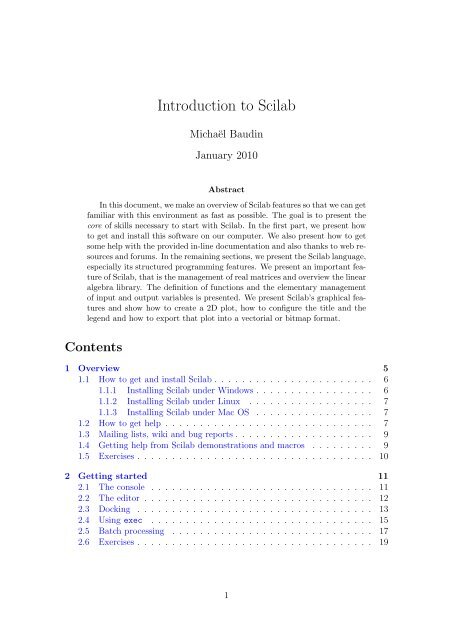
Figure 1: Scilab console under Windows.1.1 How to get and install ScilabWhatever your platform is (i.e. Windows, Linux or Mac), Scilab binaries can bedownloaded directly from the Scilab homepageor from the Download areahttp://www.scilab.orghttp://www.scilab.org/downloadScilab binaries are provided for both 32 and 64-bit platforms so that they matchthe target installation machine.Scilab can also be downloaded in source form, so that you can compile Scilab byyourself and produce your own binary. Compiling Scilab and generating a binary isespecially interesting when we want to understand or debug an existing feature, orwhen we want to add a new feature. To compile Scilab, some prerequisites binaryfiles are necessary, which are also provided in the Download center. Moreover, aFortran and a C compiler are required. Compiling Scilab is a process which will notbe detailed further in this document, because this chapter is mainly devoted to theexternal behavior of Scilab.1.1.1 Installing Scilab under WindowsScilab is distributed as a Windows binary and an installer is provided so that theinstallation is really easy. The Scilab console is presented in figure 1. Several commentsmay be made about this installation process.On Windows, if your machine is based on an Intel processor, the Intel MathKernel Library (MKL) [7] enables Scilab to perform faster numerical computations.6

1.1.2 Installing Scilab under LinuxUnder Linux, the binary versions are available from Scilab website as .tar.gz files.There is no need for an installation program with Scilab under Linux: simply unzipthe file in one target directory. Once done, the binary file is located in /scilab-5.x.x/bin/scilab. When this script is executed, the console immediately appears andlooks exactly the same as on Windows.Notice that Scilab is also distributed with the packaging system available withLinux distributions based on Debian (for example, Ubuntu). This installationmethod is extremely simple and efficient. Nevertheless, it has one little drawback:the version of Scilab packaged for your Linux distribution may not be up-to-date.This is because there is some delay (from several weeks to several months) betweenthe availability of an up-to-date version of Scilab under Linux and its release inLinux distributions.For now, Scilab comes on Linux with a binary linear algebra library which guaranteesportability. Under Linux, Scilab does not come with a binary version ofATLAS [1], so that linear algebra is a little slower for that platform, compared toWindows.1.1.3 Installing Scilab under Mac OSUnder Mac OS, the binary versions are available from Scilab website as a .dmg file.This binary works for Mac OS versions starting from version 10.5. It uses the MacOS installer, which provides a classical installation process. Scilab is not availableon Power PC systems.Scilab version 5.2 for Mac OS comes with a Tcl / Tk library which is disabled fortechnical reasons. As a consequence, there are some small limitations on the use ofScilab on this platform. For example, the Scilab / Tcl interface (TclSci), the graphiceditor and the variable editor are not working. These features will be rewritten inJava in future versions of Scilab and these limitations will disappear.Still, using Scilab on a Mac OS system is easy, and uses the shorcuts whichare familiar to the users of this platform. For example, the console and the editoruse the Cmd key (Apple key) which is found on Mac keyboards. Moreover, thereis no right-click on this platform. Instead, Scilab is sensitive to the Control-Clickkeyboard event.For now, Scilab comes on Mac OS with a linear algebra library which is optimizedand guarantees portability. Under Mac OS, Scilab does not come with a binaryversion of ATLAS [1], so that linear algebra is a little slower for that platform.1.2 How to get helpThe most simple way to get the online help integrated to Scilab is to use the functionhelp. Figure 2 presents the Scilab help window. To use this function, simply type”help” in the console and press the key, as in the following session.help7

Figure 2: Scilab help window.Suppose that you want some help about the optim function. You may try tobrowse the integrated help, find the optimization section and then click on the optimitem to display its help.Another possibility is to use the function help, followed by the name of thefunction, for which help is required, as in the following session.helpoptimScilab automatically opens the associated entry in the help.We can also use the help provided on the Scilab web sitehttp://www.scilab.org/product/manThis page always contains the help for the up-to-date version of Scilab. By usingthe ”search” feature of my web browser, I can most of the time quickly find thehelp page I need. With that method, I can see the help pages for several Scilabcommands at the same time (for example the commands derivative and optim,so that I can provide the cost function suitable for optimization with optim bycomputing derivatives with derivative).A list of commercial books, free books, online tutorials and articles is presentedon the Scilab homepage:http://www.scilab.org/publications8

1.3 Mailing lists, wiki and bug reportsThe mailing list users@lists.scilab.org is designed for all Scilab usage questions. Tosubscribe to this mailing list, send an e-mail to users-subscribe@lists.scilab.org. Themailing list dev@lists.scilab.org focuses on the development of Scilab, be it the developmentof Scilab core or of complicated modules which interacts deeply with Scilabcore. To subscribe to this mailing list, send an e-mail to dev-subscribe@lists.scilab.org.These mailing lists are archived at:and:http://dir.gmane.org/gmane.comp.mathematics.scilab.userhttp://dir.gmane.org/gmane.comp.mathematics.scilab.develTherefore, before asking a question, users should consider looking in the archiveif the same question or subject has already been answered.A question posted on the mailing list may be related to a very specific technicalpoint, so that it requires an answer which is not general enough to be public. Theaddress scilab.support@scilab.org is designed for this purpose. Developers of theScilab team provide accurate answers via this communication channel.The Scilab wiki is a public tool for reading and publishing general informationabout Scilab:http://wiki.scilab.orgIt is used both by Scilab users and developers to publish information about Scilab.From a developer’s point of view, it contains step-by-step instructions to compileScilab from the sources, dependencies of various versions of Scilab, instructions touse Scilab source code repository, etc...The Scilab Bugzilla http://bugzilla.scilab.org allows to submit a report each timewe find a new bug. It may happen that this bug has already been discovered bysomeone else. This is why it is advised to search the bug database for existing relatedproblems before reporting a new bug. If the bug is not reported yet, it is a verygood thing to report it, along with a test script. This test script should remain assimple as possible, which allows to reproduce the problem and identify the sourceof the issue.An efficient way of getting up-to-date information is to use RSS feeds. The RSSfeed associated with the Scilab website ishttp://www.scilab.org/en/rss_en.xmlThis channel regularly delivers press releases and general announces.1.4 Getting help from Scilab demonstrations and macrosThe Scilab consortium maintains a collection of demonstration scripts, which areavailable from the console, in the menu ? > Scilab Demonstrations. Figure 3presents the demonstration window. Some demonstrations are graphic, while some9

Figure 3: Scilab demos window.others are interactive, which means that the user must type on the key togo on to the next step of the demo.The associated demonstrations scripts are located in the Scilab directory, insideeach module. For example, the demonstration associated with the optimizationmodule is located in the file\scilab-5.2.0\modules\optimization\demos\datafit\datafit.dem.sceOf course, the exact path of the file depends on your particular installation and youroperating system.Analyzing the content of these demonstration files is often an efficient solutionfor solving common problems and to understand particular features.Another method to find some help is to analyze the source code of Scilab itself(Scilab is indeed open-source!). For example, the derivative function is located in\scilab-5.2.0\modules\optimization\macros\derivative.sciMost of the time, Scilab macros are very well written, taking care of all possiblecombinations of input and output arguments and many possible values of the inputarguments. Often, difficult numerical problems are solved in these scripts so thatthey provide a deep source of inspiration for developing your own scripts.TODO : CHECK THIS PART !1.5 ExercisesExercise 1.1 (Installing Scilab) Install the current version of Scilab on your system: at thetime where this document is written, this is Scilab v5.2. It is instructive to install an older versionof Scilab, in order to compare current behavior against the older one. Install Scilab 4.1.2 and seethe differences.Exercise 1.2 (Inline help: derivative) The derivative function allows to compute the numericalderivative of a function. The purpose of this exercise is to find the corresponding help page,by various means. In the inline help, find the entry corresponding to the derivative function.Find the corresponding entry in the online help. Use the console to find the help.10

Exercise 1.3 (Asking a question on the forum) You probably already have one or morequestions. Post your question on the users’ mailing list users@lists.scilab.org.2 Getting startedIn this section, we make our first steps with Scilab and present some simple taskswe can perform with the interpreter.There are several ways of using Scilab and the following paragraphs present threemethods:• using the console in the interactive mode,• using the exec function against a file,• using batch processing.2.1 The consoleThe first way is to use Scilab interactively, by typing commands in the console,analyzing the results and continuing this process until the final result is computed.This document is designed so that the Scilab examples which are printed here canbe copied into the console. The goal is that the reader can experiment by himselfScilab behavior. This is indeed a good way of understanding the behavior of theprogram and, most of the time, it allows a quick and smooth way of performing thedesired computation.In the following example, the function disp is used in the interactive mode toprint out the string ”Hello World!”.-->s=" Hello World !"s =Hello World !--> disp (s)Hello World !In the previous session, we did not type the characters ”-->” which is the prompt,and which is managed by Scilab. We only type the statement s="Hello World!"with our keyboard and then hit the key. Scilab answer is s = and HelloWorld!. Then we type disp(s) and Scilab answer is Hello World!.When we edit a command, we can use the keyboard, as with a regular editor.We can use the left ← and right → arrows in order to move the cursor on the lineand use the and keys in order to fix errors in the text.In order to get access to previously executed commands, use the up arrow ↑ key.This allows to browse the previous commands by using the up ↑ and down ↓ arrowkeys.The key provides a very convenient completion feature. In the followingsession, we type the statement disp in the console.--> disp11

Figure 4: The completion in the console.Then we can type on the key, which makes a list appear in the console,as presented in figure 4. Scilab displays a listbox, where items correspond to allfunctions which begin with the letters ”disp”. We can then use the up and downarrow keys to select the function we want.The auto-completion works with functions, variables, files and graphic handlesand makes the development of scripts easier and faster.2.2 The editorScilab version 5.2 provides a new editor which allows to edit scripts easily. Figure 5presents the editor during the editing of the previous ”Hello World!” example.The editor can be accessed from the menu of the console, under the Applications> Editor menu, or from the console, as presented in the following session.--> editor ()This editor allows to manage several files at the same time, as presented infigure 5, where we edit five files at the same time.There are many features which are worth to mention in this editor. The mostcommonly used features are under the Execute menu.• Load into Scilab allows to execute the statements in the current file, as if wedid a copy and paste. This implies that the statements which do not end withthe semicolon ”;” character will produce an output in the console.• Evaluate Selection allows to execute the statements which are currently selected.• Execute File Into Scilab allows to execute the file, as if we used the execfunction. The results which are produced in the console are only those whichare associated with printing functions, such as disp for example.12

Figure 5: The editor.We can also select a few lines in the script, right click (or Cmd+Click under Mac),and get the context menu which is presented in figure 6.The Edit menu provides a very interesting feature, commonly known as a ”prettyprinter” in most languages. This is the Edit > Correct Indentation feature, whichautomatically indents the current selection. This feature is extremelly convenient,as it allows to format algorithms, so that the if, for and other structured blocksare easy to analyze.The editor provides a fast access to the inline help. Indeed, assume that we haveselected the disp statement, as presented in figure 7. When we right-click in theeditor, we get the context menu, where the Help about ”disp” entry allows to openthe help page associated with the disp function.2.3 DockingThe graphics in Scilab version 5 has been updated so that many components arenow based on Java. This has a number of advantages, including the possibility tomanage docking windows.The docking system uses Flexdock [10], an open-source project providing a Swingdocking framework. Assume that we have both the console and the editor openedin our environment, as presented in figure 8. It might be annoying to manage twowindows, because one may hide the other, so that we constantly have to move themaround in order to actually see what happens.The Flexdock system allows to drag and drop the editor into the console, so that13

Figure 6: Context menu in the editor.Figure 7: Context help in the editor.14

Drag from hereand drop intothe consoleFigure 8: The title bar in the source window. In order to dock the editor into theconsole, drag and drop the title bar of the editor into the console.we finally have only one window, with several sub-windows. All Scilab windows aredockable, including the console, the editor, the help and the plotting windows. Infigure 9, we present a situation where we have docked four windows into the consolewindow.In order to dock one window into another window, we must drag and drop thesource window into the target window. To do this, we left-click on the title bar of thedocking window, as indicated in figure 8. Before releasing the click, let us move themouse over the target window and notice that a window, surrounded by dotted linesis displayed. This ”phantom” window indicates the location of the future dockedwindow. We can choose this location, which can be on the top, the bottom, theleft or the right of the target window. Once we have chosen the target location, werelease the click, which finally moves the source window into the target window, asin figure 9.We can also release the source window over the target window, which createstabs, as in figure 10.2.4 Using execWhen several commands are to be executed, it may be more convenient to writethese statements into a file with Scilab editor. To execute the commands located insuch a file, the exec function can be used, followed by the name of the script. Thisfile generally has the extension .sce or .sci, depending on its content:• files having the .sci extension contain Scilab functions and executing themloads the functions into Scilab environment (but does not execute them),• files having the .sce extension contain both Scilab functions and executablestatements.Executing a .sce file has generally an effect such as computing several variables anddisplaying the results in the console, creating 2D plots, reading or writing into a file,etc...Assume that the content of the file myscript.sce is the following.15

Click hereto un-dockClick here toclose the dockFigure 9: Actions in the title bar of the docking window. The round arrow in thetitle bar of the window allows to undock the window. The cross allows to close thewindow.The tabs ofthe dockFigure 10: Docking tabs.16

disp("Hello World !")In the Scilab console, we can use the exec function to execute the content of thisscript.--> exec (" myscript . sce ")--> disp (" Hello World !")Hello World !In practical situations, such as debugging a complicated algorithm, the interactivemode is used most of the time with a sequence of calls to the exec and dispfunctions.2.5 Batch processingAnother way of using Scilab is from the command line. Several command lineoptions are available and are presented in figure 11. Whatever the operating systemis, binaries are located in the directory scilab-5.2.0/bin. Command line optionsmust be appended to the binary for the specific platform, as described below. The-nw option allows to disable the display of the console. The -nwni option allowsto launch the non-graphics mode: in this mode, the console is not displayed andplotting functions are disabled (using them will generate an error).• Under Windows, two binary executable are provided. The first executable isWScilex.exe, the usual, graphics, interactive console. This executable correspondsto the icon which is available on the desktop after the installationof Scilab. The second executable is Scilex.exe, the non-graphics console.With the Scilex.exe executable, the Java-based console is not loaded andthe Windows terminal is directly used. The Scilex.exe program is sensitiveto the -nw and -nwni options.• Under Linux, the scilab script provides options which allow to configure itsbehavior. By default, the graphics mode is launched. The scilab script issensitive to the -nw and -nwni options. There are two extra executables onLinux: scilab-cli and scilab-adv-cli. The scilab-adv-cli executable isequivalent to the -nw option, while the scilab-cli is equivalent to the -nwnioption[8].• Under Mac OS, the behavior is similar to the Linux platform.In the following Windows session, we launch the Scilex.exe program with the-nwni option. Then we run the plot function in order to check that this functionis not available in the non-graphics mode.D:\ Programs \ scilab -5.2.0\ bin > Scilex . exe -nwni___________________________________________scilab -5.2.0Consortium Scilab ( DIGITEO )Copyright (c) 1989 -2009 ( INRIA )Copyright (c) 1989 -2007 ( ENPC )___________________________________________17

-e instruction execute the Scilab instruction given in instruction-f file execute the Scilab script given in the file-l lang setup the user language’fr’ for french and ’en’ for english (default is ’en’)-mem N set the initial stacksize-nsif this option is present, the startup file scilab.start is not executed-nbif this option is present, then Scilab welcome banner is not displayed-nouserstartup don’t execute user startup files SCIHOME/.scilabor SCIHOME/scilab.ini-nwstart Scilab as command line with advanced features (e.g., graphics)-nwni start Scilab as command line without advanced features-version print product version and exitFigure 11: Scilab command line options.Startup execution :loading initial environment--> plot ()!-- error 4Undefined variable : plotThe most useful command line option is the -f option, which allows to executethe commands from a given file, a method generally called batch processing. Assumethat the content of the file myscript2.sce is the following, where the quit functionis used to exit from Scilab.disp (" Hello World !")quit ()The default behavior of Scilab is to wait for new user input: this is why the quitcommand is used, so that the session terminates. To execute the demonstrationunder Windows, we created the directory ”C:\scripts” and wrote the statements inthe file C:\scripts\myscript2.sce. The following session, executed from the MSWindows terminal, shows how to use the -f option to execute the previous script.Notice that we used the absolute path of the Scilex.exe executable.C:\ scripts >D:\ Programs \ scilab -5.2.0\ bin \ Scilex . exe -f myscript2 . sce___________________________________________scilab -5.2.0Consortium Scilab ( DIGITEO )Copyright (c) 1989 -2009 ( INRIA )Copyright (c) 1989 -2007 ( ENPC )___________________________________________Startup execution :loading initial environmentHello World !C:\ scripts >Any line which begins with the two slash characters ”//” is considered by Scilabas a comment and is ignored. To check that Scilab stays by default in interactivemode, we comment out the quit statement with the ”//” syntax, as in the followingscript.18

disp (" Hello World !")// quit ()If we type the ”scilex -f myscript2.sce” command in the terminal, Scilabwill now wait for user input, as expected. To exit, we interactively type the quit()statement in the terminal.TODO : CHECK THIS PART !2.6 ExercisesExercise 2.1 (The console) Type the following statement in the console.atomsNow type on the key. What happens? Now type the ”I” letter, and type again on .What happens?Exercise 2.2 (Using exec) When we develop a Scilab, script we often use the exec functionin combination with the ls function, which displays the list of files and directories in the currentdirectory. We can also use the pwd, which displays the current directory. The SCI variable containsthe name of the directory of the current Scilab installation. We use it very often to execute thescripts which are provided in Scilab. Type the following statements in the console and see whathappens.pwdSCIls(SCI +"/ modules ")ls(SCI +"/ modules / graphics / demos ")exec ( SCI +"/ modules / graphics / demos /2 d_3d_plots / contourf . dem . sce ")exec ( SCI +"/ modules / graphics / demos /2 d_3d_plots / contourf . dem . sce ");3 Basic elements of the languageScilab is an interpreted language, which means that it allows to manipulate variablesin a very dynamic way. In this section, we present the basic features of the language,that is, we show how to create a real variable, and what elementary mathematicalfunctions can be applied to a real variable. If Scilab provided only these features,it would only be a super desktop calculator. Fortunately, it is a lot more and thisis the subject of the remaining sections, where we will show how to manage othertypes of variables, that is booleans, complex numbers, integers and strings.It seems strange at first, but it is worth to state it right from the start: inScilab, everything is a matrix. To be more accurate, we should write: all real,complex, boolean, integer, string and polynomial variables are matrices. Lists andother complex data structures (such as tlists and mlists) are not matrices (but cancontain matrices). These complex data structures will not be presented in thisdocument.This is why we could begin by presenting matrices. Still, we choose to presentbasic data types first, because Scilab matrices are in fact a special organization ofthese basic building blocks.In Scilab, we can manage real and complex numbers. This always leads to someconfusion if the context is not clear enough. In the following, when we write realvariable, we will refer to a variable which content is not complex. Complex variables19

+ addition- subtraction∗ multiplication/ right division, i.e. x/y = xy −1\ left division, i.e. x\y = x −1 yˆ power, i.e. x y∗∗ power (same as ˆ)’ transpose conjugateFigure 12: Scilab elementary mathematical operators.will be covered in section 3.7 as a special case of real variables. In most cases, realvariables and complex variables behave in a very similar way, although some extracare must be taken when complex data is to be processed. Because it would makethe presentation cumbersome, we simplify most of the discussions by consideringonly real variables, taking extra care with complex variables only when needed.3.1 Creating real variablesIn this section, we create real variables and perform simple operations with them.Scilab is an interpreted language, which implies that there is no need to declarea variable before using it. Variables are created at the moment where they are firstset.In the following example, we create and set the real variable x to 1 and performa multiplication on this variable. In Scilab, the ”=” operator means that we wantto set the variable on the left hand side to the value associated with the right handside (it is not the comparison operator, which syntax is associated with the ”==”operator).-->x=1x =1.-->x = x * 2x =2.The value of the variable is displayed each time a statement is executed. Thatbehavior can be suppressed if the line ends with the semicolon ”;” character, as inthe following example.-->y =1;-->y=y *2;All the common algebraic operators presented in figure 12 are available in Scilab.Notice that the power operator is represented by the hat ”ˆ” character so that computingx 2 in Scilab is performed by the ”xˆ2” expression or equivalently by the ”x**2”expression. The single quote ”’ ” operator will be presented in more depth in section3.7, which presents complex numbers. It will be reviewed again in section 4.12,which deals with the conjugate transpose of a matrix.20

3.2 Variable namesVariable names may be as long as the user wants, but only the first 24 charactersare taken into account in Scilab. For consistency, we should consider only variablenames which are not made of more than 24 characters. All ASCII letters from ”a”to ”z”, from ”A” to ”Z” and digits from ”0” to ”9” are allowed, with the additionalcharacters ”%”, ”_”, ”#”, ”!”, ”$”, ”?”. Notice though that variable names, whose firstletter is ”%”, have a special meaning in Scilab, as we will see in section 3.5, whichpresents the pre-defined mathematical variables.Scilab is case sensitive, which means that upper and lower case letters are consideredto be different by Scilab. In the following script, we define the two variablesA and a and check that these two variables are considered to be different by Scilab.-->A = 2A =2.-->a = 1a =1.-->AA =2.-->aa =1.3.3 Comments and continuation linesAny line which begins with two slashes ”//” is considered by Scilab as a commentand is ignored. There is no possibility to comment out a block of lines, such as withthe ”/* ... */” comments in the C language.When an executable statement is too long to be written on a single line, thesecond and subsequent lines are called continuation lines. In Scilab, any line whichends with two dots is considered to be the start of a new continuation line. In thefollowing session, we give examples of Scilab comments and continuation lines.-->// This is my comment .-->x =1..- - >+2..- - >+3..-->+4x =10.3.4 Elementary mathematical functionsTables 13 and 14 present a list of elementary mathematical functions. Most of thesefunctions take one input argument and return one output argument. These functionsare vectorized in the sense that their input and output arguments are matrices. Thisallows to compute data with higher performance, without any loop.21

acos acosd acosh acoshm acosm acot acotd acothacsc acscd acsch asec asecd asech asin asindasinh asinhm asinm atan atand atanh atanhm atanmcos cosd cosh coshm cosm cotd cotg cothcothm csc cscd csch sec secd sech sinsinc sind sinh sinhm sinm tan tand tanhtanhm tanmFigure 13: Scilab elementary mathematical functions: trigonometry.exp expm log log10 log1p log2 logm maxmaxi min mini modulo pmodulo sign signm sqrtsqrtmFigure 14: Scilab elementary mathematical functions: other functions.In the following example, we use the cos and sin functions and check the equalitycos(x) 2 + sin(x) 2 = 1.-->x = cos (2)x =- 0.4161468-->y = sin (2)y =0.9092974-->x ^2+ y^2ans =1.3.5 Pre-defined mathematical variablesIn Scilab, several mathematical variables are pre-defined variables, whose names beginwith a percent ”%” character. The variables which have a mathematical meaningare summarized in figure 15.In the following example, we use the variable %pi to check the mathematicalequality cos(x) 2 + sin(x) 2 = 1.-->c= cos ( %pi )c =- 1.-->s= sin ( %pi )s =%i the imaginary number i%e Euler’s constant e%pi the mathematical constant πFigure 15: Pre-defined mathematical variables.22

a&ba|b∼aa==ba∼=b or ababa=blogical andlogical orlogical nottrue if the two expressions are equaltrue if the two expressions are differenttrue if a is lower than btrue if a is greater than btrue if a is lower or equal to btrue if a is greater or equal to bFigure 16: Comparison operators.1.225D -16-->c ^2+ s^2ans =1.The fact that the computed value of sin(π) is not exactly equal to 0 is a consequenceof the fact that Scilab stores the real numbers with floating point numbers,that is, with limited precision.3.6 BooleansBoolean variables can store true or false values. In Scilab, true is written with %tor %T and false is written with %f or %F. Figure 16 presents the several comparisonoperators which are available in Scilab. These operators return boolean values andtake as input arguments all basic data types (i.e. real and complex numbers, integersand strings). The comparison operators are reviewed in section 4.14, where theemphasis is made on comparison of matrices.In the following example, we perform some algebraic computations with Scilabbooleans.-->a=%Ta =T-->b = ( 0 == 1 )b =F-->a&bans =F3.7 Complex numbersScilab provides complex numbers, which are stored as pairs of floating point numbers.The pre-defined variable %i represents the mathematical imaginary number i whichsatisfies i 2 = −1. All elementary functions previously presented before, such as sinfor example, are overloaded for complex numbers. This means that, if their input23

ealimagimultisrealreal partimaginary partmultiplication by i, the imaginary unitaryreturns true if the variable has no complex entryFigure 17: Scilab complex numbers elementary functions.argument is a complex number, the output is a complex number. Figure 17 presentsfunctions which allow to manage complex numbers.In the following example, we set the variable x to 1 + i, and perform severalbasic operations on it, such as retrieving its real and imaginary parts. Notice howthe single quote operator, denoted by ”’ ”, is used to compute the conjugate of acomplex number.-->x= 1+ %ix =1. + i--> isreal (x)ans =F-->x’ans =1. - i-->y=1 - %iy =1. - i--> real (y)ans =1.--> imag (y)ans =- 1.We finally check that the equality (1+i)(1−i) = 1−i 2 = 2 is verified by Scilab.-->x*yans =2.3.8 IntegersWe can create various types of integer variables with Scilab. The functions whichallow to create such integers are presented in figure 18. There is a direct link betweenthe number of bits used to store the integer and the range of values that the integercan manage. For example, an 8-bit signed integer, as created by the int8 function,can store values in the range [−2 7 , 2 7 − 1], which simplies to [−128, 127].In the following session, we check that an unsigned 32-bit integer have valuesinside the range [0, 2 32 − 1], which simplifies into [0, 4294967295].--> format (25)-->n =32n =24

int8 int16 int32uint8 uint16 uint32Figure 18: Scilab integer data types.32.-->2^n - 1ans =4294967295.-->i = uint32 (0)i =0-->j=i -1j =4294967295-->k = j+1k =03.9 Floating point integersIn Scilab, the default numerical variable is the double, that is the 64-bit floating pointnumber. This is true even if we write what is mathematically an integer. In [9],Cleve Moler call this number a ”flint”, a short for floating point integer. In practice,we can safely store integers in the interval [−2 52 , 2 52 ] into doubles. We emphasizethat, provided that all input, intermediate and output integer values are strictlyinside the [−2 52 , 2 52 ] interval, the integer computations are exact. For example, inthe following example, we perform the exact addition of two large integers whichremain in the ”safe” interval.--> format (25)-->a= 2^40 - 12a =1099511627764.-->b= 2^45 + 3b =35184372088835.-->c = a + bc =36283883716599.Instead, when we perform computations outside this interval, we may have unexpectedresults. For example, in the following session, we see that additions involvingterms slightly greater than 2 53 produce only even values.--> format (25)- - >(2^53 + (1:10)) ’ans =9007199254740992.9007199254740994.9007199254740996.9007199254740996.25

9007199254740996.9007199254740998.9007199254741000.9007199254741000.9007199254741000.9007199254741002.In the following session, we compute 2 52 using the floating point integer 2 in thefirst case, and using the 16-bit integer 2 in the second case. In the first case, nooverflow occurs, even if the number is at the limit of 64-bit floating point numbers.In the second case, the result is completely wrong, because the number 2 52 cannotbe represented as a 16-bit integer.- - >2^52ans =4503599627370496.--> uint16 (2^52)ans =0In section 4.15, we analyze the issues which arise when indexes involved to accessthe elements of a matrix are doubles.3.10 Default answerWhenever we make a computation and do not store the result into an output variable,the result is stored in the default ans variable. Once it is defined, we can use thisvariable as any other Scilab variable.In the following session, we compute exp(3) so that the result is stored in theans variable. Then we use its content as a regular variable.-->exp (3)ans =20.08553692318766792368-->t = log ( ans )t =3.In general, the ans variable should be used only in an interactive session, inorder to progress in the computation without defining a new variable. For example,we may have forgotten to store the result of an interesting computation and do notwant to recompute the result. This might be the case after a long sequence of trialsand errors, where we experimented several ways to get the result without takingcare of actually storing the result. In this interactive case, using ans may allow tosave some human (or machine) time. Instead, if we are developping a script used ina non-interactive way, it is a bad practice to rely on the ans variable and we shouldstore the results in regular variables.3.11 StringsStrings can be stored in variables, provided that they are delimited by double quotes”" ”. The concatenation operation is available from the ”+” operator. In the follow-26

ing Scilab session, we define two strings and then concatenate them with the ”+”operator.-->x = " foo "x =foo-->y=" bar "y =bar-->x+yans =foobarThey are many functions which allow to process strings, including regular expressions.We will not give further details about this topic in this document.3.12 Dynamic type of variablesWhen we create and manage variables, Scilab allows to change the type of a variabledynamically. This means that we can create a real value, and then put a stringvariable in it, as presented in the following session.-->x=1x =1.-->x+1ans =2.-->x=" foo "x =foo-->x+" bar "ans =foobarWe emphasize here that Scilab is not a typed language, that is, we do not haveto declare the type of a variable before setting its content. Moreover, the type of avariable can change during the life of the variable.3.13 ExercisesTODO : CHECK THIS PART !Exercise 3.1 (Precedence of operators) What are the results of the following computations(think about it before trying in Scilab) ?2 * 3 + 42 + 3 * 42 / 3 + 42 + 3 / 4Exercise 3.2 (Parentheses) What are the results of the following computations (think about itbefore trying in Scilab) ?2 * (3 + 4)(2 + 3) * 4(2 + 3) / 43 / (2 + 4)27

Exercise 3.3 (Exponents) What are the results of the following computations (think about itbefore trying in Scilab) ?1.23456789 d101.23456789 e101.23456789 e -5Exercise 3.4 (Functions) What are the results of the following computations (think about itbefore trying in Scilab) ?sqrt (4)sqrt (9)sqrt ( -1)sqrt ( -2)exp (1)log ( exp (2))exp ( log (2))10^2log10 (10^2)10^ log10 (2)sign (2)sign ( -2)sign (0)Exercise 3.5 (Trigonometry) What are the results of the following computations (think aboutit before trying in Scilab) ?cos (0)sin (0)cos ( %pi )sin ( %pi )cos ( %pi /4) - sin ( %pi /4)4 MatricesIn the Scilab language, matrices play a central role. In this section, we introduceScilab matrices and present how to create and query matrices. We also analyze howto access the elements of a matrix, either element by element, or by higher-leveloperations.4.1 OverviewIn Scilab, the basic data type is the matrix, which is defined by:• the number of rows,• the number of columns,• the type of data.The data type can be real, integer, boolean, string and polynomial. When twomatrices have the same number of rows and columns, we say that the two matriceshave the same shape.28

In Scilab, vectors are a particular case of matrices, where the number of rows (orthe number of columns) is equal to 1. Simple scalar variables do not exist in Scilab:a scalar variable is a matrix with 1 row and 1 column. This is why in this chapter,when we analyze the behavior of Scilab matrices, there is the same behavior for rowor column vectors (i.e. n×1 or 1×n matrices) as well as scalars (i.e. 1×1 matrices).It is fair to say that Scilab was designed mainly for matrices of real variables.This allows to perform linear algebra operations with a high-level language.By design, Scilab was created to be able to perform matrix operations as fastas possible. The building block for this feature is that Scilab matrices are storedin an internal data structure which can be managed at the interpreter level. Mostbasic linear algebra operations, such as addition, substraction, transpose or dotproduct are performed by a compiled, optimized, source code. These operations areperformed with the common operators ”+”, ”-”, ”*” and the single quote ”’ ”, sothat, at the Scilab level, the source code is both simple and fast.With these high-level operators, most matrix algorithms do not require to useloops. In fact, a Scilab script which performs the same operations with loops istypically from 10 to 100 times slower. This feature of Scilab is known as the vectorization.In order to get a fast implementation of a given algorithm, the Scilabdeveloper should always use high-level operations, so that each statement processesa matrix (or a vector) instead of a scalar.More complex tasks of linear algebra, such as the resolution of systems of linearequations Ax = b, various decompositions (for example Gauss partial pivotalP A = LU), eigenvalue/eigenvector computations, are also performed by compiledand optimized source codes. These operations are performed by common operatorslike the slash ”/” or backslash ”\” or with functions like spec, which computeseigenvalues and eigenvectors.4.2 Create a matrix of real valuesThere is a simple and efficient syntax to create a matrix with given values. Thefollowing is the list of symbols used to define a matrix:• square brackets ”[” and ”]” mark the beginning and the end of the matrix,• commas ”,” separate the values in different columns,• semicolons ”;” separate the values of different rows.The following syntax can be used to define a matrix, where blank spaces are optional(but make the line easier to read) and ”...” denotes intermediate values:A = [a11 , a12 , ... , a1n ; a21 , a22 , ... , a2n ; ...; an1 , an2 , ... , ann ].In the following example, we create a 2 × 3 matrix of real values.-->A = [1 , 2 , 3 ; 4 , 5 , 6]A =1. 2. 3.4. 5. 6.29

eyelinspaceoneszerostestmatrixgrandrandidentity matrixlinearly spaced vectormatrix made of onesmatrix made of zerosgenerate some particular matricesrandom number generatorrandom number generatorFigure 19: Functions which generate matrices.A simpler syntax is available, which does not require to use the comma and semicoloncharacters. When creating a matrix, the blank space separates the columns whilethe new line separates the rows, as in the following syntax:A = [ a11 a12 ... a1na21 a22 ... a2n...an1 an2 ... ann ]This allows to lighten considerably the management of matrices, as in the followingsession.-->A = [1 2 3-->4 5 6]A =1. 2. 3.4. 5. 6.The previous syntax for matrices is useful in the situations where matrices areto be written into data files, because it simplifies the human reading (and checking)of the values in the file, and simplifies the reading of the matrix in Scilab.Several Scilab commands allow to create matrices from a given size, i.e. from agiven number of rows and columns. These functions are presented in figure 19. Themost commonly used are eye, zeros and ones. These commands take two inputarguments, the number of rows and columns of the matrix to generate.-->A = ones (2 ,3)A =1. 1. 1.1. 1. 1.4.3 The empty matrix []An empty matrix can be created by using empty square brackets, as in the followingsession, where we create a 0 × 0 matrix.-->A =[]A =[]This syntax allows to delete the content of a matrix, so that the associatedmemory is freed.30

-->A = ones (100 ,100);-->A = []A =[]4.4 Query matricesThe functions in figure 20 allow to query or update a matrix.The size function returns the two output arguments nr and nc, which are thenumber of rows and the number of columns.-->A = ones (2 ,3)A =1. 1. 1.1. 1. 1.-->[nr ,nc ]= size (A)nc =3.nr =2.The size function is of important practical value when we design a function,since the processing that we must perform on a given matrix may depend on itsshape. For example, to compute the norm of a given matrix, different algorithmsmay be used depending on if the matrix is a column vector with size nr × 1 andnr > 0, a row vector with size 1 × nc and nc > 0, or a general matrix with sizenr × nc and nr, nc > 1.The size function has also the following syntaxnr = size ( A , sel )which allows to get only the number of rows or the number of columns and wheresel can have the following values• sel=1 or sel="r", returns the number of rows,• sel=2 or sel="c", returns the number of columns.• sel="*", returns the total number of elements, that is, the number of columnstimes the number of rows.In the following session, we use the size function in order to compute the totalnumber of elements of a matrix.-->A = ones (2 ,3)A =1. 1. 1.1. 1. 1.--> size (A,"*")ans =6.31

sizematrixresize_matrixsize of objectsreshape a vector or a matrix to a different size matrixcreate a new matrix with a different sizeFigure 20: Functions which query or modify matrices.4.5 Accessing the elements of a matrixThere are several methods to access the elements of a matrix A:• the whole matrix, with the A syntax,• element by element with the A(i,j) syntax,• a range of index values with the colon ”:” operator.The colon operator will be reviewed in the next section.To make a global access to all the elements of the matrix, the simple variablename, for example A, can be used. All elementary algebra operations are availablefor matrices, such as the addition with ”+”, subtraction with ”-”, provided that thetwo matrices have the same size. In the following script, we add all the elements oftwo matrices.-->A = ones (2 ,3)A =1. 1. 1.1. 1. 1.-->B = 2 * ones (2 ,3)B =2. 2. 2.2. 2. 2.-->A+Bans =3. 3. 3.3. 3. 3.One element of a matrix can be accessed directly with the A(i,j) syntax, providedthat i and j are valid index values.We emphasize that, by default, the first index of a matrix is 1. This contrastswith other languages, such as the C language for instance, where the first index is0. For example, assume that A is an nr × nc matrix, where nr is the number of rowsand nc is the number of columns. Therefore, the value A(i,j) has a sense only ifthe index values i and j satisfy 1 ≤ i ≤ nr and 1 ≤ j ≤ nc. If the index values arenot valid, an error is generated, as in the following session.-->A = ones (2 ,3)A =1. 1. 1.1. 1. 1.-->A (1 ,1)ans =1.-->A (12 ,1)32

!-- error 21Invalid index .-->A (0 ,1)!-- error 21Invalid index .Direct access to matrix elements with the A(i,j) syntax should be used onlywhen no other higher-level Scilab commands can be used. Indeed, Scilab providesmany features which allow to produce simpler and faster computations, based onvectorization. One of these features is the colon ”:”operator, which is very importantin practical situations.4.6 The colon ”:” operatorThe simplest syntax of the colon operator is the following:v = i:jwhere i is the starting index and j is the ending index with i ≤ j. This createsthe vector v = (i, i + 1, . . . , j). In the following session, we create a vector of indexvalues from 2 to 4 in one statement.-->v = 2:4v =2. 3. 4.The complete syntax allows to configure the increment used when generating theindex values, i.e. the step. The complete syntax for the colon operator isv = i:s:jwhere i is the starting index, j is the ending index and s is the step. This commandcreates the vector v = (i, i + s, i + 2s, . . . , i + ns) where n is the greatest integersuch that i + ns ≤ j. If s divides j − i, then the last index in the vector of indexvalues is j. In other cases, we have i + ns < j. While in most situations, the step sis positive, it might also be negative.In the following session, we create a vector of increasing index values from 3 to10 with a step equal to 2.-->v = 3:2:10v =3. 5. 7. 9.Notice that the last value in the vector v is i + ns = 9, which is smaller than j = 10.In the following session, we present two examples where the step is negative. Inthe first case, the colon operator generates decreasing index values from 10 to 4. Inthe second example, the colon operator generates an empty matrix because thereare no values lower than 3 and greater than 10 at the same time.-->v = 10: -2:3v =10. 8. 6. 4.-->v = 3: -2:10v =[]33

With a vector of index values, we can access the elements of a matrix in a givenrange, as with the following simplified syntaxA(i:j,k:l)where i,j,k,l are starting and ending index values. The complete syntax isA(i:s:j,k:t:l), where s and t are the steps.For example, suppose that A is a 4 × 5 matrix, and that we want to access theelements a i,j for i = 1, 2 and j = 3, 4. With the Scilab language, this can be donein just one statement, by using the syntax A(1:2,3:4), as showed in the followingsession.-->A = testmatrix (" hilb " ,5)A =25. - 300. 1050. - 1400. 630.- 300. 4800. - 18900. 26880. - 12600.1050. - 18900. 79380. - 117600. 56700.- 1400. 26880. - 117600. 179200. - 88200.630. - 12600. 56700. - 88200. 44100.-->A (1:2 ,3:4)ans =1050. - 1400.- 18900. 26880.In some circumstances, it may happen that the index values are the result of acomputation. For example, the algorithm may be based on a loop where the indexvalues are updated regularly. In these cases, the syntaxA(vi ,vj),where vi,vj are vectors of index values, can be used to designate the elements ofA whose subscripts are the elements of vi and vj. That syntax is illustrated in thefollowing example.-->A = testmatrix (" hilb " ,5)A =25. - 300. 1050. - 1400. 630.- 300. 4800. - 18900. 26880. - 12600.1050. - 18900. 79380. - 117600. 56700.- 1400. 26880. - 117600. 179200. - 88200.630. - 12600. 56700. - 88200. 44100.-->vi =1:2vi =1. 2.-->vj =3:4vj =3. 4.-->A(vi ,vj)ans =1050. - 1400.- 18900. 26880.-->vi=vi +1vi =2. 3.-->vj=vj +134

AA(:,:)A(i:j,k)A(i,j:k)A(i,:)A(:,j)the whole matrixthe whole matrixthe elements at rows from i to j, at column kthe elements at row i, at columns from j to kthe row ithe column jFigure 21: Access to a matrix with the colon ”:” operator.vj =4. 5.-->A(vi ,vj)ans =26880. - 12600.- 117600. 56700.There are many variations on this syntax, and figure 21 presents some of thepossible combinations.For example, in the following session, we use the colon operator in order tointerchange two rows of the matrix A.-->A = testmatrix (" hilb " ,3)A =9. - 36. 30.- 36. 192. - 180.30. - 180. 180.-->A ([1 2] ,:) = A ([2 1] ,:)A =- 36. 192. - 180.9. - 36. 30.30. - 180. 180.We could also interchange the columns of the matrix A with the statement A(:,[31 2]).In this section we have analyzed several practical use of the colon operator.Indeed, this operator is used in many scripts where performance matters, since itallows to access many elements of a matrix in just one statement. This is associatedwith the vectorization of scripts, a subject which is central to the Scilab languageand is reviewed throughout this document.4.7 The eye matrixTODO : CHECK THIS PART !The eye function allows to create the identity matrix with the size which dependson the context. Its name has been chosen in place of I in order to avoid the confusionwith an index or with the imaginary number.In the following session, we add 3 to the diagonal elements of the matrix A.-->A = ones (3 ,3)A =1. 1. 1.35

1. 1. 1.1. 1. 1.-->B = A + 3* eye ()B =4. 1. 1.1. 4. 1.1. 1. 4.In the following session, we define an identity matrix B with the eye function dependingon the size of a given matrix A.-->A = ones (2 ,2)A =1. 1.1. 1.-->B = eye (A)B =1. 0.0. 1.Finally, we can use the eye(m,n) syntax in order to create an identity matrix withm rows and n columns.4.8 Matrices are dynamicThe size of a matrix can grow or reduce dynamically. This allows to adapt the sizeof the matrix to the data it contains.Consider the following session where we define a 2 × 3 matrix.-->A = [1 2 3; 4 5 6]A =1. 2. 3.4. 5. 6.In the following session, we insert the value 7 at the indices (3, 1). This creates thethird row in the matrix, sets the A(3, 1) entry to 7 and fills the other values of thenewly created row with zeros.-->A (3 ,1) = 7A =1. 2. 3.4. 5. 6.7. 0. 0.The previous example showed that matrices can grow. In the following session, wesee that we can also reduce the size of a matrix. This is done by using the emptymatrix ”[]” operator in order to delete the third column.-->A (: ,3) = []A =1. 2.4. 5.7. 0.We can also change the shape of the matrix with the matrix function. The matrixfunction allows to reshape a source matrix into a target matrix with a different size.The transformation is performed column by column, by stacking the elements of the36

A(i,$)A($,j)A($-i,$-j)the element at row i, at column ncthe element at row nr, at column jthe element at row nr − i, at column nc − jFigure 22: Access to a matrix with the dollar ”$” operator. The ”$” operator signifies”the last index”.source matrix. In the following session, we reshape the matrix A, which has 3×2 = 6elements into a row vector with 6 columns.-->B = matrix (A ,1 ,6)B =1. 4. 7. 2. 5. 0.4.9 The dollar ”$” operatorUsually, we make use of indices to make reference from the start of a matrix. Byopposition, the dollar ”$” operator allows to reference elements from the end ofthe matrix. The ”$” operator signifies ”the index corresponding to the last” row orcolumn, depending on the context. This syntax is associated with an algebra, so thatthe index $-i corresponds to the index l−i, where l is the number of correspondingrows or columns. Various uses of the dollar operator are presented in figure 22.In the following example, we consider a 3 × 3 matrix and we access the elementA(2,1) = A(nr-1,nc-2) = A($-1,$-2) because nr = 3 and nc = 3.-->A= testmatrix (" hilb " ,3)A =9. - 36. 30.- 36. 192. - 180.30. - 180. 180.-->A($ -1 ,$ -2)ans =- 36.The dollar ”$”operator allows to add elements dynamically at the end of matrices.In the following session, we add a row at the end of the Hilbert matrix.-->A($ +1 ,:) = [1 2 3]A =9. - 36. 30.- 36. 192. - 180.30. - 180. 180.1. 2. 3.The ”$” operator is used most of the time in the context of the ”$+1” statement,which allows to add at the end of a matrix. This can be convenient, since it avoidsthe need of updating the number of rows or columns continuously although it shouldbe used with care, only in the situations where the number of rows or columns cannotbe known in advance. The reason is that the interpreter has to internally re-allocatememory for the entire matrix and to copy the old values to the new destination.This can lead to performance penalties and this is why we should be warned against37

ad uses of this operator. All in all, the only good use of the ”$+1” statement iswhen we do not know in advance the final number of rows or columns.4.10 Low-level operationsAll common algebra operators, such as ”+”, ”-”, ”*” and ”/”, are available with realmatrices. In the next sections, we focus on the exact signification of these operators,so that many sources of confusion are avoided.The rules for the ”+”and ”-”operators are directly applied from the usual algebra.In the following session, we add two 2 × 2 matrices.-->A = [1 2-->3 4]A =1. 2.3. 4.-->B =[5 6-->7 8]B =5. 6.7. 8.-->A+Bans =6. 8.10. 12.When we perform an addition of two matrices, if one operand is a 1 × 1 matrix(i.e., a scalar), the value of this scalar is added to each element of the second matrix.This feature is shown in the following session.-->A = [1 2-->3 4]A =1. 2.3. 4.-->A + 1ans =2. 3.4. 5.The addition is possible only if the two matrices are conformable to addition. Inthe following session, we try to add a 2 × 3 matrix with a 2 × 2 matrix and checkthat this is not possible.-->A = [1 2-->3 4]A =1. 2.3. 4.-->B = [1 2 3-->4 5 6]B =1. 2. 3.4. 5. 6.-->A+B!-- error 838

+ addition .+ elementwise addition- subtraction .- elementwise subtraction∗ multiplication .∗ elementwise multiplication/ right division ./ elementwise right division\ left division .\ elementwise left divisionˆ or ∗∗ power, i.e. x y .ˆ elementwise power’ transpose and conjugate .’ transpose (but not conjugate)Figure 23: Matrix operators and elementwise operators.Inconsistent addition .Elementary operators which are available for matrices are presented in figure 23.The Scilab language provides two division operators, that is,the right division ”/”and the left division ”\”. The right division is so that X = A/B = AB −1 is thesolution of XB = A. The left division is so that X = A\B = A −1 B is the solutionof AX = B. The left division A\B computes the solution of the associated leastsquare problem if A is not a square matrix.Figure 23 separates the operators which treat the matrices as a whole and theelementwise operators, which are presented in the next section.4.11 Elementwise operationsIf a dot ”.” is written before an operator, it is associated with an elementwiseoperator, i.e. the operation is performed element-by-element. For example, withthe usual multiplication operator ”*”, the content of the matrix C=A*B is c ij =∑k=1,n a ikb kj . With the elementwise multiplication ”.*” operator, the content of thematrix C=A.*B is c ij = a ij b ij .In the following session, two matrices are multiplied with the ”*” operator andthen with the elementwise ”.*” operator, so that we can check that the results aredifferent.-->A = ones (2 ,2)A =1. 1.1. 1.-->B = 2 * ones (2 ,2)B =2. 2.2. 2.-->A*Bans =4. 4.4. 4.-->A.*Bans =2. 2.2. 2.39

4.12 Conjugate transpose and non-conjugate transposeThere might be some confusion when the elementwise single quote ”.’ ” and theregular single quote ”’ ” operators are used without a careful knowledge of their exactdefinitions. With a matrix of doubles containing real values, the single quote ”’” operator only transposes the matrix. Instead, when a matrix of doubles containingcomplex values is used, the single quote ”’ ” operator transposes and conjugates thematrix. Hence, the operation A=Z’ produces a matrix with entries A jk = X kj − iY kj ,where i is the imaginary number such that i 2 = −1 and X and Y are the real andimaginary parts of the matrix Z. The elementwise single quote ”.’ ” always transposeswithout conjugating the matrix, be it real or complex. Hence, the operationA=Z.’ produces a matrix with entries A jk = X kj + iY kj .In the following session, an unsymetric matrix of doubles containing complexvalues is used, so that the difference between the two operators is obvious.-->A = [1 2;3 4] + %i * [5 6;7 8]A =1. + 5.i 2. + 6.i3. + 7.i 4. + 8.i-->A’ans =1. - 5.i 3. - 7.i2. - 6.i 4. - 8.i-->A.’ans =1. + 5.i 3. + 7.i2. + 6.i 4. + 8.iIn the following session, we define an unsymetric matrix of doubles containing realvalues and see that the results of the ”’ ” and ”.’ ” are the same in this particularcase.-->B = [1 2;3 4]B =1. 2.3. 4.-->B’ans =1. 3.2. 4.-->B.’ans =1. 3.2. 4.Many bugs are created due to this confusion, so that it is mandatory to askyourself the following question: what happens if my matrix is complex? If theanswer is ”I want to transpose only”, then the elementwise quote ”.’ ” operator isto be used.4.13 Multiplication of two vectorsLet u ∈ R n be a column vector and v T ∈ R n be a column vector. The matrixA = uv T has entries A ij = u i v j . In the following Scilab session, we multiply the40

and(A,"r")and(A,"c")or(A,"r")or(A,"c")rowwise ”and”columnwise ”and”rowwise ”or”columnwise ”or”Figure 24: Special comparison operators for matrices. The usual operators ”u = [1-->2-->3]u =1.2.3.-->v = [4 5 6]v =4. 5. 6.-->u*vans =4. 5. 6.8. 10. 12.12. 15. 18.This might lead to some confusion because linear algebra textbooks considercolumn vectors only. We usually denote by u ∈ R n a column vector, so that thecorresponding row vector is denoted by u T . In the associated Scilab implementation,a row vector can be directly stored in the variable u. It might also be a source ofbugs, if the expected vector is expected to be a row vector and is, in fact, a columnvector. This is why any algorithm which works only on a particular type of matrix(row vector or column vector) should check that the input vector has indeed thecorresponding shape and generate an error if not.4.14 Comparing two real matricesComparison of two matrices is only possible when the matrices have the same shape.The comparison operators presented in figure 16 are indeed performed when theinput arguments A and B are matrices. When two matrices are compared, the resultis a matrix of booleans. This matrix can then be combined with operators suchas and, or, which are presented in figure 24. The usual operators ”&”, ”|” are alsoavailable for matrices, but the and and or allow to perform rowwise and columnwiseoperations.In the following Scilab session, we create a matrix A and compare it against thenumber 3. Notice that this comparison is valid because the number 3 is comparedelement by element against A. We then create a matrix B and compare the twomatrices A and B. Finally, the or function is used to perform a rowwise comparison41

so that we get the columns where one value in the column of the matrix A is greaterthan one value in the column of the matrix B.-->A = [1 2 7-->6 9 8]A =1. 2. 7.6. 9. 8.-->A >3ans =F F TT T T-->B =[4 5 6-->7 8 9]B =4. 5. 6.7. 8. 9.-->A>Bans =F F TF T F-->or(A>B,"r")ans =F T T4.15 Issues with floating point integersIn this section, we analyze the problems which might arise when we use integerswhich are stored as floating point numbers. If used without caution, these numberscan lead to disastrous results, as we are going to see.Assume that the matrix A is a square 2×2 matrix. In order to access the element(2,1) of this matrix, we can use a constant index, such as A(2,1), which is safe.Moreover, we can access the element (2,1) by using floating point values, as in thefollowing session.-->A = testmatrix (" hilb " ,2)A =4. - 6.- 6. 12.Now, in order to access the element of the matrix, we can use variables i and jand use the statement A(i,j), as in the following session.-->i = 2i =2.-->j = 1j =1.-->A(i,j)ans =- 6.In the previous session, we emphasize that the variables i and j are doubles. Thisis why the following statement is valid.42

-->A( 2 , [1.0 1.1 1.5 1.9] )ans =- 6. - 6. - 6. - 6.The previous session shows that the floating point values 1.0, 1.1, 1.5 and 1.9 areall converted to the integer 1, as if the int function had been used to convert thefloating point number into an integer. Indeed, the int function returns the floatingpoint number storing the integer part of the given floating point number: in somesense, it rounds towards zero. For example, int(1.0), int(1.1), int(1.5) andint(1.9) all returns 1 while int(-1.0), int(-1.1), int(-1.5) and int(-1.9) allreturns -1.Notice that the rounding behavior can be explained by the int function, and notby the floor function. This can be seen when we consider negative integer values,where the returned values of the two functions are not the same. Indeed, assumethat the matrix A is a 4 × 4 matrix, as created by A = testmatrix("hilb",4) forexample. The triu function returns the upper triangle part of the input matrix.The statements triu(A,-1), triu(A,int(-1.5)) and triu(A,-1.5) produce thesame result. Instead, the statement triu(A,floor(-1.5)) produces the same resultas triu(A,-2).This system allows to have a language which is both simple and efficient. But itmay also have unfortunate consequences, sometimes leading to unexpected results.For example, consider the following session.--> ones (1 ,1)ans =1.--> ones (1 ,(1 -0.9)*10)ans =[]If the computations were performed in exact arithmetic, the result of (1 − 0.9) ∗ 10should be equal to 1, leading to a 1×1 matrix. Instead, the statement ones(1,(1-0.9)*10)creates an empty matrix, because the value returned by the int function is equal tozero, as presented in the following session.-->int ((1 -0.9)*10)ans =0.Indeed, the decimal number 0.9 cannot be exactly represented as a double precisionfloating point number. This leads to a rounding, so that the floating point representationof 1-0.9 is slightly smaller than 0.1. When the multiplication (1-0.9)*10 isperformed, the floating point result is therefore slightly smaller than 1, as presentedin the following session.--> format (25)- - >1 -0.9ans =0.0999999999999999777955- - >(1 -0.9)*10ans =0.999999999999999777955443

Then the floating point number 0.999999999999999 is considered as the integer zero,which makes the ones function return an empty matrix. The origin of this issue istherefore the use of the floating point number 0.1, which should not have been usedwithout caution to perform integer arithmetic with floating point numbers.4.16 More on elementary functionsIn this section, we analyse several elementary functions, especially degree-basedtrigonometry functions, logarithm functions and matrix-based elementary functions.Trigonometry functions such as sin and cos are provided with the classicalinput argument in radian. But some other trigonometry functions, such as thecosd function for example, are taking an input argument in degree. This meansthat, in the mathematical sense tand(x) = tan(xπ/180). These functions can beeasily identified because their name ends with the letter ”d”, e.g. cosd, sind amongothers. The key advantage for the degree-based elementary functions is that theyprovide exact results when their argument has special mathematical values, such asmultiples of 90 ◦ . Indeed, the implementation of the degree-based functions is basedon an argument reduction which is exact for integer values. This allows to get exactfloating point results for particular cases.In the following session, we compute sin(π) and sind(180), which are mathematicallyequal, but are associated with different floating point results.-->sin ( %pi )ans =1.225D -16--> sind (180)ans =0.The fact that sin(π) is not exactly zero is associated with the limited precision offloating point numbers. Indeed, the argument π is stored in memory with a limitednumber of significant digits, which leads to rounding. Instead, the argument 180 isrepresented exactly as a floating point number, because it is a small integer. Hence,the value of sind(180) is computed by the sind function as sin(0). Once again,the number zero is exactly represented by a floating point number. Moreover, the sinfunction is represented in the [−π/2, π/2] interval by a polynomial of the form p(x) =x+x 3 q(x 2 ) where q is a low degree polynomial. Hence, we get sind(180)=sin(0)=0,which is the exact result.The log function computes the natural logarithm of the input argument, that is,the inverse of the function exp= e x , where e is Euler’s constant. In order to computethe logarithm function for other bases, we can use the functions log10 and log2,associated with bases 10 and 2 respectively. In the following session, we computethe values of the log, log10 and log2 functions for some specific values of x.-->x = [ exp (1) exp (2) 1 10 2^1 2^10]x =2.7182818 7.3890561 1. 10. 2. 1024.-->[x’ log (x ’) log10 (x ’) log2 (x ’)]ans =2.7182818 1. 0.4342945 1.44269544

7.3890561 2. 0.8685890 2.88539011. 0. 0. 0.10. 2.3025851 1. 3.32192812. 0.6931472 0.30103 1.1024. 6.9314718 3.0103 10.The first column in the previous table contains various values of x. The columnnumber 2 contains various values of log(x), while the columns 3 and 4 containsvarious values of log10(x) and log2(x).Most functions are elementwise, that is, given an input matrix, apply the samefunction for each entry of the matrix. Still, some functions have a special meaningwith respect to linear algebra. For example, the matrix exponential of a functionis defined by e X = ∑ 1k=0,∞ k! Xk , where X is a square n × n matrix. In order tocompute the exponential of a matrix, we can use the expm function. Obviously,the elementwise exponential function exp does not returns the same result. Moregenerally, the functions which have a special meaning with respect to matrices havea name which ends with the letter ”m”, e.g. expm, sinm, among others. In thefollowing session, we define a 2 × 2 matrix containing specific multples of π/2 anduse the sin and sinm functions.-->A = [ %pi /2 %pi ; 2* %pi 3* %pi /2]A =1.5707963 3.14159276.2831853 4.712389-->sin (A)ans =1. 1.225D -16- 2.449D -16 - 1.--> sinm (A)ans =- 0.3333333 0.66666671.3333333 0.33333334.17 Higher-level linear algebra featuresIn this section, we briefly introduce higher-level linear algebra features of Scilab.Scilab has a complete linear algebra library, which is able to manage both denseand sparse matrices. A complete book on linear algebra would be required to makea description of the algorithms provided by Scilab in this field, and this is obviouslyout of the scope of this document. Figure 25 presents a list of the most commonlinear algebra functions.4.18 ExercisesTODO : CHECK THIS PART !Exercise 4.1 (Plus one) Create the vector (x 1 + 1, x 2 + 1, x 3 + 1, x 4 + 1) with the following x.x = 1:4;Exercise 4.2 (Vectorized multiplication) Create the vector (x 1 y 1 , x 2 y 2 , x 3 y 3 , x 4 y 4 ) with thefollowing x and y.45

cholcompanionconddetinvlinsolvelsqluqrrcondspecsvdtestmatrixtraceCholesky factorizationcompanion matrixcondition numberdeterminantmatrix inverselinear equation solverlinear least square problemsLU factors of Gaussian eliminationQR decompositioninverse condition numbereigenvaluessingular value decompositiona collection of test matricestraceFigure 25: Some common functions for linear algebra.x = 1:4;y = 5:8;(1Exercise 4.3 (Vectorized invert) Create the vectorx 1, 1 x 2, 1 x 3, 1 x 4).x = 1:4;Exercise 4.4 (Vectorized division) Create the vectorx = 12*(6:9);y = 1:4;(x 1y 1, x2y 2, x3y 3, x4y 4).Exercise 4.5 (Vectorized squaring) Create the vector ( x 2 1, x 2 2, x 2 3, x 2 4)with x = 1, 2, 3, 4.Exercise 4.6 (Vectorized sinus) Create the vector (sin(x 1 ), sin(x 2 ), . . . , sin(x 10 )) with x ∈[0, π].Exercise 4.7 (Vectorized function) Compute the y = f(x) values of the function f defined bythe equationwith r = 2.220.10 −16 for x ∈ [−16, 0].f(x) = log10 (r/10 x + 10 x ) (1)5 Looping and branchingIn this section, we describe how to make conditional statements, that is, we presentthe if statement. We also present the select statement, which allows to createmore complex selections. We also present Scilab loops, that is, we present the forand while statements. We also present two main tools to manage loops, that is theinterrupt statement break and the continue statement.46

5.1 The if statementThe if statement allows to perform a statement if a condition is satisfied. Theif uses a boolean variable to perform its choice: if the boolean is true, then thestatement is executed. A condition is closed when the end keyword is met. In thefollowing script, we display the string ”Hello!” if the condition %t, which is alwaystrue, is satisfied.if ( %t ) thendisp (" Hello !")endThe previous script produces:Hello !If the condition is not satisfied, the else statement allows to perform an alternativestatement, as in the following script.if ( %f ) thendisp (" Hello !")elsedisp (" Goodbye !")endThe previous script produces:Goodbye !In order to get a boolean, any comparison operator can be used, e.g. ”==”, ”>”,etc... or any function which returns a boolean. In the following session, we use the”==” operator to display the message ”Hello !”.i = 2if ( i == 2 ) thendisp (" Hello !")elsedisp (" Goodbye !")endIt is important not to use the ”=” operator in the condition, i.e. we must not usethe statement if ( i = 2 ) then. It is an error, since the ”=” operator allows toset a variable: it is different from the comparison operator ”==”. In case of an error,Scilab warns us that something wrong happened.-->i = 2i =2.-->if ( i = 2 ) thenWarning : obsolete use of ’=’ instead of ’== ’.!--> disp (" Hello !")Hello !--> else--> disp (" Goodbye !")-->end47

When we have to combine several conditions, the elseif statement is helpful.In the following script, we combine several elseif statements in order to managevarious values of the integer i.i = 2if ( i == 1 ) thendisp (" Hello !")elseif ( i == 2 ) thendisp (" Goodbye !")elseif ( i == 3 ) thendisp (" Tchao !")elsedisp ("Au Revoir !")endWe can use as many elseif statements that we need, and this allows to createas complicated branches as required. But if there are many elseif statementsrequired, most of the time that implies that a select statement should be usedinstead.5.2 The select statementThe select statement allows to combine several branches in a clear and simpleway. Depending on the value of a variable, it allows to perform the statementcorresponding to the case keyword. There can be as many branches as required.In the following script, we want to display a string which corresponds to thegiven integer i.i = 2select icase 1disp (" One ")case 2disp (" Two ")case 3disp (" Three ")elsedisp (" Other ")endThe previous script prints out ”Two”, as expected.The else branch is used if all the previous case conditions are false.TODO : CHECK THIS PART !The else statement is optional, but is considered a good programming practice.Indeed, even if the programmer thinks that the associated case cannot happen,there may still exist a bug in the logic, so that all the conditions are false while theyshould not. In this case, if the else statement does not interrupt the execution,the following statements in the script will be executed. This can lead to unexpectedresults. In the worst scenario, the script still works but with inconsistent results.Debugging such scripts is extremely difficult and may lead to a massive loss of time.Therefore, the else statement should be included in most select sequences. Inorder to manage these unexpected events, we often combine a select statementwith the error function.48

The error function generates an error associated with the given message. Whenan error is generated, the execution is interrupted and the interpreter quits all thefunctions. The call stack is therefore cleared and the script stops.In the following script, we display a message depending on the the value of thepositive variable i. If that variable is negative, we generate an error.i = -5;select icase 1disp (" One ")case 2disp (" Two ")case 3disp (" Three ")elseerror ( " Unexpected value of the parameter i" )endThe previous script produces the following output.-->i = -5;--> select i--> case 1--> disp (" One ")--> case 2--> disp (" Two ")--> case 3--> disp (" Three ")--> else--> error ( " Unexpected value of the parameter i" )Unexpected value of the parameter iIn practice, when we see a select statement without the corresponding else,we may wonder if the developer wrote this on purpose or based on the assumptionthat it will never happen. Most of the time, this assumption can be discussed.5.3 The for statementThe for statement allows to perform loops, i.e. allows to perform a given actionseveral times. Most of the time, a loop is performed over integer values, which gofrom a starting to an ending index value. We will see, at the end of this section,that the for statement is in fact much more general, as it allows to loop throughthe values of a matrix.In the following Scilab script, we display the value of i, from 1 to 5.for i = 1 : 5disp (i)endThe previous script produces the following output.1.2.3.4.5.49

In the previous example, the loop is performed over a matrix of floating pointnumbers containing integer values. Indeed, we used the colon ”:” operator in orderto produce the vector of index values [1 2 3 4 5]. The following session showsthat the statement 1:5 produces all the required integer values into a row vector.-->i = 1:5i =1. 2. 3. 4. 5.We emphasize that, in the previous loop, the matrix 1:5 is a matrix of doubles.Therefore, the variable i is also a double. This point will be reviewed later in thissection, when we will consider the general form of for loops.We can use a more complete form of the colon operator in order to display theodd integers from 1 to 5. In order to do this, we set the step of the colon operatorto 2. This is performed by the following Scilab script.for i = 1 : 2 : 5disp (i)endThe previous script produces the following output.1.3.5.The colon operator can be used to perform backward loops.script, we display the numbers from 5 to 1.for i = 5 : - 1 : 1disp (i)endThe previous script produces the following output.5.4.3.2.1.Indeed, the statement 5:-1:1 produces all the required integers.-->i = 5: -1:1i =5. 4. 3. 2. 1.In the followingThe for statement is much more general than what we have previously used inthis section. Indeed, it allows to browse through the values of many data types,including row matrices and lists. When we perform a for loop over the elements ofa matrix, this matrix may be a matrix of doubles, strings, integers or polynomials.In the following example, we perform a for loop over the double values of a rowmatrix containing (1.5, e, π).v = [1.5 exp (1) %pi ];for x = vdisp (x)end50

The previous script produces the following output.1.52.71828183.1415927We emphasize now an important point about the for statement. Anytime weuse a for loop, we must ask ourselves if a vectorized statement could perform thesame computation. There can be a 10 to 100 performance factor between vectorizedstatements and a for loop. Vectorization enables to perform fast computations,even in an interpreted environment like Scilab. This is why the for loop shouldbe used only when there is no other way to perform the same computation withvectorized functions.5.4 The while statementThe while statement allows to perform a loop while a boolean expression is true.At the beginning of the loop, if the expression is true, the statements in the bodyof the loop are executed. When the expression becomes false (an event which mustoccur at certain time), the loop is ended.In the following script, we compute the sum of the numbers i from 1 to 10 witha while statement.s = 0i = 1while ( i sum (1:10)ans =55.The while statement has the same performance issue as the for statement. Thisis why vectorized statements should be considered first, before attempting to designan algorithm based on a while loop.5.5 The break and continue statementsThe break statement allows to interrupt a loop. Usually, we use this statement inloops where, once some condition is satisfied, the loops should not be continued.51

In the following example, we use the break statement in order to compute thesum of the integers from 1 to 10. When the variable i is greater than 10, the loopis interrupted.s = 0i = 1while ( %t )if ( i > 10 ) thenbreakends = s + ii = i + 1endAt the end of the algorithm, the values of the variables i and s are:s =55.i =11.The continue statement allows to go on to the next loop, so that the statementsin the body of the loop are not executed this time. When the continue statementis executed, Scilab skips the other statements and goes directly to the while or forstatement and evaluates the next loop.In the following example, we compute the sum s = 1 + 3 + 5 + 7 + 9 = 25. Themodulo(i,2) function returns 0 if the number i is even. In this situation, the scriptgoes on to the next loop.s = 0i = 0while ( i< 10 )i = i + 1if ( modulo ( i , 2 ) == 0 ) thencontinueends = s + iendIf the previous script is executed, the final values of the variables i and s are:-->ss =25.-->ii =10.As an example of vectorized computation, the previous algorithm can be performedin one function call only. Indeed, the following script uses the sum function,combined with the colon operator ”:” and produces same the result.s = sum (1:2:10);The previous script has two main advantages over the while-based algorithm.1. The computation makes use of a higher-level language, which is easier to understandfor human beings.52

2. With large matrices, the sum-based computation will be much faster than thewhile-based algorithm.This is why a careful analysis must be done before developing an algorithm basedon a while loop.6 FunctionsIn this section, we present Scilab functions. We analyze the way to define a newfunction and the method to load it into Scilab. We present how to create and load alibrary, which is a collection of functions. Since most of Scilab features are providedas functions, we analyze the difference between macros and primitives and detailhow to inquire about Scilab functions. We also present how to manage input andoutput arguments. Finally, we present how to debug a function using the pausestatement.6.1 OverviewGathering various steps into a reusable function is one of the most common tasks ofa Scilab developer. The most simple calling sequence of a function is the following:outvar = myfunction ( invar )where the following list presents the various variables used in the syntax:• myfunction is the name of the function,• invar is the name of the input arguments,• outvar is the name of the output arguments.The values of the input arguments are not modified by the function, while the valuesof the output arguments are actually modified by the function.We have in fact already met several functions in this document. The sin function,in the y=sin(x) statement, takes the input argument x and returns the result in theoutput argument y. In Scilab vocabulary, the input arguments are called the righthand side and the output arguments are called the left hand side.Functions can have an arbitrary number of input and output arguments so thatthe complete syntax for a function which has a fixed number of arguments is thefollowing:[o1 , ... , on] = myfunction ( i1 , ... , in )The input and output arguments are separated by commas ”,”. Notice that the inputarguments are surrounded by opening and closing parentheses, while the outputarguments are surrounded by opening and closing square brackets.In the following Scilab session, we show how to compute the LU decompositionof the Hilbert matrix. The following session shows how to create a matrix with thetestmatrix function, which takes two input arguments, and returns one matrix.Then, we use the lu function, which takes one input argument and returns two orthree arguments depending on the provided output variables. If the third argumentP is provided, the permutation matrix is returned.53

functionendfunctionargnvararginvarargoutfun2stringget_function_pathgetdhead_commentslistfunctionsmacrovaropens a function definitioncloses a function definitionnumber of input/output arguments in a function callvariable numbers of arguments in an input argument listvariable numbers of arguments in an output argument listgenerates ASCII definition of a scilab functionget source file path of a library functiongetting all functions defined in a directorydisplay Scilab function header commentsproperties of all functions in the workspacevariables of functionFigure 26: Scilab functions to manage functions.-->A = testmatrix (" hilb " ,2)A =4. - 6.- 6. 12.-->[L,U] = lu(A)U =- 6. 12.0. 2.L =- 0.6666667 1.1. 0.-->[L,U,P] = lu(A)P =0. 1.1. 0.U =- 6. 12.0. 2.L =1. 0.- 0.6666667 1.Notice that the behavior of the lu function actually changes when three outputarguments are provided: the two rows of the matrix L have been swapped. Morespecifically, when two output arguments are provided, the decomposition A = LU isprovided (the statement A-L*U allows to check this). When three output argumentsare provided, permutations are performed so that the decomposition P A = LU isprovided (the statement P*A-L*U can be used to check this). In fact, when twooutput arguments are provided, the permutations are applied on the L matrix. Thismeans that the lu function knows how many input and output arguments are providedto it, and changes its algorithm accordingly. We will not present in thisdocument how to provide this feature, i.e. a variable number of input or outputarguments. But we must keep in mind that this is possible in the Scilab language.The commands provided by Scilab to manage functions are presented in figure 26.In the next sections, we will present some of the most commonly used commands.54

6.2 Defining a functionTo define a new function, we use the function and endfunction Scilab keywords.In the following example, we define the function myfunction, which takes the inputargument x, mutiplies it by 2, and returns the value in the output argument y.function y = myfunction ( x )y = 2 * xendfunctionThere are at least three possibilities to define the previous function in Scilab.• The first solution is to type the script directly into the console in an interactivemode. Notice that, once the ”function y = myfunction ( x )” statementhas been written and the enter key is typed in, Scilab creates a new line inthe console, waiting for the body of the function. When the ”endfunction”statement is typed in the console, Scilab returns back to its normal editionmode.• Another solution is available when the source code of the function is providedin a file. This is the most common case, since functions are generally quitelong and complicated. We can simply copy and paste the function definitioninto the console. When the function definition is short (typically, a dozen linesof source code), this way is very convenient. With the editor, this is very easy,thanks to the Load into Scilab feature.• We can also use the exec function. Let us consider a Windows system wherethe previous function is written in the file ”C:\myscripts\examples-functions.sce”.The following session gives an example of the use of exec to load the previousfunction.--> exec ("C:\ myscripts \ examples - functions . sce ")--> function y = myfunction ( x )--> y = 2 * x--> endfunctionThe exec function executes the content of the file as if it were written interactivelyin the console and displays the various Scilab statements, line after line.The file may contain a lot of source code so that the output may be very longand useless. In these situations, we add the semicolon caracter ”;” at the endof the line. This is what is performed by the Execute file into Scilab featureof the editor.--> exec ("C:\ myscripts \ examples - functions . sce " );Once a function is defined, it can be used as if it was any other Scilab function.--> exec ("C:\ myscripts \ examples - functions . sce ");-->y = myfunction ( 3 )y =6.Notice that the previous function sets the value of the output argument y, withthe statement y=2*x. This is mandatory. In order to see it, we define in the followingscript a function which sets the variable z, but not the output argument y.55

function y = myfunction ( x )z = 2 * xendfunctionIn the following session, we try to use our function with the input argument x=1.--> myfunction ( 1 )!-- error 4Undefined variable : yat line 4 of function myfunction called by :myfunction ( 1 )Indeed, the interpreter tells us that the output variable y has not been defined.When we make a computation, we often need more than one function in orderto perform all the steps of the algorithm. For example, consider the situation wherewe need to optimize a system. In this case, we might use an algorithm providedby Scilab, say optim for example. First, we define the cost function which is to beoptimized, according to the format expected by optim. Second, we define a driver,which calls the optim function with the required arguments. At least two functionsare used in this simple scheme. In practice, a complete computation often requiresa dozen of functions, or more. In this case, we may collect our functions in a libraryand this is the topic of the next section.6.3 Function librariesA function library is a collection of functions defined in the Scilab language andstored in a set of files.When a set of functions is simple and does not contain any help or any sourcecode in a compiled language like C/C++ or Fortran, a library is a very efficientway to proceed. Instead, when we design a Scilab component with unit tests, helppages and demonstration scripts, we develop a module. Developing a module is botheasy and efficient, but requires a more advanced knowledge of Scilab. Moreover,modules are based on function libraries, so that understanding the former allows tomaster the latter. Modules will not be described in this document. Still, in manypractical situations, function libraries allow to efficiently manage simple collectionsof functions and this is why we describe this system here.In this section, we describe a very simple library and show how to load it automaticallyat Scilab startup.Let us make a short outline of the process of creating and using a library. Weassume that we are given a set of .sci files containing functions.1. We create a binary version of the scripts containing the functions. The genlibfunction generates binary versions of the scripts, as well as additional indexingfiles.2. We load the library into Scilab. The lib function allows to load a librarystored in a particular directory.Before analyzing an example, let us consider some general rules which must befollowed when we design a function library. These rules will then be reviewed in thenext example.56

genliblibbuild library from functions in a given directorylibrary definitionFigure 27: Scilab commands to manage functions.The file names containing function definitions should end with the .sci extension.This is not mandatory, but helps in identifying the Scilab scripts on a harddrive.Several functions may be stored in each .sci file, but only the first one will beavailable from outside the file. Indeed, the first function of the file is considered to bethe only public function, while the other functions are (implicitly) private functions.The name of the .sci file must be the same as the name of the first function inthe file. For example, if the function is to be named myfun, then the file containingthis function must be myfun.sci. This is mandatory in order to make the genlibfunction work properly.The functions which allow to manage libraries are presented in figure 27.We shall now give a small example of a particular library and give some detailsabout how to actually proceed.Assume that we use a Windows system and that the samplelib directory containstwo files:• C:/samplelib/function1.sci:function y = function1 ( x )y = 1 * function1_support ( x )endfunctionfunction y = function1_support ( x )y = 3 * xendfunction• C:/samplelib/function2.sci:function y = function2 ( x )y = 2 * xendfunctionIn the following session, we generate the binary files with the genlib function, whichtakes as its first argument a string associated with the library name, and takes as itssecond argument the name of the directory containing the files. Notice that only thefunctions function1 and function2 are publicly available: the function1_supportfunction can be used inside the library, but cannot be used outside.--> genlib (" mylibrary ","C:/ samplelib ")--> mylibrarymylibrary =Functions files location : C:\ samplelib \.function1function2The genlib function generates the following files in the directory ”C:/samplelib”:• function1.bin: the binary version of the function1.sci script,57

• function2.bin: the binary version of the function2.sci script,• lib: a binary version of the library,• names: a text file containing the list of functions in the library.The binary files *.bin and the lib file are cross-platform in the sense that theywork equally well under Windows, Linux or Mac.Once the genlib function has been executed, the two functions are immediatelyavailable, as detailed in the following example.--> function1 (3)ans =9.--> function2 (3)ans =6.In practical situations, though, we would not generate the library everytime it isneeded. Once the library is ready, we would like to load the library directly. Thisis done with the lib function, which takes as its first argument the name of thedirectory containing the library and returns the library, as in the following session.--> mylibrary = lib ("C:\ samplelib \")ans =Functions files location : C:\ samplelib \.function1function2If there are many libraries, it might be inconvenient to load manually all librariesat startup. In practice, the lib statement can be written once for all, in Scilabstartup file, so that the library is immediately available at startup. The startupdirectory associated with a particular Scilab installation is stored in the variableSCIHOME, as presented in the following session, for example on Windows.--> SCIHOMESCIHOME =C:\ Users \ username \ AppData \ Roaming \ Scilab \ scilab -5.2.0In the directory associated with the SCIHOME variable, the startup file is .scilab.The startup file is automatically read by Scilab at startup. It must be a regular Scilabscript (it can contain valid comments). To make our library available at startup, wesimply write the following lines in our .scilab file.// Load my favorite library .mylibrary = lib ("C:/ samplelib /")With this startup file, the functions defined in the library are available directlyat Scilab startup.6.4 Managing output argumentsIn this section, we present the various ways to manage output arguments. A functionmay have zero or more input and/or output arguments. In the most simple case,the number of input and output arguments is pre-defined and using such a function58

whereamiwheredisplay current instruction calling treeget current instruction calling treeFigure 28: Scilab commands associated with the call stack.is easy. But, as we are going to see, even such a simple function can be called invarious ways.Assume that the function simplef is defined with 2 input arguments and 2output arguments, as following.function [y1 , y2] = simplef ( x1 , x2 )y1 = 2 * x1y2 = 3 * x2endfunctionIn fact, the number of output arguments of such a function can be 0, 1 or 2.When there is no output argument, the value of the first output argument in storedin the ans variable. We may also set the variable y1 only. Finally, we may use allthe output arguments, as expected. The following session presents all these callingsequences.--> simplef ( 1 , 2 )ans =2.-->y1 = simplef ( 1 , 2 )y1 =2.-->[y1 ,y2] = simplef ( 1 , 2 )y2 =6.y1 =2.We have seen that the most basic way of defining functions already allows tomanage a variable number of output arguments. There is an even more flexible wayof managing a variable number of input and output arguments, based on the argn,varargin and varargout variables. This more advanced topic will not be detailedin this document.6.5 Levels in the call stackObviously, function calls can be nested, i.e. a function f can call a function g, whichin turn calls a function h and so forth. When Scilab starts, the variables which aredefined are at the global scope. When we are in a function which is called from theglobal scope, we are one level down in the call stack. When nested function callsoccur, the current level in the call stack is equal to the number of previously nestedcalls. The functions presented in figure 28 allows to inquire about the state of thecall stack.In the following session, we define 3 functions which are calling one another andwe use the function whereami to display the current instruction calling tree.59

function y = fmain ( x )y = 2 * flevel1 ( x )endfunctionfunction y = flevel1 ( x )y = 2 * flevel2 ( x )endfunctionfunction y = flevel2 ( x )y = 2 * xwhereami ()endfunctionWhen we call the function fmain, the following output is produced. As we cansee, the 3 levels in the call stack are displayed, associated with the correspondingfunction.--> fmain (1)whereami called at line 3 of macro flevel2flevel2 called at line 2 of macro flevel1flevel1 called at line 2 of macro fmainans =8.In the previous example, the various calling levels are the following:• level 0 : the global level,• level -1 : the body of the fmain function,• level -2 : the body of the flevel1 function,• level -3 : the body of the flevel2 function.These calling levels are displayed in the prompt of the console when we interactivelydebug a function with the pause statement or with breakpoints.6.6 The return statementTODO : CHECK THIS PART !Inside the body of a function, the return statement allows to immediately return,i.e. immediately quit the current function. This statement can be used in cases wherethe remaining of the algorithm is not necessary.The following function computes the sum of integers from istart to iend. Inregular situations, it uses the sum function to perform its job. But if the istartvariable is negative or if the istart

pauseresumeabortwait for interactive user inputresume execution and copy some local variablesinterrupt evaluationFigure 29: Scilab functions to debug manually a function.y = sum ( istart : iend )endfunctionThe following session allows to check that the return statement is correctly usedby the mysum function.--> mysum ( 1 , 5 )ans =15.--> mysum ( -1 , 5 )ans =0.--> mysum ( 2 , 1 )ans =0.6.7 Debugging functions with pauseTODO : CHECK THIS PART !In this section, we present simple debugging methods which allow to fix mostsimple bugs in a convenient and efficient way. More specifically, we present thepause, resume and abort statements, which are presented in figure 29.A Scilab session usually consists in designing new algorithms by creating newfunctions. It is often the case that a syntax error or an error in the algorithmproduces a wrong result.Consider the problem when we want to compute the sum of integers from istartto iend. Again, this simple example is chosen for demonstration purposes, since thesum function performs it directly.The following function mysum contains a bug: the second argument ”foo” has nomeaning in this context.function y = mysum ( istart , iend )y = sum ( iend : istart , " foo " )endfunctionThe following session shows what happens when we use the mysum function.--> mysum ( 1 , 10 )!-- error 44Wrong argument 2.at line 2 of function mysum called by :mysum ( 1 , 10 )In order to interactively find the problem, we place a pause statement inside thebody of the function.61

function y = mysum ( istart , iend )pausey = sum ( iend : istart , " foo " )endfunctionWe now call the function mysum again with the same input arguments.--> mysum ( 1 , 10 )Type ’resume ’ or ’abort ’ to return to standard level prompt .-1->We are now interactively located in the body of the mysum function. The prompt”-1->” indicates that the current call stack is at level -1. We can check the value ofthe variables istart and iend by simply typing their names in the console.-1-> istartistart =1.-1-> iendiend =10.In order to progress in our function, we can copy and paste the statements and seewhat happens interactively, as in the following session.-1->y = sum ( iend : istart , " foo " )y = sum ( iend : istart , " foo " )!-- error 44Wrong argument 2.We can see that the call to the sum function does not behave how we might expect.The ”foo” input argument is definitely a bug: we remove it.-1->y = sum ( iend : istart )y =0.After the first revision, the call to the sum function is now syntactically correct. Butthe result is still wrong, since the expected result in this case is 55. We see thatthe istart and iend variables have been swapped. We correct the function call andcheck that the fixed version behaves as expected-1->y = sum ( istart : iend )y =55.The result is now correct. In order to get back to the zero level, we now use theabort statement, which interrupts the sequence and immediately returns to theglobal level.-1-> abort-->The ”-->” prompt confirms that we are now back at the zero level in the call stack.We fix the function definition, which becomes:function y = mysum ( istart , iend )pausey = sum ( istart : iend )endfunction62

In order to check our bugfix, we call the function again.--> mysum ( 1 , 10 )Type ’resume ’ or ’abort ’ to return to standard level prompt .-1->We are now confident about our code, so that we use the resume statement, whichlets Scilab execute the code as usual.--> mysum ( 1 , 10 )-1-> resumeans =55.The result is correct. All we have to do is to remove the pause statement from thefunction definition.function y = mysum ( istart , iend )y = sum ( istart : iend )endfunctionIn this section, we have seen that, used in combination, the pause, resume andabort statements are a very effective way to interactively debug a function. In fact,our example is very simple and the method we presented may appear to be toosimple to be effective. This is not the case. In practice, the pause statement hasproven to be a very fast way to find and fix bugs, even in very complex situations.7 PlottingProducing plots and graphics is a very common task for analysing data and creatingreports. Scilab offers many ways to create and customize various types of plots andcharts. In this section, we present how to create 2D plots and contour plots. Thenwe customize the title and the legend of our graphics. We finally export the plotsso that we can use it in a report.7.1 OverviewScilab can produce many types of 2D and 3D plots. The following is a short list ofseveral common charts that Scilab can create:• x-y plots: plot,• contour plots: contour,• 3D plots: surf,• histograms: histplot,• bar charts: bar,• etc...63

plotsurfcontourpiehistplotbarbarhhist3dpolarplotMatplotSgrayplotgrayplot2D plot3D plotcontour plotpie charthistogrambar charthorizontal bar chart3D histogramplot polar coordinates2D plot of a matrix using colorssmooth 2D plot of a surface using colors2D plot of a surface using colorsFigure 30: Scilab plot functionslinspacefevallegendtitlextitlelinearly spaced vectorevaluates a function on a gridconfigure the legend of the current plotconfigure the title of the current plotconfigure the title and the legends of the current plotFigure 31: Scilab functions used when creating a plot.The most commonly used plot functions are presented in figure 30.In order to get an example of a 3D plot, we can simply type the statement surf()in the Scilab console.--> surf ()During the creation of a plot, we use several functions in order to create the dataor to configure the plot. The functions which are presented in figure 31 will be usedin the examples of this section.7.2 2D plotIn this section, we present how to produce a simple x-y plot. We emphasize the useof vectorized functions, which allow to produce matrices of data in one function call.We begin by defining the function which is to be plotted. The function myquadraticsquares the input argument x with the ”ˆ” operator.function f = myquadratic ( x )f = x^2endfunctionWe can use the linspace function in order to produce 50 values in the interval[1, 10].xdata = linspace ( 1 , 10 , 50 );64

10090807060504030201001 2 3 4 5 6 7 8 9 10Figure 32: A simple x-y plot.The xdata variable now contains a row vector with 50 entries, where the first valueis equal to 1 and the last value is equal to 10. We can pass it to the myquadraticfunction and get the function value at the given points.ydata = myquadratic ( xdata );This produces the row vector ydata, which contains 50 entries. We finally use theplot function so that the data is displayed as a x-y plot.plot ( xdata , ydata )Figure 32 presents the associated x-y plot.Notice that we could have produced the same plot without generating the intermediatearray ydata. Indeed, the second input argument of the plot function canbe a function, as in the following session.plot ( xdata , myquadratic )When the number of points to manage is large, using directly the function allow tosave significant amount of memory space, since it avoids to generate the intermediatevector ydata.7.3 Contour plotsIn this section, we present the contour plots of a multivariate function and makeuse of the contour function. This type of graphics is often used in the context ofnumerical optimization as they allow to draw functions of two variables in a waythat makes apparent the location of the optimum.Assume that we are given function f with n variables f(x) = f(x 1 , . . . , x n ) andx ∈ R n . For a given α ∈ R, the equationf(x) = α, (2)65

defines a surface in the (n + 1)-dimensional space R n+1 .When n = 2, the points z = f(x 1 , x 2 ) represent a surface in the three-dimensionalspace (x 1 , x 2 , z) ∈ R 3 . This allows to draw contour plots of the cost function, aswe are going to see. For n > 3, though, these plots are not available. One possiblesolution in this case is to select two significant parameters and to draw a contourplot with these parameters varying (only).The Scilab function contour allows to plot contours of a function f. The contourfunction has the following syntaxwherecontour (x,y,z,nz)• x (resp. y) is a row vector of x (resp. y) values with size n1 (resp. n2),• z is a real matrix of size (n1,n2), containing the values of the function or aScilab function which defines the surface z=f(x,y),• nz the level values or the number of levels.In the following Scilab session, we use a simple form of the contour function,where the function myquadratic is passed as an input argument. The myquadraticfunction takes two input arguments x 1 and x 2 and returns f(x 1 , x 2 ) = x 2 1 + x 2 2.The linspace function is used to generate vectors of data so that the function isanalyzed in the range [−1, 1] 2 .function f = myquadratic2arg ( x1 , x2 )f = x1 **2 + x2 **2;endfunctionxdata = linspace ( -1 , 1 , 100 );ydata = linspace ( -1 , 1 , 100 );contour ( xdata , ydata , myquadratic2arg , 10)This produces the contour plot presented in figure 33.In practice, it may happen that our function has the header z = myfunction( x ), where the input variable x is a row vector. The problem is that there is onlyone single input argument, instead of the two arguments required by the contourfunction. There are two possibilities to solve this little problem:• provide the data to the contour function by making two nested loops,• provide the data to the contour function by using feval,• define a new function which calls the first one.These three solutions are presented in this section. The first goal is to let the readerchoose the method which best fits the situation. The second goal is to show thatperformances issues can be avoided if a consistent use of the functions provided byScilab is done.In the following Scilab naive session, we define the quadratic function myquadratic1arg,which takes one vector as its single input argument. Then we perform two nestedloops to compute the zdata matrix, which contains the z values. The z values arecomputed for all the combinations of points (x(i), y(j)) ∈ R 2 , for i = 1, 2, . . . , n x66

1.00.81.641.45 1.451.27 1.271.09 1.090.60.40.20.00.1820.3640.545 0.727-0.2-0.4-0.61.091.27-0.8 1.451.641.82-1.0-1.0 -0.8 -0.6-0.4-0.20.00.20.40.61.091.271.450.8 1.0Figure 33: Contour plot of the function f(x 1 , x 2 ) = x 2 1 + x 2 2.and j = 1, 2, . . . , n y , where n x and n y are the number of points in the x and y coordinates.In the end, we call the contour function, with the list of required levels(instead of the previous number of levels). This allows to get exactly the levels wewant, instead of letting Scilab compute the levels automatically.function f = myquadratic1arg ( x )f = x (1)**2 + x (2)**2;endfunctionxdata = linspace ( -1 , 1 , 100 );ydata = linspace ( -1 , 1 , 100 );// Caution ! Two nested loop , this is bad .for i = 1: length ( xdata )for j = 1: length ( ydata )x = [ xdata (i) ydata (j )]. ’;zdata ( i , j ) = myquadratic1arg ( x );endendcontour ( xdata , ydata , zdata , [0.1 0.3 0.5 0.7])The contour plot is presented in figure 34.The previous script perfectly works. Still, it is not efficient because it uses twonested loops and this is to avoid in Scilab for performance reasons. Another issue isthat we had to store the zdata matrix, which might consume a lot of memory spacewhen the number of points is large. This is why this method is to avoid, since it isa bad use of the features provided by Scilab.In the following script, we use the feval function, which evaluates a functionon a grid of values and returns the computed data. The generated grid is madeof all the combinations of points (x(i), y(j)) ∈ R 2 . We assume here that thereis no possibility to modify the function myquadratic1arg, which takes one inputargument. Therefore, we create an intermediate function myquadratic3, which takes2 input arguments. Once done, we pass the myquadratic3 argument to the feval67

1.00.80.60.40.20.00.1 0.3 0.50.7-0.2-0.4-0.6-0.8-1.0-1.0-0.8-0.6-0.4-0.20.00.20.40.60.81.0Figure 34: Contour plot of the function f(x 1 , x 2 ) = x 2 1+x 2 2 – The levels are explicitlyconfigured.function and generate the zdata matrix.function f = myquadratic1arg ( x )f = x (1)**2 + x (2)**2;endfunctionfunction f = myquadratic3 ( x1 , x2 )f = myquadratic1arg ( [x1 x2] )endfunctionxdata = linspace ( -1 , 1 , 100 );ydata = linspace ( -1 , 1 , 100 );zdata = feval ( xdata , ydata , myquadratic3 );contour ( xdata , ydata , zdata , [0.1 0.3 0.5 0.7])The previous script produces, of course, exactly the same plot as previously. Thismethod is also to avoid when possible, since it requires to store the zdata matrix,which has size 100 × 100.Finally, there is a third way of creating the plot. In the following Scilab session,we use the same intermediate function myquadratic3 as previously, but we pass itdirectly to the contour function.function f = myquadratic1arg ( x )f = x (1)**2 + x (2)**2;endfunctionfunction f = myquadratic3 ( x1 , x2 )f = myquadratic1arg ( [x1 x2] )endfunctionxdata = linspace ( -1 , 1 , 100 );ydata = linspace ( -1 , 1 , 100 );contour ( xdata , ydata , myquadratic3 , [0.1 0.3 0.5 0.7])The previous script produces, of course, exactly the same plot as previously. Themajor advantage is that we did not produce the zdata matrix.68

We have briefly outlined how to produce simple 2D plots. We are now interestedin the configuration of the plot, so that the titles, axis and legends corresponds toour data.7.4 Titles, axes and legendsIn this section, we present the Scilab graphics features which allow to configure thetitle, axes and legends of an x-y plot.In the following example, we define a quadratic function and plot it with theplot function.function f = myquadratic ( x )f = x .^2endfunctionxdata = linspace ( 1 , 10 , 50 );ydata = myquadratic ( xdata );plot ( xdata , ydata )We have now the plot which is presented in figure 32.Scilab graphics system is based on graphics handles. The graphics handles providean object-oriented access to the fields of a graphics entity. The graphics layoutis decomposed into sub-objects such as the line associated with the curve, the x andy axes, the title, the legends, and so forth. Each object can be in turn decomposedinto other objects if required. Each graphics object is associated with a collectionof properties, such as the width or color of the line of the curve, for example. Theseproperties can be queried and configured simply by getting or setting their values,like any other Scilab variables. Managing handles is easy and very efficient.But most basic plot configurations can be done by simple function calls and, inthis section, we will focus in these basic features.In the following script, we use the title function in order to configure the titleof our plot.title ( "My title " );We may want to configure the axes of our plot as well. For this purpose, we usethe xtitle function in the following script.xtitle ( "My title " , "X axis " , "Y axis " );Figure 35 presents the produced plot.It may happen that we want to compare two sets of data in the same 2D plot,that is, one set of x data and two sets of y data. In the following script, we definethe two functions f(x) = x 2 and f(x) = 2x 2 and plot the data on the same x-y plot.We additionally use the ”+-” and ”o-” options of the plot function, so that we candistinguish the two curves f(x) = x 2 and f(x) = 2x 2 .function f = myquadratic ( x )f = x^2endfunctionfunction f = myquadratic2 ( x )f = 2 * x^2endfunctionxdata = linspace ( 1 , 10 , 50 );69

100My title90807060Y axis5040302010012345X axis6 7 8 9 10Figure 35: The x-y plot of a quadratic function – This is the same plot as in figure 32,with title and x-y axes configured.ydata = myquadratic ( xdata );plot ( xdata , ydata , "+-" )ydata2 = myquadratic2 ( xdata );plot ( xdata , ydata2 , "o-" )xtitle ( "My title " , "X axis " , "Y axis " );Moreover, we must configure a legend so that we can know what curve is associatedwith f(x) = x 2 and what curve is associated with f(x) = 2x 2 . For thispurpose, we use the legend function in order to print the legend associated witheach curve.legend ( "x^2" , "2x^2" );Figure 36 presents the produced x-y plot.We now know how to create a graphics plot and how to configure it. If the plotis sufficiently interesting, it may be worth to put it into a report. To do so, we canexport the plot into a file, which is the subject of the next section.7.5 ExportIn this section, we present ways of exporting plots into files, either interactively orautomatically with Scilab functions.Scilab can export any graphics into the vectorial and bitmap formats presentedin figure 37. Once a plot is produced, we can export its content into a file, by usinginteractively the File > Export to... menu of the graphics window. We can then setthe name of the file and its type.We can alternatively use the xs2* functions, presented in figure 37. All thesefunctions are based on the same calling sequence:xs2png ( window_number , filename )70

200180My titlex^22x^2160140120Y axis10080604020012345X axis6 7 8 9 10Figure 36: The x-y plot of two quadratic functions – We have configured the legendso that we can distinguish the two functions f(x) = x 2 and f(x) = 2x 2 .Vectorialxs2pngxs2pdfxs2svgxs2epsxs2psBitmapxs2figxs2gifxs2jpgxs2bmpxs2ppmxs2emfexport into PNGexport into PDFexport into SVGexport into Encapsulated Postscriptexport into Postscriptexport into FIGexport into GIFexport into JPGexport into BMPexport into PPMexport into EMF (only for Windows)Figure 37: Export functions.71

where window_number is the number of the graphics window and filename is thename of the file to export. For example, the following session exports the plot whichis in the graphics window number 0, which is the default graphics window, into thefile foo.png.xs2png ( 0 , " foo . png " )If we want to produce higher quality documents, the vectorial formats are to beprefered. For example, L A TEX documents may use Scilab plots exported into PDFfiles to improve their readability, whatever the size of the document.8 Notes and referencesThere are a number of topics which have not been presented in this document. Wehope that the current document is a good starting point for using Scilab so thatlearning about these specific topics should not be a problem. We have already mentioneda number of other sources of documentation for this purpose at the beginingof this document.French readers may be interested by [5], where a good introduction is given abouthow to create and interface to an existing library, how to use Scilab to compute thesolution of an Ordinary Differential Equation, how to use Scicos and many othersubjects. The same content is presented in English in [3]. English readers should beinterested by [4], which gives a deeper overview of Scicos. These books are of greatinterest, but are rather obsolete since they were written mainly for older version ofScilab.Further reading may be obtained from the Scilab web cite [6], in the documentationsection.9 AcknowledgmentsI would like to thank Claude Gomez, Vincent Couvert, Allan Cornet and SergeSteer who let me share their comments about this document. I am also grateful toJulie Paul and Sylvestre Ledru who helped me during the writing of this document.Thanks are also expressed to Artem Glebov for proofreading this document.72

10 Answers to exercises10.1 Answers for section 1.5Answer to Exercise 1.1 (Installing Scilab) Let us install the current version of Scilab on yoursystem: at the time where this document is written, this is Scilab v5.2. Installing Scilab is veryeasy, since binaries are provided. Figure 38 present the early steps required to install Scilab v5.1.1under Windows.Answer to Exercise 1.2 (Inline help: derivative ) The derivative function allows to computethe numerical derivative of a function. The purpose of this exercise is to find the correspondinghelp page, by various means. We open the help browser from the console, in the ? > Help Browsermenu. We now select the search pane on the left, and type derivative, then press the key. All the pages containing the word derivative are displayed. The first one is the help page weare searching for. We can also use the help provided on Scilab web sitehttp://www.scilab.org/product/manWe use the find tool of our favorite web browser and search for the word derivative. We successivelyfind the functions: diff, bsplin3val, derivative, derivat and dlgamma. The searched page isthe following:http://www.scilab.org/product/man/derivative.htmlWe finally use the console to find the help.helpderivativeFigure 39 presents the help page for the derivative.10.2 Answers for section 2.6Answer to Exercise 2.1 (The console) Type the following statement in the console.atomsNow type on the key. What happens? We see that all functions which name begins withthe letters ”atoms” are displayed, as presented in figure 40. Now type the ”I” letter, and type againon . What happens ? We see that all functions which name begins with the letters ”atomsI”are displayed, as presented in figure 41.Answer to Exercise 2.2 (Using exec) The SCI variable contains the name of the directoryof the current Scilab installation. The statement SCI+"/modules" creates a string which is theconcatenation of the Scilab directory name and the ”/modules” string, as shown in the followingsession.-->SCI +"/ modules "ans =C:/ PROGRA ~1/ SCILAB ~1.0 - B/ modulesTherefore, when we perform the ls(SCI+"/modules") statement, Scilab displays the list of files inthe modules subdirectory of Scilab.-->ls(SCI +"/ modules ")ans =! xpad !! !! xcos !! !! windows_tools !! ![...]73

Figure 38: First steps during the installation of Scilab v5.1.1 under Windows.74

Figure 39: Help page for the derivative function.Figure 40: Using the completion to browse the ATOMS functions.Figure 41: Using the completion to browse the ATOMS functions.75

Figure 42: The demo contourf.dem.sce.Executing the demonstration script contourf.dem.sce produces the graphic presented in figure 42.The difference between the two statementsexec ( SCI +"/ modules / graphics / demos /2 d_3d_plots / contourf . dem . sce ")exec ( SCI +"/ modules / graphics / demos /2 d_3d_plots / contourf . dem . sce ");is that the second ends with a semicolon ”;”. We use this operator so that Scilab does not displaythe content of the file when the script is executed, which is convenient when the script containsmany lines.10.3 Answers for section 3.13Answer to Exercise 3.1 (Precedence of operators) The order of the operations when they areapplied to a mathematical expression is called the precedence. For example, when the expression2 × 3 + 4, it is equivalent to the expression (2 × 3) + 4. The following session shows that theprecedence of Scilab operators is the same as the usual mathematical operators.-->2 * 3 + 4ans =10.-->2 + 3 * 4ans =14.-->2 / 3 + 4ans =4.6666667-->2 + 3 / 4ans =2.75Answer to Exercise 3.2 (Parentheses) When the precedence of the operators does not allowto compute the result we want, parentheses can be used to force the order of the operations. InScilab, we can use the usual round brackets ”(” and ”)”.76

-->2 * (3 + 4)ans =14.-->(2 + 3) * 4ans =20.-->(2 + 3) / 4ans =1.25-->3 / (2 + 4)ans =0.5Answer to Exercise 3.3 (Exponents) When we want to define constants with exponents, asthe constant 1.23456789 × 10 10 , we use the ”d” letter to define the exponent, as in the followingsession.- - >1.23456789 d10ans =1.235 D +10We can alternatively use the ”e” letter, as in the following session which computes the constants1.23456789 × 10 10 and 1.23456789 × 10 −5 .- - >1.23456789 e10ans =1.235 D +10- - >1.23456789e -5ans =0.0000123Answer to Exercise 3.4 (Functions) The sqrt behaves exactly as mathematically expected forpositive arguments.--> sqrt (4)ans =2.--> sqrt (9)ans =3.For negative arguments x, Scilab returns y as the complex solution of the equation x 2 = y.--> sqrt ( -1)ans =i--> sqrt ( -2)ans =1.4142136 iThe exp function is the exponential function, where the base e is Euler’s constant. The log is thenatural logarithm, which is the inverse function of the exponential function.-->exp (1)ans =2.7182818-->log ( exp (2))ans =77

2.-->exp ( log (2))ans =2.The log10 function is the base-10 logarithm. Notice that if x is an integer, then log 10 (x) is thenumber of decimal digits of x.- - >10^2ans =100.--> log10 (10^2)ans =2.- - >10^ log10 (2)ans =2.The sign function returns the sign of its argument, and returns zero when x is zero.--> sign (2)ans =1.--> sign ( -2)ans =- 1.--> sign (0)ans =0.Answer to Exercise 3.5 (Trigonometry) The following session is a sample use of the cos andsin functions.-->cos (0)ans =1.-->sin (0)ans =0.Because of the limited precision of floating point numbers, the result of a trigonometry function(as any other function) is subject to rounding. In the following session, the mathematical identitysin(π) = 0 is approximated at best, given the machine precision associated with double variables.-->cos ( %pi )ans =- 1.-->sin ( %pi )ans =1.225D -16-->cos ( %pi /4) - sin ( %pi /4)ans =1.110D -1678

10.4 Answers for section 4.18Answer to Exercise 4.1 (Plus one) Let us create the vector (x 1 + 1, x 2 + 1, x 3 + 1, x 4 + 1)with the following x. The following session performs the computation and uses the usual additionoperator ”+”. In this case, the scalar 1 is added to each element of the vector x.-->x = 1:4;-->y = x + 1y =2. 3. 4. 5.Answer to Exercise 4.2 (Vectorized multiplication) Let us create the vector (x 1 y 1 , x 2 y 2 , x 3 y 3 , x 4 y 4 )with the following x and y. The following session performs the computation and uses the elementwisemultiplication operation ”.*”.-->x = 1:4;-->y = 5:8;-->z = x .* yz =5. 12. 21. 32.(1Answer to Exercise 4.3 (Vectorized invert) Let us create the vectorx 1, 1 x 2, 1 x 3, 1 x 4). Thefollowing session performs the computation and uses the elementwise division operation ”./”.-->x = 1:4;-->y = 1 ./ xy =1. 0.5 0.3333333 0.25The following session does not compute what we want, but, instead, compute the solution y of theequation xy = 1.-->y = 1 / x // This is not what we want here !y =0.03333330.06666670.10.1333333(xAnswer to Exercise 4.4 (Vectorized division) Let us create the vector 1y 1, x2y 2, x3y 3, x4y 4). Thefollowing session performs the computation and uses the elementwise division operation ”./”.-->x = 12*(6:9);-->y = 1:4;-->z = x ./ yz =72. 42. 32. 27.Answer to Exercise 4.5 (Vectorized squaring) Let us create the vector ( x 2 1, x 2 2, x 2 3, x 2 4)withx = 1, 2, 3, 4. The following session performs the computation and uses the elementwise squaringoperation ”.ˆ”.-->x = 1:4;-->y = x .^2y =1. 4. 9. 16.79

Answer to Exercise 4.6 (Vectorized sinus) Let us create the vector (sin(x 1 ), sin(x 2 ), . . . , sin(x 10 ))with x ∈ [0, π]. The following session performs the computation and uses the linspace function.-->x = linspace (0 , %pi ,10);-->y = sin (x)y =column 1 to 60. 0.3420201 0.6427876 0.8660254 0.9848078 0.9848078column 7 to 100.8660254 0.6427876 0.3420201 1.225D -16Answer to Exercise 4.7 (Vectorized function)function f defined by the equationLet us compute the y = f(x) values of thef(x) = log10 (r/10 x + 10 x ) (3)with r = 2.220.10 −16 for x ∈ [−16, 0]. The following session performs the computation and usesthe elementwise division ”./” operator.-->r = 2.220D -16;-->x = linspace ( -16 ,0 ,100);-->y = log10 (r ./10.^ x + 10.^ x);References[1] Atlas - automatically tuned linear algebra software. http://math-atlas.sourceforge.net.[2] Cecill and free software. http://www.cecill.info.[3] C Bunks, J.-P. Chancelier, F. Delebecque, C. Gomez, M. Goursat,R. Nikoukhah, and S. Steer. Engineering and Scientific Computing With Scilab.Birkhauser Boston, 1999.[4] Stephen L. Campbell, Jean-Philippe Chancelier, and Ramine Nikoukhah. Modelingand Simulation in Scilab/Scicos. Springer, 2006.[5] J.-P. Chancelier, F. Delebecque, C. Gomez, M. Goursat, R. Nikoukhah, andS. Steer. Introduction à Scilab, Deuxième Édition. Springer, 2007.[6] The Scilab Consortium. Scilab. http://www.scilab.org.[7] Intel. Intel math kernel library. http://software.intel.com/en-us/intel-mkl/.[8] Sylvestre Ledru. Different execution modes of scilab. http://wiki.scilab.org/Different_execution_modes_of_Scilab.[9] Cleve Moler. Numerical computing with matlab.[10] Flexdock project. Flexdock project home. https://flexdock.dev.java.net/.80

Indexˆ, 20’, 40.’, 40.., 21//, 21:, 33;, 20SCIHOME, 58contour, 65disp, 11exec, 55feval, 67function, 53, 55genlib, 56help, 7lib, 56linspace, 64plot, 63, 65size, 31testmatrix, 34title, 69xtitle, 69SCIHOME, 18%i, 23%pi, 22ans, 26batch, 18boolean, 23functionlibrary, 56hat, 20integer, 24Intel, 6left hand side, 53library, 56Linux, 7Mac OS, 7matrix, 28MKL, 6module, 56prompt, 11quote (’) operator, 40right hand side, 53semicolon, 20shape, 28string, 26transpose, 40variable name, 21Windows, 6colon (:) operator, 33comment, 18, 21complex number, 23conjugate, 40console, 11continuation line, 21docking, 13dot, 21elementary functions, 21elementwise, 39Flexdock, 13flint, 2581