Numerical Methods Library for OCTAVE

3.8.2 Implicit Euler . . . . . . . . . . . . . . . . . . . . . . . . . . . . . . . 203.8.3 Modified Euler . . . . . . . . . . . . . . . . . . . . . . . . . . . . . . 213.8.4 Fourth-order Rounge-Kutta . . . . . . . . . . . . . . . . . . . . . . . . 213.8.5 Fourth-order predictor . . . . . . . . . . . . . . . . . . . . . . . . . . 213.9 Boundary value problems for Ordinary differential Equations . . . . . . . . . . 223.9.1 Shooting method . . . . . . . . . . . . . . . . . . . . . . . . . . . . . 223.9.2 Finite difference method . . . . . . . . . . . . . . . . . . . . . . . . . 243.9.3 Colocation method . . . . . . . . . . . . . . . . . . . . . . . . . . . . 243.10 Partial Differential Equations . . . . . . . . . . . . . . . . . . . . . . . . . . . 253.10.1 Method of lines (for Heat equation) . . . . . . . . . . . . . . . . . . . 253.10.2 2-D solver for Advection equation . . . . . . . . . . . . . . . . . . . . 263.10.3 2-D solver for Heat equation . . . . . . . . . . . . . . . . . . . . . . . 273.10.4 2-D solver for Wave equation . . . . . . . . . . . . . . . . . . . . . . 283.10.5 2-D solver for the Poisson Equation . . . . . . . . . . . . . . . . . . . 292

1 How to install and use NMLibforOctaveIn this part we explain how to install and to use the NMLibforOctave :1.1 On WindowsOnce the installation of Octave (3.0.0 and upper version) is finished you have to add a new pathcorresponding to the NMLibforOctave directory :• Place the directory NMLibforOctave on the installation directory ∼/Octave/ .• Open ∼ /.octaverc .• Add the line : ’addpath("∼/Octave/NMLibforOctave");’.If there is a space ’ ’ in a name of a subdirectory, add the character ’\’ before.Example : "C:/Program Files/Octave/NMLibforOctave"→ addpath("C:/Program\ Files/Octave/NMLibforOctave");• Save and exit.1.2 On LinuxOnce the installation of Octave (3.0.0 and upper version) is finished you have to add a new pathcorresponding to the NMLibforOctave directory :• You can place the directory NMLibforOctave on the installation directory.For example on Ubuntu after installing octave with your package manager (package name: octave 3.0) copy NMLibforOctave in /usr/share/octave/3.0.0/m’).• Open ∼ /.octaverc .• Add the line : ’addpath("∼/NMLibforOctave");’.• Save and exit.2 About the NMLibforOctave’s contentThe library NMLibforOctave’s content can be decomposed is different application fields :1. Linear systems• Gauss elimination• LU factorization• Cholesky factorization• Jacobi• Gauss-Seidel• Conjugate Gradient3

• Euler• Implicit Euler• Modified Euler• Fourth-order Rounge-Kutta• Fourth-order predictor9. Boundary value problems for Ordinary differential Equations• Shooting method• Finite difference method• Colocation method10. Partial Differential Equations• Method of lines (for Heat equation)• Finite difference method for time-dependant PDEs (2-D solver for Advection, Heatand Wave equations) :– explicit method for Advection equation– implicit method for Advection equation– explicit method for Heat equation– implicit method for Heat equation– explicit method for Wave equation– implicit method for Wave equation• Finite difference method for time-independant PDEs (2-D solver for the Poissonequation)3 Functions’ description and use3.1 Linear systemsSystems of linear algebraic equations arise in almost every aspect of applied mathematics andscientific computation. Such systems often occur naturally, but they are also frequently theresult of approximating nonlinear equations by linear equations or differential equations by algebraicequations. For these reasons, the efficient and accurate solution of linear systems formsthe cornerstone of many numerical methods for solving a wide variety of practical computationalproblems.In matrix-vector notation, a system of linear algebraic equations has the formAx = b (1)where A is an m×n matrix, b is a given m-vector, and x is the unknown solution n-vector to bedetermined. There may or may not be a solution; and if there is a solution, it may or may notbe unique. In this section we will consider only square systems solver, which means that m =n, i.e., the matrix has the same number of rows and columns.5

3.1.1 Jacobi[X, RES, NBIT] = JACOBI(A,B,X0,ITMAX,TOL) computes the solution of the linearsystem A*X = B with the Jacobi’s method. If JACOBI fails to converge afterthe maximum number of iterations or halts for any reason, a message is displayed.ParametersA a square matrix.B right hand side vector.X0 initial point.ITMAX maximum number of iteration.TOL tolerance on the stopping criterion.ReturnsX computed solution.RES norm of the residual in X solution.NBIT number of iterations to compute X solution.3.1.2 Gauss-Seidel[X, RES, NBIT] = GAUSS_SEIDEL(A,B,X0,ITMAX,TOL) computes the solution ofthe linear system A*X = B with the Gauss-Seidel’s method. If GAUSS_SEIDELfails to converge after the maximum number of iterations or halts for anyreason, a message is displayed.ParametersA a square matrix.B right hand side vector.X0 initial point.ITMAX maximum number of iteration.TOL tolerance on the stopping criterion.ReturnsX computed solution.RES norm of the residual in X solution.NBIT number of iterations to compute X solution.3.1.3 MINRES[X,FLAG,RELRES,ITN,RESVEC] = MINRES(A,B,RTOL,MAXIT) solves the linear systemof equations A*X = B by means MINRES iterative method.ParametersA square (preferably sparse) matrix. In principle A should be symmetric.B right hand side vector.TOL relative tolerance for the residual error.MAXIT maximum allowable number of iterations.6

X0 initial guess.ReturnsX computed approximation to the solution.RELRES ratio of the final residual to its initial value, measured in theEuclidean norm.ITN actual number of iterations performed.RESVEC describes the convergence history of the method.3.1.4 GMRES[X, NBIT, BCK_ER, FLAG] = GMRES(A,B,X0,ITMAX,M,TOL,M1,M2,LOCATION) attemptsto solve the system of linear equations A*x = b for x. The n-by-n coefficientmatrix A must be square and should be large and sparse. The column vectorB must have length n. If GMRES fails to converge after the maximum numberof iterations or halts for any reason, a message is displayed. GMRES restartsall m-iterations.ParametersA a square matrix.B right hand side vector.X0 initial guess.ITMAX maximum number of iteration.M GMRES restarts all m-iterations.TOL tolerance on the stopping criterion.M1,M2 preconditionnersLOCATION preconditionners’ location : if left then location=1 else rightand location=2.ReturnsX computed solution.NBIT number of iterations to compute X solution.BCK_ER describes the convergence history of the method.FLAG if the method converges then FLAG=0 else FLAG=-1.3.1.5 Already existing functions about linear solverIt already exists function to solve linear systems in Octave. We have particularly the ConjugateGradient method pcg, the Cholesky factorization chol and finally LU factorization lu. To seehow to use these function use the command ’help ’ in Octave.3.1.6 What is hidden behind the command ’\’It is useful to know that the specific algorithm used by Octave when the command is invokeddepends upon the structure of the matrix A. For a system with dense matrix, Octave only usesthe LU or the QR factorization. When the matrix is sparse Octave follows this procedure :7

1. if the matrix is upper (with column permutations) or lower (with row permutations) triangular,perform a sparse forward or backward substitution;2. if the matrix is square, symmetric with a positive diagonal, attempt sparse Choleskyfactorization;3. if the sparse Cholesky factorization failed or the matrix is not sym- metric with a positivediagonal, factorize using the UMFPACK li- brary;4. if the matrix is square, banded and if the band density is "small enough" continue, elsegoto 3;(a) if the matrix is tridiagonal and the right-hand side is not sparse continue, else gotob);i. if the matrix is symmetric, with a positive diagonal, attempt Cholesky factorization;ii. if the above failed or the matrix is not symmetric with a positive diagonal useGaussian elimination with pivoting;(b) if the matrix is symmetric with a positive diagonal, attempt Cholesky factorization;(c) if the above failed or the matrix is not symmetric with a positive diagonal use Gaussianelimination with pivoting;5. if the matrix is not square, or any of the previous solvers flags a singular or near singularmatrix, find a solution in the least-squares sense.Among above-cited solvers, GMRES, MINRES and Conjugate Gradient are used to solve"large" linear system, i.e. , with "large" n.1. MINRES is used to solve linear systems with symmetric indefinite matrices.2. Conjugate Gradient Method is used with symmetric positive definite matrix.3. GMRES is used in other cases.Notice that there are no pre-established rules to solve a linear system. It depends on the size,on the sparse structure... of the system. Kind and location of preconditioners can also be veryimportant.3.2 Linear least squaresWhat meaning should we attribute to a system of linear equations Ax = b if the matrix A is notsquare? Since a nonsquare matrix cannot have an inverse, the system of equations must haveeither no solution or a nonunique solution. Nevertheless, it is often useful to define a uniquevector x that satisfies the linear system in an approximate sense. In this section we will considermethods for solving such problems.Let A be an m ×n matrix. We will be concerned with the most commonly occurring case,m > n, which is called overdetermined because there are more equations than unknowns.8

3.2.1 Normal equation[X, RES] = NORMALEQ(A,B) computes the solution of linear least squares problemmin(norm(A*X-B,2)) solving associated normal equation A’*A*X = A’*B.ParametersA a matrix.B right hand side vector.ReturnsX computed solution.RES value of norm(A*X-B) with X solution computed.3.2.2 Householder[X, RES] = LLS_HQR(A,B) computes the solution of linear least squares problemmin(norm(A*X-B,2)) using Householder QR.ParametersA a matrix.B right hand side vector.ReturnsX computed solution.RES value of norm(A*X-B) with X solution computed.3.2.3 SVD[X, RES] = SVD_LEAST_SQUARES(A,B) computes the solution of linear least squaresproblem min(norm(A*X-B,2)) using the singular value decomposition of A.ParametersA a matrix.B right hand side vector.ReturnsX computed solution.RES value of norm(A*X-B) with X solution computed.3.3 Nonlinear equationsWe will now consider methods for solving nonlinear equations. Given a nonlinear function f ,we seek a value x for whichf (x) = 0. (2)Such a solution value for x is called a root of the equation, and a zero of the function f .Though technically they have distinct meanings, these two terms are informally used more or9

less interchangeably, with the obvious meaning. Thus, this problem is often referred to as rootfinding or zero finding. In discussing numerical methods for solving nonlinear equations, wewill distinguish two cases:andf : R → R (scalar), (3)f : R n → R n (vector). (4)The latter is referred to as a system of nonlinear equations, in which we seek a vector xsuch that all the component functions of f (x) are zero simultaneously.3.3.1 BisectionX = BISECTION(FUN,A,B,ITMAX,TOL) tries to find a zero X of the continuousfunction FUN in the interval [A, B] using the bisection method. FUN acceptsreal scalar input x and returns a real scalar value. If the search failsan error message is displayed. FUN can also be an inline object.[X, RES, NBIT] = BISECTION(FUN,A,B,ITMAX,TOL) returns the value of the residualin X solution and the iteration number at which the solution was computed.ParametersFUN evaluated function.A,B [A,B] interval where the solution is computed, A < B and sign(FUN(A))= - sign(FUN(B)).ITMAX maximal number of iterations.TOL tolerance on the stopping criterion.ReturnsX computed solution.NBIT number of iterations to find the solution.RES value of the residual in X solution.3.3.2 Fixed-pointX = FIXED_POINT(FUN,X0,ITMAX,TOL) solves the scalar nonlinear equation suchthat ’FUN(X) == X’ with FUN continuous function. FUN accepts real scalarinput X and returns a real scalar value. If the search fails an error messageis displayed. FUN can also be inline objects.[X, RES, NBIT] = FIXED_POINT(FUN,X0,ITMAX,TOL) returns the norm of the residualin X solution and the iteration number at which the solution was computed.ParametersFUN evaluated function.DFUN f’s derivate.10

X0 initial point.ITMAX maximal number of iteration.TOL tolerance on the stopping criterion.ReturnsX computed solution.RES norm of the residual FUN(X)-X in X solution.NBIT number of iterations to find the solution.3.3.3 Newton-RaphsonX = NLE_NEWTRAPH(FUN,DFUN,X0,ITMAX,TOL) tries to find a zero X of the continuousand differentiable function FUN nearest to X0 using the Newton-Raphson method.FUN and its derivate DFUN accept real scalar input x and returns a real scalarvalue. If the search fails an error message is displayed. FUN and DFUNcan also be inline objects.[X, RES, NBIT] = NLE_NEWTRAPH(FUN,DFUN,X0,ITMAX,TOL) returns the value ofthe residual in X solution and the iteration number at which the solutionwas computed.ParametersFUN evaluated function.DFUN f’s derivate.X0 initial point.ITMAX maximal number of iterations.TOL tolerance on the stopping criterion.ReturnsX computed solution.RES value of the residual in x solution.NBIT number of iterations to find the solution.3.3.4 SecantX = SECANT(FUN,X1,X2,ITMAX,TOL) tries to find a zero X of the continuousfunction FUN using the secant method with starting points X1, X2. FUN acceptsreal scalar input X and returns a real scalar value. If the search failsan error message is displayed. FUN can also be an inline object.[X, RES, NBIT] = SECANT(FUN,X1,X2,ITMAX,TOL) returns the value of the residualin X solution and the iteration number at which the solution was computed.ParametersFUN evaluated function.X1,X2 starting points.11

ITMAX maximal number of iterations.TOL tolerance on the stopping criterion.ReturnsX computed solution.RES value of the residual in X solution.NBIT number of iterations to find the solution.3.3.5 Newton’s method for systems of nonlinear equationsX = NLE_NEWTSYS(FFUN,JFUN,X0,ITMAX,TOL) tries to find the vector X, zeroof a nonlinear system defined in FFUN with jacobian matrix defined in thefunction JFUN, nearest to the vector X0.[X, RES, NBIT] = NLE_NEWTSYS(FUN,DFUN,X0,ITMAX,TOL) returns the norm of theresidual in X solution and the iteration number at which the solution wascomputed.ParametersFFUN evaluated function.JFUN FFUN’s jacobian matrix.X0 initial point.ITMAX maximal number of iterations.TOL tolerance on the stopping criterion.ReturnsX computed solution.RES norm of the residual in X solution.NBIT number of iterations to find the solution.3.4 InterpolationInterpolation simply means fitting some function to given data so that the function has the samevalues as the given data. In general, the simplest interpolation problem in one dimension is ofthe following form: for given datawith t 1 < t 2 < . . . < t n , we seek a function f such that(t i , y i ), i = 1, ..., n, (5)f (t i ) = y i , i = 1, ..., n. (6)We call f an interpolating function, or simply an interpolant, for the given data. It is oftendesirable for f (t) to have "reasonable" values for t between the data points, but such a requirementmay be difficult to quantify. In more complicated interpolation problems, additional datamight be prescribed, such as the slope of the interpolant at given points, or additional constraintsmight be imposed on the interpolant, such as monotonicity, convexity, or the degree ofsmoothness required.12

3.4.1 Monomial basisP = ITPOL_MONOM(X,Y,x) computes the monomial basis interpolation of pointsdefined by x-coordinate X and y-coordinate Y. x can be a real vector, eachrow in the solution array P corresponds to a x-coordinate in the vector x.ParametersX abscissas of interpolated points.Y odinates of interpolated points.x can be a scalar or a vector of values.ReturnsP value of p(x).3.4.2 Lagrange interpolationP = LAGRANGE(X,Y,x) computes the polynomial Lagrange interpolation of pointsdefined by x-coordinate X and y-coordinate Y. x can be a real vector, eachrow in the solution array P corresponds to a x-coordinate in the vector x.ParametersX abscissas of interpolated points.Y odinates of interpolated points.x can be a scalar or a vector of values.ReturnsP value of P(x).3.4.3 Newton interpolationP = ITPOL_NEWT(X,Y,x) computes the polynomial Newton interpolation of pointsdefined by x-coordinate X and y-coordinate Y. x can be a real vector, eachrow in the solution array P corresponds to a x-coordinate in the vector x.ParametersX abscissas of interpolated points.Y odinates of interpolated points.x can be a scalar or a vector of values.ReturnsP value of p(x).3.5 Numerical integrationThe numerical approximation of definite integrals is known as numerical quadrature. This namederives from ancient methods for computing areas of curved figures, the most famous exampleof which is the problem of "squaring the circle" (finding a square having the same area as a13

given circle). In our case we wish to compute the area under a curve defined over an intervalon the real line. Thus, the quantity we wish to compute is of the formI( f ) =∫ baf (x)dx. (7)We will generally take the interval of integration to be finite, and we will assume for the mostpart that the integrand f is continuous and smooth. We will consider only briefly how to dealwith an infinite interval of integration or an integrand function that may have discontinuities orsingularities.Note that we seek a single number as an answer, not a function or a symbolic formula. Thisfeature distinguishes numerical quadrature from the solution of differential equations or theevaluation of indefinite integrals, as in elementary calculus and in many packages for symboliccomputation.An integral is, in effect, an infinite summation. It should come as no surprise that we willapproximate this infinite sum by a finite sum. Such a finite sum, in which the integrand functionis sampled at a finite number of points in the interval of integration, is called a quadraturerule. Our main object of study will be how to choose the sample points and how to weighttheir contributions to the quadrature formula so that we obtain a desired level of accuracy ata reasonable computational cost. For numerical quadrature, computational work is usuallymeasured by the number of evaluations of the integrand function that are required.3.5.1 Trapezoid’s ruleRES = INTE_TRAPEZ(FUN,A,B,N) computes an approximation of the integral ofthe function FUN via the trapezoid method (using N equispaced intervals).FUN accepts real scalar input x and returns a real scalar value. FUN canalso be an inline object.ParametersFUN integrated function.A,B FUN is integrated on [A,B].N number of subdivisions.ReturnsRES result of integration.3.5.2 Simpson’s ruleRES = INTE_SIMPSON(FUN,A,B,N) computes an approximation of the integral ofthe function FUN via the Simpson method (using N equispaced intervals). FUNaccepts real scalar input x and returns a real scalar value. FUN can alsobe an inline object.ParametersFUN integrated function.A,B FUN is integrated on [A,B].14

N number of subdivisions.ReturnsRES result of integration.3.5.3 Newton-Cotes’ ruleRES = INTE_NEWTCOT(FUN,A,B,N) computes an approximation of the integral ofthe function FUN via the Newton-Cotes method (using N equispaced intervals).FUN accepts real scalar input x and returns a real scalar value. FUN canalso be an inline object.Parameters FUN integrated function.of subdivisions.A,B FUN is integrated on [A,B]. N numberReturns RES result of integration.3.6 Eigenvalue problemsThe standard algebraic eigenvalue problem is as follows: Given an n ×n matrix A, find a scalarλ and a nonzero vector x such thatAx = λx. (8)Such a scalar λ is called an eigenvalue, and x is a corresponding eigenvector. The set of all theeigenvalues of a matrix A, denoted by λ(A), is called the spectrum of A.An eigenvector of a matrix determines a direction in which the effect of the matrix is particularlysimple: The matrix expands or shrinks any vector lying in that direction by a scalarmultiple, and the expansion or contraction factor is given by the corresponding eigenvalue λ.Thus, eigenvalues and eigenvectors provide a means of understanding the complicated behaviorof a general linear transformation by decomposing it into simpler actions.Eigenvalue problems occur in many areas of science and engineering. For example, thenatural modes and frequencies of vibration of a structure are determined by the eigenvectorsand eigenvalues of an appropriate matrix. The stability of the structure is determined by thelocations of the eigenvalues, and thus their computation is of critical interest. We will also seelater in this book that eigenvalues can be very useful in analyzing numerical methods, such asthe convergence analysis of iterative methods for solving systems of algebraic equations, andthe stability analysis of methods for solving systems of differential equations.3.6.1 Power iteration[LAMBDA, V, NBIT] = EIG_POWER(A, X0, ITMAX, TOL) computes dominant eigenvalueand associated eigenvector of A with power iteration method. If EIG_POWERfails to converge after the maximum number of iterations or halts for anyreason, a message is displayed.Parameters15

A a square matrix.X0 initial point.ITMAX maximal number of iterations.TOL maximum relative error.ReturnsLAMBDA dominant eigenvalue of A.V associated eigenvector.NBIT number of iteration to the solution.3.6.2 Inverse method[LAMBDA, V, NBIT] = EIG_INVERSE(A, X0, ITMAX, TOL) Compute the smallest eigenvalueof A and associated eigenvector with inverse method. If EIG_INVERSE failsto converge after the maximum number of iterations or halts for any reason,a message is displayed.ParametersA a square matrix.X0 initial point.ITMAX maximal number of iterations.TOL maximum relative error.ReturnsLAMBDA smallest eigenvalue of A.V associated eigenvector.NBIT number of iteration to the solution.3.6.3 Rayleigh quotient iteration[LAMBDA, V, NBIT] = EIG_RAYLEIGH(A, X0, ITMAX, TOL) computes the best estimateof an eigenvalue of A associated to an approximate eigenvector X0 with Rayleighquotient iteration method. If EIG_RAYLEIGH fails to converge after the maximumnumber of iterations or halts for any reason, a message is displayed. Thismethod can be used to accelerate the convergence of a method such as poweriteration.ParametersA a square matrix.X0 initial point corresponding to an approximate eigenvector.ITMAX maximal number of iterations.TOL maximum relative error.ReturnsLAMBDA the best estimate for the corresponding eigenvalue.V associated eigenvector.NBIT number of iteration to the solution.16

3.6.4 Orthogonal iteration[LAMBDA, V, NBIT] = EIG_ORTHO(A, X0, ITMAX, TOL) computes P=size(X0,2) eigenvaluesand associated eigenvectors of A with orthogonal iteration method. If EIG_ORTHOfails to converge after the maximum number of iterations or halts for anyreason, a message is displayed.ParametersA a square matrix.X0 arbitrary N x P matrix of rank P, contains X0(1),X0(2),...X0(P)linearly independant.ITMAX maximal number of iterations.TOL maximum relative error.ReturnsLAMBDA P-vector containing eigenvalues of A.V P eigenvectors.NBIT number of iteration to the solution.3.6.5 QR iteration[LAMBDA, V, NBIT] = EIG_QR(A, ITMAX, TOL) computes N (=size(A)) eigenvaluesand associated eigenvectors of A with orthogonal iteration method. If EIG_QRfails to converge after the maximum number of iterations or halts for anyreason, a message is displayed.ParametersA (N*N) matrixITMAX maximal number of iterations.TOL maximum relative error.ReturnsLAMBDA N-vector containing eigenvalues of A.V N associated eigenvectors.NBIT number of iteration to the solution.3.7 OptimizationWe now turn to the problem of determining extreme values, or optimum values (maxima orminima), that a given function has on a given domain. More formally, given a function f :R n → R, and a set S ⊆ R n , we seek x ∈ S such that f attains a minimum on S at x, i.e.,f (x) ≤ f (y) for all y ∈ S. Such a point x is called a minimizer , or simply a minimum, of f. Since a maximum of f is a minimum of f , it suffices to consider only minimization. Theobjective function, f , may be linear or nonlinear, and it is usually assumed to be differentiable.The constraint set S is usually defined by a system of equations or inequalities, or both, thatmay be linear or nonlinear. A point x ∈ S that satisfies the constraints is called a feasible point.If S = R n , then the problem is unconstrained . General continuous optimization problems have17

the formminxf (x) subject to g(x) = 0 and h(x) ≤ 0, (9)where f : R n → R, g : R n → R m , and h : R n → R k . Optimization problems are classifiedby the properties of the functions involved. For example, if f , g, and h are all linear, then wehave a linear programming problem. If any of the functions involved are nonlinear, then wehave a nonlinear programming problem. Important subclasses of the latter include problemswith a nonlinear objective function and linear constraints, or a nonlinear objective function andno constraints.Newton’s method and Conjugate Gradient’s method are directly used in unconstrained optimizationand Lagrange multipliers are used in constrained optimization.3.7.1 Newton’s method[X, FX, NBIT] = OPT_NEWTON(FUN, GFUN, HFUN, X0, ITMAX, TOL) computed theminimum of the FUN function with the newton method nearest X0. FunctionGFUN defines the gradient vector and function HFUN defines the hessian matrix.FUN accepts a real vector input and return a real vector. FUN, GFUN andHFUN can also be inline object. If OPT_NEWTON fails to converge after themaximum number of iterations or halts for any reason, a message is displayed.ParametersFUN evaluated function.GFUN FUN’s gradient function.HFUN FUN’s hessian matrix function.X0 initial point.ITMAX maximal number of iterations.TOL tolerance on the stopping criterion.ReturnsX computed solution of min(FUN).FX value of FUN(X) with X computed solution.NBIT number of iterations to find the solution.The iteration scheme for Newton’ s method has the formx k+1 = x k − H −1f (x k ) f (x k ), (10)where H f (x) is the Hessian matrix of second partial derivatives of f ,{H f (x)} i j = ∂2 f (x)∂x i ∂x j, (11)evaluated at x k . As usual, we do not explicitly invert the Hessian matrix but instead use it tosolve a linear system18

H f (xk)s k = f (x k ) (12)for s k , then take as next iteratex k+1 = x k + s k . (13)The convergence rate of Newton’s method for minimization is normally quadratic.usual, however, Newton’s method is unreliable unless started close enough to the solution.As3.7.2 Conjugate gradient method[X, FX, NBIT] = OPT_CG(FUN, X0, GFUN, HFUN, TOL, ITMAX) computed the minimumof the FUN function with the conjugate gradient method nearest X0. FunctionGFUN defines gradient vector and function HFUN defines hessian matrix. FUNaccepts a real vector input and return a real vector. FUN, GFUN and HFUNcan also be inline object. If OPT_CG fails to converge after the maximumnumber of iterations or halts for any reason, a message is displayed.ParametersFUN evaluated function.X0 initial point.GFUN FUN’s gradient function.HFUN FUN’s hessian matrix function.TOL tolerance on the stopping criterion.ITMAX maximal number of iterations.ReturnsX computed solution of min(FUN).FX value of FUN(X) with X computed solution.NBIT number of iterations to find the solution.The conjugate gradient method is another alternative to Newton’s method that does notrequire explicit second derivatives. Indeed, unlike secant updating methods, the conjugategradient method does not even store an approximation to the Hessian matrix, which makes itespecially suitable for very large problems.The conjugate gradient method uses gradients, but it avoids repeated searches by modifyingthe gradient at each step to remove components in previous directions. The resulting sequenceof conjugate (i.e., orthogonal in some inner product) search directions implicitly accumulatesinformation about the Hessian matrix as iterations proceed. Theoretically, the method is exactafter at most n iterations for a quadratic objective function in n dimensions, but it is usuallyquite effective for more general unconstrained minimization problems as well.19

3.7.3 Lagrange multipliers[XMIN, LAMBDAMIN, FMIN] = OPT_LAGRANGE(F, GRADF, G, JACG, X0) computed theminimum of the function FUN subject to ’G(X) = 0’ with the lagrange multipliermethod. Function GRADF defines the gradient vector of F. Function G representsequality-constrained and function JACG defines its jacobian matrix. F andG accept a real vector input and return a real vector. F, GRADF, G and JACGcan also be inline object.ParametersF evaluated function.GRADF F’s gradient function.G equality-constrained function : ’G(X) = 0’.X0 initial point.ReturnsXMIN computed solution of min(FUN).LAMBDAMIN vector of Lagrange multipliers on XMIN.FX value of FUN(X) with X computed solution.Consider the minimization of a nonlinear function subject to nonlinear equality constraints,where f : R n → R and g : R n → R m , with m ≤ n.The Lagrangian function, L : R n+m → R, is given byminxf (x) subject to g(x) = 0, (14)L(x, λ) = f (x) + λ T g(x), (15)whose gradient and Hessian are given by[ ] [ ]Lx (x, λ) ▽ f (x) + JT▽L(x, λ) = =g (x)L λ (x, λ) g(x)where J g is the Jacobian matrix of g and λ is an m-vector of Lagrange multipliers.Together, the necessary condition and the requirement of feasibility say that we are lookingfor a critical point of the Lagrangian function, which is expressed by the system of nonlinearequations[ ]▽ f (x) + JTg (x)= 0 (17)g(x)3.8 Initial value problems for Ordinary differential EquationsWe determine a unique solution to the ODE y ′ (t) = f (y, t) with y(t 0 ) = t 0 , provided that f iscontinuously differentiable. Because the independent variable t usually represents time, wethink of t 0 as the initial time and y 0 as the initial value. Hence, this is termed an initial valueproblem. The ODE governs the dynamic evolution of the system in time from its initial state y 0at time t 0 onward, and we seek a function y(t) that describes the state of the system as a functionof time.20(16)

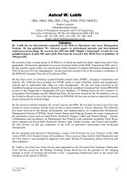
3.8.1 Euler[TT,Y] = ODE_EULER(ODEFUN,TSPAN,Y,NH) with TSPAN = [T0, TF] integrates thesystem of differential equations Y’=f(T,Y) from time T0 to TF with initialcondition Y0 using the forward Euler method on an equispaced grid of NH intervals.Function ODEFUN(T,Y) must return a column vector corresponding to f(T, Y).Each row in the solution array Y corresponds to a time returned in the columnvector T.ParametersODEFUN integrated function.TSPAN TSPAN = [T0 TF]Y initial value Y(T0).NH TT equispaced grid of NH intervals.ReturnsTT equispaced grid of NH intervals.Y solution array.3.8.2 Implicit Euler[TT,Y] = ODE_BEULER(ODEFUN,TSPAN,Y,NH) with TSPAN = [T0, TF] integrates thesystem of differential equations Y’=f(T,Y) from time T0 to TF with initialcondition Y0 using the backward Euler method on an equispaced grid of NHintervals. Function ODEFUN(T, Y) must return a column vector correspondingto f(T, Y). Each row in the solution array Y corresponds to a time returnedin the column vector T.ParametersODEFUN integrated function.TSPAN TSPAN = [T0 TF].Y initial value Y(T0).NH TT equispaced grid of NH intervals.ReturnsTT equispaced grid of NH intervals.Y solution array.Euler’s method bases its projection on the derivative at the current point, and the resultinglarge value causes the numerical solution to diverge radically from the desired solution. Thisbehavior should not surprise us. The Jacobian for this equation is J = 100, so the stabilitycondition for Euler’s method requires a stepsize h < 0.02, which we are violating.By contrast, the backward Euler method has no trouble solving this problem. In fact, thebackward Euler solution is extremely insensitive to the initial value.21

Figure 1: euler vs. beuler with a typical stiff ODE y ′ = −100y + 100t + 1013.8.3 Modified Euler[TT,Y] = ODE_EULER(ODEFUN,TSPAN,Y,NH) with TSPAN = [T0, TF] integrates thesystem of differential equations Y’=f(T,Y) from time T0 to TF with initialcondition Y0 using the modified Euler method on an equispaced grid of NHintervals. Function ODEFUN(T,Y) must return a column vector correspondingto f(T, Y). Each row in the solution array Y corresponds to a time returnedin the column vector T.ParametersODEFUN integrated function.TSPAN TSPAN = [T0 TF].Y initial value Y(T0).NH TT equispaced grid of NH intervals.ReturnsTT equispaced grid of NH intervals.Y solution array.3.8.4 Fourth-order Rounge-KuttaIt corresponds to ode23,ode45 which already exit in Octave. Write ’help ’ inOctave to have more informations.3.8.5 Fourth-order predictor[TT,Y] = ODE_FOP(ODEFUN,TSPAN,Y,NH) with TSPAN = [T0, TF] integrates thesystem of differential equations Y’=f(T,Y) from time T0 to TF with initial22

condition Y0 using the fourth-order predictor scheme on an equispaced gridof NH intervals. Function ODEFUN(T,Y) must return a column vector correspondingto f(T, Y). Each row in the solution array Y corresponds to a time returnedin the column vector T.ParametersODEFUN integrated function.TSPAN tspan = [T0 TF].Y initial value Y(T0).NH TT equispaced grid of NH intervals.ReturnsTT equispaced grid of NH intervals.Y solution array.3.9 Boundary value problems for Ordinary differential EquationsA boundary value problem for a differential equation specifies more than one point at whichthe solution or its derivatives must have given values. For example, a two-point boundary valueproblem for a second-order ODE has the formwith boundary conditionsy = f (t, y, y), a ≤ t ≤ b, (18)y(a) = α, y(b) = β. (19)An initial value problem for such a second-order equation would have specified both y and y ′at a single point, say, t 0 . These initial data would have supplied all the information necessaryto begin a numerical solution method at t 0 , stepping forward to advance the solution in time(or whatever the independent variable might be).3.9.1 Shooting method[T,Y] = ODE_SHOOT(IVP, A, B, UA, UB) integrates the system of differentialequations u”= f(t,u,u’) from time A to B with boundary conditions u(A) =UA and u(B) = UB. Function IVP(t,u,u’) must return a double column vector[u’, u”] with u”= f(t,u,u’). Each row in the solution array Y correspondsto a time returned in the column vector T.ParametersIVP integrated function.A T0.B TF.UA initial value Y(T0).UB final value Y(TF).23

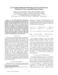
ReturnsT equispaced grid.Y solution array.The basic idea of the shooting method is illustrated in Fig. 2. Each curve represents asolution of the same second-order ODE, with different values for the initial slope giving differentsolution curves. All of the solutions start with the given initial value y(a) = α, but foronly one value of the initial slope does the resulting solution curve hit the desired boundarycondition y(b) = β.24

Figure 2: Shooting method for a two-point boundary value problem.3.9.2 Finite difference method[T,Y] = ODE_FINIT_DIFF(RHS, A, B, UA, UB, N) integrates the system of differentialequations u”= f(t,u,u’) from time A to B with boundary conditions u(A) =UA and u(B) = UB on an equispaced grid of N intervals. Function RHS(t,u,u’)must return a column vector corresponding to f(t,u,u’). Each row in thesolution array Y corresponds to a time returned in the column vector T.ParametersRHS integrated function.A T0.B TF.UA initial value Y(T0).UB final value Y(TF).N T equispaced grid of N intervals.ReturnsT equispaced grid of N intervals.Y solution array.3.9.3 Colocation method[T,Y] = ODE_COLLOC(RHS, A, B, UA, UB, DN, N) integrates the system of differentialequations u”= f(t,u,u’) from time A to B with boundary conditions u(A) =UA and u(B) = UB on an equispaced grid of N intervals. Function RHS(t,u,u’)must return a column vector corresponding to f(t,u,u’). Each row in thesolution array Y corresponds to a time returned in the column vector T.25

ParametersRHS integrated function.A T0.B TF.UA initial value Y(T0).UB final value Y(TF).N T equispaced grid of N intervals.DN degree of computed polynomial solution.ReturnsT equispaced grid of N intervals.Y solution array.3.10 Partial Differential EquationsWe turn now to partial differential equations (PDEs), where many of the numerical tech- niqueswe saw for ODEs, both initial and boundary value problems, are also applicable. The situationis more complicated with PDEs, however, because there are additional inde- pendent variables,typically one or more space dimensions and possibly a time dimension as well. Additional dimensionssignificantly increase computational complexity. Problem formulation also becomesmore complex than for ODEs, as we can have a pure initial value problem, a pure boundaryvalue problem, or a mixture of the two. Moreover, the equation and boundary data may bedefined over an irregular domain in space.First, we establish some notation. For simplicity, we will deal only with single PDEs (asopposed to systems of several PDEs) with only two independent variables (either two spacevariables, which we denote by x and y, or one space and one time variable, which we denote byx and t). In a more general setting, there could be any number of dimensions and any numberof equations in a coupled system of PDEs. We denote by u the unknown solution function to bedetermined and its partial derivatives with respect to the independent variables by appropriatesubscripts: u x = ∂u/∂x, u xy = ∂ 2 u/∂x∂y, etc.3.10.1 Method of lines (for Heat equation)[T, X, U] = PDE_HEAT_LINES(NX, NT, C, F) solves the heat equation D U/DT= C D2 U/DX2 with the method of lines on [0,1]x[0,1]. Initial conditionis U(0,X) = F. C is a positive constant. NX is the number of space integrationintervals and NT is the number of time-integration intervals.ParametersNX X equispaced grid of NX intervals.NT T equispaced grid of NX intervals.C positive constant.ReturnsT equispaced grid of NT intervals.26

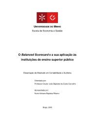
X equispaced grid of NX intervals.U solution array.Notice that we use beuler to integrate each ODE of this system. In fact if we are computingthe solution of the heat equation for example. After the finite difference approximationwe obtain the system y ′ = Ay with A = tridiag(1,-2,1). The Jacobian matrix A of this systemhas eigenvalues between 4c/(∆x)2 and 0, which makes the ODE very stiff as the spatial meshsize ∆x becomes small. This stiffness, which is typical of ODEs derived from PDEs in thismanner, must be taken into account in choosing an ODE method for solving the semidiscretesystem.3.10.2 2-D solver for Advection equationAdvection equation :u t + cu x = 0 (20)[T, X, U] = PDE_ADVEC_EXP(N, DX, K, DT, C, F) solves the advection equationD U/DT = -C D U/DX with the explicit method on [0,1]x[0,1]. Initial conditionis U(0,X) = F. C is a positive constant. N is the number of space integrationintervals and K is the number of time-integration intervals. DX is the sizeof a space integration interval and DT is the size of time-integration intervals.ParametersNX number of space integration intervals.DX size of a space integration interval.NT number of time-integration intervals.DT size of time-integration intervals.C positive constant.F initial condition U(0,X) = F(X).ReturnsT grid of NT intervals.X grid of NX intervals.U solution array.[T, X, U] = PDE_ADVEC_IMP(N, DX, K, DT, C, F) solves the advection equationD U/DT = -C D U/DX with the implicit method on [0,1]x[0,1]. Initial conditionis U(0,X) = F. C is a positive constant. N is the number of space integrationintervals and K is the number of time-integration intervals. DX is the sizeof a space integration interval and DT is the size of time-integration intervals.ParametersNX number of space integration intervals.DX size of a space integration interval.NT number of time-integration intervals.DT size of time-integration intervals.C positive constant.27

Figure 3: Solution of the Advection equation with x ∈ [0, 1] and t ∈ [0, 0.6].F initial condition U(0,X) = F(X).ReturnsT grid of NT intervals.X grid of NX intervals.U solution array.3.10.3 2-D solver for Heat equationHeat equation :u t = cu xx (21)[T, X, U] = PDE_HEAT_EXP(N, DX, K, DT, C, F, ALPHA, BETA) solves the heatequation D U/DT = C D2U/DX2 with the explicit method on [0,1]x[0,1]. Initialcondition is U(0,X) = F and boundary conditions are U(t,0) = ALPHA and U(t,1)= beta. C is a positive constant. N is the number of space integrationintervals and K is the number of time-integration intervals. DX is the sizeof a space integration interval and DT is the size of time-integration intervals.ParametersNX number of space integration intervals.DX size of a space integration interval.NT number of time-integration intervals.DT size of time-integration intervals.F initial condition U(0,X) = F(X).C positive constant.28

ReturnsT grid of NT intervals.X grid of NX intervals.U solution array.[T, X, U] = PDE_HEAT_IMP(N, DX, K, DT, C, F, ALPHA, BETA) solves the heatequation D U/DT = C D2U/DX2 with the implicit method on [0,1]x[0,1]. Initialcondition is U(0,X) = F and boundary conditions are U(t,0) = ALPHA and U(t,1)= beta. C is a positive constant. N is the number of space integrationintervals and K is the number of time-integration intervals. DX is the sizeof a space integration interval and DT is the size of time-integration intervals.ParametersNX number of space integration intervals.DX size of a space integration interval.NT number of time-integration intervals.DT size of time-integration intervals.F initial condition U(0,X) = F(X).C positive constant.ReturnsT grid of NT intervals.X grid of NX intervals.U solution array.The jacobian matrix of the semidiscrete system has eigenvalues between −4c/(∆x) 2 and 0,and hence the stability region for Euler’s method requires that the time step satisfy∆t ≤ (∆x)22c(22)3.10.4 2-D solver for Wave equationWave equation :u tt = cu xx (23)[T, X, U] = PDE_WAVE_EXP(N, DX, K, DT, C, F, G, ALPHA, BETA) solves thewave equation D2U/DT2 = C D2U/DX2 with the explicit method on [0,1]x[0,1].Initial condition is U(0,X) = F, D U/DT (0,X)= G(X) and boundary conditionsare U(t,0) = ALPHA and U(t,1) = beta. C is a positive constant. N is thenumber of space integration intervals and K is the number of time-integrationintervals. DX is the size of a space integration interval and DT is thesize of time-integration intervals.ParametersNX number of space integration intervals.DX size of a space integration interval.NT number of time-integration intervals.29

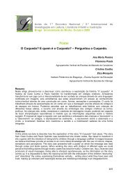
DT size of time-integration intervals.F initial condition U(0,X) = F(X).G initial condition D U/DT (0,X)= G(X).C positive constant.ReturnsT grid of NT intervals.X grid of NX intervals.U solution array.[T, X, U] = PDE_WAVE_IMP(N, DX, K, DT, C, F, G, ALPHA, BETA) solves thewave equation D2U/DT2 = C D2U/DX2 with the implicit method on [0,1]x[0,1].Initial condition is U(0,X) = F, D U/DT (0,X)= G(X) and boundary conditionsare U(t,0) = ALPHA and U(t,1) = beta. C is a positive constant. N is thenumber of space integration intervals and K is the number of time-integrationintervals. DX is the size of a space integration interval and DT is thesize of time-integration intervals.ParametersNX number of space integration intervals.DX size of a space integration interval.NT number of time-integration intervals.DT size of time-integration intervals.F initial condition U(0,X) = F(X).G initial condition D U/DT (0,X)= G(X).C positive constant.ReturnsT grid of NT intervals.X grid of NX intervals.U solution array.3.10.5 2-D solver for the Poisson EquationPoisson equation :u xx + u yy = f (x, y) (24)POISSONFD two-dimensional Poisson solver [U, X, Y] = POISSONFD(A, C, B, D,NX, NY, FUN, BOUND) solves by five-point finite difference scheme the problem-LAPL(U) = FUN in the rectangle (A,B)x(C,D) with Dirichlet boundery conditionsU(X,Y)=BOUND(X,Y) for any (X, Y) on the boundery of the rectangle.[U, X, Y, ERROR] = POISSONFD(A,C,B,D,NX,NY,FUN,BOUND,UEX) computes also themaximum nodal error ERROR with respect to the exact solution UEX. FUN, BOUNDand UEX can be online functions.Parameters30

A, BC, D rectangle (A,B)x(C,D) where the solution is computed.NX X equispaced grid of NX intervals.NY Y equispaced grid of NY intervals.FUNBOUND boundary condition.UEX exact solution.ReturnsU solution array.X equispaced grid of NX intervals.Y equispaced grid of NY intervals.ERROR maximum nodal error ERROR with respect to the exact solution UEX.Figure 4: Solution of the Poisson equation with x ∈ [0, 1] and t ∈ [0, 1].31