IV) Materials calculations with dynamical mean field theory (DMFT)

IV) Materials calculations withdynamical mean field theory (DMFT)Literature:DMFT: Kotliar and Vollhardt, Physics Today 57, No. 3 (March), 53 (2004).Georges et al., Rev. Mod. Phys. 68, 13 (1996).LDA+DMFT: Kotliar et al., Rev. Mod. Phys. 78, 865 (2006).Held, Adv. Phys. 56, 829 (2007).

Ab-initio electronic Hamiltonian(non-relativistic/Born-Oppenheimer approximation)

Ab-initio electronic Hamiltonian(non-relativistic/Born-Oppenheimer approximation)

Ab-initio electronic Hamiltonian(non-relativistic/Born-Oppenheimer approximation)kinetic energy lattice potential Coulomb interactionH = X i"− 2 ∆ i2m e+ X l−e 24πɛ 0Z l|r i − R l |#+ 1 2Xi≠je 24πɛ 01|r i − r j |

Ab-initio electronic Hamiltonian(non-relativistic/Born-Oppenheimer approximation)kinetic energy lattice potential Coulomb interactionH = X i"− 2 ∆ i2m e+ X l−e 24πɛ 0Z l|r i − R l |#+ 1 2Xi≠je 24πɛ 01|r i − r j |LDA bandstructure corresponds toH LDA = X i"− 2 ∆ i2m e+ X l−e 24πɛ 01|r i − R l | + Zd 3 r#e2 1LDAρ(r) + Vxc (ρ(r i ))4πɛ 0 |r i − r|

Ab-initio electronic Hamiltonian(non-relativistic/Born-Oppenheimer approximation)kinetic energy lattice potential Coulomb interactionH = X i"− 2 ∆ i2m e+ X l−e 24πɛ 0Z l|r i − R l |#+ 1 2Xi≠je 24πɛ 01|r i − r j |LDA bandstructure corresponds toH LDA = X i"− 2 ∆ i2m e+ X l−e 24πɛ 01|r i − R l | + Zd 3 r#e2 1LDAρ(r) + Vxc (ρ(r i ))4πɛ 0 |r i − r|LDA + local Coulomb interactionĤ = X klmσɛ LDAklm ĉ†klσĉkmσ+ 1 2| {z }H LDAXU σσ′lmi lσmσ ′ˆn ilσ ˆn imσ ′ − ∆ɛ X imσˆn imσU’Um=2U’−Jm=1

Ab-initio electronic Hamiltonian(non-relativistic/Born-Oppenheimer approximation)kinetic energy lattice potential Coulomb interactionH = X i"− 2 ∆ i2m e+ X l−e 24πɛ 0Z l|r i − R l |#+ 1 2Xi≠je 24πɛ 01|r i − r j |LDA bandstructure corresponds toH LDA = X i"− 2 ∆ i2m e+ X l−e 24πɛ 01|r i − R l | + Zd 3 r#e2 1LDAρ(r) + Vxc (ρ(r i ))4πɛ 0 |r i − r|LDA + local Coulomb interactionĤ = X ɛ LDAklm ĉ†klσĉkmσ+ 1 XU σσ′lm2 ˆn ilσ ˆn imσ ′ − ∆ɛ X ˆn imσU’ U’−Jklmσi lσmσ| {z }′ imσm=1H LDA U• non-local Coulomb interaction → Hartree term (to leading order in 1/Z; contained in LDA)• constrained LDA ⇒ U, J, V =U−2J, ∆ɛ(McMahan et al.’88, Gunnarsson et al.’89)m=2

Constrained LDA1. Calculate LDA energies E(n d ) for constrained problem, i.e., without hopping of d (orf) electrons, for differnet numbers n d of d (or f) electrons.2. Adjust U (J) and ∆ɛ inĤ that these LDA energies are obtained.E000 111000 111000 111000 111n −1 n n +1dd

LDA+UAnisimov et al.’91LDA+U: SolveĤ by symmetry broken HartreeĤ = H LDA + XU σσ′lmi lσmσ ′ˆn ilσ 〈ˆn imσ ′〉 − ∆ɛ X imσˆn imσ − 1 2Xi lσmσ ′ U σσ′lm 〈ˆn ilσ 〉 〈ˆn imσ ′〉E000000000111111111000000000111111111000000000111111111000000000111111111000000000111111111000000000111111111NkU000000000111111111000000000111111111000000000111111111000000000000000000111111111111111111000000001111111100000000111111110000000011111111000000001111111100000000111111110000000011111111LDALDA+U

LDA+DMFTSolveĤ by dynamical mean field theory(Anisimov et al.’97)UUUΣ Σ ΣDMFTUUUΣUΣUUUΣΣΣmaterial specific lattice problem ĤAnderson impurity model + Dyson equation(Metzner, Vollhardt’89; Georges, Kotliar’92)

LDA+DMFTSolveĤ by dynamical mean field theory(Anisimov et al.’97)UUUΣ Σ ΣDMFTUUUΣUΣUUUΣΣΣmaterial specific lattice problem ĤAnderson impurity model + Dyson equation(Metzner, Vollhardt’89; Georges, Kotliar’92)Spectral density functional theory: E[ρ, G ii (ω)]Savrasov, Kotliar’01

LDA+DMFT many body physicsLDA LDA+DMFT LDA+U ∗0 U/W ∞U: local Coulomb interaction, W : LDA bandwidth

¡ ¡ ¡ ¡ ¡ ¡ ¡ ¡¡ ¡ ¡ ¡ ¡ ¡ ¡ ¡¡ ¡ ¡ ¡ ¡ ¡ ¡ ¡¡ ¡ ¡ ¡ ¡ ¡ ¡ ¡¡ ¡ ¡ ¡ ¡ ¡ ¡ ¡¡ ¡ ¡ ¡ ¡ ¡ ¡ ¡LDA+DMFT many body physicsE¡ ¡ ¡ ¡ ¡ ¡ ¡ ¡Nweakly correlated metalkLDA LDA+DMFT LDA+U ∗0 U/W ∞U: local Coulomb interaction, W : LDA bandwidth

¡ ¡ ¡ ¡ ¡ ¡ ¡ ¡¡ ¡ ¡ ¡ ¡ ¡ ¡ ¡¡ ¡ ¡ ¡ ¡ ¡ ¡ ¡¡ ¡ ¡ ¡ ¡ ¡ ¡ ¡¡ ¡ ¡ ¡ ¡ ¡ ¡¡ ¡ ¡ ¡ ¡ ¡ ¡¡ ¡ ¡ ¡ ¡ ¡ ¡¡ ¡ ¡ ¡ ¡ ¡ ¡LDA+DMFT many body physicsEE¡ ¡ ¡ ¡ ¡ ¡ ¡ ¡¡ ¡ ¡ ¡ ¡ ¡ ¡ ¡¡ ¡ ¡ ¡ ¡ ¡ ¡ ¡Uor¡ ¡ ¡ ¡ ¡ ¡ ¡¡ ¡ ¡ ¡ ¡ ¡ ¡Nweakly correlated metalkNMott-Hubbard insulatorkLDA LDA+DMFT LDA+U ∗0 U/W ∞U: local Coulomb interaction, W : LDA bandwidth

¡ ¡ ¡ ¡ ¡ ¡ ¡ ¡¡ ¡ ¡ ¡ ¡ ¡ ¡ ¡¡ ¡ ¡ ¡ ¡ ¡ ¡ ¡¡ ¡ ¡ ¡ ¡ ¡ ¡ ¡¡ ¡ ¡ ¡ ¡ ¡ ¡¡ ¡ ¡ ¡ ¡ ¡ ¡¡ ¡ ¡ ¡ ¡ ¡ ¡¡ ¡ ¡ ¡ ¡ ¡ ¡LDA+DMFT many body physicsEEE¡ ¡ ¡ ¡ ¡ ¡ ¡ ¡¡ ¡ ¡ ¡ ¡ ¡ ¡ ¡¡ ¡ ¡ ¡ ¡ ¡ ¡ ¡Z

¡ ¡ ¡ ¡ ¡ ¡ ¡ ¡¡ ¡ ¡ ¡ ¡ ¡ ¡ ¡¡ ¡ ¡ ¡ ¡ ¡ ¡ ¡¡ ¡ ¡ ¡ ¡ ¡ ¡ ¡¡ ¡ ¡ ¡ ¡ ¡ ¡¡ ¡ ¡ ¡ ¡ ¡ ¡¡ ¡ ¡ ¡ ¡ ¡ ¡¡ ¡ ¡ ¡ ¡ ¡ ¡LDA+DMFT many body physicsEEE¡ ¡ ¡ ¡ ¡ ¡ ¡ ¡¡ ¡ ¡ ¡ ¡ ¡ ¡ ¡¡ ¡ ¡ ¡ ¡ ¡ ¡ ¡Z

¡ ¡ ¡ ¡ ¡ ¡ ¡ ¡¡ ¡ ¡ ¡ ¡ ¡ ¡ ¡¡ ¡ ¡ ¡ ¡ ¡ ¡ ¡¡ ¡ ¡ ¡ ¡ ¡ ¡ ¡¡ ¡ ¡ ¡ ¡ ¡ ¡¡ ¡ ¡ ¡ ¡ ¡ ¡¡ ¡ ¡ ¡ ¡ ¡ ¡¡ ¡ ¡ ¡ ¡ ¡ ¡LDA+DMFT many body physicsEEE¡ ¡ ¡ ¡ ¡ ¡ ¡ ¡¡ ¡ ¡ ¡ ¡ ¡ ¡ ¡¡ ¡ ¡ ¡ ¡ ¡ ¡ ¡Z

¡ ¡ ¡ ¡ ¡ ¡ ¡ ¡¡ ¡ ¡ ¡ ¡ ¡ ¡ ¡¡ ¡ ¡ ¡ ¡ ¡ ¡ ¡¡ ¡ ¡ ¡ ¡ ¡ ¡ ¡¡ ¡ ¡ ¡ ¡ ¡ ¡¡ ¡ ¡ ¡ ¡ ¡ ¡¡ ¡ ¡ ¡ ¡ ¡ ¡¡ ¡ ¡ ¡ ¡ ¡ ¡LDA+DMFT many body physicsEEE¡ ¡ ¡ ¡ ¡ ¡ ¡ ¡¡ ¡ ¡ ¡ ¡ ¡ ¡ ¡¡ ¡ ¡ ¡ ¡ ¡ ¡ ¡Z

¡ ¡ ¡ ¡ ¡ ¡ ¡ ¡¡ ¡ ¡ ¡ ¡ ¡ ¡ ¡¡ ¡ ¡ ¡ ¡ ¡ ¡ ¡¡ ¡ ¡ ¡ ¡ ¡ ¡ ¡¡ ¡ ¡ ¡ ¡ ¡ ¡¡ ¡ ¡ ¡ ¡ ¡ ¡¡ ¡ ¡ ¡ ¡ ¡ ¡¡ ¡ ¡ ¡ ¡ ¡ ¡LDA+DMFT many body physicsEEE¡ ¡ ¡ ¡ ¡ ¡ ¡ ¡¡ ¡ ¡ ¡ ¡ ¡ ¡ ¡¡ ¡ ¡ ¡ ¡ ¡ ¡ ¡Z

LDA+DMFT — overviewMetzner, Vollhardt PRL’89 — simplifications in d = ∞Georges, Kotliar PRB’89 — DMFTAnisimov et al. EPJ’97 — first LDA+DMFT calculation, LaTiO 3simplified DMFT solverKH, Keller, Eyert, Vollhardt, Anisimov PRL’01 — Mott-Hubbard transition in V2O 3KH, McMahan, Scalettar PRL’01 — Volume collapse in CeLichtenstein, Katsnelson PRL’01 — Ferromagnetism in Fe and NiSavrasov, Kotliar, Abrahams Nature’01 — δ-Pu

LDA+DMFT — overviewMetzner, Vollhardt PRL’89 — simplifications in d = ∞Georges, Kotliar PRB’89 — DMFTAnisimov et al. EPJ’97 — first LDA+DMFT calculation, LaTiO 3simplified DMFT solverKH, Keller, Eyert, Vollhardt, Anisimov PRL’01 — Mott-Hubbard transition in V2O 3KH, McMahan, Scalettar PRL’01 — Volume collapse in CeLichtenstein, Katsnelson PRL’01 — Ferromagnetism in Fe and NiSavrasov, Kotliar, Abrahams Nature’01 — δ-Pu... ∼ 300 publications by now ...

LDA+DMFT — overviewMetzner, Vollhardt PRL’89 — simplifications in d = ∞Georges, Kotliar PRB’89 — DMFTAnisimov et al. EPJ’97 — first LDA+DMFT calculation, LaTiO 3simplified DMFT solverKH, Keller, Eyert, Vollhardt, Anisimov PRL’01 — Mott-Hubbard transition in V2O 3KH, McMahan, Scalettar PRL’01 — Volume collapse in CeLichtenstein, Katsnelson PRL’01 — Ferromagnetism in Fe and NiSavrasov, Kotliar, Abrahams Nature’01 — δ-Pu... ∼ 300 publications by now ...P. W. Anderson, The future lies ahead in “Recent progress in many-body theories” (WorldScientific, 2006):In theory, the big news is the DMFT which gives us a systematic way todeal with the major effects of strong correlations. After nearly 50 years,we are finally able to understand the Mott transition, for instance, at leastin three dimensions, and to model the Kondo volume collapse in cerium.

Dynamical mean field theory (DMFT)d dimensional quantum system ≡ d + 1 (+time) dimensional classical system

Dynamical mean field theory (DMFT)d dimensional quantum system ≡ d + 1 (+time) dimensional classical systemMean field theories:

Dynamical mean field theory (DMFT)d dimensional quantum system ≡ d + 1 (+time) dimensional classical systemMean field theories:Weiss mean field theory:mean field in d dimensions (Ising) or d + 1 dimensions (Heisenberg)

Dynamical mean field theory (DMFT)d dimensional quantum system ≡ d + 1 (+time) dimensional classical systemMean field theories:Weiss mean field theory:mean field in d dimensions (Ising) or d + 1 dimensions (Heisenberg)Hartree Fock:mean field in d + 1 dimensions

Dynamical mean field theory (DMFT)d dimensional quantum system ≡ d + 1 (+time) dimensional classical systemMean field theories:Weiss mean field theory:mean field in d dimensions (Ising) or d + 1 dimensions (Heisenberg)Hartree Fock:mean field in d + 1 dimensionsDMFT:mean field in d spatial dimensionsbut not mean-field in timequantum fluctuations (time) keptspatial fluctuations neglected

First something easier...

First something easier......Weiss mean field theoryIsing modelĤ = J ∑ 〈ij〉s i s jLimit d → ∞ or Z → ∞; proper scaling J = J ∗ /Z

First something easier......Weiss mean field theoryIsing modelĤ = J ∑ 〈ij〉s i s jLimit d → ∞ or Z → ∞; proper scaling J = J ∗ /Z⇒ Weiss mean field theory becomes exact〈s i 〉 = ∑ s i e −βJ∗ s i 〈s j 〉 /[e βJ∗ 〈s j 〉 + e −βJ∗ 〈s j 〉 ]s i =±1

First something easier......Weiss mean field theoryIsing modelĤ = J ∑ 〈ij〉s i s jLimit d → ∞ or Z → ∞; proper scaling J = J ∗ /Z⇒ Weiss mean field theory becomes exact〈s i 〉 = ∑ s i e −βJ∗ s i 〈s j 〉 /[e βJ∗ 〈s j 〉 + e −βJ∗ 〈s j 〉 ]s i =±121 3WMFTJ * oo

First something easier......Weiss mean field theoryIsing modelĤ = J ∑ 〈ij〉s i s jLimit d → ∞ or Z → ∞; proper scaling J = J ∗ /Z⇒ Weiss mean field theory becomes exact〈s i 〉 = ∑ s i e −βJ∗ s i 〈s j 〉 /[e βJ∗ 〈s j 〉 + e −βJ∗ 〈s j 〉 ]s i =±121 3DMFTσlΣ (ω)oo

First something easier......Weiss mean field theoryIsing modelĤ = J ∑ 〈ij〉s i s jLimit d → ∞ or Z → ∞; proper scaling J = J ∗ /Z⇒ Weiss mean field theory becomes exact〈s i 〉 = ∑ s i e −βJ∗ s i 〈s j 〉 /[e βJ∗ 〈s j 〉 + e −βJ∗ 〈s j 〉 ]s i =±121 3WMFTJ * oo

DMFT self-consistency cycleG(ω) = 1V BZ∫BZG 0 = (G −1 + Σ) −1d 3 k [ ω1 + µ1 − ɛ(k) − Σ(ω)] −1Solve AIM defined by G 0 ⇒ GΣ new = (G 0 ) −1 − G −1Iterate with Σ=Σ new until ||Σ − Σ new || < ε

DMFT self-consistency cycleG(ω) = 1V BZ∫BZG 0 = (G −1 + Σ) −1d 3 k [ ω1 + µ1 − ɛ(k) − Σ(ω)] −1Solve AIM defined by G 0 ⇒ GΣ new = (G 0 ) −1 − G −1Iterate with Σ=Σ new until ||Σ − Σ new || < ε21 3DMFTσlΣ (ω)oo

DMFT self-consistency cycleG(ω) = 1V BZ∫BZG 0 = (G −1 + Σ) −1d 3 k [ ω1 + µ1 − ɛ(k) − Σ(ω)] −1Solve AIM defined by G 0 ⇒ GΣ new = (G 0 ) −1 − G −1Iterate with Σ=Σ new until ||Σ − Σ new || < εUUUΣ Σ ΣDMFTUUUΣUΣUUUΣΣΣ

DMFT self-consistency cycleG(ω) = 1V BZ∫BZG 0 = (G −1 + Σ) −1d 3 k [ ω1 + µ1 − ɛ(k) − Σ(ω)] −1Solve AIM defined by G 0 ⇒ GΣ new = (G 0 ) −1 − G −1Iterate with Σ=Σ new until ||Σ − Σ new || < εUUUΣ Σ ΣDMFTUUUΣUΣUUUΣΣΣ

Mott-Hubbard metal-insulator transition

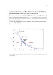
Experimental motivation — (Cr x V 1−x ) 2 O 3McWhan et al.’73Cr-doping x ≡ volume changeMcWhan, Remeika’70

Experimental motivation — (Cr x V 1−x ) 2 O 3McWhan et al.’73Cr-doping x ≡ volume changeMcWhan, Remeika’70

Experimental motivation — (Cr x V 1−x ) 2 O 3←→McWhan et al.’73Cr-doping x ≡ volume changeMcWhan, Remeika’70←→ Mott-Hubbard transitionU: local Coulomb interactionW : bandwidth

One-band Hubbard modelĤ = − t∗√Z1∑〈ij〉 σĉ σ†i ĉ σ j + U ∑ iĉ ↑ †i ĉ ↑ i ĉ↓ †i ĉ ↓ ihalf-filling — paramagnetic phase (frustration)

One-band Hubbard modelĤ = − t∗√Z1∑〈ij〉 σĉ σ†i ĉ σ j + U ∑ iĉ ↑ †i ĉ ↑ i ĉ↓ †i ĉ ↓ ihalf-filling — paramagnetic phase (frustration)Bethe lattice Z 1 → ∞N(E)−D/2 D/2E

Numerical results – spectrumSpectrum A(ω) = − 1 π ImG(ω)DMFT(NRG) Bulla’99

Numerical results – spectrumSpectrum A(ω) = − 1 π ImG(ω)DMFT(NRG) Bulla’99U=0Α(ω)−8 −4 0 4 8ω

Numerical results – spectrumSpectrum A(ω) = − 1 π ImG(ω)DMFT(NRG) Bulla’99U=0.8Α(ω)−8 −4 0 4 8ω

Numerical results – spectrumSpectrum A(ω) = − 1 π ImG(ω)DMFT(NRG) Bulla’99U=0.8 U=1.2Α(ω)−8 −4 0 4 8ω

Numerical results – spectrumSpectrum A(ω) = − 1 π ImG(ω)DMFT(NRG) Bulla’99U=0.8 U=1.2 U=2Α(ω)−8 −4 0 4 8ω

Numerical results – spectrumSpectrum A(ω) = − 1 π ImG(ω)DMFT(NRG) Bulla’99U=0.8 U=1.2U=2.8Α(ω)−8 −4 0 4 8ω

Numerical results – spectrumSpectrum A(ω) = − 1 π ImG(ω)DMFT(NRG) Bulla’99U=0.8 U=1.2U=2.8 U=3.6Α(ω)−8 −4 0 4 8ω

Numerical results – spectrumSpectrum A(ω) = − 1 π ImG(ω)DMFT(NRG) Bulla’99U=0.8 U=1.2U=2.8 U=3.6 U=4.4Α(ω)−8 −4 0 4 8ω

Numerical results – spectrumSpectrum A(ω) = − 1 π ImG(ω)DMFT(NRG) Bulla’99U=0.8 U=1.2U=2.8 U=3.6 U=4.4 U=5.2Α(ω)−8 −4 0 4 8ω

Numerical results – spectrumSpectrum A(ω) = − 1 π ImG(ω)DMFT(NRG) Bulla’99U=0.8 U=1.2U=2.8 U=3.6 U=4.4 U=5.2 U=5.6Α(ω)−8 −4 0 4 8ω

Numerical results – spectrumSpectrum A(ω) = − 1 π ImG(ω)DMFT(NRG) Bulla’99U=0.8 U=1.2U=2.8 U=3.6 U=4.4 U=5.2 U=5.6 U=5.8Α(ω)−8 −4 0 4 8ω

Numerical results – spectrumSpectrum A(ω) = − 1 π ImG(ω)DMFT(NRG) Bulla’99U=0.8 U=1.2U=2.8 U=3.6 U=4.4 U=5.2 U=5.6 U=5.8 U=6Α(ω)−8 −4 0 4 8ω

Numerical results – spectrumSpectrum A(ω) = − 1 π ImG(ω)DMFT(NRG) Bulla’99U=0.8 U=1.2U=2.8 U=3.6 U=4.4 U=5.2U=5.8 U=6 U=5.6Α(ω)−8 −4 0 4 8ω

Numerical results – spectrumSpectrum A(ω) = − 1 π ImG(ω)DMFT(NRG) Bulla’99U=0.8 U=1.2U=2.8 U=3.6 U=4.4 U=5.2U=5.8 U=6 U=5.6Α(ω)−8 −4 0 4 8ωMetal – Fermi liquidΣ(ω) = (1 − 1 Z )ω − iBω2 + O(ω 3 )m ∗m = 1 Z = 1 − ∂ReΣ(ω+i0+ ) ∣∂ωA(0) fixed∣ω=0

Numerical results – spectrumSpectrum A(ω) = − 1 π ImG(ω)U=0.8 U=1.2U=2.8 U=3.6 U=4.4 U=5.2U=5.8 U=6 U=5.6DMFT(NRG) Bulla’99Quasiparticle weightDMFT(PQMC) Feldbacher, kh, Assaad’04Α(ω)−8 −4 0 4 8ωMetal – Fermi liquidΣ(ω) = (1 − 1 Z )ω − iBω2 + O(ω 3 )m ∗m = 1 Z = 1 − ∂ReΣ(ω+i0+ ) ∣∂ωA(0) fixed∣ω=0

Numerical results – spectrumSpectrum A(ω) = − 1 π ImG(ω)U=0.8 U=1.2U=2.8 U=3.6 U=4.4 U=5.2U=5.8 U=6 U=5.6DMFT(NRG) Bulla’99Quasiparticle weightDMFT(PQMC) Feldbacher, kh, Assaad’04Α(ω)−8 −4 0 4 8ωMetal – Fermi liquidΣ(ω) = (1 − 1 Z )ω − iBω2 + O(ω 3 )m ∗m = 1 Z = 1 − ∂ReΣ(ω+i0+ ) ∣∂ωA(0) fixed∣ω=0Insulator – Mott-HubbardΣ(ω) = 1 U 24 ωG(ω) =Z= 1 2ZdɛdɛN(ɛ)ω − ɛ − Σ(ω)N(ɛ)ω − ɛ − U/2 +N(ɛ)ω − ɛ + U/2

Phase diagramDMFT(NRG) Bulla, Costi, Vollhardt’01DMFT(QMC) Blümer’030.1F LG0.08insulatingcharacter0.06← critical pointT0.04insulator0.020metal4.4 4.5 4.6 4.7 4.8 4.9 5 5.1 5.2U

Phase diagramDMFT(NRG) Bulla, Costi, Vollhardt’01DMFT(QMC) Blümer’030.1F LG0.08insulatingcharacter0.06← critical pointT0.04insulator0.020metal4.4 4.5 4.6 4.7 4.8 4.9 5 5.1 5.2U

LDA+DMFT for (V 0.962 Cr 0.038 ) 2 O 3 /V 2 O 3LDA+DMFT(QMC) spectrakh, Keller, Eyert, Vollhardt, Anisimov PRL’01 &PRB’04Intensity (arb. units)(V 0.962Cr 0.038) 2O 3a 1ge gπIntensity (arb. units)V 2O 3a 1ge gπ-2 0 2 4 6E (ev)U =5.0 eV, J =0.93 eV, T =700 K

LDA+DMFT for (V 0.962 Cr 0.038 ) 2 O 3 /V 2 O 3LDA+DMFT(QMC) spectrakh, Keller, Eyert, Vollhardt, Anisimov PRL’01 &PRB’04Intensity (arb. units)(V 0.962Cr 0.038) 2O 3a 1ge gπIntensity (arb. units)V 2O 3a 1ge gπElectronic correlations⇒ metal-insulator transition; J⇒ S=1-2 0 2 4 6E (ev)U =5.0 eV, J =0.93 eV, T =700 K

Comparison to experiment – metallic V 2 O 3kh, Keller, Eyert, Vollhardt, Anisimov PRL’01 &PRB’04Photoemission spectrumX-ray absorption spectrumLDA+DMFT, T=300KLDAMo et al. ’02, T=175KLDA+DMFT, T=300KLDAMueller et al. ’97, T=300Ka 1g+e gπe gσa 1ge gπ-3 -2 -1 00 2 4 6Energy (eV)— LDA+DMFT – 300 K, broadened with experimental resolutionGood agreement with experiment above and below Fermienergy.