Simple Random Sampling and Systematic Sampling

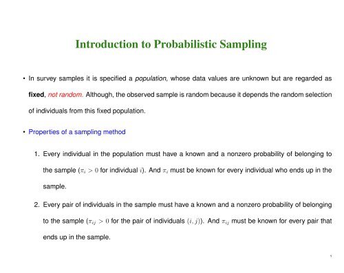
Introduction to Probabilistic Sampling• In survey samples it is specified a population, whose data values are unknown but are regarded asfixed, not random. Although, the observed sample is random because it depends the random selectionof individuals from this fixed population.• Properties of a sampling method1. Every individual in the population must have a known and a nonzero probability of belonging tothe sample (π i > 0 for individual i). And π i must be known for every individual who ends up in thesample.2. Every pair of individuals in the sample must have a known and a nonzero probability of belongingto the sample (π ij > 0 for the pair of individuals (i, j)). And π ij must be known for every pair thatends up in the sample.1

Sampling weights I• If we take a simple random sample of 3500 people from Neverland (with total population 35 million)then any person in Neverland has a chance of being sampled equal to π i = 3500/35000000 = 1/10000for every i.• Then, each of the people we sample represents 10000 Neverland inhabitants.• If 100 people of our sample are unemployed, we would expect then 100 × 10000 = 1 million unemployedin Neverland.• An individual sampled with a sampling probability of π i represents 1/π i individuals in the population.This value is called the sampling weight.2

Sampling weights II• Example: Measure the income on a sample of one individual from a population of N individuals, whereπ i might be different for each individual.• The estimate ( ̂T income ) of the total income of the population (T income ) would be the income for that individualmultiplied by the sampling weight̂T income = 1 π i× income i• Not a good estimate, it is based on only one person, but it is will be unbiased: the expected value ofthe estimate will equal the true population total:( )E ̂Tincome =N∑i=11π i× income i · π i =N∑i=1income i = income T3

The Horvitz-Thompson estimator• The so called Horvitz-Thompson estimator of the population total is the foundation for many complexanalysis• If X i is a measurement of variable X on person i , we write˜X i = 1 π iX i• Given a sample of size n the Horvitz-Thompson estimator ̂T X for the population total T X of X isˆT X =n∑i=11π iX i =n∑i=1˜X i4

• The variance estimator is( )̂V ar ˆTX = ∑ i,j(Xi X jπ ij− X iπ iX jπ j)• The formula applies to any design, however complicated, where π i and π ij are known for the sampledobservations.• The formula depends on the pairwise sampling probabilities π ij , not just on the sampling weights: sothe correlations in the sampling design enter the computations.• See formal definitions and properties in Lohr (2007) p. 240–244.5

Simple Random Sampling• Simple random sampling (SRS) provides a natural starting point for a discussion of probability samplingmethods. It is the simplest method and it underlies many of the more complex methods.• Notations: Sample size is given by n and the population size by N.• Formally defined: Simple random sampling is a sampling scheme with the property that any of thepossible subsets of n distinct elements, from the population of N elements, is equally likely to be thechosen sample.• Every element in the population has the same probability of being selected for the sample, and the jointprobabilities of sets of elements being selected are equal.6

EXAMPLE:• Suppose that a survey is to be conducted in a high school to find out about the students’ leisure habits.A list of the school’s 1872 students is available, with the list being ordered by the students’ identificationnumbers.• Suppose that an SRS of n = 250 is required for the survey. How to draw this sample?– By a lottery method: an urn. Although conceptually simple, this method is cumbersome to executeand it depends on the assumption that the representative discs (one for each student) have beenthoroughly mixed: it is seldom used.– By means of a table of random numbers. It is useful if you make it by hand: in this way is atedious task, requiring a large selection of random numbers, most of which are nonproductive.7

• There are two options:– Simple random sampling with replacement: an element can be selected more than once.sample(1:1872, size=200, replace=TRUE)– Simple random sampling without replacement: the sample must contain n distinct elements.sample(1:1872, size=200, replace=FALSE)• Sampling without replacement gives more precise estimators than sampling with replacement• Now, assume that we have responses from all those sampled (there are not problems of non-response)• Next step: Summarize the individual responses to provide estimates of characteristics of interest forthe population.For instance: average number of hours of television viewing per day and the proportion of studentscurrently reading a novel.8

See a visual demonstration about SRS:library(animation)sample.simple(nrow=10, ncol=10, size=15, p.col=c("blue", "red"), p.cex = c(1,3))NOTATIONS:• Capital letters are used for population values and parameters, and lower-case letters for sample valuesand estimators.• Y 1 , Y 2 , . . . Y N denote the values of the variable y (e.g., hours of television viewing) for the N elementsin the population.• y 1 , y 2 , . . . y n are the values for the n sampled elements.• In general, the value of variable y for the i-th element in the population is Y i (i = 1, 2, . . . N), and thatfor the i-th element in the sample is y i (i = 1, 2, . . . n).9

• The population mean is given by• and the sample mean byȲ =ȳ =N∑i=1n∑i=1Y iNy in• In survey sampling the population variance is defined asσ 2 =( N∑ Yi − Ȳ ) 2i=1N• and the sample variance ass 2 =n∑i=1(y i − ȳ) 2n − 110

Suppose that we wish to estimate the mean number of hours of television viewing per day for all thestudents in the school: ȲQuestion: how good the sample mean ȳ is as an estimator of Ȳ ?On average, the estimator must be very closed to Ȳ over repeated applications of the sampling method.• Observe that the term estimate is used for a specific value, while estimator is used for the rule ofprocedure used for obtaining the estimate.• In the example we obtain, an estimate of 2.20 hours of television viewing (computed by substituting thevalues obtained from the sampled students in the estimator).11

NOTE:Statistical theory provides a means of evaluating estimators but NOT estimates.• Properties of sample estimators are derived theoretically by considering the pattern of results that wouldbe generated by repeating the sampling procedure an infinite number of times.• Example: suppose that drawing a SRS of 250 students from the 1872 students and then calculatingthe sample mean for each sample were carried out infinite times (with replacement).• The resulting set of sample means would have a distribution, known as the sampling distribution of themean.12

• If the sample size is not too small (n ≈ 20 is sufficient) the distribution of the means of each sampleapproximates the normal distribution, and the mean of this distribution is the population mean, Ȳ .• Then it is said that the mean of the individual sample estimates ȳ over an infinite number of samples isan unbiased estimator of Ȳ .• Although the sampling distribution of ȳ is centered on Ȳ , any one estimate will differ from Ȳ .• To avoid confusion with the standard deviation of the element values, standard deviations of samplingdistributions are known as standard errors.• The variance (but it is not useful in practice) of a sample mean (ȳ 0 ) of a SRS of size n is given byV ar(ȳ 0 ) = N − nN − 1 · σ2n = N − nN − 1 · 1n · NN∑ (Yi − Ȳ ) 2i=113

• See example 2.1, p. 29 (artificial example) from Lohr (2006)Suppose we have a population with eight elements (e.g. an almost extinct species of animal...) and weknow the weight y i for each of the N = 8 units of the whole population. We want to know the wholeweight of the population.Animal i 1 2 3 4 5 6 7 8y i 1 2 4 4 7 7 7 8• We take a sample of size 4. How many samples of size 4, can be drawn without replacement from thispopulation?• There are ( 84)= 70 possible samples of size 4 that can be drawn without replacement from this population.• We define as P (S) = 1/70 for each distinct subset of size 4 from the population.14

# Consider a vector of ’observations’y

# To estimate the whole population weight, we take two times the sum# of the y values for each possible sample of indices.alltotal

• The formula V ar(ȳ 0 ) depends on N − nN − 1• The N − nN − 1and the sample size n.term reflects the fact that the survey population is finite in size and that sampling is conductedwithout replacement.• With an infinite population, or if sampling were conducted with replacement, the term is not includedand the expressions are reduced to the familiar forms.• The term indicates the gains of sampling without replacement over sampling with replacement.• In many practical situations the populations are large and, even though the samples may also be large,the sampling fractions are small.17

• In large populations, the difference between sampling with and without replacement is not important:even if the sample is drawn with replacement, the chance of selecting an element more than once isslight.• If the sampling fraction n/N is small, N − nN − 1error.is close to 1 and has a negligible effect on the standard• The correction factor is commonly neglected (i.e., treated as 1) when the sampling fraction (n/N) isless than 1 in 20, or even 1 in 10.• The larger the sample size n is, the smaller is V ar(ȳ 0 ).• For large populations it is the sample size that is dominant in determining the precision of survey results.18

• A sample of size 2000 drawn from a country with a population of 200 million yields about as preciseresults as a sample of the same size drawn from a small city of 40000 (assuming the element variancesin the two populations are the same).• The element variance in the population σ 2 is unknown in a practical application. DenoteAs (see Scheaffer et al. (1990) in Appendix)s 2 = 1n − 1E(s 2 ) =n∑(y i − ȳ) 2i=1NN − 1 σ2 ,then,̂V ar(ȳ 0 ) = N − nN(1 ·s2n = − n )· s2N n19

(• The factor 1 − n )is called the finite population correction (fpc) where n/N is the sampling fraction.N• It is easy to determine a confidence interval for the population mean, applying standard Central LimitTheorem.• Example: suppose that the mean hours watching television per day for the 250 sampled students isȳ 0 = 2.192 hours, with an element variance of s 2 = 1.008. Then a 95% confidence interval for Ȳ is√ (2.192 ± 1.96 1 − 250 ) 1.0081872 250= 2.192 ± 0.116• That is, we are 95% confident that the interval from 2.076 to 2.308 contains the population mean.• See some functions to illustrate the Central Limit Theorem and to compute confidence intervals programmedin R.20

# Using R to illustrate the Central Limit Theorem (from Venables)N

# Using the TeachingDemo librarylibrary(TeachingDemos)X11()clt.examp()X11()clt.examp(5)X11()clt.examp(30)X11()clt.examp(50)22

srs.mu

Sample size for estimation population means• How large must be a sample? ⇒ Observations cost money, time and efforts.• The number of observations needed to estimate a population mean µ with a bound on the error ofestimation of magnitude ε is obtained by solving this equation for n:2 √ V ar(ȳ) = 2√s 2n( ) N − n= εN(as z 0.025 = 1.96, we approximate this value by 2, for a 95% of confidence).• Hence, the sample size required to estimate µ with a bound on the error of estimation ε isn =N · s2N4 ε2 + s 2• Note that s 2 must be estimated previously by means of another argument.24

EXAMPLE• The average amount of money µ for a hospital’s accounts receivable must be estimated. Although noprior data is available to estimate the population variance σ 2 , it is known that most accounts lie withina e100 range. There are N = 1000 open accounts. Find the sample size needed to estimate µ with abound on the error of estimation ε = e3.• First we estimate the population variance. Since the range is often approximately equal to four or sixstandard deviations (4 · s or 6 · s), depending of the normality of data (see the Chebyshev’s inequality),thenthen s 2 ≈ 625, sos ≈ range4= 1004 = 25n =N · s2 1000 · 625=N4 ε2 + s2 10004· 9 + 625 = 217.39 ≈ 217 or 218 observations 25

See a function to calculate sample sizes programmed in R:n.mu

• Many sample surveys are interested about a population total, e.g. when analyzing total accounts.• The population total (the sum of all observations) in the population is denoted by the symbol τ. HenceNµ = τ• It is expected the estimator of τ to be N times the estimator of µ, then– Estimator of population totalˆτ = Nȳ = N ∑ ni=1 y in– Estimated variance of ˆτ̂V ar(ˆτ) = ̂V(ar(Nȳ) = N 2 1 − n ) s2N n∑where s 2 = 1 nn−1 i=1 (y i − ȳ) 2 27

Systematic Sampling• The method of systematic sampling reduces the effort required for the sample selection.• Systematic sampling is easy to apply, involving simply taking every k-th element after a random start.• Example: suppose that a sample of 250 students is required from a school with 2000 students. Thesampling fraction is 250/2000, or 1 in 8.• A systematic sample of the required size, would then be obtained by taking a random number between1 and 8, to determine the first student in the sample, and taking every eighth student thereafter.• If the random number were 5, the selected students would be the fifth, thirteenth, twenty-first, and soon, on the list.• When the sampling is not a simple integer, we can round the interval to an integer, with a resultantchange in the sample size.28

• Example: If fraction is 250/1872 or 1 in 7.488, a 1 in 7 sample would produce a sample of 267 or 268,while a 1 in 8 sample would produce a sample of 234.• Other solution is to round the interval down to start with an element selected at random from the Nelements in the population, and to proceed until the desired sample size has been achieved. Therefore,the list is treated as circular, and the last listing is followed by the first.• Like SRS, systematic sampling gives each element in the population the same chance of being selectedfor the sample.• It differs, however, from SRS in that the probabilities of different sets of elements being included in thesample are not all equal.• In systematic sampling the sample mean is a reasonable estimator of the population mean. However,the unequal probabilities of sets of elements means that the SRS standard error formulae are notdirectly applicable.29

• In order to estimate the standard error of estimators based on systematic samples. Sometimes it isreasonable to assume that the list is approximately randomly ordered, in which case the sample can betreated as if it were a simple random sample.• Lists arranged in alphabetical order may often be reasonably treated in this way.• Systematic sampling performs badly when the list is ordered in cycles of values of the survey variablesand when the sampling interval coincides with a multiple of the length of the cycle.• Systematic sampling is widely used in practice without excessive concern for the damaging effects ofundetected cycles in the ordering of the list.• See visual demonstration in:library(animation)sample.system()• See a function to calculate systematic sampling programmed in R:30

systematic.sample

Sampling with probabilities proportional to size• Sometimes is advantageous to select sampling units with different probabilities (other than uniform).• The method is called sampling with probabilities proportional to size or pps sampling.• For a sample y 1 , y 2 , . . . , y n from a population of size N, let π i the probability that y i appears in thesample.• the pps estimator of µ only produces smaller variances than an standard SRS if the weights π i areapproximately proportional to the size of the y i under investigation.32

• In this case, the estimator of the population mean µ isand the estimated variance of ˆµ iŝV ar(ˆµ pps ) =ˆµ pps = 1Nn1N 2 n(n − 1)n∑i=1n∑i=1y iπ i(yiπ i− N · ˆµ pps) 2• The best practical way to choose the weights π i ’s is to chose them proportional to a known measurementthat is highly correlated with y i .• See the library pps of R from:http://cran.r-project.org/web/packages/pps/index.html33

Example (from Scheaffer et al., p. 80):An investigator wishes to estimate the average number of defects per keyboard on keyboards of electroniccomponents manufactured for installation in computers. The keyboards contain varying numbers ofcomponents, and the investigator feels that the number of defects should be positively correlated with thenumber of components on a keyboard.Thus, pps sampling is used with the probability of selecting anyone keyboard for the sample being proportionalto the number of components on that keyboard. A sample of n = 4 keyboards is to be selectedfrom the N = 10 keyboards of one day’s production. The number of components on the 10 keyboards are,respectively: 10, 12, 22, 8, 16, 24, 9, 10, 8, 31.After the sampling was completed, the number of defects found on the four keyboards were, respectively,1, 3, 2 and 1. Estimate the average number of defects per keyboard, and place a bound on the error ofestimation.34

data

Consider a SRS based in the library survey:http://faculty.washington.edu/tlumley/survey/We consider this example# Artificial Datamydata

# Selection of a samplesrs_rows

Consider a SRS programmed with Stata:* Read the previous artificial datause C:\QM\mydata.dtacount* Fix the seed of the randomizationset seed 666* Take a sample equal to the 20\% of the populationsample 20count* Compute weights and the factor of population correctiongen pw = 235/47gen fpc = 23538

* Set the sampling designsvyset [pweight=pw], fpc(fpc)svydescribe* Compute several statisticssvy: mean incomesvy: total incomesvy linearized : tabulate regionsvy linearized : tabulate statesvy: tabulate region state, row se ci format(%7.4f)* Compute a box-plotgraph box income [pweight=pw]39