The Free Speech Calculus Text

The Free Speech Calculus TextVarious authors, Gnu Free Documentation License (see notes)November 22, 2004

iiCopyright c○2004. This work is covered by the Gnu Free Documentation license.Loosely speaking here are the terms of this license:• You are free to copy, redistribute, change, print, sell, and otherwise use inany manner part or all of this document,• Any work derived from these notes must also be covered by the GFDL. (Thisonly applies to that part of your work derived from these notes. It is up toyou whether those parts of your work which are not based on these notes iscovered by the GFDL. Also, you can quote, with attribution, and subjectto fair use provisions, from these notes like you would from any copyrightedwork.)• Anyone distributing works covered by the GFDL must provide source codeor other editable files for the material which is distributed. In the case ofthese notes that means the L A TEX code, as well as the source documents forcreating the graphics.• If you make changes to these notes and redestribute them, you should namethe finished product something different than “The Free Speech CalculusText” or “The Free Speech Calculus Text: original version”. You may choosederivative names like “The Free Speech Calculus Text: the John Doe version”.

Contents1 Background 31.1 The numbers . . . . . . . . . . . . . . . . . . . . . . . . . . . . . . 31.2 Functions . . . . . . . . . . . . . . . . . . . . . . . . . . . . . . . . 91.3 Using functions . . . . . . . . . . . . . . . . . . . . . . . . . . . . . 241.4 End of chapter problems . . . . . . . . . . . . . . . . . . . . . . . . 352 Limits 372.1 Elementary limits . . . . . . . . . . . . . . . . . . . . . . . . . . . . 372.2 Formal limits . . . . . . . . . . . . . . . . . . . . . . . . . . . . . . 432.3 Foundations of the real numbers . . . . . . . . . . . . . . . . . . . 472.4 Continuity . . . . . . . . . . . . . . . . . . . . . . . . . . . . . . . . 502.5 Limits at infinity . . . . . . . . . . . . . . . . . . . . . . . . . . . . 573 Derivatives 613.1 The idea of the derivative of a function . . . . . . . . . . . . . . . . 613.2 Derivative Shortcuts . . . . . . . . . . . . . . . . . . . . . . . . . . 673.3 An alternative approach to derivatives . . . . . . . . . . . . . . . . 743.4 Derivatives of transcendental functions . . . . . . . . . . . . . . . . 813.5 Product and quotient rule . . . . . . . . . . . . . . . . . . . . . . . 873.6 Chain rule . . . . . . . . . . . . . . . . . . . . . . . . . . . . . . . . 923.7 Hyperbolic functions . . . . . . . . . . . . . . . . . . . . . . . . . . 963.8 Tangent and Normal Lines . . . . . . . . . . . . . . . . . . . . . . . 973.9 End of chapter problems . . . . . . . . . . . . . . . . . . . . . . . . 1004 Applications of Derivatives 1054.1 Critical points, monotone increase and decrease . . . . . . . . . . . 1064.2 Minimization and Maximization . . . . . . . . . . . . . . . . . . . . 1094.3 Local minima and maxima (First Derivative Test) . . . . . . . . . 1184.4 An algebra trick . . . . . . . . . . . . . . . . . . . . . . . . . . . . 1214.5 Linear approximations: approximation by differentials . . . . . . . 1234.6 Implicit differentiation . . . . . . . . . . . . . . . . . . . . . . . . . 1284.7 Related rates . . . . . . . . . . . . . . . . . . . . . . . . . . . . . . 1324.8 The intermediate value theorem and finding roots . . . . . . . . . . 1364.9 Newton’s method . . . . . . . . . . . . . . . . . . . . . . . . . . . . 1374.10 L’Hospital’s rule . . . . . . . . . . . . . . . . . . . . . . . . . . . . 1474.11 Exponential growth and decay: a differential equation . . . . . . . 1514.12 The second and higher derivatives . . . . . . . . . . . . . . . . . . 1554.13 Inflection points, concavity upward and downward . . . . . . . . . 1564.14 Another differential equation: projectile motion . . . . . . . . . . . 1584.15 Graphing rational functions, asymptotes . . . . . . . . . . . . . . . 1604.16 The Mean Value Theorem . . . . . . . . . . . . . . . . . . . . . . . 1625 Integration 1655.1 Basic integration formulas . . . . . . . . . . . . . . . . . . . . . . . 165iii

ivCONTENTS5.2 Introduction to the Fundamental Theorem of Calculus . . . . . . . 1745.3 The simplest substitutions . . . . . . . . . . . . . . . . . . . . . . . 1765.4 Substitutions . . . . . . . . . . . . . . . . . . . . . . . . . . . . . . 1785.5 Area and definite integrals . . . . . . . . . . . . . . . . . . . . . . . 1805.6 Transcendental integration . . . . . . . . . . . . . . . . . . . . . . . 1895.7 End of chapter problems . . . . . . . . . . . . . . . . . . . . . . . . 1906 Applications of Integration 1936.1 Area between two curves . . . . . . . . . . . . . . . . . . . . . . . . 1936.2 Lengths of Curves . . . . . . . . . . . . . . . . . . . . . . . . . . . 1936.3 Numerical integration . . . . . . . . . . . . . . . . . . . . . . . . . 1976.4 Averages and Weighted Averages . . . . . . . . . . . . . . . . . . . 2006.5 Centers of Mass (Centroids) . . . . . . . . . . . . . . . . . . . . . 2016.6 Volumes by Cross Sections . . . . . . . . . . . . . . . . . . . . . . . 2046.7 Solids of Revolution . . . . . . . . . . . . . . . . . . . . . . . . . . 2076.8 Work . . . . . . . . . . . . . . . . . . . . . . . . . . . . . . . . . . . 2106.9 Surfaces of Revolution . . . . . . . . . . . . . . . . . . . . . . . . . 2117 Techniques of Integration 2157.1 Integration by parts . . . . . . . . . . . . . . . . . . . . . . . . . . 2157.2 Partial Fractions . . . . . . . . . . . . . . . . . . . . . . . . . . . . 2197.3 Trigonometric Integrals . . . . . . . . . . . . . . . . . . . . . . . . 2287.4 Trigonometric Substitutions . . . . . . . . . . . . . . . . . . . . . . 2367.5 Overview of Integration . . . . . . . . . . . . . . . . . . . . . . . . 2437.6 Improper Integrals . . . . . . . . . . . . . . . . . . . . . . . . . . . 2438 Taylor polynomials and series 2458.1 Historical and theoretical comments: Mean Value Theorem . . . . 2458.2 Taylor polynomials: formulas . . . . . . . . . . . . . . . . . . . . . 2468.3 Classic examples of Taylor polynomials . . . . . . . . . . . . . . . . 2538.4 Computational tricks regarding Taylor polynomials . . . . . . . . . 2538.5 Getting new Taylor polynomials from old . . . . . . . . . . . . . . 2568.6 Prototypes: More serious questions about Taylor polynomials . . . 2588.7 Determining Tolerance/Error . . . . . . . . . . . . . . . . . . . . . 2628.8 How large an interval with given tolerance? . . . . . . . . . . . . . 2658.9 Achieving desired tolerance on desired interval . . . . . . . . . . . 2678.10 Integrating Taylor polynomials: first example . . . . . . . . . . . . 2698.11 Integrating the error term: example . . . . . . . . . . . . . . . . . 2708.12 Applications of Taylor series . . . . . . . . . . . . . . . . . . . . . . 2709 Infinite Series 2739.1 Convergence . . . . . . . . . . . . . . . . . . . . . . . . . . . . . . . 2739.2 Various tests for convergence . . . . . . . . . . . . . . . . . . . . . 2769.3 Power series . . . . . . . . . . . . . . . . . . . . . . . . . . . . . . . 2799.4 Formal Convergence . . . . . . . . . . . . . . . . . . . . . . . . . . 28310 Ordinary Differential Equations 28910.1 Simple differential equations . . . . . . . . . . . . . . . . . . . . . . 29010.2 Basic Ordinary Differential Equations . . . . . . . . . . . . . . . . 29110.3 Higher order differential equations . . . . . . . . . . . . . . . . . . 30211 Vectors 30711.1 Basic vector arithmetic . . . . . . . . . . . . . . . . . . . . . . . . . 30711.2 Limits and Continuity in Vector calculus . . . . . . . . . . . . . . . 31611.3 Derivatives in vector calculus . . . . . . . . . . . . . . . . . . . . . 32411.4 Div, Grad, Curl, and other operators . . . . . . . . . . . . . . . . . 327

CONTENTSv11.5 Integration in vector calculus . . . . . . . . . . . . . . . . . . . . . 33112 Partial Differential Equations 33912.1 Some simple partial differential equations . . . . . . . . . . . . . . 33912.2 Quasilinear partial differential equations . . . . . . . . . . . . . . . 34112.3 Initial value problems . . . . . . . . . . . . . . . . . . . . . . . . . 34312.4 Non linear PDE’s . . . . . . . . . . . . . . . . . . . . . . . . . . . . 34812.5 Higher order PDE’s . . . . . . . . . . . . . . . . . . . . . . . . . . 34912.6 Systems of partial differential equations . . . . . . . . . . . . . . . 353Appendix: the Gnu Free Documentation License 355

viCONTENTS

CONTENTS 1IntroductionDiscussion.[author=garrett,style=friendly,label=introduction_to_whole_work,version=1, file=text_files/introduction_to_whole]Relax. Calculus doesn’t have to be hard, and its basic ideas can be understoodby anyone. So, why does it have a reputation? Well, Calculus can be hard. Huh?That’s right, it doesn’t have to be hard, but it can be.Calculus itself just involves two new processes, differentiation and integration,and applications of these new things to solution of problems that would have beenimpossible otherwise.For better or for worse, most Calculus classes increase the overall level ofdifficulty above pre-Calculus, while teaching you the subject matter. What thismeans is that in addition to learning how to take the derivative, you’ll set up wordproblems, solve some equations, interpret the results etc. Most of this is algebra,but the pieces are all held together by the Calculus.The three hardest parts about a typical Calculus class are (in my opinion):(1) Setting problems up (reading word problems, setting up equations etc), (2)manipulating functions and equations in algebraic way, (3) keeping track of abunch of parts of the problem and putting it together. Note that (1) and (3)should be really important for anyone who is going to use their head for a living.Note that none of these “hard parts” is taking derivatives or integrating. Of course,I could be biased since I teach the class!Another thing to think about as you take this course is the role of the calculator.On the one hand, since we have graphing calculators, the way we use calculusshould be a little different than how it was used in the past. However, mathteachers are still figuring out what parts should change and what parts shouldstay the same. So please forgive us if we don’t have it perfect quite yet.On the other hand, some of the parts that have changed are now harder. So,in the past, it might have been a useful exercise (in a practical sense)for a studentto learn how to graph y = e x /x by hand, now the use of this exercise is probablyone of the following: (1) purely for the sake of learning, (2) because we have to beable to double check/understand what the calculators are telling us, (3) as a warmup for the problems that the calculator can’t solve. Option (3) might mean beingable to analyze all functions of the form y = ae bx /x where a and b are constants,but we don’t know what they are ahead of time. Note that the calculator can’tgraph y = ae bx ; we can (and will) learn to do it, but this problem is a little harderthan graphing y = e x /x.Discussion.[author=duckworth,style=formal,label=introduction_to_whole_work,version=2, file=text_files/introduction_to_whole]This text book aims to provide both insight into the essential problems of Calculus(and the related field of mathematical analysis) and a rigorous proof of all of thestandard material in a Calculus class. However, we will not put rigor in the wayof leisure or explanation. Thus, while we will prove everything, we will not alwaysdo so in the most sophisticated or efficient manner manner.One of the special features of this text is to include discussion of the historical

2 CONTENTScontroversies and so-called paradoxes which made Calculus such an exciting andhard-won mathematical field.Discussion.[author=duckworth,style=middle,label=introduction_to_whole_work,version=3, file=text_files/introduction_to_whole]This text will attempt to introduce the student to all of the varied roles which Calculusplays in science and academia. Calculus is an applied subject which formsthe basis of elementary calculations in physics, biology, psychology, statistics, engineering,etc. Calculus is the first math class that most people have taken wherethey have to learn concepts that are not immediate generalizations of arithmeticor geometric intuition. Finally, and related to both of the above, Calculus is thefirst math class that many people take where statements are given that are notexercises in proof, like in geometry, but still need to be proven.It is of course not easy to satisfy all of the above goals at the same time, sowe will have to take a middle-of-the-road approach: we will offer a little bit ofmaterial towards each goal.In addition to the elusive goals just layed out, there is the difficulty of havinga widely defined audience: in a typical college Calculus class roughly one thirdof the students have seen Calculus before, and remember the material fairly well.Another third of the class has seen Calculus before, but did not absorb a significantpart of the course. The final third of the class has not seen Calculus before.It is of course not easy to write a book addressed to all of the above parts ofthe audience, so we will again take a middle-of-the-road approach: we will offerenough explanation that a student who has never seen the material before can,with diligence, learn Calculus. The phrase “with diligence” is supposed to suggestthat such a student will have to expect to spend more time figuring out examplesand discussion in this book than they needed for previous math classes. Such astudent might also want to access extra material from study guides.

Chapter 1BackgroundDiscussion.[author=duckworth, file =text_files/introduction_to_background]In this chapter we gather together bacground material. This material actuallycomes in two varieties: the stuff that is really necessary to have a good chance ofpassing the class, and the stuff that it’s ok to look up, or learn as you go along.Often Calculus books, and teachers, seem to say that you should know everythingin this chapter before you start. Well, maybe the ideal Calculus student would,but most of us aren’t ideal, and most of us can still pass a calculus class. In anycase, I will try to make it clear what is really necessary to know from what ismerely helpful.1.1 The numbersDiscussion.[author=duckworth,author=livshits, file =text_files/basics_about_numbers]The natural numbers are symbolized by N. These are the numbers 1, 2, 3, 4, . . . .The integers are symbolized by Z (from the German word “Zahl”). These arethe natural numbers, together with their negatives and together with 0. In otherwords, these are the numbers 0, ±1, ±2, ±3, ±4, . . . .The rational numbers are symbolized by Q. These are all the fractions youcan make integers on the top and bottom. In other words, these are the numbersof the form a bwith a and b integers. Every integer is a rational number becausea1= a. A decimal number is a rational number if and only if the decimal digitshave a repeating pattern.The real numbers are symbolized by R. These include the rational numbers.You can think of the real numbers as being all the points on a number line. Thereal numbers form the heart of calculus; everything we do in calculus involves themand depends intimately upon their properties.We can think of the real numbers as the set of all decimals numbers. Thisincludes decimal numbers that extend infinitely to the right. Even decimal numberswith an infinite number of digits can be approximated with decimals numbers3

4 CHAPTER 1. BACKGROUNDhaving only finitely many digits. For example, although π has an infinite numberof digits, we can approximate it as π ≈ 3.1415926 · · · . This is how our calculatorsand computers work: they approximate the set of all real numbers using only numberswith finitely many digits. This is why their answers are sometimes wrong;because they’re based on approximations.Discussion.[author=duckworth,uses=complex_numbers,uses=extended_reals,uses=hyperreals, file=text_files/basics_about_numbers]It is sometimes convenient to add some extra numbers to the real numbers. Whenwe do so we go beyond many people’s intuition, and this might make some studentsuncomfortable. Good! This discomfort is a sign of something interesting; Iencourage you to explore any topic here which you think is strange, or suspicious.I’ll just briefly say now that everything we do here can be rigorously justified, andthat it’s great fun to introduce new objects into your mathematics. With thesenew objects you can do things that were previously “forbidden”: take the squareroot of negative numbers and divide by 0,The complex numbers are denoted by C and are obtained by taking the realnumbers R and joining them with the “imaginary” number i, which satisfies i 2 =−1. By “joining” I mean that you also take all sums, differences, products andquotients of things in R together with i. In other words, every complex number canbe written in the form a + bi where a and b are any real number. The arithmeticis C is defined by the two rules:(a + bi) + (c + di) = (a + c) + (b + d)i for all real numbers a, b, c, d(a + bi)(c + di) = (ac − bd) + (ad + bc)i for all real numbers a, b, c, dThe extended real numbers do not have a standard symbol. They are obtainedby taking the real numbers R and joining them with infinity ∞. Again, “joining”means taking all sums, differences, products, and quotients of things in R with ∞.The arithmetic in the extended real numbers is (loosely speaking) defined by thefollowing rules:−∞ is also an extended real numbera ± ∞ = ±∞ for every real number aa(±∞) = ±∞ for every real number a > 0−∞ < a < ∞ for every real number aa0= ±∞ for every real number a ≠ 0a±∞= 0 for every real number a0∞ is undefined∞ − ∞ is undefinedare undefined00 and ∞ ∞The hyperreal numbers are similar to the extended real numbers. They areobtained by taking the real numbers R and joining them with ∞, as well as aninfinitesimal ɛ. The arithmetic in the hyperreals is (loosely speaking) defined by

1.1. THE NUMBERS 5the following rules:−ɛ and − ∞ are also hyperrealsa ± ∞ = ±∞ for every real number aa(±∞) = ±∞ for every real number a > 0−∞ < a < ∞ for every real number a0 < aɛ < b for all real numbers a, b > 0ab= ±∞ for b = 0, ɛ and every real number a ≠ 0a±∞= ±ɛ for every real number ab∞ is undefined for b = 0, ɛ∞ − ∞ is undefinedare undefined (where a, b = 0, ɛ)ab and ∞ ∞These three extended systems of the real numbers have quite different uses,and mathematicians view them quite differently. The complex numbers are seenas a “simple” extension of the real numbers. They are used almost exactly thesame way that real numbers are; to solve equations, to define polynomials, exponentials,logarithms, trigonometry, derivatives and anti-derivatives. The extendedreal numbers are viewed as a notational convenience. They allow one to writ thingslike 5 ∞= 0 which is useful when calculating limits. The hyperreals are a modernversion of the ideas that Newton and Leibnitz first used to develop Calculus.They are mathematically rigorous, deep, and can be used to prove all the resultsof Calculus we will use later. They also seem more abstract or foreign to manystudents than the complex numbers or the extended reals.Discussion.[author=wikibooks, file =text_files/rules_of_basic_algebra]The following rules are always true and the basis of all algebra that we do in thisclass (and in other classes, like Linear Algebra, Abstract Algebra, etc.)Algebraic Axioms for the Real Numbers 1.1.1.[author=wikibooks,uses=algebraic_axioms_for_reals,label=algebra_axiom_for_real_number_field, file =text_files/rules_of_basic_algebra]The following axioms, or rules, are satisfied by the real numbers.• Addition is commutative: a + b = b + a• Addition is associative: (a + b) + c = a + (b + c)• Defining property of zero: 0 + a = a for all numbers a• Defining property of negatives: For each number a, there is a unique number,which we write as −a, such that a + (−a) = −a + a = 0• Defining property of subtraction: a − b means a + (−b) where −b is definedas above.• Multiplication is a commutative: a · b = b · a• Multiplication is associative: (a · b) · c = a · (b · c)• Defining property of one: 1 · a = a for all numbers a

6 CHAPTER 1. BACKGROUND• Defining property of inverses: For every number a, except a = 0, there is aunique number, which we write as 1 a , such that a 1 a = 1 a a = 1.a• Defining property of division:b means a · 1bComment.[author=wikibooks,author=duckworth, file =text_files/rules_of_basic_algebra]The above laws are true for all a, b, and c. This also means that the laws are trueif a, b and c represent unknowns, or combinations of unknowns; in other words a,b and c can be variables, functions, formulas, etc. All the algebra we do in thisclass (or any other class), follows from these rules (as well as the rules of logic,and the rule that you can do the same thing to both sides an equation and youwill still have an equation). Of course, all of us know lots of other algebraic rules,but each of these other rules must be built up, or derived, from the simple onesabove.Example 1.1.1.[author=wikibooks,author=duckworth, file =text_files/rules_of_basic_algebra]When you want to cancel or simplify something, if you’re not sure what rule you’retrying to use, look up the rule. For instance, occasionally people do the following,which is incorrect2 · (x + 2)= 2 2 2 · x + 2 = x + 2 .2 2So, how do Axioms ?? apply to this situation? Well first, let’s review our rules formultiplying fractions. So, can we figure out a b · cd from Axioms ??? Well, a b doesn’tappear in Axioms ??. In fact, a 1bis shorthand notation for a ·b, which does appearin Axioms ??. So a b · cd really equals ac 1 1b d . Ok, now what. Now I claim that 1 1b d1must equalbd. Why? Well, by Axiom 1.1.1 there is a unique number which is theinverse of bd, and that number has the unique property that when you multiply itby bd you get 1. Well,Therefore, 1 bac bd =acbd .( 1 1bd )bd = ( 1 b b)( 1 dd) by Axioms 1.1.1 and 1.1.1= 1 · 1 by Axiom 1.1.1= 1 by Axiom 1.1.11d equals the inverse of bd, thus 1 1b d = 1bd . Therefore, a cb d = a 1 b c 1 d =Note: I would never suggest that you go through these steps every time. Wehave just shown how to multiply two fractions, from now on, I would always justuse the property we just derived.Ok, now that we know how to multiply two fractions, we can straighten outthe mistake above. It is not the case that 2(x+2)2= 2 x+22 2. Rather, We should have2(x+2)2= 2 x+22 1= 1(x + 2) = x + 2.Example 1.1.2.[author=wikibooks, file =text_files/rules_of_basic_algebra]

1.1. THE NUMBERS 7For example, if you’re not sure whether it’s ok to cancel the x + 3 in the followingexpression (x+2)(x+3)x+3you could justify the steps as follows:(x+2)(x+3)x+3= (x + 2)(x + 3) ·1x+3(Division definition)= (x + 2) · 1 (Associtive law and Inverse law)= x + 2 (One law)Discussion.[author=duckworth,label=discussion_of_what_less_than_means, file =text_files/inequalities]The real numbers are split in half; the positive numbers are on the right half ofthe number line and the negative numbers are on the left half.For any real numbers a and b we say a < b if a is to the left of b on the realnumber line. This is equivalent to having b − a be positive.Next, we’re going to review basic facts and arithmetic about positive and negativenumbers, and inequalities.Order Axioms for the Real Numbers 1.1.2.[author=duckworth,label=order_axioms_for_reals,label=order_axioms_for_reals,file =text_files/inequalities]In additon to the algebraic axioms for the real numbers (see 1.1), we also have thefollowing order axioms:• The trichotomy law: for all real numbers a and b we have a < b or b < a ora = b.• Transitivity: if a ≤ b and b ≤ c then a ≤ c.• Addition preserves order: if a ≤ b and c is any real number then a+c ≤ b+c.• Multiplication by positives preserves order: if a ≤ b and c ≥ 0 then ac ≤ bc.Rule 1.1.1.[author=garrett,label=rules_for_multiplying_pos_negatives, file =text_files/inequalities]First, a person must remember that the only way for a product of numbers to bezero is that one or more of the individual numbers be zero. As silly as this mayseem, it is indispensable.Next, there is the collection of slogans:• positive times positive is positive• negative times negative is positive• negative times positive is negative

8 CHAPTER 1. BACKGROUND• positive times negative is negativeOr, more cutely: the product of two numbers of the same sign is positive, whilethe product of two numbers of opposite signs is negative.Extending this just a little: for a product of real numbers to be positive, thenumber of negative ones must be even. If the number of negative ones is odd thenthe product is negative. And, of course, if there are any zeros, then the product iszero.Notation.[author=wikibooks, file =text_files/interval_notation]The notation used to denote intervals is very simple, but sometimes ambiguousbecause of the similarity to ordered pair notationLet a and b be any real numbers, or ±∞, with a ≤ b. We define the followingsets, called intervals, on the real line:[a, b] = those x of the form a ≤ x ≤ b(a, b) = those x of the form a < x < b[a, b) = those x of the form a ≤ x < b(a, b] = those x of the form a < x ≤ bUnfortunately the notation (a, b) is the same notation as is used for x, y points.I’m sorry but mathematicians re-use notation and hope that the context makes itclear which meaning is intended.There is also notation for combining intervals. The union notation ∪ meanscombine the intervals. Thus (1, 2) ∪ (3, 4) means the set of numbers that are in(1, 2) or in (3, 4).Note: the use of the word “or” here is sometimes confusing. You might thinkof (1, 2) ∪ (3, 4) as equalling the interval (1, 2) and the interval (3, 4). You’re notwrong if you think this way. But, mathematicians have learned through experiencethat it’s best, linguisticly, to talk about a single number x rather than infinite setsof numbers. Thus, a single number x is in (1, 2) ∪ (3, 4) if x is in (1, 2) or x is in(3, 4).Exercises1. Find the intervals on which f(x) = x(x − 1)(x + 1) is positive, and theintervals on which it is negative.2. Find the intervals on which f(x) = (3x − 2)(x − 1)(x + 1) is positive, andthe intervals on which it is negative.3. Find the intervals on which f(x) = (3x − 2)(3 − x)(x + 1) is positive, andthe intervals on which it is negative.

1.2. FUNCTIONS 91.2 FunctionsDefinition 1.2.1.[author=duckworth,label=definition_of_function, file =text_files/what_is_a_function]A function is something which takes a set of numbers as inputs, and converts eachinput into exactly one output.Comment.[author=duckworth,label=comment_explaining_functions, file =text_files/what_is_a_function]In our definition of function, “something” means rule or algorithm or procedure.The most familiar “something” is a formula like x 2 or x + 3.The function sin(x) gives an example of something which you might think of asa formula, but actually depends upon a procedure. To find sin(.57) one “draws”a right triangle which contains the angle .57, and then sin(.57) equals the ratio ofthe opposite side over the hypotenuse. People are often bothered by this definitionwhen the first learn it, because it’s not a formula. Eventually, time and experiencemake people more comfortable with sin(x) and we actually start to view it as oneof our basic functions, as if we knew it’s formula.Comment.[author=duckworth,label=comment_what_kind_of_functions_to_expect, file =text_files/what_is_a_function]Some of our basic “formulas” that we are familiar with, are actually defined byrules, like sin(x). In Calculus we will not add new basic functions, although laterwe will learn a rule which creates new functions from old, possibly without givinga formula for the new one.For the time being, all functions that we will see will be given by one of thefollowing:1. With a formula involving basic functions like sin(x), x 2 , e x , etc. .2. Piecwise: Giving more than one formula and piecing them together.3. Graphically: Giving a graph with inputs on one axis and outputs on theother.4. Numericaly: Listing a table of numbers for the inputs and outputs.5. Implicitly: Describing the rule verbally or in a problem, or in a formul notsolved for y.Definition 1.2.2.[author=garrett,author=duckworth,label=definition_domain_and_range, file =text_

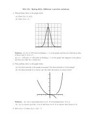
10 CHAPTER 1. BACKGROUNDfiles/what_is_a_function]The collection of all possible inputs is called the domain of the function. Thecollection of all possible outputs is the range.If the domain has not been stated explicitly, then we assume that the domainequals all real numbers which make the function defined. In this case it is usuallyeasy, with a little work, to find an explicit description of the domain. The rangeis not usually explicitly stated and it is sometimes difficult to find an explicitdescription of it.Discussion.[author=garrett,label=discussion_what_to_look_for_in_domain, file =text_files/what_is_a_function]If the domain of a function has not been explicitly stated, then here is how wecan find it. We start by asking: What be used as inputs to this function withoutanything bad happening?For our purposes, ‘anything bad happening’ just refers to one of• trying to take the square root of a negative number• trying to take a logarithm of a negative number• trying to divide by zero• trying to find arc-cosine or arc-sine of a number bigger than 1 or less than−1(We note that some of these things aren’t so bad if one is willing to work withthe complex numbers, or the hyperreals.)Discussion.2015y 105–4 –3 –2 –1 1 2 3 4–5–10simple_rational_functionFigure 1.1:[author=duckworth,label=discussion_finding_range, file =text_files/what_is_a_function]Finding the range of a function is generally harder than finding the domain. Weshould memorize the range of e x , sin, cos, x, x 2 , x 3 etc. For other functions wewill learn various techniques later in this course that will help us find the range.Sometimes, we may have to graph the function.Example 1.2.1.[author=duckworth,label=example_finding_domain_simple_rational_function, file =text_files/what_is_a_function]Find the domain of f(x) = 1x−2 +x2 . The only problem with plugging any numberinto this function comes from the division in the fraction. The only way we couldhave division by zero is is x = 2. Thus, the domain is all numbers except 2. Thisagrees with what we see in figure 1.1, namely that the graph does not exist atx = 2.

1.2. FUNCTIONS 11Example 1.2.2.[author=garrett,label=example_finding_domain_sqrt_x^2-1, file =text_files/what_is_a_function]For example, what is the domain of the functiony = √ x 2 − 1?Well, what could go wrong here? No division is indicated at all, so there is norisk of dividing by 0. But we are taking a square root, so we must insist thatx 2 − 1 ≥ 0 to avoid having complex numbers come up. That is, a preliminarydescription of the ‘domain’ of this function is that it is the set of real numbers xso that x 2 − 1 ≥ 0.But we can be clearer than this: we know how to solve such inequalities. Oftenit’s simplest to see what to exclude rather than include: here we want to excludefrom the domain any numbers x so that x 2 − 1 < 0 from the domain.We recognize that we can factorx 2 − 1 = (x − 1)(x + 1) = (x − 1) (x − (−1))This is negative exactly on the interval (−1, 1), so this is the interval we mustprohibit in order to have just the domain of the function. That is, the domain isthe union of two intervals:(−∞, −1] ∪ [1, +∞)You can also verify our answer by looking at the graph. Of course, we willalways try to solve problems algebraically when possible, rather than just relyingupon the graph. In any case, on the graph we don’t see any points between x = −1and x = 1, which is equivalent to saying that the domain equals what we describedabove.Example 1.2.3.[author=wikibooks,label=example_finding_domain_top_half_of_circle, file =text_files/what_is_a_function]Let y = √ 1 − x 2 define a function. Then this formula is only defined for valuesof x between −1 and 1, because the square root function is not defined (in theworld of real numbers) for negative values. Thus, the domain would be [−1, 1].This agrees with the fact that the graph is the top half of a circle, and not definedoutside of [−1, 1].In this case it is easy to see that √ 1 − x 2 can only equal values from 0 to 1.Thus, the range of this function is [0, 1].108642–10 –6 –4 0 2 4 6 8 10–2sqrt_x_squared_minus_14321–2 –1 0 1 2top_half_of_unit_circleExample 1.2.4.[author=duckworth,label=example_function_given_by_graph, file =text_files/what_is_a_function]Let f(x) be defined by the graph below.

12 CHAPTER 1. BACKGROUND10–3 –2 –1 1 2 3–10–20–30–40generic_cubicTo determine a function value from the graph we read the y-value (off the verticalaxis) which corresponds to some given x-value (on the horizontal axis). Forexample given the input of x = 3 the output is y = 14.A graph shows us lots of information about the function, and much of what welearn later will be how to find this information without relying upon the graph.For example, we can see that there is a certain type of maximum at x = 0.In problems like this, that depend upon the graph, we will generally not requirevery accurate answers. The answers only need to be accurate enough to show thatwe’ve read the graph correctly.Example 1.2.5.[author=duckworth,label=example_function_given_by_numbers, file =text_files/what_is_a_function]Let the table of numbers below define a function, where x is the input and y isthe output.x 1 2 2.5 2.9 3.1 3.5 4y 2.1 3.72 3.88 4.42 4.36 4.1 2.7For example, given an input of x = 1, the output is y = 2.1. Given an input ofx = 4 the output is y = 2.7. However, we can’t say for sure what happens to aninput of x = 1.5. We could make a leap of faith and guess that the correspondingoutput is somewhere between 2.1 and 3.72. For lots of functions this might be areasonable assumption, but if we don’t know anything else about this function wereally can’t be sure about this, or even if the output is defined. (Technically, if allwe’ve been given is this table, then the output is definitely not defined. But inpractice, we usually think that the table gives us a handful of values of a functionwhich is defined for more numbers than shown.) Similarly, we can’t be sure thatthis function has a maximum around x = 3, even though we probably all thinkthat it should.Example 1.2.6.[author=duckworth,label=example_piecewise_function, file =text_files/what_is_a_function]Let y be defined by the following formulas, each applying to just one range of

1.2. FUNCTIONS 13inputs.⎧⎨ x 2 if x ≤ 0y = −x 2 if 0 < x ≤ 3⎩e x if 3 < xWhich formula you use depends upon which x-value you are plugging in. Toplug in x = −1 we use the first formula. So an input of x = −1 has an output of(−1) 2 = 1. To plug in x = 2 we use the second formula, so the output is −2 2 = −4.Similarly an input of x = 4 has an output of y = e 4 .We can also graph y. In this case it looks like x 2 on the left (i.e. for x ≤ 0); itlooks like −x 2 in the middle (for 0 < x ≤ 3) and it looks like e x on the right (forx > 3). Notice that the graph looks “unnatural,” especially at x = 3 where it isdiscontinuous.5040y302010–4 –2 0 2 4two_parbs_and_exponentialExample 1.2.7.[author=duckworth,label=example_function_implicit, file =text_files/what_is_a_function]Let y be defined as a function of x, x < 0, by the equation:x 3 + y 3 = 6xyIt is difficult (but not impossible) to find an explicit equation for y as a functionof x. However, for each negative x-value, it is possible to compute a correspondingy-value, which is all we need for an abstract definition of function. For example,if x = −.5 I can have my calculator solve(−.5) 3 + y 3 = 6 · (−.5)yfor y (actually I’ll probably have to enter it in the calculator using x instead ofy!) to find y ≈ 0.04164259578. Similarly, I could do this for any negative valuefor x; this is how y can be viewed as a function of x (only for negative values of xthough).To make this more concrete, but still not rely upon a formula, I could fill in asmall table of numbers:x −1 −.75 −.5 −.25 0y 0.1659 0.0936 0.0416 0.0104 0

14 CHAPTER 1. BACKGROUNDWhat happens when we try to plug in a positive value for x like x = 1? Thereis more than one solution for y. This means that y is not a function of x for x > 0.Discussion.[author=livshits,uses=function_extensions,label=discussion_extension_restriction_of_functions, file =text_files/what_is_a_function]We think of a function as a rule by which we can figure out f(x) from x. Strictlyspeaking, we have to specify what objects x are being used, the collection of allthese objects is called the (definition) domain of the function.The home address is a real life example of a function. This function is definedfor all the people that have home address, in other words, the definition domainof the home address is the collection of all the people who live at home. Thehome address is not defined for the homeless people. On the other hand, somehomeless individuals pick up their mail at the post office and therefore have theirpostal addresses. For people who live at home their postal address and their homeaddress coincide.We say that the postal address is an extension of the home address to thehomeless individuals who pick up their mail at the post office.We also say that the home address is a restriction of the postal address to theindividuals who live at home.The notions of restriction and extension of functions are central to our approachto differentiation.Discussion.[author=duckworth,label=discussion_types_of_basic_functions, file =text_files/list_of_basic_functions]In practice, in this class, we don’t have that many basic functions. Here’s most ofthem.Polynomials These are positive powers of x, combined with addition and multiplicationby numbers. We call the highest power that appears the degreeof the polynomial. The numbers which are multiplied by x are called thecoefficients. The leading coefficent is the coefficent of the highest powerof x. The constant term is the number which has no power of x.We can write a general expression for a polynomial, but since we don’t nowexactly what the degree will be, we need to use a letter to represent it; wewill use n. Since we don’t know how big the degree is, we can’t write all theterms, thus we will leave out some number of terms in the middle, and willwrite “. . . ” in their place. Similarly, we will need to use letters to representthe coefficients. The number of coefficients equals the degree varies with thedegree, so we don’t know how many letters we’ll need. For this reason wedon’t usually write a general polynomial with letters of the form a, b, c, . . . ,but rather we use a 0 , a 1 , a 2 , etc. We summarize this terminology and showsome examples in figure 1.2Trigonometric Functions sin(x), cos(x), tan(x), sin −1 (x), cos −1 (x), tan −1 (x),csc(x), sec(x), cot(x)

1.2. FUNCTIONS 15Figure 1.2: Polynomial examplespolynomial degree coefficients leading constantcoefficient termx 3 + 5x + 6 3 1, 5, 6 1 610x 9 9 10 10 0a n x n + a n−1 x n−1 + · · · + a 1 x + a 0 n a n , a n−1 , . . . , a 1 , a 0 a n a 0Figure 1.3: y = x 3108642–3 –2 –2 0 1 2 3–4–6–8–10x_cubed_-3_to_3_manualFigure 1.4: y = 1/xy321–3 –2 –1 0 1 2 3–1–2–31_over_x_-3_to_3_manual_fitExponential and Logarithm e x , ln(x)We show some graphs of some of these functions in the next few figures.Notation.[author=duckworth,label=function_notation, file =text_files/function_notation]All functions use the following notation. When we write “f(x)” it means the Very Importantfollowing: f is the name of a function, x is the input (anything which comesinside of the parentheses ( ) is the input), f(x) is the output you get when youplug in x. We read the notation “f(x)” as “f of x”. We call x the input, or theindependent variable, or the argument to f (this sounds somewhat old-fashioned,but it is still what inputs are called in computer science).There is one family of exceptions to this notation. Out of laziness, or if youprefer, efficiency, many people write things like sin π instead of sin(π). People do

16 CHAPTER 1. BACKGROUND10.5Figure 1.5: y = sin(x)0–0.52 4 6 8 10 12–1sin_0_to_4piFigure 1.6: y = tan −1 (x)1.510.5–8 –6 –4 0 2 4 6 8–0.5–1–1.5tan_inverse_-3pi_to_3piFigure 1.7: y = e x108642–3 –2 –1 0 1 2 3e_to_the_x_-3_to_3_manualFigure 1.8: y = ln(x)1–1 1 2 3 4 5–1–2–3–4–5–6ln_of_x_neg_1_to_5

1.2. FUNCTIONS 17the same thing with ln, cos, tan and the other trig functions. In this book, wewill always use parentheses for these functions, unless the notation becomes toocomplicated and and it seems that leaving out some parenthesis would simplify it.Example 1.2.8.[author=wikibooks,label=example_simple_function_notation, file =text_files/function_notation]For example, if we write f(x) = 3x+2, then we mean that f is the function which,if you give it a number, will give you back three times that number, plus two. Wecall the input number the argument of the function, or the independent variable.The output number is the value of the function, or the dependent variable.For example, f(2), (i.e. the value of f when given argument 2) is equal tof(2) = 3 · 2 + 2 = 6 + 2 = 8.Example 1.2.9.[author=duckworth, file =text_files/function_notation]Let f be the function given by f(x) = x 2 . Then x represents the input, the outputis x 2 . For instance f(2) = 4.Discussion.[author=wikibooks,author=duckworth,label=pros_cons_function_notation, file =text_files/function_notation]Function notation has great advantages over using y = . . . notation, but these Very Importantadvantages bring with them the need to be more careful and thoughtful aboutexactly what is being written.Firstly, we can give different names to different functions. For example we coudsay f(x) = x 2 and g(x) = 3 sin(x) and then talk about f and g.Another advantage of function notation as that it clearly labels inputs andoutputs. In some of the previous function examples we had to use many phrasesof the form “given the input x = 3 the output is y = 7”. In function notation thisbecomes much more compact: “f(3) = 7”.Furthermore, it is possible to replace the input variable with any mathematicalexpression, not just a number. For instance we can write things like f(7x) or f(x 2 )or f(g(x)); we’ll talk more about what these mean below.This last point brings up what we need to be careful and thoughtful aboutin function notation. This brings up a really important point. The variable “x”doesn’t always mean x. It just stands for the input. So the function f(x) = x 2could have been described this way “f is the function which takes an input andsquare it.” Why do I care? Because we need to know how to calculate things likef(3x) and f(x + 3).If you get too focused on thinking that f squares x , then you might thinkthat f(3x) = 3x 2 . No! The function squares any input, and in the case of f(3x),the input is 3x. So the output is (3x) 2 .

18 CHAPTER 1. BACKGROUNDNow, if you really understand the notation, you should be able to say whatf(x + 3) is without a moment’s hesitation. . . . . . . . . . I hope you said (x + 3) 2 , butif not, keep practicing!Example 1.2.10.[author=duckworth,label=example_function_notation_sin,uses=sin, file =text_files/function_notation]Let f(x) = sin(x). Then f(π/2) = sin(π/2). Now it so happens that sin(π/2)equals 1, so we can say that f(π/2) = 1. Similarly, f(π/2 + 1) = sin(π/2 + 1). Believeit or not, I don’t know what sin(π/2+1) equals. It is not equal to sin(π/2)+1.According to my calculator, sin(π/2 + 1) is approximately equal to 0.54.Examples 1.2.11.[author=wikibooks,label=example_various_functions, file =text_files/function_examples]Here are some examples of various functions.1. f(x) = x. This takes an input called x and returns x as the output.2. g(x) = 3. This takes an input called x, ignores it, gives 3 as an output.3. f(x) = x + 1. This takes an input called x, and adds one to it.{ 1, if x > 04. h(x) =−1, if x < 0 .This gives 1 if the input is positive, and −1 if the input is negative. Notethat the function only accepts negative and positive numbers, not 0. In otherwords, 0 is not in the “domain” of the function.5. g(y) = y 2 . This function takes an input called y and squares it.{ ∫ ydx, if y > 06. f(y) = −y ex2 0, if y ≤ 0 .This function takes an input called y, and uses it as boundary values for anintegration (which we’ll learn about later).32.521.510.5–3 –2 –1 0 1 2 3abs_value_functionExample 1.2.12.[author=livshits,label=example_absolute_value_function,uses=absolute_value, file=text_files/function_examples]Here’s one way to define the absolute value function:{ x if x is already positive, or 0|x| =−x if x is negativeYou can think of this function as “making x positive” or “stripping the sign fromx”. You can also think of |x| as the distance from x to 0 on the real number line;

1.2. FUNCTIONS 19this is a nice way to think about it, because it’s geometric, and because the mainreason we use absolute values is to give a mathematical expression to distances.Discussion.[author=wikibooks,label=discussion_arithmetic_with_functions, file =text_files/combining_functions]Functions can be manipulated in the same manner as any other variable theycan be added, multiplied, raised to powers, etc. For instance, let f(x) = 3x + 2g(x) = x 2 .We define f + g to be the function which takes an input x to f(x) + g(x). Ifyou completely understand function notation then you know what the formula forf(x) + g(x) is . . . . . . . . . . . . . . . . . . . . . . . . . . . . . . . . . . . . . . . . . . . . . . . . . . . . . . . . . . . . . . . . . .f(x) + g(x) = (3x + 2) + (x 2 ). Of course, this formula can be simplified tof(x) + g(x) = x 2 + 3x + 2.Similarly,• f(x) − g(x) = (3x + 2) − (x 2 ) = −x 2 + 3x + 2.• f(x) · g(x) = (3x + 2) · (x 2 ) = 3x 3 + 2x 2 .• f(x)/g(x) = (3x + 2)/(x 2 ) = 3 x + 2 x 2 .However, there is one particular way to combine functions which is not likethe usual arithmetic we do with variables: you can plug one function inside ofthe other! This is possibility really opens the door to many wonderful areas ofmathematics way beyond Calculus, but for now we won’t go there.Definition 1.2.3.[author=wikibooks,label=definition_function_composition, file =text_files/combining_functions]Plugging one function inside of another is called composition. Composition isdenoted by f ◦ g = (f ◦ g)(x) = f(g(x)). In this case, g is applied first, and thenf is applied to the output of g.Example 1.2.13.[author=wikibooks,label=example_simple_function_composition, file =text_files/combining_functions]For instance, let f(x) = 3x + 2 and g(x) = x 2 then h(x) = f(g(x)) = f(x 2 ) =3(x 2 ) + 2 = 3x 2 + 2. Here, h is the composition of f and g. Note that compositionis not commutativef(g(x)) = 3x 2 + 2 ≠ 9x 2 + 12x + 4 = (3x + 2) 2 = g(3x + 2) =g(f(x)). Or, more obviously stated f(g(x)) ≠ g(f(x)).Examples 1.2.14.[author=duckworth,label=example_various_combinations_of_two_functions, file =text_

20 CHAPTER 1. BACKGROUNDfiles/combining_functions]Let f(x) = x 2 + 1 and g(x) = sin(x).1. Find a formula for f(x) + g(x).2. Find f(1) − g(1)3. Find a formula for f(x)/g(x)4. Find a formula for f(g(x)).5. Find f(g(2)).Definition 1.2.4.4321–2 –1 0 1 2top_half_of_unit_circle[author=duckworth,label=definition_one_to_one_function, file =text_files/one_to_one_functions_and_inverses]A function f(x) is one-to-one if it does not ever take to different inputs to thesame output. In symbols: if a ≠ b then f(a) ≠ f(b).Example 1.2.15.[author=wikibooks,label=example_circle_is_not_one_to_one, file =text_files/one_to_one_functions_and_inverses]The function f(x) = √ 1 − x 2 is not one-to-one, because both x = 1/2 andx = −1/2 result in f(x) = √ 3/4. You can see this graphically as the fact that thehorizontal line y = √ 3/4 crosses the graph twice.The function f(x) = x + 2 is one-to-one because for every possible value off(x) we never have two different inputs going to the same output. In symbols: ifa ≠ b then a + 2 ≠ b + 2, and therefore f(a) ≠ f(b).Definition 1.2.5.[author=duckworth,label=definition_function_inverses, file =text_files/one_to_one_functions_and_inverses]Let f(x) be a function. We say that another function g(x) is the inverse functionof f(x) if f(g(x)) = x and g(f(x)) = x for all x. This means that f and g canceleach other.An equivalent definition is that f(a) = b if and only if g(b) = a. This meansthat g reverses inputs and outputs compared to f.An equivalent way to think about this is that g(x) is the answer to the question:f of what equals x?Another equivalent way to think about this is that f(x) has an inverse functionif and only f(x) is one-to-one.

1.2. FUNCTIONS 21Example 1.2.16.[author=wikibooks,label=example_function_inverse, file =text_files/one_to_one_functions_and_inverses]For example, the inverse of f(x) = x + 2 is g(x) = x − 2. To verify this note thatf(g(x)) = f(x − 2) = (x − 2) + 2 = x.The function f(x) = √ √ 1 − x 2 has no inverse (as we saw above). The function1 + x2 is close, but it works only for positive values of x. To verify this notethat f( √ √1 + x 2 ) = 1 − ( √ 1 + x 2 ) 2 = √ 1 − (1 + x 2 ) = √ x 2 = |x| where |x| isthe absolute value of x.Example 1.2.17.[author=duckworth,label=example_function_inverse_e^x_and_ln,uses=e^x,uses=ln,file =text_files/one_to_one_functions_and_inverses]Let’s consider e x and ln(x). These functions are inverses. So, for example,since e 2 ≈ 7.39 we must have ln(7.39) ≈ 2. Another way to state this is thate ln(7.39) = 7.39 and ln(e 2 ) = 2.However, these numerical examples are not really how we use the fact thatln(x) and e x are inverses. The following would be a much more common example.Suppose that the amount of money in someone’s bank account is given by1000e .05t where t is measured in years. Find out how many years it will takebefore they have $3000.This means that we want to solve 3000 = 1000e .05t . Dividing both sides by1000 we get a new eqation3 = e .05t .Now we can take ln(x) of both sides:By the inverse property this meanswhenceln(3) = ln(e .05t ).ln(3) = .05tt = ln(3).05This is a perfectly good expression for the final answer. Of course, some readerswould rather get an explicit number for t; this is understandable, but you shouldpractice being comfortable with answers that are formulas.Example 1.2.18.[author=duckworth,label=example_function_inverse_cos,uses=cos, file =text_files/one_to_one_functions_and_inverses]Let’s consider cos(x) and cos −1 (x). If I write x = cos(y) (and x is between −π/2and π/2) this is (mathematically) equivalent to writing y = cos −1 (x). In otherwords, the two equations will be satisfied by exactly the same values of x and y.Thus, saying that cos(π/2) = 0 is equivalent to saying that π/2 = cos −1 (0).

22 CHAPTER 1. BACKGROUND(We will use this idea later to find the derivative of cos −1 (x). We will startwith y = cos(x), solve this for x = cos −1 (y) and then apply implicit derivatives.)Discussion.[author=duckworth,label=discussion_how_to_find_inverses, file =text_files/one_to_one_functions_and_inverses]Many of us learned how to find inverses by following these steps: given an equationy = . . ., (1) reverse x and y, (2) solve the new equation for y.I think this procedure sometimes makes people confused. To clear up theconfusion, I hope you realize that step (1) is purely cosmetic. In other words, theonly part of this step that matters is step (2), the reason we do step (1) is becausewe’re not used to having a function of the form x = . . ..Let’s illustrate. The equation which translates Farhenheit into Celsius is C =59(F − 32). The inverse of this equation will translate Farhenheit into Celsius. Wefind the inverse by solving for F :Now, wasn’t that simple?C = 5 9 (F − 32) −→ 9 5 C = F − 32 −→ F = 9 5 C + 32If you follow the same steps for the equation y = 5 9 (x−32) you get x = 9 5 y +32,and this is the sort of equation that step (1) was meant to prevent.The moral of this story should be: don’t get too hung up on the roles of xand y, they just represent two numbers. If you get too fixated on which what theinput and output should look like, then you will sometimes have extra work to do,to sort out purely cosmetic problems.1. Find the domain of the functionExercisesf(x) = x − 2x 2 + x − 2That is, find the largest subset of the real line on which this formula can beevaluated meaningfully.2. Find the domain of the functionf(x) =x − 2√x2 + x − 23. Find the domain of the functionf(x) = √ x(x − 1)(x + 1)

1.2. FUNCTIONS 234. What is the graph of the function y = −x?5. What is the graph of the function y = |x|?6. What is the range of f(x) = |x|?7. What is the range of the function u(x) = 5?8. The function is defined by the formula h(x) = |x|, the domain of h is all thenumbers x such that −10 ≤ x ≤ 5. What is the range of h?9. What is the graph of this function?10. What is fg? What is 1/f? What are their graphs? What is the domain of1/f? What is the range of 1/f?11. v(x) = x − 3, what is the graph of |v|?12. u(x) = (x + 1)/(x − 1), q(x) = (x 2 − 1)/(x − 1). Find the domains of u andq.13. p(x) = x 2 + 2x + 5, what is the range of p?14. What is the degree of the product fg of 2 polynomials? Hint: What is thehighest degree term of fg?15. Let f and g be 2 nonzero polynomials. Can fg be zero? Hint: What is theleading term of fg?16. Find the domain of r(x). Check that r(x) = u(x) = (x+1)/(x−1) for x ≠ 0.17. Find the domain of z(x) = 1/(1/x). Check that for x ≠ 0 z(x) = x.18. Extend the function q(x) = (x 2 − 1)/(x − 1) to x = 1 by a polynomial; inother words, find a polynomial p(x) such that p(x) = q(x) for x ≠ 1.

24 CHAPTER 1. BACKGROUNDFigure 1.9: A point in the x, y-planey(a,b)b(0,0) axpoint_in_plane1.3 Using, applying, and Manipulating functionsand equationsDiscussion.[author=duckworth,label=intro_to_manipulating_functions, file =text_files/intro_to_manipulating_functions]In this section we lay out some of the basic tools for using functions. This is sortof grab-bag of techniques.We start by reviewing how equations can represent lines, circles, and othergeometric objects.We review some applications of functions to model real-world data.We review how to solve some equations and inequalities.Discussion.[author=duckworth,label=discussion_of_point_in_xy_plane, file =text_files/cartesian_coords_and_graphs]Recall that the x, y-plane refers to an ideal mathematical plane labelled with anx-axis which is horizontal, a y-axis which is vertical and the origin which is wherethe two axes intersect. Every point in the plane can be labelled with x and y coordinateswhich measure the horizontal and vertical distance respectively betweenthe point and the origin, see figure 1.9

1.3. USING FUNCTIONS 25Definition 1.3.1.[author=duckworth,label=definition_graph_of_function, file =text_files/cartesian_coords_and_graphs]The graph of a function f(x) is the set of points (x, y) such that x is in the domainand y equals f(x). Given any equation involving x and y the graph of theequation is the set of points (x, y) which satisfy the equation.Discussion.[author=wikibooks,label=discussion_of_how_to_graph, file =text_files/cartesian_coords_and_graphs]Functions may be graphed by finding the value of f for various x, and plottingthe points (x, f(x)) in the x, y-plane.Plotting points like this is laborious (unless you have your calculator do it).Fortunately, many functions’s graphs fall into general patterns, and we can learnthese patters. For example, consider a function of the form f(x) = mx. The graphof f(x) is a straight line, and m controls how steeply angled the line is. Similarlywe can learn about the graphs of our other basic functions, and later we will learnhow to find out useful information about more complicated graphs as well.Example 1.3.1.[author=duckworth,label=example_plotting_points, file =text_files/cartesian_coords_and_graphs]Draw a picture of the graph of f(x) = 3x 3 − 10x by plotting a few points.First, we calculate some points:x −3 −2.5 −2 −1.5 −1 −.5 0 .5 1 1.5 2 2.5 3f(x) −51 −21.9 −4 4.9 7 4.6 0 −4.6 −7 −4.9 4 21.9 51These points are shown in Figure 1.10 Note, we could have saved some effort if wehad only calculated half of these points. This function is odd (in a technical sensethat we’ll define later), and this would have told us that the values in the righthalf of our table would equal the negative of the values in the left half. Now wedraw a smooth line through the points and get the graph shown in figure 1.11.4020–3 –2 –1 1 2 3–20–40cubic_plot_pointsFigure 1.10:Definitions 1.3.2.[author=garrett,author=duckworth,label=defintion_slopes_equations_lines, file =text_files/lines_and_circles]The simplest graphs are straight lines. The main things to remember are:4020–3 –2 –1 1 2 3–20–40• The slope of a line is the ratiom = ∆y∆xwhere ∆y and ∆x are the vertical and horizontal change between two points.If the two points have coordinatens (x 0 , y 0 ) and (x 1 , y 1 ) then we havecubic_plot_points_curveFigure 1.11:m = y 1 − y 0x 1 − x 0

26 CHAPTER 1. BACKGROUNDFigure 1.12: Distance formula triangle(x_1,y_1)D = \sqrt{x^2+y^2}|y_1−y_0| = \Delta y(x_0,y_0)|x_1−x_0|=\Delta xdistance_formula_triangle• A vertical line has equation x = a for some number a. A horizontal line hasequation y = c for some number c.• The slope-intercept form of the equation of a line is y = mx + b. Thisform is convenient for graphing by hand, but it is not as convenient for someother purposes.• The point-slope form of the equation of a line with slope m and containinga point (x 0 , y 0 ) is given byy = m(x − x 0 ) + y 0 .This is by far the most convenient form of the equation of a line for us touse in Calculus.12108642–4 –3 –2–2 0 1 2 3 4straight_lineExample 1.3.2.[author=duckworth, file =text_files/lines_and_circles]The line y = −2x + 5 has slope of −2 and a y-intercept of 5. It’s graph is shownin the margin figure .Definition 1.3.3.[author=duckworth,label=definition_distance_formula, file =text_files/lines_and_circles]Given two points (x 0 , y 0 ) and (x 1 , y 1 ), in the x, y-plane, their distance apart canbe computed by drawing a right triangle that contains them and applying thePythagorean theorem (see figure 1.12). This gives distance asd = √ (x 1 − x 0 ) 2 + (y 1 − y 0 ) 2Example 1.3.3.

1.3. USING FUNCTIONS 27Figure 1.13: Example of distance formula(2,5)D=\sqrt{3^2+4^2}(5,1)example_of_distance_formula[author=duckworth,label=example_distance_between_two_points, file =text_files/lines_and_circles]The distance between the points (2, 5) and (5, 1) (see figure 1.13) is√(2 − 5)2 + (5 − 1) 2 = √ 9 + 16 = 25Definition 1.3.4.[author=duckworth,label=definition_equation_of_circle, file =text_files/lines_and_circles]The equation for distance can be immediately translated into the equation for acircle.The equation of a circle centered at the origin and with radius r (see figure 1.14)is given byx 2 + y 2 = r.This can be put into function form by solving for y; if we do this we get two valuesof y, so we need two functionsy 1 = √ r − x 2 and y 2 = − √ r − x 2 .The equation of a circle with center at the point (a, b) and radius r (see figure??) is given by(x − a) 2 + (y − b) 2 = r 2Example 1.3.4.[author=livshits,label=example_graph_of_circle_and_lines, file =text_files/lines_and_circles]

28 CHAPTER 1. BACKGROUNDFigure 1.14: Generic circle centered at origin with radius rr(0,0)generic_circleFigure 1.15: Function of top half of circley=\sqrt{x^2+r^2}rtop_half_of_circleFigure 1.16: Graphs of unit circle and straigt linesyy=−xx + y = 1y=xxy=−1/2circle_and_axes

1.3. USING FUNCTIONS 29Figure 1.17:10y5–10 –5 0 5 10–5–10short_rational_fuction_standard_windowFigure 1.18:0.00080.00060.00040.0002–10 –5 0 5 10short_rational_fuction_fitIn figure 1.16 we show the graphs of the unit circle x 2 + y 2 = 1, and the straightlines y = x, y = −x and y = −1/2.Discussion.[author=duckworth,label=discussion_graphing_on_calculators_not_always_easy, file=text_files/complicated_graphs]Using calculators does not always make it perfectly easy to graph a function. Wecollect now a few examples of things which take some work to graph.Example 1.3.5.[author=duckworth,label=example_graph_squished_rational_function, file =text_files/complicated_graphs]Using your calculator, graph y =1100x 2 +1170 .In figure1.17 we show a standard view (i.e. −10 ≤ x ≤ 10, −10 ≤ y ≤ 10) ofthis graph. This view doesn’t help much.ZoomFit is a very useful feature on the calculators for graphs like this. Touse this feauter you must specify the x range, and then the calculator will fit they-values of the window to the graph. The result is shown in figure 1.18.

30 CHAPTER 1. BACKGROUNDFigure 1.19:10.5–3 –2 –1 0 1 2 3–0.5–1sin_of_5000_x_calculatorFigure 1.20:10.5–3 –2 –1 1 2 3–0.5–1sin_of_5000_x_normal_sampleExample 1.3.6.[author=duckworth,label=example_sin_of_5000x, file =text_files/complicated_graphs]Using your calculator, graph y = sin(5000x).What this figure looks like will depend upon your machine. On your calculator,with an x-range of −π ≤ x ≤ π, it might look like the graph in figure 1.19.In the computer package Maple the default graph is shown in figure 1.20.In Maple we can increase the number of points used to sample the graph. Theresult of using a large number of points is shown in figure 1.21.None of these pictures really shows the graph properly. To get a good graph,Figure 1.21:10.5–3 –2 –1 0 1 2 3–0.5–1sin_of_5000_x_massive_sample

1.3. USING FUNCTIONS 31Figure 1.22:10.5–0.0006 –0.0002 0.0002 0.0006–0.5–1sin_of_5000_x_narrow_rangewe should use our knowledge of sin(x). We know that sin(x) oscillates. It turns outthat sin(ax) still oscillates, but it oscillates faster if a is greater than 1. To showa graph that is oscillating faster, we need a smaller window. Roughly speaking,to graph sin(5000x) we should use a graph that is 5000 times smaller than usual.Thus, we try graphing with the range −π5000 ≤ x ≤ π5000. The results are shown infigure1.22.Discussion.[author=duckworth,label=discussion_graphing_with_calculators_wrap_up, file =text_files/complicated_graphs]We will see later examples of functions that are even more difficult to graph thanthe ones we have shown here. In fact, functions which are impossible to graph wellare quite common; most of the graphs in Calculus textbooks are artifically niceand well-behaved.We will also see later examples of problems that show how our calculators andcomputers can lead us to incorrect solutions.Definition 1.3.5.[author=duckworth,label=definition_mathematical_models, file =text_files/mathematical_models]A mathematical model is a function that is used to describe a real-world set ofdata. Sometimes this can be done by exactly solving equations for various parameters.Sometimes this we can only find the model which comes closest to matchingsome data; in this case we usually need to use our calculators or computers.Example 1.3.7.[author=duckworth,label=example_modelling_population,uses=e^x,uses=ln, file =text_files/mathematical_models]Use an exponential model (i.e. P = Ce kt ) to match the following populations

32 CHAPTER 1. BACKGROUND(where t = 0 corresponds to 1980), and predict the population in 2020:Year Population1980 4 billion,2000 5 billionWe wish to find k and C such that the following two equations are satisfied:4 = Ce 05 = Ce 20kFrom the first equaton we see that C = 4. Plugging this into the second equationwe get5 = 4e 20k .As soon as you see an equation with an unknown as an exponent, you can be surethat we will use ln(x) to find that unknown. In this case, I’ll divide by 4 first:5/4 = e 20kand then take ln(x) of both sides (using the cancelling property of ln(x) and e x ,see Example 1.2)ln(5/4) = 20kwhencek = 1 20 ln(5/4).Example 1.3.8.[author=garrett,label=example_solving_polynomial_inequality,version=1, file =text_files/solving_inequalities]Solve the following inequality:5(x − 1)(x + 4)(x − 2)(x + 3) < 0The roots of this polynomial are 1, −4, 2, −3, which we put in order (from left toright). . . < −4 < −3 < 1 < 2 < . . .The roots of the polynomial P break the numberline into the intervals(−∞, −4), (−4, −3), (−3, 1), (1, 2), (2, +∞)On each of these intervals the polynomial is either positive all the time, or negativeall the time, since if it were positive at one point and negative at another then itwould have to be zero at some intermediate point!For input x to the right (larger than) all the roots, all the factors x + 4, x + 3,x − 1, x − 2 are positive, and the number 5 in front also happens to be positive.Therefore, on the interval (2, +∞) the polynomial P (x) is positive.Next, moving across the root 2 to the interval (1, 2), we see that the factorx − 2 changes sign from positive to negative, while all the other factors x − 1,x + 3, and x + 4 do not change sign. (After all, if they would have done so, thenthey would have had to be 0 at some intermediate point, but they weren’t, sincewe know where they are zero...). Of course the 5 in front stays the same sign.

1.3. USING FUNCTIONS 33Therefore, since the function was positive on (2, +∞) and just one factor changedsign in crossing over the point 2, the function is negative on (1, 2).Similarly, moving across the root 1 to the interval (−3, 1), we see that thefactor x − 1 changes sign from positive to negative, while all the other factorsx − 2, x + 3, and x + 4 do not change sign. (After all, if they would have doneso, then they would have had to be 0 at some intermediate point). The 5 in frontstays the same sign. Therefore, since the function was negative on (1, 2) and justone factor changed sign in crossing over the point 1, the function is positive on(−3, 1).Similarly, moving across the root −3 to the interval (−4, −3), we see that thefactor x + 3 = x − (−3) changes sign from positive to negative, while all the otherfactors x − 2, x − 1, and x + 4 do not change sign. (If they would have done so,then they would have had to be 0 at some intermediate point). The 5 in frontstays the same sign. Therefore, since the function was positive on (−3, 1) and justone factor changed sign in crossing over the point −3, the function is negative on(−4, −3).Last, moving across the root −4 to the interval (−∞, −4), we see that thefactor x + 4 = x − (−4) changes sign from positive to negative, while all the otherfactors x − 2, x − 1, and x + 3 do not change sign. (If they would have done so,then they would have had to be 0 at some intermediate point). The 5 in frontstays the same sign. Therefore, since the function was negative on (−4, −3) andjust one factor changed sign in crossing over the point −4, the function is positiveon (−∞, −4).In summary, we have5(x − 1)(x + 4)(x − 2)(x + 3) > 0 on (2, +∞)5(x − 1)(x + 4)(x − 2)(x + 3) < 0 on (1, 2)5(x − 1)(x + 4)(x − 2)(x + 3) > 0 on (−3, 1)5(x − 1)(x + 4)(x − 2)(x + 3) < 0 on (−4, −3)5(x − 1)(x + 4)(x − 2)(x + 3) > 0 on (−∞, −4).There’s another way to write this. The polynomial is negative on (1, 2)∪(−4, −3).(The notation (1, 2) ∪ (−4, −3) means all those x-values between 1 and 2, togetherwith all those x-values betwen −4 and −3.)Example 1.3.9.[author=garrett,label=solving_polynomial_inequality,version=2, file =text_files/solving_inequalities]As another example, let’s see on which intervalsP (x) = −3(1 + x 2 )(x 2 − 4)(x 2 − 2x + 1)is positive and and on which it’s negative. We have to factor it a bit more: recallthat we have nice factsx 2 − a 2 = (x − a) (x + a) = (x − a) (x − (−a))so that we getx 2 − 2ax + a 2 = (x − a) (x − a)P (x) = −3(1 + x 2 )(x − 2)(x + 2)(x − 1)(x − 1)

34 CHAPTER 1. BACKGROUNDIt is important to note that the equation x 2 + 1 = 0 has no real roots, since thesquare of any real number is non-negative. Thus, we can’t factor any further thanthis over the real numbers. That is, the roots of P , in order, are−2 2) all the factors x + 2, x − 1,x − 1, x − 2 are positive, while the factor of −3 in front is negative. Thus, on theinterval (2, +∞) P (x) is negative.Next, moving across the root 2 to the interval (1, 2), we see that the factorx − 2 changes sign from positive to negative, while all the other factors 1 + x 2 ,(x − 1) 2 , and x + 2 do not change sign. (After all, if they would have done so,then they would have be 0 at some intermediate point, but they aren’t). The−3 in front stays the same sign. Therefore, since the function was negative on(2, +∞) and just one factor changed sign in crossing over the point 2, the functionis positive on (1, 2).A new feature in this example is that the root 1 occurs twice in the factorization,so that crossing over the root 1 from the interval (1, 2) to the interval(−2, 1) really means crossing over two roots. That is, two changes of sign meansno changes of sign, in effect. And the other factors (1 + x 2 ), x + 2, x − 2 do notchange sign, and the −3 does not change sign, so since P (x) was positive on (1, 2)it is still positive on (−2, 1). (The rest of this example is the same as the firstexample).Again, the point is that each time a root of the polynomial is crossed over, thepolynomial changes sign. So if two are crossed at once (if there is a double root)then there is really no change in sign. If three roots are crossed at once, then theeffect is to change sign.Generally, if an even number of roots are crossed-over, then there is no changein sign, while if an odd number of roots are crossed-over then there is a change insign.Exercises1. Write the equation for the line passing through the two points (1, 2) and(3, 8).2. Write the equation for the line passing through the two points (−1, 2) and(3, 8).3. Write the equation for the line passing through the point (1, 2) with slope 3.4. Write the equation for the line passing through the point (11, −5) with slope−1.

1.4. END OF CHAPTER PROBLEMS 351.4 End of chapter problemsExercises1. Two mathematicians (A and B) are taking a walk and chatting.A: I have 3 children.B: How old are they?A: The product of their ages is 36.B: I can’t figure out how old they are.A: The number on the house that we are passing is the sum of their ages.B: I still can’t figure it out.A: My oldest child is having a soccer match tomorrow.B: Now I can figure it out!How old are the children?Make a list of the possible ages whose product is 36.The only possibilities for these three ages are 1, 1, 36; 1, 6, 6; 1, 2, 18; 1, 3, 12;2, 2, 9; 2, 3, 6; 3, 3, 4. The sums of these ages are 38, 13, 21, 16, 13, 12, 10.If the house number had been any of these sums except 13, mathematicianB would have known the ages, so the street number must have been 13. Ifthere is only one oldest child, then 2, 2, 9 must be the ages.2. You have 2 identical ropes, a scissors and a box of matches. Each rope, whenignited at one of its ends, burns for 1 hour. Fugure out how to measure off45 minutes by burning these ropes. Notice: the ropes may be not uniform,so they can burn in starts and stops, not at a constant speed.Ignited from both ends sinultaneously, how long will a rope burn?3. Repeat example ??, where you replace the leaky cone-shaped bucket with aleaky cylindrical bucket.The surface area A will be proportional to H 2 , i.e. A = cH 2 the equationdH/dt = −(a/A)v(H) = −(a/A) √ 2gH still holds, stick the expression for Ainto it and try to work out the rest.

36 CHAPTER 1. BACKGROUND

Chapter 2Limits2.1 Elementary limitsDiscussion.[author=duckworth,label=discussion_overview_of_limits,style=historical, file =text_files/limits_overview]Before we begin to learn limits, it might be worth describing how the way we uselimits today is the reverse of how they came to be developed historically.Almost all modern Calculus courses (see exceptions below) start with the definitionof limit, and then everything which follows is built upon this definition:vertical and horizontal asymptotes are described using limits; derivatives are definedin terms of limits, as are definite integrals; sequences and series, Taylor polynomials,L’Hospital’s rule, all deal directly with limits. So the modern approachis limits first, and then everything else.But the modern approach reverses the order of history! Newton and Leibnitzinvented a lot of what we think of as Calculus, and they never used the conceptof limits. In fact, their work was finished around 1700, but it wasn’t until around1850’s that limits were carefully and precisely defined. Even then, it took aboutanother 100 years for Calculus books to base everything on limits. (Over this 100year period the use of limits gradually trickled from more advanced subjects downto a college freshman level Calculus course.)So, if you find it a little difficult to understand exactly what limits are, howthey are used, and why we discuss them so much, don’t feel bad! Geniuses likeNewton, Leibnitz, Euler, Gauss, Lagrange, the Bernoulli’s, etc. didn’t understandthem either! On the other hand, by now, limits have been re-worked and simplifiedso much that anyone can use them, but they still take work. The moral: don’tfeel bad if they don’t make sense at first, but don’t give up or decide that you justcan’t get it; keep working hard.So, are there alternatives to a limits based Calculus? Yes. In the 1960’s theinfinitesimal approach was put on rigorous grounds, and this made it acceptableto mathematicians to write Calculus books which based their results on this approach.Infinitesimals are very similar to how Leibnitz thought about derivativesand integrals. They involve doing calculation with infinitely small quantities; thisis a strange idea and the strangeness of it is why mathematicians didn’t feel thatit was rigorously justified until the work in the 1960’s mentioned above was complete.(For more about this approach and the the one which is described next37

38 CHAPTER 2. LIMITSsee the section on further reading.) Interestingly, even in an infinitesimal basedCalculus course, limits are still discussed and used, but not as a foundation foreverything else.Another approach to Calculus has been developed recently by a variety ofauthors. This approach uses division of functions to define derivatives and usespiecewise-linear functions to work with integrals. In this approach, somethingsimilar to limits is always lurking in the background; for example, showing thatthe exact value for the area under a curve is always between two piecewise-linearapproximations which can be made infinitely close to each other. However, limitsare never explicitly used, and instead one must use various clever calculations ofbounds and inequalities.Perhaps this discussion leaves one more question unanswered: if limits takesome hard work to understand, and if there are alternatives, and if historicallylimits weren’t used for the first 150 of Calculus, why do we learn them now? Well,for 150 years, belief in Calculus required a certain amount of faith: mathematicianswould make arguments which mentioned things like “divide two infinitely smallquantities”, or “take the ratio of the quantities just before they become zero” andthese arguments were used to justify the formulas they had. So, to prove that afalling object had a certain speed, or to prove that the planets orbited the sununder the influence of gravity, or to prove a hundred other things, one had torefer to these arguments which were not rigorous (although the answers seemedto work). Mathematically speaking there were other problems when Calculuswas not rigorous. Maybe the answers obtained in simple cases were correct, butwhat about when things got more complicated? Maybe we believe, for example,that the derivative of sin(x) is cos(x) (we’ll learn this later). But what if x isa complex number; is this result still true? What if we want to do mathematicsin 3 dimensions, or 4, or 100? Here we can’t draw pictures, and our intuitionbreaks down, so we can’t claim that “the answers seem to work”; can we stillprove anything about derivatives? What about strange counter-examples thatmathematicians had discovered; this examples showed that our intuition aboutfunctions and derivatives can be completely wrong (see below), so how do weknow that the simpler problems, whose “answers seemed right” were really right?Well, the use of limits (with work) answers all these questions. Finally, everythingthat we think is correct can be rigorously proven; the proofs work forcomplex numbers and for mathematics in 100 dimensions. We can see exactlywhich part of the proof fails in various counter-examples, and we can prove thatsome things in math are correct, but defy our intuition. Finally, the best part isthat once we learn limits we can go far beyond the pictures and numerical argumentsin Freshman Calculus. We can do Calculus in infinite-dimensional space, wecan prove statements in the space-time universe of Einstein’s General Theory ofRelativity, we can prove things about geometric spaces that exist beyond anyone’sability to intuitively understand.What are some of the counter-examples I mentioned above? Well, to fullyunderstand them you have to first understand essentially all of Freshman Calculus,but I can give you some idea of what they are about here.Here’s an intuitive idea: functions are mostly differentiable, and the derivativecan only fail to exist at a handful of points. For example, the absolute valuefunction y = |x| is differentiable everywhere except at x = 0, where it has acorner. Well, we could make a worse example which has a bunch of corners, butstill, most of the points don’t have corners, right? Wrong. Weierstrass showedthat there exist continuous functions which have infinitely many corners, and infact the corners are infinitely close to each other! Can this be true? Well, picture a

2.1. ELEMENTARY LIMITS 39line which zig-zags up and down, and then imagine that if you magnify the picture,that there are more zig-zags that were too small for you to see before; and if youmagnify the picture again, there are more zig-zags, etc. This example is correct;to prove that it is correct, you need to understand limits and continuity; but moreimportantly, it shows that you cannot rely on intuition to say things like “it’s clearthat a continuous function is differentiable”.Here’s another idea: integrals are calculated by finding anti-derivatives. Forexample, the area between the curve y = x 2 and x = 0 and x = 1 is calculated byfinding the anti-derivative 1 3 x3 , and plugging in x = 1 and x = 0 to get the area of13 . But what about the function e−x2 ? Does that have an anti-derivative? Well,it turns out that there is no formula for the anti-derivative of e −x2 . So, how canwe calculate areas under this curve? Well, with limits we can define the integral∫ b0 e−x2 dx and we can show that the limit exists, and therefore the integral exists,even though we cannot write down a formula for it.Discussion.[author=duckworth,label=overview_of_limits,style=middle, file =text_files/limits_overview]This section picks two problems to act as guiding examples for the rest of thechapter: finding the slope of a tangent line and finding the instantaneous velocity.In both cases we look at a fraction as the bottom gets smaller and smaller. (Using∆ylater notation we could say that we were approximating lim ∆x→0 ∆x , and lim ∆t→0 ∆d∆t .)Example 2.1.1.[author=duckworth,label=example_glimpse_of_deriv_as_limit, file =text_files/limits_overview]Here’s a brief glimpse of something that’s coming later. We show it now becauseit’s so important; in fact, it’s the whole reason we introduced limits now! Letf(x) = x 2 . Then the derivative of f(x) at x = 3 will be defined (later) to bef ′ f(x) − f(3)(x) = lim x → 3x − 3. We interpret the derivative to be the slope of the tangent line at x = a, or theinstantaneous velocity.Example 2.1.2.[author=duckworth,label=example_naive_approach_to_inst_vel, file =text_files/limits_overview]It can be shown through experiments (as Galileo did in the early 1600’s) that anobject thrown off of a building of height 100 m and with an intial velocity of 23 m /shas a position given by the formulah(t) = −9.8t 2 + 23t + 100.Find (without using derivatives yet) the velocity of such an object at t = 4.

40 CHAPTER 2. LIMITSThe point of this exercise is to see the steps that we’re about to do as leadingto the idea of limits, which we’ll define in the next section, and that limits willallow us to define derivatives.The definition of average velocity is ∆h∆twhere ∆h is the change in height hand ∆t is the change in time t. The probleb is that the example did not tell us tofind the velocity from t = 4 to, say, t = 6. We were given only one point in time,and so ∆t appears to be 0. We can’t plug 0 into our definition of velocity or wewould be dividing by zero.The elementary way out of this dilemma, is to find the average velocity fromt = 4 to t = 4.1, and figure that this is pretty close to the instantaneous velocityat t = 4. We have:velocity from t = 4 to t = 4.1 =h(4.1) − h(4)4.1 − 4= −7.938.1= −79.38 ms(I’ve done all the calculations in my calculator using y 1 = −9.8x 2 + 23x + 100 andenterying y 1 (4.1), etc.) Now, this answer is probably pretty close to the correctvalue. But, to make sure, we should probably compute a few more velocities overshorter intervals of time; this should get closer to the correct answer at t = 4.t = 4 to t = 4.01t = 3.999 to t = 4h(4.01)−h(4)4.01−4= −78.498h(4)−h(3.999)4−3.999= −78.3902This makes it pretty clear that the “real” answer should be somewhere around−78 ms. We can’t be sure how accurate our calculations are until we learn laterhow to get the exact expression.The idea of limit will be to take the calculations just done, and try to figureout what the limit as t approaches 4 of the velocity function h(t)−h(4)t−4is.Discussion.[author=duckworth,label=discussion_looking_forward_to_derivatives, file =text_files/limits_overview]Looking ahead to the chapter on derivatives: Once we decide that formulas forderivatives are more useful than finding the derivitive at lots of randomly chosennumbers, we want to get a list of shortcuts. To prove that these shortcuts arecorrect we need to use the long definition given above. But we only have to dothat once for each shortcut and then we will always use the shortcut.Discussion.[author=wikibooks,label=discussion_introducing_section_on_limits, file =text_files/basic_limits]Now that we have done a review of functions, we come to the central idea of calculus,the concept of limit.Example 2.1.3.[author=wikibooks,label=example_removable_discontinuity_leading_to_limits, file=text_files/basic_limits]

2.1. ELEMENTARY LIMITS 41Let’s start with a function, f(x) = x 2 . Now we know that f(2) = 4. But let’s bea bit mischevious and create a gap at 2. We can do this by creating the functionf(x) = x2 (x − 2).x − 2Now this truly is a mischevious function. It’s equal to x 2 everywhere except atx = 2, where it has no well-defined value. Now, one fact about the funny functionis that as x gets closer to 2, then f(x) gets closer to 4. This is a useful fact, andwe can express this in symbols aslim f(x) = 4.x→2Notice it doesn’t matter what f(x) is at x = 2, in this case we have left it undefined,but it could be 2 or 15 or 1, 000, 000. The idea of the limit is that that you cantalk about how a function behaves as it gets closer and closer to a value, withouttalking about how it behaves at that value. Now using variables we can say thatL is the “limit’ of the function f(x) as x approaches c if f(x) ≈ L whenever x ≈ c.Definition 2.1.1.[author=duckworth,label=definition_of_a_limit,style=informal, file =text_files/basic_limits]The notation lim x→a f(x) = L means any of the following equivalent statements(choose whichever one makes the most sense to you):1. If{ x is closeto a(but ≠ a){ f(x) is closethento L2. If x ≠ a and |x − a| is small then |f(x) − L| is small3. If x ≠ a and |x − a| < δ then |f(x) − L| < ɛ where ɛ can be chosen as smallas we want.4. If x ≠ a and a − δ < x < a + δ then L − ɛ < f(x) < L + ɛ.We also have variations on this definition if x → a + (i.e. x approaches a from theright), x → a − (i.e. x approaches a from the left), a = ±∞ (i.e. we are findinghorizontal asymptotes) or L = ±∞ (i.e. we are finding vertical asymptotes).Strategy.[author=duckworth,label=strategy_how_we_find_limits, file =text_files/basic_limits]We can find a limit in one of the following ways.1. Graph f(x), look at y-values as x gets close to a.2. Make a table of numbers for x and f(x) as x gets close to a and look for thepattern of y-values.3. Simplify f(x), if neccessary, and plug in x = a. (I call this the algebraicapproach).

42 CHAPTER 2. LIMITSOnce you’ve found the limit, you still might be asked to verify that it satisfiesthe definition. In particular, you might be given f(x), L, a and ɛ and asked tofind δ. Essentially, you do this graphically as follows: find the closest x-valuecorresponding to y = L ± ɛ and δ is the distance from this x-value to x = a.Discussion.[author=wikibooks,label=discussion_of_limits_after_definition, file =text_files/basic_limits]Now this idea of talking about a function as it approaches something was a majorbreakthrough, because it lets us talk about things that we couldn’t before. Forexample, consider the function 1/x. As x gets very big, 1/x gets very small. Infact 1/x gets closer and closer to zero, the bigger x gets. Now without limits itsvery difficult to talk about this fact, because 1/x never actually gets to zero. Butthe language of limits exists precisely to let us talk about the behavior of a functionas it approaches something, without caring about the fact that it will neverget there. So we can say1limx→∞ x = 0.Notice that we could use “=” instead of saying “close to”. Saying that the limitequals 0 already means that 1/x is close to.1. Find lim x→5 2x 2 − 3x + 4.2. Find lim x→2x+1x 2 +3 .3. Find lim x→1√ x + 1.Exercises

2.2. FORMAL LIMITS 432.2 Formal limitsDiscussion.[author=wikibooks,label=discussion_intro_to_formal_limits, file =text_files/formal_limits]In preliminary calculus, the definition of a limit is probably the most difficult conceptto grasp. If nothing else, it took some of the most brilliant mathematicians150 years to arrive at it.The intuitive definition of a limit is adequate in most cases, as the limit of afunction is the function of the limit. But what is our meaning of “close”? Howclose is close? We consider this question with the aid of an example.Example 2.2.1.[author=duckworth,label=example_limit_sin_over_x,uses=sin,uses=limits, file =text_files/formal_limits]Consider the function f(x) = sin(x)x. What happens to f(x) as x gets close to 0?Well, if you try to plug x = 0 in, you get f(0) = 0/0, and this is undefined. Butif you graph the function you figure 2.1. It seems clear that the y-value “at” (ornear) x = 0 should be 1.How do we convert that intuition into a rigorous statement? What do I mean by“rigorous statement”? Well, we need a statement that doesn’t depend on lookingat graphs. Why can we not depend on graphs? Well, we need to be able to findlimits of functions like x n , without knowing what n is! So if we don’t know n,how can we graph the function? Also, we need a statement that will work forother kinds of limits, like those we will use when we define definite integrals, andlike those we will use when we do calculus in three (or higher) dimensions, wherewe can’t rely on a graph. Finally, sometimes graphs, can be misleading, or evenwrong. See Section 1.3 for examples of this.1.41.21y 0.80.60.40.2–8 –6 –0.2 0 2 4 6 8–0.4sin_over_xFigure 2.1:Discussion.[author=duckworth,label=discussion_limit_means_infinitely_close,uses=sin,uses=limits, file =text_files/formal_limits]sin(x)So, to say, for example, that lim x→0 x= 1, how close does sin(x)xhave to getto 1? Infinitely close. In mathematics, we usually want answers that are exactlycorrect, not just “close enough” (actually, there are many parts of math where“close enough” is of interest, but if it’s possible, then exactly right is always better).So, how can we define infinitely close? The human brain doesn’t deal wellwith “infinite” statements. So in fact, we translate infinite statements into finiteones.sin(x)A first attempt at this might give something like lim x→0 x= 1 means thatxis closer to 1 than any other real number. This attempt has thelim x→0sin(x)problem that it’s circular, we explained what “lim x→0sin(x)xsin(x)about “lim x→0 x” itself.” means by talkingNo, we need to describe what this limit means by refering only to sin(x)x. Whatshould this be doing? It should be close to 1. How close? Infinitely close. How can

44 CHAPTER 2. LIMITSI state this using only “finite” concepts? By saying something like the following:“for every distance you want to pick, sin(x)xwill get at least that close to 1”. Theformal definition of limit merely names “distance” with the letter ɛ.Definition 2.2.1.[author=wikibooks,label=definition_of_limit_formal,style=formal,uses=limits,file =text_files/formal_limits]Let f(x) be a function. We writelim f(x) = Lx→aif for every number ɛ, there exists a number δ such that |x − a| < δ and x ≠ aimplies that |f(x) − L| < ɛ.Comment.[author=wikibooks,label=comment_about_what_limit_definition_means, file =text_files/formal_limits]Note that instead of saying f(x) approximately equals L, the formal definitionsays that the difference between f(x) and L is less than any number epsilon.Definition 2.2.2.[author=duckworth,label=defintion_of_one_sided_limits,uses=limits,style=formal,file =text_files/formal_limits]Let f(x) be a function. We writelim f(x) = Lx→a +if for every number ɛ, there exists a number δ such that a < x < a + δ implies that|f(x) − L| < ɛ. We writelimx→a − f(x) = Lif for every number ɛ, there exists a number δ such that a − δ < x < a implies that|f(x) − L| < ɛ.Comment.[author=wikibooks,label=comment_how_to_read_one_sided_limits, file =text_files/formal_limits]We read lim x→a − f(x) as the limit of f(x) as x approaches a from the left, andlim x→a + f(x) as x approaches a from the right.Fact.[author=wikibooks,label=fact_limit_implies_equality_of_two_sided_limits, file =text_files/formal_limits]

2.2. FORMAL LIMITS 45lim x→a f(x) = L if and only if lim x→a − f(x) = lim x→a + f(x) = LExample 2.2.2.[author=wikibooks,label=example_find_limit_of_x+7,style=formal, file =text_files/formal_limits]What is the limit of f(x) = x + 7 as x approaches 4?There are two steps to answering such a question first we must determine theanswer – this is where intuition and guessing is useful, as well as the informaldefinition of a limit. Then, we must prove that the answer is right. For thisproblem, the answer happens to be 11. Now, we must prove it using the definitionof a limitInformally, 11 is the limit because when x is close to 4, then f(x) = x + 7 isclose to 4 + 7, which equals 11.Here’s the formal approach. (Note: please keep in mind that this example isto practice the formal approach; this example is so simple that you might feel thatthere is no need for the formal approach, but we will need it later to prove moregeneral statements.) We need to prove that no matter what value of ɛ is given tous, we can find a value of δ such that |f(x) − 11| < ɛ whenever |x − 4| < δ.For this particular problem, letting δ equal ɛ works. (We’ll talk more laterabout how to pick δ in different problems.) Now, we have to prove |f(x) − 11| < ɛgiven that |x − 4| < δ = ɛ. Since |x − 4| < ɛ, we know |f(x) − 11| = |x + 7 − 11| =|x − 4| < ɛ, which is what we wished to prove.Example 2.2.3.[author=duckworth,label=example_lengthy_calculation_of_easy_limit, file =text_files/formal_limits]Suppose we want to look at the definition of the limit as applied to the functiony = 2x + 1. If we want to show that it’s continuous (which it certainly should bejudging from the graph) we would like to show that as x gets very close to a whathappens to the y-values is what we would expect, that y(x) gets very close to y(a).By the way, one hard part about all this is that it’s hard to say exactly howfastthese y-values should be getting close to y(a). On the other hand we don’t careif this is happening really quickly or not, as long as the y-values do what they’resupposed to eventually. Another way to say all this is that we can make y(x) asclose to y(a) as we want by making x close enough to a. procedure (1) FIRSTwe decide how close we want to make y(x) to y(a).(2) THEN we figure out how close we need x to be to a to accomplish (1)For example, ouppose that I want to make sure that we’ll get |y(x) − y(a)|

46 CHAPTER 2. LIMITSLet ɛ > 0 be some (small) number, and suppose that we want to get our y valuesto a distance within ɛ of 2a + 1. In other words we want |2x + 1 − (2a + 1)| < ɛwhen we make x close enough to a. How close do we need x to be to a?We want|2x + 1 − (2a + 1)| < ɛ|2x − 2a| < ɛ|2(x − a)| < ɛ2|(x − a)| < ɛ|(x − a)| < ɛ/2Ah ha!! Whatever ɛ is we can guarantee that |y(x) − y(a)| < ɛ if we pick x’swith |x − a| < ɛ/2.We have just proven that limx→a2x + 1 = 2a + 1. Note that this applies to stuffwe did before with the difference quotient where we simplified an expression downto something like limh→02h + 1 = 1Example 2.2.4.[author=wikibooks,label=example_limit_of_x^2,style=formal, file =text_files/formal_limits]What is the limit of f(x) = x 2 as x approaches 4?Informal reasoning suggests that the limit should be 16. Again, we’ll try toprove this formally.Let ɛ be any positive number. Define δ to be δ = √ (ɛ + 16) − 4. Note that δis always positive for positive ɛ. Now, we have to prove |x 2 − 16| < ɛ given that|x − 4| < δ = √ ɛ + 16 − 4.We know that |x + 4| = |(x − 4) + 8| ≤ |x − 4| + 8 < δ + 8 (because of thetriangle inequality), thus|x 2 − 16| = |x − 4| · |x + 4|< δ · (δ + 8)= ( √ 16 + ɛ − 4) · ( √ 16 + ɛ + 4)= ( √ .16 + ɛ) 2 − 4 2= ɛExample 2.2.5.[author=wikibooks,label=example_limit_of_sin_of_1_over_x_dne,style=formal, file=text_files/formal_limits]Show that the limit of sin(1/x) as x approaches 0 does not exist.We will proceed by contradiction, thus, suppose the limit exists and is L. Weshow first that L ≠ 1 is a contradiction, the case L = 1 is similar. Choose ɛ = L−1,1then for every δ > 0, there exists a large enough n such that 0 < x 0 =π/2+2πn < δ,but |sin(1/x 0 ) − l| = |L − l| = ɛ a contradiction.

2.3. FOUNDATIONS OF THE REAL NUMBERS 47The function sin(1/x) is known as the topologist’s sine curve.Example 2.2.6.[author=wikibooks,label=example_limit_x_times_sin_1_over_x, file =text_files/formal_limits]What is the limit of x sin(1/x) as x approaches 0?We will prove that the limit is 0. For every ɛ > 0, choose δ = ɛ so that for allx, if 0 < |x| < δ, then |x sin x − 0|

48 CHAPTER 2. LIMITS[author=wikibooks,label=discussion_recalling_basic_axioms_of_reals, file =text_files/foundations_of_reals]Recall that we have already assumed certain basic properties of the real numbers(see Section 1.1, Axioms 1.1 and 1.1). The real numbers have addition, multiplication,and a relation ≤Definition 2.3.1.[author=wikibooks,label=definition_upper_lower_bounds, file =text_files/foundations_of_reals]A subset E of the real numbers R is bounded above if there exists a number Mwhich is ≥ every number in E. Any M which satisfies this condition is called anupper bound of the set E. We say that M is the least upper bound if it isthe smallest number which is an upper bound of E.Similarly, E is bounded below of there exists a number M which is ≤ everynumber in E.Least Upper bound axiom 2.3.1.[author=wikibooks,label=axiom_least_upper_bound, file =text_files/foundations_of_reals]Every non-empty set E of real numbers which is bounded above has a least upperbound in R.Comment.[author=duckworth,label=comment_on_least_upper_bound_axiom, file =text_files/foundations_of_reals]The least upper bound axiom is the most subtle axiom in all of Calculus (and ina lot of other mathematics for that matter!). This axiom is what distinguishesthe real numbers (which satisfy the axiom) from the rational numbers (which donot). Historically, it was this axiom which gave the first rigorous approach to thereal numbers. One way to think about what this axiom means, is that the realnumber line does not have any holes. Because if it had a hole, it would have to beinfinitely small (since the real number line contains Q), and then you could let Ebe set of all real numbers to the left of this hole. The axiom would then say thatthe real numbers contain a least upper bound of E; this least upper bound wouldhave to be the number where the hole was located!Of course an axiom is assumed, so it’s not immediately clear how this axiomwould contribute to a rigorous study. Here’s how: before this, people made allkinds of assertions about what “continuous” meant, what “convergent” meant,what was different between the real numbers and the rational numbers. Some ofthese assertions were “clear”, some were complicated, all appeared a little different,and actually most were not even clearly articulated, but rather implicitly usedwithout specefic mention. In contrast, the least upper bound axiom (after youlook at a few pictures) is fairly clear and starting with it you can derive all thevarious other assertions people made. So at the very least you’ve replaced a varietyof implicit assumptions, with one, clear assertion.Now, if you still don’t like this axiom, that’s ok. You can try to develop a theory

2.3. FOUNDATIONS OF THE REAL NUMBERS 49of calculus without it, and you can see how far you get. Seriously, that would be afun exercise. But, if you want, you can simply preface all the statements later incalculus with the invisible statement “If the least upper bound axiom holds, then. . . ” where “. . . ” might be some rule about limits, or some rule about derivatives,or some rule about max and mins of a function. In this way, all the statementswhich follow are hypothetical statements, which are logically perfect, and then onecan debate if they are “really” true, which is to say, does the least upper boundaxiom “really” hold!Comment.[author=duckworth,label=comment_that_lub_implies_glb, file =text_files/foundations_of_reals]The least upper bound axiom is not symmetric, in that it talks only about upperbounds and not lower ones. However, the real numbers are quite symmetric, andmultiplying by −1 turns lower bounds into upper bounds and vice versa. Thefollowing theorem makes this more precise.Theorem 2.3.1.[author= wikibooks,label= theroem_ existence_ of_ glb , file =text_files/foundations_of_reals]Every non-empty set of real numbers which is bounded below has an greatest lowerbound.Proof.[author=duckworth,label=proof_that_existence_of_lub_implies_glb, file =text_files/foundations_of_reals]Let E be a non-empty set of of real numbers which is bounded below. Then −Eis bounded above (check this assertion). Let M be a least upper bound for −E.Then −M is a greatest lower bound for E (check this assertion).Notation.[author=duckworth,label=notation_for_glb_and_lub, file =text_files/foundations_of_reals]Let E be a nonempty subset of the real numbers.The greatest lower bound of E is denoted by inf E (“inf stands for the Latinword infimum which was used historically in this context).The least upper bound of E is denoted by sup E (“sup” stands for the Latinword supremum which was used historically in this context).Lemma 2.3.1.[author= wikibooks,label= lemma_ facts_ about_ infs_ and_ sups_ and_ subsets , file =text_files/foundations_of_reals]Let A and B be two nonempty subsets of the real numbers. The following hold:1. A ⊆ B ⇒ sup A ≤ sup B2. A ⊆ B ⇒ inf A ≥ inf B

50 CHAPTER 2. LIMITSb|x|=|a−b||3. sup A ∪ B = max(sup A, sup B)4. inf A ∪ B = min(inf A, inf B)|y|=|b−c||x+y| =|(a−b)+(b−c)|cx=a−b, y=b−ctriangle_inequalityFigure 2.2:aTriangle Inequality 2.3.2.[author= duckworth , file =text_files/foundations_of_reals]For all real numbers x, y we have |x + y| ≤ |x| + |y|. This inequality can be pictureas in figure ??.Comment.[author=duckworth, file =text_files/foundations_of_reals]The previous lemma is called the triangle inequality because it can be picturedthus: sidesProof.[author=duckworth, file =text_files/foundations_of_reals]Case 1: x and y are positive. Then |x + y| = x + y and |x| + |y| = x + y.Case 2: x is positive, y is negative, and x + y is positive. Then |x + y| = x + yand |x| + |y| = x − y. Now we calculate:x + y ≤ x − y ⇐⇒ y ≤ −y⇐⇒ 2y ≤ 0⇐⇒ y ≤ 0which is trueThe other cases are similar.2.4 ContinuityDiscussion.[author=garrett,label=discussion_of_limits_as_usually_easy, file =text_files/continuity]The idea of limit is intended to be merely a slight extension of our intuition. Theso-called ε, δ-definition was invented after people had been doing calculus for hundredsof years, in response to certain relatively pathological technical difficulties.For quite a while, we will be entirely concerned with situations in which we caneither ‘directly’ see the value of a limit by plugging the limit value in, or where wetransform the expression into one where we can just plug in.So long as we are dealing with functions no more complicated than polynomials,most limits are easy to understand: for example,limx→3 4x2 + 3x − 7 = 4 · (3) 2 + 3 · (3) − 7 = 384x 2 + 3x − 7limx→3 2 − x 2 = 4 · (3)2 + 3 · (3) − 72 − (3) 2 = 38−7The point is that we just substituted the ‘3’ in and nothing bad happened. This isthe way people evaluated easy limits for hundreds of years, and should always bethe first thing a person does, just to see what happens.

2.4. CONTINUITY 51Definition 2.4.1.[author=wikibooks,label=definition_of_continuity_at_point, file =text_files/continuity]We say that f(x) is at c if lim x→c f(x) = f(c).Discussion.[author=duckworth,label=discussion_of_continuous_definition, file =text_files/continuity]The definition of continuous is a technical version of something that is supposedto be intuitive. This is not done to make an easy thing seem hard. Rather, it isdone so that results can be rigorously proven. In fact, in every technical field itis common to take an intuitive idea, often an idea that that exists outside of thefield, and translate it into a technical statement that can be used within the field.Here’s two intuitive translations of the definition continuity:1. To take the limit, just plug the number in.2. What you get when you plug the number c in is what you get for numbersnear c.The main intuitive ideas of continuity that this definition is supposed to captureare these:1. Continuous should mean that there are no holes in the graph. If you thinkabout it there are two types of holes, and in both cases, what is happeningat the number x = c is different than what is happening near the number.2. The slope between x = c, y = f(c) and an other point on the curve of f(x)is bounded, i.e. the absolute value of this slope does not become infinitelylarge. The same pictures we drew showing holes in a discontinuos functionshould also show you that the slopes become infinite. It will take us sometime to prove that the slope is bounded for a continous function.jump_discontinuityDiscussion.removable_discontinuity[author=livshits,label=discussion_of_continuity_as_bounded_accuracy, file =text_files/continuity]Here is a real-life way to think about continuity. How much accuracy do we needin x in order to get a certain accuracy in f(x)?” Or, to put it more precisely, howmany accurate decimal places in x do we need to get a certain number of accuratedecimal places in f(x)? You can view continuity as saying that it’s possible to geta nice function which relates the accuracy of f(x) to the accuracy of x.Here are a few examples.1. f(x) = 100x + 7, then by taking n + 2 accurate decimal places in x we getn accurate decimal places in f(x), no matter what x is.2. f(x) = x 2 and assume |2x| < 10 k , then by taking n + k accurate decimalplaces in x we get n accurate decimal places in f(x).

52 CHAPTER 2. LIMITS3. f(x) = √ (x), x = 0, then we need 2n accurate decimal places in x to get naccurate decimal places in f(x), and it will work for x > 0 as well.4. f(x) = 1/x and |x| > 10 −k , then we can get n accurate decimal places inf(x) by taking n + 2k accurate decimal places in x.5. f(x) = sin(x), then we can get n accurate places in f(x) by taking n accurateplaces in x.The examples above suggest that as long as x stays away from the ”bad” values(such as x = 0 for f(x) = 1/x) and from infinity (which means that there is anestimate of the form |x| < A, like in example 2), we can answer the question in asatisfactory manner. In othes words, given n, we can, by taking enough (but stilla finite number) of accurate decimal places in x get n accurate decimal places inf(x).Definition 2.4.2.[author=duckworth,label=definition_of_continuous_on_interval, file =text_files/continuity]We say that a function f(x) is continous on an interval [a, b] if it is continous ateach number c in the interval.Discussion.[author=livshits, file =text_files/continuity]Actually there are two brands of continuity.If we fix x first and then worry about the question, we get continuity at thisparticular x.If we consider the whole range of values for x and then worry about the question(?n), we get the uniform continuity (for this particular range of values of x).This brand of continuity is more important for practical purposes.There is a theorem by E. Heine (1872) that says that if a function f is continuousat every x such that a ≤ x ≤ b, then f is uniformly continuous on the wholeclosed interval [a, b] (which is the set of numbers x such that a ≤ x ≤ b).This theorem becomes wrong if we replace one of the ≤ signs with the

2.4. CONTINUITY 53don’t jump, in other words, if f is a continuous function defined on an interval(a, b) and f(x) = 0 for all x ≠ c then f(c) = 0 too.Indeed, there is d ≠ c such that a < d < b and d − c is as small as we want,but f(d) = 0, therefore f(c) ≈ 0 with any accuracy we want, therefore we musthave f(c) = 0.The following properties of continuous functions are immediate.1. A sum of two continuous functions is continous.2. A constant multiple of a continuous function is continuous.It follows that our approach to differentiation (see section 2.1) works for continuousfunctions, i.e. the rule that f ′ (a) is (f(x) − f(a))/(x − a) evaluated atx = a defines f ′ (a) unambiguously if the division is carried out in the class ofcontinuous functions.It follows from the observation that any 2 continuous functions g and h suchthat (x − a)(g(x) − h(x)) = 0 must be equal because they are equal for x ≠ a aswell as for x = a (g − h can’t jump).Discussion.[author=wikibooks, file =text_files/finding_limits]Now we will concentrate on finding limits, rather than proving them. In the proofsabove, we started off with the value of the limit. How did we find it to even beginour proofs?First, if the function is continuous at a particular point c, that the limit issimply the value of the function at c, due to the definition of continuity. Allpolynomial, trigonometric, logarithmic, and exponential functions are continuousover their domains.If the function is not continuous at c, then in many cases (as with rationalfunctions) the function is continuous all around it, but there is a discontinuityat that isolated point. In that case, we want to find a similar function, exceptwith the hole is filled in. The limit of this function at c will be the same, as canbe seen from the definition of a limit. The function is the same as the previousexcept at a point c. The limit definition depends on f(x) only at the points where0 < |x − c| < δ. When x = c, that inequality is false, and so the limit at c does notdepend on the value of the function at c. Therefore, the limit is the same. Andsince our new function in continuous, we can now just evaluate the function at cas before.Lastly, note that the limit might not exist at all. There are a number of waysthat this can occur There a is gap (more than a point wide) in the function wherethe function is not defined.Example 2.4.1.[author=wikibooks, file =text_files/finding_limits]As an example, inf(x) = √ x 2 − 16f(x) does not have any limit when −4 ≤ x ≤ 4. There is no way to ”approach”

54 CHAPTER 2. LIMITSthe middle of the graph. Note also that the function also has no limit at theendpoints of the two curves generated (at x=-4 and x=4). For the limit to exist,the point must be approachable from both the left and the right. Note also thatthere is no limit at a totally isolated point on the graph.Discussion.[author=wikibooks, file =text_files/finding_limits]Let’s take a closer look at different types of discontinuities.Jump discontinuities It follows from the previous discussion that if the graphsuddenly jumps to a different level (creating a discontinuity, where the functionis not continuous), there is no limit. This is illustrated in the floor function (inwhich the output value is the greatest integer not greater than the input value).Asymptotic discontinuities In f(x) = 1 xthe graph gets arbitrarily high as2x approaches 0. There is no limit.Infinite Oscillation These next two can be tricky to visualize. In this one, wemean that a graph continually rises above and below a horizontal line. In fact, itdoes this infinitely often as you approach a certain x-value. This often means thatthere is no limit, as the graph never homes in on a particular value. However, ifthe height (and depth) of each oscillation diminishes as the graph approaches thex-value, so that the oscillations get arbitrarily smaller, then there might actuallybe a limit.The use of oscillation naturally calls to mind trigonometric functions. And,indeed, a simply-defined example of this kind of nonlimit is f(x) = sin 1x.In the plain old sine function, there are an infinite number of waves as thegraph heads out to infinity. The 1/x takes everything that in (1, ∞) and squeezesit into (0, 1). There we have it infinite oscillation over a finite interval of the graph.Incomplete graph Let us consider two examples. First, let f be the constantfunction f(q) = 2 defined for some arbitrary number q. Let q 0 be an arbitraryvalue for q.We can show that f is continuous at q 0 . Let δ > 0 then if we pick any ɛ > 0,then whenever q is a real number within ɛ of q 0 , we have |f(q 0 ) − f(q)| = |2 − 2| =0 < δ. So f is indeed continuous at q 0 .Now let g be the similar-looking function defined on the entire real line, butwe change the value of the function based on whether q is rational or not.{ 2, if q is rationalg(q) =0, if q is irrationalNow g is continuous nowhere! For let x be a real number we show that g isn’tcontinuous at x. Let δ = 2 then if g were continuous at x, there’d be a numberɛ such that whenever y was a real number at distance less than ɛ, we’d have|g(x) − g(y)| < 1. But no matter how small we make ɛ we can find a number ywithin ɛ of x such that |g(x) − g(y)| = 2 for if x is rational, just pick y irrationaland if x is irrational, pick x rational. Thus g fails to be continuous at every realnumber!Discussion.

2.4. CONTINUITY 55[author=garrett, file =text_files/limits_cancellation]But sometimes things ‘blow up’ when the limit number is substituted:x 2 − 9limx→3 x − 3 = 0 0 ?????Ick. This is not good. However, in this example, as in many examples, doing a bitof simplifying algebra first gets rid of the factors in the numerator and denominatorwhich cause them to vanish:x 2 − 9limx→3 x − 3 = lim (x − 3)(x + 3) (x + 3) (3 + 3)= lim = = 6x→3 x − 3 x→3 1 1Here at the very end we did just plug in, after all.The lesson here is that some of those darn algebra tricks (‘identities’) arehelpful, after all. If you have a ‘bad’ limit, always look for some cancellation offactors in the numerator and denominator.In fact, for hundreds of years people only evaluated limits in this style! Afterall, human beings can’t really execute infinite limiting processes, and so on.Definition 2.4.3.[author=wikibooks, file =text_files/discontinuities]A discontinuity is a point where a function is not continuous. The discontinuityis said to be removable if we can define or redefine a single value of the functionto make it continuous.Example 2.4.2.[author=wikibooks, file =text_files/discontinuities]For example, the function f(x) = x2 −9x−3is considered to have a “removable discontinuity’at x = 3.In particular, we can divide the function to get f(x) = x + 3, except at x = 3.If we let f(x) be 6 at that point, we will get a continuous function{ x + 3, if x ≠ 3g(x) =6, if x = 3But x + 3 = 6 for x = 3, and so we can simplify the function to simply g(x)= x + 3. (This is not the same as the original function, in that it has an extrapoint at (3, 6).) Thus the limit at x = 3 is 6. In fact, this kind of simplification isalways possible with a removable discontinuity in a rational function. When thedenominator is not 0, we can divide through to get a function which is the same.When it is 0, this new function will be identical to the old except for new pointswhere previously we had division by 0. And above it was proved that the limit ofthis function (since it is continuous) is the same at the limit of the old function.Exercises

56 CHAPTER 2. LIMITS1. Find lim x→5 2x 2 − 3x + 4.2. Find lim x→2x+1x 2 +3 .3. Find lim x→1√ x + 1.4. Verify the claims in these examples. (Hint: use the fact that the chord isshorter than the corresponding arc to treat the example 5.)5. Generilize example 2 to f(x) = x m and example 3 to x 1/m .6. Check that 1/x is continuous, but not uniformly continuous on (0, 1](The following exercises an outline of another approach to continuity usingthe moduli of continuity, all functions are defined on a closed interval)7. An increasing function that hits all its intermediate values is continuous.8. The inverse of an increasing function is continous.9. Bolzano theorem says that a continouous function defined on [a, b] hits all thevalues between f(a) and f(b). Derive the following: an increasing functionis continuous if and only if it hits all its intermediate values.10. A continuous function that has an inverse must be monotonic (= increasingor decreasing). (Hint: Use Bolzano).11. A one-to-one function from an interval onto another interval is continuous ifand only if its inverse is continuous.12. Assume that |f(x) − f(a)| ≤ g(|x − a|) with increasing continuous g andg(0) = 0. Then f is continuous at a.13. Let |f(x + h) − f(x)| ≤ g(|h|) for any x, with g as in the previous exercise.Then f is uniformly continuous.

2.5. LIMITS AT INFINITY 572.5 Limits at infinityDiscussion.[author=garrett, file =text_files/limits_at_infinity]On the other hand, what we really mean anyway is not that x ‘becomes infinite’ insome mystical sense, but rather that it just ‘gets larger and larger’. In this context,the crucial observation is that, as x gets larger and larger, 1/x gets smaller andsmaller (going to 0). Thus, just based on what we want this all to mean,and so on.1limx→∞ x = 0limx→∞limx→∞1x 2 = 01x 3 = 0This is the essential idea for evaluating simple kinds of limits as x → ∞:rearrange the whole thing so that everything is expressed in terms of 1/x insteadof x, and then realize thatlimx→∞is the same aslim1x →0Example 2.5.1.[author=garrett, file =text_files/limits_at_infinity]Next, let’s consider2x + 3limx→∞ 5 − xThe hazard here is that ∞ is not a number that we can do arithmetic with in thenormal way. Don’t even try it. So we can’t really just ‘plug in’ ∞ to the expressionto see what we get.So, divide numerator and denominator both by the largest power of x appearinganywhere:2x + 3limx→∞ 5 − x = lim 2 + 3 xx→∞ 5x − 1 = lim 2 + 3yy→0 5y − 1 = 2 + 3 · 05 · 0 − 1 = −2Discussion.[author=garrett, file =text_files/limits_at_infinity]The point is that we called 1/x by a new name, ‘y’, and rewrote the original limitas x → ∞ as a limit as y → 0. Since 0 is a genuine number that we can doarithmetic with, this brought us back to ordinary everyday arithmetic. Of course,it was necessary to rewrite the thing we were taking the limit of in terms of 1/x(renamed ‘y’).Notice that this is an example of a situation where we used the letter ‘y’ forsomething other than the name or value of the vertical coordinate.

58 CHAPTER 2. LIMITSDiscussion.[author=garrett, file =text_files/limits_infinity_exponential]It is important to appreciate the behavior of exponential functions as the input tothem becomes a large positive number, or a large negative number. This behavioris different from the behavior of polynomials or rational functions, which behavesimilarly for large inputs regardless of whether the input is large positive or largenegative. By contrast, for exponential functions, the behavior is radically differentfor large positive or large negative.As a reminder and an explanation, let’s remember that exponential notationstarted out simply as an abbreviation: for positive integer n,2 n = 2 × 2 × 2 × . . . × 2 (n factors)10 n = 10 × 10 × 10 × . . . × 10 (n factors)( ) n ( ( ( ( 1 1 1 1 1= × × × . . . × (n factors)2 2)2)2)2)From this idea it’s not hard to understand the fundamental properties ofexponents (they’re not laws at all):a m+n = a × a × a × . . . × a} {{ }m+n(m + n factors)and also= (a × a × a × . . . × a) × (a × a × a × . . . × a) = a m × a n} {{ } } {{ }mn= (a × a × a × . . . × a)} {{ }ma mn = (a × a × a × . . . × a) =} {{ }mn× . . . × (a × a × a × . . . × a)} {{ }m} {{ }n= (a m ) nat least for positive integers m, n. Even though we can only easily see that theseproperties are true when the exponents are positive integers, the extended notationis guaranteed (by its meaning, not by law) to follow the same rules.Discussion.[author=garrett, file =text_files/limits_infinity_exponential]Use of other numbers in the exponent is something that came later, and is also justan abbreviation, which happily was arranged to match the more intuitive simplerversion. For example,and (as consequences)a −1 = 1 aa −n = a n×(−1) = (a n ) −1 = 1a n

2.5. LIMITS AT INFINITY 59(whether n is positive or not). Just to check one example of consistency with theproperties above, notice thata = a 1 = a (−1)×(−1) = 1a −1 = 11/a = aThis is not supposed to be surprising, but rather reassuring that we won’t reachfalse conclusions by such manipulations.Also, fractional exponents fit into this scheme. For examplea 1/2 = √ aa 1/4 = 4√ aa 1/3 = 3√ aa 1/5 = 5√ aThis is consistent with earlier notation: the fundamental property of the n th rootof a number is that its n th power is the original number. We can check:a = a 1 = (a 1/n ) n = aAgain, this is not supposed to be a surprise, but rather a consistency check.Then for arbitrary rational exponents m/n we can maintain the same properties:first, the definition is justa m/n = ( n√ a) mOne hazard is that, if we want to have only real numbers (as opposed tocomplex numbers) come up, then we should not try to take square roots, 4 throots, 6 th roots, or any even order root of negative numbers.For general real exponents x we likewise should not try to understand a x exceptfor a > 0 or we’ll have to use complex numbers (which wouldn’t be so terrible).But the value of a x can only be defined as a limit: let r 1 , r 2 , . . . be a sequence ofrational numbers approaching x, and definea x = limia riWe would have to check that this definition does not accidentally depend uponthe sequence approaching x (it doesn’t), and that the same properties still work(they do).Discussion.[author=garrett, file =text_files/limits_infinity_exponential]The number e is not something that would come up in really elementary mathematics,because its reason for existence is not really elementary. Anyway, it’sapproximatelye = 2.71828182845905but if this ever really mattered you’d have a calculator at your side, hopefully.Discussion.[author=garrett, file =text_files/limits_infinity_exponential]

60 CHAPTER 2. LIMITSWith the definitions in mind it is easier to make sense of questions about limitsof exponential functions. The two companion issues are to evaluatelimx→+∞ axlimx→−∞ axSince we are allowing the exponent x to be real, we’d better demand that a be apositive real number (if we want to avoid complex numbers, anyway). Then⎧⎨+∞ if a > 1limx→+∞ ax = 1 if a = 1⎩0 if 0 < a < 1limx→−∞ ax =⎧⎨0 if a > 11 if a = 1⎩+∞ if 0 < a < 1To remember which is which, it is sufficient to use 2 for a > 1 and 1 2for0 < a < 1, and just let x run through positive integers as it goes to +∞. Likewise,it is sufficient to use 2 for a > 1 and 1 2for 0 < a < 1, and just let x run throughnegative integers as it goes to −∞.1. Find lim x→∞x+1x 2 +3 .2. Find lim x→∞x 2 +3x+1 .3. Find lim x→∞x 2 +33x 2 +x+1 .4. Find lim x→∞1−x 25x 2 +x+1 .5. Find lim x→∞ e −x2Exercises

Chapter 3Derivatives3.1 The idea of the derivative of a functionDiscussion.[author=wikibooks, file =text_files/derivatives_intro]Historically, the primary motivation for the study of ’differentiation’ was to solvea problem in mathematics known as the tangent line problem for a given curve,find the slope of the straight line that is tangent to the curve at a given point.The solution is obvious in some cases for example, a straight line, y = mx +c, is its own tangent so the slope at any point is m. For the parabola y = x 2 , theslope at the point (0,0) is 0 (the tangent line is flat). In fact, at any vertex ofany smooth function the slope is zero, because the tangent line slopes in oppositedirections on either side.But how does one find the slope of, say, y = sin(x) + x 2 at x = 1.5?The easiest way to find slopes for any function is by differentiation. Thisprocess results in another function whose value for any value of x is the slope ofthe original function at x. This function is known as the derivative of the originalfunction, and is denoted by either a prime sign, as in f ′ (x) (read ”f prime of x”),dfthe quotient notation,dx or ddx[f] (which is more useful in some cases), or thedifferential operator notation, D x [f(x)], which is generally just written as Df(x).Most of the time, the brackets are not needed, but are useful for clarity if wespeak of something like D (fg) for a product.Example 3.1.1.[author=wikibooks, file =text_files/derivatives_intro]For example, if f(x) = 3x + 5, then f ′ (x) = 3, no matter what x is. If f(x) =—x—, the absolute value function, then⎧⎨ −1, x < 0f ′ (x) = undefined, x = 0⎩1, x > 0The reason f’(x) is undefined at 0 is that the slope suddenly changes at 0, sothere is no single slope at 0 - it could be any slope from -1 to 1 inclusive.61

62 CHAPTER 3. DERIVATIVESDefinition 3.1.1.[author=wikibooks, file =text_files/derivatives_intro]The definition of slope between two points (x 1 , y 1 ) and (x 2 , y 2 ) is m = ∆y∆x = y2−y1x 2−x 1.If the two points are on a function f(x) and f(x i ) = y i .If we let h = ∆x = x 2 − x 1 then x 2 = x 1 + h and y 2 = f(x 2 ) = f(x 1 + h) andof course y 1 = f(x 1 )we find that by substituting these into the former equation, we can express itin terms of two variables (h and x 1 )m = ∆y∆x = y2−y1x 2−x 1= f(x1+h)−f(x1)h.We then, to find the slope at a single point, let x 2 → x 1 to become any pointx. This also defines h → 0. By defining h and x, we have defined the slope - orderivative - at any single point x as the [[CalculusLimits—limit]]lim h→0f(x+h)−f(x)hDefinition 3.1.2.[author=duckworth,, file =text_files/derivatives_intro]After we have absorbed the idea of the derivative at a single point x = a, we willstart looking for formulas which will work for any value of a. In this context, wedon’t know what a is and so we will write x instead of a. The derivative of f(x)is the following function:limh→0We write this as f ′ (x) or dfdx or ddx f(x).f(x + h) − f(x).hExample 3.1.2.[author=duckworth, file =text_files/derivatives_intro]For example, let f(x) = x 2 and suppose we are interested in the derivative ata = 2, 3 and 4. We can show that f ′ (2) = 4 and f ′ (3) = 6 and f ′ (4) = 8. But it ismore compact to say that f ′ (x) = 2x and let anyone who wants to plug numbersinto the formula.Discussion.[author=wikibooks, file =text_files/velocity_problem_as_limit]To see the power of the limit, let’s go back to the moving car we talked about atthe introduction. Suppose we have a car whose position is linear with respect totime (that is, that a graph plotting the position with respect to time will show astaight line). We want to find the velocity. This is easy to do from algebra, wejust take a slope, and that’s our velocity.But unfortunately (or perhaps fortunately if you are a calculus teacher), things

3.1. THE IDEA OF THE DERIVATIVE OF A FUNCTION 63in the real world don’t always travel in nice straight lines. Cars speed up, slowdown, and generally behave in ways that make it difficult to calculate their velocities.(figure 2)Now what we really want to do is to find the velocity at a given moment.(figure 3) The trouble is that in order to find the velocity we need two points,while at any given time, we only have one point. We can, of course, always findthe average speed of the car, given two points in time, but we want to find thespeed of the car at one precise moment.Here is where the basic trick of differential calculus comes in. We take theaverage speed at two moments in time, and then make those two moments in timecloser and closer together. We then see what the limit of the slope is as these twomoments in time are closer and closer, and as those two moments get closer andcloser, the slope comes out to be closer and closer to the slope at a single instant.Discussion.[author=garrett, file =text_files/derivative_idea]First we can tell what the idea of a derivative is. But the issue of computingderivatives is another thing entirely: a person can understand the idea withoutbeing able to effectively compute, and vice-versa.Suppose that f is a function of interest for some reason. We can give f somesort of ‘geometric life’ by thinking about the set of points (x, y) so thatf(x) = yWe would say that this describes a curve in the (x, y)-plane. (And sometimes wethink of x as ‘moving’ from left to right, imparting further intuitive or physicalcontent to the story).For some particular number x o , let y o be the value f(x o ) obtained as output byplugging x o into f as input. Then the point (x o , y o ) is a point on our curve. Thetangent line to the curve at the point (x o , y o ) is a line passing through (x o , y o )and ‘flat against’ the curve. (As opposed to crossing it at some definite angle).The idea of the derivative f ′ (x o ) is that it is the slope of the tangent line atx o to the curve. But this isn’t the way to compute these things...Example 3.1.3.[author=livshits, file =text_files/derivative_idea]A troublemaker on the seventh floor dropped a plastic bag filled with water. Ittook the bag 2 seconds to hit the ground. How fast was the bag moving at thatmoment? The distance the bag drops in t seconds is s(t) = 16t 2 feet.The average velocity of the bag between time t and time 2 is (s(t)−s(2))/(t−2).If we take t = 2 the expression becomes 0/0 and it is undefined. To make sense outof it we should use the formula for s(t). When we plug it in, we get 16(t 2 −2 2 )/(t−2). The numerator is divisible by the denominator because t 2 − 2 2 = (t + 2)(t − 2),therefore the expression can be rewritten as 16(t + 2), and it makes sense for t = 2too. The problem is solved; the velocity of the bag when it hits the ground is16(2 + 2) = 64 ft/sec. More generally, the velocity at time t will be 32t (exercise).Was it just luck? Not at all! The reason for our success is that the numerator

the tangent64 CHAPTER 3. DERIVATIVESis a polynomial in t that vanishes at t = 2, so the numerator is divisible by t − 2(see section 1.2); the ratio, which is 16(t + 2), is a polynomial in t and is definedfor t = 2. Now we can see that the trick will work when s(t) is any polynomialwhatsoever.But is our trick good only for polynomials? No, as we can see from the followingproblem.Example 3.1.4.[author=livshits, file =text_files/derivative_idea]The area of a circular puddle is growing at π square feet per second. How fast isthe radius of the puddle growing at time T ? Assume that the area was 0 at time0 when the puddle started growing.Let us denote by r(t) the radius of the puddle at time t. Then the area of thepuddle at time t is πr(t) 2 , which must be equal to πt. Therefore r(t) = √ πt/π =√t. Now we have to make sense out of the expression (√t−√T )/(t−T ) for t = T .To do so we can multiply both the numerator and the denominator by √ t + √ T ,then we get (t−T )/( √ t+ √ T )(t−T ) = 1/( √ t+ √ T ) which makes sense for t = T .We conclude that at time T the radius r is growing at 1/(2 √ (T )) feet per second.You may notice that it is the same trick “upside down”, because if we put z =√t and Z =√T , the undefined expression to take care of becomes (z−Z)/(z 2 −Z 2 )which is the same as (z − Z)/((z − Z)(z + Z)).Here is one more similar problem that is easy enough to do ”with the barehands”.Example 3.1.5.[author=livshits, file =text_files/derivative_idea]the slope of the tangent line to the hyperbola y = 1/x at the point x = a, y = 1/a.The slope of the secant line that passes through the points (a, 1/a) and (x, 1/x)is (1/x − 1/a)/(x − a) which is an expression that is not defined for x = a, but wecan rewrite it in the form −(x − a)/(xa)/(x − a) which becomes (after we cancelx − a) −1/(xa) which is defined for x = a and is −1/a 2 .y(x,1/x)(a,1/a)the secanty=1/xx1_over_x_tangent_secantDefinition 3.1.3.[author=wikibooks, file =text_files/derivatives_definition]f ′ (x) = limh→0f(x + h) − f(x)h

3.1. THE IDEA OF THE DERIVATIVE OF A FUNCTION 65This is known as the definition of a derivative. The more visual explanation ofthis formula is that the slope of the tangent line touching one point is the limit ofthe slopes of the secant lines intersecting two points near that point, as the twopoints merge to one.Example 3.1.6.[author=wikibooks, file =text_files/derivatives_definition]Let us try this for a simple functionf(x) = x 2f ′ (x) = lim h→0x2 + h 2 − x 2h= lim h→012 = 1 2This is consistent with the definition of the derivative as the slope of a function.Example 3.1.7.[author=wikibooks, file =text_files/derivatives_definition]Sometimes, the slope of a function varies with x. This is easily demonstrated bythe function f(x) = x 2 ,f ′ (x(x) = lim 2 +2xh+h 2 )−x 2h→0 h2xh+h= lim 2h→0 h= lim h→0 2x + h= 2x.Though this may seem surprising, because y = x 2 fits y = mx + c if m = xand c = 0, it becomes intuitive when one realizes that the slope changes twice asfast as with m = x because there are two xs that vary.Discussion.[author=livshits, file =text_files/derivatives_definition]In each of the three problems that we dealt with so far we had a function, letus call it now f(x), and we had to make sense out of the ratio q(x, a) = (f(x) −f(a))/(x − a) (which is called the difference quotient) for x = a. The differencequotient q(x, a) is well defined for x ≠ a, but when x = a both the numeratorand the denominator vanish, so q(a, a) is undefined if we treat it as the quotientof numbers (it is clear that any number c can be considered as the quotient 0/0because c · 0 = 0 for any c).Our approach was to rewrite the expression for q(x, a) in a form p(x, a) thatis well defined for x = a and that agrees with q(x, a) for x ≠ a. For example, inthe third problem f(x) = 1/x, q(x, a) = (1/x − 1/a)/(x − a) which is undefinedfor x = a, p(x, a) = −1/(xa) which is well defined for x = a, also q(x, a) = p(x, a)for x ≠ a.The key idea is to consider the numerator and the denominator in q(x, a), aswell as p(x, a), as functions of a certain class, not as numbers, to disambiguate theambiguous expression 0/0.For example, in the first problem our class of functions is the polynomials of t,

66 CHAPTER 3. DERIVATIVESin the second problem it is the class of rational functions of √ t and √ T , while inthe third problem it is the class of rational functions of x and a.Why do we need a special class of functions? Why can’t we consider all functionswhatsoever? Because the class of all functions is too wide to disambiguatethe ambiguous ratio 0/0. Indeed, if we allow p(x, a) to be any function such thatq(x, a) = p(x, a) for x ≠ a, we can get no information about p(a, a) because p(a, a)can be changed to any number if we admit all the functions into the game. Wesee that some restrictions on the functions that we treat are inevitable.The following property of the functions we treated so far was crucial for oursuccess: any 2 of such functions that are defined for x = a and coincide for all x ≠ aalso coincide for x = a. It means that the value p(a, a) is defined unambiguously bythe condition that p(x, a) = q(x, a) for x ≠ a (see the last paragraph of section ??).Later on we will describe some other classes of functions, much more generalthan the ones we dealt with so far, but still nice enough for our machinery to work.To summarize briefly, the function f is differentiable if the increment f(x)−f(a)factors as f(x) − f(a) = (x − a)p(x, a) and the function p(x, a) is well defined forx = a. The derivative f ′ (a) = p(a, a).In the next section we will consider some elementary properties (the rules) ofdifferentiation that will be handy in calculations.Discussion.[author=wikibooks, file =text_files/derivative_notation]The derivative notation is special and unique in mathematics. The most commonuse of derivatives you’ll run into when first starting out with differentiating, is thedydxdifferentiation. You can think of this as ”change in y divided by change inx”. You can also think of it as ”infinitesimal value of y divided by infinitesimalvalue of x”. Either way is a good way of thinking. Often, in an equation, you willsee just ddx, which literally means ”derivative with respect to x”. You can safelyassume that this is the equivalent of dydxfor now.Also, later, as you advance through your studies, you will see that dy anddx can act as separate entities that can be multiplied and divided (to a certaindegree). Eventually you will see derivatives such as dxdy, which sometimes will bewritten ddθdy, or you’ll see a derivative in polar coordinates marked up asdr .Notation.[author=livshits, file =text_files/derivative_notation]The standard notation (due to Lagrange) for the derivative of f for x = a is f ′ (a).We can also consider it as a function of a and then differentiation becomes theoperation of passing from a function f to its derivative f ′ (which is also a functionof x).The other notation for f ′ (due to Leibniz) is df/dx. In particular, we can saythat we calculated s ′ (2) in our first problem, r ′ (T ) in our second problem anddy/dx(a) in our third problem. We can also write the results we got so far as(16t 2 ) ′ = 32t, √ t ′ = 1/(2 √ t and d(1/x)/dx = −1/x 2 .Newton used dots on top of the letters denoting functions as the differentiationsign; for example, by solving problem 1, we got ṡ(t) = 32t. This notation is still

3.2. DERIVATIVE SHORTCUTS 67popular in mechanics.3.2 Derivative ShortcutsExample 3.2.1.[author=livshits, file =text_files/deriv_of_polys]In this section we will discuss the division of polynomials and prove that p(x) isdivisible by x − a if and only if p(a) = 0. From this fact we will derive that apolynomial of degree d can not have more than d zeroes. It will follow that 2rational functions that coincide on an infinite set also coincide wherever both ofthem are defined.Polynomials can be divided with remainder pretty much the same way as integers.Let us start with an example that will make the general rule clear. We willdivide 3x 7 + 5x 4 + x 2 + 1 by x − 3.3x 6 +9x 5 +27x 4 +86x 3 +258x 2 + 775x+2325x − 3)3x 7 + 5x 4 + x 2 + 13x 7 − 9x 69x 6 + 5x 4 + x 2 + 19x 6 −27x 527x 5 + 5x 4 + x 2 + 127x 5 − 81x 486x 4 + x 2 + 186x 4 −258x 3258x 3 + x 2 + 1258x 3 − 774x 2775x 2 + 1775x 2 −2325x2325x+ 12325x−69756976On each step we multiplied the divisor by the monomial to kill the leadingterm of the remainder obtained at the previous step. This way the degree of theremainder dropped by one every step of the process. The process stops when thedegree of the remainder is less than the degree of the divisor. The remainder inour example is 6976. On the other hand, p(3) = 6976 too. Is it a coincidence? No,because the result of the division can be written asp(x) = 3x 7 +5x 4 +x 2 +1 = (3x 6 +9x 5 +27x 4 +86x 3 +258x 2 +775x+2325)(x−3)+6976and we can plug x = 3 into this formula to see that p(3) = 6976. In general, p(a)is the remainder of the division of p(x) by x − a, in particular, p(a) = 0 if and onlyif x − a divides p(x) evenly, i.e. with zero remainder.

68 CHAPTER 3. DERIVATIVESThis is a very important fact. Assume that a 1 , ..., a k are the roots of p(x).Then each x−a j divides p(x), whence p(x) = (x−a 1 )...(x−a k )g(x), so the degreeof p is at least k. It follows that a polynomial of degree d can not have more thand different roots. In particular, no nonzero polynomial can have infinite numberof roots; in other words, if a polynomial has an infinite number of roots, it iszero. Also two polynomial functions that coincide on an infinite set must coincideeverywhere (consider their difference!).We can also see that any rational function is well defined for all the values ofthe argument except for the finite number of values at which some denominatorinvolved in this function vanishes.It also follows that a rational function can have at most a finite number ofzeroes, in particular, any two rational functions that coincide on an infinite setcoincide wherever they are both defined (exercise!).We can use this fact to check our algebraic manipulations. For example, if werewrite some formula in a different form, to catch a mistake it is usually enoughto plug in some random number into both formulas and see if they give differentresults. The probability that this approach fails is zero.Discussion.[author=garrett, file =text_files/deriv_of_polys]There are just four simple facts which suffice to take the derivative of any polynomial,and actually of somewhat more general things.Rule 3.2.1.[author=garrett, file =text_files/deriv_of_polys]First, there is the rule for taking the derivative of a power function which takesthe nth power of its input. That is, these functions are functions of the formf(x) = x n . The formula isddx xn = n x n−1That is, the exponent comes down to become a coefficient in front of the thing,and the exponent is decreased by 1.Rule 3.2.2.[author=garrett, file =text_files/deriv_of_polys]The second rule, which is really a special case of this power-function rule, is thatderivatives of constants are zero:for any constant c.ddx c = 0Rule 3.2.3.[author=garrett, file =text_files/deriv_of_polys]

3.2. DERIVATIVE SHORTCUTS 69The third thing, which reflects the innocuous role of constants in calculus, is thatfor any function f of x we haveddx c · f = c · ddx fThe fourth is that for any two functions f, g of x, the derivative of the sum is thesum of the derivatives:dd(f + g) =dx dx f + ddx gRule 3.2.4.[author=garrett, file =text_files/deriv_of_polys]Putting these four things together, we can write general formulas likeddx (axm + bx n + cx p ) = a · mx m−1 + b · nx n−1 + c · px p−1and so on, with more summands than just the three, if so desired. And in anycase here are some examples with numbers instead of letters:ddx 5x3 = 5 · 3x 3−1 = 15x 2ddx (3x7 + 5x 3 − 11) = 3 · 7x 6 + 5 · 3x 2 − 0 = 21x 6 + 15x 2ddx (2 − 3x2 − 2x 3 ) = 0 − 3 · 2x − 2 · 3x 2 = −6x − 6x 2ddx (−x4 + 2x 5 + 1) = −4x 3 + 2 · 5x 4 + 0 = −4x 3 + 10x 4Even if you do catch on to this idea right away, it is wise to practice thetechnique so that not only can you do it in principle, but also in practice.Rule 3.2.5.[author=livshits, file =text_files/deriv_of_polys]Sums Rule: (f + g) ′ (x) = f ′ (x) + g ′ (x)Multiplier Rule: (cf) ′ (x) = cf ′ (x) when c is a constantBoth rules together say that differentiation is a linear operation. These rulesare sort of obvious. For example, to calculate (f +g) ′ (a) we consider the differencequotient (f(x) + g(x) − (f(a) + g(a)))/(x − a) which can be rewritten as (f(x) −f(a))/(x − a) + (g(x) − g(a))/(x − a). Since both additive terms make sense forx = a and produce f ′ (a) and g ′ (a), we are done.

70 CHAPTER 3. DERIVATIVESExamples 3.2.2.[author=garrett, file =text_files/deriv_powers]It’s important to remember some of the other possibilities for the exponentialnotation x n . For examplex 1/2 = √ xx −1 = 1 xx −1/2 = 1 √ xand so on. The good news is that the rule given just above for taking the derivativeof powers of x still is correct here, even for exponents which are negative or fractionsor even real numbers:ddx xr = r x r−1Thus, in particular,d √ d x =dx dx x1/2 = 1 2 x−1/2d 1dx x = ddx x−1 = −1 · x −2 = −1x 2When combined with the sum rule and so on from above, we have the obviouspossibilities:Example 3.2.3.[author=garrett, file =text_files/deriv_powers]ddx (3x2 − 7 √ x + 5 x 2 = ddx (3x2 − 7x 1 2 + 5x −2 ) = 6x − 7 2 x−1/2 − 10x −3Comment.[author=garrett, file =text_files/deriv_powers]The possibility of expressing square roots, cube roots, inverses, etc., in terms ofexponents is a very important idea in algebra, and can’t be overlooked.Discussion.[author=wikibooks, file =text_files/derivative_rules]The process of differentiation is tedious for large functions. Therefore, rules fordifferentiating general functions have been developed, and can be proved with alittle effort. Once sufficient rules have been proved, it will be possible to differentiatea wide variety of functions. Some of the simplest rules involve the derivativeof linear functions.Rule 3.2.6.[author=wikibooks, file =text_files/derivative_rules]

3.2. DERIVATIVE SHORTCUTS 71Constant ruleLinear functionsddx c = 0ddx mx = mThe special case dydx= 1 shows the advantage of the d/dx notation - rulesare intuitive by basic algebra, though this does not constitute a proof, andcan lead to misconceptions to what exactly dx and dy actually are.Constant multiple and addition rules Since we already know the rules forsome very basic functions, we would like to be able to take the derivativeof more complex functions and break them up into simpler functions. Twotools that let us do this are the constant multiple rules and the addition rule.The constant multiple rule is ddx cf(x) = c ddx f(x)The reason, of course, is that one can factor the c out of the numerator, andthen of the entire limit, in the definition.Example 3.2.4.[author=wikibooks, file =text_files/derivative_rules]Example we already know that ddx x2 = 2x Suppose we want to find the derivativeof 3x 2 ddx 3x2 = 3 ddx x2 = 3 × 2x = 6xRule 3.2.7.[author=wikibooks, file =text_files/derivative_rules]Addition ruleSubtraction Ruledddx(f(x) + g(x)) =dx f(x) + ddx g(x)dddx(f(x) − g(x)) =dx f(x) − ddx g(x)Example 3.2.5.[author=wikibooks, file ( =text_files/derivative_rules]Example what is ddx 3x 2 + 5x )(ddx 3x 2 + 5x ) = ddx 3x2 + ddx 5x= 6x + ddx 5x= 6x + 5Comment.[author=wikibooks, file =text_files/derivative_rules]The fact that both of these rules work is extremely significant mathematicallybecause it means that differentiation is linear. You can take an equation, break

72 CHAPTER 3. DERIVATIVESit up into terms, figure out the derivative individually and build the answer backup, and nothing odd will happen.Rule 3.2.8.[author=wikibooks, file =text_files/derivative_rules]The Power Rule ddx xn = nx n−1 - that is, bring down the power and reduce itby one.Example 3.2.6.[author=wikibooks, file =text_files/derivative_rules]For example, in the case of x 2 , the derivative is 2x 1 = 2x, as was establishedearlier.Example 3.2.7.[author=wikibooks, file =text_files/derivative_rules]The power rule also applies to fractional and negative powers, thereforeddx [√ [x] = ] ddx x1/2= 1 2 x−1/2 = 12 √ x = √ x2xComment.[author=wikibooks, file =text_files/derivative_rules]Since polynomials are sums of monomials, using this rule and the addition rulelets you differentiate any polynomial.Example 3.2.8.[author=wikibooks, file =text_files/derivative_rules]With the rules in hand we can now find the derivative of any polynomial we want.Rather [ than write the general formula, let’s go step by step through the processddx 6x 5 + 3x 2 + 3x + 1 ] The first thing we can do is to use the addition rule tosplit the equation up into terms ddx 6x5 + ddx 3x2 + ddx 3x + ddx1 Immediately we canuse the linear and constant rules to get rid of some terms ddx 6x5 + ddx 3x2 + 3 + 0We use the constant muliplier rule to move the constants outside the derivative6 ddx x5 + 3 ddx x2 + 3 Then we use the power rule to work with the powers 6(5x 4 ) +3(2x) + 3 And then we do some simple math to get our answer 30x 4 + 6x + 31. Find ddx (3x7 + 5x 3 − 11)Exercises

3.2. DERIVATIVE SHORTCUTS 732. Find ddx (x2 + 5x 3 + 2)3. Find ddx (−x4 + 2x 5 + 1)4. Find ddx (−3x2 − x 3 − 11)5. Find ddx (3x7 + 5 √ x − 11)6. Find ddx ( 2 x + 5 3√ x + 3)7. Find ddx (7 − 5 x 3 + 5x 7 )

74 CHAPTER 3. DERIVATIVES3.3 An alternative approach to derivativesDiscussion.[author=livshits, file =text_files/increasing_function_theorem]Our treatment of differentiation in Sections ?? and ?? was rather formal. Inthis section we will try to understand why a tangent looks like a tangent andwhy the average velocity over a small time interval is a good approximation forthe instantaneous velocity. We will also prove the Increasing Function Theorem(IFT). This theorem says that if the derivative of a function is not negative, thefunction is nondecreasing. To put it informally, it says that if the velocity of a caris not negative, the car will not move backward. IFT will play the major role inour treatment of Calculus.Example 3.3.1.[author=livshits, file =text_files/increasing_function_theorem]Let us start with a rather typical example. Consider a cubic polynomial f(x) = x 3and the tangent to its graph at the point (a, a 3 ).The equation of this tangent is y = a 3 + 3a 2 (x − a), and the vertical distancefrom a point on this tangent to the graph will be |x 3 − a 3 − 3a 2 (x − a)| =|(x − a)(x 2 + xa + a 2 ) − 3a 2 (x − a)| = |(x − a)(x 2 + ax − 2a 2 )| = |(x − a)(x 2 − a 2 +a(x − a))| = |(x − a)((x − a)(x + a) + a(x − a))| = |x + 2a|(x − a) 2 .y3 3 2x −a −3a (x−a)BCAOy=x 3axx2 2|BC| = (|OB| + |AC| − |OB|strange_cubic_tangent_circleWe see that this distance has a factor (x − a) 2 in it. The other factor, |x + 2a|will be bounded by some constant K if we restrict x and a to some finite segment[A, B], in other words, if we demand that A ≤ x ≤ B and A ≤ a ≤ B (in fact wecan take K = 3max{|A|, |B|}).Now the whole estimate can be rewritten as |f(x) − f(a) − f ′ (a)(x − a)| ≤K(x − a) 2 for x and a in [A, B]. Here K may depend only on function f and onsegment [A, B], but not on x and a. We can also see that |(f(x) − f(a))/(x − a) −f ′ (a)| ≤ K|x − a| for x ≠ a.The same kind of estimates hold when f is any polynomial or a rational functiondefined everywhere in [A, B], it is also true if f is sin or cosDefinition 3.3.1.[author=livshits, file =text_files/increasing_function_theorem]We say that f is uniformly Lipschitz differentiable on [A, B] if for some constant

3.3. AN ALTERNATIVE APPROACH TO DERIVATIVES 75K we havefor all x and a in [A, B].|f(x) − f(a) − f ′ (a)(x − a)| ≤ K(x − a) 2 (3.1)Comment.[author=livshits, file =text_files/increasing_function_theorem]Geometrically speaking, ?? says that the graph y = f(x) is located between the 2parabolas: it is above the lower parabola with the equationy = f(a) + f ′ (a)(x − a) − K(x − a) 2and below the upper parabola with the equationy = f(a) + f ′ (a)(x − a) + K(x − a) 2 .To see this we only have to rewrite Equation 3.1 in the formf(a) + f ′ (a)(x − a) − K(x − a) 2 ≤ f(x) ≤ f(a) + f ′ (a)(x − a) + K(x − a) 2yy=f(a)+f (a)(x-a)+K(x-a) 2y=f(a)+f (a)(x-a)-K(x-a)2f(a)y=f(x)y=f(a)+f (a)(x-a)axtangent_parabs_bound_graphWe will often use “ULD” as an abbreviation for “uniformly Lipschitz differentiable.”The figure showing the upper and lower parabolas suggests that any ULD functionwith a positive derivative will be increasing. This is not easy to show, however,if we assume that f ′ (x) ≥ C for some C > 0, it becomes easy to demonstrate thatf is increasing.Comment.[author=livshits, file =text_files/increasing_function_theorem]Another motivation for this definition is related to the idea to view differentiationas factoring of functions of a certain class, that was developed in section 2.1. Letus say that we want to deal only with the functions that don’t change too abruptly.To insure it we can demand that |f(x) − f(a)| can be estimated in terms |x − a|,the simplest estimate of this kind is used in the following definition.Definition 3.3.2.

76 CHAPTER 3. DERIVATIVES[author=livshits, file =text_files/increasing_function_theorem]A function g defined on [A, B] is uniformly Lipschitz continuous iffor all x and a in [A, B].|g(x) − g(a)| ≤ L|x − a| (3.2)Comment.[author=livshits, file =text_files/increasing_function_theorem]Important: the constant L (which is called a Lipschitz constant for g and [A, B]) inthis definition depends only on the function and the interval, but not on individualx or a.Definition 3.3.3.[author=livshits, file =text_files/increasing_function_theorem]We will often use “ULC” as an abbreviation for “uniformly Lipschitz continuous.”Definition 3.3.4.[author=livshits, file =text_files/increasing_function_theorem]Now let us say that f(x) − f(a) factors as f(x) − f(a) = (x − a)p(x, a) wherep(x, a) is a ULC function of x and f ′ (a) = p(a, a). Then the following inequalityholds for x ≠ a:f(x) − f(a)| − f ′ (a)| ≤ L(a)|x − a|.x − aHere the function L(a) may be rather nasty, but if it is bounded by a constant,that is if L(a) ≤ K for all a between A and B, we arrive (by multiplying bothsides by |x − a| and replacing L(a) by K) at 3.1.Increasing Function Theorem 3.3.1.[author= livshits , file =text_files/increasing_function_theorem]If f is uniformly Lipschitz differentiable on [a, b] and f ′ ≥ 0 then f(a) ≤ f(b).Proof.[author=livshits, file =text_files/increasing_function_theorem]Case 1. We assume that if f ′ (x) ≥ C for some C > 0 then f is increasing.It follows from this result that f will be increasing if f ′ ≥ 0. Here is how.According to exercise ??, for any C > 0 the function f(x) + Cx will be increasing,i.e. for any a < b we will have f(a) + Ca ≤ f(b) + Cb, whence f(b) − f(a) ≥−C(b − a), and since C is arbitrary, we must have f(a) ≥ f(b).Case 2. The idea is the most popular one in Calculus: to chop up the segment[A, B] into N equal pieces, use the estimate from our definition on each piece, andthen notice what happens when N becomes large.Let us take x n = A + n(B − A)/N for n = 0, . . . , N and let us take a = x n−1and x = x n in the estimate from the definition. The estimate from ?? can be

3.3. AN ALTERNATIVE APPROACH TO DERIVATIVES 77rewritten as−K(x n − x n−1 ) 2 ≤ f(x n ) − f(x n−1 ) − f ′ (x n−1 )(x n − x n−1 ) ≤ K(x n − x n−1 ) 2 .Since f ′ ≥ 0 and x n ≥ x n−1 and therefore f ′ (x n−1 )(x n − x n−1 ) ≥ 0, we can (byalso noticing that x n − x n−1 = (B − A)/N) get the following estimate:−K(B − A) 2 /N 2 = −K(x n − x n−1 ) 2 ≤ f(x n ) − f(x n−1 ).Now let us replace f(B) − f(A) with the following telescoping sum:(f(x 1 ) − f(x 0 )) + (f(x 2 ) − f(x 1 )) + ... + (f(x N ) − f(x N−1 ))There are N terms in this sum, each one is ≥ −K(B−A) 2 /N 2 , therefore the wholesum is ≥ −K(B − A) 2 /N. But the whole sum is equal to f(B) − f(A), therefore−K(B − A) 2 /N ≤ f(B) − f(A)This inequality can hold for all N only if f(B)−f(A) ≥ 0 (this is called ArchimedesPrinciple), therefore f(A) ≤ f(B).Corollary 3.3.1.[author= livshits , file =text_files/increasing_function_theorem]If f ′ (x) = 0 for all x, then f is a constant function.Proof.[author=livshits, file =text_files/increasing_function_theorem]Let f be ULD on [A, B] and f ′ = 0. IFT tells us that f(A) ≥ f(B). But (−f) ′ = 0too, so −f(A) ≥ −f(B), and f(A) ≤ f(B), therefore f(A) = f(B). Taking A = uand B = x, u ≤ x finishes the proof.Corollary 3.3.2.[author= livshits , file =text_files/increasing_function_theorem]From this result we can conclude that any two ULD antiderivatives of the samefunction may differ only by a constant, and therefore if F ′ = f then all the ULDantiderivatives of f are of the form F + C, where C is a constant.Theorem 3.3.2.[author= livshits , file =text_files/increasing_function_theorem]The derivative of a ULD function is ULC.Proof.[author=livshits, file =text_files/increasing_function_theorem]For x ≠ a, by dividing both sides of ?? by |x − a|, we getf(x) − f(a)∣− f ′ (a)x − a ∣ ≤ K|x − a|. (3.3)This estimate may be handy to check your differentiation. If your formula for f ′is right, the left side of 3.3 will be small for x close to a (how close – will dependon K), if it is wrong – it will not be so.Interchanging x and a in formula 3.3 leads tof(a) − f(x)∣− f ′ (x)a − x ∣ ≤ K|a − x|,butf(x) − f(a)x − a=f(a) − f(x)a − x

78 CHAPTER 3. DERIVATIVESand |a − x| = |x − a|, so f ′ (x) and f ′ (a) are less than K|x − a| away from the samenumber, and therefore less than 2K|x − a| apart, i.e.|f ′ (x) − f ′ (a)| ≤ 2K|x − a|. (3.4)Comment.[author=livshits, file =text_files/increasing_function_theorem]This theorem together with the estimate 3.3 demonstrate that the time derivativeof the distance is a reasonable mathematical metaphor for instantaneous velocityif the distance is a ULD function of time. Indeed, in this case the average velocityover a short enough time interval will be close to the time derivative of the distanceat any time during this interval.Comment.[author=livshits, file =text_files/increasing_function_theorem]It is natural to ask whether any ULC function has a ULD primitive. Later on, aftertaking a closer look at area and integration, we show that it is true. Combiningthis fact with IFT, we can derive positivity of definite integrals that was promisedat the end of section ??.It is also clear that uniform Lipschitz differentiability is stronger than meredivizibility of f(x) − f(a) by x − a in the class of ULC functions of x. As anexample, consider f(x) = x 2 sin(1/x). We have f(0) = f ′ (0) = 0, but the x-axisdoesn’t look like a tangent, near x = 0 it cuts the graph of f (that looks like fuzz)at infinitely many points. However, if f ′ understood in the spirit of section 2.1turns out to be ULC, f will be ULD. To prove this fact one needs some ratherdelicate property of the real numbers (completeness) that will be treated in anotherchapter.Derivation.[author=livshits, file =text_files/increasing_function_theorem]Here we give a rigorous proof of the derivative rules for sin(x) and cos(x).Consider the following picture:yyDCBABOutsin(t+u)-sin(t)2sin(u/2)Ax= |CD| = cos(t + u/2)|DB|usin(u) < u < tan(u)CD Exderiv_sin_cos_rigorousDividing the inequality sin(u) < u < tan(u) by u (assuming π/4 > u > 0), wegetsin(u)u< 1 < tan(u)u= sin(u)/ucos(u) ,

3.3. AN ALTERNATIVE APPROACH TO DERIVATIVES 79thereforecos(u) < sin(u)uwhich holds for −π/4 < u < 0 as well since cos(−u) = cos(u) and sin(−u) =− sin(u), whence sin(−u)/(−u) = sin(u)/u. Nowsin(t + u) − sin(u)u=< 1sin(t + u) − sin(u)× 2 sin(u/2) = cos(t+u/2) sin(u/2)/(u/2).2 sin(u/2) 2(u/2)To conclude our proof that sin ′ (u) = cos(u) we have to get an estimate∣cos(t) − cos(t + u/2)sin(u/2)u/2 ∣ ≤ K|u|for some K. This is now easy because | cos(t)−cos(t+u/2)| ≤ |u|/2, | sin(u/2)/(u/2)−1| ≤ | cos(u/2) − 1| ≤ |u|/2 and | cos(t + u/2)| ≤ 1, and by the triangle inequalitywe get| cos(t)−cos(t+u/2) sin(u/2)/(u/2)| ≤ | cos(t)−cos(t+u/2)|+|cos(t+u/2)|×|sin(u/2)/(u/2)−1| ≤ |u|/2+|u|/2 ≤ |u|that demonstrates thatsin(t + u) − sin(u)∣ uand therefore sin ′ (u) = cos(u).− cos(t)∣ ≤ |u|,This takes care of sin ′ . To get the formula for cos ′ we can observe that cos(t) =sin(π/2 − t), use the chain rule and then remember that cos(π/2 − t) = sin(t). Weleave the details as an exercise.Exercises1. The same kind of estimates as in section ?? hold when f is any polynomialor a rational function defined everywhere in [A, B], it is also true if f is sinor cosProve it (sin and cos involve some geometry, they will be treated later inthis section).2. Prove all the differentiation rules for ULD functions.3. Try to show ”The figure showing the upper and lower parabolas suggeststhat any ULD function with a positive derivative will be increasing.” it andsee that it is not easy.4. Construct a demonstration that ”However, if we assume that f ′ ≥ C forsome C > 0, it becomes easy to demonstrate that f is increasing.”5. Show that functions with positive derivatives are increasing. Can you useIFT to make the argument easy?

80 CHAPTER 3. DERIVATIVES6. Fill in the details of ”This theorem together with the estimate 3.3 demonstratethat the time derivative of the distance is a reasonable mathematicalmetaphor for instantaneous velocity if the distance is a ULD function of time.Indeed, in this case the average velocity over a short enough time intervalwill be close to the time derivative of the distance at any time during thisinterval. ”

3.4. DERIVATIVES OF TRANSCENDENTAL FUNCTIONS 813.4 Derivatives of transcendental functionsDiscussion.[author=garrett, file =text_files/deriv_transcend]The new material here is just a list of formulas for taking derivatives of exponential,logarithm, trigonometric, and inverse trigonometric functions. Then any functionmade by composing these with polynomials or with each other can be differentiatedby using the chain rule, product rule, etc. (These new formulas are not easy toderive, but we don’t have to worry about that).Rule 3.4.1.[author=garrett, file =text_files/deriv_transcend]The first two are the essentials for exponential and logarithms:ddx ex = e xddx ln(x) = 1 xRule 3.4.2.[author=garrett, file =text_files/deriv_transcend]The next three are essential for trig functions:ddxddxdsin(x) = cos(x)cos(x) = − sin(x)dx tan(x) = sec2 (x)Rule 3.4.3.[author=garrett, file =text_files/deriv_transcend]The next three are essential for inverse trig functionsddx arcsin(x) = √ 11−x 2ddx arctan(x) = 11+x 2ddx arcsec(x) = 1x √ x 2 −1Comment.[author=garrett, file =text_files/deriv_transcend]The previous formulas are the indispensable ones in practice, and are the onlyones that I personally remember (if I’m lucky). Other formulas one might like tohave seen are (with a > 0 in the first two):Rule 3.4.4.

82 CHAPTER 3. DERIVATIVES[author=garrett, file =text_files/deriv_transcend]dddx ax = ln a · a xdx log 1a x =ln a·xddxsec x = tan x sec xddxcsc x = − cot x csc xddx cot x = − csc2 xddx arccos x = √ −11−x 2ddx arccot x = −11+x 2ddx arccsc x = −1x √ x 2 −1Comment.[author=garrett, file =text_files/deriv_transcend](There are always some difficulties in figuring out which of the infinitely-manypossibilities to take for the values of the inverse trig functions, and this is especiallybad with arccsc, for example. But we won’t have time to worry about such things).Comment.[author=garrett, file =text_files/deriv_transcend]To be able to use the above formulas it is not necessary to know very many otherproperties of these functions. For example, it is not necessary to be able to graphthese functions to take their derivatives!Discussion.[author=wikibooks, file =text_files/derivative_exponentials]To determine the derivative of an exponent requires use of the symmetric differenceequation for determining the derivativeddx f(x) = lim h→0 f(x+h)−f(x−h)2hFirst we will solve this for the specific case of an exponent with a base of eand then extend it to the general case with a base of a where a is a positive realnumber.Derivation.[author=wikibooks, file =text_files/derivative_exponentials]First we set up our problem using f(x) = e xddx ex e= lim x+h −e x−hh→0 2hThen we apply some basic algebra with powers (specifically that a b + c = a b a c )ddx ex e= lim x e h −e x e −hh→0 2hTreating e x as a constant with respect to what we are taking the limit of, wecan use the limit rules to move it to the outside, leaving us with

3.4. DERIVATIVES OF TRANSCENDENTAL FUNCTIONS 83ddx ex = e x e · lim h −e −hh→0 2hA careful examination of the limit reveals a hyperbolic sineddx ex = e x sinh(h)· lim h→0 hWhich for very small values of h can be approximated as h, leaving us withDerivative of the exponential function ddx ex = e x in which f ′ (x) = f(x).Derivation.[author=wikibooks, file =text_files/derivative_exponentials]Now that we have derived a specific case, let us extend things to the general case.Assuming that a is a positive real constant, we wish to calculateddx axOne of the oldest tricks in mathematics is to break a problem down into aform that we already know we can handle. Since we have already determined thederivative of e x , we will attempt to rewrite a x in that form.Using that e l n(c) = c and that ln(a b ) = b · ln(a), we find thata x = e x·ln(a)Thus, we simply apply the chain ruledex·ln(a)dx= [ ddx x · ln(a)] e x·ln(a)In which we can solve for the derivative and substitute back with e x ·ln(a) = a xto getDerivative of the exponential function’ddx ax = ln (a) a xDerivation.[author=wikibooks, file =text_files/derivatives_logarithms]Closely related to the exponentiation, is the logarithm. Just as with exponents,we will derive the equation for a specific case first (the natural log, where the baseis e), and then work to generalize it for any logarithm.First let us create a variable y such thaty = ln (x)It should be noted that what we want to find is the derivative of y or dydx .Next we will put both sides to the power of e in an attempt to remove thelogarithm from the right hand sidee y = xNow, applying the chain rule and the property of exponents we derived earlier,we take the derivative of both sidesdydx · ey = 1This leaves us with the derivativedydx = 1e y

84 CHAPTER 3. DERIVATIVESSubstituting back our original equation of x = e y , we find thatDerivative of the Natural Logarithm’ddx ln (x) = 1 xDerivation.[author=wikibooks, file =text_files/derivatives_logarithms]If we wanted, we could go through that same process again for a generalized base,but it is easier just to use properties of logs and realize thatlog b (x) = ln(x)ln(b)Since 1 / ln(b) is a constant, we can just take it outside of the derivativeddx log b(x) = 1ln(b) · ddx ln(x)Which leaves us with the generalized form ofDerivative of the Logarithm’ddx log b (x) = 1x ln(b)Discussion.[author=wikibooks, file =text_files/derivatives_trig_functions]Sine, Cosine, Tangent, Cosecant, Secant, Cotangent. These are functions thatcrop up continuously in mathematics and engineering and have a lot of practicalapplications. They also appear a lot in more advanced calculus, particularly whendealing with things such as line integrals with complex numbers and alternaterepresentations of space such as spherical coordinates.Derivation.[author=wikibooks,uses=complexnumbers, file =text_files/derivatives_trig_functions]There are two basic ways to determine the derivative of these functions. The firstis to sit down with a table of trigonometric identities and work your way throughusing the formal equation for the derivative. This is tedious and requires eithermemorizing or using a table with a lot of equations on it. It is far simpler to justuse Euler’s FormulaEuler’s Formula’ e i x = cos(x) + i sin(x)Where i = √ −1.This leads us to the equations for the sine and cosinesin(x) = ei x −e −i x2icos(x) = ei x +e −i x2Using the rules discussed above for exponents, we find thatddx sin(x) = i ei x +i e −i x2iddx cos(x) = i ei x −i e −i x2Which when we simplify them down, leaves us withdd’Derivative of Sine and Cosine’dxsin(x) = cos(x)dxcos(x) = − sin(x) We usethe definition of the derivative, i.e., f ′ f(x+h)−f(x)(x) = lim h→0 h, to work these out.

3.4. DERIVATIVES OF TRANSCENDENTAL FUNCTIONS 85Derivation.[author=wikibooks, file =text_files/derivatives_trig_functions]Let us find the derivative of sin(x), using the above definition.f(x) = sin(x) f ′ (x) = lim h→0sin(x+h)−sin(x)h= lim h→0sin(x) cos h+cos(x) sin h−sin(x)h= lim h→0sin(x)(cos h−1)+cos(x) sin hh= lim h→0sin(x)(cos h−1)h= lim h→0sin(x)(cos h−1)h= 0 + lim h→0cos(x) sin hh= cos(x)+cos(x) sin hh+ lim h→0cos(x) sin hhDerivation.[author=wikibooks, file =text_files/derivatives_trig_functions]To find the derivative of the tangent, we just remember thattan(x) = sin(x)cos(x)Which is a quotient. Applying the quotient rule, we getddx tan(x) = cos2 (x)+sin 2 (x)cos 2 (x)= 1 + tan 2 (x) = 1cos 2 (x) = sec2 (x)Derivative of the Tangent ddx tan(x) = sec2 (x)Derivation.[author=wikibooks, file =text_files/derivatives_trig_functions]For secants, we just need to apply the chain rule to the derivations we have alreadydetermined.sec(x) = 1cos(x)So for the secant, we state the equation assec(x) = 1 uu(x) = cos(x)Take the derivative of both equations, we findd−1dxsec(x) =u· du 2 dxLeaving us withdsin(x)dxsec(x) =cos 2 (x)Simplifying, we getdudx = − sin(x)Derivative of the Secant ddxsec(x) = sec(x) tan(x)Derivation.

86 CHAPTER 3. DERIVATIVES[author=wikibooks, file =text_files/derivatives_trig_functions]Using the same procedure on cosecants csc(x) = 1sin(x)We getDerivative of the Cosecant ddxcsc(x) = − csc(x) cot(x)Using the same procedure for the cotangent that we used for the tangent, wegetDerivative of the Cotangent ddx cot(x) = − csc2 (x)Discussion.[author=livshits, file =text_files/derivatives_trig_functions]Imagine a point on the x − y plane moving around the unit circle with unit speed.|OB|=|BD|=1ytD|CD|=|OA|implies sin=cos|CB|=|AB|implies cos=-sinsin(t)CBOtAcos(t)xderiv_sin_cos_circleYou can see from the figure that sin(t) ′ = cos(t) and cos(t) ′ = −sin(t).1. Find ddx (ecos x )2. Find ddx (arctan(2 − ex ))3. Find ddx (√ ln (x − 1))4. Find ddx (e2 cos x+5 )5. Find ddx(arctan(1 + sin 2x))6. Find ddx cos(ex − x 2 )7. Find3√ ddx 1 − ln 2x8. Find de x −1dx e x +19. Find ddx ( √ln ( 1 x ))Exercises

3.5. PRODUCT AND QUOTIENT RULE 873.5 Product and quotient ruleDiscussion.[author=garrett, file =text_files/product_rule]Not only will the product rule be of use in general and later on, but it’s alreadyhelpful in perhaps unexpected ways in dealing with polynomials. Anyway, here’sthe general rule.Rule 3.5.1.[author=garrett, file =text_files/product_rule]Product Ruleddx (fg) = f ′ g + fg ′Comment.[author=garrett, file =text_files/product_rule]While the product rule is certainly not as awful as the quotient rule just above,it is not as simple as the rule for sums, which was the good-sounding slogan thatthe derivative of the sum is the sum of the derivatives. It is not true that thederivative of the product is the product of the derivatives. Too bad. Still, it’s notas bad as the quotient rule.Example 3.5.1.[author=garrett, file =text_files/product_rule]One way that the product rule can be useful is in postponing or eliminating a lotof algebra. For example, to evaluated ((x 3 + x 2 + x + 1)(x 4 + x 3 + 2x + 1) )dxwe could multiply out and then take the derivative term-by-term as we did withseveral polynomials above. This would be at least mildly irritating because we’dhave to do a bit of algebra. Rather, just apply the product rule without feelingcompelled first to do any algebra:d ((x 3 + x 2 + x + 1)(x 4 + x 3 + 2x + 1) )dx= (x 3 + x 2 + x + 1) ′ (x 4 + x 3 + 2x + 1) + (x 3 + x 2 + x + 1)(x 4 + x 3 + 2x + 1) ′= (3x 2 + 2x + 1)(x 4 + x 3 + 2x + 1) + (x 3 + x 2 + x + 1)(4x 3 + 3x 2 + 2)Now if we were somehow still obliged to multiply out, then we’d still have to dosome algebra. But we can take the derivative without multiplying out, if we wantto, by using the product rule.

88 CHAPTER 3. DERIVATIVESComment.[author=garrett, file =text_files/product_rule]For that matter, once we see that there is a choice about doing algebra eitherbefore or after we take the derivative, it might be possible to make a choice whichminimizes our computational labor. This could matter.Rule 3.5.2.[author=livshits, file =text_files/product_rule]Product or Leibniz Rule: (fg) ′ = f ′ g + fg ′Derivation.[author=livshits, file =text_files/product_rule]The product rule looks a little strange, here is the derivation of it: (f(x)g(x) −f(a)g(a))/(x − a) = (f(x) − f(a))g(x)/(x − a) + f(a)(g(x) − g(a))/(x − a), bothsummands on the right of the = sign make sense for x = a, the first summandbecomes f ′ (a)g(a), the second one becomes f(a)g ′ (a).f(x)f(a)fLeibniz Rule(f(x)−f(a))g(x)f(a)(g(x)−g(a)f(a)g(a)g(a)g(x)gleibnitz_ruleDiscussion.[author=garrett, file =text_files/quotient_rule]The quotient rule is one of the more irritating and goofy things in elementarycalculus, but it just couldn’t have been any other way.Rule 3.5.3.[author=garrett, file =text_files/quotient_rule]Quotient Rule:( )d f= f ′ g − g ′ fdx g g 2Comment.[author=garrett, file =text_files/quotient_rule]The main hazard is remembering that the numerator is as it is, rather than accidentallyreversing the roles of f and g, and then being off by ±, which could befatal in real life.

3.5. PRODUCT AND QUOTIENT RULE 89Example 3.5.2.[author=garrett, file =text_files/quotient_rule]( )d 1=dx x − 2ddx 1 · (x − 2) − 1 · ddx(x − 2) 0 · (x − 2) − 1 · 1(x − 2) 2 =(x − 2) 2 = −1(x − 2) 2Example 3.5.3.[author=garrett, file =text_files/quotient_rule]( )d x − 1= (x − 1)′ (x − 2) − (x − 1)(x − 2) ′ 1 · (x − 2) − (x − 1) · 1dx x − 2(x − 2) 2 =(x − 2) 2=(x − 2) − (x − 1)(x − 2) 2 = −1(x − 2) 2Example 3.5.4.[author=garrett, file =text_files/quotient_rule](d 5x 3 )+ xdx 2 − x 7 = (5x3 + x) ′ · (2 − x 7 ) − (5x 3 + x) · (2 − x 7 )(2 − x 7 ) 2= (15x2 + 1) · (2 − x 7 ) − (5x 3 + x) · (−7x 6 )(2 − x 7 ) 2and there’s hardly any point in simplifying the last expression, unless someonegives you a good reason. In general, it’s not so easy to see how much may or maynot be gained in ‘simplifying’, and we won’t make ourselves crazy over it.Example 3.5.5.[author=livshits, file =text_files/quotient_rule](f(x)/g(x)−f(a)/g(a))/(x−a)| x=a = [(f(x)/g(x)−f(x)/g(a))+(f(x)−f(a))/g(a)]/(x−a)| x=a == (f(x)/(g(x)g(a)))(g(a)−g(x))/(x−a)| x=a +(f(x)−f(a))/(x−a)/g(a)| x=a == −f(x)g ′ (x)/(g(x)) 2 + f ′′ (x)/g(x) = (f ′′ (x)g(x) − f(x)g ′ (x))/(g(x) 2 )Discussion.[author=wikibooks, file =text_files/product_quotient_rules]When we wish to differentiate a more complicated expression such as h(x) =(x 2 +5) 5·(x 3 +2) 3 our only resort (so far) is to expand and get a messy polynomial,and then differentiate the polynomial. This can get very ugly very quickly and isparticularly error prone when doing such calculations by hand. It would be nice ifwe could just take the derivative of h(x) using just the functions f(x) = (x 2 + 5) 5

90 CHAPTER 3. DERIVATIVESand g(x) = (x 3 + 2) 3 and their derivatives.Rule 3.5.4.[author=wikibooks, file =text_files/product_quotient_rules]Product rule ddx [f(x) · g(x)] = f ′ (x) · g(x) + f(x) · g ′ (x)Proving this rule is relatively straightforward, first let us state the equation forthe derivatived[f(x) · g(x)] = limdx h→0f(x + h) · g(x + h) − f(x) · g(x).hWe will then apply one of the oldest tricks in the book – adding a term that cancelsitself out to the middled[f(x) · g(x)] = limdx h→0f(x + h) · g(x + h)−f(x) · g(x + h) + f(x) · g(x + h) − f(x) · g(x).hNotice that those terms sum to zero, and so all we have done is add 0 to theequation.Now we can split the equation up into forms that we already know how to solve[df(x + h) · g(x + h) − f(x) · g(x + h)[f(x) · g(x)] = lim+dx h→0hf(x) · g(x + h) − f(x) · g(x)hLooking at this, we see that we can separate the common terms out of the numeratorsto get[]df(x + h) − f(x) g(x + h) − g(x)[f(x) · g(x)] = lim g(x + h) + f(x) .dx h→0hhWhich, when we take the limit, turns intoddx [f(x) · g(x)] = f ′ (x) · g(x) + f(x) · g ′ (x).One mnemonic for this is “one D-two plus two D-one”This can be extended to 3 functions D[fgh] = f(x)g(x)h ′ (x)+f(x)g ′ (x)h(x)+f ′ (x)g(x)h(x) For any number of functions, the derivative of their product is thesum, for each function, of its derivative times each other function.].Derivation.[author=wikibooks, file =text_files/product_quotient_rules]Quotient rule For quotients, where one function is divided by another function,the equation is more complicated but it is simply a special case of the productrule.f(x)g(x) = f(x) · g(x)−1 .Then we can just use the product rule and the chain ruled f(x)dx g(x) = f ′ (x) · g(x) −1 − f(x) · g ′ (x) · g(x) −2 .We can then multiply through by 1, or more precisely g(x) 2 /g(x) 2 , which cancelsout into 1, to getThis leads us to the so-calledddxf(x)g(x)= f ′ (x)·g(x)g(x) 2− f(x)·g′ (x)g(x) 2

3.5. PRODUCT AND QUOTIENT RULE 91”quotient rule”Rule 3.5.5.[author=wikibooks, file =text_files/product_quotient_rules]Quotient Rule[ ]d f(x)= f ′ (x) · g(x) − f(x) · g ′ (x)dx g(x)g(x) 2 .Which some people remember with the mnemonic “low D-high minus high D-low over the square of what’s below.”Comment.[author=wikibooks, file =text_files/product_quotient_rules]Remember the derivative of a product/quotient “is not’ the product/quotient ofthe derivatives. (That is, differentiation does not distribute over multiplicationor division.) However one can distribute before taking the derivative. That isddx((a + b) × (c + d)) ≡ddx(ac + ad + bc + bd))Comment.[author=duckworth, file =text_files/product_quotient_rules]So, we do not usually have ddx f(x)g(x) = f ′ (x)g ′ (x). If allow some curiosity intothe discussion this leads to two questions: (1) When do we haveddx f(x)g(x) =f ′ (x)g ′ (x), i.e. for which functions f and g would this be true? (2) When is aproduct of derivatives equal to the derivative of something?1. Find ddx (x3 − 1)(x 6 + x 3 + 1))2. Find ddx (x2 + x + 1)(x 4 − x 2 + 1).Exercises3. Find ddx (x3 + x 2 + x + 1)(x 4 + x 2 + 1))4. Find ddx (x3 + x 2 + x + 1)(2x + √ x))5. Find ddx ( x−1x−2 )6. Find ddx ( 1x−2 )7. Find ddx ( √ x−1x 2 −5 )8. Find ddx ( 1−x32+ √ x )

92 CHAPTER 3. DERIVATIVES3.6 Chain ruleDiscussion.[author=garrett, file =text_files/chain_rule]The chain rule is subtler than the previous rules, so if it seems trickier to you,then you’re right. OK. But it is absolutely indispensable in general and later, andalready is very helpful in dealing with polynomials.The general assertion may be a little hard to fathom because it is of a differentnature than the previous ones. For one thing, now we will be talking abouta composite function instead of just adding or multiplying functions in a moreordinary way.Rule 3.6.1.[author=garrett, file =text_files/chain_rule]So, for two functions f and g,There is also the standard notationddx ((f(g(x))) = f ′ (g(x)) · g ′ (x)(f ◦ g)(x) = f(g(x))for this composite function, but using this notation doesn’t accomplish so verymuch.Comment.[author=garrett, file =text_files/chain_rule]A problem in successful use of the chain rule is that often it requires a little thoughtto recognize that some formula is (or can be looked at as) a composite function.And the very nature of the chain rule picks on weaknesses in our understandingof the notation. For example, the functionExample 3.6.1.[author=garrett, file =text_files/chain_rule]F (x) = (1 + x 2 ) 100is really obtained by first using x as input to the function which squares and adds1 to its input. Then the result of that is used as input to the function which takesthe 100th power. It is necessary to think about it this way or we’ll make a mistake.The derivative is evaluated asddx (1 + x2 ) 100 = 100(1 + x 2 ) 99 · 2xTo see that this is a special case of the general formula, we need to see whatcorresponds to the f and g in the general formula. Specifically, letf(input) = (input) 100

3.6. CHAIN RULE 93g(input) = 1 + (input) 2The reason for writing ‘input’ and not ‘x’ for the moment is to avoid a certainkind of mistake. But we can compute thatf ′ (input) = 100(input) 99g ′ (input) = 2(input)The hazard here is that the input to f is not x, but rather is g(x). So the generalformula givesddx (1 + x2 ) 100 = f ′ (g(x)) · g ′ (x) = 100g(x) 99 · 2x = 100(1 + x 2 ) 99 · 2xExamples 3.6.2.[author=garrett, file =text_files/chain_rule]More examples:d √ d3x + 2 =dxdx (3x + 2)1/2 = 1 2 (3x + 2)−1/2 · 3ddx (3x5 − x + 14) 11 = 11(3x 5 − x + 14) 10 · (15x 4 − 1)Example 3.6.3.[author=garrett, file =text_files/chain_rule]It is very important to recognize situations likeddx (ax + b)n = n(ax + b) n−1 · afor any constants a, b, n. And, of course, this includesd √ 1 ax + b =dx2 (ax + b)−1/2 · ad 1dx ax + b = −(ax + −ab)−2 · a =(ax + b) 2Example 3.6.4.[author=garrett, file =text_files/chain_rule]Of course, this idea can be combined with polynomials, quotients, and productsto give enormous and excruciating things where we need to use the chain rule, thequotient rule, the product rule, etc., and possibly several times each. But this isnot hard, merely tedious, since the only things we really do come in small steps.For example:ddx( √ )1 + x + 2(1 + 7x) 33 = (1 + √ x + 2) ′ · (1 + 7x) 33 − (1 + √ x + 2) · ((1 + 7x) 33 ) ′((1 + 7x) 33 ) 2

94 CHAPTER 3. DERIVATIVESby the quotient rule, which is then( 1 2 (x + 2)−1/2 ) · (1 + 7x) 33 − (1 + √ x + 2) · ((1 + 7x) 33 ) ′((1 + 7x) 33 ) 2because our observations just above (chain rule!) tell us thatd √ 1 x + 2 =dx 2 (x + 2)−1/2 · (x + 2) ′ = 1 (x + 2)−1/22Then we use the chain rule again to take the derivative of that big power of 1+7x,so the whole thing becomes( 1 2 (x + 2)−1/2 ) · (1 + 7x) 33 − (1 + √ x + 2) · (33(1 + 7x) 32 · 7)((1 + 7x) 33 ) 2Although we could simplify a bit here, let’s not. The point about having to doseveral things in a row to take a derivative is pretty clear without doing algebrajust now.Discussion.[author=wikibooks, file =text_files/chain_rule]We know how to differentiate regular polynomial functions. For example ddx (3x3 −6x 2 + x) = 9x 2 − 12x + 1 However, we’ve not yet explored the derivative of anunexpanded expression. If we are given the function y = (x + 5) 2 , we currentlyhave no choice but to expand it y = x 2 + 10x + 25 f ′ (x) = 2x + 10 However,there is a useful rule known as the “chain rule’. The function above (y = (x + 5) 2 )can be consolidated into y = u 2 , where u = (x + 5). Therefore y = f(u) = u 2u = g(x) = x + 5 Therefore y = f(g(x))Rule 3.6.2.[author=wikibooks, file =text_files/chain_rule]The chain rule states the following, in the situation described above ’Chain Rule’dydx = dydu · dudxExample 3.6.5.[author=wikibooks, file =text_files/chain_rule]We can now investigate the original function dydydx= 2u · 1dx= 2(x + 5) = 2x + 10Example 3.6.6.[author=wikibooks, file =text_files/chain_rule]√This can be performed for more complicated equations. If we consider ddx 1 + x2and let y = √ u and u = 1 + x 2 , so that dy/du = 1/2 √ √u and du/dx = 2x, then,by applying the chain rule, we find thatdx√ d 1 + x2 = 1 2 1 + x2 · 2x = √ x1+x 2

3.6. CHAIN RULE 95Rule 3.6.3.[author=livshits, file =text_files/chain_rule]Chain Rule: (f(g(x))) ′ = f ′ (g(x))g ′ (x)In Leibniz notation it becomes df/dx = (df/dg)(dg/dx), so it looks like dg justcancels out. To demonstrate the formula we notice that f(y)−f(b) = (y −b)p(y, b)(because f is differentiable). By taking y = g(x) and b = g(a) we get f(g(x)) −f(g(a)) = (g(x) − g(a))p(g(x), g(a)), where p(g(a), g(a)) = f ′ (g(a)). On the otherhand, g(x) − g(a) = (x − a)r(x, a) where r(a, a) = g ′ (a). Putting it all togetherand taking x = a gives the formula we wanted.1. Find ddx ((1 − x2 ) 100 )2. Find ddx√x − 33. Find ddx (x2 − √ x 2 − 3)4. Find ddx (√ x 2 + x + 1)5. Find ddx ( 3√ x 3 + x 2 + x + 1)6. Find ddx ((x3 + √ x + 1) 10 )Exercises

96 CHAPTER 3. DERIVATIVES3.7 Hyperbolic functionsDefinition 3.7.1.[author=wikibooks, file =text_files/hyperbolics]The hyperbolic functions are defined in analogy with the trigonometric functionssinh x = 1 2 (ex − e −x )cosh x = 1 2 (ex + e −x )tanh x = ex − e −x sinh xe x =+ e−x cosh xThe reciprocal functions cosech, sech, coth are defined from these functions.Facts.[author=wikibooks, file =text_files/hyperbolics]The hyperbolic trigonometric functions satisfy identities very similar to those satisfiedby the regular trigonometric functions.cosh 2 x − sinh 2 x = 11 − tanh 2 x =2sech xsinh 2x = sinh x cosh xcosh 2x = cosh 2 x + sinh 2 xRules 3.7.1.[author=wikibooks, file =text_files/hyperbolics]The hyperbolic trigonometric functions have very similar derivative rules as theregular trigonometric functions.dsinh xdx= cosh xdcosh xdx= sinh xddx tanh x = 2sech xdcosech xdx= − cosech x coth xdsech xdx= − sech x tanh xddx coth x = 2cosech x

3.8. TANGENT AND NORMAL LINES 97Definition 3.7.2.[author=wikibooks, file =text_files/hyperbolics]We define inverse functions for the hyperbolic functions. As with the usual trigonometricfunctions, we sometimes need to restrict the domain to obtain a functionwhich is one-to-one.• sinh(x) is one-to-one on the whole real number line, and its range is the wholereal number line. Therefore, sinh −1 is defined on the whole real number line.The formula is given by sinh −1 = ln(z + √ z 2 + 1).• cosh(x) is one-to-one on the domain [0, ∞). It’s range is [1, ∞). Thereforecosh −1 is defined on the interval [1, ∞). The formula is given by cosh −1 z =ln(z + √ z 2 − 1).• tanh(x) is one-to-one on the whole real number line and it’s range is theinterval (−1, 1). Thefore tanh −1 √is defined on the interval (−1, 1). Theformula is given by tanh −1 1+zz = ln1−z .Rules 3.7.2.[author=wikibooks, file =text_files/hyperbolics]Here are the derivative rules for the inverse hyperbolic trigonometric functions.• ddx sinh −1 (x) = 1 √1+x 2 .• ddx cosh −1 (x) = 1 √x 2 −1 , x > 1.• ddx tanh −1 (x) = √ 11−x, −1 < x < 1.2• ddx cosech −1 (x) = −1|x| √ 1+x 2 , x ≠ 0.• ddx sech −1 (x) = − 1x √ 1−x 2 , 0 < x < 1.• ddx coth −1 (x) = 11−x 2 , |x| > 1.3.8 Tangent and Normal LinesComment.[author=garrett, file =text_files/tangent_normal_lines]One fundamental interpretation of the derivative of a function is that it is the slopeof the tangent line to the graph of the function. (Still, it is important to realizethat this is not the definition of the thing, and that there are other possible andimportant interpretations as well).

98 CHAPTER 3. DERIVATIVESThe precise statement of this fundamental idea is as follows. Let f be a function.For each fixed value x o of the input to f, the value f ′ (x o ) of the derivativef ′ of f evaluated at x o is the slope of the tangent line to the graph of f at theparticular point (x o , f(x o )) on the graph.Rule 3.8.1.[author=garrett, file =text_files/tangent_normal_lines]Recall the point-slope form of a line with slope m through a point (x o , y o ):y − y o = m(x − x o )In the present context, the slope is f ′ (x o ) and the point is (x o , f(x o )), so theequation of the tangent line to the graph of f at (x o , f(x o )) isy − f(x o ) = f ′ (x o )(x − x o )Rule 3.8.2.[author=garrett, file =text_files/tangent_normal_lines]The normal line to a curve at a particular point is the line through that point andperpendicular to the tangent. A person might remember from analytic geometrythat the slope of any line perpendicular to a line with slope m is the negativereciprocal −1/m. Thus, just changing this aspect of the equation for the tangentline, we can say generally that the equation of the normal line to the graph of f at(x o , f(x o )) isy − f(x o ) =−1f ′ (x o ) (x − x o)The main conceptual hazard is to mistakenly name the fixed point ‘x’, as wellas naming the variable coordinate on the tangent line ‘x’. This causes a personto write down some equation which, whatever it may be, is not the equation of aline at all.Another popular boo-boo is to forget the subtraction −f(x o ) on the left handside. Don’t do it.Example 3.8.1.[author=garrett, file =text_files/tangent_normal_lines]So, as the simplest example: let’s write the equation for the tangent line to thecurve y = x 2 at the point where x = 3. The derivative of the function is y ′ = 2x,which has value 2 · 3 = 6 when x = 3. And the value of the function is 3 · 3 = 9when x = 3. Thus, the tangent line at that point isy − 9 = 6(x − 3)The normal line at the point where x = 3 isy − 9 = −1 (x − 3)6

3.8. TANGENT AND NORMAL LINES 99So the question of finding the tangent and normal lines at various points ofthe graph of a function is just a combination of the two processes: computingthe derivative at the point in question, and invoking the point-slope form of theequation for a straight line.Exercises1. Write the equation for both the tangent line and normal line to the curvey = 3x 2 − x + 1 at the point where x = 1.2. Write the equation for both the tangent line and normal line to the curvey = (x − 1)/(x + 1) at the point where x = 0.

100 CHAPTER 3. DERIVATIVES3.9 End of chapter problemsExercises1. Derive multiplier rule from the Leibniz rule.2. Find the formulas for (1/f) ′ and (g/f) ′ using Leibniz rule (Hint: differentiatethe identity (1/f)f = 1 and solve for (1/f) ′ ).3. To make our guess a theorem we observe that every time we turn the crankto get from (x n ) ′ to (x (n+1) ) ′ the pattern persists (exercise: check it).4. Write x 8 as ((x 2 ) 2 ) 2 and use the chain rule 2 times to get (x 8 ) ′ . Differentiatex 81 using a similar approach.5. Use the chain rule to get an easy solution for ex.1.66. Use the fact that (x 1/7 ) 7 =x and the chain rule to get (x 1/7 ) ′ .7. Differentiate some polynomials using the differentiation rules.8. Do the calculations (Hint: use the chain rule to get d(x(t) 5 )/dt)9. Redo problem 1.3 without solving for y (Hint: go implicit).10. sin ′ = cos (see section 2.4 for details). Compute arcsin ′ (Hint: go implicit,starting from sin(arcsin(x)) = x and use sin 2 + cos 2 = 1).11. Differentiate everything that moves to get more practice.12. For some f see how q(x, a) = (f(x) − f(a))/(x − a) behaves when x − a getssmall.13. As in the example ??, More generally, the velocity at time t will be 32t(exercise)14. Differentiate x 3 , x 5 , x 6 , x n , c (= a constant).15. Differentiate x 1/3 , x 1/5 , x 1/7 , x 1/n .16. Find the slope of the tangent to the unit circle at the point (a, √ (1 − a 2 )).Hint: the equation of the unit circle is x 2 + y 2 = 1.17. Differentiate x (m/n) . Guess the formula for (x b ) ′ , b real.18. Give an argument that (f + g) ′ = f ′ + g ′ and for any constant c (cf) ′ = cf ′ .Differentiate the following functions19. Differentiate (1 + x) 7 and find a neat formula for the answer.20. x 4 + 4x 4 − 5x 3 + x + 1 Use the constant multiplier rule, sums rule and theformula dx n /dx = nx n−1 20x 3 + 15x 2 + 121. (x 2 + 3x + 2) 10 use chain rule 10(x 2 + 3x + 2) 9 (2x + 3)22. [(x 3 + 2x + 1) 6 + (x 5 + x 3 + 2) 5 ] 10use chain rule10[(x 3 + 2x + 1) 6 + (x 5 + x 3 + 2) 5 ] 9 [6(x 3 + 2x + 1) 5 (3x 2 + 2) + 5(x 5 + x 3 +2) 4 (5x 4 + 3x 2 )]

3.9. END OF CHAPTER PROBLEMS 10123. (3x 3 + 5x + 2)(7x 8 + 5x + 5)Use the product rule(9x 2 + 5)(7x 8 + 5x + 5) + (3x 3 + 5x + 2)(56x 7 + 5)24. (5x 7 + 3)/(8x 9 − 3x − 1)Use the quotient rule(35x 6 (8x 9 + 5x + 5) − (5x 7 + 3)(72x 9 + 5))/(8x 9 + 5x + 1) 225. (x 3 + 1) √ (x)Product rule3x 2√ x + (x 3 + 1)/(2 √ x)26. Suppose that x and t satsfy the equation x 7 + x 3 + 3t 4 + 2t + 1 = 0 find aformula for dx/dt in terms of x and t.Use implicit differentiation (differentiate the equation with respect to t)You get (7x 6 +3x 2 )(dx/dt)+12t 3 +2 = 0, so dx/dt = −(12t 2 +2)/(7x 6 +3x 3 )27. Use implicit differentiation to derive the formula for d(x p/q )/dx where p andq are integers.Think about (x p/q ) q = x pBy differentiating the equation (x p/q ) q = x p we get q(x p/q ) q−1 (x p/q ) ′ =px p−1 which gives us (x p/q ) ′ = (p/q)x p−1−(q−1)p/q = (p/q)x (p/q)−128. The area of a disc of radius r is given by the formula A(r) = πr 2 Doesthe derivative A ′ (r) remind you of anything? Can you see any geometricmeaning of it?29. The volume of a 3-dimensional ball of radius r is given by the formula V (r) =4πr 3 /3 Does the derivative V ′ (r)remind you of anything? Can you see anygeometric meaning of it?30. Derive a formula for (f(x)g(x)h(x)) ′Use the product rule twicef(x)g(x)h(x) = f(x)(g(x)h(x)), so f(x)(g(x)h(x)) ′ = f ′ (x)(g(x)h(x)) +f(x)(g(x)h(x)) ′ = = f ′ (x)g(x)h(x) + f(x)g ′ (x)h(x) + f(x)g(x)h ′ (x)31. Try to generalize the previous problem to a product of more than 3 functions Find the derivatives of the followingfunctions32. tan(x) = sin(x)/cos(x)Use the quotient rule and then some trig identities to simplify.tan ′ = (sin/cos) ′ = (sin ′ cos − cos ′ sin)/cos 2 = (cos 2 + sin 2 )/cos 2 = 1/cos 22. Differentiate:33. sin(5x)Chain rule5cos(5x)34. cos(x 3 )Chair rule−sin(x 3 )3x 235. (sin(x − 2) + 3cos(x 2 )) 3Chain rule3(sin(x − 2) + 3cos(x 2 )) 2 (cos(x − 2) − 3sin(x 2 )2x)

102 CHAPTER 3. DERIVATIVES36. ln(x 3 + 3)Chain rule(1/(x 3 + 3))3x 237. (1 + ln(x 2 + 1))cos(x 3 )38. e 10xProduct rule then chain rule(2x/(x 2 + 1))cos(x 3 ) − (1 + ln(x 2 + 1))sin(x 3 )3x 2Chain rule10e 10x39. exp(x 3 + sin(x))Chain ruleexp(x 3 + sin(x))(3x 2 + cos(x))40. Find a solution to the equation y ′′ = −yThink of trig functionssin(x) or cos(x) or a sin(x)+b cos(x) with any constants a and b or Asin(x+a)with any constants A and a.41. Find a solution to the equation y ′′ = −y such that y(0) = 1 and y ′ (0) = 2.Find a multiple of sin plus a multiple of cos which satisfy the extra conditionscos(x) + 2sin(x)Find the following integrals.42. ∫ e 5x dxU-subst(e 5x /5) + C43. ∫ xe −x2 dxU-subst∫xe−x 2 dx = −(1/2) ∫ e −x2 d(−x 2 ) = −e −x2 /2 +C44. ∫ sin(x 2 )2x dxU-subst∫sin(x 2 )d(x 2 ) = −cos(x 2 ) + C45. ∫ dx/(x + 1)U-substln|1 + x| + C46. ∫ x 2 dx/(x 3 + 3)U-subst(1/3) ∫ d(x 3 + 3)/(x 3 + 3) = (1/3)ln|x 3 + 3| + C47. ∫ x 3 e x dxIntegration by parts, three times∫x 3 (e 3 ) ′ dx = x 3 e x − ∫ (x 3 ) ′ e x dx = x 3 e x − 3 ∫ x 2 e x dx, so the power of xdrops by 1, integrate by parts 2 times more to get the power of x down to 0.

3.9. END OF CHAPTER PROBLEMS 10348. ∫ e x+ex dxTry U = e x∫e x e ex dx = ∫ e ex (e x ) ′ dx = ∫ e ex d(e x ) = e ex + Ch these pic-49. ∫ x 2 cos(x)dxIntegrate by parts 2 times, cos = sin ′ etc.∫x 2 sin ′ (x)dx = x 2 sin(x) − ∫ (x 2 ) ′ sin(x)dx = x 2 sin(x) − 2 ∫ xsin(x)dx integrateby parts once more to get the power of xdown to 0 (sin = −cos ′ ).0y(t)50.A rope sliding off a tableyrope_slidingM−d/dt(Mv)Mav51.Moon surfaceA lunar landing modulerocket52. Consider the following picture of a mass with a spring and a shock absorber.m0y shock_absorber

104 CHAPTER 3. DERIVATIVES

Chapter 4Applications of DerivativesDiscussion.[author=wikibooks, file =text_files/intro_to_applications_of_derivatives]Calculus Differentiation Basic ApplicationsOne of the most useful applications of differentiation is the determination oflocal extrema of a function. The derivative of a function at a local minimumor maximum is zero, as the slope changes from negative to positive or positiveto negative, respectively. Specifically, you seperate the domain of the functioninto ranges seperated by the points where the derivative is zero, and evaluatethe derivative at a point in each of the ranges, determining whether it is positiveor negative. If, between any two ranges, the derivative changes from positive tonegative, that point is a maximum. If it goes from negative to positive, it isa minimum. Any point where the derivative is zero is called a critical number.The local minimum can be defined as the lowest point on a graph relative to itssurroundings. The local maximum can be defined as the highest point on a graphrelative to its surroundings.In physics, the derivative of a function giving position at a given point is theinstataneous velocity at that point. The derivative of a function giving velocity ata given point is the instataneous acceleration at that point.The second derivative of a function can be used to determine the concavity of afunction, or, specifically, points at which a function’s concavity changes (concavityrefers to how the graph is shaped it is concave up if the function curves like theletter ”U”, and concave down if it is more like a lower case ”n”). These placeswhere concavity changes are called points of inflection, but they are only as suchif concavity actually changes there. Whether or not it does can be discovered bya sign test, similar to that used for critical numbers. Additionally, the natureof critical numbers can be determined using the second derivative. If the secondderivative evaluated at a critical number is positive, then the critical number is aminimum, and it is a maximum if the second derivative is negative at this point (ifit is zero, then the critical number is not an extremum but a point of inflection).105

106 CHAPTER 4. APPLICATIONS OF DERIVATIVES4.1 Critical points, monotone increase and decreaseDefinition 4.1.1.[author=garrett, file =text_files/derivs_and_graphs]A function is called increasing if it increases as the input x moves from left toright, and is called decreasing if it decreases as x moves from left to right.Comment.[author=garrett, file =text_files/derivs_and_graphs]Of course, a function can be increasing in some places and decreasing in others:that’s the complication.We can notice that a function is increasing if the slope of its tangent is positive,and decreasing if the slope of its tangent is negative. Continuing with the ideathat the slope of the tangent is the derivative: a function is increasing where itsderivative is positive, and is decreasing where its derivative is negative.This is a great principle, because we don’t have to graph the function or otherwiselist lots of values to figure out where it’s increasing and decreasing. Ifanything, it should be a big help in graphing to know in advance where the graphgoes up and where it goes down.Definition 4.1.2.[author=garrett, file =text_files/derivs_and_graphs]And the points where the tangent line is horizontal, that is, where the derivativeis zero, are critical points. The points where the graph has a peak or a troughwill certainly lie among the critical points, although there are other possibilitiesfor critical points, as well.Rule 4.1.1.[author=garrett, file =text_files/derivs_and_graphs]Further, for the kind of functions we’ll deal with here, there is a fairly systematicway to get all this information: to find the intervals of increase and decrease of afunction f:• Compute the derivative f ′ of f, and solve the equation f ′ (x) = 0 for x tofind all the critical points, which we list in order as x 1 < x 2 < . . . < x n .• (If there are points of discontinuity or non-differentiability, these pointsshould be added to the list! But points of discontinuity or non-differentiabilityare not called critical points.)• We need some auxiliary points: To the left of the leftmost critical point x 1pick any convenient point t o , between each pair of consecutive critical pointsx i , x i+1 choose any convenient point t i , and to the right of the rightmostcritical point x n choose a convenient point t n .• Evaluate the derivative f ′ at all the auxiliary points t i .

4.1. CRITICAL POINTS, MONOTONE INCREASE AND DECREASE 107• Conclusion: if f ′ (t i+1 ) > 0, then f is increasing on (x i , x i+1 ), while iff ′ (t i+1 ) < 0, then f is decreasing on that interval.• Conclusion: on the ‘outside’ interval (−∞, x o ), the function f is increasingif f ′ (t o ) > 0 and is decreasing if f ′ (t o ) < 0. Similarly, on (x n , ∞), thefunction f is increasing if f ′ (t n ) > 0 and is decreasing if f ′ (t n ) < 0.Comment.[author=garrett, file =text_files/derivs_and_graphs]It is certainly true that there are many possible shortcuts to this procedure, especiallyfor polynomials of low degree or other rather special functions. However,if you are able to quickly compute values of (derivatives of!) functions on yourcalculator, you may as well use this procedure as any other.Exactly which auxiliary points we choose does not matter, as long as they fallin the correct intervals, since we just need a single sample on each interval to findout whether f ′ is positive or negative there. Usually we pick integers or some otherkind of number to make computation of the derivative there as easy as possible.It’s important to realize that even if a question does not directly ask for criticalpoints, and maybe does not ask about intervals either, still it is implicit that wehave to find the critical points and see whether the functions is increasing ordecreasing on the intervals between critical points. Examples:Example 4.1.1.[author=garrett, file =text_files/derivs_and_graphs]Find the critical points and intervals on which f(x) = x 2 + 2x + 9 is increasingand decreasing: Compute f ′ (x) = 2x+2. Solve 2x+2 = 0 to find only one criticalpoint −1. To the left of −1 let’s use the auxiliary point t o = −2 and to the rightuse t 1 = 0. Then f ′ (−2) = −2 < 0, so f is decreasing on the interval (−∞, −1).And f ′ (0) = 2 > 0, so f is increasing on the interval (−1, ∞).Example 4.1.2.[author=garrett, file =text_files/derivs_and_graphs]Find the critical points and intervals on which f(x) = x 3 − 12x + 3 is increasing,decreasing. Compute f ′ (x) = 3x 2 − 12. Solve 3x 2 − 12 = 0: this simplifies tox 2 − 4 = 0, so the critical points are ±2. To the left of −2 choose auxiliary pointt o = −3, between −2 and = 2 choose auxiliary point t 1 = 0, and to the right of+2 choose t 2 = 3. Plugging in the auxiliary points to the derivative, we find thatf ′ (−3) = 27 − 12 > 0, so f is increasing on (−∞, −2). Since f ′ (0) = −12 < 0, f isdecreasing on (−2, +2), and since f ′ (3) = 27 − 12 > 0, f is increasing on (2, ∞).Notice too that we don’t really need to know the exact value of the derivativeat the auxiliary points: all we care about is whether the derivative is positive ornegative. The point is that sometimes some tedious computation can be avoided bystopping as soon as it becomes clear whether the derivative is positive or negative.

108 CHAPTER 4. APPLICATIONS OF DERIVATIVESExercises1. Find the critical points and intervals on which f(x) = x 2 +2x+9 is increasing,decreasing.2. Find the critical points and intervals on which f(x) = 3x 2 − 6x + 7 is increasing,decreasing.3. Find the critical points and intervals on which f(x) = x 3 − 12x + 3 is increasing,decreasing.

4.2. MINIMIZATION AND MAXIMIZATION 1094.2 Minimization and MaximizationDefinition 4.2.1.[author=wikibooks, file =text_files/extreme_values]A minimum or maximum is the function value at which a function has the lowestor highest value or values. There are two typesAbsolute minima and maxima, which are on the interval (−∞, ∞). Localminima and maxima, where there exists an interval such that the value is thelowest or highest value.Theorem 4.2.1.[author= wikibooks , file =text_files/extreme_values]The extreme value theorem states that for function f(x), continuous on the closedinterval [a,b], f(x) must attain its maximum and minimum value each at leastonce. Mathematically, there exists numbers m and M such that m ≤ f(x) ≤ MAnd there exist some c and d such that f(c) = m and f(d) = MComment.[author=wikibooks, file =text_files/extreme_values]To formulate a proof of the extreme value theorem is quite hard, because it is soobviously true and that it almost seems a proof is unnecessary. However, variousproofs are available.Corollary 4.2.1.[author= wikibooks , file =text_files/extreme_values]An important result that the extreme value theorem establishes is the followingSuppose that f is differentiable and that f has a local maximum or a local minimumat x = c. Then f’(c) = 0.Definition 4.2.2.[author=duckworth, file =text_files/max_mins]Let x = a be in the domain of f(x).x = c is an absolute maximum if f(x) ≤ f(c) for all x in the domain.x = c is a local maximum if f(x) ≤ f(c) for all x near c.(c cannot be an endpoint)x = c is an absolute minimum if f(x) ≥ f(c) for all x in the domain.x = c is a local minimum if f(x) ≥ f(c) for all x near c.(c cannot be an endpoint)Example 4.2.1.[author=duckworth, file =text_files/max_mins]Make up graphs showing some of each kind of thing.Theorem 4.2.2.[author= duckworth , file =text_files/max_mins]

110 CHAPTER 4. APPLICATIONS OF DERIVATIVESIf x = c is a local min/max then f ′ (c) = 0 or f ′ (c) is undefined. Look at somepictures of local min/max. If f ′ (c) = 0 or f ′ (c) is undefined we call c a criticalpoint. This fact justifies our approach to finding local min/max’s which alwaysstarts with finding the critical points.Rule 4.2.1.[author=duckworth, file =text_files/max_mins]Finding absolute max/mins. Suppose you want to find the absolute max/minsof f(x) on an interval [a, b]1. Find f ′ (x), solve f ′ (x) = 0 and identify where f ′ (x) is undefined (i.e. findthe critical numbers).2. Plug the critical numbers (which you found in step 1) and a and b into f(x).This makes a list of y-values. The biggest y-value on this list is the absolutemaximum. The smallest y-value on this list is the absolute mininum.Rule 4.2.2.[author=duckworth, file =text_files/max_mins]Finding local min/maxs• Find f ′ (x), solve f ′ (x) = 0 and identify where f ′ (x) is undefined (i.e. findthe critical numbers).• Test each critical number (which you found in step 1) using the first derivativetest or the second derivative test.Comment.[author=duckworth, file =text_files/max_mins]So now we need to learn about the first and second derivative tests. Allthough it’snot 100% necessary, we first introduce some more vocabulary.Definition 4.2.3.[author=duckworth, file =text_files/max_mins]If f ′ (x) > 0 we say that f(x) is increasing.decreasing.If f ′ (x) < 0 we say that f(x) is14121086420 2 4 6 8 10 generic_increasing_functionf ′ (x) > 0

4.2. MINIMIZATION AND MAXIMIZATION 11114121086420 2 4 6 8 10 generic_increasing_functionf ′ (x) < 0If f ′′ (x) > 0 we say that f(x) is concave up. This means that it is curvingmore upwards (it does not mean that it is increasing). If f ′′ (x) < 0 we say thatf(x) is concave down. This means that it is curving more downwards.Comment.[author=duckworth, file =text_files/max_mins]Note that concavity is not related to whether or not the graph is increasing ordecreasing. In fact you can have any combination of concavity (up or down) withincreasing or decreasing. This gives four possible pictures which you might wantto keep in mind.increasing_concave_down_graphf ′′ (x) < 0, f ′ (x) > 0conc. down, incr.decreasing_concave_down_graphf ′′ (x) < 0, f ′ (x) < 0conc. down, decr.increasing_concave_up_graphf ′′ (x) > 0, f ′ (x) > 0conc. up, incr.(Note, you can get these pictures from the four quadrants of a circle.)decreasing_concave_up_graphf ′′ (x) > 0, f ′ (x) < 0conc. up, decr.Rule 4.2.3.[author=duckworth, file =text_files/max_mins]First and second derivative tests. You can see figure out what the tests shouldbe, just by looking at pictures of max and mins, and thinking about what the firstor second derivative is doing there.

112 CHAPTER 4. APPLICATIONS OF DERIVATIVES554321f ′ > 0 f ′ < 0concave down4321f ′ < 0 f ′ > 0concave up01 2 3 4 smooth_local_max01 2 3 4 smooth_lo43f ′ > 021f ′ > 000.5 1 1.5 2 2.5 3 smooth_crit_pt_not_max_minconcavity ?First derivative test.• If f ′ (x) changes from + on the left to − on the right at x = c then x = c isa local min.• If f ′ (x) changes from − on the left to + on the right at x = c then x = c isa local max.• If f ′ (x) stays the same sign on both sides of x = c then x = c is neither amin or max.Second derivative test.• If f ′′ (c) < 0 then x = c is a local max.• If f ′′ (c) > 0 then x = c is a local min.• If f ′′ (c) = 0 or f ′′ (c) is undefined then the second derivative test tells usnothing.Comment.[author=duckworth, file =text_files/max_mins]We will almost never do both the first and the second derivative test. Only if wewant to practice both of them will we do both.Rule 4.2.4.

4.2. MINIMIZATION AND MAXIMIZATION 113[author=duckworth, file =text_files/max_mins]Finding changens of sign To use the first derivative test we need to be able totake a function f ′ (x) and say when it is positive and when it is negative. Here’show you do this:1. Solve for when f ′ (x) = 0 or is undefined. These are the only places whenf ′ (x) can change signs. (By the Intermediate Value Theorem! Yay! Youthought you could forget about this. Not!)2. Test a single value of x between each pair of numbers you found in step 1(including a value to the right of all the numbers and a value to the left ofall the numbers)Example 4.2.2.[author=duckworth, file =text_files/max_mins]Let f(x) = x − 2 sin(x).(a) Find the critical points of f(x) in the interval 0 ≤ x ≤ 4π.(b) Apply the first derivative test to each point in (a) and determine whichpoints are local mins/max.(c) Apply the second derivative test to each point in (a) and determine whichpoints are local mins/max. (Usually we will not do both tests.)(d) Find the absolute mins and maxs on the interval 0 ≤ x ≤ 4π.textbfSolution. The derivative is f ′ (x) = 1 − 2 cos(x). The equation f ′ (x) =0 has solutions on the interval 0 ≤ x ≤ 4π of x = π/3, 5π/3, 7π/3, 11π/3which answers part (a). Testing values we find that f ′ (x) is positive (so f isincreasing) on (π/3, 5π/5)∪(7π/3, 11π/3) and f ′ (x) is negative (so f is decreasing)on [0, π/3)∪(5π/3, 7π/3)∪(11π/3, 4π]. This shows that we have local max at 5π/3and 11π/3 and local mins at π/3 and 7π/3. This answers part (b) (actually we didmore because we described the intervals where f is increasing and the intervalswhere f is decreasing). The second derivative is f ′′ (x) = 2 sin(x) and we have f ′′is positive at π/3 and 7π/3 (so these are local mins) and f ′′ is negative at 5π/3and 11π/3 (so these are local maxs). This answers part (c). To find the absolutemax and mins we compare y-values at x = 0, π/3, 5π/3, 7π/3, 11π/3 and 4π.One finds that f(π/3) = −.6849 is the absolute min and f(11π/3) = 13.25 is theabsolute max. This answers part (d).Example 4.2.3.[author=duckworth, file =text_files/max_mins]Let f(x) = 5x 2/3 + x 5/3 .(a) Find all the critical points of f(x).(b) Apply the first derivative test to each point in (a) and determine which arelocal min/max.(c) Apply the second derivative test to each point in (a) and determine whichare local min/max.

114 CHAPTER 4. APPLICATIONS OF DERIVATIVESSolution. The derivative f ′ (x) = 10 3 x−1/3 + 5 3 x2/3 . We see that f ′ (x) is undefinedat x = 0 and f ′ (x) = 0 at x = −2. This anwers part (a). Testing values we findthat f ′ (x) is positive on (−∞, −2) ∪ (0, ∞) and f ′ (x) is negative on (−2, 0) sox = −2 is a local max and x = 0 is a local max. This answers part (b). Thesecond derivative is f ′′ (x) = − 10 9 x−4/3 + 10 9 x−1/3 . We see that f ′′ (−2) is − andf ′′ (0) is + so x = −2 is a local max and x = 0 is a local min. This answers part(c).Discussion.[author=garrett, file =text_files/max_mins]The fundamental idea which makes calculus useful in understanding problems ofmaximizing and minimizing things is that at a peak of the graph of a function, orat the bottom of a trough, the tangent is horizontal. That is, the derivative f ′ (x o )is 0 at points x o at which f(x o ) is a maximum or a minimum.Well, a little sharpening of this is necessary: sometimes for either natural orartificial reasons the variable x is restricted to some interval [a, b]. In that case, wecan say that the maximum and minimum values of f on the interval [a, b] occuramong the list of critical points and endpoints of the interval.And, if there are points where f is not differentiable, or is discontinuous, thenthese have to be added in, too. But let’s stick with the basic idea, and just ignoresome of these complications.Rule 4.2.5.[author=garrett, file =text_files/max_mins]Let’s describe a systematic procedure to find the minimum and maximum valuesof a function f on an interval [a, b].• Solve f ′ (x) = 0 to find the list of critical points of f.• Exclude any critical points not inside the interval [a, b].• Add to the list the endpoints a, b of the interval (and any points of discontinuityor non-differentiability!)• At each point on the list, evaluate the function f: the biggest number thatoccurs is the maximum, and the littlest number that occurs is the minimum.Example 4.2.4.[author=garrett, file =text_files/max_mins]Find the minima and maxima of the function f(x) = x 4 − 8x 2 + 5 on the interval[−1, 3]. First, take the derivative and set it equal to zero to solve for critical points:this is4x 3 − 16x = 0or, more simply, dividing by 4, it is x 3 − 4x = 0. Luckily, we can see how to factorthis: it isx(x − 2)(x + 2)

4.2. MINIMIZATION AND MAXIMIZATION 115So the critical points are −2, 0, +2. Since the interval does not include −2, wedrop it from our list. And we add to the list the endpoints −1, 3. So the listof numbers to consider as potential spots for minima and maxima are −1, 0, 2, 3.Plugging these numbers into the function, we get (in that order) −2, 5, −11, 14.Therefore, the maximum is 14, which occurs at x = 3, and the minimum is −11,which occurs at x = 2.Notice that in the previous example the maximum did not occur at a criticalpoint, but by coincidence did occur at an endpoint.Example 4.2.5.[author=garrett, file =text_files/max_mins]You have 200 feet of fencing with which you wish to enclose the largest possiblerectangular garden. What is the largest garden you can have?Let x be the length of the garden, and y the width. Then the area is simplyxy. Since the perimeter is 200, we know that 2x + 2y = 200, which we can solveto express y as a function of x: we find that y = 100 − x. Now we can rewrite thearea as a function of x alone, which sets us up to execute our procedure:area = xy = x(100 − x)The derivative of this function with respect to x is 100 − 2x. Setting this equal to0 gives the equation100 − 2x = 0to solve for critical points: we find just one, namely x = 50.Now what about endpoints? What is the interval? In this example we mustlook at ‘physical’ considerations to figure out what interval x is restricted to.Certainly a width must be a positive number, so x > 0 and y > 0. Since y = 100−x,the inequality on y gives another inequality on x, namely that x < 100. So x is in[0, 100].When we plug the values 0, 50, 100 into the function x(100−x), we get 0, 2500, 0,in that order. Thus, the corresponding value of y is 100−50 = 50, and the maximalpossible area is 50 · 50 = 2500.Definition 4.2.4.[author=wikibooks, file =text_files/max_mins]We say that the function f is differentiable at the point x if the derivative f’(x)exists. Since the derivative f’(x) of f at x is defined as a limit, it’s quite possiblethat it won’t exist. For example, if f is not even continuous at x then it can’t bedifferentiable there (exercise). Continuity of f at x is not enough, though.Example 4.2.6.[author=wikibooks, file =text_files/max_mins]For example, consider the function f(x) = |x|. The function f is differentiableat every point x other than x = 0. To see that it’s differentiable at x for x ≠ 0,you can either informally draw a graph and ”see” it, or you can prove it with theepsilon-delta definition of differentiability as a limiting process. At x=0, though,

116 CHAPTER 4. APPLICATIONS OF DERIVATIVESthe direction of the graph changes suddenly at that point, so there is no welldefinedtangent line (and so no derivative) for f at 0. We call the point 0 a”critical point” of f.Definition 4.2.5.[author=wikibooks, file =text_files/max_mins]A critical number is defined, for the function f, as any number where the derivativef’ is zero or undefined.Example 4.2.7.[author=wikibooks, file =text_files/max_mins]For example, a critical point for the function f(x) = x 2 is 0, since f’(x) = 2x andf’(0) = 0. In fact, it is the only critcal number.Comment.[author=wikibooks, file =text_files/max_mins]Critical numbers are significant because extrema only occur at critical numbers.However, the converse is not true. An example of this is f(x) = x 3 , since it hasone critical number f ′ (x) = 3x 2 , f’(0) = 0. However, it is not an extrema.Example 4.2.8.[author=wikibooks, file =text_files/max_mins]Example What are the local extrema of f(x) = (x + 1) 2 /2x?Find the critical numbers of f(x).f(x) = (x+1)22xf ′ (x) = (x−1)(x+1)2x 2Set f ′ to zero to find the critical points.Either find the zeros of the function......or do it symbolically and find (f ′ ) − 1.f ′ (x) = (x−1)(x+1)2x 2 = 0x − 1 = 0, x = 1 x + 1 = 0, x = −1√(f ′ ) −1 (y) = ±√−12y−1 (f ′ ) −1 (0) = ± −12(0)−1 = ±1We can also see that f’(x) will be undefined at x = 0 (divide by zero).Now we know that this function may have minima or maxima at −1, 0, or1. Since f is continuous except for at 0, we can use the Intermediate ValueTheorem find out whether they are minima, maxima, or nothing at all by picking

4.2. MINIMIZATION AND MAXIMIZATION 117intermediate values and checking them. We now pick intermediate values and testto see whether they show that the function value indicates an extreme value. Useconvenient values when possible.x = −2 −1 −1/2 0 1/2 1 2f(x) = −1/4 0 −1/4 DNE 2.25 2 2.25Since f(−1) is greater than the numbers around it, 0 is a local maximum. Also,f(1) is lower than the numbers around it, it is a local minimum. However, sincef(0) is also undefined, it is not anything.Exercises1. Olivia has 200 feet of fencing with which she wishes to enclose the largestpossible rectangular garden. What is the largest garden she can have?2. Find the minima and maxima of the function f(x) = 3x 4 − 4x 3 + 5 on theinterval [−2, 3].3. The cost per hour of fuel to run a locomotive is v 2 /25 dollars, where v isspeed, and other costs are $100 per hour regardless of speed. What is thespeed that minimizes cost per mile?4. The product of two numbers x, y is 16. We know x ≥ 1 and y ≥ 1. What isthe greatest possible sum of the two numbers?5. Find both the minimum and the maximum of the function f(x) = x 3 +3x+1on the interval [−2, 2].

118 CHAPTER 4. APPLICATIONS OF DERIVATIVES4.3 Local minima and maxima (First DerivativeTest)Definition 4.3.1.[author=garrett, file =text_files/first_deriv_test]A function f has a local maximum or relative maximum at a point x o if thevalues f(x) of f for x ‘near’ x o are all less than f(x o ). Thus, the graph of f nearx o has a peak at x o . A function f has a local minimum or relative minimumat a point x o if the values f(x) of f for x ‘near’ x o are all greater than f(x o ).Thus, the graph of f near x o has a trough at x o . (To make the distinction clear,sometimes the ‘plain’ maximum and minimum are called absolute maximum andminimum.)Comment.[author=garrett, file =text_files/first_deriv_test]Yes, in both these ‘definitions’ we are tolerating ambiguity about what ‘near’ wouldmean, although the peak/trough requirement on the graph could be translated intoa less ambiguous definition. But in any case we’ll be able to execute the proceduregiven below to find local maxima and minima without worrying over a formaldefinition.This procedure is just a variant of things we’ve already done to analyze theintervals of increase and decrease of a function, or to find absolute maxima andminima. This procedure starts out the same way as does the analysis of intervalsof increase/decrease, and also the procedure for finding (‘absolute’) maxima andminima of functions.Rule 4.3.1.[author=garrett, file =text_files/first_deriv_test]To find the local maxima and minima of a function f on an interval [a, b]:• Solve f ′ (x) = 0 to find critical points of f.• Drop from the list any critical points that aren’t in the interval [a, b].• Add to the list the endpoints (and any points of discontinuity or nondifferentiability):we have an ordered list of special points in the interval:a = x o < x 1 < . . . < x n = b• Between each pair x i < x i+1 of points in the list, choose an auxiliary pointt i+1 . Evaluate the derivative f ′ at all the auxiliary points.• For each critical point x i , we have the auxiliary points to each side of it:t i < x i < t i+1 . There are four cases best remembered by drawing a picture!:• if f ′ (t i ) > 0 and f ′ (t i+1 ) < 0 (so f is increasing to the left of x idecreasing to the right of x i , then f has a local maximum at x o .• if f ′ (t i ) < 0 and f ′ (t i+1 ) > 0 (so f is decreasing to the left of x iincreasing to the right of x i , then f has a local minimum at x o .andand

4.3. LOCAL MINIMA AND MAXIMA (FIRST DERIVATIVE TEST) 119• if f ′ (t i ) < 0 and f ′ (t i+1 ) < 0 (so f is decreasing to the left of x i and alsodecreasing to the right of x i , then f has neither a local maximum nor a localminimum at x o .• if f ′ (t i ) > 0 and f ′ (t i+1 ) > 0 (so f is increasing to the left of x i and alsoincreasing to the right of x i , then f has neither a local maximum nor a localminimum at x o .The endpoints require separate treatment: There is the auxiliary point t o justto the right of the left endpoint a, and the auxiliary point t n just to the left of theright endpoint b:• At the left endpoint a, if f ′ (t o ) < 0 (so f ′ is decreasing to the right of a)then a is a local maximum.• At the left endpoint a, if f ′ (t o ) > (so f ′ is increasing to the right of a) thena is a local minimum.• At the right endpoint b, if f ′ (t n ) < 0 (so f ′ is decreasing as b is approachedfrom the left) then b is a local minimum.• At the right endpoint b, if f ′ (t n ) > (so f ′ is increasing as b is approachedfrom the left) then b is a local maximum.Comment.[author=garrett, file =text_files/first_deriv_test]The possibly bewildering list of possibilities really shouldn’t be bewildering afteryou get used to them. We are already acquainted with evaluation of f ′ at auxiliarypoints between critical points in order to see whether the function is increasingor decreasing, and now we’re just applying that information to see whether thegraph peaks, troughs, or does neither around each critical point and endpoints.That is, the geometric meaning of the derivative’s being positive or negative iseasily translated into conclusions about local maxima or minima.Example 4.3.1.[author=garrett, file =text_files/first_deriv_test]Find all the local (=relative) minima and maxima of the function f(x) = 2x 3 −9x 2 + 1 on the interval [−2, 2]: To find critical points, solve f ′ (x) = 0: this is6x 2 − 18x = 0 or x(x − 3) = 0, so there are two critical points, 0 and 3. Since 3 isnot in the interval we care about, we drop it from our list. Adding the endpointsto the list, we have−2 < 0 < 2as our ordered list of special points. Let’s use auxiliary points −1, 1. At −1 thederivative is f ′ (−1) = 24 > 0, so the function is increasing there. At +1 thederivative is f ′ (1) = −12 < 0, so the function is decreasing. Thus, since it isincreasing to the left and decreasing to the right of 0, it must be that 0 is a localmaximum. Since f is increasing to the right of the left endpoint −2, that leftendpoint must give a local minimum. Since it is decreasing to the left of the rightendpoint +2, the right endpoint must be a local minimum.

120 CHAPTER 4. APPLICATIONS OF DERIVATIVESComment.[author=garrett, file =text_files/first_deriv_test]Notice that although the processes of finding absolute maxima and minima andlocal maxima and minima have a lot in common, they have essential differences. Inparticular, the only relations between them are that critical points and endpoints(and points of discontinuity, etc.) play a big role in both, and that the absolutemaximum is certainly a local maximum, and likewise the absolute minimum iscertainly a local minimum.For example, just plugging critical points into the function does not reliablyindicate which points are local maxima and minima. And, on the other hand,knowing which of the critical points are local maxima and minima generally isonly a small step toward figuring out which are absolute: values still have to beplugged into the funciton! So don’t confuse the two procedures!(By the way: while it’s fairly easy to make up story-problems where the issueis to find the maximum or minimum value of some function on some interval, it’sharder to think of a simple application of local maxima or minima).Exercises1. Find all the local (=relative) minima and maxima of the function f(x) =(x + 1) 3 − 3(x + 1) on the interval [−2, 1].2. Find the local (=relative) minima and maxima on the interval [−3, 2] of thefunction f(x) = (x + 1) 3 − 3(x + 1).3. Find the local (relative) minima and maxima of the function f(x) = 1 −12x + x 3 on the interval [−3, 3].4. Find the local (relative) minima and maxima of the function f(x) = 3x 4 −8x 3 + 6x 2 + 17 on the interval [−3, 3].

4.4. AN ALGEBRA TRICK 1214.4 An algebra trickRule 4.4.1.[author=garrett, file =text_files/algebra_for_first_deriv_test]The algebra trick here goes back at least 350 years. This is worth looking at ifonly as an additional review of algebra, but is actually of considerable value in avariety of hand computations as well.The algebraic identity we use here starts with a product of factors each ofwhich may occur with a fractional or negative exponent. For example, with 3 suchfactors:f(x) = (x − a) k (x − b) l (x − c) mThe derivative can be computed by using the product rule twice:f ′ (x) == k(x − a) k−1 (x − b) l (x − c) m + (x − a) k l(x − b) l−1 (x − c) m + (x − a) k (x − b) l m(x − c) m−1Now all three summands here have a common factor of(x − a) k−1 (x − b) l−1 (x − c) m−1which we can take out, using the distributive law in reverse: we havef ′ (x) == (x − a) k−1 (x − b) l−1 (x − c) m−1 [k(x − b)(x − c) + l(x − a)(x − c) + m(x − a)(x − b)]The minor miracle is that the big expression inside the square brackets is a merequadratic polynomial in x.Then to determine critical points we have to figure out the roots of the equationf ′ (x) = 0: If k − 1 > 0 then x = a is a critical point, if k − 1 ≤ 0 it isn’t. Ifl − 1 > 0 then x = b is a critical point, if l − 1 ≤ 0 it isn’t. If m − 1 > 0 then x = cis a critical point, if m − 1 ≤ 0 it isn’t. And, last but not least, the two roots ofthe quadratic equationare critical points.k(x − b)(x − c) + l(x − a)(x − c) + m(x − a)(x − b) = 0There is also another issue here, about not wanting to take square roots (and soon) of negative numbers. We would exclude from the domain of the function anyvalues of x which would make us try to take a square root of a negative number.But this might also force us to give up some critical points! Still, this is not themain point here, so we will do examples which avoid this additional worry.Example 4.4.1.[author=garrett, file =text_files/algebra_for_first_deriv_test]A very simple numerical example: suppose we are to find the critical points ofthe functionf(x) = x 5/2 (x − 1) 4/3Implicitly, we have to find the critical points first. We compute the derivative byusing the product rule, the power function rule, and a tiny bit of chain rule:f ′ (x) = 5 2 x3/2 (x − 1) 4/3 + x 5/2 4 (x − 1)1/33

122 CHAPTER 4. APPLICATIONS OF DERIVATIVESAnd now solve this for x? It’s not at all a polynomial, and it is a little ugly.But our algebra trick transforms this issue into something as simple as solvinga linear equation: first figure out the largest power of x that occurs in all theterms: it is x 3/2 , since x 5/2 occurs in the first term and x 3/2 in the second. Thelargest power of x − 1 that occurs in all the terms is (x − 1) 1/3 , since (x − 1) 4/3occurs in the first, and (x − 1) 1/3 in the second. Taking these common factors out(using the distributive law ‘backward’), we rearrange tof ′ (x) = 5 2 x3/2 (x − 1) 4/3 + x 5/2 4 (x − 1)1/33( 5= x 3/2 (x − 1) 1/3 2 (x − 1) + 4 )3 x= x 3/2 (x − 1) 1/3 ( 5 2 x − 5 2 + 4 3 x)= x 3/2 (x − 1) 1/3 ( 236 x − 5 2 )Now to see when this is 0 is not so hard: first, since the power of x appearingin front is positive, x = 0 make this expression 0. Second, since the power of x + 1appearing in front is positive, if x − 1 = 0 then the whole expression is 0. Third,and perhaps unexpectedly, from the simplified form of the complicated factor, if236 x − 5 2= 0 then the whole expression is 0, as well. So, altogether, the criticalpoints would appear to bex = 0, 1523 , 1Many people would overlook the critical point 1523, which is visible only after thealgebra we did.Exercises1. Find the critical points and intervals of increase and decrease of f(x) =x 10 (x − 1) 12 .2. Find the critical points and intervals of increase and decrease of f(x) =x 10 (x − 2) 11 (x + 2) 3 .3. Find the critical points and intervals of increase and decrease of f(x) =x 5/3 (x + 1) 6/5 .4. Find the critical points and intervals of increase and decrease of f(x) =x 1/2 (x + 1) 4/3 (x − 1) −11/3 .

4.5. LINEAR APPROXIMATIONS: APPROXIMATION BY DIFFERENTIALS1234.5 Linear approximations: approximation by differentialsDiscussion.[author=garrett, file =text_files/linear_approximation]The idea here in ‘geometric’ terms is that in some vague sense a curved line canbe approximated by a straight line tangent to it. Of course, this approximationis only good at all ‘near’ the point of tangency, and so on. So the only formulahere is secretly the formula for the tangent line to the graph of a function. Thereis some hassle due to the fact that there are so many different choices of symbolsto write it.Rule 4.5.1.[author=duckworth, file =text_files/linear_approximation]Linearization. Let f be a function, fix an x-value x = a and let L(x) be thetangent line of f(x) at x = a. Then f(x) and L(x) are approximately equal forthose x-values near x = a. In symbols:for x near a =⇒ f(x) ≈ L(x)In this context we call L(x) the linearization of f(x) at x = a.Comment.[author=garrett,author=duckworth, file =text_files/linear_approximation]We note the following:• One formula for L(x) is given by L(x) = f ′ (a)(x − a) + f(a). One reallyimportant thing abouth this formula is that to make it explicit, we only needto know two numbers: f(a) and f ′ (a).• The purpose of linearization is that L(x) might be easier to calculate or workwith than f(x). In this sense, we use L(x) to tell us about f(x).• We will not spend time making precise what “near” means in this definitionor how good the approximation “≈” is. However we note that f(a) = L(a),so that at x = a the L(x) is an exact approximation of f(x). Also, f ′ (a) =ddx L(x) ∣∣∣x=a, i.e. the derivative of f at x = a equals the derivative of L(x) atx = a. So again, at x = a, the slope of L(x) is an exact approximation off(x).Notation.[author=garrett, file =text_files/linear_approximation]The aproximation statement has many paraphrases in varying choices of symbols,and a person needs to be able to recognize all of them. For example, one of

124 CHAPTER 4. APPLICATIONS OF DERIVATIVESthe more traditional paraphrases, which introduces some slightly silly but oh-sotraditionalnotation, is the following one. We might also say that y is a functionof x given by y = f(x). Let∆x = small change in x∆y = corresponding change in y = f(x + ∆x) − f(x)Then the assertion is that∆y ≈ f ′ (x) ∆xSometimes some texts introduce the following questionable (but traditionallypopular!) notation:dy = f ′ (x) dx = approximation to change in ydx = ∆xand call the dx and dy ‘differentials’. And then this whole procedure is ‘approximationby differentials’. A not particularly enlightening paraphrase, using theprevious notation, isdy ≈ ∆yEven though you may see people writing this, don’t do it.More paraphrases, with varying symbols:f(x + ∆x) ≈ f(x) + f ′ (x)∆xf(x + δ) ≈ f(x) + f ′ (x)δf(x + h) ≈ f(x) + f ′ (x)hf(x + ∆x) − f(x) ≈ f ′ (x)∆xy + ∆y ≈ f(x) + f ′ (x)∆x∆y ≈ f ′ (x)∆xComment.[author=garrett, file =text_files/linear_approximation]A little history: Until just 20 or 30 years ago, calculators were not widely available,and especially not typically able to evaluate trigonometric, exponential, and logarithmfunctions. In that context, the kind of vague and unreliable ‘approximation’furnished by ‘differentials’ was certainly worthwhile in many situations.By contrast, now that pretty sophisticated calculators are widely available,some things that once seemed sensible are no longer. For example, a very traditionaltype of question is to ‘approximate √ 10 by differentials’. A reasonablecontemporary response would be to simply punch in ‘1, 0, √ ’ on your calculatorand get the answer immediately to 10 decimal places. But this was possible onlyrelatively recently.

4.5. LINEAR APPROXIMATIONS: APPROXIMATION BY DIFFERENTIALS125Comment.[author=duckworth, file =text_files/linear_approximation]Try to keep the following in mind as we do some examples. We will start withexamples that are easy, or historically relevant, but do not show you, a modernreader, why linearization is a useful thing. These examples include anything wherewe have a formula for f(x), and we are trying to approximate f(b) for some numberb. The examples that are useful to us today will came later.Historically, using linearizaton to approximate √ 10 would have been a usefultrick for most of the last 1000 years. Today, we (or our machines) can calculate√10; we will do this example just as a means of practicing linearization.However, linearization is still very useful today. The following applications areincredibly important and we’ll return to them later in these notes.1. Solving an equation of the form f(x) = 0.Let f(x) = e x +x and consider solving e x +x = 0. I cannot solve this equationexactly, but I can find an approximation using linearization. Let L(x) bethe tangent line at x = 0. It is easy to show that L(x) = 2x + 1. Instead ofsolving f(x) = 0 I solve L(x) = 0 to get 2x + 1 = 0, x = −1/2. Since f(x)and L(x) are approximately the same thing, x = −1/2 is approximately asolution of f(x) = 0.Repeating this process will (usually) give you a more accurate approximationof f(x) = 0, and is called Newton’s Method.2. Suppose that we know only a little bit about a function. For example,suppose that we know that some moving object has position p(t) satisfyingp(0) = 7, and that the velocity is given by v(t) = (t − 1) cos(t). Can weapproximate p(.5), p(1), etc.?Let L(t) be the linear approximation of p(t) at t = 0. To write down aformula for L(t) we only need to know two numbers: p(0) and p ′ (0). Well,we were explicitly told that p(0) = 7, and we can find p ′ (0) = v(0) =(0 − 1) cos(0) = −1. Therefore L(t) = −t + 7. Therefore p(.5) ≈ L(.5) = 6.5and p(1) ≈ L(1) = 6.Example 4.5.1.[author=garrett, file =text_files/linear_approximation]For example let’s approximate √ 17 by differentials. For this problem to make senseat all you should imagine that you have no calculator. We take f(x) = √ x = x 1/2 .The idea here is that we can easily evaluate ‘by hand’ both f and f ′ at the pointx = 16 which is ‘near’ 17. (Here f ′ (x) = 1 2 x−1/2 ). Thus, here∆x = 17 − 16 = 1and√17 = f(17) ≈ f(16) + f ′ (16)∆x = √ 16 + 1 1√ · 1 = 4 + 182 16Similarly, if we wanted to approximate √ 18 ‘by differentials’, we’d again takef(x) = √ x = x 1/2 . Still we imagine that we are doing this ‘by hand’, and then

126 CHAPTER 4. APPLICATIONS OF DERIVATIVESof course we can ‘easily evaluate’ the function f and its derivative f ′ at the pointx = 16 which is ‘near’ 18. Thus, here∆x = 18 − 16 = 2and√18 = f(18) ≈ f(16) + f ′ (16)∆x = √ 16 + 1 1√ · 2 = 4 + 1 2 16 4Why not use the ‘good’ point 25 as the ‘nearby’ point to find √ 18? Well, inbroad terms, the further away your ‘good’ point is, the worse the approximationwill be. Yes, it is true that we have little idea how good or bad the approximationis anyway.Comment.[author=garrett, file =text_files/linear_approximation]It is somewhat more sensible to not use this idea for numerical work, but ratherto say things like√ √ 1 1x + 1 ≈ x + √2 xand√ √ 1 1x + h ≈ x + √ · h2 xThis kind of assertion is more than any particular numerical example would give,because it gives a relationship, telling how much the output changes for givenchange in input, depending what regime (=interval) the input is generally in. Inthis example, we can make the qualitative observation that as x increases thedifference √ x + 1 − √ x decreases.Example 4.5.2.[author=garrett, file =text_files/linear_approximation]Another numerical example: Approximate sin 31 o ‘by differentials’. Again, thepoint is not to hit 3, 1, sin on your calculator (after switching to degrees), butrather to imagine that you have no calculator. And we are supposed to rememberfrom pre-calculator days the ‘special angles’ and the values of trig functions atthem: sin 30 o = 1 2 and cos 30o = √ 32. So we’d use the function f(x) = sin x, andwe’d imagine that we can evaluate f and f ′ easily by hand at 30 o . Then∆x = 31 o − 30 o = 1 o = 1 o ·2π radians360 o = 2π360 radiansWe have to rewrite things in radians since we really only can compute derivatives oftrig functions in radians. Yes, this is a complication in our supposed ‘computationby hand’. Anyway, we havesin 31 o = f(31 o ) = f(30 o ) + f ′ (30 o )∆x = sin 30 o + cos 30 o · 2π360= 1 2 + √32 2π360Evidently we are to also imagine that we know or can easily find √ 3 (by differentials?)as well as a value of π. Yes, this is a lot of trouble in comparison to just

4.5. LINEAR APPROXIMATIONS: APPROXIMATION BY DIFFERENTIALS127punching the buttons, and from a contemporary perspective may seem senseless.Example 4.5.3.[author=garrett, file =text_files/linear_approximation]Approximate ln(x+2) ‘by differentials’, in terms of ln x and x: This non-numericalquestion is somewhat more sensible. Take f(x) = ln x, so that f ′ (x) = 1 x . Thenand by the formulas above∆x = (x + 2) − x = 2ln(x + 2) = f(x + 2) ≈ f(x) + f ′ (x) · 2 = ln x + 2 xExample 4.5.4.[author=garrett, file =text_files/linear_approximation]Approximate ln (e + 2) in terms of differentials: Use f(x) = ln x again, so f ′ (x) =1x . We probably have to imagine that we can ‘easily evaluate’ both ln x and 1 x atx = e. (Do we know a numerical approximation to e?). Nowso we have∆x = (e + 2) − e = 2since ln e = 1.ln(e + 2) = f(e + 2) ≈ f(e) + f ′ (e) · 2 = ln e + 2 e = 1 + 2 eExercises1. Approximate √ 101 ‘by differentials’ in terms of √ 100 = 10.2. Approximate √ x + 1 ‘by differentials’, in terms of √ x.3. Granting that ddx ln x = 1 x, approximate ln(x + 1) ‘by differentials’, in termsof ln x and x.4. Granting that ddx ex = e x , approximate e x+1 in terms of e x .5. Granting that ddxcos x = − sin x, approximate cos(x + 1) in terms of cos xand sin x.

128 CHAPTER 4. APPLICATIONS OF DERIVATIVES4.6 Implicit differentiationDiscussion.[author=garrett, file =text_files/implicit_derivatives]There is nothing ‘implicit’ about the differentiation we do here, it is quite ‘explicit’.The difference from earlier situations is that we have a function defined ‘implicitly’.What this means is that, instead of a clear-cut (if complicated) formula for thevalue of the function in terms of the input value, we only have a relation betweenthe two. This is best illustrated by examples.Example 4.6.1.[author=garrett, file =text_files/implicit_derivatives]For example, suppose that y is a function of x andy 5 − xy + x 5 = 1and we are to find some useful expression for dy/dx. Notice that it is not likelythat we’d be able to solve this equation for y as a function of x (nor vice-versa,either), so our previous methods do not obviously do anything here! But bothsides of that equality are functions of x, and are equal, so their derivatives areequal, surely. That is,5y 4 dydx − 1 · y − x dydx + 5x4 = 0Here the trick is that we can ‘take the derivative’ without knowing exactly whaty is as a function of x, but just using the rules for differentiation.Specifically, to take the derivative of the term y 5 , we view this as a compositefunction, obtained by applying the take-the-fifth-power function after applying the(not clearly known!) function y. Then use the chain rule!Likewise, to differentiate the term xy, we use the product rulesince, after all,d dx(x · y) =dx dx · y + x · dydx = y + x · dydxdydx = 1And the term x 5 is easy to differentiate, obtaining the 5x 4 . The other side ofthe equation, the function ‘1’, is constant, so its derivative is 0. (The fact that thismeans that the left-hand side is also constant should not be mis-used: we needto use the very non-trivial looking expression we have for that constant function,there on the left-hand side of that equation!).Now the amazing part is that this equation can be solved for y ′ , if we toleratea formula involving not only x, but also y: first, regroup terms depending onwhether they have a y ′ or not:y ′ (5y 4 − x) + (−y + 5x 4 ) = 0Then move the non-y ′ terms to the other sidey ′ (5y 4 − x) = y − 5x 4

4.6. IMPLICIT DIFFERENTIATION 129and divide by the ‘coefficient’ of the y ′ :y ′ = y − 5x45y 4 − xYes, this is not as good as if there were a formula for y ′ not needing the y. But,on the other hand, the initial situation we had did not present us with a formulafor y in terms of x, so it was necessary to lower our expectations.Yes, if we are given a value of x and told to find the corresponding y ′ , it wouldbe impossible without luck or some additional information. For example, in thecase we just looked at, if we were asked to find y ′ when x = 1 and y = 1, it’s easy:just plug these values into the formula for y ′ in terms of both x and y: when x = 1and y = 1, the corresponding value of y ′ isy ′ = 1 − 5 · 145 · 1 4 = −4/4 = −1− 1If, instead, we were asked to find y and y ′ when x = 1, not knowing in advancethat y = 1 fits into the equation when x = 1, we’d have to hope for some luck.First, we’d have to try to solve the original equation for y with x replace by itsvalue 1: solvey 5 − y + 1 = 1By luck indeed, there is some cancellation, and the equation becomesy 5 − y = 0By further luck, we can factor this ‘by hand’: it is0 = y(y 4 − 1) = y(y 2 − 1)(y 2 + 1) = y(y − 1)(y + 1)(y 2 + 1)So there are actually three real numbers which work as y for x = 1: the values−1, 0, +1. There is no clear way to see which is ‘best’. But in any case, any oneof these three values could be used as y in substituting into the formulawe obtained above.y ′ = y − 5x45y 4 − xYes, there are really three solutions, three functions, etc.Note that we could have used the Intermediate Value Theorem and/or Newton’sMethod to numerically solve the equation, even without too much luck. In‘real life’ a person should be prepared to do such things.Discussion.[author=livshits, file =text_files/implicit_derivatives]We sometimes can calculate the derivative of a function without knowing an explicitexpression of this function. This approach is called implicit differentiation. Wealready saw some simple examples of it in the exercises.Example 4.6.2.

130 CHAPTER 4. APPLICATIONS OF DERIVATIVES[author=livshits, file =text_files/implicit_derivatives]Let x(t) be the real root of the equation x 5 + x = t 2 + t (you can sketch the curvey = x 5 + x or notice that x 5 + x is an increasing function of x to see that thereis only one such solution, so the function x(t) is well defined). It turns out that itis impossible to write an expression for x(t) in terms of the familiar functions, sowe are stuck. But if we differentiate our equation (with respect to t) we will get alinear equation for x ′ (t) that is easy to solve. Doing that will give us an expressionfor x ′ (t) in terms of x(t) and t. Remembering that x(0) = 0, we can figure outthat x ′ (0) = 1.Comment.[author=livshits, file =text_files/implicit_derivatives]This example illustrates the following phenomenon: the equations usually simplifywhen we differentiate them (but at a price of the derivatives popping up in theresulting equation). As another example, you can think of the planetary motionsin the solar system. They are very complicated, but if we differentiate 2 times, weget Newton’s second law of dymnamics and his law of gravitation, both of whichcan be written in one line. We will touch upon these matters more later.There is one subtlety here: we assumed that x(t) is a differentiable function.This assumption has to be justified even if we could compute x ′ (t). To illustratewhat can go wrong, let us assume that there is a biggest natural number N. ThenN 2 ≤ N, but 1 is the only such natural number, therefore N = 1. Of course itis a joke (it’s called Perron’s paradox), but it shows that you can end up withthe wrong thing even if you find it, if you assume the existence of a thing thatdoesn’t exist. We will encounter less ridiculous examples of this phenomenon whenwe treat maxima and minima. We will return to this particular question of theexistence of x ′ (0) later.Meanwhile, there is a comforting fact that as long as we don’t have to divideby zero to carry out the implicit differentiation, the derivative that we are lookingfor indeed exists under some very mild assumptions about the equation. This factis called the implicit function theorem.Rule 4.6.1.[author=wikibooks, file =text_files/derivatives_inverse_trig]Arccsine, arccosine, arctangent. These are the functions that allow you to determinethe angle given the sine, cosine, or tangent of that angle.First, let us start with the arcsine such thaty = arcsin(x)To find dy/dx we first need to break this down into a form we can work withx = sin(y)Then we can take the derivative of that1 = cos(y) · dydx...and solve for dy / dxdydx = 1cos(y)At this point we need to go back to the unit triangle. Since y is the angle and

4.6. IMPLICIT DIFFERENTIATION 131the opposite side is sin(y) (which is equal to x), the adjacent side is cos(y) (whichis equal to the square root of 1 minus x 2 , based on the pythagorean theorem), andthe hypotenuse is 1. Since we have determined the value of cos(y) based on theunit triangle, we can substitute it back in to the above equation and getDerivative of the Arcsine ddx arcsin(x) = 1 √1+x 2Rule 4.6.2.[author=wikibooks, file =text_files/derivatives_inverse_trig]We can use an identical procedure for the arccosine and arctangentDerivative of the Arccosine ddx arccos(x) =−1 √1−x 2Derivative of the Arctangent ddx arctan(x) = 11+x 2Exercises1. Suppose that y is a function of x andFind dy/dx at the point x = 1, y = 0.2. Suppose that y is a function of x andy 5 − xy + x 5 = 1y 3 − xy 2 + x 2 y + x 5 = 7Find dy/dx at the point x = 1, y = 2. Find d2 ydx 2at that point.

132 CHAPTER 4. APPLICATIONS OF DERIVATIVES4.7 Related ratesDiscussion.[author=garrett, file =text_files/related_rates]In this section, most functions will be functions of a parameter t which we willthink of as time. There is a convention coming from physics to write the derivativeof any function y of t as ẏ = dy/dt, that is, with just a dot over the functions,rather than a prime.The issues here are variants and continuations of the previous section’s ideaabout implicit differentiation. Traditionally, there are other (non-calculus!) issuesintroduced at this point, involving both story-problem stuff as well as requirementto be able to deal with similar triangles, the Pythagorean Theorem, and to recallformulas for volumes of cones and such.Example 4.7.1.[author=garrett, file =text_files/related_rates]Continuing with the idea of describing a function by a relation, we could have twounknown functions x and y of t, related by some formula such asx 2 + y 2 = 25A typical question of this genre is ‘What is ẏ when x = 4 and ẋ = 6?’The fundamental rule of thumb in this kind of situation is differentiate therelation with respect to t: so we differentiate the relation x 2 + y 2 = 25 with respectto t, even though we don’t know any details about those two function x and y oft:2xẋ + 2yẏ = 0using the chain rule. We can solve this for ẏ:ẏ = − xẋySo at any particular moment, if we knew the values of x, ẋ, y then we could find ẏat that moment.Here it’s easy to solve the original relation to find y when x = 4: we get y = ±3.Substituting, we getẏ = − 4 · 6±3 = ±8(The ± notation means that we take + chosen if we take y = −3 and − if we takey = +3).Discussion.[author=duckworth, file =text_files/related_rates]The basic ideas of related rates are these:• You have a formula which has more than one independant variable in it.Each variable is a letter. You let each letter represent a function of t, andthen you take the derivative with respect to t. For instance, if you have

4.7. RELATED RATES 133A = fg where f and g are each functions of t, then the product rule saysthat dAdt= dfdt g + f dgdt .• Now you look at the information in the problem and plug in numbers foreverything in the formula except one unknown quantity, which you can solvefor.• We interpret dfdtas the rate of change of f with respect to t. Similarly fordA dgdtanddt .• Often, the hardest part is just figuring out what formula to start with.Example 4.7.2.[author=duckworth, file =text_files/related_rates]Let A = fg so dAdt= dfdt g + f dgdtas above.1. f = t 2 and g = cos(t). Find df dgdtanddt. If you plug all of this into the formulafor dAdtjust given do you get the same thing as if you found d dt t2 cos(t) in onestep?2. Now suppose that instead of part (a) you know that f(0) = 10, df ∣dt∣0 = 1,g(0) = 1 and dg ∣∣0 = 0. What is dA ∣∣0?dtdt3. Suppose now that you know f = t + 10 and g = cos(t). Find dA ∣dt∣0 by takingthe derivative of (t + 10) cos(t) and evaluating at 0.4. Suppose now that you know f(1) = 7, df ∣dt∣1 = 3, g(1) = 5, dA ∣dt∣1 = 2. Whatis dg ∣∣1?dtExample 4.7.3.[author=duckworth, file =text_files/related_rates]The formula for the volume of a sphere is V = 4 3 πr3 .1. Find the formula for dVdt .2. Suppose you know that the radius of the sphere is 5, and it is increasing ata rate of 10m/s. How fast is the volume increasing?3. Suppose that you know that the radius of the sphere is 10, and that thevolume is decreasing at a rate of −3m 3 /s. How fast is the radius decreasing?Example 4.7.4.

134 CHAPTER 4. APPLICATIONS OF DERIVATIVES[author=duckworth, file =text_files/related_rates]There are two cars, one going east and one going south.1. Find a formula for the distance D between the cars in terms of x and y.2. Find a formula for dDdxdt. (Hint: if you can’t figure out where to putdtanddydtthink about where the chain rule says you should put the derivative ofthe inside.)3. Suppose you know that car A is travelling at 60 m/h and is 100 miles fromthe starting point. Suppose you know that car B is travelling 30 m/h andis 50 miles from the starting point. Find how fast the distance between thecars is increasing.4. Suppose you know that the distance between the cars is increasing at therate of 37 m/h. Suppose you know that car A is 75 miles from the startingpoint and going 30 m/h. Suppose you know that car B is 55 miles from thestarting point. How fast is car B goingExample 4.7.5.[author=duckworth, file =text_files/related_rates]The volume of a cone is given by V = 1 3 πr2 h where r is the radius of the cone andh is the height.1. Find a formula for dVdt .2. Suppose dVdtdrdh= 3, r = 2,dt= 5 and h = 7. Finddt .3. Suppose you know that the volume of water is 1000, and that the height is10. Suppose also that you know that the radius is increasing at a rate of1 and that the volume is increasing at a rate of 5. How fast is the heightincreasing?Discussion.[author=duckworth, file =text_files/related_rates]The basic idea here is that we have a formula, and the letters in the formula standfor some function of t. We can take d dtof both sides of the formula and treat everyletter as a function of time. Then you plug numbers into every spot except theone you’re solving for. Then you solve for the unknown.In general, I emphasize the formula first, and taking the derivative. AfterwardsI go back to the problem and see how to plug the numbers in.Example 4.7.6.[author=duckworth, file =text_files/related_rates]

4.7. RELATED RATES 135A ladder is leaning against the wall, and sliding downwards. The ladder is 10 feetlong.The equation is x 2 + y 2 = 10. Taking d dx dydtof both sides gives 2xdt+ 2ydt = 0.(Note, we need dxdtbecause x is some function of t. If we knew the formula for xwe could write the formula for dxdt .)Now suppose that you know the base is 2 feet from the wall and moving at therate of 1 4ft/sec. How fast is the top sliding down? We plug these numbers in andwe have 2 · 2 · 1 dydy4+ 2ydt= 0. We need to get rid of y before we can solve fordt .Use the Pythagorean theorem: 2 2 + y 2 = 10 2 so y = √ 100 − 4 = 9.8. Then wehave 2 · 2 · 14+ 2 · 9.8 · dydt= 0 whencedydt= −.05 ft/sec.Notice that we took d dtof both sides first, and then plugged in numbers. Ingeneral, you cannot plug in any numbers before taking d dtunless they are numberswhich cannot change in the problem.Exercises1. Suppose that x, y are both functions of t, and that x 2 + y 2 = 25. Expressdxdydydxdtin terms of x, y, anddt. When x = 3 and y = 4 anddt= 6, what isdt ?2. A 2-foot tall dog is walking away from a streetlight which is on a 10-footpole. At a certain moment, the tip of the dog’s shadow is moving away fromthe streetlight at 5 feet per second. How fast is the dog walking at thatmoment?3. A ladder 13 feet long leans against a house, but is sliding down. How fast isthe top of the ladder moving at a moment when the base of the ladder is 12feet from the house and moving outward at 10 feet per second?

136 CHAPTER 4. APPLICATIONS OF DERIVATIVES4.8 The intermediate value theorem and findingrootsTheorem 4.8.1.[author= Garret , file =text_files/intermediate_value_theorem]If a function f is continuous on an interval [a, b] and if f(a) < 0 and f(b) > 0(or vice-versa), then there is some third point c with a < c < b so that f(c) = 0.Comment.[author=garrett, file =text_files/intermediate_value_theorem]The assertion of the Intermediate Value Theorem is something which is probably‘intuitively obvious’, and is also provably true.This result has many relatively ‘theoretical’ uses, but for our purposes can beused to give a crude but simple way to locate the roots of functions. There is alot of guessing, or trial-and-error, involved here, but that is fair. Again, in thissituation, it is to our advantage if we are reasonably proficient in using a calculatorto do simple tasks like evaluating polynomials! If this approach to estimating rootsis taken to its logical conclusion, it is called the method of interval bisection, fora reason we’ll see below. We will not pursue this method very far, because thereare better methods to use once we have invoked this just to get going.Example 4.8.1.[author=garrett, file =text_files/intermediate_value_theorem]For example, we probably don’t know a formula to solve the cubic equationx 3 − x + 1 = 0.But the function f(x) = x 3 − x + 1 is certainly continuous, so we can invoke theIntermediate Value Theorem as much as we’d like. For example, f(2) = 7 > 0and f(−2) = −5 < 0, so we know that there is a root in the interval [−2, 2].We’d like to cut down the size of the interval, so we look at what happens at themidpoint, bisecting the interval [−2, 2]: we have f(0) = 1 > 0. Therefore, sincef(−2) = −5 < 0, we can conclude that there is a root in [−2, 0]. Since bothf(0) > 0 and f(2) > 0, we can’t say anything at this point about whether or notthere are roots in [0, 2]. Again bisecting the interval [−2, 0] where we know thereis a root, we compute f(−1) = 1 > 0. Thus, since f(−2) < 0, we know that thereis a root in [−2, −1] (and have no information about [−1, 0]).Example 4.8.2.[author=garrett, file =text_files/intermediate_value_theorem]If we continue with this method, we can obtain as good an approximation as wewant! But there are faster ways to get a really good approximation, as we’ll see.Unless a person has an amazing intuition for polynomials, there is really noway to anticipate what guess is better than any other in getting started.Invoke the Intermediate Value Theorem to find an interval of length 1 or lessin which there is a root of x 3 +x+3 = 0: Let f(x) = x 3 +x+3. Just, guessing, wecompute f(0) = 3 > 0. Realizing that the x 3 term probably ‘dominates’ f whenx is large positive or large negative, and since we want to find a point where f is

4.9. NEWTON’S METHOD 137negative, our next guess will be a ‘large’ negative number: how about −1? Well,f(−1) = 1 > 0, so evidently −1 is not negative enough. How about −2? Well,f(−2) = −7 < 0, so we have succeeded. Further, the failed guess −1 actually wasworthwhile, since now we know that f(−2) < 0 and f(−1) > 0. Then, invokingthe Intermediate Value Theorem, there is a root in the interval [−2, −1].Of course, typically polynomials have several roots, but the number of roots ofa polynomial is never more than its degree. We can use the Intermediate ValueTheorem to get an idea where all of them are.Invoke the Intermediate Value Theorem to find three different intervals oflength 1 or less in each of which there is a root of x 3 − 4x + 1 = 0: first, juststarting anywhere, f(0) = 1 > 0. Next, f(1) = −2 < 0. So, since f(0) > 0 andf(1) < 0, there is at least one root in [0, 1], by the Intermediate Value Theorem.Next, f(2) = 1 > 0. So, with some luck here, since f(1) < 0 and f(2) > 0, by theIntermediate Value Theorem there is a root in [1, 2]. Now if we somehow imaginethat there is a negative root as well, then we try −1: f(−1) = 4 > 0. So we knownothing about roots in [−1, 0]. But continue: f(−2) = 1 > 0, and still no newconclusion. Continue: f(−3) = −14 < 0. Aha! So since f(−3) < 0 and f(2) > 0,by the Intermediate Value Theorem there is a third root in the interval [−3, −2].Notice how even the ‘bad’ guesses were not entirely wasted.4.9 Newton’s methodDiscussion.[author=duckworth, file =text_files/newtons_method]Recall: The equation of the tangent line of f(x) at x = a is given by:y = f ′ (a)(x − a) + f(a).Definition 4.9.1.[author=duckworth,uses=linear_approximation, file =text_files/newtons_method]Linear approximation. Let f(x) be a function and L(x) the equation of it’stangent line at x = a. Then linear approximation states thatf(x) ∼ = L(x) for x near a.Example 4.9.1.[author=duckworth,uses=sin,uses=linear_approximation, file =text_files/newtons_method]Let f(x) = sin(x). Then the equation of the tangent line at x = 0 is L(x) = x.Then sin(x) ∼ = x for x near 0. If you like, make a table of some values of y 1 = sin(x)and y 2 = x for x near 0. (By the way, this explains why lim x→0sin(x)x= 1.)

138 CHAPTER 4. APPLICATIONS OF DERIVATIVESRule 4.9.1.[author=duckworth,uses=newtons_method, file =text_files/newtons_method]One step Newton’s method. Let f(x) be a function and L(x) the equation ofthe tangent line at x = a. Suppose f(x) has a x-intercept near x = a. Thenthe solution of f(x) = 0 is approximately the solution of L(x) = 0.Notice that it may be hard to solve f(x) = 0 but it is always easy to solve L(x) = 0because this is a line.Example 4.9.2.[author=duckworth,uses=cos,uses=newtons_method, file =text_files/newtons_method]Let f(x) = x + cos(x). Then f(x) = 0 has a solution near x = 0. The equationof the tangent line at x = 0 is L(x) = x + 1. I can’t solve x + cos(x) = 0,but I can solve x + 1 = 0. This gives x = −1. This is close to the solution ofx + cos(x) = 0. To make it more accurate, repeat this whole process, starting atx = −1. The equation of the tangent line is L(x) = 1.841(x + 1) − .459. Solving1.841(x + 1) − .459 = 0 gives x = −.75 which is very close to the exact solution off(x) = 0.Rule 4.9.2.[author=duckworth,uses=newtons_method, file =text_files/newtons_method]Multi-step Newton’s method. Any tangent line at x = a has equation y =f ′ (a)(x − a) + f(a). Solving this for the x-intercept givesx = a − f(a)f ′ (a) .You can iterate this process. Start with any x = a 1 , then a 2 = a 1 − f(a 1 )/f ′ (a 1 ).Now that you have a 2 you can get a 3 = a 2 − f(a 2 )/f ′ (a 2 ). Etc.Note that this formula can easily be adapted to being run on a computer.Program.[author=duckworth,uses=program, file =text_files/newtons_method]These directions are for the TI-83, although similar directions would work on avariet of calculators and even computer systems.To use the following program you must enter y 1 = f(x) before running theprogram.Hit PRGRM , choose NEW , and enter the name “NEWT” or something likethat. To get Input you hit (while editing a program) PRGRM , choose I/O ,then hit 1. (To get out of a menu while editing a program you can hit QUIT, which takes you back to the main screen, or CLEAR , which takes you backto the program.) To get a space after “GUESS” and “STEPS” you hit the greensymbol right above the 0 button. To get For you hit PRGRM , then choose 4.

4.9. NEWTON’S METHOD 139To get → you hit the STO→ button (right above ON ). To get End you hitPRGRM and choose 7. To get Disp you hit PRGRM and choose I/O and thenchoose 3. To get y 1 you hit VARS , then choose y-vars, then choose 1. To getnDeriv( you hit MATH , then choose nDeriv( .:Input ‘‘GUESS ’’,X:Input ‘‘STEPS ’’,N:For(I,1,N):X-Y 1 /nDeriv( (Y 1 ,X,X)→X:Disp X:EndExample 4.9.3.[author=duckworth,uses=e^x,uses=newtons_method, file =text_files/newtons_method]Using the program, find an approximation of the solution of x + e x = 0. Startwith x = 0 and run five steps. , y 2 = 1 + e x . Run NEWT with an initial guess ofx = 0, and try 5 steps. You should get −.567 . If you look at the graph of y 1 thisshould be very close to the x-intercept.By the way, if you want to run it again you can just hit enter after you’ve runthe program, but before you hit anything else.Discussion.[author=garrett,uses=newtons_method, file =text_files/newtons_method]This is a method which, once you get started, quickly gives a very good approximationto a root of polynomial (and other) equations. The idea is that, if x o is nota root of a polynomial equation, but is pretty close to a root, then sliding downthe tangent line at x o to the graph of f gives a good approximation to the actualroot. The point is that this process can be repeated as much as necessary to giveas good an approximation as you want.Derivation.[author=garrett,uses=newtons_method, file =text_files/newtons_method]Let’s derive the relevant formula: if our blind guess for a root of f is x o , then thetangent line isy − f(x o ) = f ′ (x o )(x − x o )‘Sliding down’ the tangent line to hit the x-axis means to find the intersection ofthis line with the x-axis: this is where y = 0. Thus, we solve for x in0 − f(x o ) = f ′ (x o )(x − x o )to findx = x o − f(x o)f ′ (x o )Well, let’s call this first serious guess x 1 . Then, repeating this process, thesecond serious guess would bex 2 = x 1 − f(x 1)f ′ (x 1 )

140 CHAPTER 4. APPLICATIONS OF DERIVATIVESand generally, if we have the nth guess x n then the n + 1th guess x n+1 isx n+1 = x n − f(x n)f ′ (x n )OK, that’s the formula for improving our guesses. How do we decide when toquit? Well, it depends upon to how many decimal places we want our approximationto be good. Basically, if we want, for example, 3 decimal places accuracy, thenas soon as x n and x n+1 agree to three decimal places, we can presume that thoseare the true decimals of the true root of the equation. This will be illustrated inthe examples below.Comment.[author=garrett, file =text_files/newtons_method]It is important to realize that there is some uncertainty in Newton’s method, bothbecause it alone cannot assure that we have a root, and also because the idea justdescribed for approximating roots to a given accuracy is not foolproof. But toworry about what could go wrong here is counter-productive.Example 4.9.4.[author=garrett,uses=newtons_method, file =text_files/newtons_method]Approximate a root of x 3 − x + 1 = 0 using the intermediate value theorem to getstarted, and then Newton’s method:First let’s see what happens if we are a little foolish here, in terms of the ‘blind’guess we start with. If we ignore the advice about using the intermediate valuetheorem to guarantee a root in some known interval, we’ll waste time. Let’s see:The general formulabecomesx n+1 = x n − f(x n)f ′ (x n )x n+1 = x n − x3 − x + 13x 2 − 1If we take x 1 = 1 as our ‘blind’ guess, then plugging into the formula givesx 2 = 0.5x 3 = 3x 4 = 2.0384615384615383249This is discouraging, since the numbers are jumping around somewhat. But if weare stubborn and can compute quickly with a calculator (not by hand!), we’d see

4.9. NEWTON’S METHOD 141what happens:x 5 = 1.3902821472167361527x 6 = 0.9116118977179270555x 7 = 0.34502849674816926662x 8 = 1.4277507040272707783x 9 = 0.94241791250948314662x 10 = 0.40494935719938018881x 11 = 1.7069046451828553401x 12 = 1.1557563610748160521x 13 = 0.69419181332954971175x 14 = −0.74249429872066285974x 15 = −2.7812959406781381233x 16 = −1.9827252470441485421x 17 = −1.5369273797584126484x 18 = −1.3572624831877750928x 19 = −1.3256630944288703144x 20 = −1.324718788615257159x 21 = −1.3247179572453899876Well, after quite a few iterations of ‘sliding down the tangent’, the last twonumbers we got, x 20 and x 21 , agree to 5 decimal places. This would make us thinkthat the true root is approximated to five decimal places by −1.32471.The stupid aspect of this little scenario was that our initial ‘blind’ guess wastoo far from an actual root, so that there was some wacky jumping around of thenumbers before things settled down. If we had been computing by hand this wouldhave been hopeless.Let’s try this example again using the Intermediate Value Theorem to pin downa root with some degree of accuracy: First, f(1) = 1 > 0. Then f(0) = +1 > 0also, so we might doubt that there is a root in [0, 1]. Continue: f(−1) = 1 > 0again, so we might doubt that there is a root in [−1, 0], either. Continue: at lastf(−2) = −5 < 0, so since f(−1) > 0 by the Intermediate Value Theorem we doindeed know that there is a root between −2 and −1. Now to start using Newton’sMethod, we would reasonably guessx o = −1.5since this is the midpoint of the interval on which we know there is a root. Thencomputing by Newton’s method gives:x 1 = −1.3478260869565217295x 2 = −1.3252003989509069104x 3 = −1.324718173999053672x 4 = −1.3247179572447898011so right away we have what appears to be 5 decimal places accuracy, in 4 stepsrather than 21. Getting off to a good start is important.Example 4.9.5.[author=garrett,uses=newtons_method, file =text_files/newtons_method]Approximate all three roots of x 3 −3x+1 = 0 using the intermediate value theoremto get started, and then Newton’s method. Here you have to take a little care inchoice of beginning ‘guess’ for Newton’s method:

142 CHAPTER 4. APPLICATIONS OF DERIVATIVESIn this case, since we are told that there are three roots, then we shouldcertainly be wary about where we start: presumably we have to start in differentplaces in order to successfully use Newton’s method to find the differentroots. So, starting thinking in terms of the intermediate value theorem: lettingf(x) = x 3 − 3x + 1, we have f(2) = 3 > 0. Next, f(1) = −1 < 0, so we bythe Intermediate Value Theorem we know there is a root in [1, 2]. Let’s try toapproximate it pretty well before looking for the other roots: The general formulafor Newton’s method becomesx n+1 = x n − x3 − 3x + 13x 2 − 3Our initial ‘blind’ guess might reasonably be the midpoint of the interval in whichwe know there is a root: takex o = 1.5Then we can computex 1 = 1.533333333333333437x 2 = 1.5320906432748537807x 3 = 1.5320888862414665521x 4 = 1.5320888862379560269x 5 = 1.5320888862379560269x 6 = 1.5320888862379560269So it appears that we have quickly approximated a root in that interval! To whatlooks like 19 decimal places!Continuing with this example: f(0) = 1 > 0, so since f(1) < 0 we know by theintermediate value theorem that there is a root in [0, 1], since f(1) = −1 < 0. Soas our blind gues let’s use the midpoint of this interval to start Newton’s Method:that is, now take x o = 0.5:x 1 = 0.33333333333333337034x 2 = 0.3472222222222222654x 3 = 0.34729635316386797683x 4 = 0.34729635533386071788x 5 = 0.34729635533386060686x 6 = 0.34729635533386071788x 7 = 0.34729635533386060686x 8 = 0.34729635533386071788so we have a root evidently approximated to 3 decimal places after just 2 applicationsof Newton’s method. After 8 applications, we have apparently 15 correctdecimal places.Discussion.[author=livshits,uses=newtons_method,uses=sqrt, file =text_files/newtons_method]We will consider first a well known method for calculating an approximate valueof √ a. The idea is to start with a crude guess x 1 and then to improve the approximationby taking x 2 = (x 1 + a/x 1 )/2, then to improve it again by takingx 3 = (x 2 + 2/x 2 )/2 and so on, in general we takex n+1 = (x n + a/x n )/2.Let us try to figure out how fast the approximation improves. We get: x 2 n+1 −a = (x n + a/x n ) 2 /4 − a = (x 2 n + 2a + a 2 /x 2 n)/4 − a = (x 2 n − 2a + a 2 /x 2 n)/4 =

4.9. NEWTON’S METHOD 143(x 2 n − a) 2 /(4x 2 n), and therefore, assuming that x 2 n ≈ a,x 2 n+1 − a ≈ (x 2 n − a) 2 /(4a).So, roughly speaking, every iteration doubles the number of accurate decimalplaces in the approximation if the approximation is good enough to begin with. Ifthe approximation is not good – then, starting with the second iteration, we willget twice closer to the solution every time we turn the crank.This trick was already known to the Babylonians about 4000 years ago (see pp.21-23 in Analysis by Its History). By looking at it from a more modern perspectivewe will arrive at the Newton’s method. Here is how.Derivation.[author=livshits,uses=newtons_method, file =text_files/newtons_method]Assume that we have an approximate solution x n to the equation tf(x) = 0 (4.1)where f is ULD. For x close to x n f(x) is well approximated by f(x n )+f ′ (x n )(x−x n ), so we may hope that the solution to the approximate equationf(x n ) + f ′ (x n )(x − x n ) = 0 (4.2)will be a good approximation to the solution of our original equation. But theapproximate equation is easy to solve because it is linear. Its solution isx n+1 = x n − f(x n )/f ′ (x n ) (4.3)yxxn n-1x2y=x - aparab_newtons_methodDiscussion.[author=livshits, file =text_files/newtons_method]Now we want to show that Newton’s method always works for a ULD f thatchanges sign and has a positive and increasing derivative.Assume that we start with the original guess x 0 , then calculate x 1 using 4.3with n = 0, then by taking n = 1 in 4.3 we get x 2 , then x 3 by taking n = 2 andso on. Notice that f(x 1 ) ≥ 0 no matter what x 0 is.

144 CHAPTER 4. APPLICATIONS OF DERIVATIVESyy=f(x)x n -f(x n )/f’(b)x x x0 b1 xx x xn+1 n n-1We can see next that for n ≥ 1 we will have x n+1x 1 , x 2 , ..., x n ... will be decreasing.generic_newtons_method≤ x n , so the sequenceOn the other hand, there is b such that f(b) < 0 (we assumed that f changessign), therefore, since f is increasing (because f ′ > 0), we can conclude thatb < x n . It follows that for any given t > 0 there will be m such that x m −x m+1 < t(otherwise b < x n will break), whence we will have f(x m ) = (x m −x m+1 )f ′ (x m ) m it will be 0 ≤ f(x n ) ≤ f(x m ) ≤ tf ′ (x 1 ).Now we can take t small enough for the fast convergence mentioned in exercise 3to kick in and demonstrate that Newton’s method works. Here are some details.By taking a = x n and x = x n+1 in estimate ?? from section 2.4, and taking intoaccount the equation 4.2 and the formula 4.3, we get( ) 2|f(x n+1 )| ≤ K(x n − x n+1 ) 2 f(xn )= Kf ′ < K(x n ) f ′ (b) 2 f(x n) 2 = Mf(x n ) 2 ,where M = K/f ′ (b) 2 is a (positive) constant. Now, if M < 10 k and |f(x n )| < 10 −l ,then |f(x n+1 )| < 10 k−2l . To estimate how well x n approximates the true solutionwe notice that f(x n − f(x n )/f ′ (b)) ≤ 0, while f(x n ) ≥ 0 (for n > 0), thereforethe true solution will be between x n − f(x n )/f ′ (b) and x n , and will be not fartherthan f(x n )/f ′ (b) from x n .Comment.[author=livshits, file =text_files/newtons_method]A few remarks are in order here.1. As you may have noticed, all the action took place on the segment [b, x 1 ], sowe can assume that the constant K that appeared in our finite analysis ofapproximation, is good only for this segment.2. We assumed that the (there can be only one) true solution to the eqution wasbetween x n − f(x n )/f ′ (b) and x n without justifying that assumption. It isclear that the solution can not be anywhere outside of [x n −f(x n )/f ′ (b), x n ],but we haven’t shown that it exists. To do it requires some properties ofthe real numbers that we will discuss later. For now we can be content thatNewton’s method allows us to get an approximate solution of as high qualityas we want, and rather quickly at the final stage of the computation.3. The whole argument was a bit heavy, it can be made more elegant by usingconvergence of sequences, we will learn later about this powerful tool.

4.9. NEWTON’S METHOD 1454. While Newton’s method is really good for making a good approximation tothe solution much better, its perfomance may become very sluggish if theoriginal approximation is not good.Exercises1. Approximate a root of x 3 − x + 1 = 0 using the intermediate value theoremto get started, and then Newton’s method.2. Approximate a root of 3x 4 −16x 3 +18x 2 +1 = 0 using the intermediate valuetheorem to get started, and then Newton’s method. You might have to besure to get sufficiently close to a root to start so that things don’t ‘blow up’.3. Approximate all three roots of x 3 − 3x + 1 = 0 using the intermediate valuetheorem to get started, and then Newton’s method. Here you have to takea little care in choice of beginning ‘guess’ for Newton’s method.4. Approximate the unique positive root of cos x = x.5. Approximate a root of e x = 2x.6. Approximate a root of sin x = ln x. Watch out.7. Try to prove that the algorithm given in the text gives better and betterapproxmiations of the squar root of a number. Try to prove it, also see whathappens when a = 0, play with a calculator and try to understand what isgoing on).8. Check that if we take f(x) = x 2 − a we will arrive at the same Babylonianformula that we started with.9. Investigate how Newton’s iteration will improve the approximate solution,assuming that f ′ > c > 0 and the approximation that we start with isgood enough. Do some calculations to get a feel for the performance of themethod. Hint: use the inequality ?? from section 2.4 together with 4.3 toestimate f(x n+1 ) and then to estimate |x n+1 −x n+2 | in terms of |x n −x n+1 |.10. Now we want to show that Newton’s method always works for a ULD f thatchanges sign and has a positive and increasing derivative.Assume that we start with the original guess x 0 , then calculate x 1 using 4.3with n = 0, then by taking n = 1 in 4.3 we get x 2 , then x 3 by taking n = 2and so on. Notice that f(x 1 ) ≥ 0 no matter what x 0 is.Look at the diagram and see why, then prove it.11. We can see next that for n ≥ 1 we will have x n+1 ≤ x n , so the sequencex 1 , x 2 , ..., x n ... will be decreasing. Prove it12. 4) While Newton’s method is really good for making a good approximationto the solution much better, its perfomance may become very sluggish if theoriginal approximation is not good.Play with the equation e x = 2 to see that.

146 CHAPTER 4. APPLICATIONS OF DERIVATIVES13. See what can go wrong when different conditions on f don’t hold, for example,when f(x) = e x or f(x) = x + √ x 2 + 1 or f(x) = x 2 + 1 or f(x) = x 1/3 .

4.10. L’HOSPITAL’S RULE 1474.10 L’Hospital’s ruleDiscussion.[author=garrett, file =text_files/lhospitals_rule]L’Hospital’s rule is the definitive way to simplify evaluation of limits. It does notdirectly evaluate limits, but only simplifies evaluation if used appropriately.In effect, this rule is the ultimate version of ‘cancellation tricks’, applicablein situations where a more down-to-earth genuine algebraic cancellation may behidden or invisible.Rule 4.10.1.[author=garrett, file =text_files/lhospitals_rule]Suppose we want to evaluatef(x)limx→a g(x)where the limit a could also be +∞ or −∞ in addition to ‘ordinary’ numbers.Suppose that eitherlim f(x) = 0 and lim g(x) = 0x→a x→aorlim f(x) = ±∞ and lim g(x) = ±∞x→a x→a(The ±’s don’t have to be the same sign). Then we cannot just ‘plug in’ toevaluate the limit, and these are traditionally called indeterminate forms. Theunexpected trick that works often is that (amazingly) we are entitled to take thederivative of both numerator and denominator:f(x)limx→a g(x) = lim f ′ (x)x→a g ′ (x)No, this is not the quotient rule. No, it is not so clear why this would help, either,but we’ll see in examples.Example 4.10.1.[author=garrett, file =text_files/lhospitals_rule]Find lim x→0 (sin x)/x: both numerator and denominator have limit 0, so we areentitled to apply L’Hospital’s rule:limx→0sin xx= limx→0cos x1In the new expression, neither numerator nor denominator is 0 at x = 0, and wecan just plug in to see that the limit is 1.Example 4.10.2.[author=garrett, file =text_files/lhospitals_rule]Find lim x→0 x/(e 2x − 1): both numerator and denominator go to 0, so we areentitled to use L’Hospital’s rule:limx→0xe 2x − 1 = limx→012e 2x

148 CHAPTER 4. APPLICATIONS OF DERIVATIVESIn the new expression, the numerator and denominator are both non-zero whenx = 0, so we just plug in 0 to getlimx→0xe 2x − 1 = limx→012e 2x = 12e 0 = 1 2Example 4.10.3.[author=garrett, file =text_files/lhospitals_rule]Find lim x→0 + x ln x: The 0 + means that we approach 0 from the positive side,since otherwise we won’t have a real-valued logarithm. This problem illustratesthe possibility as well as necessity of rearranging a limit to make it be a ratio ofthings, in order to legitimately apply L’Hospital’s rule. Here, we rearrange toln xlim x ln x = limx→0 +x→0 1/xIn the new expressions the top goes to −∞ and the bottom goes to +∞ as x goesto 0 (from the right). Thus, we are entitled to apply L’Hospital’s rule, obtainingln xlim x ln x = limx→0 +x→0 1/x = lim 1/xx→0 −1/x 2Now it is very necessary to rearrange the expression inside the last limit: we havelimx→01/x−1/x 2 = limx→0 −xThe new expression is very easy to evaluate: the limit is 0.Comment.[author=garrett, file =text_files/lhospitals_rule]It is often necessary to apply L’Hospital’s rule repeatedly: Let’s find lim x→+∞ x 2 /e x :both numerator and denominator go to ∞ as x → +∞, so we are entitled to applyL’Hospital’s rule, to turn this into2xlimx→+∞ e xBut still both numerator and denominator go to ∞, so apply L’Hospital’s ruleagain: the limit is2limx→+∞ e x = 0since now the numerator is fixed while the denominator goes to +∞.Example 4.10.4.[author=garrett, file =text_files/lhospitals_rule]Now let’s illustrate more ways that things can be rewritten as ratios, therebypossibly making L’Hospital’s rule applicable. Let’s evaluatelimx→0 xx

4.10. L’HOSPITAL’S RULE 149It is less obvious now, but we can’t just plug in 0 for x: on one hand, we are taughtto think that x 0 = 1, but also that 0 x = 0; but then surely 0 0 can’t be both atonce. And this exponential expression is not a ratio.The trick here is to take the logarithm:ln( lim xx ) = lim )x→0 + x→0 +The reason that we are entitled to interchange the logarithm and the limit is thatlogarithm is a continuous function (on its domain). Now we use the fact thatln(a b ) = b ln a, so the log of the limit islim x ln xx→0 +Aha! The question has been turned into one we already did! But ignoring that,and repeating ourselves, we’d first rewrite this as a ratiolimx→0 +x ln x = limx→0 +and then apply L’Hospital’s rule to obtainln x1/x1/xlimx→0 + −1/x 2 = lim −x = 0x→0 +But we have to remember that we’ve computed the log of the limit, not the limit.Therefore, the actual limit islimx→0 xx = e log of the limit = e 0 = 1+This trick of taking a logarithm is important to remember.Example 4.10.5.[author=garrett, file =text_files/lhospitals_rule]Here is another issue of rearranging to fit into accessible form: Find√lim x2 + x + 1 − √ x 2 + 1x→+∞This is not a ratio, but certainly is ‘indeterminate’, since it is the difference of twoexpressions both of which go to +∞. To make it into a ratio, we take out thelargest reasonable power of x:√lim x2 + x + 1 − √ √x 2 + 1 = lim x · ( 1 + 1x→+∞x→+∞ x + 1 √1x 2 − + 1 x 2 )= limx→+∞√1 + 1 x + 1 x 2−√1 + 1 x 21/xThe last expression here fits the requirements of the L’Hospital rule, since bothnumerator and denominator go to 0. Thus, by invoking L’Hospital’s rule, it becomes= limx→+∞12− 1 x 2− 2 x 3 √1 + 1 x + 1 x 2 − −2q x31+ 1x 2−1/x 2

150 CHAPTER 4. APPLICATIONS OF DERIVATIVESThis is a large but actually tractable expression: multiply top and bottom byx 2 , so that it becomes= lim 12 + 1x√ 1 + 1x + 1x 2 + −1√1 + 1x→+∞ x x 2At this point, we can replace every 1 xby 0, finding that the limit is equal to12√ + 0 0+ √ = 1 1 + 0 + 0 1 + 0 2It is important to recognize that in additional to the actual application ofL’Hospital’s rule, it may be necessary to experiment a little to get things to settleout the way you want. Trial-and-error is not only ok, it is necessary.1. Find lim x→0 (sin x)/x2. Find lim x→0 (sin 5x)/x3. Find lim x→0 (sin (x 2 ))/x 24. Find lim x→0 x/(e 2x − 1)5. Find lim x→0 x ln xExercises6. Find7. Find8. Find9. Findlimx→0 (ex − 1) ln x+limx→1limx→+∞limx→+∞ln xx − 1ln xxln xx 210. Find lim x→0 (sin x) x

4.11. EXPONENTIAL GROWTH AND DECAY: A DIFFERENTIAL EQUATION1514.11 Exponential growth and decay: a differentialequationDiscussion.[author=garrett, file =text_files/expon_growth_diffeq]This little section is a tiny introduction to a very important subject and bunchof ideas: solving differential equations. We’ll just look at the simplest possibleexample of this.The general idea is that, instead of solving equations to find unknown numbers,we might solve equations to find unknown functions. There are many possibilitiesfor what this might mean, but one is that we have an unknown function y of xand are given that y and its derivative y ′ (with respect to x) satisfy a relationy ′ = kywhere k is some constant. Such a relation between an unknown function and itsderivative (or derivatives) is what is called a differential equation. Many basic‘physical principles’ can be written in such terms, using ‘time’ t as the independentvariable.Having been taking derivatives of exponential functions, a person might rememberthat the function f(t) = e kt has exactly this property:ddt ekt = k · e ktFor that matter, any constant multiple of this function has the same property:ddt (c · ekt ) = k · c · e ktAnd it turns out that these really are all the possible solutions to this differentialequation.There is a certain buzz-phrase which is supposed to alert a person to the occurrenceof this little story: if a function f has exponential growth or exponentialdecay then that is taken to mean that f can be written in the formf(t) = c · e ktIf the constant k is positive it has exponential growth and if k is negative then ithas exponential decay.Since we’ve described all the solutions to this equation, what questions remainto ask about this kind of thing? Well, the usual scenario is that some story problemwill give you information in a way that requires you to take some trouble in orderto determine the constants c, k. And, in case you were wondering where you getto take a derivative here, the answer is that you don’t really: all the ‘calculuswork’ was done at the point where we granted ourselves that all solutions to thatdifferential equation are given in the form f(t) = ce kt .First to look at some general ideas about determining the constants beforegetting embroiled in story problems: One simple observation is thatc = f(0)that is, that the constant c is the value of the function at time t = 0. This is truesimply becausef(0) = ce k·0 = ce 0 = c · 1 = c

152 CHAPTER 4. APPLICATIONS OF DERIVATIVESfrom properties of the exponential function.Example 4.11.1.[author=garrett, file =text_files/expon_growth_diffeq]More generally, suppose we know the values of the function at two different times:y 1 = ce kt1y 2 = ce kt2Even though we certainly do have ‘two equations and two unknowns’, these equationsinvolve the unknown constants in a manner we may not be used to. But it’sstill not so hard to solve for c, k: dividing the first equation by the second andusing properties of the exponential function, the c on the right side cancels, andwe gety 1y 2= e k(t1−t2)Taking a logarithm (base e, of course) we getDividing by t 1 − t 2 , this isln y 1 − ln y 2 = k(t 1 − t 2 )k = ln y 1 − ln y 2t 1 − t 2Substituting back in order to find c, we first haveTaking the logarithm, we haveRearranging, this isy 1 = ce ln y 1 −ln y 2t 1 −t 2t 1ln y 1 = ln c + ln y 1 − ln y 2t 1 − t 2t 1ln c = ln y 1 − ln y 1 − ln y 2t 1 − t 2t 1 = t 1 ln y 2 − t 2 ln y 1t 1 − t 2Therefore, in summary, the two equationsallow us to solve for c, k, givingy 1 = ce kt1y 2 = ce kt2k = ln y 1 − ln y 2t 1 − t 2c = e t 1 ln y 2 −t 2 ln y 1t 1 −t 2A person might manage to remember such formulas, or it might be wiser toremember the way of deriving them.

4.11. EXPONENTIAL GROWTH AND DECAY: A DIFFERENTIAL EQUATION153Example 4.11.2.[author=garrett, file =text_files/expon_growth_diffeq]A herd of llamas has 1000 llamas in it, and the population is growing exponentially.At time t = 4 it has 2000 llamas. Write a formula for the number of llamas atarbitrary time t.Here there is no direct mention of differential equations, but use of the buzzphrase‘growing exponentially’ must be taken as indicator that we are talkingabout the situationf(t) = ce ktwhere here f(t) is the number of llamas at time t and c, k are constants to bedetermined from the information given in the problem. And the use of languageshould probably be taken to mean that at time t = 0 there are 1000 llamas, and attime t = 4 there are 2000. Then, either repeating the method above or plugginginto the formula derived by the method, we findTherefore,c = value of f at t = 0 = 1000k = ln f(t 1) − ln f(t 2 ) ln 1000 − ln 2000=t 1 − t 2 0 − 4= ln 10002000 −4 = ln 1 2−4= (ln 2)/4f(t) = 1000 e ln 24 t = 1000 · 2 t/4This is the desired formula for the number of llamas at arbitrary time t.Example 4.11.3.[author=garrett, file =text_files/expon_growth_diffeq]A colony of bacteria is growing exponentially. At time t = 0 it has 10 bacteria init, and at time t = 4 it has 2000. At what time will it have 100, 000 bacteria?Even though it is not explicitly demanded, we need to find the general formulafor the number f(t) of bacteria at time t, set this expression equal to 100, 000, andsolve for t. Again, we can take a little shortcut here since we know that c = f(0)and we are given that f(0) = 10. (This is easier than using the bulkier moregeneral formula for finding c). And use the formula for k:Therefore, we havek = ln f(t 1) − ln f(t 2 ) ln 10 − ln 2, 000= =t 1 − t 2 0 − 4ln 200f(t) = 10 · e 4 t = 10 · 200 t/4as the general formula. Now we try to solveln 200100, 000 = 10 · e 4 tln102,000−4for t: divide both sides by the 10 and take logarithms, to getThus,t = 4ln 10, 000 =ln 10, 000ln 200ln 2004t≈ 6.953407835=ln 2004

154 CHAPTER 4. APPLICATIONS OF DERIVATIVESExercises1. A herd of llamas is growing exponentially. At time t = 0 it has 1000 llamasin it, and at time t = 4 it has 2000 llamas. Write a formula for the numberof llamas at arbitrary time t.2. A herd of elephants is growing exponentially. At time t = 2 it has 1000elephants in it, and at time t = 4 it has 2000 elephants. Write a formula forthe number of elephants at arbitrary time t.3. A colony of bacteria is growing exponentially. At time t = 0 it has 10bacteria in it, and at time t = 4 it has 2000. At what time will it have100, 000 bacteria?4. A colony of bacteria is growing exponentially. At time t = 2 it has 10bacteria in it, and at time t = 4 it has 2000. At what time will it have100, 000 bacteria?

4.12. THE SECOND AND HIGHER DERIVATIVES 1554.12 The second and higher derivativesDefinition 4.12.1.[author=garrett, file =text_files/higher_derivs]The second derivative of a function is simply the derivative of the derivative.The third derivative of a function is the derivative of the second derivative. Andso on.The second derivative of a function y = f(x) is written asThe third derivative isy ′′ = f ′′ (x) = d2dx 2 f = d2 fdx 2 = d2 ydx 2y ′′′ = f ′′′ (x) = d3dx 3 f = d3 fdx 3 = d3 ydx 3And, generally, we can put on a ‘prime’ for each derivative taken. Or writed ndx n f = dn fdx n = dn ydx nfor the nth derivative. There is yet another notation for high order derivativeswhere the number of ‘primes’ would become unwieldy:as well.d n fdx n = f (n) (x)The geometric interpretation of the higher derivatives is subtler than that ofthe first derivative, and we won’t do much in this direction, except for the nextlittle section.Exercises1. Find f”(x) for f(x) = x 3 − 5x + 1.2. Find f”(x) for f(x) = x 5 − 5x 2 + x − 1.3. Find f”(x) for f(x) = √ x 2 − x + 1.4. Find f”(x) for f(x) = √ x.

156 CHAPTER 4. APPLICATIONS OF DERIVATIVES4.13 Inflection points, concavity upward and downwardDefinition 4.13.1.[author=garrett, file =text_files/concavity_etc]A point of inflection of the graph of a function f is a point where the secondderivative f ′′ is 0. We have to wait a minute to clarify the geometric meaning ofthis.A piece of the graph of f is concave upward if the curve ‘bends’ upward. Forexample, the popular parabola y = x 2 is concave upward in its entirety.A piece of the graph of f is concave downward if the curve ‘bends’ downward.For example, a ‘flipped’ version y = −x 2 of the popular parabola is concavedownward in its entirety.The relation of points of inflection to intervals where the curve is concave upor down is exactly the same as the relation of critical points to intervals wherethe function is increasing or decreasing. That is, the points of inflection mark theboundaries of the two different sort of behavior Further, only one sample value off ′′ need be taken between each pair of consecutive inflection points in order to seewhether the curve bends up or down along that interval.Rule 4.13.1.[author=garrett, file =text_files/concavity_etc]Expressing this as a systematic procedure: to find the intervals along which f isconcave upward and concave downward:• Compute the second derivative f ′′ of f, and solve the equation f ′′ (x) = 0 forx to find all the inflection points, which we list in order as x 1 < x 2 < . . . < x n .(Any points of discontinuity, etc., should be added to the list!)• We need some auxiliary points: To the left of the leftmost inflection pointx 1 pick any convenient point t o , between each pair of consecutive inflectionpoints x i , x i+1 choose any convenient point t i , and to the right of therightmost inflection point x n choose a convenient point t n .• Evaluate the second derivative f ′′ at all the auxiliary points t i .• Conclusion: if f ′′ (t i+1 ) > 0, then f is concave upward on (x i , x i+1 ), while iff ′′ (t i+1 ) < 0, then f is concave downward on that interval.• Conclusion: on the ‘outside’ interval (−∞, x o ), the function f is concaveupward if f ′′ (t o ) > 0 and is concave downward if f ′′ (t o ) < 0. Similarly,on (x n , ∞), the function f is concave upward if f ′′ (t n ) > 0 and is concavedownward if f ′′ (t n ) < 0.Example 4.13.1.

4.13. INFLECTION POINTS, CONCAVITY UPWARD AND DOWNWARD157[author=garrett, file =text_files/concavity_etc]Find the inflection points and intervals of concavity up and down off(x) = 3x 2 − 9x + 6First, the second derivative is just f ′′ (x) = 6. Since this is never zero, there arenot points of inflection. And the value of f ′′ is always 6, so is always > 0, so thecurve is entirely concave upward.Example 4.13.2.[author=garrett, file =text_files/concavity_etc]Find the inflection points and intervals of concavity up and down off(x) = 2x 3 − 12x 2 + 4x − 27First, the second derivative is f ′′ (x) = 12x − 24. Thus, solving 12x − 24 = 0, thereis just the one inflection point, 2. Choose auxiliary points t o = 0 to the left ofthe inflection point and t 1 = 3 to the right of the inflection point. Then f ′′ (0) =−24 < 0, so on (−∞, 2) the curve is concave downward. And f ′′ (2) = 12 > 0, soon (2, ∞) the curve is concave upward.Example 4.13.3.[author=garrett, file =text_files/concavity_etc]Find the inflection points and intervals of concavity up and down off(x) = x 4 − 24x 2 + 11the second derivative is f ′′ (x) = 12x 2 −48. Solving the equation 12x 2 −48 = 0, wefind inflection points ±2. Choosing auxiliary points −3, 0, 3 placed between andto the left and right of the inflection points, we evaluate the second derivative:First, f ′′ (−3) = 12 · 9 − 48 > 0, so the curve is concave upward on (−∞, −2).Second, f ′′ (0) = −48 < 0, so the curve is concave downward on (−2, 2). Third,f ′′ (3) = 12 · 9 − 48 > 0, so the curve is concave upward on (2, ∞).Exercises1. Find the inflection points and intervals of concavity up and down of f(x) =3x 2 − 9x + 6.2. Find the inflection points and intervals of concavity up and down of f(x) =2x 3 − 12x 2 + 4x − 27.3. Find the inflection points and intervals of concavity up and down of f(x) =x 4 − 2x 2 + 11.

158 CHAPTER 4. APPLICATIONS OF DERIVATIVES4.14 Another differential equation: projectile motionDiscussion.[author=garrett, file =text_files/projectile_motion_diffeq]Here we encounter the fundamental idea that if s = s(t) is position, then ṡ isvelocity, and ṡ˙ is acceleration. This idea occurs in all basic physical science andengineering.Derivation.[author=garrett, file =text_files/projectile_motion_diffeq]In particular, for a projectile near the earth’s surface travelling straight up anddown, ignoring air resistance, acted upon by no other forces but gravity, we haveacceleration due to gravity = −32 feet/sec 2Thus, letting s(t) be position at time t, we have¨s(t) = −32.We take this (approximate) physical fact as our starting point.From ¨s = −32 we integrate (or anti-differentiate) once to undo one of thederivatives, getting back to velocity:v(t) = ṡ = ṡ(t) = −32t + v owhere we are calling the constant of integration ‘v o ’. (No matter which constantv o we might take, the derivative of −32t + v o with respect to t is −32.)Specifically, when t = 0, we havev(o) = v oThus, the constant of integration v o is initial velocity. And we have this formulafor the velocity at any time in terms of initial velocity.We integrate once more to undo the last derivative, getting back to the positionfunction itself:s = s(t) = −16t 2 + v o t + s owhere we are calling the constant of integration ‘s o ’. Specifically, when t = 0, wehaves(0) = s oso s o is initial position. Thus, we have a formula for position at any time interms of initial position and initial velocity.Of course, in many problems the data we are given is not just the initial positionand initial velocity, but something else, so we have to determine these constantsindirectly.Exercises

4.14. ANOTHER DIFFERENTIAL EQUATION: PROJECTILE MOTION 1591. You drop a rock down a deep well, and it takes 10 seconds to hit the bottom.How deep is it?2. You drop a rock down a well, and the rock is going 32 feet per second whenit hits bottom. How deep is the well?3. If I throw a ball straight up and it takes 12 seconds for it to go up and comedown, how high did it go?

160 CHAPTER 4. APPLICATIONS OF DERIVATIVES4.15 Graphing rational functions, asymptotesDiscussion.[author=garrett, file =text_files/graphing_with_calculus]This section shows another kind of function whose graphs we can understandeffectively by our methods.Definition 4.15.1.[author=garrett, file =text_files/graphing_with_calculus]There is one new item here, the idea of asymptote of the graph of a function.A vertical asymptote of the graph of a function f most commonly occurswhen f is defined as a ratio f(x) = g(x)/h(x) of functions g, h continuous at apoint x o , but with the denominator going to zero at that point while the numeratordoesn’t. That is, h(x o ) = 0 but g(x o ) ≠ 0. Then we say that f blows up at x o ,and that the line x = x o is a vertical asymptote of the graph of f.And as we take x closer and closer to x o , the graph of f zooms off (either upor down or both) closely to the line x = x o .Example 4.15.1.[author=garrett, file =text_files/graphing_with_calculus]A very simple example of this is f(x) = 1/(x − 1), whose denominator is 0 atx = 1, so causing a blow-up at that point, so that x = 1 is a vertical asymptote.And as x approaches 1 from the right, the values of the function zoom up to +∞.When x approaches 1 from the left, the values zoom down to −∞.Definition 4.15.2.[author=garrett, file =text_files/graphing_with_calculus]A horizontal asymptote of the graph of a function f occurs if either limitorlim f(x)x→+∞lim f(x)x→−∞exists. If R = lim x→+∞ f(x), then y = R is a horizontal asymptote of thefunction, and if L = lim x→−∞ f(x) exists then y = L is a horizontal asymptote.As x goes off to +∞ the graph of the function gets closer and closer to thehorizontal line y = R if that limit exists. As x goes of to −∞ the graph of thefunction gets closer and closer to the horizontal line y = L if that limit exists.So in rough terms asymptotes of a function are straight lines which the graphof the function approaches at infinity. In the case of vertical asymptotes, it is they-coordinate that goes off to infinity, and in the case of horizontal asymptotes itis the x-coordinate which goes off to infinity.

4.15. GRAPHING RATIONAL FUNCTIONS, ASYMPTOTES 161Example 4.15.2.[author=garrett, file =text_files/graphing_with_calculus]Find asymptotes, critical points, intervals of increase and decrease, inflectionpoints, and intervals of concavity up and down of f(x) = x+32x−6: First, let’s findthe asymptotes. The denominator is 0 for x = 3 (and this is not cancelled by thenumerator) so the line x = 3 is a vertical asymptote. And as x goes to ±∞, thefunction values go to 1/2, so the line y = 1/2 is a horizontal asymptote.The derivative isf ′ (x) =1 · (2x − 6) − (x + 3) · 2(2x − 6) 2 = −12(2x − 6) 2Since a ratio of polynomials can be zero only if the numerator is zero, this f ′ (x) cannever be zero, so there are no critical points. There is, however, the discontinuityat x = 3 which we must take into account. Choose auxiliary points 0 and 4 tothe left and right of the discontinuity. Plugging in to the derivative, we havef ′ (0) = −12/(−6) 2 < 0, so the function is decreasing on the interval (−∞, 3). Tothe right, f ′ (4) = −12/(8 − 6) 2 < 0, so the function is also decreasing on (3, +∞).The second derivative is f ′′ (x) = 48/(2x − 6) 3 . This is never zero, so thereare no inflection points. There is the discontinuity at x = 3, however. Againchoosing auxiliary points 0, 4 to the left and right of the discontinuity, we seef ′′ (0) = 48/(−6) 3 < 0 so the curve is concave downward on the interval (−∞, 3).And f ′′ (4) = 48/(8 − 6) 3 > 0, so the curve is concave upward on (3, +∞).Plugging in just two or so values into the function then is enough to enable aperson to make a fairly good qualitative sketch of the graph of the function.Exercises1. Find all asymptotes of f(x) = x−1x+2 .2. Find all asymptotes of f(x) = x+2x−1 .3. Find all asymptotes of f(x) = x2 −1x 2 −4 .4. Find all asymptotes of f(x) = x2 −1x 2 +1 .

162 CHAPTER 4. APPLICATIONS OF DERIVATIVES4.16 The Mean Value TheoremMean value theorem 4.16.1.[author= duckworth , file =text_files/mean_value_theorem]Suppose that f(x) is a continuous function on the interval [a, b] and differentiableon the interval (a, b). Then there is a number c, between a and b, such thatf ′ (c) = f(b)−f(a)b−a.equal slopescm = f ′ (c)bm = f(b)−f(a)b−aamean_ value_ theoremComment.[author=duckworth, file =text_files/mean_value_theorem]The main use we will have for theorem is to prove the Fundamental Theorem ofCalculus. However, we can do some concrete examples.Example 4.16.1.[author=duckworth, file =text_files/mean_value_theorem]Let f(x) = x + sin(x). Consider x = 0 and x = π. Can we find a number c suchthat f ′ (c) = π+sin(π)−0−0π? The theorem tells us that we will be able to solve this(not necessarily algebraically): f ′ (x) = 1 + cos(x) = π π= 1. I.e. there is a numberx, between 0 and π such that 1 + cos(x) = 1. In this case, it is easy to solve,namely let x = π/2. Again, the theorem tells us that even if the equation is noteasy to solve, that there is some solution.Comment.[author=duckworth, file =text_files/mean_value_theorem]The previous example was really stupid! Although lots of calculus books (oursincluded) have problems just like the previous one, that is not how the MeanValue Theorem is ever used! I mean, you could always set up the equation like inthe previous example and then look at it and see if there is a solution.So, if the MVT is not used to tell us that we can find a point where thederivative equals that formula using a, b, f(a) and f(b) then what does it do? I’lllet you think for a minute. You’ve got an equation:f ′ (c) =f(b) − f(a).b − aI’ve just told you that we don’t use this to tell us about f ′ (c). So it has to be thecase that we use the equation to tell us about the right hand side! In other words,

4.16. THE MEAN VALUE THEOREM 163if we know something about f ′ (c), then we can say something about f(b) − f(a).This is incredibly important. It gives us a formula for how the derivative affectswhat we know about f(x).Before we had this equation, if I told you that f ′ (x) is always ≥ 1, then allyou would have been able to conclude is that f(b) is always ≥ f(a) (since f(x) isincreasing). Now, I can tell you exactly how much bigger f(b) has to be.Example 4.16.2.[author=duckworth, file =text_files/mean_value_theorem]Suppose a = 4, f(a) = 7 and that we know f ′ (x) ≥ 1 for all x. What can we sayabout f(b) for b ≥ a? We start withf(b) − f(a)b − a= f ′ (x) ≥ 1we drop the middle term “f ′ (x)”, and multiply by b − a to get:f(b) − f(a) ≥ b − awhence f(b) ≥ f(a)+b−a. Thus, for b ≥ 4 we can say that f(b) ≥ 7+b−4 = b+3.Comment.[author=duckworth, file =text_files/mean_value_theorem]In the previous example we used the MVT to take information about f ′ (x) andturn it into very specific, quantitive information about f(x). This idea will becrucial when we prove the Fundamental Theorem of Calculus. In fact, you canalread imagine how the proof will go, in heuristic terms. In the previous exampleI used one piece of information about the derivative, namely that it was biggerthan 1, to tell us one piece of information about f(x) (when x ≥ 4), namely thatf(x) was bigger than x + 3. Now, suppose I told you exactly what the derivativewas at a whole bunch of points. Then you should be able to say more preciselywhat f(x) is. If I told you what f ′ (x) is at every point, then you should be ableto say what f(x) is every point.

164 CHAPTER 4. APPLICATIONS OF DERIVATIVES

Chapter 5Integration5.1 Basic integration formulasDiscussion.[author=garrett, file =text_files/integration_basics]The fundamental use of integration is as a continuous version of summing. But,paradoxically, often integrals are computed by viewing integration as essentiallyan inverse operation to differentiation. (That fact is the so-called FundamentalTheorem of Calculus.)The notation, which we’re stuck with for historical reasons, is as peculiar asthe notation for derivatives: the integral of a function f(x) with respect tox is written as∫f(x) dxThe remark that integration is (almost) an inverse to the operation of differentiationmeans that ifdF (x) = f(x)dxthen∫f(x) dx = F (x) + CThe extra C, called the constant of integration, is really necessary, since afterall differentiation kills off constants, which is why integration and differentiationare not exactly inverse operations of each other.Rules 5.1.1.[author=garrett, file =text_files/integration_basics]Since integration is almost the inverse operation of differentiation, recollectionof formulas and processes for differentiation already tells the most important165

166 CHAPTER 5. INTEGRATIONformulas for integration:∫∫x n dx =e x dx = e x1n + 1 xn+1unless n = −1∫∫1dxx= ln |x|sin x dx = − cos x∫cos x dx = sin x∫sec 2 x dx = tan x∫1dx1 + x2 = arctan xRule 5.1.2.[author=garrett, file =text_files/integration_basics]Since the derivative of a sum is the sum of the derivatives, the integral of a sumis the sum of the integrals:∫∫f(x) + g(x) dx =∫f(x) dx +g(x) dx.Similarly, constants ‘go through’ the integral sign:∫∫c · f(x) dx = c ·f(x) dxExample 5.1.1.[author=garrett, file =text_files/integration_basics]For example, it is easy to integrate polynomials, even including terms like √ x andmore general power functions. The only thing to watch out for is terms x −1 = 1 x ,since these integrate to ln x instead of a power of x. So∫4x 5 − 3x + 11 − 17 √ x + 3 x4x6dx =6 − 3x2 17x3/2+ 11x − + 3 ln x + C2 3/2Notice that we need to include just one ‘constant of integration’.Rule 5.1.3.[author=garrett, file =text_files/integration_basics]

5.1. BASIC INTEGRATION FORMULAS 167Other basic formulas obtained by reversing differentiation formulas:∫a x dx = axln a∫1log a x dx =ln a · 1x∫1√ dx = arcsin x1 − x2∫1x √ x 2 − 1 dx = sec −1 (x)Example 5.1.2.[author=garrett, file =text_files/integration_basics]Sums of constant multiples of all these functions are easy to integrate: for example,∫5 · 2 x 23−x √ x 2 − 1 + 5x2 dx = 5 · 2x5x3− 23 arcsec x +ln 2 3 + CDiscussion.[author=wikibooks, file =text_files/integration_basics]When we examined differentiation, we found that, graphically, the derivative ofa function at a point gives us the gradient of the curve at that point. When weexamine integration, we find two important uses for this finding what functionyields, under differentiation, a given function finding the area under a curveDiscussion.[author=wikibooks, file =text_files/integration_basics]One example of how to interpretation of the derivative is that it gives the velocityof an object from its position. We now want to reverse this process and find theposition of the object from its velocity.Suppose v is a constant velocity and let d be position. Then d = vt. However,if v is not constant, then this formula does not work.So we need to take a different approach. What we do is to break up the timeinto small chunks of time delta t, and then find the distance by summing oversmall chunks.d = v(t 0 )∆t + v(t 0 + ∆t)∆t + v(t 0 + 2∆t)∆t.Now we make the time chunks smaller and smaller until we have approximatedthe smooth curve.Since we have a new function we need a new set of symbols to represent it, thislooks likeDiscussion.

168 CHAPTER 5. INTEGRATION[author=wikibooks, file =text_files/integration_basics]Let f(x) be a function. The anti-derivative of f(x) is another function F (x)such that the derivative of F (x) equals f(x).Simple anti-derivatives can be found by guessing, or “thinking backwards”.Example 5.1.3.[author=duckworth, file =text_files/integration_basics]Let’s find an anti-derivative by guessing, or “thinking backwards”. Let f(x) = x 2 .Can we guess what function we would take the derivative of to get x 2 ?Well, at least in your head, check the derivative of a bunch of our basic functions.You should quickly decide that we won’t get x 2 by taking the derivative ofe x , ln(x), sin(x), etc. We need to take the derivative of a power of x in order toget x 2 .In fact, we will have to take the derivative of something of the form x 3 inorder to get x 2 . So let’s check: how close to the right answer is F (x) = x 3 . Well,ddx F (x) = ddx x3 = 3x 2 . We’re trying to get x 2 , not 3x 2 , so we need to change ourguess for F (x) a little bit. We want to cancel the 3. A little more thought leadsto our next guess of F (x) = x333 x23 = x2 .. Now it’s easy to check thatddx F (x) = ddxSo, we’ve done it, F (x) = x33 is an anti-derivative of x2 .x 33 =Is F (x) the only solution of this problem? Well, if you go back through ourthought process above you can see that no other power of x will work, and thecoefficent has to be 1 3. Well, you can change F (x) by adding something whosederivative will be 0. Thus, F (x) = x3x33+ 12, or F (x) =3− 13427, are alsoanti-derivatives.x 2 .In general, every function of the form F (x) = x33+ C is an anti-derivative ofExample 5.1.4.[author=wikibooks, file =text_files/integration_basics]Let us consider the example f(x) = 6x 2 . How would we go about finding theintegral of this function? Recall the rule from differentiation that Dx n = nx n−1In our circumstance, we have Dx 3 = 3x 2 This is a start! We now know that thefunction we seek will have a power of 3 in it. How would we get the constant of6? Well, 2Dx 3 = 2(3x 2 ) D2x 3 = 6x 2Thus, we say that 2x 3 is the integral of 6x 2 . We write it, generally, ∫ 6x 2 dx,or in terms of the differential operator, D −1 (6x 2 ).There is an important fact that needs to be kept in mind when we are integrating.Let us examine the above example, that ∫ 6x 2 dx = 2x 3 This is true in thefact that differentiating 2x 3 yields 6x 2 , but this is not the only solution we alsohave 2x 3 + 1, 2x 3 + 2, even 2x 3 − 98999 giving us this same solution! Constants”disappear” on differentiation– so we generally write the integral of a functionwith an arbitrary constant added to the end to show all the possible solutions. Sowe write the full equation as ∫ 6x 2 dx = 2x 3 + CThe method we have described is terribly ad-hoc, but we will be able to gen-

5.1. BASIC INTEGRATION FORMULAS 169eralize it, and obtain the polynomial formula in the next section.Rule 5.1.4.[author=duckworth, file =text_files/integration_basics]Let’s find the anti-derivative of f(x) = x n where n can be any power. One way todo this is guessing. You can probably guess and check the answer right now. It’salso kind of cute to figure this out by reversing the steps of differentiation. Forthis purpose let’s write down exactly what happens for powers of x.Derivative of power of x:Step 1: Multiply by power of xStep 2: Subtract 1 from power of xNow, I’m going to reverse each of these rules, starting at the end and movingbackwards (i.e. Step 1 for the anti-derivative will undo step 2 for the derivative,etc.).Anti-derivative of power of x:Step 1: Add 1 to power of xStep 2: Divide by the power of xO.k., now we can make a formula out of the verbal description we’ve just found.The anti-derivative of x n is xn+1n+1. Note, this formula will not be defined if n+1 = 0.Putting this all together, we have the following rule:∫x n dx = xn+1if n ≠ −1.n + 1Comment.[author=duckworth, file =text_files/integration_basics]For basic problems like the ones we’re learing now, it should always be very easyto chek if your formula F (x) for the anti-derivative of f(x) is correct: You justtake the derivative of F (x) and see if you get f(x).Example 5.1.5.[author=duckworth, file =text_files/integration_basics]Check that the anti-derivative of ln(x) is x ln(x) − x. (Note: I don’t expect thatyou could have found this anti-derivative by guessing. You will learn techniquesin Calculus II that can help you find this anti-derivative.)We check:d1x ln(x) − x = 1 · ln(x) + x · − 1 = ln(x) + 1 − 1 = ln(x).dx xDerivation.[author=wikibooks, file =text_files/integration_basics]

170 CHAPTER 5. INTEGRATIONIn this section we will concern ourselves with determining the integrals of otherfunctions, such as sin(x), cos(x), tan(x), and others.Recall the following D sin(x) = cos(x) D cos(x) = − sin(x) D tan(x) = (sec(x)) 2and given the above rule that Df(x) = g(x), ∫ g(x)dx = f(x) + Cwe instantly have the integrals of cos(x), sin(x), and (secx) 2 ∫ cos(x) dx =sin(x) + C ∫ sin(x) dx = − cos(x) + C ∫ (sec(x)) 2 dx = tan(x) + CDerivation.[author=wikibooks, file =text_files/integration_basics]Recall that when we integrate, we wish to solve the equation, given the functiong Df = g for the function f.When we look at the exponential function e x , we see immediately from theabove result that ∫ e x dx = e x + CDiscussion.[author=livshits, file =text_files/integration_basics]In the previous two sections we have developed (somewhat heuristically) differentiationas an operation on functions. As soon as a new operation is introduced, itis reasonable to consider an inverse operation.In case of differentiation this operation is (naturally) called antidifferentiation.More specifically, a function F is an antiderivative or a primitive of f if f isthe derivative of F , i.e. F ′ = f.When f(x) is the velocity at time x, the antiderivative F (x) will be the distance,when f(x) is the rate of change, F (x) will be the total change.Because the derivative of any constant is zero, there are (infinitely) many antiderivativesof a given function, we can add any constant C to F , F ′ doesn’tchange because (F + C) ′ = F ′ (differentiation kills constants and antidifferentiationresurrects them).The appearance of an arbitrary additive constant C is not surprising. Thevelocity doesn’t depend on where we measure our distance from, and whether wemeasure the total change from yesterday or from 100 years ago, the rate will bethe same, although the total change will be not.Later on we will prove that by adding different constants to a fixed antiderivativewe can get all of them. This fact would easily follow if we knew that anyfunction with zero derivative is a constant. It looks obviuos, but to prove it onehas to take a closer look at differentiation, we will do it in section ??.Notation.[author=livshits, file =text_files/integration_basics]Meanwhile we will assume that it is true and introduce the notation∫f(x)dx

5.1. BASIC INTEGRATION FORMULAS 171for the set of all the antiderivatives of a given function f. This set is also calledthe indefinite integral of f. Since all the antiderivatives of f are of the form F + Cwhere F is one of them and C is a constant, we can write∫f(x)dx = F (x) + CC is called the integration constant.Example 5.1.6.[author=livshits, file =text_files/integration_basics]We will start with a simple problem of motion under gravity.A stone is thrown vertically with the original velocity v 0 . Find the motion ofthe stone, given its original position y 0 .The motion of the stone will be described by a function of time y(t) that willsatisfy the equationy ′′ = −gwhere y ′′ denotes the derivative of y ′ that is called the second derivative of y.ya free fall of a stoney(t)v(t)=y’(t)-g=y’’(t)y=0stone_in_freefallIt follows from Newton’s Second law: F = ma, where m is the mass of thestone, a = y ′′ is its acceleration and F = −gm is the force of gravity. We alsohave two additional conditions:y(0) = y 0 and y ′ (0) = v 0 .The equation simly says that the acceleration equals to −g. We can find the velocityby integrating acceleration and using the initial velocity to get the integrationconstant. This gives usv(t) = y ′ (t) = v 0 − gt.To find the position we integrate the velocity and use the initial position to figureout the integration constant. By doing so we gety(t) = y 0 + v 0 t − gt 2 /2.In case of zero initial velocity (v 0 = 0) the velocity and the position of the stoneat time t will be:v(t) = −gt and y(t) = y 0 − gt 2 /2.In particular, it will take T = √ 2y 0 /g seconds for the stone to hit the ground.At that point its speed (which is the absolute value of the velocity) will be

172 CHAPTER 5. INTEGRATIONv(T ) = gT = √ 2gy 0 . While the stone drops, it loses height, but it picks upspeed. However, the energyE = 1 2 mv2 + mgywill stay the same. The energy of the stone consists of 2 parts:K = 1 2 mv2is called the kinetic energy, it is the energy of motion, it depends only on thespeed, andP = mgyis called the potential energy, it depends only on the position of the stone. Conservationof energy is one of the most important principles in physics.Example 5.1.7.[author=livshits, file =text_files/integration_basics]Assume there is a cylindrical bucket filled with water, and there is a small hole inthe bottom. How long will it take for the bucket to get empty? The area of thehorizontal cross-section of the bucket, the area of the hole and the original level ofwater in the bucket are given.AH(t)aa leaky bucketv(t)H0Aaa bucket full ofslick rods v(t)leaky_bucketsLet A be the area of the horizontal cross-section of the bucket, a be the area ofthe hole and H 0 be the original water level in the bucket. Assume that the hole inthe bucket was opened up at time 0, so H(0) = H 0 where H(t) is the water levelat time t.This problem of the detailed description of the flow of water is rather complicated,so we will add some simplifying assumptions to make things manageable.We first have to figure out how fast the wat water is squirting out of the hole,depending on the level of water in the bucket. Let us say it is squirting out atvelocity v. If a small mass of water, say m, escapes through the hole, the mass ofthe water left in the bucket will be reduced by m, and the reduction will take placeat the level H, so the potential energy of the water will drop by mgH. On theother hand, the kinetic energy of mass m of water moving at velocity v is mv 2 /2,and the water that escapes has the potential energy zero because the hole is atthe level zero. From the conservation of energy we must have12 mv2 = mgH, therefore v(t) = √ 2gH(t). (5.1)In other words, the velocity v(t) at which the water escapes is the same velocitythat it would pick up by a free fall from level H(t) to level 0 where the hole is(compate to the results from the previous problem). In deriving this formula forv(t) we neglected a few things, such as the internal friction in water, the changein the flow pattern inside the bucket and the variations in velocity across the jetof water squirting out of the hole.Now, after we get a handle on how fast the water is flowing out, it is easy tosee how fast the water level will drop. Indeed, the rate of change of the volume of

5.1. BASIC INTEGRATION FORMULAS 173the water in the bucket is −AH ′ (t), that must be equal to the rate at which thewater passes through the hole, which is av(t), and, using the formula 5.1 for v(t),we getH ′ (t) = − a A√2gH(t). (5.2)Dividing sides by 2 √ H(t) we can rewrite Equation ?? as( √ H(t)) ′ = − a A√g/2.Taking into account that H(0) = H 0 , we get( √ H(t)) = √ H 0 − t a A√g/2.Finally, solving the equation H(T ) = 0 leads toT = A a√2H0 /g.Let us take a closer look at this formula and see why it makes sense.The case a = A corresponds to the bottom of the bucket falling off, so all thewater will be in a free fall. As we know, it will take just √ 2H 0 /g seconds for thewater to drop the distance H 0 , and that’s exactly what the formula says.The formula also says that the time it takes the bucket to empty out is proportionalto the cross-section of the bucket and inversely proportional to the sizeof the hole, which makes sense.Now assume that the bucket is slightly inclined and filled with a bunch ofidentical well lubricated metal rods, assume that each rod fits into the hole snugly,so it slides out, as soon as it gets to it (see the picture). It takes √ 2H 0 /g secondsfor each rod to slide out, there are A/a of them that will fit into the bucket, andwe arrive at the same formula for T .1. ∫ 4x 3 − 3 cos x + 7 x+ 2 dx =?2. ∫ 3x 2 + e 2x − 11 + cos x dx =?3. ∫ sec 2 x dx =?4. ∫ 71+x 2 dx =?5. ∫ 16x 7 − √ x + 3 √ xdx =?6. ∫ 23 sin x − √ 21−xdx =?2Exercises

174 CHAPTER 5. INTEGRATION5.2 Introduction to the Fundamental Theorem ofCalculusTheorem 5.2.1.[author= wikibooks , file =text_files/introduction_to_fundamental_theorem_calculus]The Fundamental Theorem of Calculus states that If ∫ x0 f(t) dt = F (x), then ∫ f(x) dx =F (x) + C, and ∫ bf(x) dx = F (b) − F (a) for any continuous function f.a

5.2. INTRODUCTION TO THE FUNDAMENTAL THEOREM OF CALCULUS175This diagram shows the logical structure of the heart of Calculus. The mainresults are on top, the Fundamental Theorem of Calculus parts I and II. Eachresult is only true if the results below it are true, so the whole thing builds uppiece by piece. It’s pretty amazing that you can have something that works andthat has this many logical steps, each one of which could break the whole structure!If one part of this were really false, there would probably be satellites falling outof the sky!!Fundamental Theoremof Calculus part II:∫ bf(x) = F (b) − F (a)awhere F (x) is anyanti-derivativeFundamental Theoremof Calculus part I:f(s) ds = f(x)ddx∫ x0f ′ = g ′⇒ f = g + Ceeze Theoremf ′ (x) = 0 for all x⇒ f = C1 2 3 4 5eze_theoremsamelimitsMean Value Theorem✁ mean_value_✁ same✁theoremslopes✁Extreme Value Theorem:f has abs. max/min on[a, b]❆❆❆❆Fermat’s Theorem: ifx = c is local max/minthen f ′ (c) = 0The Fundamental Theorem of Calculus Definition 5.2.2. of derivative:f ′ (x) =[author= livshits Hard, proof: file =text_files/the_fundamental_theorem]not in thisIf f is uniformly book Lipschitz continuous then F f(x+h)−f(x)lim (b) h→0= ∫ bf(x)dx is uniformly Lipschitzdifferentiable and F ′ (b) = f(b). ✟a h✟✟✟✟✟✟✟✟✟Definiton of limit

176 CHAPTER 5. INTEGRATIONProof.[author=livshits, file =text_files/the_fundamental_theorem]We have to establish the inequality|F (c) − F (b) − f(b)(c − b)| ≤ K(c − b) 2but by our integration rules the LHS can be rewritten as∫ c∫ c∫ c∣ (f(x) − f(b)) dx∣ ≤ |f(x) − f(b)| dx ≤ L|x − b|dx = (L/2)(b − c) 2bband we can take K = L/2 where L is the Lipschitz constant for f.b5.3 The simplest substitutionsComment.[author=garrett, file =text_files/integration_simple_subst]The simplest kind of chain rule applicationddx f(ax + b) = a · f ′ (x)(for constants a, b) can easily be run backwards to obtain the corresponding integralformulas: some and illustrative important examples areExamples 5.3.1.[author=garrett, file =text_files/integration_simple_subst]∫cos(ax + b) dx = 1 · sin(ax + b) + Ca∫e ax+b dx = 1 a · eax+b + C∫ √ax 1 (ax + b)3/2+ b dx = · + Ca 3/2∫1ax + b dx = 1 · ln(ax + b) + CaExamples 5.3.2.[author=garrett, file =text_files/integration_simple_subst]Putting numbers in instead of letters, we have examples like∫cos(3x + 2) dx = 1 · sin(3x + 2) + C3∫e 4x+3 dx = 1 4 · e4x+3 + C∫ √−5x 1+ 1 dx =−5∫· (−5x + 1)3/23/217x − 2 dx = 1 · ln(7x − 2) + C7+ C

5.3. THE SIMPLEST SUBSTITUTIONS 177Comment.[author=garrett, file =text_files/integration_simple_subst]Since this kind of substitution is pretty undramatic, and a person should be ableto do such things by reflex rather than having to think about it very much.Rule 5.3.1.[author=livshits, file =text_files/integration_simple_subst]∫∫f(g(x))g ′ (x)dx = f(g)dgin the right-hand side of this formula g is considered as an independent variable.The formula means that the equality holds if we plug g = g(x) into the right-handside after performing the integration.1. ∫ e 3x+2 dx =?2. ∫ cos(2 − 5x) dx =?3. ∫ √ 3x − 7 dx =?4. ∫ sec 2 (2x + 1) dx =?5. ∫ (5x 7 + e 6−2x + 23 + 2 x) dx =?6. ∫ cos(7 − 11x) dx =?Exercises

178 CHAPTER 5. INTEGRATION5.4 SubstitutionsDiscussion.[author=garrett, file =text_files/integration_subst]The chain rule can also be ‘run backward’, and is called change of variables orsubstitution or sometimes u-substitution. Some examples of what happens arestraightforward, but others are less obvious. It is at this point that the capacityto recognize derivatives from past experience becomes very helpful.Examples 5.4.1.[author=garrett, file =text_files/integration_subst]Here are a variety of examples of simple backwards chain rules.1. Since (by the chain rule)ddx esin x = cos x e sin x ,then we can anticipate that∫cos x e sin x dx = e sin x + C2. Since (by the chain rule)d √x5 + 3x = 1 dx2 (x5 + 3x) −1/2 · (5x 4 + 3)then we can anticipate that∫ 12 (5x4 + 3)(x 5 + 3x) −1/2 dx = √ x 5 + 3x + C3. Since (by the chain rule)then∫d √5 + ex = 1 dx2 (5 + ex ) −1/2 · e xe x (5 + e x ) −1/2 dx = 2∫ 12 ex (5 + e x ) −1/2 dx = 2 √ 5 + e x + C.Notice how for ‘bookkeeping purposes’ we put the 1 2into the integral (tomake the constants right there) and put a compensating 2 outside.4. Since (by the chain rule)ddx sin7 (3x + 1) = 7 · sin 6 (3x + 1) · cos(3x + 1) · 3then we have∫cos(3x + 1) sin 6 (3x + 1) dx = 1 ∫217 · 3 · cos(3x + 1) sin 6 (3x + 1) dx= 121 sin7 (3x + 1) + C

5.4. SUBSTITUTIONS 1791. ∫ cos x sin x dx =?2. ∫ 2x e x2 dx =?3. ∫ 6x 5 e x6 dx =?4. ∫ cos xsin xdx =?5. ∫ cos xe sin x dx =?6. ∫ 12 √ x e√x dx =?7. ∫ cos x sin 5 x dx =?8. ∫ sec 2 x tan 7 x dx =?9. ∫ (3 cos x + x) e 6 sin x+x2 dx =?10. ∫ e x√ e x + 1 dx =?Exercises

∑ 1n180 CHAPTER 5. INTEGRATION5.5 Area and definite integralsDiscussion.[author=wikibooks, file =text_files/summation_notation]Summation notation allows an expression that contains a sum to be expressed in asimple, compact manner. The greek letter sigma, Σ, is used to denote the sum of aset of numbers. A dummy variable is substituted into the expression sequentially,and the result is summed.Examples 5.5.1.[author=wikibooks, file =text_files/summation_notation]It’s easiest to learn summation notation by example, so we list a number of examplesnow.1. ∑ 5i=1 i = 1 + 2 + 3 + 4 + 5Here, the dummy variable is i, the lower limit of summation is 1, and theupper limit is 5.2. ∑ 7j=2 j2 = 2 2 + 3 2 + 4 2 + 5 2 + 6 2 + 7 2Here, the dummy variable is j, the lower limit of summation is 2, and theupper limit is 7.3. The name of the dummy variable doesn’t matter. For example, the followingare all the same:4∑i =i=14∑j =j=14∑α = 1 + 2 + 3 + 4.α=1This means we can change the name of the dummy variable whenever welike. Conventionally we use the letters i, j, k, m.4. Sometimes, you will see summation signs with no dummy variable specified,e.g4∑i 3 = 1001In such cases the correct dummy variable should be clear from the context.5. You may also see cases where the limits are unspecified. Here too, they mustbe deduced from the context. For example, later we will always be studyinginfinite summations that start at 0 or 1, sowould mean (in that context)∞∑n=01n

5.5. AREA AND DEFINITE INTEGRALS 181Examples 5.5.2.[author=wikibooks, file =text_files/summation_notation]Here are some common summations, together with a closed form formula for theirsum (note: having a closed form formula is quite rare in general)1. ∑ ni=1c = c + c + ... + c = nc (for any real number c)2. ∑ nn(n+1)i=1i = 1 + 2 + 3 + ... + n =23. ∑ ni=1 i2 = 1 2 + 2 2 + 3 2 + ... + n 2 = n(n+1)(2n+1)64. ∑ ni=1 i3 = 1 3 + 2 3 + 3 3 + ... + n 3 = n2 (n+1) 24Notation.[author=wikibooks, file =text_files/summation_notation]In order to avoid writing long sequences of numbers, mathemeticians use summationnotation to denote sums of sequences.∑ nk=1 f(k)denotes the sum of the values of f(k) for k=1, k=2, etc., up to k=n.example,∑ 4k=12k = (2 · 1) + (2 · 2) + (2 · 3) + (2 · 4) = 2 + 4 + 6 + 8 = 20This will become useful when defining areas under curves.ForDefinition 5.5.1.[author=wikibooks, file =text_files/summation_notation]Definition of Area The area under the graph of f(x) from x = a to x = b isdenoted by∫ bf(x) dxaand is defined as∫ ba f(x) dx = lim n→∞ b−an ·[ ∑n( )]k=1 f k(b−a)nIntuitively, this can be thought of as adding the areas of ”bars” in the curveto obtain an approximation of the area, and it gets more accurate as the numberof bars (n) increases.Definition 5.5.2.[author=garrett, file =text_files/area_defn_integrals]The actual definition of ‘integral’ is as a limit of sums, which might easily be viewedas having to do with area. One of the original issues integrals were intended toaddress was computation of area.First we need more notation. Suppose that we have a function f whose integral

182 CHAPTER 5. INTEGRATIONis another function F :∫f(x) dx = F (x) + CLet a, b be two numbers. Then the definite integral of f with limits a, b is∫ baf(x) dx = F (b) − F (a)The left-hand side of this equality is just notation for the definite integral. Theuse of the word ‘limit’ here has little to do with our earlier use of the word, andmeans something more like ‘boundary’, just like it does in more ordinary English.A similar notation is to write[g(x)] b a = g(b) − g(a)for any function g. So we could also write∫ baf(x) dx = [F (x)] b aExample 5.5.3.[author=garrett, file =text_files/area_defn_integrals]For example,∫ 5x 2 dx = [ x33 ]5 0 = 53 − 0 3= 1253 3As another example,∫ 3203x + 1 dx = [ 3x22 + x]3 2 = ( 3 · 32+ 3) − ( 3 · 22+ 2) = 2122 2Comment.[author=garrett, file =text_files/area_defn_integrals]All the other integrals we had done previously would be called indefinite integralssince they didn’t have ‘limits’ a, b. So a definite integral is just the differenceof two values of the function given by an indefinite integral. That is, there is almostnothing new here except the idea of evaluating the function that we get byintegrating.But now we can do something new: compute areas:For example, if a function f is positive on an interval [a, b], then∫ baf(x) dx = area between graph and x-axis, between x = a and x = bIt is important that the function be positive, or the result is false.

5.5. AREA AND DEFINITE INTEGRALS 183Example 5.5.4.[author=garrett, file =text_files/area_defn_integrals]For example, since y = x 2 is certainly always positive (or at least non-negative,which is really enough), the area ‘under the curve’ (and, implicitly, above thex-axis) between x = 0 and x = 1 is just∫ 10x 2 dx = [ x33 ]1 0 = 13 − 0 3= 1 3 3More generally, the area below y = f(x), above y = g(x), and between x = aand x = b is=area... =∫ right limitleft limit∫ baf(x) − g(x) dx(upper curve - lower curve) dxIt is important that f(x) ≥ g(x) throughout the interval [a, b].For example, the area below y = e x and above y = x, and between x = 0 andx = 2 is∫ 20e x − x dx = [e x − x22 ]2 0 = (e 2 − 2) − (e 0 − 0) = e 2 + 1since it really is true that e x ≥ x on the interval [0, 2].As a person might be wondering, in general it may be not so easy to tellwhether the graph of one curve is above or below another. The procedure toexamine the situation is as follows: given two functions f, g, to find the intervalswhere f(x) ≤ g(x) and vice-versa:• Find where the graphs cross by solving f(x) = g(x) for x to find the x-coordinatesof the points of intersection.• Between any two solutions x 1 , x 2 of f(x) = g(x) (and also to the left and rightof the left-most and right-most solutions!), plug in one auxiliary point of yourchoosing to see which function is larger.Of course, this procedure works for a similar reason that the first derivativetest for local minima and maxima worked: we implicitly assume that the f andg are continuous, so if the graph of one is above the graph of the other, then thesituation can’t reverse itself without the graphs actually crossing.Example 5.5.5.[author=garrett, file =text_files/area_defn_integrals]As an example, and as an example of a certain delicacy of wording, consider theproblem to find the area between y = x and y = x 2 with 0 ≤ x ≤ 2. To find wherey = x and y = x 2 cross, solve x = x 2 : we find solutions x = 0, 1. In the presentproblem we don’t care what is happening to the left of 0. Plugging in the value1/2 as auxiliary point between 0 and 1, we get 1 2 ≥ ( 1 2 )2 , so we see that in [0, 1]the curve y = x is the higher. To the right of 1 we plug in the auxiliary point 2,obtaining 2 2 ≥ 2, so the curve y = x 2 is higher there.Therefore, the area between the two curves has to be broken into two parts:area =∫ 10(x − x 2 ) dx +∫ 21(x 2 − x) dx

184 CHAPTER 5. INTEGRATIONsince we must always be integrating in the form∫ rightlefthigher - lower dxIn some cases the ‘side’ boundaries are redundant or only implied. For example,the question might be to find the area between the curves y = 2 − x and y = x 2 .What is implied here is that these two curves themselves enclose one or more finitepieces of area, without the need of any ‘side’ boundaries of the form x = a. First,we need to see where the two curves intersect, by solving 2 − x = x 2 : the solutionsare x = −2, 1. So we infer that we are supposed to find the area from x = −2 tox = 1, and that the two curves close up around this chunk of area without anyneed of assistance from vertical lines x = a. We need to find which curve is higher:plugging in the point 0 between −2 and 1, we see that y = 2 − x is higher. Thus,the desired integral isarea... =∫ 1−2(2 − x) − x 2 dxDefinition 5.5.3.[author=livshits, file =text_files/area_defn_integrals]Let us say we move from time t = a to time t = b with velocity v(t) what willbe the total distance traveled? If we denote by D a (t) the total distance traveledat time t, then D ′ a(t) = v(t), so D a (t) is a primitive of v(t). We also know thatD a (a) = 0. Now, if V is any other primitive of v, then D a (t) = V (t) − V (a). Thetotal distance traveled at time t = b will be D a (b) = V (b) − V (a). This expressionis called the definite integral and is denoted by∫ bav(t)dt = V (b) − V (a),V being any primitive of v. Going back to our usual notation and using the rulesof integration for indefinite integrals, we get∫ baf = F (b) − F (a), where F is any primitive of f.Rule 5.5.1.[author=livshits, file =text_files/area_defn_integrals]We have the following rules.• Sums Rule:• Multiplier Rule:∫ b∫ bcf = caa(f + g) =∫ bf +∫ baa a∫ bf, wrere c is a constantg

ab5.5. AREA AND DEFINITE INTEGRALS 185• Integration by Parts:∫ bf ′ g = fg| b a −∫ baawhere fg| b a means f(b)g(b) − f(a)g(a).f Integration by partsf(b)fg ′ ,f(a)abg(x)dff(a)g(a)f=f(x),g=g(x)f(x)dgg(a) g(b)gintegration_by_parts• Change of Variable:∫ bf(g(x))g ′ (x)dx =∫ g(b)ag(a)• There is an additional rule for definite integrals.Additivity:∫ cf =∫ bf +∫ ca a bff(g)dg• In section ?? we will show the following (for nice enough f):Positivity:∫ baf ≥ 0 if f ≥ 0 and a ≤ bExample 5.5.6.[author=livshits, file =text_files/area_defn_integrals]Here is a bit sleeker way to finish the problem about a leaky bucket by usingdefinite integrals. We can rewrite ?? asturning it upside down producesdHdt = − a √2gH,AdtdH = − Aa √ 2gH ,multiplying both sides by dH givesdt = − A √ √ 2 dH 2a g 2 √ H = −A a g d√ H,and finally, integrating both parts yields∫ TT = dt = − A √ ∫ 2 0d √ H = A √ 2a g√ H0a g0∫ √ H 00d √ H = A a√2H0 /g

186 CHAPTER 5. INTEGRATIONDiscussion.[author=livshits, file =text_files/area_defn_integrals]As we saw in section ?? (Theorem 3.3.2), the derivative of a ULD function isULC. It is natural to ask whether any ULC function is a derivative of some ULDfunction. In this section we will see that it is indeed the case. In other words,any ULC function has a ULD primitive and it makes sense to talk about definiteand indefinite integrals of any ULC function. We will also take a closer look atthe notion of area and prove the Newton-Leibniz theorem for ULC functions Thiswill provide a rigorous foundation for Calculus in the realm of ULC and ULDfunctions.The central idea is to approximate a ULC function f from above by f andfrom below by f with some simple (piecewise-linear) functions that are easy tointegrate. Then, using positivity of definite integral (that is equivalent to IFT) wecan conclude that∫ baf(x)dx ≤∫ baf(x)dx(we assume that a < b), and if we want to keep positivity, we conclude that∫ baf(x)dx ≤∫ baf(x)dx ≤∫ baf(x)dx (5.3)The assumption that f is ULC will allow us to take f and f as close to eachother as we want, therefore their integrals can be made as close to each otheras we want, and this will define ∫ bf(x)dx uniquely. After this construction isaunderstood, the Newton-Leibniz theorem becomes an easy check and provides aconstruction for a ULD primitive of f.Y_y = f(x)y = f(x)~y=f(x)y =f(x) _abcXapprox_integralProof.[author=livshits, file =text_files/area_defn_integrals]So let us assume that f is defined on the segment [a, b] and is ULC, i.e. |f(x) −f(u)| ≤ L|x − u|. First we introduce a mesh of points a = x 0 < x 1 < ... 0 is arbitrary, there is at most one real number I such that∫ ba f(x)dx ≤ I ≤ ∫ bf(x)dx for any piecewise-linear f and f such that f ≤ f ≤ f.a

5.5. AREA AND DEFINITE INTEGRALS 187And there will be such a number because f ≤ f ≤ f implies ∫ ba∫ f(x)dx ≤ba f(x)dx, so we can define ∫ bf(x)dx = I. This works when a < b, and weacan put ∫ aa f(x)dx = 0 and ∫ ba f(x)dx = − ∫ af(x)dx when b < a.bThe piecewise-linear function ˜f such that ˜f(x k ) equals f(x k ) and ˜f is linear onevery [x k−1 , x k ] approximates f better than f or f because it sits between themtogether with f, so ∫ b ˜f(x)dx is often used in practical calculations of ∫ baa f(x)dx.It is called the trapezoid rule because the approximating integral is the sum of the(appropriately signed) areas of a bunch of trapezoids.In particular, we can conclude from the estimate 5.4 that∫ b ∫ b˜f(x)dx − f(x)dx≤ 4Lh|b − a|∣∣aaand the previous exercise shows that the factor 4 in the right-hand side can bedropped.Now, using this estimate, it is easy to see that the definite integral that wehave just constructed for ULC functions possesses the positivity and additivityproperties and satisfies the sums and the constant multiple rules from section ??.It inherits these properties from the approximations, so to speak.Discussion.[author=livshits, file =text_files/area_defn_integrals]For example, to prove positivity, we can observe that from f ≥ 0 it follows that˜f ≥ 0 and therefore ∫ b ˜f(x)dx ≥ 0 (we assume here that a ≤ b and we knowathat positivity holds for the piecewise-linear functions), so we can conclude that∫ ba f(x)dx ≥ −4Lh(b − a), and therefore ∫ bf(x)dx ≥ 0 we can take h = (b − a)/na(Archimedes principle again). Additivity and the sums and the constant multiplerules are demonstrated in a similar fashion (exercise).There is an important and easy consequence of positivity of our newly constructeddefinite integral that will be handy soon:∫ b∫ bf(x)dx∣ ∣ ≤ |f(x)|dxa(to check it one can “integrate the inequality” −|f| ≤ f ≤ |f|).aExercises1. Find the area between the curves y = x 2 and y = 2x + 3.2. Find the area of the region bounded vertically by y = x 2 and y = x + 2 andbounded horizontally by x = −1 and x = 3.3. Find the area between the curves y = x 2 and y = 8 + 6x − x 2 .4. Find the area between the curves y = x 2 + 5 and y = x + 7.

188 CHAPTER 5. INTEGRATION5. It is easy to check that f(x) ≤ f(x) ≤ f(x) for any x in [a, b].6. For example, to prove positivity, we can observe that from f ≥ 0 it followsthat ˜f ≥ 0 and therefore ∫ b ˜f(x)dx ≥ 0 (we assume here that a ≤ b andawe know that positivity holds for the piecewise-linear functions), so we canconclude that ∫ ba f(x)dx ≥ −4Lh(b − a), and therefore ∫ bf(x)dx ≥ 0 weacan take h = (b − a)/n (Archimedes principle again). Additivity and thesums and the constant multiple rules are demonstrated in a similar fashion(exercise).7. It is not too difficult to see that f and f can be chosen 4 times closertogether because already f(x k ) = f(x k ) + Lh/2 and f(x k ) = f(x k ) − Lh/2will guarantee f ≤ f ≤ f.

5.6. TRANSCENDENTAL INTEGRATION 1895.6 Transcendental integrationDiscussion.[author=duckworth, file =text_files/transcendental_integration]In this section we adopt a slightly unusual perspective. We suppose that we donot know the derivative of ln(x) or e x . We define ln as the integral of 1/x. Thenwe obtain the derivative of e x as a consequence.Discussion.[author=livshits,uses=ln,establishes=deriv_of_ln, file =text_files/transcendental_integration]Here we obtain the derivative of ln(x) by trying to find the integral of 1/x.As you may have noticed, the formula for integrating x n∫x n dx = x n+1 /(n + 1)breaks down for n = −1 because we get zero in the denominator. However, if weapply this formula to calculate a definite integral from a to b where 0 < a < b, wewill get∫ ba(1/x)dx = x 0 /0| b a = (b 0 − a 0 )/0 = (1 − 1)/0 = 0/0,and we encounter our good old friend 0/0, so there is a glimpse of hope here.Geometrically speaking, the definite integral above makes perfect sense andrepresents the area under the hyperbola y = 1/x between the vertical lines x = aand x = b. Now we have to figure out how to relate this area to somethingfamiliar. To do that, we denote by A(a, b) the area under consideration and lookat the picture.yA(1,2*3)=A(1,6)=A(1,3)+A(3,6)=A(1,2)+A(1,3)A(1,2)y=1/xA(3,6)=A(1,2)1 23 6xarea_under_1_over_xThis picture demonstrates that A(1, 2) + A(1, 3) = A(1, 6). Generalizing, weget A(1, a) + A(1, b) = A(1, ab) for 1 < a and 1 < b so A(1, x) looks like somesort of a logarighm. It is called the natural logarithm and is denoted ln(x). So for1 < a ≤ b∫ band for x ≥ 1.a(1/x)dx = ln(b) − ln(a) = ln(x)| b a∫(1/x)dx = ln(x) + C.Notice that the formulas will hold for positive a, b, or x less than 1 if we take intoaccount that ln(x) = −ln(1/x) for 0 < x < 1. These formulas can be extendedeven to the negative x as well by replacing ln(x) with ln|x|, ln(a) with ln|a| and

190 CHAPTER 5. INTEGRATIONln(b) with ln|b|, but should be treated with some caution since ln|x| and 1/x blowup at 0.Now we got yet another function that we can differentiate:(ln |x|) ′ = 1/xDefinition 5.6.1.[author=livshits,uses=e^x,establishes=deriv_of_e^x, file =text_files/transcendental_integration]The base of the natural logarithm is called the Euler number and denoted e, sowe can writeln(e x ) = x and e ln(a) = a for any a > 0.Sometimes e x is written as exp(x), soln(exp(x)) = x for any x and exp(ln(x)) = x for x > 0.We can use implicit differentiation to figure out ddx exp(x):1 = x ′ = (ln(exp(x))) ′ = ln ′ (exp(x)) exp ′ (x) = (1/ exp(x)) exp ′ (x),soexp ′ (x) = exp(x).5.7 End of chapter problemsFind the following integrals1. ∫ x 7 dxdx n /dx = nx n−1x 8 /8 + CExercises2. ∫ 5x 3 dxUse the constant multiplier rule(5/4)x 4 + C3. ∫ (3x 5 + 7x 10 )dxUse the constant multiplier rule and the sums rule.x 6 /2 + 7x 11 /11 + C4. ∫ (x 3 + 10)3x 2 dxUse U = x 3 .u = x 3 , du = 3x 2 dx, so the integral becomes ∫ (u + 10)du = u 2 /2 + 10u + C,that is x 6 /2 + 10x 3 + C (after going back to the original variable x).

5.7. END OF CHAPTER PROBLEMS 1915. ∫ (x 6 + 6x)(x 5 + x)dxExpand and integrate term by term.6. ∫ (2x/(x 2 + 3) 2 )dx(x 2 ) ′ = 2x, use U-substu = x 2 = 3, du = 2xdx, so the integral becomes ∫ u −2 du = −1/u + C =−1/(u 2 + 3) + C7. ∫ x 2√ x 3 + 2dx(x 3 ) ′ = 3x 2 , use U-substu = x 3 + 2, du = 3x 2 dx, so the integral becomes ∫ (1/3)u 1/2 = (2/9)u 3/2 +C = (2/9)(x 3 + 2) 3/2 + C8. Water is pored into a conical bucket at a rate 50 cubic inches per minute.How fast is the water level in the bucket rising at the moment when the areaof the water surface is 100 sqare inches?Differentiate the formula for the volume of a coneThe volume of the cone of height h and base area A is V = Ah/3 in ourproblem A = ah 2 , so V = ah 3 /3. The time derivative V ′ = ah 2 h ′ and finallyh ′ = V ′ /(ah 2 ) = V ′ /A = 50/100 = 1/2 inches per second.9. A sperical balloon is pumped up at 5 cubic inches per second. How fast isits area growing when its radius is 10 inches?Differentiate the formula for the volume of a ballThe volume of the balloon is V = (4/3)πr 3 , its surface area is A = 4πr 2 , soV ′ = 4πr 2 r ′ and A ′ = 8πrr ′ = 2V ′ /r = 10/10 = 110. Conservation of energy via chain rule.(a) Check that the gravity force pulling the stone down is equal to −dP/dywhere P (y) is the potential energy of the stone.(b) Check that Newton’s Second law can be rewritten as my ′′ +dP/dy = 0.(c) Use the chain rule to calculate the time derivative E ′ of the energy anduse the equation from (b) to show that E ′ = 0, which implies that Edoes not change with time, i.e. energy is conserved.For part (c) note that (y ′2 ) ′ = 2y ′ y ′′11. ∫ (x 5 + 3x 4 − 7) 10 (5x 4 + 12x 3 )dx12. f ′′ (x) = x 5 + x 3 + 7x 2 + 1, f(0) = 1, f(1) = 3. Find f13. Although about the only function that we can integrate now is x r withr ≠ −1, we can already solve some not totally trivial problems.what is the integral? why r = −1 is bad?14. Check the energy conservation in case v 0 ≠ 0.15. Solve this differential equation,read ahead if you can’t.H ′ (t) = − a A√2gH(t)

192 CHAPTER 5. INTEGRATION

Chapter 6Applications of IntegrationDiscussion.[author=duckworth, file =text_files/introduction_to_applications_of_integrals]This chapter has a bunch of applications of integration. Unfortunately we are onlygoing to learn two of them: arc-length and surface area of a revolution. These areapplications that appeal primarily to mathematicians. I wish we had time tolearn the other applications too, which are used in economics, probability, physics,statistics (and therefore every emperical subject),. . .6.1 Area between two curvesRule 6.1.1.[author=duckworth, file =text_files/area_between_two_curves]If f(x) ≥ g(x) then the area between f(x) and g(x) is ∫ bf(x) − g(x) dx. If g(x)ais sometimes on top of f(x) then the area is ∫ b|f(x) − g(x)| dx. To solve this youaneed to split the integral up into pieces so that you know on each piece whether for g is on top.6.2 Lengths of CurvesExample 6.2.1.[author=duckworth, file =text_files/arc_length]Find the distance travelled by a ball which has path given by y = −x 2 + 4.I’ll pretend I don’t know how to solve this exactly and do an approximaton in3 steps. Thus ∆x = 4/3 and so I will have points at x equal to −2, −2/3, 2/3, 2.The y-values corresponding to these x-values are 0, 32/9, 32/9, 0. Between thesepoints I will use straight lines, thus the distance at each step will be given by the193

194 CHAPTER 6. APPLICATIONS OF INTEGRATIONdistance formula (i.e. √ ∆x 2 + ∆y 2 ). So we have:Arc-length ≈ √ (4/3) 2 + (32/9) 2 + √ (4/3) 2 + 0 2 + √ (4/3) 2 + (32/9) 2= 8.928Now, I want to get an exact answer. That means that I need to figure out howto replace each of those square roots by something of the form ∗ · ∆x. If I can dothat then I can integrate ∫ 2∗ dx. So this is a trick; each of those square roots−2was of the form √ ∆x 2 + ∆y 2 , and if I really want something times ∆x (which Ido) I’ll factor that out to get:√1 + ∆y2∆x 2 · ∆x.Thus, what we should integrate is√1 +( ) 2 dydxdxIn our example we have y ′ = −2x. Thus, the exact answer should beArc-length =∫ 2−2√1 + (−2x)2 dxNote that the function is even, so we can integrate from 0 to 2 and multiply theresult by 2. Also, (−2x) 2 equals (2x) 2 , so we can findNow, substitute u = 2x to get2∫ 20√1 + (2x)2 dx∫1 42 · 20√1 + u2 duWe look up this integral in the back of our book (because we’ve already doneintegrals like this in chapter 7) to get√u2 1 + u2 + 1 2 ln(u + √ 1 + u 2 ) ∣ 4 0= 2 √ 17 + 1 2 ln(4 + √ 17) − (0 + ln(1 + 0))= 9.29Definition 6.2.1.[author=duckworth, file =text_files/arc_length]Based on this experience, we define arc-length as follows:∫ b√(( )√ )2 ( ) 2Arc-length = s = ds where ds = 1 + dydx dxdxordy + 1 dya≈ √ ∆x 2 + ∆y 2

6.2. LENGTHS OF CURVES 195Comment.[author=duckworth, file =text_files/arc_length]The problems in this section can take a long time just because there’s lots ofsimplification and/or manipulation to get the integral into the right form. Here’ssome advice:• Don’t panic if it seems like the problem is getting kind of long.• Go slowly and double check every step. If you make a mistake there’s probablyno way the stuff inside the square root will work out right.• The stuff in the square root is usually rational functions (i.e. polynomialsdivided by polynomials). To simplify these you usually use one or more ofthe following tricks: (a) get common denominators, (b) foil everything out,then cancel, then factor, (c) look for perfect squares (i.e. things of the forma 2 ± 2ab + b 2 which equals (a ± b) 2 ), (d) if you don’t have a perfect squarethen complete the square to get something of the form √ ±u 2 ± a 2 where uequals x ± a. Then try to look this integral up in the back of the book.Rule 6.2.1.[author=garrett, file =text_files/arc_length]The basic point here is a formula obtained by using the ideas of calculus: thelength of the graph of y = f(x) from x = a to x = b isarc length =∫ bOr, if the curve is parametrized in the formx = f(t)a√1 +y = g(t)with the parameter t going from a to b, then√∫ b (dx ) 2arc length =+dta( ) 2 dydxdx( ) 2 dydtdtThis formula comes from approximating the curve by straight lines connectingsuccessive points on the curve, using the Pythagorean Theorem to compute thelengths of these segments in terms of the change in x and the change in y. Inone way of writing, which also provides a good heuristic for remembering theformula, if a small change in x is dx and a small change in y is dy, then the lengthof the hypotenuse of the right triangle with base dx and altitude dy is (by thePythagorean theorem)hypotenuse = √ dx 2 + dy 2 =√1 +( ) 2 dydxdxUnfortunately, by the nature of this formula, most of the integrals which comeup are difficult or impossible to ‘do’. But if one of these really mattered, we couldstill estimate it by numerical integration.

196 CHAPTER 6. APPLICATIONS OF INTEGRATIONExercises1. Find the length of the curve y = √ 1 − x 2 from x = 0 to x = 1.2. Find the length of the curve y = 1 4 (e2x + e −2x ) from x = 0 to x = 1.3. Set up (but do not evaluate) the integral to find the length of the piece ofthe parabola y = x 2 from x = 3 to x = 4.

6.3. NUMERICAL INTEGRATION 1976.3 Numerical integrationDiscussion.[author=duckworth, file =text_files/numerical_integration]We can approximate ∫ bf(x) dx using a variety of methods: the left-hand rulea(LHR), the right-hand rule (RHR), and the midpoint rule (MP). In this sectionwe will discuss which of these is better, and also get some new rules which arebetter still.Example 6.3.1.[author=duckworth, file =text_files/numerical_integration]Consider ∫ 1dx. Let’s approximate this in four steps. So we have n = 4 and0 e−x2∆x = 1 4. We have:Rule x ∗ 1, x ∗ 2, x ∗ 3, x ∗ 4LHR x ∗ 1 = 0, x ∗ 2 = 1 4 , x∗ 3 = 2 4 , x∗ 4 = 3 414 (e−(x∗ 1 )2 + e −(x∗ 2 )2 + e −(x∗ 3 )2 + e −(x∗ 4 )2 )14 (e−02 + e −(1/4)2 + e −(2/4)2 + e −(3/4)2 ) = .821999RHR x ∗ 1 = 1 4 , x∗ 2 = 2 4 , x∗ 3 = 3 4 , x∗ 4 = 4 4 = 1 14 (e−(1/4)2 + e −(2/4)2 + e −(3/4)2 + e −12 ) = .663969MP x ∗ 1 = 1 8 , x∗ 2 = 3 8 , x∗ 3 = 5 8 , x∗ 4 = 7 814 (e−(1/8)2 + e −(3/8)2 + e −(5/8)2 + e −(7/8)2 ) = .748747The obvious questions at this point are: which one of these is best, and howclose is it? You might think just by looking at these numbers that .821999 is toohigh and .663969 is too low. In this case, this is right, but the correct way to seethis is to graph f(x) and note that it is decreasing. This implies that the LHR istoo high and the RHR is too low.Rule 6.3.1.[author=duckworth, file =text_files/numerical_integration]We can summarize this for all functions:• If f(x) is increasing then LHR > ∫• If f(x) is decreasing then RHR > ∫> RHR.> LHR.What about the MP rule? What about averaging the LHR and RHR? Let’s definea new rule: TRAP = 1 2(LHR + RHR). We give the outcome of this rule, togetherwith how to calculate in terms of the x i ∗:rule as an average forumulaTRAP = 1 2 (LHR + RHR) 1 1(f(0) + 2f(1/4) + 2f(2/4) + 2f(3/4) + f(1)) = .7429842 4So which is better, the MP or the TRAP? To figure this out draw one “rectangle”in f(x) with a quarter of a circle on top (or see the picture in the book orin lecture notes). The TRAP gives the area formed by the trapezoid connectingthe right side to the left where the vertical lines hit the curve for f(x). Draw theMP with a horizontal line coming half-way between the left and right sides (this

198 CHAPTER 6. APPLICATIONS OF INTEGRATIONis not the same as a horizontol line half-way between the top and the bottom ofthe curve). You can re-draw the MP by drawing a tangent line at the point wherethe MP line intersects f(x). The trapezoid formed with this tangent line, has thesame area as the rectangle formed with a horizontal line at the mid-point (youcan see this because you just cut off one corner of the rectangle and move it tothe other side to form the trapezoid). We can finally see whether MP or TRAP isbetter and which is too big/too small.• If f(x) is concave down, then ∓ > ∫• If f(x) is concave up, then ∓ < ∫• In all cases MP is better than TRAP> TRAP< TRAPThe preceeding discussion justifies a new rule. We want a formula for somethingbetween MP and TRAP, which comes out a little closer to MP. This is Simpson’srule (as applied to the previous example):rule as an average formula1 1SIMP(f(0) + 4f(1/8) + 2f(2/8) + 4f(3/8)2∓+TRAP33 4+2f(4/8) + 4f(5/8) + 2f(6/8) + 4f(7/8) + f(1)) = .7468261205Discussion.[author=duckworth, file =text_files/numerical_integration]This section also discusses error bounds for the rules MP, TRAP, and SIMP. Tofind K 4 = max |f (4) (x)| you need to find the fifth derivative of f (i.e. find f (5) (x)),set this equal to zero, solve for the critical points, then compare the y-values of|f (4) (x)| at the critical points and end-points. Whichever comes out biggest is themaximum. This can be a lot of work (i.e. finding 5 derivatives and setting somebig formula equal to 0).Discussion.[author=garrett, file =text_files/numerical_integration]As we start to see that integration ‘by formulas’ is a much more difficult thingthan differentiation, and sometimes is impossible to do in elementary terms, itbecomes reasonable to ask for numerical approximations to definite integrals.Since a definite integral is just a number, this is possible. By constrast, indefiniteintegrals, being functions rather than just numbers, are not easily described by‘numerical approximations’.There are several related approaches, all of which use the idea that a definiteintegral is related to area. Thus, each of these approaches is really essentially a wayof approximating area under a curve. Of course, this isn’t exactly right, becauseintegrals are not exactly areas, but thinking of area is a reasonable heuristic.Of course, an approximation is not very valuable unless there is an estimatefor the error, in other words, an idea of the tolerance.Each of the approaches starts the same way: To approximate ∫ bf(x) dx, breakathe interval [a, b] into smaller subintervals[x 0 , x 1 ], [x 1 , x 2 ], . . . , [x n−2 , x n−1 ], [x n−1 , x n ]

6.3. NUMERICAL INTEGRATION 199each of the same lengthand where x 0 = a and x n = b.∫ ba∆x = b − anTrapezoidal rule: This rule says thatf(x) dx ≈ ∆x2 [f(x 0) + 2f(x 1 ) + 2f(x 2 ) + . . . + 2f(x n−2 ) + 2f(x n−1 ) + f(x n )]Yes, all the values have a factor of ‘2’ except the first and the last. (This methodapproximates the area under the curve by trapezoids inscribed under the curve ineach subinterval).Midpoint rule: Let x i = 1 2 (x i − x i−1 ) be the midpoint of the subinterval[x i−1 , x i ]. Then the midpoint rule says that∫ baf(x) dx ≈ ∆x[f(x 1 ) + . . . + f(x n )](This method approximates the area under the curve by rectangles whose heightis the midpoint of each subinterval).Simpson’s rule: This rule says that∫ baf(x) dx ≈≈ ∆x3 [f(x 0) + 4f(x 1 ) + 2f(x 2 ) + 4f(x 3 ) + . . . + 2f(x n−2 ) + 4f(x n−1 ) + f(x n )]Yes, the first and last coefficients are ‘1’, while the ‘inner’ coefficients alternate ‘4’and ‘2’. And n has to be an even integer for this to make sense. (This methodapproximates the curve by pieces of parabolas).In general, the smaller the ∆x is, the better these approximations are. We canbe more precise: the error estimates for the trapezoidal and midpoint rules dependupon the second derivative: suppose that |f ′′ (x)| ≤ M for some constant M, forall a ≤ x ≤ b. Thenerror in trapezoidal rule ≤error in midpoint rule ≤M(b − a)312n 2M(b − a)324n 2The error estimate for Simpson’s rule depends on the fourth derivative: supposethat |f (4) (x)| ≤ N for some constant N, for all a ≤ x ≤ b. Thenerror in Simpson’s rule ≤N(b − a)5180n 4From these formulas estimating the error, it looks like the midpoint rule isalways better than the trapezoidal rule. And for high accuracy, using a largenumber n of subintervals, it looks like Simpson’s rule is the best.

200 CHAPTER 6. APPLICATIONS OF INTEGRATION6.4 Averages and Weighted AveragesDiscussion.[author=garrett, file =text_files/average_of_function]The usual notion of average of a list of n numbers x 1 , . . . , x n isaverage of x 1 , x 2 , . . . , x n = x 1 + x 2 + . . . + x nnA continuous analogue of this can be obtained as an integral, using a notationwhich matches better:Definition 6.4.1.[author=garrett, file =text_files/average_of_function]let f be a function on an interval [a, b]. Thenaverage value of f on the interval [a, b] =∫ baf(x) dxb − aExample 6.4.1.[author=garrett, file =text_files/average_of_function]For example the average value of the function y = x 2 over the interval [2, 3] isaverage value of f on the interval [a, b] =∫ 32 x2 dx3 − 2= [x3 /3] 3 23 − 2 = 33 − 2 33 · (3 − 2) = 19/3Discussion.[author=garrett, file =text_files/average_of_function]A weighted average is an average in which some of the items to be averagedare ‘more important’ or ‘less important’ than some of the others. The weights are(non-negative) numbers which measure the relative importance.For example, the weighted average of a list of numbers x 1 , . . . , x n with correspondingweights w 1 , . . . , w n isw 1 · x 1 + w 2 · x 2 + . . . + w n · x nw 1 + w 2 + . . . + w nNote that if the weights are all just 1, then the weighted average is just a plainaverage.Definition 6.4.2.[author=garrett, file =text_files/average_of_function]The continuous analogue of a weighted average can be obtained as an integral,

6.5. CENTERS OF MASS (CENTROIDS) 201using a notation which matches better: let f be a function on an interval [a, b],with weight w(x), a non-negative function on [a, b]. Thenweighted average value of f on the interval [a, b] with weight w =∫ baw(x) · f(x) dx∫ bw(x) dxaNotice that in the special case that the weight is just 1 all the time, then theweighted average is just a plain average.Example 6.4.2.[author=garrett, file =text_files/average_of_function]For example the average value of the function y = x 2 over the interval [2, 3] withweight w(x) = x isaverage value of f on the interval [a, b] with weight x=∫ 32 x · x2 dx∫ 32 x dx = [x4 /4] 3 2[x 2 /2] 3 =214 (34 − 2 4 )12(3 2 − 2 2 )Example 6.4.3.[author=duckworth, file =text_files/average_of_function]One of the best examples to think of for average value of a function is the temperatureoutside over one full day. It’s easy to understand what the high temperaturemeans, and what the low temperature means. Suppose you want to know theaverage temperature, how many times do you need to measure the temperature?1? Not enough. 4 times? Not enough if you want the most accuracy. 24 times? Inpractical terms this might be enough, but in math we always want infinite precision.That leads to the following definition. The average of f on an interval [a, b]is:f Avg = 1 ∫ bf(x) dx.b − aA rectangle with base b − a and height equal to the number f Avg has the samearea as ∫ bf(x) dx. This can be used to define/understand what we mean by theaaverage.a6.5 Centers of Mass (Centroids)Discussion.[author=garrett, file =text_files/centers_of_mass]For many (but certainly not all!) purposes in physics and mechanics, it is necessaryor useful to be able to consider a physical object as being a mass concentratedat a single point, its geometric center, also called its centroid. The centroid isessentially the ‘average’ of all the points in the object. For simplicity, we will justconsider the two-dimensional version of this, looking only at regions in the plane.

202 CHAPTER 6. APPLICATIONS OF INTEGRATIONThe simplest case is that of a rectangle: it is pretty clear that the centroidis the ‘center’ of the rectangle. That is, if the corners are (0, 0), (u, 0), (0, v) and(u, v), then the centroid is( u 2 , v 2 )The formulas below are obtained by ‘integrating up’ this simple idea:Definition 6.5.1.[author=garrett, file =text_files/centers_of_mass]For the center of mass (centroid) of the plane region described by f(x) ≤ y ≤ g(x)and a ≤ x ≤ b, we haveAnd also==x-coordinate of the centroid = average x-coordinate∫ rightleft∫ rightleft=∫ bax[g(x) − f(x)] dx∫ b[g(x) − f(x)] dxa∫ rightx[upper − lower] dx[upper − lower] dx = x[upper − lower] dxleftarea of the regiony-coordinate of the centroid = average y-coordinate∫ right 1left∫ rightleft=∫ b 1a∫ ba2 [upper2 − lower 2 ] dx=[upper − lower] dx2 [g(x)2 − f(x) 2 ] dx[g(x) − f(x)] dx∫ rightleft12 [upper2 − lower 2 ] dxarea of the regionComment.[author=garrett, file =text_files/centers_of_mass]Heuristic: For the x-coordinate: there is an amount (g(x) − f(x))dx of the regionat distance x from the y-axis. This is integrated, and then averaged dividing bythe total, that is, dividing by the area of the entire region.For the y-coordinate: in each vertical band of width dx there is amount dx dyof the region at distance y from the x-axis. This is integrated up and then averagedby dividing by the total area.Example 6.5.1.[author=garrett, file =text_files/centers_of_mass]For example, let’s find the centroid of the region bounded by x = 0, x = 1, y = x 2 ,and y = 0.∫ 10x-coordinate of the centroid =x[x2 − 0] dx∫ 10 [x2 − 0] dx= [x4 /4] 1 0[x 3 /3] 1 = 1/4 − 00 1/3 − 0 = 3 4

6.5. CENTERS OF MASS (CENTROIDS) 203Andy-coordinate of the centroid ==12 [x5 /5] 1 0[x 3 /3] 1 =0∫ 1012(1/5 − 0)= 31/3 − 0 1012 [(x2 ) 2 − 0] dx∫ 10 [x2 − 0] dxExercises1. Find the center of mass (centroid) of the region 0 ≤ x ≤ 1 and 0 ≤ y ≤ x 2 .2. Find the center of mass (centroid) of the region defined by 0 ≤ x ≤ 1, 0 ≤y ≤ 1 and x + y ≤ 1.3. Find the center of mass (centroid) of a homogeneous plate in the shape ofan equilateral triangle.

204 CHAPTER 6. APPLICATIONS OF INTEGRATION6.6 Volumes by Cross SectionsDiscussion.[author=duckworth, file =text_files/volumes_cross_section]The volume of a shape which has cross-sections of constant area of A is A · l wherel is the length of the shape. But how can we find the volume of something whosecross-section is changing in area? Well, consider the following similar problem.The area of between the x-axis and a curve with constant height h is xhwhere x is the width. But what is the area between the x-axis and a curve f(x)whose height is changing? We break the curve into pieces, on each piece we use aconstant height, i.e. we use a rectangle. Then we add all these rectangles of theform f(x i )∆x, and then we take the limit to get ∫ f(x) dx.So, suppose that we have some three dimensional shape, and we know theformlua A(x) for the area of the cross section at x. We can break the shapeup into pieces, on each piece use a constant cross-section area, and calculate thevolume of that piece. Then we add all these pieces of the form A(x i )∆x together.When we take the limit we obtain the following rule.Rule 6.6.1.[author=duckworth, file =text_files/volumes_cross_section]Let V be the volume of a shape between x = a and x = b, which has cross-sectionalarea given by the function A(x). Then V is given byV =∫ baA(x) dx.Comment.[author=duckworth, file =text_files/volumes_cross_section]When computing the volume in the previous rule, we most often have cross-sectionsthat are squares, square, triangles, or circles, or simple combinations of theseshapes. In each case you should know the how to find the area A(x).But in principle we could use the previous rule for any function A(x) thatwe know how to integrate. For example, we could have a shape where the crosssectionsare given by parabolas. In fact, we could even have a shape where wedon’t know how to integrate A(x), but then we could approximate the volumeusing either our calculators or Riemann sums.Discussion.[author=garrett, file =text_files/volumes_cross_section]Next to computing areas of regions in the plane, the easiest concept of applicationof the ideas of calculus is to computing volumes of solids where somehow we knowa formula for the areas of slices, that is, areas of cross sections. Of course, in anyparticular example, the actual issue of getting the formula for the cross section,and figuring out the appropriate limits of integration, can be difficult.

6.6. VOLUMES BY CROSS SECTIONS 205Rule 6.6.2.[author=garrett, file =text_files/volumes_cross_section]The idea is to just ‘add up slices of volume:∫ right limitvolume =left limit(area of cross section at x) dxwhere in whatever manner we describe the solid it extends from x =left limit tox =right limit. We must suppose that we have some reasonable formula for thearea of the cross section.Example 6.6.1.[author=garrett, file =text_files/volumes_cross_section]Find the volume of a solid ball of radius 1.(In effect, we’ll be deriving the formula for this). We can suppose that the ballis centered at the origin. Since the radius is 1, the range of x coordinates is from−1 to +1, so x will be integrated from −1 to +1. At a particular value of x, whatdoes the cross section look like? A disk, whose radius we’ll have to determine.To determine this radius, look at how the solid ball intersects the x, y-plane: itintesects in the disk x 2 + y 2 ≤ 1. For a particular value of x, the values of y arebetween ± √ 1 − x 2 . This line segment, having x fixed and y in this range, is theintersection of the cross section disk with the x, y-plane, and in fact is a diameterof that cross section disk. Therefore, the radius of the cross section disk at x is√1 − x2 . Use the formula that the area of a disk of radius r is πr 2 : the area ofthe cross section iscross section at x = π( √ 1 − x 2 ) 2 = π(1 − x 2 )Then integrate this from −1 to +1 to get the volume:=∫ +1−1volume =∫ rightleftarea of cross-section dxπ(1 − x 2 ) dx = π[x − x33 ]+1 −1 = π[(1 − 1 (−1)3) − (−1 − )] = 2 3 3 3 + 2 3 = 4 3Exercises1. Find the volume of a circular cone of radius 10 and height 12 (not by aformula, but by cross sections).2. Find the volume of a cone whose base is a square of side 5 and whose heightis 6, by cross-sections.

206 CHAPTER 6. APPLICATIONS OF INTEGRATION3. A hole 3 units in radius is drilled out along a diameter of a solid sphere ofradius 5 units. What is the volume of the remaining solid?4. A solid whose base is a disc of radius 3 has vertical cross sections which aresquares. What is the volume?

6.7. SOLIDS OF REVOLUTION 2076.7 Solids of RevolutionDiscussion.[author=garrett, file =text_files/solids_revolution]Another way of computing volumes of some special types of solid figures appliesto solids obtained by rotating plane regions about some axis.Rule 6.7.1.[author=garrett, file =text_files/solids_revolution]If we rotate the plane region described by f(x) ≤ y ≤ g(x) and a ≤ x ≤ b aroundthe x-axis, then the volume of the resulting solid isV =∫ baπ(g(x) 2 − f(x) 2 ) dx∫ right limit=left limitπ(upper curve 2 − lower curve 2 ) dxIt is necessary to suppose that f(x) ≥ 0 for this to be right.Comment.[author=garrett, file =text_files/solids_revolution]This formula comes from viewing the whole thing as sliced up into slices of thicknessdx, so that each slice is a disk of radius g(x) with a smaller disk of radiusf(x) removed from it. Then we use the formulaarea of disk = π radius 2and ‘add them all up’. The hypothesis that f(x) ≥ 0 is necessary to avoid differentpieces of the solid ‘overlap’ each other by accident, thus counting the same chunkof volume twice.If we rotate the plane region described by f(x) ≤ y ≤ g(x) and a ≤ x ≤ baround the y-axis (instead of the x-axis), the volume of the resulting solid isvolume =∫ ba2πx(g(x) − f(x)) dx∫ right= 2πx( upper - lower) dxleftThis second formula comes from viewing the whole thing as sliced up into thincylindrical shells of thickness dx encircling the y-axis, of radius x and of heightg(x) − f(x). The volume of each one is(area of cylinder of height g(x) − f(x) and radius x) · dx = 2πx(g(x) − f(x)) dxand ‘add them all up’ in the integral.

208 CHAPTER 6. APPLICATIONS OF INTEGRATIONExample 6.7.1.[author=garrett, file =text_files/solids_revolution]As an example, let’s consider the region 0 ≤ x ≤ 1 and x 2 ≤ y ≤ x. Note that for0 ≤ x ≤ 1 it really is the case that x 2 ≤ y ≤ x, so y = x is the upper curve of thetwo, and y = x 2 is the lower curve of the two. Invoking the formula above, thevolume of the solid obtained by rotating this plane region around the x-axis is∫ rightvolume = π(upper 2 − lower 2 ) dxleft=∫ 10π((x) 2 − (x 2 ) 2 ) dx = π[x 3 /3 − x 5 /5] 1 0 = π(1/3 − 1/5)Example 6.7.2.[author=garrett, file =text_files/solids_revolution]Let’s take the same function as in Example 6.7.1, and rotate it around the y-axisinstead of the x-axis. Then we have∫ rightvolume = 2πx(upper − lower) dx=∫ 10∫ 12πx(x − x 2 ) dx = π0left2x 33 − 2x44dx = [2x33 − 2x44 ]1 0 = 2 3 − 1 2 = 1 6Discussion.[author=duckworth, file =text_files/solids_revolution]For some functions it’s easier to slice the volume a different way. If you rotate alittle bump around the y-axis, then cross-section slices aren’t very good. In thiscase, think about a little vertical rectangle in the bump, being rotated around they-axis and making a cylindrical shell. If we add a bunch of these shells togetherwe’ll have the whole volume.Derivation.[author=duckworth, file =text_files/solids_revolution]Consider one one cylindrical shell, with height h, radius r and thickness ∆r. Toestimate it’s volume, unwrap/unroll the shell. You’ll get a rectangular piece withheight h, thickness ∆r and length of 2πr (from the circumference of the originalcylindrical shell). Thus, the volume of this shell is h · 2πr · ∆r. We translate this,and put all these pieces together as follows.To find the volume of f(x) rotated about the y-axis:cylindrical shell h 2πr ∆r↕ ↕ ↕in terms of f(x) f(x) 2πx ∆x↕ ↕ ↕add all the shells f(x) 2πx dx∫ ba

6.7. SOLIDS OF REVOLUTION 209where x is the radius because you’re rotating about the y-axis, and you need tofigure out a and b (which equal the smallest and the largest radiuses) from thepicture.Sometimes, your region isn’t defined by a single function f(x). In this case,you draw a single shell figure out what h is.For example, if the region is defined as being between two functions f and gyou’d haveh 2πr ∆rf(x) − g(x) 2πx ∆x∫ b(f(x) − g(x))a2πx dxExercises1. Find the volume of the solid obtained by rotating the region 0 ≤ x ≤ 1, 0 ≤y ≤ x around the y-axis.2. Find the volume of the solid obtained by rotating the region 0 ≤ x ≤ 1, 0 ≤y ≤ x around the x-axis.3. Set up the integral which expresses the volume of the doughnut obtained byrotating the region (x − 2) 2 + y 2 ≤ 1 around the y-axis.

210 CHAPTER 6. APPLICATIONS OF INTEGRATION6.8 WorkDiscussion.[author=duckworth, file =text_files/work_application]The amount of work required to move an object is:W = F · dwhere F is a (positive) force acting in the opposite direction of the movement andd is the distance the object is moved. Here we assume that F is constant. Also,we change this definition slightly if the force is acting in the same direction as themovement: then we use −F instead of F .Usually we deal with problems where the force is changing or the distance ischanging. In this case we figure out:(a) the formula for doing part of the work (where “part” refers to either movingpart of the object of thickness ∆x or to figuring out the force over a certaindistance of length ∆x)(b) and then we integrate the formula we found in part (a)Rule 6.8.1.[author=duckworth, file =text_files/work_application]If an object is moving against a force of strength F (x) then the work required tomove the object from x = a to x = b isW =∫ baF (x) dxExample 6.8.1.[author=duckworth, file =text_files/work_application]if a force of F (x) of strength sin(x) acts on a object at position x (for x in [0, π/2])and the direction of F (x) is towards x = 0, find the work required to move it fromx = 0 to x = 1.(a) Here the force is changing. Let ∆x be a little distance that the object willmove, at position x (for example, ∆x = .1 and x = 0 would represent thework to move from x = 0 to x = .1). On this segment, the work will besin(x) (from x = 0 to x = .1 we would take x in [0, .1], maybe sin(0), sin(.1)or sin(.05)). So the work to move a distance of ∆x around position x wouldbepart of work sin(x)∆x(b) The total work is ∫ 1sin(x) dx.0

6.9. SURFACES OF REVOLUTION 211Rule 6.8.2.[author=duckorth, file =text_files/work_application]Suppose we have a substance (usually water, gravel, dirt, lengths of rope or chain)which is being moved. Suppose that the substance covers positions from x = a tox = b. Let ∆x be given, and let the phrase “the substance at position x” mean thetotal volume of the substance which is contained in any interval of length ∆x whichcontains x (for example we could pick the interval [x − 1 2 ∆x, x + 1 2∆x]). We firstapproximate the amount of work required to move the substance at position x, byusing a constant values for the distance the substance is moved and, if necessary,using a constant value for the force. Let I(x)∆x be a formula for this constantapproxmition of the work required to move all the substance at position x. Thenthe total work is given byW =∫ baI(x) dx.Example 6.8.2.[author=duckworth, file =text_files/work_application]Suppose we are pumping water out of a tank which is a cylinder of radius 2 m andheight 9 m. Find the work required to empty the tank.(a) Here, the distance being lifted is changing. Let’s measure x from the topand consider a slice of the cylinder of thickness ∆x at depth x. The work tolift this slice of water isWork of one slice= Force × distance= weight of slice × x= volume of slice × density of water × gravity × x= area of slice × ∆x × 1000 × 9.8 × x= π · 2 2 × ∆x × 1000 × 9.8 × x(b) The total work is ∫ 9π · 4 · 1000 · 9.8 · x dx06.9 Surfaces of RevolutionDiscussion.[author=duckworth, file =text_files/surface_revolution]This section is similar in spirit and in some details to the sections on arc-lengthand on volumes generated by rotation. Whence terseness.Definition 6.9.1.[author=duckworth, file =text_files/surface_revolution]

212 CHAPTER 6. APPLICATIONS OF INTEGRATIONThe surface area generated by rotation a function around one of the axes is∫ b√(( )√ )2 ( ) 2SA = 2πr ds where ds = 1 + dydx dxdxordy + 1 dya≈ √ ∆x 2 + ∆y 2Here r is the radius of revolution. If you’re rotating around the x-axis, and yourformula √ is given as a function of x, then you will use r = function of x and ds =( 21 + dydx)dx. If you’re rotating around the x-axis and your formula is given interms of y then you’ll use r = y and ds =√ (dxdy) 2+ 1 dyComment.[author=duckworth, file =text_files/surface_revolution]One way to understand this formula is to think of ds as being approximately thelength of a diagonal line l between two points on the curve. Then 2πr times thislength is the area of a rectangle with length 2πr and height l. This rectangle hasapproximately the same area as one gets by rotating the line l around a radius ofr.Definition 6.9.2.[author=garrett, file =text_files/surface_revolution]Here is another formula obtained by using the ideas of calculus: the area of thesurface obtained by rotating the curve y = f(x) with a ≤ x ≤ b around the x-axisisarea =∫ ba2πf(x)√1 +( ) 2 dydxdxThis formula comes from extending the ideas of the previous section the lengthof a little piece of the curve is √dx2 + dy 2This gets rotated around the perimeter of a circle of radius y = f(x), so approximatelygive a band of width √ dx 2 + dy 2 and length 2πf(x), which has area2πf(x) √ √( ) 2 dydx 2 + dy 2 = 2πf(x) 1 + dxdxIntegrating this (as if it were a sum!) gives the formula.As with the formula for arc length, it is very easy to obtain integrals which aredifficult or impossible to evaluate except numerically.Similarly, we might rotate the curve y = f(x) around the y-axis instead. Thesame general ideas apply to compute the area of the resulting surface. The widthof each little band is still √ dx 2 + dy 2 , but now the length is 2πx instead. So theband has areawidth × length = 2πx √ dx 2 + dy 2Therefore, in this case the surface area is obtained by integrating this, yielding theformula√∫ b( ) 2 dyarea = 2πx 1 + dxdxa

6.9. SURFACES OF REVOLUTION 213Exercises1. Find the area of the surface obtained by rotating the curve y = 1 4 (e2x +e −2x )with 0 ≤ x ≤ 1 around the x-axis.2. Just set up the integral for the surface obtained by rotating the curve y =14 (e2x + e −2x ) with 0 ≤ x ≤ 1 around the y-axis.3. Set up the integral for the area of the surface obtained by rotating the curvey = x 2 with 0 ≤ x ≤ 1 around the x-axis.4. Set up the integral for the area of the surface obtained by rotating the curvey = x 2 with 0 ≤ x ≤ 1 around the y-axis.

214 CHAPTER 6. APPLICATIONS OF INTEGRATION

Chapter 7Techniques of Integration7.1 Integration by partsDerivation.[author=duckworth, file =text_files/integration_by_parts]The product rule says (f · g) ′ = f ′ · g + f · g ′ . Taking anti-derivatives of both sidesgives f · g = ∫ f ′ · g + ∫ f · g ′ . Solving this for ∫ f ′ · g gives:Integration by parts∫∫f ′ · g = f · g −f · g ′The book writes this a different way. Let u = f(x) and v = g(x) so du = f ′ (x) dxand dv = g ′ (x) dx. Then we have:∫∫Integration by parts v du = u · v − u dvUsually you are given something to integrate that looks like a product. You haveto choose which thing to call f ′ (or du) and which to call g (or v). The point isthat ∫ f · g ′ should be easier for some reason than ∫ f ′ · g.Example 7.1.1.[author=duckworth, file =text_files/integration_by_parts]To find ∫ xe 3x dx let f ′ = e 3x and g = x. Then f = 1 3 e3x and g ′ = 1. So we have:∫xe 3x dx = 1 ∫ 13 xe3x −3 e3x dx = x 3 e3x − 1 9 e3xDerivation.[author=garrett, file =text_files/integration_by_parts]Strangely, the subtlest standard method is just the product rule run backwards.This is called integration by parts. (This might seem strange because oftenpeople find the chain rule for differentiation harder to get a grip on than the215

216 CHAPTER 7. TECHNIQUES OF INTEGRATIONproduct rule). One way of writing the integration by parts rule is∫∫f(x) · g ′ (x) dx = f(x)g(x) − f ′ (x) · g(x) dxSometimes this is written another way: if we use the notation that for a functionu of x,du = dudx dxthen for two functions u, v of x the rule is∫∫u dv = uv −v duYes, it is hard to see how this might be helpful, but it is. The first theme we’llsee in examples is where we could do the integral except that there is a power ofx ‘in the way’:Example 7.1.2.[author=garrett, file =text_files/integration_by_parts]The simplest example is∫∫∫x e x dx = x d(e x ) = x e x − e x dx = x e x − e x + CHere we have taken u = x and v = e x . It is important to be able to see the e x asbeing the derivative of itself.Example 7.1.3.[author=garrett, file =text_files/integration_by_parts]A similar example is∫∫∫x cos x dx = x d(sin x) = x sin x − sin x dx = x sin x + cos x + CHere we have taken u = x and v = sin x. It is important to be able to see thecos x as being the derivative of sin x.Example 7.1.4.[author=garrett, file =text_files/integration_by_parts]Yet another example, illustrating also the idea of repeating the integration byparts:∫∫∫x 2 e x dx = x 2 d(e x ) = x 2 e x − e x d(x 2 )∫= x 2 e x − 2∫x e x dx = x 2 e x − 2x e x + 2= x 2 e x − 2x e x + 2e x + Ce x dx

7.1. INTEGRATION BY PARTS 217Here we integrate by parts twice. After the first integration by parts, the integralwe come up with is ∫ xe x dx, which we had dealt with in the first example.Example 7.1.5.[author=garrett, file =text_files/integration_by_parts]Sometimes it is easier to integrate the derivative of something than to integratethe thing:∫ ∫∫ln x dx = ln x d(x) = x ln x − x d(ln x)∫= x ln x −x 1 x dx = x ln x − ∫1 dx = x ln x − x + CWe took u = ln x and v = x.Example 7.1.6.[author=garrett, file =text_files/integration_by_parts]Again in this example it is easier to integrate the derivative than the thing itself:∫∫∫arctan x dx = arctan x d(x) = x arctan x − x d(arctan x)∫= x arctan x −since we should recognize thex1 + x 2 dx = x arctan x − 1 ∫2= x arctan x − 1 2 ln(1 + x2 ) + C2x1 + x 2as being the derivative (via the chain rule) of ln(1 + x 2 ).2x1 + x 2 dxRule 7.1.1.[author=livshits, file =text_files/integration_by_parts]Integration by Parts∫∫f ′ g = fg − fg ′sometimes, by the use of Leibniz notation: df = f ′ dx, this rule is written as∫∫gdf = fg − fdgExample 7.1.7.[author=livshits, file =text_files/integration_by_parts]

218 CHAPTER 7. TECHNIQUES OF INTEGRATIONHere is a “proof” that 0 = 1 from a nice book “Mathemetical Mosaic” by RaviVakil. It uses integration by parts.∫ 1x dx = ∫x ′ 1 x dx= x 1 ∫x − ∫= 1 − x= 1 +∫ 1x dx.( ) ′ 1x dxx(− 1 x 2 )dxTherefore 0 = 1. Can you find a mistake? We will learn later how to integrate1/x, so the integral is a totally legitimate one, the catch is somewhere else.1. ∫ ln x dx =?2. ∫ xe x dx =?3. ∫ (ln x) 2 dx =?4. ∫ xe 2x dx =?5. ∫ arctan 3x dx =?6. ∫ x 3 ln x dx =?7. ∫ ln 3x dx =?8. ∫ x ln x dx =?Exercises

7.2. PARTIAL FRACTIONS 2197.2 Partial FractionsStrategy.[author=duckworth, file =text_files/partial_fractions]The strategy in this section can be outlined as follows. Using basic techniques, weknow how to do the following very simple rational functions:∫and∫1dx = ln |x ± a|,x ± a∫1x 2 + a 2 dx = 1 ( a tan −1 x),axx 2 ± a dx = 1 2 ln |x2 ± a|(both U-subst)∫1x 2 − a 2 dx = 1 ∣ ∣∣∣2a ln x − ax + a∣All the rest of our work is to break down more complicated problems into piecesthat are polynomials, or which use the formulas just given.Procedure.[author=duckworth, file =text_files/partial_fractions]We start with ∫ top polybottom poly .• If degree top poly ≥ degree bottom poly, then perform polynomial divisionso that this is no longer the case.• Factor the bottom poly, so that we have only linear and quadratic factors.Then do partial fractions so that we have separate fractions, each of the form∗x±a or ∗x 2 +ax+b(in each case ∗ should be something with a lower degree thanthe bottom).• Perform completing the square on any fractions with quadratic factors so wehave:∗x 2 + ax + b → ∗u 2 ± c 2 .• This reduces the original integral as follows:∫∫poly (bottom poly = poly +∗x ± a +∗x ± b + · · · +∗u 2 ± c 2 +∗)u 2 ± d 2 + . . .• We ∫ should ∫ be able to finish the integral using our knowledge of how to dopoly,∗x±a , ∫ ∗x 2 ±a(again, ∗ always represents something with lower2degree than the bottom).Discussion.[author=duckworth, file =text_files/partial_fractions]Polynomial division. This works just like ordinary long division: you put oneguy on the side, the other guy under the division sign; at each step you put amultiplier on top, multiply it by the guy on the side, subtract the result from thestuff underneath so that you kill off the leading term.

220 CHAPTER 7. TECHNIQUES OF INTEGRATIONExample 7.2.1.[author=duckworth, file =text_files/partial_fractions]Find 1239We rewrite this as 9 123. We will put first a 1 on top because 9 goes into12 once:9 123 → 91123−93So we have a remainder of 6. We write this as1239 = 13 + 6 9 .→ 913123−933−276Example 7.2.2.[author=duckworth, file =text_files/partial_fractions]Find x4 −2x 2 +17x+2x 2 +x. We will first put a x 2 on top, because multiplying this byx 2 + x on the side will allow us to kill the x 4 underneath (note, we need to keeptrack of the x 3 column, so we write in 0x 3 ):x 2 + xx 2x 4 +0x 3 −2x 2 +17x+2−(x 4 + x 3 )− x 3 −2x 2Next, we put −x on top because when we multiply this by x 2 + x we can kill offthe −x 3 :x 2 − xx 2 + x x 4 +0x 3 −2x 2 +17x+2−(x 4 + x 3 )− x 3 −2x 2−(x 3 − x 2 )− x 2 +17x→x 2 + xx 2 − x − 1x 4 +0x 3 −2x 2 +17x+2−(x 4 + x 3 )− x 3 −2x 2−(x 3 − x 2 )− x 2 +17x−(− x 2 − x)18x+2So the remainder is 18x + 2 and we write this all asx 4 − 2x 2 + 17x + 2x 2 + x= x 2 − x − 1 + 18x + 2x 2 + x .Discussion.[author=duckworth, file =text_files/partial_fractions]Partial Fractions. This is a way to rewrite a single fraction with factors on the

7.2. PARTIAL FRACTIONS 221bottom as multiple fractions without fractions on the bottom.Example 7.2.3.[author=duckworth, file =text_files/partial_fractions]Suppose we add 1 x + 3x 2 +1 . The common denominator is x(x2 + 1) and we get1x + 3x 2 + 1 = x2 + 1x(x 2 + 1) + 3xx(x 2 + 1) = x2 + 3x + 1x(x 2 + 1) .and didn’t know that it was originallywritten as two fractions. We could figure out those fractions as follows. Solve forA, B and C:Now suppose we started with x2 +3x+1x(x 2 +1)x 2 + 3x + 1x(x 2 + 1)Multiplying both sides by x(x 2 + 1) we get:= A x + Bx + Cx 2 + 1 .x 2 + 3x + 1 = A(x 2 + 1) + (Bx + C)x= Ax 2 + A + Bx 2 + Cx= (A + B)x 2 + Cx + ANow, for these sides of the equation to be equal, we need the coefficients of x 2 tobe the same on both sides, we need the coefficients of x to be the same on bothsides, and we need the constant terms on both sides to be the same. This leads tothe following equations:x 2 coeff : 1 = A + Bx coeff : 3 = Cconstant : 1 = AThis gives us A = 1, B = 0 and C = 3. Thus we have found:x 2 + 3x + 1x(x 2 + 1)= 1 x + 3x 2 + 1 .Of course, in this example we already knew this, but the point is we figured outhow to take the fraction on the left, and write it as the sum of fractions on theright.Procedure.[author=duckworth, file =text_files/partial_fractions]Here’s the general scheme for how to do this. You factor the bottom and look atthe factors you have:• Distinct linear factors: each gets represented once on the right hand side:∗(x + a)(x + b) . . .= Ax + a + B + . . . . (a ≠ b)x + b• Repeated linear factors: the ones that are repeated get represented multipletimes on the right hand side:∗(x + a) 4 (x + b) . . .= Ax + a + B(x + a) 2 + C(x + a) 3 + D(x + a) 4 + E +. . . (a ≠ b)x + b

222 CHAPTER 7. TECHNIQUES OF INTEGRATIONHopefully the pattern is clear about what to do if you replaced (x + a) 4 with(x + a) 9 .• Distinct quadratic factors: each gets represented once on the right hand side:∗(x 2 + ax + b)(x 2 + cx + d) = Ax + Bx 2 + ax + b + Cx + Dx 2 + cx + d . . .• Repeated quadratic factors: the ones that are repeated get represented multipletimes on the right hand side:∗(x 2 + ax + b) 3 (x 2 + cx + d) = Ax + Bx 2 + ax + b + Cx + B(x 2 + ax + b) 2 + Dx + E(x 2 + ax + b) 3 + F x + Gx 2 + cx + dHopefully the patter is clear about what to do if you replaced (x + ax + b) 3with (x + ax + b) 11 .After you get the above equation set up, you multiply both sides by the denominatorfrom the left, you multiply everything out on the right, you gather thex-terms, you gather the x 2 -terms, the x 3 -terms etc. Then you get a new systemof equations by requiring that the coefficients of x be the same on both sides, thecoefficients of x 2 to be the same on both sides, etc.Discussion.[author=duckworth, file =text_files/partial_fractions]Completing the square. This is designed to turn something of the form x 2 +ax + b into (x + c) 2 + d. There are two ways to do this: (1) use a “recipe”, (2)solve equations.Example 7.2.4.[author=duckworth, file =text_files/partial_fractions]Complete the square for x 2 + 6x + 7: Take half of the x-coefficient, square this,add and subtract this into the formula, group the first three terms and note thatthey look like (x + c) 2 and simplify the last two terms into d:x 2 + 6x +7÷2 ↓3−−→9^2→x 2 + 6x+ 9 − 9+7÷2 ↓ ↖↗3−−→ ^2 9Note that x 2 + 6x + 7 = (x + 3) 2 , and simplify −9 + 7 to −2 to getx 2 + 6x + 7 = (x + 3) 2 − 2The other way to do this problem is to set:x 2 + 6x + 7 = (x + a) 2 + band solve for a and b. You get x 2 + 6x + 7 = x 2 + 2ax + a 2 + b so you see thata = 3 (because we need 6x = 2ax) thus 7 = a 2 + b implies that b = −2.

7.2. PARTIAL FRACTIONS 223Discussion.[author=garrett, file =text_files/partial_fractions]Now we return to a more special but still important technique of doing indefiniteintegrals. This depends on a good trick from algebra to transform complicatedrational functions into simpler ones. Rather than try to formally describe thegeneral fact, we’ll do the two simplest families of examples.Example 7.2.5.[author=garrett, file =text_files/partial_fractions]Consider the integral∫1x(x − 1) dxAs it stands, we do not recognize this as the derivative of anything. However, wehave1x − 1 − 1 x − (x − 1) 1= =x x(x − 1) x(x − 1)Therefore,∫∫1x(x − 1) dx =1x − 1 − 1 dx = ln(x − 1) − ln x + CxThat is, by separating the fraction 1/x(x − 1) into the ‘partial’ fractions 1/x and1/(x − 1) we were able to do the integrals immediately by using the logarithm.How to see such identities?Rule 7.2.1.[author=garrett, file =text_files/partial_fractions]Well, let’s look at a situationcx + d(x − a)(x − b) =Ax − a + Bx − bwhere a, b are given numbers (not equal) and we are to find A, B which make thistrue. If we can find the A, B then we can integrate (cx + d)/(x − a)(x − b) simplyby using logarithms:∫∫cx + d(x − a)(x − b) dx =Ax − a +B dx = A ln(x − a) + B ln(x − b) + Cx − bTo find the A, B, multiply through by (x − a)(x − b) to getcx + d = A(x − b) + B(x − a)When x = a the x − a factor is 0, so this equation becomesc · a + d = A(a − b)Likewise, when x = b the x − b factor is 0, so we also havec · b + d = B(b − a)That is,A = c · a + da − bB = c · b + db − a

224 CHAPTER 7. TECHNIQUES OF INTEGRATIONSo, yes, we can find the constants to break the fraction (cx + d)/(x − a)(x − b)down into simpler ‘partial’ fractions.Further, if the numerator is of bigger degree than 1, then before executing theprevious algebra trick we must firstdivide the numerator by the denominator to geta remainder of smaller degree.Example 7.2.6.[author=garrett, file =text_files/partial_fractions]A simple example isx 3 + 4x 2 − x + 1=?x(x − 1)We must recall how to divide polynomials by polynomials and get a remainder oflower degree than the divisor. Here we would divide the x 3 + 4x 2 − x + 1 byx(x − 1) = x 2 − x to get a remainder of degree less than 2 (the degree of x 2 − x).We would obtainx 3 + 4x 2 − x + 1x(x − 1)= x + 5 + 4x + 1x(x − 1)since the quotient is x + 5 and the remainder is 4x + 1. Thus, in this situation∫ x 3 + 4x 2 ∫− x + 1dx = x + 5 + 4x + 1x(x − 1)x(x − 1) dxNow we are ready to continue with the first algebra trick.In this case, the first trick is applied toWe want constants A, B so that4x + 1x(x − 1)4x + 1x(x − 1) = A x + Bx − 1As above, multiply through by x(x − 1) to getand plug in the two values 0, 1 to getThat is, A = −1 and B = 5.Thus,Putting this together, we have4x + 1 = A(x − 1) + Bx4 · 0 + 1 = −A 4 · 1 + 1 = Bx 3 + 4x 2 − x + 1x(x − 1)∫ x 3 + 4x 2 ∫− x + 1dx =x(x − 1)= x22= x + 5 + −1x + 5x − 1x + 5 + −1x + 5x − 1 dx+ 5x − ln x + 5 ln(x − 1) + C

7.2. PARTIAL FRACTIONS 225Rule 7.2.2.[author=garrett, file =text_files/partial_fractions]In a slightly different direction: we can do any integral of the form∫ ax + b1 + x 2 dxbecause we know two different sorts of integrals with that same denominator:∫∫11 + x 2 dx = arctan x + C 2x1 + x 2 dx = ln(1 + x2 ) + Cwhere in the second one we use a substitution. Thus, we have to break the givenintegral into two parts to do it:∫ ax + b1 + x 2 dx = a ∫∫2x2 1 + x 2 dx + b 11 + x 2 dx= a 2 ln(1 + x2 ) + b arctan x + CExample 7.2.7.[author=garrett, file =text_files/partial_fractions]And, as in the first example, if we are given a numerator of degree 2 or larger,then we divide first, to get a remainder of lower degree. For example, in the caseof ∫ x 4 + 2x 3 + x 2 + 3x + 11 + x 2 dxwe divide the numerator by the denominator, to allow us to writex 4 + 2x 3 + x 2 + 3x + 11 + x 2 = x 2 + 2x + x + 11 + x 2since the quotient is x 2 + 2x and the remainder is x + 1. Then∫ x 4 + 2x 3 + x 2 ∫+ 3x + 11 + x 2 dx = x 2 + 2x + x + 11 + x 2= x33 + x2 + 1 2 ln(1 + x2 ) + arctan x + CThese two examples are just the simplest, but illustrate the idea of using algebrato simplify rational functions.Example 7.2.8.[author=wikibooks, file =text_files/partial_fractions] ∫dx1First, an example.x 3 +x 2 +x+1 = 1 x − xx 3 +x 2 +x+1=1+xso 2∫ dxx− ∫ xdx1+x 2= ln x − 1 2 ln(1 + x2 )= lnx √1+x 2Rewriting the integrand as a sum of simpler fractions has allowed us to reducethe initial, more complex, integral to a sum of simpler integrals.

226 CHAPTER 7. TECHNIQUES OF INTEGRATIONRule 7.2.3.[author=wikibooks, file =text_files/partial_fractions]More generally, if we have a Q(x) which is the product of p factors of the form(x − a i ) ni and q factors of the form ( (x − b i ) 2 − c i) nithen we can write any P/Qas a sum of simpler terms, each with a power of only one factor in the denominator:P (x)Q(x)=d 1,1x−a 1+ · · · ++ f1,1+g1,1x(x−b 1) 2 −c 1+ · · · +d p,n1(x−a p) np + · · ·f q,nq +g q,nq x((x−b q) 2 −c q) nqthen solve for the new constants. If we were using complex numbers none of thefactors of Q would be quadratic.Example 7.2.9.[author=wikibooks, file =text_files/partial_fractions]We will consider a few more examples, to see how the procedure goes. Consider1/P (x) = 1 + x 2 and Q(x) = (x + 3)(x + 5)(x + 7).1+xWe first write 2(x+3)(x+5)(x+7) = ax+3 + bx+5 + cx+7Multiply both sides by thedenominator 1 + x 2 = a(x + 5)(x + 7) + b(x + 3)(x + 7) + c) + c(x + 3)(x + 7)Substitute in three values of x to get three equations for the unknown constants,x = −3x = −5x = −71 + 3 2 = 2 · 4a1 + 5 2 = −2 · 2b1 + 7 2 = (−4) · (−2)cso a=5/4, b=-13/2, c=25/2, and1+x 2(x+3)(x+5)(x+7) =54x+12 − 132x+10 + 252x+14 We can now integrate the left hand side. ∫ 1+x 2 dx(x+3)(x+5)(x+7) =ln (x+3) 4 5 (x+7) 252(x+5) 132Example 7.2.10.[author=wikibooks, file =text_files/partial_fractions]2/P (x) = 1, Q(x) = (x+1)(x+2) 2 1We first write(x+1)(x+2)= a2 x+1 + bx+2 + c(x+2) 2Multiply both sides by the denominator 1 = a(x + 2) 2 + b(x + 1)(x + 2) + c(x + 1)Substitute in three values of x to get three equations for the unknown constants,x = 0 1 = 2 2 a + 2b + c1x = −1 1 = a so a=1, b=-1, c=-1, and(x+1)(x+2)= 12 x+1 − 1x+2 −x = −2 1 = −c1(x+2)We can now integrate the left hand side. ∫ dx2 (x+1)(x+2)= ln x+12 x+2 + 1x+21. ∫ 1x(x−1)dx =?2. ∫ 1+x1+x 2 dx =?Exercises

7.2. PARTIAL FRACTIONS 2273. ∫ 2x 3 +4x(x+1)dx =?4. ∫ 2+2x+x 21+x 2 dx =?5. ∫ 2x 3 +4x 2 −1dx =?6. ∫ 2+3x1+x 2 dx =?7. ∫ x 3 +1(x−1)(x−2)dx =?8. ∫ x 3 +1x 2 +1dx =?

228 CHAPTER 7. TECHNIQUES OF INTEGRATION7.3 Trigonometric IntegralsDiscussion.[author=duckworth, file =text_files/trigonometric_integrals]This section gives tricks for solving integrals of the form ∫ sin n cos m and ∫ tan n sec m .Procedure.[author=duckworth, file =text_files/trigonometric_integrals]For ∫ sin n (x) cos m (x) dx use:• if n is odd get rid of all but 1 power of sin using sin 2 = 1 − cos 2 , then useu = cos and du = − sin dx.• if m is odd get rid of all but 1 power of cos using cos 2 = 1 − sin 2 , then useu = sin and du = cos dx.• if n and m are even, use sin 2 (x) = 1 2 (1−cos(2x)) and cos2 (x) = 1 2 (1+cos(2x))(may have to repeat this step) to get everything in terms of cos(2x), cos(4x)etc.Procedure.[author=duckworth, file =text_files/trigonometric_integrals]For ∫ tan n (x) sec m (x) dx use:• if n is odd get rid of all but 1 power of tan using tan 2 = sec 2 −1, force onepower of sec out next to tan, and use u = sec, du = sec tan.• if m is even get rid of all but 2 powers of sec using sec 2 = tan 2 +1, useu = tan and du = sec 2 .• if n is even and m is odd get rid of all powers of tan using tan 2 = sec 2 −1.Now we have only powers of sec, use integration by parts and ∫ sec(x) dx =ln | sec(x) + tan(x)|.Example 7.3.1.[author=duckworth, file =text_files/trigonometric_integrals]∫sin 7 (x) cos 2 (x) dx. We get rid of sin 6 (x) by rewriting it as (1 − cos 2 (x)) 3 . Thenwe have:∫∫sin 7 (x) cos 2 (x) dx =∫sin(x)(1 − cos 2 (x)) 3 cos 2 (x) dx = − (1 − u 2 ) 3 u 2 duwhich you can solve by multiplying out.

7.3. TRIGONOMETRIC INTEGRALS 229Example 7.3.2.[author=duckworth, file =text_files/trigonometric_integrals]∫tan 2 (x) sec(x) dx. We get rid of tan 2 (x) by rewriting it as sec 2 (x) − 1. Then wehave:∫∫tan 2 (x) sec(x) dx =∫(sec 2 (x) − 1) sec(x) dx =sec 3 (x) − sec(x) dxThe book does ∫ sec 3 (x) dx (the trick for this is integration by parts once, tan 2 =sec 2 −1, and solving an equation for ∫ sec 3 (x) dx) and we stated ∫ sec(x) dx above.Discussion.[author=garrett, file =text_files/trigonometric_integrals]Here we’ll just have a sample of how to use trig identities to do some more complicatedintegrals involving trigonometric functions. This is ‘just the tip of theiceberg’. We don’t do more for at least two reasons: first, hardly anyone remembersall these tricks anyway, and, second, in real life you can look these things upin tables of integrals. Perhaps even more important, in ‘real life’ there are moresophisticated viewpoints which even make the whole issue a little silly, somewhatlike evaluating √ 26 ‘by differentials’ without your calculator seems silly.The only identities we’ll need in our examples arecos 2 (x) + sin 2 (x) = 1√1−cos(2x)Pythagorean identitysin(x) =2half-angle formula√1+cos(2x)cos(x) =2half-angle formulaExample 7.3.3.[author=garrett, file =text_files/trigonometric_integrals]The first example is∫sin 3 x dxIf we ignore all trig identities, there is no easy way to do this integral. But if weuse the Pythagorean identity to rewrite it, then things improve:∫∫∫sin 3 x dx = (1 − cos 2 x) sin x dx = − (1 − cos 2 x)(− sin x) dxIn the latter expression, we can view the − sin x as the derivative of cos x, so withthe substitution u = cos x this integral is∫− (1 − u 2 ) du = −u + u33 + C = − cos x + cos3 x+ C3Example 7.3.4.

230 CHAPTER 7. TECHNIQUES OF INTEGRATION[author=garrett, file =text_files/trigonometric_integrals]This idea can be applied, more generally, to integrals∫sin m x cos n x dxwhere at least one of m, n is odd. For example, if n is odd, then usecos n x = cos n−1 x cos x = (1 − sin 2 x) n−12 cos xto write the whole thing as∫∫sin m x cos n x dx =sin m x (1 − sin 2 x) n−12 cos x dxThe point is that we have obtained something of the form∫(polynomial in sin x) cos x dxLetting u = sin x, we have cos x dx = du, and the integral becomeswhich we can do.(polynomial in u) duExample 7.3.5.[author=garrett, file =text_files/trigonometric_integrals]But this Pythagorean identity trick does not help us on the relatively simplelookingintegral∫sin 2 (x) dxsince there is no odd exponent anywhere. In effect, we ‘divide the exponent bytwo’, thereby getting an odd exponent, by using the half-angle formula:∫∫ 1 − cos 2xsin 2 x dx =dx = x sin 2x−2 2 2 · 2 + CExample 7.3.6.[author=garrett, file =text_files/trigonometric_integrals]A bigger version of this application of the half-angle formula is∫∫∫sin 6 1 − cos 2x 1x dx = ( ) 3 dx =28 − 38 cos 2x + 3 8 cos2 2x − 1 8 cos3 2x dxOf the four terms in the integrand in the last expression, we can do the first twodirectly: ∫ 18 dx = x ∫8 + C −38 cos 2x dx = −3 sin 2x + C16But the last two terms require further work: using a half-angle formula again, wehave ∫ ∫ 3 33x8 cos2 2x dx = (1 + cos 4x) dx =16 16 + 3 sin 4x + C64

7.3. TRIGONOMETRIC INTEGRALS 231And the cos 3 2x needs the Pythagorean identity trick:∫ 18 cos3 2x dx = 1 8Putting it all together, we have∫(1 − sin 2 2x) cos 2x dx = 1 8 [sin 2x − sin3 2x] + C3∫sin 6 x dx = x 8 + −3 3xsin 2x +16 16 + 3 64 sin 4x + 1 8 [sin 2x − sin3 2x] + C3This last example is typical of the kind of repeated application of all the tricksnecessary in order to treat all the possibilities.Example 7.3.7.[author=garrett, file =text_files/trigonometric_integrals]In a slightly different vein, there is the horrible∫sec x dxThere is no decent way to do this at all from a first-year calculus viewpoint. Asort of rationalized-in-hindsight way of explaining the answer is:∫∫ sec x(sec x + tan x)sec x dx =dxsec x + tan xAll we did was multiply and divide by sec x + tan x. Of course, we don’t pretendto answer the question of how a person would get the idea to do this. Butthen (another miracle?) we ‘notice’ that the numerator is the derivative of thedenominator, so ∫sec x dx = ln(sec x + tan x) + CThere is something distasteful about this rationalization, but at this level of techniquewe’re stuck with it.Comment.[author=garrett, file =text_files/trigonometric_integrals]Maybe this is enough of a sample. There are several other tricks that one wouldhave to know in order to claim to be an ‘expert’ at this, but it’s not really sensibleto want to be ‘expert’ at these games, because there are smarter alternatives.Discussion.[author=wikibooks, file =text_files/trigonometric_integrals]We’re going to find formulas for integrals of the form ∫ cos m sin n , but we startwith an example.Example 7.3.8.[author=wikibooks, file =text_files/trigonometric_integrals]

232 CHAPTER 7. TECHNIQUES OF INTEGRATIONLet I = ∫ (cos(x)) 3 (sin(x)) 2 dx. Making the substitution u = sin(x), du =cos(x)dx and using the fact cos(x) 2 = 1 − sin(x) 2 we obtain I = ∫ (1 − u 2 )u 2 duwhich we can solve easily to obtain I = ∫ u 2 du − ∫ u 4 du = 1/3u 3 + 1/5u 5 + C= 1/3(sin(x)) 3 − 1/5(sin(x)) 5 + CRule 7.3.1.[author=wikibooks, file =text_files/trigonometric_integrals]In general we have, for ∫ (cos(x)) m (sin(x)) n dx• for m odd substitute u = sin x and use the fact that (cos x) 2 = 1 − (sin x) 2• for m even substitute u = cos x and use the fact that (sin x) 2 = 1 − (cos x) 2• for m and n both even, use the fact that (sin x) 2(cos x) 2 = 1/2(1 + cos 2x)= 1/2(1 − cos 2x) andExample 7.3.9.[author=wikibooks, file =text_files/trigonometric_integrals]For example, for m and n even, say I = ∫ (sin x) 2 (cos x) 4 dx making the substitutionsgives I = ∫ ( 12 (1 − cos 2x)) ( 12 (1 + cos 2x)) 2dx(∫Expanding this out I = 1 8 1 − cos 2 2x + cos 2x − cos 3 2x dx )Using the multiple angle identities(∫ ∫1I =8 1 dx − cos 2 2x dx + ∫ cos 2x dx − ∫ cos 3 2x dx )( ∫= 1 8 x −12 (1 + cos 4x) dx +12 sin 2x − ∫ cos 2 2x cos 2x dx )( ∫ ∫x + sin 2x + cos 4x dx − 2 (1 − sin 2 2x) cos 2x dx )=116then we obtain on evaluatingI = x 16−sin 4x64+ sin3 2x48+ C.Discussion.[author=wikibooks, file =text_files/trigonometric_integrals]Another useful change of variables is t = tan(x/2). With this transformation,using the double-angle trig identities, sin x =2t1+t, cos x = 1−t22 1+t, tan x = 2t2 1−t 2and dx = 2dt1+t. This transforms a trigonometric integral into a algebraic integral,2which may be easier to integrate.Example 7.3.10.[author=wikibooks, file =text_files/trigonometric_integrals]

7.3. TRIGONOMETRIC INTEGRALS 233For example, if the integrand is 1/(1 + sin x) then∫ π/20dx1+sin x= ∫ 10=2dt(1+t) 2[− 21+t] 10= 1This method can be used to further simplify trigonometric integrals producedby the changes of variables described earlier.Example 7.3.11.[author=wikibooks, file =text_files/trigonometric_integrals]For example, if we are considering the integral∫ 1√1 − x2I =−1 1 + x 2 dxwe can first use the substition x = sin θ , which givesI =∫ π/2−π/2cos 2 θ1 + sin 2 θ dθthen use the tan-half-angle substition to obtainI =∫ 1−1(1 − t 2 ) 21 + 6t 2 + t 4 2dt1 + t 2 .In effect, we’ve removed the square root from the original integrand. We coulddo this with a single change of variables, but doing it in two steps gives us theopportunity of doing the trigonometric integral another way.Having done this, we can split the new integrand into partial fractions, andintegrate.I =∫ 1−12− √ 2t 2 +3− √ dt + ∫ 18 −1= 4−√ 8√3− √ 8 tan−1 ( √ 3 + √ 8) + 4+√ 82+ √ 2t 2 +3+ √ dt − ∫ 1 28 −1 1+tdt 2√3+ √ 8 tan−1 ( √ 3 − √ 8) − πThis result can be further simplified by use of the identities3 ± √ (√ ) 2 (√ ) ( 18 = 2 ± 1 tan 2 ± 1 =4 8)± 1 πultimately leading toI = ( √ 2 − 1)πIn principle, this approach will work with any integrand which is the square rootof a quadratic multiplied by the ratio of two polynomials. However, it should notbe applied automatically.Example 7.3.12.[author=wikibooks, file =text_files/trigonometric_integrals]E.g, in this last example, once we deduced∫ π/2cos 2 θI =−π/2 1 + sin 2 θ dθ

234 CHAPTER 7. TECHNIQUES OF INTEGRATIONwe could have used the double angle formulae, since this contains only even powersof cos and sin. Doing that givesI =∫ π/2−π/21 + cos 2θ3 − cos 2θ dθ = 1 ∫ π1 + cos φ2 −π 3 − cos φ dφUsing tan-half-angle on this new, simpler, integrand givesI == ∫ ∞−∞This can be integrated on sight to give∫ ∞ 1 dt−∞ 1+2t 2 1+t 22dt1+2t− ∫ ∞2 −∞dt1+t 2I = 4 √2π2 − 2π 2 = (√ 2 − 1)πThis is the same result as before, but obtained with less algebra, which shows whyit is best to look for the most straightforward methods at every stage.Rule 7.3.2.[author=wikibooks, file =text_files/trigonometric_integrals]For the integrals ∫ sin nx cos mx dx, ∫ sin nx sin mx dx, ∫ cos nx cos mx dx use thefollowing identities 2 sin a cos b = (sin (a + b)+sin (a − b)), 2 sin a sin b = (cos (a − b)−cos (a + b)), 2 cos a cos b = (cos (a − b) + cos (a + b))Example 7.3.13.[author=wikibooks, file =text_files/trigonometric_integrals]Find the integral ∫ sin 3x cos 5x dx.We use the fact that sin(a) cos(b) = 1 2(sin(a+b)+sin(a−b)), so sin 3x cos 5x =a 1 2(sin(7x) + sin(−2x)) = frac12(sin(7x) − sin(2x))/2, where we have used thefact that sin(x) is an odd function. And now we can integrate∫ ∫sin(3x) cos(5x) dx =12 sin(7x) − sin(2x)dx= 1 2 (− 1 7 cos(7x) + 1 2 cos(2x))Example 7.3.14.[author=wikibooks, file =text_files/trigonometric_integrals]Find the integral ∫ sin(x) sin(2x) dx.∫ ∫sin(x) sin 2x dx =Use sin x sin 2x = 1 2 (cos(−x) − cos(3x)) = 1 12 (cos x−cos 3x). Then 2 (1=2 (sRule 7.3.3.[author=wikibooks, file =text_files/trigonometric_integrals]A reduction formula is one that enables us to solve an integral problem by reducingit to a problem of solving an easier integral problem, and then reducing that to

7.3. TRIGONOMETRIC INTEGRALS 235the problem of solving an easier problem, and so on.Example 7.3.15.[author=wikibooks, file =text_files/trigonometric_integrals]For example, if we let I n = ∫ x n e x dx Integration by parts allows us to simplifythis to I n = x n e x − n ∫ x n−1 e x dx = I n = x n e x − nI n−1 which is our desiredreduction formula. Note that we stop at I 0 = e x .Similarly, if we letI n = ∫ α0 secn θ dθthen integration by parts lets us simplify this toI n = sec n−2 α tan α − (n − 2) ∫ α0 secn−2 θ tan 2 θ dθUsing the trigonometric identity, tan 2 = sec 2 − 1, we can now writeI n = sec n−2 α tan α +(n − 2) (∫ α0 secn−2 θ dθ − ∫ α0 secn θ dθ )= sec n−2 α tan α +(n − 2) (I n−2 − I n )Rearranging, we getI n = 1n−1 secn−2 α tan α + n−2n−1 I n−2Note that we stop at n=1 or 2 if n is odd or even respectively.As in these two examples, integrating by parts when the integrand contains apower often results in a reduction formula.1. ∫ cos 2 x dx =?2. ∫ cos x sin 2 x dx =?3. ∫ cos 3 x dx =?4. ∫ sin 2 5x dx =?5. ∫ sec(3x + 7) dx6. ∫ sin 2 (2x + 1) dx =?7. ∫ sin 3 (1 − x) dx =?Exercises

236 CHAPTER 7. TECHNIQUES OF INTEGRATION7.4 Trigonometric SubstitutionsDiscussion.[author=duckworth, file =text_files/trigonometric_subst]The basic idea here is that we reverse the usual role of u-substitution. Usually,we set u equal to some function of x because this “covers up” some complicatedfunction. But here, we’re going to set x equal to a more complicated function (ofθ) because of the special properties of trig functions.Procedure.[author=duckworth, file =text_files/trigonometric_subst]If the integral involves√√ a2 − x 2√ a2 + x 2x2 − a 2usex = a sin(θ)x = a tan(θ)x = a sec(θ)Example 7.4.1.[author=duckworth, file =text_files/trigonometric_subst](a) Find the area under a circle with radius 1, from x = 0 to x = 1/2. Thisis ∫ 1/2 √0 1 − x2 dx. The hard part is coming up with the definite integral.Let x = sin(θ), then dx = cos(θ) dθ. Note that √ √1 − x 2 = 1 − sin 2 (θ) =cos(θ). We also translate the endpoints of the integral. When x = 0 we havesin(θ) = 0 so θ = 0. When x = 1/2 we have sin(θ) = 1/2 so θ = π/6. So wehave∫ 1/20√ ∫ π/61 − x2 dx = cos(θ) · cos(θ) dθ =0∫ π/60cos 2 (θ) dθ.We look up this integral from section 7.1 or 7.2 as 1 2 θ + 1 2sin(θ) cos(θ) so thefinal answer is found by plugging in θ = π/6 and θ = 0.(b) Find the indefinite integral in part (a) (i.e. the anti-derivative ∫ √ 1 − x 2 dx).Well, we know this is 1 2 θ + 1 2sin(θ) cos(θ), so we just need to translate from θback to x. By the definition of our substitution we have x = sin(θ). To findcos(θ) in terms of x you can draw a right triangle, label an angle as θ, theopposite side as x, the hypotenuse as 1 (this is because sin(θ) = x) and solvefor the missing side. You should find that cos(θ) = √ 1 − x 2 (by the way, italways works out this way; the missing side is the √ that you started within the integral). Finally, θ = sin −1 (x) (because sin(θ) = x). Thus,∫ √1− x2 dx = 1 2 θ + 1 2 sin(θ) cos(θ) = 1 2 sin −1 (x) + 1 2 x√ 1 − x 2 .(If you want, you can get the same answer as in (a) by plugging in x = 1/2and x = 0 to evaluate this definite integral, i.e. to find the area under thecurve.)

7.4. TRIGONOMETRIC SUBSTITUTIONS 237Discussion.[author=garrett, file =text_files/trigonometric_subst]This section continues development of relatively special tricks to do special kindsof integrals. Even though the application of such things is limited, it’s nice to beaware of the possibilities, at least a little bit.The key idea here is to use trig functions to be able to ‘take the square root’in certain integrals. There are just three prototypes for the kind of thing we candeal with: √ √1 − x2 , 1 + x2 , √ x 2 − 1Examples will illustrate the point.In rough terms, the idea is that in an integral where the ‘worst’ part is √ 1 − x 2 ,replacing x by sin u (and, correspondingly, dx by cos u du), we will be able to takethe square root, and then obtain an integral in the variable u which is one of thetrigonometric integrals which in principle we now know how to do. The point isthat then √1 − x2 =√1 − sin 2 x = √ cos 2 x = cos xWe have ‘taken the square root’.Example 7.4.2.[author=garrett, file =text_files/trigonometric_subst]For example, in∫ √1− x2 dxwe replace x by sin u and dx by cos u du to obtain∫ √1 ∫ √ ∫ √cos2− x2 dx = 1 − sin 2 u cos u du = u cos u du =∫=∫cos u cos u du =cos 2 u duNow we have an integral we know how to integrate: using the half-angle formula,this is ∫∫ 1 + cos 2ucos 2 u du =du = u sin 2u+ + C2 2 4And there still remains the issue of substituting back to obtain an expression interms of x rather than u. Since x = sin u, it’s just the definition of inverse functionthatu = arcsin xTo express sin 2u in terms of x is more aggravating. We use another half-angleformulasin 2u = 2 sin u cos uThen14 sin 2u = 1 4 · 2 sin u cos u = 1 4 x · √1− x 2where ‘of course’ we used the Pythagorean identity to give us√cos u = 1 − sin 2 u = √ 1 − x 2

238 CHAPTER 7. TECHNIQUES OF INTEGRATIONWhew.Rule 7.4.1.[author=garrett, file =text_files/trigonometric_subst]The next type of integral we can ‘improve’ is one containing an expression√1 + x2In this case, we use another Pythagorean identity1 + tan 2 u = sec 2 u(which we can get from the usual one cos 2 u + sin 2 u = 1 by dividing by cos 2 u).So we’d letx = tan u dx = sec 2 u du(mustn’t forget the dx and du business!).Example 7.4.3.[author=garrett, file =text_files/trigonometric_subst]For example, in∫ √1 + x2dxxwe usex = tan u dx = sec 2 u duand turn the integral into∫ √1 + x2∫ √1 + tan 2 udx =sec 2 u du =xtan u∫ √ ∫∫sec2 usec u=tan u sec2 u du =tan u sec2 u du =by rewriting everything in terms of cos u and sin u.1sin u cos 2 u duRule 7.4.2.[author=garrett, file =text_files/trigonometric_subst]For integrals containing √ x 2 − 1, use x = sec u in order to invoke the Pythagoreanidentitysec 2 u − 1 = tan 2 uso as to be able to ‘take the square root’. Let’s not execute any examples of this,since nothing new really happens.Discussion.[author=garrett, file =text_files/trigonometric_subst]Let’s examine some purely algebraic variants of these trigonometric substitutions,where we can get some mileage out of completing the square.

7.4. TRIGONOMETRIC SUBSTITUTIONS 239Example 7.4.4.[author=garrett, file =text_files/trigonometric_subst]For example, consider ∫ √−2x− x2 dxThe quadratic polynomial inside the square-root is not one of the three simpletypes we’ve looked at. But, by completing the square, we’ll be able to rewrite itin essentially such forms:−2x − x 2 = −(2x + x 2 ) = −(−1 + 1 + 2x + x 2 ) = −(−1 + (1 + x) 2 ) = 1 − (1 + x) 2Note that always when completing the square we ‘take out’ the coefficient in frontof x 2 in order to see what’s going on, and then put it back at the end.So, in this case, we’d letsin u = 1 + x,cos u du = dxExample 7.4.5.[author=garrett, file =text_files/trigonometric_subst]In another example, we might have∫ √8x− 4x2 dxCompleting the square again, we have8x − 4x 2 = −4(−2 + x 2 ) = −4(−1 + 1 − 2x + x 2 ) = −4(−1 + (x − 1) 2 )Rather than put the whole ‘−4’ back, we only keep track of the ±, and take a ‘+4’outside the square root entirely:∫ √8x ∫ √−4(−1− 4x2 dx =+ (x − 1)2 ) dx= 2∫ √−(−1+ (x − 1)2 ) dx = 2∫ √1− (x − 1)2 ) dxThen we’re back to a familiar situation.Rule 7.4.3.[author=wikibooks, file =text_files/trigonometric_subst]If the integrand contains a factor of this form we can use the substitutionx = a sin(θ) dx = a cos(θ) dθThis will transform the integrand to a trigonometic function. If the new integrandcan’t be integrated on sight then the tan-half-angle substitution describedbelow will generally transform it into a more tractable algebraic integrand.

240 CHAPTER 7. TECHNIQUES OF INTEGRATIONExample 7.4.6.[author=wikibooks, file =text_files/trigonometric_subst]Find the integral of √ (1 − x 2 ),∫ 1 √0 1 − x2 dx = ∫ √π/20 1 − sin 2 θ cos θ dθ∫ π/2=cos 2 θ dθ0∫ π/201 + cos 2θ dθ1=2π=4Example 7.4.7.[author=wikibooks, file =text_files/trigonometric_subst]Find the integral of √ (1 + x)/ √ (1 − x). We first rewrite this as√ √1 + x 1 + x1 − x = 1 + x1 + x 1 − x = √ 1 + x1 − x2Then we can make the substitution∫ a01+x1+sin θ√ dx = ∫ α1−x 2 0 cos θcos θ dθ 0 < a < 1∫ α=0 1 + sin θ, dθ α = sin−1 a= α + [− cos θ] α 0= α + 1 − cos α= 1 + sin −1 a − √ 1 − a 2Rule 7.4.4.[author=wikibooks, file =text_files/trigonometric_subst]If the integrand contains a factor of the form √ x 2 − a 2 we use the substitutionx = a sec θdx = a sec θ tan θdθ√x2 − a 2 = tan θThis will transform the integrand to a trigonometic function. If the new integrandcan’t be integrated on sight then another substitution may transform it toa more tractable algebraic integrand.Example 7.4.8.[author=wikibooks, file =text_files/trigonometric_subst]Find the integral of √ (x 2 − 1)/x.We use substitution:∫ z1√x2 −1xdx = ∫ α tan θ1 sec ∫ θsec θ tan θ dθ z > 1α=0 tan2 θ dθ α = sec −1 z= [tan θ − θ] α 0tan α = √ sec 2 α − 1= tan α − α tan α = √ √z 2 − 1= z2 − 1 − sec −1 z

7.4. TRIGONOMETRIC SUBSTITUTIONS 241Since the integrand is approximately 1 for large x we should expect the integralat large z to be z plus a constant. It is actually z − π/2, as we expected. We canuse this line of reasoning to check our calculations.Example 7.4.9.[author=wikibooks, file =text_files/trigonometric_subst]Find the integral of √ (x 2 − 1)/x 2 .Note that the integrand is approximately 1/x for large x, so the antiderivativeshould be approximately ln x. Using the substitution we find∫ √ z x2 −11 xdx = ∫ α tan θ2 1 sec 2 θsec θ tan θ dθ z > 1sin=2 θcos θ dθ α = sec−1 zWe can now integrate by parts∫ z1√x 2 −1∫ α0xdx = − [tan θ cos θ] α 2 0 + ∫ αsec θ dθ0= − sin α + [ln(sec θ + tan θ)] α 0= ln(sec α + tan α) − sin α= ln(z + √ z 2 − 1) − √ z 2 −1zwhich for large z behaves like ln z + ln 2 − 1, just as expected.Rule 7.4.5.[author=wikibooks, file =text_files/trigonometric_subst]When the integrand contains a factor of this form √ a 2 + x 2 we can use the substitution√x = a tan θ x2 + a 2 = a sec θ dx = a sec 2 θdθExample 7.4.10.[author=wikibooks, file =text_files/trigonometric_subst]Find the integral of (x 2 + a 2 ) − 3/2.We make the substitution:∫ z (0 x 2 + a 2) − 3 2dx = a ∫ −2 αcos θ dθ z > 00= a −2 [sin θ] α 0α = tan −1 (z/a)= a −2 sin α= a −2 z/a√ = 1 z1+z 2 /a 2 a 2 √a 2 +z 2If the integral isI =∫ zthen on making this substitution we find0√x2 + a 2 z > 0I = a ∫ 2 α= a ∫ 2 α 0 sec3 θ dθ α = tan −1 (z/a)sec θ d tan θ0= a 2 [sec θ tan θ] α 0 − a ∫ 2 α0 sec θ tan2 θ dθ= a 2 sec α tan α − a ∫ 2 α0 sec3 θ dθ +a ∫ 2 αsec θ dθ0= a 2 sec α tan α − I +a ∫ 2 αsec θ dθ0

242 CHAPTER 7. TECHNIQUES OF INTEGRATIONAfter integrating by parts, and using trigonometric identities, we’ve ended upwith an expression involving the original integral. In cases like this we must nowrearrange the equation so that the original integral is on one side only1I =2 a2 1sec α tan α + sec θ dθ01=2 a2 sec α tan α + 1 2 a2 [ln (sec θ + tan θ)] α 01=2 a2 sec α tan α + 1 2 a2 ln (sec α + tan α)(√ )(√ )= 1 2 a2 1 + z2 za 2 a+ 1 2 a2 ln 1 + z2a+ z 2 a( √ )1=2 z√ z 2 + a 2 + 1 2 a2 zlna + 1 + z2a 22 a2 ∫ αAs we would expect from the integrand, this is approximately z 2 /2 for large z.Example 7.4.11.[author=wikibooks, file =text_files/trigonometric_subst]Consider the problem∫1x 2 + a 2 dxwith the substitution x = a tan(θ) , we have dx = asec 2 θdθ , so that∫1 arctan(x/a)x 2 dx =+ a2 aExercises1. Tell what trig substitution to use for ∫ x 8√ x 2 − 1 dx2. Tell what trig substitution to use for ∫ √ 25 + 16x 2 dx3. Tell what trig substitution to use for ∫ √ 1 − x 2 dx4. Tell what trig substitution to use for ∫ √ 9 + 4x 2 dx5. Tell what trig substitution to use for ∫ x 9√ x 2 + 1 dx6. Tell what trig substitution to use for ∫ x 8√ x 2 − 1 dx

7.5. OVERVIEW OF INTEGRATION 2437.5 Overview of IntegrationStrategy.[author=duckworth, file =text_files/integration_strategy]This is just an outline of the techniques we have developed, and what order to trythem in:• Familiarize yourself with a list of basic anti-derivatives, like the one in givenin class or elsewhere in these notes. This does mean memorizing part ofthe list. The part of the list that you don’t memorize you should at leastrecognize.• Simplify the integral.• Try u-substitution.• Classify the integral according to type:– Trigonometric functions.– Rational functions.– Integration by parts.– Radicals ( √ ±x 2 ± a 2 is in 7.3, and n√ ax + b often reduces to a rationalfunction and 7.4 via u = n√ ax + b).7.6 Improper IntegralsRule 7.6.1.[author=duckworth, file =text_files/improper_integrals]The word “improper” here just means that ∫ bf(x) dx has one (or more) of theafollowing: a = ∞, b = −∞, f(x) has a vertical asymptote (VA) in the interval[a, b] (i.e. we have y-values approaching ±∞). To handle any of these you uselimits.• ∫ b−∞ f(x), dx = lim ∫ ba→−∞ f(x) dx. If we can find F (x) then this equalsa lim a→−∞ F (x) ∣ b .a• ∫ ∞a f(x), dx = lim ∫ bb→∞ f(x) dx. If we can find F (x) then this equalsa lim b→∞ F (x) ∣ b a.• ∫ ∞−∞ = ∫ 0−∞ + ∫ ∞where both of the integrals on the right hand side have0to exist.• If x = c is a VA then ∫ ca f(x) dx = lim ∫ tt→c f(x) dx. If we can find F (x)a this equals lim t→c F (x) ∣ t a.

244 CHAPTER 7. TECHNIQUES OF INTEGRATION• If x = c is a VA then ∫ bc f(x) dx = lim t→cthen this equals lim t→c F (x) ∣ b t.∫ bf(x) dx. If we can find F (x)t• If x = c is a VA and c is in (a, b) then ∫ baintegrals have to exist.= ∫ ca + ∫ bcand both of these

Chapter 8Taylor polynomials andseries8.1 Historical and theoretical comments: MeanValue TheoremDiscussion.[author=garrett, file =text_files/taylor_background]For several reasons, the traditional way that Taylor polynomials are taught givesthe impression that the ideas are inextricably linked with issues about infiniteseries. This is not so, but every calculus book I know takes that approach. Thereasons for this systematic mistake are complicated. Anyway, we will not makethat mistake here, although we may talk about infinite series later.Instead of following the tradition, we will immediately talk about Taylor polynomials,without first tiring ourselves over infinite series, and without fooling anyoneinto thinking that Taylor polynomials have the infinite series stuff as prerequisite!The theoretical underpinning for these facts about Taylor polynomials is TheMean Value Theorem, which itself depends upon some fairly subtle properties ofthe real numbers. It asserts that, for a function f differentiable on an interval[a, b], there is a point c in the interior (a, b) of this interval so thatf ′ (c) =f(b) − f(a)b − aNote that the latter expression is the formula for the slope of the ‘chord’ or‘secant’ line connecting the two points (a, f(a)) and (b, f(b)) on the graph of f.And the f ′ (c) can be interpreted as the slope of the tangent line to the curve atthe point (c, f(c)).In many traditional scenarios a person is expected to commit the statement ofthe Mean Value Theorem to memory. And be able to respond to issues like ‘Finda point c in the interval [0, 1] satisfying the conclusion of the Mean Value Theoremfor the function f(x) = x 2 .’ This is pointless and we won’t do it.Discussion.245

246 CHAPTER 8. TAYLOR POLYNOMIALS AND SERIES[author=duckworth, file =text_files/taylor_background]We start by looking at approximating a function using polynomials. To make theapproximation more accurate we usually have to use more and more terms in thepolynomial. This leads to “infinite” polynomials (which we always approximatewith finite ones). We need tests to measure how accurately the approximationholds, and which numbers it even makes sense to plug in. For any of this to makesense, you should do about a hundred examples.8.2 Taylor polynomials: formulasDiscussion.[author=garrett, file =text_files/taylor_poly_formula]Before attempting to illustrate what these funny formulas can be used for, we justwrite them out. First, some reminders:The notation f (k) means the kth derivative of f. The notation k! means k-factorial, which by definition isk! = 1 · 2 · 3 · 4 · . . . · (k − 1) · kTaylor’s Formula with Remainder 8.2.1.[author=garrett, file =text_files/taylor_poly_formula]First somewhat verbal version: Let f be a reasonable function, and fix a positiveinteger n. Then we haverclf(input) = f(basepoint) + f ′ (basepoint)(input − basepoint)1!+ f ′′ (basepoint)(input − basepoint) 22!+ f ′′′ (basepoint)(input − basepoint) 33!+ . . .+ f (n) (basepoint)(input − basepoint) nn!+ f (n+1) (c)(input − basepoint)n+1(n + 1)!for some c between basepoint and input.That is, the value of the function f for some input presumably ‘near’ thebasepoint is expressible in terms of the values of f and its derivatives evaluated atthe basepoint, with the only mystery being the precise nature of that c betweeninput and basepoint.Taylor’s Formula with Remainder Term 8.2.2.

8.2. TAYLOR POLYNOMIALS: FORMULAS 247[author=garrett, file =text_files/taylor_poly_formula]Second somewhat verbal version: Let f be a reasonable function, and fix a positiveinteger n.f(basepoint + increment) = f(basepoint) + f ′ (basepoint)(increment)1!+ f ′′ (basepoint)(increment) 22!+ f ′′′ (basepoint)(increment) 33!+ . . .+ f (n) (basepoint)(increment) nn!+ f (n+1) (c)(n + 1)! (increment)n+1for some c between basepoint and basepoint + increment.This version is really the same as the previous, but with a different emphasis:here we still have a basepoint, but are thinking in terms of moving a little bit awayfrom it, by the amount increment.Taylors Formula with remainder 8.2.3.[author=garrett, file =text_files/taylor_poly_formula]And to get a more compact formula, we can be more symbolic: let’s repeat thesetwo versions:Let f be a reasonable function, fix an input value x o , and fix a positive integern. Then for input x we havef(x) = f(x o ) + f ′ (x o )1!for some c between x o and x.(x − x o ) + f ′′ (x o )2!(x − x o ) 2 + f ′′′ (x o )(x − x o ) 3 + . . .3!+ f (n) (x o )(x − x o ) n + f (n+1) (c)n!(n + 1)! (x − x o) n+1Comment.[author=garrett, file =text_files/taylor_poly_formula]Note that in every version, in the very last term where all the indices are n + 1,the input into f (n+1) is not the basepoint x o but is, instead, that mysterious cabout which we truly know nothing but that it lies between x o and x. The partof this formula without the error term is the degree-n Taylor polynomial forf at x o , and that last term is the error term or remainder term. The Taylorseries is said to be expanded at or expanded about or centered at or simplyat the basepoint x o .Comment.[author=garrett, file =text_files/taylor_poly_formula]There are many other possible forms for the error/remainder term. The one here

248 CHAPTER 8. TAYLOR POLYNOMIALS AND SERIESwas chosen partly because it resembles the other terms in the main part of theexpansion.Linear Taylor Polynomial with Remainder Term 8.2.4.[author=garrett, file =text_files/taylor_poly_formula]Let f be a reasonable function, fix an input value x o . For any (reasonable) inputvalue x we havef(x) = f(x o ) + f ′ (x o )1!for some c between x o and x.(x − x o ) + f ′′ (c)(x − x o ) 22!Comment.[author=garrett, file =text_files/taylor_poly_formula]The previous formula is of course a very special case of the first, more general,formula. The reason to include the ‘linear’ case is that without the error term itis the old approximation by differentials formula, which had the fundamental flawof having no way to estimate the error. Now we have the error estimate.Comment.[author=garrett, file =text_files/taylor_poly_formula]The general idea here is to approximate ‘fancy’ functions by polynomials, especiallyif we restrict ourselves to a fairly small interval around some given point. (That‘approximation by differentials’ circus was a very crude version of this idea).It is at this point that it becomes relatively easy to ‘beat’ a calculator, in thesense that the methods here can be used to give whatever precision is desired.So at the very least this methodology is not as silly and obsolete as some earliertraditional examples.But even so, there is more to this than getting numbers out: it ought to beof some intrinsic interest that pretty arbitrary functions can be approximated aswell as desired by polynomials, which are so readily computable (by hand or bymachine)!One element under our control is choice of how high degree polynomial to use.Typically, the higher the degree (meaning more terms), the better the approximationwill be. (There is nothing comparable to this in the ‘approximation bydifferentials’).Of course, for all this to really be worth anything either in theory or in practice,we do need a tangible error estimate, so that we can be sure that we are withinwhatever tolerance/error is required. (There is nothing comparable to this in the‘approximation by differentials’, either).And at this point it is not at all clear what exactly can be done with suchformulas. For one thing, there are choices.

8.2. TAYLOR POLYNOMIALS: FORMULAS 249Notation.[author=duckworth, file =text_files/taylor_poly_formula]Recall the notation f (k) means the kth derivative of f. Recall the definition of n!:0! = 1, 1! = 1, 2! = 2, 3! = 3 · 2, 4! = 4 · 3 · 2 and in general k! = k(k − 1) · · · 3 · 2.Theorem 8.2.1.[author= duckworth , file =text_files/taylor_poly_formula]If f(x) is a nice function near x = 0, then f(x) may be approximated by thefollowing degree n polynomialf(0) + f ′ (0)x + f ′′ (0)2In other words, the coefficient of x k is f (k) (0)k!.Comment.x 2 + · · · + f (n) (0)x nn![author=duckworth, file =text_files/taylor_poly_formula]The polynomial in Theorem 8.2.1 is called the Maclaurin or Taylor polynomial.Comment.[author=duckworth, file =text_files/taylor_poly_formula]You might want to think about the following questions when you look at thistheorem (we will persue these questions later):1. What does “nice” mean?2. Can we replace “near x = 0” with some other number?3. How good an approximation is it?4. How do we make the approximation better?5. Does it make sense to use infinitely many terms in the polynomial?6. Can we prove that our answers to any of the questions are correct?Comment.[author=duckworth, file =text_files/taylor_poly_formula]What does “nice” mean in Theorem 8.2.1? It means that f has as many derivativesas we want, all continuous, on some open interval containing x = 0.Example 8.2.1.[author=duckworth, file =text_files/taylor_poly_formula]Let’s find the Maclaurin polynomial for f(x) = sin(x). For the above recipe weneed to calculate f (k) (x), i.e. a bunch of derivatives, and we need to calculate

250 CHAPTER 8. TAYLOR POLYNOMIALS AND SERIESf (k) (0), i.e. evaluate these derivatives at x = 0. We calculate:f(x) = sin(x) f(0) = 0f ′ (x) = cos(x) f ′ (0) = 1f ′′ (x) = − sin(x) f ′′ (0) = 0f ′′′ (x) = − cos(x) f ′′′ (0) = −1(After this it repeats)f (4) = sin(x) f (4) = 0f (5) = cos(x) f (5) = 1..Thus we havesin(x) = x − 1 3! x3 + 1 5! x5 − 1 7! x7 + . . .We’ll worry about how to write the “last” term later, and we’ll worry about Σnotation later. Note that only odd terms remain in this polynomial. That’sbecause sin(x) is an odd function.Just to see how good this approximation is, let’s take a look at some graphs.Let’s graph y 1 = sin(x), y 2 = x − 1 3! x3 , y 3 = x − 1 3! x3 + 1 5! x5 and y 4 = x − 1 3! x3 +15! x5 − 1 7! x7 .Comment.[author=duckworth, file =text_files/taylor_poly_formula]What about the “last” term in Example 8.2.1? Judging from the above patternwe know it will be odd. We can write any odd number as 2n + 1, so the last termwill be of the form ± 1(2n+1)! x2n+1 . But that’s not very satisfying, is it “+” or isit “−”? Well, that alternates. The first term is positive, the next is negative, thenext positive, etc. So we want a formula that alternates like this between positiveand negative. The most common formula for this is (−1) n . Thus, including thelast term we have:Maclaurin poly for sin(x) is x − 1 3! x3 + 1 5! x5 − 1 7! x7 + · · · + (−1)n(2n + 1)! x2n+1Example 8.2.2.[author=duckworth, file =text_files/taylor_poly_formula]Let’s find the Maclaurin polynomial for f(x) = cos(x). We calculate:f(x) = cos(x) f(0) = 1f ′ (x) = − sin(x) f ′ (0) = 0f ′′ (x) = − cos(x) f ′′ (0) = −1f ′′′ (x) = sin(x) f ′′′ (0) = 0(After this it repeats)f (4) = cos(x) f (4) = 1f (5) = − sin(x) f (5) = 0..Thus we havecos(x) = 1 − 1 2! x2 + 1 4! x4 − 1 6! x6 + . . .

8.2. TAYLOR POLYNOMIALS: FORMULAS 251Notice that only even terms appear in this polynomial. That’s because cos(x) isan even function.Example 8.2.3.[author=duckworth, file =text_files/taylor_poly_formula]Let’s find the Maclaurin polynomial for f(x) = e x . We calculate:f(x) = e x f(0) = 1f ′ (x) = e x f ′ (0) = 1f ′′ (x) = e x f ′′ (0) = 1(After this it repeats)..Thus we havee x = 1 + x + 1 2! x2 + 1 3! x3 + 1 4! x4 + . . .Discussion.[author=duckworth, file =text_files/taylor_poly_formula]For the next example we need to change x = 0 to x = 1 (that’s because the nextfunction is not defined at x = 0). In general we can replace x = 0 with x = a, butof course we need to change the recipe in Theorem 8.2.1.Theorem 8.2.2.[author= duckworth , file =text_files/taylor_poly_formula]If f(x) is a nice function near x = a, then f(x) may be approximated by thefollowing polynomial:f(a) + f ′ (a)(x − a) + f ′′ (a)2In other words the coefficient of (x − a) k is f (k) (a)k!.Comment.(x − a) 2 + · · · + f (n) (a)(x − a) nn![author=duckworth, file =text_files/taylor_poly_formula]The polynomial in Theorem ?? is called the Taylor polynomial of f(x) at x = a.People also say that the polynomial is defined at x = a or centered at x = aor that a is the center of the polynomial.Note that for a = 0 this formula is identical to the formula for the Maclaurinpolynomial. In other words, the Maclaurin polynomial is just a special case of theTaylor polynomial. However, this “special” case is the one which we will see mostoften.Example 8.2.4.[author=duckworth, file =text_files/taylor_poly_formula]

252 CHAPTER 8. TAYLOR POLYNOMIALS AND SERIESFind the Taylor polynomial at x = 1 for f(x) = 1/x (I chose x = 1 because 1 ishalfway between 0 and ∞). Since we’ll be taking lots of derivatives let’s rewrite1/x as x −1 .Thus we havef(x) = x −1 f(1) = 1f ′ (x) = −x −2 f(1) = −1f ′′ (x) = 2x −3 f(1) = 2f ′′′ (x) = −6x −4 = −3! x −4 f(1) = −3!f (4) (x) = 24x −5 = 4! x −5 f(1) = 4!1/x ≈ 1 − (x − 1) + (x − 1) 2 − (x − 1) 3 + (x − 1) 4 − . . .Exercises1. Write the first three terms of the Taylor series at 0 of f(x) = 1/(1 + x).2. Write the first three terms of the Taylor series at 2 of f(x) = 1/(1 − x).3. Write the first three terms of the Taylor series at 0 of f(x) = e cos x .

8.3. CLASSIC EXAMPLES OF TAYLOR POLYNOMIALS 2538.3 Classic examples of Taylor polynomialsExamples 8.3.1.[author=garrett, file =text_files/taylor_examples]1Some of the most famous (and important) examples are the expansions of1−x ,e x , cos x, sin x, and log(1 + x) at 0: right from the formula, although simplifyinga little, we get1.11−x = 1 + x + x2 + x 3 + x 4 + x 5 + x 6 + . . .2. e x = 1 + x 1! + x22! + x33! + x44! + . . .3. cos x = 1 − x22! + x44! − x66! + x88! . . .4. sin x = x 1! − x33! + x55! − x77! + . . .5. log(1 + x) = x − x22 + x33 − x44 + x55 − x66 + . . .where here the dots mean to continue to whatever term you want, then stop, andstick on the appropriate remainder term.It is entirely reasonable if you can’t really see that these are what you’d get,but in any case you should do the computations to verify that these are right. It’snot so hard.Note that the expansion for cosine has no odd powers of x (meaning thatthe coefficients are zero), while the expansion for sine has no even powers of x(meaning that the coefficients are zero).Comment.[author=garrett, file =text_files/taylor_examples]At this point it is worth repeating that we are not talking about infinite sums(series) at all here, although we do allow arbitrarily large finite sums. Ratherthan worry over an infinite sum that we can never truly evaluate, we use the erroror remainder term instead. Thus, while in other contexts the dots would mean‘infinite sum’, that’s not our concern here.The first of these formulas you might recognize as being a geometric series, orat least a part of one. The other three patterns might be new to you. A personwould want to be learn to recognize these on sight, as if by reflex!8.4 Computational tricks regarding Taylor polynomialsDiscussion.[author=garrett, file =text_files/taylor_calculation_tricks]The obvious question to ask about Taylor polynomials is ‘What are the first somanyterms in the Taylor polynomial of some function expanded at some point?’.

254 CHAPTER 8. TAYLOR POLYNOMIALS AND SERIESThe most straightforward way to deal with this is just to do what is indicated bythe formula: take however high order derivatives you need and plug in. However,very often this is not at all the most efficient.Especially in a situation where we are interested in a composite function ofthe form f(x n ) or, more generally, f(polynomial in x) with a ‘familiar’ functionf, there are alternatives.Example 8.4.1.[author=garrett, file =text_files/taylor_calculation_tricks]For example, looking at f(x) = e x3 , if we start taking derivatives to expand thisat 0, there will be a big mess pretty fast. On the other hand, we might start withthe ‘familiar’ expansion for e xe x = 1 + x + x22! + x33! + ec4! x4with some c between 0 and x, where our choice to cut it off after that many termswas simply a whim. But then replacing x by x 3 givese x3= 1 + x 3 + x62! + x93! + ec4! x12with some c between 0 and x 3 . Yes, we need to keep track of c in relation to thenew x.So we get a polynomial plus that funny term with the ‘c’ in it, for the remainder.Yes, this gives us a different-looking error term, but that’s fine.So we obtain, with relative ease, the expansion of degree eleven of this function,which would have been horrible to obtain by repeated differentiation and directapplication of the general formula. Why ‘eleven’?: well, the error term has thex 12 in it, which means that the polynomial itself stopped with a x 11 term. Whydidn’t we see that term? Well, evidently the coefficients of x 11 , and of x 10 (not tomention x, x 2 , x 4 , x 5 , x 7 , x 8 !) are zero.Example 8.4.2.[author=garrett, file =text_files/taylor_calculation_tricks]As another example, let’s get the degree-eight expansion of cos x 2 at 0. Of course,it makes sense to usecos x = 1 − x22! + x44! + − sin c5!with c between 0 and x, where we note that − sin x is the fifth derivative of cos x.Replacing x by x 2 , this becomescos x 2 = 1 − x42! + x84! + − sin c5!where now we say that c is between 0 and x 2 .x 5x 10

8.4. COMPUTATIONAL TRICKS REGARDING TAYLOR POLYNOMIALS255Exercises1. Use a shortcut to compute the Taylor expansion at 0 of cos(x 5 ).2. Use a shortcut to compute the Taylor expansion at 0 of e (x2 +x) .3. Use a shortcut to compute the Taylor expansion at 0 of log( 11−x ).

256 CHAPTER 8. TAYLOR POLYNOMIALS AND SERIES8.5 Getting new Taylor polynomials from oldDiscussion.[author=duckworth, file =text_files/new_taylor_series_from_old]For our next example, we need to know how to take an old example and get a newone. In other words, there are two ways to figure out a Taylor polynomial: (1) takelots of derivatives and use the recipe given above (2) take a Taylor polynomial forsome other function, and change it to make a new function. We make this ideamore precise in the following theorem.Theorem 8.5.1.[author= duckworth , file =text_files/new_taylor_series_from_old]Suppose f(x) ≈ c 0 + c 1 (x − a) + c 2 (x − a) 2 + c 3 (x − a) 3 + . . . . Then we may findpolynomial approximations for a function g(x) as follows:1. If g(x) = f(x 2 ) (or f(2x), or f(−x 2 ) or . . . ) the polynomial for g(x) is foundby substituting x 2 (or 2x, or −x 2 or . . . ) in place of x in the polynomial forf(x).2. If g(x) is the anti-derivative of f(x) (or the derivative) then the polynomialfor g(x) is found by taking the anti-derivative (or the derivative) of thepolynomial for f(x).3. If g(x) equals f(x) times x (or sin(x), or e x , or . . . , or divided by one ofthese) then the polynomial for g(x) is found by multipliying by x (or by thepolynomial for sin(x), or the polynomial for sin(x) or by dividing by one ofthese).Example 8.5.1.[author=duckworth, file =text_files/new_taylor_series_from_old]Find the Maclaurin polynomial for sin(x 2 ).Note, if we tried to do this in the same way as our other examples it would bedifficult. For the first derivative we’d need the chain rule, after that we’d need theproduct rule and we’d get two terms. After that we’d need the product rule againand we’d need three terms, after that it just keeps getting worse.Let’s start with sin(x) = x − 1 3! x3 + 1 5! x5 − . . . . Note that if we plug in 289we have sin(289) = 289 − 1 3! 2893 + 1 5! 2895 − . . . . But, if you happen to noticethat 289 = 17 2 then you could write sin(17 2 ) = 17 2 − 1 3! (172 ) 3 + 1 5! (172 ) 5 − . . . .Replacing 17 with x and you see thatsin(x 2 ) = x 2 − 1 3! x6 + 1 5! x5 − . . .Example 8.5.2.[author=duckworth, file =text_files/new_taylor_series_from_old]Find the Taylor polynomial at x = 1 for ln(x).This problem we could do by taking lots of derivatives, but it’s easier to do itby starting with an example we already know. Let’s start with 1/x and take the

8.5. GETTING NEW TAYLOR POLYNOMIALS FROM OLD 257anti-derivative.ln(x) = ∫ 1x dx + C= ∫ 1 − (x − 1) + (x − 1) 2 − (x − 1) 3 + . . . dx + C= x − (x−1)22+ (x−1)33− (x−1)44+ · · · + CBut what’s C? Well, we know that we should have ln(1) = 0. Plugging this in weget1 = 1 − 0 + 0 − 0 + · · · + Cso C = −1 and we can writeln(x) = (x − 1) −(x − 1)22+(x − 1)33−(x − 1)44+ . . .Example 8.5.3.[author=duckworth, file =text_files/new_taylor_series_from_old]Find the Maclaurin polynomial for tan −1 (x).Again, I want to start with an example we already know. If I think aboutderivatives and anti-derivatives, I see that tan −1 1is the anti-derivative of1+x. 211So, we’d have a plan if we knew the polynomial for1+x. Well, 2 1+xlooks like21/x where we’ve replaced x with 1 + x 2 . So my plan is this: take the polynomialfor 1/x, substitute 1 + x 2 into this, then take the antiderivative:1x= 1 − (x − 1) + (x − 1) 2 − (x − 1) 3 + (x − 1) 4 − . . .↓11+x 2 = 1 − (1 + x 2 − 1) + (1 + x 2 − 1) 2 − (1 + x 2 − 1) 3 + (1 + x 2 − 1) 4 − . . .↓tan −1 (x)= 1 − x 2 + x 4 − x 6 + x 8= ∫ 1 − x 2 + x 4 − x 6 + x 8 − · · · + C= x − x33 + x55 − x77 − · · · + CAgain you can find C by plugging in tan −1 (0) = 0. In this case you find thatC = 0, thus:tan −1 (x) = x − x33 + x55 − x77 − . . .Example 8.5.4.[author=duckworth, file =text_files/new_taylor_series_from_old]Find the Maclaurin series for e x sin(x). Actually, just find the first few terms. Theidea here is just that you muliply the polynomials for e x and sin(x). So we havee x sin(x) = (1 + x + x22 + x3x3+ . . . )(x −3! 3! + x55! − . . . )Not everyone knows how to multiply things like this together. If you apply thedistributive law over and over again the result is this: pick a term on the left,

258 CHAPTER 8. TAYLOR POLYNOMIALS AND SERIESmultiply it by each term on the right, then move to the next term on the left.Thus we get:e x sin(x) =1 · x − 1 · x33! + 1 x55!− . . . (1 times the polynomial on the right)Now one simplifies this+x · x − x · x33! + x · x55!− . . . (x times the polynomial on the right)+ x22 · x − x22 · x33! + x22 · x55! − . . . ( x22times the polynomial on the right)+ x33! · x − x33! · x33! + x33! · x55! − . . . ( x33!times the polynomial on the right)= x − x33! + x55! − . . .+x 2 − x43! + x65! − . . .+ x32 − x52·3! + x72·5! − . . .+ x43! − x63!·3! + x83!·5! − . . .Now one collects the constant terms in front, then all the x terms, then all the x 2terms, etc.(= x + x 2 + − 1 3! + 1 ) ( ( 2 1x 3 + x2 3!)4 +5! − 1 )x 5 + . . .2 · 3!Note that here there is not a clear pattern as to what the next term would looklike.8.6 Prototypes: More serious questions about TaylorpolynomialsDiscussion.[author=garrett, file =text_files/taylor_questions]Beyond just writing out Taylor expansions, we could actually use them to approximatethings in a more serious way. There are roughly three different sorts ofserious questions that one can ask in this context. They all use similar words, so acareful reading of such questions is necessary to be sure of answering the questionasked.(The word ‘tolerance’ is a synonym for ‘error estimate’, meaning that we knowthat the error is no worse than such-and-such)Here are the big questions:1. Given a Taylor polynomial approximation to a function, expanded at somegiven point, and given an interval around that given point, within what tolerancedoes the Taylor polynomial approximate the function on that interval?

8.6. PROTOTYPES: MORE SERIOUS QUESTIONS ABOUT TAYLOR POLYNOMIALS2592. Given a Taylor polynomial approximation to a function, expanded at somegiven point, and given a required tolerance, on how large an interval aroundthe given point does the Taylor polynomial achieve that tolerance?3. Given a function, given a fixed point, given an interval around that fixedpoint, and given a required tolerance, find how many terms must be usedin the Taylor expansion to approximate the function to within the requiredtolerance on the given interval.As a special case of the last question, we can consider the question of approximatingf(x) to within a given tolerance/error in terms of f(x o ), f ′ (x o ), f ′′ (x o )and higher derivatives of f evaluated at a given point x o .In ‘real life’ this last question is not really so important as the third of thequestions listed above, since evaluation at just one point can often be achievedmore simply by some other means. Having a polynomial approximation thatworks all along an interval is a much more substantive thing than evaluation at asingle point.It must be noted that there are also other ways to approach the issue of bestapproximation by a polynomial on an interval. And beyond worry over approximatingthe values of the function, we might also want the values of one or moreof the derivatives to be close, as well. The theory of splines is one approach toapproximation which is very important in practical applications.Discussion.[author=duckworth, file =text_files/taylor_questions]Question: How good is the approximation? What happens as we use more terms?We saw some of this answer in the graphs of sin(x) and its Maclaurin polynomial;here we make it more precise. We start by giving an exact meaning to this question.Definition 8.6.1.[author=duckworth, file =text_files/taylor_questions]Let f(x) be a nice function and let c 0 + c 1 x + c 2 x 2 + · · · + c n x n be it’s degree nMaclaurin polynomial. The degree n remainder, or error, is defined asR n (x) = f(x) − (c 0 + c 1 x + c 2 x 2 + . . . c n x n ).In other words, R n (x) is the gap between the original function f and the polynomial.Comment.[author=ducworth, file =text_files/taylor_questions]Now we need a formula which tells us something about R n (x). Ideally, we can canuse this formula to say how big R n (x) is, and maybe even show that R n (x) goes to 0as we use more and more terms in the Maclaurin polynomial (i.e. lim n→∞ R n (x) =0).

260 CHAPTER 8. TAYLOR POLYNOMIALS AND SERIESMaclaurin remainder theorem 8.6.1.[author= duckworth , file =text_files/taylor_questions]Let R n (x) be the degree n remainder of the Maclaurin approximation of f(x).Let [a, b] be some interval containing 0 and let M be some number such that|f (n+1) (x)| ≤ M on the interval [a, b]. Thenfor all x in the interval [−a, a].Comments.|R n (x)| ≤ M(n + 1)! |x|n+1[author=duckworth, file =text_files/taylor_questions]1. Note, usually we will find M by finding the absolute max and min of f (n+1) (x)on the interval [a, b]. Sometimes, however, we can find a value for M withoutcalculating absolute max’s and min’s. For example, if f(x) equals sin(x),then we can always take M = 1.2. Note that this theorem gives some impression of why Maclaurin approximationsget better by using more terms. As n gets bigger, the fractionM(n+1)!will almost always get smaller. Why? Because (n+1)! get’s really big. O.K.,Mso does(n+1)!always get smaller? Well, be to be rigorous, M might changewith n. Off the top of my head, I can’t think of a function where M wouldMchange enough to prevent(n+1)!from getting smaller, but I believe such afunction exists.3. Note, we are often interested in bounding R n (x) on an interval; in such acase we replace |x| n+1 by its absolute max on the interval. In other words,if the interval is [a, b], we’ll replace |x| n+1 by |a| n+1 or b n+1 , whichever isbigger.Example 8.6.1.[author=duckworth, file =text_files/taylor_questions]Consider the Maclaurin polynomial for sin(x).(a) Find an upper bound for the error of approximating sin(.5) using the degreethree Maclaurin polynomial.(b) Find n so that the error would be at most .00001.Solution: (a) By the work above the degree three polynomial is x − 1 3! x3 . Thusthe error isR 3 (.5) ≤ M 4! (.5)4where M is an upper bound on the fourth derivative of sin(x). You should alwaysremember, for sin(x) and cos(x), you can always take 1 as an upper bound on anyderivative. So, let M = 1. Then we haveR 3 (.5) ≤ 1 4! (.5)4 = .0026

8.6. PROTOTYPES: MORE SERIOUS QUESTIONS ABOUT TAYLOR POLYNOMIALS261To make this more concrete, let’s calculate the approximation we’re discussing(note that so far in this problem, we’ve calculated the error without ever knowingwhat the approximation is; this is kind of strange). The approximation issin(.5) ≈ .5 − (.5)33!= .4792and our calculation above says that the “real” number is within .0026 of this.(b) Now we don’t know n, but we use the same value for M. So we want:1(n + 1)! (.5)n+1 ≤ .00001Now, the truth is, I don’t know how to solve this for n. So, I’ll just guess andcheck. Note, I’ll just guess odd values for n since there are no even terms in sin(x).n = 5 ⇒ 1 6! (.5)6 = .000022n = 7 ⇒1 8! (.5)8 = .968 × 10 −7Thus n = 7 gives an error which is quite small.Comment.[author=duckworth, file =text_files/taylor_questions]By the way, Maclaurin polynomials (or possibly a refined version of them) are howyour calculator really finds different values of sin(x). It doesn’t have a big table ofall possible values of sin(x). Instead, it first reduces an angle x, to a value between0 and π/2, and then uses a polynomial formula.Actually, it’s probably even smarter than this, and it’s an interesting topicof how to use these formulas in the most efficient way possible. Why do peoplecare about efficiency? Well, suppose you’re graphing sin(x 2 + x). This involvescalculating a y-value for each pixel on the calculator (or computer) screen. Ifeach pixel required using 30 terms in the Maclaurin polynomial, that would takea long time to graph. So, if you can reduce any angle to one near 0, you don’tneed very many terms at all to approximate sine of that angle. For example,if I wanted to calculate sin(25.23274123) that might take a lot of terms, but Iknow that sin(x) = sin(x − 2π), so I can subtract 2π first from 25.23274123.Well, 25.23274123 − 2π = 18.94955592, and I can subtract 2π again, and again,etc. Note that 25.23274123 − 8π ≈ .1 and that sin(.1) can be approximated withvery few terms. My computer says that sin(.1) ≈ 0.09983341665. You can getsin(.1) ≈ 0.09983341666 by using the first three nonzero terms of the Maclaurinpolynomial (i.e. up to degree 5).Well, the trick with subtracting 2π works well for angles that end up nearx = 0, but what if you start with an angle like x = 3.241592654. This is near π andsubtracting 2π won’t help. Well, here you use the fact that sin(x) = − sin(x − π),and this means sin(3.241592654) = − sin(.1), and of course we already know howto calculate sin(.1).The tricks I’ve just described would reduce calculations of sin(x), for all valuesof x to calculations involving only x between −π/2 and π/2. But maybe this isstill too big of a range. Maybe calculation of some angle like x = 1.47 would takea long time. My computer says that sin(1.47) ≈ 0.9949243498. Suppose I need toget 10 places of accuracy (which is actually a little less than what your calculators

262 CHAPTER 8. TAYLOR POLYNOMIALS AND SERIEShave). Then I would need the first 8 nonzero terms of the sine polynomial (i.e.up to degree 15). That’s a lot more calculation than before, especially since thiswould been raising something to the 15th power. So is there another shortcut?Sure, I can think of another approache, and allthought I’m sure that the calculatoruses something vaguely like this, it probably is much more sophisticated(i.e. efficient, but complicated) than what I’m presenting here. The goal is toreduce 1.47 to something closer to zero. One trick would be to use the identitysin(x) = cos(x − π/2). Then sin(1.47) = cos(−0.100796327) and now I would usethe cosine polynomial, probably with only a few terms since what I’m plugging inis close to zero. If I use the first four nonzero terms of the Maclaurin polynomialI find that cos(−0.100796327) ≈ 0.9949243497.Using all of the above tricks would reduce calculations of sin(x), and cos(x),for all values of x to calculations involving only x between −π/4 and π/4.What if this still isn’t good enough? What if calculating sin(.78) takes too long?Note that .78 is near π/4 and can’t be made any closer to zero by subtracting π,or 2π, or π/2 etc. Well, then you could use other identities. Remember, intrigonometry, there are a million identities! So, you could use the half angleidentity: sin(x) = 2 sin(x/2) cos(x/2). So, you could calculate sin(.78/2) andcos(.78/2) using Maclaurin series, and then multiply these together and multiplyby 2.Well, you get the idea. If time matters (which it usually does) and if calculationstake time (which they always do) and if you’re doing lots of calculations(which is probably the case in most interesting problems) then it’s worth yourtime to optimize the process using whatever tricks you can. The tricks I’ve shownyou here are “naive” in the sense that they didn’t use anything more than basictrigonometry. In real life, there are whole books and classes full tricks to speedcalculations. This topic is part of numerical analysis and numerical recipes.8.7 Determining Tolerance/ErrorDiscussion.[author=garrett, file =text_files/taylor_error]This section treats a simple example of the second kind of question mentionedabove: ‘Given a Taylor polynomial approximation to a function, expanded at somegiven point, and given an interval around that given point, within what tolerancedoes the Taylor polynomial approximate the function on that interval?’Example 8.7.1.[author=garrett, file =text_files/taylor_error]Let’s look at the approximation 1 − x22 + x44!to f(x) = cos x on the interval [− 1 2 , 1 2 ].We might ask ‘Within what tolerance does this polynomial approximate cos x onthat interval?’To answer this, we first recall that the error term we have after those first

8.7. DETERMINING TOLERANCE/ERROR 263(oh-so-familiar) terms of the expansion of cosine is− sin cx 55!For x in the indicated interval, we want to know the worst-case scenario for the sizeof this thing. A sloppy but good and simple estimate on sin c is that | sin c| ≤ 1,regardless of what c is. This is a very happy kind of estimate because it’s not sobad and because it doesn’t depend at all upon x. And the biggest that x 5 can beis ( 1 2 )5 ≈ 0.03. Then the error is estimated asThis is not so bad at all!| − sin c x 5 | ≤ 15! 2 5 · 5! ≤ 0.0003We could have been a little clever here, taking advantage of the fact that a lotof the terms in the Taylor expansion of cosine at 0 are already zero. In particular,we could choose to view the original polynomial 1− x22 + x44!as including the fifthdegreeterm of the Taylor expansion as well, which simply happens to be zero, sois invisible. Thus, instead of using the remainder term with the ‘5’ in it, we areactually entitled to use the remainder term with a ‘6’. This typically will give abetter outcome.That is, instead of the remainder we had must above, we would have an errorterm− cos cx 66!Again, in the worst-case scenario | − cos c| ≤ 1. And still |x| ≤ 1 2, so we have theerror estimate| − cos c x 6 | ≤ 16! 2 6 · 6! ≤ 0.000022This is less than a tenth as much as in the first version.But what happened here? Are there two different answers to the question ofhow well that polynomial approximates the cosine function on that interval? Ofcourse not. Rather, there were two approaches taken by us to estimate how wellit approximates cosine. In fact, we still do not know the exact error!The point is that the second estimate (being a little wiser) is closer to thetruth than the first. The first estimate is true, but is a weaker assertion than weare able to make if we try a little harder.This already illustrates the point that ‘in real life’ there is often no single ‘right’or ‘best’ estimate of an error, in the sense that the estimates that we can obtain bypractical procedures may not be perfect, but represent a trade-off between time,effort, cost, and other priorities.Exercises1. How well (meaning ‘within what tolerance’) does 1 − x 2 /2 + x 4 /24 − x 6 /720approximate cos x on the interval [−0.1, 0.1]?

264 CHAPTER 8. TAYLOR POLYNOMIALS AND SERIES2. How well (meaning ‘within what tolerance’) does 1 − x 2 /2 + x 4 /24 − x 6 /720approximate cos x on the interval [−1, 1]?3. How well (meaning ‘within what tolerance’) does 1 − x 2 /2 + x 4 /24 − x 6 /720approximate cos x on the interval [ −π2 , π 2 ]?

8.8. HOW LARGE AN INTERVAL WITH GIVEN TOLERANCE? 2658.8 How large an interval with given tolerance?Discussion.[author=garrett, file =text_files/taylor_interval_size]This section treats a simple example of the first kind of question mentioned above:‘Given a Taylor polynomial approximation to a function, expanded at some givenpoint, and given a required tolerance, on how large an interval around the givenpoint does the Taylor polynomial achieve that tolerance?’Example 8.8.1.[author=garrett, file =text_files/taylor_interval_size]The specific example we’ll get to here is ‘For what range of x ≥ 25 does 5 + 110 (x −25) approximate √ x to within .001?’Again, with the degree-one Taylor polynomial and corresponding remainderterm, for reasonable functions f we havef(x) = f(x o ) + f ′ (x o )(x − x o ) + f ′′ (c)(x − x o ) 22!for some c between x o and x. The remainder term isremainder term = f ′′ (c)(x − x o ) 22!The notation 2! means ‘2-factorial’, which is just 2, but which we write to be‘forward compatible’ with other things later.Again: no, we do not know what c is, except that it is between x o and x. Butthis is entirely reasonable, since if we really knew it exactly then we’d be able toevaluate f(x) exactly and we are evidently presuming that this isn’t possible (orwe wouldn’t be doing all this!). That is, we have limited information about whatc is, which we could view as the limitation on how precisely we can know the valuef(x).To give an example of how to use this limited information, consider f(x) = √ x(yet again!). Taking x o = 25, we have√ x = f(x) = f(xo ) + f ′ (x o )(x − x o ) + f ′′ (c)(x − x o ) 2 =2!= √ 25 + 1 1√ (x − 25) − 1 1 12 25 2! 4 (c) (x − 3/2 25)2 == 5 + 110 (x − 25) − 1 1(x − 25)28 c3/2 where all we know about c is that it is between 25 and x. What can we expect toget from this?Well, we have to make a choice or two to get started: let’s suppose that x ≥ 25(rather than smaller). Then we can write25 ≤ c ≤ xFrom this, because the three-halves-power function is increasing, we have25 3/2 ≤ c 3/2 ≤ x 3/2

266 CHAPTER 8. TAYLOR POLYNOMIALS AND SERIESTaking inverses (with positive numbers) reverses the inequalities: we have25 −3/2 ≥ c −3/2 ≥ x −3/2So, in the worst-case scenario, the value of c −3/2 is at most 25 −3/2 = 1/125.And we can rearrange the equation:√ 1 x − [5 +10 (x − 25)] = −1 1(x − 25)28 c3/2 Taking absolute values in order to talk about error, this is| √ x − [5 + 110 (x − 25)]| = |1 18 c (x − 3/2 25)2 |Now let’s use our estimate |1c 3/2 | ≤ 1/125 to write| √ x − [5 + 110 (x − 25)]| ≤ |1 18 125 (x − 25)2 |OK, having done this simplification, now we can answer questions like Forwhat range of x ≥ 25 does 5 + 110 (x − 25) approximate √ x to within .001? Wecannot hope to tell exactly, but only to give a range of values of x for which we canbe sure based upon our estimate. So the question becomes: solve the inequality| 1 18 125 (x − 25)2 | ≤ .001(with x ≥ 25). Multiplying out by the denominator of 8·125 gives (by coincidence?)so the solution is 25 ≤ x ≤ 26.|x − 25| 2 ≤ 1So we can conclude that √ x is approximated to within .001 for all x in therange 25 ≤ x ≤ 26. This is a worthwhile kind of thing to be able to find out.Exercises1. For what range of values of x is x − x36within 0.01 of sin x?2. Only consider −1 ≤ x ≤ 1. For what range of values of x inside this intervalis the polynomial 1 + x + x 2 /2 within .01 of e x ?3. On how large an interval around 0 is 1 − x within 0.01 of 1/(1 + x)?4. On how large an interval around 100 is 10 + x−10020within 0.01 of √ x?

8.9. ACHIEVING DESIRED TOLERANCE ON DESIRED INTERVAL 2678.9 Achieving desired tolerance on desired intervalDiscussion.[author=garrett, file =text_files/taylor_adjusting_degree]We saw before two questions about the accuracy of the Taylor polynomial (theywere ??). Now we look at the most difficult question about accuracy:‘Given a function, given a fixed point, given an interval around that fixed point,and given a required tolerance, find how many terms must be used in the Taylorexpansion to approximate the function to within the required tolerance on the giveninterval.Example 8.9.1.[author=garrett, file =text_files/taylor_adjusting_degree]For example, let’s get a Taylor polynomial approximation to e x which is within0.001 on the interval [− 1 2 , + 1 2]. We usee x = 1 + x + x22! + x33! + . . . + xnn! + e c(n + 1)! xn+1for some c between 0 and x, and where we do not yet know what we want n tobe. It is very convenient here that the nth derivative of e x is still just e x ! We arewanting to choose n large-enough to guarantee thate c|(n + 1)! xn+1 | ≤ 0.001for all x in that interval (without knowing anything too detailed about what thecorresponding c’s are!).The error term is estimated as follows, by thinking about the worst-case scenariofor the sizes of the parts of that term: we know that the exponential functionis increasing along the whole real line, so in any event c lies in [− 1 2 , + 1 2 ] and|e c | ≤ e 1/2 ≤ 2(where we’ve not been too fussy about being accurate about how big the squareroot of e is!). And for x in that interval we know that|x n+1 | ≤ ( 1 2 )n+1So we are wanting to choose n large-enough to guarantee thatSincee c|(n + 1)! (1 2 )n+1 | ≤ 0.001|(n + 1)! (1 22 )n+1 | ≤(n + 1)! (1 2 )n+1e cwe can be confident of the desired inequality if we can be sure that2(n + 1)! (1 2 )n+1 ≤ 0.001

268 CHAPTER 8. TAYLOR POLYNOMIALS AND SERIESThat is, we want to ‘solve’ for n in the inequality2(n + 1)! (1 2 )n+1 ≤ 0.001There is no genuine formulaic way to ‘solve’ for n to accomplish this. Rather,we just evaluate the left-hand side of the desired inequality for larger and largervalues of n until (hopefully!) we get something smaller than 0.001. So, tryingn = 3, the expression is2(3 + 1)! (1 2 )3+1 = 112 · 16which is more like 0.01 than 0.001. So just try n = 4:which is better than we need.2(4 + 1)! (1 2 )4+1 = 160 · 32 ≤ 0.00052The conclusion is that we needed to take the Taylor polynomial of degreen = 4 to achieve the desired tolerance along the whole interval indicated. Thus,the polynomial1 + x + x22 + x33 + x44approximates e x to within 0.00052 for x in the interval [− 1 2 , 1 2 ].Yes, such questions can easily become very difficult. And, as a reminder, thereis no real or genuine claim that this kind of approach to polynomial approximationis ‘the best’.Exercises1. Determine how many terms are needed in order to have the correspondingTaylor polynomial approximate e x to within 0.001 on the interval [−1, +1].2. Determine how many terms are needed in order to have the correspondingTaylor polynomial approximate cos x to within 0.001 on the interval [−1, +1].3. Determine how many terms are needed in order to have the correspondingTaylor polynomial approximate cos x to within 0.001 on the interval [ −π2 , π 2 ].4. Determine how many terms are needed in order to have the correspondingTaylor polynomial approximate cos x to within 0.001 on the interval[−0.1, +0.1].5. Approximate e 1/2 = √ e to within .01 by using a Taylor polynomial withremainder term, expanded at 0. (Do NOT add up the finite sum you get!)6. Approximate √ 101 = (101) 1/2 to within 10 −15 using a Taylor polynomialwith remainder term. (Do NOT add up the finite sum you get! One pointhere is that most hand calculators do not easily give 15 decimal places. Hah!)

8.10. INTEGRATING TAYLOR POLYNOMIALS: FIRST EXAMPLE 2698.10 Integrating Taylor polynomials: first exampleDiscussion.[author=garrett, file =text_files/taylor_integration]Thinking simultaneously about the difficulty (or impossibility) of ‘direct’ symbolicintegration of complicated expressions, by contrast to the ease of integration ofpolynomials, we might hope to get some mileage out of integrating Taylor polynomials.Example 8.10.1.[author=garrett, file =text_files/taylor_integration]As a promising example: on one hand, it’s not too hard to compute that∫ TOn the other hand, if we write outthen we could obtain0dx1 − x dx = [− log(1 − x)]T 0 = − log(1 − T )11 − x = 1 + x + x2 + x 3 + x 4 + . . .∫ T0(1 + x + x 2 + x 3 + x 4 + . . .) dx = [x + x22 + x33 + . . .]T 0= T + T 22 + T 33 + T 4Putting these two together (and changing the variable back to ‘x’) gives4 + . . .− log(1 − x) = x + x22 + x33 + x44 + . . .(For the moment let’s not worry about what happens to the error term for theTaylor polynomial).This little computation has several useful interpretations. First, we obtained aTaylor polynomial for − log(1 − T ) from that of a geometric series, without goingto the trouble of recomputing derivatives. Second, from a different perspective,we have an expression for the integral∫ T0dx1 − x dxwithout necessarily mentioning the logarithm: that is, with some suitable interpretationof the trailing dots,∫ T0dx1 − x dx = T + T 22 + T 33 + T 44 + . . .

270 CHAPTER 8. TAYLOR POLYNOMIALS AND SERIES8.11 Integrating the error term: exampleExample 8.11.1.[author=garrett, file =text_files/taylor_integrating_error]Being a little more careful, let’s keep track of the error term in the example we’vebeen doing: we have11 − x = 1 + x + x2 + . . . + x n +1(n + 1)1xn+1(1 − c)n+1for some c between 0 and x, and also depending upon x and n. One way to avoid1having the(1−c)‘blow up’ on us, is to keep x itself in the range [0, 1) so thatn+1c is in the range [0, x) which is inside [0, 1), keeping c away from 1. To do this wemight demand that 0 ≤ T < 1.For simplicity, and to illustrate the point, let’s just take 0 ≤ T ≤ 1 2. Then inthe worst-case scenario1|(1 − c) n+1 | ≤ 1(1 − 1 = 2n+12)n+1Thus, integrating the error term, we have∫ T|0∫1 1n + 1 (1 − c) n+1 xn+1 dx| ≤∫1Tn + 1 2n+1 x n+1 dx = 2n+1x n+1 dxn + 1 0= 2 n+1 n + 1[ xn+2n + 2 ]T 0 = 2n+1 T n+2(n + 1)(n + 2)Since we have cleverly required 0 ≤ T ≤ 1 2, we actually have∫ T|0That is, we have1 1n + 1 (1 − c) n+1 xn+1 dx| ≤ 2n+1 T n+2(n + 1)(n + 2) ≤≤| − log(1 − T ) − [T + T 22n+1 ( 1 2 )n+2(n + 1)(n + 2) = 12(n + 1)(n + 2)2 + . . . + T nn ]| ≤ 12(n + 1)(n + 2)for all T in the interval [0, 1 2]. Actually, we had obtained| − log(1 − T ) − [T + T 22 + . . . + T nn ]| ≤ 2 n+1 T n+22(n + 1)(n + 2)and the latter expression shrinks rapidly as T approaches 0.8.12 Applications of Taylor seriesComment.

8.12. APPLICATIONS OF TAYLOR SERIES 271[author=duckworth, file =text_files/applications_of_taylor_series]Finally, I want to show you an application of this stuff. The first application isa little artificial, since we have other ways to do it. But it’s a good applicationnone-the-less.Example 8.12.1.[author=duckworth, file =text_files/applications_of_taylor_series]∫ 1Use Maclaurin polynomials to find an approximation of the integral e −x2 dx.0We start with the polynomial for e x : namely 1 + x + x2x with −x 2 we obtaine −x2= 1 − x 2 + x42! − x63! + x84! − . . .2 + x3Now we intgrate this polynomial:∫ 1dx = ∫ 10 e−x2 0 1 − x2 + x42! − x63! + x84! − . . . ∣ ∣∣= x − x33 + x55·2! − x77·3! + x99·4! − . . . 1= 1 − 1 3 + 15·2 − 17·3! + 19·4! − . . .3! + . . . . ReplacingIf we add the first three terms here we get .7666. As a rough idea of how accuratethis is, supppose we added the next term. This would change the result to .7429.This isn’t much of a change. If we added one more term, this would change it evenless.0Discussion.[author=duckworth, file =text_files/binomial_series]Recall that(a + b) 2 = a 2 + 2ab + b 2(a + b) 3 = a 3 + 3a 2 b + 3ab 2 + b 3(a + b) 4 = a 4 + 4a 3 b + 6a 2 b 2 + 4ab 3 + b 4To get these coefficients we can look at Pascal’s triangle. In this triangle, thenumbers on row n are the coefficients used in (a + b) n . You get a coefficient byadding the two numbers above it.1 11 2 11 3 3 11 4 6 4 11 5 10 10 5 11 6 15 20 15 6 1This triangle is great, but what if we want to find (a + b) 27 ? Do we really want towrite down 27 rows of this triangle? I think not. Then, is there a closed formulafor the coefficients? Yes.Define:k factors( { }} {n n(n − 1) . . .:=k)k!

272 CHAPTER 8. TAYLOR POLYNOMIALS AND SERIESThen we have(a + b) n = a n + na n−1 b +( ( n na2)n−2 b 2 + a3)n−3 b 3 + · · · + nab n−1 + b nHow does this relate to polynomials? Newton realized first that we couldreplace whole numbers for n by any real numbers, and secondly, we could replaceb by x. (A critic of Newton once said that “any clever school boy could havethought of this”!). The following theorem is due to Newton.Theorem 8.12.1.[author= duckworth , file =text_files/binomial_series]For any real number n, and for |x| < 1, we have(1 + x) n = 1 + nx +( n2)x 2 +( n3)x 3 + . . .Proof.[author=duckworth, file =text_files/binomial_series]To prove that the binomial series is correct one just applies the Maclaurin seriesto (1 + x) n . To use the binomial series for something like (a + b) n you factorout the larger number. So suppose a ≥ b, then we write (a + b) n = a ( n.n 1 + a) bAlso, (1 − x) n we treat as (1 + u) n and substitute −x in for u. This will give analternating series.Example 8.12.2.[author=duckworth, file =text_files/binomial_series]You should double check the following yourself.n factors(1 + x) −1/2 = 1 − 1 2 x + 1 · 32! · 2 2 x2 − 1 · 3 · 53! · 2 3 x3 + 1 · 3 · 5 · 7{ }} {4! · 2 4 x 4 + · · · + (−1) n 1 · 3 · 5 · . . .n! · 2 n x n + . .To get the series forsin(x)√1+x/4one would substitute x/4 into the series for (1 +x) −1/2 , then multiply the result by the series for sin(x).

Chapter 9Infinite SeriesDefinition 9.0.1.[author=wikibooks, file =text_files/introduction_to_series]An arithmetic series is the sum of a sequence of terms. For example, an interestingseries which appears in many practical problems in science, engineering, and mathematicsis the geometric series r + r 2 + r 3 + r 4 + ... where the ... indicates that theseries continues indefinetly. A common way to study a particular series (followingCauchy) is to define a sequence consisting of the sum of the first n terms. Forexample, to study the geometric series we can consider the sequence which addstogether the first n terms S n (r) = ∑ ni=1 ri . Generally by studying the sequence ofpartial sums we can understand the behavior of the entire infinite series.Two of the most important questions about a series areDoes it converge? If so, what does it converge to?9.1 ConvergenceDefinition 9.1.1.[author=duckworth, file =text_files/introduction_to_series_convergence]If we are given a sequence of numbers a 0 , a 1 , a 2 , a 3 , . . . we say lim n→∞ a n exists,and equals L, if the values of a n get closer and closer to L as n gets bigger andbigger. We say ∑ ∞i=0 c i exists if lim n→∞ a n exists for the following sequence ofnumbers:a 0 = c 0a 1 = c 0 + c 1a 2 = c 0 + c 1 + c 2.Example 9.1.1.273

274 CHAPTER 9. INFINITE SERIES[author=duckworth, file =text_files/introduction_to_series_convergence]Let r be a real number. Then ∑ ∞i=0 ari aequals1−rif |r| < 1, and does not existotherwise.Note: this is proven in an ad hoc manner, meaning, the proof is made up justfor this series and does not follow a general strategy (essentially you multiply thepartial sum r 0 + r 1 + · · · + r n by r − 1 and simplify). If you need to find ∑ ∞i=ayou use the equation∞∑i=0}{{}use formula=a−1∑i=0}{{}finite+∞∑i=a}{{}solve for thisYou should always think of the example of Zeno’s paradox. (i.e. to get half wayacross the room, then half of the remaining distance, then half of the remainingdistance etc. So you have 1 2 + 1 4 + 1 8 + 116 + · · · = 1. ).Example 9.1.2.[author=wikibooks, file =text_files/introduction_to_series_convergence]For example, it is fairly easy to see that for r > 1, the geometric series S n (r) willnot converge to a finite number (i.e., it will diverge to infinity). To see this, notethat each time we increase the number of terms in the series S n (r) increases.Example 9.1.3.[author=wikibooks, file =text_files/introduction_to_series_convergence]Perhaps a more surprising and interesting fact is that for |r| < 1, S n (r) willconverge to a finite value. Specifically, it is possible to show that lim n→∞ S n (r) =r1−r . Indeed, consider the quantity (1 − r)S n(r) = (1 − r) ∑ ni=1 rn = ∑ ni=1 rn −∑ n+1i=2 rn = r − r n+1 Since r n+1 → 0 as n → ∞ for |r| < 1, this shows that(1 − r)S n (r) → r as n → ∞. The quantity 1 − r is non-zero and doesn’t dependon n so we can divide by it and arrive at the formula we want.We’d like to be able to draw similar conclusions about any series.Unfortunately, there is no simple way to sum a series. The most we will beable to do is determine if it converges.Example 9.1.4.[author=wikibooks, file =text_files/introduction_to_series_convergence]It is obvious that for a series to converge, the a n must tend to zero, but this is notsufficient.∑ 2m11n= 1 + 1 2 + 1 3 + 1 4 + +Consider the harmonic series, the sum of 1/n, and group terms> 3 2 + 14 2+= 3 2 + 12 +As m tends to infinity, so does this final sum, hence the series diverges.We can also deduce something about how quickly it diverges. Using the samegrouping of terms, we can get an upper limit on the sum of the first so many terms,the partial sums.1 + m 2 < ∑ 2 m11n< 1 + m or 1 +ln2 mm< ∑ m1 1 n < 1 + ln 2 m and the partial

9.1. CONVERGENCE 275sums increase like log m, very slowly.Notice that to discover this, we compared the terms of the harmonic series witha series we knew diverged.Test.[author=wikibooks, file =text_files/introduction_to_series_convergence]Comparison test This is a convergence test (also known as the direct comparisontest) we can apply to any pair of series. If b n converges and |a n | ≤ |b n | then a nconverges. If b n diverges and |a n | ≥ |b n | then a n diverges.There are many such tests, the most important of which we’ll describe in thischapter.Definition 9.1.2.[author=duckworth, file =text_files/absolute_convergence_of_series]We say ∑ ∞i=0 a i is absolutely convergent if the series ∑ ∞i=0 |a i| converges. (Note:in general, it is easier for a series to converge if some of the terms are negative.For example, see the Alternating series test.) We say the series is conditionallyconvergent if it converges but is not absolutely convergent. Any series which isabsolutely convergent is also convergent without absolute values.Theorem 9.1.1.[author= wikibooks , file =text_files/absolute_convergence_of_series]If the series of absolute values, ∑ ∞∑ n=1 |a n|, converges, then so does the series∞n=1 a nComment.[author=wikibooks, file =text_files/absolute_convergence_of_series]We say such a series converges absolutely.The converse does not hold. The series 1-1/2+1/3-1/4 ... converges, eventhough the series of its absolute values diverges.A series like this that converges, but not absolutely, is said to converge conditionally.Comment.[author=wikibooks, file =text_files/absolute_convergence_of_series]If a series converges absolutely, we can add terms in any order we like. The limitwill still be the same.If a series converges conditionally, rearranging the terms changes the limit. Infact, we can make the series converge to any limit we like by choosing a suitablerearrangement.E.g, in the series 1-1/2+1/3-1/4 ..., we can add only positive terms until thepartial sum exceeds 100, subtract 1/2, add only positive terms until the partialsum exceeds 100, subtract 1/4, and so on, getting a sequence with the same terms

276 CHAPTER 9. INFINITE SERIESthat converges to 100.This makes absolutely convergent series easier to work with. Thus, all butone of convergence tests in this chapter will be for series all of whose terms arepostive, which must be absolutely convergent or divergent series. Other series willbe studied by considering the corresponding series of absolute values.9.2 Various tests for convergenceRule 9.2.1.[author=duckworth, file =text_files/ratio_test]Consider the series ∑ ∞i=0 a ai. Let lim i+1i→∞ a i= L. If L < 1 then the series isabsolutely convergent. If L > 1 (or L = ∞) then the series diverges. If L = 1 thenthe test tells you nothing.Comment.[author=duckworth, file =text_files/ratio_test]Note: when we say that the ratio test tells us nothing about the case L = 1, thismeans that there are convergent series with L = 1 and there are divergent serieswith L = 1. Note, the test is easy to remember because for convergence we need(for positive numbers) that the terms decrease; if the terms decrease this meansthat a i+1 should be smaller than a i , and if this is the case then ai+1a i< 1. Note,we have learned how to find lim i→∞ of many fractions.Example 9.2.1.[author=wikibooks, file =text_files/ratio_test]E.g, suppose a n = n!n!(2n)!then an+1 (n+1)a n=2(2n+1)(2n+2) = n+14n+2 → 1 4so this seriesconverges.Rule 9.2.2.[author=duckworth, file =text_files/root_test_for_series]The Root Test. Consider the series ∑ ∞i=0 a √ii. Let L = lim i→∞ |ai . If L < 1then the series is absolutely convergent. If L > 1 (or L = ∞) then the seriesdiverges. If L = 1 then the test tells us nothing abouth the convergence of theseries.Comment.[author=duckworth, file =text_files/root_test_for_series]Note: the statement that the series tells us nothing when L = 1 means that thereare convergent series with L = 1 and there are divergent series with L = 1. Note:it is often easier to apply the ratio test than the root test. So the root test is best

9.2. VARIOUS TESTS FOR CONVERGENCE 277to apply when we have i th powers in a i which we are trying to cancel.Rule 9.2.3.[author=duckworth, file =text_files/integral_test]Integral Test If c i = f(i) where f(x) is some function defined on the interval[1, ∞) then ∑ ∞i=1 c i exists ⇐⇒ ∫ ∞f(x) dx exists. Of course, this is only useful1if we know how to evaluate the integral. (Note: “ ⇐⇒ ” means the things oneither side are equivalent.) Let R n = ∑ ∞i=0 c i − ∑ ni=0 c i be the error. Then wehave: ∫ ∞n+1 f(x) dx ≤ R n ≤ ∫ ∞nf(x) dx. Furthermore, the total sum ∫ ∞i=0 c i maybe estimated via s n + ∫ ∞n+1 f(x) dx ≤ ∑ ∞i=0 c i ≤ s n + ∫ ∞f(x) dx.n∫ n+1We can prove this test works by writing the integral as ∫ ∞f(x)dx = ∑ ∞1 n=1f(x) dxnand comparing each of the integrals with rectangles, giving the inequalities f(n) ≥f(x)dx ≥ f(n + 1) Applying these to the sum then shows convergence.∫ n+1nRule 9.2.4.[author=duckworth, file =text_files/integral_test]p-series Test The series ∑ ∞i=1 1iconverges ⇐⇒ p > 1.pIf p = 1 then ∫ ∞ 11 x dx = lim b→∞ ln(x) ∣ b . Since lim b→∞ ln(b) = ∞, the integral1and the series diverge.If p ≠ 1 then∫ ∞1∫1∞x p dx =1x −p dx = limb→∞x −p+1−p + 1 .If −p+1 > 0, then this last fraction has more x’s on top and therefore lim b→∞x −p+1= ∞and the series diverges. If −p+1 < 0, then this last fraction has x’s on the bottomand therefore lim b→∞x −p+1= 0.Rule 9.2.5.[author=duckworth, file =text_files/comparison_test_for_series](a) if a n ≥ b n ≥ 0 and ∑ ∞i=0 a n exists then so does ∑ ∞i=0 b n.a(b) If lim n n→∞ bnexists.equals a non-zero number, then ∑ ∞i=0 a n exists ⇐⇒ ∑ ∞i=0 b nExample 9.2.2.[author=duckworth, file =text_files/comparison_test_for_series]The comparison theorem part (b) shows that ∑ ∞i=1 i2 +i+1i 3 −100does not exist by comparingit to ∑ ∞i=1 1 i .does exist by com-The comparison theorem part (b) shows that ∑ ∞i=1 i2 +i+1i 4 −100paring it to ∑ ∞i=1 1 i. 2

278 CHAPTER 9. INFINITE SERIESRule 9.2.6.[author=wikibooks, file =text_files/limit_comparison_test]If b n converges, and lim |an|b n< ∞ then a n converges.If c n diverges, and lim |an|c n> 0 then a n convergesExample 9.2.3.[author=wikibooks, file =text_files/limit_comparison_test]Let a n = n − n+1nFor large n, the terms of this series are similar to, but smaller than, those ofthe harmonic series. We compare the limits.lim |a n|= lim nc nn n+1n= lim 1n 1 n= 1 > 0so this series diverges.Definition 9.2.1.[author=wikibooks, file =text_files/alternating_series_test]If the signs of the a n alternate, a n = (−1) n |a n | and they are decreasing, then wecall this an alternating series.Theorem 9.2.1.[author= wikibooks , file =text_files/alternating_series_test]The series sum converges provided that lim n→∞ a n = 0.The error in a partial sum of an alternating series is smaller than the firstomitted term. | ∑ ∞n=1 a n − ∑ mn=1 a n| < |a m+1 |Comment.[author=wikibooks, file =text_files/alternating_series_test]There are other tests that can be used, but these tests are sufficient for all commonlyencountered series.Theorem 9.2.2.[author= duckworth , file =text_files/alternating_series_test]If b i ≥ b i+1 (for all i) and lim i→∞ b i = 0, then ∑ ∞i=0 (−1)i b i converges. Furthermore,if R n = ∑ ∞i=0 b i − ∑ ni=0 b i is the error, then |R n | ≤ b n+1 .Comment.[author=duckworth, file =text_files/alternating_series_test]Note: the error estimate in the alternating series test is often the best error estimatewe will get.

9.3. POWER SERIES 2799.3 Power seriesDiscussion.[author=duckworth, file =text_files/power_series]First of all, a power series is different than some of the other series in these notes.Many of the other series had only fixed numbers in the terms; a power series hasx’s in it which represent an input that we plug different numbers into.Definition 9.3.1.[author=duckworth, file =text_files/power_series]A power series is one of the form: ∑ ∞i=0 c i(x − a) i where a is some constant andthe c i are coefficients. We call a the center of the series.Theorem 9.3.1.[author= duckworth , file =text_files/power_series]Given a power series ∑ ∞i=0 c i(x − a) i , one of the following situations holds:(i) The series only converges when x = a.(ii) The series converges for all x.(iii) The series converges for those x in the interval (a − R, a + R) and divergesfor those x that are > a + R and those x that are < a − R.Comment.[author=duckworth, file =text_files/power_series]Let R be as in the previous theorem part (c), or let R = 0 in part (a), or letR = ∞ in part (b). In each case we call R the radius of convergence of thepower series.Comment.[author=duckworth, file =text_files/power_series]Note: This statement does not tell us what happens for x = a ± R, thoughsometimes we can figure this out by using the another test. In general, we needto use the root or ratio test to find R.Example 9.3.1.[author=duckworth, file =text_files/power_series]∑SeriesR∞i=0 xi R = 1e x = ∑ ∞.i=0 xii!R = ∞ln(x) = ∑ ∞i=0 (−1)n+1 (x−1) nnR = 1

280 CHAPTER 9. INFINITE SERIESDiscussion.[author=wikibooks, file =text_files/power_series]The study of power series concerns ourselves with looking at series that can approximatesome function over some interval.Recall from elementary calculus that we can obtain a line that touches a curveat one point by using differentiation. So in a sense we are getting an approximationto a curve at one point. This does not help us very much however.Let’s look at the case of y = cos(x), about the point x = 0. We have a firstapproximation using differentiation by the line y = 1. Observe that cos(x) lookslike a parabola upside-down at x = 0. So naturally we think “what parabola couldapproximate cos(x) at this point?” The parabola 1 − x 2 /2 will do. In fact, it isthe best estimate using polynomials of degree 2. But how do we know this is so?This is the study of power series finding optimal approximations to functions usingpolynomials.Definition 9.3.2.[author=wikibooks, file =text_files/power_series]A power series is a series of the form a 0 x 0 + a 1 x 1 + ... + a n x n = ∑ nj=0 a jx jTheorem 9.3.2.[author= wikibooks , file =text_files/power_series]Radius of convergence We can only use the equation f(x) = ∑ nj=0 a jx j tostudy f(x) when the power series converges. This may happen for a finite range,or for all real numbers.If the series converges only for x is some interval, then the radius of convergenceis half of the length of this interval.Example 9.3.2.[author=wikibooks, file =text_files/power_series]1Consider the series1−x= ∑ ∞n=0 xn (a geometric series) this converges when—x—¡1, so the radius of convergence is 1. e x = ∑ ∞n=0 xnn!Using the [[Calculusratiotest—ratio test]], ∣this series ∣ converges when the ratio of successive terms∣∣ xis less than one, lim n+1 n! ∣∣ ∣ n→∞ (n+1)! x < 1 or n limn→∞ x ∣n < 1 which is always true,so this power series has an infinite radius of convergence.If we use the ratio test on an arbitary power series, we find it converges whenlim |an+1x||a n|< 1 and diverges when lim |an+1x||a n|> 1 The radius of convergence istherefore r = lim |an||a n+1|If this limit diverges to infinity, the series has an infiniteradius of convergence.Fact.[author=wikibooks, file =text_files/power_series]Differentiation and integration Within its radius of convergence∑a power seriesd ∞can be differentiated and integrated term by term.dx j=0 a jx j = ∑ ∞j=0 (j +1)a j+1 x j

9.3. POWER SERIES 281∫ ∑ ∞j=0 a jz j dz = ∑ ∞j=1a j−1jx jBoth the differential and the integral have the same radius of convergence asthe original series.Example 9.3.3.[author=wikibooks, file =text_files/power_series]This allows us to sum exactly suitable power series. E.g 11+x = 1−x+x2 −x 3 +. . ..This is a geometric series, which converges for |x| < 1. Integrate both sides, and weget ln(1 + x) = x − x22 + x33. . . which will also converge for |x| < 1. When x = −1this is the harmonic series, which diverges. When x = 1 this is an alternatingseries with diminishing terms, which converges to ln(2).It also lets us write power series for integrals we cannot do exactly. E.g e −x2 =∑ (−1)n x 2nn!The left hand side can not be integrated exactly, but the right handside can be. ∫ zdx = ∑ (−1) n z 2n+10 e−x2 (2n+1)n!This gives us a power series for the sum,which has an infinite radius of convergence, letting us approximate the integral asclosely as we like.Definition 9.3.3.[author=wikibooks, file =text_files/taylor_series_in_context_of_power_series]The Taylor series of an infinitely often differentiable real (or complex) function fdefined on an interval (a − r, a + r) is the power series∞∑n=0f (n) (a)(x − a) nn!Here, n! is the factorial of n and f ( n)(a) denotes the nth derivative of f at thepoint a. If this series converges for every x in the interval (a − r, a + r) and thesum is equal to f(x), then the function f(x) is called analytic. If a = 0, the seriesis also called a Maclaurin series.Comment.[author=wikibooks, file =text_files/taylor_series_in_context_of_power_series]To check whether the series converges towards f(x), one normally uses estimatesfor the remainder term of Taylor’s theorem. A function is analytic if and only if itcan be represented as a power series the coefficients in that power series are thennecessarily the ones given in the above Taylor series formula.Comment.[author=wikibooks, file =text_files/taylor_series_in_context_of_power_series]The importance of such a power series representation is threefold. First, differentiationand integration of power series can be performed term by term and ishence particularly easy. Second, an analytic function can be uniquely extended toa holomorphic function defined on an open disk in the complex number—complexplane, which makes the whole machinery of complex analysis available. Third, the

282 CHAPTER 9. INFINITE SERIES(truncated) series can be used to compute function values approximately.Example 9.3.4.[author=wikibooks, file =text_files/taylor_series_in_context_of_power_series]The function e − 1/x 2 is not analytic the Taylor series is 0, although the functionis not. Note that there are examples of infinitely often differentiable functionsf(x) whose Taylor series converge, but are not equal to f(x). For instance, for thefunction defined piecewise by saying that f(x) = e −1/x2 if x ≠ 0 and f(0) = 0,all the derivatives are zero at x = 0, so the Taylor series of f(x) is zero, andits radius of convergence is infinite, even though the function most definitely isnot zero. This particular pathology does not afflict complex-valued functions of acomplex variable. Notice that e −1/z2 does not approach 0 as z approaches 0 alongthe imaginary axis.Comment.[author=wikibooks, file =text_files/taylor_series_in_context_of_power_series]Some functions cannot be written as Taylor series because they have a singularity.In these cases, one can often still achieve a series expansion if one allows alsonegative powers of the variable x see Laurent series. For example, f(x) = e −1/x2can be written as a Laurent series.Examples 9.3.5.[author=wikibooks, file =text_files/taylor_series_in_context_of_power_series]Several important Taylor series expansions follow. All these expansions are alsovalid for complex arguments x.

9.4. FORMAL CONVERGENCE 283e x = ∑ ∞n=0 xnn!for all xln(1 + x) = ∑ ∞ (−1) n+1n=1 nx n for |x| < 111−x = ∑ ∞n=0 xn for |x| < 1(1 + x) α = ∑ ∞sin x = ∑ ∞n=0cos x = ∑ ∞n=0tan x = ∑ ∞n=1n=0 C(α, n)xn for all |x| < 1, and all complex α,(−1) n(2n+1)! x2n+1(−1) n(2n)! x2nand the C(α, n) are the Binomial coefficientswhich are defined somewhere else, or which canbe calculated on a case-by-case basisfor all xfor all xB 2n(−4) n (1−4 n )(2n)!x 2n−1 for |x| < π 2and the B 2n are the Bernoulli numbers which aredefined somewhere else, or which can be calculatedon a case-by-case basissec x = ∑ ∞ (−1) n E 2nn=0 (2n)!x 2n for |x| < π 2and the E 2n are the Euler numbers which are definedsomewhere else, or which can be calculatedon a case-by-case basisarcsin x = ∑ ∞n=0arctan x = ∑ ∞n=0sinh x = ∑ ∞n=0cosh x = ∑ ∞n=0tanh x = ∑ ∞n=1sinh −1 x = ∑ ∞n=0tanh −1 x = ∑ ∞W 0 (x) = ∑ ∞n=1(2n)!4 n (n!) 2 (2n+1) x2n+1 for |x| < 1(−1) n2n+1 x2n+1 for |x| < 11for all xx(2n+1)! x2n+11(2n)! x2nB 2n4 n (4 n −1)(2n)!x 2n−1 for |x| < π 2and the B 2n are the Bernoulli numbers which aredefined somewhere else, or which can be calculatedon a case-by-case basisn=0(−1) n (2n)!4 n (n!) 2 (2n+1) x2n+1 for |x| < 112n+1 x2n+1 for |x| < 1(−n) n−1n!x n for |x| < 1 eComment.[author=wikibooks, file =text_files/taylor_series_in_context_of_power_series]The Taylor series may be generalised to functions of more than one variable withthe formula∞∑· · ·n 1=0∞∑n d =0∂ n1∂x · · · ∂ n dn1 ∂x n df(a 1 , · · · , a d )(x 1 − a 1 ) n1 · · · (x d − a d ) n dn 1 ! · · · n d !Of course, to use this formula one must know how to take derivatives in morethan one dimension! In fact, one way to define derivatives in any dimension, is tosay that they are the functions which give you the correct coefficients for a Taylorpolynomial to work!9.4 Formal ConvergenceDefinition 9.4.1.[author=wikibooks, file =text_files/convergent_sequences_and_series]

284 CHAPTER 9. INFINITE SERIESA sequence is an infinite list of real numbers a 1 , a 2 , a 3 , . . . , where a 1 is the firtsnumber on the list, a 2 is the second number on the list etc.Comment.[author=wikibooks, file =text_files/convergent_sequences_and_series]We can also think of a sequence as a function from the natural numbers to thereal numbers: this just means that given n there’s some description of what a n is.In fact, most of the sequences we work with are explicitly given by a function, like“a n = 1/2 n ”.Since we can list the integers 1,2,3,... we likewise list a sequence f(1), f(2),f(3), f(4), . . . We shall denote a sequence by an italic capital letter, the set of realvalues that function takes by the same non-italic capital letter , and the elementsof that set with the corresponding lower case letter, and subscripts. For examplesequence S takes values in the set S with elements s 1 , s 2 , s 3 ... .S is a set of reals, S is a function from the integers to the reals, two differentconcepts. While we are being rigorous we must be careful not to confuse the two,but in general usage the concepts are interchangable.We can also denote sequences by their function. For example if we say thefunction S is 3k, then the sequence consists of 3,6,9,. . . .In particular we will be interested in special types of sequences that converge.We first introduce three definitions.Definition 9.4.2.[author=wikibooks, file =text_files/convergent_sequences_and_series]A cauchy sequence is a sequence S where for every ɛ > 0, there exists an integern(ɛ) such that for all k > n(ɛ), |s k − s n(ɛ) | < ɛ.Definition 9.4.3.[author=wikibooks, file =text_files/convergent_sequences_and_series]A sequence, a n is bounded above if there exists some number M such that a n ≤ Mfor all n. We define bounded below similarly.Definition 9.4.4.[author=wikibooks, file =text_files/convergent_sequences_and_series]A sequence, S, converges if there exists a number, s, such that for all ɛ > 0,there exists an integer n(ɛ) such that for all k > n(ɛ), |s − s n(ɛ) | < ɛ. If theseries is convergent we call the number, s, the limit of the sequence S. We write,s = lim n→∞ s nTheorem 9.4.1.[author= wikibooks , file =text_files/convergent_sequences_and_series]If there exists a number, s, such that for all ɛ > 0, there exists an integer n(ɛ)

9.4. FORMAL CONVERGENCE 285such that for all k > n(ɛ), |s − s n(ɛ) | < f(ɛ) where f is such that δ smaller than orequal to some δ(ɛ) implies f(δ) ≤ ɛ, f(x) is positive for all positive x, and f(0)=0then S converges.Proof.[author=wikibooks, file =text_files/convergent_sequences_and_series]For any ɛ consider n(δ(ɛ)).If n > n(δ(ɛ)) thenFrom given conditions, |s − s n(δ(ɛ)) | < f(δ(ɛ)) ≤ ɛSo, S meets the conditions in Definition 3.Comment.[author=wikibooks, file =text_files/convergent_sequences_and_series]This theorem means it is sufficient to prove that the difference between a termand the limit is less than some continuous positive function of ɛ.Discussion.[author=wikibooks, file =text_files/convergent_sequences_and_series]Were going to prove a sequence is Cauchy if and only if it is convergent. To dothis we need some preliminary theorems.Theorem 9.4.2.[author= wikibooks , file =text_files/convergent_sequences_and_series]Every Cauchy sequence is bounded above and below.Proof.[author=wikibooks, file =text_files/convergent_sequences_and_series]We prove only that the sequence is bounded above. By definition 1 with ɛ = 1,∃N such that ∀n > N |s n − s N | < 1. Define r = 2 + sup{s 1 , s 2 , ...s N } Then, bydefinition s n < rdefinition 2 with s + = r The cauchy sequence is bounded above.Definition 9.4.5.∀k ≤ N. If n¿N s n ≤ 1+s N < r. Therefore the sequence meets[author=wikibooks, file =text_files/convergent_sequences_and_series]A sequence is monotonically increasing if for all n, mn ≥ m implies a n ≥ a m asequence is monotonically decreasing if for all n, mn ≥ m implies a n ≤ a m .Theorem 9.4.3.[author= wikibooks , file =text_files/convergent_sequences_and_series]If S is bounded above and monotonically increasing, S converges to sup S b. If Sis bounded below and monotonically decreasing, S converges to inf SProof.[author=wikibooks, file =text_files/convergent_sequences_and_series]For a monotonically increasing sequence bounded aboveS, and all ɛ > 0, we musthave s N > sup S−ɛ for some N, else sup S−ɛ is an upper bound of S, contradictingdefinition of sup for all n > N, s N ≤ s n , by definition combine with first inequalityto get sup S > s n > supS − ɛ rearrange |s n − sup S| < ɛ for all n larger than someN Hence sup S is the limit of S 3b) is proved similarly

286 CHAPTER 9. INFINITE SERIESTheorem 9.4.4.[author= wikibooks , file =text_files/convergent_sequences_and_series](The sandwich theorem) Given three sequences, R, S , T, If R and T both converge,lim R=lim T and ∃N ∀n > N r n ≤ s n ≤ t n Sequence S converges to the samelimitProof.[author=wikibooks, file =text_files/convergent_sequences_and_series]Let s = lim R = lim T . For any ɛ > 0, by definition of convergence, there existM, N such that ∀n > M |r n − s| < ɛ ∀n > N |t n − s| < ɛ Combing these twoinequalities with the conditions on R and T gives s − ɛ < r n ≤ s n ≤ t n < s + ɛfor all n greater than the maximum of M and N on rearrangement, S satisfies thedefinition of convergence, with limit s, and n(ɛ) = max{M, N}.Theorem 9.4.5.[author= wikibooks , file =text_files/convergent_sequences_and_series]If R, and S are both convergent series ∀nr n ≤ s n ⇒ lim r n ≤ lim s nTheorem 9.4.6.[author= wikibooks , file =text_files/convergent_sequences_and_series]A sequence S is convergent if and only if it is cauchy.Proof.[author=wikibooks, file =text_files/convergent_sequences_and_series]Convergence implies cauchy. Assume S is convergent, with limit s For a ɛ >0, choose n such that ∀k > n |s k − s| < ɛ/2 (always possible by defintion ofconvegence) Via triangle inequality, |s k − s j | < |s k − s| + |s − s j | |s k − s j | n. This is defintion of cauchy.Cauchy implies convergence. ¡ Let S be a cauchy sequence Define two sequencesR and T by r n = inf{s m m ≥ n} t n = sup{s m m ≥ n} r n = min(s n , r n+1 ) ≤ r n+1R is monotonically increasing. Similarly T is monotonically decreasing. ∀m >n r 1 ≤ r n ≤ s m ≤ t n ≤ t 1 so R and T are bounded above and below respectively.Being bounded and monotonic, they converge to their supremum and infimumrepsectively. r = lim n→∞ r n = sup inf{s m } t = lim n→∞ t n = inf sup{s m } Bytheorem 5 since r n ≤ t n for all n, r ≤ t. If, for some N, all s n with n > Nare greater than r, r is a lower bound to the s n but it is also an upper bound.For r to be both the s n must be constant, making the series trivially convergent.Similarly for t So, for all N, there must be n, m larger than N, with s n ≤ r s m ≥ t∀N ∃n, m > N |s n −s m | ≥ |r−t| If r ≠ t this contradicts the definition of Cauchy,so r=t But S is bounded betweeen R and T, so by the sandwhich theorem, S isconvergentComment.[author=wikibooks, file =text_files/convergent_sequences_and_series]We can now use cauchy and convergent interchangeably, as convenient. We willoften prove a sequence is convergent by proving it to be cauchy.Discussion.[author=wikibooks, file =text_files/convergent_sequences_and_series]If can add, multiply, and divide sequences in the obvious way, then the limit of asum/product/ratio of sequences will be the sum/product/ratio of their limits.

9.4. FORMAL CONVERGENCE 287Fact.[author=wikibooks, file =text_files/convergent_sequences_and_series]We define (S + T ) by (s + t) n = s n + t n .Addition on sequences inherits the group properties of the reals.If S and T both converge, to s and t respectively, then for all ɛ > 0, ∃N∀n >N |s n −s| < ɛ/2 |t n −t| < ɛ/2 (definition of limit) |s n −s|+|t n −t| > |s n +t n −s−t|hence |s n + t n − (s + t)| < ɛ So, by definition of limit, S+T converges to s+tFact.[author=wikibooks, file =text_files/convergent_sequences_and_series]We define (ST ) by (st) n = s n t n .Mulitplication inherits commutativity and associativity from the reals.If S and T both converge, to s and t respectively, then, then for all ɛ > 0,∃N∀n > N |s n − s| < ɛ |t n − t| < ɛ (definition of limit) |s n t n − st| = |(s n −s)(t n − t) + s(t n − t) + t(s n − s)| |s n t n − st| < |s n − s||t n − t| + |s||t n − t| + |t||s n − s||(st) n − st| < ɛ 2 + 2ɛ(|s| + |t|)The right handside is a monotonic increasing function of ɛ, therefore it can bereplaced by ɛ, and hence, by the definition of limit, ST converges to st.

288 CHAPTER 9. INFINITE SERIES

Chapter 10Ordinary DifferentialEquationsDiscussion.[author=wikibooks, file =text_files/introduction_to_ordinary_diffeqs]Ordinary differential equations involve equations containing variables functionstheir derivatives and their solutions.In studying integration, you already have considered solutions to very simpledifferential equations. For example, when you look to solving ∫ f(x) dx = g(x) forg(x), you are really solving the differential equation D g(x) = f(x)Discussion.[author=duckworth, file =text_files/introduction_to_ordinary_diffeqs]A differential equation is an equation involving x, y, y ′ , possibly y ′′ etc, that weare trying to solve for y (which is a function). Here are all of the types of equationswe will solve in this course:• You will be given an equation and told what form the solution y should take.For example:1. Show that y = x − x −1 is a solution of xy ′ + y = 2x.2. Show that y = sin(x) cos(x) − cos(x) is a solution of y ′ + tan(x)y =cos 2 (x) such that y(0) = −1.3. Find r such that y = e rx is a solution of y ′′ − y ′ − 2y = 0.• We can separate the equation as f(x)dx = g(y)dy. Then we integrate bothsides. For example:1.dydx = y x which separates as 1 y dy = 1 x dx.2. (x 2 + 1)y ′ = xy which separates as 1 y dy = xx 2 +1 dx.• Exponential growth and decay. All the problems in this section are variationson the following: y ′ = cy, or dPdt= rP , or “the rate of change of thepopulation is proportional to the population”. Allthough this type of equationis very usefull, it’s kind of stupid that the book waited until the fourth289

290 CHAPTER 10. ORDINARY DIFFERENTIAL EQUATIONSsection to introduce it: we know already how to solve these, they’re all ofthe form Ce rt !10.1 Simple differential equationsNotation.[author=wikibooks, file =text_files/ordinary_diffeqs]The notations we use for solving differential equations will be crucial in the easeof solubility for these equations.This document will be using three notations primarily f ′ to denote the derivativeof f D f to denote the derivative of f dfdxto denote the derivative of f (forseparable equations).Definition 10.1.1.[author=duckworth, file =text_files/ordinary_diffeqs]The highest derivative which appears an a differential equation is called the orderof the differential equation.Example 10.1.1.[author=wikibooks, file =text_files/ordinary_diffeqs]Consider the differential equation 3f ′′ (x)+5xf(x) = 11 Since the equation’s highestderivative is 2, we say that the differential equation is of order 2.Discussion.[author=wikibooks, file =text_files/ordinary_diffeqs]A key idea in solving differential equations will be that of Integration.Let us consider the second order differential equation f = 2How would we go about solving this?. It tells us that on differentiating twice,we obtain the constant 2 so, if we integrate twice, we should obtain our result.Integrating once first of all∫f dx =∫2 dx f ′ = 2x + C 1We have transformed the apparently difficult second order differential equationinto a rather simpler one, viz.f ′ = 2x + C 1This equation tells us that if we differentiate a function once, we get 2x + C 1 .If we integrate once more, we should find the solution.∫f ′ dx = ∫ 2x + C 1 dx f = x 2 + C 1 x + C 2

10.2. BASIC ORDINARY DIFFERENTIAL EQUATIONS 291This is the solution to the differential equation. We will get f = 2 for all valuesof C 1 and C 2 .The values C 1 and C 2 are known as initial conditions.Discussion.[author=wikibooks, file =text_files/ordinary_diffeqs]Why are initial conditions useful? ODEs (ordinary differential equations) areuseful in modelling physical conditions. We may wish to model a certain physicalsystem which is initially at rest (so one initial condition may be zero), or woundup to some point (so an initial condition may be nonzero and be say 5 for instance)and we may wish to see how the system reacts under such an initial condition.When we solve a system with given initial conditions, we substitute them duringour process of integration. Without initial conditions, the answer we obtain is themost general solution.Example 10.1.2.[author=duckworth, file =text_files/ODEs_with_solution_of_known_form]One type of differential equation method involves being told what form a solutionshould have where the “form” has some unknown constant, then plugging thatform into the differential equation to solve for the unknown constant.This is similar to how we verify that a formula satisfies a certain differentialequation, so let’s start with an example like that.Example 10.1.3.[author=duckworth, file =text_files/ODEs_with_solution_of_known_form]should take the function we’ve been given, find its derivative, plug that into theequation and see if it works. We’ve been given y = x − x −1 , its derivative isy ′ = 1 + x −2 . The equation is xy ′ + y = 2x. Plugging in we getx(1 + x −2 ) + (x − x −1 ) ? = 2xwhere I’ve written ? = because I am pretending that I don’t know if the equationwill work or not. Simplifying the left hand side (I always choose to work on justone side when I can, otherwise, if you cancel stuff from both sidse, you end upgetting an equation which says “0 = 0”, which is true, but sometimes a littleconfusing):x + x −1 + x − x −1which equals 2x, as we wanted to show.10.2 Basic Ordinary Differential EquationsDiscussion.

292 CHAPTER 10. ORDINARY DIFFERENTIAL EQUATIONS[author=wikibooks, file =text_files/basic_ordinary_diffeqs]In this section we will consider four main types of differential equations separablehomogeneous linear exactThere are many other forms of differential equation, however, and these willbe dealt with in the next sectionDerivation.[author=wikibooks, file =text_files/separable_ordinary_differential_equations]A separable equation is one of the formdydx = f(x)/g(y).In this context people always use dy/dx notation. Previously we have only dealtwith simple differential equations with g(y) = 1. How do we solve such a separableequation as above?We group x and dx terms together, and y and dy terms together as well. Thisgivesg(y) dy = f(x) dx.Integrating both sides (on the left we integrate with respect to y, and on the rightwith respect to x) we get∫ ∫g(y) dy = f(x) dx + C.The resulting equation gives an implicit solution for y(x). In practice, it is oftenpossible to solve this equation for y.Example 10.2.1.[author=duckworth, file =text_files/separable_ordinary_differential_equations]Starting with dydx = y x we divide by y to get 1 dyy dx = 1 xand we multiply by dx to get1y dy = 1 xdx. Note, you should always do the separation steps using multiplicationand division. You should never wind up with something like “f(y) + dy”; this ismeaningless nonsense!O.k., so now we’ve got it separated, we integrate both sides:∫ 1y dy = ∫ 1x dxln |y| = ln |x| + C|y| = C|x| (new C!)Example 10.2.2.[author=wikibooks, file =text_files/separable_ordinary_differential_equations]Here is a worked example illustrating the process.We are asked to solve dydx = 3x2 y

10.2. BASIC ORDINARY DIFFERENTIAL EQUATIONS 293Separating dyy= (3x2 ) dx Integrating ∫ dyy = ∫ 3x 2 dx ln y = x 3 + C y = e x3 +CLetting k = e C where k is a constant we obtain y = ke x3 which is the generalsolution.Example 10.2.3.[author=wikibooks, file =text_files/separable_ordinary_differential_equations]Just for practice, let’s verify that our answer in Example 10.2.2 really was a solutionof the given differential equation. Note, this step is only for practice, it is notusually part of finding a solution.We obtained y = ke x3as the solution to dydx = 3x2 yDifferentiating the solution, dydx = 3kx2 e x3Since y = ke x3 , we can write dydx = 3x 2 y We see that we obtain our originaldifferential equation, so we can confirm our working as being correct.Discussion.[author=duckworth, file =text_files/separable_ordinary_differential_equations]There’s one kind of problem of this type which deservers special mention: themixing problem! Some people seem to hate these, but that’s only because theyhate translating words into equations. Concentrate on this step and you’ll be fine.In a mixing problem y represents some substance (often salt) which is mixed intosomething else (usually water). The basic form of the differential equation is:dy= rate in − rate out.dxSee, that’s not so hard. The part about translating is making “rate in” and “rateout” into formulas. Usually, one of these you’ve been given directly in the problem,e.g. “salty water with .5kg of salt per liter flows into the tank at rate of 7 liters perminute”. In this case you would have rate in = .5 × 7. The other rate is usuallyfound by multiplying the concentration (which is like density) by the amount offlow. E.g. “thoroughly mixed water flows out of the tank at the same rate as waterflows in”. In this case, we have:Concentration ==total amount salttotal amount of waterytotal amount of waterWhat’s the total amount of water? I haven’t told you yet. Suppose the problemstarted with the phrase “A hundred liter tank has salty water flowing in.” Thenwe would have concentration = y/100. Finally, using the fact that the flow outequals the flow in, equals 7 liters per minute, this would give usrate out = concentration × 7y=100 × 7Thus, the final differential equation would bedydx = .5 × 7 − y100 × 7

294 CHAPTER 10. ORDINARY DIFFERENTIAL EQUATIONSExample 10.2.4.[author=duckworth, file =text_files/separable_ordinary_differential_equations]A hundred liter tank has salty water flowing in. Salty water with .5 kg /L flows intothe tank at rate of 7 L /min. Thoroughly mixed water flows out of the tank at thesame rate as water flows in. Find an equation for the amount of salt in the tank.Translating these words into equations we have that the rate of salt in is .5 × 75and the rate of salt out is the concentration times 7, which becomes100×7. Thus,the differential equation would isdydx = .5 × 7 − y100 × 7.We separate this (with multiplication and division) as1dy = dx.5 × 7 − 7y/100Let’s move those constants around. Multiply both sides by 7, mulitply the topand bottom of the fraction by 100.∫100dy = 7dx50 − y∫10050 − y dx = 7dx100 ln |50 − y| = 7x + Cln |50 − y| =1(7x + C)100ln |50 − y| =7x + C (new C!)100|50 − y| = Ce .007x (new C!)y = 50 ± Ce .007xExample 10.2.5.[author=duckworth, file =text_files/ODE_lengthy_example]In this example we’re going to take a differential equation and analyze it everyway we can. (This is often done in real life problems where you don’t stop as soonas you get a solution. You graph it, you find max/mins, you analyze it every wayyou can.)Suppose that y(t) is a solution of dydt= y4 − 6y 3 + 5y 2 . (a) Which values ofy give contstant solutions? (b) Which values of y give increasing solutions? (c)Which values of y give decreasing solutions?Recall that there are infinitely many solutions to a differential equation; in ourcase, we will see below that these correspond to the different values of C one canhave when finding an anti-derivative.

10.2. BASIC ORDINARY DIFFERENTIAL EQUATIONS 295The main idea is to translate these questions into ones involving derivatives.So, (a) is equivalent to: which values of y make dydt= 0? (b) is equivalent to:which values of y make dydtpositive? (c) is equivalent to: which values of y makedydydtnegative? Since we have an equation fordt, these questions are easily solved:dydt = 0 is equivalent to 0 = y4 − 6y 3 + 5y 2is equivalent to 0 = y 2 (y − 5)(y − 1)is equivalent to y = 0, 5, 1So these are the solutions of part (a). The constant functions, y = 0, y = 5, y = 1are all solutions of the differential equation.For parts (b) and (c) we use a standard procedure: if you want to know whena function is positive or negative (in this case dydt), you find when it equals zero,and then between each pair of points where it’s zero, it will stay positive or staynegative: you can figure out which by testing a single point (or by looking atthe factors, if you have them). In our case we consider the intervals: y < 0,0 < y < 1, 1 < y < 5, 5 < y. We can see that y 2 (y − 5)(y − 1) will be positivefor y values bigger than 5, between 0 and 1, and for values less than 0. We cansee that y 2 (y − 5)(y − 1) will be negative for y values between 1 and 5. In otherwords, we have horizontal asymptotes at y = 0, y = 1 and y = 5. On one sideof an asymptote you can draw a nice curve that’s increasing, or decreasing, aswe just figured out, so that the graph curves as it gets closer and closer to theasymptote, never quite touching the asymptote. Recall again that we can haveinfinitely many solutions of this differential equation. Putting all this informationtogether, we can make a bunch of graphs of possible solutions, some of which Ishow in Figure 10.1.So far we’ve lookd at this problem without actually solving it. But, if we knowthe method of separation we can solve this differential equation.We divide both sides of dydt = y2 (y − 5)(y − 1) to get1y 2 dy = dt(y − 5)(y − 1)To integrate the left hand side we need partial fractions (yay!learned that already!). We set that up as follows:I’m so glad we1y 2 (y − 5)(y − 1) = A y + B y 2 +Cy − 5 +Dy − 1This is a relatively simple example to solve. Multiply both sides by y 2 (y−5)(y−1)to get1 = Ay(y − 5)(y − 1) + B(y − 5)(y − 1) + Cy 2 (y − 1) + Dy 2 (y − 5)If set y = 0 you get B = 1 5 . If you set y = 1 you get D = − 1 4. If you set y = 5you get C = 1100. This leaves only A to solve for. Plug in the values we’ve foundfor B, C and D, as well as any value for y that you like (besides 0, 1 or 5) andsolve for A = 625. Now we integrate both sides:∫ 6 125 y + 1 15 y 2 + 1 1100 y − 5 − 1 ∫14 y − 1 dy = dt625 ln |y| − 1 15 y + 1100 ln |y − 5| − 1 ln |y − 1| = t + C4

00296 CHAPTER 10. ORDINARY DIFFERENTIAL EQUATIONSFigure 10.1: A rough sketch of some solutionsODE_lengthy_example_first_graph

0010.2. BASIC ORDINARY DIFFERENTIAL EQUATIONS 297Figure 10.2: The whole real graph: −2 ≤ x ≤ 7ODE_lengthy_example_whole_graphNow, I want to graph this solution directly, and compare it to the graph we sortof made up in Figure 10.1. But how can we graph it? I can’t solve this equationof or y as a function of t. The trick is to graph t as a function of y; this is likegraphing the inverse of the function that we really want. Thus, the picture we getwill be like the one in Figure 10.1, except that we’ve switched the x and y axes(you can think about this as reflection of the graph across the line y = x, or youcan think about this as “flipping” the graph so that the x-axis goes where they-axis was, and you’re looking at the graph through the back of the picture). Sothe graphs below put t on the vertical axis and y on the horizontal axis (this is likeentering on our calculators t ↔ y 1 and y ↔ x). Note that the different values ofC cause the graph to shift up and down. You can see here again why there shouldbe infinitely many solutions of this differential equation.Figure 10.2 shows the whole graph for three different values of C.It’s kind of hard to see the behavior of the graph when you look at the wholepicture. This is one way that hand-drawn graphs are better than real ones: I couldmake each feature pretty clear in Figure 10.1, even though (actually because) itwas not perfectly accurate.We can work around the limitations of the real graph by looking closely at eachpart. In Figures 10.3–10.8 I zoom in on various parts of the graph. In each caseyou get (roughly) the shape that I drew in Figure 10.1.Well, I think we’ve analyzed this problem from every way we can. The pointwas just to do the problem in two different ways; we combined tricks from integration(partial fractions) and used the method of separation. I guess we also got

000000298 CHAPTER 10. ORDINARY DIFFERENTIAL EQUATIONSFigure 10.3: Real graph: −2 ≤ x ≤ 0Figure 10.4: Real graph: 0 ≤ x ≤ 1ODE_lengthy_example_graph-2to0ODE_leFigure 10.5: Real graph: 1 ≤ x ≤ 5Figure 10.6: Real graph: 1 ≤ x ≤ 1.01ODE_lengthy_example_graph_1to5ODE_le

0010.2. BASIC ORDINARY DIFFERENTIAL EQUATIONS 299Figure 10.7: Real graph: 2 ≤ x ≤ 5Figure 10.8: Real graph: 5 ≤ x ≤ 7ODE_lengthy_example_graph_2to5ODE_lengthy_example_graph_5to7practice in looking at a graph, and even a little bit of review of inverse functions(i.e. reversing the roles of x and y). Thanks for reading through this.Definition 10.2.1.[author=wikibooks, file =text_files/homogeneous_ordinary_differential_equations]A homogeneous equation is in the form dydx = f(y/x)This looks difficult as it stands, however we can utilize a substitution y=xvand use the product rule.The equation above then becomes, using the product rule dydx = v + x dvdx .Then v +x dvdvdx= f(v) xdxand can be solved as above.dv= f(v)−vdx = f(v)−vxwhich is a seperable equationHowever let’s look at a worked equation to see how homogeneous equations aresolved.Example 10.2.6.[author=wikibooks, file =text_files/homogeneous_ordinary_differential_equations]We have the equation dydx = y2 +x 2yxThis does not appear to be immediately seperable, but let us expand to getdydx = y2yx + x2 dyyx dx = x y + y xSubstituting y=xv which is the same as substituting v=y/x dydx = 1/v + vNow v + x dvdvdx= 1/v + v Cancelling v from both sides xdx= 1/v Seperatingv dv = dx/x Integrating both sides v 2 + C = ln(x) ( y 2x)= ln(x) − C y 2 =x 2 ln(x) − Cx 2 y = x √ ln(x) − Cwhich is our desired solution.

300 CHAPTER 10. ORDINARY DIFFERENTIAL EQUATIONSDefinition 10.2.2.[author=wikibooks, file =text_files/linear_ordinary_differential_equations]A linear first order differential equation is a differential equation in the forma(x) dydx+ b(x)y = c(x)Rule 10.2.1.[author=wikibooks, file =text_files/linear_ordinary_differential_equations]Multiplying or dividing a linear first order differential equation by any non-zerofunction of x makes no difference to its solutions so we could always divide by a(x)to make the coefficient of the differential 1, but writing the equation in this moregeneral form may offer insights.At first glance, it is not possible to integrate the left hand side, but there isone special case. If b happens to be the differential of a then we can writea(x) dydy+ b(x)y = a(x)dx dx + y dadx = ddxa(x)yand integration is now straightforward.Since we can freely multiply by any function, lets see if we can use this freedomto write the left hand side in this special form.We multiply the entire equation by an arbitary I(x) gettingthen impose the conditionaI dy + bIy = cIdxdaI = bI.dxIf this is satisified the new left hand side will have the special form. Note thatmultiplying I by any constant will leave this condition still satisfied.Rearranging this condition gives1 dII dx = b − dadxaWe can integrate this to get∫ b(z)Rkln I(x) = dz − ln a(x) + c I(x) =a(z) a(x) e b(z)a(z) dz .We can set the constant k to be 1, since this makes no difference. Next we use Ion the original differential equation, gettingR b(z)ea(z) dz Rdydx + e b(z)a(z) dz Rb(x)a(x) y = e b(z)a(z) dz c(x)a(x) .Because we’ve chosen I to put the left hand side in the special form we can rewritethis asRddx (ye b(z)a(z) dz R b(z)) = ea(z) dz c(x)a(x) .

10.2. BASIC ORDINARY DIFFERENTIAL EQUATIONS 301Integrating both sides and dividing by I we obtain the final resulty = e − R (∫)b(z)a(z) dz R b(z)ea(z) dz c(x)a(x) dx + C .We call I an integrating factor.calclulus problems.Similar techniques can be used on some otherExample 10.2.7.[author=wikibooks, file =text_files/linear_ordinary_differential_equations]Considerdy+ y tan x = 1 y(0) = 0.dxFirst we calculate the integrating factor.Multiplying the equation by this givesI = e R tan zdz = e ln sec x = sec x.orWe can now integratesec x dy + y sec x tan x = sec xdxdy sec x = sec xdxy = cos x∫ x0sec z dz = cos x ln(sec x + tan x)Definition 10.2.3.[author=wikibooks, file =text_files/exact_ordinary_differential_equations]An exact equation is in the form f(x, y)dx+g(x, y)dy = 0 and, has the propertythat D x f = D y gRule 10.2.2.[author=wikibooks, file =text_files/exact_ordinary_differential_equations]If we have an exact equation then there exists a function h(x, y) such that D y h =fandD x h = gSo then the solutions are in the form h(x, y) = c by using total differentials.We can find the function h(x, y) by integration.Example 10.2.8.[author=wikibooks, file =text_files/exact_ordinary_differential_equations]Consider the differential equation (3x 2 + 6y 2 )dx + ((3x 2 + 6y 2 + 4y)dyIt is exact since D x (3x 2 + 6y 2 ) = 6xD y (3x 2 + 6y 2 + 4y) = 6x

302 CHAPTER 10. ORDINARY DIFFERENTIAL EQUATIONSNow, there exists a function h such that 1)D x h = f = (3x 2 + 6y 2 ) 2) D y h =g = (3x 2 + 6y 2 + 4y)IntegrateD x h, with treating y as a constant h(x, y) = 2y 3 + 3x 2 y + r(y) (Wehave the function r(y) because on differentiating with respect to x of the aboveexpression, r(y) disappears - this is the similar procedure of adding an arbitraryconstant)So now, D y h = 3x 2 + 6y 2 + r ′ (x) Comparing with (2), we see r ′ (y) = 4y, sor(y) = 2y 2 + CSo substituting above, we get h(x, y)2y 3 + 3x 2 y + 2y 2 + C = C 1 where C 1 is aconstant, and our most general solution is then 2y 3 + 3x 2 y + 2y 2 = k and we havesimply moved the two constants to the one side of the expression and made thisone constant10.3 Higher order differential equationsDiscussion.[author=wikibooks, file =text_files/introduction_to_higher_order_diffeqs]The generic solution of a n t h order ODE will contain n constants of integration.To calculate them we need n more equations. Most often, we have either boundaryconditions, the values of y and its derivatives take for two different values of x orinitial conditions, the values of y and its first n-1 derivatives take for one particularvalue of x.Derivation.[author=wikibooks, file =text_files/reducible_higher_order_ODEs]If the independent variable x does not occur in the differential equation then itsorder can be lowered by one. This will reduce a second order ODE to first order.Consider the equationDefine u = dydx . ThenF(y, dy )dx , d2 ydx 2 = 0.d 2 ydx 2 = dudx = dudy · dydx = dudy · u.Substitute these two expression into the equationa and we get(F y, u, du )dy · u = 0which is a first order ODE.Example 10.3.1.[author=wikibooks, file =text_files/reducible_higher_order_ODEs]Solve 1 + 2y 2 D 2 y = 0 if at x=0, y=Dy=1

10.3. HIGHER ORDER DIFFERENTIAL EQUATIONS 303First, we make the substitution, getting 1 + 2y 2 u dudy= 0 This is a first orderODE. By rearranging terms we can separate the variables udu = − dy2yIntegrating2this gives u 2 /2 = c + 1/2y We know the values of y and u when x=0 so we canfind c c = u 2 /2 − 1/2y = 1 2 /2 − 1/(2 · 1) = 1/2 − 1/2 = 0 Next, we reverse thesubstitution dy 2dx = u 2 = 1 dyyand take the square rootdx = ± √ 1yTo find out whichsign of the square root to keep, we use the initial condition, Dy=1 at x=0, again,and rule out the negative square root. We now have another separable first orderODE, dyy = ( 1 + 3x 2dx = 1) 23√ yIts solution is 2 3 y 3 2 = x + d Since y=1 when x=0, d=2/3, andDefinition 10.3.1.[author=wikibooks, file =text_files/linear_higher_order_ODEs]An ODE of the form dn ydx+ a n 1 (x) dn−1 ydx+ ... + a n−1n y = F (x) is called linear. Suchequations are much simpler to solve than typical non-linear ODE’s. Though onlya few special cases can be solved exactly in terms of elementary functions, there ismuch that can be said about the solution of a generic linear ODE. A full accountwould be beyond the scope of this book If F (x) = 0 for all x the ODE is calledhomogeneous.Fact.[author=wikibooks, file =text_files/linear_higher_order_ODEs]Two useful properties of generic linear equations are Any linear combination ofsolutions of an homogenous linear equation is also a solution. If we have a solutionof a nonhomogenous linear equation and we add any solution of the correspondinghomogenous linear equation we get another solution of the nonhomogenous linearequationRule 10.3.1.[author=wikibooks, file =text_files/linear_higher_order_ODEs]Variation of constants Suppose we have a linear ODE, dn ydx+ a n 1 (x) dn−1 ydx+ ... +n−1a n y = 0 and we know one solution, y = w(x).The other solutions can always be written as y = wz. This substitution in theODE will give us terms involving every differential of z upto the n t h, no higher,so we’ll end up with an n t h order linear ODE for z.We know that z is constant is one solution, so the ODE for z must not containa z term, which means it will effectively be an n − 1th order linear ODE. We willhave reduced the order by one.Lets see how this works in practice.Example 10.3.2.[author=wikibooks, file =text_files/linear_higher_order_ODEs]Consider d2 ydx+ 2 dy2 x dx − 6 xy = 02

304 CHAPTER 10. ORDINARY DIFFERENTIAL EQUATIONSOne solution of this is y = x 2 , so substitute y = zx 2 into this equation.()x 2 d2 zdx+ 2x dz2 dx + 2z (+ 2 x x2 dzdx + 2xz) − 6 xx 2 z = 02Rearrange and simplify. x 2 D 2 z + 6xDz = 0 This is first order for Dz. We cansolve it to get z = Ax −5 y = Ax −3Since the equation is linear we can add this to any multiple of the other solutionto get the general solution,y = Ax −3 + Bx 2Rule 10.3.2.[author=wikibooks, file =text_files/linear_higher_order_ODEs]Linear homogenous ODE’s with constant coefficents Suppose we have aODE (D n + a 1 D n−1 + ... + a n−1 D + a 0 )y = 0 we can take an inspired guess at asolution (motivate this) y = e px For this function D n y = p n y so the ODE becomes(p n + a 1 p n−1 + ... + a n−1 p + a 0 )y = 0y=0 is a trivial solution of the ODE so we can discard it. We are then left withthe equation p n + a 1 p n−1 + ... + a n−1 p + a 0 ) = 0 This is called the characteristicequation of the ODE.It can have up to n roots, p 1 , p 2 . . . p n , each root giving us a different solutionof the ODE.Because the ODE is linear, we can add all those solution together in any linearcombination to get a general solution y = A 1 e p1x + A 2 e p2x + ... + A n e pnxTo see how this works in practice we will look at the second order case. Solvingequations like this of higher order uses the exact same principles only the algrebrais more complex.Rule 10.3.3.[author=wikibooks, file =text_files/linear_higher_order_ODEs]Second order If the ODE is second order, D 2 y + bDy + cy = 0 then the characteristicequation is a quadratic, p 2 + bp + c = 0 with roots p ± = −b±√ b 2 −4c2What these roots are like depends on the sign of b 2 − 4c, so we have three casesto consider.1/b 2 > 4cIn this case we have two different real roots, so we can write down the solutionstraight away. y = A + e p+ + A − e p−2/b 2 < 4cIn this case, both roots are imaginary. We could just put them directly in theformula, but if we are interested in real solutions it is more useful to write themanother way.Defining k 2 = 4c − b 2 , then the solution is y = A + e ikx− bx 2 + A − e −ikx− bx 2For this to be real, the A¡nowiki¿’¡/nowiki¿s must be complex conjugates A ± =Ae ±iaMake this substitution and we can write, y = Ae −bx/2 cos(kx + a)

10.3. HIGHER ORDER DIFFERENTIAL EQUATIONS 305If b is positive, this is a damped oscillation.3/b 2 = 4cIn this case the characteristic equation only gives us one root, p=-b/2. Wemust use another method to find the other solution.We’ll use the method of variation of constants. The ODE we need to solve is,D 2 y−2pDy+p 2 y = 0 rewriting b and cin terms of the root. From the characteristicequation we know one solution is y = e px so we make the substitution y = ze px ,giving (e px D 2 z+2pe px Dz+p 2 e px z)−2p(e px Dz+pe px z)+p 2 e px z = 0 This simplifiesto D 2 z = 0, which is easily solved. We get z = Ax + B y = (Ax + B)e px so thesecond solution is the first multiplied by x.Higher order linear constant coefficent ODE’s behave similarly an exponentialfor every real root of the characteristic and a exponent multiplied by a trig factorfor every complex conjugate pair, both being multiplied by a polynomial if theroot is repeated.E.g, if the characteristic equation factors to (p − 1) 4 (p − 3)(p 2 + 1) 2 = 0 thegeneral solution of the ODE will be y = (A+Bx+Cx 2 +Dx 3 )e x +Ee 3x +F cos(x+a) + Gx cos(x + b)The most difficult part is finding the roots of the characteristic equation.Rule 10.3.4.[author=wikibooks, file =text_files/linear_higher_order_ODEs]Linear nonhomogenous ODE’s with constant coefficents First, let’s considerthe ODE Dy − y = x a nonhomogenous first order ODE which we know howto solve.Using the integrating factor e − x we find y = ce −x + 1 − xThis is the sum of a solution of the coresponding homogenous equation, and apolynomial.Nonhomogeneous ODE’s of higher order behave similarly.If we have a single solution, y p of the nonhomogeneous ODE, called a particularsolution, (D n +a 1 D n−1 +· · ·+a n )y = F (x) then the general solution is y = y p +y h ,where y h is the general solution of the homogeneous ODE.Find y p For an arbitary F(x) requires methods beyond the scope of this chapter,but there are some special cases where finding y p is straightforward.Remember that in the first order problem y p for a polynomial F(x) was itselfa polynomial of the same order. We can extend this to higher orders.Example D 2 y + y = x 3 − x + 1 Consider a particular solution y p = b 0 +b 1 x + b 2 x 2 + x 3 Substitute for y and collect coefficients x 3 + b 2 x 2 + (6 + b 1 )x +(2b 2 + b 0 ) = x 3 − x + 1 So b 2 = 0, b 1 = −7, b 0 = 1, and the general solution isy = a sin x + b cos x + 1 − 7x + x 3This works because all the derivatives of a polynomial are themselves polynomials.Two other special cases are F (x) = P n e kx y p (x) = Q n e kx F (x) = A n sin kx+B n cos kx y p (x) = P n sin kx + Q n cos kx where P n , Q n , A n , and B n are all polynomialsof degree n.

306 CHAPTER 10. ORDINARY DIFFERENTIAL EQUATIONSMaking these substitutions will give a set of simultaneous linear equations forthe coefficients of the polynomials.Rule 10.3.5.[author=wikibooks, file =text_files/linear_higher_order_ODEs]Non-Linear ODE’s If the ODE is not linear, first check if it is reducible. If it isneither linear nor reducible there is no generic method of solution. You may, withsufficient ingenuity and algebraic skill, be able to transform it into a linear ODE.If that is not possible, solving the ODE is beyond the scope of this book.

Chapter 11VectorsDiscussion.[author=wikibooks, file =text_files/introduction_to_vectors]In most mathematics courses up until this point, we deal with scalars. These arequantities which only need one number to express. For instance, the amount ofgasoline used to drive to the grocery store is a scalar quantity because it onlyneeds one number 2 gallons.In this unit, we deal with vectors. A vector is a directed line segment – thatis, a line segment that points one direction or the other. As such, it has an initialpoint and a terminal point. The vector starts at the initial point and ends atthe terminal point, and the vector points towards the terminal point. A vector isdrawn as a line segment with an arrow at the terminal pointThe same vector can be placed anywhere on the coordinate plane and still bethe same vector – the only two bits of information a vector represents are themagnitude and the direction. The magnitude is simply the length of the vector,and the direction is the angle at which it points. Since neither of these specify astarting or ending location, the same vector can be placed anywhere. To illustrate,all of the line segments below can be defined as the vector with magnitude √ 32and angle 45 degreesMultiple locations for the same vector.It is customary, however, to place the vector with the initial point at the originas indicated by the blue vector. This is called the standard position.11.1 Basic vector arithmeticDiscussion.[author=wikibooks, file =text_files/vector_operations]In most mathematics courses up until this point, we deal with scalars. These arequantities which only need one number to express. For instance, the amount ofgasoline used to drive to the grocery store is a scalar quantity because it onlyneeds one number 2 gallons.307

308 CHAPTER 11. VECTORSIn this unit, we deal with vectors.Definition 11.1.1.[author=wikibooks, file =text_files/vector_operations]A vector is a directed line segment – that is, a line segment that points one directionor the other. As such, it has an initial point and a terminal point. The vectorstarts at the initial point and ends at the terminal point, and the vector pointstowards the terminal point. A vector is drawn as a line segment with an arrow atthe terminal pointThe same vector can be placed anywhere on the coordinate plane and still bethe same vector – the only two bits of information a vector represents are themagnitude and the direction. The magnitude is simply the length of the vector,and the direction is the angle at which it points. Since neither of these specify astarting or ending location, the same vector can be placed anywhere. To illustrate,all of the line segments below can be defined as the vector with magnitude √ 32and angle 45 degreesIt is customary, however, to place the vector with the initial point at the originas indicated by the blue vector. This is called the standard position.Comment.[author=wikibooks, file =text_files/vector_operations]In standard practice, we don’t express vectors by listing the length and the direction.We instead use component form, which lists the height (rise) and width(run) of the vectors. It is written as followsFrom the diagram we can now see the benefits of the standard position thetwo numbers for the terminal point’s coordinates are the same numbers for thevector’s rise and run. Note that we named this vector u. Just as you can assignnumbers to variables in algebra (usually x, y, and z), you can assign vectors tovariables in calculus. The letters u, v, and w are usually used, and either boldfaceor an arrow over the letter is used to identify it as a vector.When expressing a vector in component form, it is no longer obvious what themagnitude and direction are. Therefore, we have to perform some calculations tofind the magnitude and direction.Definition 11.1.2.[author=wikibooks, file =text_files/vector_operations]The magnitude of a vector is defined as|⃗u| =√u 2 x + u 2 ywhere u x is the width, or run, of the vector u y is the height, or rise, of the vector.You should recognize this formula as simply the distance formula between twopoints. It is – the magnitude is the distance between the initial point and theterminal point.

11.1. BASIC VECTOR ARITHMETIC 309Definition 11.1.3.[author=wikibooks, file =text_files/vector_operations]The direction of a vector is defined as,tan θ = u yu xwhere θ is the direction of the vector. This formula is simply the tangent formulafor right triangles.Comment.[author=duckworth, file =text_files/vector_operations]Note that the definition of direction of a vector assumes that you have fixed xand y axes in the R 2 plane. In more general settings “direction” of a vector istoo vague, instead, one would refer more speceficially to “the angle between twovectors.”Definition 11.1.4.[author=duckworth, [ ] file [ =text_files/vector_operations]]uxvxLet ⃗u = and ⃗v = be any vectors. We define ⃗u +⃗v to be the vector givenu y v yby[ ]ux + v x.u y + v yComment.[author=wikibooks, file =text_files/vector_operations]Graphically, adding two vectors together places one vector at the end of the other.This is called tip-to-tail addition The resultant vector, or solution, is the vectordrawn from the initial point of the first vector to the terminal point of the secondvector when they are drawn tip-to-tailExample 11.1.1.[author=wikibooks, file =text_files/vector_operations]For example,[ [ [ 4 1 5+ =6]−3]3]Definition 11.1.5.[author=wikibooks, file =text_files/vector_operations]Let c be a real number and ⃗u any vector. We define the scalar product c⃗u as

310 CHAPTER 11. VECTORSthe vector:c⃗u =[ ] cuxcu yComment.[author=wikibooks, file =text_files/vector_operations]Graphically, multiplying a vector by a scalar changes only the magnitude of thevector by that same scalar. That is, multiplying a vector by 2 will “stretch” thevector to twice its original magnitude, keeping the direction the same.Example 11.1.2.[author=duckworth, file =text_files/vector_operations][ 3Note that the length of is5]√ 9 + 25 = √ [ 334. Nowe we calculate 2 =5][ ] 6Note that the length of is √ 36 + 100 = √ 136 = 2 √ 34.10[ 610].Fact.[author=wikibooks, file =text_files/vector_operations]Since multiplying a vector by a constant results in a vector in the same direction,we can reason that two vectors are parallel if one is a constant multiple of theother – that is, that ⃗u is parllel to ⃗v if ⃗u = c⃗v for some constant c.Definition 11.1.6.[author=duckworth, [ ] file =text_files/vector_operations][ ]uxvxLet ⃗u = and ⃗v = be any vectors. We define the dot product ⃗u · ⃗v tou y v ybe the real number given byu x · v x + u y · v y .Comment.[author=duckworth, file =text_files/vector_operations]Note, we have used the notation “·” both for multiplying vectors and for multiplyingreal numbers. We rely on the reader to whether the things being multipliedare vectors or real numbers.Definition 11.1.7.[author=wikibooks, file =text_files/vector_operations]

11.1. BASIC VECTOR ARITHMETIC 311The angle θ between two vectors ⃗u and ⃗v is (implicitly) by the equation⃗u · ⃗v = |⃗u||⃗v| cos θwhere θ is the angle difference between the two vectors.Fact.[author=duckworth, file =text_files/vector_operations]Two vectors ⃗u and ⃗v are perpendicular to each other if and only if ⃗u · ⃗v = 0.Definition 11.1.8.[author=wikibooks, file =text_files/vector_operations]A unit vector is a vector with a magnitude of 1. The unit vector of u is avector in the same direction as ⃗u, but with a magnitude of 1. In other words, theunit vector of u is given by the formula 1|⃗u|⃗u. The process of finding the unit vectorof u is called normalization.Definition 11.1.9.[author=duckworth, file =text_files/vector_operations]We [ define the standard basis or standard unit vectors. Define the vector î as1. Thus î points from the origin directly to the right with a length of 1. Define0][ 0the vector ĵ as . Thus ĵ points from the origin directly up with a length of1]1. It may not be obvious to the student why it’s even worth giving these vectorsnames; these vectors are occasionally convenient when writing formulas.Comment.[author=duckworth, file =text_files/vector_operations]Using the standard unit vectors we can write an arbitrary vector ⃗u this wayu = u x î + u y ĵwhere u x and u y are the x and y-components of u, respectively.Discussion.[author=wikibooks, file =text_files/polar_coordinates]Polar coordinates are an alternative two-dimensional coordinate system, which isoften useful when rotations are important. Instead of specifying the position alongthe x and y axes, we specify the distance from the origin, r, and the direction, anangle θ .Looking at this diagram, we can see that the values of x and y are related tothose of r and θ by the equationsx = r cos θ r = √ x 2 + y 2y = r sin θ tan θ = y x

312 CHAPTER 11. VECTORSBecause tan −1 is multivalued, care must be taken to select the right value.Just as for Cartesian coordinates the unit vectors that point in the x and ydirections special, so in polar coordinates the unit vectors that point in the r andθ directions are special.We will call these vectors ˆr and ˆθ, pronounced r-hat and theta-hat. Puttinga circumflex over a vector this way is often used to mean the unit vector in thatdirection.Again, on looking at the diagram we see,i = ˆr cos θ − ˆθ sin θj = ˆr sin θ + ˆθ cos θˆr = x r i + y r jˆθ = −yr i + x r jDiscussion.[author=wikibooks, file =text_files/three_dimensional_vectors]Two-dimensional Cartesian coordinates as we’ve discussed so far can be easilyextended to three-dimensions by adding one more value z. If the standard (x, y)coordinate axes are drawn on a sheet of paper, the z axis would extend upwardsoff of the paper.Similar to the two coordinate axes in two-dimensional coordinates, there arethree coordinate planes in space. These are the xy-plane, the yz-plane, and thexz-place. Each plane is the “sheet of paper” that contains both axes the namementions. For instance, the yz-plane contains both the y and z axes and is perpendicularto the x axis.Therefore, vectors can be extended to three dimensions by simply adding thez value. For example:⎛ ⎞⃗u = ⎝ x y⎠zTo faciliate standard form notation, we add another standard unit vector⎛⃗ k = ⎝ 0 ⎞0⎠1Again, both forms (component and standard) are equivalent. For example,⎛⎞⎝ 1 2⎠ = 1⃗i + 2⃗j + 3 ⃗ k3Magnitude in three dimensions is the same as in two dimensions, with theaddition of a z term in the square root:|⃗u| =√u 2 x + u 2 y + u 2 z

11.1. BASIC VECTOR ARITHMETIC 313Definition 11.1.10.[author=wikibooks, file =text_files/three_dimensional_vectors]The cross product of two vectors is defined as the following determinant:∣ ⃗i ⃗j ⃗ k ∣∣∣∣∣⃗u × ⃗v =u x u y u z∣v x v y v zand is vector.The cross product of two vectors is at right angles to both vectors. The magnitudeof the cross product is the product of the magnitude of the vectors andsin(θ) where θ is the angle between the two vectors:|⃗u × ⃗v| = |⃗u||⃗v| sin(θ).This magnitude is the area of the parallelogram defined by the two vectors.Fact.[author=wikibooks, file =text_files/three_dimensional_vectors]The cross product is linear and anticommutative. In other words, for any numbersa and b, and any vectors ⃗u, ⃗v and ⃗w, we have⃗u × (a⃗v + b ⃗w) = a⃗u × ⃗v + b⃗u × ⃗wand⃗u × ⃗v = −⃗v × ⃗uIf both vectors point in the same direction, their cross product is zero.Facts.[author=wikibooks, file =text_files/three_dimensional_vectors]If we have three vectors we can combine them in two ways, a triple scalar product,⃗u · (⃗v × ⃗w)and a triple vector product⃗u × (⃗v × ⃗w)The triple scalar product is a determinant∣ u x u y u z ∣∣∣∣∣⃗u · (⃗v × ⃗w) =v x v y v z∣w x w y w zIf the three vectors are listed clockwise, looking from the origin, the sign of thisproduct is positive. If they are listed anticlockwise the sign is negative.The order of the cross and dot products doesn’t matter:⃗u · (⃗v × ⃗w) = (⃗u × ⃗v) · ⃗wEither way, the absolute value of this product is the volume of the paralllelpipeddefined by the three vectors, u, v, and w

314 CHAPTER 11. VECTORSThe triple vector product can be simplified:⃗u × (⃗v × ⃗w) = (⃗u · ⃗w)⃗v − (⃗u · ⃗v) ⃗wThis form is easier to do calculations with.The triple vector product is not associative.⃗u × (⃗v × ⃗w) ≠ (⃗u × ⃗v) × ⃗w.There are special cases where the two sides are equal, but in general the bracketsmatter and must not be omitted.Discussion.[author=wikibooks, file =text_files/three_dimensional_vectors]We will use r to denote the position of a point.The multiples of a vector, a all lie on a line through the origin. Adding aconstant vector b will shift the line, but leave it straight, so the equation of a lineis, ⃗r = ⃗as + ⃗ bThis is a parametric equation. The position is specified in terms of the parameters.Any linear combination of two vectors, a and b lies on a single plane throughthe origin, provided the two vectors are not colinear. We can shift this plane by aconstant vector again and write ⃗r = ⃗as + ⃗ bt + ⃗cIf we choose a and b to be orthonormal vectors in the plane (i.e unit vectorsat right angles) then s and t are cartesian coordiantes for points in the plane.These parametric equations can be extended to higher dimensions.Instead of giving parametic equations for the line and plane, we could useconstraints. E.g, for any point in the x − y-plane z = 0.For a plane through the origin, the single vector normal to the plane, n, is atright angle with every vector in the plane, by defintion, so ⃗r · ⃗n = 0 is a planethrough the origin, normal to n.For planes not through the origin we get (⃗r − ⃗a) · ⃗n = 0⃗r · ⃗n = aA line lies on the intersection of two planes, so it must obey the constraint forboth planes, i.e ⃗r · ⃗n = a ⃗r · ⃗m = bThese constraint equations con also be extended to higher dimensions.Discussion.[author=wikibooks, file =text_files/three_dimensional_vectors]For any curve given by vector function of t, f(t), we can define a unit tangentvector t,1 df⃗t =⃗ |df/dt|⃗ dt ,where t depends only on the geometry of the curve, not on the parameterisation.

11.1. BASIC VECTOR ARITHMETIC 315Now, for any unit vector v we have1 = ⃗v · ⃗v1 = v x v x + v y v y + v z v z0 = 2v x v˙x + 2v y v˙y + 2v x ˙0 = ⃗v · ˙⃗vso v and its derivative are always at right angles.This lets us define a second unit vector, at right angles to the tangent, whichalso depends only on the geometry of the curve.1 d⃗t⃗n =|d⃗t/dt| dt ,n is called the normal to the curve. The curve lies in its n−t-plane near any point.This plane is called the osculating plane.Since we’ve got two perpendicular unit vectors we can define a third.⃗ b = ⃗t × ⃗nThis vector is called the binormal. All three of these vectors depend only on thegeometry of the curve, which makes them useful when studying that curve.We can, for example, use them to define curvature.v yDiscussion.[author=wikibooks, file =text_files/three_dimensional_vectors]Suppose x = (x(t), y(t), z(t)). We can use Pythagoras to calculate the length ofan infintesimal segment of the curve.ds = √ dx√2 + dy 2 + dz 2= dt vx 2 + vy 2 + vz2where s is the length measured along the curve and v is the derivative of x withrespect to t, analogous to velocity.Integrating this, we gets =∫ √v 2 x + v 2 y + v 2 z dtdsdt = |⃗v|For a circle, x = (a cos(t), a sin(t), 0), this gives d dtof the circle as 2πa just as expected.The curvature of a curve ⃗x is defined to beκ = |d⃗x∣ ds ∣= a and the circumferenceFor circles, this is the reciprocal of the radius. E.gκ = ∣ dds (cos t, sin t)∣ ∣= dt ∣ dds dt (cos t, sin t)∣ ∣|(− sin t, cos t)|= 1 a1=a

316 CHAPTER 11. VECTORSWe can get the general expression for κ by writing v and a in terms of t and n⃗v = ⃗t( dsdt )⃗a = d ⃗dtt dsdtd= 2 s ⃗ dtt 2d= 2 s ⃗ dtt 2d= 2 s ⃗ dtt 2+ ds d⃗tdt) dt 2 d ⃗tds+ ( dsdt+ ( dsdt) 2κ⃗nwhere the last line follows from the definitions of n and κ.We can now take the cross product of velocity and acceleration to get( ) 3⃗b ds⃗v × ⃗a = κdtbut b is a unit vector and |ds/dt| = |v| soκ =|⃗v × ⃗a||⃗v| 3For a two-dimensional curve there is an alternative interpretation of κ. Sincet and n are both unit vectors they must be of the formDifferentiating these vectors gives⃗t = (cos θ, sin θ) ⃗t = (− sin θ, cos θ)dds ⃗ t = (− sin θ, cos θ) dθdsdds ⃗ t = (− cos θ, − sin θ) dθds .Comparing this with the previous definitions we see thatκ = dθdsdds ⃗ t = κ⃗ndds ⃗n = −κ ⃗tSo for a two-dimensional curve, the curvature is the rate at which the tangent andnormal vectors rotate.A similar expression can be deduced for three dimensional curves.11.2 Limits and Continuity in Vector calculusDiscussion.[author=wikibooks, file =text_files/formal_issues_of_vector_calculus]In your previous study of calculus, we have looked at functions and their behaviour.Most of these functions we have examined have been all in the form f : R → R, andonly occasional examination of functions of two variables. However, the study offunctions of several variables is quite rich in itself, and has applications in severalfields.We write functions of vectors - many variables - as follows fR m → R n and f(x)for the function that maps a vector in R m to a vector in R n .Before we can do calculus in R n , we must familiarise ourselves with the structureof R n . We need to know which properties of R can be extended to R n

11.2. LIMITS AND CONTINUITY IN VECTOR CALCULUS 317Discussion.[author=wikibooks, file =text_files/formal_issues_of_vector_calculus]Topology in R n We are already familar with the nature of the regular real numberline, which is the set R, and the two-dimensional plane, R 2 . This examination oftopology in R n attempts to look at a generalization of the nature of n-dimensionalspaces; R, or R 23 , or R n .Discussion.[author=wikibooks, file =text_files/formal_issues_of_vector_calculus]Lengths and distances If we have a vector in R 2 , we can calculate its lengthusing the Pythagorean theorem. For instance, the length of the vector (2, 3) is√22 + 3 2 = √ 13Definition 11.2.1.[author=wikibooks, file =text_files/formal_issues_of_vector_calculus]We can generalize this to R n . We define a vector’s length, written —x—, as thesquare root of the squares of each of its components. That is, if we have a vectorx = (x 1 , ..., x n ), |x| = √ x 2 1 + x2 2 + · · · + x2 nNow that we have established some concept of length, we can establish thedistance between two vectors. We define this distance to be the length of the twovectors’ difference. We write this distance d(x, y), and it is d(x, y) = |x − y| =√∑ (xi − y i ) 2This distance function is sometimes referred to as a metric. Other metricsarise in different circumstances. The metric we have just defined is known as theEuclidean metric.Definition 11.2.2.[author=wikibooks, file =text_files/formal_issues_of_vector_calculus]Open and closed balls In R, we have the concept of an interval, in that wechoose a certain number of other points about some central point. For example,the interval [-1, 1] is centered about the point 0, and includes points to the leftand right of zero.In R 2 and up, the idea is a little more difficult to carry on. For R 2 , we needto consider points to the left, right, above, and below a certain point. This maybe fine, but for R 3 we need to include points in more directions.We generalize the idea of the interval by considering all the points that are agiven, fixed distance from a certain point - now we know how to calculate distancesin R n , we can make our generalization as follows, by introducing the concept of anopen ball and a closed ball respectively, which are analogous to the open and closedinterval respectively. an open ball B(a, r) is a set in the form {x ∈ R n |d(x, a) < r}an closed ball B(a, r) is a set in the form {x ∈ R n |d(x, a) ≤ r}In R, we have seen that the open ball is simply an open interval centered aboutthe point x=a. In R 2 this is a circle with no boundary, and in R 3 it is a spherewith no outer surface. (What would the closed ball be?)

318 CHAPTER 11. VECTORSNeighbourhoods A neighbourhood is an important concept to determine whethera set later, is open or closed. A set N in R n is called a neighbourhood (usuallyjust abbreviated to nhd) of a in R n such that a is contained in N, and that forsome r, an open ball of radius r about a is a subset of N.More symbolically, for every r > 0, x ∈ N when d(x, a) < r.Simply put, all points sufficiently close to a, are also in N. We have someterminology with certain points and their neighbourhoods - a point in a set witha neighbourhood lying completely in that set is known as an interior point of thatset. The set of all interior points of a set S is known as the interior of the set Sand is written S o .Definition 11.2.3.[author=wikibooks, file =text_files/formal_issues_of_vector_calculus]Open and closed sets With these ideas now, we can formulate the concept ofan open set and a closed set.We say that a set is open if every point in that set is an interior point of thatset, which means that we can construct a neighbourhood of every point in thatset. Symbolically, for all a ∈ S, there is a r > 0, so all x satisfying d(x, a) < r isin S.We have the fact that open balls are open sets. With the idea of the complementof a set S being all the points that are not in S, written S c or S ′ , a closed set isa set with its complement being open.Example 11.2.1.[author=wikibooks, file =text_files/formal_issues_of_vector_calculus]It is important to note that most sets are not open or closed. Think about a boxin R 2 with its top and bottom included, and it’s left and right sides open - thisset is {(x, y)||x| < 1and|y| ≤ 1}.Definition 11.2.4.[author=wikibooks, file =text_files/formal_issues_of_vector_calculus]Limit points A limit point of some set S is a point where, if we construct aneighbourhood about that point, that neighbourhood always contains some otherpoint in S.Example 11.2.2.[author=wikibooks, file =text_files/formal_issues_of_vector_calculus]Here’s an example. If S = {1/n|n ∈ Z + }, and we pick the point 0, we can alwaysconstruct a neighbourhood about 0 which includes some other point of S. Thisbrings up the important point that a limit point need not be in that set. Notethat 0 is clearly not in S - but is a limit point of that set.

11.2. LIMITS AND CONTINUITY IN VECTOR CALCULUS 319Definition 11.2.5.[author=wikibooks, file =text_files/formal_issues_of_vector_calculus]If we include all the limit points of a set including that set, we call that set theclosure of S, and we write it S.Comment.[author=wikibooks, file =text_files/formal_issues_of_vector_calculus]Limit points allow us to also characterize whether a set is open or closed - a set isclosed if it contains all its limit points.Definition 11.2.6.[author=wikibooks, file =text_files/formal_issues_of_vector_calculus]Boundary points If we have some area, say a field, then the common sensenotion of the boundary is the points next to both the inside and outside of thefield. For any set S we can define this rigorously by saying the boundary of theset contains all those points such that we can find points both inside and outsidethe set. We call the set of such points ∂S.Typically, when it exists the dimension of ∂S is one lower than the dimensionof S. e.g the boundary of a volume is a surface and the boundary of a surface is acurve.This isn’t always true but it is true of all the sets we will be using.Example 11.2.3.[author=wikibooks, file =text_files/formal_issues_of_vector_calculus]The boundary of a closed ball in R 2 is the circle surrounding the interior of thatball. In symbols this means that ∂B((0, 0), 1) = {(x, y)|x 2 + y 2 = 1}Definition 11.2.7.[author=wikibooks, file =text_files/formal_issues_of_vector_calculus]Bounded sets A set S is bounded if it is contained in some ball centered at 0.Definition 11.2.8.[author=wikibooks, file =text_files/formal_issues_of_vector_calculus]Curves and parametrizations If we have a function f : R → R n , we say thatthe image of f (i.e. the set {f(t)|t ∈ R}) is a curve in R n and that f is itsparametrization.Parametrizations are not necessarily unique - for example, f(t) = (cos t, sin t)such that t ∈ [0, 2π) is one parametrization of the unit circle, and g(t) = (cos 7t, sin 7t)such that t ∈ [0, 2π/7) is another parameterization.

320 CHAPTER 11. VECTORSDefinition 11.2.9.[author=wikibooks, file =text_files/formal_issues_of_vector_calculus]Collision and intersection points Say we have two different curves. It may beimportant to consider when the two curves cross each other - where they intersectwhen the two curves hit each other at the same time - where they collide.Definition 11.2.10.[author=wikibooks, file =text_files/formal_issues_of_vector_calculus]Intersection points Firstly, we have two parametrizations f(t) and g(t), and wewant to find out when they intersect, this means that we want to know when thefunction values of each parametrization are the same. This means that we needto solve f(t) = g(s) because were seeking the function values independent of thetimes they intersect.Example 11.2.4.[author=wikibooks, file =text_files/formal_issues_of_vector_calculus]For example, if we have f(t) = (t, 3t) and g(t) = (t, t 2 ), and we want to findintersection points f(t) = g(s) = (t, 3t) = (s, s 2 ), t = s and 3t = s 2 with solutions(t, s) = (0, 0) and (3, 3)So, the two curves intersect at the points (0, 0) and (3, 9).However, if we want to know when the points ”collide”, with f(t) and g(t), weneed to know when both the function values and the times are the same, so weneed to solve instead f(t) = g(t)For example, using the same functions as before, f(t) = (t, 3t) and g(t) = (t, t 2 ),and we want to find collision points f(t) = g(t)(t, 3t) = (t, t 2 ), t = t and 3t = t 2which gives solutions t = 0, 3 So the collision points are (0, 0) and (3, 9).We may want to do this to actually model physical problems, such as in ballistics.Definition 11.2.11.[author=wikibooks, file =text_files/formal_issues_of_vector_calculus]Continuity and differentiability If we have a parametrization f : R → R n ,which is built up out of component functions in the form f(t) = (f 1 (t), ..., f n (t)),then we say that f is continuous if and only if each component function is also.In this case the derivative of f(t) is a i = (f 1 (t), ..., f n (t)). This is actually aspecific consequence of a more general fact we will see later.Definition 11.2.12.[author=wikibooks, file =text_files/formal_issues_of_vector_calculus]Tangent vectors Recall in single-variable calculus that on a curve, at a certainpoint, we can draw a line that is tangent to that curve at exactly at that point.This line is called a tangent. In the several variable case, we can do something

11.2. LIMITS AND CONTINUITY IN VECTOR CALCULUS 321similar.We can expect the tangent vector to depend on f ′ (t) and we know that a lineis its own tangent, so looking at a parametrised line will show us precisely how todefine the tangent vector for a curve.An arbitary line is f(t) = at + b, with f i (t) = a i t + b i , so f i (t) = a i andf(t) = a, which is the direction of the line, its tangent vector.Similarly, for any curve, the tangent vector is f ′ (t).The gradient of the line f(t) in the one-variable case is f ′ (t), likewise, thetangent vector to a curve in the several variable case is the vector f ′ (t) (thisvector must not be 0).Definition 11.2.13.[author=wikibooks, file =text_files/formal_issues_of_vector_calculus]Angle between curves We can then formulate the concept of the angle betweentwo curves by considering the angle between the two tangent vectors. If twocurves, parametrized by f 1 and f 2 intersect at some point, which means thatf 1 (s) = f 2 (t) = c, the angle between these two curves at c is the angle betweenthe tangent vectors f 1 (s) and f 2 (t) is given by arccos f ′ 1 (s)−f ′ 2 (s)|f 1 ′(s)||f 2 ′(t)|Definition 11.2.14.[author=wikibooks, file =text_files/formal_issues_of_vector_calculus]Tangent lines With the concept of the tangent vector as being analogous tobeing the gradient of the line in the one variable case, we can form the idea of thetangent line. Recall that we need a point on the line and its direction.If we want to form the tangent line to a point on the curve, say p, we have thedirection of the line f ′ (p), so we can form the tangent line x(t) = p + tf ′ (p)Definition 11.2.15.[author=wikibooks, file =text_files/formal_issues_of_vector_calculus]Different parametrizations One such parametrization of a curve is not necessarilyunique. Curves can have several different parametrizations. For example,we already saw that the unit circle can be parametrized by g(t) = (cos(at), sin(at))such that t ∈ [0, 2π/a).Generally, if f is one parametrization of a curve, and g is another, with f(t 0 ) =g(s 0 ) there is a function u(t) such that u(t 0 ) = s 0 , and g(u(t)) = f(t) near t 0 .This means, in a sense, the function u(t) ”speeds up” the curve, but keeps thecurves shape.Definition 11.2.16.[author=wikibooks, file =text_files/formal_issues_of_vector_calculus]Surfaces A surface in space can be described by the image of a function f : R 2 →R n . We call f the parametrization of that surface.

322 CHAPTER 11. VECTORSExample 11.2.5.[author=wikibooks, file =text_files/formal_issues_of_vector_calculus]For example, consider the function f(α, β) = α(2, 1, 3) + β(−1, 2, 0) This describesan infinite plane in R 3 . If we restrict α and β to some domain, we geta parallelogram-shaped surface in R 3 .Comment.[author=wikibooks, file =text_files/formal_issues_of_vector_calculus]Surfaces can also be described explicitly, as the graph of a function z = f(x, y)which has a standard parametrization as f(x, y) = (x, y, f(x, y)), or implictly, inthe form f(x, y, z) = c.Definition 11.2.17.[author=wikibooks, file =text_files/formal_issues_of_vector_calculus]Level sets The concept of the level set (or contour) is an important one. Ifyou have a function f(x, y, z), a level set in R 3 is a set of the form {(x, y, z) |f(x, y, z) = c}. Each of these level sets is a surface.Level sets can be similarly defined in any R n .Level sets in two dimensions may be familiar from maps, or weather charts.Each line represents a level set. For example, on a map, each contour representsall the points where the height is the same. On a weather chart, the contoursrepresent all the points where the air pressure is the same.Discussion.[author=wikibooks, file =text_files/formal_issues_of_vector_calculus]Intersections of surfaces Different surfaces can intersect and produce curvesas well. How can these be found? If the surfaces are simple, we can try and solvethe two equations of the surfaces simultaneously.Discussion.[author=wikibooks, file =text_files/formal_issues_of_vector_calculus]Limits and continuity Before we can look at derivatives of multivariate functions,we need to look at how limits work with functions of several variables first,just like in the single variable case.Definition 11.2.18.[author=wikibooks, file =text_files/formal_issues_of_vector_calculus]If we have a function f : R → R n , we writelim f(x) = bx→a

11.2. LIMITS AND CONTINUITY IN VECTOR CALCULUS 323if for all positive ɛ, there is a corresponding positive number δ such that |f(x)−b|

324 CHAPTER 11. VECTORSlim x→a f(x) = f(a)Comment.[author=wikibooks, file =text_files/formal_issues_of_vector_calculus]Just as for functions of one dimension, if f, g are both continuous at x = a, thenf + g, λf (for a scalar λ ), f · g, and f × g are also continuous at x = a. Ifφ : R m → R is continus at x = a, and φ(a) ≠ 0, then φ(x)f(x), f/φ are alsocontinuous at x = a.Comment.[author=wikibooks, file =text_files/formal_issues_of_vector_calculus]From these facts we also have that if A is some matrix which is n × m in size, withx in R m , a function f(x) = Ax is continuous in that the function can be expandedin the form x 1 a 1 + ... + x m a m , which can be easily verified from the points above.Fact.[author=wikibooks, file =text_files/formal_issues_of_vector_calculus]Let f : R m → R n and write f(x) in the form f(x) = (f 1 (x), ..., f n (x). Then f iscontinuous if and only if each f i is continuous.Fact.[author=wikibooks, file =text_files/formal_issues_of_vector_calculus]Finally, if f is continuous at x = a, and g is continuos at f(a), then g(f(x)) iscontinuous at x = a.Comment.[author=wikibooks, file =text_files/formal_issues_of_vector_calculus]Special note about limits It is important to note that 1-variable functions canhave multiple limits too since we are looking at limits of functions of more than onevariable, we must note that we can approach a point in more than one direction,and thus, the direction that we approach that point counts in our evaluation ofthe limit. It may be the case that a limit may exist moving in one direction, butnot in another. ex11.3 Derivatives in vector calculusDiscussion.[author=wikibooks, file =text_files/derivatives_in_vector_calculus]

11.3. DERIVATIVES IN VECTOR CALCULUS 325Before we define the derivative in higher dimensions, it’s worth looking again atthe definition of derivative in one variable.For one variable the definition of the derivative at a point p, is lim x→pf(x)−f(p)x−p=f(p)We cant divide by vectors, so this defintion cant be immediately extended tothe multiple variable case. However, we can divide by the absolute value of avector, so lets rewrite this definition in terms of absolute valuesStill needs probably a little more explanation here lim x→p|f(x)−f(p)−f(p)(x−p)||x−p|=0 after pulling f(p) inside and putting it over a common denominator.So, how can we use this for the several-variable case?If we switch all the variables over to vectors and replace the constant,(whichperforms a linear map in one dimension) with a matrix (which is also a linear map),|f(x)−f(p)−A(x−p)|we have lim x→p |x−p|= 0 If this limit exists for some fR m → R n ,and there is a matrix A which is m × n, we refer to this matrix as being thederivative and we write it as D p f.A point on terminology - in referring to the action of taking the derivative, wewrite D p f, but in referring to this matrix itself, it is known as the Jacobian matrixand is also written J p f. More on the Jacobian later.Discussion.[author=wikibooks, file =text_files/derivatives_in_vector_calculus]Affine approximations We say that f is differentiable at p if we have, for xclose to p, that |f(x) − (f(p) + A(x − p)| is small compared to |x − p|. If this holdsthen f(x) is approximately equal to f(p) + A(x − p).We call an expression of the form g(x) + c affine, when g(x) is linear and c isa constant. f(p) + A(x − p) is an affine approximation to f(x).Discussion.[author=wikibooks, file =text_files/derivatives_in_vector_calculus]Jacobian matrix and partial derivatives The Jacobian matrix of a functionis in the form (J p f) ij= ∂fi∂x j∣ ∣∣pfor a fR m → R n , J p f is a m × n matrix.The consequence of this is that if f is differentiable at p, all the partial derivativesof f exist at p.However, it is possible that all the partial derivatives of a function exist atsome point yet that function is not differentiable there.Discussion.[author=wikibooks, file =text_files/derivatives_in_vector_calculus]Continuity and differentiabilityFurthermore, if all the partial derivatives exist, and are continuous in someneighbourhood of a point p, then f is differentiable at p. This has the consequencethat functions which have their component functions built from continuous

326 CHAPTER 11. VECTORSfunctions (such as rational functions, differentiable functions or otherwise), f isdifferentiable everywhere f is defined.We use the terminology continuously differentiable for a function differentiableat p which has all its partial derivatives existing and are continuous in someneighbourhood at p.Discussion.[author=wikibooks, file =text_files/derivatives_in_vector_calculus]Rules of taking Jacobians If fR m → R n , and h(x)R m → R are differentiableat p J p (f + g) = J p f + J p g J p (hf) = hJ p f + f(p)J p h J p (f · g) = g T J p f + f T J p gImportant make sure the order is right - matrix multiplication is not commutative!Discussion.[author=wikibooks, file =text_files/derivatives_in_vector_calculus]Chain rule The chain rule for functions of several variables is as follows. ForfR m → R n and gR n → R p , and g◦f differentiable at p, then the Jacobian is givenby ( J f(p) g ) (J p f) Again, we have matrix multiplication, so one must preserve thisexact order. Compositions in one order may be defined, but not necessarily in theother way.come back to this Higher derivatives If one wishes to take higher-order partialderivatives, we can proceed in two ways if the order is small, calculate the firstderivative, and then calculate the derivative of that and so forth, or nest using thechain rule as followsDiscussion.[author=wikibooks, file =text_files/derivatives_in_vector_calculus]Alternate notations For simplicity, we will often use various standard abbreviations,so we can write most of the formulae on one line. This can make it easierto see the important details.Notation.[author=wikibooks, file =text_files/derivatives_in_vector_calculus]We can abbreviate partial differentials with a subscript, e.g, ∂ x h(x, y) = ∂h∂x∂ x ∂ y h =∂ y ∂ x h When we are using a subscript this way we will generally use the HeavisideD rather than ∂, D x h(x, y) = ∂h∂xD x D y h = D y D x h Mostly, to make theformulae even more compact, we will put the subscript on the function itself.D x h = h x h xy = h yxIf we are using subscripts to label the axes, x 1 , x 2 , . . . , then, rather than havingtwo layers of subscripts, we will use the number as the subscript.h 1 = D 1 h = ∂ 1 h = ∂ x1 h = ∂h∂x 1We can also use subscripts for the components of a vector function, u =(u x , u y , u y ) or u = (u 1 , u 2 . . . u n ).

11.4. DIV, GRAD, CURL, AND OTHER OPERATORS 327If we are using subscripts for both the components of a vector and for partialderivatives we will separate them with a comma.u x,y = ∂ux∂yThe most widely used notation is h x . Both h 1 and ∂ 1 h are also quite widelyused whenever the axes are numbered. The notation ∂ x h is used least frequently.We will use whichever notation best suits the equation we are working with.Discussion.[author=wikibooks, file =text_files/derivatives_in_vector_calculus]Directional derivatives Normally, a partial derivative of a function with respectto one of its variables, say, x j , takes the derivative of that “slice” of that functionparallel to the x j th axis. needs picMore precisely, we can think of cutting a function f(x 1 , ..., x n ) in space alongthe x j th axis, with keeping everything but the x j variable constant.From the definition, we have the partial derivative at a point p of the functionalong this slice as ∂ff(p+te∂x j= lim j)−f(p)t→0 tprovided this limit exists.Discussion.[author=wikibooks, file =text_files/derivatives_in_vector_calculus]Instead of the basis vector, which corresponds to taking the derivative alongthat axis, we can pick a vector in any direction (which we usually take as beinga unit vector), and we take the directional derivative of a function as ∂flim t→0f(p+td)−f(p)twhere d is the direction vector.∂d =If we want to calculate directional derivatives, calculating them from the limitdefinition is rather painful, but, we have the following if fR → R is differentiableat a point p, —p—=1, ∂f∂d = D pf(d)There is a closely related formulation which well look at in the next section.11.4 Div, Grad, Curl, and other operatorsDefinition 11.4.1.[author=wikibooks, file =text_files/gradients_divergence_curl]Gradient vectors The partial derivatives of a scalar tell us how much it changesif we move along one of the axes. What if we move in a different direction?Well call the scalar f, and consider what happens if we move an infintesimaldirection dr=(dx,dy,dz), using the chain rule. df = dx ∂f ∂f ∂f∂x+ dy∂y+ dz∂zThis is the dot product of dr with a vector whose components are the partialderivatives of f, called the gradient of f

328 CHAPTER 11. VECTORSgrad f = ∇f =(∂f(p)∂x 1), · · · , ∂f(p)∂x nWe can form directional derivatives at a point p, in the direction d then bytaking the dot product of the gradient with d ∂f(p)∂d= d · ∇f(p).Notice that grad f looks like a vector multiplied by a scalar. This particularcombination ( ) of partial derivatives is commonplace, so we abbreviate it to ∇ =∂∂x , ∂∂y , ∂ ∂zWe can write the action of taking the gradient vector by writing this as anoperator. Recall that in the one-variable case we can write d/dx for the actionof taking the derivative with respect to x. This case is similar, but ∇ acts like avector.(We can also write the action of taking the gradient vector as ∇ =∂ ∂∂x 1,∂x 2, · · ·)∂∂x nComment.[author=wikibooks, file =text_files/gradients_divergence_curl]Properties of the gradient vector Let f be a vector function and p a pointin the domain of f. Then ∇f(p) is a vector pointing in the direction of steepestslope of f. Therefore |∇f(p)| is the rate of change of that slope at that point.Example 11.4.1.[author=wikibooks, file =text_files/gradients_divergence_curl]For example, if we consider h(x, y) = x 2 + y 2 . The level sets of h are concentriccircles, centred on the origin, and ∇h = (h x , h y ) = 2(x, y) = 2r grad h pointsdirectly away from the origin, at right angles to the contours.Along a level set, (∇f)(p) is perpendicular to the level set {x|f(x) = f(p) at x =p}.If dr points along the contours of f, where the function is constant, then dfwill be zero. Since df is a dot product, that means that the two vectors, df andgrad f, must be at right angles, i.e the gradient is at right angles to the contours.Fact.[author=wikibooks, file =text_files/gradients_divergence_curl]Algebraic properties Like d/dx, ∇ is linear. For any pair of constants, a and b,and any pair of scalar functions, f and g dddx(af +bg) = adx f +b ddxg ∇(af +bg) =a∇f + b∇gSince its a vector, we can try taking its dot and cross product with othervectors, and with itself.Definition 11.4.2.[author=wikibooks, file =text_files/gradients_divergence_curl]Divergence If the vector function u maps R n to itself, then we can take the dot

11.4. DIV, GRAD, CURL, AND OTHER OPERATORS 329product of u and ∇ . This dot product is called the divergence. In symbolsdiverge u = ∇u · u = ∂u1∂x 1+ ∂u2∂x 2+ · · · ∂un∂x nComment.[author=wikibooks, file =text_files/gradients_divergence_curl]diverge v tells us how much u is converging or diverging. It is positive when thevector is diverging from some point, and negative when the vector is convergingon that point.Example 11.4.2.[author=wikibooks, file =text_files/gradients_divergence_curl]Define the vector function v = (1 + x 2 , xy). Then diverge v = 3x, which is positiveto the right of the origin, where v is diverging, and negative to the left of theorigin, where v is diverging.Fact.[author=wikibooks, file =text_files/gradients_divergence_curl]Like ddxand ∇, diverge is linear. In symbols: if u and v are vector functions anda and b are scalars, then ∇ · (au + bv) = a∇u · u + b∇v · vComment.[author=wikibooks, file =text_files/gradients_divergence_curl]Later in this chapter we will see how the divergence of a vector function can beintegrated to tell us more about the behaviour of that function.Comment.[author=wikibooks, file =text_files/gradients_divergence_curl]To find the divergence we took the dot product of ∇ and a vector with ∇ on theleft. If we reverse the order we get u · ∇ = u x D x + u y D y + u z D zTo see what this means consider i · ∇ This is D x , the partial differential inthe i direction. Similarly, u · ∇ is the the partial differential in the u direction,multiplied by —u—Definition 11.4.3.[author=wikibooks, file =text_files/gradients_divergence_curl]If u is a three-dimensional vector function on R 3 then we can take its cross productwith ∇u. This cross product is called the curl. In symbols:∣ i j k ∣∣∣∣∣curl u = ∇u × u =D x D y D z∣ u x u y u z

330 CHAPTER 11. VECTORSThe curl of u tells us if the vector u is rotating around a point. The directionof curl u is the axis of rotation.We can treat vectors in two dimensions as a special case of three dimensions,with u z = 0 and D z u = 0. We can then extend the definition of curl u to twodimensionalvectors and obtain curl u = D y u x − D x u y . This two dimensional curlis a scalar. In four, or more, dimensions there is no vector equivalent to the curl.Example 11.4.3.[author=wikibooks, file =text_files/gradients_divergence_curl]Consider the function u defined by u = (−y, x). These vectors are tangent tocircles centred on the origin, so appear to be rotating around it anticlockwise. Itis easy to calculate curl u = D y (−y) − D x x = −2.Example 11.4.4.[author=wikibooks, file =text_files/gradients_divergence_curl]Consider the function u defined by u = (−y, x − z, y), which is similar to theprevious example. An easy calculation shows thati j kcurl u =D x D y D z= 2i + 2k.∣−y x − z y ∣This u is rotating round the axis i + k.Comment.[author=wikibooks, file =text_files/gradients_divergence_curl]Later in this chapter we will see how the curl of a vector function can be integratedto tell us more about the behaviour of that function.Rules 11.4.1.[author=wikibooks, file =text_files/gradients_divergence_curl]Product and chain rules Just as with ordinary differentiation, there are productrules for ∇, diverge and curl.Let g be a scalar and v a vector function.The divergence of gv is ∇(gv) · gv = g∇ · v + (v · ∇)g.The curl of gv is ∇ × (gv) = g(∇ × v) + (∇g) × v.Let u and v be two vector functions.The gradient of u · v is ∇(u · v) = u × (∇ × v) + v × (∇ × u) + (u · ∇)v + (v · ∇)u.The divergence of u × v is ∇ · (u × v) = v · (∇ × u) − u · (∇ × v).The curl of u × v is ∇ × (u × v) = (v · ∇)u − (u · ∇)v + u(∇ · v) − v(∇ · u).Rules 11.4.2.

11.5. INTEGRATION IN VECTOR CALCULUS 331[author=wikibooks, file =text_files/gradients_divergence_curl]We can also write chain rules. In the general case, when both functions are vectorsand the composition is defined, we can use the Jacobian defined earlier. ∇u(v)| r=J v ∇v| rwhere J u is the Jacobian of u at the point v.Normally J is a matrix but if either the range or the domain of u is R 1 thenit becomes a vector. In these special cases we can compactly write the chain ruleusing only vector notation.If g is a scalar function of a vector and h is a scalar function of g then ∇h(g) =dhdg ∇g If g is a scalar function of a vector then ∇ = (∇g) d dgThis substitution canbe made in any of the equations containing ∇.Definition 11.4.4.[author=wikibooks, file =text_files/gradients_divergence_curl]Second order differentials We can also consider dot and cross products of ∇with itself, whenever they can be defined. Once we know how to simplify productsof two ∇’s well know out to simplify products with three or more.The divergence of the gradient of a scalar f is ∇ 2 f(x 1 , x 2 , . . . x n ) = ∂2 f+ ∂2 f+∂x 2 1 ∂x 2 2. . . + ∂2 f∂x 2 nThis combination of derivatives is the Laplacian of f. It is commmonplace inphysics and multidimensional calculus because of its simplicity and symmetry.Discussion.[author=wikibooks, file =text_files/gradients_divergence_curl]We can also take the Laplacian of a vector, ∇ 2 u(x 1 , x 2 , . . . x n ) = ∂2 u∂ 2 u∂x 2 n∂x 2 1+ ∂2 u∂x 2 2+ . . . +The Laplacian of a vector is not the same as the divergence of its gradient∇(∇ · u) − ∇ 2 u = ∇ × (∇ × u)Both the curl of the gradient and the divergence of the curl are always zero.∇ × ∇f = 0 ∇ · (∇ × u) = 0This pair of rules will prove useful.11.5 Integration in vector calculusDiscussion.[author=wikibooks, file =text_files/integration_in_vector_calculus]We have already considered differentiation of functions of more than one variable,which leads us to consider how we can meaningfully look at integration.In the single variable case, we interpret the definite integral of a function tomean the area under the function. There is a similar interpretation in the multiple

332 CHAPTER 11. VECTORSvariable case for example, if we have a paraboloid in R 3 , we may want to look atthe integral of that paraboloid over some region of the xy plane, which will be thevolume under that curve and inside that region.Definition 11.5.1.[author=wikibooks, file =text_files/integration_in_vector_calculus]Riemann sums When looking at these forms of integrals, we look at the Riemannsum. Recall in the one-variable case we divide the interval we are integrating overinto rectangles and summing the areas of these rectangles as their widths getsmaller and smaller. For the multiple-variable case, we need to do somethingsimilar, but the problem arises how to split up R 2 , or R 3 , for instance.To do this, we extend the concept of the interval, and consider what we call an-interval. An n-interval is a set of points in some rectangular region with sides ofsome fixed with in each dimension, that is, a set in the form {x ∈ R n | a i ≤ x i ≤b i with i = 0, ..., n}, and its area/size/volume (which we simply call its measureto avoid confusin) is the product of the lengths of all its sides.So, an n-interval in R 2 could be some rectangular partition of the plane, suchas {(x, y) | x ∈ [0, 1]andy ∈ [0, 2]|}. Its measure is 2.If we are to consider the Riemann sum now in terms of sub-n-intervals of aregion Ω, it is ∑ iS i⊂Ω f(x∗ i )m(S i) where m(S i ) is the measure of the division of Ωinto k sub-n-intervals S i , and x ∗ i is a point in S i. The index is important - we onlyperform the sum where S i falls completely within Ω - any S i that is not completelycontained in Ω we ignore.As we take the limit as k goes to infinity, that is, we divide up Ω into finer andfiner sub-n-intervals, and this sum is the same no matter how we divide up Ω ,we get the integral of f over Ω which we write ∫ f For two dimensions, we mayΩwrite ∫ ∫ f and likewise for n dimensions.ΩIterated integrals Thankfully, we need not always work with Riemann sumsevery time we want to calculate an integral in more than one variable. There aresome results that make life a bit easier for us.For R 2 , if we have some region bounded between two functions of the othervariable (so two functions in the form f(x) = y, or f(y) = x), between a constantboundary (so, between x = a and x =b or y = a and y = b), we have∫ g(x)h(x, y) dxf(x)∫ baAn important theorem (called Fubinis theorem) assures us that this integral isthe same as ∫ ∫ Ω f.Definition 11.5.2.[author=wikibooks, file =text_files/integration_in_vector_calculus]Parametric integrals If we have a vector function, u, of a scalar parameter,s, we can integrate with respect to s simply by integrating each component of useperately.v(s) = ∫ u(s) ds ⇒ v i (s) = ∫ u i (s) dsSimilarly, if u is given a function of vector of parameters, s, lying in R n , integrationwith respect to the parameters reduces to a multiple integral of each

11.5. INTEGRATION IN VECTOR CALCULUS 333component.Definition 11.5.3.[author=wikibooks, file =text_files/integration_in_vector_calculus]Line integrals In one dimension, saying we are integrating from a to b uniquelyspecifies the integral.In higher dimensions, saying we are integrating from a to b is not sufficient. Ingeneral, we must also specify the path taken between a and b.We can then write the integrand as a function of the arclength along the curve,and integrate by components.Example 11.5.1.[author=wikibooks, file =text_files/integration_in_vector_calculus]Given a scalar function h(r) we write∫C∫h(r) dr =Ch(r) drds∫Cds = h(r(s))t(s) dswhere C is the curve being integrated along, and t is the unit vector tangent tothe curve.Rule 11.5.1.[author=wikibooks, file =text_files/integration_in_vector_calculus]There are some particularly natural ways to integrate a vector function, u, alonga curve,∫ ∫ ∫ ∫u ds u · dr u × dr u · ndsCwhere the third possibility only applies in 3 dimensions.CAgain, these integrals can all be written as integrals with respect to the arclength,s.∫ ∫∫ ∫u · dr = u · t ds or u × dr = u × t dsCCIf the curve is planar and u a vector lieing in the same plane, the secondintegral can be usefully rewritten. Say, u = u t t + u n n + u b b where t, n, and b arethe tangent, normal, and binormal vectors uniquely defined by the curve.Then u × t = −bu n + nu bFor the 2-d curves specified b is the constant unit vector normal to their plane,and u b is always zero.Therefore, for such curves, ∫ C u × dr = ∫ C u · ndsCCCCDiscussion.[author=wikibooks, file =text_files/integration_in_vector_calculus]

334 CHAPTER 11. VECTORSInverting differentials We can use line integrals to calculate functions withspecified divergence, gradient, or curl.If grad V = u V (p) = ∫ pp 0u · dr + h(p) where h is any function of zero gradientand curl u must be zero.If div u = V u(p) = ∫ pp 0V dr + w(p) where w is any function of zero divergence.∫If curl u = v u(p) = 1 p2 p 0v × dr + w(p) where w is any function of zero curl.Example 11.5.2.[author=wikibooks, file =text_files/integration_in_vector_calculus]For example, if V = r 2 then ∇V = 2(x, y, z) = 2r and∫ r02u · du =∫ r02 (udu + vdv + wdw)∣= u 2 ∣∣r ∣ ∣∣ + r ∣ ∣∣0 v2 + r0 w2 0= x 2 + y 2 + z 2 = r 2so this line integral of the gradient gives the original function.Example 11.5.3.[author=wikibooks, file =text_files/integration_in_vector_calculus]Similarly, if v = k then u(p) = ∫ pp 0k × drConsider any curve from 0 to p = (x, y, z), given by r = r(s) with r(0) = 0 andr(S) = p for some S, and do the above integral along that curve.u(p) ==∫ S0∫ S0∫ Sk × drds ds( drxds j − dr yds i )ds∫dr Sx= j0 ds ds − i 0= jr x (s) ∣ S − ir y(s) ∣ S0 0= p x j − p y i = xj − yidr yds dsThe curl of u isas expected.12i j kD x D y D z∣−y x 0 ∣ = k = vComment.[author=wikibooks, file =text_files/integration_in_vector_calculus]We will soon see that these three integrals do not depend on the path, apart froma constant.

11.5. INTEGRATION IN VECTOR CALCULUS 335Discussion.[author=wikibooks, file =text_files/integration_in_vector_calculus]Surface and Volume Integrals Just as with curves, it is possible to parameterisesurfaces then integrate over those parameters without regard to geometry of thesurface.That is, to integrate a scalar function V over a surface A parameterised by rand s we calculate∫ ∫ ∫V (x, y, z) dS = V (r, s) det J drdsAAwhere J is the Jacobian of the tranformation to the parameters.To integrate a vector this way, we integrate each component seperately.However, in three dimensions, every surface has an associated normal vectorn, which can be used in integration. We writedS = ndS.For a scalar function V and a vector function v this gives us the integrals∫ ∫ ∫V dS, v · dS, v × dSAAThese integrals can be reduced to parametric integrals but, written this way, it isclear that they reflect more of the geometry of the surface.When working in three dimensions, dV is a scalar, so there is only one optionfor integrals over volumes.ADiscussion.[author=wikibooks, file =text_files/integration_in_vector_calculus]Gausss divergence theorem We know that, in one dimension, ∫ ba Dfdx = f|b aIntegration is the inverse of differentiation, so integrating the differential of afunction returns the original function.This can be extended to two or more dimensions in a natural way, drawing onthe analogies between single variable and multivariable calculus.The analog of D is ∇ , so we should consider cases where the integrand is adivergence.Instead of integrating over a one-dimensional interval, we need to integrateover a n-dimensional volume.In one dimension, the integral depends on the values at the edges of the interval,so we expect the result to be connected with values on the boundary.This suggests the following theorem.Theorem 11.5.1.[author= wikibooks , file =text_files/integration_in_vector_calculus]∫V ∇ · u dV = ∫ ∂V n · udS

336 CHAPTER 11. VECTORSComment.[author=wikibooks, file =text_files/integration_in_vector_calculus]This is indeed true, for vector fields in any number of dimensions.This is called Gausss theorem.Theorem 11.5.2.[author= wikibooks , file =text_files/integration_in_vector_calculus]There are two other, closely related, theorems for grad and curl∫∫∇u dV = undS,V∂Vand∫V∫∇ × u dV =∂Vn × udS,with the last theorem only being valid where curl is defined.Discussion.[author=wikibooks, file =text_files/integration_in_vector_calculus]Stokes curl theorem These theorems also hold in two dimensions, where theyrelate surface and line integrals. Gausss divergence theorem becomesTheorem 11.5.3.[author= wikibooks , file =text_files/integration_in_vector_calculus]∫∮∇ · u dS = n · udsS∂Swhere s is arclength along the boundary curvw and the vector n is the unit normalto the curve that lies in the surface S, i.e in the tangent plane of the surface atits boundary, which is not necessarily the same as the unit normal associated withthe boundary curve itself.Theorem 11.5.4.[author= wikibooks , file =text_files/integration_in_vector_calculus]Similarly, we get ∫∫∇ × u ds = n × uds (1),sCwhere C is the boundary of S.Comment.[author=wikibooks, file =text_files/integration_in_vector_calculus]In the last theorem the integral does not depend on the surface S.To see this, suppose we have different surfaces, S 1 and S 2 , spanning the samecurve C, then by switching the direction of the normal on one of the surfaces wecan write ∫∫∫∇ × u dS = ∇ × u dS − ∇ × u dS (2).S 1+S 2 SSThe left hand side is an integral over a closed surface bounding some volumeV so we can use Gausss divergence theorem.

11.5. INTEGRATION IN VECTOR CALCULUS 337∫S 1+S 2∇ × u dS = ∫ V ∇ · ∇ × u dVbut we know this integrand is always zero so the right hand side of (2) mustalways be zero, i.e the integral is independant of the surface.This means we can choose the surface so that the normal to the curve lieing inthe surface is the same as the curves intrinsic normalThen, if u itself lies in the surface, we can writeu = (u · n) n + (u · t) tjust as we did for line integrals in the plane earlier, and substitute this into (1)to get the following.Stokes’s Curl Theorem 11.5.5.[author= wikibooks , file =text_files/integration_in_vector_calculus]∫∫∇ × u dS = u · drSC

338 CHAPTER 11. VECTORS

Chapter 12Partial DifferentialEquationsDiscussion.[author=wikibooks, file =text_files/introduction_partial_diffeqs]∂u ∂u∂uAny partial differential equation of the form h 1 ∂x 1+ h 2 ∂x 2· · · + h n ∂x n= b whereh 1 , h 2 , . . . h n , and b are all functions of both u and R n can be reduced to a set ofordinary differential equations.To see how to do this, we will first consider some simpler problems.12.1 Some simple partial differential equationsDiscussion.[author=wikibooks, file =text_files/partial_diffeqs]We will start with the simple PDE u z (x, y, z) = u(x, y, z) (1) Because u is onlydifferentiated with respect to z, for any fixed x and y we can treat this like theODE, du/dz=u. The solution of that ODE is ce z , where c is the value of u whenz=0, for the fixed x and yTherefore, the solution of the PDE is u(x, y, z) = u(x, y, 0)e zInstead of just having a constant of integration, we have an arbitary function.This will be true for any PDE.Notice the shape of the solution, an arbitary function of points in the xy, plane,which is normal to the z axis, and the solution of an ODE in the z direction.Discussion.[author=wikibooks, file =text_files/partial_diffeqs]Now consider the slightly more complex PDE a x u x + a y u y + a z u z = h(u) (2)where h can be any function, and each a is a real constant.339

340 CHAPTER 12. PARTIAL DIFFERENTIAL EQUATIONSWe recognise the left hand side as being a · ∇ , so this equation says that thedifferential of u in the a direction is h(u). Comparing this with the first equationsuggests that the solution can be written as an arbitary function on the planenormal to a combined with the solution of an ODE.Remembering from earlier that any vector r can ( be split up into componentsparallel and perpendicular to a, r = r ⊥ + r ‖ = r − (r·a)a we will use|a| 2 )+ (r·a)a|a| 2this to split the components of r in a way suggested by the analogy with (1).Lets write r = (x, y, z) = r ⊥ + sa s = r·aa·aand substitute this into (2), usingthe chain rule. Because we are only differentiating in the a direction, adding anyfunction of the perpendicular vector to s will make no difference.First we calculate grad s, for use in the chain rule, ∇s = a a 2On making the substitution into (2), we get, h(u) = a·∇s d a·a ddsu(s) =a·a ds u(s) =duds which is an ordinary differential equation with the solution s = c(r ⊥) + ∫ u dth(t)The constant c can depend on the perpendicular components, but not upon theparallel coordinate. Replacing s with a monotonic scalar function of s multipliesthe ODE by a function of s, which doesn’t affect the solution.ddsExample 12.1.1.[author=wikibooks, file =text_files/partial_diffeqs]Consider the equation: u(x, t) x = u(x, t) tFor this equation, a is (1, −1), s = x − t, and the perpendicular vector is(x + t)(1, 1). The reduced ODE is du/ds = 0 so the solution is u = f(x + t).To find f we need initial conditions on u. Are there any constraints on whatinitial conditions are suitable?Consider, if we are given u(x, 0), this is exactly f(x), u(3t, t), this is f(4t)and f(t) follows immediately u(t 3 + 2t, t), this is f(t 3 + 3t) and f(t) follows, onsolving the cubic. Consider u(−t, t), then this is f(0), so if the given function isn’tconstant we have a inconsistancy, and if it is the solution isn’t specified off theinitial line.Similarly, if we are given u on any curve which the lines x + t = c intersectonly once, and to which they are not tangent, we can deduce f.Derivation.[author=wikibooks, file =text_files/partial_diffeqs]For any first order PDE with constant coefficients, the same will be true. Wewill have a set of lines, parallel to r = at, along which the solution is gained byintegrating an ODE with initial conditions specified on some surface to which thelines arent tangent.If we look at how this works, well see we havent actually used the constancyof a, so lets drop that assumption and look for a similar solution.The important point was that the solution was of the form u = f(x(s), y(s)),where (x(s), y(s)) is the curve we integrated along – a straight line in the previouscase. We can add constant functions of integration to s without changing thisform.

12.2. QUASILINEAR PARTIAL DIFFERENTIAL EQUATIONS 341Consider a PDE, a(x, y)u x + b(x, y)u y = c(x, y, u) For the suggested solution,u = f(x(s), y(s)), the chain rule gives duds = dxds u x + dyds u y Comparing coefficientsthen gives dxdyduds= a(x, y)ds= b(x, y)ds= c(x, y, u) so weve reduced our originalPDE to a set of simultaneous ODEs. This procedure can be reversed.The curves (x(s), y(s)) are called characteristics of the equation.Example 12.1.2.[author=wikibooks, file =text_files/partial_diffeqs]Solve yu x = xu y given u = f(x) for x ≥ 0. The ODEs are dxds = y dyds =−xduds= 0 subject to the initial conditions at s = 0, x(0) = r y(0) = 0 u(0) =f(r) r ≥ 0 This ODE is easily solved, giving x(s) = r cos s y(s) = sin s u(s) =f(r) so the characteristics are concentric circles round the origin, and in polarcoordinates u(r, θ) = f(r).Considering the logic of this method, we see that the independance of a and bfrom u has not been used either, so that assumption too can be dropped, givingthe general method for equations of this quasilinear form.12.2 Quasilinear partial differential equationsDiscussion.[author=wikibooks, file =text_files/quasilinear_partial_diffeqs]Summarising the conclusions of the last section, to solve a PDE a 1 (u, x) ∂u∂x 1+a 2 (u, x) ∂u∂x 2· · · + a n (u, x) ∂u∂x n= b(u, x) subject to the initial condition that on thesurface, (x 1 (r 1 , . . . , r n − 1, . . . x n (r 1 , . . . , r n − 1), u = f(r 1 , . . . , r n − 1) –this beingan arbitary paremetrisation of the initial surface–dx nds =We transform the equation to the equivalant set of ODEs, dx1ds = a 1 . . .dua n ds = b subject to the initial conditions x i(0) = f(r 1 , . . . , r n−1 ) u = f(r 1 , r 2 , . . . r n−1 )Solve the ODEs, giving x i as a function of s and the r i . Invert this to get s andthe r i as functions of the x i . Substitute these inverse functions into the expressionfor u as a function of s and the r i obtained in the second step.Both the second and third steps may be troublesome.The set of ODEs is generally non-linear and without analytical solution. Itmay even be easier to work with the PDE than with the ODEs.In the third step, the r i together with s form a coordinate system adapted forthe PDE. We can only make the inversion at all if the Jacobian of ∣the transfor-∂x 1∂x ∂r 1· · ·1∂r n−1a 1 ∣∣∣∣∣∣∣mation to Cartesian coordinates is not zero,. . .. . ≠ 0 This is∂x∣ n∂x∂r 1· · ·n∂r n−1a nequivalent to saying that the vector (a 1 , . . . , a n ) is never in the tangent plane to asurface of constant s.If this condition is not false when s=0 it may become so as the equations areintegrated. We will soon consider ways of dealing with the problems this can cause.

342 CHAPTER 12. PARTIAL DIFFERENTIAL EQUATIONSEven when it is technically possible to invert the algebraic equations it isobvious inconvenient to do so.Example 12.2.1.[author=wikibooks, file =text_files/quasilinear_partial_diffeqs]To see how this works in practice, we will a/ consider the PDE, uu x + u y + u t = 0with generic initial condition, u = f(x, y) on t = 0Naming variables for future convenience, the corresponding ODEs are dxdτ =udydτ = 1 dzdτ = 1 dudτ= 0 subject to the initial conditions at τ = 0, x =r y = s t = 0 u = f(r, s)These ODEs are easily solved to give x = r + f(r, s)τ y = s + τ t = τ u =f(r, s)These are the parametric equations of a set of straight lines, the characteristics.1 + τ ∂f∂rτ ∂f∂sfThe determinant of the Jacobian of this coordinate transformation is0 1 1∣ 0 0 1∣ =1 + τ ∂f∂rThis determinant is 1 when t=0, but if f r is anywhere negative this determinantwill eventually be zero, and this solution fails.In this case, the failure is because the surface sf r = −1 is an envelope of thecharacteristics.For arbitary f we can invert the transformation and obtain an implicit expressionfor u u = f(x − tu, y − x) If f is given this can be solved for u.Example 12.2.2.[author=wikibooks, file =text_files/quasilinear_partial_diffeqs]Consider the form of equation ax = f(x, y). The implicit solution is u = a(x −tu) ⇒ u =ax1+atThis is a line in the u-x plane, rotating clockwise as t increases. Ifa is negative, this line eventually become vertical. If a is positive, this line tendstowards u=0, and the solution is valid for all t.Example 12.2.3.[author=wikibooks, file =text_files/quasilinear_partial_diffeqs]Consider the form of equation f(x, y) = x 2 . The implicit solution is u = (x −tu) 2 ⇒ u = 1+2tx−√ 1+4tx2twhich looks like [[ImageQuasilinearPDEexample1.png—2equation solution]] This solution clearly fails when 1 + 4tx < 0, which is just whensf r = −1 . For any t¿0 this happens somewhere. As t increases this point offailure moves toward the origin.Notice that the point where u=0 stays fixed. This is true for any solution ofthis equation, whatever f is.We will see later that we can find a solution after this time, if we considerdiscontinuous solutions. We can think of this as a shockwave.

12.3. INITIAL VALUE PROBLEMS 343Example 12.2.4.[author=wikibooks, file =text_files/quasilinear_partial_diffeqs]Consider the form of equation f(x, y) = sin(xy). The implicit solution is u(x, y, t) =sin ((x − tu)(y − x)) and we can not solve this explitly for u. The best we can manageis a numerical solution of this equation.Example 12.2.5.[author=wikibooks, file =text_files/quasilinear_partial_diffeqs]/We can also consider the closely related PDE uu x +u y +u t = y The correspondingODEs are dxdτ = u dydτ = 1 dzdτ = 1 dudτ = y subject to the initial conditions atτ = 0, x = r y = s t = 0 u = f(r, s)These ODEs are easily solved to give x = r + τf + 1 2 sτ 2 + 1 6 τ 3 y = s + τ t =τ u = f + sτ + 1 2 τ 2 Writing f in terms of u, s, and τ , then substituting into theequation for x gives an implicit solution u(x, y, t) = f(x − ut + 1 2 yt2 − 1 6 t3 , y − t) +yt − 1 2 t2It is possible to solve this for u in some special cases, but in general we canonly solve this equation numerically. However, we can learn much about the globalproperties of the solution from further analysis12.3 Initial value problemsDiscussion.[author=wikibooks, file =text_files/intial_value_partial_diffeqs_with_discontin_sols]So far, weve only considered smooth solutions of the PDE, but this is too restrictive.We may encounter initial conditions which arent smooth, e.g.{ 1, x ≥ 0u t = cu x u(x, 0) =0, x < 0If we were to simply use the general solution of this equation for smooth initialconditions,u(x, t) = u(x + ct, 0)we would getu(x, t) ={1, x + ct ≥ 00, x + ct < 0which appears to be a solution to the original equation. However, since the partialdifferentials are undefined on the characteristic x+ct=0, so it becomes unclearwhat it means to say that the equation is true at that point.We need to investigate further, starting by considering the possible types ofdiscontinuities.If we look at the derivations above, we see weve never use any second or higherorder derivatives so it doesnt matter if they arent continuous, the results abovewill still apply.

344 CHAPTER 12. PARTIAL DIFFERENTIAL EQUATIONSThe next simplest case is when the function is continuous, but the first derivativeis not, e.g |x|. Well initially restrict ourselves to the two-dimensional case,u(x, t) for the generic equation.a(x, t)u x + b(x, t)u t = c(u, x, t) (1)Typically, the discontinuity is not confined to a single point, but is shared byall points on some curve, (x 0 (s), t 0 (s))Then we have x > x 0 lim x→x0 = u +x < x 0 lim x→x0 = u −We can then compare u and its derivatives on both sides of this curve.It will prove useful to name the jumps across the discontinuity. We say[u] = u + − u − [u x ] = u x+ − u x− [u t ] = u t+ − u t−Now, since the equation (1) is true on both sides of the discontinuity, we cansee that both u + and u − , being the limits of solutions, must themselves satisfythe equation. That is,a(x, t)u +x + b(x, t)u +t = c(u + , x, t)a(x, t)u −x + b(x, t)u −t = c(u − , x, t) where x = x 0(s)t = t 0 (s)Subtracting then gives us an equation for the jumps in the differentialsa(x, t)[u x ] + b(x, t)[u t ] = 0We are considering the case where u itself is continuous so we know that [u]=0.Differentiating this with respect to s will give us a second equation in the differentialjumps.dx 0ds [u x] + dx0dt [u t] = 0The last two equations can only be both true if one is a multiple of the other,but multiplying s by a constant also multiplies the second equation by that sameconstant while leaving the curve of discontinuity unchanged, hence we can withoutloss of generality define s to be such thatdx 0ds = a dt 0ds= bBut these are the equations for a characteristic, i.e discontinuities propagatealong characteristics. We could use this property as an alternative definition ofcharacteristics.We can deal similarly with discontinuous functions by first writing the equationin conservation form, so called because conservation laws can always be writtenthis way.(au) x + (bu) t = a x u + b t u + c (1)Notice that the left hand side can be regarded as the divergence of (au, bu).Writing the equation this way allows us to use the theorems of vector calculus.Consider a narrow strip with sides parallel to the discontinuity and width h[[imagePDEsJumpsSetup.PNG]] could be improvedWe can integrate both sides of (1) over R, giving∫R (au) x + (bu) t dxdt = ∫ R (a x + b t )u + c dxdtNext we use Greens theorem to convert the left hand side into a line integral.∮∂R audt − budx = ∫ R (a x + b t )u + c dxdt

12.3. INITIAL VALUE PROBLEMS 345Now we let the width of the strip fall to zero. The right hand side also tendsto zero but the left hand side reduces to the difference between two integrals alongthe part of the boundary of R parallel to the curve.∫au+ dt − bu + dx − ∫ au − dt − bu − dx = 0The integrals along the opposite sides of R have different signs because theyare in opposite directions.For the last equation to always be true, the integrand must always be zero, i.e(adt 0ds − b ) dx0ds [u] = 0Since, by assumption [u] isnt zero, the other factor must be, which immediatelyimplies the curve of discontinuity is a characteristic.Once again, discontinuities propagate along characteristics.Discussion.[author=wikibooks, file =text_files/intial_value_partial_diffeqs_with_discontin_sols]Above, we only considered functions of two variables, but it is straightforward toextend this to functions of n variables.The initial condition is given on an n-1 dimensional surface, which evolvesalong the characteristics. Typical discontinuities in the initial condition will lieon a n-2 dimensional surface embedded within the initial surface. This surface ofdiscontinuity will propagate along the characteristics that pass through the initialdiscontinuity. diagram neededThe jumps themselves obey ordinary differential equations, much as u itselfdoes on a characteristic. In the two dimensional case, for u continuous but notsmooth, a little algebra shows thatd[u x]ds= [u x ] ( ∂c∂u + a bx b− a )xwhile u obeys the same equation as before,duds = cWe can integrate these equations to see how the discontinuity evolves as wemove along the characteristic.We may find that, for some future s, [u t , x t ] passes through zero. At suchpoints, the discontinuity has vanished, and we can treat the function as smoothat that characteristic from then on.Conversely, we can expect that smooth functions may, under the righr circumstances,become discontinuous.To see how all this works in practice well consider the solutions of the equationu t + uu x = 0u(x, 0) = f(x)for three different initial conditions.The general solution, using the techniques outlined earlier, isu = f(x − tu)u is constant on the characteristics, which are straight lines with slope dependenton u.

346 CHAPTER 12. PARTIAL DIFFERENTIAL EQUATIONSFirst consider f such that⎧⎨1 x > axf(x) =⎩aa ≥ x > 0 a > 00 x ≤ 0While u is continuous its derivative is discontinuous at x=0, where u=0, andat x=a, where u=1. The characteristics through these points divide the solutioninto three regions.[[ImagePDEexcont1.png]]All the characteristics to the right of the characteristic through x=a, t=0 intersectthe x-axis to the right of x=1, where u=1 so u is 1 on all those characteristics,i.e whenever x-t¿a.Similarly the characteristic through the origin is the line x=0, to the left ofwhich u remains zero.We could find the value of u at a point in between those two characteristicseither by finding which intermediate characteristic it lies on and tracing it back tothe initial line, or via the general solution.Either way, we get⎧⎨f(x) =⎩1 x − t > axa+ta + t ≥ x > 00 x ≤ 0At larger t the solution u is more spread out than at t=0 but still the sameshape.We can also consider what happens when a tends to 0, so that u itself isdiscontinuous at x=0.If we write the PDE in conservation form then use Greens theorem, as we didabove for the linear case, we get[u] dx0ds= 1 2 [u2 ] dt0ds[u 2 ] is the difference of two squares, so if we take s=t we getdx 0dt= 1 2 (u − + u + )In this case the discontinuity behaves as if the value of u on it were the averageof the limiting values on either side.However, there is a caveat.Since the limiting value to the left is u − the discontinuity must lie on thatcharacteristic, and similarly for u + i.e the jump discontinuity must be on an intersectionof characteristics, at a point where u would otherwise be multivalued.For this PDE the characteristic can only intersect on the discontinuity ifu − > u +If this is not true the discontinuity can not propogate. Something else musthappen.The limit a=0 is an example of a jump discontinuity for which this conditionis false, so we can see what happens in such cases by studying it.Taking the limit of the solution derived above gives

12.3. INITIAL VALUE PROBLEMS 347⎧⎨1 x > txf(x) =⎩tt ≥ x > 00 x ≤ 0If we had taken the limit of any other sequence of initials conditions tendingto the same limit we would have obtained a trivially equivalent result.Looking at the characteristics of this solution, we see that at the jump discontinuitycharacteristics on which u takes every value betweeen 0 and 1 all intersect.At later times, there are two slope discontinuities, at x=0 and x=t, but nojump discontinuity.This behaviour is typical in such cases. The jump discontinuity becomes a pairof slope discontinuities between which the solution takes all appropriate values.Example 12.3.1.[author=wikibooks, file =text_files/intial_value_partial_diffeqs_with_discontin_sols]Now, lets consider the same equation with the initial condition⎧⎨ 1 x ≤ 0f(x) = 1 − x⎩aa ≥ x > 0 a > 00 x > aThis has slope discontinuities at x=0 and x=a, dividing the solution into threeregions.The boundaries between these regions are given by the characteristics throughthese initial points, namely the two linesx = tx = aThese characteristics intersect at t=a, so the nature of the solution must changethen.In between these two discontinuities, the characteristic through x=b at t=0 isclearlyx = ( 1 − b a)t + b 0 ≤ b ≤ aAll these characteristics intersect at the same point, (x,t)=(a,a).We can use these characteristics, or the general solution, to write u for t¡a⎧⎨ 1 x ≤ ta−xu(x, t) =⎩a−ta ≥ x > t a > t ≥ 00 x > aAs t tends to a, this becomes a step function. Since u is greater to the leftthan the right of the discontinuity, it meeets the condition for propogation deducedabove, so for t¿a u is a step function moving at the average speed of the two sides.{ 1 x ≤a+tu(x, t) =20 x > a+t t ≥ a ≥ 02This is the reverse of what we saw for the initial condition previously considered,two slope discontinuities merging into a step discontinuity rather than viceversa. Which actually happens depends entirely on the initial conditions. Indeed,examples could be given for which both processes happen.In the two examples above, we started with a discontinuity and investigated

348 CHAPTER 12. PARTIAL DIFFERENTIAL EQUATIONShow it evolved. It is also possible for solutions which are initially smooth to becomediscontinuous.For example, we saw earlier for this particular PDE that the solution with theinitial condition u = x 2 breaks down when 2xt+1=0. At these points the solutionbecomes discontinuous.Typically, discontinuities in the solution of any partial differential equation,not merely ones of first order, arise when solutions break down in this way andprogogate similarly, merging and splitting in the same fashion.12.4 Non linear PDE’sDiscussion.[author=wikibooks, file =text_files/nonlinear_partial_diffeqs]It is possible to extend the approach of the previous sections to reduce any equationof the form F (x 1 , x 2 , . . . , x n , u, u x1 , u x2 , . . . , u xn ) = 0 to a set of ODEs, for anyfunction, F.−We will not prove this here, but the corresponding ODEs are)dxidτ∂F du+ u i ∂u dτ = ∑ ni=1 u i ∂F∂u i(∂F∂x i= ∂F∂u idu idτ =If u is given on a surface parameterised by r 1 . . . r n then we have, as before, ninitial conditions on the n, x i , τ = 0 x i = f i (r 1 , r 2 , . . . , r n−1 ) given by the parameterisationand one initial condition on u itself, τ = 0 u = f(r 1 , r 2 , . . . , r n−1 )but, because we have an extra n ODEs for the u i ’s, we need an extra n initialconditions.∂fThese are, n-1 consistency conditions, τ = 0∂r i= ∑ n−1j=1 u i ∂fi∂r jwhich statethat the u i ’s are the partial derivatives of u on the initial surface, and one initialcondition τ = 0 F (x 1 , x 2 , . . . , x n , u, u 1 , u 2 , . . . , u n ) = 0 stating that the PDEitself holds on the initial surface.These n initial conditions for the u i will be a set of algebraic equations, whichmay have multiple solutions. Each solution will give a different solution of thePDE.Example 12.4.1.[author=wikibooks, file =text_files/nonlinear_partial_diffeqs]Consider u t = u 2 x + u 2 y, u(x, y, 0) = x 2 + y 2 The initial conditions at τ = 0 arex = r y = s t = 0 u = r 2 + s 2u x = 2r u y = 2s u t = 4(r 2 + s 2 )dxand the ODEs aredτ = −2u xNote that the partial derivatives are constant on the characteristics. Thisalways happen when the PDE contains only partial derivatives, simplifying theprocedure.These equations are readily solved to give x = r(1 − 4τ) y = s(1 − 4τ) t =τ u = (r 2 + s 2 )(1 − 4τ)On eliminating the parameters we get the solution, u = x2 +y 2which can easily1−4tdydτ = −2u ydddu xdτ = 0 du ydτ = 0 dd

12.5. HIGHER ORDER PDE’S 349be checked.12.5 Higher order PDE’sDerivation.[author=wikibooks, file =text_files/second_order_partial_diffeqs]Suppose we are given a second order linear PDE to solvea(x, y)u xx +b(x, y)u xy +c(x, y)u yy = d(x, y)u x +e(x, y)u y +p(x, y)u+q(x, y) (1)The natural approach, after our experience with ordinary differential equationsand with simple algebraic equations, is attempt a factorisation. Lets see how farthis takes us.We would expect factoring the left hand of (1) to give us an equivalent equationof the forma(x, y)(D x + α + (x, y)D y )(D x + α − (x, y)D y )uand we can immediately divide through by a. This suggests that those particularcombinations of first order derivatives will play a special role.Now, when studying first order PDEs we saw that such combinations wereequivalent to the derivatives along characteristic curves. Effectively, we changedto a coordinate system defined by the characteristic curve and the initial curve.Here, we have two combinations of first order derivatives each of which maydefine a different characteristic curve. If so, the two sets of characteristics willdefine a natural coordinate system for the problem, much as in the first ordercase.In the new coordinates we will haveD x + α + (x, y)D y = D rD x + α − (x, y)D y = D swith each of the factors having become a differentiation along its respective characteristiccurve, and the left hand side will become simply u r ’s giving us an equationof the formu rs = A(r, s)u r + B(r, s)u s + C(r, s)u + D(r, s).If A, B, and C all happen to be zero, the solution is obvious. If not, we can hopethat the simpler form of the left hand side will enable us to make progress.However, before we can do all this, we must see if (1) can actually be factorised.Multiplying out the factors givesu xx +b(x, y)a(x, y) u c(x, y)xy +a(x, y) c(x, y)u yy = u xx + (α + + α − )u xy + α + α − u yyOn comparing coefficients, and solving for the α s we see that they are the rootsofa(x, y)α 2 + b(x, y)α + c(x, y) = 0Since we are discussing real functions, we are only interested in real roots, sothe existence of the desired factorisation will depend on the discriminant of thisquadratic equation.

350 CHAPTER 12. PARTIAL DIFFERENTIAL EQUATIONSIf b(x, y) 2 > 4a(x, y)c(x, y) then we have two factors, and can follow the procedureoutlined above. Equations like this are called hyperbolicIf b(x, y) 2 = 4a(x, y)c(x, y) then we have only factor, giving us a single characteristiccurve. It will be natural to use distance along these curves as one coordinate,but the second must be determined by other considerations. The sameline of argument as before shows that use the characteristic curve this way givesa second order term of the form u r,r , where weve only taken the second derivativewith respect to one of the two coordinates. Equations like this are called parabolicIf b(x, y) 2 < 4a(x, y)c(x, y) then we have no real factors. In this case the bestwe can do is reduce the second order terms to the simplest possible form satisfyingthis inequality, i.e u r,r +u s,s It can be shown that this reduction is always possible.Equations like this are called ellipticIt can be shown that, just as for first order PDEs, discontinuities propagatealong characteristics. Since elliptic equations have no real characteristics, thisimplies that any discontinuities they may have will be restricted to isolated pointsi.e, that the solution is almost everywhere smooth.This is not true for hyperbolic equations. Their behaviour is largely controlledby the shape of their characteristic curves.These differences mean different methods are required to study the three typesof second equation. Fortunately, changing variables as indicated by the factorisationabove lets us reduce any second order PDE to one in which the coefficients ofthe second order terms are constant, which means it is sufficient to consider onlythree standard equations.u xx + u yy = 0 u xx − u yy = 0 u xx − u y = 0We could also consider the cases where the right hand side of these equationsis a given function, or proportional to u or to one of its first order derivatives,but all the essential properties of hyperbolic, parabolic, and elliptic equations aredemonstrated by these three standard forms.Derivation.[author=wikibooks, file =text_files/second_order_partial_diffeqs]While weve only demonstrated the reduction in two dimensions, a similar reductionapplies in higher dimensions, leading to a similar classification. We get, as thereduced form of the second order terms,∂a 2 u ∂ 1 + a 2 u∂∂x 2 2 + · · · + a 2 u1 ∂x 2 n2∂x 2 nwhere each of the a i ’s is equal to either 0, +1, or -1.If all the a i ’s have the same sign the equation is ellipticIf any of the a i ’s are zero the equation is parabolicIf exactly one of the a i ’s has the opposite sign to the rest the equation ishyperbolicIn 2 or 3 dimensions these are the only possibilities, but in 4 or more dimensionsthere is a fourth possibility at least two of the a i ’s are positive, and at least twoof the a i ’s are negative.Such equations are called ultrahyperbolic. They are less commonly encounteredthan the other three types, so will not be studied here.

12.5. HIGHER ORDER PDE’S 351When the coefficients are not constant, an equation can be hyperbolic in someregions of the xy plane, and elliptic in others. If so, different methods must beused for the solutions in the two regions.Derivation.[author=wikibooks, file =text_files/second_order_partial_diffeqs]The canonical parabolic equation is the diffusion equation∇ 2 h = h tHere, we will consider some simple solutions of the one-dimensional case.The properties of this equation are in many respects intermediate betweenthose of hyperbolic and elliptic equation.As with hyperbolic equations but not elliptic, the solution is well behaved ifthe value is given on the initial surface t=0.However, the characteristic surfaces of this equation are the surfaces of constantt, thus there is no way for discontinuities to propagate to positive t.Therefore, as with elliptic equations but not hyberbolic, the solutions are typicallysmooth, even when the initial conditions arent.Furthermore, at a local maximum of h, its Laplacian is negative, so h is decreasingwith t, while at local minima, where the Laplacian will be positive, h willincrease with t. Thus, initial variations in h will be smoothed out as t increases.In one dimension, we can learn more by integrating both sides,∫ b−a h tdt = ∫ b−a h xxdx∫ b−a h dt = [h x] b −addtProvided that h x tends to zero for large x, we can take the limit as a and btend to infinity, deducing∫d ∞h dtdt −∞so the integral of h over all space is constant.This means this PDE can be thought of as describing some conserved quantity,initially concentrated but spreading out, or diffusing, over time.This last result can be extended to two or more dimensions, using the theoremsof vector calculus.We can also differentiate any solution with respect to any coordinate to obtainanother solution. E.g if h is a solution then∇ 2 h x = ∂ x ∇ 2 h = ∂ x ∂ t h = ∂ t h xso h x also satisfies the diffusion equation.Derivation.

352 CHAPTER 12. PARTIAL DIFFERENTIAL EQUATIONS[author=wikibooks, file =text_files/second_order_partial_diffeqs]Looking at this equation, we might notice that if we make the change of variablesr = αx τ = α 2then the equation retains the same form. This suggests that the combination ofvariables x 2 /t, which is unaffected by this variable change, may be significant.thenWe therefore assume this equation to have a solution of the special formh(x, t) = f(η) where η =h x = η x f η = t −1/2 f ηxt 1/2h t = η t f η = − η 2t f ηand substituting into the diffusion equation eventually givesf ηη + η 2 f η = 0which is an ordinary differential equation.Integrating once givesReverting to h, we findf η = Ae − η2 4h x =A √t e − η2 4h = A √t∫ x−∞ e−s2 /4t ds + B= A ∫ x/2 √ tdz + B−∞e−z2This last integral can not be written in terms of elementary functions, but itsvalues are well known.In particular the limiting values of h at infinity areh(−∞, t) = B h(∞, t) = B + A √ π,taking the limit as t tends to zero gives{B x < 0h =B + A √ π x > 0and the entire solution looks like We see that the initial discontinuity is immediatelysmoothed out. The solution at later times retains the same shape, but ismore stretched out.The derivative of this solution with respect to xh x = A √te −x2 /4tis itself a solution, with h spreading out from its initial peak, and plays a significantrole in the further analysis of this equation.The same similiarity method can also be applied to some non-linear equations.

12.6. SYSTEMS OF PARTIAL DIFFERENTIAL EQUATIONS 353Derivation.[author=wikibooks, file =text_files/second_order_partial_diffeqs]We can also obtain some solutions of this equation by separating variables.h(x, t) = X(x)T (t) ⇒ X ′′ T = X ˙ Tgiving us the two ordinary differential equationsand solutions of the general formd 2 Xdx 2 + k2 X = 0dTdt = −kTh(x, t) = Ae −kt sin(kx + α).12.6 Systems of partial differential equationsDiscussion.[author=wikibooks, file =text_files/systems_of_partial_diffeqs]We have already examined cases where we have a single differential equation andfound several methods to aid us in finding solutions to these equations. Butwhat happens if we have two or more differential equations, that depend on eachother? For example, consider the case where D t x(t) = 3y(t) 2 + x(t)t and D t y(t) =x(t) + y(t) Such a set of differential equations are said to be coupled. Systemsof ordinary differential equations such as these are what we will look into in thissection.First order systems A general system of differential equations can be writtenin the form D t x = F(x, t)Instead of writing the set of equations in a vector, we can write out eachequation explicitly, in the form D t x 1 = F 1 (x 1 , . . . , x n , t) . D t x i = F i (x 1 , . . . , x n , t)If we have the system at the very beginning, we can write it as D t x = G(x, t)where x = (x(t), y(t)) = (x, y) and G(x, t) = (3y 2 + xt, x + y) or, writing eachequation out as shown above.Why are these forms important? Often, this arises as a single, higher orderdifferential equation that is changed into a simpler form in a system. For example,with the same example, D t x(t) = 3y(t) 2 + x(t)t D t y(t) = x(t) + y(t)we can write this as a higher order differential equation by simple substitution.D t y(t) − y(t) = x(t) then D t x(t) = 3y(t) 2 + (D t y(t) − y(t))t D t x(t) = 3y(t) 2 +tD t y(t) − ty(t)Notice now that the vector form of the system is dependent on t since G(x, t) =(3y 2 + xt, x + y) the first component is dependent on t. However, if instead wehad H(x) = (3y 2 + x, x + y) notice the vector field is no longer dependent ont. We call such systems autonomous. They appear in the form D t x = H(x)We can convert between an autonomous system and a non-autonomous one bysimply making a substitution that involves t, such as y=(x, t), to get a systemD t y = (F(y), 1) = (F(x, t), 1)

354 CHAPTER 12. PARTIAL DIFFERENTIAL EQUATIONSIn vector form, we may be able to seperate f in a linear fashion to get somethingthat looks like F(x, t) = A(t)x + b(t) where A(t) is a matrix and b is a vector.The matrix could contain functions or constants, clearly, depending on whetherthe matrix depends on t or not.

Appendix: the Gnu FreeDocumentation LicenseVersion 1.2, November 2002Copyright c○2000,2001,2002 Free Software Foundation, Inc.59 Temple Place, Suite 330, Boston, MA 02111-1307 USAEveryone is permitted to copy and distribute verbatim copies of this licensedocument, but changing it is not allowed.PreambleThe purpose of this License is to make a manual, textbook, or other functionaland useful document “free” in the sense of freedom: to assure everyone the effectivefreedom to copy and redistribute it, with or without modifying it, eithercommercially or noncommercially. Secondarily, this License preserves for the authorand publisher a way to get credit for their work, while not being consideredresponsible for modifications made by others.This License is a kind of “copyleft”, which means that derivative works of thedocument must themselves be free in the same sense. It complements the GNUGeneral Public License, which is a copyleft license designed for free software.We have designed this License in order to use it for manuals for free software,because free software needs free documentation: a free program should come withmanuals providing the same freedoms that the software does. But this License isnot limited to software manuals; it can be used for any textual work, regardless ofsubject matter or whether it is published as a printed book. We recommend thisLicense principally for works whose purpose is instruction or reference.APPLICABILITY AND DEFINITIONSThis License applies to any manual or other work, in any medium, that containsa notice placed by the copyright holder saying it can be distributed under the termsof this License. Such a notice grants a world-wide, royalty-free license, unlimited induration, to use that work under the conditions stated herein. The “Document”,below, refers to any such manual or work. Any member of the public is a licensee,and is addressed as “you”. You accept the license if you copy, modify or distributethe work in a way requiring permission under copyright law.A “Modified Version” of the Document means any work containing theDocument or a portion of it, either copied verbatim, or with modifications and/ortranslated into another language.355

356 CHAPTER 12. PARTIAL DIFFERENTIAL EQUATIONSA “Secondary Section” is a named appendix or a front-matter section ofthe Document that deals exclusively with the relationship of the publishers or authorsof the Document to the Document’s overall subject (or to related matters)and contains nothing that could fall directly within that overall subject. (Thus,if the Document is in part a textbook of mathematics, a Secondary Section maynot explain any mathematics.) The relationship could be a matter of historicalconnection with the subject or with related matters, or of legal, commercial,philosophical, ethical or political position regarding them.The “Invariant Sections” are certain Secondary Sections whose titles aredesignated, as being those of Invariant Sections, in the notice that says that theDocument is released under this License. If a section does not fit the above definitionof Secondary then it is not allowed to be designated as Invariant. TheDocument may contain zero Invariant Sections. If the Document does not identifyany Invariant Sections then there are none.The “Cover Texts” are certain short passages of text that are listed, as Front-Cover Texts or Back-Cover Texts, in the notice that says that the Document isreleased under this License. A Front-Cover Text may be at most 5 words, and aBack-Cover Text may be at most 25 words.A “Transparent” copy of the Document means a machine-readable copy,represented in a format whose specification is available to the general public, thatis suitable for revising the document straightforwardly with generic text editorsor (for images composed of pixels) generic paint programs or (for drawings) somewidely available drawing editor, and that is suitable for input to text formattersor for automatic translation to a variety of formats suitable for input to textformatters. A copy made in an otherwise Transparent file format whose markup,or absence of markup, has been arranged to thwart or discourage subsequentmodification by readers is not Transparent. An image format is not Transparentif used for any substantial amount of text. A copy that is not “Transparent” iscalled “Opaque”.Examples of suitable formats for Transparent copies include plain ASCII withoutmarkup, Texinfo input format, LaTeX input format, SGML or XML usinga publicly available DTD, and standard-conforming simple HTML, PostScriptor PDF designed for human modification. Examples of transparent image formatsinclude PNG, XCF and JPG. Opaque formats include proprietary formatsthat can be read and edited only by proprietary word processors, SGML or XMLfor which the DTD and/or processing tools are not generally available, and themachine-generated HTML, PostScript or PDF produced by some word processorsfor output purposes only.The “Title Page” means, for a printed book, the title page itself, plus suchfollowing pages as are needed to hold, legibly, the material this License requiresto appear in the title page. For works in formats which do not have any title pageas such, “Title Page” means the text near the most prominent appearance of thework’s title, preceding the beginning of the body of the text.A section “Entitled XYZ” means a named subunit of the Document whosetitle either is precisely XYZ or contains XYZ in parentheses following text thattranslates XYZ in another language. (Here XYZ stands for a specific section namementioned below, such as “Acknowledgements”, “Dedications”, “Endorsements”,or “History”.) To “Preserve the Title” of such a section when youmodify the Document means that it remains a section “Entitled XYZ” accordingto this definition.The Document may include Warranty Disclaimers next to the notice which

12.6. SYSTEMS OF PARTIAL DIFFERENTIAL EQUATIONS 357states that this License applies to the Document. These Warranty Disclaimersare considered to be included by reference in this License, but only as regardsdisclaiming warranties: any other implication that these Warranty Disclaimersmay have is void and has no effect on the meaning of this License.VERBATIM COPYINGYou may copy and distribute the Document in any medium, either commerciallyor noncommercially, provided that this License, the copyright notices, andthe license notice saying this License applies to the Document are reproduced inall copies, and that you add no other conditions whatsoever to those of this License.You may not use technical measures to obstruct or control the reading orfurther copying of the copies you make or distribute. However, you may acceptcompensation in exchange for copies. If you distribute a large enough number ofcopies you must also follow the conditions in section 3.You may also lend copies, under the same conditions stated above, and youmay publicly display copies.COPYING IN QUANTITYIf you publish printed copies (or copies in media that commonly have printedcovers) of the Document, numbering more than 100, and the Document’s licensenotice requires Cover Texts, you must enclose the copies in covers that carry,clearly and legibly, all these Cover Texts: Front-Cover Texts on the front cover,and Back-Cover Texts on the back cover. Both covers must also clearly and legiblyidentify you as the publisher of these copies. The front cover must present the fulltitle with all words of the title equally prominent and visible. You may add othermaterial on the covers in addition. Copying with changes limited to the covers, aslong as they preserve the title of the Document and satisfy these conditions, canbe treated as verbatim copying in other respects.If the required texts for either cover are too voluminous to fit legibly, youshould put the first ones listed (as many as fit reasonably) on the actual cover,and continue the rest onto adjacent pages.If you publish or distribute Opaque copies of the Document numbering morethan 100, you must either include a machine-readable Transparent copy alongwith each Opaque copy, or state in or with each Opaque copy a computer-networklocation from which the general network-using public has access to download usingpublic-standard network protocols a complete Transparent copy of the Document,free of added material. If you use the latter option, you must take reasonablyprudent steps, when you begin distribution of Opaque copies in quantity, to ensurethat this Transparent copy will remain thus accessible at the stated location untilat least one year after the last time you distribute an Opaque copy (directly orthrough your agents or retailers) of that edition to the public.It is requested, but not required, that you contact the authors of the Documentwell before redistributing any large number of copies, to give them a chance toprovide you with an updated version of the Document.MODIFICATIONSYou may copy and distribute a Modified Version of the Document under theconditions of sections 2 and 3 above, provided that you release the Modified Versionunder precisely this License, with the Modified Version filling the role of theDocument, thus licensing distribution and modification of the Modified Versionto whoever possesses a copy of it. In addition, you must do these things in theModified Version:

358 CHAPTER 12. PARTIAL DIFFERENTIAL EQUATIONSA. Use in the Title Page (and on the covers, if any) a title distinct from that ofthe Document, and from those of previous versions (which should, if therewere any, be listed in the History section of the Document). You may usethe same title as a previous version if the original publisher of that versiongives permission.B. List on the Title Page, as authors, one or more persons or entities responsiblefor authorship of the modifications in the Modified Version, togetherwith at least five of the principal authors of the Document (all of its principalauthors, if it has fewer than five), unless they release you from thisrequirement.C. State on the Title page the name of the publisher of the Modified Version,as the publisher.D. Preserve all the copyright notices of the Document.E. Add an appropriate copyright notice for your modifications adjacent to theother copyright notices.F. Include, immediately after the copyright notices, a license notice giving thepublic permission to use the Modified Version under the terms of this License,in the form shown in the Addendum below.G. Preserve in that license notice the full lists of Invariant Sections and requiredCover Texts given in the Document’s license notice.H. Include an unaltered copy of this License.I. Preserve the section Entitled “History”, Preserve its Title, and add to itan item stating at least the title, year, new authors, and publisher of theModified Version as given on the Title Page. If there is no section Entitled“History” in the Document, create one stating the title, year, authors, andpublisher of the Document as given on its Title Page, then add an itemdescribing the Modified Version as stated in the previous sentence.J. Preserve the network location, if any, given in the Document for public accessto a Transparent copy of the Document, and likewise the network locationsgiven in the Document for previous versions it was based on. These maybe placed in the “History” section. You may omit a network location for awork that was published at least four years before the Document itself, or ifthe original publisher of the version it refers to gives permission.K. For any section Entitled “Acknowledgements” or “Dedications”, Preservethe Title of the section, and preserve in the section all the substance andtone of each of the contributor acknowledgements and/or dedications giventherein.L. Preserve all the Invariant Sections of the Document, unaltered in their textand in their titles. Section numbers or the equivalent are not considered partof the section titles.M. Delete any section Entitled “Endorsements”. Such a section may not beincluded in the Modified Version.N. Do not retitle any existing section to be Entitled “Endorsements” or toconflict in title with any Invariant Section.O. Preserve any Warranty Disclaimers.

12.6. SYSTEMS OF PARTIAL DIFFERENTIAL EQUATIONS 359If the Modified Version includes new front-matter sections or appendices thatqualify as Secondary Sections and contain no material copied from the Document,you may at your option designate some or all of these sections as invariant. Todo this, add their titles to the list of Invariant Sections in the Modified Version’slicense notice. These titles must be distinct from any other section titles.You may add a section Entitled “Endorsements”, provided it contains nothingbut endorsements of your Modified Version by various parties–for example, statementsof peer review or that the text has been approved by an organization as theauthoritative definition of a standard.You may add a passage of up to five words as a Front-Cover Text, and a passageof up to 25 words as a Back-Cover Text, to the end of the list of Cover Texts in theModified Version. Only one passage of Front-Cover Text and one of Back-CoverText may be added by (or through arrangements made by) any one entity. If theDocument already includes a cover text for the same cover, previously added byyou or by arrangement made by the same entity you are acting on behalf of, youmay not add another; but you may replace the old one, on explicit permissionfrom the previous publisher that added the old one.The author(s) and publisher(s) of the Document do not by this License givepermission to use their names for publicity for or to assert or imply endorsementof any Modified Version.COMBINING DOCUMENTSYou may combine the Document with other documents released under thisLicense, under the terms defined in section 4 above for modified versions, providedthat you include in the combination all of the Invariant Sections of all of the originaldocuments, unmodified, and list them all as Invariant Sections of your combinedwork in its license notice, and that you preserve all their Warranty Disclaimers.The combined work need only contain one copy of this License, and multipleidentical Invariant Sections may be replaced with a single copy. If there are multipleInvariant Sections with the same name but different contents, make the titleof each such section unique by adding at the end of it, in parentheses, the name ofthe original author or publisher of that section if known, or else a unique number.Make the same adjustment to the section titles in the list of Invariant Sections inthe license notice of the combined work.In the combination, you must combine any sections Entitled “History” in thevarious original documents, forming one section Entitled “History”; likewise combineany sections Entitled “Acknowledgements”, and any sections Entitled “Dedications”.You must delete all sections Entitled “Endorsements”.COLLECTIONS OF DOCUMENTSYou may make a collection consisting of the Document and other documentsreleased under this License, and replace the individual copies of this License inthe various documents with a single copy that is included in the collection, providedthat you follow the rules of this License for verbatim copying of each of thedocuments in all other respects.You may extract a single document from such a collection, and distribute itindividually under this License, provided you insert a copy of this License intothe extracted document, and follow this License in all other respects regardingverbatim copying of that document.AGGREGATION WITH INDEPENDENT WORKSA compilation of the Document or its derivatives with other separate and

360 CHAPTER 12. PARTIAL DIFFERENTIAL EQUATIONSindependent documents or works, in or on a volume of a storage or distributionmedium, is called an “aggregate” if the copyright resulting from the compilationis not used to limit the legal rights of the compilation’s users beyond what theindividual works permit. When the Document is included in an aggregate, thisLicense does not apply to the other works in the aggregate which are not themselvesderivative works of the Document.If the Cover Text requirement of section 3 is applicable to these copies of theDocument, then if the Document is less than one half of the entire aggregate,the Document’s Cover Texts may be placed on covers that bracket the Documentwithin the aggregate, or the electronic equivalent of covers if the Document is inelectronic form. Otherwise they must appear on printed covers that bracket thewhole aggregate.TRANSLATIONTranslation is considered a kind of modification, so you may distribute translationsof the Document under the terms of section 4. Replacing Invariant Sectionswith translations requires special permission from their copyright holders, butyou may include translations of some or all Invariant Sections in addition to theoriginal versions of these Invariant Sections. You may include a translation ofthis License, and all the license notices in the Document, and any Warranty Disclaimers,provided that you also include the original English version of this Licenseand the original versions of those notices and disclaimers. In case of a disagreementbetween the translation and the original version of this License or a noticeor disclaimer, the original version will prevail.If a section in the Document is Entitled “Acknowledgements”, “Dedications”,or “History”, the requirement (section 4) to Preserve its Title (section 1) willtypically require changing the actual title.TERMINATIONYou may not copy, modify, sublicense, or distribute the Document except asexpressly provided for under this License. Any other attempt to copy, modify,sublicense or distribute the Document is void, and will automatically terminateyour rights under this License. However, parties who have received copies, orrights, from you under this License will not have their licenses terminated so longas such parties remain in full compliance.FUTURE REVISIONS OF THIS LICENSEThe Free Software Foundation may publish new, revised versions of the GNUFree Documentation License from time to time. Such new versions will be similarin spirit to the present version, but may differ in detail to address new problemsor concerns. See http://www.gnu.org/copyleft/.Each version of the License is given a distinguishing version number. If theDocument specifies that a particular numbered version of this License “or any laterversion” applies to it, you have the option of following the terms and conditionseither of that specified version or of any later version that has been published (notas a draft) by the Free Software Foundation. If the Document does not specify aversion number of this License, you may choose any version ever published (notas a draft) by the Free Software Foundation.ADDENDUM: How to use this License for your documentsTo use this License in a document you have written, include a copy of theLicense in the document and put the following copyright and license notices justafter the title page:

12.6. SYSTEMS OF PARTIAL DIFFERENTIAL EQUATIONS 361Copyright c○YEAR YOUR NAME. Permission is granted to copy, distributeand/or modify this document under the terms of the GNU FreeDocumentation License, Version 1.2 or any later version published bythe Free Software Foundation; with no Invariant Sections, no Front-Cover Texts, and no Back-Cover Texts. A copy of the license is includedin the section entitled “GNU Free Documentation License”.If you have Invariant Sections, Front-Cover Texts and Back-Cover Texts, replacethe “with...Texts.” line with this:with the Invariant Sections being LIST THEIR TITLES, with theFront-Cover Texts being LIST, and with the Back-Cover Texts beingLIST.If you have Invariant Sections without Cover Texts, or some other combinationof the three, merge those two alternatives to suit the situation.If your document contains nontrivial examples of program code, we recommendreleasing these examples in parallel under your choice of free software license, suchas the GNU General Public License, to permit their use in free software.