Scoring, Term Weighting, The Vector Space Model

Introduction to Information Retrievalhttp://informationretrieval.orgIIR 6: Scoring, Term Weighting, The Vector Space ModelHinrich Schütze, Christina LiomaInstitute for Natural Language Processing, University of Stuttgart2010-05-111/ 64

Outline1 Recap2 Why ranked retrieval?3 Term frequency4 tf-idf weighting5 The vector space model3/ 64

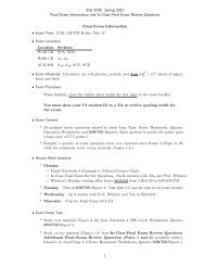
Heaps’ lawlog10 M0 1 2 3 4 5 6Vocabulary size M as afunction of collection sizeT (number of tokens) forReuters-RCV1. For thesedata, the dashed linelog 10 M =0.49 ∗ log 10 T + 1.64 is thebest least squares fit.Thus, M = 10 1.64 T 0.49and k = 10 1.64 ≈ 44 andb = 0.49.0 2 4 6 8log10 T4/ 64

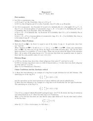
Zipf’s lawlog10 cf0 1 2 3 4 5 6 7cf i ∝ 1 iThe most frequent term(the) occurs cf 1 times, thesecond most frequent term(of) occurs cf 2 = 1 2 cf 1times, the third mostfrequent term (and) occurscf 3 = 1 3 cf 1 times etc.0 1 2 3 4 5 6 7log10 rank5/ 64

Dictionary as a string. . .syst i lesyzyget icsyzygial syzygyszaibelyi teszecinszono. . .freq.99257112. ..4 bytespostings ptr. term ptr.→→→→→. ..4 bytes...3 bytes6/ 64

Gap encodingencoding postings listthe docIDs ... 283042 283043 283044 283045 . ..gaps 1 1 1 . ..computer docIDs ... 283047 283154 283159 283202 . ..gaps 107 5 43 . ..arachnocentric docIDs 252000 500100gaps 252000 2481007/ 64

Variable byte (VB) codeDedicate 1 bit (high bit) to be a continuation bit c.If the gap G fits within 7 bits, binary-encode it in the 7available bits and set c = 1.Else: set c = 0, encode high-order 7 bits and then use one ormore additional bytes to encode the lower order bits using thesame algorithm.8/ 64

Gamma codes for gap encodingRepresent a gap G as a pair of length and offset.Offset is the gap in binary, with the leading bit chopped off.Length is the length of offset.Encode length in unary codeThe Gamma code is the concatenation of length and offset.9/ 64

Compression of Reutersdata structuresize in MBdictionary, fixed-width 11.2dictionary, term pointers into string 7.6∼, with blocking, k = 4 7.1∼, with blocking & front coding 5.9collection (text, xml markup etc) 3600.0collection (text) 960.0T/D incidence matrix 40,000.0postings, uncompressed (32-bit words) 400.0postings, uncompressed (20 bits) 250.0postings, variable byte encoded 116.0postings, γ encoded 101.010/ 64

Take-away todayRanking search results: why it is important (as opposed tojust presenting a set of unordered Boolean results)Term frequency: This is a key ingredient for ranking.Tf-idf ranking: best known traditional ranking schemeVector space model: One of the most important formalmodels for information retrieval (along with Boolean andprobabilistic models)11/ 64

Outline1 Recap2 Why ranked retrieval?3 Term frequency4 tf-idf weighting5 The vector space model12/ 64

Ranked retrievalThus far, our queries have all been Boolean.Documents either match or don’t.Good for expert users with precise understanding of theirneeds and of the collection.Also good for applications: Applications can easily consume1000s of results.Not good for the majority of usersMost users are not capable of writing Boolean queries .... . . or they are, but they think it’s too much work.Most users don’t want to wade through 1000s of results.This is particularly true of web search.13/ 64

Problem with Boolean search: Feast or famineBoolean queries often result in either too few (=0) or toomany (1000s) results.Query 1 (boolean conjunction): [standard user dlink 650]→ 200,000 hits – feastQuery 2 (boolean conjunction): [standard user dlink 650 nocard found]→ 0 hits – famineIn Boolean retrieval, it takes a lot of skill to come up with aquery that produces a manageable number of hits.14/ 64

Feast or famine: No problem in ranked retrievalWith ranking, large result sets are not an issue.Just show the top 10 resultsDoesn’t overwhelm the userPremise: the ranking algorithm works: More relevant resultsare ranked higher than less relevant results.15/ 64

Scoring as the basis of ranked retrievalWe wish to rank documents that are more relevant higherthan documents that are less relevant.How can we accomplish such a ranking of the documents inthe collection with respect to a query?Assign a score to each query-document pair, say in [0,1].This score measures how well document and query “match”.16/ 64

Query-document matching scoresHow do we compute the score of a query-document pair?Let’s start with a one-term query.If the query term does not occur in the document: scoreshould be 0.The more frequent the query term in the document, thehigher the scoreWe will look at a number of alternatives for doing this.17/ 64

Take 1: Jaccard coefficientA commonly used measure of overlap of two setsLet A and B be two setsJaccard coefficient:(A ≠ ∅ or B ≠ ∅)jaccard(A,A) = 1jaccard(A,B) =jaccard(A,B) = 0 if A ∩ B = 0|A ∩ B||A ∪ B|A and B don’t have to be the same size.Always assigns a number between 0 and 1.18/ 64

Jaccard coefficient: ExampleWhat is the query-document match score that the Jaccardcoefficient computes for:Query: “ides of March”Document “Caesar died in March”jaccard(q, d) = 1/619/ 64

What’s wrong with Jaccard?It doesn’t consider term frequency (how many occurrences aterm has).Rare terms are more informative than frequent terms. Jaccarddoes not consider this information.We need a more sophisticated way of normalizing for thelength of a document.Later in this lecture, we’ll use |A ∩ B|/ √ |A ∪ B| (cosine) ......instead of |A ∩ B|/|A ∪ B| (Jaccard) for lengthnormalization.20/ 64

Binary incidence matrixAnthony Julius The Hamlet Othello Macbeth ...and Caesar TempestCleopatraAnthony 1 1 0 0 0 1Brutus 1 1 0 1 0 0Caesar 1 1 0 1 1 1Calpurnia 0 1 0 0 0 0Cleopatra 1 0 0 0 0 0mercy 1 0 1 1 1 1worser 1 0 1 1 1 0. ..Each document is represented as a binary vector ∈ {0,1} |V | .22/ 64

Count matrixAnthony Julius The Hamlet Othello Macbeth ...and Caesar TempestCleopatraAnthony 157 73 0 0 0 1Brutus 4 157 0 2 0 0Caesar 232 227 0 2 1 0Calpurnia 0 10 0 0 0 0Cleopatra 57 0 0 0 0 0mercy 2 0 3 8 5 8worser 2 0 1 1 1 5. ..Each document is now represented as a count vector ∈ N |V | .23/ 64

Bag of words modelWe do not consider the order of words in a document.John is quicker than Mary and Mary is quicker than John arerepresented the same way.This is called a bag of words model.In a sense, this is a step back: The positional index was ableto distinguish these two documents.We will look at “recovering” positional information later inthis course.For now: bag of words model24/ 64

Term frequency tfThe term frequency tf t,d of term t in document d is definedas the number of times that t occurs in d.We want to use tf when computing query-document matchscores.But how?Raw term frequency is not what we want because:A document with tf = 10 occurrences of the term is morerelevant than a document with tf = 1 occurrence of the term.But not 10 times more relevant.Relevance does not increase proportionally with termfrequency.25/ 64

Instead of raw frequency: Log frequency weightingThe log frequency weight of term t in d is defined as follows{ 1 + log10 tfw t,d =t,d if tf t,d > 00 otherwisetf t,d → w t,d :0 → 0, 1 → 1, 2 → 1.3, 10 → 2, 1000 → 4, etc.Score for a document-query pair: sum over terms t in both qand d:tf-matching-score(q,d) = ∑ t∈q∩d (1 + log tf t,d)The score is 0 if none of the query terms is present in thedocument.26/ 64

ExerciseCompute the Jaccard matching score and the tf matchingscore for the following query-document pairs.q: [information on cars] d: “all you’ve ever wanted to knowabout cars”q: [information on cars] d: “information on trucks,information on planes, information on trains”q: [red cars and red trucks] d: “cops stop red cars moreoften”27/ 64

Outline1 Recap2 Why ranked retrieval?3 Term frequency4 tf-idf weighting5 The vector space model28/ 64

Frequency in document vs. frequency in collectionIn addition, to term frequency (the frequency of the term inthe document) ......we also want to use the frequency of the term in thecollection for weighting and ranking.29/ 64

Desired weight for rare termsRare terms are more informative than frequent terms.Consider a term in the query that is rare in the collection(e.g., arachnocentric).A document containing this term is very likely to be relevant.→ We want high weights for rare terms likearachnocentric.30/ 64

Desired weight for frequent termsFrequent terms are less informative than rare terms.Consider a term in the query that is frequent in the collection(e.g., good, increase, line).A document containing this term is more likely to be relevantthan a document that doesn’t ......but words like good, increase and line are not sureindicators of relevance.→ For frequent terms like good, increase, and line, wewant positive weights . .....but lower weights than for rare terms.31/ 64

Document frequencyWe want high weights for rare terms like arachnocentric.We want low (positive) weights for frequent words like good,increase, and line.We will use document frequency to factor this into computingthe matching score.The document frequency is the number of documents in thecollection that the term occurs in.32/ 64

idf weightdf t is the document frequency, the number of documents thatt occurs in.df t is an inverse measure of the informativeness of term t.We define the idf weight of term t as follows:idf t = log 10Ndf t(N is the number of documents in the collection.)idf t is a measure of the informativeness of the term.[log N/df t ] instead of [N/df t ] to “dampen” the effect of idfNote that we use the log transformation for both termfrequency and document frequency.33/ 64

Examples for idf1,000,000Compute idf t using the formula: idf t = log 10 df tterm df t idf tcalpurnia 1 6animal 100 4sunday 1000 3fly 10,000 2under 100,000 1the 1,000,000 034/ 64

Effect of idf on rankingidf affects the ranking of documents for queries with at leasttwo terms.For example, in the query “arachnocentric line”, idf weightingincreases the relative weight of arachnocentric anddecreases the relative weight of line.idf has little effect on ranking for one-term queries.35/ 64

Collection frequency vs. Document frequencyword collection frequency document frequencyinsurance 10440 3997try 10422 8760Collection frequency of t: number of tokens of t in thecollectionDocument frequency of t: number of documents t occurs inWhy these numbers?Which word is a better search term (and should get a higherweight)?This example suggests that df (and idf) is better for weightingthan cf (and “icf”).36/ 64

tf-idf weightingThe tf-idf weight of a term is the product of its tf weight andits idf weight.w t,d = (1 + log tf t,d ) · log N df ttf-weightidf-weightBest known weighting scheme in information retrievalNote: the “-” in tf-idf is a hyphen, not a minus sign!Alternative names: tf.idf, tf x idf37/ 64

Summary: tf-idfAssign a tf-idf weight for each term t in each document d:w t,d = (1 + log tf t,d ) · logdf N tThe tf-idf weight .... . . increases with the number of occurrences within adocument. (term frequency). . . increases with the rarity of the term in the collection.(inverse document frequency)38/ 64

Exercise: Term, collection and document frequencyQuantity Symbol Definitionterm frequency tf t,d number of occurrences of t inddocument frequency df t number of documents in thecollection that t occurs incollection frequency cf t total number of occurrences oft in the collectionRelationship between df and cf?Relationship between tf and cf?Relationship between tf and df?39/ 64

Outline1 Recap2 Why ranked retrieval?3 Term frequency4 tf-idf weighting5 The vector space model40/ 64

Binary incidence matrixAnthony Julius The Hamlet Othello Macbeth ...and Caesar TempestCleopatraAnthony 1 1 0 0 0 1Brutus 1 1 0 1 0 0Caesar 1 1 0 1 1 1Calpurnia 0 1 0 0 0 0Cleopatra 1 0 0 0 0 0mercy 1 0 1 1 1 1worser 1 0 1 1 1 0. ..Each document is represented as a binary vector ∈ {0,1} |V | .41/ 64

Count matrixAnthony Julius The Hamlet Othello Macbeth ...and Caesar TempestCleopatraAnthony 157 73 0 0 0 1Brutus 4 157 0 2 0 0Caesar 232 227 0 2 1 0Calpurnia 0 10 0 0 0 0Cleopatra 57 0 0 0 0 0mercy 2 0 3 8 5 8worser 2 0 1 1 1 5. ..Each document is now represented as a count vector ∈ N |V | .42/ 64

Binary → count → weight matrixAnthony Julius The Hamlet Othello Macbeth ...and Caesar TempestCleopatraAnthony 5.25 3.18 0.0 0.0 0.0 0.35Brutus 1.21 6.10 0.0 1.0 0.0 0.0Caesar 8.59 2.54 0.0 1.51 0.25 0.0Calpurnia 0.0 1.54 0.0 0.0 0.0 0.0Cleopatra 2.85 0.0 0.0 0.0 0.0 0.0mercy 1.51 0.0 1.90 0.12 5.25 0.88worser 1.37 0.0 0.11 4.15 0.25 1.95. ..Each document is now represented as a real-valued vector of tf-idfweights ∈ R |V | .43/ 64

Documents as vectorsEach document is now represented as a real-valued vector oftf-idf weights ∈ R |V | .So we have a |V |-dimensional real-valued vector space.Terms are axes of the space.Documents are points or vectors in this space.Very high-dimensional: tens of millions of dimensions whenyou apply this to web search enginesEach vector is very sparse - most entries are zero.44/ 64

Queries as vectorsKey idea 1: do the same for queries: represent them asvectors in the high-dimensional spaceKey idea 2: Rank documents according to their proximity tothe queryproximity = similarityproximity ≈ negative distanceRecall: We’re doing this because we want to get away fromthe you’re-either-in-or-out, feast-or-famine Boolean model.Instead: rank relevant documents higher than nonrelevantdocuments45/ 64

How do we formalize vector space similarity?First cut: (negative) distance between two points( = distance between the end points of the two vectors)Euclidean distance?Euclidean distance is a bad idea . .....because Euclidean distance is large for vectors of differentlengths.46/ 64

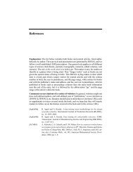
Why distance is a bad ideapoor1d 1 :Ranks of starving poets swelld 2 :Rich poor gap growsq:[rich poor]0d 3 :Record baseball salaries in 2010rich0 1 The Euclidean distance of⃗q and ⃗ d 2 is large although the distribution of terms in the query qand the distribution of terms in the document d 2 are very similar.Questions about basic vector space setup?47/ 64

Use angle instead of distanceRank documents according to angle with queryThought experiment: take a document d and append it toitself. Call this document d ′ . d ′ is twice as long as d.“Semantically” d and d ′ have the same content.The angle between the two documents is 0, corresponding tomaximal similarity . .....even though the Euclidean distance between the twodocuments can be quite large.48/ 64

From angles to cosinesThe following two notions are equivalent.Rank documents according to the angle between query anddocument in decreasing orderRank documents according to cosine(query,document) inincreasing orderCosine is a monotonically decreasing function of the angle forthe interval [0 ◦ ,180 ◦ ]49/ 64

Cosine50/ 64

Length normalizationHow do we compute the cosine?A vector can be (length-) normalized by dividing each of itscomponents by its length – here we use the L 2 norm:||x|| 2 =√ ∑i x2 iThis maps vectors onto the unit sphere ......since after normalization: ||x|| 2 =√ ∑i x2 i= 1.0As a result, longer documents and shorter documents haveweights of the same order of magnitude.Effect on the two documents d and d ′ (d appended to itself)from earlier slide: they have identical vectors afterlength-normalization.51/ 64

Cosine similarity between query and documentcos(⃗q, ⃗ d) = sim(⃗q, ⃗ d) =∑⃗q · ⃗d|V ||⃗q|| ⃗ d| = i=1 q id i√ ∑|V |i=1 q2 i√ ∑|V |i=1 d2 iq i is the tf-idf weight of term i in the query.d i is the tf-idf weight of term i in the document.|⃗q| and | ⃗ d| are the lengths of ⃗q and ⃗ d.This is the cosine similarity of ⃗q and ⃗ d . .....or, equivalently,the cosine of the angle between ⃗q and ⃗ d.52/ 64

Cosine for normalized vectorsFor normalized vectors, the cosine is equivalent to the dotproduct or scalar product.cos(⃗q, ⃗ d) = ⃗q · ⃗d = ∑ i q i · d i(if ⃗q and ⃗ d are length-normalized).53/ 64

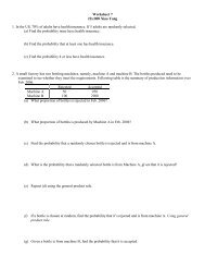
Cosine similarity illustratedpoor1 ⃗v(d 1 )⃗v(q)⃗v(d 2 )θ00 1⃗v(d 3 )rich54/ 64

Cosine: Exampleterm frequencies (counts)How similar arethese novels? SaS:Sense andSensibility PaP:Pride andPrejudice WH:WutheringHeightsterm SaS PaP WHaffection 115 58 20jealous 10 7 11gossip 2 0 6wuthering 0 0 3855/ 64

Cosine: Exampleterm frequencies (counts)term SaS PaP WHaffection 115 58 20jealous 10 7 11gossip 2 0 6wuthering 0 0 38log frequency weightingterm SaS PaP WHaffection 3.06 2.76 2.30jealous 2.0 1.85 2.04gossip 1.30 0 1.78wuthering 0 0 2.58(To simplify this example, we don’t do idf weighting.)56/ 64

Cosine: Examplelog frequency weightingterm SaS PaP WHaffection 3.06 2.76 2.30jealous 2.0 1.85 2.04gossip 1.30 0 1.78wuthering 0 0 2.58log frequency weighting& cosine normalizationterm SaS PaP WHaffection 0.789 0.832 0.524jealous 0.515 0.555 0.465gossip 0.335 0.0 0.405wuthering 0.0 0.0 0.588cos(SaS,PaP) ≈0.789 ∗ 0.832 + 0.515 ∗ 0.555 + 0.335 ∗ 0.0 + 0.0 ∗ 0.0 ≈ 0.94.cos(SaS,WH) ≈ 0.79cos(PaP,WH) ≈ 0.69Why do we have cos(SaS,PaP) > cos(SAS,WH)?57/ 64

Computing the cosine scoreCosineScore(q)1 float Scores[N] = 02 float Length[N]3 for each query term t4 do calculate w t,q and fetch postings list for t5 for each pair(d,tf t,d ) in postings list6 do Scores[d]+ = w t,d × w t,q7 Read the array Length8 for each d9 do Scores[d] = Scores[d]/Length[d]10 return Top K components of Scores[]58/ 64

Components of tf-idf weightingTerm frequency Document frequency Normalizationn (natural) tf t,d n (no) 1 n (none) 1l (logarithm) 1 + log(tf t,d ) t (idf) log N dfta (augmented)b (boolean)0.5 + 0.5×tft,dmaxt(tft,d){ 1 if tft,d > 00 otherwisep (prob idf)1+log(tft,d)L (log ave) 1+log(avet∈d(tft,d))Best known combination of weighting options Default: nomax{0,log N−dft } u (pivoteddftunique)1c (cosine) √ w 21 +w2 2+...+w2 M1/ub (byte size) 1/CharLength α ,α < 1weighting59/ 64

tf-idf exampleWe often use different weightings for queries and documents.Notation: ddd.qqqExample: lnc.ltndocument: logarithmic tf, no df weighting, cosinenormalizationquery: logarithmic tf, idf, no normalizationIsn’t it bad to not idf-weight the document?Example query: “best car insurance”Example document: “car insurance auto insurance”60/ 64

tf-idf example: lnc.ltnQuery: “best car insurance”. Document: “car insurance auto insurance”.word query document producttf-raw tf-wght df idf weight tf-raw tf-wght weight n’lizedauto 0 0 5000 2.3 0 1 1 1 0.52 0best 1 1 50000 1.3 1.3 0 0 0 0 0car 1 1 10000 2.0 2.0 1 1 1 0.52 1.04insurance 1 1 1000 3.0 3.0 2 1.3 1.3 0.68 2.04Key to columns: tf-raw: raw (unweighted) term frequency, tf-wght: logarithmically weightedterm frequency, df: document frequency, idf: inverse document frequency, weight: the finalweight of the term in the query or document, n’lized: document weights after cosinenormalization, product: the product of final query weight and final document weight√1 2 + 0 2 + 1 2 + 1.3 2 ≈ 1.921/1.92 ≈ 0.521.3/1.92 ≈ 0.68 Final similarity score between query anddocument: ∑ i w qi · w di = 0 + 0 + 1.04 + 2.04 = 3.08 Questions?61/ 64

Summary: Ranked retrieval in the vector space modelRepresent the query as a weighted tf-idf vectorRepresent each document as a weighted tf-idf vectorCompute the cosine similarity between the query vector andeach document vectorRank documents with respect to the queryReturn the top K (e.g., K = 10) to the user62/ 64

Take-away todayRanking search results: why it is important (as opposed tojust presenting a set of unordered Boolean results)Term frequency: This is a key ingredient for ranking.Tf-idf ranking: best known traditional ranking schemeVector space model: One of the most important formalmodels for information retrieval (along with Boolean andprobabilistic models)63/ 64

ResourcesChapters 6 and 7 of IIRResources at http://ifnlp.org/irVector space for dummiesExploring the similarity space (Moffat and Zobel, 2005)Okapi BM25 (a state-of-the-art weighting method, 11.4.3 ofIIR)64/ 64