Crop yield response to water - Cra

Crop yieldresponse to waterFAOIRRIGATIONANDDRAINAGEPAPER66byPasquale Steduto(FAO, Land and Water Division, Rome, Italy)Theodore C. Hsiao(University of California, Davis, USA)Elias Fereres(University of Cordoba and IAS-CSIC, Cordoba, Spain)Dirk Raes(KU Leuven University, Leuven, Belgium)FOOD AND AGRICULTURE ORGANIZATION OF THE UNITED NATIONSRome, 2012

ISPA:IVIA:KESREF:LARI:LLNL:SARDI:SASRI:SIA:USDA-ARS:WB:VLIR-UOS:ZIS:Istituto di Scienze delle Produzioni Alimentari, ItalyInstituto Valenciano de Investigaciones Agrarias, SpainKenya Sugar Research Foundation, KenyaLebanese Agricultural Research Institute, LebanonLaurence Livermore National Laboratory, USASouth Australian Research and Development Institute, AustraliaSouth African Sugarcane Research Institute, South AfricaServicio de Investigación Agraria, SpainUnited States Department of Agriculture – Agricultural Research Service, USAWorld Bank, USAFlemish Inter-University Council, BelgiumZhanghe Irrigation System, Chinaix

1. IntroductionFood production and water use are inextricably linked. Water has always been the mainfactor limiting crop production in much of the world where rainfall is insufficient to meetcrop demand. With the ever-increasing competition for finite water resources worldwideand the steadily rising demand for agricultural commodities, the call to improve the efficiencyand productivity of water use for crop production, to ensure future food security and addressthe uncertainties associated with climate change, has never been more urgent.To examine the pathways for increasing the efficiency and productivity of water use, the yieldresponse of crops to water must be known. This relationship is complex in nature and variousattempts have been made to provide simplified, though sound, approaches to capture thebasic features of the response.FAO’s first publication that presented a relationship between crop yield and water consumedwas Irrigation and Drainage Paper No. 33 Yield Response to Water (Doorenbos and Kassam,1979). This approach, discussed in Chapter 2, is based on one single equation relating therelative yield loss of any crop (either herbaceous or woody species) to the relative reductionof water consumption, i.e. evapotranspiration, by way of a coefficient (k y ), which is specificfor any given crop and condition. This approach has provided a widely-used standard forsynthetic water production functions, still in use today. This simplification, however, made thisapproach more suitable for general planning, project design and rapid appraisal purposes,often providing a first-order approximation.Over the last three and half decades, new knowledge has enlighten processes underlyingthe relationship between crop yield and water use and technology has improved. Further,novel needs have emerged related to the planning and management of water in agriculture,including those arising from climate change. FAO has, therefore, revisited the approach toquantify crop yields in response to water use and water deficit. The end product of this effort isa crop simulation model named AquaCrop, which balances accuracy, simplicity and robustnessand is described in Chapter 3. The conceptualization and development of this modellingapproach is the result of a number of years of consultation and collaboration with scientists,crop specialists and practitioners worldwide, consolidating the vast amount of knowledgeand information available since 1979.AquaCrop uses the original equation of Doorenbos and Kassam (1979) as a point of departureand evolves from it by calculating the crop biomass, based on the amount of water transpired,and the crop yield as the proportion of biomass that goes into the harvestable parts. AnINTRODUCTION 1

important evolution is the separation of the non-productive consumption of water (soilevaporation) from the productive consumption of water (transpiration). Furthermore,the timescale of the original equation is seasonal, or growth-stages that are weeks longin duration, while the timescale used in AquaCrop is daily, in order to better represent thedynamics of crop response to water. Finally, the model allows for the assessment of responsesunder different climate change scenarios in terms of altered water and temperature regimesand elevated carbon dioxide concentration in the atmosphere. AquaCrop simulates growth,productivity and water use of a crop day-by-day, as affected by changing water availability andenvironmental conditions. The results of calibration and testing of the model so far providegrounds for confidence in its performance.The development of standard crop parameters has made the model accessible to several typesof users in different disciplines and for a wide-range of applications. AquaCrop is mainlyaimed at practitioner-type end users such as those working for extension services, consultingengineers, irrigation districts, governmental agencies, nongovernmental organizations, andvarious kinds of farmer associations for use in the development of irrigation schedules andmanagement decisions. Economists and policy specialists can also use this model for planningand scenario analysis. In addition, research scientists should find the model valuable as atool for analysis and conceptualization. Overall, AquaCrop allows proper investigation ofstrategic planning and management to improve the efficiency and productivity of water usein herbaceous crop production. It is not designed for use with trees and vines.Chapter 3 not only describes AquaCrop but also provides samples of applications for specificpurposes and guidelines for calibration.Chapter 3 also provides the agronomic features of the sixteen crops for which the model has beencalibrated and validated. The crops covered are: wheat, rice, maize, soybean, barley, sorghum,cotton, sunflower, sugarcane, potato, tomato, sugar beet, alfalfa, bambara groundnut, quinoaand tef. Additional crops will soon be calibrated and their agronomic features described. Thegoal is to provide an overview of each crop’s physiology and agronomy for users interestedin applying the model to a particular crop at a given location. Furthermore, the overview canserve as a reference when calibrating the model for different crop classes. The description ofeach crop includes crop growth and development, water use and productivity, responses towater deficits and expected yields.Fruit production has risen in importance over the past decades for increasing the productivityand competitiveness of small-scale farmers around the world. Fruit not only provides betterincome opportunities for growers, but is also pivotal in providing more healthy diets toconsumers. The yield response to water of fruit trees and vines forms the second major partof this publication, presented in Chapter 4. The complexity of tree crops resulting from carryovereffects from one year to the next and the large divergence among cultivars, however,precluded using a relatively simple modelling approach, as that used for herbaceous crops.Therefore, a Guideline is presented instead, which includes a general section on the irrigationof fruit trees and vines, and a special section covering physiological and agronomic features ofeach individual crop species. While the general section provides the technical background andguidelines for efficient irrigation management, the sections on individual crops give specificresponses to water, with a common format, covering the following key items: growth anddevelopment, crop water requirements, yield response to water supply, and recommended2crop yield response to water

Lead AuthorsMartin Smith(formerly FAO, Land and WaterDivision, Rome, Italy;currently retired)Pasquale Steduto(FAO, Land and Water Division,Rome, Italy)2. Yield response to water:the original FAO waterproduction functionGeneral descriptionFAO addressed the relationship between crop yield and water use in thelate seventies proposing a simple equation where relative yield reductionis related to the corresponding relative reduction in evapotranspiration(ET). Specifically, the yield response to ET is expressed as:(1)⎛ ⎞⎜ 1−Y ⎛a⎟ = K y1−ET ⎞a⎜ ⎟⎝ Y x ⎠ ⎝ ET x ⎠where Y x and Y a are the maximum and actual yields, ET x and ET a are themaximum and actual evapotranspiration, and K y is a yield response factorrepresenting the effect of a reduction in evapotranspiration on yieldlosses. Equation 1 is a water production function and can be applied to allagricultural crops, i.e. herbaceous, trees and vines.The yield response factor (K y ) captures the essence of the complex linkagesbetween production and water use by a crop, where many biological,physical and chemical processes are involved. The relationship has showna remarkable validity and allowed a workable procedure to quantify theeffects of water deficits on yield.This approach and the calculation procedures for estimating yield responseto water were published in the FAO Irrigation and Drainage Paper No. 33(Doorenbos and Kassam, 1979), which was considered one of FAO'smilestone publications, and were used widely worldwide for a broad rangeof applications.In this Chapter, the procedures used to quantify the yield response to waterdeficits using Equation 1 are briefly described. To get fully acquainted withthe original procedures, the K y use and related applications, the reader isreferred to the original publication.6crop yield response to water

Maximum Yield (Y x )The FAO I&D No. 33 recommended procedures for estimating maximum yield either fromavailable local data for maximum crop yields or based on the calculation of maximum biomassand a corresponding harvest index, following two different procedures:I. Wageningen procedure (De Wit, 1968; Slabbers, 1978)II. Ecological zone approach (Kassam, 1977)These procedures for yield estimation were developed in the late sixties and seventies. Theconsiderable advances in agronomy and crop physiology, though, allow for the use of moreprecise methods to estimate maximum yields.Maximum Crop EvAPOTRANSPIRATION (ET x )Procedures for determining ET x were based on FAO guidelines for crop-water requirements(ET c ), and the ET x component of Equation 1, which is equal to ET c , was determined throughthe product of the reference-crop evapotranspiration (ET o ) times the crop coefficient (K c ), i.e.(2) ET x = K c ET oOriginal procedures for determining ET o are described in FAO I&D No. 24 (Doorenbos andPruitt, 1977), offering different equations for its calculation according to the availableclimate data. K c values were provided for a large number of crops and procedures todetermine ET c over the growing season. Subsequently, revised procedures for calculatingET o were introduced in FAO I&D No. 56 (Allen et al., 1998), according to the FAO Penman-Monteith equation, which has now become the standard for estimating reference cropevapotranspiration.Actual Crop EvAPOTRANSPIRATION (ET a )It is very difficult to estimate the actual crop evapotranspiration with precision. FAO I&D No. 33provided tables from which ET a could be estimated from data on evapotranspiration rate,available soil water and wetting intervals. The tables however proved cumbersome and laterwere replaced by more accurate ET a calculations based on daily water balance calculations anddigital computation methods.Water balance calculations allow the level of available soil water in the root zone to bedetermined on a daily basis. As long as soil water is readily available for the crop, then ET a =ET x . When a critical soil moisture level is reached, defined as a fraction of the total availablesoil water content (p), transpiration is reduced because the stomata close and thus ET a < ET x ,until the level of soil water in the root zone reaches the permanent wilting point, when ET ais assumed to be zero. This critical soil-water content is estimated from soil, crop and rootingcharacteristics and from the ET o rate. Depletion of soil-water content between p and thepermanent wilting point will result in a proportional reduction of ET a .Yield Response to Water of All Crop Types 9

3. Yield response to waterof herbaceous crops:the AquaCrop simulation modelThis Chapter presents the main features of AquaCrop, the dynamic crop-growth modeldeveloped to predict yield response to water of herbaceous crops. The scientific basisof AquaCrop has been previously described (Steduto et al., 2009; Raes et al., 2009;Hsiao et al., 2009) and only the basic concepts and fundamental calculation procedures arebriefly explained here, along with additional descriptions related to the input requirements,the user interface and the model outputs. Sample applications are provided to illustrate theusefulness of AquaCrop for benchmarking, irrigation scheduling, and for studying the effectof various soils, crop management practices, and the impact of climate change, on crop yieldand water productivity. Finally, guidelines for parameterizing, calibrating and validatingAquaCrop are presented. For further insights on the operation of the model and on the fullalgorithms details, the reader is referred to the AquaCrop Reference Manual (Raes et al., 2011).16crop yield response to water

figure 3 An example of the progress of green canopy cover through a crop life-cycle under non-stressconditions, for maize.MeasuredSimulated10080Canopy cover (%)60402000 20 40 60 80 100 120 140Days after planting (DAP)figure 4 Schematic representation of a generalized rooting depth with time, in the presence (dashed line)and absence (full line) of a restrictive soil layer limiting root development.SowingTransplantingTimeZnEffective rooting depth (Z)Z x (restrictive soil layer)Z xZ x = Maximum effective rooting depthZ n = Minimum effective rooting depthAquaCrop: concepts, rationale and operation 23

The WP parameter introduced in AquaCrop is normalized for atmospheric evaporative demand,defined by ET o , and for the CO 2 concentration of the atmosphere. The normalized biomasswater productivity (WP*) proved to be nearly constant for a given crop when mineral nutrientsare not limiting, regardless of water stress except for extremely severe cases. Calibration of WPand normalization for evaporative demands has been based on the equation:(5)WP* =ΣBTrET O[CO 2]The summation is taken over the time intervals spanning the period when B is produced.[CO 2 ] outside the bracket indicates that the normalized value is for a particular air CO 2concentration. For most crop species, WP* increases as air CO 2 concentration increases,allowing the simulation of impact on yield under various CO 2 and climate change scenarios.The equation is directly applicable when Tr and ET o data are for daily time intervals. WhenTr and ET o are available for time interval larger than daily, the normalization requirescaution. Background information and more details on normalization, including that for CO 2concentration, are given in Steduto et al. (2007).In the literature WP is commonly normalized for evaporative demand using air vapourpressure deficit (VPD) instead of ET o . The choice of using ET o was made because it has beendemonstrated to be superior and accounts for advective energy transfer, which is ignoredusing VPD (Steduto et al., 2007). WP* is conservative for a given level of mineral nutrition,but may be reduced by nutrient deficiencies, particularly nitrogen. The calibrated WP* inthe model for various crops are for situations where nutrients are ample. For nutrient limitedsituations, the model provides categories of soil fertility stress ranging from mild to severenutrient deficiencies, with corresponding lower default WP* values.The conservative nature of WP* is demonstrated in Figure 5, where cumulative B vs.cumulative Tr are plotted in (a), and cumulative B vs. cumulative normalized Tr (Tr/ET o )in (b), over the season for sweet sorghum (a C 4 crop), sunflower, wheat and chickpea (allthree are C 3 ). It is seen in Figure 5a that the regression lines for different crops are linearbut with different slopes. This means WP is constant for each crop but differs among thecrops. In Figure 5b it is seen that normalization by ET o has coalesced the lines for the threeC 3 crops into one, meaning their WP* are very similar. In this study sunflower was grownin May-August, wheat in February-May, and chickpea in April-June. So growth of thesecrops occurred in periods differing in atmospheric evaporative demand. Normalizing by ET oaccounted for the difference in evaporative demand and showed that the three crops havevery similar intrinsic water productivity (very similar WP*).The single value of WP*, as show in Figure 5b, is used for the entire crop cycle for most ofthe crops. However, for crops with yields high in fat and protein content, more photosyntheticassimilates or energy is required per unit of dry matter produced after flowering and duringthe grain/fruit filling stage. For such crops, AquaCrop uses a single value for the WP* up toflowering, then declining gradually towards a lower WP* value to account for yield composition.AquaCrop: concepts, rationale and operation 25

figure 5 Relationship (a) between aboveground biomass and cumulative transpiration (ΣTr) and (b)between aboveground biomass and cumulative normalized transpiration [Σ(Tr/ET o )], during thecropcycle of sunflower (under two N levels and up to anthesis), sorghum, wheat, and chickpea(redrawn from Steduto and Albrizio, 2005).Aboveground biomass (kg m -2 )Sorghum (N1) Sunflower (N0) Sunflower (N1) Wheat Chickpea3ab2100 100 200 300 400 500 0 20 40 60 80 100ΣTr (mm) Σ(Tr/ET °)Harvestable yieldThe partition of biomass into yield part (Y) is simulated by means of a harvest index (HI). Forfruit or grain crops, published data on different species indicate there is a linear increase withtime in the ratio of fruit or grain biomass to total above-ground biomass, from the time nottoo long after pollination and fruit set until maturity or near maturity. In common usage, HI isthis ratio at maturity or harvest time. In AquaCrop, this ratio at earlier stages is also referredto as HI, for simplicity. For fruit/grain crops, HI is set to increase from zero at flowering, firstover a short lag phase, when the increase starts slowly but accelerates with time, followed bya steady phase with the highest, but at constant rate of, increase (Figure 6). For root/tubercrops, HI is the ratio of the storage organ biomass to the total biomass (root plus shoot). Thelimited published data on root/tuber crops indicate that instead of increasing linearly after alag phase, HI increases quickly shortly after storage organ initiation, then gradually slows untilmaturity. So HI is described by a logistic curve for these crops.A reference point is needed for the upper range of HI. This point, termed reference HI (HI o ),is the HI representative of well-developed cultivars adapted to their environments and grownunder optimal conditions without limiting inputs. Calibrated HI o can be changed based on gooddata for a particular cultivar. The progression of HI for fruit/grain crops is exemplified in Figure 6.The soilIn AquaCrop the soil is described by a soil profile and the characteristics of the groundwatertable (if any). In AquaCrop the soil can be subdivided vertically up to five layers of variabledepth, each layer (or horizon) accommodating different soil physical characteristics: the soilwatercontent at saturation; the upper limit of water content under gravity (commonly referredas field capacity (FC) for easy of reference); the lower limit of water content where a crop canreach the permanent wilting point (PWP); and the hydraulic conductivity at saturation (K sat ).From these characteristics AquaCrop derives other parameters governing soil evaporation,26crop yield response to water

figure 7 The root zone depicted as a reservoir with indication of the equivalent water depth (Wr) and rootzone depletion (D r ).Evapo-transpiration (ET)Irrigation (I)Rainfall (P)Runoff(RO)Stored soil water (mm)0.0Field capacityD rW r Permanent wilting point0.0Root zone depletion (mm)TAWCapillaryrise(CR)Deeppercolation(DP)but increases exponentially with depth, so that infiltration, evaporation and transpirationfrom the top soil layers can be described with sufficient detail.To simulate water movement in and out of the soil profile, AquaCrop considers surface runoff,infiltration, capillary rise, soil evaporation and crop transpiration. To simulate the redistributionof water into a soil layer, the drainage out of a soil profile, and the infiltration of rainfall and/or irrigation, AquaCrop makes use of an exponential drainage function that describes thedeclining water movement between saturation and field capacity. Upward water movementfrom a groundwater table to the soil profile is described by an exponential relationshipbetween the capacity for capillary rise and the height above the groundwater table. Theamount of water that moves upward depends not only on the depth of the groundwater tablebut also on the wetness of the top soil and the hydraulic characteristics of the soil layers. Byconsidering the water fluxes in response to the processes listed above, the soil-water contentis updated at the end of the daily time step in each of the 12 compartments (for full detailssee Raes et al., 2011).While performing the water balance, AquaCrop also deploys the salt balance. Salts enter thesoil profile by capillary rise from a saline groundwater table or together with the irrigationwater. Salts are leached out of the soil profile by excessive rainfall or irrigation. Vertical saltmovement in a soil profile is described by assuming that salts are transferred downwards bysoil-water flow in macro pores as simulated by the drainage function. Since the solute transportin the macro pores bypass the soil water in the matrix, a diffusion process is consideredto describe the transfer of solutes from macro pores to the soil matrix. Therefore the soil28crop yield response to water

FIGURE 8 A soil profile with more than one soil horizon and 12 soil compartments. The total number ofcompartnents remains always 12, regardless of the number of horizon (varying from 1 to 5).Soilhorizon 1Soilhorizon n123456789101112Soil compartmentscompartments are divided into a number of cells where salts can be figuratively stored. A cellis a representation of a bundle of pores with a specific diameter. The driving force for thehorizontal diffusion is the salt concentration gradient that exists between the water solutionin the cells at a particular soil depth. To avoid the building up of high salt concentrations ata particular depth, vertical salt diffusion is also taken into account. The driving force for thisvertical redistribution process is the salt concentration gradient that builds up at various soildepths in the soil matrix.The managementAquaCrop encompasses two categories of management practices: the irrigation management,which is quite complete in its various features, and the field management, which is limited toselected aspects and is relatively simple in approaches.Irrigation managementHere options are provided to assess and analyse crop production and water managementand use, under either rainfed or irrigated conditions. Management options includethe selection of water application methods (sprinkler, surface, or drip either surface orunderground), defining the schedule by specifying the time, depth and quality of theirrigation water of each application, or let the model automatically generate the schedulebased on fixed time interval, fixed depth per application, or fixed percentage of allowablewater depletion. An additional feature is the estimation of full water requirement of acrop in a given climate.AquACrop: ConCepts, rAtionAle And operAtion 29

threshold and 1.0 at the lower threshold (Figure 10). The shape of most of the Ks curves aretypically convex, and the degree of curvature is set during model calibration.water stressAquaCrop distinguishes stresses related to deficit and to excess water. In this publication, waterstress routinely refers to the stress caused by a lack of water, and stress caused by excessivewater is referred to as aeration stress. Water stress effects on productivity and water useprocesses are simulated by impacting: (1) canopy growth; (2) stomata conductance; (3) canopysenescence; (4) root deepening, and (5) harvest index. The normalized water productivity isassumed to be not impacted, based on extensive evaluation of the literature. The discoursethat follows discusses the first three impacted processes together, and includes root dependingat the end. Harvest index, a complex subject, is covered on its own in the last section on waterstress.water stress response functionsFor water stresses, the stress indicator is the root zone depletion (D r ), and the thresholds aresoil water depletions from the root zone expressed as fractions (p) of the total available soilwater (TAW). At the point when there is no depletion Ks = 1.0. As depletion progresses Ksdoes not drop below 1.0 until the upper threshold for stress effect is reached. This thresholdis referred to as p upper . Further increase in root zone depletion, brings about lower values ofKs, until the lower threshold (designated as p lower ) is reached, where Ks becomes zero and thestress effect is maximum (Figure 11). Further depletion below p lower has no additional effectand Ks remains zero. For water stresses the shape of the curve can vary between very convexto mildly convex to linear. Conceptually, the more convex the curve, the higher is the crop’scapacity to adjust and acclimate to the stress. A linear relationship indicates minimal or noFIGURE 10 The stress coefficient (Ks) for various degrees of stress and for 2 sample shapes of the Ks curve.No stress1.0convex0.8KsStress coefficient0.60.4linear0.2Full stress0.0UpperthresholdLowerthresholdStressindicator0.0 0.2 0.4 0.6 0.8 1.0Relative stress32crop yield response to water

acclimation. The stress thresholds, as well as the curve shape, are set by calibration and shouldbe based on knowledge of the crop’s drought resistance or tolerance.Being the middle link in the soil-plant-atmosphere continuum, the plant water status dependsnot only on soil-water status, but also on the rate of transpiration determined by atmosphericevaporative demand. The crop is more sensitive to soil-water depletion on days of high ET o ,and less on days of low ET o . For simplicity, instead of modelling the soil-plant-atmospherecontinuum, AquaCrop adjusts the thresholds of the Ks curve according to ET o , a measureof evaporative demand. As the threshold is set for environments with ET o = 5 mm/day, themodel automatically adjusts the thresholds each day according to daily ET o when running asimulation. The extent of the adjustment is depicted in Figure 11.FIGURE 11 Sample Ks curve for canopy expansion. The thick blue line represents Ks for days whenET o = 5 mm/day. The line on the left indicates that the value of Ks decreases (stronger stresseffect) when ET o increases, and the line on the right that Ks increases when ET o decreases. Thehatched area spans the range of adjustment as dictated by ET o .HighETOKs curve forcanopy expansion growthwith ETO = 5 mm/dayWater stress coefficient (Ks, leaf)1.00.80.60.40.2LowETO0.0Fieldcapacityp upperp lowerRoot zone depletionOf the first three processes affected by water stress, extensive studies have shown thatexpansion of the leaf (hence the canopy) is the most sensitive, and stomatal conductance issubstantially less sensitive. Depending on the species, leaf (hence canopy) senescence may beequally or slightly less sensitive than stomatal conductance (Bradford and Hsiao, 1982). Settingof the three upper thresholds for water stress for a crop should be consistent with theseobservations. Differences in the Ks curves for the three processes can be seen in the examplefor maize in Figure 12.AquACrop: ConCepts, rAtionAle And operAtion 33

also calculated by multiplying with its Ks, and is not affected by water stress as long as rootzone depletion is less than the upper threshold for its Ks. As more water depletes and theupper threshold (point c in Figure 12) is passed, Ks drops below 1.0 and calculated Tr becomesless than potential. Further depletion causes more reduction in Tr, and if it passes the upperthreshold for senescence (point d in Figure 12), canopy starts to senesce and CC, made up ofgreen foliage, decreases. If root zone water is replenished to above the upper thresholds atthis point, stomata would open fully and Tr will increase, and canopy senescence will cease.Tr, however, will be lower than if there had not been water stress, because CC is now smaller.CC would increase gradually if the crop is at a stage when the potential for leaf growth is stillthere; otherwise CC would remain smaller, but would endure to the normal time of maturationif there is no additional depletion passing the upper threshold for senescence.Senescence of the canopy can be triggered and accelerated by water stress any time duringthe crop life-cycle, provided the stress is severe enough. This is simulated by adjusting CDC, inunits of fractional reduction of CC per unit of time, with an empirical equation based on Ksfor senescence arranged in such a way that the value of CDC is zero when Ks is 1.0, but risesexponentially above zero when Ks falls below 1.0.Root deepening is another process affected by water stress. It is well established that rootgrowth is substantially less sensitive to water stress than leaves, and that the ratio of root toshoot is enhanced by mild to moderate water stress (Hsiao and Xu, 2000). In AquaCrop thereis no link between roots and shoot (canopy and biomass) except indirectly via the effect ofroot zone water depletion on components of the production process. Specifically, deepeningenlarges the root zone and reduces Dr (fractional water depletion) if the deeper soil layersare high in water content. This raises the value of particular Ks, leading to favourable changesin shoot processes. On the other hand, deepening into quite dry soil layers may actuallyincrease Dr, because volume of the root zone becomes larger but there is little increase in itswater the volume. Fractional depletion could then become larger with lower Ks and negativeconsequences on shoot processes.Because root growth is less sensitive to water stress than leaves, root deepening is simulatedin AquaCrop to proceed normally as root zone water depletes until p upper for stomatal closureis reached. At this point, a reduction as a function of Tr (hence Ks for stomata) is applied tothe deepening rate. In this simple way, the model mimics the increase in root-shoot ratiounder mild to moderate water stress, because canopy expansion starts to be inhibited at amuch higher fractional water content of the root zone than Tr. So roots grow better than thecanopy, down at least to the upper threshold for stomata.Water stress effects on harvest indexSo far attention has been on processes leading to biomass production, on which yielddepends (Equation 2). Yield also depends on HI, and the impact of water stresses on HI canbe pronounced, depending on the timing and extent of stress during the crop cycle. Effects ofwater stress on HI can be negative or positive.Two of the negative effects are more straightforward. One is the inhibition of water stress onpollination and fruit set (successful formation of the embryo). If the stress is severe and longenough, the number of set fruit (or grain) would be reduced sufficiently to reduce HI and limityield, in some cases drastically. Under good conditions most, if not all crop species, have beenAquaCrop: concepts, rationale and operation 35

selected with a tendency to set more fruit than can be filled with the available photosyntheticassimilates, leading to the abortion of a portion of the set fruit early in their development.So reduction of fruit set by water stress may or may not reduce HI, depending on the extentof the reduction and the extent of the excessive fruit setting. AquaCrop simulates this alsowith the Ks approach, to reduce pollination (hence fruit set) each day according to the extentof water depletion. The effect on HI is adjusted for tendency to set excess fruit by providingcategories differing in excessiveness.Another negative impact on HI is the underfilling and abortion of younger fruits resultingfrom a lack of photosynthetic assimilates. Photosynthesis is tightly correlated with stomatalconductance. Water stress, by reducing stomatal opening, diminishes the amount of assimilatesavailable to fill all developing fruit. The youngest fruit are then the most likely to be abortedand only the older fruit mature, but likely underfilled. This occurs during the grain filling andmaturing period, when most of the vegetative growth has already taken place and most ofthe assimilates go to the grain. AquaCrop simulates this in two ways, one is simply by reducingHI with a coefficient that is a function of Ks for stomata. Stomatal closure may often be onlythe minor cause, however, because water stress at this growth stage commonly acceleratescanopy senescence, resulting in an early decline in photosynthetic surface area and shortensthe duration of the canopy. As programmed in AquaCrop, HI increases continuously up tothe time of normal maturity (Figure 6), but only if a portion of the green canopy remains. AsCC declines to some low limit value, HI is considered to have reached its final value. With CCreaching this low limit earlier because of stress induced early senescence, HI is automaticallyreduced. This effect can be dramatic if canopy duration is shortened substantially.The last of the negative impacts on HI has to do with not having sufficient water stress. Thiscentres on the competition between vegetative and reproductive growth, which also accountsfor the positive impact of water stress on HI. As demonstrated for cotton and some other crops,HI can be reduced by overly luxurious vegetative (leaf) growth during the reproductive phasewhen water is fully available, while restricting vegetative growth by mild water (and nitrogen)stress is known to enhance HI. The cause is apparently the competition for assimilates. Negativeeffect on HI comes about when high water availability stimulates fast leaf growth, with toomany assimilates diverted to the vegetative organs, depriving the younger potential flowers ornascent fruits so they drop off the crop. The end result is that too few fruits mature, reducingHI. On the other hand, mild water stress would reduce leaf growth substantially because it ismost sensitive to water stress, while stomata, being substantially less sensitive, would remainopen to maintain photosynthesis. Consequently, without the excessive diversion to vegetativeorgans, an ample amount of assimilates are available to enhance fruit retention and growth,leading to higher HI. AquaCrop simulates this behaviour relying on the Ks functions for leafgrowth (Ks exp,w ) and for stomata closure (Ks sto ), with HI being enhanced as Ks exp,w declines,and being reduced as Ks sto declines. In the adjustment, HI is first enhanced as stress developsand vegetative growth is inhibited, then is more enhanced as stress intensifies, until stomatabegin to close restricting photosynthesis, at which point the HI does not change. At some levelof stress severity HI is reduced to the normal value because the positive effect of leaf growthinhibition is counterbalanced by the negative effect of stomata closure. As stress intensifiesbeyond this level, the overall effects would switch to negative with proper programme settingparameters (Figure 13).36crop yield response to water

FIGURE 14 Schematic representation of the crop response to water stress, as simulated by AquaCrop,with indication (dotted arrows) of the processes (a to e) affected by water stress. CC is thesimulated canopy cover, CC pot the potential canopy cover, Ks sto the water stress for stomatalclosure, K c,Tr the crop transpiration coefficient (determined by CC and K c,Trx ), ET o the referenceevapotranspiration, WP* the normalized water productivity and HI the harvest index (adjustedfrom Raes et al., 2009).CCCanopycoverCC potCCTranspirationtimea.Canopy expansionc.EarlycanopysenescenseEvapotranspirationWeather dataFAO-Penman MonteithEquationIrrigationRainfallTr = Ks stoK c,TrET oRunoffWP*Biomass (B)HIb. Stomatalclosured.Harvest indexadjustmentCapillaryriseZSoilwaterbalancee.Root zoneexpansionDeeppercolation timeYield (Y)RootingdepthTemperature stressBy using GDD as the thermal clock, much of the temperature effects on crops, such ason phenology and canopy expansion rate, are presumably accounted for. The effect oftemperature on transpiration is accounted for separately by ET o . Damaging effects of extremeor close to extreme temperatures, however, fall into the stress category and require differentconsiderations.In general AquaCrop simulates temperature stress effects with temperature stress coefficients,which vary from zero to 1.0 and are functions of air temperature or GDD. Value of GDD for agiven day may be considered as an integrated measure of the daily temperature. Lower andupper thresholds delineate the temperature window wherein the process is affected. Lackingmore definitive data currently, the shape of the Ks vs. temperature curve (Figure 15) is takento be logistic, and may be changed in the future when better data become available.38crop yield response to water

occupied by air in the root zone. The function is assumed to be linear with a settable upperthreshold and the lower threshold fixed at zero (fully saturated soil). When the percentageair volume drops below the upper threshold, Ks aer starts to decrease below 1.0, causingproportional reduction in Tr.The sensitivity of the crop to waterlogging is specified by setting the upper threshold, andby indicating the number of days waterlogging must remain before the stress becomes fullyeffective and Tr is affected. It should be pointed out that so far aeration stress parametersgiven for the crops already calibrated are all default values, because definitive data for cropunder aeration stress are rare.Low soil fertility (or mineral nutrient stress)As already mentioned under Field management, AquaCrop does not simulate nutrient cyclesand balances, but provides the means to adjust for fertility effects with a set of soil fertilitystress coefficients, to simulate the impact on the growing capacity of the crop in terms offour pivotal components of productivity: canopy growth coefficient (CGC), maximum canopycover (CC x ), canopy decline, which includes a slow but substantial decline upon reaching CC xin addition to the senescence near maturity, and WP*. Accounting for the first three of thesecomponents, as affected by fertility, results in simulated pattern of CC vs. time very similar toplots based on measured data (Figure 16). The last component, WP*, is also adjusted downwardfor low fertility. The basis for making these adjustments are the following observations,well established in the literature: plants grown on soil deficient in nutrients (N, P, and/or K)produce leaves more slowly, with lower leaves senescing quite or very early but the upper andyoungest leaves remain green until maturity or very near maturity. Photosynthetic capacity offigure 16 Green canopy cover (CC) for unlimited (light shaded area) and limited (dark shaded area)soil fertility with indication of the processes resulting in (a) a reduced maximum canopycover, (b) a slower canopy development, as indicated by the reduced slope of CC vs. time inearly season, and (c) a continuous and slow decline of CC once the maximum canopy coveris reached.Green canopy cover(b)(a)(c)Growing cycle (days)40crop yield response to water

figure 17ClimateInput data defining the environment in which the crop develops.Weather data collected at field or from agro-meteorological stations• Minimum and maximum air temperatureCrop• ET o• Rainfall• CO 2concentrationsMauna Loa Observatory(Hawaii)ET o calculatorCalibrated and validated crop characteristics from data bankAdjust cultivar specific and less conservative parametersSoilManagementSoil profile characteristics• Field observations• Default values in data bank• Pedo transfer functions• SalinityCharacteristics of groundwater table• Depth below soil surface• Salinitysoil textureField management practices• Soil fertility level• Practices that affect the soil water balanceIrrigation management practices• Irrigation method• Application depth and time of irrigation events• Salinity of the irrigation waterClimate dataFor each day of the simulation period, AquaCrop requires minimum (T n ) and maximum (T x ) airtemperature, rainfall, and reference evapotranspiration (ET o ) as a measure of the evaporativedemand of the atmosphere. Further, the yearly mean atmospheric CO 2 concentration has tobe known.For consistency and as the standard, ET o is to be calculated using the Penman-Monteithequation (Allen et al., 1998), from full daily weather data sets. The full data set consists ofradiation, T x and T n , wind run or speed, and humidity, all daily. An ET o calculator, a free publicdomain software, is available from the FAO website for the calculation (FAO, 2009). Thecalculator accepts weather data given in a wide variety of units. In the absence of full dailydata set, the calculator can also estimate ET o from 10-day or monthly mean data, and makeapproximations when one or several kinds of the required weather data are missing. Thismakes it possible for a user to run rough simulations even when the weather data are minimal.42crop yield response to water

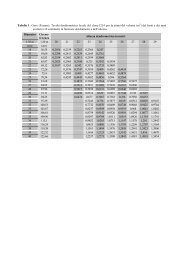
Care must be taken, however, to avoid misuse of the calculator’s versatility. For validation andparameterization of the model for a particular crop, such approximation should not be reliedon. The more the weather elements are missing the rougher the approximation of ET o , the lessreliable would be the simulated results and derived AquaCrop parameters.The daily, 10-day or monthly air temperature, ET o and rainfall data for each specific environmentare stored in their own climate folder in the AquaCrop database from where the programmeretrieves data at run time. In the absence of daily weather data, because the programme runsin daily steps, it invokes built-in procedures to approximate the required daily data from the10-day or monthly means. Again, the more approximate, the less reliable is the outcome. This isparticularly an acute problem for rainfall data. With its extremely heterogeneous distributionover time, the use of 10-day or monthly rainfall data completely grosses over the dynamicnature of crop response to water stress.Additionally, AquaCrop provides the mean yearly CO 2 concentration required for thesimulation, applicable for most locations. These yearly values are measured at the Mauna LoaObservatory in Hawaii and encompass the period from 1902 to the most recent available data.Several projected values can be retrieved from the AquaCrop database or entered by the user,following the climate change scenario to be investigated.Crop parametersAlthough grounded on basic and complex biophysical processes, AquaCrop uses a relativesmall number of crop parameters to characterize the crop. FAO has calibrated crop parametersfor several crops (Section 3.4), and provides them as default values in the crop files stored inAquaCrop database. The parameters fall into two categories, distinguished as conservative orcultivar and conditions dependent (see also Section 3.3).• The conservative crop parameters do not change with time, management practices, climate,or geographical location. Regarding cultivar differences, so far tests show the same valueof a conservative parameter is applicable to many cultivars, although some deviation maybe expected for cultivars of extreme characteristics. The decision to assign a particularparameter to the conservative category is based on conceptual and theoretical analysis, andon extensive empirical data demonstrating near constancy. Depending on extensiveness ofthe data sets used for the calibration, the calibrated value for a conservative parametermay require some small adjustment. This should be done, however, only if the adjustmentis based on high quality experimental data. Generally and in principle, the conservativeparameters require no adjustment to the local conditions or for the common cultivars, andcan be used as such in simulations. The conservative crop parameters are listed in Table 1. • The cultivar and condition dependent crop parameters are generally known to vary withcultivars and situations. Outstanding examples are life-cycle length and phenology ofcultivars. In Table 2, an overview is given of crop parameters that are likely to require anadjustment to account for the local cultivar and or local environmental and managementconditions. Reference HI (HI o ) is usually conservative for well developed high yieldingcultivars, and therefore is not included in Table 2 as a cultivar specific parameter. It isknown, however, that some special cultivar may have HI consistently either slightly higheror lower than the common cultivars. Adjustment in HI o would be justified in such cases.AquaCrop: concepts, rationale and operation 43

Table 1 Conservative crop parameters.Crop growth and development• Base temperature and upper temperature for growing degree days• Canopy size of the average seedling at 90 percent emergence (cc o )• Canopy growth coefficient (CGC); Canopy decline coefficient (CDC)• Crop determinacy linked/unlinked with flowering; Excess of potential fruit (%)Crop transpiration• Decline of crop coefficient as a result of ageingBiomass production and yield formation• Water productivity normalized for ET o and CO 2 (WP*)• Reduction coefficient describing the effect of the products synthesized during yield formation on thenormalized water productivity• Reference harvest index (HI o )StressesWater stresses• Upper and lower thresholds of soil-water depletion for canopy expansion and shape of the stress curve• Upper threshold of soil-water depletion for stomatal closure and shape of the stress curve• Upper threshold of soil-water depletion for early senescence and shape of the stress curve• Upper threshold of soil-water depletion for failure of pollination and shape of the stress curve• Possible increase of HI resulting from water stress before flowering• Coefficient describing positive impact of restricted vegetative growth during yield formation on HI• Coefficient describing negative impact of stomatal closure during yield formation on HI• Allowable maximum increase of specified HI• Anaerobiotic point (for effect of waterlogging on Tr)Temperature stress• Minimum and maximum air temperature below which pollination starts to fail• Minimum growing degrees required for full biomass productionTable 2List of crop parameters likely to require adjustments to account for the characteristics of thecultivar and local environment and management.Phenology (cultivar specific)• Time to flowering or the start of yield formation• Length of the flowering stage• Time to start of canopy senescence• Time to maturity (i.e. the length of crop cycle)Management dependent• Plant density• Time to 90 percent emergence• Maximum canopy cover (depends on plant density and cultivar, see Section 3.3)Soil dependent• Maximum rooting depth• Time to reach maximum rooting depthSoil and management dependent• Response to soil fertility• Soil salinity stress44crop yield response to water

It should be emphasized that for temperature dependent processes, such as canopy expansionwith its conservative parameter CGC, the constancy of their parameters is entirely based onoperating the model in the GDD mode. It is obvious, that for simulation of production andwater use under different yearly climate or different times of the season, AquaCrop mustbe run in the GDD mode, otherwise temperature effects on key crop processes would becompletely ignored by the model.Another important consideration is the thoroughness of the calibration and the extensivenessof the data set on which the calibration is based. Diverse data sets are necessary to cover awide-range of climate and soil conditions, and more cultivars. Particularly crucial are datasets for water-deficient conditions, on which the calibration of the water-stress parametersdepend, and are often not readily available.Of the number of crops calibrated by FAO, the thoroughness ranges from very good to fair andlimited. Users need to consult the rating, available on the AquaCrop website, to determine thefirmness of the conservative parameters. With time, calibration of the various crops will beimproved based on additional data sets, and more crop species will be calibrated.The reader is referred to Section 3.3 of this Chapter and the AquaCrop Reference Manual(Raes et al., 2011) for procedures on how to calibrate a crop for local conditions and how tomodify the crop parameters in the data files.Soil dataNeeded parameters are: volumetric water content at field capacity (FC), permanent wiltingpoint (PWP), and saturation, and the saturated hydraulic conductivity (K sat ), for eachdifferentiated soil layers encompassing the root zone. From these characteristics AquaCropderives other parameters governing soil evaporation, internal drainage and deep percolation,surface runoff and capillary rise (Raes et al., 2011). The default values for these parameterscan be adjusted if the user has access to more precise information. In case some of the firstfour parameters values are missing, the user can make use of the indicative values provided byAquaCrop for various soil texture classes, or import locally-determined or derived data fromsoil texture with the help of pedo-transfer functions (see for example The Hydraulic PropertiesCalculator on the web: http://hydrolab.arsusda.gov/soilwater/Index.htm). These functions arebased on primary particle size distribution of the different soil textures. Since these functionsdepend on texture class only, they do not account for differences in soil aggregation andshould be taken as rough approximations. Users should adjust their estimates based on theirown data and experience.If a layer exists in the soil to stop root deepening, its depth has to be specified as well. Inaddition, the water content of the soil profile layers at the start of the simulation period needto be specified if it is not at field capacity.Management dataManagement practices are divided into irrigation management and field management. Underfield management practices are choices of soil fertility levels, level of weed infestation, andpractices that affect the soil-water balance such as mulching to reduce soil evaporation, soilbunds to store water on the field, and the elimination of runoff by conservation practices.AquaCrop: concepts, rationale and operation 45

figure 18 The Main AquaCrop menu.displays on tab sheets for different aspect of crop, soil water and salt balance, the user canobserve and analyse a particular event on a specific parameter.Climate-Crop-Soil water is the most useful of the tab sheets (Figure 19). It displays three graphsplotted as a function of time: (i) depletion of root zone soil water (D r ), with the three water stressthresholds represents by lines of different colours; (ii) the corresponding progression of greencanopy cover (CC), with the potential CC (no stresses) shaded gray; and (iii) the transpiration (Tr)of the canopy (for the simulated CC size), with potential Tr shaded gray. On top of the menu thebiomass and yield are displayed along with the status of the water, temperature, soil fertilityand salinity stresses. The graphs vividly show how canopy expansion and transpiration areaffected when the absence of rain and irrigation led to drops in root zone water content belowthe threshold (green line, bottom graph) affecting canopy expansion, below the thresholdfor stomata (red line) affecting Tr, and below the threshold (yellow line) triggering canopysenescence. The reversal effects of water supply or irrigation are also obvious in the graphs.One feature of the Simulation run menu is particularly helpful to users seeking to develop aregulated deficit irrigation schedule to optimize water use. By selecting short simulation timesteps (1 to 3 days), a chosen amount of irrigation can be specified on the upper left panelat any time step (and date) during a simulation run, allowing quick and close scrutiny of theresultant benefits in the context of irrigation time, frequency, and amount. For more details,see Section 3.3 and the AquaCrop Reference Manual (Raes et al., 2011).AquaCrop: concepts, rationale and operation 47

Users should change the first part (Project) of file name to identify the particular simulation,otherwise the next simulation would be automatically assigned the same default file nameand overwrite the files resulting from the preceding simulation. Daily simulation results arealso summarized as seasonal totals. The files are stored by default in the OUTP directoryof AquaCrop. The data in the files can be retrieved in spreadsheet programmes for furtherprocessing and analysis.REFERENCESAdams, J.E., Arkin, G.F. & Ritchie, J. T. 1976. Influence of row spacing and straw mulch on first stage drying. SoilScience Society American Journal 40: 436-442.Allen R.G., Pereira L.S., Raes D. & Smith M. 1998. Crop evapotranspiration. Guidelines for computing crop waterrequirements. FAO Irrigation and Drainage Paper No. 56.Ayers, R.S. & Westcot, D.W. 1985. Water quality for agriculture. FAO Irrigation and Drainage Paper No. 29. FAO,Rome.Bradford, K.J. & Hsiao, T.C. 1982. Physiological responses to moderate water stress. pages 264-324. In: Lange, O.R., P. S. Nobel, C.B. Osmond & H. Ziegler, eds. Encyclopedia Plant Physiol. New Series, Vol. 12B. Physiological PlantEcology II. Berlin, Springer-Verlag.de Wit, C.T. 1958. Transpiration and crop yields. Versl. Landbouwk. Onderz. 64.6 Institute of Biological ChemistryResearch On Field Crops and Herbage, Wageningen, The Netherlands.Doorenbos, J. & Kasssam, A.H. 1979. Yield response to Water. FAO Irrigation and Drainage Paper No. 33. Rome, FAO.FAO, 2009. ET o Calculator, Land and Water Digital Media Series No. 36, Rome.Heng, L.K., Hsiao, T.C., Evett, S., Howell, T. & Steduto, P. 2009. Validating the FAO Aquacrop model for irrigated andwater deficient field maize. Agronomy Journal 101:488-498.Hsiao, T.C. & Bradford K.J. 1983. Physiological consequences of cellular water deficits. In: Taylor H.M., Jordan, W.A.,Sinclair, T.R., eds. Limitations to efficient water use in crop production. Madison, Wisconsin, USA, ASA, pp. 227–265.Hsiao, T.C., Lee H., Steduto, B., Basilio, R.L., Raes, D. & Fereres, E. 2009. Aquacrop - The FAO crop model to simulateyield response to water: III. Parameterization and testing for maize. Agronomy Journal 101:448–459.Hsiao, T.C. & Xu, L.K. 2000. Sensitivity of growth of roots vs. leaves to water stress: biophysical analysis and relationto water transport. Journal of Experimental Botany 51: 1595-1616.McMaster, G.S. & Wilhelm, W.W. 1997. Growing degree-days: one equation, two interpretations. Agricultural andForestry Meteorology, 87: 291-300.Raes, D., Steduto, P., Hsiao, T.C., & Fereres, E. 2009. Aquacrop - The FAO Crop Model to Simulate Yield Response toWater: II. Main Algorithms and Software Description. Agronomy Journal 101:438–447.Raes, D., Steduto, P., Hsiao, T.C. & Fereres, E. 2011. Aquacrop – Reference Manual. Available at:http://www.fao.org/nr/water/aquacrop.htmlSteduto P. & Albrizio R., 2005. Resource use efficiency of field-grown sunflower, sorghum, wheat and chickpea- II. Water use efficiency and comparison with radiation use efficiency. Journal of Agricultural And ForestMeteorology, 130 (3-4), 269-281.Steduto P., Hsiao, T.C. & Fereres, E. 2007. On the conservative behavior of biomass water productivity. IrrigationScience, 25:189–207.Steduto, P., Hsiao, T.C., Raes, D. & Fereres, E. 2009. Aquacrop - The FAO Crop Model to Simulate Yield Response toWater: I. Concepts and Underlying Principles. Agronomy Journal, 101:426–437.Tanner C.B. & Sinclair T.R. 1983. Efficient water use in crop production: research or re-search? In: Taylor H.M., JordanW.A., Sinclair T.R. (eds) Limitations to efficient water use in crop production. Madison, Wisconsin, USA, ASA, pp1–27.Villalobos, F. J. & Fereres, E. 1990. Evaporation measurements beneath corn, cotton, and sunflower canopies.Agronomy Journal 82:1153-1159.AquaCrop: concepts, rationale and operation 49

Applications to Irrigation ManagementAT the Field and Farm ScalesTwo types of applications are described. The first describes applications when the water supplyis adequate, while the second type refers to examples of how to use AquaCrop to assist incoping with irrigation management under water scarcity.CASE 1 - Developing a seasonal irrigation schedule for a specific crop and fieldSpecific data requirements:• long-term climatic data (Rain and ET o ) statistically processed to determine typical climaticconditions of dry, wet, or average years. Note that average ET o is much less variable thanaverage rainfall; thus, the user could combine average ET o information with seasonal dailyrainfall from different years, representing dry, wet, and average years, if long-term ET odata is not available;• soil profile characteristics of the field as needed to run AquaCrop; and• crop characteristics as needed to run AquaCrop.Approach:The model is run for the season of typical year (dry, wet, average year) using the feature‘Generation of Irrigation Schedule’ where the timing and depth of irrigation are determinedby selected criteria. The selected time criterion depends on the objectives of the manager;for instance, the user can choose to irrigate every time the root zone water content isdepleted down to 50 percent of its total available water or can choose to irrigate every timea certain depth of water has been depleted, such as 25 or 40 mm or even at a fixed timeinterval as used on many irrigation schemes. A ‘fixed application depth’ is typically selectedas depth criterion. The selection of the fixed amount of water to apply depends on manyfactors such as farmers’ practices, the irrigation method, the irrigation interval, the rootingdepth and soil type.Output:An indicative irrigation schedule for the crop-climate-soil combination is produced based onthe criteria selected by the manager. This simulated schedule may be used for benchmarkingthe actual irrigation performance of a specific farmer against the ideal for that particularyear or different schedules according to different irrigation criteria could be presented to thefarmers for discussion.CASE 2 - Determining the date of next irrigation with AquaCropSpecific data requirements:• real-time weather data are used to run AquaCrop. Current season daily weather data areused to compute actual ET o and the soil-water balance from planting until the last day ofavailable weather data, before the simulation of next irrigation date;• soil profile characteristics as needed to run AquaCrop; and• crop characteristics as needed to run AquaCrop.52crop yield response to water

conducted (and saved to disk) to reach the best solution in terms of maximum harvest indexwhich would lead to the maximum yield for the given IW.c) Supplemental irrigation programme to determine the best timing for a single irrigationapplicationSpecific data requirements• In addition to the standard data requirements of it, it is useful to have rainfall probabilityinformation to optimize the timing of a single application.Approach:In the real world, the availability of water determines the timing of application. In collectivenetworks, the timing is imposed by the delivery schedule. If farmers have on-farm storage oraccess to groundwater, then there is flexibility in the timing of applications. The AquaCropsimulations will differ in each of these cases. It is also possible to use AquaCrop to simulate DIprogrammes in near real-time, i.e. for the current year, by running the model up-to-date, andthen use rainfall probabilities for the coming weeks (available from weather services), andsimulate the subsequent week (with long-term mean ET o and expected rainfall in the climatefile). It is then possible to assess the impact on yield of applying the single irrigation in thefollowing week, relative to postponing it. It is also possible to quantify the E vs. Tr effects of thesingle irrigation; if canopy cover is still developing, the E component will be more importantthan if the irrigation is applied when maximum cover is reached. On the other hand, earlyirrigation would enhance canopy cover leading to more intercepted radiation (and relativelylower E) and consequently more biomass production. But the crop-water requirement of awell-developed crop early in the season might largely exceeds the limited amount of wateravailable in the root zone, triggering an early senescence of the canopy. The user is encouragedto evaluate these trade-offs in each specific case and compare the final yields.Output:In an example run of AquaCrop for wheat in a semi-arid climate, on a soil of medium waterstorage capacity (110 mm of TAW) with an increasing drought probability as the seasonprogresses, the best timing for a single irrigation is around early grain filling. AquaCropsimulated yields with a single 60 mm irrigation just after end of flowering were 4.1 tonne/ha, relative to a yield of 2.4 tonne/ha under rainfed, and 3.5 tonne/ha if the irrigation isdelayed 10 days. In another example, when only two irrigations 10 days apart were applied ona very deep soil, maize yielded either 6 tonne/ha or 9 tonne/ha when irrigation started on day30 and on day 80 after planting, respectively. In this example, early applications were moredetrimental to yield as the crop ran out of water too early in the season before its normalsenescence date.One example of the effects on E and Tr of a single irrigation on cotton, when applied duringcanopy development (at 30-40 percent of maximum), had 7 percent more E than when thesingle 60 mm irrigation was applied after attaining full canopy. The lower E (and higher Tr)in the second case, together with the beneficial effects of the stress pattern (better waterstatus during reproductive development), led to higher water productivity, with more than10 percent increase in yield with the same amount of irrigation water (2.7 vs. 2.4 tonne/ha).A specific case study of simulation of deficit irrigation of cotton is presented in Box 1.56crop yield response to water

Box 1 Simulating deficit irrigation in cotton productionBackgroundCotton is grown in many water limited regions where deficit irrigation may be practisedeither as a necessity driven by lack of water or for economic reasons (costs of water and/orenergy for pumping). The United States southern high plains region is exemplary of bothlimited water and high pumping costs. AquaCrop simulations were carried out for a Texaslocation at 35°11′ N, 102°6′ W, 1170 m elevation above sea level. The slowly permeablesoil is a Pullman silty clay loam with a strong argillic horizon containing approximately50 percent clay above a wavy boundary of a calcic horizon at 0.1 to 0.14 m depth. The soilwater-holding capacity is about 200 mm to 1.5-m depth (Tolk and Howell 2001). Meanannual precipitation is 490 mm, 65 percent of which falls during the growing season (May-August). ET o greatly exceeds precipitation in all months.AquaCrop simulationSimulations were performed for cotton sown in rows on raised beds and with the furrowsdiked to store irrigation and precipitation. Irrigation was either Full (FI), indicating thatsoil water was replenished to replace that lost to ET, or one half of that (Deficit, DI).Irrigation scheduling was performed assuming a lateral-move sprinkler irrigation systemthat applies ~25 mm per irrigation. The sowing rate was at 21 seeds/m 2 . Late in theseason, FI was reduced relative to the crop-water requirement (ET c demand), so as toenhance crop maturation.Reference evapotranspiration for input into AquaCrop was calculated using the FAOET o Calc computer programme (FAO, 2009) and weather data measured at a weatherstation close to the cotton field. AquaCrop field management parameters were set so thatno runoff occurred (due to the furrow dikes), and soil fertility was non-limiting. Five soildepths were considered, with initial water contents of 23, 33, 34, 30, and 27 vol percentat depths of 0.10, 0.29, 0.45, 0.66, and 1.00 m, respectively, as measured in the field. Thecrop calendar was set as 10 days from sowing to emergence, 94 days from sowing tomaximum root depth, 121 days from sowing to start of senescence, 140 days from sowingto maturity, 60 days from sowing to flowering, and 71 days the duration of flowering.ResultsSimulated yields were in the range of 3.3 to 3.6 tonne/ha, (equivalent to 1.3 to 1.4 tonne/haof lint) and were comparable to values reported in the region. Deficit irrigation (DI) seedlintyields were ~95 percent of full irrigation (FI) yields. The water productivity of DI cottonwas ~10 percent greater than that of FI (both in the range of 0.49 to 0.54 kg/m 3 (seed pluslint), or 0.19 to 0.21 kg lint/m 3 ). Crop ET was about 15 percent greater for FI than for DI,both in the range of 625 to 720 mm, which matches well observed values in several regions.However, DI received 240 mm of irrigation, only 43 percent of the FI amount.Conclusions and recommendationsFarmers in the region pump from a water table about 90 m below ground and, givenrising fuel costs, the energy savings of DI were more than US$250/ha. At cotton pricesranging from US$0.4 to 0.8/kg, the loss in production associated with DI represents onlyUS$100 to 200/ha, giving the economic edge to deficit irrigation.AQUACROP APPLICATIONS 57

Applications related to agronomy and crop management atfield and farm scales.CASE 9 - Benchmarking yield gaps in rainfed and irrigated agriculture and assessment oflong-term productivitySpecific data requirements• climate (long-term data set) and soil profile characteristics as needed to run AquaCrop;• crop specific characteristics as required to run AquaCrop; and• current practices related to irrigation management, fertilization, level of crop protectionand other agronomic practices relevant to actual yields.ApproachIt is important to determine the differences between potential, attainable and actual yields(Loomis and Connor, 1992) at various scales, from a field to a region. If all information isavailable, the model should be run to determine the attainable yield for each year. Severalyears of data (standard is 30 years) would be desirable for the comparison of the long-termproductivity under various production systems, using the cumulative distribution functions toshow the relative risk levels.OutputGiven the actual yield information and the simulated yield, the capacity of rainfed environmentsand the yield gap (simulated minus actual yield) can be determined. Results from differentyears will give some clues as to the possible reasons for the yield gap (i.e. low soil fertility,pest, disease, and weed limitations, socio-economic constraints, or low-yielding crop varieties,etc.). A specific application of this approach for assessing wheat yield constraints in a regionmay be found in Calviño and Sadras (2002). Additional simulations with AquaCrop varying thescenarios, with possible remedial actions, would also help in identifying the possible underlyingcauses of the yield gap and identify regions and crops where substantial improvements inproduction and productivity may be possible. If combined with geographical informationsystems (GIS), yield gap maps for regions could be developed.CASE 10 - Determining the optimal planting date based on probability analysisSpecific data requirements• at least 20 years of ET o and rainfall data are needed for the area; and• crop and soil characteristics as required to run AquaCrop and representative of the area.Approach:Early, middle, and late planting dates are used to simulate 20 or more seasons with AquaCrop.For this application, AquaCrop should be run in the multiple project mode, as a minimum of 60simulations need to be done. If a much larger number of runs are required, the plug-in versionof the model should be used (downloadable at www.fao.org/nr/water/aquacrop).OutputOnce the yields for every year and for the different planting dates (keeping all otherparameters the same) have been simulated, the values are organized from lowest to highest,AQUACROP APPLICATIONS 59

for each planting date. If there are 20 years of simulations, each value represents a 5 percentprobability. Then, the yield can be plotted against the cumulative probability graphically, andit is possible to choose the most favourable option with least risk from the graph or comparedifferent options for years with differing conditions, say amounts of rainfall or El Niño phases.A specific example of an AquaCrop application to determine the optimal sowing date forwheat as a function of the initial soil moisture conditions is reported in Box 2.Box 2 Determining the optimal sowing date for wheatBackgroundThe AquaCrop model was used to analyse the optimum sowing date at three differentinitial soil water conditions under rainfed Mediterranean conditions. The importance ofearly sowing has been emphasized by many authors (Photiades and Hadjichristodoulou,1984; Anderson and Smith, 1990 and Connor et al., 1992), who reported a declinein yield when sowing is delayed after the first sowing opportunity (initial rainfall inautumn) within an optimum sowing window. Wheat yields are estimated to be reducedby 4.2 percent (Stapper and Harris, 1989) to 10 percent (Asseng et al., 2008) for eachweek of any delay in sowing in autumn in Mediterranean environment. On the otherhand, soil water conditions at sowing can also be important for wheat production,particularly in low rainfall regions (Rinaldi, 2004; Heng et al., 2007; Asseng et al., 2008).Initial soil water from summer rainfall or left over from the previous year can influenceearly establishment of the crop and can contribute to water use and yield later in theseason, in particularly in low rainfall seasons. Therefore, simulations were carried outwith AquaCrop to determine the optimal sowing date in relation to initial soil water tomaximize wheat grain yields.Location and simulation experimentsThe site of the simulation experiments was selected within the northern part ofthe Western Australia wheat-belt, at Buntine (29.51°S, 116.34°E, 365 m elevation)one of the main wheat-growing regions of Australia, where wheat is grown underrainfed conditions. The location is a relative low-yielding environment with a typicalMediterranean-type climate. Rainfall mainly falls in winter, but varies from season-toseasonin terms of seasonal distribution and amount. Rainfall quickly declines in springduring grain filling. Average long-term annual rainfall is 329 mm. Average seasonal(May to October is the main growing season in the Southern Hemisphere) rainfall was243 mm over the last 30 years period (1979-2008), varying between 125 and 417 mm.In such an environment, a mild winter is followed by increasing temperatures in spring.60crop yield response to water

Box 2 (CONTINUED)A common soil for the study region was used in the simulation experiment, a loamysandy soil with 101 mm of plant available soil water to the maximum rooting depth of1.7 m.Simulations were carried out using measured daily weather records from 1999 to 2008.Crops were sown when rainfall was at least 20 mm during the previous 10 days during asowing window of May to July and again at 30 days after the first sowing opportunityas a delayed sowing practice (e.g. to manage weeds or due to technical limits of sowingall crops early on a farm).Each sowing date treatment was simulated with an initial soil water of 0, 30 and 60mm plant available soil water stored below 20 cm depth. The earliest sowing datepossible was 1 May, the date at which the initial soil water conditions were set everyyear. Nitrogen was assumed to be not limiting for crop growth.A bread-wheat spring cultivar was used in the experiments, cv. Wyalkatchem, astandard early-medium flowering cultivar for this region. Conservative parametersbased on typical growth and development in the considered environment were usedas inputs (See wheat Section in Chapter 4).ResultsThe simulated differences in grain yields between the first and the second sowingdates as a function of the seasonal rainfall for different initial soil-water contents areshown in Figure 1. Simulated differences in grain yield became negative at zero mmof initial soil water, but were positive at 30 and 60 mm initial soil water. When thesoil profile was dry, 70 percent of the crops sown with an early sowing opportunityfailed, while this percentage decreased to 40 percent with the second sowing date.But, crops which were sown early in to dry subsoil with the first rainfall in autumnwhich did not fail yielded on average 30 percent more than the second sowing date.On average, the first sowing yielded 35 percent more than the second sowing with30 and 60 mm of initial water, but 13 percent less with zero mm of initial soil water.Conclusions and recommendationsThe results of the simulation experiments indicate that in a Mediterraneanenvironment, sowing a wheat crop early with the first rainfall events in autumn cangive higher yields, consistent with other simulation and field experimental studies.However, early sowing can increase the risk of crop failure if the subsoil profile is dryat sowing. Therefore, early sowing is only warranted if there is some initial soil waterin the soil profile from summer rainfall or left over from the previous year. If the soilprofile is dry at the beginning of the season, delaying sowing, despite some loss ofyield potential, reduces the risk of crop failure in such an environment.AQUACROP APPLICATIONS 61

ox 2 (CONTINUED)FIGURE 1 Differences in simulated grain yields between the first and the second sowingopportunity as a function of the seasonal rainfall at different initial soil water (0, 30and 60 mm) for the period between 1999 and 2008 at Buntine, Western Australia.3Difference in grain yield betweenFirst and second sowing (tonne/ha)210-1-2-3-4-5100 120 140 160 180 200 220 240 260 280 300Seasonal rainfall (May-Oct) (mm)In similar regions, but with water resources available for irrigation, applying a smallamount of water (about 30 mm) before sowing will significantly reduce the risk of cropfailure with an early sowing opportunities and would allow to maximize yield potentialin such an environment.CASE 11 - Developing water production functions with AquaCropand using them in Decision Support SystemsSpecific data requirements• average or historical series of preferably 20-30 year, or at least 10 years, of data on ET o anddaily rainfall; and• crop and soil characteristics necessary to run AquaCrop.ApproachTwo approaches may be used: (i) with the average climatic records, the user will simulate theyield response to different amounts of applied irrigation (IW) changing the level of applicationin 30-50 mm step intervals (’Irrigation Events’ tab sheet in ’Irrigation Management’); (ii) if a62crop yield response to water

• typical crops with representative soil and irrigation management conditions, as needed torun AquaCrop.ApproachAquaCrop outputs may be the input of water allocation optimization models that have strongeconomic and institutional components. Such models are needed to assist in the managementof water by institutions in charge of water governance. AquaCrop inputs would be particularlyvaluable in the event of a drought, where different scenarios are considered and yield/incomepredictions for the area are essential to make informed decisions when allocating limited supplies.One example of an application at the farm scale is given in García-Vila and Fereres (2012).ConclusionThese case studies are a small sample of the applications that may be possible to tackle withthe assistance of AquaCrop and illustrate the use of the simulation model. The exampleshave also illustrated the possibilities that AquaCrop offers for various types of users – namelyirrigation specialists, agricultural engineers and agronomists, agricultural extension personnel.Additional users include water engineers, hydrologists, and economists working at catchmentscale and climate scientists wanting to investigate the effect of different climate changescenarios on the water-use of various crops. There are many more applications of AquaCropthat may be used in practical ways and which will be revealed as users around the worldincorporate this simulation model in their assessments of crop yield response to water.ReferencesAnderson, W.K. & Smith, W.R. 1990. Yield advantage of two semi-dwarf compared with two tall wheats depends onsowing time. Australian Journal Agricultural Research, 41: 811-826.Asseng, S., Milroy, S. P. & Poole, M. L. 2008. Systems analysis of wheat production on low water-holding soils in aMediterranean-type environment I. Yield potential and quality. Field Crops Research, 105: 97-106.Calviño, P. & Sadras, V. 2002. On-farm assessment of constraints to wheat yield in the south-eastern Pampas. FieldCrops Research, 74:1-11.Connor, D.J., Theiveyanathan, S. & Rimmington, G.M. 1992. Development, growth, water-use and yield of a springand a winter wheat in response to time of sowing. Australian Journal Agricultural Research, 43: 493-516.Dimes, J., Cooper, P. & Rao, K.P.C. 2009. Climate change impact on crop productivity in the semi-arid tropicsof Zimbabwe in the twenty-first century. Proceedings of the Workshop on Increasing the Productivity andSustainability of Rainfed Cropping Systems of Poor, Smallholder Farmers, Tamale, Ghana, 22-25 September 2008.p189-198.FAO. 2009. ET o Calculator, land and water digital media Series No. 36., Rome.Farahani, H. J., Izzi, G. & Oweis, T.Y. 2009. Parameterization and Evaluation of the AquaCrop Model for Full andDeficit Irrigated Cotton. Agronomy Journal 101: 469-476.Fereres, E. & Soriano, M.A. 2007. Deficit irrigation for reducing agricultural water use. Journal of ExperimentalBotany 58(2): 147–159.García-Vila, M. & Fereres. E. 2012. Combining the simulation crop model AquaCrop with an economic model for theoptimization of irrigation management at farm level. European Journal of Agronomy, 36: 21-31.García-Vila, M., Fereres, E., Mateos, L., Orgaz, F. & Steduto, P. 2009. Deficit irrigation optimization of cotton withAquaCrop. Agronomy Journal 101: 477-487.Geerts, S., Raes, D., Garcia, M., Taboada, C., Miranda, R., Cusicanqui, J., Mhizha, T. & Vacher, J. 2009. Modellingthe potential for closing quinoa yield gaps under varying water availability in the Bolivian Altiplano. AgriculturalWater Management 96: 1652–1658.Heng, L.K., Asseng, S., Mejahed, K. & Rusan, M. 2007. Optimizing wheat productivity in two rainfed environmentsof the West Asia-North Africa region using a simulation model. European Journal of Agronomy, 26: 121-129.AQUACROP APPLICATIONS 67

Heng, L.K., Hsiao,T.C., Evett, S., Howell, T. & Steduto P. 2009.Validating the FAO AquaCrop Model for Irrigated andWater Deficient Field Maize. Agronomy Journal 101: 488-498.Loomis, R.S. & Connor, D.A. 1992. Crop ecology: productivity and management of agricultural systems. UK,Cambridge University Press. 538 p.Mainuddin, M., Hoanh, C.T., Jirayoot, K., Halls, A.S., Kirby, M., Lacombe, G. & Srinetr, V. 2010. Adaptation options toreduce the vulnerability of mekong water resources, food security and the environment to impacts of developmentand climate change. CSIRO: Water for a Healthy Country National Research Flagship. 152 pp.Photiades, I. & Hadjichristodoulou, A. 1984. Sowing date, sowing depth, seed rate and row spacing of wheat andbarley under dryland conditions. Field Crops Research, 9: 151-162.Rinaldi, M. 2004. Water availability at sowing and nitrogen management of durum wheat: a seasonal analysis withthe CERES-Wheat model. Field Crops Research 89: 27-37.Stapper, M. & Harris, H.C. 1989. Assessing the productivity of wheat genotypes in a Mediterranean climate, using acrop simulation model. Field Crops Research, 20: 129-152.Steduto, P., Hsiao, T.C., Raes, D. & Fereres, E. 2009. AquaCrop – the FAO crop model to simulate yield response towater: I. Concepts and underlying principles. Agronomy Journal. 101: 426–437.Todorovic, M., Albrizio,R., Zivotic, L., Abi Saab, M.T., Stockle, C. & Steduto, P. 2009. Assessment of AquaCrop,CropSyst, and WOFOST Models in the Simulation of Sunflower Growth under Different Water Regimes. AgronomyJournal 101: 509-521.Tolk, J.A. & Howell, T.A. 2001. Measured and simulated evapo-transpiration of grain sorghum with full and limitedirrigation in three High Plains soils.Trans. ASAE, 44: 1553–1558.Vanuytrecht, E., Raes, D. & Willems, P. 2011. Considering sink strength to model crop production under elevatedatmospheric CO 2 . Agricultural and Forest Meteorology 151: 1753– 1762.68crop yield response to water

AQUACROP APPLICATIONS 69

Table 2Additional information and data needed for parameterization and validation of AquaCrop.The required data include those not mentioned here but listed in Column 2 of Table 1.1. Minimal additional beyond Column 2 of Table 1 2. Additional for reliable parameterizationPeriodic measurements of leaf area index(LAI) or canopy cover over the seasonCropPeriodic measurements of above-groundbiomass over the seasonDate when foliage canopy begins to turnvisibly yellowMeasured rooting depthSigns of water stress and datesData as in Column 1 but obtainedat several locations and climates ondifferent soil typesClimate and ETDaily maximum and minimum temperatureand humidityDaily solar radiation and wind runET by soil water balance (optional)Data as in Column 1 but obtainedat several locations and climates fordifferent soil typesMeasured daily ETSoil and fertilityMust have one treatment with optimal soilfertilityField capacity and permanent wilting pointof soil horizonsInfiltration rate or saturated hydraulicconductivity of the soilData as in Column 1 but obtainedat several locations and climates fordifferent soil typesIrrigation and water in soilMust include a well-watered (full irrigation)treatment and water-stress treatmentsAmount of water applied at each of theirrigationsMeasured or good estimate of soil-watercontent for different soil depths at plantingPeriodic measurements of soil-watercontents at various depths of the root zone(optional alternative to soil-water balance)Data as in Column 1 but obtainedat several locations and climates fordifferent soil typesMust include treatments with waterstress at different times and differentseveritiesRule 3: Differentiate the input information and measured or observed data according to theirreliability and exactness, and make rational adjustment to the vague or rough estimates ofinput first to see if the simulated results better match the measured results, before changingthe model parameters. In later Sections, many of the uncertainties of the input informationor data, and the measurements taken on crops, are mentioned and discussed to decide whichinputs can be altered based on a rational evaluation of its likely range of uncertainty.Rule 4: When simulated results and measured data do not agree, the problem could alsobe in the measured data. If simulated results coincide with measured data obtained inseveral different studies, but not with that of another study, the data in the other studyare more suspect and additional data sets should be sought to complete the validation orparameterization.AquaCrop parameterization, calibration, and validation Guide 73

Location and User Specific Parameters and InputClimate and soil are location specific, and crop cultivar, timing of crop cycle, water managementand agronomic practices are user specific.Climate data and reference evapotranspiration (ET o )AquaCrop simulates in daily time steps because plant responses to water status are highlydynamic and cannot be easily represented as weekly or 10-day means. The model runs with10-day or monthly mean temperature and ET o files, through interpolations. The results are,however, obviously approximations, and should not be used to calibrate or validate the modelexcept as the last resort. ET o is a key input for AquaCrop as the model calculates daily croptranspiration (Tr) and soil evaporation (E) using daily ET o values.ET o is to be calculated using the FAO Penman-Monteith equation from full daily weather datasets, as described by Allen et al. (1998). A programme to do this calculation, named ET o Calculator(FAO, 2009) is available on the FAO website. The ET o Calculator has the advantage of allowingapproximations when one or several kinds of the required weather data are missing, also followingthe approximation procedure of Allen et al. (1998). This makes it possible for a user to run roughsimulations, even when the weather data are minimal, but can be easily misused. For validation andparameterization, such approximation should not be relied upon. The rougher the approximationof ET o , the less reliable would be the simulated results and derived AquaCrop parameters. Forexample, ET o Calculator can use daily maximum and minimum temperature, relative humidity,wind run, and sunshine hours in place of radiation, to calculate ET o , and also can calculate ET osimply from daily minimum and maximum temperature data and general information on sitelocation such as whether it is arid or humid and windy or calm. Obviously, the ET o calculated fromthe sunshine hours would be somewhat less reliable than that calculated with daily radiation,and the ET o simply estimated with the daily minimum and maximum air temperature would beessentially worthless for the purpose of model validation and parameterization. Thus, it must beunderstood that reliable climatic data are critical in AquaCrop.Growing degree day (GDD)AquaCrop is designed for use under different climatic conditions and hence should beparameterized in the growing degree day (GDD) mode to account for different temperatureregimes. This may be difficult, however, because many users may only have data for theirspecific locations with their limited temperature range. In this case, it is best to select dataobtained when cold temperature is not a limiting factor and run the model first in the calendartime mode for parameterization. After arriving at reasonably acceptable parameter values, byswitching the model to the GDD mode, the parameters are automatically converted to units interms of GDD. The challenge is then to define: (1) the base temperature and upper temperatureto calculate the GDD, and (2) the temperature thresholds for biomass accumulation and forpollination and fruit set of the specific crop. These are to be discussed later.Soil water characteristicsIn AquaCrop, the extent of water limitation is expressed as a fraction of the total availablewater (TAW) in the root zone, with TAW defined as the water held in the soil between its field74crop yield response to water

capacity (FC) and permanent wilting point (PWP). In the case that the soil has layers differingin FC and PWP, the different values for the layers encompassing the maximum rooting depthneed to be entered into the model.Accurate FC and PWP are only important to specify the local conditions if water is a significantlimiting factor. If the simulation is for conditions where water is either not limiting or onlyminimally limiting, approximate FC and PWP would do, but the water-stress functions(threshold and curve shape) derived cannot be relied on for conditions limited more by waterdeficits. Approximate FC and PWP may be estimated simply from the textural class of thesoil. In AquaCrop there are default soil files for a number of textural classes. In each file therelevant water parameters are given in the ‘Characteristics of soil horizons’ tab sheet. Moreaccuracy is required to calibrate the model for the various water-stress functions using dataobtained when water is limiting.Spatial heterogeneity of the soil can be a problem for accurate simulation for a given waterlimiting location, because FC and PWP, and hence TAW, can vary sufficiently from area-to-areain a field, reducing the accuracy of the simulated results for the field. If data are available fordifferent parts of a field, simulation should be run for each part of the field that differs in soilwater characteristics.Saturated hydraulic conductivity (K sat ) of the top soil determines the internal drainage in thesoil profile, losses from deep percolation and the amount of water infiltrated in the rootzone and the surface runoff after an irrigation or rainfall. Surface runoff is only importantif the amount of water applied per irrigation is excessive or the rainfall is intense and heavy.In such situations, the measured K sat should be used for simulation. If measured value isunavailable, the default value provided by AquaCrop for the given soil textural class (basedon the difference in soil-water content (θ) between saturated soil and FC) should be adjustedaccording to general knowledge of the local condition.Initial soil water contentAnother local specific factor is the initial water content of the soil for the maximum rootingdepth at start of the simulation run. If the values are not measured, estimates may be madebased on knowledge of the local climate, particularly rainfall, and the preceding crop or weedhistory. For example, for a climate with winter rainfall, sufficient to completely charge thesoil profile, and dry summer, and the field is kept fallow and weed free, one may assume thedeeper layers of the soil to be at FC but reduce soil-water content of the upper layer of the soilby estimating the extent of soil evaporation taking place before the simulation starting time.If weather data before the starting time of simulation are available, AquaCrop can be used tomake that estimate by setting the start time as the end of the last significant rain. If weeds arepresent, however, some estimates would have to be made on canopy cover (CC) of the weedin order for AquaCrop to simulate a reasonable profile of initial soil-water content.Crop phenologyMany of the differences among crop cultivars are related to the timing of developmentalstages. The timing to reach a particular stage, or its duration for the local cultivar, needs tobe specified by the user. These stages are: time to 90 percent seedling emergence, to theAquaCrop parameterization, calibration, and validation Guide 75

eginning of flowering, to the beginning of canopy senescence, and to physiological maturity,and the duration of flowering.Time to 90 percent emergenceThe particular choice of time to 90 percent emergence is explained later, under Initial canopysize per seedling. In nearly all the cases, this time is likely to be estimated and not determinedby actual counting of the seedlings. It should be adjusted to have a good match betweenthe simulated and measured canopy cover (CC) at the seedling stage and in early season. Theadjustment, however, should be taken only after the relevant conservative parameters (initialcanopy size per seedling and canopy growth coefficient) are well parameterized and the plantdensity is ascertained.Time to start of flowering and duration of floweringFor determinate crops with their short flowering duration (e.g. 15 days), it is important tohave an accurate time for start of flowering. For indeterminate crops with their long floweringduration, the timing can be more approximate. In cases where there is no significant waterstress, the model is constructed in such a way that timing of flowering does not matter.Time to maximum canopy coverThis parameter is provided in AquaCrop to allow simulation runs when the conservativeparameter, canopy growth coefficient (CGC) of the crop, is not known, and should be usedonly as a last resort. See the later section Canopy growth coefficient for more explanation.Time to canopy senescenceIn AquaCrop, the timing to the start of canopy senescence is defined as the time when greenleaf area falls to or below LAI = 4 as a result of yellowing of leaves, under optimal conditionswith no water stress. By this definition, if the plant density is low and the maximum LAI is lessthan 4.0, canopy senescence starts once there is significant senescence of lower leaves. But ifthe maximum LAI is considerably higher than 4.0, enough of the lower leaves must senesce toreduce LAI to 4.0 before the canopy is considered to be at the beginning of senescence.Time to physiological maturityDifferent crop species may each have its own specific definition of physiological maturity (e.g.black layer formation in maize grains). To be general, however, AquaCrop uses as default thetime when canopy cover is reduced to 5 percent of the achieved maximum canopy cover as thetime of maturity. Users can change the maturity time according to their own data on the Canopydevelopment tab sheet. Clearly, maturity is closely linked to the time of canopy senescence,and this may be one practical way to estimate maturity time if no detailed determination ofmaturity is made. Seed companies usually supply information on the life-cycle duration oftheir cultivars. This, however, can be very general, in terms of short, medium, or long season.The information can also be given in degree days, but unfortunately defined in ways differentfrom that used in AquaCrop. For accuracy, experimental observations or data are necessary todetermine the time to maturity. It would be justified to take the time when only a little greenleaf area remains in the canopy as the time of maturity.Rooting depth and deepening rateRoot development is highly site specific because of differences in soil physical (temperature,76crop yield response to water

densities. This range is referred to in this writing as full canopy cover and the time when thisis reached is referred to as canopy closure. However, these terms are used rather loosely in theliterature, and can be referred to CC substantially less than 0.95, as low as 0.9 or even lower insome writings. As a general guide, CC is 0.95 or higher when LAI exceeds about 4.5 or 5.0 (Figure1), with some exceptions. One exception is species exhibiting strong sun-tracking behaviour,such as sunflower, which requires an LAI of 3.5 to achieve full canopy cover. Another exceptionis if the crop is planted in clumps, or very close to each other in rows that are spaced widelyapart. In this case LAI significantly higher than 5.0 is necessary to achieve full canopy cover.As plant density is reduced below a particular level, the density is insufficient for the canopyto close and CC falls substantially below 0.95. This point depends on the kind of crop, eachwith its particular limit of potential leaf area per plant. Ideally, for each kind of crop a curve ofCC x vs. plant density, based on experimental data, should be constructed for use in AquaCropsimulations. Unfortunately, for some species, the required experimental data are lacking. Ifthe user has CC x measurements of his/her crop at the plant density in question under optimalgrowth conditions, these CC x values are obviously the best to use in the simulation. OtherwiseCC x needs to be estimated. One way is simply visual, judging the extent of CC by eye aroundthe time when CC is maximum. A word of caution here, viewing the canopy from the side oreven at a downward angle (or photograph taken from similar positions) tends to overestimatethe CC because this view may include too many plant layers. Viewing the canopy from directlyabove, or viewing the proportion of the soil shaded by the canopy when full sun is directlyoverhead, is the better way to make the estimate. Estimates can also be made based on generalknowledge of the crop or similar crops.If the CC x of a particular crop is known for a particular plant density (reference planting), toestimate CC x of a planting of the same kind of crop but planted at a different density (d p ), onecan start by estimating the maximum LAI of the planting of known CC x (LAI ref ) from Figure1 (or a similar relationship if more accurate), and calculating first the LAI of the plantingassuming leaf area per plant is independent of plant density, then make a rough adjustmentfor the impact of change in plant density. This is summarized as an equation:⎛dp⎞ ⎛(1) LAI = LAI ref ⎜ ⎟ ⎜⎝ d ref ⎠ ⎝1F adj⎞⎟⎠where d ref is the plant density of the reference, and F adj is the adjustment factor.F adj is limited between the range of d/d ref and 1.0, for cases where d p > d ref , as well as whered < d ref . To illustrate, first take the case of d p > d ref . If the d p /d ref = 1.3, F adj would be limitedto the range of 1 to 1.3. At one extreme where F adj = 1, the leaf area per plant would beindependent of plant density. At the other extreme where F adj = 1.3, the leaf area per plant isreduced by the increase in plant density so much that the LAI of the planting remains the sameas LAI ref . In the case of d p < d ref , if d p /d ref = 0.7, F adj would be limited to the range of 1 to 0.7.Obviously, in most cases, the limit values of F adj should not be used to estimate LAI. The extentthe plant adjusts its leaf area in response to crowding is related to how determinate the cropis in growth habit. So the more indeterminate the crop is, the more F adj should deviate from1.0, either smaller or larger.80crop yield response to water

After LAI of the planting is estimated, the corresponding CC can be read off Figure 1 or similarrelations, and used as CC x for the simulation. As is obvious in Figure 1, for cases where thecanopy is full or nearly full and the plant density is not widely different from that of thereference, the CC x estimate made with the above procedure should be accurate within a fewpercentage points. The estimates become less and less reliable as the difference in densitybecomes greater, or if CC x or reference CC x is substantially less than full cover. On the otherhand, for cases where there is little interplant competition for PAR because of a sparse canopy(e.g. CC < 0.5), Equation 1 can be used along with Figure 1 to obtain a reasonable estimate ofCC x by setting F adj close to 1.0.Canopy growth coefficient (CGC)CGC is a measure of the intrinsic ability of the canopy to expand. A CGC of 0.11, for example,means that each day the CC is 11 percent greater than the CC of the day before during thefirst half of canopy development. CGC is virtually a constant when temperature effects areaccounted for by using GDD as the driver and there is no stress. Because CGC is based on firstorder kinetics (Bradford and Hsiao, 1982), a good way to derive CGC is to plot the log of CCvs. time and take the slope of the linearly fitted curve to be CGC, provided that only CC datameasured from shortly after seedling emergence to approximately 60 percent cover, that donot include periods of heavy fruit load on the crop, are used. If CC data are too limited forthe period specified above, but additional data have been collected up to canopy closure ornear full cover, CGC can be parameterized using the canopy growth components of AquaCrop.Instead of running the model, which is more time consuming, a simple Excel programmelimited only to canopy growth is available on the FAO AquaCrop website for this purpose.Commonly, both cc o and CGC would be unknown, requiring trial-and-error iterations to findthe best values for the two parameters. As general guiding principles for parameterizing CGC,the main considerations appear to be whether the crop is C 3 or C 4 , and whether the crop ismore efficient in the capture of PAR. For maize and sorghum, two important C 4 crops alreadyparameterized for AquaCrop, the CGC is 0.17 per day on a calendar time basis and 0.013 on aGDD basis. For a number of C 3 species, the CGC is around 0.09 to 0.12 per day on a calendartime basis. There are exceptions. One is the C 3 crop sunflower, its CGC is in the order of 0.22per day (calendar time), presumably because of its solar tracking ability to capture more PARper unit of canopy. In the trial-and-error runs to parameterize cc o and CGC, several scenariosof outcome are possible when the simulated CC over time are compared with the measureddata. These are listed in the first column of Table 3. In the second column are given possiblecauses for the lack of agreement and adjustments to make.If the comparison of simulated vs. measured data does not follow any of the scenarios in thetable, it is possible that either the experimental data are questionable, or the weather datamay be deficient. The weather data are particularly suspect if 10-day or monthly minimum andmaximum temperature are used instead of daily valuesAquaCrop has built in an alternative to estimate CGC, based on the time required for CC toreach CC x . This feature is provided for users who want to simulate roughly the production andwater use of a crop with some or many of the crop parameters not known. It should not berelied on to parameterize CGC, because in such cases cc o and plant density or initial canopycover (CC o ), which are equally important in determining the time to reach maximum cover, aremost certainly not known.AquaCrop parameterization, calibration, and validation Guide 81

Table 3Comparison of simulated with measured canopy cover and possible adjustments in the modelparameters to improve the match.Agreement between simulated CC(CC sim ) and measured CC (CC meas )CC sim is either lower or higher than CC meas fromtime of emergence to CC x . Same CC x reached butat different times. Slopes of the two curves forthe period of rapid canopy growth are similarPossible cause(s) of discrepancyand suggested remedial actionEither cc o is too low or plant density is too low,or, respectively, cc o is too high or plant densityis too high. Check plant density data and trylarger (or smaller) cc o . CGC and CC x probably OKCC sim coincides with CC meas early in season butgradually becomes either lower or higher. SameCC x reached but at different timesCGC is either too low or too high, respectively.Make the appropriate adjustment in CGC. CC xand cc o probably OKCC sim is either lower or higher than CC meas earlyin season but the trend reverses gradually laterand the same CC x is reached but at differenttimesEither cc o is too low or plant density is too low,or, respectively, cc o is too high or plant densityis too high. CGC is either too high or too lowrespectively. Check plant density data and trylarger (or smaller) cc o and lower (or higher)CGC. CC x probably OKCC sim coincide well with CC meas over the seasonValues of cc o , CGC, and CC x are good for this setof experimental dataCanopy decline coefficient (CDC)After the canopy begins to senesce, CC is reduced progressively by applying an empirical canopydecline coefficient (CDC) (Raes et al., 2011). If there are LAI data spanning the senescencephase, they should be converted to CC using Equation 1 and a value for CDC selected to matchthe simulated CC decline with the measured values. Regrettably, in many studies detailed LAIdata are lacking for this phase. In this case, CDC may be set initially according to observationsof the canopy's speed of yellowing, and then refined by trial-and-error simulations to findthe CDC that gives the best fit of the measured biomass data during the senescence phase.In terms of predicting biomass and yield, AquaCrop is not very sensitive to the extent of CCdecline near maturity, because the model assumes a continuous decrease in the efficiency ofconverting normalized Tr to biomass for that period.Normalized water productivity (WP*)The water productivity (WP) of concern here is the ratio of biomass produced to the amount ofwater transpired (WP B/Tr ), and the normalized water productivity (WP*) is the ratio of biomassproduced to water transpired, normalized for the evaporative demand and CO 2 concentrationof the atmosphere.WP normalized for evaporative demandTranspiration, the denominator of WP, is extremely difficult to measure and separate from soilevaporation in the field. Fortunately, there are numerous sets of data on biomass productionvs. consumptive water use, which can be used to derive WP B/Tr , and hence WP* if the requiredweather data are available. Plots of biomass vs. normalized ET, based on sequential samplingover the season, should exhibit a portion of rising slope at the beginning followed by a straight-82crop yield response to water

line portion of near constant slope, and then ending with the slope being reduced for one toseveral data points sampled near the end of the crop life-cycle. The slope at any given point,of course, is the water productivity at that point in terms of normalized ET, not just normalizedtranspiration. The early rising slopes represent a period of low water productivity, when CCis small and much of the soil is exposed, and soil evaporation accounts for much of the ET.The middle portion of the plot, encompassing the data points collected from the time whenthe crop canopy covered more than about 70 percent of the ground to the time when aboutone-fourth of the maximum LAI has senesced as maturity is approached, are to be fitted witha linear equation. The slope of this linear regression is the WP normalized for evaporativedemand, but only after a correction is made for soil evaporation. Once the canopy is nearlyfull, even when the soil surface is wet, evaporation may constitute only 12 to 18 percent of thetotal ET (Villalobos and Fereres, 1990). So, depending on how frequently the soil is wetted byrain or irrigation during the period spanning the middle portion of the plot, its slope shouldbe reduced by 5 to 15 percent to obtain normalized WP.For the plotting of biomass vs. normalized ET, ET o is used to normalize for each time intervalencompassing a biomass sample (Steduto et al., 2007) according to the equation:(2) Normalized ET =nTrEToi=1 iwhere i is a running number designating the sequential time interval between two adjacentbiomass samples, Tr is the cumulative transpiration within that interval, and ET ois the meanof daily ET o within that interval, and n is the number of the biomass sample in question. Theinterval may not be fixed in duration and represents the time preceding the biomass samplingto the previous sampling time, e.g. for i = 5, the relevant time interval is the time betweensample No. 4 and No. 5. For each biomass sample (n), the summation starts at the beginning (i= 1) and ends when i = n. If there are no ET and weather data for the time preceding the firstbiomass sample (i = 1), they can be assumed to be zero.The reason for using Equation 2 to normalize is to account for any variation in ET o amongthe different time intervals. If daily weather data are lacking and the weather is relativelystable, plots of biomass vs. ET instead of normalized ET can be used to obtain WP in a wayanalogous to the procedure above. Then the WP can be divided by a mean ET o calculatedfrom less detailed weather data to estimate normalized WP. However, this clearly is a roughapproximation.Normalization for atmospheric CO 2The concentration of CO 2 in the atmosphere increases each year with time and impacts WP ofcrops. AquaCrop accounts for this effect by normalizing WP for CO 2 in a general way basedon conceptual understanding and empirical data (Steduto et al., 2007). The WP alreadynormalized for evaporative demand is multiplied by a factor, f co2 , defined by Equation 3below, to obtain WP*.(C a /C a,o )(3) f CO 2=1+0.000138 (C a − C a,o )AquaCrop parameterization, calibration, and validation Guide 83

In Equation 3 C a is the mean air CO 2 concentration for the year of the experimental data, andC a,o is the mean CO 2 concentration for the year 2000 (equals 369.77 μLL -1 ), both measured atthe observatory at Mauna Loa, Hawaii. The C a measured for the years 1980 up to present, arelisted in AquaCrop in the climate file under the atmospheric CO 2 tab. The numerical valuesof the measured data can be found in the Mauna Loa CO 2 file in the SIMUL subdirectory ofAquaCrop. The C a of future years varies with the selected greenhouse gas-emission scenario(e.g. A2, A1B, B2 and B1 storylines). Users can enter their own projections or select one of theCO 2 files available in the DATA subdirectory of AquaCrop.Reference harvest index (HI o )The value of reference harvest index is chosen as the middle high end of HI values reportedfor the majority of the given crop species or class. This value should be carefully chosenand not altered without good reason, because a change in reference HI would require therecalibration of the parameters modulating water stress effects on HI. In terms of guidingprinciples, reference HI can be 0.50 or even slightly higher for modern high-yielding cultivarsof grain crops, but considerably lower for earlier cultivars and land races. Over the last centuryplant breeders selected for high HI by selecting for higher-yielding ability (Evans, 1993). Forexample, HI for wheat and rice were in the range of 0.33 at the beginning of the twentiethcentury and rose to as high as 0.53 in the 1980s (Evans, 1993). Since the 1980s only marginalimprovements have been made in the HI of the major crops (Evans and Fischer, 1999). Thereason could be that the limits for stems strong enough to support the grain weight andfor the amount of leaves needed to support photosynthesis have been reached (Hsiao et al.,2007). It should be noted that HI considerably higher than 0.50 for grain crops have beenreported from time to time in the literature. These values should be viewed with caution, tosee if there is any indication of substantial loss of biomass such as the old and dead leaves tothe wind just before harvest.HI for oil seed crops and root crops differ from those of grains. Because it takes approximately2.5 times as much assimilate to make a gram of oil as compared to sugar or starch, HI for oilseed crops are substantially lower than for grain crops, between 0.25 to 0.4. HI for root crops,on the other hand, are usually much higher, with the range of 0.7 to 0.8 being common forhigh-yielding cultivars of potato, sweet potato, and sugar beet, presumably because strongstems are not required to support the harvestable product.Water Stress Response Functions (K s )Water stress effects on leaf growth, stomata conductance, and accelerated canopy senescenceare mediated through the stress response function (K s ) for these processes, with theircharacteristic thresholds expressed in terms of the fractional depletion (p) of the potentialtotal available water in the root zone (TAW). As elaborated in Steduto et al. (2009), of thethree processes leaf growth is the most sensitive to water stress; hence, its upper threshold(p upper ) should not be much below field capacity of the root zone soil (very small depletion)for virtually all the crops. Leaf growth is stopped completely at the lower threshold (p lower ),a point where water content in the root zone is still considerably above PWP, i.e. depletion isconsiderably smaller than complete. For stomatal conductance and accelerated senescence,p upper should be considerably larger than that for leaf growth, and p lower is fixed as 1 (complete84crop yield response to water

depletion) in AquaCrop. Depending on the tendency to senesce of the kind of crop, p upperfor conductance may be the same, slightly or substantially smaller than that for senescence.Senescence is presumably much less sensitive to water stress in ‘stay green’ cultivars. A guidingprinciple is that crops possessing strong osmotic adjustment capability should have largerp upper for conductance and senescence than those that do not. But p upper for leaf growthmay not be that different, although p lower could also be larger. In setting the thresholds, it isnot necessary to base the values too literally on results reported in short-term physiologicalstudies, because AquaCrop runs in daily time steps and the thresholds represent integratedvalues over a diurnal cycle.The shape of each stress response function (K s vs. p) also needs to be parameterized. In mostcases the shape should be convex. The convex shape may be interpreted as a reflection ofcrop acclimation to water stress, with earlier responses under milder water stresses beingmodulated by acclimation, and the limits of acclimation as stress becomes more and moresevere.During trial-and-error runs of AquaCrop to calibrate the stress response functions, the choicesare to adjust either the thresholds or shape of the curve, or both. Obviously, if the time of thestart of the stress effect is either clearly ahead or behind the effect shown by the measureddata, the first adjustment should be in p upper , by making it larger and smaller, respectively.After the starting times of the effect are matched between the simulated and measured, thedegree of convex curvature can then be adjusted to match the progression of the stress effectsbetween the simulated and measured. The more convex the curve is, the more graduallythe stress effect intensifies initially as soil water depletes (p increases), but the stress effectintensifies more readily as p approaches the lower threshold. In the case of the stress functionfor leaf growth, p lower may also need to be adjusted.Because at the same soil water status plants experience more severe stress on days of hightranspiration and less stress on days of low transpiration, AquaCrop automatically adjusts thevarious stress thresholds according to the evaporative demand of the atmosphere, representedby the daily ET o . In most cases the default setting for this adjustment should suffice. Only inthe rarest cases, where good data indicate a clear need, should this setting be changed underthe Programme Setting tab sheet.Water Stress Effects on Harvest Index (HI)AquaCrop accounts for three different effects of water stress on HI. The first is the effectrelated to accelerated senescence of canopy, shortening the life-cycle of the crop. In AquaCropHI increases linearly with time shortly after the start of flowering to the time of maturity,when the reference HI value is reached (provided there is no modulation due to stress alongthe way). This increase is stopped automatically when CC drops to a threshold value (defaultvalue is 5 percent of the maximum CC reached). Early senescence of the canopy reduces HIby shortening the time available for HI to increase, because of the shortened life-span of thecrop. If the resultant final HI simulated by the model does not match the measured HI, thematch may be improved by altering the parameters that affect the timing and accelerationof canopy senescence, or by changing the threshold of percent CC remaining for stopping HIincrease. The latter, however, should not be done unless there are good data supporting theAquaCrop parameterization, calibration, and validation Guide 85

REFERENCESAllen, R., Pereira, L., Raes, D. & Smith, M. 1998. Crop evapotranspiration (Guidelines for computing crop waterrequirements). FAO Irrigation and Drainage Paper, No. 56. Rome. 297 p.Bradford, K.J. & Hsiao, T.C. 1982. Physiological responses to moderate water stress. In: Lange, O.R., Nobel, P.S.,Osmond, C.B., Ziegler, H., eds. Encyclopedia plant physiology new series, Physiological plant ecology II, Vol. 12B.Heidelberg, Springer. pp. 264–324.Evans, L.T. 1993. Crop evolution, adaptation and yield. UK, Cambridge University Press, 500 pp.Evans, L.T. & Fischer, R.A. 1999. Yield potential: its definition, measurement, and significance. Crop Sci 39:1544–1551.FAO. 2009. ET o calculator, land and water digital media Series No. 36, Rome.Hsiao, T.C., Heng, L., Steduto, P., Rojas-Lara, B., Raes, D. & Fereres, E. 2009. AquaCrop—the FAO crop model to simulateyield response to water: III. Model parameterization and testing for maize. Agronomy Journal 101:448-459.McMaster, G.S. & Wilhelm, W.W. 1997. Growing degree-days: One equation, two interpretations. Agricultural andForestry Meteorology 87:291–300.Raes, D., Steduto, P., Hsiao, T.C. & Fereres, E. 2009. AquaCrop—the FAO crop model to simulated yield response towater: II. Main algorithms and software description. Agronomy Journal 101:438-447.Raes, D., Steduto, P., Hsiao, T.C. & Fereres, E. 2011. AquaCrop Reference Manual, Rome, FAO (available athttp://www.fao.org/nr/water/aquacrop.html).Steduto, P., Hsiao, T.C. & Fereres, E. 2007. On the conservative behavior of biomass water productivity. IrrigationScience 25:189-207.Steduto, P., Hsiao, T.C., Raes, D. & Fereres, E. 2009. AquaCrop—the FAO crop model to simulated yield response towater: Concepts and underlying principles. Agronomy Journal 101:426-437.Villalobos, F.J. & Fereres, E. 1990. Evaporation measurements beneath corn, cotton, and sunflower canopies.Agronomy Journal. 82: 1153-1159.Xu, L.K. & Hsiao, T.C. 2004. Predicted vs. measured photosynthetic water use efficiency of crops stands underdynamically changing field environments. Journal of Experimental Botany 55:2395-2411.AquaCrop parameterization, calibration, and validation Guide 87

3.4 Herbaceous cropsEditor:Theodore C. Hsiao(University of California, Davis, USA)botanic Illustrations:Margherita Bongiovanni(Formerly professor of Design and Art History,and Fine Art, Ministry of Education, Rome, Italy)

Lead AuthorSenthold Asseng(formerly CSIRO, Wembley,Australia; currently University ofFlorida, Gainesville, USA)Contributing AuthorsSteve Milroy (CSIRO,Wembley, Australia),Simona Bassu(University of Sassari,Sassari, Italy),Marie-Therese Abi Saab(formerly CIHEAM-IAMB, Bari,Italy; currently LARI,Fanar, Lebanon)AcknowledgmentsRossella Albrizio(formerly CIHEAM-IAMB,Bari, Italy;currently CNR-ISAFOM,Ercolano, Italy),John Angus(CSIRO, Camberra, Australia),Francesco Giunta(University of Sassari,Sassari, Italy),Gerrit Hoogenboom(University of Georgia,Athens, USA),Matthew Reynoldand Ivan Ortiz-Monasterio(CIMMYT, El Batán, Mexico),Victor O. Sadras(SARDI Waite Campus,Australia)WheatGeneral descriptionBread and durum wheat (Triticum aestivum and Triticum turgidumdurum, respectively) comprise the third largest crop in the world.In 2009, 226 million ha were sown to wheat, producing 685 milliontonne of grain at an average grain yield of 3 tonne/ha (FAO, 2011). Overthe last 50 years, the average yield per hectare has increased dramatically,particularly between the 1950s and 1980s. Since the area cropped hasremained relatively constant, global production has reflected the increasein yield (Figure 1).Wheat is a cool season crop originating in the Fertile Crescent but nowwidely spread around the world. It is grown in arctic and humid regionsas well as the tropical highlands and from sea level on the Dutch Poldersto 4 500 m altitude in Tibet. The growing conditions are very diverse, notonly because of the widespread climatic regions and altitudes, but alsobecause of variability of soil types and crop management. Currently, thecountries with the largest wheat production are China, India, the RussianFederation, the United States, France, Canada, Germany, Pakistan, Australiaand Ukraine in that order. These countries totally cover more than twothirdsof the global wheat production (Figure 2).In many annual cropping areas, wheat is grown in rotation with a varietyof other winter annuals such as other cereals, oilseed crops, and pulses,although wheat following wheat often occurs. In other cases it is sown asa second crop after summer cereals or cotton. Two systems of particularimportance are the rice-wheat and maize-wheat systems.Growth and developmentWinter wheat is sown in autumn, while spring wheat is sown in autumn orspring. Winter wheat requires a cold period or chilling (vernalization) duringearly growth for normal heading under long days. Wheat is usually sownat a depth of around 5 cm, although greater depths may be used underdry conditions, to attempt to place the seed into moist soil. While this canbe successful, it delays emergence and growth and in extreme situationsmay reduce stand density. Sowing is usually into moist soil but in some dryenvironments ‘dry sowing’ may be practised shortly before the expectedstart of the rainy season. Plant densities range from 50 to over 500 plant/m 292crop yield response to water

with the lower densities being used in drier environments. Row spacingranges typically from 0.15 to 0.25 m, depending on the production system.Sowing is by broadcasting in some cases. In many developing countriesthe use of reduced tillage and stubble retention systems is increasingbut in developed countries multiple pre-sowing cultivations are morecommon. Stubble retention and the degree of cultivation influence therates of infiltration, evaporation, and runoff. The impact of soil type andmanagement, particularly cultivation and irrigation, on soil compactionhas a profound effect on the depth of root exploration, and hence accessto soil water, and the frequency of anaerobic conditions resulting fromwaterlogging.The length of the total growing period (life cycle) of spring wheat (sown inspring) ranges from 100 to 170 days while winter wheat needs about 180 to300 days to mature. In some exceptional cases, season lengths of more than300 days have been recorded. Day length and temperature requirements arekey factors in cultivar selection. Cultivars can be grouped as winter or springtypes according to chilling requirements, winter hardiness and day lengthsensitivity. Some winter wheat cultivars in early stages of developmentexhibit a strong resistance to cold temperature, surviving down to -20 ºC.The resistance is lost in the active growth period in spring, and during thehead development and flowering period frost may lead to loss of spikelets,and in extreme circumstances, loss of the whole head.In areas with severe winters, cold winds and little snow, spring wheatcultivars are planted after winter. Spring wheat is also sown in the autumnto over-winter in regions with winter dominant rainfall and mild wintertemperatures such as some arid and Mediterranean regions, as well as inthe cool season of high lands in the tropics. Spring wheat requires little orno chilling to initiate head development. Winter wheat and some springwheat cultivars are also photoperiod sensitive, which delays the end of thetillering phase to long sunshine days.Crop development or phenology is dependent on temperature (Porterand Gawith, 1999). For crop growth, minimum mean daily temperature formeasurable growth is about 5ºC for winter and spring wheat. Mean dailytemperature for optimum growth is between 15 and 23 ºC. In AquaCrop, thegrowing degree day (GDD) for wheat is calculated with a base temperatureof 0°C and an upper temperature of 26 °C. This means crop developmentspeeds up as the mean daily temperature increases from 0 °C to 26 °C, andfurther increase above 26 °C does not enhance growth and development.Maximum canopy is often reached before heading at booting stage whileflowering of individual heads can last between one and 10 days. Grainfilling usually occurs into the warming part of the year when averagemaximum temperatures are between 20-30 ºC. Prolonged periods below5 ºC can cause dormancy in winter wheat. Vernalization requirements andphotoperiod sensitivity vary substantially between cultivars and alter theduration of the tillering phase. Table 1 shows the duration from sowing toScientists contributingwith experimentalDATA and tests for thecalibration of AquaCropMarie-Therese Abi Saab(formerly CIHEAM-IAMB,Bari, Italy; currently LARI,Fanar, Lebanon),Rossella Albrizio(formerly CIHEAM-IAMB,Bari, Italy; currently CNR-ISAFOM,Ercolano, Italy),John Angus(CSIRO, Canberra, Australia),Senthold Asseng(formerly CSIRO, Wembley,Australia; currently Universityof Florida, Gainesville, USA),Simona Bassu, Francesco Giunta(University of Sassari, Sassari, Italy),Adriana Bruggeman, Theib Oweis(ICARDA, Aleppo, Syria),Angelo Caliandro, Pietro Rubino(University of Bari, Bari, Italy),David B. Cobell(LLNL, Livermore, California, USA),Mariano Cossani(University of Lleida, Lleida, Spain),Steven R. Evett, Terry A. Howell(USDA-ARS, Conservation& Production ResearchLaboratory, Bushland, Texas, USA),Hamid J. Farahani(formerly ICARDA, Aleppo, Syria;currently Clemson University,Clemson, South Carolina, USA),Bram Govaerts,Ivan Ortiz-Monasterio(CMMYT, El Batán, Mexico),Gerrit Hoogenboom(University of Georgia,Athens, USA),Gabriella Izzi(formerly FAO, Land and WaterDivision, Rome, Italy; currently WB,Washington, USA),Riza Kanber and Mustapha Ünlu(University of Çukurova, Adana,Turkey),Victor O. Sadras(SARDI Waite Campus, Australia),Gustavo A. Slafer(University of Lleida, ICREA,Lleida, Spain),Mladen Todorovic(CIHEAM-IAMB, Bari, Italy),Yuming Zhang(Institute of Genetics andDevelopment Biology,Chinese Academy of Science,Shijiazhuang, China)wheat 93

Figure 1 World wheat harvested area and average yield over the period 1961-2009 (FAO, 2011).Area harvestedYield3003.5Area harvested (million ha)2502001501005032.521.510.5Average yield (tonne/ha)0019611964196719701973197619791982198519881991199419972000200320062009Figure 2 Wheat harvested area (GAEZ, 2011).Reference year 200094crop yield response to water

TAbLE 1Duration of the main phenological phases of wheat in days from sowing (S)for various wheat producing areas.wheat areas S-Emergence S-Heading S-Anthesis S-maturity Cultivar typeCentral and Northern Europe 12-48 54-250 71-280 spring, winterItaly 12-19 62-166 67-170 100-213 springChina 67- -217 83-251 spring, winterIndia 4- ca. 77 70-103 85-145 springRussia 39- 76-305 spring, winterNorth Africa and West Asia 6-16 116-138 158-178 springUSA 55-210 113-310 spring, winterCanada 5-15 50-250 90-300 spring, winterSouth America 6-12 70-135 112-186 springAustralia 7-17 35-90 60-170 90-215 spring, winterFIGURE 3 Typical developmental stages of wheat.sowingemergencefirst tillerfloral initiationfirst nodeterminal spikeletflagleafliguleheightreach max. growth rate: up to 250 kg/ha/day dry matter and 3 kg N/ha/daybasespikepeduncle4th node3rd node2nd node1st nodeleaf.: 1 2 3 4 5 6 7 9 11 main stem leavesleaf emergencebootingheading flowering kernel growthestablishemergence - tiller - survivalspike growthgrain growthspike initiationpotential - kernel number - actualpotential kernel sizestem elongationpedunclewheat 95

When nutrition is limiting, yield potential and canopy expansion are constrained, reducing thetotal water requirement of the crop. Excessively high nutrient levels, particularly N, result inluxuriant vegetative growth and high water consumption but usually without a commensurateincrease in grain yield. A possible cause is reduced HI since an excessive number of tillers areformed and many of them either do not have time to form heads or die off as a result of heavyshading by older tillers.TemperatureTemperature requirements of wheat, especially with respect to cold temperature, have alreadybeen discussed under Growth and Development. Temperatures above 34 o C are possible inmost wheat-growing regions during grain filling. Such temperatures accelerate senescenceand can cause significant reduction in grain yield through reduced grain size and increase theproportions of shrivelled and undersized grain. Cultivars are available that can tolerate hightemperatures to some degree, to minimize heat stress damage.SalinityWheat is considered moderately tolerant to soil salinity. The reduction in shoot growth withincreasing sodium concentration in a sand or solution culture is approximately linear witha concentration of 100 mM (about 10 dS/m) reducing shoot growth by around 45 percentin bread wheat and about 50 percent in durum. By comparison, the reduction in barley isaround 40 percent and in rice about 75 percent. Wheat cultivars with higher salt tolerance arebecoming available.Irrigation practiceWhile much wheat is grown solely under rainfall and stored soil water, the importance offully or partially irrigated production is very high in some countries. Irrigation practices forwheat production are diverse. In arid areas, or when grown in the dry season of monsoonalregions, wheat may be grown under full irrigation. In Mediterranean and semi-arid systems,supplemental irrigation may be used to alleviate intermittent drought or to reduce the impactof increasing water deficits as spring progresses (Oweis, et al., 1999).On a global scale the most common method of application is flood irrigation in bordered basins.Furrow application and overhead application by a variety of sprinkler methods are also used.Irrigation is frequently applied to wheat with little knowledge of its moisture requirementsor the available soil moisture at the time of application. Because wheat is so widely grown,a variety of scheduling systems and tools have been developed including methods based onwater budgets, in-field soil moisture measurement and canopy temperature. However theextent of their use in commercial production is very limited, particularly in less economicallydeveloped countries. Where rainfall is low and irrigation water supply is limited, the precedingcrop and the interval between the crops, in combination with the rainfall pattern and soil watercharacteristics, dictate whether there is a need for irrigation at or before seeding to establisha crop stand. Subsequently, generally speaking, irrigation should be managed to avoid or98crop yield response to water

minimize water deficits during the three periods already mentioned: (a) tillering to stemelongation, (b) time of flowering, and (c) early to mid-grain filling. After the development of areasonable canopy, subsequent irrigations may be scheduled such that up to 50-60 percent oftotal available soil water (TAW) is depleted between applications without a notable negativeimpact on yield (Geerts and Raes, 2009).Over irrigation is common in wheat, even under supplemental irrigation: two or threeirrigations are sometimes applied in a short interval with little consideration of soil waterstatus or crop demand. Excessive water supply results in lower water productivity in termsof yield per unit of water applied. In extreme situations, excessive water (from rainfall orirrigation) results in waterlogging which, as mentioned earlier, can substantially depressgrowth and yield. Over-generous water supply during the vegetative period, particularly incombination with high fertility, produces luxuriant vegetation and may result in lodging afterhead formation. Lodging may also occur if an excessive amount of water is applied in a singleirrigation late in development, particularly with sprinkler irrigation.YieldWheat grain yields (at 11 percent moisture) can vary from crop failures in seasons with less than 100to 150 mm available water, to 1-3 tonne/ha in water limited rainfed conditions (Mediterranean,arid, dry-season subtropical environments) and 4-10 tonne/ha in rainfed temperate (westernand northern Europe) climates or irrigated systems (China). Exceptionally, grain yields can reacha maximum of 15 tonne/ha in cool, long season (life cycle of over 300 days) environments withhigh solar radiation input such as southern New Zealand, Southern Chile, Ireland, England andsome regions of China. In 2009, average country yields ranged from less than 0.5 tonne/ha inHonduras, Lesotho, Somalia, Venezuela and Eritrea to more than 9 tonne/ha in Belgium.A major factor contributing to the improvement in yield over the last century is the increases ofHI brought about by breeding for shorter statue. Under favourable conditions with no stress,HI ranges between 0.45 and 0.55 for modern wheat cultivars (Austin, 1999). However, whenthere is water stress after flowering or when the cultivar is poorly matched to the productionenvironment, HI can fall to as low as 0.20 to 0.30.The balance of water supply before and after flowering can have a substantial effect on grainquality. Water stress during grain filling leads to shrivelled grain with a low milling percentage(flour produced per grain input). On the other hand, high water supply late in the seasonleads to increased yield with low protein concentration. These changes alter the suitability ofthe grain for various end uses.wheat 99

wheat 101

Lead AuthorBas A.M. Bouman(IRRI, Los Baños, Philippines)Contributing AuthorsStephan M. Haefele(IRRI, Los Baños, Philippines),Gabriella Izzi(formerly FAO, Land and WaterDivision, Rome, Italy;currently WB, Washington, USA),Shaobing Peng(IRRI, Los Baños, Philippines),Theodore C. Hsiao(University of California,Davis, USA)AcknowledgmentsEline Vanuytrecht(KU Leuven University,Leuven, Belgium)SCIENTISTS contribUTINGwITH exPERImENTALDATA and tests for theCALIbRATION of AQUACROPStaff of the IRRI, and in particular:Anita Boling,Bas Bouman(Head of the Crop andEnvironmental Sciences Division),Romeo Cabangon,Amnart Chinchest,Syed Jabbar,Shaobing Peng,Rachid Serraj,and Joel Siopongco;Ebrahim Amiri(University of Tehran, Karaj, Iran)Eline Vanuytrecht(KU Leuven University,Leuven, Belgium),Hua Zhong(Wuhan University,Wuhan, China)ZIS(Hubei, China)RiceGeneral descriptionCultivated rice is represented by two main species: (i) Oryza sativa,grown worldwide, with its two ecogeographic races indica, adapted tothe tropics, and japonica, adapted to temperate regions and tropicaluplands; and (ii) Oryza glaberrima, grown in parts of West Africa. In the midnineties,a new rice called NERICA (New Rice for Africa) was developed fromcrosses between O. glaberrima and O. sativa species specifically targeted atthe upland and dryland areas of sub-Sahara Africa (Jones et al. 1997). Twomain rice growing environments are distinguished: lowland (or paddy) rice,where fields have saturated soils with ponded water during crop growth,and upland rice, where fields have well-drained, nonsaturated soils withoutponded water. Rice is grown throughout the year in the tropics, and in thesummer in the subtropics and temperate regions.Rice represents the food of 3 billion people worldwide. The global annualproduction of rough (unmilled) rice is about 650-700 million tonne,of which 90 percent is produced and consumed in Asia (Figure 1). Maincropping countries are China, India, Indonesia, Bangladesh, Viet Nam,Myanmar, Thailand and Philippines (FAO, 2011). Worldwide, there areabout 158 million ha of lowland rice (including double cropping), of which101 million ha are harvested for irrigated rice and provide 75 percent ofthe world’s rice production, while the remaining 57 million ha of rainfedlowland rice contribute 19 percent to the world’s rice production. Some11 million ha of lowland rice area is prone to uncontrolled flooding. Theseinclude deepwater areas, low-lying coastal areas subject to daily tidalsubmergence, and areas affected by flash floods of 1-2 weeks, where theproblem is often excess water but not necessarily prolonged submergence.About 14 million ha of upland rice are usually not equipped with irrigationfacilities, and contribute 6 percent to the world’s rice production. (Figure 2).In most tropical irrigated areas, rice is grown as a monoculture with twocrops per year, while three crops per year occur in places like the MekongDelta in Vietnam. In Pakistan, India, Nepal, Bangladesh, and central China,rice is often grown under irrigation over the summer, in rotation with arange of other crops in winter, including 15-20 million ha of rice-wheatsystems. In China, some 19 of the 30 million ha rice are planted to modernhybrid rice cultivars, which usually outyield the best parent. Rainfedlowland rice is mainly grown in the monsoon season, with large areas inEastern India, northeast Thailand, Laos, and Cambodia. Upland rice was104crop yield response to water

Figure 1 World rice harvested area and average yield over the period 1961-2009 (FAO, 2011).Area harvestedYield20051804.5Area harvested (million ha)1601401201008060402001961196419671970197319761979198219851988199119941997200020032006200943.532.521.510.50Average yield (t / ha)Figure 2 Rice harvested area (GAEZ, 2011).Reference year 2000rice 105

historically grown under shifting cultivation with long fallow periods (more than 15 years). Atthe turn of the twentieth century, most of Asia’s upland rice areas have made the transition topermanent systems where rice is grown every year, while 14 percent of the Asian upland ricearea still practises shifting cultivation with shorter fallow periods (3-5 years). In Central andWest Africa, the rice belt of Africa, upland areas represent about 40 percent of the area underrice cultivation but involve about 70 percent of the region’s rice farmers.Growth and developmentLowland rice is usually grown in ‘puddled’ fields. Puddling consists of harrowing or rototillingunder shallow submerged conditions, and is done to control weeds, to reduce soil permeability,and to ease transplanting. After puddling, land is levelled under wet conditions. A typicalvertical cross-section through a puddled rice field shows a layer of 0-0.10 m ponded water,a puddled, muddy topsoil of 0.10-0.20 m, a plow pan that is formed by decades or centuriesof puddling, and an undisturbed subsoil. Rice roots are usually contained within the puddledlayer and are quite shallow.The dominant method of crop establishment in most rice areas is by transplanting. Rice is firstraised in a separate seedbed. Seeds are pre-germinated and are broadcast into either a floodedor wet soil surface in the nursery at a rate of 500 to 800 kg/ha. At transplanting (12-25 days afterestablishment for modern cultivars, whereas it takes 40 days or more for traditional cultivars),the plant densities are equivalent to seeding rates of 40-50 kg/ha. Two to three seedlings arenormally hand transplanted in hills 0.15 to 0.30 m apart. Hybrid rice is usually transplanted asone seedling per hill, while some local cultivars are planted with 5-6 seedlings per hill. Each plantdevelops three to seven tillers, dependent on nutrient status, cultivar, and seedling density. In agood crop stand, the number of grain-bearing panicles will reach 400-600/ m 2 in the dry season,and 300-400/m 2 in the wet season (for common indica cultivars in the tropics).Rice can also be established directly in the field by wet or dry seeding (broadcasting pregerminatedseeds onto wet or flooded soil or sowing dry seeds in dry or moist soil). Seeds arebroadcast or sown in rows of 20-30 cm spacing, at the rate of 80 to 250 kg/ha (Rice KnowledgeBank, IRRI). In recent years the trend in Asia is toward more direct seeding. In commercialproduction fields of the United States and Spain, seeds are commonly broadcast from airplanes.The duration of the growing cycle (from germination to maturity) of rice depends on cultivarand location, ranging from 90 days for short-duration modern tropical cultivars, to 180 daysfor traditional or modern cultivars in subtropical and temperate environments. Cultivardifferences in growth duration are determined by changes in the time from germination tobeginning flowering (60 to 150 days), while the time from beginning flowering to maturityis pretty constant and lasts about 30 days in the tropics but can go up to 65 days in cool,temperate regions The growth and development of rice is temperature dependent (Kropff etal., 1994), stopping at average temperatures below the base temperature, which is tentativelyset at 8 °C for rice in AquaCrop. Most tropical cultivars die when, in the early vegetativegrowth phase, the average daytime temperature drops below 12 °C for more than threeconsecutive days. Generally, damage to the pollen occurs when the temperature at floweringis outside the range of 8 to 35 °C. Though many traditional rice cultivars are photoperiodsensitive (shortening day lengths induce flowering), most modern high-yielding ones are not.(See Figure 3 for typical development).106crop yield response to water

Response to StressesBecause rice evolved from a semi-aquatic ancestor, it is extremely sensitive to water shortage.The main reason is its shallow root system; in terms of sensitivity of rice organs to low waterpotential, it is actually not that different from many other crops (Hsiao et al., 1984). Leaf andcanopy expansion are reduced soon after the soil dries below saturation in most cultivars; evenin upland cultivars, expansion begins to be inhibited when only a small fraction of the totalavailable water (TAW) has been depleted (Lilley and Fukai, 1994; Wopereis et al., 1996). Rice issusceptible to large yield losses at the time of flowering because of reduced water availability.The spikelets scheduled to pollinate on a day when panicle water potential is low (e.g. -1.8MPa) do not open to shed pollens, causing spikelet sterility and reducing the harvest index (HI).Another stress is combined high temperature and strong wind at flowering time. Spikelets ofnewly emerged panicles have low epidermal resistance to water vapour apparently related tothe slow formation of epicuticular wax. On days of high temperature and wind, such spikeletsdesiccate and die and turn white (O’Toole et al., 1984), symptom referred to as ‘white heads’or ‘blasting’. This again reduces HI. A large part of rainfed lowlands are frequently affectedby drought, the largest and most frequently and severely affected areas being eastern India(about 20 million ha) and northeastern Thailand and Laos (7 million ha).Although rice is adapted to waterlogging, complete submergence can be lethal. Most ricevarieties can survive complete submergence of only 3-4 days though some rainfed lowlandrice varieties can survive up to 14 days (depending on depth, temperature, and turbidity of thewater). Recently, a gene has been discovered (sub1) that confers tolerance to submergence inthe early vegetative growth stage of up to 14 days, and which has successfully been introducedinto a number of popular lowland varieties using marker-assisted breeding techniques. Tallplants tend to lodge when the water level recedes, resulting in additional yield losses andpoor grain quality.Rice is salt-sensitive (Shannon, 1997). Some 9-12 million ha of lowland rice area in South Asiais estimated to be affected by salinity and/or alkalinity (Bouman et al., 2006) either from seawater intrusion in the coastal areas or from water and/or soil salinity inland. The thresholdfor yield reduction is 3 dS/m of soil electric conductivity (EC e ), with 90 percent yield loss at10 dS/m EC e . Rice is relatively salt tolerant during germination, tillering, and toward maturity,but is sensitive during early seedling and at flowering and grain filling.Fertilizer needs depend on targeted yield, the fertility of the soil, residue management,and the amount of nutrients coming into the rice field by irrigation water and atmosphericdeposition. The rice crop needs the following uptake of major nutrients to produce 1 tonne ofgrain per hectare: 15-20 kg N/ha, 2-3 kg P/ha, and 15-20 kg K/ha (Rice Knowledge Bank, IRRI).Irrigation practiceLowland riceIrrigated lowland rice is mostly grown with supplementary irrigation in the wet season(monsoon), and is entirely reliant on irrigation in the dry season. Fields are bunded with smalldykes about 0.20 m high and 0.20-0.30 m wide to keep ponded water in the field (basin).Farmers with access to irrigation aim to maintain 50-100 mm of ponded water (‘floodwater’)108crop yield response to water

and 6-8 tonne/ha in the wet season. Good yields of long duration (120-150 days) cultivarsin subtropical and temperate climates are around 12 tonne/ha, while maximum yields of upto 17 tonne/ha have been reported (Yunnan province in China, and in Australia), althoughsuch reported record yields are often open to question. Significant yield improvement hasrecently come only from the development of hybrid rice, which has increased yield potentialby 5-15 percent over inbred cultivars in the same environment (Peng et al., 1999). Lowland ricewith uncontrolled flooding has average yields of around 1.5 tonne/ha, most likely the resultof occasional water deficit, as well as deprivation of oxygen supply when flooded excessively.For good conditions yields of rainfed lowland rice average 4-5 tonne/ha. With frequent abioticstresses (mainly drought), however, yields are considerably lower, only around 2 tonne/ha.Average upland rice yields are around 1 tonne/ha, while aerobic rice with application ofaround 90 kg N/ha can reach 4-6 tonne/ha.HI varies with cultivar, location, season, and growth conditions. HI of modern, short-durationtropical cultivars is about 0.45 to 0.5 (45 to 50 percent) in the dry season and 0.35 to 0.4 inthe wet season. The HI of many long-duration cultivars used in rainfed lowlands is about 0.35.HI of modern hybrid rice in China range from 0.4 to 0.5. With drought, HI decreases and canreach close to zero in extreme situations.110crop yield response to water

Lead AuthorTheodore C. Hsiao(University of California,Davis, USA)Contributing AuthorElias Fereres(University of Cordoba andIAS-CSIC, Cordoba, Spain)ACKNOWLEDGMENTSLee K. Heng(Soil and Water Management &Crop Nutrition Section Joint FAO/IAEA Division, Vienna, Austria)Scientists contributingwith experimental dataand tests for thecalibration of AquaCropEdmundo Acevedo(University of Chile,Santiago de Chile, Chile),Jerry M. Benner,Benjamin Zur,L.C. Hammond,James W. Jones(University of Florida,Gainesville, Florida, USA),Jose Cavero(EEAD-CSIC, Zaragoza, Spain),Philippe Debaecke(INRA, Toulouse, France),Steve R. Evett,Terry A. Howell(USDA-ARS, Conservation &Production Research Laboratory,Bushland, Texas, USA),Jose Faci(SIA, Zaragoza, Spain),Lee K. Heng(Soil and Water Management &Crop Nutrition Section Joint FAO/IAEA Division, Vienna, Austria),Gerrit Hoogenboom(University of Georgia,Athens, USA),Immaculada Farré(Department of Agriculture andFood, Perth, Western Australia),Fadi Karam(formerly LARI, Tal Amara, Lebanon;currently ICARDA, Aleppo, Syria),Basilio Rojas-Lara(formerly University of California,Davis, USA; deceased),Pasquale Steduto(FAO, Land and Water Division,Rome, Italy),Patrick Wall(CMMYT, El Batán, Mexico)MaizeGeneral descriptionMaize (Zea mays L.) ranks as the most important crop worldwidein terms of grain production; although wheat and rice are themost important for direct human consumption. Maize seeds areconsumed by humans directly or after processing, and are often the maincomponent of animal feed. Vegetable oil, sugar syrup, alcohol as biofuel,and feedstock for the manufacturing of plastic are commonly derived frommaize seeds. The area devoted to maize and the yield per hectare have beenincreasing over time (Figure 1), total production was 819 million tonne in2009 (FAO, 2011), the last year of available statistics. The grain productionof wheat and paddy rice that year were each about 16 percent less thanthat of maize, with rice planted on about the same of area as maize andwheat planted on 30 percent more than maize. Nearly all the high-yieldingmaize cultivars are hybrids. The increasing use of hybrids in the 1930s ledto a clear acceleration in the yield increase over time. Maize is a C 4 species,which originated in a climate with warm summers. It is grown, however,extensively in temperate regions for grain (Figure 2) as well as for silage.For the latter, the crop is harvested before full maturity, when the grainsare in the late phase of filling and the vegetative material still mostly green,is coarsely chopped and partially fermented as animal feed. Even in areaswith a growing season too short for grain to mature, maize is popular asa crop for silage and forage. The dominant producer of grain maize is theUnited States, with about 41 percent of the world’s total, followed by othertop producing countries China (20 percent), Brazil (6 percent), Mexico,Indonesia and India (2 percent).The crop originated in Central America, where it is traditionally planted inhills. Nonetheless, most of the world’s maize is grown as a row crop and assingle crop. In Mexico and some subtropical countries in Africa and America,maize is frequently grown intercropped with beans. In the corn belt of theUnited States, it is often grown in rotation with soybean. On the northernplain of China, it is commonly grown in rotation with winter wheat. Othercrops grown in rotation with maize include other winter cereals, and severalforage and grain legumes.Growth and DevelopmentMaize germplasm is very diverse (Duncan, 1975), with a wide range of seedsize, plant height, tillering habit, number of leaves per stem, number of114crop yield response to water

Figure 1 World maize harvested area and average yield over the period 1961-2009 (FAO, 2011).Area harvestedYield2006Area harvested (million ha)18016014012010080604020019611964196719701973197619791982198519881991199419972000200320062009543210Average yield (tonne/ha)Figure 2 Maize harvested area (GAEZ, 2011).Reference year 2000maize 115

emergence to flowering is about 65 to 70 days; the start of canopy senescence is about 105days. Short-season cultivars for more northern latitudes flower 10 to 15 days earlier. Maximumcanopy cover (CC x ) is achieved at flowering if plant density is 70 000 plant/ha or less; and undergood conditions full canopy cover is achieved sooner if the density is substantially higher,because the leaf area per unit land area (leaf area index, LAI) needed to close the canopy isreached earlier, before flowering.The emergence of all the silks on an ear and their pollination may take 7 or 8 days whentemperature and water regimes are favourable. Because of heterogeneity of a field plantpopulation, the overall pollination time for a field may last at least twice as long as that for asingle ear.Kernel weight increases after pollination (Duncan, 1975) follows the classical time course curvefor cereal grains. The grain maturation process is associated with declines in kernel watercontent and full maturity is generally considered to be at the time when a ‘black layer’ formsat the base of the germ of the kernel (Daynard, 1972). At full maturity and under favourableconditions, the grain of modern cultivars comprises around 50 percent of the above-groundbiomass produced by the crop, that is, the harvest index is close to 0.50 (or 50 percent). Forunimproved cultivars or land races, the harvest index may be as low as 0.3. The AquaCropsimulation recommends that HI be set to increase until the time of full maturity, with the lattertaken to be the time when green canopy cover declines to 10 percent of the maximum canopycover reached. As for many other crops (Evans, 1993), maize grain yield is often correlatedwith green leaf area duration (Wolfe et al., 1988a). Reduced green leaf area duration may bethe result of the leaf growth rate being reduced and/or premature leaf senescence, caused bywater stress or the nitrogen or other nutrients deficiency, as discussed below.Irrigation, Water Use and ProductivityIn the United States corn belt, where rainfall amount and distribution are usually favourableand the soil is deep with a high water-holding capacity, maize is grown without irrigation oronly with supplemental irrigation. In the more arid areas of the United States, maize is irrigated.In northern China, where rainfall coincides with the maize-growing season, the crop can berainfed or grown with supplemental irrigation. The common application methods includefurrow and centre pivot irrigation. Seasonal maize water use varies according to evaporativedemand of the atmosphere, and hence according to climate, time of season when the cropis grown, life cycle length of the crop, and water availability. For well-watered situations,seasonal ET ranges from less than 500 to more than 800 mm, the typical seasonal ET of acultivar of medium-season length grown in a temperate climate at latitude of 35º to 40º beingaround 650 mm.At midseason, when there is complete canopy cover of the ground and water and mineralnutrients are not limiting, maize transpires at a rate slightly higher than the reference ET(ET o ). Detailed data (Steduto and Hsiao, 1998) show the crop coefficient (K c ) is slightly lessthan the values used earlier, only in the range of 1.07 to 1.12. This presumably is the result oflower stomatal conductance of maize leaves relative to most broad-leaf crop species. As a C 4crop, maize water use efficiency is high (de Wit, 1958; Steduto et al., 2007), mostly becauseof the high rate of photosynthesis, with only a minor contribution from the slightly moremaize 117

estricted transpiration rate. Contrary to earlier opinions, maize under favourable conditionsresponds positively to increases in atmospheric CO 2 , as shown by increases in leaf area (Hsiaoand Jackson, 1999) and biomass at least up to 520 ppm CO 2 . Hence, AquaCrop adjustmentsnormalize water productivity (WP*) according to atmospheric CO 2 concentration, year‐by‐year.For example, maize WP* was adjusted from 32.4 g/m 2 in 1990 to 33.7 g/m 2 in 2000.Responses to StressesWater stress develops when rain and irrigation are absent and the water stored in the rootzone is depleted to the point where plant processes are affected. In AquaCrop, the thresholdlevel that triggers stress responses are set for different key processes. As for virtually all crops,leaf expansive growth of maize is the most sensitive of all the stress responses (Bradford andHsiao, 1982; Hsiao and Xu, 2000) and its stress response threshold in AquaCrop is set not farbelow soil field capacity. Very mild water stress, lasting for many days can lead to a muchsmaller canopy cover during the vegetative stage. If stress is sufficiently more severe, stomatalconductance are also reduced, and at a similar stress level senescence of older leaves beginsto accelerate. Crop transpiration and photosynthesis would be reduced both as the result ofless green canopy cover (because of reduced growth or more senescence) and lower stomatalconductance. This of course leads directly to reduced rate of biomass production, and hencereduced grain yield. An added negative effect is that the acceleration of canopy senescencewould reduce the canopy duration and shorten the grain-filling period. There would not besufficient time for the harvest index to build up and reach its normal maximum. The end resultis that the percentage reduction of grain yield would be even more than the percentagereduction of biomass.As a result of the monoecious nature of maize, fairly severe to severe water stress can cause apeculiar problem of reproduction. In addition to expansive growth of leaves, expansive growthof stems as well as silk and tassel are also inhibited by the stress. The slower silk growth orelongation leads to delayed emergence of silk from the husk. Tassel emergence is also delayedby water stress, but the delay is less than that for silk (T.C. Hsiao, personal observation). Thisdifference in delay can cause pollination failure as, by the time the silk emerges, there may notbe sufficient pollen left to fully pollinate the crop. On the other hand, the failure to pollinate thelate silks on an ear and the very late ears of a plant population must be substantial to negativelyimpact yield because in dense plantings the number of grains (kernels) a plant is able to matureis only 65 to 75 percent of its number of silks, and the late emerging silks do not form maturekernels even when pollens are ample (Duncan, 1975; T.C. Hsiao, unpublished). Also, the verylate ears are formed by the smallest plants in the population and their contribution to yield isminimal even when pollinated. The time interval between tassel emergence and silk emergenceappears to vary with different genetic lines (Bolaños and Edmeades, 1996), but is minimal forlines well-adapted to the local environment. As the severity of water stress increases, however,this interval is lengthened more and more and grain yield can be drastically reduced as a resultof pollination failure (Bolaños and Edmeades, 1996). As mentioned, modern maize is highlydeterminant with a narrow time interval for pollination. This means there is no opportunity tomake up for reduced pollination with later flowers when rain or irrigation comes.Overall, and relative to other crops, maize is considered to be sensitive to water stress. Maizedoes not osmotically adjust as well as cotton, sorghum or wheat to low water status. In118crop yield response to water

ReferencesAyers, R.S. & Westcot, D.W. 1985. Water quality for agriculture. FAO Irrigation and Drainage Paper No. 29 (Rev. 1).Rome, FAO. ISBN 92-5-102263-1.Bolaños, J. & Edmeades, G.O. 1996. The importance of the anthesis-silking interval in breeding for drought tolerancein tropical maize. Field Crops Research 48:65-80.Bradford, K.J. & Hsiao, T.C. 1982. Physiological responses to moderate water stress. In: Lange, O. R., Nobel, P. S.,Osmond, C. B. and Ziegler, H. eds. Encyclopedia Plant Physiology New Series, Vol. 12B. Physiological Plant EcologyII. Berlin, Springer-Verlag, pp. 264-324.Daynard, T.B. 1972. Relationships among black layer formation, grain moisture percentage, and heat unitaccumulation in corn. Agronomy Journal 64:716-719.de Wit, C.T. 1958. Transpiration and crop yields. Versl. Landbouwk. Onderz. No. 64.6. Inst. of Biol. and Chem. Res. OnField Crops and Herbage, The Netherlands, Wageningen, 88 pages.Duncan, W.G. 1975. Maize. In: Evans, L.T. (ed), Crop physiology: some case histories. UK, Cambridge University Press.Evans, L.T. 1993. Crop evolution, adaptation, and yield. 500 pp. UK, Cambridge University Press.FAO. 2011. FAOSTAT online database, available at link http://faostat.fao.org/. Accessed on December 2011.GAEZ. 2011. Global Agro-Ecological Zones ver. 3.0, FAO, IIASA.Hsiao, T.C., Fereres, E., Acevedo, E. & Henderson, D. W. 1976. Water stress and dynamics of growth and yield of cropplants. In: Lange, O. L., Kappen, L., and Schulze, E. D. (eds.), Ecological studies. Analysis and synthesis, Volume 19,Water and Plant Life. Berlin, Springer-Verlag. pp. 281-305.Hsiao, T.C. & Jackson, R.B. 1999. Interactive effects of water stress and elevated CO 2 on growth, photosynthesis,and water use efficiency. In: Luo, Y. and Mooney, H.A. (eds.) Carbon dioxide and environmental stress. New York,Academic Press, pp. 3-31Hsiao, T.C. & Xu, L.K. 2000. Sensitivity of growth of roots vs. leaves to water stress: biophysical analysis and relationto water transport. Journal of Experimental Botany 51: 1595-1616.Rhoads, F.M. & Bennett, J.M. 1990. Corn. In: Stewart, B.A. and Nielsen, D.R., eds. Irrigation of Agricultural Crops.Madison, Wisconsin, American Society of Agronomists, Crop Science Society of America and Soil Science Societyof America.Steduto, P. & T.C. Hsiao. 1998. Maize canopies under two soil water regimes. II. Seasonal trends of evapotranspiration,carbon dioxide assimilation and canopy conductance, and as related to leaf area index. Agricultural and ForestryMeteorology 89:185-200.Steduto, P., Hsiao, T.C. and Fereres, E. 2007. On the conservative behaviour of biomass water productivity. IrrigationScience 25:189-207.Wolfe, D. W., Henderson, D. W., Hsiao, T. C. & Alvino, A. 1988a. Interactive water and nitrogen effects on senescenceof maize. I. Leaf area duration, nitrogen distribution, and yield. Agronomy Journal 80:859-864.Wolfe, D. W., Henderson, D. W., Hsiao, T. C. & Alvino, A. 1988b. Interactive water and nitrogen effects on senescenceof maize. II. Photosynthetic decline and longevity of individual leaves. Agronomy Journal 80:865-870.120crop yield response to water

maize 121

Figure 1 World soybean harvested area and average yield over the period 1961-2009 (FAO, 2011).Area harvestedYield1003Area harvested (million ha)9080706050403020100196119641967197019731976197919821985198819911994199720002003200620092.521.510.50Average yield (tonne/ha)Figure 2 Soybean harvested area (GAEZ, 2011).Reference year 2000soybean 125

can continue to grow after this. Maximum canopy cover varies between 65 and 95 percentdepending mostly on row spacing and plant density. Soybean flowers are white or purple,very small and borne in short clusters. Only about 25 to 60 percent of the flowers actuallyproduce pods, which become prominent one to two weeks after the flowers appear. Podsetting lasts two to several weeks, longer for the indeterminate cultivars. When conditions arenot limiting, a pod produces three to four seeds and they fill in about one month.As for all crops, soybean preferentially grow roots relative to shoot at germination to shortlyafter emergence. Maximum depth of rooting for soybean is about 1.3 to 1.8 m deep andcan reach up to 2.40 m, depending on water status, soil type and temperature, and life cyclelength of the cultivar (Kanemasu, 1981). Most roots are located in the upper 0.3 m of soil, butprolonged dry periods cause roots to proliferate more in the deeper soil layers. As is the casefor other crops, water stress increases the root to shoot ratio, and tends to increase total rootlength. Soybean genotypes vary in their growth and development of root systems.Water use & ProductivityDepending on climate, soils, crop cultivar, and management practices, evapotranspiration (ET)of soybean varies between 300 mm and 800 mm. In India, soybean ET was reported to bearound 450 mm. Seasonal water use of 330 mm to 760 mm has been reported in the UnitedStates, and similar values in Australia. FAO Irrigation and Drainage Paper No. 56 presentedvalues between 450 and 825 mm. Peak daily water use of soybean is about 8-9 mm/day, whichnormally occurs as maximum canopy cover is reached (near full bloom to beginning of podfilling).Biomass water productivity (WP B/ET ) of soybean, i.e. slope of the linear relationship betweenbiomass and cumulated ET, has been found to vary from 1.2 to 1.6 kg/m 3 in studies carriedout in different parts of the world. Higher WP B/ET values were observed in the United States/Canada studies while lower values were found in India. The difference may be due to limitationof nitrogen and other mineral nutrients in the latter. For oilseed crops such as sunflowerand soybean, WP B/ET decreases after anthesis because the protein and oil in the seed requiremore energy and photosynthetic assimilates to make than cell walls or starch. Soybean showedsignificant increase in seed yield with elevated atmospheric CO 2 , by up to 35 percent.Response to StressesWater, temperature, nutrient stresses affect the growth and development of soybean.Vegetative (leaf and stem) growth is very sensitive to water deficits. Water stress that occursat the beginning of podsetting to full seed-filling has a greater negative impact on yield thanwhen it occurs at other stages. The seed-filling period is very critical to yield. If environmentalconditions are adverse (drought, hail, or disease), seed-fill will be restricted and yields will becut severely (Doorenboos and Kassam, 1986).Soybean is very sensitive to frost at seed emergence and pod filling, but losses due to frostin grain yields for indeterminate cultivars are less compared to other cultivars because of theextended flowering period.128crop yield response to water

A number of studies indicate that soybean yields are not substantially affected until the rootzone soil has been depleted below 60 percent of total available water (TAW), provided canopydevelopment has not been hampered by prolonged mild water deficits during the vegetativephase. Water stress during grain filling reduces seed size considerably, and water stress afterflowering and during pod filling is most critical (Doss and Thurlow, 1974). In addition to theusual inhibitory effects on leaf expansion, transpiration and photosynthesis, water deficitsalso inhibits nitrogen fixation in soybean.Excess moisture severely affects germination and early growth of soybean. However soybeantolerates flooding or waterlogging up to 7 days, but yield can be reduced by more than40 percent if prolonged flooding occurs at floral initiation or beginning of the seed fillingstage. In addition to being detrimental to root activities, flooding reduces nodulation.Soybean exposed to flooding for more than 8 days produce adventitious roots on the stemwith aerenchyma tissue which facilitates oxygen diffusion to the submerged apical rootportion (Mayaki et al., 1976).Soybean can be grown in a wide range of soils, except those that are very sandy, with optimumgrowth in alluvial soils high in organic matter. Usually, the fertilizer phosphorus and potassiumrequirements are 35 to 70 kg/ha P 2 O 5 , and 36 to 84 kg/ha K 2 O. Soybean is often assumed tobe capable of fixing atmospheric nitrogen to meet its requirement for high yield; althoughbenefit from a starter dose of 10 to 20 kg/ha N is recognized. However, this assumption maynot hold under conditions of high yield potential but with a soil low in organic and mineralnitrogen. A soybean crop at maturity contains on average 70 kg of N, 30 kg of P 2 O 5 , and 60 kgof K 2 O per tonne of grain produced. So a yield of 3 tonne/ha would require at least 210 kg/ha of N by symbiotic fixation and uptake from the soil. A number of studies have shown thateven under favourable conditions, symbiotic fixation usually supplies not much more than halfof the N, with the rest coming from the soil. Nitrogen fixation is reduced under water stress;irrigation and rainfall distribution greatly affect N accumulation and N supplies from thosefixed.Soybean cultivation is successful in climates with warm summers, and optimum growingconditions at mean temperatures of 20 o C to 30 o C. Days to flowering of soybean were shortestat 30 o C, and an increase in days to flowering at 25 o C, 35 o C and 20 o C has been observed. At20 o C self pollination without opening of the flowers has been reported for various cultivars,so has abortion of flower and newly set fruit at 35 o C. High canopy temperature (approaching40 o C) reduces CO 2 assimilation rate, and low stem temperature slows translocation, whichstops in soybean at 2 o C to 3 o C.Soybean is generally sensitive to salinity, but cultivars differ substantially in their salt tolerance.Some moderately tolerant cultivars exclude chloride from their leaves. High phosphate supplyin the growth medium increases sodium uptake and reduces salt tolerance of some cultivars.Irrigation practiceSoybean is commonly grown under rainfed conditions; for example, only 8 percent of the totalarea in the United States is irrigated. Efficiency of applied water is highest when irrigationis applied during the reproductive stage (around R3 stage) relative to applications beforesoybean 129

flowering. Irrigation during pod filling also prevents or stops accelerated canopy senescencecaused by water stress, ensuring good green canopy cover to continue photosynthesis andmaximize translocation of assimilates and minerals from leaves to seeds. As with other crops,the irrigation requirement of soybean varies, depending on rainfall, climate, water storagecapacity of the soil and rooting depth. The number of applications varies from a minimumof 2 to a maximum of 8 irrigations in the season to ensure that the crop is not exposed tosubstantial stress once pod setting has begun. Irrigation scheduling, based on 60 percentdepletion of TAW, consumes less water without severely affecting crop yields if soil watercontent is adequate at sowing. In many cases a single irrigation at late bloom is most beneficialcompared to any other growth stage.Surface irrigation by flooding, ridge and furrow, basin, and border application methods arecommonly practised. Sprinkler irrigation by center-pivot, side-roll, traveling-gun, tow-line, andsolid-set, is also practised in some countries. When soil water is deficient, irrigation increasesplant height, leaf area, leaf number and length of primary root, as well as the dry weight ofstems, leaves, reproductive organs and roots (Rhine et al., 2009).YieldSoybean yield averages around 2.0 to 2.5 tonne seed/ha (at 13-14 percent seed moisturecontent) for major producing countries but in developing countries, a large yield gap existsbetween farmers’ yields and achievable soybean yield. Average soybean yields in the UnitedStates approach 3 tonne/ha, and in Brazil, 2.7 tonne/ha (Bhatia et al., 2008; Singh et al., 2009).In Europe, Italy has the highest average yield, at 3.5 tonne/ha. The yield is 1.6 tonne/ha in Chinawhile it is only 1 tonne/ha in India. The yield potential of cultivars of variable duration (65-130days) in India ranges between 1.2 to over 4 tonne/ha with low to high input crop management(Singh et al. 2009). In the United States, top yields of over 5 tonne are not unusual in someareas. This difference in yield is probably related to differences in management practices andto the different nutrient status of the soil, including nitrogen, with a tendency of the crop tobe exposed to nutritional stress in low-yielding farming systems. Soybean is primarily utilizedas the source of protein and oil. The seeds contain 40-42 percent protein and 17.5 percent to20 percent oil, with polyunsaturated fatty acids such As oleic and linoleic acids dominating.Soybeans grown in different locations can vary substantially in protein, amino acids andlipid concentrations, as indicated by a study comparing the chemical compositions of beansgrown in China with those grown in the United States and Brazil (Grieshop and Fahey, 2001).It appears that environmental conditions under which soybeans are grown can significantlyimpact chemical composition and nutritional quality.130crop yield response to water

ReferencesBhatia, V.S., Piara Singh, Wani, S.P, Chauhan, G.S., Kesava Rao, A.V.R., Mishra, A.V.R. & Srinivas, K. 2008. Analysis ofpotential yields and yield gaps of rainfed soybean in India using CROPGRO-Soybean model. Agricultural and ForestMeteorology. 148 1252-1265.Doorenbos, J. & Kasssam, A.H. 1979. Yield response to Water. FAO Irrigation and Drainage Paper No. 33. Rome, FAO.Doss, B.D., & Thurlow, D.L. 1974. Irrigation, row width and plant population in relation to growth characteristics oftwo soybean varieties. Agronomy Journal 65: 620-623.FAO. 2011. FAOSTAT online database, available at link http://faostat.fao.org/. Accessed on December 2011.GAEZ. 2011. Global Agro-Ecological Zones ver. 3.0, FAO, IIASA.Grieshop, C. & G. G. Fahey, Jr. 2001. Comparison of quality characteristics of soybeans from Brazil, China, and UnitedStates. Journal of Agricultural Food Chemistry 49: 2669-2673.Kanemasu, E. T. 1981. Irrigation water requirements and water stress. In: Proceedings irrigated soybean productionin arid and semi-arid regions. Ed. W.H. Judy and J.A. Jackobs., 31 August–6 September 1979. International SoybeanProgramme Series No.20.Mayaki, W.C., Teare, L. D. & Stone, L. R. 1976. Top and root growth of irrigated and non-irrigated soybeans. CropScience 16:92-94. Madison, WI, USA, Crop Science Society of America.Rhine, M. D., Stevens, G., Shannon, G., Wrather, A. & Sleper, D. (2009). Yield and nutritional responses towaterlogging of soybean cultivars. Irrigation science (on-line, July 2009). Berlin, Springer-Verlag.Singh P., Aggarwal, P.K., Bhatia, V.S., Murty, M.V.R., Pala, M., Oweis, T., Benli, B., Rao, K.P.C., & Wani, S.P. 2009.Yield gap analysis: modelling of achievable yields at farm level. In: Rainfed agriculture: Unlocking the potential.Wani, S.P., Rockström, J. and Oweis, T., eds. Comprehensive assessment of water management in agriculture series,Wallingford, UK, CAB International. pp. 81-123.soybean 131

Lead AuthorRoxana Savin(University of Lleida, Lleida,Spain)Contributing AuthorGustavo A. Slafer(University of Lleida, ICREA,Lleida, Spain)Rossella Albrizio(formerly CIHEAM-IAMB, Bari,Italy; currently CNR-ISAFOM,Ercolano, Italy),AcknowledgmentTheodore C. Hsiao(University of California, Davis,USA)Scientists contributingwith experimentalDATA and tests for thecalibration of AquaCropMarie Therese Abi Saab(formerly CIHEAM-IAMB, Bari,Italy; currently LARI, Fanar,Lebanon),Rossella Albrizio(formerly CIHEAM-IAMB, Bari,Italy; currently CNR-ISAFOM,Ercolano, Italy),Mladen Todorovic(CIHEAM-IAMB, Bari, Italy)BarleyGeneral descriptionBarley (Hordeum vulgare L.) ranks fourth among cereals in termsof total world production. In 2009, around 54 million ha of barleywere harvested, producing 152 million tonne of grain at an averageyield of 2.8 tonne/ha (FAO, 2011). Over the last 50 years, the average yieldper hectare has increased noticeably. However, because of changes inthe area cropped, total production rose only to the 1980s, followed by adecline in the 1990s, and possibly stabilizing since then (Figure 1). Barley isthe main feedstock for beer and also an important feedstock for whisky.The fluctuation in area harvested may partly be the result of changingmarket demand.Barley was one of the first domesticated cereals, originating in the FertileCrescent area of the Near East about 10 000 years ago. It is adapted toand produced over a wide range of environmental conditions. It is a coolseasoncrop cultivated in the spring and summer at higher latitudes andin the tropics at high elevations, and in the winter and spring at lowerto semitropical latitudes. The main production countries are the RussianFederation, Ukraine, France, Germany, Spain and Australia (Figure 2).Two botanical types can be distinguished, two- and six-row barleys,depending on the number of fertile and developed spikelets at eachnode of the rachis. Spikelets alternate on nodes along the rachis. Inwild relatives, the two lateral spikelets are infertile and only the centralspikelet is fertile, giving the appearance of having two-rows of spikelets,one at each side. Cultivars that retain this wild characteristic are tworowbarleys. In six-row barleys, mutations resulted in the lateral spikeletsbeing fertile, with three (one central and two lateral) spikelets at eachnode of the rachis.The two main uses of barley grains are as animal feed and as malting forbeer and whisky. In general, six-row barley tends to have higher proteinconcentration than two-rowed barley and, therefore, it is better suitedfor animal feed. Two-row malting barley has been traditionally grown inEurope, Australia, South America, and some other regions of the world,while six-row malting barley is more common in North America. Currently,two- and six-row malting barley can be found in all growing areas of theworld.Barley is similar to wheat and consequently several aspects of the crops`management are analogous. Although direct comparisons between the134crop yield response to water

Figure 1 World barley harvested area and average yield over the period 1961-2009 (FAO, 2011).Area harvestedYield1003Area harvested (million ha)9080706050403020102.521.510.5Average yield (tonne/ha)0019611964196719701973197619791982198519881991199419972000200320062009Figure 2 Barley harvested area (GAEZ, 2011).Reference year 2000barley 135

two cereals are scarce, one of the main differences is that barley is generally believed to bebetter adapted than wheat to stressful situations and therefore it is normally sown in harsherenvironments than wheat (see Cossani et al., 2009). In many areas, where one crop is producedper year, barley is grown in rotation with a variety of other winter annuals such as other cereals,oilseed crops, and pulses; but in dry environments barley monoculture is common (i.e. in theMediterranean basin in areas where annual rainfall is less than 350 mm). The season length ofbarley tends to be shorter than that of wheat, making it more suitable for double cropping. Forinstance, barley may be followed immediately by either maize or soybean.Growth and DevelopmentBarley genotypes are generally grouped into two categories according to their sowing time:winter and spring cultivars. Winter barley is sown in autumn and requires a cold period(vernalization) during early growth for flowering under long days, and matures in latespring to early summer. This ensures flowering when the risk of late frost is low, leading toa long yield formation period that maximizes potential yield. In areas where winter is harshenough to kill a significant number of seedlings, instead of winter barley, spring barley,not requiring vernalization, is sown in the spring when soil temperatures are adequate forgermination and seedling emergence and it is also photoperiod sensitive. Because of themuch shortened duration in the field, spring barley has lower yield potential than wintertypes. In environments with quite mild winters, winter type may be sown in the middleof winter and still flowers (mid-spring) and matures (early summer) under favourableconditions to give yields similar to those obtained when winter types are sown in autumn.This practice of sowing winter types late is traditional for much of the barley growingregion of the Mediterranean Basin, particularly in North Africa, and the cultivars can betermed Mediterranean genotypes. They are usually facultatively sensitive to vernalization(facultative barleys). It is generally accepted that within the normal growing season a delayin sowing date has a negative effect on grain yield. The season length of a spring typeranges from 90 to 130 days while a winter type needs about 180 to 250 days to mature, andMediterranean types are intermediate. Samples of duration of various growth phases aregiven in Table 1.Table 1Sample duration (calendar days) of different stages of Mediterranean, springand winter barley from the literature. Data are averages of different cultivars.Barley typeSowingemergenceSowingheading*SowingmaturityMediterranean 10-12 107-118 137-150Spring 10-14 45-52 91-96ReferenceAbeledo et al., 2003;Abeledo, 2009 unpublishedMuurinen et al., 2007;Peltonen-Sainio, P., pers. Comm.Winter,Southern Europe14-16 144-169 172-212Albrizio et al., 2010;Cossani et al., 2009Winter,Northern Europe- 225 280 HGCA, 2006*pollination in barley, unlike in wheat, occurs at heading136crop yield response to water

Barley development may be thought of as occuring in three phases, vegetative, reproductiveand grain filling. During vegetative phase all leaves are initiated and then emerge continuouslyuntil the final leaf emerges. Tillers are initiated after leaf 3-4 emerges from nodes on themain shoot and continues until stem elongation. During the reproductive phase, spikeletdifferentiation starts in the apex and continues with the development of floret primordiawithin previously differentiated spiklelets and finishes with the determination of fertileflorets. During the second half of the reproductive phase the stems, and later the spikes,grow rapidly while some tillers die and some of the initiated spikelets do not progress intheir development towards a fertile spikelet at heading. During this period dry matter of thejuvenile spike is accumulated and this growth of the spike is related to the survival of floretand spikelet primordia. This is the reason why there is a close relationship between grainnumber per unit area and the dry weight of the heads at anthesis (Prystupa et al., 2004),provided there is no post anthesis stress. Barley florets are self-pollinating and anthesis startsas the head emerges from the flag leaf sheath.In the grain-filling phase, grains accumulate dry matter up to their final grain weight. Again,if assimilates are limiting, some of the potential grains may be aborted early or fail to developfully.The major environmental factors affecting barley phenology are temperature and photoperiod.As for all crops, temperature affects the rate of progression through the various phases, andis accounted for when AquaCrop is run in the growing degree day (GDD) mode. The basetemperature and upper temperature for barley should be similar to that of wheat, 0 o C andaround 25 o C, respectively. Another key temperature effect is on vernalization, which requirescold temperature. Vernalization, together with photoperiod, largely determines the time ofheading and flowering of winter cultivars. Figure 3 shows typical development of a barleyplant, illustrating the particular developmental phases.Plant density is a management practice that modifies the crop canopy size and development,and hence ability of the crop to capture photosynthetically active radiation. As for othertemperate cereals with tillering habits, plant densities may range widely, with low densitybeing compensated for by more tiller formation. For this reason, planting densities arenormally higher for spring than for winter or Mediterranean type. Actual sowing rates aimto establish stands of 50 to 300 seedlings/m 2 , with most common densities being between150 and 250 plants/m 2 for temperate zone with adequate rainfall. For rainfed semi-arid andarid areas, the sowing rates would be at the low end of the range. Row spacing is typicallybetween 0.15 and 0.25 m. When barley is grown as a forage crop, the optimum plant densityis higher than that for grain production.The pattern of root growth can be described as exponential between sowing and the onsetof stem elongation (when more assimilates are used for stem and spike growth), and thencontinues some past anthesis. Maximum rooting depth can vary from 0.30 m in shallow soilsto more than 2 m on deep sands and loams. Root growth patterns are strongly modified byfertilizer locations in the soil and soil moisture conditions. Barley, like wheat, can grow on awide range of soils from deep sands and shallow soils to loams to heavy clays.barley 137

the onset of stem elongation to the end of anthesis, when stress may limit the number of fertileflorets produced from the florets initiated, and the proportion of the fertile florets pollinatedand set. During the grain filling period, yield is also reduced by water stress strong enoughto inhibit assimilation, leading to reduced weight per grain. In terminal drought situationscommon to the Mediterranean climate, yield loss is most likely the combined result of fewergrains resulting from early abortion of young developing embryos, and reduced weight pergrain. In addition to reducing stomatal opening and photosynthesis, terminal drought alsoaccelerates leaf and hence canopy senescence, causing premature cessation of assimilateproduction. Consequently, harvest index is reduced because vegetative biomass is formedmostly in the early part of the season when water is not as limiting whereas grain biomassderives largely from that assimilated during the late part of the season under drought.Yield is also significantly affected by stresses during the early part of the grain filling periodwhen potential grain size is being determined and grain number may be reduced by abortionof the developing embryos. Before the onset of stem elongation, the detrimental effects ofstress are due to either poor stand establishment and/or slow tiller and canopy development.Either a poor stand or slow canopy development reduces radiation captured for photosynthesis,and hence, biomass accumulation rate. Slow development of tillers also reduces the numberof heads per unit of land area. That is why for instance an early control of weeds is essentialto avoid yield penalties.Various aspects of temperature effects have already been discussed under Growth andDevelopment. An additional effect is that on grain filling. In most temperate conditions grainfilling occurs when the weather is getting hotter. High temperatures (above 30-32 ºC) accelerateseed development towards maturity, shortening the grain filling period and hence reducesweight per grain at harvest. The effect is noticeable even if periods of high temperature areshort (even only 3 days). Another possible negative effect of high temperature late in theseason is acceleration of canopy senescence, although this may partly be the indirect effect ofwater stress induced by high transpiration under high temperature. In addition to lower yields,stresses over grain filling may reduce grain quality for malting, by increasing the proportionof grains smaller than 2.5 mm, increasing protein percentage and reducing the malt extract.Salinity is a prominent stress for barley production in some irrigated areas. However, barley isconsidered to be the most salt tolerant of cereals. Regarding mineral nutrients, soil fertilizationrequirements can only be determined in relation to achievable yield and soil type and nativefertility. As a rough guide, for each tonne of yield per hectare, barley needs to take up about30 kg of N, 5 kg of P and 20 kg of K. The amount of actual uptake depends on the availabilityof the native and fertilizer nutrients as well as the crop uptake efficiency. Broadly speaking,uptake efficiency is seldom higher than 0.6. The crop N status not only influences yield butalso grain protein percentage. Low protein percentage is more suitable for malting, whereashigh percentage is more suitable for animal feed.Irrigation practiceBarley is usually grown under rainfed situations. In some cases, however, full or partial irrigationmay be applied, especially when barley is grown for malting or where double cropping ispractised, with an early-maturing barley followed by late-sown maize (or soybean).barley 139

The seasonal water requirements for barley depend on cultivar, target yield and cropmanagement. Malt barley requires better water management than food barley to meet thestandards set by the industry. During initial growth stages, crop water use ranges from 1 to 3 mm/day, rising to 5 - 8 mm/day after canopy approaches complete cover (usually at the appearanceof flag leaves), and remains high until the beginning of canopy senescence. Although winterrainfall is sufficient in many climates to supply the full barley water requirements in the earlyvegetative phase, effective rootzone soil moisture should not be depleted beyond 50 percentof total available water from emergence until flag leaf, after which depletions should probablynot exceed 60 percent of the total available soil water until the soft dough stage. Normally,with adequate winter rainfall, border or flood irrigation of malt barley will require 2 to 3irrigations on heavier soils corresponding with the critical growth stages. Light, sandy soilswould require more frequent irrigations.Excessive soil moisture during the jointing and boot stage, coupled with high nitrogen fertility,may promote vegetative growth that could result in lodging as the crop develops. Excessiveirrigation after the crop is well developed also promotes lodging.YieldBarley yields can vary from less than 1 to about 3 tonne/ha in water-limited rainfed conditionsto 4-10 tonne/ha in rainfed temperate (such as western and northern Europe) climates.Potential yields up to 12 tonne/ha have been observed. As discussed earlier, barley yield ismore sensitive to changes in growing conditions during the period when grain number is set,from stem elongation to just before the onset of grain filling. The cumulative growth duringthis phase is important enough to justify the assumption of some risk of frost at flowering;the sooner the flowering occurs the higher the crop growth throughout the phase from stemelongation to the onset of grain filling.Harvest index for barley is similar or only slightly lower than for wheat, and ranges from 0.45 to0.5 for modern cultivars under favourable conditions. As is the case for other cereals, the risein yield over time owes much to the rise in HI as the result of plant breeding. Interestingly,the increase in HI over time for barley has been somewhat slower than that for wheat andrice (Evans, 1993), possibly because of the grain quality constraints imposed by brewers. Thereis no simple, clear and unanimously accepted quality standard based on a set of variablesfor malt barley. Quality requirements represent a consensus of specifications commercialbrewers developed to ensure efficient production consistent with desired product propertiesor traditional methodologies (Savin and Molina-Cano, 2002), which vary with geographicalregions. However, protein content is regarded as one of the main quality attributes. In generalthere is a negative relationship between protein content and malting quality; the target is tokeep maximum grain protein content of malt barley around 10-12 percent.140crop yield response to water

ReferencesAbeledo, L.G., Calderini, D.F. & Slafer, G.A. 2003. Genetic improvement of barley yield potential and its physiologicaldeterminants in Argentina (1944-1998). Euphytica 130: 325-334.Albrizio, R., Todorovic, M., Matic, T. & Stellacci, A.M. 2010. Comparing the interactive effects of water and nitrogenon durum wheat and barley grown in a Mediterranean environment. Field Crops Research 115:179–190.Cossani, C.M., Savin, R. & Slafer, G.A. 2007. Contrasting performance of barley and wheat in a wide range ofconditions in Mediterranean Catalonia (Spain). Annals of Applied Biology 151, 167-173.Cossani, M.C, Slafer, G.A. & Savin, R. 2009. Yield and biomass in wheat, and barley under a range of conditions in aMediterranean site. Field Crops Research 112: 205-213.Evans, L.T. 1993. Crop evolution, adaptation, and yield. Cambridge, UK, Cambridge University Press. 500 pp.FAO. 2011. FAOSTAT online database, available at link http://faostat.fao.org/. Accessed on December 2011.GAEZ. 2011. Global Agro-Ecological Zones ver. 3.0, FAO, IIASA.Garcia del Moral, L., Miralles, D.J. & Slafer, G.A. 2002. Initiation and appearance of vegetative and reproductivestructures throughout barley development. In: Barley Science. Recent advances from molecular biology toagronomy of yield and quality. Slafer, G.A., Molina-Cano, J.L., Savin, R., Araus, J.L. & Romagosa, I., eds. New York,USA, Food Product Press, pp. 243-268.HGCA, 2006. The barley growth guide, HGCA, London, Caledonia House, p. 28.Muurinen, S., Kleemola, J. & Peltonen-Sainio, P. 2007 Accumulation and translocation of nitrogen in spring cerealcultivars differing in nitrogen use efficiency. Agronomy Journal 99:441–449.Prystupa, P., Savin, R. & Slafer, G.A. 2004 Grain number and its relationship with dry matter, N and P in the spikes atheading in response to NxP fertilization in barley. Field Crops Research 90: 245-254.Savin, R. & Molina-Cano, J.L. 2002. Changes in malting quality and its determinants in response to abiotic stresses.In: Barley Science. Recent advances from molecular biology to agronomy of yield and quality. Slafer, G.A., Molina-Cano, J.L., Savin, R., Araus, J.L. & Romagosa, I., eds. New York, Food Product Press, pp. 523-550.barley 141

Lead AuthorSuhas P. Wani(ICRISAT, Andhra Pradesh,India)Contributing AuthorsRossella Albrizio(formerly CIHEAM-IAMB, Bari,Italy; currently CNR-ISAFOM,Ercolano, Italy),Nageswara Rao Vajja(ICRISAT, Andhra Pradesh, India)AcknowledgmentsElias Fereres(University of Cordoba andIAS-CSIC, Cordoba, Spain),Lee K. Heng(Soil and Water Management& Crop Nutrition Section, JointFAO/IAEA Division, Vienna,Austria),Theodore C. Hsiao(University of California,Davis, USA),Pasquale Steduto(FAO, Land and Water Division,Rome, Italy)Scientists contributingwith experimentalDATA and tests forthe calibration ofAquaCropPeter Cooper(ICRISAT, Andhra Pradesh,India),Lee K. Heng(Soil and Water Management& Crop Nutrition Section JointFAO/IAEA Division, Vienna,Austria),Gerrit Hoogenboom(University of Georgia,Athens, USA),Theodore C. Hsiao(University of California,Davis, USA),Pasquale Steduto(FAO, Land and WaterDivision, Rome, Italy)SorghumGeneral descriptionSorghum (Sorghum bicolor [L.] Moench) is a crop indigenous toAfrica, where it appears to have been domesticated in Ethiopiaabout 5 000 years ago. It is now widely cultivated in dry areas ofAfrica, Asia, the Americas, Europe and Australia between latitudes ofup to 50 °N in North America and Russia and 40 °S in Argentine. Sweetsorghum is a variant closely related to grain sorghum; it differs mainly inthat its stalks are taller and juicier with higher sugar content than the grainsorghum type. Sorghum is the fifth most important cereal in the worldafter wheat, rice, maize and barley. In Africa it comes second after maizein terms of production. Sorghum is well adapted to tropical climates withseveral traits making it a drought-tolerant crop that survives under adverseclimatic conditions, and thus is often relegated to poor soils and low-inputmanagement. It is extensively grown under rainfed conditions for grainand forage production. High production may be achieved when sufficientwater and nutrients are applied especially at critical stages of crop growth.World sorghum production during 2009 was about 59 million tonne of grainfrom 40 million ha with an average productivity of 1.4 tonne/ha (FAO, 2011),with the United States, India, Mexico, Nigeria, Sudan, Ethiopia, Australia, andBrazil as major producing countries, in that order (FAO, 2011) (Figure 1).Sorghum is mainly cultivated in dry areas, often on shallow to mediumdeep, lighter to medium textured soils, and also on medium to deep soils ofhigh water retention capacity as a post-rainy season crop (Figure 2).In India, rainy season (kharif) sorghum is sown between the second weekof June and the first week of July, with rains of the southwest monsoon.However, sorghums are prone to fungal attacks leading to grain mouldif late season rains occur during grain maturity. Post-rainy season (rabi)sorghum is sown generally from the last week of September to secondweek of October, and is generally exposed to low winter temperatures atsowing resulting in low germination and poor stand establishment. Latesown rabi season crops are exposed to terminal drought when grown onblack soils (Vertisols) with stored soil moisture and are prone to diseasesuch as charcoal rot. Sorghum planting season in the United States startsfrom the second week of May to first week of August in Kansas and SouthDakota, and from the last week of March until the first week of August onthe Great Plains. In the subtropical and temperate regions of Argentina,144crop yield response to water

Figure 1 Typical developmental stages of sorghum (FAO 2011).Area harvestedYield1001.8901.6Area harvested (million ha)80706050403020100196119641967197019731976197919821985198819911994199720002003200620091.41.210.80.60.40.20Average yield (tonne/ha)Figure 2 Sorghum harvested area (GAEZ, 2011).Reference year 2000Sorghum 145

sowing usually starts in late September and continues to October; although late sowing maytake place between the end of November to the beginning of January. In Sudan and BurkinaFaso, sorghum planting starts in late May and continues up to early July, but late plantingstake place from late July until early August in areas of erratic rainfall in West Africa. Sorghum isnormally planted from mid-October to mid-December in Southern Africa. Season length of earlymaturing sorghum cultivars, which include most hybrids, is 110 days or even less, whereas longseason sorghum may last as long as 5 to 7 months.In rainfed situations, plant populations may range from 50 000 to 150 000 plant/ha, withlow densities in the low rainfall areas. Under irrigation or non-limiting moisture, 120 000 to200 000 plant/ha are generally recommended. Overly high plant populations increase plantcompetition, increase the chances of charcoal rot, and may increase water use. The advantageof more heads per unit land area is counterbalanced by reduced head size, leading to verylittle increase in grain yield. On low fertility soils with low input management in some Africancountries, 50 000 plant/ha have been found to be optimal. As for sweet sorghum, 110 000 to120 000 plant/ha have been found to be optimal for the rainy season in India.Sorghum grown mixed with assorted pulse crops for domestic consumption is a traditional practiceof poor dryland farmers in India and Africa. Sorghum intercropped with pigeonpea at 2:1 rowratio is a prevalent cropping system on Vertisols in India. Paired rows of sorghum intercroppedwith paired rows of groundnut at a 4:2 row ratio in India, and sorghum intercropping withcowpea at 2:2 row ratios in Africa, are also popular with farmers on Alfisols with short growingseasons. Post-rainy season sorghum, after rainy season fallow, is most common on Vertisols inIndia and Ethiopia. In China and the United States sorghum is frequently grown with irrigationafter the first season soybean, or after winter wheat as a double crop.Growth and DevelopmentAs a C 4 crop, sorghum does not tolerate cool temperature regimes. For seed germination, theminimum temperature is about 8 o C, and optimum temperature, 21–35 o C (Peacock, 1982).Under field conditions, a minimum soil temperature in the range of 15–18 o C is required for80 percent emergence in 10-12 days. Normally in the field emergence takes 5–10 days. Panicleinitiation takes place after approximately one-third of the growth cycle, after the last leaf hasinitiated and about one-third of total leaf area has developed. Rapid leaf development andstem elongation follow panicle initiation. Rapid growth of the panicle starts after all but thelast two or three leaves emerge. By the time the flag leaf is visible, all but the final 3 to 4 leavesare fully expanded and light interception is approaching its maximum; a few lower leaves maybegin to senesce if nitrogen is not plentiful or the crop is planted very densely.The rate of leaf appearance in sorghum is closely related to thermal time. When temperatureis not limiting, it takes about 2 days for each new leaf to emerge. For a cultivar with 18 leaves,in India a typical phenology and growth stages of 0 to 9 (as defined by Vanderlip and Reeves,1972) are as follows: emergence (0); 3-leaf stage (6 days after emergence, 6 DAE/6); 5-leaf stage(16 DAE/10); panicle initiation (32 DAE/16, approximately 9 leaf stage); flag leaf appearance(50 DAE/18, tip of final leaf visible in the whorl); boot stage (head enlarges in flag leaf sheath,60 DAE/10 ); 50 percent flowering (68 DAE/8, half of the plants complete pollination, fromthe tip downwards); soft dough stage (80 DAE/12 squeezing kernel between fingers results146crop yield response to water

15 °C, grain sorghum takes 250 to 300 days to mature. It follows that in cool climates, sorghumis grown mostly as a forage crop.As for all cereals, the root system has two components, the seminal root system and asecondary root system that develops from nodes below and just above the soil surface. Nodalroots start appearing at the third and fourth leaf stage and branches both laterally anddownwards. Roots initiated at nodes close to and above the soil (so called prop roots) developand penetrate into the soil only when the surface soil is moist. The fully developed root systemis approximately 1 m wide laterally and down to about 2 m into the soil, and can reach 3 m invery open subsoils. The maximum depth is generally approached at the time of flowering, butthe roots continue to extend during the reproductive phase, at least under dryland conditions.When the soil profile is moist, most of the water is taken up from the top one-fifth of the rootzone. As the soil water depletes and the upper part of the profile dries out, the uptake zonemoves progressively downward. This uptake pattern repeats after each irrigation or heavyrain. Normally, when sorghum is full grown, nearly all of the water extracted is from the top1 to 2 m of soil.Water Use and ProductivityRainfall of 500–800 mm well distributed over the cropping season is normally adequate forcultivars maturing in 3–4 months. Sorghum tolerates water logging and can also be grownin areas of high rainfall. The consumptive use (ET) of 110 to 130-day sorghum crops rangebetween 450 and 750 mm, depending on evaporative demand. Seasonal water use is higherfor late maturing genotypes because of longer growing periods. For rainy season sorghumin India, consumptive water productivity for biomass (WP B/et ) ranges from 2.3 to 6.0 kg/m 3 ,and consumptive water productivity for grain yield (WP y/ET ) ranges from 1.0 to 1.5 kg/m 3 , indifferent environments. For post-rainy season sorghum in India, WP y/ET ranges from 0.23 to2.2 kg/m 3 , with a mean of 1.2 kg/m 3 from several studies across many soil types and cultivars.An analysis of many years of data in Texas, the United States, yielded a mean WP y/ET of 1.5 kg/m 3 (Krieg and Lascano, 1990). One study at the same location varying planting density andgeometry found WP B/et of dryland sorghum to be in the range of 3.0 to 3.6 kg/m 3 , but WP y/ETto be more variable, in the range of 0.8 to 1.3 (Steiner, 1986). Harvest index was different fordifferent densities, accounting for the wider range of WP y/ET . In Nebraska, the United States,another study found WP y/ET to be 1.2, 1.8, and 1.9 kg/m 3 for three different cultivars (Garrityet al., 1982).Responses to stressesSorghum is considered to be drought resistant, especially in comparison to maize. A part ofthe perceived resistance may be because sorghum cultivars grown in water-limited areas arethe short-season type, thus their water requirement is less than that of maize, a crop generallywith a longer life cycle. That said, there are real differences in drought-resistance traits.Sorghum with its tillering habit is much less determinant than maize, and therefore is more‘plastic’ in reproductive development. If short water stress during the panicle initiation stagereduces the potential grain number of the main stem panicle, panicles on the tillers that areinitiated later, after the stress is over, can produce more grain and make up for much of the148crop yield response to water

loss. If water stress is severe enough at flowering to cause head blast (death of a portion orwhole head) tillers may emerge from nodes high on the stem to form branch heads to producegrain and compensate for at least part of the loss, provided that harvest can be delayed (Hsiaoet al., 1976). Such compensations are not possible with modern maize cultivars having verylimited tillering capacity. The flip side is that if water is ample during the vegetative period,many sorghum cultivars would tiller excessively, with a high portion of the tillers being barren,leading to high biomass produced but with a low harvest index.Sorghum accumulates solutes and osmotically adjusts in response to developing water stress,apparently more so than maize (Fereres et al., 1978). This would allow sorghum to maintainstomatal opening and carry on photosynthesis longer as the soil water depletes, and possiblyalso aid in delaying canopy senescence induced by water stress. In addition to stomatal closure,sorghum leaves roll noticeably under water stress, reducing the effective transpiration surface.The rolling is attributed to turgor changes in the rows of motor cells along the midrib andveins on the upper surface of the leaf. Motor cells are also present in maize leaves, but maizeleaves roll only minimally under water stress. Leaf growth by expansion is highly sensitive towater stress in both sorghum and maize.In terminal drought-prone areas such as the Mediterranean region and Australia, lodging ofdryland sorghum as the crop matures is often a problem. Breeders have developed cultivarsthat maintain a green canopy longer at maturity, the so called ‘stay-green’ trait. Such cultivarsapparently have better lodging resistance, presumably because less of the stalk material isremobilized and translocated to the grain at maturity. In terms of AquaCrop parameters, thecanopy decline coefficient (CDC) would have to be adjusted to a lower value, and probablyalso the stress coefficient (K s ) for senescence, adjusted by making it less sensitive to waterstress, for the stay-green cultivars.Sorghum is moderately tolerant to salinity. As EC increased from 11 to 18 dS/m, grain yield wasreduced from 50 percent to 100 percent. Much of the temperate effects on sorghum have alreadybeen discussed under Growth and Development. Leaf extension closely parallels air temperatureto approximately 34 °C. Pollination and fruit setting may fail when night temperatures fallbelow 12-15 o C at flowering, and pollens produced below 10 °C and above 40 °C are most likelynon-viable. Sorghum grain contains around 1.5 percent nitrogen and 0.25 percent phosphorus.For a high yield of 8 tonne, the grain alone removes 120 kg of N and 20 kg of P. To achieve thisyield, fertilization must account also for the N and P in the stover residue and the efficiency ofapplied nutrients and native soil supply. For water‐limited situations, fertilization rates would beadjusted downward. In areas prone to terminal drought, care must be taken to avoid too muchN supply early in the season because the resultant fast early growth would exhaust water storedin the soil and accentuate the terminal drought damage.Irrigation PracticeIn dry areas with low and/or erratic rainfall the crop responds well to supplemental irrigation.However, considerable differences exist among cultivars in their response to irrigation. Thetiming of irrigation should aim to avoid water deficits during the critical growth stages of thecrop, the period that starts at panicle initiation and ends at early grain filling. Water stressduring panicle initiation would reduce panicle size and potential grain number; severe stressSorghum 149

at flowering would inhibit pollination; and stress at early grain filling would cause abortionof youngest developing grains and reduce weight per grain. Grain size is also reduced if stressoccurs late during grain filling and causes early canopy senescence, with the consequence ofpremature ending of CO 2 assimilation. In terms of total available water (TAW) in the root zone,about two-thirds can be depleted before irrigation without significant effect on transpiration.Up to 75 percent may be depleted during the ripening phase. When water supply is limited,irrigation around booting/flowering, after moderate stress during the vegetative phase, andincreasing stress during the ripening period is a deficit irrigation strategy that minimizes yieldloss. For fodder sorghum, a late light irrigation maintains stalk quality at harvest. The numberof irrigations normally varies between one and four, depending on climatic conditions, andsoil texture. Methods of irrigation include furrow irrigation, often in alternate rows, and othersurface methods (border, basin or corrugation).YieldAverage yield of sorghum varies widely from the high productivity country averages of4.7 tonne/ ha in the the United States and Argentina, and 4.3 tonne/ha in China to productivitylevels of 0.6 tonne/ha in Sudan, and 1.0-1.5 tonne/ha in India, Burkina Faso or Ethiopia. Modernhigh-yielding cultivars are bred with heads held high above the foliage for machine harvest. Onsmall farms in developing countries, harvesting is mostly done by hand cutting the panicles placingthem in sacks and taking them to the threshing floor for further drying to a moisture content of12–13 percent. Sorghum grain can only be threshed when seed moisture is 20-25 percent or less,even though the seed is physiologically mature at higher moisture levels (around 30-35 percent).Some hybrids have a loose, open type of panicle, which hastens field drying. In India and for fodderproduction, sweet sorghum is harvested generally at milk-ripe stage and when sucrose content isin the range of 17 to 18 percent. Sweet sorghum yields between 35 to 45 tonne per hectare offresh biomass and grain yields are in the range of 1-1.5 tonne/ha (Rao et al., 2008). Productivity ofpost-rainy season sown (October-November) sweet sorghums are less than rainy-season sorghumsin India (by 30-35 percent) because of short day length and low night temperature.Average yield under irrigation is 5 to 7 tonne/ha while yield potential exceeds 12 tonne/ha,substantially less than a comparable maize crop. Average sorghum grain yields on farmers’fields in Africa are as low as 0.5–0.9 tonne/ha because sorghum is often grown in marginalareas under traditional low input practices based on landraces. Forage yields from openpollinatedand hybrid cultivars can reach 25 tonne/ha of dry matter.Harvest index of sorghum is more variable than that of maize, mainly because of variabletillering in sorghum. Generally, reported HI of sorghum are more frequently low, between0.3 to 0.4 (e.g. Muchow, 1989; Steiner, 1986). Higher HI (>0.5), however, have been observedand are apparently the result of vegetative (tiller) growth being inhibited by water deficit,which differ among cultivars (Hsiao et al., 1976). High HI can also be deduced from the data ofGarrity et al. 1982, Prihar and Stewart, 1991.150crop yield response to water

ReferencesFAO. 2011. FAOSTAT online database, available at link http://faostat.fao.org/. Accessed on December 2011.Fereres, E., Acevedo, E., Henderson, D. W. & Hsiao, T. C. 1978. Seasonal changes in water potential and turgormaintenance in sorghum and maize under water stress. Physiol. Plantarum 44:261-267.GAEZ. 2011. Global Agro-Ecological Zones ver. 3.0, FAO, IIASA.Garrity, D.P., Watts, D.G., Sullivan, C.Y. & Gilley, J.R. 1982. Moisture deficits and grain sorghum performance:evapotranspiration-yield relationships. Agronomy Journal Vol. 74 No. 5, p. 815-820.Hsiao, T. C., E. Fereres, E. Acevedo & D. W. Henderson. 1976. Water stress and dynamics of growth and yield of cropplants. pages 281-305. In: Lange, O.L., Kappen, L. & Schulze, E.D., eds. Ecological studies. Analysis and synthesis,Volume 19, Water and plant life. Berlin, Springer-Verlag.Krieg, D. & Lascano, R. 1990. Sorghum. In: Steward, B.A. & Nielsen, D.R., eds. Irrigation of Agricultural Crops.Agronomy Monograph No. 30. Madison, WI, USA. American Society of Agronomy. (Monograph)Morgan, P. W., Williams Guy, L. & Pao, C-I. 1987. Genetic regulation of development in sorghum bicolor. III.Asynchrony of thermoperiods with photoperiods promotes floral initiation. Plant Physiology 83:448-450.Muchow, R. C. 1989. Comparative productivity of maize, sorghum and pearl millet in a semi-arid tropical environment.I. Yield potential. Field Crops Research 20:191-205.Peacock, J. M. 1982. Response and tolerance of sorghum to temperature stress. Pages 143-160. In: Sorghum in theeighties. Proceedings of the International symposium on sorghum. ICRISAT, 2-7 November 1981. Patancheru, A.P.,India.Prihar, S.S. & Stewart, B.A. 1991. Sorghum harvest index in relation to plant size, environment and cultivar. AgronomyJournal 83: 603-608.Quinby, J. R., Hesketh, J. D. & Voigt, R. L. 1973. Influence of temperature and photoperiod on floral initiation andleaf number in sorghum. Crop Science 13:243-246.Rao, S. S., Seetharama, N., Dayakar Rao, B., Ratnavathi, C. V., & Reddy, Ch. S. 2008. Sweet sorghum – A potentialenergy crop for bio-fuel production in India. In: Reddy, B.V.S., Ramesh, S., Ashok Kumar, A. & Gowda, C.L.L. eds.Sorghum improvement in the new millennium, pp. 281-288.Steiner, J. L. 1986. Dryland grain sorghum water use, light interception, and growth responses to planting geometry.Agronomy Journal 78:720-726.Vanderlip, R. L. & Reeves, H. E. 1972. Growth stages of sorghum [Sorghum bicolor, (L.) Moench.]. Agronomy Journal64:13-17.Sorghum 151

Lead AuthorSteven R. Evett(USDA-ARS, Conservation &Production Research Laboratory,Bushland, Texas, USA)Contributing AuthorsR. Louis Baumhardt, Terry A. Howell(USDA-ARS, Conservation & ProductionResearch Laboratory, Bushland,Texas, USA)Nazar M. Ibragimov(CRI, Tashkent, Uzbekistan)Douglas J. Hunsaker(USDA-ARS, Conservation & ProductionResearch Laboratory, Maricopa,Arizona, USA)AcknowledgmentsWe gratefully acknowledge supportfrom IAEA Research Contract no.11186/FAO, and from the USDA-ARSOgallala Aquifer Program, a consortiumbetween USDA-ARS, Kansas StateUniversity, Texas AgriLife Research,Texas AgriLife Extension Service, TexasTech University, and West Texas A&MUniversity. Theodore C. Hsiao (Universityof California, Davis, USA) providedvaluable assistance.Scientists contributingwith experimental data andtests for the calibration ofAquaCropMarie-Therese Abi Saab(formerly CIHEAM-IAMB, Bari, Italy;currently LARI, Fanar, Lebanon),Steven R. Evett, Terry A. Howell(USDA-ARS, Conservation & ProductionResearch Laboratory, Bushland,Texas, USA),Hamid J. Farahani(formerly ICARDA, Aleppo, Syria;currently Clemson University, Clemson,South Carolina, USA),Margarita García-Vila(University of Cordoba, Spain),Theodore C. Hsiao(University of California, Davis, USA),Riza Kanber, Mustapha Ünlu(University of Çukurova, Adana, Turkey),Fadi Karam(formerly LARI, Tal Amara, Lebanon;currently ICARDA, Aleppo, Syria),Francisco Orgaz(IAS-CSIC, Cordoba, Spain),Theib Y. Oweis(ICARDA, Aleppo, Syria),Eline Vanuytrecht(KU Leuven University, Leuven, Belgium)CottonGeneral descriptionCotton is a woody, perennial, indeterminate plant with the C 3photosynthesis pathway grown in warm and some temperateclimates for fibre, but also for its seeds high in oil and proteincontent. Of the four cultivated species of cotton, the dominant onein production is Gossypium hirsutum, also known as Upland cotton,which is managed as an annual. Long staple (Pima) cotton (Gossypiumbarbadense) is also produced, but it accounts for

Figure 1 World cotton harvested area and average yield over the period 1961-2009 (FAO, 2011).Area harvestedYield1002.590Area harvested (million ha)807060504030201001961196419671970197319761979198219851988199119941997200020032006200921.510.50Average yield (tonne / ha)Figure 2 Cotton harvested area (GAEZ, 2011).Reference year 2000cotton 155

Table 1Days for development stage by cropping region.Emergence 1 st square 1 st flower 1 st open boll Harvest Cropping region5 38 59 116 140 Tifton, Georgia, USA (31.5°N)7 45 65 110 15210 -- 70 115 1705–15 35–50 55–70 100–120 150–1809-12 155-181138-151-- -- 60 115 --South Texas, USA(Ko et al. 2009)Khorezm, Uzbekistan (41°N),(Sommer et al., 2008)Southern TexasHigh Plains, USA(Gowda et al., 2007)Texas, USA (39°N)(Howell et al., 2002)Henan, China (32-36°N)(Zhang et al., 2008)Egypt, Pakistan,California USA-- -- 60 115 -- YemenWater use and ProductivityWater requirements vary widely depending on growing season length, climate, cultivar,irrigation method, and production goals, but may range from 700 to 1 200 mm. In regionswith limited rainfall, yields increase linearly with irrigation application over the range of 600to 900 mm, depending on the cultivar and provided the growing season is long enough toallow for complete boll and fibre development.Cotton water use and water productivity (WP) can be affected by irrigation method and amount.In several experimental studies at different locations (Texas, California and Uzbekistan),WP lint/et as well as lint yield have been shown to be improved substantially (e.g., by 50 percentfor WP lint/et ) by using drip instead of furrow irrigation. Values of WP lint/et ranged from 0.15kg/m 3 to 0.33 kg/m 3 . The improvement in WP lint/et is most likely attributable to the enhancedyield as well as to reduced soil evaporation and transpiration. How these improvements comeabout are discussed in the following sections.Water use (ET) varies from 410 to 780 mm per season depending on irrigation method (less fordrip and low energy precision application (LEPA) drag socks compared with furrow irrigation)and how much deficit irrigation is applied; but the range is similar for several different climates:410 to 720 mm and 560 to 780 mm on the United States southern high plains, 590 to 780 mmin the California Central Valley, and 430 to 740 mm in Uzbekistan (Ayars et al., 1999 ; Colaizziet al., 2005; Grismer, 2002 ; Howell et al., 2004; Howell et al., 1987; Ibragimov et al., 2007).cotton 157

Response to StressesCotton stands out among crops as one with extraordinary vegetative/reproductive growthratio dependence on plant water status. High water status promotes vegetative growth andsuppresses reproductive growth. Adequate water is essential for vegetation growth prior toand during flower bud formation. Conversely, overly abundant water supply during flowering,boll growth and fibre development will result in rapid and continued vegetative growth andthe dropping of early flowers and young bolls. Alternatively, water stress at reproductivestage, if severe enough, also causes abscission of flowers and bolls. Abundant rainfall orirrigation late in the season can encourage ranky vegetative growth at the expense of bollmaturation and fibre development. If water becomes limiting enough to restrict leaf growthmarkedly, but not yet sufficient to cause boll abscission, cotton then goes into a cutout phase.During this phase the existing bolls mature but almost no new flowers or bolls develop. Afterthe existing bolls mature, the plant would resume producing flowers and bolls, especially ifwater became plentiful again. Thus, irrigation management of cotton has to strike a delicatebalance at different times.Fertilizer requirements will vary with crop yield and above ground biomass goals, which aretypically greater under irrigation, and range from 100 to 180 kg N/ha, 20 to 60 kg P/ha and 50to 80 kg K/ha. Fertilizers are typically applied at the beginning of the growing season and upto flowering. Excessive nitrogen encourages excessive vegetative growth, which may requireapplications of growth regulators to control (e.g. mepiquat chloride). Nitrogen applicationtypically follows lint yield goals and is influenced by irrigation capacity and length of growingseason. The N application rate ranges from 0.1 to 0.3 kg N/ ha per kg/ha cotton lint, withthe lower rate applying to yield goals greater than 500 kg/ha. Phosphorus rates are typically33 percent of N; and where needed, K is typically 75 percent of N for the first 500 kg/ha oflint yield and 33 percent thereafter. Potassium is important for achieving good fibre quality.Calcium demands are high and application of boron is necessary in some soils.Much of the temperature effects on cotton have already been discussed in the Growthand Development section. Cotton is sensitive to temperature extremes, particularly soiltemperature, with cool temperatures inhibiting fruiting and cool soil temperatures inhibitingemergence and rooting. Excessive water early in the season may cool the soil and inhibitgrowth as will saturated soil. It is very sensitive to frost. Variations in temperature toleranceof different processes within the cotton plant and with different cultivars, plus complicatingeffects of diurnal temperature oscillations and extremes, have led some studies to questionwhether cotton growth modelling should be based on growing degree days (Bange and Milroy,2004; Bradow and Davidonis, 2000; Constable, 1976; Sommer et al., 2008). For instance, CO 2assimilation varies with enzymatic activity and can decrease as leaf or canopy air temperaturesexceed 35 ºC.Conversely when night temperatures exceed 21 ºC, respiration rates increase markedly andduring warm night substantial photosynthate is lost to respiration. Both high daytime andnight-time temperature conditions limit the effectiveness of GDD for quantifying plant andboll development. The less extreme daytime temperatures and cooler nights during floweringand boll formation (which corresponds to August in the northern half of the Texas high plainsand in Kansas) may explain the more rapid crop maturation in terms of GDD observed duringthe later growing season as compared with warmer, more southern growing regions (Alam158crop yield response to water

from 0.65 to 1.3 tonne/ha for surface and sprinkler irrigation, and from 0.9 to 1.6 tonne/ha fordrip irrigation in the United States southern high plains, depending on irrigation level, versusan average of 1.3 tonne/ha for Upland and 1.1 tonne/ha for Pima in the Central Valley ofCalifornia. This contrasts with lint yields ranging from 1 to 1.7 tonne/ha in sub-humid Alabamawhere irrigation is supplemental (Balkcom et al., 2006). Excessive irrigation (> 700 mm ortotal of irrigation + precipitation > 900 mm) causes yield declines. Narrow row (< 0.76 m rowwidth) cotton may increase yields by 10 to 30 percent in many environments. Yield levels inother cotton production regions of the world range from 0.5 to 1.9 tonne/ha. The impact ofirrigation and water regimes on yield can be caused at least in part by changes in harvestindex which is increased (up to 0.46, for yield of lint plus seed, (Garcia-Vila et al., 2009) bywater deficit sufficient to inhibit vegetative growth but not enough to suppress substantiallyphotosynthesis per canopy area. Alternatively, yield is reduced by high plant water statusstimulating rank growth and biomass production (down to HI=0.35 with biomass >12 tonne/ha). If water deficit restricts vegetative growth and canopy development from very early on,canopy would be too sparse and would capture less of the incident solar radiation for growthand production. In that case, biomass production could be reduced sufficiently to result in lessyield in spite of a high HI. AquaCrop has been constructed to account for these rather nuancedeffects of water status on HI and yield.The cases of highest WP lint/et under drip irrigation, mentioned earlier, are likely the combinedeffects of reduced soil evaporation and a more controlled deficit. Surface irrigation, generallywith a minimum of 30 to 40 mm applied periodically, provides enough water for goodvegetative growth at least for a few days, whereas drip irrigation can be managed to keep theplant within a more controlled range of mild water deficit.ReferencesAlam, M., Colaizzi, P.D., Rogers, D.H. & Shaw, L. K. 2008. Irrigating cotton in a thermally-limited area. Proceedings2008 Irrigation Show and Conference, Nov. 2-4, 2008, Anaheim, California.Ayars, J.E., Phene, C.J., Hutmacher, R.B., Davis, K.R., Schoneman, R.A., Vail, S.S. &Mead, R.M. 1999. Subsurfacedrip irrigation of row crops: a review of 15 years of research at the Water Management Research Laboratory.Agricultural Water Management, Vol. 42, pp. 1-27.Balkcom, K.S., Reeves, D.W., Shaw, J.N., Burmester, C.H. & Curtisl, L.M. 2006. Cotton yield and fibre quality fromirrigated tillage systems in the Tennessee valley. Agronomy Journal 98:596–602.Bange, M.P. & Milroy, S.P. 2004. Impact of short term exposure to cold night temperatures on early development ofcotton (Gossypium hirsutum L.). Australian Journal of Agricultural Research 55(6): 655-664.Baumhardt, R. Louis, and Jaime Salinas-Garcia. 2006. Mexico and the US Southern Great Plains. p. 341-364. In:Peterson, G.A., Unger, P.W. & Payne, W.A., eds. Dryland Agriculture. Second edition. Madison, Wisc., AgronomyMonograph No. 23. ASA, CSSA, and SSSA.Bradow, J.M. & Davidonis, G.H. 2000. Quantitation of fibre quality and the cotton production-processing interface:A physiologists perspective. Journal of Cotton Science 4:34–64.Colaizzi, P.D., Evett, S.R. & Howell, T.A. 2005. Cotton production with SDI, LEPA, and spray irrigation in a thermallylimited climate. In: Conference Proceedings Emerging Irrigation Technology. Phoenix, Arizona, November 6–8,2005, (CD ROM), The Irrigation Association, pp. 15–30.Colaizzi, P. D., Evett, S.R. & Howell, T. A. 2006. Near-surface soil water and temperature for SDI, LEPA, and sprayirrigation. In: Proceedings Technical Conference, 27th Annual International Irrigation Show, San Antonio, TX, 5-7November, 2006. Irrigation Association.Constable, G.A. 1976. Temperature effects on the early field development of cotton. Australian Journal ofExperimental Agriculture Animal Husbandry 16:905–910.160crop yield response to water

FAO. 2011. FAOSTAT online database, available at link http://faostat.fao.org/. Accessed on December 2011.GAEZ. 2011. Global Agro-Ecological Zones ver. 3.0, FAO, IIASA.Garcia-Vila, M., Fereres, E., Mateos, L., Orgaz, F. & Steduto, P. 2009. Deficit irrigation optimization of cotton withAquaCrop. Agronomy Journal 101: 477-487.Gowda, P.H., Baumhardt, R.L., Esparza, A.M., Marek, T.H. & Howell, T.A. 2007. Suitability of cotton as an alternativecrop in the Ogallala Aquifer Region. Agronomy Journal 99: 1397-1403.Grismer, M.E. 2002. Regional cotton line yield, ET c , and water value in Arizona and California. Agric. Water Manage.54, 227–242.Howell, T.A., Meron, M., Davis, K.R., Phene, C.J. & Yamada, H. 1987. Water management of trickle and furrowirrigated narrow row cotton in the San Joaquin Valley. Appl. Eng. Agric. 3, 222–227.Howell, T.A., Evett, S.R., Tolk, J.A. & Schneider, A.D. 2002. Evapotranspiration of full-, deficit-irrigated and drylandcotton on the northern Texas High Plains. In: C.M Burt and S.S. Anderson (eds.) Proceedings 2002 USCID/EWRIConference. Energy, Climate, Environment and Water - Issues and Opportunities for Irrigation and Drainage. USCommittee on Irrigation and Drainage. pp. 321-339.Howell, T.A., Evett, S.R., Tolk, J.A. & Schneider, A.D. 2004. Evapotranspiration of full-, deficit-irrigated, and drylandcotton on the Northern Texas High Plains. Journal of Irrigation and Drainage Engineering (ASCE) 130(4):277-285.Hunsaker, D.J. 1999. Basal crop coefficients and water use for early maturity cotton. Trans. ASAE 42(4): 927-936.Hunsaker, D.J., Barnes, E.M., Clarke, T.R., Fitzgerald, G.J. & G.J. Pinter, G.J., Jr. 2005. Cotton irrigation schedulingusing remotely sensed and FAO-56 basal crop coefficients. Trans. ASAE 48(4):1395−1407.Ibragimov, Nazirbay, Evett, S. R., Esanbekov, Y., Kamilov, B.S., Mirzaev, L. & Lamers, John P.A. 2007. Water useefficiency of irrigated cotton in Uzbekistan under drip and furrow irrigation. Agricultural Water Management90(2007):112–120.Ko, J., Piccinni, G., Marek, T. & Howell, T. 2009. Determination of growth-stage-specific crop coefficients (K c ) ofcotton and wheat. Agricultural Water Management. 96:1691–1697.Martin, E.C., Stephens, W., Wiedenfeld, R., Bittenbender, H.C., Beasly Jr., J.P., Moore, J.M., Neibling, H. & Gallian,J.J. 2007. Chapter 9, Sugar, oil, and fibre. pp. 279-335. In: Lascano, R.J. & Sojka, R.E., eds. Irrigation of AgriculturalCrops, Second Edition, Madison, Wisconsin, USA, ASA-CSSA-SSSA.Ng, N., & Loomis, R.S. 1984. Simulation of growth and yield of the potato crop. Wageningen, The Netherlands,PUDOC.Roussopoulos, D., Liakatas, A. & Whittington, W.J. 1998. Controlled-temperature effects on cotton growth anddevelopment. Journal Agricultural Science 130:451-462.Sommer, R., Kienzler, K., Conrad, C., Ibragimov, N., Lamers, J., Martius, C. & Vlek, P. 2008. Evaluation of the CropSystmodel for simulating the potential yield of cotton. Agronomy and Sustainable Development 28:345-354. DOI:10.1051/agro:2008008.Zhang, L., van der Werf, W., Zhang, S., Li, B. & Spiertz, J.H.J. 2008. Temperature-mediated developmental delay maylimit yield of cotton in relay intercrops with wheat. Field Crops Research 106:258–268.cotton 161

Lead AuthorsMargarita Garcia-Vila(University of Cordoba, Spain)Elias Fereres(University of Cordobaand IAS-CSIC, Cordoba, Spain)Contributing AuthorsM. Henar Prieto(SIA, Junta de Extremadura,Badajoz, Spain),Carmen Ruz(IAS-CSIC, Cordoba, Spain),Rossella Albrizio(formerly CIHEAM-IAMB, Bari,Italy; currently CNR-ISAFOM,Ercolano, Italy),Mladen Todorovic(CIHEAM-IAMB, Bari, Italy)M. Auxiliadora Soriano(University of Cordoba, Spain).AcknowledgmentsTheodore C. Hsiao(University of California,Davis, USA)Scientists contributingwith experimentalDATA and tests for thecalibration of AquaCroPMarie-Therese Abi Saab(formerly CIHEAM-IAMB, Bari,Italy; currently LARI,Fanar, Lebanon),Rossella Albrizio(formerly CIHEAM-IAMB, Bari,Italy; currently CNR-ISAFOM,Ercolano, Italy),Carmen Gimenez(University of Cordoba,Cordoba, Spain),Theodore C. Hsiao(University of California,Davis, USA),M. Henar Prieto(SIA, Junta de Extremadura,Badajoz, Spain),Claudio Stöckle(Washington State University,Washington, USA),Mladen Todorovic(CIHEAM-IAMB, Bari, Italy),Ljubomir Zivotic(CIHEAM-IAMB, Bari, Italy)SunflowerGeneral descriptionSunflower (Helianthus annuus L.) is an annual plant that originatedin Central and North America and is now widely grown throughoutthe world. Among oil crops, sunflower is the fifth most cultivatedannual crop with 23.7 million ha in 2009, after soybean, rapeseed, cottonand groundnuts (FAO, 2011). The sunflower area greatly increased afterthe introduction of hybrids in the early 1970s, and since then average yieldincreased moderately (Figure 1). World production of sunflower oil (13million tonne) represents around 9 percent of total world oil production,ranking fourth after palm (30 percent), soybean (26 percent), and rapeseed(15 percent) oil.Sunflower is grown in arid and semi-arid climates under irrigation or rainfed,and in temperate zones under rainfed conditions. The main producingcountries are the Russian Federation, Ukraine, Argentina, China, France,the United States, and Hungary, in that order (see Figure 2 for harvestedareas). Growing sunflower in rotation with other crops is very important forthe sustainability of the cropping system. In fact, sunflower fits in well as ascavenger crop following shallow-rooted crops, as its deep root system canrecover some of the nitrogen applied to the previous crop that has beenleached to below its root zone. Residual water left in the subsoil by previouscrops can also be exploited by sunflower (Fereres et al., 1993). In addition, itsshorter growing season, compared to many other summer crops makes it anattractive option for double cropping. Because of its high water extractioncapacity, sunflower can be important in rotations at locations with highprobabilities of annual replenishment of soil water at depth. Sunflower isusually grown in 3-4 year rotations (reducing the likelihood of disease) withcereals (e.g. wheat, maize, sorghum), soybean, and beans.Growth and DevelopmentEven though sunflower was originally a summer crop, it can be sown overa wide time period (once soils have warmed to 7-9 °C) because of its fastgrowth at relatively low temperatures; efficient photosynthetic radiationcapture by sun tracking; and the early maturity of most cultivars. Intemperate regions with mild winters, highest yields and oil percentages areobtained by sowing quite early, before spring arrives (Gimeno et al., 1989).Normal sowing dates in colder environments range from early to late164crop yield response to water

spring. In double cropping, sowing as soon as possible after harvesting the first crop is alwaysdesirable to minimize risks (cold, rains) at the end of the season. With early plantings, moreof the growing takes place under low evaporative demand, so water productivity is higher,and high summer temperatures during grain filling are avoided. However, the risk of losingthe plant stand increases as planting date is advanced because of cold or frost damage toseedlings, which are quite sensitive up to the sixth-leaf stage (Villalobos and Ritchie, 1992).The cardinal temperatures for crop development are: basal temperature = 4 ºC; optimumtemperature = 28 ºC, and maximum temperature = 40 ºC. The tentative setting of T upper forthe calculation of growing degree day (GDD) in AquaCrop for sunflower is 30 ºC, i.e. GDD doesnot increase further when temperature rises above 30 ºC.Direct sowing is normally practised with a recommended seeding depth of around 5 cm.Plant density depends on rainfall, cultivars, water availability and fertility management.Sunflower is a crop having high plasticity giving similar yields over a wide-range of plantpopulations. Row spacing for water-limited plantings is customarily wider than under amplewater supply (75 -100 cm vs. 50-75 cm). Plant densities between 45 000 and 60 000 plant/ haare common under rainfed conditions, while up to 80 000-100 000 plant/ha can be plantedwith irrigation. In disease-prone areas, planting densities are in the low range (50 000 to70 000 plant/ha) even with ample water and nitrogen availability to reduce the incidenceof disease and lodging risks. Given the plant's high capacity to intercept radiation, yieldsare relatively insensitive to variations in plant density provided near full cover is achieved atmaximum canopy cover, and similar grain yields are obtained over wide variations in plantspacing above 50 000 plant/ha.The duration from sowing to emergence varies between 7 and 30 days. Sunflower requiresaround 4 to 5 days to emerge when shallowly planted in warm soil, while it will take a numberof days more in cooler soils or when planted deeper. Minimum temperature for germination canbe as low as 3 °C, although it may go up to 5 to 10 °C depending on the various field conditions.The maximum germination percentage is maintained from 6 to 23 ºC, declining rapidly above25 ºC (Connor and Sadras, 1992). Seedlings in the cotyledon stage can survive temperaturesdown to -5 °C. Failure of emergence may result in suboptimal plant populations.Sunflower grows rapidly, producing large and rough leaves. Leaf appearance rate is affectedby temperature and photoperiod (Rawson et al., 1984). Temperature affects the growthpattern and final area of individual leaves, along the cardinal temperatures described above.Thermal time per leaf is between 20 and 25 ºC day, calculated with a base temperature of4 ºC (Villalobos and Ritchie, 1992). Maximum canopy cover under standard densities is high,between 90 and 98 percent, and is reached quite quickly. This is because the light extinctioncoefficient of sunflower canopies is quite high and a leaf area index (LAI) of 2 is sufficient tointercept more than 90 percent of the incoming radiation, while a maize canopy with an LAI of2 only intercepts around 70 percent of the radiation. Possibly, as the results of canopy growthcoefficient (CGC) of sunflower, a C 3 species, is considerably higher than that of most other C 3crops, about the same as for maize, a C 4 species. Under near optimal temperatures, sunflowermaximum canopy cover is reached between 40 and 50 days after planting. For early plantingsin cool climates, 60 to 70 days must pass before maximum canopy cover is reached.Floral initiation occurs early in the growth cycle, 25 to 25 days after sowing, and its timingis predominantly controlled by thermal time and photoperiod. The response of sunflower166crop yield response to water

genotypes to photoperiod is variable, exhibiting a long-day response for floral initiation inmost sunflower genotypes. Water and N supply are secondary factors in determining thetiming of floral initiation. Cultivar differences for maturity date are usually associated withchanges in the length of the vegetative period before the head becomes visible, and longerperiods usually are associated with higher leaf numbers per plant. Therefore, the length ofthe vegetative period depends on the cultivar, temperature and photoperiod (Rawson et al.,1984). As the head enlarges and the two or three leaves subtending the head approach theirfinal size, anthesis begins and lasts 8 to 12 days. The number of grains per head are determinedin a period lasting 30 to 40 days centred around anthesis. Post-anthesis effect on grain numberis mostly the result of abortion of the youngest developing grains, apparently as determinedby the amount of available assimilate to fill them. Canopy senescence starts with the oldestleaves soon after anthesis, but the upper part of the canopy stays green until a couple ofweeks before physiological maturity.Sunflower has a deep and aggressive root system and, as already mentioned, is capable offully depleting the water present in subsoil layers (Bremner et al., 1986; Sadras et al., 1989).Rooting depth is one of the highest among annual crops, with some studies reporting arooting depth beyond 3 m in easily penetrable soils. Rooting depth depends on life cycle lengthof the cultivar; long-season cultivars may reach 3 m while the root system of short-seasoncultivars in the same soil would not extend beyond 2.3 m (Gimenez and Fereres, 1986). Therate of root deepening of the sunflower is also very high, averaging 3.5 cm/day in the abovementionedstudy. In the very open soils of the experimental farm at University of California,Davis, apparent deepening rates of sunflower of about 4.5 cm/day have been observed in afield where maize and sorghum root systems deepened at about 3 cm/day (Berengena, 1976,unpublished).Water Use and ProductivityThe combination of season length and different climate generates a wide range of consumptivewater use (ET) by sunflower. ET for short-season cultivars may be less than 450 mm, while forlong-season cultivars it may exceed 800 mm in some situations (Gimenez and Fereres, 1986).Typical values between 500 and 650 mm are normally found. For a C 3 species sunflower hasa high photosynthetic rate, and its efficiency in the use of transpired water for biomassproduction (WP B/et ) is between 2.5 and 3.5 kg/m 3 (25 to 35 kg/ha per mm). WP B/et decreasesafter anthesis because of the high energy requirements for the biosynthesis of sunflowerseeds high in oil content (Villalobos et al., 1996; Steduto et al., 2007).Responses to stressesSunflower is often reported as a drought-tolerant crop given its high capacity to extract waterfrom the subsoil. Water deficits have differential effects on leaf expansion and stomatalconductance, and hence on transpiration of sunflower genotypes (Connor and Jones, 1985;Connor et al., 1985). No impact has been observed on leaf expansion until the fraction of totalavailable water (TAW) in the root zone declined below 0.85, but it has to decline below 0.4to induce stomatal closure. The threshold for leaf expansion rate depends on the evaporativedemand (Sadras et al., 1993). Prior to anthesis, transpiration is largely dependent on canopysunflower 167

size as affected by soil water deficit, and stomatal control plays a minor role. After anthesis,the leaves are fully grown and consequently the control of transpiration is more dependentupon stomatal closure and the extent of canopy senescence. Periods of water deficit at anygrowth stage can cause canopy senescence with subsequent reduction in seed yield. Thereis genetic variability in the response of sunflower genotypes to water deficits. Long-seasongenotypes have greater canopy cover and produce more biomass under drought conditions,because of their ability to extract more water from the subsoil (Gimenez and Fereres, 1986).Also, it has been observed that sunflower cultivars adapted to an arid climate are less sensitiveto water stress than the cultivars developed for humid climates.Under water stress, the time between planting and flowering remains relatively constant, andinflorescence initiation is also relatively insensitive to water stress. Subsequent developmentof the inflorescence is, however, affected by water deficits and water stress reduces thenumber of flowers. The entire flowering period is thus the most sensitive to water deficits asthe number of seeds may be negatively affected. Seed filling following flowering is the nextmost sensitive period to water deficits that reduce both seed weight, seed number (because ofabortion) and oil content. Therefore, the reproductive stages (flowering and ripening stages)are more sensitive to water stress than the vegetative stages. Maintenance of green leaf areaand photosynthesis after anthesis is key, as seed weight and oil content are mostly influencedby intercepted radiation and carbon assimilation during seed filling. During this phase, bothstomatal closure and leaf senescence play a role in the control of plant water status. On theother hand, there is the associated cost of reduced CO 2 assimilation. The contribution thatcarbon fixed before anthesis makes to grain-filling of sunflower may be important underwater stress after anthesis. Nevertheless, the harvest index of sunflower is often negativelyaffected by water deficits during the reproductive phase.Genotypes having a gradual response to water stress may be most suited to environmentswith severe water deficits. In environments with short, frequent and moderate soil waterdeficits alternating with well-watered periods, maintaining organ expansion and biomassproduction would result in better agronomic performance. Several studies of sunflower havedemonstrated that there is a close relationship between canopy size at flowering and cropseed yield. The plasticity of the crop, in terms of adapting leaf area development to wateravailability, is well known.Sunflower is moderately tolerant to salinity, being unaffected by soil salinity up to 4.8 dS/m. Itis currently cultivated in dry areas where salinity can be a threat. Thus, it could be adapted tosalt-affected soils, provided irrigation management is adequate and salt leaching is practised.In all cases, leaching is important to limit salt accumulation in the root zone, avoiding thereduction of seed and oil yield under salt stress. It would be feasible to use moderately salinewater to irrigate sunflower. Nevertheless it is necessary to maintain high soil water content inthe root zone all the time, and to minimize salinity built up by leaching.The nutrient content extracted by a sunflower crop producing around 1 tonne of seed yieldper hectare includes around: 50 kg/ha of N, 15 kg/ha of P 2 O 5 , and 35 kg/ha of K 2 O. Fertilizerapplication depends on the expected yields and the residual nutrients, varying from 20 to 140kg/ha of N, 15 to 70 kg/ha of P 2 O 5 , and 15 to 150 kg/ha of K 2 O.168crop yield response to water

Irrigation practiceSunflower is grown without irrigation in many areas around the world. In subhumid andsemiarid regions with limited precipitation, however, irrigation is practised. The ideal scheduleunder full irrigation must ensure the quick development of a canopy, avoid water deficitsat anthesis, and maintain a green canopy throughout the seed-filling period all the way tomaturity, thus fully exploiting the genetic potential of the cultivar. This would be achievedby refilling the root zone before damaging water deficits develop at any stage. However, theirrigation schedule should take into account the capacity of this crop to extract subsoil waterby conserving irrigation water near the end of the season. Furrow and sprinkler are the mostcommon water application methods for sunflower.Deficit irrigation is frequently practised. In areas having winter rainfall, the best strategyis to develop the canopy based on stored soil water at planting and concentrate irrigationapplications during flowering and seed filling. During these two periods, the ideal scheduleshould avoid stomatal closure and the hastening of canopy senescence, while the root zoneshould be fully depleted of soil water at maturity. In situations where water resources arevery limited, the best choice for deficit irrigation is to concentrate the irrigation water aroundflowering and early seed filling. It has been shown that when vegetative growth is manipulatedby delayed irrigation, which conserves water for the flowering and seed-filling period, theharvest index can be increased relative to full irrigation regimes.YieldSunflower yields vary between less than 0.5 tonne/ha in rainfed production on shallow soilsor in low rainfall areas to over 5 tonne/ha under ample water and nitrogen supply. Typically,rainfed production between 1.5 to 2.0 tonne/ha is achieved in semiarid areas, reaching3-3.5 tonne/ha in subhumid areas of good soils. When short season cultivars are grown asa double crop under irrigation, yields of around 3 tonne/ha are obtained. Maximum yieldsof a single crop under irrigation are around 5-5.5 tonne/ha. Sunflower seeds contain a veryhigh percentage of oil (around 50 percent) and between 15 and 17 percent of protein.Consequently, the harvest index of sunflower (computed on a dry matter basis) is relativelylow, from less than 0.3 in long-season cultivars up to 0.4 in short-season hybrids. Sunfloweroil is accepted as high quality oil and is in high demand, not only for human consumption,but also for the chemical and cosmetic industries. The oil contains two main unsaturatedfatty acids (oleic acid and linoleic acid) and saturated fatty acids (palmitic and stearic). Highquality of sunflower oil is associated with higher oleic acid content. Oil concentration isincreased when adequate irrigation is provided, especially in the grain-filling stage. However,irrigation does not increase significantly the amount of oleic and linoleic acids. Direct effectsof water deficits on oil content of the seed are less than those on seed yield.sunflower 169

sunflower 171

Figure 1 World sugarcane harvested area and average fresh stalk yield over the period 1961-2009 (FAO, 2011).Area harvestedYield100809070Area harvested (million ha)807060504030206050403020Average yield (tonne/ ha)10019611964196719701973197619791982198519881991199419972000200320062009100Figure 2 Sugarcane harvested area (GAEZ, 2011).Reference year 2000Sugarcane 175

to produce energy (electricity from burning stalk fibre and ethanol from fermenting sugars) ona large scale in several countries and this is gaining momentum because it is a renewable source.In Brazil about 40 percent of the cane is used to produce alcohol as auto fuel.Growth and developmentThe stalk cuttings to establish a plant crop are termed setts and are several internodes long.One primary shoot and many sett roots are produced from each viable node of the sett. Theseare later followed by roots that grow rapidly (up to 22 mm/day) from shoot nodes and enablesdeep (up to 4.7 m) exploration of soil profiles (Carr and Knox, 2011). The rate of bud sproutingand primary shoot emergence depends on planting depth, temperature and soil water status(van Dillewijn, 1952). The number of shoots that emerge and the subsequent rate of tillering,depends on the amount of viable buds that were planted (typically 10 to 30 buds/m 2 ) and rowconfiguration. Sugarcane tillers profusely from the time shortly after primary shoot emergenceto canopy closure. At canopy closure, peak tiller population (up to 40/m 2 ) is reached and theyoungest tillers start to senesce, leaving between 4 to 18 tillers/m 2 to develop into stalks thatelongate, thicken and accumulate sucrose (Singels et al., 2005; Bell and Garside, 2005). Unlessflowering is initiated, stalks will continue to grow and add nodes and internodes as long aswater and nutrients are available and temperature is not limiting. Leaves will appear on eachnew node, expand and senesce at given GGD intervals (Inman-Bamber 1994b).Table 1Range in duration of different development stages (in calendar days).Development stagePlanting/ratooning toemergencePlanting/ratooning tostart of yield formation(coincides roughly withachieving maximumcanopy)Plant cropRatoon cropTropical 1 Subtropical 1 Tropical Subtropical21-40 28-70 5-10 7 - 21110-130 135-175 85-105 105-145Planting/ratooning to startof maturation 2 335-395 335-700 335-395 335-700Planting/ratooning toharvest 3 365-425 365-730 365-425 365-730Building harvest index 225-275 200-544 250-300 230-5851Assumed annual range in daily mean temperature: Tropical – 20-28 o C; Subtropical 17 -26 o C2Assumed 30 days before harvest3Harvest at 12 to 14 months in tropical areas, 12 to 24 months in subtropical areas176crop yield response to water

The stalk is composed of an immature, rapidly growing section at the top with a low sucrosecontent (top 8 internodes) and a mature, slower growing section with high sucrose contentat the bottom. As the stalks become longer (up to 3 m) and older (8 months and older) themature section forms a large portion of the stalk making it suitable for harvest. The maturationprocess can be enhanced by withholding irrigation to induce a mild water deficit (Smith andInman-Bamber, 2005) or by applying chemical ripeners.Flowering is initiated when minimum temperature exceeds 18 o C and water status is favourableduring a 3-week window period of declining photoperiod at about 12.5 hours (Bull andGlasziou, 1976). When a stalk has initiated a flower, it will cease initiating new leaves andinternodes and the stalk will mature and, if left long enough, produce side shoots resulting ininferior cane quality. Cultivars differ hugely in their propensity to flower.The duration of the different development stages are shown in Table 1. With its tropicalorigin, sugarcane is intolerant to cold temperature. Studies of various growth and relatedprocesses of sugarcane have pegged the base temperature in a range of 8 to 18 o C, and theoptimum temperature in the range of 30 to 35 o C (Ebrahim et al., 1998; van Dillewijn, 1952;Inman-Bamber, 1994). At the time of this publication, the T base and T upper are set at 9 o C and32 o C in the preliminary calibration of AquaCrop for sugarcane, and may be adjusted slightlyas more data become available for calibration and testing.Water use and irrigation practicesAlthough sugarcane develops a canopy relatively slowly (especially for a C 4 species),evapotranspiration of a fully canopied crop is a little higher than that from short grass(Inman-Bamber and McGlinchey, 2003). Depending on climate, peak evapotranspiration ratesranges from 6 to 15 mm/day (Thompson, 1976), and annual ET is between 800 and 2 000 mmof water. At least 850 mm of water per year is required for sustainable rainfed production.For commercial production, full irrigation is practised when annual rainfall is less than800 mm and supplemental irrigation is applied when annual rainfall is less than 1 000 mm.Irrigation is applied using furrow, sprinkler (portable and centre pivot) and drip systemsand scheduled according to soil water status as determined by (1) direct measurements ofsoil water potential (threshold -40 to -80 kPa) or soil water content (threshold 50 percentof available capacity) or by (2) profit and loss method using weather data (Carr and Knox,2011). The latter involves estimates of reference evapotranspiration determined from UnitedStates Department of Agriculture (USDA) Class A-pan evaporation, evaporation mini-pansor weather data and crop canopy cover (crop factor). Profit and loss methods include simplecalculations or complex methods using simulation models.Adequate irrigation is important during crop establishment and during the stalk growthphase. Irrigations could be reduced during the tiller and maturation phases withoutsignificant yield losses (Carr and Knox, 2011). In fact, controlled water deficit during the dryout period near harvest increases sugar content per unit dry stalk biomass and can enhancesugar yield.Sugarcane 177

Response to stressLow temperatureSugarcane is sensitive to low temperatures. A substantial amount of work has been done toassess the minimum temperature required in the field for various developmental and growthprocesses. Depending on the process and the particular study, the minimum temperaturerequired was found in the range of 9 o C to 19 o C (Inman-Bamber 1994; Lingle, 1999).Nonetheless, as mentioned, the base temperature for AquaCrop is tentatively set at 9 o C at thetime of this publication. Frost damage occurs on actively growing parts when they are exposedto freezing temperatures, resulting in the death of the growing points and a subsequent dropin cane quality due to side shooting. In severe cases the entire stalk may die.WaterSugarcane can tolerate some drought. Elongation of leaves and stalk are much more sensitivethan photosynthesis to water stress. Stalk height and its increase has been used as an indicatorof irrigation needs in management. Although growth and cane yield are reduced generallywhen available soil-water content (TAW) drops below 50 percent, during the maturationphase, periods of mild water deficit (TAW between 80 and 50 percent) actually enhancedsucrose accumulation and sucrose yields (Inman-Bamber et al., 2002; Smith and Inman-Bamber,2005), by restricting leaf and stalk fibre growth and storing the assimilates as sucrose in thestalk. Largely grown in tropical and subtropical climates with substantial rainfall, sugarcaneappears to be exceptionally resistant to waterlogging, withstanding periods of up to 14 daysof shallow standing water or saturated soil in a Florida study (Glaz and Morris, 2010).FertilitySugarcane requires appreciable quantities of fertilizer because of its high biomass production.As for other crops, nutrient uptake rates are most rapid during the early phase (tillering and stalkelongation) when biomass accumulation rates are high (Golden and Ricaud, 1963). Sugarcanecan grow in a wide range of soils but prefers deep, well-drained soils with an optimum pH ofbetween 6 and 7.5. A sugarcane crop producing 100 tonne of fresh stalks can remove 120-200 kgnitrogen/ha, 20-40 kg phosphorus/ha and 150-300 kg potassium/ha. High levels of nitrogenare undesirable during the maturation phase as nitrogen promotes vegetative growth at theexpense of sucrose accumulation.SalinitySugarcane is moderately sensitive to salinity and sensitive to sodicity (Nelson and Ham,2000). High salinity can induce water stress and symptoms include wilting, scorching of leavesand restricted growth. Soil salinity, measured as saturated paste electrical conductivity, ofless than 20 dS/m have little or no effect on crop growth, cane yields decrease between30-40 dS/m, with 40 dS/m representing the economic production threshold (Rozeff, 1995).178crop yield response to water

Yield and harvest indexCommercial yields vary hugely. Under favourable climatic conditions (7 300 MJ/m 2 of radiationover the life cycle, 4 000 GDD using a base temperature of 10 o C) and adequate water supply(1 800 mm net) experimental yield of 200 tonne/ha fresh cane (24 tonne sucrose/ha) per yearcan be achieved (derived from Inman-Bamber, 1995). Actual commercial yields under irrigationvary from 80 to 150 tonne/ha fresh cane (10 to 17 tonne sucrose/ha) (Waclawovsky et al., 2010).Worldwide a yield of 120 tonne/ha (14 tonne sucrose/ha) is considered a good yield under fullirrigation. Rainfed cane yields vary from 30 to 90 tonne/ha of fresh cane per year depending onsoil and climatic conditions, with a yield of 60 tonne/ha considered as good. Water productivityin terms of above ground biomass and evapotranspiration (WP B/et ) ranges from 3.5 to 5.5 kg/m 3 ,and, in terms of sucrose and evapotranspiration (WP sucrose/et ), from 1.3 to 2.2 kg/m 3 (derivedfrom Thompson, 1976; Olivier and Singels, 2003; Carr and Knox, 2011).The sucrose content of fresh stalk varies in extremes from 5 to 16 percent and from 20 percentto 58 percent on a dry mass basis, depending on genotype, crop age and growth conditions(temperature and water status) during the last four weeks preceding harvest. Typical stalksucrose content at harvest is around 12.5 percent on a fresh mass basis and around 50 percenton a dry mass basis. Expressed as sucrose mass per unit of aboveground biomass the harvestindex varies around 35 percent (derived from Thompson et al., 1976; Inman-Bamber et al.,2002; Carr and Knox, 2011)ReferencesBell, M.J. & Garside A.L. 2005. Shoot and stalk dynamics and the yield of sugarcane crops in tropical and subtropicalQueensland, Australia. Field Crop Research 92: 231-248.Bull & Glasziou. 1976. Sugar cane. In: Evans, L.T. ed. Crop physiology. Cambridge, UK, Cambridge University Press.pp. 51-72.Carr, M.K.V. & Knox J.W. 2011. The water relations and irrigation requirements of sugar cane (Saccharum officinarum):a review. Experimental Agriculture 47: 1-25.Ebrahim, M.K., Zingsheim, O., El-Shourbagy, M.N., Moore P.H. & Komor E. 1998. Growth and sugar storage insugarcane grown at temperatures below and above optimum. Journal of Plant Physiology 153: 593–602.FAO. 2011. FAOSTAT online database, available at link http://faostat.fao.org/. Accessed on December 2011.GAEZ. 2011. Global Agro-Ecological Zones ver. 3.0, FAO, IIASA.Glaz B. & Morris D.R. 2010.Sugarcane responses to water-table depth and periodic flood. Agronomy Journal 102(2): 372-380.Golden L.E. & Ricaud R. 1963. The nitrogen, phosphorus and potassium contents of sugarcane in Louisiana. LouisianaAgric. Exp. Stn. Bulletin 574.Inman-Bamber N.G. 1994. Temperature and seasonal effects on canopy development and light interception ofsugarcane. Field Crops Research 36: 41-51.Inman-Bamber, N.G. 1995. Climate and water as constraints to production in the South African sugar industry. In:Proceedings of Conference South African Sugar Technology Association 69: 55-59.Inman-Bamber, N.G., Muchow, R.C. & Robertson, M.J. 2002. Dry matter partitioning of sugarcane in Australia andSouth Africa. Field Crops Research 76: 71–84.Inman-Bamber N.G. & McGlinchey M.G. 2003. Crop coefficients and water-use estimates for sugarcane based onlong-term Bowen ratio energy balance measurements. Field Crops Research 83 (2): 125-138.Lingle, S.E. 1999. Sugar metabolism during growth and development in sugarcane internodes. Crop Science 39,480–486.Nelson P.N. & Ham G.J. 2000. Exploring the response of sugar cane to sodic and saline conditions through naturalvariation in the field. Field Crops Research 66: 245-255.Sugarcane 179

Sugarcane 181

Lead AuthorRoberto Quiroz(CIP, Lima, Peru)PotatoContributing AuthorsEnrique Chujoy,Victor Mares(CIP, Lima, Peru)AcknowledgmentsMargarita García-Vila(University of Cordoba,Cordoba, Spain),Christian R. Jensen(Royal Veterinary and AgriculturalUniversity, Copenhagen,Denmark),Ne Bambi Lutaladio(FAO, Plant Production andProtection Division, Rome, Italy)scientists contributingwith experimentalDATA and tests for thecalibration of AquaCroPJohn Annandale,Martin J. Steyn(University of Pretoria,Pretoria, South Africa),Carolina Barreda, KeithMacKerron(Scottish Crop Research Institute,Dundee, UK),Roberto Quiroz, RaymundoGutierrez and Carla Gavilán(CIP, Lima, Peru),David Wolfe(Cornell University,New York, USA)General descriptionPotato (Solanum tuberosum) is a starchy tuberous crop that originatedin the Andes, and the two subspecies of the cultivated potato,S. tuberosum tuberosum and S. tuberosum andigena, account fornearly all of the world’s production. Potato ranks as the fourth largest foodcrop in the world, following rice, wheat, and maize, with a production of329 million tonne on 18.6 million ha (FAO, 2011) (Figure 1). The largestpotato production continents are Asia and Europe with 44 percent and 37percent of the world’s production, respectively. China, India, the RussianFederation, Ukraine and the United States are the largest producers. Rapidexpansion of potato production over the past 20 years has occurred indeveloping countries, particularly in Africa and Asia where production hasmore than doubled. Potato remains an essential crop in developed countrieswhere per capita production is still the highest in the world (Figure 2).Potato is particularly suited to a cool climate. It is widely cultivated in thetemperate, subtropical, and cool tropical regions where it is grown as amonoculture, in crop rotation, or in multiple cropping. Rotation with othercrops is often necessary to ameliorate problems of disease and other pests.In temperate regions, cold temperature and a short frost-free period limitpotato production to once a year as a monoculture, or in a three or moreyear crop rotation with maize, soybean, sorghum, or sugar beet in areas withhigh rainfall or irrigation; and with wheat, maize, millet, barley, and oatsin arid and semi-arid environments. This region includes the water deficitareas of northern China where potato is a rainfed and short season crop (90-110 days); supplementary irrigation is needed but not frequently applied. Innorthern Europe and North America, potato production is generally carriedout with intensive agricultural practices, including high rates of fertilization,pesticide use, and irrigation where necessary. Two- to four-year rotationsinclude oilseeds, cereals and legumes. In the subtropics potato is found ina range of cropping systems. It is in multiple cropping systems with two oreven three crops per year in rotation with wheat or maize in the centralplains of China, in intercropping systems particularly with maize at lowerelevations there, as a single spring crop in higher altitudes of southwestChina, or as an irrigated and short season winter crop in rotation with riceor wheat in the Indogangetic plains, lower elevations of southwest Chinaand North Vietnam. In the cool tropics, potato is commonly a once-a-year(in a couple of countries twice-a-year) rainfed crop, a long growing season(180 days) monoculture or is included in rotations with maize, legumes,184crop yield response to water

Figure 1 World potato harvested area and average yield over the period 1961-2009 (FAO, 2011).Area harvestedYield10020Area harvested (million ha)908070605040302010019611964196719701973197619791982198519881991199419972000200320062009181614121086420Average yield (tonne / ha)Figure 2 Potato harvested area (GAEZ, 2011).Reference year 2000POTATO 185

quinoa, or vegetables as in the Andean and East Africa highlands. Two crops per year are notuncommon at lower elevations.Growth and developmentPotato is grown on ridges or on flat soil. For rainfed production in dry conditions, such as insouthwest China and at higher elevations of semi-arid cool tropics, flat planting tends to givehigher yields as a result of soil-water conservation. Under irrigation the crop is mainly grownon ridges. Although potato can be planted as botanical seeds, in nearly all cases it is plantedas tubers. The tuber seed should have two to three eyes, from which the new buds and shootssprout. The sowing depth is generally 5 to 10 cm, while deeper planting is preferred in dryareas. Plant density ranges from 30 000 to 60 000 plant/ha and varies depending on seed size,cultivar, and use. Higher plant density is used under irrigation and lower density in rainfedconditions. Cultivation during the growing period must avoid damage to roots and tubers,and often ridges are earthed up to avoid greening of tubers.The plant emerges about 7 days after planting under good conditions. Emergence may bedelayed by lower soil temperature, limited soil moisture, unsprouted or young tubers, anddeep planting. Initial canopy cover (CC o ) depends on seed tuber density and the numbers ofdeveloping shoots per seed tuber, and whether beds are widely or narrowly spaced. Cultivarsmay also differ in this regard. The time from planting to maximum canopy cover (CC x ) can beshortened by denser planting, and by practices conducive to earlier plant emergence, warmtemperatures, and good water supply. At maximum canopy, the percentage of canopy coverranges from 45 percent to nearly 100 percent in the cool tropics. At the early vegetative stage,between emergence and tuber initiation, stolon formation begins, followed by tuberizationand tuber enlargement. The duration of the growth cycle and total tuber production dependson cultivar, temperature and day length. Tuberization comes before flowering and floweringis not necessary to produce tubers.As is true for other crops, the rooting depth of potato depends strongly on soil conditions, theabsence of impeding layers and soil temperature. Root water extraction has been shown to godeeper than 1.8 m under favourable conditions (Wolfe et al., 1983), although often potato issaid to be shallow rooted. Normally, when the upper soil profile is not dry, 70 percent of thetotal water uptake occurs from the upper 0.30 m and nearly 100 percent from the upper 0.40to 0.60 m soil depth. The uptake pattern is, however, also dependent on the location of waterand nutrients, with water extraction mainly from deeper layers when the upper part of thesoil profile is dry.The subspecies tuberosum tuberizes under the 14 to 17 hours photoperiod prevalent in thehigher latitude regions but is grown worldwide as it adapts to shorter photoperiods. Somecultivars of S. tuberosum tuberosum, when grown under short days may initiate tubers earlier,have a reduced canopy with little or no flowering, and mature earlier but with less tuber yieldpotential (Condori et al., 2010). S. tuberosum andigena and the other seven cultivated Solanumspecies (other than Solanum tuberosum) tuberize under 10 to 12 hours photoperiod prevalentin the tropical region and are grown in the Andes. Hybrids of tuberosum and andigena arebeing increasingly grown in developing countries where and when day length is short. S.tuberosum andigena and its hybrids, when grown under long days, may have a late tuber186crop yield response to water

initiation, vigorous canopy, profuse flowering, and mature later, but also have a reducedtuber yield potential. Nonetheless, the breeding of long-day adapted andigena resulted inlarge increases in yield (Bradshaw, 2009).Water Use & ProductivityPotato requires from 0.35 to 0.8 m 3 of water to produce 1 kg of tuber dry matter. Underfield conditions, this translates into a water requirement during the growing period of 350to 650 mm, which is dependent on climate and cultivar (Sood and Singh, 2003). The waterproductivity for yield of fresh tuber (WP fresh y/ET ), which contains about 75 percent moisture,is 4 to 11 kg/m 3 . Expressed as dry tuber mass, the yield water productivity (WP y/ET ) rangesfrom 1.3 to 2.8 kg/m 3 . Under conditions of limited water supply the available supply shouldpreferably be directed towards maximizing yield per hectare rather than spreading the limitedwater over a larger area. Savings in water can be made mainly through improved timing anddepth of irrigation application.Responses to stressesPotato is sensitive to water deficits. Water shortages may result in a reduced tuber yield,number and size, and loss of tuber quality. To optimize yield, generally the total available soilwater (TAW) should not be depleted by more than 30 to 50 percent. Water deficit in the earlystages, during stolon formation, tuber initiation, and after tuber initiation have the greatestadverse effect on final yield. Although leaf growth is very sensitive to water deficit, if thedeficit is moderate and short, leaf growth after the defict is released by rain or irrigation cancompensate, and the effect on yield would be minor. The senescence stage is less sensitive,provided the deficit is not severe enough to shorten the duration of green canopy markedly.In general, water deficits in the middle to late part of the growing period tend to reduceyield less than in the early part, but this can vary with cultivar. Some cultivars respond betterto irrigation in the earlier tuber formation stage while others show a better response in thelatter part of that stage.Soil and air temperatures affect growth and tuber yield. The temperature for frost or coldstress for potato is considered 1 o C and less, whereas that of heat stress is 35 o C or higher.However, potato cultivars vary in their tolerance to frost, cold and heat stress, and theextent of damage depends on stress intensity and duration. A base temperature of 2 o Chas been used in some potato crop models for growing degree days (GDD) computation(Stol et al., 1991). A base temperature of 0 o C can be used for the subspecies S. tuberosumandigena. Optimum soil temperature for tuber growth is 15 to 18 o C whereas air temperaturerequirements for growing potatoes are a diurnal temperature of 25 to 32 o C and nighttemperature of 12 to 18 o C. As temperature increases from the low end of the optimum,vegetative growth of potato is enhanced, whereas tuber initiation and growth begin to besuppressed as temperature rises further.Fertilizer requirements of the potato crop are relatively high. The amount of NPK removedby potato plants is estimated at 4 to 6 kg N, 0.6 to 1.1 kg P and 7 to 11 kg K per tonneof fresh tubers produced. Depending on nutrient status of the soil, to obtain high yieldPOTATO 187

ecommended fertilization rates range from 100 to 250 kg/ha N, 50 to 100 kg/ha P 2 O 5 ,and 60 to 260 kg/ha K 2 O, for soils ranging from highly fertile to highly deficient in thespecific nutrient.The crop is moderately sensitive to soil salinity with a threshold of the electrical conductivityof the saturated soil paste extract (EC e ) of 2-3 dS/m, reaching 100 percent yield loss at 10 dS/m.Irrigation practiceMost common irrigation methods for potato are furrow and sprinkler. Yield response tofrequent irrigation is considerable and very high yields are obtained with the mechanizedsprinkler systems where evapotranspiration losses are replenished each or every two days.Frequent and timely irrigation reduces the proportion of malformed tubers at harvest. Whererainfall is low and water supply is restricted, irrigation scheduling should be aimed at avoidingwater deficits during the stage of stolon formation, tuber initiation and after tuber initiation.Supply of water can be restricted during the early growth, i.e. before flowering, but canopygrowth would be slowed so the restriction must be within bounds. To use up more of thewater stored in the soil, irrigation should be cut back toward or at the senescence stage. Thispractice may also hasten maturity and increase dry matter content of tubers. Correct timing ofirrigation may save 1 to 4 irrigation applications, including the last irrigation prior to harvest,depending on the situation.YieldIn the temperate region of northern Europe and North America, a good yield, under irrigationwhere required, is more than 40-50 tonne of fresh tubers per ha. In very humid regions, yieldtends to be less as diseases are more difficult to control. Yields of rainfed and even irrigatedpotato in the subtropics and cool tropics are much lower, ranging from 5 to 25 tonne per ha.Planting low quality seed tubers, less dense planting, lower rates of fertilizer and irrigation,and pest and disease problems led to the low yields. Seed tuber quality is very important forhigh production, as reflected in the large amount of seed tuber in world trade, amounting toabout 1.4 million tonne per year. Dry matter content of fresh tubers normally varies between20-25 percent of fresh weight.Economic yield depends strongly on tuber quality, and can be affected by irrigationmanagement. Water deficit in the early part of the tuberization stage increases the occurrenceof spindled tubers, which is more noticeable in cultivars of cylindrical tuber compared to thoseof round tuber. Water deficit during this stage followed by irrigation may result in tubercracking or tubers with black heart. Water deficit following tuber initiation can reduce theyield of marketable tubers from 90 percent to 70 percent or even 50 percent.188crop yield response to water

ReferencesBradshaw, J.E. 2009. A genetic perspective on yield plateau in potato. Potato Journal 36 (3-4):79-94.Condori, B., Hijmans, R.J., Quiroz, R. & Ledent, J.-F. 2010. Quantifying the expression of potato genetic diversity inthe high Andes through growth analysis and modelling. Field Crops Research 119(1):135-144.FAO. 2011. FAOSTAT online database, available at link http://faostat.fao.org/. Accessed on December 2011.GAEZ. 2011. Global Agro-Ecological Zones ver. 3.0, FAO, IIASA.Sood, M.C. & Singh, N. 2003. Water Management. In: Khurana, S.M.P., Minhas, J.S., Pandey, S.K., eds. The potato:Production and utilization in Sub-Tropics. New Delhi, India, Mehta Publishers, pp. 111-120.Stol, W., De Koning, G.H.J., Kooman, P.L., Haverkort, A.J., Van Keulen, H. & Penning de Vries, F.W.T. 1991. Agroecologicalcharacterization for potato production. A simulation study at the request of the International PotatoCenter (CIP), Lima, Peru. TPE/CABO-DLO Report 155, Wageningen, The Netherlands, 53 pp.Wolfe, D. W., Henderson, D. W., Hsiao, T. C. & Alvino, A. 1988. Interactive water and nitrogen effects on senescenceof maize. I. Leaf area duration, nitrogen distribution, and yield. Agronomy Journal 80:859-864.POTATO 189

Figure 1 World tomato harvested area and average yield over the period 1961-2009 (FAO, 2011).Area harvestedYield1040935Area harvested (million ha)8765432130252015105Average yield (tonne/ha)001961196519691973197719811985198919931997200120052009Figure 2 Tomato harvested area (SAGE, 2000).Reference year 2000TOMATO 193

Tomato requires soils with proper water-holding capacity and aeration. Well drained, deep,sandy loam soils are preferred, but heavier soils can also be highly productive under propermanagement. Tomato is intolerant to soil compaction and waterlogging, thus the upper 15-20 cm soil layer needs to be permeable. In clay soils, deep ploughing is sometimes necessaryto allows for water drainage and better root penetration. At some locations tomato needs a3-year rotation, with crops other than solanaceous (e.g. potato, pepper, eggplant, tobacco),to minimize nematodes, virus and bacterial diseases. Generally tomato is grown in rotation,often with only a 2-year cycle.Growth and developmentMore commonly, tomatoes are transplanted to achieve more uniform plant emergence,density and development. Because of its small seeds it is difficult to attain uniformity andhigh percentage of emergence when sown in the field. Direct sowing is usually limited tostandard cultivars, with hybrids this method is uneconomic because of the high seed cost.Seed beds must be carefully prepared to eliminate soil clogs for direct sowing. The use ofprecision sowing machines, compared to traditional planters or manual sowing, allows for theuse of pelleted seed and avoids the thinning at the fourth leaf or later stage. Tomatoes arebest sown when the 7-day average soil temperature of the top 100 mm layer is ≥ 10 °C. Sowingperiod ranges from end of February to May in the Northern Hemisphere, or from August tomid-December in the Southern Hemisphere. Of course, the season is much less defined in thetropics and subtropics.The optimal sowing depth is 2-4 cm. The density of sown processing tomatoes is generallyhigher than those that are transplanted because, up to a point, higher plant densities lead tohigher yields and this is counter-balanced by the increasing cost of seedlings for transplantingat higher densities. About 100 000 seeds per hectare (1-1.5 kg/ha) are necessary whentraditionally sowing processing tomato. In contrast, 0.3-0.5 kg/ha of seeds are used in caseof precision sowing with pelleted seeds. Seedlings for transplanting are sown in a nursery inplug trays (25-35 mm diameter per seedling) at a density of between 750 and 1 000 seedlings/m 2 , and transplanted at 25 000-33 000 plant/ha. Seedlings are commonly transplanted atthe 4-5 true-leaf stage, 4 to 7 weeks after sowing. Seedlings should be short, 150-200 mm,including the root clod, and less if transplanting is by machine, and should have a thick stembase (diameter ≥ 4 mm). These requirements are met only if the radiation level is high in thenursery. The transplanting period ranges from the end of March to the end of June-early July inthe Northern Hemisphere, or from September to mid-December in the Southern Hemisphere.Plant spacing varies widely depending on conditions, seed or seedling cost, plant type andcultivars and local practices. Density ranges from 2 to 6 plants/m 2 and row spacing ranges from0.75 m to 1.6 m, with processing tomato often planted more densely than market tomato. inthe latter case, wider space is left for picker’s access, so that the ripe fruit can be harvestedfrequently. On wide beds, processing tomato may be planted in double rows to obtain aslightly higher yield. Generally, tomato starts to flower early, 25-40 days after transplantingor 35-50 days after emergence, depending largely on temperature. The life cycle varies from95-115 days for processing tomato or up to more than 145 days for undetermined fresh markettomato.194crop yield response to water

Tomato flowers develop from buds situated in the axis of the angle between the leaf and stem.Consequently, flowers form in sequence as the number of leaves increases on the stem, andflower and fruit initiation overlap vegetative growth for the whole period. This period lastslonger in the indeterminate than the determinate type because of the difference in how longnew leaves keep on developing. The first nodes on the stem that can potentially form flowersoccur between the fifth and the seventh node, according to cultivar and temperatures in theinitial weeks of crop (Dieleman and Heuvelink, 1992); however, there is not much differentbetween the three determinacy types.Tomato has a strong tendency to drop early flower buds, flowers and young fruit under certainconditions, including low solar radiation level and temperature and high humidity. Nitrogenand water status of the plant are equally influential. High nitrogen and/or high water statusstimulates vegetative growth, this apparently competes with the developing flowers and fruitfor assimilates, causing abscission of flowers and abortion of young fruit. In addition, restrictedwater supply can suppress new leaf development, resulting in a shortened yield formationperiod. Hence, field observation of phenological stages of tomato can be quite variable at times,even for the same cultivar and plant type, making it difficult to generalize. On the other hand,the remarkable adaptability of the tomato plant means cultivation worldwide is possible alongwith the application of diverse cropping techniques in greenhouses and in the field.Tomato plants grown from seed develop a strong taproot that reaches a depth > 1.5 m insoils without impeding layers restricting root growth (Battilani et al., 2002). In good anddeep soils in California, rooting down to nearly 3 m has been documented. However, mostwater and nutrient uptake occurs in the 0.2-0.75 m soil layer, where 50-80 percent of theroots concentrate. Lateral roots are normally initiated within 5 cm of the tip of the taproot,increasing in length upward along the taproot to a position about 20 cm from the taproot tip.The taproot of transplant is broken or curved, thus, several large laterals develop in the first3-4 weeks as main roots and penetrated downward. When soil receives water intermittentlyas rain or irrigation, the higher root length density is in the top 40 cm soil layer, where themajority of the active roots are concentrated. Drip irrigation alters root development pattern;however, roots grow preferentially in wet soil, irrespective of the areas wetted by surface orsubsurface drip (Oliveira et al., 1996).Water Use and ProductivityProcessing tomato consumes 400-800 mm of water from emergence/transplanting to harvest,depending on climate, plant type, soil, irrigation and crop management. Tomato plants cantolerate drought to some degree, therefore soil moisture levels can reach 50 percent of totalavailable water (TAW) without significant yield losses after the development of the canopyis completed. It is important to maintain adequate soil moisture levels early in the life cycle,at transplanting, and from the first flower until complete fruit setting (e.g. of the fifth trusson the main axes). Irrigation can stop a few weeks prior to harvest, depending on soil waterstorage and rainfall expectancy. Over the peak growing period, maximum water use averages4-7 mm/day in a sub humid climate, but can reach 8-9 mm/day in more arid areas. Tomato waterproductivity for biomass (WP B/et ) ranges from 1.3 to 3.5 kg/m 3 , with 3 kg/m 3 being consideredas common for favourable conditions and practices (Battilani, 2006). The low end of the rangeis likely observed in climates of high evaporative demand, as well as where canopy cover is lowTOMATO 195

and there is frequent wetting of exposed soil surface by rain or irrigation. The latter increasesthe E part of the ET. WP B/et was found in some studies to be largely independent of nitrogenfertilization and of salinity, but within limits. If nitrogen or salinity is limiting, WP B/et wouldbe reduced (Heuvelink and Dorais, 2005). AquaCrop then requires a local calibration withbiomass produced by a treatment of optimal nitrogen (or a non-saline treatment), in order tosimulate such cases realistically.Response to stressesSimilar to cotton (see Cotton chapter), the vegetative/reproductive ratio of tomato alsodepends on plant-water status, but to a lesser degree. As already mentioned, high waterstatus stimulates vegetative growth and commonly leads to the dropping of flowers andnewly set fruit early in the season. On the other hand, mild to moderate water stress earlyin the season, if lasting for many days, can result in a markedly smaller canopy, and hence,less biomass production resulting from reduced radiation capture. Photosynthesis per unitleaf area is moderately resistant to water stress. Thus, the crop is fairly resistant to moderatedrought once good canopy cover is achieved. Over irrigation causes excessive leaf growth, andplants high in vegetative vigour tend to produce low quality fruit because of reduced contentof soluble solids. Moreover, excess water near harvest can cause nitrate accumulation in thefruit. For some cultivars, wide fluctuations in soil moisture levels during fruit maturation cancause fruit cracking, blotchy ripening, blossom-end rot and varied size and shape.The crop is sensitive to frost. Low temperatures, if persisting for more than a few days, reducesleaf and truss initiation rates, and the plant produces thicker leaves, so they intercept lesslight; fruit set is reduced as a result of poor pollination. Dropping of flowers and young fruitunder cold temperatures has already been noted. Exposure to high temperatures causes areduction in the number of pollen grains and impairs their viability and germinability, markedlyaffecting fruit set. High day and night temperatures cause hastening in flowering and markedreduction in number of trusses, flowers per truss and an increase of blossom drop and fruitabortion. High humidity, combined with temperatures above about 27 °C, also affects pollengermination, resulting in reduced yield. Tomato, as with many other crops, can compensate forday and night temperatures, mitigating the stresses already suffered. Nevertheless, differencesbetween day and night temperatures of less than about 12 °C adversely affect yield of manycultivars (Gent and Ma, 1998). Processing tomato cultivars bred for semi-arid warm climates,however, do not respond negatively to maximum temperatures in the range of 35-40 ºC.As is true for other crops, mineral nutrient requirement is high for high production. Fertilizerapplications may be up to 220-250 kg N, 40-80 kg P 2 O 5 , 300 kg K 2 O, and 20-50 kg MgO perha for crops yielding about 100 tonne/ha. Fresh market tomatoes yielding over 150 tonne/harequires up to 300-600 kg N, 150-300 kg P 2 O 5 , 600-1000 kg K 2 O per ha. Nitrogen is often givenin split applications, at planting and one at the early stage of fruit setting. Nitrogen, either inexcess or when applied late during the growing season, affects fruit ripening by delaying fruitmaturation. Too much nitrogen early in the season induces fruit drop and minimizes fruit set(Adam, 1986; Benton,1999).The crop is moderately sensitive to salinity. The average root zone salinity threshold (EC e ) isabout 2.5 dS/m. Yield decreases as EC e increases, to about 50 percent at EC e of 8 dS/m, and196crop yield response to water

nil at EC e of 13 dS/m in some studies. For practical purposes, the irrigation water salinitythreshold for long-term use is about 3.5 dS/m on sandy soils, 2.0 dS/m on loamy soils and1.2 dS/m on clay soils (Ayers and Westcot, 1985). During fruit ripening, light saline stressescan improve the fruit quality without any detrimental effect on yield. In fact, fruit qualityis better with moderate salinity but at the cost of reduced yield, as shown by a number ofstudies in Israel.Irrigation practiceSurface irrigation by furrow is still commonly practised. Pressurised irrigation methods(sprinkler, mini-sprinkler and drip irrigation) are now common in many main croppingcountries. Large-scale tomato growers have long learned to limit irrigation as the cropapproaches maturity. Because of its vegetative vs. reproductive changes in response to waterstatus, irrigation management should focus on water saving while maintaining yield andenhancing fruit quality. In recent years, experiments with deficit irrigation have been directedat these objectives, with either the deficit maintained at a selected level over a long time(often referred to as DI), or with the irrigation being deficit only at selected stages of thecrop’s life cycle, referred to as regulated deficit irrigation (RDI) (Battilani et al., 2008). In morearid areas preplant irrigation is practised when past rainfall is insufficient to replenish the soilprofile. Preplant irrigations are also used to leach more saline soils. Frequently, if soil is wellcharged initially, one to two irrigations over a 2-4 week period are used for stand establishmentafter transplant or seeding. During canopy development and much of the flowering period,irrigation needs to be sufficient to ensure fast canopy growth and yet not so much as to causeexcessive leaf growth and the associated dropping of flowers and young fruit. Soon after fruitcolour change, irrigation should be reduced, but the start of irrigation cutback depends onthe water remaining in the root zone of the soil, and the ET rate for that period. These arereadily simulated by AquaCrop. The cutback over the ripening stage saves water but needsto be optimal to improve fruit quality while allowing last fruits to reach commercial size andmaintaining the canopy coverage to protect fruit from sunburn.YieldYield of processing tomatoes has increased by more than 50 percent over the past 30 years inCalifornia and Mediterranean countries. A good commercial fresh fruit yield ranges from 60to 120 tonne/ha for processing tomatoes and up to more than 150 tonne/ha for fresh marketcultivars. Yield can be much higher in greenhouse production for fresh markets. In drier areas,rainfed crop production ranges from 40 to 70 percent of irrigated. Soluble solids content ofthe juice of most widely used cultivars can vary between 4.2 and 5.5 percent. Factories requiresa minimal quality for processing tomatoes: juice acidity must range between 0.34 and 0.40g/100 ml, reducing sugars between 2.5 and 3.0 g/100 ml and Bostwick consistency between 8and 12 cm/30 s. Dry matter content of fresh fruit ranges from 4.0 to 7.0 percent (Leoni, 2002).Harvest Index (HI, the ratio of yield measured as dry matter to total above ground biomass)normally ranges from 0.5 to 0.65. HI decreases when plants are over watered or receiveexcessive nitrogen fertilization because of excessive vegetative growth, but yield may not beaffected or even slightly increased, as long as the increased biomass production compensatesfor the lower HI. On the other hand, yield can be negatively affected when vegetative growthTOMATO 197

is so excessive that fruit setting is much delayed and HI is reduced sufficiently. AquaCropprovides the means to simulate this behaviour and the possibility of optimizing yield by usingthe appropriate irrigation strategy.ReferencesAdams, P. 1986. Mineral nutrition. In: Atherton, J.G. & Rudich, J., eds. The Tomato Crop. London, Chapman & Hall,pp. 281–334.Ayers, R.S. & Westcot, D.W. 1985. Water quality for agriculture. FAO Irrigation and Drainage Paper No. 29 rev. 1. Rome,FAO.Battilani, A. 2006. Water and nitrogen use efficiency, dry matter accumulation and nitrogen uptake in fertigatedprocessing tomato. IX ISHS Symposium on Processing Tomato, Melbourne Nov 15-18 2004. Acta Horticulturae,724:67:74.Battilani, A., Bonetti, G. & Di Lucca, G. 2002. Tomato root growth under different soil and climate conditions. ActaHorticulturae, 613:47-56.Battilani, A., Plauborg, F.L., Andersen, M.N., Jensen, C.R., Sandei, L. & Solimando, D. 2008. Water saving irrigationstrategies for processing tomato. XI ISHS Symposium on Processing Tomato, Toronto 2008. Acta Horticulturae,823:69-76.Benton, J.J. 1999. Tomato plant culture. London, UK, CRC Press.Dieleman, J.A. & Heuvelink, E. 1992. Factors affecting the number of leaves preceding the first inflorescence in thetomato. Journal of Horticultural Science 67:1–10.FAO. 2011. FAOSTAT online database, available at link http://faostat.fao.org/. Accessed on December 2011.Gent, M.P.N. & Ma, Y.Z. 1998. Diurnal temperature variation of the root and shoot affects yield of greenhousetomato. Horticultural Science 33, 47–51.Heuvelink, E. & Dorais, M. 2005. Crop growth and yield. In: Heuvelink, E., ed. Tomatoes. CABI Publishing, Cropproduction science in horticulture No. 13.Leoni, C., 2002. Improving the nutritional quality of processed fruit and vegetables: the case of tomatoes. In:Jorgen, W.M.F., ed. Fruit and vegetable processing – improving quality, Woodhead Publishing and CRC Press LLC.Oliveira M.R.G., Calado, A.M. & Portas, C.A.M. 1996. Tomato root distribution under drip irrigation. Journal of theAmerican Society for Horticultural Science, 121: 644–648.SAGE. 2000. Center for Sustainability and the Global Environment, University of Wisconsin-Madison. Online databaseavailable at link http://www.sage.wisc.edu/mapsdatamodels.html. Accessed on December 2011.WPTC, 2011. World processing Tomato Council Releases, available at: www.wptc.to/Releases-wptc.aspx . Last accessed11 December 2011.198crop yield response to water

TOMATO 199

Lead AuthorsMichele Rinaldi(CRA, Bari, Italy)Sugar BeetContributing AuthorsStefaan Horemans(SESVanderhave, Tienen, Belgium)AcknowledgmentsPasquale Garofalo(CRA, Bari, Italy),Theodore C. Hsiao(University of California,Davis, USA)Scientists contributingwith experimentalDATA and tests for thecalibration of AquaCroPPhilippe Clouet(Cristal Union, France),Sam Geerts,Nirman Shrestha(KU Leuven University,Leuven, Belgium),Michele Rinaldi,Pasquale Garofalo(CRA, Bari, Italy)General descriptionSugar beet (Beta vulgaris) is a biennial plant that produces a largestorage root as a part of tap root containing 14 to 20 percent sucroseon a fresh mass basis. When cultivated for sugar production, it isharvested in the first season, while for flowering and seed production thecultivation is prolonged to the second year. The first season for autumnplanted crop is autumn to early summer of the next year, and for springplanted crop, from spring to autumn of the same year.Current world production is about 227 million tonne of beets produced on4.2 million ha (FAO, 2011). The cropped area has been decreasing over thepast two decades; total root production, however, remained stable over thesame period because of increasing yields (Figure 1). Sugar beet is croppedin the belt from 60° LAT N to 30° LAT S, with the main producing countriesbeing France, United States, Germany, Russian Federation, Turkey, Poland,Ukraine, United Kingdom and China, in that order (FAO, 2011) (Figure 2).Sugar beet is usually cropped in rotation with cereals (Europe, RussianFederation, Ukraine), maize (Southern Europe, America), beans andsoybean (United States, China), in 3-5 year rotations (e.g. wheat – sugarbeet – barley – peas). Optimal beet yields are obtained following wheat orbarley, while excessive nitrogen availability after maize or soybean reducessugar yield. At least a 3-year rotation is required to minimize root disease,Cercospora leaf spot, and herbicide carryover.Growth and developmentBeet seeds are bulky and light in mass, one seed weighs only about 10 mg.Seeds are planted 1 to 2 cm deep in a single row, seldom in a double row,with rows spaced 0.40 to 0.76 m apart. Monogerm seeds allow precisionsowing with 120 000 seeds/ha to obtain 60 000 to 110 000 plant/ha atharvest. In some situations, thinning by hand or by machine is needed toobtain optimal plant density and uniform spacing. Planting should be donewhen soil temperature is higher than 4 °C and the risks of frost is nil, andalso depends on crop management and harvest scheduling. The sowingperiod ranges from autumn (India, Mediterranean-type climates), to earlyspring (Western and Eastern Europe, Eastern Europe, United States), tolate spring (Russian Federation, United Kingdom, United States). Sowing in202crop yield response to water

Figure 1 World sugar beet harvested area and average yield over the period 1961-2009 (FAO, 2011).Area harvestedYield30602550Area harvested (million ha)20151050196119641967197019731976197919821985Figure 2 Sugar beet harvested area (GAEZ, 2011).19881991199419972000200320062009403020100Average yield (tonne/ha)Reference year 2000SUGAR BEET 203

North Africa and near East ranges from September to December, depending on the beginningof rainfall. Sowing in India can be in summer, winter and kharif period. Extending the sowingtime of sugar beet in winter and autumn has been an important breeding goal in the lastdecades, in order to reduce water requirement by avoiding parts of the summer, whilelengthening the crop cycle and thus increasing productivity (Rinaldi and Vonella, 2005).Minimum soil temperature for germination can be as low as 4 o C. Once established, theseedling enters a period of leaf initiation with virtually no enlargement of the upper portionof tap root for storage. By six weeks the plant has 8-10 leaves but the storage portion of theroot is just enlarging (see Table 1 and Figure 3). From this stage onwards, growth of leavesand storage portion of root occur simultaneously with the root making up an increasingproportion of total plant dry weight.Sugar beets develop an effective root zone of 1.20 m or deeper. In deep soils the crop candevelop a deep tap root system. As is the case for other crops, when the soil profile is relativelywet, normally most of the water is extracted from the upper half of the soil of the root zone,although water extraction down to 3 m has been reported for deficit-irrigated sugar beetin very deep, open soils. Since this crop is cultivated for sugar production, the season lengthinfluences the root sucrose concentration. The length of time when the crop is in the field islimited by the biennial cycle duration and by the water, light and temperature constraints; ingeneral, a prolonged crop cycle during the summer can modify the source-sink relationshipbetween leaves and root and, consequently, reduce the storage root sucrose content that canflow to the leaves.The evolution of canopy cover (CC) is mainly temperature dependent, and often maximum CC(CC x ) is reached after about 8 to 10 weeks. The duration in days is merely indicative becausetemperatures and water availability can influence the length of each phase. How long theleaves (hence the canopy) remain green depends on temperature and water stress. Springplanted crops in western and Eastern Europe and United States are harvested betweenSeptember and November, while autumn planted crops are harvested at the end of springor early summer (May to July in the Northern Hemisphere). Lengths of main crop stages arereported in Table 1 with reference to different cropping regions and sowing dates.When grown at several constant temperatures (range of 7 to 31 o C, spaced 4 to 7 o C apart),fastest leaf growth was obtained at 24 o C, and fastest tap/storage-root growth was observeda considerably lower temperature, at less than 17 o C (Terry, 1968; Milford and Riley, 1980).Leaf growth is a linear function of temperature above 3 o C, and in the field leaf growth isclose to a linear function of growing degree days calculated with a base temperature of 1 o C(Milford et al., 1985).Modern sugar beet cultivars are almost insensitive to day-length, and bolting (appearanceof flowering stalk) and flowering do not take place under normal cropping conditions in thefirst season. Bolting reduces sucrose yield and is induced by a combination of low wintertemperatures (0-10 o C) and long days. Breeders have selected cultivars with very strong flowerinduction requirements that can now be used for early sowing. The plant only flowers in thesecond year when seed production is the goal.204crop yield response to water

TAbLE 1Phenology of sugar beet in several environments (durations are in days).Sowing periodSowingemergenceSowingmaximumcanopy coverSowingstartcanopysenescenceSowing-maturityMediterraneancountriesNovember 10-14 100-130 130-160 200-250February 16-20 80-100 100-130 150-180Northern EuropeMarch 18-22 80-100 100-120 160-190April 18-22 70-90 90-120 150-180India October 8-12 40-60 60-80 120-140September 8-20 90-110 110-130 240-270USAMarch 16-20 80-100 100-120 170-190June 7-17 70-80 80-90 130-150FIGURE 3 Typical developmental stages of sugar beet.SUGAR BEET 205

Water use & ProductivitySugar beets consume 500-800 mm of water during the growing season. The seasonal waterrequirements depend on climate and weather conditions, planting date and density, irrigation,and crop management (Allen et al., 1998). Sugar beets are most sensitive to moisture shortagesin the early growing stages but their peak water consumption comes late in the season whenmaximum canopy cover is reached. Soil moisture levels should be maintained above one-halfto one‐third of total available water (TAW) to avoid stomatal closure. Over the peak 30‐daygrowing period, maximum water use ranges from 6 to 9 mm/day, depending on climate.Commonly there is a positive relationship between water use, root production, and sugarcontent. Water stress reduces yield, while overirrigation near harvest reduces root sucroseconcentration and increases processing costs, thus reducing profit (Ehlig and LeMert, 1979).As for water productivity, spring sown beet commonly studied in Northern Europe andAmerica, have reported consumptive water productivity for dry matter production (WP B/et )between 2.1 and 6.8 kg/m 3 (Dunham, 1993). This wide range of values reflect the diversityof climates in terms of evaporative demand and the fact that many WP B/et values were notnormalized for this parameter. It is pertinent to indicate here that the dry matter of concernis mainly composed of storage root dry matter, with shoot dry matter making up only a smallportion (e.g. 20 percent). This is in contrast to all non-root crops, for which dry matter ofconcern is focused on the above–ground portion, neglecting the root portion because it isextremely difficult to extract quantitatively from the soil (Rinaldi et al., 2006).Response to StressesSugar beet is sensitive to water deficits at the time of crop emergence and for a period of aboutone month after emergence. Frequent, light irrigations are preferred during this period, andirrigation may also be needed to reduce crust formation on the soil and to reduce salinity ofthe top soil. Early over-watering may retard leaf development and can encourage floweringduring the first year (bolting). Water deficits in the middle of the growing period (vegetativeand yield formation periods) tend to affect sugar yields more strongly than when occurringduring later periods. Unrestricted water supply near harvest time tends to reduce root sugarconcentration although it increases root fresh weight, with the final effect on sucrose yieldbeing small. Moderate water deficits, together with mild nitrogen deficiency towards the endof the growing period, reduce root growth but increase sucrose concentration. In general, topgrowth toward the end of the growing period tends to be negatively correlated with sugarproduction, apparently the result of competition for assimilates between vegetative growthand root storage. Normally, the irrigation season ends between 2 to 4 weeks before harvest,depending on the water‐holding capacity of the soil, to increase sucrose concentration in thebeets. The soil should, however, not be too dry to hamper lifting the beets at harvest. Thus,except during emergence and early growth, it appears that the crop is not very sensitive tomoderate water deficits. When plants are under water stress, leaves become dark green incolour and if the stress is severe, the leaves fail to recover from midday wilting in the evening(Hanks et al., 1981).Adequate soil nitrogen availability is required to ensure a good vegetative growth in spring.Nitrogen is often given in split applications, a small amount at planting and the rest after206crop yield response to water

thinning. As mentioned, excessive nitrogen, especially late in the season, encourages excessiveleaf growth and reduces sugar concentration of the beet. Fertilizer applications may be up to150 kg/ha N, and 50 to 70 kg/ha P 2 O 5 and 100 to 160 kg/ha K 2 O at planting.Except for during the early growth stages following stand establishment, the crop is quitetolerant to salinity (Katerji et al., 1997). Yield decrease is 0 percent at an EC e of 7 dS/m, 50percent at EC e of 15 dS/m, and 100 percent at EC e of 24 dS/m. During early growth EC e shouldnot exceed 3 dS/m.Irrigation practiceAbout one-fourth of the world’s 4.2 million ha of sugar beet receives irrigation, but thefraction varies greatly from region-to-region. In the United States, Eastern Mediterranean,Iran and Chile between 80 and 100 percent of the sugar beet area is irrigated; in the westernMediterranean irrigated area amounts to 20-80 percent of total, while in Central and NorthernEurope, it is less than 40 percent. In most sugar beet growing areas of the world irrigation issupplemental and typically only 100-200 mm are needed. In other areas (United States, Egypt,Pakistan) irrigation is essential for beet production and 500-1 000 mm are commonly applied.Practically, all irrigation methods are used for sugar beet, mainly sprinkler (pivot, booms), butalso surface irrigation, and in rare cases, even drip irrigation.When water supply is limited but land is not, water should not be used to meet the full waterrequirement of the crop. Instead irrigation should cutoff earlier and the water saved used toexpand the area cropped. This is because the efficiency of water utilization for sucrose yieldincreases when water is restricted near harvest, for reasons already discussed. Under thoseconditions, harvest index increases significantly over the value achieved under full irrigation.YieldA good commercial yield of 160 to 200 days sugar beet is 40 to 60 tonne/ha of fresh beet.Under very favourable conditions yields of up to 100 tonne/ha or more have been obtained.Total dry matter production varies from less than 10 tonne/ha to more than 20 tonne/ha.Sucrose content varies, mainly between 14 and 18 percent on a fresh mass basis, correspondingto sucrose yields of 5 up to 15 tonne/ha. WP sucrose/ET varies from 0.9 to 1.7 kg/m 3 .Harvest index (HI) for sugar beet is best defined as the ratio of sucrose produced to biomassof the storage root and shoot. Biomass of fibrous roots is neglected because most studies donot attempt to measure it. Also, shoot biomass is often not measured. On the assumption thatstorage root biomass is four to eight times the shoot biomass, HI in terms of sucrose producedwould commonly fall in the range of 0.4 to 0.55, although values outside of this range arealso encountered in the literature. HI tends to decrease when conditions favour luxuriousvegetative growth, mainly high nitrogen and high water supply, especially as the harvestingtime approaches. Extending the harvesting time to later in the season usually enhances HI,but only up to a point.SUGAR BEET 207

ReferencesAllen, R.G., Pereira, L.S., Raes, D. & Smith, M. 1998. Crop evapotranspiration: Guidelines for computing croprequirements. Irrigation and Drainage Paper No. 56, Rome, FAO, 300 pp.Dunham, R.J. 1993. Water use and irrigation. In: Cooke, D.A. & Scott, R.K., eds. The Sugar Beet Crop: Science intopractice. Chapman & Hall. pp. 279-309Ehlig C.F. & LeMert R.D. 1979. Water use and yields of sugar beet over a range from excessive to limited irrigation.Soil Science Society American Journal, 43:403-407.FAO. 2011. FAOSTAT online database, available at link http://faostat.fao.org/. Accessed on December 2011.GAEZ. 2011. Global Agro-Ecological Zones ver. 3.0, FAO, IIASA.Hanks, R.J., Riley, J.P., Danielson, R.E., Pruitt, W.O., Martin, P.E., Hagan, R.M. & Jackson, E.B. 1981. Predicting cropproduction as related to drought stress under irrigation. Utah Agriculture Experiment Station Research Report 65,pp. 17-202.Katerji, N., van Hoorn, J.W., Hamdy, A., Mastrorilli, M. & Muo Karzel, E. 1997. Osmotic adjustment of sugar beetsin response to soil salinity and its influence on stomatal conductance, growth and yield. Agricultural WaterManagement, 34:57-69.Milford G.F.J. & Riley J. 1980. The effects of temperature on leaf growth of sugar beet varieties. Annales of AppliedBiology, 94:431-443.Milford, G.F.J., Pocock, T.O. & Riley, J. 1985. An analysis of leaf growth in sugar beet. II. Leaf appearance in fieldcrops. Annals of Applied Biology, 106:173-185.Rinaldi, M. & Vonella, A.V. 2005. The response of autumn and spring sown sugar beet (Beta vulgaris L.) to irrigationin Southern Italy: water and radiation use efficiency. Field Crops Research, 95, 2-3:103-114.Rinaldi, M., Di Paolo E. & Vonella, A.V. 2006. Efficiency of water use in sugar beet (Beta vulgaris L.) and processingtomato (Lycopersicon esculentum Mill.) cropped in Southern Italy. Italian Journal of Agronomy, 3:369-377.Terry, N. 1968. Developmental Physiology of Sugar Beet: I. The influence of light and temperature on growth.Journal of Experimental Botany, 19, 4:795-811.208crop yield response to water

SUGAR BEET 209

Figure 1 Alfalfa harvested area (SAGE, 2000).Growth and DevelopmentSowing of alfalfa can occur throughout the year depending on environmental conditionssuch as the availability of soil moisture and the occurrence of frosts. In temperate andcontinental climates that experience cold winters, stands must be established before theend of summer to enable plants to survive through winter. The earlier the sowing date inspring or summer, the higher the production in the following spring (Justes et al., 2002).The timing and rate of germination are dependent on temperature, moisture conditions,soil salinity and seedling depth. In regions with warm winters, autumn sowing is preferredto ensure adequate weed control and obtain suitable soil moisture and temperatureconditions.Once the crop is established, stand longevity depends largely on plant population,climate and stand management. The initial plant population, determined by sowing andemergence rates, progressively self-thins and consequently the population declines. Inmost cases this progressive decline does not immediately affect shoot yield. Alfalfa standshave been shown to maintain maximum yields with populations declining from 140 to lessthan 60 plant/m 2 . Yields are maintained over a wide range of populations because the selfthinningis compensated by increases in other yield components namely; (i) the number ofshoots per plant (ii) the individual shoot weight, and (iii) the degree of branching. PlantALFALFA 213

death is mainly caused by competition for light, among alfalfa plants or with other species(e.g. weeds), and accentuated by poor management (e.g. not allowing sufficient regrowthbefore winter dormancy). Additional stresses such as the occurrence of pests and diseasesaccelerate plant death. Yield and stand longevity are compromised once plant populationsfall below a critical level at which compensation by other yield components is impossible. Atthis point, re-establishment of the stand is necessary to recover productivity. To maintainhigh yielding (greater than 10 tonne DM/ha) stands, a plant population of higher than 40plant/m 2 or about 450 stems/m 2 is required.The phenological development of alfalfa, from emergence to maturity (Figure 2), is mainlydriven by temperature (Fick et al., 1988), quantified by accumulated temperature units(thermal-time in degree-days: °Cd). Development rates are negligible below 5 °C, whichdefines the base temperature (T base ) of alfalfa. Above T base , development rates increaselinearly with temperature until an optimum (T opt ) of ~30 °C. Above T opt , development ratesdecline to be zero at greater than 45 °C. Daylength also influences alfalfa developmentduring the vegetative stage. Alfalfa is a long-day plant and reaches reproductive stage(characterized by the appearance of floral buds) faster during summer when daylengthsare longest, whereas the vegetative stage is extended when daylength shortens in latesummer and autumn. After emergence, in the seedling stage, growth and developmentis slower than during regrowth. This is because seedlings lack a mature root system,nodulate and preferentially accumulate carbon and nitrogen reserves in perennial organsduring this early stage. The seedling crop goes through a ‘juvenile’ period of vegetativegrowth when development is insensitive to daylength and flowering is delayed relative toregrowth crops (Teixeira et al., 2011).FIGURE 2 Typical developmental stages of alfalfa.214crop yield response to water

Water use & ProductivityAs a perennial crop, alfalfa can produce dry matter throughout the year if environmentalconditions are favourable. During the most active growth period from spring to autumn, dailyvalues of evapotranspiration (ET) are driven by the interaction of environment and defoliation(cutting) management. The removal of leaf area reduces transpiration so ET values less than1 mm/day occur immediately after defoliation, mainly through soil evaporation, and in coolwinter conditions. When the crop reaches full canopy, ET can rise to over 8 mm/day. As thecanopy recovers and leaf area index increases the daily ET can be estimated from potentialET multiplied by the fraction of canopy cover (French and Legg, 1979). During this phase theproportion of soil evaporation in relation to ET declines and transpiration increases. The ratioof actual to reference ET peaks at around 1.1-1.15 at full canopy and declines when senescenceoccurs as a result of self-shading (i.e. at high leaf area indices), the onset of flowering or frostevents. Total cumulative ET ranges from less than 200 mm in arid conditions to over 1 000 mmin well watered conditions.The slope of the relationship between cumulative herbage yield against cumulative wateruse gives an indication of water productivity (WP y/ET ). The average WP y/ET is typically around1.0–2.6 kg/m 3 (Grimes et al., 1992) but has been reported as high as 2.9 kg/m 3 (Brown et al.,2005). In one study, WP y/ET dropped from 2.1 kg/m 3 to 0.4 kg/m 3 immediately after defoliation(Asseng and Hsiao, 2000). In temperate climates, the highest water productivities are recordedin the spring and values decrease through summer and autumn. The high spring time waterproductivity results from low vapour pressure deficits in the atmosphere and the highestproportions of total biomass production being partitioned to the harvested shoot (leaf andstem) fraction. Water productivity is lower in the summer because of the high evaporativedemand and concomitant higher vapour pressure deficits. Water productivity declines in theautumn because of changes in crop partitioning to roots and cold temperatures. This reducesshoot production per unit of water use. The linear relationship between dry matter productionand ET appears stable across cultivars of different fall dormancy ratings.The annual water requirement of an alfalfa crop can be estimated for any location by thesum of daily estimate of ET for the period that the crop is actively growing. The irrigationrequirement can then be estimated by subtraction of effective rainfall during the growthperiod plus the amount of readily available soil water at the start of the growing season fromthe total crop water demand. If complete recharge of soil water is achieved prior to the startof the growing season a value of 50 percent of the soils available water capacity (field capacityminus lower limit to a depth of 1.5 m) is commonly taken to represent the readily availablewater. If incomplete recharge occurs, a simple water balance can be used to estimate soilwater content at the start of the season and 50 percent of this value used to represent readilyavailable water.Response to wATER stressAlfalfa has a strategy of drought avoidance by accessing water through its deep rootsystem but has poor drought resistance and is rapidly affected by water shortage(Sheaffer et al., 1988). Water shortage occurs when water supply is insufficient to meetwater demand. When soil moisture is near field capacity the water use of alfalfa is limited216crop yield response to water

y the requirement set by transpiration demand for the crop canopy which is driven byatmospheric conditions.When crop water requirements are greater than total soil water available in the root zone,it restricts the major plant processes of canopy expansion, transpiration and photosynthesisor radiation use efficiency, and accelerates leaf senescence. Relative leaf area expansionrates decrease from their maximum at a threshold between 15-20 percent below fieldcapacity, to be negligible as the total available soil water decreases from field capacitydown to about 30 percent or more of the total available water capacity of the soil. Radiationuse efficiency is less sensitive to water stress than canopy expansion and declines in a 1:1response to the decrease in available soil water (Brown et al., 2009). If water supply is onlyhalf of crop demand, production will only be half of potential.The amount of water extraction can be calculated for different layers of soil (Brown et al.2009). Starting in the top layer, extraction is the minimum of potential supply from that layerand demand from the atmosphere. Water extraction from underlying layers depends on theremaining demand after extraction by overlying layers. Effectively, alfalfa has a top-downwater extraction pattern throughout the growing season for seedling and regrowth crops.Reductions in water extraction rates are observed in situations of water shortage. In theabsence of other measurements, it can be assumed that alfalfa can extract about 3 percentof the plant available water from the soil on any day. Effectively the potential daily watersupply can be estimated from the available water capacity of the soil and the rooting depth ofthe alfalfa crop. The extraction rate coefficients of alfalfa are low compared with other crops(Dardanelli et al., 1997) so alfalfa will prolong the use of the soil water it has access to, mainlybecause its deep rooting enlarging the supply reservoir.Alfalfa is less tolerant of waterlogging (saturated soils) than other forage (grass) species.Anaerobic conditions for more than 7-14 days lead to root death and secondary diseaseinfection, particularly from Phytophthora species.Soil fertilitySuccessful alfalfa stands are grown on deep (>1.0 m) free-draining soils, to take advantageof its taproot, with a pH of 6.0–8.0. Adequate phosphorous (P), Sulphur (S), Boron (B) andMolybdenum (Mo) are usually required depending on soil nutrient status. Potassium (K) basedfertilizers are recommended, particularly under intensive cutting, because leaves of alfalfa, anatrophobe, have a higher potassium and lower sodium (Na) content than many other foragespecies.TemperatureAt temperatures less than 5 °C or greater than 45 °C, alfalfa development is negligible.Between these thresholds, alfalfa development rates increase linearly to reach a maximum at~30 °C. Low temperatures also limit net canopy photosynthesis rates. Radiation use efficiencywas shown to increase linearly from 0.6 g/MJ at 6 °C to 1.6 g/MJ at 18 °C (Brown et al. 2006).ALFALFA 217

SalinityAlfalfa is tolerant to relatively high salinity in the lower root zone provided the upper zoneis saline free. It is more sensitive to Na + than Cl - so that sodium accumulation is the dominantreason for yield decreases when irrigating with saline water. Irrigation, even with moderatelysaline water, can cause salts to accumulate deeper into the soil profile which enables roots toproliferate in regions of relatively low salinity. At salt concentrations above 10 dS/m significantyield reductions are expected. In these conditions, the absolute yield of alfalfa may still begreater more than ‘salt-tolerant’ grasses.Yield and QualityThe diversity of climate and soil types used to grow alfalfa means reported yields rangefrom less than 1 tonne DM/ha in rainfed systems, on soils of low water holding capacitycombined with low annual rainfall (

ReferencesAsseng, S. & Hsiao, T.C. 2000. Canopy CO 2 assimilation, energy balance, and water use efficiency of an alfalfa cropbefore and after cutting. Field Crops Research 67(3): 191-206.Avice J.C., Lemaire G., Ourry, A. & Boucaud, J. 1997. Effects of the previous shoot removal frequency on subsequentshoot regrowth in two Medicago sativa L. cultivars. Plant and Soil 188, 189-198.Brown, H. E., Moot, D. J., Fletcher, A. L. & Jamieson, P. D. 2009. A framework for quantifying water extraction andwater stress responses of perennial lucerne. Crop & Pasture Science, 60, 785-794.Brown, H. E., Moot, D. J. & Pollock, K. M. 2005. Herbage production, persistence, nutritive characteristics and wateruse of perennial forages grown over 6 years on a Wakanui silt loam. New Zealand Journal of Agricultural Research,48, 423-439.Brown, H.E., Moot, D.J. & Teixeira, E.I. 2006. Radiation use efficiency and biomass partitioning of lucerne (Medicagosativa) in a temperate climate. European Journal of Agronomy 25: 319-327.Dardanelli, J. L., Bachmeier, O. A., Sereno, R. & Gil, R. 1997. Rooting depth and soil water extraction patterns ofdifferent crops in a silty loam Haplustoll. Field Crops Research, 54, 29-38.Fick, G.W., Holt, D.A. & Lugg D.G. 1988. Environmental physiology and crop growth. In: Hanson, A.A., Barnes, D.K. &Hill, R.R., Jr. eds. Alfalfa and alfalfa improvement. Madison, Wisconsin: American Society of Agronomy, Inc., CropScience Society of America, Inc., Soil Science Society of America, Inc., Vol. 29, 163-194.French, B.K. & Legg, B.J. 1979. Rothamsted irrigation 1964–76. Journal of Agricultural Science, U.K. 92, 15 – 37. doi:10.1017/S0021859600060469.Grimes, D.W., Wiley, P.L. & Sheesley, W.R. 1992. Alfalfa Yield and Plant Water Relations with Variable Irrigation.Crop Science 32: 1381-1387.Justes, E., Thiébeau, P., Avice, J.C., Lemaire, G., Volenec, J.J. & Ourry, A. 2002. Influence of summer sowing dates,N fertilization and irrigation on autumn VSP accumulation and dynamics of spring regrowth in alfalfa (Medicagosativa L.). Journal of Experimental Botany 53:111-2121.Marten, G.C., Buxton, D.R. & Barnes, R.F. 1988. Feeding value (Forage Quality). In: Hanson, A.A., Barnes, D.K. &Hill, R.R., Jr. eds. Alfalfa and alfalfa improvement. Madison, Wisconsin: American Society of Agronomy, Inc., CropScience Society of America, Inc., Soil Science Society of America, Inc., Vol. 29, 463-491.Michaud, R., Lehman, W. F. & Rumbaugh, M. D. 1988. World distribution and historical development. In: Hanson,A.A., Barnes, D.K. & Hill, R.R., Jr. eds. Alfalfa and alfalfa improvement. Madison, Wisconsin: American Society ofAgronomy, Inc., Crop Science Society of America, Inc., Soil Science Society of America, Inc, Vol. 29, 25-91.Moot, D.J., Brown, H.E., Teixiera, E. & Pollock, K.M. 2003. Crop growth and development affect seasonal priorities forlucerne management. In: Moot, D.J., ed. Legumes for dryland pastures. Proceedings of a New Zealand GrasslandsAssociation Symposium, Lincoln University, 18–19 November 2003. Grassland Research and Practice Series No. 11,pp. 201–208.SAGE. 2000. Center for Sustainability and the Global Environment, University of Wisconsin-Madison. Online databaseavailable at link http://www.sage.wisc.edu/mapsdatamodels.html. Accessed on December 2011.Sheaffer, C. C., Tanner, C. B. & Kirkham, M. B. 1988. Alfalfa water relations and irrigation. In: Hanson, A.A., Barnes,D.K. & Hill, R.R., Jr. eds. Alfalfa and alfalfa improvement. Madison, Wisconsin: American Society of Agronomy, Inc.,Crop Science Society of America, Inc., Soil Science Society of America, Inc., Vol. 29, 373-409.Teixeira, E.I., Moot, D.J., Pollock, K.J. & Brown H.E. 2007. How does defoliation management affect yield, canopyforming processes and light interception in lucerne (Medicago sativa L.) crops? European Journal of Agronomy 27,154-164.Teixeira, E. I., Moot, D. J. & Brown, H. E. 2008. Defoliation frequency and season affected radiation use efficiencyand dry matter partitioning to roots of lucerne (Medicago sativa L.) crops. European Journal of Agronomy, 28 (2):103-111.Teixeira, E.I., Brown, H., Moot, D.J. & Meenken, E.D. 2011. Growth and phenological development patterns differbetween seedling and regrowth alfalfa crops (Medicago sativa L.). European Journal of Agronomy 35(1): 47-55Willems, A. 2006. The taxonomy of rhizobia: an overview. Plant and Soil 287: 3-14.ALFALFA 219

Lead AuthorAsha Karunaratne(formerly University ofNottingham, School ofBiosciences, UK; currentlyUniversity of Sabaragamuwa,Belihuloya, Sri Lanka)Bambara GroundnutContributing AuthorSayed Azam-Ali(University of Nottingham andCFFRC, Malaysia Campus,Jalang Broga, SelangorDarul Ehsan, Malaysia)AcknowledgmentsGabriella Izzi(formerly FAO, Land andWater Division, Rome, Italy;currently WB,Washington, USA),Pasquale Steduto(FAO, Land and WaterDivision, Rome, Italy),European Union INCO STD-3,FP5 and FP6 ProgrammesScientistscontributing withexperimental dataand tests for thecalibration ofAquaCroPIbraheem Al-Shareef,Stanley Noah,Rutger Cornelissen(University of Nottingham,School of Biosciences,Nottingham, UK),Abu Sesay(Botswana College ofAgriculture, Gaborone,Botswana)General descriptionBambara groundnut (Vigna subterranea) is an indigenous foodlegume crop that originated in the regions between the Jos Plateauin northern Nigeria and Garu in Cameroon. The variety subterraneais the cultivated form with wild forms belonging to variety spontanea(Pasquet et al., 1999). No established varieties exist and, to date, there havebeen no coordinated programmes of crop improvement, resulting in highgenetic variability within cropped fields. Marginal and subsistence farmersin Africa grow locally selected ‘landraces’, which are often grown fromseeds stored from previous harvests or from unregulated supplies of seedsbought from local markets.Bambara groundnut has been grown widely in Africa for many centuriesand now plays a significant role in cropping systems in semi-arid sub-Saharan Africa. It is mainly grown by women farmers for the subsistence oftheir families, often intercropped with cereals, tuber crops, vegetables, andother legumes (Linnemann, 1991). Bambara groundnut has been introducedthrough historical migrations to Indonesia, Thailand and Malaysia. Morerecently, the crop has been experimentally evaluated in India. (See Figure 1for area harvested and yield).Growth and developmentBecause pod formation occurs at or just below the soil surface, this cropbenefits from a well-prepared seedbed. The planting density is variableand there seems to be significant plasticity in response to planting density.In Swaziland, five plant densities between 33 000 to 267 000 plant/ha wereinvestigated (Edje et al., 2003). Across this range, the number of pods perplant varied between 40.5 and 5.8. However, there was no effect of theseplanting densities on seed yield.222crop yield response to water

Figure 1 World bambara groundnut harvested area and average yield over the period 1961-2009(FAO, 2011).Area harvestedYield14031202.5Area harvested (1 000 ha)10080604021.51Average yield (tonne/ha)200.50196119641967197019731976197919821985198819911994199720002003200620090Table 1Duration of developmental stages in bambara groundnut landrace-UniswaRed with differentsowing dates in Botswana and Swaziland.RegionNotwane, BotswanaMalkerns,SwazilandLandrace Uniswa Red Uniswa RedSowing dateSowing date21 Dec 2006 18 Jan 2007 1 Feb 2007 26 Nov 2002Days after sowing to:Emergence 7 7 7 11Flowering 55 55 57 74Max rooting depth 58 58 60 79Max canopy 68 69 72 93Canopy senescence 77 80 84 105Maturity 127 130 135 130Duration ofyield formation40 48 66 58Duration of flowering 23 25 28 31BAMBARA GROUNDNUT 223

Generally, the growing season begins in December in most of the Southern African regionwhereas in parts of Eastern African farmers may plant in two seasons around December andJune. When water supply is unlimited, the rate of germination is dependent on temperature,genetic variability, and seed size and age. Germination generally takes 7 to 15 days and themaximum rate of seed germination occurs around 30 ºC, with no germination below 9 ºCor above 45 ºC (Massawe et al., 2003). The length of the main growth stages is reported inTable 1. Once established, the seedling enters a period of leaf initiation with very little rootgrowth. By about 35 days, the plant has 6-10 leaves with a shallow root system. From thisstage onward leaf and root growth occur simultaneously with the above ground parts makingup an increasing proportion of total plant dry weight. The evolution of canopy cover (CC) istemperature dependent and, at optimal temperature, maximum CC (CC x ) is reached afterabout 60 days in field conditions. Onset of flowering ranges between about 45 and 70 daysafter sowing. Bambara groundnut is an indeterminate crop, with overlapping of vegetativeand reproductive phases, as leaf production continues alongside flowering and podding.The total growing period ranges from 120 to 140 days. Across landraces, stands of bambaragroundnut effectively extract water down to at least 0.90 m under drought whilst when wateris unlimited most extraction occurs in the top 0.50 m of the soil profile.A major labour requirement is the practice of earthing up, also known as ridging, which involvescovering the developing pods with soil. Different reasons are given for this practice, includingbetter pod development, protection of the pods against pests and disease and avoidanceof waterlogging where rainfall intensities are high. However, there is no clear quantitativeevidence for the benefits of earthing up across different environments.Water Use & ProductivitySeasonal transpiration under adequate water supply varies between 500 to more than 600 mm,depending on land races and environment. There is little information on the transpiration ofwater-limited crops. Water productivity (WP Y/ET ) varies with landrace and possibly ranges from2-3 kg/m 3 .Response to StressesBambara groundnut tolerates a wide range of agroecological conditions and poor soilsand this resilience to variable and low-input systems makes it popular among farmers withlimited resources. In particular, it exhibits a number of drought tolerance traits that conferagronomic advantages over other legumes in low and variable rainfall areas. Nevertheless,severe drought during the vegetative phase affects leaf and dry matter production. Wateravailability influences the allocation of dry matter to reproductive yield with harvest index(HI) reduced by up to 16 percent under water limitation.There are reports of significant effect of heat stress on pod formation in some landraces(e.g. Uniswa Red from Swaziland). Experimental evidence from controlled environmentglasshouses at Nottingham, United Kingdom showed that, whilst Uniswa Red produced amassive vegetative canopy through unrestricted leaf production and expansion, it exhibiteda 45 percent reduction in HI when exposed to temperatures above 33 ºC. Whilst high224crop yield response to water

temperatures clearly influence reproductive performance disproportionately more thanvegetative performance, it is not known how temperature stress reduces pod formation.Whether the maintenance of leaf production and expansion at high temperatures may be acause or a consequence of poor pod formation, it results in the major proportion of biomassbeing allocated to vegetative development. The reduction in pollen viability due to heat stressmay be associated with poor pod set.Bambara groundnut is a short-day species. While flowering is generally set by thermal time,very unusually, the onset of pod growth is affected by photoperiod (Harris and Azam-Ali,1993). At daylengths longer than 12 hours, the crop will take longer to initiate pod filling,delaying maturity.Irrigation practiceGenerally, bambara groundnut is grown as a rainfed crop in semi-arid Africa. Where available,irrigation practices enhance the total productivity of the crop. However, even when water isnot limiting yield is still subjected to the daylength control of pod growth. This has importantimplications both for rainfed and irrigated production as sowing date needs to be set by theoptimal daylength for pod filling and seasonal rainfall and/or irrigation need to fit withinthis production interval. When water resources are limited and daylength is not a constraint,any available water should be applied during the late vegetative period (up to flowering) toensure that the maximum numbers of pods are set, provided that water is not so restricted asto shorten the crop life cycle markedly.YieldYields under favourable conditions may range from 3.0 to 3.8 tonne/ha (Collinson et al., 2000).However, as a result of genetic variability and because the environments in which bambaragroundnut is grown are characterized by various biotic and abiotic stresses, typical yields areextremely low and vary between 0.65 and 0.85 tonne/ha for most of the semi-arid tropics(Hampson et al., 2000). In practice, there are large differences in reported yields between andwithin countries, with yields as low as 0.06 to 0.11 tonne/ha (Zambia), 0.05 to 0.66 tonne/ha(Swaziland), and 0.07 to 0.86 tonne/ha (Zimbabwe). At harvest, the ratio of pods to total drymatter (Harvest Index, HI) is in the range of 0.30 to 0.45. The HI decreases under drought,temperature stress and longer day lengths, and is maximal when applied water is sufficientfor maximum canopy cover to be achieved and daylength and temperatures are optimal.The nutritional composition of bambara groundnut (protein content is 16-25 percent) iscomparable or superior to other legumes (Linnemann and Azam-Ali, 1993), providing animportant supplement to cereal-based diets.ReferencesCollinson, S. T., Sibuga, K. P., Tarimo, A.J.P. & Azam-Ali, S.N. 2000. Influence of sowing date on the growth and yieldof bambara groundnut landraces in Tanzania. Experimental Agriculture, 36, 1-13.Edje, O.T., Mavimbela, E.K. & Sesay, A. 2003. Effect of seed source on growth and yield of three landraces ofbambara groundnut (Vigna subterranea) in Swaziland. In: Proceedings of the International Symposium on BambaraGroundnut, Botswana College of Agriculture, 8-12 September, 2003.BAMBARA GROUNDNUT 225

FAO. 2011. FAOSTAT online database, available at link http://faostat.fao.org/. Accessed on December 2011.Hampson, K., Azam-Ali, S.H., Sesay, A., Mukwaya, S.M., Azam-Ali, S.N. 2000. Assessing opportunities for increasedutilisation of bambara groundnut in Southern Africa. Tropical Crops Research Unit, School of Biosciences, Universityof Nottingham. DFID CPHP Project R-7527.Harris, D. & Azam-Ali, S.N. 1993. Implication of daylength sensitivity in bambara groundnut (Vigna subterranea) forproduction in Botswana. Journal of Agricultural Sciences (Cambridge), 120, 75-78.Linnemann, A.R. 1991. Preliminary observations on photoperiod regulation of phonological development inbambara groundnut (Vigna subterranea). Field Crop Research, 26, 295-304.Linnemann, A.R. & Azam-Ali, S.N. 1993. Bambara groundnut (Vigna subteranea). In:Underutilised crops pulses andvegetables, London, Chapman and Hall.Massawe, F.J., Azam-Ali, S.N. & Roberts, J. A. 2003. The impact of temperature on leaf appearance in bambaragroundnut landraces. Crop Science, 43, 1375-1379.Mwale, S.S., Azam-Ali, S.N. & Massawe, F.J. 2007. Growth and development of bambara groundnut (Vignasubterranea) in response to soil moisture 1. Dry matter and yield. European Journal of Agronomy, 26, 345-353.Pasquet, R. S., Schwedes, S. & Gepts, P. 1999. Isozyme diversity in bambara groundnut. Crop Science, 39, 1228-1236.226crop yield response to water

BAMBARA GROUNDNUT 227

*Flower and grain colour presented in the figure are only an example. Depending on the quantity of anthocyans,this colour varies from green-yellowish to deep purple and even black throughout quinoa varieties.

Lead AuthorSam Geerts(KU Leuven University, Leuven,Belgium) , Magali Garcia(Universidad Mayor de SanAndrès, La Paz, Bolivia)ContributingAuthors & InstitutionsSven-Erik Jacobsen(University of Copenhagen,Taastrup, Denmark),Jean Vacher(Ambassade de France,Lima, Peru),Thierry Winkel(IRD, CEFE-CNRS,Montpellier, France),Daniel Bertero(Universidad de BuenosAires and CONICET, BuenosAires Argentina)AcknowledgmentsWe thank the Faculty ofAgronomy of the Universityof San Andres, La Paz, Bolivia(UMSA) for the support to thework leading to the resultspresented here.We are also thankful for thefinancial support for field workfrom the VLIR-UOS,Brussels, Belgium.Dirk Raes(KU Leuven University,Leuven, Belgium)Pasquale Steduto(FAO, Land and Water Division,Rome, Italy)scientists contributingwith experimentalDATA and tests for thecalibration of AquaCroPEdwin Yucra,Cristal Taboada,Roberto Miranda,Jorge Cusicanqui,Felix Mamani(Universidad Mayor de SanAndrès, La Paz, Bolivia)QuinoaGeneral descriptionQuinoa (Chenopodium quinoa Willd.), a species of the goosefoot(Chenopodium) genus of the family of sugar beet, beetroot,mangold and spinach, is a grain-like crop grown primarily for itsedible seeds. It is a seed crop, rather than a true cereal, or a grain, as itis not a member of the grass family. It is native to the Andean mountainswhere this traditional seed crop has been cultivated in the Peruvian andBolivian Andes for more than 7 000 years. Although the productiondeclined significantly during the Spanish conquest, popularity of quinoarose again in the last century. Production is now widespread in the Andes,covering Bolivia, Peru, Ecuador, Colombia and the north of Argentina andChile. As a crop with a large food utilization potential, it is rapidly gaininginterest globally, being already fairly known in North and Central America,Brazil, Europe and Asia (Schulte auf’m Erley et al., 2005). First results alsoindicate the potential of quinoa in Africa. In 2009, 83 thousand hectareswere sown to quinoa, producing 69 000 tonne of grain at an average grainyield of 0.8 tonne/ha (FAO, 2011). The worldwide trend for cropping areaand production over the last 50 years is shown in Figure 1.Quinoa is characterized by an enormous intra-species variety and plasticitythat allows the crop to grow under highly diverse climatic and agronomicconditions. It is well adapted to arid and semi-arid locations and grows fromsea-level to high altitudes, up to Andean Altiplano at around 4 000 m abovesea level, where its cultivation is of special importance. Quinoa is cultivated asa mono-culture (e.g. Southern Bolivian Altiplano) or in rotation with potatoand barley, and sometimes with wheat and maize at the low altitudes. Whencultivated as mono-culture, fields are left fallow for 1 to 3 years and sometimeseven longer (up to 10-12 years) for pest control, soil fertility regeneration andbuild up of the soil water reserve. Traditionally, a range of quinoa landracesis cultivated in the same vicinity, though for export purposes a few localcultivars sown in monoculture are generally preferred (e.g. quinoa var. RealBlanca). Daylength neutral cultivars of quinoa can be grown under the longday conditions of northern Europe (Christiansen et al., 2010).Growth and developmentQuinoa is a C 3 annual dicot of 0.5 to 2 m height, terminating in a panicleconsisting of small flowers, and with only one seed of around 2 mm230crop yield response to water

Figure 1 World quinoa harvested area and average yield over the period 1961-2009 (FAO, 2011).100Area harvestedYield3Area harvested (1 000 ha)908070605040302010019611964196719701973197619791982198519881991199419972000200320062009produced per flower. In the Andean highlands, quinoa is grown from September to May, andnormally without any fertilizer or pesticide. In the Bolivian Altiplano, the sowing date variesbetween the beginning of September and the end of November, according to the crop cyclelength of the different cultivars and local climate, particularly when the soil is moist enoughfor germination. Sowing practice is the key for the success of quinoa. Superficial sowing runsthe risk of seed dehydration or sunburn whereas deep sowing can prevent emergence; inboth cases, a poor stand and uneven canopy cover occurs with detrimental effects on finalyield. Common practice is to sow between 8 to 15 kg of seeds per hectare in rows 0.4 to 0.8 mapart, either on top of the bed or in the furrow, with plants spaced about 10 cm apart withinthe row after thinning. Another practice, adapted to arid environments where commercialproduction is widespread, is to group several plants each in pits spaced about 1 m apart. Lesscommon are transplanting (Inter-Andean valleys) or broadcasting of the seeds. As nutrientsare often scarce in the Altiplano, early weeding (± about 30 days after sowing) and thinningof excessive plants are important activities in the areas where rain is sufficient to allow forrapid plant growth. In arid areas, instead, weeding and thinning are not practised, even incommercial production.Phenological development is highly variable among varieties. Additionally, phenology is highlyflexible in response to water stress, with differences in time to maturity of as much as 30 daysfor the same cultivar (Geerts et al., 2008c). Under no stress conditions, time from sowing toemergence is 3 to 10 days. The time to maximum canopy cover (CC x ) depends on plant densityand temperature regime. Phenology is further complicated by a response to photoperiod— a short day response for duration of emergence to flowering, and for the duration ofall developmental phases in some cultivars (Bertero, 2003). The time from emergence to2.521.510.50Average yield (tonne/ha)Quinoa 231

physiological maturity varies between 100 and 230 days, again because of wide variationamong cultivars. Flowering starts between 60 to 120 days, and lasts around 20 days. Canopysenescence starts generally about one month before physiological maturity, and progressesrelatively fast. It is important to note that these indicative values are given for cultivarscultivated at high elevations, and could be biased because growing conditions (temperature,fertility, water supply) are not optimal. Roots, often with numerous ramifications, can deepento 1.80 m depth in cases of drought stress in light soils.In the southern Andes, quinoa is harvested in April-May, mainly by pulling out or cuttingthe plants and leaving them in stacks on the field to dry. Harvest can take up to 1.5 monthsbecause of asynchronous flowering and ripening. In principle, realistic simulation of suchproduction practice with AquaCrop would entail simulations runs for each maturity group,and then summing up the yields of all groups in proportion to their population density or landarea occupied (Figure 2. Example of quinoa).wATER USE & PRODUCTIvITyIn midseason, quinoa reaches maximum canopy cover (CC x ), shortly after first anthesis. CC x islargely dependent on the management conditions and, to a large extent, determines quinoatranspiration. For a complete canopy cover of the ground and under non-limiting nutrientconditions, quinoa transpires at a rate similar to the reference evapotranspiration (ET o ).Seasonal ET values for quinoa with a normal season length of 150-170 days are around 500 mmunder non-stressed conditions. As a C 3 crop, normalized crop water productivity (WP*) is low,FIGURE 2Flower and grain colour presented in the figure are only an example. Depending on thequantity of anthocyanins, this colour varies from green-yellowish to deep purple and even blackthroughout quinoa cultivars.232crop yield response to water

with typical values around 10.5 g/m 2 under the low, natural fertility in the Bolivian Altiplano(Geerts et al., 2009). Still-under poor fertility conditions, a decrease of the reference biomasswater productivity (WP*) value only occurs at higher total transpiration sums, and only by10 percent. The C 3 pathway is well adapted to the prevailing low average temperatures in theAltiplano. Reported values of seed yield per unit of water consumed (WP y/ET ) are rather low andlie between 0.3 and 0.6 kg/m³ because of the generally prevailing low fertility conditions (Geertset al., 2009). On the other hand, it is a crop with a large nitrogen-sink thus causing an increasedmetabolic cost or higher glucose-equivalent per unit dry matter produced. To our knowledge,no research has been conducted on the response of quinoa to increases in atmospheric CO 2 .Response to StressesQuinoa is highly resistant to a number of abiotic stresses (Jacobsen et al., 2003). Severaldrought resistant mechanisms are present in quinoa. Drought in early vegetative stages mayprolong its life cycle, allowing the plant to make up for growth lost during the early droughtif water is available later. Also, the availability of cultivars with different season length makesit possible to match the water requirement of the quinoa crop to the available rainfall or thestored soil water at a given location. Quinoa tissue is relatively high in osmotic solutes andundergoessubstantial osmotic adjustment under drought, which enable stomata to remainsomewhatopen down to a leaf water potential range of -1.5 MPa. During soil drying the plantsare able to maintain leaf water potential and photosynthesis due to the complex stomatalresponse, resulting in an increase of leaf water use efficiency. Root originated ABA playsa role in stomata performance during soil drying. ABA regulation seems to be one of themechanisms utilized by quinoa when facing drought inducing decrease of turgor of stomataguard cells (Jacobsen et al., 2009). The plant also avoids negative effects of drought throughfast and deep rooting particularly in dry soils. Quinoa also reduces its leaf area by controlledleaf senescense under drought.Quinoa is a facultative halophyte (Bosque-Sanchez et al., 2003) and can grow in non-salineto extremely saline conditions, depending on the cultivar. Seed production is enhanced bymoderate salinity (EC in the 5-15 dS/m range) and may not be drastically reduced even at EC of40 to 50 dS/m in some cultivars (Jacobsen et al., 2003). Osmotic adjustment by the accumulationof salt ions in tissues enables the plant to maintain cell turgor and transpiration under salineconditions.Apart from drought, frost and cold are the other major growth limiting factors in the Altiplano.Quinoa is tolerant to frost, partly because of the protection provided by its heterogeneouscanopy (Winkel et al., 2009), although the tolerance varies with cultivar and appears todiminish at the late phenological stages (Jacobsen et al., 2005). Leaf freezing of quinoaoccurred only between -5 and -6 °C, and is delayed in case of mild water stress (Bois et al.,2006). The resistance to frost is associated with super cooling of tissue water and tolerance ofextracellular ice formation (in the cell wall), as is common for most winter crops.Linked to frost resistance is a low base temperature (T b ase ) for plant processes. In a studyof the leaf appearance rate of different quinoa cultivars originating from various altitudesand latitudes, T base averaged 2 ºC and the temperature at which maximum rate was reachedaveraged 22 o C. Other studies found a T base of 3 °C, T opt of 30-35 °C and T max estimated to 50 °CQuinoa 233

(Bertero et al., 2000; Jacobsen and Bach, 1998).Temperature sensitivity of quinoa was highestin cultivars originating in cold and dry climates and lower in cultivars from warmer and humidclimates (Bertero et al., 2000).Because soil fertility is generally poor in its centre of origin, cases of quinoa cultivation undernon-limiting soil fertility are very rare. Research into nitrogen and phosphorus requirementsconducted in Colorado, United States, found that maximum yields over 4.5 tonne per ha arepossible when 170 to 200 kg N/ha were applied (Oelke et al., 1992). If these results are confirmedin other studies, the WP* of quinoa under non-limiting fertility would be much higher thanthe value of 10.5 g/m 2 reported earlier for the low fertility natural conditions of the AndeanAltiplano. No effect on yield was observed when 34 kg of phosphorus (as phosphoric acid)per ha was applied, in comparison to an untreated field plot (Oelke et al., 1992). In areas oftraditional cultivation, some sheep or lama dung is applied when available; but mostly, quinoais sown in unfertilized fields. If sown after potato, nutrient supply is generally better becauseof the nutrients left over from the potato fertilization.Irrigation practiceAs quinoa is drought resistant, it is traditionally cultivated under rainfed conditions, evenin semi-arid locations. Researchers, though, started to study the impact of additional wateron quinoa production and found that deficit irrigation (DI) was highly beneficial in variousexperimental locations. DI is already practised for the reintroduction of quinoa in arid regionsof Chile. On the other hand, currently quinoa is rarely cultivated under full irrigation, asresearch of quinoa under full irrigation gave only slightly better results than quinoa cultivatedunder deficit irrigation (Geerts et al., 2008a and b), besides the issue that sufficient water forfull irrigation is mostly unavailable.YieldQuinoa produces nutritious seeds (Alvarez-Jubete et al., 2009) with high protein content (from12 up to 20 percent), as compared to maize, rice or even wheat. The balanced amino acidscomposition makes the protein quality comparable to that of milk, making it an effective meatand milk substitute. Additionally, quinoa is gluten free, which is advantageous for commercialfood manufacturing for celiac consumption. On the other hand, the seeds also contain theanti-nutritional component saponin (Mastebroek et al., 2000), that the plant produces as aninherent protection against pests. Saponin is removed by washing or dry polishing beforeconsumption.Although high yields (up to 4.5 tonne/ha and more) have been occasionally reported forsome quinoa cultivars under non-limiting fertility and water conditions, rainfed yields in thePeruvian and Bolivian Altiplano do not exceed 0.85 tonne/ha as an average. Pests, includingbirds and rodents, and diseases are major causes of yield loss, in addition to low fertility andwater deficits. Harvest index (HI) of quinoa in the field ranges between 0.3 and 0.5. Buildingup of HI takes a short time for the short season cultivars, and up from 80 to 100 days for thelong season cultivars. Individual grain size is quite variable among cultivars, with 1 000 grainweight ranging from 1.2 to 6.0 g in non-stress conditions (Rojas, 2003).234crop yield response to water

ReferencesAlvarez-Jubete, L., Arendt, E.K., Gallagher, E. 2009. Nutritive value of pseudocereals and their increasing use asfunctional gluten-free ingredients. Trends in Food Science & Technology 21: 106-113.Bertero, H.D. 2003. Response of Developmental Processes to Temperature and Photoperiod in Quinoa (Chenopodiumquinoa Willd.). Food Reviews International 19, 87-97.Bertero, H.D., King, R.W. & Hall, A.J. 2000. Photoperiod and temperature effects on the rate of leaf appearance inquinoa (Chenopodium quinoa Willd.). Australian Journal of Plant Physiology 27, 349-356.Bois, J.F., Winkel, T., Lhomme, J.P., Raffaillac, J.P. & Rocheteau, A. 2006. Response of some Andean cultivars ofquinoa (Chenopodium quinoa Willd.) to temperature: Effects on germination, phenology, growth and freezing.European Journal of Agronomy 25, 299-308.Bosque-Sanchez, H., Lemeur, R., Van Damme, P. & Jacobsen, S.E. 2003. Ecophysiological analysis of drought andsalinity stress of quinoa (Chenopodium quinoa Willd.). Food Reviews International 19: 111–119.Christiansen, J.L., Jacobsen, S.-E. & Jørgensen, S. T. 2010. Photoperiodic effect on flowering and seed developmentin quinoa (Chenopodium quinoa Willd.). Acta Agriculturae Scandinavica, Section B - Plant Soil Science, 1-6.FAO. 2011. FAOSTAT online database, available at link http://faostat.fao.org/. Accessed on December 2011.Geerts, S., Raes, D., Garcia, M., Vacher, J., Mamani, R., Mendoza, J., Huanca, R., Morales, B., Miranda, R., Cusicanqui,J. & Taboada, C. 2008a. Introducing deficit irrigation to stablize yields of quinoa (Chenopodium quinoa Willd.).European Journal of Agronomy 28, 427-436.Geerts, S., Raes, D., Garcia, M., Condori, O., Mamani, J., Miranda, R., Cusicanqui, J., Taboada, C. & Vacher, J. 2008b.Could deficit irrigation be a sustainable practice for quinoa (Chenopodium quinoa Willd.) in the Southern BolivianAltiplano? Agricultural Water Management 95, 909-917.Geerts, S., Raes, D., Garcia, M., Mendoza, J. & Huanca, R. 2008c. Indicators to quantify the flexible phenology ofquinoa (Chenopodium quinoa Willd.) in response to drought stress. Field Crops Research 108, 150-156.Geerts, S., Raes, D., Garcia, M., Taboada, C., Miranda, R., Cusicanqui, J., Mhizha, T. & Vacher, J. 2009. Modellingthe potential for closing quinoa yield gaps under varying water availability in the Bolivian Altiplano. AgriculturalWater Management 96, 1652-1658.Jacobsen, S.-E. & A.P. Bach. 1998. The influence of temperature on seed germination rate in quinoa (Chenopodiumquinoa Willd.). Seed Science and Technology 26, 515-523.Jacobsen, S.E., Mujica, A. & Jensen, C.R. 2003. The Resistance of Quinoa (Chenopodium quinoaWilld.) to AdverseAbiotic Factors. Food Reviews International 19, 99-109.Jacobsen, S.-E., Monteros, C., Christiansen, J.L., Bravo, L.A., Corcuera, L.J. & Mujica, A. 2005. Plant responses ofquinoa (Chenopodium quinoa Willd.) to frost at various phenological stages. European Journal of Agronomy 22,131-139.Jacobsen, S.-E., Liu, F. & Jensen, C.R. 2009. Does root-sourced ABA play a role for regulation of stomata underdrought in quinoa (Chenopodium quinoa Willd.). Scientia Horticulturae 122, 281-287.Mastebroek, H.D., Limburg, H., Gilles, T. & Marvin, H.J.P. 2000. Occurrence of sapogenins in leaves and seeds ofquinoa (Chenopodium quinoa Willd). Journal of the Science of Food and Agriculture 80(1): 152-156.Oelke, E.A., Putnam, D.H., Teynor, D.M. & Oplinger, E.S. 1992. Alternative field crops manual–quinoa. USA, Universityof Purdue.Rojas, W. 2003. Multivariate Analysis of Genetic Diversity of Bolivian Quinoa Germplasm. Food Reviews International19, 9-23.Schulte auf'm Erley, G., Kaul, H.-P., Kruse, M. & Aufhammer, W. 2005. Yield and nitrogen utilization efficiency ofthe pseudocereals amaranth, quinoa, and buckwheat under differing nitrogen fertilization. European Journal ofAgronomy 22, 95-100.Winkel, T., Lhomme, J. P., Nina Laura, J.P., Mamani Alcon, C., del Castillo, C., Rocheteau, A. 2009. Assessing theprotective effect of vertically heterogeneous canopies against radiative frost: The case of quinoa on the AndeanAltiplano. Agricultural and Forest Meteorology, 149, 1759-1768.Quinoa 235

Lead AuthorAlemtsehay Tsegay(Mekelle University, Tigray,Ethiopia)Contributing AuthorsDirk Raes,Sam Geerts,Eline Vanuytrecht(KU Leuven University,Leuven, Belgium),Margarita Garcia-Vila(University of Cordoba,Cordoba, Spain),Berhanu Abrha(Mekelle University, Tigray,Ethiopia)AcknowledgmentsTheodore C. Hsiao(University of California,Davis,USA),Gabriella Izzi(formerly FAO,Land and Water Division,Rome, Italy; currently WBWashington, USA),Pasquale Steduto(FAO, Land and WaterDivision,Rome, Italy)Scientists contributingwith experimentalDATA and tests for thecalibration of AquaCroPReinout Reggers,Nikolaas Viaene,Willem Raes,Nele Delbecque,Hanne Van Gaelen(KU Leuven University,Leuven, Belgium)TefGeneral descriptionTef (Eragrostis tef [Zucc.] Trotter) is a C 4 annual grass (Holden, 1973;Hirut et al., 1989) also known as bunch grass, which originated anddiversified in Ethiopia (Vavilov, 1951). It is one of the most importantcereal crops in that country, ranks first in cultivated area among all annualcrops and occupies about 29 percent of the land devoted to cereals. Tefyield is quite low (averages around 1 tonne/ha or less), but accounts forabout 20 percent of the total cereal production (in most cases second tomaize) in Ethiopia. The trend there over the last decade is an increase incultivated area (about 25 percent) and a 45 percent increase in yield perhectare. Outside Ethiopia, tef is also traditionally grown in Eritrea, and to alesser extent in India.Tef is predominantly grown alone, though it is intercropped occasionally withoil crops such as rapeseed, safflower and sunflower or relay-cropped withmaize and sorghum (Seyfu, 1997). In Ethiopia, tef is often rotated with pulses,such as field pea, faba bean, chickpea, or oil crops like linseed depending onlocation and the type of soil. In most cases a 4 or 5-year rotation is common,with pulse/tef/tef, wheat or barley/pulse, and pulse/tef/tef/other cereal/pulse.Tef is predominantly produced as a staple food for local consumption and animportant cash crop for farm households. The grain is grounded into flour tomake a pancake-like local bread called Injera. It provides about two-thirds ofthe daily dietary protein intake for most Ethiopians (NRC, 1996). The proteincontent of the grain is about 9-11 percent, slightly higher than sorghum,maize or oats, but lower than wheat or barley. Tef is also appreciated as afodder crop, with nutritious straw preferentially given to lactating cows andoxen used for traction. Moreover, its straw is the preferred binding materialin Ethiopia for walls, bricks and household containers made of clay.Tef grain contains gluten lacking the gliadin fraction that causes coeliacdisease; therefore it can be consumed by gluten intolerant people. Theamino acids of protein in tef grain are fairly balanced. These propertiesmake tef an attractive potential crop for cultivation outside its traditionalareas. Countries like the United States, Canada, Australia, South Africa, andKenya began production of tef for different purposes, as a forage crop, asa component of porridges and pancakes, and as a thickener for soup andgravy, probably because tef flour imparts the product a short, stiff textureand a slight molasses-like sweetness.238crop yield response to water

Growth and developmentThe common method of sowing tef is hand broadcasting. The tef seeds are extremely small,weighing 250 to 350 mg per 1 000 seeds (NRC, 1996). Hence, special care is necessary to preparea fine and smooth seed bed. This entails ploughing the field between 3 to 6 times (Aune et al.,2001) to pulverize the soil and cover the seeds lightly after sowing. A seeding rate of 25-30 kg/ha is recommended for broadcast sowing (Fufa, et al., 2000 and Seyfu, 1997). Sowing periodin Ethiopia ranges between mid-July to early August, depending on local climate, soil type andlife cycle length of the cultivar, and usually when the soil water is near field capacity.Emergence takes a few days or longer (between four and 11 days), depending on soil moistureand temperature. Soil temperature below 19 °C slows the rate of emergence. Vegetativegrowth and canopy development (Alemtsehay et al., 2011) follows the common pattern forother crops, as does biomass accumulation. Because tef is usually planted at high density (e.g.2 000 plant/m 2 ), full canopy cover (CC x ) is reached early. Final height of the plant ranges from0.6 m to just above 1 m.Tef is self-pollinating, with very small inconspicuous flowers typical of grasses borne on panicles(Figure 1), which can range from loose to compact (Seyfu, 1997). It is photoperiod sensitiveand its time to flowering is accelerated by short days. Under certain conditions, flowering canstart as early as 40 days after sowing or even earlier. Since the stem terminates at the panicle,the earlier the flowering, the fewer the leaves produced on the stem. Time to floweringranges from about 35 to 65 days, as observed in various studies. Canopy senescence startsFigure 1Tef showing panicle type of inflorescence on the left and panicles bearing seeds on the right.tef 239

about 55 days or more after planting, depending on genotype and environmental conditions.Rooting depth of tef grown in plastic tubes differs with genotype and ranges from 0.6 to 1.0m at heading (Mulu et al., 2001).As tef grain fills and approaches maturity, lodging is often a problem, especially if the grain isbountiful and there is strong wind and heavy rain. Tef is harvested when the vegetative partturns yellow or brown. Depending on the maturity group of the cultivar and photoperiod, tefmay be harvested between 60 and 150 days after sowing (Fufa et al., 2001).Water use & ProductivityIn Ethiopia, tef performs well with annual rainfall of 750-850 mm and 450-550 mm during itsgrowing season, but reasonable yield can be obtained with 300 mm of rainfall in its growingseason (Seyfu, 1997). There is very little reported research on its water productivity (WP)other than the first attempts to estimate normalized WP (WP*) of tef for use in AquaCropsimulations. The values arrived at in two studies (Araya et al., 2010; Alemtsehay et al., 2011)fell in the range of 14 to 20 g/m 2 , similar to values common for C 3 species but much lowerthan the 30 g/m 2 found for other C 4 species. The low WP* of tef is attributable at least partlyto low N fertilization, as the crop was fertilized with only 60 kg/ha of N, in both studies.The general WP* values noted above for C 3 and C 4 species are for crops grown with optimalmineral nutrition (receiving 150 to 250 kg N/ha). Additional and more definitive study of tefWP is much needed.Response to StressesTef is genetically diverse, grown at elevations of 1 000 to 2 500 m and a mean temperaturerange of 10°C to 27°C (Seyfu, 1997). The crop is considered to be tolerant to both drought andwaterlogging (Mulu et al., 2001). This feature is valuable to poor farmers in locations withhighly variable environmental conditions.With regard to water stress, at least one of the coping mechanisms is apparently osmoticadjustment. In a study (Mulu et al., 2001) with many genotypes, it was found that most of thetef lines osmotically adjusted by more than 0.4 MPa to slowly developing drought. However,under water stress canopy senescence is accelerated (Araya et al., 2010) as in most crops. Manycultivars require 200 to 300 mm of water during their early growth (NRC, 1996). Seyfu (1997)mentioned that 300 to 500 mm of rainfall is adequate in a growing season and even less than300 mm seasonal rainfall may be sufficient for early-maturing cultivars. This is the reason why tefis often planted after a cereal fails because of early drought, as a rescue crop in the same season,taking advantage of later rains to yield some grain and straw. Seasonal ET of early maturing tefestimated using AquaCrop or other simulation models for Ethiopian high lands would fall in therange of 280 to 300 mm. Hence, a short life-cycle tef may not even experience water stress insuch a situation, albeit the yield would be less compared to longer cycle cultivars.Tef grows on a wide range of soil types. To improve the yield where nutrients are limiting, onerecommendation is to apply phosphorus at the rate of 60 kg P 2 O 5 /ha at sowing to both lightand heavy soils, and 40 kg and 60 kg of nitrogen per hectare, respectively, to light and heavy240crop yield response to water

soils (EARO, 2002). Tef has some tolerance to frost and flooding, and to high temperatures upto 35 °C, but cannot survive a prolonged freeze (NRC, 1996).Irrigation practiceIrrigation is not commonly practised in the traditional culture areas, though water scarcity isthe major limiting factor for tef growth in arid and semi-arid regions of Ethiopia because ofinadequate and erratic rainfall. Research shows clearly that tef benefits from supplementaryirrigation in locations prone to terminal drought by maintaining the green canopy longer(Araya et al., 2010).YieldThe national average yield under rainfed condition in Ethiopia is around 1 tonne/ha, althoughyields more than 2 tonne/ha may be attainable with good agronomy. One reason for the lowyield is the nitrogen limitation. In one study (Tulema et al., 2005) on two soil types and threelocations in Central Ethiopia, a late-maturing cultivar of tef yielded 0.77, 1.6 and 1.9 tonne/ha,and the measured N (grain plus straw) totaled 58, 103 and 126 kg/ha, at the three locations.64 kg/ha of N was applied to the soil in all cases. For the highest yield, the amount of N appliedwas only about half of the N removed by 1.9 tonne/ha crop. These results indicate that N maybe a major factor limiting current yields. Nevertheless, increasing N fertilization may increaselodging, and another likely reason for low yield is tef’s tendency to lodge while the canopyis still green. The potential for yield increase by minimizing lodging was shown in a study(Teklu and Tefera, 2005) where many cultivars were optimally grown in the field through fixednettings to provide support for the stems and prevent lodging. The yields varied from 2.9 to4.6 tonne/ha, with a mean of 3.8 tonne/ha. Efforts are apparently underway to breed forlodging resistance (van Delden et al., 2010).Still another reason for the low yield of tef is its low harvest index (HI). As a national averagefor Ethiopia, an HI of 0.24 is reported by Seyfu (1997). Teklu and Tefera (2005) found HI tobe in a similar range for their many tef cultivars. On the other hand, Temesgen et al. (2005)reported mean HI ranging from 0.33 to 0.38 for different clusters of germplasm accessions,but did not specify the plant density. In contrast, HI of modern cultivars of other cereal cropsfall around 0.45 to 0.50.ReferencesAraya, A., Keesstra, S.D. & Stroosnijder, L. 2010. Simulating yield response to water of Teff (Eragrostis tef) withFAO's AquaCrop model. Field Crops Research 116:196–204.Aune, J., Mateweos, T.B., Fenta, G.A. & Abyie, A.N. 2001. The oxen ploughing system in Ethiopia: can it be sustained?Outlook Agriculture, 30, 275–280.EARO. 2002. Research recommendations for improved crop production. Addis Ababa, Crop Research Directorate:Ethiopian agricultural research organization.Fufa, H., Tesfa, B., Hailu T., Kebebew, A., Tiruneh, K., Aberra, D. & Seyfu, K. 2001. Agronomy research in Tef. In: HailuTefera, Getachew Beley and Sorrells, M., eds. Narrowing the Rift. Tef Research and Development. Proceedingsof the International Workshop on Tef Genetics and Improvement, Debre Zeit, Ethiopia, 16-19 October 2000,pp. 167-176.tef 241

Hirut, K., Johnson, R.C. & Ferris, D.M. 1989. Photosynthetic response of Eragrostis tef to temperature. PhysiologiaPlantarum, 77, 262-266.Holden, M. 1973. Chloroplast pigments in plants with the C 4 -dicarboxylic acid pathway of photosynthesis.Photosynthetica 7: 41-49;Mulu, A., Blum, A. & Nguyen, H.T. 2001. Diversity for osmotic adjustment and root depth in TEF. [Eragrostis tef (Zucc)Trotter]. Euphytica, 121: 237–249.NRC. 1996. National Research Council. Lost crops of Africa. Volume I: Grains. Washington, DC, National Academy Press.Seyfu, K. 1997. Tef. Eragrostis tef (Zucc.) Trotter. Promoting the conservation and use of underutilized and neglectedcrops. Institute of Plant Genetics and Crop Plant Research, Gatersleben/International Plant Genetic ResourcesInstitute, Rome.Temesgen, A., Seifu, K, Hailu, T. & Sridhara, H. 2005. Genetic diversity in tef [Eragrostis tef (Zucc.) Trotter] germplasm.Genetic Resources and Crop Evolution, 52, 891–902.Teklu, Y. & Tefera, H. 2005. Genetic improvement in grain yield potentialand associated agronomic traits of tef(Eragrostis tef ). Euphytica, International Journal of Plant Breeding 141: 247–254.Tulema, B., Zapata, F., Aune, J. & Sitaula, B. 2005. N fertilisation, soil type and cultivars effects on N use efficiency intef [Eragrostis tef (Zucc.) Trotter]. Nutrient Cycling in Agroecosystems 71: 203–211.van Delden, S. H., Vos, J., Ennos, A. R. & Stomph, T. J. 2010. Analysing lodging of the panicle bearing cereal teff(Eragrostis tef). New Phytologist 186: 696–707.Vavilov, N.I. 1951. The origin, variation, immunity and breeding of cultivated plants. New York, The Ronald Press Co.,[Translated from the Russian by K. StarrChester].242crop yield response to water

tef 243

Yield response to waterof fruit trees and vines:guidelines

Lead AuthorsElias Fereres(University of Cordoba andIAS-CSIC, Cordoba, Spain),David A. Goldhamer(formerly University of California,Davis, USA; currentlyCooperative Extension Emeritus),Victor O. Sadras(SARDI Waite Campus,Australia)Contributing AuthorsMartin Smith(formerly FAO, Land and WaterDivision, Rome, Italy)Jordi Marsal(IRTA, Lleida, Spain),Joan Girona(IRTA, Lleida, Spain),Amos Naor(GRI, University of Haifa, andMigal - Galilee TechnologyCenter, Israel),Riccardo Gucci(University of Pisa, Pisa, Italy),Angelo Caliandro(University of Bari, Italy),Carmen Ruz(IAS-CSIC, Cordoba, Spain)ACKNOWLEDGEMENTSCristos Xiloyannis(Università degli studi dellaBasilicata, Potenza, Italy)Elias Fereres, Joan Gironaand Jordi Marsal arethankful to the Ministry ofEducation of Spain for theCONSOLIDER-RIDECO grant.4. Yield response to waterof fruit trees and vines:guidelinesIntroduction and BackgroundOrchards and vineyards are long-term, costly investments. Thedevelopment of plantations must avoid two critical issues: a) poorsoil conditions (e.g. too shallow, poor drainage, high salinity); and b)uncertainty in irrigation water supply. Limiting soil conditions are a threat tothe long-term viability of plantations, and the severe water deficits imposedby lack of irrigation water not only would reduce current year yields but couldnegatively affect production in subsequent years, enhance alternate bearingand damage or kill trees, either directly or indirectly. In perennial plantations,growers need to keep the risks to the minimum, thus orchards and vineyardstraditionally have been developed under good environmental conditions.However, due to water scarcity, orchards and vineyards are subjected toperiodic droughts and, more recently, many orchards and vineyards have beenplanted in situations where the soil and/or the water may be limiting. This iswhy it is important to understand the responses of orchards and vineyards tovariations in water supply so as to manage water judiciously.Tree crops and vines have more complex behaviour and have been lessstudied than the major annual crops. Therefore, it is not possible at thistime to build a simple and robust dynamic simulation model of the yieldresponse to water, as AquaCrop is for the herbaceous crops in Chapter 3.Alternatively, we provide first an overview of the generalized responsesto water supply of tree crops and vines, followed by Sections on each cropthat delineate the specific responses of each major tree and vine crop,for which there is sufficient information, grown primarily in temperateand subtropical climates. The material presented focuses on the relevantissues related to orchard and vineyard development in relation to: a)water requirements; b) responses to water deficits; c) irrigation scheduling246crop yield response to water

techniques; d) relations between yield and water use; and e) water management strategiessuggested under limited water supply.World trends in fruit tree and vine productionThe rapid rate of world economic development in recent decades has been accompanied bymany transformations; an important one is the change in human diet, such as the increase indemand for animal products in many emerging economies. In most countries, health-relatedconcerns have led to a renewed interest and increased consumption of fruit and vegetables.Strong consumer demand has resulted in the production of high-quality horticultural products;a very high priority of both public and private institutions worldwide. This increased demandfor fruit is expected to continue and presents an incentive for growers to develop efficienthorticultural industries, which in most areas will be dependent on irrigation.Current water demands by other sectors of society require that the agricultural sector reduceswater use for irrigation; the world primary user of diverted (developed) water. Indeed, currentagricultural water use is considered by some competing interests simply another ‘source’ of water,since the development of additional water supplies has been limited, especially in developedcountries. In many parts of the world, one result of reduced water supply for agriculture hasbeen a shift in cropping patterns to economically more viable crops; from annual field crops tohorticultural crops, such as fruit trees and vegetables. Figure 1 shows that the areas devoted togrowing fruit and vines in a number of countries have increased significantly over the last 20years, indicating that this is a general trend in irrigated agriculture in most parts of the world.Recent improvement of irrigation and management methods have reduced irrigation-relatedwater losses, thus decreasing the amount of applied water per unit of irrigated land. Both theshifts towards high-value crops and towards higher application efficiency suggest that morewater should be available for irrigation of trees and vines. However, these improvements havecoincided with an expansion of irrigated land, to the extent that most of the water saved hasgenerally been used to irrigate additional land or crops that have higher water requirements.In many cases, the water requirements of tree crops exceed those of the major field crops thatwere previously grown in these areas. Therefore, the availability of water for tree and vineirrigation most likely will continue to decline. This will be more so in areas where the supplieshave been stretched to the limit and where environmental water needs are considered highpriority by society and are in direct competition with irrigation needs.Towards intensification in fruit and vine productionThe general trend in fruit-tree production over the last decades, as in other forms ofagriculture, has been towards intensification. This trend is manifested as an increase intree or vine density, often coupled with the use of dwarfing rootstocks to reduce treevigour. There are many reasons for the success of these intensive plantations, relative tothose that are traditional low density. Greater radiation interception results in increasedcarbon assimilation and productivity and lower vigour reduces pruning needs and oftenharvesting costs; both of which are significant expenses in orchard production. Since accessto the orchard is improved because the drive rows (areas between the tree rows) are notusually wetted by microirrigation, pest control applications are easier and on time. In short,high-intensity orchards are more manageable. Their major limitation is the higher capitalYield Response to Water of Fruit Trees and Vines 247

equirements per unit land area for orchard establishment, but smaller orchards can beeconomically sustainable if they are adequately designed for intensive production. Anotherdrawback is the higher water requirements associated with greater radiation interception,especially during the first years of the orchards (Box 1).Methods of irrigationIrrigation has both scientific and technological components and recent improvements oftree and vine crops have involved primarily the latter; the adoption of improved irrigationsystems. The traditional method used in the past was surface irrigation, primarily with furrowsor small basins, as is still practised today in many areas (Figures 2 and 3). The introduction ofsprinkler irrigation in the 1950s had limited impact on tree crops, although it was useful todevelop new plantations on steep land that was not amenable to surface irrigation (Figure 4).In the mid-1960s, drip and other forms of microirrigation were invented, which portended adrastic change in tree and vine irrigation. For the first time, growers had not only control ofhow much water was applied but could fully overcome the limitations of harsh topography.Furthermore, it was possible to apply water only to the areas near trees planted on unevenland, thus avoiding conveyance and evaporation losses from the zones not explored by treeroots. This was particularly important in the first years of the orchard when significant watersavings could be achieved by using microirrigation. This benefit diminishes with time and asorchards approach maturity, and more ground area is shaded, evaporation losses become onlya small component of consumptive water use. Nevertheless, if trees are widely spaced and thewetted soil areas are extensive and sunlit, surface evaporation can still be a significant part oforchard water use, as in the photograph in Figure 5.Another significant advantage of microirrigation is its adaptability to large and small growers,and the simplicity of its management. The success of the drip method for orchard irrigationBox 1 Investment costs (US$/ha) of conventional and intensive irrigated orchards: an example.Conventional Tree Spacing: 8 x 6 m equivalent to 208 tree/haIntensive Tree Spacing: 5 x 2 m, equivalent to 1 000 tree/ha208 tree/haCosts (US$/ha)1 000 tree/haCosts (US$/ha)Trees 505 2 438Tutoring 169 810Holes 1 685 8 100Microirrigation system 3 650 13 740Total 6 009 25 078Costs (determined in Spain in 2010) are around four times higher for the intensive orchard in this case;however, benefits will also differ and it is possible that, in certain situations, the greater production inthe first years and the higher productivity of intensive orchards may outweigh the costs.Yield Response to Water of Fruit Trees and Vines 249

has been such that wherever farmers can afford to purchase such systems, they are very muchpreferred for use in new plantations worldwide. As with other permanent irrigation systems,the most important management issue is to determine the amount of water to apply, whilethe frequency of application is much less important. While irrigation is applied to meet thesum of transpiration loss from the leaves and evaporation from the soil surface, some lossesnormally take place in the process of irrigation, even though these should be relatively smallwith well-designed and managed microirrigation systems.Efficient use of water in orchard irrigationThe key to efficient use of water for irrigation is to quantify the disposition of the water appliedto a field. A schematic water balance for an orchard under microirrigation is shown in Figure 6,in which the various losses that occur during and after irrigation are shown. Efficient irrigationis achieved when most of the water applied is consumed as Tr and the losses in E, runoff andpercolation are kept to a minimum. Traditionally, irrigation efficiency under surface irrigationwas low and less than 50 percent of the applied water was used in ET. Precise land levellingand adequate management can raise efficiency values to 70 percent or more. Efficiency ofmicroirrigation systems that are well designed, operated and maintained may reach 90 percent.An important contribution of research to improving water management has been theestablishment of the consumptive use requirements of crops. In the case of tree crops, becausein many areas trees and vines were grown rainfed, the amount of irrigation traditionally usedwas insufficient to achieve maximum yields. As the accuracy of crop-water use estimates fortree crops improved and, with production intensification, the water requirements of treecrops have been increased. This change has led to greater irrigation water use but to increasedproduction as well.Worldwide, irrigation management decisions are based primarily on local experience, withvery limited technical input. The main reason for the lack of adoption of the many technicalprocedures that now exist is the growers’ perception that there is no need to improve oncurrent practices. As irrigation methods improve and water becomes scarcer, this perceptionis changing and growers are beginning to see the need to be much more precise in themanagement of irrigation for orchards and vineyards. Increased governmental regulation,and even some legal decisions, can force the issue of improved irrigation management. Thechallenges that fruit tree and vine producers face to maximize their sustained productivityrequire: i) knowledge of the irrigation requirements to meet the full tree needs; ii) determiningthe irrigation schedule that will be best in terms of net profits, which may include a moderatereduction in applied water relative to the maximum needs determined in i) ; iii) tailoring thatschedule to their own conditions and monitoring the tree response to the water applied, andiv) knowledge of the orchard response to a reduction in irrigation water below that neededfor maximum net profits, which may be caused by regional droughts or other restrictions.Water management under scarcityFarmers that face irrigation supply restrictions must make decisions at the farm level byallocating the available supply to the various crops. The initial response to water scarcity isnormally focused on reducing irrigation system losses thus improving irrigation efficiency(see Figure 6). This is achieved by improving existing or installing newer systems, such as252crop yield response to water

figure 6 The water balance of an orchard showing the disposition of irrigation water. E: Evaporation fromsoil; Tr: Transpiration; RO: Runoff; DP: Deep percolation, and, ±SW: Changes in water content ofthe root zone. Note that irrigation system losses in RO and DP may be recovered if the returnflows are used elsewhere.microirrigation, that have high potential application efficiency. Also, technical irrigationscheduling procedures that match water applications close to the water-use rates, are usedmore often when irrigation water is scarce. However, there are practical limits to reducingwater losses associated with irrigation. Once these losses are nearly eliminated, furtherreductions in water supply will unavoidably result in crop-water deficits. When this occurs, itis important to understand the species-specific physiological responses to water deficits.Water deficits that reduce plant transpiration also decrease the production of biomass inall crops. If the crop is being grown for its biomass, such as alfalfa or corn silage, there willbe a reduction in farmers’ income. For the main annual crops such as wheat, maize, andrice, a reduction in transpiration also decreases grain yield and gross income. However, formany tree crops and vines (and for some annual crops, such as cotton) where the fruit is theeconomic product, a reduction in biomass production does not always result in a parallelreduction in fruit production. Nevertheless, some quality parameters, such as fruit size orappearance, may be negatively affected.The other distinctive feature of the response of perennial crops to water deficits is thecarryover effects of water deficits that affect production in subsequent years. It is notknown if the longevity of plantations may be affected by long-term water deficits; insome species, such as peach or some citrus, shorter longevity may not be too important, asnew cultivars with better market opportunities are replacing older ones well ahead of fullorchard maturity. In other species, however, it may have important economic consequencesthat must be considered.Further, there may be cases of water deficits having beneficial effects on the production oftrees and vines. It has long been known that fruit from trees grown under water deficitsYield Response to Water of Fruit Trees and Vines 253

tasted better than those from fully irrigated trees. Much research in recent years has shownthat water deficits affect many fruit quality features, and that they can also positively impacton the quality of products derived from fruit juices, such as wine. Therefore, in additionto saving water, there may be other incentives to applying and managing water stress inperennial crops in terms of improving product quality and growers’ revenues.EVAPOTRANSPIRATION AND IRRIGATION REQUIREMENTSOF FRUIT TREES AND VINESBackgroundWater evaporates from soils (E) and from inside plant leaves, a process that is called transpiration(Tr). The sum of evaporation from soil and plant transpiration (Box 2) from a field is termedevapotranspiration (ET; Figure 6) and is equivalent to the consumptive water use of that field.Evaporation of water requires energy that is provided by solar radiation, the primary energysource and the driving force for the ET process. The ET is the result of the interception of solarradiation by the wet soil surfaces and by the vegetation. Other meteorological factors thatinfluence the rate of ET are temperature, humidity and wind.Because the ET process is complex, very dynamic and is affected by local environmentalconditions, researchers have developed equations to estimate ET using meteorologicalparameters. The FAO Penman-Monteith equation, currently accepted worldwide as thestandard method, calculates the water loss from a theoretical grass surface that fully shadesthe ground and is never short of water, providing the reference ET (ET o ). The procedures tocalculate ET o from radiation, wind, humidity and temperature data are presented in the FAOI&D No. 56. The ET o is a measure of the evaporative demand of a given environment. Thereare many other methods to calculate ET o , some of them use temperature data only and areuseful in locations where other climatic data are not available. In any case, they should not beused unless there is insufficient information to calculate ET o with the FAO Penman-Monteithequation.The ET o provides a reference that is useful for calculating the maximum ET (ET c ) from any givencrop. Past research has generated information on the ratio between ET and ET o , defined as acrop coefficient, K c . Thus, if K c is known, the ET c is calculated as:(1) ET c = K c ET oThis is the standard procedure for estimating the crop consumptive use requirements as shownin FAO I&D No. 56, where a list of K c values for each crop and developmental stage is provided.This K c approach may also be used to obtain the ET c for the various tree crops and vines, as shownbelow.The FAO I&D No. 56 publication also offers the option of differentiating E from Tr by using adual crop coefficient approach, according to the equation:(2) ET c = (K cb + K e ) ET oWhere K cb is a transpiration coefficient and K e is an evaporation coefficient.254crop yield response to water

ox 2 Understanding the transpiration process.Water loss from plant leaves takes place primarily through pores called stomata thatare opened during daylight hours and close at night. Stomata are also the path forthe entrance of carbon dioxide into the leaves, the necessary input for photosynthesis.Transpiration losses from leaves trigger a sequence of events in the soil tree system;water moves from the shoots into the leaves to compensate for leaf losses, drawingwater from the trunk into the shoots; this in turn, draws water from the roots to thetrunk, and finally, from the soil to the roots. Thus, liquid water flows from the soilto the sites in the leaves where it evaporates before diffusing through the stomatato the atmosphere. Water moves passively through this path following a gradientin potential energy, from the soil to the leaves. In any location along this path, suchenergy level may be determined and is called water potential. Furthermore, the waterflow encounters resistance all along the pathway from the soil to the atmosphere (seediagram). The tree exerts some control on this water flow, which is needed to matchthe transpirational loss to the evaporative demand of the environment. When there areimbalances between supply and demand, the tree controls its water loss through theadjustment of the degree of stomatal opening and by other means.The water flow from soil through tree to the atmosphere.Yield Response to Water of Fruit Trees and Vines 255

The orchard ET processThe ET c from an orchard is more complex than from a uniform herbaceous crop because thereare different components that contribute to the water loss from an orchard. In addition totree Tr, there could be Tr losses from a cover crop or from weeds, and there are E losses fromthe soil. In the case of microirrigation, there are two E components that may differ in theirrates: one is the E from the soil areas wetted by the emitters, and the other is the E fromthe rest of the soil surface which is only wetted by rainfall. Figure 7 shows the four differentcomponents of water vapour that contribute to orchard ET and are further explained below.figure 7 The evapotranspiration process from an orchard under microirrigation.256crop yield response to water

Orchard transpirationTree Tr is determined by the amount of radiation intercepted by the tree canopy and by thebehaviour of stomata. The degree of stomatal aperture is influenced by the climate driversmentioned before: radiation, temperature, humidity and wind. The stomatal behaviour of treeleaves is complex; it reflects a trade-off between maximizing the uptake of carbon dioxide andminimizing Tr loss, and is affected not only by environmental, but by internal tree factors as well.While individual leaf Tr depends on its stomatal conductance and on the environment aroundit, tree Tr depends on the number and behaviour of all individual leaves and on their dispositionin relation to the incoming radiation. The integration of the conductance of individual leavesover the whole tree canopy, yields the canopy conductance, a useful concept to understandthe Tr process. In herbaceous crops, the canopy may be considered as a ‘big leaf’; for trees andvines, while the canopies are more complex because of their three dimensional nature and thegaps between individual trees, the concept of canopy conductance is also valid to represent thebehaviour of the whole tree. It is important to characterize canopy size because it determinesthe amount of solar radiation that is intercepted, which is directly related to Tr. Box 3 shows howto estimate some parameters that relate to canopy size.box 3 How to characterize the size of tree canopies.Tree canopies may be characterized using two parameters: canopy volume (m 3 of treevolume/m 2 of ground surface) and leaf area density (m 2 of leaf area /m 3 of tree volume).The first one may be estimated easily with a measuring rod once the tree shape has beenapproximated as a sphere, an ellipsoid, or a truncated inverted cone. However, the secondparameter is much more difficult to assess and requires specialized instruments. As analternative to the measurements or calculations of the radiation actually intercepted bythe tree, a simple parameter that is easy to determine is the degree of ground cover. Theground cover (normally expressed in percentage) is obtained by measuring the shadedarea outlined from the horizontal projection of the tree canopy (See Figure below).d 1d 2Percent Ground Cover2π d 4Shaded area = A = (m 2 )4APercent Ground Cover =tree spacingd 3Example :Shaded area diameter = d 4 = 1.5 mTree spacing= 5 x 2 md 4A = 1.77 m 2Percent Ground cover = A x 10 = 17.7%1 d21d23Canopy Volume: π d 2 + + d 1d 33 4 4Yield Response to Water of Fruit Trees and Vines 257

The model AquaCrop computes E for the two stages according to the equations:(3)E Stage I =(1-CC*)Ke x ET oE Stage II =Kr(1-CC*)Ke x ET oWhere, CC is canopy cover, (1-CC*) is the non-shaded, exposed soil from which evaporationtakes place, corrected with an advection coefficient; Ke x is a coefficient set at 1.1, and Kr is areduction coefficient, which is calculated as a function of the soil-water content of the uppersoil surface layers.Figure 9 shows a calculation of bare soil evaporation using the AquaCrop model for a periodof 15 days after a thorough irrigation.figure 9 Evaporation from bare soil in midsummer calculated with the AquaCrop model following60 mm irrigation.876E (mm)5432100 1 2 3 4 5 6 7 8 9 10 11 12 13 14 15 16DayThe major complication in computing E from an orchard or vineyard is that the soil is partiallyand dynamically shaded by the crop canopy, and even if the surface is wet, E is limited by theincoming energy.The spatial variation of incoming energy within the orchard floor depends on tree spacing,canopy size and architecture and on the leaf area density. Some models have been developedto compute E under orchards and they can be used to compute E from soil that is wetted byeither rainfall or by full coverage irrigation.Yield Response to Water of Fruit Trees and Vines 259

ox 4 Sample calculation of E dz , E wz , and Tr cc .Assume an olive orchard with a tree ground cover, G, of 0.33; the average monthly ET o inApril is 3.5 mm/day; the emitters wet 7 percent of the ground (wz=0.07), and there are 7rainy days per month (F=7/30 = 0.23).a) Calculation of E from soil not wetted by emitters, E dz ,Using Equation 5 and 6, the average E dz for the month of April is:K s,e = 0.31 x (1-0.07) = 0.29E dz = 0. 29 x 3.5 = 1.01 mm/day or 30.4 mm/monthb) Calculation of E from wet spots E wzEquation 8 yields:E wz = 0.6 x 3.5 x 0.07 = 0.147 mm/day or 4.4 mm/monthc) Calculation of cover crop Tr cc ,If the olive orchard with 8 x 6 m tree spacing, has a cover crop that covers a strip 4 m wideevery tree row (f cc = 4/8), and is fairly dense and kept cut about 5-8 cm height, the wateruse of the cover crop would be estimated as:Tr cc = 0.45 x 3.5 mm/day x 0.5 = 0.79 mm/day or 23.6 mm for the month of AprilCalculation of E wzHere, as a first approximation, E wz is calculated as(7) E wz = 0.6 ET o wzWhere 0.6 is an empirical factor described above and wz is the fraction of the soil surface thatis kept wet by the emitters.Calculation of transpiration from the cover crop, Tr ccOrchards with cover crops have higher ET rates than orchards that are clean cultivated. Thewater-use rate of cover crops in orchards is difficult to measure and has not been thoroughlyinvestigated. Either cover crops are planted in strips of variable width between tree rowsor, sometimes, weeds are allowed to grow in these areas and are controlled periodically bycutting or with herbicides. Cover crops are shaded at least part of the day, and it is difficultto measure their ET independently of the other ET c components. The Tr cc will vary widely,depending on the cutting frequency, plant density, degree of shading by the tree canopies,and whether it has sufficient water available, i.e. whether the cover crop is fully wetted by theirrigation applications. Thus, the estimation of Tr cc is site specific. The approach to calculate ituses a coefficient, K cc and the ET o as follows:Yield Response to Water of Fruit Trees and Vines 261

(8) Tr cc = K cc ET o f ccWhere, f cc is the fraction of the orchard ground surface occupied by the cover crop, and K cc isa cover crop coefficient that varies from 0.25-0.35 for sparse vegetation, to 0.4-0.5 for fairlydense, short (less than 10 cm) cover crops, up to 0.6-0.8 for dense cover crops.Calculation of tree transpiration TrThe approach here is to use a transpiration coefficient (K c,Tr ) which multiplied by the ET o wouldyield the Tr.Tr = K c,Tr ET oThe different crop sections offer information that could be used to derive the K c,Tr values;although for many species the information that exists is not sufficiently accurate to generalizethe values. There are several factors that affect the seasonal K c,Tr values of mature orchards orvineyards well supplied with water. In addition to the level of intercepted radiation, whetherthe species is deciduous or evergreen, the stomatal responses to the environment, the presenceor absence of fruit, are factors that influence the K c,Tr , and even some cultivar differenceswithin a species have been described.The K c,Tr values of mature deciduous orchards vary from nearly zero at bud break to a maximumvalue after leaf growth is sufficient to intercept all incoming radiation. The maximum value(which varies between 0.75 and 1.0) is maintained throughout the rest of the season until leafsenescence starts, provided the tree is supplied with sufficient water. Fruit harvest decreasestemporarily the value of the maximum transpiration coefficient (K c,Trx ), down to a level that isspecies dependent, but the K c,Tr usually recovers two to three weeks after harvest. Figure 10shows a typical seasonal pattern of the crop coefficient for apple (obtained in a drip-irrigatedlysimeter, thus including the E component of ET c ), and similar information for other crops maybe found in the various specific sections.In the case of evergreen fruit trees, the two major evergreen tree crop species are citrusand olive. Citrus trees have K c,Trx values that depend on air humidity levels; in dry climatesmature orchard K c,Tr values vary within the season between 0.6 and 0.7, while in humid areasit oscillates between 0.7-0.85. Olive K c,Tr values also vary within the season and are affected byclimatic conditions. In temperate, semi-arid climates, it has a minimum of about 0.4 in spring,about 0.5 in the summer and may reach 0.6-0.65 in the autumn. A model to compute K c,Tr andTr for olive trees has been developed (Testi et al., 2006 and Orgaz et al., 2006), and is brieflydescribed in Box 5. Similar models are now being developed for other fruit tree species andwill be available soon.262crop yield response to water

ox 5 Computing olive tree transpiration independently of the other ET components.After E is calculated following the methods described above in Box 4, tree transpiration,Tr (mm), may be calculated as the product of the intercepted radiation by the treeand two factors (F 1 and F 2 ) which are related to canopy conductance. These factorswere calibrated and tested for olive in a Mediterranean environment (Testi et al., 2006and Orgaz et al., 2006). The method has also been tested in an arid environment inArgentina and in other Mediterranean-type environments.Tr = ET o K c,TrWhere, K c,Tr is a transpiration coefficient calculated as:K c,Tr = (Q d F 1 ) F 2Where, Q d is the intercepted radiation by the tree (fraction), calculated as:Q d = 1 – e - K ext V uWhere,K ext = 0.52 + 0.00079 d p – 0.76 e – 1.25 DAF,DAF = 2 – 0.53 (Vu – 0.5); (Note: DAF must be < 2),V u = V o (d p /10 000), and,V o = 1/6 π D 2 HSymbols:Tr : Tree Transpiration (mm)ET o : Reference evapotranspiration(mm)K c,Tr : Transpiration coefficientF 1 : Depends on tree density; F 1 = 0.72for tree densities of < 250 tree/haand F 1 = 0.66 for tree densities >250 tree/ha.F 2 : Monthly coefficient from TablebelowK ext : Radiation extinction coefficientd p : Tree density (tree/ha)DAF: Leaf area densityV u : Canopy volume per unit groundsurface (m 3 /m 2 )V o : Canopy volume (m 3 /tree)D : Canopy average diameter (m)H : Canopy height (m)e: Exponent (2.718)Yield Response to Water of Fruit Trees and Vines 263

ox 5 (CONTINUED)F 2 VALUES (Northern Hemisphere)Month F 2January 0.70February 0.75March 0.80April 0.90May 1.05June 1.25July 1.25August 1.20September 1.10October 1.20November 1.10December 0.70B CALCULATING EVAPOTRANSPIRATION with the K c MethodIf it is not possible to calculate Tr separately, what is needed is an overall crop coefficient (K c )that embodies all the components of ET c . The FAO I&D No. 56 provides the K c values for treecrops and vines, derived from the original values published in FAO I&D No. 24. The differentcrop sections in this publication provide sets of K c values for the different tree crops and vines,which are an update of those published earlier in FAO I&D No. 56.As shown in Figure 10, the crop coefficient (K c ) for deciduous orchards on bare soil, increasessharply in spring in response to bud break and leafout until it reaches a maximum in earlysummer. The peak K c value is maintained until harvest, after which it declines temporarily forsome tree crops. In others, the maximum K c stays more or less the same until the beginningof senescence, when it starts to decline until leaf fall is complete. For evergreen trees, theremay be variations in K c within the season, caused by changes in leaf area, and by responseseither to environmental changes or to internal tree signals. It should be emphasized that thestandard K c values include an average E component but do not include the Tr cc from covercrops, unless specifically stated.Determining the ET of partial tree canopiesWhen information exists to compute ET c as the sum of its components (Equation 4), the sameprocedure may be applied to non-mature, developing orchards where trees have not yetachieved their mature size. It suffices to measure the canopy parameters that characterizethe radiation intercepted by the young trees and to compute the Tr, using a method suchas the one in Box 5. The standard K c procedure described above specifically applies to264crop yield response to water

FIGURE 10 Crop coefficient (K c ) curve determined for a mature, drip-irrigated, apple orchard with a weighinglysimeter in 2006, at Lleida, Spain. Note that the decline in K c after harvest occurs close to theonset of leaf senescence in apple trees.K c1.21.0Apple2006Harvest0.80.60.40.20.00 50 100 150 200 250 300Day of yearmature trees that have reached their maximum size. In intensive production systems, thisis equivalent to attaining a percent ground cover (horizontal projection) of no more than70-80 percent; maximum ground cover values are generally dictated by harvesting and otherorchard mechanized operations. Mature traditional orchards and vineyards generally havelower ground cover values, although such values can be over 80 percent in a few species, suchas walnuts or table grapes.To schedule irrigation for developing plantations or in sparsely planted orchards, as is thecase in traditional plantations under limited water supply, it is necessary to relate the ET of ayoung orchard to that of a mature orchard, for which the K c values were developed. If the K capproach is used, a new coefficient is needed to compute ET as:(9) ET c = ET o K c K r,tWhere, K r,t is an empirical coefficient relating the ET of an orchard of incomplete cover to thatof a mature orchard. Here, the K r,t is related to the horizontal projection of the tree shade(ground cover).Figure 11 shows the relation between percent ground cover and percent ET of a matureorchard, based on an original one obtained experimentally for almond trees (Fereres et al.,1982) and adjusted with data from experiments on several tree species. Box 6 shows twoexamples on how to calculate the ET of immature tree canopies of different sizes. The treecanopy parameter used in the equation in Figure 11, is the horizontal projection of the canopy,without correcting for differences in leaf area density that could leave gaps within the treeshade. Note that this relationship has been developed for tree canopies of various shapes butall of them formed as isolated trees, with some sort of spherical or conical shape.Yield Response to WateR of fRuit tRees and Vines 265

ox 6 Examples for determining ET of canopies with partial cover.The relationship shown in Figure 11 may be approximated between 0 and 70 percentground cover (G%) using the equation:(10) K r,t = -0.00012 (G%) 2 + 0.0226 (G%)The two examples below refer to citrus and almond trees where the average horizontalprojection of the tree canopy has diameters of 2.8 and 1.2 m, respectively.Diameter(m)Treespacing(m)% GroundcoverK r,tET o(mm/day)K cET c1(mm/day)Examplecitrus2.8 5 x 4 30.8 0.58 5.0 0.70 2.03Examplealmond1.2 7 x 6 2.7 0.06 7.4 1.05 0.471 ET c = ET o K c K r,tfigure 11 Relationship between tree horizontal projection at midday (Percent ground cover) and thereduction coefficient, K r,t , relating the ET of orchards with partial cover to that of mature, fullcover plantations formed by isolated trees (for hedgerows, see Apple Section).K r,t1.00.80.60.40.200 10 20 30 40 50 60 70 80Percent ground cover266crop yield response to water

For training systems on a vertical plane, such as many trellis systems used for winegrapes,pears and apples, a different relation from that of Figure 11 between percent ground coveror intercepted radiation at noon and percent of ET would apply. This is because, as thesecanopies expand, they grow vertically with little increase in percent ground cover or noonintercepted radiation but their Tr increases nevertheless. This is because of the vertical growth(wall) intercepting more radiation in the morning and afternoon and also to more advectiveenergy transfer to the trellis rows. The apple and pear Sections describe specific relationsbetween intercepted radiation and percent mature ET for such crops, which should be usedfor hedgerows and other types of canopies.Another aspect specific to young plantations is that their canopies grow and expand as timeadvances until close to leaf fall. Therefore, the seasonal evolution of K c is different in youngorchards than in mature orchards. Thus, estimates of ground cover should be updated on amonthly or bimonthly basis in young orchards/vineyards to adjust the estimation of ET and theresulting irrigation rates.Variations in the E and Tr of orchards and vineyardsSite specificity affects the ET c of orchards and vineyards more than that of herbaceous crops.In perennial crops, tree or vine canopy size and leaf area density determine the Tr rate, whilerainfall and irrigation frequency determine the E rate. In arboriculture, canopy size may bemanipulated by pruning, and hence Tr can vary depending on pruning practices. In intensiveproduction systems, however, pruning is kept to a minimum and Tr is not subjected to wideyear-to-year variations, other than those caused by changes in evaporative demand or byinternal tree controls, often related to crop load.The E losses from an orchard or vineyard are somewhat easier to manipulate. Evaporation fromsoil is minimized when irrigation applications are as infrequent as possible (without causingtree-water deficits). If trees have small canopies and a significant fraction of the soil is exposedto direct solar radiation, E can be an important ET component, in particular if the irrigationmethod wets a significant portion of the soil surface. In these cases, irrigation frequencyshould be managed to minimize E loss. Under microirrigation, E losses are comparatively muchless, because the wetted areas of soil are smaller and normally located under the canopyshade. Nevertheless, high (daily) irrigation frequency is common for drip systems, and theareas wetted by the emitters always stay wet. If the number of emitters per tree is high andthe wetted areas are exposed, significant E losses may occur from these spots. In situationswhere water is in short supply, microirrigation frequency should be decreased to the longestinterval compatible with having an optimal soil water regime, such as a week or even more inextreme cases of very low supply. In these cases, subsurface drip systems that eliminate E fromirrigation applications should be considered.Since Tr and E, do not occur independently, it is important to understand their interactionsthat are related to the energy balance of the orchard. Adjective energy transfer from thehot, dry soil surfaces in the rows towards the trees will increase Tr. On the other hand, Tr willdecrease when E is high following an irrigation or rain. These interactions have not been fullydocumented, and thus, cannot be included in current procedures for calculating orchard orvineyard ET. However, they need to be considered at least qualitatively.Yield Response to Water of Fruit Trees and Vines 267

Determining irrigation requirementsThere are a number of losses from irrigated agriculture, often unavoidable, associated withthe application of irrigation water that the grower must consider when determining theactual water requirements of an orchard or vineyard. It should be noted that in this context,the term ‘losses’ does not apply to E and Tr, which are consumptive uses of water rather thanlosses.Until now, when determining the ET c , a situation has been considered in which the calculationapplies to an ideal, uniform orchard with all the trees having the same ET c . However, theuniformity of irrigation water application over a field is not perfect and some areas getmore water than others. To adequately irrigate areas that get less, the system must applymore water than required to meet the overall needs of the field. Thus, some areas of thefield will receive water in excess of ET and this can result in the deep percolation (loss) ofwater below the root zone. Additionally, some irrigation water may inadvertently run offthe field and this is also considered a loss, at least for that particular field.Whether deep percolation and runoff are true losses depend on the scale under consideration(field, farm, district, basin), and whether any or all of these losses can be recovered. Forexample, if runoff from one field is collected and then applied to the same or an adjacentfield, it is not a true loss. The same applies to deep percolation that enters a groundwatertable and is eventually pumped and reused, although its quality may be degraded. If waterenters a saline sink, such as a perched saline water table or the ultimate saline sink, theocean, it is a true loss.To maintain a favourable salt balance, some deep percolation of water is needed totransport the salt introduced by the irrigation water out of the root zone. The amount ofdeep percolation required is referred to as the ‘leaching fraction’ and depends on irrigationwater quality as well as the crop sensitivity to salinity. Methods have been established toestimate appropriate leaching fractions and can be obtained in FAO I&D No. 29. Leaching ofexcess salts is a requisite for the sustainabiliy of irrigated agriculture.Application efficiency is used to express irrigation efficacy and is described as the percentageof applied water that is available for tree use. Variations depend on the irrigation systemand skill of the irrigator and on whether an individual field, series of fields, entire farm orregion is considered. The chart in Box 7 indicates the disposition of irrigation water intoconsumptive and non-consumptive uses, and into beneficial and non-beneficial uses. It isimportant for the grower to understand that some irrigation losses are unavoidable, butthat they should be minimized.For the grower, it is important to have high application efficiency and as good distributionuniformity of applied water as possible. Distribution uniformity (DU) for surface and sprinklerirrigation methods applied to systems operating with trees and vines can be determinedusing farm-system evaluation techniques. With microirrigation systems, it is relatively easyto measure DU by checking either emitter flow rates or operating pressures throughout thesystem. In orchards or vineyards under microirrigation, it is possible to attain DU values of 80to 90 percent and thus, equally high application efficiencies if the systems are well designed,maintained and managed.268crop yield response to water

ox 7Consumptive and non-consumptive uses of water.Water may be used beneficially for irrigation if used considering ET c for salt leaching or forfrost protection. Irrigation efficiency (IE) is the ratio of beneficial to non-beneficial uses ofwater. Also shown are the various consumptive and non-consumptive uses of water.• Crop ETc• Evaporation for frostprotection or for cooling• Deep percolationfor salt leachingBenef.UsesIE%100%• Weed & Phreatophyte ET• E from spray jets• E from soil, reservoirs& canals• Excess deep percolation• Excess runoff• SpillsNon-Benef.Uses(100-IE)%ConsumptiveUseNon-ConsumptiveUseBox 8 illustrates how the distribution of irrigation water varies in different parts of the field;in some, it exceeds the required depth, while in others it is less than required. The shaded areaindicates the degree of deficit in the field. This deficit could be reduced or even eliminated byapplying a gross irrigation depth in excess of that required, leading to more deep percolationlosses. Systems with high DU have water distribution lines in the Figure of Box 8 that are closeto horizontal, with little water excess and deficit, while lower DU values cause the line to besteeper (more variation among sites within the field) and hence there will be greater lossesand deficits in the field.In order to calculate the gross irrigation requirement (GIR) of an orchard or vineyard, thecomputed ET c , which is considered as the net irrigation requirement (NIR), should be dividedby the application efficiency (AE), as:(11) GIR = NIR / AEWhere AE is expressed as a fraction.This effectively increases the net irrigation amount by an amount determined by the applicationefficiency. For example, an application efficiency of 80 percent requires that 20 percent morewater than the ET c is applied to the field. Knowing the system application efficiency is just asimportant as knowing the ET c when calculating irrigation requirements. It would be uselessto devote effort to calculate precisely calculating the ET c and then not pay attention to theactual delivery process to the field and the degree of uniformity of the irrigation system.Yield Response to Water of Fruit Trees and Vines 269

ox 8 Spatial relation between the distribution of water over a field and its area.The Figure shows a simplified diagram of the spatial distribution of irrigation depth,X, as a function of fractional irrigated area. The two straight lines represent thehypothetical relationships between the depth of water applied (X, normalized withrespect to the required depth to refill the soil water deficit prior to irrigation) as afunction of the fraction of the irrigated area. The two inclined lines represent thedistribution of water for full and for deficit irrigation. Note that under full irrigation,50 percent of the area receives water in excess of the required depth, X R , needed torefill the root zone. The slope of the line represents the degree of uniformity; thesteeper the slope, the less uniform the irrigation application would be.Normalizedirrigationwater (X)0Deficit irrigationX R1OverirrigationFull irrigationDeficit200.25 0.50 0.751.00Fraction of irrigated areaPeriodic monitoring of irrigation uniformity is an important component of a good irrigationmaintenance programme.IRRIGATION SCHEDULINGBackgroundThe goal of irrigation scheduling is to determine how to supply the tree or vine with thecorrect amount of water at the appropriate time. Irrigation is applied to avoid tree waterdeficits that are not compatible with management objectives. The usual objective of themanager is to maximize net economic benefit, which does not always coincide with maximumyields, as when deficit irrigation can improve fruit quality and thus crop value. Most growersmake irrigation decisions based on their practical experience and consider the practicallimitations of their systems. Research has developed technical scheduling procedures tooptimize orchard water management. Technical procedures are adopted by growers who270crop yield response to water

are seeking more precision in their irrigation management towards their primary objectiveof greater revenues (net profits). Conserving water reduces grower input that, by itself,increases revenue by a magnitude that depends on the water cost. However, reducing theconsumptive use of water also conserves a resource considered quite valuable by the rest ofsociety. Demonstrating that they are good stewards of their water resources should servegrowers well in the ever-increasing competition for existing water supplies.Three technical approaches may be used for making scheduling decisions. They are basedon: a) monitoring soil water status; b) monitoring plant water status; and c) computing awater budget of the tree root zone. It is possible, and often convenient, to combine morethan one of these approaches to arrive at the desired procedure. Despite the huge amountof scientific literature on the many methods developed using the different approaches, onlycomparatively few have proven practical and are being used for irrigation scheduling of treecrops and vines. Even the methods that have proven useful are used by a limited number ofgrowers.There are many reasons for the limited adoption of technical procedures; the one mostfrequently mentioned by growers is the lack of perceived benefits relative to their currentpractices, which they considered adequate. However, as water scarcity becomes morecommon, and when the crop value is high, as is the case for tree crops and vines, more andmore growers are attempting to improve their conventional irrigation practices by adoptingnew technical procedures for irrigation management. The choice of procedure is primarilydetermined by the degree of precision required by the manager, which would normallyincrease in deficit irrigation situations, and/or where water supply is limited or expensive.Ease of use and the expenses involved are also important grower considerations. In somecountries, irrigation scheduling services are offered to growers either by public agencies orprivate consultants in the form of software packages and sensor installation and monitoring.Monitoring soil water statusInstruments to determine either the soil water content or the soil water tension weredeveloped long ago; although in the last decade techniques have become more sophisticatedwith the improvements in electronics. The usual approach has been to monitor soil water atone or more depths until a threshold that indicates the need for irrigation is reached. Lately,continuous records of soil water status can be obtained and decisions are made based on thewater extraction trends rather than on setting an absolute threshold point.Traditional soil-based sensors include the tensiometer, which measures soil water tension,and the gypsum block, which measures electrical resistance. Both of these devices andothers developed more recently, such as the granular matrix sensors, use porous mediawhere water enters and is in energy equilibrium with the surrounding soil. More recentlydeveloped sensors are based on measuring the dielectric properties of the soil or the heatdissipation. There are two approaches based on the dielectric constant of the soil media:time domain reflectometry (TDR) and frequency domain reflectometry (FDR). So far thesensors based on heat dissipation are primarily research tools.There are advantages to knowing the volumetric water content of soils in that it allowsthe manager to determine quantitatively the amount of water in the soil. In order toYield Response to Water of Fruit Trees and Vines 271

accurately determine volumetric soil water content, all the previously-mentioned sensorsmust be calibrated for a particular soil, with the exception of TDR. Soil water content may bemeasured gravimetrically or with the neutron probe. A recent study comparing the neutronprobe, against many other devices developed more recently, revealed that there is nosuitable replacement technology for the neutron probe for measuring volumetric soil watercontent. The main advantage of the new sensors is that they provide continuous soil waterrecords that can be useful for adjusting the irrigation schedule and they lend themselves toautomated irrigation control. One limitation of many of the newer sensors is the very smallsoil volume that they explore, leading to large variability among replications.Use of soil water sensors for irrigation schedulingThe two critical issues with this method are where to place the sensors in the field and howmany observation locations (sensors) are needed to adequately characterize a field. It isinstructive to conduct a soil survey in terms of soil depth and texture to find a location thatis representative of a given field. The decision concerning placement will depend on whetherthe grower wants to irrigate the field according to the areas where the plants exhibit waterdeficits first (shallower and/or lighter-textured soils), to an average location, or based onany other management criteria. The number of sensors that should be installed depends ontheir cost and on the degree of precision demanded by the manager. Two sensors placed inthe same location at two different depths provide more useful information than if they areinstalled separately in two different spots because they can detect the direction of soil watermovement (Box 9). The sensor at the shallow depth is installed at 20-30 cm deep, while thedeeper sensor is placed at 50-60 cm or even deeper, depending on root system depth. Moresophisticated instruments can give continuous records of soil moisture at several depths in anyone location.Plant water monitoringWhile soil-based instruments give information of soil moisture levels in the plant root zone,the plant itself is the best indicator of its water status. There has been extensive researchin measuring plant water status and its impact on plant physiological processes; however,much less work has been conducted on developing specific protocols for using plant-basedmeasurements for irrigation scheduling. The main difficulty is related to the dynamic natureof tree water status, which is affected by both the soil water status and the atmosphericenvironment. Tree water status changes diurnally and over the season; thus it is not easy todefine thresholds for practical use. Tree water status measurements need to be benchmarkedagainst equivalent measurements representing fully irrigated plants in the same environment. Thiscan be accomplished by developing ‘references’ or ‘baselines’, representing the behaviour of plantsunder non-limiting soil water conditions, which can be used to normalize plant water measurements.Plant water potentialThe parameter used for characterizing the state of water in plants is the water potential.This is commonly measured with a pressure chamber. The measurement requires that a leafbe excised, placed and sealed in a chamber with the cut petiole end sticking out, and thenpressurizing the chamber with nitrogen gas until the xylem sap just appears at the cut end ofthe petiole (Box 10). This pressure balances the leaf water potential under certain assumptions.The established method used to assess water status of trees is the stem-water potential (SWP).To measure SWP, an interior, shaded leaf close to a main branch is covered (a small plastic bag272crop yield response to water

ox 9 Examples of soil water monitoring in different situationsShallowDeepDeficitDeepExcessShallowDeepShallowCorrectThe three soil water status trends were obtained with sensors installed in shallow (dottedlines) and deep (solid lines) soil layers. The top example indicates insufficient water application(deficit irrigation), based on the decline of soil water in the lower depth (solid line). Thecenter graph shows an increase with time in soil water deep in the profile which indicatesexcessive applications. The soil water fluctuations in the shallow depth (dotted line) show thetypical responses to irrigation applications followed by fast extraction at shallow depths. Thethird graph at the bottom represents a pattern indicative of adequate irrigation applications.Note that even if the water content in the deep layer does not change deep percolation mayoccur even without apparent water content changes.overlaid with aluminum foil or any opaque, sealed bag) for a period of time (around 20 min)prior to excision. The practical elimination of transpiration by enclosing the leaf equilibratesits water status with that of the adjacent stem and presumably, the trunk. The SWP is lessaffected by evaporative demand (and by leaf-to-leaf variations in stomatal opening) and ismore representative of the water status of the whole tree than the water potential of anexposed leaf. In some species, measurements of the water potential of uncovered, shadedleaves inside the canopy have proven to be closely correlated with SWP. Thus, taking themeasurement on shaded leaves may be a viable, faster alternative to having to bag the leaves.Plant water status varies in response to atmospheric demand and soil water levels. Even whenthe soil water level is high, the SWP varies, declining from predawn hours until about solarnoon when a plateau is reached through the midday hours, at least on clear days. The SWPmeasurements are normally taken during this plateau period; from solar noon to 1400, andrepresent the minimum for the day. The maximum value taken at predawn is used in somecases to represent a SWP close to equilibrium with the soil water. It is not practical to measurepredawn water potential for commercial scheduling given the time of day and the limitedtime to make the measurements.Yield Response to Water of Fruit Trees and Vines 273

ox 10 This page: Examples of the diurnal evolution of leaf water potential for: a) olive (rainfed treesin early spring and mid-summer); and, b) for peach trees under full irrigation and under waterstress. Next page: the pressure chamber instrument used to measure the plant water status.a0.0high evaporative demandlow evaporative demandStemwaterpotetial(MPa)-1.0-2.0-3.04 6 8 10 12 14 16 18 20Solar time (h)bStemwaterpotetial(MPa)0.0-0.2-0.4-0.6-0.8-1.0-1.2-1.4-1.6Full irrigationWater stress-1.824 6 8 10 12 14 16 18 20Solar time (h)274crop yield response to water

ox 10 (CONTINUED)The major limitation of using SWP for irrigation management is its labor requirement, alimitation that greatly increases for the predawn measurements, because the measurementsrequire trips to the fields, and they cannot be automated. Alternative techniques to thepressure chamber have been proposed, such as measuring the diurnal trunk diameter changeswith dendrometers. This technique provides continuous records automatically and it has beentested in a few species, although it is not widely used outside research activities. Anothershortcoming of plant-based scheduling approaches is that they do not provide quantitativeinformation on how much water should be applied, as the soil water monitoring and thewater budget methods offer. Research information on SWP of the various tree and vinespecies is available to diagnose the relative level of water status in an orchard, and this is oneof the most useful applications of SWP measurements. Box 11 provides indicative values forsome tree species and further details are given in the specific crop chapters. Both evaporativedemand and time of the season may affect the reference SWP values.Canopy temperatureTree canopy temperature is another indicator of water stress. The underlying mechanism isthat the closure of stomata induced by water deficits causes an increase in canopy temperaturebecause of a lower transpirational cooling. On a clear day, plant canopies well supplied withwater are cooler than the surrounding air by several degrees. As water supply is restrictedand water stress is imposed, the canopies warm up as transpiration is reduced, and theirtemperatures can be equal or higher than that of the air. In a given environment, canopytemperature increases with the severity of water stress. The development of the infraredthermometer (IRT) made it possible to measure canopy temperature remotely, withoutphysical contact with the plant and this made it possible to use canopy temperatures forirrigation management. As an example, the difference between canopy and air temperaturemay range from -3 ºC when canopies are well watered to +3 ºC under significant stress, whichoffers a wide window to detect stress.Yield Response to Water of Fruit Trees and Vines 275

ox 11 Reference values of stem-water potential (SWP) in some species of fruit trees and vines.Range of SWP values for well-irrigated trees (no stress) of several perennial crop species.Values were observed around midday on clear days. The range indicates the variationobserved at the low and high evaporative demands, and early (soon after full canopydevelopment) vs. late in the season (before leaf senescence visual symptoms).SWP (MPa) Early season Mid-to-late seasonOlive, Citrus -0.8 to -1.0 -1.0 to -1.2Grapes -0.4 to -0.6 -0.6 to -0.8Pistachio -0.7 to -0.8 -1.0 to -1.2Almonds -0.6 to -0.8 -0.8 to -1.0Peach -0.5 to -0.6 -0.7 to -0.9Walnuts -0.4 to -0.5 -0.5 to -0.7Based on canopy temperatures, a crop water stress index (CWSI) has been developed toquantify the level of water stress of crop canopies. The CWSI uses the temperature differencebetween the canopy (T c ) and surrounding air (T) which is normalized for differences in climaticconditions using the vapour pressure deficit of the air.Box 12 shows how the CWSI is calculated using two baselines, one for a fully irrigated canopy(lower baseline) and another for a severely stressed canopy (upper baseline). Both lines areeither empirically determined or theoretically derived under equivalent evaporative demandconditions. Protocols for use in irrigation scheduling focus on not exceeding predeterminedCWSI thresholds during specific periods of the season. Canopies under no stress have CWSIvalues near zero while in severely stressed crops, CWSI approaches one.The CWSI indicator has been successful in detecting the water status of homogeneouscanopies of the major field crops. It is more difficult to apply it to the heterogeneous canopiesof trees and vines because the bare soil, which has a much higher temperature, interfereswith the readings of surface temperature of isolated tree crowns within hot soil surfaces.Also, in the case of tree crops, the use of CWSI has been limited by the smaller differences inthe canopy-air temperature gradient because of the rougher tree canopy as compared to thesmooth canopies of homogeneous field crops. With the latter, the crop canopy temperaturesget hotter than tree canopies for the same relative decline in temperature. However, recentlyit has been shown that the CWSI approach is capable of detecting water stress in fruit treecanopies, as seen in Box 12 for pistachio trees.276crop yield response to water

ox 12Definition of CWSI and an example showing the relations between CWSI and Leaf WPin pistachio trees.The point C depicts the measured T c - T of a canopy; B is the lower limit of T c - T forthe canopy transpiring at its maximum potential, and C is the T c - T of a non-transpiringcanopy, both for the existing VPD.+T c-T-0ACCWSI= CB/ABBVapour pressure deficit (VPD)Diurnal CWSI trends in control pistachio trees (dots) and in trees under water deficits (RDI;black squares) on 3 July 2006, in Madera, California. The values of leaf water potential arealso represented in the Figure (adapted from Testi et al., 2008).1.00.8Control CWSIRDI CWSIRDI Ψ leafControl Ψ leaf-30.6-2CWSI0.4Ψ leaf(MPa)0.2-10.010 12 14 160HourYield Response to Water of Fruit Trees and Vines 277

A major advantage of the canopy temperature techniques is the possibility of acquiring thermalimages that represent complete orchards from aerial vehicles or satellites. This allows an entirefield to be characterized rather than monitoring only a few points or trees, as is now the case withsoil and plant-based techniques. Additionally, analysing the tree-to-tree variability of remotelysensed canopy temperature data may produce other indicators of orchard water needs. Box 13shows maps of CWSI for an orchard and the degree of detail that can be obtained from thermalimages that have sufficient resolution to map each tree crown with detail.box 13 Thermal orthomosaic obtained from the UAV over the peach orchard at 40-cm resolution.The zoomed image on the top shows the water stressed trees (warmer, in red and yellow) ascompared with the fully irrigated trees (blue). The bottom right image shows a low-altitudeimage where within-crown thermal variability is observed (adapted from Berni et al., 2009).278crop yield response to water

The water budget methodWith this method, the tree root zone is considered a reservoir of soil water that is depletedas E and Tr take place. The soil reservoir of available water that the tree depletes through ETis allowed to lose water until a soil water threshold (allowable depletion) is reached, belowwhich water stress is detrimental to crop production, quality or both. At this point, irrigationmust be applied to refill the soil profile and the amount needed is equivalent to the ET c lossessince last irrigation. Box 14 describes the process of how to schedule irrigation with the waterbudget for tree crops.box 14Applying the water budget method of irrigation scheduling.Information needed• Available soil water holding capacity or total available water (TAW)Defined as the difference between field capacity and permanent wilting point, itvaries according to soil texture between 50 mm/m to 200 mm/m.• Rooting depthTree roots extend deeply into open soils and can reach several metres, but theirdepth may be much more limited by mechanical restrictions in the soil profile.• The allowable depletion(AD)This is the threshold level of the root zone storage capacity below which the level ofwater deficit in the tree is undesirable. At this point, an irrigation is applied. UsualAD levels vary between 50-70 percent of TAW.• The ET c rateThe ET c losses are accumulated until the allowable depletion level is reached.Practical considerationsAlthough tree roots may reach several metres, the effective depth of rooting for irrigationpurposes is considered much less for practical reasons. Even in deep, open soils, 1.5 to 2 m isthe maximum depth considered for water budget calculations. A 2 m soil profile can holdup to 400 mm of H 2 O, and if the AD is 50 percent of the TAW, the crop can extract 200 mmbefore the next irrigation is applied. At an ET c rate of 5 mm/day, the next irrigation wouldbe applied after 40 days! This is not practical for many reasons; for example, it wouldbe difficult to replenish that deficit in a reasonable time period, as it is very difficult toinfiltrate 200 mm of water into most soils within the standard irrigation time. Therefore,what is commonly done is to fix a certain depth of water to be applied, often muchless than the AD, (between 50 and 100 mm of water), and vary the irrigation intervalsaccording to the ET c loss. Thus, setting the AD is primarily a management decision, andmust consider all practical aspects of the farm irrigation processes.Yield Response to Water of Fruit Trees and Vines 279

The water budget technique is very useful when significant labour is needed to irrigate,because it permits water to be applied as infrequently as possible, minimizing the numberof irrigations per season and thus, labour costs. This is the case for the surface and portablesprinkler methods. When the irrigation system is permanent and covers the whole orchard orvineyard, such as for microirrigation, the issue of irrigation frequency is much less relevant,and the grower should irrigate as frequently as desired, taking into account the potential Elosses. Nevertheless, it is important to keep some account of the water budget for seasonalplanning, even under high-frequency irrigation.Under microirrigation, the goal is not to refill the entire profile but only to replace the waterconsumed by ET c since the previous application. Thus, the primary role of the water budgetusing microirrigation is to determine the amount of water that needs to be applied. However,it can also be used to keep track of the soil moisture depletion of the root zone. This can bebeneficial if deficit irrigation is practised or, in the event of a water delivery problem, becauseit can be used to determine how much available water is left in the profile. It is therefore agood planning tool, as shown in Box 15.RESPONSES TO WATER DEFICITS OF TREE CROPS AND VINESIn every diurnal cycle, water evaporates from the leaves, internal water deficits develop andwater flows from the bulk soil towards the leaves to replace the losses. For water to movefrom the soil to the leaves, the trees must experience some water deficits during the courseof the day. However, when the soil cannot supply water at a sufficient rate to replenish thelosses, or when Tr is very high because of the evaporative demand, the tree dehydrates partiallyand experiences water deficits that may be excessive and may affect important physiologicalprocesses that result in lower yields, fruit quality deterioration or both.Effects on phenological developmentWater deficits affect the development of fruit trees and vines. Flower bud formation, floraldevelopment and fruit set are the main processes relevant to fruit production. For deciduoustrees, fruit evolves from bud differentiation that occurs in the previous year. Thus, water deficitsin one year may affect the return bloom and production of the following year. For some treecrops, water deficits negatively affect floral viability the following year, but there are alsoreports of enhanced return bloom following water stress in the previous summer. This responseis critical for determining fruit load and therefore yield in relation to water. Since this responseis species-dependent it is presented in the specific crop sections. However, a general truism isthat periods of floral development and fruit set are very sensitive to water deficits, and thus,damaging water stress should be avoided. Nevertheless, occurrence of water stress during thesedevelopmental events is relatively rare for deciduous species since Tr is very low early in theseason because of lack of leaf area and the generally low evaporative demand in temperateclimates. In subtropical climates and for evergreen species, the likelihood of stress at floweringand fruit set is greater and should be managed accordingly.Effects on vegetative growth and CO 2 assimilationGrowth is among the first processes that are affected by water deficits. When a water deficit280crop yield response to water

ox 15 Evolution of soil water under deficit irrigation.If irrigation is applied at rates below the ET c , soil water deficits develop. Such deficitsmay not be detrimental unless they reach levels that negatively impact the orchard orvineyard. When microirrigation is applied with a fixed rate, water budget schedulingkeeps track of the soil water reservoir and facilitates the safe extraction of part of thisreservoir, making the best use of the stored soil water. However, note that, in areas oryears where seasonal rainfall is insufficient to wet the potential root zone, the soil waterreservoir with microirrigation may be much smaller than under full-coverage irrigation.Thus, deficit irrigation will manifest crop water stress sooner with microirrigation underthose specific conditions. On the other hand, since irrigation can be applied frequently,it is easier to overcome the onset of detrimental stress with frequent applications undermicroirrigation, provided the system has enough capacity. The graph below shows theseasonal evolution of soil water under deficit irrigation, with both conventional andmicroirrigation systems. In both cases, the applied water is less than the ET c and the soilwater reservoir is being depleted, but the threshold is not reached.100IrrigIrrigIrrigIrrigTimeRoot zonewater content(relative)IrrigConventional systemMicroirrigationsystemAD threshold0develops, any organ that may be expanding at that time, be it a leaf, a fruit, a branch, or thetrunk, slows its rate of growth. This is because high rates of expansion require high internalpressure inside the growing cells, or turgor, which is directly dependent on the water statusof the tissue. The high sensitivity of shoot growth to water stress has important implicationsfor tree irrigation; on the one hand, it may be desirable in some cases to reduce the growth ofvegetative shoots relative to their potential growth under unlimited water supply. On the otherhand, if large fruit size is an important factor in determining growers’ revenues, water stressmust be completely avoided during the period of fast fruit expansion. There is evidence fordifferent species that the various growth processes, shoot initiation, shoot extension, leaf andfruit growth, and trunk growth all have differential sensitivity to water stress within a generallyYield Response to Water of Fruit Trees and Vines 281

high sensitivity level, as discussed in the different crop sections. It should be emphasized thatduring the first years of the orchard or vineyard, canopy expansion is the most importantprocess leading to high productivity. As the plantation reaches maturity, the importance ofwater deficits that affect vegetative growth is reduced. Another important response to waterdeficits is accelerated leaf senescence. In some species such as almonds, this response is quitemarked, while in others it requires severe water deficits to be detectable, as for olives.Carbon assimilation of plants depends on CO 2 uptake through stomata, which responds towater deficits by partially closing. The behaviour of stomata in many fruit trees follows apattern that maximizes CO 2 uptake per unit water loss. However, stomatal regulation may alsoinvolve trade-offs between maximizing CO 2 uptake per unit water loss (which may requirestomatal closure at times of high evaporative demand) and tolerance to heat stress (whichrequires high stomatal conductance to allow for evaporative cooling). Different patterns ofstomatal behaviour are shown in Box 16 for several tree species. Stomatal conductance ishighest during the morning when the vapour pressure deficit is low and declines to a plateauat midday when VPD is high (Box 16, C). This pattern has been observed in many fruit treespecies but is different in others, such as apple and in grapevines (Box16, A) where stomatastay wide open for most of the day if the plant is well supplied with water.It has been thoroughly documented that stomatal conductance and the rate of CO 2 assimilationper unit leaf area of the major field crops are not as sensitive as is vegetative growth to waterdeficits. Significant water deficits are required in most annual crops to reduce stomatalbox 16 Examples of diurnal patterns of stomatal conductanceThe graph below shows A) wide open stomata with a small midday depression, typical ofapple or grapevines under ample water supply; B) continuous decline of stomatal openingfollowing the increase in VPD, typical of citrus; C) Morning peak with substantial middaydepression, typical of many deciduous fruit species, and of the olive; D) same pattern asin C but when the trees are under significant water stress. The relative scale may differfor the different patterns.RelativestomatalconductanceBACDHour of day282crop yield response to water

opening and photosynthesis relative to maximum levels. The response of many fruit treespecies appears to be similar, although there is less solid evidence that for fruit trees and vinesthese two processes are as insensitive to mild water stress as they are for the major annualcrops. In addition to trees' stomatal regulation, in response to water status, crop load andother endogenous factors can also affect gas exchange rates, making it difficult to generalizethe observed patterns of stomatal behaviour across species. Also, there are gradients of waterstatus within the tree and these differences in water supply can induce partial stomatal closurefor some branches of the tree but not in others. The characteristic response of stomata towater deficits is shown in Box 16, where increasing stress levels impact both the magnitude ofthe peak and the plateau levels of stomatal conductance.Mechanisms involved in the responsesThe understanding of the physiological mechanisms involved in the response to water deficitsis well developed for water relations and hydraulic and chemical signals, but there is a needto have a framework that integrates these processes into a whole-crop model accounting forboth resource capture and efficiency in the use of resources. Box 17 shows the mechanismsbox 17 Physiological mechanisms of crop responses to soil water deficit.Pathway (1) involves direct root perception of soil water deficit, and root signals inducingreduction in shoot growth; the two-way arrow allows for shoot-to-root feedback signalling.Pathway (2) involves a strong, reinforcing loop of reduced shoot and root growth, which ismediated by impairment of the ability of root systems and canopies to capture resources.Pathway (3) involves reductions in the efficiency in the use of resources, as exemplified byradiation use efficiency (RUE) and transpiration efficiency (TE) (Sadras, 2009).(2)Reduced shoot growth(3)Reduced capture ofresources (radiation, CO 2)(2)(1)(2)Reduced RUE & TE(3)(2)(2)Reduced capture ofresources (water, N, P)Altered root function(2)Soil water deficitYield Response to Water of Fruit Trees and Vines 283

of crop responses to water deficits grouped into three classes. Pathway (1) involves rootto-shootand shoot-to-root hydraulic and chemical signals, which have attracted profuseattention. Pathway (2) contains a very strong reinforcing loop, whereby initial reduction ingrowth of shoot, root or both, forms a loop that may eventually override other processes.Pathway (3) involves changes in radiation- and transpiration-efficiency; these efficienciesare stable except for conditions of severe stress. This model illustrates the interactions andinterdependence of the multitude of physiological processes involved in water relationsand plant growth and, as such, is an integral part of understanding crop responses to waterdeficits. This understanding is fundamental and forms the basis for the development ofimproved irrigation practices.Effects on yieldKnowledge of yield and fruit quality responses to water deficits is required to predict theorchard response to reductions in water supply in water-short years or in areas of waterscarcity, where it is not possible to supply the amounts needed to meet maximum ET c .Normally, the prospect of water deficits increases the risk of yield reductions and these fearsare often realized if the water deficits are severe enough and occur at critical stages whensome of the components of yield are determined. However, it is sometimes possible to avoidthe negative impacts of reduced irrigation supplies by confining the plant water deficits tostress-tolerant periods of the season. Moreover, there are some cases where it is possible toactually exploit the positive responses to water deficits to improve fruit quality and thus,enhance crop value with reduced consumptive use. Thus, growers would profit from bothhigher gross revenue and reduced water costs.To assess the response of fruit trees and vines to water deficits, multiyear trials are necessarybecause perennial plants require time to acclimatize to a new water regime and becausethere may be carryover affects of water deficits on subsequent season(s)' productivity.In other words, stress history is an important aspect of permanent crop deficit irrigation.Normally, stored soil water, shoot, leaf, root, and fruit development are all affected by thefirst season of water deficits and all that influences the results of that year. After the firstyear, a minimum of two additional years are needed to evaluate the response, primarily is theresult of both carryover impacts of stress and the alternate bearing tendency of many treespecies that would affect the yield, regardless of the water deficits. To characterize the yieldresponse to water for perennial crops it is necessary to conduct experiments for 3-4 yearsminimum, and preferably more. The tree-to-tree variability increases the number of replicateplots needed to detect statistically significant differences in both physiological processes andyield components among treatments. All these make tree and vine irrigation experiments verytime consuming and expensive and thus scarce, particularly those that are long term.Fruit and product qualityMany fruit quality features may be affected by water deficits and it is ultimately the cumulativeimpact on yield and quality of a product that will inform deficit irrigation strategies. Thus,only those quality factors that influence product prices should be considered when evaluatingthe effects of water deficits on quality. The size of fresh fruit is one of the most importantquality aspects affecting orchard revenue. Fruit size is generally reduced by water deficits284crop yield response to water

that occur during the periods of fruit growth. However, the impact depends on stress timing;early season growth rate reductions may not be evident at harvest because of acceleratedfruit growth if and when full irrigation is restored. Regardless, since large fruit at harvest isgenerally desirable, water deficits should be avoided during most species' fruit growth. On thecontrary, the eating quality of many pome and stone fruit is enhanced by mild water deficits,normally by increasing their sugar content, or by increasing the sugar/acid ratios and otherchemical compounds responsible for flavour and aroma. There are other positive responsesof fruit quality to water deficits, such as improved colour, but the incidence of a number ofdisorders have been known to increase with water stress. The responses are certainly speciesand even cultivar-specific (see specific crop Sections). In the case of grapevines, the qualityissue is of paramount importance for wine production. The price that grapes fetch may differby an order of magnitude in some regions, depending on their fruit size, chemistry, andcolour, and water management is the primary factor determining this quality, as discussed inthe Section of Grapevine.WATER PRODUCTION FUNCTIONS IN TREE CROPS AND VINESFrom the practical standpoint, it is important to know how yield and quality responds tovariations in water used; i.e. the relation between water and yield, which is termed the waterproduction function. Such functions quantify the sensitivity of yield to a reduction in theconsumptive use or ET below the maximum potential, and therefore describe the expectedyield response to water. Water production functions were defined in the FAO I&D No. 33Publication for most field crops, but at that time, there were insufficient data to formulatesimilar functions for the tree crops and vines. An important goal of the following paragraphsis to develop the production functions for different fruit tree species based on researchconducted over the last 30 years. While each species has its own response, there is a generalpattern of response for most fruit tree species, as shown in Box 18.The generalized relationship between applied irrigation water (AIW), ET c and yield of treecrops shown in Box 18 has different response regions. Starting at Point 1, maximum yield isnormally achieved at maximum ET; at this point, the level of AIW is such that there are nodrainage losses and the level of allowable depletion has been reached. To ensure that ETneeds are met, some growers apply more irrigation (Region A) but the yield is maintained atmaximum, albeit with some drainage losses. For many tree crops, there is an irrigation levelbeyond which yield starts to decline, either as a result of the direct effects of waterlogging orthe indirect effects caused by diseases associated with very high soil water levels, which mayeven cause tree death in extreme cases (Region B).When AIW is reduced below the level of Point 1 (deficit irrigation), initially, yield may not bereduced (Region C, Box 18); the extent of this region depends on the species and the irrigationregime, but is generally limited to a range of actual ET c between 75 and 100 percent. As AIWis further reduced, yields finally decline due to the irrigation deficit (Region D), and will befurther reduced at a faster rate if AIW is decreased further (Region E). In this last region, thelikelihood of large yield losses is high because of the sharp decline in yield in response to thedecrease in AIW. Note that because of the steep slope in Region E, the water productivity(yield per unit AIW) of the initial irrigation amounts is highest.Yield Response to Water of Fruit Trees and Vines 285

ox 18 Generalized relationships between yield, ET c and applied irrigation water in fruit trees.The dotted line represents the expected response of fruit and nut trees while the solid blueline indicates the typical response of an annual field crop for comparative purposes.Applied irrigation1001Relativeyield %EDCAB00Relative ET100A = Maximum yield region with increasing drainage losses after Point 1.(The soil water level increases with the amount of irrigation).B = Region of excess water reducing yield.C = Region of yield maintenance with deficit irrigation.D = Region of yield loss with deficit irrigation.E = Region of high risk of commercial losses as a result of severe water stress.Yield response functions and fruit qualityFarmers’ objectives are focused on achieving the maximum net income, and in many cases infruit production, income is not only determined by the amount of production but there arequality factors that may also affect the price of the product. In these cases, the crop value notonly depends on the total weight of the harvest, but on its quality as well. As discussed above,water has been shown to affect fruit quality parameters, and water stress can have positiveand negative effects on fruit quality.Markets value fruit quality in complex ways; in some, a high premium is paid for the largefruit of some species (apple, peach) while other markets do not value size as much even forthe same species. Markets do not specifically consider quality features of most fruit, such ashigh sugar or better flavour, because quantification is difficult, and the price is based solelyon weight and general appearance. Some varieties are valued more than others but this alsodepends on the market. The same variety may be appreciated more in some countries andregions than in others. Although fruit quality has not been an important factor in the past fordetermining the value of fruit, the situation is changing, as a result of both better consumereducation and new techniques that permit the quantification of some quality features.286crop yield response to water

The crop, where price can vary more depending on its quality, is wine grapes. In this case, itis known that prices may vary almost an order of magnitude even for the same variety andregion, depending on the quality of the grapes. This is (partly) reflected in the price of thewine, which is known to vary widely depending on its quality, as assessed by the markets. Ithas been shown that, generally, water stress improves the quality of wine grapes, dependingon its severity and on how the stress is managed.To quantitatively illustrate the influence of quality as affected by irrigation, Box 19 shows thegeneral yield production function of Box 18 with a revenue (relative gross income) productionfunction for two cases, which differ in the response to irrigation of fruit quality. In the firstcase (Box 19 a), water deficits have beneficial effects on fruit quality up to a point, after whichquality is reduced and so is the price of the product (red line).Strategies for reducing irrigation water use in fruit trees and vinesA major purpose of this publication is to offer practitioners a number of options for dealingwith water scarcity; where the supply of irrigation water is insufficient to meet the full cropdemand. In some cases, the strategies devised to apply less irrigation than that needed tobox 19 Relative revenue responses to variations in ET c when fruit quality affects product prices.In the first case (a), the revenue (blue line) increases with water deficits because prices(red line) are directly related to quality, which increases with water deficits until a point,and then decreases as water deficits become more severe. The price curve together withthe yield response line yield a revenue production function that has an optimum ET c andAIW below that needed to obtain maximum yields.a1000Applied irrigation4Relativerevenue%3Relative yield %503002Relativeprice %100Relative ET c10000Yield Response to Water of Fruit Trees and Vines 287

ox 19 (CONTINUED)(b) In the second case where fruit size determines the crop value, the price (redline) is negatively affected by the water deficits as water stress reduces fruit size,even more severely as the deficits intensify. Here, the revenue function (blue line) isdifferent and steeper than the yield function, thus favouring the application of highlevels of AIW at or very close to that needed to ensure maximum ET.b0Applied irrigation water2100Relativeyield %Relativerevenue%20050Relativeprice %11000Relative ET c10000achieve maximum ET c may also be the best for maximizing revenue. There are many possibilitiesthat can be effective for increasing the efficiency of water use when the supply is scarce, aspresented below.Irrigation system managementImproving the uniformity of water distribution over the field and maximizing applicationefficiency are two key goals that must be pursued in deficit situations. The goal is to eliminate,as much as possible, any unproductive water loss; to ensure that most of the applied wateris available for plant use. High application efficiency requires both good scheduling decisions(when to irrigate and how much water to apply) and irrigation systems designed and maintainedto achieve high uniformity. Lack of uniformity, when water is in short supply, might leaveareas in the orchard with supply levels so low that severe water stress could be induced. Themaximum attainable uniformity depends on the method of irrigation and it is difficult to exceed90 percent in practice, but it is critical to reach the highest possible level with any method used.An important consideration when irrigation scheduling with limited water is to exploit all thestored soil water available in the root zone of the tree so that the season ends with a dry soilprofile ready to be refilled by seasonal rainfall, in the geographical areas where this is feasible.288crop yield response to water

Modify horticultural practicesPruning – More severe pruning may be effective in reducing water use since Tr is related tocanopy size and leaf area density. However, the relationships between canopy size and Trare not linear (see Figure 11) and significant pruning may be needed to change Tr. When thereduction in water supply is going to be drastic (a small fraction of tree Tr), a mature plantationcan be saved for later years by heavy pruning (sometimes called ‘dehorning’ or ‘stumping’).The objective is to remove most of the canopy, leaving only short primary scaffolds. Thiseffectively eliminates any yield for that season but it permits the tree to survive the drought.Full production may not resume for several years.Fruit thinning – Heavy fruit thinning under limited water allows the grower to produce fruit ofmarketable sizes, thus increasing crop value relative to normal thinning. This practice is commonand achieves higher grower revenue, even though yields are lower. Also, because the presenceof fruit enhances Tr, heavy thinning can reduce Tr rates somewhat in many tree species anddecrease the level of water stress in the trees, leading to an acceptable commercial size for theremaining fruit. As a general conclusion, it must be said that there is not much evidence thatthese measures are very effective, relative to others discussed in this Section, except in extreme,very low water supply situations. Further, because the reduction in transpiration associated withfruit thinning is mediated by reduced stomatal conductance, this practice might increase heatdamage where water deficit and high temperatures occur at the same time.Reduce evaporation from soil – If runoff is avoided and deep percolation is minimized, theonly option left to decrease unproductive water use is to reduce or even eliminate E loss. Infull coverage systems, irrigating as infrequently as possible would also minimize E. Evaporationlosses from drip irrigation are low but they can be reduced further if the systems are notrun daily, but every few days. The optimum interval would depend on the depth of waterrequired and on soil type, as deep percolation must also be avoided. Because the depth ofapplied water is reduced under deficit, the irrigation set (duration of irrigation) should notbe changed, but the interval between applications should be expanded (irrigation frequencylowered). Having the drip lines under the canopy will contribute to the E reduction because ofboth the shade and the mulch layer of dead leaves over the wetted soil. Buried drip networkscan theoretically eliminate E. However, some surface wetting has been reported with manyburied drip systems, even with line placement 45 cm deep. The magnitude of this problemseems to depend on soil transport properties, the installation depth, the method used forline installation, and the duration of the irrigation. Moreover, these systems are relativelyexpensive and more difficult to maintain. Thus, the installation of buried drip systems for thepurpose of reducing E is generally not justified, as the savings relative to surface drip would besmall in absolute terms. In cases where the amount of water applied is very low, the relativeimportance of E increases, and the small E savings from buried drip may pay off.Deficit irrigationOnce all the measures described above have been considered and adopted as needed, the onlyoption left to cope with water scarcity is to reduce the application of irrigation water. Deficitirrigation (DI) is defined as a regime where the irrigation water applied is less than the orchardET requirements. When the irrigation rate is below the ET rate, there will be a net extraction ofwater from the soil reservoir. Two situations may then develop. In one case, if sufficient wateris stored in the soil and transpiration is not limited by soil water, the consumptive use (ET)Yield Response to Water of Fruit Trees and Vines 289

Figure 12Patterns of seasonal applied water to an orchard under full, regulated (RDI), andsustained (SDI) deficit irrigation.Appliedwater(mm)700600500RDISDIControl400300200100Harvest0120 140 160 180 200 220 240 260Day of yearversus the alternate drying cycles. Indeed, the comparisons between PRD and other forms ofDI, which apply the same irrigation levels under field conditions, have not shown any specificadvantage of PRD over RDI in terms of production per unit irrigation water in a significantnumber of experiments (Figure 13) (Sadras, 2009).Responses to deficit irrigationAll DI strategies aim to control crop water deficits by manipulating water supply as best aspossible to maintain growers’ revenues in water–limiting situations. Contrary to the responsesof most annual crops, where yield declines linearly with ET under many watering regimes, themodulation of water deficits have a different impact on tree crops and vines. As an example,Figure 14 shows that three different DI strategies for almond trees had very different impactson the yield response to applied water.Most current RDI management approaches are based on irrigating a certain percentage ofET during stress-tolerant periods of the season. This concept works relative well in the midand later parts of the season, after the soil moisture reservoir has been depleted of winterrainfall. However, early in the season stored water in the soil profile often buffers the impactof deficit irrigation on plant stress. Thus, even though one reduces irrigation, there will likelybe a lag in terms of producing the desired plant stress. The duration of the lag depends on thedepth of the root zone, soil water holding capacity, effective winter rainfall, and atmosphericevaporative demand. Therefore, there is greater need for precise plant-based water stressindicators, such as pressure chamber measurements, early in the season when using RDI. Forexample, one winegrape RDI strategy recommends delaying irrigation until a target leaf waterpotential is reached and then irrigating at a certain percentage of ET until after fruit colourchange (veraison stage).Yield Response to Water of Fruit Trees and Vines 291

FIGURE 13Comparison of yield per unit irrigation between crops managed with partial root-zone drying(PRD) and conventionally irrigated crops with similar amounts of water. (a) Fruit trees (b) Detailof grapevine cultivars (Sadras, 2009).a80slope = 1.05 ± 0.017n = 59y = xYield per unit applied irrigation water in partial rootzone drying (g/litre)6040200b60402000 20 40 60 800 20 40 60applegrapevinemandarinorangepearpeachraspberrystrawberrytomatoslope = 1.05 ± 0.029y = xn = 59Cabernet SauvignonCastelaoChardonnayMerlotMoscatelSauvignon BlancShirazTempranilloYield per unit applied irrigation water in controls (g/l)The DI practices discussed here refer to mature trees and vines. It has been shown thatdeveloping orchards should not be stressed until their canopies reach mature size to ensurethat maximum production is achieved as early in the life of the orchard/vineyard as possible.Vegetative growth is very sensitive to water deficits and should be avoided if possible. Therefore,meeting the full needs of young orchards and vineyards is particularly important from theeconomic viewpoint, and the allocation of total farm supplies should take into considerationthe objective of meeting full needs of the young orchard blocks whenever possible.Soil fertility and pest management under DI has not been sufficiently researched to makegeneralizations. Since fertilizers are commonly applied through the irrigation system, reducedapplied water will have a concomitant reduction in the amount of applied fertilizer. This should292crop yield response to water

figure 14Response of an almond orchard to three DI regimes: pre- and postharvest DI, and SDI over fouryears. Note that the yield decline is highest for the postharvest DI and that in this case, the SDIis the most advantageous DI strategy (after Goldhamer et al., 2006).A preharvest deficitsB postharvest deficitsC sustained DI2 200Kernel yield (kg ha -1 )2 0001 800CACABCBA(control)1 600B1 400500 600 700 800 900 1 000Applied water (mm)be avoided by adjusting the fertilizer application scheme to ensure that the recommendedamounts are added. There is little evidence that RDI results in lower levels of nutrients inthe plant, at least based on leaf tissue analysis. This may be because RDI reduces leaf growthand thus, tissue concentrations are the same even though there is less nutrient uptake fromthe soil. There are positive and negative interactions between DI and the incidence of pestand diseases. In the specific crop sections, stress-related pest management and plant diseaseconsiderations are presented where appropriate.Salinity management under deficit irrigationAll irrigation water contains salts but only pure water evaporates from plants and from thesoil and the salts are left behind. Therefore, the process of irrigation concentrates salts in thesoil profile to the point that they can reach harmful levels unless they are leached out of theroot zone. The rate at which salts are concentrated as a result of irrigation depends on thequality of the irrigation water, the amount of annual rainfall, the irrigation amounts and theET c . If the seasonal water balance is such that there is a certain amount of drainage, salts willbe displaced from the root zone and will move with the drainage waters below the root zone.In many cases, artificial drainage networks are needed to evacuate the excess water and thesalts outside irrigated areas to ensure the sustainability of irrigated agriculture. The FAO I&DNo. 25 publication provides water quality guidelines and procedures to assess the leachingrequirements, and on how to quantify the impact of salinity on crop yields.When DI is practised, the amount of applied irrigation water is less than the ET c and the waterbalance of the root zone is such that little or no leaching would occur during the irrigationYield Response to Water of Fruit Trees and Vines 293

season. Thus the risks of salinity buildup are higher under DI than under full irrigation. Whenreductions in water supply last only a year or two, it is possible to use mild to moderate DIwith limited impact on yield and net income and with little salt accumulation. This is becausenormally, there is sufficient stored soil water to contribute to ET from the previous, normalyear, and the salinity risks are limited if full irrigation resumes one or two years after theimposition of DI.If DI is practised over the long term, a strategy for salinity management under DI must bedevised to make DI sustainable. In areas where annual rainfall is significant (average, above300 mm) and drainage is feasible, salinity buildup is controlled by the annual rainfall forwaters of good to medium quality. Poor quality water may require some additional leachingin dry years, depending on the rainfall patterns. When annual rainfall is insufficient to leachthe salts and microirrigation is practised, salts will accumulate and remain at the boundariesof the wetted zones by the emitters, and they may be harmful to the crop. Light rainfall maymove these salts into the active root zones, and this is why in some dry areas drip irrigationsystems are turned on when light rainfall is predicted. Sometimes, full coverage irrigationsystems are used to leach the salts after leaf fall in deciduous tree plantations. Monitoringsalinity is essential to anticipate possible problems, more so in dry areas and poor qualityirrigation waters.An important consideration in the case of salinity is that it is a gradual problem that in mostcases takes time to build up. The limited experience with DI is that salts may be periodicallycontrolled, even in dry areas, in the high-rainfall years or when irrigation supply conditionspermit the return to full irrigation once every several years. Nevertheless, to sustain theplantations throughout their normal life cycle under DI, salinity monitoring and a soundmanagement strategy for salinity control will be critical.ReferencesBerni, J.A.J., Zarco-Tejada, P.J., Suárez, L., & Fereres, E. 2009. Thermal and narrowband multispectral remote sensingfor vegetation monitoring from an unmanned aerial vehicle. IEEE Transactions on Geoscience and Remote Sensing47: 722 – 738.Bonachela, S., Orgaz, F., Villalobos, F.J. & Fereres, E. 2001. Soil evaporation from drip-irrigated olive orchards.Irrigation Science 20:65-71.FAO. 2011. FAOSTAT online database, available at link http://faostat.fao.org/. Accessed on December 2011.Fereres, E., Martinich, D.A., Aldrich, T.M., Castel, J.R., Holzapfel, E. & Schulbach, H.1982. Drip irrigation saves moneyin young almond orchards. California Agriculture 36:12–13.Goldhamer, D.A., Viveros, M. & Salinas, M. 2006. Regulated deficit irrigation in almonds: effects of variations inapplied water and stress timing on yield and yield components. Irrigation Science 24(2):101-114.Orgaz, F., Testi, L., Villalobos, F.J. & Fereres, E. 2006. Water requirements of olive orchards II: determination of cropcoefficients for irrigation scheduling. Irrigation Science 24:77-84.Sadras, V.O. 2009. Does partial root-zone drying improve irrigation water productivity in the field? A meta-analysis.Irrigation Science 27: 183-190.Testi, L., Villalobos, F.J., Orgaz, F. & Fereres, E. 2006. Water requirements of olive orchards: I simulation of dailyevapotranspiration for scenario analysis. Irrigation Science 24:69-76.Testi, L., Goldhamer, D.A., Iniesta, F. & Salinas, M. 2008. Crop Water Stress Index Is a Sensitive Water Stress Indicatorin Pistachio Trees. Irrigation Science, 26: 395-405.294crop yield response to water

Additional ReadingFollowing are a number of general references on irrigation of fruit treesand vines that provide additional background and information to this Section.Allen, R.G., Pereira, L.S., Raes, D. & Smith, M. 1998. Crop Water Requirements. FAO Irrigation and Drainage. PaperNo. 56, Rome, FAO.Ayers, R.S. & Westcot, D.W. 1985. Water quality for agriculture. FAO Irrigation and Drainage. Paper No. 29, Rome,FAO.Behboudian, M.H., Girona, J., Marsal, J. & Lopez, G. 2010. Quality and yield responses of deciduous fruit to reducedirrigation. Horticultural Reviews. 21: 149-188.Charlesworth, P. 2005. Soil water monitoring. Irrigation Insights No.1. Second Edition 96p. Available at: http://www.irrigationfutures.org.au/imagesDB/news/soilwatermonitoring2ed.pdfDoorenbos, J. & Kassam, A.H. 1979. Yield Response to Water. FAO Irrigation Drainage. Paper No. 33, Rome, FAO.Fereres, E., Goldhamer, D. & Parsons, L.R. 2003. Irrigation water management of horticultural crops. HistoricalReview Compiled for the American Society of Horticultural Science's Hundredth Anniversary. Horticultural Science38(5):1036-1042.Fereres, E. & Soriano, M.A. 2007. Deficit irrigation for reducing agricultural water use. Journal of ExperimentalBotany 58:147-159.Fereres, E. & Goldhamer, D.A. 1990. Deciduous fruit and nut trees. In: Stewart, B.A. & Nielsen, D.R., eds. Irrigationof agricultural crops, American Society of Agronomy Monograph. No. 30, Madison, Wisconsin. pp. 987-1017.(Monograph)Fereres, E. & Evans, R.G. (eds). 2006. Irrigation of Fruit Trees and Vines. Special Issue of Irrigation Science, 24:55Girona, J., del Campo, J., Mata, M., Lopez, G. & Marsal, J. 2011. A comparative study of apple and pear tree waterconsumption measured with two weighing lysimeters. Irrigation Science. 29:55-63.Jones, H. G. 2004. Irrigation Scheduling: advantages and pitfalls of plant-based methods. Journal of ExperimentalBotany, 55:2427-2436.Lamm, F.R., Ayars, J.E. & Nakayama, F.S. 2007. Microirrigation for Crop Production. Volume 13: Design, Operationand Management. Elsevier Publications. 642p.Marsal, J., Lopez, G. & Girona, J. 2008. Recent advances in regulated deficit irrigation (RDI) in woody perennials andfuture perspectives. Acta Horticulturae 792:429-439Naor, A. 2006. Irrigation scheduling and evaluation of tree water status in deciduous orchards. Horticultural Reviews32:111-166.Shaffer, B. & Anderson, P.C. 1994. Handbook of Environmental Physiology of Fruit Crops: Temperate Crops, Volume I.Boca Raton, FL, USA, CRC Press.White, S. & Raine, S.R. 2008. A growers guide for plant based sensing for irrigation scheduling. National Centre forEngineering for Agriculture Publication 1001574/6, USQ, Toowoomba, Australia. 52 pp.Yield Response to Water of Fruit Trees and Vines 295

4.1 Fruit trees and vinesEditor:Elias Fereres(University of Cordoba and IAS-CSIC, Cordoba, Spain)Botanic Illustrations:Margherita Bongiovanni(Formerly professor of Design and Art History,and Fine Art, Ministry of Education, Rome, Italy)

Lead AuthorSRiccardo Gucci,(University of Pisa, Pisa, Italy),Elias Fereres(University of Cordoba andIAS-CSIC, Cordoba, Spain)Contributing AuthorDavid A. Goldhamer(formerly University of California,Davis, USA; currentlyCooperative Extension Emeritus)OliveGeneral descriptionOlive (Olea europaea L.) is an evergreen tree grown primarilybetween 30 and 45° latitude in both hemispheres. In 2008 totalharvested area was over 10 500 000 ha, 95.5 percent of which wasconcentrated in ten countries surrounding the Mediterranean Sea (FAO,2011). Spain, Italy and Greece are the main producers of virgin oil followedby Tunisia, Syria, Turkey and Morocco (years 2002-2008). About 90 percentof the world production of olive fruit is for oil extraction, the remaining10 percent for table olives. The world cultivated area of olives in 2009was over 9.2 million ha with an average yield of 2.1 tonne/ha (FAO, 2011).Figure 1 shows the evolution of olive production over the last decades inthe principal countries. European Union countries produce 78 percent andconsume 68 percent of the world's olive oil.Olive trees have been sparsely planted for centuries, without irrigation, onmarginal lands in Mediterranean climate conditions because of their highresistance to drought, lime and salinity. Typical densities of traditionalgroves are between 50 and 100 tree/ha with trees severely pruned tostimulate vegetative growth and renewal of the fruiting surface, andthe soil periodically tilled. Fruit yields are low, ranging from less than 1up to 5 tonne/ha of olives. Although traditional groves vary in cultivarcomposition, tree density, training system, degree of mechanization andchemical inputs, they are still the most widespread production systemand a landmark of Mediterranean landscapes. Intensive orchards have adensity of between 200 and 550 tree/ha, which translates into a higherfraction of intercepted radiation that leads to higher productivity per unitland area than traditional systems, particularly during the first 10 years ofproduction. Trees are trained to a single trunk for mechanical harvestingand the soil is often managed by temporary or permanent grass coverto reduce erosion and ease traffic in wet periods. In areas of annualrainfall higher than 600 mm, production can be maintained under rainfedconditions in soils with good water-holding capacity. However, irrigationplays an important role in the drier areas, and/or for soils with limitedwater storage. Elsewhere, irrigation plays an important role to stabilizingyields in the years of low rainfall. Irrigation is becoming common in theintensive orchards as it allows early onset of production (from the secondto forth year after planting), high yields (averages up to 10-15 tonne/ha)under optimal conditions and less variability because of alternate bearing.300crop yield response to water

Figure 1 Production trends for olives in the principal countries (FAO, 2011).Spain Italy Greece Turkey Tunisia Syria9 0008 000Production (tonne x 1 000)7 0006 0005 0004 0003 0002 0001 0000198519901995200020052009Quality considerationsOf the several categories of olive oils, defined according by the European Union legislation(Reg. EEC 2568/91, UE 702/07 and 640/08), and widely accepted internationally, the conceptof quality only pertains to virgin olive oil (VOO), the main product of the olive industry.In order to qualify as VOO, it is required that oils satisfy analytical parameters and betested and approved for their sensory characteristics by a panel of experts. Moreover, thecurrent perception of quality is mainly based on the sensory and health-related properties,which are closely related to the concentration and composition of the phenolic and volatilefractions, respectively. Oleic acid is the most abundant fatty acid followed by palmiticacid, linoleic acid and others that do not exceed 2 percent of fatty acid composition.Fatty acid composition is cultivar dependent and changes with climatic conditions andprogression of ripening. The ratio between mono-unsaturated and poly-unsaturatedfatty acids first increases, then it reaches a maximum and then decreases in overripe fruit.The concentration of phenolic compounds in the fruit, and consequently in the oil, is alsocultivar dependent and reaches a maximum at the beginning of ripening, when the skin(epicarp) is still partially green, to decline sharply in overripe fruit. Qualitative features oftable olives are similar to those of other stone fruit used for fresh consumption and includefruit size, pulp-to-pit ratio, pulp firmness, colour and soluble carbohydrate concentration.Most of the world's olive area is composed of the two systems described above. However, inthe last 15 years very high density, hedgerow type, olive orchards (from 1 000 to 2 000 tree ha)have been developed to further reduce harvesting costs using over-the tree harvestingmachines. Because of the higher ET c demand of the dense canopies and the low soil volumeavailable for each tree, irrigation is needed. Average yields can be quite high (5-15 tonne/ha)Olive 301

in the first years of production (third to seventh year after planting) and may average 10-14tonne/ha over a 10-year period, but there are questions about the sustainability of high yieldsin the long term, and about the adaptation of many cultivars to this production system. Thearea devoted to these super-intensive plantations is about 100 000 ha worldwide.Stages of development in relation to yield determinationYield is the result of three main developmental processes that occur between flowering andharvest: fruit set, fruit growth and oil accumulation in the fruit pulp (mesocarp). Vegetativegrowth is critical in terms of olive fruit production, because flowering and fruit set originate inthe axillary buds of past year’s growth. The reproductive cycle from flower bud induction to fruitripening takes 15-18 months depending on cultivar and growing conditions, as it starts in thesummer and ends in the autumn of the following year. Flowers are usually borne in inflorescencesat the axil of leaves of one-year old wood, whereas the terminal bud of the shoot is almost alwaysvegetative (Rapoport, 2008). Shoot growth starts with bud break in spring and resumes whentemperatures are above 12 °C, as long as it is not inhibited by temperatures above 35 °C, soilwater deficit or other environmental stresses. A second flush of shoot growth is common after thesummer. Olive trees are sensitive to waterlogging and temperatures below -10 °C.Chilling is needed for flower bud differentiation. Lack of chilling results in scarce and unevenformation of flower buds. Chilling requirements vary with the cultivar but at least 10 weeksbelow 12 °C are usually needed for abundant flowering. Main phenological stages for olivetrees, described according to the two-digit Biologische Bundesanstalt, Bundessortenamt andChemical industry (BBCH) scale, include bud break, bud development, leaf full expansion,beginning of flower cluster development, full elongation of flower clusters, full flowering, fruitset, fruit development, maturity and senescence. The time sequence of main developmentalprocesses is reported in Figure 2.Olives flower in late spring, a month or two later than to many deciduous trees; timing and durationdepend on cultivar, temperature and soil water availability. Fruit set is generally low (less than 2percent of flowers) but suboptimal conditions (temperature, rain, winds) can reduce it further.Fruit growth apparently follows the typical double-sigmoidal pattern of stone fruit, althoughthere are some questions as to whether this pattern is inherent to olive fruit development oris a consequence of the interaction with environmental constraints in midsummer such as hightemperature and low water availability. Fruit pit hardening occurs about two months after fruitset. Oil accumulation in the fruit is proportional to the intercepted solar radiation and becomessubstantial in late summer for most cultivars, right after the end of massive pit lignification.At harvest, fruit contain between 10 and 25 percent oil on a fresh weight basis, depending oncultivar, crop load and growing conditions. Oil accumulation patterns in the mesocarp follow asimple sigmoid curve, but may vary with cultivar and environmental conditions.Responses to wATER deficitsOlive trees are very resistant to drought and show a high capacity to recover from prolongeddrought periods. Trees can completely re-hydrate within three days of irrigation after a waterdeficit that reached a leaf water potential (LWP) of -4.0 MPa. Even during a severe drought that302crop yield response to water

Figure 2Occurrence and duration of main phenological stages of olive trees during the growing season(n). Flower bud induction occurs during the summer of the previous year (n-1). Shoot and leafdevelopment are often inhibited by high temperatures and water deficit during the summer(vertical shading). Modified from Sans-Cortes et al., (2002).Jan. Feb. Mar. Apr. May June July Aug. Sept. Oct. Nov. Dec.LeafdevelopmentShootdevelopmentInflorescencedevelopmentFlower budinductionFloweringFruitdevelopmentPit hardeningRipeningOilaccumulationlowered the LWP down to -8.0 MPa, the trees rehydrated in less than a week following the onsetof rains (Connor and Fereres, 2005). Nevertheless, as for all terrestrial plants, expansive growthof olive leaves, branches, fruit, and trunk, is sensitive to water deficits. Water stress also affectsstomatal opening and photosynthesis. It is well known that olive stomata close partially duringthe day (Fereres, 1984) in response to increases in vapour pressure deficit, even if the treesare well watered, with corresponding decreases in CO 2 assimilation. Leaf photosynthetic rate isrelatively high, of the order of 12-20 µmol CO 2 m -2 s -1 , but is reduced under and following waterstress because of stomatal closure. When water deficits are severe (LWP below -4 to -5 MPa),photosynthetic rate does not exceed one-third of normal values, reaching a maximum early inthe morning and then declining as the day advances (Angelopulos et al., 1996).The olive root system is extensive and vigorous and, therefore, can explore the soil profilethoroughly after the first years of tree establishment. In general, it can be assumed that mostof the absorbing roots are in the first 1 m depth. However, in deep alluvial soils, roots canreach 2-3 m depth or more, whereas in marginal soils the rooting depth may be less than 0.5m. Given the capacity of olive trees to lower their LWP to -7 MPa or less, the soil water contentin parts of the root zone can easily reach values below the standard permanent wilting point.Given the shape of the moisture release curve of most soils, the amount of additional waterextracted would be small. Nevertheless, such small amounts may be critical for survivingextreme droughts.Olive 303

Because olives flower late, the risk of low temperature damage is significantly reduced;however, the risk is increased of being affected by water and/or high temperature stress inthe Mediterranean climate, and also fruit growth is delayed into the summer, normally anextended period of water shortage. It has been observed that for rainfed trees in years whenwinter rainfall has been very limited, that flowering and fruit set are processes that are quitesensitive to water deficits. Thus, water stress should be avoided from floral development tofruit set in spring. However, in relatively humid climates (e.g. central and northern Italy) stressseldom develops in spring and irrigation is usually unnecessary. Once the fruit is set, it growsmore or less linearly by cell division and subsequent expansion, unless water deficits and hightemperatures slow its growth rate. Initial rapid fruit growth (Stage I) and the period when oilis actively accumulated in the fruit (Stage III), are also sensitive to water deficit.Given that water deficits reduce fruit growth, irrigation that avoids water deficits increasesfruit size, although the effect is mediated by the amount fruit borne on the tree. Once thefruit is set, its growth rate may be slowed down by water deficits, but growth quickly resumesupon relief from stress by rainfall or irrigation. Complete recovery of endocarp growth occurseven after several weeks of deficit, whereas recovery of mesocarp growth is less certain. Thepulp-to-pit ratio, an important quality feature for both table and olive oil fruit, is increasedunder irrigated conditions, but it has been observed that mild water deficits during fruitdevelopment have a positive effect on the pulp-to-pit ratio (Gucci et al., 2007).Soil water availability affects colour change and ripening of fruit. The effect of irrigation onoil content may be apparently contradictory as it affects water content and the process of oilaccumulation in the fruit in different ways. It is well known that severe stress during the oilaccumulation period (from mid-August through the end of October for most cultivars in theNorthern Hemisphere), reduces the oil percentage on a dry weight basis at harvest. As stressbecomes less intense the oil percentage increases, although at a relatively low rate. Undernon-stress conditions the variability of data on the relationship between predawn LWP andoil content increases and oil concentration may be even less than for mildly stressed fruit(Figure 3).While irrigation does not usually alter the fatty acid composition or basic parameters usedfor the classification of VOO (e.g. free acidity, peroxide value, spectrophotometric indexes),increasing volumes of water applied decrease the concentration of phenolic compounds inthe oil, namely the concentration of secoiridoid derivatives of oils, such as 3,4-DHPEA-EDA,3,4-DHPEA-EA and p-HPEA-EDA (Gomez-Rico et al., 2007 and Servili et al., 2007), which actas natural antioxidants during oil storage and play important functions in human diet andprevention of cardiovascular diseases. As a result, oils from irrigated orchards are usually lessbitter and pungent that those from rainfed ones (Servili et al., 2007).Assessment of tree water statusThe established method of measuring tree-water status is the measurement of stem-waterpotential or leaf-water potential. Exposed leaves are used for the latter while shaded or coveredleaves are used for SWP; in some cases, small terminal branches have been used to characterizetree water status. Predawn LWP is a reliable indicator of tree water status in mature trees, but it isinconvenient in practice because of the need for early morning measurement.304crop yield response to water

The use of displacement sensors to monitor olive trunk growth and trunk diameter fluctuationshas yielded information that confirms the high sensitivity of expansive growth to waterdeficits. These highly sensitive sensors could be used in young, intensive plantations wherethe objective is to maximize canopy growth and reach full production as early as possible. Sapflow sensors have also been used to determine changes in sap velocity, which are indicative oftranspiration rate and of its changes in response to water deficits. All these instruments arestill in the research and development stages and are not yet used commercially for irrigationscheduling.Water RequirementsOlive trees withstand long periods of drought and can survive in very sparse plantings even inclimates with only 150-200 mm annual rainfall. However, economic production requires muchhigher annual precipitation or irrigation. Table 1a summarizes the crop coefficient (K c ) valuesproposed by various authors that have been developed in different environments. The rangeof K c values is quite wide, varying from less than 0.5 to about 0.75, average values varyingTable 1a Monthly crop coefficients (K c ) used for olive orchards in different olive-growing regions andrecommended average values.Site, region Latitude ET o Rainfall Mar. Apr. May June July Aug. Sept. Oct. Nov.(mm)(mm)Bibbona,Tuscany43° 16 N 1 000772(30-yearmean)- - - 0.60 0.55 0.65 0.65 - -Metaponto,Basilicata40° 22 N 1 270 492 0.7 0.65 0.6 0.55 0.5 0.5 0.6 0.65 -Sassari,Sardinia40° 42 N - - - 0.55 0.5 0.5 0.5 0.5 0.5 0.55 -Cordoba,Andalusia37° 50 N1 420(mean of3 years)639(mean of3 years)0.65 0.6 0.55 0.55 0.5 0.5 0.55 0.6 0.65Fresno,California36° 44 - - 0.75 0.75 0.75 0.75 0.75 0.75 0.75 0.75 -Benevento,Campania41° 06 N1 240(20-yearmean)714(20-yearmean)- - - 0.65 0.65 0.65 0.65 - -Recommendedvalues, cleancultivated- -0.45 *to0.750.45to0.750.5 *to0.650.55 0.550.5to0.550.5to0.550.55to0.60.6to0.650.6to0.65* In winter and spring only, the low K c applies to dry, cold climates, while the high K c applies to areas frequently wetted by rainfall.306crop yield response to water

Table 1b Summary of recommended olive K c values.Climate* Semi-arid AridSpring 0.65-0.75 0.45-0.55Summer 0.50-0.55 0.50-0.55Fall 0.60-0.70 0.55-0.65Winter 0.65-0.75 0.40-0.55* Mediterranean-type climates; the one labelled semi-arid has seasonal rainfall values around 500 mm or more, mostly betweenautumn and spring, while the arid climate would have less than 400 mm rainfall and is more continental, with relatively coldwinters. The higher K c values of the range should be used for high rainfall situations. K c values to be used with ET o calculatedfollowing FAO I&D Paper No. 56.from 0.55 to 0.65, depending on the season. A synthesis of current estimates of K c developedrecently (Fereres et al., 2011) is given at the end of Table 1b.Despite the evergreen nature of the olive, the K c is not constant throughout the year, becauseof tree transpiration responses to environmental and endogenous factors. Measurements haveshown that relative transpiration is lowest in spring and highest in early autumn. However, theK c also must reflect the rate of evaporation from the soil surface, which is quite high in springin many Mediterranean environments. Thus, K c values reflecting olive orchard water use do notdiffer as much between spring and autumn (see Table 1). In midsummer relatively low valuesof K c are found because of partial stomatal closure in response to high vapour pressure deficit.If more precise estimates of water use are needed, an alternative method has been proposedto calculate transpiration and evaporation independently (Orgaz et al., 2006) (See Chapter 4,Box 5). For table or canning fruit production, the higher range of K c values is recommended.Crop coefficients should be further increased (up to about 0.8 to 1.0 in winter and early spring,depending on the type of the cover crop and its density) if the orchard floor has a permanentgrass cover.Water Production FunctionOlive fruit yield decreases as ET c decreases below its maximum. However, it has been foundthat the decline in production is hardly detectable with small reductions in ET c (Figure 4). AsET c is further reduced, however, yields decline more. Thus, the response curve of yield (fruitor oil) to ET c is almost linear at low levels of consumptive water use, but levels off whenwater consumption is high. As a result, the overall response curves are parabolic and can bedescribed by second order equations, such as the one presented in Figure 4. The shape ofthe curve implies that the water productivity (WP) increases as ET decreases and, therefore,one can find an economic optimum, in terms of ET and therefore of irrigation amount, if theprice of oil and the irrigation water costs are taken into consideration. The curve shown inFigure 4 is the best fit line to a dataset obtained for the cv. Picual at Cordoba, Spain (Morianaet al., 2003). Additional data published for the cvs. Arbequina, Morisca, Mulhasan, Frantoio,Leccino, and also for the cv. Picual collected at another location, are also plotted in Figure 4.It appears that the data from other varieties/locations fall within the margins of error, on thecurve originally obtained at Cordoba, with perhaps the cv. Morisca showing higher sensitivityOlive 307

Figure 4 Relationship between relative fruit yield and relative ET c for olive. Curve was obtained forthe cv. Picual in Cordoba, Spain (Moriana et al., 2003), and data points obtained fromadditional studies (Lavee et al., 2007; Iniesta et al., 2009; Martin-Vertedor et al., 2011;Gucci et al., 2007 and Caruso et al., 2011) for different cultivars, as shown in the graph.100Fruit Yield (%)80604020040 50 60 70 80 90 100ETc (%)to mild ET c deficits than the cv. Picual. More research is needed to characterize the responseof the other cultivars in different environments. From the original data sets and equationsin Figure 4 for Cordoba, Spain, over 700 mm of water consumed in ET c are needed to reachthe maximum olive fruit yield in that particular environment. If the effective rainfall is 400mm, at least 300 mm would have to be supplied by irrigation to achieve maximum yields inthat particular location. However, because of the shape of the yield response to ET c , oliveproduction responds very well when small irrigation amounts are applied to rainfed orchards.In different locations in southern and northeastern Spain (between 350-500 mm of annualrainfall), farmers are achieving WP values of up to 30 kg/ha/mm (fresh fruit) with seasonalirrigation applications of 100 to 150 mm in orchards that were previously rainfed. In coastal,central Italy (about 600 mm annual precipitation), less than 100 mm of irrigation water aresufficient to obtain yields that are over 80 percent of those of fully irrigated orchards (Gucciet al., 2007). Significant increases in yield were obtained in Israel using a single irrigation of75 mm in the middle of the summer (Lavee et al., 2007).The yield response curve to applied irrigation water is similar to Figure 4 but flatter at highirrigation levels, because the olive is capable of extracting substantial stored soil water andcan compensate for reductions in applied water, as long as there is sufficient water in the rootzone. The level of irrigation savings depends on the storage capacity of the soil and on theamount of rainfall needed for the sustainable replenishment of stored soil water. The responseof oil production is similar to that of the response of fruit production, and the responses of oilquality are discussed below.The yield response of table olives to a reduction in applied water (AW) is shown in Table 2 fromone study (Goldhamer et al., 1994). A reduction in AW of 21 percent did not affect fruit yield orrevenue. A further reduction down to 62 percent of maximum AW, decreased relative fruit yieldby 10 percent, and relative revenue by 25 percent. The more drastic reduction in revenue wasassociated with a lower price due to the reduction in fruit size.308crop yield response to water

Table 2 Relative yield and gross revenue of table olives under deficit irrigation (Goldhamer et al., 1994).RegulateddeficitirrigationregimeConsumptiveuse(mm)Gross fruityield(t/ha)Grossrevenue(US$/ha)RelativeET c (%)Relativeyield (%)Relativegrossrevenue(%)Control 881 12.0 6725 100 100 100T2 759 12.3 6750 83.9 103.1 100.4T3 693 12.5 6700 75.4 103.7 99.6T5 546 10.8 5050 56.3 90.0 75.1Suggested RDI RegimesSeveral specific cases are developed below for different environments and water supplysituations. Table 3 illustrates an example of the water budget approach for irrigationscheduling of a young olive orchard in central Italy. Values are reported on a monthly basis,but during normal irrigation practice water budgets are calculated weekly. Two irrigationlevels are used, full irrigation and 50 percent deficit irrigation. It should be noted that theearly water deficit that occurred in April was unusual for this location, where the irrigationseason normally starts in June. In more arid climates it is normal that irrigation starts in springand may extend well into the fall season. Water is preferably applied to satisfy tree dailyneeds by microirrigation, but in poorly-drained soils it is desirable to reduce the frequencyof irrigation to 1-2 times a week. The use of longer intervals with microirrigation is ofteninefficient because there may be significant losses to deep percolation. When water agenciessupply water at longer intervals (2-4 weeks), it is desirable to build on-farm storage facilitiesto irrigate as frequently as needed.Three different RDI strategies have been successfully demonstrated for olive irrigation. Inthe first, the planned deficit is distributed evenly throughout the whole irrigation season(sustained deficit irrigation or SDI). In the second, the deficit is concentrated in the summerperiod, from pit hardening until the end of the summer (RDI 1 ). The third strategy (RDI 2 ) whichis intermediate between the previous two, alternates short cycles of stress and relief duringthe irrigation period, maintaining the SWP or predawn LWP at variable levels which aremoderately low during the fruit development period. The hypothetical seasonal course of treewater status under the three different DI strategies is represented schematically in Figure 5.There is no evidence to demonstrate the superiority of one RDI strategy over the others, asthey all seem to give good results (see below). In areas where rainfall patterns are typicallyMediterranean, and where soils have a reasonable water storage capacity (over 100 mm ofextractable water), the RDI strategies are easily implemented with irrigation systems that havelimited (below the ET needs) and fixed capacity (i.e. two emitters per tree). The irrigationsystem is run for the same period more or less throughout the entire season. In late spring,Olive 309

Table 3 Sample calculation of monthly water budget for irrigation scheduling in a high density (510tree/ha), 5-year-old olive orchard grown in a loam soil at Venturina (central Italy). Two levels(full, deficit) of irrigation are reported yearly ET o = 965 mm; precipitation 708 mm. Floweringoccurred on 13 May 2007. The crop coefficient was 0.55, the coefficient of ground cover 0.8.Average monthly min and max temperatures and ET o are reported. Effective rainfall (ERain)was calculated as 70 percent of total rainfall (Rain), excluding precipitations less than 4 mm.(Caruso et al., 2011)Month T max (°C) T min (°C)ET o(mm/day)ET c(mm/month)Rain(mm/month)ERain(mm/month)ET c - ERain(mm/month)Fullirrigation(mm/month)Deficitirrigation(mm/month)J 14.7 5.5 0.7 9.6 30 21 -11.4F 15.6 4.6 1 12.3 96.6 67.62 -55.32M 16.4 5.3 1.9 25.9 76.6 53.62 -27.72A 22.3 6.9 3.3 43.6 6.8 4.76 38.84 2.8 2.8M 24.2 10.6 4.3 58.7 130.8 91.56 -32.86 2.8 2.8J 27 14 4.8 63.4 68.8 48.16 15.24 3.9 3.9J 30.3 14.6 5.4 73.7 0.6 0.42 73.28 58.9 19.7A 29.8 12.9 4.3 58.7 36.2 25.34 33.36 36 13S 26.7 10.2 2.8 37 19 13.3 23.7 30.4 30.4O 22.5 7.9 1.5 20.5 88 61.6 -41.1N 16.8 4.7 0.9 11.9 102.6 71.82 -59.92D 18.1 -1.6 0.7 9.24 52.2 36.54 -27.3the water supply is normally adequate to meet the full ET needs, but as the summer starts andthe ET o increases, supply from the drip system is insufficient and water is extracted from thesoil reservoir to meet the demand.As the season progresses, water deficits set in, to increase in severity as the summer advances,but by the end of summer ET o start to decline and the rains may arrive. At this time, the levelof stress is reduced or eliminated, which is desirable during the fruit growth and maturationperiod. By manipulating irrigation frequency, the grower can run the system a fixed time(normally at its maximum capacity) and scheduling becomes straightforward. The RDI 2approach permits the installation of irrigation systems designed to cope with situations ofvery limited water allocation, for instance in cases when water is drastically restricted duringmidsummer (mid-July, end of August) for conflicting urban uses (e.g. tourism in Liguria, Italy).A key factor for success with the RDI 2 approach is to start irrigating early enough to conservethe soil water reserve for when the ET o demand is high.The sustained deficit irrigation strategy (SDI) is planned by distributing the water deficitproportionally to the monthly ET requirements. In this case, for the same amount of water,the anticipated water deficits are of less magnitude at midsummer than in RDI 1 , while thestress that develops earlier and later in SDI, should be of greater magnitude than in the RDI 1 .310crop yield response to water

Figure 5Hypothetical seasonal course of leaf or stem-water potential for olive trees subjected todifferent strategies of deficit irrigation. Green horizontal lines bracket the range betweenfully hydrated trees and turgor loss point, vertical orange lines limit the interval of waterdeficit. Values will vary in different climate and soil conditions. Legend: broken line, fullyirrigatedbaseline; solid line, SDI; dotted line, RDI 1 ; broken and dotted line, RDI 2 .RDI 2 RDI 1SDIcontrol-1-2ψ (MPa)-3-4-5180 200 220 240 260 280Day of yearThe RDI 2 strategy may be useful in soils with a high clay percentage to allow the root systemnot to be exposed to high humidity for long periods.Other RDI strategies that have been sought include the concentration of the water deficit inthe ‘off’ year, when the crop load is so low that vegetative growth in not affected much bythe water deficits. In the ‘on’ year, the water saved in the previous year is applied to maximizefruit production with minimum water deficits. The only published test performed with thisstrategy (Moriana et al., 2003) did not give as good results as the previous three strategiesdescribed above. Also, the management of water supply under this strategy is not easy, and itwill require commitments of water supply that exceed the current season and that, therefore,may be hard to implement by many water agencies.Because olive irrigation is a relatively new practice, often irrigation authorities cannot deliversufficient water to meet the full orchard requirements and are promoting deficit irrigationpractices. Reasons include lack of sufficient water supply, equity considerations, the limitationsimposed by the original tree spacing of the rainfed orchards, and priority for urban uses. Whensupply is limited to such levels, use of drip irrigation is a must, with as few emitters per treeas possible. Also, growers should irrigate as infrequently as feasible (once or twice a week)to minimize E losses and avoid prolonged exposure of olive roots to high soil-water levels inOlive 311

clayey soils. If supply is very limited, and a new irrigation system is going to be installed, oneoption would be to use subsurface drip as E losses would then be negligible.The goals of water saving using RDI in olive orchards appear particularly interesting. Mostdocumented evidence indicates that RDI strategies supply only 30 to 70 percent of the volumeneeded for fully-irrigated trees. Seasonal water volumes of as little as 50 mm are sufficient toincrease yields significantly in subhumid climates, whereas about 100 mm are needed in drierclimates. These amounts are definitely much less than that used in most other crops.Today, an important issue is the use of RDI to optimize oil quality. Recent evidence shows thatthe concentration of phenolic compounds and volatile compounds with sensory impact can beoptimized using RDI strategies rather than by applying full irrigation or under rainfed (Gomez-Rico et al., 2007; Motilva et al., 2000 and Servili et al., 2007). The beneficial effects of moderatewater deficits that are imposed by RDI on olive oil composition stemmed the term ‘qualitativeirrigation’, an aspect which will probably be more important. There are some reports thatrecommend restricting irrigation before harvest to limit or avoid trunk damage during mechanicalharvesting by trunk shakers and/or problems of oil extractability during processing in the mill.Deficit irrigation appears to be beneficial for optimizing the pulp-to-pit ratio in of table olives(Gucci et al., 2009).Additional considerationsIntroducing irrigation to rainfed olive growing involves a number of potential side effects.Increasing incidence of Verticillium wilt (Verticillium dahliae) disease has been reported,especially for young orchards. There is documented evidence that inoculum density of thepathogen is higher in wet areas than in dry. Although the cause of greater incidence ofVerticillium wilt in irrigated orchards is unclear, it is likely that susceptible secondary oliveroots increase close to the drippers where the soil may be quite wet favouring infection, weedssurvive longer and temporarily host the pathogen, and infected leaves decompose quickerunder high humidity conditions (Lopez-Escudero and Blanco-Lopez, 2005). The Verticilliumwilt disease is a limiting factor for irrigated orchards in some areas where localized, lowfrequencyirrigation is recommended as a management technique.Further, reportedly here is an increasing damage by the olive fruit fly (Bactrocera oleae Gmel.)in irrigated orchards, but supporting evidence is not strong. The olive fruit fly preferablydamages large fruit (cultivars of large fruit size and olive fruit with high water content aremore susceptible than small), so its effect may be indirect because irrigation increases fruit size.However, it is likely that the fruit fly also enjoys more favourable conditions when humidity ishigher because of irrigation in the olive orchard.Problems of the low oil yield of fruit from fully-irrigated, very high density orchards of somecultivars have been reported, but they appear to be related to technological problems in oilextraction when fruit is highly hydrated rather than to less oil in the fruit itself. Because of therelatively high resistance to salinity, olive trees yield well when irrigated with saline waters(Gucci and Tattini, 1997).312crop yield response to water

ReferencesAngelopulos, K., Dichio, B., & Xiloyannis, C. 1996. Inhibition of photosynthesis in olive trees during water stressand rewatering. Journal of Experimental Botany 47: 1093-1100.Caruso, G., Rapoport, H.F. & Gucci, R. 2011. Long-term evaluation of yield components of young olive trees duringthe onset of fruit production under different irrigation regimes. Irrigation Science (DOI: 10.1007/s00271-011-0286-0)Connor, D.J. & Fereres, E. 2005. The physiology of adaptation and yield expression in olive. In: Darnell, R.,Ferguson, I.B. & Hokanson, S.C., eds. Horticultural Reviews (31). USA, Canada, John Wiley & Sons. pp. 155-229.FAO. 2011. FAOSTAT online database, available at link http://faostat.fao.org/. Accessed on December 2011.Fereres, E. 1984. Variability in adaptive mechanisms to water deficits in annual and perennial crop plants. Bulletinde la Société Botanique de France. Actualités Botaniques 131: 17 32.Fereres, E., Villalobos, FJ, Orgaz, F. & Testi, L. 2011. Water requirements and irrigation scheduling in olive. ActaHorticulturae, (ISHS), 888:31-40.Gimenez, C., Fereres E., Ruz, C. & Orgaz. O. 1997. Water relations and gas exchange of olive trees: diurnal andseasonal patterns of leaf water potential, photosynthesis and stomatal conductance. Acta Horticulturae,449(2):411-415.Goldhamer, D., Dunai, & Ferguson, L. 1994. Irrigation requirements of olive trees and responses to sustaineddeficit irrigation. Acta Horticulturae 356: 172-176.Gomez-Rico, A., Salvador, M.D., La Greca, M. & Fregapane, G. 2006. Phenolic and volatile compounds of extravirgin olive oil (Olea europaea L. Cv. Cornicabra) with regard to fruit ripening and irrigation management.Journal of Agricultural and Food Chemistry 54: 7130-7136.Gomez-Rico, A., Salvador, M.D., Moriana, A., Perez D., Olmedilla, N., Ribas, F. & Fregapane, G. 2007. Influenceof different irrigation strategies in a traditional Cornicabra cv. olive orchard on virgin olive oil composition andquality. Food Chemistry 100: 568-578.Gucci, R. & Tattini, M. 1997. Salinity tolerance in olive. Horticultural Reviews 21: 177-214.Gucci, R., Lodolini, E.M. & Rapoport, H.F. 2007. Productivity of olive trees with different water status and cropload. Journal Horticultural Science Biotechnology, 82(4): 648-656.Gucci, R., Lodolini, E.M. & Rapoport, H.F. 2009. Water deficit-induced changes in mesocarp cellular processes andthe relationship between mesocarp and endocarp during olive fruit development. Tree Physiology 29: 1575-1585Iniesta, F., Testi L., Orgaz. F., & Villalobos, F.J. 2009. The effects of regulated and continuous deficit irrigation onthe water use, growth and yield of olive trees. European Journal of Agronomy 30: 258-265.Lavee, S., Hanoch, E., Wodner, M., & Abramowitch, H. 2007. The effect of predetermined deficit irrigation on theperformance of cv. Muhasan olives (Olea europaea L.) in the eastern coastal plain of Israel. Scientia Horticulturae112: 156-163.Lopez-Escudero, F.J. & Blanco-Lopez, M.A. 2005. Effects of drip irrigation on population of Verticillium dahliae inolive orchards. Journal of Phytopathology 153: 238-9.Martin-Vertedor, A., Pérez Rodríguez, J., Prieto Losada, H., & Fereres, E. 2011. Interactive responses to waterdeficits and crop load in olive (olea europaea L., cv. Morisca) II. – Water use, fruit and oil yield. AgriculturalWater Management 98: 950-958.Moriana, A., Orgaz, F., Pastor, M. & Fereres, E. 2003. Yield responses of a mature olive orchard to water deficits.Journal of the American Society for Horticultural Science 128: 425-431.Motilva, M.J., Tovar, M.J., Romero, M.P., Alegre, S. & Girona, J. 2000. Influence of regulated deficit irrigationstrategies applied to olive trees (Arbequina cultivar) on oil yield and oil composition during the fruit ripeningperiod. Journal of Food Science and Agriculture 80: 2037-2043.Orgaz, F., Testi, L., Villalobos, FJ & Fereres, E. 2006. Water requirements of olive orchards II: determination of cropcoefficients for irrigation scheduling. Irrigation Science 24: 77-84.Rapoport, H.F., 2008. Botanica y morfologia. In: Barranco, D., Fernàndez-Escobar, R., Rallo L., eds. El Cultivo delOlivo. Ed. Mundi-Prensa, Madrid, pp. 37-62.Sanz-Cortés, F., Martínez-Calvo, J., Badenes, M.L., Bleiholder, H., Hack, H., Llacer, G. & Meier, U. 2002. Phenologicalgrowth stages of olive trees (Olea europaea). Annals Applied Biology 140: 151-157.Servili, M., Esposto, S., Lodolini, E., Selvaggini, R., Taticchi, A., Urbani, S. Montedoro, G.F., Serravalle, M. & Gucci,R. 2007. Irrigation effects on quality, phenolic composition and selected volatiles of virgin olive oil cv. Leccino.Journal of Agricultural and Food Chemistry 55: 6609-6618.Olive 313

Lead AuthorDavid A. Goldhamer(formerly University of California,Davis, USA; currentlyCooperative Extension Emeritus)Contributing AuthorsDiego S. Intrigliolo(IVIA, Moncada, Valencia, Spain)Juan R. Castel(IVIA, Moncada, Valencia, Spain)Elias Fereres(University of Cordobaand IAS-CSIC, Cordoba, Spain)CitrusIntroduction and BackgroundCitrus fruit include oranges, which account for about 70 percent ofworldwide production, small citrus fruit, such as mandarins, tangerines,tangelos, clementines, satsumas, lemons, limes and grapefruit. Orangesare produced for both the fresh market and for juice — chilled single strengthand concentrate. Until the middle of the twentieth century, citrus was almostexclusively cultivated locally. Speed and care when shipping the perishablefruit was of great concern. However, the development of citrus concentratehad a lasting impact on the citrus industry worldwide. Concentrating the fruitpermitted the storage, transportation, and transformation of the productfar from the groves. In addition to fresh fruit and juice, there are citrus byproductssuch as food additives, pectin, marmalade, cattle feed (from thepeel), cosmetics, essential oils, chemicals and medicines.Because citrus is an evergreen crop sensitive to low temperatures, subtropicalregions produce the bulk of the world’s citrus. Tropical cultivation is not asproductive since seasonal changes in temperature favour adequate bloomingpatterns, fruit growth and fruit colour development during ripening. Infact, the high temperatures of the tropics induce fast development andproduction of large fruit that ripen quickly, remaining marketable for a veryshort time. In contrast, growth in the subtropical zones slows in the winterand fruit can remain mature on the tree for longer before it is harvestedand marketed. Frost damages citrus fruit although the trees can withstandshort periods of light frost. However, hard frosts of long duration kill treesand can be devastating.Citrus fruit value ranks first in international fruit trade. In 2009, there wereover 5.4 million ha of citrus (4.1 million ha of oranges) with an average yieldof 16.3 tonne/ha. Figure 1 presents the trends since 1985 of the productionof the world principal countries (FAO, 2011). As a result of trade liberalizationand technological advances in fruit transport and storage, the citrus fruitindustry is becoming more global. During the last decades, citrus productionand trade have increased steadily; although the intensity of growth variedaccording to the type of fruit (it has been stronger for small fruit and juice).Citrus production is evolving in a context of highly competitive globalmarkets. There is an apparent ever-increasing focus on the quality and thevalue-added aspects of the products. Citrus is often promoted for its healthand nutritive properties; rich in Vitamin C, folic acid, and fibre.316crop yield response to water

Early vegetative and reproductive growthUnder subtropical climate conditions in the Northern Hemisphere (California, for example),the main vegetative growth flush occurs in late February and March. There are normallyadditional growth flushes in the summer and autumn. Leaves are viable for about two years.Leaves are continuously replenished although leaf drop is generally highest during the spring.Most citrus cultivars produce flowers in the spring and are self-compatible; they may befertilized by their own pollen. In cool, coastal climates, flowers may be produced throughoutthe year but maximum flowering is also in the spring. Flowers develop in leaf axils on oldershoots as opposed to shoots developing in growth flushes.Citrus trees produce a large amount of flowers resulting in small fruit. However, a largepercentage of these small fruit drop from the tree apparently because of a combination ofphysiological and environmental factors. There appears to be a hierarchy of flowers relativeto fruit drop; flower in locations with a higher flower/leaf ratio are more subject to drop.Flowers that open late in the bloom period are more likely to set fruit that survives to harvestthan fruit set from early flowers. Likewise, faster growing fruit is less apt to drop than slowgrowing fruit.The primary factor controlling the dropping of flowers and young fruit is a weakening oftissue in a preformed abscission zone at the point of attachment at the base of the ovaryto the disk or of the pedicel to the stem. The actual mechanism of the process is not wellunderstood but is believed to be triggered by growth regulators in response to either externalor internal changes. Young fruit that remain after the first period of dropping presumably arecapable of developing to maturity if the weather is favourable. Nevertheless, some droppingof fruit occurs throughout the season. As the weather becomes hotter in the early summermonths, there is generally a period of accelerated fruit drop, which is often referred to asthe ‘June drop’ period. If the heat is severe and prolonged for several days, fruit drop can beheavy, resulting in a greatly reduced crop. This has been observed in several cultivars of thenavel and Valencia types. Some cultivars, notably Valencia and mandarins, have an alternatebearing cycle; light crop years following heavy crop years.Fruit development stageFollowing early season fruit drop, and after the leaves of new flushes have fully expanded, theremaining fruit begin to develop initially by rapid cell division. At this point, a cross-section ofthe fruit clearly reveals its component parts:• Flavedo (epicarp) – a rough, robust and bright colour (from yellow to orange) skin or rindthat covers the fruit and protects it from damage. Its glands contain the essential oils thatgive the fruit its typical citrus fragrance.• Albedo (mesocarp) – a white, spongy tissue that, together with the flavedo, forms the peel(pericarp) of the fruit. • Pulp (endocarp) – the internal part is comprised of individual segments or juice sacs. This isthe edible part of the fruit and the source of the juice.318crop yield response to water

Fruit growth during this stage is temperature dependent; extremely high or low temperaturecan slow growth. Cell division is followed by cell enlargement. It is during this period that thepeel reaches maximum thickness. Later, as the pulp expands, the peel becomes thinner. Thefruit continues to grow as long as it is on the tree, albeit slower as temperatures fall.The potential fruit size at harvest is highly dependent on environmental factors that exist duringcell division. The conventional wisdom is that any decrease in the rate of cell division will directlytranslate into reduced potential fruit size at harvest. Once the fruit growth cycle passes from apredominant cell division phase to a primarily cell expansion phase, fruit size at harvest is not assusceptible to growing conditions. As for other fruit crops, there are trade-offs in citrus betweenfruit number and size; large numbers per tree leads to small individual size. Both very small andvery large fruit fetch lower prices in most fresh markets but there is a wide range of acceptablesizes for citrus. When citrus are grown for juice, fruit size is relatively unimportant.Fruit maturation stageThe beginning of this stage is usually characterized by the onset of fruit colour change, triggeredby the cooler night temperatures in the subtropical regions. The fruit is still increasing in sizebut at a much slower rate than previously. During fruit maturation, the juice content of thepulp increases. The acid content of the fruit decreases as the sugar content increases. Unlikemany deciduous fruit, there is no precise point that indicates maturity in citrus. In California,the basis for legal maturity of oranges is a ratio of 8-to-1 for total soluble solids to titratableacidity (TSS/TA); the so-called sugar-acid ratio. The balance between sugars, which accountsfor about 75 percent of the total soluble solids, and the sourness produced by acidity is thebest criterion in correlating fruit quality with consumer acceptance.Peel colour is also used as a maturity index but this approach is not reliable since peel colourdepends on temperature. Moreover, harvest timing is highly influenced by market pricesand processor availability. Hormonal sprays, such as gibberellic acid, are used to prolong theviability of fruit on the tree. If left on the tree too long, the fruit is subject to drop, insect/disease damage, and breakdown of the acid and flavor components.Responses to Water DeficitsThere is a large body of work on the responses of different citrus physiological processesto water stress. Many species, cultivars, and growing conditions have been studied. Sinceresponses vary with the timing of stress during the season, the year was divided into seasonsand unless otherwise noted the information focused on orange response.Spring stressIn terms of eventual impact on yields, the flowering and fruit set period has been repeatedlyidentified as the most sensitive to stress for small citrus, such as clementines (Gonzalez-Altozanoand Castel, 1999) and oranges (Pérez-Pérez et al., 2007). This resulted in the increased abortionof small fruit (June drop). On the other hand, there are reports indicating that early seasonstress significantly reduced peel creasing in a particularly vulnerable navel cv. (Frost Nucellar)without negative impacts on harvest fruit load or size (Goldhamer and Salinas, 2000).CITRUS 319

Summer stressDuring this period of cell expansion in the fruit, deficit irrigation can reduce the fruit growth rate.In fact, severe stress can result in fruit shrinkage. However, reintroduction of full irrigation canincrease the fruit growth rate, such that harvest fruit size is unaffected (Goldhamer and Salinas,2000). This has been attributed to the maintenance of dry matter accumulation in the fruit duringthe stress period and/or full rehydration of the fruit upon reirrigation. Under the experimentalconditions on the east coast of Spain (Gonzalez-Altozano and Castel, 1999), summer stress hadno impact on clementine yield as long as predawn leaf water potential (LWP) was not reducedbelow -1.3 MPa. However, severe stress for a prolonged duration during the summer can reduceharvest fruit size, tree growth and increase sugars (Mantell, 1977). Harvest sugar concentrationcan increase because of summer stress, presumably the result of fruit dehydration. Of the twoprimary yield components, fruit size is more susceptible to reduction than fruit load as a resultof summer stress. Working with cv. Valencia, it was found that moderate stress in the summerand fall did not reduce yields in Arizona (Hilgeman and Sharp, 1970).It should be noted that the imposition of severe stress during the summer has been usedwith lemons to induce an off-season bloom and resulting summer harvest fruit. This is knownas the Forzatura technique or the Verdelli effect. In one study that withdrew irrigation fornine weeks starting in June, predawn LWP reached - 2.7 MPa (Barbera and Carimi, 1988).This regime yielded 30 kg/tree in each of the summer and winter harvests. They found thatinsufficient stress resulted in the lack of off-season flowering but that when stress was toosevere, it produced excessive leaf drop, higher flower abortion, winter fruit drop and reducedwinter harvest fruit quality (Barbera and Carimi, 1988).Autumn stressAs opposed to stress-induced reductions in fruit growth being overcome upon thereintroduction of full irrigation, reducing fruit growth in the autumn usually results in smallerfruit at harvest. Irrigation of clementines at 25 and 50 percent ET c during late summer/earlyfall reduced harvest fruit size by 11 and 25 percent, respectively (Gonzalez-Altozano andCastel, 1999) and produced more fruit peel creasing, as has been found with navel oranges(Goldhamer and Salinas, 2000). Both studies found no influence of autumn stress on fruit load.In addition to reducing fruit size, numerous studies have shown that autumn stress can increaseboth the sugar and acid content of the fruit as well as increase the peel thickness.Winter stressIn most citrus producing areas of the world, winter soil water deficits are unlikely to occurbecause of rainfall. However, in Florida, water restrictions applied to Valencia oranges, duringthe winter were used to modify the timing of flowering, delaying bloom dates by two to fourweeks (Melgar et al., 2010). The fruit were able to overcome a fruit size reduction duringthe following spring when irrigation was restored to full crop water needs. This was becauseValencia is a very late-season cultivar and fruit had three to four months to recover to theoptimum size. In this case, winter stress was used to reduce immature fruit drop for the nextseason’s crop during mechanical harvesting with trunk shakers.320crop yield response to water

Season-long stressSeveral studies have imposed deficit irrigation throughout the season. Some of these imposedirrigation regimes based on tensiometer readings. A value of 70 kPa as a threshold was usedwhich caused delayed bloom, flower opening, and decreased fruit set with cv. Valencia(Davies and Bower, 1994). In a study with the cv. Shamouti where tensiometers were used,with 35 percent less applied water than fully irrigated trees, flowers per tree increased by52 percent but the flower abscission rate was high. This resulted in a 20 percent lower yieldbut higher sugars and acid (Moreshet et al., 1983). Another study showed that allowing 80percent depletion of available water in the surface 1 m in the summer and winter and 60percent depletion in spring and autumn did not reduced yields with navels (Wiegand andSwanson, 1982). The same regime reduced fruit weight in cv. Valencia. No applied water datawas given and it was difficult to judge the level of stress that the depletion of soil waterinduced in the trees. Another approach to produce season-long stress is to irrigate at fractionsof ET c . For grapefruit, applying 35 percent less than full ET c delayed maturity and reduced yieldby 13 percent due to both smaller fruit and lower fruit load. The sugar and acid content washigher while there was no impact on the sugar/acid ratio (Eliades, 1994). For navels, irrigatingwith 22 and 46 percent less than full ET c reduced yields by 7 and 22 percent, respectively (Brychand Luedders, 1988). Finally, for clementines the application of 55 percent of tree water needsduring the entire season reduced yields by only 17 percent (Gonzalez-Altozano and Castel,1999).Indicators of tree water statusThe established indicator of tree water status is the stem-water potential (SWP) as measuredwith the pressure chamber. A simpler and less time-consuming approach is to measure thewater potential of shaded leaves. Both Goldhamer with navels, and Castel with clementines,found the slope of regression lines very close to unity and high correlations between thismeasurement and SWP (slopes of 0.97 and 0.98; R 2 of 0.95 and 0.96, respectively). MiddaySWP values above – 1.0 MPa indicate the absence of water stress for a typical summer day ofET o about 6-7 mm/day. Values between – 1.0 and -1.5 MPA are indicative of mild stress. Citruscan withstand more negative SWP than other fruit trees and vines. Trees show hardly anyvisual symptoms of stress with SWP of -2.0 to -2.5 MPa. Severely stressed orange trees thathad predawn LWP around -6.5 MPa recovered their water status within a week of rewateringalthough they experienced severe defoliation and took several weeks more for completefunctional recovery (Fereres et al., 1979).Water Use RequirementsOrchard transpiration, the primary component of ET c , depends directly on stomatalconductance and scientists recognized early on that the stomatal behaviour of citrus differssignificantly from that of most other crop plants. An early comparative study found thatmaximum stomatal conductance (Gl) of soybean, wheat, and orange under fully irrigatedconditions was 1.0, 0.60, and 0.48 cm/s, respectively, and occurred at about 09:00 hours. Theyattributed this to differences in stomatal opening and densities (Meyer and Green, 1981).A comparison of citrus Gl against that of almond and pistachio under similar conditions inthe San Joaquin Valley of California carried out by Goldhamer showed that citrus reached aGl maximum of around 0.4 cm/s at 08:00 hours and declined steadily thereafter. By contrast,CITRUS 321

almond had its highest Gl of close to 1 cm/s at 12:00 hours, and pistachio reached an evengreater Gl value of 1.15 cm/s at 10:00 hours, more than twice the maximum citrus Gl. Bothpistachio and almond maintained similar high values throughout most of the day.Since citrus is an evergreen plant, many water use studies report a single crop coefficient(K c ) value. These include 0.62 for Valencia in Sunraysia (Grieve, 1989), 0.44 for clementines inMazagon, Spain (Villalobos et al., 2009), and 0.52 for lemons in Ventura, California (Grismer,2000). Others have divided the season into winter and summer and suggested that the K c was0.70 and 0.65, respectively. They suggested increasing these values by 0.1 or 0.2 for humid andsemi humid regions (Allen et al., 1998).Many studies indicate that, compared to the summer, the citrus K c is slightly higher in thewinter and early spring and appreciably higher in the autumn. This is generally attributedto the citrus stomata being sensitive to evaporative demand (the air vapour pressure deficit,VPD), closing under dry, hot, windy conditions and opening under the opposite conditions.Thus, the K c in the mild Mediterranean and coastal climates should be higher than those ofmore arid, inland valleys. In addition, in Mediterranean environments, high K c values in winterreflect high soil evaporation rates from frequent rainfall during that part of the season. Notall studies found that the K c was minimum in the summer. One study for cv. Valencia (Hoffmanet al., 1982) and another for navels (Chartzoulakis et al., 1999) reported just the opposite.The monthly K c values published in six studies are summarized in Table 1. These include the cvs.Salustiana and Valencia under a variety of different climatic conditions. Spring K c ranged from0.49 in Valencia, Spain (navel) to 0.77 (Valencia) in Kiyú, Uruguay with a mean value of 0.63.For the summer, minimum and maximum values were 0.52 for cv. Shamouti in Rehovot, Israeland 0.87 for cv. Valencia in Kiyú, Uruguay, respectively, with a mean value of 0.66. Autumnminimum and maximum values were 0.58 for Shamouti in Rehovot, Israel and 0.85 for navelsin Tempe, Arizona, respectively, with a mean value of 0.73.Working with drip irrigated clementines in a precise weighing lysimeter in Valencia, Spain,Castel found that the annual K c was linearly related to ground cover and reported thefollowing relationship:K c = 0.006 ground cover + 0.272 (R 2 = 0.96)He also emphasized that the K c will depend on the frequency of wetting of the orchard floor;he found that without rain, surface evaporation for young drip irrigated trees varied between8 to 30 percent of total ET c while after a rain, it reached 30 to 50 percent of total (Castel, 1997).Actual annual ET c values will, of course, depend not only on the K c but on evaporativedemand and, to some degree, irrigation frequency and the amount of wetted surface area.The range of reported ET c worldwide include 820-1 200 mm in Florida and 1 080-1 500 mmin Arizona, Unites States, 1 300 mm in South Africa, and 800- 850 mm for the coastal areasof East Spain and Israel.322crop yield response to water

Table 1Published monthly crop coefficients (K c ) for different mature orange cultivars from differentlocations. All studies used the water budget to determine consumptive use.Source:Castel & Buj,1989Castel et al.,1987Van Bavelet al.,1967Hoffmanet al.,1982Kalma andStanhill,1969García-Petilloand Castel,2007Cultivar:SalustianaWashingtonNavelWashingtonNavelValencia Shamouti ValenciaLocation:Valencia,SpainValencia,SpainTempe,ArizonaYuma,ArizonaRehovot,IsraelKiyú,UruguayJanuary 0.66 0.54 0.57 0.43 1.08 0.51February 0.65 0.63 0.46 0.42 1.37 0.62March 0.66 0.47 0.43 0.66 0.73 0.71April 0.62 0.53 0.55 0.56 0.63 0.78May 0.55 0.48 0.72 0.69 0.70 0.83June 0.62 0.57 0.74 0.74 0.56 0.86July 0.68 0.59 0.75 0.78 0.56 0.88Aug. 0.79 0.68 0.76 0.87 0.45 0.87Sept. 0.74 0.62 0.76 0.87 0.41 0.85Oct. 0.84 0.68 0.85 0.79 0.62 0.81Nov. 0.73 0.75 0.93 0.45 0.70 0.75Dec. 0.63 0.79 0.75 0.34 1.34 0.67Mean 0.68 0.61 0.69 0.63 0.76 0.76Dec., Jan., Feb. 0.65 0.65 0.59 0.40 1.27* 0.87March, April, May 0.61 0.49 0.57 0.64 0.69 0.80June, July, Aug. 0.70 0.61 0.75 0.80 0.52 0.60Sept., Oct., Nov. 0.77 0.68 0.85 0.70 0.58 0.77* High K c values in winter reflect high soil evaporation rates from seasonal rainfall in a Mediterraneanenvironment.CITRUS 323

Water Production FunctionsThe two primary yield components of citrus are fruit load and individual fruit weight. Visualappearance and the market values of different size fruit play a large role in determining thenet worth of a citrus crop, as they are in many tree and vine crops. This is illustrated with twoexamples from orange navels in the San Joaquin Valley, California (Goldhamer and Salinas,2000 and Goldhamer, 2007). The mean gross tonnage from the final three years of a fouryearexperiment where 13 different RDI regimes of various stress timings and durations wereimposed is shown versus applied water in Figure 2a. A linear expression fairly well describesthe relationship (R 2 =0.59) with a slope of about 2:1 in terms of reduced applied water: grosstonnage reduction. The primary difference in crop performance between the RDI regimes wasFigure 2(a) Crop, and (b) Gross revenue versus applied irrigation water for Frost Nucellar navels grownin the southern San Joaquin Valley of CA, USA. Data are mean values of the final three yearsof a four year RDI study (adapted from Goldhamer and Salinas, 2000).a484747Full irrigationGross fruit yield (tonne/ha)464645454444y = 0.0143x + 35.82R = 0.5991:1 Relationship43500550600650 700 750 800850Applied water (mm)b22 00021 50021 000Gross revenue (US$/ha)20 50020 00019 50019 000Full irrigation18 50018 0001:1 Relationship500550600650 700 750 800850Applied water (mm)324crop yield response to water

Four crop-water-production functions are shown in Figure 3a, each for a different cultivar.Three are from California and one from Spain. Each of the data sets involved field experimentson mature trees that were conducted over at least four years. First order best fit lines for allstudies show fairly strong correlations with correlation coefficients ranging from 0.68 to 0.98.The best fit linear expressions for the Frost Nucellar and the Lane Late studies in Californiahave slopes less than one; the Parent Washington study in California has a slope of almostexactly one, and the Clementine study in Spain has a slope greater than one, suggesting thatthis cultivar may be more sensitive to water deficits than navel oranges.The revenue-water-production functions (Figure 3b) generated from three of these studies (theClementine study did not include revenue data) have a much different appearance than theircompanion crop-water-production functions. With the exception of the Parent Washingtonstudy, it is obvious that the relationships between gross revenue and consumptive use are notlinear. The Lane Late study shows that revenues can be increased by about 80 percent with RDIregimes that reduce consumptive use by either 10 (late season stress) or 40 percent (seasonlongstress). On the other hand, a less successful RDI regime (midseason stress) reducedrevenue by 15 percent with a 23 percent reduction in consumptive use. This large range inrelative gross revenues for different RDI regimes clearly illustrates the importance of stresstiming in some citrus varieties.Both the Lane Late and Frost Nucellar orange studies show that gross revenue can beincreased and/or consumptive use dramatically reduced with optimal RDI regimes. The resultsfrom these cultivars differ markedly than that of Parent Washington. The reason is that bothof the former cultivars had production problems that were lessened with the successful RDIregimes — peel creasing with Frost Nucellar and excessively large fruit with Lane Late. Therewere no identifiable issues of peel appearance and/or fruit size with the Parent Washington.Nevertheless, the Parent Washington data show that consumptive use can be reduced by7 percent with no impact on gross revenue or 18 percent with only a 6 percent decrease ingross revenue (Figure 3b).Suggested RDI RegimesSoil water instrumentation has been used for many years to monitor irrigation and imposewater deficits in citrus. Hilgeman and Sharp (1970) used tensiometers in their RDI work withValencia oranges. They recommend full irrigation from March through mid-July, then irrigatingwhen tensiometers reach 75 cbar. This regime reduced irrigation by 66 percent relative to fullyirrigated trees. Yield was not reduced, sugars were higher, and the resulting smaller treeswere easier to pick. However, since fruit value depends on many factors discussed previously, itmust be emphasized that a successful RDI approach on a given cultivar in a given location willnot likely be optimal for other cropping situations. Additionally, it is dangerous to recommendsoil-based stress thresholds because of differences in soils, placement of the instrument (depthand location), irrigation methods, and varieties/cultivars.The easiest approach to imposing RDI regimes is to irrigate at given percentages of maximumET c at specific periods of the season. For the Frost Nucellar cv., it is recommended to irrigateat 50 percent ET c from mid-May through early July (Goldhamer and Salinas, 2000). Goldhamerfound that a late summer/early autumn stress was optimal with Lane Late in shifting the fruit326crop yield response to water

Figure 3aCrop-water production functions for four studies of different orange cultivars from Spain(Castel and Buj, 1989) and CA, USA (Goldhamer and Salinas, 2000; and Goldhamer et al., 2007).Each study was at least four years in duration. Slopes, intercepts, and correlations coefficientsfor the best fit lines are shown in Table 3.11010090++ +Relative yield80706050+++Clementines; Moncada, SpainFrost Nucellar Navels; SJV; CALane Late Navels; SJV; CAWashington Navels; SJV; CA4040506070 80 90100Relative consumptive useFigure 3b Gross revenue-water production functions for three of the studies shown in Figure 3a.Lane Late Navels; SJV; CAFrost Nucellar Navels; SJV; CA220+Washington Navels; SJV; CA180160Relative gross revenue140120100801:1 Relationship+++ +604040506070 80 90 100110Relative consumptive useCITRUS 327

size distribution toward more favourable fruit value and thus, increasing grower revenue.On the other hand, in a small citrus fruit such as Clementina de Nules, it was concluded thatthe best RDI strategy was irrigation at around 50 percent ET c from July (after June fruit drop)to the beginning of September when late summer autumn rainfall helped to quickly releaseplant water stress (Gonzalez-Altozano and Castel, 1999). The usefulness of this strategy hasalso been recently corroborated in commercial situations (Ballester et al., 2011).It should be noted that the utility of ET c -based RDI regimes depends, in part, on soil conditionsand the amount and storage of winter rainfall in the root zone, especially early in the season.For example, with relatively high winter rainfall, deep soils, and a full coverage irrigationsystem that promotes roots in the entire potential root zone, reducing applied water early inthe season may not induce tree water deficits and will not have much impact on tree waterstatus. On the other hand, with the opposite conditions — low winter rainfall, shallow soils,and localized (drip, microsprinkler) irrigation, there will likely be a rapid decline in tree waterstatus in response to deficit irrigation soon after is imposed.For this reason, the use of a plant-based indicator of tree water status is highly recommendedwhen applying RDI for validating that the desired stress level is being achieved in the tree.In conclusion, given the very wide diversity of combinations of species, cultivars, market andgrowing conditions that exist in citrus, the need to tailor RDI strategies to specific conditions iseven more pressing that for other fruit trees and makes it difficult to recommend generalizedRDI programmes.ReferencesAllen, R.G., S. Pereira, L., Raes, D. & Smith, M. 1998. Crop evapotranspirations-Guidelines for computing waterrequirements. In: FAO Irrigation and drainage paper No. 56. Rome, FAO.Ballester, C., Castel, J., Intrigliolo, D.S. & Castel, J.R. 2011. Response of Clementina de Nules citrus trees to regulateddeficit irrigation. Yield components and fruit composition. Agricultural Water Management. 98:1027-1032.Barbera, G, & Carimi, F. 1988. Effects of different levels of water stress on yield and quality of lemon trees. In:Proceedings of the sixth international citrus congress, pp. 717-722.Brych & Luedders. 1988. Citrus responses to different irrigation levels in South Portugal (Algarve). Proceedings SixthInternational Citrus Congress 1831-1836.Castel, J.R. 1997. Evapotranspiration of a drip-irrigated Clementine citrus tree in a weighing lysimeter. ActaHorticulturae, 449 (1), 91-98.Castel, J. R., Bautista, I., Ramos, C. & Cruz, G. 1987. Evapotranspiration and irrigation efficiency of mature orangeorchards in Valencia (Spain). Irrigation and Drainage Systems, 1(3):205-217.Castel J.R. & Buj, A. 1989. Response of mature ‘Salustiana’ oranges to high frequency deficit irrigation. IrrigationScience 11:121-127.Chartzoulakis, K., Michelakis, N. & Stefanoudaki, E. 1999. Water use, growth, yieldand fruit quality of ‘Bonanza’ orangesunder different soil water. Advances in Horticultural Science 13:6-11.Davies, F.S. & Bower, J. 1994. Water Stress, gas exchange and fruit set of ‘Olinda’ Valencia orange trees in EasternTransvaal area of South Africa. Acta Horticulturae 365:121-127.Eliades, G. 1994. Response of grapefruit to different amounts of water applied by drippers and minisprinklers. ActaHorticulturae 365:129-146.FAO. 2011. FAOSTAT online database, available at link http://faostat.fao.org/. Accessed on December 2011.Fereres, E., Cruz-Romero, G., Hoffman, G. L. & Rawlins, S. L. 1979. Recovery of orange trees following severe waterstress. Journal of Applied Ecology 16:833-842.García-Petillo, M. & Castel, J. R. 2007. Water balance and crop coefficient estimation of a citrus orchard in Uruguay.Spanish Journal of Agriclutural Research, 5(2):232-243.328crop yield response to water

Goldhamer, D. A. & Salinas, M. 2000. Evaluation of regulated deficit irrigation on mature orange trees grown underhigh evaporative demand. In: Proceedings of the International Society of Citriculture IX Congress. Orlando, FL.December 3-7, 2000: 227-231.Goldhamer, D. A. 2007. Regulated deficit irrigation of trees and vines in Agricultural Water Management.In: Proceedings of a Workshop in Tunisia (Series: Strengthening science-based decision making in developingcountries), L. Holliday, ed. National Research Council of The National Academies, Washington, DC, NationalAcademies Press, pp. 70-80.Gonzalez-Altozano, P. & Castel, J. R. 1999. Regulated deficit irrigation in ‘Clementina de Nules’ citrus trees. I. Yieldand fruit quality effects. Journal of Horticultural Science & Biotechnology, 74(6):706-713.Grieve, A. M. 1989. Water use efficiency, nutrient uptake and productivity of micro-irrigated citrus. AustralianJournal of Experimental Agriculture, 29(1):111-118.Grismer, M. E. 2000. Long-term evapotranspiration from coastal avocado/citrus orchard. Journal of Irrigation andDrainage Engineering, 126(1):1-7.Hilgeman, R. H. & Sharp F. O. 1970. Response of ‘Valencia’ orange trees to four soil water schedules during 20 years.Journal of the American Society for Horticultural Science 95(6):739-745.Hoffman, G. J., Oster, J. D. & Alves, W. J. 1982. Evapotranspiration of mature orange trees under drip irrigation in anarid climate. Transactions of the ASAE (American Society of Agricultural Engineers), 25(4): 992-996.Kalma, J. D. & Stanhill, G. 1969. Transpiration, evaporation and deep drainage losses from an orange plantation.Israel Journal of Agricultural Research, 19(1):11-24.Mantell, A. 1977. Water use efficiency of citrus: room for improvement? In: Proceedings of the International SocietyCitriculture 1: 74-79.Melgar, J.C., Dunlop, J.M., Albrigo, L.G. & Syverstsen, J.P. 2010. Winter Drought Stress Can Delay Flowering andAvoid Immature Fruit Loss during Late-season Mechanical Harvesting of 'Valencia' Oranges. Horticultural Science,45(2) 271-276.Meyer, W.S. & Green, G.C. 1981. Comparison of stomatal action of orange, soybean, and wheat under fieldconditions. Australian Journal of Plant Physiology 8:65-76Moreshet, S., Cohen, Y. & Fuchs, M. 1983. Response of mature Shamouti orange trees to irrigation of different soilvolumes at similar levels of available water. Irrigation Science 3(4): 223-236.Pérez-Pérez, J.G., Romero, P. Navarro, J.M. & Botía, P. 2007. Response of sweet orange cv. ‘Lane late’ to deficitirrigationstrategy in two rootstocks. II: Flowering, fruit growth, yield and fruit quality. Irrigation Science 26:519-529.Van Bavel, C. H. M., Newman, J. E. & Hilgeman, R. H. 1967. Climate and estimated water use by an orange orchard.Agricultural and Forest Meteorology 4:27-37.Villalobos, F.J., Testi, L. & Moreno-Pérez, M.F. 2009. Evaporation and canopy conductance of citrus orchards.Agricultural Water Management, 96 (4): 565-573.Wiegand, C.L. & Swanson, W.A. 1982. Citrus responses to irrigation. II. Fruit yield, size, and number. Journal RioGrande Valley Horticultural Society 35: 87-96.CITRUS 329

Lead AuthorSAmos Naor(GRI, University of Haifa, andMigal - Galilee TechnologyCenter, Israel)Joan Girona(IRTA, Lleida, Spain)Contributing AuthorsHussein Behboudian(Massey University, Institute ofNatural Resources, PalmerstonNorth, New Zealand),Robert G. Evans(USDA-ARS, Sidney,Montana, USA)Jordi Marsal(IRTA, Lleida, Spain)AppleIntroduction and BackgroundApple (Malus domestica Mill.) is one of the most widely cultivatedfruit crops and is produced commercially in over 80 countriesaround the world (FAO, 2011). Its production is the third highestfruit crop in the world after banana and grape and is ranked secondbehind grape for area. Most apples are grown in temperate zones becauseof the high chilling requirements for proper bud break in the spring. Thedevelopment of apple varieties with low chilling requirement and theuse of dormancy‐breaking chemicals has enabled the migration of applestowards warmer regions. Production areas have increased significantlyin recent decades until 2000, when China took the lead in production.Total production of apples stabilized during 2000-2010 at 60 to 70 milliontonne/ year. In 2009, the harvested area exceeded 4.9 million ha with anaverage yield of 14.7 tonne/ha (FAO, 2011). Figure 1 shows the productiontrends of the principal countries. China is the largest apple-producingcountry (42 percent of world production) and its production is six-foldlarger than the second country (United States, 7 percent).The duration of the season from bud break to harvest varies widely amongvarieties, from 70 days up to 210 days (Westwood, 1993) and it is correlatedwith the storability duration.Apple originated in Central Asia, where its wild ancestor is still foundtoday. There are more than 7 500 known cultivars resulting in a wide‐rangeof fruit characteristics. Cultivars vary in their yield, fruit size, colour, taste,and the ultimate size of the tree, even when grown on the same rootstock.Apple is grown in a wide‐range of environments, in many areas of Asiaand other continents. In Europe from Scandinavian countries in the northto Italy in the south, in South Africa, Australia and New Zealand, UnitedStates and Canada, and in the southern countries of South America. Theoptimum climatic requirements might be characterized as cool to coldwinters followed by a rapid rise in temperature in spring.Apple has two types of buds, pure vegetative and mixed buds containinga floral bud that has several vegetative buds at its base. The floral budgenerates an inflorescence that usually has five flowers. Flower buds areborne terminally on shoots and spurs and, to some extent, on lateral budsof one year-old shoots. Most apple varieties have self-incompatibility(Goldway et al., 2007) thus growers usually include more than one varietywithin each plot, and some orchard growers use crab apples as pollinators.332crop yield response to water

Figure 1 Production trends for apples in the principal countries (FAO, 2011).China USA IranPolandTurkey40 00030 00020 000Production (1 000 tonne)10 00005 0004 0003 0002 0001 0000198519901995200020052010Quality considerationsThere are many features that affect apple fruit quality for the fresh market. Externalfeatures such as size, colour, shape and appearance are very important. For many markets,fruit that is smaller than 65-70 mm in diameter have a price penalty. Depending onthe variety, the background and superficial skin colours, whether green, yellow, red orred striped play an important role in fruit appearance, and therefore its fresh marketvalue. Skin blemishes such as sunburn, russeting and other markings negatively affectfresh quality. Flesh texture and firmness are important attributes, and are affected byenvironmental factors, cell wall properties and calcium content. Fruit composition in termsof sugars, acids and different aromas is variety dependant and has a strong influence onfruit taste and quality. Postharvest handling in controlled atmospheres, now commonlyfor this fruit months after harvest, is critical in terms of maintaining fruit quality and tolimit the numerous physiological disorders that may appear during storage.APPLE 333

Apples tend to have a biennial bearing pattern where the degree of biennial bearing varieswith varieties (Lauri et al., 1996) and potential crop yield is highly affected by the timing offruit thinning and the crop load in the previous season.Stages of development in relation to yield determinationBloom date varies with varieties and climatic regions. Most varieties flower in April (NorthernHemisphere), whereas early (low chilling requirement) varieties can bloom at the end ofFebruary and early March. Apple fruit has an expo-linear growth pattern where much of thedry mass accumulation occurs in the linear phase that starts ~30 days after full bloom in somevarieties while in others the linear phase starts ~60 days after full bloom (Goffinet et al., 1995)Figure 2 shows the patterns of fruit growth as affected by different irrigation treatments.The reproductive cell division phase lasts 40-50 days post bloom (Westwood, 1993).Fruit size is a major determinant of fresh fruit quality and is highly dependent on tree waterstatus and irrigation. However, there are many other factors that will affect the response of fruitsize to irrigation including the number of cells in the fruit pericarp, crop load, the number ofseeds per fruit, factors that interact with each other.Temperatures lower than 25 °C during the reproductive cell division phase reduce apple fruitsize (Tromp, 1997 and Warrington et al., 1999); on the other hand, it has been found that thenumber of cells in apples decreased when the trees were grown at 35/15 °C (day/night) ratherthan at 25/15 °C. This suggests that there is an optimum temperature for reproductive cellFigure 2Seasonal patterns of apple fruit growth in response to various irrigation treatments: Dark andlight blue, grey and red – 100 percent of estimated ET c for various drip irrigation arrangements;Dark and light green – 100 percent of estimated ET c applied after two years of severe waterrestrictions (between 50 to 70 percent of estimated ET c ); Light and dark orange, black andviolet - Different water restriction levels (50 - 70 percent of estimated ET c ) (Girona et al., 2011and unpublished data).300250200Fruit volume (ml)150100500100300 500 700 900 1 100 1 300 1 500 1 700Acumulated degree days334crop yield response to water

division, and that limitation of potential fruit size should be expected in both cold and hotclimates. The previous-year crop yield (Bergh, 1985), the current-year crop level, and the timingof fruit thinning affect the number of cells and therefore potential fruit size (Goffinet, 1995 andQuinlan and Preston, 1968). The number of seeds per fruit has a dramatic effect on final fruitsize as shown in Figure 3 where, for the cv. Golden Delicious, the fruit diameter when no seedswere apparent was ~52 mm, while it reached ~73 mm when ten seeds per fruit were apparent.There is the perception that water stress affects cell division, however, studies of other fruit trees(olives and pears) showed no effect of water stress on fruit cell numbers even where predawnleaf water potential (LWP) reached -4.0 MPa in olive (Rapoport et al., 2004).Crop load in the current season affects the fulfillment of potential fruit size and it interactswith irrigation and fruit water status, which is discussed later. Information about the positiveor negative effects of postharvest water deficits on the yield and quality responses of applein the following growing season is limited, but it appears that severe stress can have negativeeffects on return bloom.Responses to Water DeficitsIrrigation is a major horticultural activity and is the most intensively practiced operationthroughout the season. Its importance depends on the climate, and increases as one moves fromtemperate to drier and to arid zones. Rainfed apple orchards can survive and be productive intemperate zones without irrigation, whereas the survival of apple orchards in arid and semi-aridzones depends on the availability of water for irrigation throughout most of the growing season.The performance of apple in terms of crop yield, fruit size, fruit quality, storability, and longtermproductivity are highly dependent on irrigation and irrigation management. Irrigationlevel and water status are known to affect yield and yield components: crop yield, fruit size andquality, growth habit, precocity, and long-term productivity. Apple fruit size is very sensitive toFigure 3The effect of the number of seeds per fruit on fruit size at harvest for Golden Delicious applesin Israel (Naor, unpublished).8075Fruit diameter (mm)70656055500246 8 101214Seeds per fruitAPPLE 335

water stress and thus highly responsive to irrigation (Naor, 2006; Naor et al., 1995 and Gironaet al., 2010). It is also highly responsive to crop load (Naor et al., 2008). Assimilate availability isthus the limiting factor for fulfilling potential fruit size (Naschitz et al., 2010). Water stress notonly limits cell and fruit expansion but also reduces photosynthesis (the source for assimilates),while primarily crop load determines the demand for assimilates and to a certain extent thephotosynthetic rate.Unlike peach, apple does not have distinct stages of fruit growth and a large part of vegetativeand reproductive growth overlap during the growing season. For this reason, deficit irrigationresearchers normally use the terms ‘early-season’ or ‘late-season’ to describe the timing of theirtreatment application. Early season normally indicates the time period before flowering budsare formed for the next season fruit. For most varieties, early season will be before July in theNorthern Hemisphere and before January in the Southern Hemisphere.Early-season water stress reduces apple fruit size (Failla et al., 1992 and Rufat et al., 2003).It also reduces fruit set by dramatically increasing fruitlet drop in temperate zones; in oneexperiment (Powell, 1974), final fruit set decreased from 24 percent for irrigated trees to8.7 percent for non-irrigated trees. In a semi-arid area of Israel, final fruit set of fully-irrigatedtrees was 15 percent decreased to 8 percent in severely stressed trees. Water storage fromwinter precipitation avoids rapid development of severe water stress in most temperateclimatic conditions, but for containerized apples with a limited rooting zone, severe waterstress may cause up to 100 percent fruitlet drop. This suggests that growers should be awareof the risk of severe water stress development early in the season especially during droughtyears, and/or in very shallow soils having low water-holding capacity.Late-season water stress that occurs in the post-reproductive cell division stage affects appledepending on the degree of severity. Moderate water stress up to 102 days after full bloomreduced canopy growth (Behboudian et al., 1998), whereas water stress after this period hadno effect. This indicates that shoot growth ends within three months after bloom (Forsheyand Elfving, 1989). An early deficit created moderate water stress and resulted in a lowerreturn bloom, whereas no reduction in return bloom was apparent in a late-deficit treatment(Behboudian et al., 1998). However, if water stress is severe during these later stages it may affectnext year’s growth (Ebel, 1991 and Girona, 2010a). Reductions in return bloom and productivityunder severe water stress have been found in apple. Fruit numbers in the following years wereaffected by severe stress the previous year generated by terminating irrigation in early summer.This was particularly evident in early varieties (Ebel, 1991).The other, above-mentioned studies, where return bloom was not reduced, did not involve sucha severe level of water stress (Behboudian et al., 1998). The reduction in the proportion of returnbloom of apple trees that were moderately stressed early in the season could reduce the size of thebourse shoot that emerges from apple flower buds below the threshold required for its terminalbud to produce a viable flower bud (Lauri et al., 1996). It may well be that bourse shoots had alreadyreached the threshold length prior to the start of late-deficit treatments thus no effect on returnbloom during late water stress was apparent. It has been observed that excessive shading by a densecanopy can also negatively affect return bloom.In most studies early water deficits (for about 2 months post reproductive cell division) reducedapple fruit size (Naor, 2006 and Rufat et al., 2003). In general, total crop yield increases with336crop yield response to water

oth irrigation level and crop load. However, as fruit size is a major attribute of fruit quality,growers are interested in larger fruit up to a certain limit, where oversize apples will fetch alower price. The yield of large fruit is affected by both irrigation and crop load (Figure 4). At lowcrop loads, there is no advantage of increasing irrigation, as similar crop yields were obtainedin one experiment where irrigation levels between June and harvest ranged from 46 percent to119 percent of ET o (Naor et al., 1997).Figure 4 Effect of the number of fruit per tree (1 250 trees/ha) on apple yield (>70 mm in diameter) atdifferent irrigation levels (ET o ) from mid-June to harvest. Bars denote Standard Error (Naoret al., 1997).80Crop yield >70 mm in diameter (tonne/ha)604020Irrigation coefficientrelative to ETo0.470.650.841.011.1900100200300 400500Fruit per treeThe water deficits may reduce tree size in the following year, but do not negatively affectflower bud number or fruit load (Girona et al., 2008). As crop load increased (double numberof fruit per tree), yield of large fruit increased with increasing irrigation levels. This indicates anincreased limitation in assimilate availability that cannot be overcome by supplying additionalwater above full requirements. At the highest crop load, yield of large fruit did not respond toa seasonal irrigation level above 84 percent of ET o , which is more or less equivalent to apple ET cduring the irrigation period (see below).Fruit size increased with increasing midday stem-water potential (SWP: Figure 5) where differentresponse curves were observed for different crop loads. The threshold of midday SWP to reachmarketable size fruit shifted to higher stem-water potentials with increasing crop load. For croploads up to medium levels, maximum fruit size can be achevied by improving tree water status.However, at extremely high crop load, marketable size fruit cannot be reached even undernon-stress conditions. Therefore, there is an upper limit of crop load that would enable largefruit size, suggesting that both irrigation and fruit-thinning practices should be employed tomaximize crop yield of large, marketable fruit. In some cases, summer pruning can help achievemarketable sizes, as for peach.APPLE 337

indicate that deficit irrigation advances maturity (and related red colour) in most cases. Studieson the effect of deficit irrigation on aroma volatiles yielded inconsistent results (Behboudianet al., 1998 and Mpelasoka et al., 2002) probably because of a dramatic rise of these compoundsat a certain point together with the fact that there is no distinct definition of maturation andthe advancement of maturity in response to deficit irrigation. Deficit irrigation increased totalsoluble solids in apple at harvest (Ebel et al., 1993; Behboudian et al., 1994; Behboudian et al.,1998; Mills et al., 1994; Kilili et al., 1996; Mpelasoka et al., 2001a and Mpelasoka et al., 2002),and the differences were retained during storage. The increased total soluble solids content wasaccompanied by an increased percentage of dry matter, suggesting part of the increase in solublesolids resulted from to water losses from the fruit. However, deficit irrigation elicited specificmetabolic effects that were manifested in changed proportions of specific sugars by increasingfructose or sorbitol content (Mills et al., 1994) compared with unstressed treatments.Deficit irrigation increased the red colour (Mills et al., 1994 and Kilili et al., 1996) or didnot affect it in apple. Enhancement of the red colour could be an indirect effect of deficitirrigation, via a reduction in vegetative growth, which affects light regime within the canopy.It could also be associated with the advancement of maturity induced by the water deficit.More details of the effects of reduced irrigation on fruit quality for important deciduous fruit,including apple, have been recently published (Behboudian et al., 2011).Water RequirementsTwo key factors determining apple tree water consumption are the evaporative demand ofthe atmosphere and the canopy size that determines the amount of energy intercepted by thecanopy. A recent lysimeter study (Girona et al., 2011) showed that the crop coefficient increasesfrom bud break parallel with the development of canopy coverage where canopy coveragereaches a maximum ~60 days after full bloom (Figure 6). A slight increase in K c was apparentcloser to harvest followed by a sharp decline right after harvest. This decline was first probablythe result of crop removal, which is known to affect transpiration, while the additional decreasethereafter was related to leaf senescence. The sharp decline in K c right after harvest, from 1.0to 0.6 in 2-3 weeks without evidence of leaf senescence (Figure 6) repeats every season (Gironaet al., 2011) because fruit is a very important carbon sink and removal feeds back to carbonassimilation and reduces stomatal conductance and transpiration. Trees with very low crop loadstherefore use less water than trees with commercial loads, which indicates that the K c valuesshould be adjusted downward from the values of Figure 6 for low to negligible crop loads.Excessive vegetative growth is expected in the spring in low crop loaded trees and its suppressionis difficult because of the low ET in the spring, thus summer pruning should be employed.Recommended K c values for various locations in the world are presented in Table 1. The K c valuesfor apple orchards depend on the intercepted radiation and may vary with different orchardconditions (row and tree spacing, tree age and size, training system, row orientation, etc.).For intensive, hedgerows plantations, a relationship between K c and midday light interception(Girona et al., 2011) is presented in Figure 7. Given that maximum K c is around 1.0 (Figure 6),the relationship shown in Figure 7 may be used to determine the specific K c values for appleorchards that have not achieved maturity.APPLE 339

Figure 6Seasonal reference ET o crop coefficients for apple. Data from a weighing lysimeter studyof commercial size trees within an orchard in Mollerussa (Lleida, Spain) (Girona et al., 2011).1.21K C 20050.8Kc0.60.40.20050100150 200 250 300 350400Day of yearTable 1Common sets of seasonal reference ET o crop coefficients (monthly averages) fromvarious countries throughout the world (Australia, Israel, and Spain).MonthSpain(fraction of ET o )Israel(fraction of ET o )MonthAustraliaMar. 0.30/0.30 Sep.Apr. 0.40/0.45 * Oct. 0.64May 0.60/0.75 0.42 Nov. 0.64June 0.82/0.87 0.73 Dec. 0.74July 0.92/0.93 0.98 Jan. 0.95Aug. 0.93/0.94 1.05 Feb. 0.95Sept. 0.95/0.75** 1.05/0.48** Mar. 0.95/0.42**Oct. 0.60/0.55 0.32 Apr. 0.42* irrigation based on soil moisture measurements** preharvest/postharvest340crop yield response to water

Figure 7Effect of midday light interception of apples on their K c values - data from a weighinglysimeter study of commercial size trees within an orchard in Mollerussa (Lleida, Spain)(Girona et al., 2011).1.21y = 0.2e0.03xR² = 0.89470.8Kc0.60.40.200102030 40 5060Average midday light interception (%)Water Production FunctionsWater production functions for apple are difficult to generalize because they are affected bymany factors such as training system, crop load, pruning and thinning practices, and whetherthe target is total (as for juice production) or fresh marketable yields.Figures 8 and 9 present the response of total and marketable yield to a decrease in ET c determinedin Lleida, Spain. In both cases, it seems that relative ET c may be reduced by about 15- 20 percentwithout having a negative impact on final yield. Similar results were found in Israel where fruityield >70 mm was unaffected by increasing K c above 0.84 (Figure 10).Water management of fresh market apple production should take into account that: 1) fruit sizeis highly dependent on crop load thus it should be optimized to maximize yield of marketable sizefruit; 2) apples tend to have a biennial bearing pattern in response to high crop load, thus crop loadshould be optimized to allow stable production for each season. In one specific experiment withGolden Delicious (Figure 10), crop yield of marketable size (>70 mm) increased with both annualirrigation level and crop load, and the maximum crop yield was achieved at the highest load atmaximum apple ET c (equivalent to 84 percent of the seasonal ET o ). It should be emphasized thatpotential fruit size was high during this season and, although the threshold of maximum commercialcrop yield could be higher; optimal crop load that avoids biennial bearing lies between the twohighest crop loads (Figure 10) and may change with climatic conditions.APPLE 341

Figure 8 Water production function for apple (cv. Golden Smoothee) based on total yield obtained inLleida, Spain (Girona, unpublished).1.21.0Total yield0.8Relative yield0.60.40.20.00.00.20.40.6 0.8 1.01.2Relative ETFigure 9Water production function for apple (cv. Golden Smoothee) based on marketable yieldobtained in Lleida, Spain (Girona, unpublished).1.2Marketable yield1.00.8Relative yield0.60.40.20.00.00.20.40.6 0.8 1.01.2Relative ET342crop yield response to water

Figure 10Response of marketable fruit yield (>70 mm) and revenue of Golden Delicious apple toirrigation rates (average seasonal reference ET o K c ) at various crop levels (1 250 tree/ha).Different irrigation rates were applied from mid-June to harvest – K c values were 0.44, 0.65,0.84, 1.01, and 1.19; seasonal ET o (1/5-1/11) was 1 172 mm.91 182 286 424Crop yield >70 mm (tonne/ha)10080604020Fruit/treeRevenue *1 000 in US$/ha1401201008060402000.0 0.2 0.4 0.6 0.8Average seasonal crop coefficient00.0 0.2 0.4 0.6 0.8Average seasonal crop coefficientSuggested RDI RegimesGiven the growth patterns of the apple, and the sensitivity of fruit size to water deficits, itappears that only mild water deficits may be applied to this crop, when grown for fresh market,without impacting negatively on farmers’ income. However, RDI has some positive effects onquality that should be exploited, in particular in water scarcity situations. The objective of appleirrigation management under suboptimal water allocation would be to minimize damage andmaximize irrigation water productivity. If a small reduction in supply is considered, it should occurpreferably during the postharvest period. In common varieties that are harvested in September(Northern Hemisphere) it leaves some period of irrigation up to the start of leaf senescence, aperiod that will be shorter with increasing latitude. In water shortage conditions one can skipthe postharvest irrigation for common varieties but that should not be done in early maturingvarieties that have long postharvest period. If water shortages exceed the level equivalent tothe amount used for postharvest irrigation, growers should apply the deficit on a continuousbasis after the early fruit growth period (avoid stress in the first 30 to 60 days after fruit set,depending on variety), and adjust the crop load by thinning to ensure that the remaining fruitwill reach commercial size. A recommendation on irrigation for different water allocations andoptimal crop loads for production in warm climates is presented in Table 2.It is important to monitor soil or tree water status when applying RDI (see Chapter 4). Climatecontrol for apple (frost protection and/or cooling for sunburn protection or to enhance redcolour in warm areas) is carried out using sprinkler irrigation and its use, in the case of cooling,may disrupt the RDI programme. Evaporative cooling reduces actual ET on the order of 20percent, but total seasonal irrigation water requirements would be much higher than the fullorchard ET c , as calculated in Chapter 4.APPLE 343

Table 2 Apple orchard water requirements, based on an orchard planted at 4 x 1.6 m, trained with a centralleader and with a ground cover about 45-50 percent and tree heights > 3.5 m. Located in Mollerussa(Lleida, Spain). ET o values used are the average daily data from the last 8 years (2002-2009).FULL IRRIGATION MODERATE RDI SEVERE RDIET o K c ET c K c ET c K c ET c(mm/day) (mm/day) (mm/day) (mm/day)March 1-15 2.19 0.30 0.66 0.30 0.66 0.30 0.66March 16-31 2.61 0.30 0.78 0.30 0.78 0.30 0.78April 1-15 2.70 0.40 1.08 0.40 1.08 0.30 0.81April 16-30 3.75 0.45 1.69 0.45 1.69 0.30 1.13May 1-15 3.95 0.60 2.37 0.60 2.37 0.40 1.58May 16-31 4.64 0.75 3.48 0.75 3.48 0.40 1.86June 1-15 5.08 0.82 4.17 0.82 4.17 0.50 2.54June 16-30 5.45 0.87 4.74 0.87 4.74 0.50 2.73July 1-15 5.40 0.92 4.97 0.90 4.86 0.50 2.70July 16-31 5.47 0.93 5.09 0.70 2.74 0.45 2.46August 1-15 4.90 0.93 4.56 0.50 2.45 0.45 2.21August 16-31 4.45 0.94 4.18 0.50 2.22 0.45 2.00September 1-15 3.57 0.95 3.39 0.50 1.78 0.45 1.61September 16-30 3.01 0.75 2.26 0.50 1.51 0.45 1.35October 1-15 2.44 0.60 1.46 0.50 1.22 0.45 1.10October 16-31 1.60 0.55 0.88 0.55 0.88 0.55 0.88ReferencesBehboudian, M.H., Lawes, G.S. & Griffiths, K.M. 1994. Influence of water deficit on water relations, photosynthesisand fruit growth in Asian pear (Pyrus serotina Rehd.). Scientia Horticulturae. 60:89-99.Behboudian, M.H. & Mills, T.M. 1997. Deficit irrigation in deciduous orchards. Horticultural Reviews 21:105-130.Behboudian, M.H., Dixson, J. & Pothamshetty, K. 1998. Plant and fruit responses of lysimeter-grown ‘Braeburn’ appleto deficit irrigation. Journal of Horticultural Science and Biotechnology 73:781-785.Behboudian, M.H., Marsal, J., Girona, J. & Lopez, G. 2011. Quality and yield responses of deciduous fruit to reducedirrigation. Horticultural Reviews 38:149-189.Bergh, O. 1985. Effect of the previous crop on cortical cell number of Malus domestica cv. Starking Delicious appleflower primordial, flowers and fruit. South African Journal of Plant Soil. 2:191-196.Ebel, R.C. 1991. Apple tree and fruit response to drought. Pullman, Washington State University (Ph.D. Thesis)Ebel, R.C., Proebsting, E.L. & Patterson, M.E. 1993. Regulated deficit irrigation may alter apple maturity, quality, andstorage life. Horticultural Science 28:141-143.344crop yield response to water

Failla, O., Zocchi, Z., Treccani, C. & Socucci, S. 1992. Growth, development and mineral content of apple fruit in differentwater status conditions. Journal of Horticultural Science 67:265-271.FAO. 2011. FAOSTAT online database, available at link http://faostat.fao.org/. Accessed on December 2011.Forshey, C.G. & Elfving, D.C. 1989. The relationship between vegetative growth and fruiting in apple trees. HorticulturalReviews 11:229-288.Girona, J., Mata, M., Del Campo, J. & Marsal, J. 2008. Manejo del riego del manzano en condiciones de sequía extrema.Dossier Tècnic DAR (Geeneralitat de Catalunya) 30:5-8.Girona, J., Del Campo, J., Bonastre, N., Paris, C., Mata, M., Arbones, A. & Marsal, J. 2010a. Evaluation of DifferentIrrigation Strategies on Apple (Malus domestica). Physiological and Productive Results. Acta Horticulturae (in press).Girona, J., Behboudian, M.H., Mata, M., Del Campo, J., & Marsal, J. 2010. Exploring six reduced irrigation optionsunder water shortage for ‘Golden Smoothee’ apple: Responses of yield components over three years. AgriculturalWater Management 98:370–375.Goffinet, M.C., Robinson, T.L. & Lakso, A.N. 1995. A comparison of Empire apple fruit size and anatomy in unthinnedand hand-thinned trees. Journal of Horticultural Science 70:375-387.Goldway, M., Sapir, G. & Stern, R.A. 2007. Molecular basis and horticultural application of the gametophytic selfincompatibilitysystem in rosaceae tree fruit. In: J. Janick (Ed.). Plant Breeding Reviews, 28: 215-237.Kilili, A.W., Behboudian, M.H. & Mills, T.M. 1996. Postharvest performance of ‘Braeburn’ apples in relations towithholding of irrigation at different stages of the growing season. Journal of Horticultural Science 71:693-701.Lauri, P.E., Terouanne, E. & Lespinasse, J.M. 1996. Quantitative analysis of relationships between inflorescence size,bearing-axis size and fruit set – an apple tree case study. Annals of Botany 77:277-286.Mills, T.M., Behboudian, M.H., Tan, P.Y. & Clothier, B.E. 1994. Plant water status and fruit quality in ‘Braeburn’ apples.Horticultural Science 29:1274-1278.Mpelasoka, B.S., Behboudian, M.H. & Green, S.R. 2001. Water use, yield and fruit quality of lysimeter-grown appletrees: responses to deficit irrigation and crop load. Irrigation Science 20:107-113.Mpelasoka, B.S. & Behboudian, M.H. 2002. Production of aroma volatiles in response to deficit irrigation and crop loadin relation to fruit maturity for ‘Braeburn’ apple. Postharvest Biological Technology 24:1-11.Naor, A., Klein, I. & Doron, I. 1995. Stem-water potential and apple fruit size. Journal of the American Society ofHorticultural Science 120:577-582.Naor, A., Klein, I., Doron, I., Gal, Y., Ben-David, Z. & Bravdo B. 1997. Irrigation and fruit level interactions in relations toyield and fruit size distribution. Journal of the American Society for Horticultural Science 122: 411-414.Naor, A. 2006. Irrigation scheduling and evaluation of tree water status in deciduous orchards. Horticultural Reviews32:111-166.Naor, A., Naschitz, S., Peres, M., Gal, Y. 2008. Response of apple fruit size to tree water status and crop load. TreePhysiology 28:1255-1261.Naschitz, S., Naor, A., Genish, S., Wolf, S. & Goldschmidt, E. 2010. Internal management of non-structural carbohydrateresources in apple leaves and stems under a broad range of sink and source capacity manipulations. Tree Physiology30:715-27.Powell, D.B.B. 1974. Some effects of water stress in late spring on apple trees. Journal of Horticultural Science 49:257-272.Quinlan, J.D. & Preston, A.P. 1968. Effect of thinning blossom and fruitlets on growth and cropping of Sunset apple.Journal of Horticultural Science 43:373-381.Rapoport H.F., Costagli, F. & Gucci, R. 2004. The effect of water deficit during early fruit development on olive fruitmorphogenesis. Journal of the American Society for Horticultural Science 129:121-127.Rufat, J., Mata, M., Arbonés, A., Del Campo, J., Gelly, M., Marsal, J., & Girona, J. 2003. Fruit development, yield andquality in response to irrigation and nitrogen application on Golden Delicious apples. Fifth International Conferenceon integrated fruit production IOBC/WPES Bulletin 24(5):359-365.Tromp, J. 1997. Maturity of apple cv. Elstar as affected by temperature during a six-week period following bloom.Journal of Horticultural Science 72:811-819.Warrington, I.J., Fulton, T.A., Halligan, E.A. & de Silva, H.N. 1999. Apple fruit growth and maturity are affected byearly season temperatures. Journal of the American Society for Horticultural Science 124:468-477.Westwood, M.N. 1993. Temperate-zone pomology. Portland, Oregon, USA, Timber Press, Inc.APPLE 345

Lead AuthorSDiego S. Intrigliolo,Juan R. Castel(IVIA, Moncada, Valencia, Spain)PlumContributing AuthorAmos Naor(GRI, University of Haifa, andMigal - Galilee TechnologyCenter, Israel)Introduction and BackgroundPlum species of commercial importance originated between EasternEurope and Central Asia. Cultivated plums include two main species,European (Prunus domestica L.) or ‘prunes’ and Japanese plums (Prunussalicina L.). Both species are medium-size deciduous stone fruit‐trees thatdiffer notably in respect to their climatic requirements. European plums arecultivated in temperate climates to fulfil chilling requirements and to enableproper bud break. They are relatively late flowering, while Japanese plumsgrow better in temperate-warmer regions, as their chilling requirementsare less. Their productive use also differs, as Japanese plums are mainlygrown for fresh fruit, while dried fruit (prunes) is mainly obtained fromEuropean plum varieties. World acreage was over 2.5 million ha in 2009with an average yield of 4.3 tonne/ha. China and Serbia are the two mainworld producers, followed by the United States and Romania (Figure 1).Spain occupies the eighth place with about 191 000 tonne mostly of freshfruit, but is among the three world highest exporters. France is the mainEuropean producer of dried fruit, and Chile is now an important producerand exporter in the Southern Hemisphere (FAO, 2011).Plum species can adapt to different soil types, although they are sensitive towater‐logging, iron chlorosis and salinity. Therefore, the use of rootstocksto cope with these adverse environmental conditions is common. Plum treesgenerally bear fruit at an early age and the fruiting period lasts 5-35 years.Early varieties can be grown without irrigation in arid climates with rainfallas low as 300 mm/ season, and midseason varieties require at least 400-500mm/ season. However, productivity and fruit size in these conditions areusually low and, therefore, most plantations are irrigated, especially in aridand semi-arid climates.The quality features for fresh market include size, colour and a good balancebetween soluble solids and acidity, while for dry fruit production, solublesolids and size are the two most important quality parameters.Developmental Stages in relationto Yield DeterminationCommercial plum tree varieties break dormancy and begin flowering in theNorthern Hemisphere between late-February and mid-April, depending on348crop yield response to water

Figure 1 Production trends for plums in the principal countries (FAO, 2011).6 000China Serbia Turkey USA RomaniaChile4 0002 000Production (1 000 tonnes)1 0008006004002000198519901995200020052010the environmental conditions and the cultivar. Bud formation starts with the appearance of thefirst basal leaves and continues through June on mature trees (Westwood, 1993). Reproductivebuds are in a lateral position on terminal shoots or on short shoots called spurs. Flower budsare initiated in the growing season prior to anthesis, and development continues throughthe dormant season until the following spring just before bud break. The proportion of spurand terminal shoots varies largely with variety and species and so does the proportion of fruitborne on spurs and shoots, which also varies with tree age. Most commercial plum cultivarsare not self-pollinating and therefore the use of pollinators is required. Plum trees bloom veryprofusely and thinning is required, either performed manually, chemically or mechanicallyto obtain commercial fruit sizes. For example, Black-Gold in Mediterranean conditions mayset around 10-40 percent of the flowers produced, but good commercial yields are obtainedwith only about 5-10 percent of fruit set (Intrigliolo and Castel, 2005). Normally, floweringis completed by late April (Northern Hemisphere) and is followed by rapid fruit expansivegrowth with concomitant rapid shoot growth.PLUM 349

The fruit with fleshy pericarp is classified as a drupe and is single-seeded. Fruit growth followsthe typical double-sigmoid pattern, with rapid exponential growth during the cell divisionphase (Stage I, ~ 30 days in length), followed by a relatively short period of slow growth duringpit hardening and embryo development (lag phase, Stage II). Finally, a second period of rapidcell and fruit enlargement prior to harvest (Stage III), when the fruit can increase in size ca. 40-60 percent, although this is linked to accumulated heat units (degree-days) after flowering, ina similar fashion to other Prunus species (DeJong and Goudriaan, 1989). Therefore, the lengthof each stage varies with variety and location. During the postharvest period, some shootgrowth and carbohydrate storage for reserves are the primary sinks for carbon assimilation,which continues until leaf fall.Effects of Water DeficitsA distinction should be made between plums for fresh fruit production and those for driedfruit production (prunes), as dry matter accumulation is less sensitive to water stress thanis the increase in fresh weight, particularly during the last stages of fruit development. Inaddition, lower fruit hydration rates resulting from water deficits may also offer an advantagefor post‐harvest fruit processing in the case of prunes for dry fruit production (Lampinenet al., 1995). Thus, prune trees are considered to be moderately resistant to water stress,as indicated by early experiments (Hendrickson and Veihmeyer, 1945) in the deep soils ofCalifornia’s Sacramento Valley, where it took 4 years of no irrigation to detect decreased trunkgrowth, and 5 years of water deprivation to detect a significant reduction of fruit yields. Thisis also supported by more recent findings (Goldhamer et al., 1994) where irrigation cutoff, upto 37 days before harvest did not have any negative impact on dry fruit yields of French prune.Water stress during fruit growthIn Japanese plums for fresh markets, water stress in the final stages of fruit growthsignificantly decreased fruit size, but accelerate ripening and lead to an increase in fruitsugar concentration (Naor, 2004). Under water stress, average fruit weight and yield wereaffected by increased tree crop load for Japanese plum (Intrigliolo and Castel, 2005; Naor,2004) but under minimum stress conditions, the fruit size distribution was unaffected by fruitnumber per tree, possibly because of low crop yields, which did not introduce significantlimitation of assimilates (Naor, 2004). Irrigation of previously water-stressed prune treeshas been found to induce fruit-end cracking (Uriu et al., 1962); the formation of cracks wasaccompanied by increased osmotic potential gradients along the fruit in re-watered trees(Milad and Shackel, 1992).Water stress during postharvestThe practice of reducing or eliminating irrigation after harvest of an early-maturing plumcultivar (P. salicina) irrigated with foggers was studied in California (Johnson et al., 1994),where completely cutting off irrigation led to partial defoliation within a few weeks andloss of yield in the subsequent year. Postharvest midday stem-water potential (SWP) reached~-3.3 MPa with no symptoms of defoliation in Black Amber (Naor, 2004). For trees that wereirrigated daily, but at half the rate of the fully irrigated control, no reduction of yield orfruit quality occurred over a 3-year period, possibly because of the contribution of stored350crop yield response to water

soil water. In young orchards, postharvest water restrictions did not affect yield in the shortterm (Intrigliolo and Castel, 2005). However, after four seasons of deficit irrigation, therewas a 10 percent reduction in yield compared with fully irrigated trees because the stressedtrees were smaller. Thus, long-term deficit irrigation of young trees causes a reduction inproductivity by reducing tree size. Post harvest water stress, despite its moderate detrimentaleffect in the long term, should be considered for commercial orchards not only in the case ofwater scarcity, but also as a tool for controlling vegetative growth in areas where vigorousgrowth may be a problem.Plant water stress is known to potentially affect flower bud development for the next season,but there are only a few reports on a decrease in next season crop level because of buddamage (Johnson et al., 1994). Water stress during postharvest, as measured by the SWP, wasalso correlated with the following season’s crop yields.In some cases, there was even an increase in return bloom leading to larger yield in prune treeswhere a high crop level was the target (Lampinen et al., 1995). In plum trees, water stress did notappear to be associated with the appearance of fruit disorders such as double fruit formation orfruit deep suture, as occurs in other stone fruit‐trees such as peach (Johnson and Handley, 2000).Plant water stress indicatorsMidday SWP is the most useful indicator of plant water stress in plum trees, since prior to harvestit was highly correlated with tree performance (Naor, 2004; Intrigliolo and Castel, 2005; andIntrigliolo and Castel, 2006a). Figure 2 presents the results of two studies on different varietiesof Japanese plums: Black-Gold plums (Intrigliolo and Castel, 2006a) and Black Amber plums(Naor, 2004) in the semi-arid climates of Valencia, Spain and Upper Galilee, Israel, respectively.In each location and season, tree-to tree variations of SWP were well correlated with theaverage fruit weight at harvest. However, there was no unique relationship relating SWP tofruit weight valid for all data across experiments (Figure 2). The differences in the interceptof the lines reported between seasons and locations indicate that fruit weight is not only afunction of plant-water status. In addition, the different slopes of the linear relationshipsbetween locations suggest that the effect of plant water stress on fruit growth might changeaccording to different environmental or cultural conditions. Overall these results highlight theimportance of conducting local experiments when attempting to predict the effect of plantwater stress on fruit weight at harvest.Studies using other water status indicators for plum trees have also shown that daily trunkcontraction, continuously measured with stem dendrometers (Intrigliolo and Castel, 2006b), ishighly correlated to SWP, but other factors such as tree age and tree crop load also influencethe relationship between trunk contraction and SWP (Intrigliolo and Castel, 2006b; andIntrigliolo and Castel, 2007).Water RequirementsOnly a few early studies quantified the consumptive water use of plum orchards. Therecommended crop coefficient values for plum trees are included in the stone fruit tree sectiontogether with peach trees in the FAO I&D No. 56 publication (Allen et al., 1998). A specific studyPLUM 351

Figure 2 Relationships between average fruit weight at harvest and average midday stem-waterpotential (SWP) during the last phase of fruit growth. Data correspond to the regulateddeficit irrigation experiments carried out with Japanese plum cv. Black-Gold andcv. Black-Amber during different seasons.120110Naor et al., 2004 season 2001Naor et al., 2004 season 2002y = 44.8x + 145.6r2= 0.91Intrigliolo and Castel 2006a season 2003Intrigliolo and Castel 2006a season 2004100Average fruit weight (g)9080706050y = 52.0x + 170.9r2=0.69y = 17.6x + 98.7r2= 0.75y = 20.0x + 107.3r2= 0.8840- 0.9 -1.2 -1.5 -1.8 -2.1 -2.4 -2.7 -3.0SWP (MPa)of the water use of plum trees trained to different canopy arrangements (Chootummatatet al., 1990) found that mature trees under a Tatura training system reaching full cover,used 92 percent of class-A pan evaporation in midsummer. Lower water use (82 percent ofpan evaporation) was determined for trees trained as vase or palmette systems. As a firstapproximation, the K c values for peach (see Peach) should be used for plum orchards.Water Production FunctionIt seems that there are no deficit irrigation trials investigating the relationship between treewater use and yield either for Japanese plums or European prunes. However, from mainresults reported in the literature it is possible to derive some water productivity functionsbased on applied water by irrigation. Three studies on different varieties of Japanese plumswere included in the analysis: Fortune plums in the humid climate of the Po Valley in Italy(Battilani, 2004), Black-Gold plums (Intrigliolo and Castel, 2006a; Intrigliolo and Castel, 2010)and Black Amber plums (Naor, 2004; Naor et al., 2004) in Valencia, Spain and Upper Galilee,Israel, respectively. In all cases curvilinear functions fit the relationships between relativeyield and relative irrigation (Figure 3), but there were differences in the threshold values ofrelative applied irrigation for no yield reduction. The data from Spain and Israel fell on a singlepolynomial regression line, which fitted both data set well. In cv. Black-Gold and Black-Amberonly 10 percent of reduction in applied water appears to be admissible for no yield penalty,352crop yield response to water

Figure 3 Relationships between relative yield and relative irrigation. Data correspond to regulateddeficit irrigation experiments carried out with Japanese plum cvs. Fortune, Black-Gold andBlack-Amber. The data from cvs. Black-Gold and Black-Amber were pooled together. All valuesare calculated relative to the fully-irrigated control plots.1.1Battilani 2004 Intrigliolo & Castel 2005 and 2010Naor et al. 20041.00.92y = -0.44x + 0.65x + 0.78r 2= 0.99Relative yield0.82y = -3.74x + 7.03x - 2.3r2= 0.810.70.60.0 0.1 0.2 0.3 0.4 0.5 0.6 0.7 0.8 0.9 1.0Relative irrigationwhereas in the study in Italy with the cv. Fortune, it was possible to reduce irrigation by 20-25 percent without any yield reduction. In addition, the response of Black-Gold and Black-Amber plums showed a much sharper decrease in relative yield with irrigation deprivationrelative to Fortune plums. The differences in the relationships between applied water and yieldare related to the unknown contribution of stored soil water and of in-season precipitation tothe crop ET c under water deficits. The similarity in the response of two different varieties inSpain and Israel probably reflect the limited contribution of soil storage in both studies (hencethe sharp decline in relative yield when irrigation decreases). Additionally, the differencesbetween the study in Italy and the other two might be the result of climatic conditions, withhigher winter and growing season precipitation in the Po Valley and tree age; mature trees inItaly and younger orchards in the studies in Spain and Israel.The patterns obtained in the above-mentioned studies are in line with general tree responsesto water supply, where yield increases with increasing water application but up to a pointwhere further increases in water application do not produce any increase in yield. Since thereare no studies relating yield to ET c in plum trees, overall data reported in Figure 3 showedthat for plum trees deficit irrigation could save around 10-20 percent of applied water withminimum or no yield loss.PLUM 353

Suggested Deficit Irrigation StrategiesThe suggested deficit irrigation strategy may greatly vary depending on the final marketproduct, dried fruit or fresh fruit, and on specific phenological aspects of each varietyaffecting bloom intensity and fruit set levels and particularly, earliness. The general strategyused to impose the water deficits for French prune was to limit water deficits during earlystages of tree and crop development, imposing more severe stress during mid and late season.In this sense, in a clay loam soil in California, allowing a progressive decline in midday SWPto approximately -1.5 MPa by harvest, e.g. irrigating at about 50-60 percent ET c from spring,resulted in an effective way to reduce irrigation and maintain an economic return over a3-year period (Lampinen et al., 2001a).For early season fresh market varieties it can be concluded that water stress after harvest thatlimits the decline in SWP below -2.0 MPa, despite some possible slight detrimental effect in thelong term, should be considered in commercial orchards not only for water scarcity, but alsoas a tool to control vegetative growth. In young orchards, postharvest deficit irrigation maybe combined with closer tree spacing, a feature very common in modern fruit tree plantationswhere new cultivars and orchards have a short life.For fresh market varieties water stress, if applied during fruit growth, should be concentratedduring pit hardening. The length of this phase depends on the harvest date. Hence, in earlyand even midseason maturing cultivars there is a risk of extending the water stress into thefinal fruit growth stage with detrimental effects on fruit size. Recent results (Intrigliolo andCastel, 2010) suggest that some degree of water stress can be applied during the early stageof fruit growth, providing that plant-water stress is mild (SWP > -1.4 MPa) and trees returnto optimum water status at least one month before harvest. The convenience of water stressapplied during fruit growth would indeed depend upon price market values of differentfruit size categories and fruit quality effects of water restrictions. In this sense it should beconsidered that deficit irrigation during fruit growth advances maturity, increases total solublesolids content and firmness, and may improve fruit colour. The effects of water restrictions onvolatile aroma compounds and particularly fibre and other fruit quality components relatedwith human health have not been extensively studied and could be of great importance forplum growers if the consumption of plums is promoted.354crop yield response to water

ReferencesAllen, R.G., Pereira, L.S., Raes, D. & Smith, M. 1998. Crop evapotranspiration. Guidelines for computing crop waterrequirements. FAO Irrigation and Drainage Paper 56. Rome, FAO pp.15-27.Battilani, A. 2004. Regulated deficit irrigation. Effects on growth and yield of plum trees. Acta Horticulturae.664:55-62.Chootummatat, V., Turner, D.W. & Cripps, J.V.E. 1990. Water use of plum trees (Prunus salicina) trained to fourcanopy arrangements. Scientia Horticulturae, 43:255-271.DeJong, T.M. & Goudriaan, J. 1989. Modelling peach fruit growth and carbohydrate requirements: reevaluation ofthe double-sigmoid pattern. Journal of the American Society for Horticultural Science, 114:800–804.FAO. 2011. FAOSTAT online database, available at link http://faostat.fao.org/. Accessed on December 2011.Goldhamer, D.A., Sibbett, D.S., Phene, R.C. & Katayama, D.G. 1994. Early irrigation cutoff has little effect onFrench prune production. California Agriculture, 48:13-17.Hendrickson, A.H. & Veihmeyer, F.J. 1945. Some effects of irrigation on the interrelations of growth, yields anddrying ratios of French prunes. Journal of the American Society for Horticultural Science, 46:187–190.Intrigliolo, D.S. & Castel, J.R. 2005. Effects of regulated deficit irrigation on growth and yield in young Japaneseplum. Journal Horticultural Science & Biotechnology, 80:177–182.Intrigliolo, D.S. & Castel, J.R. 2006a. Performance of various water stress indicators for prediction of fruit sizeresponse to deficit irrigation in plum. Agricultural Water Management, 83:173-180.Intrigliolo, D.S. & Castel, J.R. 2006b. Usefulness of diurnal trunk shrinkage as a water stress indicator in plumtrees. Tree Physiology, 26:303-311.Intrigliolo, D.S. & Castel, J.R. 2007. Crop load affects maximum daily trunk shrinkage of plum trees. Tree Physiology,27:89-96.Intrigliolo, D.S. & Castel, J.R. 2010. Response of plum trees to deficit irrigation under two crop levels. Tree growth,yield and fruit quality. Irrigation Science, 28:525-534.Johnson, R.S, Handley, D.F. & Day, K.R. 1994. Postharvest water stress of an early maturing plum. JournalHorticultural Science, 69:1035–1041.Johnson, R.S. & Handley, D.F. 2000. Using water stress to control vegetative growth and productivity of temperatefruit trees. Horticultural Science, 69:1048–1050.Lampinen, B.D., Shackel, K.A., Southwick, S.M., Olson, B. & Yeager, J.T. 1995. Sensitivity of yield and fruit qualityof French prune to water deprivation at different fruit growth stages. Journal of the American Society forHorticultural Science, 120:139–147.Lampinen, B.D., Shackel, K.A., Southwick, S.M. & Olson, B. 2001. Deficit irrigation strategies using midday stemwaterpotential in prune. Irrigation Science, 20:47-54.Milad, R.E. & Shackel, K.A. 1992. Water relations of fruit end cracking in French prune. Journal of the AmericanSociety for Horticultural Science,117:824–828.Naor, A. 2004. The interactions of soil- and stem-water potentials with crop level, fruit size and stomatalconductance of field-grown ‘Black Amber’ Japanese plum. Journal Horticultural Science & Biotechnology,79:273–280.Naor, A., Peres, M., Greenblat, Y., Gal, Y. & Ben Arie, R. 2004. Effects of preharvest irrigation regime and croplevel on yield, fruit size distribution and fruit quality of field-grown ‘Black Amber’ Japanese plum. JournalHorticultural Science & Biotechnology, 79:281–288.Uriu, K., Hansen, C.J. & Smith, J.J. 1962. The cracking of prunes in relation to irrigation. Proceedings of theAmerican Society for Horticultural Science, 80:211–219.Westwood, M.N. 1993. Temperate-zone pomology: physiology and culture. Third Edition. USA, Portland, Oregon,Timber Press, pp 523.PLUM 355

Lead AuthorDavid A. Goldhamer(formerly University of California,Davis, USA; currentlyCooperative Extension Emeritus)Contributing AuthorJoan Girona(IRTA, Lleida, Spain)AlmondIntroduction and BackgroundAlmonds are grown under both rainfed and irrigated conditions;production in semi-arid zones, such as the western United Statesand Spain, reflects the drought tolerance of the tree. In many areasof the Mediterranean Basin, almond trees are grown on marginal soils inareas where annual rainfall does not exceed 300 mm, being important forerosion control and to prevent desertification. As a result of the limitedwater supply and poor soil conditions of the rainfed areas, tree densities arequite low and yields are also low and variable from year-to-year. However,they can be much higher when the water-use requirements of the treesare fully met and, in most areas of the world, this requires irrigation. Newirrigated almond plantations have expanded in recent decades in manyareas and are highly productive. Nevertheless, almonds are an importantcrop in very diverse agricultural systems, from very marginal to highlyintensive. In 2009, the cultivated area worldwide amounted to 1.8 millionha with an average yield (with shell) of 1.3 tonne/ha (FAO, 2011). Figure 1shows the recent trends in production of the major producing countries.Modern almond cultivation presents unique challenges to irrigation ingeneral and regulated deficit irrigation (RDI) in particular. These includedealing with multiple cultivars in each orchard, a long period betweenflowering and fruit maturity the need to dry the soil prior to harvest in orderto mechanically shake nuts from the trees, and a relatively late reproductivebud morphogenesis period. On the other hand, since the fruit is sold dry,many of the problems associated with fresh fruit production, includingphysical appearance, handling and storage are absent.The almond flower of most varieties is self-infertile; it cannot pollinateitself. Even for cultivars that are self-compatible, production is enhancedby cross-pollination. Thus, each orchard normally contains at least twodifferent cultivars with overlapping bloom periods to help the processof cross-pollination; the transfer of pollen from the anthers of a flowerfrom one cultivar to the stigma of a flower from another cultivar. Thistransfer is facilitated by the introduction of honey bees into the orchardduring flowering. To maximize pollen exchange, a common arrangementis single, alternating rows of each cultivar. The fact that two or morecultivars exist in a field complicates irrigation management in thatthe different harvest periods usually result in harvest-related waterdeprivation for one cultivar, while kernel filling is occurring in the othercultivar. Further, there is some evidence that different cultivars havedifferent stress sensitivities.358crop yield response to water

Figure 1 Production trends for almonds in the principal countries (FAO, 2011).1 600USA Spain Syria Turkey Algeria1 4001 200Production (1 000 tonne)1 000800600400200019851990199520002005 20082009Quality considerationsInsect damage, shrivel, kernel colour, and broken kernels are quality criteria worldwide.Additionally, marketplace differences result in cultivar-dependent crop values.Some markets also place a premium value on larger nuts; the United States, forexample.Description of the stages of developmentin relation to yield determinationAlmond trees require very low chilling and thus, vegetative growth and flowering begin veryearly in the season relative to other deciduous tree species; although plant breeders aim todevelop cultivars that bloom late to avoid chilling injuries. This earliness feature relates tothe evolution of almonds in mild, subtropical climates with prolonged summer drought. Theperiod from flowering to fruit maturation of almond is relatively long, depending on climateand cultivar; from late January-March to August-September in the Northern. Hemisphere, andthe sensitivity of each of the physiological processes during this time to water deficits must beconsidered to assess the impact of stress on the yield and quality of the fruit at harvest. Notonly current season impacts but those of subsequent seasons must be taken into account.ALMOND 359

Early Vegetative and Reproductive growthFlowering and initial leaf development occur almost simultaneously from late January inthe Northern. Hemisphere for the earliest blooming cultivars until the end of March for thelate blooming. Fertilization of the flower is followed by growth of the pollen tube into theovary, which will evolve into the marketable kernel. The maximum potential fruit productionis determined during this early period. It is established by the number of flowers produced(flower set) and the percentage of these that are successfully pollinated (fruit set). Early fruitdevelopment is largely the result of cell division. The early stages of fruit growth occur atthe same time as most of the leaf expansion and shoot growth. This results in considerablecompetition for tree resources, principally carbohydrates. Thus, if flowering and fruit setare high, shoot growth may be lower. Since fruit are borne on spurs, this may reduce thenumber of new reproductive buds produced and, in turn, reduce the crop potential for thefollowing year. In addition to its impact on fruiting positions, this carbohydrate competitioncan influence fruit set. If carbohydrate reserves from the previous year are low, the currentyear fruit set may be reduced (Esparza et al., 2001). This effect may enhance alternate bearingin almonds, especially under rainfed conditions.Stages of fruit growthFigure 2 shows the pattern of fruit growth where three stages may be defined:Stage I is one of rapid growth of the hull, shell, and integuments. The entire fruit remainssoft and reaches its maximum size. Cell division is completed in a few weeks; the major partof growth thereafter is expansion. At this point, the kernel is a white structure filled withwatery, translucent tissue. The time between fertilization of the flower to the end of fruitdevelopment is about two months. The end of Stage I is marked by the attainment of themaximum external dimensions of the hull, shell, and kernel.Stage II is characterized by shell hardening and kernel expansion. There are two types ofalmond varieties: hard and soft shelled. Hard shelled, which are many of the Mediterraneanvarieties, have shelling percentages of 25-35 percent, while soft shelled have 70 percent. Theycompletely harden in Stage II while the soft shelled remain soft. The growth of the embryoinvolves clear watery tissue becoming translucent, starting at the apical end. This white,opaque embryo rapidly expands during this period. Toward the end of Stage II, kernel dryweight begins to increase.In Stage III, the major event is the steady dry matter accumulation in the kernel. Themorphological differentiation of the hull, shell and kernel are complete. Dry matteraccumulation of assimilates continues at a steady rate until maturity, as long as the vascularconnections remain intact. Two events signal the approach of maturity: hull split (endocarpdehiscence) and the formation of an abscission layer at the nut-peduncle connection. Completedehiscence requires an adequate tree-water status because the sides of the hull must be turgidto separate properly. Excessive stress may cause the hulls to adhere to the shells (hull-tights),which complicates processing. Maturity is also characterized by a sharp slowing in the rateof kernel dry matter accumulation. In some areas, commercial harvests occur prior to kernelmaturation to avoid insect navel orange worm (NOW) damage.360crop yield response to water

FIGURE 2The three stages of almond fruit development and the typical length and weight of thefruit at each stage. Adapted from the UC Almond Production Manual, 1996.4.0Pericarp length (outside hull dimension)3.0Length (cm)Seed length2.0 Endosperm2.0lengthEmbryo length1.0 1.0Weight (g)0Embryo dry weightMarch April May June July August Sept.STAGE IGrowth of fruitSTAGE IIGrowthof embryoSTAGE IIIIncrease inweight of seedbud developmentThe reproductive buds are borne on spurs and are initiated in the spring as the spurs develop.There are three subsequent stages of flower-bud development. The first is induction wherethe internal physiology of the growing point changes. This occurs in mid-August and thevegetative and reproductive buds are indistinguishable. Second are the morphologicalanatomicalchanges in the internal structure, which are readily observable in September. Thirdis gradual growth of the reproductive parts during the autumn and winter, i.e. developmentof the sepals, petals, stamens and ovaries.RESPONSES TO wATER DEFICITSAs for most crop plants, vegetative growth of almonds is very sensitive to water deficits.Avoidance of water deficits throughout the season in young trees is critical to reach fullproduction in the shortest time period (Fereres et al., 1981). In mature plantations, responsesto water deficits depend on the timing of the stress.In areas that receive substantial winter rainfall, tree processes that occur very early in theseason, such as leaf out, flowering, pollination and fruit set, will be under non-limitingsoil water levels. However, as the season progresses and evaporative demand increases,shoot, spur, and fruit growth will be subjected to water deficits without irrigation or inseasonrainfall. Several reports state almond vegetative growth is very sensitive and directlyaffected by tree-water deficits.ALMOND 361

The research results on preharvest impacts of stress on kernel filling are seemingly contradictoryand may reflect the importance of stress timing and cultivar differences. A study in Spain (Gironaet al., 2005) with cv. Ferragnes, reported that kernel dry weight accumulation was not influencedduring the first two seasons of an RDI regime that irrigated at 20 percent of ET c during late Junethrough the mid-September harvest (minimum predawn leaf water potential of -1.7 MPa inAugust) but was lower during the final two seasons of the study, which was attributed to thecumulative impacts of stress reducing the reserves of carbohydrates available for kernel fillingand to relatively low soil water levels during those years. However, a California study (Goldhamerand Viveros, 2000) with higher evaporative demand (minimum predawn leaf water potential of-3.5 MPa) and earlier stress reported significant reductions in kernel dry matter accumulationwith cv. Non Pareil in all experimental years. Dry matter accumulation in the hull and shell afterthree successive years of preharvest stress, diverged from the fully irrigated in late April, wellbefore there were differences in tree stress, as shown in Figure 3. This was likely because of earlyseason competition for carbohydrates. A study (Romero et al., 2004) with cv. ‘Cartagenera’ thatimposed an RDI regime that resulted in a minimum predawn leaf water potential of -2.5 MPa inlate July found no reduction in dry kernel weight at the mid-August harvest.A recent study with cv. Non Pareil in California showed that imposing water deficits primarilyfrom early July through an early September harvest over a four-year period did not reducekernel weight or nut load (Stewart et al., 2011). These workers attempted to maintain middaystem-water potential between -1.4 and -1.8 MPa during this period. The objective was reducedhull rot, a disease that damages the fruit (Teviotdale et al., 2001), while reducing consumptiveuse. Other efforts using this same philosophy have achieved positive results and this practiceis now being widely adopted by California almond growers with trees afflicted by severe hullrot. However, it should be noted that detailed analysis of the fruit components (hull, shell,and kernel) suggests that the impact of preharvest stress on hull splitting may impact kernelweights. In numerous studies, California researchers found that slight reductions of kernel drymatter accumulation occurred concomitant with the onset of hull split, while at the same time,there were slight increases in the rate of dry matter accumulation in the hulls. The net resultwas slightly lighter kernels (generally 2-3 percent relative to full irrigation) but no differencein the dry weight of the entire nut. They hypothesized that hull split resulted in some physicaldisruption in assimilate transport in the pathway leading to the kernel.It appears that there are two factors involving early season stress timing that can contribute toreduced kernel size: lower cell division and/or expansion, which is enhanced by carbohydratecompetition, and the disruption in assimilate transport to the kernels because of acceleratedhull split. These stress impacts may well be cultivar-dependent although comparative researchstudies are lacking.Of the two primary yield components of almond, fruit load appears to be the most sensitive interms of water stress impacts on yield. A study in Spain found that fruit loads were reduced inthe final two years of a four-year RDI treatment and attributed this to the cumulative impactsof stress on the bearing surface, and thus fruiting positions, of the tree. Another study inCalifornia also reported that yield reductions associated with water deprivation in August andSeptember (minimum midday stem-water potential of -2.5 MPa) were the result of a reducedbearing surface resulting from less shoot and spur growth. This study found that yields werereduced only after two years of stress. Other studies have found little impact of preharveststress on fruit load.362crop yield response to water

Figure 3Differences in the cultivar Non Pareil trees subjected to preharvest water deficits (720A)and those fully irrigated (Control) in: (a) dry matter accumulation in the hulls+shells andkernels with time in the third year of the stress treatments, and (b) corresponding predawnleaf water potentials. Adapted from Goldhamer et al. (2006).4.54.03.5aHull+Shell; ControlKernel; ControlHull+Shell; 720AKernel; 720ADry weight (g)3.02.52.01.51.00.50.0Mar. 15 Apr. 3 Apr. 22 May 11 May 30 June July 7 July 26 Aug. 140.0720AControlPredawn leaf water potential (MPa)-0.5-1.0-1.5-2.0b-2.5ALMOND 363

Much less work has been done on the impacts of postharvest stress on almond production,in part, because in many parts of the world, autumn rains eliminate this possibility. However,a dramatic impact of the presence or absence of postharvest irrigation on the followingseason’s fruit load has been detected (Goldhamer and Viveros, 2000) (Figure 4). Even whenthe trees were near fully irrigated prior to harvest, postharvest water deprivation resultedin 40 percent reduction in fruit load the following season, relative to trees that receivedpostharvest irrigation. It should be emphasized that this was with a mid-August harvestunder high evaporative demand; predawn leaf water potential was below -4.0 MPa in midSeptember. For this same stress level at preharvest, there was near complete defoliation butafter the reintroduction of full irrigation postharvest, there was vegetative bud break andnew leaf growth, alleviation of the stress, and no reduction in fruit load the following season(Goldhamer and Viveros, 2000).The dramatic impact of postharvest water deprivation on fruit load was attributed to stressimpacts on reproductive bud development. Early work (Tufts and Morrow, 1925) showedthat bud differentiation in almond occurred from late August through early September, andthis has been confirmed by more recent work. The timing of bud development showed noclear pattern between cultivars or locations within California, spanning a distance of morethan 500 km (Lamp et al., 2001). Thus, bud development can occur both after and beforeharvest, depending on the cultivar and geographic location. Moreover, bud development isnot related to hull split: it occurred three weeks after hull split in Non Pareil but prior tohull split in ‘Butte’ and ‘Carmel.‘ Stresses that occur during flower development are likely toadversely affect flower quality to the extent that the next season’s crop load, and thus yield,would be reduced.Figure 4 Relationships between fruit load in the season following the imposition of different preharvestirrigation cutoff regimes for conditions with and without postharvest irrigation. Vertical lines areplus and minus one standard error. Adapted from Goldhamer and Viveros (2000).16 000Nut load the following season (No./tree)14 00012 00010 0008 0006 0004 0002 000With postharvest irrigationWithout postharvest irrigation00 10 20 30 40 50 60Preharvest cutoff duration (days)364crop yield response to water

Indicators of tree water statusTo precisely schedule irrigation, it may be necessary to monitor a given soil and/or plantparameter and make decisions according to some pre-established criteria. Also, implementingan RDI regime may have to be based on estimates of tree water status, such as the stem-waterpotential (SWP). The SWP values of well-irrigated almond trees in mid-summer range from -0.5to -1.0 MPa at midday, depending on the evaporative demand and the time of the year. In onestudy, there was a 0.2 MPa decrease in the SWP of fully irrigated trees on different days (from-0.7 to -0.9 MPa) when the air temperature increased from 25 to 40 ºC. The SWP values decreaseas stress increases but in almond, it seldom exceeds -4.0 MPa even under very severe stress(Castel and Fereres, 1982). The tree will shed its leaves before reaching the extreme dehydrationlevels that would induce lower water potential, as measured in other fruit tree species.Water RequirementsMost of the almond water use estimates in the literature were developed using soil water balanceapproaches rather than from more accurate weighing lysimeters. The monthly crop coefficientvalues (K c ) for clean cultivated, weed free, high evaporative demand conditions published byseveral authors are shown in Table 1. Because almond ET has often been grouped with peach,apricot, and plum, weighing lysimeter K c data for peach determined in California are also shownin Table 1 for comparison (Ayars, 2003). Early season crop K c values for the peach used in their workare relatively low owing primarily to the slow canopy development of this cultivar. Maximum K cvalues (July-August) for all the presented data range from 0.95 to 1.08. Recent data from Californiasuggests that almond peak K c values of an intensive, mature orchard irrigated with microsprinklersmay reach as high as 1.17 (Goldhamer, unpublished), which is considerably higher than previouslyreported. Similar high K c values have been recently reported in Australia (Stevens et al., 2011). Itshould be noted that when the early ET data were developed, surface irrigation (border strip)was the primary irrigation method, whereas drip or microsprinklers were used in the more recentstudies. The higher K c values are likely due to the increase in tree densities in recent plantations,larger tree canopies (there is much less annual pruning now than previously), and higher fruitloads. Also, the more frequent wetting of the orchard floor with microirrigation and thus, highersurface evaporation may be another factor for the higher K c values.Water Production FunctionRelative yield versus relative applied water data derived from fourteen irrigation studies arepresented in Figure 5. It was not possible to estimate ET c in many of the studies and therefore,the actual production function based on consumptive use could not be drawn. These studieswere done over a wide range of evaporative demands, cultivars, and soils with various deficitirrigation regimes; different timing and magnitudes of stress. The correlation coefficients ofthe linear regressions for these studies ranged from 0.87 to 0.98, indicating a strong functionalrelationship between yield and applied water. Some of these studies had similar slopes rangingfrom 0.7 to 0.9, whereas others had a milder slope above 0.3. The lower yield sensitivity of thesestudies is likely due to a combination of deep soils, relatively low crop loads, and relatively widetree spacing. Thus, the impact of instantaneous stresses was buffered by the high potential rateof water supply to the trees. It should be noted that these studies generally had consumptiveuse rates that deprived the trees of up to 30-50 percent of maximum ET c . Close inspection ofALMOND 365

Figure 5 shows that with mild deficit irrigation that would reduce relative ET c by only 10-15percent, the impact on production is negligible.SUGGESTED RDI REGImESGrowers with limited water supplies must make a decision on when to stress trees. Based onresearch results, we believe the two most stress sensitive periods are in the Spring when theTAbLE 1Estimates of the monthly crop coefficient (K c ) values for mature deciduous trees (first column),almond (columns two-five) and peach trees (last column).Doorenbosand Pruitt(1977)Fereres andPuech (1981)Sanden(2007)Goldhamer(unpublished)Girona(2006)Ayars et al.(2003)March 0.50 0.60 0.59 0.20 0.40 0.28April 0.75 0.71 0.78 0.67 0.65 0.48May 0.90 0.84 0.92 0.95 0.80 0.68June 0.95 0.92 1.01 1.09 0.92 0.88July 0.95 0.96 1.08 1.15 0.96 1.06Aug. 0.95 0.96 1.08 1.17 1.05 1.06Sept. 0.85 0.91 1.02 1.12 0.85(*) 1.06Oct. 0.80 0.79 0.89 0.85 0.60 0.90Nov. 0.70 0.69 0.40FIGURE 5 Relationships between relative yield and relative applied water for 14 deficit irrigation studieson almond with a wide variety of cultivars, locations, soils, rainfall, stress timing patterns, andevaporative demand.1.2Hutmacher et al., 19941Romero et al., 2004Girona et al., 2005Goldhamer et al., 20060.8Goldhamer Carmel 325Relative Yield0.60.4Torrecillas et al., 1989Girona et al., 1997Goldhamer Non Pareil 338Goldhamer Monterey 338Goldhamer Butte HD0.2Goldhamer Butte LDGoldhamer Padre HD00 0.2 0.4 0.6 0.8 1 1.2Goldhamer Padre LDGirona et al., 2011Relative Applied Water366crop yield response to water

nuts are rapidly expanding and late summer/autumn when bud morphogenesis is occurring.This second stress-sensitive period is usually postharvest for early harvest cultivars but prior toharvest with later maturing cultivars. The results of an experiment (Goldhamer et al., 2006)provide useful information on the relative sensitivity of pre and postharvest stress to aid RDIdecision making. It was found that the greater the preharvest water deprivation, the greaterwas the reduction in kernel dry weight at harvest (Figure 6a). However, minimizing preharveststress at the expense of postharvest irrigation resulted in significantly lower fruit loads insubsequent seasons (Figure 6b). Yield, the integrator of fruit weight and fruit load, was leastaffected by minimizing stress after harvest (Figure 6c). These regimes also resulted in thehighest irrigation water productivity (Figure 6d).Water supply constraints may be temporary, as a result of one year drought. Single seasondrought RDI strategies were tested (Goldhamer and Smith, 1995) where they applied lessthan 40 percent (400 mm) of potential seasonal ET c with different timing regimes: irrigatingat 100 percent, 75 percent, and 50 percent ET c until the 400 mm was exhausted, whichoccurred in early June, mid July, and late August, respectively. They found that full irrigationearly in the season limited reductions in fruit size but resulted in dramatic reductions inthe following seasons’ fruit load (Table 2) (Goldhamer and Smith, 1995). They attributedthis to the negative impact of stress on reproductive bud differentiation. The treatmentthat irrigated at 50 percent ET c , which applied water longer (through August; two weeksafter harvest), did not suffer any significant decrease in fruit load the following season.When they averaged the drought year and the following two fully irrigated recovery years,they found that the 50 percent ET c treatment had higher yields that the other two RDIregimes; those that applied their available water supply all preharvest. Nevertheless, noneof the RDI regimes achieved complete production recovery even after two seasons of fullirrigation following the single drought year, suggesting that impacts of reduced shoot andspur growth may have also been a factor (Goldhamer and Smith, 1995).Suggested RDI regimes for five different levels of available water supply (300, 450, 600, 750,and 900 mm where full ET c is 1250 mm) expressing irrigation rates as percentages of ET c arepresented in Table 3. To show how these regimes would affect applied water, we used as anexample long term values of ET o from western Fresno County, California and bimonthly cropcoefficients (K c ) from Goldhamer (unpublished) for ‘Non Pareil’ almonds. When the watersupply was relatively high, the stress is biased to the preharvest period, saving as muchwater as possible for the most stress sensitive period; from mid August through the end ofSeptember. With a severely restricted water supply, the concern is about tree survival andgeneral health in addition to maximizing stress impacts on time-averaged yields. It mustbe emphasized that when applying very low amounts of potential seasonal water supply,surface evaporation, and thus, the number of irrigations, should be minimized. Therefore,the duration (amount of applied water) of each irrigation should be maintained as normalbut the frequency of irrigation should be changed. For example, if microsprinkler irrigationis normally operated every three days, an RDI strategy that applies 25 percent ET c wouldextend the frequency to every 12 days.Since RDI reduces vegetative growth, it should not be used on young trees where the objectiveis to grow the canopy to full size, and thus attain maximum yields, as fast as possible. It hasbeen confirmed (Girona et al., 2005) that RDI imposed too early in the life of the orchard canreduce potential yields.ALMOND 367

FIGURE 6Relationships between applied water and a) kernel dry weight, b) fruit load, c) kernelyield, d) irrigation water productivity, and e) fruit density. Vertical lines are plus and minusone standard error. Data are mean values from four experimental years with Non Pareil.Adapted from Goldhamer et al. (2006).aKernel dry weight (g/kernel)400 500 600 700 800 900 1 000 1 1001.351.31.251.21.151.11.051dIrrigation water productivity kg/m 3400 500 600 700 800 900 1 000 1 1000.340.320.300.280.260.240.220.20b 11 0004002e10 50035010 0009 5003009 0008 5002508 0002007 5007 000150Applied water (mm)c2 2002 1002 000Season-long stress1 900Postharvest stress bias1 800Preharvest stress bias1 700Control1 600Nut load (No./tree)Dry kernel yield (kg/ha)1 5001 400Applied water (mm))Fruiting density (nuts/mAdditional considerationsWater stress in almonds has been known to increase spider mite levels (Youngman and Barnes,1986) and the navel orangeworm (Goldhamer, unpublished data). The latter becomes moreof a problem when the onset of hull split is accelerated by preharvest stress and/or the nutsremain longer on the tree before shaking. Hull rot can be dramatically reduced by imposingwater deficits during the first two weeks of July (Teviotdale et al., 2001). Their target predawnleaf water potential value was -1.6 MPa.368crop yield response to water

ReferencesAyars, J.E., Johnson, R. S., Phene, C.J., Clark, D.A. & Mead, R.M. 2003. Water use by drip irrigated late seasonpeaches. Irrigation Science 22: 187-194.Castel, J.R. & Fereres, E. 1982. Responses of young almond trees to two drought periods in the field. Journal ofHorticultural Science, 57:175-187.Esparza, G., DeJong, T.M., Weinbaum, S.A. & Klein, I. 2001. Effects of irrigation deprivation during the harvestperiod on yield determinants in almond trees. Tree Physiology, 21: 1073-1079.FAO. 2011. FAOSTAT online database, available at link http://faostat.fao.org/. Accessed on December 2011.Fereres, E., Aldrich, T.M., Schulbach, H. & Martinich, D. A. 1981. Responses of almond trees to late season drought.California Agriculture, 42: 10-13.Girona, J., Mata, M. & Marsal, J. 2005. Regulated deficit irrigation during the kernel-filling period and optimalirrigation rates in almond. Agricultural Water Management, 75(2):152-167.Goldhamer, D.A. & Smith, T. 1995. Single season drought irrigation strategies influence almond production.California Agriculture, 49(1):19-22.Goldhamer, D.A. & Viveros, M. 2000. Effects of preharvest irrigation cutoff durations and postharvest waterdeprivation on almond tree performance. Irrigation Science, 19:125-131.Goldhamer, D.A., Viveros, M. & Salinas, M. 2006. Regulated deficit irrigation in almonds: effects of variations inapplied water and stress timing on yield and yield components. Irrigation Science, 24(2):101-114.Lamp, T.M., Connell, J.H., Duncan, R.A., Viveros, M. & Polito, V.S. 2001. Almond flower development: Floral initiationand organogenesis. Journal of the American Society of Horticultural Science, 126(6): 698-696.Romero, P., Navarro, J.M., Garcia, F. & Ordaz, P.B. 2004. Effects of regulated deficit irrigation during pre-harvestperiod on gas exchange, leaf development and crop yield of mature almond trees. Tree Physiology, 24:303-312.Stevens, Rob M., Caecilia M. Ewenz, Gary Grigson, Samantha M. Conner. 2011. Water use by an irrigated almondorchard. Irrigation Science. DOI 10.1007/s00271-011-0270-8.Stewart, W., Fulton, A, Krueger, W.H., Lampinen, B. D. & Shackel, K. A. 2011. Regulated deficit irrigation reduceswater use of almonds without affecting yield. California Agriculture, 65(2)90-95.Teviotdale, B.L., Goldhamer, D.A. & Viveros, M. 2001. The effects of deficit irrigation on hull rot disease of almondtrees caused by Monilinia fructicola and Rhizopus stolonifer. Plant Disease, 85(4):399-403.Tufts, W.P. & E.B., Morrow. 1925. Fruit-bud differentiation in deciduous fruit. Hilgardia. California Agriculture ExpSta, 1(1). 26 pp.Youngman, R.R. & Barnes, M.M. 1986. Interaction of spider mites (Acari: Tetranychidae) and water stress on gasexchangerates and water potential of almond leaves. Environmental Entomology, 15: 594-600.ALMOND 369

Table 2 Irrigation management, yield, and nut quality data for a single year droughtirrigation study conducted in western Fresno County, California.Year TreatmentWaterappliedthroughWaterallotmentapplied **(mm)Totalkernelyield(lbs/acre)Individualkernel weight(grams)Treenut load(No./tree)Full hullsplitHull splittingPartialhull split(- - - - - % of tree nut load - - - - -)HulltightDroughtFull irrigationcontrolFull season 1 024 1 653 a*** 1.24 a 7 100 a 98.9 a 0.4 a 0.7 aYear 100%DY ET c * June 19 409 1 362 b 0.97 b 8 160 a 38.2 b 48.1 b 13.7 b75%DY ET c July 11 411 1 236 b 1.10 bc 6 340 a 85.3 a 11.4 a 3.3 a50%DY ET c August 28 414 1 448 ab 1.03 bc 7 000 a 99.0 a 0.6 a 0.4 aRecoveryFull irrigationcontrolFull season 843 2 730 a 1.04 a 1 2850 a 99.7 a 0.0 a 0.3 aYear 1 100%DY ET c * Full season 836 911 b 1.03 a 4 770 b 99.7 a 0.1 a 0.2 a75%DY ET c Full season 836 1 493 c 0.99 ab 8250 c 99.9 a 0.0 a 0.1 a50%DY ET c Full season 846 2 010 d 0.89 b 1 1690 a d 99.6 a 0.0 a 0.4 aRecoveryFull irrigationcontrolFull season 838 2 358 a 0.97 a 9 890 a 98.3 a 1.3 a 0.4 a370crop yield response to water

Table 2 (Continued)Year TreatmentWaterappliedthroughWaterallotmentapplied **(mm)Totalkernelyield(lbs/acre)Individualkernel weight(grams)Treenut load(No./tree)Full hullsplitHull splittingPartialhull split(- - - - - % of tree nut load - - - - -)HulltightYear 2 100%DY ET c * Full season 838 2 327 a 1.02 a 9 200 a 98.8 a 0.7 a 0.5 ab75%DY ET c Full season 838 1 975 b 1.02 a 7 900 b 97.9 a 1.2 a 0.9 b50%DY ET c Full season 838 1 949 b 1.13 b 7 050 b 98.5 a 1.0 a 0.5 abYear 3Full irrigationcontrol902 2 247 a 1.08 a 9 948 a 99.0 a 0.5 a 0.5 aMean 100%DY ET c * 693 1 534 b 1.01 a 7 378 b 78.9 b 16.3 b 4.8 b75%DY ET c 696 1 568 b 1.04 a 7 498 b 94.4 a 4.2 a 1.5 a50%DY ET c 699 1 802 c 1.02 a 8 581 b 99.0 a 0.5 a 0.5 a* Irrigation rate until allotment applied; no additional irrigation for the remainder of the season.** Does not include 100 mm pre-season irrigation applied each year.*** Numbers for each year followed by a different letter are significantly differentat the 5% confidence level using Duncan's New Multiple Range Test.ALMOND 371

Table 3 Suggested RDI strategies for different available water supply scenariosfrom 900 to 300 mm when potential ETc is 1250 mm.Potential900 mmavailable case750 mmavailable case600 mmavailable case450 mmavailable case300 mmavailable caseET c in Irrigation Applied Irrigation Applied Irrigation Applied Irrigation Applied Irrigation AppliedDate Period Rate Amount Rate Amount Rate Amount Rate Amount Rate Amount(mm) (% ET c ) (mm) (% ET c ) (mm) (% ET c ) (mm) (% ET c ) (mm) (% ET c ) (mm)Mar. 16-31 12 75 9 70 9 60 7 40 5 25 3April 1-15 35 75 27 70 25 60 21 40 14 25 9April 16-30 57 75 43 70 40 60 34 40 23 25 14May 1-15 82 75 61 50 41 30 25 25 20 25 20May 16-31 106 75 80 50 53 30 32 25 27 25 27June 1-15 114 75 86 50 57 30 34 25 29 25 29June 16-30 120 75 90 50 60 30 36 25 30 25 30July 1-15 121 50 60 25 30 25 30 25 30 20 24July 16-31 125 100 125 100 125 90 112 75 93 25 31372crop yield response to water

Table 3 (continued)Potential900 mmAvailable Case750 mmAvailable Case600 mmAvailable Case450 mmAvailable Case300 mmAvailable CaseET c in Irri. Applied Irri. Applied Irri. Applied Irri. Applied Irri. AppliedDate Period Rate Amount Rate Amount Rate Amount Rate Amount Rate Amount(mm) (% ET c ) (mm) (% ET c ) (mm) (% ET c ) (mm) (% ET c ) (mm) (% ET c ) (mm)Aug. 1-15 111 100 111 100 111 90 100 60 67 25 28Aug. 16-31 109 75 82 60 65 50 54 60 65 50 54Sept. 1-15 90 75 67 60 54 50 45 25 22 25 22Sept. 16-30 72 75 54 60 43 50 36 25 18 25 18Oct. 1-15 55 25 14 60 33 50 27 25 14 0 0Oct. 16-31 32 0 0 0 0 0 0 0 0 0 0Total 1242 909 746 595 458 298Irrigations 33* 24 20 16 12 8* The grower would keep track of cumulative amounts to be applied with RDI scenarios. When they total 37 mm (the amountapplied by the microsprinklers in 24 hrs in this example), he irrigates. Thus, there would be one irrigation in the first week of Aprilwith full water supply but with 300 mm available case, first irrigation would not be until the first week of May.ALMOND 373

Lead AuthorJordi Marsal(IRTA, Lleida, Spain)Contributing AuthorsJoan Girona(IRTA, Lleida, Spain),Amos Naor(GRI, University of Haifa, andMigal - Galilee TechnologyCenter, Israel)PearIntroduction and BackgroundPears, along with peaches, are the second deciduous fruit tree speciesin economical importance after apples. The genus Pyrus includes about20 wild species and its primary centre of origin is Europe, and regionsin temperate Asia. Two main species are cultivated. European pear (Pyruscommunis L.) is grown in Europe, United States, South Africa and Oceania,and the Asian pear or Nashi (Pyrus pyrifolia Burm.) (syn. Pyrus serotina) istraditionally grown in Asia. Other species of the genus have been used asrootstocks such as Pyrus calleryana Dcne. Today the most widespread rootstockis clonal quince (Cydonia oblonga L.), though its graft compatibility is not goodfor all cultivars.The cultivated pear is self-incompatible, and cross-pollination with othercultivars is required for optimum fruit production, with the exception ofsome varieties such as Bartlett and to some extent Conference. Pears typicallybear fruit on spurs in terminal buds. Flower buds are initiated at the end ofshoot development during the preceding season, and the formation of theseflowers depends on the light received by spurs in the previous season. An opencanopy is thus required for full fruitfulness by training branches and pruningto specific shapes.Other factors that influence flower bud initiation are previous crop load andwater stress. Water stress, to a certain extent, can be a positive stimulus for budinitiation, but a high crop load has a negative influence in the next season. Forthis reason pears often exhibit biennial alternate bearing. Another key issuein pear orchards is growth control to prevent decreased light penetration intothe canopy. Water stress, vigour controlling rootstocks, and growth regulatorsare means available to reduce vigour in pear orchards. Pears are grown in awide-range of climates, from cool to warm and from humid to arid-areas. In2009, there were 1.58 million ha of pear orchards globally with an averageyield of 14.2 tonne/ha (FAO, 2011). Figure 1 presents the production trends ofthe major producing countries. The major factors limiting for the expansionof pear production in warm regions are insufficient chilling temperaturesduring winter and the occurrence of diseases such as fireblight. Pear trees arenot a drought resistant species and its commercial production in areas withdry seasons depends entirely on irrigation. As far as irrigation is concerned,pear orchards may benefit from judicial use of deficit irrigation because it canhave positive effects by controlling tree vigour during current season and onflowering in the following season.376crop yield response to water

Figure 1 Production trends for pears in the principal countries (FAO, 2011).ItalySpainUSAChinaArgentina15 00010 0005 000Production (1 000 tonne)1 0008006004002000198519901995200020052010Description of the Stages of Developmentin relation to Yield DeterminationThe reproductive growth of pear trees can be divided into two stages based on the growthrate of the fruit (Figure 2). Stage I of pear fruit development, corresponds to the initialslow growth phase, and Stage II corresponds to the rapid growth phase (Mitchell et al.,1989) which in the cultivar Bartlett the second stage could be differentiated when growth(volume increase) surpasses the rate of 1.5 cm 3·day -1 .pear 377

Figure 2Reproductive growth of pear trees.220200Stage IStage IIFruit fresh mass (grams)180160140120100806040LSD 0.0520013-Apr.3-May23-May12-June 2-July 22-July11-Aug.31-Aug.DateEarly vegetative and reproductive growth; growth Stage IPear flowers commonly open almost synchronously with leaf appearance. Shoot growthstarts after first leaf appearance and occurs concomitantly with the current seasonreproductive growth. Vigour-conditions will determine the extent and the timing of shootgrowth enlargement. In trees grafted on vigour controlling rootstocks such as quince, shootdevelopment occurs in one-to-two flushes during spring (April and May in the NorthernHemisphere). Under more vigorous conditions shoot growth extends into early summerthroughout all Stage I. At this time, vegetative growth of the scion is a stronger sink than fruit,and fruit growth is quite slow in terms of dry mass accumulation. Root growth in spring is alsorelevant and occurs concomitantly with shoot development and ceases near the end of May.Root growth, however, depends on inter-organ competition and availability of carbohydrates.The end of rapid shoot growth is signalled by the appearance of a terminal bud.Fruit growth starts right after ovary fertilization and this can be measured in the field at aboutone month after full bloom. Physiological fruit drop, however, lasts longer and can extenduntil the end of Stage I or onset of Stage II (in midseason cultivars). Stage I corresponds to thefruit main cell-division period, and takes place during the first 7 to 8 weeks after bloom (Bain,1961). The remainder of fruit development constitutes Stage II when the major increase in cellvolume occurs (Bain, 1961). Cell expansion, however, is also active during Stage I, but its effectis masked by the simultaneous occurrence of cell division.Fruit growth during Stage IIExpansive fruit growth is the main growth event for the tree during Stage II. Stage IIcorresponds to the period of rapid fruit cell enlargement. Nevertheless, bud development alsobecomes relevant after cessation of shoot enlargement. Differentiation of buds into flowerbuds usually occurs at the beginning of Stage II in midseason cultivars (early to mid-June)378crop yield response to water

(Elkins et al., 2007). The appearance of flower structures takes place during Stage II. However,this process is influenced and modified by climatic conditions and a number of factors thatare not yet well understood. Although shoot extension growth is minimal during that time,branch thickening may occur if fruit load is low and water status is optimal.PostharvestBud will continue to develop during postharvest and at a slower rate throughout winter.During this period, buds will increase in size by 25 percent, which mainly corresponds withthe elongation of the carpels. During the postharvest period, there is a second peak of rootgrowth activity, and this period is also important for reserve accumulation in roots and stemsbefore the start of defoliation. This tends to occur somewhat sooner than in apple and otherdeciduous species and it is accelerated by low temperatures. Anomalous postharvest floweringcan occur in autumn after a period of severe postharvest water stress, if this stress is relievedby irrigation or rainfall a month before leaf die back (Naor et al., 2006).Responses to Water StressAlthough pear is not considered drought resistant, its organs and tissues can withstand acertain degree of dehydration, which surpasses the capacity of other deciduous fruit trees suchas peach, plum or apple. During summer, leaf turgor loss occurs in the cv. ‘Barlett’ at values ofmidday stem-water potential (SWP) close to -3.1 MPa (Marsal and Girona, 1997), which is quitelow relative to the other deciduous fruit trees. It has also been reported that recovery fromwater deficits is delayed if SWP reaches values below -3.5 MPa, suggesting this threshold as alimit for the occurrence of vascular embolism (Marsal et al., 2002b). Stomatal conductance andleaf photosynthesis decrease linearly with midday SWP in response to irrigation reductions.For European pear, nearly zero values in both stomatal conductance and leaf photosynthesishave been reported at SWP values of -2.5 MPa (Naor et al., 2000; and Marsal et al., 2002b).Trunk growth ceases at SWP below -2.2 MPa, but shoot extension growth stops sooner, atabout -1.7 MPa in the case of moderately low vigour conditions. For more vigorous conditions(i.e. young, defruited trees) extension growth precedes up to -2.0 MPa of SWP. Fruit growth(fresh weight) is somewhat less sensitive to water deficits, stopping at about -2.5 MPa, eitherduring Stage I or Stage II (Marsal et al., 2002b). The SWP values discussed above are indicativeof full impairment, but the processes, whether fruit or vegetative growth, are affected bymuch milder water deficits. For instance, for cv. ‘Conference’ it was found that to achieve freshmarket standards of fruit size for at least 50 percent of harvested fruit, SWP values below -1.1MPa should be avoided during the Stage II of fruit growing period.In terms of flowering, moderate water stress during the fruit-growing season (Marsal et al.,2002a) or postharvest (Naor et al., 2006) increases bloom the following season as comparedto fully irrigated trees. This behaviour is attributed to the fact that moderate water stresslevels hasten development of flower organs (Forshey and Elfving, 1989). However, severewater stress (SWP values below -2.8 MPa) can induce cropping deficiencies next season (Naoret al., 2006). The data in Figure 3 shows that moderate water stress was the best postharveststrategy in terms of subsequent season productivity (Naor et al., 2006). Contrary to Europeanpear, Asian pear seems to have a differential flowering response to water deficit the previousyear. In general, water stress reduced return bloom in Asian pears (Caspari et al., 1994).pear 379

Figure 3Effects of postharvest irrigation levels on next season crop yield (cumulative of two years).Midday stem-water potential was -2.8 MPa, -2.4 MPa, and -1.5 MPa in the Low, Medium andHigh irrigation levels, respectively (source: Naor et al., 2006).Total crop yield (tonne/ha)403020bab100High Medium LowPost harvest irrigation levelIn general terms it can be stated that for favourable growing conditions reference middaySWP values for unstressed pear trees oscillate between -0.65 and -0.95 MPa depending onevaporative demand; values below -1.1 MPa are indicative of water stress conditions. On theother hand, it is difficult to diagnose early waterlogging effects from SWP values.Water stress responses during Stage IPear trees are highly responsive to seasonal water stress. Water stress during Stage I decreasesshoot growth, fruit growth, final fruit size at harvest, and can increase fruit drop (Marsalet al., 2000; and Naor et al., 2000). Water stress during Stage I can potentially affect fruit celldivision, cell enlargement or both processes (Marsal et al., 2000). Only in few cases and undermoderate water stress conditions (LWP above -2.5 MPa), final fruit size was not impairedor favoured by the application of early water stress (Behboudian et al., 1994; and Mitchellet al., 1989). These authors argued that such responses were achieved by the occurrence offruit osmotic adjustment that increased fruit growth after the early water stress. However,other interpretations of these positive effects, such as the different conditions in the timingand duration of the applied water stress, are also possible (Naor et al., 2006). Other factorssuch as vigour and tree-to tree shading conditions can also be added to this controversy. Theearly literature from Australia described the application of water deficits to cv. ‘Barlett’ peartrees in high density orchards (from 2 500 to 5 000 plant/ha) growing on largely vigorousrootstocks (Pyrus calleriana). In those experiments, fruit under RDI during Stage I sized largerthan Control fruit at harvest, and water stress during Stage I helped reduce vegetative growththat was considered excessive. The growing conditions in these studies were site-specific anddo not represent the typical pear-growing conditions around the world where canopy shadingis optimized by the introduction of new vigour controlling rootstocks. Experiments carried380crop yield response to water

out in Spain under more common growing conditions including moderate density orchards(1 100-1 600 plant/ha), and using vigour-reducing rootstocks such as clonal quince (BA-29or M-C) indicated no significant effect on fruit size at harvest in response to RDI Stage I ascompared to Control irrigated trees (Marsal et al., 2002a; and Asin et al., 2007). In one case,where trees grew in isolated large containers of 120 litre, deficit irrigation during Stage Iactually reduced final fruit size at harvest (Marsal et al., 2000). Furthermore, several attemptsin Spain during the nineties to use RDI during Stage I in commercial orchards aimed to increasefruit size above that of fully-irrigated trees, proved unsuccessful.Water stress responses during Stage IIWater stress during Stage II of fruit development decreased final fruit weight and lower fruitdiameter (Behboudian et al., 1994; Marsal et al., 2000; Naor, 2001; Marsal et al., 2002a; andO’Connel and Goodwin, 2007). Water stress at this time mainly reduces fruit cell size (Marsalet al., 2000) and, as a consequence, final fruit size at harvest.Water stress responses during postharvestThere are few studies available on this topic. One study attempted to use RDI in postharvest forSpadona European pear where the elapsed time for deficit irrigation was three months (fromAugust to the end of October) (Naor et al., 2006). The results of the experiment indicatedthat water could be saved, provided midday SWP did not surpass the threshold of -2.2 MPa.A positive effect related to moderate postharvest water stress (i.e. SWP >-2.2 MPa) was that,during the following season, return bloom and fruit yield increased significantly compared tofully irrigated and severely stressed trees (Naor et al., 2006).Similar results regarding increased return bloom have been found by Marsal in Spain for thecultivar Conference. However, in his study fruit set was lower for these trees with higher bloomand this ended up reducing yield but increasing fruit size.Water RequirementsThere are only a few reports available on ET c information for pear trees. One study useddrainage lysimeters of 105 litre capacity and conditions close to hydroponics with the soilsurface covered to avoid soil evaporation (Buwalda and Lenz, 1995). The study consideredthree different cultivars, two training systems and presence or absence of fruit. The effectof both cultivar and training system on tree water consumption was significant; althoughthe differences can be explained by differences in leaf area. However, the presence of fruitincreased tree water consumption by 36 percent as compared to de-fruited trees, independentlyof leaf area (Buwalda and Lenz, 1995). These differences were probably related to increasesin stomatal conductance and therefore leaf photosynthesis and transpiration which arefrequently observed under higher cropping conditions of pear (Marsal et al., 2008).The crop coefficients obtained in the lysimeter study (Buwalda and Lenz, 1995) were referredto the Priestley and Taylor ET o equation, and did not consider a soil evaporation component.Nevertheless, the reported values were quite low, with maximum values of 0.38 for cv.Conference with a leaf area index (LAI) of 2.0. Water use in this study must have been restrictedpear 381

Table 1Crop coefficients relative to grass reference crop (ET o ) for mature pear trees (Conference onquince) grown in a central leader training system and measured using a lysimeter locatedin an experimental orchard at Lleida, EEL (Spain) by Girona et al. (unpublished).DateCropcoefficient(K c )Ground cover(%)Apr. 1-15 0.30 23Apr. 16-30 0.48 30May 1-15 0.70 36May 16-31 0.80 39June 1-15 0.85 40June 16-30 0.90 40July 1-15 0.90 40July 16-31 0.90 40Aug. 1-15 0.90 40Aug. 16-31 0.70 40Sept. 1-15 0.60 40Sept. 16-30 0.50 40Oct. 1-15 0.40 40Oct. 16-31 0.35 36Nov. 1-15 0.35 25by the size of the containers because a field study found a midsummer K c of 0.9 for a pearorchard of the cv. Blanquilla with trees trained to a palmete system (Marsal et al., 2002a). ThisK c value is slightly lower than the 0.95-1.0 value that has been traditionally recommended(Allen et al., 1998). A weighing lysimeter study within a pear orchard, measured the ET cof three pear trees, cv. Conference, trained to a central leader (Girona et al., 2010). Valuesfor crop coefficients (ET o calculated according to FAO I&D Paper No. 56 Penman-Monteithequation) in midsummer were around 0.9 with a LAI of 1.4. The seasonal changes in K c valuesfor Conference trees are presented in Table 1.It must be emphasized that K c values in Table 1 are only indicative, and that they may requireadjustment to each specific training system and growing conditions. In fact, in the lysimeterstudy (Girona et al., 2010), K c showed ample variation over the years (see Figure 4), and therewere variations even within the same season after full canopy development. It appears that,at least for the cv. Conference in a semi-arid climate, pear K c increases under high air vapourpressure deficits (Girona et al., 2010), suggesting that transpiration (Tr) in pears is enhancedrelatively more than grass Tr, which is the reference crop for ET o . This effect makes the use of382crop yield response to water

Figure 4Relationships between the percentage of photosynthetically active radiation (PAR) intercepted atsolar noon and daily crop coefficients (K c ) for individual lysimeter-grown apple and pear trees frombud-break until harvest. The relationships between the percentage of PAR intercepted and dailyK c were fitted to exponential equations. Each K c value represents the average K c calculated threedays before and after the PAR measurements (source: Girona et al., 2010).Crop coefficient (Kc)1.21.00.80.60.40.2200220032004200520062002 & 2003y = 0.1189e 0.0595xR 2 = 0.82792004y = 0.0727e 0.0662xR 2 = 0.95190.00102030 4050 60Intercepted PAR at solar noon (%)a relationship between K c and the fraction of midday crop intercepted radiation less useful inpear than in peach or apple (see both Sections). Nevertheless, the use of the midday fraction ofcrop intercepted radiation (or, if midday intercepted radiation data is unavailable, the percentground cover may be used as a surrogate; see Chapter 4) provides a first approximation foradjusting the K c values for pear trees.A water-use study of Asian pear measured the water consumption of trees planted in12 medium-large drainage lysimeters (9 100 litre) and with a soil surface covered with reflectivenet (Chalmers et al., 1992). Trees were trained to a Tatura trellis and ET was determined frompan evaporation. This and another study of Asian pears (Caspari et al., 1993; and Caspari etal., 1994), reported their K c values on a per tree canopy area basis instead of ground area,and thus cannot be compared with the standard K c values. Nevertheless, the conclusion ofthe Asian pear studies is that their water requirements are somewhat lower than the valuesrecommended in FAO I&D Paper No. 56 for this crop.An inherent risk of calculating orchard water requirements is irrigation overestimation. Inthe case of pears, over-irrigation can have a remarkable negative impact on floweringduring subsequent seasons (Marsal et al., 2002a). To avoid this negative impact, accuratedetermination of crop-water requirements is essential in pear irrigation. One useful strategycould be to apply a mild deficit irrigation programme and monitor the level of stress with soilor plant measurements.Water production functionsWater production functions have been derived from four studies: Two of them for the cvs.Blanquilla and Spadona (Spadona and Blanquilla are denominations corresponding to thepear 383

same cultivar but used in Italy and Spain, respectively); (Naor et al., 2000; and Marsal et al.,2002a), and two other studies on the cv. Conference; the latter dealing with postharvestdeficit irrigation (Marsal et al., 2008; and Marsal et al., 2010). In these four studies it has beenconsidered that: i) annual ET o and effective rainfall were known, ii) ET c was estimated fromsoil-water content variation and applied water, and iii) the effects of irrigation on fruit yieldwere considered for two consecutive years. Figure 5 shows the relation between relative fruityield and relative ET c . Relative yield is unaffected by ET c deficits of 15-20 percent and thendeclines more or less linearly as ET c deficits become more severe.Figure 6 shows the water production function considering relative gross revenue instead ofyield as a productive parameter. The relative gross revenue penalizes fruit with cheek diametersof less than 65 mm. The prevailing market conditions are very different between these twocultivars, since Conference pears commonly receive a better price than Blanquilla. Prices maychange from country-to-country. For the sake of a fair cultivar comparison and to avoid thespecificity of country market effects on gross revenues, the pricing criterion of Conference inSpain was applied to all reported experiments.Figure 5Production function developed for RDI strategies that imposed stress during Stages I and II.Data points were obtained from studies of at least two-year duration. Three studies from Spainand one from Israel were used for the relationship (Source: Marsal et al., 2002a in Blanquilla;Marsal et al., 2008 in Conference; Marsal et al., unpublished in Conference; and Naor et al., 2000in Spadona). Linear boundary lines consider separate cultivar fitting through linear regressionfrom the observations defining an upper boundary. FI, RDI-SI, RDI-SII, RDI-PH and SSDI standfor full irrigation, RDI during Stage I of fruit growth, RDI during SII of fruit growth, RDI duringpostharvest and seasonal sustained deficit irrigation, respectively.1.00.8Blanquilla - Spain OverirrgationBlanquilla - Spain FIBlanquilla - Spain RDI-SIBlanquilla - Spain RDI-SIIConference - Spain FIConference - Spain RDI-SIIConference - Spain RDI-PHSpadona - Israel SSDIRelative yield0.60.4Slope Blanquilla = 1.2Slope Conference = 1.00.20.00.00.20.40.6 0.81.0Relative ET C384crop yield response to water

Data in Figure 5 suggest that there are cultivar differences in the response to ET c deficits, cv.Conference being more sensitive than Blanquilla (or Spadona). A 30 percent reduction in ET ccaused only a 12 percent yield reduction in Blanquilla-Spadona but a 22 percent decrease inConference. However, cultivar yield sensitivity to ET c deficits was similar once they showed aresponse to decreasing relative ET c ; their sensitivity remained similar with a slope for the yieldresponse to ET c of 1.2 and 1.0 for Blanquilla and Conference, respectively (Figure 5).An explanation of the differences between cultivars in the yield-response thresholdto reduction in ET c may be related to a complex interaction between three factors: i) thepositive effect of moderate water stress on increasing return bloom in the next season, ii)the limited use of fruit thinning as a commercial practice for pear, and iii) the possible fruitsetresponse to previous season water stress. In other words, changes in return bloom as aconsequence of incipient ET c reductions in the previous season, may produce higher croppingnext season, provided fruit set is unaffected. Under these circumstances, increases in cropload leads to the production of smaller fruit, but the smaller fruit size at harvest is often morethan compensated by the positive impact of higher fruit number on yield. It is interesting toFigure 6Relative revenue function developed for RDI strategies that imposed stress during StagesI and II. Data points obtained from studies of at least two year duration. Three studiesfrom Spain and one from Israel were used for the relationship (Source: Marsal et al., 2002ain Blanquilla; Marsal et al., 2008 in Conference; Marsal et al., unpublished in Conference;and Naor et al., 2000 in Spadona). Linear boundary lines consider no differences in cultivarresponse and fitting is performed through linear regression from the observations definingan upper boundary. Note the greater sensitivity to ET deficits in terms of revenue than inyield terms. FI, RDI-SI, RDI-SII, RDI-PH and SSDI stands for full irrigation, RDI during Stage I offruit growth, RDI during SII of fruit growth, RDI during postharvest and seasonal sustaineddeficit irrigation, respectively.Relative gross revenue1.00.80.60.4'Blanquilla'- Spain Overirrgation'Blanquilla'- Spain FI'Blanquilla'- Spain RDI-SI'Blanquilla'- Spain RDI-SII'Conference'- Spain FI'Conference'- Spain RDI-SII'Conference'- Spain RDI-PH'Spadona'- Israel SSDISlope = 1.30.20.00.00.20.40.6 0.81.0Relative ET Cpear 385

notice that this was the case for Blanquilla for RDI-SII in Spain and also for the mild irrigationreductions in the Spadona experiment in Israel (Figure 3). However, this was not found to beso Conference, because RDI-SII, besides increasing blooming return, it also reduced fruit setthe next season so that competition between fruit was lowered. Specificity of cultivar yieldresponse to ET deficits could be explained by a different sensitivity of fruit set to current bloomdensity and past history of water stress. On the other hand, the advantageous yield responseobserved in Blanquilla was lost when analysed in terms of relative revenue (Figure 6). This wasbecause of the price penalty related to the production of smaller fruit under deficit with highcropping conditions (Figure 6). Therefore Conference and Blanquilla revenue responses wereapproximated by only one boundary line, which corresponded to the conditions of deficitirrigation applied during the fruit-growing season (Figure 6).In the case of postharvest deficit irrigation for Conference, it was found that relative revenuesrose above the boundary line (Figure 6). Curiously, postharvest water deficit produced yieldreductions that were accompanied by reductions in fruit set and associated with increased fruitsize. Accordingly, postharvest RDI fruit received a higher price and relative gross revenue wasnot reduced by the slight ET c reductions attained in the above-mentioned experiment (Figures5 and 6). However, under more significant stress during Stage II, which caused a 30 percentreduction in ET c , the decrease in gross revenue of the cv. Conference reached 60 percent(Figure 6), a response that is substantially more negative than what could be predicted fromthe yield-ET c relationship (Figure 5).Suggested RDI RegimesConsistency of results across the different experiments on RDI suggests that this techniquemay be safely used for pear production. However, the myriad of possible combinations ofpear growing conditions (cv. x rootstock x planting density x fruit load x soil type x climate)offer a wide spectrum of possibilities that have not been fully investigated in relation toRDI. Nevertheless, there is no doubt that, in climates having low rainfall during the hotseason, reducing irrigation during Stage II should be avoided to guarantee maximum fruitsize at harvest (Figure 6). Early water stress should also be avoided in most cases, except forhigh‐density orchards growing under vigorous conditions. The period in which RDI could beapplied to save water is postharvest, provided excessive water stress is not achieved. This riskof applying too much water stress during postharvest may depend on each specific situation.Risks increase where growing conditions are suboptimal. Bad weather can affect pollinationand fruit set, and fruit drop can occur especially during late spring. Postharvest water stresshas been hypothesized to reduce winter reserves in the tree (no data available on pear) andsubsequently impair fruit set and yield following season.The data available on responses to RDI make it difficult to propose a strategy that is applicableto all possible combinations of management practices. Nevertheless, the postharvest periodis the safest to apply RDI, but water savings can be short if a late maturing cultivar is used.Therefore, if water shortages have to be more severe, RDI could be applied in combinationwith other periods. Table 2 presents various RDI strategies for different water allocations thatare simulated for specific experimental and environmental conditions (Marsal et al., 2008;and Marsal et al., 2010). Water deficit in Stage I (RDI-SI), only allows a 6 percent reduction ofthe annual applied water. By using RDI in Stage II (RDI-SII), 33 percent of applied water can386crop yield response to water

e saved, but this causes a reduction in growers' gross revenues (Table 2). A more sensibleapproach would be to use a combination of deficit irrigation during Stage I and postharvest, incombination with a slight reduction during the first part of Stage II fruit growth (Table 2). Thelatter strategy would reduce the annual water use by 33 percent (from 600 mm to 400 mm)and probably would have less negative impact on fruit growth than an RDI-SII strategy.Table 2Suggested RDI strategies for different available water supply scenarios from 600 to 400 mmwhen potential ET c is 600 mm. Weather data corresponds to Ebro valley Northeast Spain andK c corresponds to those presented in Table 1.PotentialET cWaterreq.RDI-SI (560 mm)RDI-SII(400 mm)Irri. rate (mm)(%)RDI-Postharvest(460 mm)Irri. rate (mm)(%)RDI-Combined(400 mm)Irri. rate (mm)(%)Date (mm) (mm) Irri. rate(%)(mm)March 15-30 9 10 100 10 100 10 100 10 100 10Apr. 1-15 13 14 100 14 100 14 100 14 100 14Apr. 16-30 15 10 100 10 100 10 100 10 100 10May 1-15 28 17 40 7 100 17 100 17 40 7May 16-31 37 28 40 11 100 28 100 28 40 11June 1-15 56 62 100 62 50 31 100 62 80 49June 16-30 71 79 100 79 50 39 100 79 80 63July 1-15 72 74 100 74 50 37 100 74 80 59July 16-31 77 84 100 84 50 42 100 84 100 84Aug. 1-15 67 73 100 73 50 37 100 73 100 73Aug 16-31 65 71 100 71 100 71 10 7 10 7Sept. 1-15 36 39 100 39 100 39 10 4 10 4Sept. 16-30 27 30 100 30 100 30 10 3 10 3Oct. 1-15 16 1 100 1 100 1 10 0 10 0Oct. 16-31 9 0 100 0 100 0 10 0 10 0Nov. 1-15 5 0 100 0 100 0 10 0 10 0Total 602 591 - 564 - 405 - 464 - 395pear 387

REFERENCESAllen, R.G., Pereira, L.S., Raes, D. & Smith, M. 1998. Crop evapotranspiration: Guidelines for computing crop waterrequirements. Irrigation and & Drainage Paper 56. Rome, FAO.Asin, L., Alegre, S. & Montserrat, R. 2007. Effect of paclobutrazol, prohexadione-Ca, deficit irrigation, summerpruning and root pruning on shoot growth, yield, and return bloom, in a 'Blanquilla' pear orchard. ScientiaHorticulturae, 113:142-148.Bain, J.M. 1961. Some morphological, anatomical, and physiological changes in the pear fruit (Pyrus communis var.Williams Bon Chrétien) during development and following harvest. Australian Journal Botany, 9(2):99-123.Behboudian, M.H., Lawes, G.S. & Griffiths, K.M. 1994. The influence of water deficit on water relations, photosynthesisand fruit growth in Asian pear (Pyrus serotina Rehd). Scientia Horticulturae, 60:89-99.Buwalda, J.G. & Lenz, E. 1995. Water use by European pear trees growing in drainage lysimeters. Journal ofHorticultural Science, 70:531-540.Caspari, H.W., Behboudian, M.H., Chalmers, D.J. & Renquist, A.R. 1993. Pattern of seasonal water use of asian pearsdetermined by lysimeters and the heat pulse technique. Journal of the American Society for Horticultural Science,118(5):562-569.Caspari, H.W., Behboudian, M.H. & Chalmers, D.J. 1994. Water use, growth and fruit yield of ‘Hossui’ asian pearunder deficit irrigation. Journal of the American Society for Horticultural Science, 119:383-388.Caspari, H.W., Behboudian, M.H. & Chalmers, D.J. 1994. Water use, growth and fruit yield of ‘Hossui’ asian pearunder deficit irrigation. Journal of the American Society for Horticultural Science, 119:383-388.Chalmers, D.J., Andrews, P.K., Harris, K.M., Cameron, E.A., & Caspari, H.W. 1992. Performance of drainage lysimetersfor the evaluation of water use by Asian pears. Horticultural Science, 27: 263-265.Elkins, R.B., Van den End, B. & Beutel, J. 2007. Vegetative growth and development. In: Mitcham, E.J. & Elkins, R.B.,eds. Pear Production and Handling Manual. University of California Agriculture and Natural Resources, Publication3483. 199 pp.FAO. 2011. FAOSTAT online database, available at link http://faostat.fao.org/. Accessed on December 2011.Forshey, C.G. & Elfving, D.C., 1989. The relationship between vegetative growth and fruiting in apple trees.Horticultural Reviews, 11:229-288.Girona, J., del Campo, J., Mata, M., Lopez, G. & Marsal, J. 2010. A comparative study of apple and pear tree waterconsumption measured with two weighing lysimeters. Irrigation Science. Online publication DOI 10.1007/s00271-010-02175-5.Marsal, J. & Girona, J. 1997. Effects of water stress cycles on turgor maintenance process in pear leaves (Pyruscommunis L.). Tree Physiology, 17:327-333.Marsal, J., Rapoport, H.F., Manrique, T. & Girona, J. 2000. Pear fruit growth under regulated deficit irrigation incontainer-grown trees. Scientia Horticulturae, 85: 243-259.Marsal, J., Mata, M., Arbones, A., Rufat, J. & Girona, J. 2002a. Regulated deficit irrigation and rectification ofirrigation scheduling in young pear trees: an evaluation based on vegetative and productive response. EuropeanJournal of Agronomy, 17: 111-122.Marsal, J., Mata, M., Arbonès, A., Rufat, J. & J. Girona. 2002b. Water stress limits for vegetative and reproductivegrowth of ‘Barlett’ pears. Acta Hortaculturae, 596:659-663.Marsal, J., Arbones, A., Mata, M., del Campo, J., Girona, J. & Lopez, G. 2008. Factors involved in alleviating waterstress by partial crop removal in pear trees. Tree Physiology, 28:1375-1382.Marsal, J., Behboudian, M.H., Mata, M., del Campo, J., Basile, B., Girona, J. & Lopez, G. 2010. Fruit thinning in‘Conference’ pear grown under deficit irrigation to optimize yield and to improve tree water status. Journal ofHorticultural Science & Biotechnology, 85:125-130.Mitchell, P.D., Van Den Ende, B., Jerie, P.H. & Chalmers, D.J. 1989. Responses of 'Barlett' pear irrigation to witholdingirrigation, regulated deficit irrigation and tree spacing. Journal of the American Society for HorticulturalScience,109:604-606.Naor, A., Peres, M., Greenblat, Y., Doron, Y., Gal, Y. & Stern, R.A. 2000. Irrigation and crop load interactions inrelation to pear yield and fruit-size distribution. Horticultural Science & Biotechnology, 75:555-561.Naor A., 2001. Irrigation and crop load influence fruit size and water relations in field-grown ‘Spadona’ pear. Journalof the American Society for Horticultural Science, 126:252-255.Naor, A., Stern, R., Flaishman, M., Gal, Y. & Peres, M. 2006. Effects of postharvest water stress on autumnal bloom andsubsequent-season productivity in midseason ‘Spadona’ pear. Horticultural Science & Biotechnology, 81:365-370.O’Connell, M. & Goodwin, I. 2007. Water stress and reduced fruit size in micro-irrigated pear trees under deficitpartial rootzone drying. Australian Journal of Agricultural Research, 58:670-679.388crop yield response to water

pear 389

Lead AuthorSJoan Girona(IRTA, Lleida, Spain),Elias Fereres(University of Cordoba andIAS-CSIC, Cordoba, Spain)Contributing AuthorsJordi Marsal(IRTA, Lleida, Spain),David A. Goldhamer(formerly University of California,Davis, USA; currentlyCooperative Extension Emeritus),Amos Naor(GRI, University of Haifa, andMigal - Galilee TechnologyCenter, Israel),M. Auxiliadora Soriano(University of Cordoba,Cordoba, Spain)PeachIntroduction and BackgroundPeach (Prunus Persica L.), was originally from China, but in ancient Greeceand Rome it was thought to have originated in Persia, is a stone fruittree that exhibits ample diversity in terms of fruit types: freestone orcling; round or flat shape; hairy or smooth skins; flesh that is either firm orsoft and white or yellow. There is also a wide-range of maturity dates for thepeach cultivars; from very early where the fruit matures at the end of spring,to very late that reach maturity at the end of summer, as much as four monthsafter the earliest varieties arrive at the market. The tree is vigourous and canreach more than 5 m in height, but peach production is limited worldwide byits relatively narrow range of climatic adaptation. On the one hand, it flowersearly and is quite sensitive to frost–particularly at flowering- but on the other,it has chilling requirements that are not met in some of the frost-free areas ofthe temperate zones and the subtropics.The evolution of peach production in selected countries in the last tenyears is shown in Figure 1. In 2009 there were over 1.5 million ha of peachand nectarine globally with an average yield of 13.0 tonne/ha (FAO, 2011).The main producing country is China, which represents 50 percent of theworld peach production. Production in China rose spectacularly over the lastdecades from 380 000 tonne in 1970 and an average yield of 3.6 tonne/ hato over 10 million tonne in 2009 with an average yield of 14.4 tonne/ ha,followed by Italy (FAO, 2011). Other major commercial production areasare located in southern Europe (Spain, Greece, and France), United States(California, Georgia), Chile, and Australia. Highest yields are obtained inUnited States with almost 20 tonne/ha.The fruit is usually consumed fresh and, because consumers in many worldareas prefer large-size fruit, peach is grown mostly under irrigation evenin many subhumid areas. There, the most important role of irrigation is tostabilize production in years of below-normal rainfall, and to guaranteeadequate soil moisture during the critical fruit enlarging period, just prior toharvest. In more arid areas where rainfall is only a fraction of ET c , irrigation isessential for commercial production, as the period of fruit growth can spanall summer in the late maturing varieties. Most peach production systemsare quite intensive, with orchards planted at high densities (from 400 upto 1 000 tree/ha); the highest densities are normally for peach productionused in industry (canning and food processing). A wide-variety of trainingsystems are used, designed to maximize the distribution of solar radiation toall tree parts in order to achieve good fruit colour, and to promote fruiting392crop yield response to water

Figure 1 Production trends for peaches in the principal countries (FAO, 2011).ItalyTurkeySpainUSAGreeceChinaFrance8 0004 0000Production (1 000 tonne)2 0001 5001 0005000198519901995200020052010Fruit qualityThere are many factors determining peach fruit quality and some of them have asignificant influence in the crop value, particularly, fruit size. Fresh market peaches arevalued for their size, and large sizes fetch premium prices in many markets. Fruit sizedepends on tree fruit numbers and is affected by environmental factors such as waterdeficits. Colour and lack of visual defects are also important quality aspects; the colouris determined by light exposure during fruit growth that, in turn depends, on treeconfiguration, degree of vegetative growth and fruit position on the tree. Other qualityfactors include firmness, concentrations of total soluble solids (TSS), soluble sugars,titratable acidity (TA), sugar to acid ratio, aroma volatiles, enhanced maturity and betterstorability (shelf-life). All of these parameters respond to variations in the tree watersupply that affect tree water status.branches throughout the tree canopy. Sometimes, trellises are used with the trees shaped in ahorizontal plane, or in a V shape. For the very intensive plantations, low tree vigour is favouredto reduce mutual shading and harvest costs. Some dwarf tree cultivars have been bred in thepast, but have had little commercial success.peach 393

Description of the stages of developmentin relation to yield determinationVegetative and reproductive growthAs with other stone fruit, peach flowering is immediately followed by vegetative growth in earlyspring. Peach chilling requirements, usually computed during dormancy as hours above 7 ºC, varywidely among varieties, but in some may be substantial. During the canopy development period,fruit set and initial fruit growth take place simultaneously. Figure 2a depicts the patterns of fruitgrowth for three cultivars differing in maturity and the relative rate of vegetative growth forthe late-maturing cultivar. Although early maturing cultivars bloom earlier than the late, initialfruit growth is very similar for the three types. In the early cultivar, such initial growth is directlyfollowed by a fast fruit enlargement phase (Figure 2a) that ends with fruit ripening. In the othercultivars, there is a slowdown in growth rate of the fruit, coinciding with the acceleration ofvegetative growth (Figure 2a). Vegetative growth, measured as seasonal shoot length or theincrease in trunk diameter, has similar trends for the different cultivars. Extension of primaryshoots occurs first followed by the growth of secondary shoots. In the early cultivars there aretwo peaks of rapid extension growth, the second one taking place after fruit harvest. In themedium and late-maturing cultivars, there is normally only one peak of fast shoot growth, butthere may be another one after harvest in some cultivars and environments. At some point inthe season, shoot growth slows and the rapid fruit expansion rate period begins (Figure 2b).This last fruit enlargement phase extends until the fruit matures prior to harvest, and the longerthis period, the greater is the accumulation of dry matter in the fruit and the larger is the finalpotential fruit size (Figures 2a and 2b).Because bud emergence usually occurs with a fully charged soil profile, water deficits affectingthe early growth stages of fruit and canopies are uncommon. When they occur, tree leaf areaand final fruit size will be reduced, because in the latter case, initial growth is mostly causedat cell division stage that sets the final number of cells that a fruit will have.Figure 2aEvolution of fruit fresh weight for early (A), medium (B) and late (C) maturing peach cultivars.Stages I, II, and III of fruit growth and postharvest (PH) maturing peach cultivars. Stages I, II,and III of fruit growth and postharvest (PH) for a medium cultivar grown in the NorthernHemisphere are shown.200150S-IIS-IIICFresh fruit weight (g)10050S-IABPH01-Apr.1-May1-June1-July 1-Aug. 31-Aug.1-Oct.Date394crop yield response to water

Figure 2bEvolution of vegetative (shoot) growth (triangles) and of fruit growth (circles) in peach treesunder RDI (closed symbols) and under a fully-irrigated control (open symbols) at Lleida, Spain.14070Fresh fruit weight (g)120100806040IIIIII6050403020Shoot lenght (cm)2010001-Apr. 21-Apr. 11-May 31-May 20-June 10-July 30-Aug.While flower buds are quite resistant to freezing temperatures above -7 to -10 ºC duringdormancy, flowers and recently formed fruit are very sensitive to mild frosts, with minimumtemperatures below -2 to -3 ºC. Thus, peaches are very sensitive to spring frosts that cancompletely wipe out fruit production.Stages of fruit growthAs discussed above, fruit growth, measured by either increase in fruit volume or in dry weight,follows a double sigmoid curve in peach. From Figure 2 it can be seen that there are threeapparent stages of fruit growth, although in early varieties, it is difficult to detect more thantwo from periodic measurements of fruit volume. The first stage, defined as Stage I, startssoon after pollination and is a period of active cell division that ends around pit hardening,when the fruit has reached about 20 to 25 percent of its final size. Fruit growth slows in thesecond stage and this coincides with a period of active shoot extension and leaf development(Figure 2b). The duration of this second phase (Stage II) varies; in early varieties, it is hardlydetectable, while in very late varieties it can lasts for more than 40 days. Following Stage II,fruit enlargement resumes at a very high rate in what is called Stage III, proceeding more orless in an exponential fashion until harvest (Figure 2b). Dry matter accumulation in the fruitlags behind fruit enlargement, but also follows a double sigmoid pattern, less marked thanfor the accumulation of fresh weight, and more evident in late varieties but hardly detectablein medium and early varieties. The most relevant difference among cultivars varying in seasonlength, from early to late maturity, is the duration of Stage II (Figure 2a).Final fruit size is determined primarily by fruit load (number of fruit per tree), but tree size,canopy configuration and pruning, water and nutrient status are also important factors.The relationship between final fruit size and fruit load is cultivar dependent as shown onFigure 3 (Johnson and Handley, 1989) where these relationships are shown for several earlypeach 395

Figure 3(a): Relationship between average fruit weight and number of fruit per tree of four peach cultivars(b): Relationship between yield per tree and number of fruit per tree of four peach cultivars(Johnson and Handley, 1989).300abx xxx300Average fruit weight (g)250200150100xxx O’HENRYxxxx xxxx ELEGANT LADY++++ + + + +++++ + ++++ + + JUNE LADYMAY CREST +Yield kg / tree (kg/tree)24018012060xxx+++O’HENRYx xxxxx x+++ +++ + ++ +xxxx+ + ++xELEGANT LADYJUNE LADY+MAY CREST0 400 800 1 200 1 600 2 0000 400 800 1 200 1 600 2 000Fruit number / treeFruit number / treeand midseason cultivars. Both final fruit size (Figure 3a) and total yield per tree (Figure 3b)are fruit load dependent. Fruit size increases as fruit load decreases (Figure 3a), while finalyield increases with increases in fruit load (Figure 3b) For each cultivar, and depending onmarket prices, the total number of fruit per tree that are left after thinning should be chosento optimize profits by obtaining a maximum yield with a minimum fruit load. Final fruit sizedepends also on the timing of hand thinning. Early hand thinning reduces fruit competitionand allows larger fruit.Bud developmentThe terminal peach bud at the end of a shoot is always vegetative and produces a leafy shoot.Auxiliary buds develop during the summer at the base of leaves on the current season'sshoots and can be either leaf or flower buds. A flower bud produces a single flower thatcan set one fruit. Each node on a vegetative shoot may have from zero to three buds. Thebuds that generate vegetative growth are small and pointed while flower buds are larger,rounder, and more hairy. Many of the nodes on the lower two-thirds of a shoot have twoor three buds arranged side by side. Most often a leaf bud is flanked by flower buds. Thenumber and distribution of flower buds on a shoot varies with tree vigour, cultivar, and theradiation environment that the shoot experiences. Short shoots generally have the most fruitbuds per unit length. Moderately vigorous shoots have a high proportion of nodes with twoflower buds. The leaf buds at most nodes develop into lateral shoots that may be fruitful insubsequent years. In the very vigorous current season's shoots, a number of auxiliary budsproduce secondary shoots that are not desirable because fruit buds do not develop at manyof their nodes. Ideal shoots (between 30 and 50 cm long) have enough growth to producesufficient fruit buds for the following season but do not have secondary shoots.396crop yield response to water

The postharvest period is important for peach trees, as it is during this period when nextseason's flower buds are initiated (usually around August) and when these buds are clearlydifferentiate from vegetative buds they start to develop floral organs (Handley and Johnson,2000). Another important feature of the period between harvest and leaf fall is theaccumulation of carbohydrate reserves, needed for continuous bud development processesuntil bloom, and also because fruit set is highly dependent upon carbohydrate availability(Arbeloa and Herrero, 1991). Heat and water stress during post harvest enhances the formationof abnormal fruit (Naor et al., 2005).Responses to Water DeficitsPeach water relations have been studied in more detail than most other deciduous fruit treespecies. As for most plants, vegetative growth is extremely sensitive to water deficits, andseveral studies have shown that leaf and young shoot expansive growth are slowed by mildwater deficits that are difficult to detect.Peach trees are mostly grown to produce fresh fruit, where both size and some qualitycharacteristics are important. However, while there is a premium paid for large fruit sizein most markets (or a penalty for the small sizes), quality features, other than size, do notgenerally influence growers’ revenue, although many consumers are well aware of theimportant differences in quality among and within peach and nectarine varieties.Final fruit size depends directly on the number of cells and the average cell size of the mesocarp.The number of cells is primarily determined during Stage I and several experiments (somein container-grown trees) have demonstrated that this is a very sensitive period for waterdeficits in terms of final yield and revenue. One field study (Girona et al., 2004) with mild tomoderate stress at Stage I demonstrated that fruit dry matter was affected at high fruit loads,but that fresh weight could recover if the water supply during Stages II and III was adequate.Nevertheless, risks of inducing damaging stress levels at Stage I are low because the initial soilprofile is usually full, evaporative demand is low and the canopy development process has notbeen completed (and thus the crop coefficient, K c , is below the maximum that will be achievedwhen canopy growth is near completion). Thus, peach transpiration (Tr) is relatively low atthis time, which also coincides with seasonal spring rains in many peach growing regions. It istherefore not difficult to avoid water deficits in Stage I, even inadvertently. Nevertheless, inshallow soils and/or very dry environments, or in drought years when the soil profile is dry, itis possible to induce significant levels of water stress that will impact negatively on fruit sizeand yield (Girona et al., 2004).As the fruit continue to grow and the pit starts to harden, the rate of vegetative growthaccelerates and fruit growth slows at the onset of Stage II. The duration of this phase variesfrom only a few days in early varieties (and thus is almost impossible to detect) to about 60days in the very late varieties. Water deficits during Stage II affect primarily lateral shootexpansion and trunk growth while having minimal or no impact on fruit growth. Figure 2bshows the impact of water deficits in shoot extension growth and the negligible influencethat it has on fruit growth and final fruit size (Girona et al., 2003). This differential sensitivitybetween vegetative and fruit growth formed the basis for the successful application of waterstress in Stage II in peach first described by Mitchell and Chalmers (1982). These authors andpeach 397

several others since that time have found that Stage II is not sensitive to water deficits interms of negatively impacting yield. It has been shown (Girona et al., 2003) that significantwater deficits applied during Stage II may induce some dehydration of the fruit, but thatsubsequent recovery of fruit growth is usually complete after the water stress is relieved atthe onset of Stage III, and that Stage II water deficits have no impact on final yield.Even though there has been an initial report showing (Chalmers et al., 1981) increased fruitsize, relative to fully irrigated controls, when applying RDI in Stage II, no other publishedpapers reported such results, with one exception (Girona et al., 2003) for a single season in athree-year study, where low temperatures at blooming time damaged many fruit and the finalfruit load was very low. A comprehensive analysis of the effect of fruit load on the response toRDI at Stage II (Girona et al., 2004), detected larger fruit in the RDI treatment compared withan unstressed control only with low fruit loads, and as the fruit load increased, no effects weredetected and in some cases, even a reduction in fruit size was observed. Presumably the RDI inStage II enhances fruit growth relative to unstressed controls by directing more carbohydratesto fruit growth, but this phenomenon apparently occurs only with low fruit loads (Girona etal., 2004). There have been reports of less fruit drop before harvest under RDI (Girona et al.,2003), and this could explain the few observations where water deficits during Stage II hadpositive effects on yield, relative to fully-irrigated treatments.Vigorous fruit expansion takes place during Stage III when the rate of fruit expansion ishighest and most sensitive to water deficits. Fruit water content is more sensitive to waterdeficits than fruit dry weight during this period. A reduction of 25 percent in fruit watercontent occurred with Stage III water deficits in a medium peach cultivar (Girona et al., 2004).Water deficits that affect fruit dry matter accumulation must be quite severe because, notonly must they decrease photosynthesis but they must also counterbalance the tendencyof many fruit trees, including peach, where assimilate allocation to fruit has higher priorityrelative to its distribution to other tree parts (DeJong et al., 1987). Leaf photosynthesis andtree transpiration in peach are not affected by water deficits until more than 50 percent ofthe available water in the root zone is depleted (Girona et al., 2002). When water deficitsoccur under these conditions, the peak of daily Tr moves from a plateau between noon and14:00 hours towards the morning hours, and by the time Tr was reduced by 70 percent, themaximum Tr rate occurred at 9:00 am hours (Girona et al., 2002).Indicators of peach tree water status are used to quantify the water stress levels. A comparativestudy among different indicators (Goldhamer et al., 1999) found that indices derived frommicrometric measurements of trunk diameter fluctuations were the most sensitive forwater stress detection, followed by stem-water potential. Other indicators such as stomatalconductance, leaf photosynthesis, and leaf temperature were less sensitive (Goldhamer et al.,1999).Water deficits may have a negative impact on fruit appearance in the next season. Anincreased frequency of fruit doubles and deep sutures have been observed in water-stressedpeach trees (Johnson and Phene, 2008). These problems have been overcome by relievingthe water stress shortly before and during carpel differentiation (Johnson et al., 1992). Withearly-season cultivars, this stress-sensitive period is in August and September and suggestsavoidance of water deficits during these months (Johnson and Phene, 2008). For a midseasoncultivar, the increase in occurrence of double and deep suture fruit is highly correlated with398crop yield response to water

the midday stem-water potential in August of the previous year, i.e. during the initial stagesof flower bud development (Naor et al., 2005). The occurrence of double fruit was observedto increase sharply as the midday stem-water potentials fell below -2.0 MPa, suggesting thata midday stem-water potential of -2.0 MPa could serve as threshold for postharvest irrigationscheduling (Naor et al., 2005).Fruit set can also be influenced by postharvest stress. Both early season (Johnson and Phene,2008) and midseason (Goodwin and Bruce, 2011) cultivars found that fruit set was moderatelysensitive to the degree of water stress during the previous season’s postharvest period. In lateseason-cultivars, fruit set was highly affected by the level of water stress during postharvest,as shown by the strong correlation between the average leaf water potential during thepostharvest period and the fruit set (Girona et al., 2004) (Figure 4). The negative impact ofwater deficits on fruit set in the next year may not be important as thinning is a commonpractice in peach, but severe impacts on fruit set cannot be corrected by thinning (Goodwinand Bruce, 2011).Moderate water deficits applied during Stage II improved fruit quality (firmness, colour,improved TSS) without affecting yield (Gelly et al., 2003 and Gelly et al., 2004). Moderatewater stress in Stage III also improves fruit quality, but a negative impact on fruit size and yieldis very likely. The trade-offs between quality and size must be resolved bearing in mind themarket where the produce will be sold.Figure 4Relationship between fruit set 2 months after full bloom in 1996 and seasonal average middayleaf water potential experienced under several irrigation treatments during the previous yearat postharvest (Girona et al., 2004).ControlRDI -SIIRDI -P RDI -SII -P3025R 2 = 0.83Fruit set (%)2015105- 1.20 - 1.70 - 2.20 - 2.70 - 3.20Leaf water potential at midday during postharvest (MPa)peach 399

BOXDetecting water stress in peachAlthough the established method of detecting tree water stress in peach is the leaf orstem-water potential (Goldhamer et al., 1999), visual indicators may be used to estimatestem-water potential when it is not possible to take actual SWP measurements.In a normal summer day, typical stem-water potential patterns are shown in the figurebelow.FigureDiurnal patterns of stem-water potential for fully irrigated (control) and RDI for peach,Lleida, Spain. In both cases, midday stem-water potential values are the lowest andvalues at predawn (before sunrise) are the least negative, for both well-irrigated andRDI peach trees.Full irrigationRDI0.0- 0.2Stem-water potential (MPa)- 0.4- 0.6- 0.8- 1.0- 1.2- 1.4- 1.6- 1.802:00 04:00 06:00 08:00 10:00 12:00 14:00 16:00 18:00 20:00Hour at solar timeVisually, it is possible to differentiate a leaf that has a water potential of -0.9 MPafrom one that has a value of -1.9 MPa. The first is fully expanded and usually orientedtowards the sun (Photo D), while the second is partially rolled and droops (Photo A).For the optimal RDI regime that applies stress on Stage II, it is good practise to arriveat midday SWP values close to -1.5 MPa. At that SWP level, some leaf-rolling symptomsmay be observed, but without leaf drop or yellowing, which will indicate excessivewater stress. In the morning, growers should observe expanded leaves. A lead rollingsymptom of water stress in the morning will indicate excessive stress, while nosymptoms at midday will indicate lack of the desired level of stress during Stage II.400crop yield response to water

PHOTOPeach leaf appearance under three different levels of plant water status.A: Severe stress (stem-water potential (SWP) = -1.9 MPa); b: Very mild stress (SWP = -0.9 MPa);C: Moderate stress (SWP = -1.1 MPa); D: Well irrigated (-0.8 MPa).AbCDpeach 401

Water RequirementsThe water use rates of peach trees are similar to other Prunus species, such as nectarines orplums. Table 1 lists the crop coefficients for mature peach trees, and an estimation of the wateruse at Lleida, Spain. The crop coefficients were obtained from lysimeter studies (Ayars et al.,2003). In one study, the ET c of a peach tree in a weighing lysimeter was followed for severalyears since its planting until it reached maturity. This study has provided data on the evolutionof K c for a peach orchard, as the canopy expands (Ayars et al., 2003), and the results are shown inFigure 5. The lysimeter studies have shown that Tr in peach does not decrease much from peakvalues until soon before leaf fall, unless the water deficits imposed by restricting irrigation in thepostharvest period induced stomatal control of Tr and early leaf senescence.Water Production FunctionsA number of experiments have been conducted to quantify the relation between yield andapplied irrigation water for peach (Girona et al., 2002). A summary of some of the experimentsTable 1Crop coefficients relative to grass reference crop (ET o ) for mature peach trees (Phenologicalstages for midseason cultivar at Lleida, Spain).Date Crop Coefficient (K c ) Growth StageMar. 1-15 0.25Mar.16-31 0.30 BloomApr. 1-15 0.45Apr. 16-30 0.60May 1-15 0.70May 16-31 0.80 End of FGS I *June 1-15 0.90June 16-30 0.95 Beginning of FGS III *July 1-15 1.05July 16-31 1.05Aug. 1-15 1.05 HarvestAug. 16-31 1.00**Sept. 1-15 1.00**Sept. 16-30 1.00**Oct. 1-15 0.75Oct. 16-31 0.55Nov. 1-15 0.45* FGS = Fruit growth stage** Management reductions in postharvest irrigation may lower these K c values402crop yield response to water

FIGURE 5Relation between the crop coefficient (K c ) for drip-irrigated peach trees measured in aweighing lysimeter in central California and the proportion of light interception by the trees.The linear equation approximation to calculate the K c is:K c = 0.082 +1.59 (PMLI) (Ayars et al., 2003)1990 1991 1992 199319941.61.41.21Kc0.80.60.40.200 0.1 0.2 0.3 0.4 0.5 0.6 0.7 0.8Proportion midday light interceptionconcluded that applied water may be reduced by 10- 20 percent below the maximum needswithout a negative impact on yield. However, the analyses have very seldom included revenueconsiderations, relative to the price differential that different sized peach fruit fetches inthe market. The response to applied water depends on the water storage capacity of thesoil, and thus cannot be generalized. Figure 6 shows the relation between yield and ET c inrelative terms for different irrigations strategies, full irrigation (Control), RDI, and sustainedDI (SDI). For the optimal RDI regime, it is possible to reduce the ET c by 15-20 percent withouta detrimental impact on yield. However, when the water deficits were imposed on sensitivestages or throughout the season (SDI), a reduction in ET c was accompanied by a yield reduction(Figure 6). The differences in the responses to the various DI regimes illustrate the benefits ofstress management when planning deficit irrigation programmes.SUGGESTED RDI REGImESBased on the results shown above, it can be concluded that RDI strategies applied duringStage II in peach, especially when a fast recovery at the beginning of Stage III can be achieved,has proved to be very effective in controlling excessive vegetative growth and improving fruitquality without a yield penalty. For early season cultivars, RDI that concentrates the waterdeficits in the postharvest period is an effective strategy, provided severe water stress isavoided (Tables 2 and 3). Given the impact that different root zone water storage capacitieshave to the response to RDI, Tables 2 and 3 present different RDI schedules for two types ofsoils (shallow and deep), also giving indications of the minimum stem-water potential treescan withstand without having a detrimental effect on yield.peach 403

Figure 6Relation between relative yield and relative ET c for peach. The black continuous line representsthe production function under no effective RDI irrigation strategies and the dotted black linerepresents the possible production function under effective RDI (data from Girona et al., 2002;Girona et al., 2005; Fereres, unpublished; and, Rufat and Villar, unpublished).Relative yield1.21.11.00.90.80.70.6 0.7 0.8 0.9 1.0 1.1Relative ETcC (S)C (D)RDI-SII (S)RDI-SII (D)RDI- PH (S)RDI-PH (D)RDI-SII- PH (S)RDI-SII- PH (D)C (Com)RDI-SII (Com)RDI-SIII (Com)RDI-SIII (1)RDI-SIII (2)CExces SIIIC (Deep S)RDI (Deep S)SDI (Deep S)Table 2FruitgrowthstageSuggested limits of midday stem-water potential for late-season cultivars.Late-season cultivar% of ET c Suggested limits of stem-waterpotential at middayShallow soils (%) Deep soils (%)I 100 100 -0.9 MPaII 65 35 -1.8 MPaIII 100 100 -1.1 MPaPh 80 50 -1.8 MPaTable 3FruitgrowthstageSuggested limits of midday stem-water potential for early-season cultivars (PH: post-harvest stage).Early-season cultivar% of ET c Suggested limits of stem-waterpotential at middayShallow soils (%) Deep soils (%)I 100 100 -0.9 MPaIII 100 100 -1.0 MPaEarly Ph 50 35 -1.8 MPaLate Ph 80 80 -1.2 MPa ** To prevent next year crop failure404crop yield response to water

In applying RDI strategies an important factor is fruit load, and to manage the degree of plantwater stress according to the number of fruit per tree. As has been discussed previously, thefruit load per se has a strong influence on the final size of the fruit (Naor et al., 1999). If fruitnumbers are very high and water is limited, there is a risk that imposing an RDI regime wouldinduce a fruit size reduction. In that case it would be better to reduce fruit load by thinningto achieve the fruit size distribution of the crop that economically provides the highest netprofit to the grower. If fruit load is low, RDI may even increase fruit size above that of fullirrigation and will decrease vegetative growth and summer pruning costs. With medium fruitloads, optimal RDI that reduce ET c by 15-20 percent would not have a negative impact on yieldin most cases.REFERENCESArbeloa, A. & Herrero, M. 1991. Development of the ovular structures in peach (Prunus persica (L.) Batsch). NewPhytologist 118: 527–534.Ayars, J.E., Johnson, R.S., Phene, C.J., Trout, T.J., Clark, D.A. & Mead, R.M. 2003. Water use by drip-irrigated lateseasonpeaches. Irrigation Science 22:187-194.Chalmers, D.J., Mitchell, P.D. & Van Heek, L. 1981. Control of peach tree growth and productivity by regulatedwater supply, tree density and summer pruning. Journal of the American Society for Horticultural Science106:307-312.DeJong, T.M., Doyle, J.F., & Day, K.R. 1987. Seasonal patterns of reproductive and vegetative sink activity in earlyand late maturing peach (Prunus persica) cultivars. Physiologia Plantarum 71:83-88.FAO. 2011. FAOSTAT online database, available at link http://faostat.fao.org/. Accessed on December 2011.Gelly, M., Recasens, I., Mata, M., Arbones, A., Rufat, J., Girona, J. & Marsal, J. 2003. Effects of water deficitduring stage II of peach fruit development and postharvest on fruit quality and ethylene production. Journal ofHorticultural Science & Biotechnology 78:324-330.Gelly, M., Recasens, I., Girona, J., Mata, M., Arbones, A., Rufat, J. & Marsal, J. 2004. Effects of stage II andpostharvest deficit irrigation peach quality during maturation and after cold storage. Journal of the Science ofFood and Agriculture 84:561-568.Girona, J., Mata, M., Fereres, E., Goldhamer, D.A. & Cohen, M. 2002. Evapotranspiration and soil wáter dynamicsof peach tres under wáter déficits. Agricultural Water Management 54:107-122.Girona, J., Mata, M., Arbones, A., Alegre, S., Rufat, J. & Marsal, J. 2003. Peach tree response to single and combinedregulated deficit irrigation regimes under shallow soils. Journal of the American Society for Horticultural Science128:432-440.Girona, J., Marsal, J., Mata, J., Arbones, J. & DeJong, T.M. 2004. A comparison of the combined effect of waterstress and crop load on fruit growth during different phenological stages in young peach trees. Journal ofHorticultural Science & Biotechnology 79:308-315.Girona, J., Gelly, M., Mata, M., Arbones, A., Rufat, J. & Marsal, J. 2005. Peach tree response to single and combineddeficit irrigation regimes in deep soils. Agricultural Water Management 72:97-108.Goldhamer, D.A., Fereres, E., Mata, M., Girona, J. & Cohen, M. 1999. Sensitivity of continuous and discrete plantand soil water status monitoring in peach trees subjected to deficit irrigation. Journal of the American Societyfor Horticultural Science 124:437-444.Goodwin, I. & Bruce, R. 2011. Postharvest deficit irrigation decreases subsequent fruit number in T204 peach. ActaHorticulturae 889: 205-212.Handley, D.F. & Johnson, R.S. 2000. Late summer irrigation of water-stressed peach trees reduces fruit doublesand deep sutures. Horticultural Science, 35(4):771.Johnson, R.S. & Handley, D.F. 1989. Thinning response of early, mid-, and late-season peaches. Journal of theAmerican Society for Horticultural Science, 114(6):5-12.Johnson, R.S., Handley, D.F. & DeJong, T.M. 1992. Long-term response of early maturing peach trees to postharvestwater deficits. Journal of the American Society for Horticultural Science, 117(6):881-886.Johnson, R.S. & Handley, D.F. 2000. Using water stress to control vegetative growth and productivity of temperatefruit trees. Horticultural Science, 35(6):1048-1050.peach 405

Johnson, R.S. & Phene, B.C. 2008. Fruit quality disorders in an early maturing peach cultivar caused by postharvestwater stress. Acta Horticulturae 792:385-390.Mitchell, P.D. & Chalmers, D.J. 1982. The effect of reduced water supply on peach tree growth and yields. Journal ofthe American Society for Horticultural Science 107:853-856.Naor, A., Klein, I., Hupert, H., Grinblat, Y., Peres M. & Kaufman, A. 1999. Water stress and crop level interactionsin relation to nectarine yield, fruit size distribution, and water potentials. Journal of the American Society forHorticultural Science 124:189-193.Naor, A., Stern R., Peres M., Greenblat Y., Gal, Y. & Flaishman, M.A. 2005. Timing and severity of postharvest waterstress affect following-year productivity and fruit quality of field-grown Snow Queen nectarine. Journal of theAmerican Society for Horticultural Science 130: 806-812.406crop yield response to water

peach 407

Lead AuthorDavid A. Goldhamer(formerly University of California,Davis, USA; currentlyCooperative Extension Emeritus)WalnutIntroduction and BackgroundWalnuts (Juglans regia L.) are large trees that are cultivated intemperate climates for their nuts, rich in oil, and for their wood.Plantations are relatively widely spaced as this species does nottolerate mutual shading well. Common spacing of vigorous varieties variesbetween 8 x 8 and 10 x 10 m, while the less vigorous cultivars may be plantedat 7 x 7 m spacing. Experiments that have increased tree density above thespacing mentioned have resulted in higher yields during the first years ofthe orchard but this may be at the expense of reduced orchard longevity.In 2009, world acreage was 843 000 ha and average global yield (with shell)was 2.7 tonne/ha (FAO, 2011). Figure 1 presents the production trends of themain producing countries. China and the United States are the two mainworld producers, followed by Iran, Turkey, and Ukraine. France is the mainEuropean producer and Chile is now an important producer in the SouthernHemisphere.Vegetative and Reproductive DevelopmentCommercial varieties of walnut trees break dormancy and begin to leaf outin the Northern Hemisphere between mid-March and mid-April, dependingon the environmental conditions and the cultivar. This is followed byflowering, both the emergence of pollen-producing male flowers and thefemale flowers that evolve into the nut after pollination. Normally, floweringis completed by late April and is followed by rapid fruit expansive growthwith concomitant rapid shoot growth. Bud formation occurs from leaf outthrough June on mature trees. By early June, the fruit has reached its fullsize and this is followed immediately by the internal development of the nut.At this time, shoot growth slows. The internal nut development sequencebegins with shell expansion and hardening and dry matter accumulation inthe kernel that continues through harvest. The indicator for physiologicalmaturity is the development of ‘packing tissue brown’ which occurs beforehull split. This can be identified by cracking open the nuts and observing thecolour of the tissue surrounding the kernel inside the shell. If this tissue iswhite, the nuts have not reached maturity and there will likely be continueddry matter accumulation in the kernel. A brown colour indicates the nutshave matured and kernel development has ceased. Hull split generally followsclosely after walnuts have reached physiological maturity. After splitting, thehulls break down rapidly. During the postharvest period, some shoot growthand carbohydrate storage are the primary sinks of photosynthesis products.410crop yield response to water

Figure 1 Production trends of walnuts in the principal countries (FAO, 2011).ChinaIranTurkeyUSA1 2001 000Production (1 000 tonne)8006004002000198519901995200020052009Effects of Water DeficitsWater stress can decrease nut size and quality (kernel colour and shrivel). Stress-relatedreductions in shoot growth can reduce fruiting wood for the following season(s). Thereis some evidence that not only are the number of reproductive buds less because of lowervegetative growth but that some flower buds are not viable, resulting in fewer flowers andultimately less fruit. Further, the reduction of shoot growth causes higher fruit temperaturesas a result of both more sunlight penetration into the canopy and thus, more direct solarradiation on a higher percentage of the fruit, and higher canopy temperatures becauseof less transpiration, that can darken kernel colour, reducing crop value. This temperatureeffect is very cultivar dependent.As walnut fruit load is very dependent on the previous year’s shoot growth, the impact ofwater deficits is much more severe in the season following the imposition of water deficits.The primary impact in the year that stress is imposed is on fruit size and quality while inthe following season, the impact is on fruit load, regardless of the irrigation regime usedin the following season. One California study found that hedgerow walnuts (cv. Chico)irrigated at 33 and 66 percent ET c suffered marketable nut yield reductions of 32 and 50percent, respectively, after three years because of reduced nut size, fruit load, and cropquality (Goldhamer, 1997). Upon returning these trees to full irrigation, tree growth andgas exchange immediately recovered but yields were little changed the first recovery year,even though shoot growth dramatically increased. It wasn’t until the second recovery yearthat harvest yields completely recovered as a result of the fruiting positions created by thefirst recovery year’s shoot growth. Similar stress impacts and recovery results have beenobtained from other studies in California (cv. Chandler) (Lampinen et al., 2004). The rapidWALNUT 411

production recovery from severe water stress was possible because of the absence of stressinduceddisease or insect pressures. Trunk diseases such as deep bark canker that often occurin water stressed orchards were not evident in these studies.Water UseWalnut orchards have high water use rates as because of the high leaf, tall tree stature, andnear full ground cover when the trees are fully mature. Table 1 provides the crop coefficientsfor mature walnut orchards obtained from studies in California (Goldhamer, 1997).Table 1DateCrop coefficients for maturewalnut trees (Goldhamer, 1997).Cropcoefficient(K c )Mar. 16-31 0.12Apr. 1-15 0.53Apr. 16-30 0.68May 1-15 0.79May 16-31 0.86June 1-15 0.93June 16-30 1.00July 1-15 1.14July 16-31 1.14Aug. 1-15 1.14Aug. 16-31 1.14Sept. 1-15 1.08Sept. 16-30 0.97Oct. 1-15 0.88Oct. 16-31 0.51Nov. 1-15 0.28Deficit Irrigation StrategiesThe general strategy followed experimentally forreducing irrigation in walnut orchards has beento limit water deficits during early stages of treeand crop development in favour of imposingthem during mid and late season. One study innorthern California used midday stem-waterpotential to impose the ‘low’ and ‘moderate’stress treatments. The target midday stem-waterpotential values were -0.5 to -0.7 MPa and -1.2 to-1.4 MPa during the bulk of the season for thesetwo regimes with corresponding reductions inapplied water of 30 and 50 percent of potentialET c , respectively (Fulton et al., 2002). It shouldbe noted that the water potential values of fullyirrigated walnut trees are much less negative thenthe two primary nut crops, almond and pistachio.Walnut predawn leaf water potential values forfully irrigated trees range between -0.15 and -0.2MPa and midday stem-water potential between-0.40 to -0.60 MPa. After three seasons, yields inthese stress treatments had declined by 26 and40 percent, respectively, relative to fully irrigatedtrees (Lampinen et al., 2004). Full recovery wasachieved after two years of full irrigation. Acompanion study was conducted on deeper soilswith older trees with a lower tree density. Yieldreductions were appreciably lower at this site,which was attributed to the stress developmentbeing relatively slow because of the largersoil moisture reservoir and possibly the largercarbohydrate reserves of the bigger trees.To simulate a one-year drought with a watersupply of 400 mm where potential ET c was412crop yield response to water

1 100 mm, a team in California applied 85 percent of ET c through April to mature cv. Chicotrees and then progressively lower percentages of ET c as the season progressed (25 percentwas the minimum from early July through the early September harvest) and no postharvestirrigation (Goldhamer et al., 1989). Fruit yields in the drought year were about 10 percentlower than the fully irrigated control (not statistically significant). However in the followingrecovery year, when full irrigation was applied to all trees, the drought year trees had about80 percent lower yields almost entirely the result of a lower fruit load. Yields returned to nearfull levels during the second recovery year (Goldhamer et al., 1990).It appears that walnut trees do not respond well to water deficits, regardless of the deficitirrigation strategy, in terms of nut yield. This is probably because of the high sensitivity ofshoot growth to water deficits and, in turn, to the heavy dependence of fruit load on theshoot growth of the previous year in walnuts.ReferencesFAO. 2011. FAOSTAT online database, available at link http://faostat.fao.org/. Accessed on December 2011.Fulton, A., Buchner, R., Little, C., Gilles, C., Grant, J., Lampinen, B., Schackel, K., Schwankl, L., Prichard, T. & Rivers,D. 2002. Relationships between midday stem-water potential, soil moisture measurements, and walnut shootgrowth. In: Walnut Research Reports. Sacramento, CA, USA, Walnut Marketing Board, pp. 135-143.Goldhamer, D.A., Beede, R., Sibbett, S., Fereres, E., DeJong, T.M., Ramos, D., Katayama, D., Doyle, J. & Day, K.1989. First year effects of controlled deficit irrigation on walnut tree performance. In: Walnut Research Reports.Sacramento, CA, USA, Walnut Marketing Board, pp. 91-100.Goldhamer, D. A., Beede, R., Sibbett, S., Ramos, D. & Van Brocklin, F. 1990. First year recovery following a simulateddrought in walnut. In: Walnut Research Reports. Sacramento, CA, USA, Walnut Marketing Board, pp. 66-72.Goldhamer, D. A. 1997. Irrigation scheduling for walnut orchards. In: Walnut Orchard Management. D. E. Ramos, ed.University of California Publication No. 3373, Oakland, CA pp. 159-166; p. 328.Lampinen, B., Buchner, R., Fulton, A., Frant, J., Mills, N., Prichard, T., Schwankl, L., Shackel, K., Gilles, C., Little, C.,Metcalf, S., Rivers, D. & Gamble, V. 2004. Irrigation management in walnut using evapotranspiration, soil and plantbased data. In: Walnut Research Reports. Sacramento, CA, USA, Walnut Marketing Board, pp. 113-136.WALNUT 413

Lead AuthorDavid A. Goldhamer(formerly University of California,Davis, USA; currentlyCooperative Extension Emeritus)Contributing AuthorRiza Kanber(Cukurova University,Adana, Turkey)PistachioIntroduction and BackgroundPistachio (Pistacia vera L.), is native to the Near East, primarily Syriaand Iran, with large areas planted just recently in the United States.In 2009, there were 586 000 ha globally with an average yield of 1.1tonne/ha (FAO, 2011). Figure 1 presents the production trends of the mainproducing countries since 1985. The bulk of Near East production is drylandas the pistachio tree is very drought tolerant. Most of the production in theUnited States is in California, which is irrigated. There is a huge difference inproductivity between dryland and irrigated trees. For example, the averagedryland yield in Turkey is only 1.4 kg per tree compared with 16-18 kg pertree under irrigation in California (Tekin et al., 1990). While the value ofirrigation for pistachio production is currently unchallenged, there are stillsome growers in rainfed areas who have the misconception that irrigation isharmful (Kanber et al., 1993). Much of the Near East production is on marginalsoils because the tree is perceived to be drought tolerant and good soils arescarce. This is not the case in California where irrigated orchards have beenplanted on productive valley soils.The pistachio tree is dioecious; the male flowers are borne on one tree andfemale flowers on another. The male trees do not produce nuts. However, acertain percentage of the orchard, generally around 4 percent in commercialorchards, must be planted with male trees to ensure adequate pollination.Among fruit and nut trees, pistachio has one of the highest degrees ofalternate bearing. Crop yields can show up to a 90 percent year-to-yearreduction. The physiological mechanisms of alternate bearing in pistachioare not well understood. It is likely to involve carbohydrate levels and/orcompetition with hormonal activity also being a possible factor. Alternatebearing is first manifested during nut filling in early July when the fruit buds(for next year) die and abscise. The heavier the crop, the greater is the budabscission. The alternate bearing cycle is expressed not only for individualtrees but for entire growing regions. It is thought that low productionresulting from poor weather in a given year puts the entire region on thesame alternate bearing cycle. Excessive alternate bearing in a region can causea marketing problem for the industry. The current state of the art controlof alternate bearing is pruning; heavily prior to an ‘on’ year and minimallygoing into an ‘off’ alternate bearing year. The fact that pistachio fruit areborne on year-old wood dictate the location and severity of pruning practicesdesigned to mitigate alternate bearing. Moreover, pistachio shoot growth canbe characterized as either preformed or neoformed, which is based on when416crop yield response to water

Figure 1 Production trends for pistachios in the principal countries (FAO, 2011).IranTurkeyUSASyria300250Production (1 000 tonne)200150100500198519901995200020052009Quality considerationsPistachio is distinguished by having more quality components than other nut crops. Theseinclude not only the alternate bearing feature that affects nut size but also embryoabortion; nuts that have full size hulls and shells but where the kernels die prematurelyor don’t fill at all. Also, endocarp dehiscence (shell splitting) is required to produce thehighest value nuts. Closed nuts shell at harvest cannot be marketed as snack food, whichis the largest market for pistachios. Another type of fruit that is not commercially viableare early splits; nuts that split well before the onset of normal shell splitting. Not onlyare these nuts worthless but they are prone to fungal disease infection that can lead tothe formation of Aflatoxin. Finally, the percentage removal of filled nuts by mechanicalshaking also impacts harvest yields.the tissue was differentiated. Virtually, all the crop is borne on the preformed growth and this hasimplications for irrigation management.Although pistachios have been cultivated for centuries in countries of the Near East and WestAsia, the industry is relatively young in California compared with the other nut crops grownthere. The California pistachio industry is dominated by one variety, Kerman, and large growersand processors have readily embraced advanced practices, including drip or microsprinklerirrigation. In the main producing countries of the Near East, there is a wide-range of varietiesand irrigation is being introduced, even though much production is still rainfed. Californiapistachio growers were very quick to adopt useful research results on water requirements andthe impact of water stress on yield and crop quality partly because much of the acreage islocated in high water cost and/or low availability areas.PISTACHIO 417

Description of the stages of developmentin relation to yield determinationThe reproductive growth of pistachio trees can be divided into three stages based upon thedevelopment of the nut component parts: the hull+shell and the kernel. The developmentpatterns of the nut components are shown in Figure 2. The hull+shell grows rapidly from lateApril through mid-May (Northern Hemisphere), after which full size is attained. This periodis referred to as Stage I. However, the feniculous (embryo), which will eventually evolve intothe kernel, normally does not begin to grow until early July. From mid-May through earlyJuly, the nut's primary growth activity is thickening of the shell. This period, characterizedby a relatively low rate of dry matter accumulation in the nut, is known as Stage II. Rapidgrowth of the kernel begins in early July and remains so as harvest is approached. The biofixfor this period, which is known as Stage III, is the appearance of a distinct green colour in thefeniculous. Research (Spann et al., 2009) has identified the concomitant vegetative growthassociated with these stages and their eventual importance as locations for fruiting positions.Early vegetative and reproductive growth; growth Stage 1Shoot growth occurs simultaneously with the current season reproductive growth (swellingbuds that will form the crop) as well as with embryonic (inflorescence primordia) buddevelopment for the following season’s crop from late April through mid May. Lateralinflorescences in the leaf axils are borne on shoots with, generally, a single apical vegetativebud. Buds differentiate in April, May and June, remain quiescent from July to September,and resume differentiation in October.Figure 2Time course development of dry matter accumulation in pistachio nuts illustrating the threegrowth stages. Vertical bars are plus and minus one standard error of the mean.Fruit dry matter accumulation rate (g/day)0.0200.0180.0160.0140.0120.0100.0080.0060.0040.002Stage IStage IIStage III0.000Apr. 16May 1May 16May 31June 15June 30July 15July 30Aug. 14Aug. 29418crop yield response to water

There are two types of shoot growth; the above-mentioned preformed or neoformed.All components of a preformed shoot are differentiated in the dormant bud whereas inneoformed growth, some differentiation of its component parts can occur during the growingseason. Most of the buds found on preformed growth are reproductive; there are very fewlateral vegetative buds on preformed shoots. Most of the vegetative growth occurs fromterminal buds. Preformed shoots tend to be short compared with neoformed shoots whichare longer. This longer shoot growth is undesirable because it tends to be weak and hangsdown in the orchard rows, making management and harvest difficult. For these reasons,growers typically remove these shoots on mature trees by pruning during the dormant season.However, long shoot growth may be desirable in young, developing trees to ensure the mostrapid development of the tree canopy.Reproductive bud swelling begins in March. By mid-April, there are 100-300 flowers per rachis.Pollination and fruit set occur at this time. There are generally 20-25 developing fruit perrachis and they grow rapidly, with the hull+shell attaining full size by about mid-May. Thisevent also coincides with a hardening of the shell.Lag phase of reproductive growth: growth Stage IIFrom mid-May through early July, the primary activity in the nut is thickening and hardeningof the shells, a process called lignification. However, dry matter accumulation in the fruitduring this growth phase is low relative to the preceding (Stage I) and succeeding (Stage III)periods. There may also be some additional shoot growth in late May. Reproductive buds thatwill form the following season’s fruit continue to differentiate through June. Sometimes thereis an additional vegetative flush of growth in late June.Rapid kernel development: growth Stage IIIThis phase is characterized by the resumption of a high rate of dry matter accumulationin the nut almost entirely results from the rapid growth of the kernel. Within a matterof a few weeks, the kernel will entirely fill the nut cavity and begin to exert pressure onthe shell. Shell splitting is primarily because of this expansion of the kernel (Polito andPinney, 1999). Shell splitting generally begins in early August. At this time, the hull beginsto breakdown, changing from turgid tissue that is tightly bound to the shell with a papery,loosely connected covering that can easily be peeled from the shell. During Stage III, leaveson the same shoot as developing fruit sometimes become yellow and defoliate. This isthought to be the consequence of translocation of resources from the leaves to the fruit.A certain percentage of the nuts, generally from 10 to 30 percent, do not fill. These are knownas ‘blanks’ or ‘aborted’ nuts. With the former, there is no evidence of any development of theembryo whereas with the latter, the embryo development is aborted. The term ‘blanking’is sometimes used to describe both phenomena. The hulls of these nuts do not breakdownas with the filled nuts. Also they are much more difficult to remove from the tree withmechanical shaking at harvest, resulting in a high percentage remaining on the tree.Harvest is generally from late August to mid-September. Where it is done mechanically byshaking machines, similar to those used for almonds, which remove the nuts. In addition to theshaker, a companion machine, the receiver, is located on the opposite side of the tree and isPISTACHIO 419

used to collect the nuts, which are not allowed to drop to the ground. Drying is accomplishedat the processing plant rather than on the ground as for almonds. One primary reason for thisis that pistachio nuts need to be dried quickly, otherwise the shell can become stained, makingthem less attractive to buyers.PostharvestFrom harvest to the onset of defoliation, there is very little outward appearance of treeactivity. Following the removal of fruit, reproductive bud differentiation resumes andcontinues through October. Trees generally defoliate in mid to late November because of leafsenescence, which is accelerated by low temperatures.Responses to Water DeficitsPistachio has a well-deserved reputation as being drought tolerant. Measurable photosyntheticactivity in the leaf has been measured even when leaf water potential (LWP) was in excess of-5 MPa (Behboudian et al., 1986). This was attributed to the fact that pistachio trees had aturgor pressure of about 3 MPa even when the LWP was -6 MPa; a higher value that for evenother xerophytes. Pistachio can maintain high turgor even with high soil salinity levels (Walteret al., 1988), and high photosynthesis and stomatal conductance were found in differentpistachio species under severe stress (Steduto et al., 2002). Researchers ascribed this primarilyto an extensive rooting system rather than xerophytic morphologic characteristics. Unirrigatedtrees of P. atlantica had transpiration rates about three times higher than P. terebinthus(Germana, 1997).’ This suggests that pistachio trees can transpire at rates far higher than thosenormally found in mesophytes and that carbon assimilation with limited water supplies can bemuch higher than in other fruit crops, such as apple, peach, plum, cherry, citrus and almond.Pistachio exhibited a strong photosynthetic response to high N and water supply, althoughthe rates of unirrigated trees were also quite high (Steduto et al., 2002 and Aydın, 2004). Withrespect to water, pistachio is somewhat of a paradox; it transpires at an extremely rapid rate,in partly because the fact that its leaves are isolaterals meaning the upper and lower sides aresimilarly structured with almost identical stomatal density and conductance but, at the sametime, it is also extremely drought tolerant.Effects during Stage ISpann and others tested RDI regimes that imposed water deficits of about -1.6 MPa middayshaded LWP on mature trees of Kerman on PG1, Atlantica, and UCB rootstocks during Stage Iand both Stage I and Stage II. They found that especially for the ‘short’ shoots, those that arecharacterized as preformed growth, full elongation occurred by about the third week of April;well before the onset of Stage II. There were generally no reductions in this short shoot lengthbecause of these early season water deficits (Figure 3). However, stress during both Stages Iand II significantly reduced the growth of the ‘long’ shoots; the neoformed growth (Figure3). This did not decrease the number of fruiting positions since they are located mostly on theshort shoots. Indeed, they found no differences in fruit load, fruit size and yield between theseRDI regimes and the fully irrigated control. This was attributed to the fact that most fruit wasborne on the preformed growth and that reducing neoformed growth was actually beneficial incommercial production since it must be pruned. Water and pruning costs are about 30 percent420crop yield response to water

FIGURE 3Time course development of shoot length for both short (open symbols) and long (solid symbols)shoots of different cultivars for fully irrigated (Control) and two RDI regimes that imposed stressin Stage I (T1) and both Stage I and Stage II (T2). Vertical bars are plus and minus one standarderror of the mean.of the total for California pistachio growers and thus, the reductions in consumptive use andpruning attributed to the early season stress would likely increase grower profit (Beede et al.,2004). Recent research with the UCB rootstock found some reduction in the total number ofgrowing shoots per tree with both Stage I and Stage II stress that could reduce future yield ifit continued for a number of years. This confirmed earlier work (Goldhamer et al., 1987) thatstress-related reductions in fruit load were primarily because of the reduction in the initiationof short shoots rather than potential or actual number of nuts per rachis.Goldhamer and Beede imposed dryland conditions during Stage I with Kerman on Atlanticarootstock. They found that nut size was reduced by 6.1 percent relative to fully irrigated treesbut that shell splitting was increased by 14.0 percent. They theorized that the stress impactedshell growth more than kernel growth, resulting in a greater splitting percentage. Since noother yield components were significantly affected, they reported slightly better total kernelPISTACHIO 421

yield of marketable product (split nuts) with Stage I stress (Goldhamer and Beede, 2004).More recent research has confirmed that shell splitting can be increased with Stage I stressbut at the expense of nut size (Goldhamer et al., 2005). Thus, the decision to use this strategywould depend on whether the grower had a severe problem with the production of closedshell nuts. Closed shell nuts can be as low as 5 percent of the harvested nut load and as highas 60 percent. Further, Stage I stress not only increased shell splitting but it increased the shellopening; the distance between shell halves at the distal end of the nut. This can result in theshell detaching from the kernel during commercial nut processing and the loose kernels candecrease the harvest value.Effects during Stage IIGoldhamer and Beede evaluated an array of RDI treatments that imposed either dryland,applied water at 25 percent ET c , or applied water at 50 percent ET c during Stage II on matureKerman on Atlantica rootstock under the high evaporative demand conditions of the westernSan Joaquin Valley in California (Goldhamer and Beede, 2004). These Stage II deficit irrigationtreatments were coupled with different postharverst water regimes. They found that noneof the Stage II stresses significantly reduced individual nut weight although there was a trendtoward lighter nuts when Stage II irrigation was totally eliminated. One of these Stage IIdryland treatments, when coupled with irrigation at 25 percent ET c postharvest, significantlyreduced the yield of split nuts. They concluded that Stage II was, indeed, a stress tolerantperiod, as has been found for other double sigmoid development fruit crops, such as peach,plum, and nectarine, and recommended an RDI regime that irrigated at 50 percent ET c duringStage II (Goldhamer and Beede, 2004).A June deficit irrigation schedule of 20 percent less than full irrigation doubled early splits,while a July deficit of 35 percent increased early splits by 30 percent (Sedaghati and Alipour,2006). Early splits are nuts that split well before the onset of normal shell splitting. Thesenuts are not commercially viable. Moreover, they are susceptible to fungal diseases that caneventually result in Aflatoxin contamination. Doster and Michailides (1995) recommendedthat water stress in mid-May be avoided to decrease the incidence of early splits.Effects during Stage IIIStress imposed during Stage III can have a dramatically negative impact on virtually all theyield components of pistachio. When a dryland treatment was imposed during Stage III, itwas found that this reduced individual kernel weight by 10.6 percent, increased the sum ofblanking and kernel abortion in the total tree nut load by 22.7 percent, and increased theproduction of closed shell nuts by 175 percent. Somewhat remarkably, the Stage III drylandtreatment had no affect on total tree nut load. However, the yield of split nuts was reducedby 62.6 percent (Goldhamer and Beede, 2004).Earlier work indicated that withholding irrigation during the first half of Stage III, whichreduced consumptive use by 320 mm, had no significant impact on shell splitting but increasedthe number of filled nuts left in the trees after mechanical shaking by 119 percent. On the otherhand, dryland conditions during the last half of Stage III (a 200 mm reduction in consumptive use)both increased the production of closed shell nuts at harvest by 31.6 percent and the number offilled nuts retained on the tree after mechanical shaking by 50 percent. It was concluded that422crop yield response to water

Stage III was the most stress sensitive period of the season for pistachio (Goldhamer et al., 1991).Of the numerous pistachio yield components, it is remarkable that tree nut load was unaffectedby any of the nine deficit irrigation treatments imposed, including dryland conditions duringStage I, Stage II, Stage III, and postharvest and the various Stage II and postharvest stresscombinations (Goldhamer and Beede, 2004). When averaged over the last two years of theirfour-year study, tree nut load ranged from 10 900 to 12 300 with the fully irrigated treesaveraging 11 500 nuts per tree (Goldhamer and Beede, 2004). This suggests that there wasenough preformed shoot growth very early in the season, even with Stage I dryland conditions,to produce the number of nodes (fruiting positions) necessary to support a full crop and thatstored winter rainfall (200 mm per year) was sufficient to support this growth. This ability ofthe pistachio tree to produce equal fruit loads under a variety of stress regimes highlights theimportance of the preformed shoot growth from mid-April to mid-May; a period when treeswould normally rely on stored winter rainfall rather than irrigation. Indeed, the early work ofSpiegel-Roy et al. (1977) found that 54 to 163 mm of annual precipitation was sufficient fordryland trees to differentiate enough flower buds to obtain appreciable yields.Effects on alternate bearingKanber and others observed that a long duration of water stress aggravated alternatebearing and suggested that irrigation could alter periodicity, presumably by making morecarbohydrates available during peak carbon demand periods (Kermani and Salehi, 2006).Goldhamer found that Stage I stress during an ‘on’ year (shown as 2004 in Figure 4) resultedin more than a three-fold increase in fruit load the following season (the subsequent ‘off’year) relative to fully irrigated trees. The mechanisms of why this happened are unknown andit should be emphasized that the early season stress was possible only because winter rainfallwas abnormally low. The following season, the winter rainfall eliminated any Stage I stress butthe fruit loads of this RDI regime were 25 percent lower than the fully irrigated trees (Figure4). This pattern continued in the succeeding season when this RDI regime had a fruit load 25percent higher than those under full irrigation. It appears that regardless of why there arehigher yields in a normally ‘off’ year, the one time higher yields can alter the alternate bearingpattern for the following years.Crop load also influences the impact of deficit irrigation on the various yield components ofpistachio. This was observed when dryland conditions with Kerman on Atlantica rootstock wereimposed in both ‘off’ and ‘on’ alternate bearing years (Figure 5). All the yield components, withthe exception of harvestability, were more negatively impacted in the ‘on’ year. Harvestabilitywas higher in the ‘on’ year only because entire rachises, rather than individual nuts, wereremoved from the tree with the mechanical shaking. Thus, growers can anticipate greaternegative impacts of serious droughts during ‘on’ versus ‘off’ alternate bearing years. In fact, apossible management strategy, with very limited water supplies under microirrigation, wouldbe to cutoff irrigation to the trees with low fruit loads (those in the ‘off’ year), making thatwater available for the trees in the orchard with the high fruit loads.Indicators of tree water statusThe established method to quantify water stress for pistachio is to measure water potentialwith a pressure chamber. Although the standard method is to measure stem-water potentialPISTACHIO 423

Figure 4Total tree nut load for trees subjected to RDI regime that imposed stress in Stage I comparedwith a fully irrigated control. Note the impact of RDI on the alternate bearing pattern. Verticalbars are plus and minus one standard error.Stage IFully irrigated control30 000Total tree nut load (No./tree)25 00020 00015 00010 0005 00002004 2005 2006 2007Figure 5The impact of the first year of dryland conditions during both ‘on’ and ‘off’ alternate bearingyears on the yield and yield components of previously fully irrigated pistachio trees.300Relative performance (% fully irrigated)25020015010050OffOn0Split NutWeightTotal Nut Load Splitting(Harvest)Harvestibility(Filled)Harvestibility(Splits)Blanks+AbortYield(Splits)424crop yield response to water

(see Chapter 4), as in other species, there is a good correlation between midday shaded LWP(faster to measure) and stem-water potential (Goldhamer et al., 2005).One factor that complicates taking LWP measurement on pistachio leaves is that at the onsetof gas injection into the chamber, exudates, presumably from the phloem, appear at the cutend of the petiole. These can interfere with identifying the instant xylem fluids appear. Oneapproach to eliminating this problem is to use a cotton swab to soak up these exudates priorto the appearance of the xylem fluid. Another approach to eliminating this problem usesblotting paper positioned at the cut end of the petiole that absorbs only xylem fluid butexcludes the other interfering fluids. A third approach is not to use individual leaves but small,interior shaded spurs that may have one to four leaves. The procedure involves covering thespur with a damp cloth just prior to excision. A few millimiters of bark is removed at the cutend with either a small knife or a thumbnail. The entire spur is placed in the chamber afterthe cloth is removed and the reading is taken. It is quite easy to identify the appearance ofthe xylem since there is no interference of phloem exudates and the cross-sectional area ofview is larger than the leaf petiole. Goldhamer also found a good correlation between spurwater potential and midday shaded LWP. The slope of the relationship was about unity butthe intercept indicated that the spur water potential differs from the shaded LWP reading byabout -0.7 MPa.Water RequirementsRelatively few studies have quantified pistachio ET c . Research in Iran with Ohadi on BadamiZarand rootstock (Kermani and Salehi, 2006), concluded that 600 and 1 200 mm per seasonshould be applied with drip and flood irrigation, respectively, although 910 mm was reportedas a ‘previously determined’ irrigation amount for mature pistachio trees (Kermani and Salehi,2006). Early studies found that trees irrigated with a K p (pan evaporation) value of 0.50produced equally as well as those irrigated with a K p of 0.75 for Larnaka on P. integerrimarootstock (Monstra et al., 1995). In Southeast Turkey, the K c values for Antep and Uzun varietiesrose from 0.49 in May to 0.80 in August and continued at this magnitude through the firstweek of September when they declined to 0.32 during October because of leaf senescence(Kanber et al., 1993). However, it was noted that while all irrigation regimes began the seasonwith a nearly full soil water profile, they all ended with it nearly depleted. The researcherssuspected that there was insufficient irrigation to meet ET c for their most heavily irrigatedtrees (Kanber et al., 1993).A soil water balance approach with arrays of neutron probe access tubes to a depth of 3 mand ET o estimates from a nearby weather station was used to calculate bimonthly K c valuesfor mature Kerman on Atlantica rootstock (Table 1) (Goldhamer et al., 1985). A unique aspectof this approach was to make use of soil hydraulic conductivity data obtained in a separateexperiment to eliminate one of the shortcomings of the water balance approach to determineET c : deep percolation below the deepest depth monitored.PISTACHIO 425

Figure 6Production function developed using RDI strategies that imposed stress during Stages I, II, andpostharvest only for at least a four-year duration. Eight studies from USA and Europe met thiscriterion and are presented. The dashed line shows linear regression from full yield, throughzero yield with a 7% ET c ; the level assumed necessary for tree survival.110+100Relative yield of split nuts9080706050++Kettleman City, CA, AtlanticaMadera, CA, PG1Parlier, CA, AtlanticaParlier, CA, PG1Lost Hills, CA, AtlanticaMadera, CA, AtlanticaTurkey, UzunSpain, Terebinthus+4040506070 80 90 100110Relative consumptive use (ETc)Since the contribution of soil moisture to ET c is difficult to determine, especially early inthe season, the RDI management strategy of only irrigating at certain percentages of ET c isproblematic. An alternative is to use a plant-based indicator of tree water stress, such as leaf/spur water potential with the pressure chamber. In the studies cited above, midday shaded LWPduring Stage I, Stage II, and postharvest did not exceed -1.8 to -2.0 MPa. Recommended valuesfor fully irrigated, mature pistachio trees grown under high evaporative demand conditionsshould have midday shaded LWP values for Stage I, Stage II, Stage III, and postharvest of -0.7to -0.8 MPa, -0.8 to -1.0 MPa, -1.0 to -1.1 MPa, and -1.0 to -1.2 MPa, respectively.One pistachio grower in California has observed that there is little need to irrigate male treesat full ET c since their only role is to supply pollen very early in the season. He suggests thatmale tree irrigation can be eliminated or substantially reduced after Stage I with no negativeimpact on the subsequent season’s pollen formation. This can be accomplished relatively easilywith microirrigation systems. However, given that male trees usually make up only about4 percent of all trees, the reduction in irrigation would be small.Typical microsprinkler application:Tree spacing 289 ft 2Application rate1.47 ft 3 /hrDepth application rate per plant 0.01 ft/hr (0.06 in/hr)Amount per irrigation 1.47 in/24 hr (37.2 mm/24 hr)The grower would keep track of cumulative amounts to be applied with RDI scenarios. Whenthe total is 37 mm, he irrigates. Thus, there would be one irrigation in April 16-30 with full watersupply but with 300 mm available case, first irrigation would not be until third week of June.PISTACHIO 427

Table 2 Suggested RDI strategies for different available water supply senarios from 900 to 300 mm when ET c is 1 100 mm.Potential900 mmavailable case750 mmavailable case600 mmavailable case450 mmavailable case300 mmavailable caseDateGrowthStageET c inPeriod(mm)IrrigationRate(% ET c )AppliedAmount(mm)IrrigationRate(% ET c )AppliedAmount(mm)IrrigationRate(% ET c )AppliedAmount(mm)IrrigationRate(% ET c )AppliedAmount(mm)IrrigationRate(% ET c )AppliedAmount(mm)Apr. 16-30 1Leafout, flowering;shoot elongation33 100 33 50 16 50 16 25 8 10 3May 1-15 1Fruit set; hull, shellexpansion59 100 59 50 30 50 30 25 15 10 6May 16-31 2 Shell hardening 91 50 45 25 23 25 23 25 23 10 9June 1-15 2 Shell hardening 122 50 61 25 31 25 31 10 12 10 12June 16-30 2 Shell hardening 137 50 68 25 34 25 34 10 14 10 14July 1-15 3 Rapid kernel growth 128 100 128 100 128 75 96 10 13 10 13July 16-31 3 Rapid kernel growth 123 100 123 100 123 75 93 75 93 50 62Aug. 1-15 3 Shell splitting 124 100 124 100 124 75 93 75 93 50 62Aug. 16-31 3 Hull breakdown 100 100 100 100 100 75 75 75 75 50 50Sept. 1-15 Harvest 83 100 83 100 83 75 62 75 62 50 42Sept. 16-30 Posthavest Bud differentiation 56 100 56 25 14 25 14 25 14 10 6Oct. 1-15 Posthavest Bud differentiation 35 100 35 25 9 25 9 25 9 10 4Oct. 16-31 Postharvest Bud differentiation 19 100 19 25 5 25 5 25 5 10 2Nov. 1-15 Postharvest Defoliation 10 100 10 25 2 25 2 25 2 10 1Total 1 121 946 722 583 438 284Irrigations perseason30 25 19 16 12 8428crop yield response to water

ReferencesAydın, Y. 2004. The effects of different irrigation water and nitrogen levels on yield and alternate bearing onpistachio. Dep. of Agric. Struc. and Irrig. Basic and Applied Sciences, University of Çukurova, Adana, 145 pp. (Ph.D.Thesis)Beede, R.H, C.E. Kallsen, M.W. Freeman, L. Ferguson, B.A. Holtz, K.M. Klonskey, & DeMoura, R.L. 2004. Sample coststo establish and produce pistachios. University of California Coop. Extn. Publ. PI-SJ-04. 25 p.Behboudian, M.H, Walker, R.R. & Torokfalvy, E. 1986. Effects of water stress and salinity on photosynthesis ofpistachio. Scientia Horticulturae 29:251-261.Doster, M.A. & Michailides, T.J. 1995. The development of early split pistachio nuts and their contamination bymolds, aflatoxins, and insects. Acta Horticulturae 419:359-364.FAO. 2011. FAOSTAT online database, available at link http://faostat.fao.org/. Accessed on December 2011.Germana, C. 1997. The response of pistachio trees to water stress as affected by two different rootstocks. ActaHorticulturae 449:513-520.Goldhamer, D.A., Kjelgren, R., Beede, R., Moore, J.M., Lane, J., Menezes Jr., J., & Weinberger, G. 1984. Physiologicalresponse of pistachio to severe water stress. In: Annual Report. Crop Year 1983-1984. Fresno, CA, CaliforniaPistachio Industry, pp. 44-47.Goldhamer, D.A., Kjelgren, R.K., Williams, L., & Beede, R. 1985. Water use requirements of pistachio trees andresponse to water stress. In: Proceedings of the National Conference on Advances in Evapotranspiration. AmericanSociety of Agricultural and Biological Engineers, Chicago, IL, USA, December 16-17 216-223.Goldhamer, D.A., Kjelgren, R.K., Beede, R., Williams, L., Moore, J.M., Lane, J., Weinberger, G., & J. Menezes, Jr. 1985.Water use requirements of pistachio trees and response to water stress. In: Annual Report. Crop Year 1984-1985.California Pistachio Industry, Fresno, CA, pp. 85-92.Goldhamer, D.A., Phene, B.C., Beede, R., Sherlin, L., Mahan, S., & Rose, D. 1987. Effects of sustained deficit irrigationon pistachio tree performance. In: Annual Report. Crop Year 1986-1987. Fresno, CA, California Pistachio Industry,pp. 61-66.Goldhamer, D.A., Beede, R. H., & Fusi, S. 1991. Effects of deficit irrigation timing on pistachio tree productivity. In:Annual Report, crop year 1990-1991. California Pistachio Industry, Fresno, CA, pp. 84-87.Goldhamer, D.A., & Beede, R. H. 2004. Regulated deficit irrigation effects on yield, nut quality and water-useefficiency of mature pistachio trees. Journal of Horticultural Science & Biotechnology, 79(4):538-545.Goldhamer, D.A., Beede, R.H., Michailides, T.J., Salinas, M. & Doster, M. 2005. Effects of regulated deficit irrigationon shell splitting and nut quality at harvest (second year report). In: Annual Report, crop year 2004-2005. Fresno,CA, California Pistachio Industry, pp. 104-106.Kanber, R., Yazar, A., Onder, S. & Koksal, H. 1993. Irrigation response of pistachio (Pistacia vera L.). Irrigation Science14:7-14.Kermani, M.M. & Salesi, F. 2006. Determination of pistachio crop evapotranspiration (ET c ). Acta Horticulturae726:441-448.Monstra, F., Avanzato, D., Martelli, S. & Dascanio, D. 1995. Pistachio trial under different volumes of irrigation inItaly. Acta Horticulturae 419:249-252.Polito, V.S. & Pinney, K. 1999. Endocarp dehiscence in pistachio (Pistacia vera L.). International Journal of PlantSciences 160:827-835.Sedaghati, N. & Alipour, H. 2006. The effect of different time of irrigation on occurrence of early split (ES) ofpistachio nuts. Acta Horticulturae 726:583-586.Spann, T.M, Beede, R.H. & DeJong, T.M. 2009. Contributions of short- and long-shoots to yield of ‘Kerman’ pistachio(Pistaca vera L.) Scientia Horticulturae, 121(4):495-500.Spiegel-Roy, P., Mazigh, D. & Evenari, M. 1977. Response of pistachio to low soil moisture conditions. Journal of theAmerican Society for Horticultural Science, 102(4):470-473.Steduto, P., Kanber, R., Yükçeken, Y., Unlu, M., Özekici, B., Çetinkökü, Ö. & Others. 2002. Growth, yield andperiodicity of pistachio under different water and nutritional levels: Investigation in the Southeastern AnatoliaProject Region (GAP). Final Report of WASIA PROJECT. CIHAEM-IAM/Bari, 112 pp.Tekin, H., Genc, C., Kuru, C. & Akkok, F. 1990. Determining the nutrition levels and suitable time for leaf sampling ofpistachio. In: Proceedings of the First Pistachio Symposium, Gazeiantep, Turkey, pp. 120-138.Walter, R.R., Torokfalvy, E., & Behboudian, M.H. 1988. Photosynthetic rates and solute partitioning in relation togrowth of salt-treated pistachio plants. Australian Journal of Plant Physiology, 15(6):787-798.PISTACHIO 429

Lead AuthorSCristos Xiloyannis(Università degli studi dellaBasilicata, Potenza, Italy),Bartolomeo Dichio(Università degli studi dellaBasilicata, Potenza, Italy)Contributing AuthorsElias Fereres(University of Cordoba andIAS-CSIC, Cordoba, Spain),Giuseppe Montanaro(Università degli studi dellaBasilicata, Potenza, Italy)ApricotIntroduction and BackgroundThroughout the world, 90 percent of commercially grown apricots arederived from the Prunus armeniaca (L.) specie, a few cultivars arefrom P. mume or P. sibirica, or more recently, originate from apricot× plum (and vice versa) hybrids. Apricots are small-to-medium sized treeswith spreading canopies (usually kept under 3.5 m), cultivated for freshor processed fruit (dried, jam, juice), and for their oil extracted from thekernel. Apricot grows well in temperate regions; however, it is also able totolerate very low temperatures during winter. Particularly, P. sibirica cantolerate air temperatures of about -35 °C, and soil temperatures down to-13 °C at the 40 cm depth did not damage its roots (Kramarenko, 2010).Total global production in 2009 was 3.73 million tonne on 504 000 ha(FAO, 2011). Figure 1 presents the evolution of production since 1985.Turkey is the main producer, followed by Iran; Italy is the first producer inthe European Union. Most cultivars mature between the end of April andend of June (Northern Hemisphere). Over the last five years, new cultivarswith a much later maturity date (August-September) have been bred andintroduced in some areas.Normal plantation density is about 400-500 tree/ha, using some trainingsystems (e.g. transverse Y) density could reach 1 200–1 500 tree/ha. In thiscase careful canopy management (e.g. summer pruning) is required tominimize excessive shading that reduces water-use efficiency at the leaflevel (Figure 2), the size, sugar content and colour of the fruit, bud inductionand flower quality for next year yield and the level of carbohydrate stored inthe buds, flowers and shoots (Nuzzo et al., 1999 and Xiloyannis et al., 2000).Stages of Development in relationto Yield DeterminationFloral bud induction begins in late spring or summer. The chilling requirementsfor flowering (No.of hours < 7 °C), range from 300 to 1 200, dependingon the cultivar. The minimum bloom temperature (namely the GDH heatunits required after rest (Ruiz et al., 2007)) is relatively low, causing apricotsto bloom (and leaf out) early in most locations, thus apricot flowers andnew shoots tend to suffer frost injury in early spring. Apricot trees breakdormancy and begin to bloom in the Northern Hemisphere by mid-February,depending on the environmental conditions and cultivar. Usually, flowering432crop yield response to water

Figure 1 Production trends for apricots in the principal countries (FAO, 2011).1 000TurkeyItalyAlgeriaIranUzbekistanProduction (1 000 tonnes)8006004002000198519901995200020052010Figure 2Seasonal variation of the daily mean water-use efficiency (WUE) (±SE) measured in exposedand shaded (< 350 μmol m -2 s -1 PAR) leaves in apricot trees trained to transverse-Y(cv. Tyrinthos, 1 111 plant/ha) (source: Xiloyannis et al., 2000).Exposed Shaded10WUE( mol m -2 s -1 CO 2/ mmol m -2 s -1 H 2O)864200 20 40 60 80 100 120 140 160 180 200Days from leaf outapricot 433

is completed within 20 days; thereafter fruit grows rapidly and attains its maximum size bymid-May (Northern Hemisphere). At this time, about 90 percent of total fruit dry matter hasbeen gained (in early cultivars). In temperate regions, harvest starts by the end of May andlasts until the end of July; Northern Hemisphere).Leaf emergence takes place at the end of February followed by fast shoot growth rates. About80 percent of full leaf area is completed by the end of May. Thereafter, about 95 percent offinal leaf area is achieved by the end of June (Figure 3). Values of leaf area index (LAI) rangefrom about 2 in orchards with normal plantation density (∼400 plant/ha) up to 4.5 in orchardsplanted in high density systems (∼1 100 plant/ha) (Figure 3).In Mediterranean climates, vegetative shoot growth of apricot trees continues (especially inyoung orchards) for several months after fruit have been picked, until October. During thispostharvest period, carbohydrates and mineral elements stored in the different plant organs areof primary importance. Thus, it is important to provide sufficient mineral nutrition and watersupply from irrigation to protect the trees from abiotic stress, during the postharvest period. Inthis way leaf photosynthetic activity is maintained and extended until natural leaf senescence,and in turn, storage of reserves in shoots, buds, branches and main roots is maximized.Figure 3Seasonal LAI evolution in apricot orchards (cv. Tyrinthos) trained to Vase (400 plant/ha) andTransverse Y (1 111 plant/ha) (redrawn from Dichio et al., 1999).Transverse Y Vase5.04.54.03.53.0LAI2.52.01.51.00.50.00 50 100 150 200Days from leaf out434crop yield response to water

Responses to Water DeficitsIn areas of winter and spring rainfall, water stress conditions rarely occur before harvest inearly cultivars, particularly when soils are deep and with high water-holding capacity. Theeffects of reduced soil water availability, as well as the level of stress experienced by plants,depend on the intensity and duration of the water deficit, and on the plant phenologicalstage. Generally in June, July and August (months with high evaporative demand) the effectsof water deficit are more evident.Apricots, like most stone fruit trees, are sensitive to water shortages during the entire fruitdevelopment period. The early stages of fruit growth are of great significance not only forfruit size but also for the accumulation of some phloem-immobile nutrients (e.g. calcium,Ca). About 85 percent of fruit Ca content at harvest is gained within the early four weeks ofdevelopment (Montanaro et al., 2010). Hence optimal soil water supply during these weeks isessential to avoid reduction of water (and nutrients) uptake.Water deficits during the later stages of fruit growth lead to smaller fruit at harvest. However,it has been reported that for the cv. Búlida, recovery from water stress (-1.0 MPa predawnleaf water potential (LWP)) during Stage II of fruit growth, induced a compensatory fruitgrowth rate during the final stages, which allowed the fruit to reach a similar diameter asfruit from fully irrigated plants (Torrecillas et al., 2000). In the same experiment, water deficitsapplied during Stages I and II that imposed mild to moderate stress from mid-March to mid-May (predawn LWP of -1.1 MPa) caused a yield decline of about 15 percent in the last threeyears of a four-year experiment. Surprisingly, this difference was not statistically significantfrom the yield of a fully irrigated control (predawn LWP of -0.4 MPa) (Torrecillas et al., 2000).For mature trees water deficits (-1.0 MPa predawn LWP) negatively affected trunk growthduring the drought period (Perez-Pastor et al., 2009). However, upon recovery of optimal soilwater condition trunk circumference may easily recover (Torrecillas et al., 2000).Water stress (-1.5 to -2.2 MPa of predawn LWP) occurring during the early postharvest period(~30 days after harvest), could have detrimental effects on the potential yield of the followingyear, particularly for early cultivars. This is because water deficits at this time negatively affectbud induction and the floral differentiation process, which happen in the early postharvestperiod.Water RequirementsThe water requirements for irrigation depend primarily on the annual water deficit of theenvironment, than on cultivar and yield target. For example, the amount of irrigation waterneeded to produce 1 kg of fruit in southern Italy, where the seasonal water deficit (ET o -rainfall)is around 850 mm/year, is about 160 litre (~30 tonne/ha yield). For the same cultivar, this valuedecreases to about 40 litre/kg in northern Italy (44°08’ N; 12°44’ E) where the seasonal waterdeficit is only around 160 mm/year.There have been very few measurements of the consumptive use (ET c ) of apricot trees. Cropcoefficients (K c ) for apricot orchards are similar to those of other stone fruit such as plumapricot 435

or peach. However, because fruit is harvested quite early, limited post harvest irrigation iscommon, which affects the reported K c values, sometimes much lower than the values thatmay be observed in orchards where the water supply is not limiting transpiration after harvest.Table 1 provides adjusted K c values for mature drip-irrigated apricot orchards based on anexperiment in southeastern Spain (37°52’ N; 1°25’ W) (Abrisqueta et al., 2001).Table 1Crop coefficients for mature apricot trees (soil was not tilled, trees were drip irrigated).Mar. Apr. May June July Aug. Sept. Oct.0.4 0.7 0.8 1.0 1.0 0.85 0.7 0.5WATER PRODUCTION FUNCTIONBased on results from published experiments relating yield to different irrigation regimes forapricots (Torrecillas et al., 2000 and Perez-Pastor et al., 2009) and from our own experience, anSDI programme has been outlined in Table 2 and an RDI strategy in Figure 5. This programmereduces the seasonal applied water by 20 percent relative to a fully irrigated orchard, willdecrease irrigation water use without impacting negatively on yield.Table 2Recommended crop coefficients for a SDI strategy. Data obtained in Southern Italy(40 N; 16°38’ E; C. Xiloyannis, unpublished).Mar. Apr. May June July Aug. Sept. Oct.0.4 0.5 0.6 0.7 0.85 0.5 0.5 0.5Suggested RDI RegimesAs described above, apricot trees have some positive characteristics that help them face waterrestrictions and these can be used in RDI strategies. Moreover, shoot and fruit growth areseparated (Figure 4) in late cultivars. As for peach, this is highly relevant when adopting deficitirrigation strategies devoted to the control of vegetation without affecting fruit growth.However, the opportunity to reduce water application in Stage II is limited for apricots, inparticular in early cultivars where the duration of Stage II is quite limited.A regulated deficit irrigation strategy should avoid water deficits during the critical period ofhigh sensitivity to water stress (i.e. the whole fruit growth and the early postharvest period,around 30 days after harvest). After this period, based on the amount of water available in thesoil volume explored by roots, irrigation could start being reduced just after harvest. In thisway, the trees deplete water from the deep soil layers and gradually adjust their water statuswithout affecting bud induction and differentiation processes. It is recommended that in theearly 30-day period after harvest, the predawn Y leaf should not be below -0.7 MPa. After thisperiod, a reduction of about 50 percent of the ET c is a practicable deficit irrigation strategy(Figure 5). To avoid excessive tree water stress it is desirable to monitor tree water status(minimum predawn Y leaf should not be below a threshold of -1.30 MPa, which corresponds436crop yield response to water

Figure 4Apricot (cv. Búlida) shoot length and fruit diameter as % of their final value(Torrecillas et al. 2000).shoot fruit10080% Growth60402000 20 40 60 80Days from full bloomFigure 5Schematic representation of the recommended RDI strategy during the season. A reductiondown to 30-50 percent ET c (depending on soil water holding capacity) should be evaluatedaccording to the water availability in the soil explored by roots. Ψ indicates the minimumpredawn leaf water potential below which there is risk of yield reduction. The developmentalpattern is that of an early ripening cultivar.MAR. APR. MAY JUNE JULY AUG. SEPT. OCT. NOV.FRUIT GROWTHPOSTHARVESTSTAGE I II III EARLY LATE100 % ET c30-50 % ETc-0.45 MPa -0.7 MPa-1.30 MPaapricot 437

to a midday value varying between -2.5 to 3.0 MPa). The percentage of ET c reduction shouldbe carefully evaluated according to the available water in the root zones, which is affectedby soil hydraulic characteristics and rootstocks. Table 2 presents recommended K c values foran SDI strategy tested in Southern Italy. This strategy was tested for three years in a dripirrigated apricot orchard (cv. S.Castrese, Palmette 740 plant/ha) grown in an area with 980mm ET o from April to September. About 5 600 m 3 /ha were supplied during the whole season.Long-term application of the SDI strategy should be evaluated locally and season-by-season.The sustainability of the orchard under the RDI/SDI regime in the long run depends on howeffectively winter rainfall refills the soil volume explored by roots.REFERENCESAbrisqueta J.M., Ruiz A. & Franco, J.A. 2001. Water balance of apricot trees (Prunus armeniaca L. cv. Búlida) under dripirrigation. Agricultural Water Management 50:211-227.Dichio B., Montanaro G., Nuzzo V., Xiloyannis C. & Giandomenico I., 1999. Leaf area evolution, light interception, yieldand quality of apricot trees (cultivar Tyrinthos) trained to transverse Y and Vase. Acta Horticulturae, 488: 527-532.FAO. 2011. FAOSTAT online database, available at link http://faostat.fao.org/. Accessed on December 2011.Kramarenko, L.A. 2010. Withstanding of Moscow apricots under extremely low (winter 2006) and extremely high(winter 2006-07) temperatures. Acta Horticulturae (ISHS) 862:453-458Montanaro, G., Dichio, B. & Xiloyannis, C. 2010. Significance of fruit transpiration on calcium nutrition in developingapricot fruit. Journal of Plant Nutrition Soil Science, 173: 618–622. doi: 10.1002/jpln.200900376.Nuzzo, V., Biasi, R., Dichio, B., Montanaro, G., Xiloyannis, C. & Lanzieri, A. 1999. Influence of different light availabilityon flower bud quality in cultivar Tyrinthos (Prunus armeniaca L.). Acta Horticulturae, 488: 477-482.Perez-Pastor, A., Domingo, R., Torrecillas, A. & Ruiz-Sanchez, M. 2009. Response of apricot trees to deficit irrigationstrategies. Irrigation Science 27:231-242.Ruiz, D., Campoy, J.A. & Egea, J. 2007. Chilling and heat requirements of apricot cultivars for flowering. Environmentaland Experimental Botany 61 (2007) 254–263.Torrecillas, A., Domingo, R., Galego, R. & Ruiz-Sanchez, M.C. 2000. Apricot tree response to withholding irrigation indifferent phenological periods. Scientia Horticulturae 85:201-215.Xiloyannis, C., Nuzzo, V., Dichio, B., Celano, G. & Montanaro, G. 2000. Characterization of training system in relationto water use efficiency in apricot and kiwifruit plants. Acta Horticulturae, 537: 207-213.438crop yield response to water

apricot 439

Lead AuthorRaúl Ferreyraand Gabriel Selles(INIA, Santiago, Chile)Contributing AuthorElias Fereres(University of Cordoba andIAS-CSIC, Cordoba, Spain)AvocadoIntroduction and BackgroundAvocado (Persea americana Mill) is a tree that has been known forcenturies in areas of Central and South America, but only recently hasbecome a commercial crop. In 2009, there were over 430 000 ha ofcommercial plantings with a world average yield of 8.8 tonne/ha, with Mexico(100 000 ha), Chile and the United States as the main producing countries.Other countries with significant exports are South Africa, Spain, and Israel(FAO, 2011). Figure 1 presents the production trends of the main producingcountries. Avocado fruit yields are comparatively low relative to those of otherfruit trees because of the high energy requirements of producing fruit, becauseof both its large seed size and its composition, rich in oil (Wolstenholme,1986). Average yields of the variety Hass, one of the most popular commercialcultivars, are around 12 tonne/ha, but may reach 25 tonne/ha in very goodyears, with the fruit containing up to 20 percent oil. There are three avocadoraces: Mexican, Guatemalan and West Indies, with different sensitivity in theirresponses to the environment. Avocadoes have evolved in volcanic soils thathave very low bulk density, acid pH, and very high pore volume. It is thereforenot surprising that this species is extremely sensitive to waterlogging and doesnot do well in heavy soils with aeration problems. Planting on berms or ridgesis customary when feasible to improve drainage around the areas close to thetrunk base. For this reason, sandy rather than heavy soils are preferred forplanting avocados. Avocados are also very sensitive to low temperatures, andeven light frosts (temperatures below -1 to -2 ºC) may cause significant damage.Among the three races, the Mexican is most tolerant to cold temperatures, asit originated in the cool highlands of Mexico.Growth and Development in Relationto Yield Determination.Vegetative growth occurs in two flushes; a strong one in spring and aweaker one in the autumn. Flowering occurs in spring (between earlyOctober and mid-November in the Southern Hemisphere) and is followedby fruit set. Heavy fruit drop takes place during the first 3-4 weeks afterfruit set, at the end of spring, leading to a first adjustment in fruit number,which is further adjusted with an additional fruit drop period, which takesplace around the end of summer, when fruit size is between 10-40 percentof mature size. Figure 2 depicts the developmental stages of the cultivarHass in Central Chile showing also two root growth periods occurring inearly summer and at the beginning of fall.442crop yield response to water

Figure 1 Production trends for avocado in the principal countries (FAO, 2011).MexicoChile USA Dominican RepublicIndonesia1 4001 2001 000800Production (1 000 tonne)600400350300250200150100500198519901995200020052010Figure 2Developmental patterns of avocado (cv. Hass) as observed in the Central Valley of Chile.Budbreak Roots FruitFruit dropFloweringFlower buds(1 000 000 15 000)# flowersGrowth rate (relative)15 000 300 300 150# fruit # fruitMayJuneJulyAug. Sept. Oct. Nov. Dec. Jan. Feb.Mar.Apr.(S. Hem.)Oct.Nov.Dec.Jan. Feb. Mar. Apr. May June JulyAug.Sept.(N. Hem.)avocado 443

The most critical developmental period for avocado take place between late spring and earlysummer. At this time, there is vigorous shoot and root growth, the fruit are set and their finalsize is defined. Environmental stress could negatively affect fruit set, final fruit numbers andfruit size. It may induce some fruit internal defects as well. During that period, evaporativedemand is relatively low and variable, and thus it is possible this inadequate irrigation practicescause water deficit or excess. Even though fruit expansion rates are quite high during a shorttime period, as shown in Figure 3, fruit growth and development takes a long time, fromspring to fall. Fruit shape is also affected by temperature; it becomes more elongated withlower average temperatures.Responses to Water DeficitsAvocado trees are quite sensitive to water deficits; it has been determined that theirinflorescences are more sensitive to water deficits than the surrounding leaves. The sensitivityof fruit set to water deficits is also quite high, and fruit drop may occur at any time betweenfruit set and about 50 percent of final size, if water stress is induced by lack of irrigation. Fruitsize is affected by water deficits during its growth period that lasts about four months afterfruit set. Water stress during fruit development in the later stages of fruit growth negativelyaffects the quality of mature fruit. When trees are frequently irrigated calcium concentrationin the fruit increases and this seems to prevent several fruit physiological disorders.Figure 3Expansive growth of an avocado fruit of the cv. Hass, monitored continuously in central Chile.5045Growth (mm)40353025Nov. 2004 Dec. 2004 Jan. 2005 Feb. 2005 Mar. 2005 Apr. 2005 May 2005 June 2005Date444crop yield response to water

Stem-water potential (SWP) values at midday of well-watered trees on a typical summer dayoscillate between 0.5 MPa and -0.6 MPa. These values should be the reference threshold levelsof SWP. Mild water deficits induce midday SWP values between -0.6 and -1.0 MPa. More severewater deficits are indicated by SWP levels below -1.0 MPa reaching down to -2.0 to -3.0 MPa.Stomatal conductance values are somewhat above those of citrus leaves but below the valuesobserved in deciduous orchards. Average leaf conductance values around 0.3 cm/s have beenmeasured for well-watered trees (Ferreyra et al., 2007). Excess water in poorly drained soilsdoes affect avocado tree water relations and, therefore, its overall performance. Low oxygenlevels in the soil reduce leaf expansion rates as well as root growth and, if prolonged, maycause root necrosis and leaf abscission. Several studies measuring the oxygen diffusion ratehave shown that avocado roots are extremely sensitive to anaerobic conditions. While mostspecies vegetate well in soils, where just 10 percent of the pore volume is air filled, avocadoroots seem to require a minimum of about 30 percent pore volume air filled for optimumperformance (Ferreyra and Selles, 2007). In addition to the aeration problem, there is apathogen, Phytophthora cinamomi, which thrives in waterlogged soils and can kill avocadotrees upon infection (Stolzy et al., 1967).Avocado trees are also quite sensitive to salinity, the Mexican race being the most sensitive andthe West Indian, the least. While sodium is excluded by the roots up to some level, chloridemoves freely along with the transpirational stream and causes tip burn and leaf abscission.Water RequirementsAvocado is an evergreen tree that follows the evaporative demand of the environment.Studies in Chile and in California indicate that an average crop coefficient (K c ) between 0.7and 0.72 throughout the year adequately represents the ET c of avocado. One additionalstudy in California has suggested a somewhat lower K c of 0.64. However, there are tradeoffsbetween irrigation amounts, canopy size and production efficiency (Faber et al., 1995)Figure 4 shows that the canopy size increases and yield per unit canopy volume drops as thefraction of ET c increases from 60 to 115 percent of the requirements. Canopy size is thereforethe determining factor of actual ET c , but yields were maximized in the study when a K c of 0.64was used throughout the year (Faber et al., 1995).Part of the avocado water requirements are met by rainfall; in central Chile, annual grossirrigation needs vary between 800-900 mm, while in the drier areas of Southern California itmay reach values of over 1 000 mm. To determine the actual irrigation needs in an area, therewould be a need to carry out a water budget that takes into account the effective rainfall andthe actual ET c .Irrigation scheduling and Deficit IrrigationThe extreme sensitivity to water deficits and water excess indicate that irrigation schedulingin avocado must focus on maintaining adequate aeration at the same time that tree waterdeficits are avoided (Lahav and Kalmar, 1983). In this situation, irrigation frequency is animportant issue; in coarse-textured, well-drained soils, daily applications using drip or microsprinklersare appropriate. However, in heavier-textured soils that could suffer anaerobicavocado 445

Figure 4Effects of the level of applied water expressed as a fraction of reference ET (ET o ) on canopy volumeand on the yield canopy volume ratio.11014100yield/canopy9012Canopy volume (m 3 )807060504030canopy volume10864Yield/canopy volume (kg/m )320102020 40 60 80 100 120Percent ET o0conditions, irrigating every 2-3 days is more desirable. Experiments in Chile have shown thatallowing 50 to 60 percent soil water depletion between irrigation applications (every 5-6 days)did not affect yield and fruit size as compared to more frequent applications (Ferreyra, et al.,2006). Irrigation frequencies that deplete about 25-30 percent of the tree-water reservoir areadequate for most soils as a compromise to maintain both adequate water and oxygen supplyto the avocado root system. Under drip irrigation, it is important to be able to leach the excesssalts out of the potential root zone, and to wet enough soil volume particularly in shallow,coarse-textured soils. Fruit oil content is an important quality feature that is negatively affectedby inadequate irrigation.All experimental evidence so far indicates that RDI is not a recommendable practice for irrigationof avocadoes, because of the high sensitivity of commercial yields to water deficits duringmost of the irrigation season. On the other hand, excess irrigation is highly detrimental, giventhe sensitivity to water logging and the high risks of fungal disease infection. Best irrigationpractices for avocado should be based on supplying ET c at optimal intervals that both preventtree water deficits and supply adequate oxygen to the root system.446crop yield response to water

ReferencesFaber, B., Apaia, M. & M. Yates. 1995. Irrigation management of avocado in a California coastal environment. In:Proceedings of the World Avocado Congress III, pp. 189 – 195.FAO. 2011. FAOSTAT online database, available at link http://faostat.fao.org/. Accessed on December 2011.Ferreyra, R., Selles, G., Maldonado, P., Celedon, J. & Torres, A. 2006. Efecto de la macroporosidad y atmósfera delsuelo en el estado hídrico del palto. V Congreso Internacional de Ingeniería agrícola, 9 – 12 mayo 2006, Chillan,Chile 208 p.Ferreyra, R., Selles, G., Maldonado, P., Celedón, J. & Gil, P. 2007. Efecto del Clima, de las Características de la Hojay de la Metodología de Medición en el Potencial Hídrico Xilemático en Palto (Persea americana Mill.) AgriculturaTécnica (Chile) 67(2):182-188Ferreyra, R. & Selles, G. 2007. Manejo del suelo y riego en palto. La Cruz Chile. Instituto de InvestigacionesAgropecuarias. Boletín 160 p. 120.Lahav, E. & Kalmar, D. 1983. Determination of irrigation regimes for an avocado plantation in spring and autumn.Australian Journal of Agricultural Research 34, 717–724.Stolzy, L., Zentmyer , G., Klotz, A. & Labanauskas, C. 1967. Oxygen diffusion, water, and Phytophthora cinnamomiin root decay and nutrition of avocados. American Society for Horticultural Science. 90:67-76.Wolstenholme, B. 1986. Energy costs of fruiting as a yield limiting factor. Acta Horticulturae 175: 121-126.avocado 447

Lead AuthorJordi Marsal(IRTA, Lleida, Spain)Sweet cherryIntroduction and BackgroundSweet cherry (Prunus avium L.), contribute modestly to the globaleconomy of deciduous fruit tree species. However cherry productioncan be crucial at local level in regions specialized for cherry growing,while for other areas it can become a good alternative whenever the marketfor the main fruit trees, such as apple, peach, and pears slows down. In 2009,there were 381 000 ha with an average world yield of 5.8 tonne/ha (FAO,2011). Figure 1 presents the production trends for the principal countries.Foliage development of cherries follows a pattern similar to that described inthe peach chapter. Cherry flowers develop in clusters from individual buds. Eachbud bears two-to-five flowers. These buds can be borne laterally in individualbuds or can be grouped in short spurs on two-year old twigs. Although cherryflowers are monopistil, in very hot summers many form two pistils that result indouble fruit. It has been argued that water stress could have a role in helpingthe formation of undesired double fruit, as it occurs in peaches, but there islittle evidence for this in sweet cherries (Beppu and Kataoka, 1999). In addition,air temperatures also affect fruit shape, becoming more irregular at high airtemperatures. Canopies can be cooled by using overhead sprinkler irrigation.The majority of commercial sweet cherry cultivars are self-sterile and thus theyrequire the use of pollinizers. Cherry trees are very vigorous and annual shootextension rates can surpass 1 m when they are young. Cherry trees have anupright growth habit and may need the use of adequate rootstocks to helpcontrolling vigour and induce early appearance of reproductive buds. Vigourcontrol is commonly managed with growth regulators.Stages of DevelopmentCherry flower buds, initiate just before the end of the shoot enlargementphase, and will continue to form and develop throughout postharvest (Flore,1994). Next spring cherry flowers will open before leaf appearance. Thereproductive growth can be divided into approximately three growth stages;similar to the case of early maturing peach fruit. Stage I comprises the firstmonth after full bloom and it is characterized by a rapid increase of fruitvolume which is mainly produced by cell division (Figure 2). The extent of theactivity in cell division will have a major contribution to fruit final size. StageII corresponds to the pit hardening phase and it can coincide with a slowingof the fruit growth rate (Figure 2). Finally, Stage III takes place around 20 days450crop yield response to water

Figure 1 Production trends for sweet cherries in the principal countries (FAO, 2011).TurkeyIranUSAItalySpain450400350Production (1 000 tonne)300250200150100500198519901995200020052009before maturation and leads to a rapid increase in fruit size (Figure 2). This is a phase of rapidexpansive growth. All three stages may take place in less than three months depending on thecultivar used and the temperature regime (growing degree days) of the site.Responses to Water DeficitsThe timing of water stress is important for cherry. Stages I and III are short and very sensitive towater stress. Stage II can be even shorter and usually overlaps with Stages I and III; for this reasonFigure 2Daily patterns of mean individual Summit cherry fresh mass grown in fully irrigated trees. Fruitgrowth stages are signalled in-between vertical lines.1412Fruit fresh mass (g)10864Stage III2Stage II0Stage I8-April 23-April 8-May 23-Maysweet CHERRY 451

water stress should not be imposed on any of the fruit growth stages. However, irrigation can bereduced under certain conditions i.e. deep soils and low evaporimetric demand, without inducingplant water stress. The postharvest phase is the period for accumulation of reserves. Fruit setin the following spring will be affected by the level of carbohydrate reserves, which have beenaccumulated during the previous growing season, and more so if flower buds developed earlierthan vegetative buds as for cherries. Sweet cherry trees do not grow well without irrigation in areashaving dry and warm seasons (Proebsting et al., 1981). Providing accurate information on how toirrigate cherry trees requires a good assessment of plant water status. The standard method ofassessing plant water status in cherry orchards is to measure midday stem-water potential (SWP).Air vapour pressure deficit (VPD) has a definite impact on the measures of SWP in cherry treesand VPD reference lines need to be developed to account for this effect. In cherry, Ψstem valuesbelow -1.0 MPa during midseason are likely to be indicative of water stress conditions (Marsal,2009 and Marsal, 2010). Therefore, the level of water stress in a tree having a SWP lower than-1.0 MPa would depend on the prevailing VPD conditions. For instance, early season (from lateApril until the end of May, Northern Hemisphere), with typically low VPD (< 1.5 kPa) and a canopystill under development, a non-water stressed cherry tree would have a Ψstem less than -0.7 MPa(Marsal, 2009 and Marsal, 2010). The level of SWP is related to tree transpiration because, as waterstress increases leaf conductance to water vapour decreases. The response of leaf conductance toSWP for cherry trees follows a standard exponential function (Figure 3); however the response oftree transpiration to midday SWP has not yet been described. Incipient leaf wilting in cherry treescan be observed in the field at a SWP of -1.8 MPa. At this value, stomata are mostly closed andvegetative growth hastened (Figure 3 – midseason conditions). However, leaf wilting can be moreclearly observed at SWP values below -2.2 MPa.Figure 3Relationship between midday stem-water potential and midday leaf conductance in two differenttimes of its seasonal development (at harvest and at postharvest early September) in ‘Summit’sweet cherry, obtained in different irrigation treatments.HarvestSeptember350-2s-1)300Leaf conductance (mmol m250200150100y = 690.72e 1.5484xR² = 0.759350y = 3E+07e 13.379xR² = 0.68440-0.5-1-1.5-2Midday stem water potential (-MPa)452crop yield response to water

Figure 4Daily patterns of sunlit leaf net assimilation rate measured after harvest with IRGA in Summitsweet cherry trees. Trees were fully irrigated throughout the season.Net assimilation rate (µmol m -2 s -1 )161412108642harvest013 May 2 June 22 June 12 July 1 Aug. 21 Aug. 10 Sept. 30 Sept.Figure 5Estimated crop coefficients for mature sweet cherry trees grown in a vase training system undertwo different growing conditions (high vigour in squares and low vigour in rhomboids). Themidday intercepted radiation for the high vigour and low vigour orchards during midseason was0.54 and 0.45, respectively.Low vigourHigh vigour1.210.8Estimated Kc0.60.40.20March 15-...Apr. 1-15Apr. 16-30May 1-15May 16-31June 1-15June 16-30July 1-15July 16-31Aug. 1-15Aug. 16-31Sept. 1-15Sept. 16-30Oct. 1-15Oct. 16-31Nov. 1-15sweet CHERRY 453

Under certain growing conditions, stomata remain slightly closed at the end of the postharvestseason, even when the trees are not water stressed (Figure 3 – September conditions). This hasbeen found in cherry orchards growing under warm Mediterranean conditions. Since the cherrymarket in these regions sets pressure for the use of early ripening cultivars, the postharvestperiod may last more than four months. During this period, little growth is being accomplishedbecause tree growth is checked by the application of growth regulators. After harvest, leaf netphotosynthetic rates tend to decrease with time (Figure 4). Reductions in photosynthesis usuallycome with reductions in stomata aperture and consequently, the transpiration also declines withtime. This is referred in the physiology literature as photosynthetic down-regulation.Water UseAlthough some preliminary work on modelling cherry tree transpiration has been done recently(Antunez, 2006), specific reports on measurements of cherry ET c or K c values are lacking in theliterature. Cherry irrigation requirements could be approximated by using the informationdeveloped for peach trees (see Peach Section) where the K c is related to tree intercepted radiationat midday. An example of the seasonal evolution of K c is provided in Figure 5 where cherry treeintercepted radiation was measured every two weeks until mid-August. A steady decrease in K cis assumed after mid-August. This K c decline is due to a leaf die-back process, but also to thepreviously referred effect of the down-regulation of photosynthesis, which may already apparentby late July (Figure 5). Two different tree vigour conditions are considered in Figure 5, and theeffects on crop intercepted radiation and estimated K c is evident. Low vigour conditions hadnoticeable lower K c , resulting in a 18 percent reduction in annual water requirements for theconditions in the Ebro basin, Spain (Marsal, 2010). This emphasizes the need to adjust the K c valuesto the specific orchard conditions.Suggested RDI RegimesThe application of RDI is currently widespread in some regions along with the use of growthregulators. However RDI before harvest is rarely used because besides reducing fruit growthand fruit final size (Werenfels, 1967), it can also increase cracking if stress is relieved duringripening (Sekse, 1995). RDI is more commonly applied after harvest. The reason for the groweracceptance of using postharvest RDI is because it decreases tree internal shading and controlsexcessive vigour. However, deficit irrigation is often applied after harvest in the absence ofresearch-based recommendations. For instance, in certain areas irrigation is commonly reduceduntil visual leaf wilting without being aware of possible carryover effects during the followingseason. From the few research reports published it can be inferred that, under certain conditions,postharvest water deficits can negatively affect cherry quality the following season, withexcessive water stress exacerbating this problem. A study on postharvest RDI in New Star sweetcherry grown in the semi-arid climate of Catalonia, Spain found a significant linear relationshipbetween reduction in cherry firmness and soluble solids with the average midday stem-waterpotential experienced the previous postharvest season (Marsal, 2009). Another issue related tothe use of postharvest RDI is the possibility of applying excessive water stress and negativelyinfluencing fruit set and crop load in the next season, as it has been reported for peach andalmond. In a recent study on Summit cherry, a postharvest RDI treatment, receiving 50 percentof the water given to a Control treatment, reduced fruit set and crop load in the following454crop yield response to water

season (Marsal, 2010). However, the realization of possible yield reductions in the next seasonafter a RDI postharvest treatment will depend on whether cherry thinning is being used tomaintain fruit size (Marsal, 2010). Nevertheless, if water stress during postharvest is maintainedabove -1.5 MPa in midday stem-water potential, large savings of up to 40 percent of the waterused in a fully irrigated control during postharvest can be achieved without noticeable negativeimpact on fruit yield and quality. The avoidance of water stress, more severe than a certain level(i.e. -1.5 MPa), implies that irrigation reduction must be adjusted with time and a fixed irrigationrate should only be maintained for a certain period to avoid surpassing such tree water statusthreshold. For this reason significant irrigation reductions during postharvest have to be appliedcautiously. Irrigation could also be reduced during postharvest at lower rates (i.e. 80 percentfull irrigation). The use of 80 percent full irrigation during postharvest produced water savingsup to 15 percent of annual applied water with no detrimental effects on fruit yield and quality(Table 1) (Marsal, 2009 and Marsal, 2010) although the research indicated that cherry qualityand yield responses to RDI are cultivar dependent. Therefore more research is needed beforereliable assessments can be made for each specific growing condition.Table 1Suggested Postharvest RDI strategies for different available water supply scenarios from 690 to430 mm. Weather data corresponds to the Ebro valley (Northeast Spain) and K c corresponds tothose presented in Figure 2 for high vigour growing conditions.Potential ET c Water req. RDI-Postharvest (580 mm) RDI-Postharvest (430 mm)(mm)(mm)Irrigationrate (%)(mm)Irrigationrate (%)(mm)March 15-30 9 10 100 10 100 10Apr. 1-15 24 26 100 26 100 26Apr. 16-30 34 31 100 31 100 31May 1-15 50 42 100 42 100 42May 16-31 49 40 100 40 100 40June 1-15 66 72 80 58 50 36June 16-30 80 88 80 70 50 44July 1-15 76 78 80 62 50 39July 16-31 81 89 80 71 50 44Aug. 1-15 70 77 80 62 50 39Aug. 16-31 68 75 80 60 65 49Sept. 1-15 38 42 80 34 50 21Sept. 16-30 23 25 80 20 50 12Oct. 1-15 11 0 80 0 50 0Oct. 16-31 7 0 80 0 50 0Nov. 1-15 5 0 80 0 50 0Total 690 696 587 434sweet CHERRY 455

ReferencesAntunez A., Stockle, C. & Whiting, M.D. 2006. A gravimetric lysimeter for modelling transpiration in young cherry trees.Acta Horticulture 707:127-133.Beppu, K. & Kataoka, I. 1999. High temperature rather than drought stress is responsible for the occurrence of doublepistils in ‘Satohnishiki’ sweet cherry. Scientia Horticulturae 81:125-134.FAO. 2011. FAOSTAT online database, available at link http://faostat.fao.org/. Accessed on December 2011.Flore, J.A. 1994. Stone fruit. In: Schaffer, B.& Andersen, P.C., eds. Handbook of environmental physiology of fruit crops.Boca Raton, FL, USA, CRC Press, Inc. pp. 233-270Marsal, J., Lopez, G., Arbones, A., Mata, M., Vallverdu, X. & Girona, J. 2009. Influence of postharvest deficit irrigationand pre-harvest fruit thinning on sweet cherry (cv. New Star) fruit firmness and quality. Journal of Horticultural Scienceand Biotechnology 84:273-278.Marsal, J., Lopez, G., J. del Campo, Mata, M., Arbones, A. & Girona, J. 2010. Postharvest regulated deficit irrigation inSummit sweet cherry: fruit yield and quality in the following season. Irrigation Science 28: 181-189Proebsting, E.L., Middleton, J.E. & Mahan, M.O. 1981. Performance of bearing cherry and prune trees under very lowirrigation rates. Journal of the American Society for Horticultural Science 106: 243-246.Sekse, L. 1995. Cuticular fracturing in fruit of sweet cherry (Prunus avium L.) resulting from changing soil water contents.Journal of Horticultural Science 63:135-141.Werenfels, L.F., Uriu, K., Paul, H. & Charles, F. 1967. Effects of preharvest irrigation on cherry fruit size. CaliforniaAgriculture 21(8):15-16.456crop yield response to water

sweet CHERRY 457

Lead AuthorSVictor O. Sadras(SARDI Waite Campus,Australia)Heinz R. Schultz(GRC, Geisenheim,Germany)GrapevineContributingAuthorsJoan Girona, Jordi Marsal(IRTA, Lleida, Spain)AcknowledgementsVS research in grapevinephysiology is funded by theRiver Murray ImprovementProgramme and theAustralian Grapes and WineResearch and DevelopmentCorporationIntroduction and BackgroundGrapevine is a long-lived deciduous crop traditionally grown in alatitudinal range between 30 o and 50 o . The geographical rangeof wine grapes includes the traditional European countries Italy,France and Spain that account for most of world production, and othercountries where the industry has achieved different degrees of maturity(Figure 1). The crop is expanding into new areas in countries with anincipient industry; in 2000, Denmark was accepted as a commercial wineproducing nation within the European Union and the Association of DanishWinegrowers had 1 400 members in 2009 (Bentzen and Smith, 2009).Tonietto and Carbonneau (2004) characterized worldwide macroclimatesfor viticulture using three indices: soil water balance over the growing cycle,solar radiation and temperature conditions, and night temperature duringmaturation relative to variety requirements, vintage and wine quality.Profitability of the wine industry is related to both production volumeand value per unit volume. The relative contribution of these two factorsranges from enterprises specializing in a high-volume approach to thosetargeting low-volume, high-value product. Trade-offs between high yieldand berry traits related to wine quality are not universal but are commonand may constrain the dual maximization of volume and value per unitvolume of production. The trade-off between yield and quality underliesregulations in some European countries where no irrigation is allowed forquality wine production. Accepting that wines attracting higher prices areoften from vines producing low to moderate yields, the critical questionfrom an irrigation viewpoint is how to manage irrigation to capture thebenefit of high yield while achieving a level of quality that maximizeseconomic returns.Thus, whereas the core of the grapevine crop remains in the temperatelatitudinal band, there is an increasing diversity of environments that,together with diverse production objectives and potential trade-offs dictatecontrasting water-management practices in the vineyard. Additionally,the grape and wine industries operate in a global context of competingagricultural and non-agricultural uses of scarce resources – chiefly land,water, and energy – increasing environmental concerns, and shifts inclimates and markets.460crop yield response to water

Figure 1 Grape production between 1990 and 2008 (FAO, 2011).1 2000EuropeItaly8 000FranceSpain4 000TurkeyProduction (thousands of tonne)08 0004 000OtherGermanyUSAChinaArgentinaChileAustraliaSouth AfricaIndiaBrazil1990 1995 2000 2005 2010YearStages of development in relation to yield determinationOverviewThe annual cycle of grapevine in temperate and cool environments includes a dormancy phase anda phase of active vegetative and reproductive development and growth. In tropical environments,vine physiological activity is continuous during the year. Figure 2 shows a scale accounting forphenological stages in temperate environments and Table 1 illustrates the range of key vegetativeand reproductive components of grapevines in vineyards with contrasting yield targets.After an overwintering period, when vegetative and reproductive buds remain dormant, visible leaftissue marks the beginning of budburst (Stage IV in Figure 2). Early shoot growth depends on plantreserves and is initially slow; it then accelerates in late spring. Parallel to root and vegetative shootgrowth, two important reproductive processes take place: (a) inflorescence primordia initiated inthe previous season resume growth, branching, branch elongation and flower formation, and (b)a new set of reproductive buds is induced and starts differentiation that will be completed in thefollowing season (Dunn, 2005). Bunch number is generally the largest source of seasonal and siterelatedvariation in grapevine yield (Tables 1 and 3).grapevine 461

Current season inflorescences become visible several weeks after budburst. Flower cap fall andstamen release marks the full bloom stage (Stage 23 in Figure 2). Berries per bunch, the secondyield component, depend on number of flowers and berry set, which may be particularly affectedin some particular combinations of sites, seasons and cultivars, e.g. Chardonnay in cool conditions.As in most flowering plants, however, only a fraction of flowers set fruit, typically for grapevinethis is 20-50 percent.FIGURE 2 Major stages in the modified Eichhorn and Lorenz (E-L) phenological scale (from Coombe 1995).MAJOR STAGESE-LnumberALL STAGESIV BudburstXII Shoots 10 cmXIX Flowering, beginsXXIII Full bloomXXVII SettingXXXI Berries pea-sizeXXXV VeraisonXXXVIII HarvestInflorescence clear,5 leaves50% caps offYoung berries growingBunch at right anglesto stemBunches hangingdownBerry softening beginsBerry colouring beginsBerries ripeModified from Eich horn andLorenz 1977 by B.G. CoombeI Winter budII BudswellIII Woolly bud-brown wool visibleIV Green tip: first leaf tissue visibleV Rosette of leaf tips visibleVII First leaf separated from shoot tipIX 2 to 3 leaves separated; shoots 2-4 cm longXI 4 leaves separatedXII 5 leaves separated; shoots about 10 cmlong; inflorescence clearXIII 6 leaves separatedXIV 7 leaves separatedXV 8 leaves separated, shoot elongattingrapidly; single flowers in compact groupsXVI 10 leaves separatedXVII 12 leaves separated; inflorescence welldeveloped, single flowers separatedXVIII 14 leaves separated; flower caps still inplace, but cap colour fading from greenXIX About 16 leaves separated; beginning offlowering (first flower caps loosening)XX 10% caps offXXI 30% caps offXXIII 17-20 leaves separated: 50% caps offXXV 80% caps off (= full-bloom)XXVI cap-fall completeXXVII Setting: young berries enlarging (>2 mmdiam.), bunch at right angles to stemXXIX Berries pepper-corn size (4 mm diam.);bunches tending downwardsXXXI Berries pea-size (7 mm diam.)XXXII Beginning of bunch closure, berriestouching (if bunches are tight)XXXIII Berries still hard and greenXXXIV Berries begin to soften;Brix starts increasingXXXV Berries begin to colour and enlargeXXXVI Berries with intermediate Brix valuesXXXVII Berries not quite ripeXXXVIII Berries harvest-ripeXXXIX Berries over-ripeXXXXI After harvest; cane maturation completeXXXXIII Beginning of leaf fallXXXXVII End of leaf fallShoot and inflorescence development Flowering Berry development Ripening Senescence462crop yield response to water

Table 1Key vegetative and reproductive components in low and high-yielding vineyards (Pearce andCoombe, 2005).Component Low HighYield (kg m -2 ) 0.20 5.0Equivalent volume of table wine (litre m -2 ) 0.12 3.0Pruning weight (kg m -2 ) 0.03 1.0Leaf area index (m 2 m -2 ) 0.50 5.0Number of nodes (m -2 ) 3 30Number of shoots (m -2 ) 2.5 25Number of bunches (m -2 ) 5 50Berry growth has a characteristic double-sigmoidal pattern; it is dominated by cell division in thefirst two weeks after flowering and by cell expansion afterwards. The first sigmoidal trajectoryreaches a plateau in synchrony with full seed size in seeded varieties. After an interveninglag-phase, the onset of the second sigmoidal phase is characterized by berry softening,accumulation of sugars, decline in acid concentration and accumulation of pigments in the skinof coloured varieties. This stage is called veraison (Stage 35 in Figure 2) and is very responsive toenvironmental factors. For example in physically constrained berries, the threshold cell turgorpressure ≈ 0.1 MPa associated with veraison under the experimental conditions of Matthewset al. (2009) was delayed by two weeks in relation to controls, and a similar delay was recordedfor the onset of sugar accumulation. The second sigmoidal stage ends in a plateau correspondingto variety- and environment-specific maximum berry size. Varieties like Shiraz, which oftenexhibit substantial berry dehydration late in the season are characterized by a decline in freshweight rather than a plateau at the end of the second phase (Sadras and McCarthy, 2007). Thisdecline is also observed when harvest is delayed to enhance berry traits associated with winequality at the expense of fruit weight and yield. Harvest maturity (Stage 38 in Figure 2) is definedby winemaking criteria for fruit composition; it is often specified in terms of sugar concentrationor sugar: acid ratio in cooler climates, but colour and flavour criteria complement these simpledefinitions. Environmental variables including temperature, radiation and water availabilityduring berry growth and ripening can have substantial impact on berry composition and henceon wine attributes. This viticulturally important aspect of berry biology is beyond the scope ofthis section, but readers are referred to reviews by Coombe and Iland (2005), Conde et al. (2007),and Dai et al. (2010). We focus on the effects of water deficits on berry and wine attributes in afurther on in this section.Varietal differences in developmentThe developmental plan outlined in the previous section applies to all grape varieties. However,grapevine 463

the actual timing of each critical stage and the resultant season length are genetically controlledand modulated by the environment, chiefly temperature. Some phenological stages may also beresponsive to management practices, e.g. timing of pruning may shift the timing of budburst,and manipulation of canopy-to-fruit ratio by defoliation or bunch removal may delay or advanceripening in some conditions.There are two distinct aspects related to the variety-dependent phenological pattern. One isthe average time to reach a certain stage; for example Gladstones (1992) classified varieties ineight maturity groups (Table 2). The other aspect is the plasticity of phenological development,defined as the degree of response in phenology to environmental conditions. Cabernet francand Riesling, for example, have comparable maturity requirements ~ 1 200-1 250 o Cd (Table2), but under South Australian conditions Cabernet franc is phenologically more plastic thanRiesling (Figure 3), as its flowering date varies more in different environments than that ofTable 2Maturity groups and biologically effective thermal time* from October 1st (Southern hemisphere)or April 1st (Northern Hemisphere) to ripeness of grapevines according to Gladstones (1992).Maturity group( o Cd to maturity)Red wineWhite or rosé wine1 (1 050) Madeleine, Madeleine-Sylvaner2 (1 100) Blue PortugueseChasselas, Müller-Thurgau, Siegerrebe,Bacchus, Pinot Gris, Muscat Ottonel, RedVeltliner, Pinot Noir, Meunier3 (1 150)4 (1 200)5 (1 250)6 (1 300)7 (1 350)Pinot Noir, Meunier, Gamay, Dolcetto,Bastardo, Tinta Carvalla, TintaAmarellaMalbec, Durif, Zinfandel, Schiava,Tempranillo, Tinta Madeira, PinotageMerlot, Cabernet Franc, Shiraz,Cinsaut, Barbera, Sangiovese, Touriga,Cabernet Sauvignon, Ruby Cabernet,Mondeuse, Tannat, Kadarka, Corvina,Nebbiolo, Ramisco, Alvarelhão,Mourisco Tinto, ValdiguiéAramon, Petit Verdot, Mataro,Carignan, Grenache, Freisa, Negrara,Grignolino, Souzão, Graciano,MonastrellTraminer, Sylvaner, Scheurebe, Elbling,Morio-Muskat, Kerner, Green Veltliner,Cardonnay, Aligoté, Melon, SauvignonBlanc, Frontignac, Pedro Ximenes,Verdelho, SultanaSémillon, Muscadelle, Riesling,Welschriesling, Furmint, Leanyka,Harslevelu, Sercial, Malvasia Bianca,Cabernet FrancChenin Blanc, Folle Blanche, Crouchen,Roussanne, Marsanne, Viognier,Taminga, Cabernet SauvignonColombard, Palomino, Dona Branca,Rabigato, GrenacheMuscat Gordo Blanco, Trebbiano,Montils8 (1 400) Tarrango, Terret NoirClairette, Grenache Blanc, Doradillo,Biancone* calculated using a base temperature of 10 o C, and a cutoff in the monthly average temperature at 19 o C.464crop yield response to water

Figure 3Plasticity of flowering of grapevine varieties in southeastern Australia. Plasticity is calculated asthe slopes of the lines relating date of flowering of each variety and the environmental meandate of flowering (inset). Adapted from Sadras et al. (2009).Cab SauvignonRieslingSemillonShirazMerlotChardonnayCabernet Franc0.6 0.8 1.0 1.2Plasticity of floweringDate of flowering of individual varietySlope > 1 (above-average plasticity)Slope = 1 (average plasticity)Slope < 1 (below-average plasticity)Environmental mean date of floweringRiesling. The actual timing of occurrence of critical phenological stages, total season lengthand phenological plasticity are critical traits in the quest to match varieties and environmentsincluding the fine-tuning of irrigation management.Grapevine development and warming trendsPhenology is temperature driven; therefore warming trends recorded since the middle ofthe twentieth century are reflected in grapevine phenological shifts of great significance forvine management and winemaking (Duchene et al., 2010). Several studies have assessed therates of change associated with phenological variables in both the northern and SouthernHemisphere (Wolfe et al., 2005 and Duchene and Schneider, 2005). Not surprisingly, vinesdevelop faster in warmer conditions but the actual rates need consideration. Two importantaspects of these responses are the differential sensitivity of particular phenological phases,and the potential decoupling of berry attributes. For example faster sugar accumulation thatis not fully compensated by early harvest means higher sugar content in berries and higheralcohol potential, as suggested for Riesling in Alsace and for Cabernet Sauvignon and Shiraz inAustralia (Petrie and Sadras, 2008 and Duchene and Schneider, 2005).Response to wATER deficitsOverview: rainfall patterns and development of water deficitRainfall pattern and soil-water storage capacity are major drivers of the temporal pattern ofwater supply and water deficit in rainfed systems, as illustrated by comparison of winter- andsummer-rainfall viticultural regions. Aschmann (1973) highlighted the concentration of rainfall inthe winter half-year as the most distinctive element of the Mediterranean climate, and proposed65 percent of annual rainfall in this period as a boundary in his definition. Grapevines are grown inMediterranean-type climates in southern Europe, California, and parts of South Africa, Chile andAustralia. Winter rainfall often ensures soil water storage that allows for early growth, whereas apattern of terminal drought is typical of rainfed vines in Mediterranean environments. Temporarywater deficits are common in temperate, summer rainfall regions of western and central Europewhere vineyards are established in shallow soils or soils with low water-holding capacity. In thesegrapevine 465

environments, rainfall pulses and limited buffering capacity of soils drive marked wet-dry cycles.The frequency, duration and severity of the dry spells in these cycles are largely unpredictable.Owing to drying trends and reliability of quality wine supply required by globalized markets,supplemental irrigation is likely to increase even in these areas that have been traditionally rainfed.Figure 4 compares the plant water status of rainfed vines from contrasting climates and soils withina given region; examples from irrigated vines are also included. It is clear that irrigation stabilizespredawn leaf water potential at a level rarely found naturally over the growing season in theseareas, including the very cool climate regions of the Loire Valley in France and the Rheingau inGermany. Figure 4 also shows that the differences in water status between vineyards within eachof the regions could be larger than the differences in general water status between differentclimate zones. It is also clear that variation in water status during a particular season increasesfrom warm and dry climates to summer rainfall because of the irregularity of the frequency andintensity of summer precipitation in the latter.Growth and yieldCrop responses to water deficit depend on the intensity, duration and timing of stress. Intraspecificvariation has been reported for major traits related to the development, water and carboneconomy of grapevine including phenology, susceptibility to embolism, stomatal density andstomatal conductance in response to both soil water content and vapour pressure deficit, biomassper unit transpiration, dry mater partitioning, and rootstock response to water deficit, salinity andsoil-borne diseases.466Figure 4 Seasonal courses of predawn leaf water potential from different vineyard sites in contrastingenvironments. Left panel is Syrah from two warm, dry areas in southern France: Pic St. Loup areanorth of Montpellier (Schultz, 2003) and Aude region (Winkel and Rambal, 1993). Central panelis Cabernet franc from vineyards with three contrasting soils in the cool, summery rainfall LoireValley of France (Morlat et al.,1992), the warm, summer rainfall St. Emilion region of France (vanLeeuwen and Seguin, 1994), Loire, sandy clay the warm, dry Napa Valley of California for an irrigated treatmentand a water deficit treatment Loire, sand after on deep veraison clay (Schultz and Matthews unpublished). Right panel isNapa Valley, irrigatedWhite Riesling from the cool, summer rainfall Rheingau region in Germany collected in 1999 (openNapa Valley, not irrigatedRheingau, shallow soilsymbol and dotted line) and 2002 (closed symbols); adapted from Gruber and Schultz (Gruber andpre-dawn leaf water potential (MPa)0.0-0.2-0.4-0.6-0.8-1.0-1.2-1.4Pic. Schultz, St. Loup, irrigated 2005). All treatments clay layerwere rainfed, unless otherwise indicated.Pic. St. Loup, calcareous soilAude, calcareous soilSyrahcrop yield response to water-0.4aSt. Emilion, sand onSt. Emilion, gravelyLoire, sand on sandstoneCabernet francRheingau, deep loess soilRheingau, med. loamirrigatedRheingau, med. loamRieslingPic. St. Loup, calcareous soilLoire, sandy clayAude,Loire,calcareoussand on deepsoilclay -0.60.0Napa Valley, irrigatedNapa Valley, not irrigated Syrah-0.8St. Emilion, sand onPic. St. Loup, irrigated -0.2clay layer160 200 240 280 160 Pic. St. 200 Loup, calcareous 240 280 soil 160 St. 200 Emilion, 240 gravely 280 -1.0Aude, calcareous soilLoire, sand on sandstoneday of year -0.40.0-1.2SyrahCabernet franc-0.6-0.2-1.4r potential (MPa)-0.6bawn leaf water potential (MPa)-0.8-1.0cpre-dawn leaf water potential (MPa)Pic. St. Loup, irrigated0.0-0.2-0.4Pic. St. Loup, irrigatedPic. St. Loup, calcareous soilAude, calcareous soilLoire, sandy clayLoire, sand on deep clayNapa Valley, irrigatedSyrahNapa Valley, not irrigatedSt. Emilion, sand onclay layerSt. Emilion, gravelyLoire, sand on sandstoneRheingau, Cabernet shallow soil francRheingau, deep loess soilRheingau, med. loamirrigatedRheingau, med. loamRieslingLoire, sandy clayLoire, sand on deep clayNapa Valley, irrigatedNapa Valley, not irrigatedSt. Emilion, sand onclay layerSt. Emilion, gravelyLoire, sand on sandstoneCabernet francRheingau, shallow soilRheingau, deep loess soilRheingau, med. loamirrigatedRheingau, med. loam160 200 240 280 160 200 240 280abcday of yearRiesling

In common with most crops, tissue expansion in grapevine is more sensitive to water deficit thanstomatal regulation and gas exchange (Figure 5a-d). The effects of intensity and duration ofwater stress have been integrated in stress indices based, for example, on soil water status (Figure5a-d), plant-water status or canopy temperature (Figure 6). Box 2 summarizes techniques usedto monitor water status of vines, and below analyses yield response to water deficit from theperspective of production functions.Owing to the developmental programme of the plant and the definition of yield over twoconsecutive seasons, we need to consider the effects of water deficits in the previous season on thegrowth and yield in the current season. All possible responses have been reported, namely effectsFIGURE 5 Scheme for water management derived for Shiraz, Grenache and Mourvèdre in southernFrance. Relationships between fraction of transpirable soil water (FTSW) and the rate of(a) light-saturated net photosynthesis; leaf emergence rate in (b) first-, or (c) second-order lateralbranches, and (d) final length of first-order lateral branches. Rates measured in water-deficittreatments are normalized with respect to well-watered controls. The boxes (0 to 7) representeight classes with characteristic impairment of plant function by drying soil; for instance in (a)light saturated photosynthesis is above 80 percent of controls in classes 0 to 3, and is reduced to60, 40, 20 and 7 percent of controls as soil dries from classes 4 to 7. The table shows recommendedlevel of water stress (FTSW class) for quality red wine production at different phenological stages.Adapted from Pellegrino et al. (2006).aAnnax(% of control)120100806040200 to 33 4567Phenophase(E-L stage)Budburst to flowering(4 to 23)FTSW class forquality red wineproduction0 to 1bLER I(% of control)01201008060402000 1 2345Flowering to bunch closure(23 to 32)Bunch closure to veraison(32 to 35)Veraison to harvest(35 to 38)235 to 66 77120cLER II(% of control)1008060402000123456dBLI(% of control)1201000180260402001.0 0.8 0.63456 70.4 0.2 0.0FTSWgrapevine 467

Figure 6Yield reduction with increasing water deficit quantified using (a) the integral of stem-waterpotential and (b) the difference between canopy and air temperature corrected by vapourpressure deficit. Sources: (a) Salón et al. (2005), (b) Grimes and Williams (1990).1.00.8r 2 = 0.810.60.4aRelative yield1.00 10 20 30 40 50Water stress integral (MPa day)0.90.8r 2 = 0.430.7b0.60.0 0.1 0.2 0.3 0.4 0.5 0.6 0.7 0.8Crop water stress indexof water deficit in season 1 had negative, neutral or positive effect on reproductive outcomein season 2 (Williams and Matthews, 1990). This diversity of responses is partially the result ofdifferences in varietal sensitivity, timing, intensity and duration of water deficit, interactions withother factors, and in same cases to poorly designed experiments. In a well-designed factorialexperiment looking at the combined effects of pruning and post-veraison irrigation on Shiraz,Petrie et al. (2004) measured statistically significant reductions in shoot number, bunch numberand yield in season 2 in response to reduction in irrigation rate in season 1 (Figure 7). In an equallywell designed experiment with Tempranillo, Intrigliolo and Castel (2010) found no carry overeffect of irrigation regime on bud fertility. Nevertheless, grape growers do have some capacity toregulate yield components by pruning and bunch thinning (Table 1, Figure 8).Many studies measured the effect of in-season water supply on yield and its components,as illustrated in Table 3 for three contrasting production systems. The combination of cultivar,environment and management resulted in yield of fully irrigated vines from 10 kg/vine for Bobalin Requena and Chardonnay in Niagara to 20 kg per vine for Shiraz in Riverland. Comparison ofrainfed and fully irrigated crops shows a large (up to twofold) benefit of irrigation in the drierenvironments (Riverland, Requena) in comparison to yield gains of only 10-25 percent in thecooler, humid environment (Niagara). Bunch number shows large variation among productionsystems, but is relatively stable in response to in-season water supply, as expected from thereproductive cycle of vines. In-season water deficit therefore reduces yield by reducing bunchweight, and the relative importance of its components, namely berry number and size, dependson the timing of water deficits. Water deficit around anthesis and berry set has the potentialto reduce berry number and size, whereas water deficit at later stages only reduces berry size.The post-veraison period is particularly critical because of the trade-off between maintenance468crop yield response to water

minimal4season 1 (l h -1 )4eason 1 (l h -1 )4Figure 7 Reduction in irrigation rate post-veraison in season 1 reduced yield and bunch number ofShiraz in season 2 irrespective of pruning system. Yield and bunch number are expressed as per2metre of canopy. Source: Petrie et al. (2004).0spur mechanical minimal0 2 4spur mechanical minimalspur mechanical minimalPost-veraison irrigation in season 1 (l h -1 )8886120664irrigation: P < 0.058044pruning: n.s.irrigation: P < 0.05irrigation: P < 0.052interaction: n.s.pruning: n.s.pruning: n.s.4022interaction: n.s.interaction: n.s.00 2 40Post-veraison irrigation 0 in season 1 (l h -1 )00 2 0 4 2 40 2 4120Post-veraison irrigation in season Post-veraison 1 (l h -1 ) irrigation in season 1 (l hPost-veraison -1 )irrigation in season 1 (l h -1 )Brunch number in season 2 (m -1 ) Yield in season 2 (kg m -1 )Brunch number in season 2 (m -1 ) Yield in season 2 (kg m -1 )irrigation: 120 P < 0.0580pruning: n.s.interaction: n.s.80 40Brunch number in season 2 (m -1 ) Yield in season 2 (kg m -1 )12080Brunch number in season 2 (m -1 ) Yield in season 2 (kg m -1 )86irrigation: P < 0.05pruning: P < 0.01interaction: n.s.irrigation: P < 0.05pruning: P < 0.01interaction: n.s.spur mechanical minimalirrigation: P < 0.05pruning: P < 0.01interaction: n.s.40Figure 80400 2 4Shoot development recorded on mid-October (photographs) and yield components at harvest0 (numbers)Post-veraisonin Merlotirrigation season 1 (l h -1 )0 vines pruned at monthly intervals between mid-July to mid-October.0Source: Friend and 2 Trought 0 (2007) for 4 experiments 2 in Marlborough 4 (41 o S, 174 o E), New Zealand.irrigation: P < 0.05Post-veraison irrigation in season Post-veraison 1 (l h -1 ) irrigation in season 1 (l h -1 )pruning: P < 0.01JulyAugust September Octoberinteraction: n.s.Bunches per vine:Berries per bunch:Berry size (g):52860.4570820.5765680.8862491.16irrigation: P < 0.05pruning: n.s.interaction: n.s.irrigation: P < 0.05pruning: P < 0.01interaction: n.s.of water supply to ensure berry growth and the requirements of berry composition, which maybenefit from controlled water deficit.Fewer studies characterized the long-term effect of water deficit on grapevine yield. For Riesling ona steep slope vineyard in Germany, the combination of in-season and across-season temporary waterdeficits reduced long-term production from an average 7.6 tonne/ha in vines with small amounts ofsupplementary irrigation (29 litre/m 2 per season) to 5.0 tonne/ha for rainfed vines (Table 4).Availability of water after harvest has at least two effects. First, it may influence canopy activity,build up of reserves and hence the performance of the crop in the following growing cycle.Second, irrigation between harvest and leaf fall may alter phenology under some conditions; forinstance reduced irrigation after harvest may advance budburst in the following season (Williamset al., 1991), potentially increasing frost risk in some environments.grapevine 469

Table 3Yield and yield components of Shiraz in Riverland (Australia), Bobal in Utiel Requena (Spain)and Chardonnay in Niagara-on-the-Lake (Canada) in response to irrigation regime. Values areranges over three seasons. Sources: Riverland, McCarthy (1997); Utiel Requena, Salón et al.(2005); Niagara, Reynolds et al. (2005).Irrigation regimeYield(kg/vine)Bunchesper vineBunchweight(g)Berriesper bunchBerryweight(g)RiverlandFully irrigatedPost-anthesisdeficitPre-veraisondeficitPost-veraisondeficitPre-harvest deficitAnthesis-veraisondeficitVeraison-harvestdeficit(between budburstand harvest)(irrigation withheld for1 month after anthesis)(irrigation withheldfor 1 month beforeveraison)(irrigation withheld for1 month after veraison)(irrigation withheld for1 month before harvest)(irrigation withheldbetween anthesis andveraison)(irrigation whithheldbetween veraison andharvest)13.4-19.5 166-182 81-108 67-81 1.2-1.59.8-18.3 156-190 63-104 57-81 1.1-1.511.4-20.1 168-210 68-97 62-75 1.1-1.311.2-18.2 160-193 71-98 63-77 1.1-1.312.4-20.1 154-197 81-106 67-78 1.2-1.59.6-19.9 164-204 58-99 59-77 1.0-1.411.2-17.3 154-176 73-99 62-76 1.2-1.4Rainfed (no irrigation) 4.7-13.8 153-200 29-80 42-73 0.7-1.3Utiel RequenaFully irrigatedPost-veraisonmild deficitPost-veraisonsevere deficit(between anthesis andharvest)(50% of controlirrigation fromveraison)(irrigation withheldfrom veraison)6.4-9.5 11-14 613-711 107-263 2.7-3.06.7-8.0 11-14 549-738 193-271 2.7-2.96.8-8.6 10-14 488-727 202-253 2.4-3.0Rainfed (no irrigation) 3.5-4.2 9-13 346-476 169-248 1.8-2.1NiagaraFully irrigated 3.2-9.2 39-84 83-110 56-66 1.4-1.7Post-set deficitPost-lag phasedeficitPost-veraisondeficit(irrigation withheldafter fruit set)(irrigation withheldafter lag phase)(irrigation withheldafter veraison)3.2-8.4 39-88 81-106 58-67 1.4-1.62.7-8.7 35-84 76-103 54-65 1.4-1.62.6-10.0 33-78 79-128 60-83 1.3-1.7Rainfed (no irrigation) 2.9-7.8 36-84 81-102 60-66 1.4-1.6470crop yield response to water

Table 4Yield, fruit sugar concentration and sugar yield of irrigated and rainfed Riesling on a steepslope vineyard close to Geisenheim (50 o N), Germany. Values are mean ± standard deviation foreight consecutive years since 2002. Combination of an irrigation threshold of -0.3 MPa predawnwater potential and weekly irrigation decision interval resulted in 7.4 ± 3.4 irrigation events perseason, and applied water 29.3 ± 12.2 litre/m 2 (Gruber and Schultz, unpublished).Response variable Irrigated RainfedYield (tonne/ha) 7.6 ± 3.22 5.0 ± 2.16sugar conc. (g/litre) 212 ± 19.5 204 ± 29.7sugar yield (kg/ha) 1 182 ± 460.1 728 ± 280.1Berry and wine attributesWine quality is an elusive concept and attempts to quantify it are bound to be controversial(Box 1). Quantitative assessments of berry and wine attributes in response to water deficit are,however, essential for irrigation scheduling. Indeed, regulation of grapevine water relations isan important tool for quality management in irrigated viticulture. There is a significant body ofliterature dealing with the effects of water relations on the composition of red grapes, especially onphenolic compounds; information regarding the effects of plant water status on the compositionof white varieties is scarce.Red varietiesFigure 9 illustrates a typical, although not universal, relationship between wine quality andirrigation for red varieties. The negative association between water supply and wine qualityis partially mediated by an apparent trade-off between yield and quality attributes of berries(Figure 10, Figure 11). The negative associations between rate of accumulation of sugar andanthocyanins and yield components in Figure 10b probably reflect a high fruit-to-canopy ratio,rather than high yield per se. If this hypothesis is correct, manipulation of this ratio by irrigation,BOX 1 Wine qualityThe elusiveness of ‘wine quality’ stems from the complexity of wine attributes compoundedby the complexity and variability of human smell and taste sensitivity. Temporal andregional variation in wine quality has been assessed with price and vintage ratings(Cicchetti and Cicchetti, 2009 and Almenberg and Dreber, 2009). The drawbacks of eachof these approaches are many, including marketing factors influencing price beyondspecific quality parameters, and vintage scores derived from expert, albeit subjectiveevaluations (Sadras et al., 2007). Views on vintage scores range from “…controversial,potentially misleading and essentially impossible to get consistently correct…” (Fullerand Walsh, 1999) to the proposal of ratings that “…express the likelihood of what mightreasonably be expected from a wine of a given year…” (Stevenson, 2005). Individualattributes of berries and wine such as colour or content of many critical compounds,on the other hand, can be measured with accuracy. The challenge to this approachis however, the integration of individual measurements into a complete measure ofquality. There is no doubt that wine quality is a controversial concept, and there is nodoubt either that, however imperfect, quantification of key berry and wine attributes isessential to irrigation management.grapevine 471

Figure 9Wine quality score as a function of total irrigation for Cabernet Sauvignon in Adulam, Israel.Source: Bravdo et al. (1985).20 bunches per vine 40 bunches per vine 60 bunches per vine1413Wine quality score1211109200 250 300 350 400 450Irrigation (mm)pruning, thinning, and canopy management maybe important to achieve both high yield andhigh quality.Water deficit generally increases the concentration of phenolic compounds, but has a differentialeffect on individual groups of phenols depending on timing and severity of the stress. Tanninbiosynthesis can be negatively affected by severe stress after anthesis (Ojeda, 2002), but laterdeficits often increase tannin concentration (Roby et al., 2004). In most cases, anthocyaninconcentration responds positively to water shortage after veraison but less frequently topre-veraison deficits (Matthews and Anderson, 1988); although the expression of genes involvedin anthocyanin biosynthesis can be increased by water stress pre-veraison (Castellarin et al.,2007). Aside from phenolic compounds, aroma attributes may also be affected (Chapman et al.,2005). Differences in the response of varieties are likely but not well documented (see: SuggestedRDI regimes below for examples). In addition to the effects on amount and proportion of keycompounds, water deficit can cause more subtle but relevant effects. For example, water deficitafter veraison has been shown to increase the structural complexity (degree of polymerisation)and to reduce the extractability of phenolic compounds in berries of several red varieties (Ojedaet al., 2002; Sivilotti et al., 2005). The effects of water deficit on berry attributes are partiallyrelated to reductions in berry size, although size-independent effects have also been reported.Allometric analysis is required (i) to separate size-dependent effects of water deficit on aparticular component, e.g. sugar, and (ii) to compare the relative responsiveness of differentberry components to water deficit (Sadras et al., 2007 and Sadras and McCarthy, 2007). Forexample, allometric analysis revealed that water deficit accelerated the rate of accumulation ofanthocyanins with respect to sugar of Cabernet Sauvignon in a warm environment (Figure 12).Water management is therefore important to ensure a certain coupling of key berry componentsduring ripening; this will eventually affect wine balance.472crop yield response to water

Figure 10Negative associations between berry traits related to wine quality and yield. (a) Totalred pigments in berry skins of Pinot Noir grown in a cool climate. (b) Correlationcoefficients of the regressions between the rate of anthocyanins or soluble solidaccumulation in berries and yield related variables in Cabernet Sauvignon grown in awarm environment. Sources of variation were (a) source: sink manipulation throughbunch thinning and pruning, and (b) season, water supply and fruit load. Asterisksindicate P < 0.05 (*), P < 0.01 (**) and P < 0.0001 (***). Adapted from (a) Dunn et al.(2005) and (b) Sadras et al. (2007).14aTotal red pigment (au)1210r = - 0.96***80 1 2 3 4Yield (kg/vine)0.0bCorrelation coefficient-0.2-0.4-0.6-0.8************-1.0***Bunch massBerries per bunchBerry massYieldWhite varietiesCompared to red varieties, white varieties are generally more sensitive to stress periods andcan show negative compositional changes (Christoph et al., 1998 and Peyrot des Gachonset al., 2005). Phenolic compounds are judged less desirable in white grapes, since sensoryattributes such as astringency or bitterness, associated with both flavonoid, i.e. flavan-3-ols and proanthocyanidins (Singleton and Noble, 1976 and Brossaud et al., 2001) andnonflavonoid phenols, i.e. hydroxycinnamic acids or their esters (Arnold et al., 1980 andHufnagel and Hofmann, 2008) are incompatible with the current type of white wine populargrapevine 473

Figure 11Wine attributes of Tempranillo in Requena, Spain, as a function of relative evapotranspirationand relative yield. Fitted models are shown when significant (P < 0.05).Source: Intrigliolo and Castel (2008).Total phenolic indexz(Au)908070605040P < 0.005Antocyanins(mg )-1 -1Colour intensity(AU)Tritable acidity(g tartaric acid l )1200900600300211815129687654211815129687654P < 0.005P < 0.02pH4.24.03.83.63.43.2164.24.03.83.63.43.216P < 0.02P < 0.001Ethanol(º vol)1412141210100.4 0.6 0.8 1.00.0 0.2 0.4 0.6 0.8 1.0Relative evapotranspirationRelative yieldwith the consumer. Flavonoids undergo oxidative polymerisation, thus lowering their flavourthreshold during wine ageing (Schneider, 1995) and can negatively affect the volatility offlavour compounds (Aronson and Ebeler, 2004). Depending on the variety, water stress andassociated reduction in nitrogen uptake, have been implicated in alterations of flavour-qualityof various white varieties such as Chasselas, Silvaner, Sauvignon blanc and Riesling (Peyrot desGachons et al., 2005 and Linsenmeier, 2008). In one example, the development of negativelyjudged wine attributes after only a short period of bottle ageing was retarded by irrigation(Table 5). However, there has been at least one report showing an increase in glycosidicallybound monoterpenes contributing to the flavour profile of White Riesling under water deficit474crop yield response to water

Table 5Sensory evaluation of experimental wines from White Riesling either receiving supplementalirrigation or only natural precipitation from the 2003 vintage in the Rheingau region,Germany. Bottled wines (screw cap) of both treatments were in part ‘artificially aged’ bywarm-storing these bottles at 25 °C for three months. Wine attributes were rated on a scalefrom 0-5 (higher values indicated more intense perception of the respective attribute) by 115judges on 7 September, 2004. Source: Schultz and Gruber (2005).Attribute Irrigated Non-irrigatednot aged artificially aged not aged artificially agedPositive aromaattributes3.45 2.37 2.85 1.93Negative aromaattributes2.10 2.61 2.43 3.79Acidity 2.35 2.95 2.43 2.95Bitterness 2.40 2.63 2.70 2.87Figure 12 (a) Allometric relationship between amount of sugars and amount of anthocyaninsduring the linear phase of accumulation in Cabernet Sauvignon berries under fivetreatments (irrigation and fruit load) during three seasons. The scaling exponent (i.e.slope of the regression in a log-log scale) is greater than 1, thus indicating that therelative rate of accumulation of anthocyanins was greater than the relative rate ofaccumulation of sugar across treatments. (b) Relationship between the sugar-anthocyaninscaling exponent and irrigation; the standard treatment received 160 mm in 2003-2004,210 mm in 2004-2005, and 220 mm in 2005-2006. Source: Sadras et al. (2007).T1 T2 T3 T4 T5log anthocyanins (mg/berry)0.20.10.0-0.1-0.2-0.3scaling exponent = 1.32s.e. = 0.094a-0.4-1.0-0.9 -0.8 -0.7 -0.6 -0.5log soluble solids (g/berry)anthocyanin-sugar scaling exponent1.61.51.41.31.21.1b1.00.2 0.4 0.6 0.8 1.0 1.2 1.4 1.6Irrigation (fraction of standard practice)grapevine 475

(McCarthy and Coombe, 1999), but even in that particular trial, sensory attributes changeddifferentially over time.Water requirementsCrop evapotranspiration increases with vine age from establishment until the canopy and rootsystem reach their full capacity to capture radiation and water (Figure 13). For established vines,seasonal ET c in semi-arid to arid environments, e.g. central California (United States), and Riverina(Australia) ranges from approximately 500 to 800 mm (Williams and Matthews, 1990). Figure14 shows the seasonal dynamics of K c as affected by crop age and environment (temperate vstropical). The seasonal dynamics of crop coefficients comprises two phases with increasing K c fromonset of active growth to peak canopy size, and decreasing K c during leaf senescence. Assuminglinearity, the average rate of increase of K c was 0.005 d -1 for young vines, 0.007 d -1 for older vinesin Washington, and 0.013 d -1 in the tropical São Francisco region. In the declining stage, the rateof change in K c was 0.006, 0.011, and 0.042 d -1 , respectively. In addition to differences in rate ofchange in K c , non-zero K c at the onset of the irrigation season in tropical environments reflects thelack of dormancy and continuous physiological activity during the year in tropical environments.More refined crop coefficients could be obtained on the grounds of a direct, often non-linearassociation with canopy light interception or related variables such as leaf area index. Owing tolarge variation in canopy structure with pruning and training systems, however, the relationshipFigure 13Change in crop evapotranspiration (ET c ) with vine age in Washington, USA. ET c was measuredin large drainage lysimeters. Seasonal (1 April to 31 October) reference evapotranspiration(ET o ) derived from Penman (alfalfa reference) is also shown; the dotted line is the average.Adapted from Evans et al. (1993).1400ETo (mm)1300120011001000500400ETc (mm)3002001000Vine age (years after planting)RieslingChenin BlancCabernet Sauvignon1 2 3 4 5 6 7 8476crop yield response to water

FIGURE 14Seasonal dynamics of crop coefficients for vines in (a) central Washington (46 o N, USA) and (b)São Francisco (9 o S, Brazil). Sources: (a) Evans et al. (1993) and (b) Teixeira (1999).0.8a0.60.40.2oldergenericThompson SeedlessCrop coefficient0.070 90 110 130 150 170 190 210 230 250 270 2901.21.0byoungerChenin Blanc, Cab SauvignonRiesling0.80.6Italy0.40.2140 160 180 200 220 240 260Day of yearbetween crop coefficient and leaf area index is not unique. The relationship between cropcoefficient and leaf area index may also show hysteresis, i.e. the relationship is different forincreasing or decreasing K c (Netzer et al., 2009). To deal with these problems, Williams andAyars (2005) proposed an approach to characterize crop coefficients on the basis of canopy lightinterception, and demonstrated the robustness of a practical grid-method to measure the amountof shade cast on the ground by table grapes.wATER PRODUCTION FUNCTIONSThe diversity of production systems targeting different combinations of fruit volume and qualitycontribute to the large scatter in the relationship between yield and water use. Furthermore,scarcity of data means the actual shape of the function remains speculative in particular forrelative ET c below 0.4 (Figure 15). In common with other tree crops yield is maintained untilrelative ET c approximates 0.8, and a consistent almost linear decline is observed in the rangeof relative ET c from 0.8 to 0.4. The data for Tempranillo wine grapes suggest a more sensitiveresponse to relative ET deficits in contrast with the response of table grapes (Figure 15). Thisis probably because of a limitation in the maximum ET c imposed by pruning and other culturaltechniques in the case of wine grapes, while such limitation is not normally imposed in tablegrapevine 477

Figure 15Relative yield as a function of relative evapotranspiration in wine grapes (closed symbols).The solid and dashed lines attempt to capture the upper limit for wine grapes. Table grapes(open symbols) and the function fitted for Thompson Seedless (dotted line) are shown forcomparison. Sources: Messaoudi and El-Fellah (2004), Intrigliolo and Castel (2008), Du et al.(2006) and Grimes and Williams (1990).Merlot, Morocco Tempranillo, Spain Thompson Seedless, USA Rizamat, China1.21.00.8Relative yield0.60.40.20.00.0 0.2 0.4 0.6 0.8 1.0 1.2Relative evapotranspirationgrapes. The variations in the scarce data in wine grapes of Figure 15 suggest that the productionfunction is probably variety and cropping system dependent.Qualitatively, the relationship between gross revenue and ET c in wine grapes is expected to featurean optimum resulting from the mismatch between the ET c required to maximize yield and the ET crequired to maximize quality and value per unit volume (Box 19 in Chapter 4). The actual parametersof this function, however, are likely to be specific for local production systems with their own waterand grape prices.Suggested RDI RegimesFor wine grapes, where the quality objective is critical to profit, the recommended irrigationregime must account for many more factors than in most other crops. To achieve the tripleaim of high yield, quality and irrigation water productivity, irrigation of red grape varieties intemperate environments needs to ensure vegetative growth and early reproductive growth inspring, and allow for progressive water deficit to develop towards maturity. For white grapes,water management should seek to avoid both severe water deficit and excess water supply.Management of irrigation after harvest accounts for the need to build up carbohydrate reservesin vines. Owing to the many factors involved, we selected five case studies to illustrate thisgeneral pattern, and the variations particular to the target production system. These examplesalso highlight the application of different monitoring methods (Box 2).478crop yield response to water

Box 2 Crop and soil measurements to schedule grapevine irrigationPlant, crop and soil indices of water status have been tested in vines grown indiverse environments. The table below presents some examples, and: Suggested RDIregimes outlines the application of some of these methods in irrigation scheduling.Measurement of leaf water potential is time consuming and requires considerableexpertise, but seems more consistent than faster measurements including trunkdiameter and stomatal conductance.Under the conditions of the study of Girona et al. (2006), midday leaf water potentialoutperformed soil water balance as a trigger for irrigation, i.e. leaf water potentialcaptured spatial variability better, and crops managed using this plant-based indexhad less variability in yield and berry composition, that could potentially improvethe homogeneity of grape juice. Thermal, visible and hyperspectral imagery areattracting increasing attention (Moller et al., 2007; Rodriguez-Perez et al., 2007).These technologies, coupled with GIS, allow for effective account of spatial variationat relevant scales from region to fields. There is a large variation in cost and expertiserequired for the implementation of these approaches, form relatively cheap, easyto-usehand-held infra-red thermometers to tractor-mounted, air-borne or satelliteimagery across wide spectral ranges. Soil water status can be assessed indirectlythrough predawn leaf water potential, and directly through measurements with arange of instruments including neutron probes, time domain reflectometry andpressure transducer tensiometers (Chapter 4). A water balance model is often apractical alternative to direct measurements of soil water status (Pellegrino et al.,2006).Suitable indices for irrigation management need to combine flexibility, and a reasonableaccuracy-to-acquisition cost ratio in terms of time, resources and skills. In addition to tradeoffsbetween accuracy and cost, there are also trade-offs between the multiple effects ofirrigation on yield, quality, reserves and diseases (Pellegrino et al., 2006). Pellegrino et al.(2006) developed an elegant method that combines a soil water model and simple, empiricalresponse function that allow for the changes in crop responsiveness to water deficit throughthe growing season (Section 5.1).grapevine 479

Shiraz, Grenache and Mourvèdre in southern FranceFigure 5 outlines a scheme for water management derived for Shiraz, Grenache and Mourvèdrein vineyards of southern France (43 o N) with contrasting soil types (Pellegrino et al., 2006). Thisscheme is based on eight classes of water deficit and aims at quality wine production. It highlightsthe need for good water supply, i.e. fraction of transpirable soil water (FTSW) above 0.6, earlyin the season. This allows for the establishment of a balanced canopy and fruit load, and properdevelopment of inflorescence buds that would largely determine next season's yield. A mildwater deficit from flowering to veraison, (FTSW between 0.6 and 0.4) leads to a drier finish toaccount for disease and berry composition at harvest. High water supply, particularly duringripening, may lead to a combination of undesirable indirect (e.g. disease) and direct effects onberry composition and wine quality. The goal of this RDI regime is to achieve a dry finish thatoften leads to higher concentration of colour and flavour compounds in berries.Cabernet Sauvignon in California, United StatesPrichard (2009) derived an RDI regime based on extensive experimentation with matureCabernet Sauvignon at Lodi (38 o N). The regime aims at the best yield/quality relationshipand is conceptually similar to the general pattern outlined above, namely ensure goodwater supply at the beginning of the growing season, and progressively reduce water supplytowards ripening. After harvest, full watering is recommended to encourage root growthand accumulation of plant reserves in an environment notably warmer and with greaterevaporative demand than in the previous case study.Pinot Noir and Tempranillo in Lleida, SpainGirona et al. (2006) used mid-day leaf water potential to schedule irrigation of 12-year-oldPinot Noir vines at Raïmat (42 o N) during three consecutive seasons. They used the samegeneral principle of ensuring water supply early in the season and allowing for a deficit at latereproductive stages using the thresholds summarized in Table 6. The RDI in this study reducedyield by 14-43 percent, increased irrigation water productivity by 28-46 percent and improvedconcentration of anthocyanins and polyphenols in berries by 10-19 percent (Table 6).Working with Tempranillo in the same environment, Girona et al. (2009) measured the effectof timing of water deficit on must attributes including soluble solids content, polyphenol,and anthocyanin concentration. They found negative impact of water deficit between fruitset and veraison and positive effects of mild water deficit after veraison. They proposed thatirrigation management should aim to avoid severe water deficits for Tempranillo beforeveraison and that RDI should target the window between veraison and harvest.Sauvignon Blanc in Marlborough, New ZealandIrrigation in this cool climate needs to account for the high evaporative demand in mid-summer(ET o > 7 mm/d) and the risk of excess irrigation with negative effects in terms of both wine qualityand environmental deterioration associated with leaching of nutrients and pesticides. Grevenet al. (2005) established an RDI study on 5 ha of 9-year old Sauvignon Blanc. They combinedmeasurements of vine water use, assessments of vegetative and berry growth, and modelling tocalculate transpiration. Before veraison, vines were irrigated when predawn leaf water potentialwas below –0.2 MPa and the threshold was –0.4 MPa between veraison and harvest. Preliminarygrapevine 481

ReferencesAlmenberg, J. & Dreber, A. 2009. When does the price affect the taste? Results from a wine experiment. AmericanAssociation of Wine Economists Working Paper 35.Arnold, R.A., Noble, A.C. & Singleton, V.L. 1980. Bitterness and astringency of phenolic fractions in wine. Journal ofAgricultural and Food Chemistry 28: 675-678.Aronson, J. & Ebeler, S.E. 2004. Effect of polyphenol compounds on the headspace volatility of flavors. AmericanJournal of Enology and Viticulture 55: 13-21.Aschmann, H. 1973. Distribution and peculiarity of Mediterranean ecosystems. In: Mediterranean type ecosystems(di Castri, F. & Mooney, H.A., eds), pp.11-19, Springer-Verlag.Baeza, P., Sánchez-de-Miguel, P., Centeno, A., Junquera, P., Linares, R. & Cifre, J., Bota, J., Escalona, J.M., Medrano,H. & Flexas, J. 2005. Physiological tools for irrigation scheduling in grapevine (Vitis vinifera L.) An open gate toimprove water-use efficiency? Agriculture, Ecosystems & Environment 106: 159-170.Bentzen, J. & Smith, V. 2009. Wine production in Denmark. Do the characteristics of the vineyards affect the chancesfor awards? Working Papers 09-21, University of Aarhus, Aarhus School of Business, Department of Economics.Bravdo, B., Hepner, Y., Loinger, C., Cohen, S. & Tabacman, H. 1985. Effect of irrigation and crop level on growth,yield and wine quality of Cabernet Sauvignon. American Journal of Enology and Viticulture 36: 132-139.Brossaud, F., Chenier, V. & Noble, A.C. 2001. Bitterness and astringency of grape and wine polyphenols. AustralianJournal of Grape and Wine Research 7: 33-39.Castellarin, S.D., Matthews, M.A., Di Gaspero, G. & Gambetta, G.A. 2007. Water deficit accelerate ripening andinduce changes in gene expression regulating flavonoid biosynthesis in grape berries. Planta 227: 101-112.Chapman, D.M., Roby, G., Ebeler, S.E., Guinard, J.X. & Matthews, M.A. 2005. Sensory attributes of CabernetSauvignon wines made from vines with different water status. Journal of Grape and Wine Research 11: 339-347.Christoph, N., Bauer-Christoph, C., Geßner, M., Köhler, H.-J., Simat, T.J. & Hoenicke, K. 1998. Bildung von2-Aminoacetophenon und Formylaminoacetophenon im Wein durch Einwirkung von schwefliger Säure auf Indol-3-essigsäure. Viticulture Enology Science 53: 79-86.Cicchetti, D.V. & Cicchetti, A.F. 2009. Wine rating scales: Assessing their utility for producers, consumers, andoenologic researchers. International Journal of Wine Research 1: 73-83.Conde, C., Silva, P., Fontes, N., Dias, A.C.P., Tavares, R.M., Sousa, M.J., Agasse, A., Coombe, B.G. & Iland, P.G.2005. Grape berry development and winegrape quality. In: Dry, P.R., & Coombe, B.G., eds, Viticulture. Volume 1 -Resources, Winetitles. pp. 210-248.Coombe, B.G. 1995. Adoption of a system for identifying grapevine growth stages. Australian Journal of Grape andWine Research 1: 104-110.Dai, Z.W., Vivin, P., Barrieu, F., Ollat, N. & Delrot, S. 2010. Physiological and modelling approaches to understandwater and carbon fluxes during grape berry growth and quality development: a review. Australian Journal ofGrape and Wine Research 16: 70-85.Du, T., Kang, S., Zhang, J., Li, F. & Hu, X. 2006. Yield and physiological responses of cotton to partial root-zoneirrigation in the oasis field of northwest China. Agricultural Water Management 84: 41-52.Duchene, E. & Schneider, C. 2005. Grapevine and climatic changes: a glance at the situation in Alsace. Agronomy forSustainable Development 25: 93-99.Duchene, E., Huard, F., Dumas, V., Schneider, C. & Merdinoglu, D. 2010. The challenge of adapting grapevinevarieties to climate change. Climate Research 41: 193-204.Dunn G.M. 2005. Factors that control flower formation in grapevines. In: Australian Society for Vitictulrure and OenologyWorkshop Proceedings - Transforming Flowers to Fruit, 11-18, Australian Society for Viticulture and Oenology.Dunn, G.M., Martin, S.R. & Petrie, P.R. 2005. Managing yield variation in vineyards. In: eds. Blair et al., TwelfthAustralian Wine Industry Conference, Australian Wine Industry Technical Conference Inc. pp. 51-56,Evans, R.G., Spayd, S.E., Wample, R.L., Kroeger, M.W., & Mahan, M.O. 1993. Water-use of Vitis vinifera grapes inWashington. Agricultural Water Management 23: 109-124.FAO. 2011. FAOSTAT online database, available at link http://faostat.fao.org/. Accessed on December 2009.Friend, A.P. & Trought, M.C. 2007. Delayed winter spur-pruning in New Zealand can alter yield components of Merlotgrapevines. Australian Journal of Grape and Wine Research 13: 157-164.Fuller, P. & Walsh, B. 1999. Barossa Vintage Classification 1947-1998. Barossa Wine and Tourism Association.Hufnagel, J.C. & Hofmann, T. 2008. Orosensory-directed identification of astringent mouthfeel and bitter-tastingcompounds in red wine. Journal of Agricultural and Food Chemistry 56: 1376-1386.grapevine 483

Girona, J., Mata, M., del Campo, J., Arbones, A., Bartra, E. & Marsal, J. 2006. The use of midday leaf water potentialfor scheduling deficit irrigation in vineyards. Irrigation Science 24: 115-127.Girona, J., Marsal, J., Mata, M., Del Campo, J. & Basile, B. 2009. Phenological sensitivity of berry growth andcomposition of Tempranillo grapevines (Vitis vinifera L.) to water stress. Australian Journal of Grape and WineResearch 15: 268-277.Gladstones, J.S. 1992. Viticulture and environment. Winetitles.Greven, M., Green, S., Neal, S., Clothier, B., Neal, M., Dryden, G. & Davidson, P. 2005. Regulated deficit irrigation(RDI) to save water and improve Sauvignon Blanc quality? Water Science and Technology 51: 9-17.Grimes, D.W. & Williams, L.E. 1990. Irrigation Effects on Plant Water Relations and Productivity of ThompsonSeedless Grapevines. Crop Science 30: 255-260.Gruber, B.R. & Schultz, H.R. 2005. Coupling of plant to soil water status at different vineyard sites. Acta Horticulturae689: 381-390.Intrigliolo, D.S. & Castel, J.R. 2006. Vine and soil-based measures of water status in a Tempranillo vineyard. Vitis 45:157-163.Intrigliolo, D. & Castel, J. 2007. Evaluation of grapevine water status from trunk diameter variations. IrrigationScience 26: 49-59.Intrigliolo, D.S. & Castel, J.R. 2008. Effects of irrigation on the performance of grapevine cv. Tempranillo in Requena,Spain. American Journal of Enology and Viticulture 59: 30-38.Intrigliolo, D. & Castel, J. 2010. Response of grapevine cv. ‘Tempranillo’ to timing and amount of irrigation: waterrelations, vine growth, yield and berry and wine composition. Irrigation Science 28: 113-125.Linsenmeier, A.W., Loos, U. & Löhnertz, O. 2008. Must composition and nitrogen uptake in a long-term trial asaffected by timing of nitrogen fertilization in a cool-climate Riesling vineyard. American Journal of Enology andViticulture 59: 255-264.Matthews, M.A. & Anderson, M.M. 1988. Fruit Ripening in Vitis vinifera L.: Responses to Seasonal Water Deficits.American Journal of Enology and Viticulture 39: 313-320.Matthews, M.A., Thomas, T.R., & Shackel, K.A. 2009. Fruit ripening in Vitis vinifera L.: possible relation of veraisonto turgor and berry softening. Australian Journal of Grape and Wine Research 15: 278-283.McCarthy, M.G. 1997. Timing of water deficit on fruit development and composition of Vitis vinifera, cv. Shiraz.University of Adelaide. (PhD. Thesis)McCarthy, M.G. & Coombe, B.G. 1999. Water status and winegrape quality. Acta Horticulturae 171: 447-456.Messaoudi, Z. & El-Fellah, A. 2004. Optimisation de l’irrigation de la vigne dans le plateau de Meknès (Maroc).Cahiers Options Méditerranéennes 62: 197-201.Moller, M., Alchanatis, V., Cohen, Y., Meron, M., Tsipris, J., Naor, A., Ostrovsky, V., Sprintsin, M. & Cohen, S. 2007.Use of thermal and visible imagery for estimating crop water status of irrigated grapevine. Journal of ExperimentalBotany 58: 827-838.Morlat, R., Penavayre, M., Jacquet, A., Asselein, C. & Lemaitre, C. 1992. Influence des terroirs sur le fonctionnementhydrique et la photosynthèse de la vigne en millésime exceptionellement sec 1990). Conséquence sur la maturationdu raisin. Journal International des Sciences dela Vigne et du Vin 26: 197-218.Netzer, Y., Yao, C.R., Shenker, M., Bravdo, B.A. & Schwartz, A. 2009. Water use and the development of seasonalcrop coefficients for Superior Seedless grapevines trained to an open-gable trellis system. Irrigation Science 27:109-120.Ojeda, H., Andari, C., Kraeva, E., Carbonneau, A. & Deloire, A. 2002. Influence of pre- and postveraison waterdeficit on synthesis and concentration of skin phenolic compounds during berry growth of Vitis vinifera cv. Shiraz.American Journal of Enology and Viticulture 53: 261-267.Pearce, I. & Coombe, B.G. 2005. Grapevine phenology. In: Dry, P.R. & Coombe, B.G., eds. Viticulture. Volume 1 -Resources, Winetitles. pp.150-166.Pellegrino, A., Lebon, E., Simonneau, T. & Wery, J. 2005. Towards a simple indicator of water stress in grapevine(Vitis vinifera L.) based on the differential sensitivities of vegetative growth components. Australian Journal ofGrape and Wine Research 11: 306-315.Pellegrino, A., Goze, E., Lebon, E. & Wery, J. 2006. A model-based diagnosis tool to evaluate the water stressexperienced by grapevine in field sites. European Journal of Agronomy 25: 49-59.Petrie, P.R., Cooley, N.M. & Clingeleffer, P.R. 2004. The effect of post-veraison water deficit on yield componentsand maturation of irrigated Shiraz (Vitis vinifera L.) in the current and following season. Australian Journal ofGrape and Wine Research 10: 203-215.484crop yield response to water

Petrie, P.R. & Sadras, V.O. 2008. Advancement of grapevine maturity in Australia between 1993 and 2006: putativecauses, magnitude of trends and viticultural consequences American Journal of Enology and Viticulture14: 33-45.Peyrot des Gachons, C., Van Leeuwen, C., Tominaga, T., Soyer, J.-P., Gaudillère, J.-P. & Dubourdieu, D. 2005. Influenceof water and nitrogen deficit on fruit ripening and aroma potential of Vitis vinifera L. cv. Sauvignon blanc in fieldconditions. Journal of the Science of Food and Agriculture 85: 73-85.Prichard, T.L. 2009. Winegrape irrigation scheduling using deficit irrigation techniques. (unpublished, ed).Reynolds, A.G., Lowrey, W.D. & De Savigny, C. 2005. Influence of Irrigation and Fertigation on Fruit Composition,Vine Performance, and Water Relations of Concord and Niagara Grapevines. American Journal of Enology andViticulture 56: 110-128.Roby, G., Harbertson, J.F., Adams, D.A. & Matthews, M.A. 2004. Berry size and vine water deficits as factors inwinegrape composition: Anthocyanins and tannins. Australian Journal of Grape and Wine Research 10: 100-107.Rodriguez-Perez, J.R., Riano, D., Carlisle, E., Ustin, S. & Smart, D.R. 2007. Evaluation of hyperspectral reflectanceindexes to detect grapevine water status in vineyards. American Journal of Enology and Viticulture. 58: 302-317.Sadras, V.O. & McCarthy, M.G. 2007. Quantifying the dynamics of sugar concentration in berries of Vitis vinifera cv.Shiraz: a novel approach based on allometric analysis Australian Journal of Grape and Wine Research 13: 66-71.Sadras, V.O., Soar, C.J. & Petrie, P.R. 2007. Quantification of time trends in vintage scores and their variability formajor wine regions of Australia. Australian Journal of Grape and Wine Research 13: 117-123.Sadras, V.O., Stevens, R.M., Pech, J.M., Taylor, E.J., Nicholas, P.R. & McCarthy, M.G. 2007. Quantifying phenotypicplasticity of berry traits using an allometric-type approach: A case study on anthocyanins and sugars in berries ofCabernet Sauvignon. Australian Journal of Grape and Wine Research 13: 72-80.Sadras, V.O., Reynolds, M., De la Vega, A.J., Petrie, P.R. & Robinson, R. 2009. Phenotypic plasticity of phenology andyield in wheat, sunflower and grapevine. Field Crops Research 110: 242–250.Salón, J.L., Chirivella, C. & Castel, J.R. 2005. Response of cv. Bobal to timing of deficit irrigation in Requena, Spain:water relations, yield and wine quality. American Journal of Enology and Viticulture 56: 1-8.Schneider, V. 1995. Evaluation of small amounts of flavonoid phenols in white wines by colorimetric assays. AmericanJournal of Enology and Viticulture 46: 274-277.Schultz, H.R. 2003. Differences in hydraulic architecture account for near-isohydric and anisohydric behaviour of twofield-grown Vitis vinifera L. cultivars during drought. Plant, Cell and Environment 26: 1393-1405.Schultz, H.R. & Gruber, B.R. 2005. Bewässerung und "Terroir" - Ergänzung oder Gegensatz. Das deutscheweinmagazin 1/8: 24-28.Singleton, V.L. & Noble, A.C. 1976. Wine flavor and phenolic substances. In: Charalambous, G. & Katz, I., eds. Phenolic,Sulfur and Nitrogen Compounds in Food Flavors. Symposium Series No. 26, American Chemical Society. pp. 47-70.Sivilotti, P., Bonetto, C., Paladin, M. & Peterlunger, E. 2005. Effect of soil moisture availability on Merlot: From leafwater potential to grape composition. American Journal of Enology and Viticulture 56: 9-18.Stevenson, T. 2005. The Sotheby's Wine Encyclopaedia. Dorling Kindersley.Teixeira, A.H., Azevedo, P.V.d., da Silva, B.B. & Soares, J.M. 1999. Consumo hidrico e coeficiente de cultura da videirana region de Petrolina, PE. Revista Brasileira de Engenharia Agricola e Ambiental 3: 413-416.Tonietto, J. & Carbonneau, A. 2004. A multicriteria climatic classification system for grape-growing regionsworldwide. Agriultural and Forest Meteorology 124: 81-97.van Leeuwen, C. & Seguin, G. 1994. Incidences de l’alimentation en eau de la vigne, appreciée par l’etat hydriquedu feuillage, sur le développement de l’appareil végétatif et al.maturation du raisin (Vitis vinifera variété Cabernetfranc, Saint-Emilion 1990). Journal international des sciences de la vigne et du vin 28: 81-110.Williams, L.E. & Matthews, M.A. 1990. Grapevine. In: Stewart, B.A. & Nielsen, D.R., eds. Irrigation of agriculturalcrops, 1019-1055, ASA, CSSA, SSSA.Williams, L.E., Neja, R.A., Meyer, J.L., Yates, L.A. & Walker, E.L. 1991. Postharvest irrigation influences budbreak of'Perlette' grapevines. Horticultural Science 26, 1081Williams, L.E. & Ayars, J.E. 2005. Grapevine water use and the crop coefficient are linear functions of the shadedarea measured beneath the canopy. Agricultural and Forest Meteorology 132: 201-211.Winkel, T. & Rambal, S. 1993. Influence of water stress on grapevines growing in the field: from leaf to whole-plantresponse. Australian Journal of Plant Physiology 20: 143-157.Wolfe, D.W., Schwartz, M.D., Lakso, A.N., Otsuki, Y., Pool, R.M. & Shaulis, N.J. 2005. Climate change and shiftsin spring phenology of three horticultural woody perennials in northeastern USA. International Journal ofBiometeorology 49: 303-309.grapevine 485

Lead AuthorSCristos Xiloyannis(Università degli studi dellaBasilicata, Potenza, Italy),Giuseppe Montanaro(Università degli studi dellaBasilicata, Potenza, Italy)KiwifruitContributing AuthorBartolomeo Dichio(Università degli studi dellaBasilicata, Potenza, Italy)Introduction and BackgroundGlobally, the green kiwifruit (Actinidia deliciosa [A.Chev.] C.F. Liangand A.R. Ferguson), represents about 95 percent of the commercialkiwifruit, all produced with just one variety, Hayward. Otherspecies, such as Actinidia arguta (known as baby kiwi) is grown for a nichemarket and is also recognized for ornamental purposes. Only recently,some yellow fleshed varieties that originated in in New Zealand and Italy(Actinidia chinensis Planch.) have appeared on the international markets.The main training systems adopted for the kiwifruit are the T-bar and thePergola, with plantation densities ranging from 400-600 (Pergola) up to720 plant/ha (T-bar). Canopy management should focus on determining theappropriate bud load (150 000 -200 000 bud/ha) in winter and on maximizingthe carbon budget during the growing season by reducing the amountof shaded leaves by summer pruning (Xiloyannis et al., 1999). This in turnenhances light availability within the canopy improving fruit growth andsome fruit quality traits (e.g. calcium content, Montanaro et al., 2006).As for pistachio, kiwifruit needs male plants to produce pollen for thefemale. The standard male to female plant ratio adopted is 1:6. Distributionof male plants is important to ensure pollination and adequate fruit sizeand yield. The use of bee hives or artificial pollen distribution during bloomis recommended.Total global production in 2008 was 1.31 tonne, on 82 547 ha productionarea (FAO, 2011). Italy is the first producing country in the world (36 percent)followed by New Zealand (28 percent) and Chile (13 percent). However,these statistics do not include China, whose production has been estimatedat 403 000 tonne of fruit in 2004 (about 65 000 ha producing area). Figure 1presents the production trends of the main countries since 1985.In addition to the green cultivar Hayward, a recent review describes thenew cultivars of A. deliciosa and A. chinensis (yellow fleshed), which havebeen recently selected and released (Testolin and Ferguson, 2009).488crop yield response to water

Figure 1 Production trends for kiwifruit in the principal countries (FAO, 2011).New ZelandChileGreeceItalyFrance500450Production (1 000 tonne)400350300250200150100500198519901995200020052009Quality considerationsParticular attention should be paid to kiwifruit calcium (Ca) nutrition because of itsinvolvement in determining tissue mechanical strength and tolerance to biotic andabiotic stresses. Cessation of Ca import into fruit has been linked to a number ofmorpho-anatomical changes of fruit properties related to reductions in fruit waterloss, as transpiration from the fruit is the only mechanism responsible for Ca import.Therefore, it is desirable that canopy and irrigation management ensure adequatelight distribution and windspeed within the canopy to enhance fruit transpiration andCa accumulation. (Montanaro et al., 2006; Xiloyannis et al., 2008).Stages of development in relation to yield determinationBud development starts in spring and is largely completed by midsummer. Some buds arevegetative in that they give rise to vegetative shoots, while others are mixed, generatingboth leaves and flowers that develop from the same bud. The induction of the reproductivedevelopment of the bud occurs during late-summer to autumn followed by inflorescencedifferentiation, which will be completed by the next spring.The chilling requirement to break dormancy is about 700-800 Richardson units for the Haywardcultivar (Linsley-Noakes, 1989), while for the yellow-fleshed cultivars chilling requirements arelower (500-600 units). The growing-degree-hours for bud break range from about 9 000 to16 000 (Wall et al., 2008). The buds break in spring which takes 10-15 days, thereafter shootselongate quickly reaching 20-30 cm after 3 weeks. Leaves expand very rapidly during the early30 days of growth, and the full leaf area is reached within three months (Figure 2). Values of LAIKIWIFRUIT 489

Figure 2Seasonal pattern of the leaf area index (LAI) in a A. deliciosa (Hayward) mature orchard inItaly (Pergola, 625 plants/ha). The day 0 is the April 10 th (Xiloyannis et al., 1999).4.54.03.53.0LAI2.52.01.51.00.50.00 20 40 60 80 100 120 140Days from leaf outare around 2.5-3 in orchards trained to T-bar (~400 vine/ha), and up to 4-5 in orchards trainedto the pergola system (~700 vine/ha). Different vigour rootstocks could greatly affect the LAI(Figure 3) particularly during the early years after planting. The evolution of LAI during thefirst years of planting is shown in Figure 4. Because the fraction of shaded leaves may representup to 60 percent of LAI in pergola trained vines (Figure 5), it is important to control growthby summer pruning so that the proportion of leaves with high water use efficiency increases(Figure 6) and some fruit quality traits (e.g. calcium content) related to light availability areenhanced (Montanaro et al., 2006).After fruit set, the development of a fruit entails an initial rapid growth (predominant celldivision stage) which spans about 50 days and is followed by the cell enlargement stage thatslows down late in the season. The pattern of fruit growth, described as changes in fruit lengthor surface area, is shown in Figure 7.Responses to Water DeficitsKiwifruit is quite sensitive to water deficit; vines do not survive stress levels associated withpredawn leaf water potential values (LWP) below -1.5 MPa. Even mild water deficits determinerapid stomatal closure and increase in leaf temperature, which results initially in leaf tip burn andlater leads to necrosis of the entire lamina. Restriction of water supply over the summer easilyreduces fruit size at harvest. Mild water stress (about -0.5 MPa predawn LWP) occurring duringthe early growth of fruit (cell division stage) or later during fruit growth, causes a reduction infruit size (Figure 8). However, in the case of deep soils with high water-holding capacity, an initialirrigation deficit may be tolerated without affecting fruit size (Reid et al., 1996) as long as the soil490crop yield response to water

Figure 3Evolution of the LAI in A. chinensis (cv. Hort16A) scion grafted on two Actinidia rootstocks inthe Southern Hemisphere (Clearwater et al., 2004).A. hemsleyana A. polygama4.54.03.53.0LAI2.52.01.51.00 50 100 150 200 250Days from leaf outFigure 4Variation of LAI in kiwifruit vines (cv. Hayward) trained to T-bar during the early 4 years afterplanting. Vines were planted at distances of 4.5 m between rows and 3 m along the row. Theyield at the third year was 7 tonne/ha. (Xiloyannis et al., 1999).2.01.61.2LAI0.80.40.01 2 3 4Years after plantingKIWIFRUIT 491

Figure 5Fraction of the exposed and shaded (< 350 μmol m -2 s -1 PAR) LAI in a Pergola-trainedHayward kiwifruit.ExposedShaded1008060LAI (%)4020030 48 87Days from leaf outFigure 6Daily mean water use efficiency (WUE) in exposed (•) and shaded (o) leaves during theseason. DOY = Day of Year (Xiloyannis et al., 1999).ExposedShaded8WUE(mmol m -2 s -1 CO 2/ mmol m -2 s -1 H 2O)765432100 30 60 90 120 150 180Days from leaf out492crop yield response to water

Figure 7Schematic representation of the seasonal evolution of fruit length (continuous line) and ofthe fruit surface area (dotted line) in a mature kiwifruit orchard (cv. Hayward).LengthSurface6.51206.0Fruit length (cm)5.55.04.510080Fruit surface (cm 2 f -1 )4.0603.5400 20 40 60 80 100 120 140 160Days after fruit setFigure 8Effects on kiwifruit volume of water stress period (21 days) imposed in early (green line) orlate summer (red line) compared to well-irrigated vines (blue line).The grey strips represent the period of water deficit (Redrawn from Miller et al., 1998).Irrigated Late stress Early stress120100Fruit volume (cm 3 )8060402000 20 40 60 80 100 120 140 160 180Days after full bloomKIWIFRUIT 493

FIGURE 9Soil volume explored by roots and the relative available water in an ownrooted kiwifruitorchard (740 plant/ha) during the early 4-years after planting. The yield at the third year was7 tonne/ha. (Field capacity: 22.3 percent DW; wilting point: 11 percent DW) (Adapted fromxiloyannis et al., 1993).1.5aSoil volume(m 3 ha -1 ) x 10001.00.50.0AW (m 3 ha -1 )100806040b2001 2 3 4Years after plantingFIGURE 10 Variation of the volumetric soil-water content in a 0-70 cm soil layer. Irrigation has beenscheduled when soil water content was below the lower threshold of the readily availablewater (RAW) (seasonal irrigation volume = 10 012 m 3 /ha; ET o from April to September =993.7 mm). The grey strip represents the RAW. Bars are the effective rainfall. DOY = day ofyear. (Soil was not tilled, vines were irrigated by microjet wetting the whole soil surface)(from Montanaro et al., in preparation).Soil-water content (m 3 ha -1 )60040020015105Effective rain (mm)0 20 40 60 80 100 120 140 1600Days from leaf out494crop yield response to water

water content is high enough to avoid mild water stress. Further, the evaporative demand andvine water consumption are low at this time.Achieving a specific fruit dry matter (DM) target has been identified by the industry as a keycomponent in the ongoing sustainability of kiwifruit production. Moreover, the minimum DMcontent for marketable fruit has been established in some countries (e.g. 15 percent DM isthe minimum threshold for European markets (EC, 2004). The accumulation of DM in the fruitdepends on maintaining high canopy photosynthesis, which is related to the training system, thelight distribution inside the canopy and the level of orchard management (irrigation, fertilization,protection from biotic stress). Photosynthetic rates recover within about 10 days upon re-wateringin severely (-1.0 MPa predawn LWP) stressed vines (Montanaro et al., 2007) but apparently the lossin dry matter accumulation during a stressed period is never recovered.Kiwifruit is quite sensitive to water stress throughout the whole growing season, hence soil watercontent should not decline below 70 percent of the water available in the root zone (Miller etal., 1998). Knowledge of the effective soil volume explored by roots is of great significance whendesigning and managing irrigation of both mature and young orchards (Figure 8). Because of thepeculiar kiwifruit root system, which has low dominance of root apex and a high number of lateralroots (Figure 9 and Photo 1), the kiwifruit has an overall high rooting density in the explored soilvolume (~ 0.9 cm per cm 3 ) (Miller et al., 1998) in comparison to other fruit tree species, but thelack of dominance of a tap root slows down and limits the exploration of the subsoil by kiwi roots.This pattern of root exploration may be partly responsible for the high sensitivity of kiwi to waterdeficits.photo 1 Root system of a self-rooted kiwifruit vine uprooted at the end of the fourth year afterplanting.KIWIFRUIT 495

Water Requirements and IrrigationManagement RecommendationOn a midsummer day, a Mediterranean kiwifruit orchard consumes ~ 60-70 m 3 of water perha, and seasonally, around 300-350 litre of water per kg of fruit are supplied (for a yield of35 tonne/ha). Because of its high water demand and the sensitivity to dry environments, kiwifruitgrown in areas of high evaporative demand must be irrigated by microsprinklers in order tomaximize the soil surface area that is wetted. Volumetric soil water content should remain closeto field capacity at all times (never reaching values below 30 percent of the root zone waterstorage capacity), hence the need for frequent irrigation applications. The recommended cropcoefficients for kiwi are reported in Table 1, and Figure 10 shows an example of the seasonalvariation of soil water content in a Hayward kiwifruit orchard (southern Italy 40°08’ N; 16°38’ E).Table 1Crop coefficients for a mature microjet irrigated kiwifruit (Hayward) orchard grown in theNorthern Hemisphere (N 40° 23’ E 16° 45’). (seasonal irrigation volume = 10 012 m 3 /ha).Note that the whole soil surface area was wetted and the soil was not tilled.Apr. May June July Aug. Sept. Oct.0.5 0.7 0.9 1.1 1.1 0.80 0.80In conclusion, because of the sensitivity of kiwifruit to water deficits, RDI is not feasible inthis species, and full water supply to meet the crop water requirements must be ensured forsustainable kiwifruit production.496crop yield response to water

REFERENCESClearwater, M.J., Lowe, R.G., Hofstee, B.J., Barclay, C., Mandemaker, A.J. & Blattmann, P. 2004. Hydraulic conductanceand rootstock effects in grafted vines of kiwifruit. Journal of Experimental Botany, Vol. 55, No. 401, pp. 1371-1382.EC. 2004. European Commission Regulation (EC) No. 1673/2004 laying down the marketing standard applicable tokiwifruit. Official Journal L 300, 25/09/2004.FAO. 2011. FAOSTAT online database, available at link http://faostat.fao.org/. Accessed on December 2011.Linsley-Noakes, C.G. 1989. Improving flowering of kiwifruit in climatically marginal areas using hydrogen cynamide.Scientia Horticulturae 38: 247-259.Miller, S.A., Smith, G.S., Boldingh, H.L. & Johansson, A. 1998. Effects of water stress on fruit quality attributes ofkiwifruit. Annals of Botany 81: 73– 81.Montanaro, G., Dichio, B., Xiloyannis, C., G. & Celano. 2006. Light influences transpiration and calcium accumulationin fruit of kiwifruit plants (Actinidia deliciosa var. deliciosa). Plant Science 170: 520-527.Montanaro, G., Dichio, B. & Xiloyannis, C. 2007. Response of photosynthetic machinery of field-grown kiwifruitunder Mediterranean conditions during drought and rewatering. Photosynthetica 45(4): 533-540.Reid, J. B., Brash, D. W., Sorensen, I. B. & Bycroft, B. 1996. Improvement in kiwifruit storage life caused by withholdingearly-season irrigation. New Zeal. Journal of Crop and Horticultural Science 24: 21—28.Testolin, R. & Ferguson, A.R. 2009. Kiwifruit (Actinidia spp.) production and marketing in Italy. New Zealand Journalof Crop and Horticultural Science 37: 1–32.Wall, C., Dozier, W., Ebel, R.C., Wilkins, B., Woods, F. & Foshee, W.III. 2008. Vegetative and floral chilling requirementsof four new kiwi cultivars of Actinidia chinensis and A. deliciosa. Horticultural Science 43: 644-647.Xiloyannis, C., Massai, R., Piccotino, D., Baroni, G. & Bovo, M. 1993. Method and technique of irrigation in relationto root system characteristics in fruit growing. Acta Horticulturae 335:505-510.Xiloyannis, C., Dichio, B., Montanaro, G., Biasi, R. & Nuzzo, V. 1999. Water use efficiency of pergola-trained kiwifruitplants. Acta Horticulturae 498: 151-158.Xiloyannis, C., Dichio B., Montanaro, G., Lang A., Celano, G. & Mazzeo, M. 2008. Fruit morphological and physiologicaltraits influence calcium transport and accumulation in kiwifruit. Acta Horticulturae, 767:369-378KIWIFRUIT 497

5. EpilogueThis publication, Irrigation and Drainage Paper No. 66, follows the tradition of FAO inproducing papers addressing pressing land and water issues and providing guidelines toimprove agricultural resources management.With this new I&D paper, FAO is providing an enhanced set of tools, methods and knowledge,for the analysis and assessment of crop production in relation to climate, to water supplyand shortage, to advance management strategies for improving crop productivity andwater saving. The targeted potential users are agricultural practitioners, including farmerassociations, irrigation districts, extension services, consulting engineers, governmental andnon-governmental agencies, research scientists, agricultural and natural resource economists.In the face of the increased threats of water scarcity worldwide, this publication comes ata time of great demand for maximizing the efficiency and productive water use. There isa need to sustainably intensify agricultural production in the face of incessant accelerationof competition for finite water resources, along with the uncertainties arising from climatechange.The tools and methods presented are effective as long as the user is fully aware of the strengthsand limitations of their applications. The user is urged to carefully read the various Chapters,so not to fall into simplistic and inappropriate assessments.Chapter 2 discusses the original FAO water production function method (I&D No. 33) ofassessing yield response to water. This empirical approach is mostly suitable when a quick andfirst approximation of yield reduction related to water limitation is needed. This method hasfound many applications, particularly in various interdisciplinary studies at regional or evennational scales, where generalized crop conditions prevaile and rapid assessments of yieldreductions under limited water supply are required. Caution is necessary as the simplificationintroduced limits its applicability for accurate estimates of yield responses to water.The use of AquaCrop (Chapter 3) is confined to herbaceous crops only, but with a widespectrum of applications from the plot to field level and can be scaled up to watershed orregional level through aggregation. It can be used for yield gap assessment, to benchmarkirrigation performance, and can assist in making informed water-related operationalmanagement decisions ranging from tactical to strategic. It can be used to optimize thecropping system in terms of crop and cultivar choice, planting time, and irrigation schedulefor a given soil-climate combination where water is limiting. AquaCrop is also particularlysuitable for the analysis of the impact of climate change scenarios on crop productivity,water requirements and consumption. Caution is required in the use of AquaCrop as itsperformance mostly depends on the accuracy of the input information and how well thecrop has been calibrated. A well-calibrated crop and accurate local parameters, particularlythe weather data, soil water characteristics, and phenology of the cultivar, are prerequisitefor high-quality simulation results. Therefore the users are recommended to not rely solelyon the crop file for the parameters of a particular crop, but check the AquaCrop web-page(www.fao.org/nr/water/aquacrop.html) for update of the crop parameters, and pay special498crop yield response to water

attention to rough estimations or approximations involved in determining the local parameters.Questions and request for assistance regarding the model should be directed to the AquaCrophelp-desk at its dedicated e-mail address (AquaCrop@fao.org).The yield response to water of tree crops and vines is tackled through Guidelines for Trees andVines (Chapter 4), as the current level of knowledge and the complexity of perennial cropsprevented the development of a simulation model such as AquaCrop. Irrigation managementof fruit and vine production must be based on accurate estimates of crop water requirementsand on the crop-specific responses to water deficits, with emphasis on fruit quality. Generalconcepts and applications are discussed first, followed by sections on specific crops whereyield responses to water supply are generalized in the form of production functions. Formany of these perennial crop plants, there are trade-offs between fruit quality and yield,as the maximum net economic return is achieved at irrigation levels below those neededfor maximum yield. One outstanding example of this response is described in the section ongrapes for wine production. Given such trade-offs and the increased water scarcity of manyworld areas, guidelines on the use of regulated deficit irrigation are included in every chapter,under certain assumptions on the restriction levels of water supply. The focus is on providingguidelines to optimize the use of a limited water supply, taking into account the sensitivity ofcertain growth stages to water deficits.The perennial crops tackled in Chapter 4 are mostly grown in the temperate zones becauseinsufficient information prevented inclusion of some important tropical tree crops. Given thegrowing demand for fruit, this subject matter is now receiving increased attention in researchprogrammes. Guidelines for additional perennial crops will be introduced in future versionsof this publication. The synthesis responses of fruit trees and vines to water presented hereoffers guidelines not only for improving the efficiency of water use in plantations but, also,for dealing with situations of water scarcity, which are a major threat to the viability andsustainability of fruit production in many areas of the world.Included in this new publication is a CD containing a copy of each of the following: (i)this whole publication (I&D Paper No. 66), (ii) the original FAO water production function(I&D Paper No. 33), (iii) the FAO guideline on crop evapotranspiration (I&D Paper No. 56), and(iv) a document listing potentially useful free-ware software and the internet link.As next steps, the maintenance and development of the model AquaCrop has three aspects.(1) One is the continuous improvement of the model and refinement of the parameters forthe crops already calibrated. It is anticipated that a new version of the model, promptedby feedbacks from users and testing with more extensive experimental data sets, may bereleased on the AquaCrop web-page as and when warranted. Regarding the crop parameters,as indicated on the AquaCrop website, the thoroughness of the parameterization variesfrom crop-to-crop. As more experimental data becomes available for calibration and testing,refinement in the parameter values are expected, and they will be posted on the website.(2)Additional herbaceous crops are and will continue to be calibrated. These may include commonbean, millet, cassava, sweet potato, chickpea, forage crops and leafy vegetables. Some ofthese are among the so-called locally-important crops, to which particular attention will bepaid. New crop sections, as well as the calibrated crop files with the calibrated parameters,will be provided on the AquaCrop web-page as they are finalized. (3) As part of the ongoingdevelopment of the software, special versions will be made available for use with variousEpilogue 499

operating systems (e.g., Linux, Unix, etc.) and platforms for spatial analysis (e.g. GIS, DSS, etc.).For update, the user is recommended to visit the AquaCrop web-page periodically.Special attention will also be given to the community of AquaCrop users and data andinformation providers. An AquaCrop Network is established with the purpose of sharingexperience and scaling-up significant results. Particularly relevant is the scaling-up andpropagation of ‘training’ in the use and application of AquaCrop and of the Guidelines fortrees and vines, as well as of other related tools. Face-to-face workshops, training-of-trainersapproaches, distance-and e-learning methods and other capacity development activities arebeing developed to respond to this need.The overall goal is to reach out and engage a large community of users and potential users,and researchers with good experimental data, to enhance and expand the utilization ofthese tools, methods, and knowledge, and to improve them based on community inputand feedback. This will ultimately lead to an augmented capacity of the users to sustainablymanage water and crops while enhancing their productivity.500crop yield response to water

FAO IRRIGATION AND DRAINAGE PAPERS1 Irrigation practice and water management,1972 (Ar* E* F* S*)1 Rev.1 Irrigation practice and water management, 1984 (E)2 Irrigation canal lining, 1971 (New edition, 1977, availablein E, F and S in the FAO Land and Water DevelopmentSeries, No. 1)3 Design criteria for basin irrigation systems, 1971 (E*)4 Village irrigation programmes - a new approach inwater economy, 1971 (F E*)5 Automated irrigation, 1971 (E* F* S*)6 Drainage of heavy soils, 1971 (E* F* S*)7 Salinity seminar, Baghdad, 1971 (F E*)8 Water and the environment, 1971 (E* F* S*)9 Drainage materials, 1972 (E* F* S*)10 Integrated farm water management, 1971 (E* F* S*)11 Planning methodology seminar, Bucharest, 1972 (E* F*)12 Farm water management seminar, Manila, 1972 (E*)13 Water use seminar, Damascus, 1972 (F* E*)14 Trickle irrigation, 1973 (E* F* S*)15 Drainage machinery, 1973 (F* E*)16 Drainage of salty soils, 1973 (C* E* F* S*)17 Man’s influence on the hydrological cycle, 1973 (E* F* S*)18 Groundwater seminar, Granada, 1973 (E* F S*)19 Mathematical models in hydrology, 1973 (E)20/1 Water laws in Moslem countries - Vol. 1, 1973 (F* E*)20/2 Water laws in Moslem countries - Vol. 2, 1978 (F E)21 Groundwater models, 1973 (E)22 Water for agriculture - index, 1973 (E/F/S*)23 Simulation methods in water development,1974 (E* F* S*)24 Crop water requirements, (rev.) 1977 (C* E F S)25 Effective rainfall, 1974 (C* E* F* S*)26/1 Small hydraulic structures – Vol. 1, 1975 (E* F* S*)26/2 Small hydraulic structures – Vol. 2, 1975 (E* F* S*)27 Agro-meteorological field stations, 1976 (E* F* S*)28 Drainage testing, 1976 (E* F* S*)29 Water quality for agriculture, 1976 (E* F* S*)29 Rev.1 Water quality for agriculture, 1985 (C** E* F* S*)30 Self help wells, 1977 (E)*31 Groundwater pollution, 1979 (C* E* S)32 Deterministic models in hydrology, 1979 (E)*33 Yield response to water, 1979 (C* E F S)34 Corrosion and encrustation in water wells, 1980 (E)35 Mechanized sprinkler irrigation, 1982 (C E* F S*)36 Localized irrigation, 1980 (Ar C E* F S*)37 Arid zone hydrology, 1981 (C E)38 Drainage design factors, 1980 (Ar C E F S)39 Lysimeters, 1982 (C E* F* S*)40 Organization, operation and maintenance of irrigationschemes, 1982 (C E* F S*)41 Environmental management for vector control in ricefields, 1984 (E* F* S*)42 Consultation on irrigation in Africa, 1987 (F E)43 Water lifting devices, 1986 (F E)44 Design and optimization of irrigation distributionnetworks, 1988 (F E)45 Guidelines for designing and evaluating surfaceirrigation systems, 1989 (E)46 CROPWAT – a computer program for irrigation planningand management, 1992 (E F* S*)47 Wastewater treatment and use in agriculture, 1992 (E)48 The use of saline waters for crop production, 1993 (E)49 CLIMWAT for CROPWAT, 1993 (E)50 Le pompage éolien, 1994 (F)51 Prospects for the drainage of clay soils, 1995 (E)52 Reforming water resources policy, 1995 (E)53 Environmental impact assessment of irrigation anddrainage projects, 1995 (E)54 Crues et apports, 1996 (F)55 Control of water pollution from agriculture, 1996 (E* S)56 Crop evapotranspiration, 2006 (E S)57 Soil salinity assessment, 1999 (E)58 Transfer of irrigation management services: guidelines,1999 (E F R S)59 Performance analysis of on-demand pressurizedirrigation systems, 2000 (E)60 Rev.1 Materials for subsurface land drainage systems, 2005 (E)61 Agricultural drainage water management in aridand semi-arid areas, 2002 (E)62 Guidelines and computer programs for the planning anddesign of land drainage systems, 2007 (E)63 Modernizing Irrigation Management – the MASSCOTEapproach. Mapping System and Services for CanalOperation Techniques, 2007 (E)64 Manual on small earth dams. A guide to siting, designand construction, 2010 (E)65 Guidelines on spate irrigation, 2010 (E)66 Crop yield response to water, 2012 (E)Ar – Arabic Multil – MultilingualC – Chinese * Out of printE – English ** In preparationF – FrenchP – PortugueseR – RussianS – Spanish

Crop yield response to waterAbstracting from the scientific understanding and technological advances achieved over the last few decades,and relying on a network of several scientific institutions, FAO has packaged a set of tools in this Irrigation and DrainagePaper to better appraise and enhance crop yield response to water.These tools provide the means to sharpen assessment and management capacities required to: compare the resultof several water allocations plans: improve soil-moisture control-practices under rainfed conditions; optimize irrigationscheduling (either full, deficit or supplementary); sustainably intensify crop production; close the yield andwater-productivity gaps; quantify the impact of climate variability and change on cropping systems; enhance strategiesfor increased water productivity and water savings; minimize the negative impact on the environment caused by agriculture.These tools are invaluable to various agricultural practitioners including, but not limited to: water managers and planners;extension services; irrigation districts; consulting engineers; governmental agencies; non-governmental organizations andfarmers´ associations; agricultural economists and research scientists.CONTRIBUTING INSTITUTIONSUnited StatesDepartment ofAgricultureAgriculturalResearchServiceS A R D I&SOUTH AUSTRALIANRESEARCH ANDDEVELOPMENTINSTITUTEINIAMinisterio de Agricultura