Chapter 1 Topics in Analytic Geometry
Chapter 1 Topics in Analytic Geometry Chapter 1 Topics in Analytic Geometry
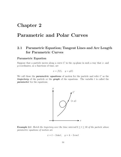
Chapter 2Parametric and Polar Curves2.1 Parametric Equation; TangentLinesandArc Lengthfor Parametric CurvesParametric EquationSuppose that a particle moves along a curve C in the xy-plane in such a way that x- andy-coordinates, as a functions of time, arex = f(t), y = g(t)We call these the parametric equations of motion for the particle and refer C as thetrajectory of the particle or the graph of the equations. The variable t is called theparameter for the equations.yC• (x,y)xExample 2.1 Sketch the trajectory over the time interval 0 ≤ t ≤ 10 of the particle whoseparametric equations of motion arex = t−3sint, y = 4−3cost14
•••••••••••MA112 Section 750001: Prepared by Dr.Archara Pacheenburawana 15Solution One way to sketch the trajectory is to plot the (x,y) coordinate of points on thetrajectory at those times, and connect the points with a smooth curve.t x y0 0.0 1.01 -1.5 2.42 -0.7 5.23 2.6 7.04 6.3 6.05 7.9 3.16 6.8 1.17 5.0 1.78 5.0 4.49 7.8 6.710 11.6 6.5yx✠Example 2.2 Find the graph of the parametric equationsx = cost, y = sint (0 ≤ t ≤ 2π) (2.1)Solution One way to find the graph is to eliminate the parameter t by noting thatx 2 +y 2 = sin 2 t+cos 2 t = 1Thus, the graph is contained in the unit circle x 2 +y 2 = 1. Geometrically, the parametert can be interpreted as the angle swept out by the radial line from the origin to the point(x,y) = (cost,sint) on the unit circle. As t increases from 0 to 2π, the point traces thecircle counterclockwise, starting at (1,0) when t = 0 and completing one full revolutionwhen t = 2π.y1tx•(x,y)y(0,1)x✠
- Page 2: •••••MA112 Section 750001
- Page 5 and 6: •••••MA112 Section 750001
- Page 7 and 8: MA112 Section 750001: Prepared by D
- Page 9 and 10: MA112 Section 750001: Prepared by D
- Page 11 and 12: •MA112 Section 750001: Prepared b
- Page 13: MA112 Section 750001: Prepared by D
- Page 17 and 18: MA112 Section 750001: Prepared by D
- Page 19 and 20: MA112 Section 750001: Prepared by D
- Page 21 and 22: MA112 Section 750001: Prepared by D
- Page 23 and 24: MA112 Section 750001: Prepared by D
- Page 25 and 26: MA112 Section 750001: Prepared by D
- Page 27 and 28: MA112 Section 750001: Prepared by D
- Page 29 and 30: MA112 Section 750001: Prepared by D
- Page 31 and 32: MA112 Section 750001: Prepared by D
- Page 33 and 34: MA112 Section 750001: Prepared by D
- Page 35 and 36: MA112 Section 750001: Prepared by D
- Page 37 and 38: MA112 Section 750001: Prepared by D
- Page 39 and 40: MA112 Section 750001: Prepared by D
- Page 41 and 42: •MA112 Section 750001: Prepared b
- Page 43 and 44: MA112 Section 750001: Prepared by D
- Page 45 and 46: MA112 Section 750001: Prepared by D
- Page 47 and 48: MA112 Section 750001: Prepared by D
- Page 49 and 50: MA112 Section 750001: Prepared by D
- Page 51 and 52: MA112 Section 750001: Prepared by D
- Page 53 and 54: •MA112 Section 750001: Prepared b
- Page 55 and 56: MA112 Section 750001: Prepared by D
- Page 57 and 58: MA112 Section 750001: Prepared by D
- Page 59 and 60: MA112 Section 750001: Prepared by D
- Page 61 and 62: MA112 Section 750001: Prepared by D
- Page 63 and 64: MA112 Section 750001: Prepared by D
<strong>Chapter</strong> 2Parametric and Polar Curves2.1 Parametric Equation; TangentL<strong>in</strong>esandArc Lengthfor Parametric CurvesParametric EquationSuppose that a particle moves along a curve C <strong>in</strong> the xy-plane <strong>in</strong> such a way that x- andy-coord<strong>in</strong>ates, as a functions of time, arex = f(t), y = g(t)We call these the parametric equations of motion for the particle and refer C as thetrajectory of the particle or the graph of the equations. The variable t is called theparameter for the equations.yC• (x,y)xExample 2.1 Sketch the trajectory over the time <strong>in</strong>terval 0 ≤ t ≤ 10 of the particle whoseparametric equations of motion arex = t−3s<strong>in</strong>t, y = 4−3cost14


