Multiple Linear Regression

We see from the output that for the trees data our parameter estimates are b = [ −58.0 4.7 0.3 ] ,and consequently our estimate of the mean response is ˆµ given byˆµ(x 1 , x 2 ) = b 0 + b 1 x 1 + b 2 x 2 , (10)≈ − 58.0 + 4.7x 1 + 0.3x 2 . (11)We could see the entire model matrix X with the model.matrix function.> head(model.matrix(trees.lm))(Intercept) Girth Height1 1 8.3 702 1 8.6 653 1 8.8 634 1 10.5 725 1 10.7 816 1 10.8 832.3 Point Estimates of the Regression SurfaceThe parameter estimates b make it easy to find the fitted values, Ŷ. We write them individually asŶ i , i = 1, 2, . . . , n, and recall that they are defined byŶ i = ˆµ(x 1i , x 2i ), (12)= b 0 + b 1 x 1i + b 2 x 2i , i = 1, 2, . . . , n. (13)They are expressed more compactly by the matrix equationŶ = Xb. (14)From Equation 9 we know that b = ( X T X ) −1X T Y, so we can rewrite[(Ŷ = X X T X ) ]−1X T Y , (15)= HY, (16)where H = X ( X T X ) −1X T is the hat matrix. Some facts about H are• H is a symmetric square matrix, of dimension n × n.• The diagonal entries h ii satisfy 0 ≤ h ii ≤ 1.5

2.8 How to do it with RTo get confidence intervals for the parameters we need only use confint:> confint(trees.lm)2.5 % 97.5 %(Intercept) -75.68226247 -40.2930554Girth 4.16683899 5.2494820Height 0.07264863 0.6058538For example, using the calculations above we say that for the regression model Volume~Girth + Height we are 95% confident that the parameter β 1 lies somewhere in the interval[4.2, 5.2].2.9 Confidence and Prediction IntervalsWe use confidence and prediction intervals to gauge the accuracy of our parameter estimates.We know Ŷ(x 0 ) = x T 0b, and we also know(b ∼ mvnorm mean = β, sigma = σ ( 2 X T X ) ) −1, (27)so we get(Ŷ(x 0 ) ∼ mvnorm mean = x T 0 β, sigma = ( σ2 x T 0 X T X ) )−1x0 . (28)and confidence intervals for the mean value of a future observation at the location x 0 = [ x 10 x 20 . . . x p0] Tare given byŶ(x 0 ) ± t α/2 (df = n − p − 1) SPrediction intervals for a new observation at x 0 are given byŶ(x 0 ) ± t α/2 (df = n − p − 1) S√x T (0 XT X ) −1 x 0 . (29)√1 + x T (0 XT X ) −1 x 0 . (30)Note that the prediction intervals are wider than the confidence intervals.2.10 How to do it with R> new

predict(trees.lm, newdata = new, interval = "confidence")fit lwr upr1 8.264937 5.77240 10.757472 21.731594 20.11110 23.352083 30.379205 26.90964 33.84877Prediction intervals are given by> predict(trees.lm, newdata = new, interval = "prediction")fit lwr upr1 8.264937 -0.06814444 16.598022 21.731594 13.61657775 29.846613 30.379205 21.70364103 39.05477As before, the interval type is decided by the interval argument and the default confidencelevel is 95% (which can be changed with the level argument).Using the trees data,1. A 95% confidence interval for the mean Volume of a tree of Girth 9.1 in and Height 69 ftis given by [5.8, 10.8]. so with 95% confidence the mean Volume lies somewhere between5.8 cubic feet and 10.8 cubic feet.2. A 95% prediction interval for the Volume of a hypothetical tree of Girth 12.5 in and Height87 ft is given by [26.9, 33.8], so with 95% confidence the hypothetical Volume of a tree ofGirth 12.5 in and Height 87 ft would lie somewhere between 26.9 cubic feet and 33.8 feet.3 Model Utility and Inference3.1 Multiple Coefficient of DeterminationThe error sum of squares S S E can be conveniently written in MLR asS S E = Y T (I − H)Y. (31)The ANOVA decomposition saysS S TO =Y T (I − 1 n J )Y (32)10

andS S R =Y T (H − 1 n J )Y. (33)Immediately from Equations 31, 32, and 33 we get the Anova EqualityS S TO = S S E + S S R. (34)The multiple coefficient of determination is defined by the formulaR 2 = 1 − S S ES S TO . (35)R 2 is the proportion of total variation that is explained by the multiple regression model. InMLR we must be careful, however, because the value of R 2 can be artificially inflated by theaddition of explanatory variables to the model, regardless of whether or not the added variables areuseful with respect to prediction of the response variable.We address the problem by penalizing R 2 when parameters are added to the model. The resultis an adjusted R 2 which we denote by R 2 .R 2 =(R 2 −p ) (n − 1n − 1n − p − 1). (36)It is good practice for the statistician to weigh both R 2 and R 2 during assessment of model utility.In many cases their values will be very close to each other. If their values differ substantially, orif one changes dramatically when an explanatory variable is added, then (s)he should take a closerlook at the explanatory variables in the model.3.2 How to do it with RFor the trees data, we can get R 2 and R 2 from the summary output or access the values directlyby name as shown (recall that we stored the summary object in treesumry).> treesumry$r.squared[1] 0.94795> treesumry$adj.r.squared[1] 0.9442322High values of R 2 and R 2 such as these indicate that the model fits very well, which agrees withwhat we saw in Figure 2.11

3.3 Overall F-TestAnother way to assess the model’s utility is to to test the hypothesisH 0 : β 1 = β 2 = · · · = β p = 0 versus H 1 : at least one β i 0.The idea is that if all β i ’s were zero, then the explanatory variables X 1 , . . . , X p would be worthlesspredictors for the response variable Y. We can test the above hypothesis with the overall F statistic,which in MLR is defined byF =S S R/pS S E/(n − p − 1) . (37)When the regression assumptions hold and under H 0 then F ∼ f(df1 = p, df2 = n − p − 1). Wereject H 0 when F is large, that is, when the explained variation is large relative to the unexplainedvariation.3.4 How to do it with RThe overall F statistic and its associated p-value is listed at the bottom of the summary output,or we can access it directly by name; it is stored in the fstatistic component of the summaryobject.> treesumry$fstatisticvalue numdf dendf254.9723 2.0000 28.0000For the trees data, we see that F = 254.972337410669 with a p-value < 2.2e-16. Consequentlywe reject H 0 , that is, the data provide strong evidence that not all β i ’s are zero.3.5 Student’s t TestsWe know thatand we now test(b ∼ mvnorm mean = β, sigma = σ ( 2 X T X ) ) −1(38)H 0 : β i = 0 versus H 1 : β i 0, (39)where β i is the coefficient for the i th independent variable. If H 0 is rejected, then we conclude thatthere is a significant relationship between Y and x i in the regression model Y ∼ (x 1 , . . . , x p ). This12

last part of the sentence is very important because the significance of the variable x i sometimesdepends on the presence of other independent variables in the model 1 .The quantityT i = b i − β iS bi(40)has a Student’s t distribution with n − (p + 1) degrees of freedom, so under the null hypothesisH 0 : β i = 0 the statistic t i = b i /S bi has a t(df = n − p − 1) distribution.3.6 How to do it with RThe Student’s t tests for significance of the individual explanatory variables are shown in thesummary output.> treesumryCall:lm(formula = Volume ~ Girth + Height, data = trees)Residuals:Min 1Q Median 3Q Max-6.4065 -2.6493 -0.2876 2.2003 8.4847Coefficients:Estimate Std. Error t value Pr(>|t|)(Intercept) -57.9877 8.6382 -6.713 2.75e-07 ***Girth 4.7082 0.2643 17.816 < 2e-16 ***Height 0.3393 0.1302 2.607 0.0145 *---Signif. codes: 0 ‘***’ 0.001 ‘**’ 0.01 ‘*’ 0.05 ‘.’ 0.1 ‘ ’ 1Residual standard error: 3.882 on 28 degrees of freedomMultiple R-squared: 0.948, Adjusted R-squared: 0.9442F-statistic: 255 on 2 and 28 DF, p-value: < 2.2e-16We see from the p-values that there is a significant linear relationship between Volume andGirth and between Volume and Height in the regression model Volume ~Girth + Height.Further, it appears that the Intercept is significant in the aforementioned model.1 In other words, a variable might be highly significant one moment but then fail to be significant when anothervariable is added to the model. When this happens it often indicates a problem with the explanatory variables, such asmulticollinearity. See Section ??.13

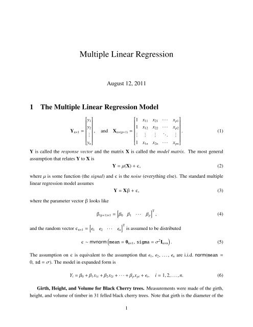
●Volume10 30 50 70● ●●● ●● ● ● ● ●●● ●●●●● ● ●●●●●●●● ● ●8 10 12 14 16 18 20GirthFigure 3: Scatterplot of Volume versus Girth for the trees data4 Polynomial Regression4.1 Quadratic Regression ModelAbove we assumed that µ was a linear function of the explanatory variables, that is we assumedµ(x 1 , x 2 ) = β 0 + β 1 x 1 + β 2 x 2 . In every case the scatterplots indicated that our assumption wasreasonable. Sometimes, however, plots of the data suggest that the linear model is incomplete andshould be modified.For example, let us examine a scatterplot of Volume versus Girth a little more closely. SeeFigure 3. There might be a slight curvature to the data; the volume curves ever so slightly upwardas the girth increases. After looking at the plot we might try to capture the curvature with a meanresponse such asµ(x 1 ) = β 0 + β 1 x 1 + β 2 x 2 1 , (41)which is associated with the modelY = β 0 + β 1 x 1 + β 2 x 2 1 + ɛ. (42)The regression assumptions are the same.14

When we introduce the squared variable in the model, though, we inadvertently also introducestrong dependence between the terms which can cause significant numerical problems when itcomes time to calculate the parameter estimates. Therefore, we should usually rescale the independentvariable to have mean zero (and even variance one if we wish) before fitting the model.That is, we replace the x i ’s with x i − x (or (x i − x)/s) before fitting the model.How to do it with RThere are multiple ways to fit a quadratic model to the variables Volume and Girth using R.1. One way would be to square the values for Girth and save them in a vector Girthsq. Next,fit the linear model Volume ~Girth + Girthsq.2. A second way would be to use the insulate function in R, denoted by I:Volume ~ Girth + I(Girth^2)The second method is shorter than the first but the end result is the same. And once wecalculate and store the fitted model (in, say, treesquad.lm) all of the previous commentsregarding R apply.3. A third and “right” way to do it is with orthogonal polynomials:Volume ~ poly(Girth , degree = 2)Note that we can recover the approach in 2 with poly(Girth, degree = 2, raw =TRUE).We will fit the quadratic model to the trees data and display the results with summary, beingcareful to rescale the data before fitting the model. We may rescale the Girth variable to havezero mean and unit variance on-the-fly with the scale function.> treesquad.lm summary(treesquad.lm)Call:lm(formula = Volume ~ scale(Girth) + I(scale(Girth)^2), data = trees)Residuals:Min 1Q Median 3Q Max-5.4889 -2.4293 -0.3718 2.0764 7.644715

Coefficients:Estimate Std. Error t value Pr(>|t|)(Intercept) 27.7452 0.8161 33.996 < 2e-16 ***scale(Girth) 14.5995 0.6773 21.557 < 2e-16 ***I(scale(Girth)^2) 2.5067 0.5729 4.376 0.000152 ***---Signif. codes: 0 ‘***’ 0.001 ‘**’ 0.01 ‘*’ 0.05 ‘.’ 0.1 ‘ ’ 1Residual standard error: 3.335 on 28 degrees of freedomMultiple R-squared: 0.9616, Adjusted R-squared: 0.9588F-statistic: 350.5 on 2 and 28 DF, p-value: < 2.2e-16We see that the F statistic indicates the overall model including Girth and Girth^2 is significant.Further, there is strong evidence that both Girth and Girth^2 are significantly related toVolume. We may examine a scatterplot together with the fitted quadratic function using the linesfunction, which adds a line to the plot tracing the estimated mean response.> plot(Volume ~ scale(Girth), data = trees)> lines(fitted(treesquad.lm) ~ scale(Girth), data = trees)The plot is shown in Figure 4. Pay attention to the scale on the x-axis: it is on the scale of thetransformed Girth data and not on the original scale.We do estimation/prediction as above, except we do not need a Height column in the dataframenew since the variable is not included in the quadratic model.> new predict(treesquad.lm, newdata = new, interval = "prediction")fit lwr upr1 11.56982 4.347426 18.792212 20.30615 13.299050 27.313253 25.92290 18.972934 32.87286The predictions and intervals are slightly different from what they were previously. Notice thatit was not necessary to rescale the Girth prediction data before input to the predict function; themodel did the rescaling for us automatically.We have mentioned on several occasions that it is important to rescale the explanatory variablesfor polynomial regression. Watch what happens if we ignore this advice:16

●Volume10 30 50 70● ●●● ●● ● ● ● ●●● ●●●●● ● ●●●●●●●● ● ●−1 0 1 2scale(Girth)Figure 4: A quadratic model for the trees data> summary(lm(Volume ~ Girth + I(Girth^2), data = trees))Call:lm(formula = Volume ~ Girth + I(Girth^2), data = trees)Residuals:Min 1Q Median 3Q Max-5.4889 -2.4293 -0.3718 2.0764 7.6447Coefficients:Estimate Std. Error t value Pr(>|t|)(Intercept) 10.78627 11.22282 0.961 0.344728Girth -2.09214 1.64734 -1.270 0.214534I(Girth^2) 0.25454 0.05817 4.376 0.000152 ***---Signif. codes: 0 ‘***’ 0.001 ‘**’ 0.01 ‘*’ 0.05 ‘.’ 0.1 ‘ ’ 1Residual standard error: 3.335 on 28 degrees of freedomMultiple R-squared: 0.9616, Adjusted R-squared: 0.958817

F-statistic: 350.5 on 2 and 28 DF,p-value: < 2.2e-16Now nothing is significant in the model except Girth^2. We could delete the Intercept andGirth from the model, but the model would no longer be parsimonious. A novice may see theoutput and be confused about how to proceed, while the seasoned statistician recognizes immediatelythat Girth and Girth^2 are highly correlated. The only remedy to this ailment is to rescaleGirth, which we should have done in the first place.5 InteractionIn our model for tree volume there have been two independent variables: Girth and Height. Wemay suspect that the independent variables are related, that is, values of one variable may tend toinfluence values of the other. We include an additional term in our model to try and capture thedependence between the variables.Perhaps the Girth and Height of the tree interact to influence the its Volume; we would liketo investigate whether the model (Girth = x 1 and Height = x 2 )Y = β 0 + β 1 x 1 + β 2 x 2 + ɛ (43)would be significantly improved by the modelY = β 0 + β 1 x 1 + β 2 x 2 + β 1:2 x 1 x 2 + ɛ, (44)where the subscript 1 : 2 denotes that β 1:2 is a coefficient of an interaction term between x 1 and x 2 .Interpretation: The mean response µ(x 1 , x 2 ) as a function of x 2 :µ(x 2 ) = (β 0 + β 1 x 1 ) + β 2 x 2 (45)is a linear function of x 2 with slope β 2 . As x 1 changes, the y-intercept of the mean response in x 2changes, but the slope remains the same. So the mean response in x 2 is represented by a collectionof parallel lines all with common slope β 2 .When the interaction term β 1:2 x 1 x 2 is included the mean response in x 2 then looks likeµ(x 2 ) = (β 0 + β 1 x 1 ) + (β 2 + β 1:2 x 1 )x 2 . (46)In this case we see that not only the y-intercept changes when x 1 varies, but the slope also changesin x 1 . Thus, the interaction term allows the slope of the mean response in x 2 to increase anddecrease as x 1 varies.18

How to do it with RThere are several ways to introduce an interaction term into the model.1. Make a new variable prod treesint.lm summary(treesint.lm)Call:lm(formula = Volume ~ Girth + Height + Girth:Height, data = trees)Residuals:Min 1Q Median 3Q Max-6.5821 -1.0673 0.3026 1.5641 4.6649Coefficients:Estimate Std. Error t value Pr(>|t|)(Intercept) 69.39632 23.83575 2.911 0.00713 **Girth -5.85585 1.92134 -3.048 0.00511 **Height -1.29708 0.30984 -4.186 0.00027 ***Girth:Height 0.13465 0.02438 5.524 7.48e-06 ***---Signif. codes: 0 ‘***’ 0.001 ‘**’ 0.01 ‘*’ 0.05 ‘.’ 0.1 ‘ ’ 1Residual standard error: 2.709 on 27 degrees of freedomMultiple R-squared: 0.9756, Adjusted R-squared: 0.9728F-statistic: 359.3 on 3 and 27 DF, p-value: < 2.2e-16We can see from the output that the interaction term is highly significant. Further, the estimateb 1:2 is positive. This means that the slope of µ(x 2 ) is steeper for bigger values of Girth. Keep inmind: the same interpretation holds for µ(x 1 ); that is, the slope of µ(x 1 ) is steeper for bigger valuesof Height.19

Height by a new variable Tall which indicates whether or not the cherry tree is taller than acertain threshold (which for the sake of argument will be the sample median height of 76 ft). Thatis, Tall will be defined by⎧⎪⎨ yes, if Height > 76,Tall =(47)⎪⎩ no, if Height ≤ 76.We can construct Tall very quickly in R with the cut function:> trees$Tall trees$Tall[1:5][1] no no no no yesLevels: no yesNote that Tall is automatically generated to be a factor with the labels in the correct order.See ?cut for more.Once we have Tall, we include it in the regression model just like we would any other variable.It is handled internally in the following way. Define the “dummy variable” Tallyes that takesvalues⎧⎪⎨ 1, if Tall = yes,Tallyes =(48)⎪⎩ 0, otherwise.That is, Tallyes is an indicator variable which indicates when a respective tree is tall. The modelmay now be written asVolume = β 0 + β 1 Girth + β 2 Tallyes + ɛ. (49)Let us take a look at what this definition does to the mean response. Trees with Tall = yes willhave the mean responseµ(Girth) = (β 0 + β 2 ) + β 1 Girth, (50)while trees with Tall = no will have the mean responseµ(Girth) = β 0 + β 1 Girth. (51)In essence, we are fitting two regression lines: one for tall trees, and one for short trees. Theregression lines have the same slope but they have different y intercepts (which are exactly |β 2 | farapart).21

How to do it with RThe important thing is to double check that the qualitative variable in question is stored as a factor.The way to check is with the class command. For example,> class(trees$Tall)[1] "factor"If the qualitative variable is not yet stored as a factor then we may convert it to one with thefactor command. Other than this we perform MLR as we normally would.> treesdummy.lm summary(treesdummy.lm)Call:lm(formula = Volume ~ Girth + Tall, data = trees)Residuals:Min 1Q Median 3Q Max-5.7788 -3.1710 0.4888 2.6737 10.0619Coefficients:Estimate Std. Error t value Pr(>|t|)(Intercept) -34.1652 3.2438 -10.53 3.02e-11 ***Girth 4.6988 0.2652 17.72 < 2e-16 ***Tallyes 4.3072 1.6380 2.63 0.0137 *---Signif. codes: 0 ‘***’ 0.001 ‘**’ 0.01 ‘*’ 0.05 ‘.’ 0.1 ‘ ’ 1Residual standard error: 3.875 on 28 degrees of freedomMultiple R-squared: 0.9481, Adjusted R-squared: 0.9444F-statistic: 255.9 on 2 and 28 DF,p-value: < 2.2e-16From the output we see that all parameter estimates are statistically significant and we concludethat the mean response differs for trees with Tall = yes and trees with Tall = no.We were somewhat disingenuous when we defined the dummy variable Tallyes because,in truth, R defines Tallyes automatically without input from the user 3 . Indeed, I fit the model3 That is, R by default handles contrasts according to its internal settings which may be customized by the user forfine control. Given that we will not investigate contrasts further in this book it does not serve the discussion to delveinto those settings, either. The interested reader should check ?contrasts for details.22

eforehand and wrote the discussion afterward with the knowledge of what R would do so thatthe output the reader saw would match what (s)he had previously read. The way that R handlesfactors internally is part of a much larger topic concerning contrasts. The interested reader shouldsee Neter et al [?] or Fox [?] for more.In general, if an explanatory variable foo is qualitative with n levels bar1, bar2, . . . , barnthen R will by default automatically define n − 1 indicator variables in the following way:⎧⎧⎪⎨ 1, if foo = ”bar2”,⎪⎨ 1, if foo = ”barn”,foobar2 =, . . . , foobarn =⎪⎩ 0, otherwise.⎪⎩ 0, otherwise.The level bar1 is represented by foobar2 = · · · = foobarn = 0. We just need to make sure thatfoo is stored as a factor and R will take care of the rest.Graphing the Regression LinesWe can see a plot of the two regression lines with the following mouthful of code.> treesTall treesTall[["yes"]]$Fit treesTall[["no"]]$Fit plot(Volume ~ Girth, data = trees, type = "n")> points(Volume ~ Girth, data = treesTall[["yes"]], pch = 1)> points(Volume ~ Girth, data = treesTall[["no"]], pch = 2)> lines(Fit ~ Girth, data = treesTall[["yes"]])> lines(Fit ~ Girth, data = treesTall[["no"]])Here is how it works: first we split the trees data into two pieces, with groups determinedby the Tall variable. Next we add the Fitted values to each piece via predict. Then we setup a plot for the variables Volume versus Girth, but we do not plot anything yet (type = n)because we want to use different symbols for the two groups. Next we add points to the plot forthe Tall = yes trees and use an open circle for a plot character (pch = 1), followed by pointsfor the Tall = no trees with a triangle character (pch = 2). Finally, we add regression lines tothe plot, one for each group.There are other – shorter – ways to plot regression lines by groups, namely the scatterplotfunction in the car package and the xyplot function in the lattice package. We elected tointroduce the reader to the above approach since many advanced plots in R are done in a similar,consecutive fashion.23

●Volume10 30 50 70● ● ●●●●●●●●● ● ●8 10 12 14 16 18 20GirthFigure 5: A dummy variable model for the trees data7 Partial F StatisticWe saw in Section 3.3 how to test H 0 : β 0 = β 1 = · · · = β p = 0 with the overall F statistic andwe saw in Section 3.5 how to test H 0 : β i = 0 that a particular coefficient β i is zero. Here we testwhether a certain part of the model is significant. Consider the regression modelY = β 0 + β 1 x 1 + · · · + β j x j + β j+1 x j+1 + · · · + β p x p + ɛ, (52)where j ≥ 1 and p ≥ 2. Now we wish to test the hypothesisH 0 : β j+1 = β j+2 = · · · = β p = 0 (53)versus the alternativeH 1 : at least one of β j+1 , β j+2 , , . . . , β p 0. (54)The interpretation of H 0 is that none of the variables x j+1 , . . . ,x p is significantly related to Y andthe interpretation of H 1 is that at least one of x j+1 , . . . ,x p is significantly related to Y. In essence,24

for this hypothesis test there are two competing models under consideration:the full model: y = β 0 + β 1 x 1 + · · · + β p x p + ɛ, (55)the reduced model: y = β 0 + β 1 x 1 + · · · + β j x j + ɛ, (56)Of course, the full model will always explain the data better than the reduced model, but does thefull model explain the data significantly better than the reduced model? This question is exactlywhat the partial F statistic is designed to answer.We first calculate S S E f , the unexplained variation in the full model, and S S E r , the unexplainedvariation in the reduced model. We base our test on the difference S S E r − S S E f which measuresthe reduction in unexplained variation attributable to the variables x j+1 , . . . ,x p . In the full modelthere are p + 1 parameters and in the reduced model there are j + 1 parameters, which gives adifference of p − j parameters (hence degrees of freedom). The partial F statistic isF = (S S E r − S S E f )/(p − j). (57)S S E f /(n − p − 1)It can be shown when the regression assumptions hold under H 0 that the partial F statistic has anf(df1 = p − j, df2 = n − p − 1) distribution. We calculate the p-value of the observed partial Fstatistic and reject H 0 if the p-value is small.How to do it with RThe key ingredient above is that the two competing models are nested in the sense that the reducedmodel is entirely contained within the complete model. The way to test whether the improvementis significant is to compute lm objects both for the complete model and the reduced model thencompare the answers with the anova function.For the trees data, let us fit a polynomial regression model and for the sake of argument wewill ignore our own good advice and fail to rescale the explanatory variables.> treesfull.lm summary(treesfull.lm)Call:lm(formula = Volume ~ Girth + I(Girth^2) + Height + I(Height^2),data = trees)Residuals:Min 1Q Median 3Q Max25

-4.368 -1.670 -0.158 1.792 4.358Coefficients:Estimate Std. Error t value Pr(>|t|)(Intercept) -0.955101 63.013630 -0.015 0.988Girth -2.796569 1.468677 -1.904 0.068 .I(Girth^2) 0.265446 0.051689 5.135 2.35e-05 ***Height 0.119372 1.784588 0.067 0.947I(Height^2) 0.001717 0.011905 0.144 0.886---Signif. codes: 0 ‘***’ 0.001 ‘**’ 0.01 ‘*’ 0.05 ‘.’ 0.1 ‘ ’ 1Residual standard error: 2.674 on 26 degrees of freedomMultiple R-squared: 0.9771, Adjusted R-squared: 0.9735F-statistic: 277 on 4 and 26 DF, p-value: < 2.2e-16In this ill-formed model nothing is significant except Girth and Girth^2. Let us continuedown this path and suppose that we would like to try a reduced model which contains nothing butGirth and Girth^2 (not even an Intercept). Our two models are nowthe full model: Y = β 0 + β 1 x 1 + β 2 x 2 1 + β 3x 2 + β 4 x 2 2 + ɛ,the reduced model: Y = β 1 x 1 + β 2 x 2 1 + ɛ,We fit the reduced model with lm and store the results:> treesreduced.lm anova(treesreduced.lm, treesfull.lm)Analysis of Variance TableModel 1: Volume ~ -1 + Girth + I(Girth^2)Model 2: Volume ~ Girth + I(Girth^2) + Height + I(Height^2)Res.Df RSS Df Sum of Sq F Pr(>F)1 29 321.652 26 185.86 3 135.79 6.3319 0.002279 **26

---Signif. codes: 0 ‘***’ 0.001 ‘**’ 0.01 ‘*’ 0.05 ‘.’ 0.1 ‘ ’ 1We see from the output that the complete model is highly significant compared to the modelthat does not incorporate Height or the Intercept. We wonder (with our tongue in our cheek) ifthe Height^2 term in the full model is causing all of the trouble. We will fit an alternative reducedmodel that only deletes Height^2.> treesreduced2.lm anova(treesreduced2.lm, treesfull.lm)Analysis of Variance TableModel 1: Volume ~ Girth + I(Girth^2) + HeightModel 2: Volume ~ Girth + I(Girth^2) + Height + I(Height^2)Res.Df RSS Df Sum of Sq F Pr(>F)1 27 186.012 26 185.86 1 0.14865 0.0208 0.8865In this case, the improvement to the reduced model that is attributable to Height^2 is notsignificant, so we can delete Height^2 from the model with a clear conscience. We notice that thep-value for this latest partial F test is 0.8865, which seems to be remarkably close to the p-valuewe saw for the univariate t test of Height^2 at the beginning of this example. In fact, the p-valuesare exactly the same. Perhaps now we gain some insight into the true meaning of the univariatetests.8 Residual Analysis and Diagnostic ToolsAll of the tools from SLR are valid in multiple linear regression, too, but there are some slightchanges for the multivariate case. We list these below, and apply them to the trees example.Shapiro-Wilk, Breusch-Pagan, Durbin-Watson: unchanged from SLR, but we are now equippedto talk about the Shapiro-Wilk test statistic for the residuals. It is defined by the formulawhere E ∗ is the sorted residuals and a 1×n is defined byW = aT E ∗E T E , (58)a =m T V −1√mT V −1 V −1 m , (59)27

where m n×1 and V n×n are the mean and covariance matrix, respectively, of the order statisticsfrom an mvnorm (mean = 0, sigma = I) distribution.Leverages: are defined to be the diagonal entries of the hat matrix H (which is why we calledthem h ii in Section 2.3). The sum of the leverages is tr(H) = p + 1. One rule of thumbconsiders a leverage extreme if it is larger than double the mean leverage value, which is2(p + 1)/n, and another rule of thumb considers leverages bigger than 0.5 to indicate highleverage, while values between 0.3 and 0.5 indicate moderate leverage.Standardized residuals: unchanged. Considered extreme if |R i | > 2.Studentized residuals: compared to a t(df = n − p − 2) distribution.DFBET AS : The formula is generalized to(DFBET AS ) j(i) = b j − b j(i)S (i)√ c j j, j = 0, . . . p, i = 1, . . . , n, (60)where c j j is the j th diagonal entry of (X T X) −1 . Values larger than one for small data sets or2/ √ n for large data sets should be investigated.DFFITS : unchanged. Larger than one in absolute value is considered extreme.Cook’s D: compared to an f(df1 = p + 1, df2 = n − p − 1) distribution. Observations fallinghigher than the 50 th percentile are extreme.9 Additional Topics9.1 Nonlinear RegressionAll of our models so far have looked like Volume ~Girth + Height or a variant of this model.But let us think again: we know from elementary school that the volume of a rectangle is V = lwhand the volume of a cylinder (which is closer to what a black cherry tree looks like) isV = πr 2 h or V = 4πdh, (61)where r and d represent the radius and diameter of the tree, respectively. With this in mind, itwould seem that a more appropriate model for µ might beµ(x 1 , x 2 ) = β 0 x β 11 xβ 22 , (62)where β 1 and β 2 are parameters to adjust for the fact that a black cherry tree is not a perfect cylinder.28

In the trees example we may take the logarithm of both sides of Equation 62 to getµ ∗ (x 1 , x 2 ) = ln [ µ(x 1 , x 2 ) ] = ln β 0 + β 1 ln x 1 + β 2 ln x 2 , (63)and this new model µ ∗ is linear in the parameters β ∗ 0 = ln β 0, β ∗ 1 = β 1 and β ∗ 2 = β 2. We can use whatwe have learned to fit a linear model log(Volume)~log(Girth)+ log(Height), and everythingwill proceed as before, with one exception: we will need to be mindful when it comes time to makepredictions because the model will have been fit on the log scale, and we will need to transformour predictions back to the original scale (by exponentiating with exp) to make sense.> treesNonlin.lm summary(treesNonlin.lm)Call:lm(formula = log(Volume) ~ log(Girth) + log(Height), data = trees)Residuals:Min 1Q Median 3Q Max-0.168561 -0.048488 0.002431 0.063637 0.129223Coefficients:Estimate Std. Error t value Pr(>|t|)(Intercept) -6.63162 0.79979 -8.292 5.06e-09 ***log(Girth) 1.98265 0.07501 26.432 < 2e-16 ***log(Height) 1.11712 0.20444 5.464 7.81e-06 ***---Signif. codes: 0 ‘***’ 0.001 ‘**’ 0.01 ‘*’ 0.05 ‘.’ 0.1 ‘ ’ 1Residual standard error: 0.08139 on 28 degrees of freedomMultiple R-squared: 0.9777, Adjusted R-squared: 0.9761F-statistic: 613.2 on 2 and 28 DF, p-value: < 2.2e-16This is our best model yet (judging by R 2 and R 2 ), all of the parameters are significant, it issimpler than the quadratic or interaction models, and it even makes theoretical sense. It rarely getsany better than that.We may get confidence intervals for the parameters, but remember that it is usually better totransform back to the original scale for interpretation purposes :> exp(confint(treesNonlin.lm))29

2.5 % 97.5 %(Intercept) 0.0002561078 0.006783093log(Girth) 6.2276411645 8.468066317log(Height) 2.0104387829 4.645475188(Note that we did not update the row labels of the matrix to show that we exponentiated andso they are misleading as written.) We do predictions just as before. Remember to transform theresponse variable back to the original scale after prediction.> new exp(predict(treesNonlin.lm, newdata = new, interval = "confidence"))fit lwr upr1 11.90117 11.25908 12.579892 20.82261 20.14652 21.521393 28.93317 27.03755 30.96169The predictions and intervals are slightly different from those calculated earlier, but they areclose. Note that we did not need to transform the Girth and Height arguments in the dataframenew. All transformations are done for us automatically.9.2 Real Nonlinear RegressionWe saw with the trees data that a nonlinear model might be more appropriate for the data basedon theoretical considerations, and we were lucky because the functional form of µ allowed us totake logarithms to transform the nonlinear model to a linear one. The same trick will not work inother circumstances, however. We need techniques to fit general models of the formY = µ(X) + ɛ, (64)where µ is some crazy function that does not lend itself to linear transformations.There are a host of methods to address problems like these which are studied in advancedregression classes. The interested reader should see Neter et al [?] or Tabachnick and Fidell [?].It turns out that John Fox has posted an Appendix to his book [?] which discusses some of themethods and issues associated with nonlinear regression; seehttp://cran.r-project.org/doc/contrib/Fox-Companion/appendix.html30

Here is an example of how it works, based on a question from R-help. We would like to fit amodel that looks like> set.seed(1)( ) 2 2πY = α + β sin360 x − γ + ɛ.> x y acc.nls summary(acc.nls)Formula: y ~ a + b * (sin((2 * pi * x/360) - c))^2Parameters:Estimate Std. Error t value Pr(>|t|)a 0.95884 0.23097 4.151 4.92e-05 ***b 2.22868 0.37114 6.005 9.07e-09 ***c 3.04343 0.08434 36.084 < 2e-16 ***---Signif. codes: 0 ‘***’ 0.001 ‘**’ 0.01 ‘*’ 0.05 ‘.’ 0.1 ‘ ’ 1Residual standard error: 1.865 on 197 degrees of freedomNumber of iterations to convergence: 3Achieved convergence tolerance: 6.554e-0831

y−2 0 2 4 6● ●●●●●●●●●●●●●● ●●●● ●●● ●●●●● ●● ●●●●●● ●● ● ●●●● ●● ●●●● ●●● ● ●● ●●● ●●●● ● ●●● ● ●●●● ● ● ● ●● ●●●●● ● ●●●●● ● ● ● ●●● ● ● ●● ● ● ●●●●●● ● ● ●●●● ● ● ●● ● ● ● ●●●●● ●●●●●●●●●● ●●● ●●●●●●●●● ● ●● ●●● ●●● ●●●● ●●● ●●●●●●●●●0 200 400 600 800 1000xFigure 6: Nonlinear regressiony−2 0 2 4 6● ●●●●●●●●●●●●●● ●●●● ●●● ●●●●● ●● ●●●●●● ●● ● ●●●● ●● ●●●● ●●● ● ●● ●●● ●●●● ● ●●● ● ●●●● ● ● ● ●● ●●●●● ● ●●●●● ● ● ● ●●● ● ● ●● ● ● ●●●●●● ● ● ●●●● ● ● ●● ● ● ● ●●●●● ●●●●●●●●●● ●●● ●●●●●●●●● ● ●● ●●● ●●● ●●●● ●●● ●●●●●●●●●0 200 400 600 800 1000xFigure 7: Nonlinear regression, fitted model32