CHAPTER 1 - Biomedical Simulations Resource

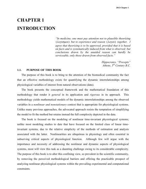
2012-Chapter 1CHAPTER 1INTRODUCTION1.1. PURPOSE OF THIS BOOKThe purpose of this book is to bring to the attention of the biomedical community the factthat an effective methodology exists for quantifying the dynamic interrelationships amongphysiological variables of interest from natural observations (data).The book presents the conceptual framework and the mathematical foundation of thismethodology that render it general in its application and rigorous in its approach.methodology yields mathematical models of the dynamic interrelationships among the observedvariables in a nonlinear and nonstationary context that is appropriate for physiological systems.Unlike many previous approaches, the advocated approach resists the temptation of simplifyingthe model to fit the method but retains instead the full complexity depicted in the data.The book is focused on the modeling of nonlinear time-invariant physiological systems;unlike most modeling studies to date that have focused on the limited class of linear timeinvariantsystems, due to the relative simplicity of the methods of estimation and analysisassociated with the latter. Nonlinearities are ubiquitous in physiology and often essential insubserving critical aspects of physiological function.ThisAlthough few will argue with theimportance and necessity of addressing the nonlinear and dynamic aspects of physiologicalsystems, most will view this task as a daunting challenge owing to its considerable complexity.The purpose of this book is to alter this confining view, so prevalent in the scientific community,by removing the perceived methodological barriers and offering the practicable prospect ofanalyzing nonlinear physiological systems within the prevailing experimental and computationalconstraints.“In medicine, one must pay attention not to plausible theorizing( s)but to experience and reason ( s)together. Iagree that theorizing is to be approved, provided that it is basedon facts and is systematically induced from what is observed; butconclusions drawn by the unaided reason can hardly beserviceable, only those drawn from observed facts.”Hippocrates, “Precepts”Athens, 5 th Century B.C.

Timeline for ImplementationWhat Do The Standards Mean For Teachers?Transitioning from existing state standards to the Common Core State Standards will impact curriculum and instruction in schools.• The Common Core State Standards represent a real shift in instructional intent from high school completion to college- and careerreadinessfor every student.• The CCSS will emphasize application and higher-order thinking skills.• When the standards are fully implemented, educators will see that each grade covers fewer topics, but teaches content in muchgreater depth.• The coherent progression of the Common Core State Standards will demand increased vertical articulation in K-12.What Can Teachers Do Now?The standards will be fully implemented in Maryland by school year 2013-2014. In the meantime, changes are being made toinstruction that will prepare students for the CCSS while helping succeed on current State assessments. To lay the groundwork for asmooth transition to the new standards, teachers can:• Inform colleagues and parents that there will be new standards in English/language arts (ELA) and mathematics.• Meet with department heads and school leadership teams to discuss how schools are transitioning to the Common Core.• Begin reviewing instructional materials and curriculum for alignment to the Common Core.• Assess professional development needs and begin to seek out and participate in such opportunities.• In English/Language Arts (ELA) ...– Incorporate into instruction more text-dependent questions that require students to read a text closely to determine what itsays explicitly and to make logical inferences from it.– Have students read more non-fiction and complex texts.– Focus writing instruction substantially on writing to inform and structure an argument, not only writing stories.• In Mathematics ...– Focus instruction more on the few key topics emphasized in each grade in the standards.– Emphasize problem-solving and real-world application.Preparing World-Class Students

over the centuries through the reductionist approach that have advanced scientific progress. Theadvocated viewpoint simply seeks to establish the proper balance between the two approaches inpursuing scientific knowledge, so that their synergistic contributions serve scientific progress andprevent the establishment of a mutually-impeding antagonism so often fostered in the past by anunwise inclination for polarized thinking.It is the ambitious goal of this book to contribute to a new movement (with ancient roots) thatwill restore the key Hippocratic-Galenic tenets to their rightful position in scientific thinking andpractice through adoption of the dynamic systems viewpoint, in order to bring about thedesirable leap of progress in physiology and medicine.1.2 ADVOCATED APPROACHThe advocated approach offers the effective methodological framework for obtaining reliableand objective (i.e., devoid of subjective modeling notions) descriptors of the system nonlineardynamics based on the available experimental or natural data. This approach employs generalmodel forms that do not require specific model postulates and yield inductively “data-true”models in the stochastic broadband context of natural operating conditions.Due to the complexity of this fundamental problem, we have taken a gradualist step-by-stepapproach, building on the rigorous and general mathematical foundation of the Volterra-Wienerapproach as extended and modified for various applications over the last thirty years. It isgratifying to note that our efforts have succeeded in developing a solid foundation for a generalmodeling approach capable of tackling this problem in a practical context.This novel modeling methodology has been tested in pilot applications from the nervous,cardiovascular, renal, respiratory and metabolic/endocrine systems. These applications haveshowcased the efficacy of the developed methodology and have allowed important advances insystems physiology by assigning physiological significance to the obtained model components ina manner that deepens the scientific understanding of the system under study. This demonstratesthe potential benefits of the advocated approach that are expected to enable improvements indiagnostic as well as therapeutic procedures.Standing on this solid foundation, we are poised to address the next generation of challengesthat pertain to the multi-variate and highly interconnected nature of physiological systems. ThisChapter 1Page 5 of 39

direction represents the natural extension of our efforts in reaching our ultimate objective ofmodeling the true physiological systems, and not their simplified “surrogates” born ofmethodological inadequacy. This forward looking task is commenced with the important case ofmultiple inputs and multiple outputs that is discussed in Chapter 8. The complexity thatemerges from the interconnections among multiple physiological variables of interest (often inclosed-loop or nested-loop configurations) must be placed in a nonlinear dynamic context, withpossible nonstationarities. Since we seek to study the physiological system under “natural”operating conditions (i.e., exposed to an ensemble of natural stimuli and unconstrained byarbitrary experimental manipulations), the ultimate modeling task must be placed in a multivariatestochastic broadband context, without artificially imposed constraints (e.g., fixedoperating points or specialized input waveforms) in order to achieve a globally valid model ofthe real system.A measure of the posed challenge is attained when we note that proper study of the realphysiological systems requires reliable modeling methods that are capable of dealing with:• nonlinear dynamics (of arbitrary order)• multiple variables of interest (observable/measurable)• multiple interconnections (possibly in closed-loop)• possible nonstationarities in system dynamics• broadband stochastic input/output signals• considerable measurement noise and systemic interferenceLast, but not least, the obtained models must be amenable to meaningful physiologicalinterpretation and offer the prospect for achieving significant diagnostic and/or therapeuticimprovements.The critical task of meaningful interpretation of the obtained models and their properutilization in clinical practice is formidable, as much as it is important, because the wealth ofinformation contained within these complicated models may be overwhelming and difficult toharness. Nonetheless, it is incumbent on us to perform this task in order to realize the benefits ofthe advocated new approach and achieve the ambitious goal of a quantum leap in the state of theart.Chapter 1Page 6 of 39

Interpretation of the obtained models will focus on relating their characteristics to specificphysiological mechanisms that are either known qualitatively or can be explored experimentally.It will also examine the effects of changes in certain physiological variables (in a dynamiccontext) and the robustness of the overall system in the event of internal or external perturbations(homeostasis). The latter study may demarcate the bounds of normal vs. pathological states.Utilization of the obtained models in a clinical context will seek to examine their use forimproved diagnosis of disease (i.e., more and better clinically relevant information) and for thequantitative assessment of pharmaceutical treatment or therapeutic intervention. The latter willallow optimization of treatment (with regard to specific clinical goals) and the design ofimproved therapeutic procedures, consistent with the key Hippocratic exhortation: “first, do noharm…”.The progress made to date in the development of effective methodologies for nonlinearand/or nonstationary modeling of physiological systems is summarized in this book and hasgiven rise to a new generation of issues associated with the study of greater system complexityand the analysis of expanded experimental/clinical databases - - both direct consequences ofadvances in the state of the art - - consistent with Socrates’ aphorism: “the more I learn, the moreI realize how much I do not know”.The advocated approach stands on the confluence of methodological (nonlinear andnonstationary) and technological (computational and experimental) advancements, and seeks toleverage on their synergistic utilization in order to tackle the formidable challenges inphysiological system modeling from natural (i.e., random broadband) data. Pilot applications areselected from physiological domains that exhibit essential nonlinearities /nonstationarities(neural, cardiovascular, respiratory, renal, endocrine and metabolic systems) in order todemonstrate the wide applicability and unique capabilities of the advocated novel methodologies.In this sense, the advocated approach is at the cutting edge of scientific developments and has auniversal appeal to all physiological domains in terms of scientific advancement, as well aspotential impact across a broad swath of clinical applications.The immense variety of nonlinear behavior makes it desirable that the developedmethodologies retain a high degree of generality and the ability to gracefully transition intointerpretable models for each particular application.Chapter 1Page 7 of 39

1.3 THE PROBLEM OF SYSTEM MODELING IN PHYSIOLOGYThe purpose of physiological system modeling is to advance our quantitative understandingof biological function and improve medical science and practice by utilizing the acquiredquantitative knowledge. In modeling physiological systems, we seek to summarize all availableexperimental evidence about the functional characteristics of a system in the form ofmathematical relations among variables of physiological interest. The resulting mathematicalmodels ought to emulate the observed functional behavior of the system under natural operatingconditions, when simulated on the computer.Ideally, such a model must be accurate (i.e., reproduce precisely the observed data), global(i.e., be accurate under all natural operating conditions), compact (i.e., have the minimummathematical and computational complexity) and interpretable (i.e., be amenable tophysiological interpretation that advances our understanding of the mechanisms subserving thesystem function). Implicit in the first attribute is the robustness of the model which provides forstable behavior in the face of internal or external random perturbations. The latter, and theomnipresence of noise, require that our modeling efforts be cast in a stochastic context.Furthermore, the development of a global model (valid under all natural operating conditions)presumes our ability to observe and measure the spontaneous activity of the variables of interestwith sufficient accuracy and sampling resolution over representative time intervals. Thesevariables can be viewed as inputs, outputs or internal state variables depending on our specificmodeling goals.Such an “ideal” model would offer a succinct quantitative representation of the functionalcharacteristics of the system and would allow the study of its behavior under arbitrary conditionsthrough computer simulations (thus maximizing the “yield” of physiological research). Inaddition to being a complete “capsule of knowledge” that advances scientific understanding ofhow and why physiological systems function in the way they do, such a model can improveclinical diagnosis (by providing more and better relevant information) and treatment (by properlyguiding therapeutic procedures and assessing their effects). The implications are immense andpromise to usher a new era of advanced medical care.The development of such an “ideal” model is a formidable task, because of the functionalcomplexity of physiological systems which are typically dynamic, nonlinear, nonstationary,highly interconnected (often in closed-loop configurations) and subject to stochasticChapter 1Page 9 of 39

perturbations and noise. Furthermore, the modeling process has been constrained in practice bylimitations of the available experimental, computational and analytical methods, leadingheretofore to the development of “less than ideal” models in the sense defined above, i.e.,inability to reach the desired attributes of accuracy, globality, compactness and interpretability.This sobering reality is put in perspective when one notes that many of the current modelingefforts are still confined to rudimentary methods of static and linear analysis. The course ofmethodological evolution started with static linear analysis (linear regression among variables ofinterest) and gradually progressed into dynamic (differential or integral equations) and nonlinearanalysis. Although linear dynamic analysis has been increasingly used, the use of nonlineardynamic analysis remains rather limited due to the scarcity of practical methods and the intrinsiccomplexity of the problem. This shortcoming would not be alarming, if it were not for the factthat most physiological systems exhibit significant and essential dynamic nonlinearities. Thisproblem is compounded by the fact that physiological systems are also often nonstationary (i.e.,their functional characteristics vary with time) necessitating models whose parameters alsochange with time. The need for proper modeling methodologies in this realistic context isincreasingly pressing and provides the motivation for this book.Physiological system modeling provides the means of summarizing vast amounts ofexperimental data into relatively compact mathematical (or computational) forms that allow theformulation and testing of scientific hypotheses regarding the functional properties of the system-- an iterative process that should lead to successive refinement and evolution of the systemmodel. Thus, system modeling attains a central role in the scientific process of generation anddissemination of knowledge -- consistent with the credo “model or muddle.” Models can beapplied to arbitrary levels of system decomposition or integration depending on the availabilityof appropriate data -- hence providing the conceptual and methodological means for developinga hierarchical understanding of integrative systems physiology.The fundamental question of the functional relationships between observed physiologicalvariables drives the system modeling effort. The variables are observed experimentally overtime (occasionally over space or wavelength) and are viewed as signals (or datasets) that arelinked by a causal relationship. The direction of this causal relationship (cause-to effectsequence) defines some of them as inputs and some of them as outputs of a conceptual operator(the system) that transforms the inputs into the outputs (Figure 1.1). This transformation isChapter 1Page 10 of 39

generally dynamic in the sense that the present values of the outputs depend not only on thepresent but also on the past values of the inputs. Another way of describing the same (defining)characteristic of dynamic systems is to state that the effect of an input change upon the outputsignal spreads over time.Figure 1.1Schematic of a “black-box” system operator S transforming M input signals { x1( t), , xM( t )} into N outputsignals { y1( t), , yN( t )}.It is worth noting that the system is defined by means of its inputs and outputs (and not by aphysical entity). Thus, we may define many different systems using the same physical entity byaltering the selected inputs and outputs, as long as causality is not violated. This point isillustrated in Figure 1.2 where a physical entity is comprised of five components( A , B , C , D , E ) and the designated connections (arrows) represent directional causalrelationships. If we stimulate component A with input xA()t and record output yC() t fromcomponent C , then we define the system S as the signal transformation from A to C .However, if we record from another component (e.g.,another component (e.g., ACyD t out of component D ) and stimulatexBt into component B ), then we define a different systemBDrepresenting the signal transformation from input B to output D , even though the underlyingphysical entity remains the same.The input-output signal transformation describes the functional properties of the system andmay be linear or nonlinear, time-invariant (stationary) or time-varying (nonstationary), anddeterministic or stochastic. A mathematical expression describing quantitatively this inputoutputsignal transformation is the sought model of the system. For our purposes, the soughtmodel will be deterministic, implying that possible stochastic variations of the systemSChapter 1Page 11 of 39

characteristics will be relegated to the status of systemic noise or modeling errors and will beincorporated in the stochastic error term of the model. The latter will also incorporate othermodeling errors and possible measurement noise or external/systemic interference.(a)(b)Figure 1.2Schematic diagram of causal connections (denoted by arrows) among five physical variables (A,B,C,D,E). Theselected input(s) and output(s) define the particular system operator. For instance, an input x () t stimulating Aand an output yC() t recorded from C define a system operator SAC(left panel) or an input xB()and an output yD()t recorded from D define a different system operator SBD(right panel).At stimulating BChapter 1Page 12 of 39

If we limit ourselves, at first, to the single-input/single-output case, we can use theconvenient mathematical notation of a functional S [ ]to denote the causal relationship betweenpast and present values of the input x and the present value of the output y as:y( t) S[ x( t), t t] ( t)(1.1)where the functional S [ ]represents the deterministic system as it maps the input past andpresent values onto the output present value, and (t) represents the stochastic error term. Theerror term is assumed stochastic and additive – the latter is a common assumption that simplifiesthe estimation task but may not correspond to reality in some cases where the error may have amultiplicative or other modulatory effect on the input/output signals. The error term is alsocalled the “residual” and may contain modeling errors (including possible stochastic variations ofthe system characteristics), systemic noise or interference and measurement noise. For analysisand estimation purposes, the residual is usually treated as a stationary random process (with zeromean) that is statistically independent from the input and the noise-free output signals (althoughit is contained in the output data measurements). Note that deviation from this assumptionregarding the residual term may cause significant estimation errors.The convenient mathematical notation of Equation (1.1) can be extended to the case of causalsystems with multiple inputs and multiple outputs by adopting a vector notation (shown in bold)for the input/output signals, the residual terms and the functionals:y( t) S[ x( t), t t] ( t)(1.2)Clearly each output signal must have its own distinct functional implicating (potentially) allinputs. The case of multi-input/multi-output systems is discussed extensively in Chapter 8.However, the main methodological developments are presented in Chapters 2-5 for the singleinput/single-outputcase to avoid the burden of the inevitably increased complexity ofmathematical expressions resulting from the multiple inputs and outputs.Chapter 1Page 13 of 39

1.3.1 Model Specification and EstimationThe goal of mathematical modeling is to obtain an explicit mathematical expression for thefunctional S [ ]using experimental or natural input-output data and all other available knowledgeabout the system. This goal is generally achieved in two steps. At first, a suitable mathematicalform is selected for S [ ] , containing unknown parameters and/or functions, which aresubsequently estimated by use of input-output data in the second step. This two-step procedureis often referred to as “System Identification” in the engineering literature, and the two steps aretermed “Model Specification” and “Model Estimation” respectively.The Model Specification task is generally more challenging and the critical step to successfulmodeling. It utilizes all prior knowledge and information regarding the system under study andseeks to select the appropriate model form in each case. Typically the selection is made fromamong four classes of models: nonparametric, parametric, modular, and connectionist (see Table1.1). The criteria for selection of the appropriate model class are discussed in Chapters 2-5 andconstitute a critical issue.Table 1.1 Nonlinear System Modeling MethodologiesNonparametric Parametric Modular ConnectionistModel Specification + Interpretability + + Robustness to Noise + - + Compactness + + Adaptable to Time-Varying + +The Model Estimation task employs estimation methods suitable for the specificcharacteristics of each case and seeks to maximize the accuracy of the resulting model predictionfor given data types and noise conditions. Various measures and norms of model predictionaccuracy can be used, but the most common is the mean-square error of the output prediction(the sum of the squared residuals).The Model Estimation task is important because it yields the desired result, but it ismeaningful only when the Model Specification task is performed successfully. The highlytechnical nature of the Model Estimation task has attracted most of the attention in theengineering literature, and the contents of this book reflect this fact by delving into the manytechnical details of the various estimation methods. Nonetheless, it is useful to remember that,Chapter 1Page 14 of 39

although the estimation methods are necessary tools for accomplishing the modeling task, the artof modeling and the impact of its scientific applications hinge primarily on the successfulperformance of the Model Specification task and the meaningful interpretation of the obtainedmodel. It is for this reason that the overall modeling philosophy advocated by this book placesthe emphasis on securing first the best possible Model Specification results and then performaccurate Model Estimation.Since system modeling seeks to find and quantify the causal functional relationships amongobserved variables, it occupies a central position in the process of scientific discovery. Althoughit addresses only the functional aspects of the system under study, structural information can beused to assist the Model Specification task by properly constraining the postulated model.Conversely, system models can be used to examine alternative hypotheses regarding thestructural composition of a given system (e.g., interconnections of neuronal circuitry) and thuscan advance our structural knowledge of physiological systems.It is critical to note that the selection of the model form must not constrain unduly the rangeof functional possibilities of a system, lest it will lead to biased and inaccurate results. Thusextreme care must be taken to avoid such inappropriate constraining of the model either in termsof its mathematical form or in terms of its operational range (i.e., dynamic range and bandwidth).At the same time, the efficiency of the employed estimation methods and the utility of theobtained model in terms of scientific interpretability are compromised when the model is notadequately constrained. This key trade-off between model parsimony and its global validitypervades all modeling studies and is of fundamental importance, as discussed later in connectionwith the various classes of model forms.Related to the Model Specification task is the issue of inductive versus deductive modeldevelopment, discussed in Section 1.5. Deductive modeling is possible only in those rareoccasions where sufficient knowledge exists about the detailed functional properties of thesystem, so that its internal workings can be described accurately by use of first physical and/orchemical principles. In these fortunate, but rare, occasions the system model can be reliablypostulated in the form of precise mathematical expressions using a deductive process. Thecomplexity of physiological systems rarely affords this kind of opportunity and, consequently,modeling of physiological systems is usually inductive (i.e., it is based on accumulated empiricalevidence from experimental data). This distinction between inductive and deductive modelingChapter 1Page 15 of 39

has been made before with the use of the terms “empirical or external” and “axiomatic orinternal” models respectively [Arbib et al. 1969; Astrom & Eykhoff, 1971; Bellman & Astrom,1969; Rosenblueth & Wiener, 1945; Yates, 1973; Zadeh, 1956].Although prior knowledge about the system can be used to assist the Model Specificationtask, the modeling approaches presented herein are based entirely on experimental or naturalinput-output data and exclude the favorable -- but rare -- occasions where the model form can bederived from first principles or can be reliably postulated on the basis of prior knowledge aboutthe system. Therefore, our approach to physiological system modeling is inductive and datadriven.The necessity of inductive modeling for most physiological systems elevates the importanceof the type and quality of experimental or natural data needed for our modeling purposes. It isimperative, for instance, that the data cover the entire functional space of the system (e.g., theentire bandwidth and dynamic range of interest) and that the noise levels remain low relative tothe power of the signal of interest. It must be noted in this connection that the systemic noise orinterference (which is prevalent in physiological systems) is usually more harmful for theestimation process than the measurement noise.1.3.2 Nonlinearity and NonstationarityA critical issue that complicates the modeling task is the presence of nonlinearities in thephysiological system. Since this is the focus of the book, it is discussed in detail in the followingsection and in Chapters 2-7. Here, we limit ourselves to the definition of nonlinearities andnonstationarities with regard to the functional notation of Equation (1.1). A note should be madeabout static nonlinearities, whereby y( t) depends only on the value of x( t) and the functionalS[ ] reduces to a function. Static nonlinearities are easy to model (graphically or with simplenumerical fitting procedures), leaving dynamic nonlinearities as the true challenge.With reference to the functional notation of Equation (1.1), linearity of the system impliesthat S [ ]obeys the “superposition principle”, which states that if y ( 1t ) and y 2( t ) are the systemoutputs for inputs x ( 1t ) and x 2( t ) respectively, then for an input x( t) 1 x1 ( t) 2x2( t)theoutput is: y( t) 1 y1( t) 2 y2( t). This can be expressed by the mathematical condition:Chapter 1Page 16 of 39

S x ( t) x ( t) S x ( t) S x ( t)(1.3)1 1 2 2 1 1 2 2where x 1 (t) and x 2 (t) are linearly independent signals, and 1 and 2 are nonzero scalarcoefficients.The above condition can be tested experimentally with any pair of linearlyindependent inputs and scalar coefficients, and it must be satisfied by all such pairs. Thiscondition for linear superposition can be extended to any number of linearly independent signalsand remains by practical necessity a necessary, but not sufficient, condition (since all possiblecombinations cannot be practically tested).Appendix I provides the definition of linearindependence between two or more signals. Elaboration on the experimental testing of systemlinearity is given in Section 5.2.4.Returning to the functional notation of Equation (1.1), we can point out that stationarity (ortime-invariance) of the system implies that the input-output mapping rule represented byS [ ]remains invariant through time. It should be stressed that S [ ]denotes the rule by which thesystem constructs the output at time t using the input values at time t and before. Thus,nonstationarity (or time-variance) should not be confused with the inevitable temporal changes inthe output signal caused by temporal changes in the input signal, that occur whether the system isstationary or not. Experimental testing of the stationarity of a system requires the repetition ofidentical experiments at different times and the comparison of the obtained results. The test forstationarity of a system can be based on the following conditional statement: if the system outputfor input x( t) is y( t), then the output for input x( t ) is y( t ) for every time-shift .Since all experimental studies are subject to random influences and disturbances, this assessmentis not straightforward in practice and requires statistical analysis of sufficient data, as discussedin Section 5.2.3. and in Chapter 9.An experimental complication, often encountered in physiological systems, is the presence ofpossible nonstationarities in the experimental preparation caused by inadvertent injuries ofsurgical procedures. Thus an important distinction must be made between nonstationarties thatare intrinsic to the system operation (e.g., endocrine/hormonal cycles or biological rhythms) andpertain to the actual physiological function of the system, and those that affect our measurementbut are of no interest vis-à-vis the physiological function of the system under study. The formertype of nonstationarity ought to be incorporated into the estimated model by propermethodological means, as discussed in Chapter 9. The latter type of nonstationarity degrades theChapter 1Page 17 of 39

quality of the data and, although it can be often viewed as low-frequency noise, it may not have asimple additive effect on the observed output data (e.g., it may have a multiplicative ormodulatory effect).Therefore, it is important to remember that the employed modelingmethodologies for physiological systems must be robust in the presence of noise or systemicinterference and must not require very long experimentation time over which measurementnonstationarities may develop or have significant effect.Since the input-output data are collected and processed in sampled digital form, it is evidentthat the actual implementation of these modeling approaches takes place in discrete time. Thus,the continuous-time input-output signals xt () and yt () must be converted into discrete-timesignals xn ( ) and yn ( ) using a fixed sampling intervalT , where n denotes the discrete-timeindex (i.e.,t nT ). Provided that proper attention is paid to the issue of aliasing (by sampling ata sufficiently high rate that secures a Nyquist frequency greater than the bandwidth of thesampled input-output signals, as discussed in Section 5.1.3), the presented mathematical methodsgenerally transfer to the discrete-time case with minor modifications (e.g., converting an integralinto summation). Both discrete and continuous cases are presented throughout the book, and wemake special note in the few cases where the transition from continuous to discrete time requiresspecial attention (e.g., from nonlinear differential to difference equations).1.3.3 Definition of the Modeling ProblemWith all these considerations in mind, the physiological system modeling problem is definedas:Given a set of input-output experimental or natural data, find a mathematical model thatdescribes the dynamic input-output relationship with sufficient accuracy (using a mean-squareerrorcriterion for the output model prediction) under the following conditions: no prior knowledge is available about the internal workings of the system nonlinearities and/or nonstationarities may be present in the system extraneous noise and/or systemic interference may be present in the data the obtained model must be amenable to physiological interpretation experimentation time and computational requirements may not be excessiveA practical guide for the solution of the modeling problem in the context of physiologicalsystems is provided in Chapter 5.Chapter 1Page 18 of 39

1.4. TYPES OF NONLINEAR MODELS OF PHYSIOLOGICAL SYSTEMSThe challenge of modeling nonlinear physiological systems derives from the immensevariety of nonlinearities in living systems and the complex interactions among multiplemechanisms linked together within these systems.We summarize in Table 1.1 the four main nonlinear modeling approaches and classes ofnonlinear models used to date: nonparametric, parametric, modular, and connectionist.In the nonparametric approach, the input-output relation is represented either analytically inintegral equation form where the unknown quantities are kernel functions (e.g., Volterra-Wienerexpansions) or computationally as input-output mapping combinations (e.g., look-up tables oroperational surfaces /subspaces in phase-space). Nonparametric models are easy to postulate(because of their generality) but typically lack parsimony of representation. Of the variousnonparametric approaches, the discrete-time Volterra-Wiener (kernel) formulation has been usedmost extensively for nonlinear modeling of physiological systems and will form themathematical foundation of this book, along with its relations to the other modeling approaches.In the parametric approach, algebraic or differential/difference equation models are typicallyused to represent the input-output relation for static or dynamic systems, respectively. Thesemodels contain typically a small number of unknown parameters that may be constant or timevaryingdepending on whether the model is stationary or nonstationary. The specific form ofthese parametric models is usually postulated a priori but the selection of certain structuralparameters (e.g., degree/order of equation) are guided by the data.The modular approach is a hybrid between the parametric and the nonparametric approachthat makes use of block-structured models composed of parametric and/or nonparametriccomponents properly connected to represent the input-output relation in a manner that reflectsour evolving understanding of the functional organization of the system. The model specificationtask for this class of models is more demanding and may utilize previous parametric and/ornonparametric modeling results. A promising variant of this approach, which derives from thegeneral Volterra-Wiener formulation, employs principal dynamic modes as a minimum set offilters to represent parsimoniously a nonlinear dynamic system of the broad Volterra class (seeSection 4.1.1).The connectionist approach has recently acquired considerable popularity and makes use ofChapter 1Page 19 of 39

generic model configurations/architectures, known as artificial neural networks, to representinput-output nonlinear mappings in discrete time. These connectionist models are fullyparameterized, making this approach akin to parametric modeling, although typically lacking theparsimony and interpretability of parametric models. A hybrid nonparametric/connectionistapproach is at the core of the modeling methodology that is advocated as the best overall optionat present.The relations among these four approaches are of critical practical importance, sinceconsiderable benefits may accrue from the combined use of these approaches in a cooperativemanner. This synergistic use aims at securing the full gamut of advantages specific to eachapproach. The relative advantages and disadvantages in practical applications of the fourmodeling approaches will be discussed in Chapters 2-4.The ultimate selection of a particular methodology (or combinations thereof) hinges upon thespecific characteristics of the application at hand and the prioritization of objectives by theindividual investigator. Nonetheless, it is appropriate to state that no single methodology isglobally superior to all others (i.e., excelling with regard to all criteria and under all possiblecircumstances) and much can be gained by the synergistic use of the various modelingapproaches in a combination that takes into account the specific characteristics/requirements ofeach application. Judgment must be exercised in each individual case to select the combinationof methods that yields the greatest insight within the given experimental constraints. Since thegeneral nonlinear system identification problem remains a challenge of considerable complexity,one must not be lulled into the risk-prone complacency of blind algorithmic processing. Manychallenging issues remain that require vigilant attention, since there is no substitute forintelligence and educated judgment in resolving these issues. Four examples are given below toillustrate the various model forms employed by these approaches in different physiologicaldomains.Example 1.1Vertebrate retinaThe early stage of the vertebrate visual system (retina) is chosen as the first illustrativeexample to honor the historical fact that this was the first physiological system extensivelystudied with the Volterra-Wiener approach. A schematic of the neuronal architecture of theChapter 1Page 20 of 39

etina is shown in Figure 1.3. The natural input to the retina is light intensity (photon flux perunit surface) impinging on the photoreceptor cells that convert the photon energy intointracellular potential through a chain of photochemical and biochemical reactions. Thegenerated photoreceptor potential is synaptically transferred to downstream horizontal cells andbipolar cells through triadic synapses in the photoreceptor pedicle. The intracellular potentialsthus generated within horizontal and bipolar cells are synaptically transferred to the postsynapticganglion cells and to the interneurons of the inner plexiform layer (various types of amacrinecells).Figure 1.3Schematic of the neuronal organization of the retina (Dowling & Boycott, 1966).Chapter 1Page 21 of 39

Thus, visual information conveyed by the time variations of light intensity is converted(encoded) into sequences of action potentials by the ganglion cells and transmitted to higherlevels of the visual system via the optic nerve. This “encoding” process represents cascadedsignal transformations effected by the various retinal neurons and their multiple interconnections.Therefore, one “system of interest” can be defined by considering as input signal the variationsof light intensity impinging on the photoreceptors and as output signal the resulting sequence ofaction potentials generated by the ganglion cells. The induced intracellular potential in any otherretinal neuron along this cascade of signal transformations can be used as an output signal inorder to define a different “system of interest”. A block diagram depicting the main neuronalinterconnections in the retina is shown in Figure 1.4 that suggests many different possibilities fordefining input/output signals and the corresponding “systems of interest”.Figure 1.4A block diagram depicting the main signal-flow pathways in the vertebrate retina and a light stimulus with theresulting ganglion cell response. Other stimulus-response pairs can be chosen experimentally (Marmarelis &Marmarelis, 1978).In the foregoing, we described briefly the temporal sequence of causal effects from inputphotons impinging on the photoreceptor cell to the output action potentials generated by theganglion cells. However, it is clear that complicated causal effects also occur in space throughthe multiple lateral interconnections among retinal neurons and interneurons. Thus, space can beviewed as another independent variable (in addition to time) to define retinal input-output signaltransformations. This leads to the advanced spatio-temporal analysis of the visual systemChapter 1Page 22 of 39

discussed in Section 7.4.1. Note that the wavelength of the input photons can be viewed as yetanother independent variable in studies of color vision.The first successful application of the cross-correlation technique of modeling (see Section2.2.3) on visual neuronal pathways using band-limited Gaussian white noise (GWN) test inputswas performed on the catfish retina [Marmarelis & Naka, 1972]. The recorded output signal wasthe sequence of action potentials generated by a ganglion cell (actually the “probability of firing”measured by superimposing the outputs of repeated trials with the same GWN input, also calledthe “peristimulus histogram”). The obtained nonparametric model took the form of a discretetimesecond-order Wiener model: (1.4) , , y n h h m x n m h m m x n m x n m P h m m0 1 2 1 2 1 2 2m m1 m2mwhere h0, h1, h2denote the discretized Wiener kernels of zeroth, first and second order, P isthe power level of the discretized GWN inputxn (light intensity), and the summation overm, m1, and m2covers the entire memory of the system kernels. The discretized output ynrepresents the probability of firing an action potential by a single ganglion cell at discrete-timeindex n (t nT , where T is the sampling interval).The first-order and second-order Wiener kernels of the horizontal-to-ganglion neuronalpathway, estimated through the cross-correlation technique, are shown in Figure 1.5.interpretation of these kernels became a key issue from the very beginning, instigating intensivedebates regarding the potential utility of this approach. Many arguments were voiced for andagainst this approach, some of which remain the fodder of lively debate to date. However, thefact remains that this general nonparametric approach represents a quantum leap of improvementover any other method used heretofore and, although some interpretation issues remain open, ithas already elucidated immensely our understanding of retinal function. For instance, it isevident from the waveform of h1that the system is encoding both intensity and rate-of-changeinformation (as discussed further in Section 6.1.1). It is also evident from the form of h2that thesystem exhibits rectifying nonlinearities, consistent with the presence of a threshold for thegeneration of action potentials (see the contribution of h2to the model prediction in Figure 1.6).The validation for this model is provided by its ability to predict the output signal to any giveninput signal, as demonstrated in Figure 1.6.TheChapter 1Page 23 of 39

Many other “systems of interest” have been defined in the retina by considering the outputsof other retinal neurons (e.g., horizontal, bipolar, amacrine) and/or other inputs (e.g., lightintensity, current injected into various cells, or light stimuli of different wavelengths). Extensivemodeling studies have been reported for these systems by Naka and his associates following thenonparametric approach (see Section 6.1.1).Figure 1.5The first and second order Wiener kernel estimates of the horizontal-to-ganglion cell system in the catfish retina,obtained via the cross-correlation technique using band-limited GWN stimuli of current injected into the horizontalcell layer (Marmarelis & Naka, 1972).Figure 1.6The recorded experimental response of the ganglion cell (second trace) represented as “frequency of firing” (orperistimulus histogram) for repeated trials of the band-limited GWN current stimulus shown in the top trace. Thepredictions of the linear (i.e., first-order) model and of the nonlinear (i.e., second-order) model using the Wienerkernels of Figure 1.5 are shown in the third and fourth traces respectively (Marmarelis & Naka, 1972).Chapter 1Page 24 of 39

Example 1.2Invertebrate photoreceptorAs a second illustrative example, we consider the modular (block-structured) model derivedfor the photoreceptor of the fly eye (retinula cells 1-6 in an ommatidium of the composite eye ofthe fly Calliphora erythrocephala) using CSRS quasi-white stimuli under light-adaptedconditions [Marmarelis & McCann, 1977]. We have found that the input-output relation of thissystem can be described by means of a modular model comprised of the cascade of a linear filterL followed by a quadratic static nonlinearity N (see Figure 1.7). If the impulse responsefunction of the filter L is denoted by gm and the static nonlinearity N is the quadraticfunction: y c v c v2 , then the equivalent discrete-time nonparametric model takes the form of1 2a discrete Volterra model similar to the Wiener model of Equation (1.4), except for the first andlast terms of the right-hand side that become zero in the Volterra model (see Section 2.2.1). Thefirst and second order discrete Volterra kernels of this model (all other kernels are zero) aregiven by the expressions: k m c g m u m(1.5)1 1 , k m m c g m g m u m u m(1.6)2 1 2 2 1 2 1 2where um ( ) denotes the discrete step function (zero for m 0 and 1 for m 0 ) manifesting thecausality of the model, and gm is shown in Figure 1.7 (for the proof, see Section 4.1.2).We can obtain the equivalent parametric discrete-time model through “parametric realization”of gm (see Section 3.4), given by the two equations:v( n) v( n 1) v( n K) x( n)(1.7)12y( n) c v( n) c v ( n)1 2where the linear difference equation (1.7) describes the linear filter L (for properly chosen orderK) and the algebraic equation (1.8) describes the static nonlinearity N . It is evident that if weseek to substitute v in terms of y in Equation (1.7) by solving Equation (1.8) with respect to v ,we arrive at an irrational expression in terms of y (i.e., this system cannot be represented by asingle rational nonlinear difference equation). In control engineering terminology, EquationK(1.8)Chapter 1Page 25 of 39

(1.7) can be viewed as a "state equation" and Equation (1.8) as the "output equation". Thisparametric model is also isomorphic to the L-N modular model in this case.The equivalent connectionist model for this system requires an infinite number of hiddenunits, if the conventional sigmoidal activation functions are used (see Section 4.2.1). However,the use of polynomial activation functions allows for an equivalent connectionist model with asingle hidden unit, as discussed in Section 4.2.1.Figure 1.7The L-N cascade model (a linear filter L followed by a static nonlinearity N) obtained for the photoreceptor of thefly Calliphora erythrocephala (Marmarelis & McCann, 1977).Example 1.3Volterra analysis of Riccati equationThe third example is chosen to be a parametric model of a nonlinear differential systemdescribed by the well-studied Riccati equation:wherext is viewed as the input andsquared-output nonlinearity and can be also written as:where dy2ay by cxdt (1.9)yt as the output of the system. This model exhibits a2LD y cx by(1.10)L D represents the differential operator: Da, with D denoting differentiation overtime. The form of Equation (1.10) implies that this model can be also viewed as a nonlinear1feedback model with a linear feedforward component: cL D, and a static nonlinear (square)negative feedback, as shown in Figure 1.8. This negative feedback formulation represents aChapter 1Page 26 of 39

modular (block-structured) model, equivalent to the parametric model of Equation (1.9). InFigure 1.8, we also show an equivalent “circuit model”, since this type of equivalent model formhas been used extensively in physiology for parametric models described by differentialequations. We consider the equivalent circuit model as another form of a parametric model(since it can be directly converted into a system of differential equations, and vice versa).Figure 1.8Equivalent modular (block-structured) model for the parametric model defined by the Riccati equation (1.9),depicting linear dynamic feedforward and nonlinear static feedback components (left panel). The equivalent “circuitmodel” (right panel) has a current source x flowing through a fixed conductance c , and the output is representedby the voltage y applied to a unit capacitance and a voltage-dependent conductance: G=a+by.The equivalent nonparametric model for the Riccati equation is derived in Section 3.2 andcorresponds to an infinite-order Volterra series. However, if we assume that b is very small,then the higher order Volterra functional terms (higher than second order) can be neglected andthe equivalent nonparametric Volterra model becomes approximately of second order, expressedin continuous time as:where , (1.11)y t k k x t d k x t x t d dxt andare given by the expressions:0 1 2 1 2 1 2 1 20 0yt denote the input and output signals respectively, and the Volterra kernelsak1ce uk0 0(1.12) (1.13)bck e e u ua 2a1 2 amin 1 , 22 1, 2 1 1 2 (1.14)Chapter 1Page 27 of 39

whereu denotes the continuous-time step function (0 for 0 , 1 for 0 ). Note that theVolterra kernels depend on the Riccati parameters (as expected), but terms of order2b or higherhave been neglected. In practice, these Volterra kernels are estimated from sampled input-outputdata (i.e., discretized signals) and they yield a discrete-time Volterra model. An equivalentcontinuous-time model can be obtained subsequently (if needed) by means of the “kernelinvariance method” presented in Section 3.5.The discrete-time Volterra kernels of first-order and second-order can be obtain bydiscretization of their continuous-time counterparts of Equations (1.13) and (1.14):1 mk m u ( m )(1.15)22 1 2 1 2m1 m min( mm21, 2 ) , 1 k m m u m u mln(1.16)where the discrete-time parameters , , of the equivalent discrete-time parametric modelthat takes the form of a first-order nonlinear difference equation:2y( n) y( n 1) y( n 1) x( n)(1.17)are distinct from the continuous-time parameters ( abc , , ) and expressed in terms of thecontinuous parameters of the Riccati equation as: the sampling interval. exp aT , bT, cT , where T isThe mathematical analysis of the equivalence between nonlinear differential and differenceequation models is based on the “kernel invariance method” presented in Section 3.5. We notethat the nonparametric model is not as compact as its parametric counterpart. On the other hand,the model specification task is greatly simplified in the nonparametric approach, and theestimation of the kernels of the nonparametric model can be accomplished by various methodsusing input-output data, as described in Chapter 2.Example 1.4Glucose-insulin minimal modelThe fourth example is drawn from the metabolic/endocrine system and concerns theextensively studied dynamic interrelationship between blood glucose and insulin. The widelyaccepted “minimal model”, used in connection with glucose tolerance tests, is a good example ofChapter 1Page 28 of 39

a parametric model for this nonlinear dynamic interrelationship [Bergman et al. 1981; Carson etal. 1983; Cobelli & Marmarelis, 1983]. This model is comprised of the following two first-orderdifferential equations:where dG tdt dX tdt p1 G t Gb X t G t(1.18) p2X t p3I t Ib (1.19)Gt is the glucose plasma concentration (in mg/dl),It is the insulin plasma concentration (in μU/ml),X t is the insulin action (in min -1 ),Gbis the basal glucose plasmaconcentration (in mg/dl), Ibis the basal insulin plasma concentration (in μU/ml), p1and p2aretwo characteristic parameters describing the kinetics of glucose and insulin action respectively(in min -1 ) and p3(in min -2 ml/μU) is a parameter determining the modulatory influence ofinsulin action on glucose uptake dynamics. It should be noted that this model does not take intoconsideration the pancreatic secretion of insulin induced by changes in glucose plasmaconcentration or the production of new glucose from internal organs (e.g., liver in response toelevation of plasma insulin), which can be described by separate differential equations (althoughthis is far from a trivial task). The physiological parameters of glucose effectiveness SG p1(inmin -1 ) and insulin sensitivity SI p3/p2(in ml min -1 /μU) have been defined and usedextensively in the literature for physiological/clinical purposes.The above system is nonlinear, due to the bilinear term present in Equation (1.18) whichgives rise to an equivalent nonparametric Volterra model of infinite order. However, it can beshown that, for the physiological range of the parameter values, a second-order Volterra modelapproximation is adequate for all practical purposes. Considering the variations ofIbas the input of the system andIt aroundGt as the output, we can derive the Volterra kernels of thesystem analytically using the generalized harmonic balance method (see Section 3.2). Theresulting expressions for the zeroth, first, and second order kernels are (in first approximation,for p3 p1):k G(1.20)0 bChapter 1Page 29 of 39

where:k1 3 b p G h(1.21)2min( 1, 2)Gp b 3 k2 1, 2 h1 h 2 p1 exp( p1 ) h( 1 ) h( 2- )d 2 (1.22) 01h p pp p exp exp 2 11 2(1.23)rThe rth-order Volterra kernel is proportional to p3and can be neglected if p3is very small.Many other parametric models have been proposed for this system, typically comprising a largernumber of “compartments” [Cobelli & Pacini, 1988; Vicini et al. 1999]. The equivalent first andsecond order Volterra kernels of the “minimal model” are shown in Figure 1.9 for typicalparameters: p1 0.023 , p2 0.033 ,5 , Gb 80.25p 31.783 10. An equivalent modular modelis shown in Figure 1.10, utilizing two linear filters, a multiplier, an adder and a feedbackpathway. This modular (block-structured) model depicts the fact that the minimum model can beviewed as expressing a nonlinear (modulatory) control mechanism implemented by the feedbackpathway into the multiplier.Figure 1.9The equivalent first and second order Volterra kernels given by the Equations (1.21) and (1.22) for the insulinglucose“minimal” model defined by Equations (1.18) – (1.19).Chapter 1Page 30 of 39

Figure 1.10Equivalent modular (block-structured) model for insulin-glucose minimal model, utilizing two linear filters withimpulse response functions: p3exp( p2) and exp( p1) , an adder and a multiplier for negative multiplicative(modulatory) feedback ( pG1 bis a fixed reference defined level by the basal glucose value).Example 1.5Cerebral autoregulationThe fifth example is drawn from the cardiovascular system and concerns cerebralautoregulation. This is a challenging example of a physiological system with multiple closed(nested) loops that involve biomechanical, neural, endocrine and metabolic mechanismsinteracting with each other. A simplified schematic of the protagonists in cerebral autoregulationis shown in Figure 1.11. A modular model obtained from real data is shown in Figure 1.12,depicting three parallel branches that correspond to the “principal dynamic modes” of thissystem (see Section 4.1.1). This modular model was obtained via the Laguerre-VolterraNetwork approach presented in Section 4.3, using mean arterial blood pressure data as input andmean cerebral blood flow velocity data as output. The model reveals the presence of (at least)three nonlinear dynamic mechanisms of cerebral autoregulation (see Section 6.2). Equivalentparametric, connectionist and nonparametric models can be obtained from this modular model(see Chapter 4).The many technical details surrounding the derivation of these equivalent model forms arediscussed in Chapters 2-4, along with the corresponding estimation methods and their relativeperformance characteristics. Important practical considerations for the successful application ofthese modeling methodologies and the required preliminary testing and error analysis in actualmodeling applications are given in Chapter 5.Chapter 1Page 31 of 39

Figure 1.11Schematic of the main protagonists in cerebral flow autoregulation.Figure 1.12Modular model of cerebral flow autoregulation in a normal human subject, using the advocated methodology thatstarts with the general Volterra model and derives an equivalent “Principal Dynamic Mode” model of lowercomplexity. Each of the three branches is composed of a linear filter (a “principal dynamic mode” of the system)followed by a static nonlinearity. The model was obtained from 6 min long data of mean arterial blood pressure(input) and the corresponding mean cerebral blood flow velocity (output) sampled every 1 sec (for details, seeSection 6.2).Chapter 1Page 32 of 39

1.5 DEDUCTIVE AND INDUCTIVE MODELINGThe hypothesis-driven approach to scientific research offers a time-honored deductive path toscientific discovery that has been proven effective in the development of the physical sciences,closely associated with the reductionist viewpoint (i.e., proceeding deductively from firstprinciples). However, this traditional approach encounters difficulties as the complexity of theproblem under study increases, making the effective use of first principles unwieldy. This facthas given rise to a complementary approach that follows an inductive method based on theavailable data. In the inductive (data-driven) approach, priority is given to the data and theresearch effort is directed towards developing rigorous and robust mathematical andcomputational methods that extract the relevant information (models in our case) in a generalcontext. This general context minimizes the a priori assumptions made about the system understudy and, therefore, avoids possible “biasing” of the results by preconceived (and possiblyrestrictive) notions of the individual investigator. To the extent “unbiased knowledge” isacquired by this data-true inductive process, it can be incorporated in subsequent hypothesisdrivenresearch to answer specific questions of interest and ultimately derive “general laws” thatcan be used deductively to advance scientific knowledge.A synergistic approach is advocated in this book that commences with inductive (datadriven)modeling, following the methodologies presented in this book, and then formulatesspecific hypotheses that can be tested to answer unambiguously specific scientific questions ofinterest. In this manner, we secure the advantages of both approaches (inductive and deductive)and avoid their mutual shortcomings. In addition, this synergistic approach is time-efficient andcost-effective, because the inductive method places us quickly in the “neighborhood” of thecorrect model that can be further elaborated with regard to specific scientific questions of interestby use of hypothesis-driven research. The specific hypotheses depend, of course, on the goals ofthe study and therefore, cannot be prescribed beforehand, other than to indicate that they will bestructured in a manner compatible with the available models.Examples of the advocated synergistic approach are given in Chapter 6 where specificparametric or modular (block-structured) models are examined along with the previouslyobtained (data-true) nonparametric models in order to answer specific scientific questions andassist the interpretation of the models. Another class of examples pertains to the effects causedby the experimental change of a key controlling variable and the assessment of the resultingChapter 1Page 33 of 39

quantitative changes in the model characteristics (e.g., effect of various drugs on cardiovascular,neural or metabolic function).The advocated synergistic approach is appropriate for complex systems (because it obviatesthe need for vast reductionist/hierarchical structures) and protects the investigator from possiblemisleading results (when the assumptions made are restrictive or the testing conditions are not“natural”). It is hard to imagine a “downside” to this synergistic approach. In the worst case,when it is not necessary because the investigator is able to construct “perfect” hypothesis-driventests, then we get definitive validation of the hypothesis-based results - - hardly a uselessoutcome. In all other cases, where existing reductionist knowledge and subjective intuition areeither limited or yield unwieldy model postulates, the initial use of the data-driven approach canprotect from potentially misleading results and can accelerate the pace of progress by placing usin the “neighborhood” of the correct answer. Further refinements/elaborations using thehypothesis-driven approach are subsequently possible and desirable.One may wonder then why the advocated data-driven approach has not been used moreextensively. The answer is that appropriate methodologies capable of tackling the truecomplexity of the problem (i.e., nonlinear, dynamic, nonstationary, multi-variate, nested-loop)have not been available heretofore. Lack of such methodologies forces investigators to useinadequate (restrictive) methods that are often unable to achieve the intended goals (i.e., theresults are “biased” and often obtained under restrictive experimental conditions that do notplace us in the “neighborhood” of the correct answer). As a result, the data-driven approach hasnot yet “proven” itself for lack of appropriate practicable methodologies, and investigators haveseen no compelling reason yet to depart from the traditional hypothesis-driven approach. Theoverall goal of this book is to make available such appropriate methodologies to the biomedicalresearch community at large and help usher a new era of advanced research on the truephysiological systems - - and help the peer community avoid unrealistic simplifications, born ofperceived necessity, that may breed misconceptions and perpetuate a state of studious confusion.It is useful to remind the reader that the long debate between the reductionist and theintegrative viewpoint (originating with Hippocrates in the 5 th century B.C. and lasting withundiminished intensity until the present time) is intertwined with the issue of hypothesis-drivenresearch. The latter fosters a tendency towards fragmentation and static inquiry in a legitimizedeffort to construct and test clear and comprehensible hypotheses. This approach has borneChapter 1Page 34 of 39

considerable benefits but also has placed serious limitations on those cases where multi-partdynamic interactions are of critical importance. For instance, when Erasistratus and theAnatomists were generating a wealth of anatomic knowledge in Alexandria of the 3 rd centuryB.C., they were inadvertently diverting medical thought away from the fundamental Hippocraticconcepts of the unity of organism and the dynamic disease process. This fact should not detractfrom the indisputable contributions of the Anatomists to medical science but should serve as aconstructive reminder of the balance required in pursuing scientific research. Advancingknowledge is a multi-faceted endeavor and requires a multi-prong approach.This point is not a mere historical curiosity, because a similar tag-of-ideas is taking place inour times (only in a much larger scale) between the reductionist approach espoused by molecularbiology and the integrative approach advocated by systems biology/physiology. Nor is thisdebate an idle intellectual exercise, since it affects critically the direction of future researchefforts. Although the integrative approach may follow either hypothesis-driven or data-drivenmethods, this book argues for a synergistic approach that gives priority to the data-drivenmethods in order to avoid self-entrapment within the comfortable confines of establishedviewpoints. A synergistic approach is also sensible in order to combine the benefits of thereductionist and integrative viewpoints. Although the desirability of this combination is selfevident,the historical record shows that even the best human minds have a tendency towardspolarized binary thinking. The reasons for this tendency towards “binary thinking” are beyondthe scope of this book, but certainly the root causes must be searched in the psycho-philosophicalplexus of the human mind. The reader is urged to contemplate a way out of this “failing of thehuman mind” by taking into consideration the Galenic philosophical exhortations (see HistoricalNote #1 below).Chapter 1Page 35 of 39

Historical Note #1: Hippocratic and Galenic Views of Integrative Physiology Hippocrates is considered the founder of the medical profession, since he was the first toseparate medicine from priestcraft and give it the independent status of a scientific discipline inGreece of the 5 th century B.C. He was affiliated with the Asclepeion of Cos (a Greek island inthe southeast Aegean) but also lived and worked in post-Periclean Athens. By providing arational basis for medical practice and emphasizing the importance of clinical observation,Hippocrates did to medical thought what his contemporary Socrates did to thought in general:separated it from cosmological speculation. He gave the physician an independent status butheld him to a high professional standard embodied in the “Hippocratic oath” that still defines theelevated duties of physicians worldwide.Hippocrates observed that the human organism responds to external stresses/assaults(including disease) in a homeostatic manner (recuperation in the case of disease), i.e., the livingorganism possesses self-preserving powers and tends to maintain stable operation throughcomplicated intrinsic mechanisms. He observed that each disease tends to follow a specificcourse through time and, therefore, it is a dynamic process (as opposed to a static state, whichwas the prevailing view at the time). Consequently, he emphasized prognosis over diagnosis andbelieved in the recuperative powers of the living organism. He advocated “giving nature achance” to effect over time the adjustments that will cure the disease and restore health in mostcases.This broadly-defined homeostatic view led Hippocrates to the notion of the “unity oforganism” that underpins integrative systems physiology to the present day. This integrativeview tended to overlook the importance of the constituent parts and set him apart from the“reductionist” viewpoint espoused by the Anatomists of Alexandria. The labours of the latter inthe 3 rd century B.C. (especially Erasistratus) made outstanding contributions to medicine andgave rise to the sect of the Empiricists who proclaimed their concern with “the cure, and not thecause, of disease”.The reductionist viewpoint promulgated by the Empiricists was reinforced by the atomictheory of Leucippus and Democritus, as adapted to medicine by Asclepiades (1 st century B.C.) Following A.J. Brock’s introductory comments in his translation of Galen’s “On the Natural Faculties”, Harvard UniversityPress, 1979 (first printed in 1916).Chapter 1Page 36 of 39

who introduced Greek medicine to Rome. A man of forceful personality and broad education,Asclepiades combined flamboyance with sharp intellect to achieve professional success andpromote the view that physiological processes depend upon the particular way in which theindivisible particles of atomic theory come together. Although the validity of this fundamentalview is indisputable (and self-evident), it did not lead to any constructive proposition for medicalpractice but served only as a public-relations vehicle for self-promotion in the intellectuallyshallow and “faddish prone” society of 1 st -century Rome - - a phenomenon that is frequentlyrecurring in history and all too familiar in our times as well. In fact, it can be argued that thedisbelief of Asclepiades in the self-maintaining powers of the living organism and the intrinsicobstructionism of his maximalist approach caused a serious regression in the progress ofmedicine at that time. His views gave rise to the “Methodists” (founded by his pupil Themison)who espoused the simplistic pathological theory that all diseases belonged to two classes: onecaused by constricted and the other by dilated pores traversing the molecular groups thatcompose all tissues. Another dubious trait established by the Methodists (and still prevalent topresent time) is the tendency to invent a label for a perceived “disease” and then “treat the label”with no regard to the actual physiological processes that underpin the perceived disease.The Empiricists and the Methodists were dominating Graeco-Roman medicine when Galenwas born circa 131 A.D. as Claudius Galenos in Pergamos (a major Greek cultural center in AsiaMinor during the Roman period). Galen, or more appropriately, Galenos ( nos , meaning“tranquil” in Greek) had a benevolent and well-educated father, Nicon, who was a distinguishedarchitect, mathematician and philosopher.Galenos received eclectic liberal education andstudied the four main philosophical systems: Platonic, Aristotelian, Stoic and Epicurean. Hepursued medical studies under the best teachers in Pergamos and afterwards in the other Helleniccenters of medical studies: Smyrna, Corinth and Alexandria. At the age of 27, he returned toPergamos and was appointed surgeon to the gladiators. Four years later, driven by professionalambition, he went to Rome where he quickly achieved high distinction, rising to the covetedposition of physician to the emperor Marcus Aurelius.Despite his broad acceptance andpopularity, Galenos made no effort to conceal his contempt for the ignorance and charlatanism ofmost physicians in Rome. His courageous stand against corrupt medical practice, combined withprofessional envy, earned him many enemies in the medical circles of Rome who conspiredagainst his life. To save his life, he fled Rome secretly at the age of 37 and retuned to his oldChapter 1Page 37 of 39

home in Pergamos, where he settled down to a literary life of philosophical contemplation andmedical research. Even an imperial mandate a year later was not able to summon him back toItaly. Galenos pleaded vigorously to be excused and the emperor eventually consented, whiletrusting to his care the young prince Commodus. During the remaining 30 years of his life,Galenos wrote extensively on physiology, anatomy, and logic, providing the foundation formedieval medicine as the supreme authority (he was called the “Medical Pope of the MiddleAges”) until Vesalius and Harvey disproved some of Galenos’ basic cardiovascular premiseswith their seminal experiments and laid the foundation of modern anatomy and physiology,respectively, in the 16 th and 17 th century A.D.In the six centuries that elapsed between Hippocrates and Galenos, the big debate inmedicine revolved around the interrelated issues of integrative vs. reductionist viewpoint ofphysiology (Hippocrates’ view of the unity of organism vs. the Atomists’ view of decompositioninto indivisible particles) and dynamic vs. static view of disease (Hippocrates’ view of disease asa process vs. the anatomical view of the Empiricists). Galenos managed to put this debate to restfor 14 centuries by convincingly making the Hippocratic case. He re-established the Hippocraticideas of the unity of the organism, the dynamic interdependence of its parts and its interactionwith the environment (homeostasis). This constitutes the common conceptual foundation withour contemporary view of integrative systems physiology in a dynamic and homeostatic contextthat is espoused by this book. The living system can only be understood as a dynamic whole andnot by static isolation of its component parts.This fundamental principle is in direct opposition to the widespread view (even in our owntimes) that the whole can be understood by careful summation of the elaborated parts(reductionist viewpoint). The key difference concerns the emerging physiological propertiesfrom the dynamic interactions of the component parts and the interaction of the whole livingsystem with its environment. In this, we stand today with Hippocrates and Galenos inuncompromising solidarity.Galenos was not only a man of great intellect but also possessed a strong moral constitution.In his book “That the best Physician is also a Philosopher”, he stipulated that a physician shouldhave perfect self-control, should live laborious days and should be disinterested in money andthe weak pleasures of the senses. Clearly, he would be a “hard sell” today. He calls on thephysicians to be versed in: (a) logic, the science of how to think; (b) physics, the science of whatChapter 1Page 38 of 39

is nature; (c) ethics, the science of what to do. We must always remain aware of his concernsthat medicine should not be allowed to fall into the hands of competing specialists without anyorganizing scientific, philosophical and moral principles. His recorded thoughts remain aninspiration forever and guide the constant evolution of medical science and practice.Chapter 1Page 39 of 39

CHAPTER 2NONPARAMETRIC MODELINGINTRODUCTIONNonparametric modeling constitutes, at present, the most general and mature (i.e., tested and reliable)methodology for nonlinear modeling of physiological systems. Its main strengths and weaknesses aresummarized below.The main strengths of nonparametric modeling are: it simplifies the model specification task and yields nonlinear dynamic “data-true” modelsfor almost all physiological systems it yields robust model estimates from input-output data in the presence of ambient noiseand systemic interference it allows derivation of equivalent parametric and modular model forms that facilitatephysiological interpretation of the model it is extendable to nonlinear dynamic modeling of physiological systems with multipleinputs and outputs (including spatio-temporal, spectro-temporal and spike-train data) it is extendable to nonlinear dynamic modeling of many nonstationary physiologicalsystems (including adapting and cyclical behavior)The main weaknesses of nonparametric modeling are: it requires judicious attention to maintain the compactness of the model, lest it becomeunwieldy for highly nonlinear systems it requires appropriate input-output experimental or natural data (i.e., broadband and insufficient quantity) physiological interpretation of the model may require derivation of equivalent parametricor modular (e.g., PDM model) formsNonparametric modeling employs the mathematical tool of a functional (a term due to Hadamard)that is a function of a function. As an alternative, the term “function of a line” was used by Volterra inhis early work. A functional can represent mathematically the input-output transformation performed by

a causal system. The functional defines the mapping F of the past and present values of the input signalxt ()(a function) onto the present value of the output signal yt ()(a scalar):y( t) F x( t '), t ' t(2.1)The objective of nonparametric modeling is to obtain an explicit mathematical representation of thefunctional F using input-output data (i.e., to derive inductively an empirical, true-to-the-datamathematical model of the system input-output transformation).This conceptual/mathematical framework can be extended to the case of multiple inputs and multipleoutputs, whereby each output in characterized by its own functional operating on all inputs that have acausal link to this specific output. Thus, the “system” is defined by its inputs and outputs, that areselected by the investigator to serve the objectives of the specific study. It is important to realize theimmense flexibility afforded the investigators in defining the “system of interest” and the criticalramifications of this selection vis-à-vis the objectives of their study.When the system is stationary (time-invariant), this mapping rule F remains fixed through time,facilitating the modeling task. The reader is alerted to avoid the pitfall of confusing an output signalvarying through time (which is always the case) with temporal variation of the rule F . The case ofnonstationary systems (whereby the mapping rule F varies through time) is far more challenging fromthe point of view of obtaining an explicit mathematical model from input-output data. This bookfocuses on stationary system modeling that has been the subject of most studies to date, althoughnonstationary modeling methods are also discussed in Chapter 9.It is important to note that the mathematical formulation of Equation 2.1 applies to dynamic systemsalthough the latter are often associated with differential equation models (parametric models). A systemis dynamic (and causal) when the present value of the output depends on the present and past values ofthe input, as indicated by the functional notation of Equation 2.1. Another definition of dynamicsystems, beyond the conventional differential equation formalism, can be based on whether or not theeffects of an instantaneous (impulsive) input on the output spread over time. This is illustrated in Figure2.1, where the distinction is also made between amplitude nonlinearity and dynamic nonlinearity.The general approach to nonparametric modeling of nonlinear dynamic systems from input-outputdata is based on the Volterra functional expansion (or Volterra series) and its many elaborations orvariants, including the orthogonal Wiener series for Gaussian white noise inputs.Because of itsfundamental importance, we begin the chapter with a thorough discussion of the Volterra series andmodels (Section 2.1) in continuous and discrete time, as well as practical issues of Volterra kernelChapter 2Page 2 of 144

estimation. We continue with the orthogonal Wiener series (Section 2.2), although its early importanceis rapidly waning due to novel estimation methods, which do not require orthogonality. Methodologiesfor the estimation of the Wiener kernels (the unknown quantities in Wiener models) or kernels fromother orthogonal functional expansions using quasi-white test inputs (e.g., CSRS) are also presented inSection 2.2. Efficient methodologies for the estimation of Volterra kernels, that are critically importantin actual applications, are discussed in Section 2.3, including the most efficient method to date (Laguerreexpansion technique). Emerging alternative methods for Volterra system modeling, based on equivalentnetwork models and iterative estimation techniques, are discussed in Section 2.4. Chapter 2 concludeswith a discussion of model estimation errors in a practical context using actual experimental data.Figure 2.1Illustration of dynamic effects of an impulsive input xa() t at time t1, manifested as the spread of the elicited responset (top trace). The first three traces illustrate the violation of the superposition principle by this systemy () at beyond time 1for two impulsive inputs that indicate the presence of dynamic nonlinearity in this system (in contradistinction to an amplitudenonlinearity that will be manifested as a violation of a linear scaling relation between input and output) [Marmarelis &Marmarelis, 1978].The extension of these methodologies to the case of multiple inputs and multiple outputs is presentedseparately in Chapter 7 (including the case of spatio-temporal inputs and outputs), because it is attractinggrowing attention and importance. Likewise, the case of neural systems with spike inputs and/or outputs(sequences of action potentials) is discussed separately in Chapter 8, because of the significantmethodological modifications required by this distinct signal modality.Chapter 2Page 3 of 144

2.1. VOLTERRA MODELSThe development of Volterra models relies on the mathematical notion of the Volterra series (afunctional power series expansion) introduced by the distinguished Italian mathematician Vito Volterra 1about a century ago [Volterra, 1930]. The term “Volterra series” is used to denote the (generallyinfinite) functional expansion of an analytic functional representing the input-output relation of anycontinuous and stable nonlinear dynamic system with finite memory.The requirement of finite memory is necessary for the convergence of the Volterra functional seriesexpansion (i.e., for the stability of the system) and excludes chaotic systems and autonomous (but notforced) nonlinear oscillators from this mathematical representation. The term “continuous” isappropriate for physiological systems and seeks to waive the mathematical requirement of analyticity ofthe system functional, because even non-analytic, but continuous, functionals (corresponding to systemswith non-differentiable continuous input-output relations) can be approximated to any desired degree ofaccuracy by an analytic functional (and therefore a Volterra series) in a matter akin to the Weierstrasspolynomial approximation theorem for non-analytic continuous functions. Thus the applicability of theVolterra series expansion to system modeling is very broad and requires a minimum of priorassumptions. We advocate its use because it offers practically a universal modeling framework forphysiological systems.It is unclear whether Volterra anticipated the profound implications of the proposed functional seriesexpansion on the system modeling problem. At that time, his work on functionals and integrodifferentialequations was primarily motivated by the desire to understand phenomena in nonlinearmechanics (e.g., hereditary elasticity and plasticity extending to hysteresis) and later in populationdynamics (e.g., prey-predator models). Since the conceptual framework of system science (i.e., thenotion of a system as an operator transforming an input into an output) was not part of the scientificthinking in the beginning of the 20 th century, it is likely that Volterra never conceived his functionalexpansion ideas in the context of the system modeling problem as we currently conceptualize it. Thiswas evidently done in the 1940’s by another great thinker and mathematician of the 20 th century, NorbertWiener, the father of cybernetics 2 . Wiener, in his seminal monograph [Wiener, 1958], made this criticalconnection between the nonlinear system modeling /identification problem and functional expansions1 For brief bio of Vito Volterra, see Historical Note #2 at the end of this chapter2 For brief bio of Norbert Wiener, see Historical Note #2 at the end of this chapterChapter 2Page 4 of 144

(surprisingly, without acknowledgement of Volterra’s preceding work).contributions will be discussed in the following section.Wiener’s fundamentalReturning to Volterra’s fundamental contributions to our subject, we note that the introduction of theVolterra “functional power series” (as he termed it) occupies only one page in his seminal monograph onthe “Theory of Functionals and Integro-Differential Equations” (p. 21 in the Dover edition). Two morepages (pp. 19-20) are devoted to the introduction of the “regular homogeneous functionals” of higherdegree (what we now call the Volterra functionals) and the extension of the Weierstrass theorem tocontinuous functionals – also a Frechet contribution around the same time [Frechet, 1928]. It is worthnoting the disproportionate impact of these three pages (out of a 160-page monograph) on the futuredevelopment of system modeling theory and on Volterra’s posterity. Nonetheless, in acknowledginghim, we honor the great impact of his entire scientific work, as well as the brilliance and overallintellectual stature of a remarkable individual.Volterra’s pivotal idea is the transition from a finite dimensional vector space to an enumerablyinfinite vector space and then to a continuous function space. In other words, the Volterra series may beviewed as a generalization of the well-known Taylor multi-variate series expansion of an analyticfunction, f , of m variables as m . The multi-variate Taylor series expansion of an analytic* *f x x about a reference point ( x ,..., 1xm) in the m -dimensional vector is space definedfunction 1 ,..., mby these m variables as:m m m* * *1 m 1 mi i ii 1,i2 i1 i1 i2 i2i1 i11 i22 (2.2)f ( x ,..., x ) f ( x *,..., x *) ( x x ) ( x x )( x x ) ...and evolves into the Volterra functional power series as m , where the origin of the real axis is usedas the reference point (i.e., x 0 ). Then the vector x ,..., 1xm turns into a continuous function x( )*ifor in the intervalab , , and the analytic function f turns into the analytic functional F that can beexpressed as the Volterra series expansion:b ( ) , F x k k x d k x x d db0 1 2 1 2 1 2 1 2aab k r 1 r x 1 x r d 1d r(2.3)a... ... ,..., ... ... ...Chapter 2Page 5 of 144

where krrepresents the limit of the multi-variate Taylor expansion coefficients“Volterra kernel” ofor, simply, “Volterra functionals”. and is termed thethr order. The multiple integrals are termed the “regular homogeneous functionals”The coefficients of the Taylor series expansion in Equation (2.2) are determined by the partialderivatives of the analytic function f evaluated at the reference point. Likewise, the kernels of theVolterra series expansion in Equation (2.3) are determined by the partial derivatives of the analyticfunctional F as defined by Volterra and others. This does not necessarily provide the requisite physicalor physiological insight into the meaning of the Volterra kernels for an actual system – an importantissue that will be addressed later in the context of nonlinear system dynamics using illustrativeexamples.With regard to the analyticity requirement of the Volterra series expansion, we already indicated thatit can be relaxed to continuous system functionals based on an extension of the Weierstrass theorem dueto Frechet and Volterra. This implies broad applicability of the Volterra expansion in practice, since it isdifficult to disprove experimentally the continuity of a physiological system.i1 ... irNonetheless, ifdiscontinuity exists, then either separate Volterra representations can be sought for the differentoperational regions where the system is continuous or a satisfactory continuous model approximationmay be obtained for the entire operational region of the system. After all, the difference between a“discontinuous” jump and a “very rapid” (but continuous) change is expected to be experimentallyopaque in most cases. This remains a topic of open inquiry, although it is not expected to affectpractically but a minute percentage of applications to physiological systems.With regard to the issue of convergence of the Volterra series, we note that lack of convergence isexperimentally manifested either as an instability of the system output for certain inputs or as theinability of the Volterra model to represent the system output with satisfactory accuracy. The formermanifestation is experimentally evident, however the latter may be ambiguous since other factors (e.g.,noise or inadequate model specification and/or estimation) may prevent the model from achievingsatisfactory accuracy.The mathematical condition for convergence of the Volterra series can beexpressed as follows for the case of uniformly bounded inputs (i.e., x()tr B ):Ar... kr ( 1,... r) d1... dr(2.4)rB0where A is a convergent series of nonnegative scalars. Note that the absolute integrability conditionof Equation (2.4) incorporates the requirement of finite memory that was placed earlier on theChapter 2Page 6 of 144

applicability of the Volterra modeling approach. It is evident that the finite-memory requirement issatisfied both in the strict sense of the finite kernel support (i.e., finite domain of nonzero kernel values)and in the asymptotic sense of kernel absolute integrability.The form of the Volterra series that we will use throughout the book is slightly different fromEquation (2.3) to conform with established practice of how the input signal is represented. Connectingalso with the system perspective depicted by Equation (2.1), we can state that the output yt () of astationary stable causal system (and all physiological systems are assumed causal) can be expressed interms of its input signal xt () by means of the Volterra series expansion as: y( t) k k ( ) x( t ) d k ( , ) x( t ) x( t ) d d ... ... k ( ,..., ) x( t )... x( t ) d ... d... (2.5)0 1 2 1 2 1 2 1 2 r 1 r 1 r 1 r0 0 0where the range of integration ( ifrom 0 to ) indicates that the input past and present values affectthe output present value in a manner determined by the Volterra kernels (i.e., the kernels should beviewed as weighting functions in this integration). Therefore, the kernels represent the system-specificpatterns of input-output causal effects that practically extend over a finite time interval (i.e., itakesvalues from 0 to ) termed the “memory extent” of the system.Note that the Volterra kernels are causal functions (i.e., zero for negative arguments) and symmetricwith respect to their arguments (i.e., invariant to permutations of their arguments). They characterizecompletely the system dynamics and form a hierarchy of nonlinear terms (the Volterra functionals)representing system nonlinearity in ascending order. The order of each kernel corresponds to themultiplicity of distinct values of the input past and present (termed the input “epoch”) that partake informing the system present output. In practical terms, the kernels ought to be estimated over the finitememory extent of the system, using input-output data.The zeroth-order Volterra kernel, k , is the value of0F (and of the output) when the input is absent(i.e., the input is the null function). For a stationary system, k0is constant. However, in an actualphysiological context, the system output will not be generally constant even in the absence of input, dueto the effects of a multitude of unobservable factors that act as noise or systemic interference. In thispractical context, the constant k , selected for a stationary Volterra model, becomes the average value of0the output variations due to this noise/interference (or, in other words, the average of the spontaneousactivity of the system in the absence of any input). Note that k can be expressed explicitly as a function0of time for a nonstationary system/model (along with all other kernels), as discussed in Chapter 9.Chapter 2Page 7 of 144

1 The first-order Volterra kernel, k , is akin to the “impulse response function” of linear systemtheory, although it does not determine the response to an impulsive input in the nonlinear context (seeSection 2.1.2). It should be viewed as the linear component of the nonlinear system, describing thepattern by which the system weighs the input past and present values (termed hereafter the “inputepoch”) in order to generate the linear portion of the output signal (i.e., no nonlinear interactions areincluded).As an illustrative example, consider the first-order kernel of the fly photoreceptor model shown inFigure 1.7 (i.e., the impulse response function of the filter L ). It depicts the fact that input values of lightintensity impinging on the photoreceptor have maximum positive impact on the output value ofintracellular potential generated at the photoreceptor soma about 12 ms later (lag) and maximumnegative impact at about 20 ms lag (in a linear context). The total impact is quantified for all time lagsbetween input and output by the values of the first-order kernel (in a linear context). The actual impacton the output depends, of course, on the input epoch and the static nonlinearity N .The linearcomponent of the system output can be computed by means of the convolution between the first-orderkernel and any given input signal, as indicated by the first-order Volterra functional. The first-orderkernel provides a complete quantitative description of the linear dynamic characteristics of the system,and its Fourier transform provides the frequency response characteristics of the system in a linear context(akin to the “transfer function” of linear system theory). Most physiological systems exhibit linearizedbehavior for very small input signals, therefore the first-order kernel usually yields a good approximationof the entire system output for small input signals.An illustration of the convolution operation performed by the first-order Volterra functional is givenin Figure 2.2, where an arbitrary input signal xt () is approximated by contiguous rectangular pulses ofnarrow width t . As t 0 , r( t t ) tends to k ( t t ) x( t ) tand the first-order Volterram 1 m mfunctional computes for each time t the summation of all r( t t m) for t mbetween t and t , where is the extent of the first order kernel k () . 1The second-order kernel, k2( 1, 2), represents the lowest order nonlinear interactions (i.e., betweentwo values of the input epoch as they affect the output present value) in the Volterra modelingframework. It can be viewed as the two-dimensional pattern (a surface) by which the system weighs allpossible pairwise product combinations of input epoch values in order to generate the second-ordercomponent of the system output (see Figure 2.3). For a second-order Volterra system, this can beChapter 2Page 8 of 144

illustrated by the interaction term depicted in Figrure 2.1, that represents the second-order1,2 tinteraction between the two impulses at the input and is equal to a slice of the second-order kernel of thissystem (parallel to the diagonal) as shown in Figure 2.4. For higher order systems, there are also higherorder interactions between the two input impulses that are represented by “slices” of higher orderkernels.Figure 2.2Illustration of the convolution operation performed by the first-order Volterra functional. The input signal xt () isapproximated by contiguous rectangular pulses pt () of narrow width t and the resulting output signal yt () is thesummation (superposition) of the individual responses r( t t n) over the “memory” extent of the first-order kernelk () 1 . Thus, the output at time t 1contains contributions from all input pulses from ( t1 )to t 1.Figure 2.3Second-order interaction of input epoch valuesdetermined by the value* *2 1 2xt*( ) and1xt ( ) as they affect the output ()*2yt in the mannerk ( , ) of the second-order Volterra kernel. Contributions from all possible pairs of input epochvalues are integrated to produce the second-order output component according to Equation (2.5).Chapter 2Page 9 of 144

As an example from a real second-order Volterra system, consider the aforementioned model of thefly photoreceptor. Its second-order kernel is shown in Figure 6.9 and depicts the fact that the maximumsecond-order effect on the present value of the system output is from the negative square of the inputepoch values at about 12 ms lag. The maximum negative effect is from the product combination ofinput values at about 12 ms and 20 ms lags. The entire second-order impact of the input epoch values onthe system present output is quantified by the second-order kernel for all possible pairwise combinationsof input lagged values over the memory extent of the system.The second-order component of the system output can be computed for any given input using thedouble convolution operation indicated by the second-order Volterra functional. The two-dimensionalFourier transform of the second-order kernel provides the complete bi-frequency response characteristicsof the system, as discussed in Section 2.1.3. An illustration of the double convolution operationperformed by the second-order Volterra functional is given in Figure 2.3 for a two-impulse input. Theoperational meaning of the second-order kernels is discussed further in Sections 2.1.2 and 2.1.3.Figure 2.4For a second-order Volterra system, the nonlinear interaction between two impulsive inputs (see Figure 2.1) is represented bya “slice” of the second-order Volterra kernel parallel to the diagonal (at 1 t2 t1).Chapter 2Page 10 of 144

Higher order kernels represent the patterns of nonlinear interactions among a number of input epochvalues equal to the order of the kernel. Their operational meaning will be further discussed in Sections2.1.2 and 2.1.3. They are seldom obtained in actual applications (for order higher than second) sincetheir estimation and interpretation becomes a formidable challenge due to the increasing dimensionalityof the argument space. For this reason, we have developed an alternate approach to modeling higherorder nonlinearities that facilitates estimation and interpretation (see Section 2.3.3).Note that the Volterra functional expansion can be defined around any reference function (in additionto the null reference function for which it was initially defined) as long as we remain within regions ofcontinuity and convergence. For instance, it is often the case in practice that a physical input signalcannot attain negative values (e.g., light intensity in visual stimulation). Then a non-zero (positive)reference level can be used to deliver physical stimuli with positive and negative deviations from thisreference level that secures positive physical stimulus values. For stochastic stimuli (e.g., white noise),this reference level represents usually the mean of the random input signal and its value is greater thanthe maximum deviation from the mean.This reference level can be used as a “computational zero” and the Volterra series expansion isdefined around it. Of course, the obtained Volterra kernels depend on the specific reference level (in thesame manner that the Taylor series coefficients depend on the reference point of the expansion) and theemployed reference level must be explicitly reported when such kernels are published. For a nonzeroreference level c , the associated set of Volterra kernels through the relation [Marmarelis & Marmarelis, 1978]:c (1,... ) j j rr r r...j( 1,..., r, r 1,..., j) r 1...jjr0k c r is related to the zero reference level set k0 r (2.6)k c k d dSome analytical examples of Volterra models are given below, followed by further discussion on theoperational meaning of the Volterra kernels (Section 2.1.2) and the frequency-domain representation ofVolterra models (Section 2.1.3) Since inductive modeling of physiological systems (i.e., directly fromdata) is performed in practice using sampled data, the mathematical expressions of the Volterra modelsmust be adapted to discrete-time form, as discussed in Section 2.1.4. The practical estimation of thediscrete-time Volterra kernels, that are involved in the discretized Volterra models, is initially discussedin Section 2.1.5 and elaborated further in Sections 2.3 and 2.4.Chapter 2Page 11 of 144

2.1.1. Examples of Volterra ModelsTo illustrate the use of Volterra models for nonlinear systems and their relation to equivalentparametric models, we use the following four examples.Example 2.1Static nonlinear systemWe start with the simplest case of a static nonlinear system:If the function f is analytic, then we can use its Taylor series expansion:y f ( x)(2.7)y x x x (2.8)2r0 1 2...r...( rwhere, ) ( rr f (0) / r!, with ) thf (0) denoting the r derivative ofdetermines the equivalent Volterra series with kernelsr 0:r 1 r r 1 rwhere () denotes the Dirac delta (impulse) function. 2 f x at x 0 . This Taylor expansionk ( ,..., ) ( )... ( )(2.9)If the function f is continuous (but not analytic), then a finite-degree polynomial approximation ofany desired accuracy can be obtained based on the Weierstrass theorem:Qf ( x) x ... x(2.10)0 1and the Volterra kernels are given by Equation (2.9) for 0 r Q.The evaluation of the coefficients { } of the Weierstrass approximation can be made by use ofrpolynomial expansions on bases defined over an expansion interval equal to the amplitude range of thesystem input (see Appendix I). This is illustrated in Figure 2.5 for one analytic and two non-analyticnonlinearities (one continuous and one discontinuous).QNote that the expansion coefficients ofpolynomial approximations depend on the selected expansion interval, unlike the Taylor expansion thatonly depends on the derivatives of the (analytic) function at the reference point.Chapter 2Page 12 of 144

Figure 2.5An analytic function and its Taylor series expansion valid for all x (exponential in left panel). Note that the coefficients ofthe second-degree polynomial (quadratic) approximations of the non-analytic continuous function (middle panel) and of thediscontinuous function (right panel) in the interval AA , depend on A and (see Appendix I).Example 2.2L-N cascade systemWe continue with a simple nonlinear dynamic system given by the cascade of a linear filter followedby a static nonlinearity (like the L N cascade model of the fly photoreceptor presented in Section 1.4and shown in Figure 1.7). The equivalent Volterra model for this cascade system can be found byconsidering a polynomial representation of the static nonlinearity, as in Equation (2.8) or Equation(2.10):y tQrrv tr0 (2.11)where Q may be finite or infinite. Then, substitution of v given by Equation (2.12) as the convolutionintegral describing the input-output relation for the linear filter: v t g x t d(2.12)0thinto Equation (2.11) yields the following analytical expression for the r order Volterra kernel of thisL N cascade:k ( ,..., ) g( )... g( )(2.13)r 1 r r 1 r2 The Dirac delta function ( t t0)(also known as the impulse function) is defined as zero whenever its argument is nonzero(i.e., t t ) and tends to infinity at0t t . The key defining relation is: 0 0f ( t) ( t t0) dt f ( t0)for any continuoust0function f()t in the -neighborhood of t 0 .t Chapter 2Page 13 of 144

where g() is the impulse response function of the linear filter L (for detailed derivation see Section4.1.2). It is evident that the Volterra kernels of such a cascade system have a very particular structurethat is amenable to interpretation and can be quickly ascertained by visual inspection, viz., for specificvalues of j tau arguments, the r th-order Volterra kernel is proportional to the ( rj)th-order Volterrakernel of this system. This is typically ascertained in practice by examining a possible scaling relationbetween a “slice” of the 2 nd -order kernel estimate (along 1or 2) and the 1 st -order kernel estimate.This scaling relationship is illustrated in Figure 2.6 for the Volterra model of the fly photoreceptor, and itis only approximate for this real sensory system (under certain light-adapted conditions).Figure 2.6Comparison of the first-order kernel (A) with a “slice” of the second-order kernel (B) for the fly photoreceptor (Marmarelis &McCann, 1977).Example 2.3L-N-M “sandwich” systemAnother modular cascade model that has been developed in the study of the visual system is the socalled“sandwich” model comprised of two linear filters L and M separated by a static nonlinearity N(see Figure 2.7). This cascade model has been extensively studied analytically and experimentally[Korenberg, 1973a; Marmarelis & Marmarelis, 1978; Korenberg & Hunter, 1986]. Its Volterra kernelscan be derived by combining the results of the two previous examples and are given by (see Section 4.1for detailed derivation):min( 1,..., r) ,..., ... k h g g d(2.14)r 1 r r 1r0Chapter 2Page 14 of 144

where g() and h() are the impulse response functions of the prior filter L and the posterior filter Mr respectively and a are the polynomial coefficients of the static nonlinearity N (as before).We observe that the simple scaling relation established in the L-N cascade between “cuts” ofVolterra kernels of various orders (at arbitrary values ofi) does not hold for the L-N-M cascade.However, in this case, the kernel values along any axes are proportional to each other (as long as theyhave the same dimensionality), because of the causality of the filters L and M [Chen et al. 1985]. Forinstance, if 0r , then g 0r only for 0 , and therefore: ,..., ,0 0 0 ...k h g g g(2.15)r 1 r1 r 1 r1jwhich is proportional to: k ,..., ,0,...,0 h0 g 0 1g ...g for any j . Inr j 1 r1 r j 1 r1practice, this test is not easily applied to ascertain the possible suitability of the L-N-M cascade model,because it requires at least a third-order kernel estimate (i.e., it cannot be applied between the first-orderand the second-order kernels that are typically estimated in practice). Therefore, an alternative test hasbeen developed for this purpose, as described in Section 4.1 along with further elaboration on theanalysis of the L-N-M cascade model.One of the initial applications of the L-N-M cascade model was in the vertebrate retina, where it wasfound suitable for modeling the amacrine cells (see Section 6.1.1).Figure 2.7The L N M cascade (sandwich) model, comprised of two linear filters ( L and M ) and a static nonlinearity ( N )“sandwiched” between them ( denotes convolution).Chapter 2Page 15 of 144

2.1.2. Operational Meaning of the Volterra KernelsIn this section, we seek to provide an operational meaning to the Volterra kernels, so that they do notremain abstract mathematical objects but become useful instruments for enhancing our understanding ofthe functional properties of physiological systems.Let us begin by pointing out that the zeroth-order kernel is a simple reference constant (for stationarysystems) representing the output value when no input is applied to the system. The 1 st -order Volterrafunctional is the well-known convolution integral that represents the input-output relation of linear timeinvariant(LTI) systems. In this convolution, the 1 st -order kernel plays the role of the “impulse responsefunction” for LTI systems, which is the system response (output) to an impulsive input for LTI systemsbut not for nonlinear systems. As will be seen below, the response of a nonlinear system to an impulsiveinput involves additionally the diagonal values of all higher order kernels.The 1 st -order kernelrepresents the pattern by which the systems weight the input epoch values (past and present) to generatethe present value of the system output through linear superposition (weighted summation in discrete timeor integration in continuous time). An illustration of this is presented in Figure 2.2.The nonlinear behavior is represented by the multiple convolution integrals of the Volterrathfunctionals of order second and higher. The r -order Volterra functional: ... 1,..., 1... 1...(2.19)V x t k x t x t d dr r r r r0is an r -tuple convolution of r time-shifted versions of the input signal with an r -dimensional functionththk , termed therr -order Volterra kernel. The latter describes the weighting pattern of r -order nonlinearinteractions that the system uses in order to generate the present value of the system output throughintegration of all product combinations of r input epoch values.An illustration of this is given in Figure 2.3 for the second-order kernel. Each value of this kernel(depicted as a surface), for instance , k2 1 2at lags1 and 2, represents the weight (i.e., the relativeimportance) of the product xt xt in constructing the system output 1 2y t . All such weightedproduct combinations are integrated in order to construct the second order nonlinear component of thesystem output described by the second-order Volterra functional. A large positive value of k , implies strong mutual facilitation of the input lagged values xt 1 and xt 2 affect the system output y t . Note that this often occurs at the diagonal points 2 1 2 in the way they1 2, as in the caseof the retinal ganglion cell whose second-order kernel peaks around 1 2 35ms as shown in FigureChapter 2Page 17 of 144

1.5. Conversely, a negative value of , k implies mutual inhibition between the input lagged2 1 2values xt 1 and xt 2 in the way they affect the system output y t -- see, for instance, thenegative “trough” along the diagonal of the 2 nd -order kernel of the ganglion cell between a lag of 80 msand 160 ms (shown in Figure 1.5). Small kernel values imply that the corresponding combinations ofinput lagged values do not affect significantly the present output value.It is critical to note that the Volterra kernel values are fixed (for a given stationary system) andrepresent characteristic system signatures (i.e., they are unique in the Volterra context). Therefore, theycan be used for unambiguous classification of nonlinear physiological systems and hold great promisefor improved diagnostic purposes. The Volterra kernels of a given system are also complete descriptorsof the system nonlinear dynamics of the corresponding order (i.e., for 2 nd -order interactions, there isnothing left out of the 2 nd -order Volterra kernel pertaining to the manner in which pairs of input laggedvalues affect the output of the system). Therefore, the Volterra kernels contain complete and reliableinformation regarding the system function at the respective order of nonlinear interactions (nothingmissing, nothing spurious) and offer the ultimate tools for proper understanding of physiologicalfunction—upon successful interpretation.Thus, the Volterra kernels of the system form a hierarchy of system nonlinearities (according tomultiplicity rank of input interactions) and constitute a canonical representation of the system nonlineardynamics. They are the complete and reliable descriptors of the system function (i.e., allow accurateprediction of the system output for any given input). Their estimation from input-output data is theobjective of the system identification task in the nonparametric context. Methodologies to this purposeare discussed in Sections 2.1.5 and 2.3.The elegant and insightful hierarchical organization of the Volterra functionals is clearly depicted inththExample 2.2, where the r -degree term of the polynomial static nonlinearity gives rise to the r -orderthVolterra functional (involving the associated r -order Volterra kernel). An instructive look into thethoperational meaning of the r -order Volterra functional (and kernel) is provided by the use of sinusoidaland impulsive inputs, as discussed below.Chapter 2Page 18 of 144

Impulsive InputsFor an impulsive input x( t) A( t), the output of the Volterra model is:2r y t k0 Ak1 t A k2 t, t ... A krt,..., t ...(2.20)i.e., it involves all the main diagonal values of all kernels in the system and forms a power series (orpolynomial, if the model is finite) in terms of the amplitude A of the impulsive input. This fact drawsthe clear distinction between the impulse response of a nonlinear system (which contains the maindiagonal values of all kernels) and the impulse response of a linear system (which corresponds to the 1 st -order Volterra kernel). Thus, we must avoid the use of the term “impulse response function” to denotethe 1 st -order kernel of a nonlinear system, since this is clearly misleading.Let us now consider a pair of impulses in the input: x t A t B t t 0. Then the Volterramodel output is: y t k Ak t Bk t t0 1 1 0A k ( t, t) B k ( t t , t t ) 2 ABk ( t, t t )2 22 2 0 0 2 0 , , , , 3 , , 3 , , A k t t t B k t t t t t t A Bk t t t t AB k t t t t t3 3 2 23 3 0 0 0 3 0 3 0 0 ...(2.21)where the first three terms are the 1 st -order (“linear”) component of the output, the following three termsare the 2 nd -order component of the output, the following four terms are the 3 rd -order component of theoutput, etc. Note that the expression of Equation (2.21) is condensed by using the fact that the Volterrakernels are symmetric about the diagonals (i.e., invariant for any permutation of their arguments).Clearly, for the pair-of-impulses input, the high-order kernels generate interaction terms in the output(e.g., the term 2 ABk t,t t 2 0 for second-order interaction) that represent the nonlinear “cross-talk”between the two impulses in generating the output. This is the effect of “dynamic nonlinearity” that ismanifested in the output as interactions of input values at different (lagged) points in time (e.g., at timepointst and ( t t0)in this example). This effect of “dynamic nonlinearity” can be contrasted to the“amplitude nonlinearity” effect manifested in this example by the terms involving only the maindiagonal values of the kernels and the powers of only A or only B . Note that both effects spread overtime in a manner determined by the kernel values, as illustrated in Figure 2.1.It is evident that if the output components due to each impulse (applied separately) get subtractedfrom the pair-of-impulses output (the test for the superposition principle), then the residual correspondsstrictly to the “dynamic nonlinearity” terms and depends on the off-diagonal values of the kernels. ThisChapter 2Page 19 of 144

is further elaborated in Section 2.1.5, in connection with the issue of Volterra kernel estimation usingmultiple impulses as experimental test inputs.It is also evident from Equation (2.21) that “amplitude nonlinearities” cannot be detected with thepair-of-impulses test, unless the amplitude of the impulses is varied. The same is true for any sequenceof impulses (including random or pseudorandom sequences) that maintain fixed magnitude. Thisimplies that the main diagonal values of the kernels cannot be estimated by use of impulses with fixedmagnitude (although the remaining kernel values can be estimated), a fact that has importantimplications in modeling studies of neuronal systems with spike-train inputs (as elaborated in Chapter8). This limitation can be overcome, of course, if the impulses are allowed to vary in amplitude or ajudicious form of interpolation can be used.This type of analysis can be extended to three or more impulses and can yield Volterra kernelestimates for finite-order systems, as discussed for a limited experimental context in Section 2.1.5, or beextended to arbitrary impulse sequences in a general methodological context germane to neuronalsystems, as discussed in Chapter 8. Due to its relative simplicity, the study of the system response toimpulsive stimuli can provide useful preliminary information about the system memory and dynamics,as discussed in Section 5.2.Sinusoidal InputsththFor a sinusoidal input of frequency 0, the r -order Volterra functional V generates anrr harmonic(i.e., a sinusoidal signal of frequency( r 0)) and lower harmonics of the same parity (i.e., odd or even),namely the harmonics r,( r 2),( r 4),...,( r 2 q), where q is the integer part of r /2, as can be shown byuse of trigonometric formulae [Bedrosian & Rice, 1971]. The amplitude and phase of these harmonics isthdetermined by the values of the r -order Volterra kernel k . This is demonstrated below for the 2 nd -rorder case.For a sinusoidal input x( t) cos0t, the 2 nd -order Volterra functional is: , cos cos V x t k t t d d2 2 1 2 0 1 0 2 1 201 1 k , cos d d k , cos 2t d d2 22 1 2 0 1 2 1 2 2 1 2 0 1 2 1 20 0 (2.22)Chapter 2Page 20 of 144

Clearly the first term is constant over time (zeroth harmonic) and the second term yields the secondharmonic:1 cos 2 0t k2 1, 2 cos 0 1 2 d 1d 12sin 20t k2 1, 2 sin0 1 2 d 1d22 2 Re K , cos2 t Im K , sin2t(2.23)2 22 0 0 0 2 0 0 0where K2( 1, 2)is the two-dimensional Fourier transform of the 2 nd -order Volterra kernel. It is evidentfrom Equation (2.23) that the amplitude and the phase of the second harmonic depend on the value ofthe two-dimensional Fourier transform (2D-FT) of the 2 nd -order Volterra kernel at the bifrequency0,0 cos cos , x t t t2 1 2. It can be further shown that, if two sinusoidal frequencies are used at the input:1 2components at frequencies , then the 2 nd -order Volterra functional will generate sinusoidal12 , 2 , , indicating that the complex values of K2 i j21 21 2, in addition to constant terms; , where i, j 1,2 , determine the 2 nd -order response ofthe system. This result can be generalized for any number M of sinusoids in the input signal by lettingthe indices i and j take all integer values from 1 to M . Specifically:M M2 i j i j i j i j V x t const. Re K cos t Im K sin t (2.24)2 2 2 2i1 j1This expression (2.24) governs the 2 nd -order response of any Volterra system to an arbitrary inputwaveform expressed in terms of its Fourier decomposition. Thus, 2 nd -order nonlinear interactions in thefrequency domain (intermodulation effects) involve all possible pair combinations i jofsinusoidal components of the input signal weighted by the values of the 2D-FT of the 2 nd -order kernel atthe respective bi-frequency points .ijFollowing the same line of analysis, we can show that the r th-order Volterra functional generatesoutput components at all frequencies ... weighted by the respective values ofr i1 j2i ri1 j2i rK ... , where the indices i through 1irtake all integer values from 1 to M . Thefrequency response characteristics of the Volterra functionals are discussed more broadly in thefollowing section dealing with frequency-domain representations of the Volterra models.Chapter 2Page 21 of 144

Remarks on the Meaning of Volterra KernelsFrom the foregoing discussion, it is evident that the Volterra kernels (of any order) can be viewed asthe multi-dimensional weighing patterns by which the system weighs all product combinations of inputlagged values or sum/difference combinations of multi-sinusoid input frequencies in order to produce thesystem output through weighted integration (or summation, in discrete time). These patterns ofnonlinear interactions among different values of the input signal (as they are encapsulated by the systemkernels) allow prediction of the system output to any given input and constitute a completerepresentation of the system functional properties, as well as characteristic “signatures” of the systemfunction. As such, they can be used to simulate and analyze the functional properties of the system, aswell as to characterize it for classification or diagnostic purposes.The far-reaching implications for physiology and medicine are evident (physiological understanding,hypothesis testing, clinical diagnosis and monitoring, closed-loop treatment, therapy assessment, designof prosthetics and implants, tissue characterization, physiological control and regulation, etc.), if we canonly harness this modeling power in an experimental and clinical context [Brillinger, 1970; Bedrosian &Rice, 1971].It should be emphasized that the Volterra kernels representation is not an ad hoc scheme based onintuition or serendipitous inspiration but a complete, rigorous, canonical representation of the systemfunctional properties that possesses the requisite credibility and reliability for critical, life-affectingapplications.2.1.3. Frequency-Domain Representation of the Volterra ModelsThe useful insight gained by frequency-domain analysis provide the motivation for studying theVolterra models in the frequency domain. This is accomplished with the use of multi-dimensionalFourier transforms for the high-order kernels. It has been found that the Volterra series can be expressedin the frequency domain as [Brillinger, 1970; Rugh, 1981]:Y 1 2 k K X K , u X X u du ... 0 1 221... ,..., , ... ... ... ... ... ...2 r 1 r 11 r 1 1 r 1 1 r 1(2.25) 1 r1K u u u u X u X u X u u du dur1for deterministic inputs and kernels that have proper Fourier transforms. The latter are guaranteedbecause the kernels must satisfy the absolute integrability condition (Dirichlet condition) for purposes ofChapter 2Page 22 of 144

Volterra series convergence and system stability (asymptotic finite-memory requirement), as indicatedby Equation (2.4).Although certain input signals may not have proper Fourier transforms (e.g.,stationary random signals such as white noise), the use of finite data-records in practice makes thismathematical issue moot. Note that and uidenote frequency in rad/sec giving rise to the powers of( 2 ) scaling terms in Equation (2.25). If frequency is measured in Hz, then these scaling factors areeliminated.j 0tEquation (2.25) indicates that for a generalized sinusoidal input x()t Ae th, the r -order Volterrathfunctional generates at the system output the r harmonic:rr 2 , ,..., , Y A K r(2.26)r0 0 0 0 0since X ( ui) 2 A( ui 0)in this case. Note that no lower harmonics are generated here because of thecomplex analytic form (phasor) of the generalized sinusoidal input that simplifies the mathematicalexpressions.However, in practice, the input is not complex analytic and the resulting outputcomponents include lower harmonics of the same parity (odd or even). For instance, the 5 th -orderVolterra functional will give rise to a first, third and fifth harmonic. This odd/even separation of theVolterra functionals can be used in practice to gain additional insight into the possible odd/evensymmetries of the system nonlinearity.j1t j2tIf we consider an input comprised of a pair of complex analytic sinusoids: then: X 2 A B 2 1 2x t Ae Be , , and intermodulation terms are generated by the Volterrafunctionals due to nonlinear interactions. For instance, the 2 nd -order functional contributes the followingthree terms to the system output in the frequency domain: 2 2 , 2 2 2 , 2 4 , Y A K B K ABK (2.27)2 2 1 1 1 2 2 2 2 2 1 2 1 2that represent second harmonics at frequencies (2 1)and (2 2), as well as an intermodulation term atfrequency . In the time domain, the second-order Volterra functional for this input is:1 22 j 2 1t 2j 2, , 2 t 2 , V x t A K e B K e ABK e j 12 t2 2 2 1 1 2 2 2 2 1 2(2.28)The resulting second-order output component has three generalized sinusoidal terms at thefrequencies (2 1), (2 2), ( 1 2)with amplitudes and phases determined by the values of K2at therespective frequencies, as illustrated in Figure 2.8 for a second-order kernel from renal autoregulation.The expressions for inputs with multiple sinusoids and higher-order functionals are, of course, morecomplicated. For an input with M complex analytic sinusoids:2Chapter 2Page 23 of 144

1 j t jMtxMt Ae1... AMe(2.29)the r th order Volterra functional contributes in the frequency domain the r th-order output component:M M 2 ... ... ,..., ... (2.30)1 r 1 r 1rY A A Kr m m r m m m mm1 1 mr 1which yields in the time domain complex analytic sinusoidal components at all possiblefrequencies (with repetitions) from the M frequencies present in the input signal:Mr sums of rM Mjm ...1 m ... ... ,..., rt (2.31)1 r1rV x t A A K e r M m m m mm11 mr1The main point is that the harmonics and intermodulation terms generated by the system nonlinearitiescan be predicted explicitly and accounted quantitatively by the system kernels.Equation (2.25) also shows that a broadband input may lead to an output with even broaderbandwidth, depending on the spectral characteristics of the kernels. For instance, a static nonlinearitywill generally lead to broadening of the output bandwidth (relative to the input bandwidth) but this maynot happen for certain types of kernels. Another interesting possibility raised by Equation (2.25) is thatthe various orders of kernels of the same system may have different bandwidths and, therefore, differentnonlinearities may be activated by higher or lower input frequencies.Figure 2.8The magnitude (left) of the 2-D Fourier transform of the second-order kernel shown in the right panel (from renalautoregulation). For given pair of stimulation frequencies * *1,2, the resulting second-order output component has threeterms at frequencies 2 * * * *1, 2 2 , 1 2values of K * * * * * *2 1,1, K2 2, 2, K2 1,2 as indicated in Equation (2.28). The corresponding magnitudes depend on the as marked in the figure with solid circles.Chapter 2Page 24 of 144

2.1.4. Discrete-Time Volterra ModelsIn actual applications, the input-output signals are sampled at a fixed sampling rate that must exceedthe bandwidths of both signals (Nyquist frequency). These sampled data constitute discrete-time signals,also referred to as time-series data. These discrete-time signals are used to model the system in practiceand to estimate the requisite Volterra models in discrete form, as discussed in Sections 2.1.5 and 2.3.This gives rise to the discrete-time Volterra model of the form: (2.32)2 y n k T k m x n m T k m , m x n m x n m ...where n represents the discrete-time index n0 1 2 1 2 1 2m m1 m2T is the sampling interval. The discretized kernels t / T , m denotes the discrete-time lag m / T , andk1 m k1 2m1 , m2,... are sampled versions of thetrue continuous-time Volterra kernels of the system. Thus, the discretization of the Volterra model isstraightforward as long as T is sufficiently small relative to the bandwidth(i.e., T B 1/ 2 sBsof the system). A note of caution is in order, regarding the selection of T , when the bandwidth ofthe input signal is narrower than the system bandwidth. The reader should be alerted that kernelestimation is not possible in this case (without aliasing) if T is selected on the basis of the input Nyquistfrequency. Therefore, T must be selected according to the maximum bandwidth of the system and ofthe input-output signals.It is evident from Equation (2.32) that the discrete-time Volterra series expansion depends on thesampling intervalT . Since the latter is not usually incorporated into the discrete Volterra model used forkernel estimation, the resulting discrete kernel estimates are scaled by a power of T equal to the order ofthe kernel. In order to remove the dependence of the estimated discrete kernel values onT , we musteither includeT explicitly in the discrete Volterra model as shown in Equation (2.32) or divide theobtained kernel values byrT where r is the order of the kernel. We adopt the latter convention, whichis also important in order to maintain the proper physical units for the estimated kernel values. Underthis convention, the physical units for the r th-order kernel remain what they ought to be: (outputunits)/[(input units) r (time units) r ]. Note, however, that under this convention the estimated values ofthe discrete Volterra kernels must be divided byrT , in order to retain their physical unitsAn important practical attribute of the discrete Volterra kernels is the number of samples (lags) alongeach dimension of the kernel that are required in order to represent properly the kernel in discrete time.This number M is determined as the ratio of the effective kernel memory (i.e., the domain of overChapter 2Page 25 of 144

which the kernel has significant values) to the sampling interval T . Since the latter may not exceed theinverse of twice the system bandwidthBs(in Hz) to avoid aliasing, we conclude that the minimum Mis equal to twice the memory-bandwidth product of the system. In general:where is measured in sec andM B (2.33)2 sBsin Hz. The parameter M is critical in practice because itdetermines the number of unknowns that need be estimated when the kernel is represented by itsrdiscrete-time samples. This number increases geometrically with the order r of the kernel (i.e., as M ).Therefore, high-order kernels with large memory-bandwidth product are difficult to estimate. Thisproblem is mitigated by the introduction of appropriate kernel expansions that reduce the number ofunknowns to be estimated, as discussed in Section 2.3.The equivalence between discrete Volterra models (kernels) and discretized parametric models ofdifferential equations (i.e., nonlinear difference equations) is discussed in Section 3.3. In general,discrete Volterra kernels of difference-equation models can be derived analytically using the“generalized harmonic balance” method. This provides a methodological bridge between parametric andnonparametric models in discrete time. However, this methodology tends to be rather cumbersome inthe general case and may prove practical only in a limited number of applications—an issue thatdeserves further investigation, since it has received only a rudimentary treatment to date.The frequency-domain analysis of the discrete Volterra models/kernels employs discrete Fouriertransforms (DFT) or its computationally efficient version, the fast Fourier transform (FFT). The DFT orFFT of the discrete Volterra kernels are approximations of the kernel Fourier transforms discussed inSection 2.1.3, within the frequency resolution defined by the fundamental frequency of the DFT/FFT(i.e., the inverse of the kernel length). The minimum frequency resolution is established by the kernelmemory, but higher resolution can be had by increasing the length of the kernel estimate with zeropacking(i.e., decreasing the fundamental frequency of the DFT/FFT), if so desired. A parsimoniousapproach is always recommended, due to the dimensionality of high-order kernels (e.g., a doubling offrequency resolution quadruples the number of points in the 2D-FFT of the 2 nd -order kernel).For analytical manipulations in discrete time, the z -transform can be used as indicated in Sections3.3-3.5. Note that the primary utility of the z -transform is in solving analytically difference equations.Chapter 2Page 26 of 144

2.1.5. Estimation of Volterra KernelsFrom the point of view of system modeling, the critical issue is the practical and accurate estimationof the discrete-time Volterra kernels from input-output experimental data. It is evident from Equation(2.32) that the unknown kernel sampled values enter linearly in this estimation problem (although themodel is nonlinear in terms of the input-output relation), thus facilitating the solution of the set of linearequations written in matrix form as:where y1 , y2 ,...,yNy Xk ε (2.34)y is the output data vector (with prime denoting “transpose”),2 2 2 2 2 20 1 1 1 2 2 2 2 2 2 k k , Tk 0 , Tk 1 ,..., Tk M , T K 0,0 ,2T k 1,0 , T k 1,1 ,2T k 2,0 ,2T k 2,1 , T k 2,2 ,...,2 22 T k2 M, M 1 , T k2M,M is the vector of unknown kernel values (to be estimated) for a 2nd -orderdiscrete-time Volterra model with memory-bandwidth product M( M T), X is the input data matrixconstructed according to Equation (2.32) using the above definition of the kernel vector k that takesinto account the kernel symmetries, and is the error vector 1 , 2 ,..., N defined fromEquation (2.32) for each discrete time n as the difference between the model-predicted and themeasured output value (the error terms are also called “residuals”). Note that the estimated discretekernel values are scaled by constantsrlT dependent on the specific kernel order r and point location,where l accounts for the intrinsic kernel symmetries (e.g., l r!for all off-diagonal points but l 1 forfull-diagonal points). As discussed in the previous section, the estimated discrete kernel values dependon the sampling interval T , which is determined by the system bandwidth and the samplingrequirements of the input-output signals. The size of P of the unknown kernel vector k (whichdetermines the computational burden of this estimation problem) depends on the system memorybandwidthproduct M and on the nonlinear order of the systemQ max r, roughly increasing asQM .There are two confounding issues in practice. The first issue concerns the rapid increase of discretekernel values that need be estimated as the model order and/or the system memory-bandwidth productincrease.For a kernel with M discrete sampled values in each dimension (representing a fixedcharacteristic of the system determined by the product of the system bandwidth with the system memory)the number of estimated discrete values for the r th -order kernel is: M M 1 ... M r 1 r!, whenthe kernel symmetries are taken into account. By summing all kernel orders from 0 to Q , we find thatthe total number of discrete kernel values for a Q th-order system is:Chapter 2Page 27 of 144

We describe below several methodologies that have been used thus far for the estimation of theVolterra kernels. These methodologies can be clustered in two groups: one is employing specializedexperimental inputs (e.g., multiple impulses or sums of sinusoids) and the other is applicable forarbitrary input signals. These methods are not recommended for efficacy but are presented forcompleteness of methodological backgroundSpecialized Test InputsSince impulsive and sinusoidal inputs have been used extensively in the study of linear systems, itwas natural that early attempts to estimate Volterra kernels employed similar test input waveforms. Inorder to account for multiple time or frequency interactions, these inputs took the form of sequences ofimpulses (with variable inter-impulse intervals) and sums of sinusoids (with incommensuratefrequencies), as discussed below.In the case of impulse sequences, the order Q of the Volterra model has to be determined first fromsingle-impulse experiments using the variable impulse strength input x t AtA that elicits theoutput [Schetzen, 1965a]:2Q yAt Ak1 t A k2 t, t ... A kQt,...,t(2.36)The model order Q is determined by finding the polynomial dependence of(usually near the peak output value).yAon Q for some tThe diagonal values of the kernels can be estimated, along with k 1() t , from single-impulse elicitedoutput data by solving a system of linear simultaneous equations given by Equation (2.36) for various Avalues. The number of A values ought to be at least Q times the memory-bandwidth product of thesystem to have a critically determined set of equations, although a larger number of A values iswelcome since it offers noise-suppressing possibilities through an overdetermined set of equations.In order to estimate the off-diagonal values of the kernels, a sequence of two, three,…, up to Q impulsesof variable timing and amplitude is presented to the system in a manner that covers all timing andamplitude combinations of interest. Upon completion of this long sequence of such experiments, thevarious kernels are estimated in ascending order starting with the second-order kernel through the propersubtraction of multiple experimental outputs, as demonstrated below.For a second-order system, a two-impulse sequence:AB x t A t B t t(2.37)0Chapter 2Page 29 of 144

is used as experimental input to produce the output (omitting k0for simplicity):AB 2 , 2 , 2 , y t Ak t Bk t t A k t t B k t t t t ABk t t t (2.38)1 1 0 2 2 0 0 2 0for all values of t0from T (the sampling interval) to (the system memory). Note that the secondorderkernel is symmetric about its diagonal (i.e., k t t , t k t,t t ). Although only single values2 0 2 0of A and B are required in theory, several values may be used to cover the input amplitude range ofinterest (in order to secure the global validity of the model) and improve its accuracy in the presence ofinevitable noise by affording some averaging. The values A and B can be randomly selected accordingto a prescribed probability distribution representing our understanding of the likelihood of inputamplitudes occurring under the real operating conditions of the system. Then, it is evident that: 2 , y t y t y t t ABk t t t(2.39)AB A Bwhich yields an estimate of a slice k t,t t2 00 2 0of the second-order kernel parallel to the diagonal forgiven values of A and B (which can be divided out). Using different values of A and B , we can obtainmultiple estimates of the same para-diagonal slice of the second-order kernel and suppress inevitableerrors (from measurements and noise) through averaging. By varying t0, we cover the entire secondorderkernel slice by slice (up to the system memory, fort0 ) except for its diagonal.The apparent simplicity of this approach conceals the onerous experimentation required, especiallyfor high-order systems, and its vulnerability to noise. Nonetheless, it may represent an attractive optionin certain cases. A variant of this procedure can be used in the study of neural systems with spike inputs(action potentials), as discussed in Chapter 8.Another specialized test input that was introduced in the early years of this approach is the sum ofsinusoids of incommensurate frequencies [Victor et al. 1977; Victor, 1979]:where the frequenciesthe record length R 0 2 /R x tj it Ae i(2.40)i i are not multiples of the fundamental frequency 0defined by the inverse of. The summation index i takes the same positive and negative values,andAi because the input signal is real.*A iWhen this input is presented to a nonlinear (Volterra) system, thethr -order Volterra kernel will giverise to sinusoidal terms at the output that have frequencies defined by the sums or differences of theseChapter 2Page 30 of 144

incommensurate frequencies (see Section 2.1.3). For instance, a second-order system will generate theoutput:where 1 ijitji 1 i2t i1i i 1 i2 2i , 1 i(2.41)2y t A K e A A K e K and2 i,i i i1 i2K are the 1-D and 2-D Fourier transforms of the first and second order1 2Volterra kernels respectively, sampled at the input frequencies. Note that the summation indices inEquation (2.41) account for sums and differences of input frequencies, since the summation indices takesymmetric positive and negative values. Because the input-output signals are real, the differencesbetween these input frequencies also arise (e.g., i 1 i 2 i 1 i).2Based on Equation (2.41), the Fourier transform ofyt will reveal the values of the Fouriertransforms of the Volterra kernels at the input frequencies and their sum/difference combinationsthereof. The fact that the input frequencies are incommensurate secures that no overlapping frequencieswill exist at the output because of high-order sum/difference combinations (i.e., the sum or thedifference of two or more input frequencies will not coincide with another input frequency). A keypractical issue is the ability to reconstruct accurately the values of the kernels at these incommensuratefrequencies using FFT computed values that are found by numerical necessity at commensuratefrequencies (leakage correction).Note also that the highest significant harmonic of each of the input frequencies indicates the order ofthe system, since thethQ -order kernel will give rise to a maximumthQ harmonic. This is an importantpractical advantage of this method, since it obviates the need for selecting a priori the order of theVolterra model. Another advantage of this method is that it is rather robust in the presence of noisesince it concentrates the signal power at a few specific frequencies. In addition, it is experimentally andcomputationally efficient.The main drawback of this method is the leakage correction problem and the fact that it estimates theVolterra kernels of the system only at a few specific points in the frequency domain. Thus, if the kernelsare relatively smooth in the frequency domain, this approach can be very efficient. However, if thekernels have multiple resonances and/or dissonances, then this approach is rendered ineffective for alimited number of input frequencies.Chapter 2Page 31 of 144

Arbitrary InputsThe adjective “arbitrary” implies input signals that are not specially designed to attain specificwaveforms, but they are input signals that occur naturally during the normal operation of the system.The only desirable (and, in fact, necessary) feature of these inputs is to be relatively broadband (but notnecessarily white) so that they cover the entire range of frequencies of interest which determines with thesystem bandwidth. Naturally, the special case of random inputs (white or non-white) is covered by thesemethods.inputs,The direct approach to the estimation of the discrete Volterra kernels using arbitrary (sampled)xn , and the resulting outputs,yn , is to formulate the problem in the vector-matrix form ofEquation. (2.34). Then the simplest solution to this estimation problem is given by the ordinary leastsquares(OLS) estimate [Eykhoff, 1963,1974; Hsieh, 1964]:'1ˆ 'k OLSX XX y (2.42) where the prime denotes transpose. This OLS estimate is unbiased, consistent and minimum-variance ifthe error terms in the vector are uncorrelated and zero-mean Gaussian—an assumption that cannot bemade easily, especially for truncated Volterra models where the residuals are correlated and possiblynon-Gaussian. In addition, physiological noise may exhibit outliers or other non-Gaussian statisticalcharacteristics that call for robust estimation methods, as discussed later in this section.This OLS estimate represents the most basic and direct approach to the Volterra kernel estimationproblem and may yield satisfactory results if the P P“Gram matrix” 'XX is not ill-conditioned(i.e., a numerically stable inverse exists) and the error terms (also termed “residuals”) are approximatelyuncorrelated and Gaussian. Let us examine the estimation errors associated with the OLS estimator ofEquation (2.42). By substitution of the OLS estimate of Equation (2.42) into the model of Equation(2.34), the estimated model output becomes:and the estimated output residuals are: 1y X X X Xy (2.43)ε y y 1I X X X Xy (2.44)where I is the N Nidentity matrix. Then the following measure of the OLS estimation errors canbe derived that is given by the covariance matrix of the estimated parameter vector:Chapter 2Page 32 of 144

whereE 2 1k - k k - k X X (2.45)2 is the computed variance of the output residuals. It is evident that the kernel estimationvariance is determined by the Gram matrix, which relates to the input autocorrelation. The key practical'problem is the possible ill-conditioning of the Gram matrix XX , which requires robust inversionmethods such as singular value decomposition (SVD) or other generalized inverse methods [Fan &Kalaba, 2003; Kalaba & Tesfatsion, 1990; Udwadia & Kalaba, 1996].In cases where the illconditioningmay be caused by insufficient input bandwidth, the issue of proper testing or observation ofthe system must be addressed. This is particularly important for nonlinear systems that are prone topitfalls regarding the adequacy of the input ensemble and deserves careful attention in practice.'Note that when the input vectors are orthogonal, then the Gram matrix XX becomes diagonal andthe matrix inversion problems are avoided. This apparently attractive situation exists when the inputsignal is white (or quasi-white) and the Volterra functional expansion is orthogonalized, as discussed inSection 2.2 for the Wiener modeling approach.If the residuals are correlated, then they can be pre-whitened with a linear transformation and thekernel estimate becomes the “generalized least squares” (GLS) solution given by:1 11kGLSXS XXS y (2.46) where S is the covariance matrix of the residuals. Note that this GLS estimate will minimize theestimation variance under the Gaussian assumption and remains unbiased and consistent. The GLSestimate of Equation (2.46) implies a change in the coordinate system defined by the columns of theinput matrix X :Z = BX (2.47)where the coordinate transformation matrix B is based on the residual covariance matrix as:1B B = S (2.48)so that the residuals become uncorrelated. Note that the application of the GLS method requiresknowledge of the residual covariance matrix--not a simple requirement in practice.If the residuals are not Gaussian, then an estimate with smaller variance can be obtained by utilizingthe log-likelihood function of the residuals (if such can be evaluated) as the cost function which isdistinct from the quadratic cost function used in least-squares estimation methods (see below). This costfunction is minimized through iterative procedures using gradient descent, as discussed in Section 4.2, orChapter 2Page 33 of 144

other minimization methods.This case has been receiving increasing attention in recent years,especially when the residuals exhibit outliers (caused by impulsive noise or spurious measurements) thataffect significantly the quadratic cost function (robust estimation).It is evident from the foregoing that the size NPof the matrix X must remain withincomputationally feasible bounds. This may become a serious problem for high-order systems (large Q )with large memory-bandwidth product ( M ). This problem is compounded by the fact that N must bemuch larger than P in order to obtain an estimate of reasonable accuracy in the presence of noise. Thelatter constraint impacts the length of the experimental data record and prolongs the experiment as Mand/or Q increase.For instance, a typical physiological system will have2M ~10 and, therefore, the data-record mustbe much larger than ~210 Q / !Q for athQ -order model. Thus, if Q 3, the minimum number of inputoutputsamples is6N ~10 and probably closer to710 , depending on the noise level. This requirementcan be experimentally onerous or even infeasible (due, for instance, to system nonstationarities thatprevent the collection of long data-records under the stationary assumption).In order to address the practically serious problem of required record length, we advocate the keyidea of kernel expansions on properly chosen bases to reduce the size of the unknown coefficient vectorand, consequently, reduce the length of the required experimental data-record. This idea was originallyproposed by Wiener and various implementations have been explored by several investigators [Bose,1956; Lee, 1964; Amorocho & Brandstetter, 1971; Watanabe & Stark, 1975]. We have developed andadvocate a variant of demonstrated efficacy that employs discrete-time Laguerre expansions[Marmarelis, 1993].The kernel expansion approach represents the core of the advocated modeling methodology, basedon extensive experience with various physiological systems. It usually reduces the required recordlength by a factor of 10 Qand results in significant benefits in terms of estimation accuracy and reductionin the experimental, as well as the computational, burden. Because of its importance, this methodologyis discussed in detail in Section 2.3.Fast Exact Orthogonalization and Parallel-Cascade MethodsSolution of the least-squares problem of Equation (2.34) can be also achieved with a variant of theCholesky (QR) decomposition that is computationally efficient [Korenberg, 1988]. This technique,Chapter 2Page 34 of 144

termed “fast exact orthogonalization”, develops the kernels estimates by successive orthogonalization ofinput data vectors (having the structure of a column of matrix X ) with respect to each other and to theoutput residuals. This method has been applied successfully to various biological systems but remainscomputationally intensive when the system memory-bandwidth product is large or when kernels of orderhigher than second need be estimated. It also remains vulnerable to noise in the data, especially noisecorrupting the input data.In order to make the practical estimation of high-order kernels more efficient, the “parallel cascade”approach was introduced by the same investigator, whereby the system model is developed by addingsuccessive parallel branches of LNcascades (a linear filter followed by a static nonlinearity) until asatisfactory prediction error criterion is met [Korenberg, 1991]. The linear filters of these parallelcascades are estimated by “cross-correlation slices” and the unknown parameters of the staticnonlinearities are determined by fitting procedures. This method is computationally efficient, even forhigh-order models with large memory-bandwidth product, but remains sensitive to noise in the data andusually yields a very large number of parallel cascades (in the hundreds). Although the latter can beconsolidated in the form of equivalent kernels computed from the parameters of the parallel cascades,this “parallel-cascade” model does not lend itself to physiological interpretation--unlike the method of“principal dynamic modes” discussed in Section 4.2 that employs a small number of parallel cascades.Iterative Cost-Minimization Methods for Non-Gaussian ResidualsWe begin with the linear estimation problem described by Equation (2.34) for the case of residualswith arbitrary joint probability density function (joint PDF)p . Following the maximum likelihoodframework, that has been proven to yield optimal (i.e., minimum variance) estimates, we seek tomaximize over the parameter vector k the likelihood function:L p k y Xk (2.49)In practice, we often minimize the negative log-likelihood function (viewed as a cost function) becausemany PDFs take a decaying exponential form. Furthermore, the joint PDF is avoided as impractical byperforming “pre-whitening” of the model residuals (if necessary) with the transformation indicated inEquation (2.47). It is understood that the latter transformation simply provides uncorrelated residuals,which implies true “pre-whitening” (i.e., statistical independence) only in the Gaussian case.Nonetheless, in the spirit of pragmatic accommodation, we replace in practice the joint PDF with theproduct of the single-variable PDFs for all residuals (assuming statistical independence of the residualsafter pre-whitening).Chapter 2Page 35 of 144

For instance, in the Gaussian case, the likelihood function becomes under the assumption of white(i.e., statistically independent) residuals:2NN2 2 1'Lk 2 exp y2 n n2 x k (2.50)n1where 2 is the residual variance, N is the number of samples andx nis the transpose of the n th row ofthe matrix X . Instead of maximizing L over k , we can minimize log Lover k . This leads to aquadratic cost function:N1C k log L log 2 y n 2 2 x k (2.51)N2 '2nn 1which can be minimized in closed form by the ordinary least-squares estimate of Equation (2.42). Notethat the GLS estimate of Equation (2.46) is the closed form solution of this cost minimization problemfor correlated residuals with covariance matrix S . Of course, Equation (2.51) can be also solvediteratively using gradient descent (or any other minimization) methods.Let us now consider a case of non-Gaussian, white residuals with PDF:p exp (2.52) where , 0are dispersion and shape parameters respectively, and the value of that satisfies thePDF normalization condition is: 212(2.53)where denotes the Gamma function. This class of PDFs includes the Gaussian 2and theLaplacian 1, and yields the cost function: Nn1 C k logy n xk (2.54)which can be minimized over k through gradient-descent iterative methods, since it is differentiable'except at yn xk.nNote that the gradient components are given by:nN 1Q sgn nxni, nk (2.55)in1when n 0 (the gradient should be set to zero if n 0 ), x is the i th element of the vector x n(for i1,..., M ).ni ,sgn denotes the signum function andChapter 2Page 36 of 144

The estimation errors associated with iterative cost-minimization procedures haven been studiedextensively in the literature in connection with a variety of procedures. Since a host of availableprocedures exists (based on gradient descent or random search), we will defer to the vast literature on thesubject [Eykhoff, 1974; Haykin, 1994; Hassoun, 1995]. We simply note that the key issues are: (a)avoidance of local minima; and (b) rapid convergence of the iterative algorithm.These iterative cost-minimization procedures can be used also to solve the daunting nonlinearregression problem, where the nonlinearity arises from the model form and not from the non-Gaussianresiduals. An example is the training (i.e., the iterative parameter estimation) of the network modelsdiscussed in Section 2.3.3 that are equivalent to the Volterra models of nonlinear systems. In thesenetwork models, certain unknown parameters enter nonlinearly and, therefore, the simple formulation ofEquation (2.34) is not applicable. The chain rule of differentiation has to be used in this context (refer toas “error back propagation”) for iterative estimation of the unknown network parameters. Although thisiterative method has been used extensively, it still offers challenges in some applications.2.2. WIENER MODELSThe motivation for the introduction of the Wiener series (and the associated Wiener models) is foundin the desire to diagonalize the Gram matrix XX of the previous section by orthogonalizing the “inputvectors”. This also addresses the “model truncation” problem by decoupling the various kernels throughorthogonalization of their corresponding functionals, and subsequently facilitates their separateestimation and reduces the size of the estimation problem. This is similar to the procedure followed inorder to facilitate the estimation of the expansion coefficients of a function expansion on a basis offunctions by orthogonalizing the expansion basis over the selected domain of the independent variable(see Appendix I).Wiener proposed this approach in the context of functionals (systems) by orthogonalizing theVolterra functionals for a Gaussian white noise (GWN) input using a Gram-Schmidt orthogonalizationprocedure (see Appendix III). The basic properties of GWN are discussed in Appendix II. The GWNinput power level defines the region of functional orthogonality (i.e., the range of input power for whichorthogonality holds) in a manner akin to the role of the domain of the independent variable in definingorthogonal basis functions. Wiener studied extensively the stochastic process of Brownian motion andthe mathematical properties of its “derivative” (the GWN), including its stochastic integrals that led himChapter 2Page 37 of 144

to the introduction of what he termed the “homogeneous chaos” – a hierarchy of stochastic integralsinvolving GWN that was a forerunner of the Wiener series [Wiener, 1938].Wiener’s idea extends to functional spaces the logic established in function spaces by theintroduction of orthogonal function bases to facilitate the evaluation of the expansion coefficients ofsquare-integrable functions. This logic entails the decoupling of simultaneous equations throughorthogonalization and was extended by Wiener to functional expansions of unknown system functionalsby combining Volterra’s key idea of extending the mathematical formalism from enumerably infinitevector spaces to continuous function spaces on one hand, with the statistical properties of GWN and itsintegrals (homogeneous chaos) on the other hand. It is critical for the comprehension of the functionalexpansions to view a function as a “vector” with enumerably infinite number of dimensions.If one draws the analogy between the Volterra series expansion of an analytic functional and a Taylorseries expansion of an analytic function, then the analogy can be also drawn between the Wiener seriesof orthogonal functionals with GWN input and a Hermite orthogonal expansion of a square-integrablefunction, because the latter employs a Gaussian weighting function. In fact, the structure of the Wienerfunctionals resembles the structure of the Hermite polynomials. It must be noted again that the Wienerkernels of a system are generally different from its Volterra kernels, although specific analytical relationsexist between the two sets that are presented below.Even though Wiener’s ideas had great influence and shaped constructively our thinking on nonlinearsystem identification/modeling, the practical relevance of the orthogonal Wiener series (for GWNinputs) has diminished in recent years due to the advent of superior kernel estimation methodologies thatare applicable for non-GWN inputs, and the practical necessity of utilizing non-GWN inputs in the studyof physiological system under natural operating conditions. Nonetheless, we will present Wiener’sseminal ideas in this section, because they still exert considerable influence and are instructive inunderstanding the evolution of this field.Wiener’s critical contributions to the problem of nonlinear system identification/modeling are two:(1) the suggestion that GWN is an effective test input for identifying nonlinear dynamic systems of avery broad class, and (2) the introduction of specific procedures for the estimation of the unknownsystem kernels from input-output data in the framework of the orthogonal Wiener series. Even thoughbetter kernel estimation procedures (that do not require orthogonalization of the functional expansion orwhite-noise inputs) have been developed in recent years, Wiener’s seminal contributions gavetremendous initial impetus to the field and “blazed the trail” for many investigators who followed hisChapter 2Page 38 of 144

lead and advanced the state of the art. For this, he is properly considered a pioneer and a prominentfounder of the field.The idea that GWN is an effective test input for nonlinear system identification and modeling (thesame way the impulse function is an effective test input for linear time-invariant system identification) isof particular importance and interest. Aside of the mathematical properties of GWN that facilitate theWiener kernel estimation, the idea engenders the notion that the nonlinear system must be tested by allpossible input waveforms that are expected to stimulate the system under normal operation or by adense, representative subset of this “natural input ensemble”. This fundamental idea is revisitedthroughout the book in a context broader than the original Wiener suggestion (i.e., only a subset ofGWN comprises the “natural input ensemble” and, therefore, GWN--even band-limited--may exhibitunnecessary redundancy). The concept is clear but the practical implications depend on the degree ofredundancy of GWN relative to the natural input ensemble of the system.In principle, the Volterra kernels of a system cannot be directly determined from input-output dataunless the Volterra expansion is of finite order. For a finite-order Volterra expansion, kernelmeasurement methods through least-squares fitting procedures or by use of specialized inputs (e.g.,multiple impulses or multiple sinusoids) were discussed in the previous section. These methods havenumerical or experimental limitations and potential pitfalls, related primarily to the effects of the modeltruncation error (correlated residuals leading to estimation biases) and the “richness” of the utilized inputensemble (misleading results, if the system functional space is not probed densely by the input signals).These two fundamental limitations motivated Wiener to introduce the GWN as an “effective testinput” (i.e., an input signal that probes densely the operational space of all systems) and to propose theorthogonalization of the Volterra functional expansion (i.e., the orthogonal Wiener expansion makes theresiduals orthogonal to the estimated model prediction for a GWN input). The latter results in a new setof kernels (Wiener kernels), which are distinct from the Volterra kernels of the system, in general. Thiscan be viewed as a “structural bias” of the Wiener kernels relative to the Volterra kernels of a system,since the residuals of a truncated Wiener model remain correlated (i.e., non-white). The difference isthat the “structural bias” of the Wiener kernels is determined by the GWN input power level (oneparameter), whereas the estimation bias of the Volterra kernels (in a truncated model) depend on theutilized input ensemble that can be different from case to case--thus introducing a source ofinconsistency in the obtained results (estimated kernels).Chapter 2Page 39 of 144

For these reasons, Wiener suggested the orthogonalization of the Volterra series for a GWN testinput (see Appendix III and the Historical Note #2 at the end of this chapter). The resulting orthogonalfunctional series is termed the “Wiener series” and exhibits the aforementioned advantages. Additionaladvantages, due to its orthogonality, are the “finality” of the Wiener kernel estimates (i.e., they do notchange if additional higher-order terms are added) and the rapid convergence of the expansion for aGWN input (i.e., least truncation error for given model order). Note, however, that the latter advantageis true only for GWN inputs (as discussed later).The functional terms of the Wiener series are termed the “Wiener functionals” and are constructed onthe basis of a Gram-Schmidt orthogonalization procedure requiring that the covariance between any twoWiener functionals be zero for a GWN input, as detailed in Appendix III. The resulting Wiener seriesexpansion of the output signal takes the form:y( t) G [ h ; x( t '), t ' t]n0nn[ / 2]m nm 1 nP ! ... hn 1,..., n 2m, 1, 1,..., m, m 1... n 2m 1... n 2m 1...m x t x t d d d dmnmn 2 m! m!2 (2.56) 0 0 0 0where [n/2] is the integer part of n/2 and P is the power level of the GWN input. The leading integralterm of the n th-order Wiener functionals has the form of the n th-order Volterra functional (of coursewith a different kernel). The Wiener kernel is integrated in the non-leading integral terms (of lowerhomogeneous order) for each Wiener functional to reduce appropriately the dimensionality and securethe orthogonality of the Wiener functionals. Note that the n th order Wiener functional has n/2integral terms that contain the same Wiener kernel convolved with the input n , 2n ,…, n 1 / 2times (i.e., each of these integral terms has the form of a homogeneous functional of order equal to thenumber of convolved inputs).The Wiener functionalsG t are constructed orthogonal in the statistical sense of zero covariance:E G tG t 0n n m , for m n and for all values of t and t ; where E denotes the“expected value” operator which forms the statistical average of the random quantity within the bracketsover the entire ensemble of this random quantity. For ergodic and stationary random processes, thisensemble average can be replaced by a time average over the entire time axis (from to ). Inpractice, of course, these averages (both over ensemble and over time) form incompletely, because of theChapter 2Page 40 of 144

inevitably finite ensemble and/or time record of data, leading to inaccuracies that are discussed in detailin Section 2.4.2.The orthogonality of the Wiener functionals is also compromised in practice by the necessity ofusing band-limited GWN inputs (instead of the ideal GWN that has infinite bandwidth and is, therefore,not physically realizable). This situation is akin to the common approximation of the Dirac deltafunction (a mathematical idealization that is not physically realizable) with an impulse waveform offinite time-support (width) that is sufficiently small for the requirements of each specific application. Inthe same vein, the ideal GWN input is approximated in practice by a band-limited GWN signal withsufficiently broad bandwidth as to cover the bandwidth of the system under study.2.2.1. Relation Between Volterra and Wiener ModelsThe set of Wiener kernels { h n} is, in general, different from the set of Volterra kernels{ k n} of thesystem and dependent on the GWN input power level P . Specific mathematical relations exist betweenthe two sets of kernels (when they both exist) that can be derived by equating the two series expansions.These relations are given in the time domain by:or in the frequency domain:whereiorm n 2 m ! Ph ,..., ... k ,..., , , ,..., , d ... dn 1 n mn2m 1 n 1 1 m m 1 mm0 nm ! !20 0 (2.57)m n 2 m!P mmm0nm ! !2 2 (2.58) H ,..., ... K ,..., , u , u ,..., u , u du ... dun 1 n n 2m 1 n 1 1 m m 1 muidenote frequency in rad/sec. It is evident from Equation (2.57) that the n th-orderWiener kernel depends, not only on the n th-order Volterra kernel, but also on all higher order Volterrakernels of the same parity. Note that the parity (odd/even) separation in the expressions of the Wienerkernels provides that the even/odd order Wiener kernels are polynomials in P with coefficientsdepending on all the higher even/odd order Volterra kernels. Thus, a system with an even symmetric (orodd-symmetric) nonlinearity will have only even-order (or odd-order) Volterra and Wiener kernels.Similar expressions can be derived for the Volterra kernels of the system in terms of the Wienerkernels of higher (and equal) order and the respective power level P , by collecting the terms in theWiener functional with the same number of input product terms from all the Wiener functionals[Marmarelis, 1976]. Note that, for finite order models, the Volterra and Wiener kernels of the twoChapter 2Page 41 of 144

highest orders (odd and even) are identical, because of the absence of higher order kernels of the sameparity.As an illustrative example, consider the L N cascade system of Example 2.2, but with a cubicnonlinearity. Its Volterra kernels are given by Equation (2.13) for r 1,2,3 , with k 0 0 . According toEquation (2.57), the equivalent Wiener kernels of this system for GWN input power level P are:2 , (2.59)h P k d P g d0 2 20 02 3 , , 3 h k P k d g P g g d1 1 3 1 30 0 (2.60) , , h k g g(2.61)2 1 2 2 1 2 2 1 2 , , , , h k g g g(2.62)3 1 2 3 3 1 2 3 3 1 2 3If we wish to express the Volterra kernels in terms of the Wiener kernels of this system, then:0 0 20k h P h , d(2.63) 3 , , k h P h d(2.64)1 1 30since the first three Wiener functionals have the structure: G t h x t d(2.65)1 10 , , (2.66)G t h x t x t d d P h d2 2 1 2 1 2 1 2 20 0 , , 3 , , (2.67)G t h x t x t x t d d d P h x t d d3 3 1 2 3 1 2 3 1 2 3 30 0One interesting implication of the derived relation between the Volterra and the Wiener kernels ofthe system is that the first-order Wiener kernel of a nonlinear system is, in general, different from thelinear part of the system (the first-order Volterra kernel), and it is actually dependent on all higher oddorderVolterra kernels, i.e., contains some of the odd-order system nonlinearities. This demonstrates thefaster convergence of the Wiener orthogonal expansion, where even the first-order functional termreflects some of the nonlinear characteristics of the system (see Equation (2.57) for n 1 or Equation(2.60) in the example). At the same time, this “projection” of higher odd-order Volterra kernels on thefirst-order Wiener kernel may obscure the interpretation of “linearized approximations” obtained in theChapter 2Page 42 of 144

Wiener framework. This point has important practical implications on “apparent transfer function”measurements often used in practice and the corresponding coherence measurements, as discussed inSection 2.2.5.With regard to possible pitfalls in the interpretation of Wiener kernels, the reader must be remindedthat the Wiener series is constructed orthogonal with respect to GWN inputs of certain power level Pwhich determines the range of validity of the orthogonality between any two Wiener functionals. This“range of orthogonality” in function space is determined by the product of the input bandwidth andvariance. Therefore, since P determines the range of the orthogonal “coordinate system” represented bythe Wiener functionals, the obtained Wiener kernel estimates depend on the specific P value of theutilized white (or quasi-white) input, as indicated by Equation (2.57), and should be expected to providegood model predictions for input signals with bandwidth-variance products comparable to P (if themodel is truncated). If the model is complete, then the predictions will be good for any input signal.Since the estimated Wiener kernels are generally different for different P values, they should bereported in the literature with reference to the P value for which they were obtained.The reader may wonder why orthogonality is sought. As mentioned briefly earlier, there are threemain reasons why orthogonality is desirable. The first reason is that an orthogonal basis spans thefunctional space (within the range of its validity) most efficiently. That is, the Wiener series is expectedto have faster convergence than the Volterra series for a GWN input (i.e., smaller output prediction errorfor given order of truncated model). However, this cannot be guaranteed for an arbitrarily chosen inputsignal. Recall that GWN is an ergodic random process with the same power over all frequencies, andthus constitutes an exhaustive test input, i.e., it tests the system with all possible input waveforms, givensufficient time. Consequently, it can be expected to provide a better truncated model of the system overall possible inputs. This is the rationale for Wiener’s suggestion of using GWN test inputs for kernelestimation. However, this fact does not exclude the possibility of the opposite to be true for certainspecific input signals, raising the important issue of defining a “natural ensemble” of inputs for eachspecific system, that should be used for kernel estimation in order to provide the truncated model withthe best convergence for the system at hand (the issue is moot for a complete model).The second reason for seeking orthogonality is that, if the expansion basis is orthogonal, then thetruncated model can be extended to include higher-order terms without affecting the lower-order termsalready estimated (finality of orthogonal expansions). The third reason is that the orthogonality allowsthe estimation of the system kernels in a relatively simple way using cross-correlation (or co-variance)Chapter 2Page 43 of 144

when the input is GWN (as discussed in Section 2.2.3) or through diagonalization of the Gram matrix(as discussed in Section 2.1.5). This is analogous to the determination of the expansion coefficients of agiven vector or function on an orthogonal vector or function basis (discussed in Appendix I).This last advantage of orthogonality has been the primary motivation for the initial use of the Wienerseries in the actual identification of nonlinear systems, although the first advantage of orthogonality(faster convergence) was the primary motivation for its introduction in connection with GWN testinputs.It must be noted that the GWN input is not the only signal with respect to which the Volterrafunctional series can be orthogonalized. The orthogonalization can be achieved for other classes of inputsignals that possess suitable autocorrelation properties, such as the CSRS class of quasi-white signalsdiscussed in Section 2.2.4. For each such signal class, a corresponding orthogonal functional series canbe constructed and the associated set of kernels can be estimated.The Wiener Class of SystemsThe class of nonlinear time-invariant systems for which a Wiener series expansion exists is differentfrom the Volterra class defined by the absolute integrability condition of Equation (2.4). The Wienerclass is comprised of systems that generate outputs with finite variance in response to a GWN input.Since the output variance of the Wiener model for a GWN input is (see Appendix III for derivation):2 2! ryr P ... hr 1,..., r d 1...drr0 0 (2.69)the condition for finite output variance becomes the square-integrability condition on the Wienerkernels:where { c n} is a convergent series of non-negative scalars.2r... hr 1,..., r d1...dr(2.70)r0Therefore, the Wiener class of systems is defined by a square integrability condition for the Wienerkernels with a radius of convergence determined by the power level of the GWN input (unlike theabsolute integrability condition for the Volterra kernels that has a radius of convergence determined bythe uniform bound on the amplitude of the input signal). This square-integrability condition excludeskernels with delta functions from the Wiener class (e.g., solitary static nonlinearities) which areadmissible in the Volterra class of systems.crP !Chapter 2Page 44 of 144

We should note at this point that the output of a Wiener model is a stationary random process – ingeneral, non-white. Therefore the analysis of such output signals has to be statistical and make use ofprobability density functions, correlation functions, and spectra (including high-order ones because ofthe system nonlinearities). Thus, it is deemed useful to provide a brief overview of the basic tools forthe characterization and analysis of stationary random processes (signals) in Appendix IV. Because ofits pivotal importance, we discuss the basic properties of the GWN process separately in Appendix II.Examples of Wiener ModelsAs illustrative examples, let us examine the equivalent Wiener models for the systems usedpreviously as Examples 2.1-2.4 for Volterra models.Example 2.1 of a static nonlinear system has no formal equivalent Wiener model because its kernelsare not square integrable (being composed of delta functions) and do not satisfy the condition (2.70).Example 2.2 of the L N cascade system has Volterra kernels given by Equation (2.13). The Wienerkernels for this system (in the general case of infinite order nonlinearity and not the case of cubicnonlinearity discussed earlier) are found by use of Equation (2.57) as:m m r 2 m!P 2m (2.71)hr 1,..., r r 2m g dg 1... g rm0 rm ! !2 0This illustrates again the general observation that the Wiener series has a different pattern ofconvergence than the Volterra series and, therefore, truncated models will yield different predictionaccuracies depending on the specific input. The closer the input signal comes to the GWN input thatwas used to estimate the Wiener kernels, the better the relative performance of the Wiener model.However, this performance advantage may turn into a deficit for certain inputs that deviate significantlyfrom the aforementioned GWN input.Example 2.3 of the L N M cascade has Wiener kernels given by combining Equation (2.14) withEquation (2.57) as:min( 1,..., )m m rr 2 m!P 2m (2.72)hr 1,..., r r 2m g d h g 1 ... g r dm0 rm ! !20 Note that as the posterior filterh tends to a delta function (i.e., its memory decreases or itsbandwidth increases), the Wiener kernels for this “sandwich” model tend to their Volterra counterpartsof Equation (2.14), as expected, since the L-N-M cascade tends to the L-N cascade in this case.Chapter 2Page 45 of 144

Example 2.4 presents a greater challenge in evaluating its Wiener kernels because of the complexityof the expressions for its high-order Volterra kernels. This subject will be examined in Section 3.2,when we analyze the relation between Volterra models and nonlinear differential equations, inconnection with studies of nonlinear feedback.Comparison of Volterra/Wiener Model PredictionsIt is important to re-emphasize that the Wiener kernels depend on the GWN input power level,whereas the Volterra kernels are independent of any input characteristics. This is due to the fact that theWiener kernels are associated with an orthogonal functional expansion (when the input is GWN of somepower level P), whereas the Volterra kernels are associated with an analytic functional expansion thatonly depends on the functional derivatives, which are characteristic of the system but independent of thespecific input. This situation can be likened to the difference between the coefficients of an orthogonaland an analytic expansion of a function – where the coefficients of the orthogonal expansion depend onthe interval of expansion whereas the coefficients of the analytic expansion depend only on thederivatives of the function at the reference point (see Appendix I). It is therefore imperative that Wienerkernel estimates be reported in the literature with reference to the GWN input power level that was usedto estimate them. On the other hand, the Volterra kernels are fixed for a given system and theirestimates are input-invariant for a complete model.When a complete set of Wiener kernels is obtained for a given system, then the complete set ofVolterra kernels of the system can be evaluated using the following relationship:m m 1 n 2 m ! Pk ,..., ... h ,..., , , ,..., , d ... dn 1 n mn2m 1 n 1 1 m m 1 mm0 nm ! !20 (2.73)which bears an astonishing resemblance with the reverse relationship (expressing the Wiener kernels interms of the Volterra kernels) given by Equation (2.57), i.e., the only difference is the 1mterm in theseries.When a complete set of Wiener kernels cannot be obtained, then approximations of Volterra kernelscan be obtained from Wiener kernels of the same order measured with various input power levels,utilizing the polynomial dependence of the Wiener kernels on the GWN input power level P , asdescribed by Equation (2.57). For instance, the 1 st -order Wiener kernel as a function of different valuesof P is given by Equation (2.57) as:Chapter 2Page 46 of 144

m 2m1 ! Ph ; P k , , ,..., , d ... d1 m 2m1 1 1 m m 1 mm0 m!20 (2.74)which can be used to eliminate the contribution of k3from two measurements of h1for two different P1and P2values (following a form of Gaussian elimination):P P P h P h P k ; 1 ; 2 1 1 1 1 2 1P2 P2m m2m1 !P2 P1 P 12m 1 ,1, 1,..., m, m 1...m m k d d (2.75)mm!2P P m2 2 2This procedure can be continued with a third measurement for P P3in order to eliminate thecontribution of k5by computing the expression: P P P P h 1 1 2 11; P1 h1 ; P2 h1 ; P1 h1 ; P3 P2 P1 P3 P3 P2 P1 P3 P2k1 k7PP2 3 Terms involving and higher order Volterra kernels (2.76)Therefore, this procedure can be continued until the contribution of all significant Volterra kernels iseliminated, yielding a good estimate ofk1 . This procedure can be used for any order of estimatedWiener kernel and can be formulated mathematically as an inversion of a Vandermonde matrix definedby the various values of the GWN input power level used [Marmarelis & Sams, 1982].Complete sets of either the Wiener or the Volterra kernels can be used to predict the system output toany given input (for which the series converge). However, if the obtained Wiener or Volterra model isincomplete (truncated), then the accuracy of the predicted system output will be, in general, different forthe two models and for each different input signal.For instance, using the cascade example above, the complete 3 rd -order Volterra or Wiener modelswill predict precisely the output for any given input. However, if an incomplete model (e.g., truncated atthe 2 nd -order) is used, then the difference in output prediction between the 2 nd -order Wiener ( y ˆ ) andVolterra ( y ˆ ) models is:vv , 3 , , wy t y t P k d P k x t d2 30 0 wChapter 2Page 47 of 144

2 3 P g d g x t d2 3 20 0 (2.77)i.e., the difference depends on the 2 nd -order and 3 rd -order Volterra kernels (because of the lower orderprojections of higher order terms in the Wiener functionals) which reduces to a simpler relation in thisspecific example, given by Equation (2.77) as proportional to the 1 st -order Volterra functional. Thismodel prediction difference depends generally on P and the specific input xt (), as expected. Thetruncated Wiener model will have the minimum prediction mean-square error for a GWN input withpower level P , due to its orthogonality. However, for arbitrary input signals, the relative predictionaccuracy of the two truncated models (of the same order) will vary.The proper way of comparing the Volterra/Wiener model predictions is to evaluate the mean-squareerrors in the two cases for a certain ensemble of inputs. This task tends to be rather cumbersomeanalytically, when we go beyond the 2 nd -order functionals. Therefore, we will use here a 2 nd -orderexample for simplicity of derivations, with the understanding that the essential conclusions hold forhigher order cases as well.We will compare the mean-square errors (MSEs) of the two types of 1 st -order model predictions forarbitrary random inputs. For the 1 st -order Volterra model, the MSE is: , , QvE V t k k E x t x t x t x t d d d d (2.78) 22 2 1 2 2 1 2 1 2 1 2 1 2 1 20and depends on the fourth-order autocorrelation function of the input. The MSE of the 1 st -order Wienermodel prediction is: , , QwE G t h h E x t x t x t x t d d d d 22 2 1 2 2 1 2 1 2 1 2 1 2 1 20 2 P h , d h , E x t x t d d P h2 2 1 2 1 2 1 20 022 , d(2.79)0and depends on the fourth-order and second-order autocorrelation functions of the input.It is evident from these expressions that a comparison between the two MSEs would not be a simplematter for an arbitrary ensemble of inputs, if it were not for the fact that k2 1, 2 h2 1, 2 order system. Therefore, for this example of a 2 nd -order system, we have: for a 2 nd -Chapter 2Page 48 of 144

QvQw 2 P h2 , d h2 1, 2 1 2 d1d 2 P h2, d0 0 0 (2.80)where denotes the second-order autocorrelation function of the input signal.For an arbitrary input ensemble, Equation (2.80) indicates that a reduction in prediction MSE willoccur for the Wiener model Q 0if:1h d d P h d , , 2 1 2 1 2 1 2 220 0 (2.81)Therefore, the improvement of the Wiener model prediction depends on the autocorrelation properties ofthe input ensemble and its relation to the 2 nd -order kernel (i.e., the nonlinear characteristics of thesystem). It is conceivable that for some inputs the Wiener model prediction may be worse than theVolterra model prediction of the same order. However, as the input ensemble tends to GWN(i.e., P ), the improvement of the Wiener model prediction becomes guaranteed,1 2 1 2since the left-hand side of (2.81) becomes twice the right-hand side. It must be emphasized that thesestatements apply only to truncated models, and the complete models (Volterra or Wiener) give the sameoutput prediction.For an alternate GWN test input of power level P, the MSE difference between the two-modelpredictions is given by:QP 2 P P P h ,d2 2(2.82)0which indicates that the reduction in the MSE of the Wiener model prediction increases as the alternateGWN input power level P increases (relative to the power level P of the GWN input for which theWiener series was orthogonalized) but it may become negative if P P/2. For PP, a reduction inprediction MSE occurs Q 0as expected. Note that the rate of this reduction is proportional to thesquare of the integral of the 2 nd -order kernel diagonal (i.e., it depends on the system nonlinearcharacteristics). This illustrative result is strictly limited to 2 nd -order systems and must not begeneralized to higher order systems and models.2Chapter 2Page 49 of 144

2.2.2. Wiener Approach to Kernel EstimationThe estimation of the unknown system kernels is the key task in nonparametric system modeling andidentification. As discussed earlier, the primary motivation for the introduction of the Wiener series hasbeen the facilitation of the kernel estimation task.In the general case of an infinite Volterra series, the accurate (unbiased) estimation of the Volterrakernels from input-output data using the methods of Section 2.1.5 is not possible, in principle, due to theunavoidable truncation of the Volterra series that results in correlated residuals. The severity of thiskernel estimation bias depends on the size of the correlated residuals relative to the prediction of thetruncated Volterra model. If more high-order terms are included in the truncated model in order toreduce the size of the residuals, then the estimation task becomes more cumbersome and oftenimpractical. Although a practicable solution for this important problem has been recently proposed inthe form of trainable network models of high-order systems (see Sections 2.3 and 4.3), this seriouslimitation gave initial impetus to the Wiener approach and its variants that were developed to overcomespecific practical shortcomings of the initial Wiener methodology. The Wiener approach addresses theproblem of biased kernel estimation in the general context of an infinite series expansion by decouplingthe various Wiener kernels through orthogonalization of the respective Wiener functionals. Nonetheless,the resulting Wiener kernels are distinct from the Volterra kernels of the system and can be viewed ashaving a “structured bias” related to the employed GWN input, as discussed previously.In this section, we present Wiener’s original approach to kernel estimation in order to providehistorical perspective and allow the reader to appreciate the many subtleties of this modeling problem,although Wiener’s approach is not deemed the best choice at present, in light of recent developmentsthat have made available powerful methodologies for the estimation of Volterra (not Wiener) modelswith superior performance in a practical context.Following presentation of the rudiments of the Wiener approach, we will elaborate on its mostpopular implementation (the cross-correlation technique) in Section 2.2.3 and discuss its practicallyuseful variants using quasi-white test inputs in Section 2.2.4. We note that the recommended and mostpromising estimation methods at present (using kernel expansions, iterative estimation techniques andequivalent network models) are presented in Sections 2.3 and 2.4, and they yield Volterra (not Wiener)models.The orthogonality of the Wiener series allows decoupling of the Wiener functionals throughcovariance computations and estimation of the Wiener kernels from the GWN input and theChapter 2Page 50 of 144

corresponding output data. Since the orthogonality of the Wiener functionals is independent of thespecific kernel functions involved, a known “instrumental” Wiener functional can be used to isolate eachterm in the Wiener series (by computing its covariance with the system output) and subsequently obtainthe corresponding kernel. For instance, if anconstructed with a known kernel yt , then:sincethm -order instrumental functional Q q x t t t; ( '), 'm m ,q ,...,m1 m, is used to compute the covariance with the output signal E y t Q t E G t Q t m n mn0 E G mt Qmt 0 0 m! P m... h ,..., q ,..., d ... d(2.83)m 1 m m 1 m 1 mQnis orthogonal (i.e., it has zero covariance) with allinstrumental functionalQm G functionals for mn. Note that thent has the form of the m th-order Wiener functional given by Equation(2.57) with the kernel qmreplacing the kernel hm; hence it can be computed for a given input signalxt .The “instrumental” kernel qm( 1,... m)is judiciously chosen in order to facilitate the evaluation ofthe unknown kernel hm( 1,... m), after the left-hand-side of Equation (2.83) is evaluated from inputoutputdata. Wiener suggested the use of a multi-dimensional orthonormal basis for defining theinstrumental kernels. So, if b j() is a complete orthonormal (CON) basis over the range of systemmemory, 0,, then instrumental kernels of the form:q ( ,..., ) b ( )... b ( )(2.84)m 1 m j11 jmmcan be used to obtain the expansion coefficients a j j of the unknown kernel over the specified CONbasis as:where,1,..., m1aj ( ) ( ) 1,..., j E y t Qmmmt(2.85)mP !h ( ,..., ) ... a b ( )... b ( )(2.86)m 1 m j1,... jmj11 jmmj1jmChapter 2Page 51 of 144

Note that in this case:where,( 1) Pm!Q t v t v tm/2l lm( ) j( )...1 j( ) j22 1, ...m l j m 2l 2 jm 1,j(2.87)lmlml 0 ( m 2 l)! l!2 vj( t) bj( ) x( t ) d(2.88)0and and i,j denote the system memory and the Kronecker delta 3 respectively. Since the input xt ()is GWN and the basis functions b j are orthonormal, the signals vj() t are independent Gaussian (nonwhite)random processes with zero mean and variance P [Marmarelis, 1979b].instrumental functionals mTherefore, theQ can be seen as orthogonal multinomials in the variables a structure akin to multi-variate Hermite polynomials.v ,..., 1vm, withMotivated by this observation, Wiener proposed a general model (for the Wiener class of systems)comprised of a known set of parallel linear filters with impulse response functions b j() (i.e.,comprising an orthonormal complete basis of functions, such as the Laguerre set) receiving the GWNinput signal and feeding the filter-bank outputs into a multi-input static nonlinearity, y f ( v1, v2,...),that he decomposed into the cascade of a known “Hermite-polynomial” component and an unknown“coefficients” component to be determined from the data, as shown in Figure 2.9.The latterdecomposition was viewed as an efficient way of implementing the mathematical structure of thefunctionals Qm, although one may question this assertion of efficiency in light of the complexityintroduced by the Hermite expansion.The system identification/modeling task then reduces toevaluating the “coefficients” component from input-output data for a GWN input, since all othercomponents are known and fixed.3 The Kronecker delta i,jzero elsewhere. is the discrete-time equivalent of the Dirac delta function (impulse), defined as 1 for i j and asChapter 2Page 52 of 144

Figure 2.9The block-structured Wiener model that is equivalent to the Wiener series for a GWN input when L and M tend to infinity.The suggested filterbank ib by Wiener was the complete othonormal (CON) Laguerre basis of functions. Since theLaguerre and Hermite bases are known (selected), the problem reduces to determining the expansion coefficients , , j1 jRfrom input—output data when the input is GWN.In the original Wiener formulation, the output values of the filterbank v i are viewed as variablescompletely describing the input signal from up to the present time x( ); t. Wiener chose theLaguerre set of functions to expand the past (and present) of the input signal because these functionsform a complete orthonormal (CON) basis in the semi-infinite interval 0,and have certain desirablemathematical properties (which will be described in Section 2.3.2). In addition, the outputs of theLaguerre “filterbank” can be easily generated in analog form by linear ladder R-C circuits (an importantissue at that time).When we employ L filters in the filterbank, we use L variables v () t to describe the past (andpresent) of the input signal at each time t . Thus, the system output can be considered a function of Lvariables and it can be expanded in terms of the CON basis of Hermite polynomialsH as:MM j ... i jR j11 jRL0(2.89)y( t) lim ... H v ... H v hM Rj1 0 jR 0Clearly, in practice, both M and R must be finite and determine the maximum order of nonlinearityapproximated by the finite-order model, where M is the maximum order of Hermite polynomials usedin the expansion. Note that the nonlinear order r is defined by the sum of the indices: j1 ... jR .The Hermite polynomial of j th order is given by:ij Chapter 2Page 53 of 144

j2 2vd vHj v e ejdv where the parameter determines the Gaussian weighting functionorthogonality of the Hermite polynomials as:2exp 2v(2.90)that defines the22ve Hj vH j1 jv dv 21,j (2.91)2The proper selection of the parameter is important in practice, because it determines the convergenceof the Hermite expansion of the static nonlinearity f v ,..., 1vL in conjunction with the GWN inputpower level P , since the variance of eachi v t process is P .For any GWN input, the terms of the multi-dimensional Hermite expansion in Equation (2.89) arestatistically orthogonal (i.e., have zero covariance) and are normalized to unity Euclidean norm becausethe joint PDF of thev i processes has the same form as the Hermite weighting function (i.e., multivariateGaussian). Therefore, the expansion coefficients in Equation (2.89) can be evaluated through theensemble average: i ... iE y t h0 H1 1...R i v t Hi v R Rt (2.92)where all terms of the expansion of Equation (2.89) with indices j,...,j distinct from the indicesii,...,iRvanish. The indices i 1through iRtake values from 0 to M and add up to the order of theiestimated Wiener functional component. Note that the multi-index subscript ( i 1... i R) is ordered (i.e., it isnon-permutable) and all possible combinations of L functions v i taken by R must be considered inthe expansion of Equation (2.89). The mean h0of the output(2.92) because it is separated out in Equation (2.89).Ryt must be subtracted in EquationAccording to the Wiener approach, the coefficients characterize the system completely and theidentification problem reduces to the problem of determining these coefficients through the averagingoperation indicated in Equation (2.92). The ensemble average of Equation (2.92) can be implemented bytime-averaging in practice, due to the ergodicity and stationarity of the input-output processes. Oncethese coefficients have been determined, they can be used to synthesize (predict) the output of thenonlinear model for any given input, according to Equation (2.89). Of course, the output prediction forany given input will be accurate only if the model is (nearly) complete, as discussed earlier.i1 ... iRChapter 2Page 54 of 144

This approach, which was deciphered for Wiener’s MIT colleagues in the 50’s by Amar Bose (seeHistorical Note #2), is difficult to apply to physiological systems in a practical context for the followingreasons:(a) The form of the output expression is alienating to many physiologists, because it isdifficult to assign some physiological meaning to the characterizing coefficients thatwould reveal some functional features of the system under study.(b) The experimentation and computing time required for the evaluation of the characterizingcoefficients is long, because long data-records are required in general for reducing thevariance of the estimates down to acceptable levels.For these reasons, this original Wiener approach has been viewed by most investigators as impractical,and has not found any applications to physiology in the originally proposed form. However, variants ofthis approach have found many applications, primarily by means of the cross-correlation techniquediscussed in Section 2.2.3 and multinomial expansions of the multi-input static nonlinearity in terms ofmthe orthogonal polynomials Q given by Equation (2.87) to yield estimates of the expansioncoefficientsa of the Wiener kernels, as described by Equation (2.85) [Marmarelis, 1987].j1, j2,...To avoid the complexity introduced by the Hermite expansion, Bose proposed the use of anorthogonal class of functions that he called “gate” functions, which are simply square unit pulses that areused to partition the output function space into non-overlapping cells (hence orthogonality of the gatefunctions) [Bose, 1956]. This formulation is conceptually simple and appears suitable for systems thathave strong saturating elements. Nonetheless, it has found very limited applications, due to the stillcumbersome model form and the demanding requirement for long input-output data records.It must be emphasized that the main contribution of Wiener’s formulation is in suggesting thedecomposition of the general nonlinear model into a linear filter-bank (using a complete set of filters thatspan the system functional space) and a multi-input static nonlinearity receiving the outputs of the filterbankand producing the system output (see Figure 2.9). This is a powerful statement in terms ofnonlinear dynamic system modeling, because it separates the dynamics (the filter-bank stage) from thenonlinearities and reduces the latter to static form that is much easier to represent/estimate, for any givenapplication.In the many possible variants of the Wiener approach, different orthogonal or non-orthogonal basesof functions can be used both for the linear filter-bank and the static nonlinearity. We have found thatthe Laguerre basis (in discrete time) is a good choice for filter-bank in general, as discussed in SectionChapter 2Page 55 of 144

2.3.2. We have also found that polynomial nonlinearities are good choices in the general case, althoughcombinations with specialized forms (e.g., sigmoidal) may also be suitable in certain cases. Theseimportant issues are discussed further in Section 2.3 and constitute the present state of the art, inconnection with iterative (gradient-based) estimation methods and equivalent network structures (seeSection 4.2).It should be noted that a general, yet rudimentary, approach in discretized, input-output space(having common characteristics with the Bose approach), may utilize a grid of the discrete input valuesthat cover the memory of the system and the dynamic range of amplitudes of the input. At any discretetime t , the present and past values of the input are described by a vector of real numbers x0, x1,..., xMthat can be put in correspondence with the value, y0, of the system output at this time, thus forming the“mapping” input-output vector x , x ,..., x , y . As the system is being tested with an ergodic input0 1 M 0(e.g., white noise), input-output vectors are formed until the system is densely tested by combinations ofvalues of the input vectors.All these input-output vectors define an input-output mapping thatrepresents a “digital model” of the system in a most rudimentary form.In the next two sections, we complete the traditional approaches to Wiener kernel estimation thathave found many applications to date but have seen their utility eclipsed by more recent methodologiespresented in Sections 2.3 and 4.2.2.2.3. The Cross-Correlation Technique for Wiener Kernel EstimationLee and Schetzen (1965) proposed a different implementation of Wiener’s original idea for kernelestimation that has been widely used because of its relative simplicity. The Lee and Schetzen method,termed the “cross-correlation technique”, is based on the observation that the product of m time-shiftedversions of the GWN input can be written in the form of the leading term of thefunctional using delta functions:thm -order Wienerx( t )... x( t ) ... ( 11)... ( mm)x( t )... x( t ) d ... d(2.93)1m 1 m 10 0The expression of Equation (2.93) has the form of a homogeneous (Volterra) functional of m th-orderand, therefore, it is orthogonal to all Wiener functionals of higher order. Based on this observation, theywere able to show that, using this product as the leading term of an “instrumental functional” inconnection with Equation (2.83), the Wiener kernel estimation is possible through input-output cross-mChapter 2Page 56 of 144

correlations of the respective order. The resulting expression for the estimation of the m th-orderWiener kernel is:where y () t is them1hm 1,..., m E ym t xt 1...xmt m (2.94)mP !thm -order output residual defined by the expression:m1y ( t) y( t) G ( t)(2.95)mThe use of the output residual in the cross-correlation formula of Equation (2.94) is necessitated bythe fact that the input-output expression of Equation (2.93), having the form of a homogeneous(Volterra) functional of m th-order, is orthogonal to all higher order Wiener functionals but not to thelower order ones whose contributions must be subtracted. It is seen later that this subtraction is requiredonly by the lower order terms of the same parity (odd/even) in principle. Failure to use the outputresidual in Equation (2.94) leads to severe misestimation of the Wiener kernels at the diagonal valuesgiving rise to impulse-like errors along the kernel diagonals.n0nIn practice, this output residual iscomputed on the basis of the previously estimated lower-order Wiener kernels and functionals. Thus,the use of the output residual in Equation (2.94) implies the application of the cross-correlationtechnique in ascending order of Wiener kernel estimation.The statistical ensemble average denoted by the “expected value” operator E in Equation (2.94)can be replaced in practice by time-averaging over the length of the data record, assuming stationarity ofthe system. Since the data record is finite, these time-averages form with certain statistical variance (i.e.,they are not precise). This variance depends on the record length and the GWN input power level, inaddition to the ambient noise and the system characteristics, as detailed in Section 2.4.2. At the risk ofbecoming somewhat pedantic, we detail below the successive steps in the actual implementation of thecross-correlation technique for Wiener kernel estimation [Marmarelis & Marmarelis, 1978; Schetzen1980].Estimation of h0The expected value of each Wiener functional Gnh ; ( ) nx t (for n 1) is zero if xt () is GWN, sincethe Wiener functionals for n 1 are constructed orthogonal to the constant zeroth-order Wienerfunctional h0. Therefore, taking the expected value of the output signal yt () yields:E y()t h(2.96)0Chapter 2Page 57 of 144

which indicates that h0is the ensemble average (mean) or the time average of the output signal for aGWN input.Estimation of h1( )The shifted input xt is a first-order homogeneous (Volterra) functional according to Equation(2.93) where it is written as a convolution of the GWN input with a delta function. Since xt ( ) canbe also viewed as a Wiener functional of first order (no other terms are required in the first-order case),its covariance with any other order of Wiener functional will be zero. Thus:E y t x t E x t h x t d 010 h E x t x t d1 h1 P d(2.97)0since the second-order autocorrelation function of GWN is a delta function with strength P . Therefore,the first-order Wiener kernel is given by the cross-correlation between the GWN input and the respectiveoutput, normalized by the input power level P : P E yt xth1 1/ (2.98)Note that the cross-correlation formula (2.98) for the estimation of h1does not require in principle theuse of the 1 st -order output residual prescribed by Equation (2.94). The reason is the parity (odd/even)separation of the homogeneous functionals (and, by extension, of the Wiener functionals) due to the factthat the odd-order autocorrelation functions of GWN are uniformly zero (see Appendix II). Nonetheless,since the orthogonality between Wiener functionals is only approximate in practice due to the finite datarecords, it is advisable to use always the output residual as prescribed by Equation (2.94). This impliessubtraction of the previously estimated h0frompractical estimation of h1 .yt prior to cross-correlation with xt for theChapter 2Page 58 of 144

Estimation of h2 ( 1, 2)Since x( t 1) x( t 2)is a 2 nd -order homogeneous (Volterra) functional of xt () (see Equation(2.93)), it is orthogonal to all Wiener functionals of higher order, i.e., EG t x t x t i 2 . Thus, the cross-correlation between x( t ) x( t ) and the output 1 2contributions of all Wiener functionals, except G0, G1, and G2. Furthermore:0 1 2 0 1 2i( ) ( ) ( ) 0 for1 2y t eliminates theE G x( t ) x( t ) h P ( )(2.99)indicating that the estimate of h0ought to be subtracted from1 1 2 1 1 20yt prior to cross-correlation, and:E G t xt xt h E xt xt xt d 0 (2.100)since all the odd-order autocorrelation functions of GWN are zero (see Appendix II). For the secondorderWiener functional, we have: E G t x t x t2 1 22 2 2( 1, 2) ( 1 2) ( 1 2) ( 1 1) ( 22) ( 21) ( 1 2) 1 2 12 2( 1, 1)10 02 2 Ph2 ( 1, 2)(2.101) P h d d P h dusing the Gaussian decomposition property (see Appendix II) and the symmetry of the second-orderkernel. Thus, the cross-correlation between the output yt () and x( t ) x( t ) yields:1 2 2 2 , E y t x t x t Ph P h(2.102)1 2 0 1 2 2 1 2which demonstrates the previously stated fact of impulse-like estimation errors along the kerneldiagonals when the output residual is not used in the cross-correlation formula of Equation (2.94). Thisexample also demonstrates the fact that there is an odd/even separation of the Wiener functionals (i.e.,h1is not present in Equation (2.102) but h0is). In order to eliminate the contribution of h0to thissecond-order cross-correlation, it suffices in practice to subtract from the output signal yt () thepreviously estimated value of h 0(which is the average value of the output signal). However, it isgenerally advisable to subtract all lower order functional contributions from the output signal, asprescribed by Equation (2.95), because the theoretical orthogonality between x( t ) x( t ) and1 2G ; ( )1h1 x t is only approximate for finite data-records in practice. Therefore, in order to minimize theChapter 2Page 59 of 144

estimation errors due to the finite data records, we cross-correlate the 2 nd -order output residual (the“hats” denote estimates of the Wiener kernels): 0 1 y2t y t h h x t d(2.103)with x( t ) x( t ) to obtain the 2 nd -order Wiener kernel estimate as:1 22 , 1/ 2 2 1 2 2 1 20h P E y t x t x t (2.104)It should be noted that a possible error h0in the estimate of h 0used for the computation of the outputresidual causes some error h2at the diagonal points of the 2 nd -order Wiener kernel estimate that takesthe form of a delta function along the diagonal:2 , 1/ 2 h P h (2.105)2 1 2 0 1 2Estimation of h , , 3 1 2 3Following the same reasoning as for h 2, we first compute the third-order output residual3 y t y t G t G t Gy3t : 2 1 0(2.106)using the previously estimated h0, h1,and h2(even though the subtraction of G2and G0is nottheoretically required due to the odd/even separation), and then we estimate the third-order Wienerkernel by computing the third-order cross-correlation:3 , , 1/ 6 h P E y t x t x t x t (2.107)3 1 2 3 3 1 2 3It must be noted that any imprecision h1in the estimation of h1, that is used for the computation of theoutput residual, will cause some error h3along the diagonals of the h3estimate that will have theimpulse form: , , 1/ 6 h3 1 2 3 P h1 1 23 h1 2 31 h1 3 12 (2.108)because:2 E G1 t x t1x t2x t3P h1 1 2 3h1 2 3 1h1 3 1 2 (2.109)Chapter 2Page 60 of 144

Figure 2.10Illustration of the successive steps for the estimation of zero-, first- and second-order Wiener kernels via the cross-correlationtechnique [Marmarelis & Marmarelis, 1978].The successive steps of Wiener kernel estimation using the cross-correlation technique are illustratedin Figure 2.10. The aforementioned errors due to the finite data records (see Equations (2.105) and(2.108)) occur along the diagonals, but additional estimation errors occur throughout the kernel space fora variety of reasons detailed in Section 2.4.2 and become more severe as the order of kernel estimationincreases. A complete analysis of estimation errors associated with the cross-correlation technique andtheir dependence on the input and system characteristics is given in Section 2.4.2.Chapter 2Page 61 of 144

The computation of the output residuals in ascending order also provides in practice a measure ofmodel adequacy at each order of Wiener kernel estimation. This measure of model adequacy is typicallythe normalized mean-square error (NMSE)the variance of the r th-order output residualresidual is simply the de-meaned output):rQrof the r th-order output prediction, defined as the ratio ofyr t to the output variance (note that the 1 st -order output 2 2r1 Q E y t E y t(2.110)The NMSE measureQrlies between 0 and 1 (for r 1) and quantifies the portion of the outputsignal power that is not predicted by the model. If this quantityQrdrops below a selected critical value(e.g., a value Qr 0.1 would correspond to 10% NMSE of the r th-order model prediction, indicatingthat 90% of the output signal power is explained/predicted by the model) then the kernel estimationprocedure can be terminated and a truncated Wiener model of r th order is obtained. Obviously, theselection of this critical NMSE value depends on the specific requirements of each application and onthe prevailing signal-to-noise ratio (that provides a lower bound for this value). In applications to date,this value has ranged from 0.02 to 0.20.As a practical matter, the actual estimation of Wiener kernels has been limited to 2 nd -order to date(with rare occasions of 3 rd -order Wiener kernel estimation but no further) due to the multi-dimensionalstructure of high-order kernels.This is dictated by practical limitations of data-record length,computational burden and estimation accuracy that become rather severe for multi-dimensional highorderkernels.Some Practical ConsiderationsWiener kernel estimation through the cross-correlation technique has several advantages over theoriginal Wiener formulation, because: (1) it directly estimates the Wiener kernels, which can revealinterpretable features of the system under study; (2) it is much simpler computationally, since it does notinvolve the concatenated Laguerre and Hermite expansions.Because of its apparent simplicity, the cross-correlation technique has found many applications inphysiological system modeling and fomented the initial interest in the Wiener approach. Nonetheless,the application of the original cross-correlation technique exposed a host of practical shortcomings thatwere addressed over time by various investigators. These shortcomings concerned primarily issues ofChapter 2Page 62 of 144

estimation errors regarding the dependence of estimation variance on the input length and bandwidth, aswell as the generation and application of physically realizable approximate GWN inputs. This promptedthe introduction of a broad class of quasi-white test input signals that address some of these applicabilityissues, as discussed in Section 2.2.4.Among the important practical issues that had to be explored in actual applications of the crosscorrelationtechnique are: the generation of appropriate quasi-white test signals (since ideal GWN is notphysically realizable); the choice of input bandwidth; the accuracy of the obtained kernel estimates as afunction of input bandwidth and record length; the effect of extraneous noise and experimentaltransducer errors. A comprehensive and detailed study of these practical issues was first presented inMarmarelis & Marmarelis (1978). A summary of the types of estimation errors associated with thecross-correlation technique is provided in Section 2.4.2, since the cross-correlation technique is a“legacy methodology” but not the best choice at present time.It is evident that, in actual applications, the ideal GWN input has to be approximated in terms ofpractical limitations on bandwidth and amplitude. Since the latter are both infinite in the ideal GWNcase, we have to accept in practice a band-limited and amplitude-truncated GWN input.In light of these inevitable approximations, non-Gaussian quasi-white input signals were introducedthat exhibited whiteness within a given finite bandwidth and remained within a specified finiteamplitude range. In addition, these quasi-white test signals were easy to generate and offeredcomputational advantages in certain cases (e.g., binary or ternary signals). A broad family of such quasiwhitetest input signals was introduced in 1975 by the author during his Ph.D. studies. These signals canbe used in connection with the cross-correlation technique for Wiener kernel estimation and give rise totheir own orthogonal functional series, as discussed in Section 2.2.4.We must note that a fair amount of variance is introduced into the Wiener kernel estimates (obtainedvia cross-correlation) because of the stochastic nature of the (quasi-) white noise input. This hasprompted the use of pseudorandom m -sequences which, however, present some problems in their highorderautocorrelation functions (see Section 2.2.4). The use of deterministic inputs (such as multipleimpulses or sums of sinusoids of incommensurate frequencies) alleviates this problem but places us inthe context of Volterra kernels, as discussed in Section 2.1.5.An interesting estimation method, that reduces the estimation variance for arbitrary stochasticinputs, is based on exact orthogonalization of the expansion terms for the given input data record[Korenberg, 1988]. However, this method (and any other method based on least-squares fitting forChapter 2Page 63 of 144

arbitrary input signals) yields a hybrid between the Wiener and the Volterra kernels of the system, thatdepends on the spectral characteristics of the specific input signal. This hybrid can be viewed as abiased estimate of the Wiener and/or Volterra kernels, if significant higher order terms exist beyond theorder of the estimated truncated model.Another obstacle in the broader use of the cross-correlation technique has been the heavycomputational burden associated with the estimation of high-order kernels. The amount of requiredcomputations increases geometrically with the order of estimated kernel, since the estimated kernelvalues are roughly proportional toQM whereQ is the kernel order and M is the kernel memorybandwidthproduct. This prevents the practical estimation of kernels above a certain order, depending onthe kernel memory-bandwidth product (i.e., the number of sample values per kernel dimension). Anadditional practical limitation is imposed by the fact that the kernels with more than three dimensions aredifficult to represent, inspect or interpret meaningfully. As a result, successful application of the crosscorrelationtechnique has been limited to weakly nonlinear systems (typically second-order or rarelythird-order) to date.Illustrative ExampleTo illustrate the application of the cross-correlation technique on a real system, we present below oneof its first successful applications to a physiological system that transforms light intensity variations,impinging upon the catfish retina, into a variable ganglion cell discharge rate [Marmarelis & Naka,1972,1973b]. The latter is measured by superimposing multiple spike-train responses (sequences ofaction potentials generated by the ganglion cell) to the same (repeated) light-intensity stimulus signal.The physical stimulus is monochromatic light intensity modulated in band-limited GWN fashion arounda reference level of mean light intensity (light-adapted preparation). The response is the extracellularlyrecorded ganglion cell response (spike trains superimposed and binned to yield a measure ofinstantaneous firing frequency). The stimulus-response data are processed using the cross-correlationtechnique to estimate the first-order and second-order Wiener kernels of the light-to-ganglion cell systemshown in Figure 2.11.Chapter 2Page 64 of 144

Figure 2.11The Wiener kernel estimates of first-order (left) and second-order (right) obtained via the cross-correlation technique for thelight-to-ganglion cell system in the catfish retina [Marmarelis & Naka, 1973b].Frequency-Domain Estimation of Wiener KernelsWiener kernel estimation is also possible in the frequency domain through the evaluation of highordercross-spectra [Brillinger, 1970; French & Butz, 1974; Barker & Davy, 1975; French, 1976] whichrepresent the frequency-domain counterparts of the high-order cross-correlations. The problem ofestimation variance due to the stochastic nature of the GWN input persists in this approach as well.The efficient implementation of the frequency-domain approach calls for the use of Fast FourierTransforms (FFT) with a data-length size equal to the smallest power of 2 that is greater than or equal totwice the memory-bandwidth product of the system. Thus, if the FFT size is M (a power of two byalgorithmic necessity), then the input-output data record is segmented into K contiguous segments ofM data points each. An estimate of the r th-order cross-spectrum: ,..., ... * ...*S Y X X(2.111)ri , 1 r r, i 1 r i 1 i r*can be obtained from the i th segment, where X segment and Y ri ,i denotes the FFT conjugate of the i th input denotes the FFT of the corresponding i th segment of the r th output residual.Then, the r th-order Wiener kernel can be estimated in the frequency-domain by averaging the varioussegment estimates of Equation (2.111):HrK1 (2.112) ,..., Sri, ,..., 1 rr1r!P K i1rChapter 2Page 65 of 144

where P is the input power level and KM is the total number of input-output data points. The r thorderWiener kernel estimate can be converted into the time domain via an r -dimensional inverse FFT.This approach offers some computational advantages over direct cross-correlation (especially forsystems with large memory-bandwidth product) but exhibits the same vulnerabilities in terms of kernelestimation errors.2.2.4. Quasi-White Test InputsThe aforementioned quasi-white random signals, that can be used as test inputs in the context ofWiener modeling, have been termed “Constant-switching-pace Symmetric Random Signals” (CSRS)and they are defined by the following generation procedure [Marmarelis, 1975,1977]:(1) select the bandwidth of interest, B x(in Hz), and the desirable finite-range symmetricamplitude distribution (with zero-mean), p x , for the discrete-time CSRS input signalx(n);(2) draw an independent sample x(n) at every time step t B number generator according to the probability distribution p(x). 1/ 2 x(in sec) from a randomIt has been shown [Marmarelis, 1975,1977] that a quasi-white signal thus generated possesses theappropriate autocorrelation properties of all orders that allow its use for Wiener-type modeling ofnonlinear systems with bandwidths: B 1/ 2t , via the cross-correlation technique.In analog form, the CSRS remains constant at the selected value, x(n), for the duration of eachinterval t (i.e., for n t t n 1 t) and switches to the statistically independent value 1where it stays constant until the next switching time 2x n ,t n t . The fundamental time interval t iscalled the “step” of the CSRS, and it directly determines the bandwidth of the signal, within whichwhiteness is secured: B 1/ 2tx .It has been shown that the statistical independence of any two steps of a CSRS is sufficient toguarantee its whiteness within the bandwidth determined by the specified step size t . The symmetricprobability density function (PDF) px ( ) with which a CSRS is generated has zero mean, and,consequently, all its odd-order moments are zero. The even-order moments of px ( ) are non-zero andChapter 2Page 66 of 144

finite, because the CSRS has finite amplitude range. The power level of the CSRS is ( M2M2is the second moment ofp x--also the variance sincep x has zero mean.This random quasi-white signal approaches the ideal white-noise process asthat in order to maintain constant CSRS power level asdivided by t), where t tends to zero. Note t decreases, the signal amplitude must be t . This implies that the distribution of the asymptotic white-noise process as t 0 ist p x t and has infinite variance. For instance, if the standardized normal/Gaussian distributionis used to generate the CSRS (zero-mean and unit variance), then the asymptotic PDF is: t 02 lim t / 2 exp x t/ 2, having variance equal to 1/ t .We note that every member of the CSRS family is by construction a stationary and ergodic process.For a given step size t and a proper amplitude PDFp x , an ensemble of random processes is definedwithin the CSRS family. Because of the ergodicity and stationarity of the CSRS, the ensemble-throughand time-through statistics of the signal are invariant over the ensemble and over time respectively. Thisallows us to define its autocorrelation functions in both the temporal and the statistical (ensemble) sense.In practice, we have finite-length signals and we are practically restricted to obtaining only estimatesof the autocorrelation functions, usually by time averaging over the record length R , as:where max ,..., Tm1 n 1Rˆ 1,..., xt xt ...xt dt (2.113)n 1 n1 1 n1R Tm Tm and stationarity has suppressed one tau argument (e.g., no shift for the firstterm of the product). For discrete-time (sampled) data, the integral of Equation (2.113) becomes asummation.The estimate ˆ ,..., is a random variable itself and its statistical properties must be studied inn1 n 1order to achieve an understanding of the statistical properties of the kernel estimates obtained by thecross-correlation technique. It was found that the expected value of ˆ ,..., is ,..., which makes it an unbiased estimate, and the variance of ˆ ,..., nn1 n 11 n 1 ,n1 n 1 at all points tends to zeroasymptotically with increasing record length R , which makes it a consistent estimate [Marmarelis,1977].It has been shown [Marmarelis, 1975,1977] that the autocorrelation functions of a CSRS are those ofa quasi-white signal; viz., the odd-order autocorrelation functions are uniformly zero, while the even-Chapter 2Page 67 of 144

order ones are zero everywhere except at the diagonal strips. Note that the diagonal strips are areaswithin t (the step size of a CSRS) around every full diagonal of the argument space (i.e., where allthe arguments form pairs of identical values).If we visualize the autocorrelation function estimate as a surface in n -dimensional space, then1 n 1ˆ ,..., appears to have apexes corresponding to the nodal points of the n -dimensional spacen(i.e., the points with coordinates that are multiples of t ). These apexes are connected with n -dimensional surface segments which are of first degree (planar) with respect to each argument i. Thedirect implication of this morphology is that the “extrema” of the surface ˆ ( ,..., )n1 n 1must be soughtamong its apexes (i.e., among the nodal points of the argument space). This simplifies the analysis ofthis multi-dimensional surface that determines the statistical characteristics of the CSRS kernelestimates.To illustrate this, we consider the second-order autocorrelation function of a CSRS:2 1 1M21 for 1 t T 0 for 1t(2.114)shown in Figure 2.12 along with a cross-section of the fourth-order autocorrelation function. The quasiwhiteautocorrelation properties of the CSRS family are manifested by the impulse-like structure of theireven-order autocorrelation functions and justify their use in kernel estimation via the cross-correlationtechnique.However, the kernel estimates that are obtained through the use of CSRS test inputscorrespond to an orthogonal functional series that is slightly different in structure from the originalWiener series. This structural difference is due to the statistical properties of the CSRS, as expressed bythe moments of its amplitude PDF, which are different in general from the moments of the Gaussiandistribution (although the latter is included in the CSRS family).The decomposition property of even products of Gaussian random variables (see Appendix II) resultsin great simplification of the expressions describing the orthogonal Wiener functionals. In the generalcase of a non-Gaussian CSRS, however, the decomposition property does not hold and completedescription of the amplitude PDF may require several of its moments, which results in greatercomplexity of the form of the CSRS orthogonal functionals. Nevertheless, the construction of the CSRSfunctionals can be made routinely on the basis of an orthogonalization (Gram-Schmidt) procedureChapter 2Page 68 of 144

similar to the one that was used in the construction of the Wiener series, under the assumption that theCSRS bandwidth is broader than the system bandwidth.Figure 2.12Portion of a CSRS quasi-white signal (top left), its second-order autocorrelation function (top right) and its power spectrum inlinear and logarithmic scales (bottom) [Marmarelis & Marmarelis, 1978].In the special case where a Gaussian amplitude PDF is chosen for the CSRS, the CSRS functionalseries takes the form of the Wiener series, where the power level of the quasi-white input is equal to theproduct of the second moment with the step size of the CSRS P M t. Thus, it becomes clear thatthe CSRS functional series is a more general orthogonal functional expansion than the Wiener series,extending the basic idea of orthogonal expansions using Volterra-type functionals throughout the spaceof symmetric probability distributions. The advantages of such a generalization are those that accrue inany optimization problem where the parameter space is augmented. This generality is achieved at theexpense of more complexity in the expressions for the orthogonal functionals, if a non-Gaussian PDF ischosen.2Chapter 2Page 69 of 144

Under the assumption that the CSRS bandwidth is broader than the system bandwidth, the first fourorthogonal functionals G * r that correspond to a CSRS quasi-white input take the form [Marmarelis,1977]:G g x t t t g(2.115)* ; ( '), ' 0 0 0*11 1 ; ' , ' 1 1 110G g x t t t g x t d(2.116) (2.117)G g ( , ); x( t '), t ' t g ( , ) x( t ) x( t ) d d M t g ( , ) d* 2 2 1 2 2 1 2 1 2 1 2 2 2 1 1 10 0 0G g ( , , ); x( t '), t ' t g ( , , ) x( t ) x( t ) x( t ) d d d* 3 3 1 2 3 3 1 2 3 1 2 3 1 2 3000 M 423 M 2t g3( 1, 2, 2) x( t 1) d1d 2 3 M2 t g3( 1, 1, 1) x( t 1)d1M0 0 2 0where xt () is a CSRS, (2.118)i t is its step size, g are its associated CSRS kernels, and M M , 2, 4etc are thesecond, fourth, etc. moments of its amplitude PDF px. ( )It is evident that the deviation of the CSRSfunctionals (and associated kernels) from their Wiener counterparts diminishes as the CSRS amplitudedistribution approaches the Gaussian profile, since thenM 3Mand24 2*G3attains exactly the form of a3 rd -order Wiener functional with power level PM2 t.The expressions for higher-order functionals become quite complicated since they involve all thehigher even moments of the CSRS input, but their derivation can be made routinely on the basis of aGram-Schmidt orthogonalization procedure. Notice that the basic even/odd separation in the structuralform of the CSRS functionals is the same as in the Wiener functionals, i.e., the odd- (even-) orderfunctionals consist solely of all odd- (even-) order homogeneous functionals of equal and lower order.The CSRS functionals should be viewed as slightly modified Wiener functionals. The integral terms(i.e., the homogeneous functionals) of the CSRS functionals that contain higher even moments (>2)contain also a higher power ofcontaining only the second moment, since t as a factor. This makes them significantly smaller than the terms t attains small values. Therefore, the CSRS functionalsbecome (for all practical purposes) the same as the Wiener functionals for very smallin turn that, whenever t . This implies t is very small, the CSRS kernels are approximately the same as the WienerChapter 2Page 70 of 144

kernels except possibly at the diagonal points where the finite number of CSRS amplitude levels (e.g.,binary, ternary, etc.) limits estimability, as discussed below.The power spectrum of a CSRS with step size t and second moment M2is shown in Fig. 2.12 andis independent of the amplitude PDF. The bandwidth of the signal is inversely proportional toapproaches the ideal white noise (infinite bandwidth) as t , and it t approaches zero (provided that the powerlevel PM2 t remains finite). The orthogonality of the CSRS functionals is satisfactory when thebandwidth of the CSRS exceeds the bandwidth of the system under study.In order to estimate thethr -order CSRS kernel, we cross-correlate thethr -order output residualwith r time-shifted versions of the CSRS input (as in the GWN input case) and scale the outcome:where:and r 1 r r r 1rytgˆ ,..., C E y t x t ... x t (2.119)r1* 1(2.120)y ( t) y( t) G g ( ,..., ); x( t '), t ' tr i i ii0Cris the proper scaling factor that depends on the even moments and the step size of the CSRS, aswell as the location of the estimated point in the kernel (e.g., diagonal vs. non-diagonal).It was shown earlier that, in the case of GWN inputs, the scaling factorrC isrP! 1. However, inrthe case of CSRS inputs, the scaling factors differ for the diagonal and non-diagonal points of thekernels. For the non-diagonal points (i.e., when all iare distinct) the scaling factor is the same as inthe GWN case, where PM2 t. However, the determination of the appropriate scaling factors for thediagonal points involves higher even moments. For example, in the second-order case the scaling factorfor the diagonal points is found to be:1 2C12M 2 24M 2t(2.121)CSRS and Volterra KernelsIt is instructive to examine the relation between the Volterra and the CSRS kernels of a system (atthe non-diagonal points, for simplicity of expression) in order to demonstrate the dependence of theCSRS kernels upon the even moments and the step size of the specific CSRS that is used to estimate thekernels. Recall that the Volterra kernels of a system are independent of input characteristics, unlike theChapter 2Page 71 of 144

Wiener or CSRS kernels that depend on the GWN or CSRS input characteristics (i.e., the power level orthe step site and even moments respectively) [Marmarelis & Marmarelis, 1978].The resultingexpressions for the CSRS kernels in terms of the Volterra kernels k i of the system are morecomplicated than their Wiener counterparts given by Equation (2.57). The general expression for thenon-diagonal points of the even-order CSRS kernels is: g ,..., C P ... k ,..., , ,..., d ... d 2n 1 2 n m, n 1 2n 1 2m2n 1 2n 1 2m2nmn0 0mnl t Dl , m, n P1 ,..., Pl 1 ... k2m( 1,..., 2m2n2l, 1,..., 2n) d1...d2m2n2l(2.122)l1 0 0where Plis a “generalized power level of l th-order” for CSRS inputs, defined as:P M tll2l (2.123)The function Cmn ,depends only on the conventional power level P P1, but the function Dl, m,nis arational expression of the generalized power levels. Note, however, that the terms of the secondsummation in the expression (2.122) are negligible in comparison with the terms of the first summation,since t is very small. Furthermore, the function C P tends to the coefficient found in the relationmn , 1between the Wiener and the Volterra kernels given by Equation (2.57) as t tends to zero. Hence, theCSRS kernels at the non-diagonal points are approximately the same as the Wiener kernels (as long asthey have the same power level PM2 t). The only significant difference between the CSRS and theWiener kernels of a system is found at some diagonal points whenever the CSRS attains a finite numberof amplitude levels, as discussed below.The Diagonal Estimability ProblemEvery CSRS waveform attains (by construction) a finite number L of amplitude levels. This limitsour ability to estimate via cross-correlation the kernel values at diagonal points that have dimension Lor above. For instance, a binary CSRS inputconstantxt attains the values of2 A . Therefore, x t is a2A for this binary CSRS input and the cross-correlation formula of Equation (2.119) yields atthe diagonal points of the 2 nd -order binary kernel:1 22 b2,2 20g C A E y t (2.124)Chapter 2Page 72 of 144

since the 2 nd -order output residual has zero mean by construction. The same zero value is obtained forall diagonal points of higher order binary kernels with even parity (i.e., when an even number of 2n2narguments are the same) because x t A and the high-order cross-correlations reduce to lowerorder ones that are orthogonal to the output residual.By the same token, the estimated values of binary kernels at diagonal points with odd parity are zero,because all the odd-order cross-correlations reduce to a first-order one that is zero for all residuals oforder higher than first. For instance, the 3 rd -order binary kernel estimate at the diagonal of parity two(i.e., 1 , 23 ) is:2 b3, , 3 3 0since the 3 rd -order output residual is orthogonal to xt g C A E y t x t (2.125). The estimates at the diagonal points ofparity three also yield zero result, because the 3 rd -order cross-correlation reduces to the1 2 31 st -order one indicated by Equation (2.125).It can be stated, in general, that the binary CSRS input “folds” all diagonal kernel estimates ofdimension two or above (obtained via cross-correlation) into lower order projections and yields a zeroestimated value (inability to estimate these diagonal kernel values) because of the orthogonality betweenthe output residual and the reduced order of the instrumental homogeneous functional (i.e., the numberof cross-correlated input product terms is smaller than the order of the output residual).The same can be stated for a ternary CSRS input with regard to the diagonal of the 3 rd -order ternarykernel estimate or all diagonal values of dimension three and above in higher order ternary kernels.In general, a CSRS input with L amplitude levels cannot yield kernel estimates (via crosscorrelation)at diagonal points of dimension L or above. The contributions of these diagonal points tothe system output are folded into lower order functional terms and the resulting cross-correlationestimates of the CSRS kernels for these diagonal points are zero. An analytical example is given belowthat elucidates these points.Since kernel estimation via cross-correlation has been limited in practice to second order (and rarelyextending to third order), the practical implications of the aforementioned fact of “diagonal estimability”attain importance only for binary (and occasionally ternary) quasi-white inputs. The binary test inputshave been rather popular among investigators, in either the CSRS form or in the pseudorandom m-sequence form (discussed below). Therefore, the issue of “diagonal estimability” attains practicalimportance, since many investigators have been perplexed in the past by the so-called “diagonalChapter 2Page 73 of 144

problem” when binary test inputs are used to estimate 2 nd -order kernels. This discussion elucidates theproblem and provides useful guidance in actual applications.An illustrative example from a real physiological system (the fly photoreceptor) is given in Figure2.13, where the 2 nd -order kernel estimates obtained via cross-correlation using binary and ternary CSRStest inputs are shown. The differences along the diagonal points are evident and point to the potentialpitfalls of the common (but questionable) practice of interpolating the diagonal values of the binarykernel estimate to overcome the “diagonal problem”. It is evident from Figure 2.13 that diagonalinterpolation of the binary kernel estimate would not reproduce the correct kernel values (represented bythe ternary estimate) especially along two segments of the diagonal (the part between the two positivehumps and for latencies shorter than 8 msec). There may be certain cases where interpolation may yieldreasonable approximations along the diagonal (depending on the true kernel morphology) but this cannotbe asserted in general. However, even in those cases where interpolation in justifiable, adjustments mustbe made to the lower order kernel estimates of the same parity (e.g., the zero-order kernel estimate whenthe second-order kernel is interpolated along the diagonal) in order to balance properly the contributionsof these kernel values to the system output.Figure 2.13The first and second order CSRS kernel estimates of the fly photoreceptor obtained with the use of binary (right) and ternary(left) test inputs. The differences along the diagonal of the second-order kernel are evident [Marmarelis & McCann, 1977].Chapter 2Page 74 of 144

An Analytical ExampleAs an analytical example of the relation between CSRS and Volterra kernels, consider a third-orderVolterra system (i.e., a system for which kn( 1, 2,..., n) 0 for n 3). If k0 0 , the system responseto a CSRS xt () is: y( t) k x t d k , x t x t d d1 1 1 1 2 1 2 1 2 1 20 0 k3 1, 2,3 xt 1 xt 2 xt 3 d1d 2d3(2.126)0 If we consider a CSRS input with more than three amplitude levels (to avoid the aforementionedproblem of “diagonal estimability”), then the CSRS kernels of the system (for the non-diagonal points)are: , g M t k d(2.127)0 2 2 1 1 10 M42g1( 1) k1( 1) 3 M2t k3( 1, 1, 1) d 1 3 M2 t k3 1, 1,1M(2.128)02 gg , k , (2.129)2 1 2 2 1 2 , , k , , (2.130)3 1 2 3 3 1 2 3The second-order and third-order CSRS kernels are identical to the Volterra kernels because of theabsence of nonlinearities of order higher than third and the multi-level structure of the CSRS input (morethan three levels). The zeroth-order CSRS kernel depends upon the second-order Volterra kernel, andthe first-order CSRS kernel depends upon the first-order and third-order Volterra kernels in a mannersimilar to the dependence on the Wiener kernels as t tends to zero.If a binary CSRS input is used, then the diagonal values of the estimated 2 nd -order and 3 rd -orderbbbinary kernels are zero. The “nulling” of the diagonal values of g2and g3simplifies the form of theCSRS functionals given by Equations (2.115) – (2.118), because only the leading term of each functionalremains non-zero for a binary CSRS input: G g ; x t , t t g , x t x t d d(2.131)b b b2 2 2 1 2 1 2 1 20 G g ; x t , t t g , , x t x t x t d d d(2.132)b b b3 3 3 1 2 3 1 2 3 1 2 30Chapter 2Page 75 of 144

where the superscript “ b ” denotes “binary” functionals or kernels. This simplification applies to allhigher order functionals that may be present in a system. This modified form of the CSRS functionalseries for binary inputs will be revisited in the study of neuronal systems with spike-train inputs (seeChapter 8).If a ternary CSRS input is used, then only the main diagonal values of g3become zero and only the3 rd -order CSRS functional is simplified by elimination of its last term (for this example of a 3 rd -ordersystem). For a high-order system, the kernel values for all diagonal points of parity three or above attainzero values, with concomitant simplifications of the respective ternary functionals.Since mostapplications have been limited to 2 nd -order models thus far, the ternary CSRS inputs appear to be a betterchoice than their more popular binary counterparts in terms of avoiding the “diagonal problem” in the2 nd -order kernel estimate.It is instructive to explore also the form of the Wiener kernels of this 3 rd -order system as anillustrative example.The second-order and third-order Wiener kernels are identical to their Volterra(and non-diagonal CSRS) counterparts for this system. The zeroth-order and first-order Wiener kernelsare given by:0 2 1 1 10h P k , d(2.133) 3 , , h k P k d(2.134)1 1 1 1 3 1 1 1 10where P is the power level of the GWN input. In other words, the Wiener kernels can be viewed as aspecial case of CSRS kernels, whenM 3M(i.e., when the amplitude distribution is Gaussian), or24 2when t is very small (i.e., when the third term of g1in Equation (2.128) becomes negligible relative tothe second term).Comparison of Model Prediction ErrorsOf importance in system modeling is the accuracy (in the mean-square error sense) of the modelpredictedresponse to a given stimulus. This issue was discussed previously with regard to Wienermodels and is examined here with regard to the predictive ability of a CSRS model relative to a Volterramodel of the same order. To simplify the mathematical expressions (without loss of conceptualChapter 2Page 76 of 144

generality), we consider the zeroth-order model of the system in the previous analytical example. Themean-square error (MSE) of the zeroth-order Volterra model prediction is: 2QvE y t (2.135)because we considered k0 0 , while the MSE of the zeroth-order CSRS model prediction is:c 2 0Q E y t g 2 20 0 E y t g 2g E y t(2.136)Therefore, the improvement in accuracy of the zeroth-order model prediction, using a CSRS modelinstead of a Volterra model for an arbitrary input, is:i0 Qv Qc2 g2g E y t (2.137)0 0If the input signal is the CSRS with which the model was estimated, then:i g20 02P1 k2 1, 1d10(2.138) 0As expected, we always have improvement in predicting the system output for a CSRS input of the samepower level with which kernel estimation was performed.If other CSRS inputs of different power level*P1are used to evaluate the zeroth-order model, then:*i0 P1 2 P1 P1 k2 1,1d1(2.139)0which is similar to the result for the Wiener model (see Equation (2.82)).2Thus, we can haveimprovement or deterioration in the accuracy of the zeroth-order model prediction, depending on therelative size of the power levels.If the input xt () is an arbitrary signal, then:i P k d k d k d d d k P d d , 2 2 , , , , , 2 , (2.140)0 1 2 1 1 1 1 1 1 3 1 2 3 3 1 2 3 1 2 3 2 1 2 2 1 2 1 1 2 1 20 0 0 0where 2and 3are the second and third order autocorrelation functions of the input signal, and isthe input mean. Equation (2.140) clearly demonstrates the fact that the improvement (or deterioration)Chapter 2Page 77 of 144

in the case of an arbitrary input signal depends upon the autocorrelation functions of this signal. Thisestablishes the important fact that the performance of models obtained with quasi-white test inputs(including band-limited GWN) depends crucially on the relation of the autocorrelation functions of thespecific input with the ones of the quasi-white test signal used to obtain the model.Discrete-Time Representation of the CSRS Functional SeriesSince sampled data are used in practice to perform the modeling task, it is useful to examine theform of the CSRS functional series in discrete time. This form is simplified when the sampling intervalT is equal to the CSRS step size t . Because of aliasing considerations, T cannot be greater thanand, if T t, the integrals of the continuous-time representation of the CSRS functionals attaincomplicated discretized forms. Therefore, we adopt the convention that T t t for actual applications,which allows the conversion of the integrals of the CSRS functionals into summations to yield thediscrete-time representation (for t T ):G n T g m xn m(2.141)*1 1m (2.142)2 2 , , *2 2 1 2 1 2 2 2m1 m2mG n T g m m x n m x n m M T g m m3 *3 3 1, 2,3 1 2 3m1 m2 m3G n T g m m m x n m x n m x n m3M33 M2T g m, m , m x n m 3 M2T g m, m,m x n mm mM2 m4 3 3 (2.143)where the tilde denotes the discrete-time (sampled) counterparts of the continuous-time variables. Asideof possible scaling factors involvingT , the discretized values of the kernels and input variables aresimply the corresponding sampled values.These discretized forms should be used in practice tointerpret the CSRS kernels and functionals, when the cross-correlation technique is used for CSRSkernel estimation.Pseudorandom Signals Based on m-SequencesIn order to reduce the natural redundancy of the random quasi-white signals, while still preservingquasi-white autocorrelation properties, one may employ specially crafted pseudorandom signals(PRS)based on m-sequences, which are deterministic periodic signals with quasi-white autocorrelationproperties within a period of the PRS. These PRS signals are generated with linear auto-recursiveChapter 2Page 78 of 144

elations designed to yield sequences with maximum period (see below) [Zierler, 1959; Gyftopoulos &Hooper, 1964; Barker, 1967; Davies, 1970; Moller, 1973; Sutter, 1975].An important advantage of the PRS is the fact that their second-order autocorrelation function is zerooutside the neighborhood of the origin (zero lag) and within, of course, the period of the signal (since theautocorrelation functions are also periodic). This is an advantage over random quasi-white signals (suchas the CSRS), which exhibit small nonzero values in this region of their second-order autocorrelationfunction. The latter cause some statistical error in CSRS kernel estimation (see Section 2.4.2).However, the PRS exhibit significant imperfections in their higher even-order autocorrelation functions,which offset their superiority in the second-order autocorrelation properties and may cause significanterrors in the estimation of high-order kernels. For this reason, the PRS are most advantageous inidentification of linear systems, while the presence of nonlinearities in the system makes the choicebetween random and pseudorandom quasi-white test signals dependent upon the specific characteristicsof the system at hand.The PRS exhibit the same stair-like form as the CSRS, i.e., they remain constant within small timeintervals defined by the step size t and switch abruptly at multiples ofare determined by a linear recurrence formula of the formwhere the coefficientsi 1 i1 2 i2 ...m im t . Their values at each stepx a x a x a x(2.144)ajand the signal values xicorrespond to the elements of a finite Galois field(i.e., a finite set of integer values equal to a power of a prime number). The operations aredefined to be internal operations of multiplication and addition for the specified Galois field. Forexample, in the case of a binary pseudorandom signal, the Galois field has two elements (0 and 1) andthe operations and are defined to be modulo 2 (i.e., corresponding to “AND” and “OR” Booleanlogic operations), so that the outcome of the recurrence formula (2.144) is also an element of sameGalois field (i.e., binary).It is evident that a sequence x i constructed on the basis of the linear recurrence formula (2.144) isperiodic, because the root string of m consecutive values of xiwill repeat after a finite number of steps.The length of this period depends on the specific values of the coefficientsajand the order m of therecurrence formula (for a given Galois field). Among all the sequences x i constructed from the Lmembers of a certain Galois field (a prime number) and with linear recurrence formulae of order m, thereChapter 2Page 79 of 144

mare some that have the maximum period. Since L is the number of all possible distinct arrangementsmwith repetitions of L elements in strings of m, this maximum period is L 1, where L is a primenumber and the null string is excluded.These maximum period sequences are called “maximum-length” or “m-sequences,” and theycorrespond to a special choice of the coefficientsa ,..., 1amthat coincide with the coefficients of aprimitive (or irreducible) polynomial of degree m 1in the respective Galois field [cf. Zierler, 1959].Thus, we can always select the number of elements L and the order of the recurrence formula m in sucha way that we get an m -sequence with a desirable period (within the limitations imposed by the integernature of m and prime L ).The generation of PRS in the laboratory is a relatively simple task. Suppose we have decided uponthe prime number L of amplitude values that the signal will attain and the required maximum periodmL 1 (i.e., the order m of the linear recurrence formula (2.144)). Now, we only need the coefficientsof a primitive polynomial of degree m 1in the respective L -element Galois field. If such a primitivepolynomial is available (such polynomials have been tabulated, cf. Church, 1935), then we choose aninitial string of values and construct the corresponding m-sequence. Any initial string (except the nullone) will give the same m-sequence (for a given set of coefficientsaj), merely shifted.Specialized pieces of hardware can be used for real-time generation. For example, a binary m-sequence can be generated through a digital shift-register, composed of a cascade of flip-flops (0 or 1)and an “exclusive OR” feedback connection, as shown in Figure 2.14. Upon receipt of a shift (or clock)pulse, the content of each flip-flop is transferred to its neighbor and the input to the first stage is beingreceived from the output of the “exclusive OR” gate (that generates a 0 when the two inputs are same,and 1 otherwise).Figure 2.14Shift-register with “exclusive OR” feedback for the generation of pseudorandom sequences [Marmarelis & Marmarelis,1978].Chapter 2Page 80 of 144

We note that a 15-bit m -sequence can be generated by this four-stage shift-register, corresponding to4the maximum number 2 1of possible four-bit binary numbers, except for the null one (since if 0000ever occurred, the output thereafter would be zero).Such pseudorandom sequences, produced by shift-registers with feedback, have been studiedextensively cf. Davies, 1970; Golomb, 1976; Gold, 1984 in connection with many engineeringapplications, especially in communication systems (spread-spectrum communications and CDMAprotocols of wireless telephony). Table 2.1 gives the possible stage numbers in the shift-register fromwhich the output, along with the output from the last stage, could be fed into the “exclusive-OR” gateand fed back into the first stage, in order to obtain a maximum-length binary sequence [Davies, 1970].The quasi-whiteness of a pseudorandom signal (and consequently its use for Wiener/CSRS kernelestimation in connection with the cross-correlation technique) is due to the shift-and-add property of them-sequences (cf. Ream, 1970). According to this property, the product (of the proper modulo) of anynumber of sequence elements is another sequence element:x x ... x x(2.145)k j1 k j2 k jmkj0where j depends on 0j1, j2,..., jmbut not on k. A slight modification must be made in the m-sequenceswith even numbers of levels in order to possess the anti-symmetric property, which entails the inversionof every other bit of the m-sequence (doubling the period of the sequence) and makes the odd-orderautocorrelation functions uniformly zero. As a result of the shift-and-add property and the basicstructural characteristics of the m-sequences (i.e., maximum period and anti-symmetry), the odd-orderautocorrelation functions are uniformly zero everywhere (within a period of the signal) and the evenorderones approximate quasi-whiteness.Note that the even-order autocorrelation functions of order higher than second exhibit some seriousimperfections (termed “anomalies” in the literature), which constitute a serious impediment in the use ofPRS test inputs for nonlinear system identification using the cross-correlation technique [Barker et al.1972]. These anomalies, first observed by Gyftopoulos and Hooper (1964, 1967), have been studiedextensively by Barker and Pradisthayon (1970). Barker et al. (1972) studied several PRS (binary,ternary, and quinary) and compared their relative performance, showing that these anomalies are due toexisting linear relationships among the elements of the m -sequence and that their exact position andmagnitude can be determined from the generating recurrence equation through a laborious algorithmrelated to polynomial division. Since these anomalies are proven to be inherent characteristics of the m-Chapter 2Page 81 of 144

sequences related to their mathematical structure, their effect can be anticipated and potentially mitigatedthrough an elaborate iterative scheme.The kernels estimated by the use of a PRS and the corresponding functional series are akin to theCSRS kernels of the associated multi-level amplitude distribution, corresponding to of the specific PRS.Comparative Use of GWN, PRS, and CSRSThe quasi-white test input signals that have been used so far to estimate the Wiener/CSRS kernels ofnonlinear systems through cross-correlation are: band-limited GWN, PRS, and CSRS. Each one ofthese classes of quasi-white input signals exhibits its own characteristic set of advantages anddisadvantages, summarized below.(I) For the GWN. The main advantage of band-limited GWN derives from its Gaussian nature thatsecures the simplest expressions for the orthogonal functional series (the Wiener series) because of thedecomposition property of Gaussian random variables (which allows all the even-order autocorrelationfunctions to be expressed in terms of the second-order one). Additionally, the use of a GWN test inputavoids the estimation problems at diagonal kernel points, associated with the use of binary or ternaryPRS/CSRS.The main disadvantages of GWN are the actual generation and application in the laboratory (includingthe unavoidable truncation of the Gaussian amplitude distribution), as well as the imperfections in theautocorrelation functions due to its stochastic nature and the finite data-records.(II) For the PRS. The main advantages of binary or ternary PRS are two:(1) easy generation and application;(2) short records required to form the desirable autocorrelation functions.The main disadvantages of PRS are two:(1) the anomalies in their higher (>2) even-order autocorrelation functions, which mayinduce considerable kernel estimation errors if the system contains significantnonlinearities;(2) the inability to estimate the diagonal kernel values using binary PRS.(III) For the CSRS. The main advantages of the CSRS are four:(1) easy generation and application;(2) their autocorrelation functions do not exhibit any “anomalies” as in the case of PRS;Chapter 2Page 82 of 144

(3) error analysis is facilitated by the simple structure of CSRS, allowing the design of anoptimum test input;(4) the user is given flexibility in choosing the signal with the number of levels andamplitude PDF that fits best the specific case at hand.The main disadvantages of the CSRS are three:(1) they require fairly long records in order to reduce the statistical error in the kernelestimates (as in the case of GWN);(2) the analytical expressions concerning the corresponding functional series and kernels arefairly complicated (e.g., relation of CSRS kernels with Volterra kernels, normalizingfactors of the cross-correlation estimates, etc.);(3) the inability to estimate the diagonal kernel values using binary CSRS. Note that for aternary test input (CSRS or PRS), this inability concerns the estimation of the 3 rd -orderkernel main diagonal (or higher order diagonals).Besides these basic advantages and disadvantages of GWN, PRS, and CSRS, there may be otherfactors that become important in a specific application because of particular experimental orcomputational considerations.2.2.5. Apparent Transfer Function and Coherence MeasurementsOne of the questionable habits forced upon investigators by the lack of effective methodologies forthe study of nonlinear systems is the tendency to “linearize” physiological systems with intrinsicnonlinearities by applying uncritically linear modeling methods in the frequency domain. An “apparenttransfer function” measurement is typically sought in those cases, often accompanied by “coherencefunction” measurements in order to test the validity of the linear assumption or establish the extent of the“linearized” approximation. Specifically, the “coherence function” is computed over the entirefrequency range of interest using Equation (2.149), and the proximity of its values to unity is examined(coherence values are by definition between 0 and 1). If the coherence values are found to be close tounity over the frequency range of interest, then the inference is made that the linear time-invariantassumption is valid and the noise content of the experimental data is low. In the opposite case, thereduced coherence is thought to indicate the presence of either system nonlinearities (and/ornonstationarities) and/or high noise content in the data. Distinguishing among those possible culprits forthe reduction in coherence values requires specialized testing and analysis (e.g., repetition of identicalChapter 2Page 83 of 144

experiments and averaging to reduce possible noise effects, or application of nonlinear/nonstationaryanalysis to assess the respective effects). As a rule of thumb, coherence values above 0.8 are thought tovalidate the linearized approximation.In this section, we examine the apparent transfer function and coherence function measurements inthe general framework of nonlinear systems with GWN inputs following the Wiener approach[Marmarelis, 1988], thus offering a rigorous guide for the proper interpretation of these two popularexperimental measurements.In the Wiener series representation of nonlinear systems/models, the Wiener functionals areconstructed to be mutually orthogonal (or have zero covariance) for a GWN input with power level P .Thus, using this statistical orthogonality (zero covariance) and the basic properties of high-orderautocorrelation functions of GWN summarized in Appendix II, we can find the output spectrum to be:where2 2 r 2 (2.146)S f h f P H f r! P ... H u ,..., u , f u ... u du ... duy 0 1 r 1 r1 1 r1 1 r1r2thH is therr -dimensional Fourier transform of the r -order Wiener kernel of the system hr, andf denotes frequency in Hz. Since the input-output cross-correlation is the 1 st -order Wiener kernelscaled by P (see Equation (2.98)), its Fourier transform yields the cross-spectrum when the input isGWN:yw S f PH f(2.147)Therefore, the commonly evaluated “apparent transfer function” (ATF) is the 1 st -order Wiener kernel inthe frequency domain:S1ywHappf H1fSwfsince Sw( f ) P for a GWN input. The coherence function becomes:f (2.148)2fyw 2 2S f H1fS 2 2wf SyfH f r! P ... H u ,..., u , f u ... u du ... dur1 1 r 1 r1 1 r1 1 r1r2(2.149)for all frequencies other than f 0 . Since the summation in the denominator of Equation (2.149)includes only nonnegative terms, it is clear that the coherence function will be less than unity to theextent determined by the GWN input power level and the indicated integrals of the high-order kernels ofthe system. Equation (2.149) shows that for a linear system or very small P , the coherence function isclose to unity.Chapter 2Page 84 of 144

Note that the coherence function is further reduced in the presence of noise. For instance, in thepresence of output-additive noisent the output signal is:which leaves the input-output cross-spectrum unchanged ( Syt yt nt(2.150)yw Sstatistically independent from the output signal, but the output spectrum becomes:where S ny ynyw) if the noise has zero mean and isS f S f S f(2.151)f is the noise spectrum. Thus, the coherence function for the noise-contaminated outputdata is reduced according to the relation:2 f f 2 yyS f S f S fn(2.152)Since the ATF equals the Fourier transform of the 1 st -order Wiener kernel, we can express it in terms ofthe Volterra kernels of the system:m(2m1)!PH ( f ) ... K ( f , u , u ,..., u , u ) du ... du (2.153)app m2m1 1 1 m m 1 mm0m!2which indicates that the ATF of a nonlinear system depends on all odd-order Volterra kernels of thesystem and the GWN input power level. Therefore, measurements of H ( f ) with GWN inputs differfrom the linear transfer function of the system (represented by the 1 st -order Volterra kernel K1( f )) andvary with the power level of the GWN input as a power series, according to Equation (2.153).In many studies of physiological systems, experimental considerations dictate that GWN test inputsof various nonzero mean levels be used (e.g., in the visual system the input light intensity can assume,physically, only positive values). In those cases, the computation of the Wiener kernels requires demeaningof the input and the resulting kernel estimates depend on the input mean level.Thus, the ATF in this case becomes: m2m 1 !P0 ( 0) ... 2 1 ,1, 1,..., , ,0,...,0 1...(2.154)H f K f u u u u du duapp m m m mm0 l0m! ! 2 where is the nonzero mean of the GWN test input and is the reference mean level (possibly but not00necessarily, zero) for the nominal Volterra kernels { K }. The coherence function measurement is alsoaffected, because the Wiener kernel estimates depend on the GWN input used in the experiment.iappChapter 2Page 85 of 144

Example 2.5L-N cascade systemAs an illustrative example, we consider the case of a simple L N cascade of a linear filter, withimpulse response function g() , followed by a static nonlinearity that is represented by a Taylor seriesexpansion with coefficientsar where vt is the output of the linear filter.. The system output is: y()t a v t a g x t dr0 r0 0r rr (2.155)The Volterra kernels of this system in the frequency domain are (see Section 4.1): ,..., ... K f f a G f G f(2.156)r 1 r r 1 rand the ATF can be found using Equation (2.53) to be:m m 2m1 ! P Happ f am 2m1G u duG fm0m!2 2 c G f(2.157)i.e., it is a scaled version of G( f ) which is the transfer function of the linear component of the cascade.The scaling factor c depends on the static nonlinearity, the input power level and the Euclidean norm ofG( f ).The coherence function in this example is found from Equations (2.57) and (2.149) to be (for f 0):r22c G( f ) ( f ) c G f r P A G u G u G f u u du du222 1 2( ) ! r r ... (1)... (r1) ( 1... r1) 1...r1r22(2.158)where:( r 2 m)!PA a G u dum2mr r 2m( ) m m0rm ! !2 (2.159)This indicates that, even in this relatively simple case, the coherence function is a rather complicatedexpression, dependent on the system nonlinearities and the input power level in the manner described bythe denominator of Equation (2.158). To reduce the complexity, let us consider a quadratic nonlinearity(i.e., ar 0 for r 2). Then, H f a G f(2.160)app1Chapter 2Page 86 of 144

and:2f2Gf 22 a2 2G f 2P G uG f udu a1 (2.161)for f 0. Equation (2.161) indicates clearly that the quadratic nonlinearity reduces the coherence valuesmore as P and/or 2a / a increase.2 1An illustration of this is given in Figure 2.15 where part (a) shows the first and second order kernelsof a quadratic cascade system in the frequency domain (gain functions only) and part (b) shows the ATFmeasurements for three different values of GWN input power level ( P 0.25 , 1, and 4 ) obtained frominput-output records of 4,096 data points each. We observe slight variations in the ATF measurementsdue to the finite data-record which leads to imperfectly forming averages. Part (c) of Figure 2.15 showsthe coherence function measurements obtained from the same input-output data records and values of P .The observed effect of P on the coherence function measurement is in agreement with Equation(2.161).Figure 2.15(a) The first and second order kernels of the quadratic cascade system in the frequency domain (magnitude only); (b) the gainof the apparent transfer function for three different power levels of GWN input ( P 0.25,1 and 4 ); (c) the coherencefunction measurements for the three GWN power input levels [Marmarelis, 1988].Chapter 2Page 87 of 144

Example 2.6Quadratic Volterra systemSince quadratic nonlinear systems are quite common in physiology (e.g., in the visual system), weuse them in a second example which is more general than the first in that the system is described by twogeneral kernels ( K1,K ) and is not limited to a cascade arrangement. Note that these kernels are the2same for the Volterra and the Wiener expansions--a fact that holds for all 2 nd -order systems ( Kr 0, forr 2). For this general 2 nd -order system, we have (for f 0 ):2app H f K f(2.162)f12K1 f 2 , 2 2K f P K u f u du1 2(2.163)Equation (2.162) shows that the ATF in this case is identical to the linear portion (1 st -order Volterrakernel) of the system. However, if a nonzero mean GWN test input is used, then we can find fromEquation (2.154) that:app 0 2 0 ,0H f K f K f(2.164)1 0 2i.e., the ATF measurement is affected by the 2 nd -order kernel and the non-zero mean of the GWN testinput signal.Equation (2.163) shows that the coherence function values are reduced as the relative nonlinearcontribution increases.corresponding K f or H f 1The latter is different for different GWN input mean level , since the1will vary with as:K ( f ) K ( f ) 2( ) K ( f ,0)(2.165)0 01 1 0 2while K (or H22) remains the same for all values of .Example 2.7Non-white Gaussian inputsWe can use the case of quadratic nonlinear systems to demonstrate also the effect of nonlinearities oncoherence and apparent transfer function measurements when the input xt () is zero-mean Gaussian butnon-white. In this case, the cross-spectrum is:Chapter 2Page 88 of 144

yx S f K f S f(2.166)1xand the output spectrum is (for f 0 ):where S is the input spectrum.x 2 2 , 2 S f K f S f K u f u S u S f u du (2.167)y 1 x 2x xConsequently, the ATF for quadratic systems is exactly the linear component of the system, K1( f ),regardless of whiteness of the input. On the other hand, the coherence function is (for f 0):2f121 2K2u,f u Sxu Sx f u duK1 f Sxf(2.168)which is clearly less than unity to the extent determined by the degree of nonlinearity and the inputspectrum, as indicated in the second term of the denominator.Example 2.8Duffing systemAs a final example, let us consider a system described by a relatively simple nonlinear differentialequation:3Ly y x (2.169)where L is a linear differential operator of q th-order with constant coefficients (i.e.,L( D) c D q ... c D c , where D denotes the differential operatorq1 0d() ). When L is of second-order,dtEquation (2.169) is the Duffing equation, popular in nonlinear mechanics because it describes a massspringsystem with cubic elastic characteristics.The Volterra kernels of this nonlinear differential system are [Marmarelis et al. 1979]: K1 f 1/ L f(2.170)2 1 2K f , f 0(2.171) , , K f f f K f K f K f K f f f(2.172)3 1 2 3 1 1 1 2 1 3 1 1 2 3The general expression for the odd-order Volterra kernels of this system is:Chapter 2Page 89 of 144

3 K f ,..., f K f ... K f K f ... f K f f f (2.173)2r1 1 2r1 2 1 1 1 2r1 1 1 2r1 1 j1 j2 j3r 4r1j1 , j2 , j3where the summation is taken over all combinations of ( j1, j2, j3)indices from the integers 1 through(2r 1) . All the even-order Volterra kernels of this system are zero. Since the (2r 1)th-order Volterrakernel is proportional tor , we can simplify the equivalent Volterra model when 1 by neglectingthe odd-order Volterra kernels of order higher than third. Then:and:app2 H f K f K f(2.174)1 1where:2f21K1 f 2 2 2 21 K f 6 P K u K u K f u u du du1 1 1 1 2 1 1 2 1 2(2.175)1 2 3P K u du(2.176)Note that Equation (2.174) provides a practical tool for exploring a class of nonlinear feedback systems,as discussed in Section 4.1.5.Concluding RemarksIn conclusion, it has been shown that for the case of GWN inputs:1. The coherence function measurements reflect the presence of high-order (nonlinear) kernelsand depend on the GWN input power level. Specifically, the coherence values are reducedfrom unity as the input power level P and/or the degree of nonlinearity increase.2. The apparent transfer function is identical to the Fourier transform of the 1 st -order Wienerkernel of the system, which is not, in general, the same as the linear component of thesystem (formally represented by the 1 st -order Volterra kernel). The apparent transferfunction depends on the system odd-order nonlinearities and on the power level of the GWNinput.3. In those physiological studies where the physical test input is a GWN perturbation around anonzero mean (e.g., in vision), the apparent transfer function and the coherence functionmeasurements depend on . Therefore, they will vary as may vary from experiment toexperiment.Chapter 2Page 90 of 144

4. The same observations hold true for non-white broadband inputs, where additionally thespecific form of the input spectrum affects the apparent transfer function (unless it is asecond-order system) and the coherence measurements.It is hoped that the presented analysis will assist investigators of physiological systems ininterpreting their experimental results, obtained with these traditional frequency-domain measurementsof the apparent transfer function and the coherence function, in the presence of intrinsic systemnonlinearities.2.3. EFFICIENT VOLTERRA KERNEL ESTIMATIONIn Section 2.2, we described methods for the estimation of the Wiener kernels of a nonlinear systemthat receives a GWN (or quasi-white) input. For such inputs, the most widely used method to date hasbeen the cross-correlation technique in spite of its numerous limitations and inefficiencies. Part of thereason is that, although the Wiener functional terms are decoupled (i.e., they are orthogonal for GWNinputs), their orthogonality (zero covariance) is approximate in practice, since their covariance is notexactly zero for finite data-records and causes estimation errors in the Wiener kernel estimates.Additional estimation errors associated with the cross-correlation technique are caused by the finitebandwidth of the input and the presence of noise/interference. These errors depend on the systemcharacteristics and decrease with increasing data-record length, as discussed in Section 2.4.2.The most important limitations of the cross-correlation technique are: (a) the stringent requirementof a band-limited white-noise input; (b) the input-dependence of the estimated Wiener (instead ofVolterra) kernels; (c) the experimental and computational burden of long data-records; (d) theconsiderable estimation variance of the obtained kernel estimates (especially of order higher than first).The latter two limitations are an inevitable consequence of the stochastic nature of the employed GWN(or quasi-white) input and the fact that the cross-correlation estimates are computed from input-outputdata-records with finite length. These estimates converge to the true values at a rate proportional to thesquare-root of the record length. Note that this limitation is also incumbent on the initially proposedWiener implementation using time-averaging computation of the covariance between any two Wienerfunctionals over finite data-records [Marmarelis & Marmarelis, 1978]. Thus, long data-records arerequired to obtain cross-correlation or covariance estimates of satisfactory accuracy, resulting in heavyexperimental and computational burden.Chapter 2Page 91 of 144

In addition to the various estimation errors, the Wiener kernels are not input-independent and,therefore, the Volterra kernels are deemed more desirable in actual applications from the viewpoint ofphysiological interpretation. Methods for Volterra kernel estimation were discussed in Section 2.1.5, butthey were also shown to exhibit practical limitations and inefficiencies. More efficient methods forVolterra kernel estimation are discussed in this section. These methods can be applied to systems witharbitrary (broadband) inputs typical of spontaneous/natural operation, thus removing a serious practicallimitation of the Wiener approach (i.e., the requirement for white or quasi-white inputs) or the need forspecialized inputs (e.g., impulses or sinusoids).It is evident that, in practice, we can obtain unbiased estimates of the Volterra kernels only forsystems of finite-order. These Volterra kernel estimates do not depend on input characteristics, when acomplete (non-truncated) model is obtained for the system at hand. However, the Volterra kernelestimates for a truncated model generally have biases resulting from the correlated residuals which aredependent of the specific input used for kernel estimation. Thus, the attraction of obtaining directly theVolterra kernels of a system has been tempered by the fact that model truncation is necessitated in thepractical modeling of high-order systems, which in turn introduces input-dependent estimation biasesbecause the residuals are correlated and input-dependent since the functional terms of the Volterrramodels are coupled.Naturally, the biases and other estimation errors of the Volterra kernels depend on the specificcharacteristics of each application (e.g., system order, data record length, input characteristics etc.) andshould be minimized in each particular case. To accomplish this error minimization, we must have athorough understanding of the methodological issues regarding kernel estimation in a general, yetrealistic, context.The emphasis here will be placed on the most promising methods of Volterra kernel estimation thatare applicable for nearly arbitrary inputs and high-order models. These methods employ Volterra kernelexpansions, direct inversion and iterative estimation methods in connection with equivalent networkmodel structures.2.3.1. Volterra Kernel ExpansionsThe introduction of the kernel expansion approach was prompted by the fact that the use of the crosscorrelationtechnique for kernel estimation revealed serious practical problems with the estimation ofChapter 2Page 92 of 144

multi-dimensonal (high-order) kernels. These problems are rooted in the unwieldy multi-dimensionalrepresentation of high-order kernels and the statistical variation of covariance estimates.The Volterra kernel expansion approach presented in this section mitigates some of the problems ofkernel estimation by compacting the kernel representation and avoiding the computation of crosscorrelation(or covariance) averages, performing instead least-squares fitting of the actual data toestimate the expansion coefficients of the Volterra kernels. This alternative strategy also removes thewhiteness requirements of the experimental input, although broadband inputs remain desirable. Thedifference between this approach and the direct least-squares estimation of Volterra kernels discussed inSection 2.1.5 is that the representation of the Volterra kernels in expansion form is more compact thanthe discrete-time formulation of Section 2.1.5, especially for systems with large memory-bandwidthproducts, as discussed below. The more compact kernel representations result in higher estimationaccuracy and reduced computational burden, especially in high-order kernel estimation.The basic kernel expansion methodology employs a properly selected basis of L causal functions bj( ) defined over the kernel memory, which can be viewed as the impulse response functions of alinear filterbank receiving the input signalxt .efficiently (i.e., with fast convergence) the kernel function space over this filterbank ( j1,..., L) are given by:j This basis is assumed to span completely and0, . The outputs jv t of j (2.177)0v t b x t dand can be used to express the system outputthrough a multinomial expression:Q L Lyt according to the Volterra model of Equation (2.5), ... ,..., ... y t k a j j v t v t (2.178)0 r 1 r j1jrr1 j11 jr1which results from substituting the kernels in Equation (2.5) with their expansions:whereLL k ( ,..., ) ... a j ,..., j b ... b (2.179)r 1 r r 1 r j11 jrrj11 jr1a r are the coefficients of the r th-order kernel expansion. Note that this modified expression ofthe Volterra model (using the kernel expansions) is isomorphic to the block-structured model of Figure2.16, which is equivalent to the Volterra class of systems if and only if the kernel expansions ofChapter 2Page 93 of 144

Equation (2.179) hold for all r . In other words, the selected basisj b must be complete for theexpansion of the particular kernels of the system under study or, at least, provide adequateapproximations for the requirements of the study. The kernel estimation problem thus reduces to theestimation of the unknown expansion coefficients using the expression (2.178) that is linear in terms ofthe unknown coefficients. Note that the signalsvj t are known as convolutions of the input signalwith the selected filterbank (see Equation (2.177)), but are available only in sampled form (discretized)in practice.Figure 2.16The modular form of the Volterra model, akin to the modular Wiener model of Figure 2.9. This modular model is isomorphicto the modified Volterra model of Equation (2.178), where the multi-input static nonlinearity f is represented/approximated by a multinomial expansion. For this reason, the advocated methodology is cast in a discrete-time context by letting n replace t ,m replace , and summation replace integral. This leads to the modified discrete Volterra (MDV)model:QLj (2.180)r1 ... ( ,..., ) ... y n c c j j v n v n n0 r 1 r j1jrr1 j11 jr1where the expansion coefficients c r take into account the symmetries of the Volterra kernels, i.e., ,..., ,..., c j j a j j(2.181)r 1 r r r 1 rChapter 2Page 94 of 144

where rdepends on the multiplicity of the specific indices j ,..., 1jr . For instance, if all indices aredistinct, then r 1; but if the indices form p groups with multiplicities1m i 1,..., p, and m ... m r , then m !... ! 1m . The error term ( n)incorporates possibleipmodel truncation errors and noise/interference in the data. The filterbank outputs are:jrpM 1 j(2.182)m0 v n T b m x n mwhere M denotes the memory-bandwidth product of the system and T is the sampling interval.For estimation efficiency, the number of required basis functions L must be much smaller than thememory-bandwidth product M of the system, which is the number of discrete samples required forrepresenting each kernel dimension.With regard to the estimation of the unknown expansioncoefficients, the methods discussed in Section 2.1.5 apply here as well, since the unknown coefficientvector c must be estimated from the matrix equation:y Vc ε (2.183)where the matrix V is constructed with the outputs of the filterbank according to Equation (2.180).Note that the symmetries of the kernels have been taken into account by requiring that ji ji 1inEquation (2.180).For instance, for a second-order system, the n th row of the matrix V is:2 2 21, v1 ( n),..., vL( n), v1 ( n), v2( n) v1( n),..., vL nv1 n, v2 n, v3 nv2 n,..., vL nvL 1 n, vL( n).The number of columns in matrix V for a Q th-order MDV model is: !/ ! ! P L Q L Q(2.184)and the number of rows is equal to the number of output samples N . Solution of the estimationproblem formulated in Equation (2.183) can be achieved by direct inversion of the square Gram matrixG VV if it is non-singular, or through pseudo-inversion of the rectangular matrix V if G is singular (or ill-conditioned), as discussed in Section 2.1.5. Iterative schemes based on gradient descentcan also be used instead of matrix inversion, especially if the residuals are non-Gaussian, as discussed inSection 2.1.5. The number of columns of the matrix V determines the computational burden in thedirect inversion approach and depends on the parameters L and Q , as indicated n Equation (2.184).Therefore, it is evident that practical solution of this estimation problem is subject to the “curse ofdimensionality” for high-order systems, since the number of columns P in matrix V increasesChapter 2Page 95 of 144

geometrically with Q or L . For this reason, our efforts should aim at minimizing L by judiciouschoice of the expansion basis, since Q is an invariant system characteristic.If the matrix V is full-rank, then the coefficient vector can be estimated by means of ordinary leastsquaresas: 1c V V Vy (2.185)This unbiased and consistent estimate is also efficient (i.e., it has minimum variance among all linearestimators) if the residuals are white (i.e., statistically independent with zero mean) and Gaussian. If theresiduals are not white, then the generalized least-squares estimate of Equation (2.46) can be used, asdiscussed in Section 2.1.5. In that same section, an iterative procedure was described for obtainingefficient estimates when the residuals are not Gaussian, by minimizing a cost function defined by thelog-likelihood function (not repeated here in the interest of space).A practical problem arises when the matrix V is not full-rank or, equivalently, when the Grammatrix G is singular. In this case, a generalized inverse (or pseudo-inverse)the coefficient estimates as [Fan & Kalaba, 2003]:V can be used to obtainc V y (2.186)Another problematic situation arises when the Gram matrix G is ill-conditioned (a frequentoccurrence in practice). In this case, a generalized inverse can be used or a reduced rank inverse can befound by means of singular-value decomposition to improve numerical stability. The resulting solutionin the latter case depends on the selection of the threshold used for determining the “significant” singularvalues.Model Order DeterminationOf particular practical importance is the determination of the structural parameters L and Q of theMDV model, which determine the size of matrix V . A statistical criterion for MDV model orderselection has been developed by the author that proceeds sequentially in ascending order, as describedbelow for the case of Gaussian white output-additive noise (i.e., the residual vector ε for the true modelorder). If the residuals are not white, then the prewhitening indicated by Equation (2.47) must beapplied.Chapter 2Page 96 of 144

First we consider a sequence of MDV models of increasing order “ r ”, where r is a sequential indexsweeping through the double loop of increasing L and Q values ( L being the fast loop). Thus, startingwith ( Q1, L 1) for r 1, we go to ( Q1, L 2 ) for r 2 etc. After ( Q 1,L Lmax) for r Lmax,we have ( Q 2, L 1) for r Lmax 1 etc. until we reach ( Q Qmax , L Lmax) for r Qmax Lmax. Forthe true model order r R (corresponding to the true Q and L values), we have:y V c ε (2.187)R R Rwhere the residual vector εRis white and Gaussian, and the coefficient vector cRreconstructs the trueVolterra kernels of the system according to:jL q1 1,..., ... 1,..., 1... (2.188)k m m c j j b m b mq q q q j1jqqj11 jq1However, for an incomplete order r , we have the truncated model:y V c ε (2.189)r r rwhere the residual vector contains portion of the input-output relationship and is given by:where the “projection” matrix 1ε rr r r rI V V V V yHris idempotent (i.e.,Hyr(2.190)H H ) and of rank: ( N Pr2rr), with Prdenotingthe number of free parameters given by Equation (2.184) for the respective L and Q . Note that:ε H H εr r r1 r1which relates the residuals at successive model orders through the matrixSrε r1(2.191)Srthat depends on the inputdata. Since ε0is the same as y (by definition), the r th-order residual vector can be expressed as:ε S S ... S yr r r1 1 Hyr(2.192)because the concatenation of the linear operators S S ... S simply reduces to Hr. The residuals ofrr1 1an incomplete model r are composed of an input-dependent term ur(the unexplained part of the systemoutput) and a stochastic termmatrixHr. Therefore:wrthat represents the output-additive noise after being transformed by theChapter 2Page 97 of 144

ε u w (2.193)r r rwhere uris input-dependent and:wr Hrw 0(2.194)ur Hru 0(2.195)Note that w0denotes the output-additive noise in the data and u0represents the noise-free output data.For the true order R , we must have u 0 Rsince all the input-dependent information in the output datahas been captured and explained by the MDV model of order R .whereThe expected value of the sum of the squared residuals (SSR) at order r is given by: εεE E r r r20is the variance of the initial white residuals, and2uu Trr r0HHr r(2.196)Tr denotes the trace of the subject matrix.The latter is found to be: Tr HHr rN Pr !/ ! ! N L Q L Q(2.197)r r r rwhere LrandQrare the structural parameter values that correspond to model order r .To test whether r is the true order of the system, we postulate the null hypothesis that it is the trueorder, which implies that u 0 r, and an estimate of the initial noise variance can be obtained from thecomputed SSR as:20 r/r N P(2.198)Then the expected value of the reduction in the computed SSR for the next order ( r 1) is:2 E P P(2.199)r r1 0 r1r2under this null hypothesis. Therefore, using the estimate of 0given by Equation (2.198), we see thatthis reduction in computed SSR ought to be greater than the critical value: rrPr1 PN Prr(2.200)to reject this null hypothesis and continue the search to higher orders. We can select: 1 2 2 ,because the SSR follows approximately a chi-square distribution. If the reduction in computed SSR isChapter 2Page 98 of 144

smaller than the critical value given by Equation (2.200), then the order r is accepted as the true order ofthe MDV model for this system; otherwise we proceed with the next order ( r 1) and repeat the test.As an alternative approach, we can employ a constrained configuration of the MDV model in theform of equivalent feedforward networks, that reduce significantly the number of free parameters forhigh-order systems regardless of the value of L , as discussed in Section 2.3.3. However, the estimationproblem ceases to be linear in terms of the unknown parameters and estimation of the networkparameters is achieved with iterative schemes based on gradient descent, as discussed in Chapter 4. Theuse of gradient-based iterative estimation of system kernels was first attempted with “stochasticapproximation” methods [Groussard et al. 1991], but it became more attractive and more widely usedwith the introduction of the equivalent network models discussed in Section 2.3.3. It should be notedthat these methods offer computational advantages when the size of the Gram matrix G becomes verylarge, but they are exposed to problems of convergence (speed and local minima). They also allowrobust estimation in the presence of noise outliers (i.e., when the model residuals are not Gaussian andexhibit occasional outliers) by utilizing non-quadratic cost functions compatible with the log-likelihoodfunction of the residuals, since least-squares estimation methods are prone to serious errors in thosecases (as discussed in Sections 2.1.5 and 2.4.4).The key to the efficacy of the kernel expansion approach is in finding the proper basisb j thatreduces the number L to a minimum for a given application (since Q is fixed for a given system, thenumber of free parameters depends only on L ). The search for the putative “minimum set” of such basisfunctions may commence with the use of a general complete orthonormal basis (such as the Laguerrebasis discussed in Section 2.3.2 below) and advance with the notion of “principal dynamic models”(discussed in Section 4.1.1) in order to extract the significant dynamic components of the specific systemand eliminate spurious or insignificant terms.2.3.2 THE LAGUERRE EXPANSION TECHNIQUETo date the best implementation of the kernel expansion approach (discussed in the previous section)has been made with the use of discrete Laguerre functions. The Laguerre basis (in continuous time) wasWiener’s original suggestion for expansion of the Wiener kernels, because the Laguerre functions areorthogonal over a domain from zero to infinity (consistent with the kernel domain) and have a built-inexponential (consistent with the relaxation dynamic characteristics of physical systems). Furthermore,the Laguerre expansions can be easily generated in continuous time with analog means (ladder R-CChapter 2Page 99 of 144

network) that enhanced their popularity at that time when analog processing was in vogue. With theadvancing digital computer technology, the data processing focus shifted to discretized signals and,consequently, to sampled versions of the continuous-time Laguerre functions. The first applications ofLaguerre kernel expansions were made in the early seventies on the eye pupil reflex [Watanabe & Stark,1975] and on hydrological rainfall-runoff processes [Amorocho & Branstetter, 1971] using sampledversions of the continuous-time Laguerre functions. Note that these discretized Laguerre functions aredistinct from the “discrete Laguerre functions” (DLFs) advocated herein, which are constructed to beorthogonal in discrete time [Ogura, 1985] (the discretized versions are not generally orthogonal indiscrete time but tend to orthogonality as the sampling interval tends to zero). Wide application of theLaguerre kernel expansion approach commenced in the nineties with the successful introduction of theDLFs discussed below [Marmarelis, 1993].The Laguerre expansion technique (LET) for Volterra kernel estimation is cast in discrete time by theuse of the orthonormal set of discrete Laguerre functions (DLFs) given by [Ogura, 1985]:bjm m j jmj/2 121 kjkk 1 1k0k k(2.201)where bjm denotes the j th-order orthonormal DLF, the integer m ranges from 0 to M 1 (thememory-bandwidth product of the system), and the real positive number 0 1is the criticalDLF parameter which determines the rate of exponential (asymptotic) decline of these functions. Weconsider a DLF filter-bank (for j 0,1,..., L 1output of each filter the key variables ) receiving the input signal (2.182) between the input and the respective DLF.jx n and generating at thev n as the discrete-time convolutions given by EquationSince the sampled versions of the traditional continuous-time Laguerre functions, that wereoriginally proposed by Wiener and used by Watanabe and Stark in the first known application ofLaguerre kernel expansions to physiological systems [Watanabe & Stark, 1975], are not necessarilyorthogonal in discrete time (depending on the sampling interval), Ogura constructed the DLFs to beorthogonal in discrete time and introduced their use in connection with Wiener-type kernel estimationthat involves the computation of covariances by time-averaging over the available data-records (with allthe shortcomings of the covariance approach discussed earlier) [Ogura, 1985]. The advocated LETcombines Ogura’s DLFs (which are easily computed using an auto-recursive relation) with least-squaresfitting (instead of covariance computation) as was initially done by Stark and Watanabe. An importantChapter 2Page 100 of 144

enhancement of the LET was introduced by the author in terms of adaptive estimation of the criticalLaguerre parameter from the input-output data, as elaborated below. This is a critical issue in actualapplications of the Laguerre expansion approach because it determines the rate of convergence of theDLF expansion and the efficiency of the method.It should be noted that LET was introduced in connection with Volterra kernel estimation but couldbe also used for Wiener kernel estimation if the Wiener series is employed as the model structure.However, there is no apparent reason to use the Wiener series formulation, especially when a complete(non-truncated) model is employed. Of course, the Volterra formulation must be used when the inputsignal is non-white.When the discretized Volterra kernels of the system are expanded on the DLF basis as:L1jr1 ,..., ... ,..., ... k m m c j j b m b m (2.202)r 1 r r 1 r j11 jrrj10 jr0then the resulting MDV model of Q th-order is given by Equation (2.180), where a finite number L ofDLFs is used to represent the kernels as in Equation (2.202).The task of Volterra system modeling now reduces to estimating the unknown kernel expansioncoefficients c j j from Equation (2.180), where the output data input datar 1 ,...,ry n and the transformedv n (which are the outputs of the DLF filter-bank) are known. This task can bejperformed either through direct inversion of the matrix V in the formulation of Equation (2.183) orusing iterative (gradient based) techniques that can be more robust when the errors are non-Gaussian(with possible outliers) and/or the size of the V matrix is very large.The total number of free parameters P that must be estimated (which is equal to the number ofcolumns of matrix V given by Equation (2.184) remains the critical consideration with regard toestimation accuracy and computational burden. Estimation accuracy generally improves as the ratioP/N decreases, where N is the total number of input-output data points. The computational burdenincreases with P or N , but is more sensitive to increases in P . Thus, minimizing L is practicallyimportant in order to minimize P , since the model order Q is dictated by the nonlinear characteristicsof the system (beyond our control). A complete model (i.e., when Q is the highest-order of significantnonlinearity in the system) is required in order to avoid estimation biases in the obtained Volterra kernelestimates. This also alleviates the strict requirement of input whiteness, and thus naturally occurringdata can be used for kernel estimation.Chapter 2Page 101 of 144

jThe computations required for given L and Q can be reduced by computing the key variables v n using the auto-recursive relation [Ogura, 1985]: 1 1vjn v jn v j 1n v j 1n (2.203)which is due to the particular form of the DLF. Computation of this auto-recursive relation must beinitialized by the following auto-recursive equation of first order that yieldsv0 n for given stimulusxn : v0 n v0 n 1 T 1 x n(2.204)where T is the sampling interval. These computations can be preformed rather fast for n j,...,N andj0,1,..., L 1; where L is the total number of DLF used in the kernel expansion. Note also thesymmetry between j and n , i.e., v n v jj .nThe choice of the Laguerre parameter is critical in achieving efficient kernel expansions (i.e.,minimize L ) and, consequently, fast and accurate kernel estimation. Its judicious selection was initiallymade on the basis of the parameter values L and M [Marmarelis, 1993] or by successive trials.However, this author recently proposed its estimation through an iterative adaptive scheme based on theauto-recursive relation of Equation (2.203). This estimation task is embedded in the broader estimationprocedure for the kernel expansion coefficients using iterative gradient-based methods.Specifically, we seek the minimization of a selected non-negative cost function F (usually thesquare of the residual term in Equation (2.180) by means of the iterative gradient-based expression:i1 iF ,..., icr j1,... jr cr j1,...,jr(2.205) c j jwhere denotes the adaptation step (learning constant), i is the iteration index, and the gradientF is evaluated for the i th-iteration error (i.e., the model residual or prediction error is computed/ crfrom Equation (2.180) for the i th-iteration parameter estimates). In the case of the Laguerre expansion,the iterative estimation of the expansion coefficients based on the expressions (2.205) can be combined1/ 2with the iterative estimation of the square-root of the DLF parameter :i1 i F r1ir(2.206)Chapter 2Page 102 of 144

Clearly, changes in (or v n according to the autorecursiverelation (2.202):2 ) alter the values of the key variablesj vjnj 1 v n v nj1(2.207)This simple gradient relation (with respect to 1/ 2) allows iterative estimation of along with theexpansion coefficients in a practical context. For instance, in the case of a quadratic cost function:Fand:2 (corresponding to least-squares fitting), the gradient components are:rFnv n v n2 ...j1jr1,..., rc j j(2.208)FQ L jr1jr 2 n 1/ 2... cr j1,..., jr v j n... v 1 1pn vp 1n ... vjnr (2.209) r1 j10 jr0pj1Although this procedure appears to be laborious for high-order models, it becomes drasticallyaccelerated when an equivalent network structure is used to represent the high-order model, as discussedin Section 2.3.3.It is instructive to illustrate certain basic properties of the DLFs. The first 5 DLFs for 0.2 areshown in Figure 2.17 T 1. We note that the number of zero-crossing (roots) of each DLF equals itsorder. Furthermore, the higher the order the longer the significant values of a DLF spread over time, andthe time separation between zero-crossing increases. This is further illustrated in Figure 2.18, where theDLFs of order 4, 8, 12, and 16 are shown for 0.2 .An interesting illustration of the first 50 DLFs for 0.2 is given in Figure 2.19, plotted as a square matrix over 50 time lags in 3-D perspective (topdisplay) and contour plot (bottom display). We note the symmetry of this matrix and the fact that higherorder DLFs are increasingly “delayed” in their significant values. Note that Volterra kernels with a puredelay may require use of “associated DLFs” of appropriate order for efficient kernel representation[Ogura, 1985].In the frequency domain, the FFT magnitude of all DLFs for a given is identical, as illustrated inFigure 2.20 for the 5 DLFs of Figure 2.17. However, the FFT phase of these DLFs is different, asillustrated also in Figure 2.20. We note that the n th-order DLF exhibits a maximum phase shift ofn , with the odd-order ones commencing at radians and the even order ones commencing at 0radians (at zero frequency). Thus, the “minimum-phase” DLF is always for order zero.Chapter 2Page 103 of 144

Figure 2.17Discrete-time Laguerre functions (DLF) of order 0 (solid), 1 (dotted), 2 (dashed), 3 (dot-dash), 4 (dot-dot-dot-dash) for 0.2 , plotted over the first 25 lags [Marmarelis, 1993].Figure 2.18Discrete-time Laguerre functions (DLF) of order 4 (solid), 8 (dotted), 12 (dashed), 16 (dot-dash) for 0.2 , plotted overthe first 25 lags [Marmarelis, 1993].Chapter 2Page 104 of 144

Figure 2.19The first 50 DLFs for 0.2 , plotted form 0 to 49 lags in 3-D perspective plot (left panel) and contour plot (right panel)[Marmarelis, 1993].(a)(b)Figure 2.20(a)FFT magnitude of the first 5 (orders 0 to 4) DLFs (shown in Figure 2.17) for 0.2 , plotted up to the normalizedNyquist frequency of 0.5 [Marmarelis, 1993]. (b) FFT phase of the first 5 (orders 0 to 4) DLFs (shown in Figure 2.17) for 0.2 , plotted up to the normalized Nyquist frequency of 0.5 [Marmarelis, 1993].In order to examine the effect of on the form of the DLFs, we show in Figure 2.21 the 4 th -orderDLF for 0.1, 0.2, and 0.4 . We observe that increasing results in longer spread of significantvalues and zero-crossings. Thus, kernels with longer memory may require a larger for efficientrepresentation.Chapter 2Page 105 of 144

Figure 2.21The 4 th -order DLFs for 0.2 (solid), 0.2n (dotted), 0.4 (dashed), plotted from 0 to 49 lags [Marmarelis, 1993].In the frequency domain, the FFT magnitudes and phases of the DLFs of Figure 2.21 are shown inFigure 2.22. We observe that for larger , the lower frequencies are emphasized more and the phaselags more rapidly, although the total phase shift is the same ( 4 for all 4 th -order DLFs).(a)(b)Figure 2.22(a) FFT magnitude of the 4 th -order DLFs shown in Figure 2.21, for 0.1 (solid), 0.2 (dotted), 0.4[Marmarelis, 1993]. (b) FFT phase of the 4 th -order DLFs shown in Figure 2.21, for 0.1 (solid), 0.20.4 (dashed) [Marmarelis, 1993]. (dashed) (dotted),Chapter 2Page 106 of 144

A more complete illustration of the effect of is given in Figure 2.23, where the matrix of the first50 DLFs for 0.1 is plotted in the same fashion as in Figure 2.19 (for 0.2 ). It is clear from thesefigures that increasing increases the separation between the zero crossings (ripple in 3-D perspectiveplots) and broadens the “fan” formation evident in the contour plots.These observations provide an initial guide in selecting an approximate value of for given kernelmemory-bandwidth product ( M ) and number of DLFs ( L ). For instance, we may select the value forwhich the significant values of the DLFs extend from 0 to M while, at the same time, the DLFs valuesare diminished for mM (in order to secure their orthogonality). In other words, for given values Mand L , must be chosen so that the point (M,L) in the contour plane be near the edge of the “fanformation” but outside this “fan”.Figure 2.23The first 50 DLFs for 0.1, plotted from 0 to 49 lags in 3-D perspective plot (top panel) and contour plot (bottom panel)[Marmarelis, 1993].Illustrative ExamplesWe now demonstrate the use of DLF expansions for kernel estimation. Consider first a second-ordernonlinear system with the 1 st - and 2 nd -order Volterra kernels shown in Figure 2.24, corresponding to asimple L N cascade. This system is simulated for a band-limited GWN input of 512 datapoints, andthe kernels are estimated using both the cross-correlation technique (CCT) and the advocated Laguerreexpansion technique (LET). The 1 st -order kernel estimates are shown in Figure 2.25, where the LETestimate is plotted with solid line (almost exactly identical to the true kernel) and the CCT estimate isChapter 2Page 107 of 144

plotted with dashed line. The 2 nd -order kernel estimates are shown in Figure 2.26, demonstrating thesuperiority of the LET estimates. Note that for a second-order system the Volterra and Wiener kernelsare identical (except for the zeroth order one). Thus, the Volterra kernel estimates obtained via LET canbe directly compared with Wiener kernel estimates obtained via CCT.(a)Figure 2.24(a) Exact 1 st -order kernel of simulated system [Marmarelis, 1993]. (b) Exact 2 nd -order kernel of simulated system[Marmarelis, 1993].(b)Figure 2.25The estimated first-order kernel via LET (solid line) and CCT (dashed line) [Marmarelis, 1993].Chapter 2Page 108 of 144

These LET estimates were obtained for L 10 and 0.1, and the estimates of the Laguerrecoefficients in this case are shown in Figure 2.27 for the 1 st -order and 2 nd -order kernels. Note that the2 nd -order coefficients are plotted as a symmetric matrix, even though only the entries of one triangularregion are estimated. It is evident from Figure 2.27 that an adequate estimation of these kernels can alsobe accomplished with L 8 (due to the very small values of the 9 th and 10 th coefficients), whichdemonstrates the significant compactness in kernel representation accomplished by the Laguerreexpansion (for M 50 and L 8, the savings factor is about 35 for a 2 nd -order model and grows rapidlyfor higher-order models).(a)Figure 2.26(a) 2 nd -order kernel estimated via LET [Marmarelis, 1993]. (b) 2 nd -order kernel estimated via CCT [Marmarelis, 1993].(b)(a)Figure 2.27(a) Estimates of the first 10 (order 0 to 9) Laguerre expansion coefficients for the 1 st -order kernel [Marmarelis, 1993].(b) Estimates of the Laguerre expansion coefficients (order 0 to 9 in each dimension) for the 2 nd -order kernel, plotted as asymmetric 2-D array (total number of distinct coefficients is 55 ) [Marmarelis, 1993].(b)Chapter 2Page 109 of 144

Recall that the number L of required DLFs for accurate representation of the kernels of a givensystem critically affects the computational burden associated with this method. In general, the totalnumber of resulting expansion coefficients (free parameters of the model) for a system of order Q is:( L Q)!/( L! Q!). Note that this number includes all kernels up to order Q and takes into account thesymmetries in high-order kernels.The required L in a given application can be determined by the statistical procedure described in theprevious section (see Equation (2.200)) or can be empirically selected by estimating the 1 st -order kernelfor a large L, and then by inspecting the obtained coefficient estimates we can select the minimumnumber that corresponds to significant values. The same reasoning can be applied to high-order kernels(e.g., the 2 nd -order coefficients shown in Figure 2.27), although the pattern of convergence of theLaguerre expansion depends on -- a fact that prompted the introduction of the iterative scheme(discussed above) for estimating (along with the expansion coefficients) on the basis of the data.Selection of the required maximum kernel order Q can also be made using the statistical procedure ofEquation (2.200) or can be empirically based on preliminary tests or on the adequacy of the outputprediction accuracy of a given model order (as in all previous applications of the Volterra-Wienerapproach). We strongly recommend the selection of the key model parameters L and Q using thestatistical criterion of Equation (2.200) and successive trials in ascending order, as discussed above. Theuse of the popular criteria (e.g., Akaike Information Criterion or Minimum Description Length),although rather common in established practice, is discouraged as potentially misleading.Figure 2.281 st -order kernel estimates obtained via LET (solid) and CCT (dotted) for noisy data (SNR=10dB) [Marmarelis, 1993].Chapter 2Page 110 of 144

We now examine the effect of noise on the obtained kernel estimates by adding independent GWNto the output signal for a signal-to-noise ratio (SNR) of 10 dB. The 1 st -order kernel estimates obtainedby LET and CCT are shown in Figure 2.28 in solid line for LET and in dotted line for CCT. Thecorresponding 2 nd -order kernel estimates are shown in Figure 2.29 and demonstrate the superiority of theLET approach in terms of robustness under noisy conditions. Note that the LET estimates in thisdemonstration were computed with L 8, and required very short computing time. The fact that kernelsestimates of this quality can be obtained from such short data-records (512 input-output data points),even in cases with significant noise (SNR=10 dB), can have important implications in actualapplications of the advocated modeling approach to physiological systems.(a)Figure 2.29(a) 2 nd -order kernel estimated obtained via LET for noisy data [Marmarelis, 1993].(b) 2 nd -order kernel estimated obtained via CCT for noisy data [Marmarelis, 1993].(b)Figure 2.30Chapter 2Page 111 of 144

1 st -order kernel estimates for 4 th -order simulated system obtained via LET (dotted) and CCT (dashed). The exact kernel isplotted with solid line and is almost identical with the LET estimate [Marmarelis, 1993].Another important issue in actual applications is the effect of higher order nonlinearities on theobtained lower order kernel estimates when a truncated (incomplete) Volterra model is used. Since mostapplications limit themselves to the first two kernels, the presence of higher-order 2Volterrafunctionals acts as a source of “correlated noise” which is dependent on the input. To illustrate thiseffect, we add 3 rd -order and 4 th -order nonlinearities to the previous system and recompute the kernelestimates. Note that the simulated system is a simple L N cascade of a linear filter followed by astatic nonlinearity of the form:2y z z (for the 2 nd -order system) andy z z z z2 3 4 /3 / 4 (for the4 th -order system), where zt () is the output of the linear filter. The obtained 1 st -order kernel estimatesare shown in Figure 2.30, where the exact Volterra kernel is plotted with solid line, the LET estimatewith dotted line, and the CCT estimate with dashed line. The LET estimate is much better than its CCTcounterpart, but it exhibits certain minor deviations from the exact Volterra kernel due to the presence ofthe 3 rd -order and 4 th -order terms. The exact 2 nd -order Volterra kernel of the 4 th -order system has thesame form as in Figure 2.24, but its 2 nd -order Wiener kernel is scaled by a factor of 2.23 because of thepresence of the 4 th -order nonlinearity (see Equation (2.57) for P 1). The 2 nd -order kernel estimatesobtained via LET and CCT are shown in Figure 2.31 and demonstrate that the LET estimate is betterthan its CCT counterpart. Note that the LET estimate closely resembles the exact Wiener or Volterrakernel in form (since both have the same shape in this simulated system), but has the size of the Wienerkernel because the input is GWN and the estimated model is truncated to second order.(a)Figure 2.31(a) 2 nd -order kernel estimated for the 4 th -order simulated system obtained via LET [Marmarelis, 1993].(b)Chapter 2Page 112 of 144

(b) 2 nd -order kernel estimated for the 4 th -order simulated system obtained via CCT [Marmarelis, 1993].Figure 2.321 st -order kernel estimates for non-white stimulus obtained via LET (dotted) and CCT (dashed). The exact kernel in solid lineis nearly superimposed on the LET estimate [Marmarelis, 1993].Figure 2.33(a) 2 nd -order kernel estimated for non-white stimulus via LET [Marmarelis, 1993].(b) 2 nd -order kernel estimated for non-white stimulus via CCT [Marmarelis, 1993].An important advantage of the advocated technique (LET) is its ability to yield accurate kernelestimates even when the input signal deviates from white noise (as long as the model order is correct).This is critically important in experimental studies where a white-noise (or quasi-white) input cannot beeasily secured. As an illustrative example, consider the previous 2 nd -order system being simulated for anon-white (broad-band) input with two resonant peaks [Marmarelis, 1993]. The 1 st -order kernelestimates obtained via LET and CCT are shown in Figure 2.32, where the LET estimate (solid line) isalmost identical to the exact kernel (solid line), while the CCT estimate (dashed line) shows the effectsChapter 2Page 113 of 144

of the non-white stimulus in terms of estimation bias (in addition to the anticipated estimation variance).The 2 nd -order kernel estimates obtained via LET and CCT are shown in Figure 2.33 and clearlydemonstrate that the LET estimate is far better than the CCT estimate and is not affected by the nonwhitespectral characteristics of the input. Note, however, that the LET estimates will be affected by thespectral characteristics of a non-white input in the presence of higher order nonlinearities. This isillustrated by simulating the previous 4 th -order system with the non-white input. The obtained 1 st -orderkernel estimates via LET and CCT are shown in Figure 2.34, along with the exact kernel. The LETestimate is affected by showing some additional estimation bias relative to the previous case of whiteinput for the 4 th -order system (see Figure 2.30), but still remains much better than its CCT counterpart.The same is true for the 2nd-order kernel estimates shown in Figure 2.35. It is interesting to note thatthe overall form ofthe CCT 2 nd -orderkernel estimates for the non-whiteinput (see Figures2.33 and 2.35) isnot affected muchby the presence ofhigher order terms, even though theestimates are ratherpoor in both cases.Figure 2.341 st -order kernel estimates for non-white stimulus and 4 th -order system obtained via LET (dotted) and CCT (dashed). Theexact kernel is plotted with a solid line [Marmarelis, 1993].These results demonstrate the fact that the advocated LET approach yields accurate kernel estimatesfrom short experimental data-records, even for non-white (but broadband) inputs, when there are nosignificant nonlinearities higher than the estimated ones (non-truncated models). However, these kernelestimates may be seriously affected when the experimental input is non-white and significant higherChapter 2Page 114 of 144

order nonlinearities exist beyond the estimated model order (truncated model). This is due to the factthat the model residuals are correlated resulting in certain estimation bias owing to lower-order“projections” from the omitted higher order terms (that are distinct from the projections associated withthe structure of the Wiener series). Of course, this problem is alleviated when all significantnonlinearities (kernels) are included in the estimated model. This is illustrated below with the accurateestimation of 3 rd -order kernels from short data-records (made possible by the ability of the LET approachto reduce the number of required parameters for kernel representation). Although this compactness ofkernel representation cannot be guaranteed in every case, the structure of the DLFs (i.e., exponentiallyweighted polynomials) makes it likely for most physiological systems, since their kernels usually exhibitasymptotically exponential structure.(a)Figure 2.35(a)The 2 nd -order kernel estimate for the non-white stimulus and 4 th -order system obtained via LET [Marmarelis, 1993].(b)The 2 nd -order kernel estimate for the non-white stimulus and 4 th -order system obtained via CCT [Marmarelis, 1993].(b)Figure 2.36(a)(b)Chapter 2Page 115 of 144

(a) 3 rd -order kernel estimate (2-D “slice” at m3 4 ) obtained via LET [Marmarelis, 1993].(b) Exact 3 rd -order kernel “slice” at m3 4 [Marmarelis, 1993].Let us now consider the previously simulated system extending to the 3 rd -order nonlinearity:2 3y z z z , receiving a band-limited GWN input of 1024 data points. The resulting 3 rd -order kernelestimate via LET is shown in Figure 2.36, as a 3-D “slice” for m3 4 (note that visualization of 3 rd -orderkernels requires taking “3D-slices” for specific values of m3). Comparison with the exact 3 rd -orderkernel “slice” at m3 4, shown also in Figure 2.36, indicates the efficacy of the LET technique for 3 rd -order kernel estimation. Results of similar quality were obtained for all other values of m3. It has beenshown that 3 rd -order kernel estimate obtained via the traditional CCT in this case is rather poor[Marmarelis, 1993].The ability of the advocated LET approach to make the estimation of 3 rd -order kernels practical andaccurate from short data-records creates a host of exciting possibilities for the effective nonlinearanalysis of physiological systems with significant 3 rd -order nonlinearities.This can give goodapproximations of nonlinearities with an inflection point (such as sigmoid-type nonlinearities that havegained increasing prominence in recent years) that are expected to be rather common in physiologybecause of the requirement for bounded operation for very large positive or negative input values. Theefficacy of the advocated kernel estimation technique (LET) is further demonstrated in Chapter 6 withresults obtained from actual experimental data in various physiological systems.2.3.3. High-Order Volterra Modeling with Equivalent NetworksThe use of a basis of functions for kernel expansion (discussed in the previous two sections) isequivalent to using a linear filterbank to pre-process the input in order to arrive at a static nonlinearrelation between the system output and the multiple outputs of the filterbank, in accordance withWiener’s original suggestion (see Figure 2.9).As discussed in Section 2.2.2, Wiener further suggested the expansion of the multi-input staticnonlinearity into a set of Hermite functions, giving rise to a network of adjustable coefficients of thesefunctions that are characteristic of each system and must be estimated from the input-output data (i.e., aparametric description of the system). This model structure (often referred to as the Wiener-Bose modeland shown in Figure 2.9) is an early network configuration that served as an equivalent model for theWiener class of nonlinear dynamic systems. For reasons discussed in Section 2.2.2, this particularChapter 2Page 116 of 144

model form was never adopted by users. However, Wiener’s idea has been adapted successfully in theVolterra context, where the multi-input static nonlinear relation can be expressed in multinomial form,as shown in Equation (2.178) for the general Volterra model representation (see Figure 2.16). Thismodular structure of the general Volterra model can be also cast as an equivalent feedforward networkconfiguration that may offer certain practical/methodological advantages presented below.Various architectures can be utilized to define equivalent networks for Volterra models ofphysiological systems. Different types of input pre-processing can be used (i.e., different filter-banks)depending on the dynamic characteristics of the system, and different numbers or types of hidden units(e.g., activation functions) can be used depending on the nonlinear characteristics of the system. Theselected architecture affects the performance of the model in terms of parsimony, robustness andprediction accuracy, as elaborated in Chapter 4 where the connectionist modeling approach is discussedfurther. In this section, we will limit ourselves to discussing the network architectures that follow mostdirectly from the Volterra model forms discussed in Section 2.3.1.Specifically, we focus on the use of filterbanks for input pre-processing and polynomial-typedecompositions of the static nonlinearity (i.e., polynomial activation functions of the hidden units)transforming the multiple outputs of the filterbank into the system output. One fundamental feature ofthese basic architectures is that there are no recurrent connections in these equivalent networks and,therefore, they attain forms akin to feedforward “artificial neural networks” that have receivedconsiderable attention in recent years. Nonetheless, recurrent connections may offer significantadvantages in certain cases and are discussed in Chapter 10. Due to the successful track record of theLaguerre expansion technique (presented in Section 2.3.2), the particular feed-forward networkarchitecture that utilizes the discrete-time Laguerre filterbank, termed the “Laguerre-Volterra network”,has found many successful applications in recent years and is elaborated in Section 4.3.The modular representation of the general Volterra model shown in Figure 2.16 is equivalent to afeedforward network architecture that can be used to obtain accurate and robust high-order Volterramodels using relatively short data-records. One particular implementation that has been usedsuccessfully in several applications to physiological system modeling is the aforementioned Laguerre-Volterra Network (discussed in Section 4.3). In this section, we discuss the general features of thefeedforward “Volterra-Wiener Network” (VWN) which implements directly the block-structured modelof Figure 2.16 with a single hidden layer having polynomial activation functions. The VWN employs adiscrete-time filter-bank with trainable parameter(s) for input pre-processing and is equivalent to aChapter 2Page 117 of 144

“separable Volterra network”, discussed earlier. The applicability of the VWN is premised on theseparability of the multi-input static nonlinearity f into a sum of polynomial transformations of linearcombinations of the L outputs v j of the filterbank as:H QLy n f ( v1,..., vL) c0 ch, q wh , jv jn h1 q1 j1 (2.210)where w hi , are the connection weights from the L outputs of the filterbank to the H hidden units andhq ,c are the coefficients of the polynomial activation functions of the hidden units.Although this separability cannot be guaranteed in the general case for finite H, it has been foundempirically that such separability is possible (with satisfactory approximation accuracy) for all cases ofphysiological systems modeling attempted to date.qIn fact, it has been found that reasonableapproximation accuracy is achieved even for small H , leading to the notion of “principal dynamicmodes” discussed in Section 4.1.1.It can be shown that exact representation of any Volterra system can be achieved by letting L andH approach infinity [Marmarelis & Zhao, 1994,1997]. However, this mathematical result is of nopractical utility as we must keep L and H to small values by practical necessity.Estimation of the unknown parameters of the VWN (i.e., the w ’s and c ’s) is achieved by iterativeschemes based on gradient descent and the chain rule of differentiation for error back-propagation, asdiscussed in detail in Section 4.2. Here we limit ourselves to discussing the main advantage of the VWNmodel (i.e., the reduction in the number of unknown parameters) relative to conventional Volterra orMDV models, as well as the major considerations governing their applicability to physiological systems.In terms of model compactness, the VWN has H LQ 1 free parameters (excluding anytrainable parameters of the filterbank), while the MDV model of Equation (2.180) based on kernelexpansions has L Q!/ L! Q!DLF parameter ). free parameters (in addition to any filterbank parameters, such as theThe conventional discrete Volterra model of Equation (2.42) with memorybandwidthproduct M has M Q!/ M ! Q! free parameters. Since typically M L, theconventional discrete Volterra model is much less compact than the MDV model and we will focus oncomparing the MDV with the VWN. It is evident that the VWN is more compact when: H L Q 1 ... L 1 / Q!Chapter 2Page 118 of 144

Clearly, the potential benefits of using the VWN increase for larger Q , given that H is expected toretain small values in practice (less than five). Since L is typically less than ten, the VWN is generallyexpected to be more compact than the MDV model (provided the separability property applies to oursystem). As an example, for H 3, L 10, Q 3, we have a compactness ratio of 7 in favor of VWN,which grows to about 67 for Q 5 . This implies significant savings in data-record length requirementswhen the VWN is used, especially for high-order models. Note that the savings ratio is much higherrelative to conventional discrete Volterra models (about 4,000 for Q 3 ).Another network model architecture emerges when the separability concept used in VWN is appliedto the conventional discrete Volterra model, without a filterbank for pre-processing the input. This leadsto the “separable Volterra network” (SVN) that exhibits performance characteristics between VWN andMDV, since its number of free parameters isH( M Q) 1 . For instance, the VWN is about 8 timesmore compact than the SVN when M 100, L 10, Q 3, regardless of the number of hidden units.The SVN is also useful in demonstrating the equivalence between discrete Volterra models and threelayerperceptrons or feedforward artificial neural networks [Marmarelis & Zhao, 1997] as discussed inSection 4.2.1.It is evident that a variety of filterbanks can be used in given applications to achieve the greatestmodel compactness. Naturally, the performance improvement in the modeling task depends on howwell the chosen filterbank matches the dynamics of the particular system under study. This has givenrise to the concept of the “principal dynamic modes”, which represent the optimal (minimal) set of filtersin terms of MDV model compactness for a given system, as discussed in Section 4.1.1.It is also worth noting that different types of activation functions (other than polynomial) can be usedin these network architectures, as long as they retain the equivalence with the Volterra class of models.Specifically, any complete set of analytic functions will retain this equivalence (e.g., exponential,trigonometric, polynomial and combinations thereof). Of course the key practical criterion in assessingsuitability for a specific system is the resulting model compactness for a given level of predictionaccuracy. The latter is determined by the combination of the selected filterbank and activation functions(in form and numbers). A promising approach to near-optimal selection of a network model forphysiological systems is presented in Section 4.4.The model compactness determines the required length of experimental data and the robustness ofthe obtained parameter estimates (i.e., estimation accuracy) for given signal-to-noise ratio (SNR) -- bothChapter 2Page 119 of 144

important practical considerations. In general, more free parameters and/or lower SNR in the data implylonger data-record requirements -- a fact that impacts critically the experiment design and ourfundamental ability to achieve our scientific goal of understanding the system function under theprevailing experimental/operational conditions. For instance, issues of nonstationarity of theexperimental preparation may impose strict limits on the length of the experimental data that can becollected in a stationary context, with obvious implications on model parameter estimation. In addition,lower SNR in the data raises the specter of unintentional overfitting when the model is not properlyconstrained (i.e., having the minimum necessary number of free parameters). This risk is mitigated bythe use of statistical criteria for model order selection, like the one presented in Section 2.3.1 for MDVmodels. Finally, it must be noted that the model compactness may affect our ability to properly interpretthe results in a physiologically meaningful context.It is conceivable that the introduction of more “hidden layers” in the network architecture (i.e., morelayers of units with nonlinear activation functions) may lead to greater overall model compactness byallowing reduction in the number of hidden units in each hidden layer (so that the total number ofparameters is reduced). The introduction of additional hidden layers also relaxes the aforementionedrequirement of separability, expressed by Equation (2.210). The estimation/training procedure isminimally impacted by the presence of multiple hidden layers. The case of multiple hidden layers willbe discussed in Sections 4.2 and 4.4 and may attain critical importance in connection with multi-inputand spatio-temporal models (see Chapter 7).2.4. ANALYSIS OF ESTIMATION ERRORSIn this section, we elaborate on the specific estimation errors associated with the use of each of thepresented kernel estimation methods: (1) the cross-correlation technique (Section 2.4.2); (2) the directinversion methods (Section 2.4.3); and (3) the iterative cost minimization methods (Section 2.4.4). Webegin with an overview of the various sources of estimation errors in the following section.2.4.1. Sources of Estimation ErrorsThe main sources of estimation errors in nonparametric modeling can be classified into threecategories:Chapter 2Page 120 of 144

(1) model specification errors, due to mismatch between the system characteristics and thespecified model structure;(2) estimation method errors, due to imperfections of the selected estimation method for thegiven input and model structure;(3) noise/interference errors, due to the presence of ambient noise (including measurementerrors) and systemic interference.In the advocated modeling approach that employs kernel expansions or equivalent networkstructures, the model specification errors arise from incorrect selection of the key structural parametersof the model. For instance, in the Laguerre expansion technique (LET), the key structural parametersare: the number L of discrete-time Laguerre functions (DLFs), the order of nonlinearity Q , and theDLF parameter . In the case of a Volterra-Wiener Network (VWN), the key structural parameters are:the number L of filters in the filterbank, the number H of hidden units, and the order of nonlinearityQin the polynomial activation functions. Misspecification of these structural parameters will causemodeling errors whose severity will depend on the specific input signals and, of course, on the degree ofmisspecification. This type of error is very important, as it has broad ramifications both on the accuracyand the interpretation of the obtained models. It can be avoided (or at least minimized) by the use of astatistical search procedure utilizing successive trials, where the parameter values are gradually increaseduntil a certain statistical criterion on the incremental improvement of the output prediction (typicallyqualified by the sum of the squared residuals) is met. This procedure is described in detail in Section2.3.1.The errors associated with the selected estimation method depend also on the specific input signalsas they relate to the selected model structure. In the case of LET, the direct inversion method is typicallyused, since the estimation problem is linear in the unknown parameters. The required matrix inversion(or pseudo-inversion if the matrix is ill-conditioned) is subject to all the subtleties and pitfalls of thiswell-studied subject. In short, the quality of the result depends on the input data and the structuralparameters of the model that determine the Gram matrix to be inverted. Generally, if the input is abroadband random signal and the model structure is adequate for the system at hand, then the results areexpected to be very good—provided that the effects of noise/interference are not excessive (see thirdtype of error below). However, if the model structure is inadequate or the input signal is a simplewaveform with limited information content (e.g., pulse, impulse, sinusoid or narrowband random), thenChapter 2Page 121 of 144

the resulting Gram matrix is likely to be ill-conditioned and the results are expected to be poor unless apseudo-inverse of reduced rank is used.In the case of VWN, the iterative cost-minimization method is typically used, since the estimationproblem is nonlinear in some of the unknown parameters (i.e., the weights of the filterbank outputs). Avariety of algorithms are available for this purpose, most of them based on gradient descent. Generally,the key issues with these algorithms are the rate of convergence and the search for the global minimum(avoidance of local minima)—both of which depend on the model structure and the input characteristics.The proper definition of the minimized cost function depends on the prediction error statistics thatinclude the noise/interference contaminating the data. Although a quadratic cost function is commonlyused, the log-likelihood function of the model residuals can define the cost function in order to achieveestimates with minimum variance. Many important details concerning the application of thesealgorithms are discussed in Sections 4.2 and 4.3, or can be found in the extensive literature on thissubject that has received a lot of attention in recent years in the application context of artificial neuralnetworks (see, for instance, Haykin 1994 and Hassoun 1995).The last type of estimation error is due to the effects of ambient noise and/or systemic interferencecontaminating the input-output data. The extent of this error depends on the statistical and spectralcharacteristics of the noise/interference as they relate to the respective data characteristics, the selectedmodel structure and the employed estimation method. For instance, if there is considerablenoise/interference at high frequencies but little noise-free output power at these high frequencies, thenthe resulting estimation errors will be significant if the selected model structure allows high-frequencydynamics. On the other hand, these errors will be minimal if the selected model structure constrains thehigh-frequency dynamics (e.g., a large DLF parameter and/or small L in the LET method) or if theinput-output data are low-pass filtered prior to processing in order to eliminate the high-frequencynoise/interference. It should be noted that the iterative cost-minimization methods allow for explicitincorporation of the specific noise/interference statistics (if known or estimable) in the minimized costfunction to reduce the estimation variance and achieve robust parameter estimates (see Sections 2.1.5,4.2 and 4.3).Naturally, there is a tremendous variety in the possible noise/interference characteristics that can beencountered in practice, and many possible interrelationships with the model/method characteristics toprovide general practical guidelines for this type of error. However, it can be generally said that thenoise/interference characteristics should be carefully studied and intelligently managed by proper pre-Chapter 2Page 122 of 144

processing of the data (e.g., filtering) and judicious selection of the model structural parameters for thechosen estimation method and available data. This general strategy is summarized in Chapter 5 andillustrated with actual applications in Chapter 6. It is accurate to say that the proper management of theeffects of noise/interference is of paramount importance in physiological system modeling and oftendetermines the success of the whole undertaking. Note that, unlike man-made systems where highfrequencynoise is often dominant, physiological systems are often burdened with low-frequencynoise/interference that has been given traditionally less attention.The modeling errors that result from possible random fluctuations in system characteristics areviewed as being part of the systemic noise, since the scope of the advocated methodology is limited todeterministic models. Such stochastic system variations can be studied statistically on the basis of theresulting model residuals.The effects of noise and interference are intrinsic to the experimental preparation and do not dependon the analysis procedure. However, the specification and estimation errors depend on the selectedmodeling and estimation methodology. The issue of model specification errors runs through the book asa central issue best addressed in the nonparametric context (minimum prior assumptions about the modelstructure). A major thrust of this book is to emphasize this point and develop the synergistic aspectswith other modeling approaches (parametric, modular and connectionist).The model specification and estimation errors are discussed in the following section for the variousnonparametric methods presented in this book: the cross-correlation technique, the direct-inversionmethods, and the iterative cost minimization methods.2.4.2. Estimation Errors Associated with the Cross-Correlation TechniqueIn this section, we concentrate on the estimation errors associated with the use of the crosscorrelationtechnique for the estimation of the Wiener or CSRS kernels of a nonlinear system (seeSections 2.2.3 and 2.2.4). Although the introduction of the cross-correlation technique is theoreticallyconnected to GWN inputs, it has been extended (by practical necessity) to the case of quasi-white (CSRSor PRS) inputs used in actual applications, as discussed in Section 2.2.4. Since we are interested instudying the estimation errors during actual applications of the cross-correlation technique, we focushere on the broad class of CSRS quasi-white inputs (that includes the band-limited GWN as a specialcase) and the discrete-time formulation of the problem, as relevant to practice. Detailed analysis wasfirst provided in [Marmarelis & Marmarelis, 1978].Chapter 2Page 123 of 144

The estimation of the r th-order CSRS kernel,gr, requires the computation of the r th-order crosscorrelationbetween sampled input-output data of finite record length N , and its subsequent scaling as:whereCris the scaling constant,NCrgˆ m ,..., m y( n) xn m ...xn m (2.211)r 1 r 1rN n 1xn is the discretized CSRS input, and yn ( ) is the discretizedoutput, used here instead of the r th-order output residual (as properly defined in Section 2.2.4) tofacilitate the analytical derivations, i.e., the analysis applies to the nondiagonal points of the kernelargument space. It is evident that the estimation error is more severe at the diagonal points, because ofthe presence of low order terms in the CSRS orthogonal functionals; however, the number of diagonalpoints in a kernel is much smaller than the number of nondiagonal points. Thus the overall kernelestimation error will be determined primarily by the cumulative errors at the nondiagonal points. Wenote that the study of the errors at diagonal points of the kernels makes use of the higher moments of theinput CSRS, thus complicating considerably the analytical derivations. The important issues related toCSRS kernel estimation at the diagonal points are discussed in Section 2.2.4.The estimation errors for the r th-order CSRS kernel estimate, g ˆ r, given by Equation (2.211) dependon the step sizethat t of the particular quasi-white CSRS input t may not be equal to the sampling interval T T txn and on the record length N . Note, and that the initial portion of the actualexperimental data record (equal to the extent of the computed kernel memory) is not included in thesummation interval of Equation (2.211) in order to prevent estimation bias resulting from null inputvalues.The use of Equation (2.211) for the estimation of the CSRS results in two main types of errors,which are due to the finite record length and the finite input bandwidth. These two limitations of finiterecord and bandwidth are imposed in any actual application of the method, and consequently the study oftheir effect on the accuracy of the obtained kernel estimates becomes of paramount importance.In addition to the aforementioned sources of estimation error, there are errors due to the finite rise-timeof input transducers, discretization and digitization errors can be made negligible in practice [Marmarelis& Marmarelis, 1978]. Of particular importance is the sampling rate, which must be higher than theNyquist frequency of the input-output signals in order to alleviate the aliasing problem T tandChapter 2Page 124 of 144

must exceed the system bandwidth B T 2s1B sneeded to provide the numerical accuracy sufficient for most applications.. Also, digitization length of at least 12 bits isWe concentrate on the two main types of errors caused by the finite record length and bandwidth ofthe CSRS family of quasi-white test signals [Marmarelis, 1975,1977,1979]. The relatively simplestatistical structure of the CSRS facilitates the study of their autocorrelation properties (as discussed inSection 2.2.4), which are essential in the analysis of the kernel estimation errors.Substitutingyn in terms of its Volterra expansion in Equation (2.211), we obtain the followingexpression for the nondiagonal points of the r th-order CSRS kernel estimate:where the factoris the estimate of the r ˆ gˆ m ,..., m C ... k ,..., ,..., , m ,..., m (2.212)r 1 r r i 1 i ri 1 i 1 ri01iiT has been incorporated in the discretized Volterra kernel ki, and:Nˆ 1 ( ,..., , m ,..., m ) x n ... x( n ) x( n m )... x( n m ) (2.213)ri 1 i 1 r 1 i 1rN n1 ith autocorrelation function of the CSRS input x n .Clearly, the error analysis for the obtained CSRS kernel estimate gˆ rnecessitates the study of thestatistical properties of the autocorrelation function estimateˆr i, as they affect the outcome of thesummation in Equation (2.212). The estimation error in gˆ rconsists of two parts: the bias and thevariance.Estimation BiasThe bias in the CSRS kernel estimate is due to the finite bandwidth of the quasi-white input (i.e., thefinite step size t ). The possible deviation of the CSRS input amplitude distribution from Gaussian mayalso cause a bias (with respect to the Wiener kernels) but it is not actually an error, since it represents thelegitimate difference between the Wiener kernels and the CSRS kernels of the system. Therefore, thistype of bias will not be included in the error analysis and was studied separately in Section 2.2.4. Notethat the difference between Wiener and CSRS kernels vanishes as ttends to zero (see, for instance,Equations (2.128) and (2.134)).Chapter 2Page 125 of 144

The estimation bias due to the finite input bandwidth amounts to an attenuation of high frequenciesin the kernel estimate. The extent of this attenuation can be studied in the time domain by consideringthat the 2r th-order autocorrelation function 2rof a CSRS at the nondiagonal points ( m1,..., mr) , whichwas found to be [Marmarelis, 1977]: rr miiM 21 ;for miit2r 1,..., r, m1,..., mr i1 t(2.214) 0 elsewhere.Assuming the r th-order Volterra kernel kris analytic in the neighborhood of the nondiagonal point( m,..., m ), we can expand it in a multi-variate Taylor series about that point. With the use of Equation1r(2.214), we can obtain:where2l 2l E gˆ m ,..., m k m ,..., m t D j ,..., j k m ,..., mr 1 r r 1 r l 1 l r 1 rl1 j1,..., jl1r (2.215)2l k ,...,rm1 mrdenotes the 2l -th partial derivative of krwith respect to each of its argumentstwice, evaluated at the discrete point m ,..., 1mr , and Dl( j1,..., jl)depends on the multiplicity of the setsof indices ( j1,..., j l) . More specifically, if a certain combination ( j1,..., j l) consists of I distinct groupsof identical indices, andpiis the population number (multiplicity) of the i th group, then:I1Dl( j1,..., jl) .(2.216)2 p ! p 12 p 1i1i i iIn all practical situations, t is much smaller than unity, which allows us to obtain a simplerapproximate expression for the expected value of the kernel estimate given by: k ,..., rE g ˆ m ,..., m k m ,..., m . (2.217)2 r 2tr 1r 1 r r 1 r 212 j1jTherefore, if higher order Volterra functionals are present in the system (note that the lower orderones will vanish for nondiagonal points), then we can show that, in first approximation, they give rise toterms of the form [Marmarelis, 1979]:r 2 l!M tl2 lr 1 r l r2l 1 r r1 r1rl rll0rl ! !2mr1 mr1E g ˆ m ,..., m t ... k m ,..., m , m , m ,..., m , m2t12rlj12k ,..., , , ,..., , r2l 1 r r1 r1rl rl2jjmj jmj(2.218)Chapter 2Page 126 of 144

where r 2lrepresents the order of each existing higher order Volterra kernel. We conclude that, forsmall t , the bias of the r th-order kernel estimate at the nondiagonal points can be approximatelyexpressed as:The function 2E gˆ m ,..., m g m ,..., m A m ,..., m t r 1 r r 1 rr 1 r(2.219)A ,...,rm1 mrdepends on the second partial derivative of the Volterra kernels of the sameor higher order as indicated by Equations (2.217) and (2.218). We must note that the validity of thederived expressions is limited to the analytic regions of the kernel (a point of only theoretical interest).Estimation VarianceThe variance of the CSRS kernel estimate gˆ ris due to the statistical variation of the estimates of theinput autocorrelation functions for finite data-records. This variance diminishes as N increases, but itremains significant for values of N used in practice. Thus, if we consider the random deviation iofthe i th-order autocorrelation function, then the variance of the r th order kernel estimate at thenondiagonal points, is equal to the second moment of the random quantity: s m ,..., m C ... k ,..., ,..., , m ,..., m d ... d r 1 r r i i 1 i ri 1 i 1 r 1 ii0 0i0r, i 1 u m ,..., m(2.220)where the scaling factor C for nondiagonal points is [Marmarelis, 1977]rr1r!M tC r r2(2.221)Each of the random functions uri ,can be evaluated by utilizing the basic properties of the randomdeviation functions r i. Namely, that r iis of first degree (i.e., piecewise linear) with respect to eachof its arguments and that its values at the nodal points (i.e., the points where each argument is a multipleof t ) determine uniquely its values over the whole argument space through multi-linear interpolation[Marmarelis, 1975,1977; Marmarelis & Marmarelis, 1978].function of theFurthermore, the probability densityr irandom values at nodal points will tend to the zero-mean Gaussian due to theChapter 2Page 127 of 144

Central Unit Theorem and the statistical properties of the CSRS input. If we expand the kernel kiinto amulti-variate Taylor series about the nodal points and evaluate the integral over each elementary segmentof the space within which r iremains analytic (and piecewise linear), then the variance of each randomquantity uri ,(for small t ) is approximately [cf. Marmarelis, 1979]:iPvar u m ,..., m U m ,..., mNt r, i 1 r r r, i 1 rwhere PM2tis the power level of the input CSRS, and U,ri(2.222)is a square-integral quantity dependent onthe i th-order Volterra kernel of the system. Combining Equation (2.222) with (2.220), we find that thevariance of the r th order CSRS kernel estimate at the nondiagonal points is approximately:where:2r 1r1 rrvar g ˆ m ,..., mB P; m ,..., mNt2r 1 r r, i 1 ri0 ; ,..., i ,..., r(2.223)B P m m P U m m(2.224)depends on the Volterra kernels of the system and the input power level (for details, see Marmarelis,1979).Optimization of Input ParametersThe combined error, due to the estimation variance and bias, can be minimized by judicious choiceof the CSRS input parametersand (2.223). Therefore, it is valid for very small values ofactual applications.We seek to minimize the total mean-square errorbe found by summation of2Arandwhere rand rare the summations ofkernel memory. Note that t and N . This optimization procedure is based on Equations (2.219)t--a condition that is always satisfied inQrof the r th-order CSRS kernel estimate that can2Brover the effective memory extent of the kernel:Q4 rr r r P tNt2Arand2r(2.225)B , respectively, over m ,..., 1mr that cover the entireQrdecreases monotonically with increasing N but, in practice, limitations areimposed on N by experimental or computational considerations.Therefore, the optimization taskChapter 2Page 128 of 144

consists of selectingtas to minimize Q for a given value of N (set at the maximum possible for a givenrapplication).The functionQrhas always a single minimum with respect toconstants. The position of this minimum defines the optimum t , becauserandrare positive t for each order r and is given by1 r4P r rtoptr 4NrConsideration must be given to the fact that the optimum(2.226) t depends implicitly through ron thepower level P, which is proportional to t . Therefore, the optimization of tfor a fixed P necessitatesthe adjustment of the second moment of the CSRS input signal asdividing its amplitude with t . t changes (since P M2 t ) byNote also that Equation (2.226) gives a different optimum tfor each order of kernel.determination of each optimum t requires the knowledge of the corresponding constants and ,which depend on the (unknown) Volterra kernels of the system. Therefore, these constants must beestimated through properly designed preliminary tests, on the basis of the analysis given above. Forinstance, if we obtain several r th order kernel estimates for various values of t,while keeping theinput power level constant and varying the record length as to keep the second term of (2.225) constant,then ncan be estimated through a least-squares regression procedure. A regression procedure can berTheralso used to estimate by varying the input record length, while keeping tand P constant. Thesenprocedures have been illustrated with computer simulated examples [Marmarelis, 1977] and elaboratedextensively in the first monograph by the Marmarelis brothers [Marmarelis & Marmarelis, 1978].Chapter 2Page 129 of 144

Figure 2.37Dependence of first-order CSRS kernel estimation bias on CSRS step size (left) for the simulated example defined by thefirst-order Volterra kernel shown as a curve D in the right panel, along with the CSRS kernel estimates (right) for t equal to0.1 (A), 0.2 (B) and 0.4 (C) [Marmarelis & Marmarelis, 1978].We illustrate below the findings of the presented analysis through computer simulated examples anddemonstrate the proposed optimization method in an actual application. The dependence of theestimation bias upon the step size tof the CSRS input (cf. Equation (2.219)) is illustrated in Figure2.37, where the kernel estimates obtained for three different step sizes are shown. The bias of thoseestimates at each point is approximately proportional to the second derivative of the kernel and thesquare of the respective step size, confirming Equation (2.219).Chapter 2Page 130 of 144

Figure 2.38First and second order CSRS kernel estimates for various data-record lengths: 500 (A), 1000 (B), and 2000 (C) data points.The exact kernel is shown in (D) [Marmarelis & Marmarelis, 1978].Figure 2.39Second-order CSRS kernel estimates for various step sizes of the CSRS input. The exact kernel is shown in Figure 2.38 (D)[Marmarelis & Marmarelis, 1978].The dependence of the estimation variance upon the record length (cf. Equation (2.223)) is illustratedin Figure 2.38, where the first and second order CSRS kernel estimates, obtained for three differentrecord lengths, are shown. The step size tof the CSRS input in all three cases is 0.1 sec. Thenormalized mean-square errors of those estimates (as percentages of the respective summed squaredkernels) are given in Table 2.2. These numerical values confirm, within some statistical deviation, thetheoretical relation given by Equation (2.223).Chapter 2Page 131 of 144

The dependence of the total estimation error (bias and variance) upon the step size t of the CSRSinput (see Equation (2.223)) is illustrated in Figure 2.39, where the second-order CSRS kernel estimatesobtained for three different step sizes are shown. The data-record length in all three cases is 500 CSRSsteps (i.e., N 500). The statistical error (estimationvariance) for multiple kernelestimates of first and secondorderis plotted in FigureNote that the same data-these estimates and the input2.40 for various step sizes.record length is used forpower level is kept constantwhile varying t by adjusting the variance of theCSRS input signal. The totalkernel estimates, obtained forrecord lengths, are shown inmean-square errors of severalvarious CSRS step sizes andFigure 2.41, along with thecurves representing the theoretical relation describedby Equation (2.225).Figure 2.40The statistical error (estimation variance) of first and second-order CSRS kernel estimates for various CSRS step sizes (meanand standard deviation bars) [Marmarelis & Marmarelis, 1978].Chapter 2Page 132 of 144

Figure 2.41The total mean-square error of CSRS kernel estimates for various CSRS step sizes t and record lengths T : Q0, (zerothorder),Q1(first-order), Q2(second-order),Noise EffectsQtot(all orders together) [Marmarelis & Marmarelis, 1978].The effect of noise in the data is examined in the context of the cross-correlation technique byconsidering first the most common case of output-additive noise: y n y n n(2.227)then the r th –order CSRS kernel estimate obtained via cross-correlation becomes:NCrg m ,..., m gˆm ,..., m nx n m ...xn m (2.228)r 1 r r 1 r 1rN n1The last term of Equation (2.228) represents the effect of output-additive noise on the CSRS kernelestimate and will diminish as the record length N increases, because the noisezero mean and finite variance.nis assumed to haveIn the case of input-additive noise, the effect is more complicated since substitution of xxintothe cross-correlation formula (2.211) for CSRS kernel estimation gives rise to many multiplicative termsinvolving the noise term and the input signal. Furthermore, some of the input-additive noise (if notsimply measurement errors) may propagate through the system and give rise to noise-generateddeviations in the output signal. This further complicates matters and causes multiplicative terms thatmay not have zero mean (e.g., products of correlated noise values) whose effect will not diminish as fastwith increasing N . Fortunately, in practice, input-additive noise is not significant in most cases and careChapter 2Page 133 of 144

must be taken to remain minimized by paying proper attention to the way the input is applied to thesystem (e.g., careful design of D-to-A devices and transducers).The effect of systemic noise or interference (i.e., random variations of the system characteristics dueto interfering factors) is potentially the most detrimental and most difficult to alleviate in practice, sinceits effect on the output signal is generally dependent on the input and may result in significant estimationerrors when the cross-correlation technique is used for kernel estimation. Nonetheless, if the systemicnoise/interference has zero mean, then sufficiently long data-records may alleviate its effectconsiderably. Careful attention must be given to the nature of the systemic noise/interference andexperimental care must be taken to minimize its effects.Erroneous Scaling of Kernel EstimatesIn the cross-correlation method, we obtain the r th-order CSRS kernel estimate by scaling the r thordercross-correlation function estimate with the appropriate factors that depend on the even momentsof the CSRS, its step sizefor diagonal points). t and the location of the estimated kernel point (i.e., multiplicity of indicesThe problem that is encountered in practice, with regard to the accurate scaling of the CSRS kernelestimates, derives from the fact that the actual input signal, which stimulates the system under study,deviates somewhat from the exact theoretical CSRS waveform that is intended to be delivered as testinputto the system. This deviation is usually caused by the finite response time of the experimentaltransducers, which convert the string of numbers generated by the digital computer into an analogphysical signal that stimulates the system under study.This does not affect the quasi-whiteautocorrelation properties of the test input signal but it causes some changes in the values of the evenmoments (which define the scaling factors) from the ones which are theoretically anticipated.If the measurement of the actual even moments of the applied input signal is not possible, then afinal correctional procedure can be used that is based on a least-squares fit between the actual systemoutput and the estimated contributions of the estimated CSRS orthogonal functionals, in order todetermine the accurate scaling of the CSRS kernel estimates [Marmarelis & Marmarelis, 1978].Chapter 2Page 134 of 144

2.4.3. Estimation Errors Associated with Direct Inversion MethodsThe direct inversion methods for Volterra kernel estimation employ the Modified Discrete Volterra(MDV) model of Equation (2.180) in its matrix formulation of Equation (2.183). Although pseudoinversionmay be required when the matrix V is not full-rank or simply ill-conditioned (as discussed inSection 2.3.1), the error analysis will be performed below for the case when the matrix V is full-rankand, equivalently, the Gram matrix “projection” matrix:G V V is non-singular. In this case, we can define the 1H I V V V V (2.229)r r r r rfor an MDV model or order r that corresponds to structural parameter values of L basis functions forthe expansion of the Volterra kernels of highest order Q . The matrix ), where N is the number of output data points and P Q L!/ Q! L!( N PrrHris idempotent and has rank is the total number offree parameters in the MDV model (i.e., the total number of kernel expansion coefficients that need beestimated).In Section 2.3.1, we showed that that residual vector for model order r is given by:ε = H yrrru w (2.230)rwhereuris input-dependent (the unexplained part of the system output that vanishes for the correctmodel order), andwris the transformation of the input-independent noise w0(that is added to theoutput data and assumed to be white and Gaussian) using the “projection” matrix:Note that the matrixwr Hrw 0(2.231)Hrdepends on the input data and the MDV model structure of order r . Therefore,even if w0is white, the residuals for r 0 are not generally white. Furthermore, we note that theresiduals for an incomplete model order r contain a term:u H u (2.232)rthat represents the model “truncation error” of order r (because it is the part of the noise-free output thatis not captured by the model order r ), where u0represents the noise-free output data.r0Chapter 2Page 135 of 144

Thus for a MDV model of order r , the “model specification” error is represented by urand vanishesfor the time system order R , i.e., u 0 R. The size of this error in the estimated expansion coefficientsfor a truncated model ( rR) is given by:θ E c c A A c c (2.233)r r r r R R rwhere crand cRdenote the kernel expansion coefficients for the model orders r and R respectively( R is the true system order), ARdenotes the generalized inverse of the PR N matrix AR, andthe input-dependent matrix that yields the coefficient vector estimate for model order r :Ariscr Ary (2.234)where: 1A V V V (2.235)r r r rNote that the coefficient vector estimate is composed of two parts:c A u A w (2.236)r r 0 r 0where the first term represents the deterministic biasθr, of the estimatec r (due to the modeltruncation), and the second term represents the random variation in the estimate due to the outputadditivenoise w0(statistical error). Since:Ecr A ur0 ArARc R(2.237)which yields the result of Equation (2.233), quantifying the estimation bias due to the truncation of themodel order. It is evident form Equation (2.233) that the model specification error depends on the modelstructure and the input data.The statistical estimation error Awr 0has zero mean and covariance matrix: 2cov cr E Arww0 0Ar 0ArAr 1 VV (2.238)2 0 r r2when the output-additive noise is white with variance 0(note that the SNR is:uu / ). Thus the20 0 0coefficient estimates are correlated with each other and their covariance depends on the input data andChapter 2Page 136 of 144

the structure of the model. The estimation variance will be minimum for Gaussian noise (for given inputdata). The statistics of the estimation error are multi-variate Gaussian if w0is Gaussian, or will tend tomulti-variate Gaussian even if w0is not Gaussian (but reasonably concentrated) because of the CentralLimit Theorem.When the output-additive noise w0is not white but has some covariance matrix S , then we canperform pre-whitening of the output data in the manner similar to the one described earlier by Equations(2.46)-(2.48). This results in alteration of the fundamental matrix Aras:1 11r r r rA V S V V S (2.239)that determines the estimation bias in Equation (2.233) and the estimation variance in Equation (2.238).Thus, the estimation bias and variance of the kernel expansions are affected by the covariance matrix ofthe output-additive noise, when the latter is not white.The case of non-Gaussian output-additive noise is discussed in the following section in connectionwith iterative cost-minimization methods, since the estimation problem becomes nonlinear in theunknown expansion coefficients when non-quadratic cost functions are used.2.4.4. Estimation Errors Associated with Iterative Cost-Minimization MethodsThese iterative estimation methods are used typically in connection with the network modelsintroduced in Section 2.3.3 and elaborated further in Sections 4.2-4.4, because the estimation problembecomes nonlinear with respect to the unknown network parameters in those cases. The eliminationproblem also becomes nonlinear when non-quadratic cost functions are used (see Section 2.1.5), even ifthe model remains linear with respect to the unknown parameters. It is also plausible that these methodscan be used for practical advantage in certain cases with quadratic cost function where the model islinear with respect to the unknown parameters (e.g., for very large and/or ill-conditioned Gram matrix)resulting in the “iterative least-squares” method [Goodwin & Sin, 1984; Ljung, 1987; Haykin, 1994].The model specification error for these methods relates to the selection of the structural parameters(e.g., number L of basis filters, number H of hidden units, number Q of nonlinear order). This errorcan be minimized by use of a statistical selection criterion such as the one described in Section 2.3.1 inconnection with the modified discrete Volterra (MDV) model. However, the size of the resultingspecification error depends on the particular iterative method used. The same is true for the parameterestimation error, which depends on the ability of the selected iterative method to converge to the globalChapter 2Page 137 of 144

minimum of the cost function (for the specified model). Since there is a great variety of such iterativemethods (from gradient-based to random search or genetic algorithms), a comprehensive error analysis isnot possible within the bounds of this section. The reader can find ample information on this subject inthe extensive literature on the training of “artificial neural networks” that are recently in vogue, or ongeneral minimization methods dating all the way back to the days of Newton [Eykhoff, 1974; Haykin,1994; Hassoun, 1995].For the modest objectives of this section, we limit our discussion to simple gradient-based methodsin connection to the MDV model (see Equations (2.204) and (2.207)). Generally speaking, the efficacyof all these iterative cost-minimization methods relies on the ability of the employed algorithm to findthe global minimum (thus avoiding being trapped in the possible local minima) within a reasonablenumber of iterations (fast convergence). Clearly this task depends on the “morphology of the surfacedefined by the cost function” in the parameter space (to use a geometric notion). If this surface isconvex with a single minimum, the task is trivial. However, this is seldom the case in practice, wherethe task is further complicated by the fact that the “surface morphology” changes at each iteration. Inaddition, the presence of noise introduces additional “wrinkles” onto this surface. The presence ofmultiple local minima (related to noise or not) makes the choice of the initialization point rather critical.Therefore, this task is formidable and remains an open challenge in its general formulation (althoughconsiderable progress has been made in many cases with the introduction of clever algorithms forspecific classes of problems).As an example, we consider the case of the MDV model of Equation (2.180) and the gradientdescentmethod of Equation (2.204) with a quadratic cost functionthe “update rule” of the iterative procedure for the expansion coefficient F as in Equation (2.207). Then,c ,..., rj1 jris: 1 where i is the iteration index and i i i i ir 1 r r 1 r j1jr c j ,..., j c j ,..., j 2 n v n ... v n(2.240)iv n denotes the i th-iteration estimate of v jjn . It is evident fromEquation (2.240) that the method utilizes an estimate of the gradient of the cost-function surface at eachiteration. This estimate can be rather poor and further degraded by the presence of output-additive noise(i.e., a term could be added at the end of Equation (2.240) representing the gradient of the inputdependentresidualwrin Equation (2.231). Therefore, the reader should be disabused of any simplisticChapter 2Page 138 of 144

notions of reliable gradient evaluation of the putative cost-function surface or of the certitude of smoothconvergence in general.It is evident that, even in this relatively simple case where the model is linear with respect to theunknown parameters and the cost function is quadratic, the convergence of the gradient-descentalgorithm raises a host of potential pitfalls. Nonetheless, experience has shown that gradient-descentmethods perform (on the average) at least as well as any existing alternative search methods that havetheir own set of potential pitfalls.It should be also noted that the three types of error defined in the introduction of this section (modelspecification, model estimation and noise related) are intertwined in their effects following the iterativecost-minimization approach. For instance, the use of the proper model order does not guaranteeelimination of the model specification error (since entrapment in a local minimum is still possible), orthe use of very long data records does not guarantee diminution of the model estimation error (no claimof “consistent estimation” can be made). Likewise, it is not possible to quantify separately the effects ofnoise based on a measure of signal-to-noise ratio in the data, as these effects depend on the unpredictabledistortion of the cost-function surface in the neighborhood of the global minimum. For all these reasons,reliable quantitative analysis of estimation errors is not generally possible for the iterative costminimizationmethods.Chapter 2Page 139 of 144

Historical Note #2: Vito Volterra and Norbert WienerThe field of mathematical modeling of nonlinear dynamic systems was founded on the pioneering ideasof the Italian mathematician Vito Volterra and of his American counterpart Nobert Wiener, the “father ofcybernetics”. Vito Volterra was born at Ancona, Italy in 1860 and was raised in Florence. His stronginterest in mathematics and physics convinced his reluctant middle-class family to let him attend theuniversity, receiving a Doctorate in Physics from the University of Pisa in 1882. He rose quickly inmathematical prominence to become the youngest Professor of the University of Pisa in 1883 at the ageof 23. In 1890, he was invited to assume the Chair of Mathematical Physics in the University of Rome,reaching the highest professional status in Italian academe.In his many contributions to mathematical physics and nonlinear mechanics, Volterra emphasized amethod of analysis that he described as “passing from the finite to the infinite”. This allowed him toextend the mathematical body of knowledge on vector spaces to the study of functional spaces. In doingso, he created a general theory of functionals (a function of a function) as early as 1883 and applied it toa class of problems that he termed “the inversion of definite integrals”. This allowed solution of longstandingproblems in nonlinear mechanics (e.g., hereditary elasticity and hysteresis) and other fields ofmathematical physics in terms of integral and integro-differential equations. In his seminal monograph“Theory of Functionals and of Integral and Integro-differential Equations”, Volterra discusses theconceptual and mathematical extension of the Taylor series expansion to the theory of analyticfunctionals, resulting in what we now call the Volterra series expansion, which is at the core of oursubject matter.The introduction of the Volterra series as a general explicit representation of a functional (output) interms of a causally related arbitrary function (input) occupies only one page in Volterra’s seminalmonograph (p. 21 in the Dover edition of 1930) and the definition of the homogeneous Volterrafunctionals occupies only two pages (pp. 19-20). Nonetheless, the impact of these seminal ideas on thedevelopment of methods for nonlinear system modeling from input-output data has been immense,starting with the pivotal influence on Wiener’s ideas on this subject (as discussed below).The breadth of Volterra’s intellect and sociopolitical awareness led him to become a Senator of theKingdom of Italy in 1905 and to take active part in World War I (1914-18). He was instrumental inbringing Italy to the side of the Allies (Entente) and, although in his mid-50s, he joined the Air ForceChapter 2Page 140 of 144

and developed its capabilities flying himself with youthful enthusiasm in the Italian skies. He promotedassiduously scientific and technical collaboration with the French and English allies.At the end of WWI in 1918, Volterra returned to university teaching and commenced research onmathematical biology regarding population dynamics of competitive species in a shared environment.This work was stimulated by extensive interactions with Umberto D’Ancona, a Professor of Biology inthe University of Siena, and remained his primary research interest until the end of his life in 1940.Volterra’s later years were shadowed by the oppressive grip of fascism rising over Italy in the 1920s.He was one of the few Senators who had the courage to oppose vocally the rise of fascism at greatpersonal risk--offering to all of us a life model of scientific excellence coupled with moral convictionsand liberal thinking. When democracy was completely abolished by the fascists in 1930, he was forcedto leave the University of Rome and resign from all positions of influence. His life was saved by theinternational renown of his scientific stature. Since 1930 and until his death in 1940, he lived mostly inParis and other European cities, returning only occasionally to his country house in Ariccia where hetook refuge from the turmoil of a tormented Europe.Volterra lived a productive and noble life. He remains an inspiration not only for his pioneeringscientific contributions but also for his highly ethical and principled conduct in life. In the words ofGriffith Evans from his Preface to Volterra’s monograph (Dover edition): “His career gives usconfidence that the Renaissance ideal of a free and widely ranging knowledge will not vanish, howevergreat the presence of specialization”. Let me add to that: “Volterra’s noble life offers a model of thestruggle of enlightened intellect against the dark impulses of human nature, that remains the only meansfor sustaining the advancement of civilization against reactionary forces”.It is intriguing that with Vito Volterra’s passing in 1940, and as the world was getting embroiled inthe savagery of World War II, Norbert Wiener was joining the war effort against the Axis on the otherside of the Atlantic and was assuming the scientific mantle of advancing Volterra’s pivotal ideas(regrettably without explicit acknowledgement) with regard to the problem of nonlinear systemmodeling from input-output data.Norbert Wiener was born in 1894 and demonstrated an early aptitude in mathematics (a childprodigy) receiving his Ph.D. at Harvard at the age of 19 and becoming a Professor of mathematics atMIT at the age of 25, where he remained until the end of his life in 1964. Among his manycontributions, the ones with high scientific impact have been the solution of the “optimal linear filtering”problem (the Wiener-Hopf equation) and its extension to nonlinear filtering and system identificationChapter 2Page 141 of 144

(the Wiener functional series) that is germane to our subject. However, the most influential and bestknown of his intellectual contributions has been the introduction of “cybernetics” in 1948 as the scienceof “communication and control in the animal and the machine”.Wiener authored several books and monographs on the mathematical analysis of data, including“The Fourier Integral and Certain of its Applications” (1933) and “Extrapolation and Interpolation andSmoothing of Stationary Time Series with Engineering Applications” (1949). He also authored a twovolumeautobiography: “Ex-Prodigy: My Childhood and Youth” (1953) and “I Am a Mathematician”(1956); as well as a novel, “The Temper” (1959). In the last year of his life, he published “God andGolem” (1964) which received posthumously the National Book Award in 1965.Wiener was an original thinker and a grand intellectual force throughout his life. His ideas hadbroad impact that extended beyond science as it shaped the forward perspective of our society withregard to cybernetics and ushered in the “information age”. Germane to our subject matter is Wiener’sfundamental view “…that the physical functioning of the living individual and the operation of some ofthe newer communication machines are precisely parallel in their analogous attempts to control entropythrough feedback” (from “The Human Use of Human Beings: Cybernetics and Society” (1950) p. 26).This view forms the foundation for seeking mathematical or robotic emulators of living systems andasserts the fundamental importance of feedback in physiological system function (i.e., homeostaticmechanisms constraining disorganization, which is analogous to “controlling entropy”). This view is theconceptual continuation of the Hippocratic views on “the unity of organism” and “the recuperativemechanisms against the disease process” with regard to the feasibility of prognosis. Furthermore,Wiener’s specific mathematical ideas for modeling nonlinear dynamic systems in a stochastic context,presented in his seminal monograph “Nonlinear Problems in Random Theory” (1958), have providedgreat impetus to our collective efforts for modeling physiological systems.Wiener’s seminal ideas on systems and cybernetics have shaped the entire field of systems scienceand have inspired its tremendous growth in the last 50 years. This development was greatly assisted byhis interactions with the MIT “statistical communication theory group” under the stewardship of Y.W.Lee (Wiener’s former doctoral student). Through these interactions, Wiener’s ideas were adapted to thepractical context of electrical engineering and were elaborated for the benefit of the broader researchcommunity by Lee’s graduate students (primarily Amar Bose who first expounded on Wiener’s theory ofnonlinear systems in a 1956 RLE Technical Report). Lee himself worked with Wiener (initially for hisdoctoral Thesis) on the use of Laguerre filters for the synthesis of networks/systems (a pivotal WienerChapter 2Page 142 of 144

idea that has proven very useful in recent applications) and the use of high-order cross-correlations forestimation of Wiener kernels (in collaboration with Lee’s doctoral student Martin Schetzen). Wiener’sideas on nonlinear system modeling were presented in a series of lectures to Lee’s group in 1956 andwere transcribed by this group into the seminal monograph “Nonlinear Problems in Random Theory”.Wiener’s ideas on nonlinear system identification were first recorded in a brief 1942 paper where theVolterra series expansion was applied to a nonlinear circuit with Gaussian white noise excitation.Following on the orthogonalization ideas of Cameron and Martin (1947), and combining them with hispreviously published ideas on the “homogeneous chaos” (1938), he developed the orthogonal Wienerseries expansion for Gaussian white noise inputs that is the main thrust of the aforementioned seminalmonograph and his main contribution to our subject matter (see Section 2.2).Wiener’s ideas were further developed, elaborated and promulgated by Lee’s group in the 1950s(Bose, 1956; Brilliant, 1958; George, 1959) and in the 1960s with the Lee-Schetzen cross-correlationtechnique (1965) having the greatest impact on future developments. However, the overall impetus ofthe MIT group began to wane in the 1970s, while at the same time the vigor of Wiener’s ideas sproutedconsiderable research activity at Caltech on the subject of visual system modeling, spearheaded by mybrother Panos in collaboration with Ken Naka and Gilbert McCann (see Prologue). As these ideas wereput to the test of actual physiological system modeling, the weaknesses of the Wiener approach becameevident (as well as its strengths) and stimulated an intensive effort for the development of variants thatoffered more effective methodologies in a practical context. This effort spread nationally and bore fruitin the form of more effective methodologies by the late 1970s, when the Caltech group was dissolvedthrough administrative fiat in one of the least commendable moments of the school administration. Thestate of the art at that time was imprinted on the monograph “Analysis of Physiological Systems: TheWhite-Noise Approach” authored by the Marmarelis brothersThe torch was passed on to a nationwide community of researchers who undertook to apply thismethodology to a variety of physiological systems and further explore its efficacy. It became evident bythis time that only some core elements of the original Wiener ideas remained essential. For instance, itis essential to have broadband (preferably stochastic) inputs and kernel expansions for improvedefficiency of estimation, but there is no need to orthogonalize the Volterra series or use necessarilyGaussian white noise inputs. This process culminated in the early 1990s, with the development ofefficient methodologies that are far more powerful than the original methods in a practical applicationcontext (see Section 2.3). On this research front, a leading role was played by the BiomedicalChapter 2Page 143 of 144

Simulations Resource at the University of Southern California (a research center funded by the NationalInstitutes of Health since 1985) through the efforts of the author and his many collaborators worldwide.As we pause on the threshold of the new century to reflect on this scientific journey that started withVolterra and Wiener, we can assert with a measure of satisfaction that the roots planted by Hippocratesand Galen grew through numerous efforts all the way to the point where we can confidently avail thepresent generation of scientists with the powerful methodological tools to realize the “quantum leap” insystems physiology through reliable models that capture the essential complexity of living systems.Chapter 2Page 144 of 144

2012 - Chapter 4CHAPTER 4MODULAR AND CONNECTIONIST MODELINGINTRODUCTIONIn this chapter, we review the other two modeling approaches (modular and connectionist) thatsupplement the traditional parametric and nonparametric approaches discussed in the previous twochapters. The potential utility of these approaches depends on the characteristics of each specificapplication (as discussed in Section 1.4). Generally, the connectionist approach offers methodologicaladvantages in a synergistic context, especially in conjunction with the nonparametric modeling approachas discussed in Sections 4.2-4.4. The primary motivation for connectionist (network-structured)modeling is the desire for greater efficiency in extracting the causal relationships between input andoutput data without the benefit of prior knowledge (as discussed in Sections 4.2 and 4.3). On the otherhand, the primary motivation for modular (block-structured) modeling is the desire to compact theestimated nonparametric models and facilitate their physiological interpretation (as discussed in Sections4.1 and 4.4).The equivalence among these model forms is established through detailed mathematical analysis inorder to allow their synergistic use, since each approach exhibits its own blend of advantages anddisadvantages vis-à-vis the specific requirements of a given application.Some modular forms that have been proven useful in practice and derive from nonparametric modelsare discussed in Section 4.1. The connectionist modeling approach and its relation to nonparametric(Volterra) models is discussed in Section 4.2, and Section 4.3 presents its most successfulimplementation to date (the Laguerre-Volterra network). The chapter concludes with a general modelform that is advocated as the ultimate tool for open-loop physiological system modeling from inputoutputdata (the VWM model).

4.1. MODULAR FORM OF NONPARAMETRIC MODELSIn this section, we present a general modular form of nonparametric (Volterra) models employingthe concept of “principal dynamic modes,” as well as specific modular forms (cascades and feedback)derived from nonparametric models, that have been found useful in actual applications as they assistphysiological interpretation of the obtained models. We begin with the general modular form that isequivalent to a Volterra model and employs the concept of “principal dynamic modes” in order tofacilitate model interpretation.4.1.1. Principal Dynamic ModesThe general modular form that is equivalent to a Volterra model derives from the block-structuredmodel of Figure 2.16 which results from the modified discrete Volterra model of Equation (2.180). Thediscrete impulse response functions jb m of the filter-bank constitute generally a complete basis forthe functional space of the system kernels and is selected a priori as a general “coordinate system” forkernel representation. However, this is not generally the most efficient representation of the system interms of parsimony.The pursuit of parsimony raises the important practical issue of finding the “minimum set” of linearfilters ip m that yield an adequate approximation of the system output and can be used in connectionwith the modular form of Figure 2.16 as an efficient/parsimonious model of the system. This “minimumset” is termed the “principal dynamic modes” (PDMs) of the system and defines a parsimoniousmodular model in conjunction with its respective static nonlinearity that is equivalent to the discreteVolterra model and shown schematically in Figure 4.1 [Marmarelis, 1997].It is evident that the reduction in dimensionality of the functional space defined by the filter-bankrequires a criterion regarding the adequacy of the PDM model prediction for the given ensemble ofinput-output data. This criterion must also take into account the possible presence of noise in the data.The general approach to this question can be based on the matrix formulation of the modifieddiscrete Volterra (MDV) model of Equation (2.180) that is given in Equation (2.183). For the correctmodel order R , the MDV model is:y V c H w (4.1)R R Rwhere cRis the true vector of Volterra kernel expansion coefficients for the general basis employed in0the filter-bank,VRis the input-dependent matrix of model order R ,HRis the “projection” matrixdefined in Equation (2.229), and w0is the output-additive noise vector.Chapter 4Page 2 of 102

Figure 4.1Structure of the PDM model composed of a filterbank of H filters (PDMs) that span the dynamics of the system and whoseoutputs j u feed into an H -input static nonlinearity f u u to generate the output of the model.1,..., HWe seek a parsimonious representation in terms of the size PRof the coefficient vector cR, so thatthe sum of the squared residuals of the model output prediction remains below an acceptable level 0.Let us use the following notation for the “parsimonious” model:where the input-dependent matrixformulation ( Hy Ψ γ ζ (4.2)s s sΨsis composed of the outputs of the H PDMs in the MDV model L), γsis the vector of the respective expansion coefficients that can reconstruct theVolterra kernel estimates using the PDMs whose Euclidean norm cannot exceed 0.The task is to find a Pip m ( i1,..., HR Psmatrix Γ that transformsRwhere P Q L!/ Q! L! and P Q H !/ Q! H ! RsRsV into), and ζsis the resulting residual vectorΨs:V (4.3) , so that the resulting prediction error remainsbelow the acceptable level 0. Note that the residual vector ζscontains generally a deterministic inputdependentcomponent that results from the reduction in dimensionality of the filter-bank and a stochasticcomponent that is due to the output-additive noise but is different (in general) from Hwr 0.model:The transformation of Equation (4.3) gives rise to a different “projection” matrix for the PDM 1G IΨ Ψ Ψ Ψ s s s s sChapter 4Page 3 of 102

1IV Γ Γ V V Γ ΓV (4.4)R R R Rwhich defines the deterministic error in the output prediction as GsVRc R, and the stochastic componentof ζsas: Gw.s 0Therefore, the prediction error for the PDM model is:ζ G V c G w (4.5)s s R R swhich implies that the mean of the Euclidean norm of this prediction error is:whereE02ζs ζs cR V RGs GsVRc R0TrGs Gs(4.6)20is the variance of the output-additive noise (assumed white for simplification) andTrdenotes the trace of the subject matrix. Thus, the task becomes one of finding a matrix (whichdetermines the matrixGsfrom Equation (4.4)) so that the right-hand side of Equation (4.6) is no more2than 0for a given system c R , input data ( VR,HR) and output-additive noise variance 0.It is evident from Equations (4.4) and (4.6) that the general solution to this problem is rathercomplicated, however an approximate solution can be obtained with equivalent model networks (seeSection 4.2.2), and a practical solution has been proposed for second-order systems [Marmarelis &Orme, 1993; Marmarelis, 1994,1997], which is discussed below.whereFor a second order MDV model, the output signal can be expressed as a quadratic form: v nis the augmented vector of the filter-bank outputs nand C is the symmetric coefficient matrix:y n v n Cv n(4.7)n v n v n v njv at each discrete time n :v 1 1 2L(4.8) 1 1 1 c0 c1 1 c1 2 c1L2 2 2 1c1 1 c2 1,1 c2 1,2 c21,L 2C 1 c1 2 c2 2,1 c2 2,2 c22,L(4.9)21c1 L c2 L,1 c2 L,2 c2L,L2Because of the symmetry of the square matrix C , there exists always an orthonormal (unitary) matrixR (composed of the eigenvectors of C ) such that:Chapter 4Page 4 of 102

C R R(4.10)where is the diagonal matrix of the eigenvalues (i.e., a diagonal matrix with the ( L 1) distincteigenvalues i of matrix C as diagonal elements). Therefore:where:Therefore, each component v RRv y n n nn(i.e., the i th column of matrix R ) and the vectornuuLi02i in u n(4.11)nu Rv (4.12)uin is the inner product between the i th eigenvectoriμ of matrix Cv nwhich is defined by the outputs of the filter-bankat each discrete time n . The first element, i,0, of each eigenvector μicorresponds to the constantwhich is the first element of the vectorfilter-bank outputs:v n. The other eigenvector elements define the transformed i i,0 i,j jj1L u n v n(4.13)Because the eigenvectors have unity Euclidean norm, the eigenvalues i in Equation (4.11) quantifythe relative contribution of the components2ui n to the model output. Thus, inspection of the relativemagnitude of the ordered eigenvalues (by absolute value) allows us to determine which componentsu n in Equation (4.11) make significant contributions to the output 2iy n .Naturally, the selection of the “significant” eigenvalues calls for a criterion, such asibeinggreater than a set percentage (e.g., 5%) of the maximum absolute eigenvalue 0. Having made theselection of H “significant” eigenvalues, the model output signal is approximated as:H 12y n iuini0 H1 M1 i i,0 pim xn mi0 m02Chapter 4Page 5 of 102

H1 M1 2 i i,0 2i,0pim x n mi0 m0 M1 M1 m10m20 pim1 pim2 xn m1 xn m2(4.14)where:L p m b m(4.15)i i,j jj1is the i th “principal dynamic mode” (PDM) of the system. It is evident that the selection of H PDMscompacts the MDV model representation by reducing the number of filter-bank outputs and,consequently, the dimensionality of the static nonlinearity that generates the model output. Theresulting reduction in the number of free parameters for the second-order MDV model is:L H L H 3 2. This reduction in the number of free parameters has multiple computational andmethodological benefits that become even more dramatic for higher order models (provided that thePDMs can be determined for higher order models). As a matter of practice, the PDMs thus determinedby the second-order model can be used for higher order models as well, on the premise that the PDMs ofa system are reflected on all kernels. However, this may not be always true and the issue of determiningthe PDMs of a higher order model is addressed more properly in the context of equivalent networkmodels, as discussed in Section 4.2.The resulting Volterra kernels of the PDM model are:kH 10 2i i ,0i0 (4.16)H 1 2 k m p m1 i i,0ii0H1Li0 j1i i,0 i,j j 2 b m(4.17)H 1 , k m m p m p m2 1 2 i i 1 i 2i0H 1L Li0 j11 j21 b m b m(4.18)i i, j1 i, j2 j1 1 j22Chapter 4Page 6 of 102

which indicates the effect of the elimination of the “insignificant” eigenvalues by the PDM analysis onthe original expansion coefficients of the Volterra kernels.coefficients after the PDM analysis are: H 11 i i,0 i,ji0Specifically, the kernel expansionc j 2 (4.19)H 1 , i i j1 i j2c j j (4.20)2 1 2 , ,i0Note that another criterion for selecting the PDMs (i.e., the “significant” eigenvalues) can be basedon the mean-square value of the model output for a GWN input, after the zero-order Volterra kernel issubtracted (this represents a measure of output signal power for the broadest possible ensemble of inputepochs). Implementation of this criterion requires an analytical expression of this mean-square value in terms of the expansion coefficients for the orthonormal basis found to be:jb m for any H from 1 to L . This isL L LL0 1 2 j1 j11 j21 j12 2 2H, P E y n k P c 2 1 j 2 P c 2 j , j P c 2 j,j (4.21)where P is the power level of the GWN input, and c1,c 2 depend on H as indicated by Equations (4.19)and (4.20) respectively. The quantity HP, H, P / L,P is evaluated for H 1,..., L, and the ratio (that is between 0 and 1) is compared to a critical threshold value that is slightly lessthan unity (e.g., 0.95), representing the percentage of output signal power captured by the H PDMs forthe input power level of interest. The minimum H for which the ratio exceeds the threshold valuedetermines the number of PDMsThe presented PDM analysis can be performed directly in the discrete-time representation of thekernels without employing any expansion on a discrete-time basis [Marmarelis, 1997]. However, theuse of a general orthonormal filter-bank (i.e., a complete basis of expansion) usually improves thecomputational efficiency of this task.Note that a similar type of analysis can be performed through eigen-decomposition of the secondorderkernel alone and selection of its “significant” eigenvalues that determine the PDMs in the form ofthe respective eigenvectors [Westwick & Kearney, 1994]. The first-order kernel is then included asanother (separate) PDM in this approach, unless it can be represented as a linear combination of thePDMs selected from the eigen-decomposition of the second-order kernel.2Chapter 4Page 7 of 102

This approach can be extended to higher order kernels, whereby the eigen-decomposition is replacedby singular-value decomposition of rectangular matrices, properly constructed to represent thecontribution of the respective discrete Volterra functional to the output of the model. The columnvectors that correspond to the “significant” singular values are the selected PDMs for each order ofkernel.The fundamental tradeoff in the PDM modeling approach regards the compactness versus theaccuracy of the model as the number of PDMs changes. This issue can be addressed in a rigorousmathematical framework by considering the following matrix-vector representation of the input-outputrelation: x k x x x x x x y n y0 1n1 1n K2 1n1n K3 2n ...1n KR R1n (4.22)where n xn xn xn M x 1 1 1 is the vector of input epoch values affecting theoutput at discrete time n , k 0 k 1 k M1k 1 1 1 1is the vector of first-order kernel values,K2is a symmetric matrix defined by the values of the second-order Volterra kernel, and generally thevectornxr1and the matrixrK are constructed so that they represent the contribution of the r thorderVolterra functional term. For instance, if x n xn xn 11, then:2x n x n1k0,0,0 3k0,0,10 x x 0 3k0,1,1 k 1,1,1 3 31n K3 2n x n x n 1 x n x n 1 (4.23)3 3 2Following this formulation, we may pose the mathematical question of how to reduce the rank of thematrices K2, K3,…,KRfor a certain threshold of significant “singular values” when a canonical input(such as GWN) is used. Then, singular-value decomposition (SVD) of these matrices:whereK US V (4.24)R R R RSRis the diagonal matrix of singular values, can yield the singular column vectors of matrixcorresponding to the “significant” singular values that are greater than the specified threshold (rankreduction). All these “singular vectors” thus selected from all matrices K2throughVRKR(and the vectork1) can form a new rectangular matrix that can be subjected again to rank reduction through SVD inorder to arrive at the final PDMs of the system. To account for the relative importance of differentnonlinear orders, we can weigh each singular vector by the square-root of the product of the respectiveChapter 4Page 8 of 102

singular value with the input power level. This process represents a rigorous way of determining thePDMs of a system (or the structural parameters H in Volterra-equivalent network models) but requiresknowledge of the Volterra kernels of the system--which is impractical. It is presented here only as ageneral mathematical framework to assist the reader in understanding the meaning and the role of thePDMs in Volterra-type modeling.A more practical approach to the problem of selecting the PDMs is to use the estimated coefficientsfrom the direct inversion of the MDV model estimation to form a rectangular matrix C that comprisesall the column vectors of all estimated kernel expansions (i.e., the first-order kernel expansion has onecolumn vector, the second-order kernel expansion has L column vectors, the third-order kernelexpansion has LL 12 column vectors, etc.). Then application of SVD on the matrix C yields thePDMs of the system as the singular vectors corresponding to the most significant singular values. Toaccount for the different effect of input power on the various orders of nonlinearity, we may weigh thecolumn vectors of the r th-order kernel by the r th power of the root-mean-square value of the demeanedinput signal.Illustrative ExamplesTwo simulated examples are given below to illustrate the PDM analysis using a second-order and afourth-order Volterra system. Examples of PDM analysis using real data from physiological systems aregiven in Chapter 6.whereIn the first example, a second-order system with two PDMs is described by the output equation: 1 y n v n v n v n v n(4.25)1 2 1 2y n is the system output and ( v 1, v 2) are the convolutions of the system inputxn--a 1,024-point GWN signal in this simulation--with the two impulse response functions, g1and g2, respectively,shown in Figure 4.2. The first-order and second-order kernels of this system are shown in Figure 4.3and can be precisely estimated from these data via the Laguerre expansion technique (LET) (see Section2.3.2). As anticipated by theory, these kernels can be expressed as (note that k0=1): k m g m g m(4.26)1 1 21k2 m1 , m2 g1 m1 g2 m2 g1 m2 g2 m12 (4.27)Chapter 4Page 9 of 102

Equation (4.25) can be viewed as the static nonlinearity of a system with two PDMs g1and g2(andtheir corresponding outputs v1and v2) having a bilinear cross-term: v1v2. This nonlinearity can also beexpressed without cross-terms using the “decoupled” PDMs: ( g1 g2) and ( g1g2), and theircorresponding outputs: u v v and u v v (see Equation (4.13)) as:1 1 2 , with offsets 1 2 and 2 0 , respectively2 1 21 2 1 2 1 2 1 2y u1 2 u2 1 u1 u1 u2(4.28)4 4 4 4Note that, if we apply the convention of normalizing the PDMs to unity Euclidean norm, the resultingnormalized PDMs are: p 0.60 g g , p 0.92 g g nonlinearity:1 1 2 , in this case, and have an associated2 1 2y 11.67u 0.69u 0.30u(4.29)2 21 1 2Application of the eigen-decomposition (ED) approach based on LET kernel estimates (outlinedabove) yields the two PDMs shown in Figure 4.4. Note that the first PDM (solid line) has the same formas the first-order kernel in this case. As indicated previously, these two PDMs are the normalized sumand difference of g1and g2of Figure 4.2. The estimated nonlinear function (through regression) forthese PDM estimates is precisely the one given by Equation (4.29).Figure 4.2Impulse response functions of the two filters g , g used in the simulation example [Marmarelis, 1997].1 2Chapter 4Page 10 of 102

(a)(b)Figure 4.3First-order (left) and second-order (right) kernels of the simulated system described by Equation (4.25) [Marmarelis, 1997].The presence of contaminating noise may introduce estimation errors (random fluctuations) in theobtained PDMs. The point is illustrated by adding independent GWN to the output signal for an SNR of6dB and, subsequently, estimating the PDMs using LET-ED that are shown in Figure 4.5. We observeexcellent noise resistance of the LET-ED approach, especially for the first PDM (solid line) thatcorresponds to the highest eigenvalue. The obtained output nonlinearity associated with the normalizedPDMs estimated via LET-ED is:y 1.02 1.66u 0.70u 0.32u, demonstrating the robustness of2 21 1 2this method by comparing with the precise output nonlinearity of Equation (4.29). Although theseChapter 4Page 11 of 102

estimates are somewhat affected by the noise in the data, the estimation accuracy of the resultingnonlinear model in the presence of considerable noise (SNR=6dB) demonstrates the robustness of theproposed approach.Figure 4.4Two PDMs obtained via eigen-decomposition (ED) using the first two LET kernel estimates. They correspond to thenormalized functions: p1 0.60 g1 g2and p20.92 g1 g2, associated with the nonlinearity of Equation (4.29) [Marmarelis,1997].Figure 4.5Estimated PDMs from noisy data (SNR=6dB) using LET-ED [Marmarelis, 1997].Chapter 4Page 12 of 102

Next, we examine the efficacy of this approach for high-order systems by considering the fourthordersystem described by the output nonlinearity:where ( v 1, v 2) are as defined previously.1 3 1 4y v1 v2 v1v 2 v1 v2(4.30)3 4This example serves the purpose of demonstrating theperformance of the proposed method in a high-order case where it is not feasible to estimate all of thesystem kernels in a conventional manner, whereas the proposed method may yield a complete model(i.e., one containing all nonlinear terms present in the system).Note that the quadratic part of Equation (4.30) is identical to the output nonlinearity of the previousexample given by Equation (4.25). The addition of the third-order and fourth-order terms will introducesome bias into the first-order and second-order kernel estimates obtained for the truncated second-ordermodel. This bias is likely to prevent precise estimation of the previous PDMs: ( g1 g2) and ( g1 g2),via LET-ED based on the first two kernel estimates. Furthermore, more than two PDMs will be requiredfor a model of this system without cross-terms in the output nonlinearity. For instance, the use of threePDMs corresponding to g1, g2and a linear combination ( g1 g2) should be adequate, because g1andg2give rise to v1and v2, respectively, and the cross-term ( v 1v2) can be expressed in terms of these v1 v2 v1 v 22. Thus, three separate polynomial functions correspondingthree PDMs as: 2 2 2 2to these three PDMs can be found to fully represent the system output. The LET-ED analysis based onthe first two kernel estimates obtained from the simulated data still yields two PDMs corresponding totwo significant eigenvalues: 1 2.38 and 2 0.65 (with the subsequent eigenvalues being:3 0.14 , 4 0.12 , etc.). Note that the sign of the eigenvalues signifies how the respective PDMoutput contributes to the system output (excitatory or inhibitory).The obtained PDMs via LET-ED for 1and 2are shown in Figure 4.6, and resemble the PDMs ofthe previous example, although considerable distortion (estimation bias) is evident due to theaforementioned influence of the high-order nonlinearities. These two PDMs correspond to a bivariateoutput nonlinearity that only yields an approximation of the system output. This distortion can beremoved by increasing the order of estimated nonlinearities. This can be done by means of equivalentnetwork models discussed in Section 4.2. In this simulated example, the use of a fourth-order modelyields the three PDMs shown in Figure 4.7 that correspond precisely to g1, g2and a linear combinationof g1and g2, as discussed above [Marmarelis, 1997].Chapter 4Page 13 of 102

Figure 4.6The two estimated PDMs for the fourth-order system described by Equation (4.30) using the LET-ED method, correspondingto two significant eigenvalues: 1 2.38 and, 2 0.65 . Considerable distortion relative to the previous two PDMs isevident, due to the influence of the higher order terms (third and fourth order) [Marmarelis, 1997].Figure 4.7The three estimated PDMs for the fourth-order system described by Equation (4.30) using a fourth-order model. Theobtained PDMs correspond to g 1, g 2 , and a linear combination of g 1 and g2, as anticipated by theory [Marmarelis, 1997].These results are extendable to systems of arbitrary order of nonlinearity with multiple PDMs,endowing this approach with unprecedented power of modeling applications of highly nonlinearsystems. An illustrative example of infinite-order Volterra system is given for a simulated systemdescribed by the output nonlinearity:Chapter 4Page 14 of 102

y exp v1 sin v1 v22 (4.31)where v1and v2are as defined previously. This Volterra system has kernels of all orders with decliningmagnitudes as the order increases. This becomes evident when the Taylor series expansions of theexponential and trigonometric functions are used in Equation (4.31). Application of the LET-EDmethod yields only two PDMs (i.e., only two significant eigenvalues: 1 1.86 and 2 1.09 , with theremaining eigenvalues being at least one order of magnitude smaller). The prediction of the fifth-orderPDM model (based on two PDMs) is shown in Figure 4.8 along with the exact output of the infiniteordersystem described by Equation (4.31). Note that the corresponding normalized mean-square error(NMSE) of the model prediction is only 6.8% for the fifth-order PDM model, demonstrating thepotential of the PDM modeling approach for high-order Volterra systems.In closing this section, we must emphasize that the use of the PDM modeling approach is not onlymotivated by our desire to achieve an accurate model (of possibly high-order Volterra systems) but alsoby the need to provide meaningful physiological interpretation for the obtained nonlinear models, asdemonstrated in Chapter 6.Figure 4.8Actual output of infinite-order Volterra system (trace 1) and output prediction by a fifth-order PDM model using twoestimated PDMs (trace 2). The resulting NMSE of output prediction is only 6.8% [Marmarelis, 1997].Chapter 4Page 15 of 102

4.1.2. Volterra Models of System CascadesThe cascade of two Volterra systems A and B (shown in Figure 4.9) with Volterra kernelsa , a , a ,... and b , b , b ,... 0 1 20 1 2, respectively, has Volterra kernels that can be expressed in terms of theVolterra kernels of the cascade components. The analytical expressions can be derived by the followingprocedure where the short-hand notation:r -th order kernel krwith the signalexpressed by the Volterra series expansion:wherext as:krr x , is employed to denote the r -tuple convolution of thext . It is evident that the output of the A-B cascade system can bey b b z b z (4.32)20 1 2...zt is the output of the first cascade component A that can be expressed in terms of the inputz a a x a x (4.33)20 1 2...By substitution of z from Equation (4.33) into Equation (4.32), we have the input-output expression forthe cascade system:2 2y b0 b1 a0 a1 x a2 x ... b 2 a0 a1 x a2 x ...2 b0 b1 a0 b2 a0 ... b 1a0 b2 a0 a1 a1 a0 ... x b a b a a a a a x 2 21 2 2 1 0 2 2 0... ...2(4.34)which directly determines the Volterra kernels k , k , k ,... of the cascade system by equatingfunctional terms of a given order. Thus:0 1 2 2r (4.35)k b a b d a b , d d ... a ... b ,..., d ... d...0 0 0 1 0 2 1 2 1 2 0 r 1 r 1 r0 0 0 2 , k a u b d a a u b d d1 1 1 0 1 1 1 2 1 2 1 20 0r 10 1 1 1 r 1 r 1 r0... ra a u b ,..., d ... d...(4.36)Chapter 4Page 16 of 102

, , k a u u b d d2 1 2 2 1 1 2 2 1 1 2 2 1 1 1 2 1 200where u 00 , a a u u b d d1 1 1 1 2 2 1 1 2 2 2 1 2 1 2 , , , a a a u u b d d 0 2 1 1 2 2 2 1 2 2 1 1 1 2 2 2 1 2 1 200 ...(4.37) denotes the step function (1 for , 0 otherwise). These expressions can also begiven in terms of the multi-dimensional Fourier (or Laplace) transforms of these causal Volterra kernels(denoted with capital letters):2 r k0 b0 a0B1 a0 B2 a0B r 0 0,0 ... 0,...,0 ...(4.38)r1 K1 A1 B1 a0 A1 B2 ra0 A1B r 2 ,0 ... ,0,...,0 ...(4.39) K , A A B , A , B 2 a A , B , ... (4.40)2 1 2 1 1 1 2 2 1 2 2 1 2 1 1 2 0 2 1 2 2 1 2It is evident that these expressions are simplified considerably when a0 0 (i.e., when the firstsubsystem has no output basal value), especially the expressions for higher order kernels. In this case,the third-order Volterra kernel of the cascade is given in the frequency domain by: , , , , K A A A B3 1 2 3 1 1 1 2 1 3 3 1 2 3 23 A A B A A B , , , , 1 1 2 2 3 2 1 2 3 1 2 2 3 1 2 2 3 1 , , , , A A B A B (4.41)1 3 2 1 2 2 3 1 2 3 1 2 3 1 1 2 3The frequency-domain expressions of the Volterra kernels indicate how the frequency-responsecharacteristics of the two cascade components combine at multiple frequencies in a nonlinear context.For instance, the interaction between input power at two frequencies 1and 2is reflected on thecascade output in a manner determined by the first-order response characteristics of A at these twofrequencies combined in product with the second-order response characteristics of B at the at the bifrequencypoint (i.e., the term A A B , 1,2 ) etc.1 1 2 2 1 2For cascade systems with more than two components, the associative property can be applied,whereby the kernels of the first two components are evaluated first and then the result is combined withChapter 4Page 17 of 102

the third component and so on. The reverse route can be followed in decomposing a cascade into itsconstituent components.For finite-order cascade components, the order of the cascade is the product of the orders of thecascade components. For instance, in the A-B cascade, ifQAandQBare the finite orders of A and Brespectively, then the order of the overall cascade is QAQB, as can be easily derived from Equations(4.32) and (4.33).Figure 4.9The cascade configuration of two Volterra Systems A and B.The L-N-M, L-N and N-M CascadesThe most widely studied cascade systems to date are the L-N-M, L-N and N-M cascades, where Land M represent linear filters and N is a static nonlinearity. These three types of cascades have beenused extensively to model physiological systems in a manner that lends itself to interpretation andcontrol (see Chapter 6). Note that the L-N-M cascade (also called “the sandwich model”) was initiallyused for the study of the visual system in the context of “describing functions” [Spekreije, 1969] andseveral interesting results were obtained outside the context of Volterra-Wiener modeling. In theVolterra-Wiener context, pioneering was the work of Korenberg (1973b).The expressions for the Volterra kernels of the L-N-M cascade can be easily adapted to the other twotypes of cascades by setting one filter to unity transfer function (all-pass). Thus, we will start byderiving the kernel expressions for the L-N-M cascade first, and then the expressions for the other twocascades L-N and N-M can immediately follow.Chapter 4Page 18 of 102

The L-N-M cascade is composed of two linear filters L and M with impulse response functionsg andh respectively, separated by a static nonlinearity N defined by the functionf that canbe represented as a polynomial or a power series. The latter can be viewed as the Taylor seriesexpansion for any analytic nonlinearity. If the nonlinearity is not analytic, a polynomial approximationof arbitrary accuracy can be obtained over the domain of values defined by the output of the first filterL using any polynomial basis in the context of function expansions detailed in Appendix I. Theconstitutive equations for the L-N-M cascade shown in Figure 4.10 are: v t g x t d(4.42)0 Q r(4.43)r0r z t f v t v t y t h z t d(4.44)0where Q may tend to infinity for a general analytic nonlinearity. Combining these three equations toeliminatevt andzt , we can obtain the input-output relation in the form of a Volterra model oforder Q as follows. Substitution of zt from Equation (4.43) into Equation (4.44) yields:Q (4.45)r y t h v t drr0 0and substitution of vt from Equation (4.42) into Equation (4.45) yields the input-output relation: Q min 1,...,rr ... 1 ... r 1... r 1...r(4.46)y t h d g g x t x t d dr0 0 0 0Therefore, the r th-order Volterra kernel of the L-N-M cascade is: min 1,...,rLNMr 1 r r 1 r 1r0 ,..., ... ... k h g g u u d(4.47)This expression yields the Volterra kernels of the L-N and N-M cascades by letting h former case and g in the in the latter case. Thus, the r th-order Volterra kernel for the L-Ncascade (sometimes called the “Wiener model”--somewhat confusingly, since Wiener’s modelingconcept is far broader than this extremely simple model) has the r th-order Volterra kernel:k g g u u(4.48)LN ,..., ... ...r 1 r r 1 r 1 rChapter 4Page 19 of 102

and the N-M cascade (also called the “Hammerstein model”) has the r th-order Volterra kernel:NM1kr 1,..., r r h j j j ... j j u 1... u rr j1,..., jr (4.49)1 2 1 r 1where the summation over ( j 1,..., jr) takes place for j1 1,..., r and ( j 2,..., jr) being all other ( r 1)indices except j1. This rotational summation is necessary to make the Volterra kernel invariant to anypermutation of its arguments (i.e., symmetric by definition).Figure 4.10The L-N-M configuration composed of two linear filters L and M separated by a static nonlinearity N (see text).The relative simplicity of these kernel expressions has made the use of these cascade models ratherpopular. Some illustrative examples were given in Sections 1.4 and 2.1. Additional applications ofthese cascade models are given in Chapter 6 and more can be found in the literature [Hunter &Korenberg, 1986; Korenberg & Hunter, 1986; Naka et al. 1988; Sakai et al. 1985,1987; Sakuranaga &Naka, 1985].It is evident from the Volterra kernel expressions (4.47), (4.48), (4.49), that the different cascadestructures can be distinguished by simple comparisons of the first and second (or higher) order Volterrakernels. For instance, any “slice” of the second-order kernel at a fixed 2value in the L-N model isproportional to the first-order kernel--an observation used in the fly photoreceptor model discussed inSections 1.4 and 2.1. The same is true for slices of higher order kernels of the L-N model. Furthermore,the first-order Volterra kernel is proportional to the impulse response functionL .g of the linear filterLikewise, the N-M model is distinguished by the fact that the second-order kernel is zeroeverywhere except at the main diagonal ( 1 2), where the second-order kernel values are proportionalto the first-order kernel, which is in turn proportional to the impulse response functionh of the linearChapter 4Page 20 of 102

filter M . Similar facts hold for the higher order kernels of the N-M cascade (i.e., zero everywhereexcept at the main diagonal, 1 2 ... r, where the kernel values are proportional to the first-orderkernel). Note that kernels of order higher than second have rarely been estimated in practice and,therefore, these useful observations have been used so far primarily in comparisons between first andsecond order kernels.For the L-N-M cascade, the relation between the first-order and the second-order Volterra kernels isa bit more complicated in the time domain but becomes simplified in the frequency domain where:and consequently:K G H(4.50)LNM 1 1K G G H (4.51)LNM , 2 1 2 2 1 2 1 2K G K(4.52)2LNM,0 0 LNM2 11This relation can be used to distinguish the L-N-M structure, provided thatG0 0. The frequencydomainexpression for the r th-order Volterra kernel of the L-N-M cascade is: ,..., ... ... r 1 r r 1 r 1rK G G H (4.53)A time-domain relation can also be found for the L-N-M model, when we observe that the values ofthe r th-order kernel along any axis (i.e., when any iis zero) become proportional to the values of the( r 1)th-order kernel along any two axes, due to the causality ofg [Chen et al. 1985]: ,..., ,0,0 0 0 ...k h g g gLNM 2r1 1 r1 r1 1 r1LNM0 k ,..., ,0r1 g r 1 r1(4.54)rThis relation, however, requires at least third-order kernel estimates for meaningful implementation,provided also thatg 0 0 and h 0 0. These requirements have limited its practical use to date.Nonetheless, the kernel values along an axis offer an easy way of estimating the prior filter(within a scalar), provided thatSubsequently, the posterior filterestimatedg0h0 0 , since:LNM ,0 0 0 2 1 2 1g k h g g(4.55)h can be estimated (within a scalar) through deconvolution of theg from the first-order Volterra kernel (see Equation (4.50)).Chapter 4Page 21 of 102

It is evident that the prior filter L and/or the posterior filter M can be estimated (within a scalar)from the first-order and second-order Volterra kernels of any of these cascades (L-N-M, L-N, N-M),following the steps described above. Subsequently, the static nonlinearity can be estimated by plotting(or regressing) the reconstructed internal signalzt on the reconstructed internal signalvt in thecase of the L-N-M cascade, or the corresponding signals in the other two cases (e.g., plotting the outputyt versus the reconstructed internal signalvt in the case of the L-N cascade). “Reconstructed”vt signal implies convolution of the input signal with the estimated prior filter“reconstructed”signal.zt signal implies deconvolution of the estimated posterior filterg , andh from the outputClearly, there is a scaling ambiguity between the filters and the static nonlinearity (i.e., the filters canbe multiplied by an arbitrary nonzero scalar and the input-output relation of the cascade remains intactby adjusting properly the scale(s) of the static nonlinearity). For instance, let us assume that the priorand the posterior filters of the L-N-M cascade are multiplied by the scalars cLand c respectively.MThen the static nonlinearity z f v is adjusted to the nonlinearity:1L(4.56)c f c vf vMin order to maintain the same input-output relation in the overall cascade model. This fact implies thatthe estimated filters can be normalized without any loss of generality.The foregoing discussion elucidates the way of how to achieve complete identification of these threetypes of cascade systems, provided that their first-order and second-order Volterra kernels can beestimated accurately (within a scalar). This raises the issue of possible estimation bias due to higherorder terms when a truncated second-order Volterra model is used for kernel estimation. For such biasto be avoided, either a complete Volterra model (with all the significant nonlinear terms) ought to beused or a Wiener model of second order that offers an unbiased solution in this particular case. It is thislatter case that deserves proper attention for these cascade systems, because it offers an attractivepractical solution to the problem of high-order model estimation. The reason for this is found in the factthat the Wiener kernels of first-order and second-order are proportional to their Volterra counterparts forthese cascades systems [Marmarelis & Marmarelis, 1978]. Specifically, the Wiener kernel expressionsfor the L-N-M cascade are found using Equation (2.57) to be:Chapter 4Page 22 of 102

m 2m1 ! 2m m (4.57)h1 k1 2 1 P g dm0 m!2 0 , , m12 m!2 m m mm1 !2 (4.58)h2 1 2k2 1 2 2P g d1 0 The proportionality factor between the Volterra and the Wiener kernels depends on the coefficients ofthe polynomial (or Taylor series) static nonlinearity of the same parity (i.e., odd for h1and even for h2).The proportionality factor also depends on the variance of the prior filter L for a GWN input withpower level P , which is given by :Var v t2 P g d 0 (4.59)Thus, estimation of the normalized first-order and second-order Volterra kernels can be achieved inpractice for an L-N-M cascade system of any order by means of estimation of their Wiener counterpartswhen a GWN input is available. Subsequently, the estimation of each cascade component separatelycan be achieved by the aforementioned methods for any order of nonlinearity.The feasibility of estimating such cascade models of arbitrary order of nonlinearity has contributedto their popularity. Some illustrative examples are given in Chapter 6.Because of its relative simplicity and the fact that cascade operations appear natural for informationprocessing in the nervous system, the L-N-M cascade (or “sandwich model”) received early attention inthe study of sensory systems by Spekreijese and his colleagues, who used a variant of the “describingfunction” approach employing a combination of sinusoidal and noise stimuli [Spekreije, 1969]. A fewyears later, Korenberg analyzed the sandwich model in the Volterra-Wiener context [Korenberg, 1973b].This pioneering work was largely ignored until it was properly highlighted in [Marmarelis &Marmarelis, 1978], leading to a number of subsequent applications to physiological systems.We conclude this section by pointing out that the aforementioned three types of cascade systemscannot be distinguished by means of the first-order kernel alone (Volterra or Wiener), but the secondorderkernel is necessary if the static nonlinearity has an even component, or the third-order kernel isrequired if the static nonlinearity is odd. Longer cascades can also be studied using the general resultson cascaded Volterra systems presented earlier; however, the attractive simplifications of the L-N-Mcascade (and its L-N or N-M offsprings) are lost when more nonlinearities are appended to the cascade.Chapter 4Page 23 of 102

4.1.3. Volterra Models of Systems with Lateral BranchesThe possible presence of lateral feedforward branches in a system may take the form of additiveparallel branches (the simplest case) or modulatory feedforward branches that either multiply the outputof another branch or affect the characteristics (parameters or kernels) of another system component (seeFigure 4.11).In the simple case of additive parallel branches (see Figure 4.11a), the Volterra kernels of the overallsystem are simply the sum of the component kernels of the respective order:where r a and r ,..., ,..., ,..., k a b(4.60)r 1 r r 1 r r 1 rb are the r th-order Volterra kernels of A and B respectively.In the case of a multiplicative branch (see Figure 4.11b), the system output is given by:Thus, the Volterra kernels of the overall system are:k0 0 0y a a x a x b b x b x 2 2 0 1 2... 0 1 2... (4.61) a b(4.62) k a b b a(4.63)1 0 1 0 11k2 1, 2 a0b2 1, 2 b0a2 1,2 a1 1 b1 2 a1 2 b1 12 (4.64)r1,..., 1,..., 1,..., k a b(4.65)r r j j r j j rj0for 1 2 ... r, so that the general expression for the r th-order kernel need not be symmetrizedwith respect to the arguments ,..., 1r .In the case of the “regulatory” branch B of Figure 4.11c, the Volterra kernel expressions for theoverall system will depend on the specific manner in which the output z of component B influences theinternal characteristics of the output-generating component A. For instance, if zt multiplies(modulates) the first-order kernel of component A, then:and the Volterra kernels of this system are:2 2y a0 b0 b1 x b2 x ... a1 x a2 x ...(4.66) ,..., ,..., ,..., k a a b(4.67)r 1 r r 1 r 1 1 r1 1 rfor 1 2 ... r, to avoid symmetrizing the last term of Equation (4.67).Chapter 4Page 24 of 102

This latter category of “regulatory” branches may attain numerous diverse forms that will definedifferent kernel relations. However, the method by which the kernel expressions are derived in all casesremains the same and relies on expressing the output in terms of the input using Volterrarepresentations.Note that the component subsystems may also be expressed in terms of parametric models (e.g.,differential equations). Then, the equivalent nonparametric model of each component must be used toderive the Volterra kernels of the overall system in terms of the component kernels. An example of thiswas given in Section 1.4 for the “minimal model” of insulin-glucose interactions.Figure 4.11Configurations of modular models with lateral branches (a) two parallel branches converging at an adder; (b) two parallelbranches converging at a multiplier; (c) a lateral branch B modulating component A.4.1.4. Volterra Models of Systems with Feedback BranchesSystems with feedback branches constitute a very important class of physiological systems becauseof the critical role of feedback mechanisms in maintaining stable operation under normal or perturbedconditions (homeostasis and autoregulation). Feedback mechanisms may attain diverse forms, includingclosed-loop and nested-loop configurations discussed in Chapter 10. In this section, we derive theVolterra kernels for certain basic feedback configurations depicted in Figure 4.12.The simplest case of Figure 4.12a exhibits additive feedback that can be expressed as the integralinput-output equation:2 2y a1 x b1 y b2 y ... a 2 x b1 y b2 y ... ...(4.68)where we have assumed that a0 0 and b0 0 to simplify matters (which implies that k0 0 ). Thisintegral equation contains Volterra functionals of the input and output, suggesting the rudiments of thegeneral theory presented in Chapter 10. The explicit solution of this integral equation (i.e., expressingthe output signal as a Volterra series of the input signal) is rather complicated but it may be achieved bybalancing Volterra terms of the same order. Thus, balancing terms of first-order yields:k1 x a1 x a1 b1 k1 x(4.69)2Chapter 4Page 25 of 102

which can be solved in the frequency domain to yield:K11 B A 1 A(4.70)1 1Equation (4.70) is well known from linear feedback system theory. Balancing terms of second order, weobtain:2 2 2 2 2k2 x a1 b1 k2 x b2 k1 x a2 x b1 k1 x x b1 k1 x (4.71)which can be solved in the frequency domain to yield the second-order Volterra kernel of the feedbacksystem: , , , 1 K2 1 2 A1 12B2 1 2K1 1K2 A2 1 2 B1 1B1 2K1 1K1 212 B K B K A B 1 1 1 1 1 1 2 1 2 1 1 2 1 1 2(4.72)This approach can be extended to any order, resulting in kernel expressions of increasing complexity.Obviously, these expressions are simplified when either A or B is linear. For instance, if the forwardcomponent A is linear, then the second-order kernel becomes: , , 1 1K2 1 2 A1 1 2 B2 1 2 K1 1 K1 2 A1 1 2 B1 1 2 (4.73)and the third-order kernel is given by:2K3 1, 2, 3 A1 1 2 3 B2 1, 2 K2 1,2 K1 3 3 , , , , B2 2 3K2 2 3K1 1B2 3 1K2 3 1K1 2 , , 1 1B3 1 2 3 K1 1 K1 2 K1 3 A1 1 2 3 B1 1 2 3 (4.74)This case of the linear forward and nonlinear feedback is discussed again in the following section inconnection with nonlinear differential equation models.We examine now the multiplicative feedback of Figure 4.12b. The input-output integral equation(assuming a0 k0 0 but b0 0) is:2 2 2y a1 x b0 b1 y b2 y ... a 2x b0 b1 y b2y ... ...which yields the first-order balance equation:1 1 0(4.75)k x a b x(4.76)Chapter 4Page 26 of 102

from which the first-order Volterra kernel of the multiplicative feedback system is derived to be:K b A (4.77)1 0 1The second-order balance equation is:which yields the second-order Volterra kernel: 22k2 x a1 x b1 k1 x a2 b0x(4.78)bK 2 021 2 b0 A2 1,2 A1 1 2 B1 1 A1 1 A1 2 A1 22 (4.79)Note that the kernel expressions for multiplicative nonlinear feedback are simpler than their counterpartsfor additive nonlinear feedback. The case of “regulatory” feedback of Figure 4.12c depends on thespecific manner in which the feedback signalcomponent A and will not be discussed further in the interest of space.zt influences the characteristics of the forwardFigure 4.12Configurations of modular models with feedback branches: (a) additive feedback branch B; (b) multiplicative feedbackbranch B; (c) modulatory feedback branch B; all acting on the forward component A.4.1.5. Nonlinear Feedback Described by Differential EquationsThis case was first discussed in Section 3.2 and is revisited here in order to elaborate on therelationship between parametric models described by nonlinear differential equations and modularfeedback models. It is evident that any of the component subsystems ( A and/or B ), discussed above inconnection with modular feedback systems/models, can be described equivalently by a parametricmodel and converted into an equivalent nonparametric model using the methods presented in SectionChapter 4Page 27 of 102

3.4. In this section, we will elaborate further on the case of a system with a linear forward and weaknonlinear feedback shown in Figure 4.13, that is described by the differential equation:LD y f y M Dx(4.80)where 1, and LD , MD are polynomials in the differential operatorDd dt. If the functionf is analytic or can be approximated to an arbitrary degree of accuracy by a power series (note thatthe linear term is excluded since it can be absorbed into L ) as [Marmarelis, 1991]:then the resulting Volterra kernels are:where terms of order nn(4.81)n2f y yK1s M s (4.82)L s ,..., ... ... K s s K s K s L s s(4.83)n 1 n n 1 1 1 n 1 n2 or higher have been considered negligible.The first-order Wiener kernel in this case is:m 2m1 ! P1 1 1 2m1L jm1m! 2H j K j K1j 1 C1P Lj where is the integral of the square of k1and P ( P). The second-order Wiener kernel is: mK1 j1K1 j22m 2 ! P2 1,2 2m2L j1, j2 m0m!2 2 H j j jK j K j L j1 1 1 21 2C2P(4.84)(4.85)We observe that, as the input power level varies, the waveform of the first-order Wiener kernelchanges but the second-order Wiener kernel remains unchanged in shape and changes only in scale.Note that the functions C1P and C 2P are power series (or polynomials) in ( P ) and characteristicChapter 4Page 28 of 102

of the system nonlinearities. The Wiener kernels approach their Volterra counterparts as the inputpower level diminishes (as expected). iThese results indicate that, for a system with linear forward and weak nonlinear feedback (i.e.,1), the first-order Wiener kernel in the time domain will be:and the second-order Wiener kernel will be:where h k C P k g d(4.86)1 1 1 10 min 1,2 , h C P k k g d(4.87)2 1 2 2 1 1 1 20g is the inverse Fourier transform of 1 L j .A companion issue to that of changing input power level is the effect of changing mean level of theexperimental input (with white-noise or other perturbations superimposed on them) in order to exploredifferent ranges of the system function. The resulting kernels for each different mean level of theinput will vary, if the input data are defined as the deviations from the mean level each time. Toreconcile these different measurements, we can use a reference mean level 0in order to refer thekernels relation:k n obtained from different mean levels to the reference kernels 0 n ni!i 0 k ,..., ... k ,..., , ,..., d ... dn 1 n 0 ni 1 n 1 i 1 ii0 ni !!0k according to the (4.88)The first-order Wiener kernel for this class of systems with static nonlinear feedback is given interms of the reference Volterra kernels (when 0 0 ) by the expression:where:and is the integral of0 0 h k A g k d(4.89)1 1 10A m2mi1 !P i 2mi 1(4.90)m0 i0mi 1mi ! ! 2 0k1. Note that the first-order Wiener kernel for 0 is also affected by theeven-order terms of the nonlinearity in this case, unlike the case of 0 where it is affected only bythe odd-order terms of the nonlinearity.Chapter 4Page 29 of 102

We use below computer simulations of systems with cubic and sigmoidal feedback to demonstratethe effect of changing GWN input power level and/or mean level on the waveform of the first-orderWiener kernel. This will help us explain the changes observed in the first-order Wiener kernels of somesensory systems when the GWN input power level and/order mean level is varied experimentally.Figure 4.13The modular form of the nonlinear feedback system described by Equation (4.80): L and M are linear dynamic operatorsandf is an analytic function (or a function approximated by a polynomial). The factor in the feedback componentdenotes weak negative feedback.Example 1Cubic feedback systems1First, we consider a system with a low-pass forward linear subsystem ( L ) and a cubic negative3feedback y , as shown in Figure 4.13 (for M 1). For 1, the first-order Wiener kernel isgiven by Equation (4.86) as:where the first-order Volterra kernel 3 h1 g P g g d(4.91)0k1 is identical to the impulse response functiong of thelow-pass linear forward subsystem in this case. For a zero-mean GWN input with power levels ofP 1,2,4 and cubic feedback coefficient 0.01, the first-order Wiener kernel estimates are shown inFigure 4.14 along with the estimate for 0 (i.e., no cubic feedback) which corresponds tok1 g . We observe a gradual decrease of damping (i.e., emergence of an increasing“undershoot”) in the kernel estimates as P increases, consistent with Equation (4.91). This correspondsto a gradual increase of their bandwidth as P increases, as shown in Figure 4.15, where the FFTmagnitudes of these kernel estimates are shown up to normalized frequency 0.1Hz (Nyquist frequency isChapter 4Page 30 of 102

0.5Hz). We observe the gradual transition from an overdamped to an underdamped mode and acompanion decrease of zero-frequency gain as P increases, similar to what has been observed in certainlow-pass sensory systems such as retinal horizontal cells. Note that this system becomes unstable whenP increases beyond a certain value.Figure 4.14First-order Wiener kernel estimates of the system with negative cubic feedback ( 0.001 ) and a low-pass forwardsubsystem g , obtained for P 1,2 , and 4, along with the first-order Volterra kernel of the system ( P 0 ) which isidentical to g in this case. Observe the increasing undershoot in the kernel waveform as P increases [Marmarelis,1991].Figure 4.15FFT magnitudes of the first-order kernels in Figure 4.14, plotted up to normalized frequency of 0.1 Hz. Observe the gradualtransition from overdamped to underdamped mode and the increase of bandwidth as P increases [Marmarelis, 1991].Chapter 4Page 31 of 102

Next we explore the effect of varying the GWN input mean level while keeping and Pconstant ( 0.001 and P 1) using input mean levels of 0,1,2 , and 3, successively. The obtainedfirst-order Wiener kernel estimates are shown in Figure 4.16 and exhibit changes in their waveform as increases that are qualitatively similar to the ones induced by increasing P (i.e., increasingbandwidth and decreasing damping). According to the general expression of Equation (4.89), we havefor this system:2 3 h1 g P g g d(4.92) 0We see that the effect of increasing P is similar to the effect of increasingis proportional to and2 and the differential effect2 , respectively. Another point of practical interest is the difference betweenthe first-order kernel (Volterra or Wiener) and the system response to an impulse. This point is often thesource of confusion due to misconceptions ingrained by linear system analysis. For a third-ordersystem, such as in this example for small , the response to an impulse input xt At3 3 t0 is:r t Ag t A g g t d(4.93)which is clearly different from the first-order Volterra kernel k t g t1, or its Wiener counterpartgiven by Equation (4.91). Another point of practical interest is the response of this nonlinear feedbacksystem to a step/pulse input xt Au tphysiological studies. The system response to the pulse input is:, since pulse inputs have been used extensively int t t3rut A g d A g g dd0 0 (4.94)and the changes in the response waveforms as the pulse amplitude increases are demonstrated in Figure4.17, where the responses of this system are shown for pulse amplitudes of 1, 2, and 4. The observedchanges are qualitatively consistent with the previous discussion (i.e., the responses are less damped forstronger pulse inputs). However, the reader must note that we cannot obtain the first-order kernel(Volterra or Wiener) or the response to an impulse by differentiating the pulse response over time, as inthe linear case.Observe also the sharp difference between on-set and off-set transient response,characteristic of nonlinear systems and so often seen in physiological systems.3Chapter 4Page 32 of 102

Figure 4.16First-order Wiener kernel estimates of system with negative cubic feedback and a low-pass forward subsystem, obtained for 0,1, 2 , and 3 ( P 1, 0.001 in all cases). The changes in kernel waveform follow the same qualitative pattern as inFigure 4.14 [Marmarelis, 1991].Figure 4.17Responses of negative cubic feedback system ( 0.001 ) to pulse inputs of different amplitudes (1,2, and 4). Observe thegradual decrease of damping and latency of the on-set response as the pulse amplitude increases, as well as the differencebetween on-set and off-set transient responses [Marmarelis, 1991].Chapter 4Page 33 of 102

The steady-state value of the step response for various values of A is given by:30 (in the region of stability of this system) where L0 1 K 0L y y A(4.95) for this system. The steady-state valuesof the pulse response as a function of pulse amplitude are shown in Figure 4.18. Note that these valuesare different, in general, from the mean response values when the GWN input has nonzero mean.Having examined the behavior of this nonlinear feedback system with a low-pass (overdamped)forward subsystem, we now examine the case of a band-pass (underdamped) forward subsystem withnegative cubic feedback of 0.008 . The resulting first-order Wiener kernel estimates for increasingGWN input power level (viz., P 1,2, and 4) are shown in Figure 4.19, along with the first-orderVolterra kernel of the system (which is the same as the impulse response function of the linear forwardsubsystem) that corresponds to the case of P 0 . We observe a gradual deepening of the undershootportion of the band-pass kernel accompanied by a gradual shortening of its duration as P increases (i.e.,we see a gradual broadening of the system bandwidth and upward shift of the resonance frequency as Pincreases). This is demonstrated in Figure 4.20 in the frequency domain, where the FFT magnitudes ofthe kernels of Figure 4.19 are shown. The changes in the waveform of these kernels with increasing Pare consistent with our theoretical analysis and mimic changes observed experimentally in band-passsystems (e.g. primary auditory fibers).1Figure 4.18The steady-state values of the pulse responses as a function of input pulse amplitude for the negative cubic feedback system( 0.001 ) [Marmarelis, 1991].Chapter 4Page 34 of 102

Figure 4.19First-order Wiener kernels of the negative cubic feedback system ( 0.008 ) with the band-pass (underdamped) linearforward subsystem (corresponding to P 0 ), for P 0.1,1, 2, and 4. Observe the increasing undershoot as P increases[Marmarelis, 1991].Note that the effect of increasing GWN input mean level on the first-order Wiener kernels is notsignificant, due to the fact that (i.e., the integral of k1) is extremely small in this case—cf. Equation(4.92). Finally, the system response to input pulses of increasing amplitude ( A 1,2, and 4) are shownin Figure 4.21 and demonstrate increasing resonance frequency and decreasing damping in the pulseresponse as A increases. Note also that the steady-state values of the pulse responses are extremelysmall, and the on-set/off-set response waveforms are similar (with received polarity), due to the very small value of K 0 1(cf. Equation (4.95)).Figure 4.20FFT magnitudes of the first-order Wiener kernels shown in Figure 4.19. Observe the gradual increase of bandwidth andupward shift of resonant frequency as P increases [Marmarelis, 1991].Chapter 4Page 35 of 102

Example 2Sigmoid feedback systemsThe next example deals with a sigmoid feedback nonlinearity which, unlike the cubic one, isbounded for any response signal amplitude. The arctangent function:2 f y arctan y (4.96)was used in the simulations ( 0.25 ) with the previous low-pass forward subsystem and the resultingfirst-order Wiener kernels for P 1 and 0,0.125, and 0.5 are shown in Figure 4.22. The qualitativechanges in waveform are similar to the cubic feedback case for increasing input power level P orfeedback strength . However, for fixed sigmoid feedback strength () the kernels resulting fromincreasing GWN input power level P follow the reverse transition in waveform, as demonstrated inFigure 4.23, where the kernels obtained for P 1, 4, 16, and 64 are shown for 0.25 in all cases.Bear in mind that the first-order Volterra kernel of this sigmoid feedback system is not the same asthe impulse response function of the forward subsystem, but it is the impulse response function of theoverall linear feedback system when the linear term of the sigmoid nonlinearity (i.e., its slope at zero) isincorporated in the (negative) feedback loop.Thus, the kernel waveform follows the previouslydescribed gradual changes from the impulse response function of the linear feedback system to that ofthe linear forward subsystem as P increases (i.e., the kernel waveform changes gradually fromunderdamped to overdamped as P increases and the gain of the equivalent linearized feedbackdecreases).Because of the bounded nature of the (negative) sigmoid nonlinearity, large values of and/or Pdo not lead to system instabilities as in the case of cubic feedback. Increasing values of result indecreasing damping, eventually leading to oscillatory behavior. This is demonstrated in Figure 4.24,where the kernels for 0.5, 1, 2, and 4 are shown ( P 1). The oscillatory behavior of this system, forlarge values of , is more dramatically demonstrated in Figure 4.25, where the actual system responsesyt for 100 and 1000 are shown ( P 1). The system goes into perfect oscillation regardless of theGWN input, due to the overwhelming action of the negative sigmoid feedback that is bounded andsymmetric about the origin. The amplitude of this oscillation is proportional to , but is independent ofthe input power level. In fact, the oscillatory response remains the same in amplitude and frequency forany input signal (regardless of its amplitude and waveform) as long as the value of is much largerthan the maximum value of the input. The initial transient and the phase of the oscillation, however,Chapter 4Page 36 of 102

may vary according to the input power and waveform. The frequency of oscillation depends on thedynamics (time constants) of the linear forward subsystem. For instance, a low-pass subsystem withshorter memory (i.e., shorter time constants) leads to higher frequency of oscillation, and so does anunderdamped system with the same memory extent.Figure 4.21Response of negative feedback system ( 0.008 ) with underdamped forward to pulse inputs of different amplitudes A 1,2, and 4. Observe the increasingly underdamped response as A increases, and the negligible steady-state responses[Marmarelis, 1991].Figure 4.22First-order Wiener kernel estimates of negative sigmoid feedback system with the previous low-pass forward subsystem for 0,0.125, and 0.5 ( P 1, 0.25 in all cases). Observe the similarity in changes of kernel waveform with the onesshown in Figure 4.14 [Marmarelis, 1991].Chapter 4Page 37 of 102

Although the case of oscillatory behavior is not covered formally by the Volterra-Wiener analysisbecause it violates the finite-memory requirement, it is of great interest in physiology because of thenumerous and functionally important physiological oscillators. Therefore, it is a subject worthy offurther exploration in the context of large negative compressive (e.g., sigmoid) feedback, because theforegoing observations are rather intriguing. For instance, can an oscillation of fixed frequency beinitiated by a broad ensemble of stimuli that share only minimal attributes irrespective of waveform(e.g., having bandwidth and dynamic range within certain bounds) as long as the feedback gain is large?Figure 4.23First order Wiener kernel estimates of negative sigmoid feedback system with the previous low-pass forward subsystem forP 1, 4,16, and 64 ( 0.25 , 0.25 in all cases). Observe reverse pattern of kernel waveform changes from the ones inFigure 4.22 or 4.14 [Marmarelis, 1991].Figure 4.24First-order Wiener kernels of negative sigmoid feedback system with low-pass (overdamped) forward, for 0.5, 1, 2, and 4. Observe transition to oscillatory behavior as increases [Marmarelis, 1991].Chapter 4Page 38 of 102

The effect of varying slope of the sigmoid nonlinearity was also studied and a gradually decreasingdamping with increasing slope was observed [Marmarelis, 1991]. This transition reaches asymptoticallya limit in both directions of changing values, as expected. For , the sigmoid nonlinearitybecomes the signum function and leads to perfect oscillations; and for 0 the gain of the feedbackloop diminishes leading to a kernel identical to the impulse response function of the forward linearsubsystem.The effect of nonzero GWN input mean is similar to the effect of increasing P , i.e., the firstorderWiener kernels become more damped as increases, which indicates decreasing gain of theequivalent linearized feedback.In the case of the underdamped forward subsystem and negative sigmoid feedback, the changes inthe kernel waveform undergo a gradual transition from the linearized feedback system to the forwardlinear subsystem as the GWN input power level P increases. The two limit waveforms (for P 0 andP ) of the first-order Wiener kernel are shown in Figure 4.26 for 1, 0.25 . The effect of thenegative sigmoid feedback is less dramatic in this case, since the kernel retains its underdamped modefor all values of P . There is, however, a downward shift of resonance frequency and increase ofdamping when P increases, as indicated by the FFT magnitudes of the “limit” kernel waveforms shownin the right panel of Figure 4.26.Figure 4.25Oscillatory response of negative sigmoid feedback system for very large feedback gain 100 and 1000 , and GWN input( P 1) [Marmarelis, 1991].Chapter 4Page 39 of 102

Figure 4.26The two limit waveforms of the first-order Wiener kernel for the negative sigmoid feedback system ( 1, 0.258 ) withunderdamped forward, obtained for P 0 and P (left panel), and their FFT magnitudes (right panel). Observe thelower resonance frequency and increased damping for P [Marmarelis, 1991].Example 3Positive nonlinear feedbackThe reverse transition in the first-order Wiener kernel waveform is observed when the polarity of theweak nonlinear feedback is changed, as dictated by Equation (4.91). Positive decompressive (e.g.,cubic) feedback leads to a decrease in resonance frequency and higher gain values in the resonantregion. Also, the reverse transition in kernel waveform occurs (i.e., upward shift of resonance frequencyand decrease of damping with increasing P values) when the compressive (e.g., sigmoid) feedbackbecomes positive.Chapter 4Page 40 of 102

The great advantage of sigmoid versus cubic feedback is that stability of the system behavior isretained over a broader range of the input power level. For this reason, sigmoid feedback is anappealing candidate for plausible models of physiological feedback systems. For those systems thatexhibit transitions to broader bandwidth and decreased damping as P increases, candidate models mayinclude either negative decompressive (e.g., cubic) or positive compressive (e.g., sigmoid) feedback.For those systems that exhibit the reverse transition pattern (i.e., to narrower bandwidth and increaseddamping as P increases), candidate models may include either positive decompressive or negativecompressive feedback.Example 4Second-order kernels of nonlinear feedback systemsOur examples so far have employed nonlinear feedback with odd symmetry (cubic and sigmoid),and our attention has focused on first-order Wiener kernels because these systems do not have evenorderkernels. However, if the feedback nonlinearity is not odd-symmetric, then even-order kernelsexist. An example of this is given for negative quadratic feedback of the form2 y (for 0.08,P 1) where the previous band-pass (underdamped) forward subsystem is used. The resulting secondorderWiener kernel is shown in Figure 4.27 and has the form and size predicted by the analyticalexpression of Equation (4.87). The first-order Wiener kernel is not affected by the quadratic feedbackfor small values of .It is important to note that Wiener analysis with nonzero GWN input mean yields even-order Wienerkernels (dependent on the nonzero input mean ) even for cubic or sigmoid feedback systems, becausea nonzero input mean defines an “operating point” that breaks the odd symmetry of the cubic or sigmoidnonlinearity. For instance, a negative cubic feedback system, where only K1and K3are assumed to besignificant for small values of , has the second-order Wiener kernel: , 3 K , ,0H 2 1 2 3 1 2 3 K K K (4.97)1 1 1 2 1 1 2Equation (4.97) implies that the second-order Wiener kernel will retain its shape but increase linearly insize with increasing (provided, of course, that is small).Chapter 4Page 41 of 102

Figure 4.27Second-order Wiener kernel of the negative quadratic feedback system with a band-pass (underdamped) forward subsystem( 0.08 , P 1) [Marmarelis, 1991].Nonlinear Feedback in Sensory SystemsThe presented analysis of nonlinear feedback systems is useful in interpreting the Wiener kernelmeasurements obtained for certain visual and auditory systems under various conditions of GWNstimulation, as discussed below.The Wiener approach has been applied extensively to the study of retinal cells using band-limitedGWN stimuli [e.g., Marmarelis & Naka, 1972,1973abcd,1974abcd]. In these studies, the experimentalstimulus consists of band-limited GWN modulation of light intensity about a constant level ofillumination, and the response is the intracellular or extracellular potential of a certain retinal cell(receptor, horizontal, bipolar, amacrine, ganglion). Wiener kernels (typically of first and second order)are subsequently computed from the stimulus-response data. The experiments are typically repeated fordifferent levels of mean illumination (input mean) and various GWN input power levels in order tocover the entire physiological range of interest. It has been observed that the waveform of the resultingkernels generally varies with different input mean and/or power level. We propose that these changes inwaveform may be explained by the presence of a nonlinear feedback mechanism, in accordance with theprevious analysis. Note that these changes cannot be explained by the simple cascade models discussedin Section 4.1.2.The first such observation was made in the early 1970s [Marmarelis & Naka, 1973b] on thechanging waveform of first-order Wiener kernel estimates of horizontal cells in the catfish retina,obtained for two different levels of stimulation (low and high mean illumination levels with proportionalChapter 4Page 42 of 102

GWN modulation). The kernel corresponding to high level of stimulation was less damped and hadshorter latency (shorter peak-response time) as shown in Figure 6.2. This observation was repeated later(e.g., [Naka et al. 1988; Sakai & Naka, 1985,1987]) for graduated values of increasing P and . Theobserved changes are qualitatively similar to the ones observed in our simulations of negativedecompressive (cubic) feedback systems with an overdamped forward subsystem. However, thechanges in latency time and kernel size are much more pronounced in the experimental kernels than inour simulations of negative cubic feedback systems presented earlier.To account for the greater reduction in kernel size observed experimentally, we may introduce acompressive (static) nonlinearity in cascade with the overall feedback system that leads to an additionalreduction of the gain of the overall cascade system as P and/or increase. On the other hand, a greaterreduction in the peak-response (latency) time may require the introduction of another dynamiccomponent in cascade with the feedback system.Figure 4.28Schematic of the modular (block-structured) model of light horizontal cell system. Inputstimulus and outputxt represents the lightyt the horizontal cell response. Each of the three cascaded segments of the model contains negativedecompressive feedback and an overdamped forward component (shown in Figure 4.29). The static nonlinearity CN betweenthe outer and inner segment of the receptor model component is compressive (sigmoidal) [Marmarelis, 1991].Led by these observations, we propose the modular (block-structured) model, shown in Figure 4.28,for the light-to-horizontal cell system [Marmarelis, 1987]. This model is comprised of the cascade ofthree negative decompressive (cubic) feedback subsystems with different overdamped forwardcomponents (shown in Figure 4.29) and a compressive (sigmoidal) nonlinearity between the outer andthe inner segments of the photoreceptor model component. The first part of this cascade model,comprised of the PL / PN feedback loop and the compressive nonlinearity CN , corresponds to thetransformations taking place in the outer segment of the photoreceptor and represents the nonlineardynamics of the phototransduction process. The second part, comprised of the RL / RN feedback loop,represents the nonlinear dynamic transformations taking place in the inner segment of thephotoreceptors (including the receptor terminals). The third part, comprised of the HL / HN feedbackChapter 4Page 43 of 102

loop, represents the nonlinear dynamic transformations taking place in the horizontal cell and itssynaptic junction with the receptor. Note that this model does not differentiate between cone/rodreceptors and does not take into account spatial interactions or the triadic synapse with bipolar cells (seebelow).Figure 4.29Impulse response functions of the linear overdamped forward components PL, RL, and HL used in the model of Figure 4.28.Note that the feedback nonlinearities PN, RN, and HN used in the model are decompressive (cubic) with coefficients 0.05,0.10, and 0.01 , respectively. The static nonlinearity CN is compressive (sigmoidal) of the form described byEquation (4.96) with 0.2 ( 2 ) [Marmarelis, 1991].Chapter 4Page 44 of 102

a)b)Figure 4.30(a) First-order Wiener kernels of the light-to-horizontal cell model shown in Figure 4.28, for P 0.5, 1, 2, and 4 . Observethe gradual transition in kernel waveform akin to the experimentally observed; (b) the same kernels plotted in contrastsensitivity scale (i.e., each kernel scaled by its corresponding power level) [Marmarelis, 1991].Chapter 4Page 45 of 102

The first-order Wiener kernels of this model are shown in Figure 4.30 for GWN input power levelsP 0.5, 1, 2, and 4, for the parameter values indicated in the caption of Figure 4.29. We observe kernelwaveform changes that resemble closely the experimentally observed changes (note thathyperpolarization is plotted as a positive deflection) that are discussed in Section 6.1.Sinceexperimentally obtained horizontal-cell kernels are usually plotted in the contrast sensitivity scale (i.e.,scaled by the respective GWN input power level), we show in the same figure the kernels plotted incontrast sensitivity scale. The purpose of this demonstration is to show that the experimentally observedkernel waveform changes can be reproduced fairly well by a model of this form employing nonlinearfeedback. The selected model components and parameters are dependent on the specific species, andthe precise parameter values can be determined by repeated experiments (for different values of P and ) and kernel analysis in the presented context for each particular physiological preparation.We can extend the light-to-horizontal cell model to explain the experimentally observed changes inthe waveform of first-order Wiener kernels of the light-to bipolar cell system (for increasing GWN inputpower level) [Marmarelis, 1987]. As shown in Figure 4.31, the response of the horizontal cell issubtracted from the response of the receptor (inner segment), and the resulting signal is passed through anonlinear feedback component representing the triadic synapses (from the receptor terminals to thehorizontal processes and bipolar dendrites) as well as the transformation of the postsynaptic potentialthrough the bipolar dendrites. The resulting first-order Wiener kernels are similar to the experimentallyobserved ones (i.e., shorter latency, increased bandwidth, and increased sensitivity with increasing P )that are presented in Section 6.1.Figure 4.31Schematic of the modular (block-structured) model of the light bipolar cell system described in the text [Marmarelis,1991].Chapter 4Page 46 of 102

Beyond these mechanistic explanations, an important scientific question can be posed about theteleological reasons for the existence of decompressive feedback in retinal cells, in tandem withcompressive nonlinearities. The presented analysis suggests that this is an effective functional designthat secures sensory transduction over a very broad range of stimulus intensities while, at the same time,provides adequate (practically undiminishing) dynamic range of operation about a dynamically changingoperating point (attuned to changing stimulus conditions). Furthermore, the gradual transition of thesystem functional characteristics towards faster response when the stimulus intensity and temporalchanges are greater, would be a suitable attribute for a sensory system that has evolved under therequirements of rapid detection of changes in the visual field (threat detection) for survival purposes.Another interesting example of a sensory system is the auditory nerve fibers, whose band-pass firstorderWiener kernel undergoes a transition to lower resonance frequencies as the input power levelincreases [Marmarelis, 1991]. This has been observed experimentally in primary auditory nerve fibersthat have center (resonance) frequencies between 1.5 and 6KHz [Moller, 1983; Lewis et al. 2002b], asdiscussed in Section 6.1.To explore whether nonlinear feedback may constitute a plausible model in this case, we consider aband-pass linear forward subsystem and negative sigmoid feedback, like the one discussed earlier. Theobtained first-order Wiener kernel estimates for GWN input power level P 1, 16,256, and 4096 areshown in Figure 4.32 (with appropriate plotting offsets to allow easier visual inspection) and replicatethe gradual shift in resonance frequency and contraction of the “envelope” of the kernel with increasingP , which were also observed experimentally [Moller, 1975ab,1976ab]. Since these changes are moreeasily seen in the frequency domain (the preferred domain in auditory studies), we also show the FFTmagnitudes of these kernels in Figure 4.32 (right panel). Note that the latter are approximate “invertedtuning curves” exhibiting decreasing resonance frequency and broadening fractional bandwidth as Pincreases, similar to the experimental observations in auditory nerve fibers.This nonlinear feedback model appears to capture the essential functional characteristics of primaryauditory nerve fibers that have been observed experimentally. The negative compressive feedback canbe thought as intensity-reduced stiffness, which has been observed in studies of the transductionproperties of cochlear hair cells. Accurate quantitative measures of the functional components andparameters of this feedback system (e.g., the precise form of the feedback nonlinearity) can be obtainedon the basis of the analysis presented earlier and will require a series of properly designed experimentsfor various values of P . Furthermore, the presence of a negative compressive feedback in the auditoryfiber response characteristics may provide a plausible explanation for the onset of pathologicalChapter 4Page 47 of 102

conditions such as tinnitus, as a situation where the strength of the negative compressive feedbackincreases beyond normal values and leads to undiminishing oscillatory behavior irrespective of thespecific auditory input waveform, as demonstrated earlier (see Figure 4.25).a)b)Figure 4.32(a) First-order Wiener kernels of negative sigmoid feedback system ( 1, 0.25 ) with a band-pass forward component,for P 1 (trace 1), 16 (trace 2), 256 (trace 3), and 4096 (trace 4) emulating primary auditory fibers. Observe the contractingenvelope and decreasing resonance frequency as P increases. (b) FFT magnitudes of the kernels shown in (a). We observedecreasing resonance frequency and gain as P increases, as well as broadening of the tuning curve in reverse relation to theenvelope of the kernel. When these curves are plotted in contrast sensitivity scale (i.e., each scaled by its corresponding Pvalue), then the resonance-frequency gain will appear increasing with increasing P [Marmarelis, 1991].Chapter 4Page 48 of 102

Concluding Remarks on Nonlinear FeedbackNonlinear feedback has been long thought to exist in many important physiological systems and beof critical importance for maintaining proper physiological function. However, its systematic andrigorous study has been hindered by the complexity of the subject matter and the inadequacy of practicalmethods of analysis. The study of Volterra-Wiener expansions of nonlinear differential equations hasled to some analytical results that begin to shed light on the analysis of nonlinear feedback systems in amanner that advances our understanding of the system under study. The results obtained for a class ofnonlinear feedback systems relate Wiener kernel measurements with the effects of nonlinear feedbackunder various experimental conditions. Explicit mathematical expressions were derived that relateWiener kernel measurements to the characteristics of the feedback system and the stimulus parameters.The theoretical results were tested with simulations, and their validity was demonstrated in a variety ofcases (cubic and sigmoid feedback with overdamped or underdamped forward subsystem). These testcases were chosen as to suggest possible interpretations of experimental results, including results thathave been published in recent years for two types of sensory systems: retinal horizontal and bipolarcells, and primary auditory nerve fibers. It was shown that relatively simple nonlinear feedback modelscan reproduce the qualitative changes in kernel waveforms observed experimentally in these sensorysystems. Precise quantitative determination of the parameters of the feedback models requires analysis(in the presented context) of data from a series of properly designed experiments.Specifically, it was shown that negative decompressive feedback (e.g., cubic) or positivecompressive feedback (e.g., sigmoid) result in gradually decreasing damping (increasing bandwidth) ofthe first-order Wiener kernel as the GWN input power level and/or mean level increase. Conversely,positive decompressive or negative compressive feedback result in the reverse pattern of changes. Theextent of these effects depends, of course, on the exact type of feedback nonlinearity and/or thedynamics of the linear forward subsystem. It was demonstrated through analysis and computersimulations that the experimentally observed changes in the waveform of the first-order Wiener kernelmeasurements for retinal horizontal and bipolar cells can be explained with the use of negativedecompressive (cubic) feedback and low-pass forward subsystems (viz., the gradual transition from anoverdamped to an underdamped mode as the GWN stimulus power and/or mean level increase). In thecase of auditory nerve fibers, it was shown that the use of negative compressive (sigmoid) feedback anda band-pass forward subsystem can reproduce the effects observed experimentally on their “tuningChapter 4Page 49 of 102

curves” for increasing stimulus intensity (viz., a gradual downward shift of the resonance frequency andbroadening of the bandwidth of the tuning curve with increasing stimulus power level).It is hoped that this work will inseminate an interest among systems physiologists to explore thepossibility of nonlinear feedback models in order to explain changes in response characteristics when theexperimental stimulus conditions vary. This is critical when such changes cannot be explained bysimple cascade models of linear and static nonlinear components (like the ones discussed earlier), whichare currently popular in efforts to construct equivalent block-structured models from kernelmeasurements. For instance, in the case of the auditory nerve fibers, the suggested model of negativesigmoid feedback may offer a plausible explanation for pathological states of the auditory system, suchas tinnitus. Likewise, in the case of retinal cells, negative decompressive feedback in tandem withcompressive nonlinearites may explain the ability of the “front end” of the visual system toaccommodate a very broad range of visual stimulus intensities while preserving adequate dynamic rangefor effective information processing, as well as retain the ability to respond rapidly to changes instimulus intensity.4.2. CONNECTIONIST MODELSThe idea behind connectionist models is that the relationships among variables of interest can berepresented in the form of connected graphs with generic architectures, so that claims of universalapplicability can be supported for certain broad classes of problems. The most celebrated example ofthis approach has been the class of “artificial neural networks” (ANN) with forward and/or recurrent(feedback) interconnections. The latter types with recurrent interconnections have found certainspecialized applications (e.g., Hopfield nets solution to the notorious “traveling salesman problem”) andhave made, largely unsubstantiated, claims of affinity to biological neural networks; however it is fair tosay that they have not lived up to their promise (until now) and their current use in modelingapplications is rather limited. The former types of ANN with forward interconnections have found (andcontinue to find) numerous applications and have demonstrated considerable utility in various fields.These types of ANN can be used for modeling purposes by representing arbitrary input-outputmappings, and they derive their scientific pedigree from Hilbert’s “13 th Problem” and Kolmogorov’s“representation theorem” in the early part of the 20 th century.The fundamental mathematical problem concerns the mapping of a multivariate function onto aunivariate function by means of a reference set of “activation functions” and interconnection weights.Chapter 4Page 50 of 102

Kolmogorov’s constructive theorem provided theoretical impetus to this effort, but the practical solutionof this problem came through the methodological evolution of the concept of a “perceptron” that wasproposed by Rosenblatt. The field was further advanced through the pioneering work of Widrow,Grossberg, and the contributions of numerous others, leading to the burgenoning field of feedforwardANN (for review see [Haykin, 1994;Hassoun, 1995; Rumellhard & McCleland, 1987]).The adjective “neural” is used for historical reasons, since some of the pioneering work alluded tosimilarities with information processing in the central nervous system--a point that remains conjecturaland largely wishful rather than corroborated by real data in a convincing manner (yet). Nonetheless, themere allusion to analogies with natural “thinking processes” seems to magnetize people’s attention andto lower the threshold of initial acceptance of related ideas. Although this practice was proven to offerpromotional advantages, the tenuous connection with reality and certain distaste for promotional hypehas led us to dispense with this adjective in the sequel and refer to this type of connectionist model as“Volterra-equivalent networks” (VEN).For our purposes, the problem of nonlinear system modeling from input-output data relatesintimately with the problem of mapping multivariate functions onto a univariate function, when theinput-output data are discretized (sampled). Since the latter is always the case in practice, we haveexplored the use of Volterra-equivalent network architectures as an alternative approach to achievenonlinear system modeling in a practical context. We have found that certain architectures offerpractical advantages in some cases, as discussed below.4.2.1. Equivalence Between Connectionist and Volterra ModelsWe start by exploring the conditions for equivalence between feedforward connectionist models anddiscrete Volterra models [Marmarelis, 1993; Marmarelis & Zhao, 1994,1997]. The latter generallyx onto the outputrepresent a mapping of the input epoch vector: n xn, xn 1 ,..., xn M 1present scalar valueyn , where M is the memory-bandwidth product of the system. This mapping ofthe M 1input epoch vector onto the output scalar can be expressed in terms of the discrete Volterraseries expansion of Equation (2.32). On the other hand, this mapping can be implemented by means of afeedforward network architecture that receives as input the input epoch vector and generates as outputthe scalar valueyn . The general architecture of a “Volterra-equivalent network” (VEN) is shown inFigure 4.33 and employs an input layer of M units (introducing the input epoch values into theChapter 4Page 51 of 102

network) and two hidden-layers of units (that apply nonlinear transformations on weighted sums of theinput values). The VEN output is formed by the sum of the outputs of the hidden units of the secondlayerand an offset value.Figure 4.33The general architecture of a “Volterra-equivalent network” (VEN) receiving the input epoch and generating thecorresponding system output after processing through two hidden layers. Each hidden unit performs a polynomialtransformation weighted sum of its inputs. Arbitrary activation functions can be used and be approximated bypolynomial expressions within the range of interest. The output unit performs a simple summation of the outputs ofthe second hidden layer (also called “interaction layer”) and an output offset.A more restricted but practically useful VEN class follows the general architecture of a “three-layerperceptron” (TLP) with a “tapped-delay” input and a single hidden layer (shown in Figure 4.34) thatutilizes polynomial activation functions instead of the conventional sigmoidal activation functionsemployed by TLP and other ANN. The output may have its own nonlinearity (e.g., a hard-threshold inthe initial perceptron architecture that generated binary outputs, consistent with the all-or-none datamodality of action potentials in the nervous system).Chapter 4Page 52 of 102

The TLP architecture shown in Figure 4.34 corresponds to the class of “separable Volterranetworks” (SVN) whose basic operations are described below [Marmarelis & Zhao, 1997]. The weightsjm ,w are used to form the input unit as:ujn into the nonlinear “activation function”jf of the j th hiddenleading to the output of the j th hidden unit:jM 1 j,m(4.98)m0 u n w x n m j j j z n f u n (4.99)where the activation functionfunctions are chosen to be polynomials:fjis a static nonlinear function. For SVN or VEN models, the activationQ ,f u c u(4.100)qj j j q jq1although any analytic function or non-analytic function approximated by polynomials (or power series)can be used.The SVN/VEN output unit is a simple adder (i.e., no output weights are necessary) that sums theoutputs z j of the hidden units and an offset y0as: 0Hj1j y n y z n(4.101)Combining Equations (4.98), (4.99), (4.100) and (4.101), we obtain the SVN/VEN input-outputrelation:Q H M 1 M 1 0 j, q ... j, m... 1 j, m1... qq(4.102)y n y c w w x n m x n mq1 j1 m10 mq0which is isomorphic to the discrete Volterra model (DVM) of order Q as H tends to infinity. Equation(4.102) demonstrates the equivalence between SVN/VEN and DVM, which is expected to hold inpractice for infinite H . It has been found empirically that satisfactory DVM approximations can beobtained with small H for many physiological systems.It is evident that the discrete Volterra kernels can be estimated by means of the SVN/VENparameters as:H 1k m ,..., m c w ... w(4.103)q 1 q j, q j, m j,mqj1Chapter 4Page 53 of 102

offering an alternative for Volterra kernel estimation through SVN/VEN training that has proven to havecertain practical advantages [Marmarelis & Zhao, 1997]. Naturally, the same equivalence holds for thebroader class of VEN models shown in Figure 4.33 as H and I tend to infinity. However the Volterrakernel expressions become more complicated for the general form of the VEN model in Figure 4.33.Figure 4.34The single-layer architecture of the special class of VEN that corresponds to the “separable Volterra network” (SVN). Theoutput unit is a simple adder. This network configuration is similar to the traditional “three-layer perceptron” (TLP) albeitwith polynomial activation functions { f i} in the hidden units, instead of the conventional sigmoidal activation functionsused in TLP.The use of polynomial activation functions in connection with SVN/VEN models directly maintainsthe mathematical affinity with the Volterra models [Marmarelis, 1994,1997], and typically reduces therequired number H of hidden units (relative to perceptron-type models). This is demonstrated below bycomparing the two classes of models.The activation functions used for conventional TLP architectures are selected to have the sigmoidalshape of the “logistic” function:Chapter 4Page 54 of 102

or the “hyperbolic tangent” function:SSjjuujj11expujj 1 exp ujj 1exp uj j (4.104)(4.105)depending on whether we want a unipolar (between 0 and 1) or a bipolar (between 1 and 1) output,asujtends to . The parameter defines the slope of this sigmoidal curve at the inflection pointuj and is typically specified by the user in the conventional TLP architectures (i.e., it is notjestimated from the data). However, the offset parameter jis estimated from the data for each hiddenunit separately, during the “training” process of the TLP. Since the specific value of can affect thestability and the convergence rate of the training algorithm (e.g., through error back-propagationdiscussed in Section 4.2.2), we recommend that be trained along with the other network parameters(contrary to established practice). As increases, the sigmoidal function approaches a “hard threshold”at jand can be used in connection with binary output variables. In the latter case, it is necessary toinclude a hard-threshold 0in the output unit, as:Hy n T0 r z n j1 j j (4.106)where r j are the output weights and T0denotes a hard-threshold operator (i.e., equal to 1 when itsargument is greater than a threshold value 0, and 0 otherwise).In order to simplify the comparison and study of equivalence between the SVN/VEN and the TLPclass of models, we consider a linear TLP output unit: Hj1jj y n r z n(4.107)Then, combining Equations (4.98) and (4.107), we obtain the input-output relation of the TLP model:H M1y n rjS j wj,mxn mj1 m0 (4.108)which can be put in a DVM form by representing each sigmoidal activation functionrespective Taylor expansion:Sjwith itsChapter 4Page 55 of 102

i S u u n(4.109)j j i j ji0where the Taylor expansion coefficients depend on the offset parameter jof the sigmoidal activationfunction (and on the slope parameter , if it is allowed to be trained). If the selected activation functionis not analytic (e.g., a hard-threshold function that does not have a proper Taylor expansion), then apolynomial approximation of arbitrary accuracy can be obtained according to the Weierstrass theorem,following the method presented in Appendix I.Combining Equations (4.108) and (4.109), we obtain the equivalent DVM: H M 1 M 1 ji j ... j, m... 1 j, m1... ii(4.110)y n r w w x n m x n mi0 j1 m10 mi0for this class of TLP models, where the i th-order discrete Volterra kernel is given by:H 1k m ,..., m r w ... w(4.111)i 1 i j i j j, m j,mij1Therefore, an SVN/VEN or a TLP model has an equivalent DVM whose kernels are defined byEquation (4.103) or (4.111) respectively. The possible presence of an activation function at the outputunit (e.g., a hard threshold) does not alter this fundamental fact but it makes the analytical expressionsfor the equivalent Volterra kernels more complicated. The fundamental question remains as to therelative efficiency of an equivalent SVN/VEN or TLP representation of a given DVM. This questioncan be answered by considering the total number of free parameters for each model type that yields thesame approximation of the kernel values for a Q th-order DVM. It has been found that the TLP modelrequires generally a much larger number of hidden units and therefore more free parameters.This important point can be elucidated geometrically by introducing a hard threshold at the output ofboth models and let in the sigmoidal activation functions of the TLP so that eachhard-threshold operator Tj uj j Sjbecomes a. Furthermore, to facilitate the demonstration, consider the simplecase of Q 2 and M 2 , where the input-output relation before the application of the output thresholdis simply given by:2 2 1y n x n x n (4.112)Application of a hard threshold 0 1 at the output of this DVM yields a circular binary boundarydefining the input-output relation, as shown in Figure 4.35. To approximate this input-output relationChapter 4Page 56 of 102

with a TLP architecture, we need to use a very large number H of hidden units, since each hidden unityields a rectilinear segment after network training for the best mean-square approximation of the output,according to the binary output approximation:where T u 1j j j when 0H rjTj ujj(4.113)j1wj,0 x n wj,1x n 1 j, otherwise Tjis zero. Thus, the linear equation: w x n w x n (4.114)j,0 j,1 1jdefines the rectilinear segment of the output approximation due to the j th hidden unit, and the resultingTLP polygonal approximation is defined by the output Equation (4.113)). For instance, if H is only 3,then the TLP triangular approximation is shown in Figure 4.35 with dotted line. If the training of theTLP is perfect, then the shaded area is minimized in a mean-square sense and the resulting polygonalapproximation is canonical (i.e., symmetric for a symmetric boundary). This, of course, is seldom thecase in practice because the TLP training is imperfect due to noise in the data or incomplete trainingconvergence, and an approximation similar to the one depicted in Figure 4.34 typically emerges.Naturally, as H increases, the polygonal TLP approximation of the circle improves, reachingasymptotically a perfect representation when H and if the training data set is noise-free and fullyrepresentative of the actual input ensemble of the system. Note however that a perfect SVN/VENrepresentation of this input-output relation (for noise-free data) requires only two hidden units withquadratic activation functions!This simple illustrative example punctuates a very important point that forms the foundation ofunderstanding the relative efficacy of SVN/VEN and TLP models in representing nonlinear dynamicinput-output relationships/mappings. The key point is that the use of sigmoidal activation functionsunduly constrains the ability of the network to represent a broad variety of input-output mappings with asmall number of hidden units. This is true even when multiple hidden layers are used, because theaforementioned rectilinear constraint remains in force. On the other hand, if polynomial activationfunctions are used, then a much broader variety of input-output mappings can be represented by a smallnumber of hidden units.This potential parsimony in the complexity of the required network architecture (in terms of thenumber of hidden units) is of critical importance in practice, because the complexity of the modelingtask is directly related to the number of hidden units (both in terms of estimation and interpretation).This holds true for single or multiple hidden layers. However, the use of polynomial activationChapter 4Page 57 of 102

functions may give rise to some additional problems in the network training process by introducingmore local minima during minimization of the cost function. It is also contrary to Kolmogorov’sconstructionist approach in his representation theorem (requiring monotonic activation functions) thatretains a degree of reverence within the peer community. With all due respect to Kolmogorov’s seminalcontributions, it is claimed herein that non-monotonic activation functions (such as polynomials) offer,on balance, a more efficient approach to the problem of modeling arbitrary input-output mappings withfeedforward network architectures.This proposition gives rise to a new class of feedforward Volterra-equivalent network architecturesthat employ polynomial (or generally non-monotomic) activation functions and can be efficient modelsof nonlinear input-output mappings. Note that this is consistent with Gabor’s proposition of a“universal” input-output model, akin in form to a discrete Volterra model [Eykhoff, 1974].Figure 4.35Illustrative example of a circular output “trigger boundary” (solid line) being approximated by a three-layer perceptron (TLP)with three hidden units defining the piecewise rectilinear (triangular) approximation of the “trigger boundary” marked by thedotted lines. The training set is generated by 500 datapoints of uniform white noise input that defines the square domaindemarcated by dashed lines. The piecewise rectilinear approximation improves with increasing number of hidden units of theTLP, assuming polygonal form and approaching asymptotically more precise representations of the circular boundary.Nonetheless, a VEN with two hidden units having quadratic activation functions yields a precise and parsimoniousrepresentation of the circular boundary.Chapter 4Page 58 of 102

Relation with PDM ModelingIf a feedforward network architecture with polynomial activation functions is shown to beappropriate for a certain system, then the number of hidden units in the first hidden layer defines thenumber of PDMs of this system. This is easily proven for the single hidden-layer SVN/VEN modelsshown in Figure 4.34 by considering as the j th PDM output the “internal variable”hidden unit given by the convolution of Equation (4.98), where the j th PDM p juj n of the j thm is defined by therespective weights w jm , that form a discrete “impulse response function”. This internal variableujn is subsequently transformed by the polynomial activation functionj jof the j th hidden unitf u to generate the outputzjn according to Equation (4.100), where the polynomial coefficients cjq , are estimated from the data during SVN/VEN training.It is evident that the equivalent Volterra kernels of the SVN/VEN model are given by:H 1,..., , 1... k m m c p m p m(4.115)q q j q j j qj1Therefore, this network model corresponds to the case of a “separable PDM model” where the staticnonlinearity associated with the PDMs can be “separated” into individual polynomial nonlinearitiescorresponding to each PDM and defined by the respective activation functions, as shown in Figure 4.36.This separable PDM model can be viewed as a special case of the general PDM model of Figure 4.1 andcorresponds to “separable Volterra network” (SVN) architecture.The PDMs capture the systemdynamics in a most efficient manner (although other filterbanks can be also used) and the nonlinearitiesmay or may not be separable. In the latter case, the general VEN model of Figure 4.33 must be used torepresent the general PDM model of Figure 4.1.The SVN architecture is obviously very convenient in practice but cannot be proposed as havinggeneral applicability. Even though it has been found to be appropriate for many actual applications todate (see Chapter 6), the general VEN model would require multiple hidden layers that can representstatic nonlinearities of arbitrary complexity in the PDM model. The additional hidden layers mayincorporate other analytic functions (such as sigmoidal, Gaussian, etc.), although the polynomialfunctions would yield directly the familiar multinomial form of the modified Volterra model with crossterms.Chapter 4Page 59 of 102

Figure 4.36The VEN model architecture for input pre-processing by the filterbank b l .The relation of PDM models with the VEN architectures also points to the relation with the modifieddiscrete Volterra (MDV) models that employ kernel expansions on selected bases. In this case, the inputcan be viewed as being pre-processed through the respective filterbank prior to weighting andprocessing by the hidden layer, resulting in the architecture of Figure 4.36. The only difference with theprevious case of the VEN model shown in Figure 4.33 is that the internal variables of the first hiddenlayer are now weighted sums of the filterbank outputs Li v n :j j,l ll1 u n w v n(4.116)Chapter 4Page 60 of 102

instead of the weighted sum of the input lags shown in Equation (4.98). The critical point is that whenL M , VEN model parsimony results. By definition, the use of the PDMs in the filterbank yields themost parsimonious VEN model (minimum L ).In order to establish a clear terminology, we will use the term SVN for the VEN model of Figure4.34 with a single hidden layer and polynomial activation functions, and the term TLP when theactivation functions are sigmoidal. Note that the VEN model can generally have multiple hidden layersto represent arbitrary nonlinearities (not necessarily separable), as shown in Figure 4.33.The important practical issue of how we determine the appropriate memory-bandwidth product Mand degree of polynomial nonlinearity Q in the activation functions of the SVN model is addressed bypreliminary experiments discussed in Section 5.2. For instance, the degree of polynomial nonlinearitycan be established by preliminary testing of the system with sinusoidal inputs and subsequentdetermination of the highest harmonic in the output via discrete Fourier transform, or by varying thepower level of a white-noise input and fitting the resulting output variance to a polynomial expression.On another critical issue, the number of hidden units can be determined by successive trials in ascendingorder and application of the statistical criterion of Section 2.3.1 on the resulting reduction of residualvariance. Note that the input weights in the SVN model are normalized to unity Euclidean norm foreach hidden unit so that the polynomial coefficients give a direct measure of the relative importance ofeach hidden unit.Illustrative examples are given below for a second-order and an infinite-order simulated system withtwo PDMs [Marmarelis, 1997; Marmarelis & Zhao, 1997].Illustrative ExamplesFirst we consider a second-order Volterra system with memory-bandwidth product M 25 , havingthe first-order kernel shown in Figure 4.37 with solid line and the second-order kernel shown in the toppanel of Figure 4.38. This system is simulated using a uniform white-noise input of 500 datapoints. Weestimate the first-order and second-order Volterra kernels of this system using TLP and SVN models, aswell as LET which was introduced in Section 2.3.2 to improve Volterra kernel estimation by use ofLaguerre expansions of the kernels and least-squares estimation of the expansion coefficients[Marmarelis, 1993]. In the noise-free case, the LET and SVN approaches yield precise first-order andsecond-order Volterra kernel estimates, although at considerably different computational cost (LET isChapter 4Page 61 of 102

about 20 times faster than SVN in this case). Note that LET approach requires five discrete Laguerrefunctions (DLFs) in this example (i.e., 21 free parameters need be estimated) while the SVN approachneeds only one hidden unit with a second-degree activation function (resulting in 28 free parameters).Figure 4.37The exact first-order kernel (solid line) and the three estimates obtained in the noisy case (SNR=0 dB) via LET (dashed line),SVN (dot-dashed line), and TLP (dotted line). The LET estimate is the best in this example, followed closely by the SVNestimate in terms of accuracy. The TLP estimate (obtained with four hidden units) is the worst in accuracy andcomputationally most demanding [Marmarelis & Zhao, 1997].As expected, the TLP model requires more free parameters in this example, (i.e., more hidden units)and its predictive accuracy is rather inferior, although it incrementally improves with increasing numberH of hidden units. This incremental improvement gradually diminishes, because of the finite datarecord. Since the computational burden for network training increases with increasing H , we are facedwith an important tradeoff: incremental improvement in accuracy versus additional computationalburden. By varying H , we determine a reasonable compromise for a TLP model with four hidden units,where the number of free parameters is 112 and the required training time is about 20 times longer thanSVN (or 400 times longer than LET). The resulting TLP kernel estimates are not as accurate as theirSVN or LET counterparts, as illustrated in Figures 4.37 and 4.38 for the first-order and second-orderChapter 4Page 62 of 102

kernels, respectively, for a signal-to-noise ratio of 0 dB in the output data (i.e., the output-additiveindependent GWN variance is equal to the noise-free de-meaned output mean-square value). Note thatthe SVN training required 200 iterations in this example versus 2000 iterations required for TLPtraining. Thus, SVN appears preferable to TLP in terms of accuracy and computational effort in thisexample of a second-order Volterra system.Figure 4.38The second-order Volterra kernel estimates obtained in the noisy case (SNR=0 dB) via LET (a), SVN (b), TLP (c). Therelative performance of the three methods is the same as described in the case of first-order kernels (see caption of Figure4.37) [Marmarelis & Zhao, 1997].Chapter 4Page 63 of 102

The obtained Volterra kernel estimates via the three methods (LET, SVN, TLP) demonstrate that theLET estimates are the most accurate and quickest to obtain, followed by the SVN estimates in terms ofaccuracy and computation—although SVN requires longer computing time (by a factor of 20). The TLPestimates are clearly inferior to either LET or SVN estimates in this example and require longercomputing time (about 20 times longer than SVN for H 4). These results demonstrate theconsiderable benefits of using SVN configurations instead of TLP for Volterra system modelingpurposes, although there may be some cases where the TLP configuration has a natural advantage (e.g.,systems with sigmoidal output nonlinearities).Although LET appears to yield the best kernel estimates, its application is practically limited to loworderkernels (up to third) and, therefore, it is the preferred method only for systems with low-ordernonlinearites. On the other hand, SVN offers not only an attractive alternative for low-order kernelestimation and modeling, but also a unique practical solution when the system nonlinearities are of highorder. The latter constitutes the primary motivation for introducing the SVN configuration for nonlinearsystem modeling.To demonstrate the efficacy of SVN modeling for high-order systems, we consider an infinite-ordernonlinear system described by the output equation:2 2 1 2 1 2 1 2 y v 0.8v 0.6v v sin v v 5 (4.117)where the sine function can be expressed as a Taylor series expansion, and the “internal” variables( v 1, v 2) are given by the difference equations:The discrete-time input signal 1.2 1 0.6 2 0.5 1v n v n v n x n (4.118)1 1 1 1.8 1 1.1 2 0.2 3v n v n v n x n2 2 2 xn 0.1x n 1 0.1 2(4.119)xn is chosen in this simulation to be a 1024-point segment of GWNwith unit variance. Use of LET with six DLFs to estimate the truncated second-order and third-orderVolterra models yields output predictions with normalized mean-square errors (NMSE) of 47.2% and34.7%, respectively. Note that the obtained kernel estimates are seriously biased because of thepresence of higher order terms in the output equation that are treated by LET as correlated residuals inleast-squares estimation. Use of the SVN approach (employing five hidden units of seventh-degree)yields a model of improved prediction accuracy (NMSE=6.1%) and mitigates the problem of kernelestimation bias by allowing estimation of nonlinear terms up to seventh-order. Note that, although theChapter 4Page 64 of 102

selected system is of infinite order, the higher order Volterra kernels are of gradually diminishing sizeconsistent with the Taylor series expansion of the sine function. Training of a TLP model with thesedata yields less prediction accuracy than the SVN model for comparable numbers of hidden units. Forinstance, a TLP model with H 8 yields an output prediction NMSE of 10.3% (an error that can begradually, but slowly, reduced by increasing the number of hidden units) corresponding to 216 freeparameters, which compares with 156 free parameters for the aforementioned SVN model with H 5and Q 7 that yields an output prediction NMSE of 6.1%.4.2.2. Volterra-Equivalent Network Architectures for Nonlinear System ModelingThis section discusses the basic principles and methods that govern the use of Volterra-equivalentnetwork (VEN) architectures for nonlinear system modeling.The previously established Volterramodeling framework will remain the mathematical foundation for evaluating the performance ofalternative network architectures. The key principles that will be followed are:(1) the network architecture must retain equivalence to the Volterra class of models;(2) generality and parsimony will be sought, so that the model is compact but not undulyconstrained.The study will be limited here to feedforward network architectures of single-input/single-output modelsfor which broadband time-series data are available. The case of multiple inputs and outputs, as well asthe case of auto-regressive models with recurrent network connections, will be discussed in Chapters 7and 10 respectively. The underlying physiological system is assumed to be stationary and belong to theVolterra class. The nonstationary case will be discussed in Chapter 9.The network architectures considered herein may have multiple hidden layers and arbitraryactivation function (as long as the latter can be expressed or approximated by polynomials or Taylorseries expansions in order to maintain equivalence with the Volterra class of models). For simplicity ofrepresentation, all considered networks will have a filterbank for input preprocessing, which can bereplaced by the basis of sampling functions if no preprocessing is desired. In general, the selection ofthe filterbank will be assumed “judicious” in order to yield compact representations of the systemkernels (see Section 4.1.1). Although the filterbank may incorporate trainable parameters (see nextsection on the Laguerre-Volterra network), this will not be a consideration here. With these stipulationsin mind, we consider the general VEN architecture shown in Figure 4.36 that has two hidden layers,j f and gi, and a filterbank b l for input convolutional preprocessing according to:Chapter 4Page 65 of 102

lM 1 l(4.120)m0 v n b m x n mThe first hidden layer has H units with activation functions f j transforming the internal variables:into the hidden unit output: Lj j,l ll1 u n w v n(4.121) zjn f j u jn The outputsj Qq1j,qqj c u n(4.122)z n of the first hidden layer are the inputs to the second hidden layer (also termed the“interaction layer”) that has I units with activation functions g transforming the i th internalvariable: Hi i,j jj1 i n z n(4.123)into the i th interaction unit output: i n gi in Rr1i,rrjn (4.124)Note that R and/or Q may tend to infinity if the activation function is expressed as a Taylor seriesexpansion.Therefore, activation functions other than polynomials (e.g., sigmoidal, exponential,sinusoidal) are admissible under this network architecture (note that monotonicity is not a requirement incontrast to the conventional approach). For instance, a sensible choice might involve polynomialactivation functions in the first hidden layer (for the reason expounded in the previous section), butcascaded with sigmoidal activation functions to secure stability of the model output, as discussed inSection 4.4.It is evident that the presence of a second hidden layer distinguishes this architecture from theseparable Volterra networks (SVN) discussed in the previous section and endows them with broaderapplicability. However, as previously for the SVN model, the “principal dynamic modes” (PDMs)corresponding to this VEN model architecture remain the equivalent filters generating the internalvariablesuj n of the first hidden layer, i.e., the j th PDM is:Chapter 4Page 66 of 102

and the PDM outputs:L p m w b m(4.125)j j,l ll1jM 1 j(4.126)m0 u n p m x n mare fed into a multi-input static nonlinearity that maps the H PDM outputs VEN outputyn after transformation through the interaction layer.z1 n ,..., zHn onto theThus, the non-separablenonlinearity of the equivalent PDM model is represented by the cascaded operations of the hidden andinteraction layers, yielding the input-output relation:IH L M 1y n y0 gi i, jfj wj,lblm x n mi1 j1 l1 m0 (4.127) which provides guidance for the application of the chain rule of differentiation for network trainingthrough the error back-propagation method (see below). When the quadratic cost function: J n12n2 (4.128)is sought to be minimized for all n in the training set of data, where:n yn yn(4.129)is the output prediction error ( y denotes the output measurements), we need to evaluate the gradient ofthe cost function with respect to all network parameters. The network parameter space which iscomposed of the weights w jl , and i,j, as well as the parameters of the activation functions f j i and g . For instance, the gradient component with respect to the weight wks ,is: J nwn wnk, sk,sby application of the chain rule of differentiation we have: n y n nIi giink, s k, s i1k,sw w wunIHjg i i n i,jf juj ni1 j1 wks, (4.130)Chapter 4Page 67 of 102

I gi i n i,kf k uk nvsn(4.131)i1 where f and g denote the derivatives of f and g respectively. These gradient components areevaluated, of course, for the current parameter values that are continuously updated through the trainingprocedure. For instance, the value of the weight wks ,is updated at the i th iteration as: n wk , swk , s w nwks, i 1 i i i(4.132)where the gradient component is given by Equation (4.131), wdenotes the “training step” or “learningconstant” for the weights wjl ,, and the superscript ( i ) denotes quantities evaluated for the i thiterationparameter values. The update schemes that are based on local gradient information usuallyemploy a “momentum” term that reduces the random variability from iteration to iteration byperforming first-order low-pass filtering (exponentially weighted smoothing).Analogous expressions can be developed for the other network parameters using the chain rule ofdifferentiation. A specific example is given in the following section for the Laguerre-Volterra networkthat has been used extensively in actual applications to date. In this section, we will concentrate on threekey issues:(1) equivalence with Volterra kernels/models;(2) selection of the structural parameters of the network model;(3) convergence and accuracy of the training procedure.Note that the training of the network is based on the training dataset (using either single error/residualpoints or summing many squared residuals in batch form), however the cost function computation isbased on the testing dataset (different residuals than the training dataset) that has been randomly selectedaccording to the method described earlier in order to reduce possible correlations among the residuals.Note also that, if the actual prediction errors are not Gaussian, then a non-quadratic cost function can beused to attain efficient estimates of the network (i.e., minimum estimation variance). The appropriatecost function in this case is determined by the minus log-likelihood function of the actual predictionerrors, as described in Section 2.1.5.Equivalence with Volterra Kernels/ModelsChapter 4Page 68 of 102

The input-output relation of the VEN model shown in Figure 4.36 is given by Equation (4.127). Theequivalent Volterra model, when the activation functions are expressed either as polynomials or asTaylor series expansions, yields the Volterra kernel expressions:k y(4.133)0 0I H L k m c w b m (4.134)1 i,1 i, j j,1 j,l li1 j1 l1I H L L , k m m c w w b m b m 2 1 2 i,1 i, j j,2 j, l1 j, l2 l1 1 l22i1 j1 l11 l21I H H L L i,2 i, j 1 i, jc2 j1 ,1cj2 ,1 wj 1, lw1 j2 , lb2 lm1 1blm2 2(4.135)i1 j1 1 j2 1 l1 1 l21The expressions for the higher order kernels grow more complicated but are not needed in practice,since the interpretation of high-order nonlinearities will rely on the PDM model form and not onindividual kernels. It is evident that the complete representation of the general Volterra system willrequire infinite number of hidden units and filterbank basis functions. However, we posit that, for mostphysiological systems, finite numbers of L , H and I will provide satisfactory model approximations.The same is posited for the order of nonlinearity which is determined by the product (QR) in thenetwork of Figure 4.36.Selection of the Structural Parameters of the VEN ModelThe selection of the structural parameters ( L , H , Q , I , R ) that define the architecture of the VENmodel in Figure 4.36, is a very crucial matter because it determines the ability of the network structureto approximate the function of the actual physiological system (with regard to the input-output mapping)for properly selected parameter values and for a broad ensemble of inputs. It should be clearlyunderstood that the ability of a given network model to achieve a satisfactory approximation of theinput-output mapping (with properly selected parameter values) is critically constrained by the selectednetwork structure.In the case of the VEN models, this selection task is as formidable as it is crucial, because some ofthe model parameters enter nonlinearly in the estimation process--unlike the case of the discrete Volterramodel, where the parameters enter linearly and a model order selection criterion can be rigorouslyapplied (see Section 2.3.1). Therefore, even if one assumes that proper convergence can be achieved inChapter 4Page 69 of 102

the iterative cost-minimization procedure (discussed below), the issue of rigorously assessing thesignificance of residual reduction with increasing model complexity remains a formidable challenge.To address this issue, we establish the following guiding principles:(1) the assessment of significance of residual reduction must be statistical, since the datacontaminatingnoise/interference is expected to be stochastic (at least in part);(2) the simplest measure of residual reduction is the change in the sum of the squared residuals(SSR) as the model complexity increases (i.e., for increasing values of L , H , Q , I , R );(3) proceeding in ascending model complexity, a statistical hypothesis test is performed at eachstep, based on the “null hypothesis” that the current model structure is the right one andexamining the residual reduction in the next step (i.e., the next model order) using astatistical criterion constructed under the null hypothesis;(4) to maximize the statistical independence of the model residuals used for the SSRcomputation (a fact that simplifies the construction of the statistical criterion by assumingwhiteness of these residuals), we evaluate the SSR from randomly selected data-points ofthe output (the “testing dataset”) while using the remaining output data-points for networktraining (the “training dataset”);(5) the statistics of the residuals used for the SSR computation are assumed to beapproximately Gaussian in order to simplify the statistical derivations and justify the use ofa quadratic cost function.Based on these principles, we examine a sequence of network model structures S in ascendingorder of complexity, starting with L H Q I R 1 and incrementing each structural parametersequentially in the presented rightward order (i.e., first we increment L all the way tok Lmaxand thenincrement H , etc.). At the k th step, the network structure Skis trained with the “training dataset” andthe resulting SSRJkis computed from the “testing dataset”. Because the residuals are assumedGaussian and white (see #4 and #5 above), Jkfollows a chi-square distribution with degrees of freedomequal to the size of the “testing dataset” minus the number of free parameters in Sk. Subsequently, an Fstatistic can be used to test the ratio JkJk 1against a statistical threshold for a specified level ofconfidence. If the threshold is not exceeded, then the null hypothesis is accepted and the networkstructureSkis anointed the “right one” for this system; otherwise the statistical testing procedurecontinues with the next network structure of higher complexity.Chapter 4Page 70 of 102

This selection procedure appears straightforward but is subject to various pitfalls, rooted primarily inthe stated assumptions regarding the nature of the actual residuals and their interrelationship with thespecific input data used in this procedure. It is evident that the pitfalls are minimized when the inputdata are close to band-limited white noise (covering the entire bandwidth and dynamic range of thesystem) and the actual residuals are truly white and Gaussian, as well as totally independent from boththe input and the output.The application of this procedure is demonstrated is Section 4.3 in connection with the Laguerre-Volterra network, which is the most widely used Volterra-equivalent network model to date.Convergence and Accuracy of the Training ProcedureHaving selected the structural parameters ( L , H , Q , I , R ) of the VEN model, we must “train” itusing the “training set” of input-output data. The verb “train” is used to indicate the iterative estimationof the VEN model parameters through minimization of a cost function defined by the “testing set” of theinput-output data.As indicated above, the available input-output data are divided into a “training set” (typically about80% of the total) and a complementary “testing set” using random sampling to maximize the statisticalindependence of the model prediction errors/residuals at the points of the training set. This randomsampling is also useful in mitigating the effects of possible nonstationarities in the system, as discussedin Chapter 9. Note that the input data is comprised of the vector of preprocessed data of the filterbankoutputs: v , which are contemporaneous with the corresponding output n v1 n ,..., vLn y n .Thus the random sampling selects about 20% of the time indices n for the testing set prior tocommencing the training procedure on the basis of the remaining 80% samples of the training set.For each data-point in the training set, the output prediction residual nis computed for thecurrent values of the network parameters. This residual error is used to update the values of the VENparameter estimates, based on a gradient-descent procedure, such as the one shown in Equation (4.132)or a variant of it, as discussed below. Search procedures, either deterministic or stochastic (e.g., geneticalgorithms), are also possible candidates for this purpose but are typically more time consuming. Thereader is urged to explore the multitude of interesting approaches and algorithms that are currentlyavailable in the extensive literature on artificial neural networks [Haykin, 1994; Hassoun, 1995] on theChapter 4Page 71 of 102

classic problem of nonlinear cost minimization that has been around since the days of Newton and stilldefies a “definitive solution”.In this section, we will touch on some of the key issues germane to the training of feedforwardVolterra-equivalent network models of the type depicted in Figure 4.36. These issues are:(1) selection of the training and testing data sets;(2) network initialization;(3) enhanced convergence for fixed step;(4) variable step algorithmsThe selection of the training and testing data sets entails, in addition to the aforementioned randomsampling, the sorting of the input data vectorsnv so that if their Euclidean distance in the L -dimensional space is shorter thana specified “minimal proximity” value, then the data can beconsolidated by using the vector averages within each “proximity cell”.consolidation is that proximal input vectorsThe rationale for thisv nare expected to have small differential effect on theoutput (in which case their “training value” is small) or, if the respective observed outputs areconsiderably different, then this difference is likely due to noise/interference and will be potentiallymisleading in the training context. This “data consolidation” is beneficial in the testing context as well,because it improves the signal-to-noise ratio and makes the measurements of the quadratic cost functionmore robust.The “proximity cells” can be defined either through a Cartesian grid in the L -dimensional space orthrough a clustering procedure. In both cases, a “minimal proximity” value v must be specified thatquantifies our assessment of the input signal-to-noise ratio (which determines the input vector “jitter”)and the differential sensitivity of the input-output mapping for the system at hand. This value vdefines the spacing of the grid or the cluster size. Note that this “minimal proximity” value v mayvary depending on an estimate of the gradient of the output at each specific location in the L -dimensional space. Since this gradient is not known a priori, a conservative estimate can be used or the“data consolidation” procedure can be applied iteratively. The downside risk of this procedure is thepossibility of excessive smoothing of the surface that defines the mapping of the input vectorv nontothe outputyn . Finally, the random sampling of the consolidated data for the selection of the testingdata set is subject to a minimum time-separation between selected datapoints in order to minimize theprobability of correlated residuals. The remaining datapoints form the training data set.Chapter 4Page 72 of 102

The network initialization concerns the critical issue of possible entrapment in local minima duringthe training procedures. This is one of the fundamental pitfalls of gradient-based iterative procedures,since unfortunate initialization may lead to a “stable” local minimum (i.e., a locally “deep” trough of thecost function surface that remains much higher than the global minimum). This risk is often mitigatedby selecting multiple initialization points (that “sample” the parameter space with sufficient densityeither randomly or with a deterministic grid) and comparing the resulting minima in order to select theglobal minimum. This procedure is sound but can be very time-consuming when the parameter space ismultidimensional. This problem also gave impetus to search algorithms (including genetic algorithmsthat make random “mutation” jumps) which, however, remain rather time-consuming.In general, there are no definitive solutions to this problem. However, for Volterra-type models ofphysiological systems, one may surmise that the higher order Volterra terms/functionals will be ofgradually declining importance relative to the first two orders in most cases. Consequently, one mayobtain initial second-order Volterra approximations (using direct inversion or iterative methods) and usethese approximations to set many of the initial network parameter values in the “neighborhood” of theglobal minimum. Subsequently, the correct model order can be selected without second-order limitationand the training procedure can be properly performed to yield the final parameter estimates withminimal risk of “local minimum” entrapment.It is worth noting that the aforementioned “data consolidation” procedure is expected to alleviatesome of the local minima that are due to noise in the data (input and output). However, the morphologyof the minimized cost function depends on the current estimates of the network parameters and,therefore, changes continuously throughout the training process. The general morphology also changesfor each different datapoint in the training set, and the location of the global minimum may shiftdepending on the actual residual/noise at each datapoint of the testing set. It is expected that the globalminimum for the entire testing set will be very close to the location defined by the true parameter valuesof the network model. The basic notion of the changing surface morphology of the cost function duringthe training process is not widely understood or appreciated, although its implications for the trainingprocess can be very important (e.g., appearance and disappearance of local minima during the iterativeprocess). A static notion of the cost function can be seriously misleading as it supports an unjustifiablefaith in the chancy estimates of the gradient which is everchanging. When the cost function is formedby the summation of all squared residuals in the testing set, then this morphology remains invariant atleast with respect to the individual datapoints, but still changes with respect to the continuously updatedparameter values. Note that these updates are based on gradient estimates of the everchanging costChapter 4Page 73 of 102

function surfaces for the various datapoints in the training set. Although one may be tempted tocombine many training datapoints in batch form in order to make the cost function surface less variablein this regard, this has been shown empirically to retard the convergence of the training algorithm.Somewhat counter-intuitively, the individual training datapoints seem to facilitate the convergencespeed of the gradient-descent algorithm.Enhanced convergence algorithms for fixed training step have been extensively studied, startingwith the Newton-Raphson method that employs “curvature information” by means of the second partialderivatives forming the Hessian matrix [Eykhoff, 1974; Haykin, 1994]. This approach has also led tothe so-called “natural gradient” method that takes into account the coupling between the updates of thevarious parameters during the training procedure using eigendecomposition of the Hessian matrix inorder to follow a “most efficient” path to cost minimization. Generally, the gradient-based update of theparameterpkat the ( i 1) iteration step is given by:However, this update of parameternext parameter pk 1by approximately:i i1 iJpk pk pk pink(4.136)pkchanges the cost function surface that is used for the update of thei i 2J n iJ n J k, i1n pk pkpk(4.137)Thus, the update of the pk 1parameter should be based on the gradient of the “new” cost functioniJ n : 2 i i i i iJ J J iJ J pk pk 1 pk 1 pk 1pk pk 1 pk 1pk 2(4.138)It is evident that the “correction” of the cost-function gradient depends on the second partial derivative(curvature) of the i th update of the cost function (i.e., depends on the Hessian matrix of the costfunction update, if the entire parameter vector is considered), leading to the second-order i th update ofp :k 1iiJ Ji2pk1 pk 1 pk 1pk2(4.139)Chapter 4Page 74 of 102

which reduces back to the first-order i th update of the type indicated in Equation (4.136) when isvery small.Because of the aforementioned fundamental observation regarding the changeability of the costfunctionsurface during the training process, it appears imprudent to place high confidence in thesegradient estimates (or their Hessian-based corrections). Nonetheless, the gradient-based approacheshave found many useful applications and their refinement remains an active area of research. Sincethese requirements are elaborate and deserve more space than we can dedicate here, we refer the readerto numerous excellent sources in the extensive bibliography on this subject. We note the currentpopularity of the Levenberg-Marquardt algorithm (in part because it is available in MATLAB) and theuseful notion, embedded in the “normalized least mean-squares” method, that the fixed step size may bechosen inversely proportional to the mean-square value of the input. The use of a momentum term inthe update formula has also been found useful, whereby the update indicated by Equation (4.136) is notdirectly applied but is subject to first-order autorecursive filtering. The choice of the fixed step valueremains a key practical issue in this iterative gradient-based approach.The variable step algorithms for enhanced convergence deserve a brief overview because they werefound to perform well in certain cases were convergence with fixed step proved to be problematic[Haykin, 1994]. Of these algorithms, some use alternate trials (e.g., the “beta rule”) and others useprevious updates of the parameters to adjust the stepsize (e.g., the “delta-bar-delta” rule). Note that theidea of reducing the step as a monotonic function of the iteration index, originating in “stochasticapproximation” methods, was found to be of very limited utility.The “beta rule” provides that the step size for the training of a specific parameter is either multipliedor divided by a fixed scalar depending on which of the alternate trials yields a smaller cost function.Thus, both options are evaluated at each step and the one that leads to greater reduction of the costfunction is selected. The proper value of the fixed scalar has been determined empirically to be about1.7 in the case of artificial neural networks.The “delta-bar-delta” rule is rooted on two heuristic observations by Jacobs who suggested that if thevalue of the gradient retains its algebraic sign for several consecutive iterations then the correspondingstep size should be increased. Conversely, if the algebraic sign of the gradient alternates over severalsuccessive iterations, then the corresponding stepsize should be decreased. These ideas were firstimplemented in the “delta-delta rule” that changes the stepsize according to the product of the last twogradient values. However, observed deficiencies in the application of the “delta-delta rule” led to thevariant of the “delta-bar-delta” rule, that increases the step size by a small fixed quantity if theChapter 4Page 75 of 102

gradient has the same sign with a low-pass filtered (smoothed) measure of previous gradient values,otherwise it decreases the step size by a quantity proportional to its current value (so that the step sizeremains always positive but may diminish asymptotically) [Haykin, 1994].Breaking altogether with the conventional thinking of incremental updates, we propose a methodthat uses successive parabolic fits (based on local estimates of first and second derivatives) to definevariable “leaps” in search of the global minimum. According to this method, the morphology of thecost-function surface with respect to a specific parameterFigure 4.39. The parameter change (leap) is defined by the iterative relation:pi1 i J pkkpk kpkmay be one of the three types shown in (4.140)J p where J and J denote the first and second partial derivatives of the cost function evaluated atand is a very small positive “floor value” used to avoid numerical instabilities when J approacheszero. Alternatively, the parameter is not changed when J is very close to zero, since the cost-functionsurface is continuously altered by the updates of the other parameters and, consequently, J is likely toattain non-zero values at the next iteration(s) (moving away from an inflection point on the surface).Clearly this method is a slight modification of the classic Newton-Raphson method that extends toconcave morphologies and inflection points. The rationale of this approach is depicted in Figure 4.39.ip ,kChapter 4Page 76 of 102

Figure 4.39Illustration of the three main cases encountered in the use of the “parabolic leap” method of cost minimization. TheJ with solid line and the parabolic local fits with dashed line. Thesimplified 2-D drawings show the cost function pabscissa is the value of the trained parameter p , whose starting value p r at the r th iteration is marked with a circle and“landing” value (after the “leap”) is marked with an asterisk. Case I of a convex morphology (left) illustrates the efficiencyand reliable convergence of defining the “leap” using the minimum of the local parabolic fit (the classic Newton-Raphsonmethod). Case II of a concave morphology (middle) illustrates the use of the symmetric point relative to the maximum of thelocal parabolic fit. Case III of convex/concave morphology with an inflection point (right) illustrates the low likelihood of apotential pitfall at the inflection point. The local parabolic fit has the same first and second derivative values as the costfunction at the pivot point p , and consequently has the analytical form:r12f p J pr ppr J pr p pr J pr2*p p Jp Jpwhich defines a “leap landing” point: as long as 0r r rThis is a slightly modified form of the Newton-Raphson method that covers concave morphologies.J p r (i.e., avoiding inflection points).The Pseudo-Mode-Peeling MethodOne practical way of addressing the problem of local minima in the training of separable VEN(SVN) models is the use of the “pseudo-mode-peeling” method, whereby a single-hidden-unit SVNmodel is initially fitted to the input-output data and, subsequently, another single-hidden-unit SVNmodel is fitted to the input-residual data, and so on until the residual is minimized (i.e., meets ourcriterion for model-order selection given in Section 2.3.1). Each of the single-hidden-unit SVN “submodels”thus obtained corresponds to a “pseudo-PDM” of the system (termed the “pseudo-mode”) withits associated nonlinearity. All the obtained SVN “sub-models” are combined by summation of theiroutputs to form the output of the overall SVN model of the system.Although this method protects the user from getting “trapped” in a local minimum (by virtue of itsability to repeat the training task on the residual error and “peel” new pseudo-modes as needed), it isgenerally expected to yield different pseudo-modes for different initializations of the successiveChapter 4Page 77 of 102

“peeling” steps. Also, there is no guarantee that this procedure will always converge to the correctoverall model, because it is still subject to the uncertainties of iterative minimization methods.Nonetheless, it is expected to reach the neighborhood of the correct overall model in most cases.Another practical advantage of this method is that it simplifies the model-order selection task bylimiting it to the structural parameters L and Q at each “peeling” step. Note that the overall model(comprised of all the “peeled” pseudo-modes) can be used to construct the unique Volterra kernels of thesystem, which can be used subsequently to determine the PDMs of the system using the singular-valuedecomposition method presented in Section 4.1.1. In this manner, the proposed approach is expected toarrive at similar overall PDM models regardless of the particular initializations used during the pseudomode-peelingprocedure.An alternative utilization of the overall model resulting from the pseudo-mode-peeling method is toview it as a “de-noising” tool, whereby the output noise is equated with the final residuals of the overallmodel. The “de-noised” data can be subsequently used to perform any other modeling or analysisprocedure at a higher output SNR. This can offer significant practical advantages in low-SNR cases.Figure 4.40The L-N-M equivalent network model for a “peeling mode”, employing two filterbanks b l and mand m1, , M . The second filterbank processes the output zt of the hidden unit mfilter operation through the output weights r . where l 1, , LHU and captures the “posterior”Chapter 4Page 78 of 102

Another variant of the pseudo-mode-peeling method, that may be useful in certain cases, involvesthe use of a “posterior” filter in each mode branch (akin to an L-N-M cascade). This method can beimplemented by the network model architecture shown in Figure 4.40, whereby two filterbanks areemployed to represent the two filtering operations: one pre-processes the input signal (prior filter) andthe other processes the output of the hidden unit for each “peeling pseudo-mode” (posterior filter). It isevident that this network model architecture gives rise to an overall model of parallel L-N-M cascadesthat deviates from the basic Volterra-Wiener modular form or from the equivalent PDM model form ofFigure 4.1. This model form can be more efficient (i.e., less modes required) in certain cases.Nonlinear Auto-Regressive Modeling (Open-Loop)The Volterra-equivalent network models discussed above can be also deployed in an auto-regressivecontext without recurrent connections (i.e., open-loop configurations), whereby the “input” is defined asthe past epoch of the signal from discrete time ( n 1) to ( nM ) and the output is defined as the valueof the signal at discrete time n . Thus, we can obtain the nonlinear mapping of the past epoch of a signal 1 ,..., y n y n M onto its present value yn in the form of a feedforward network model thatconstitutes an “open loop” nonlinear auto-regressive (NAR) model of the signalyn . Clearly, thisNAR model attains the form of an auto-regressive discrete Volterra model (with well-defined autoregressivekernels) that is equivalent to a nonlinear difference equation and describes the “internaldynamics” of a single process/signal.The residual of this NAR model can be viewed as the“innovations process” of conventional auto-regressive terminology (i.e., the unknown signal that drivesthe generation of the observed signal through the NAR model). It is evident that this class of models canhave broad utility in physiology, since it pertains to the characterization of single processes (e.g., heartrate variability, neuronal rhythms, endocrine cycles, etc.).The estimation approach for this NAR model form is determined by the criterion imposed on theproperties of the residuals. For instance, if we seek to minimize the variance of these residuals, then theestimation approach is similar to the aforementioned ones (i.e., least-squares estimation). However,residual variance minimization may not be a sensible requirement in the auto-regressive case, becausethe residuals represent an “innovation process” and do not quantify a “prediction error” as before. Thus,we may require that the residuals be white (i.e., statistically independent innovations that yield the“maximum entropy” solution) or that they have minimum correlations with certain specified variablesChapter 4Page 79 of 102

(maximizing the “mutual information” criterion) or that they exhibit specific statistical and/or spectralproperties (as prescribed by previous knowledge about the process). This important issue is revisited inChapter 10 in connection wit the modeling of multiple interconnected physiological variables operatingin closed-loop or nested-loop configurations that represent the ultimate modeling challenge in systemsphysiology.Figure 4.41The Laguerre-Volterra Network (LVN) architecture employing a discrete Laguerre filterbank for input pre-processing and asingle hidden layer with polynomial activation functions distinct for each hidden unit HUh(see text).Chapter 4Page 80 of 102

4.3. THE LAGUERRE-VOLTERRA NETWORKThe most widely used Volterra-equivalent network model to date has been the so-called “Laguerre-Volterra Network” (LVN) which employs a filterbank of discrete-time Laguerre functions (DLFs) topreprocess the input signal (as discussed in Section 2.3.2 in connection with the Laguerre expansiontechnique) and a single hidden layer with polynomial activation functions, as shown in Figure 4.41[Marmarelis, 1997; Alataris et al. 2000; Mitsis & Marmarelis, 2002]. The LVN can be viewed as anetwork-based implementation of the Laguerre expansion technique (LET) for Volterra systemmodeling that employs iterative cost minimization algorithms (instead of direct least-squares inversionemployed by LET) to estimate the unknown kernel expansion coefficients (through the estimates of theLVN parameters) and the DLF parameter . The latter has proven to be extremely important in actualapplications, because it determines the efficiency of the Laguerre expansion of the kernels andconstitutes a critical contribution by the author to the long evolution of Laguerre expansion methods.The LVN approach has yielded accurate and reliable models of various physiological systems since itsrecent introduction, using relatively short input-output data-records (see Chapter 6).The basic architecture of the LVN is shown in Figure 4.41 and follows the standard architecture of asingle-layer fully-connected feedforward artificial neural network, with three distinctive features thatplace it in the SVN/VEN class of models: (1) the DLF filterbank that pre-processes the input withtrainable parameter ; (2) the polynomial (instead of the conventional sigmoidal) activation functionsin the hidden units; (3) the non-weighted summative output unit (no output weights are necessarybecause the coefficients of the polynomial activation functions in the hidden units are trainable). Notethat the polynomial activation functions do not have constant terms, but the output unit has a trainableoffset value. The LVN has been shown to be equivalent to the Volterra class of finite-order models[Marmarelis, 1997] and yields interpretable PDM models (see Chapter 6).As discussed in Section 2.3.2, the outputvj n of the j -th DLF can be computed by means of therecursive relation (2.203) that improves the computational efficiency of the DLF expansion, providedthe parameter can be properly selected. A major advantage of the LVN approach over the Laguerreexpansion technique is the iterative estimation of (along with the other LVN parameters).The input of the h -th hidden unit is the weighted sum of the DLF filterbank outputs: L1h j,h jj0 u n w v n(4.141)Chapter 4Page 81 of 102

where h 1,2,..., H and the DLF index j ranges from 0 to L 1, instead of the conventional rangefrom 1 to L used in Section 2.3.1 (since the zero-order DLF is defined as the first term in thefilterbank). The output of the h -th hidden unit is given by the polynomial activation function:Qqh q,h hq1 z n c u n(4.142)where Q is the nonlinear order of the equivalent Volterra model. The LVN output is given by the nonweightedsummation of the hidden-unit outputs, including a trainable offset value y 0:Hyn zhn y0(4.143)h1The parameter a is critical for the efficacy of this modeling procedure because it defines the form ofthe DLFs and it determines the convergence of the DLF expansion, which in turn determines thecomputational efficiency of this approach.In the original introduction of the Laguerre expansiontechnique, the key parameter a was specified beforehand and remained constant throughout the modelestimation process. This presented a serious practical impediment in the application of the method,because it required tedious and time-consuming trials to select the proper a value that yielded anefficient Laguerre expansion (i.e., with rapid convergence and capable of accurate kernelrepresentation). As discussed in Section 2.3.2, the recursive relation (2.203) allows the computationallyefficient evaluation of the prediction error gradient with respect to , so that the iterative estimation ofthe parameter a from the data is feasible, thus removing a serious practical limitation of the originalLaguerre expansion approach.It is evident from Equations (2.203) and (2.207) that the parameter can be estimated usingthe iterative expression:where r nHL1r1 r r r n f h uh w h, jvj n 1 vj1n(4.144) h1 j0 is the output prediction error at the r -th iteration, is the fixed learning constant(update stepsize) andhrhidden unit at the r -th iteration:hf u is the derivative of the polynomial activation function of the h -thrr rr h h q h hq1Q q1 , (4.145)fu n qcu nwhere the superscript ( r ) denotes the value of the subject variable/parameter at the r th iteration.Chapter 4Page 82 of 102

The iterative relations for the estimation of the other trainable parameters of the LVN are: 1 r r r r r rw h, jwh , j wn f h uh n vjn(4.146) 1 r r r rc q, hcq,h cn uhn r1 r r 0 0where j 0,1,..., L 1; h 1,2,..., H ; q 1,2..., Q; w,yq(4.147)y y n(4.148)candconstants for the weights, the polynomial coefficients and the output offset.ydenote the respective learningIn order to assist the reader in making the formal connection between the LVN and the Volterramodels, we note that successive substitution of the variables h z in terms of u hand, in turn, j yields an expression of the output in terms of the input that is equivalent to the discrete Volterra model.Then it can be seen that the Volterra kernels can be expressed in terms of the LVN parameters as:k y(4.149)0 0HL1 k m c w b m (4.150)1 1 1, h h, j j 1h1 j0H L1 L1 , k m m c w w b m b m2 1 2 2, h h, j1 h, j2 j1 1 j22h1 j1 0 j20…v , (4.151)H L1 L1 1,..., , ... ,..., 1... (4.152)k m m c w w b m b mQ Q Q h h j1 h jQj1jQQh1 j10 jQ0If so desired, once the training of the LVN is performed, the Volterra kernels can be evaluated fromEquations (4.149)-(4.152). However, it is recommended that the physiological interpretation of theobtained model be based on the equivalent PDM model, and thus the Volterra kernels serve only as ageneral framework of reference and a means of validation/evaluation.A critical practical issue is the selection of the LVN structural parameters, namely the number L ofDLFs, the number H of hidden units and the degree Q of the polynomial activation functions, so thatthe LVN model is not underspecified or overspecified. This is done by successive trials in ascendingorder (i.e., moving from lower to higher parameter values, starting with L 1, H 1, Q 1 andincrementing from left to right) using a statistical criterion to test the reduction in the computed meansquareerror of the output prediction achieved by the model, properly balanced against the total numberChapter 4Page 83 of 102

of free parameters. To this purpose, we have developed the Model Order Selection (MOS) criterion thatis described in Section 2.3.1.Concerning the number L of DLFs, it was found that it can affect the convergence of the iterativeestimation of the a parameter in certain cases where more DLFs in the LVN make a converge to asmaller value. The reason is that increasing DLF order results in a longer spread of significant valuesand increased distance between zero crossings in each DLF, which is also what happens when a isincreased. Note that Q is independent of the L selection since it represents the intrinsic nonlinearity ofthe system. Likewise, the selection of L does not affect (in principle) the selection of H , whichdetermines the number of required PDMs in the system under study. We must emphasize that theselection of these structural parameters of the LVN model is not unique in general, but the equivalentVolterra model ought to be unique.Illustrative Example of LVN ModelingTo illustrate the efficacy of the LVN modeling approach, we simulate a 5 th -order system describedby the following difference and algebraic equations: 1 2 1v n Av n A v n B x n B x n (4.153)1 2 0 11 2 1 3 1 4 1 5yn vn v n v n v n v n(4.154)2 3 4 5where the coefficient values are arbitrarily chosen to be: A1 1.77 , A2 0.78, B0 0.25 , B1 0.27 .This system is equivalent to the cascade of a linear filter with two poles (defined by Equation (4.153))followed by a fifth-degree polynomial static nonlinearity (defined by Equation (4.154)).In thisexample, we know neither the appropriate value of a nor the appropriate number L of DLFs, but we doknow the appropriate values of the structural parameters: H 1, Q 5 -- knowledge that can be used as“ground-truth” for testing and validation purposes..analytically by solving the difference equation (4.153) that yields:where p1 exp 0.2,2exp 0.05in terms of the first-order kernel as:The first-order Volterra kernel can be found11 2m mk m p1 p2(4.155)4p . The high-order Volterra kernels of this system are expressedChapter 4Page 84 of 102

for r 2,3,4,5 (of course kris zero for r 5 ).1kr m1 ,..., mr k1 m1 ...k1mr(4.156)rThe simulation of this system is performed with a unit-variance 1024-point Gaussian CSRS inputand the selected LVN model has structural parameters: L 4, H 1, Q 5 . The obtained Volterrakernel estimates are identical to the true Volterra kernels of the system given by Equations (4.155) and(4.156). In order to examine the performance of the LVN approach in the presence of noise, thesimulation is repeated for noisy output data, whereby an independent GWN signal is added to the outputfor a signal-to-noise ratio (SNR) equal to 0dB (i.e., the output signal power is equal to the noisevariance). The a learning curves for both the noise-free and noisy cases are shown in Figure 4.42. Wecan see that a converges to nearby values: 0.814 in the noise-free case and 0.836 in the noisy case. Itsconvergence is not affected significantly by the presence of noise. The large values of a in thisexample reflect the fact that this system has slow dynamics (the spread of significant values of the firstorderkernel is about 100 lags, which corresponds to the memory-bandwidth product of the system).Figure 4.42The learning curves of a for the simulated 5 th -order system for noise-free and noisy outputs. Note that the learning constantfor the noisy case is ten times smaller [Mitsis & Marmarelis, 2002].Chapter 4Page 85 of 102

a)b)Figure 4.43(a) The true and estimated first-order Volterra kernel of the simulated 5 th -order system using LVN ( L 4, H 1, Q 5 )for the noisy case of SNR=0 db [Mitsis & Marmarelis, 2002].(b) The true (left) and estimated (right) second-order Volterra kernel of the simulated 5 th -order system using LVN( L 4, H 1, Q 5) for the noisy case of SNR=0 db [Mitsis & Marmarelis, 2002].Chapter 4Page 86 of 102

The estimated first-order and second-order kernels in the noisy case are shown along with the trueones (which are identical to the noise-free estimate) in Figure 4.43. The noisy estimates exhibitexcellent resemblance to the noise-free estimates (which are identical to the true kernels) despite thelow-SNR data and the relatively short data-record of 1024 samples. However, it is evident that thesecond-order kernel estimate is affected more than its first-order counterpart by the presence of noise.The NMSE values of the LVN model prediction for a different GWN input and output data (out-ofsampleprediction) are 0.2% and 49.41% for the noise-free and noisy cases respectively. Note that aperfect output prediction in the noisy case for SNR=0dB corresponds to 50% NMSE value. Theseresults demonstrate the efficacy and the robustness of the LVN modeling approach, even for high-ordersystems (5 th -order in this example), low SNR (0dB) and short data-records (1024 samples).In actual applications to physiological systems, the SNR rarely drops below 10dB and almost neverbelow 0dB. Likewise, it is very rare to require a model order higher than fifth and it is not unusual tohave data records of size comparable to 1024 (in fact, in the early days of the cross-correlation techniquethe data records had typically tens of thousands of samples). Therefore, this illustrative example offers arealistic glimpse at the quality of the modeling results achievable by the LVN approach.The application of this modeling approach to actual physiological systems is illustrated in Chapter 6.It is accurate to say that the LVN approach has yielded the best Volterra modeling results to date withreal physiological data and, therefore, points to a promising direction for future modeling efforts--without precluding further refinements or enhanced variants of this approach in the future.Modeling Systems with Fast and Slow Dynamics (LVN-2)Of the many possible extensions of the LVN approach, the most immediate concerns the use ofmultiple Laguerre filterbanks (with distinct parameters ) in order to capture multiple time-scales ofdynamics intrinsic to a system. This is practically important because many physiological systemsexhibit vastly different scales of fast and slow dynamics which may also be interdependent—a fact thatmakes their simultaneous estimation a serious challenge in a practical context. Note that fast dynamicsrequire high sampling rates and slow dynamics necessitate long experiments, resulting in extremely longdata-records (with all the burdensome experimental and computational ramifications). A practicalsolution to this problem can be achieved by a variant of the LVN approach with two filterbanks (one forfast and one for slow dynamics) discussed below [Mitsis & Marmarelis, 2002].Chapter 4Page 87 of 102

Figure 4.4412The LVN-2 model architecture with two Laguerre filterbanks b j and b j that preprocess the input xn . Thehidden units in the hidden layer have polynomial activation functions f and receive input from the outputs of bothfilterbanks. The output[Mitsis & Marmarelis, 2002].yn is formed by summation of the outputs of the hidden units h h z and the output offset y0The proposed architecture of the LVN variant with two filter-banks (LVN-2) is shown in Figure4.44. The two filterbanks preprocess the input separately and are characterized by different Laguerreparameters 1 and 2corresponding generally to different numbers of DLFs ( L 1and L2). A smallvalue of 1for the first filterbank and a large value for 2for the second filterbank allows thesimultaneous modeling of the fast and the slow components of a system, as well as their interaction.As was discussed in Section 2.3.2, the asymptotically exponential structure of the DLFs makes thema good choice for modeling physiological systems, since the latter often exhibit asymptoticallyexponential structure in their Volterra kernels. However, one cannot rule out the possibility of systemChapter 4Page 88 of 102

kernels that do not decay smoothly—a situation that will require either a large number of DLFs or analternate (more suitable) filterbank. The reader must be reminded that the parameter defines theexponential relaxation rate of the DLFs and determines the convergence of the Laguerre expansion for agiven kernel function. Larger values result in longer spread of significant values (slow dynamics).Therefore the choice of the DLF parameters 1 and 2for the two filterbanks of the LVN-2 modelmust not be arbitrary and is critical in achieving an efficient model representation of a system with fastand slow dynamics. This choice is made automatically by an iterative estimation procedure using theactual experimental data, as discussed earlier for the LVN model. For the LVN-2 model, the iterativeestimation formula is:H Q L i 1r1 r r i 1 i iiii nq cq hwh juh n vjn vjnh1 q1 j0r q , , 11 (4.157)where i 1,2 is the filterbank index,rn is the output prediction error at the r th iteration, ii, and i are fixed positive learning constants. The notation rmeans that the quantity inthe brackets is evaluated for the parameter estimates at the r -th iteration.The remaining variables and parameters are defined in a manner similar to the LVN case, asindicated in Figure 4.44. Note, however, that the filterbank index i appears as a subscript of L (sincethe two filter-banks may have different numbers of DLFs in general) and as a superscript of the weightsih,jw and of the DLF outputsi jv n , indicating their dependence on the respective filterbank. Theinputs to the polynomial activation functions of the hidden units are:and the LVN-2 output is given by: 2 L i 1ih h,j ji1 j0i u n w v n(4.158) H h h (4.159)y n y0 f u n where each polynomial activation function performs the polynomial transformation:h1Qqh h q,h hq1f u c u(4.160)that scrambles the contributions of the two filterbanks and generates output components that mix (orsolely retain, if appropriate) the characteristics of the two filterbanks.Chapter 4Page 89 of 102

For instance, the equivalent first-order Volterra kernel of the LVN-2 model is composed of a fastcomponent (denoted by subscript “ f ” and corresponding to i 1):H L1 1 1 1f 1, h h,j jh1 j0 k m c w b m (4.161)and a slow component (denoted by subscript “ s ” and corresponding to i 2 ):where:H L2 1 2 2s 2, h h,j jh1 j0 k m c w b m (4.162) k m k m k m(4.163)1 f sThe equivalent higher order Volterra kernels of the LVN-2 model contain also components that mix thefast with the slow dynamics (cross-terms). For instance, the 2 nd -order kernel is composed of threecomponents: a fast kff, a slow k ssand a fast-slow cross-term kfs, that are given by the expressions:HL11 L111 1 1 1 k m , m c w w b m b m (4.164)ff 1 2 2, h h, j1 h, j2 j1 1 j22h1 j10 j20HL21L212 2 2 2 k m , m c w w b m b mH (4.165)ss 1 2 2, h h, j1 h, j2 j1 1 j22h1 j1 0 j20LL1 21 2 1 2 2 1 1 2 (4.166)1 2 1 2 1 2 1 2k m , m cw w b m b m w w b m b mfs 1 2 2, h h, j h, j j 1 j 2 h, j h, j j 2 j 1h1 j11 j21The second-order kernel is the summation of these three components. In general, the equivalent q thorderVolterra kernel can be reconstructed from the LVN-2 parameters as:L 1L 1H 2 2 i1 i qi i 1 q ii1q1,..., , ... ... ,..., 1... (4.167)k m m c w w b m b mq q q h h j1 h jqj1jqqh1 i11 iq1 j1 0 jq0It is evident that there is a wealth of information in these kernel components that cannot be retrievedwith any other existing method. This approach can be extended to any number of filterbanks.A critical practical issue for the successful application of the LVN-2 model is the proper selection ofits structural parameters, i.e., the size of the DLF filterbanks L1and L 2, the number H of hidden units,and the degree Q of the polynomial activation functions. As in the LVN case discussed previously, thisselection can be made by successive trials in ascending order (i.e., moving from lower to higher valuesof the parameters) until a proper criterion is met (e.g., the statistical MOS criterion presented in Section2.3.1) that defines statistically the minimum reduction in the normalized mean-square error (NMSE) ofChapter 4Page 90 of 102

the output prediction achieved by the model for an increment in the structural parameters. Specifically,we commence the LVN-2 training with structural parameter values: L1 L2 1, H 1, Q 1 andincrement the structural parameters sequentially (starting with L1and L 2, and continuing with H and Q )until the MOS criterion is met. The training of the LVN-2 is performed in a manner similar to thetraining of the LVN (based on gradient descent) and has not presented any additional problems.Illustrative Examples of LVN-2 ModelingTo illustrate the performance of the LVN-2 modeling approach, we use three simulated nonlinearsystems: the first system is isomorphic to the LVN-2 model shown in Figure 4.44, (used as a “groundtruth”validation test), the second is a high-order modular system, and the third is a nonlinear parametricmodel defined by the differential equations (4.176)-(4.178) that are frequently used to describebiophysical and biochemical processes [Mitsis & Marmarelis, 2002].The first simulated system has Volterra kernels that are composed of linear combinations of the firstthree DLFs with two distinct Laguerre parameters: 1 0.2 and 2 0.8 . It can also be represented bythe modular model of Figure 4.45 with two branches of linear filters ( h 1and h 2representing the fast andslow dynamics respectively) feeding into the output static nonlinearity N given by the second-orderexpression:2 2 y n u n u n u n u n u n u n(4.168)1 2 1 2 1 2where u1and u2are the outputs of h1and h2respectively, given by:wherei 1 1 11 0 1 2h m b m 2b m b m(4.169) 2 2 22 0 1 2h m b m b m 2b m(4.170)bjm denotes the j th-order DLF with parameteri .By substituting the convolutions of the input with h1and h2for u1and u2, respectively, in Equation(4.168), the first-order and second-order Volterra kernels of this system are found to be: k m h m h m(4.171)1 1 2 , k m m h m h m h m h m2 1 2 1 1 1 2 2 1 2 212 h m h m h m h m 1 1 2 2 1 2 2 1 (4.172)Chapter 4Page 91 of 102

These kernels contain fast and slow components corresponding to the two distinct Laguerre parameters,as indicated in Equations (4.171) and (4.172).Figure 4.45The modular model of the first simulated example of a second-order system [Mitsis & Marmarelis, 2002].The system is simulated with a Gaussian CSRS input of unit variance and length of 1024 data pointst T 1 . Following the ascending-order MOS procedure described earlier, we determine that threeDLFs in each filterbank LL and three hidden units 31 23H with distinct second-degreepolynomial activation functions Q 2are adequate to model the system, as theoretically anticipated.The number of free parameters of this LVN-2 model is: L1 L2 QH 3 27 . Note that the obtainedstructural parameter values in the selected LVN-2 model are not unique in general, although in thisexample they match the values anticipated by the construction of simulated system. Different structuralparameters (i.e., LVN-2 model configurations) may be selected for different data from the same system,and the corresponding LVN-2 parameter values (e.g., weights and polynomial coefficients) will begenerally different as well. However, what remains constant is the equivalent Volterra representation ofthe system (i.e., the Volterra kernels of the system), regardless of the specific LVN-2 configurationselected or the corresponding parameter values.In the noise-free case, the estimated LVN-2 kernels of first and second order are identical to theirtrue counterparts, given by Equations (4.171) and (4.172) respectively, and the normalized mean-squareerror (NMSE) of the output prediction achieved by the LVN-2 model is on the order of310 ,demonstrating the excellent performance of this modeling procedure. The first-order kernel is shown inFigure 4.46, along with its slow and fast components estimated by LVN-2. The estimated second-orderChapter 4Page 92 of 102

kernel and its three components are shown in Figure 4.47, demonstrating the ability of the LVN-2 tocapture slow and fast dynamics.Figure 4.46Estimated first-order Volterra kernel for the first simulated system and its slow/fast components [Mitsis & Marmarelis,2002].Figure 4.47Estimated second-order Volterra kernel for the first simulated system (a), and its three components: (b) fast component, (c)slow component , and (d) fast-slow cross component [Mitsis & Marmarelis, 2002].Chapter 4Page 93 of 102

The utility of employing two filterbanks in modeling systems with fast and slow dynamics can bedemonstrated by comparing the performance of the LVN-2 model with an LVN model (one filter-bank)having the same total number of free parameters L 6, H 3, Q 2. In order to achieve comparableperformance with a single filterbank, it was found that we have to almost double the total number of freeparameters to 44 from 27 [Mitsis & Marmarelis, 2002].In order to examine the effect of noise on the performance of the LVN-2 model, we add independentGWN to the system output for a signal-to-noise ratio (SNR) equal to 0 dB (i.e., the noise variance equalsthe mean-square value of the de-meaned noise-free output). Convergence occurs in about 600 iterations(peculiarly, faster than in the noise-free case) and the final estimates of 1, 2are not affected much bythe presence severe noise ( 1=0.165 and 2=0.811). The resulting NMSE value for the LVN-2 modelprediction is 53.78 % in the noisy case, which is deemed satisfactory, since the ideal NMSE level is 50%for SNR=0dB. The NMSEs of the estimated first-order and second-order Volterra kernels in the noisycase are given in Table 4.1 along with the estimates of 1and 2that corroborate the previousfavorable conclusion regarding the efficacy of the LVN approach, especially when compared to theestimates obtained via the conventional cross-correlation technique (also given in Table 4.1).Table 4.1 Normalized mean-square errors (NMSEs) for model prediction and kernel estimates using LVN-2 andconventional cross-correlation.The second simulated system also has the modular architecture shown in Figure 4.45 but with afourth-order nonlinearity given by:2 2 1 3 1 3 3 4 1 4yn u1 n 2u1 n 4u1 n 4u2 n 4u1 nu2 n u1 n u2 n u1 n u2n(4.173)3 2 4 2and linear filter impulse responses that are not linear combinations of DLFs but given by: m mh1 mexp sin (4.174) 3 5 m mh2 m exp exp (4.175) 20 10Chapter 4Page 94 of 102

Employing the ascending-order MOS procedure for the selection of the structural parameters of theLVN-2 model, we select: L1 L2 7, H 4, Q 4 (a total of 75 LVN-2 model parameters). The resultsfor a Gaussian CSRS input of 4096 data points are excellent in the noise-free case, as before, anddemonstrate the efficacy of the method for this high-order system.The effect of output-additive noise on the performance of the LVN-2 model is examined for thissystem by adding 20 different independent GWN signals to the output for an SNR of 0 dB. Theresulting NMSE values (computed over the 20 independent trials) for the output prediction and for theestimated kernels [mean value standard deviation] are: [ 48.42 2.64% ] for the output prediction,[3.72 2.37% ] for the k1estimate, and [ 6.22 3.82% ] for the k2estimate. The robustness of themethod is evident since the prediction NMSE is close to 50% (ideal NMSE for SNR=0 dB) and thekernel NMSEs are low compared to the variance of the output-additive noise. In fact, the NMSE of thekernel estimates can be used to define an SNR measure for the kernel estimates as: 10log NMSE ,which yields about 14 dB for the k1estimate and about 12 dB for the k2estimate.Finally, a third system of different structure is simulated, that is described by the followingdifferential equations (the input-output data are properly discretized after continuous-time simulation ofthese differential equations): dy tdzdzdt1tdt2dtt b0 y t c1z 1t c2z2 t y t y0(4.176)1 1 b z t x t(4.177)2 2 where y0is the output baseline (basal) value andproducts with the outputb z t x t(4.178)z1t , z 2t are internal state variables whoseyt in the bilinear terms of Equation (4.176) constitute the nonlinearity of thissystem, which gives rise to an equivalent Volterra model of infinite order. The nonlinearities of thissystem (i.e., the bilinear terms of Equation (4.176)) may represent modulatory effects that are oftenencountered in physiological regulation (neural, endocrine, cardiovascular, metabolic, immune systems)or in intermodulatory interactions of cellular/molecular mechanisms (including voltage-dependentconductances of ion channels in neuronal membranes or ligand-dependent conductances in synapses--see Chapter 8).Chapter 4Page 95 of 102

The contribution of the q th-order Volterra kernel of this system is proportional to the q th powers ofRc1and Rc2, where R is the root-mean-square value of the input. When the magnitudes of c1and c2are smaller than one, a truncated Volterra model can be used to approximate the system. For theparameter values of b0 0.5 , b1 0.2 , b2 0.02 , c1 0.3 and c2 0.1, it was found that a fourth-orderLVN-2 model was sufficient to represent the system output for a Gaussian CSRS input with unity powerlevel and length of 2048 data points.Following the proposed MOS search procedure for the selection of the structural parameters of themodel, an LVN-2 with L1 L2 5, H 3, Q 4 was selected (a total of 45 free parameters). Theobtained results for the noise-free and noisy (SNR=0dB) conditions are given in Table 4.2,demonstrating the excellent performance of the LVN-2 model for this system as well. It should be notedthat the estimated zeroth-order kernel was equal to 1.996, very close to its true value of 2.Table 4.2 LVN-2 model performance for the system described by Equations (4.176)-(4.178).Output PredictionNMSE1 st -Order KernelNMSE(%)12(%)Noise-free output 0.505 0.903 0.28 0.10Noisy output(SNR = 0 dB)0.366 0.853 47.49 4.13The equivalent Volterra kernels for this system can be analytically derived by using the generalizedharmonic balance method described in Section 3.2. The resulting analytical expressions for the zerothand first-order kernels are:ky00 (4.179)b0y c ck 0 1 21m exp b0m exp b1m exp b0m exp b2mb0 b1 b 0b2 b (4.180) 0The analytical forms of the higher-order kernels are rather complex and are not given here in theinterest of space, but the general expression for the second-order Volterra kernel is given by Equation(3.71). The fast component of the first-order kernel corresponds to the first exponential difference inChapter 4Page 96 of 102

Equation (4.180), whereas the slow component corresponds to the second exponential difference inEquation (4.180) (recall that b 1is ten times bigger than b 2in this simulated example).We close this section with the conclusion that the use of LVN offers powerful means for efficientmodeling of nonlinear physiological systems from short input-output data records. The problem ofefficient modeling of nonlinear systems with fast and slow dynamics can also be addressed byemploying two filterbanks characterized by distinct Laguerre parameters (the LVN-2 model). Theefficiency and robustness of this approach were demonstrated in the presence of severe output-additivenoise.4.4. THE VWM MODELThe basic rationale for the use of the Volterra-equivalent network models is twofold: (1) theseparation of the dynamics from the nonlinearities occurring at the first hidden layer, and (2) thecompact representation of the dynamics with a “judiciously chosen” filterbank and of the nonlinearitieswith a “properly chosen” structure of activation functions in the hidden layer(s).Figure 4.48Schematic of the VWM model. Each input-preprocessing Mode # l ( l 1,..., Lvariable (ARX) difference equation of order ( Kl,Ml), the activation functions Q and R respectively as shown in Equations (4.182) and (4.184), hi(4.183), and the weights w lh , and hi , h ) is an Auto-Regressive with eXogenoush f and g are polynomials of degreeiS are sigmoidal functions given by Equation are applied according to Equations (4.182) and (4.184) respectively.Chapter 4Page 97 of 102

This basic rationale is encapsulated in the proposed Volterra-Wiener-Marmarelis (VWM) model in amanner considered both general and efficient that obviates the need for a pre-selected basis in thefilterbank and provides additional stability of operation with the use of a trainable compressivetransformation cascaded with the polynomial activation functions. The overall structure of the VWMmodel exhibits close affinity with the Volterra-equivalent network models shown in Figure 4.36 anddiscussed in Section 4.2.2.Specifically, the VWM model is composed of cascaded and lateral operators (both linear andnonlinear) forming a layered architecture, as shown in Figure 4.48 and described below.The previously employed filterbank for input preprocessing is replaced in the VWM model with aset of linear difference equations of the form: ,1 1 ... , ,1 1 ... , v n v n v n K x n x n x n M (4.181)j j j j K j j j j j M jjwhich define the “modes” of the system, wherexn is the input andvj n is the output of the j thmode. Note that j,0is set equal to 1, because subsequent weighting of the mode outputs in Equation(4.182) makes these coefficients redundant. The modes defined in Equation (4.181) for j 1, , L,serve as the input pre-processing filterbank but take the form of trainable ARX models instead of thepre-selected filterbank basis in the VEN architecture. The mode outputs are fed into the units of the firsthidden layer (after proper weighting) and are transformed first polynomially and subsequentlysigmoidally to generate the output of the h th hidden unit as:q QL zh n Sh ch q wj hv jn q1 j1 h , , (4.182)where the sigmoidal transformation (denoted by Sh) is distinct for each hidden unit (with trainable slopehand offset h) and is given by the bipolar sigmoidal expression of the hyperbolic tangent:Shu1 exp hu h 1 exp hu h (4.183)The outputs of these hidden units are combined linearly with weights hi , and entered into the units ofa second hidden layer that will be termed the “interaction layer” for clarity of communication. Each“interaction unit” generates an output:Chapter 4Page 98 of 102

y means of a polynomial transformation of degree Ri.R H i n i r h izhn r1 h1ri , , (4.184)The VWM model output is formed simply by summing the outputs of the interaction units and an outputoffset y0: 0Ii1i y n y n(4.185)No output weights are needed because the scaling of the contributions of the interaction units isabsorbed by the coefficients ir , .The equivalence of the VWM model with the discrete Volterra model is evident from the discussionof Section 4.2.1. Note that the cascaded polynomial-sigmoidal nonlinear transformation in the hiddenlayer endows the VWM model with the potential capabilities of both polynomial and sigmoidalactivation functions in a data-adaptive manner, so that the combined advantages can be secured. Weexpounded the advantages of polynomial activation function previously. The additional sigmoidaloperation is meant to secure stability of bounded outputs in the hidden units (which is a potentialdrawback of polynomial transformations) and facilitate the convergence of the training process.However, it may not be needed, in which case the trained values of the slopes become very small(being reduced to a linear scaling transformation) and the respective hi , values becomecommensurably large to compensate for the scaling of the small slope values. The key practicalquestions are: (1) how to select appropriately the structural parameters of this model; (2) how to estimatethe model parameters from input-output data (via cost function minimization, since many parametersenter nonlinearly in this estimation problem).The selection of the structural parameters follows the guidelines of the search procedure presented inSection 4.2.2. A simplification occurs when we accept uniform structure for the same type of units ineach layer (i.e.,Kj K, Mj M , Qh Q, Ri R). Then the structural parameters of the VWMmodel are: L , K , M , H , Q , I , R . Certain additional simplifications are advisable in practice. Forinstance, K and M can be fixed to 4 or 6, since most physiological systems to date have exhibitedmodes with no more than two or three resonances (from the PDM analysis of actual physiologicalh Chapter 4Page 99 of 102

systems). Although this is not asserted as a general rule and there are no guarantees of generalapplicability, one has to maintain a practicable methodological sense rooted in the accumulatedexperience. Naturally, if this rule appears inappropriate in a certain case, different values of K and Mshould be explored. Following the same reasoning, R can be limited to 2, since the purpose of theinteraction units is to introduce the “cross-terms” missing in the “separable Volterra network”architecture and in achieving a better approximation of the multi-input static nonlinearity of the system.This is largely achieved by setting R 2 . Finally, Q can be set to 3 on the basis of the accumulatedexperience to date regarding the observable order of the actual physiological systems in a practicalcontext.Recall that in the presence of the cascaded polynomial-sigmoidal transformations, thenonlinear order of the VWM model becomes infinite. However, lower order models are possible whenthe trained slopes of the sigmoidal transformations become very small (effectively a lineartransformation with the dynamic range of the input).Note that the inclusion of the sigmoidaltransformation (of trainable slope) at the outputs of the hidden units is motivated by the desire to avoidpossible numerical instabilities (due to the polynomial transformations) by bounding the outputs of thehidden units. Because of the trainable slope of the sigmoidal functions, no such “bounding” is applied ifnot needed (corresponding to a very small value of h, compensated by the trained values of hi ,).With these practical simplifications in the structure of the VWM model, the remaining structuralparameters are L , H and I . The model order selection procedure presented in Section 4.2.2 (utilizingthe statistical criterion presented in Section 2.3.1) can be applied for these three structural parameters inthe prescribed rightward ascending order (i.e., starting with L H I 1, continue with increasing Lup to Lmaxand then increase H and I in successively slower “looping speeds”).Having determined the structure of the VWM model, the parameter estimates are obtained via thetraining procedures discussed in the previous section by application of the chain rule of differentiation inerror back-propagation. It should be emphasized that the training of the mode equations obviates theneed for “judicious selection” of the input filterbank basis (a major practical advantage) and is expectedto yield the minimum set of filters for input preprocessing based on guidance from the input-output data.One cannot ask for more--provided the training procedure converges properly.The equivalent Volterra kernels for the VWM model can be obtained by expressing the sigmoidalfunctions in terms of Taylor series expansions or finite polynomial approximations within the range oftheir abscissa values. For instance, the analytical expression for the first-order Volterra kernel of theVWM model is:Chapter 4Page 100 of 102

where hcoefficient ofI H L , k m c p m (4.186)1 i,1 h, i h,1 h h h,1ji1 h1 j1p m denotes the h th PDM defined by Equation (4.187) and h,1is the first-order TaylorShthat depends on the respective slopehand the offseth. The resulting analyticalexpressions for the high-order kernels are rather complex in the general case and are omitted in theinterest of space. Furthermore, their practical utility is marginal because the physiological interpretationof the VWM model ought to be based on the equivalent PDM model shown in Figure 4.1. Note that theh th PDM is given by: h j,h jj1Lp m w g m(4.187)where gjm denotes the impulse response function of the ARX (mode) Equation (4.181).The number of free parameters in the VWM model is: P L K M H L Q I H R 3 1(4.188)which indicates that the VWM model complexity is linear with respect to each structural parameterseparately, although it is bilinear with respect to pairs of parameters. This fact is of fundamentalpractical importance, especially with regard to the nonlinear order Q and R , and constitutes the primaryadvantage (model compactness) of the use of the VWM model and generally Volterra-equivalentnetworks for nonlinear dynamic system modeling. In most actual applications, we expect K M 4 ,Q 3 , R 2 and L 4 , H 3, I 2. Therefore, the maximum number of free parameters in apractical context is expected to be about 70 (for L 4 , H 3 , I 2). In the few cases whereK M 6, the maximum number of free parameters becomes 86. In most cases we expect P to bebetween 30 and 50. This implies that effective modeling is possible with a few hundred input-outputdatapoints.The structural parameter H is the most critical because it defines the number of “principal dynamicmodes” (PDMs) in the Volterra-equivalent PDM model that is used for physiological interpretation (i.e.,each hidden unit corresponds to a distinct PDM).A smaller number of PDMs facilitates thephysiological interpretation of the VWM model and affects significantly the computational complexityof the VWM model because P H L Q I . Likewise, the computational complexity is affectedsignificantly by the necessary number of modes L , because P L K M H . Each of the PDMsChapter 4Page 101 of 102

corresponds to the linear combination of the VWM modes given by Equation (4.187), that defines theinput entering into each hidden unit in the VWM model.In closing, we note that the mode equations of the VWM model can be viewed also as “stateequations”, since the mode outputsj v n describe the dynamic state of the system at time n . Thisdynamic state is subject to a static nonlinear transformation to generate the system output.Thenonlinear transformation is implemented (approximated) by means of the activation functions of thehidden and interaction layers in the combination prescribed by the VWM model structures of Figure4.48.Finally, we note that the VWM approach can be extended to the case of multiple inputs and multipleoutputs with immense scalability advantages through the use of the interaction layer, as discussed inChapter 7.Chapter 4Page 102 of 102