Selection Models - Political Science

Tobit Model: Caveat EmptorInterpreting Coefficients1. Expected value of the underlying latent variable (Y*)E ( Y*|x i )= x i′ β2. Estimated probability of exceeding C( )⎛ x′pr y > = Φ⎞⎜iβi C ⎟⎝ σ ⎠3. Expected, unconditional value of the realized variable (Y)⎛ φE y x xi⎞(i|i)= Φi⎜i′β + σ⎟+( 1−Φi)C⎝ Φi⎠4. Expected Y, conditional on exceeding CφiE( yi | y > C,xi) = xi′β+σ + CΦiIf we decide to estimate a tobit model, there are a couple of things we need to be awareof. First, is the tricky interpretation of the coefficients.1. Most statistical packages estimate coefficients that are related to the latent variableY*. Thus, taken by themselves, each shows the effect of a change in a given xvariable on the expected value of the latent variable, holding all other x variablesconstant. In other words, with respect to the latent variable, tobit betas can beinterpreted in just the same way as the betas are from a regular OLS model. Thatsaid, this is not very useful because we do not observe the latent variable. If wedid, we would not be estimating a tobit model. Other interpretations are morerelevant.2. Alternatively we could use the coefficient to calculate the probability thatobservations will exceed C. In this case the interpretation is the same as theinterpretation in a probit model except that the coefficients need to be divided bysigma. This is because, whereas sigma is not estimable separately from the betas inprobit, it is separately estimable in a tobit model.3. The expected value of the observed y is equal to the relevant coefficient weightedby the probability that an observation will be uncensored. The greater thisprobability the bigger is the change in the expectation of y for a fixed change in aparticular x.4. Finally, we could calculate the expected value of y conditional on y exceeding thecensoring threshold. All of these expectations look a little complicated, but we caneasily get 1, 3, and 4 from postestimation commands in stata. I will tell you how todo next.There are some other caveats that apply to the tobit model (having to do with theassumptions inherent in regression analysis). They apply equally to censored andsample selected models, so I am going to discuss them at the end of the7

Estimating Tobit in Stata 7.0Estimating the modeltobit y x1 x2…, ll and/or ulPost Estimation CommandsPredict newvare newvarystar newvar⎛ φ i ⎞E(yi| xi) = Φ i⎜xi′β + σ⎟ + ( 1−Φ i )C⎝ Φ i ⎠Ei( y | y > C,x ) = x′β + σ Ci i i+ΦiE ( Y*|x i)= x i′ βφThe command to estimate a tobit model in stata is tobit. Themodel equation is laid out as the equations are laid out for otherregression models. That is first the dependent variable then a listof the independent variables. You can, but do not have to, tellstata where your data is censored with the lower limit and upperlimit commands. It is thus possible to estimate a model on datathat is left censored, right censored, or both.Three of the four interpretations of the coefficients from the lastslide can be estimated with the postestimation commands.First, the usual predict command gives you the third type ofinterpretation from the previous slide. That of the observed yconditional on x.Second, e calculates the expected value of the observed yconditional on it being uncensored, the fourth interpretation fromthe previous slide.Finally, the command ystar calculated the expected value of thelatent dependent variable y* conditional on the xs.8

Sample Selection Modelso Tobit Model Limitations• Same set of variables, same coefficientsdetermine both pr(censored) and the DV• Lack of theory as to why obs. are censoredo Selection Models• Different variables and coefficients in censoring(selection equation) and DV (outcome equation)• Allow theory of censoring, obs. are censored bysome variable Z• Allow us to take account of the censoringprocess because selection and outcome are notindependent.The Tobit model has some notable limitations that can beremedied with the use of a sample selection model in its place.(CLICK) First, in the tobit model the same set of variables andcoefficients determine both the probability that an observation willbe censored and the value of the dependent variable. (CLICK)Second, this does not allow a full theoretical explanation of whythe observations that are censored are censored. It is easy to seewhy this may be important, and I will demonstrate with Tobin’soriginal example in a moment.(CLICK) Sample selection models address these shortcomings bymodifying the likelihood function. (CLICK) First, a different set ofvariables and coefficients determine the probability of censoringand the value of the dependent variable given that it is observed.These variables may overlap, to a point, or may be completelydifferent. (CLICK) Second, sample selection models allow for, inmy opinion, greater theoretical development because theobservations are said to be censored by some other variable,which we call Z. (CLICK) This allows us to take account of thecensoring process, as we will see, because selection and outcomeare not independent.9

Sample Selection Models IPoverty LineY*:HouseholdLuxuryExpenditure$0 CX: Household IncomeRecall the example Tobin used to motivate the development of thetobit model. Here we were trying to explain Household LuxuryExpenditure as a function of Household income. We onlyobserved Expenditure for those households that spent more than$0. There could be a very clear theoretical reason why somehouseholds do not purchase luxury items. (CLICK) My take onthis is that perhaps the censoring occurs at the poverty line. Youcould easily have a theory that specifies this… households belowthe poverty line are primarily concerned with subsistence and havelittle or no money to spend on luxury items. In the framework ofthe sample selection model, you could specify one equation forwhether or not a household is at or below the poverty line, and adifferent equation for how much that household spent on luxuryitems, given that it is above the poverty line. In fact, as Heckmandemonstrated, if the processes are related, estimating a model ofluxury expenditure with out first estimating an equation of whetheror not the household was below the poverty line, would lead tobiased results. To see this, lets consider the inner workings of theHeckman Model.10

The Form of Sample Selection Modelsz*i= w′α + ez = 0 if zii*ii≤ 0;Selection Equationzi= 1ifz 〉 0*iyy*ii= x′β + u=yi*iifzii= 1Outcome Equationyinotobservedifzi= 0The basic idea of a sample selection model is that the outcomevariable, y, is only observed if some criterion, defined with respectto a variable z, is met. The common form of the model has twostages. In the first stage, a dichotomous variable z determineswhether or not y is observed, y being observed only if z=1 (andyou estimate a model with some matrix of independent variables wand get some coefficients alpha, the model is estimated, of course,with an error term, e); in the second state, we model the expectedvalue of y, conditional on its being observed. So, we observe z, adummy variable, which is a realization of an unobserved (or latent)continuous variable z*, having a normally distributed, independenterror, e, with a mean zero and a constant variance sigma squarede. For values of z=1, we observe y, which is the observedrealization of a second latent variable (and model that with someindependent variables X and get a vector of coefficients beta), y*,which has a normally distributed, independent error, u, with amean zero and a constant variance sigma squared U. The twoerrors are assumed to have a correlation rho. The joint distributionof u and e is bivariate normal.11

Where does the Bias Come From?To begin, estimate a probit model:Next, estimate the expected valueof y, conditional on z=1, and x i:Evaluate the conditional expectation( u | z 1)E( y | z 1, x ) = x′β + E =i( )pr ( z i= 1)= Φ w i′ α=i ii i( u | e 〉 wα) (1)x ′ β+E ′of u in (1):E( ui| ei〉 w′iα)Substitute (2) into (1):iiiφ= ρσσe uΦi( wi′ α)( w′α)φE(yi| z = 1, xi)= xi′β + ρσeσuΦi( wi′α)( w′i(2)(3)Use OLS to regress y on x iand λ i= (φ i/Φ i):E( y z = 1, x ) = x′βˆ+ Θλˆ(4)i | i i iIn order to see where this bias comes from, let us consider heckman’s selection model is slightlymore detail.(CLICK)To begin with, we estimate a probit model for the probability that z=1, in our example,for the probability that a household’s income is above the poverty line. This model is estimatedwith all of our observations using a set of covariates called w and yielding a coefficient vectoralpha.(CLICK)The second step is to estimate the expected value of the outcome dependent variable, y,conditional on z=1 and the variables denoted x. This yields a coefficient vector beta. Skippingahead a few steps, we end up with equation (1).(Click)To evaluate the conditional expectation of U in equation (1) we make use of the fact thatthe expected value of one of the variables in a bivariate distribution (in this case U) censored withrespect to the value of the other variable (in this case e) is given by equation (2).(CLICK)Inserting equation (2) into equation (1) we get equation (3), which gives the expectedvalue of y given that z=1 – exactly what we are looking for in our outcome equation.(CLICK)To estimate the OLS, we first that the probit results and, for the subsample for whomz=1, we compute the estimate of little phi over big phi, the inverse mills ratio, symbolized bylambda. Then, for this same subsample, we use OLS to regress y on X and on our estimate oflambda. This will yield estimates of of the familiar vector of coefficients (beta), and of theta,which is the covariance between u and e. Equation (4) shows that the resulting estimates of thevector beta, in general, will be biased if the variable lambda has been omitted. The problem ofsample selection bias thus becomes equivalent to a misspecification problem arising through theomission of a regressor variable. There are only two cases where bias will not be a problem: First,if rho =0, second, if the correlation between the estimate of lambda and any x variable is zero. Wewill come back to this last point when we estimate one of these models on the machines.12

The Likelihood Function⎡ ⎛ y ⎞⎤i− x′β⎢w′⎜⎟iα+ ρ ⎥= 1log( 1 ) log ⎢ ⎝ σuL⎠⎥∑ −Φ + ∑ Φ+ −1⎢0 1 2⎥1( )∑i212⎢ − ρ ⎥⎢⎣⎥⎦If ρ = 0[ ( )] ( ) 22⎡ Yi− β ′ Xilog 2πσu+⎢⎣σu⎥⎦⎤L =( 1−Φ) + logΦ( α)∑ log i ∑ w′i0Probit11L=∑−21OLS[ ( )] ( ) 22 ⎡ Yi−β′Xi⎤log2πσu+⎢⎣σu⎥⎦The likelihood function for the Sample selection model is quitecomplicated, Heckman did win a nobel prize for this, but showing itillustrates the same point in a different way. (CLICK) Note herethat if rho =0 the likelihood function can be split into two parts: aprobit for the probability of being selected and an OLS regressionfor the expected value of Y in the selected subsample.Furthermore, because these two parts share no commonparameters, the can be estimated separately. This shows that ifthere is no residual correlation between e and u, the simple OLSapproach is all we need to explain Y. Herein lies the mostimportant fact about sample selection models: it is not the fact thatobservations on Y are only available for a selected sample thatcauses the difficulty; rather, it is that the selection is not randomwith respect to Y. We will revisit some of these points when weinterpret the results from the heckman model we are about toestimate.13

Onto the Machines!1.Log in, if you are not already logged in.2.Open Stata3.Open a log file so you can save the stuff we dotoday.4.Type: setmem 100m5.Open: "I:\general\Methods Lunch\heckman.dta“6.Open Notepad7.Open: “I:\general\Methods Lunch\heckcode”8.Copy the first line of text in notepad into theStata command line to estimate a HeckmanModel.Alright, now we officially know enough about sample selectionmodels to be able to estimate one. So, (CLICK) log in, if you havenot already done so. If you do not have a network account raiseyour hand and I will come log you in. (CLICK) Open Stata, thereshould be an icon on the desktop. If not do it from the start menu.(CLICK) The first thing you should do is open a log file so you cansave all we do today. If you don’t have a network place to save,save it to the desktop and we will get you a disk to transfer the fileto. (CLICK) We need to increase the memory stata is using, sotype setmem 100m. (CLICK) Now get the data, some real livedissertation data I would point out, from the I: drive at the locationon the screen here. (CLICK) After the data comes up in stata,open a notepad. (CLICK) Once the notepad is open, find andopen the text file called heckcode. It is in the same file as the datawas on the I: drive. We’ll be cutting and pasting some stuff fromhere to minimize the amount of typing you need to do. (CLICK)Copy that first line of text from the hackcode file into the commandline in stata. Note that you will need to use edit… paste in stata,right mouse clicking does not work. After that is pasted, hit enter.Stata is now estimating a sample selection model on the data.14

Estimating a Heckman Model in Stata 7.0CensoringOutcome eq. ResultsSelection eq. ResultsRho is significant!While the model is converging, I’ll tell you a little about the data.The unit of observation is the interstate dyad year. The dependentvariable in the outcome equation (brl2) is a measure of disputeseverity. Now, most dyads do not have interstate disputes, so theselection equation predicts which dyads will have a dispute (thedependent variable there is disputex). That equation is the wellknown democratic peace equation. I could go lots more into detailabout these results, but I will spare you. Notice that some of thevariables in the outcome equation are also in the selectionequation, this is going to have implications for interpretation.(CLICK) OK, by now you should have results on the screen thatlook something like this. There are a couple of things to notice.(CLICK) First, stata gave you estimates for two equations. Theresults for the selection equation are on the bottom (CLICK) andthe results for the outcome equation are on the top (Click). Youcan also see (CLICK) at the top that there are 31,132 observationsin the dataset, but that 30315 of them are censored (Z=0), whichmeans we do not have observations on the dependent variable inthe outcome equation (BRL2 or y). And you can see (CLICK) thatstata gives you an estimate for rho, and tests that estimate and inthis case we can reject the null that rho = 0, so indeed we shouldbe using a Sample Selection model on this data!15

Interpreting the Coefficients( y | z*> 0 x)∂ E ,∂xk= β −α ρσ δFor LN_CAPRATIO…kku( − wα)β k = 139.95 α k = -.48 ρ = -.194 σ u = 48.89gen real_lncap = 139.95 - (-.48*-.194*48.89*Dpr)Variable |Obs Mean SD. Min Max----------+---------------------------------------real_lncap|31170 135.9 .162 135.6062 137.0012Once the model is estimated we are probably interested in substantively interpreting the coefficients inthe outcome equation. You may think that, because the outcome equation is analogous to an OLS,interpretation is easy. But, this is not the case for some variables in the model. If a variable appearsONLY in the outcome equation the coefficient on it can be interpreted as the marginal effect of a oneunit change in that variable on Y. If, on the other hand, the variable appears in both the selection andoutcome equations the coefficient in the outcome equation is affected by its presence in the selectionequation as well. Sigelman and Zeng give us the marginal effect of the kth element of x on theconditional expectation of y as this formula. (CLICK) Beta is the coefficient in the outcome equation,alpha is the corresponding coefficient in the selection equation, rho (which stata spits out) is thecorrelation between the errors in the two equations and sigma is the error from the outcome equation(which stata also spits out) and d is a function of the inverse mills ratio (remember that from a fewslides back), which we can compute.An example is useful, because this rather daunting formula can be pretty easily computed in stata.Notice the variable LN_Capratio appears in both the outcome and selection equations in the model wejust ran, so interpreting that beta as an OLS coefficient would be wrong. We have all of thecomponents to this equation right on our output (CLICK), except for the function d. In order to get thatfunction we first generate the probability that an observation will be selected. Go to the heckprob textfile and copy the next line of code (predict selxbpr, xbs) and paste it into the command line. Hit return.The we need to generate the inverse mills ratio, so go back to the text file and copy the next line ofcode (gen testpr = normden(selxbpr)/norm(selxbpr)) into the command line, and hit return. Finally, weneed to get the proper function, which is the inverse mills ratio multiplied by the inverse mills ratio plusthe probability of being selected, so go back to the text file and copy the next line of code (gen Dpr =testpr*(testpr+selxbpr)) and paste it into the command line. That is it, you have everything you need toadjust the coefficients in the outcome equation, so you can calculate the real ln capratio coefficient withthis formula (CLICK) which you can also copy out of the text file and paste into the command line soyou don’t have to type it. This will give you an estimate of the adjusted beta for every observation inthe data, so what segilman and zeng say to do is use the average of these, and assess the sensitivity. So,sum the new variable (which you can do by copying the final line of code from the text file into thecommand line), and you should get something that looks like this (CLICK). Not too bad, the averagebeta is close to the estimated beta and the sensitivities are tight.16

Interpreting RhoIs Risky…Generally if ρ is negative… any unobserved thingthat makes selection more likely makes y less,and the converse. E.G. ResolveThe nature of ρ makes it very sensitive to modelspecificationSome people who use sample selection models do not even mention rho, others try tointerpret it. I think interpretation is a risky strategy (CLICK).Generally speaking if rho is negative, any component of the error that makes selectionmore likely makes y less. So in the equation we just estimated recall that dyads wereselected if they had a militarized interstate dispute and Y was the severity of thedispute. I could think of a possible explanation for this. There are plenty of things wecannot observe (or not observe well) in international relations. Erik Gartzke wrote anarticle in the journal international organization about this called, war is in the errorterm. One such thing in this case could be resolve. So the interpretation would gosomething like this… when two states have a disagreement they are more likely tomilitarize that disagreement the more resolved they are to winning it, but once thedispute is militarized both sides realize the resolve of the other and, not wanting tohave a long, costly conflict, work out a solution short of war (so Y is less).But, I don’t interpret rho in my dissertation because its nature makes it extremelysensitive to model specification. (Click) Remember rho is the correlation between theerrors in the selection and outcome equations. Errors are, of course, necessarily tied upwith model specification. So, alternative specifications change the errors, which inturn changes rho. Moreover, the correlation, I think, should be thought of as intrinsicto the model. In other words, we assume rho does not equal zero in the theoreticalmodel that we posit for the population and not simply for the sample in which we mayhave omitted some varaible common to x and z. Thus, whatever is the cause of thecorrelation between u and e should be inherently unmeasurable.17

Censored Probit…When the dependent variable in the outcomeequation is dichotomous1.Type: clear2.Open: "I:\general\Methods Lunch\censored probit.dta“3.Copy the next line of code from the heckcode notepadfile, notice the command for censored probit isheckprob.4.Your output should look exactly the same as theheckman model, note the location of the selection andoutcome equations, the censoring, and the estimateof ρ.It is possible to estimate a sample selection model when bothdependent variables (selection and outcome) are dichotomous, butwe would not run a regular heckman model (this would be akin torunning an ols on a binary dependent variable), we would do acensored probit. I will dispense with the likelihood function stuff,you can trust me on this (or consult Greene or Dubin and Rivers),but the censored probit is like running two probits linked bycorrelated errors. If the errors are uncorrelated, you can unlink thelikelihood and run separate models on the selection an outcomeequations.We can provide a stata example, but you will need to open a newdataset. (Click) First, type clear in the command line. (Click) Now,go back to the I general folder where you found the first datasetand open the dataset entitled censored probit. While it is openinglet me tell you a little about the data. It is from a paper that PaulFritz and I have that tests whether great power actually balance asoften as balance of power theory says they do. We find they donot, and we are going to estimate an equation to explain thelikelihood of bandwagoning behavior (which is the opposite ofbalancing). The only reason I bring this up is because I want togive you access to two very cool programs I have written to aid inthe interpretation of this type of model.(Click) Once the data is opened, go back to the heckcode notepadand copy the next line of code into the stata command line. Notethat the command for a censored probit is heckprob (see if you wina nobel prize, the folks at stata will name not one, but two,commands after you.)18

Censored Probit: How WellDoes the Selection eq. predict?A major assumption of selection modeling is that you have arobust prediction of whether an observations will be censored.• Capture Matrices from your estimation and draw uncertainestimates from the normal distribution - DON’ T DO THIS!!!matrix params = e(b)matrix P = e(V)drawnorm b16-b33, means(params) cov(P)2. In stata, click file and then do.3. A dialog box will pop up, you should change the folder to:"I:\general\Methods Lunch\ePCPtest.txt“Note: you will need to change the file type to all filesOne of the most important things in selection modeling is having a robust selection equation. We can seefrom the censored probit estimates that you just got, that the selection equation in this case has lots of verystatistically significant coefficients. And I can tell you that they are all in the correct direction. Turns out weknow a lot about whether great powers will sign alliances. Yet, having significant coefficients in and of itselfis not enough to say that the selection equation is robust. One thing we might think about doing it running theselection equation by itself (as a probit) and seeing what percentage of cases it correctly predicts.Generally, what people do in this case is to calculate xb and say those predictions with likelihoods greater than.5 are 1’s and those predictions with likelihoods less than .5 are zeros, then compare this to their dependentvariable and see how many they got right. Michael Herron (Political Analysis 1999?) argued (in a very clarifysort of way) that this is less than correct because we are not incorporating the uncertainty that is associatedwith our model estimates (the standard errors) into the prediction. He argued, instead, we should usesimulation to calculate the percent correctly predicted, and here is how. (CLICK)We need to get estimates from our model that reflect some sort of uncertainty. We can do this by capturingthe betas and the variance-covariance matrix post-estimation in stata, they we can draw uncertain estimatesfrom the normal distribution where the mean for each beta is its estimate from the probit model we just ranand the variance for each beta is taken directly from the variance-covariance matrix we just capture. A coupleof notes: DON’T DO THIS NOW. It would take about 20 minutes because the default in stata is to draw asmany estimates as there are observations in your data (in this case 10980). I have already drawn them, andthey are in the data set. Second, the b16-b33 are the random names I named these new variables, they are 16 ththrough the 33 rd variables in the censored probit if you started counting from the top. (Click)I have written a do file to do the rest, so in stata, click file and do. When the dialog box pops up change thefolder to I/General/Methods Lunch/ePCPtest.txt. Note you will have to change the file type to all filesbecause this is a text file and not a stata .do file. Stata will now do a 10 loop simulations, that basicallycalculate linear prediction for each observation in the data set, factoring uncertainty into the estimates,according the the Herron method. I would encourage you, if you are interested, to compare this do file to theherron article. If the programming and code looks unfamiliar, I would encourage you to come back for myPRL brownbag on programming in stata.The rest of what you need to do is in a do file in the same folder on the I drive that the rest of the stuff is in.19

Results!Variable| Obs Percentile Centile[95% Conf. Interval]---------+------------------------------------------------------p_ally | 10 2.5 .9133 .9133 .9133| 50 .9153 .9133 .9168| 97.5 .9181 .9171 .9181Percent Correctly Predicted91.53%(91.33%, 91.81%)Not too shabby!In general, we would want to run more simulations than just ten,usually a thousand, but that would take a long time. What we seehere, is that our selection equation really predicts very well. Youcould say something like… it predicts 91.53% of Great Poweralliance onsets between 1816 and 1992 correctly, and we are 95%sure that it predicts at least 91.33% correctly. Cool, huh?20

Uncertainty and First DifferencesYou have already got all of the stuff that you need to doClarify-like things to your results!drop b16-33matrix params = e(b)matrix P = e(V)drawnorm b1-b33, means(params) cov(P)For instance, calculating first differences with confidence intervals:1. In stata, click file and then do.2. A dialog box will pop up, you should change the folderto: "I:\general\Methods Lunch\clarify.txt“Note: you will need to change the file type to all filesOne of the most influential stats articles in recent years was King et al.’s “Making the Mostof Statistical Analysis” in which they introduced their software clarify. One of the centralarguments of the article (as we’ve sort of touched on a couple of times up until now) wasthat while it is laudable that political scientists are increasingly turning to substantiveinterpretation of their model results through predicted probabilities, first differences, andthe like; they often do it wrong. Calculating a predicted probability requires, basically,multiplying Xb – which is what most people do. However, the betas are uncertain –remember they have standard errors attached to them! (Click)Clarify is a great program that supports a number of statistical models. Unfortunatelysample selection models are not among them, but we have everything we need to do clarifylike stuff on our results already in the data. The first thing you would need to do, but don’tdo here, is parallel to what we did to calculate the percent correctly predicted. We need toreestimate the censored probit model, capture the vector of parameters and the variancecovariancematrix, and draw uncertain betas for all parameters in the model. Actually, ifyou were doing this on the exact dataset in front of you, you would have to drop the betasyou generated for the percent correctly predicted estimate. So, don’t do this (CLICK).Now we can run a simulation program to generate first differences, with clarify-likeuncertainty, for, say, the first variable in the model. (CLICK) In stata, click file… do…,change the file type to all files and surf over to our folder on the I: drive, and select theclarify text file. What this program is doing, and see Rich Timpone’s 2002 PoliticalAnalysis article for details, is generating an uncertain base model prediction for theprobability of bandwagoning (remember, that was our dependent variable in the outcomeequation). Then, it is calculation an uncertain model prediction for when we add onestandard deviation to that first variable. We will be able to take the results from this simple.do file and calculate one first difference.21

Results II--for the entire modelMinus 2 SD Minus 1 SD Continuous Variables Plus 1 SD Plus 2 SD-94.9 - 71.1 Interest Similarity ally 220.3 469.1(-98.9, -85.5) (-87.1, -51.7) (126.7, 259.7) (217.6, 691.1)41.5 9.9 Interest Similarity Other -35.2 -51.0(23.3, 49.3) (-3.1, 10.0) (-57.0, -16.1) (-72.5, -24.6)Ally -12.1 -6.4 Regime Dissimilarity 7.1 15.5(-15.3, -4.7) (-8.3, -2.2) (-2.9, 10.4) (-0.6, 23.7)15.2 7.4 Regime DissimilarityOther -6.2 -10.4(13.1, 15.4) (4.0, 8.1) (-7.0, -0.5) (-12.6, -0.1)-9.1 -6.4 Common Threat Ally -0.2 4.0(-52.0, 29.9) (-39.6, 14.4) (-4.1, 7.5) (-12.4, 7.4)-5.9 -4.0 Common Threat Other 0.8 4.2(-21.4, 6.6) (-14.0, 3.4) (0.2, 1.2) (2.6, 7.6)86.0 39.1 Military Capability -24.9 -46.5(48.0, 116.2) (23.1, 56.2) (-27.6, -11.7) (-55.5, -25.3)12.9 7.0 Threat -1.0 -5.1(-10.7, 30.0) (-4.8, 14.1) (-1.9, -1.1) (-5.3, -2.3)44.8 17.2 Security -24.6 -49.1(-8.9, 66.7) (16.9, 21.8) (-46.7, 4.2) (-78.7, 19.1)36.5 25.0 Free Great Powers -16.2 -32.2(24.4, 37.3) (15.9, 25.9) (-22.2, -9.6) (-42.3, -19.8)Dichotomous Variables 0 118.3 Current War Ally -21.8(9.0,19.9) (-33.6,-12.6)-1.1 Current War Other 2.2(-3.1,0.0) (-0.1,3.3)4.4 Colonial Contiguity Ally -3.5(-3.3, 10.0) (-9.3, 3.4)-0.3 Colonial Contiguity Other 0.3(-0.6, 0.2) (-0.1, 0.4)If we wrote a much longer program, we could calculate these typesof uncertain first differences for all of the variables in the model, forsay plus or minus one or two standard deviations. If you did that,you would end up with a table that looked like this, except youwould be able to read it.23

Related Models: Event CountsEvent Count Models, in general…The Hurdle ModelReference: Mullahy. 1986. “Specification and Testing of SomeModified Count Data Models.” Journal of Econometrics 33:341-65The ZIP ModelReference: King. 1989. “Event Count Models for InternationalRelations: Generalizations and Applications.” InternationalStudies Quarterly 33:123-47Or King. 1989. Unifying Political Methodology.There are probably models related to the sample selection model in a number of different estimators ofwhich I do not know. Sorry about that, you’ll have to go out and find the stuff yourself. ConsultGreene first.(CLICK) One area in which there are clear links, however, is event count models. Event count models,in general, deal estimate the number of occurrences of an event, where the count of occurrences is nonnegativeand discrete. Typically they employ the poisson distribution to estimate the count. Suchmodels have been used to account for a number of diverse events, such as the famous study thatanalyzed the number of soldiers kicked to death by horses in the Prussian Army (Bortkewitsch 1898).Sometimes there in no reason to believe any of the possible counts are qualitatively different, butsometimes there is reason to believe that the zero counts are different from the non-zero counts.(CLICK)Hurdle models account for this qualitative difference in the data generating process for zeros andnonzeros. In this model, a binary probit model determines whether a zero or a nonzero outcomeoccurs, then, in the latter case, a truncated poisson distribution describes the positive outcomes. Thekey here is that the nonzero outcomes in the second stage are exactly that, not zero. This presentsconceptual problems when we begin to think of suitable applications, as will become clear in a minute.To be honest, I don’t know of a statistical package that estimates hurdle models (perhaps limdep?), butthis is the appropriate reference. (CLICK)(CLICK) Far more popular are the zero inflated models, like the zip model (this stands for zero inflatedpoisson). In the ZIP model the outcome can arise from one of two processes. In the first the outcomeis always zero. In the other the poisson process is at work and the outcome can be any nonnegativenumber, zero included. Basically this model is akin to running a logit or a probit, linked to the countmodel for the nonnegative numbers. Consider an example from the stata manual… we may count howmany fish arch visitor to a park catches. A large number of visitors may catch zero, because they donot fish (as opposed to being unsuccessful). We may be able to model whether a person fishesdepending on a number of covariates related to fishing activity (camper, child, male…) and we maymodel how many fish a person catches depending on a number of covariates having to do with fishing(lure, bait, time of day, temperature…). This type of model is estimable in stata with the command zip24

Applications in Political Scienceo American Politics• Rich Timpone APSR 1998,PA 2002• Kevin Grier et al. APSR1994• McCarty and RothenbergAJPS 1996• Jay Goodliffe AJPS 2001• Adam Berinsky AJPS 1999o International Relations• Paul Huth, Standing YourGround 1996• Bill Reed AJPS 2000• Bill Reed and Doug LemkeAJPS 2001• Special Issue Of II 2002• Poe and Meernick JoPR1995There are lots of applications of these types of models in AmericanPolitics and International Relations. Here are a few. Generally, Iwould say that there are roughly twice as many American politicsapplications are there are IR applications, but this is really a hotmethodology in IR. Also, notice the quality of the journals…25

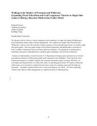
Censored, Sample Selected,and Truncated VariablesSampleCensoredSampleSelectedTruncatedy variabley is known only ifsome criterion df.in terms of y ismet.y is observed onlyif a criteria df. interms of anothervariable (Z) is met.y is known only ifsome criterion df.In terms of y ismet.x variablesx variables areobserved for theentire sample.x and w areobserved for theentire sample.x variables areobserved only if y isobserved.26