Project: 2D Stokes equations and geodynamic deformation

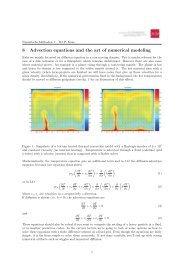
Numerische Methoden 1 – B.J.P. KausProject: 2D Stokes equations and geodynamic deformationIntroductionThe basis of basically all mantle convection and lithospheric dynamics codes are the so called Stokesequations for slowly moving viscous fluids. Here we will describe the governing equations. There areseveral ways to solve those equations, and the goal of this project is to use a staggered finite differenceapproach in primitive variables. In normal words: we solve the governing equations for v x , v z (velocities)and P (pressure). Staggered finite differences means that the different unknowns v x , v z , P are definedat physically different grid points. The main challenges of this project are (1) having several variablesinstead of only one (like e.g. temperature) and (2) do the bookkeeping for the present case that thevariables are at different grid points.Governing equationsIt is assumed that the rheology is incompressible and that the rheology is Newtonian viscous. In thiscase, the governing equations are (see equation cheat sheet):∂σ xz∂x∂v x∂x + ∂v z∂z∂σ xx∂x+ ∂σ zz∂z+ ∂σ xz∂z= 0 (1)= 0 (2)− ρg = 0 (3)σ xx = −P + 2µ ∂v x∂xσ zz = −P + 2µ ∂v z(∂z∂vxσ xz = µ∂z + ∂v )z∂xIt has been suggested that a particular nice way to solve these equations is to use a staggered grid(more about this later) and to keep as variables v x , v z and P . Since there are three variables, we needthree equations. Substituting eqns. 4-6 into 2 and 3 leads to:(4)(5)(6)− ∂P∂x + 2 ∂ (∂x− ∂P∂z + 2 ∂ ∂zµ ∂v )x+ ∂ (µ∂x ∂z(µ ∂v )z+ ∂ (µ∂z ∂x∂v x∂x + ∂v z∂z( ))∂vx∂z + ∂v z∂x( ∂vx∂z + ∂v ))z∂x= P γ(7)= 0 (8)= ρg (9)Note that we added the term P γto the incompressibility equations. This is a ’trick’ called the penaltymethod, which ensures that the system of equations does not become ill-posed. For this to work, γshould be sufficiently large (∼ 10 4 or so).Exercise1. Discretize the equations (7-9) on a staggered grid as shown on fig. 1.1

Numerische Methoden 1 – B.J.P. KausBoundary5/23/21/2-1/2Fictious boundary pointsFigure 2: Staggered grid definition with the boundary points. Within the purple domain, the finitedifference scheme for center points can be applied. At the boundaries around, we have to apply specialboundary finite difference scheme’s, which employ fictious boundary nodes to correctly set the boundaryequations.3

Numerische Methoden 1 – B.J.P. Kaus%Staggered_Stokes%% Solve the 2D Stokes equations on a staggered grid, using the Vx,Vz,P% formulation.%clear% Material properties% phase #1 phase #2mu_vec = [1 1 ];rho_vec = [1 2 ];% Input parametersNx = 20;Nz = .9*Nx;W = 1;H = 1;g = 1;% Setup the interfacex_int = 0:.01:W;z_int = cos(x_int*2*pi/W)*1e-2 - 0.5;% Setup the grids----------------------------------------------------------dz = H/(Nz-1);dx = W/(Nx-1);[X2d,Z2d] = meshgrid(0:dx:W,-H:dz:0);% Vx-gridXVx = [X2d(2:end,:) + X2d(1:end-1,:)]/2;ZVx = [Z2d(2:end,:) + Z2d(1:end-1,:)]/2;% Vz-gridXVz = [X2d(:,2:end) + X2d(:,1:end-1)]/2;ZVz = [Z2d(:,2:end) + Z2d(:,1:end-1)]/2;% P-gridXP = [X2d(2:end,2:end) + X2d(1:end-1,1:end-1)]/2;ZP = [Z2d(2:end,2:end) + Z2d(1:end-1,1:end-1)]/2;%--------------------------------------------------------------------------% Compute material properties from interface-------------------------------% Properties are computed in the center of a control volumeRho = ones(Nz-1,Nx-1)*rho_vec(2);Mu = ones(Nz-1,Nx-1)*mu_vec(2);z_int_intp = interp1(x_int,z_int,XP(1,:));for ix = 1:length(z_int_intp)ind = find(ZVz(:,1)

Numerische Methoden 1 – B.J.P. Kausfunction [ind_list,ind_val] = Add_coeffs(ind_list,ind_val,ind_add,val_add)% Add coefficients to an array%if (length(val_add(:))==1)val_add = ones(size(ind_add))*val_add;endind_list = [ind_list, ind_add(:)];ind_val = [ind_val , val_add(:)];Figure 4: MATLAB script Add coeffs.m, used by Staggered Stokes.m.5