Maxwell SV Getting Started: A 2D Magnetostatic Problem - LES
Maxwell SV Getting Started: A 2D Magnetostatic Problem - LES
Maxwell SV Getting Started: A 2D Magnetostatic Problem - LES

You also want an ePaper? Increase the reach of your titles
YUMPU automatically turns print PDFs into web optimized ePapers that Google loves.
November 2002<br />
<strong>Maxwell</strong> ® <strong>2D</strong><br />
Student Version<br />
A <strong>2D</strong> <strong>Magnetostatic</strong> <strong>Problem</strong><br />
�
Notice<br />
The information contained in this document is subject to change without notice.<br />
Ansoft makes no warranty of any kind with regard to this material, including, but not limited to, the<br />
implied warranties of merchantability and fitness for a particular purpose. Ansoft shall not be liable<br />
for errors contained herein or for incidental or consequential damages in connection with the furnishing,<br />
performance, or use of this material.<br />
This document contains proprietary information which is protected by copyright. All rights are<br />
reserved.<br />
Ansoft Corporation<br />
Four Station Square�<br />
Suite 200�<br />
Pittsburgh, PA 15219�<br />
(412) 261 - 3200<br />
Microsoft ® Windows ® is a registered trademark of Microsoft Corporation.<br />
UNIX� is a registered trademark of UNIX Systems Laboratories, Inc.<br />
<strong>Maxwell</strong>� is a registered trademark of Ansoft Corporation.<br />
© Copyright 1993-2002 Ansoft Corporation
Printing History<br />
<strong>Getting</strong> <strong>Started</strong>: A <strong>2D</strong> <strong>Magnetostatic</strong> <strong>Problem</strong><br />
New editions of this manual incorporate all material updated since the previous edition. The manual<br />
printing date, which indicates the manual’s current edition, changes when a new edition is<br />
printed. Minor corrections and updates which are incorporated at reprint do not cause the date to<br />
change.<br />
Update packages, which may contain additional and/or replacement pages for you to merge into the<br />
manual, may be issued between editions. Pages that are rearranged due to changes on a previous<br />
page are not considered to be revised.<br />
Edition Date<br />
Software<br />
Revision<br />
1 May 2001 8.1<br />
2 November 2002 9.0<br />
iii
<strong>Getting</strong> <strong>Started</strong>: A <strong>2D</strong> <strong>Magnetostatic</strong> <strong>Problem</strong><br />
Installation<br />
<strong>Getting</strong> <strong>Started</strong><br />
iv<br />
Before you use <strong>Maxwell</strong> <strong>SV</strong>, you must:<br />
1. Set up your system’s graphical windowing system.<br />
2. Install the Ansoft software, using the directions in the Ansoft PC Installation Guide.<br />
If you have not yet done these steps, refer to the Ansoft installation guides and the documentation<br />
that came with your computer system, or ask your system administrator for assistance.<br />
If you are using <strong>Maxwell</strong> <strong>SV</strong> for the first time, the following two guides are available for the Student<br />
Version of <strong>Maxwell</strong> <strong>2D</strong>:<br />
• <strong>Getting</strong> <strong>Started</strong>: A <strong>2D</strong> Electrostatic <strong>Problem</strong><br />
• <strong>Getting</strong> <strong>Started</strong>: A <strong>2D</strong> <strong>Magnetostatic</strong> <strong>Problem</strong><br />
Additional <strong>Getting</strong> <strong>Started</strong> guides are available for the standard version of <strong>Maxwell</strong> <strong>2D</strong>.<br />
These short tutorials guide you through the process of setting up and solving simple problems in<br />
<strong>Maxwell</strong> <strong>SV</strong>, providing you with an overview of how to use the software.<br />
Other References<br />
To start <strong>Maxwell</strong> <strong>SV</strong>, you must first access the <strong>Maxwell</strong> Control Panel.<br />
For information on all <strong>Maxwell</strong> Control Panel and <strong>Maxwell</strong> <strong>SV</strong> commands, refer to the following<br />
online documentation:<br />
• <strong>Maxwell</strong> Control Panel online help. The Control panel online help contains a detailed<br />
description of all of the commands in the <strong>Maxwell</strong> Control Panel and in the Utilities Panel.<br />
The <strong>Maxwell</strong> Control Panel allows you to create and open projects, print screens, and<br />
translate files. The Utilities Panel is accessible through the <strong>Maxwell</strong> Control Panel and<br />
enables you to view licensing information, adjust colors, open and create <strong>2D</strong> models, open<br />
and create plots using parametric equations, and evaluate mathematical expressions.<br />
• <strong>Maxwell</strong> <strong>2D</strong> online help. The <strong>Maxwell</strong> <strong>2D</strong> online help contains a detailed description of<br />
the <strong>Maxwell</strong> <strong>2D</strong> software and the Parametric Analysis module. <strong>Maxwell</strong> <strong>SV</strong> does not provide<br />
parametric capabilities.
Typeface Conventions<br />
<strong>Getting</strong> <strong>Started</strong>: A <strong>2D</strong> <strong>Magnetostatic</strong> <strong>Problem</strong><br />
Field Names Bold type is used for on-screen prompts, field names, and messages.<br />
Keyboard Entries Bold type is used for entries that must be entered as specified.<br />
Example: Enter 0.005 in the Nonlinear Residual field.<br />
Menu Commands Bold type is used to display menu commands selected to perform a<br />
specific task. Menu levels are separated by a carat.<br />
Example 1: The instruction “Click File>Open” means to select the<br />
Open command on the File menu within an application.<br />
Example 2: The instruction “Click Define Model>Draw Model”<br />
means to select the Draw Model command from the Define Model<br />
button on the <strong>Maxwell</strong> <strong>SV</strong> Executive Commands menu.<br />
Variable Names Italic type is used for keyboard entries when a name or variable must<br />
be typed in place of the words in italics.<br />
Example: The instruction “copy filename” means to type the word<br />
copy, to type a space, and then to type the name of a file, such as<br />
file1.<br />
Emphasis and<br />
Titles<br />
Italic type is used for emphasis and for the titles of manuals and<br />
other publications.<br />
Keyboard Keys Bold type, in Arial font, is used for labeled keys on the computer<br />
keyboard.<br />
Example: The instruction “Press Return” means to press the key on<br />
the computer that is labeled Return.<br />
v
<strong>Getting</strong> <strong>Started</strong>: A <strong>2D</strong> <strong>Magnetostatic</strong> <strong>Problem</strong><br />
vi
Table of Contents<br />
1. Introduction . . . . . . . . . . . . . . . . . . . . . . . . . . . . . . . . . . 1-1<br />
The Sample <strong>Problem</strong> . . . . . . . . . . . . . . . . . . . . . . . . . . . . . . . . . . . . . . . . . 1-2<br />
General Procedure for Creating and Solving a <strong>2D</strong> Model . . . . . . . . . . . . . 1-3<br />
Goals . . . . . . . . . . . . . . . . . . . . . . . . . . . . . . . . . . . . . . . . . . . . . . . . . . . . . 1-5<br />
2. Creating the Project . . . . . . . . . . . . . . . . . . . . . . . . . . . 2-1<br />
Access the Control Panel . . . . . . . . . . . . . . . . . . . . . . . . . . . . . . . . . . . . . . 2-2<br />
Start the Project Manager . . . . . . . . . . . . . . . . . . . . . . . . . . . . . . . . . . . . . 2-2<br />
Create a Project Directory . . . . . . . . . . . . . . . . . . . . . . . . . . . . . . . . . . . . 2-3<br />
Create a New Project . . . . . . . . . . . . . . . . . . . . . . . . . . . . . . . . . . . . . . . . . 2-4<br />
Access the Project Directory . . . . . . . . . . . . . . . . . . . . . . . . . . . . . . . . . . 2-4<br />
Add the New Project . . . . . . . . . . . . . . . . . . . . . . . . . . . . . . . . . . . . . . . . 2-4<br />
Save Project Notes . . . . . . . . . . . . . . . . . . . . . . . . . . . . . . . . . . . . . . . . . . 2-5<br />
Open the New Project and Run <strong>Maxwell</strong> <strong>SV</strong> . . . . . . . . . . . . . . . . . . . . . . 2-6<br />
Overview of the Executive Commands Window . . . . . . . . . . . . . . . . . . . 2-7<br />
Executive Commands Menu . . . . . . . . . . . . . . . . . . . . . . . . . . . . . . . . . . 2-7<br />
Display Area . . . . . . . . . . . . . . . . . . . . . . . . . . . . . . . . . . . . . . . . . . . . . . 2-7<br />
3. Creating the Model . . . . . . . . . . . . . . . . . . . . . . . . . . . . 3-1<br />
Define Model Type . . . . . . . . . . . . . . . . . . . . . . . . . . . . . . . . . . . . . . . . . . 3-2<br />
Select the Solver Type . . . . . . . . . . . . . . . . . . . . . . . . . . . . . . . . . . . . . . . 3-2<br />
Define the Drawing Plane . . . . . . . . . . . . . . . . . . . . . . . . . . . . . . . . . . . . 3-2<br />
Access the <strong>2D</strong> Modeler . . . . . . . . . . . . . . . . . . . . . . . . . . . . . . . . . . . . . . . 3-3<br />
Screen Layout . . . . . . . . . . . . . . . . . . . . . . . . . . . . . . . . . . . . . . . . . . . . . 3-3<br />
The Solenoid Model . . . . . . . . . . . . . . . . . . . . . . . . . . . . . . . . . . . . . . . . . . 3-5<br />
Contents-1
<strong>Getting</strong> <strong>Started</strong>: A <strong>2D</strong> <strong>Magnetostatic</strong> <strong>Problem</strong><br />
Set Up the Drawing Region . . . . . . . . . . . . . . . . . . . . . . . . . . . . . . . . . . . . 3-6<br />
Change the Drawing Size . . . . . . . . . . . . . . . . . . . . . . . . . . . . . . . . . . . . . 3-7<br />
Change Grid Spacing . . . . . . . . . . . . . . . . . . . . . . . . . . . . . . . . . . . . . . . . . 3-8<br />
Create the Geometry . . . . . . . . . . . . . . . . . . . . . . . . . . . . . . . . . . . . . . . . . 3-9<br />
Draw the Plugnut . . . . . . . . . . . . . . . . . . . . . . . . . . . . . . . . . . . . . . . . . . . . 3-9<br />
Create a Rectangle . . . . . . . . . . . . . . . . . . . . . . . . . . . . . . . . . . . . . . . . . . 3-9<br />
Change the Plugnut’s Name and Color . . . . . . . . . . . . . . . . . . . . . . . . . . 3-10<br />
Keyboard Entry . . . . . . . . . . . . . . . . . . . . . . . . . . . . . . . . . . . . . . . . . . . . . 3-10<br />
Draw the Core . . . . . . . . . . . . . . . . . . . . . . . . . . . . . . . . . . . . . . . . . . . . . . 3-11<br />
Draw the Coil . . . . . . . . . . . . . . . . . . . . . . . . . . . . . . . . . . . . . . . . . . . . . . . 3-12<br />
Save the Geometry . . . . . . . . . . . . . . . . . . . . . . . . . . . . . . . . . . . . . . . . . . 3-13<br />
Draw the Yoke . . . . . . . . . . . . . . . . . . . . . . . . . . . . . . . . . . . . . . . . . . . . . . 3-13<br />
Draw the Bonnet . . . . . . . . . . . . . . . . . . . . . . . . . . . . . . . . . . . . . . . . . . . . 3-14<br />
Completed Geometry . . . . . . . . . . . . . . . . . . . . . . . . . . . . . . . . . . . . . . . . . 3-14<br />
Exit the <strong>2D</strong> Modeler . . . . . . . . . . . . . . . . . . . . . . . . . . . . . . . . . . . . . . . . . 3-15<br />
4. Setting Up the Model . . . . . . . . . . . . . . . . . . . . . . . . . . . 4-1<br />
Assign Materials to Objects . . . . . . . . . . . . . . . . . . . . . . . . . . . . . . . . . . . 4-2<br />
Access Material Manager . . . . . . . . . . . . . . . . . . . . . . . . . . . . . . . . . . . . . 4-2<br />
Assign Copper to the Coil . . . . . . . . . . . . . . . . . . . . . . . . . . . . . . . . . . . . 4-3<br />
Assign Cold Rolled Steel to the Bonnet and Yoke . . . . . . . . . . . . . . . . . 4-3<br />
Assign Neo35 to the Core . . . . . . . . . . . . . . . . . . . . . . . . . . . . . . . . . . . . 4-7<br />
Assign SS430 to the Plugnut . . . . . . . . . . . . . . . . . . . . . . . . . . . . . . . . . . 4-10<br />
Accept Default Material for Background . . . . . . . . . . . . . . . . . . . . . . . . . 4-12<br />
Exit the Material Manager . . . . . . . . . . . . . . . . . . . . . . . . . . . . . . . . . . . . 4-12<br />
Set Up Boundaries and Current Sources . . . . . . . . . . . . . . . . . . . . . . . . . . 4-12<br />
Access the <strong>2D</strong> Boundary/Source Manager . . . . . . . . . . . . . . . . . . . . . . . 4-13<br />
Boundary Manager Screen Layout . . . . . . . . . . . . . . . . . . . . . . . . . . . . . 4-13<br />
Types of Boundary Conditions and Sources . . . . . . . . . . . . . . . . . . . . . . 4-14<br />
Set Source Current on the Coil . . . . . . . . . . . . . . . . . . . . . . . . . . . . . . . . 4-14<br />
Assign Balloon Boundary to the Background . . . . . . . . . . . . . . . . . . . . . 4-15<br />
Exit the Boundary Manager . . . . . . . . . . . . . . . . . . . . . . . . . . . . . . . . . . . 4-16<br />
Set Up Force Computation . . . . . . . . . . . . . . . . . . . . . . . . . . . . . . . . . . . . 4-16<br />
5. Generating a Solution . . . . . . . . . . . . . . . . . . . . . . . . . . 5-1<br />
Contents-2<br />
View Solution Criteria . . . . . . . . . . . . . . . . . . . . . . . . . . . . . . . . . . . . . . . . 5-2<br />
Starting Mesh . . . . . . . . . . . . . . . . . . . . . . . . . . . . . . . . . . . . . . . . . . . . . . 5-2<br />
Manual Mesh . . . . . . . . . . . . . . . . . . . . . . . . . . . . . . . . . . . . . . . . . . . . . . 5-2<br />
Solver Choice . . . . . . . . . . . . . . . . . . . . . . . . . . . . . . . . . . . . . . . . . . . . . . 5-3<br />
Solver Residual . . . . . . . . . . . . . . . . . . . . . . . . . . . . . . . . . . . . . . . . . . . . 5-3
<strong>Getting</strong> <strong>Started</strong>: A <strong>2D</strong> <strong>Magnetostatic</strong> <strong>Problem</strong><br />
Solve for Fields and Parameters . . . . . . . . . . . . . . . . . . . . . . . . . . . . . . . . 5-3<br />
Adaptive Analysis . . . . . . . . . . . . . . . . . . . . . . . . . . . . . . . . . . . . . . . . . . 5-3<br />
Exit Setup Solution Options . . . . . . . . . . . . . . . . . . . . . . . . . . . . . . . . . . . 5-3<br />
Start the Solution . . . . . . . . . . . . . . . . . . . . . . . . . . . . . . . . . . . . . . . . . . . 5-4<br />
Monitoring the Solution . . . . . . . . . . . . . . . . . . . . . . . . . . . . . . . . . . . . . . . 5-4<br />
Viewing Convergence Data . . . . . . . . . . . . . . . . . . . . . . . . . . . . . . . . . . . . 5-5<br />
Solution Criteria . . . . . . . . . . . . . . . . . . . . . . . . . . . . . . . . . . . . . . . . . . . . 5-5<br />
Completed Solutions . . . . . . . . . . . . . . . . . . . . . . . . . . . . . . . . . . . . . . . . 5-6<br />
Completing the Solution Process . . . . . . . . . . . . . . . . . . . . . . . . . . . . . . . . 5-6<br />
Viewing Final Convergence Data . . . . . . . . . . . . . . . . . . . . . . . . . . . . . . . 5-7<br />
Plotting Convergence Data . . . . . . . . . . . . . . . . . . . . . . . . . . . . . . . . . . . 5-8<br />
Viewing Statistics . . . . . . . . . . . . . . . . . . . . . . . . . . . . . . . . . . . . . . . . . . 5-9<br />
6. Analyzing the Solution . . . . . . . . . . . . . . . . . . . . . . . . . 6-1<br />
View Force Solution . . . . . . . . . . . . . . . . . . . . . . . . . . . . . . . . . . . . . . . . . 6-2<br />
Access the Post Processor . . . . . . . . . . . . . . . . . . . . . . . . . . . . . . . . . . . . . 6-2<br />
Post Processor Screen Layout . . . . . . . . . . . . . . . . . . . . . . . . . . . . . . . . . . 6-3<br />
General Areas . . . . . . . . . . . . . . . . . . . . . . . . . . . . . . . . . . . . . . . . . . . . . 6-3<br />
Plot the Magnetic Field . . . . . . . . . . . . . . . . . . . . . . . . . . . . . . . . . . . . . . . 6-3<br />
Redisplay the Magnetic FIeld Plot . . . . . . . . . . . . . . . . . . . . . . . . . . . . . . 6-5<br />
Identify Saturated Materials . . . . . . . . . . . . . . . . . . . . . . . . . . . . . . . . . . . 6-6<br />
Plot Magnetic Flux Density . . . . . . . . . . . . . . . . . . . . . . . . . . . . . . . . . . . 6-6<br />
Plot the B-H Curve . . . . . . . . . . . . . . . . . . . . . . . . . . . . . . . . . . . . . . . . . . 6-8<br />
Exit the Post Processor . . . . . . . . . . . . . . . . . . . . . . . . . . . . . . . . . . . . . . . 6-9<br />
Exit <strong>Maxwell</strong> <strong>SV</strong> . . . . . . . . . . . . . . . . . . . . . . . . . . . . . . . . . . . . . . . . . . . . 6-9<br />
Exit the <strong>Maxwell</strong> Software . . . . . . . . . . . . . . . . . . . . . . . . . . . . . . . . . . . . 6-9<br />
Contents-3
<strong>Getting</strong> <strong>Started</strong>: A <strong>2D</strong> <strong>Magnetostatic</strong> <strong>Problem</strong><br />
Contents-4
Introduction<br />
This guide is a tutorial for setting up a magnetostatic problem using version 9.0 of <strong>Maxwell</strong> <strong>2D</strong> Student<br />
Version (<strong>SV</strong>), a software package for analyzing electromagnetic fields in cross-sections of<br />
structures. <strong>Maxwell</strong> <strong>SV</strong> uses finite element analysis (FEA) to solve two-dimensional (<strong>2D</strong>) electromagnetic<br />
problems.<br />
To analyze a problem, you need to specify the appropriate geometry, material properties, and excitations<br />
for a device or system of devices. The <strong>Maxwell</strong> software then does the following:<br />
• Automatically creates the required finite element mesh.<br />
• Calculates the desired electric or magnetic field solution and special quantities of interest,<br />
such as force, torque, inductance, capacitance, or power loss. You can select any of the<br />
following solution types: Electrostatic, <strong>Magnetostatic</strong>, Electrostatic, Eddy Current, DC<br />
Conduction, AC Conduction, Eddy Axial. The student version does not contain thermal,<br />
transient, or parametric capabilities.<br />
• Allows you to analyze, manipulate, and display field solutions.<br />
Many models are actually a collection of three-dimensional (3D) objects. <strong>Maxwell</strong> <strong>SV</strong> analyzes a<br />
<strong>2D</strong> cross-section of the model, then generates a solution for that cross-section, using FEA to solve<br />
the problem. Dividing a structure into many smaller regions (finite elements) allows the system to<br />
compute the field solution separately in each element. The smaller the elements, the more accurate<br />
the final solution.<br />
Introduction 1-1
<strong>Getting</strong> <strong>Started</strong>: A <strong>2D</strong> <strong>Magnetostatic</strong> <strong>Problem</strong><br />
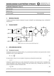
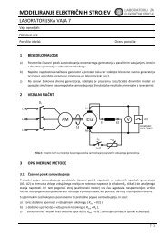
The Sample <strong>Problem</strong><br />
The sample problem, shown below, is a solenoid that consists of the following objects:<br />
• Core<br />
• Bonnet<br />
• Coil<br />
• Yoke<br />
• Plugnut<br />
CORE<br />
COIL<br />
BONNET<br />
The <strong>2D</strong> diagram above actually represents a 3D structure that has been revolved around an axis of<br />
symmetry, as shown in the figure below. In this figure, part of the 3D model has been cut away so<br />
that you can see the interior of the solenoid.<br />
Since the cross-section of the solenoid is constant, it can be modeled as an axisymmetric model in<br />
<strong>Maxwell</strong> <strong>SV</strong>.<br />
1-2 Introduction<br />
YOKE<br />
PLUGNUT<br />
BACKGROUND
<strong>Getting</strong> <strong>Started</strong>: A <strong>2D</strong> <strong>Magnetostatic</strong> <strong>Problem</strong><br />
General Procedure for Creating and Solving a <strong>2D</strong> Model<br />
The general procedure to follow when using the software to create and solve a <strong>2D</strong> problem is given<br />
below:<br />
1. Use the Solver command to specify which of the following electric or magnetic field quantities<br />
to compute:<br />
• Electrostatic<br />
• <strong>Magnetostatic</strong><br />
• Eddy Current<br />
• DC Conduction<br />
• AC Conduction<br />
• Eddy Axial<br />
2. Use the Drawing command to select one of the following model planes:<br />
XY Plane Cartesian models appear to sweep perpendicularly to the cross-section.<br />
RZ Plane Axisymmetric models appear to revolve around an axis of symmetry in the<br />
cross-section.<br />
3. Use the Define Model commands to create the geometric model. When you click Define<br />
Model, the following menu appears:<br />
Draw Model Allows you to access the <strong>2D</strong> Modeler and build the objects that make<br />
up the geometric model.<br />
Group ObjectsAllows you to group discrete objects that are actually one electrical<br />
object. For instance, two terminations of a conductor that are drawn as<br />
separate objects in the cross-section can be grouped to represent one<br />
conductor.<br />
4. Use the Setup Materials command to assign materials to all objects in the geometric model.<br />
5. Use the Setup Boundaries/Sources command to define the boundaries and sources for the<br />
problem. This determines the electromagnetic excitations and field behavior for the model.<br />
6. Use the Setup Executive Parameters command to instruct the simulator to compute one or<br />
more of the following special quantities during the solution process:<br />
• Matrix (capacitance, inductance, admittance, impedance, or conductance matrix, depending<br />
on the selected solver).<br />
• Force<br />
• Torque<br />
• Flux lines<br />
• Post Processor macros<br />
• Core loss<br />
• Current flow<br />
7. Use the Setup Solution Options command to enter parameters that affect how the solution is<br />
computed.<br />
Introduction 1-3
<strong>Getting</strong> <strong>Started</strong>: A <strong>2D</strong> <strong>Magnetostatic</strong> <strong>Problem</strong><br />
8. Use the Solve command to solve for the appropriate field quantities.<br />
9. Use the Post Process command to analyze the solution.<br />
These commands must be chosen in the sequence in which they appear. You must first create a geometric<br />
model using the Define Model command before you specify material characteristics for<br />
objects using the Setup Materials command. A check mark appears on the menu next to each step<br />
which has been completed.<br />
Select solver and drawing plane.<br />
Draw geometric model and<br />
(optionally) identify grouped objects.<br />
Assign material properties.<br />
1-4 Introduction<br />
Assign boundary conditions and sources.<br />
Compute other<br />
quantities during<br />
solution?<br />
No<br />
Set up solution criteria and<br />
(optionally) refine the mesh.<br />
Generate solution.<br />
Yes<br />
Inspect parameter solutions; view<br />
solution information; display plots of<br />
fields and manipulate basic field<br />
quantities.<br />
Request that force, torque,<br />
capacitance, inductance,<br />
admittance, impedance, flux<br />
linkage, core loss, conductance,<br />
or current flow be computed<br />
during the solution process.
<strong>Getting</strong> <strong>Started</strong>: A <strong>2D</strong> <strong>Magnetostatic</strong> <strong>Problem</strong><br />
Goals The goals in <strong>Getting</strong> <strong>Started</strong>: A <strong>2D</strong> <strong>Magnetostatic</strong> <strong>Problem</strong> are as follows:<br />
• Determine the force on the core due to the source current in the coil.<br />
• Determine whether any of the nonlinear materials reach their saturation point.<br />
Do the following to accomplish these goals:<br />
1. Draw the plugnut, core, coil, yoke, and bonnet using the Draw Model command under Define<br />
Model.<br />
2. Define materials using the Setup Materials command.<br />
3. Define boundary conditions and current sources using the Setup Boundaries/Sources command.<br />
4. Request that the force on the core be computed, using the Setup Executive Parameters command.<br />
5. Specify solution criteria and generate a solution using the Setup Solution Parameters and<br />
Solve commands. You will compute both a magnetostatic field solution and the force on the<br />
core.<br />
6. View the results of the force computation, using the Solutions>Force command.<br />
7. Plot saturation levels and contours of equal magnetic potential via the Post Process command.<br />
This simple problem illustrates the most commonly used features of <strong>Maxwell</strong> <strong>SV</strong>.<br />
Time This guide should take approximately 3 hours to work through.<br />
Introduction 1-5
<strong>Getting</strong> <strong>Started</strong>: A <strong>2D</strong> <strong>Magnetostatic</strong> <strong>Problem</strong><br />
1-6 Introduction
Creating the Project<br />
This guide assumes that <strong>Maxwell</strong> <strong>SV</strong> has already been installed as described in the Ansoft PC<br />
Installation Guide.<br />
The goals for this chapter are to:<br />
• Create a project directory in which to save sample problems.<br />
• Create a new project in that directory in which to save the solenoid problem.<br />
• Open the project and run <strong>Maxwell</strong> <strong>SV</strong>.<br />
This chapter also includes a description of the sample problem and your goals for solving it.<br />
Time This chapter should take approximately 15 minutes to work through.<br />
Creating the Project 2-1
<strong>Getting</strong> <strong>Started</strong>: A <strong>2D</strong> <strong>Magnetostatic</strong> <strong>Problem</strong><br />
Access the Control Panel<br />
The <strong>Maxwell</strong> Control Panel allows you to create and open projects and directly access program<br />
modules shared by Ansoft products. You must start the Control Panel in order to start <strong>Maxwell</strong> <strong>SV</strong>.<br />
To start the <strong>Maxwell</strong> Control Panel, do one of the following:<br />
• Use the Start menu to select Programs>Ansoft><strong>Maxwell</strong> <strong>SV</strong>.<br />
• Double-click the <strong>Maxwell</strong> <strong>SV</strong> icon.<br />
The <strong>Maxwell</strong> Control Panel appears.<br />
If the <strong>Maxwell</strong> Control Panel does not appear, see the Ansoft installation guides for possible reasons.<br />
See the online help on the <strong>Maxwell</strong> Control Panel for a detailed description of other control<br />
panel options.<br />
Start the Project Manager<br />
Use the Project Manager to create, rename, or delete project files and to access projects created<br />
with other Ansoft products.<br />
To display the Project Manager, click PROJECTS in the <strong>Maxwell</strong> Control Panel. The Project<br />
Manager appears.<br />
2-2 Creating the Project
Create a Project Directory<br />
<strong>Getting</strong> <strong>Started</strong>: A <strong>2D</strong> <strong>Magnetostatic</strong> <strong>Problem</strong><br />
A project directory contains a specific set of projects created with Ansoft software. You can use<br />
project directories to categorize projects. For example, you might want to store all projects related<br />
to a particular application in one project directory. You will add the getting_started_<strong>SV</strong> directory<br />
for the <strong>Maxwell</strong> project you create using this <strong>Getting</strong> <strong>Started</strong> guide.<br />
Note If you have already created a project directory while working through another <strong>Getting</strong><br />
<strong>Started</strong> guide, such as <strong>Getting</strong> <strong>Started</strong>: An Electrostatic <strong>Problem</strong>, use the same directory<br />
and skip to the “Create the Solenoid Project” section.<br />
To add a project directory, do the following in the Project Manager:<br />
1. Click Add from the Project Directories area at the lower-left corner of the window. The Add<br />
a new project directory window appears, listing the directories and subdirectories.<br />
2. Type the following in the Alias field:<br />
getting_started_<strong>SV</strong><br />
<strong>Maxwell</strong> <strong>SV</strong> projects are usually created in directories which have aliases — that is, directories<br />
that have been identified as project directories using the Add command.<br />
3. Select Make New Directory near the bottom of the window. The name you entered as the<br />
alias automatically appears in the field beside this option.<br />
4. Click OK.<br />
You return to the Project Manager menu. The getting_started_<strong>SV</strong> directory is created under the<br />
current default project directory, and getting_started_<strong>SV</strong> now appears in the Project Directories<br />
list.<br />
Creating the Project 2-3
<strong>Getting</strong> <strong>Started</strong>: A <strong>2D</strong> <strong>Magnetostatic</strong> <strong>Problem</strong><br />
Create a New Project<br />
You are now ready to create a new project named solenoid in the getting_started_<strong>SV</strong> project<br />
directory.<br />
Access the Project Directory<br />
Before you create the new project, select getting_started_<strong>SV</strong> from the Project Directories list at<br />
the bottom left of the menu.<br />
The current directory displayed at the top of the Project Manager menu changes to show the path<br />
name of the directory associated with the getting_started_<strong>SV</strong> alias. If you have previously created<br />
the microstrip model, it will be listed in the Projects box. Otherwise, the Projects box is empty —<br />
no projects have been created yet in the getting_started_<strong>SV</strong> project directory.<br />
Add the New Project<br />
To add the new project:<br />
1. Click New in the Projects box at the top left of the menu. The Enter project name and select<br />
project type window appears.<br />
2. Enter solenoid in the Name field.<br />
3. Select the type of project to be created.<br />
a. To display all available project types, click the button next to the Type field. A menu<br />
appears, listing all Ansoft software packages that have been installed.<br />
b. Click <strong>Maxwell</strong> <strong>SV</strong> Version 9.<br />
4. Optionally, enter your name in the Created By field. The name of the person who logged onto<br />
the system appears by default.<br />
5. Deselect Open Project Upon Creation. You do not want to automatically open the project at<br />
this point, so that you may enter project notes first.<br />
6. Click OK. The information you just entered appears in the corresponding fields in the Selected<br />
Project box. Because you created the project, Writeable is selected, showing that you have<br />
access to the project.<br />
2-4 Creating the Project
Save Project Notes<br />
<strong>Getting</strong> <strong>Started</strong>: A <strong>2D</strong> <strong>Magnetostatic</strong> <strong>Problem</strong><br />
It is a good idea to save a description of your new project so that next time you can view information<br />
about the project without opening it.<br />
To enter a description of the project:<br />
1. Leave the Notes radio button selected; this is the default.<br />
2. Click in the Notes area. The cursor changes to an I-beam in the upper-left corner of the Notes<br />
box, indicating that you can begin typing text.<br />
3. Enter a description of the project. �<br />
For example, enter the following text:<br />
This sample magnetostatic problem was created using <strong>Maxwell</strong><br />
<strong>SV</strong> and the magnetostatic <strong>Getting</strong> <strong>Started</strong> guide.<br />
After you begin entering text, the text of the Save Notes button that appears below the Notes<br />
box now becomes black, indicating that it is enabled. Before you began typing in the Notes<br />
box, Save Notes was grayed out, or disabled.<br />
4. When you are done entering the description, click Save Notes. After you do, the Save Notes<br />
button is disabled again.<br />
Note Grayed out text on commands or buttons means that the command or button is<br />
temporarily disabled.<br />
Creating the Project 2-5
<strong>Getting</strong> <strong>Started</strong>: A <strong>2D</strong> <strong>Magnetostatic</strong> <strong>Problem</strong><br />
Open the New Project and Run <strong>Maxwell</strong> <strong>SV</strong><br />
The newly created project solenoid should still be selected in the Projects list. (If it is not, simply<br />
select it.) Now you are ready to run <strong>Maxwell</strong> <strong>SV</strong>.<br />
To start <strong>Maxwell</strong> <strong>SV</strong>, click Open in the Project window. The Executive Commands menu of<br />
<strong>Maxwell</strong> <strong>SV</strong> appears.<br />
2-6 Creating the Project
Overview of the Executive Commands Window<br />
<strong>Getting</strong> <strong>Started</strong>: A <strong>2D</strong> <strong>Magnetostatic</strong> <strong>Problem</strong><br />
The Executive Commands window acts as a path to each step of creating and solving the model<br />
problem. You select each module through the Executive Commands menu, and the software<br />
brings you back to this menu when you are finished. You also view the solution process through<br />
this menu.<br />
The Executive Commands window is divided into two major sections: the Executive Commands<br />
menu and a Display area.<br />
Executive Commands Menu<br />
The Executive Commands menu on the left side of the screen let you define the type of problem<br />
you are solving and then call up the various modules you will need to create and solve the problem.<br />
The function of each button is explained under “General Procedure for Creating and Solving a <strong>2D</strong><br />
Model” on page 1-3.<br />
Display Area<br />
The display area shows the project’s geometry. Since you have not yet drawn the model, this area is<br />
blank. The commands along the bottom of the window allow you to change your view of it as follows:<br />
Zoom In Zooms in on an area of the window, magnifying the view.<br />
Zoom Out Zooms out from an area, shrinking the view.<br />
Fit All Changes the view to display all items in the window. Items<br />
will appear as large as possible without extending beyond<br />
the window.<br />
Fit Drawing Displays the entire drawing space.<br />
Fill Solids Displays objects as solids rather than outlined objects.<br />
Toggles with Wire Frame.<br />
Wire Frame Displays objects as wire-frame outlines. Toggles with Fill<br />
Solids.<br />
This window can also display solution profile and convergence information while the problem is<br />
being solved, as detailed in Chapter 6, “Analyzing the Solution.”<br />
Creating the Project 2-7
<strong>Getting</strong> <strong>Started</strong>: A <strong>2D</strong> <strong>Magnetostatic</strong> <strong>Problem</strong><br />
2-8 Creating the Project
Creating the Model<br />
In the last chapter, you created and opened the solenoid project and reviewed the general procedure<br />
for drawing, setting up, and solving <strong>2D</strong> problems. Now you are ready to use <strong>Maxwell</strong> <strong>SV</strong> to solve<br />
the solenoid problem. This chapter shows you how to select the type of field solution that’s computed<br />
and create the geometry for the solenoid problem that was described in Chapter 1, “Introduction.”<br />
The goals for this chapter are to:<br />
• Define the type of model — which includes selecting the solver type and the drawing<br />
plane.<br />
• Set up the problem region.<br />
• Draw the objects that make up the solenoid model.<br />
• Save the solenoid model.<br />
You are now ready to start using the simulator.<br />
Time This chapter should take approximately 30 minutes to work through.<br />
Creating the Model 3-1
<strong>Getting</strong> <strong>Started</strong>: A <strong>2D</strong> <strong>Magnetostatic</strong> <strong>Problem</strong><br />
Define Model Type<br />
Before you start drawing the model, you need to specify which field quantities to compute and<br />
whether the model will be cartesian (XY plane) or axisymmetric (RZ plane).<br />
Select the Solver Type<br />
<strong>Maxwell</strong> <strong>SV</strong> can compute the following types of field quantities:<br />
Electrostatic Static electric fields.<br />
<strong>Magnetostatic</strong> Static magnetic fields.<br />
Eddy Current Time-varying magnetic fields and eddy currents.<br />
DC Conduction Conduction currents caused by DC voltage differentials.<br />
AC Conduction Conduction currents caused by AC voltage differentials.<br />
Eddy Axial Eddy currents induced by time-varying magnetic fields.<br />
For the solenoid problem, you will compute the static magnetic fields in the device and find the<br />
force on the core due to these fields. Therefore, select <strong>Magnetostatic</strong> as the field solver.<br />
To select the <strong>Magnetostatic</strong> field solver, click Solver><strong>Magnetostatic</strong> on the Executive Commands<br />
menu.<br />
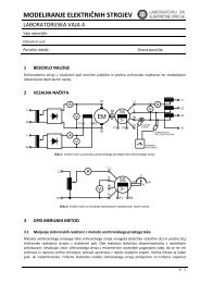
Define the Drawing Plane<br />
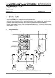
In <strong>Maxwell</strong> <strong>2D</strong> and <strong>SV</strong>, you can choose from two different types of geometric models:<br />
• Cartesian. Visualize a cartesian (XY plane) geometry as a rectangle extending perpendicular<br />
to the plane being modeled.<br />
• Axisymmetric. Visualize an axisymmetric (RZ plane) geometry as a rectangle revolving<br />
around an axis of symmetry, Z.<br />
Both types of geometry are illustrated below.<br />
Geometric Model<br />
Cartesian (XY Plane) Axisymmetric (RZ Plane)<br />
Y<br />
Z<br />
Since it represents a device that is revolved around an axis of symmetry, the solenoid will be drawn<br />
in the RZ plane.<br />
To define the drawing plane, click Drawing>RZ Plane.<br />
3-2 Creating the Model<br />
Z<br />
X<br />
�<br />
R
Access the <strong>2D</strong> Modeler<br />
Use the <strong>2D</strong> Modeler to create the objects in the model.<br />
<strong>Getting</strong> <strong>Started</strong>: A <strong>2D</strong> <strong>Magnetostatic</strong> <strong>Problem</strong><br />
To access the <strong>2D</strong> Modeler:<br />
• Click Define Model>Draw Model from the Executive Commands window. The <strong>2D</strong> Modeler<br />
appears.<br />
Screen Layout<br />
The following sections provide a brief overview of the <strong>2D</strong> Modeler.<br />
Menu Bar<br />
The <strong>2D</strong> Modeler’s menu bar appears at the top of the window. Each item in the menu bar has a<br />
menu of commands associated with it. If a command name has an arrow next to it, that command<br />
also has a menu of commands associated with it. If a command name has an ellipsis next to it, that<br />
command has a window or panel associated with it.<br />
To display the menu associated with a command in the menu bar, do one of the following:<br />
• Click on it.<br />
• Press and hold down the Alt, and then press the key o the underlined letter on the command<br />
name.<br />
For example, to display the Window command’s menu, do one of the following:<br />
• Click on it.<br />
• Press the Alt key, and type a W.<br />
After you click Window, the Window menu appears. Click outside the Window menu to make it<br />
disappear.<br />
Creating the Model 3-3
<strong>Getting</strong> <strong>Started</strong>: A <strong>2D</strong> <strong>Magnetostatic</strong> <strong>Problem</strong><br />
Project Window<br />
The main <strong>2D</strong> Modeler window contains the Drawing Region, the grid-covered area where you<br />
draw the objects that make up your model. This main window in the <strong>2D</strong> Modeler is called the<br />
project window. A project window contains the geometry for a specific project and displays the<br />
project’s name in its title bar. By default, one subwindow is contained within the project window.<br />
Optionally, you can open additional projects in the <strong>2D</strong> Modeler using the File>Open command.<br />
Opening several projects at once is useful if you want to copy objects between geometries. See the<br />
<strong>Maxwell</strong> <strong>2D</strong> online help for more details.<br />
Subwindows<br />
Subwindows are the windows in which you create the objects that make up the geometric model.<br />
By default, this window:<br />
• Has points specified in relation to a local uv coordinate system. The u-axis is horizontal, the vaxis<br />
is vertical, and the origin is marked by a cross in the middle of the screen.<br />
• Uses millimeters as the default drawing unit.<br />
• Has grid points 2 millimeters apart. The default window size is 100 millimeters by 70 millimeters.<br />
Note If a geometry is complex, you may want to open additional subwindows for the same<br />
project so that you can alter your view of the geometry from one subwindow to the next.<br />
To do so, use the Window>New command as described in the <strong>Maxwell</strong> <strong>2D</strong> online help.<br />
For this geometry, however, a single subwindow should be sufficient.<br />
Status Bar<br />
The status bar, which appears at the bottom of the <strong>2D</strong> Modeler screen, displays the following:<br />
U and V Displays the coordinates of the mouse’s position on the screen and allows<br />
you to enter coordinates using the keyboard.<br />
UNITS Drawing units in which the geometry is entered.<br />
SNAPTO Which point — grid point or object vertex — is selected when you<br />
choose points using the mouse. By default, both grid and object points are<br />
selected so that the mouse snaps to whichever one is closest.<br />
Message Bar<br />
A message bar, which appears above the status bar, displays the functions of the left and right<br />
mouse buttons. When selecting or deselecting objects, the message bar displays the number of<br />
items that are currently selected. When you change the view in a subwindow, it displays the current<br />
magnification level.<br />
Toolbar<br />
The toolbar is the vertical stack of icons that appears on the left side of the <strong>2D</strong> Modeler screen.<br />
Icons give you easy access to the most frequently used commands that allow you to draw objects,<br />
change your view of the problem region, deselect objects, and so on. Click an icon and hold the<br />
button down to display a brief description of the command in the message bar at the bottom of the<br />
screen.<br />
For more information on these areas of the <strong>2D</strong> Modeler, refer to the <strong>Maxwell</strong> <strong>2D</strong> online help.<br />
3-4 Creating the Model
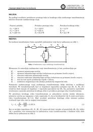
The Solenoid Model<br />
<strong>Getting</strong> <strong>Started</strong>: A <strong>2D</strong> <strong>Magnetostatic</strong> <strong>Problem</strong><br />
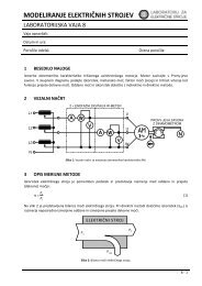
The dimensions of the solenoid that you will be modeling are shown below. Use these dimensions,<br />
which are given in inches, to create the geometric model.<br />
1.35<br />
1.0<br />
0.05<br />
0.15<br />
0.1<br />
0.2<br />
0.3<br />
0.1<br />
0.05<br />
0.05<br />
0.227<br />
0.75<br />
0.05<br />
0.05<br />
The following pages step you through drawing the above model.<br />
1.5<br />
0.4<br />
0.075<br />
0.075<br />
0.2<br />
0.05<br />
1.75<br />
Creating the Model 3-5
<strong>Getting</strong> <strong>Started</strong>: A <strong>2D</strong> <strong>Magnetostatic</strong> <strong>Problem</strong><br />
Set Up the Drawing Region<br />
The first step in using the <strong>2D</strong> Modeler is to specify the drawing units to use in creating the model.<br />
In this case, you must change the units from millimeters to inches.<br />
To set up the drawing region:<br />
1. Click Model>Drawing Units from the menu bar. The Drawing Units window appears.<br />
2. Select Inches.<br />
3. Click the Rescale to new units radio button so the drawing area size will be converted to<br />
inches.<br />
4. Click OK.<br />
The units are changed from millimeters to inches, and inches now appears next to UNITS in the<br />
status bar.<br />
Note Throughout the rest of this guide, all commands will be given as Menu>Command.<br />
For example, the command you just used to change the drawing units would be given<br />
as: Click Model>Drawing Units.<br />
3-6 Creating the Model
Change the Drawing Size<br />
<strong>Getting</strong> <strong>Started</strong>: A <strong>2D</strong> <strong>Magnetostatic</strong> <strong>Problem</strong><br />
Because the size of the solenoid model is relatively small compared to the area now represented on<br />
the screen, you will need to reduce the size of the drawing space.<br />
To change the drawing size:<br />
1. Click Model>Drawing Size. The Drawing Size window appears.<br />
2. The Minima fields set the coordinates for the lower-left corner of the drawing. Change the<br />
Minima coordinates to (0,–4.5) by doing the following:<br />
a. Leave the Minima R value set to 0.<br />
Note Because the simulator assumes that the Z-axis (the left edge of the drawing region)<br />
represents the axis of rotational symmetry in an axisymmetric model, you cannot enter a<br />
value for R that is less than zero.<br />
b. Double-click the left mouse button in the Minima Z field.<br />
c. Type -4.5.<br />
3. The Maxima fields set the coordinates for the upper-right corner of the drawing. Change the<br />
Maxima coordinates, using the procedure you just used to change the Minima coordinates:<br />
a. Change the Maxima R value to 3.<br />
b. Change the Maxima Z value to 4.5.<br />
4. Click OK.<br />
Creating the Model 3-7
<strong>Getting</strong> <strong>Started</strong>: A <strong>2D</strong> <strong>Magnetostatic</strong> <strong>Problem</strong><br />
Change Grid Spacing<br />
The final adjustment that needs to be made in the problem region is setting the spacing between the<br />
grid of points to which the cursor “snaps.” This also sets the visible grid in the subwindow. Because<br />
snap-to-grids is selected, the mouse snaps to the visible grid.<br />
When you changed the drawing units, the <strong>2D</strong> Modeler set the grid spacing to 0.5. This means that<br />
there are 0.5 inches between each grid point. To simplify drawing the solenoid’s geometry, change<br />
the spacing between grid points to 0.05 inches.<br />
To change the grid spacing:<br />
1. Click Window>Grid. The following window appears:<br />
2. Leave CARTESIAN selected. You want a rectangular grid displayed in the window.<br />
3. Change the grid spacing in the dU field to 0.1. This changes the grid spacing in the U direction.<br />
4. Change the grid spacing in the dV field to 0.1. This changes the grid spacing in the V direction.<br />
5. Leave the Grid Visible and Draw Key check boxes selected. These display the u- and v-axes<br />
in the lower-left corner of the region and cause the grid to be displayed in the subwindow.<br />
6. Click OK.<br />
Now you are ready to create the geometry.<br />
3-8 Creating the Model
Create the Geometry<br />
<strong>Getting</strong> <strong>Started</strong>: A <strong>2D</strong> <strong>Magnetostatic</strong> <strong>Problem</strong><br />
The solenoid is made up of five objects: a plugnut, core, coil, yoke, and bonnet. All objects are created<br />
using the Object commands as described in the following sections.<br />
A sixth object — the “background” object — contains all areas of the model that are not occupied<br />
by other objects and does not have to be explicitly drawn. The background object is used when<br />
defining material properties and boundary conditions in Chapter 4, “Setting Up the Model.”<br />
Draw the Plugnut<br />
First, draw the plugnut, and specify its name and color.<br />
Create a Rectangle<br />
To create the plugnut:<br />
1. Click Object>Rectangle. The cursor turns into crosshairs and the following text appears in the<br />
message bar:<br />
MOUSE LEFT: Select first corner point of rectangle�<br />
MOUSE RIGHT: Abort command<br />
2. Select the first corner of the plugnut, the upper-left corner, as follows:<br />
a. Move the mouse to the point on the grid where the u- and v-coordinates are (0, –0.2). �<br />
Remember that the coordinates of the cursor’s current location are displayed in the U<br />
and V fields in the status bar.<br />
b. Click the left mouse button to select the point. A new message appears in the message<br />
bar:<br />
MOUSE LEFT: Select second corner point of rectangle�<br />
MOUSE RIGHT: Abort command<br />
3. Select the second corner, the lower right corner, as follows:<br />
a. Move the mouse to the point on the grid where the u- and v-coordinates are (0.3, –<br />
1.2).<br />
b. Click the left mouse button to select the point.<br />
The New Object window appears.<br />
Creating the Model 3-9
<strong>Getting</strong> <strong>Started</strong>: A <strong>2D</strong> <strong>Magnetostatic</strong> <strong>Problem</strong><br />
Change the Plugnut’s Name and Color<br />
By default, the object you are creating is assigned the name object1 and the color red. The field<br />
Name is selected by default.<br />
To change the name and color:<br />
1. Type plugnut in the Name field.<br />
2. Click the left mouse button on the red box. A palette of 16 colors appears.<br />
3. Click on the blue box in the palette.<br />
4. Click OK.<br />
Keyboard Entry<br />
The object now appears as shown below. It is blue and has the name plugnut.<br />
In the “Change the Drawing Size” section, you changed the drawing units from millimeters to<br />
inches and left the default grid spacing set to 0.1 inches. However, several of the points that you<br />
will select as you draw the objects in the solenoid model lie between grid points. You can select<br />
those in-between points in one of two ways:<br />
• Use keyboard entry, that is, enter the coordinates directly into the U and V fields in the status<br />
bar.<br />
• Change the grid spacing to produce a tighter grid. If you do this, the screen may become cluttered<br />
with tightly-spaced grid points and make point selection difficult.<br />
Use keyboard entry to enter several of the dimensions of the solenoid’s geometry.<br />
Note As you enter points using the keyboard, be careful that you do not move the mouse. If<br />
the cursor leaves the status area, the coordinates will change to reflect the cursor’s new<br />
position.<br />
3-10 Creating the Model
Draw the Core<br />
Use the Object>Polyline command to draw the irregular solenoid core.<br />
To draw the core of the solenoid:<br />
<strong>Getting</strong> <strong>Started</strong>: A <strong>2D</strong> <strong>Magnetostatic</strong> <strong>Problem</strong><br />
1. Click Object>Polyline. The following text appears in the message bar:<br />
MOUSE LEFT: Click to enter point, click at previous point to<br />
finish �<br />
MOUSE Right: Back up to previous point<br />
2. Click the left mouse button at the u-and v-coordinates (0.1, 1.2) to select the first point of the<br />
core.<br />
3. Click the left mouse button at the u-and v-coordinates (0.1, –0.15) to select the next point. A<br />
line connects the two points.<br />
4. Select the following points in the same manner:<br />
U V<br />
0.2 –0.15<br />
0.2 –0.1<br />
0.3 –0.1<br />
0.3 1.2<br />
5. Double-click at (0.1, 1.2) to complete the object, or press Enter twice. The New Object window<br />
appears, prompting you to change the object’s name.<br />
6. Change the Name to core, its Color to light green, and click OK.<br />
The completed core should appear as shown below:<br />
Creating the Model 3-11
<strong>Getting</strong> <strong>Started</strong>: A <strong>2D</strong> <strong>Magnetostatic</strong> <strong>Problem</strong><br />
Draw the Coil<br />
To draw the coil using keyboard entry:<br />
1. Click Object>Rectangle.<br />
2. To select the first corner of the coil, enter its coordinates on the keyboard. The u-coordinate of<br />
the upper left corner, 0.375, lies between grid points. Select this corner as follows:<br />
a. Double-click in the U field in the status bar.<br />
b. Type 0.375.<br />
c. Press the Tab key to move to the V field in the status bar.<br />
d. Type 0.7.<br />
e. Do one of the following to accept the point:<br />
• Press Return.<br />
• Click Enter from the status bar.<br />
3. Select the lower right corner of the coil (0.775, – 0.8) in the same way:<br />
a. Enter 0.775 in the U field in the status bar.<br />
b. Enter –0.8 in the V field in the status bar.<br />
c. Press Return or click Enter from the status bar to accept the point.<br />
The New Object window appears, prompting you to change the object’s color and name.<br />
4. Change the object’s Name to coil and its Color to red, and then click OK.<br />
The coil should appear as shown below:<br />
Note From this point on, help text that is displayed in the message bar will generally not be<br />
included in this manual. Therefore, be sure to look at the message bar if you need to<br />
know what effect clicking a mouse button has for a command.<br />
3-12 Creating the Model
<strong>Getting</strong> <strong>Started</strong>: A <strong>2D</strong> <strong>Magnetostatic</strong> <strong>Problem</strong><br />
Save the Geometry<br />
<strong>Maxwell</strong> <strong>SV</strong> does not automatically save your work while you are drawing. It is a good idea to<br />
periodically save the geometry while you are working on it.<br />
To save the solenoid model, click File>Save. The geometry is saved in a file called solenoid.sm2<br />
in the solenoid.pjt directory (in which the files for the solenoid project are stored). This directory<br />
is located under the getting_started_<strong>SV</strong> project directory.<br />
Draw the Yoke<br />
After you draw the coil and save the geometric model, draw the yoke for the solenoid.<br />
To draw the solenoid’s yoke:<br />
1. Click Object>Polyline, and then click on the point (0.35, –1.05) to select the first corner of the<br />
yoke. Click OK after clicking on the point for the first corner.<br />
2. Select the remaining points for the yoke, using the following coordinates:<br />
U V<br />
1.1 –1.05<br />
1.1 0.8<br />
0.35 0.8<br />
0.35 0.75<br />
1.05 0.75<br />
1.05 –1.0<br />
0.35 –1.0<br />
0.35 –1.05<br />
After you enter the final coordinate (0.35, –1.05), press Enter twice. The New Object window<br />
appears.<br />
3. Change the object’s Name to yoke and its Color to purple, and click OK.<br />
Creating the Model 3-13
<strong>Getting</strong> <strong>Started</strong>: A <strong>2D</strong> <strong>Magnetostatic</strong> <strong>Problem</strong><br />
Draw the Bonnet<br />
The last object you need to draw is the bonnet. Use keyboard entry to specify coordinates that lie<br />
between grid points.<br />
To draw the bonnet:<br />
1. Click Object>Polyline.<br />
2. To select the first corner of the bonnet, use the keyboard to enter the following coordinates:<br />
3. After selecting the point, press the Tab key to highlight the U field again.<br />
4. To select the remaining points, use the keyboard to enter the following coordinates:<br />
U V<br />
0.50 0.8<br />
After entering the final point in the bonnet (0.35, 0.8) twice, the New Object window appears.<br />
5. Change the object’s Name to bonnet and its Color to light blue, and click OK.<br />
Completed Geometry<br />
The geometric model is now complete.<br />
3-14 Creating the Model<br />
U 0.35 Press Tab.<br />
V 0.8 Press Return.<br />
0.50 0.95<br />
0.425 0.95<br />
0.425 1.177<br />
0.35 1.177<br />
0.35 0.8<br />
0.35 0.8
Exit the <strong>2D</strong> Modeler<br />
To save your model and exit:<br />
<strong>Getting</strong> <strong>Started</strong>: A <strong>2D</strong> <strong>Magnetostatic</strong> <strong>Problem</strong><br />
1. Click File>Exit. A message appears asking if you want to save the subwindow settings as the<br />
defaults for new ones.<br />
2. Click No. You do not need to use the grid settings for the solenoid model as the default for new<br />
projects. A new message appears:<br />
Save changes to “solenoid” before closing?<br />
3. Click Yes.<br />
The geometry is saved in the solenoid.pjt directory, and the Executive Commands menu reappears.<br />
A check mark appears next to Define Model, indicating that this step has been completed.<br />
Note The Group Objects command under Define Model is not required for setting up a<br />
model in <strong>Maxwell</strong> <strong>SV</strong>. For this example, none of the objects you created are connected<br />
at any point in a 3D rendering of the model; therefore, you do not need to group any<br />
objects. See the <strong>Maxwell</strong> <strong>2D</strong> online help for further details on grouping objects.<br />
Creating the Model 3-15
<strong>Getting</strong> <strong>Started</strong>: A <strong>2D</strong> <strong>Magnetostatic</strong> <strong>Problem</strong><br />
3-16 Creating the Model
Setting Up the Model<br />
Now that you have drawn the geometry for the solenoid problem and returned to the Executive<br />
Commands menu, you are ready to set up the model.<br />
The goals for this chapter are to:<br />
• Assign materials with the appropriate material attributes to each object in the geometric model.<br />
• Define any boundary conditions and sources that need to be specified, such as the source �<br />
current of the coil.<br />
• Request that the force acting on the core be calculated during the solution.<br />
Time This chapter should take approximately 30 minutes to work through.<br />
Setting Up the Model 4-1
<strong>Getting</strong> <strong>Started</strong>: A <strong>2D</strong> <strong>Magnetostatic</strong> <strong>Problem</strong><br />
Assign Materials to Objects<br />
The next step in setting up the solenoid model is to assign materials to the objects in the model.<br />
Materials are assigned to objects via the Material Manager, which is accessed through the Setup<br />
Materials command. You will do the following:<br />
• Assign copper to the coil.<br />
• Define the material cold rolled steel (a nonlinear magnetic material) and assign it to the bonnet<br />
and yoke.<br />
• Define the material Neo35 (a permanent magnet) and assign it to the core.<br />
• Define the material SS430 (a nonlinear magnetic material) and assign it to the plugnut.<br />
• Accept the default material that is assigned to the background object, which is vacuum.<br />
Access Material Manager<br />
To access the Material Manager, click Setup Materials. The Material Manager appears.<br />
4-2 Setting Up the Model
Assign Copper to the Coil<br />
<strong>Getting</strong> <strong>Started</strong>: A <strong>2D</strong> <strong>Magnetostatic</strong> <strong>Problem</strong><br />
The Material Manager should still be on the screen. In the actual solenoid, the coil is made of �<br />
copper.<br />
To assign the material copper to the coil:<br />
1. Select the object that is to be assigned a material — the coil — in one of two ways:<br />
• Click the name coil in the Object list.<br />
• Click the object coil in the geometry.<br />
Both the object and its name are highlighted.<br />
Note To deselect an object, simply click on it. To select multiple objects from the Object list,<br />
click Multiple Select, and hold down the Ctrl key and click each object.<br />
As an alternative to selecting and deselecting objects with the mouse, use the Select<br />
commands (which appear beneath the Multiple Select button in the Material Manager).<br />
They are described in <strong>Maxwell</strong> <strong>2D</strong>’s online help.<br />
2. Select copper from the Material database listing. If it does not appear in the box, use the scroll<br />
bars to pan through the list as described in Chapter 3, “Creating the Model.”<br />
3. Click the Assign button, which is located above the Material list.<br />
Copper now appears next to coil in the Objects list.<br />
Assign Cold Rolled Steel to the Bonnet and Yoke<br />
The bonnet and yoke of the solenoid are made of cold rolled steel. Since this material is not in the<br />
database, you must create a new material, ColdRolledSteel. This material is nonlinear — that is, its<br />
relative permeability is not constant and must be defined using a B vs. H curve. Therefore, when<br />
you enter the material attributes for cold rolled steel, you will also define a B-H curve.<br />
Select Objects and Create the Material<br />
To select the objects and create the new material:<br />
1. If it is not already selected, select the Multiple Select radio button from the top of the menu.<br />
2. Select bonnet and yoke.<br />
3. Click Material>Add from the Material pull-down menu.<br />
4. Under Material Properties, change the name of the new material from Material80 to Cold-<br />
RolledSteel.<br />
5. Select B-H Nonlinear Material. The Rel. Permeability (Mu) field changes to a button<br />
labeled B H Curve.<br />
Setting Up the Model 4-3
<strong>Getting</strong> <strong>Started</strong>: A <strong>2D</strong> <strong>Magnetostatic</strong> <strong>Problem</strong><br />
Define the B-H Curve<br />
To define the B-H curve, click B H Curve. The B-H Curve Entry window appears.<br />
On the left is a blank BH-table where the B and H values of individual points in the B-H curve are<br />
displayed as they are entered. On the right is a graph where the points in the B-H curve are plotted<br />
as they are entered.<br />
Note When defining B-H curves, keep the following in mind:<br />
• A B-H curve may be used in more than one model. To do so, save (export) it to a<br />
disk file, which can then be imported into other <strong>Maxwell</strong> <strong>2D</strong> and 3D models.<br />
In this guide, you will not be exporting them to files.<br />
4-4 Setting Up the Model
Define the Minimum and Maximum Values for B and H<br />
<strong>Getting</strong> <strong>Started</strong>: A <strong>2D</strong> <strong>Magnetostatic</strong> <strong>Problem</strong><br />
Before entering the curve’s B and H values, you need to make sure the data will fit on the graph.<br />
Minimum and maximum values for the graph are entered under AXES. The H values for cold<br />
rolled steel will fall between zero and 35,000 amperes per meter. The B values will fall between<br />
zero and 2.0 tesla.<br />
To change the graph size:<br />
1. Enter 0 in the Minimum H field.<br />
2. Enter 0 in the Minimum B field.<br />
3. Enter 35000 in the Maximum H field.<br />
4. Enter 2 in the Maximum B field.<br />
5. Click Accept.<br />
Note Numeric values — like the minimum and maximum B and H values — may be entered<br />
and displayed in Ansoft’s shorthand for scientific notation. For instance, 35000 could<br />
also be entered as 3.5e4. When entering numeric values, you can use either notation.<br />
Add B-H Curve Points<br />
To enter the points in the B-H curve:<br />
1. Click Add Point.<br />
2. Click the left mouse button at the point (0, 0) — the origin of the B- and H-axes. The coordinates<br />
are displayed in the H and B fields in the status bar. The values for H and B are entered in<br />
the B-H Curve table, and a point is entered on the graph.<br />
3. To enter the rest of the values for the B-H curve, do the following:<br />
a. To enter the next point, double-click in the H field in the status bar.<br />
b. Enter 779. Press the Tab key to go to the B field.<br />
c. Enter 0.644.<br />
d. Click Enter. Press Tab again to return to the H field.<br />
A line connects the two points on the curve.<br />
4. Repeat step three, entering the following data:<br />
H B<br />
1080 0.858<br />
1480 1.06<br />
2090 1.26<br />
3120 1.44<br />
5160 1.61<br />
9930 1.77<br />
1.55e4 1.86<br />
Setting Up the Model 4-5
<strong>Getting</strong> <strong>Started</strong>: A <strong>2D</strong> <strong>Magnetostatic</strong> <strong>Problem</strong><br />
H B<br />
2.50e4 1.88<br />
3.50e4 1.90<br />
5. After you enter the last value, click the mouse button on Enter twice. The software automatically<br />
fits a curve to the points you entered and displays a list of all �<br />
B-H curve points, as shown below:<br />
6. Click Exit to return to the Material Setup window.<br />
Assign ColdRolledSteel to the Yoke and Bonnet<br />
Now that you have returned to the Material Manager, enter ColdRolledSteel into the database and<br />
assign it to the selected objects:<br />
To save and assign the new material:<br />
1. Click Enter to save the material properties you have entered for ColdRolledSteel — including<br />
the B-H curve you have just defined — and add it to the material database. ColdRolledSteel<br />
appears in the Material list. The word Local appears next to it, indicating that this material is<br />
specific to the solenoid project.<br />
2. Click Assign to assign ColdRolledSteel to the yoke and bonnet.<br />
4-6 Setting Up the Model
Assign Neo35 to the Core<br />
<strong>Getting</strong> <strong>Started</strong>: A <strong>2D</strong> <strong>Magnetostatic</strong> <strong>Problem</strong><br />
Next, create the new material Neo35, and assign it to the core. Neo35 is a permanently magnetic<br />
material.<br />
Note In the actual solenoid, the core was assigned the same material as the plugnut — SS430.<br />
However, for this problem, a permanent magnet is assigned to the core to demonstrate<br />
how to set up a permanent magnetic material.<br />
Select the Object and Create the Material<br />
To select the core and create the material:<br />
1. Select core from the Object list.<br />
2. Click Material>Add.<br />
3. Under Material Properties, change the name of the new material to Neo35.<br />
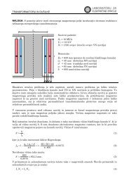
Select Independent Material Properties<br />
In magnetostatic problems, only two of the four available material properties need to be specified.<br />
The values of the other two properties are dependent upon these properties, according to the relationships<br />
shown below.<br />
B<br />
Br<br />
Magnetic<br />
Retentivity<br />
Hc<br />
Magnetic<br />
Coercivity<br />
� = B r /H c<br />
You will be specifying values for relative permeability, �, and magnetic retentivity, B r . The values<br />
of the other two properties, magnetic coercivity, H c , and magnetization, M p , will be computed<br />
using the relationships shown above.<br />
H<br />
Br = �oMp = �o� rHc Setting Up the Model 4-7
<strong>Getting</strong> <strong>Started</strong>: A <strong>2D</strong> <strong>Magnetostatic</strong> <strong>Problem</strong><br />
To specify which properties are to be entered:<br />
1. Click Options. The Property Options window appears.<br />
Initially, the only properties that can be specified are the relative permeability (� r ) and the magnetic<br />
coercivity (H c ). To define the permanent magnet, you will need to specify the magnetic retentivity.<br />
2. Click on the check box next to Hc to deselect it.<br />
3. Click on the check box next to Br to select it.<br />
4. Click OK.<br />
Enter Material Properties<br />
Now enter the values for the material attributes of Neo35. Only the two material attributes that were<br />
turned on in the Property Options window need to be entered — the other two attributes will be<br />
calculated automatically.<br />
To enter the properties for Neo35:<br />
1. Enter 1.05 in the Rel. Permeability (Mu) field.<br />
2. Enter 1.25 in the Mag. Retentivity (Br) field. Values automatically appear in the other fields.<br />
3. Click Enter.<br />
Neo35 is now listed as a local material in the database.<br />
4-8 Setting Up the Model
<strong>Getting</strong> <strong>Started</strong>: A <strong>2D</strong> <strong>Magnetostatic</strong> <strong>Problem</strong><br />
Assign Neo35 to the Core and Specify Direction of Magnetization<br />
Now that you have created the material Neo35, all that remains is to assign it to the core and specify<br />
the direction of magnetization.<br />
By default, the direction of magnetization in materials is along the R-axis (or the x-axis). However,<br />
in this problem, the direction of magnetization in the core points along the positive z-axis. To<br />
model this, you must change the direction of magnetization to act at a 90� angle from the default.<br />
To assign Neo35 to the core:<br />
1. Make certain that Neo35 is highlighted in the Material list.<br />
2. Click Assign to assign the material Neo35 to the core object. The Assign Coordinate System<br />
window appears.<br />
3. Select Align with a given direction to align the magnetization with the entered value.<br />
4. Enter 90 degrees in the Angle field.<br />
Note Make certain you enter a positive value for the angle. For instance, if you had entered<br />
90 degrees, the magnetization of the core would point in the opposite direction and<br />
would tend to push the core out of the solenoid.<br />
5. Click OK.<br />
Setting Up the Model 4-9
<strong>Getting</strong> <strong>Started</strong>: A <strong>2D</strong> <strong>Magnetostatic</strong> <strong>Problem</strong><br />
Assign SS430 to the Plugnut<br />
Next, create a new material — SS430 — for the plugnut. Like the material ColdRolledSteel, it is a<br />
nonlinear material whose relative permeability must be defined using a B-H curve. The first step<br />
includes selecting the plugnut and creating the material.<br />
Select Objects and Create Material<br />
To select the plugnut, and create the material:<br />
1. Select plugnut from the Object list.<br />
2. Click Material>Add.<br />
3. Under Material Properties, change the name of the new material to SS430.<br />
4. Select B-H Nonlinear Material.<br />
Define the B-H Curve<br />
To define the B-H curve for SS430, click B H curve.<br />
The B-H Curve Entry window appears.<br />
Define Maximum and Minimum Values for B and H<br />
For SS340, the values for H will fall between zero and 40,000 amperes per meter. The values for B<br />
will fall between zero and 2.0 tesla.<br />
To change the graph size of the B-H curve:<br />
1. Enter 0 in the Minimum H field.<br />
2. Enter 0 in the Minimum B field.<br />
3. Enter 40000 in the Maximum H field.<br />
4. Enter 2.0 in the Maximum B field.<br />
5. Click Accept.<br />
Add B-H Curve Points<br />
To enter the points in the B-H curve:<br />
1. Click Add Point.<br />
2. Click the left mouse button at the origin of the B- and H-axes (0, 0).<br />
3. Enter the following points using keyboard entry, as described under “Define the B-H Curve” in<br />
“Assign Cold Rolled Steel to the Bonnet and Yoke.”<br />
H B<br />
143 0.125<br />
180 0.206<br />
219 0.394<br />
259 0.589<br />
298 0.743<br />
338 0.853<br />
378 0.932<br />
4-10 Setting Up the Model
H B<br />
438 1.01<br />
517 1.08<br />
597 1.11<br />
716 1.16<br />
955 1.20<br />
1590 1.27<br />
3980 1.37<br />
6370 1.43<br />
1.19e4 1.49<br />
2.39e4 1.55<br />
3.98e4 1.59<br />
<strong>Getting</strong> <strong>Started</strong>: A <strong>2D</strong> <strong>Magnetostatic</strong> <strong>Problem</strong><br />
4. After you enter the last value, click Enter twice. The software automatically fits a curve to the<br />
points you entered on the graph, as shown below:<br />
5. Click Exit to return to the Material Setup window.<br />
Setting Up the Model 4-11
<strong>Getting</strong> <strong>Started</strong>: A <strong>2D</strong> <strong>Magnetostatic</strong> <strong>Problem</strong><br />
Assign SS430 to the Plugnut<br />
Finally, add SS430 to the material database, and assign it to the selected object:<br />
To add and assign SS430:<br />
1. Click Enter to save the material attributes you entered for SS430 and add it to the material<br />
database.<br />
2. Make certain SS430 is selected in the Material list.<br />
3. Click Assign to assign SS430 to the plugnut.<br />
Accept Default Material for Background<br />
Accept the following default parameters for the object background:<br />
• The material vacuum, which has the material attributes of a vacuum. The object background<br />
is the only object that is assigned a material by default.<br />
• Include it as part of the problem region in which to generate the solution. When a material<br />
name — such as vacuum, the material that is assigned to background by default — appears<br />
next to background in the Object list, it is included as part of the solution region.<br />
Exit the Material Manager<br />
Now that materials have been assigned to each object, exit the Material Setup window:<br />
To exit the Material Setup window:<br />
1. Click Exit from the bottom-left of the Material Setup window. A window with the following<br />
prompt appears:<br />
Save changes before closing?<br />
2. Click Yes.<br />
You are returned to the Executive Commands menu. A check mark now appears next to Setup<br />
Materials, and Setup Boundaries/Sources remains enabled.<br />
If you exit the Material Manager before assigning a material to each object in the model, a check<br />
mark does not appear next to Setup Materials on the Executive Commands menu, and Setup<br />
Boundaries/Sources is disabled. You will not be allowed to continue setting up your model until<br />
materials are assigned to all objects in the model.<br />
Set Up Boundaries and Current Sources<br />
After you set material properties, you must define boundary conditions and sources of current for<br />
the solenoid model. Boundary conditions and sources are defined in the Boundary Manager, which<br />
is accessed through the Setup Boundaries/Sources command.<br />
By default, the surfaces of all objects are Neumann or natural boundaries. That is, the magnetic<br />
field is defined to be perpendicular to the edges of the problem space and continuous across all<br />
object interfaces. To finish setting up the solenoid problem, you must explicitly define the following<br />
boundaries and sources:<br />
• The boundary condition at all surfaces exposed to the area outside of the problem region.<br />
Because you included the background as part of the problem region as described in the<br />
“Accept Default Material for Background” section, this exposed surface is that of the object<br />
4-12 Setting Up the Model
<strong>Getting</strong> <strong>Started</strong>: A <strong>2D</strong> <strong>Magnetostatic</strong> <strong>Problem</strong><br />
background. Since the solenoid is assumed to be very far away from other magnetic fields or<br />
sources of current, those boundaries will be defined as “balloon boundaries.”<br />
• The source current on the coil. Since the coil has 10,000 turns of wire, and one ampere flows<br />
through each turn, the net source current is 10,000 amperes.<br />
Note <strong>Maxwell</strong> <strong>SV</strong> will not solve the problem unless you specify some type of source or<br />
magnetic field — either a current source, an external field source using boundary<br />
conditions, or a permanent magnet. In this problem, both the permanent magnet<br />
assigned to the core and the current flowing in the coil act as magnetic field sources.<br />
Access the <strong>2D</strong> Boundary/Source Manager<br />
Define the boundary conditions for the model.<br />
To access the Boundary Manager:<br />
• Click Setup Boundaries/Sources. The <strong>2D</strong> Boundary/Source Manager appears.<br />
Boundary Manager Screen Layout<br />
Menu Bar and Toolbar<br />
Like <strong>2D</strong> Modeler commands, <strong>2D</strong> Boundary/Source Manager commands may be accessed from the<br />
following:<br />
• The menu bar, which is located along the top of the <strong>2D</strong> Boundary/Source Manager window.<br />
• The toolbar, which is located on the top of the window.<br />
Setting Up the Model 4-13
<strong>Getting</strong> <strong>Started</strong>: A <strong>2D</strong> <strong>Magnetostatic</strong> <strong>Problem</strong><br />
Boundary<br />
Each time you choose one of the Assign>Boundary or Assign>Source commands, an entry is<br />
added to the Boundary list on the left side of the menu. When you first access the <strong>2D</strong> Boundary/<br />
Source Manager, the Boundary list is empty.<br />
Display Area<br />
The geometric model is displayed on the menu so that you can choose objects using the<br />
Edit>Select commands. Use the Window>Change View commands, described in the <strong>Maxwell</strong> <strong>2D</strong><br />
online help, to change your view of the model.<br />
Boundary/Source Information<br />
The box that appears below the geometric model allows you to assign boundaries and sources to<br />
objects and surfaces, and to display the parameters associated with the selected boundary or source.<br />
Types of Boundary Conditions and Sources<br />
There are two types of boundary conditions and sources that you will use in this problem:<br />
Balloon �<br />
boundary<br />
In this example, you will assign boundary conditions and sources to the following objects in the<br />
solenoid geometry:<br />
Background At the outer boundary of the problem region, the outside edges of this<br />
surface are to be ballooned to simulate an insulated system.<br />
Coil This object is to be defined as a 10,000-amp DC current source. The<br />
current is uniformly distributed over the cross-section of the coil and<br />
flows in the positive perpendicular direction to the cross-section.<br />
Set Source Current on the Coil<br />
Before you identify a boundary condition or source, you must first identify the object or surface to<br />
which the condition is to be applied. In this section, you will pick the coil as a source and then<br />
assign a current to it.<br />
Pick the Coil<br />
To select the coil as a source:<br />
1. Click Edit>Select>Object>By Clicking.<br />
2. Click the left mouse button on the object coil, highlighting it.<br />
3. Click the right mouse button anywhere in the display area to stop selecting objects.<br />
4-14 Setting Up the Model<br />
Can only be applied to the outer boundary. Models the case in which<br />
the structure is infinitely far away from all other electromagnetic<br />
sources.<br />
Solid source Specifies the DC source current flowing through an object in the<br />
model.<br />
Note If the appropriate object is not highlighted, or if more than one object is highlighted, do<br />
the following:<br />
1. Click Edit>Deselect All. After you do, no objects are highlighted.<br />
2. Follow the instructions again to pick the object.
<strong>Getting</strong> <strong>Started</strong>: A <strong>2D</strong> <strong>Magnetostatic</strong> <strong>Problem</strong><br />
Assign a Current Source to the Coil<br />
To specify the current flowing through the coil:<br />
1. Click Assign>Source>Solid. The name source1 appears in the Boundary list, and NEW<br />
appears next to source1, indicating that the source has not yet been assigned to an object or<br />
surface. Fields appear in the boundary information area at the bottom of the window:<br />
2. Leave the Current check box selected.<br />
3. Leave the Total radio button selected.<br />
4. Enter 10000 in the Value field, and click Assign. The label current replaces NEW next to<br />
source1 in the Boundary list.<br />
Assign Balloon Boundary to the Background<br />
The structure is a magnetically isolated system. Therefore, you must create a balloon boundary by<br />
assigning balloon boundaries to the outside edges of the background object.<br />
Pick the Background<br />
To select the background as a boundary.<br />
1. Click Edit>Select>Object>By Clicking, and click the left mouse button anywhere on the<br />
background.<br />
2. Click the right mouse button to abort the command.<br />
Now you are ready to balloon the background.<br />
Assign Balloon Boundary<br />
To assign a balloon boundary to the background:<br />
1. Click Assign>Boundary>Balloon. The balloon1 boundary name appears in the Name field.<br />
2. Click Assign. The background is ballooned and balloon replaces NEW next to the boundary<br />
name in the Boundary list.<br />
Note In cartesian (XY) models, all outer edges may be defined as boundaries. However, in<br />
axisymmetric (RZ) models, the left edge of the problem region cannot be assigned a<br />
boundary condition. Because the solenoid model is axisymmetric (representing the<br />
cross-section of a device that is revolved 360 degrees around its central axis), the<br />
simulator ignores the balloon boundary you defined on the left edge of the geometry.<br />
Instead, it automatically imposes a different boundary condition, in order to model that<br />
left edge as an axis of rotational symmetry.<br />
Setting Up the Model 4-15
<strong>Getting</strong> <strong>Started</strong>: A <strong>2D</strong> <strong>Magnetostatic</strong> <strong>Problem</strong><br />
Exit the Boundary Manager<br />
To exit the Boundary Manager:<br />
1. Click File>Exit. A window appears with the following message:<br />
Save changes to “solenoid” before closing?<br />
2. Click Yes.<br />
You return to the Executive Commands menu. A check mark appears next to Setup Boundaries/<br />
Sources, indicating that this step has been completed. Note that a check mark also appears next to<br />
Setup Solution Options, indicating that a set of default solution parameters has been defined for<br />
the problem.<br />
You are now ready to set up the force computation for the model.<br />
Set Up Force Computation<br />
One of your goals for this problem is to determine the force acting on the core of the solenoid. To<br />
find the force on this object, you must select it using the Force command under Setup Executive<br />
Parameters. The force (in newtons) acting on the core will then be computed during the solution<br />
process.<br />
To select the core object for the force computation:<br />
1. Click Setup Executive Parameters. The following menu appears:<br />
Force�<br />
Core Loss�<br />
Torque�<br />
Flux Lines�<br />
Post Processor Macros�<br />
Matrix/Flux�<br />
Select Matrix/Flux Entries<br />
Quantities that may not be computed are grayed out and cannot be accessed. The Select<br />
Matrix/Flux Entries option is not enabled for <strong>Maxwell</strong> <strong>SV</strong> because the student version does<br />
not use the parametric analysis capability.<br />
2. Click Force. The Force Setup window appears. All objects in the model are listed on the left<br />
4-16 Setting Up the Model
side of the window. The geometric model is shown on the right.<br />
<strong>Getting</strong> <strong>Started</strong>: A <strong>2D</strong> <strong>Magnetostatic</strong> <strong>Problem</strong><br />
3. Select the object on which force is to be computed — the core — in one of two ways:<br />
• Select core from the Object list.<br />
• Click on the object core in the geometry.<br />
Both the object and its name are highlighted.<br />
4. To include the core object in the force computation, click Yes next to Include selected<br />
objects. The word Yes appears next to core in the Object list.<br />
5. Click Exit to exit the Force Setup window. The following message appears:<br />
Save changes before closing?<br />
6. Click Yes to save the force setup and exit. You return to the Executive Commands menu.<br />
The force on the core will now be computed during the solution. You are now ready to enter the<br />
solution criteria.<br />
Setting Up the Model 4-17
<strong>Getting</strong> <strong>Started</strong>: A <strong>2D</strong> <strong>Magnetostatic</strong> <strong>Problem</strong><br />
4-18 Setting Up the Model
Generating a Solution<br />
Now you are ready to specify solution parameters and generate a solution for the solenoid model.<br />
You will do the following:<br />
The goals for this chapter are to:<br />
• View the criteria that affect how <strong>Maxwell</strong> <strong>SV</strong> computes the solution.<br />
• Generate the magnetostatic solution. The axisymmetric magnetostatic solver calculates the<br />
magnetic vector potential, A�, at all points in the problem region. From this, the magnetic field,<br />
H, and magnetic flux density, B, can be determined.<br />
• Compute the force on the core. Since you requested force using the Setup Executive Parameters<br />
command, this automatically occurs during the general solution process.<br />
• View information about how the solution converged and what computing resources were used.<br />
Time This chapter should take approximately 40 minutes to work through.<br />
Generating a Solution 5-1
<strong>Getting</strong> <strong>Started</strong>: A <strong>2D</strong> <strong>Magnetostatic</strong> <strong>Problem</strong><br />
View Solution Criteria<br />
Use the default criteria to generate the solution for the solenoid problem.<br />
To view the solution criteria, click Setup Solution Options. The Solve Setup window appears.<br />
When the system generates a solution, it explicitly calculates the field values at each node in the<br />
finite element mesh and interpolates the values at all other points in the problem region.<br />
Starting Mesh<br />
Leave the Starting Mesh command set to Initial. This instructs the system to use the only mesh<br />
available, the coarse initial mesh when it begins the solution process. If you had already generated<br />
a solution and wanted to take advantage of the most recently refined mesh, you would click Current.<br />
Manual Mesh<br />
To get a head start on refining the initial mesh or the current mesh, you could choose the Manual<br />
Mesh command. This would allow you to manually break large triangles down into smaller ones,<br />
increasing the accuracy of the solution in the desired areas.<br />
5-2 Generating a Solution
Solver Choice<br />
<strong>Getting</strong> <strong>Started</strong>: A <strong>2D</strong> <strong>Magnetostatic</strong> <strong>Problem</strong><br />
You can specify which type of matrix solver to use to solve the problem. In the default Auto position,<br />
the software makes the choice. The ICCG solver is faster for large matrices, but occasionally<br />
fails to converge (usually on magnetic problems with high permeabilities and small air-gaps). The<br />
Direct solver will always converge, but is much slower for large matrices. In the Auto position, the<br />
software evaluates the matrix before attempting to solve; if it appears to be ill-conditioned, the<br />
Direct solver is used, otherwise the ICCG solver is used. If the ICCG solver fails to converge<br />
while the solver choice is in the Auto position, the software will fall back to the Direct solver automatically.<br />
Leave the Solver Choice option set to Auto.<br />
Solver Residual<br />
Leave the Residual field set to 0.001 for Linear, and to 0.005 for Nonlinear. These values specify<br />
how close each solution must come to satisfying the equations that are used to compute the magnetic<br />
field.<br />
Solve for Fields and Parameters<br />
The Solve for options tell the system what types of solutions to generate.<br />
Fields A field solution is generated.<br />
Parameters Any quantities that you set up using the Setup Executive Parameters<br />
command are computed (in this case, the force on the core).<br />
Leave both the Fields and Parameters check boxes selected, to solve for both fields and parameters<br />
in this example.<br />
Adaptive Analysis<br />
Do the following to have the system adaptively refine the mesh and solution:<br />
• Leave Adaptive Analysis selected. Doing so instructs the system to solve the problem iteratively,<br />
refining the regions of the mesh in which the largest error exists. Refining the mesh<br />
makes it more dense in the areas of highest error, resulting in a more accurate field solution.<br />
• Leave Number of requested passes and Percent error set to their defaults. After each iteration,<br />
the system calculates the total energy of the system and the percentage of this energy that<br />
is caused by solution error. It then checks to see if the number of requested passes has been<br />
completed, or if the percent error and the change in percent error between the last two passes<br />
match the requested values.<br />
• Leave Percent refinement per pass set to its default value. In most cases, the default refinement<br />
value is acceptable.<br />
If any of these criteria has been met, the solution process is complete and no more iterations are<br />
done.<br />
Exit Setup Solution Options<br />
To exit the Solve Setup window, click OK. You return to the Executive Commands menu.<br />
Generating a Solution 5-3
<strong>Getting</strong> <strong>Started</strong>: A <strong>2D</strong> <strong>Magnetostatic</strong> <strong>Problem</strong><br />
Start the Solution<br />
Now that you have examined the solution parameters, the problem is ready to be solved.<br />
To start the solution, click Solve.<br />
The solution process begins and the following changes occur:<br />
• The system creates the initial finite element mesh for the solenoid structure. A bar labeled<br />
Making Initial Mesh appears in the Solution Monitoring area at the bottom of the screen. It<br />
shows the system’s progress as it generates the mesh.<br />
• A bar labeled Solving Fields appears in the Solution Monitoring area.<br />
• A button labeled Abort appears next to the progress bar and remains there throughout the<br />
entire solution process. If desired, you can use it to stop the solution process.<br />
• A bar labeled Setting up solution files appears.<br />
After the system makes the initial finite element mesh, the magnetostatic field solution process<br />
begins.<br />
Values you obtain for percent energy error, total energy, or force may differ slightly from the ones<br />
given in this guide. Depending upon how closely you followed the directions for setting up the<br />
solenoid model, the results that you obtain should be approximately the same as the ones given<br />
here.<br />
Monitoring the Solution<br />
The following monitoring bars alternate in the Solution Monitoring box at the bottom of the<br />
menu. They allow you to monitor the system’s progress as it computes each adaptive pass (solve —<br />
error analysis — refine cycle) of the magnetostatic solution. Periodically, the solver also displays<br />
messages beneath the progress bars. The following table explains some of the messages that may<br />
appear:<br />
Solving Fields Displayed as <strong>Maxwell</strong> <strong>SV</strong> computes the field solution. After it<br />
finishes computing a solution, it identifies the triangles that<br />
have the highest energy error.<br />
Refining �<br />
Mesh<br />
5-4 Generating a Solution<br />
Displayed as the system refines the regions of the finite element<br />
mesh with the highest error energy. Since the default<br />
specification for mesh refinement is 15 percent, the system<br />
refines triangles that have the top 15 percent of the error.<br />
Solving matrix � Displayed as the system calculates a solution for the<br />
(nonlinear itera- relationship between the current and the field solution. This<br />
tion)<br />
may go on for several iterations before the general field solution<br />
continues. Because there are nonlinear materials in the model,<br />
the magnetostatic field solver uses a somewhat different<br />
solution process than if linear materials were present.<br />
Computing force Displayed as the simulator solves for the force on the core due<br />
value<br />
to the source current in the coil.
Viewing Convergence Data<br />
<strong>Getting</strong> <strong>Started</strong>: A <strong>2D</strong> <strong>Magnetostatic</strong> <strong>Problem</strong><br />
After a few adaptive passes are completed, click the Convergence button at the top of the Executive<br />
Commands menu to monitor how the solution is progressing. Convergence information<br />
appears as shown below. In this example, the system has completed eight adaptive passes.<br />
Solution Criteria<br />
Information about the solution criteria is displayed on the left side of the convergence display.<br />
Number of passes Displays how many adaptive passes have been completed and<br />
still remain.<br />
Target�<br />
Error<br />
Energy �<br />
Error<br />
Delta �<br />
Energy<br />
Displays the percent error value — 1% — that was entered<br />
using the Setup Solution Options command.<br />
Displays the percent error from the last completed solution —<br />
in this case, 0.754%. Allows you to see at a glance whether the<br />
solution is close to the desired error energy.<br />
Displays the change in the total energy between the last two<br />
solutions — in this case, 0.144%. Because this value and the<br />
Energy Error value are less than the Target Error, the<br />
solution is considered to be converged.<br />
Generating a Solution 5-5
<strong>Getting</strong> <strong>Started</strong>: A <strong>2D</strong> <strong>Magnetostatic</strong> <strong>Problem</strong><br />
Completed Solutions<br />
Information about each completed solution is displayed on the right side of the screen.<br />
Pass Displays the number of the completed solutions. In the previous<br />
figure, eight adaptive passes were completed.<br />
Triangles Displays the number of triangles in the mesh for a solution. In<br />
the previous figure, the mesh used for the eighth solution had<br />
826 triangles.<br />
Total Energy (J) Displays the total energy of a solution in Joules. In the previous<br />
figure, the total energy for the eighth solution was 1.98714<br />
Joules.<br />
Energy Error (%) Displays the percent energy error of the completed solutions. In<br />
the previous figure, the energy error for the eighth solution was<br />
.7543%.<br />
Mag Force �<br />
(N)<br />
Completing the Solution Process<br />
When the solution is complete, a pop-up window with the following message appears:<br />
Solution Process is complete<br />
Click OK to continue.<br />
You are now ready to view final convergence information for the completed solution.<br />
5-6 Generating a Solution<br />
Displays the magnitude of the force on the core in newtons.<br />
Force is computed after each adaptive pass, allowing you to see<br />
if it is converging to a stable value. In the previous figure, the<br />
force on the core during the tenth solution was 1.17639E+02, or<br />
117.459 newtons. This value only represents the total force<br />
acting on the object and does not indicate its direction.<br />
Note After a solution is generated, the system does not allow you to change the geometry,<br />
material properties, or boundary conditions of the model unless you first delete the<br />
solution. Therefore, you must generate a new solution if you change the model.
Viewing Final Convergence Data<br />
If convergence data is not displayed on the screen, click Convergence again.<br />
<strong>Getting</strong> <strong>Started</strong>: A <strong>2D</strong> <strong>Magnetostatic</strong> <strong>Problem</strong><br />
Note If a problem does not begin to converge after several adaptive passes, the problem is<br />
probably ill-defined — for instance, boundary conditions may not have been specified<br />
correctly. If this ever happens, do the following to interrupt the solution process:<br />
1. Click the Abort button in the Solution Monitoring box.<br />
2. Check the problem definition, and then solve the problem again.<br />
Generating a Solution 5-7
<strong>Getting</strong> <strong>Started</strong>: A <strong>2D</strong> <strong>Magnetostatic</strong> <strong>Problem</strong><br />
Plotting Convergence Data<br />
By default, convergence data is displayed in table format as shown in the previous figure. This data<br />
can also be displayed graphically.<br />
To plot the magnitude of force computed during each adaptive pass:<br />
• Click Convergence Display>Plot Force from the bottom of the display area. The following<br />
plot appears:<br />
Displaying this data graphically often makes it easier to see how the solution is converging. For<br />
instance, above, the curve begins to level off after the second pass as the total force starts to stabilize.<br />
Optionally, use the other commands under Convergence Display to plot the number of triangles,<br />
total energy, or percent error for all adaptive passes.<br />
5-8 Generating a Solution
Viewing Statistics<br />
<strong>Getting</strong> <strong>Started</strong>: A <strong>2D</strong> <strong>Magnetostatic</strong> <strong>Problem</strong><br />
Click Profile from the top of the Executive Commands menu to see what computing resources<br />
were used during the solution process. The following screen appears.<br />
The time that the solution process began is displayed at the top of the box. Beneath it, the following<br />
information is displayed for each adaptive field solution and mesh refinement step that was completed:<br />
Command/ Displays the name of the system command that was used.<br />
Info<br />
Real time Displays the time taken to complete the step.<br />
Cpu time Displays the amount of time taken by the CPU (central<br />
processing unit) to complete the step.<br />
Mem size Displays the amount of memory used.<br />
Num ElementsDisplays the of number of triangles in the finite element mesh.<br />
If more data is available than can fit on a single screen, scroll bars appear. To display more data,<br />
manipulate the display as described in Chapter 3, “Creating the Model”<br />
Generating a Solution 5-9
<strong>Getting</strong> <strong>Started</strong>: A <strong>2D</strong> <strong>Magnetostatic</strong> <strong>Problem</strong><br />
5-10 Generating a Solution
Analyzing the Solution<br />
Now that you have generated a magnetostatic solution for the solenoid problem, you can analyze it<br />
using <strong>Maxwell</strong> <strong>SV</strong>’s post processing features.<br />
The goals for this chapter are to:<br />
• Examine computed force values.<br />
• Plot the magnetic flux and magnetic fields in and around the solenoid.<br />
• Observe the nonlinear properties of the model using B-H curves.<br />
Time This chapter should take approximately 25 minutes to work through.<br />
Analyzing the Solution 6-1
<strong>Getting</strong> <strong>Started</strong>: A <strong>2D</strong> <strong>Magnetostatic</strong> <strong>Problem</strong><br />
View Force Solution<br />
Now that the solution is complete, examine the results of the force computation.<br />
To view the force results, click Solutions>Force. The final force value computed during the adaptive<br />
solution appears as shown below.<br />
• The object(s) that were selected for the force computation — in this case, the core — are listed<br />
under Force Setup Objects.<br />
• The results of the force solution (each force component) are given under Force Value (newtons).<br />
The net force on the core is approximately 117.459 newtons, acting in the negative z<br />
direction (pulling the core down into the solenoid). There is no component of force in the r<br />
direction because of the axial symmetry.<br />
Access the Post Processor<br />
Use the <strong>2D</strong> Post Processor to plot the lines of magnetic flux and saturation levels in materials.<br />
To access the Post Processor, click Post Process. The <strong>2D</strong> Post Processor appears.<br />
6-2 Analyzing the Solution
Post Processor Screen Layout<br />
<strong>Getting</strong> <strong>Started</strong>: A <strong>2D</strong> <strong>Magnetostatic</strong> <strong>Problem</strong><br />
This section provides a brief overview of the <strong>2D</strong> Post Processor. For further details, refer to the Post<br />
Process section in the <strong>Maxwell</strong> <strong>2D</strong> online help.<br />
General Areas<br />
The Post Processor is divided into the following general areas:.<br />
Menu Bar The menu bar appears at the top of the Post Processor window.<br />
Viewing WindowThe model appears in what is called the viewing window. This window<br />
displays the project name, solenoid, in its title bar.<br />
Side Window This area displays the vertex and snap behavior, and lists the coordinates of<br />
the selected points.<br />
Status Bar This area displays the following information:<br />
• The version number of <strong>Maxwell</strong> <strong>SV</strong>.<br />
• The function of each mouse button.<br />
Plot the Magnetic Field<br />
All objects created in the modeler, plus the background, represent the modeling region.<br />
In this project, the balloon boundary is used to model the case<br />
where the modeling structure is infinitely far away from other<br />
magnetic fields or current sources. Therefore, an object<br />
called “balloon” is shown in the On Geometry list in the<br />
Create New Plot window (accessed using the Plot>Field<br />
command).<br />
To define the problem region for post-processing purposes:<br />
1. Click Geometry>Create>Object List. The<br />
object list information appears in the bottom<br />
half of the side window.<br />
2. Change the Name to model.<br />
3. In the Objects list, select all objects except<br />
balloon, and then click OK.<br />
Analyzing the Solution 6-3
<strong>Getting</strong> <strong>Started</strong>: A <strong>2D</strong> <strong>Magnetostatic</strong> <strong>Problem</strong><br />
To create a magnetic field plot (showing the magnetic field throughout the problem region):<br />
1. Click Plot>Field. The Create New Plot window appears.<br />
2. Under Plot Quantity, select mag H. Under On Geometry, select Surface model. Under In<br />
Area, select model.<br />
3. Click OK. The Scalar Surface Plot window appears.<br />
4. Make certain that Show color key and Filled are selected.<br />
6-4 Analyzing the Solution
<strong>Getting</strong> <strong>Started</strong>: A <strong>2D</strong> <strong>Magnetostatic</strong> <strong>Problem</strong><br />
5. Click OK. The field plot appears. The plot should resemble the following:<br />
Redisplay the Magnetic FIeld Plot<br />
Now, redisplay the plot to show a more definitive range of current density distribution. To do this,<br />
first zoom in on the model, then redefine the range of values that are displayed.<br />
To redisplay the plot:<br />
1. Click View>Zoom In. The cursor changes to crosshairs.<br />
2. Click the left mouse button on a point to the upper left of the solenoid model.<br />
3. Click the left mouse button on a point just to the lower right of the solenoid model. A more<br />
detailed image of the plot appears, allowing you to more easily observe the differences in current<br />
density.<br />
4. Double-click on the plot key. The Scalar Surface Plot window appears.<br />
5. Under Plot Scale, select Use Limits.<br />
6. Leave the default value in the Maximum field.<br />
7. Enter 10000 in the Minimum field.<br />
8. Enter 21 in the Divisions field to display more layers.<br />
Analyzing the Solution 6-5
<strong>Getting</strong> <strong>Started</strong>: A <strong>2D</strong> <strong>Magnetostatic</strong> <strong>Problem</strong><br />
9. Click OK. The plot should resemble the following one:<br />
Identify Saturated Materials<br />
As the final step in your analysis of the solenoid model, you will determine saturation levels in the<br />
solenoid’s plugnut. In magnetically saturated materials, large changes in the magnetic field, H, produce<br />
relatively small changes in the magnetic flux density, B. In this problem, only the yoke, plugnut,<br />
and bonnet were assigned nonlinear materials. For this example, you will plot the saturation<br />
levels in the plugnut.<br />
To analyze the saturation level in the plugnut, you will plot the magnetic flux density in the solenoid<br />
to see which areas have a high B-field, and may be saturated. You will then select the object<br />
with the highest saturation and plot its B-H curve using the Plot>BH Curves command.<br />
Plot Magnetic Flux Density<br />
The problem region should still be enlarged as a result of the zoom function in the last step. Now<br />
you are ready to plot the magnetic flux density.<br />
To plot the magnetic flux density:<br />
1. Click Plot>Visibility. The Plot Visibility window appears.<br />
2. Select H[A/m] from the list, and click OK. The magnetic field plot is hidden.<br />
3. Click Plot>Field. The Create New Plot window appears.<br />
4. Under Plot Quantity, select mag B. Under On Geometry, select Surface model. Under In<br />
6-6 Analyzing the Solution
<strong>Getting</strong> <strong>Started</strong>: A <strong>2D</strong> <strong>Magnetostatic</strong> <strong>Problem</strong><br />
Area, select model.<br />
5. Click OK. The Scalar Surface Plot window appears.<br />
6. Under Plot Scale, select Auto Scale, and click OK. The flux plot appears, showing the magnetic<br />
flux density of each object in the geometry.<br />
Any areas colored completely green, like the one on the upper-right edge of the plugnut, may be<br />
saturated.<br />
Analyzing the Solution 6-7
<strong>Getting</strong> <strong>Started</strong>: A <strong>2D</strong> <strong>Magnetostatic</strong> <strong>Problem</strong><br />
Plot the B-H Curve<br />
Now you can plot H versus B, using the Plot>BH Curves command, and graphically view the nonlinear<br />
properties of the plugnut.<br />
To analyze the B-H curve of the plugnut:<br />
1. Click Plot>BH Curves. The Select Object B-H Curves window appears.<br />
2. Select plugnut from the list, and click OK. The B-H curve associated with the plugnut<br />
appears, as shown below:<br />
When the B-field in a nonlinear material rises above the “knee” of the material’s B-H curve, further<br />
increases in H result in relatively small increases in B. At this point, the material is said to be magnetically<br />
saturated.<br />
6-8 Analyzing the Solution
Exit the Post Processor<br />
To exit the <strong>2D</strong> Post Processor:<br />
<strong>Getting</strong> <strong>Started</strong>: A <strong>2D</strong> <strong>Magnetostatic</strong> <strong>Problem</strong><br />
1. Click File>Exit from the post processor. A window with the following prompt appears:<br />
Exit Post Processor?<br />
2. Click Yes. The Executive Commands window appears.<br />
Exit <strong>Maxwell</strong> <strong>SV</strong><br />
Once you have finished the post processing functions, you are ready to exit the software.<br />
To exit <strong>Maxwell</strong> <strong>SV</strong>:<br />
1. Click Exit from the bottom of the Executive Commands menu. The following prompt<br />
appears:<br />
Exit <strong>Maxwell</strong> <strong>SV</strong>?<br />
2. Click Yes. The Executive Commands window closes, and the Project Manager reappears.<br />
Exit the <strong>Maxwell</strong> Software<br />
To exit the Project Manager, click Exit. The Project Manager closes, and the Control Panel reappears.<br />
To exit the <strong>Maxwell</strong> Control Panel:<br />
1. Click EXIT. A window with the following prompt appears:<br />
Exit <strong>Maxwell</strong>?<br />
2. Click Yes. You return to Microsoft Windows.<br />
You have completed <strong>Getting</strong> <strong>Started</strong>: A <strong>2D</strong> <strong>Magnetostatic</strong> <strong>Problem</strong>, the second <strong>Getting</strong> <strong>Started</strong><br />
guide for <strong>Maxwell</strong> <strong>SV</strong>. (The first guide in the <strong>SV</strong> <strong>Getting</strong> <strong>Started</strong> series is called <strong>Getting</strong> <strong>Started</strong>: A<br />
<strong>2D</strong> Electrostatic <strong>Problem</strong>.)<br />
Analyzing the Solution 6-9
<strong>Getting</strong> <strong>Started</strong>: A <strong>2D</strong> <strong>Magnetostatic</strong> <strong>Problem</strong><br />
6-10 Analyzing the Solution
A<br />
adaptive analysis 5-3<br />
Ansoft software, installing 1-iv<br />
Assign/Boundary commands, Balloon 4-15<br />
Assign/Source commands, Solid 4-15<br />
axisymmetric models 1-2, 3-2<br />
boundary conditions 4-16<br />
drawing size 3-7<br />
B<br />
background<br />
and boundary conditions 4-12<br />
ballooning 4-15<br />
default material for 4-12<br />
definition of 3-9<br />
extending 4-15<br />
including in solution region 4-12<br />
balloon boundary<br />
assigning 4-15<br />
definition of 4-14<br />
B-H curve<br />
adding points to 4-5, 4-10<br />
defining 4-4, 4-10<br />
fitting curve to points 4-6<br />
for cold rolled steel 4-4<br />
Index<br />
for SS430 4-10<br />
keyboard entry 4-5<br />
maximum B and H values 4-5, 4-10<br />
minimum B and H values 4-5, 4-10<br />
plotting saturation levels on 6-8<br />
B-H Plot (Post Processor Plot menu commands) 6-8<br />
bonnet<br />
assigning a material to 4-3<br />
creating 3-14<br />
boundary conditions 4-12<br />
and axisymmetric models 4-16<br />
and cartesian models 4-16<br />
balloon 4-14, 4-15<br />
displaying 4-14<br />
for sample problem 4-14<br />
screen layout 4-14<br />
use of 4-12<br />
buttons<br />
disabled 2-5<br />
C<br />
cartesian models 3-2<br />
coil<br />
assigning a material to 4-3<br />
assigning source current to 4-14, 4-15<br />
creating 3-12<br />
picking as a current source 4-14<br />
Index-1
<strong>Getting</strong> <strong>Started</strong>: A <strong>2D</strong> <strong>Magnetostatic</strong> <strong>Problem</strong><br />
cold rolled steel<br />
defining as a material 4-3<br />
entering B-H curve for 4-4<br />
colors, changing for objects 3-10<br />
commands<br />
accessing from menus 3-3, 4-13<br />
accessing with the keyboard 3-3<br />
accessing with the mouse 3-3<br />
accessing with the toolbar 4-13<br />
computing resources<br />
clock time 5-9<br />
commands executed 5-9<br />
CPU time 5-9<br />
memory size 5-9<br />
number of elements 5-9<br />
viewing 5-9<br />
Control Panel<br />
icon 2-2<br />
Convergence 5-5, 5-7<br />
convergence data<br />
delta energy 5-5<br />
energy error 5-5, 5-6<br />
force 5-6<br />
mesh size 5-6<br />
number of passes 5-6<br />
pass number 5-6<br />
plotting 5-8<br />
target error 5-5<br />
total energy 5-6<br />
viewing 5-5, 5-7, 5-8<br />
Convergence Display, Plot Force 5-8<br />
coordinate system, uv (local) 3-4<br />
coordinates<br />
entering via keyboard 3-4<br />
of cursor 3-4<br />
core<br />
assigning a material to 4-10<br />
convergence of force solution 5-6, 5-8<br />
creating 3-11<br />
selecting for force computation 4-17<br />
current 4-14<br />
and balloon boundaries 4-15<br />
assigning to coil 4-14, 4-15<br />
Index-2<br />
D<br />
Define Model 1-3, 3-3<br />
Draw Model 1-3<br />
Group Objects 1-3<br />
dimensions of sample problem 3-5<br />
direct solver 5-3<br />
directories, project<br />
creating 2-3<br />
selecting 2-4<br />
Draw Model 1-3<br />
Drawing 1-3, 3-2<br />
drawing plane 3-2<br />
drawing region<br />
adjusting view of 2-7, 3-14<br />
and axisymmetric models 3-7<br />
maximum x- and y-coordinates 3-7<br />
minimum x- and y-coordinates 3-7<br />
setting up 3-6<br />
size of 3-7<br />
Drawing Size 3-7<br />
Drawing, RZ Plane 3-2<br />
E<br />
energy<br />
error 5-3, 5-5, 5-6<br />
fluctuations in energy error 5-7<br />
total 5-6<br />
error<br />
energy 5-5, 5-6<br />
fluctuations in energy error 5-7<br />
of solution 5-3<br />
Executive Commands menu 2-7<br />
Convergence 5-5, 5-7<br />
Define Model 3-3<br />
Drawing 3-2<br />
Post Process 6-2<br />
Profile 5-9<br />
Setup Boundaries/Sources 4-12<br />
Setup Executive Parameters 4-16<br />
Setup Materials 4-2<br />
Setup Solution Parameters 5-1, 5-2
Solutions 6-2<br />
Solve 5-4<br />
Solver 3-2<br />
Exit 3-15, 4-16<br />
F<br />
field of view<br />
fitting all objects in 2-7, 3-14<br />
fitting drawing space in 2-7<br />
zooming in on 2-7<br />
zooming out of 2-7<br />
fields<br />
entering text and numbers in 3-7<br />
selecting with the mouse 3-7<br />
File commands<br />
Exit 3-15, 4-16<br />
Open 3-4<br />
Save 3-13<br />
files, saving geometry to 3-13<br />
Fill Solids 2-7<br />
Fit All 2-7<br />
Fit Drawing 2-7<br />
force<br />
and solution process 4-16<br />
components of 6-2<br />
computing for the solenoid core 4-16<br />
convergence of solution 5-8<br />
direction of 6-2<br />
magnetic 5-6<br />
magnitude of 5-6, 6-2<br />
objects in computation 4-17<br />
plotting magnitude of 5-8<br />
viewing solution results 6-2<br />
G<br />
geometric models<br />
axisymmetric 1-2, 3-2<br />
cartesian 3-2<br />
general strategy for creating 3-3<br />
saving 3-13<br />
grid<br />
changing point spacing 3-10<br />
<strong>Getting</strong> <strong>Started</strong>: A <strong>2D</strong> <strong>Magnetostatic</strong> <strong>Problem</strong><br />
in subwindows 3-4<br />
modify spacing of 3-8<br />
snapping to 3-4<br />
grid points, snapping to 3-4<br />
Group Objects 1-3<br />
I<br />
ICCG solver 5-3<br />
installing Ansoft software 1-iv<br />
insulated system 4-15<br />
K<br />
keyboard<br />
accessing commands with 3-3<br />
selecting points with 3-4, 3-10, 3-14, 4-5, 4-10<br />
M<br />
magnetic coercivity 4-7<br />
magnetic field<br />
and balloon boundaries 4-15<br />
and saturation 6-6<br />
solving for 5-4<br />
magnetic flux density<br />
and saturation 6-6<br />
plotting 6-6<br />
magnetic retentivity 4-7<br />
magnetization<br />
relationship to other properties 4-7<br />
specifying direction of 4-9<br />
Material, Add 4-3<br />
materials<br />
adding materials to material database 4-2<br />
adding to local database 4-2<br />
assigning to objects 4-2<br />
assigning to the background 4-12<br />
assigning to the bonnet 4-3<br />
assigning to the coil 4-3<br />
assigning to the core 4-10<br />
assigning to the plugnut 4-10<br />
assigning to the yoke 4-3<br />
material database 4-2<br />
Index-3
<strong>Getting</strong> <strong>Started</strong>: A <strong>2D</strong> <strong>Magnetostatic</strong> <strong>Problem</strong><br />
nonlinear 4-3, 4-10<br />
permanent magnets 4-7<br />
<strong>Maxwell</strong> <strong>2D</strong> Field Simulator<br />
executive commands 1-3<br />
exiting 6-9<br />
general procedure 1-3<br />
starting 2-6<br />
<strong>Maxwell</strong> Control Panel<br />
accessing 2-2<br />
exiting 6-9<br />
Projects command 2-3<br />
memory used during solution 5-9<br />
menu bar<br />
for <strong>2D</strong> Modeler 3-3<br />
for Boundary Manager 4-13<br />
in Post Processor 6-3<br />
mesh<br />
and solution accuracy 5-2<br />
default 5-2<br />
example of 1-1<br />
initial 5-4<br />
number of triangles in 5-6<br />
starting 5-2<br />
use of 1-1<br />
mesh refinement<br />
adaptive 5-3<br />
and error energy 5-3<br />
manual 5-2<br />
percentage refined 5-3<br />
message bar<br />
during solution process 5-4<br />
in <strong>2D</strong> modeler 3-4<br />
Model commands<br />
Drawing Size 3-7<br />
Drawing Units 3-6<br />
mouse<br />
accessing commands with 3-3<br />
selecting objects with 4-3<br />
snap-to behavior of 3-4, 3-8<br />
mouse buttons functions 3-4<br />
mouse coordinates, displaying 3-4<br />
Index-4<br />
N<br />
names, changing for objects 3-10<br />
Neo35<br />
creating 4-7<br />
specifying direction of permanent magnetization<br />
4-9<br />
specifying properties of 4-8<br />
nominal problem<br />
generating a solution for 5-4<br />
post processing 6-2<br />
nonlinear materials<br />
adding 4-3, 4-10<br />
defining B-H curve for 4-4, 4-10<br />
identifying saturated materials 6-6<br />
plotting saturation levels 6-8<br />
O<br />
Object commands<br />
Polyline 3-11, 3-13, 3-14<br />
Rectangle 3-9, 3-12<br />
objects<br />
assigning materials to 4-2<br />
background 3-9<br />
changing the colors of 3-10<br />
changing the names of 3-10<br />
creating 3-9<br />
deselecting 4-3<br />
dimensions of 3-5<br />
displaying as filled-in solids 2-7<br />
displaying as outlines 2-7<br />
polylines 3-11, 3-13, 3-14<br />
rectangles 3-9<br />
selecting 4-3, 4-10<br />
selecting for force computation 4-17<br />
P<br />
permanent magnets<br />
creating 4-7<br />
direction of magnetization in 4-9<br />
Pick commands, Object 4-14
Plot 6-6<br />
Plot Force 5-8<br />
plots<br />
convergence data 5-8<br />
force 5-8<br />
saturation levels 6-8<br />
plots, field<br />
common quantities 6-6<br />
magnetic flux density 6-6<br />
shaded plots 6-6<br />
plugnut<br />
assigning a material to 4-10<br />
creating 3-9<br />
viewing saturation levels in 6-6<br />
points<br />
entering from the keyboard 3-4, 3-10, 3-14, 4-5,<br />
4-10<br />
Polyline 3-11, 3-13<br />
Post Process 1-4, 6-2<br />
post processing 6-2<br />
exiting 6-9<br />
Post Processor Plot menu commands<br />
B-H Plot 6-8<br />
Visibility 6-6<br />
Profile 5-9<br />
Project Manager commands<br />
Add 2-3<br />
Open 2-6<br />
Save Notes 2-5<br />
Project Manager, New 2-4<br />
projects<br />
creating 2-4<br />
entering descriptions of 2-5<br />
opening 2-6<br />
R<br />
Rectangle 3-9, 3-12<br />
relative permeability 4-7<br />
residual 5-3<br />
S<br />
saturation<br />
<strong>Getting</strong> <strong>Started</strong>: A <strong>2D</strong> <strong>Magnetostatic</strong> <strong>Problem</strong><br />
in nonlinear materials 6-6<br />
plotting levels of 6-8<br />
saving geometry files 3-13, 3-15<br />
scientific notation, Ansoft’s 4-5<br />
scroll bars 5-9<br />
Setup Boundaries/Sources 1-3, 4-12<br />
Setup Executive Parameters 1-3, 5-3<br />
Setup Executive Parameters, Force 4-16<br />
Setup Materials 1-3, 4-2<br />
Setup Solution Parameters 1-3, 5-1, 5-2<br />
size<br />
of finite element mesh 5-6, 5-9<br />
of memory during solution 5-9<br />
of the drawing region 3-4, 3-7<br />
snap-to behavior of mouse 3-4, 3-8<br />
solutions<br />
adaptive analysis of 5-3<br />
and adaptive mesh refinement 5-3<br />
calculated values 5-2<br />
changing boundaries and sources after generating<br />
solution 5-7<br />
changing geometry after generating solution 5-7<br />
changing materials after generating solution 5-7<br />
completing 5-6<br />
computing 5-4<br />
convergence 5-5<br />
criteria for computing 5-2<br />
effect of mesh 5-2<br />
force 6-2<br />
interpolated values 5-2<br />
interrupting 5-4, 5-8<br />
monitoring 5-4<br />
plotting 6-6<br />
refinement of 5-3<br />
satisfying equations 5-3<br />
total energy 5-6<br />
types 5-3<br />
viewing convergence data for 5-7<br />
viewing fields 6-1<br />
viewing profile data for 5-9<br />
Solutions, Force 6-2<br />
Solve 1-4, 5-4<br />
Solver 3-2<br />
AC Conduction 3-2<br />
Index-5
<strong>Getting</strong> <strong>Started</strong>: A <strong>2D</strong> <strong>Magnetostatic</strong> <strong>Problem</strong><br />
DC Conduction 3-2<br />
Eddy Axial 3-2<br />
Eddy Current 3-2<br />
Electrostatic 3-2<br />
<strong>Magnetostatic</strong> 3-2<br />
Solver 1-3<br />
solver choice 5-3<br />
solver residual 5-3<br />
solvers<br />
auto 5-3<br />
direct 5-3<br />
ICCG 5-3<br />
sources 4-12<br />
assigning to objects 4-15<br />
current 4-14<br />
displaying 4-14<br />
for sample problem 4-14<br />
screen layout 4-14<br />
SS430<br />
defining material 4-10<br />
entering B-H curve for 4-10<br />
starting mesh 5-2<br />
status information<br />
cursor position 3-4<br />
snap-to behavior of mouse 3-4<br />
unit of length 3-4<br />
subwindows<br />
and complex geometries 3-4<br />
and project windows 3-4<br />
coordinate system 3-4<br />
drawing grid 3-4<br />
size 3-4<br />
T<br />
toolbar<br />
in Boundary Manager 4-13<br />
triangles<br />
manually refining 5-2<br />
number in mesh 5-6, 5-9<br />
<strong>2D</strong> Modeler<br />
accessing 3-3<br />
exiting 3-15<br />
screen layout<br />
Index-6<br />
U<br />
accessing commands 3-3<br />
menu bar 3-3<br />
message bar 3-4<br />
project window 3-4<br />
status bar 3-4<br />
subwindows 3-4<br />
units<br />
changing 3-6<br />
default 3-4<br />
displaying 3-6<br />
rescaling geometric models 3-6<br />
V<br />
vertex points, snapping to 3-4<br />
W<br />
Window commands (<strong>2D</strong> Modeler), Grid 3-8<br />
windows, project 3-4<br />
Wire Frame 2-7<br />
Y<br />
yoke<br />
assigning a material to 4-3<br />
creating 3-13<br />
Z<br />
Zoom In 2-7<br />
Zoom Out 2-7