Maxwell SV Getting Started: A 2D Electrostatic Problem - LES
Maxwell SV Getting Started: A 2D Electrostatic Problem - LES
Maxwell SV Getting Started: A 2D Electrostatic Problem - LES

Create successful ePaper yourself
Turn your PDF publications into a flip-book with our unique Google optimized e-Paper software.
November 2002<br />
<strong>Maxwell</strong> ® <strong>2D</strong><br />
Student Version<br />
A <strong>2D</strong> <strong>Electrostatic</strong> <strong>Problem</strong><br />
�
Notice<br />
The information contained in this document is subject to change without notice.<br />
Ansoft makes no warranty of any kind with regard to this material, including, but not limited to, the<br />
implied warranties of merchantability and fitness for a particular purpose. Ansoft shall not be liable<br />
for errors contained herein or for incidental or consequential damages in connection with the �<br />
furnishing, performance, or use of this material.<br />
This document contains proprietary information which is protected by copyright. All rights are<br />
reserved.<br />
Ansoft Corporation<br />
Four Station Square�<br />
Suite 200�<br />
Pittsburgh, PA 15219�<br />
(412) 261 - 3200<br />
Microsoft ® Windows ® is a registered trademark of Microsoft Corporation.<br />
UNIX� is a registered trademark of UNIX Systems Laboratories, Inc.<br />
<strong>Maxwell</strong>� is a registered trademark of Ansoft Corporation.<br />
© Copyright 2002 Ansoft Corporation
Printing History<br />
<strong>Getting</strong> <strong>Started</strong>: A <strong>2D</strong> <strong>Electrostatic</strong> <strong>Problem</strong><br />
New editions of this manual will incorporate all material updated since the previous edition. The<br />
manual printing date, which indicates the manual’s current edition, changes when a new edition is<br />
printed. Minor corrections and updates that are incorporated at reprint do not cause the date to<br />
change.<br />
Update packages may be issued between editions and contain additional and/or replacement pages<br />
to be merged into the manual by the user. Pages that are rearranged due to changes on a previous<br />
page are not considered to be revised.<br />
Edition Date<br />
Software<br />
Revision<br />
1 June 1994 6.2<br />
2 November 2002 9.0<br />
iii
<strong>Getting</strong> <strong>Started</strong>: A <strong>2D</strong> <strong>Electrostatic</strong> <strong>Problem</strong><br />
Installation<br />
<strong>Getting</strong> <strong>Started</strong><br />
iv<br />
Before you use <strong>Maxwell</strong> <strong>SV</strong>, you must:<br />
1. Set up your system’s graphical windowing system.<br />
2. Install the <strong>Maxwell</strong> software, using the directions in the Ansoft PC Installation Guide.<br />
If you have not yet done these steps, refer to the Ansoft Installation guides and the documentation<br />
that came with your computer system, or ask your system administrator for help.<br />
If you are using <strong>Maxwell</strong> <strong>SV</strong> for the first time, the following two guides are available for the Student<br />
Version of <strong>Maxwell</strong> <strong>2D</strong>:<br />
• <strong>Getting</strong> <strong>Started</strong>: A <strong>2D</strong> <strong>Electrostatic</strong> <strong>Problem</strong><br />
• <strong>Getting</strong> <strong>Started</strong>: A <strong>2D</strong> Magnetostatic <strong>Problem</strong><br />
Additional <strong>Getting</strong> <strong>Started</strong> guides are available for the standard version of <strong>Maxwell</strong> <strong>2D</strong>.<br />
These short tutorials guide you through the process of setting up and solving simple problems in<br />
<strong>Maxwell</strong> <strong>SV</strong>, providing you with an overview of how to use the software.<br />
Other References<br />
To start <strong>Maxwell</strong> <strong>SV</strong>, you must first access the <strong>Maxwell</strong> Control Panel.<br />
For information on all <strong>Maxwell</strong> Control Panel and <strong>Maxwell</strong> <strong>SV</strong> commands, refer to the following<br />
online documentation:<br />
• <strong>Maxwell</strong> Control Panel online help. This online manual contains a detailed description of all of<br />
the commands in the <strong>Maxwell</strong> Control Panel and in the Utilities panel. The <strong>Maxwell</strong> Control<br />
Panel allows you to create and open projects, print screens, and translate files. The Utilities<br />
panel is accessible through the <strong>Maxwell</strong> Control Panel and enables you to view licensing information,<br />
adjust colors, open and create <strong>2D</strong> models, open and create plots using parametric �<br />
equations, and evaluate mathematical expressions.<br />
• <strong>Maxwell</strong> <strong>2D</strong> online help. This online manual contains a detailed description of the <strong>Maxwell</strong> <strong>2D</strong><br />
and the Parametric Analysis modules. <strong>Maxwell</strong> <strong>SV</strong> does not provide parametric capabilities.
Typeface Conventions<br />
<strong>Getting</strong> <strong>Started</strong>: A <strong>2D</strong> <strong>Electrostatic</strong> <strong>Problem</strong><br />
Field Names Bold type is used for on-screen prompts, field names, and messages.<br />
Keyboard Entries Bold type is used for entries that must be entered as specified.<br />
Example: Enter 0.005 in the Nonlinear Residual field.<br />
Menu Commands Bold type is used to display menu commands selected to perform a<br />
specific task. Menu levels are separated by a carat.<br />
Example 1: The instruction “Click File>Open” means to select the<br />
Open command on the File menu within an application.<br />
Example 2: The instruction “Click Define Model>Draw Model”<br />
means to select the Draw Model command from the Define Model<br />
button on the <strong>Maxwell</strong> <strong>SV</strong> Executive Commands menu.<br />
Variable Names Italic type is used for keyboard entries when a name or variable must<br />
be typed in place of the words in italics.<br />
Example: The instruction “copy filename” means to type the word<br />
copy, to type a space, and then to type the name of a file, such as<br />
file1.<br />
Emphasis and<br />
Titles<br />
Italic type is used for emphasis and for the titles of manuals and<br />
other publications.<br />
Keyboard Keys Bold Arial type is used for labeled keys on the computer keyboard.<br />
For key combinations, such as shortcut keys, a plus sign is used.<br />
Example 1: The instruction “Press Return” means to press the key<br />
on the computer that is labeled Return.<br />
Example 2: The instructions “Press Ctrl+D” means to press and hold<br />
down the Ctrl key and then press the D key.<br />
v
<strong>Getting</strong> <strong>Started</strong>: A <strong>2D</strong> <strong>Electrostatic</strong> <strong>Problem</strong><br />
vi
Table of Contents<br />
1. Introduction . . . . . . . . . . . . . . . . . . . . . . . . . . . . . . . . . . 1-1<br />
Sample <strong>Problem</strong> . . . . . . . . . . . . . . . . . . . . . . . . . . . . . . . . . . . . . . . . . . . . . 1-2<br />
General Procedure . . . . . . . . . . . . . . . . . . . . . . . . . . . . . . . . . . . . . . . . . . . 1-3<br />
Results to Expect . . . . . . . . . . . . . . . . . . . . . . . . . . . . . . . . . . . . . . . . . . . . 1-5<br />
2. Creating the Microstrip Project . . . . . . . . . . . . . . . . . . 2-1<br />
Access the <strong>Maxwell</strong> Control Panel . . . . . . . . . . . . . . . . . . . . . . . . . . . . . . 2-2<br />
Access the Project Manager . . . . . . . . . . . . . . . . . . . . . . . . . . . . . . . . . . . . 2-2<br />
Create a Project Directory . . . . . . . . . . . . . . . . . . . . . . . . . . . . . . . . . . . . . 2-3<br />
Create a Project . . . . . . . . . . . . . . . . . . . . . . . . . . . . . . . . . . . . . . . . . . . . . 2-4<br />
Access the Project Directory . . . . . . . . . . . . . . . . . . . . . . . . . . . . . . . . . . 2-4<br />
Create the New Project . . . . . . . . . . . . . . . . . . . . . . . . . . . . . . . . . . . . . . 2-4<br />
Save Project Notes . . . . . . . . . . . . . . . . . . . . . . . . . . . . . . . . . . . . . . . . . . 2-5<br />
3. Accessing the Software . . . . . . . . . . . . . . . . . . . . . . . . 3-1<br />
Open the New Project and Run the Simulator . . . . . . . . . . . . . . . . . . . . . . 3-2<br />
Executive Commands Window . . . . . . . . . . . . . . . . . . . . . . . . . . . . . . . . . 3-3<br />
Executive Commands Menu . . . . . . . . . . . . . . . . . . . . . . . . . . . . . . . . . . 3-3<br />
Display Area . . . . . . . . . . . . . . . . . . . . . . . . . . . . . . . . . . . . . . . . . . . . . . 3-3<br />
Solution Monitoring Area . . . . . . . . . . . . . . . . . . . . . . . . . . . . . . . . . . . . 3-3<br />
4. Creating the Model . . . . . . . . . . . . . . . . . . . . . . . . . . . . 4-1<br />
Specify Solver Type . . . . . . . . . . . . . . . . . . . . . . . . . . . . . . . . . . . . . . . . . . 4-2<br />
Specify Drawing Plane . . . . . . . . . . . . . . . . . . . . . . . . . . . . . . . . . . . . . . . 4-2<br />
Access the <strong>2D</strong> Modeler . . . . . . . . . . . . . . . . . . . . . . . . . . . . . . . . . . . . . . . 4-2<br />
Contents-1
<strong>Getting</strong> <strong>Started</strong>: A <strong>2D</strong> <strong>Electrostatic</strong> <strong>Problem</strong><br />
Screen Layout . . . . . . . . . . . . . . . . . . . . . . . . . . . . . . . . . . . . . . . . . . . . . 4-3<br />
The Microstrip Model . . . . . . . . . . . . . . . . . . . . . . . . . . . . . . . . . . . . . . . . 4-4<br />
Set Up the Drawing Region . . . . . . . . . . . . . . . . . . . . . . . . . . . . . . . . . . . . 4-5<br />
Create the Geometry . . . . . . . . . . . . . . . . . . . . . . . . . . . . . . . . . . . . . . . . . 4-6<br />
Keyboard Entry . . . . . . . . . . . . . . . . . . . . . . . . . . . . . . . . . . . . . . . . . . . . 4-6<br />
Create the Substrate . . . . . . . . . . . . . . . . . . . . . . . . . . . . . . . . . . . . . . . . . 4-6<br />
Create the Left Microstrip . . . . . . . . . . . . . . . . . . . . . . . . . . . . . . . . . . . . 4-8<br />
Create the Right Microstrip . . . . . . . . . . . . . . . . . . . . . . . . . . . . . . . . . . . 4-9<br />
Save the Geometry . . . . . . . . . . . . . . . . . . . . . . . . . . . . . . . . . . . . . . . . . . 4-10<br />
Create the Ground Plane . . . . . . . . . . . . . . . . . . . . . . . . . . . . . . . . . . . . . 4-11<br />
Completed Geometry . . . . . . . . . . . . . . . . . . . . . . . . . . . . . . . . . . . . . . . . . 4-13<br />
Exit the <strong>2D</strong> Modeler . . . . . . . . . . . . . . . . . . . . . . . . . . . . . . . . . . . . . . . . . 4-13<br />
5. Defining Materials and Boundaries . . . . . . . . . . . . . . . 5-1<br />
Set Up Materials . . . . . . . . . . . . . . . . . . . . . . . . . . . . . . . . . . . . . . . . . . . . 5-2<br />
Access the Material Manager . . . . . . . . . . . . . . . . . . . . . . . . . . . . . . . . . . 5-2<br />
Assign a Material to the Substrate . . . . . . . . . . . . . . . . . . . . . . . . . . . . . . 5-3<br />
Assign a Material to the Microstrips and Ground Plane . . . . . . . . . . . . . 5-4<br />
Assigning Materials to the Background . . . . . . . . . . . . . . . . . . . . . . . . . . 5-4<br />
Exit the Material Manager . . . . . . . . . . . . . . . . . . . . . . . . . . . . . . . . . . . . 5-5<br />
Set Up Boundaries and Sources . . . . . . . . . . . . . . . . . . . . . . . . . . . . . . . . . 5-5<br />
Display the <strong>2D</strong> Boundary/Source Manager . . . . . . . . . . . . . . . . . . . . . . . 5-6<br />
Boundary Manager Screen Layout . . . . . . . . . . . . . . . . . . . . . . . . . . . . . 5-6<br />
Types of Boundary Conditions and Sources . . . . . . . . . . . . . . . . . . . . . . 5-7<br />
Set the Voltage on the Left Microstrip . . . . . . . . . . . . . . . . . . . . . . . . . . . 5-8<br />
Set the Voltage on the Right Microstrip . . . . . . . . . . . . . . . . . . . . . . . . . 5-8<br />
Set the Voltage on the Ground Plane . . . . . . . . . . . . . . . . . . . . . . . . . . . . 5-9<br />
Assign a Balloon Boundary to the Background . . . . . . . . . . . . . . . . . . . . 5-9<br />
Leave Substrate with a Natural Surface . . . . . . . . . . . . . . . . . . . . . . . . . . 5-10<br />
Exit the Boundary Manager . . . . . . . . . . . . . . . . . . . . . . . . . . . . . . . . . . . 5-10<br />
6. Generating a Solution . . . . . . . . . . . . . . . . . . . . . . . . . . 6-1<br />
Contents-2<br />
Set Up a Matrix Calculation . . . . . . . . . . . . . . . . . . . . . . . . . . . . . . . . . . . 6-2<br />
Access the Setup Solution Menu . . . . . . . . . . . . . . . . . . . . . . . . . . . . . . . . 6-3<br />
Modify Solution Criteria . . . . . . . . . . . . . . . . . . . . . . . . . . . . . . . . . . . . . . 6-4<br />
Specify the Starting Mesh . . . . . . . . . . . . . . . . . . . . . . . . . . . . . . . . . . . . 6-4<br />
Specify the Solver Residual . . . . . . . . . . . . . . . . . . . . . . . . . . . . . . . . . . . 6-4<br />
Specify the Solver Choice . . . . . . . . . . . . . . . . . . . . . . . . . . . . . . . . . . . . 6-5<br />
Specify the “Solve for” Options . . . . . . . . . . . . . . . . . . . . . . . . . . . . . . . . 6-5<br />
Specify the Adaptive Analysis Settings . . . . . . . . . . . . . . . . . . . . . . . . . . 6-5
<strong>Getting</strong> <strong>Started</strong>: A <strong>2D</strong> <strong>Electrostatic</strong> <strong>Problem</strong><br />
Exit Setup Solution . . . . . . . . . . . . . . . . . . . . . . . . . . . . . . . . . . . . . . . . . 6-5<br />
Generate the Solution . . . . . . . . . . . . . . . . . . . . . . . . . . . . . . . . . . . . . . . . . 6-6<br />
Monitoring the Solution . . . . . . . . . . . . . . . . . . . . . . . . . . . . . . . . . . . . . . . 6-6<br />
Solution Criteria . . . . . . . . . . . . . . . . . . . . . . . . . . . . . . . . . . . . . . . . . . . . 6-6<br />
Completed Solutions . . . . . . . . . . . . . . . . . . . . . . . . . . . . . . . . . . . . . . . . 6-7<br />
Completing the Solution Process . . . . . . . . . . . . . . . . . . . . . . . . . . . . . . . . 6-7<br />
Viewing Final Convergence Data . . . . . . . . . . . . . . . . . . . . . . . . . . . . . . 6-8<br />
Plotting Convergence Data . . . . . . . . . . . . . . . . . . . . . . . . . . . . . . . . . . . 6-9<br />
Viewing Statistics . . . . . . . . . . . . . . . . . . . . . . . . . . . . . . . . . . . . . . . . . . 6-10<br />
7. Analyzing the Solution . . . . . . . . . . . . . . . . . . . . . . . . . 7-1<br />
Access the Post Processor . . . . . . . . . . . . . . . . . . . . . . . . . . . . . . . . . . . . . 7-2<br />
Post Processor Screen Layout . . . . . . . . . . . . . . . . . . . . . . . . . . . . . . . . . . 7-2<br />
General Areas . . . . . . . . . . . . . . . . . . . . . . . . . . . . . . . . . . . . . . . . . . . . . . 7-2<br />
Menu Bar . . . . . . . . . . . . . . . . . . . . . . . . . . . . . . . . . . . . . . . . . . . . . . . . . 7-3<br />
Status Bar . . . . . . . . . . . . . . . . . . . . . . . . . . . . . . . . . . . . . . . . . . . . . . . . . 7-3<br />
Scientific Notation . . . . . . . . . . . . . . . . . . . . . . . . . . . . . . . . . . . . . . . . . . 7-3<br />
Plot the Electric Field . . . . . . . . . . . . . . . . . . . . . . . . . . . . . . . . . . . . . . . . 7-4<br />
Formatting and Manipulating Plots . . . . . . . . . . . . . . . . . . . . . . . . . . . . . . 7-6<br />
Rotate a Plot . . . . . . . . . . . . . . . . . . . . . . . . . . . . . . . . . . . . . . . . . . . . . . . 7-7<br />
Hide or Show a Plot . . . . . . . . . . . . . . . . . . . . . . . . . . . . . . . . . . . . . . . . . 7-7<br />
Open Multiple Plots . . . . . . . . . . . . . . . . . . . . . . . . . . . . . . . . . . . . . . . . . 7-7<br />
The <strong>2D</strong> Calculator . . . . . . . . . . . . . . . . . . . . . . . . . . . . . . . . . . . . . . . . . . . 7-8<br />
Examine Results of Capacitance Computation . . . . . . . . . . . . . . . . . . . . . 7-9<br />
Verify Capacitance Calculation . . . . . . . . . . . . . . . . . . . . . . . . . . . . . . . . . 7-9<br />
Reset the Conductor Values . . . . . . . . . . . . . . . . . . . . . . . . . . . . . . . . . . . 7-9<br />
Remove Mesh Refinement . . . . . . . . . . . . . . . . . . . . . . . . . . . . . . . . . . . . 7-9<br />
Run the Solution Again . . . . . . . . . . . . . . . . . . . . . . . . . . . . . . . . . . . . . . 7-10<br />
Calculate Capacitance . . . . . . . . . . . . . . . . . . . . . . . . . . . . . . . . . . . . . . . . 7-10<br />
Enter the Post Processor Field Calculator Again . . . . . . . . . . . . . . . . . . . 7-10<br />
Compute the Energy . . . . . . . . . . . . . . . . . . . . . . . . . . . . . . . . . . . . . . . . . 7-10<br />
Compute the Capacitance Value . . . . . . . . . . . . . . . . . . . . . . . . . . . . . . . 7-12<br />
Exit the Calculator . . . . . . . . . . . . . . . . . . . . . . . . . . . . . . . . . . . . . . . . . . 7-13<br />
Exit the Post Processor . . . . . . . . . . . . . . . . . . . . . . . . . . . . . . . . . . . . . . . 7-13<br />
Exit <strong>Maxwell</strong> <strong>2D</strong> . . . . . . . . . . . . . . . . . . . . . . . . . . . . . . . . . . . . . . . . . . . . 7-13<br />
Exit the <strong>Maxwell</strong> Software . . . . . . . . . . . . . . . . . . . . . . . . . . . . . . . . . . . . 7-13<br />
Contents-3
<strong>Getting</strong> <strong>Started</strong>: A <strong>2D</strong> <strong>Electrostatic</strong> <strong>Problem</strong><br />
Contents-4
Introduction<br />
This guide is a tutorial for setting up an electrostatic problem using version 9.0 of <strong>Maxwell</strong> <strong>2D</strong> Student<br />
Version (<strong>SV</strong>), a software package for analyzing electromagnetic fields in cross-sections of<br />
structures. <strong>Maxwell</strong> <strong>SV</strong> uses finite element analysis (FEA) to solve two-dimensional (<strong>2D</strong>) electromagnetic<br />
problems.<br />
To analyze a problem, you need to specify the appropriate geometry, material properties, and excitations<br />
for a device or system of devices. The <strong>Maxwell</strong> software then does the following:<br />
• Automatically creates the required finite element mesh.<br />
• Iteratively calculates the desired electrostatic or magnetostatic field solution and special quantities<br />
of interest, including force, torque, inductance, capacitance, and power loss. You can<br />
select any of the following solution types: <strong>Electrostatic</strong>, Magnetostatic, <strong>Electrostatic</strong>, Eddy<br />
Current, DC Conduction, AC Conduction, Eddy Axial. The student version does not contain<br />
thermal, transient, or parametric capabilities.<br />
• Provides the ability to analyze, manipulate, and display field solutions.<br />
Many models are actually a collection of three-dimensional (3D) objects. <strong>Maxwell</strong> <strong>SV</strong> analyzes a<br />
<strong>2D</strong> cross-section of the model, then generates a solution for that cross-section, using FEA to solve<br />
the problem. Dividing a structure into many smaller regions (finite elements) allows the system to<br />
compute the field solution separately in each element. The smaller the elements, the more accurate<br />
the final solution.<br />
Introduction 1-1
<strong>Getting</strong> <strong>Started</strong>: A <strong>2D</strong> <strong>Electrostatic</strong> <strong>Problem</strong><br />
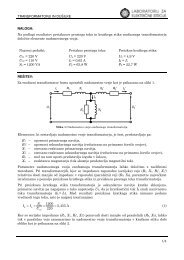
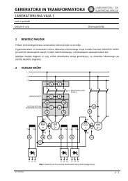
Sample <strong>Problem</strong><br />
After starting the software and introducing the Executive Commands window, this guide steps you<br />
through the setup, solution, and analysis of a simple electrostatic problem. The sample �<br />
problem, shown below, is an electrically insulated structure that includes the following:<br />
• Two microstrip lines, one set to +1 volt, and the other set to -1 volt.<br />
• A substrate.<br />
• A ground plane.<br />
In this guide, you will draw, set up, and solve the sample microstrip problem shown below.<br />
Detailed dimensions and instructions for drawing this model are given in Chapter 4, “Creating the<br />
Model.”<br />
Microstrips<br />
Substrate<br />
Ground Plane<br />
1-2 Introduction
General Procedure<br />
<strong>Getting</strong> <strong>Started</strong>: A <strong>2D</strong> <strong>Electrostatic</strong> <strong>Problem</strong><br />
Follows this general procedure when using the simulator to solve <strong>2D</strong> problems:<br />
1. Use the Solver command to specify which of the following electric or magnetic field quantities<br />
to compute:<br />
• <strong>Electrostatic</strong><br />
• Magnetostatic<br />
• Eddy Current<br />
• DC Conduction<br />
• AC Conduction<br />
• Eddy Axial<br />
2. Use the Drawing command to select one of the following model types:<br />
XY Plane Visualizes cartesian models as sweeping perpendicularly to the cross-section.<br />
RZ Plane Visualizes axisymmetric models as revolving around an axis of symmetry in<br />
the cross-section.<br />
3. Use the Define Model command to access the following options:<br />
Draw Model Allows you to access the <strong>2D</strong> Modeler and draw the objects that make up<br />
the geometric model.<br />
Group Objects Allows you to group discrete objects that are actually one electrical<br />
object. For instance, two terminations of a conductor that are drawn as<br />
separate objects in the cross-section can be grouped to represent one<br />
conductor.<br />
Couple Model Allows you to define thermal coupling for a project.<br />
4. Use the Setup Materials command to assign materials to all objects in the geometric model.<br />
5. Use the Setup Boundaries/Sources command to define the boundaries and sources for the<br />
problem.<br />
6. Use the Setup Executive Parameters command to instruct the simulator to compute the �<br />
following special quantities:<br />
• Matrix (capacitance, inductance, admittance, impedance, or conductance matrix, �<br />
depending on the selected solver)<br />
• Force<br />
• Torque<br />
• Flux Linkage<br />
• Current Flow<br />
7. Use the Setup Solution Options command to specify how the solution is computed.<br />
8. Use the Solve command to solve for the appropriate field quantities. For electrostatic �<br />
problems, the simulator computes �, the electric potential, from which it derives E and D.<br />
9. Use the Post Process command to analyze the solution, as follows:<br />
• Plot the field solution. Common quantities (such as �, E, and D) are directly accessible<br />
Introduction 1-3
<strong>Getting</strong> <strong>Started</strong>: A <strong>2D</strong> <strong>Electrostatic</strong> <strong>Problem</strong><br />
from menus and can be plotted a number of ways. For instance, you can display a plot of<br />
equipotential contours or you can graph potential as a function of distance.<br />
• Use the calculators. The post processor allows you to take curls, divergences, integrals,<br />
and cross and dot products to derive special quantities of interest.<br />
The commands shown on the Executive Commands menu must be chosen in the sequence in<br />
which they appear. For example, you must first create a geometric model with the Define Model<br />
command before you specify material characteristics for objects with the Setup Materials command.<br />
A check mark appears on the menu next to the completed steps.<br />
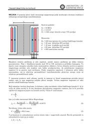
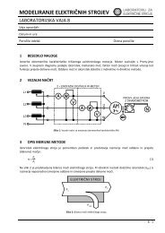
These steps are summarized in the following flowchart:<br />
1-4 Introduction<br />
Select solver and drawing type.<br />
Draw geometric model and<br />
(optionally) identify grouped objects.<br />
Assign material properties.<br />
Assign boundary conditions and sources.<br />
Compute other<br />
quantities during<br />
solution?<br />
No<br />
Generate solution.<br />
Yes<br />
Set up solution criteria and<br />
(optionally) refine the mesh.<br />
Inspect solutions, view solution<br />
information, display field plots, and<br />
manipulate basic field quantities.<br />
Request that force, torque,<br />
capacitance, inductance,<br />
admittance, impedance, flux<br />
linkage, conductance, or<br />
current flow be computed<br />
during the solution process.
Results to Expect<br />
<strong>Getting</strong> <strong>Started</strong>: A <strong>2D</strong> <strong>Electrostatic</strong> <strong>Problem</strong><br />
After setting up the microstrip problem and generating a solution, you will:<br />
• Plot and analyze voltage contours to view the voltage distribution around the conductors.<br />
• Compute capacitance.<br />
Time This guide should take approximately 3 hours to work through.<br />
Introduction 1-5
<strong>Getting</strong> <strong>Started</strong>: A <strong>2D</strong> <strong>Electrostatic</strong> <strong>Problem</strong><br />
1-6 Introduction
Creating the Microstrip Project<br />
This guide assumes that <strong>Maxwell</strong> <strong>SV</strong> has already been installed as described in the Ansoft PC<br />
Installation Guide.<br />
Your goals in this chapter are as follows:<br />
• Create a project directory in which to save sample problems.<br />
• Create a new project in that directory in which to save the microstrip problem.<br />
Time This chapter should take approximately 15 minutes to work through.<br />
Creating the Microstrip Project 2-1
<strong>Getting</strong> <strong>Started</strong>: A <strong>2D</strong> <strong>Electrostatic</strong> <strong>Problem</strong><br />
Access the <strong>Maxwell</strong> Control Panel<br />
To access <strong>Maxwell</strong> <strong>SV</strong>, you must first open the <strong>Maxwell</strong> Control Panel, which allows you to create<br />
and open projects for all Ansoft projects.<br />
To start the <strong>Maxwell</strong> Control Panel, do one of the following:<br />
• Use the Start menu to select Programs>Ansoft><strong>Maxwell</strong> <strong>SV</strong>.<br />
• Double-click the <strong>Maxwell</strong> <strong>SV</strong> icon.<br />
The <strong>Maxwell</strong> Control Panel appears. If not, refer to the Ansoft installation guides for assistance.<br />
See the <strong>Maxwell</strong> Control Panel online help for a detailed description of the other options in the<br />
<strong>Maxwell</strong> Control Panel.<br />
Access the Project Manager<br />
The Project Manager enables you to create and manage Ansoft products. You can add new project<br />
directories, create projects in existing directories, and rename and copy projects.<br />
To access the Project Manager, click PROJECTS from the <strong>Maxwell</strong> Control Panel. The Project<br />
Manager appears.<br />
2-2 Creating the Microstrip Project
Create a Project Directory<br />
<strong>Getting</strong> <strong>Started</strong>: A <strong>2D</strong> <strong>Electrostatic</strong> <strong>Problem</strong><br />
The first step in using <strong>Maxwell</strong> <strong>SV</strong> to solve a problem is to create a project directory and a project<br />
in which to save all the data associated with the problem.<br />
A project directory contains a specific set of projects created with the Ansoft software. You can use<br />
project directories to categorize projects any number of ways. For example, you might want to store<br />
all projects related to a particular facility or application in one project directory. You will now create<br />
a project directory.<br />
The Project Manager should still be on the screen. You will add the getting_started_<strong>SV</strong> directory<br />
that will contain the <strong>Maxwell</strong> <strong>SV</strong> project you create using this <strong>Getting</strong> <strong>Started</strong> guide.<br />
Note If you have already created a project directory while working through one of the other<br />
Ansoft <strong>Getting</strong> <strong>Started</strong> guides, skip to the “Create a Project” section.<br />
To add a project directories, do the following in the Project Manager:<br />
1. Click Add from the Project Directories list. The Add a new project directory window<br />
appears, listing the directories and subdirectories.<br />
2. Type the following in the Alias field:<br />
getting_started_<strong>SV</strong><br />
<strong>Maxwell</strong> <strong>SV</strong> projects are usually created in directories that have aliases — that is, directories<br />
that have been identified as project directories using the Add command.<br />
3. Select Make New Directory near the bottom of the window. By default, getting_started_<strong>SV</strong><br />
appears in this field.<br />
4. Click OK.<br />
The getting_started_<strong>SV</strong> directory is created under the current default project directory. You return<br />
to the Project Manager, and getting_started_<strong>SV</strong> now appears in the Project Directories list.<br />
Creating the Microstrip Project 2-3
<strong>Getting</strong> <strong>Started</strong>: A <strong>2D</strong> <strong>Electrostatic</strong> <strong>Problem</strong><br />
Create a Project<br />
Now you are ready to create a new project named microstrip in the getting_started_<strong>SV</strong> project<br />
directory.<br />
Access the Project Directory<br />
Before you create the new project, access the getting_started_<strong>SV</strong> project directory.<br />
To access the project directory, click getting_started_<strong>SV</strong> in the Project Directories list of the<br />
Project Manager.<br />
The current directory displayed at the top of the Project Manager menu changes to show the path<br />
name of the directory associated with the getting_started_<strong>SV</strong> alias. If you have previously created<br />
a model, it will be listed in the Projects list. Otherwise, the Projects list is empty — no projects<br />
have been created yet in this project directory.<br />
Create the New Project<br />
To create a new project:<br />
1. In the Project Manager, click New in the Projects list. The Enter project name and select<br />
project type window appears.<br />
2. Type microstrip in the Name field. Use the Back Space and Delete keys to correct typos.<br />
3. If <strong>Maxwell</strong> <strong>SV</strong> Version 9 does not appear in the Type field, do the following:<br />
a. Click the left mouse button on the software package listed in the Type field. A menu<br />
appears, listing all Ansoft software packages that have been installed.<br />
b. Click <strong>Maxwell</strong> <strong>SV</strong> Version 9.<br />
4. Optionally, enter your name in the Created By field. The name of the person who logged onto<br />
the system appears by default.<br />
5. Clear Open project upon creation. You do not want to automatically open the project at this<br />
point, so that you may enter project notes first.<br />
6. Click OK.<br />
2-4 Creating the Microstrip Project
<strong>Getting</strong> <strong>Started</strong>: A <strong>2D</strong> <strong>Electrostatic</strong> <strong>Problem</strong><br />
The information that you just entered is now displayed in the corresponding fields in the Projects<br />
list. Because you created the project, Writable is selected, showing that you have access to the<br />
project.<br />
Save Project Notes<br />
It is a good idea to save notes about your new project so that the next time you use <strong>Maxwell</strong> <strong>SV</strong>,<br />
you can view information about a project without opening it.<br />
To enter notes for the microstrip problem:<br />
1. Leave Notes selected by default.<br />
2. Click in the area under the Notes option. This places an I-beam cursor in the upper-left corner<br />
of the Notes area, indicating that you can begin typing text.<br />
Note The Model option displays a picture of the selected model in the Notes area. It is disabled<br />
now because you are creating a new project. After you create the microstrip problem, its<br />
geometry will appear in this area by default when the microstrip project is selected. For a<br />
detailed description of the Model option, refer to the <strong>Maxwell</strong> Control Panel online help.<br />
3. Enter your notes about the project, such as the following:<br />
This is the sample electrostatic problem created using<br />
<strong>Maxwell</strong> <strong>SV</strong> and the <strong>Electrostatic</strong> <strong>Getting</strong> <strong>Started</strong> guide.<br />
When you start entering project notes, the Save Notes button (located below the Notes area)<br />
becomes black, indicating that it is enabled. Before you began typing in the Notes area, Save<br />
Notes was grayed out, or disabled.<br />
4. When you are done entering the description, click Save Notes to save it. After you do, the<br />
Save Notes button is disabled again.<br />
Now you are ready to open the new <strong>Maxwell</strong> <strong>SV</strong> project and run the software.<br />
Creating the Microstrip Project 2-5
<strong>Getting</strong> <strong>Started</strong>: A <strong>2D</strong> <strong>Electrostatic</strong> <strong>Problem</strong><br />
2-6 Creating the Microstrip Project
Accessing the Software<br />
In the last chapter, you created the getting_started_<strong>SV</strong> project directory and created the �<br />
microstrip project within that directory.<br />
This chapter describes:<br />
• How to open the project you just created and run <strong>Maxwell</strong> <strong>SV</strong>.<br />
• The <strong>Maxwell</strong> <strong>SV</strong> Executive Commands window.<br />
• The general procedure for creating an electrostatic problem in <strong>Maxwell</strong> <strong>SV</strong>.<br />
• The sample problem and the procedures you will use to simulate its electric fields.<br />
Time This chapter should take approximately 10 minutes to work through.<br />
Accessing the Software 3-1
<strong>Getting</strong> <strong>Started</strong>: A <strong>2D</strong> <strong>Electrostatic</strong> <strong>Problem</strong><br />
Open the New Project and Run the Simulator<br />
The newly created microstrip project should still be highlighted in the Projects list. (If it is not,<br />
click the left mouse button on it in the list.)<br />
To run <strong>Maxwell</strong> <strong>SV</strong>, click Open in the project area. The <strong>Maxwell</strong> <strong>SV</strong> Executive Commands menu<br />
appears.<br />
3-2 Accessing the Software
Executive Commands Window<br />
<strong>Getting</strong> <strong>Started</strong>: A <strong>2D</strong> <strong>Electrostatic</strong> <strong>Problem</strong><br />
The Executive Commands window is divided into three sections: the Executive Commands<br />
menu, display area, and the solution monitoring area.<br />
Executive Commands Menu<br />
The Executive Commands menu acts as a doorway to each step of creating and solving the model<br />
problem. You select each module through the Executive Commands menu, and the software<br />
returns you to this menu when you are finished. You also view the solution process through this<br />
menu.<br />
Display Area<br />
The display area shows either the project’s geometry in a model window or the solution to the �<br />
problem once a solution has been generated. Since you have not yet drawn the model, this area is<br />
blank. The commands along the bottom of the window allow you to change your view of the<br />
model:<br />
Zoom In Zooms in on an area of the window, magnifying the view.<br />
Zoom Out Zooms out of an area, shrinking the view.<br />
Fit All Changes the view to display all items in the window. Items will<br />
appear as large as possible without extending beyond the window.<br />
Fit Drawing Displays the entire drawing space.<br />
Fill Solids Displays objects as solids rather than outlined objects. Toggles with<br />
Wire Frame.<br />
Wire Frame Displays objects as wire-frame outlines. Toggles with Fill Solids.<br />
The buttons along the top of the window are used when you are generating and analyzing a �<br />
solution. These are described in more detail in Chapter 6, “Generating a Solution.”<br />
Solution Monitoring Area<br />
This area displays solution profile and convergence information while the problem is solving, as<br />
described in Chapter 6, “Generating a Solution.”<br />
Accessing the Software 3-3
<strong>Getting</strong> <strong>Started</strong>: A <strong>2D</strong> <strong>Electrostatic</strong> <strong>Problem</strong><br />
3-4 Accessing the Software
Creating the Model<br />
In the last chapter, you opened the microstrip project, examined the Executive Commands window,<br />
and reviewed the procedure for creating a <strong>2D</strong> model. Now you are ready to use <strong>Maxwell</strong> <strong>SV</strong><br />
to solve an electrostatic problem. The first step is to create the geometry for the system being �<br />
studied.<br />
This chapter shows you how to create the geometry for the microstrip problem that was described<br />
in Chapter 1, “Introduction,” and in Chapter 3, “Accessing the Software.”<br />
Your goals for this chapter are as follows:<br />
• Set up the problem region.<br />
• Create the objects that make up the geometric model.<br />
• Save the geometric model to a disk file.<br />
Time This chapter should take approximately 35 minutes to work through.<br />
Creating the Model 4-1
<strong>Getting</strong> <strong>Started</strong>: A <strong>2D</strong> <strong>Electrostatic</strong> <strong>Problem</strong><br />
Specify Solver Type<br />
The <strong>Maxwell</strong> <strong>SV</strong> Executive Commands window should still be on the screen. Before you start<br />
drawing your model, you need to specify which field quantities to compute. By default, <strong>Electrostatic</strong><br />
appears as the Solver type. Because you will be solving an electrostatic problem, leave this<br />
type as it appears.<br />
Specify Drawing Plane<br />
The microstrip model you will be drawing is actually the XY cross-section of a structure that<br />
extends into the z-direction. This is known as a cartesian or XY plane model. By default, XY Plane<br />
appears as the Drawing plane. Because the model you will be creating is in the XY plane, leave<br />
this type as it appears.<br />
Now, you are ready to draw the model.<br />
Access the <strong>2D</strong> Modeler<br />
To draw the geometric model, use the <strong>2D</strong> Modeler, which allows you to create <strong>2D</strong> structures.<br />
To access the <strong>2D</strong> Modeler, click Define Model>Draw Model. The <strong>2D</strong> Modeler appears.<br />
4-2 Creating the Model
Screen Layout<br />
The following sections provide a brief overview of the <strong>2D</strong> Modeler.<br />
<strong>Getting</strong> <strong>Started</strong>: A <strong>2D</strong> <strong>Electrostatic</strong> <strong>Problem</strong><br />
Menu Bar<br />
The <strong>2D</strong> Modeler’s menu bar appears at the top of the window. Each item in the menu bar has a<br />
menu of commands associated with it. If a command name has an arrow next to it, that command<br />
also has a menu of commands associated with it. If a command name has an ellipsis next to it, that<br />
command has a window or panel associated with it.<br />
To display the menu associated with a command in the menu bar, do one of the following:<br />
• Click on it.<br />
• Press and hold down Alt, and then press the key of the underlined letter on the command name.<br />
For example, to display the Window command’s menu, do one of the following:<br />
• Click it.<br />
• Press Alt, and type a W.<br />
The Window menu appears. Click outside the Window menu to make it disappear.<br />
Project Window<br />
The main <strong>2D</strong> Modeler window contains the Drawing Region, the grid-covered area where you<br />
draw the objects that make up your model. This main window in the <strong>2D</strong> Modeler is called the<br />
project window. A project window contains the geometry for a specific project and displays the<br />
project’s name in its title bar. By default, one subwindow is contained within the project window.<br />
Optionally, you can open additional projects in the <strong>2D</strong> Modeler clicking the File>Open command.<br />
Opening several projects at once is useful if you want to copy objects between geometries. See the<br />
<strong>Maxwell</strong> <strong>2D</strong> online help for more details.<br />
Subwindows<br />
Subwindows are the windows in which you create the objects that make up the geometric model.<br />
By default, this window:<br />
• Has points specified in relation to a local uv coordinate system. The u-axis is horizontal, the vaxis<br />
is vertical, and the origin is marked by a cross in the middle of the screen.<br />
• Uses millimeters (mm) as the default drawing unit.<br />
• Has grid points 2 millimeters apart. The default window size is 100 millimeters by 70 millimeters.<br />
Note If a geometry is complex, you may want to open additional subwindows for the same<br />
project so that you can alter your view of the geometry from one subwindow to the next.<br />
To do so, use the Window>New command as described in the <strong>Maxwell</strong> <strong>2D</strong> online help.<br />
For this geometry, however, a single subwindow should be sufficient.<br />
Creating the Model 4-3
<strong>Getting</strong> <strong>Started</strong>: A <strong>2D</strong> <strong>Electrostatic</strong> <strong>Problem</strong><br />
Status Bar<br />
The status bar, which appears at the bottom of the <strong>2D</strong> Modeler screen, displays the following:<br />
U and V Displays the coordinates of the mouse’s position on the screen and allows<br />
you to enter coordinates using the keyboard.<br />
UNITS Drawing units in which the geometry is entered.<br />
SNAPTO Which point — grid point or object vertex — is selected when you<br />
choose points using the mouse. By default, both grid and object points are<br />
selected so that the mouse snaps to whichever one is closest.<br />
Message Bar<br />
A message bar, which appears above the status bar, displays the functions of the left and right<br />
mouse buttons. When selecting or deselecting objects, the message bar displays the number of<br />
items that are currently selected. When you change the view in a subwindow, it displays the current<br />
magnification level.<br />
Toolbar<br />
The toolbar is the vertical stack of icons that appears on the left side of the <strong>2D</strong> Modeler screen.<br />
Icons give you easy access to the most frequently used commands that allow you to draw objects,<br />
change your view of the problem region, deselect objects, and so on. Click an icon and hold the<br />
button down to display a brief description of the command in the message bar at the bottom of the<br />
screen.<br />
For more information on these areas of the <strong>2D</strong> Modeler, refer to the <strong>Maxwell</strong> <strong>2D</strong> online help.<br />
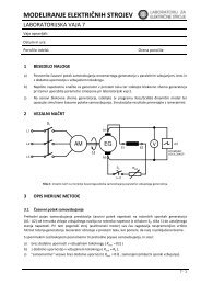
The Microstrip Model<br />
Use the following dimensions, which are given in mils, to create the geometric model of the<br />
microstrip you are modeling:<br />
20.0<br />
2.0<br />
0.2<br />
Note In this example, the default drawing size is appropriate. However, if your model were<br />
much larger or smaller, you would need to change the model size by clicking the<br />
Model>Drawing Size command. In general, the width of the drawing area should be three<br />
to five times longer than the width of the geometric model, and the height of the drawing<br />
area should be three to five times longer than the height of the geometric model.<br />
4-4 Creating the Model<br />
40.0<br />
4.0<br />
0.2
Set Up the Drawing Region<br />
The first step is to specify the drawing units to use in creating the model.<br />
To set up the drawing region:<br />
1. Click Model>Drawing Units. The Drawing Units window appears.<br />
<strong>Getting</strong> <strong>Started</strong>: A <strong>2D</strong> <strong>Electrostatic</strong> <strong>Problem</strong><br />
2. Select mils from the list, and then click the Rescale to new units radio button, if it is not<br />
already selected.<br />
3. Click OK.<br />
The units are changed from millimeters to mils, and mils now appears next to UNITS in the status<br />
bar at the bottom of the modeling window.<br />
Creating the Model 4-5
<strong>Getting</strong> <strong>Started</strong>: A <strong>2D</strong> <strong>Electrostatic</strong> <strong>Problem</strong><br />
Create the Geometry<br />
Now you are ready to draw the objects that make up the geometric model.<br />
Keyboard Entry<br />
In the following section, several of the points lie between grid points. You can position these points<br />
in one of two ways:<br />
• Change the grid spacing so that the object’s dimensions lie on grid points.<br />
• Use “keyboard entry” — that is, enter the coordinates directly into the U and V fields in the<br />
status bar.<br />
If you change the grid spacing, the screen may become cluttered with too many tightly-spaced grid<br />
points and make point selection difficult. Therefore, use keyboard entry to enter several of the<br />
dimensions of the sample geometry.<br />
Note To change the grid spacing, click the Window>Grid command.<br />
To change the size of the problem region, click the Model>Drawing Size command.<br />
Create the Substrate<br />
The substrate consists of a simple rectangle on which the two rectangular microstrips will rest.<br />
Draw a Rectangle<br />
To create the rectangle to represent the substrate:<br />
1. Click Object>Rectangle. After you do, the pointer changes to crosshairs.<br />
2. Select the first corner of the substrate, the upper-left corner, as follows:<br />
a. Move the crosshairs to the point on the grid where the u- and v- coordinates are (-20, 0).<br />
Remember that the coordinates of the cursor’s current location are displayed in the U and<br />
V fields in the status bar.<br />
b. Click the point to select it.<br />
3. To select the second corner of the substrate, use keyboard entry because -4, the v-coordinate,<br />
lies between grid points. To specify the lower-right corner:<br />
a. Double-click in the U field in the status bar.<br />
b. Type 20, using the Backspace and Delete keys to correct typos.<br />
c. Press Tab to move to the V field in the status bar. The value in the dU field changed. The<br />
dU and dV fields display the values of the offset from the previous point.<br />
d. Type –4.<br />
4. To accept the point, press Return or click Enter in the status bar. After you do, the New<br />
4-6 Creating the Model
Object window appears.<br />
<strong>Getting</strong> <strong>Started</strong>: A <strong>2D</strong> <strong>Electrostatic</strong> <strong>Problem</strong><br />
Assign a Name and Color<br />
By default, the object that you are creating is assigned the name object1 and the color red, and the<br />
Name field is selected.<br />
Note Be sure to change the name of the object to indicate its function and to assign a different<br />
color to different objects. This will be important later when you assign boundary<br />
conditions, voltages, and so forth.<br />
To define the name and color for the substrate:<br />
1. Type substrate in the Name field. Do not press Return.<br />
2. Click the solid red square next to Color. A palette of 16 colors appears.<br />
3. Click one of the green boxes in the palette.<br />
4. Click OK.<br />
The object now appears in the drawing region as shown below. It is green and has the name �<br />
substrate:<br />
Creating the Model 4-7
<strong>Getting</strong> <strong>Started</strong>: A <strong>2D</strong> <strong>Electrostatic</strong> <strong>Problem</strong><br />
Create the Left Microstrip<br />
Now that you have drawn the substrate, draw the left microstrip. Because the microstrip is relatively<br />
small compared to the substrate, you need to zoom in on the top part of the substrate and then<br />
use keyboard entry to draw it.<br />
Zoom In on Top of the Substrate<br />
To zoom in on the top of the substrate:<br />
1. Click Window>Change View>Zoom In. The pointer changes to crosshairs.<br />
2. Click on the point on the grid that is slightly to the left of the upper-left corner of the substrate<br />
and one grid point above it.<br />
3. Move the crosshairs to the point on the grid that is slightly to the right of the upper-right corner<br />
of the substrate and one grid point below it. As you move the crosshairs, the system draws a<br />
box on the screen that encloses the selected area.<br />
4. Click to select the point. The area you selected is enlarged to fill the <strong>2D</strong> Modeler window, as<br />
shown below.<br />
4-8 Creating the Model
Draw a Rectangle<br />
Create a rectangle to represent the microstrip.<br />
To create the rectangle:<br />
<strong>Getting</strong> <strong>Started</strong>: A <strong>2D</strong> <strong>Electrostatic</strong> <strong>Problem</strong><br />
1. Click Object>Rectangle.<br />
2. Select the first corner of the microstrip, the upper-left corner, by entering the following coordinates<br />
using the keyboard:<br />
U -12 Press Tab.<br />
V 0.2 Press Return.<br />
3. Select the second corner of the microstrip, the lower-right corner, by entering the following<br />
coordinates as you did in the previous step:<br />
U -10<br />
V 0<br />
The offset values dU and dV change as you enter the points. The New Object window<br />
appears.<br />
Assign a Name and Color<br />
To define the name and color for the left microstrip:<br />
1. Change the object’s Name to left.<br />
2. Leave the object’s Color the default color of red.<br />
3. Click OK.<br />
The substrate and the left microstrip appear as shown below:<br />
Create the Right Microstrip<br />
Because the left and right microstrip have the same dimensions, create the right microstrip by copying<br />
the left one.<br />
Duplicate the Left Microstrip<br />
To create the right microstrip:<br />
1. Click the left microstrip to select it as the object to be copied. A double outline appears around<br />
it, indicating that it has been selected.<br />
Note As an alternative to selecting an object by clicking on it, use the Edit>Select commands.<br />
After an object or objects are selected, they are the objects on which all other Edit<br />
commands are carried out.<br />
2. Click Edit>Duplicate>Along Line. You must now select two points: first an “anchor” point,<br />
Creating the Model 4-9
<strong>Getting</strong> <strong>Started</strong>: A <strong>2D</strong> <strong>Electrostatic</strong> <strong>Problem</strong><br />
and then a “target” point, which will be the new location for the anchor point.<br />
3. Click the lower-left corner of the left microstrip as the anchor point. After you do, two new<br />
fields appear in the status bar: dU and dV. These fields allow you to select the target point by<br />
specifying its offset from the anchor point rather than its u- and v- coordinates.<br />
4. Enter 22 in the field dU to specify the offset between the anchor and target points.<br />
5. Press Return or click Enter. The Linear Duplicates window appears.<br />
6. Leave the default 2 in the Total Number field.<br />
7. Click OK to accept the value and complete the command.<br />
Now both microstrips have been created. By default, the new object — the right microstrip — is the<br />
selected object.<br />
Assign a Name and Color<br />
The <strong>2D</strong> Modeler automatically assigns names to copied objects by appending a number to the end<br />
of the original object’s name. For instance, the right microstrip is assigned the name left1 because it<br />
is the first copy of the object left. To assign meaningful names to the object, change the name of<br />
left1 to right.<br />
To rename the right microstrip:<br />
1. Click Edit>Attributes>Rename. The Rename Selected Objects window appears, listing the<br />
names of all selected objects. Because left1 is the only selected object, it appears in the field<br />
beneath the Object list.<br />
2. Change the name left1 that appears below the list box to right.<br />
3. Click Rename. The new name now appears in the Object list at the top of the window.<br />
4. Click OK.<br />
Since you will be creating other objects, you should deselect the right microstrip.<br />
To deselect the right microstrip:<br />
• Click Edit>Deselect All. If a submenu appears, select either Current Project or All Projects.<br />
The microstrip is deselected.<br />
Save the Geometry<br />
<strong>Maxwell</strong> <strong>SV</strong> does not automatically save your work. Therefore, periodically save the geometry to a<br />
set of disk files while you are working on it. If you have saved your files and a problem occurs that<br />
causes an unexpected abort, you will not have to re-create the model.<br />
To save the microstrip model now:<br />
• Click File>Save. The pointer changes to a watch while the geometry is written to files. When<br />
the pointer reappears, the geometry has been saved in a disk file in the microstrip.pjt directory.<br />
4-10 Creating the Model
Create the Ground Plane<br />
The last object that you need to create is the ground plane.<br />
Zoom In on the Bottom of the Substrate<br />
<strong>Getting</strong> <strong>Started</strong>: A <strong>2D</strong> <strong>Electrostatic</strong> <strong>Problem</strong><br />
Before you zoom in on the bottom of the substrate, you must return to a pre-zoomed view of the<br />
drawing region as follows:<br />
To zoom out of the drawing:<br />
1. Click Window>Change View>Fit Drawing. After you do, all objects are displayed in the<br />
drawing region.<br />
2. Click Window>Change View>Zoom In. You can also click the toolbar icon. �<br />
3. Select a point slightly to the left and one grid point above the lower-left corner of the substrate.<br />
4. Select a point slightly to the right and one grid point below the lower-right corner of the �<br />
substrate. The selected area is enlarged, along with the rest of the model:<br />
Creating the Model 4-11
<strong>Getting</strong> <strong>Started</strong>: A <strong>2D</strong> <strong>Electrostatic</strong> <strong>Problem</strong><br />
Displaying Zoomed Models<br />
You can also use the scroll bars on the right side and bottom of the subwindow to change your view.<br />
Scroll bars appear only when the entire geometric model is not displayed in the window.<br />
To change your view, do one of the following:<br />
• Click the arrow buttons at the top and bottom of the scroll bar.<br />
• To scroll through the model:<br />
1. Move the cursor to the off-colored bar, or “thumb scroll,” visible on the scroll bar.<br />
2. Drag the thumb scroll up, down, left, or right in the scroll bar to the portion of the model<br />
that you want to display.<br />
For instance, to pan down a geometric model, drag the thumb scroll in the vertical scroll bar down.<br />
If the portion of the geometry in which you are interested does not appear, continue to manipulate<br />
the thumb scrolls until it does.<br />
Draw a Rectangle<br />
The Object>Rectangle command is generally used to create rectangular objects, such as the<br />
ground plane, while the Object>Polyline command is used to create lines and other simple closed<br />
shapes. However, to illustrate its use, Object>Polyline is used in this section to create a rectangle.<br />
To create the ground plane:<br />
1. Click Object>Polyline. To create a rectangle using this command, you will select four points<br />
representing the four corners of the rectangle.<br />
2. Select the lower-left corner of the substrate (–20, –4) as the first point of the rectangle.<br />
3. Select the lower-right corner of the substrate (20, –4) as the second point in the rectangle. The<br />
<strong>2D</strong> Modeler draws a line connecting the points.<br />
4. Use the U and V fields to enter the following coordinates for the third point on the rectangle:<br />
U 20<br />
V -4.2<br />
5. Use the U and V fields to enter the following coordinates for the fourth point on the rectangle:<br />
U -20<br />
V -4.2<br />
Again, the offset distances change as you enter the coordinates of the second point.<br />
6. Select the first point — the lower-left corner of the substrate (–20, –4) — twice, either by �<br />
double-clicking or by entering the values and pressing Enter twice. The New Objects window<br />
appears.<br />
Assign a Name and Color<br />
To define the name and color for the left microstrip:<br />
1. Change the object’s Name to ground.<br />
2. Change the object’s Color to magenta.<br />
3. Click OK to complete the command.<br />
The object ground occupies a thin region along the bottom edge of the substrate.<br />
4-12 Creating the Model
Completed Geometry<br />
The geometric model is now complete.<br />
<strong>Getting</strong> <strong>Started</strong>: A <strong>2D</strong> <strong>Electrostatic</strong> <strong>Problem</strong><br />
Click Window>Change View>Fit All to fit all objects on the screen and make them appear as<br />
large as possible. Your completed geometry should now resemble the one shown below.<br />
Exit the <strong>2D</strong> Modeler<br />
To exit the <strong>2D</strong> Modeler:<br />
1. Click File>Exit. A window appears, prompting you to save the changes before exiting.<br />
2. Click Yes. The geometry is saved to a disk file in the microstrip.pjt project directory, and the<br />
Executive Commands window appears. A check mark appears next to Define Model, indicating<br />
that this step has been completed.<br />
Note Because none of the objects are electrically connected at any point in a 3D rendering of<br />
the model, you do not need to use the Define>Model>Group Objects command.<br />
Creating the Model 4-13
<strong>Getting</strong> <strong>Started</strong>: A <strong>2D</strong> <strong>Electrostatic</strong> <strong>Problem</strong><br />
4-14 Creating the Model
Defining Materials and Boundaries<br />
Now that you have drawn the geometry for the microstrip problem and returned to the Executive<br />
Commands window, you are ready to set up the problem.<br />
Your goals for this chapter are as follows:<br />
• Assign material attributes to each object in the geometric model.<br />
• Define any boundary conditions that need to be specified, such as the behavior of the electric<br />
field at the edge of the problem region, and potentials on the surfaces of the microstrips and<br />
ground plane.<br />
Time This chapter should take approximately 35 minutes to work through.<br />
Defining Materials and Boundaries 5-1
<strong>Getting</strong> <strong>Started</strong>: A <strong>2D</strong> <strong>Electrostatic</strong> <strong>Problem</strong><br />
Set Up Materials<br />
To define the material properties for the objects in the geometric model, you must:<br />
• Assign the properties of a perfect conductor to both microstrips and the ground plane.<br />
• Assign FR4-epoxy, a dielectric commonly used in circuit boards, to the substrate.<br />
In general, to assign materials to objects:<br />
1. If necessary, add materials with the properties of the objects in your model to the material database.<br />
2. Assign a material to each object in the geometric model as follows:<br />
a. Select the object(s) for which a specific material applies.<br />
b. Select the appropriate material.<br />
c. Click Assign to assign the selected material to the selected object(s).<br />
In this sample problem, you do not have to add materials to the material database — all materials<br />
that you will need are already included in the global material database that the simulator makes<br />
available to every project.<br />
Note You must assign a material to each object in the model.<br />
Access the Material Manager<br />
To access the Material Manager:<br />
1. Click Setup Materials. A warning window appears, explaining that materials with a conductivity<br />
greater than 10000 siemens per meter will be treated as perfect conductors and will be<br />
excluded from the solution region. Materials with lower conductivities will be included in the<br />
solution region; the conductivities of such materials will not effect the electrostatic simulation,<br />
since no current flow is modeled.�<br />
Note For highly conductive materials such as copper, the potential is the same across an object<br />
that is assigned the material. Because of this, <strong>Maxwell</strong> <strong>2D</strong>’s electrostatic field solver does<br />
not generate a solution inside objects assigned these materials. Instead, it treats them as<br />
though they were perfectly conducting.<br />
5-2 Defining Materials and Boundaries
Assign a Material to the Substrate<br />
Now assign a material to the substrate.<br />
To assign a material to the substrate:<br />
<strong>Getting</strong> <strong>Started</strong>: A <strong>2D</strong> <strong>Electrostatic</strong> <strong>Problem</strong><br />
1. Click substrate in the Object list, or click on the substrate object in the geometric model.<br />
2. Click FR4_epoxy in the Material list. If it does not appear in the list, use the scroll bars to<br />
scroll through the list as described in Chapter 4, “Creating the Model.” Capitalized material<br />
names are listed first.<br />
3. Click Assign.<br />
FR4_epoxy now appears next to substrate in the Object list.<br />
Defining Materials and Boundaries 5-3
<strong>Getting</strong> <strong>Started</strong>: A <strong>2D</strong> <strong>Electrostatic</strong> <strong>Problem</strong><br />
Assign a Material to the Microstrips and Ground Plane<br />
Now you can assign materials to the microstrips and ground. which are the conductors.<br />
To assign materials to the conductors:<br />
1. Click Multiple Select at the top of the window, if it is not already enabled.<br />
2. Do one of the following to select left, right, and ground from the Object list:<br />
• Press and hold down Ctrl, and then click each of the object names.<br />
• Press and hold down Shift, and then drag the pointer over the object names.<br />
To deselect an object, click it.<br />
3. Click perf_conductor in the Material list.<br />
4. Click Assign.<br />
The microstrips and the ground plane have now been assigned the properties of a perfect conductor<br />
(a good approximation of which is copper). Also, perf_conductor appears next to those objects’<br />
names.<br />
Note The potentials on the surfaces of conductors are specified with the Setup Boundaries/<br />
Sources command that is described later in this chapter.<br />
Assigning Materials to the Background<br />
The background object is the only object that is assigned a material by default. Include it as part of<br />
the problem region in which to generate the solution. When a material name — such as vacuum —<br />
appears next to background in the Objects list, the background object is included as part of the<br />
solution region.<br />
Because the model is assumed to be surrounded by a vacuum, accept the default material, vacuum,<br />
for the background.<br />
Note In some cases, such as when all objects and electromagetic fields of interest are contained<br />
within an enclosure, including the background as part of the problem region wastes<br />
computing resources. It also prevents you from setting boundary conditions defining an<br />
external electric or magnetic field for the model.<br />
In these cases, you can manually exclude the background from the solution.<br />
5-4 Defining Materials and Boundaries
Exit the Material Manager<br />
<strong>Getting</strong> <strong>Started</strong>: A <strong>2D</strong> <strong>Electrostatic</strong> <strong>Problem</strong><br />
Now that you ave assigned materials to the objects, exit the Material Manager and return to the<br />
Executive Commands window where you will continue setting up the project.<br />
To exit the Material Setup window:<br />
1. Click Exit at the bottom-left of the Material Setup window. A window with the following<br />
prompt appears:<br />
Save changes before closing?<br />
2. Click Yes.<br />
You are returned to the Executive Commands window. A check mark now appears next to Setup<br />
Materials, and Setup Boundaries/Sources is enabled.<br />
Note If you exit the Material Manager before excluding or assigning a material to each object<br />
in the model, a check mark does not appear next to Setup Materials on the Executive<br />
Commands menu, and Setup Boundaries/Sources remains disabled.<br />
Set Up Boundaries and Sources<br />
After setting material properties, the next step in creating the microstrip model is to define �<br />
boundary conditions and sources.<br />
Initially, all object surfaces are defined as natural boundaries, which simply means that E is �<br />
continuous across the surface. All outside edges are defined as Neumann boundaries, which means<br />
that the tangential components of E and the normal components of D are continuous across the �<br />
surface.<br />
To finish setting up the microstrip problem, you need to explicitly define the following:<br />
• The voltages on the two microstrips and the ground plane.<br />
• The behavior of the electric field on all surfaces exposed to the area beyond the problem<br />
region. Because you included the background as part of the problem region, this exposed surface<br />
is that of the background object.<br />
<strong>Maxwell</strong> <strong>SV</strong> is unable to compute a solution for the model unless you specify some source of �<br />
electric field. In this model, the microstrips serve as sources of electric potential.<br />
Note Setup Boundaries/Sources will not have a check mark, and the simulator will not<br />
attempt to solve the problem unless the potential on at least one object’s surface has been<br />
explicitly defined using the <strong>2D</strong> Boundary/Source Manager.<br />
Defining Materials and Boundaries 5-5
<strong>Getting</strong> <strong>Started</strong>: A <strong>2D</strong> <strong>Electrostatic</strong> <strong>Problem</strong><br />
Display the <strong>2D</strong> Boundary/Source Manager<br />
To display the Boundary Manager:<br />
• Click Setup Boundaries/Sources. The <strong>2D</strong> Boundary/Source Manager appears.<br />
Boundary Manager Screen Layout<br />
The Boundary Manager is divided into several sections, each displaying information about a �<br />
particular property of the model and its boundaries.<br />
Boundary<br />
Each time you choose one of the Assign>Boundary or Assign>Source commands, an entry is<br />
added to the Boundary list on the left side of the window. When you first access the <strong>2D</strong> Boundary/<br />
Source Manager, the Boundary list is empty.<br />
Display Area<br />
The geometric model is displayed so that you can select the objects or edges to be used as �<br />
boundaries or sources, using the Edit>Select commands.<br />
Boundary/Source Information<br />
The area that appears below the geometric model allows you to assign boundaries and sources to<br />
objects and surfaces and display the parameters associated with the selected boundary or source.<br />
5-6 Defining Materials and Boundaries
Types of Boundary Conditions and Sources<br />
<strong>Getting</strong> <strong>Started</strong>: A <strong>2D</strong> <strong>Electrostatic</strong> <strong>Problem</strong><br />
There are two types of boundary conditions and sources that you will use in this problem:<br />
Balloon boundary Can only be applied to the outer boundary, and models the case<br />
in which the structure is infinitely far away from all other<br />
electromagnetic sources.<br />
Voltage sources Specifies the voltage on an object in the model. The electric<br />
scalar potential, �, is set to a constant value, forcing the<br />
electric field to be perpendicular to the objects’ surfaces.<br />
You must assign boundary conditions and sources to the following objects in the microstrip �<br />
geometry:<br />
Left microstrip This surface is to be set to 1 volt.<br />
Right microstrip This surface is to be set to –1 volt.<br />
Ground plane The grounded reference. This surface is to be set to zero volts.<br />
Background The outer boundary of the problem region. This surface is to be<br />
ballooned to simulate an electrically insulated system.<br />
Before you identify a boundary condition or source, you must first identify the surface to which the<br />
condition is to be applied. You will select and then assign boundaries and sources for the following<br />
objects:<br />
• left<br />
• right<br />
• ground<br />
• background<br />
There are several ways to select objects’ surfaces, but in this sample problem you will select each<br />
object individually. As a result, the object’s surface will be selected. There are also several ways to<br />
assign values to surfaces. The sample problem illustrates two ways to do so.<br />
Defining Materials and Boundaries 5-7
<strong>Getting</strong> <strong>Started</strong>: A <strong>2D</strong> <strong>Electrostatic</strong> <strong>Problem</strong><br />
Set the Voltage on the Left Microstrip<br />
Because the microstrips appear very small, you must first make the model appear larger before<br />
assigning the voltages. Then you need to select each microstrip and assign a voltage of 1 volt.<br />
To select the left microstrip and assign the voltage:<br />
1. Zoom in on the two microstrips:<br />
a. Click Window>Change View>Zoom In. The cursor changes to crosshairs.<br />
b. Select two corners of a rectangle that encloses both microstrips.<br />
2. Click Edit>Select>Object>By Clicking. The menu bar commands are disabled, and the system<br />
expects you to select an item by clicking on it in the model.<br />
3. Click on the left microstrip. After you do, it is highlighted.<br />
4. Right-click anywhere in the display area to stop selecting objects. The commands in the menu<br />
bar are enabled again, and the left microstrip is the only highlighted object on the screen. Now<br />
you are ready to assign a voltage to the surface of the left microstrip.<br />
Note If the appropriate object is not highlighted, or if more than one object is highlighted, do<br />
the following:<br />
5. Click Assign>Source>Solid. The name source1 appears in the Boundary list, and NEW<br />
appears next to it, indicating that it has not yet been assigned to an object or surface.<br />
6. In the properties section below the model diagram, verify that Voltage is selected.<br />
7. Change the Value field to 1 V.<br />
8. Click Assign. A value of one volt has now been specified for the left microstrip, and voltage<br />
replaces NEW next to source1 in the Boundary list.<br />
Set the Voltage on the Right Microstrip<br />
Now set the voltage on the right microstrip to -1 volt.<br />
To select the left microstrip and assign the voltage:<br />
1. Click Edit>Select>Object>By Clicking.<br />
2. Click on the right microstrip.<br />
3. Right-click anywhere in the display area to stop selecting objects.<br />
4. Click Assign>Source>Solid. The name source2 appears in the Boundary list, and the source<br />
information appears below the model.<br />
5. Verify that Voltage is selected.<br />
6. Change the Value field to –1 volt.<br />
7. Click Assign. A value of –1 volt has been specified for the right microstrip, and voltage<br />
replaces NEW next to source2.<br />
5-8 Defining Materials and Boundaries<br />
1. Click Edit>Deselect All. After you do, no objects are highlighted.<br />
2. Click Edit>Select>Object>By Clicking, and select the object.
Set the Voltage on the Ground Plane<br />
Now set the voltage on the ground plane to 0 volts.<br />
To select the ground and assign a voltage:<br />
<strong>Getting</strong> <strong>Started</strong>: A <strong>2D</strong> <strong>Electrostatic</strong> <strong>Problem</strong><br />
1. Click Window>Change View>Fit All to make all objects — including the object representing<br />
the ground plane — appear as large as possible in the subwindow.<br />
2. Click Edit>Select>Object>By Name. A prompt with the following message appears:<br />
Enter item name/regular expression<br />
3. Enter ground, and click OK. The ground appears highlighted in the model.<br />
4. Click Assign>Source>Solid. The name source3 appears in the Boundary list, and the source<br />
information appears below the model.<br />
5. Verify that Voltage is selected.<br />
6. Verify that the Value field is set to 0 volts.<br />
7. Click Assign. Now the voltage has been specified for the ground plane, and voltage replaces<br />
NEW next to source3.<br />
Assign a Balloon Boundary to the Background<br />
The balloon boundary extends the object to which it is assigned infinitely far away from all other<br />
sources in all directions. Since the structure of the microstrip problem is an electrically insulated<br />
system, the background should be ballooned.<br />
Note For this sample problem, all surfaces of the background are ballooned. Thus, you select<br />
background to pick its entire surface before ballooning it. If you create only part of an<br />
electromagnetically symmetrical model, at least one surface — the one representing the<br />
symmetry plane — would not be ballooned. In such a case, do not select the object’s<br />
entire surface using the Edit>Select>Object commands. Instead, use the<br />
Edit>Select>Edge command, described in the <strong>Maxwell</strong> <strong>2D</strong> online help, to select the<br />
three edges to balloon separately from the edge representing the symmetry plane.<br />
To select the background and assign a balloon boundary:<br />
1. Click Window>Change View>Fit Drawing so that the limits of the drawing region are �<br />
displayed.<br />
2. Click Edit>Select>Object>By Clicking.<br />
3. Click anywhere on the background so that the boundary of the drawing region is highlighted.<br />
4. Right-click to stop selecting. The background is the only object selected in the drawing region.<br />
Now you are ready to assign a balloon boundary to the background.<br />
Defining Materials and Boundaries 5-9
<strong>Getting</strong> <strong>Started</strong>: A <strong>2D</strong> <strong>Electrostatic</strong> <strong>Problem</strong><br />
5. Click Assign>Boundary>Balloon. The balloon1 boundary appears in the Boundary list, and<br />
the following types of balloon boundaries appear at the bottom of the window:<br />
Charge Models an electrically insulated system. That is, the charge at infinity<br />
balances the charge in the problem region, forcing the net charge to be zero.<br />
Voltage Models an electrically grounded system (voltage at infinity is zero).<br />
However, the charge at infinity may not exactly balance the charge in the<br />
problem region.<br />
6. Verify that Charge is selected, and then click Assign to define the balloon boundary. The<br />
background is ballooned, and balloon replaces NEW next to balloon1 in the Boundary list.<br />
Leave Substrate with a Natural Surface<br />
The substrate is to remain with a natural surface. Therefore, its boundary does not need to be<br />
explicitly defined.<br />
Exit the Boundary Manager<br />
Once the boundaries and sources have been defined, you can exit the Boundary Manager.<br />
To exit the Boundary Manager:<br />
1. Click File>Exit. A window appears, displaying the following prompt:<br />
Save changes to “microstrip” before closing?<br />
2. Click Yes.<br />
You are returned to the Executive Commands window. A check mark now appears next to Setup<br />
Boundaries/Sources, and Setup Solution Options and Solve are now enabled.<br />
5-10 Defining Materials and Boundaries
Generating a Solution<br />
Now that you have created the geometry and set up the problem, you are ready to specify solution<br />
parameters and generate a field solution.<br />
Your goals for this chapter are as follows:<br />
• Set up an automatic capacitance calculation.<br />
• Modify the criteria that affect how <strong>Maxwell</strong> <strong>2D</strong> computes the solution.<br />
• Generate the electrostatic solution. The electrostatic solver calculates electric potential at all<br />
points in the problem region.<br />
• View information about how the solution converged and what computing resources were used.<br />
Time This chapter should take approximately 35 minutes to work through.<br />
Generating a Solution 6-1
<strong>Getting</strong> <strong>Started</strong>: A <strong>2D</strong> <strong>Electrostatic</strong> <strong>Problem</strong><br />
Set Up a Matrix Calculation<br />
After solving the problem, you will use a capacitance matrix to calculate the capacitance. The<br />
matrix calculation is defined using the Setup Executive Parameters command.<br />
To set up the capacitance matrix calculation:<br />
1. Click Setup Executive Parameters>Matrix from the Executive Commands menu. The<br />
Capacitance Matrix Setup window appears.<br />
2. Assign the two microstrips as signal lines:<br />
a. Click left and right in the Object list.<br />
b. Select the Include in matrix check box.<br />
c. Select Signal Line, and click Assign.<br />
3. Assign the ground as ground:<br />
a. Click ground in the Object list.<br />
b. Select the Include in matrix check box.<br />
c. Select Ground, and click Assign.<br />
4. Click Exit to close the Capacitance Matrix Setup window. A message appears, asking if you<br />
want to save your changes.<br />
5. Click Yes.<br />
You return to the Executive Commands window. A check mark now appears next to the Setup<br />
Executive Parameters and Setup Executive Parameters>Matrix commands.<br />
6-2 Generating a Solution
Access the Setup Solution Menu<br />
<strong>Getting</strong> <strong>Started</strong>: A <strong>2D</strong> <strong>Electrostatic</strong> <strong>Problem</strong><br />
<strong>Maxwell</strong> <strong>2D</strong> automatically assigns a set of default solution criteria after you assign boundaries and<br />
sources. As a result, a check mark automatically appears next to the Setup Solution Options button<br />
on the Executive Commands menu after you use the Setup Boundaries/Sources command.<br />
You can generate a solution using the default criteria. In this problem, however, you will change<br />
two of the criteria to make the solution converge more quickly.<br />
To access and set up the solution options, click Setup Solution Options. The Solve Setup window<br />
appears.<br />
Generating a Solution 6-3
<strong>Getting</strong> <strong>Started</strong>: A <strong>2D</strong> <strong>Electrostatic</strong> <strong>Problem</strong><br />
Modify Solution Criteria<br />
When the simulator generates a solution, it explicitly calculates the potential values at each node in<br />
the finite element mesh and interpolates the values at all other points in the problem region.<br />
Specify the Starting Mesh<br />
For this problem, you will use the coarse mesh that is first generated when you begin the solution<br />
process. This is referred to as the initial mesh.<br />
Leave the Starting Mesh option set to Initial.<br />
The coarse initial mesh for the microstrip problem is shown below:<br />
Note If you had already generated a solution and wanted to take advantage of the most recently<br />
refined mesh, you would click Current.<br />
Specify the Solver Residual<br />
The solver residual specifies how close each solution must come to satisfying the equations that are<br />
used to generate the solution. For this model, the default setting is sufficient.<br />
Leave the Solver Residual field set to the default.<br />
Note Some solution criteria are given in scientific notation shorthand. For instance, 1e-05 is<br />
equal to 1x10 -5 , or 0.00001. When entering numeric values, you can use either notation.<br />
6-4 Generating a Solution
Specify the Solver Choice<br />
<strong>Getting</strong> <strong>Started</strong>: A <strong>2D</strong> <strong>Electrostatic</strong> <strong>Problem</strong><br />
You can specify which type of matrix solver to use to solve the problem. In the default Auto position,<br />
the software makes the choice. The ICCG solver is faster for large matrices, but occasionally<br />
fails to converge (usually on magnetic problems with high permeabilities and small air-gaps). The<br />
Direct solver will always converge, but is much slower for large matrices. In the Auto position, the<br />
software evaluates the matrix before attempting to solve; if it appears to be ill-conditioned, the<br />
Direct solver is used, otherwise the ICCG solver is used. If the ICCG solver fails to converge<br />
while the solver choice is in the Auto position, the software will fall back to the Direct solver automatically.<br />
Leave the Solver Choice option set to Auto.<br />
Specify the “Solve for” Options<br />
The Solve for options tell the system what types of solutions to generate.<br />
Fields A field solution is generated.<br />
Parameters Any special quantities that you set up using the Setup Executive<br />
Parameters command are computed.<br />
Leave both the Fields and Parameters check boxes selected, to solve for both fields and parameters<br />
in this example.<br />
Specify the Adaptive Analysis Settings<br />
Set the adaptive refinement settings.<br />
To adaptively refine the mesh and solution:<br />
• Leave Adaptive Analysis selected.<br />
This allows the simulator to solve the problem iteratively, refining the regions of the mesh in<br />
which the largest error exists. Refining the mesh makes it more dense in the areas of highest<br />
error, resulting in a more accurate field solution.<br />
• Change Percent refinement per pass to 25.<br />
This causes 25 percent of the mesh with the highest error energy to be refined during each<br />
adaptive solution (that is, each solve-refine cycle).<br />
• Leave Number of requested passes and Percent error set to their defaults of 10 and 1.<br />
After each iteration, the simulator calculates the total energy of the system and the percent of<br />
this energy that is caused by solution error. It then checks to see if the number of requested<br />
passes has been completed, or if the percent error and the change in percent error between the<br />
last two passes match the requested values. If either of the criteria have been met, the solution<br />
process is complete and no more iterations are done.<br />
Exit Setup Solution<br />
When the solution criteria have been defined, you can exit the Solve Setup window. The solution<br />
criteria are saved automatically upon exiting.<br />
To save your changes and exit the Solve Setup window, click OK. You return to the Executive<br />
Commands menu.<br />
Generating a Solution 6-5
<strong>Getting</strong> <strong>Started</strong>: A <strong>2D</strong> <strong>Electrostatic</strong> <strong>Problem</strong><br />
Generate the Solution<br />
Now that you have set up the solution parameters, the problem is ready to be solved. In the sample,<br />
the default number of 10 passes is more than enough to ensure the solution converges.<br />
To execute the solution, click Solve. The solution process begins, and the following actions occur:<br />
• The system creates the initial finite element mesh for the microstrip structure. A bar<br />
labeled Making Initial Mesh appears in the Solution Monitoring box at the bottom of<br />
the screen. It shows the system’s progress as it generates the mesh.<br />
• A button labeled Abort appears next to the progress bar and remains there throughout the<br />
entire solution process. You can click it to stop the solution process.<br />
• A bar labeled Setting up solution files appears.<br />
After the system makes the initial mesh, the electrostatic field solution process begins.<br />
Monitoring the Solution<br />
The following two monitoring bars alternate in the Solution Monitoring area at the bottom.<br />
Solving Displayed as the simulator computes the field solution. After computing<br />
Fields a solution, identifies the triangles with the highest energy error.<br />
Refining Displayed as the simulator refines the regions of the finite element mesh<br />
Mesh with the highest error energy. Since you specified 25% as the portion<br />
mesh to refine, the simulator refines triangles with the top 25% error.<br />
Periodically, the solver also displays messages beneath these progress bars.<br />
To monitor the solution after a few adaptive passes are completed, click the Convergence button.<br />
Solution Criteria<br />
Information about the solution criteria is displayed on the left side of the convergence display, as<br />
shown in the previous figure.<br />
Number of passes Displays how many adaptive passes have been completed and still<br />
remain.<br />
Target Error Displays the percent error value that was entered using the Setup<br />
Solution Options command — in this case, one percent.<br />
Energy Error Displays the percent error from the last completed solution — in<br />
this case, 1.61 percent. Allows you to see at a glance whether the<br />
solution is close to the desired error energy.<br />
Delta Energy Displays the change in the percent error between the last two<br />
solutions — in this case, 5.94 percent.<br />
6-6 Generating a Solution
Completed Solutions<br />
<strong>Getting</strong> <strong>Started</strong>: A <strong>2D</strong> <strong>Electrostatic</strong> <strong>Problem</strong><br />
Information about each completed solution is displayed on the right side of the screen.<br />
Pass Displays the number of the completed solutions.<br />
Triangles Displays the number of triangles in the mesh for a solution.<br />
Total Energy (J) Displays the total energy of a solution.<br />
Energy Error (%) Displays the percent error of the completed solutions.<br />
Completing the Solution Process<br />
When the solution is complete, a window with the following message appears:<br />
Solution Process is complete.<br />
Click OK to continue.<br />
You are now ready to view the final convergence for the completed solution.<br />
Note After a solution is generated, the system does not allow you to change the geometry,<br />
material properties, or boundary conditions of the model unless you first delete the<br />
solution. Therefore, you must generate a new solution if you change the model after<br />
generating a solution.<br />
Generating a Solution 6-7
<strong>Getting</strong> <strong>Started</strong>: A <strong>2D</strong> <strong>Electrostatic</strong> <strong>Problem</strong><br />
Viewing Final Convergence Data<br />
If you have selected another button from the top of the display area, click the Convergence button<br />
above the viewing window to view the convergence data for the problem. Convergence data for the<br />
completed solution appears as shown below:<br />
Because the Energy Error (0.144) and the Delta Energy (0.402) for the seventh pass were both<br />
less than the specified stopping criterion of one percent, the solution process stopped before all 10<br />
requested passes were completed. The relatively small changes in the total energy between the last<br />
few adaptive passes indicate that the solution has converged to the defined criteria.<br />
Note Generally, the energy error decreases after each adaptive pass as the simulator converges<br />
on an accurate solution. If a problem does not begin to converge after several adaptive<br />
passes, the problem is probably ill-defined; for instance, boundary conditions may not<br />
have been specified correctly.<br />
If this ever happens, do the following:<br />
1. Interrupt the simulator by clicking the Abort button in the Solution Monitoring<br />
box.<br />
2. Check the problem definition.<br />
3. Generate a new solution for the problem.<br />
6-8 Generating a Solution
Plotting Convergence Data<br />
<strong>Getting</strong> <strong>Started</strong>: A <strong>2D</strong> <strong>Electrostatic</strong> <strong>Problem</strong><br />
By default, convergence data is displayed in table format. This data can also be displayed �<br />
graphically.<br />
To plot the total energy associated with each pass:<br />
• Click Convergence Display>Plot Total Energy from the bottom of the display area. The �<br />
following plot appears:<br />
Displaying the data graphically often makes it easier to see how the solution is converging. For<br />
instance, in the previous plot, the curve begins to level off after the fourth pass as the total energy<br />
starts to stabilize.<br />
Optionally, use the other commands under Convergence Display to plot the number of triangles or<br />
percent error for all adaptive passes.<br />
Generating a Solution 6-9
<strong>Getting</strong> <strong>Started</strong>: A <strong>2D</strong> <strong>Electrostatic</strong> <strong>Problem</strong><br />
Viewing Statistics<br />
Click Profile at the top of the Executive Commands window to see what computing resources<br />
were used during the solution process.<br />
The time the solution process began is displayed at the top of the window. Beneath it, the following<br />
information is displayed for each adaptive field solution and mesh refinement step completed:<br />
Command/Info Displays the name of the simulator command that was used.<br />
Real Time Displays the time taken to complete the step.<br />
CPU Time Displays the amount of time taken by the PC’s CPU (central<br />
processing unit) to complete the step.<br />
Mem Size Displays the amount of memory used.<br />
Num Elements Displays the of number of triangles in the finite element mesh.<br />
Note If more data is available than can fit on a single screen, scroll bars appear.<br />
6-10 Generating a Solution
Analyzing the Solution<br />
Now that you have generated an electrostatic solution for the microstrip problem, you can analyze<br />
it using the post processing features of <strong>Maxwell</strong> <strong>2D</strong>.<br />
Your goals for this chapter are as follows:<br />
• Plot the voltage.<br />
• Print a hardcopy of the plot.<br />
• Calculate the capacitance between the two microstrips in the structure.<br />
Time This chapter should take approximately 35 minutes to work through.<br />
Analyzing the Solution 7-1
<strong>Getting</strong> <strong>Started</strong>: A <strong>2D</strong> <strong>Electrostatic</strong> <strong>Problem</strong><br />
Access the Post Processor<br />
Use the Post Processor to plot quantities and access the calculator menus.<br />
To access the Post Processor, click Post Process. The <strong>2D</strong> Post Processor appears.<br />
Post Processor Screen Layout<br />
The following sections provide a brief overview of the Post Processor in <strong>Maxwell</strong> <strong>2D</strong>. For more<br />
details, refer to the <strong>Maxwell</strong> <strong>2D</strong> online help.<br />
With version 9, the Post Processor is now common to both the <strong>Maxwell</strong> <strong>2D</strong> and the <strong>Maxwell</strong> 3D<br />
solvers. Most visualization techniques available in 3D can also be used in <strong>2D</strong>.<br />
General Areas<br />
The Post Processor is divided into the following general areas:<br />
Menu Bar Appears at the top of the <strong>2D</strong> Post Processor window. Generally, it is<br />
set up the same way as the <strong>2D</strong> Modeler’s menu bar.<br />
Toolbar Appears at the top of the <strong>2D</strong> Post Processor window as a row of<br />
icons. Includes icons with easy access to frequently used commands.<br />
Viewing Window Contains the geometry, allowing you to view the model and plots.<br />
Displays <strong>2D</strong> Post Processor and project name in title bar.<br />
Side Window Displays the vertex and snap behavior, and shows the coordinates,<br />
type of coordinate system, and units of length.<br />
Status Area Displays the version number of the <strong>Maxwell</strong> <strong>2D</strong> Post Processor, and<br />
any status help on the menu command.<br />
7-2 Analyzing the Solution
Menu Bar<br />
<strong>Getting</strong> <strong>Started</strong>: A <strong>2D</strong> <strong>Electrostatic</strong> <strong>Problem</strong><br />
The post processor’s menu bar appears at the top of the window. Generally, it is set up the same<br />
way as the <strong>2D</strong> Modeler’s menu bar.<br />
Status Bar<br />
The status bar, which appears on the right side of the post processor screen, displays the following:<br />
Mouse Mode Displays the “snap-to-point” behavior of the mouse when points are<br />
picked from the screen. For instance, when the following is<br />
displayed:<br />
Maximums and<br />
Minimums<br />
Scientific Notation<br />
Mouse Mode<br />
Object Yes<br />
Grid Yes<br />
Keyboard No<br />
the simulator will snap to the closest grid point or object vertex. See<br />
the description of the command Global/Defaults in <strong>Maxwell</strong> <strong>2D</strong><br />
Field Simulator User’s Reference for more details.<br />
Display the maximum and minimum values of x- and y-coordinates<br />
associated with objects that are being displayed. Essentially, these<br />
coordinates define the diagonal corners of the problem region.<br />
Mouse position Displays the coordinates of the cursor.<br />
Units Displays the current unit of length.<br />
Mouse functions Display the effect of clicking the left and right mouse buttons. For<br />
instance, when the simulator is waiting for you to choose a<br />
command, the following is displayed:<br />
Mouse Left MENU PICK<br />
Mouse Right<br />
Generally, the left button allows you to perform some function while<br />
the right button allows you to abort the command.<br />
The simulator displays most values in scientific notation. For example, the value 234 is displayed<br />
as:<br />
+2.3400e+02<br />
which is equivalent to 2.34x10 2 . When entering values, you can use scientific notation or regular<br />
notation. For example, you can type the value .00021 as .00021 or 2.1e-4.<br />
Analyzing the Solution 7-3
<strong>Getting</strong> <strong>Started</strong>: A <strong>2D</strong> <strong>Electrostatic</strong> <strong>Problem</strong><br />
Plot the Electric Field<br />
Now you are ready to plot the electric field. Use the Plot>Field command as follows to plot the<br />
field throughout the problem region.<br />
To plot the voltage:<br />
1. Click Plot>Field. The Create New Plot window appears.<br />
2. Click mag E in the Plot Quantity list. This is magnitude of the electric field.<br />
3. Click Surface -all- in the On Geometry list. This instructs the software to plot the field over<br />
the surfaces of all the objects in the model.<br />
4. Click -all- in the In Area list. This option plots the field over the entire model. You can define<br />
other areas using the Geometry>Create commands. Once an area is defined, it appears in this<br />
list.<br />
7-4 Analyzing the Solution
5. Click OK. The Scalar Surface Plot window appears.<br />
<strong>Getting</strong> <strong>Started</strong>: A <strong>2D</strong> <strong>Electrostatic</strong> <strong>Problem</strong><br />
6. Verify that the Show color key and Filled check boxes are selected. This allows you to<br />
observe both the color key and the shading of the created plot.<br />
Analyzing the Solution 7-5
<strong>Getting</strong> <strong>Started</strong>: A <strong>2D</strong> <strong>Electrostatic</strong> <strong>Problem</strong><br />
7. Accept the remaining default settings, and then click OK. The field plot appears.<br />
The plotted field range appears in the plot key at the upper-left corner of the screen. By default, this<br />
range has ten divisions. <strong>Maxwell</strong> <strong>2D</strong> set this range up automatically based on the E-field solution.<br />
Note You can change the number of divisions and the range for this contour plot by doubleclicking<br />
on the plot key. For more details, refer to the <strong>Maxwell</strong> <strong>2D</strong> online help.<br />
Formatting and Manipulating Plots<br />
Use the Post Processor Plot menu to edit plot attributes.<br />
7-6 Analyzing the Solution
<strong>Getting</strong> <strong>Started</strong>: A <strong>2D</strong> <strong>Electrostatic</strong> <strong>Problem</strong><br />
To make a plot easier to read, you can move the legend by clicking the right mouse button on it,<br />
then dragging it into position. You can also adjust the axes to make the plot more readable.You may<br />
also need to move plots, hide plots, or manipulate other plot characteristics.<br />
Rotate a Plot<br />
You may want to rotate a plot to view different angles.<br />
To rotate a plot, use the hot keys in the following manner:<br />
1. Press and hold down Ctrl, and then click.<br />
2. Move the pointer to the right to rotate the plot.<br />
Note After you have rotated the plot, to return to XY view, use the following hot key command:<br />
Hide or Show a Plot<br />
You may want to hide plots to make the remaining plots more readable.<br />
To set a plot’s visibility:<br />
1. Click Plot>Visibility. The Plot Visibility window appears.<br />
2. In the list, click on the plot you want to hide. The Visible column changes to No, and the plot<br />
disappears.<br />
3. Click on the plot again to show it. The Visible column changes back to Yes, and the plot �<br />
reappears.<br />
4. Click OK to close the Plot Visibility window.<br />
Open Multiple Plots<br />
Ctrl+Double-click in upper center of view<br />
When you do this, you return to the original position, rotated by 90 degrees.<br />
You can create or open multiple plots and display them individually or tile your windows so that<br />
you see all of the plots at once.<br />
To open another plot:<br />
1. Click Plot>Open><strong>2D</strong> Plot. The Load <strong>2D</strong> plot file window appears.<br />
2. Find and select the plot you want to open.<br />
3. Click OK.<br />
To view multiple plots at once, do one of the following:<br />
• Click Window>Tile. Plot windows are arranged so that all are displayed on the screen at the<br />
same time.<br />
• Click Window>Cascade. All plot windows are stacked.<br />
Analyzing the Solution 7-7
<strong>Getting</strong> <strong>Started</strong>: A <strong>2D</strong> <strong>Electrostatic</strong> <strong>Problem</strong><br />
The <strong>2D</strong> Calculator<br />
To calculate capacitance, use the <strong>2D</strong> field calculator. The field calculator allows you to manipulate<br />
the field quantities. All functions of the <strong>2D</strong> field calculator are described in the <strong>Maxwell</strong> <strong>2D</strong> online<br />
help.<br />
To access the <strong>2D</strong> Field Calculator:<br />
1. Click Data>Calculator. The Field Calculator appears.<br />
The calculator is divided into two parts: the top portion displays the contents of the register stack,<br />
and the bottom portion displays the functions of the calculator. The calculator already contains the<br />
results of the previous field plot, which is the magnitude of the E-field plotted on all the object<br />
faces.<br />
2. Click Done to close the Field Calculator.<br />
7-8 Analyzing the Solution
<strong>Getting</strong> <strong>Started</strong>: A <strong>2D</strong> <strong>Electrostatic</strong> <strong>Problem</strong><br />
Examine Results of Capacitance Computation<br />
Before using the capacitance matrix results to calculate the capacitance in the Field Calculator, first<br />
exit the Post Processor, and then examine the results of the capacitance matrix calculation.<br />
To exit the Post Processor and examine the resultant capacitance matrix:<br />
1. Click File>Exit to exit the Post Processor.<br />
2. In the Executive Commands window, click Solutions>Matrix. The capacitance in the C11<br />
entry should be approximately 6.2 e-11 or 6.3e-11 F/m.<br />
The electrostatic solver calculates the capacitance matrix by solving the final mesh again, this time<br />
applying a 1 volt excitation to the test conductor and grounding all other signal conductors included<br />
in the matrix. In this example, the final mesh is solved twice after the final pass: once for the left<br />
conductor, and once for the right conductor.<br />
The energy for the two 1 volt solutions is used to compute the capacitance for the test electrode,<br />
using the following equation:<br />
1<br />
U --CV<br />
2<br />
Since the voltage was set to 1 volt, the capacitance is equal to 2 x the energy:<br />
2 =<br />
2U<br />
C<br />
V<br />
In the next section, you will verify this calculation.<br />
2<br />
=<br />
------<br />
Verify Capacitance Calculation<br />
You can verify this calculation by returning to the Boundary/Source Manager, resetting the left conductor<br />
to 1 volt, and the right conductor to ground.<br />
Reset the Conductor Values<br />
Reset the left microstrip to 1 volt and the right microstrip to 0 volts.<br />
To reset the conductor values:<br />
1. From the Executive Commands menu, click Setup Boundaries/Sources, and click Modify.<br />
The Boundary/Source Manager appears.<br />
2. Keep the left microstrip Value set to 1 V.<br />
3. Select the right microstrip, reset the Value to 0 V, and then click Assign.<br />
4. Click File>Exit to exit the Boundary/Source Manager, and save changes when prompted.<br />
Remove Mesh Refinement<br />
Set the project up so that it will not refine the mesh this time. Doing so decreases the number of<br />
passes needed to solve the project.<br />
To remove mesh refinement:<br />
1. Click Setup Solution Options. The Solve Setup window appears.<br />
2. Clear the Adaptive Analysis check box.<br />
3. Click OK.<br />
Analyzing the Solution 7-9
<strong>Getting</strong> <strong>Started</strong>: A <strong>2D</strong> <strong>Electrostatic</strong> <strong>Problem</strong><br />
Run the Solution Again<br />
To run the solution again:<br />
1. Click Solve>Nominal <strong>Problem</strong>.<br />
2. When the solution is complete, click Solutions>Matrix to view the capacitance calculation<br />
again. It should still be between 6.2 e-11 and 6.3e-11 F/m.<br />
Calculate Capacitance<br />
The energy for the two 1 volt solutions is used to compute the capacitance for the test electrode,<br />
using the following equations:<br />
1<br />
U = -- E � Ddv<br />
2 � and<br />
Since the voltage was set to 1 volt, the capacitance is equal to 2 x the energy:<br />
C<br />
2U<br />
V<br />
Note Regardless of the drawing units used in the <strong>Maxwell</strong> <strong>2D</strong> Modeler, the field calculator<br />
expresses all output quantities in MKS (SI) units.<br />
2<br />
=<br />
------<br />
Enter the Post Processor Field Calculator Again<br />
Compute the capacitance manually from the energy, and compare this result to the total energy in<br />
the convergence table.<br />
To open the Post Processor and the Field Calculator:<br />
1. Click Post Process. The <strong>2D</strong> Post Processor window appears.<br />
2. Click Data>Calculator. The <strong>2D</strong> Field Calculator appears.<br />
Compute the Energy<br />
The first step in computing capacitance is to load the E-field and the D-field into the register stack.<br />
To load the E-field and the D-field:<br />
1. If any entries remain on the calculator stack, click Clear to remove them. A message appears,<br />
asking you to confirm your command. Click Yes. The calculator stack is cleared of any existing<br />
values.<br />
2. Click Qty/E from the Input column to load the electric field vector E into the top register of<br />
the calculator first. After E is loaded, the top register appears as follows:<br />
Vec: <br />
3. Click Qty/D to load the electric flux density vector D into the top register of the calculator.<br />
The top register appears as follows:<br />
Vec: <br />
The register stack now contains the following:<br />
7-10 Analyzing the Solution<br />
vol<br />
U<br />
=<br />
1<br />
--CV<br />
2<br />
2
Calculate the Dot Product<br />
Calculate the dot product of the two vector fields.<br />
To calculate the dot product:<br />
<strong>Getting</strong> <strong>Started</strong>: A <strong>2D</strong> <strong>Electrostatic</strong> <strong>Problem</strong><br />
1. Click Dot from the Vector column of calculator commands. After the dot product has been calculated,<br />
the top register of the calculator appears as follows:<br />
Scl: Dot(, )<br />
2. Click Geom>Surface from the Input column. The Select Surface window appears.<br />
3. Select all from the list, and click OK.�<br />
The register stack now contains the following:<br />
Integrate the Values<br />
Integrate the value in the top register of the calculator, and save �<br />
it in the top register of the calculator stack.<br />
To integrate the values:<br />
1. Click the integrate button from the Scalar column. �<br />
The register stack now contains the following:<br />
2. Click Eval from the Output column. �<br />
The register stack now contains the following:<br />
The value in the top register is integrated and summed for all surfaces. The result of that �<br />
integration — 6.277609e -11 — is displayed in the top register of the stack. That sum represents:<br />
�<br />
vol<br />
3. Enter a constant value of 2 as follows:<br />
E�Ddv a. Click Num>Scalar from the Input column. The Scalar Constant window appears.<br />
Analyzing the Solution 7-11
<strong>Getting</strong> <strong>Started</strong>: A <strong>2D</strong> <strong>Electrostatic</strong> <strong>Problem</strong><br />
b. Enter 2 in the Scalar Value field.<br />
c. Click OK.�<br />
The register stack now contains the following:<br />
4. Click / from the General column to divide the top two quantities in the calculator stack. �<br />
The register now contains the total energy of the system, which is 3.1388e -11 joules per meter.�<br />
The register stack now contains the following:<br />
Compute the Capacitance Value<br />
You are now ready to compute the value of the mutual capacitance between the electrodes. The<br />
energy was calculated in the previous section to be approximately 3.1388e -11 . This value should<br />
still appear in the top register of the calculator stack.<br />
To obtain the capacitance, you need to multiply the energy by 2.<br />
To compute the capacitance:<br />
1. Click Num>Scalar from the Input column. The Scalar Constant window appears.<br />
2. Enter 2 in the Scalar Value field.<br />
3. Click OK.<br />
4. Click * from the General column to multiply the first two quantities in the calculator stack.�<br />
The register now contains the capacitance, which is approximately 6.2776e -11 farads per<br />
meter.<br />
7-12 Analyzing the Solution
<strong>Getting</strong> <strong>Started</strong>: A <strong>2D</strong> <strong>Electrostatic</strong> <strong>Problem</strong><br />
Compare these total energy and capacitance values (3.1388e -11 and 6.2776e -11 ) to the total energy<br />
and capacitance listed in the convergence table in the Executive Commands window (which are<br />
3.1365e -11 and 6.2732e -11 ).<br />
Exit the Calculator<br />
Once the calculations are complete, you can exit the calculator and return to the Post Processor.<br />
To exit the calculator:<br />
• Click Done from the bottom of the calculator.<br />
You return to the <strong>2D</strong> Post Processor.<br />
Exit the Post Processor<br />
To exit <strong>Maxwell</strong> <strong>2D</strong>:<br />
1. Click File>Exit from the post processor. A window with the following prompt appears:<br />
Exit Post Processor?<br />
2. Click Yes. The Executive Commands window appears.<br />
Exit <strong>Maxwell</strong> <strong>2D</strong><br />
Note To view the total energy, click the Convergence button in the Executive Commands<br />
window. To view the capacitance matrix, click Solutions>Matrix.<br />
Once you have finished the post processing functions, you are ready to exit the software.<br />
To exit <strong>Maxwell</strong> <strong>2D</strong>:<br />
1. Click Exit from the bottom of the Executive Commands menu. The following prompt<br />
appears:<br />
Exit <strong>Maxwell</strong> <strong>2D</strong>?<br />
2. Click Yes. The Executive Commands window closes, and the Project Manager reappears.<br />
Exit the <strong>Maxwell</strong> Software<br />
To exit the Project Manager, click Exit. The Project Manager closes, and the Control Panel �<br />
reappears.<br />
To exit the <strong>Maxwell</strong> Control Panel:<br />
1. Click EXIT. A window with the following prompt appears:<br />
Exit <strong>Maxwell</strong>?<br />
2. Click Yes. You return to Microsoft Windows.<br />
You have completed <strong>Getting</strong> <strong>Started</strong>: A <strong>2D</strong> <strong>Electrostatic</strong> <strong>Problem</strong>, the first <strong>Getting</strong> <strong>Started</strong> guide for<br />
<strong>Maxwell</strong> <strong>2D</strong> <strong>SV</strong>. You can now continue with the second guide in the <strong>SV</strong> <strong>Getting</strong> <strong>Started</strong> series, <strong>Getting</strong><br />
<strong>Started</strong>: A <strong>2D</strong> Magnetostatic <strong>Problem</strong>.<br />
Analyzing the Solution 7-13
<strong>Getting</strong> <strong>Started</strong>: A <strong>2D</strong> <strong>Electrostatic</strong> <strong>Problem</strong><br />
7-14 Analyzing the Solution
Numerics<br />
<strong>2D</strong> Modeler<br />
accessing 4-2<br />
exiting 4-13<br />
<strong>2D</strong> Post Processor 7-2<br />
A<br />
adaptive analysis 6-5<br />
adaptive refinement 6-5<br />
aliases 2-3<br />
Ansoft software, installing 1-iv<br />
B<br />
background<br />
and boundary conditions 5-5<br />
ballooning 5-9<br />
default material for 5-4<br />
excluding from solution region 5-4<br />
extending 5-9<br />
including in solution region 5-4<br />
boundary conditions 5-5<br />
displaying 5-6<br />
for sample problem 5-7<br />
screen layout 5-6<br />
substrate 5-10<br />
use of 5-5<br />
Boundary Manager 5-6<br />
Boundary Manager, exiting 5-10<br />
buttons, disabled 2-5<br />
C<br />
calculators<br />
display of functions 7-8<br />
display of registers 7-8<br />
menu 7-8<br />
overview 7-8<br />
quitting 7-13<br />
capacitance<br />
calculating with solution calculators 7-8<br />
equations for calculating 7-10<br />
colors, changing for objects 4-7, 4-9, 4-12<br />
commands<br />
accessing from menus 4-3<br />
accessing with the keyboard 4-3<br />
accessing with the mouse 4-3<br />
computing resources<br />
and background 5-4<br />
viewing 6-10<br />
Control Panel<br />
icon 2-2<br />
Index<br />
Index-1
<strong>Getting</strong> <strong>Started</strong>: A <strong>2D</strong> <strong>Electrostatic</strong> <strong>Problem</strong><br />
convergence data<br />
plotting 6-9<br />
viewing 6-6, 6-8, 6-9<br />
coordinate system, uv (local) 4-3<br />
coordinates<br />
entering via keyboard 4-4<br />
maximums and minimums 7-3<br />
of cursor 4-4<br />
CPU time 6-10<br />
D<br />
Define Model 1-3, 4-2<br />
D-field 7-10<br />
direct solver 6-5<br />
directories<br />
project 4-1<br />
selecting project 2-4<br />
dot product calculations 7-11<br />
Draw Model 1-3<br />
Drawing 1-3<br />
drawing plane 4-2<br />
drawing region<br />
adjusting view of 4-8, 4-11, 4-13<br />
enlarging objects 4-11<br />
setting up 4-5<br />
E<br />
Edit>Duplicate>Along Line command 4-9<br />
Edit>Select commands 4-9<br />
E-field 7-10<br />
electric fields 5-7<br />
electric scalar potential<br />
and electric fields 5-7<br />
<strong>Electrostatic</strong> 4-2<br />
electrostatic solver 4-2<br />
energy<br />
error 6-5, 6-6, 6-7<br />
plotting total energy 6-9<br />
total 6-7<br />
error<br />
energy 6-6, 6-7<br />
of solution 6-5<br />
Index-2<br />
Executive Commands menu<br />
Define Model 4-2<br />
Post Process 7-2, 7-10<br />
Setup Boundaries/Sources 5-5<br />
Setup Materials 5-2<br />
Setup Solution 6-1<br />
Solve 6-6<br />
Solver 4-2<br />
executive commands menu 3-3<br />
executive commands window 3-3<br />
F<br />
farads 7-12<br />
field of view<br />
fitting all objects in 4-13<br />
zooming in 4-8, 4-11<br />
field quantities<br />
dot products of 7-11<br />
loading into registers 7-10<br />
manipulating with solution calculators 7-8<br />
File commands<br />
Open 4-3<br />
File commands<br />
Exit 4-13<br />
Save 4-10<br />
files, saving modeler files 4-10<br />
Fit All 4-13<br />
Fit Drawing 4-11<br />
G<br />
geometric models<br />
general strategy for creating 4-2<br />
saving 4-10<br />
geometry, sample problem model 1-2<br />
grid<br />
in subwindows 4-3<br />
snapping to 4-4<br />
grid points, snapping to 4-4<br />
grids, changing point spacing 4-6<br />
ground plane<br />
applying voltage to 5-9<br />
assigning a material to 5-4
Group Objects 1-3, 4-13<br />
I<br />
ICCG solver 6-5<br />
inductance<br />
plotting 7-7<br />
installing Ansoft software 1-iv<br />
integrating, over a plane 7-11<br />
K<br />
keyboard<br />
accessing commands with 4-3<br />
selecting points with 4-4, 4-6<br />
M<br />
material database<br />
adding materials to 5-2<br />
Material Manager, accessing 5-2<br />
materials<br />
adding to database 5-2<br />
assigning to microstrips 5-4<br />
assigning to objects 5-2<br />
assigning to the background 5-4<br />
assigning to the ground plane 5-4<br />
assigning to the substrate 5-3<br />
<strong>Maxwell</strong> <strong>2D</strong> Field Simulator<br />
executive commands 1-3<br />
exiting 7-13<br />
general procedure 1-3<br />
model window 3-3<br />
starting 3-2<br />
<strong>Maxwell</strong> <strong>2D</strong> Modeler 4-2<br />
<strong>Maxwell</strong> Control Panel<br />
accessing 2-2<br />
exiting 7-13<br />
<strong>Maxwell</strong> software, installing 1-iv<br />
memory size 6-10<br />
menu bar<br />
for <strong>2D</strong> Modeler 4-3<br />
for post processor 7-3<br />
<strong>Getting</strong> <strong>Started</strong>: A <strong>2D</strong> <strong>Electrostatic</strong> <strong>Problem</strong><br />
mesh<br />
and solution accuracy 6-4<br />
default 6-4<br />
example of 1-1<br />
initial 6-6<br />
number of triangles in 6-7<br />
starting 6-4<br />
use of 1-1<br />
mesh refinement<br />
adaptive 6-5<br />
and error energy 6-5<br />
percentage refined 6-5<br />
message bar 6-6<br />
in <strong>2D</strong> modeler 4-4<br />
microstrip model 4-4<br />
microstrips<br />
applying voltages to 5-8<br />
assigning a material to 5-4<br />
creating 4-9<br />
MKS units, farads 7-12<br />
Model>Drawing Units command 4-5<br />
modeling<br />
creating the geometry 4-6<br />
drawing microstrips 4-8<br />
using the keyboard 4-6<br />
mouse<br />
accessing commands with 4-3<br />
snap-to behavior of 4-4, 7-3<br />
mouse buttons 7-3<br />
functions of 7-3<br />
mouse buttons functions 4-4<br />
mouse coordinates<br />
displaying 7-3<br />
mouse coordinates, displaying 4-4<br />
N<br />
names<br />
changing for objects 4-7, 4-9, 4-12<br />
defining object names 4-7, 4-9, 4-12<br />
Index-3
<strong>Getting</strong> <strong>Started</strong>: A <strong>2D</strong> <strong>Electrostatic</strong> <strong>Problem</strong><br />
O<br />
Object commands<br />
Rectangle 4-6<br />
objects<br />
appearing larger 4-11<br />
assigning materials to 5-2<br />
changing the colors of 4-7, 4-9, 4-12<br />
changing the names of 4-7, 4-9, 4-12<br />
copying 4-9<br />
creating 4-6<br />
rectangles 4-6<br />
P<br />
plots<br />
convergence 6-9<br />
from calculator registers 7-8<br />
plotting (signals)<br />
multiple variables 7-7<br />
points<br />
entering from the keyboard 4-4, 4-6, 4-9<br />
selecting with the mouse 4-6<br />
points, grid<br />
snapping to 7-3<br />
points, vertex<br />
snapping to 7-3<br />
Post Process 1-3, 7-2, 7-10<br />
post processing 7-2<br />
exiting 7-13<br />
menu bar 7-3<br />
post processing, screen layout 7-2<br />
accessing commands 7-3<br />
status bar 7-3<br />
post processor, screen layout 7-2<br />
project alias 2-3<br />
project directory<br />
creating 2-3<br />
definition of 2-3<br />
Project Manager commands<br />
Projects 2-3<br />
Project Manager options<br />
New 2-4<br />
Index-4<br />
Open 3-2<br />
Save Notes 2-5<br />
Projects 2-3<br />
projects<br />
creating 2-4<br />
entering descriptions of 2-5<br />
naming 2-4<br />
opening 3-2<br />
project notes 2-5<br />
selecting and accessing 2-4<br />
selecting project type 2-4<br />
R<br />
Rectangle 4-6<br />
registers<br />
loading values into the plane 7-10<br />
residual 6-4<br />
S<br />
saving geometry files 4-10, 4-13<br />
scientific notation 6-5, 7-3<br />
scroll bars 6-10<br />
Setup Boundaries/Sources 1-3, 5-5<br />
Setup Executive Parameters 1-3<br />
Setup Materials 1-3, 5-2<br />
Setup Solution Options 1-3, 6-1<br />
size<br />
of the drawing region 4-3<br />
snap-to behavior of mouse 4-4, 7-3<br />
solution monitoring area 3-3<br />
solutions<br />
adaptive analysis of 6-5<br />
analysis 7-1<br />
and adaptive mesh refinement 6-5<br />
calculated values 6-4<br />
changing boundary conditions 6-8<br />
changing materials 6-8<br />
changing sources 6-8<br />
changing the geometry 6-8<br />
completed solutions 6-7<br />
computing 6-6<br />
convergence 6-6, 6-8
CPU time 6-10<br />
criteria for computing 6-4<br />
effect of mesh 6-4<br />
generating 6-6<br />
interpolated values 6-4<br />
interrupting 6-6, 6-8<br />
memory used 6-10<br />
monitoring 6-6<br />
percent error 6-8<br />
plotting 6-9<br />
real time used 6-10<br />
refinement of 6-5<br />
satisfying equations 6-4<br />
total energy 6-7<br />
viewing convergence data for 6-8<br />
viewing profile data for 6-8<br />
Solve 1-3, 6-6<br />
Solver 1-3, 4-2<br />
solver choice 6-5<br />
solver residual 6-4<br />
solver type 4-2<br />
solvers<br />
auto 6-5<br />
direct 6-5<br />
ICCG 6-5<br />
sources 5-5<br />
displaying 5-6<br />
for sample problem 5-7<br />
screen layout 5-6<br />
specifying drawing planes 4-2<br />
starting mesh 6-4<br />
status information<br />
cursor position 4-4, 7-3<br />
maximums and minimums 7-3<br />
mouse buttons 7-3<br />
snap-to behavior of mouse 4-4, 7-3<br />
unit of length 4-4, 7-3<br />
substrate<br />
assigning a material to 5-3<br />
creating 4-6<br />
subwindows<br />
and complex geometries 4-3<br />
and project windows 4-3<br />
coordinate system 4-3<br />
T<br />
drawing grid 4-3<br />
size 4-3<br />
<strong>Getting</strong> <strong>Started</strong>: A <strong>2D</strong> <strong>Electrostatic</strong> <strong>Problem</strong><br />
<strong>2D</strong> Modeler<br />
screen layout<br />
accessing commands 4-3<br />
menu bar 4-3<br />
message bar 4-4<br />
project window 4-3<br />
status bar 4-4<br />
subwindows 4-3<br />
U<br />
units<br />
changing 4-5<br />
default 4-3<br />
displaying 4-5<br />
of length 7-3<br />
rescaling geometric models 4-5<br />
V<br />
variables<br />
plotting multiple 7-7<br />
vertex points, snapping to 4-4<br />
voltages<br />
applying to ground plane 5-9<br />
applying to microstrips 5-8<br />
W<br />
Window>Change View commands<br />
Fit Drawing 4-11<br />
Zoom In 4-8, 4-11<br />
windows, project 4-3<br />
Z<br />
Zoom In 4-8, 4-11<br />
Index-5
<strong>Getting</strong> <strong>Started</strong>: A <strong>2D</strong> <strong>Electrostatic</strong> <strong>Problem</strong><br />
Index-6