Non-Equilibrium Statistical Physics of Queueing-Networks: Theory ...
Non-Equilibrium Statistical Physics of Queueing-Networks: Theory ...
Non-Equilibrium Statistical Physics of Queueing-Networks: Theory ...

You also want an ePaper? Increase the reach of your titles
YUMPU automatically turns print PDFs into web optimized ePapers that Google loves.
<strong>Non</strong>-<strong>Equilibrium</strong> <strong>Statistical</strong> <strong>Physics</strong> <strong>of</strong><br />
<strong>Queueing</strong>-<strong>Networks</strong>: <strong>Theory</strong>, Numerics and<br />
Application<br />
vorgelegt von<br />
René Pfitzner<br />
April 2011
Contents<br />
0. How to read this thesis 15<br />
I. <strong>Theory</strong> 17<br />
1. <strong>Non</strong>-<strong>Equilibrium</strong> <strong>Statistical</strong> <strong>Physics</strong> 19<br />
1.1. Introduction . . . . . . . . . . . . . . . . . . . . . . . . . . . . . . . . . . . 19<br />
1.2. Stochastic Processes . . . . . . . . . . . . . . . . . . . . . . . . . . . . . . 21<br />
1.3. Markov Processes . . . . . . . . . . . . . . . . . . . . . . . . . . . . . . . . 23<br />
1.4. The Birth-Death Process . . . . . . . . . . . . . . . . . . . . . . . . . . . . 26<br />
2. <strong>Queueing</strong> <strong>Theory</strong> 29<br />
2.1. A short glance on history . . . . . . . . . . . . . . . . . . . . . . . . . . . 29<br />
2.2. <strong>Theory</strong> <strong>of</strong> Single Queues . . . . . . . . . . . . . . . . . . . . . . . . . . . . 29<br />
2.3. The Single Markovian Queue as Birth-Death System . . . . . . . . . . . . 33<br />
2.4. <strong>Networks</strong> <strong>of</strong> M/M/1/∞ queues . . . . . . . . . . . . . . . . . . . . . . . . 36<br />
2.5. Operator technique to solve ME for <strong>Queueing</strong> <strong>Networks</strong> . . . . . . . . . . 39<br />
3. Zero-Range Processes and Exclusion Processes 43<br />
3.1. The Zero-Range Process . . . . . . . . . . . . . . . . . . . . . . . . . . . . 43<br />
3.2. The Exclusion Process . . . . . . . . . . . . . . . . . . . . . . . . . . . . . 47<br />
II. Application and Numerics 49<br />
4. A <strong>Queueing</strong> Network based description <strong>of</strong> General Zero-Range Processes 51<br />
4.1. Introduction . . . . . . . . . . . . . . . . . . . . . . . . . . . . . . . . . . . 51<br />
4.2. Mapping between queueing networks and zero-range processes . . . . . . . 51<br />
4.3. The general n-dimensional Zero-Range Process . . . . . . . . . . . . . . . 52<br />
4.4. Condensation and renormalization . . . . . . . . . . . . . . . . . . . . . . 55<br />
5. Numerical and analytical results for the n-dimensional ZRP 59<br />
5.1. Introduction . . . . . . . . . . . . . . . . . . . . . . . . . . . . . . . . . . . 59<br />
5.2. Description and general behavior <strong>of</strong> a global µ i -model . . . . . . . . . . . 59<br />
6. Conclusion and Further Studies 75<br />
3
Before I start...<br />
Und jedem Anfang wohnt ein Zauber inne,<br />
Der uns beschützt und der uns hilft, zu leben.<br />
- Hermann Hesse<br />
The history <strong>of</strong> this thesis is somewhat unusual and its existence due to a couple<br />
<strong>of</strong> people, who I want to thank before I dive into the material <strong>of</strong> this work. Officially<br />
this diploma thesis is submitted to the Faculty <strong>of</strong> <strong>Physics</strong> and Astronomy at<br />
Friedrich-Schiller-University Jena, Germany under the <strong>of</strong>ficial supervision <strong>of</strong> Pr<strong>of</strong>. Gerhard<br />
Schäfer. I am inexpressibly thankful to Pr<strong>of</strong>. Schäfer for the freedom he gave me<br />
in my thesis studies and for being a great mentor in the last years.<br />
The research presented in this work was conducted at Los Alamos National Laboratory<br />
in Los Alamos, NM, USA from April 2010 to April 2011 under the guidance <strong>of</strong> Dr.<br />
Michael ”Misha” Chertkov and Dr. Konstantin ”Kostya” Turitsyn. I am enormously<br />
thankful to Dr. Chertkov for providing me with a very inspiring, diverse and excellent<br />
research environment as well as the necessary funding via NFS grant ”Harnessing <strong>Statistical</strong><br />
<strong>Physics</strong> for Computing and Communication”. I am grateful to both, Dr. Chertkov<br />
and Dr. Turitsyn, for their countless hours <strong>of</strong> discussion, inspiration and expertise which<br />
always led me the right way. My experience in Los Alamos and the USA in general is<br />
priceless and influenced my thinking and world view in a pr<strong>of</strong>ound way.<br />
There have been several other people in the past who influenced my thinking as well as<br />
personal and pr<strong>of</strong>essional development strongly. I especially want to thank Pr<strong>of</strong>. Erik<br />
Aurell, who basically was the seed for my pr<strong>of</strong>essional development and made my stay<br />
in Los Alamos possible. He was the first one to teach me what interdisciplinarity and<br />
broadness in theoretical research means.<br />
At the end I want to thank my parents, who always encouraged me in my path, provided<br />
me with the necessary resources and always have been and will be there for me.<br />
5
Abstract<br />
Science is not an end in itself, but is there to improve society by improving knowledge.<br />
Hence modern theoretical physics is interdisciplinary - and it has to be. This thesis is an<br />
attempt to make this thinking clear. Not only are a lot <strong>of</strong> tools and concepts developed<br />
in theoretical physics used in other context, but also concepts from other disciplines can<br />
pro<strong>of</strong> enormously useful when talking about ”native” physics issues. In this thesis I am<br />
buildingexactlysuchaconnection. Theconcept<strong>of</strong>queueingnetworksanditsestablished<br />
mathematical theory is transferred into a physics context and is shown to be useful in<br />
extending the non-equilibrium statistical physics framework <strong>of</strong> zero-range processes. In<br />
detail, the 1-dimensional zero-range process is extended to the n-dimensional case. The<br />
behavior <strong>of</strong> a special n = 2 model is studied analytically and numerically. In such a<br />
setting new effects, not known in the 1-dimensional case, emerge. This study is far from<br />
exhausted and <strong>of</strong>fers material for further research.<br />
7
Zu aller erst...<br />
Und jedem Anfang wohnt ein Zauber inne,<br />
Der uns beschützt und der uns hilft, zu leben.<br />
- Hermann Hesse<br />
Die Entstehungsgeschichte dieser Arbeit ist etwas ungewöhnlich und ihre Existenz<br />
verschiedenen Menschen zu verdanken, denen ich an dieser Stelle danken möchte. Diese<br />
Diplomarbeit ist <strong>of</strong>fiziell an der Physikalisch-Astronomischen Fakultät der Friedrich-<br />
Schiller Universität Jena, unter der Betreuung von Pr<strong>of</strong>essor Gerhard Schäfer, eingereicht<br />
worden. Ich bin Herrn Pr<strong>of</strong>essor Schäfer unsäglich dankbar für die Freiheiten, die<br />
er mir in meinen Studien gelassen hat, sowie dafür in den letzten Jahren ein wertvoller<br />
Mentor gewesen zu sein.<br />
Diese Arbeit wurde am Los Alamos National Laboratory, NM, USA von April 2010<br />
bis April 2011 unter Anleitung von Dr. Michael ”Misha” Chertkov und Dr. Konstantin<br />
”Kostya” Turitsyn angefertigt. Ich bin Dr. Chertkov überaus dankbar dafür, dass ich in<br />
seiner Arbeitsgruppe in Los Alamos eine sehr inspirierende, vielfältige und schlichtweg<br />
exzellente Forschungsumgebung finden durfte, sowie die Bereitstellung finanzieller Mittel<br />
unter US National Science Foundation grant ”Harnessing <strong>Statistical</strong> <strong>Physics</strong> for Computation<br />
and Communication”. Ich bin beiden, Dr. Chertkov und Dr. Turitsyn dankbar<br />
für die unzähligen Stunden wissenschaftlicher Diskussionen, Inspirationen und das Weitergeben<br />
ihrer Expertise, die mich stets in die richtige Richtung geführt hat. Meine Erfahrung<br />
in Los Alamos und den USA ganz allgemein ist unbezahlbar und hat mich tief<br />
beeinflusst.<br />
Natürlich haben verschiedene andere Menschen in der Vergangenheit mein Denken sowie<br />
meine persönliche und akademische Entwicklung positiv beeinflusst. An dieser Stelle<br />
möchte ich ganz besonders Pr<strong>of</strong>essor Erik Aurell danken. Er war der Grundstein für<br />
meine akademische Entwicklung in den letzten zwei Jahren und hat meinen Aufenthalt<br />
in Los Alamos möglich gemacht. Er war der erste von dem ich erfahren durfte, was<br />
Interdisziplinarität und Breite in der theoretischen Forschung bedeuten kann.<br />
Zum Schluss möchte ich auch, und vor allem, meinen Eltern danken. Sie haben mich<br />
stets in meinem Weg unterstützt, waren immer für mich da und werden es immer sein.<br />
9
Zusammenfassung<br />
Wissenschaft hat keinen Selbstzweck. Ihre Aufgabe ist es, unsere Gesellschaft durch die<br />
Erweiterung des menschlichen Wissens voranzutreiben. Daher ist moderne theoretische<br />
Physik interdisziplinär - und sie muss es auch sein. Diese Arbeit ist ein Versuch genau<br />
diesesDenkenvonInterdisziplinaritätexemplarischdarzustellen. Esistnichtnurso, dass<br />
viele in der theoretischen Physik angesiedelte Methoden in vielen anderen Disziplinen<br />
nutzbar und nützlich sind, sondern gibt es auch Methodiken aus anderen Fachbereichen,<br />
die in der theoretischen Physik angewendet werden können. In dieser Arbeit baue ich<br />
genau eine solche Verbindung. Das Konzept der Warteschlangennetzwerke (queueing<br />
networks) und ihre etablierte mathematische Theorie wird in einen physikalischen Kontext<br />
gesetzt. Es wird gezeigt, dass mit dieser Symbiose die Erweiterung der Theorie<br />
der zero-range Prozesse aus der nicht-Gleichgewichts statistischen Physik möglich ist.<br />
Um genau zu sein, die 1-dimensionale Theorie der zero-range Prozesse wird auf eine n-<br />
dimensionale Theorie erweitert. das Verhalten des speziellen n = 2 Falls wird analytisch<br />
und numerisch untersucht. Neue Effekte, bislang unbekannt in der n = 1 Theorie, bilden<br />
sich heraus. Diese Arbeit ist weit davon entfernt vollständig zu sein, sondern bietet<br />
Material für weitere Studien dieser generellen Theorie der n-dimensionalen zero-range<br />
Prozesse.<br />
11
Notations and Conventions<br />
P<br />
usually denotes a probability or probability distribution.<br />
W kk ′ denotes the transition rate from state k ′ to k.<br />
Y<br />
capital roman letters usually denote a random variable.<br />
〈x〉, x denotes the average <strong>of</strong> x.<br />
X ∼ P if X is a random variable, this denotes that X is distributed according to distribution P.<br />
P ∼ f<br />
denotes that P is (up to a constant) equal to f. This is <strong>of</strong>ten used when P is a probability<br />
distribution and f is not yet normalized.<br />
a ≈ b denotes that a is approximately b.<br />
N<br />
bold letters denote vectors or matrices.<br />
∂i denotes the graph neighbor <strong>of</strong> i.<br />
(a) i = a i denotes the i-th element <strong>of</strong> vector a.<br />
â<br />
denotes that a is an operator.<br />
|s〉 denotes the ket-vector s.<br />
13
0. How to read this thesis<br />
This thesis consists <strong>of</strong> two parts and is divided into six consecutive chapters. Part one<br />
provides the necessary theoretical foundations to understand the material presented in<br />
part two.<br />
Part one is mostly a repetition <strong>of</strong> known concepts and results. We will either show<br />
short pro<strong>of</strong>s/derivations <strong>of</strong> important results or otherwise cite appropriate references.<br />
• Chapter one begins with a short introduction into the theory <strong>of</strong> non-equilibrium<br />
statistical physics and proceeds by presenting important results in the field <strong>of</strong><br />
stochastic processes. To understand this chapter basic knowledge <strong>of</strong> probability<br />
theory is necessary.<br />
• Chapter two is devoted to the mathematical theory <strong>of</strong> queues. Building on the<br />
material presented in chapter one, we will introduce the basic concept thoroughly<br />
and proceed with the more advanced theory <strong>of</strong> queueing networks. We put special<br />
emphasis on Burke’s theorem, which will provide us with a strong concept to find<br />
the steady-state solution <strong>of</strong> a queueing network without the necessity to solve the<br />
Master Equation.<br />
• Chapter three is an introduction into the concepts <strong>of</strong> (1-dimensional) zero-range<br />
processes and exclusion processes, which are famous in non-equilibrium statistical<br />
physics.<br />
Part two presents new ideas and original research conducted for this thesis.<br />
• Chapter four presents the main contribution <strong>of</strong> this research, which is to establish<br />
a strong connection between the theory <strong>of</strong> queueing networks and zero-range processes.<br />
Building on that we suggest a possible queueing-network-based treatment<br />
<strong>of</strong> a general n-dimensional zero-range process.<br />
• Chapter five provides, based on the material <strong>of</strong> chapter four, numerical studies <strong>of</strong><br />
the general 2-dimensional zero-range process.<br />
• Chapter six provides a summary as well as a path forward.<br />
15
Part I.<br />
<strong>Theory</strong><br />
17
1. <strong>Non</strong>-<strong>Equilibrium</strong> <strong>Statistical</strong> <strong>Physics</strong><br />
1.1. Introduction<br />
The classical theory <strong>of</strong> thermodynamics is concerned with providing a phenomenological<br />
understanding and mathematical framework to deal with systems <strong>of</strong> many particles. The<br />
prime example here, and the motivation <strong>of</strong> developing such a theory, was to understand<br />
thebehavior<strong>of</strong>gasesusingtheirmaincharacteristics: temperature, pressureandvolume.<br />
Dating back to the early 19th century and Sadi Carnot’s (1796-1832) theory <strong>of</strong> the<br />
principles and fundamental limits <strong>of</strong> the newly emerging steam engine, thermodynamics<br />
was from the beginning a very applied theory, almost an engineering discipline. It<br />
was only with Ludwig Boltzmann (1844-1906), Josiah Willard Gibbs (1839-1903) and<br />
James Clerk Maxwell (1831-1879) that phenomenological thermodynamics got a more<br />
mathematical flavor. <strong>Statistical</strong> mechanics was used to describe the gas as a manyparticle<br />
system. This newly emerged theory was able to reproduce the phenomenological<br />
results <strong>of</strong> thermodynamics from a statistics based point <strong>of</strong> view and is the foundation <strong>of</strong><br />
what today is called statistical physics. <strong>Statistical</strong> physics is a very general theory (or<br />
maybe more precise: a set <strong>of</strong> tools) to describe many-particle systems <strong>of</strong> every kind in<br />
a statistical/probabilistic fashion where, due to the vast number <strong>of</strong> degrees <strong>of</strong> freedom<br />
and interaction, a classical (mechanical) Hamiltonian approach is not feasible. Most<br />
famously, the Boltzmann-Gibbs distribution links the variables Energy <strong>of</strong> a state and<br />
Temperature <strong>of</strong> a system in thermodynamic equilibrium to its microscopic probability<br />
distribution<br />
P(x) = 1<br />
Z(β) e−E(x)β , (1.1.1)<br />
where x denotes the state <strong>of</strong> the system, P(x) the probability that the system will be<br />
found in that state, Z(β) is the partition function (the normalization factor) and β is<br />
the inverse temperature, scaled by the Boltzmann constant k B<br />
β = 1<br />
k B T . (1.1.2)<br />
This result is remarkable, since it builds the connection between phenomenological thermodynamics<br />
and microscopic statistical physics. Even more remarkable is, that there<br />
exists one distribution which is able to describe the statistics <strong>of</strong> every system in thermodynamic<br />
equilibrium. It is also this one distribution which is at the very heart <strong>of</strong><br />
equilibrium thermodynamics and statistical physics. From it, and specifically the partition<br />
function Z(β), every thermodynamic quantity can be derived. This is, because the<br />
partition function is directly linked to the free energy F = −β −1 ln(Z(β)), which is a<br />
thermodynamic potential and hence contains every thermodynamical information about<br />
19
Chapter 1: <strong>Non</strong>-<strong>Equilibrium</strong> <strong>Statistical</strong> <strong>Physics</strong><br />
the system.<br />
In equilibrium settings the Boltzmann distribution provides the correct statistical description<br />
<strong>of</strong> the system. In systems out <strong>of</strong> equilibrium (and here we will be mainly<br />
concerned with systems out <strong>of</strong> ”chemical” equilibrium, i.e. systems with changing particle<br />
number) this elegant approach does not hold - in general there is no energy function<br />
which can be assigned to the system and no universal statistical description exists. Instead,<br />
in such settings one must employ other methods. One such method is to solve for<br />
the Master Equation <strong>of</strong> the system directly 1 , which <strong>of</strong>ten is an exceptionally hard problem<br />
and does not guarantee analytical feasibility[25]. The concept <strong>of</strong> Master Equations<br />
will play an important role in this thesis and will be outlined in more details later.<br />
Theboundarybetweenequilibriumandnon-equilibriumphenomenais<strong>of</strong>tenveryloose<br />
so that we feel to elaborate on this issue in more details. In classical thermodynamics a<br />
system is said to be in equilibrium, if it is in<br />
• thermal equilibrium, i.e. the temperature <strong>of</strong> the system is constant<br />
• mechanical equilibrium, i.e. the system is mechanically stable<br />
• chemical equilibrium, i.e. the concentration <strong>of</strong> its compounds is constant<br />
simultaneously. Every completely isolated system will eventually arrive at such an equilibrium<br />
state when time t → ∞. Those are however phenomenological measures. What<br />
does this mean from a statistical point <strong>of</strong> view? Let’s assume that the process we are<br />
interested in is Markovian, which is true for most ”physical” processes. Then the Master<br />
Equation 2 <strong>of</strong> the system provides a set <strong>of</strong> differential-difference equations for the<br />
probability distribution for every state:<br />
dP k (t)<br />
dt<br />
= ∑ k ′ [W kk ′P k ′(t)−W k ′ kP k (t)]. (1.1.3)<br />
Informally, as an easy analogy to classical mechanics, one would expect to find an equilibrium<br />
solution via solving the Master Equation for<br />
dP k (t)<br />
dt<br />
= 0. (1.1.4)<br />
However, this is not a sufficient equilibrium condition but merely the weaker condition<br />
<strong>of</strong> stationarity. Solving this equation one finds a time-independent, stationary solution,<br />
at which a real-world system eventually arrives in the large t limit. In this case it clearly<br />
holds: ∑<br />
W kk ′P k ′(t) = ∑ W k ′ kP k (t) (1.1.5)<br />
k k<br />
1 The Master Equation exists for systems whose underlying microscopic description as a stochastic<br />
processes shows the Markov property, which is the case for the vast majority <strong>of</strong> physical systems.<br />
2 For a detailed treatment and derivation <strong>of</strong> the Master Equation, see the section on Markov Processes.<br />
We merely state it here to be able to introduce the notion <strong>of</strong> detailed balance in an early stage <strong>of</strong> this<br />
thesis.<br />
20
Chapter 1: <strong>Non</strong>-<strong>Equilibrium</strong> <strong>Statistical</strong> <strong>Physics</strong><br />
To arrive at an equilibrium solution, in the sense defined above, one needs to impose the<br />
stronger condition <strong>of</strong> detailed balance:<br />
W kk ′P k ′(t) = W k ′ kP k (t) (1.1.6)<br />
on the underlying process. Clearly stationarity is a necessary condition for detailed<br />
balance and an equilibrium state is a special steady state. It can be shown rigorously<br />
(see e.g. [36]) that detailed balance holds in closed and isolated physical systems, which<br />
matches our phenomenological definition <strong>of</strong> equilibrium. This also means that for all<br />
processes which show detailed balance (and even stronger: only for those) equilibrium<br />
statistical physics can be applied and the Boltzmann-Gibbs distribution is the correct<br />
probability measure. Again, in a non-equilibrium setting, i.e. a setting with detailed<br />
balance being broken, no such universal measure exists, but the Master Equation has to<br />
be solved for its steady state. It is rather rare that in such cases the Master Equation<br />
can be solved exactly. In this work however, we will deal with exactly such a solvable<br />
non-equilibrium system, which hence is <strong>of</strong>ten called the Ising-model <strong>of</strong> non-equilibrium<br />
statistical physics.<br />
Due to its generality, modern <strong>Statistical</strong> <strong>Physics</strong> is highly interdisciplinary. Its methods<br />
are used far beyond solid state physics - basically everywhere where a statistical<br />
description <strong>of</strong> a large number <strong>of</strong> (interacting) ”particles” or the concept <strong>of</strong> entropy is<br />
needed. So for example in computer science, the theory <strong>of</strong> optimization (and all its<br />
applications), complex network theory or engineering disciplines.<br />
For further reading on equilibrium and non-equilibrium statistical physics in general,<br />
see references [27, 28, 25, 16]. For its treatment in modern, interdisciplinary contexts see<br />
especially [34]. For some applications in different disciplines see e.g. [1] (complex networks),<br />
[32] (optimization), [22, 2] (Belief Propagation and distributed message passing)<br />
or [35] (power grid engineering and mitigation <strong>of</strong> blackouts).<br />
1.2. Stochastic Processes<br />
In this section we will introduce the notion <strong>of</strong> a stochastic process. This concept will play<br />
an important role in this thesis, especially in the form <strong>of</strong> so called Markov Processes,<br />
which will be the subject <strong>of</strong> the next section.<br />
Before talking about stochastic processes, it is necessary to briefly review the idea <strong>of</strong><br />
a stochastic variable. We will not go too much into detail, but rather choose only to<br />
present the basic ideas, which are necessary to understand the material <strong>of</strong> this thesis.<br />
For a very readable (and classic) treatment <strong>of</strong> probability theory, see e.g. [15].<br />
Stochastic variables are mathematical objects used to capture the outcome <strong>of</strong> a random<br />
experiment. Associated with a stochastic variable X is a set Ω <strong>of</strong> possible values x ∈ Ω<br />
the variable can take. Also, for every value (outcome) x there exists a number P(X =<br />
x) ∈ [0,1] (which is called a probability), such that<br />
∑<br />
∫<br />
P(X = x)dx = 1 (1.2.1)<br />
x∈Ω<br />
21
Chapter 1: <strong>Non</strong>-<strong>Equilibrium</strong> <strong>Statistical</strong> <strong>Physics</strong><br />
holds 3 . For example, in a standard throw-a-dice experiment, one could define a random<br />
variable X =outcome <strong>of</strong> the throw. In this case, the value x <strong>of</strong> the stochastic variable X<br />
can take the values x ∈ {1,2,3,4,5,6}. If the dice is fair P(x) = 1/6 ∀x, since every<br />
outcome <strong>of</strong> the experiment would be equally probable.<br />
From a mathematical point <strong>of</strong> view, every function (mapping) <strong>of</strong> a stochastic variable<br />
is again a stochastic variable: Y = f(X) is a stochastic variable and its probability<br />
distribution is naturally given via:<br />
∑<br />
∫<br />
P(Y = y) = δ(y −f(x))P(X = x)dx, (1.2.2)<br />
which is<br />
x∈Ω<br />
P(Y = y) =<br />
∑<br />
x∈Ω:y=f(x)<br />
P(X = x) (1.2.3)<br />
in the discrete case. Especially, every function <strong>of</strong> a stochastic variable and a parameter<br />
t, would be a perfectly fine random variable on its own<br />
Y(t) = f(X,t). (1.2.4)<br />
Y(t) is called a random function or a series <strong>of</strong> random variables (if t is discrete). If t<br />
has the notion <strong>of</strong> being a parameter measuring time, then Y(t) is said to be a stochastic<br />
process. For every parameter value (t ∗ ), Y(t ∗ ) is a stochastic variable. And <strong>of</strong> course<br />
there is a probability distribution associated with each <strong>of</strong> those stochastic variables<br />
P(Y = y,t), (1.2.5)<br />
which now is a function <strong>of</strong> parameter t as well. It is exactly this last statement, which<br />
makes the use <strong>of</strong> stochastic processes interesting in a (timely evolving) physical world:<br />
the concept <strong>of</strong> a stochastic process captures the idea <strong>of</strong> randomness and time evolution:<br />
P(Y = y,t) is the timely evolving probability distribution <strong>of</strong> a stochastic variable Y.<br />
How one exactly obtains this quantity for a stochastic process Y(t) will be shown in the<br />
next section for a certain type <strong>of</strong> stochastic processes, so called Markov processes.<br />
In this work we will basically deal with stochastic processes over discrete states. Specializing<br />
to the discrete case, we will re-formulate P(Y = y;t) as P(k,t) = P k (t), denoting<br />
the probability that a system is in the discrete state k at time t. In some sense, this<br />
is a more general notation, since it allows in an easy way to talk about systems with<br />
more than one stochastic variables at once. A state k is here defined as a particular<br />
realization <strong>of</strong> the random variable(s) in a system. For example, consider a system which<br />
can be described by two random variables, Y 1 and Y 2 . Let each <strong>of</strong> those variables take<br />
a value from the finite set Ω = {0,1} 4 . We then define exactly four distinct states <strong>of</strong><br />
the system (table 1.1). Of course, if one wants to talk about a set <strong>of</strong> random variables<br />
in a system one could (instead <strong>of</strong> talking about states) just replace Y in (1.2.5) by a<br />
3 Here we choose to combine two possibilities: if x is discrete then the summation applies. If x is<br />
continuous we have to integrate.<br />
4 One may think about a system <strong>of</strong> two spins.<br />
22
Chapter 1: <strong>Non</strong>-<strong>Equilibrium</strong> <strong>Statistical</strong> <strong>Physics</strong><br />
k y 1 y 2 P(Y 1 = y 1 ,Y 2 = y 2 ;t)<br />
1 0 0 P 1 (t)<br />
2 1 0 P 2 (t)<br />
3 0 1 P 3 (t)<br />
4 1 1 P 4 (t)<br />
Table 1.1.: A possible mapping <strong>of</strong> a 2-spin system to a state variable k.<br />
stochastic vector Y = (Y 1 ,Y 2 ), each element Y i being a stochastic variable. However,<br />
here we choose to stick (mainly for notation purposes) with the description in terms <strong>of</strong><br />
states.<br />
Stochastic processesareamathematical tool for modelingalot<strong>of</strong> physical (”real-world”)<br />
phenomena: BrownianMotion(theWienerProcess), changesinthestockmarketorpopulation<br />
dynamics. For a nice textbook on this issue see [36]. For the new emerging field<br />
<strong>of</strong> Econophysics, in which the theory <strong>of</strong> stochastic processes plays a central role, see e.g.<br />
[31].<br />
1.3. Markov Processes<br />
We now proceed to describe a special stochastic process and some (for this work) important<br />
properties <strong>of</strong> it: the Markov Process. A stochastic process is called a Markov<br />
Process, if for the conditional (transition) probabilities the Markov Property holds:<br />
P(X(t n ) = x n |X(t 1 ) = x 1 ,...,X(t n−1 ) = x n−1 ) = P(X(t n ) = x n |X(t n−1 ) = x n−1 )<br />
(1.3.1)<br />
or using the notation <strong>of</strong> states<br />
P(k n ,t n |k 1 ,t 1 ...k n−1 ,t n−1 ) = P(k n ,t n |k n−1 ,t n−1 ) (1.3.2)<br />
with t n > t n−1 > ... > t 1 . This property is quite remarkable and <strong>of</strong> big physical<br />
significance. It basically says, that in a process holding this property, the value <strong>of</strong> the<br />
random variable X (or the state) at time t n will only depend on the previous state <strong>of</strong><br />
the process, i.e. the value X obtained at time t n−1 . This is a good model for a lot <strong>of</strong><br />
significant real-world processes without memory, like Brownian motion: the place and<br />
momentum <strong>of</strong> a particle will only depend on the at time t n sampled perturbation in<br />
momentum, given the place and momentum at time t n−1 , and will not depend on its<br />
past.<br />
The Markov property also leads directly to what is formally known as memorylessness.<br />
Memorylessness makes a statement about the distribution <strong>of</strong> times τ a stochastic process<br />
spends in a state i, specifically it states that a continuous time, memoryless stochastic<br />
process has exponentially distributed transitions times τ:<br />
τ ∼ 1¯τ e−τ¯τ (1.3.3)<br />
23
Chapter 1: <strong>Non</strong>-<strong>Equilibrium</strong> <strong>Statistical</strong> <strong>Physics</strong><br />
where ¯τ is the mean transition time. That an exponentially distributed random variable<br />
in a stochastic process is a sign <strong>of</strong> memorylessness, is due to the fact that the exponential<br />
function locally, i.e. in an ǫ-environment, ”looks the same” everywhere on the whole<br />
domain due to the fact, that f ′ (x) = f(x) whereas f ′ (x) denotes the first derivative <strong>of</strong><br />
f with respect to x. Let me demonstrate this statement and make it mathematically<br />
more precise:<br />
The exponential distribution is a sign <strong>of</strong> memorylessness. Consider a random variable<br />
T, distributed with P(T = τ) = ¯τ −1 e −τ¯τ. If a stochastic process is supposed to be<br />
memoryless, the outcome <strong>of</strong> sampling the random variable describing it needs to be<br />
independent <strong>of</strong> its past. In plain language, that means that the probability distribution<br />
P(T) has to be independent <strong>of</strong> an <strong>of</strong>fset τ 0 . Since for the exponential function the<br />
functional equation<br />
f(x+y) = f(x)·f(y) (1.3.4)<br />
holds, one arrives at<br />
P(T = τ +τ 0 ) = 1¯τ e−τ+τ 0<br />
¯τ (1.3.5)<br />
= 1¯τ e−τ¯τ e<br />
− τ 0¯τ (1.3.6)<br />
= e−τ 0¯τ<br />
¯τ<br />
e −τ¯τ . (1.3.7)<br />
Normalizing this with help <strong>of</strong><br />
∫ ∞<br />
τ 0<br />
e −τ¯τ = ¯τe<br />
− τ 0¯τ (1.3.8)<br />
one arrives at the new probability density P ′ (T = τ) function for τ > τ 0<br />
P ′ (X = τ) = 1¯τ eτ 0¯τ e<br />
− τ¯τ (1.3.9)<br />
But this is exactly the initial probability distribution, only with a new normalization<br />
constant. Thisiswhatwemeanby”looksthesame”-thefunctionalrelationshipbetween<br />
the probability and the argument τ is identical.<br />
In this demonstration, it is exactly the functional equation (1.3.4) which leads to<br />
the statement. Since this functional relation is unique to the exponential function [3],<br />
the vice versa statement <strong>of</strong> the above also holds: it is only the exponential function,<br />
which shows the property <strong>of</strong> memorylessness. This is an important result in the area <strong>of</strong><br />
stochastic processes and the direct link between theory and real-world phenomenon.<br />
A well known result (see e.g. [36]) connects the Markov process and the exponential<br />
distribution <strong>of</strong> transition times:<br />
Every continuous-time Markov process shows the property <strong>of</strong> memorylessness. Hence<br />
state-transition times in such processes are exponentially distributed.<br />
24
Chapter 1: <strong>Non</strong>-<strong>Equilibrium</strong> <strong>Statistical</strong> <strong>Physics</strong><br />
This is a key result in the theory <strong>of</strong> stochastic processes and again one reason why<br />
Markov chains and Markov processes are <strong>of</strong> interest in the physical sciences.<br />
Markov processes have the nice property that there exists a unique differential-difference<br />
equation for every system, which allows to solve for the probability density: the Master<br />
Equation (1.1.3). The Master Equation is a direct consequence <strong>of</strong> the Chapman-<br />
Kolmogorov equation. The Chapman-Kolmogorov equation itself follows directly from<br />
the Markov property and states:<br />
P(k 3 ,t 3 |k 1 ,t 1 ) = ∑ k 2<br />
P(k 3 ,t 3 |k 2 ,t 2 )P(k 2 ,t 2 |k 1 ,t 1 ). (1.3.10)<br />
This is basically a ”path-integral” kind <strong>of</strong> logic: the probability to be in state k 3 at time<br />
t 3 , given that the system was in state k 1 at time t 1 , is equal to the sum over probabilities<br />
<strong>of</strong> all possible paths (states) between t 1 and t 3 . Employing Bayes’ theorem 5 , one finds<br />
that the above equation is equivalent to<br />
P(k 3 ,t 3 |k 1 ,t 1 ) = ∑ k 2<br />
P(k 3 ,t 3 ;k 2 ,t 2 |k 1 ,t 1 ). (1.3.11)<br />
We can use this property <strong>of</strong> the Markov process to directly derive the Master Equation.<br />
Derivation <strong>of</strong> the Master Equation. We want to find an expression for<br />
dP(k,t)<br />
dt<br />
= dP(k,t|k 0,t 0 )<br />
dt<br />
P(k,t+∆t|k 0 ,t 0 )−P(k,t|k 0 ,t 0 )<br />
= lim<br />
∆t→0 ∆t<br />
(1.3.12)<br />
where we conditioned on a universal beginning state k 0 at time t 0 . Now, using equation<br />
(1.3.11) and again Bayes’ theorem one finds<br />
P(k,t+∆t|k 0 ,t 0 ) = ∑ k ′ P(k,t+∆t|k ′ ,t)P(k ′ ,t|k 0 ,t 0 ) (1.3.13)<br />
P(k,t|k 0 ,t 0 ) = ∑ k ′ P(k ′ ,t+∆t|k,t)P(k,t|k 0 ,t 0 ). (1.3.14)<br />
Plugging those two identities into equation (1.3.12):<br />
dP(k,t|k 0 ,t 0 )<br />
dt<br />
= ∑ [ P(k,t+∆t|k ′ ]<br />
,t)<br />
lim P(k ′ ,t|k 0 ,t 0 )− P(k′ ,t+∆t|k,t)<br />
P(k,t|k 0 ,t 0 )<br />
k ′ ∆t→0 ∆t<br />
∆t<br />
= ∑ [<br />
Wkk ′P(k ′ ,t|k 0 ,t 0 )−W k ′ kP(k,t|k 0 ,t 0 ) ]<br />
k ′<br />
dP(k,t)<br />
dt<br />
= ∑ k ′ [<br />
Wkk ′P(k ′ ,t)−W k ′ kP(k,t) ] (1.3.15)<br />
5 Bayes’ theorem relates the conditional probability <strong>of</strong> two random variables X and Y with its joint<br />
probability: P(X;Y) = P(X|Y)P(Y) = P(Y|X)P(X).<br />
25
Chapter 1: <strong>Non</strong>-<strong>Equilibrium</strong> <strong>Statistical</strong> <strong>Physics</strong><br />
λ 0 λ 1 λ k−2 λ k−1 λ k λ k+1<br />
0 1 ... k −1 k k +1 ...<br />
µ k−1<br />
µ 1 µ 2 µ k µ k+1 µ k+2<br />
Figure 1.1.: State diagram <strong>of</strong> a simple birth-death process.<br />
which is exactly the Master Equation. During this derivation we substituted<br />
W kk ′<br />
P(k,t+∆t|k ′ ,t)<br />
= lim<br />
∆t→0 ∆t<br />
W k ′ k = lim<br />
∆t→0<br />
P(k ′ ,t+∆t|k,t)<br />
∆t<br />
(1.3.16)<br />
(1.3.17)<br />
which hence have the meaning <strong>of</strong> infinitesimal (unit time) transition probabilities (rates).<br />
The Master Equation (1.3.15) can be nicely interpreted as an ”equality <strong>of</strong> probability<br />
flows”: the temporal change <strong>of</strong> the probability <strong>of</strong> being in state k equals the sum <strong>of</strong><br />
probability flows into that state minus the sum <strong>of</strong> probability flows out <strong>of</strong> that state.<br />
This interpretation provides at the same time a rule for the construction <strong>of</strong> the Master<br />
Equation <strong>of</strong> a Markov Process, given the rates (unit time conditional probabilities) for<br />
changing a state. An example will be given in the next section on birth-death processes.<br />
For a nice text book on Markov processes see [36].<br />
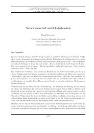
1.4. The Birth-Death Process<br />
A special Markov process, and <strong>of</strong> interest in understanding queueing theory later, is<br />
the Birth-Death process. Figure 1.1 shows the state diagram <strong>of</strong> such a process. State<br />
diagrams are a very useful tool to visualize a Markov process: it shows every possible<br />
state <strong>of</strong> the system and its unit transition probabilities (rates) W kk ′. Here the rates are<br />
labeled λ i = W i,i+1 and µ i = W i,i−1 . As opposed to a general Markov process, there are<br />
only allowed transitions between two neighboring states. If k is the occupation <strong>of</strong> the<br />
state, then an allowed transition can go to k+1, which is called a birth and k−1, which<br />
is called a death. The transition rates from occupation state k to k ± 1 are in general<br />
dependent on the state <strong>of</strong> departure. λ k is called the birth rate, µ k the death rate. From<br />
a physics point <strong>of</strong> view, the connection to (second quantization) ladder operator techniques<br />
famous is fairly obvious and will play a role later, when looking at the treatment<br />
<strong>of</strong> queueing networks by Massey [33] and Chernyak et al. [6].<br />
To answer the question what the density pr<strong>of</strong>ile/probability distribution <strong>of</strong> the states k<br />
in such a system is, one looks for the Master Equation <strong>of</strong> the system. Using the probabil-<br />
26
Chapter 1: <strong>Non</strong>-<strong>Equilibrium</strong> <strong>Statistical</strong> <strong>Physics</strong><br />
ity flow interpretation <strong>of</strong> the Master Equation and the state diagram as a visualization<br />
tool, one finds the following Mater Equation for a general Birth-Death process:<br />
dP k (t)<br />
dt<br />
dP 0 (t)<br />
dt<br />
= −(λ k +µ k )P k (t)+µ k+1 P k+1 (t)+λ k−1 P k−1 (t) (1.4.1)<br />
= −λ 0 P 0 (t)+µ 1 P 1 (t) (1.4.2)<br />
To solve this equation, the technique <strong>of</strong> z-transforms is very useful [24]. However, since<br />
this is not really a necessary result for this thesis, we will not do the calculation and<br />
rather look at an important special case <strong>of</strong> the birth-death process.<br />
The uniform pure birth-process, i.e. a birth-death process with µ k = 0, is <strong>of</strong> special<br />
interest since it is a model for a Markovian, memoryless process. The Master Equation<br />
for this process reads<br />
dP k (t)<br />
dt<br />
dP 0 (t)<br />
dt<br />
= −λP k (t)+λP k−1 (t) (1.4.3)<br />
= −λP 0 (t). (1.4.4)<br />
This system is easily solved iteratively. For k = 0 the solution is (simply via integration)<br />
For k = 1 the differential equation reads<br />
dP 1 (t)<br />
dt<br />
P 0 (t) = e −λt . (1.4.5)<br />
+λP 1 (t) = λe −λt (1.4.6)<br />
which is a non-homogeneous and not-separable ordinary differential equation, which can<br />
be solved by the method <strong>of</strong> introducing an integrating factor (see e.g. [3]). Thus one<br />
arrives at<br />
P 1 (t) = λte −λt . (1.4.7)<br />
Iterating this procedure, one arrives again at a differential equation <strong>of</strong> the same type<br />
and, via an integrating factor, yields the iterative equation<br />
P k (t) = e −λt ∫<br />
λe λt P k−1 (t)dt (1.4.8)<br />
with solution<br />
P k (t) = (λt)k e −λt . (1.4.9)<br />
k!<br />
Hence the occupation numbers <strong>of</strong> every Markovian birth process are Poisson distributed.<br />
An interesting and important feature <strong>of</strong> the Poisson distribution is, that a Poisson distributed<br />
stochastic process, like here the process <strong>of</strong> births, has exponentially distributed<br />
inter-birth times. This means, that the time-span between two consecutive births is an<br />
exponentially distributed random variable and can be seen via the following consideration.<br />
27
Chapter 1: <strong>Non</strong>-<strong>Equilibrium</strong> <strong>Statistical</strong> <strong>Physics</strong><br />
The inter-birth time is exponentially distributed. Let τ be the inter-birth time, i.e. the<br />
time between to consecutive births and let X(τ 0 ,τ 0 +τ) define the random variable <strong>of</strong><br />
the number <strong>of</strong> births between time span (τ 0 ,τ 0 +τ). Then, according to the dynamics<br />
<strong>of</strong> a Markovian birth process with rate λ, it holds:<br />
P(X(τ 0 ,τ 0 +τ) = k) = (λτ)k e −λτ (1.4.10)<br />
k!<br />
Hence, letting k be the parameter and τ the free variable, the probability <strong>of</strong> having<br />
exactly one birth after duration τ is nothing but P(X(τ 0 ,τ 0 +τ) = 1). Hence letting T<br />
denote the random variable <strong>of</strong> having exactly one birth after time T = τ one finds<br />
for the distribution <strong>of</strong> inter-birth time T 6 .<br />
P(T = τ) = λe −λτ (1.4.11)<br />
Later the birth process will be used to describe any memoryless, Markovian process<br />
<strong>of</strong> arrivals <strong>of</strong> customers to the queuing system.<br />
In this chapter we introduced the notion <strong>of</strong> non-equilibrium statistical physics on a<br />
formal level. We furthermore provided the concept <strong>of</strong> stochastic and especially Markov<br />
processes. In the next chapter we will use these concepts to address the mathematical<br />
concept <strong>of</strong> queues and queueing networks.<br />
6 The notation <strong>of</strong> T and τ as inter-birth time seems eventually a bit confusing. But T denotes the<br />
random variable, whereas τ denotes the value this variable can take. In (1.4.10) τ is a parameter and<br />
k the free variable, the value the random variable X can take. Whereas in this equation τ is the free<br />
variable denoting the value the random variable T can take.<br />
28
2. <strong>Queueing</strong> <strong>Theory</strong><br />
2.1. A short glance on history<br />
<strong>Queueing</strong> <strong>Theory</strong> is traditionally an Operations Research discipline. It was developed<br />
andisemployedtooptimizeandanalyzeprocessesincludingwaitinglines(queues), s<strong>of</strong>or<br />
example telecommunication processes, production processes or network traffic in applied<br />
computer science. For a nice introduction see e.g. [24], for a more advanced treatment<br />
see e.g. [5].<br />
2.2. <strong>Theory</strong> <strong>of</strong> Single Queues<br />
This chapter is devoted to introducing the basic mathematical object queue as well as<br />
presenting general features and theorems. Especially Burke’s theorem will play a central<br />
role here and later. As stated earlier, one <strong>of</strong> the goals <strong>of</strong> this thesis is to establish<br />
a connection between the Operations Research native theory <strong>of</strong> queues and a possible<br />
analogy in physics. However, in this chapter we will mostly use the Operations Research<br />
terminology and will later build the desired connection.<br />
A queue is a mathematical object combining two ideas:<br />
a) the idea <strong>of</strong> a service facility. Its purpose is to complete jobs/serve customers which<br />
are arriving at this facility.<br />
b) the idea <strong>of</strong> a storage, in which arriving jobs can be queued if the facility is busy<br />
(Fig. 2.1).<br />
Such a general system is normally notated as a G/G/m/n system. So what does this<br />
mean? To describe a queueing system completely one has to specify four parameters:<br />
1. A parameter to quantify how jobs enter the system.<br />
2. A parameter to quantify how jobs are completed in the facility.<br />
3. A parameter to quantify the ”parallelness” <strong>of</strong> job completion, i.e. how many jobs<br />
can a facility complete at the same time.<br />
4. A parameter to specify the capacity/storage space <strong>of</strong> a system, i.e. how many jobs<br />
can be queued before being processed in the facility.<br />
The above notation is used to denote a very general queue: jobs enter the system in a<br />
General fashion, are completed in a General fashion, at most m jobs in parallel and the<br />
29
•<br />
•<br />
•<br />
•<br />
•<br />
•<br />
Chapter 2: <strong>Queueing</strong> <strong>Theory</strong><br />
A(t)<br />
n<br />
m<br />
• • • • • •<br />
B(t)<br />
Figure 2.1.: Illustration <strong>of</strong> a single A(t)/B(t)/m/n queue. Red squares denote jobs entering<br />
the system, green squares denote completed jobs leaving the system.<br />
storage capacity is n jobs.<br />
However, the notion <strong>of</strong> ”how jobs enter the system” and ”how jobs are completed in the<br />
facility” is not very precise. Every model and every specification in a model is based<br />
on the desired result. In the case <strong>of</strong> queueing systems one is mostly interested in the<br />
number <strong>of</strong> total jobs in the system, the time a job spends in the system and the number<br />
<strong>of</strong> jobs waiting in the queue. Of course, from a physics point <strong>of</strong> view a Hamiltonian<br />
standpoint would be totally acceptable and a solution <strong>of</strong> the problem: specify the exact<br />
times at which jobs arrive to the system as well as the microscopic dynamics <strong>of</strong> how jobs<br />
are completed. Then construct the Hamiltonian <strong>of</strong> the system and solve a general kind<br />
<strong>of</strong> equations <strong>of</strong> motion. However, such an approach is certainly very limited. In most<br />
systems, especially those arising in Operations Research, one has to deal with a large<br />
number <strong>of</strong> unpredictable jobs arriving at the system. In such cases a statistical approach<br />
is much more preferable. Hence it is useful to specify the distribution <strong>of</strong> inter-arrival<br />
times t i <strong>of</strong> jobs entering the system<br />
P(t i ≤ t) = A(t) (2.2.1)<br />
and the distribution <strong>of</strong> service times t s <strong>of</strong> completing a job in the facility<br />
P(t s ≤ t) = B(t). (2.2.2)<br />
NotethatA(t)andB(t)arecumulativedistributions, tostickwiththestandardnotation<br />
in queueing theory [24]. The inter-arrival time t i is defined as the time interval between<br />
the consecutive arrival <strong>of</strong> two jobs to the system.<br />
We specified the system in terms <strong>of</strong> constant integer-valued variables m and n as well<br />
as real-valued, positive random variables t i and t s , which we will call the free variables<br />
<strong>of</strong> our system. As is well known, every function <strong>of</strong> one or more random variables is<br />
itself again a random [15]. Hence the results <strong>of</strong> the queueing network analysis will be<br />
randomvariablesaswellandweendupwithacompletelyprobabilisticdescription<strong>of</strong>our<br />
underlying real-world phenomenon. This is important to keep in mind for interpretation<br />
30
Chapter 2: <strong>Queueing</strong> <strong>Theory</strong><br />
<strong>of</strong> results. It also opens the way to a statistical physics treatment <strong>of</strong> the problem, which<br />
will be presented later.<br />
After defining the basic quantities <strong>of</strong> a single queue it is rather straight forward to get<br />
some first interesting results. First let us define a couple <strong>of</strong> more quantities, following<br />
directly from the basic free variables already defined. Denoting the absolute arrival time<br />
to the system <strong>of</strong> some job n with τ n , it is clear that the inter-arrival time t n between job<br />
n−1 and n is<br />
t i (n) = τ n −τ n−1 . (2.2.3)<br />
Defining the waiting time t w (n) <strong>of</strong> a job in the system, i.e. the time it waits in the<br />
queue before the service facility will start processing it, the system time t Σ (n) <strong>of</strong> job n,<br />
is defined as<br />
t Σ (n) = t s (n)+t w (n). (2.2.4)<br />
The waiting time t w and its distribution will be a property <strong>of</strong> the system, following from<br />
the free variables in a non-trivial way.<br />
Calculating some basic average properties, like the average inter-arrival time 1<br />
∑<br />
∫<br />
¯t i = t i P(t i )dt i (2.2.5)<br />
t i<br />
and the average service time 1 ∑<br />
∫<br />
¯t s = t s P(t s )dt s (2.2.6)<br />
t s<br />
one defines the average arrival rate<br />
λ = ¯t i<br />
−1<br />
(2.2.7)<br />
and the average service rate<br />
µ = ¯t s −1 . (2.2.8)<br />
This definition is, from a physics point <strong>of</strong> view, quite natural. Additionally, it will<br />
pro<strong>of</strong> useful later when talking about continuously exponentially distributed inter-arrival<br />
times, since in this case the inverse <strong>of</strong> the distribution parameter exactly equals the<br />
average in such ∫<br />
¯t = tλe −λt dt = λ −1 . (2.2.9)<br />
Another interesting quantity is the distribution P(α(t ′ )) <strong>of</strong> customers α(t ′ ) arriving to<br />
the system within the time interval [0,t ′ ]. Here α(t ′ ) is a random variable with parameter<br />
t ′ . Obviously the probability <strong>of</strong> arrival <strong>of</strong> exactly one customer is exactly the probability<br />
<strong>of</strong> having inter-arrival time t ′ P(α(t ′ ) = 1) = P(t i = t ′ ). (2.2.10)<br />
1 Using ∑ or ∫ depending on whether we talk about discrete or continuous time variables respectively.<br />
31
Chapter 2: <strong>Queueing</strong> <strong>Theory</strong><br />
The probability <strong>of</strong> having exactly two arrivals in [0,t ′ ] is given via the convolution <strong>of</strong> the<br />
inter-arrival time distribution<br />
∫<br />
P(α(t ′ ) = 2) = dτ 1 P(t i = τ 1 )P(t i = t ′ −τ 1 ). (2.2.11)<br />
Thus the probability <strong>of</strong> having exactly n arrivals in [0,t ′ ] is given by the following<br />
recursion<br />
∫<br />
P(α(t ′ ) = n) =<br />
dτ 1<br />
∫<br />
∫<br />
dτ 2 ...<br />
n−1<br />
∏<br />
dτ n−1<br />
j=1<br />
n−1<br />
∑<br />
P(t i = τ j )P(t i = t ′ −<br />
k=1<br />
τ k ). (2.2.12)<br />
Note that, in our interpretation, t ′ is a parameter and n is the free variable. If the<br />
inter-arrival times are exponentially distributed with parameter λ, the average number<br />
<strong>of</strong> arrivals within [0,t ′ ] is given by<br />
¯ α(t ′ ) = λt ′ , (2.2.13)<br />
The most interesting queueing theoretical quantity for this thesis will be the number<br />
<strong>of</strong> customers in the system at time t, which we will denote by<br />
N(t). (2.2.14)<br />
Again, this quantity is a random variable. We are most interested in a possible steadystate<br />
solution <strong>of</strong> the system, i.e. the limit<br />
lim N(t) = N. (2.2.15)<br />
t→∞<br />
Such a limit does not necessarily exist and even if it does, its calculation can be far from<br />
trivial, since generally one would have to solve for the Master Equation <strong>of</strong> the system.<br />
An important queueing theorem correlates the average number <strong>of</strong> customers in the system<br />
(in the t → ∞ limit), ¯N, to the average system time, t¯<br />
Σ :<br />
¯N = λt Σ (2.2.16)<br />
This result is known as Little’s result in queueing theory and can be translated as<br />
”average customers in the system=(average arrival time to the system)×(average system<br />
time)”. This seems from a physics point <strong>of</strong> view fairly obvious. However, the pro<strong>of</strong> for<br />
this theorem was only established in 1961 by John D. C. Little’s[30].<br />
In a system containing a simple queue with only one facility, the following measure is<br />
an important quantity:<br />
ρ = λ µ . (2.2.17)<br />
In queueing theory this is called the utilization factor. Its meaning is important for<br />
deciding <strong>of</strong> whether or not a stable steady-state solution for the system exists. If<br />
ρ > 1 (2.2.18)<br />
32
Chapter 2: <strong>Queueing</strong> <strong>Theory</strong><br />
holds, the system will not be stable, in the sense that the average waiting time <strong>of</strong> a<br />
customer will go to infinity, since lim t→∞ N(t) = ∞ will hold. This is easily seen, since<br />
in this case (via (2.2.7) and (2.2.8)) the service rate would exceed the arrival rate and<br />
hencecongestioninthewaitingqueuewillresult 2 . Anotherinterpretation<strong>of</strong>ρisinterms<br />
<strong>of</strong> “fraction <strong>of</strong> time the facility is busy”. We will show later that (quite remarkably)<br />
equation (2.2.18) holds as a stability condition in a much more general setting than the<br />
one-queue system.<br />
2.3. The Single Markovian Queue as Birth-Death System<br />
In the previous chapter we said that the number <strong>of</strong> customers in the system is an important<br />
quantity for this thesis. However, its computation seems not so straight forward.<br />
The knowledge <strong>of</strong> this quantity is also important to be able to make a theoretical statement<br />
about the number <strong>of</strong> customers leaving the system, which clearly is a function <strong>of</strong><br />
how many customers are present in the system.<br />
Developing an universal description <strong>of</strong> the general G/G/m/n system <strong>of</strong> one queue seems<br />
to be a bit too optimistic. Also, from a physics perspective, this generality is mostly<br />
not needed. Instead, a very common queueing system which has been studied a lot is<br />
denoted by M/M/n/m. This system is one with Markovian input, Markovian service<br />
completion, n servers and storage <strong>of</strong> size m. As pointed out earlier, Markovity and<br />
memorylessness are highly coupled and the underlying principles governing a vast number<br />
<strong>of</strong> real-world stochastic processes. From the things pointed out earlier, it is directly<br />
possible to specify the stochastic processes underlying an M/M/n/m system in more<br />
detail using the analogy to Birth-Death processes. In such a mapping the arrival <strong>of</strong> a<br />
customer to the system is modeled as birth <strong>of</strong> a customer to the system and the completion<br />
<strong>of</strong> service as death. In a M/M/n/m system with customer arrival rate λ, this rate<br />
is directly related to the birth-rate λ <strong>of</strong> a corresponding pure birth process. Since in this<br />
Markovian queueing system the arrival <strong>of</strong> customers is supposed to be Markovian (i.e.<br />
independent <strong>of</strong> the history <strong>of</strong> arrivals), we find (transferring the results from section 1.4)<br />
that the arrival process to the system is a Poisson distributed stochastic process<br />
with exponentially distributed inter-arrival times<br />
P(N arr = k,t) = (λt)k e −λt (2.3.1)<br />
k!<br />
P(t i = t) = λe −λt . (2.3.2)<br />
Also, if we denote the completion rate <strong>of</strong> every facility in this system with µ, the Master<br />
Equation for the distribution <strong>of</strong> number <strong>of</strong> customers in the system for every given time<br />
2 For illustration, the reader may think <strong>of</strong> its last visit to whatever (German) public administrative<br />
<strong>of</strong>fice.<br />
33
Chapter 2: <strong>Queueing</strong> <strong>Theory</strong><br />
t is in analogy to equation (1.4.2) given by<br />
dP k (t)<br />
dt<br />
dP 0 (t)<br />
dt<br />
= −(Θ(m−k)λ+min(n,k)µ)P k (t)+min(n,k +1)µP k+1 (t)<br />
+Θ(m−k +1)λP k−1 (t) (2.3.3)<br />
= −λP 0 (t)+min(n,1)µP 1 (t)<br />
Here Θ is a Heaviside-like function with Θ(x) = 1, if x ≥ 0 and Θ(x) = 0, otherwise.<br />
WhatdistinguishesthisMasterEquationfromtheone<strong>of</strong>thepurebirth-deathprocessare<br />
the multiplicities <strong>of</strong> the facilities n. This basically leads to a linear increase in customer<br />
service completion and is accounted for by multiplying the death-rates by min(n,k).<br />
The restriction <strong>of</strong> storage capacity is here modeled via the Θ-function.<br />
We will not solve this Master Equation but rather look at the important case <strong>of</strong> the<br />
M/M/1/∞ queue, i.e. a system with one facility and infinite storage. In this case the<br />
Master Equation is just (1.4.2) and as mentioned earlier the time-dependent solution<br />
rather complicated. However, considering the steady-state case<br />
0 = −(λ+µ)Pk ss +µPss k+1 +λPss k−1<br />
0 = −λP0 ss +µP1<br />
ss<br />
finding a solution is possible iteratively and the steady-state solution <strong>of</strong> the distribution<br />
<strong>of</strong> customers N in the M/M/1/∞ system is given by<br />
( ) λ k<br />
P ss (N = k) = P0<br />
ss , (2.3.4)<br />
µ<br />
as one easily checks via substituting back into the homogeneous Master Equation. This<br />
result is a power-law distribution. P 0 serves as the normalization constant and can be<br />
found, via the convergence <strong>of</strong> the geometric series, to be<br />
( ∞<br />
) −1<br />
∑<br />
P 0 = ρ k<br />
k=0<br />
= 1−ρ, (2.3.5)<br />
where<br />
ρ = λ µ<br />
(2.3.6)<br />
is the previously introduced utilization factor. Probability distribution (2.3.4) is only<br />
normalizable, if the geometric series in (2.3.5) converges. Convergence is assured only<br />
for 0 < ρ < 1 and hence a steady-state solution for this system only exists if λ < µ,<br />
which matches the criterium pointed out in (2.2.18) and provides for this system a<br />
strict mathematical explanation. Having obtained this solution, the average number <strong>of</strong><br />
customers in the steady-state is given by<br />
¯N = ρ<br />
1−ρ . (2.3.7)<br />
34
Chapter 2: <strong>Queueing</strong> <strong>Theory</strong><br />
In the steady-state the distribution <strong>of</strong> customers N out leaving the facility can also be<br />
computed. On a first thought one might guess that the P(N out ) will be highly coupled<br />
to the number <strong>of</strong> customers N in the system and will be a complicated result. However,<br />
the following consideration shows that the solution is in fact rather simple - albeit very<br />
surprising:<br />
Burke’s theorem. Consider a M/M/1/∞ system <strong>of</strong> a single queue with customer arrival<br />
rate λ and job-completion rate µ. As established earlier, in a Markovian system, the<br />
inter-arrival time and facility completion time are exponentially distributed. As seen<br />
earlier, if there is a constant Markovian birth process with rate λ, the number <strong>of</strong> births<br />
in every time period is Poisson distributed with rate λ. Since the facility completion<br />
process is such a process, the number <strong>of</strong> customers leaving the queue would be Poisson<br />
distributed with rate µ, iff there would be a constant supply <strong>of</strong> customers. However,<br />
in this model the supply <strong>of</strong> customers is regulated by the number <strong>of</strong> customers in the<br />
system N, which is in the steady state case distributed with (2.3.4). Hence the supply<br />
<strong>of</strong> customers to the service facility is constrained exactly by this distribution. Let me<br />
derive the statistics <strong>of</strong> the output:<br />
P(N out = k,t) ∼ e −µt(µt)k<br />
k!<br />
∼ e −µt(µt)k<br />
k!<br />
·P(N ≥ k)<br />
∞∑<br />
(1−ρ)ρ k (2.3.8)<br />
l=k<br />
∼ e −µt(µt)k ρ k .<br />
k!<br />
Using (2.3.6) and normalizing correctly we finally get<br />
P(N out = k,t) = e −λt(λt)k . (2.3.9)<br />
k!<br />
This rather surprising result says, that in the steady-state case the output <strong>of</strong> the<br />
M/M/1/∞ system is, as the input, Poisson distributed with the arrival-rate λ. This<br />
result is <strong>of</strong>ten known as Burke’s theorem[4]. Interestingly, there is (in physics terms)<br />
something like a first order phase transition in the following sense. As we have shown,<br />
a solution for the distribution <strong>of</strong> the number <strong>of</strong> customers N in the system only exists if<br />
ρ ≤ 1. In a M/M/1/∞ system with infinite storage space <strong>of</strong> arriving jobs, this means<br />
that in the case ρ ≥ 1 the number <strong>of</strong> customers will diverge, i.e. go to N → ∞. Restating<br />
this fact, there is an infinite number <strong>of</strong> supply for the facility, keeping it constantly busy.<br />
Hence the output <strong>of</strong> the queueing system will, opposed to the ρ ≤ 1 case, solely depend<br />
on the dynamics <strong>of</strong> the service facility and not anymore on the input. Hence Burke’s<br />
theorem will not hold in this scenario. Instead the output <strong>of</strong> the system will be Poisson<br />
distributed with rate µ (since the service time is exponentially distributed with rate µ).<br />
So with ρ → 1 there is an abrupt (first order) change (phase transition) in the output <strong>of</strong><br />
the system from a Poisson distribution with rate λ to a Poisson distribution with rate<br />
µ.<br />
35
Chapter 2: <strong>Queueing</strong> <strong>Theory</strong><br />
λ 31<br />
Q1<br />
λ 13<br />
Q3<br />
λ 01<br />
λ 20<br />
λ 30<br />
λ 12 λ 23<br />
Q2<br />
Figure 2.2.: Illustration <strong>of</strong> a queueing network with 3 nodes.<br />
2.4. <strong>Networks</strong> <strong>of</strong> M/M/1/∞ queues<br />
A straight forward extension <strong>of</strong> the theory <strong>of</strong> a single queue is to consider networks <strong>of</strong><br />
queues. Figure 2.2 illustrates a possible queueing network. These systems are more<br />
elaborate and complex than the former one. The input <strong>of</strong> one queue in the network<br />
might not only depend on customers arriving from outside <strong>of</strong> the system, but will also<br />
depend on transitions <strong>of</strong> customers from the output <strong>of</strong> one queue to an adjacent queue 3 .<br />
Thisleavesuswithahighlycoupledsystemwhichneedstobeanalyzed. Thistaskisvery<br />
much simplified by Burke’s theorem: even queues, which are being fed by transitioning<br />
customers, i.e. customers just leaving another queue, will have Poissonian input and<br />
hence can be treated as as a single, independent M/M/1/∞ queue, as presented in the<br />
previous chapter:<br />
The sum <strong>of</strong> two independent Poisson distributed variables is again Poisson distributed.<br />
Consider two consecutive M/M/1/∞ queues Q1 and Q2. Assume that Q1 has, with<br />
Burke’s theorem, Poissonian output with rate λ 12 . Furthermore assume that Q2 has<br />
customers arriving externally with rate λ 02 and customers arriving from Q2 with exactly<br />
its leaving rate λ 12 . Considering the sum S = K+L <strong>of</strong> two independently Poisson<br />
distributed random variables K and L:<br />
P(S = s) = (P(K)∗P(L))(s)<br />
∞∑<br />
= P(K = k)P(L = s−k) (2.4.1)<br />
=<br />
k=0<br />
∞∑<br />
k=0<br />
e λ 12t (λ 12t) k<br />
e λ 02t (λ 02t) (s−k)<br />
k! (s−k)!<br />
(2.4.2)<br />
3 The term adjacent here is meant in the graph-theoretical way, i.e. neighboring in the sense <strong>of</strong> being<br />
connected by an edge.<br />
36
Chapter 2: <strong>Queueing</strong> <strong>Theory</strong><br />
The infinite sum on the rhs is convergent and the sum is given by 4<br />
∞∑ (λ 12 t) k<br />
k=0<br />
k!<br />
(λ 02 t) (s−k)<br />
(s−k)!<br />
= (λ 12t+λ 02 t) s<br />
s!<br />
(2.4.3)<br />
which leaves us with<br />
P(S = s) = e (λ 12+λ 02 )t (λ 12t+λ 02 t) s<br />
(2.4.4)<br />
s!<br />
showing that the sum <strong>of</strong> two independently Poissonian distributed variables is again<br />
Poisson distributed with the sum <strong>of</strong> the single rates.<br />
Having shown that and keeping Burke’s theorem in mind, the steady-state transition<br />
rates λ ij in a network <strong>of</strong> queues can be calculated via<br />
λ ij = (λ 0i −λ i0 )−<br />
k∈∂i/jλ ∑<br />
ik + ∑ λ ki (2.4.5)<br />
k∈∂i<br />
where ∂i/j denotes the set <strong>of</strong> all neighbors <strong>of</strong> i without j. This is a very general<br />
expression which, thinking <strong>of</strong> systems <strong>of</strong> flows, basically equates influx and outflux for<br />
every queue in the system. That such an ”average flux” conversation holds is not at all<br />
obvious, sinceoursystemisequippedwiththepossibility<strong>of</strong>storingjobsinaqueue. That<br />
this result nevertheless holds is due to the double-Markovity in the system (Markovian<br />
input and Markovian service completion) and the resulting Burke’s theorem.<br />
In a case as described here, it is clear that transition rates λ ik for all neighbors k <strong>of</strong> i<br />
and λ i0 must be interrelated. Concretely, denoting the effective service rate at queue i<br />
with λ i < µ i , the following equation must hold:<br />
λ i = ∑ k∈∂iλ ik +λ i0 . (2.4.6)<br />
Assuming λ ik = λ i p ik with ∑ k p ik = 1 and p ik being the probability that a served<br />
customer is transferred from node i to node k or leaving the network (k = 0), one finds<br />
for the local, effective steady-state service rates<br />
λ i = λ 0i + ∑ k<br />
λ k p ki . (2.4.7)<br />
This is a well-posed system <strong>of</strong> n variables and n equations which can in principal be<br />
solved using standard methods. However, if the system is large n >> 1, the solution<br />
<strong>of</strong> such a linear system is far from trivial and special computational algorithms need to<br />
be employed. However, in most cases the underlying network <strong>of</strong> queues will be weekly<br />
connected, i.e. the linear system very sparse and efficient sparse-matrix algorithms like<br />
the Conjugate Gradient method or Gaussian Belief Propagation can be used to do the<br />
job.<br />
The first one to mathematically describe such kinds <strong>of</strong> systems was James R. Jackson<br />
4 Using e.g. Mathematica.<br />
37
Chapter 2: <strong>Queueing</strong> <strong>Theory</strong><br />
in his seminal 1963 paper [21]. He even generalized the ideas presented above to a less<br />
restrictive setting, with arrival and completion rates not constant but dependent on the<br />
number <strong>of</strong> customers in the queue.<br />
After the effective rates <strong>of</strong> the system have been calculated and (as we have shown<br />
previously) in the steady state every queueing system in the network can be treated as<br />
an independent queueing system with the new effective rates, the solution for the system<br />
P(N) has to be a factorized form <strong>of</strong> the independent random variables N i :<br />
P(N) = ∏ i<br />
P(N i ) (2.4.8)<br />
Again, for the i−th subsystem there is an effective Poissonian arrival rate λ i and an<br />
inherent service rate µ i associated. We define the i−th utilization factor via<br />
ρ i = λ i<br />
µ i<br />
. (2.4.9)<br />
Let us note that it is also possible to introduce the nominal transition rate from queue i<br />
to queue j as µ ij = µ i p ij , for which then the following relation to the effective transition<br />
rate holds:<br />
λ ij = ρ i µ ij (2.4.10)<br />
This leads us directly to<br />
and with 2.4.8 to the joint probability distribution<br />
P(N i = k i ) = (1−ρ i )ρ k i<br />
i<br />
(2.4.11)<br />
P(N = k) = ∏ i<br />
(1−ρ i )ρ k i<br />
i . (2.4.12)<br />
This result is quite remarkable. There are very few non-equilibrium systems for which<br />
the solution is nicely factorized. However, we want to stress that it is Burke’s theorem<br />
and hence the double-Markovian nature <strong>of</strong> the system which ensures this nice property.<br />
We also want to stress that we were able to obtain this solution without solving the<br />
Master Equation for this coupled system but just via employing Burke’s theorem.<br />
Using the above introduced utilization factors, one can write (2.4.5) in a convenient<br />
form as:<br />
∑<br />
M ij ρ j = λ 0i (2.4.13)<br />
with<br />
M ij =<br />
j<br />
{<br />
−µ ji i ≠ j<br />
µ i0 + ∑ k µ ik i = j.<br />
(2.4.14)<br />
If there is no misunderstanding possible, we will use the Einstein-convention and e.g. in<br />
(2.4.13) drop the sum sign and assume summation over double indices.<br />
As shortly mentioned earlier, the result obtained by Jackson [21] is more general.<br />
More specifically, he does not restrict himself to constant service rates µ i , but consider<br />
38
Chapter 2: <strong>Queueing</strong> <strong>Theory</strong><br />
service rates which can be dependent on the current number <strong>of</strong> jobs present in the single<br />
queue. However, the result is remarkably similar and again factorized:<br />
with<br />
P(N = k) ∼ ∏ i<br />
˜ρ k i<br />
i<br />
∏k i<br />
l<br />
µ −1<br />
i<br />
(l). (2.4.15)<br />
λ 0i = ˜M ij˜ρ j<br />
{<br />
(2.4.16)<br />
−p ji i ≠ j<br />
˜M ij =<br />
p i0 + ∑ k p ik i = j.<br />
(2.4.17)<br />
Often it is more convenient to write equation (2.4.16) as a matrix equation:<br />
λ = ˜M˜ρ˜ρ˜ρ<br />
where we defined the vector if arrival rates λ, the vector ˜ρ˜ρ˜ρ and matrix ˜M. We want to<br />
note that in the standard case the diagonal elements <strong>of</strong> ˜M will be ˜M ii = 1.<br />
2.5. Operator technique to solve ME for <strong>Queueing</strong> <strong>Networks</strong><br />
In this chapter we want to introduce a more theoretical physics based description <strong>of</strong> the<br />
openqueueingnetwork,suggestedbyChernyaketal. [6],basedonthesocalledDoi-Peliti<br />
[12] technique and Massey’s operator theory treatment <strong>of</strong> such systems [33]. Since we<br />
already solved the steady-state <strong>of</strong> the <strong>Queueing</strong> network in the previous section 5 , we will<br />
not go too much into detail here but rather restrict ourselves to present the basic idea.<br />
We choose to present this material mainly for purposes <strong>of</strong> interest and because it again<br />
outlines a very nice connection between a theoretical physics based theory/methodology<br />
and the seemingly far distant field <strong>of</strong> Operations Research.<br />
In general, the so called Doi-Peliti technique is a very useful operator theory to describe<br />
classical many-particle systems and the production/annihilation <strong>of</strong> particles in<br />
such systems. It is based on the second quantization method in quantum theory, which<br />
is exhaustively used in high-energy particle physics to describe the creation and annihilation<br />
<strong>of</strong> elementary particles as described by the standard model <strong>of</strong> particle physics.<br />
The value <strong>of</strong> such a second quantization technique for classical systems is that one does<br />
not have to solve the Master Equation by using classical approaches to solve differentialdifference<br />
equations. Since this is <strong>of</strong>ten a hard and eventually not feasible problem using<br />
the standard methods known in the theory <strong>of</strong> stochastic processes, the Doi-Peliti technique<br />
<strong>of</strong>fers for birth-death processes a second path to the solution. Since a queue can<br />
be described as a birth-death process, this technique can be applied in such systems.<br />
In a discrete stochastic system, like the queueing network, the joint probability distribution<br />
<strong>of</strong> having N i customers accumulated at queue Qi i = 1...n is the quantity<br />
<strong>of</strong> interest. From a quantization point <strong>of</strong> view, on can hence define a base state<br />
5 Albeit not by solving the Master Equation directly but by employing Burke’s theorem.<br />
39
Chapter 2: <strong>Queueing</strong> <strong>Theory</strong><br />
|N〉 = |N 1 = k 1 ,N 2 = k 2 ,...N L = k L 〉 = |k 1 ,k 2 ,...,k L 〉 <strong>of</strong> the system to have exactly k i<br />
customers in queue Qi. Since here we are dealing with a stochastic system, the actual<br />
state |s〉 <strong>of</strong> the system is only given by a stochastic linear combination <strong>of</strong> the base states<br />
(mixed state)<br />
|s〉 = ∑ P(N)|N〉 (2.5.1)<br />
with P(N) being the probability <strong>of</strong> finding the system in state |N〉 6 . The idea in this<br />
approach is to transform the Master Equation <strong>of</strong> a queueing network (here we choose to<br />
present the ME for the M/M/1/∞) network)<br />
dP(k 1 ,...,k L ;t)<br />
dt<br />
= ∑<br />
+<br />
−<br />
(i,j)∈E<br />
µ ij Θ(k j )P(...,k i +1,..,k j −1,...;t)−µ ij Θ(k i )P(...,k i ,...,k j )<br />
L∑<br />
P(...,k i −1...)µ 0i Θ(k i )+P(...,k i +1...)µ i0<br />
i=1<br />
L∑<br />
P(...,k i ,...)µ 0i +P(...,k i ,...)µ i0 Θ(k i )<br />
i=1<br />
(2.5.2)<br />
with Θ(k) being a Heaviside-like function with<br />
{<br />
1 if k > 0<br />
Θ(k) =<br />
0 else<br />
(2.5.3)<br />
and E the set <strong>of</strong> all edges in the system, into a time-dependent Schrödinger-like equation<br />
d<br />
|s〉 = Ĥ|s〉. (2.5.4)<br />
dt<br />
In order to find the steady state we are interested in the time-independent solution<br />
0 = 0|s ss 〉 = Ĥ|s ss〉 (2.5.5)<br />
which hence constitutes the problem <strong>of</strong> finding the eigenstate |s ss 〉 <strong>of</strong> the Hamiltonian<br />
Ĥ with eigenvalue 0 7 . However, we need to transform the rhs <strong>of</strong> the Master Equation<br />
into a second-quantization Hamiltonian. Following the notation <strong>of</strong> [6], this can be done<br />
in the following way. Define particle creation (birth) and particle annihilation (death)<br />
operators in such a way, that the standard algebra for ladder operators (see e.g. [8]) is<br />
fulfilled<br />
â † i |...,k i,...〉 = |...,k i +1,...〉 (2.5.6)<br />
â i |...,k i ,...〉 = k i |...,k i −1,...〉, (2.5.7)<br />
6 This idea is clearly borrowed from the theory <strong>of</strong> many-particle quantum systems where e.g. the effect<br />
<strong>of</strong> entanglement arises.<br />
7 This would be the state with lowest energy or ”base state”.<br />
40
Chapter 2: <strong>Queueing</strong> <strong>Theory</strong><br />
which is the usual definition. Since in the ME we have to deal with a couple <strong>of</strong> Heavisidelike<br />
functions, it makes sense to introduce a ”skewed”[6] annihilation operator ˆb, which<br />
is in some sense a ”logical” operator:<br />
ˆbi |...,k i ,...〉 = Θ(k i )|...,k i −1,...〉. (2.5.8)<br />
Using the so defined operators, one sees that the Master Equation translates into equation<br />
(2.5.4) with Hamiltonian<br />
Ĥ = ∑<br />
(i,j)∈E<br />
µ ij (â † j −↠i )ˆb i +<br />
L∑<br />
i=1<br />
(µ 0i (â † i −1)+µ i0(1−â † i )ˆb i<br />
)<br />
, (2.5.9)<br />
which then will be used to solve the eigenvalue problem. We will not solve this problem<br />
here but merely state the solution and refer for details to references [6, 33]. One finds<br />
that the eigenstate elements |s ss 〉 i = ∑ k i<br />
P(N i = k i )|N i = k+i〉 <strong>of</strong> the Hamiltonian are<br />
eigenstates <strong>of</strong> the corresponding annihilation operator ˆb i |s ss 〉 i = ρ i |s ss 〉 i to eigenvalue ρ i<br />
and that they have the form<br />
|s ss 〉 i =<br />
1<br />
1−ρ i â † |0〉 =<br />
i<br />
∞∑<br />
(ρ i â † i )n |0〉 (2.5.10)<br />
n=0<br />
which translates for the complete state |s ss 〉 into<br />
|s ss 〉 = ∏ i<br />
= ∑ k<br />
|s ss 〉 i (2.5.11)<br />
∏<br />
i<br />
ρ k i<br />
i<br />
|k〉 (2.5.12)<br />
which yields, after normalization and comparing with (2.5.1):<br />
P(N = k) = 1 Z<br />
= ∏ i<br />
∏<br />
i<br />
ρ k i<br />
i<br />
(2.5.13)<br />
(1−ρ i )ρ k i<br />
i . (2.5.14)<br />
This is is exactly result (2.4.15) from the previous section.<br />
For further literature on this technique in connection to queueing networks, see especially<br />
[6] and the Massey paper [33]. For a general introduction into the Doi-Peliti<br />
technique see [12].<br />
In this chapter we have introduced the concept <strong>of</strong> queues and queueing networks. We<br />
have shown that it is possible for these kind <strong>of</strong> systems to obtain a closed analytical<br />
form <strong>of</strong> the steady-state solution. Quite remarkably this solution turned out to be nicely<br />
factorized due to Burke’s theorem.<br />
41
3. Zero-Range Processes and Exclusion<br />
Processes<br />
3.1. The Zero-Range Process<br />
As mentioned in the introduction, the purpose <strong>of</strong> non-equilibrium thermodynamics is to<br />
solve the Master Equation <strong>of</strong> the system under consideration. Often knowledge <strong>of</strong> the<br />
steady state distribution is sufficient for the theoretician, hence solving the homogeneous<br />
form <strong>of</strong> the Master Equation is enough. But even obtaining this special solution in closed<br />
analytical form is very <strong>of</strong>ten not possible. It is, however, well known that the so called<br />
zero-range process (ZRP) can (at least in its 1 dimensional form) be solved exactly and<br />
exhibits an amazingly simple factorized form <strong>of</strong> the steady-state distribution. The ZRP<br />
is defined as follow: consider a 1-dimensional lattice such that there are exactly L sites<br />
in the lattice. There are N = ∑ L<br />
i=1 N i particles on the lattice, with site i containing N i<br />
particles. If N is fixed, then the system is said to be closed. If N is variable, due to<br />
particles entering and leaving the network, the system is said to be open. Each site can<br />
potentially hold an infinitely number <strong>of</strong> particles. Particles can hop from site i to one<br />
<strong>of</strong> its neighboring sites i+1 or i−1 with probability p i,i+1 and p i,i−1 , respectively. For<br />
the probabilities it is generally assumed that<br />
p i,i+1 +p i,i−1 = 1 ∀i (3.1.1)<br />
holds. In this particular process the hopping dynamics are zero-range, meaning that the<br />
rate u i <strong>of</strong> one particle at site i to jump to one <strong>of</strong> its neighboring sites is solely a function<br />
<strong>of</strong> the occupation <strong>of</strong> the departure site:<br />
u i = u i (N i ). (3.1.2)<br />
Figure 3.1 illustrates the dynamics. In the zero-range process literature it is mostly<br />
assumed that every site is identical and hence<br />
u i (N i ) = u(N i ) (3.1.3)<br />
holds. A closed system corresponds to p i0 = u 0i = 0 ∀i. Also, a common choice is to<br />
assume that in this 1-dimensional system p i,i+1 = p and p i,i−1 = q for all i holds (see<br />
e.g. [29]).<br />
If we want to describe this system from a statistical point <strong>of</strong> view, we need to know<br />
the underlying stochastic processes, so for example how the number <strong>of</strong> arriving particles<br />
43
Chapter 3: Zero-Range Processes and Exclusion Processes<br />
p 10 u 1<br />
p 21 u 2 p 32 u 3 p 43 u 4 u 04<br />
u 01<br />
p 12 u 1 p 23 u 2 p 34 u 3 p 40 u 4<br />
site 1 site 2 site 3 site 4<br />
Figure 3.1.: Illustration <strong>of</strong> the 1 dimensional zero-range process with associated rates. The<br />
probability p i0 and the rate u 0i represent the probability that a particle will leave<br />
the grid at site i and the rate <strong>of</strong> particles entering the grid at site i, respectively.<br />
or the number <strong>of</strong> particles leaving a site is distributed. The rate u <strong>of</strong> a physical process,<br />
as macroscopic property, is defined as average quantity per time:<br />
u = 〈n〉<br />
t . (3.1.4)<br />
This however implies < n >= ut and is a property <strong>of</strong> the Poisson process. Also, it is<br />
physical to assume that the observed processes are Markovian and memoryless, which<br />
again is a striking property <strong>of</strong> the Poisson distribution. Hence one chooses to model the<br />
number <strong>of</strong> particles n i hopping from site i as a Poisson distributed random variable<br />
n i ∼ Pois(u i ) (3.1.5)<br />
and equivalently the number <strong>of</strong> particles arriving to the system.<br />
The Master Equation <strong>of</strong> a system as shown in figure 3.1 can be seen to be:<br />
dP(N 1 = k 1 ,...,N L = k L ;t)<br />
dt<br />
=<br />
−<br />
+<br />
−<br />
+<br />
−<br />
L−1<br />
∑<br />
P(...,N i = k i +1,N i+1 = k i+1 −1,...)p i,i+1 u i Θ(k i+1 )<br />
i=1<br />
L−1<br />
∑<br />
P(...,N i = k i ,N i+1 = k i+1 ,...)p i,i+1 u i<br />
i=1<br />
L−1<br />
∑<br />
P(...,N i = k i −1,N i+1 = k i+1 +1,...)p i+1,i u i+1 Θ(k i )<br />
i=1<br />
L−1<br />
∑<br />
P(...,N i = k i ,N i+1 = k i+1 ,...)p i+1,i u i+1<br />
i=1<br />
L∑<br />
P(...,N i = k i −1...)u 0i Θ(k i )+P(...,N i = k i +1...)p i0 u i<br />
i=1<br />
L∑<br />
P(...,N i = k i ,...)u 0i +P(...,N i = k i ...)p i0 u i .<br />
i=1<br />
(3.1.6)<br />
44
Chapter 3: Zero-Range Processes and Exclusion Processes<br />
and can be straight forwardly generalized to a case with general underlying geometry<br />
and L sites:<br />
dP(N 1 = k 1 ,...,N L = k L ;t)<br />
dt<br />
=<br />
−<br />
+<br />
−<br />
+<br />
−<br />
L−1<br />
∑<br />
∑<br />
P(...,N i = k i +1,N i+1 = k i+1 −1,...)p i,i+1 u i Θ(k i+1 )<br />
i=1 j∈∂i<br />
L−1<br />
∑<br />
∑<br />
P(...,N i = k i ,N i+1 = k i+1 ,...)p i,i+1 u i<br />
i=1 j∈∂i<br />
L−1<br />
∑<br />
∑<br />
P(...,N i = k i −1,N i+1 = k i+1 +1,...)p i+1,i u i+1 Θ(k i )<br />
i=1 j∈∂i<br />
L−1<br />
∑<br />
∑<br />
P(...,N i = k i ,N i+1 = k i+1 ,...)p i+1,i u i+1<br />
i=1 j∈∂i<br />
L∑<br />
P(...,N i = k i −1...)u 0i Θ(k i )+P(...,N i = k i +1...)p i0 u i<br />
i=1<br />
L∑<br />
P(...,N i = k i ,...)u 0i +P(...,N i = k i ...)p i0 u i .<br />
i=1<br />
(3.1.7)<br />
where ∂i denotes the set <strong>of</strong> all direct neighbors <strong>of</strong> site i. Here again, Θ(x) is a Heavisidelike<br />
logical function with Θ(x) = 1 iff x > 0 and Θ(x) = 0 else to guarantee that only<br />
states with occupation numbers k ≥ 0 are counted in the sum.<br />
As to our knowledge, a solution to this very general system is in the physics literature<br />
not known. However, it is known that the closed general-topology system is equivalent to<br />
a ”weighted” random-walk process and its steady-state distribution is known and given<br />
by [14, 29]<br />
P(N) =<br />
L∏<br />
i<br />
z N i<br />
i<br />
∏N i<br />
n<br />
u i (n) −1 . (3.1.8)<br />
with the fugacities z i<br />
z i = ∑ j<br />
p ji z j . (3.1.9)<br />
Now, solvingaclosedZRPonlycorrespondstosolvingthelastequationforthefugacities<br />
z i .<br />
We will show later, using the connection to queueing networks, that (3.1.8) is the steadystate<br />
distribution even for a general n-dimensional, opened or closed zero-range process.<br />
The fugacities z i however will in such a general case not be given by (3.1.9) but a more<br />
evolved equation.<br />
45
Chapter 3: Zero-Range Processes and Exclusion Processes<br />
The open 1-dimensional ZRP<br />
Levine et al. [29] considered the one dimensional, driven, open zero-range process. In<br />
this setting there exists a preferred direction <strong>of</strong> particles 1 modeled via the following<br />
parameters<br />
⎧<br />
p j = i+1<br />
⎪⎨<br />
q i = j −1<br />
p ij =<br />
(3.1.10)<br />
β i = L, j = 0<br />
⎪⎩<br />
γ i = 1, j = 0<br />
u 01 = α (3.1.11)<br />
u L0 = δ. (3.1.12)<br />
The authors were able to derive the steady-state solution using a grand-canonical distribution<br />
as Ansatz for the Master Equation. The solution again factorizes and is, as<br />
expected, given by (3.1.8) with the fugacities satisfying<br />
z i =<br />
) Ns−1<br />
i−1 (<br />
[(α+δ)(p−q)−αβ +γδ](<br />
p<br />
q)<br />
−γδ +αβ<br />
p<br />
q<br />
) L−1<br />
. (3.1.13)<br />
γ(p−q −β)+β(p−q +γ)(<br />
p<br />
q<br />
Once the steady-state solution is known, every thermodynamic quantity can be derived<br />
via the partition function.<br />
Some known results<br />
ZRP’s have been studied quite a lot in the last years. Here we quickly review some <strong>of</strong><br />
the previous work and results.<br />
In [29] the authors study a 1-dimensional ZRP model with open boundary conditions.<br />
They divide their study into two seemingly important cases: (i) the totally asymmetric<br />
ZRP (sometimes called a driven system), in which particle transition is only possible<br />
in one direction, e.g. q = γ = δ = 0 and (ii) the partially asymmetric case with<br />
p ≠ q, p+q = 1. Both are studied in a special ”condensation model” with<br />
u n = 1+ b n . (3.1.14)<br />
The authors show that in both cases condensation is possible, in the sense that in the<br />
large-time limit an infinite number <strong>of</strong> particles gather on at least one site. In this case<br />
no complete steady-state solution exists since at least one fugacity is z ≥ 1. The authors<br />
also find that in the totally asymmetric case different condensation regimes, depending<br />
on parameter b exist. In most <strong>of</strong> these condensation regimes the average number <strong>of</strong><br />
particles at a condensate site either increases linearly or as a power law.<br />
1 One might think <strong>of</strong> an external electromagnetic field.<br />
46
Chapter 3: Zero-Range Processes and Exclusion Processes<br />
q<br />
p<br />
q<br />
q<br />
p<br />
site 1 site 2 site 3 site 4<br />
Figure 3.2.: Illustration <strong>of</strong> the 1 dimensional exclusion process with associated rates.<br />
In [19] the authors study current fluctuations in the 1-d ZRP. Their findings coincide<br />
with a more general treatment <strong>of</strong> large deviations functions for currents in queueing<br />
networks as presented in [6]. These results are inter-transferable between the disciplines<br />
using the analogy which will be established in this thesis.<br />
In [23] the authors study the influence <strong>of</strong> ”quenched disorder” on the 1-d ZRP, i.e. the<br />
effect <strong>of</strong> non-homogeneous, temporally constant hopping rates from site to site. Whereas<br />
in the asymmetric cases p ≠ q holds for every site, here the authors assign different p i ’s<br />
and q i ’s to every site i, with p i +q i = 1. This treatment will be included in the general<br />
n-dimensional ZRP model, which we propose in this work.<br />
3.2. The Exclusion Process<br />
When talking about the zero-range process, a seemingly different process <strong>of</strong>ten studied<br />
in non-equilibrium statistical physics has to be mentioned: the exclusion process (EP).<br />
This kind <strong>of</strong> process has been studied a lot by e.g. Bernard Derrida (see his lecture notes<br />
[11] for a nice summary). The EP is defined as follows. Consider ”fermionic” particles<br />
on a 1-dimensional lattice, i.e. each site <strong>of</strong> the lattice can be occupied by at most one<br />
particle. Assume again that with each time step dt there is a probability pdt associated,<br />
that a particle will jump to the site to its right/left, given that this site is empty (see<br />
figure 3.2). These dynamics imply the following:<br />
• The waiting time for a particle leaving the site it occupies is exponentially distributed<br />
with parameter p.<br />
• In contrast to the ZRP, this process is not ”zero-range” since the possibility for a<br />
particle<strong>of</strong>leavingitscurrentsiteisdependentontheoccupation<strong>of</strong>theneighboring<br />
sites.<br />
Because <strong>of</strong> the last point, this process seems to be much more evolved than the ZRP<br />
and one would not expect a factorized solution for the Master Equation <strong>of</strong> this system.<br />
However, as Evans and Hanney point out [14], there exists a unique mapping between<br />
the 1-d EP and the 1-d ZRP (see figure 3.3):<br />
P EP (s 1 ,s 2 ,s 3 ,...,s L ) = P ZRP (N 1 = s 1 −1,N 2 = s 2 −s 1 −1,...,N L = s L −s L−1 −1)<br />
(3.2.1)<br />
47
Chapter 3: Zero-Range Processes and Exclusion Processes<br />
exclusion process<br />
1 2 3<br />
site 1 site 2 site 3 site 4<br />
zero-range process<br />
site 1 particle 1<br />
site 2 particle 2 site 3 particle 3<br />
Figure 3.3.: Illustration <strong>of</strong> the mapping from a 1-d EP to a 1-d ZRP.<br />
ThebasicideaistotreatparticlesintheEPcaseassitesintheZRP.Thentheoccupation<br />
<strong>of</strong> site i with k i particles in the ZRP case corresponds to the fact that between particle<br />
i and particle i − 1 in the EP case there are k i vacant sites. Denoting the site which<br />
is occupied by particle i in the EP case with s i , then the occupation number <strong>of</strong> site N i<br />
in the ZRP case will be given via N i = s i − s i−1 − 1. This leads to the above stated<br />
mapping. Evans and Hanney point out that this mapping only holds for the case where<br />
the order <strong>of</strong> particles is reserved. However, we want to stress that this mapping also only<br />
seems valid, if in the EP case the amount <strong>of</strong> particles present on the lattice is preserved,<br />
otherwise the mapping would have to go to a ZRP model with changing grid-size. At<br />
this point we do not see a simple way to treat such a case. The general 1-d exclusion<br />
process, with open boundaries, can be very elegantly solved using Derrida’s ”Matrix<br />
Ansatz”[10].<br />
The exclusion process, as a certain particle hopping process, has been utilized as a<br />
model for a variety <strong>of</strong> transport phenomena. Most popular is certainly its use as a<br />
agent-based (microscopic) approach for traffic modeling, as nicely reviewed by Helbing<br />
in [20]. Also in the biological sciences exclusion process can be employed, e.g. for the<br />
description <strong>of</strong> certain phenomena in mRNA translation as suggested by [7].<br />
It also has been pointed out, independently by Krug and Ferrari [26] as well as by<br />
Evans [13], that disordered 1-dimensional exclusion processes, i.e. exclusion processes<br />
with non-uniform transition rates, are highly coupled to the theory <strong>of</strong> Bose-Einstein<br />
condensation.<br />
After having introduced the concept <strong>of</strong> zero-range processes and exclusion processes,<br />
we proceed in the next chapter with the main statement <strong>of</strong> this thesis. We will show<br />
that the theory <strong>of</strong> 1-dimensional zero-range processes can be extended to a theory <strong>of</strong><br />
general n-dimensional zero-range processes. This will be done via building a connection<br />
to the previously studied concept <strong>of</strong> queueing networks.<br />
48
Part II.<br />
Application and Numerics<br />
49
4. A <strong>Queueing</strong> Network based description<br />
<strong>of</strong> General Zero-Range Processes<br />
4.1. Introduction<br />
So far we have presented the theory <strong>of</strong> queues and networks <strong>of</strong> queues, in particular the<br />
M/M/1/∞ queue, as applied in Operations Research and the physics-native theory <strong>of</strong><br />
zero-rangeprocesses. However, thesetwonon-equilibriumprocessesarehighlylinked. To<br />
beprecise: thezero-rangeprocessisaspecialqueueingsystem. Theunderlyingstochastic<br />
processesarethesame. Themathematicaldescriptionsaspresentedareslightlydifferent,<br />
due to the different origins. The results are the same: a factorized, universal solution<br />
<strong>of</strong> the steady-states. Here we will describe the connection in detail and will present<br />
limitations <strong>of</strong> this correspondence as well as a straight-forward extension <strong>of</strong> the theory<br />
<strong>of</strong> zero-range processes.<br />
4.2. Mapping between queueing networks and zero-range<br />
processes<br />
Taking into account account the things presented so far, the formal connection is easily<br />
established: the zero-range process in 1-d corresponds to the M/M/1/∞ queuing network.<br />
In the queueing system case one talks about customers arriving at a system and<br />
getting processed by the service facilities. In the zero-range terminology customers are<br />
referred to as particles, who enter the grid and proceed along the sites, due to the underlying<br />
dynamics <strong>of</strong> a zero-range process. Both cases have in common that there is no<br />
precise (deterministic) microscopic description for the actual processes at the service facilities/<br />
sites provided. Instead the assumption is that the processes acting there can be<br />
sufficiently described via a stochastic approach. In both models the underlying processes<br />
are supposed to be Markovian and memoryless. The rates <strong>of</strong> customers getting served<br />
corresponds to the rate particles leave a site and does in both cases only depend on the<br />
number <strong>of</strong> customers/particles present in the queue/ at the site. The number <strong>of</strong> particles<br />
N i waiting in the queue i to get served corresponds to the number <strong>of</strong> particles N i site i<br />
is occupied by. The possibility <strong>of</strong> congestion in the queueing system, i.e. the divergence<br />
<strong>of</strong> the number <strong>of</strong> customers (achieved when ρ i ≥ 1), can be interpreted as a certain<br />
kind <strong>of</strong> condensation in the zero-range process. However, in the queueing network (as a<br />
very application-oriented model) congestion is <strong>of</strong>ten equivalent to failure <strong>of</strong> the system,<br />
since in the large time limit newly arrived customers will never get processed through<br />
the complete network. In the zero-range process, considering particles and with no spe-<br />
51
Chapter 4: A <strong>Queueing</strong> Network based description <strong>of</strong> General<br />
Zero-Range Processes<br />
<strong>Queueing</strong> networks<br />
Zero-Range process<br />
customers<br />
particles<br />
local Markovian and memoryless process local Markovian and memoryless process<br />
service rate µ i<br />
transition rate u i<br />
congestion<br />
condensation<br />
Table 4.1.: Correspondence <strong>Queueing</strong> - ZRP<br />
cific application in mind, condensation is not an exit-criteria and one will naturally ask<br />
what happens after one <strong>of</strong> the sites experiences condensation. This question leads us to<br />
suggest a ”renormalization” procedure and will be discussed more formally in one <strong>of</strong> the<br />
next chapters. Table 4.1 provides a comprehensive list <strong>of</strong> the formal analogy between<br />
the queueing network model and the zero-range process. This very strong formal correspondence,<br />
as strong as to the point <strong>of</strong> the underlying stochastic principles, leads <strong>of</strong><br />
course also to a similar quantitative description and equivalent results.<br />
• Because <strong>of</strong> the Markovity and memorylessness underlying in both processes, the<br />
times between the arrival/departure <strong>of</strong> a customer/particle are exponentially distributed<br />
(1.4.11).<br />
• The number <strong>of</strong> customers/particles arriving at a site during an interval τ = dt is<br />
Poisson distributed (1.4.10).<br />
• Burke’stheoremholdsinbothmodels. Hence, PoissonianinputleadstoPoissonian<br />
output.<br />
• The steady state solutions to the master equations <strong>of</strong> both systems are factorized.<br />
Compare equations (3.1.8) and (2.4.12).<br />
• The fugacities z i in the zero-range case are given by the generalized utilization<br />
factors ˜ρ.<br />
Hence, results obtained for each <strong>of</strong> those two models can be easily transferred to the<br />
other. It is rather surprising to us that this equivalence has not been explicitly pointed<br />
out before. Also, until now the description and research on zero-range processes was<br />
mainly limited to the 1-dimensional case. Here, with the direct correspondence to the<br />
queueing network, it is easily possible to generalize to the n-dimensional zero-range<br />
process.<br />
4.3. The general n-dimensional Zero-Range Process<br />
Herewewillgeneralizetheclassicalnotion<strong>of</strong>azero-rangeprocess(definedin1-dimension)<br />
to a general n-dimensional zero-range process.<br />
Letusdefinethegeneral n-dimensional zero-range process asfollows: consideragraph/network<br />
G = (V,E) with V and E denoting the set <strong>of</strong> vertices and edges <strong>of</strong> the graph, respectively.<br />
Allow particles to enter the network at node i in a Poisson distributed fashion<br />
52
•<br />
•<br />
•<br />
Chapter 4: A <strong>Queueing</strong> Network based description <strong>of</strong> General<br />
Zero-Range Processes<br />
•<br />
•<br />
•<br />
1 2 3 4<br />
5 6 7<br />
• • •<br />
•• •<br />
8 9 10 11<br />
12 13 14 15<br />
•<br />
•<br />
•<br />
Figure 4.1.: Illustration <strong>of</strong> a possible underlying graph structure <strong>of</strong> the n-dimensional zerorange<br />
process. Here the graph structure is a 4×4 grid with one defect. Transitions<br />
<strong>of</strong> particles are only allowed along the graphs <strong>of</strong> the edge. Particles can enter the<br />
grid at sites 5, 7 and 14 and can leave the network at sites 3 and 7.<br />
with rate λ 0i . We will refer to those rates as the arrival rates. Let also be the time<br />
between the departure <strong>of</strong> two particles from node i be exponentially distributed with<br />
rate µ i (departure rates). Let also be a number 0 ≤ p ij ≤ 1 associated to every directed<br />
edge, representing the probability that a particle departing at node i will transfer to site<br />
j. Here j is a graph-neighbor <strong>of</strong> site i. Let p i0 be the probability that a particle at node<br />
i will leave the network (figure 4.1). Then the Master Equation <strong>of</strong> this system is given<br />
by equation (3.1.7):<br />
dP(N 1 = k 1 ,...,N L = k L ;t)<br />
dt<br />
= ∑<br />
(i,j)∈E<br />
− ∑<br />
(i,j)∈E<br />
+ ∑<br />
(i,j)∈E<br />
− ∑<br />
+<br />
−<br />
(i,j)∈E<br />
P(...,N i = k i +1,N i+1 = k i+1 −1,...)p i,i+1 u i Θ(k i+1 )<br />
P(...,N i = k i ,N i+1 = k i+1 ,...)p i,i+1 u i<br />
P(...,N i = k i −1,N i+1 = k i+1 +1,...)p i+1,i u i+1 Θ(k i )<br />
P(...,N i = k i ,N i+1 = k i+1 ,...)p i+1,i u i+1<br />
L∑<br />
P(...,N i = k i −1...)u 0i Θ(k i )+P(...,N i = k i +1...)p i0 u i<br />
i=1<br />
L∑<br />
P(...,N i = k i ,...)u 0i +P(...,N i = k i ...)p i0 u i .<br />
i=1<br />
(4.3.1)<br />
53
Chapter 4: A <strong>Queueing</strong> Network based description <strong>of</strong> General<br />
Zero-Range Processes<br />
which we quickly introduced in chapter 3.1. This equation is, however, equivalent to the<br />
Master Equation <strong>of</strong> a queueing-network with site-dependent hopping rates (equation<br />
(2.5.2)). To be precise, building the connection to the queueing network with constant<br />
hopping rates µ i (N i ) = µ i , equation (3.1.7) transforms to equation (2.5.2) with<br />
u i p ij = µ ij Θ(k i )<br />
= µ i p ij Θ(k i )u i = µ i Θ(k i ).<br />
That the hopping rate (function) in the ZRP will be given by a function <strong>of</strong> form (4.3.2)<br />
and hence be truncated for the case that the departing site is empty, is a natural assumption.<br />
Hence we can conclude that a general ZRP process as described above can be<br />
directly and without loss <strong>of</strong> generality mapped to a M/M/1/∞ queueing network. The<br />
steady-state ( dP<br />
dt = 0) <strong>of</strong> the general case is hence given by1 equation (2.4.15)<br />
P(N = k) ∼ ∏ i<br />
˜ρ k i<br />
i<br />
∏k i<br />
l<br />
µ i (l) −1 .<br />
with equation (2.4.16):<br />
λ 0i = ˜M ij˜ρ j<br />
{<br />
−p ji i ≠ j<br />
˜M ij =<br />
p i0 + ∑ k p ik i = j.<br />
This is, from a physics point <strong>of</strong> view, again a remarkable result. Like the 1-dimensional<br />
ZRP, the general (open or closed) n-dimensional ZRP (a non-equilibrium system) shows<br />
a factorized steady-state with the universal measure (2.4.15). This result also shows that<br />
the previously known steady-state solution <strong>of</strong> the closed n-dimensional ZRP (3.1.8) holds<br />
for the open case as well, with fugacities z i = ˜ρ i however given by the above equation.<br />
This formalism also allows for the treatment <strong>of</strong> locally different departure rates µ i (l),<br />
which has to our knowledge not been studied in the ZRP-literature. In general, finding<br />
a solution to a given setting now ”only” corresponds to solving (2.4.16) for ˜ρ˜ρ˜ρ, i.e.<br />
˜ρ˜ρ˜ρ = ˜M −1 λ. (4.3.2)<br />
As said earlier, this corresponds to inverting matrix ˜M, which today can be most effectively<br />
solved using the Coppersmith-Winograd algorithm in O(L 2.376 ) time (when the<br />
system is <strong>of</strong> size L) and is in general conjectured to be O(L 2 ) in computational complexity<br />
[9]. Hence, in a big system this procedure can be very resource consuming. However,<br />
<strong>of</strong>ten the system will be sparse and sparse-matrix algorithms can be employed.<br />
To connect this result, and to justify its correctness, we prove that the fugacities computed<br />
by Levine et al. [29] and given in (3.1.13) can be obtained using the here presented<br />
formulation.<br />
1 Here and henceforth we will stick with the queueing-network notation, but with table 4.1 the transfer<br />
is straight forward.<br />
54
Chapter 4: A <strong>Queueing</strong> Network based description <strong>of</strong> General<br />
Zero-Range Processes<br />
The 1-d open ZRP can be treated with the general n-dimensional theory. In[29]equation<br />
(3.1.13) was derived as the unique solution <strong>of</strong> the recursion relation<br />
pz k −qz k+1 = α−γz 1 = βz L −δ (4.3.3)<br />
In the following we will show that this recursion relation is equivalent to (4.3.2) for the<br />
1-d asymmetric setting, which means solving<br />
−z k (p+q)+z k−1 p+z k+1 q = 0 k ≠ 1,L, (4.3.4)<br />
−z 1 p+z 2 q +α−z 1 γ = 0 k = 1, (4.3.5)<br />
−z L q +z L−1 p+δ −z L β = 0 k = L. (4.3.6)<br />
To show the equality <strong>of</strong> (4.3.3) and (4.3.4)-(4.3.6) we use a simple pro<strong>of</strong>-by-induction<br />
technique.<br />
a) Assumption: Let (4.3.3) be valid, i.e. pz k −qz k+1 = α−γz 1 .<br />
b) Induction begin: For k = 1, (4.3.3) obviously is identical to (4.3.5).<br />
c) Induction step: For k → k +1, (4.3.3) yields<br />
pz k+1 −qz k+2 = α−γz 1 (4.3.7)<br />
= pz k −qz k+1 (assumption) (4.3.8)<br />
and renaming the indices k +1 → k leads to (4.3.4).<br />
d) Induction end: For k = L (4.3.3) obviously is identical to (4.3.6).<br />
Hence, we have shown that in the n = 1 case, the here presented general n-dimensional<br />
theory connects to previously known results.<br />
4.4. Condensation and renormalization<br />
If one considers the case <strong>of</strong> constant µ i (l) = µ i , the steady state solution reads<br />
P(N = k) ∼ ∏ i<br />
(˜ρi<br />
µ i<br />
) ki<br />
. (4.4.1)<br />
In such a case, if for at least one i<br />
(˜ρi<br />
µ i<br />
)<br />
≥ 1 (4.4.2)<br />
holds, the system is non-ergodic since the probability distribution is not normalizable.<br />
However, keeping in mind that the above equation is a factorized probability distribution,<br />
the condition above does not necessarily mean that the whole system diverges.<br />
Instead, if (4.4.2) holds only for a finite number <strong>of</strong> sites i, there will only be condensates<br />
(i.e. a diverging number <strong>of</strong> particles gathering) at those particular sites. The occupation<br />
numbers <strong>of</strong> other sites might still be given by a proper probability distribution. However,<br />
55
Chapter 4: A <strong>Queueing</strong> Network based description <strong>of</strong> General<br />
Zero-Range Processes<br />
in the current framework it is not obvious how to obtain a ”renormalized” 2 steady-state<br />
probability distribution, given that one or more sites will form a condensate in the above<br />
sense. We propose the following general scheme to obtain such a renormalized solution.<br />
Renormalizing the model<br />
We propose a renormalization procedure to calculate the steady-state distribution in the<br />
case that condensates emerged at a finite number <strong>of</strong> sites. This procedure builds on the<br />
idea that a congested site is occupied by virtually an infinite number <strong>of</strong> particles in the<br />
large-time limit, hence acting as a source. This means that the effective rate <strong>of</strong> particles<br />
leaving site i to arrive at a neighboring site j is independent <strong>of</strong> the size <strong>of</strong> the queue (the<br />
reservoir is always big enough), hence Burke’s theorem does not apply and the rate <strong>of</strong><br />
particles leaving that site is equivalent to the intrinsic departure rate µ i :<br />
λ R ij = p ij µ i . (4.4.3)<br />
We use this fact to renormalize the model in the following way:<br />
1. Move the congested site ξ to spatial infinity, i.e. exclude it from the model.<br />
2. Assign to every former neighbor k <strong>of</strong> the congested site a new external in-link, i.e.<br />
increase the external arrival rate at this node to λ R 0k = λ 0k +µ ξ p ξk .<br />
3. Assign to every former neighbor k <strong>of</strong> the congested site a new external out-link,<br />
maintaining the former transition rate µ kξ = µ k p kξ .<br />
Thesoconstructedmodelisnormalizablebydefinition(Weremovedallnon-normalizable<br />
parts). Figure 4.2 shows an illustration <strong>of</strong> the renormalization procedure. We want to<br />
stress that this procedure is only applicable if<br />
• the rates µ i are constants.<br />
• the rates functions µ i (n i ) are globally defined, i.e. µ i (n i ) = µ(n i ).<br />
Verification <strong>of</strong> this renormalization procedure will be illustrated by numerical simulations<br />
in the next chapter.<br />
Since the renormalized model is a proper M/M/1/∞ queue again, the probability distribution<br />
is factorized. However, the fugacities ˜ρ i will have changed, which we denote<br />
by<br />
˜ρ i → ˜ρ R i . (4.4.4)<br />
Hence the renormalized solution is given via:<br />
P(N = k) R ∼ ∏ {i R }(˜ρ<br />
R<br />
i<br />
µ i<br />
) ki<br />
. (4.4.5)<br />
2 Here we use the term ”renormalization” in its general meaning <strong>of</strong> finding a new base, such that there<br />
are no infinities in the system anymore.<br />
56
Chapter 4: A <strong>Queueing</strong> Network based description <strong>of</strong> General<br />
Zero-Range Processes<br />
p 10<br />
0<br />
0<br />
p 21<br />
p 32<br />
µ 03<br />
1 2 3<br />
µ 1<br />
p 12 µ 2<br />
p 23 µ 3 p 30<br />
µ 01<br />
0<br />
p R 10 = p 10 +p 12<br />
µ R 03 = µ 03 +µ 2 p 23<br />
0 1 3<br />
µ R 01 = µ 01 +µ 2 p 21<br />
µ 1 µ 3 p R 30 = p 30 +p 23<br />
Figure 4.2.: Illustration<strong>of</strong>thegeneralrenormalizationprocedureforapossiblesub-graph, given<br />
that there is a condensate at site 2. Top figure shows the pure (not-normalizable<br />
model) with infinite number <strong>of</strong> particles at site 2. This model is transformed<br />
into the new renormalized model (bottom), without infinity <strong>of</strong> the congested site<br />
entering the analysis.<br />
Here the product goes over all nodes present in the new model. If it is clear from the context,wechoosetodropthesuperscriptRdenotingtherenormalizedsolution/parameters.<br />
In a model described by a product measure <strong>of</strong> geometric distributions as the here<br />
presented, the mean number <strong>of</strong> particles to occupy site i is given by<br />
〈N i 〉 =<br />
=<br />
=<br />
∞∑<br />
P(N i = k i )k i<br />
k i =0<br />
∞∑<br />
k i =0<br />
(<br />
1− ˜ρ i<br />
µ i<br />
)(˜ρi<br />
µ i<br />
) ki<br />
k i<br />
(˜ρi<br />
µ i<br />
)(<br />
1− ˜ρ i<br />
µ i<br />
) −1<br />
. (4.4.6)<br />
This can be easily seen using the sum-formula for the geometric series.<br />
Similarly one finds that the variance Var(N i ) = σ 2 (N i ) holds:<br />
Var(N i ) =<br />
(˜ρi<br />
µ i<br />
)(<br />
1− ˜ρ i<br />
µ i<br />
) −2<br />
. (4.4.7)<br />
There are also statements which can be made about the currents <strong>of</strong> particles over<br />
every link in the model. As we showed earlier, the distribution <strong>of</strong> particles leaving a<br />
site is a Poisson distributed variable with effective rate λ ij = µ ij ρ i and in this model<br />
57
Chapter 4: A <strong>Queueing</strong> Network based description <strong>of</strong> General<br />
Zero-Range Processes<br />
λ ij = ˜ρ ij . So that we find for the current J ij between sites i and j:<br />
J ij = −J ji = ˜ρ i − ˜ρ j . (4.4.8)<br />
In this chapter we introduced the notion <strong>of</strong> a general zero-range process. We showed that<br />
it is from a mathematical point <strong>of</strong> view equivalent to the Jackson network, i.e. a network<br />
<strong>of</strong> M/M/1/∞ queues. We provided the necessary mathematical formalism and showed<br />
that the steady-state solution is given by a universal product measure. The fugacities<br />
entering this product measure can be calculated by solving a linear system <strong>of</strong> equations<br />
<strong>of</strong> size L, where L is the number <strong>of</strong> sites in the zero-range process. We also introduced<br />
a renormalization technique to solve n-dimensional zero-range processes in the case <strong>of</strong><br />
condensation. In the next chapter we will provide numerical evidence for the validity <strong>of</strong><br />
the introduced theory and will study some interesting effects <strong>of</strong> condensation.<br />
58
5. Numerical and analytical results for the<br />
n-dimensional ZRP<br />
5.1. Introduction<br />
In this chapter we will present numerical results for the n-dimensional zero-range process/<br />
M/M/1/∞-queueing network to get a general impression <strong>of</strong> how such systems<br />
can behave and eventually differ from the well-studied 1-d model. The dynamics and<br />
steady-state solution <strong>of</strong> a n-dimensional ZRP will be highly dependent on the topology<br />
<strong>of</strong> the network which we choose to study. Here it is not our aim to conclude any general<br />
statements, rather we choose to study the easiest possible n > 1−dimensional structure,<br />
which is the 2-dimensional grid as in figure 4.1. Our results include:<br />
• a phase transition/condensation phenomenon<br />
• the influence <strong>of</strong> boundary conditions<br />
• symmetry with respect to in- and outflux in the model<br />
• the influence <strong>of</strong> in- and outflux.<br />
5.2. Description and general behavior <strong>of</strong> a global µ i -model<br />
We choose to study the general behavior <strong>of</strong> a zero-range process with constant and<br />
globally defined µ i = µ = const on a 5 × 5 homogeneous, finite grid (figure 5.1). Also<br />
we define a global rate <strong>of</strong> particles arriving to the grid λ 0i = λ. Then, looking at the<br />
steady-state probability distribution, we have for this system<br />
P(N = k) ∼ ∏ i<br />
) ki<br />
(˜ρi<br />
(5.2.1)<br />
µ<br />
with<br />
˜M −1 λ = ˜ρ˜ρ˜ρ (5.2.2)<br />
or in a more compact form<br />
P(N = k) ∼ ∏ i<br />
∼ ∏ i<br />
( ˜M −1 e λ ) k i<br />
i<br />
( λ<br />
µ) ki<br />
( ˜M −1 e λ ) k i<br />
i κk i<br />
(5.2.3)<br />
59
•<br />
•<br />
•<br />
•<br />
•<br />
•<br />
Chapter 5: Numerical and analytical results for the n-dimensional ZRP<br />
1 2 3 4<br />
5<br />
6 7 8 9 10<br />
11<br />
12 13 14 15<br />
16<br />
17 18 19 20<br />
21<br />
22 23 24 25<br />
Figure 5.1.: Illustration <strong>of</strong> a 5×5 grid with particle influx solely at node 1 and outflux solely at<br />
node 3. We define the sets I = {1} and O = {3} as the sets <strong>of</strong> nodes with particle<br />
influx and outflux, respectively. The transition probabilities in this model do only<br />
depend on the number <strong>of</strong> neighbors and out-links <strong>of</strong> a site. See table 5.1 for some<br />
transition probabilities in this structure.<br />
where we defined<br />
κ = λ µ<br />
(5.2.4)<br />
and e λ as the unitary vector <strong>of</strong> all in-links<br />
e λ = λ 1 λ<br />
(5.2.5)<br />
Hence the local utilization factor, controlling the convergence <strong>of</strong> the sum, for every site<br />
i is give by<br />
ρ i = ( ˜M −1 e λ ) i κ, (5.2.6)<br />
and the average steady-state occupation number<br />
〈N i 〉 = 1<br />
1−ρ i<br />
. (5.2.7)<br />
The parameter κ is the ratio between arrival and hopping rate and is independent <strong>of</strong><br />
the structure <strong>of</strong> the underlying network. If one fixes the underlying network structure,<br />
i.e. matrix ˜M which defines the structure <strong>of</strong> the underlying process and the ”routing”<br />
<strong>of</strong> particles (the probabilities <strong>of</strong> a particle leaving site i to transfer to site j), hen κ<br />
is the only adjustable parameter influencing the steady-state solution and whether or<br />
not condensates will emerge. Here we choose to study a homogeneous model, with<br />
probability p ij <strong>of</strong> transferring from site i to j given as<br />
p ij = 1<br />
|∂i| , (5.2.8)<br />
where |∂i| denotes the cardinality <strong>of</strong> the set <strong>of</strong> all graph-neighbors <strong>of</strong> site i, including<br />
edgestoleavethenetwork. Forexampleinfigure5.1theprobabilityforaparticleleaving<br />
60
Chapter 5: Numerical and analytical results for the n-dimensional ZRP<br />
a site in the bulk <strong>of</strong> the system 1 to one <strong>of</strong> the 4 neighboring sites would be 1/4 = 0.25.<br />
For illustration purposes, some more transfer probabilities are shown in table 5.1.<br />
departure site i arrival site j p ij<br />
13 {8,12,14,18} 1/4<br />
11 {6,12,16} 1/3<br />
25 {20,24} 1/2<br />
3 {0,2,4,8} 1/4<br />
1 {2,6} 1/2<br />
Table 5.1.: Some transition probabilities according to the ZRP on a 2-dimensional 5×5 closed<br />
grid as shown in figure 5.1. Site index 0 denotes the environment.<br />
Dynamical modeling <strong>of</strong> n-dimensional ZRP<br />
We now compare simulation results with our theory for the 2-d ZRP with global µ i .<br />
For the simulations it is necessary to sample a valid trajectory <strong>of</strong> the ongoing stochastic<br />
processes in the ZRP. In general, in a model with total L sites and I sites with particle<br />
in-flux, we need to sample a consistent trajectory <strong>of</strong> L + I independent and parallel<br />
stochastic processes (L processes <strong>of</strong> particles leaving any <strong>of</strong> the L sites and I processes<br />
<strong>of</strong> particle influx). From a sequential programming point <strong>of</strong> view, it is not directly clear<br />
how to achieve this task. However, sampling such a trajectory can be done via the<br />
Gillespie-algorithm [17]. The idea <strong>of</strong> this algorithm is the following:<br />
a) Sample a global time τ, which is the time span between the last stochastic event<br />
(at time t) and the next stochastic event in the complete system. In the ZRP as<br />
considered here, an event can either be the arrival <strong>of</strong> a new particle to the system<br />
at site i (we denote this event by A i ) or the departure <strong>of</strong> one particle from site<br />
i (which we denote by D i ). Here the waiting times between any two consecutive<br />
events <strong>of</strong> the same type is exponentially distributed with rate λ 0i for events A i (i.e.<br />
particles arriving at site i) and with rate µ i for event D i (i.e. particles leaving site<br />
i). Then the global time τ for the next event will be exponentially distributed<br />
τ ∼ µ Σ e −µ Σt<br />
(5.2.9)<br />
with<br />
µ Σ = ∑ i<br />
(µ i +λ 0i ). (5.2.10)<br />
b) Sample the kind <strong>of</strong> event, which will take place at t+τ according to the rates <strong>of</strong><br />
the single event. Specifically, the probability p Ai that event A i will take place is<br />
p Ai = λ 0i<br />
µ Σ<br />
(5.2.11)<br />
1 The bulk is defined as all sites which are not at the boundary. In the case <strong>of</strong> figure 5.1 this would be<br />
the 3×3 square at the center <strong>of</strong> the grid.<br />
61
Chapter 5: Numerical and analytical results for the n-dimensional ZRP<br />
i ρ i 〈N i 〉 theo σ theo 〈N i 〉 exp<br />
1 0.6467 1.83 2.28 2.20<br />
5 0.3615 0.57 0.94 0.60<br />
7 0.9125 10.42 10.91 11.10<br />
12 0.8905 8.13 8.61 9.77<br />
17 0.8761 7.07 7.55 7.08<br />
Table 5.2.: Comparison<strong>of</strong>meansiteoccupationsobtaineda)viadynamicalsimulation(〈N i 〉 exp )<br />
and b) as analytical result using equations (5.2.6) and (5.2.7).<br />
10.5<br />
0<br />
9.0<br />
1<br />
7.5<br />
6.0<br />
2<br />
4.5<br />
3<br />
3.0<br />
4<br />
1.5<br />
0 1 2 3 4<br />
0.0<br />
Figure 5.2.: Average occupation numbers <strong>of</strong> a ZRP on a 5×5 grid as in figure 5.1 with κ = 0.15.<br />
Average particle numbers obtained using the Gillespie-algorithm over 10.000 time<br />
units after allowing to converge to the steady-state solution in 200.000 time units.<br />
and equivalently for events <strong>of</strong> the D-type:<br />
p Di = µ i<br />
µ Σ<br />
. (5.2.12)<br />
Using this algorithm, one obtains a valid trajectory for the multiple parallel stochastic<br />
processes.<br />
For illustration purposes, we do not show detailed long-term dynamics <strong>of</strong> the model<br />
obtained using the described algorithm, but restrict ourselves to show the average number<br />
<strong>of</strong> particles occupying every site for λ = 0.15, µ = 1, κ = 0.15 in Figure 5.2. In<br />
this example, sites 7,12 and 17 show the highest average occupations. For this case it<br />
is possible to calculate the ρ i ’s using equation (5.2.6). Comparing the numerical and<br />
analytical results (table 5.2) obtained using equation (4.4.6) one concludes that the<br />
theoretical prediction holds (within the standard deviation).<br />
62
Chapter 5: Numerical and analytical results for the n-dimensional ZRP<br />
WethusillustratethatthetheoreticalframeworkseemstodescribestheZRPcorrectly.<br />
We will now study the influence <strong>of</strong> the parameter κ and the topology.<br />
Influence <strong>of</strong> parameter κ<br />
In this model the global parameter κ is certainly the most important and easy-to-study<br />
parameter which influences the steady-state behavior <strong>of</strong> the system. To get an impression<br />
<strong>of</strong> its impact, figures 5.3 (a)-(h) show the average number <strong>of</strong> particles occupying<br />
the sites, obtained analytically from results <strong>of</strong> equation (5.2.6) for different κ (after<br />
correct renormalization). The following general statements can be made based on the<br />
observation:<br />
1. With increasing κ the total number <strong>of</strong> particles in the complete system seems to<br />
increase.<br />
2. With increasing κ the number <strong>of</strong> condensates seems to increase until the system<br />
reaches a stationary state, where further increase in κ does not lead to more condensates.<br />
The explanation for the first observation is directly given by equation (4.4.6) - with<br />
increasing κ the average number <strong>of</strong> particles at every site increases. The first part<br />
<strong>of</strong> the second observation is somewhat intuitive: if we pump more particles into the<br />
system, more sites will get congested. However, the second part <strong>of</strong> this observation is<br />
somewhat counter intuitive. It seems that the system falls into a stable state, where no<br />
more condensates emerge if κ is increased. A rigorous explanation for this observation<br />
will be given later. If one takes a look at figure 5.3 again, it appears that in general<br />
(independent <strong>of</strong> κ) more particles gather in average in the bulk <strong>of</strong> the system than on<br />
the rim. However, this is certainly more a topology-effect and will be discussed later.<br />
Condensation and phase transition<br />
In the description <strong>of</strong> a global µ and λ ZRP model, introduced previously, the convergence<br />
factors ρ i are given by (5.2.6). From this equation it is possible to calculate the critical<br />
κ c ’s at which condensates (in the aforementioned sense) will emerge, given matrix ˜M.<br />
Let us illustrate this. As said earlier, the first condensate will emerge at some site ξ, if<br />
for the utilization factor it holds ρ ξ ≥ 1. This happens for the first time, if<br />
ρ i = ( ˜M −1 e λ ) i κ = 1 (5.2.13)<br />
for any i. Hence we find the first critical value <strong>of</strong> κ after which at least one <strong>of</strong> the sites<br />
will experience condensation to be<br />
κ c = min<br />
i<br />
{<br />
}<br />
1<br />
. (5.2.14)<br />
( ˜M −1 e λ ) i<br />
63
Chapter 5: Numerical and analytical results for the n-dimensional ZRP<br />
0<br />
1.50<br />
1.35<br />
0<br />
10<br />
9<br />
1<br />
2<br />
1.20<br />
1.05<br />
0.90<br />
1<br />
2<br />
8<br />
7<br />
6<br />
5<br />
3<br />
0.75<br />
0.60<br />
3<br />
4<br />
3<br />
4 0.45<br />
4<br />
2<br />
1<br />
0 1 2 3 4<br />
0 1 2 3 4<br />
(a) κ = 0.10<br />
(b) κ = 0.15<br />
200<br />
0<br />
1<br />
2<br />
.<br />
120<br />
105<br />
90<br />
75<br />
60<br />
0<br />
1<br />
2<br />
.<br />
.<br />
175<br />
150<br />
125<br />
100<br />
3<br />
45<br />
30<br />
3<br />
75<br />
50<br />
4<br />
15<br />
4<br />
25<br />
0 1 2 3 4<br />
0 1 2 3 4<br />
(c) κ = 0.20<br />
(d) κ = 0.25<br />
0<br />
1<br />
2<br />
3<br />
.<br />
.<br />
.<br />
360<br />
320<br />
280<br />
240<br />
200<br />
160<br />
120<br />
0<br />
1<br />
2<br />
3<br />
. .<br />
.<br />
.<br />
54<br />
48<br />
42<br />
36<br />
30<br />
24<br />
18<br />
80<br />
12<br />
4<br />
40<br />
4<br />
6<br />
0 1 2 3 4<br />
0 1 2 3 4<br />
(e) κ = 0.30<br />
(f) κ = 0.34<br />
0<br />
1<br />
2<br />
3<br />
.<br />
. .<br />
.<br />
.<br />
27<br />
24<br />
21<br />
18<br />
15<br />
12<br />
9<br />
0<br />
1<br />
2<br />
3<br />
.<br />
. .<br />
.<br />
.<br />
27<br />
24<br />
21<br />
18<br />
15<br />
12<br />
9<br />
6<br />
6<br />
64<br />
4<br />
0 1 2 3 4<br />
3<br />
4<br />
0 1 2 3 4<br />
3<br />
(g) κ = 0.40<br />
(h) κ = 0.80<br />
Figure 5.3.: Average occupation <strong>of</strong> sites for different κ on the setting shown in figure 5.1. The<br />
dark red, dotted sites are condensates. The first condensate emerges at κ = 0.164.<br />
Note: the color maps are always normalized for every instance and not necessarily<br />
inter-comparable.
Chapter 5: Numerical and analytical results for the n-dimensional ZRP<br />
One can indeed say more: if the values in the above set are not degenerated, exactly one<br />
condensate will emerge when approaching κ = κ c and the critical site ξ is obviously<br />
{ }<br />
1<br />
ξ = argmin . (5.2.15)<br />
i ( ˜M −1 e λ ) i<br />
Here we defined the critical value κ c as the one where the first <strong>of</strong> (eventually) multiple<br />
condensates will emerge. In a sense, one can say that a phase transition takes place at<br />
κ c , transforming the system from the uncongested phase to the 1-site-congested phase.<br />
However, if one looks at the steady-states obtained for different κ (figure 5.3) it seems<br />
that there are more than just one condensates in the large κ limit, hence multiple phase<br />
transitions took place. Interestingly, the system seems to have a stable phase as well.<br />
Once the system reached that phase, increasing κ does not lead to the emergence <strong>of</strong><br />
further condensates.<br />
Calculating the critical κ values for every <strong>of</strong> those phase transitions is an extension <strong>of</strong><br />
the method presented above, utilizing the former described re-normalization procedure.<br />
However, (5.2.14) and (5.2.15) will not hold any longer in a renormalized model, since<br />
a new in-link at one <strong>of</strong> the neighbor nodes k <strong>of</strong> ξ will not have the universal arrival rate<br />
λ, but arrival rates<br />
λ R 0k = λ 0k +µp ξk . (5.2.16)<br />
However, to account for this effect the scheme presented above can be generalized in the<br />
following way. Let be λ R = e R λ λ+wR µ µ, where e R λ<br />
denotes the unit vector containing<br />
all in-links in the renormalized model with global arrival rate λ<br />
(e R λ ) k = λ 0k<br />
1<br />
λ<br />
and w R µ the weighted unit vector <strong>of</strong> new in-links due to the re-normalization<br />
(5.2.17)<br />
(w R µ ) k = p ξk . (5.2.18)<br />
Using this more general formulation, the utilization factors read<br />
ρ i = ( ˜M −1 e R λ ) iκ+( ˜M −1 w R µ ) i (5.2.19)<br />
and equation (5.2.14) generalizes to<br />
{ }<br />
1−( ˜M −1 wµ R ) i<br />
κ c = min<br />
i ( ˜M −1 e R λ ) . (5.2.20)<br />
i<br />
Again, the site at which the condensate emerges is obtained by replacing min by argmin<br />
in the equation above.<br />
To show that the method works, we calculate the critical values κ c and the corresponding<br />
sites at which the condensates emerge for the model studied earlier. The results are<br />
shown in table 5.3. Comparing with the sequence earlier (figures 5.3 (a)-(h)), our prediction<br />
seems to hold. After the threshold κ c = 0.355 there are no more condensates,<br />
65
Chapter 5: Numerical and analytical results for the n-dimensional ZRP<br />
# condensates κ c site<br />
1 0.164 7<br />
2 0.218 12<br />
3 0.279 16<br />
4 0.303 6<br />
5 0.355 1<br />
Table 5.3.: Order <strong>of</strong> emerging condensates, with critical values κ c , for the zero-range process<br />
on a 5×5 structure as in figure 5.1.<br />
since in this case the denominator <strong>of</strong> equation (5.2.20) becomes zero, meaning that the<br />
next such phase transition will occur for κ → ∞. To explain this behavior, let us look<br />
at the denominator<br />
( ˜M −1 e λ ) i (5.2.21)<br />
and determine when this quantity is zero for all i. This will obviously be the case, when<br />
the unit vector e λ is the null vector. This however is exactly the case, when there are no<br />
more in-links into the system with global rate λ, which can happen when all sites with<br />
such an in-link in the base (not renormalized) scenario <strong>of</strong> the system form condensates.<br />
This explanation fits exactly the data obtained in table 5.3 and figure 5.3 since here the<br />
last site which experiences condensation is site 1, the only site with an λ-in-link. Hence<br />
we have the following general statement.<br />
Stable configuration In a global µ i , n-dimensional zero-range process, the stable configuration<br />
is exactly then achieved, when all sites with λ-in-links formed condensates.<br />
Mathematically, this results is clear. From a high-level point <strong>of</strong> view it is rather remarkable<br />
for the following reason. To increase parameter κ we have two possibilities:<br />
a) either choose to increase λ or b) choose to decrease the global parameter µ. That<br />
increasing λ has no further effect if all λ-in-link sites already formed islands (and hence<br />
provide the system in the large time limit with infinite supply <strong>of</strong> particles) is easily<br />
seen. That decreasing µ has no effect is more subtle: since there are still out-links <strong>of</strong><br />
the system, one would suggest that decreasing µ and hence decreasing the effective rate<br />
<strong>of</strong> particles leaving the network will lead to more congestion in the system. This seems<br />
numerically and theoretically not to be the case. One has to keep in mind that in the<br />
stable configuration µ is not only the rate <strong>of</strong> particles leaving the network but is also the<br />
rate <strong>of</strong> particles entering the uncongested part <strong>of</strong> the system and the rate <strong>of</strong> particles<br />
departing at a site and transferring to one <strong>of</strong> its neighboring sites. Hence the local utilization<br />
factors ρ i , which basically are the ratio between local in-rate and local effective<br />
departure-rate will stay the same. This is true, since all effective departure-rates and<br />
in-rates are multiples <strong>of</strong> the global rate µ. Thus, if one scales (decrease/increase) µ by<br />
a factor <strong>of</strong> α, the utilization factors are not changed:<br />
ρ i = µ in<br />
µ out<br />
→ α·µ in<br />
α·µ out<br />
= µ in<br />
µ out<br />
= ρ i (5.2.22)<br />
66
•<br />
•<br />
•<br />
•<br />
•<br />
•<br />
Chapter 5: Numerical and analytical results for the n-dimensional ZRP<br />
1 2 3 4<br />
5<br />
6 7 8 9 10<br />
11<br />
12 13 14 15<br />
16<br />
17 18 19 20<br />
21<br />
22 23 24 25<br />
Figure 5.4.: Illustration <strong>of</strong> a 5 × 5 torus with possible particle influx at site 1 and outflux<br />
at site 3. On a torus periodic boundary conditions are imposed, i.e. every site<br />
has 4 nearest neighbors (plus eventual in- or out-links). As an illustration <strong>of</strong> this<br />
periodicity, we hint to the fact that in such a setting e.g. site 25 has not only sites<br />
20 and 24 as graph neighbors, but also sites 5 and 21.<br />
Hence we directly conclude, that in the stable configuration not only the number <strong>of</strong><br />
condensates will be stable, but also the utilization factors ρ i and hence the steady-state<br />
distribution <strong>of</strong> the system (including the mean number <strong>of</strong> particles present at a notcongested<br />
site) will stay the same. This is a very interesting observation since it implies<br />
robustness <strong>of</strong> the system after a critical value <strong>of</strong> κ is passed. Once in the stable phase,<br />
local fluctuations in λ and global fluctuations in µ will not perturbate the system out <strong>of</strong><br />
the stable solution.<br />
Study <strong>of</strong> some topological influence<br />
After we have shown the influence <strong>of</strong> parameter κ, we will now take a look at the second<br />
factor which influences the non-equilibrium steady state <strong>of</strong> such a global µ i system: the<br />
topology.<br />
The torus<br />
In the former studied realization we chose to consider a finite grid (figure 5.1). Here we<br />
deviate from this setting and introduce the ZRP on a torus, i.e. a periodic grid (figure<br />
5.4). The torus is more homogeneous than the closed grid since there is no rim and bulk<br />
- every site has 4 nearest neighbors and hence particle routing is equivalent. The only<br />
deviation from the transfer probabilities p ij = 0.25 is seen at nodes with out-links, where<br />
p i0 = p ij = 0.2. Figures 5.5 (a)-(c) show the average particle occupations <strong>of</strong> the ZRP<br />
on a torus. The first striking difference is that, compared to the finite grid, the stable<br />
solution is achieved at a much lower value <strong>of</strong> κ and with only one condensate emerging<br />
at the site which hosts the in-link. This is a very interesting result for which we unfortunately<br />
lack intuitive understanding at this point. What is also very apparent is the<br />
67
Chapter 5: Numerical and analytical results for the n-dimensional ZRP<br />
0<br />
1.9<br />
1.8<br />
0<br />
.<br />
7.0<br />
6.5<br />
1<br />
1.7<br />
1.6<br />
1.5<br />
1<br />
6.0<br />
5.5<br />
2<br />
1.4<br />
2<br />
5.0<br />
1.3<br />
4.5<br />
3<br />
1.2<br />
3<br />
4.0<br />
4<br />
0 1 2 3 4<br />
1.1<br />
1.0<br />
4<br />
0 1 2 3 4<br />
3.5<br />
3.0<br />
(a) κ = 0.10<br />
(b) κ = 0.20<br />
0<br />
.<br />
7.0<br />
6.5<br />
1<br />
6.0<br />
5.5<br />
2<br />
5.0<br />
3<br />
4.5<br />
4.0<br />
4<br />
0 1 2 3 4<br />
3.5<br />
3.0<br />
(c) κ = 0.80<br />
Figure 5.5.: Average occupation <strong>of</strong> sites for different κ on the 5×5 torus setting as in figure 5.4.<br />
The dark red, dotted site is the condensate. The condensate emerges at κ = 0.152<br />
.<br />
symmetry in the solution, due to the perfect symmetry <strong>of</strong> the underlying grid. Basically<br />
in this easy setting <strong>of</strong> one in- and one out-link, the local solution is solely dependent<br />
on the distance and relative position <strong>of</strong> the local site to the in-link site and the out-link<br />
site. For example sites 7 and 22 are equivalent in this regards and hence show the same<br />
steady-state. There are no boundary effects in such a setting.<br />
Position <strong>of</strong> in- and out-links:<br />
Since the base models studied so far are highly symmetric (torus) or somewhat symmetric<br />
(closed grid), changing the in- and out-link from figure 5.1 and 5.4 in a ”correlation”<br />
preserving way, should not change the quantitative behavior <strong>of</strong> the system. To illustrate<br />
thisprinciple, figures5.6(a)and(b)showtheinfluence<strong>of</strong>mirroringthesetting<strong>of</strong>in-and<br />
out-links for the ZRP on a finite 5×5 grid (figure 5.1) along the central vertical axis as<br />
well as rotating by π 2<br />
around site 13. As expected, the steady-states stay quantitatively<br />
the same and are only a mirrored/rotated version <strong>of</strong> the former solution. However, in<br />
68
Chapter 5: Numerical and analytical results for the n-dimensional ZRP<br />
0<br />
1<br />
2<br />
3<br />
.<br />
.<br />
.<br />
.<br />
.<br />
27<br />
24<br />
21<br />
18<br />
15<br />
12<br />
9<br />
0<br />
1<br />
2<br />
3<br />
. .<br />
.<br />
.<br />
.<br />
27<br />
24<br />
21<br />
18<br />
15<br />
12<br />
9<br />
6<br />
6<br />
4<br />
3<br />
4<br />
3<br />
0 1 2 3 4<br />
0 1 2 3 4<br />
(a) mirrored<br />
(b) rotated<br />
0<br />
1<br />
2<br />
3<br />
4<br />
.<br />
.<br />
22.5<br />
20.0<br />
17.5<br />
15.0<br />
12.5<br />
10.0<br />
7.5<br />
5.0<br />
2.5<br />
0 1 2 3 4<br />
(c) translated<br />
Figure 5.6.: Stable configuration with mirrored, rotated and translated in- and out-links <strong>of</strong> the<br />
ZRP on a finite 5×5 grid with boundaries, as in figure 5.1.<br />
this special case with boundary there is no general rotational or translative symmetry,<br />
as can be seen in figure 5.6 (c), where the in- and out-links have been translated to the<br />
right by a distance <strong>of</strong> one. That this symmetry does not hold is because in this model<br />
the routing dynamics are different between bulk and rim sites. In general, a change <strong>of</strong> inand<br />
out-links will only give an equivalent solution if their positions have been changed<br />
using such a transformation, which is a symmetry-preserving transformation for the underlying<br />
routing-network (as is clearly the case with the previous mirror and π 2 -rotation<br />
for the boundary case). The torus is completely symmetric and so is a transformed<br />
solution, given that the relative distances between all in- and out-links stay the same.<br />
Figure 5.7 (a)-(c) show again the steady-states <strong>of</strong> the torus setting with mirrored (a),<br />
rotated (b) and translated (c) in- and out-links.<br />
Number <strong>of</strong> in- and out-links<br />
Certainly, the number <strong>of</strong> in- and out-links will have an influence on the steady-states<br />
and the stable configuration as well. Just to illustrate this influence, figure 5.8 shows<br />
69
Chapter 5: Numerical and analytical results for the n-dimensional ZRP<br />
0<br />
.<br />
7.0<br />
6.5<br />
0<br />
.<br />
7.0<br />
6.5<br />
1<br />
6.0<br />
1<br />
6.0<br />
5.5<br />
5.5<br />
2<br />
5.0<br />
2<br />
5.0<br />
4.5<br />
4.5<br />
3<br />
4.0<br />
3<br />
4.0<br />
4<br />
3.5<br />
4<br />
3.5<br />
0 1 2 3 4<br />
3.0<br />
0 1 2 3 4<br />
3.0<br />
(a) mirrored<br />
(b) rotated<br />
0<br />
.<br />
7.0<br />
6.5<br />
1<br />
6.0<br />
5.5<br />
2<br />
5.0<br />
4.5<br />
3<br />
4.0<br />
4<br />
0 1 2 3 4<br />
3.5<br />
3.0<br />
(c) translated<br />
Figure 5.7.: Stable configuration with mirrored, rotated and translated in- and out-links <strong>of</strong> the<br />
ZRP on a periodic 5×5 grid (torus), as in figure 5.4.<br />
the stable configurations for one random assignment <strong>of</strong> 3 in- and 4 out-links in the finite<br />
grid and the torus. The steady-states in the stable configurations are very different from<br />
the so far studied model <strong>of</strong> one in- and one out-link. A common observation for the<br />
torus is however that in this model with 3 sites having in-links, the stable configuration<br />
again consists <strong>of</strong> exactly three condensates. Nevertheless, due to the vast possible combinations<br />
<strong>of</strong> assignments <strong>of</strong> in- and out-links, we are not able to conclude any general<br />
statements from this example. Hence we choose to perform Monte-Carlo sampling to<br />
study several relations:<br />
a) Phase diagram: no condensate → one condensate<br />
An interesting transition in the studied models is certainly the transition <strong>of</strong> the phase<br />
without any condensates to the phase with one condensate. This transition occurs at<br />
a (for every model) typical value κ c . Hence we choose to show in figure 5.9 the phase<br />
diagram <strong>of</strong> this transition in a plot spanning the space <strong>of</strong> parameters in our model: the<br />
number <strong>of</strong> in-links I, the number <strong>of</strong> out-links O and the parameter κ. Since the number<br />
70
Chapter 5: Numerical and analytical results for the n-dimensional ZRP<br />
0<br />
1<br />
2<br />
3<br />
.<br />
.<br />
.<br />
.<br />
.<br />
.<br />
72<br />
64<br />
56<br />
48<br />
40<br />
32<br />
24<br />
0<br />
1<br />
2<br />
3<br />
.<br />
.<br />
.<br />
7.2<br />
6.6<br />
6.0<br />
5.4<br />
4.8<br />
4.2<br />
3.6<br />
16<br />
3.0<br />
4<br />
8<br />
4<br />
2.4<br />
0 1 2 3 4<br />
0 1 2 3 4<br />
(a) grid<br />
(b) torus<br />
Figure 5.8.: Stable configuration for one randomly chosen combinations <strong>of</strong> 3 in-links (at sites<br />
1, 4 and 17) and 5 out-linkes (at sites 4, 10, 19 and 25) for the closed 5 grid (a)<br />
and the 5×5 torus.<br />
<strong>of</strong> combinations <strong>of</strong> possible in- and out-link assignments is huge 2 we choose to sample for<br />
every pair (O,I) over 100 random samples. Although the sampling has been random,<br />
there appears to be a smooth phase-dividing surface, with the condensate-phase lying<br />
above it. Hence κ c (O,I) seems to be a self-averaging quantity in this kind <strong>of</strong> system.<br />
Also, somehow surprisingly, the qualitative behavior <strong>of</strong> the phase diagram seems to be<br />
equivalent for the grid and the much more symmetric torus. However, looking at the<br />
standard deviations for both diagrams, the statistics in the torus case is more smooth<br />
than for the closed grid (table 5.4), as can be seen by the smaller maximum relative<br />
standard deviation. In general the relative standard deviation is biggest for those samcase<br />
I O 〈κ c 〉<br />
σ<br />
〈κ c〉<br />
grid (1,25) (1,25) (0.005,0.75) (0.04,0.24)<br />
torus (1,25) (1,25) (0.005,0.75) (0.005,0.09)<br />
Table 5.4.: Range <strong>of</strong> means for the first critical value <strong>of</strong> κ and their relative standard deviations<br />
for the data shown in figure 5.9.<br />
ples involving a lot <strong>of</strong> disorder, i.e. systems with small I and O. One observed difference<br />
though is that whereas in the torus case the relative standard deviation decreases most<br />
significantly in the direction <strong>of</strong> increasing I, in the closed grid case this quantity decreases<br />
most in direction <strong>of</strong> increasing O.<br />
b) Maximum number <strong>of</strong> condensates/stable configuration<br />
As we have illustrated earlier, the number <strong>of</strong> maximum condensates (i.e. the number<br />
<strong>of</strong> condensates in the stable configuration) seems to be much closer to the number <strong>of</strong><br />
2 To<br />
(<br />
be precise, in a 5×5 model the number <strong>of</strong> combinations for I in-links and O out-links is exactly<br />
25<br />
)·( 25<br />
I O)<br />
, which is maximal at O = I = {12,13} with sim10 13 combinations.<br />
71
Chapter 5: Numerical and analytical results for the n-dimensional ZRP<br />
0.7<br />
0.6<br />
0.5<br />
0.4<br />
0.3<br />
0.2<br />
0.1<br />
kappa_c<br />
0.7<br />
0.6<br />
0.5<br />
0.4<br />
0.3<br />
0.2<br />
0.1<br />
kappa_c<br />
5<br />
10<br />
15<br />
in nodes<br />
20<br />
5<br />
10<br />
15<br />
20<br />
out nodes<br />
5<br />
10<br />
15<br />
in nodes<br />
20<br />
5<br />
10<br />
15<br />
20<br />
out nodes<br />
(a) grid<br />
(b) torus<br />
Figure 5.9.: 2-Phase diagram over the space <strong>of</strong> free parameters O, I and κ for the closed 5×5<br />
grid (a) and the 5×5 torus (b). Each data point was obtained via Monte-Carlo<br />
sampling over 100 instances.<br />
in-links in the case <strong>of</strong> a totally symmetric torus, than in the case <strong>of</strong> a finite grid with<br />
boundary. To study this effect further, we performed again Monte-Carlo sampling in<br />
the 5 × 5 grid and torus and show the results in figure 5.10. Figure 5.10 (b) clearly<br />
reinforces the observation that in the completely symmetric case <strong>of</strong> a torus, the number<br />
<strong>of</strong> condensates, C, in the stable configuration equals the number <strong>of</strong> sites with in-links:<br />
C ≈ I. (5.2.23)<br />
The model only deviates from this behavior for the case <strong>of</strong> relatively large numbers<br />
<strong>of</strong> in-links and small number <strong>of</strong> out-links. The closed grid on the contrary shows the<br />
opposite behavior (see also figure 5.10 (c)). In the vast majority <strong>of</strong> cases the number<br />
<strong>of</strong> condensates in the stable solution is larger than the number <strong>of</strong> sites having in-links:<br />
C > I. It is only in the case <strong>of</strong> large amounts <strong>of</strong> in-links that the number <strong>of</strong> condensates<br />
is somewhat equal. However, this might only be due to the fact that in those cases<br />
the maximum number <strong>of</strong> condensates is anyways bounded from above by the number <strong>of</strong><br />
sites in the system, hence no large deviations are possible. Also, in both cases (torus<br />
and finite grid), with increasing number <strong>of</strong> out-links the maximal number <strong>of</strong> condensates<br />
seems in average to be closer to the number <strong>of</strong> sites with in-links<br />
C ≈ I if O ≈ 25, (5.2.24)<br />
hence providing more evidence for above statement positively.<br />
Before we close this chapter, we want to stress that although most effects in this<br />
chapter were studied on a relatively small toy-example with two different boundary conditions,<br />
we expect a lot <strong>of</strong> the statements to hold in more general settings. For grids in<br />
size much larger than 5×5, their behavior should be very close to the here studied torus<br />
model, since in those cases the boundary is virtually only present at (spatial) infinity.<br />
Hence boundary effects will not have a big influence on the dynamics and statistics in<br />
72
Chapter 5: Numerical and analytical results for the n-dimensional ZRP<br />
20<br />
15<br />
10<br />
max. condensates<br />
20<br />
15<br />
10<br />
5<br />
max. condensates<br />
5<br />
5<br />
10<br />
15<br />
in nodes<br />
20<br />
5<br />
10<br />
15<br />
20<br />
out nodes<br />
5<br />
10<br />
15<br />
in nodes<br />
20<br />
15<br />
10<br />
5<br />
20<br />
out nodes<br />
(a) grid<br />
(b) torus<br />
25<br />
20<br />
max. condensates<br />
15<br />
10<br />
5<br />
0<br />
0 5 10 15 20 25<br />
in nodes<br />
(c) grid - projection<br />
Figure 5.10.: Number <strong>of</strong> maximal condensates C as a function <strong>of</strong> O and I for the closed 5×5<br />
grid (a) and the 5×5 torus (b). Each data point was obtained via Monte-Carlo<br />
sampling over 100 instances. (c) shows a projection <strong>of</strong> (a) on the C-I subspace.<br />
the bulk <strong>of</strong> the system.<br />
Disordered n-dimensional ZRP<br />
Although here we studied a global µ i = µ and λ 0 i = λ model, the analysis can be easily<br />
extended to a case with quenched disorder in the rates. If one defines the locally different<br />
rates µ i with respect to some base µ as<br />
µ i = α i µ (5.2.25)<br />
and the same with λ 0i<br />
λ 0i = β i λ (5.2.26)<br />
equation (5.2.6) will be transformed into<br />
ρ i =<br />
˜M<br />
−1<br />
( ˜M −1 e λ ) i<br />
κ. (5.2.27)<br />
α i<br />
73
Chapter 5: Numerical and analytical results for the n-dimensional ZRP<br />
with the definition<br />
e λ = λ 1 λ<br />
unchanged, but now due to λ i = β i λ, will be evaluated as e λi = β i . Hence our model<br />
provides a natural way <strong>of</strong> treating disordered n-dimensional zero-range processes. It<br />
should also be clear that the study <strong>of</strong> topological irregularities is easily possible within<br />
the presented framework via routing matrix ˜M. In general, the framework <strong>of</strong>fers a wide<br />
variety <strong>of</strong> possible future studies, may it be theoretical or application-close.<br />
In this chapter we gave some numerical evidence for the correctness <strong>of</strong> our proposed<br />
n-dimensional ZRP framework. We also studied the influence <strong>of</strong> a global parameter κ<br />
and established that the system eventually falls into a stable configuration, where any<br />
increase <strong>of</strong> κ will not have an influence on the steady-state <strong>of</strong> the system. We also<br />
showed that there are eventually multiple phase transitions with the appearance <strong>of</strong> multiple<br />
condensates before the stable configuration is achieved. We also showed that the<br />
behavior <strong>of</strong> the finite and periodic 5×5 grid is rather different, due to boundary effects.<br />
74
6. Conclusion and Further Studies<br />
Inthisworkweestablishedastrongconnectionbetweentheconcept<strong>of</strong>queueingnetworks<br />
and the zero-range process. We showed that it is possible to extent the 1-dimensional<br />
theory <strong>of</strong> zero-range processes to a more general n-dimensional theory and that one is<br />
still able to solve this non-equilibrium problem for the steady-state solution. Based on<br />
this theory we studied the ZRP on a 2-dimensional grid, especially focusing on the influence<br />
<strong>of</strong> an external parameter κ as well as several topological properties. We furthermore<br />
observed an interesting condensation phenomenon, which is similar but in detail distinct<br />
from the 1-dimensional case.<br />
The here presented treatment and study <strong>of</strong> the n-dimensional ZRP allows for a number<br />
<strong>of</strong> natural extensions and further studies:<br />
• Percolation. As we have shown, the n-dimensional ZRP may exhibit condensation<br />
at eventually a large number <strong>of</strong> sites. We have also shown, that such sites can<br />
basically be considered as ”excluded” from the model. Hence starting from a ZRP<br />
onaconnectedgraph, thiseffectmayleadtoseparation<strong>of</strong>thegraph(breakdown<strong>of</strong><br />
the giant connected component). This can be considered an ”inverse” percolation<br />
problem[18], starting in the supercritical phase and via increasing κ leading to<br />
undergo the percolation threshold. If one denotes the (percolation) critical value<br />
<strong>of</strong> κ with κ pc , the following expression for the percolation threshold should hold:<br />
p c = N −N c(κ pc )<br />
. (6.0.1)<br />
N<br />
Here N is the total number <strong>of</strong> sites and N c (κ) the number <strong>of</strong> congested sites for<br />
given κ. To prove percolation, one would have to study the sub-critical phase<br />
(which here is the phase with κ > κ pc ) and whether or not the cluster size decays<br />
exponentially with increasing κ. Based on preliminary results, we suspect that the<br />
2-dimensional ZRP, as presented here, undergoes a percolation transition. This<br />
however work in progress and provides an interesting research question for further<br />
studies.<br />
• Disorder. As mentioned in the last chapter, the treatment <strong>of</strong> a disordered n-<br />
dimensional ZRP model is easily possible within the proposed framework and provides<br />
an interesting direction for further research.<br />
• Different topologies. In this thesis we focused in the last chapter on an exemplary<br />
treatment <strong>of</strong> the 5×5 grid to illustrate the power <strong>of</strong> the proposed framework. This<br />
can however be naturally extended to the study <strong>of</strong> ZRP’s on other topologies, for<br />
75
Chapter 6: Conclusion and Further Studies<br />
example also including the study <strong>of</strong> zero-range processes on (3-dimensional) cubes<br />
or classes <strong>of</strong> famous network types like random graphs.<br />
• Applications. It would be interesting to see if the here presented theory <strong>of</strong> n-<br />
dimensional ZRP’s can be applied e.g. as a straight forward extension <strong>of</strong> an 1-d<br />
ZRP application. In the field <strong>of</strong> porous materials this could be <strong>of</strong> interest. Also<br />
one could ask if the recent 1-dimensional EP/ZRP based treatment <strong>of</strong> traffic flows<br />
can be enhanced[20].<br />
76
Bibliography<br />
[1] R.AlbertandA.-L.Barabási, <strong>Statistical</strong>mechanics<strong>of</strong>complexnetworks, Rev.Mod.<br />
Phys. 74 (2002), no. 1, 47–97.<br />
[2] E. Aurell and R. Pfitzner, Gaussian belief with dynamic data and in dynamic<br />
network, EPL (Europhysics Letters) 87 (2009), no. 6, 68004.<br />
[3] I. N. Bronstein, K. A. Semendjajew, G. Musiol, and H. Mühlig, Taschenbuch der<br />
mathematik, 5 ed., Harri Deutsch, 2000.<br />
[4] P. J. Burke, The output <strong>of</strong> a queuing system, Operations Research 4 (1956), no. 6,<br />
pp. 699–704 (English).<br />
[5] H. Chen and D. D. Yao, Fundamentals <strong>of</strong> queueing networks, Springer-Verlag New<br />
York, Inc., 2001.<br />
[6] V. Y. Chernyak, M. Chertkov, D. A. Goldberg, and K. Turitsyn, <strong>Non</strong>-equilibrium<br />
statistical physics <strong>of</strong> currents in queuing networks, Journal <strong>of</strong> <strong>Statistical</strong> Physisc<br />
140 (2010), no. 5, pp. 819–345.<br />
[7] T. Chou and G. Lakatos, Clustered bottlenecks in mrna translation and protein<br />
synthesis, Phys. Rev. Lett. 93 (2004), no. 19, 198101.<br />
[8] C. Cohen-Tannoudji, B. Diu, and F. Laloe, Quantum mechanics, vol. 1, John Wiley<br />
& Sons, 1977.<br />
[9] D. Coppersmith and S. Winograd, Matrix multiplication via arithmetic<br />
progressions, Journal <strong>of</strong> Symbolic Computation 9 (1990), no. 3, 251 – 280, Computational<br />
algebraic complexity editorial.<br />
[10] B. Derrida, An exactly soluble non-equilibrium system: The asymmetric simple<br />
exclusion process, <strong>Physics</strong> Reports 301 (1998), no. 1-3, 65–83.<br />
[11] B. Derrida, <strong>Non</strong>-equilibrium steady states: fluctuations and large deviations <strong>of</strong> the<br />
densityand<strong>of</strong>thecurrent,Journal<strong>of</strong><strong>Statistical</strong>Mechanics: <strong>Theory</strong>andExperiment<br />
2007 (2007), no. 07, P07023.<br />
[12] M.Doi, Secondquantizationrepresentationforclassicalmany-particlesystem,Journal<br />
<strong>of</strong> <strong>Physics</strong> A: Mathematical and General 9 (1976), no. 9.<br />
[13] M.R.Evans, Bose-einsteincondensationindisorderedexclusionmodelsandrelation<br />
to traffic flow, EPL (Europhysics Letters) 36 (1996), no. 1, 13.<br />
77
Bibliography<br />
[14] M. R. Evans and T. Hanney, <strong>Non</strong>equilibrium statistical mechanics <strong>of</strong> the zero-range<br />
process and related models, Journal <strong>of</strong> <strong>Physics</strong> A: Mathematical and General 38<br />
(2005), no. 19, R195.<br />
[15] W. Feller, An introduction to probability theory and its applications, 3 ed., vol. 1,<br />
Wiley, 1968.<br />
[16] R. P. Feynman, <strong>Statistical</strong> mechanics: A set <strong>of</strong> lectures, 2 ed., Westview Press,<br />
1998.<br />
[17] D. T. Gillespie, Exact stochastic simulation <strong>of</strong> coupled chemical reactions, The<br />
Journal <strong>of</strong> Physical Chemistry 81 (1977), no. 25, 2340–2361.<br />
[18] G. Grimmett, Percolation, Springer Berlin Heidelberg, 1999.<br />
[19] R. J. Harris, A. Rákos, and G. M. Schütz, Current fluctuations in the zero-range<br />
process with open boundaries, Journal <strong>of</strong> <strong>Statistical</strong> Mechanics: <strong>Theory</strong> and Experiment<br />
2005 (2005), no. 08, P08003.<br />
[20] D. Helbing, Traffic and related self-driven many-particle systems, Rev. Mod. Phys.<br />
73 (2001), no. 4, 1067–1141.<br />
[21] J.R.Jackson, Jobshop-likequeueingsystems, Management Science50(Dec., 2004),<br />
no. 12, 1796–1802.<br />
[22] W. T. Freeman, J. S. Yedidia, and Y. Weiss, Understanding belief propagation and<br />
its generalizations, Tech. report, Mitsubishi Electric Research Laboratories, 2002.<br />
[23] R. Juhász, L. Santen, and F. Iglói, Partially asymmetric zero-range process with<br />
quenched disorder, Phys. Rev. E 72 (2005), no. 4, 046129.<br />
[24] L. Kleinrock, <strong>Queueing</strong> systems, vol. I: <strong>Theory</strong>, John Wiley & Sons, 1975.<br />
[25] P. L. Krapivski, S. Redner, and E. Ben-Naim, A kinetic view <strong>of</strong> statistical physics,<br />
Cambridge University Press, 2010.<br />
[26] J. Krug and P. A. Ferrari, Phase transitions in driven diffusive systems with random<br />
rates, Journal <strong>of</strong> <strong>Physics</strong> A: Mathematical and General 29 (1996), no. 18, L465.<br />
[27] L. D. Landau and E.M. Lifshitz, <strong>Statistical</strong> physics, 3 ed., Butterworth-Heinemann,<br />
1980.<br />
[28] M.LeBellac, F.Mortessagne, andG.G.Batrouni, <strong>Equilibrium</strong>andnon-equilibrium<br />
statistical thermodynamics, Cambridge University Press, 2004.<br />
[29] E. Levine, D. Mukamel, and G. Schütz, Zero-range process with open boundaries,<br />
Journal <strong>of</strong> <strong>Statistical</strong> <strong>Physics</strong> 120 (2005), no. 5, 759–778.<br />
[30] J.D.C. Little, A pro<strong>of</strong> <strong>of</strong> the queueing formula l = λw., Operations Research 9<br />
(1961), no. 3, 383–387.<br />
78
Bibliography<br />
[31] R. N. Mantegna and H. E. Stanley, An introduction to econophysics - correlations<br />
and complexity in finance, Cambridge University Press, 2000.<br />
[32] O. C. Martin, R. Monasson, and R. Zecchina, <strong>Statistical</strong> mechanics methods and<br />
phase transitions in optimization problems, Theoretical Computer Science 265<br />
(2001), no. 1-2, 3–67.<br />
[33] W. A. Massey, Open networks <strong>of</strong> queues: Their algebraic structure and estimating<br />
their transient behavior, Advances in Appplied Probability 16 (1984), no. 1, 176–<br />
201.<br />
[34] M. Mézard and A. Montanari, Information, physics, and computation, Oxford University<br />
Press, 2009.<br />
[35] R. Pfitzner, K. Turitsyn, and M. Chertkov, <strong>Statistical</strong> classification <strong>of</strong> cascading<br />
failuresinpowergrids,(toappearin)Proceedings<strong>of</strong>theIEEEPESGeneralMeeting<br />
2011, 2011.<br />
[36] N. G. van Kampen, Stochastic processes in physics and chemistry, 2 ed., Elsevier<br />
Science, 1997.<br />
79