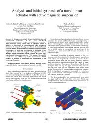
Advanced Techniques For Greater Accuracy, Capacity and Speed ...

Advanced Techniques for Greater 

Accuracy, Capacity, and Speed 

using Maxwell 11 

Julius Saitz 

Ansoft Corporation

Overview 

• Curved versus Faceted Surfaces 

• Mesh Operations 

• Data Link 

• Advanced Field Plotting Techniques 

• Scripting 

• Magnetization modeling 

• Useful hints

Curved vs. Faceted Surfaces 

• The Maxwell 11 interface encourages the use of curved 

surfaces 

• Many CAD programs use curved surfaces 

• Curved surfaces do not directly translate into a better 

solution, due to the nature of the finite tetrahedral mesh 

elements – there is always some deviation from the curved 

surface and the meshed surface 

• Using faceted surfaces can be more robust in many cases 

• Faceted surfaces may converge in fewer iterations and 

may use fewer mesh elements – therefore, there is a 

possible large speed improvement!


Curved Faceted


• Calculate force until 1% force change and 1% Energy Error 

Initial mesh 

(tets) 

Adaptive 

Passes 

Final mesh 

(tets) 

Simulation 

Time 

Curved Faceted 

3331 1535 

9 7 

22020 7484 

03:53 min 01:08 min

Mesh Operations 

• Mesh operations provide a tool of manually refining the 

mesh in/on selected objects 

• The mesh determines both the field solution as well as 

the consistency of the results – mesh operations can be 

used to assist both 

• The initial mesh is determined by the geometry only – 

mesh operations improve the mesh consistency and 

improve the solution process – this is especially 

important for transient simulations 

• Importing or linking a mesh is an advanced mesh 

technique that allows for efficient mesh use 

• To assign different mesh operation select an object or 

face and choose Maxwell > Mesh Operations > Assign

Mesh Operations – Surface 

Approximation

Mesh Operations – Surface 

Initial Surface Normal 

Deviation – 5 deg 

(default 15 deg) 

Approximation 

Maximum 

Aspect Ratio – 3 

(default 10) 

Both

Mesh Operations – Skin Depth 

Based

Mesh Operations – Skin Depth 

Initial 

Based 

Top and bottom face Side face

Mesh Operations – Model 

Resolution 

Small box subtracted from the cylinder


Resolution 

• Select the object and specify the size of the small feature 

that needs to be ignored


Resolution 

No model resolution Model resolution larger that the small 

box edge length

Data Link - Mesh 

• For identical geometries Maxwell allows to reuse the 

existing mesh in another Design or Project through the 

Data Link 

• As an example consider a solenoid which we wish to solve 

at two different current levels for the same position of the 

armature: 

I1 = 1000 At 

I2 = 5000 At

1) Solve Design 1 (5000 At) 

using adaptive technology 


2) Link mesh from Design 1 to 

Design 2 

3) Solve Design 2 (1000 At)

Data Link - Mesh

1) Solve Eddy Current 

problem in Maxwell 


2) Link losses (Joule and 

possibly core) from Maxwell to 

ePhysics) 

3) Solve ePhysics problem for 

temperature distribution

Advanced Field Plotting 

Techniques 

• Multiple windows can be opened and arranged to 

show geometry, field plots, 2D and 3D graphs and 

tables 

• Multiple field plots can be created, overlaid and 

displayed in flexible and general formats 

• Field plots can be animated and exported 

• Any quantity that can be derived from the solved 

quantities can be plotted using the functionality of 

the Fields Calculator

Multiple windows

Multiple plots

• Allows to define any arbitrary 

expression by manipulating 

computed field quantities and 

geometrical and mathematical 

functions 

Fields Calculator 

• Example: radial component of B 

Brad = Bx*cos(phi) + By*sin(phi)

Plot on a line 

• Any calculated quantity or expression defined in the Fields Calculator can 

be plotted on a line or surface

Multiple windows with multiple 

plots

Surface plot - tone 

• Color varies continuously between isovalues

Surface plot - lines 

• Lines are drawn along the isovalues

Surface plot – outlined fringe 

• Color is constant between isovalues

Multiple surface plot

Animation of slice plots

Transient animation

Current density plot

Transient animation

Scripting 

• Scripting is a powerful tool of automation 

• In Maxwell everything starting from preprocessing 

(geometry creation), materials and 

boundary assignment, through analysis setup, 

ending with post-processing and export of data 

can be scripted 

• VB Script used by default (Tools > Record/Run 

Script) 

• Matlab and Java Scripts can be used if desired

Scripting – VB Script 

• Simple example: create a regular polyhedron

Scripting – Matlab 

• Replace CreateObject command with actxserver(): 

Set oAnsoftApp = CreateObject("AnsoftMaxwell.MaxwellScriptInterface") 

iMaxwell = actxserver('AnsoftMaxwell.MaxwellScriptInterface'); 

• Remove Set from the Object definitions: 

Set oDesktop = oAnsoftApp.GetAppDesktop() 

Desktop = iMaxwell.GetAppDesktop(); 

• Use Invoke to execute the command: 

oEditor.CreateRegularPolyhedron 

invoke(Editor, 'CreateRegularPolyhedron', ...


• Replace all Arrays with the proper elements enclosed in { }: 

• End Maxwell session with: 

• For any strings replace “ with ‘ 

Array("NAME:CylinderParameters,… 

{'NAME:CylinderParameters',… 

Delete(iMaxwell)


• Simple example: create a regular polyhedron

User Defined Primitives 

• Allow automated creation and parameterization of complicated 

geometrical structures

Radial Magnetization

Radial Magnetization 

• Create 2 magnet materials – positive and negative 

direction of magnetization (R component + 1 and -1) 

• Choose Cylindrical material coordinate system type

Parallel Magnetization



Parallel Magnetization 

• Create 2 magnet materials – positive and negative direction of 

magnetization (X or Y component + 1 and -1) 

• Choose Cartesian material coordinate system type 

• Create as many rotated or face coordinate systems as many there are 

magnets in the design 

• Associate each magnet with appropriate coordinate system

Arbitrary Magnetization - Script 

• Create as many magnet segments as desired (magnet discretization) 

• Create as many different materials as many there are segments 

• Each material will have a unique Coercive Field, Relative Permeability 

and Direction of Magnetization 

• Assign appropriate material to each magnet segment

Arbitrary Magnetization - Script

Spin 

• Observe the geometry or field plot on a self-rotating model 

• View > Spin

Select All Object Faces 

• Objects may consist of many faces that need to be 

selected typically for boundary assignment 

• Edit > Select > All Object Faces

Visualize History of Objects 

• Visualization is updated on subsequent history playback 

• Tools > Options > 3D Modeler Options > Display Tab

Point and Dialog Entry Modes 

• Editing properties of new primitives: use F3 and F4 to 

switch between Point and Dialog entry modes 

Dialog entry mode window

Maxwell Keyboard Shortcuts 

General Shortcuts 

�F1: Help 

�Shift + F1: Context help 

�CTRL: + F4: Close program 

�CTRL + C: Copy 

�CTRL + N: New project 

�CTRL + O: Open... 

�CTRL + S: Save 

�CTRL + P: Print... 

�CTRL + V: Paste 

�CTRL + X: Cut 

�CTRL + Y: Redo 

�CTRL + Z: Undo 

�CTRL + 0: Cascade windows 

�CTRL + 1: Tile windows 

horizontally 

�CTRL + 2: Tile windows 

vertically 

3D Modeller Shortcuts 

�B: Select face/object behind current 

selection 

�F: Face select mode 

�O: Object select mode 

�CTRL + A: Select all visible objects 

�CTRL + SHIFT + A: Deselect all 

objects 

�CTRL + D: Fit view 

�CTRL + E: Zoom in, screen center 

�CTRL + F: Zoom out, screen center 

�CTRL + Enter: Shifts the local 

coordinate system temporarily 

�SHIFT + Left Mouse Button: Drag 

�Alt + Left Mouse Button: Rotate model 

�Alt + SHIFT + Left Mouse Button: 

Zoom in / out 

�F3: Switch to point entry mode (i.e. 

draw objects by mouse) 

�F4: Switch to dialogue entry mode 

(i.e. draw object solely by entry in 

command and attributes box.) 

�F6: Render model wire frame 

�F7: Render model smooth shaded 

Left 

�Alt + Double Click Left Mouse Button at points 

on screen: Sets model projection to standard 

isometric projections (see diagram below). 

�ALT + Right Mouse Button + Double Click Left 

Mouse Button at points on screen: give the 

nine opposite projections. 

Predefined View Angles 

Top 

Bottom 

Right

Summary 

• Curved surfaces can be conveniently used in Maxwell 11, however, 

their usage may slow down the mesh generation and solution process 

• Maxwell 11 comes with variety of different Mesh Operations that 

provide opportunities for user to control the mesh generation if desired 

• Data Link technology in Maxwell 11 allows powerful data exchange 

between different projects and designs within Maxwell as well as 

between Maxwell and other Ansoft products (e.g. Maxwell – ePhysics) 

• Any basic quantity along with any arbitrarily defined expression in 

Fields Calculator can be graphically displayed using range of Field 

Plotting Techniques available in Maxwell 11 

• Maxwell 11 is fully scripted which makes from this simulation software 

a powerful tool of design automation

Advanced Techniques For Greater Accuracy, Capacity and Speed ...

Create successful ePaper yourself

Delete template?

Save as template?