CARDINAL MiniLab Manual - Digital Audio Corporation
CARDINAL MiniLab Manual - Digital Audio Corporation CARDINAL MiniLab Manual - Digital Audio Corporation
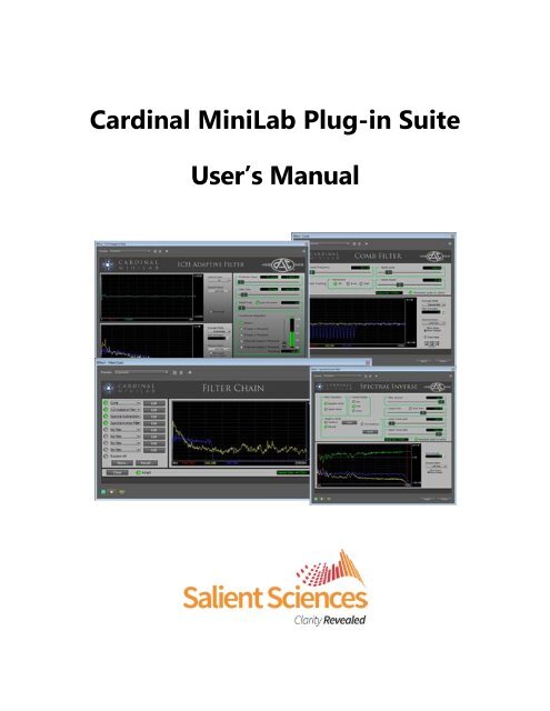
Cardinal MiniLab Plug-in Suite User’s Manual
- Page 3: Cardinal MiniLab Plug-in Suite User
- Page 6 and 7: 6.3.1 Filter Operation ............
- Page 8 and 9: 14 Filter Chain ...................
- Page 10 and 11: 2.1 SOFTWARE INSTALLATION 2 SOFTWAR
- Page 12 and 13: Figure 2: Plug-in waiting for Activ
- Page 14 and 15: 3.1 LAUNCHING A PLUG-IN 3 GENERAL P
- Page 16 and 17: Only, Right Only or Mix. The Mix se
- Page 18 and 19: 4 1-CH ADAPTIVE FILTER 4.1 OVERVIEW
- Page 20 and 21: Figure 8: Prediciton Span Sets the
- Page 22 and 23: exactly what is being removed by th
- Page 24 and 25: Figure 13: Reference Canceller Filt
- Page 26 and 27: filter convergence without greatly
- Page 28 and 29: 6 SPECTRAL INVERSE FILTER 6.1 OVERV
- Page 30 and 31: Figure 21: Spectral Inverse Filter
- Page 32 and 33: 6.3.2 Output Shape Figure 23: Outpu
- Page 34 and 35: 6.3.5 Lower and Upper Voice Limits
- Page 36 and 37: 6.3.7 Manual Mode Figure 28: Manual
- Page 38 and 39: 7 COMB FILTER 7.1 OVERVIEW OF THE C
- Page 40 and 41: Figure 31: Comb Filter Main Window
- Page 42 and 43: 7.2.4 Notch Harmonics Figure 35: No
- Page 44 and 45: Figure 37: X-Pass Main Window 8.2 M
- Page 46 and 47: Figure 38: Lowpass Filter Controls
- Page 48 and 49: Attenuation) can also be controlled
- Page 50 and 51: The Upper Cutoff Frequency is usual
Cardinal <strong>MiniLab</strong> Plug-in Suite<br />
User’s <strong>Manual</strong>
Cardinal <strong>MiniLab</strong><br />
Plug-in Suite<br />
User's <strong>Manual</strong><br />
February 2015<br />
<strong>Digital</strong> <strong>Audio</strong> <strong>Corporation</strong><br />
d/b/a Salient Sciences<br />
4018 Patriot Drive Suite 300<br />
Durham, NC 27703<br />
Phone: +1 (919) 572 6767<br />
Fax: +1 (919) 572 6786<br />
sales@salientsciences.com<br />
www.salientsciences.com<br />
Copyright © 2015 by Salient Sciences.<br />
All rights reserved.<br />
3
TABLE OF CONTENTS<br />
1 Cardinal <strong>MiniLab</strong> Introduction ...................................................................... 9<br />
2 Software Installation .................................................................................... 10<br />
2.1 Software Installation ............................................................................. 10<br />
2.2 Licensing And Activation ....................................................................... 10<br />
3 General Plug-in Concepts ............................................................................ 14<br />
3.1 Launching a Plug-in .............................................................................. 14<br />
3.1 Spectrum Analyzer ................................................................................ 14<br />
3.2 Coefficient display ................................................................................. 16<br />
3.3 Sample Rate Conversion ....................................................................... 17<br />
4 1-CH Adaptive Filter .................................................................................... 18<br />
4.1 Overview of the 1-CH Adaptive Filter ..................................................... 18<br />
4.2 Main Plug-In Window ............................................................................ 19<br />
4.3 Filter Controls ....................................................................................... 19<br />
4.3.1 Prediction Span .............................................................................. 19<br />
4.3.2 Filter Size........................................................................................ 20<br />
4.3.3 Adapt Rate ...................................................................................... 20<br />
4.3.4 Conditional Adaptation ................................................................... 21<br />
4.3.5 Filter Output................................................................................... 21<br />
4.3.6 Freeze Filter .................................................................................... 22<br />
4.3.7 Clear Filter ...................................................................................... 22<br />
5 Reference Canceller Filter ............................................................................ 23<br />
5.1 Overview of the Reference Canceller Filter ............................................ 23<br />
5.2 Main Plug-In Window ............................................................................ 24<br />
5.3 Filter Controls ....................................................................................... 24<br />
5.3.1 Delay .............................................................................................. 24<br />
5.3.2 Filter Size........................................................................................ 25<br />
5.3.3 Adapt Rate ...................................................................................... 25<br />
5.3.4 Conditional Adaptation ................................................................... 26<br />
5.3.5 Reference Gain ............................................................................... 26<br />
5.3.6 Filter Output................................................................................... 27<br />
5.3.7 Freeze Filter .................................................................................... 27<br />
5.3.8 Clear Filter ...................................................................................... 27<br />
6 Spectral Inverse Filter .................................................................................. 28<br />
6.1 Overview of the Spectral Inverse Filter .................................................. 28<br />
6.2 Main Plug-In Window ............................................................................ 30<br />
6.3 Filter Controls ....................................................................................... 31<br />
5
6.3.1 Filter Operation .............................................................................. 31<br />
6.3.2 Output Shape ................................................................................. 32<br />
6.3.3 Filter Amount ................................................................................. 32<br />
6.3.4 Output Gain and Auto Gain ............................................................ 33<br />
6.3.5 Lower and Upper Voice Limits ........................................................ 34<br />
6.3.6 Adaptive Mode ................................................................................ 35<br />
6.3.7 <strong>Manual</strong> Mode .................................................................................. 36<br />
6.3.8 Display ........................................................................................... 36<br />
7 Comb Filter .................................................................................................. 38<br />
7.1 Overview of the Comb Filter .................................................................. 38<br />
7.1 Main Plug-In Window ............................................................................ 40<br />
7.2 Filter Controls ....................................................................................... 41<br />
7.2.1 Comb Frequency ............................................................................. 41<br />
7.2.2 Notch Limit ..................................................................................... 41<br />
7.2.3 Notch Depth ................................................................................... 41<br />
7.2.4 Notch Harmonics ............................................................................ 42<br />
7.2.5 Auto Tracking ................................................................................. 42<br />
8 X-Pass Filter ................................................................................................ 43<br />
8.1 Overview of the X-pass Filter ................................................................. 43<br />
8.2 Main Plug-in Window ............................................................................ 44<br />
8.3 Lowpass Filter ....................................................................................... 45<br />
8.3.1 Filter Controls ................................................................................. 46<br />
8.4 Highpass Filter ...................................................................................... 47<br />
8.4.1 Filter Controls ................................................................................. 48<br />
8.5 Bandpass Filter ..................................................................................... 49<br />
8.5.1 Filter Controls ................................................................................. 50<br />
8.6 Bandstop Filter ..................................................................................... 52<br />
8.6.1 Filter Controls ................................................................................. 53<br />
8.7 Notch Filter ........................................................................................... 55<br />
8.7.1 Filter Controls ................................................................................. 56<br />
8.8 Slot Filter .............................................................................................. 57<br />
8.8.1 Filter Controls ................................................................................. 58<br />
9 Spectral Subtraction Filter .......................................................................... 60<br />
9.1 Overview of the Spectral Subtraction Filter ........................................... 60<br />
9.2 Main Plug-in Window ............................................................................ 62<br />
9.3 Filter Controls ....................................................................................... 63<br />
9.3.1 Filter Controls ................................................................................. 63<br />
9.3.2 Clear ............................................................................................... 63<br />
9.3.3 Filter Output Gain .......................................................................... 64<br />
9.3.4 Noise EQ Controls........................................................................... 64<br />
9.3.5 Noise Reducer Controls................................................................... 66<br />
6
10 Multi-Band Filter ....................................................................................... 67<br />
10.1 Overview of the Multi-Band Filter ........................................................ 67<br />
10.1.1 Overview of Multiple-Notch ........................................................... 67<br />
10.1.2 Overview of Multiple-Slot .............................................................. 68<br />
10.2 Main Plug-in Window .......................................................................... 70<br />
10.3 Filter Controls ..................................................................................... 71<br />
10.3.1 Filter Mode ................................................................................... 71<br />
10.3.2 Multiple Notch Filter Controls ....................................................... 71<br />
10.3.3 Multiple Slot Controls ................................................................... 75<br />
11 Graphic EQ ................................................................................................ 80<br />
11.1 Overview of the Graphic Equalizer ...................................................... 80<br />
11.1.1 Overview of Graphic EQ ................................................................ 80<br />
11.1.2 Overview of Hi-Res Graphic .......................................................... 80<br />
11.1 Main Plug-in Window .......................................................................... 82<br />
11.2 Equalizer Controls ............................................................................... 83<br />
11.2.1 Equalizer Mode ............................................................................. 83<br />
11.2.2 Graphic EQ Controls ..................................................................... 83<br />
11.2.3 Hi-Res Graphic Controls ............................................................... 84<br />
12 Gain Stage ................................................................................................. 87<br />
12.1 Overview of the Gain Stage .................................................................. 87<br />
12.1.1 Overview of AGC ........................................................................... 87<br />
12.1.2 Overview of LCE ............................................................................ 87<br />
12.2 Main Plug-in Window .......................................................................... 90<br />
12.3 Gain Controls ...................................................................................... 91<br />
12.3.1 Gain Mode .................................................................................... 91<br />
12.3.2 AGC Controls ................................................................................ 91<br />
12.3.3 LCE Controls ................................................................................ 92<br />
13 Parametric Equalizer ................................................................................. 95<br />
13.1 Overview of the Parametric Equalizer .................................................. 95<br />
13.2 Main Plug-in Window .......................................................................... 96<br />
13.3 Filter Controls ..................................................................................... 97<br />
13.3.1 Current Stage ............................................................................... 97<br />
13.3.2 Center Frequency ......................................................................... 97<br />
13.3.3 Width Factor ................................................................................. 97<br />
13.3.4 Boost/Cut ..................................................................................... 98<br />
13.3.5 Stage Active .................................................................................. 98<br />
13.3.6 Output Gain ................................................................................. 98<br />
13.3.7 Reset All ....................................................................................... 98<br />
13.3.8 Show Inactive ............................................................................... 99<br />
13.3.9 Store Button ................................................................................. 99<br />
13.3.10 Recall Button .............................................................................. 99<br />
7
14 Filter Chain ............................................................................................... 99<br />
14.1 Overview of the Filter Chain ................................................................ 99<br />
14.2 Main Plug-in Window ........................................................................ 100<br />
14.3 Filter Chain Controls ......................................................................... 101<br />
14.3.1 Filter Select................................................................................. 101<br />
14.3.2 Filter Control Button Group ........................................................ 101<br />
14.3.3 Bypass All ................................................................................... 102<br />
14.3.4 Store Button ............................................................................... 102<br />
14.3.5 Recall Button .............................................................................. 102<br />
14.3.6 Clear Button ............................................................................... 102<br />
8
1 <strong>CARDINAL</strong> MINILAB INTRODUCTION<br />
Thank you for purchasing the Cardinal <strong>MiniLab</strong> Plug-ins. The entire suite of<br />
plug-ins includes the following:<br />
<br />
<br />
<br />
<br />
<br />
<br />
<br />
<br />
<br />
<br />
<br />
1-CH Adaptive Filter<br />
Comb Filter<br />
Filter Chain<br />
Gain Stage<br />
Graphic Equalizer<br />
Multi-Band Filter<br />
Parametric Equalizer<br />
Reference Canceller Filter<br />
Spectral Inverse Filter<br />
Spectral Subtraction Filter<br />
X-Pass Filter (6 filter set)<br />
The <strong>MiniLab</strong> Suite includes all the above filters with the exception of the<br />
Reference Canceller and Filter Chain plug-ins. The Advanced Suite contains all<br />
the <strong>MiniLab</strong> plug-ins, plus an additional stand-alone application called<br />
Cardinal Batch Utility.<br />
9
2.1 SOFTWARE INSTALLATION<br />
2 SOFTWARE INSTALLATION<br />
The software requires that a host audio editing environment that supports the<br />
VST standard be installed. The computer on which the audio editing<br />
environment is installed must meet all the requirements of that audio editing<br />
environment for the plug-in to work. Please consult the documentation of your<br />
audio editing environment for its requirements.<br />
NOTE: Because of the processing requirements of the plug-in, the filters will benefit<br />
from a faster computer.<br />
To start the installation, insert the CD containing the plug-in software into your<br />
PC. If the installation does not begin automatically run the file “Setup.exe”<br />
located in the root folder of the CD. You can run this file by clicking on the<br />
“Start” menu, then on “Run”, and typing “X:\Setup.exe” (where “X” is the drive<br />
letter of your CD-ROM drive). Follow the instructions on the screen to complete<br />
the installation. If you have any questions or problems with the installation,<br />
please contact DAC for further assistance.<br />
In addition to its own installation directory, the VST plug-in will also be copied to<br />
the default Steinberg VST plug-in folder (normally, “C:\Program<br />
Files\Steinberg\VstPlugins”). If this folder is not found, it will be created. Most<br />
audio editors will look in this directory by default for new plug-ins.<br />
2.2 LICENSING AND ACTIVATION<br />
When you first launch your plug-in, it will be running in Demo mode. This is<br />
normal operation until you enter the Serial Key you received from <strong>Digital</strong> <strong>Audio</strong><br />
<strong>Corporation</strong> when you purchased your plug-in.<br />
NOTE: In Demo mode, the plug-in will insert 1 second of silence for every<br />
10 seconds of audio processed. There is nothing wrong with your plug-in,<br />
you simply need to enter your Serial Key to unlock the plug-in from Demo<br />
mode.<br />
The plug-in itself provides a field to enter the Serial Key as shown in the<br />
following figure:<br />
10
Figure 1: Plug-in in demo mode<br />
Simply enter your Serial Key in the black text field provided in the lower-right<br />
of the screen and press Enter. The Serial Key MUST be entered exactly as<br />
provided by DAC. If the Serial Key is valid, it will be registered with your<br />
system and you will now have 30 days to activate the plug-in with DAC.<br />
11
Figure 2: Plug-in waiting for Activation<br />
To Activate, simply click the Activate button. This will send the necessary<br />
information to the DAC servers to activate the software on your PC. The ONLY<br />
information sent and stored at DAC is the Serial Key and a hardware identifier<br />
(usually a serial number from your System hard drive). No other personally<br />
identifiable information is sent.<br />
If the workstation you installed the software on does not have a network<br />
connection, the plug-in will display the Serial Key and HWID (Hardware<br />
Identifier) to you. You must then contact DAC with this information and we<br />
will generate a valid License Key for you that you can then enter as shown in<br />
the figure below.<br />
12
Figure 3: Plug-in waiting for manual License Key entry<br />
Once activation is completed, either over the network or manually, a persistent<br />
license will be installed on the machine. If the software is not activated within<br />
30 days, it will revert back to Demo mode.<br />
You must uninstall the software (which will deactivate it as well) before<br />
installing the software on another machine.<br />
If you have purchased one of the suites, you will only need to enter your serial<br />
key one time and activate it. All the other plug-ins in the suite will recognize the<br />
license and run normally. If you purchase plug-ins individually, then you will<br />
have to enter a separate serial key for each plug-in you purchased.<br />
13
3.1 LAUNCHING A PLUG-IN<br />
3 GENERAL PLUG-IN CONCEPTS<br />
The Cardinal <strong>MiniLab</strong> suite of plug-ins are not stand-alone applications. They<br />
are plug-ins that execute from within a host environment such as Acon<br />
<strong>Digital</strong>’s Acoustica, Adobe’s Audition, Sony’s SoundForge and other similar<br />
audio editors.<br />
Plug-ins are launched from host applications in various ways depending on the<br />
host. Usually the plug-in can be found in the “Effects”, “Tools” or “VST” menu.<br />
If the currently loaded audio file is not compatible with a plug-in, the plug-in<br />
choice will usually be grayed out (disabled).<br />
In general, upon startup the host application will scan a well-known VST plugin<br />
folder for valid VST plug-ins. Usually, new folders can be added to the<br />
scanned list.<br />
Please consult your audio editor manual to determine how to recognize and<br />
launch a VST plug-in.<br />
3.1 SPECTRUM ANALYZER<br />
Figure 4: Spectrum Analyzer<br />
Most plug-ins have an integrated spectrum analyzer to display frequency<br />
content of the audio. Most will look similar to the figure above.<br />
The Spectrum Analyzer displays the frequency content of the input and/or<br />
output audio. The frequency axis of the Spectrum Analyzer plot goes from left<br />
to right, with the lowest frequency at the leftmost side and the highest<br />
frequency at the rightmost side. The "energy" (loudness) axis of the Spectrum<br />
Analyzer plot goes from top to bottom, with stronger (louder) frequencies<br />
14
indicated by higher peaks on the plot.<br />
For example, a signal consisting of a single tone will appear as a single peak,<br />
located at the tone frequency. A "white noise" signal, which contains equal<br />
amounts of every frequency in the signal bandwidth, will appear as an<br />
(approximately) flat line across the entire frequency range.<br />
The spectrum analyzer can display the Input audio, the Output audio, or both.<br />
To enable the Input and/or Output trace, click the corresponding LED button<br />
so that the indicator "light" is on. The Input audio is the signal before the filter<br />
is applied. The Output audio is the signal after the filter is applied. When both<br />
signals are shown, each signal is indicated by a line, using yellow for the Input<br />
and blue for the Output.<br />
The Spectrum Analyzer provides a cursor marker to help in identifying<br />
specific frequency values. At any time when the Spectrum Analyzer is<br />
activated, clicking in the graph area displays a red vertical marker at the<br />
frequency location clicked. The frequency (in Hz) of the location clicked is<br />
displayed in red text on the bottom left of the graph. The input level (in dB) is<br />
given in yellow text and the output level (in dB) is given in blue text.<br />
The Track Peak feature displays a green vertical line in the graph display at<br />
the strongest (loudest) frequency. When this feature is enabled, the maximum<br />
peak value (in dB) and frequency (in Hz) is displayed in green text on the<br />
bottom right of the graph. To enable this indicator, click the button beside the<br />
Track Peak text so that the indicator “light” turns green.<br />
Use the Averager Mode control to select what type of averaging is done to the<br />
signals displayed. No Average applies no averaging and the traces will move<br />
very rapidly. Exponential applies averaging to the trace values based on the<br />
Num Averages value. Peak Hold will hold the maximum value for each data<br />
point of the trace. Trace data will never leak down in this mode. This is useful<br />
for determining peak energy for a given frequency.<br />
Use the Num Averages control to increase or decrease the number of averages<br />
applied to the frequency spectrum. A small Num Averages value allows a more<br />
accurate snapshot of the spectrum at a given time, but the trace values will<br />
change rapidly, making longer-term spectral characteristics difficult to see.<br />
Larger Num Averages values result in a smoother spectral plot that represents<br />
stable frequency characteristics well but does not accurately show rapidly timevarying<br />
signal characteristics. This control only has an effect when<br />
Exponential is selected for the Averager Mode.<br />
The Channel Select control allows you to choose which channel of audio you<br />
wish to see displayed in the spectrum analyzer window. You can choose Left<br />
15
Only, Right Only or Mix. The Mix selection sums the two audio channels<br />
together before performing the FFT analysis. Right Only and Mix are only<br />
available for stereo audio files.<br />
The analyzer also has three Zoom controls: Zoom In, Zoom Out and Zoom<br />
Full. When zooming, the graph will always try to center the graph on wherever<br />
the red user marker is located. Each level of zoom halves the current<br />
frequency span of the display. For instance, if the current sample rate is<br />
44100Hz, the first level of zoom will cause the analyzer to display 11025Hz<br />
instead of 22050Hz worth of spectral data. Zoom Full will always cause the<br />
analyzer to reset back to the full bandwidth of the signal.<br />
3.2 COEFFICIENT DISPLAY<br />
Figure 5: Coefficient Display<br />
A few filters contain a Coefficient Display, particularly the 1-CH Adaptive Filter<br />
and Reference Canceller Filter. This graph can be useful in setting up these<br />
filters.<br />
The Coefficient Display displays the impulse response (filter coefficients) of the<br />
filter. Vertical scaling of the filter’s coefficients for display is accomplished by<br />
clicking on the Vertical Zoom combo box control. Supported zoom factors<br />
range from 1x to 32x.<br />
The Track Peak feature displays a green vertical line in the graph display at<br />
the coefficient with the largest (absolute) value. When this feature is enabled,<br />
the maximum peak value and coefficient number is displayed in green text on<br />
the bottom right of the graph. To enable this indicator, click the button beside<br />
the Track Peak text so that the indicator “light” turns green.<br />
The Channel Select control allows you to choose which channel’s filter<br />
coefficients you wish to see displayed in the coefficient display window. You<br />
can choose Left Only, or Right Only. Right Only is only available for stereo<br />
audio files.<br />
16
3.3 SAMPLE RATE CONVERSION<br />
Figure 6: Sample Rate Conversion<br />
All Cardinal <strong>MiniLab</strong> plug-ins contain a resampling feature that utilizes a true<br />
Whittaker-Shannon Interpolation to resample the incoming audio at 16kHz.<br />
This method eliminates any distortion components commonly found in cruder<br />
resampling techniques (such as linear interpolation).<br />
Resampling the audio down at 16kHz sample rate primarily does two things for<br />
forensic audio:<br />
1) Bandlimits the audio to the forensic voice spectrum (200 – 5000Hz)<br />
2) Allows for larger filter sizes with less computational requirements. For<br />
example, a 1024-point filter at 48kHz will require roughly 3x the CPU<br />
resources that the same 1024-point filter will require at 16kHz.<br />
Note: After processing, the plug-in resamples the audio back to the original<br />
sample rate to return it to the audio editor environment. If you process a 44.1kHz<br />
WAV file, you will still have a 44.1kHz WAV file in the end, but any information<br />
above 8kHz will have been eliminated.<br />
17
4 1-CH ADAPTIVE FILTER<br />
4.1 OVERVIEW OF THE 1-CH ADAPTIVE FILTER<br />
The 1-Channel Adaptive filter is used to automatically cancel predictable and<br />
convolutional noises from the input audio. Predictable noises include tones,<br />
hum, buzz, engine/motor noise, and, to some degree, music. Convolutional<br />
noises include echoes, reverberations, and room acoustics.<br />
The 1-CH Adaptive Filter is a forensic plug-in that has been specifically designed<br />
to work with VST host audio editing systems.<br />
The 1-CH Adaptive Filter comes equipped with the following features:<br />
<br />
<br />
<br />
<br />
<br />
<br />
<br />
Filter sizes up to 8192 taps<br />
Prediction Span up to 32768 samples<br />
Auto-Normalizing adapt rate<br />
Conditional Adaptation<br />
Selectable Filter Output<br />
Coefficient Display (with max peak indicator)<br />
Dual-trace spectral analysis (with max peak indicator and averaging)<br />
18
Figure 7: 1-CH Adaptive Filter Main Window<br />
4.2 MAIN PLUG-IN WINDOW<br />
Figure 7 shows the plug-in as it would be displayed if used in Adobe Audition.<br />
The buttons above and below the plug-in window will appear differently<br />
depending upon your audio editing environment. Please consult the<br />
documentation on your specific audio editing environment for details of how to<br />
use these features.<br />
This window provides access to all the functionality of the plug-in. A coefficient<br />
display and spectrum analyzer are also provided as aides in determining the<br />
characteristics of the target audio. Details of the plug-in are described in the<br />
following sections.<br />
4.3 FILTER CONTROLS<br />
4.3.1 Prediction Span<br />
19
Figure 8: Prediciton Span<br />
Sets the number of samples in the prediction span delay line. Prediction span<br />
is indicated both in samples and in milliseconds. Shorter prediction spans<br />
allow maximum noise removal, while longer prediction spans preserve voice<br />
naturalness and quality. A prediction span of 2 or 3 samples is normally<br />
recommended.<br />
4.3.2 Filter Size<br />
Figure 9: Filter Size<br />
Sets the number of FIR filter taps in the adaptive filter. Filter size is indicated<br />
both in taps (filter order) and in milliseconds. The maximum filter size is 8192<br />
taps. Small filters are most effective with simple noises such as tones and<br />
music. Larger filters should be used with complex noises such as severe<br />
reverberations and raspy power hums. A nominal filter size of 512 to 1024 taps<br />
is a good overall general recommendation.<br />
CAUTION: Large filter sizes (> 2048 taps) will require large computing resources<br />
to maintain real-time audio processing. You may begin to hear skips in the audio<br />
during preview if your computer cannot keep up with the processing requirements.<br />
However, during render the audio will not contain any skips but may take longer<br />
than real-time to process the file.<br />
4.3.3 Adapt Rate<br />
Figure 10: Adapt Rate<br />
Used to set the rate at which the adaptive filter adapts to changing signal<br />
conditions. An adapt rate of 1 provides very slow adaptation, while an adapt<br />
rate of 5884 provides fastest adaptation. A good approach is to start with an<br />
adapt rate of approximately 100-200 to establish convergence, and then back off<br />
to a smaller value to maintain cancellation.<br />
Larger adapt rates should be used with changing noises such as music;<br />
whereas, smaller adapt rates are acceptable for stable tones and<br />
reverberations. Larger adapt rates sometimes affect voice quality, as the filter<br />
may attack sustained vowel sounds.<br />
When Auto Normalize is turned on, the specified adapt rate is continuously<br />
scaled based upon the input signal level. This scaling generally results in faster<br />
20
filter convergence without greatly increasing the risk of a filter crash. It is<br />
recommended that Auto Normalize be enabled for most speech signal processing.<br />
4.3.4 Conditional Adaptation<br />
Figure 11: Conditional Adaptation<br />
For advanced users only. Novice users should keep Conditional Adaptation set to<br />
Always. The threshold setting has no effect when Always is selected.<br />
Conditional Adaptation allows the adaptive filter to automatically Adapt/Freeze<br />
based upon signal bargraph levels. This can be very useful in situations where<br />
there are pauses or breaks in the speech being processed.<br />
Hint: Conditional adaptation is useful for maintaining adaptation once the<br />
filter has converged. Recording environment factors such as air temperature<br />
and motion in the room can cause the signal characteristics to change over the<br />
course of a recording. For this reason, simply freezing the filter once<br />
convergence is reached may mean that noise cancellation will degrade over<br />
time. Instead of freezing the filter, use Conditional Adaptation. First allow the<br />
filter to converge in Always mode, and then select If Normal Output <<br />
Threshold, and adjust the threshold by observing the bargraph levels during<br />
pauses in speech<br />
Click on the Clear button if you desire the filter to completely readapt based<br />
upon the new Conditional Adaptation settings.<br />
4.3.5 Filter Output<br />
Figure 12: Filter Output<br />
Used to optionally listen to the “rejected” audio that is being cancelled by the<br />
adaptive filter. Normal should almost always be selected, but the Predicted<br />
setting can be useful when configuring the filter, allowing the user to hear<br />
21
exactly what is being removed by the filter.<br />
4.3.6 Freeze Filter<br />
Used to enable or disable filter adaptation. When Freeze is off, the filter adapts<br />
according to its settings. When Freeze is on, the filter never adapts regardless<br />
of the other settings.<br />
4.3.7 Clear Filter<br />
Used to reset the coefficients of the 1-CH Adaptive Filter. Clearing a filter is<br />
useful when the audio characteristics change dramatically, so that the filter<br />
can readapt to a new, clean solution. Clearing is also useful in the case of a<br />
filter “crash,” when the filter coefficients diverge to an unstable state, usually in<br />
response to a large and abrupt change in the signal coupled with a fast adapt<br />
rate.<br />
22
5 REFERENCE CANCELLER FILTER<br />
5.1 OVERVIEW OF THE REFERENCE CANCELLER FILTER<br />
The Reference Canceller adaptive filter is used to automatically cancel from the<br />
Primary channel any audio which matches the Reference channel. For<br />
example, the Primary channel may be microphone audio with desired voices<br />
masked by radio or TV noise. The radio/TV interference can be cancelled in<br />
real-time if the original broadcast audio, usually available from a second<br />
receiver, is simultaneously recorded to the Reference channel.<br />
The Reference Canceller Filter is a forensic plug-in that has been specifically<br />
designed to work with VST host audio editing systems. Since it is an inherently<br />
two-channel filter, it is only available for stereo audio files. The Primary channel<br />
MUST be on the left channel, while the Reference channel consequentially MUST<br />
be on the right channel. Future updates of this plug-in will allow these channels<br />
to be switched if desired.<br />
The Reference Canceller Filter comes equipped with the following features:<br />
<br />
<br />
<br />
<br />
<br />
<br />
<br />
<br />
Filter sizes up to 8192 taps<br />
Delay line up to 32768 samples<br />
Auto-Normalizing adapt rate<br />
Conditional Adaptation<br />
Reference Gain<br />
Selectable Filter Output<br />
Coefficient Display (with max peak indicator)<br />
Dual-trace spectral analysis (with max peak indicator and averaging)<br />
23
Figure 13: Reference Canceller Filter Main Window<br />
5.2 MAIN PLUG-IN WINDOW<br />
Figure 13 shows the plug-in as it would be displayed if used in Adobe Audition.<br />
The buttons above and below the plug-in window will appear differently<br />
depending upon your audio editing environment. Please consult the<br />
documentation on your specific audio editing environment for details of how to<br />
use these features.<br />
This window provides access to all the functionality of the plug-in. A coefficient<br />
display and spectrum analyzer are also provided as aides in determining the<br />
characteristics of the target audio. Details of the plug-in are described in the<br />
following sections.<br />
5.3 FILTER CONTROLS<br />
5.3.1 Delay<br />
24
Figure 14: Delay<br />
Sets the number of audio samples by which the selected channel should be<br />
delayed. Adjusting the Delay allows the alignment of the Primary and Reference<br />
channels to be adjusted. Minimum Delay is 1 sample, but can be set to as high<br />
as 32768 samples.<br />
Specifies whether the delay line is to go into either the Primary channel (Delay<br />
Pri) or the Reference channel (Delay Ref). For most applications, a slight delay<br />
(typically 5 msec) is placed in the Primary channel, For applications with long<br />
distances between the microphone and radio/TV, a delay in the Reference<br />
channel may be required. Extreme caution should be exercised when using<br />
reference channel delay; allowing the reference to lag the target noise in the<br />
primary signal will result in poor cancellation.<br />
5.3.2 Filter Size<br />
Figure 15: Filter Size<br />
Sets the number of filter taps in the adaptive filter. Filter size is indicated both<br />
in taps (filter order) and in milliseconds. The maximum filter size is 8192 taps.<br />
Normally, larger filters sizes are used in the Reference Canceller adaptive filter.<br />
CAUTION: Large filter sizes (> 2048 taps) will require large computing resources<br />
to maintain real-time audio processing. You may begin to hear skips in the audio<br />
during preview if your computer cannot keep up with the processing requirements.<br />
However, during render the audio will not contain any skips but may take longer<br />
than real-time to process the file.<br />
5.3.3 Adapt Rate<br />
Figure 16: Adapt Rate<br />
Used to set the rate at which the adaptive filter adapts to changing signal<br />
conditions. An adapt rate of 1 provides very slow adaptation, while an adapt<br />
rate of 5884 provides fastest adaptation. A good approach is to start with an<br />
adapt rate of approximately 100-200 to establish convergence, and then back off<br />
to a smaller value to maintain cancellation.<br />
When Auto Normalize is turned on, the specified adapt rate is continuously<br />
scaled based upon the input signal level. This scaling generally results in faster<br />
25
filter convergence without greatly increasing the risk of a filter crash. It is<br />
recommended that Auto Normalize be enabled for most speech signal processing.<br />
5.3.4 Conditional Adaptation<br />
Figure 17: Conditional Adaptation<br />
For advanced users only. Novice users should keep Conditional Adaptation set to<br />
Always. The threshold setting has no effect when Always is selected.<br />
Conditional Adaptation allows the adaptive filter to automatically Adapt/Freeze<br />
based upon signal bargraph levels. This can be very useful in situations where<br />
there are pauses or breaks in the speech being processed.<br />
Hint: Conditional adaptation is useful for maintaining adaptation once the<br />
filter has converged. Recording environment factors such as air temperature<br />
and motion in the room can cause the signal characteristics to change over the<br />
course of a recording. For this reason, simply freezing the filter once<br />
convergence is reached may mean that noise cancellation will degrade over<br />
time. Instead of freezing the filter, use Conditional Adaptation. First allow the<br />
filter to converge in Always mode, and then select If Normal Output <<br />
Threshold, and adjust the Threshold by observing the bargraph levels during<br />
pauses in speech<br />
Click on the Clear button if you desire the filter to completely readapt based<br />
upon the new Conditional Adaptation settings.<br />
5.3.5 Reference Gain<br />
26
Figure 18: Reference Gain<br />
Ref Gain is used to add gain to the reference channel audio if necessary. To<br />
achieve good cancellation, it is important that the reference audio be at least as<br />
loud as the noise it is intended to cancel from the primary audio.<br />
5.3.6 Filter Output<br />
Figure 19: Filter Output<br />
Used to optionally listen to the “rejected” audio that is being cancelled by the<br />
adaptive filter. Normal should almost always be selected, but the Rejected<br />
setting can be useful when configuring the filter, allowing the user to hear<br />
exactly what is being removed by the filter.<br />
5.3.7 Freeze Filter<br />
Used to enable or disable filter adaptation. When Freeze is off, the filter adapts<br />
according to its settings. When Freeze is on, the filter never adapts regardless<br />
of the other settings.<br />
5.3.8 Clear Filter<br />
Used to reset the coefficients of the Reference Canceller Filter. Clearing a filter<br />
is useful when the audio characteristics change dramatically, so that the filter<br />
can readapt to a new, clean solution. Clearing is also useful in the case of a<br />
filter “crash,” when the filter coefficients diverge to an unstable state, usually in<br />
response to a large and abrupt change in the signal coupled with a fast adapt<br />
rate.<br />
27
6 SPECTRAL INVERSE FILTER<br />
6.1 OVERVIEW OF THE SPECTRAL INVERSE FILTER<br />
The Spectral Inverse Filter (SIF) has two modes: an adaptive mode and a<br />
manual mode. Thus it is actually a combination of the Adaptive Spectral<br />
Inverse Filter (ASIF) and the traditional Spectral Inverse Filter (SIF). Both are<br />
equalization filters that readjust the spectrum to match an expected spectral<br />
shape. It is especially useful when the target voice has been exposed to<br />
spectral coloration (i.e. muffling, hollowness, or tinniness), but it can also be<br />
used to remove bandlimited noises. The ASIF is much like the SIF, except it<br />
continually updates the spectral solution, whereas the SIF only updates the<br />
solution when it is “built”.<br />
The filter maintains an average of the signal’s spectrum and uses this<br />
information to implement a high-resolution digital filter for correcting long-term<br />
spectral irregularities. The goal of the filter is to reshape the overall spectral<br />
envelope of the audio, not to respond to transient noises and characteristics.<br />
Several user controls are available for refinement of SIF operation. The user<br />
can specify the expected spectrum so that the output audio is reshaped to a<br />
flat, pink or voice-like curve. An adapt rate setting controls the update rate for<br />
the spectral average, which in turn determines how quickly the filter responds<br />
to changes in the input audio. Upper and lower limit controls allow the user to<br />
specify the range over which equalization is applied, and a mode setting<br />
controls whether frequencies outside the equalization range are attenuated or<br />
left unaffected. The amount of spectral correction is adjustable using the Filter<br />
Amount control. The user can enable the auto-gain functionality to ensure<br />
that the output audio level is maintained at approximately the same as the<br />
input audio level. If the user disables the auto-gain, an output gain slider is<br />
available to manually boost the level of the output signal.<br />
As an aid to visualizing the filter operation, the user can view the input and<br />
output audio traces as well as the filter coefficient trace.<br />
28
Figure 20: Spectral Inverse Filter Main Window (in Adaptive Mode)<br />
29
Figure 21: Spectral Inverse Filter Main Window (in <strong>Manual</strong> Mode)<br />
6.2 MAIN PLUG-IN WINDOW<br />
Figure 20 and Figure 21 show the plug-in as it would be displayed if used in<br />
Adobe Audition in Adaptive mode and <strong>Manual</strong> mode repsectively. The buttons<br />
above and below the plug-in window will appear differently depending upon<br />
your audio editing environment. Please consult the documentation on your<br />
specific audio editing environment for details of how to use these features.<br />
This window provides access to all the functionality of the plug-in. A spectrum<br />
30
analyzer is provided as an aid in determining the characteristics of the target<br />
audio. Details of the plug-in are described in the following sections.<br />
6.3 FILTER CONTROLS<br />
6.3.1 Filter Operation<br />
Figure 22: Filter Operation<br />
In this block, the user can select the operational mode of the filter. If the filter<br />
is being used to correct spectral coloration, the Equalize Voice mode should<br />
be selected. If the filter is being used to remove bandlimited noise, the Attack<br />
Noise mode should be selected.<br />
Note: The Filter Operation mode selection only affects the behavior of the<br />
filter outside the range selected by the upper and lower limits. In Equalize<br />
Voice mode, the frequency ranges outside the limits are attenuated. In Attack<br />
Noise mode, the frequency ranges outside the limits are left unaffected (subject<br />
to a transition region near the limits). If the auto gain is disabled and the<br />
manual gain is set to 0 dB, frequencies outside the limits and transition<br />
regions will be unaffected. However, if gain is applied, the gain will be reflected<br />
over the entire frequency range. See the section on Upper and Lower Voice<br />
Limits for more information on selecting the range.<br />
Note: Changing the filter operation mode does not require an adaptation<br />
period to arrive at a “good” solution. Because a full average spectrum is<br />
maintained regardless of the mode setting, the new mode takes effect<br />
instantaneously in both the output audio and the display traces. However,<br />
since the auto gain adapts based on the actual applied filter with operational<br />
mode taken into account, there may be some adaptation time required to reach<br />
a stable auto gain value after the mode is changed.<br />
31
6.3.2 Output Shape<br />
Figure 23: Output Shape<br />
In this block, the user can select the target spectral shape that the filter<br />
attempts to achieve. The SIF has an inherent spectral flattening effect on the<br />
audio. The selected spectral shape is applied to further reshape the audio<br />
spectrum. The following output shapes are available:<br />
<br />
<br />
<br />
Flat – no additional shaping after ASIF flattening<br />
Pink -- 3 dB per octave rolloff above 100 Hz is applied in addition to ASIF<br />
flattening<br />
Voice – 6 dB/octave rolloff above and below 500 Hz in addition to ASIF<br />
flattening<br />
Note: Changing the output shape does not require an adaptation period to<br />
arrive at a “good” solution. Because a full average spectrum is maintained<br />
regardless of the output shape setting, the new output shape takes effect<br />
instantaneously in both the output audio and the display traces. However,<br />
since the auto gain adapts based on the actual applied filter with the shaping<br />
curve taken into account, there may be some adaptation time required to reach<br />
a stable auto gain value after the shaping curve is changed.<br />
6.3.3 Filter Amount<br />
Figure 24: Filter Amount<br />
This setting controls the degree to which the SIF can affect the signal, with 0%<br />
corresponding to no filtering and 100% corresponding to full filtering. In<br />
general, it is best to use the minimum Filter Amount setting that produces the<br />
desired result. When Equalize Voice mode is used, a lower Filter Amount<br />
can reduce artifacts that result from a fast adapt rate, so the Filter Amount<br />
can be used to help strike a balance between responsiveness and stability.<br />
When Attack Noise mode is used to reduce bandlimited noise, a lower Filter<br />
32
Amount setting will often be a better choice to prevent the elevation of<br />
background noises.<br />
Note: Changing the Filter Amount setting does not require an adaptation<br />
period to arrive at a “good” solution. Because a full average spectrum is<br />
maintained regardless of the setting, the new filter amount setting takes effect<br />
instantaneously in both the output audio and the display traces. However,<br />
since the auto gain adapts based on the actual applied filter with filter amount<br />
taken into account, there may be some adaptation time required to reach a<br />
stable auto gain value after the filter amount is adjusted.<br />
6.3.4 Output Gain and Auto Gain<br />
Figure 25: Output Gain and Auto Gain<br />
These controls provide two options for adjusting the level of the SIF output.<br />
When Auto Gain is enabled, the SIF automatically monitors the input and<br />
output levels and applies a gain value that matches the output level to the<br />
input level. When Auto Gain is disabled, the user can use the Output Gain<br />
setting to specify the amount of boost applied to the SIF output. If Auto Gain<br />
is enabled, then the Output Gain slider is ignored.<br />
The Auto Gain is an adaptive value whose rate of change depends on the same<br />
Adapt Rate slider setting that controls filter coefficient averaging. This means<br />
that when the filter response changes rapidly and dramatically, the auto gain<br />
will take some time to “catch up” to these changes. In particular, the output<br />
audio may clip when user settings are changed in a ways that have a boosting<br />
effect, such as switching from a pink to a flat shaping curve, adjusting the filter<br />
amount, or increasing the size of the ASIF region in Equalize Voice mode so<br />
that some frequencies that had been heavily attenuated are now present.<br />
While these settings changes will take effect immediately, the Auto Gain may<br />
take some time to adapt to the change. For this reason, when the user expects<br />
to be making many changes in the settings, it is often better to disable Auto<br />
Gain and instead choose a manual gain setting that avoids clipping.<br />
33
6.3.5 Lower and Upper Voice Limits<br />
Figure 26: Lower and Upper Voice Limit<br />
The Lower and Upper Voice Limits allow the user to specify the frequency<br />
range, or “SIF region,” over which the SIF is applied. Two red markers on the<br />
Spectrum Analyzer indicate where the lower and upper voice limits are<br />
located. Viewing audio on the display trace while manipulating the markers is<br />
an easy way to identify where your SIF region limits should fall.<br />
In Equalize Voice mode, the SIF region is typically chosen to be the range over<br />
which speech frequencies are found. Setting a Lower Limit above 300 Hz or<br />
an Upper Limit below 3000 Hz is not recommended in equalize voice mode, as<br />
intelligibility may suffer. When in Equalize Voice mode, all frequencies<br />
outside the SIF region are assumed to be non-speech and are therefore<br />
attenuated.<br />
In Attack Noise mode, the SIF region is typically chosen to “bracket” the<br />
bandlimited noise as closely as possible. Frequencies outside the ASIF region<br />
will be “passed through,” i.e. there will be little or no effect outside the SIF<br />
region except for a narrow transition band between the SIF region and the<br />
passbands.<br />
Note: Changing the Voice Limits does not require an adaptation period to<br />
arrive at a “good” solution. Because a full average spectrum is maintained<br />
regardless of the Voice Limit settings, the new Voice Limits will take effect<br />
instantaneously in both the output audio and the display traces. However,<br />
since the auto gain adapts based on the actual applied filter with voice limits<br />
taken into account, there may be some adaptation time required to reach a<br />
stable auto gain value after the limits are changed.<br />
34
6.3.6 Adaptive Mode<br />
Figure 27: Adaptive Mode<br />
In Adaptive mode, the above figure is displayed and gives the user access to<br />
the Adapt, Clear and Adapt Rate controls. This puts the plug-in in the ASIF<br />
mode.<br />
When the Adapt button is lit green, the ASIF is adapting in response to<br />
incoming audio. When the button is grayed, the ASIF response is frozen.<br />
The Clear button allows the user to re-initialize the ASIF response and restart<br />
adaptation.<br />
Note: After a Clear operation or after re-enabling adaptation, there will be an<br />
adaptation period while the filter adapts to the current input signal. The<br />
length of this adaptation period depends on the Adapt Rate control setting.<br />
The Adapt Rate control allows the user to select the rate of adaptation for the<br />
spectral average on which the ASIF response is based. The spectral averager<br />
uses an exponential average of the form Hi+1 = (α)(Xi+1) + (1- α)(Hi). The value<br />
shown in the display box corresponds to the averaging constant α in the<br />
exponential average. The lower the adapt rate value, the slower the filter will<br />
respond to changes in the input audio.<br />
Note: “Fast response” sounds like a good thing, so it can be tempting to set the<br />
adapt rate to a high value. However, the goal of the ASIF is not to remove<br />
transient noises, but rather to reshape the long-term spectral envelope of the<br />
signal. If the adapt rate is too fast, the filter will respond too quickly to<br />
transient audio characteristics, which will produce artifacts in the output<br />
audio and will prevent the filter from settling on a good average solution. For<br />
this reason, most applications will work best with adapt rates at the low end of<br />
the available range. If you hear tonal artifacts that come and go in the output<br />
audio, or if the filter trace display coefficients seem to be changing rapidly, you<br />
probably need to reduce the adapt rate.<br />
35
6.3.7 <strong>Manual</strong> Mode<br />
Figure 28: <strong>Manual</strong> Mode<br />
In <strong>Manual</strong> mode, the above figure is displayed and gives the user access to the<br />
Run Analyzer, Clear and Build controls. This puts the plug-in in the SIF<br />
mode.<br />
The Clear button is used to zero the averager memory and causes the averaged<br />
spectrum to be recalculated anew.<br />
The Run Analyzer button allows the user to start or stop the update of the<br />
averaged spectrum.<br />
The Build button builds the spectral inverse filter based on the original input<br />
audio spectrum and the SIF control settings. Once the filter build is complete<br />
the calculated spectral inverse filter curve will be displayed as a green trace in<br />
the Filter Display area.<br />
Hint: Before clicking the Build button, it is recommended that the spectrum<br />
analyzer be stopped (using the Run Analyzer button) to allow experimentation<br />
with the control settings for the same input spectrum.<br />
6.3.8 Display<br />
Figure 29: SIF Display<br />
36
The display trace is used to view the filter input and output audio and the SIF<br />
filter response. The input audio is always shown in yellow, the output trace in<br />
blue and the filter trace in green. The Lower and Upper Voice Limits are<br />
shown in red.<br />
The controls for this display are identical to the controls for the Spectrum<br />
Analyzer, except for the analyzer is always in the Exponential averaging mode<br />
(hence, no choice is given to change the averaging mode).<br />
37
7 COMB FILTER<br />
7.1 OVERVIEW OF THE COMB FILTER<br />
The Comb filter is used to remove, or "notch out", harmonically related noises<br />
(noises which have exactly equally-spaced frequency components), such as<br />
power-line hum, constant-speed motor/generator noises, etc., from the input<br />
audio. The filter response consists of a series of equally-spaced notches which<br />
resemble a hair comb, hence the name "Comb filter".<br />
Adjust the Comb Frequency to the desired spacing between notches (also<br />
known as "fundamental frequency"). Set the Notch Limit to the frequency<br />
beyond which you do not want any more notches. Set the Notch Depth to the<br />
amount in dB by which noise frequency components are to be reduced.<br />
Normally, the Notch Harmonics option will be set to All, causing frequencies at<br />
all multiples of the Comb Frequency (within the Notch Limit) to be reduced.<br />
However, certain types of noises have only the odd or even harmonic components<br />
present. In these situations, set the Notch Harmonics option to either Odd or<br />
Even.<br />
The Auto Tracking feature allows the filter to automatically hone in on the<br />
exact fundamental frequency and continually track it even if it shifts slightly.<br />
38
Figure 30: Comb Filter Main Window – <strong>Manual</strong> mode<br />
39
Figure 31: Comb Filter Main Window - Auto Tracking<br />
7.1 MAIN PLUG-IN WINDOW<br />
Figure 30 and Figure 31 above show the plug-in as it would be displayed if<br />
used in Adobe Audition in <strong>Manual</strong> mode and Auto Tracking mode respectively.<br />
The buttons above and below the plug-in window will appear differently<br />
depending upon your audio editing environment. Please consult the<br />
documentation on your specific audio editing environment for details of how to<br />
use these features.<br />
This window provides access to all the functionality of the plug-in. A spectrum<br />
analyzer is provided as an aid in determining the characteristics of the target<br />
audio. Details of the plug-in are described in the following sections.<br />
40
7.2 FILTER CONTROLS<br />
7.2.1 Comb Frequency<br />
Figure 32: Comb Frequency<br />
Specifies fundamental frequency in Hertz of comb filter. Notches are generated<br />
at multiples, or harmonics, of this frequency. When Auto Tracking is turned<br />
on, this control does not appear.<br />
7.2.2 Notch Limit<br />
Figure 33: Notch Limit<br />
Specifies frequency in Hertz above which no notches are generated. Minimum<br />
Notch Limit is half the Comb Frequency, while maximum Notch Limit depends<br />
upon the sample rate.<br />
7.2.3 Notch Depth<br />
Figure 34: Notch Depth<br />
Specifies the depth of notches that are generated. Notch Depth is adjustable<br />
from 0 dB to 120 dB in 1 dB steps.<br />
41
7.2.4 Notch Harmonics<br />
Figure 35: Notch Harmonics<br />
Specifies whether notches will be generated at All, Odd, or Even multiples, or<br />
harmonics, of the Comb Frequency. If, for example, the Comb Frequency is set<br />
to 60.0 Hz, then selecting All will generate notches at 60 Hz, 120 Hz, 180 Hz,<br />
240 Hz, 300 Hz, etc. Selecting Odd will generate notches at 60 Hz, 180 Hz, 300<br />
Hz, etc. Selecting Even will generate notches at 120 Hz, 240 Hz, 360 Hz etc.<br />
7.2.5 Auto Tracking<br />
Figure 36: Auto Tracking<br />
Enables Auto Tracking for the Comb filter. When enabled, the Comb<br />
Frequency control is no longer available and the filter will determine the<br />
fundamental frequency to use.<br />
When disabled, the last calculated frequency will then be loaded into the Comb<br />
Frequency control.<br />
NOTE: It is advised that you adjust the Comb Frequency manually to get it as<br />
close as possible to the desired fundamental frequency before enabling Auto<br />
Tracking.<br />
42
8 X-PASS FILTER<br />
8.1 OVERVIEW OF THE X-PASS FILTER<br />
The X-Pass Filter provides six different bandlimiting filters in a single plug-in.<br />
The following filters are included:<br />
Filter<br />
Lowpass<br />
Highpass<br />
Bandpass<br />
Bandstop<br />
Notch<br />
Slot<br />
Application<br />
Decrease the energy level of high frequency noises<br />
Decrease the energy level of low frequency noises<br />
Decrease the energy level of noises above and below<br />
a passband region<br />
Decrease the energy level of noises within a<br />
stopband region<br />
Remove a narrow-band noise<br />
Isolate a narrow-band signal<br />
Only one filter can be operational at a time. While they all share similar<br />
controls, they perform different functions (as detailed below). Whichever filter<br />
you select, its transfer function (or envelope) is displayed in the Spectrum<br />
Analyzer as a light gray trace.<br />
43
Figure 37: X-Pass Main Window<br />
8.2 MAIN PLUG-IN WINDOW<br />
Figure 37 above shows the plug-in as it would be displayed if used in Adobe<br />
Audition. The buttons above and below the plug-in window will appear<br />
differently depending upon your audio editing environment. Please consult the<br />
documentation on your specific audio editing environment for details of how to<br />
use these features.<br />
The Filter Type control selects which of the six filters is currently engaged.<br />
Only one filter is operational at a time. If you desire to apply more than one of<br />
the filters on a given piece of audio, you must either use multiple instances of<br />
the plug-in in an effects chainer (not available in all audio editor environments)<br />
or render the audio multiple times (using a different filter each time). When a<br />
filter is selected, that filter’s controls are displayed in the main window.<br />
44
This window provides access to all the functionality of the plug-in. A spectrum<br />
analyzer is provided as an aid in determining the characteristics of the target<br />
audio. Details of the plug-in are described in the following sections.<br />
8.3 LOWPASS FILTER<br />
The Lowpass filter is used to decrease the energy level (lower the volume) of all<br />
signal frequencies above a specified Cutoff Frequency, thus reducing highfrequency<br />
noises, such as tape hiss, from the input audio. The Lowpass filter is<br />
sometimes called a "hiss filter."<br />
The Cutoff Frequency is usually set above the voice frequency range so that the<br />
voice signal will not be disturbed. While listening to the filter output audio, the<br />
Cutoff Frequency can be incrementally lowered from its maximum frequency<br />
until the quality of the voice just begins to be affected, achieving maximum<br />
elimination of high-frequency noise.<br />
The amount of volume reduction above the Cutoff Frequency can further be<br />
controlled by adjusting the Stopband Attenuation setting (maximum volume<br />
reduction is 120dB). The slope at which the volume is reduced from normal (at<br />
the Cutoff Frequency) to the minimum volume (specified by Stopband<br />
Attenuation) can also be controlled by adjusting the Transition Slope setting.<br />
45
Figure 38: Lowpass Filter Controls<br />
8.3.1 Filter Controls<br />
8.3.1.1 Cutoff Frequency<br />
Figure 39: Cutoff Frequency<br />
Specifies frequency in Hertz above which all signals are attenuated. Frequencies<br />
below this cutoff are unaffected. Maximum Cutoff Frequency depends upon the<br />
Sample Rate. Cutoff Frequency can be adjusted in 1 Hz steps.<br />
46
8.3.1.2 Transition Slope<br />
Figure 40: Transition Slope<br />
Specifies slope at which frequencies above the Cutoff Frequency are rolled off in<br />
dB per octave. Sharpest roll off occurs when Transition Slope is set to maximum,<br />
while gentlest roll off occurs when Transition Slope is set to minimum. Sharp<br />
rolloffs may cause the voice to sound hollow but will allow more precise removal<br />
of high frequency noises. Note that the indicated value changes depending upon<br />
the Cutoff Frequency and Sample Rate.<br />
8.3.1.3 Stopband Attenuation<br />
Figure 41: Stopband Attenuation<br />
Specifies amount in dB by which frequencies above the Cutoff Frequency are<br />
ultimately attenuated. Stopband attenuation is adjustable from 0dB to 120dB in<br />
1 dB steps.<br />
8.4 HIGHPASS FILTER<br />
The Highpass filter is used to decrease the energy level (lower the volume) of all<br />
signal frequencies below a specified Cutoff Frequency, thus reducing lowfrequency<br />
noises, such as tape or acoustic room rumble, from the input audio<br />
(The Highpass filter is sometimes called a "rumble filter").<br />
The Cutoff Frequency is usually set below the voice frequency range (somewhere<br />
below 300 Hz) so that the voice signal will not be disturbed. While listening to<br />
the filter output audio, the Cutoff Frequency, initially set to 0 Hz, can be<br />
incrementally increased until the quality of the voice just begins to be affected,<br />
achieving maximum elimination of low-frequency noise.<br />
The amount of volume reduction below the Cutoff Frequency can further be<br />
controlled by adjusting the Stopband Attenuation setting (maximum volume<br />
reduction is 120dB). The slope at which the volume is reduced from normal (at<br />
the Cutoff Frequency) to the minimum volume (specified by Stopband<br />
47
Attenuation) can also be controlled by adjusting the Transition Slope setting.<br />
Figure 42: HIghpass Filter Controls<br />
8.4.1 Filter Controls<br />
8.4.1.1 Cutoff Frequency<br />
Figure 43: Cutoff Frequency<br />
Specifies frequency in Hertz below which all signals are attenuated. Frequencies<br />
48
above this cutoff are unaffected. Minimum Cutoff Frequency is 0 Hz (no<br />
frequencies attenuated), while the maximum Cutoff Frequency depends upon the<br />
Sample Rate. Cutoff Frequency can be adjusted in 1 Hz steps.<br />
8.4.1.2 Transition Slope<br />
Figure 44: Transition Slope<br />
Specifies slope at which frequencies below the Cutoff Frequency are attenuated<br />
in dB per octave. Sharpest attenuation occurs when Transition Slope is set to<br />
maximum, while gentlest attenuation occurs when Transition Slope is set to<br />
minimum. Note that the indicated value changes depending upon the Cutoff<br />
Frequency and Sample Rates.<br />
8.4.1.3 Stopband Attenuation<br />
Figure 45: Stopband Attenuation<br />
Specifies amount in dB by which frequencies below the Cutoff Frequency are<br />
ultimately attenuated.<br />
8.5 BANDPASS FILTER<br />
The Bandpass filter is used to decrease the energy level (lower the volume) of all<br />
signal frequencies below a specified Lower Cutoff Frequency and above a<br />
specified Upper Cutoff Frequency, thus combining the functions of a Lowpass<br />
and Highpass filter connected in series into a single filter. The signal region<br />
between the Lower Cutoff Frequency and the Upper Cutoff Frequency is called<br />
the passband region. The Bandpass filter is useful for simultaneously reducing<br />
both low-frequency rumble and high-frequency hiss.<br />
The Lower Cutoff Frequency is usually set below the voice frequency range<br />
(somewhere below 300 Hz) so that the voice signal will not be disturbed. While<br />
listening to the filter output audio, the Lower Cutoff Frequency, initially set to 0<br />
Hz, can be incrementally increased until the quality of the voice just begins to be<br />
affected, achieving maximum elimination of low-frequency noise.<br />
49
The Upper Cutoff Frequency is usually set above the voice frequency range<br />
(somewhere above 3000 Hz) so that the voice signal will not be disturbed. While<br />
listening to the filter output audio, the Upper Cutoff Frequency, initially set to its<br />
maximum frequency, can be incrementally lowered until the quality of the voice<br />
just begins to be affected, achieving maximum elimination of high-frequency<br />
noise.<br />
The amount of volume reduction outside the passband region can further be<br />
controlled by adjusting the Stopband Attenuation setting (maximum volume<br />
reduction is 120dB). The slope at which the volume is reduced from normal (at<br />
each Cutoff Frequency) to the minimum volume (specified by Stopband<br />
Attenuation) can also be controlled by adjusting the Transition Slope setting.<br />
Figure 46: Bandpass Filter Controls<br />
8.5.1 Filter Controls<br />
50
8.5.1.1 Lower Cutoff Frequency<br />
Figure 47: Lower Cutoff Frequency<br />
Specifies frequency in Hertz below which all signals are attenuated. Frequencies<br />
between this cutoff and the Upper Cutoff Frequency are unaffected. Minimum<br />
Lower Cutoff Frequency is 0 Hz, while the maximum Lower Cutoff Frequency is<br />
10 Hz below the Upper Cutoff Frequency. Lower Cutoff Frequency can be<br />
adjusted in 1 Hz steps.<br />
NOTE: The Lower Cutoff Frequency can never be set higher than 10 Hz below<br />
the Upper Cutoff Frequency.<br />
8.5.1.2 Upper Cutoff Frequency<br />
Figure 48: Upper Cutoff Frequency<br />
Specifies frequency in Hertz above which all signals are attenuated. Frequencies<br />
between this cutoff and the Lower Cutoff Frequency are unaffected. Minimum<br />
Upper Cutoff Frequency is 10 Hz above the Lower Cutoff Frequency, while the<br />
maximum Upper Cutoff Frequency depends upon the Sample Rate. Upper Cutoff<br />
Frequency can be adjusted in 1 Hz steps.<br />
NOTE: The Upper Cutoff Frequency can never be set lower than 10 Hz above the<br />
Lower Cutoff Frequency.<br />
8.5.1.3 Transition Slope<br />
Figure 49: Transition Slope<br />
Specifies slope at which frequencies below the Lower Cutoff Frequency and above<br />
the Upper Cutoff Frequency are attenuated in dB per octave. Sharpest<br />
attenuation occurs when Transition Slope is set to maximum, while gentlest<br />
51
attenuation occurs when Transition Slope is set to minimum. Note that the<br />
indicated value changes depending upon the Cutoff Frequency and Sample<br />
Rates. Also, note that the Lower and Upper Transition Slopes always have<br />
different values; this is because the frequency width of an octave is proportional<br />
to Cutoff Frequency.<br />
8.5.1.4 Stopband Attenuation<br />
Figure 50: Stopband Attenuation<br />
Specifies amount in dB by which frequencies below the Lower Cutoff Frequency<br />
and above the Upper Cutoff Frequency are ultimately attenuated.<br />
8.6 BANDSTOP FILTER<br />
The Bandstop filter is used to decrease the energy level (lower the volume) of all<br />
signal frequencies above a specified Lower Cutoff Frequency and below a<br />
specified Upper Cutoff Frequency. The signal region between the Lower Cutoff<br />
Frequency and the Upper Cutoff Frequency is called the stopband region. The<br />
Bandstop filter is useful for removing in-band noise from the input signal.<br />
The Lower Cutoff Frequency is usually set below the frequency range of the<br />
noise, while the Upper Cutoff Frequency is set above the frequency range of the<br />
noise. While listening to the filter output audio, the Lower and Upper Cutoff<br />
Frequencies can be incrementally adjusted to achieve maximum elimination of<br />
noise while minimizing loss of voice.<br />
The amount of volume reduction in the stopband region can further be<br />
controlled by adjusting the Stopband Attenuation setting (maximum volume<br />
reduction is 120dB). The slope at which the volume is reduced from normal (at<br />
each Cutoff Frequency) to the minimum volume (specified by Stopband<br />
Attenuation) can also be controlled by adjusting the Transition Slope setting.<br />
52
Figure 51: Bandstop Filter Controls<br />
8.6.1 Filter Controls<br />
8.6.1.1 Lower Cutoff Frequency<br />
Figure 52: Lower Cutoff Frequency<br />
Specifies frequency in Hertz below which no signals are attenuated. Frequencies<br />
between this cutoff and the Upper Cutoff Frequency are attenuated. Minimum<br />
Lower Cutoff Frequency is 0 Hz, while the maximum Lower Cutoff Frequency is<br />
53
10 Hz below the Upper Cutoff Frequency. Lower Cutoff Frequency can be<br />
adjusted in 1 Hz steps.<br />
NOTE: The Lower Cutoff Frequency can never be set higher than 10 Hz below<br />
the Upper Cutoff Frequency.<br />
8.6.1.2 Upper Cutoff Frequency<br />
Figure 53: Upper Cutoff Frequency<br />
Specifies frequency in Hertz above which no signals are attenuated. Frequencies<br />
between this cutoff and the Lower Cutoff Frequency are attenuated. Minimum<br />
Upper Cutoff Frequency is 10 Hz above the Lower Cutoff Frequency, while the<br />
maximum Upper Cutoff Frequency depends upon the Sample Rate. Upper Cutoff<br />
Frequency can be adjusted in 1 Hz steps.<br />
NOTE: The Upper Cutoff Frequency can never be set lower than 10 Hz above the<br />
Lower Cutoff Frequency.<br />
8.6.1.3 Transition Slope<br />
Figure 54: Transition Slope<br />
Specifies slope at which frequencies above the Lower Cutoff Frequency and below<br />
the Upper Cutoff Frequency are attenuated in dB per octave. Sharpest<br />
attenuation occurs when Transition Slope is set to maximum, while gentlest<br />
attenuation occurs when Transition Slope is set to minimum. Note that the<br />
indicated value changes depending upon the Cutoff Frequency and Sample<br />
Rates. Also, note that the Lower and Upper Transition Slopes always have<br />
different values; this is because the frequency width of an octave is proportional<br />
to Cutoff Frequency.<br />
8.6.1.4 Stopband Attenuation<br />
54
Figure 55: Stopband Attenuation<br />
Specifies amount in dB by which frequencies above the Lower Cutoff Frequency<br />
and below the Upper Cutoff Frequency are attenuated.<br />
8.7 NOTCH FILTER<br />
The Notch filter is used to remove, or "notch out", a narrow-band noise, such as<br />
a tone or a whistle, from the input audio with minimal effect to the remaining<br />
audio. The Notch filter works best with stable noise sources which have constant<br />
frequency; if the frequency of the noise source varies, the 1-Channel Adaptive<br />
filter is recommended.<br />
To properly utilize the Notch filter, you will first need to identify the frequency of<br />
the noise; this is best done using the Spectrum Analyzer window.<br />
Initially set the Notch Depth to 120 dB and the Notch Width to the narrowest<br />
possible value. Next, set the Notch Frequency to the noise frequency. Fine<br />
adjustment of the Notch Frequency may be necessary to place the notch<br />
precisely on top of the noise signal and achieve maximum reduction of the noise.<br />
This is best done by adjusting the Notch Frequency up or down 1 Hz at a time<br />
while listening to the Notch filter output on the headphones.<br />
Often, the noise frequency will not remain absolutely constant but will vary<br />
slightly due to modulation, recorder wow and flutter, and acoustic "beating."<br />
Therefore, you may need to increase the Notch Width from its minimum setting<br />
to keep the noise within the notch.<br />
For maximum noise reduction, set the Notch Depth to 120dB. It is best to<br />
adjust the Notch Depth up from 120 dB until the tone is observed, then increase<br />
the depth 5 dB.<br />
55
Figure 56: Notch Filter Controls<br />
8.7.1 Filter Controls<br />
8.7.1.1 Notch Frequency<br />
Figure 57: Notch Frequency<br />
Specifies frequency in Hertz which is to be removed from the input audio.<br />
Minimum Notch Frequency is 10 Hz, while maximum Notch Frequency depends<br />
upon the Sample Rate. Notch Frequency is adjustable in 1 Hz steps.<br />
56
8.7.1.2 Notch Width<br />
Figure 58: Notch Width<br />
Width of the generated notch in Hertz.<br />
NOTE: Notch Width varies with the Sample Rate.<br />
8.7.1.3 Notch Depth<br />
Depth of the notch that is generated.<br />
Figure 59: Notch Depth<br />
8.8 SLOT FILTER<br />
The Slot filter is used to isolate, or "slot", a single-frequency signal, such as a<br />
tone or a whistle, in the input audio, attenuating all other audio. This is the<br />
exact opposite of the Notch filter function.<br />
NOTE: The Slot filter has very little use in speech enhancement<br />
applications; the main value is in isolating other types of signals that are<br />
non-speech in nature.<br />
To properly utilize the Slot filter, you will first need to identify the frequency of<br />
the signal to be isolated; this is best done using the Spectrum Analyzer window.<br />
Once the frequency of the signal has been identified, initially set Stopband<br />
Attenuation to 120 dB and the Slot Width to the narrowest possible value. Next,<br />
set the Slot Frequency to the signal frequency. Fine adjustment of the Slot<br />
Frequency may be necessary to place the slot right on top of the signal. This is<br />
best done by adjusting the Slot Frequency up or down 1 Hz at a time while<br />
listening to the Slot filter output on the headphones.<br />
Usually, the signal frequency will not remain constant but will vary slightly due<br />
to modulation, recorder wow and flutter, and acoustic "beating". Therefore, you<br />
57
may need to increase the Slot Width from its minimum setting to avoid having<br />
the signal move in and out of the slot.<br />
To optimize background noise reduction for your application, set the Stopband<br />
Attenuation to 120dB. If, however, you wish to leave a small amount of the<br />
background noise mixed in with the isolated signal, adjust the Stopband<br />
Attenuation to the desired value.<br />
Figure 60: Slot Filter Controls<br />
8.8.1 Filter Controls<br />
8.8.1.1 Slot Frequency<br />
58
Figure 61: Slot Frequency<br />
Specifies frequency in Hertz which is to be enhanced in the input audio.<br />
Minimum Slot Frequency is 10 Hz, while maximum Slot Frequency depends<br />
upon the Sample Rate. Slot Frequency is adjustable in 1 Hz steps.<br />
8.8.1.2 Slot Width<br />
Figure 62: Slot Width<br />
Width of the generated slot in Hertz.<br />
NOTE: Slot Width varies with the Sample Rate.<br />
8.8.1.3 Stopband Attenuation<br />
Figure 63: Stopband Attenuation<br />
Specifies amount in dB by which frequencies other than the Slot Frequency are<br />
attenuated.<br />
59
9 SPECTRAL SUBTRACTION FILTER<br />
9.1 OVERVIEW OF THE SPECTRAL SUBTRACTION FILTER<br />
The Spectral Subtraction filter is a frequency-domain filter that implements<br />
automatic noise reduction over the entire frequency spectrum. It operates by<br />
continually measuring the spectrum of the input signal and attempting to<br />
identify which portions of the signal are voice and which portions are non-voice<br />
(or noise). All portions determined to be noise are used to continually update a<br />
noise estimate calculation; this is used to calculate the equalization curve that<br />
needs to be applied to the input signal to reduce each band’s energy by the<br />
amount of noise energy calculated to be in that band.<br />
The net result is an output signal that has all non-voice signals reduced in level<br />
as much as possible, thereby “polishing” the enhanced voice signal as much as<br />
possible prior to final equalization and AGC.<br />
The Spectral Subtraction filter has two modes: the Noise Reducer mode and the<br />
Noise EQ mode.<br />
Operation in the Noise EQ mode is governed by 20 control sliders, each<br />
representing a frequency band. Adjusting the control sliders allows the user to<br />
precisely control the amount of noise reduction being applied within each of 20<br />
distinct groups of frequency bands, offering much more precise control of the<br />
spectral subtraction than is available in the Noise Reducer mode, though it does<br />
take more time to setup.<br />
In the Noise Reducer mode all 20 control sliders are linked together and are<br />
adjusted using the first slider. Adjusting the master slider allows the user to<br />
precisely control the amount of noise reduction being applied to all frequency<br />
bands; the greater the value, the more aggressive the operation of the Noise<br />
Reducer.<br />
Because large amounts of noise reduction invariably create audible “birdy noise”<br />
artifacts in the output audio due to the nature of adaptive frequency-domain<br />
processing, the user should always try to minimize the amount of noise<br />
reduction being applied to achieve the best balance between maximal noise<br />
reduction and minimal audible artifacts.<br />
Finally, for convenience an Output Gain control and Output level bargraph are<br />
provided to enable the user to adjust the processed output signal to maximum<br />
level for better listening and recording.<br />
60
Figure 64: Spectral Subtraction Main Window – Noise Reducer Mode<br />
61
Figure 65: Spectral Subtraction Main Window - Noise EQ Mode<br />
9.2 MAIN PLUG-IN WINDOW<br />
Figure 64 and Figure 65 above show the plug-in as it would be displayed if<br />
used in Adobe Audition in Noise Reducer mode and Noise EQ mode<br />
respectively. The buttons above and below the plug-in window will appear<br />
differently depending upon your audio editing environment. Please consult the<br />
documentation on your specific audio editing environment for details of how to<br />
use these features.<br />
This window provides access to all the functionality of the plug-in. A spectrum<br />
analyzer is provided as an aid in determining the characteristics of the target<br />
audio. Details of the plug-in are described in the following sections.<br />
62
9.3 FILTER CONTROLS<br />
9.3.1 Filter Controls<br />
Figure 66: Filter Controls<br />
The Filter Controls combo box allows the user to select either the Noise EQ<br />
mode or the Noise Reducer mode (displayed as N. Reducer). When switching<br />
from one mode to the other, the previous mode’s controls are remembered and<br />
preserved.<br />
9.3.2 Clear<br />
Figure 67: Clear Button<br />
Used to clear the spectral subtraction solution currently in memory and restart<br />
the algorithm from scratch.<br />
63
9.3.3 Filter Output Gain<br />
Figure 68: Filter Output Controls<br />
The Output Gain control allows user to apply between 0 and 30dB of makeup<br />
gain to the processed output signal to maximize the signal level prior to final<br />
equalization, AGC, and listening/recording. The associated bargraph shows the<br />
actual output signal level after the gain has been applied.<br />
9.3.4 Noise EQ Controls<br />
The following sections apply only to the Noise EQ mode.<br />
9.3.4.1 Slider Controls<br />
Figure 69: Noise EQ Slider Controls<br />
The slider controls are used to specify the amount of noise reduction that the<br />
spectral subtraction attempts to apply to the input signal within each of 20<br />
separate groups of frequency bands. Within each band, adjustment range is 0<br />
(no attenuation) to 100% (maximal attenuation) in 1% increments.<br />
64
9.3.4.2 Zero All<br />
Figure 70: Zero All Button<br />
This button instantly moves the slider controls for all bands to 0%, defeating the<br />
entire equalizer. This is a useful feature when it is desired to reset all sliders<br />
from scratch.<br />
9.3.4.3 Normalize<br />
Figure 71: Normalize Button<br />
This button instantly shifts all slider controls up together until the top slider is<br />
at 0%. After normalization, the relative positioning of the sliders remains the<br />
same. This allows the filter to implement the desired equalization curve with<br />
minimum signal loss.<br />
9.3.4.4 Maximize All<br />
Figure 72: Maximize All Button<br />
This button instantly moves the slider controls for all bands to 100%,<br />
maximizing the attenuation for all bands. This is a useful feature when it is<br />
desired to quickly adjust the sliders such that only a few bands are passed with<br />
all others rejected.<br />
9.3.4.5 All Up 1<br />
Figure 73: All Up 1 Button<br />
This button shifts all sliders up 1%, while maintaining the desired curve. This<br />
is useful when the desired shape is found, but you want the filter to be less<br />
aggressive as a whole. No slider will be allowed to go less than 0%.<br />
65
9.3.4.6 All Down 1<br />
Figure 74: All Down 1 Button<br />
This button shifts all sliders down 1%, while maintaining the desired curve.<br />
This is useful when the desired shape is found, but you want the filter to be<br />
more aggressive as a whole. No slider will be allowed to go more than 100%.<br />
9.3.4.7 Store / Recall<br />
Figure 75: Store and Recall Buttons<br />
These buttons allow the user to store and recall a slider configuration to a userspecified<br />
disk file that will not be lost when the computer is turned off.<br />
9.3.5 Noise Reducer Controls<br />
The following sections apply only to the Noise Reducer mode.<br />
9.3.5.1 Slider Control<br />
Figure 76: Noise Reducer Slider Controls<br />
When in Noise Reducer mode, all the slider controls are linked to the first slider<br />
control. This slider is used to specify the amount of noise reduction that the<br />
spectral subtraction attempts to apply to the input signal across all frequency<br />
bands. Adjustment range is 0 (no attenuation) to 100% (maximal attenuation)<br />
in 1% increments.<br />
66
10 MULTI-BAND FILTER<br />
10.1 OVERVIEW OF THE MULTI-BAND FILTER<br />
The Multi-Band filter provides two different filters in a single plug-in – the<br />
Multiple Notch and Multiple Slot.<br />
Only one filter can be operational at a time.<br />
10.1.1 Overview of Multiple-Notch<br />
The Multiple Notch filter is used to remove, or “notch out,” single-frequency<br />
noises such as tones or whistles with minimal effect on signal frequencies other<br />
than the notch frequency. Single notches can be added one at a time and<br />
configured individually. Also, notch “groups” can be added to cancel many<br />
harmonically related frequencies at once.<br />
The Multiple Notch filter is synthesized from a frequency-domain<br />
representation of the desired notch profile. An inverse FFT builds FIR<br />
coefficients based on the frequency-domain representation. For this reason,<br />
the notches in this filter are “square” notches rather than “V” notches. Square<br />
notches mean that frequencies very close to the specified center frequency will<br />
be cancelled along with the center frequency. However, the square notches<br />
also mean that the Multiple Notch filter is able to tolerate moderate variances<br />
in the specified frequency such as those caused by “wow and flutter” effects.<br />
(Filters that use “V” notches include the Notch filter, the Comb filter, and the<br />
Parametric Equalizer.)<br />
To properly utilize the Multiple Notch filter, you will first need to identify the<br />
noise frequencies. The easiest way to do this is to use the included spectrum<br />
analyzer. Once the noise frequencies have been identified, add a notch for<br />
each frequency.<br />
Notches are defined by three values: the notch frequency, the notch width, and<br />
the notch depth. The notch frequency is simply the frequency at which the<br />
notch should be centered. The notch width defines the desired width of the<br />
square notch in Hz, and the notch depth defines the desired depth in dB.<br />
Often, tonal noises include not only the fundamental frequency, but also<br />
harmonic multiples of that frequency. Instead of requiring the addition of an<br />
individual notch for each harmonic, the Cardinal Multiple Notch filter allows<br />
the addition of Notch Groups to cancel harmonically related tones in a single<br />
action. A Notch Group is defined in relation to its Base Notch. The Base Notch<br />
is defined with a frequency, width, and depth just like a single notch.<br />
Frequency, width, and depth of all other notches in the group will be calculated<br />
67
ased on these parameters.<br />
10.1.2 Overview of Multiple-Slot<br />
The Multiple Slot filter is used to isolate, or "slot" single-frequency noises such<br />
as tones or whistles in the input audio, attenuating all other audio. This is the<br />
exact opposite of the Multiple Notch filter function. Single slots can be added<br />
one at a time and configured individually. Also, slot “groups” can be added to<br />
isolate many harmonically related frequencies at once.<br />
The Multiple Slot filter is synthesized from a frequency-domain representation<br />
of the desired slot profile. An inverse FFT builds FIR coefficients based on the<br />
frequency-domain representation. For this reason, the slots in this filter are<br />
“square” slots rather than “V” slots. Square slots mean that frequencies very<br />
close to the specified center frequency will be cancelled along with the center<br />
frequency. However, the square slots also mean that the Multiple Slot filter is<br />
able to tolerate moderate variances in the specified frequency such as those<br />
caused by “wow and flutter” effects.<br />
To properly utilize the Multiple Slot filter, you will first need to identify the<br />
noise frequencies. The easiest way to do this is to use the included spectrum<br />
analyzer. Once the noise frequencies have been identified, add a slot for each<br />
frequency.<br />
Slots are defined by three values: the slot frequency, the slot width, and the<br />
slot gain. The slot frequency is simply the frequency at which the slot should<br />
be centered. The slot width defines the desired width of the square slot in Hz,<br />
and the slot gain defines the desired amplitude in dB.<br />
Often, tonal noises include not only the fundamental frequency, but also<br />
harmonic multiples of that frequency. Instead of requiring the addition of an<br />
individual slot for each harmonic, the Cardinal Multiple Slot filter allows the<br />
addition of Slot Groups to cancel harmonically related tones in a single action.<br />
A Slot Group is defined in relation to its Base Slot. The Base Slot is defined<br />
with a frequency, width, and gain just like a single slot. Frequency, width, and<br />
gain of all other slots in the group will be calculated based on these<br />
parameters.<br />
68
Figure 77: Multi-Band Main Window – Multiple Notch Mode<br />
69
Figure 78: Multi-Band Main Window – Multiple Slot Mode<br />
10.2 MAIN PLUG-IN WINDOW<br />
Figure 77 and Figure 78 above show the plug-in as it would be displayed if<br />
used in Adobe Audition in Multiple Notch mode and Multiple Slot mode<br />
respectively. The buttons above and below the plug-in window will appear<br />
differently depending upon your audio editing environment. Please consult the<br />
documentation on your specific audio editing environment for details of how to<br />
use these features.<br />
70
This window provides access to all the functionality of the plug-in. A spectrum<br />
analyzer is provided as an aid in determining the characteristics of the target<br />
audio. Details of the plug-in are described in the following sections.<br />
10.3 FILTER CONTROLS<br />
10.3.1 Filter Mode<br />
Figure 79: Filter Mode<br />
The Filter Mode combo box allows the user to select either the Multiple Notch<br />
mode or the Multiple Slot mode. When switching from one mode to the other,<br />
the previous mode’s controls are remembered and preserved.<br />
10.3.2 Multiple Notch Filter Controls<br />
10.3.2.1 Notch Frequency<br />
Figure 80: Notch Frequency<br />
Specifies frequency in Hertz which is to be removed from the input audio.<br />
Minimum Notch Frequency is 10 Hz, while maximum Notch Frequency depends<br />
upon the Sample Rate. Notch Frequency is adjustable in 1 Hz steps. Also sets<br />
the Base Frequency for a Notch Group.<br />
10.3.2.2 Notch Width<br />
Width of the generated notch in Hertz.<br />
10.3.2.3 Notch Depth<br />
Figure 81: Notch Width<br />
71
Depth of the generated notch in dB.<br />
10.3.2.4 Notch Spacing<br />
Figure 82: Notch Depth<br />
Figure 83: Notch Spacing<br />
Notch Spacing defines where the other notches in the group are to be placed. if<br />
the Base Notch frequency is F, and the spacing is set to S, then notches will be<br />
placed at frequencies F, F+S, F+2S, F+3S, etc.<br />
10.3.2.5 Width Factor<br />
Figure 84: Width Factor<br />
Width Factor defines how wide the group notches should be. Frequency<br />
variations often occur as a percentage of the frequency, so the variation width<br />
in Hz is much larger at high frequencies. The Width Factor defines a<br />
percentage width up to a maximum of 1.9%, and each notch will be at least the<br />
width defined by that percentage. For instance, if a notch group has width<br />
factor = 0.015, and one of the notches in that group is at 1000 Hz, then the<br />
width of the 1000 Hz notch will be at least 1000 × 0.015 = 15 Hz.<br />
NOTE: The frequency-domain representation used to build the Multiple Notch<br />
filter has an inherent minimum notch width. Especially at the lower frequency<br />
notches, the width specified by the Width Factor will often fall below that<br />
minimum width, in which case the minimum width is used. For this reason,<br />
the effect of the Width Factor control may only be visible at the higher<br />
frequency notches.<br />
10.3.2.6 Depth Factor<br />
72
Figure 85: Depth Factor<br />
Depth Factor defines how deep the group notches should be. Many harmonic<br />
tonal noises have a “1/f” volume profile, where the lower harmonics are strong<br />
and higher harmonics are progressively weaker. The Depth Factor controls the<br />
depth taper of the notches so that the notch depth can parallel the harmonic<br />
strength profile. The base notch always has the specified Notch Depth, while<br />
subsequent notches taper to smaller depths as frequency increases. The<br />
higher the Depth Factor, the more gradual the taper. A Depth Factor of 0.0<br />
produces the most severe taper and means effectively that there are no<br />
harmonics at all. A Depth Factor of 1.0 means that notches have uniform<br />
depth at the Base Notch depth setting.<br />
10.3.2.7 Upper Limit<br />
Figure 86: Upper Limit<br />
Upper Limit defines how many notches there are in the group. If a harmonic<br />
tonal noise only extends up to a certain frequency, it may be undesirable to<br />
notch out all multiples of the base frequency when only a few are needed. In<br />
this case, set the Upper Limit just above the highest frequency where a notch is<br />
desired; notches will be added up to that limit, and no notches will be added<br />
above the limit.<br />
10.3.2.8 Add Notch<br />
Figure 87: Add Notch Button<br />
Adds a new single notch at the frequency indicated in the Notch Frequency box<br />
and by a marker on the visualization axis. The notch is added with default<br />
settings, and the user is presented with controls to adjust the frequency, width,<br />
and depth of the notch.<br />
10.3.2.9 Add Group<br />
73
Figure 88: Add Group Button<br />
Adds a new notch group with its base notch at the frequency indicated in the<br />
Notch Frequency box and by a marker on the visualization axis. The notch<br />
group is added with default settings, and the user is presented with controls to<br />
adjust the frequency, width, depth, notch spacing, depth factor, width factor,<br />
and upper limit of the notch group.<br />
10.3.2.10 DTMF Button<br />
Figure 89: DTMF Button<br />
Inserts 8 pre-defined frequencies that make up the Dual-tone multi-frequency<br />
(DTMF). The version of DTMF used for telephone tone dialing is known by the<br />
trademarked term Touch-Tone, and is standardized by ITU-T<br />
Recommendation.<br />
10.3.2.11 Remove Button<br />
Figure 90: Remove Button<br />
Removes the currently selected notch or notch group from the filter.<br />
10.3.2.12 Remove All Button<br />
Figure 91: Remove All Button<br />
Removes all notches and notch groups from the filter.<br />
10.3.2.13 Store Button<br />
74
Figure 92: Store Button<br />
Saves the filter’s current configuration to a disk file.<br />
10.3.2.14 Recall Button<br />
Figure 93: Recall Button<br />
Loads a previously saved filter configuration from a disk file.<br />
10.3.3 Multiple Slot Controls<br />
10.3.3.1 Slot Frequency<br />
Figure 94: Slot Frequency<br />
Specifies frequency in Hertz which is to be enhanced in the input audio.<br />
Minimum Slot Frequency is 10 Hz, while maximum Slot Frequency depends<br />
upon the Sample Rate. Slot Frequency is adjustable in 1 Hz steps.<br />
10.3.3.2 Slot Width<br />
Width of the generated slot in Hz.<br />
10.3.3.3 Slot Gain<br />
Figure 95: Slot Width<br />
The gain of the base slot, in dB.<br />
Figure 96: Slot Gain<br />
75
10.3.3.4 Stopband Depth<br />
Figure 97: Stopband Depth<br />
Specifies amount in dB by which frequencies other than the Slot Frequency are<br />
attenuated.<br />
10.3.3.5 Slot Spacing<br />
Figure 98: Slot Spacing<br />
Slot Spacing defines where the other slots in the group are to be placed. if the<br />
Base Slot frequency is F, and the spacing is set to S, then slots will be placed<br />
at frequencies F, F+S, F+2S, F+3S, etc.<br />
10.3.3.6 Width Factor<br />
Figure 99: Width Factor<br />
Width Factor defines how wide the group slots should be. Frequency variations<br />
often occur as a percentage of the frequency, so the variation width in Hz is<br />
much larger at high frequencies. The Width Factor defines a percentage width<br />
up to a maximum of 1.9%, and each notch will be at least the width defined by<br />
that percentage. For instance, if a slot group has width factor = 0.015, and one<br />
of the slots in that group is at 1000 Hz, then the width of the 1000 Hz slot will<br />
be at least 1000 × 0.015 = 15 Hz.<br />
NOTE: The frequency-domain representation used to build the Multiple Slot<br />
filter has an inherent minimum slot width. Especially at the lower frequency<br />
slots, the width specified by the Width Factor will often fall below that<br />
minimum width, in which case the minimum width is used. For this reason,<br />
the effect of the Width Factor control may only be visible at the higher<br />
frequency notches.<br />
76
10.3.3.7 Gain Factor<br />
Figure 100: Gain Factor<br />
Gain Factor defines how much gain is applied to the group slots. Many<br />
harmonic tonal noises have a “1/f” volume profile, where the lower harmonics<br />
are strong and higher harmonics are progressively weaker. The Gain Factor<br />
controls the gain taper of the slots so that the slot gain can parallel the<br />
harmonic strength profile. The base slot always has the specified Slot Gain,<br />
while subsequent slots taper to smaller gains as frequency increases. The<br />
higher the Gain Factor, the more gradual the taper. A Gain Factor of 0.0<br />
produces the most severe taper and means effectively that there are no<br />
harmonics at all. A Gain Factor of 1.0 means that slots have uniform gain at<br />
the Base Slot gain setting.<br />
10.3.3.8 Upper Limit<br />
Figure 101: Upper Limit<br />
Upper Limit defines how many slots there are in the group. If a harmonic tonal<br />
noise only extends up to a certain frequency, it may be undesirable to slot out<br />
all multiples of the base frequency when only a few are needed. In this case,<br />
set the Upper Limit just above the highest frequency where a slot is desired;<br />
slots will be added up to that limit, and no slots will be added above the limit.<br />
10.3.3.9 Add Slot<br />
Figure 102: Add Slot Button<br />
Adds a new single slot at the frequency indicated in the Slot Frequency box and<br />
by a marker on the visualization axis. The slot is added with default settings,<br />
and the user is presented with controls to adjust the frequency, width, and gain<br />
of the slot.<br />
10.3.3.10 Add Group<br />
77
Figure 103: Add Group Button<br />
Adds a new slot group with its base slot at the frequency indicated in the Slot<br />
Frequency box and by a marker on the visualization axis. The slot group is<br />
added with default settings, and the user is presented with controls to adjust the<br />
frequency, width, gain, slot spacing, gain factor, width factor, and upper limit of<br />
the slot group.<br />
10.3.3.11 DTMF Button<br />
Figure 104: DTMF Button<br />
Inserts 8 pre-defined frequencies that make up the Dual-tone multi-frequency<br />
(DTMF). The version of DTMF used for telephone tone dialing is known by the<br />
trademarked term Touch-Tone, and is standardized by ITU-T<br />
Recommendation.<br />
10.3.3.12 Remove Button<br />
Figure 105: Remove Button<br />
Removes the currently selected slot or slot group from the filter.<br />
10.3.3.13 Remove All Button<br />
Figure 106: Remove All Button<br />
Removes all slots and slot groups from the filter.<br />
10.3.3.14 Store Button<br />
Figure 107: Store Button<br />
78
Saves the filter’s current configuration to a disk file.<br />
10.3.3.15 Recall Button<br />
Figure 108: Recall Button<br />
Loads a previously saved filter configuration from a disk file.<br />
79
11 GRAPHIC EQ<br />
11.1 OVERVIEW OF THE GRAPHIC EQUALIZER<br />
The Graphic EQ provides two different equalizers in a single plug-in – the<br />
Graphic EQ and Hi-Res Graphic.<br />
Only one equalizer can be operational at a time.<br />
11.1.1 Overview of Graphic EQ<br />
The 20-band Graphic Equalizer is an easy-to-use linear-phase FIR digital filter<br />
that is used to reshape the spectrum of the final output signal. Reshaping is<br />
accomplished with twenty vertical scroll bars (also called "slider" controls) which<br />
adjust the attenuation of each frequency band. These controls are very similar<br />
to the slider controls found on analog graphic equalizers found on many<br />
consumer stereo systems, and thus should be very familiar to even the novice<br />
user.<br />
However, unlike analog graphic equalizers, this digital equalizer has some very<br />
powerful additional capabilities. For example, the Normalize button allows the<br />
user to instantly move all slider controls up until the top slider is at 0dB. The<br />
Zero All button instantly sets all the sliders to 0dB, while the Maximize button<br />
instantly sets all the sliders to -100dB. The All Down 1dB button instantly<br />
moves all sliders down in 1dB increments, while the All Up 1dB button moves all<br />
sliders up in 1dB increments. None of these functions are available in an analog<br />
graphic equalizer! Notice also that the 20 sliders are spread across the selected<br />
Bandwidth and that the frequency spacing is optimized for voice processing.<br />
Additionally, since a computer with a disk drive operates the equalizer, a Store<br />
and Recall capability is available. This allows the user to store commonly-used<br />
slider configurations in disk memories so that they can be instantly recalled later<br />
whenever they are needed, without having to manually adjust the slider controls.<br />
11.1.2 Overview of Hi-Res Graphic<br />
In some applications, it may be necessary to precisely reshape the spectrum of<br />
input audio prior to passing it through successive filter stages. For example, if<br />
the audio is from a microphone which has an unusual frequency response curve<br />
(for example, a microphone acoustically modified as a result of concealment), a<br />
compensation filter that reshapes the audio to a normal spectral shape might be<br />
desirable.<br />
The Hi-Res Graphic Filter is essentially a 460-band graphic equalizer; however,<br />
instead of having 460 separate slider controls, it allows the user to precisely<br />
80
draw the desired filter shape on the computer screen, using the mouse, with as<br />
much or as little detail as desired. Once the filter shape has been drawn, a<br />
linear-phase digital filter is constructed in the PC and transferred to the external<br />
processor.<br />
The Normalize button allows the user to shift the entire filter curve up until the<br />
highest point is at 0dB.<br />
A Store and Recall capability is also provided to allow the user to store<br />
commonly-used filter shapes to disk memories so that they can be recalled later.<br />
Figure 109: Graphic EQ Main Window – Graphic EQ Mode<br />
81
Figure 110: Graphic EQ Main Window – Hi-Res Graphic Mode<br />
11.1 MAIN PLUG-IN WINDOW<br />
Figure 109 and Figure 110 above show the plug-in as it would be displayed if<br />
used in Adobe Audition in Graphic EQ mode and Hi-Res Graphic mode<br />
respectively. The buttons above and below the plug-in window will appear<br />
differently depending upon your audio editing environment. Please consult the<br />
documentation on your specific audio editing environment for details of how to<br />
use these features.<br />
This window provides access to all the functionality of the plug-in. A spectrum<br />
82
analyzer is provided as an aid in determining the characteristics of the target<br />
audio. Details of the plug-in are described in the following sections.<br />
11.2 EQUALIZER CONTROLS<br />
11.2.1 Equalizer Mode<br />
Figure 111: Equalizer Mode<br />
The Equalizer Mode combo box allows the user to select either the Graphic<br />
EQ mode or the Hi-Res Graphic mode. When switching from one mode to the<br />
other, the previous mode’s controls are remembered and preserved.<br />
11.2.2 Graphic EQ Controls<br />
11.2.2.1 Slider Controls<br />
Figure 112: Slider Controls<br />
The twenty vertical scroll bar "slider" controls are used to set the frequency<br />
response of the equalizer. Each slider can set the gain of its frequency band to<br />
any value between 0dB and -100 dB in 1dB steps.<br />
11.2.2.2 Zero All<br />
Figure 113: Zero All Button<br />
This button instantly moves the slider controls for all bands to 0dB, defeating<br />
the entire equalizer. This is a useful feature when it is desired to reset all sliders<br />
from scratch.<br />
83
11.2.2.3 Normalize Button<br />
Figure 114: Normalize Button<br />
This button instantly shifts all slider controls up together until the top slider is<br />
at 0dB. After normalization, the relative positioning of the sliders remains the<br />
same. This allows the digital equalizer to implement the desired equalization<br />
curve with minimum signal loss.<br />
11.2.2.4 Maximize All<br />
Figure 115: Maximize All Button<br />
This button instantly moves the slider controls for all bands to -100dB,<br />
maximizing the attenuation for all bands. This is a useful feature when it is<br />
desired to quickly adjust the sliders such that only a few bands are passed with<br />
all others rejected.<br />
11.2.2.5 All Up 1<br />
Figure 116: All Up 1 Button<br />
This button shifts all sliders up by 1dB from their current position; no slider,<br />
however, will be allowed to go above 0dB. This button allows the user to shift<br />
the entire equalizer curve up so that there will be room to move one or more<br />
sliders down relative to the others.<br />
11.2.2.6 All Down 1<br />
Figure 117: All Down 1 Button<br />
This button shifts all sliders down by 1dB from their current position; no slider,<br />
however, will be allowed to go below -100dB. This button allows the user to shift<br />
the entire equalizer curve down so that there will be room to move one or more<br />
sliders up relative to the others.<br />
11.2.3 Hi-Res Graphic Controls<br />
11.2.3.1 Hi-Res Graphic Mini-Tutorial<br />
The smoothing curve is graphed by the user using control points. These control<br />
84
points are seen in Figure 110 as large circles on the graph. Control points<br />
represent a point on the curve where the slope of the line changes. Users can<br />
manipulate these control points in one of three ways:<br />
Add a control point<br />
Delete a control point<br />
Move a control point<br />
To add a control point, simply click on the graph where you want it to be. The<br />
control point will immediately appear and you will hear the audio change<br />
immediately.<br />
To delete a control point, click on an existing control point (it will turn red) and<br />
then click the Delete button (except the first and the last points, they cannot<br />
be deleted). This will remove the control point and the curve will snap back<br />
between the control points on either side.<br />
To move a control point, click on an existing control point (it will turn red) and<br />
drag it with the mouse. Control points can only be moved vertically, which<br />
adjusts the gain at that point. Control points cannot be moved horizontally in<br />
an attempt to change the frequency at which the control point exists.<br />
11.2.3.2 Store Button<br />
Figure 118: Store Button<br />
This button allows the user to store the current configuration to a user-specified<br />
disk file that will not be lost when the computer is turned off.<br />
11.2.3.3 Recall Button<br />
Figure 119: Recall Button<br />
This button allows the user to recall a previously stored configuration from any<br />
of the saved disk files previously generated using the Store button.<br />
11.2.3.4 Normalize Button<br />
Figure 120: Normalize Button<br />
The Normalize button allows the user to shift the entire filter curve up until the<br />
highest point is at 0dB.<br />
85
11.2.3.5 Clear All<br />
Figure 121: Clear All Button<br />
The Clear All button will clear all graph control points and reset the filter to a<br />
passthrough.<br />
11.2.3.6 Delete Button<br />
Figure 122: Delete Button<br />
The Delete button will delete the current control point (highlighted in red) in<br />
the graph.<br />
86
12 GAIN STAGE<br />
12.1 OVERVIEW OF THE GAIN STAGE<br />
The Gain Stage provides two different gain stages in a single plug-in – the<br />
Automatic Gain Control (AGC) and Limiter/Compressor/Expander (LCE).<br />
Only one gain stage can be operational at a time.<br />
12.1.1 Overview of AGC<br />
The Automatic Gain Control automatically attempts to boost low-level output<br />
signals to a peak reference level (-18dB bargraph level) by gradually increasing<br />
output signal gain over a specified Release Time interval until either the proper<br />
level or Maximum Gain has been reached. This compensates for near party/far<br />
party conversations and for losses in signal level which may have occurred<br />
during the enhancement process. If the output signal levels are at or above the -<br />
12 dB reference level, the AGC will have no effect.<br />
12.1.2 Overview of LCE<br />
The Limiter/Compressor/Expander (LCE) is a three-section signal level<br />
processor allowing manipulation of the overall dynamic range of a signal. The<br />
LCE is typically used to correct for near-party/far-party or quiet talker<br />
scenarios.<br />
The three sections correspond to three types of level processing available –<br />
limiting, compression, and expansion. Limiting is applied to the loudest levels<br />
in a signal. Compression is the middle region, and expansion is applied to the<br />
quietest levels.<br />
<br />
<br />
In the Limiting region, the output signal level is “damped” to the Limiting<br />
Threshold level. When the input signal level is in the Limiting region,<br />
attenuation is applied to keep the output level from exceeding the<br />
specified Limit Threshold.<br />
In the Compression region, levels are adjusted so that output signal level<br />
changes are smaller than their corresponding input signal level changes.<br />
Thus, the LCE decreases the dynamic range of the signal for levels in the<br />
Compression region. As an example, a 2:1 compressor would produce an<br />
output level change of only 10 dB when the input signal changes by 20<br />
dB. Compression is often used to correct near-party/far-party level<br />
differences, boosting the lower-level far-party speech relative to the<br />
louder near-party speech. Compression also eases listening, especially<br />
for noisy audio. Compressors are generally preferred over AGCs since<br />
input signal level differences are more closely preserved.<br />
87
In the Expansion region, levels are adjusted so that output signal level<br />
changes are larger than their corresponding input signal level changes.<br />
Thus, the LCE increases the dynamic range of the signal for levels in the<br />
Expansion region. Expansion is the opposite of compression. For<br />
example, a 1:3 expander would produce an output level change of 30 dB<br />
when the input signal changes by 10 dB. A 1:2 expansion would restore<br />
a signal’s dynamic range following a 2:1 compression. Expansion is also<br />
used to attenuate objectionable low-level background noise that is below<br />
the voice level.<br />
Figure 123 shows an example LCE curve. In this example, the Limiting<br />
Threshold is set at -20dB, and the Compression Threshold is set at -60dB. The<br />
Compression Ratio is 2:1, and the Expansion Ratio is 1:3.<br />
Figure 123: Example LCE Curve<br />
In each section, the LCE modifies the amplitude of the signal using a variablegain<br />
digital amplifier. The amplitude is a rectified and smoothed version of the<br />
signal waveform, as measured by a real-time digital envelope detector. So, in<br />
the figure above, the “Input Level” actually refers to the smoothed level<br />
envelope rather than the sample-by-sample instantaneous input level. The<br />
operation of the envelope detector is governed by the Attack Time, Release<br />
Time, and Lookahead controls.<br />
88
Figure 124: Gain Stage Main Window – AGC Mode<br />
89
Figure 125: Gain Stage Main Window – LCE Mode<br />
12.2 MAIN PLUG-IN WINDOW<br />
Figure 124 and Figure 125 above show the plug-in as it would be displayed if<br />
used in Adobe Audition in AGC mode and LCE mode respectively. The buttons<br />
above and below the plug-in window will appear differently depending upon<br />
your audio editing environment. Please consult the documentation on your<br />
specific audio editing environment for details of how to use these features.<br />
This window provides access to all the functionality of the plug-in. A spectrum<br />
analyzer is provided as an aid in determining the characteristics of the target<br />
audio. Details of the plug-in are described in the following sections.<br />
90
12.3 GAIN CONTROLS<br />
12.3.1 Gain Mode<br />
Figure 126: Gain Mode<br />
The Gain Mode combo box allows the user to select either the AGC mode or<br />
the LCE mode. When switching from one mode to the other, the previous<br />
mode’s controls are remembered and preserved.<br />
12.3.2 AGC Controls<br />
12.3.2.1 Maximum Gain<br />
Figure 127: Maximum Gain<br />
Maximum Gain specified how much gain the AGC can apply in its attempt to<br />
bring the output signal up to the desired level. The greater the Maximum Gain,<br />
the lower the signal that can be brought up to the threshold level. The<br />
Maximum Gain range is 0-100dB. For most near-party/far-party applications,<br />
around 10dB is recommended. Settings greater than 10dB may elevate<br />
background noise to an objectionable level during pauses in speech. A “soft<br />
AGC” using of 5dB is often useful even when large voice level differences are not<br />
present.<br />
12.3.2.2 Release Time<br />
Figure 128: Release Time<br />
Release Time controls how quickly the LCE will respond to decreases in input<br />
signal level. The shorter the Release Time, the more quickly the AGC will react.<br />
For most voice applications, a release time of about 200 milliseconds in<br />
recommended. Release Time settings less than 200 milliseconds may result in<br />
annoying “pumping” sounds as the AGC changes gain during rapid-fire<br />
91
conversations.<br />
12.3.3 LCE Controls<br />
12.3.3.1 Compression Threshold<br />
Figure 129: Compression Threshold<br />
The level above which compression is applied to the signal. The specified<br />
compression ratio is applied to the input signal whenever the input level is<br />
between the Compression Threshold and the Limit Threshold.<br />
12.3.3.2 Limiting Threshold<br />
Figure 130: Limiting Threshold<br />
The level above which the signal is damped. For instance, if the Limit Threshold<br />
is –20dB, all signal levels above –20dB will be attenuated to –20dB.<br />
12.3.3.3 Expansion Ratio<br />
Figure 131: Expansion Ratio<br />
Specifies the amount of expansion to be applied to the signal when the input<br />
level falls in the Expansion Region. The Expansion Ratio is expressed as a ratio<br />
1:N. Jumps in the output signal are N times larger than their corresponding<br />
jumps in the input signal. For example, with an Expansion Ratio of 1:3, a 10 dB<br />
jump in input level becomes a 30dB jump in output level.<br />
12.3.3.4 Compression Ratio<br />
Figure 132: Compression Ratio<br />
Specifies the amount of compression to be applied to the signal when the input<br />
level falls in the Compression Region. The Compression Ratio is expressed as a<br />
ratio N:1. Jumps in the output signal are N times smaller than their<br />
92
corresponding jumps in the input signal. For example, with a Compression<br />
Ratio of 3:1, a 30dB jump in input level becomes a 10dB jump in output level.<br />
12.3.3.5 Attack Time<br />
Figure 133: Attack Time<br />
Controls how quickly the LCE responds to increases in input signal level. For a<br />
more peak-sensitive processor, use a short Attack Time. For a more averagesensitive<br />
processor, use a longer Attack Time. For most speech applications, a<br />
fast Attack Time of 2-5 milliseconds is recommended.<br />
12.3.3.6 Release Time<br />
Figure 134: Release Time<br />
Controls how quickly the LCE responds to decreases in input signal level.<br />
Short Release Times (500 milliseconds) may fail to respond to breath group pauses<br />
and exchanges between speakers. For most speech applications, a Release<br />
Time of 200-400 milliseconds is recommended.<br />
12.3.3.7 Look Ahead Time<br />
Figure 135: Look Ahead Time<br />
Lookahead controls the alignment of the envelope detector with the output<br />
signal. Since the envelope is a smoothed version of the signal waveform, level<br />
changes in the envelope will lag corresponding changes in the signal itself. The<br />
applied LCE gain depends on the envelope level, so the same lag is reflected in<br />
the applied gain.<br />
The Lookahead control adjusts an internal delay that compensates for this lag.<br />
The larger the Lookahead setting, the earlier the gain adjustments will be<br />
shifted. For most speech applications, a Lookahead of 1-5 milliseconds is<br />
recommended.<br />
93
12.3.3.8 Reset Button<br />
Figure 136: Reset Button<br />
The Reset button resets all the LCE parameters to their default values, which<br />
are:<br />
Parameter<br />
Default Value<br />
Limiting Threshold<br />
-10dB<br />
Compression Threshold<br />
-50dB<br />
Compression Ratio 1.5:1<br />
Expansion Ratio 1:1.2<br />
Attack Time<br />
50ms<br />
Release Time<br />
200ms<br />
Look Ahead Time<br />
5ms<br />
12.3.3.9 Store Button<br />
Figure 137: Store Button<br />
This button allows the user to store the current configuration to a user-specified<br />
disk file that will not be lost when the computer is turned off.<br />
12.3.3.10 Recall Button<br />
Figure 138: Recall Button<br />
This button allows the user to recall a previously stored configuration from any<br />
of the saved disk files previously generated using the Store button.<br />
94
13 PARAMETRIC EQUALIZER<br />
13.1 OVERVIEW OF THE PARAMETRIC EQUALIZER<br />
The Parametric Equalizer consists of a variable number of IIR filter stages,<br />
connected in series, which can be used for boosting (or peaking) and cutting (or<br />
nulling) portions of the input signal’s frequency spectrum. Each stage is<br />
described by a center frequency, a frequency width, and a boost/cut amount,<br />
and can be configured independently. A common application of the parametric<br />
equalizer is to construct a precision notch filter which will perform nulling of<br />
the input signal at the specified center frequencies.<br />
In the Current Stage block, the eight available stages can be selected one at a<br />
time to adjust their individual configurations. Individual stages can be toggled<br />
between Active and Inactive. An active stage is applied to the audio, while an<br />
inactive stage is bypassed. When a stage is made inactive, its settings are<br />
preserved.<br />
HINT: It is often helpful to activate only one stage at a time when adjusting the<br />
stage settings. Then, once satisfactory settings have been found for each<br />
individual stage, all stages can be activated for audio processing.<br />
When multiple stages are in use, their effects can overlap so that the overall<br />
signal level is reduced or boosted more than expected. For this reason, an<br />
output gain control is available as part of the Parametric Equalizer, allowing<br />
the user to compensate for overall level changes that may result from<br />
Parametric Equalizer filtering. (Advanced users may note that many<br />
Parametric EQ filters provide an input attenuation control so that fixed-point<br />
saturation can be avoided. Since Cardinal uses a floating-point<br />
implementation, saturation is not a concern, so only output level adjustment is<br />
provided.)<br />
95
Figure 139: Parametric Equalizer Main Window<br />
13.2 MAIN PLUG-IN WINDOW<br />
Figure 139 above shows the plug-in as it would be displayed if used in Adobe<br />
Audition. The buttons above and below the plug-in window will appear<br />
differently depending upon your audio editing environment. Please consult the<br />
documentation on your specific audio editing environment for details of how to<br />
use these features.<br />
This window provides access to all the functionality of the plug-in. A spectrum<br />
96
analyzer is provided as an aid in determining the characteristics of the target<br />
audio. Details of the plug-in are described in the following sections.<br />
13.3 FILTER CONTROLS<br />
13.3.1 Current Stage<br />
Figure 140: Current Stage<br />
The buttons in the Current Stage box allow the user to select the current<br />
equalizer stage for adjustment. When a stage is selected, its settings populate<br />
the Center Frequency, Width Factor, Boost/Cut and Stage Active controls.<br />
13.3.2 Center Frequency<br />
Figure 141: Center Frequency<br />
The frequency at which the current stage’s boost/cut region is centered.<br />
13.3.3 Width Factor<br />
Figure 142: Width Factor<br />
A factor controlling the width of the current stage’s boost/cut region.<br />
97
13.3.4 Boost/Cut<br />
Figure 143: Boost/Cut<br />
The amount of boost or cut to be applied by the current stage.<br />
13.3.5 Stage Active<br />
Figure 144: Stage Active<br />
If the indicator is lit, the current stage is being applied to audio. If the indicator<br />
is dark, the current stage is bypassed.<br />
13.3.6 Output Gain<br />
Figure 145: Output Gain<br />
Amount of gain or attenuation applied to the audio after all active parametric EQ<br />
stages have been applied.<br />
13.3.7 Reset All<br />
Figure 146: Reset All<br />
Returns all stages back to their default settings, which has no effect on the<br />
98
audio (Center Frequency: 0Hz, Boost/Cut: 0dB, Stage Inactive).<br />
13.3.8 Show Inactive<br />
Figure 147: Show Inactive<br />
Displays an orange trace on the graph to indicate what the transfer curve looks<br />
like if all the stages are enabled.<br />
13.3.9 Store Button<br />
Figure 148: Store Button<br />
This button allows the user to store the current configuration to a user-specified<br />
disk file that will not be lost when the computer is turned off.<br />
13.3.10 Recall Button<br />
Figure 149: Recall Button<br />
This button allows the user to recall a previously stored configuration from any<br />
of the saved disk files previously generated using the Store button.<br />
14 FILTER CHAIN<br />
14.1 OVERVIEW OF THE FILTER CHAIN<br />
The Filter Chain plug-in provides the ability to put up to 8 <strong>MiniLab</strong> plug-ins in<br />
series and render the cumulative effect in one pass of the audio. Normally,<br />
each plug-in must be brought up separately in the editor and rendered on the<br />
audio independent from one another. This process can be time consuming and<br />
inefficient if you wish to apply more than one plug-in. With the Filter Chain, it<br />
is possible to create a chain of plug-ins, modify their settings and listen to their<br />
cumulative effect before rendering the audio just once.<br />
Some audio editors provide their own “Effects Rack” or “Filter Chain”, but most<br />
do not. If you wish to chain together Cardinal <strong>MiniLab</strong> plug-ins, it is<br />
recommended that you use the Filter Chain plug-in to do it, as it is designed<br />
specifically to work with our plug-ins.<br />
The spectrum analyzer displays the unmodified input from the audio editor and<br />
99
the total resulting output audio after the last stage of the filter chain.<br />
Figure 150: Filter Chain Main Window<br />
14.2 MAIN PLUG-IN WINDOW<br />
Figure 150 above shows the plug-in as it would be displayed if used in Adobe<br />
Audition. The buttons above and below the plug-in window will appear<br />
differently depending upon your audio editing environment. Please consult the<br />
documentation on your specific audio editing environment for details of how to<br />
use these features.<br />
This window provides access to all the functionality of the plug-in. A spectrum<br />
analyzer is provided as an aid in determining the characteristics of the target<br />
audio. Details of the plug-in are described in the following sections.<br />
100
14.3 FILTER CHAIN CONTROLS<br />
14.3.1 Filter Select<br />
Figure 151: Filter Select Controls<br />
The Filter Select controls are a set of 8 combo boxes that allow you to select<br />
from all the available Cardinal <strong>MiniLab</strong> plug-ins that are installed on your<br />
system. Some filters are only available if the audio presented matches their<br />
criteria (e.g. Reference Canceller is only available for stereo audio files).<br />
The button next to each filter select control enables the filter. The audio<br />
always runs through each filter, however if the filter is disabled, its audio<br />
output is discarded. This allows adaptive filters to keep their solution in sync<br />
with the audio playback, but prevents the output of the filter to continue down<br />
the chain.<br />
14.3.2 Filter Control Button Group<br />
Figure 152: Filter Control Group<br />
The Filter Control Group of buttons allows the user to move, delete and edit the<br />
corresponding plug-in.<br />
The Move button<br />
altering its settings.<br />
will shift the plug-in up and down in the chain without<br />
101
The Delete button will remove the corresponding plug-in from the chain<br />
and shift any filters below it up to fill the gap.<br />
The Edit button brings up the graphical interface for the corresponding<br />
plug-in. You can have multiple plug-in windows open at one time.<br />
14.3.3 Bypass All<br />
Figure 153: Bypass All<br />
The Bypass All control will disable all the filters in the chain. This is useful to<br />
easily hear before and after the filter chain processing to see if you are<br />
achieving the desired result.<br />
14.3.4 Store Button<br />
Figure 154: Store Button<br />
The Store button will save the entire filter chain configuration, including all<br />
filter parameters, into a Filter Chain Settings (FCS) file for recall later. These<br />
files can also be used by the Error! Reference source not found. to apply the<br />
settings to a large number of audio files in batch mode.<br />
14.3.5 Recall Button<br />
Figure 155: Recall Button<br />
The Recall button will restore the entire filter chain configuration from a Filter<br />
Chain Settings (FCS) file that was preserved using the Store button. Using<br />
this feature will wipe out the current Filter Chain configuration.<br />
14.3.6 Clear Button<br />
Figure 156: Clear Button<br />
The Clear button will clear all the adaptive filters in the chain. It does not<br />
remove any filters from the chain.<br />
102


