Review of Probability Theory - Sorry

http://www.survey.ntua.gr/main/labs/rsens/DeCETI/IRIT/MSI-FUSION/index.html
Review of Probability Theory
1. Basic Notions
Event
The sample space, S, is the set of all possible outcomes of a random experiment. A subset of
the sample space is called an event. An event of a single element of the sample space is called
an elementary event.
Example:
• Random experiment: tossing a coin
• Sample space: {head, tail}
• An elementary event: {tail}
Probability
If the sample space consists of N outcomes and the probabilities p of the elementary events
are all equal, then
p = 1 / N
An event A consisting of r elements then has a probability
For the previous example, we get
Random Variable and Probability Distribution
A random variable X is a number assigned to every outcome of an experiment.

The probability of the event X=x is denoted as P X (x) or P X (X=x).
P X (x) is often called the probability mass (or density function) or the probability distribution
for X.
It follows that and .
Example:
Outcome Random variable X P X (X=x)
head 0 P X (0) = 1/2
tail 1 P X (1) = 1/2
Expectation
1. The expectation (alias mean value, average) of a random variable X is defined as
Example:
2. The expectation of a function F=F(X) is defined as
Example: if
we get

4. Bayes‘ Decision theory
Bayes‘ decision theory has been developed in the book [Duda and Hart, 1973], from which we
summarize the following fundamentals.
Bayes‘ decision theory is a fundamental statistical approach to the problem of pattern
classification. This approach is based on the assumption that the decision problem is posed in
probabilistic terms, and that all of the relevant probability values are known.
The aim of the decision is to assign an object to a class. This classification is only carried out
by means of measurements taken over the objects.
Example
Let us reconsider the problem, posed in the previous pages, of designing a classifier to
separate two kinds of marble pieces, Carrara marble and Thassos marble.
Suppose that an observer, watching marble emerge from the mill, finds it so hard to predict
what type will emerge next, that the sequence of types of marble appears to be random.
Using decision-theoretic terminology, we say that as each piece of marble emerges, nature is
in one or the other of the two possible states: either the marble is Carrara marble, or Thassos
marble. We let
• = 1 for Carrara,
• = 2 for Thassos.
denote the state of nature, with:
Because the state of nature is so unpredictable, we consider
to be a random variable.
If the mill produced as much Carrara marble than Thassos marble, we would say that the next
piece of marble is equally likely to be Carrara marble or Thassos marble. More generally, we
assume that there is some a priori probability P( 1 ) that the next piece is Carrara marble,
and some a priori probability P( 2 ) that the next piece is Thassos marble. These a priori
probabilities reflect our prior knowledge of how likely we are to see Carrara marble or
Thassos marble before the marble actually appears. P( 1 ) and P( 2 ) are non negative and
sum to one.
Now, if we have to make a decision about the type of marble that will appear next, without
being allowed to see it, the only information we are allowed to use is the value of the a priori
probabilities. It seems reasonable to use the following decision rule:
In this situation, we always make the same decision, even though we know that both types of
marble will appear. How well it works depends upon the values of the a priori probabilities:

• If P( 1 ) is very much greater than P( 2 ), our decision in favour of 1 will be right
most of the time.
• If P( 1 ) = P( 2 ), we have only a fifty-fifty chance of being right.
In general, the probability of error is the smaller of P( 1 ) and P( 2 ).
In most circumstances, we have not to make decisions with so little evidence. In our example
example, we can use the brightness measurement x as evidence, as Thassos marble is lighter
than Carrara marble. Different samples of marble will yield different brightness readings, and
it is natural to express this variability in probabilistic terms; we consider x as a continuous
random variable whose distribution depends on the state of nature.
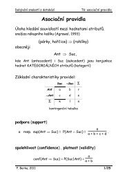
Let p(x | j ) be the state-conditional probability density function for x, i.e. the probability
density function for x given that the state of nature is j . Then, the difference between
p(x | 1 ) and p(x | 2 ) describes the difference in brightness between Carrara and Thassos
marble (see figure 16)
Figure 16: Hypothetical class-conditional probability density functions.
Suppose that we know both the a priori probabilities P( j ) and the conditional densities
p(x | j ). Suppose further that we measure the brightness of a piece of marble and discover
the value of x. How does this measurement influence our attitude concerning the true state of
nature? The answer to this question is provided by Bayes‘ rule:
(3)

where
(4)
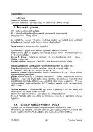
Bayes‘rule shows how the observation of value x changes the a priori probability P( j ) into
the a posteriori probability P( j | x). Variation of P( j | x) with x is illustrated in Figure 17
for the case
.
Figure 17: A posteriori probabilities for and .
If we have an observation x for which P( 1 | x) is greater than P( 2 | x)., we would be
naturally inclined to decide that the true state of nature is 1 . Similarly, if P( 2 | x). is
greater than P( 1 | x)., we would be naturally inclined to choose 2 .

To justify this procedure, let us calculate the probability of error whenever we make a
decision. Whenever we observe a particular x,
Clearly, in every instance in which we observe the same value for x, we can minimize the
probability error by deciding:
• if , and
• if .
Of course, we may never observe exactly the same value of x twice. Will this rule minimize
the average probability of error? Yes, because the average probability of error is given by:
and if for every x, P(error/ x) is as small as possible, the integral must be as small as possible.
Thus, we have justified the following Bayes‘ decision rule for minimizing the probability of
error:
This form of the decision rule emphasizes the role of the a posteriori probabilities. By using
equation 3, we can express the rule in terms of conditional and a priori probabilities.
Note that p(x) in equation 3 is unimportant as far as making a decision is concerned. It is
basically just a scale factor that assures us that
By eliminating this scale factor, we obtain the following completely equivalent decision rule:
.

Some additional insight can be obtained by considering a few special cases:
• if for some x, p(x | 1 ) = p(x | 2 ) , then that particular observation gives us no
information about the state of nature; in this case, the decision hinges entirely on the a
priori probabilities.
• On the other hand, if P( 1 ) = P( 2 ), then the states of nature are equally likely a
priori; in this case the decision is based entirely on , p(x | j ), the likelihood of j
with respect to x.
In general, both of these factors are important in making a decision, and the Bayes‘ decision
rule combines them to achieve the minimum probability of error.
3. Classifier
Consider a set
of elements. With Bayes' decision rule, it is possible to divide the elements
of into p classes C 1 , C 2 , …, C p , from n discriminant attributes A 1 , A 2 , …, A n . We must
already have examples of each class to choose typical values for the attributes of each class.
The probability of meeting element ∈ , having attribute A i , given that we consider
class C l , will be denoted by p Ai ( | C l ).
If we put all these probabilities together for each attribute, we obtain the global probability of
meeting element , given that the class is C l :
(5)
Classification must allow the class of unknown element to be decided with the lowest risk
of error. Decision in Bayes' theory chooses the class C l for which the a posteriori membership
probability p(C l | ). is the highest:
(6)
According to Bayes' rule, the a posteriori probability of membership p(C l | ) is calculated
from the a priori probabilities of membership of element to class C l :

(7)
Denominator p() is a normalization factor. It ensures that the sum of probabilities p(C l | )
is equal to 1 when l varies.
Some classes appear more frequently than others, and P(C l ) denotes the a priori probability of
meeting class C l .
p( | C l ). denotes the conditional probability of meeting the element
on class C l ( given that class C l is true).
, given that we focus
Parameters
The use of a Bayesian classifier implies that we know:
• the a priori probabilities P(C l ) that class C l appears;
• and the conditional probability p( | C l ) of being in the presence of element ,
given that the observation class is C l .
1. A priori probability P(C l )
If the examples used to sympl the system to recognize each sympl, are sufficiently
numerous, then a priori probability P(C l ) can be estimated as the frequency of
appearance of this sympl in comparison with the other classes. This is the most often
observed approach when the system is taught to recognize classes from symplex.
2. Conditional probability p( | C l )
The estimation of the conditional probability p( | C l ) represents the main problem.
It is very difficult because it requires the estimation of the conditional probabilities for
all the possible combinations of elements, given one particular class.
In reality, it is impossible to calculate these estimations. Some assumptions of
simplification are often used in order to make the training of the system feasible. The
assumption most frequently used is that of conditional independence which states that
the probability of two elements 1 and 2 ,given that class is C l , is the product of the
probabilities of each element taken separately, given that class is C l :

(8)
With such an assumption, conditional probability p( | C l ) of an element
according to attributes A i becomes:
(9)
Bayesian decision rule
This leads to the following Bayesian decision rule, where class C l represents the class
selected:
(10)
p Ai ( | C l ) represents the proportion of examples taking the value of element
attribute A i in all examples belonging to class C j .
The product of these probabilities proposed by each attribute A i for element
element for information fusion in this rule of Bayes.
for
is the