Principal Component Analysis: For a geometric interpretation of ...

Principal Component Analysis:
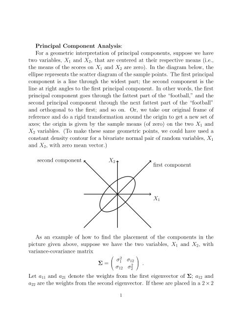
For a geometric interpretation of principal components, suppose we have
two variables, X 1 and X 2 , that are centered at their respective means (i.e.,
the means of the scores on X 1 and X 2 are zero). In the diagram below, the
ellipse represents the scatter diagram of the sample points. The first principal
component is a line through the widest part; the second component is the
line at right angles to the first principal component. In other words, the first
principal component goes through the fattest part of the “football,” and the
second principal component through the next fattest part of the “football”
and orthogonal to the first; and so on. Or, we take our original frame of
reference and do a rigid transformation around the origin to get a new set of
axes; the origin is given by the sample means (of zero) on the two X 1 and
X 2 variables. (To make these same geometric points, we could have used a
constant density contour for a bivariate normal pair of random variables, X 1
and X 2 , with zero mean vector.)
second component
X 2
first component
X 1
As an example of how to find the placement of the components in the
picture given above, suppose we have the two variables, X 1 and X 2 , with
variance-covariance matrix
Σ =
⎛
⎝ σ2 1 σ 12
σ 12 σ 2 2
Let a 11 and a 21 denote the weights from the first eigenvector of Σ; a 12 and
a 22 are the weights from the second eigenvector. If these are placed in a 2 × 2
1
⎞
⎠ .

orthogonal (or rotation) matrix T, with the first column containing the first
eigenvector weights and the second column the second eigenvector weights,
we can obtain the direction cosines of the new axes system from the following:
T =
⎛
⎝ a 11 a 12
a 21
⎞ ⎛
⎠ = ⎝
a 22
cos(θ) cos(90 + θ)
cos(θ − 90) cos(θ)
⎞
⎛
⎠ = ⎝
cos(θ) − sin(θ)
sin(θ) cos(θ)
These are the cosines of the angles with the positive (horizontal and vertical)
axes. If we wish to change the orientation of a transformed axis (i.e., to
make the arrow go in the other direction), we merely use a multiplication of
the relevant eigenvector values by −1 (i.e., we choose the other normalized
eigenvector for that same eigenvalue, which still has unit length).
⎞
⎠ .
90 + θ
θ
θ − 90
θ
If we denote the data matrix in this simple two variable problem as X n×2 ,
where n is the number of subjects and the two columns represent the values
on variables X 1 and X 2 (i.e., the coordinates of each subject on the original
axes), the n × 2 matrix of coordinates of the subjects on the transformed
axes, say X trans can be given as XT.
Hotelling’s Power method:
From Morrison (1967):
2

Let A be the p × p matrix of real elements. It is not necessary that A be
symmetric. Order the characteristic roots λ i of A by their absolute values:
|λ 1 | > |λ 2 | ≥ · · · ≥ |λ p | ,
and denote their respective characteristic vectors as a 1 , . . . , a p . Initially we
shall require that only |λ 1 | > |λ 2 | . Let x 0 be any vector of p real components,
and form the sequence: x 1 = Ax 0 ; . . . x n = Ax n−1 = A n x 0 of
vectors. Then if the successive x i are scaled in some fashion, the sequence of
standardized vectors will converge to the characteristic vector a 1 . Probably
the most convenient scaling is performed by dividing the elements by their
maximum, with normalization to unit length merely reserved for the last, or
exact, vector. Since Aa 1 = λ 1 a 1 , the characteristic root itself can be found
by dividing any element of Aa 1 by the corresponding element of a 1 .
The same iterative procedure can be used to compute any distinct characteristic
root of A. To extract the second largest root and its vector we normalize
the first characteristic vector a 1 to unit length, form the p × p matrix
λ 1 a 1 a ′ 1 and subtract it from A to give the residual matrix A 1 = A − λ 1 a 1 a ′ 1.
Kelley’s method (from Essential Traits of Mental Life (1935)):
If it is desired to create two new variables, x ′ and y ′ , which are completely
defined by the given variables, x and y, all that is necessary is to write
x ′ = a 1 x + b 1 y
y ′ = a 2 x + b 2 y
and assign any values to a 1 , a 2 , b 1 , and b 2 . Solving these equations for x and
y we have
x = b 2x ′ − b 1 y ′
a 1 b 2 − a 2 b 1
y = a 1y ′ − a 2 x ′
a 1 b 2 − a 2 b 1
Of the infinite number of new sets of equivalent variables, x ′ and y ′ , which
can be derived by substituting different values for a 1 , a 2 , b 1 , and b 2 , that one
is considered to have special merit which is a rotation of the x and y axes to
3

the position of the major and minor axes of the ellipse. These particular new
variables, which we designate x 1 and y 1 , are given by the equations
x 1 = x cos θ + y sin θ
y 1 = −x sin θ + y cos θ
where θ is the angle of rotation and is given by
tan 2θ =
2p
v 1 − v 2
[p = σ 12 ; v 1 = σ 2 1; v 2 = σ 2 2] The peculiar merit of the new variables, v 1 and
y 1 , lies in the facts which can be immediately surmised by thinking of the
elementary geometry involved.
(a) x 1 and y 1 are uncorrelated.
(b) x 1 and y 1 axes are at right angles to each other.
(c) The variance of x 1 distance from the minor axis in the direction of the
major axis, is a maximum, for no other rotation of axes yields a variable with
as large a variance.
(d) The variance of y 1 , distance measured in the direction of the minor
axis, is a minimum.
The advantage of (a), lack of correlation, need scarcely be dwelt upon, as
it is the essential purpose of factorization to obtain independent measures.
The advantage of (b), orthogonality, is not quite so obvious. Though a
point in two-dimensional space may be completely defined by distance from
two oblique axes, nevertheless the simplicity of thought (and to create such
simplicity is a basic purpose of factorization) when a point is defined in terms
of perpendicular distance from two perpendicular axes, should be sufficient
to commend the use of such axis.
The advantage of (c) making the variance of one of the new variables a
maximum is particularly apparent when the major axis is much greater than
the minor. In this case, much more about the total situation or the total field
wherein variation can take place is known if variability in any other direction
is known. The principle of parsimony of thought recommends a knowledge of
4

the x 1 variable if but a single item of knowledge is available. The operation of
this principle will be much more apparent when thinking of many variables,
for here the variances of some of the smaller ones may be such that entire
lack of knowledge of them will not be serious.
It is obvious from the geometry of the situation that there is but a single
solution yielding variables with the properties mentioned. These constitute
the components in the two-variable problem.
5

Kelley True Score Prediction (James-Stein Estimation):
In prediction, two aspects of variable unreliability have consequences for
ethical reasoning. One is in estimating a person’s true score on a variable; the
second is in how regression might be handled when there is measurement error
in the independent and/or dependent variables. In both of these instances,
there is an implicit underlying model for how any observed score, X, might be
constructed additively from a true score, T X , and an error score, E X , where
E X is typically assumed uncorrelated with T X : X = T X + E X . When we
consider the distribution of an observed variable over, say, a population of
individuals, there are two sources of variability present in the true and the
error scores. If we are interested primarily in structural models among true
scores, then some correction must be made because the common regression
models implicitly assume that variables are measured without error.
The estimation, ˆTX , of a true score from an observed score, X, was derived
using the regression model by Kelley in the 1920s (Kelley, 1947), with a
reliance on the algebraic equivalence that the squared correlation between observed
and true score is the reliability. If we let ˆρ be the estimated reliability,
Kelley’s equation can be written as
ˆT X = ˆρX + (1 − ˆρ) ¯X ,
where ¯X is the mean of the group to which the individual belongs. In other
words, depending on the size of ˆρ, a person’s estimate is partly due to where
the person is in relation to the group—upward if below the mean, downward
if above. The application of this statistical tautology in the examination of
group differences provides such a surprising result to the statistically naive
that this equation has been labeled “Kelley’s Paradox” (Wainer, 2005, pp.
67–70).
In addition to obtaining a true score estimate from an obtained score,
Kelly’s regression model also provides a standard error of estimation (which
in this case is now referred to as the standard error of measurement). An
approximate 95% confidence interval on an examinee’s true score is given by
ˆT X ± 2ˆσ X (( √ 1 − ˆρ) √ˆρ) ,
where ˆσ X is the (estimated) standard deviation of the observed scores. By
itself, the term ˆσ X (( √ 1 − ˆρ) √ˆρ) is the standard error of measurement, and
6

is generated from the usual regression formula for the standard error of estimation
but applied to Kelly’s model predicting true scores. The standard
error of measurement most commonly used in the literature is not Kelly’s but
rather ˆσ X
√ 1 − ˆρ, and a 95% confidence interval taken as the observed score
plus or minus twice this standard error. An argument can be made that this
latter procedure leads to “reasonable limits” (after Gulliksen, 1950) whenever
ˆρ is reasonably high, and the obtained score is not extremely deviant from
the reference group mean. Why we should assume these latter preconditions
and not use the more appropriate procedure to begin with, reminds us of a
Bertrand Russell quotation (1919, p. 71): “The method of postulating what
we want has many advantages; they are the same as the advantages of theft
over honest toil.”
There are several remarkable connections between Kelley’s work in the
first third of the twentieth century and the modern theory of statistical estimation
developed in the last half of the century. In considering the model for
an observed score, X, to be a sum of a true score, T , and an error score, E,
plot the observed test scores on the x-axis and their true scores on the y-axis.
As noted by Galton in the 1880s (Galton, 1886), any such scatterplot suggests
two regression lines. One is of true score regressed on observed score (generating
Kelley’s true score estimation equation given in the text); the second
is the regression of observed score being regressed on true score (generating
the use of an observed score to directly estimate the observed score). Kelley
clearly knew the importance for measurement theory of this distinction
between two possible regression lines in a true-score versus observed-score
scatterplot. The quotation given below is from his 1927 text, Interpretation
of Educational Measurements. The reference to the “last section” is where
the true score was estimated directly by the observed score; the “present
section” refers to his true score regression estimator:
This tendency of the estimated true score to lie closer to the mean than the obtained score
is the principle of regression. It was first discovered by Francis Galton and is a universal
phenomenon in correlated data. We may now characterize the procedure of the last and
present sections by saying that in the last section regression was not allowed for and in
the present it is. If the reliability is very high, then there is little difference between [the
two methods], so that this second technique, which is slightly the more laborious, is not
demanded, but if the reliability is low, there is much difference in individual outcome, and
7

the refined procedure is always to be used in making individual diagnoses. (p. 177)
Kelley’s preference for the refined procedure when reliability is low (that
is, for the regression estimate of true score) is due to the standard error of
measurement being smaller (unless reliability is perfect); this is observable
directly from the formulas given earlier. There is a trade-off in moving to the
regression estimator of the true score in that a smaller error in estimation is
paid for by using an estimator that is now biased. Such trade-offs are common
in modern statistics in the use of “shrinkage” estimators (for example,
ridge regression, empirical Bayes methods, James–Stein estimators). Other
psychometricians, however, apparently just don’t buy the trade-off; for example,
see Gulliksen (Theory of Mental Tests; 1950); Gulliksen wrote that
“no practical advantage is gained from using the regression equation to estimate
true scores” (p. 45). We disagree—who really cares about bias when a
generally more accurate prediction strategy can be defined?
What may be most remarkable about Kelley’s regression estimate of true
score is that it predates the work in the 1950s on “Stein’s Paradox” that shook
the foundations of mathematical statistics. A readable general introduction
to this whole statistical kerfuffle is the 1977 Scientific American article by
Bradley Efron and Carl Morris, “Stein’s Paradox in Statistics” (236 (5), 119-
127). When reading this popular source, keep in mind that the class referred
to as James–Stein estimators (where bias is traded off for lower estimation
error) includes Kelley’s regression estimate of the true score. We give an
excerpt below from Stephen Stigler’s 1988 Neyman Memorial Lecture, “A
Galtonian Perspective on Shrinkage Estimators” (Statistical Science, 1990,
5, 147-155), that makes this historical connection explicit:
The use of least squares estimators for the adjustment of data of course goes back well
into the previous century, as does Galton’s more subtle idea that there are two regression
lines. . . . Earlier in this century, regression was employed in educational psychology in a
setting quite like that considered here. Truman Kelley developed models for ability which
hypothesized that individuals had true scores . . . measured by fallible testing instruments
to give observed scores . . . ; the observed scores could be improved as estimates of the true
scores by allowing for the regression effect and shrinking toward the average, by a procedure
quite similar to the Efron–Morris estimator. (p. 152)
Before we leave the topic of true score estimation by regression, we might
8

also note what it does not imply. When considering an action for an individual
where the goal is to help make, for example, the right level of placement
in a course or the best medical treatment and diagnosis, then using group
membership information to obtain more accurate estimates is the appropriate
course to follow. But if we are facing a contest, such as awarding scholarships,
or offering admission or a job, then it is inappropriate (and ethically
questionable) to search for identifiable subgroups that a particular person
might belong to and then adjust that person’s score accordingly. Shrinkage
estimators are “group blind.” Their use is justified for whatever population
is being observed; it is generally best for accuracy of estimation to discount
extremes and ”pull them in” toward the (estimated) mean of the population.
9

From Talents and Tasks; Canonical Correlation Calculations:
Problem 4: To determine that combination of the u measures and that
combination of the w measures that yields the greatest consociated covariance,
thence the second combination of each to yield the greatest consociated
covariance in the residual variances, thence with third, fourth, and further
combinations. The solution of this problem defines the activity which will
yield the greatest happiness to the largest numbers and produce the greatest
amount of that which society most needs. The “greatest happinness to the
largest numbers” is a loose way of saying that both the degree of happiness
and the number affected are involved in the maximizing process. Should one
such activity be found, perhaps farming, it is obvious that other activities,
enjoyable to lesser numbers and serving lesser social needs, are necessary; so
second, third, fourth, etc., types as defined by the subsequent consociated
covariances must be found. In spite of the seeming verbal contradiction there
is meaning in the statement “Happy is the man whose vocation is his avocation
and sound is that society the fulfillment of whose needs is the pleasure
of its citizens.”
Computational Steps:
The solution of Problem 4 is readily accomplished by successive rotations
of axes so as to maximize covariance. For simplicity of explanation let us arrange
the given w variables in an order which we will call x 1 , . . . , x w such that
the sum of the squares of the interaction covariances (those from the upper
right quadrant) involving x 1 is greater than that involving x 2 , etc. Similarly,
let us arrange the u variables in an order which we will call x w+1 , . . . , x w+u
which is greater than that involving x w+3 , etc.
We now need the general formulas for rotating any two variables x 1 and x 2
through an angle θ to obtain new variables y 1 and y 2 . (the bracket notation
used below is for the covariance of the included variables) These are
y 1 = x 1 cos θ + x 2 sin θ
y 2 = −x 1 sin θ + x 2 cos θ
[y 1 y 1 ] = [x 1 x 1 ](cos θ) 2 + [x 2 x 2 ](sin θ) 2 + 2[x 1 x 2 ](sin θ)(cos θ)
[y 2 y 2 ] = [x 1 x 1 ](sin θ) 2 + [x 2 x 2 ](cos θ) 2 − 2[x 1 x 2 ](sin θ)(cos θ)
10

[y 1 y 2 ] = [x 1 x 2 ]((cos θ) 2 − (sin θ) 2 ) − ([x 1 x 1 ] − [x 2 x 2 ])(cos θ)(sin θ))
[y 1 x 3 ] = [x 1 x 3 ] cos θ + [x 2 x 3 ] sin θ
[y 2 x 3 ] = −[x 1 x 3 ] sin θ + [x 2 x 3 ] cos θ
If the angle θ has been so chosen as to make [y 1 x 3 ] a maximum, we have
or
d[y 1 x 3 ]
dθ
= −[x 1 x 3 ] sin θ + [x 2 x 3 ] cos θ = 0
tan θ = [x 2x 3 ]
[x 1 x 3 ] ,
giving θ to maximize [y 1 x 3 ]
We note that rotating through this angle makes [y 2 x 3 ] a minimum, for
. Also upon squaring the equation
[y 2 x 3 ] = −[x 1 x 3 ] sin θ + [x 2 x 3 ] cos θ = 0
[y 1 x 3 ] = [x 1 x 3 ] cos θ + [x 2 x 3 ] sin θ
we find that for rotation through the angle given by θ
[y 1 x 3 ] 2 = [x 1 x 3 ] 2 + [x 2 x 3 ] 2
giving the squared covariance as the sum of squared covariances. This rotation
has transferred the squared covariance [x 2 x 3 ] 2 to the (1,3) cell.
11

Kelley’s Will:
The fitter, the richer
Prof’s will sets up fitness tests for sons
Santa Barbara, Calif. (AP) – A retired Harvard professor has willed his
two sons an extra inheritance–scaled to how they and their future wives rate
in a series of mental-physical-character tests.
The unique bequest is from Dr. Truman Lee Kelley, authority on psychological
testing and measurement, and one of the authors of the widely used
Stanford achievement test battery.
He died May 2 at 76, and terms of his will and its so-called “eugenics
trust” were disclosed when it was filed Thursday with the county clerk.
His apparent goal: To obtain for his sons superior marriages through eugenic
selection. Eugenics is a process of race improvement by mating superior
types suited to each other.
The will sets up a complicated series of tests for his sons, Kenneth, 22, Air
Force lieutenant stationed at Wurtsmith AFB, Mich., and Kalon, 24, reportedly
working for a Ph.D. degree at the Massachusetts Institute of Technology.
Neither could be reached immediately for comment
Both are single. They and the women they marry are to receive cash
awards in proportion to their fitness as determined by the tests. The birth
of children to a high-scoring couple calls for additional awards.
Dr. Kelley named a group of trustees headed by Eric F. Gardner of Syracuse
University, to devise the test and administer the “eugenics trusts” for
his sons, and left 50 shares of Illinois Terminal stock plus other funds to pay
the awards.
The trusts were established, the 1954-dated will says, “to promote the
eugenic marriage of my sons through counseling, marriage and birth awards.”
To be eligible for a marriage award the son and his prospective bride must
give the trustees any information they need to determine prior to marriage
the couple’s “E” (for eugenics) score.
The “E” score would be set by the couple’s deviation about or below the
American white population average in three categories: health, intellect, and
character.
For each point about average, the son and his bride would receive $400
12

each, from which would be deducted $400 for each point below average. On
the birth of a child, a similar award of $600 per point would be paid.
Since the number of possible points still is to be determined by the trustees,
the highest amount available was not stated. The total value of property
owned by Dr. Kelley was estimated at $175,000.
In addition to the fund set up to finance the eugenics trusts, Dr. Kelley
left half his estate to his widow, Grace, and one-fourth each to the sons.
May 12, 1961
Father’s will prods sons to improve human race
Trust fund to reward future weddings if science approves
Santa Barbara, Calif., May 12 (AP) – A Harvard psychologist who died
after a lifetime devoted to studying the human race has left a will devoted to
improving it.
Method: Cash bonuses for his two sons. Condition: They and the wives
they select must score well on a series of mental-physical-character tests.
The will, admitted to probate yesterday, got this reaction from the widow
of Truman Lee Kelley:
“We pay so much attention to our prize cattle, but we haven’t paid too
much attention to the human race.”
Said Mrs. Kelley: “This is a step in the right direction.”
Sons Say Yes and No
But Dr. Kelley’s two sons had varying reactions.
“I see some disadvantages in it,” said his son Kenneth, 21, an air force
second lieutenant. “For one thing, I don’t want to select a wife solely on
the standards he imposed in his will. I don’t want to place money before
marriage itself.”
The other son, Kalon, 24, a staff member at Massachusetts Institute of
Technology said he agrees with terms of the will and “very definitely intends
to comply” he added.
“What my father tried to do when he instituted and authored the will was
to instill in my brother and myself a consideration of eugenic aspects he and
I consider important.”
(Eugenics is the study of selective breeding.)
13

No Marriage Plans
Neither son plans to marry in the near future, they said. Both said they
discussed the unusual will with their father, who died last May at the age of
76.
Dr. Kelley achieved fame in 1923 as one of the authors of the widely used
Stanford achievement test battery. He served the Government as a psychological
testing authority in World War II. After his retirement from Harvard
about 12 years ago, he and his family moved to this southern California
seaside city.
The will estimates his total worth at about $175,000.
His will, written in 1954, provides for two trust funds: one for his sons
and one for other young persons whose marriages, he believed, would result
in superior children.
Trust to Help PhDs
Mrs. Kelley indicated that the second trust fund was primarily for college
graduates seeking advanced degrees she explained.
“He always was bothered by the fact that candidates for the PhD degree
had to choose between getting the degree or marrying and having children.”
“Usually they married and delayed having children, so he thought that in
some small way he might enable these students to continue their studies and
have youngsters.”
Dr. Kelley appointed a group of trustees, headed by Eric F. Gardner of
Syracuse University, to administer the “eugenics trusts.”
The amount of each trust fund, based on stock holdings, was not disclosed.
Test For Candidates
To qualify for the money, the sons and their prospective brides – before
marrying – must give the trustees information required to determine the
couple’s “E” (for eugenics) score.
The “E” score would be based on the pair’s deviation above or below the
American white population averages for health, intellect and character.
Each point above average would bring the son and his bride $400; each
point below average would result in a $400 deduction.
The couples would get $600 for each child.
The maximum amount available will be determined by the trustees.
14

Part of an interview with Gene Golub by Thomas Haigh for
SIAM (2005):
HAIGH: Actually, I’m seeing you mentioned here. So this is Progress Report
#9 covering January 1, 1954 to June 30, 1954. The report says that
you were a half-time research assistant, and it says, “Mr. Golub has been
studying the problems associated with factor analysis and is also working
on other problems associated particularly with matrix operations. He has
programmed Rao’s Maximum Likelihood Factor Analysis Method, and has
obtained new results, which he will publish. This summer, he presented a
paper on tests of significance in factor analysis at the International Psychological
Congress in Montreal, and in September will present another at the
meeting of the American Psychological Association in New York.”
GOLUB: That was very interesting. One of the groups that was very
active at Illinois was the psychologists, or psychometricians, and they had a
group of first-rate people there. I got to know a man by the name of Charles
Wrigley quite well. He was a psychologist. I guess he was on a research
appointment. He was from New Zealand originally. Wrigley got his Ph.D. in
London under a man by the name of Cyril Burt; he was the originator of the
Eleven Plus exam. He has been subsequently discredited because it appears
that some of his research data on twins reared apart was made up.
HAIGH: The identical twins that no one could find. Was that him?
GOLUB: In this case, it was a secretary that no one could find. Anyway,
Wrigley worked for him, and he was a very powerful man and intellectual man,
although rather sloppy in his presentations. Wrigley had a job in Montreal
when he came to North America after he got his Ph.D. Then he was being
looked over at Illinois. When he saw the ILLIAC, he didn’t want to do any
further numerical computations. I guess he had used an old hand calculator,
and he saw this machine that could do all these computations. The guys at
Illinois, the psychologists who were there, they knew they needed somebody
who had some experience in numerical computing, so they hired him. He was
an inspiration to me. He was so positive and helpful. He was just a very nice
man and invited people to his house—just a terrifically good human being.
So I got in with that factor analysis group, and I learned a lot. It was
really important for me subsequently. Nowadays, there’s this whole tendency
15

to look at larger and larger data sets. It’s interesting. The people who first
started this, I think, were the psychologists. They had large sets of data
coming out of educational testing and so forth. So they were the ones that
first began this whole interest in analyzing large data sets. Factor analysis is
the term used for that, and they were very involved. Illinois was a hot center
of this because of the people that they had, plus, they had a big Air Force
contract. So this area of research, of data analysis, went on. For instance,
electrical engineers had been involved in that. And then finally, I was saying
in the last ten years, computer scientists began to realize that they’re getting
masses of data, and then the question is how to analyze this data and what
to do with it. It started me off in an area that has been of great interest
to me. Simultaneously, when I was a graduate student, there was a man by
the name of C.R. Rao. He’s probably one of the world’s great statisticians.
He developed this technique for canonical factor analysis. He’s still alive at
Penn State University, and I’m going to actually visit him next summer.
HAIGH: Were there a number of Ph.D. students?
GOLUB: There were a few around. So the idea was that I was going to
continue in statistics, and I was going to write a thesis, possibly, under a
man called Bill Madow. So the sequence of events is: the first year, I was a
graduate student. Madow was on sabbatical, and C.R. Rao was at Illinois.
The next year Rao left and Madow came back, but he came back without
his wife. They had been in California on a sabbatical. He was not a welltempered
person. He was a very smart guy, but he was very difficult. Then
after the year, he left to go back to California. So this guy, Madow, ended
up here in Northern California, working for SRI. All right. Then (Abraham)
Taub suddenly grabs a hold of me, so I could be his student. So he took me
on as a student.
HAIGH: Was Taub head of the lab at that point?
GOLUB: Well, as soon as Nash left. I don’t know what year Nash left.
Taub became the head. So I was supposed to be Taub’s student. He said,
”Here, read this,” and there was some paper he gave me by von Neumann
that hadn’t been published yet. So I looked at it. I didn’t really see how to go
from there, but eventually, that paper played an enormous role in what I did.
So I started to work on that. He didn’t know that field so well himself. He
16

just put me into it. So I was no longer doing statistics, although I was getting
my degree in statistics, I was doing numerical analysis. In the meantime, I
was subject to a lot of abuse by Taub. He would just yell and scream at me.
Did [Bill] Gear talk to you about this at all?
HAIGH: Yes.
GOLUB: I think he liked Gear better. Maybe Gear is a more secure and
sophisticated person. I think the weaker you are as a person, the more he
hammered at you. He was really a nasty piece. At any rate, I finished the
thesis.
HAIGH: Had work began on ILLIAC 2 while you were there?
GOLUB: Yes, there was talk about it in the background, but I didn’t
participate. There was another student amongst the people. His name is
Roger Farrell, and we’ve remained very good friends. He’s now a retired
professor of statistics at Cornell University. Roger was really a statistician.
He got his degree under Burkholder at Illinois. So it was just a good place
and things were expanding. With respect to new ideas coming out of Illinois
in terms of computation, Gregory had programmed the Jacobi method for
computing eigenvalues. He wrote an article about that, which alerted a lot of
people to the use of the Jacobi method. It was a method that von Neumann
and Goldstein had advocated. Then Gregory wrote this little short-page
paper showing what accuracy it obtained, and that pricked up a lot of ears
to the use of the Jacobi method.
But there wasn’t a lot of innovation in numerical methods. That’s what
I’m trying to say. There wasn’t enough leadership. I once got into an argument
with Taub at Bill Gear’s wedding party about the fact that there were
no real numerical analysts at Illinois. [laughs] Maybe that’s what led to his
being angry with me, I don’t know. Our relationship went up and down, and
there were times even after that it was up, but then I think at the end it was
down again for various reasons. He died about four or five years ago.
17

From an interview with Darrell Bock in JEBS (2006) :
I had heard from Charles Wrigley at Michigan State University that the
new Illiac electronic computer at Champaign-Urbana had programs for both
the one- and two-matrix eigenproblems. On his advice, I phoned Kern Dickman,
who had helped Charles perform a principal component analysis on the
machine, and explained my needs. He invited me to come down to Urbana
and bring the matrices to be analyzed with me. By that time, I had become
sufficiently proficient in using punched card equipment in the business office
of the University–in particular a new electronic calculating punch that could
store constants and performed cumulative multiplications as fast as the cards
passed through the machine. I used this machine to convert Likert scores of
the categories into scale values by a method I had described previously in my
1956 Psychometrika paper, “Selection of Judges for Preference Testing.”
I arrived in Urbana and found Kern; he took me directly to the computation
Center to see the Illiac. But there was very little to see–only a photoelectric
reader of teletype tape and a box with a small slit where punched
tape spewed from the machine; a few dimly revealed electronic parts could
be seen behind a plate-glass window. Elsewhere in the room were teletype
machines for punching numbers and letters onto paper tape, printing out the
characters of an existing tape, or copying all or parts of one tape to another.
My first job was to key the elements of the two covariance matrices onto tape,
which in spite of my best efforts to avoid errors, took most of the afternoon.
When I finished that task, Kern suggested that we should meet for dinner
at his favorite watering hole in Urbana. When I arrived there I found him
sitting with another person whom he introduced as Gene Golub, adding that
Gene had programmed the eigenroutines for the Illiac. At Kern’s suggestion
Gene had brought along some papers for me–an introduction to programming
the Illiac and the documentation of the eigenroutines. He said that his code
was similar to that of Goldstein, who had programmed the eigen-procedures
for the Maniac machine built by Metropolis at Los Alamos. It used the Jacobi
iterative method, which consists of repeated orthogonal transformations of
pairs of variables to reduce the elements in the off-diagonal of a real symmetric
matrix to zero, all the while performing the same operation on an identity
matrix. Although a given element of the matrix does not necessarily remain
18

zero, the iterations converge to a diagonal matrix containing the eigenvalues,
and the identity matrix becomes the corresponding eigenvectors.
Gene told the story that Goldstein, having heard the Jacobi method described
by a colleague, stopped by John von Neumann’s office to ask if the
method was strictly convergent. Gazing at the ceiling for about five seconds,
von Neumann replied “yes, of course.” Goldstein was amazed, thinking this
was another of von Neuman’s fabled feats of mental calculation, but as Golub
and Van Loan show in their 1996 reference, Matrix Computations, the proof
requires only a few lines of matrix expressions, which von Neumann could
have easily visualized. I already knew of this method, not as Jacobi’s, but as
the “method of sine and cosine transformations” described by Truman Kelley
in his 1935 book, Essential Traits of Mental Life. He presented the method as
his own creation, including a proof of convergence requiring several pages of
geometric argument. Considering that Jacobi had introduced the method in
the middle of the 19th-century, I wondered if Kelley had heard of it from one
of his fellow professors at Harvard. But I found in his 1928 book, Crossroads
in the Mind of Man, that he had already used sine and cosine transformations
in connection with Spearman’s one-factor model, and I now believe that he
rediscovered Jacobi’s method independently.
Next morning, Kern showed me how to feed my tape into the reader, and
after about 20 minutes I saw the output tape race out of the machine and
fall into a large wastebasket that was sitting below. My job was then to
pull the free rear end of the tape over to a geared-up hand-cranked reel and
quickly pulled the rest of the tape out of the basket. I took the roll of tape
to the teletype machine and printed the incredibly rewarding twelve-variable
eigenvalues and eigenvectors of my two-matrix eigen-problem.
Later than day, after profuse thanks to Kern, I caught the northbound City
of New Orleans back to Chicago. While perusing the eigen-routine documentation
during the trip, I saw that Golub had reduced the two-matrix problem
to a one-matrix problem by pre- and post-multiplying the first matrix by the
inverse of the so-called “grammian square root” of the second matrix. The
resulting matrix is symmetric. The grammian square root is a diagonal matrix
containing the square roots of the eigenvalues (which must be positive),
pre-and post-multiplied by the matrix of eigenvectors and its transpose. If
19

the diagonal matrix contains the reciprocal square roots of the eigenvalues,
the result is the inverse matrix. This method has the disadvantage, however,
of requiring the calculation of the eigenvalues and vectors of two symmetric
matrices rather than one. But it occurred to me that the computations could
be shortened considerably by pre- and post-multiplying by the inverse of the
so-called “false square root” of the symmetric positive definite matrix—that
is, by the inverse of the triangular Cholesky decomposition of the matrix. For
some time I had been solving least-squares regression problems by Cholesky
decomposition rather than less accurate conventional Gaussian elimination.
This quicker method of solving the two-matrix eigen-problem is in the
MATCAL subroutines programmed by Bruno Repp and me in 1974; the resulting
one-matrix eigen-problem is solved by the Householder-Ortega-Wilkinson
method as programmed by Richard Wolfe. From the Illiac programming manual
I learned a truth that has proved invaluable to me: it said, “Remember
that the best programmer is not necessarily the one who makes the fewest
mistakes, but one who can find his mistakes most quickly.” I soon learned
that as a programmer, I was one of the latter. Lyle wrote up the Illiac results
in the paper, “Multivariate Discriminant Analysis Applied to ‘Ways to
Live’ ratings from Six Cultural Groups,” which subsequently appeared in the
June 1960, issue of Sociometry, then published by the American Sociological
Association. (The paper is also now online at JSTOR.) To the best of my
knowledge it is the first application of multiple discriminant analysis on as
many as 12 variables. It paved the way for my later work on multivariate
analysis of variance and covariance.
20