Introduction to Information Retrieval
Introduction to Information Retrieval
Introduction to Information Retrieval

Create successful ePaper yourself
Turn your PDF publications into a flip-book with our unique Google optimized e-Paper software.
<strong>Introduction</strong> <strong>to</strong> <strong>Information</strong> <strong>Retrieval</strong><br />
<strong>Introduction</strong> <strong>to</strong><br />
<strong>Information</strong> <strong>Retrieval</strong><br />
Hinrich Schütze and Christina Lioma<br />
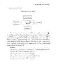
Lecture 5: Scoring, Term Weighting, The Vec<strong>to</strong>r<br />
Space Model<br />
1
<strong>Introduction</strong> <strong>to</strong> <strong>Information</strong> <strong>Retrieval</strong><br />
Take-away <strong>to</strong>day<br />
• Ranking search results: why it is important (as opposed <strong>to</strong> just<br />
presenting a set of unordered Boolean results)<br />
• Term frequency: This is a key ingredient for ranking.<br />
• Tf-idf ranking: best known traditional ranking scheme<br />
• Vec<strong>to</strong>r space model: One of the most important formal<br />
models for information retrieval (along with Boolean and<br />
probabilistic models)<br />
2
<strong>Introduction</strong> <strong>to</strong> <strong>Information</strong> <strong>Retrieval</strong><br />
Outline<br />
❶ Take-away <strong>to</strong>day<br />
❷ Why ranked retrieval?<br />
❸ Term frequency<br />
❹ tf-idf weighting<br />
❺ The vec<strong>to</strong>r space model<br />
3
<strong>Introduction</strong> <strong>to</strong> <strong>Information</strong> <strong>Retrieval</strong><br />
Ranked retrieval<br />
• Thus far, our queries have all been Boolean.<br />
• Documents either match or don’t.<br />
• Good for expert users with precise understanding of their<br />
needs and of the collection.<br />
• Also good for applications: Applications can easily consum<br />
1000s of results.<br />
• Not good for the majority of users<br />
• Most users are not capable of writing Boolean queries . . .<br />
• . . . or they are, but they think it’s <strong>to</strong>o much work.<br />
• Most users don’t want <strong>to</strong> wade through 1000s of results.<br />
• This is particularly true of web search.<br />
4
<strong>Introduction</strong> <strong>to</strong> <strong>Information</strong> <strong>Retrieval</strong><br />
Problem with Boolean search: Feast or famine<br />
• Boolean queries often result in either <strong>to</strong>o few (=0) or <strong>to</strong>o<br />
many (1000s) results.<br />
• Query 1 (boolean conjunction): [standard user dlink 650]<br />
• → 200,000 hits – feast<br />
• Query 2 (boolean conjunction): [standard user dlink 650 no<br />
card found]<br />
• → 0 hits – famine<br />
• In Boolean retrieval, it takes a lot of skill <strong>to</strong> come up with a<br />
query that produces a manageable number of hits.<br />
5
<strong>Introduction</strong> <strong>to</strong> <strong>Information</strong> <strong>Retrieval</strong><br />
Feast or famine: No problem in ranked retrieval<br />
• With ranking, large result sets are not an issue.<br />
• Just show the <strong>to</strong>p 10 results<br />
• Doesn’t overwhelm the user<br />
• Premise: the ranking algorithm works: More relevant results<br />
are ranked higher than less relevant results.<br />
6
<strong>Introduction</strong> <strong>to</strong> <strong>Information</strong> <strong>Retrieval</strong><br />
Scoring as the basis of ranked retrieval<br />
• We wish <strong>to</strong> rank documents that are more relevant higher<br />
than documents that are less relevant.<br />
• How can we accomplish such a ranking of the documents in<br />
the collection with respect <strong>to</strong> a query?<br />
• Assign a score <strong>to</strong> each query-document pair, say in [0, 1].<br />
• This score measures how well document and query “match”.<br />
7
<strong>Introduction</strong> <strong>to</strong> <strong>Information</strong> <strong>Retrieval</strong><br />
Query-document matching scores<br />
• How do we compute the score of a query-document pair?<br />
• Let’s start with a one-term query.<br />
• If the query term does not occur in the document: score<br />
should be 0.<br />
• The more frequent the query term in the document, the<br />
higher the score<br />
• We will look at a number of alternatives for doing this.<br />
8
<strong>Introduction</strong> <strong>to</strong> <strong>Information</strong> <strong>Retrieval</strong><br />
Take 1: Jaccard coefficient<br />
• A commonly used measure of overlap of two sets<br />
• Let A and B be two sets<br />
• Jaccard coefficient:<br />
• JACCARD (A, A) = 1<br />
• JACCARD (A, B) = 0 if A ∩ B = 0<br />
• A and B don’t have <strong>to</strong> be the same size.<br />
• Always assigns a number between 0 and 1.<br />
9
<strong>Introduction</strong> <strong>to</strong> <strong>Information</strong> <strong>Retrieval</strong><br />
Jaccard coefficient: Example<br />
• What is the query-document match score that the Jaccard<br />
coefficient computes for:<br />
• Query: “ides of March”<br />
• Document “Caesar died in March”<br />
• JACCARD(q, d) = 1/6<br />
10
<strong>Introduction</strong> <strong>to</strong> <strong>Information</strong> <strong>Retrieval</strong><br />
What’s wrong with Jaccard?<br />
• It doesn’t consider term frequency (how many occurrences a<br />
term has).<br />
• Rare terms are more informative than frequent terms.<br />
Jaccard does not consider this information.<br />
• We need a more sophisticated way of normalizing for the<br />
length of a document.<br />
• Later in this lecture, we’ll use (cosine) . . .<br />
• . . . instead of |A ∩ B|/|A ∪ B| (Jaccard) for length<br />
normalization.<br />
11
<strong>Introduction</strong> <strong>to</strong> <strong>Information</strong> <strong>Retrieval</strong><br />
Outline<br />
❶ Recap<br />
❷ Why ranked retrieval?<br />
❸ Term frequency<br />
❹ tf-idf weighting<br />
❺ The vec<strong>to</strong>r space model<br />
12
<strong>Introduction</strong> <strong>to</strong> <strong>Information</strong> <strong>Retrieval</strong><br />
Binary incidence matrix<br />
Anthony<br />
and<br />
Cleopatra<br />
Julius<br />
Caesar<br />
The<br />
Tempest<br />
Hamlet Othello Macbeth<br />
. . .<br />
ANTHONY<br />
BRUTUS<br />
CAESAR<br />
CALPURNIA<br />
CLEOPATRA<br />
MERCY<br />
WORSER<br />
. . .<br />
1<br />
1<br />
1<br />
0<br />
1<br />
1<br />
1<br />
1<br />
1<br />
1<br />
1<br />
0<br />
0<br />
0<br />
0<br />
0<br />
0<br />
0<br />
0<br />
1<br />
1<br />
0<br />
1<br />
1<br />
0<br />
0<br />
1<br />
1<br />
0<br />
0<br />
1<br />
0<br />
0<br />
1<br />
1<br />
1<br />
0<br />
1<br />
0<br />
0<br />
1<br />
0<br />
Each document is represented as a binary vec<strong>to</strong>r ∈ {0, 1} |V|. 13<br />
13
<strong>Introduction</strong> <strong>to</strong> <strong>Information</strong> <strong>Retrieval</strong><br />
Binary incidence matrix<br />
Anthony<br />
and<br />
Cleopatra<br />
Julius<br />
Caesar<br />
The<br />
Tempest<br />
Hamlet Othello Macbeth<br />
. . .<br />
ANTHONY<br />
BRUTUS<br />
CAESAR<br />
CALPURNIA<br />
CLEOPATRA<br />
MERCY<br />
WORSER<br />
. . .<br />
157<br />
4<br />
232<br />
0<br />
57<br />
2<br />
2<br />
73<br />
157<br />
227<br />
10<br />
0<br />
0<br />
0<br />
0<br />
0<br />
0<br />
0<br />
0<br />
3<br />
1<br />
0<br />
2<br />
2<br />
0<br />
0<br />
8<br />
1<br />
0<br />
0<br />
1<br />
0<br />
0<br />
5<br />
1<br />
1<br />
0<br />
0<br />
0<br />
0<br />
8<br />
5<br />
Each document is now represented as a count vec<strong>to</strong>r ∈ N |V|. 14<br />
14
<strong>Introduction</strong> <strong>to</strong> <strong>Information</strong> <strong>Retrieval</strong><br />
Bag of words model<br />
• We do not consider the order of words in a document.<br />
• John is quicker than Mary and Mary is quicker than John<br />
are represented the same way.<br />
• This is called a bag of words model.<br />
• In a sense, this is a step back: The positional index was able<br />
<strong>to</strong> distinguish these two documents.<br />
• We will look at “recovering” positional information later in<br />
this course.<br />
• For now: bag of words model<br />
15
<strong>Introduction</strong> <strong>to</strong> <strong>Information</strong> <strong>Retrieval</strong><br />
Term frequency tf<br />
• The term frequency tf t,d of term t in document d is defined<br />
as the number of times that t occurs in d.<br />
• We want <strong>to</strong> use tf when computing query-document match<br />
scores.<br />
• But how?<br />
• Raw term frequency is not what we want because:<br />
• A document with tf = 10 occurrences of the term is more<br />
relevant than a document with tf = 1 occurrence of the<br />
term.<br />
• But not 10 times more relevant.<br />
• Relevance does not increase proportionally with term<br />
frequency.<br />
16
<strong>Introduction</strong> <strong>to</strong> <strong>Information</strong> <strong>Retrieval</strong><br />
Instead of raw frequency: Log frequency<br />
weighting<br />
• The log frequency weight of term t in d is defined as follows<br />
• tf t,d → w t,d :<br />
0 → 0, 1 → 1, 2 → 1.3, 10 → 2, 1000 → 4, etc.<br />
• Score for a document-query pair: sum over terms t in both q<br />
and d:<br />
tf-matching-score(q, d) = t∈q∩d (1 + log tf t,d )<br />
<br />
• The score is 0 if none of the query terms is present in the<br />
document.<br />
17
<strong>Introduction</strong> <strong>to</strong> <strong>Information</strong> <strong>Retrieval</strong><br />
Outline<br />
❶ Recap<br />
❷ Why ranked retrieval?<br />
❸ Term frequency<br />
❹ tf-idf weighting<br />
❺ The vec<strong>to</strong>r space model<br />
18
<strong>Introduction</strong> <strong>to</strong> <strong>Information</strong> <strong>Retrieval</strong><br />
Frequency in document vs. frequency in<br />
collection<br />
• In addition, <strong>to</strong> term frequency (the frequency of the term<br />
in the document) . . .<br />
• . . .we also want <strong>to</strong> use the frequency of the term in the<br />
collection for weighting and ranking.<br />
19
<strong>Introduction</strong> <strong>to</strong> <strong>Information</strong> <strong>Retrieval</strong><br />
Desired weight for rare terms<br />
• Rare terms are more informative than frequent terms.<br />
• Consider a term in the query that is rare in the collection<br />
(e.g., ARACHNOCENTRIC).<br />
• A document containing this term is very likely <strong>to</strong> be<br />
relevant.<br />
• → We want high weights for rare terms like<br />
ARACHNOCENTRIC.<br />
20
<strong>Introduction</strong> <strong>to</strong> <strong>Information</strong> <strong>Retrieval</strong><br />
Desired weight for frequent terms<br />
• Frequent terms are less informative than rare terms.<br />
• Consider a term in the query that is frequent in the<br />
collection (e.g., GOOD, INCREASE, LINE).<br />
• A document containing this term is more likely <strong>to</strong> be<br />
relevant than a document that doesn’t . . .<br />
• . . . but words like GOOD, INCREASE and LINE are not sure<br />
indica<strong>to</strong>rs of relevance.<br />
• → For frequent terms like GOOD, INCREASE and LINE, we<br />
want positive weights . . .<br />
• . . . but lower weights than for rare terms.<br />
21
<strong>Introduction</strong> <strong>to</strong> <strong>Information</strong> <strong>Retrieval</strong><br />
Document frequency<br />
• We want high weights for rare terms like ARACHNOCENTRIC.<br />
• We want low (positive) weights for frequent words like<br />
GOOD, INCREASE and LINE.<br />
• We will use document frequency <strong>to</strong> fac<strong>to</strong>r this in<strong>to</strong><br />
computing the matching score.<br />
• The document frequency is the number of documents in<br />
the collection that the term occurs in.<br />
22
<strong>Introduction</strong> <strong>to</strong> <strong>Information</strong> <strong>Retrieval</strong><br />
idf weight<br />
• df t is the document frequency, the number of documents<br />
that t occurs in.<br />
• df t is an inverse measure of the informativeness of term t.<br />
• We define the idf weight of term t as follows:<br />
(N is the number of documents in the collection.)<br />
• idf t is a measure of the informativeness of the term.<br />
• [log N/df t ] instead of [N/df t ] <strong>to</strong> “dampen” the effect of idf<br />
• Note that we use the log transformation for both term<br />
frequency and document frequency.<br />
23
<strong>Introduction</strong> <strong>to</strong> <strong>Information</strong> <strong>Retrieval</strong><br />
Examples for idf<br />
• Compute idf t using the formula:<br />
term df t idf t<br />
calpurnia<br />
animal<br />
sunday<br />
fly<br />
under<br />
the<br />
1<br />
100<br />
1000<br />
10,000<br />
100,000<br />
1,000,000<br />
6<br />
4<br />
3<br />
2<br />
1<br />
0<br />
24
<strong>Introduction</strong> <strong>to</strong> <strong>Information</strong> <strong>Retrieval</strong><br />
Effect of idf on ranking<br />
• idf affects the ranking of documents for queries with at<br />
least two terms.<br />
• For example, in the query “arachnocentric line”, idf<br />
weighting increases the relative weight of ARACHNOCENTRIC<br />
and decreases the relative weight of LINE.<br />
• idf has little effect on ranking for one-term queries.<br />
25
<strong>Introduction</strong> <strong>to</strong> <strong>Information</strong> <strong>Retrieval</strong><br />
Collection frequency vs. Document frequency<br />
word collection frequency document frequency<br />
INSURANCE<br />
TRY<br />
• Collection frequency of t: number of <strong>to</strong>kens of t in the<br />
collection<br />
• Document frequency of t: number of documents t occurs in<br />
• Why these numbers?<br />
10440<br />
10422<br />
• Which word is a better search term (and should get a<br />
higher weight)?<br />
• This example suggests that df (and idf) is better for<br />
weighting than cf (and “icf”).<br />
3997<br />
8760<br />
26
<strong>Introduction</strong> <strong>to</strong> <strong>Information</strong> <strong>Retrieval</strong><br />
tf-idf weighting<br />
• The tf-idf weight of a term is the product of its tf weight<br />
and its idf weight.<br />
• tf-weight<br />
• idf-weight<br />
• Best known weighting scheme in information retrieval<br />
• Note: the “-” in tf-idf is a hyphen, not a minus sign!<br />
• Alternative names: tf.idf, tf x idf<br />
27
<strong>Introduction</strong> <strong>to</strong> <strong>Information</strong> <strong>Retrieval</strong><br />
Summary: tf-idf<br />
• Assign a tf-idf weight for each term t in each document d:<br />
• The tf-idf weight . . .<br />
• . . . increases with the number of occurrences within a<br />
document. (term frequency)<br />
• . . . increases with the rarity of the term in the collection.<br />
(inverse document frequency)<br />
28
<strong>Introduction</strong> <strong>to</strong> <strong>Information</strong> <strong>Retrieval</strong><br />
Exercise: Term, collection and document<br />
frequency<br />
Quantity<br />
term frequency<br />
document frequency<br />
collection frequency<br />
Symbol Definition<br />
tf t,d<br />
df t<br />
cf t<br />
number of occurrences of t in<br />
d<br />
number of documents in the<br />
collection that t occurs in<br />
<strong>to</strong>tal number of occurrences of<br />
t in the collection<br />
• Relationship between df and cf?<br />
• Relationship between tf and cf?<br />
• Relationship between tf and df?<br />
29
<strong>Introduction</strong> <strong>to</strong> <strong>Information</strong> <strong>Retrieval</strong><br />
Outline<br />
❶ Recap<br />
❷ Why ranked retrieval?<br />
❸ Term frequency<br />
❹ tf-idf weighting<br />
❺ The vec<strong>to</strong>r space model<br />
30
<strong>Introduction</strong> <strong>to</strong> <strong>Information</strong> <strong>Retrieval</strong><br />
Binary incidence matrix<br />
Anthony<br />
and<br />
Cleopatra<br />
Julius<br />
Caesar<br />
The<br />
Tempest<br />
Hamlet Othello Macbeth<br />
. . .<br />
ANTHONY<br />
BRUTUS<br />
CAESAR<br />
CALPURNIA<br />
CLEOPATRA<br />
MERCY<br />
WORSER<br />
. . .<br />
1<br />
1<br />
1<br />
0<br />
1<br />
1<br />
1<br />
1<br />
1<br />
1<br />
1<br />
0<br />
0<br />
0<br />
0<br />
0<br />
0<br />
0<br />
0<br />
1<br />
1<br />
0<br />
1<br />
1<br />
0<br />
0<br />
1<br />
1<br />
0<br />
0<br />
1<br />
0<br />
0<br />
1<br />
1<br />
1<br />
0<br />
1<br />
0<br />
0<br />
1<br />
0<br />
Each document is represented as a binary vec<strong>to</strong>r ∈ {0, 1} |V|. 31<br />
31
<strong>Introduction</strong> <strong>to</strong> <strong>Information</strong> <strong>Retrieval</strong><br />
Count matrix<br />
Anthony<br />
and<br />
Cleopatra<br />
Julius<br />
Caesar<br />
The<br />
Tempest<br />
Hamlet Othello Macbeth<br />
. . .<br />
ANTHONY<br />
BRUTUS<br />
CAESAR<br />
CALPURNIA<br />
CLEOPATRA<br />
MERCY<br />
WORSER<br />
. . .<br />
157<br />
4<br />
232<br />
0<br />
57<br />
2<br />
2<br />
73<br />
157<br />
227<br />
10<br />
0<br />
0<br />
0<br />
0<br />
0<br />
0<br />
0<br />
0<br />
3<br />
1<br />
0<br />
2<br />
2<br />
0<br />
0<br />
8<br />
1<br />
0<br />
0<br />
1<br />
0<br />
0<br />
5<br />
1<br />
1<br />
0<br />
0<br />
0<br />
0<br />
8<br />
5<br />
Each document is now represented as a count vec<strong>to</strong>r ∈ N |V|. 32<br />
32
<strong>Introduction</strong> <strong>to</strong> <strong>Information</strong> <strong>Retrieval</strong><br />
Binary → count → weight matrix<br />
Anthony<br />
and<br />
Cleopatra<br />
Julius<br />
Caesar<br />
The<br />
Tempest<br />
Hamlet Othello Macbeth<br />
. . .<br />
ANTHONY<br />
BRUTUS<br />
CAESAR<br />
CALPURNIA<br />
CLEOPATRA<br />
MERCY<br />
WORSER<br />
. . .<br />
5.25<br />
1.21<br />
8.59<br />
0.0<br />
2.85<br />
1.51<br />
1.37<br />
3.18<br />
6.10<br />
2.54<br />
1.54<br />
0.0<br />
0.0<br />
0.0<br />
0.0<br />
0.0<br />
0.0<br />
0.0<br />
0.0<br />
1.90<br />
0.11<br />
0.0<br />
1.0<br />
1.51<br />
0.0<br />
0.0<br />
0.12<br />
4.15<br />
0.0<br />
0.0<br />
0.25<br />
0.0<br />
0.0<br />
5.25<br />
0.25<br />
0.35<br />
0.0<br />
0.0<br />
0.0<br />
0.0<br />
0.88<br />
1.95<br />
Each document is now represented as a real-valued vec<strong>to</strong>r of tf<br />
idf weights ∈ R |V|. 33<br />
33
<strong>Introduction</strong> <strong>to</strong> <strong>Information</strong> <strong>Retrieval</strong><br />
Documents as vec<strong>to</strong>rs<br />
• Each document is now represented as a real-valued vec<strong>to</strong>r<br />
of tf-idf weights ∈ R |V|.<br />
• So we have a |V|-dimensional real-valued vec<strong>to</strong>r space.<br />
• Terms are axes of the space.<br />
• Documents are points or vec<strong>to</strong>rs in this space.<br />
• Very high-dimensional: tens of millions of dimensions when<br />
you apply this <strong>to</strong> web search engines<br />
• Each vec<strong>to</strong>r is very sparse - most entries are zero.<br />
34
<strong>Introduction</strong> <strong>to</strong> <strong>Information</strong> <strong>Retrieval</strong><br />
Queries as vec<strong>to</strong>rs<br />
• Key idea 1: do the same for queries: represent them as<br />
vec<strong>to</strong>rs in the high-dimensional space<br />
• Key idea 2: Rank documents according <strong>to</strong> their proximity <strong>to</strong><br />
the query<br />
• proximity = similarity<br />
• proximity ≈ negative distance<br />
• Recall: We’re doing this because we want <strong>to</strong> get away from<br />
the you’re-either-in-or-out, feast-or-famine Boolean<br />
model.<br />
• Instead: rank relevant documents higher than nonrelevant<br />
documents<br />
35
<strong>Introduction</strong> <strong>to</strong> <strong>Information</strong> <strong>Retrieval</strong><br />
How do we formalize vec<strong>to</strong>r space similarity?<br />
• First cut: (negative) distance between two points<br />
• ( = distance between the end points of the two vec<strong>to</strong>rs)<br />
• Euclidean distance?<br />
• Euclidean distance is a bad idea . . .<br />
• . . . because Euclidean distance is large for vec<strong>to</strong>rs of<br />
different lengths.<br />
36
<strong>Introduction</strong> <strong>to</strong> <strong>Information</strong> <strong>Retrieval</strong><br />
Why distance is a bad idea<br />
The Euclidean distance of and is large although the distribution<br />
of terms in the query q<br />
and the distribution of terms in the document d 2 are very similar.<br />
Questions about basic vec<strong>to</strong>r space setup?<br />
37
<strong>Introduction</strong> <strong>to</strong> <strong>Information</strong> <strong>Retrieval</strong><br />
Use angle instead of distance<br />
• Rank documents according <strong>to</strong> angle with query<br />
• Thought experiment: take a document d and append it <strong>to</strong><br />
itself. Call this document d′. d′ is twice as long as d.<br />
• “Semantically” d and d′ have the same content.<br />
• The angle between the two documents is 0, corresponding<br />
<strong>to</strong> maximal similarity . . .<br />
• . . . even though the Euclidean distance between the two<br />
documents can be quite large.<br />
38
<strong>Introduction</strong> <strong>to</strong> <strong>Information</strong> <strong>Retrieval</strong><br />
From angles <strong>to</strong> cosines<br />
• The following two notions are equivalent.<br />
• Rank documents according <strong>to</strong> the angle between query and<br />
document in decreasing order<br />
• Rank documents according <strong>to</strong> cosine(query,document) in<br />
increasing order<br />
• Cosine is a mono<strong>to</strong>nically decreasing function of the angle<br />
for the interval [0 ◦ , 180 ◦ ]<br />
39
<strong>Introduction</strong> <strong>to</strong> <strong>Information</strong> <strong>Retrieval</strong><br />
Cosine<br />
40
<strong>Introduction</strong> <strong>to</strong> <strong>Information</strong> <strong>Retrieval</strong><br />
Length normalization<br />
• How do we compute the cosine?<br />
• A vec<strong>to</strong>r can be (length-) normalized by dividing each of its<br />
components by its length – here we use the L 2 norm:<br />
• This maps vec<strong>to</strong>rs on<strong>to</strong> the unit sphere<br />
• As a result, longer documents and shorter documents have<br />
weights of the same order of magnitude.<br />
• Effect on the two documents d and d′ (d appended <strong>to</strong> itself)<br />
from earlier slide: they have identical vec<strong>to</strong>rs after lengthnormalization.<br />
41
<strong>Introduction</strong> <strong>to</strong> <strong>Information</strong> <strong>Retrieval</strong><br />
Cosine similarity between query and<br />
document<br />
• q i is the tf-idf weight of term i in the query.<br />
• d i is the tf-idf weight of term i in the document.<br />
• | | and | | are the lengths of<br />
and<br />
• This is the cosine similarity of and . . . . . . or,<br />
equivalently, the cosine of the angle between and<br />
42
<strong>Introduction</strong> <strong>to</strong> <strong>Information</strong> <strong>Retrieval</strong><br />
Cosine for normalized vec<strong>to</strong>rs<br />
• For normalized vec<strong>to</strong>rs, the cosine is equivalent <strong>to</strong> the dot<br />
product or scalar product.<br />
• (if and are length-normalized).<br />
43
<strong>Introduction</strong> <strong>to</strong> <strong>Information</strong> <strong>Retrieval</strong><br />
Cosine similarity illustrated<br />
44
<strong>Introduction</strong> <strong>to</strong> <strong>Information</strong> <strong>Retrieval</strong><br />
Cosine: Example<br />
term frequencies (counts)<br />
How similar are<br />
these novels?<br />
SaS: Sense and<br />
Sensibility<br />
PaP: Pride and<br />
Prejudice<br />
WH: Wuthering<br />
Heights<br />
term SaS PaP WH<br />
AFFECTION<br />
JEALOUS<br />
GOSSIP<br />
WUTHERING<br />
115<br />
10<br />
2<br />
0<br />
58<br />
7<br />
0<br />
0<br />
20<br />
11<br />
6<br />
38<br />
45
<strong>Introduction</strong> <strong>to</strong> <strong>Information</strong> <strong>Retrieval</strong><br />
Cosine: Example<br />
term frequencies (counts)<br />
log frequency weighting<br />
term<br />
AFFECTION<br />
JEALOUS<br />
GOSSIP<br />
WUTHERING<br />
SaS PaP WH<br />
115<br />
10<br />
2<br />
0<br />
58<br />
7<br />
0<br />
0<br />
20<br />
11<br />
6<br />
38<br />
term SaS PaP WH<br />
AFFECTION<br />
JEALOUS<br />
GOSSIP<br />
WUTHERING<br />
3.06<br />
2.0<br />
1.30<br />
0<br />
2.76<br />
1.85<br />
0<br />
0<br />
2.30<br />
2.04<br />
1.78<br />
2.58<br />
(To simplify this example, we don ' t do idf weighting.)<br />
46
<strong>Introduction</strong> <strong>to</strong> <strong>Information</strong> <strong>Retrieval</strong><br />
Cosine: Example<br />
log frequency weighting<br />
term SaS PaP WH<br />
AFFECTION<br />
JEALOUS<br />
GOSSIP<br />
WUTHERING<br />
3.06<br />
2.0<br />
1.30<br />
0<br />
2.76<br />
1.85<br />
0<br />
0<br />
2.30<br />
2.04<br />
1.78<br />
2.58<br />
log frequency weighting &<br />
cosine normalization<br />
term SaS PaP WH<br />
AFFECTION<br />
JEALOUS<br />
GOSSIP<br />
WUTHERING<br />
0.789<br />
0.515<br />
0.335<br />
0.0<br />
0.832<br />
0.555<br />
0.0<br />
0.0<br />
0.524<br />
0.465<br />
0.405<br />
0.588<br />
• cos(SaS,PaP) ≈<br />
0.789 ∗ 0.832 + 0.515 ∗ 0.555 + 0.335 ∗ 0.0 + 0.0 ∗ 0.0 ≈ 0.94.<br />
• cos(SaS,WH) ≈ 0.79<br />
• cos(PaP,WH) ≈ 0.69<br />
• Why do we have cos(SaS,PaP) > cos(SAS,WH)?<br />
47
<strong>Introduction</strong> <strong>to</strong> <strong>Information</strong> <strong>Retrieval</strong><br />
Computing the cosine score<br />
48
<strong>Introduction</strong> <strong>to</strong> <strong>Information</strong> <strong>Retrieval</strong><br />
Components of tf-idf weighting<br />
49
<strong>Introduction</strong> <strong>to</strong> <strong>Information</strong> <strong>Retrieval</strong><br />
tf-idf example<br />
• We often use different weightings for queries and documents.<br />
• Notation: ddd.qqq<br />
• Example: lnc.ltn<br />
• document: logarithmic tf, no df weighting, cosine<br />
normalization<br />
• query: logarithmic tf, idf, no normalization<br />
50
<strong>Introduction</strong> <strong>to</strong> <strong>Information</strong> <strong>Retrieval</strong><br />
Summary: Ranked retrieval in the vec<strong>to</strong>r space<br />
model<br />
• Represent the query as a weighted tf-idf vec<strong>to</strong>r<br />
• Represent each document as a weighted tf-idf vec<strong>to</strong>r<br />
• Compute the cosine similarity between the query vec<strong>to</strong>r and<br />
each document vec<strong>to</strong>r<br />
• Rank documents with respect <strong>to</strong> the query<br />
• Return the <strong>to</strong>p K (e.g., K = 10) <strong>to</strong> the user<br />
51
<strong>Introduction</strong> <strong>to</strong> <strong>Information</strong> <strong>Retrieval</strong><br />
Take-away <strong>to</strong>day<br />
• Ranking search results: why it is important (as opposed <strong>to</strong> just<br />
presenting a set of unordered Boolean results)<br />
• Term frequency: This is a key ingredient for ranking.<br />
• Tf-idf ranking: best known traditional ranking scheme<br />
• Vec<strong>to</strong>r space model: One of the most important formal<br />
models for information retrieval (along with Boolean and<br />
probabilistic models)<br />
52
<strong>Introduction</strong> <strong>to</strong> <strong>Information</strong> <strong>Retrieval</strong><br />
Resources<br />
• Chapters 6 and 7 of IIR<br />
• Resources at http://ifnlp.org/ir<br />
• Vec<strong>to</strong>r space for dummies<br />
• Exploring the similarity space (Moffat and Zobel, 2005)<br />
• Okapi BM25 (a state-of-the-art weighting method, 11.4.3 of IIR)<br />
53