Lectures on Dynamical Systems
Lectures on Dynamical Systems
Lectures on Dynamical Systems

Create successful ePaper yourself
Turn your PDF publications into a flip-book with our unique Google optimized e-Paper software.
<str<strong>on</strong>g>Lectures</str<strong>on</strong>g> <strong>on</strong> <strong>Dynamical</strong> <strong>Systems</strong><br />
Anatoly Neishtadt<br />
<str<strong>on</strong>g>Lectures</str<strong>on</strong>g> for ”Mathematics Access Grid Instructi<strong>on</strong> and Collaborati<strong>on</strong>”<br />
(MAGIC) c<strong>on</strong>sortium, Loughborough University, 2007<br />
Part 1
LECTURE 1
Introducti<strong>on</strong><br />
Theory of dynamical systems studies processes which are evolving in time. The<br />
descripti<strong>on</strong> of these processes is given in terms of difference or differential<br />
equati<strong>on</strong>s, or iterati<strong>on</strong>s of maps.
Introducti<strong>on</strong><br />
Theory of dynamical systems studies processes which are evolving in time. The<br />
descripti<strong>on</strong> of these processes is given in terms of difference or differential<br />
equati<strong>on</strong>s, or iterati<strong>on</strong>s of maps.<br />
Example (Fib<strong>on</strong>acci sequence, 1202)<br />
bk+1 = bk + bk−1, k = 1, 2, . . . ; b0 = 0, b1 = 1
Introducti<strong>on</strong><br />
Theory of dynamical systems studies processes which are evolving in time. The<br />
descripti<strong>on</strong> of these processes is given in terms of difference or differential<br />
equati<strong>on</strong>s, or iterati<strong>on</strong>s of maps.<br />
Example (Fib<strong>on</strong>acci sequence, 1202)<br />
bk+1 = bk + bk−1, k = 1, 2, . . . ; b0 = 0, b1 = 1<br />
I.Newt<strong>on</strong> (1676): “ 6 aeccdae 13eff 7i 3l 9n 4o 4qrr 4s 9t 12vx” (fundamental<br />
anagram of calculus, in a modern terminology, “It is useful to solve differential<br />
equati<strong>on</strong>s”).
Introducti<strong>on</strong><br />
Theory of dynamical systems studies processes which are evolving in time. The<br />
descripti<strong>on</strong> of these processes is given in terms of difference or differential<br />
equati<strong>on</strong>s, or iterati<strong>on</strong>s of maps.<br />
Example (Fib<strong>on</strong>acci sequence, 1202)<br />
bk+1 = bk + bk−1, k = 1, 2, . . . ; b0 = 0, b1 = 1<br />
I.Newt<strong>on</strong> (1676): “ 6 aeccdae 13eff 7i 3l 9n 4o 4qrr 4s 9t 12vx” (fundamental<br />
anagram of calculus, in a modern terminology, “It is useful to solve differential<br />
equati<strong>on</strong>s”).<br />
H.Poincaré is a founder of the modern theory of dynamical systems.
Introducti<strong>on</strong><br />
Theory of dynamical systems studies processes which are evolving in time. The<br />
descripti<strong>on</strong> of these processes is given in terms of difference or differential<br />
equati<strong>on</strong>s, or iterati<strong>on</strong>s of maps.<br />
Example (Fib<strong>on</strong>acci sequence, 1202)<br />
bk+1 = bk + bk−1, k = 1, 2, . . . ; b0 = 0, b1 = 1<br />
I.Newt<strong>on</strong> (1676): “ 6 aeccdae 13eff 7i 3l 9n 4o 4qrr 4s 9t 12vx” (fundamental<br />
anagram of calculus, in a modern terminology, “It is useful to solve differential<br />
equati<strong>on</strong>s”).<br />
H.Poincaré is a founder of the modern theory of dynamical systems.<br />
The name of the subject, ”DYNAMICAL SYSTEMS”, came from the title of<br />
classical book: G.D.Birkhoff, <strong>Dynamical</strong> <strong>Systems</strong>. Amer. Math. Soc. Colloq.<br />
Publ. 9. American Mathematical Society, New York (1927), 295 pp.
Definiti<strong>on</strong> of dynamical system<br />
Definiti<strong>on</strong> of dynamical system includes three comp<strong>on</strong>ents:<br />
◮ phase space (also called state space),<br />
◮ time,<br />
◮ law of evoluti<strong>on</strong>.
Definiti<strong>on</strong> of dynamical system<br />
Definiti<strong>on</strong> of dynamical system includes three comp<strong>on</strong>ents:<br />
◮ phase space (also called state space),<br />
◮ time,<br />
◮ law of evoluti<strong>on</strong>.<br />
Rather general (but not the most general) definiti<strong>on</strong> for these comp<strong>on</strong>ents is as<br />
follows.
Definiti<strong>on</strong> of dynamical system<br />
Definiti<strong>on</strong> of dynamical system includes three comp<strong>on</strong>ents:<br />
◮ phase space (also called state space),<br />
◮ time,<br />
◮ law of evoluti<strong>on</strong>.<br />
Rather general (but not the most general) definiti<strong>on</strong> for these comp<strong>on</strong>ents is as<br />
follows.<br />
I. Phase space is a set whose elements (called “points”) present possible states<br />
of the system at any moment of time. (In our course phase space will usually<br />
be a smooth finite-dimensi<strong>on</strong>al manifold.)
Definiti<strong>on</strong> of dynamical system<br />
Definiti<strong>on</strong> of dynamical system includes three comp<strong>on</strong>ents:<br />
◮ phase space (also called state space),<br />
◮ time,<br />
◮ law of evoluti<strong>on</strong>.<br />
Rather general (but not the most general) definiti<strong>on</strong> for these comp<strong>on</strong>ents is as<br />
follows.<br />
I. Phase space is a set whose elements (called “points”) present possible states<br />
of the system at any moment of time. (In our course phase space will usually<br />
be a smooth finite-dimensi<strong>on</strong>al manifold.)<br />
II. Time can be either discrete, whose set of values is the set of integer<br />
numbers Z, or c<strong>on</strong>tinuous, whose set of values is the set of real numbers R.
Definiti<strong>on</strong> of dynamical system<br />
Definiti<strong>on</strong> of dynamical system includes three comp<strong>on</strong>ents:<br />
◮ phase space (also called state space),<br />
◮ time,<br />
◮ law of evoluti<strong>on</strong>.<br />
Rather general (but not the most general) definiti<strong>on</strong> for these comp<strong>on</strong>ents is as<br />
follows.<br />
I. Phase space is a set whose elements (called “points”) present possible states<br />
of the system at any moment of time. (In our course phase space will usually<br />
be a smooth finite-dimensi<strong>on</strong>al manifold.)<br />
II. Time can be either discrete, whose set of values is the set of integer<br />
numbers Z, or c<strong>on</strong>tinuous, whose set of values is the set of real numbers R.<br />
III. Law of evoluti<strong>on</strong> is the rule which allows us, if we know the state of the<br />
system at some moment of time, to determine the state of the system at any<br />
other moment of time. (The existence of this law is equivalent to the<br />
assumpti<strong>on</strong> that our process is deterministic in the past and in the future.)
Definiti<strong>on</strong> of dynamical system<br />
Definiti<strong>on</strong> of dynamical system includes three comp<strong>on</strong>ents:<br />
◮ phase space (also called state space),<br />
◮ time,<br />
◮ law of evoluti<strong>on</strong>.<br />
Rather general (but not the most general) definiti<strong>on</strong> for these comp<strong>on</strong>ents is as<br />
follows.<br />
I. Phase space is a set whose elements (called “points”) present possible states<br />
of the system at any moment of time. (In our course phase space will usually<br />
be a smooth finite-dimensi<strong>on</strong>al manifold.)<br />
II. Time can be either discrete, whose set of values is the set of integer<br />
numbers Z, or c<strong>on</strong>tinuous, whose set of values is the set of real numbers R.<br />
III. Law of evoluti<strong>on</strong> is the rule which allows us, if we know the state of the<br />
system at some moment of time, to determine the state of the system at any<br />
other moment of time. (The existence of this law is equivalent to the<br />
assumpti<strong>on</strong> that our process is deterministic in the past and in the future.)<br />
It is assumed that the law of evoluti<strong>on</strong> itself does not depend <strong>on</strong> time, i.e for<br />
any values t, t0 the result of the evoluti<strong>on</strong> during the time t starting from the<br />
moment of time t0 does not depend <strong>on</strong> t0.
Definiti<strong>on</strong> of dynamical system, c<strong>on</strong>tinued<br />
Denote X the phase space of our system. Let us introduce the evoluti<strong>on</strong><br />
operator g t for the time t by means of the following relati<strong>on</strong>: for any state<br />
x ∈ X of the system at the moment of time 0 the state of the system at the<br />
moment of time t is g t x.<br />
So, g t : X → X .
Definiti<strong>on</strong> of dynamical system, c<strong>on</strong>tinued<br />
Denote X the phase space of our system. Let us introduce the evoluti<strong>on</strong><br />
operator g t for the time t by means of the following relati<strong>on</strong>: for any state<br />
x ∈ X of the system at the moment of time 0 the state of the system at the<br />
moment of time t is g t x.<br />
So, g t : X → X .<br />
The assumpti<strong>on</strong>, that the law of evoluti<strong>on</strong> itself does not depend <strong>on</strong> time and,<br />
thus, there exists the evoluti<strong>on</strong> operator, implies the following fundamental<br />
identity:<br />
g s (g t x) = g t+s (x).
Definiti<strong>on</strong> of dynamical system, c<strong>on</strong>tinued<br />
Denote X the phase space of our system. Let us introduce the evoluti<strong>on</strong><br />
operator g t for the time t by means of the following relati<strong>on</strong>: for any state<br />
x ∈ X of the system at the moment of time 0 the state of the system at the<br />
moment of time t is g t x.<br />
So, g t : X → X .<br />
The assumpti<strong>on</strong>, that the law of evoluti<strong>on</strong> itself does not depend <strong>on</strong> time and,<br />
thus, there exists the evoluti<strong>on</strong> operator, implies the following fundamental<br />
identity:<br />
g s (g t x) = g t+s (x).<br />
Therefore, the set {g t } is commutative group with respect to the compositi<strong>on</strong><br />
operati<strong>on</strong>: g s g t = g s (g t ).<br />
Unity of this group is g 0 which is the identity transformati<strong>on</strong>.<br />
The inverse element to g t is g −t .<br />
This group is isomorphic to Z or R for the cases of discrete or c<strong>on</strong>tinuous time<br />
respectively.<br />
In the case of discrete time, such groups are called <strong>on</strong>e-parametric groups of<br />
transformati<strong>on</strong>s with discrete time, or phase cascades.<br />
In the case of c<strong>on</strong>tinuous time, such groups are just called <strong>on</strong>e-parametric<br />
groups of transformati<strong>on</strong>s, or phase flows.
Definiti<strong>on</strong> of dynamical system, c<strong>on</strong>tinued<br />
Now we can give a formal definiti<strong>on</strong>.<br />
Definiti<strong>on</strong><br />
<strong>Dynamical</strong> system is a triple (X , Ξ, G), where X is a set (phase space), Ξ is<br />
either Z or R, and G is a <strong>on</strong>e-parametric group of transformati<strong>on</strong> of X (with<br />
discrete time if Ξ = Z).
Definiti<strong>on</strong> of dynamical system, c<strong>on</strong>tinued<br />
Now we can give a formal definiti<strong>on</strong>.<br />
Definiti<strong>on</strong><br />
<strong>Dynamical</strong> system is a triple (X , Ξ, G), where X is a set (phase space), Ξ is<br />
either Z or R, and G is a <strong>on</strong>e-parametric group of transformati<strong>on</strong> of X (with<br />
discrete time if Ξ = Z).<br />
The set {g t x, t ∈ Ξ} is called a trajectory, or an orbit, of the point x ∈ X .
Definiti<strong>on</strong> of dynamical system, c<strong>on</strong>tinued<br />
Now we can give a formal definiti<strong>on</strong>.<br />
Definiti<strong>on</strong><br />
<strong>Dynamical</strong> system is a triple (X , Ξ, G), where X is a set (phase space), Ξ is<br />
either Z or R, and G is a <strong>on</strong>e-parametric group of transformati<strong>on</strong> of X (with<br />
discrete time if Ξ = Z).<br />
The set {g t x, t ∈ Ξ} is called a trajectory, or an orbit, of the point x ∈ X .<br />
Remark<br />
For the case of discrete time g n = (g 1 ) n . So, the orbit of the point x is<br />
. . . , x, g 1 x, (g 1 ) 2 x, (g 1 ) 3 x, . . .
Definiti<strong>on</strong> of dynamical system, c<strong>on</strong>tinued<br />
Now we can give a formal definiti<strong>on</strong>.<br />
Definiti<strong>on</strong><br />
<strong>Dynamical</strong> system is a triple (X , Ξ, G), where X is a set (phase space), Ξ is<br />
either Z or R, and G is a <strong>on</strong>e-parametric group of transformati<strong>on</strong> of X (with<br />
discrete time if Ξ = Z).<br />
The set {g t x, t ∈ Ξ} is called a trajectory, or an orbit, of the point x ∈ X .<br />
Remark<br />
For the case of discrete time g n = (g 1 ) n . So, the orbit of the point x is<br />
. . . , x, g 1 x, (g 1 ) 2 x, (g 1 ) 3 x, . . .<br />
In our course we almost always will have a finite-dimensi<strong>on</strong>al smooth manifold<br />
as X and will assume that g t x is smooth with respect to x if Ξ = Z and with<br />
respect to (x, t) if Ξ = R. So, we c<strong>on</strong>sider smooth dynamical systems.
Simple examples
Simple examples<br />
Example (Circle rotati<strong>on</strong>)<br />
X = S 1 = R/(2πZ), Ξ = Z, g 1 : S 1 → S 1 , g 1 x = x + α mod 2π, α ∈ R.
Simple examples<br />
Example (Circle rotati<strong>on</strong>)<br />
X = S 1 = R/(2πZ), Ξ = Z, g 1 : S 1 → S 1 , g 1 x = x + α mod 2π, α ∈ R.<br />
Example ( Torus winding)<br />
X = T 2 = S 1 × S 1 , Ξ = R, g t : T 2 → T 2 ,<br />
g t<br />
„ « „ «<br />
x1 x1 + tω1 mod 2π<br />
=<br />
x2 + tω2 mod 2π<br />
x2
Simple examples<br />
Example (Circle rotati<strong>on</strong>)<br />
X = S 1 = R/(2πZ), Ξ = Z, g 1 : S 1 → S 1 , g 1 x = x + α mod 2π, α ∈ R.<br />
Example ( Torus winding)<br />
X = T 2 = S 1 × S 1 , Ξ = R, g t : T 2 → T 2 ,<br />
g t<br />
„ « „ «<br />
x1 x1 + tω1 mod 2π<br />
=<br />
x2 + tω2 mod 2π<br />
x2<br />
Example (Exp<strong>on</strong>ent)<br />
X = R, Ξ = R, g t : R → R, g t x = e t x.
More examples
More examples<br />
Example (Fib<strong>on</strong>acci sequence)<br />
bk+1 = bk + bk−1, k = 1, 2, . . . ; b0 = 0, b1 = 1<br />
„ « „ «<br />
bk−1 0 1<br />
Denote xk = , A = .<br />
1 1<br />
bk<br />
Then xk+1 = Axk. Therefore xk+1 = A k x1.<br />
In this example X = R 2 , Ξ = Z.
More examples<br />
Example (Fib<strong>on</strong>acci sequence)<br />
bk+1 = bk + bk−1, k = 1, 2, . . . ; b0 = 0, b1 = 1<br />
„ « „ «<br />
bk−1 0 1<br />
Denote xk = , A = .<br />
1 1<br />
bk<br />
Then xk+1 = Axk. Therefore xk+1 = A k x1.<br />
In this example X = R 2 , Ξ = „ Z. «<br />
−λ 1<br />
Characteristic equati<strong>on</strong> is det<br />
= 0, or λ<br />
1 1 − λ<br />
2 − λ − 1 = 0.<br />
Eigenvalues are λ1,2 = 1<br />
2 (1 ± √ „ «<br />
1<br />
5). Eigenvectors are ξ1,2 = .<br />
If x1 = c1ξ1 + c2ξ2, then xk+1 = c1λ k 1ξ1 + c2λ k 2ξ2.<br />
From initial data c1 = −c2 = 1/(λ1 − λ2) = 1/ √ 5.<br />
In particular, bk = (λ k 1 − λ k 2)/ √ 5.<br />
λ1,2
More examples<br />
Example (Fib<strong>on</strong>acci sequence)<br />
bk+1 = bk + bk−1, k = 1, 2, . . . ; b0 = 0, b1 = 1<br />
„ « „ «<br />
bk−1 0 1<br />
Denote xk = , A = .<br />
1 1<br />
bk<br />
Then xk+1 = Axk. Therefore xk+1 = A k x1.<br />
In this example X = R 2 , Ξ = „ Z. «<br />
−λ 1<br />
Characteristic equati<strong>on</strong> is det<br />
= 0, or λ<br />
1 1 − λ<br />
2 − λ − 1 = 0.<br />
Eigenvalues are λ1,2 = 1<br />
2 (1 ± √ „ «<br />
1<br />
5). Eigenvectors are ξ1,2 = .<br />
If x1 = c1ξ1 + c2ξ2, then xk+1 = c1λ k 1ξ1 + c2λ k 2ξ2.<br />
From initial data c1 = −c2 = 1/(λ1 − λ2) = 1/ √ 5.<br />
In particular, bk = (λ k 1 − λ k 2)/ √ 5.<br />
Example (Two body problem)<br />
X = R 12 , Ξ = R<br />
λ1,2
<strong>Dynamical</strong> systems, vector fields and aut<strong>on</strong>omous ODEs<br />
Let (X , R, G) be a smooth dynamical system, G = {g t , t ∈ R}. It defines a<br />
vector field v <strong>on</strong> X :<br />
v(x) = ( d<br />
dt g t x)t=0<br />
This vector field defines an aut<strong>on</strong>omous ODE<br />
dx<br />
dt<br />
= v(x)<br />
Then g t x, t ∈ R is the soluti<strong>on</strong> to this ODE with the initial c<strong>on</strong>diti<strong>on</strong> x at<br />
t = 0. Indeed,<br />
d<br />
dt g t x = ( d<br />
dε g t+ε x)ε=0 = ( d<br />
dε g ε g t x)ε=0 = v(g t x)
<strong>Dynamical</strong> systems, vector fields and aut<strong>on</strong>omous ODEs<br />
Let (X , R, G) be a smooth dynamical system, G = {g t , t ∈ R}. It defines a<br />
vector field v <strong>on</strong> X :<br />
v(x) = ( d<br />
dt g t x)t=0<br />
This vector field defines an aut<strong>on</strong>omous ODE<br />
dx<br />
dt<br />
= v(x)<br />
Then g t x, t ∈ R is the soluti<strong>on</strong> to this ODE with the initial c<strong>on</strong>diti<strong>on</strong> x at<br />
t = 0. Indeed,<br />
d<br />
dt g t x = ( d<br />
dε g t+ε x)ε=0 = ( d<br />
dε g ε g t x)ε=0 = v(g t x)<br />
The other way around, any aut<strong>on</strong>omous ODE whose soluti<strong>on</strong>s for all initial<br />
c<strong>on</strong>diti<strong>on</strong>s are defined for all values of time generates a dynamical system: a<br />
shift al<strong>on</strong>g trajectories of the ODE is the evoluti<strong>on</strong> operator of this dynamical<br />
system.
<strong>Dynamical</strong> systems, vector fields and aut<strong>on</strong>omous ODEs<br />
Let (X , R, G) be a smooth dynamical system, G = {g t , t ∈ R}. It defines a<br />
vector field v <strong>on</strong> X :<br />
v(x) = ( d<br />
dt g t x)t=0<br />
This vector field defines an aut<strong>on</strong>omous ODE<br />
dx<br />
dt<br />
= v(x)<br />
Then g t x, t ∈ R is the soluti<strong>on</strong> to this ODE with the initial c<strong>on</strong>diti<strong>on</strong> x at<br />
t = 0. Indeed,<br />
d<br />
dt g t x = ( d<br />
dε g t+ε x)ε=0 = ( d<br />
dε g ε g t x)ε=0 = v(g t x)<br />
The other way around, any aut<strong>on</strong>omous ODE whose soluti<strong>on</strong>s for all initial<br />
c<strong>on</strong>diti<strong>on</strong>s are defined for all values of time generates a dynamical system: a<br />
shift al<strong>on</strong>g trajectories of the ODE is the evoluti<strong>on</strong> operator of this dynamical<br />
system.<br />
<strong>Dynamical</strong> systems with c<strong>on</strong>tinuous time are usually described via<br />
corresp<strong>on</strong>ding aut<strong>on</strong>omous ODEs.
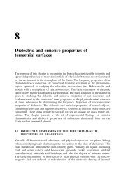
Poincaré secti<strong>on</strong><br />
P : Σ → Σ<br />
Σ is called a Poincaré surface of secti<strong>on</strong>.<br />
P is called a Poincaré first return map. It generates a new dynamical system<br />
with discrete time.
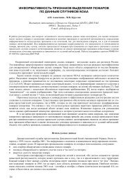
Poincaré secti<strong>on</strong>, c<strong>on</strong>tinued<br />
Example<br />
Secti<strong>on</strong> of torus<br />
For this surface of secti<strong>on</strong> the Poincaré first return map for a torus winding is a<br />
rotati<strong>on</strong> of the circle.
N<strong>on</strong>-aut<strong>on</strong>omous ODE’s<br />
A n<strong>on</strong>-aut<strong>on</strong>omous ODE<br />
dx<br />
= v(x, t)<br />
dt<br />
can be reduced to an aut<strong>on</strong>omous <strong>on</strong>e by introducing a new dependent variable<br />
y: dy/dt = 1. However, this is often an inappropriate approach because the<br />
recurrence properties of the time dependence are thus hidden.
N<strong>on</strong>-aut<strong>on</strong>omous ODE’s<br />
A n<strong>on</strong>-aut<strong>on</strong>omous ODE<br />
dx<br />
= v(x, t)<br />
dt<br />
can be reduced to an aut<strong>on</strong>omous <strong>on</strong>e by introducing a new dependent variable<br />
y: dy/dt = 1. However, this is often an inappropriate approach because the<br />
recurrence properties of the time dependence are thus hidden.<br />
Example (Quasi-periodic time dependence)<br />
dx<br />
dt = v(x, tω), x ∈ Rn , ω ∈ R m ,<br />
functi<strong>on</strong> v is 2π-periodic in each of the last m arguments. It is useful to study<br />
the aut<strong>on</strong>omous ODE<br />
dx<br />
dt<br />
= v(x, ϕ), dϕ<br />
dt<br />
whose phase space is R n × T m . For m = 1 the Poincaré return map for the<br />
secti<strong>on</strong> ϕ = 0 mod 2π reduces the problem to a dynamical system with discrete<br />
time.<br />
= ω
Blow-up<br />
For ODEs some soluti<strong>on</strong>s may be defined <strong>on</strong>ly locally in time, for t− < t < t+,<br />
where t−, t+ depend <strong>on</strong> initial c<strong>on</strong>diti<strong>on</strong>. An important example of such a<br />
behavior is a “blow-up”, when a soluti<strong>on</strong> of a c<strong>on</strong>tinuous-time system in<br />
X = R n approaches infinity within a finite time.<br />
Example<br />
For equati<strong>on</strong><br />
˙x = x 2 , x ∈ R<br />
each soluti<strong>on</strong> with a positive (respectively, a negative) initial c<strong>on</strong>diti<strong>on</strong> at t = 0<br />
tends to +∞ (respectively, −∞) when time approaches some finite moment in<br />
the future (respectively, in the past). The <strong>on</strong>ly soluti<strong>on</strong> defined for all times is<br />
x ≡ 0.<br />
Such equati<strong>on</strong>s define <strong>on</strong>ly local phase flows.
Some generalisati<strong>on</strong>s<br />
1. One can modify the definiti<strong>on</strong> of dynamical system taking Ξ = Z + or<br />
Ξ = R + , and G being semigroup of transformati<strong>on</strong>s.<br />
2. There are theories in which phase space is an infinite-dimensi<strong>on</strong>al functi<strong>on</strong>al<br />
space. (However, even in these theories very often essential events occur in a<br />
finite-dimensi<strong>on</strong>al submanifold, and so the finite-dimensi<strong>on</strong>al case is at the core<br />
of the problem. Moreover, analysis of infinite-dimensi<strong>on</strong>al problems often<br />
follows the schemes developed for finite-dimensi<strong>on</strong>al problems.)
Topics in the course<br />
1. Linear dynamical systems.<br />
2. Normal forms of n<strong>on</strong>linear systems.<br />
3. Bifurcati<strong>on</strong>s.<br />
4. Perturbati<strong>on</strong>s of integrable systems, in particular, KAM-theory.
Exercises<br />
Exercises<br />
1. C<strong>on</strong>sider the sequence<br />
1, 2, 4, 8, 1, 3, 6, 1, 2, 5, 1, 2 ,4, 8,. . .<br />
of first digits of c<strong>on</strong>secutive powers of 2. Does a 7 ever appears in this<br />
sequence? More generally, does 2 n begin with an arbitrary combinati<strong>on</strong> of<br />
digits?<br />
2. Prove that sup<br />
0
LECTURE 2
LINEAR DYNAMICAL SYSTEMS
Example: variati<strong>on</strong> equati<strong>on</strong><br />
C<strong>on</strong>sider ODE<br />
˙x = v(t, x), t ∈ R, x ∈ D ⊂ R n , v(·, ·) ∈ C 2 (R × D)<br />
Let x∗(t), t ∈ R be a soluti<strong>on</strong> to this equati<strong>on</strong>.<br />
Introduce ξ = x − x∗(t). Then<br />
˙ξ = v(t, x∗(t) + ξ) − v(t, x∗(t)) =<br />
Denote A(t) = ∂v(t,x∗(t))<br />
∂x<br />
Definiti<strong>on</strong><br />
Linear n<strong>on</strong>-aut<strong>on</strong>omous ODE<br />
˙ξ = A(t)ξ<br />
is called the variati<strong>on</strong> equati<strong>on</strong> near soluti<strong>on</strong> x∗(t).<br />
∂v(t, x∗(t))<br />
ξ + O(|ξ|<br />
∂x<br />
2 )
Linear n<strong>on</strong>-aut<strong>on</strong>omous ODEs<br />
C<strong>on</strong>sider a linear (homogeneous) n<strong>on</strong>-aut<strong>on</strong>omous ODE<br />
˙x = A(t)x, x ∈ R n<br />
where A(t) is a linear operator, A(t): R n → R n , A(·) ∈ C 0 (R).
Linear n<strong>on</strong>-aut<strong>on</strong>omous ODEs<br />
C<strong>on</strong>sider a linear (homogeneous) n<strong>on</strong>-aut<strong>on</strong>omous ODE<br />
˙x = A(t)x, x ∈ R n<br />
where A(t) is a linear operator, A(t): R n → R n , A(·) ∈ C 0 (R).<br />
In a fixed basis in R n <strong>on</strong>e can identify the vector x with the column of its<br />
coordinates in this basis and the operator A(t) with its matrix in this basis:<br />
0 1<br />
x1<br />
Bx2C<br />
B C<br />
x = B . C ,<br />
@ . A<br />
0<br />
a11(t)<br />
B<br />
a21(t)<br />
A(t) = B .<br />
@ .<br />
a12(t)<br />
a22(t)<br />
.<br />
. . .<br />
. . .<br />
. ..<br />
1<br />
a1n(t)<br />
a2n(t) C<br />
. C<br />
. A<br />
an1(t) an2(t) . . . ann(t)<br />
xn
Linear n<strong>on</strong>-aut<strong>on</strong>omous ODEs<br />
C<strong>on</strong>sider a linear (homogeneous) n<strong>on</strong>-aut<strong>on</strong>omous ODE<br />
˙x = A(t)x, x ∈ R n<br />
where A(t) is a linear operator, A(t): R n → R n , A(·) ∈ C 0 (R).<br />
In a fixed basis in R n <strong>on</strong>e can identify the vector x with the column of its<br />
coordinates in this basis and the operator A(t) with its matrix in this basis:<br />
0 1<br />
x1<br />
Bx2C<br />
B C<br />
x = B . C ,<br />
@ . A<br />
0<br />
a11(t)<br />
B<br />
a21(t)<br />
A(t) = B .<br />
@ .<br />
a12(t)<br />
a22(t)<br />
.<br />
. . .<br />
. . .<br />
. ..<br />
1<br />
a1n(t)<br />
a2n(t) C<br />
. C<br />
. A<br />
an1(t) an2(t) . . . ann(t)<br />
xn<br />
Then the equati<strong>on</strong> takes the form:<br />
˙x1 = a11(t)x1 + a12(t)x2 + . . . + a1n(t)xn<br />
˙x2 = a21(t)x1 + a22(t)x2 + . . . + a2n(t)xn<br />
. . . . . . . . . . . . . . . . . . . . . . . . . . . . . . . . . . . . . .<br />
˙xn = an1(t)x1 + an2(t)x2 + . . . + ann(t)xn<br />
In this form the equati<strong>on</strong> is called “a system of n homogeneous linear<br />
n<strong>on</strong>-aut<strong>on</strong>omous differential equati<strong>on</strong>s of the first order”.
Linear n<strong>on</strong>-aut<strong>on</strong>omous ODEs, c<strong>on</strong>tinued<br />
Theorem<br />
Every soluti<strong>on</strong> of a linear n<strong>on</strong>-aut<strong>on</strong>omous ODE can be extended <strong>on</strong>to the<br />
whole time axis R.<br />
So, there is no blow-up for linear ODEs.
Linear n<strong>on</strong>-aut<strong>on</strong>omous ODEs, c<strong>on</strong>tinued<br />
Theorem<br />
Every soluti<strong>on</strong> of a linear n<strong>on</strong>-aut<strong>on</strong>omous ODE can be extended <strong>on</strong>to the<br />
whole time axis R.<br />
So, there is no blow-up for linear ODEs.<br />
Theorem<br />
The set of all soluti<strong>on</strong>s of a linear n<strong>on</strong>-aut<strong>on</strong>omous ODE in R n is a linear<br />
n-dimensi<strong>on</strong>al space.<br />
Proof.<br />
The set of soluti<strong>on</strong>s is isomorphic to the phase space, i.e. to R n . An<br />
isomorphism maps a soluti<strong>on</strong> to its initial (say, at t = 0) datum.<br />
Definiti<strong>on</strong><br />
Any basis in the space of soluti<strong>on</strong>s is called a fundamental system of soluti<strong>on</strong>s.
Linear c<strong>on</strong>stant-coefficient ODEs<br />
C<strong>on</strong>sider an ODE<br />
˙x = Ax, x ∈ R n ,<br />
where A is a linear operator, A : R n → R n .<br />
Denote {g t } the phase flow associated with this equati<strong>on</strong>.
Linear c<strong>on</strong>stant-coefficient ODEs<br />
C<strong>on</strong>sider an ODE<br />
˙x = Ax, x ∈ R n ,<br />
where A is a linear operator, A : R n → R n .<br />
Denote {g t } the phase flow associated with this equati<strong>on</strong>.<br />
Definiti<strong>on</strong><br />
The exp<strong>on</strong>ent of the operator tA is the linear operator e tA : R n → R n :<br />
where E is the identity operator.<br />
e tA = E + tA + 1<br />
2 (tA)2 + 1<br />
3! (tA)3 + . . . ,
Linear c<strong>on</strong>stant-coefficient ODEs<br />
C<strong>on</strong>sider an ODE<br />
˙x = Ax, x ∈ R n ,<br />
where A is a linear operator, A : R n → R n .<br />
Denote {g t } the phase flow associated with this equati<strong>on</strong>.<br />
Definiti<strong>on</strong><br />
The exp<strong>on</strong>ent of the operator tA is the linear operator e tA : R n → R n :<br />
where E is the identity operator.<br />
Theorem<br />
g t = e tA<br />
Proof.<br />
d<br />
dt etA x = Ae tA x, e 0·A x = x<br />
e tA = E + tA + 1<br />
2 (tA)2 + 1<br />
3! (tA)3 + . . . ,
Linear c<strong>on</strong>stant-coefficient ODEs<br />
C<strong>on</strong>sider an ODE<br />
˙x = Ax, x ∈ R n ,<br />
where A is a linear operator, A : R n → R n .<br />
Denote {g t } the phase flow associated with this equati<strong>on</strong>.<br />
Definiti<strong>on</strong><br />
The exp<strong>on</strong>ent of the operator tA is the linear operator e tA : R n → R n :<br />
where E is the identity operator.<br />
Theorem<br />
g t = e tA<br />
e tA = E + tA + 1<br />
2 (tA)2 + 1<br />
3! (tA)3 + . . . ,<br />
Proof.<br />
d<br />
dt etA x = Ae tA x, e 0·A x = x<br />
The eigenvalues of A are roots of the characteristic equati<strong>on</strong>: det(A − λE) = 0.<br />
If there are complex eigenvalues, then it is useful to complexify the problem.<br />
Complexified equati<strong>on</strong>:<br />
˙z = Az, z ∈ C n ,<br />
and now A: C n → C n , A(x + iy) = Ax + iAy.
Linear c<strong>on</strong>stant-coefficient ODEs, c<strong>on</strong>tinued<br />
Let V be an l-dimensi<strong>on</strong>al linear vector space over C, B be a linear operator,<br />
B : V → V .<br />
Definiti<strong>on</strong><br />
Operator B is called a Jordan block with eigenvalue λ, if its matrix in a certain<br />
basis (called the Jordan basis) is the Jordan block:<br />
0<br />
λ 1 0 . . .<br />
1<br />
0<br />
B<br />
0<br />
B .<br />
B .<br />
B .<br />
@0<br />
λ<br />
.<br />
0<br />
1<br />
.<br />
. . .<br />
. . .<br />
. ..<br />
λ<br />
0 C<br />
.<br />
C<br />
. C<br />
1A<br />
0 0 . . . 0 λ
Linear c<strong>on</strong>stant-coefficient ODEs, c<strong>on</strong>tinued<br />
Let V be an l-dimensi<strong>on</strong>al linear vector space over C, B be a linear operator,<br />
B : V → V .<br />
Definiti<strong>on</strong><br />
Operator B is called a Jordan block with eigenvalue λ, if its matrix in a certain<br />
basis (called the Jordan basis) is the Jordan block:<br />
0<br />
λ 1 0 . . .<br />
1<br />
0<br />
B<br />
0<br />
B .<br />
B .<br />
B .<br />
@0<br />
λ<br />
.<br />
0<br />
1<br />
.<br />
. . .<br />
. . .<br />
. ..<br />
λ<br />
0 C<br />
.<br />
C<br />
. C<br />
1A<br />
0 0 . . . 0 λ<br />
If B is a Jordan block with eigenvalue λ, then the matrix of the exp<strong>on</strong>ent of tB<br />
in this basis is<br />
e λt<br />
0<br />
1 t t<br />
B<br />
@<br />
2 /2 . . . t l−1 /(l − 1)!<br />
0 1 t . . . t l−2 1<br />
.<br />
0<br />
.<br />
0<br />
.<br />
. . .<br />
. ..<br />
1<br />
/(l − 2)! C<br />
. C<br />
. C<br />
t A<br />
0 0 . . . 0 1
Linear c<strong>on</strong>stant-coefficient ODEs, c<strong>on</strong>tinued<br />
Theorem (The Jordan normal form)<br />
Space C n decomposes into a direct sum of invariant with respect to A and e tA<br />
subspaces, C n = V1 ⊕ V2 ⊕ . . . ⊕ Vm, such that in each of this subspaces A acts<br />
as a Jordan block. For Vj such that the eigenvalue of the corresp<strong>on</strong>ding Jordan<br />
block is not real, both Vj and its complex c<strong>on</strong>jugate ¯ Vj are presented in this<br />
decompositi<strong>on</strong>.
Linear c<strong>on</strong>stant-coefficient ODEs, c<strong>on</strong>tinued<br />
Theorem (The Jordan normal form)<br />
Space C n decomposes into a direct sum of invariant with respect to A and e tA<br />
subspaces, C n = V1 ⊕ V2 ⊕ . . . ⊕ Vm, such that in each of this subspaces A acts<br />
as a Jordan block. For Vj such that the eigenvalue of the corresp<strong>on</strong>ding Jordan<br />
block is not real, both Vj and its complex c<strong>on</strong>jugate ¯ Vj are presented in this<br />
decompositi<strong>on</strong>.<br />
De-complexificati<strong>on</strong><br />
Note that Vj ⊕ ¯ Vj = Re Vj ⊕ Im Vj over C.<br />
Thus, C n = V1 ⊕ . . . ⊕ Vr ⊕ (Re Vr+1 ⊕ Im Vr+1) ⊕ . . . ⊕ (Re Vk ⊕ Im Vk) if the<br />
field of the coefficients is C. In this decompositi<strong>on</strong>s subspaces V1, . . . , Vr<br />
corresp<strong>on</strong>d to real eigenvalues, and subspaces Vr+1, . . . , Vk corresp<strong>on</strong>d to<br />
complex eigenvalues, r + 2k = m.<br />
Now<br />
R n = ReV1 ⊕ . . . ⊕ ReVr ⊕ (Re Vr+1 ⊕ Im Vr+1) ⊕ . . . ⊕ (Re Vk ⊕ Im Vk)<br />
over the field of the coefficients R.<br />
Thus we can calculate e tA x for any x ∈ R n .
Linear c<strong>on</strong>stant-coefficient ODEs, stability<br />
Definiti<strong>on</strong><br />
A linear ODE is stable if all its soluti<strong>on</strong>s are bounded.<br />
A linear ODE is asymptotically stable if all its soluti<strong>on</strong>s tend to 0 as t → +∞.<br />
Theorem<br />
A linear c<strong>on</strong>stant-coefficient ODE is<br />
a) stable iff there are no eigenvalues in the right complex half-plane, and to all<br />
eigenvalues <strong>on</strong> the imaginary axis corresp<strong>on</strong>d Jordan blocks of size 1.<br />
b) asymptotically stable iff all eigenvalues are in the left complex half-plane.
Exercises<br />
Exercises<br />
1. Draw all possible phase portraits of linear ODEs in R 2 .<br />
2. Prove that det(e A ) = e tr A .<br />
3. May linear operators A and B not commute (i.e. AB �= BA) if<br />
e A = e B = e A+B = E ?<br />
4. Prove that there is no “blow-up” for a linear n<strong>on</strong>-aut<strong>on</strong>omous ODE.
LECTURE 3
LINEAR DYNAMICAL SYSTEMS
Linear periodic-coefficient ODEs<br />
C<strong>on</strong>sider an ODE<br />
˙x = A(t)x, x ∈ R n , A(t + T ) = A(t)<br />
where A(t) is a linear operator, A(t): R n → R n , A(·) ∈ C 0 (R),T = c<strong>on</strong>st > 0.<br />
Denote Π the Poincaré return map for the plane {t = 0 mod T }.
Linear periodic-coefficient ODEs<br />
C<strong>on</strong>sider an ODE<br />
˙x = A(t)x, x ∈ R n , A(t + T ) = A(t)<br />
where A(t) is a linear operator, A(t): R n → R n , A(·) ∈ C 0 (R),T = c<strong>on</strong>st > 0.<br />
Denote Π the Poincaré return map for the plane {t = 0 mod T }.<br />
Propositi<strong>on</strong>.<br />
Π is a linear operator, Π: R n → R n , Π is n<strong>on</strong>-degenerate and preserves<br />
orientati<strong>on</strong> of R n : det Π > 0.<br />
Π is called the m<strong>on</strong>odromy operator, its matrix is called the m<strong>on</strong>odromy<br />
matrix, its eigenvalues are called the Floquet multilpliers. The Floquet<br />
multilpliers are roots of the characteristic equati<strong>on</strong> det(Π − ρE) = 0.
Linear periodic-coefficient ODEs, a logarithm<br />
One can complexify both A(t) and Π:<br />
A(t): C n → C n , A(t)(x + iy) = A(t)x + iA(t)y,<br />
Π: C n → C n , Π(x + iy) = Πx + iΠy.<br />
Let B be a linear operator, B : C n → C n .<br />
Definiti<strong>on</strong><br />
A linear operator K : C n → C n is called a logarithm of B if B = e K .<br />
Theorem (Existence of a logarithm)<br />
Any n<strong>on</strong>-degenerate operator has a logarithm.
Linear periodic-coefficient ODEs, a logarithm<br />
One can complexify both A(t) and Π:<br />
A(t): C n → C n , A(t)(x + iy) = A(t)x + iA(t)y,<br />
Π: C n → C n , Π(x + iy) = Πx + iΠy.<br />
Let B be a linear operator, B : C n → C n .<br />
Definiti<strong>on</strong><br />
A linear operator K : C n → C n is called a logarithm of B if B = e K .<br />
Theorem (Existence of a logarithm)<br />
Any n<strong>on</strong>-degenerate operator has a logarithm.<br />
Remark<br />
Logarithm is not unique; logarithm of a real operator may be complex (example:<br />
e iπ+2πk = −1, k ∈ Z). Logarithm is a multi-valued functi<strong>on</strong>. Notati<strong>on</strong>: Ln .
Linear periodic-coefficient ODEs, a logarithm<br />
One can complexify both A(t) and Π:<br />
A(t): C n → C n , A(t)(x + iy) = A(t)x + iA(t)y,<br />
Π: C n → C n , Π(x + iy) = Πx + iΠy.<br />
Let B be a linear operator, B : C n → C n .<br />
Definiti<strong>on</strong><br />
A linear operator K : C n → C n is called a logarithm of B if B = e K .<br />
Theorem (Existence of a logarithm)<br />
Any n<strong>on</strong>-degenerate operator has a logarithm.<br />
Remark<br />
Logarithm is not unique; logarithm of a real operator may be complex (example:<br />
e iπ+2πk = −1, k ∈ Z). Logarithm is a multi-valued functi<strong>on</strong>. Notati<strong>on</strong>: Ln .<br />
Corollary<br />
Take Λ = 1<br />
Ln Π. Then Π coincides with the evoluti<strong>on</strong> operator for the time T<br />
T<br />
of the c<strong>on</strong>stant-coefficient linear ODE ˙z = Λz.<br />
Eigenvalues of K are called Floquet exp<strong>on</strong>ents. The relati<strong>on</strong> between Floquet<br />
multipliers ρj and Floquet exp<strong>on</strong>ents λj is ρj = e T λ j . Real parts of Floquet<br />
exp<strong>on</strong>ents are Lyapunov exp<strong>on</strong>ents.
Linear periodic-coefficient ODEs, a logarithm, c<strong>on</strong>tinued<br />
Proof.<br />
Because of the theorem about the Jordan normal form it is enough to c<strong>on</strong>sider<br />
the case when original operator B is a Jordan block. Let ρ be the eigenvalue of<br />
this block, ρ �= 0 because of n<strong>on</strong>-degeneracy of B. Then B = ρ(E + 1<br />
I ) , ρ<br />
where I is the Jordan block with the eigenvalue 0. Take<br />
K = (Ln ρ)E + Y , Y =<br />
∞X (−1) m−1<br />
1<br />
(<br />
m ρ<br />
where Ln ρ = ln |ρ| + iArg ρ. The series for Y actually c<strong>on</strong>tains <strong>on</strong>ly a finite<br />
number of terms because I n = 0. For z ∈ C we have e ln(1+z) = 1 + z and<br />
m=1<br />
I )m<br />
ln(1 + z) = z − 1<br />
2 z 2 + 1<br />
3 z 3 + . . . , e y = 1 + 1<br />
2 y 2 + 1<br />
3! y 3 + . . .<br />
provided that the series for the logarithm c<strong>on</strong>verges. Thus, plugging the series<br />
for y = ln(1 + z) to the series for e y after rearranging of terms gives 1 + z.<br />
Thus,<br />
e K = e (Ln ρ)E+Y = e (Ln ρ)E e Y = ρ(E + 1<br />
I ) = B<br />
ρ<br />
(we use that if HL = LH, then e H+L = e H e L , and that all the series here are<br />
absolutely c<strong>on</strong>vergent).
Linear periodic-coefficient ODEs, real logarithm<br />
Theorem (Existence of real logarithm)<br />
Any n<strong>on</strong>-degenerate real operator which does not have real negative<br />
eigenvalues has a real logarithm.
Linear periodic-coefficient ODEs, real logarithm<br />
Theorem (Existence of real logarithm)<br />
Any n<strong>on</strong>-degenerate real operator which does not have real negative<br />
eigenvalues has a real logarithm.<br />
Proof.<br />
Let Π be our real operator. There is a decompositi<strong>on</strong> of C n into a direct sum of<br />
invariant subspaces such that in each of subspaces Π acts as a Jordan block:<br />
C n = V1 ⊕ . . . ⊕ Vr ⊕ (Vr+1 ⊕ ¯Vr+1) ⊕ . . . ⊕ (Vk ⊕ ¯Vk)<br />
In this decompositi<strong>on</strong>s subspaces V1, . . . , Vr corresp<strong>on</strong>d to real positive<br />
eigenvalues of Π and have real Jordan bases.<br />
Subspaces Vr+1, . . . , Vk corresp<strong>on</strong>d to complex eigenvalues, Jordan bases in Vj<br />
and ¯ Vj are chosen to be complex c<strong>on</strong>jugated.<br />
In ReVj, j = 1, . . . , r previous formulas allow to define the real logarithm.<br />
In Vj, ¯Vj, j = r + 1, . . . , k previous formulas allow to define logarithms K and<br />
¯K respectively such that if w ∈ Vj and ¯w ∈ ¯Vj, then Kw = ¯K ¯w. Then we<br />
define real logarithm K acting <strong>on</strong> (Re Vj ⊕ Im Vj) by formulas<br />
K Rew = K 1<br />
1<br />
(w + ¯w) = 2 2 (Kw + ¯K ¯w), K Imw = K 1 1<br />
1 1<br />
(w − ¯w) = 2 i 2 i (Kw − ¯K ¯w).<br />
Thus, the real logarithm is defined <strong>on</strong><br />
R n = ReV1 ⊕ . . . ⊕ ReVr ⊕ (Re Vr+1 ⊕ Im ¯ Vr+1) ⊕ . . . ⊕ (Re Vk ⊕ Im Vk).
Linear periodic-coefficient ODEs, real logarithm, c<strong>on</strong>tinued<br />
Corollary<br />
Square of any n<strong>on</strong>-degenerate real operator has real logarithm.<br />
Corollary<br />
Take ˜Λ such that T ˜Λ is a real logarithm of Π 2 . Then Π 2 coincides with the<br />
evoluti<strong>on</strong> operator for the time 2T of the c<strong>on</strong>stant-coefficient linear ODE<br />
˙z = ˜ Λz.
Linear periodic-coefficient ODEs, Floquet-Lyapunov theory<br />
Fix a basis in R n . It serves also as the basis in C n which is complexificati<strong>on</strong> of<br />
R n . Identify linear operators with their matrices in this basis. So, now Π is the<br />
matrix of m<strong>on</strong>odromy operator, E is the unit matrix.
Linear periodic-coefficient ODEs, Floquet-Lyapunov theory<br />
Fix a basis in R n . It serves also as the basis in C n which is complexificati<strong>on</strong> of<br />
R n . Identify linear operators with their matrices in this basis. So, now Π is the<br />
matrix of m<strong>on</strong>odromy operator, E is the unit matrix.<br />
Let X (t) be the Cauchy fundamental matrix for our T -periodic equati<strong>on</strong> (i.e.<br />
the columns of X (t) are n linearly independent soluti<strong>on</strong>s to this equati<strong>on</strong>,<br />
X (0) = E).<br />
Lemma<br />
a) X (T ) = Π, b) X (t + T ) = X (t)Π<br />
Proof.<br />
a) x(t) = X (t)x(0) ⇒ x(T ) = X (T )x(0). b) X (t + T ) = X (t)R for a certain<br />
R = c<strong>on</strong>st. Plugging t = 0 gives R = X (T ) = Π
Linear periodic-coefficient ODEs, Floquet-Lyapunov theory<br />
Fix a basis in R n . It serves also as the basis in C n which is complexificati<strong>on</strong> of<br />
R n . Identify linear operators with their matrices in this basis. So, now Π is the<br />
matrix of m<strong>on</strong>odromy operator, E is the unit matrix.<br />
Let X (t) be the Cauchy fundamental matrix for our T -periodic equati<strong>on</strong> (i.e.<br />
the columns of X (t) are n linearly independent soluti<strong>on</strong>s to this equati<strong>on</strong>,<br />
X (0) = E).<br />
Lemma<br />
a) X (T ) = Π, b) X (t + T ) = X (t)Π<br />
Proof.<br />
a) x(t) = X (t)x(0) ⇒ x(T ) = X (T )x(0). b) X (t + T ) = X (t)R for a certain<br />
R = c<strong>on</strong>st. Plugging t = 0 gives R = X (T ) = Π<br />
Theorem (The Floquet theorem)<br />
X (t) = Φ(t)e tΛ , where Φ(·) ∈ C 1 , Φ(t + T ) = Φ(t), Λ = 1<br />
Ln Π T<br />
Proof.<br />
Take Φ(t) = X (t)e −tΛ . Then<br />
Φ(t + T ) = X (t + T )e −(t+T )Λ = X (t)Πe −T Λ e −tΛ = X (t)e −tΛ = Φ(t)
Linear periodic-coefficient ODEs, Floquet-Lyapunov theory<br />
Fix a basis in R n . It serves also as the basis in C n which is complexificati<strong>on</strong> of<br />
R n . Identify linear operators with their matrices in this basis. So, now Π is the<br />
matrix of m<strong>on</strong>odromy operator, E is the unit matrix.<br />
Let X (t) be the Cauchy fundamental matrix for our T -periodic equati<strong>on</strong> (i.e.<br />
the columns of X (t) are n linearly independent soluti<strong>on</strong>s to this equati<strong>on</strong>,<br />
X (0) = E).<br />
Lemma<br />
a) X (T ) = Π, b) X (t + T ) = X (t)Π<br />
Proof.<br />
a) x(t) = X (t)x(0) ⇒ x(T ) = X (T )x(0). b) X (t + T ) = X (t)R for a certain<br />
R = c<strong>on</strong>st. Plugging t = 0 gives R = X (T ) = Π<br />
Theorem (The Floquet theorem)<br />
X (t) = Φ(t)e tΛ , where Φ(·) ∈ C 1 , Φ(t + T ) = Φ(t), Λ = 1<br />
Ln Π T<br />
Proof.<br />
Take Φ(t) = X (t)e −tΛ . Then<br />
Φ(t + T ) = X (t + T )e −(t+T )Λ = X (t)Πe −T Λ e −tΛ = X (t)e −tΛ = Φ(t)<br />
Remark<br />
The Floquet theorem plays a fundamental role in the solid state physics under<br />
the name the Bloch theorem.
Linear periodic-coefficient ODEs, Floquet-Lyapunov theory, c<strong>on</strong>tinued<br />
Theorem (The Lyapunov theorem)<br />
Any linear T -periodic ODE is reducible to a linear c<strong>on</strong>stant-coefficient ODE by<br />
means of a smooth linear T -periodic transformati<strong>on</strong> of variables.<br />
Proof.<br />
Let matrices Φ(t) and Λ be as in the Floquet theorem. The required<br />
transformati<strong>on</strong> of variables x ↦→ y is given by the formula x = Φ(t)y. The<br />
equati<strong>on</strong> in the new variables has the form ˙y = Λy.<br />
Remark<br />
Any linear real T -periodic ODE is reducible to a linear real c<strong>on</strong>stant-coefficient<br />
ODE by means of a smooth linear real 2T -periodic transformati<strong>on</strong> of variables<br />
(because Π 2 has a real logarithm).
Linear periodic-coefficient ODEs, Floquet-Lyapunov theory, c<strong>on</strong>tinued<br />
Theorem (The Lyapunov theorem)<br />
Any linear T -periodic ODE is reducible to a linear c<strong>on</strong>stant-coefficient ODE by<br />
means of a smooth linear T -periodic transformati<strong>on</strong> of variables.<br />
Proof.<br />
Let matrices Φ(t) and Λ be as in the Floquet theorem. The required<br />
transformati<strong>on</strong> of variables x ↦→ y is given by the formula x = Φ(t)y. The<br />
equati<strong>on</strong> in the new variables has the form ˙y = Λy.<br />
Remark<br />
Any linear real T -periodic ODE is reducible to a linear real c<strong>on</strong>stant-coefficient<br />
ODE by means of a smooth linear real 2T -periodic transformati<strong>on</strong> of variables<br />
(because Π 2 has a real logarithm).<br />
Remark<br />
If a T -periodic ODE depends smoothly <strong>on</strong> a parameter, then the transformati<strong>on</strong><br />
of variables in the Lyapunov theorem can also be chosen to be smooth in this<br />
parameter. (Note that this asserti<strong>on</strong> does not follow from the presented proof<br />
of the Lyapunov theorem. This property is needed for analysis of bifurcati<strong>on</strong>s.)
Linear periodic-coefficient ODEs, stability<br />
Theorem<br />
A linear periodic-coefficient ODE is<br />
a)stable iff there are no Floquet multipliers outside the unit circle in the<br />
complex plane, and to all multipliers <strong>on</strong> the unit circle corresp<strong>on</strong>d Jordan<br />
blocks of size 1.<br />
b) asymptotically stable iff all Floquet multipliers are within the unit circle.<br />
Proof.<br />
The Floquet-Lyapunov theory reduces problem of stability for a linear<br />
periodic-coefficient ODE to the already solved problem of stability for a linear<br />
c<strong>on</strong>stant-coefficient ODE. One should note relati<strong>on</strong> ρj = e T λ j between Floquet<br />
multipliers and Floquet exp<strong>on</strong>ents and the fact that the Jordan block structure<br />
is the same for operators Λ and e T Λ .
Linear maps<br />
C<strong>on</strong>sider a map<br />
x ↦→ Πx, x ∈ R n ,<br />
where Π is a n<strong>on</strong>-degenerate linear operator, Π: R n → R n , det Π �= 0.<br />
The eigenvalues of Π are called the multipliers.<br />
According to the theorem about existence of a logarithm there exists a linear<br />
operator Λ: C n → C n such that Π = e Λ . Then Π k = e kΛ , k ∈ Z.<br />
This allows to study iterati<strong>on</strong>s of linear maps.<br />
One can use also the representati<strong>on</strong> Π 2 = e ˜Λ , where ˜Λ is a real linear operator,<br />
˜Λ: R n → R n .
Exercises<br />
Exercises<br />
1. Prove that square of any n<strong>on</strong>-degenerate linear real operator has a real<br />
logarithm.<br />
2. Give an example of a real linear ODE with T -periodic coefficients which<br />
cannot be transformed into c<strong>on</strong>stant-coefficient ODE by any real T -periodic<br />
linear transformati<strong>on</strong> of variables.<br />
3. Find Ln<br />
„ cos α − sin α<br />
sin α cos α<br />
«<br />
.
Bibliography<br />
Arnold, V.I. Ordinary differential equati<strong>on</strong>s. Springer-Verlag, Berlin, 2006.<br />
Arnold, V. I. Geometrical methods in the theory of ordinary differential<br />
equati<strong>on</strong>s. Springer-Verlag, New York, 1988.<br />
Arnold, V. I. Mathematical methods of classical mechanics. Springer-Verlag,<br />
New York, 1989. p<br />
Coddingt<strong>on</strong>, E. A.; Levins<strong>on</strong>, N. Theory of ordinary differential equati<strong>on</strong>s.<br />
McGraw-Hill Book Company, Inc., New York-Tor<strong>on</strong>to-L<strong>on</strong>d<strong>on</strong>, 1955.<br />
<strong>Dynamical</strong> systems. I, Encyclopaedia Math. Sci., 1, Springer-Verlag, Berlin,<br />
1998<br />
Hartman, P. Ordinary differential equati<strong>on</strong>s. (SIAM), Philadelphia, PA, 2002.<br />
Shilnikov, L. P.; Shilnikov, A. L.; Turaev, D. V.; Chua, L. O. Methods of<br />
qualitative theory in n<strong>on</strong>linear dynamics. Part I. World Scientific, Inc., River<br />
Edge, NJ, 1998.<br />
Yakubovich, V. A.; Starzhinskii, V. M. Linear differential equati<strong>on</strong>s with<br />
periodic coefficients. 1, 2. Halsted Press [John Wiley and S<strong>on</strong>s] New<br />
York-Tor<strong>on</strong>to, 1975
LECTURE 4
LINEAR DYNAMICAL SYSTEMS
Lyapunov exp<strong>on</strong>ents<br />
Definiti<strong>on</strong><br />
For a functi<strong>on</strong> f , f : [a, +∞) → R n , a = c<strong>on</strong>st, the characteristic Lyapunov<br />
exp<strong>on</strong>ent is<br />
χ[f ] = lim sup<br />
t→+∞<br />
ln |f (t)|<br />
t<br />
This is either a number or <strong>on</strong>e of the symbols +∞, −∞.<br />
Example<br />
χ[e αt ] = α, χ[t β e αt ] = α, χ[sin(γt)e αt ] = α, χ[e t2<br />
] = +∞ (γ �= 0)
Lyapunov exp<strong>on</strong>ents<br />
Definiti<strong>on</strong><br />
For a functi<strong>on</strong> f , f : [a, +∞) → R n , a = c<strong>on</strong>st, the characteristic Lyapunov<br />
exp<strong>on</strong>ent is<br />
χ[f ] = lim sup<br />
t→+∞<br />
ln |f (t)|<br />
t<br />
This is either a number or <strong>on</strong>e of the symbols +∞, −∞.<br />
Example<br />
χ[e αt ] = α, χ[t β e αt ] = α, χ[sin(γt)e αt ] = α, χ[e t2<br />
] = +∞ (γ �= 0)<br />
Propositi<strong>on</strong>.<br />
If functi<strong>on</strong>s f1, f2, . . . , fn have different finite characteristic Lyapunov exp<strong>on</strong>ents,<br />
then these functi<strong>on</strong>s are linearly independent.
Lyapunov exp<strong>on</strong>ents<br />
Definiti<strong>on</strong><br />
For a functi<strong>on</strong> f , f : [a, +∞) → R n , a = c<strong>on</strong>st, the characteristic Lyapunov<br />
exp<strong>on</strong>ent is<br />
χ[f ] = lim sup<br />
t→+∞<br />
ln |f (t)|<br />
t<br />
This is either a number or <strong>on</strong>e of the symbols +∞, −∞.<br />
Example<br />
χ[e αt ] = α, χ[t β e αt ] = α, χ[sin(γt)e αt ] = α, χ[e t2<br />
] = +∞ (γ �= 0)<br />
Propositi<strong>on</strong>.<br />
If functi<strong>on</strong>s f1, f2, . . . , fn have different finite characteristic Lyapunov exp<strong>on</strong>ents,<br />
then these functi<strong>on</strong>s are linearly independent.<br />
Definiti<strong>on</strong><br />
The set of the characteristic Lyapunov exp<strong>on</strong>ents of all soluti<strong>on</strong>s of an ODE is<br />
called the Lyapunov spectrum of this ODE<br />
Example<br />
C<strong>on</strong>sider equati<strong>on</strong> ˙x = (x/t) ln x, t > 0, x > 0. Its general soluti<strong>on</strong> is x = e ct<br />
with an arbitrary c<strong>on</strong>stant c. So, the Lyapunov spectrum is R.
Linear n<strong>on</strong>-aut<strong>on</strong>omous ODEs, Lyapunov exp<strong>on</strong>ents<br />
C<strong>on</strong>sider a linear n<strong>on</strong>-aut<strong>on</strong>omous ODE<br />
˙x = A(t)x, x ∈ R n<br />
where A(t) is a linear operator, A(t): R n → R n , A(·) ∈ C 0 (R).<br />
Recall that �A� = sup �Ax�/�x�.<br />
x�=0<br />
Theorem (Lyapunov)<br />
If �A(·)� is bounded <strong>on</strong> [0, +∞), then each n<strong>on</strong>trivial soluti<strong>on</strong> has a finite<br />
characteristic Lyapunov exp<strong>on</strong>ent.<br />
Corollary<br />
Lyapunov spectrum of a linear n<strong>on</strong>-aut<strong>on</strong>omous ODE in R n with a bounded<br />
matrix of coefficients c<strong>on</strong>tains no more than n elements.
Exercises<br />
Exercises<br />
1. Prove that the equati<strong>on</strong><br />
„<br />
0 1<br />
˙x =<br />
2/t 2<br />
«<br />
x<br />
0<br />
can not be transformed into a c<strong>on</strong>stant-coefficient linear equati<strong>on</strong> by means of<br />
transformati<strong>on</strong> of variables of the form y = L(t)x, where<br />
L(·) ∈ C 1 (R), |L| < c<strong>on</strong>st, | ˙L| < c<strong>on</strong>st, |L −1 | < c<strong>on</strong>st.<br />
2. Let X (t) be a fundamental matrix for the equati<strong>on</strong> ˙x = A(t)x. Prove the<br />
Liouville - Ostrogradski formula:<br />
.<br />
R t0<br />
tr A(τ)dτ<br />
det(X (t)) = det(X (0))e
Linear Hamilt<strong>on</strong>ian systems<br />
A Hamilt<strong>on</strong>ian system with a Hamilt<strong>on</strong> functi<strong>on</strong> H is ODE system of the form<br />
„ « T „ « T<br />
∂H<br />
∂H<br />
˙p = − , ˙q =<br />
∂q<br />
∂p<br />
Here p ∈ R n , q ∈ R n , p and q are c<strong>on</strong>sidered as vector-columns, H is a<br />
functi<strong>on</strong> of p, q, t, the superscript “T” denotes the matrix transpositi<strong>on</strong>.<br />
Comp<strong>on</strong>ents of p are called “impulses”, comp<strong>on</strong>ents of q are called<br />
“coordinates”.
Linear Hamilt<strong>on</strong>ian systems<br />
A Hamilt<strong>on</strong>ian system with a Hamilt<strong>on</strong> functi<strong>on</strong> H is ODE system of the form<br />
„ « T „ « T<br />
∂H<br />
∂H<br />
˙p = − , ˙q =<br />
∂q<br />
∂p<br />
Here p ∈ R n , q ∈ R n , p and q are c<strong>on</strong>sidered as vector-columns, H is a<br />
functi<strong>on</strong> of p, q, t, the superscript “T” denotes the matrix transpositi<strong>on</strong>.<br />
Comp<strong>on</strong>ents of p are called “impulses”, comp<strong>on</strong>ents of q are called<br />
“coordinates”. Let x be the vector-column combined of p and q. Then<br />
„ « T<br />
„ «<br />
∂H<br />
0 −En<br />
˙x = J , where J =<br />
∂x<br />
En 0<br />
Here En is the n × n unit matrix. The matrix J is called the symplectic unity.<br />
J 2 = −E2n. If H is a quadratic form, H = 1<br />
2 x T A(t)x, where A(t) is a<br />
symmetric 2n × 2n matrix, A(·) ∈ C 0 , then we get a linear Hamilt<strong>on</strong>ian system<br />
˙x = JA(t)x
Linear Hamilt<strong>on</strong>ian systems<br />
A Hamilt<strong>on</strong>ian system with a Hamilt<strong>on</strong> functi<strong>on</strong> H is ODE system of the form<br />
„ « T „ « T<br />
∂H<br />
∂H<br />
˙p = − , ˙q =<br />
∂q<br />
∂p<br />
Here p ∈ R n , q ∈ R n , p and q are c<strong>on</strong>sidered as vector-columns, H is a<br />
functi<strong>on</strong> of p, q, t, the superscript “T” denotes the matrix transpositi<strong>on</strong>.<br />
Comp<strong>on</strong>ents of p are called “impulses”, comp<strong>on</strong>ents of q are called<br />
“coordinates”. Let x be the vector-column combined of p and q. Then<br />
„ « T<br />
„ «<br />
∂H<br />
0 −En<br />
˙x = J , where J =<br />
∂x<br />
En 0<br />
Here En is the n × n unit matrix. The matrix J is called the symplectic unity.<br />
J 2 = −E2n. If H is a quadratic form, H = 1<br />
2 x T A(t)x, where A(t) is a<br />
symmetric 2n × 2n matrix, A(·) ∈ C 0 , then we get a linear Hamilt<strong>on</strong>ian system<br />
Theorem (The Liouville theorem)<br />
˙x = JA(t)x<br />
Shift al<strong>on</strong>g soluti<strong>on</strong>s of a Hamilt<strong>on</strong>ian system preserves the standard phase<br />
volume in R 2n .<br />
Corollary<br />
A linear Hamilt<strong>on</strong>ian system can not be asymptotically stable.
Linear Hamilt<strong>on</strong>ian systems, skew-scalar product<br />
Definiti<strong>on</strong><br />
The skew-symmetric bilinear form [η, ξ] = ξ T Jη in R 2n is called the skew-scalar<br />
product or the standard linear symplectic structure. (Note: [η, ξ] = (Jη, ξ).)
Linear Hamilt<strong>on</strong>ian systems, skew-scalar product<br />
Definiti<strong>on</strong><br />
The skew-symmetric bilinear form [η, ξ] = ξ T Jη in R 2n is called the skew-scalar<br />
product or the standard linear symplectic structure. (Note: [η, ξ] = (Jη, ξ).)<br />
Theorem<br />
A shift al<strong>on</strong>g soluti<strong>on</strong>s of a linear Hamilt<strong>on</strong>ian system preserves the skew-scalar<br />
product: if x(t) and y(t) are soluti<strong>on</strong>s of the system, then [x(t), y(t)] ≡ c<strong>on</strong>st.<br />
Proof.<br />
d<br />
dt<br />
[y(t), x(t)] = d<br />
dt x(t)T Jy(t) = (JAx) T Jy + x T JJAy = x T A T J T Jy − x T Ay =<br />
x T Ay − x T Ay = 0
Linear Hamilt<strong>on</strong>ian systems, skew-scalar product<br />
Definiti<strong>on</strong><br />
The skew-symmetric bilinear form [η, ξ] = ξ T Jη in R 2n is called the skew-scalar<br />
product or the standard linear symplectic structure. (Note: [η, ξ] = (Jη, ξ).)<br />
Theorem<br />
A shift al<strong>on</strong>g soluti<strong>on</strong>s of a linear Hamilt<strong>on</strong>ian system preserves the skew-scalar<br />
product: if x(t) and y(t) are soluti<strong>on</strong>s of the system, then [x(t), y(t)] ≡ c<strong>on</strong>st.<br />
Proof.<br />
d<br />
dt<br />
[y(t), x(t)] = d<br />
dt x(t)T Jy(t) = (JAx) T Jy + x T JJAy = x T A T J T Jy − x T Ay =<br />
x T Ay − x T Ay = 0<br />
Corollary<br />
Let X (t) be the Cauchy fundamental matrix for our Hamilt<strong>on</strong>ian system (i.e.<br />
the columns of X (t) are n linearly independent soluti<strong>on</strong>s to this system,<br />
X (0) = E2n). Then X T (t)JX (t) = J for all t ∈ R.<br />
Proof.<br />
Elements of matrix X T (t)JX (t) are skew-scalar products of soluti<strong>on</strong>s, and so<br />
this is a c<strong>on</strong>stant matrix.<br />
From the c<strong>on</strong>diti<strong>on</strong> at t = 0 we get X T (t)JX (t) = J.
Linear symplectic transformati<strong>on</strong>s<br />
Definiti<strong>on</strong><br />
A 2n × 2n matrix M which satisfies the relati<strong>on</strong> M T JM = J is called a<br />
symplectic matrix. A linear transformati<strong>on</strong> of variables with a symplectic matrix<br />
is called a linear symplectic transformati<strong>on</strong> of variables.<br />
Corollary<br />
The Cauchy fundamental matrix for linear Hamilt<strong>on</strong>ian system at any moment<br />
of time is a symplectic matrix. A shift al<strong>on</strong>g soluti<strong>on</strong>s of a linear Hamilt<strong>on</strong>ian<br />
system is a linear symplectic transformati<strong>on</strong>.
Linear symplectic transformati<strong>on</strong>s<br />
Definiti<strong>on</strong><br />
A 2n × 2n matrix M which satisfies the relati<strong>on</strong> M T JM = J is called a<br />
symplectic matrix. A linear transformati<strong>on</strong> of variables with a symplectic matrix<br />
is called a linear symplectic transformati<strong>on</strong> of variables.<br />
Corollary<br />
The Cauchy fundamental matrix for linear Hamilt<strong>on</strong>ian system at any moment<br />
of time is a symplectic matrix. A shift al<strong>on</strong>g soluti<strong>on</strong>s of a linear Hamilt<strong>on</strong>ian<br />
system is a linear symplectic transformati<strong>on</strong>.<br />
Theorem<br />
A linear transformati<strong>on</strong>s of variables is a symplectic transformati<strong>on</strong>s if and <strong>on</strong>ly<br />
if it preserves the skew-scalar product: [Mη, Mξ] = [η, ξ] for any<br />
ξ ∈ R 2n , η ∈ R 2n ; here M is the matrix of the transformati<strong>on</strong>.<br />
Proof.<br />
[Mη, Mξ] = ξ T M T JMη
Linear symplectic transformati<strong>on</strong>s<br />
Definiti<strong>on</strong><br />
A 2n × 2n matrix M which satisfies the relati<strong>on</strong> M T JM = J is called a<br />
symplectic matrix. A linear transformati<strong>on</strong> of variables with a symplectic matrix<br />
is called a linear symplectic transformati<strong>on</strong> of variables.<br />
Corollary<br />
The Cauchy fundamental matrix for linear Hamilt<strong>on</strong>ian system at any moment<br />
of time is a symplectic matrix. A shift al<strong>on</strong>g soluti<strong>on</strong>s of a linear Hamilt<strong>on</strong>ian<br />
system is a linear symplectic transformati<strong>on</strong>.<br />
Theorem<br />
A linear transformati<strong>on</strong>s of variables is a symplectic transformati<strong>on</strong>s if and <strong>on</strong>ly<br />
if it preserves the skew-scalar product: [Mη, Mξ] = [η, ξ] for any<br />
ξ ∈ R 2n , η ∈ R 2n ; here M is the matrix of the transformati<strong>on</strong>.<br />
Proof.<br />
[Mη, Mξ] = ξ T M T JMη<br />
Theorem<br />
Symplectic matrices form a group.<br />
The group of symplectic 2n × 2n matrices is called the symplectic group of<br />
degree 2n and is denoted as Sp(2n). (The same name is used for the group of<br />
linear symplectic transformati<strong>on</strong>s of R 2n .)
Symplectic transformati<strong>on</strong>s in linear Hamilt<strong>on</strong>ian systems<br />
Make in a Hamilt<strong>on</strong>ian system ˙x = JA(t)x with a Hamilt<strong>on</strong> functi<strong>on</strong><br />
H = 1<br />
2 x T A(t)x a symplectic transformati<strong>on</strong> of variables y = M(t)x. We have<br />
˙y = M ˙x+ ˙ Mx = MJAx+ ˙ Mx = (MJAM −1 + ˙ MM −1 )y = J(−JMJAM −1 −J ˙ MM −1 )y<br />
Let us show that the obtained equati<strong>on</strong> for y is a Hamilt<strong>on</strong>ian <strong>on</strong>e. Because M<br />
is a symplectic matrix, we have<br />
M T JM = J, ˙<br />
M T JM + M T J ˙M = 0, M = −J(M −1 ) T J, ˙<br />
M T = M T J ˙MM −1 J<br />
Thus<br />
−JMJAM −1 = JJ(M −1 ) T JJAM −1 = (M −1 ) T AM −1 ,<br />
and this is a symmetric matrix. And<br />
(J ˙MM −1 ) T = −(M −1 ) T ˙<br />
M T J = −(M −1 ) T M T J ˙ MM −1 JJ = J ˙ MM −1<br />
and this also is a symmetric matrix. So, equati<strong>on</strong> for y is a Hamilt<strong>on</strong>ian <strong>on</strong>e.
Symplectic transformati<strong>on</strong>s in linear Hamilt<strong>on</strong>ian systems<br />
Make in a Hamilt<strong>on</strong>ian system ˙x = JA(t)x with a Hamilt<strong>on</strong> functi<strong>on</strong><br />
H = 1<br />
2 x T A(t)x a symplectic transformati<strong>on</strong> of variables y = M(t)x. We have<br />
˙y = M ˙x+ ˙ Mx = MJAx+ ˙ Mx = (MJAM −1 + ˙ MM −1 )y = J(−JMJAM −1 −J ˙ MM −1 )y<br />
Let us show that the obtained equati<strong>on</strong> for y is a Hamilt<strong>on</strong>ian <strong>on</strong>e. Because M<br />
is a symplectic matrix, we have<br />
M T JM = J, ˙<br />
M T JM + M T J ˙M = 0, M = −J(M −1 ) T J, ˙<br />
M T = M T J ˙MM −1 J<br />
Thus<br />
−JMJAM −1 = JJ(M −1 ) T JJAM −1 = (M −1 ) T AM −1 ,<br />
and this is a symmetric matrix. And<br />
(J ˙MM −1 ) T = −(M −1 ) T ˙<br />
M T J = −(M −1 ) T M T J ˙ MM −1 JJ = J ˙ MM −1<br />
and this also is a symmetric matrix. So, equati<strong>on</strong> for y is a Hamilt<strong>on</strong>ian <strong>on</strong>e.<br />
Note, that if M = c<strong>on</strong>st, then the Hamilt<strong>on</strong> functi<strong>on</strong> for the new system<br />
H = 1<br />
2 y T (M −1 ) T A(t)M −1 y<br />
is just the old Hamilt<strong>on</strong> functi<strong>on</strong> expressed through the new variables.
C<strong>on</strong>stant-coefficient linear Hamilt<strong>on</strong>ian system<br />
C<strong>on</strong>sider an aut<strong>on</strong>omous linear Hamilt<strong>on</strong>ian system;<br />
˙x = JAx<br />
where A is a c<strong>on</strong>stant symmetric 2n × 2n matrix.<br />
Propositi<strong>on</strong>.<br />
The matrix JA is similar to the matrix (−JA) T .<br />
Proof.<br />
J −1 (−JA) T J = −J −1 A T J T J = JA<br />
Corollary<br />
If λ is an eigenvalue, then −λ is an eigenvalue.<br />
Eigenvalues λ and −λ have equal multiplicities and the corresp<strong>on</strong>ding Jordan<br />
structures are the same.<br />
If λ = 0 is an eigenvalue, then it necessarily has even multiplicity.<br />
Corollary<br />
Characteristic polynomial det(JA − λE2n) of a matrix JA is a polynomial in λ 2 .
C<strong>on</strong>stant-coefficient linear Hamilt<strong>on</strong>ian system, locati<strong>on</strong> of eigenvalues<br />
Theorem<br />
The eigenvalues of aut<strong>on</strong>omous linear Hamilt<strong>on</strong>ian system are situated <strong>on</strong> the<br />
plane of complex variable symmetrically with respect to the coordinate cross: if<br />
λ is an eigenvalue, then −λ, ¯λ, −¯λ are also eigenvalues. The eigenvalues λ,<br />
−λ, ¯λ, −¯λ have equal multiplicities and the corresp<strong>on</strong>ding Jordan structures<br />
are the same.<br />
So, eigenvalues may be of four types: real pairs (a, −a), purely imaginary pairs<br />
(ib, −ib), quadruplets (±a ± ib) and zero eigenvalues.
C<strong>on</strong>stant-coefficient linear Hamilt<strong>on</strong>ian system, locati<strong>on</strong> of eigenvalues<br />
Theorem<br />
The eigenvalues of aut<strong>on</strong>omous linear Hamilt<strong>on</strong>ian system are situated <strong>on</strong> the<br />
plane of complex variable symmetrically with respect to the coordinate cross: if<br />
λ is an eigenvalue, then −λ, ¯λ, −¯λ are also eigenvalues. The eigenvalues λ,<br />
−λ, ¯λ, −¯λ have equal multiplicities and the corresp<strong>on</strong>ding Jordan structures<br />
are the same.<br />
So, eigenvalues may be of four types: real pairs (a, −a), purely imaginary pairs<br />
(ib, −ib), quadruplets (±a ± ib) and zero eigenvalues.<br />
Corollary<br />
If there is a purely imaginary simple eigenvalue, then it remains <strong>on</strong> the<br />
imaginary axis under a small perturbati<strong>on</strong> of the Hamilt<strong>on</strong>ian. Similarly, a real<br />
simple eigenvalue remains real under a small perturbati<strong>on</strong> of the Hamilt<strong>on</strong>ian.<br />
So, the system may loss stability under a small perturbati<strong>on</strong> of the Hamilt<strong>on</strong>ian<br />
<strong>on</strong>ly if there is 1 : 1 res<strong>on</strong>ance.
Bibliography<br />
Arnold, V.I. Ordinary differential equati<strong>on</strong>s. Springer-Verlag, Berlin, 2006.<br />
Arnold, V. I. Geometrical methods in the theory of ordinary differential<br />
equati<strong>on</strong>s. Springer-Verlag, New York, 1988.<br />
Arnold, V. I. Mathematical methods of classical mechanics. Springer-Verlag,<br />
New York, 1989. p<br />
Coddingt<strong>on</strong>, E. A.; Levins<strong>on</strong>, N. Theory of ordinary differential equati<strong>on</strong>s.<br />
McGraw-Hill Book Company, Inc., New York-Tor<strong>on</strong>to-L<strong>on</strong>d<strong>on</strong>, 1955.<br />
<strong>Dynamical</strong> systems. I, Encyclopaedia Math. Sci., 1, Springer-Verlag, Berlin,<br />
1998<br />
Hartman, P. Ordinary differential equati<strong>on</strong>s. (SIAM), Philadelphia, PA, 2002.<br />
Shilnikov, L. P.; Shilnikov, A. L.; Turaev, D. V.; Chua, L. O. Methods of<br />
qualitative theory in n<strong>on</strong>linear dynamics. Part I. World Scientific, Inc., River<br />
Edge, NJ, 1998.<br />
Yakubovich, V. A.; Starzhinskii, V. M. Linear differential equati<strong>on</strong>s with<br />
periodic coefficients. 1, 2. Halsted Press [John Wiley and S<strong>on</strong>s] New<br />
York-Tor<strong>on</strong>to, 1975
LECTURE 5
LINEAR HAMILTONIAN SYSTEMS
List of formulas<br />
A Hamilt<strong>on</strong>ian system with a Hamilt<strong>on</strong> functi<strong>on</strong> H is an ODE system of the<br />
form<br />
„ « T „ « T<br />
∂H<br />
∂H<br />
˙p = − , ˙q =<br />
∂q<br />
∂p<br />
Here p ∈ R n , q ∈ R n , p and q are c<strong>on</strong>sidered as vector-columns, H is a functi<strong>on</strong><br />
of p, q, t, the superscript “T” denotes the matrix transpositi<strong>on</strong>. Comp<strong>on</strong>ents of<br />
p are called “impulses”, comp<strong>on</strong>ents of q are called “coordinates”.
List of formulas<br />
A Hamilt<strong>on</strong>ian system with a Hamilt<strong>on</strong> functi<strong>on</strong> H is an ODE system of the<br />
form<br />
„ « T „ « T<br />
∂H<br />
∂H<br />
˙p = − , ˙q =<br />
∂q<br />
∂p<br />
Here p ∈ R n , q ∈ R n , p and q are c<strong>on</strong>sidered as vector-columns, H is a functi<strong>on</strong><br />
of p, q, t, the superscript “T” denotes the matrix transpositi<strong>on</strong>. Comp<strong>on</strong>ents of<br />
p are called “impulses”, comp<strong>on</strong>ents of q are called “coordinates”.<br />
Let x be the vector-column combined of p and q. Then<br />
„ « T<br />
„ «<br />
∂H<br />
0 −En<br />
˙x = J , where J =<br />
∂x<br />
En 0<br />
The matrix J is called the symplectic unity. J 2 = −E2n.<br />
If H is a quadratic form, H = 1<br />
2 x T A(t)x, where A(t) is a symmetric 2n × 2n<br />
matrix, A(·) ∈ C 0 , then we get a linear Hamilt<strong>on</strong>ian system<br />
˙x = JA(t)x
List of formulas, c<strong>on</strong>tinued<br />
The skew-symmetric bilinear form [η, ξ] = ξ T Jη in R 2n is called the skew-scalar<br />
product or the standard linear symplectic structure.<br />
A 2n × 2n matrix M which satisfies the relati<strong>on</strong> M T JM = J is called a<br />
symplectic matrix. A linear transformati<strong>on</strong> of variables with a symplectic matrix<br />
is called a linear symplectic transformati<strong>on</strong> of variables.<br />
A linear transformati<strong>on</strong>s of variables is a symplectic transformati<strong>on</strong>s if and <strong>on</strong>ly<br />
if it preserves the skew-scalar product: [Mη, Mξ] = [η, ξ] for any<br />
ξ ∈ R 2n , η ∈ R 2n ; here M is the matrix of the transformati<strong>on</strong>.<br />
The eigenvalues of aut<strong>on</strong>omous linear Hamilt<strong>on</strong>ian system are situated <strong>on</strong> the<br />
plane of complex variable symmetrically with respect to the coordinate cross.
Normal form of quadratic Hamilt<strong>on</strong>ian in the case of pairwise different<br />
eigen-frequencies<br />
Let matrix JA has purely imaginary pairwise different eigenvalues<br />
±iω1, ±iω2, . . . , ±iωn. Let ξk, ¯ξk be eigenvectors of JA corresp<strong>on</strong>ding to<br />
eigenvalues ±iωk.<br />
Theorem<br />
By a certain linear symplectic transformati<strong>on</strong> of variables the Hamilt<strong>on</strong> functi<strong>on</strong><br />
H = 1<br />
2 x T Ax can be transformed to the form<br />
H = 1<br />
2 Ω1(p2 1 + q 2 1) + 1<br />
2 Ω2(p2 2 + q 2 2) + . . . + 1<br />
2 Ωn(p2 n + q 2 n)<br />
where pk are “impulses”, and qk are “coordinates”, Ωk = ±ωk.
Normal form of quadratic Hamilt<strong>on</strong>ian in the case of pairwise different<br />
eigen-frequencies<br />
Let matrix JA has purely imaginary pairwise different eigenvalues<br />
±iω1, ±iω2, . . . , ±iωn. Let ξk, ¯ξk be eigenvectors of JA corresp<strong>on</strong>ding to<br />
eigenvalues ±iωk.<br />
Theorem<br />
By a certain linear symplectic transformati<strong>on</strong> of variables the Hamilt<strong>on</strong> functi<strong>on</strong><br />
H = 1<br />
2 x T Ax can be transformed to the form<br />
H = 1<br />
2 Ω1(p2 1 + q 2 1) + 1<br />
2 Ω2(p2 2 + q 2 2) + . . . + 1<br />
2 Ωn(p2 n + q 2 n)<br />
where pk are “impulses”, and qk are “coordinates”, Ωk = ±ωk.<br />
Lemma<br />
Let η1, η2 be eigenvectors of a matrix JA, and λ1, λ2 be the corresp<strong>on</strong>ding<br />
eigenvalues. If λ1 �= −λ2, then η1 and η2 are scew-orthog<strong>on</strong>al: [η2, η1] = 0.<br />
Proof.<br />
JAηk = λkηk. Thus, Aηk = −λkJηj, and η T 1 Aη2 = −λ2η T 1 Jη2 = λ1η T 1 Jη2
Normal form of quadratic Hamilt<strong>on</strong>ian in the case of pairwise different<br />
eigen-frequencies<br />
Let matrix JA has purely imaginary pairwise different eigenvalues<br />
±iω1, ±iω2, . . . , ±iωn. Let ξk, ¯ξk be eigenvectors of JA corresp<strong>on</strong>ding to<br />
eigenvalues ±iωk.<br />
Theorem<br />
By a certain linear symplectic transformati<strong>on</strong> of variables the Hamilt<strong>on</strong> functi<strong>on</strong><br />
H = 1<br />
2 x T Ax can be transformed to the form<br />
H = 1<br />
2 Ω1(p2 1 + q 2 1) + 1<br />
2 Ω2(p2 2 + q 2 2) + . . . + 1<br />
2 Ωn(p2 n + q 2 n)<br />
where pk are “impulses”, and qk are “coordinates”, Ωk = ±ωk.<br />
Lemma<br />
Let η1, η2 be eigenvectors of a matrix JA, and λ1, λ2 be the corresp<strong>on</strong>ding<br />
eigenvalues. If λ1 �= −λ2, then η1 and η2 are scew-orthog<strong>on</strong>al: [η2, η1] = 0.<br />
Proof.<br />
JAηk = λkηk. Thus, Aηk = −λkJηj, and η T 1 Aη2 = −λ2η T 1 Jη2 = λ1η T 1 Jη2<br />
Lemma<br />
[ξk, ¯ξk] is purely imaginary number, [ξk, ¯ξk] �= 0 .<br />
Proof.<br />
The complex c<strong>on</strong>jugati<strong>on</strong> change sign of [ξk, ¯ ξk].
Proof of the theorem about normal form of quadratic Hamilt<strong>on</strong>ian<br />
Proof of the theorem.<br />
Without loss of generality we may assume that [ξk, ¯ξk] is equal to either i or<br />
−i. Introduce ak = (ξk + ¯ξk)/ √ 2, bk = (ξk − ¯ξk)/( √ 2i).
Proof of the theorem about normal form of quadratic Hamilt<strong>on</strong>ian<br />
Proof of the theorem.<br />
Without loss of generality we may assume that [ξk, ¯ξk] is equal to either i or<br />
−i. Introduce ak = (ξk + ¯ξk)/ √ 2, bk = (ξk − ¯ξk)/( √ 2i). Then<br />
[ak, bk] = (−[ξk, ¯ξk] + [¯ξk, ξk])/(2i) = [¯ξk, ξk]/i<br />
is equal to either 1 or −1.
Proof of the theorem about normal form of quadratic Hamilt<strong>on</strong>ian<br />
Proof of the theorem.<br />
Without loss of generality we may assume that [ξk, ¯ξk] is equal to either i or<br />
−i. Introduce ak = (ξk + ¯ξk)/ √ 2, bk = (ξk − ¯ξk)/( √ 2i). Then<br />
[ak, bk] = (−[ξk, ¯ξk] + [¯ξk, ξk])/(2i) = [¯ξk, ξk]/i<br />
is equal to either 1 or −1. Introduce new vectors uk, vk as follows.<br />
If [ak, bk] = 1, then uk = ak, vk = bk.<br />
If [ak, bk] = −1, then uk = bk, vk = ak.
Proof of the theorem about normal form of quadratic Hamilt<strong>on</strong>ian<br />
Proof of the theorem.<br />
Without loss of generality we may assume that [ξk, ¯ξk] is equal to either i or<br />
−i. Introduce ak = (ξk + ¯ξk)/ √ 2, bk = (ξk − ¯ξk)/( √ 2i). Then<br />
[ak, bk] = (−[ξk, ¯ξk] + [¯ξk, ξk])/(2i) = [¯ξk, ξk]/i<br />
is equal to either 1 or −1. Introduce new vectors uk, vk as follows.<br />
If [ak, bk] = 1, then uk = ak, vk = bk.<br />
If [ak, bk] = −1, then uk = bk, vk = ak.<br />
Thus, [uk, vk] = 1, [uk, vj] = 0, j �= k.
Proof of the theorem about normal form of quadratic Hamilt<strong>on</strong>ian<br />
Proof of the theorem.<br />
Without loss of generality we may assume that [ξk, ¯ξk] is equal to either i or<br />
−i. Introduce ak = (ξk + ¯ξk)/ √ 2, bk = (ξk − ¯ξk)/( √ 2i). Then<br />
[ak, bk] = (−[ξk, ¯ξk] + [¯ξk, ξk])/(2i) = [¯ξk, ξk]/i<br />
is equal to either 1 or −1. Introduce new vectors uk, vk as follows.<br />
If [ak, bk] = 1, then uk = ak, vk = bk.<br />
If [ak, bk] = −1, then uk = bk, vk = ak.<br />
Thus, [uk, vk] = 1, [uk, vj] = 0, j �= k.<br />
Choose as the new basis in R 2n vectors u1, u2, . . . , un, v1, v2, . . . , vn (in this<br />
order). The matrix of transformati<strong>on</strong> of vector’s coordinates for this change of<br />
basis is a symplectic <strong>on</strong>e.
Proof of the theorem about normal form of quadratic Hamilt<strong>on</strong>ian<br />
Proof of the theorem.<br />
Without loss of generality we may assume that [ξk, ¯ξk] is equal to either i or<br />
−i. Introduce ak = (ξk + ¯ξk)/ √ 2, bk = (ξk − ¯ξk)/( √ 2i). Then<br />
[ak, bk] = (−[ξk, ¯ξk] + [¯ξk, ξk])/(2i) = [¯ξk, ξk]/i<br />
is equal to either 1 or −1. Introduce new vectors uk, vk as follows.<br />
If [ak, bk] = 1, then uk = ak, vk = bk.<br />
If [ak, bk] = −1, then uk = bk, vk = ak.<br />
Thus, [uk, vk] = 1, [uk, vj] = 0, j �= k.<br />
Choose as the new basis in R 2n vectors u1, u2, . . . , un, v1, v2, . . . , vn (in this<br />
order). The matrix of transformati<strong>on</strong> of vector’s coordinates for this change of<br />
basis is a symplectic <strong>on</strong>e. In the new coordinates the Hamilt<strong>on</strong> functi<strong>on</strong> has<br />
the required form.
Proof of the theorem about normal form of quadratic Hamilt<strong>on</strong>ian<br />
Proof of the theorem.<br />
Without loss of generality we may assume that [ξk, ¯ξk] is equal to either i or<br />
−i. Introduce ak = (ξk + ¯ξk)/ √ 2, bk = (ξk − ¯ξk)/( √ 2i). Then<br />
[ak, bk] = (−[ξk, ¯ξk] + [¯ξk, ξk])/(2i) = [¯ξk, ξk]/i<br />
is equal to either 1 or −1. Introduce new vectors uk, vk as follows.<br />
If [ak, bk] = 1, then uk = ak, vk = bk.<br />
If [ak, bk] = −1, then uk = bk, vk = ak.<br />
Thus, [uk, vk] = 1, [uk, vj] = 0, j �= k.<br />
Choose as the new basis in R 2n vectors u1, u2, . . . , un, v1, v2, . . . , vn (in this<br />
order). The matrix of transformati<strong>on</strong> of vector’s coordinates for this change of<br />
basis is a symplectic <strong>on</strong>e. In the new coordinates the Hamilt<strong>on</strong> functi<strong>on</strong> has<br />
the required form.<br />
The form of the Hamilt<strong>on</strong>ian shows that the phase space is a direct product of<br />
of invariant two-dimensi<strong>on</strong>al mutually skew-orthog<strong>on</strong>al planes. Dynamics in kth<br />
plane is decribed by the Hamilt<strong>on</strong> functi<strong>on</strong> Hk = 1<br />
2 Ωk(p 2 k + q 2 k); it is called a<br />
partial Hamilt<strong>on</strong> functi<strong>on</strong>, or just a partial Hamilt<strong>on</strong>ian. This is the Hamilt<strong>on</strong><br />
functi<strong>on</strong> of a linear oscillator with the frequency Ωk. In the plane qk, pk phase<br />
curves are circles. Rotati<strong>on</strong> <strong>on</strong> this circles is clockwise, if Ωk > 0, and<br />
counterclockwise, if Ωk < 0. Values |Ωk| are called eigen-frequencies of the<br />
system. Phase space R 2n is foliated (with singularities) by n-dimensi<strong>on</strong>al<br />
invariant tori.
On normal forms of quadratic Hamilt<strong>on</strong>ians<br />
Theorem (Williams<strong>on</strong>)<br />
There exists a real symplectic linear change of variables reducing the<br />
Hamilt<strong>on</strong>ian to a sum of partial Hamilt<strong>on</strong>ians (functi<strong>on</strong>s of disjoint subsets of<br />
c<strong>on</strong>jugate variables), and the matrix of the system, corresp<strong>on</strong>dingly, to a<br />
block-diag<strong>on</strong>al form. Each partial Hamilt<strong>on</strong>ian corresp<strong>on</strong>ds either to a real pair,<br />
or to an imaginary pair, or to a quadruplet of eigenvalues, or to a zero<br />
eigenvalue. The partial Hamilt<strong>on</strong>ians are determined, up to a sign, by the<br />
Jordan blocks of the operator JA.<br />
The list of partial Hamilt<strong>on</strong>ians is c<strong>on</strong>tained in the paper by J.Williams<strong>on</strong><br />
(1936).
On stability loss in c<strong>on</strong>stant-coefficient linear Hamilt<strong>on</strong>ian systems<br />
When parameters of a stable c<strong>on</strong>stant-coefficient linear Hamilt<strong>on</strong>ian system are<br />
changing, the eigenvalues move <strong>on</strong> the imaginary axis. When eigenvalues<br />
collide they may leave the imaginary axis. However, collisi<strong>on</strong> of not each pair of<br />
eigenvalues is dangerous, some eigenvalues necessarily pass through each other<br />
without leaving the imaginary axis.
On stability loss in c<strong>on</strong>stant-coefficient linear Hamilt<strong>on</strong>ian systems<br />
When parameters of a stable c<strong>on</strong>stant-coefficient linear Hamilt<strong>on</strong>ian system are<br />
changing, the eigenvalues move <strong>on</strong> the imaginary axis. When eigenvalues<br />
collide they may leave the imaginary axis. However, collisi<strong>on</strong> of not each pair of<br />
eigenvalues is dangerous, some eigenvalues necessarily pass through each other<br />
without leaving the imaginary axis.<br />
While all eigenvalues are simple the Hamilt<strong>on</strong> functi<strong>on</strong> can be reduced to the<br />
normal form<br />
H = 1<br />
2 Ω1(p2 1 + q 2 1) + 1<br />
2 Ω2(p2 2 + q 2 2) + . . . + 1<br />
2 Ωn(p2 n + q 2 n)<br />
We say that a partial Hamilt<strong>on</strong> functi<strong>on</strong> Hk = 1<br />
2 Ωk(p 2 k + q 2 k) is positive<br />
(negative), if Ωk is positive (respectively, negative).
On stability loss in c<strong>on</strong>stant-coefficient linear Hamilt<strong>on</strong>ian systems<br />
When parameters of a stable c<strong>on</strong>stant-coefficient linear Hamilt<strong>on</strong>ian system are<br />
changing, the eigenvalues move <strong>on</strong> the imaginary axis. When eigenvalues<br />
collide they may leave the imaginary axis. However, collisi<strong>on</strong> of not each pair of<br />
eigenvalues is dangerous, some eigenvalues necessarily pass through each other<br />
without leaving the imaginary axis.<br />
While all eigenvalues are simple the Hamilt<strong>on</strong> functi<strong>on</strong> can be reduced to the<br />
normal form<br />
H = 1<br />
2 Ω1(p2 1 + q 2 1) + 1<br />
2 Ω2(p2 2 + q 2 2) + . . . + 1<br />
2 Ωn(p2 n + q 2 n)<br />
We say that a partial Hamilt<strong>on</strong> functi<strong>on</strong> Hk = 1<br />
2 Ωk(p 2 k + q 2 k) is positive<br />
(negative), if Ωk is positive (respectively, negative).<br />
Theorem<br />
If imaginary eigenvalues corresp<strong>on</strong>ding to partial Hamilt<strong>on</strong> functi<strong>on</strong>s having the<br />
same sign collide not at the point 0, the system does not loss its stability. In<br />
particular, when these eigenvalues collide, the matrix of the Hamilt<strong>on</strong>ian<br />
system does not have Jordan blocks of sizes bigger than 1.
On linear natural Hamilt<strong>on</strong>ian systems<br />
For a natural Hamilt<strong>on</strong>ian system its Hamilt<strong>on</strong> functi<strong>on</strong> H is the sum of a<br />
kinetic energy T = T (p, q) = 1<br />
2 pT K −1 (q)p and a potential energy V (q) :<br />
H = T + V .<br />
Here K(q) is a positive definite matrix.
On linear natural Hamilt<strong>on</strong>ian systems<br />
For a natural Hamilt<strong>on</strong>ian system its Hamilt<strong>on</strong> functi<strong>on</strong> H is the sum of a<br />
kinetic energy T = T (p, q) = 1<br />
2 pT K −1 (q)p and a potential energy V (q) :<br />
H = T + V .<br />
Here K(q) is a positive definite matrix. For a linear natural Hamilt<strong>on</strong>ian<br />
system K = c<strong>on</strong>st and V is a quadratic form: V = 1<br />
2 qT Dq.
On linear natural Hamilt<strong>on</strong>ian systems<br />
For a natural Hamilt<strong>on</strong>ian system its Hamilt<strong>on</strong> functi<strong>on</strong> H is the sum of a<br />
kinetic energy T = T (p, q) = 1<br />
2 pT K −1 (q)p and a potential energy V (q) :<br />
H = T + V .<br />
Here K(q) is a positive definite matrix. For a linear natural Hamilt<strong>on</strong>ian<br />
system K = c<strong>on</strong>st and V is a quadratic form: V = 1<br />
2 qT Dq.<br />
Theorem<br />
In any linear natural Hamilt<strong>on</strong>ian system all n<strong>on</strong>-zero eigenvalues are either real<br />
or pure imaginary. To each n<strong>on</strong>-zero eigenvalue corresp<strong>on</strong>d <strong>on</strong>ly Jordan blocks<br />
of size 1. To zero eigenvalue corresp<strong>on</strong>d Jordan blocks of size 2.
On linear natural Hamilt<strong>on</strong>ian systems<br />
For a natural Hamilt<strong>on</strong>ian system its Hamilt<strong>on</strong> functi<strong>on</strong> H is the sum of a<br />
kinetic energy T = T (p, q) = 1<br />
2 pT K −1 (q)p and a potential energy V (q) :<br />
H = T + V .<br />
Here K(q) is a positive definite matrix. For a linear natural Hamilt<strong>on</strong>ian<br />
system K = c<strong>on</strong>st and V is a quadratic form: V = 1<br />
2 qT Dq.<br />
Theorem<br />
In any linear natural Hamilt<strong>on</strong>ian system all n<strong>on</strong>-zero eigenvalues are either real<br />
or pure imaginary. To each n<strong>on</strong>-zero eigenvalue corresp<strong>on</strong>d <strong>on</strong>ly Jordan blocks<br />
of size 1. To zero eigenvalue corresp<strong>on</strong>d Jordan blocks of size 2.<br />
Corollary<br />
For linear natural Hamilt<strong>on</strong>ian system collisi<strong>on</strong> of n<strong>on</strong>-zero eigenvalues <strong>on</strong> the<br />
imaginary axis does not lead to a stability loss. Collisi<strong>on</strong> of eigenvalues at 0<br />
leads to the stability loss.
On linear natural Hamilt<strong>on</strong>ian systems, c<strong>on</strong>tinued<br />
Proof of the theorem.<br />
There exists a matrix C which simultaneously transforms the quadratic form<br />
y T Ky to sum of squares, and the quadratic form y T Dy to a diag<strong>on</strong>al form, i.e.<br />
C T KC = En, C T DC = diag(µ1, µ2, . . . , µn)<br />
The transformati<strong>on</strong> of variables p, q ↦→ P, Q, p = (C −1 ) T P, q = CQ is a<br />
symplectic <strong>on</strong>e. Indeed, if ˜p = (C −1 ) T ˜P, ˜q = C ˜Q, then<br />
˜P T Q − ˜ Q T P ≡ ˜p T q − ˜q T p<br />
The Hamilt<strong>on</strong> functi<strong>on</strong> in the new variables is<br />
H = 1<br />
2 (P2 1 + P 2 2 + . . . + P 2 n ) + 1<br />
2 (µ1Q2 1 + µ2Q 2 2 + . . . + µnQ 2 n)<br />
It is the sum of the partial Hamilt<strong>on</strong> functi<strong>on</strong>s of the form Hk = 1<br />
2 (P2 k + µkQ 2 k ).<br />
The equati<strong>on</strong> of the moti<strong>on</strong> for a Hamilt<strong>on</strong> functi<strong>on</strong> Hk has the form<br />
¨Qk + µkQk = 0<br />
Eigenvalues are ±i √ µ k , if µk > 0, and ± √ −µk, if µk < 0. Only for µk = 0 the<br />
soluti<strong>on</strong> c<strong>on</strong>tains multiplier t, and so <strong>on</strong>ly to eigenvalue 0 there corresp<strong>on</strong>d the<br />
Jordan block of the size 2.
Exercises<br />
Exercises<br />
1. C<strong>on</strong>sider an equati<strong>on</strong> ˙x = v(t, x), x ∈ R k . Prove that if divv ≡ 0, then the<br />
shift al<strong>on</strong>g trajectories of this equati<strong>on</strong> preserves the standard phase volume in<br />
R k . (Hint: divv = tr(∂v/∂x).)<br />
2. Give a geometric interpretati<strong>on</strong> for skew-scalar product in the case of <strong>on</strong>e<br />
degree of freedom (n=1) and in the case of several degrees of freedom.<br />
3. Obtain formulas for partial Hamilt<strong>on</strong> functi<strong>on</strong>s corresp<strong>on</strong>ding to the pair of<br />
a simple real eigenvalues (±a), to the quadruplet of a simple complex<br />
eigenvalues (±a ± ib) and to the eigenvalue 0 of multiplicity 2 (a �= 0, b �= 0).
Periodic-coefficient linear Hamilt<strong>on</strong>ian system.<br />
C<strong>on</strong>sider a periodic linear Hamilt<strong>on</strong>ian system;<br />
˙x = JA(t)x<br />
where A(t) is a symmetric 2n × 2n matrix, A(t + T ) = A(t), A(·) ∈ C 0 .<br />
Let X (t) be the Cauchy fundamental matrix for this system (i.e. the columns<br />
of X (t) are n linearly independent soluti<strong>on</strong>s to this system, X (0) = E2n).<br />
We know that X T (t)JX (t) ≡ J. This implies that det X (t) ≡ 1.
Periodic-coefficient linear Hamilt<strong>on</strong>ian system.<br />
C<strong>on</strong>sider a periodic linear Hamilt<strong>on</strong>ian system;<br />
˙x = JA(t)x<br />
where A(t) is a symmetric 2n × 2n matrix, A(t + T ) = A(t), A(·) ∈ C 0 .<br />
Let X (t) be the Cauchy fundamental matrix for this system (i.e. the columns<br />
of X (t) are n linearly independent soluti<strong>on</strong>s to this system, X (0) = E2n).<br />
We know that X T (t)JX (t) ≡ J. This implies that det X (t) ≡ 1.<br />
Let Π be the m<strong>on</strong>odromy matrix for this system. We know that Π = X (T ).<br />
Thus Π T JΠ = J (so, Π is a symplectic matrix) and det Π = 1
Periodic-coefficient linear Hamilt<strong>on</strong>ian system, properties of multipliers<br />
Recall the definiti<strong>on</strong>: Multipliers a eigenvalues of the m<strong>on</strong>odromy matrix.<br />
Propositi<strong>on</strong>.<br />
The matrix Π is similar to the matrix ` Π −1´ T .<br />
Proof.<br />
Π T JΠ = J implies that ` Π −1´ T = JΠJ −1
Periodic-coefficient linear Hamilt<strong>on</strong>ian system, properties of multipliers<br />
Recall the definiti<strong>on</strong>: Multipliers a eigenvalues of the m<strong>on</strong>odromy matrix.<br />
Propositi<strong>on</strong>.<br />
The matrix Π is similar to the matrix ` Π −1´ T .<br />
Proof.<br />
Π T JΠ = J implies that ` Π −1´ T = JΠJ −1<br />
Corollary<br />
If ρ is a multiplier , then 1/ρ is a multiplier.<br />
Multipliers ρ and 1/ρ have equal multiplicities and the corresp<strong>on</strong>ding Jordan<br />
structures in Π are the same.<br />
If ρ = −1 is a multiplier, then it necessarily has even multiplicity.<br />
If ρ = 1 is a multiplier, then it necessarily has even multiplicity.
Periodic-coefficient linear Hamilt<strong>on</strong>ian system, properties of multipliers<br />
Recall the definiti<strong>on</strong>: Multipliers a eigenvalues of the m<strong>on</strong>odromy matrix.<br />
Propositi<strong>on</strong>.<br />
The matrix Π is similar to the matrix ` Π −1´ T .<br />
Proof.<br />
Π T JΠ = J implies that ` Π −1´ T = JΠJ −1<br />
Corollary<br />
If ρ is a multiplier , then 1/ρ is a multiplier.<br />
Multipliers ρ and 1/ρ have equal multiplicities and the corresp<strong>on</strong>ding Jordan<br />
structures in Π are the same.<br />
If ρ = −1 is a multiplier, then it necessarily has even multiplicity.<br />
If ρ = 1 is a multiplier, then it necessarily has even multiplicity.<br />
Corollary<br />
Characteristic polynomial d(ρ) = det(Π − ρE2n) of the matrix Π is a<br />
self-reciprocal (or, palindromic) <strong>on</strong>e: d(1/ρ) = d(ρ)/ρ 2n . So, the characteristic<br />
equati<strong>on</strong> d(ρ) = 0 can be reduced to the form f (ρ + 1/ρ) = 0, where f (·) is a<br />
polynomial of degree n.
Periodic-coefficient linear Hamilt<strong>on</strong>ian system, locati<strong>on</strong> of multipliers<br />
Theorem<br />
Multipliers of a periodic-coefficient linear Hamilt<strong>on</strong>ian system are situated <strong>on</strong><br />
the plane of complex variable symmetrically with respect to the unit circle (in<br />
the sense of the inversi<strong>on</strong>) and with respect to the real axis: if ρ is a multiplier,<br />
then 1/ρ, ¯ρ, 1/¯ρ are also multipliers. The multipliers ρ, 1/ρ, ¯ρ, 1/¯ρ have equal<br />
multiplicities and the corresp<strong>on</strong>ding Jordan structures are the same.<br />
So, multipliers may be of five types: real pairs (a, 1/a), pairs <strong>on</strong> the unit circle<br />
e iφ , e −iφ , quadruplets (a ±1 e ±iφ ), −1, and 1.
Periodic-coefficient linear Hamilt<strong>on</strong>ian system, locati<strong>on</strong> of multipliers<br />
Theorem<br />
Multipliers of a periodic-coefficient linear Hamilt<strong>on</strong>ian system are situated <strong>on</strong><br />
the plane of complex variable symmetrically with respect to the unit circle (in<br />
the sense of the inversi<strong>on</strong>) and with respect to the real axis: if ρ is a multiplier,<br />
then 1/ρ, ¯ρ, 1/¯ρ are also multipliers. The multipliers ρ, 1/ρ, ¯ρ, 1/¯ρ have equal<br />
multiplicities and the corresp<strong>on</strong>ding Jordan structures are the same.<br />
So, multipliers may be of five types: real pairs (a, 1/a), pairs <strong>on</strong> the unit circle<br />
e iφ , e −iφ , quadruplets (a ±1 e ±iφ ), −1, and 1.<br />
Corollary<br />
If there is a simple eigenvalue <strong>on</strong> the unit circle, then it remains <strong>on</strong> the unit<br />
circle under a small perturbati<strong>on</strong> of the Hamilt<strong>on</strong>ian. Similarly, a real simple<br />
eigenvalue remains real under a small perturbati<strong>on</strong> of the Hamilt<strong>on</strong>ian.<br />
So, the system may loss stability under a small perturbati<strong>on</strong> of the Hamilt<strong>on</strong>ian<br />
<strong>on</strong>ly if there is a res<strong>on</strong>ance.
Periodic-coefficient linear Hamilt<strong>on</strong>ian system, locati<strong>on</strong> of multipliers<br />
Theorem<br />
Multipliers of a periodic-coefficient linear Hamilt<strong>on</strong>ian system are situated <strong>on</strong><br />
the plane of complex variable symmetrically with respect to the unit circle (in<br />
the sense of the inversi<strong>on</strong>) and with respect to the real axis: if ρ is a multiplier,<br />
then 1/ρ, ¯ρ, 1/¯ρ are also multipliers. The multipliers ρ, 1/ρ, ¯ρ, 1/¯ρ have equal<br />
multiplicities and the corresp<strong>on</strong>ding Jordan structures are the same.<br />
So, multipliers may be of five types: real pairs (a, 1/a), pairs <strong>on</strong> the unit circle<br />
e iφ , e −iφ , quadruplets (a ±1 e ±iφ ), −1, and 1.<br />
Corollary<br />
If there is a simple eigenvalue <strong>on</strong> the unit circle, then it remains <strong>on</strong> the unit<br />
circle under a small perturbati<strong>on</strong> of the Hamilt<strong>on</strong>ian. Similarly, a real simple<br />
eigenvalue remains real under a small perturbati<strong>on</strong> of the Hamilt<strong>on</strong>ian.<br />
So, the system may loss stability under a small perturbati<strong>on</strong> of the Hamilt<strong>on</strong>ian<br />
<strong>on</strong>ly if there is a res<strong>on</strong>ance.<br />
When parameters of a stable periodic-coefficient linear Hamilt<strong>on</strong>ian system are<br />
changing, the multipliers move <strong>on</strong> the unit circle. When multipliers collide they<br />
may leave the unit circle; this result in loss of stability. However, collisi<strong>on</strong> of<br />
not each pair of multipliers is dangerous, some multipliers necessarily pass<br />
through each other without leaving the unit circle (M.G.Krein’s theory).
Bibliography<br />
Arnold, V.I. Ordinary differential equati<strong>on</strong>s. Springer-Verlag, Berlin, 2006.<br />
Arnold, V. I. Geometrical methods in the theory of ordinary differential<br />
equati<strong>on</strong>s. Springer-Verlag, New York, 1988.<br />
Arnold, V. I. Mathematical methods of classical mechanics. Springer-Verlag,<br />
New York, 1989. p<br />
Coddingt<strong>on</strong>, E. A.; Levins<strong>on</strong>, N. Theory of ordinary differential equati<strong>on</strong>s.<br />
McGraw-Hill Book Company, Inc., New York-Tor<strong>on</strong>to-L<strong>on</strong>d<strong>on</strong>, 1955.<br />
<strong>Dynamical</strong> systems. I, Encyclopaedia Math. Sci., 1, Springer-Verlag, Berlin,<br />
1998<br />
Hartman, P. Ordinary differential equati<strong>on</strong>s. (SIAM), Philadelphia, PA, 2002.<br />
Shilnikov, L. P.; Shilnikov, A. L.; Turaev, D. V.; Chua, L. O. Methods of<br />
qualitative theory in n<strong>on</strong>linear dynamics. Part I. World Scientific, Inc., River<br />
Edge, NJ, 1998.<br />
Yakubovich, V. A.; Starzhinskii, V. M. Linear differential equati<strong>on</strong>s with<br />
periodic coefficients. 1, 2. Halsted Press [John Wiley and S<strong>on</strong>s] New<br />
York-Tor<strong>on</strong>to, 1975
LECTURE 6
LINEAR HAMILTONIAN SYSTEMS
List of formulas<br />
A Hamilt<strong>on</strong>ian system with a Hamilt<strong>on</strong> functi<strong>on</strong> H is an ODE system of the<br />
form<br />
„ « T „ « T<br />
∂H<br />
∂H<br />
˙p = − , ˙q =<br />
∂q<br />
∂p<br />
Here p ∈ R n , q ∈ R n , p and q are c<strong>on</strong>sidered as vector-columns, H is a functi<strong>on</strong><br />
of p, q, t, the superscript “T” denotes the matrix transpositi<strong>on</strong>. Comp<strong>on</strong>ents of<br />
p are called “impulses”, comp<strong>on</strong>ents of q are called “coordinates”.
List of formulas<br />
A Hamilt<strong>on</strong>ian system with a Hamilt<strong>on</strong> functi<strong>on</strong> H is an ODE system of the<br />
form<br />
„ « T „ « T<br />
∂H<br />
∂H<br />
˙p = − , ˙q =<br />
∂q<br />
∂p<br />
Here p ∈ R n , q ∈ R n , p and q are c<strong>on</strong>sidered as vector-columns, H is a functi<strong>on</strong><br />
of p, q, t, the superscript “T” denotes the matrix transpositi<strong>on</strong>. Comp<strong>on</strong>ents of<br />
p are called “impulses”, comp<strong>on</strong>ents of q are called “coordinates”.<br />
Let x be the vector-column combined of p and q. Then<br />
„ « T<br />
„ «<br />
∂H<br />
0 −En<br />
˙x = J , where J =<br />
∂x<br />
En 0<br />
The matrix J is called the symplectic unity. J 2 = −E2n.<br />
If H is a quadratic form, H = 1<br />
2 x T A(t)x, where A(t) is a symmetric 2n × 2n<br />
matrix, A(·) ∈ C 0 , then we get a linear Hamilt<strong>on</strong>ian system<br />
˙x = JA(t)x
List of formulas, c<strong>on</strong>tinued<br />
The skew-symmetric bilinear form [η, ξ] = ξ T Jη in R 2n is called the skew-scalar<br />
product or the standard linear symplectic structure.<br />
A 2n × 2n matrix M which satisfies the relati<strong>on</strong> M T JM = J is called a<br />
symplectic matrix. A linear transformati<strong>on</strong> of variables with a symplectic matrix<br />
is called a linear symplectic transformati<strong>on</strong> of variables.<br />
A linear transformati<strong>on</strong>s of variables is a symplectic transformati<strong>on</strong>s if and <strong>on</strong>ly<br />
if it preserves the skew-scalar product: [Mη, Mξ] = [η, ξ] for any<br />
ξ ∈ R 2n , η ∈ R 2n ; here M is the matrix of the transformati<strong>on</strong>.<br />
The Cauchy fundamental matrix X (t) for a linear Hamilt<strong>on</strong>ian system (i.e. the<br />
matrix X (t) such that its columns are n linearly independent soluti<strong>on</strong>s to this<br />
system, X (0) = E2n) is a symplectic matrix , i. e. X T (t)JX (t) = J for all<br />
t ∈ R.<br />
For any linear T periodic ODE the matrix of the m<strong>on</strong>odromy map is equal to<br />
the value of Cauchy fundamental matrix X (t) at the moment of time T :<br />
Π = X (T ).
Periodic-coefficient linear Hamilt<strong>on</strong>ian system.<br />
C<strong>on</strong>sider a periodic linear Hamilt<strong>on</strong>ian system;<br />
˙x = JA(t)x<br />
where A(t) is a symmetric 2n × 2n matrix, A(t + T ) = A(t), A(·) ∈ C 0 .<br />
Let X (t) be the Cauchy fundamental matrix for this system (i.e. the columns<br />
of X (t) are n linearly independent soluti<strong>on</strong>s to this system, X (0) = E2n).<br />
We know that X T (t)JX (t) ≡ J. This implies that det X (t) ≡ 1.
Periodic-coefficient linear Hamilt<strong>on</strong>ian system.<br />
C<strong>on</strong>sider a periodic linear Hamilt<strong>on</strong>ian system;<br />
˙x = JA(t)x<br />
where A(t) is a symmetric 2n × 2n matrix, A(t + T ) = A(t), A(·) ∈ C 0 .<br />
Let X (t) be the Cauchy fundamental matrix for this system (i.e. the columns<br />
of X (t) are n linearly independent soluti<strong>on</strong>s to this system, X (0) = E2n).<br />
We know that X T (t)JX (t) ≡ J. This implies that det X (t) ≡ 1.<br />
Let Π be the m<strong>on</strong>odromy matrix for this system. We know that Π = X (T ).<br />
Thus Π T JΠ = J (so, Π is a symplectic matrix) and det Π = 1
Periodic-coefficient linear Hamilt<strong>on</strong>ian system, properties of multipliers<br />
Recall the definiti<strong>on</strong>: Multipliers a eigenvalues of the m<strong>on</strong>odromy matrix.<br />
Propositi<strong>on</strong>.<br />
The matrix Π is similar to the matrix ` Π −1´ T .<br />
Proof.<br />
Π T JΠ = J implies that ` Π −1´ T = JΠJ −1
Periodic-coefficient linear Hamilt<strong>on</strong>ian system, properties of multipliers<br />
Recall the definiti<strong>on</strong>: Multipliers a eigenvalues of the m<strong>on</strong>odromy matrix.<br />
Propositi<strong>on</strong>.<br />
The matrix Π is similar to the matrix ` Π −1´ T .<br />
Proof.<br />
Π T JΠ = J implies that ` Π −1´ T = JΠJ −1<br />
Corollary<br />
If ρ is a multiplier , then 1/ρ is a multiplier.<br />
Multipliers ρ and 1/ρ have equal multiplicities and the corresp<strong>on</strong>ding Jordan<br />
structures in Π are the same.<br />
If ρ = −1 is a multiplier, then it necessarily has even multiplicity.<br />
If ρ = 1 is a multiplier, then it necessarily has even multiplicity.
Periodic-coefficient linear Hamilt<strong>on</strong>ian system, properties of multipliers<br />
Recall the definiti<strong>on</strong>: Multipliers a eigenvalues of the m<strong>on</strong>odromy matrix.<br />
Propositi<strong>on</strong>.<br />
The matrix Π is similar to the matrix ` Π −1´ T .<br />
Proof.<br />
Π T JΠ = J implies that ` Π −1´ T = JΠJ −1<br />
Corollary<br />
If ρ is a multiplier , then 1/ρ is a multiplier.<br />
Multipliers ρ and 1/ρ have equal multiplicities and the corresp<strong>on</strong>ding Jordan<br />
structures in Π are the same.<br />
If ρ = −1 is a multiplier, then it necessarily has even multiplicity.<br />
If ρ = 1 is a multiplier, then it necessarily has even multiplicity.<br />
Corollary<br />
Characteristic polynomial d(ρ) = det(Π − ρE2n) of the matrix Π is a<br />
self-reciprocal (or, palindromic) <strong>on</strong>e: d(1/ρ) = d(ρ)/ρ 2n . So, the characteristic<br />
equati<strong>on</strong> d(ρ) = 0 can be reduced to the form f (ρ + 1/ρ) = 0, where f (·) is a<br />
polynomial of degree n.
Periodic-coefficient linear Hamilt<strong>on</strong>ian system, locati<strong>on</strong> of multipliers<br />
Theorem<br />
Multipliers of a periodic-coefficient linear Hamilt<strong>on</strong>ian system are situated <strong>on</strong><br />
the plane of complex variable symmetrically with respect to the unit circle (in<br />
the sense of the inversi<strong>on</strong>) and with respect to the real axis: if ρ is a multiplier,<br />
then 1/ρ, ¯ρ, 1/¯ρ are also multipliers. The multipliers ρ, 1/ρ, ¯ρ, 1/¯ρ have equal<br />
multiplicities and the corresp<strong>on</strong>ding Jordan structures are the same.<br />
So, multipliers may be of five types: real pairs (a, 1/a), pairs <strong>on</strong> the unit circle<br />
e iφ , e −iφ , quadruplets (a ±1 e ±iφ ), −1, and 1.
Periodic-coefficient linear Hamilt<strong>on</strong>ian system, locati<strong>on</strong> of multipliers<br />
Theorem<br />
Multipliers of a periodic-coefficient linear Hamilt<strong>on</strong>ian system are situated <strong>on</strong><br />
the plane of complex variable symmetrically with respect to the unit circle (in<br />
the sense of the inversi<strong>on</strong>) and with respect to the real axis: if ρ is a multiplier,<br />
then 1/ρ, ¯ρ, 1/¯ρ are also multipliers. The multipliers ρ, 1/ρ, ¯ρ, 1/¯ρ have equal<br />
multiplicities and the corresp<strong>on</strong>ding Jordan structures are the same.<br />
So, multipliers may be of five types: real pairs (a, 1/a), pairs <strong>on</strong> the unit circle<br />
e iφ , e −iφ , quadruplets (a ±1 e ±iφ ), −1, and 1.<br />
Corollary<br />
If there is a simple eigenvalue <strong>on</strong> the unit circle, then it remains <strong>on</strong> the unit<br />
circle under a small perturbati<strong>on</strong> of the Hamilt<strong>on</strong>ian. Similarly, a real simple<br />
eigenvalue remains real under a small perturbati<strong>on</strong> of the Hamilt<strong>on</strong>ian.<br />
So, the system may loss stability under a small perturbati<strong>on</strong> of the Hamilt<strong>on</strong>ian<br />
<strong>on</strong>ly if there is a res<strong>on</strong>ance.
Periodic-coefficient linear Hamilt<strong>on</strong>ian system, locati<strong>on</strong> of multipliers<br />
Theorem<br />
Multipliers of a periodic-coefficient linear Hamilt<strong>on</strong>ian system are situated <strong>on</strong><br />
the plane of complex variable symmetrically with respect to the unit circle (in<br />
the sense of the inversi<strong>on</strong>) and with respect to the real axis: if ρ is a multiplier,<br />
then 1/ρ, ¯ρ, 1/¯ρ are also multipliers. The multipliers ρ, 1/ρ, ¯ρ, 1/¯ρ have equal<br />
multiplicities and the corresp<strong>on</strong>ding Jordan structures are the same.<br />
So, multipliers may be of five types: real pairs (a, 1/a), pairs <strong>on</strong> the unit circle<br />
e iφ , e −iφ , quadruplets (a ±1 e ±iφ ), −1, and 1.<br />
Corollary<br />
If there is a simple eigenvalue <strong>on</strong> the unit circle, then it remains <strong>on</strong> the unit<br />
circle under a small perturbati<strong>on</strong> of the Hamilt<strong>on</strong>ian. Similarly, a real simple<br />
eigenvalue remains real under a small perturbati<strong>on</strong> of the Hamilt<strong>on</strong>ian.<br />
So, the system may loss stability under a small perturbati<strong>on</strong> of the Hamilt<strong>on</strong>ian<br />
<strong>on</strong>ly if there is a res<strong>on</strong>ance.<br />
When parameters of a stable periodic-coefficient linear Hamilt<strong>on</strong>ian system are<br />
changing, the multipliers move <strong>on</strong> the unit circle. When multipliers collide they<br />
may leave the unit circle; this result in loss of stability. However, collisi<strong>on</strong> of<br />
not each pair of multipliers is dangerous, some multipliers necessarily pass<br />
through each other without leaving the unit circle (M.G.Krein’s theory).
Periodic-coefficient linear Hamilt<strong>on</strong>ian system, Krein’s theory<br />
In the Krein’s theory each simple multiplier <strong>on</strong> the unit circle has a property<br />
which is called the Krein signature.<br />
The Krein signature may be either positive or negative.<br />
If two multipliers <strong>on</strong> the unit circle with the same Krein signature collide, they<br />
pass through each other. If two multipliers <strong>on</strong> the unit circle with different<br />
Krein signatures collide, they typically leave the unit circle; the multiplier with<br />
the positive Krein signature is moving inside the unit circle, and the multiplier<br />
with the negative Krein signature is moving outside the unit circle.
Periodic-coefficient linear Hamilt<strong>on</strong>ian system, Krein’s theory<br />
In the Krein’s theory each simple multiplier <strong>on</strong> the unit circle has a property<br />
which is called the Krein signature.<br />
The Krein signature may be either positive or negative.<br />
If two multipliers <strong>on</strong> the unit circle with the same Krein signature collide, they<br />
pass through each other. If two multipliers <strong>on</strong> the unit circle with different<br />
Krein signatures collide, they typically leave the unit circle; the multiplier with<br />
the positive Krein signature is moving inside the unit circle, and the multiplier<br />
with the negative Krein signature is moving outside the unit circle.<br />
One can distinguish multipliers with different Krein signatures <strong>on</strong> the basis of<br />
the following test:<br />
C<strong>on</strong>sider perturbed system<br />
˙x = J(A(t) + δB(t))x<br />
B(t) is a symmetric positive-definite 2n × 2n matrix, B(t + T ) = B(t),<br />
0 < δ ≪ 1.<br />
Theorem (Krein’s test)<br />
For small enough δ, when δ groves, <strong>on</strong> the unit circle multipliers with the<br />
positive signature move counterclockwise, and multipliers with the negative<br />
signature move clockwise.
Parametric res<strong>on</strong>ance<br />
C<strong>on</strong>sider a periodic-coefficient linear Hamilt<strong>on</strong>ian system which is a small<br />
time-periodic perturbati<strong>on</strong> of a stable c<strong>on</strong>stant-coefficient Hamilt<strong>on</strong>ian system:<br />
˙x = J(A + εB(t))x<br />
where A and B(t) are a symmetric 2n × 2n matrices, B(t + T ) = B(t),<br />
B(·) ∈ C 0 , 0 < ε ≪ 1.<br />
We assume that the eigenvalues of JA are different purely imaginary numbers<br />
±iω1, ±iω2, . . . , ±iωn. This guarantees stability of the unperturbed system.<br />
Values |ω1|, |ω2|, . . . , |ωn| are the eigen-frequencies of the unperturbed system.
Parametric res<strong>on</strong>ance<br />
C<strong>on</strong>sider a periodic-coefficient linear Hamilt<strong>on</strong>ian system which is a small<br />
time-periodic perturbati<strong>on</strong> of a stable c<strong>on</strong>stant-coefficient Hamilt<strong>on</strong>ian system:<br />
˙x = J(A + εB(t))x<br />
where A and B(t) are a symmetric 2n × 2n matrices, B(t + T ) = B(t),<br />
B(·) ∈ C 0 , 0 < ε ≪ 1.<br />
We assume that the eigenvalues of JA are different purely imaginary numbers<br />
±iω1, ±iω2, . . . , ±iωn. This guarantees stability of the unperturbed system.<br />
Values |ω1|, |ω2|, . . . , |ωn| are the eigen-frequencies of the unperturbed system.<br />
If B were c<strong>on</strong>stant, then the system would be stable provided that ε is small<br />
enough. It turns out that the system can be made unstable by an arbitrary<br />
small periodic perturbati<strong>on</strong> of an appropriate period T . This phenomen<strong>on</strong> is<br />
called the parametric res<strong>on</strong>ance. The necessary c<strong>on</strong>diti<strong>on</strong> for the parametric<br />
res<strong>on</strong>ance is that the unperturbed system c<strong>on</strong>sidered as T -periodic system<br />
has n<strong>on</strong>-simple multipliers.
Parametric res<strong>on</strong>ance<br />
C<strong>on</strong>sider a periodic-coefficient linear Hamilt<strong>on</strong>ian system which is a small<br />
time-periodic perturbati<strong>on</strong> of a stable c<strong>on</strong>stant-coefficient Hamilt<strong>on</strong>ian system:<br />
˙x = J(A + εB(t))x<br />
where A and B(t) are a symmetric 2n × 2n matrices, B(t + T ) = B(t),<br />
B(·) ∈ C 0 , 0 < ε ≪ 1.<br />
We assume that the eigenvalues of JA are different purely imaginary numbers<br />
±iω1, ±iω2, . . . , ±iωn. This guarantees stability of the unperturbed system.<br />
Values |ω1|, |ω2|, . . . , |ωn| are the eigen-frequencies of the unperturbed system.<br />
If B were c<strong>on</strong>stant, then the system would be stable provided that ε is small<br />
enough. It turns out that the system can be made unstable by an arbitrary<br />
small periodic perturbati<strong>on</strong> of an appropriate period T . This phenomen<strong>on</strong> is<br />
called the parametric res<strong>on</strong>ance. The necessary c<strong>on</strong>diti<strong>on</strong> for the parametric<br />
res<strong>on</strong>ance is that the unperturbed system c<strong>on</strong>sidered as T -periodic system<br />
has n<strong>on</strong>-simple multipliers.<br />
The multipliers are e ±iω1T ±iω2T ±iωnT<br />
, e , . . . , e . So, in the case of a parametric<br />
res<strong>on</strong>ance e ±iωj T ±iωmT<br />
= e for some j, m. This implies that<br />
±ωjT = ±ωmT + 2πk for a certain integer k. For j = m we get ωm = k 2π<br />
2 T .
Parametric res<strong>on</strong>ance, applicati<strong>on</strong> of the Krein theory<br />
Let the normal form of the Hamilt<strong>on</strong>ian functi<strong>on</strong> for the Hamilt<strong>on</strong>ian system<br />
˙x = JAx be<br />
H = 1<br />
2 Ω1(p2 1 + q 2 1) + 1<br />
2 Ω2(p2 2 + q 2 2) + . . . + 1<br />
2 Ωn(p2 n + q 2 n)<br />
Then eigenvalues of the matrix JA are ±iΩ1, ±iΩ2, . . . , ±iΩn.<br />
C<strong>on</strong>sider Hamilt<strong>on</strong>ian system whose Hamilt<strong>on</strong>ian in the variables p, q is<br />
F = H + 1<br />
2 δ(p2 1 + q 2 1 + p 2 2 + q 2 2 + . . . + p 2 n + q 2 n)<br />
The eigenvalues of the matrix of this Hamilt<strong>on</strong>ian system are<br />
± i(Ω1 + δ), ±i(Ω2 + δ), . . . , ±i(Ωn + δ).<br />
The eigenvalues of the m<strong>on</strong>odromy matrix for the time T are<br />
e ±i(Ω1+δ)T , e ±i(Ω2+δ)T , . . . , e ±i(Ωn+δ)T .<br />
According to the Krein test, when δ grows, the multipliers with the positive<br />
Krein signature should move counterclockwise, and multipliers with the<br />
negative signature should move clockwise. Therefore, here multipliers with the<br />
sign “+” in the exp<strong>on</strong>ent have positive Krein signature, and those with the<br />
sign “-” have negative Krein signature.<br />
Thus, if a relati<strong>on</strong> e iΩ j T = e iΩmT for some j, m is satisfied, then a T -periodic<br />
perturbati<strong>on</strong> can not destroy stability (there is no parametric res<strong>on</strong>ance). In<br />
opposite, if a relati<strong>on</strong> e iΩ j T = e −iΩmT for some j, m is satisfied, then there<br />
exists a T -periodic perturbati<strong>on</strong> that destroy stability, i.e. leads to a parametric<br />
res<strong>on</strong>ance.
Symplectic versi<strong>on</strong> of Floquet-Lyapunov theory<br />
Theorem<br />
A linear Hamilt<strong>on</strong>ian system that is T -periodic in time can be reduced to an<br />
aut<strong>on</strong>omous form by a linear symplectic transformati<strong>on</strong> of variables. If the<br />
system has no negative real multipliers, then the reducing transformati<strong>on</strong> of<br />
variables can be chosen to be T -periodic in time, and if the system has<br />
negative real multipliers, then 2T -periodic. If the system depends smoothly <strong>on</strong><br />
a parameter, then the transformati<strong>on</strong> of variables can also be chosen to be<br />
smooth in this parameter.
Symplectic versi<strong>on</strong> of Floquet-Lyapunov theory<br />
Theorem<br />
A linear Hamilt<strong>on</strong>ian system that is T -periodic in time can be reduced to an<br />
aut<strong>on</strong>omous form by a linear symplectic transformati<strong>on</strong> of variables. If the<br />
system has no negative real multipliers, then the reducing transformati<strong>on</strong> of<br />
variables can be chosen to be T -periodic in time, and if the system has<br />
negative real multipliers, then 2T -periodic. If the system depends smoothly <strong>on</strong><br />
a parameter, then the transformati<strong>on</strong> of variables can also be chosen to be<br />
smooth in this parameter.<br />
Remark<br />
Let a periodic-coefficient linear Hamilt<strong>on</strong>ian system has the form<br />
˙x = J(A + εB(t, ε))x<br />
with a smooth dependence of B <strong>on</strong> ε. Then, according to the previous theorem<br />
it can be reduced to an aut<strong>on</strong>omous system<br />
˙y = J(A0 + εA1(ε))y<br />
However, it can happens that the reducing transformati<strong>on</strong> is not close to the<br />
aut<strong>on</strong>omous <strong>on</strong>e and A0 �= A. The reas<strong>on</strong> is similar to that for a parametric<br />
res<strong>on</strong>ance. It can happens that the matrix A has simple eigenvalues λ1 and λ2<br />
such that λ2 − λ1 = 2πi<br />
m with an integer m. Then for ε = 0 the m<strong>on</strong>odromy<br />
T<br />
matrix Π = e TA has the eigenvalue (the multiplier) e T λ1 of multiplicity 2.
Exercises<br />
Exercises<br />
1. C<strong>on</strong>sider an equati<strong>on</strong> ¨y + p(t)y = 0, y ∈ R, p(t + T ) = p(t). Let Π be a<br />
m<strong>on</strong>odromy matrix for this equati<strong>on</strong> (what is the definiti<strong>on</strong> of a m<strong>on</strong>odromy<br />
matrix for this equati<strong>on</strong>?). Prove that if |tr Π| < 2, then this equati<strong>on</strong> is stable,<br />
and if |tr Π| > 2, it is unstable.<br />
2. Let in the previous exercise p(t + 2π) = p(t), ε ≪ 1 and<br />
(<br />
(ω + ε)<br />
p(t) =<br />
2 , if 0 ≤ t < π;<br />
(ω − ε) 2 , if π ≤ t < 2π.<br />
Find domains of stability in the plane ω, ε.
LINEARISATION
Variati<strong>on</strong> equati<strong>on</strong><br />
C<strong>on</strong>sider an ODE<br />
˙x = v(x), x ∈ D ⊂ R n , v ∈ C 2 (D)<br />
Denote {g t } the phase flow associated with this equati<strong>on</strong>. For an arbitrary<br />
x∗ ∈ D c<strong>on</strong>sider the soluti<strong>on</strong> g t x∗, t ∈ R to this ODE.<br />
Introduce ξ = x − g t x∗. Then<br />
˙ξ = v(g t x∗ + ξ) − v(g t x∗) = ∂v(g t x∗)<br />
ξ + O(|ξ|<br />
∂x<br />
2 )<br />
Denote A(t) = ∂v(g t x∗)<br />
∂x<br />
Definiti<strong>on</strong><br />
The linear n<strong>on</strong>-aut<strong>on</strong>omous ODE<br />
˙ξ = A(t)ξ<br />
is called the variati<strong>on</strong> equati<strong>on</strong> near the soluti<strong>on</strong> g t x∗.
Variati<strong>on</strong> equati<strong>on</strong><br />
C<strong>on</strong>sider an ODE<br />
˙x = v(x), x ∈ D ⊂ R n , v ∈ C 2 (D)<br />
Denote {g t } the phase flow associated with this equati<strong>on</strong>. For an arbitrary<br />
x∗ ∈ D c<strong>on</strong>sider the soluti<strong>on</strong> g t x∗, t ∈ R to this ODE.<br />
Introduce ξ = x − g t x∗. Then<br />
˙ξ = v(g t x∗ + ξ) − v(g t x∗) = ∂v(g t x∗)<br />
ξ + O(|ξ|<br />
∂x<br />
2 )<br />
Denote A(t) = ∂v(g t x∗)<br />
∂x<br />
Definiti<strong>on</strong><br />
The linear n<strong>on</strong>-aut<strong>on</strong>omous ODE<br />
˙ξ = A(t)ξ<br />
is called the variati<strong>on</strong> equati<strong>on</strong> near the soluti<strong>on</strong> g t x∗.<br />
Denote ϕ(t) = dg t x∗<br />
dt .<br />
Propositi<strong>on</strong>.<br />
ϕ(t) is a soluti<strong>on</strong> to the variati<strong>on</strong> equati<strong>on</strong>.<br />
Proof.<br />
˙ϕ = d<br />
dt ( dg t x∗<br />
dt<br />
) = d<br />
dt v(g t x∗) = ∂v(g t x∗)<br />
∂x<br />
dg t x∗<br />
dt<br />
= A(t)ϕ
Linearisati<strong>on</strong> of ODE near equilibrium positi<strong>on</strong><br />
Definiti<strong>on</strong><br />
A point x∗ ∈ D is called an equilibrium positi<strong>on</strong> for the equati<strong>on</strong> ˙x = v(x) if<br />
v(x∗) = 0, or, equivalently, g t x∗ = x∗ ∀t ∈ R.<br />
The variati<strong>on</strong> equati<strong>on</strong> near the soluti<strong>on</strong> x ≡ x∗ is the linear<br />
c<strong>on</strong>stant-coefficient ODE<br />
˙ξ = Aξ, A = ∂v(x∗)<br />
∂x<br />
This equati<strong>on</strong> is called the linearisati<strong>on</strong> of the original ODE near the<br />
equilibrium positi<strong>on</strong> x∗.
Linearisati<strong>on</strong> of ODE near periodic soluti<strong>on</strong><br />
Definiti<strong>on</strong><br />
A soluti<strong>on</strong> g t x∗, t ∈ R to the equati<strong>on</strong> ˙x = v(x) is called a T -periodic<br />
soluti<strong>on</strong>, if g t x∗ is a periodic functi<strong>on</strong> of the time t with the minimal period T .<br />
The trajectory of this soluti<strong>on</strong> is the closed curve which is called a T -periodic<br />
trajectory (or an orbit, or a cycle).<br />
The variati<strong>on</strong> equati<strong>on</strong> near such periodic soluti<strong>on</strong> is the linear<br />
periodic-coefficient ODE<br />
˙ξ = Aξ, A = ∂v(g t x∗)<br />
∂x<br />
This equati<strong>on</strong> is called the linearisati<strong>on</strong> of the original ODE near the periodic<br />
soluti<strong>on</strong> g t x∗, t ∈ R.<br />
Note that ϕ(t) = dg t x∗<br />
dt<br />
is a T -periodic soluti<strong>on</strong> to the variati<strong>on</strong> equati<strong>on</strong>.
Normal coordinates in a neighborhood of periodic trajectory<br />
Theorem<br />
In a small neighborhood of any periodic trajectory there exists a transformati<strong>on</strong><br />
of variables x ↦→ (y, θ), y ∈ R n−1 , θ ∈ S 1 such that the system takes the form<br />
˙y = u(y, θ), u(0, θ) ≡ 0<br />
˙θ = ω + w(y, θ), ω = c<strong>on</strong>st > 0, w(0, θ) ≡ 0<br />
The variables y in such representati<strong>on</strong> are called normal variables. The periodic<br />
trajectory has the equati<strong>on</strong> y = 0 and is parametrized by the angle θ.
Variati<strong>on</strong> equati<strong>on</strong> near periodic trajectory in normal coordinates<br />
Using normal coordinates in a neighborhood of a periodic trajectory with θ as<br />
the new time leads to the equati<strong>on</strong><br />
Denote B(θ) = 1 ∂u(0,θ)<br />
.<br />
ω ∂y<br />
dy 1<br />
=<br />
dθ ω u(y, θ) + O(|y|2 )<br />
Definiti<strong>on</strong><br />
The linear 2π-periodic ODE<br />
dy<br />
= B(θ)y<br />
dθ<br />
is called the linearisati<strong>on</strong>, or the variati<strong>on</strong> equati<strong>on</strong>, of the original ODE near<br />
the periodic trajectory in the normal coordinates.
Variati<strong>on</strong> equati<strong>on</strong> near periodic trajectory in normal coordinates<br />
Using normal coordinates in a neighborhood of a periodic trajectory with θ as<br />
the new time leads to the equati<strong>on</strong><br />
Denote B(θ) = 1 ∂u(0,θ)<br />
.<br />
ω ∂y<br />
dy 1<br />
=<br />
dθ ω u(y, θ) + O(|y|2 )<br />
Definiti<strong>on</strong><br />
The linear 2π-periodic ODE<br />
dy<br />
= B(θ)y<br />
dθ<br />
is called the linearisati<strong>on</strong>, or the variati<strong>on</strong> equati<strong>on</strong>, of the original ODE near<br />
the periodic trajectory in the normal coordinates.<br />
According to Floquet-Lyapunov theory this ODE can be transformed into an<br />
aut<strong>on</strong>omous ODE by a linear 2π- or 4π-periodic in θ transformati<strong>on</strong> of<br />
variables.
LECTURE 7
LINEARISATION
Variati<strong>on</strong> equati<strong>on</strong><br />
C<strong>on</strong>sider an ODE<br />
˙x = v(x), x ∈ D ⊂ R n , v ∈ C 2 (D)<br />
Denote {g t } the phase flow associated with this equati<strong>on</strong>. For an arbitrary<br />
x∗ ∈ D c<strong>on</strong>sider the soluti<strong>on</strong> g t x∗, t ∈ R to this ODE.<br />
Introduce ξ = x − g t x∗. Then<br />
˙ξ = v(g t x∗ + ξ) − v(g t x∗) = ∂v(g t x∗)<br />
ξ + O(|ξ|<br />
∂x<br />
2 )<br />
Denote A(t) = ∂v(g t x∗)<br />
∂x<br />
Definiti<strong>on</strong><br />
The linear n<strong>on</strong>-aut<strong>on</strong>omous ODE<br />
˙ξ = A(t)ξ<br />
is called the variati<strong>on</strong> equati<strong>on</strong> near the soluti<strong>on</strong> g t x∗.
Variati<strong>on</strong> equati<strong>on</strong><br />
C<strong>on</strong>sider an ODE<br />
˙x = v(x), x ∈ D ⊂ R n , v ∈ C 2 (D)<br />
Denote {g t } the phase flow associated with this equati<strong>on</strong>. For an arbitrary<br />
x∗ ∈ D c<strong>on</strong>sider the soluti<strong>on</strong> g t x∗, t ∈ R to this ODE.<br />
Introduce ξ = x − g t x∗. Then<br />
˙ξ = v(g t x∗ + ξ) − v(g t x∗) = ∂v(g t x∗)<br />
ξ + O(|ξ|<br />
∂x<br />
2 )<br />
Denote A(t) = ∂v(g t x∗)<br />
∂x<br />
Definiti<strong>on</strong><br />
The linear n<strong>on</strong>-aut<strong>on</strong>omous ODE<br />
˙ξ = A(t)ξ<br />
is called the variati<strong>on</strong> equati<strong>on</strong> near the soluti<strong>on</strong> g t x∗.<br />
Denote ϕ(t) = dg t x∗<br />
dt .<br />
Propositi<strong>on</strong>.<br />
ϕ(t) is a soluti<strong>on</strong> to the variati<strong>on</strong> equati<strong>on</strong>.<br />
Proof.<br />
˙ϕ = d<br />
dt ( dg t x∗<br />
dt<br />
) = d<br />
dt v(g t x∗) = ∂v(g t x∗)<br />
∂x<br />
dg t x∗<br />
dt<br />
= A(t)ϕ
Linearisati<strong>on</strong> of ODE near equilibrium positi<strong>on</strong><br />
Definiti<strong>on</strong><br />
A point x∗ ∈ D is called an equilibrium positi<strong>on</strong>, or just an equilibrium, for the<br />
equati<strong>on</strong> ˙x = v(x) if v(x∗) = 0, or, equivalently, g t x∗ = x∗ ∀t ∈ R.<br />
The variati<strong>on</strong> equati<strong>on</strong> near the soluti<strong>on</strong> x ≡ x∗ is the linear<br />
c<strong>on</strong>stant-coefficient ODE<br />
˙ξ = Aξ, A = ∂v(x∗)<br />
∂x<br />
This equati<strong>on</strong> is called the linearisati<strong>on</strong> of the original ODE near the<br />
equilibrium x∗.<br />
Eigenvalues of the linear operator A are called eigenvalues of the equilibrium x∗.
Linearisati<strong>on</strong> of ODE near periodic soluti<strong>on</strong><br />
Definiti<strong>on</strong><br />
A soluti<strong>on</strong> g t x∗, t ∈ R to the equati<strong>on</strong> ˙x = v(x) is called a T -periodic<br />
soluti<strong>on</strong>, if g t x∗ is a periodic functi<strong>on</strong> of the time t with the minimal period T .<br />
The trajectory of this soluti<strong>on</strong> is the closed curve which is called a T -periodic<br />
trajectory (or an orbit, or a cycle).<br />
The variati<strong>on</strong> equati<strong>on</strong> near such periodic soluti<strong>on</strong> is the linear<br />
periodic-coefficient ODE<br />
˙ξ = A(t)ξ, A(t) = ∂v(g t x∗)<br />
∂x<br />
This equati<strong>on</strong> is called the linearisati<strong>on</strong> of the original ODE near the periodic<br />
soluti<strong>on</strong> g t x∗, t ∈ R.<br />
Mutlipliers of this linear periodic-coefficient ODE are called multipliers of the<br />
periodic soluti<strong>on</strong> g t x∗, t ∈ R.
Linearisati<strong>on</strong> of ODE near periodic soluti<strong>on</strong><br />
Definiti<strong>on</strong><br />
A soluti<strong>on</strong> g t x∗, t ∈ R to the equati<strong>on</strong> ˙x = v(x) is called a T -periodic<br />
soluti<strong>on</strong>, if g t x∗ is a periodic functi<strong>on</strong> of the time t with the minimal period T .<br />
The trajectory of this soluti<strong>on</strong> is the closed curve which is called a T -periodic<br />
trajectory (or an orbit, or a cycle).<br />
The variati<strong>on</strong> equati<strong>on</strong> near such periodic soluti<strong>on</strong> is the linear<br />
periodic-coefficient ODE<br />
˙ξ = A(t)ξ, A(t) = ∂v(g t x∗)<br />
∂x<br />
This equati<strong>on</strong> is called the linearisati<strong>on</strong> of the original ODE near the periodic<br />
soluti<strong>on</strong> g t x∗, t ∈ R.<br />
Mutlipliers of this linear periodic-coefficient ODE are called multipliers of the<br />
periodic soluti<strong>on</strong> g t x∗, t ∈ R.<br />
Note that ϕ(t) = dg t x∗<br />
dt<br />
is a T -periodic soluti<strong>on</strong> to the variati<strong>on</strong> equati<strong>on</strong>.<br />
Thus, periodic soluti<strong>on</strong> always have 1 as a multiplier.
Normal coordinates in a neighborhood of periodic trajectory<br />
Theorem<br />
In a small neighborhood of any periodic trajectory there exists a transformati<strong>on</strong><br />
of variables x ↦→ (y, θ), y ∈ R n−1 , θ ∈ S 1 such that the system takes the form<br />
˙y = u(y, θ), u(0, θ) ≡ 0<br />
˙θ = ω + w(y, θ), ω = c<strong>on</strong>st > 0, w(0, θ) ≡ 0<br />
The variables y in such representati<strong>on</strong> are called normal variables. The periodic<br />
trajectory has the equati<strong>on</strong> y = 0 and is parametrized by the angle θ.
Variati<strong>on</strong> equati<strong>on</strong> near periodic trajectory in normal coordinates<br />
Using normal coordinates in a neighborhood of a periodic trajectory with θ as<br />
the new time leads to the equati<strong>on</strong><br />
Denote B(θ) = 1 ∂u(0,θ)<br />
.<br />
ω ∂y<br />
dy 1<br />
=<br />
dθ ω u(y, θ) + O(|y|2 )<br />
Definiti<strong>on</strong><br />
The linear 2π-periodic ODE<br />
dy<br />
= B(θ)y<br />
dθ<br />
is called the linearisati<strong>on</strong>, or the variati<strong>on</strong> equati<strong>on</strong>, of the original ODE near<br />
the periodic trajectory in the normal coordinates.
Variati<strong>on</strong> equati<strong>on</strong> near periodic trajectory in normal coordinates<br />
Using normal coordinates in a neighborhood of a periodic trajectory with θ as<br />
the new time leads to the equati<strong>on</strong><br />
Denote B(θ) = 1 ∂u(0,θ)<br />
.<br />
ω ∂y<br />
dy 1<br />
=<br />
dθ ω u(y, θ) + O(|y|2 )<br />
Definiti<strong>on</strong><br />
The linear 2π-periodic ODE<br />
dy<br />
= B(θ)y<br />
dθ<br />
is called the linearisati<strong>on</strong>, or the variati<strong>on</strong> equati<strong>on</strong>, of the original ODE near<br />
the periodic trajectory in the normal coordinates.<br />
According to Floquet-Lyapunov theory this ODE can be transformed into an<br />
aut<strong>on</strong>omous ODE by a linear 2π- or 4π-periodic in θ transformati<strong>on</strong> of<br />
variables.
Variati<strong>on</strong> equati<strong>on</strong> near periodic trajectory in normal coordinates<br />
Using normal coordinates in a neighborhood of a periodic trajectory with θ as<br />
the new time leads to the equati<strong>on</strong><br />
Denote B(θ) = 1 ∂u(0,θ)<br />
.<br />
ω ∂y<br />
dy 1<br />
=<br />
dθ ω u(y, θ) + O(|y|2 )<br />
Definiti<strong>on</strong><br />
The linear 2π-periodic ODE<br />
dy<br />
= B(θ)y<br />
dθ<br />
is called the linearisati<strong>on</strong>, or the variati<strong>on</strong> equati<strong>on</strong>, of the original ODE near<br />
the periodic trajectory in the normal coordinates.<br />
According to Floquet-Lyapunov theory this ODE can be transformed into an<br />
aut<strong>on</strong>omous ODE by a linear 2π- or 4π-periodic in θ transformati<strong>on</strong> of<br />
variables.<br />
Multipliers of the variati<strong>on</strong> equati<strong>on</strong> near the periodic trajectory in the normal<br />
coordinates are called multipliers of the periodic trajectory. (Note: this<br />
multipliers are also multipliers of corresp<strong>on</strong>ding periodic soluti<strong>on</strong>, which have<br />
also 1 as the multiplier.)
Poincaré return map near periodic trajectory<br />
Use normal coordinates in a neighborhood of the periodic trajectory. Take<br />
θ = 0 as the surface of the Poincaré secti<strong>on</strong>. C<strong>on</strong>sider the Poincaré first return<br />
map. (In this case it is called also the m<strong>on</strong>odromy map.)<br />
The Poincaré map has the form<br />
y ↦→ Ky + O(|y| 2 )<br />
where K is a linear operator, K : R n−1 → R n−1 .<br />
The operator K is the shift operator during the “time” θ = 2π for the variati<strong>on</strong><br />
equati<strong>on</strong> in the normal coordinates. It is n<strong>on</strong>-degenerate and homotopic to the<br />
identity. So, it preserves the orientati<strong>on</strong> of R n−1 : det K > 0.
Linearisati<strong>on</strong> of map near fixed point<br />
C<strong>on</strong>sider a map<br />
P : D → D, D ⊂ R n , P ∈ C 2 (D)<br />
This map sends a point x to a point P(x).<br />
Definiti<strong>on</strong><br />
The point x∗ ∈ D is called a fixed point of the map P if P(x∗) = x∗.<br />
Introduce ξ = x − x∗. Then<br />
Denote A = ∂P(x∗)<br />
∂x<br />
Definiti<strong>on</strong><br />
The linear map<br />
x∗ + ξ ↦→ P(x∗ + ξ) = x∗ + ∂P(x∗)<br />
ξ + O(|ξ|<br />
∂x<br />
2 )<br />
ξ ↦→ Aξ<br />
is called the linearisati<strong>on</strong> of the original map P near the fixed point x∗.<br />
The eigenvalues of the operator A are called the multipliers of the fixed point<br />
x∗.
Linearisati<strong>on</strong> of map near fixed point<br />
C<strong>on</strong>sider a map<br />
P : D → D, D ⊂ R n , P ∈ C 2 (D)<br />
This map sends a point x to a point P(x).<br />
Definiti<strong>on</strong><br />
The point x∗ ∈ D is called a fixed point of the map P if P(x∗) = x∗.<br />
Introduce ξ = x − x∗. Then<br />
Denote A = ∂P(x∗)<br />
∂x<br />
Definiti<strong>on</strong><br />
The linear map<br />
x∗ + ξ ↦→ P(x∗ + ξ) = x∗ + ∂P(x∗)<br />
ξ + O(|ξ|<br />
∂x<br />
2 )<br />
ξ ↦→ Aξ<br />
is called the linearisati<strong>on</strong> of the original map P near the fixed point x∗.<br />
The eigenvalues of the operator A are called the multipliers of the fixed point<br />
x∗.<br />
Multipliers of the fixed point of Poincare return map near a periodic trajectory<br />
coincide with the defined earlier mutipliers of this periodic trajectory.
Linearisati<strong>on</strong> of Hamilt<strong>on</strong>ian system near equilibrium positi<strong>on</strong><br />
C<strong>on</strong>sider a Hamilt<strong>on</strong>ian system with a Hamilt<strong>on</strong> functi<strong>on</strong> H :<br />
˙p = −<br />
„ « T<br />
∂H<br />
, ˙q =<br />
∂q<br />
„ « T<br />
∂H<br />
∂p<br />
Let a point p = p∗, q = q∗ be an equilibrium positi<strong>on</strong> of this system. Then at<br />
this point partial derivatives of the Hamilt<strong>on</strong> functi<strong>on</strong> vanish, and so this point<br />
is a critical point of the Hamilt<strong>on</strong> functi<strong>on</strong>. Linearised near the equilibrium<br />
positi<strong>on</strong> system is again a Hamilt<strong>on</strong>ian system. Its Hamilt<strong>on</strong> functi<strong>on</strong> is the<br />
quadratic part of the original Hamilt<strong>on</strong> functi<strong>on</strong> near the equilibrium positi<strong>on</strong>.
Linearisati<strong>on</strong> of Hamilt<strong>on</strong>ian system near periodic trajectory<br />
Suppose that an aut<strong>on</strong>omous Hamilt<strong>on</strong>ian system in R 2n has a periodic<br />
trajectory which is not an equilibrium positi<strong>on</strong>. Such trajectories are not<br />
isolated but, as a rule, form families.
Linearisati<strong>on</strong> of Hamilt<strong>on</strong>ian system near periodic trajectory<br />
Suppose that an aut<strong>on</strong>omous Hamilt<strong>on</strong>ian system in R 2n has a periodic<br />
trajectory which is not an equilibrium positi<strong>on</strong>. Such trajectories are not<br />
isolated but, as a rule, form families.<br />
Propositi<strong>on</strong>.<br />
In a neighbourhood of a periodic trajectory there exist new symplectic<br />
coordinates θ mod 2π, I ∈ R 1 and z ∈ R 2(n−1) , such that I = 0 and z = 0 <strong>on</strong><br />
the trajectory under c<strong>on</strong>siderati<strong>on</strong>, and going around this trajectory changes θ<br />
by 2π; <strong>on</strong> the trajectory itself ˙θ = Ω = c<strong>on</strong>st > 0. In the new coordinates the<br />
Hamilt<strong>on</strong>ian functi<strong>on</strong> takes the form H = ΩI + H(z, θ, I ) , where the expansi<strong>on</strong><br />
of H in z, I begins with terms of the sec<strong>on</strong>d order of smallness.
Linearisati<strong>on</strong> of Hamilt<strong>on</strong>ian system near periodic trajectory<br />
Suppose that an aut<strong>on</strong>omous Hamilt<strong>on</strong>ian system in R 2n has a periodic<br />
trajectory which is not an equilibrium positi<strong>on</strong>. Such trajectories are not<br />
isolated but, as a rule, form families.<br />
Propositi<strong>on</strong>.<br />
In a neighbourhood of a periodic trajectory there exist new symplectic<br />
coordinates θ mod 2π, I ∈ R 1 and z ∈ R 2(n−1) , such that I = 0 and z = 0 <strong>on</strong><br />
the trajectory under c<strong>on</strong>siderati<strong>on</strong>, and going around this trajectory changes θ<br />
by 2π; <strong>on</strong> the trajectory itself ˙θ = Ω = c<strong>on</strong>st > 0. In the new coordinates the<br />
Hamilt<strong>on</strong>ian functi<strong>on</strong> takes the form H = ΩI + H(z, θ, I ) , where the expansi<strong>on</strong><br />
of H in z, I begins with terms of the sec<strong>on</strong>d order of smallness.<br />
Perform the isoenergetic reducti<strong>on</strong> (also called Whittaker transformati<strong>on</strong>)<br />
choosing, <strong>on</strong> each energy level H = h close to the original <strong>on</strong>e, the phase θ for<br />
the new time. The Hamilt<strong>on</strong>ian of the problem takes the form F = F (z, θ, h).<br />
For h = 0 the origin is an equilibrium positi<strong>on</strong> of the system.
Linearisati<strong>on</strong> of Hamilt<strong>on</strong>ian system near periodic trajectory<br />
Suppose that an aut<strong>on</strong>omous Hamilt<strong>on</strong>ian system in R 2n has a periodic<br />
trajectory which is not an equilibrium positi<strong>on</strong>. Such trajectories are not<br />
isolated but, as a rule, form families.<br />
Propositi<strong>on</strong>.<br />
In a neighbourhood of a periodic trajectory there exist new symplectic<br />
coordinates θ mod 2π, I ∈ R 1 and z ∈ R 2(n−1) , such that I = 0 and z = 0 <strong>on</strong><br />
the trajectory under c<strong>on</strong>siderati<strong>on</strong>, and going around this trajectory changes θ<br />
by 2π; <strong>on</strong> the trajectory itself ˙θ = Ω = c<strong>on</strong>st > 0. In the new coordinates the<br />
Hamilt<strong>on</strong>ian functi<strong>on</strong> takes the form H = ΩI + H(z, θ, I ) , where the expansi<strong>on</strong><br />
of H in z, I begins with terms of the sec<strong>on</strong>d order of smallness.<br />
Perform the isoenergetic reducti<strong>on</strong> (also called Whittaker transformati<strong>on</strong>)<br />
choosing, <strong>on</strong> each energy level H = h close to the original <strong>on</strong>e, the phase θ for<br />
the new time. The Hamilt<strong>on</strong>ian of the problem takes the form F = F (z, θ, h).<br />
For h = 0 the origin is an equilibrium positi<strong>on</strong> of the system. Suppose that<br />
this equilibrium positi<strong>on</strong> is n<strong>on</strong>-degenerate. Then for small h the system has a<br />
n<strong>on</strong>-degenerate periodic soluti<strong>on</strong>. By a change of variables smooth in the<br />
parameter <strong>on</strong>e can shift origin of coordinates to this periodic soluti<strong>on</strong>. The<br />
Hamilt<strong>on</strong>ian takes the form<br />
F = 1<br />
2 z T A(θ, h)z + G(z, θ, h)<br />
where the expansi<strong>on</strong> of G in z begins with terms of the third order of<br />
smallness; the Hamilt<strong>on</strong>ian has period 2π in θ.
Linearisati<strong>on</strong> of Hamilt<strong>on</strong>ian system near periodic trajectory, c<strong>on</strong>tinued<br />
Symplectic versi<strong>on</strong> of the Floquet-Lyapunov theory allows to reduce the<br />
problem to the case when the quadratic part of the Hamilt<strong>on</strong>ian does not<br />
depend <strong>on</strong> θ:<br />
˜F = 1<br />
2 z T Ã(h)z + G(z, θ, h) .
Exercises<br />
Exercises<br />
1. Prove that multipliers of a periodic trajectory coincide with multipliers of<br />
the fixed point of the corresp<strong>on</strong>ding Poincaré return map.<br />
2. Let for isoenergetic reducti<strong>on</strong> procedure some coordinate is introduced as<br />
the new time. Proof that the new Hamilt<strong>on</strong> functi<strong>on</strong> is the impulse c<strong>on</strong>jugated<br />
to this coordinate, expressed through value of energy and remaining phase<br />
variables and taken with the sign ”-”.
LOCAL TOPOLOGICAL EQUIVALENCE<br />
TO LINEAR SYSTEM
Definiti<strong>on</strong> of topological equivalence<br />
Definiti<strong>on</strong><br />
Two dynamical systems with phase spaces X1 ⊆ R n and X2 ⊆ R n are<br />
topologically equivalent in the domains U1 ⊆ X1, U2 ⊆ X2 if there exists a<br />
homeomorphism η : U1 → U2 which maps trajectories, half-trajectories,<br />
segments of trajectories of the first system to trajectories, half-trajectories,<br />
segments of trajectories of the sec<strong>on</strong>d system preserving the directi<strong>on</strong> of time.
Definiti<strong>on</strong> of topological equivalence<br />
Definiti<strong>on</strong><br />
Two dynamical systems with phase spaces X1 ⊆ R n and X2 ⊆ R n are<br />
topologically equivalent in the domains U1 ⊆ X1, U2 ⊆ X2 if there exists a<br />
homeomorphism η : U1 → U2 which maps trajectories, half-trajectories,<br />
segments of trajectories of the first system to trajectories, half-trajectories,<br />
segments of trajectories of the sec<strong>on</strong>d system preserving the directi<strong>on</strong> of time.<br />
For dynamical systems with discrete time the topological equivalency is<br />
equivalent to the topological c<strong>on</strong>jugacy of evoluti<strong>on</strong>ary operators for time 1.
Definiti<strong>on</strong> of topological equivalence<br />
Definiti<strong>on</strong><br />
Two dynamical systems with phase spaces X1 ⊆ R n and X2 ⊆ R n are<br />
topologically equivalent in the domains U1 ⊆ X1, U2 ⊆ X2 if there exists a<br />
homeomorphism η : U1 → U2 which maps trajectories, half-trajectories,<br />
segments of trajectories of the first system to trajectories, half-trajectories,<br />
segments of trajectories of the sec<strong>on</strong>d system preserving the directi<strong>on</strong> of time.<br />
For dynamical systems with discrete time the topological equivalency is<br />
equivalent to the topological c<strong>on</strong>jugacy of evoluti<strong>on</strong>ary operators for time 1.<br />
Definiti<strong>on</strong><br />
Two diffeomorphisms, g1 and g2, which are defined in the domains X1 ⊆ R n<br />
and X2 ⊆ R n respectively, are topologically c<strong>on</strong>jugate in the domains<br />
U1 ⊆ X1, U2 ⊆ X2 if there exists a homeomorphism η : U1 → U2 such that<br />
η(g1(x)) = g2(η(x)) for any x ∈ U1.
Definiti<strong>on</strong> of topological equivalence<br />
Definiti<strong>on</strong><br />
Two dynamical systems with phase spaces X1 ⊆ R n and X2 ⊆ R n are<br />
topologically equivalent in the domains U1 ⊆ X1, U2 ⊆ X2 if there exists a<br />
homeomorphism η : U1 → U2 which maps trajectories, half-trajectories,<br />
segments of trajectories of the first system to trajectories, half-trajectories,<br />
segments of trajectories of the sec<strong>on</strong>d system preserving the directi<strong>on</strong> of time.<br />
For dynamical systems with discrete time the topological equivalency is<br />
equivalent to the topological c<strong>on</strong>jugacy of evoluti<strong>on</strong>ary operators for time 1.<br />
Definiti<strong>on</strong><br />
Two diffeomorphisms, g1 and g2, which are defined in the domains X1 ⊆ R n<br />
and X2 ⊆ R n respectively, are topologically c<strong>on</strong>jugate in the domains<br />
U1 ⊆ X1, U2 ⊆ X2 if there exists a homeomorphism η : U1 → U2 such that<br />
η(g1(x)) = g2(η(x)) for any x ∈ U1.<br />
If g1 and g2 are topologically c<strong>on</strong>jugate then we have the commutative diagram:<br />
−−−−→ U1<br />
?<br />
y η<br />
−−−−→ U2<br />
g1<br />
−−−−→ U1<br />
?<br />
y η<br />
g2<br />
−−−−→ U2<br />
g1<br />
−−−−→ U1 −−−−→<br />
?<br />
yη g2<br />
−−−−→ U2 −−−−→
Local topological equivalence to linearisati<strong>on</strong><br />
A questi<strong>on</strong> about local topological equivalence to linearisati<strong>on</strong> make sense <strong>on</strong>ly<br />
for neighborhoods of equilibria without eigenvalues <strong>on</strong> imaginary axis, for<br />
periodic trajectories (fixed points of maps) without multipliers <strong>on</strong> the unit<br />
circle.
Local topological equivalence to linearisati<strong>on</strong><br />
A questi<strong>on</strong> about local topological equivalence to linearisati<strong>on</strong> make sense <strong>on</strong>ly<br />
for neighborhoods of equilibria without eigenvalues <strong>on</strong> imaginary axis, for<br />
periodic trajectories (fixed points of maps) without multipliers <strong>on</strong> the unit<br />
circle.<br />
Definiti<strong>on</strong><br />
An equilibrium positi<strong>on</strong> of an ODE is called hyperbolic if it does not have<br />
eigenvalues <strong>on</strong> the imaginary axis.<br />
A periodic trajectory of an ODE is called hyperbolic if it does not have<br />
multipliers <strong>on</strong> the unit circle.<br />
A fixed point of a map is called hyperbolic if it does not have multipliers <strong>on</strong> the<br />
unit circle.
Bibliography<br />
Arnold, V.I. Ordinary differential equati<strong>on</strong>s. Springer-Verlag, Berlin, 2006.<br />
Arnold, V. I. Geometrical methods in the theory of ordinary differential<br />
equati<strong>on</strong>s. Springer-Verlag, New York, 1988.<br />
Arnold, V. I. Mathematical methods of classical mechanics. Springer-Verlag,<br />
New York, 1989.<br />
Arrowsmith, D. , Place, C. An introducti<strong>on</strong> to dynamical systems, Cambridge<br />
University Press, Cambridge, 1990.<br />
<strong>Dynamical</strong> systems. I, Encyclopaedia Math. Sci., 1, Springer-Verlag, Berlin,<br />
1998.<br />
Guckenheimer, J. Holmes, P . N<strong>on</strong>linear oscillati<strong>on</strong>s, dynamical systems and<br />
bifurcati<strong>on</strong>s of vector fields, Springer-Verlag, Berlin, 1990.<br />
Ilyashenko, Yu., Weigu Li, N<strong>on</strong>local Bifurcati<strong>on</strong>s , AMS, 1999.<br />
Hartman, P. Ordinary differential equati<strong>on</strong>s. (SIAM), Philadelphia, PA, 2002.<br />
Kuznetsov, Yu.A. Elements of applied bifurcati<strong>on</strong> theory. Springer-Verlag, New<br />
York, 2004.<br />
Shilnikov, L. P.; Shilnikov, A. L.; Turaev, D. V.; Chua, L. O. Methods of<br />
qualitative theory in n<strong>on</strong>linear dynamics. Part I. World Scientific, Inc., River<br />
Edge, NJ, 1998.
LECTURE 8
LOCAL TOPOLOGICAL EQUIVALENCE<br />
TO LINEAR SYSTEM
Definiti<strong>on</strong> of topological equivalence<br />
Definiti<strong>on</strong><br />
Two dynamical systems with phase spaces X1 ⊆ R n and X2 ⊆ R n are<br />
topologically equivalent in the domains U1 ⊆ X1, U2 ⊆ X2 if there exists a<br />
homeomorphism η : U1 → U2 which maps trajectories, half-trajectories,<br />
segments of trajectories of the first system to trajectories, half-trajectories,<br />
segments of trajectories of the sec<strong>on</strong>d system preserving the directi<strong>on</strong> of time.
Definiti<strong>on</strong> of topological equivalence<br />
Definiti<strong>on</strong><br />
Two dynamical systems with phase spaces X1 ⊆ R n and X2 ⊆ R n are<br />
topologically equivalent in the domains U1 ⊆ X1, U2 ⊆ X2 if there exists a<br />
homeomorphism η : U1 → U2 which maps trajectories, half-trajectories,<br />
segments of trajectories of the first system to trajectories, half-trajectories,<br />
segments of trajectories of the sec<strong>on</strong>d system preserving the directi<strong>on</strong> of time.<br />
For dynamical systems with discrete time the topological equivalency is<br />
equivalent to the topological c<strong>on</strong>jugacy of evoluti<strong>on</strong>ary operators for time 1.
Definiti<strong>on</strong> of topological equivalence<br />
Definiti<strong>on</strong><br />
Two dynamical systems with phase spaces X1 ⊆ R n and X2 ⊆ R n are<br />
topologically equivalent in the domains U1 ⊆ X1, U2 ⊆ X2 if there exists a<br />
homeomorphism η : U1 → U2 which maps trajectories, half-trajectories,<br />
segments of trajectories of the first system to trajectories, half-trajectories,<br />
segments of trajectories of the sec<strong>on</strong>d system preserving the directi<strong>on</strong> of time.<br />
For dynamical systems with discrete time the topological equivalency is<br />
equivalent to the topological c<strong>on</strong>jugacy of evoluti<strong>on</strong>ary operators for time 1.<br />
Definiti<strong>on</strong><br />
Two diffeomorphisms, g1 and g2, which are defined in the domains X1 ⊆ R n<br />
and X2 ⊆ R n respectively, are topologically c<strong>on</strong>jugate in the domains<br />
U1 ⊆ X1, U2 ⊆ X2 if there exists a homeomorphism η : U1 → U2 such that<br />
η(g1(x)) = g2(η(x)) for any x ∈ U1.
Definiti<strong>on</strong> of topological equivalence<br />
Definiti<strong>on</strong><br />
Two dynamical systems with phase spaces X1 ⊆ R n and X2 ⊆ R n are<br />
topologically equivalent in the domains U1 ⊆ X1, U2 ⊆ X2 if there exists a<br />
homeomorphism η : U1 → U2 which maps trajectories, half-trajectories,<br />
segments of trajectories of the first system to trajectories, half-trajectories,<br />
segments of trajectories of the sec<strong>on</strong>d system preserving the directi<strong>on</strong> of time.<br />
For dynamical systems with discrete time the topological equivalency is<br />
equivalent to the topological c<strong>on</strong>jugacy of evoluti<strong>on</strong>ary operators for time 1.<br />
Definiti<strong>on</strong><br />
Two diffeomorphisms, g1 and g2, which are defined in the domains X1 ⊆ R n<br />
and X2 ⊆ R n respectively, are topologically c<strong>on</strong>jugate in the domains<br />
U1 ⊆ X1, U2 ⊆ X2 if there exists a homeomorphism η : U1 → U2 such that<br />
η(g1(x)) = g2(η(x)) for any x ∈ U1.<br />
If g1 and g2 are topologically c<strong>on</strong>jugate then we have the commutative diagram:<br />
−−−−→ U1<br />
?<br />
y η<br />
−−−−→ U2<br />
g1<br />
−−−−→ U1<br />
?<br />
y η<br />
g2<br />
−−−−→ U2<br />
g1<br />
−−−−→ U1 −−−−→<br />
?<br />
yη g2<br />
−−−−→ U2 −−−−→
Local topological equivalence to linearisati<strong>on</strong><br />
A questi<strong>on</strong> about local topological equivalence to linearisati<strong>on</strong> make sense <strong>on</strong>ly<br />
for neighborhoods of equilibria without eigenvalues <strong>on</strong> imaginary axis, for<br />
periodic trajectories (fixed points of maps) without multipliers <strong>on</strong> the unit<br />
circle.
Local topological equivalence to linearisati<strong>on</strong><br />
A questi<strong>on</strong> about local topological equivalence to linearisati<strong>on</strong> make sense <strong>on</strong>ly<br />
for neighborhoods of equilibria without eigenvalues <strong>on</strong> imaginary axis, for<br />
periodic trajectories (fixed points of maps) without multipliers <strong>on</strong> the unit<br />
circle.<br />
Definiti<strong>on</strong><br />
An equilibrium positi<strong>on</strong> of an ODE is called hyperbolic if it does not have<br />
eigenvalues <strong>on</strong> the imaginary axis.<br />
A periodic trajectory of an ODE is called hyperbolic if it does not have<br />
multipliers <strong>on</strong> the unit circle.<br />
A fixed point of a map is called hyperbolic if it does not have multipliers <strong>on</strong> the<br />
unit circle.
Local topological equivalence to linearisati<strong>on</strong>, Grobman-Hartman theorem<br />
Theorem (The Grobman-Hartman theorem)<br />
Any aut<strong>on</strong>omous ODE with a C 1 -smooth right hand side in a neighborhood of<br />
a hyperbolic equilibrium positi<strong>on</strong> (or a hyperbolic periodic trajectory) is<br />
topologically equivalent to its linearisati<strong>on</strong> near this equilibrium positi<strong>on</strong><br />
(respectively, near this periodic trajectory).<br />
Any C 1 -smooth map in a neighborhood of a hyperbolic fixed point is<br />
topologically c<strong>on</strong>jugate to its linearisati<strong>on</strong> near this fixed point.
Topological classificati<strong>on</strong> of aut<strong>on</strong>omous ODEs near hyperbolic equilibria<br />
Definiti<strong>on</strong><br />
A topological type of a hyperbolic equilibrium is a pair (ns, nu), were ns and nu<br />
are the numbers of the eigenvalues of this equilibrium in the left and right<br />
complex half-plane respectively (note: “s” is for “stable”, “u” is for<br />
“unstable”).
Topological classificati<strong>on</strong> of aut<strong>on</strong>omous ODEs near hyperbolic equilibria<br />
Definiti<strong>on</strong><br />
A topological type of a hyperbolic equilibrium is a pair (ns, nu), were ns and nu<br />
are the numbers of the eigenvalues of this equilibrium in the left and right<br />
complex half-plane respectively (note: “s” is for “stable”, “u” is for<br />
“unstable”).<br />
Theorem<br />
Linear (hyperbolic) aut<strong>on</strong>omous ODEs in R n of the same topological type are<br />
topologically equivalent.
Topological classificati<strong>on</strong> of aut<strong>on</strong>omous ODEs near hyperbolic equilibria<br />
Definiti<strong>on</strong><br />
A topological type of a hyperbolic equilibrium is a pair (ns, nu), were ns and nu<br />
are the numbers of the eigenvalues of this equilibrium in the left and right<br />
complex half-plane respectively (note: “s” is for “stable”, “u” is for<br />
“unstable”).<br />
Theorem<br />
Linear (hyperbolic) aut<strong>on</strong>omous ODEs in R n of the same topological type are<br />
topologically equivalent.<br />
Corollary<br />
Any aut<strong>on</strong>omous ODE in R n with a C 1 -smooth right hand side in a<br />
neighborhood of a hyperbolic equilibrium positi<strong>on</strong> of a topological type (ns, nu)<br />
is topologically equivalent to the system of linear ODEs<br />
˙ξ = −ξ, ξ ∈ R ns , ˙η = η, η ∈ R nu
Topological classificati<strong>on</strong> of aut<strong>on</strong>omous ODEs near hyperbolic equilibria<br />
Definiti<strong>on</strong><br />
A topological type of a hyperbolic equilibrium is a pair (ns, nu), were ns and nu<br />
are the numbers of the eigenvalues of this equilibrium in the left and right<br />
complex half-plane respectively (note: “s” is for “stable”, “u” is for<br />
“unstable”).<br />
Theorem<br />
Linear (hyperbolic) aut<strong>on</strong>omous ODEs in R n of the same topological type are<br />
topologically equivalent.<br />
Corollary<br />
Any aut<strong>on</strong>omous ODE in R n with a C 1 -smooth right hand side in a<br />
neighborhood of a hyperbolic equilibrium positi<strong>on</strong> of a topological type (ns, nu)<br />
is topologically equivalent to the system of linear ODEs<br />
˙ξ = −ξ, ξ ∈ R ns , ˙η = η, η ∈ R nu<br />
A hyperbolic equilibrium positi<strong>on</strong> of a topological type (ns, nu) is called a<br />
topological saddle if both ns and nu are different from 0. It is called a stable<br />
(respectively, unstable) topological node if nu = 0 (respectively, ns = 0).
Topological classificati<strong>on</strong> of maps near hyperbolic fixed points<br />
Definiti<strong>on</strong><br />
A topological type of a hyperbolic fixed point of a map is a quadruple<br />
(ns, δs, nu, δu), were ns and nu are the numbers of the multipliers of this fixed<br />
point inside and outside of the unit circle respectively, δs and δu are signs of<br />
products of these multipliers.
Topological classificati<strong>on</strong> of maps near hyperbolic fixed points<br />
Definiti<strong>on</strong><br />
A topological type of a hyperbolic fixed point of a map is a quadruple<br />
(ns, δs, nu, δu), were ns and nu are the numbers of the multipliers of this fixed<br />
point inside and outside of the unit circle respectively, δs and δu are signs of<br />
products of these multipliers.<br />
Theorem<br />
Linear (hyperbolic) maps in R n of the same topological type are topologically<br />
c<strong>on</strong>jugate.
Topological classificati<strong>on</strong> of maps near hyperbolic fixed points<br />
Definiti<strong>on</strong><br />
A topological type of a hyperbolic fixed point of a map is a quadruple<br />
(ns, δs, nu, δu), were ns and nu are the numbers of the multipliers of this fixed<br />
point inside and outside of the unit circle respectively, δs and δu are signs of<br />
products of these multipliers.<br />
Theorem<br />
Linear (hyperbolic) maps in R n of the same topological type are topologically<br />
c<strong>on</strong>jugate.<br />
Corollary<br />
Any C 1 -smooth hyperbolic map in R n in a neighborhood of a hyperbolic fixed<br />
point of a topological type (ns, δs, nu, δu) is topologically c<strong>on</strong>jugate to the<br />
linear map<br />
ξ ↦→ Asξ, ξ ∈ R ns , η ↦→ Auη, η ∈ R nu ,<br />
where As is the diag<strong>on</strong>al matrix with all diag<strong>on</strong>al elements equal to 1/2 but the<br />
last <strong>on</strong>e which is equal to δs/2, and Au is the diag<strong>on</strong>al matrix with all diag<strong>on</strong>al<br />
elements equal to 2 but the last <strong>on</strong>e which is equal to 2δu.
Topological classificati<strong>on</strong> of maps near hyperbolic fixed points<br />
Definiti<strong>on</strong><br />
A topological type of a hyperbolic fixed point of a map is a quadruple<br />
(ns, δs, nu, δu), were ns and nu are the numbers of the multipliers of this fixed<br />
point inside and outside of the unit circle respectively, δs and δu are signs of<br />
products of these multipliers.<br />
Theorem<br />
Linear (hyperbolic) maps in R n of the same topological type are topologically<br />
c<strong>on</strong>jugate.<br />
Corollary<br />
Any C 1 -smooth hyperbolic map in R n in a neighborhood of a hyperbolic fixed<br />
point of a topological type (ns, δs, nu, δu) is topologically c<strong>on</strong>jugate to the<br />
linear map<br />
ξ ↦→ Asξ, ξ ∈ R ns , η ↦→ Auη, η ∈ R nu ,<br />
where As is the diag<strong>on</strong>al matrix with all diag<strong>on</strong>al elements equal to 1/2 but the<br />
last <strong>on</strong>e which is equal to δs/2, and Au is the diag<strong>on</strong>al matrix with all diag<strong>on</strong>al<br />
elements equal to 2 but the last <strong>on</strong>e which is equal to 2δu.<br />
For the linear maps above the plane {η = 0} is called the stable plane, and the<br />
plane {ξ = 0} is called the unstable plane. The maps with δs = −1,<br />
(respectively, with δu = −1) change the orientati<strong>on</strong> of the stable (respectively,<br />
unstable) plane.<br />
The maps with different topological types are topologically not equivalent.
Topological classificati<strong>on</strong> of ODEs near hyperbolic periodic trajectories<br />
ODEs near hyperbolic periodic trajectories are topologically equivalent if and<br />
<strong>on</strong>ly if the corresp<strong>on</strong>ding m<strong>on</strong>odromy maps are topologically equivalent.
Topological classificati<strong>on</strong> of ODEs near hyperbolic periodic trajectories<br />
ODEs near hyperbolic periodic trajectories are topologically equivalent if and<br />
<strong>on</strong>ly if the corresp<strong>on</strong>ding m<strong>on</strong>odromy maps are topologically equivalent.<br />
Because any m<strong>on</strong>odromy map in R n preserves the orientati<strong>on</strong> of R n , for such<br />
map necessarily δsδu = 1. So, for given (ns, nu) there are two topologically<br />
n<strong>on</strong>-equivalent classes of ODEs near hyperbolic periodic trajectories.
Exercises<br />
Exercises<br />
1. Provide explicit formulas for homeomorphism of phase portraits of systems<br />
and<br />
˙x1 = −x1, ˙x2 = −x2/3<br />
˙x1 = −x1 + x2, ˙x2 = −x1 − x2<br />
2. Prove that eigenvalues of equilibria and multipliers of periodic trajectories<br />
are invariant under smooth transformati<strong>on</strong>s of variables.
LOCAL INVARIANT MANIFOLDS
Stable and unstable invariant manifolds<br />
Definiti<strong>on</strong><br />
A manifold is called an invariant manifold for a dynamical system if this<br />
manifold together with each its point c<strong>on</strong>tains the whole trajectory of this<br />
dynamical system.<br />
Example<br />
C<strong>on</strong>sider the linear system<br />
˙ξ = −ξ, ξ ∈ R ns , ˙η = η, η ∈ R nu<br />
It has two invariant planes: plane {η = 0} is called the stable plane, and the<br />
plane {ξ = 0} is called the unstable plane; trajectories in these planes<br />
exp<strong>on</strong>entially fast tend to the origin of the coordinates as t → +∞ and<br />
t → −∞ respectively. Similarly, <strong>on</strong>e can define the stable and the unstable<br />
planes T s and T u for any hyperbolic linear system.
Stable and unstable manifolds of hyperbolic equilibria, periodic trajectories<br />
and fixed points<br />
C<strong>on</strong>sider an ODE<br />
˙x = Ax + O(|x| 2 ), x ∈ R n<br />
with the right hand side of smoothness C r (here <strong>on</strong>e can c<strong>on</strong>sider also r = ∞<br />
and r = ω; the last notati<strong>on</strong> is for the class of analytic functi<strong>on</strong>s). Assume that<br />
the matrix A has ns and nu eigenvalues in the left and right complex half-plane<br />
respectively, ns + nu = n. Denote T s and T u the corresp<strong>on</strong>ding invariant<br />
planes of A.
Stable and unstable manifolds of hyperbolic equilibria, periodic trajectories<br />
and fixed points<br />
C<strong>on</strong>sider an ODE<br />
˙x = Ax + O(|x| 2 ), x ∈ R n<br />
with the right hand side of smoothness C r (here <strong>on</strong>e can c<strong>on</strong>sider also r = ∞<br />
and r = ω; the last notati<strong>on</strong> is for the class of analytic functi<strong>on</strong>s). Assume that<br />
the matrix A has ns and nu eigenvalues in the left and right complex half-plane<br />
respectively, ns + nu = n. Denote T s and T u the corresp<strong>on</strong>ding invariant<br />
planes of A.<br />
Theorem (The Hadamard-Perr<strong>on</strong> theorem)<br />
In some neighborhood of the origin this ODE has two C r -smooth invariant<br />
manifolds W s and W u , which are tangent at the origin to the planes T s and<br />
T u respectively. Trajectories in these manifolds exp<strong>on</strong>entially fast tend to the<br />
origin of the coordinates as t → +∞ and t → −∞ respectively. W s and W u<br />
are called stable and unstable manifolds of the equilibrium 0 respectively.
Stable and unstable manifolds of hyperbolic equilibria, periodic trajectories<br />
and fixed points<br />
C<strong>on</strong>sider an ODE<br />
˙x = Ax + O(|x| 2 ), x ∈ R n<br />
with the right hand side of smoothness C r (here <strong>on</strong>e can c<strong>on</strong>sider also r = ∞<br />
and r = ω; the last notati<strong>on</strong> is for the class of analytic functi<strong>on</strong>s). Assume that<br />
the matrix A has ns and nu eigenvalues in the left and right complex half-plane<br />
respectively, ns + nu = n. Denote T s and T u the corresp<strong>on</strong>ding invariant<br />
planes of A.<br />
Theorem (The Hadamard-Perr<strong>on</strong> theorem)<br />
In some neighborhood of the origin this ODE has two C r -smooth invariant<br />
manifolds W s and W u , which are tangent at the origin to the planes T s and<br />
T u respectively. Trajectories in these manifolds exp<strong>on</strong>entially fast tend to the<br />
origin of the coordinates as t → +∞ and t → −∞ respectively. W s and W u<br />
are called stable and unstable manifolds of the equilibrium 0 respectively.<br />
Remark<br />
For analytic systems this result was obtained by A.M.Lyapunov and A.Poincaré.
Stable and unstable manifolds of hyperbolic equilibria, periodic trajectories<br />
and fixed points<br />
C<strong>on</strong>sider an ODE<br />
˙x = Ax + O(|x| 2 ), x ∈ R n<br />
with the right hand side of smoothness C r (here <strong>on</strong>e can c<strong>on</strong>sider also r = ∞<br />
and r = ω; the last notati<strong>on</strong> is for the class of analytic functi<strong>on</strong>s). Assume that<br />
the matrix A has ns and nu eigenvalues in the left and right complex half-plane<br />
respectively, ns + nu = n. Denote T s and T u the corresp<strong>on</strong>ding invariant<br />
planes of A.<br />
Theorem (The Hadamard-Perr<strong>on</strong> theorem)<br />
In some neighborhood of the origin this ODE has two C r -smooth invariant<br />
manifolds W s and W u , which are tangent at the origin to the planes T s and<br />
T u respectively. Trajectories in these manifolds exp<strong>on</strong>entially fast tend to the<br />
origin of the coordinates as t → +∞ and t → −∞ respectively. W s and W u<br />
are called stable and unstable manifolds of the equilibrium 0 respectively.<br />
Remark<br />
For analytic systems this result was obtained by A.M.Lyapunov and A.Poincaré.<br />
Similar theorem is valid for maps in neighborhoods of hyperbolic fixed points<br />
and for ODEs in neighborhoods of hyperbolic periodic trajectories.
LECTURE 9
LOCAL INVARIANT MANIFOLDS
Stable and unstable invariant manifolds<br />
Definiti<strong>on</strong><br />
A manifold is called an invariant manifold for a dynamical system if this<br />
manifold together with each its point c<strong>on</strong>tains the whole trajectory of this<br />
dynamical system.<br />
Example<br />
C<strong>on</strong>sider the linear system<br />
˙ξ = −ξ, ξ ∈ R ns , ˙η = η, η ∈ R nu<br />
It has two invariant planes: plane {η = 0} is called the stable plane, and the<br />
plane {ξ = 0} is called the unstable plane; trajectories in these planes<br />
exp<strong>on</strong>entially fast tend to the origin of the coordinates as t → +∞ and<br />
t → −∞ respectively. Similarly, <strong>on</strong>e can define the stable and the unstable<br />
planes T s and T u for any hyperbolic linear system.
Stable and unstable manifolds of hyperbolic equilibria, periodic trajectories<br />
and fixed points<br />
C<strong>on</strong>sider an ODE<br />
˙x = Ax + O(|x| 2 ), x ∈ R n<br />
with the right hand side of smoothness C r (here <strong>on</strong>e can c<strong>on</strong>sider also r = ∞<br />
and r = ω; the last notati<strong>on</strong> is for the class of analytic functi<strong>on</strong>s). Assume that<br />
the matrix A has ns and nu eigenvalues in the left and right complex half-plane<br />
respectively, ns + nu = n. Denote T s and T u the corresp<strong>on</strong>ding invariant<br />
planes of A.<br />
Theorem (The Hadamard-Perr<strong>on</strong> theorem)<br />
In some neighborhood of the origin this ODE has two C r -smooth invariant<br />
manifolds W s and W u , which are tangent at the origin to the planes T s and<br />
T u respectively. Trajectories in these manifolds exp<strong>on</strong>entially fast tend to the<br />
origin of the coordinates as t → +∞ and t → −∞ respectively. W s and W u<br />
are called stable and unstable manifolds of the equilibrium 0 respectively.<br />
Similar theorem is valid for maps in neighborhoods of hyperbolic fixed points<br />
and for ODEs in neighborhoods of hyperbolic periodic trajectories.
Stable and unstable manifolds, c<strong>on</strong>tinued
The center manifold theorem<br />
C<strong>on</strong>sider an ODE<br />
˙x = Ax + O(|x| 2 ), x ∈ R n<br />
with the right hand side of smoothness C r , r < ∞. Assume that the matrix A<br />
has ns, nu and nc eigenvalues in the left complex half-plane, right complex<br />
half-plane and <strong>on</strong> imaginary axis respectively, ns + nu + nc = n. Denote T s , T u<br />
and T c the corresp<strong>on</strong>ding invariant planes of A . (Note: “s” is for “stable”,<br />
“u” is for “unstable”, “c” is for “center ”).
The center manifold theorem<br />
C<strong>on</strong>sider an ODE<br />
˙x = Ax + O(|x| 2 ), x ∈ R n<br />
with the right hand side of smoothness C r , r < ∞. Assume that the matrix A<br />
has ns, nu and nc eigenvalues in the left complex half-plane, right complex<br />
half-plane and <strong>on</strong> imaginary axis respectively, ns + nu + nc = n. Denote T s , T u<br />
and T c the corresp<strong>on</strong>ding invariant planes of A . (Note: “s” is for “stable”,<br />
“u” is for “unstable”, “c” is for “center ”).<br />
Theorem (The center manifold theorem: Pliss-Kelley-Hirsch-Pugh-Shub)<br />
In some neighborhood U of the origin this ODE has C r -smooth invariant<br />
manifolds W s , W u and C r−1 -smooth invariant manifold W c , which are<br />
tangent at the origin to the planes T s , T u and T c respectively. Trajectories in<br />
the manifolds W s and W u exp<strong>on</strong>entially fast tend to the origin as t → +∞<br />
and t → −∞ respectively. Trajectories which remain in U for all t ≥ 0 (t ≤ 0)<br />
tend to W c as t → +∞ (t → −∞). W s , W u and W c are called the stable,<br />
the unstable and a center manifolds of the equilibrium 0 respectively.
The center manifold theorem<br />
C<strong>on</strong>sider an ODE<br />
˙x = Ax + O(|x| 2 ), x ∈ R n<br />
with the right hand side of smoothness C r , r < ∞. Assume that the matrix A<br />
has ns, nu and nc eigenvalues in the left complex half-plane, right complex<br />
half-plane and <strong>on</strong> imaginary axis respectively, ns + nu + nc = n. Denote T s , T u<br />
and T c the corresp<strong>on</strong>ding invariant planes of A . (Note: “s” is for “stable”,<br />
“u” is for “unstable”, “c” is for “center ”).<br />
Theorem (The center manifold theorem: Pliss-Kelley-Hirsch-Pugh-Shub)<br />
In some neighborhood U of the origin this ODE has C r -smooth invariant<br />
manifolds W s , W u and C r−1 -smooth invariant manifold W c , which are<br />
tangent at the origin to the planes T s , T u and T c respectively. Trajectories in<br />
the manifolds W s and W u exp<strong>on</strong>entially fast tend to the origin as t → +∞<br />
and t → −∞ respectively. Trajectories which remain in U for all t ≥ 0 (t ≤ 0)<br />
tend to W c as t → +∞ (t → −∞). W s , W u and W c are called the stable,<br />
the unstable and a center manifolds of the equilibrium 0 respectively.<br />
Remark<br />
Behavior of trajectories <strong>on</strong> W c is determined by n<strong>on</strong>linear terms.
The center manifold theorem, c<strong>on</strong>tinued
The center manifold theorem, c<strong>on</strong>tinued<br />
Remark<br />
If the original equati<strong>on</strong> has smoothness C ∞ or C ω , then W s and W u also have<br />
smoothness C ∞ or C ω . However W c in general has <strong>on</strong>ly a finite smoothness.
The center manifold theorem, c<strong>on</strong>tinued<br />
Remark<br />
If the original equati<strong>on</strong> has smoothness C ∞ or C ω , then W s and W u also have<br />
smoothness C ∞ or C ω . However W c in general has <strong>on</strong>ly a finite smoothness.<br />
Remark<br />
If ns = 0 or nu = 0 and the original equati<strong>on</strong> has smoothness C r , r < ∞ , then<br />
W c has smoothness C r .
The center manifold theorem, examples
The center manifold theorem, examples<br />
Example (A center manifold need not be unique)<br />
˙x = x 2 , ˙y = −y
The center manifold theorem, examples<br />
Example (A center manifold need not be unique)<br />
˙x = x 2 , ˙y = −y<br />
Example (A center manifold in general has <strong>on</strong>ly finite smoothness)<br />
˙x = xz − x 3 , ˙y = y + x 4 , ˙z = 0
Center manifold reducti<strong>on</strong><br />
C<strong>on</strong>sider an ODE<br />
˙x = Ax + O(|x| 2 ), x ∈ R n<br />
with the right hand side of smoothness C 2 . Assume that the matrix A has<br />
ns, nu and nc eigenvalues in the left complex half-plane, right complex<br />
half-plane and <strong>on</strong> imaginary axis respectively, ns + nu + nc = n.
Center manifold reducti<strong>on</strong><br />
C<strong>on</strong>sider an ODE<br />
˙x = Ax + O(|x| 2 ), x ∈ R n<br />
with the right hand side of smoothness C 2 . Assume that the matrix A has<br />
ns, nu and nc eigenvalues in the left complex half-plane, right complex<br />
half-plane and <strong>on</strong> imaginary axis respectively, ns + nu + nc = n.<br />
Theorem ( Center manifold reducti<strong>on</strong>: Pliss-Kelley-Hirsch-Pugh-Shub)<br />
In a neighborhood of the coordinate origin this ODE is topologically equivalent<br />
to the direct product of restricti<strong>on</strong> of this equati<strong>on</strong> to the center manifold and<br />
the “standard saddle”:<br />
˙κ = w(κ), κ ∈ W c , ˙ξ = −ξ, ξ ∈ R ns , ˙η = η, η ∈ R nu
Center manifold reducti<strong>on</strong><br />
C<strong>on</strong>sider an ODE<br />
˙x = Ax + O(|x| 2 ), x ∈ R n<br />
with the right hand side of smoothness C 2 . Assume that the matrix A has<br />
ns, nu and nc eigenvalues in the left complex half-plane, right complex<br />
half-plane and <strong>on</strong> imaginary axis respectively, ns + nu + nc = n.<br />
Theorem ( Center manifold reducti<strong>on</strong>: Pliss-Kelley-Hirsch-Pugh-Shub)<br />
In a neighborhood of the coordinate origin this ODE is topologically equivalent<br />
to the direct product of restricti<strong>on</strong> of this equati<strong>on</strong> to the center manifold and<br />
the “standard saddle”:<br />
˙κ = w(κ), κ ∈ W c , ˙ξ = −ξ, ξ ∈ R ns , ˙η = η, η ∈ R nu<br />
The Tailor expansi<strong>on</strong> for a center manifold can be computed by the method of<br />
undetermined coefficients.
Example: center manifold reducti<strong>on</strong><br />
Example<br />
C<strong>on</strong>sider the system<br />
˙x = ax 2 + xb T y + cx 3 + . . . , x ∈ R 1 , ˙y = By + dx 2 + . . . , y ∈ R m .<br />
where B is a matrix without imaginary eigenvalues.
Example: center manifold reducti<strong>on</strong><br />
Example<br />
C<strong>on</strong>sider the system<br />
˙x = ax 2 + xb T y + cx 3 + . . . , x ∈ R 1 , ˙y = By + dx 2 + . . . , y ∈ R m .<br />
where B is a matrix without imaginary eigenvalues. The Taylor expansi<strong>on</strong> for<br />
a center manifold should have form<br />
with yet unknown vector coefficient σ.<br />
y = σx 2 + O(x 3 )
Example: center manifold reducti<strong>on</strong><br />
Example<br />
C<strong>on</strong>sider the system<br />
˙x = ax 2 + xb T y + cx 3 + . . . , x ∈ R 1 , ˙y = By + dx 2 + . . . , y ∈ R m .<br />
where B is a matrix without imaginary eigenvalues. The Taylor expansi<strong>on</strong> for<br />
a center manifold should have form<br />
y = σx 2 + O(x 3 )<br />
with yet unknown vector coefficient σ.<br />
Plugging this y into the sec<strong>on</strong>d equati<strong>on</strong> of the system, we get<br />
2σx(ax 2 + xb T y + cx 3 + . . .) + . . . =
Example: center manifold reducti<strong>on</strong><br />
Example<br />
C<strong>on</strong>sider the system<br />
˙x = ax 2 + xb T y + cx 3 + . . . , x ∈ R 1 , ˙y = By + dx 2 + . . . , y ∈ R m .<br />
where B is a matrix without imaginary eigenvalues. The Taylor expansi<strong>on</strong> for<br />
a center manifold should have form<br />
y = σx 2 + O(x 3 )<br />
with yet unknown vector coefficient σ.<br />
Plugging this y into the sec<strong>on</strong>d equati<strong>on</strong> of the system, we get<br />
2σx(ax 2 + xb T y + cx 3 + . . .) + . . . = B(σx 2 + O(x 3 )) +
Example: center manifold reducti<strong>on</strong><br />
Example<br />
C<strong>on</strong>sider the system<br />
˙x = ax 2 + xb T y + cx 3 + . . . , x ∈ R 1 , ˙y = By + dx 2 + . . . , y ∈ R m .<br />
where B is a matrix without imaginary eigenvalues. The Taylor expansi<strong>on</strong> for<br />
a center manifold should have form<br />
y = σx 2 + O(x 3 )<br />
with yet unknown vector coefficient σ.<br />
Plugging this y into the sec<strong>on</strong>d equati<strong>on</strong> of the system, we get<br />
2σx(ax 2 + xb T y + cx 3 + . . .) + . . . = B(σx 2 + O(x 3 )) + dx 2 + . . .
Example: center manifold reducti<strong>on</strong><br />
Example<br />
C<strong>on</strong>sider the system<br />
˙x = ax 2 + xb T y + cx 3 + . . . , x ∈ R 1 , ˙y = By + dx 2 + . . . , y ∈ R m .<br />
where B is a matrix without imaginary eigenvalues. The Taylor expansi<strong>on</strong> for<br />
a center manifold should have form<br />
y = σx 2 + O(x 3 )<br />
with yet unknown vector coefficient σ.<br />
Plugging this y into the sec<strong>on</strong>d equati<strong>on</strong> of the system, we get<br />
2σx(ax 2 + xb T y + cx 3 + . . .) + . . . = B(σx 2 + O(x 3 )) + dx 2 + . . .<br />
Equating terms of order x 2 we get Bσ + d = 0. Thus σ = −B −1 d.
Example: center manifold reducti<strong>on</strong><br />
Example<br />
C<strong>on</strong>sider the system<br />
˙x = ax 2 + xb T y + cx 3 + . . . , x ∈ R 1 , ˙y = By + dx 2 + . . . , y ∈ R m .<br />
where B is a matrix without imaginary eigenvalues. The Taylor expansi<strong>on</strong> for<br />
a center manifold should have form<br />
y = σx 2 + O(x 3 )<br />
with yet unknown vector coefficient σ.<br />
Plugging this y into the sec<strong>on</strong>d equati<strong>on</strong> of the system, we get<br />
2σx(ax 2 + xb T y + cx 3 + . . .) + . . . = B(σx 2 + O(x 3 )) + dx 2 + . . .<br />
Equating terms of order x 2 we get Bσ + d = 0. Thus σ = −B −1 d.<br />
Reduced <strong>on</strong>to the center manifold equati<strong>on</strong> is<br />
˙x = ax 2 + (c − b T Bd)x 3 + O(x 4 ).
Center manifold reducti<strong>on</strong> for systems with parameters<br />
C<strong>on</strong>sider an ODE (actually, k-parametric family of ODE’s)<br />
˙x = v(x, α), v = A(α)x + O(|x| 2 ), x ∈ R n , α ∈ R k<br />
with the right hand side of smoothness C 2 . Assume that the matrix A(0) has<br />
ns, nu and nc eigenvalues in the left complex half-plane, right complex<br />
half-plane and <strong>on</strong> imaginary axis respectively, ns + nu + nc = n.
Center manifold reducti<strong>on</strong> for systems with parameters<br />
C<strong>on</strong>sider an ODE (actually, k-parametric family of ODE’s)<br />
˙x = v(x, α), v = A(α)x + O(|x| 2 ), x ∈ R n , α ∈ R k<br />
with the right hand side of smoothness C 2 . Assume that the matrix A(0) has<br />
ns, nu and nc eigenvalues in the left complex half-plane, right complex<br />
half-plane and <strong>on</strong> imaginary axis respectively, ns + nu + nc = n.<br />
C<strong>on</strong>sider the extended system<br />
˙x = v(x, α), ˙α = 0<br />
This system has in a neighborhood of the origin of the coordinates (x, α) a<br />
center manifold of dimensi<strong>on</strong> nc + k.
Center manifold reducti<strong>on</strong> for systems with parameters<br />
C<strong>on</strong>sider an ODE (actually, k-parametric family of ODE’s)<br />
˙x = v(x, α), v = A(α)x + O(|x| 2 ), x ∈ R n , α ∈ R k<br />
with the right hand side of smoothness C 2 . Assume that the matrix A(0) has<br />
ns, nu and nc eigenvalues in the left complex half-plane, right complex<br />
half-plane and <strong>on</strong> imaginary axis respectively, ns + nu + nc = n.<br />
C<strong>on</strong>sider the extended system<br />
˙x = v(x, α), ˙α = 0<br />
This system has in a neighborhood of the origin of the coordinates (x, α) a<br />
center manifold of dimensi<strong>on</strong> nc + k.<br />
Theorem ( Shoshitaishvili reducti<strong>on</strong> principle)<br />
In a neighborhood of the coordinates’ origin this ODE is topologically<br />
equivalent to the direct product of restricti<strong>on</strong> of this equati<strong>on</strong> to the center<br />
manifold and the “standard saddle”:<br />
˙κ = w(κ, α), κ ∈ R nc , ˙α = 0, α ∈ R k , ˙ξ = −ξ, ξ ∈ R ns , ˙η = η, η ∈ R nu<br />
The homeomorphism which realizes equivalence does not change α.
Center manifold reducti<strong>on</strong> for systems with parameters<br />
C<strong>on</strong>sider an ODE (actually, k-parametric family of ODE’s)<br />
˙x = v(x, α), v = A(α)x + O(|x| 2 ), x ∈ R n , α ∈ R k<br />
with the right hand side of smoothness C 2 . Assume that the matrix A(0) has<br />
ns, nu and nc eigenvalues in the left complex half-plane, right complex<br />
half-plane and <strong>on</strong> imaginary axis respectively, ns + nu + nc = n.<br />
C<strong>on</strong>sider the extended system<br />
˙x = v(x, α), ˙α = 0<br />
This system has in a neighborhood of the origin of the coordinates (x, α) a<br />
center manifold of dimensi<strong>on</strong> nc + k.<br />
Theorem ( Shoshitaishvili reducti<strong>on</strong> principle)<br />
In a neighborhood of the coordinates’ origin this ODE is topologically<br />
equivalent to the direct product of restricti<strong>on</strong> of this equati<strong>on</strong> to the center<br />
manifold and the “standard saddle”:<br />
˙κ = w(κ, α), κ ∈ R nc , ˙α = 0, α ∈ R k , ˙ξ = −ξ, ξ ∈ R ns , ˙η = η, η ∈ R nu<br />
The homeomorphism which realizes equivalence does not change α.<br />
The restricti<strong>on</strong> of the original family ODE’s to the central manifold of the<br />
extended system is called the reduced family. According to the reducti<strong>on</strong><br />
principle in the problem of the topological classificati<strong>on</strong> without loss of<br />
generality <strong>on</strong>e may c<strong>on</strong>sider <strong>on</strong>ly reduced families.
Some definiti<strong>on</strong>s in bifurcati<strong>on</strong> theory
Some definiti<strong>on</strong>s in bifurcati<strong>on</strong> theory<br />
The phase portrait of a dynamical system is a partiti<strong>on</strong>ing of the state space<br />
into orbits.
Some definiti<strong>on</strong>s in bifurcati<strong>on</strong> theory<br />
The phase portrait of a dynamical system is a partiti<strong>on</strong>ing of the state space<br />
into orbits.<br />
C<strong>on</strong>sider a dynamical system that depends <strong>on</strong> parameters (actually, family of<br />
dynamical systems).
Some definiti<strong>on</strong>s in bifurcati<strong>on</strong> theory<br />
The phase portrait of a dynamical system is a partiti<strong>on</strong>ing of the state space<br />
into orbits.<br />
C<strong>on</strong>sider a dynamical system that depends <strong>on</strong> parameters (actually, family of<br />
dynamical systems).<br />
The appearance of a topologically n<strong>on</strong>equivalent phase portraits under variati<strong>on</strong><br />
of parameters is called a bifurcati<strong>on</strong>.
Some definiti<strong>on</strong>s in bifurcati<strong>on</strong> theory<br />
The phase portrait of a dynamical system is a partiti<strong>on</strong>ing of the state space<br />
into orbits.<br />
C<strong>on</strong>sider a dynamical system that depends <strong>on</strong> parameters (actually, family of<br />
dynamical systems).<br />
The appearance of a topologically n<strong>on</strong>equivalent phase portraits under variati<strong>on</strong><br />
of parameters is called a bifurcati<strong>on</strong>.<br />
A bifurcati<strong>on</strong> diagram of the dynamical system is a stratificati<strong>on</strong> of its<br />
parameter space induced by the topological equivalence, together with<br />
representative phase portraits for each stratum.
Some definiti<strong>on</strong>s in bifurcati<strong>on</strong> theory<br />
The phase portrait of a dynamical system is a partiti<strong>on</strong>ing of the state space<br />
into orbits.<br />
C<strong>on</strong>sider a dynamical system that depends <strong>on</strong> parameters (actually, family of<br />
dynamical systems).<br />
The appearance of a topologically n<strong>on</strong>equivalent phase portraits under variati<strong>on</strong><br />
of parameters is called a bifurcati<strong>on</strong>.<br />
A bifurcati<strong>on</strong> diagram of the dynamical system is a stratificati<strong>on</strong> of its<br />
parameter space induced by the topological equivalence, together with<br />
representative phase portraits for each stratum.<br />
A bifurcati<strong>on</strong> boundary is a surface in the parameter space <strong>on</strong> which a<br />
bifurcati<strong>on</strong> occurs.
Some definiti<strong>on</strong>s in bifurcati<strong>on</strong> theory<br />
The phase portrait of a dynamical system is a partiti<strong>on</strong>ing of the state space<br />
into orbits.<br />
C<strong>on</strong>sider a dynamical system that depends <strong>on</strong> parameters (actually, family of<br />
dynamical systems).<br />
The appearance of a topologically n<strong>on</strong>equivalent phase portraits under variati<strong>on</strong><br />
of parameters is called a bifurcati<strong>on</strong>.<br />
A bifurcati<strong>on</strong> diagram of the dynamical system is a stratificati<strong>on</strong> of its<br />
parameter space induced by the topological equivalence, together with<br />
representative phase portraits for each stratum.<br />
A bifurcati<strong>on</strong> boundary is a surface in the parameter space <strong>on</strong> which a<br />
bifurcati<strong>on</strong> occurs.<br />
If family of dynamical systems is generic, then the codimensi<strong>on</strong> of a bifurcati<strong>on</strong><br />
is the difference between the dimensi<strong>on</strong> of the parameter space and the<br />
dimensi<strong>on</strong> of the corresp<strong>on</strong>ding bifurcati<strong>on</strong> boundary.
Some definiti<strong>on</strong>s in bifurcati<strong>on</strong> theory<br />
The phase portrait of a dynamical system is a partiti<strong>on</strong>ing of the state space<br />
into orbits.<br />
C<strong>on</strong>sider a dynamical system that depends <strong>on</strong> parameters (actually, family of<br />
dynamical systems).<br />
The appearance of a topologically n<strong>on</strong>equivalent phase portraits under variati<strong>on</strong><br />
of parameters is called a bifurcati<strong>on</strong>.<br />
A bifurcati<strong>on</strong> diagram of the dynamical system is a stratificati<strong>on</strong> of its<br />
parameter space induced by the topological equivalence, together with<br />
representative phase portraits for each stratum.<br />
A bifurcati<strong>on</strong> boundary is a surface in the parameter space <strong>on</strong> which a<br />
bifurcati<strong>on</strong> occurs.<br />
If family of dynamical systems is generic, then the codimensi<strong>on</strong> of a bifurcati<strong>on</strong><br />
is the difference between the dimensi<strong>on</strong> of the parameter space and the<br />
dimensi<strong>on</strong> of the corresp<strong>on</strong>ding bifurcati<strong>on</strong> boundary. The codimensi<strong>on</strong> of<br />
the bifurcati<strong>on</strong> of a given type is the minimal number of parameters of families<br />
in which that bifurcati<strong>on</strong> type occurs. Equivalently, the codimensi<strong>on</strong> is the<br />
number of equality c<strong>on</strong>diti<strong>on</strong>s that characterize a bifurcati<strong>on</strong>.
Exercises<br />
Exercises<br />
1. C<strong>on</strong>sider the system<br />
˙x = xz − x 3 , ˙y = y + x 4 , ˙z = 0<br />
Show that this system has a center manifold given by y = V (x, z) , where V is<br />
a C 6 functi<strong>on</strong> in x if |z| < 1/6, but <strong>on</strong>ly a C 4 functi<strong>on</strong> in x for |z| < 1/4.<br />
2. C<strong>on</strong>sider the system<br />
˙x = ax 2 +xb T y +cx 3 +. . . , x ∈ R 1 , ˙y = By +dx 2 +px 3 +xq T y +. . . , y ∈ R m .<br />
where B is a matrix without imaginary eigenvalues. Find center manifold of 0<br />
with accuracy O(x 4 ).
Bibliography<br />
Arnold, V.I. Ordinary differential equati<strong>on</strong>s. Springer-Verlag, Berlin, 2006.<br />
Arnold, V. I. Geometrical methods in the theory of ordinary differential<br />
equati<strong>on</strong>s. Springer-Verlag, New York, 1988.<br />
Arnold, V. I. Mathematical methods of classical mechanics. Springer-Verlag,<br />
New York, 1989.<br />
Arrowsmith, D. , Place, C. An introducti<strong>on</strong> to dynamical systems, Cambridge<br />
University Press, Cambridge, 1990.<br />
<strong>Dynamical</strong> systems. I, Encyclopaedia Math. Sci., 1, Springer-Verlag, Berlin,<br />
1998.<br />
Guckenheimer, J. Holmes, P . N<strong>on</strong>linear oscillati<strong>on</strong>s, dynamical systems and<br />
bifurcati<strong>on</strong>s of vector fields, Springer-Verlag, Berlin, 1990.<br />
Ilyashenko, Yu., Weigu Li, N<strong>on</strong>local Bifurcati<strong>on</strong>s, AMS, 1999.<br />
Hartman, P. Ordinary differential equati<strong>on</strong>s. (SIAM), Philadelphia, PA, 2002.<br />
Kuznetsov, Yu.A. Elements of applied bifurcati<strong>on</strong> theory. Springer-Verlag, New<br />
York, 2004.<br />
Shilnikov, L. P.; Shilnikov, A. L.; Turaev, D. V.; Chua, L. O. Methods of<br />
qualitative theory in n<strong>on</strong>linear dynamics. Part I. World Scientific, Inc., River<br />
Edge, NJ, 1998.