Thermo-mechanical simulation of a laboratory test ... - COMSOL.com

Thermo-mechanical simulation of a laboratory test
to determine mechanical properties of steel near the
solidus temperature
Jürgen Reiter und Robert Pierer
Christian Doppler Laboratory for Metallurgical Fundamentals of Continuous Casting
Processes (CDL-MCC), Franz-Josef-Straße 15, A-8700 Leoben, Austria, juergen.reiter@muleoben.at
1 Introduction
Continuous casting (CC) is nowadays the dominating technology in the transformation from
liquid to solid steel. 90% of the annual worldwide production of more than 1 billion tons are
produced via the continuous casting process. Although CC is a widely optimised technology,
increasing demands on product quality and the basic necessity of higher economical and
ecological efficiency lead to a continuous enhancement of the process.
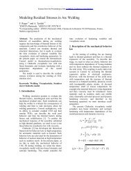
The right side of fig. 1 shows a schematic diagram of the CC process. The liquid steel is cast
into a water-cooled copper mould, where a thin shell solidifies around the liquid metal. In
contrast with other metals, like e.g. aluminium, solid steel is a relatively poor heat conductor.
This reduces the heat removal from the surface and leads to an extremely long solidification
time. The distance between the mould and the point of total solidification extends to more
than 35 m in slab casting. This makes it necessary to bend and straighten the partially
solidified strand in order to minimize the height of the casting machine. As the solidified steel
is very crack sensitive in certain temperature ranges, this deformation may be the reason for
defect formation. The process-sure prevention of defect formation demands for detailed
knowledge of the casting process and the properties of the cast material.
For this reason, the combination of numerical and experimental simulation is a very
promising way. The present paper describes a laboratory test method, the so-called
Submerged Split-Chill Tensile (SSCT) test, which allows a process-near tensile test on
solidifying steel in order to estimate the strength and the crack susceptibility of the strand
shell. This test has been thermo-mechanically modelled, using the FEMLAB software
package. The model allows, among other things, the adjustment of parameters in constitutive
material laws to the test results. The resulting material properties, characteristic for the
behaviour of steel under CC conditions and specific for every steel composition, are an
important input for the numerical simulation of the CC process.
2 Experiment
Excerpt from the Proceedings of the COMSOL Multiphysics User's Conference 2005 Frankfurt
Fig. 1 shows a schematic view of the SSCT test method (Bernhard et al. 1996) and the
solidification conditions compared to the continuous casting process. A solid steel test body,
split in two halves, is submerged into the liquid melt in an induction furnace. The surface of
the test body is spray-coated with a thin zirconium oxide layer in order to control the cooling
rate (CR) and to minimize friction. A steel shell solidifies around the test body with the main
crystallographic orientation perpendicular to the interface, similar to the situation in a
continuous casting mould. The force between the upper and lower part of the test dummy is
measured by a load cell, the position of the lower part by an inductive position sensor. A
servo-hydraulic controller controls force and position. This allows a number of different
testing procedures, including the hot tensile test, in which, after a certain holding time, the

lower half of the test body is moved downwards at a controlled velocity at strain rates (SR)
typically between 10 -3 and 10 -2 s -1 , while the necessary tensile force is recorded.
The calculations presented in this paper refer to two SSCT test series. The first was
performed at varying temperatures (holding times), cooling rates (coating thicknesses) and
strain rates and the second one with different steel compositions (carbon content from 0.05%
to 0.70%).
Force, kN
Excerpt from the Proceedings of the COMSOL Multiphysics User's Conference 2005 Frankfurt
Elongation, mm
Solidified
shell
Upper
part
Lower
part
Fig. 1. The SSCT test, schematic and solidification conditions during the laboratory test and the CC
process.
3 The FEMLAB model
Melt
Mushy zone
For a detailed analysis of the SSCT test two FEMLAB application modes are necessary:
Firstly, the solidification of the steel shell around the test body inside the induction furnace is
solely a heat transfer problem and can be solved with the corresponding application mode.
Secondly, the simulation of the hot tensile test requires the structural mechanics module.
With regard to the conditions during the SSCT test it is necessary to consider that, in contrast
to the isothermal condition of the specimen during conventional hot tensile testing, the SSCT
test is a gradient test under unsteady state conditions. Due to the progress of solidification
during the test, the shell thickness, and consequently the stressed cross-section are not
constant but a function of time, similar to continuous casting. The temperature at the
interface between the test body and the shell ranges between 1000 and 1300 °C at the end
of testing, depending on solidification time and cooling rate. This results in a time-dependent
temperature distribution up to the solidus temperature inside the solidified steel shell. Hence,
a coupled time-dependent thermo-mechanical analysis is essential with all necessary
material parameters such as thermal conductivity (k in W/mK), density (ρ in kg/m 3 ), heat
capacity (cP in J/kgK), Young’s modulus (E in N/m 2 ), Poisson’s ratio and the thermal
expansion coefficient (α in K -1 ) defined as functions of temperature. In addition, elasto-plastic
material data are necessary for an accurate analysis.
The cylindrical geometry of the test body and the induction furnace allows the use of an
axisymmetric 2D geometry for the realisation in FEMLAB. Thereby, only the domain of the
melt is considered. The geometry and the mesh are shown in fig. 2, in which the mesh at the
interface between the test body and the melt is refined because of the high temperature
gradients at the interface.
A transient analysis of heat transfer by conduction is used for the thermal analysis of the
SSCT test. The necessary subdomain parameters thermal conductivity, density and heat
capacity as functions of temperature were calculated using the software package IDS
(Miettienen 1997). When solidification occurs, it is very important to consider the latent heat

(LH in J/kg) of solidification in the heat transfer analysis. Therefore, the following equation is
used to implement the latent heat by means of a modified heat capacity CP mod between the
liquidus (TL) and solidus temperature (TS):
c
mod
P
Excerpt from the Proceedings of the COMSOL Multiphysics User's Conference 2005 Frankfurt
∂f
L
( T ) = cP
( T ) + LH
∂T
In equation (1), T denotes the temperature and fL the fraction of liquid, which was also
calculated using the software package IDS. The heat transfer needed for solving the thermal
analysis of the problem is that occurring at the interface between the liquid melt and the solid
steel test body. Seeing that the heat flux itself is difficult to measure in this environment, the
temperature inside the test dummy is recorded throughout the experimental procedure. In
order to further determine the removed heat from this measured temperature, an inverse
algorithm for the solution of the heat-conduction equation is used (Michelic 2005). This
algorithm has been developed in MATLAB and is generally based on a variation of a
maximum-a-posteriori method which has been proposed by Beck 1977 and adjusted to a
similar problem by Bass et al. 1980. The general objective of such an application is to reach
closest agreement of measured and calculated temperature values by a variation of the timedependent
heat-flux q. This is accomplished by a minimization of the sum of difference
squares S:
N N
t m
2
S(
q)
=
⎡
⎤
∑ ∑ T
m
− T
c
( q)
(2)
⎢⎣ ij ij ⎥⎦
i = 1j= 1
Equation (2) considers Nm thermocouples at positions j, measuring the temperature T m at
every timestep i (1

al. 1986, Sorimachi et al. 1977 and Kelly et al. 1988). However, it should be mentioned that
at high temperatures the mechanical properties are very sensitive to the strain rate. The
Ramberg-Osgood law provides elasto-plastic material data by isotropic hardening. Thereby
the yield stress σyield is defined as a function of the plastic strain εP:
σ ( ε ) ⋅ε
yield
p
n
= K p p ( t)
(3)
Equation (3) is used as the required hardening function in the elasto-plastic material settings,
where KP and n are temperature-dependent material properties called the plastic resistance
and the strain hardening exponent respectively. The procedure outlined by Uehara et al.
1986 was applied to determine n, assuming KP to be constant. However, the comparison with
own experimental results points at a significant temperature- and composition-dependence of
KP for a given strain rate (Pierer et al. 2005). Thereby, a simple thermo-mechanical model of
the SSCT test was developed to adjust high temperature mechanical properties to the SSCT
test. A result of this model was the requirement of defining the plastic resistance as a
function of temperature, strain rate and carbon content.
For the temperature-dependent Young’s modulus different approaches can be found in the
literature. All presented simulation results in this paper refer to the temperature-dependent
Young´s modulus, proposed by Kinoshita et al 1979.
In case of the hot tensile testing the lower part of the test body is moved downwards with a
predefined velocity to a certain elongation, which is controlled by the adjusted testing time.
The realisation of displacement in FEMLAB takes place by regulating the z-position of the
horizontal interface between the test body and the melt as a function of time (see fig. 2). The
determination of the force-elongation curve is carried out using the integration coupling
variables function provided by the software.
ρ=f(T) c P=f(T)
Thermal analysis
k=f(T)
Excerpt from the Proceedings of the COMSOL Multiphysics User's Conference 2005 Frankfurt
q=f(t)
Time dependent
solver
Temperature
distribution
Coupling
RESULTS
Mechanical analysis
E=f(T)
α=f(T)
Fig. 3. Procedure of the FEMLAB simulation of the SSCT test
Elasto-plastic
data
ν=f(T)
Parametric nonlinear
solver
RESULTS
Stress and strain
distribution
Force elongation
curve
The procedure of the complete simulation is shown in fig. 3, in which the two analysis models
– thermal analysis by the heat transfer module and mechanical analysis by the structural
mechanics module – are illustrated together with the necessary input data and solvers. To
determine the shell thickness s(t) as a function of time the heat transfer problem has to be
solved by transient analysis using the time-dependent solver. An accurate calculation of s(t)
is very important, because the results of the experiment and, as a matter of course, the
numerical calculations, strongly depend on the shell thickness. However, the mechanical
analysis using elasto-plastic material data can not be used for any type of transient
problems, it can only be used together with the nonlinear parametric solver (FEMLAB 3
Structural mechanics module, User’s guide 2004). Due to the necessity of these two different
solvers, the coupling of the analysis is not possible at present. To consider the shell

thickness as a function of time and the temperature-dependency of the material data, the
following procedure enables the analysis of the SSCT test in a sufficiently accurate manner:
the temperature distribution as a function of time and as a result of the thermal analysis has
been exported from the post processing subdomain data. Thereby a regular grid with
300x200 points was used and saved as a text-file for defined time steps. The mechanical
analysis of the SSCT test imports these files using the interpolation function application of
the software. This procedure is illustrated on top of fig. 3, whereby the temperaturedependent
material data as well as the solidification process during the hot tensile test can
be considered.
4 Results
Excerpt from the Proceedings of the COMSOL Multiphysics User's Conference 2005 Frankfurt
To validate the thermal analysis, the calculated shell thickness at the end of testing can be
compared with measurements of the solidified steel shell. Fig. 4a and 4b show the
solidification process during the hot tensile test. The minimum and maximum values of the
plotted temperature correspond to TS and TL, thus the illustrations show the mushy zone of
the solidified steel shell.
a) Begin of testing b) End of testing
T L=1515°C
T S=1461°C
8
8 9 10 11 12 13 14
Fig. 4. Shell thickness at the begin a) and end b) of testing together with a comparison of calculated
and measured shell thickness for the 0.16% carbon steels and the carbon test series (0.05 - 0.70%C)
Fig. 4c shows the calculated over the measured shell thickness. The calculated values
illustrated in the diagram in all cases refer to fS = 0.1 and show good agreement with the
measured shell thickness. In addition, the scatter band of the measurements are illustrated
for the four tests of the first series. Beside the temperature-dependent thermo-physical data,
the thermal analysis depends on many other parameters such as the measured
temperatures during the SSCT test: the steel bath temperature as an initial value for the
simulation as well as the measured temperature increase inside the test body which is
required for calculating the heat flux. As a matter of course, the accuracy of the simulation is
influenced by the size and number of the elements (1585). To get comparable simulation
results the same mesh was used for all calculations. It can be summarised that the thermal
analysis using the above described material data, boundary conditions and mesh describes
the solidification of the steel shell.
Fig. 5 shows the von Mises stress inside the solidified steel shell at the end of testing
resulting from the mechanical analysis. The picture refers to two tests of the first series with a
Calculated shell thickness, mm
14
13
12
11
10
9
c)
High CR, low SR
High CR, high SR
Low CR, high SR
Low CR, low SR
Carbon test series
Measured shell thickness, mm

holding time of 12 s, a strain rate of 2 . 10 -3 s -1 and two different cooling rates. In addition, the
sampling site of the micrographs is illustrated. The results of the von Mises stress show a
homogeneous distribution over the micrographs at both cooling rates, which is essential for
an interpretation and assessment of crack formation. The validation of the model is very
important for further interpretations of the mechanical analysis. In doing so, the calculated
results of the force-elongation curves can be compared with measured results.
Sampling point of
micrographs
Excerpt from the Proceedings of the COMSOL Multiphysics User's Conference 2005 Frankfurt
a) b)
High cooling rate
Fig. 5. Von Mises stress of a 0.16% carbon steel for a SR of 2 . 10 -3 s -1 and two different CR
Fig. 6 shows the experimentally determined force-elongation curves of four experiments at
different strain rates and cooling rates together with the simulation results. In all cases the
holding time amounts to 12 s. Owing to the lower shell thickness and the higher
temperatures in the solidified shell, the lower cooling rate leads – at both strain rates – to
lower tensile forces. A higher strain rate leads to a slight increase in the force-elongation
curves at both low and high cooling rates. When comparing the FEMLAB solutions to the
experimentally determined force-elongation curves the following aspects can be pointed out:
The calculated curves reproduce the measured curves in all cases and are in good
agreement with them. At a strain rate of 2 . 10 -3 s -1 the results of the calculated forceelongation
curves are higher than the experimentally determined curves. The result of the
high cooling rate is nearly identical. The result of the lower cooling rate shows higher
calculated values. This can be explained by the much higher calculated shell thickness and a
possible crack formation during the test. At a strain rate of 6 . 10 -3 s -1 the simulation leads to
lower values at the high cooling rate and higher values at the low cooling rate. However, at
high temperatures the mechanical properties are very sensitive to strain rate. To account for
the influence of strain rate the elasto-plastic approach must be replaced by a strain rate
dependent (elasto-viscoplastic) model. Using the elasto-plastic model provided by FEMLAB
requires a modification of the thermo-mechanical material data to get realistic results.
Therefore, the plastic resistance KP was modified in order to consider the effect of strain rate,
which leads to satisfying results.
5 Conclusion and outlook
Low cooling rate
Max: 1.6 . 10 6
Min: 0
The SSCT test is a proven method for the characterization of high-temperature mechanical
properties and the crack susceptibility of steel under continuous casting conditions. The
development of a thermo-mechanical model of the SSCT test is an important foundation for
the interpretation of experimental results. When using FEMLAB to simulate the SSCT test, it
was necessary to split the analysis in two parts: the thermal analysis using the heat transfer

application and the mechanical analysis using the structural mechanics module. Naturally,
the accuracy of a computer simulation greatly depends on the quality of the input
parameters. The validation of the thermal analysis takes place by comparing the measured
and calculated shell thickness and plays an important role for the mechanical analysis. The
high temperature mechanical material properties up to the solidus temperature are of great
interest regarding the simulation of continuous casting process. In order to evaluate these
high temperature properties, the SSCT test itself and the simulation of the test provide a very
good possibility. Moreover, it allows the adjustment of common constitutive models to fit the
experiment. The FEMLAB calculations using the elasto-plastic material data describe the
SSCT test in an accurate manner for a constant strain rate. Further work will focus on taking
the strain rate dependency into account, by implementing an an elasto-viscoplastic model
(e.g. creep-law).
Force, kN
16
14
12
10
8
6
4
2
Experiment - high CR
Experiment - low CR
FEMLAB solution - high CR
FEMLAB solution - low CR
0
0,0 0,2 0,4 0,6 0,8 1,0
Fig. 6. Experimental determined and calculated force elongation curves for a strain rate of 2 . 10 -3 s -1
and 6 . 10 -3 s -1 b) and two cooling rates (0.16% C, 0.25% Si and 1.4% Mn)
Literature
Excerpt from the Proceedings of the COMSOL Multiphysics User's Conference 2005 Frankfurt
Strain rate = 2 . 10 -3 s -1
Elongation, mm
4
2
Experiment - high CR
Experiment - low CR
FEMLAB solution - high CR
FEMLAB solution - low CR
0
0,0 0,2 0,4 0,6 0,8 1,0
Bass, B. R.; Drake, J. B.; Ott, L. J. (1980) A finite element program for two-dimensional nonlinear
inverse heat conduction analysis. Oak Ridge National Laboratory, Tennessee
Beck, J. (1977) Parameter estimation in engeineering and science. John Wiley & Sons Inc., New York
Bernhard, C.; Hiebler H.; Wolf, M. (1996) Simulation of Shell Strength Properties by the SSCT Test.
Trans. ISIJ, Vol. 36, Supplement: 163-166
Kelly, J. E.; Michalek, K. P.; O’Connor T. G; Thomas B. G. (1988) Initial Development of thermal and
stress fields in continuously cast steel billets. Metallurgical and Materials Transactions A, Vol. 19,
No. 10: 2589-2602
Kinoshita, K.; Emi T.; Kasai M. (1979) Thermal elasto-plastic stress analysis of solidifying shell in
continuous casting mold. Tetsu-to-Hagane, Vol. 65, No. 14: 2022-2031
Michelic, S. (2005) Development of an inverse thermal model of the SSCT test. Baccalaureate Thesis,
Department of Metallurgy, University of Leoben
Miettinen, J. (1997) Calculation of solidification-related thermophysical properties for steels.
Metallurgical and Materials Transactions B, Vol. 28B, No. 2: 281-297
Pierer, R.; Bernhard C.; Chimani C. (2005) Experimental and analytical analysis of the hightemperature
mechanical properties of steel under continuous casting conditions. 12 th International
Conference on Computational Methods and Experimental Measurement, Malta: 757-768
Pierer, R.; Bernhard C.; Chimani C. (2005) Evaluation of Common Constitutive Equations for
Solidifying Steel, BHM, Vol. 150: 163-169
Sorimachi, K.; Brimacombe J. K. (1977) Improvements in mathematical modelling of stresses in
continuous casting of steel. Ironmaking and Steelmaking, Vol. 4, No. 4: 240-245
Uehara, M.; Samarasekera I. V.; Brimacombe J. K. (1986) Mathematical modelling of unbending of
continuously cast steel slabs. Ironmaking and Steelmaking, Vol. 3, No. 3: 138-153
Force, kN
16
14
12
10
8
6
Strain rate = 6 . 10 -3 s -1
Elongation, mm