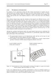
Example 1: Calculate the theoretical velocity distribution u(z) using ...

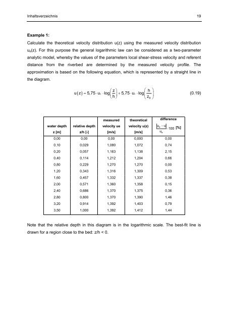
Inhaltsverzeichnis 19
Example 1:
Calculate the theoretical velocity distribution u(z) using the measured velocity distribution
u e (z). For this purpose the general logarithmic law can be considered as a two-parameter
analytic model, whereby the values of the parameters local shear-stress velocity and referent
distance from the riverbed are determined by the measured velocity profile. The
approximation is based on the following equation, which is represented by a straight line in
the diagram.
⎛z⎞
⎛ h ⎞
u( z)
= 5,75 ⋅u* ⋅ log⎜
⎟+ 5,75 ⋅u*
⋅log⎜ ⎟
⎝h⎠ ⎝z0
⎠
(0.19)
measured theoretical
water depth relative depth velocity ue velocity u(z)
z [m]
z/h [-]
[m/s]
[m/s]
difference
ue
− u
⋅ 100 [%]
u
0,00 0,00 0,00 0,000 0,00
0,10 0,029 1,080 1,072 0,74
0,20 0,057 1,163 1,138 2,15
0,40 0,114 1,212 1,204 0,66
0,80 0,229 1,270 1,270 0,00
1,20 0,343 1,316 1,309 0,53
1,60 0,457 1,332 1,337 0,38
2,00 0,571 1,360 1,358 0,15
2,40 0,686 1,370 1,375 0,36
2,80 0,800 1,370 1,390 1,46
3,20 0,914 1,392 1,403 0,79
3,50 1,000 1,392 1,412 1,44
e
Note that the relative depth in this diagram is in the logarithmic scale. The best-fit line is
drawn for a region close to the bed: z/h < 0.

20 Inhaltsverzeichnis

Inhaltsverzeichnis 21
Solution 1:
Two characteristic values u(z/h) are determined:
⎛z
⎞
⎛ h ⎞
u⎜
= 1⎟
= 0,0+ 5,75⋅u* ⋅ log⎜
⎟ = u1
= 1,41m/s
⎝h
⎠ ⎝z0
⎠
⎛z
⎞
⎛ h ⎞
u⎜
= 0,1⎟
= −5,75 ⋅ u* + 5,75 ⋅u* ⋅ log⎜
⎟ = u2
= 1,19 m / s
⎝h
⎠ ⎝z0
⎠
By the subtraction of the second equation from the first one, the expression in order to
calculate the value of the local shear velocity is derived:
u
*
u1 − u2
= = 0,038 m/s
5,75
The calculation of the distance from the referent distance yields to:
u
− 1
5,75⋅u
−6
z = h⋅ 10
*
= 1,4⋅10 m
0
The calculated velocity distribution is graphically represented
The relative differences between the theoretical and empirical velocity distributions are given
in the last column of Table 1. The best match appears near the bed, whereas errors increase
towards the free-surface, as expected.