Numerical integration

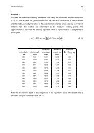
Lecture material – Environmental Hydraulic Simulation Page 99
3.1.6 NUMERICAL INTEGRATION
For purposes of error minimization during the finite element discretization of complex and nonuniform
model areas, arbitrary triangles and squares are used as finite elements (see Fig. 3-1). Please
note, that for triangles and also squares it is important to comply with specific rules including side
lengths, angle and the ratio to the neighbour elements as well as with criteria such as the Delauny
criterion.
These arbitrary element shapes make the calculation of the integrals more difficult, however, as for
example for the coefficient matrix from Eq. 3-19 or 3-20. For this reason, a coordinate transformation
is done, which maps the elements from a global coordinate system (x,y) to a so-called master element
in a local coordinate system (ξ,η). The coordinate transformation for a square is exemplarily displayed
in Fig. 3-6. The master element is selected with thought of the numerical solving method used. If
Gauss integration is used ( this method is used in the program RMA2) for rectangular elements, for
example, a square master element of edge length 2 having its midpoint in the origin of the coordinate
system (ξ,η) and its edges parallel to the axes of the coordinate system is selected (see Fig. 3-3). The
Gauss integration method is presumed to be used further on.
Although the coordinate transformation makes the wanted integral expression more complicated, the
following simplifications are achieved by the introduction of a geometrically simple master element
that is used in place of the actual elements:
(1) The approximation functions can be obtained quiet easily and they are the same for each
element since they are always applied to the master element.
(2) The calculation of the integrals for the element is simplified by a common, simple element
geometry. Commonly available numerical integration methods can be used.
Lokales Local coordinate Koordinatensystem system ( ξ,η (ξη) )
Of the master element Ω
des Master-Elementes Ω
Global Globales coordinate Koordinatensystem system (x,y) (x,y)
of the model area
des Modellgebietes
y
η
η=1
dη
2
Ω
dξ
ξ=1
ξ
Ω e
Ω 3
Ω 2
Ω 1
x
2
Figure 3-6: Transformation of a finite element graph consisting of rectangles to a square unit element
(master element), taken from [Reddy et al., 1994].
It has to be emphasized that the coordinate transformation is done for calculation purposes of
numerical integration only. The algebraic equations that have to be solved always refer to the wanted
degrees of freedom (vertex values) in the global coordinate system.

Lecture material – Environmental Hydraulic Simulation Page 100
The transformation of any element of the global coordinate system (x,y) to the master element of the
local system (ξ,η) is described by the following, for example:
x =
k
∑
j=
1
x
k
e m
j
ψ
j ∑ j j
,
j=
1
e m
( ξ,
η) , y = y ψ ( ξ η)
Eq. 3-36
where ψ j m is the approximation function for the master element. In order to make this transformation
function clearer, we can assume a square master element with linear approximation functions, and the
local coordinates satisfy the relation –1 ≤ (ξ,η) ≤ 1 (see Fig. 3-3). This is called a rectangular Lagrange
element with vertex count k=4. The approximation functions for a master element of this type can be
derived according to Eq. 3-28. If these linear approximation functions are used, the straight line ξ=1
(local coordinate system) can be describe by the following equations in the global coordinate system:
m
( η) = x ψ ( 1, η) = x 0 + x ( 1− η) + x ( 1+ η)
x 1,
1
=
2
4
∑
i=
1
( x + x ) + ( x − x )
4
∑
m
( η) = y ψ ( 1, η) = ( y + y ) + ( y − y ) η
y 1,
i=
1
2
i
i
i
i
3
1
2
3
1
1
2
2
1
2
2
η
3
2
1
2
3
1
2
2
3
+ x
4
0
Eq. 3-37
This means that x and y are well-defined linear functions of η meaning that the transformation maps
the straight line ξ=1 also to a straight line in the global coordinate system.
Before we go into deeper detail of coordinate transformation, a few terms have to be explained. We
recall the approximation for the solution of the wanted variable from Eq. 3-5 for this. It contains
approximation functions just as in Eq. 3-36. If an approximation of the same order (k=n) is chosen for
the transformation (geometry) and the wanted variable, the finite elements are called isoparametric. If
the order of the approximation for the geometry is bigger than the order of the wanted variable (kΘn),
the elements are superparametric, and in the opposite case they are subparametric [Helmig, 1996],
[Reddy et al., 1994]. Only isoparametric finite elements are used in the context of this chapter.
Our knowledge of coordinate transformation that we have now enables us to recognize that a different
shape (e.g. triangle or rectangle) or order (e.g. linear or square) of the master element leads to different
transformations and thus to different representations of the elements in the global coordinate system. It
is important that the transformation does not introduce unwanted gaps or overlapping elements into the
finite element graph. In order to set up appropriate requirements for the transformation, we have a look
at the elements of the coefficient matrix from Eq. 3-20.
⎛ e e
e e
∂ψ ∂ψ ⎞
e ⎜
∂ψ
i j ∂ψ
i j
K
⎟
ij
= ∫ k + k dx dy
Eq. 3-38
⎜
⎟
e
Ω ⎝
∂x
∂x
∂y
∂y
⎠

Lecture material – Environmental Hydraulic Simulation Page 101
The integrand that not only contains functions but also derivatives with respect to the global
coordinates x and y, now has to be expressed in dependence of ξ and η. The transformation from Eq.
3-36 is applied to get the result. We first have to apply rules of partial differentiation however:
∂ψ
∂ξ
e
i
e
∂ψ i
=
∂x
e
∂x
∂ψ i
+
∂ξ ∂y
∂y
∂ξ
∂ψ
e
i
∂η
e
∂ψ
i
=
∂x
∂x
+
∂η
∂ψ
e
i
∂y
∂y
∂η
Eq. 3-39
e
⎧∂ψ
⎫
i ⎡∂x
⎪ ⎪
∂ξ
⎢
∂ξ
⎨ ⎬ = ⎢
e
⎢∂
⎪∂ψ
x
i ⎪
⎪ ⎪ ⎢⎣
∂η
⎩ ∂η ⎭
e
∂y
⎤⎧∂ψ
i
⎪
∂ξ
⎥
∂x
⎥
∂y
⎨ e
⎥⎪∂ψ
i
∂η⎥⎦
⎪
⎩ ∂y
⎫
⎪
⎬
⎪
⎪
⎭
This equation reflects a connection between the derivatives of the approximation functions with
respect to the global and local coordinates. The matrix in Eq. 3-39 is also called Jacobi transformation
matrix. In order to obtain the needed expressions, we have to invert the equation above:
e
⎧∂ψ
⎫
i
⎪ ⎪
∂x
⎨ ⎬ =
e
⎪∂ψi
⎪
⎪
⎩ ∂y
⎪
⎭
[ J]
−1
e
⎧∂ψ
⎫
i
⎪ ⎪
∂ξ
⎨
e
⎬
⎪∂ψi
⎪
⎪
⎩ ∂η ⎪
⎭
Eq. 3-40
Provided the transformation from Eq. 3-36 the individual components of the Jacobi matrix can be
calculated as:
∂x
=
∂ξ
k
∑
j=
1
x
j
∂ψ
∂ξ
m
j
,
∂y
=
∂ξ
k
∑
j=
1
y
j
∂ψ
∂ξ
m
j
Eq. 3-41
∂x
=
∂η
k
∑
j=
1
x
j
∂ψ
∂η
m
j
,
∂y
=
∂η
k
∑
j=
1
y
j
∂ψ
∂η
m
j
In this case, the Jacobi matrix can be written as:
[ J]
⎡∂ψ
1
⎢
⎢ ∂ξ
=
⎢∂ψ
1
⎢
⎣ ∂η
m
m
∂ψ
∂ξ
∂ψ
∂η
m
2
m
2
⋯
⋯
∂ψ
∂ξ
∂ψ
∂η
m
n
m
n
⎤ ⎡x
⎥ ⎢
⎢
x
⎥
⎥ ⎢ ⋮
⎥ ⎢
⎦ ⎣x
1
2
n
y1
⎤
⎥
y
2 ⎥
⋮ ⎥
⎥
y
n ⎦
Eq. 3-42

Lecture material – Environmental Hydraulic Simulation Page 102
The inverse (reciprocal) Jacobi matrix [J] -1 only exists if [J] is non-singular, i.e. the determinante of
the Jacobi matrix is unequal to zero for each point (ξ,η) of the master element [Zurmühl et al., 1984]:
det
∂x
∂y
∂x
∂y
= Eq. 3-43
∂ξ ∂η ∂η ∂ξ
[ J] − ≠ 0
Altogether it can be stated that the transformation has to be continuous, differentiable and invertible.
At the same time it should be relatively simple, so that the Jacobi matrix can be calculated with little
effort.
In order to be able to apply the integration completely to Eq. 3-38, we need a transformation of the
area expression dA of the global element that corresponds to the transformation that is used:
[ J] dξ
dη
dA ≡ dx dy = det
Eq. 3-44
Eq. 3-38 can now be written as follows on the basis of the transformation:
( ξ,
η) dξ
dη
e
K
ij =
∫
Fij
Eq. 3-45
m
Ω
The integrals in Eq. 3-45 that refer to the square master element can be calculated with the help of the
Gauss quadrature method, so that the integral above can be calculated as follows for the twodimensional
case:
1 1
K N
∫
F
m
Ω
−1
−1
i= 1 j=
1
( , η) dξ
dη =
∫ ∫
F ( ξ,
η) dξ
dη ≈ ∑∑ F ( ξ
i
, η
j
) Wi
Wj
ξ Eq. 3-46
where K and N are the number of Gauss quadrature points, (ξ i ,η j ) are the Gauss coordinates, and W i
and W j are the values of the weighting functions.
More detailed information about the application of the Gauss quadrature method can be found in
[Reddy, 1993] among others.