Reynolds average Navier-Stokes equation

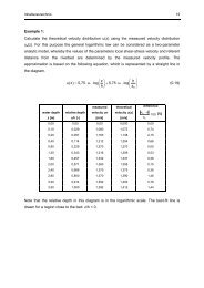
Lecture material – Environmental Hydraulic Simulation Page 66
2.2.1.2.2 REYNOLDS AVERAGED NAVIER-STOKES EQUATIONS
By hand of a time-averaging of the NS equations and the continuity equation for incompressible
fluids, the basic equations for the averaged turbulent flow will be derived in the following. The flow
field can then be described only with help of the mean values.
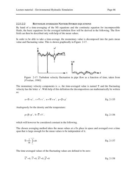
In order to be able to take a time-average, the momentary value is decomposed into the parts mean
value and fluctuating value. This is shown graphically in Figure 2-17.
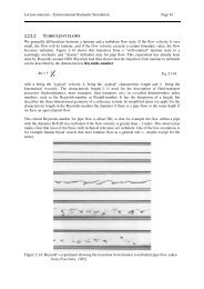
Figure 2-17: Turbulent velocity fluctuation in pipe flow as a function of time, taken from
[Fredsøe, 1990].
The momentary velocity components is u , the time-averaged value is named u and the fluctuating
velocity has the letter u′ . With help of this definition the decomposition can mathematically be written
as:
u = u + u′
, v = v + v′
, w = w + w′
, p = p + p′
Eq. 2-135
Analogously for the density and the temperature:
ρ = ρ +ρ′ , T = T + T′
, Eq. 2-136
which will however be considered constant in the following.
The chosen averaging method takes the mean values at a fix place in space and averaged over a time
span that is large enough for the mean values to be independent of it.
t + t
0 1
1
u =
∆ ∫ u dt
Eq. 2-137
t
t
0
The time-averaged values of the fluctuating values are defined to be zero:
u ′ = 0, v′=
0, w′=
0, p′
= 0
Eq. 2-138

Lecture material – Environmental Hydraulic Simulation Page 67
Firstly the continuity equation is averaged. If we substitute the expressions for the velocities from Eq.
2-135 into the continuity equation (see Eq. 2-131) we get:
∂u
∂u′
∂v
∂v′
∂w
∂w′
+ + + + + = 0
∂x
∂x
∂y
∂y
∂z
∂z
Eq. 2-139
The time-average of the last equation is written as:
∂u
∂u′
∂v
∂v′
∂w
∂w′
+ + + + + = 0
∂x
∂x
∂y
∂y
∂z
∂z
Eq. 2-140
Before we look at the transformation and reduction of Eq. 2-140, a summary of rules for timeaveraging
shall be given:
∂u
∂x
=
1
∆t
to
+ t1
∫
t 0
∂u
dt =
∂x
1
x ∆t
∂
∂
to
+ t1
∫
t0
u dt =
∂u
∂x
Eq. 2-141
∂u′
∂x
=
1
∆t
t o + t1
∫
t0
∂u′
dt =
∂x
∂
∂
1
x ∆t
t o + t1
∫
t0
u′
dt =
0
f
∂f
∂f
= f , f + g = f + g , f ⋅ g = f ⋅ g , = , f ds =
∂s
∂s
∫ ∫
f
ds
Eq. 2-142
but
f
⋅ g ≠
f
⋅ g
The averaged derivatives of the fluctuations are also zero according to these rules, so that the timeaveraged
continuity equation is:
∂u
∂v
∂w
+ + = 0
∂x
∂y
∂z
Eq. 2-143
Now the NS equations will be time-averaged. The averaging will be exemplified for the x-component.
Beforehand a small transformation of the advection term from Eq. 2-131:
∂u
∂u
∂u
∂
u + v + w =
∂x
∂y
∂z
∂x
∂
=
∂x
2
( u ) ∂( uv) ∂( uw)
2
( u ) ∂( uv) ∂( uw)
+
+
∂y
∂y
+
+
∂z
∂z
⎛ ∂u
∂v
∂w
⎞
− u
⎜ + +
x y z
⎟
⎝ ∂ ∂ ∂
⎠
= 0
Eq. 2-144

Lecture material – Environmental Hydraulic Simulation Page 68
The expressions for the decomposition of the velocities from Eq. 2-135 are now substituted into the
transformed Navier-Stokes equation (see Eq. 2-131) and a time-average is done:
⎧∂
ρ ⎨
⎩
2
( u + u′
) ∂( u + u′
) ∂( u + u′
)( v + v′
) ∂( u + u′
)( w + w′
)
∂t
+
∂x
+
∂y
+
∂z
⎫
⎬
⎭
=
F
is not subject to
turbulent
fluctuation
∂
−
2
2
2
( p + p′
) ⎛ ∂ ( u + u′
) ∂ ( u + u′
) ∂ ( u + u′
)
∂x
+
x
µ
⎜
⎝
∂x
2
+
∂y
2
+
∂z
2
⎞
⎟
⎠
Eq. 2-145
Application of the rules from Eq. 2-141 and Eq. 2-142 shows that among others the terms
∂( u
iu′
j
) ∂u′
i
∂u′
i
, , from the equation above can be reduced and the equation can be transformed to:
∂x
∂t
∂x
j
j
⎛ u uu u u uv u v u w uw ⎞
⎜
∂ ∂ ∂ ′ ′ ∂ ∂ ′ ′ ∂ ′ ′ ∂
ρ
⎟
+ + + + + +
t x x y y z z
⎝ ∂ ∂ ∂ ∂ ∂ ∂ ∂ ⎠
= F
x
∂p
−
∂x
2 2 2
⎛ ∂ u ∂ u ∂ u ⎞
+µ
⎜ + +
2 2 2
x y z
⎟
⎝ ∂ ∂ ∂
⎠
∆ u
Eq. 2-146
Further small transformations, for example a repeated application of the product rule and the
continuity equation to the advection term, lead to a form of the time-averaged NS equations for all
three directions as:
⎛ ∂u
∂u
∂u
∂u
⎞
ρ
⎜ + u + v + w
⎟ = F
⎝ ∂t
∂x
∂y
∂z
⎠
x
∂p
⎛
⎞
⎜
∂u′
u′
∂u′
v′
∂u′
w′
− +µ ∆ u −ρ
⎟
+ +
∂x
⎝ ∂x
∂y
∂z
⎠
⎛
⎞
⎜
∂v
∂v
∂v
∂v
ρ
⎟
+ u + v + w
= F
⎝ ∂t
∂x
∂y
∂z
⎠
y
∂p
⎛
⎞
⎜
∂u′
v′
∂v′
v′
∂v′
w′
− +µ ∆ v −ρ
⎟
+ +
∂y
⎝ ∂x
∂y
∂z
⎠
Eq. 2-147
⎛ ∂w
∂w
∂w
∂w
⎞
ρ
⎜ + u + v + w
⎟ = F
⎝ ∂t
∂x
∂y
∂z
⎠
z
∂p
⎛
⎞
⎜
∂u′
w′
∂v′
w′
∂w′
w′
− +µ ∆ w −ρ
⎟
+ +
∂z
⎝ ∂x
∂y
∂z
⎠
Or in tensor form:
D ui
∂ p
⎛ ∂ u′
i
u′
⎞
j
ρ = Fi
− + µ ∆ u ⎜ ⎟
i
− ρ
Eq. 2-148
Dt ∂x
⎜
i
x ⎟
⎝
∂
j
⎠
Re ynolds−stress

Lecture material – Environmental Hydraulic Simulation Page 69
From now on the time-averaged fields will not be overlined anymore. So for example u stands for the
time-averaged velocity component in direction of the x-axis.
We pay attention to the last two terms of the right side of Eq. 2-148:
µ ∆ u
i
⎛ ⎞
⎜
∂u′
′
iu
j
− ρ ⎟
⎜ ∂x
⎟
⎝
j
⎠
= µ
∂
∂x
j
⎛
⎜
∂u
⎝
∂x
i
j
⎞
⎟ − ρ
⎠
∂
∂x
j
( u′
u′
)
i
j
Eq. 2-149
=
∂
∂x
j
⎛
⎜
∂u
µ
⎝
∂x
i
j
− ρu′
u′
i
j
⎞
⎟
⎠
The expression in the brackets above corresponds to the total shear stress:
∂u
i
τ
ij
= µ − ρ u ′
i
u ′
j
Eq. 2-150
∂x
j
If we compare to the Navier-Stokes equations Eq. 2-131, it is conspicuous that besides the viscous part
an additional term has been added to the total shear stress. This term results from the time-average and
is generally the dominant part of the total shear stress. Since the term only appears due to the Reynolds
average, it is called Reynolds stress or apparent turbulent shear stress. As stated in the introduction to
the RANS approach, to lead to the closure of the equation system, an approximation for the Reynolds
stresses has to be done, which sets in relation the apparent shear stresses with the velocity field of the
average flow.
With the approach of the eddy viscosity principle after Boussinesq 1877, the general time-averaged
NS equations, also called Reynolds equations, can thus be written in tensor form as:
⎛ Dui
ρ ⎜
⎝ Dt
⎞
⎟
⎠
=
F
i
−
∂p
∂x
i
+
∂
∂x
j
τ
ij
Eq. 2-151
with
τ
ij
∂u
= µ
∂x
i
j
⎛
+ ρ ⎜ν
T
⎜
⎝
⎛
⎜
∂u
⎝ ∂x
i
j
∂u
j
+
∂x
i
⎞
⎟ −
⎠
2
3
⎞
k δ ⎟
ij
⎟
⎠