Using Thermocouples

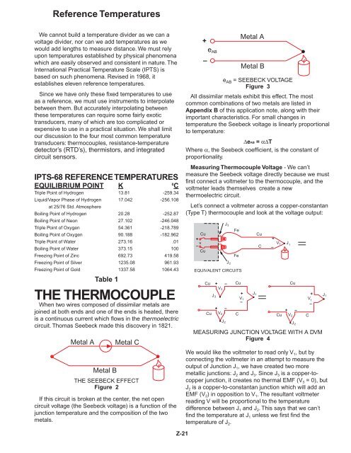
Reference Temperatures 

We cannot build a temperature divider as we can a 

voltage divider, nor can we add temperatures as we 

would add lengths to measure distance. We must rely 

upon temperatures established by physical phenomena 

which are easily observed and consistent in nature. The 

International Practical Temperature Scale (IPTS) is 

based on such phenomena. Revised in 1968, it 

establishes eleven reference temperatures. 

Since we have only these fixed temperatures to use 

as a reference, we must use instruments to interpolate 

between them. But accurately interpolating between 

these temperatures can require some fairly exotic 

transducers, many of which are too complicated or 

expensive to use in a practical situation. We shall limit 

our discussion to the four most common temperature 

transducers: thermocouples, resistance-temperature 

detector’s (RTD’s), thermistors, and integrated 

circuit sensors. 

IPTS-68 REFERENCE TEMPERATURES 

EQUILIBRIUM POINT K 0 

C 

Triple Point of Hydrogen 13.81 -259.34 

Liquid/Vapor Phase of Hydrogen 17.042 -256.108 

at 25/76 Std. Atmosphere 

Boiling Point of Hydrogen 20.28 -252.87 

Boiling Point of Neon 27.102 -246.048 

Triple Point of Oxygen 54.361 -218.789 

Boiling Point of Oxygen 90.188 -182.962 

Triple Point of Water 273.16 .01 

Boiling Point of Water 373.15 100 

Freezing Point of Zinc 692.73 419.58 

Freezing Point of Silver 1235.08 961.93 

Freezing Point of Gold 1337.58 1064.43 

Table 1 

THE THERMOCOUPLE 

When two wires composed of dissimilar metals are 

joined at both ends and one of the ends is heated, there 

is a continuous current which flows in the thermoelectric 

circuit. Thomas Seebeck made this discovery in 1821. 

Metal A 

Metal C 

Metal B 

THE SEEBECK EFFECT 

Figure 2 

If this circuit is broken at the center, the net open 

circuit voltage (the Seebeck voltage) is a function of the 

junction temperature and the composition of the two 

metals. 

+ 

e AB 

– 

Metal A 

Metal B 

All dissimilar metals exhibit this effect. The most 

common combinations of two metals are listed in 

Appendix B of this application note, along with their 

important characteristics. For small changes in 

temperature the Seebeck voltage is linearly proportional 

to temperature: 

∆eAB = α∆T 

Where α, the Seebeck coefficient, is the constant of 

proportionality. 

Measuring Thermocouple Voltage - We can’t 

measure the Seebeck voltage directly because we must 

first connect a voltmeter to the thermocouple, and the 

voltmeter leads themselves create a new 

thermoelectric circuit. 

Let’s connect a voltmeter across a copper-constantan 

(Type T) thermocouple and look at the voltage output: 

Cu 

+ 

v 

– 

Cu 

Fe 

Cu 

J 3 

+ 

C – 

V 1 

Fe 

EQUIVALENT CIRCUITS 

Cu 

Cu 

+ 

V 3 

J 3 

+ 

V 2 

e AB = SEEBECK VOLTAGE 

Figure 3 

J 2 

– 

– 

J 2 

Cu 

C 

+ 

V 1 

– 

J 1 

MEASURING V 3 = 0 JUNCTION VOLTAGE WITH A DVM 

Figure 4 

We would like the voltmeter to read only V 1 , but by 

connecting the voltmeter in an attempt to measure the 

output of Junction J 1 , we have created two more 

metallic junctions: J 2 and J 3 . Since J 3 is a copper-tocopper 

junction, it creates no thermal EMF (V 3 = 0), but 

J 2 is a copper-to-constantan junction which will add an 

EMF (V 2 ) in opposition to V 1 . The resultant voltmeter 

reading V will be proportional to the temperature 

difference between J 1 and J 2 . This says that we can’t 

find the temperature at J 1 unless we first find the 

temperature of J 2 . 

Cu 

+ 

J 1 

Cu 

V 2 

J 2 

– 

C 

V 1 

+ 

– 

J 1 

Z-21

The Reference Junction 

Cu 

+ 

v 

– 

Cu 

Voltmeter 

Cu 

+ – 

Cu V2 

+ 

– 

C 

V 1 

J 1 

+ 

– 

v 

+ 

V 2 

– 

+ T 

V 1 

– 

J 1 

EXTERNAL REFERENCE JUNCTION 

Figure 5 

One way to determine the temperature of J 2 is to 

physically put the junction into an ice bath, forcing its 

temperature to be 0ºC and establishing J 2 as the 

Reference Junction. Since both voltmeter terminal 

junctions are now copper-copper, they create no 

thermal emf and the reading V on the voltmeter is 

proportional to the temperature difference between J 1 

and J 2 . 

Now the voltmeter reading is (see Figure 5): 

V = (V 1 - V 2 ) ≅α(t J1 - t J2 ) 

If we specify T J1 in degrees Celsius: 

T J1 (ºC) + 273.15 = t J1 

then V becomes: 

V = V 1 - V 2 = α [(T J1 + 273.15) - (T J2 + 273.15)] 

= α (T J1 - T J2 ) = α (T J1 - 0) 

V = αT J1 

J 2 

Ice Bath 

J 2 

T=0°C 

The copper-constantan thermocouple shown in 

Figure 5 is a unique example because the copper wire 

is the same metal as the voltmeter terminals. Let’s use 

an iron-constantan (Type J) thermocouple instead of the 

copper-constantan. The iron wire (Figure 6) increases 

the number of dissimilar metal junctions in the circuit, as 

both voltmeter terminals become Cu-Fe thermocouple 

junctions. 

V 3 

J 3 

- + 

+ 

v V 1 

– 

- + 

V 1 = V 

Voltmeter 

V 4 J 4 

if V 

3 = V4 

i.e., if 

T J 3 

= T J4 

JUNCTION VOLTAGE CANCELLATION 

Figure 7 

Z 

We use this protracted derivation to emphasize that 

the ice bath junction output, V 2 , is not zero volts. It is a 

function of absolute temperature. 

By adding the voltage of the ice point reference 

junction, we have now referenced the reading V to 0ºC. 

This method is very accurate because the ice point 

temperature can be precisely controlled. The ice point is 

used by the National Bureau of Standards (NBS) as the 

fundamental reference point for their thermocouple 

tables, so we can now look at the NBS tables and 

directly convert from voltage V to Temperature T J1 . 

Cu 

+ 

v 

– 

Cu 

J 3 

J 4 

Fe 

Fe 

J 2 

Ice Bath 

IRON-CONSTANTAN COUPLE 

Figure 6 

C 

J 1 

Z-22 

If both front panel terminals are not at the same 

temperature, there will be an error. For a more precise 

measurement, the copper voltmeter leads should be 

extended so the copper-to-iron junctions are made on 

an isothermal (same temperature) block: 

Cu 

+ 

v 

– 

Cu 

Voltmeter 

Cu 

Cu 

J 3 

J 4 

Ice Bath 

REMOVING JUNCTIONS FROM DVM TERMINALS 

Figure 8 

Fe 

Isothermal Block 

The isothermal block is an electrical insulator but a 

good heat conductor, and it serves to hold J 3 and J 4 at 

the same temperature. The absolute block temperature 

is unimportant because the two Cu-Fe junctions act in 

opposition. We still have 

V = α (T 1 - T REF ) 

Fe 

V 2 

T REF 

C 

T 1

Reference Circuit 

Let’s replace the ice bath with another isothermal 

block 

HI 

LO 

Voltmeter 

Cu 

Cu 

J 3 

J 4 


The new block is at Reference Temperature TREF, and 

because J 3 and J 4 are still at the same temperature, we 

can again show that 

V = α (T 1 -T REF ) 

This is still a rather inconvenient circuit because we 

have to connect two thermocouples. Let’s eliminate the 

extra Fe wire in the negative (LO) lead by combining the 

Cu-Fe junction (J 4 ) and the Fe-C junction (J REF ). 

We can do this by first joining the two isothermal 

blocks (Figure 9b). 

Fe 

J REF 

Fe 

ELIMINATING THE ICE BATH 

Figure 9a 

C 

J 1 

T REF Isothermal Block 

This is a useful conclusion, as it completely eliminates 

the need for the iron (Fe) wire in the LO lead: 

+ 

v 

– 

Cu 

Cu 

J 3 

J 4 

Again, V = α (TJ 1 - T REF ), where α is the Seebeck 

coefficient for an Fe-C thermocouple.| 

Junctions J 3 and J 4 , take the place of the ice bath. 

These two junctions now become the Reference 

Junction. 

Now we can proceed to the next logical step: Directly 

measure the temperature of the isothermal block (the 

Reference Junction) and use that information to 

compute the unknown temperature, TJ 1 . 

Fe 

C 

T REF 

EQUIVALENT CIRCUIT 

Figure 11 

J 1 

Cu 

HI 

Fe 

J 

J 1 

3 

LO + 

Cu 

Fe 

C 

v 

J 

– 

4 J REF 

Isothermal Bloc k @ T REF 

JOINING THE ISOTHERMAL BLOCKS 

Figure 9b 

We haven’t changed the output voltage V. It is still 

V = α (TJ 1 - TJ REF ) 

Now we call upon the law of intermediate metals (see 

Appendix A) to eliminate the extra junction. This 

empirical “law” states that a third metal (in this case, 

iron) inserted between the two dissimilar metals of a 

thermocouple junction will have no effect upon the 

output voltage as long as the two junctions formed by 

the additional metal are at the same temperature: 

Metal A 

Isothermal Connection 

Thus the low lead in Fig. 9b: Becomes: 

Cu 

Metal C 

Metal B = 

C 

Fe = 

T REF 

Metal A 

Cu 

LAW OF INTERMEDIATE METALS 

Figure 10 

Metal C 

T REF 

C 

Z-23 

Voltmeter 

Cu 

Cu 

J 3 

R T 

J 4 

Block Temperature = T REF 

EXTERNAL REFERENCE JUNCTION-NO ICE BATH 

Figure 12 

A thermistor, whose resistance R T is a function of 

temperature, provides us with a way to measure the 

absolute temperature of the reference junction. 

Junctions J 3 and J 4 and the thermistor are all assumed 

to be at the same temperature, due to the design of the 

isothermal block. Using a digital multimeter under 

computer control, we simply: 

1) Measure R T to find T REF and convert T REF 

to its equivalent reference junction 

voltage, V REF , then 

2) Measure V and subtract V REF to find V 1 , 

and convert V 1 to temperature T J1 . 

This procedure is known as Software Compensation 

because it relies upon the software of a computer to 

compensate for the effect of the reference junction. The 

isothermal terminal block temperature sensor can be 

any device which has a characteristic proportional to 

absolute temperature: an RTD, a thermistor, or an 

integrated circuit sensor. 

It seems logical to ask: If we already have a device 

that will measure absolute temperature (like an RTD or 

thermistor), why do we even bother with a thermocouple 

that requires reference junction compensation? The 

Fe 

C 

+ 

V 1 

– 

J 1

single most important answer to this question is that the 

thermistor, the RTD, and the integrated circuit 

transducer are only useful over a certain temperature 

range. Thermocouples, on the other hand, can be used 

over a range of temperatures, and optimized for various 

atmospheres. They are much more rugged than 

thermistors, as evidenced by the fact that 

thermocouples are often welded to a metal part or 

clamped under a screw. They can be manufactured on 

the spot, either by soldering or welding. In short, 

thermocouples are the most versatile temperature 

transducers available and, since the measurement 

system performs the entire task of reference 

compensation and software voltage to-temperature 

conversion, using a thermocouple becomes as easy as 

connecting a pair of wires. 

Thermocouple measurement becomes especially 

convenient when we are required to monitor a large 

number of data points. This is accomplished by using 

the isothermal reference junction for more than one 

thermocouple element (see Figure 13). 

A reed relay scanner connects the voltmeter to the 

various thermocouples in sequence. All of the voltmeter 

and scanner wires are copper, independent of the type 

of thermocouple chosen. In fact, as long as we know 

what each thermocouple is, we can mix thermocouple 

types on the same isothermal junction block (often 

called a zone box) and make the appropriate 

modifications in software. The junction block 

temperature sensor R T is located at the center of the 

block to minimize errors due to thermal gradients. 

Software compensation is the most versatile 

technique we have for measuring thermocouples. Many 

thermocouples are connected on the same block, 

copper leads are used throughout the scanner, and the 

technique is independent of the types of thermocouples 

chosen. In addition, when using a data acquisition 

system with a built-in zone box, we simply connect the 

thermocouple as we would a pair of test leads. All of the 

conversions are performed by the computer. The one 

disadvantage is that the computer requires a small 

amount of additional time to calculate the reference 

junction temperature. For maximum speed we can use 

hardware compensation. 

+ 

– 

Voltmeter 

HI 

LO 

All Copper Wires 

ZONE BOX SWITCHING 

Figure 13 

Hardware Compensation 

Rather than measuring the temperature of the 

reference junction and computing its equivalent voltage 

as we did with software compensation, we could insert 

a battery to cancel the offset voltage of the reference 

junction. The combination of this hardware 

compensation voltage and the reference junction 

voltage is equal to that of a 0ºC junction. 

The compensation voltage, e, is a function of the 

temperature sensing resistor, R T . The voltage V is now 

referenced to 0ºC, and may be read directly and 

converted to temperature by using the NBS tables. 

Another name for this circuit is the electronic ice point 

reference. 2 These circuits are commercially available for 

use with any voltmeter and with a wide variety of 

thermocouples. The major drawback is that a unique ice 

point reference circuit is usually needed for each 

individual thermocouple type. 

Figure 15 shows a practical ice point reference circuit 

that can be used in conjunction with a reed relay 

scanner to compensate an entire block of thermocouple 

inputs. All the thermocouples in the block must be of the 

same type, but each block of inputs can accommodate 

a different thermocouple type by simply changing gain 

resistors. 

Fe 

C 

R T 

Pt 

Pt - 10% Rh 


(Zone Box) 

Z 

+ 

– 

v 

Cu 

Cu 

Fe 

Fe 

C 

Fe 

– + 

T 

+ 

Cu 

Fe 

T + 

v 

C 

= = 

Cu 

– 

Fe 

– 

Cu 

+ 

Cu 

R T 

Fe 

C 

Cu 

Cu 

- 

T 

e 

2 

Refer to Bibliography 6. 

Z-24 

0°C 

HARDWARE COMPENSATION CIRCUIT 

Figure 14

OMEGA TAC-Electronic Ice Point and 

Thermocouple Preamplifier/Linearizer Plugs 

into Standard Connector 

OMEGA Electronic Ice Point Built into Thermocouple Connector -”MCJ” 

Cu 

Fe 

Cu 

C 

OMEGA Ice Point Reference Chamber. 

Electronic Refigeration Eliminates Ice Bath 

R H 

PRACTICAL HARDWARE COMPENSATION 

Figure 15 

The advantage of the hardware compensation circuit 

or electronic ice point reference is that we eliminate the 

need to compute the reference temperature. This saves 

us two computation steps and makes a hardware 

compensation temperature measurement somewhat 

faster than a software compensation measurement. 

HARDWARE COMPENSATION 

Fast 

Restricted to one thermocouple 

type per card 

Voltage-To-Temperature Conversion 

We have used hardware and software compensation 

to synthesize an ice-point reference. Now all we have to 

do is to read the digital voltmeter and convert the 

voltage reading to a temperature. Unfortunately, the 

temperature-versus-voltage relationship of a 

thermocouple is not linear. Output voltages for the more 

common thermocouples are plotted as a function of 

temperature in Figure 16. If the slope of the curve (the 

Seebeck coefficient) is plotted vs. temperature, as in 

Figure 17, it becomes quite obvious that the 

thermocouple is a non-linear device. 

A horizontal line in Figure 17 would indicate a 

constant α, in other words, a linear device. We notice 

that the slope of the type K thermocouple approaches a 

constant over a temperature range from 0ºC to 1000ºC. 

Consequently, the type K can be used with a multiplying 

voltmeter and an external ice point reference to obtain a 

moderately accurate direct readout of temperature. That 

is, the temperature display involves only a scale factor. 

This procedure works with voltmeters. 

By examining the variations in Seebeck coefficient, 

3 

Refer to Bibliography 4. 

TABLE 2 

Integrated Temperature 

Sensor 

SOFTWARE COMPENSATION 

Requires more computer 

manipulation time 

Versatile - accepts any thermocouple 

we can easily see that using one constant scale factor 

would limit the temperature range of the system and 

restrict the system accuracy. Better conversion accuracy 

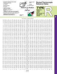
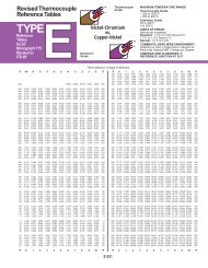
can be obtained by reading the voltmeter and consulting 

the National Bureau of Standards Thermocouple 

Tables 3 in Section T of the OMEGA TEMPERATURE 

MEASUREMENT HANDBOOK - see Table 3. 

T = a 0 +a 1 x + a 2 x 2 + a 3 x 3 ...+a n x n 

where 

T = Temperature 

x = Thermocouple EMF in Volts 

a = Polynomial coefficients unique to each 

thermocouple 

n = Maximum order of the polynomial 

As n increases, the accuracy of the polynomial 

improves. A representative number is n = 9 for ± 1ºC 

accuracy. Lower order polynomials may be used over a 

narrow temperature range to obtain higher system 

speed. 

Table 4 is an example of the polynomials used to 

convert voltage to temperature. Data may be utilized in 

packages for a data acquisition system. Rather than 

directly calculating the exponentials, the computer is 

programmed to use the nested polynomial form to save 

execution time. The polynomial fit rapidly degrades 

outside the temperature range shown in Table 4 and 

should not be extrapolated outside those limits. 

Z-25 

Millivolts 

80 

60 

40 

20 

0° 

E 

J 

K 

R 

S 

500° 1000° 1500° 2000° 

Temperature °C 

Type 

E 

J 

K 

R 

S 

T 

Metals 

+ – 

Chromel vs. Constantan 

Iron vs. Constantan 

Chromel vs. Alumel 

Platinum vs. Platinum 

13% Rhodium 

Platinum vs. Platinum 

10% Rhodium 

Copper vs. Constantan 

THERMOCOUPLE TEMPERATURE 

vs. 

VOLTAGE GRAPH 

Figure 16

100 

mV .00 .01 .02 .03 .04 .05 .06 .07 .08 .09 .10 mV 

TEMPERATURES IN DEGREES C (IPTS 1968) 

0.00 0.00 0.17 0.34 0.51 0.68 0.85 1.02 1.19 1.36 1.53 1.70 0.00 

0.10 1.70 1.87 2.04 2.21 2.38 2.55 2.72 2.89 3.06 3.23 3.40 0.10 

0.20 3.40 3.57 3.74 3.91 4.08 4.25 4.42 4.58 4.75 4.92 5.09 0.20 

0.30 5.09 5.26 5.43 5.60 5.77 5.94 6.11 6.27 6.44 6.61 6.78 0.30 

0.40 6.78 6.95 7.12 7.29 7.46 7.62 7.79 7.96 8.13 8.30 8.47 0.40 

0.50 8.47 8.63 8.80 8.97 9.14 9.31 9.47 9.64 9.81 9.98 10.15 0.50 

0.60 10.15 10.31 10.48 10.65 10.82 10.98 11.15 11.32 11.49 11.65 11.82 0.60 

0.70 11.82 11.99 12.16 12.32 12.49 12.66 12.83 12.99 13.16 13.33 13.49 0.70 

0.80 13.49 13.66 13.83 13.99 14.16 14.33 14.49 14.66 14.83 14.99 15.16 0.80 

0.90 15.16 15.33 15.49 15.66 15.83 15.99 16.16 16.33 16.49 16.66 16.83 0.90 

1.00 16.83 16.99 17.16 17.32 17.49 17.66 17.82 17.99 18.15 18.32 18.48 1.00 

1.10 18.48 18.65 18.82 18.98 19.15 19.31 19.48 19.64 19.81 19.97 20.14 1.10 

1.20 20.14 20.31 20.47 20.64 20.80 20.97 21.13 21.30 21.46 21.63 21.79 1.20 

1.30 21.79 21.96 22.12 22.29 22.45 22.62 22.78 22.94 23.11 23.27 23.44 1.30 

1.40 23.44 23.60 23.77 23.93 24.10 24.26 24.42 24.59 24.75 24.92 25.08 1.40 

Seebeck Coefficient V/°C 

80 

60 

40 

20 

T 

E 

J 

Linear Region 

(SeeText) 

K 

R 

S 

a 0 

a 1 

a 2 

a 3 

a 4 

a 5 

a 6 

a 7 

a 8 

a 9 

–500° 

0° 500° 1000° 1500° 2000° 

Temperature °C 

SEEBECK COEFFICIENT vs. TEMPERATURE 

Figure 17 

TYPE E THERMOCOUPLE 

Table 3 

TYPE E TYPE J TYPE K TYPE R TYPE S TYPE T 

Nickel-10% Chromium(+) Iron(+) Nickel-10% Chromium(+) Platinum-13% Rhodium(+) Platinum-10% Rhodium(+) Copper(+) 

Versus Versus Versus Versus Versus Versus 

Constantan(-) Constantan(-) Nickel-5%(-) Platinum(-) Platinum(-) Constantan(-) 

(Aluminum Silicon) 

-100ºC to 1000ºC 0ºC to 760ºC 0ºC to 1370ºC 0ºC to 1000ºC 0ºC to 1750ºC -160ºC to 400ºC 

± 0.5ºC ± 0.1ºC ± 0.7ºC ± 0.5ºC ± 1ºC ±0.5ºC 

9th order 5th order 8th order 8th order 9th order 7th order 

0.104967248 -0.048868252 0.226584602 0.263632917 0.927763167 0.100860910 

17189.45282 19873.14503 24152.10900 179075.491 169526.5150 25727.94369 

-282639. 0850 -218614.5353 67233.4248 -48840341.37 -31568363.94 -767345.8295 

12695339.5 11569199.78 2210340.682 1.90002E + 10 8990730663 78025595.81 

-448703084.6 -264917531.4 -860963914.9 -4.82704E + 12 -1.63565E + 12 -9247486589 

1.10866E + 10 2018441314 4.83506E + 10 7.62091E + 14 1.88027E + 14 6.97688E + 11 

-1. 76807E + 11 -1. 18452E + 12 -7.20026E + 16 -1.37241E + 16 -2.66192E + 13 

1.71842E + 12 1.38690E + 13 3.71496E + 18 6.17501E + 17 3.94078E + 14 

-9.19278E + 12 -6.33708E + 13 -8.03104E + 19 -1.56105E + 19 

2.06132E + 13 1.69535E + 20 

Z 

TEMPERATURE CONVERSION EQUATION: T = a 0 +a 1 x + a 2 x 2 + ...+a n x n 

NESTED POLYNOMIAL FORM: T = a 0 + x(a 1 + x(a 2 + x (a 3 + x(a 4 

where x is in Volts, T is in °C 

NBS POLYNOMIAL COEFFICIENTS 

Table 4 

The calculation of high-order polynomials is a timeconsuming 

task for a computer. As we mentioned 

before, we can save time by using a lower order 

polynomial for a smaller temperature range. In the 

software for one data acquisition system, the 

thermocouple characteristic curve is divided into eight 

sectors, and each sector is approximated by a thirdorder 

polynomial.* 

* HEWLETT PACKARD 3054A. 

Temp. 

a 

{ 

Voltage 

2 3 

T a = bx + cx + dx 

CURVE DIVIDED INTO SECTORS 

Figure 18 

Z-26 

+ a 5 x)))) (5th order) 

All the foregoing procedures assume the 

thermocouple voltage can be measured accurately and 

easily; however, a quick glance at Table 3 shows us that 

thermocouple output voltages are very small indeed. 

Examine the requirements of the system voltmeter: 

THERMOCOUPLE SEEBECK DVM SENSITIVITY 

TYPE COEFFICIENT FOR 0.1ºC 

(µV/ºC) @ 20ºC 

(µV) 

E 62 6.2 

J 51 5.1 

K 40 4.0 

R 7 0.7 

S 7 0.7 

T 40 4.0 

REQUIRED DVM SENSITIVITY 

Table 5 

Even for the common type K thermocouple, the 

voltmeter must be able to resolve 4 µV to detect a 

0. 1ºC change. The magnitude of this signal is an open 

invitation for noise to creep into any system. For this 

reason, instrument designers utilize several 

fundamental noise rejection techniques, including tree 

switching, normal mode filtering, integration and 

guarding.

PRACTICAL THERMOCOUPLE MEASUREMENT 

Noise Rejection 

C 

+ 

Signal 

– 

C 

(20 Channels) 

C 

Tree 

Switch 1 

HI 

DVM 

Noise 

Sour ce 

~ 

C 

Next 20 Channels 

C 

Tree 

Switch 2 

+ 

+ 

Signal 

Signal 

= ~ 

– 

DVM = – 

20 C C HI 

Noise 

Source 

~ 

Stray capacitance to noise 

source is reduced nearly 

20:1 by leaving Tree 

Switch 2 open. 

TREE SWITCHING 

Figure 19 

~ 

C 

HI 

DVM 

Tree Switching - Tree switching is a method of 

organizing the channels of a scanner into groups, each 

with its own main switch. 

Without tree switching, every channel can contribute 

noise directly through its stray capacitance. With tree 

switching, groups of parallel channel capacitances are 

in series with a single tree switch capacitance. The 

result is greatly reduced crosstalk in a large data 

acquisition system, due to the reduced interchannel 

capacitance. 

Analog Filter - A filter may be used directly at the 

input of a voltmeter to reduce noise. It reduces 

interference dramatically, but causes the voltmeter to 

respond more slowly to step inputs. 

Integration - Integration is an A/D technique which 

essentially averages noise over a full line cycle; thus, 

power line related noise and its harmonics are virtually 

eliminated. If the integration period is chosen to be less 

than an integer line cycle, its noise rejection properties 

are essentially negated. 

Since thermocouple circuits that cover long distances 

are especially susceptible to power line related noise, it 

is advisable to use an integrating analog-to-digital 

converter to measure the thermocouple voltage. 

Integration is an especially attractive A/D technique in 

light of recent innovations which allow reading rates of 

48 samples per second with full cycle integration. 

V IN 

Z-27 

Guarding - Guarding is a technique used to reduce 

interference from any noise source that is common to 

both high and low measurement leads, i.e., from 

common mode noise sources. 

Let’s assume a thermocouple wire has been pulled 

through the same conduit as a 220 Vac supply line. The 

capacitance between the power lines and the 

thermocouple lines will create an AC signal of 

approximately equal magnitude on both thermocouple 

wires. This common mode signal is not a problem in an 

ideal circuit, but the voltmeter is not ideal. It has some 

capacitance between its low terminal and safety ground 

(chassis). Current flows through this capacitance and 

through the thermocouple lead resistance, creating a 

normal mode noise signal. The guard, physically a 

floating metal box surrounding the entire voltmeter 

circuit, is connected to a shield surrounding the 

thermocouple wire, and serves to shunt the interfering 

current. 

t 

ANALOG FILTER 

Figure 20 

V OUT 

t

Distributed 

Capacitance 

220 V AC Line 

HI 

Distributed 

Resistance 

Without Guard 

LO 

DVM 

Without Guard 

HI 

LO 

Guard 

DVM 

Z 

Each shielded thermocouple junction can directly 

contact an interfering source with no adverse effects, 

since provision is made on the scanner to switch the 

guard terminal separately for each thermocouple 

channel. This method of connecting the shield to guard 

serves to eliminate ground loops often created when 

the shields are connected to earth ground. 

The dvm guard is especially useful in eliminating 

noise voltages created when the thermocouple junction 

comes into direct contact with a common mode noise 

source. 

240 VRMS 

In Figure 22 we want to measure the temperature at 

the center of a molten metal bath that is being heated 

by electric current. The potential at the center of the 

bath is 120 V RMS. The equivalent circuit is: 

120VRMS 

Figure 22 

Figure 23 

GUARD SHUNTS INTERFERING WITH CURRENT 

Figure 21 

R S 

Noise Current 

HI 

LO 

Noise Current 

Figure 24 

Notice that we can also minimize the noise by 

minimizing R s . We do this by using larger thermocouple 

wire that has a smaller series resistance. 

To reduce the possibility of magnetically induced 

noise, the thermocouple should be twisted in a uniform 

manner. Thermocouple extension wires are available 

commercially in a twisted pair configuration. 

Practical Precautions - We have discussed the 

concepts of the reference junction, how to use a 

polynomial to extract absolute temperature data, and 

what to look for in a data acquisition system, to 

minimize the effects of noise. Now let’s look at the 

thermocouple wire itself. The polynomial curve fit relies 

upon the thermocouple wire’s being perfect; that is, it 

must not become decalibrated during the act of making 

a temperature measurement. We shall now discuss 

some of the pitfalls of thermocouple thermometry. 

Aside from the specified accuracies of the data 

acquisition system and its zone box, most measurement 

errors may be traced to one of these primary sources: 

1. Poor junction connection 

The stray capacitance from the dvm Lo terminal to 2. Decalibration of thermocouple wire 

chassis causes a current to flow in the low lead, which 

3. Shunt impedance and galvanic action 

in turn causes a noise voltage to be dropped across the 

series resistance of the thermocouple, R s . This voltage 4. Thermal shunting 

appears directly across the dvm Hi to Lo terminals and 5. Noise and leakage currents 

causes a noisy measurement. If we use a guard lead 6. Thermocouple specifications 

connected directly to the thermocouple, we drastically 

7. Documentation 

reduce the current flowing in the Lo lead. The noise 

current now flows in the guard lead where it cannot 

affect the reading: 

Z-28 

R S 

HI 

LO 

Guard

Poor Junction Connection 

There are a number of acceptable ways to connect 

two thermocouple wires: soldering, silver-soldering, 

welding, etc. When the thermocouple wires are 

soldered together, we introduce a third metal into the 

thermocouple circuit, but as long as the temperatures 

on both sides of the thermocouple are the same, the 

solder should not introduce any error. The solder does 

limit the maximum temperature to which we can subject 

this junction. To reach a higher measurement 

temperature, the joint must be welded. But welding is 

not a process to be taken lightly. 3 Overheating can 

degrade the wire, and the welding gas and the 

atmosphere in which the wire is welded can both diffuse 

into the thermocouple metal, changing its 

characteristics. The difficulty is compounded by the very 

different nature of the two metals being joined. 

Commercial thermocouples are welded on expensive 

machinery using a capacitive-discharge technique to 

insure uniformity. 

Fe 

C 

Junction: Fe - Pb, Sn - C = Fe - C 

A poor weld can, of course, result in an open 

connection, which can be detected in a measurement 

situation by performing an open thermocouple check. 

This is a common test function available with 

dataloggers. While the open thermocouple is the 

easiest malfunction to detect, it is not necessarily the 

most common mode of failure. 

Decalibration 

Decalibration is a far more serious fault condition than 

the open thermocouple because it can result in a 

temperature reading that appears to be correct. 

Decalibration describes the process of unintentionally 

altering the physical makeup of the thermocouple wire 

so that it no longer conforms to the NBS polynomial 

within specified limits. Decalibration can result from 

diffusion of atmospheric particles into the metal caused 

by temperature extremes. It can be caused by high 

temperature annealing or by cold-working the metal, an 

effect that can occur when the wire is drawn through a 

conduit or strained by rough handling or vibration. 

Annealing can occur within the section of wire that 

undergoes a temperature gradient. 

3 Refer to Bibliography 5 



SOLDERING A THERMOCOUPLE 

Figure 25 

Solder (Pb, Sn) 

Robert Moffat in his Gradient Approach to 

Thermocouple Thermometry explains that the 

thermocouple voltage is actually generated by the 

section of wire that contains the temperature gradient, 

and not necessarily by the junction. 4 For example, if we 

have a thermal probe located in a molten metal bath, 

there will be two regions that are virtually isothermal 

and one that has a large gradient. 

In Figure 26, the thermocouple junction will not 

produce any part of the output voltage. The shaded 

section will be the one producing virtually the entire 

thermocouple output voltage. If, due to aging or 

annealing, the output of this thermocouple were found 

25˚C 

100˚C 

500˚C 

Metal Bath 

200 

300 

400 

500 

GRADIENT PRODUCES VOLTAGE 

Figure 26 

to be drifting, then replacing the thermocouple junction 

alone would not solve the problem. We would have to 

replace the entire shaded section, since it is the source 

of the thermocouple voltage. 

Thermocouple wire obviously can’t be manufactured 

perfectly; there will be some defects which will cause 

output voltage errors. These inhomogeneities can be 

especially disruptive if they occur in a region of steep 

temperature gradient. Since we don’t know where an 

imperfection will occur within a wire, the best thing we 

can do is to avoid creating a steep gradient. Gradients 

can be reduced by using metallic sleeving or by careful 

placement of the thermocouple wire. 

Shunt Impedance 

High temperatures can also take their toll on 

thermocouple wire insulators. Insulation resistance 

decreases exponentially with increasing temperature, 

even to the point that it creates a virtual junction. 5 

Assume we have a completely open thermocouple 

operating at a high temperature. 

The leakage Resistance, R L , can be sufficiently low to 

complete the circuit path and give us an improper 

voltage reading. Now let’s assume the thermocouple is 

not open, but we are using a very long section of small 

diameter wire. 

Z-29

( ) 

To DVM 

R L 

LEAKAGE RESISTANCE 

Figure 27 

R S 

R S 

To DVM 

R L 

T 2 

R S 

T 1 

R S 

VIRTUAL JUNCTION 

Figure 28 

Z 

If the thermocouple wire is small, its series resistance, 

R S , will be quite high and under extreme conditions R L 

< < R S . This means that the thermocouple junction will 

appear to be at R L and the output will be proportional to 

T 1 not T 2 . 

High temperatures have other detrimental effects on 

thermocouple wire. The impurities and chemicals within 

the insulation can actually diffuse into the thermocouple 

metal causing the temperature-voltage dependence to 

deviate from published values. When using 

thermocouples at high temperatures, the insulation 

should be chosen carefully. Atmospheric effects can be 

minimized by choosing the proper protective metallic or 

ceramic sheath 

Galvanic Action 

The dyes used in some thermocouple insulation will 

form an electrolyte in the presence of water. This 

creates a galvanic action, with a resultant output 

hundreds of times greater than the Seebeck effect. 

Precautions should be taken to shield thermocouple 

wires from all harsh atmospheres and liquids. 

Thermal Shunting 

No thermocouple can be made without mass. Since it 

takes energy to heat any mass, the thermocouple will 

slightly alter the temperature it is meant to measure. If 

the mass to be measured is small, the thermocouple 

must naturally be small. But a thermocouple made with 

small wire is far more susceptible to the problems of 

contamination, annealing, strain, and shunt impedance. 

To minimize these effects, thermocouple extension wire 

can be used. Extension wire is commercially available 

wire primarily intended to cover long distances between 

the measuring thermocouple and the voltmeter. 

Extension wire is made of metals having Seebeck 

coefficients very similar to a particular thermocouple 

type. It is generally larger in size so that its series 

resistance does not become a factor when traversing 

long distances. It can also be pulled more readily 

through a conduit than can very small thermocouple 

wire. It generally is specified over a much lower 

temperature range than premium grade thermocouple 

wire. In addition to offering a practical size advantage, 

extension wire is less expensive than standard 

thermocouple wire. This is especially true in the case of 

platinum-based thermocouples. 

Since the extension wire is specified over a narrower 

temperature range and it is more likely to receive 

mechanical stress, the temperature gradient across the 

extension wire should be kept to a minimum. This, 

according to the gradient theory, assures that virtually 

none of the output signal will be affected by the 

extension wire. 

Noise - We have already discussed line-related noise 

as it pertains to the data acquisition system. The 

techniques of integration, tree switching and guarding 

serve to cancel most line-related interference. 

Broadband noise can be rejected with the analog filter. 

The one type of noise the data acquisition system 

cannot reject is a dc offset caused by a dc leakage 

current in the system. While it is less common to see dc 

leakage currents of sufficient magnitude to cause 

appreciable error, the possibility of their presence 

should be noted and prevented, especially if the 

thermocouple wire is very small and the related series 

impedance is high. 

Wire Calibration 

Thermocouple wire is manufactured to a certain 

specification, signifying its conformance with the NBS 

tables. The specification can sometimes be enhanced 

by calibrating the wire (testing it at known 

temperatures). Consecutive pieces of wire on a 

continuous spool will generally track each other more 

closely than the specified tolerance, although their 

output voltages may be slightly removed from the center 

of the absolute specification. 

If the wire is calibrated in an effort to improve its 

fundamental specifications, it becomes even more 

imperative that all of the aforementioned conditions be 

heeded in order to avoid decalibration. 

Z-30

Documentation - It may seem incongruous to speak 

of documentation as being a source of voltage 

measurement error, but the fact is that thermocouple 

systems, by their very ease of use, invite a large number 

of data points. The sheer magnitude of the data can 

become quite unwieldy. When a large amount of data is 

taken, there is an increased probability of error due to 

mislabeling of lines, using the wrong NBS curve, etc. 

Since channel numbers invariably change, data 

should be categorized by measureand, not just channel 

number. 6 Information about any given measureand, 

such as transducer type, output voltage, typical value 

and location, can be maintained in a data file. This can 

be done under computer control or simply by filling out 

a pre-printed form. No matter how the data is 

maintained, the importance of a concise system should 

not be underestimated, especially at the outset of a 

complex data gathering project. 

Diagnostics 

Most of the sources of error that we have mentioned 

are aggravated by using the thermocouple near its 

temperature limits. These conditions will be 

encountered infrequently in most applications. But what 

about the situation where we are using small 

thermocouples in a harsh atmosphere at high 

temperatures? How can we tell when the thermocouple 

is producing erroneous results? We need to develop a 

reliable set of diagnostic procedures. 

Through the use of diagnostic techniques, R.P. Reed 

has developed an excellent system for detecting faulty 

thermocouples and data channels. 6 Three components 

of this system are the event record, the zone box test, 

and the thermocouple resistance history. 

Event Record - The first diagnostic is not a test at all, 

but a recording of all pertinent events that could even 

remotely affect the measurements. An example would be: 

MARCH 18 EVENT RECORD 

10:43 Power failure 

10:47 System power returned 

11:05 Changed M821 to type K thermocouple 

13:51 New data acquisition program 

16:07 M821 appears to be bad reading 

Figure 29 

We look at our program listing and find that measurand 

#M821 uses a type J thermocouple and that our new data 

acquisition program interprets it as a type J. But from the 

event record, apparently thermocouple M821 was 

changed to a type K, and the change was not entered into 

the program. While most anomalies are not discovered 

this easily, the event record can provide valuable insight 

into the reason for an unexplained change in a system 

measurement. This is especially true in a system 

configured to measure hundreds of data points. 


Z-31 

Zone Box Test - A zone box is an isothermal terminal 

block of known temperature used in place of an ice bath 

reference. If we temporarily short-circuit the 

thermocouple directly at the zone box, the system 

should read a temperature very close to that of the zone 

box, i.e., close to room temperature. 

If the thermocouple lead resistance is much greater 

than the shunting resistance, the copper wire shunt 

forces V = 0. In the normal unshorted case, we want to 

measure T J , and the system reads: 

V ≅α(T J - T REF ) 

But, for the functional test, we have shorted the terminals 

so that V=0. The indicated temperature T’ J is thus: 

0 = α (T’ J - T REF ) 

T’ J = T REF 

Thus, for a dvm reading of V = 0, the system will 

indicate the zone box temperature. First we observe the 

temperature T J (forced to be different from T REF ), then 

we short the thermocouple with a copper wire and 

make sure that the system indicates the zone box 

temperature instead of T J . 

Cu 

+ 

v 

– 

Cu 

Voltmeter 

Cu 

Cu 

T REF 

Copper Wire Short 

C 

Zone Box 


SHORTING THE THERMOCOUPLE AT THE TERMINALS 

Figure 30 

This simple test verifies that the controller, scanner, 

voltmeter and zone box compensation are all operating 

correctly. In fact, this simple procedure tests everything 

but the thermocouple wire itself. 

Thermocouple Resistance - A sudden change in the 

resistance of a thermocouple circuit can act as a 

warning indicator. If we plot resistance vs. time for each 

set of thermocouple wires, we can immediately spot a 

sudden resistance change, which could be an indication 

of an open wire, a wire shorted due to insulation failure, 

changes due to vibration fatigue, or one of many failure 

mechanisms. 

For example, assume we have the thermocouple 

measurement shown in Figure 31. 

We want to measure the temperature profile of an 

underground seam of coal that has been ignited. The 

wire passes through a high temperature region, into a 

cooler region. Suddenly, the temperature we measure 

rises from 300°C to 1200°C. Has the burning section of 

the coal seam migrated to a different location, or has 

the thermocouple insulation failed, thus causing a short 

circuit between the two wires at the point of a hot spot? 

Fe 

T J

To Data 

Acquisition 

System 

If we have a continuous history of the thermocouple 

wire resistance, we can deduce what has actually 

happened. 

R 

T = 1200˚C 

BURNING COAL SEAM 

Figure 31 

T = 300˚C 

T 1 

switched on and the voltage across the resistance is 

measured again. The voltmeter software compensates 

for the offset voltage of the thermocouple and 

calculates the actual thermocouple source resistance. 

Special Thermocouples - Under extreme conditions, 

we can even use diagnostic thermocouple circuit 

configurations. Tip-branched and leg-branched 

thermocouples are four-wire thermocouple circuits that 

allow redundant measurement of temperature, noise, 

voltage and resistance for checking wire integrity. Their 

respective merits are discussed in detail in REF. 8. 

Only severe thermocouple applications require such 

extensive diagnostics, but it is comforting to know that 

there are procedures that can be used to verify the 

integrity of an important thermocouple measurement. 

Z 

t 1 

Time 

THERMOCOUPLE RESISTANCE vs. TIME 

Figure 32 

The resistance of a thermocouple will naturally 

change with time as the resistivity of the wire changes 

due to varying temperature. But a sudden change in 

resistance is an indication that something is wrong. In 

this case, the resistance has dropped abruptly, 

indicating that the insulation has failed, effectively 

shortening the thermocouple loop. 

T S 

Short 

CAUSE OF THE RESISTANCE CHANGE 

Figure 33 

The new junction will measure temperature T s , not T 1 . 

The resistance measurement has given us additional 

information to help interpret the physical phenomenon 

detected by a standard open thermocouple check. 

Measuring Resistance - We have casually 

mentioned checking the resistance of the thermocouple 

wire as if it were a straightforward measurement. But 

keep in mind that when the thermocouple is producing a 

voltage, this voltage can cause a large resistance 

measurement error. Measuring the resistance of a 

thermocouple is akin to measuring the internal 

resistance of a battery. We can attack this problem with 

a technique known as offset compensated ohms 

measurement. 

As the name implies, the voltmeter first measures the 

thermocouple offset voltage without the ohms current 

source applied. Then the ohms current source is 

T 1 

Leg-Branched Thermocouple 

Tip-Branched Thermocouple 

Figure 34 

Summary 

In summary, the integrity of a thermocouple system 

can be improved by following these precautions: 

• Use the largest wire possible that will not 

shunt heat away from the measurement area. 

• If small wire is required, use it only in the region 

of the measurement and use extension wire for 

the region with no temperature gradient. 

• Avoid mechanical stress and vibration which 

could strain the wires. 

• When using long thermocouple wires, connect 

the wire shield to the dvm guard terminal and use 

twisted pair extension wire. 

• Avoid steep temperature gradients. 

• Try to use the thermocouple wire well within its 

temperature rating. 

• Use a guarded integrating A/D converter. 

• Use the proper sheathing material in hostile 

environments to protect the thermocouple wire. 

• Use extension wire only at low temperatures and 

only in regions of small gradients. 

• Keep an event log and a continuous record of 

thermocouple resistance. 

Z-32

Using Thermocouples

Create successful ePaper yourself

Delete template?

Save as template?