Ground Penetrating Radar (GPR)
Ground Penetrating Radar (GPR)
Ground Penetrating Radar (GPR)

You also want an ePaper? Increase the reach of your titles
YUMPU automatically turns print PDFs into web optimized ePapers that Google loves.
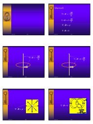
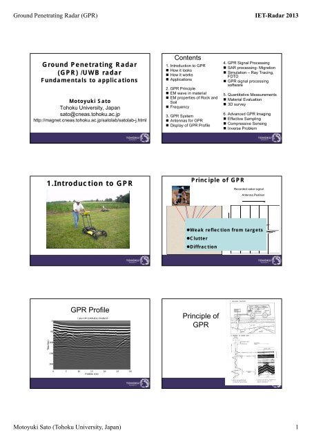
<strong>Ground</strong> <strong>Penetrating</strong> <strong>Radar</strong> (<strong>GPR</strong>) IET-<strong>Radar</strong> 2013<br />
<strong>Ground</strong> <strong>Penetrating</strong> <strong>Radar</strong><br />
(<strong>GPR</strong>) /UWB radar<br />
Fundamentals to applications<br />
Motoyuki Sato<br />
Tohoku University, Japan<br />
sato@cneas.tohoku.ac.jp<br />
http://magnet.cneas.tohoku.ac.jp/satolab/satolab-j.html<br />
Contents<br />
1. Introduction to <strong>GPR</strong><br />
• How it looks<br />
• How it works<br />
• Applications<br />
2. <strong>GPR</strong> Principle<br />
• EM wave in material<br />
• EM properties of Rock and<br />
Soil<br />
• Frequency<br />
3. <strong>GPR</strong> System<br />
• Antennas for <strong>GPR</strong><br />
• Display of <strong>GPR</strong> Profile<br />
4. <strong>GPR</strong> Signal Processing<br />
• SAR processing- Migration<br />
• Simulation – Ray Tracing,<br />
FDTD<br />
• <strong>GPR</strong> signal processing<br />
software<br />
5. Quantitative Measurements<br />
• Material Evaluation<br />
• 3D survey<br />
6. Advanced <strong>GPR</strong> Imaging<br />
• Effective Sampling<br />
• Compressive Sensing<br />
• Inverse Problem<br />
1<br />
2<br />
1.Introduction to <strong>GPR</strong><br />
Principle of <strong>GPR</strong><br />
Recorded radar signal<br />
Antenna Position<br />
Time<br />
•Weak reflection from targets<br />
•Clutter<br />
•Diffraction<br />
3<br />
4<br />
<strong>GPR</strong> Profile<br />
Principle of<br />
<strong>GPR</strong><br />
5<br />
6<br />
Motoyuki Sato (Tohoku University, Japan) 1
<strong>Ground</strong> <strong>Penetrating</strong> <strong>Radar</strong> (<strong>GPR</strong>) IET-<strong>Radar</strong> 2013<br />
出 前 授 業<br />
1 Introduction 7 1 Introduction 8<br />
地 表 レーダ 計 測 I<br />
<strong>GPR</strong> System<br />
1 Introduction 9<br />
10<br />
<strong>GPR</strong> system<br />
ALIS<br />
ALIS: Dual Sensor<br />
•Metal Detector(MD)<br />
•<strong>Ground</strong> <strong>Penetrating</strong><br />
<strong>Radar</strong>(<strong>GPR</strong>)<br />
11<br />
12<br />
Motoyuki Sato (Tohoku University, Japan) 2
<strong>Ground</strong> <strong>Penetrating</strong> <strong>Radar</strong> (<strong>GPR</strong>) IET-<strong>Radar</strong> 2013<br />
ALIS in Cambodia<br />
Mines detected by ALIS<br />
14<br />
Deminer’s report 11-32<br />
MD quality: good<br />
<strong>GPR</strong> quality: good<br />
Object:AP mine<br />
Deminer’s report 12-33<br />
MD quality: good<br />
<strong>GPR</strong> quality: good<br />
Object:AP mine<br />
Real object : PMN @ 10 cm<br />
Out of test site, VANNA, SOKHA<br />
Real object : MN79 @ 5 cm<br />
15<br />
Out of test site, VANNA, SOKHA<br />
16<br />
Application to Geological Survey(Deren Fault, Mongolai)<br />
Deren Fault<br />
Trench Observation<br />
(Gobi, Mongolia)<br />
:Top soil<br />
:Weathering rock<br />
:Basite<br />
F?Fault<br />
17<br />
18<br />
Motoyuki Sato (Tohoku University, Japan) 3
<strong>Ground</strong> <strong>Penetrating</strong> <strong>Radar</strong> (<strong>GPR</strong>) IET-<strong>Radar</strong> 2013<br />
Pavement Inspection<br />
<strong>Radar</strong> Analysis of Asphalt and<br />
Base Course Thickness<br />
19<br />
20<br />
<strong>GPR</strong> system<br />
Application of <strong>GPR</strong><br />
Detection of Buried<br />
Objects<br />
•pipe, cable<br />
•Landmine<br />
Non Destructive Inspection<br />
(NDI)<br />
•Concrete<br />
•Construction<br />
•Tunnel<br />
•Pavement<br />
Environment<br />
•<strong>Ground</strong> water<br />
•Geology<br />
Agriculture<br />
•Irrigation monitoring<br />
Archaeology<br />
21<br />
22<br />
Feature of <strong>GPR</strong><br />
High speed, High resolution<br />
–On site subsurface imaging<br />
Metal +Nonmetal<br />
–Wide applications<br />
–High sensitivity to water<br />
–Detection of water<br />
2. <strong>GPR</strong> Principle<br />
• EM Wave propagation in Soil/Rock<br />
Wave Velocity<br />
c 3<br />
v 10 8 ( m/ s)<br />
<br />
r<br />
Wavelength<br />
v<br />
vT ( m)<br />
f<br />
r<br />
23<br />
24<br />
Motoyuki Sato (Tohoku University, Japan) 4
<strong>Ground</strong> <strong>Penetrating</strong> <strong>Radar</strong> (<strong>GPR</strong>) IET-<strong>Radar</strong> 2013<br />
Reflection of EM wave<br />
Travel Time and Depth of<br />
Target<br />
v<br />
d m<br />
2 ( )<br />
Reflectivity of Layer<br />
Boundary<br />
<br />
<br />
<br />
<br />
<br />
1 2<br />
1 2<br />
25<br />
Material Attenuation (dB/m) Relative<br />
permittivity<br />
Air 0 1<br />
Clay 10-100 2-40<br />
Coal: dry 1-10 3.5-9<br />
Coal: wet 2-20 8-25<br />
Concrete: dry 2-12 4-10<br />
Concrete: wet 10-25 10-20<br />
Fresh water 0.1 80<br />
Fresh water ice 0.1-2 4<br />
Granite: dry 0.5-3 5<br />
Granite: wet 2-5 7<br />
Lime stone: dry 0.5-10 7<br />
Lime stone: wet 10-25 8<br />
Permafrost 0.1-5 4-8<br />
Sand: dry 0.01-1 4-6<br />
Sand: saturated 0.03-0.3 10-30<br />
Sandstone: dry 2-10 2-3<br />
Sandstone: wet 10-20 5-10<br />
Shale: saturated 10-100 6-9<br />
Soil: firm 0.1-2 8-12<br />
Soil: sandy dry 0.1-2 4-6<br />
Soil: sandy wet 1-5 15-30<br />
Electrical<br />
properties of<br />
Rock/Soil<br />
26<br />
Dielectric Constant of Soil/Rock<br />
• Water content and Dielectric Constant<br />
3. <strong>GPR</strong> System<br />
• Evaluation of radar System<br />
Dielectric Constant<br />
Frequency<br />
Wavelength<br />
Attenuation<br />
Resolution<br />
Low - High<br />
Long - Short<br />
Small - Large<br />
Low - High<br />
Water Content<br />
Penetration depth<br />
Deep - Shallow<br />
27<br />
28<br />
Penetration<br />
Depth<br />
Transmitter<br />
Direct wave<br />
Receiver<br />
Surface reflection<br />
Target<br />
<strong>Radar</strong><br />
system<br />
光 Optical ファイバfiber<br />
コントロールユニット<br />
Control Unit<br />
Transmitter Power<br />
PF=<br />
Receiver Noise Level<br />
送 Transmitter 信 アンテナ<br />
接 Cable 続 ケーブル<br />
29<br />
受 Receiver 1 信 Introduction アンテナ<br />
30<br />
コンピュータ<br />
PC<br />
Motoyuki Sato (Tohoku University, Japan) 5
<strong>Ground</strong> <strong>Penetrating</strong> <strong>Radar</strong> (<strong>GPR</strong>) IET-<strong>Radar</strong> 2013<br />
Size of Antenna and its<br />
operation Frequency<br />
EM Radiation from a Dipole Antenna<br />
31<br />
32<br />
Transmitted signal<br />
Antenna for <strong>GPR</strong><br />
1<br />
30<br />
Amplitude<br />
0.8<br />
0.6<br />
0.4<br />
0.2<br />
0<br />
-0.2<br />
-0.4<br />
-0.6<br />
-0.8<br />
-1<br />
0 50 100 150 200 250<br />
Time (ns)<br />
Amplitude (dB(dB)<br />
p ( )<br />
20<br />
10<br />
0<br />
-10<br />
-20<br />
-30<br />
-40<br />
0 100 200 300 400 500<br />
Frequency (MHz)<br />
1.Broadband<br />
2.Phase characteristics<br />
3.Polarization<br />
4.Tx-Rx Isolation<br />
5.Size<br />
waveform<br />
spectrum<br />
33<br />
GICHD 21 March 2007 34<br />
Antenna Design<br />
Transient Radiation from a<br />
Vivaldi antenna (FD-TD)<br />
Vivaldi antenna<br />
GICHD 21 March 2007 35<br />
GICHD 21 March 2007 36<br />
Motoyuki Sato (Tohoku University, Japan) 6
<strong>Ground</strong> <strong>Penetrating</strong> <strong>Radar</strong> (<strong>GPR</strong>) IET-<strong>Radar</strong> 2013<br />
Direct Signal for the Large Antenna<br />
2 identical large Vivaldi antennas<br />
Distance 40 cm and 100 cm<br />
S21 measurement<br />
Near Field<br />
4<br />
Cavity-back Spiral Antenna<br />
Far field condition<br />
R>2D 2 / R > 2.38 m<br />
D=0.189 m<br />
=0.03 m (f=10 GHz)<br />
GICHD 21 March 2007 37<br />
GICHD 21 March 2007 38<br />
<strong>GPR</strong> antenna and EMI coil<br />
Sensor head for Hand-Held<br />
system: ALIS<br />
Raw signal<br />
GICHD 21 March 2007 39<br />
Reflection from a Metal Plate<br />
GICHD 21 March 2007 40<br />
ALIS with Vivaldi antenna<br />
<strong>GPR</strong> Profile A & B -Scan<br />
GICHD 21 March 2007 41<br />
42<br />
Motoyuki Sato (Tohoku University, Japan) 7
<strong>Ground</strong> <strong>Penetrating</strong> <strong>Radar</strong> (<strong>GPR</strong>) IET-<strong>Radar</strong> 2013<br />
<strong>GPR</strong> Profile A & B Scan<br />
<strong>GPR</strong> Profile C-Scan & 3D<br />
A-scope<br />
B-scope<br />
C-scope 3-D<br />
43<br />
44<br />
Archaeological Survey by 3D <strong>GPR</strong><br />
(Tohoku University-University of Miami)<br />
45<br />
46<br />
47 48<br />
Motoyuki Sato (Tohoku University, Japan) 8
<strong>Ground</strong> <strong>Penetrating</strong> <strong>Radar</strong> (<strong>GPR</strong>) IET-<strong>Radar</strong> 2013<br />
4. <strong>GPR</strong> Signal Processing<br />
<strong>Radar</strong> reflection from buried pipes<br />
49<br />
1 Introduction 50<br />
図 1 地 中 レーダによる 埋 設 管 検 知 例 ( 大 阪 ガス 早 川 秀 樹 氏 提 供 )<br />
After<br />
Migration<br />
processing<br />
<strong>GPR</strong><br />
profile<br />
Raw<br />
signal<br />
Signal Processing in <strong>GPR</strong><br />
DC removal<br />
Frequency filtering<br />
Spatial filtering<br />
Frequency-Spatial (f-k) filtering<br />
Deconvolution<br />
Smoothing<br />
Average subtraction<br />
Migration<br />
Amplitude correction (AGC 、STC)<br />
1 Introduction 51<br />
52<br />
図 2<br />
f-kマイグレーション 処 理 を 行 った 波 形<br />
<strong>GPR</strong> Profile<br />
Raw Profile<br />
What does <strong>GPR</strong> see?<br />
Time-shift<br />
Subtraction of the<br />
averaged signal<br />
マイグレーショ<br />
ン 処 理<br />
Image reconstruction<br />
by Migration<br />
53<br />
54<br />
Motoyuki Sato (Tohoku University, Japan) 9
<strong>Ground</strong> <strong>Penetrating</strong> <strong>Radar</strong> (<strong>GPR</strong>) IET-<strong>Radar</strong> 2013<br />
Forward Modeling<br />
•Inversion Scheme is not<br />
always effective<br />
•Forward Modeling<br />
Ray Tracing<br />
Ray Tracing<br />
FDTD<br />
55<br />
56<br />
<strong>GPR</strong> profile by Ray Tracing<br />
<strong>GPR</strong>MAX<br />
http://www.gprmax.org<br />
FDTD<br />
57<br />
58<br />
5. Quantitative Measurements<br />
Measurement of Electrical<br />
Properties of Material<br />
•<strong>GPR</strong><br />
•Laboratory<br />
•In-Situ<br />
59 60<br />
Motoyuki Sato (Tohoku University, Japan) 10
<strong>Ground</strong> <strong>Penetrating</strong> <strong>Radar</strong> (<strong>GPR</strong>) IET-<strong>Radar</strong> 2013<br />
Parallel Plate<br />
Easy at Low<br />
Frequency<br />
(
<strong>Ground</strong> <strong>Penetrating</strong> <strong>Radar</strong> (<strong>GPR</strong>) IET-<strong>Radar</strong> 2013<br />
同 軸 管 法 による 誘 電 率 測 定<br />
TDR<br />
Time Domain<br />
Reflectrometer<br />
(a) 周 波 数 特 性<br />
(b) 水 分 率<br />
•Easy to use<br />
•Good for In-Situ<br />
measurement<br />
•Not applicable to hard<br />
material<br />
•Only near surface<br />
information<br />
2013/4/7 <strong>GPR</strong> 67<br />
2013/4/7<br />
<strong>GPR</strong><br />
68<br />
TDR equipment and a probe<br />
Dielectric Properties of Water<br />
Microwave<br />
Oven<br />
2.45GHz<br />
<br />
S<br />
<br />
<br />
<br />
' j"<br />
1<br />
j<br />
Debye-Model<br />
2013/4/7 69<br />
2013/4/7 70<br />
Observation of Dynamic Behavior of<br />
<strong>Ground</strong> water level by <strong>GPR</strong><br />
Static State<br />
Production State<br />
ポンプ 小 屋 の 前 での 地 中 レーダ 計 測<br />
(モンゴル・ウランバートル 市 )<br />
71<br />
72<br />
Motoyuki Sato (Tohoku University, Japan) 12
<strong>Ground</strong> <strong>Penetrating</strong> <strong>Radar</strong> (<strong>GPR</strong>) IET-<strong>Radar</strong> 2013<br />
<strong>GPR</strong> A-scope B-scope<br />
High Water Level<br />
Low Water Level<br />
Monitoring of <strong>Ground</strong><br />
Water Migration<br />
Residual<br />
<strong>GPR</strong> profile along the survey line N.(a)Profile1,water<br />
level is 5.30m(+1.15m).(b)Profile12,water level is<br />
4.65m(+1.15m offset).(c)Residual profile of (a) and<br />
(b).<br />
73<br />
Aスコープ<br />
Bスコープ<br />
74<br />
<strong>GPR</strong> Survey Techniques<br />
Wide angle Survey<br />
Tx Tx Tx Rx Rx Rx<br />
<strong>Ground</strong> Surface<br />
• Common-offset<br />
Offset Trace Interval<br />
• Common midpoint<br />
(CMP)<br />
CMP<br />
<strong>Ground</strong>water Table<br />
Tx<br />
Rx<br />
Tx<br />
Rx<br />
Reflector<br />
Reflector<br />
Direct Wave<br />
Reflection<br />
75<br />
76<br />
Velocity Spectrum<br />
CMP gathers along survey line N<br />
Measurement of Material for<br />
Construction<br />
Nuclea<br />
r waste<br />
35cm<br />
The low water condition.<br />
Water Level in the well<br />
-5.30m(+1.15m offset)<br />
The high water condition.<br />
Water Level in the<br />
well<br />
-4.65m(+1.15m offset)<br />
77<br />
Special material with high<br />
attenuation to prevent nuclear<br />
radiation<br />
Experimental purpose:<br />
‣ Dielectric constant<br />
‣ Attenuation<br />
Motoyuki Sato (Tohoku University, Japan) 13
<strong>Ground</strong> <strong>Penetrating</strong> <strong>Radar</strong> (<strong>GPR</strong>) IET-<strong>Radar</strong> 2013<br />
Electromagnetic wave around a<br />
Material Specimen<br />
Air-Coupled Wave<br />
Air-coupled Wave<br />
Tx Tx Tx Rx Rx Rx<br />
<strong>Ground</strong> Surface<br />
Lateral Wave<br />
Time (ns)<br />
<strong>Ground</strong>water Table<br />
Body Wave<br />
Offset Distance (m)<br />
79<br />
80<br />
1 Specimen (35cm)<br />
S11 test of 1 specimen (35cm)<br />
2 Specimen (70cm)<br />
S11 test of 2 specimen (70cm)<br />
4<br />
35cm (with metal plate)<br />
70cm (with metal plate)<br />
35cm (without metal plate)<br />
2<br />
2<br />
70cm (without metal plate)<br />
Amplitude<br />
0<br />
-2<br />
6 x 10⁻³ Time [ns]<br />
S11 test of 1 specimen (35cm)<br />
Amplitude<br />
0<br />
-2<br />
4 x 10⁻³ Time [ns]<br />
S11 test of 2 specimen (70cm)<br />
6 x 10⁻³ Time [ns]<br />
4 x 10⁻³ Time [ns]<br />
-4<br />
35cm (with metal plate)<br />
4<br />
35cm (without metal plate)<br />
35cm<br />
-6<br />
-150 -100<br />
2<br />
-50 0 50 100 150<br />
Amplitude<br />
0<br />
-2<br />
-4<br />
70c<br />
-4<br />
70cm (with metal plate)<br />
2<br />
70cm (without metal plate)<br />
m -6<br />
-150 -100 -50 0 50 100 150<br />
0<br />
Amplitude<br />
-2<br />
-4<br />
-6<br />
-20 -15 -10 -5 0 5 10 15 20<br />
-6<br />
-20 -15 -10 -5 0 5 10 15 20<br />
6.4cm gypsum<br />
Frequency spectrum<br />
Vivaldi transmitter Spiral transmitter<br />
Reflection signals in Frequency Domain Reflection signals in Frequency Domain<br />
0<br />
-20<br />
-10<br />
-30<br />
Tx<br />
6.4cm<br />
2cm<br />
Metal plate<br />
Tx<br />
Raw data<br />
Amplitude [dB]<br />
After<br />
Deconvolution<br />
Amplitude [dB]<br />
-20<br />
-30<br />
Rx1<br />
-40<br />
Rx2<br />
Rx3<br />
-50<br />
Rx4<br />
Rx5<br />
-60<br />
0 1 2 3 4 5 6<br />
Frequency [GHz]<br />
Reflection signals in Frequency Domain<br />
40<br />
Rx1<br />
30<br />
Rx2<br />
Rx3<br />
20<br />
Rx4<br />
Rx5<br />
10<br />
0<br />
-10<br />
-20<br />
0 1 2 3 4 5 6<br />
Frequency [GHz]<br />
Amplitude [dB]<br />
Amplitude [dB]<br />
-40<br />
-50<br />
-60<br />
-70<br />
-80<br />
0 1 2 3 4 5 6<br />
Frequency [GHz]<br />
Reflection signals in Frequency Domain<br />
10<br />
0<br />
-10<br />
-20<br />
-30<br />
Rx1<br />
Rx2<br />
Rx3<br />
Rx4<br />
Rx5<br />
Rx1<br />
Rx2<br />
Rx3<br />
Rx4<br />
Rx5<br />
-40<br />
0 1 2 3 4 5 6<br />
Frequency [GHz]<br />
Motoyuki Sato (Tohoku University, Japan) 14
<strong>Ground</strong> <strong>Penetrating</strong> <strong>Radar</strong> (<strong>GPR</strong>) IET-<strong>Radar</strong> 2013<br />
Raw data<br />
Amplitude<br />
After<br />
Deconvolution<br />
Amplitude<br />
Time domain signal<br />
Vivaldi transmitter<br />
Reflection signals<br />
Rx1<br />
Rx2<br />
Rx3<br />
Rx4<br />
Rx5<br />
1.5 x 10⁻³ 1<br />
0.5<br />
0<br />
-0.5<br />
-1<br />
-1.5<br />
-2<br />
0 1 2<br />
Time [ns]<br />
3 4<br />
Reflection signals<br />
0.03<br />
Rx1<br />
0.02<br />
0.01<br />
0<br />
-0.01<br />
-0.02<br />
c<br />
Rx2<br />
Rx3<br />
Rx4<br />
Rx5<br />
-0.03<br />
0 1 2 3 4<br />
Time [ns]<br />
Amplitude<br />
Amplitude<br />
Spiral transmitter<br />
Reflection signals<br />
Rx1<br />
Rx2<br />
Rx3<br />
Rx4<br />
Rx5<br />
4 x 10⁻⁴ 2<br />
0<br />
-2<br />
-4<br />
0 1 2<br />
Time [ns]<br />
3 4<br />
Reflection signals<br />
Rx1<br />
c<br />
Rx2<br />
Rx3<br />
Rx4<br />
Rx5<br />
6 x 10⁻³ 4<br />
2<br />
0<br />
-2<br />
-4<br />
-6<br />
0 1 2<br />
Time [ns]<br />
3 4<br />
Velocity and thickness estimate<br />
Raw data<br />
(x 2 [m 2 ]<br />
(x 2 [m 2 ]<br />
0.02<br />
0.01<br />
0.02<br />
After 0.01<br />
Deconvolution<br />
0<br />
0<br />
Vivaldi transmitter<br />
t 2 - x 2<br />
-0.02<br />
0 0.2 0.4 0.6 0.8<br />
t 2 [ns 2 ]<br />
t 2 - x 2<br />
-0.02<br />
0 0.2 0.4 0.6 0.8<br />
t 2 [ns 2 ]<br />
(x 2 [m 2 ]<br />
0.03<br />
0.02<br />
0.01<br />
0<br />
t 2 - x 2<br />
-0.03<br />
0 0.5 1 1.5<br />
t 2 [ns 2 ]<br />
-0.01<br />
-0.01<br />
Epsilon=2.25, D=6.3cmEpsilon=2.13, -0.02<br />
D=7.1c<br />
(x 2 [m 2 ]<br />
Spiral transmitter<br />
-0.01<br />
-0.01<br />
Epsilon=2.13, D=6.6cm Epsilon=2.0, -0.02<br />
D=7.5cm<br />
0.03<br />
0.02<br />
0.01<br />
0<br />
t 2 - x 2<br />
-0.03<br />
0 0.5 1 1.5<br />
t 2 [ns 2 ]<br />
Velocity and thickness estimate<br />
Raw data<br />
Time (ns)<br />
Vivaldi transmitter Spiral transmitter<br />
Velocity spectrum<br />
0<br />
0.5<br />
1<br />
1.5<br />
2<br />
2.5<br />
2.5<br />
3<br />
Epsilon=2.10,<br />
3<br />
D=6.7cm3.5<br />
3.5<br />
0.1 0.15 0.2 0.25 0.3<br />
0.1 0.15 0.2 0.25 0.3<br />
Velocity (m/ns)<br />
Velocity (m/ns)<br />
Time (ns)<br />
Velocity spectrum<br />
0<br />
0.5<br />
1<br />
1.5<br />
2<br />
Epsilon=2.12, D=7.6c<br />
3- Dimensional Subsurface Fracture Estimation<br />
RX<br />
After<br />
Deconvolution<br />
Time (ns)<br />
Velocity spectrum<br />
0<br />
0.5<br />
1<br />
1.5<br />
2<br />
Time (ns)<br />
Velocity spectrum<br />
0<br />
0.5<br />
1<br />
1.5<br />
2<br />
2.5<br />
2.5<br />
3<br />
3<br />
Epsilon=2.16, D=6.7cmEpsilon=1.72, D=6.7c<br />
3.5<br />
3.5<br />
TX<br />
0.1 0.15 0.2 0.25 0.3<br />
Velocity (m/ns)<br />
0.1 0.15 0.2 0.25 0.3<br />
Velocity (m/ns)<br />
3-D Subsurface<br />
Fracture<br />
Orientation<br />
S E30S E30N<br />
Survey for Subway<br />
Construction<br />
N<br />
W30N<br />
W30S<br />
E30N<br />
E30S<br />
S<br />
N W30N W30S<br />
W<br />
N<br />
S<br />
E<br />
90<br />
Motoyuki Sato (Tohoku University, Japan) 15
<strong>Ground</strong> <strong>Penetrating</strong> <strong>Radar</strong> (<strong>GPR</strong>) IET-<strong>Radar</strong> 2013<br />
Frequency Dependency<br />
Introduction of <strong>GPR</strong> Survey<br />
Time (ns)<br />
0<br />
20<br />
4<br />
0<br />
60<br />
• Selection of Frequency<br />
• Selection of Survey Lines<br />
• Accurate Antenna positioning<br />
• Combination of other methods (c.f. Electrical<br />
Survey)<br />
Time (ns)<br />
0<br />
20<br />
4<br />
0<br />
60<br />
Time (ns)<br />
0<br />
20<br />
4<br />
0<br />
60<br />
91<br />
• Try again<br />
• Understand the physical limitation<br />
92<br />
6. Advanced <strong>GPR</strong> techniques<br />
(Practice)<br />
•Detection of smaller objects<br />
•Nondestructive Testing<br />
(Research)<br />
•Quantitative Evaluation<br />
•Precise Measurement<br />
•4D(Time-Lapse)<br />
•Continuous Monitoring<br />
Tohoku University<br />
After 3.11 East Japan Earthquake<br />
93<br />
Earthquake and Tsunami<br />
Grand slide area in Arato-zawa<br />
North Japan<br />
• 2006 Banda Ache, Indonesia<br />
• 2008 Sichuan, China<br />
• 2008 Iwate-Miyagi, Japan<br />
• 2011 Christ Church, New Zealand,<br />
• 2011 East Japan<br />
• 2012 Bologna, Italy<br />
Motoyuki Sato (Tohoku University, Japan) 16
<strong>Ground</strong> <strong>Penetrating</strong> <strong>Radar</strong> (<strong>GPR</strong>) IET-<strong>Radar</strong> 2013<br />
GB-SAR system in Aratozawa<br />
<strong>Ground</strong> surface deformation<br />
measured by GB-SAR<br />
EMI survey for<br />
buried cars by land<br />
slide<br />
Metal Detector Visualization using Differential GPS<br />
総 合 評 価 図<br />
99<br />
100<br />
Pi-SAR2 (NICT, Japan)<br />
Motoyuki Sato (Tohoku University, Japan) 17
<strong>Ground</strong> <strong>Penetrating</strong> <strong>Radar</strong> (<strong>GPR</strong>) IET-<strong>Radar</strong> 2013<br />
Sendai-Natori<br />
Pi-SAR2<br />
(NICT) Mar<br />
12 th 2011<br />
HH:R<br />
HV:G<br />
VV:B<br />
Archaeological Survey for<br />
Moving Houses to higher sites<br />
Miyako, Iwate<br />
Iwaki-city, Fukushima, April 2004<br />
3D<strong>GPR</strong> imaging<br />
250MHz Antenna<br />
Precise Subsurface Structure<br />
up to 2 ma could be imaged<br />
100MHz Antenna<br />
Subsurface Structure up to<br />
10m could be visualized<br />
Motoyuki Sato (Tohoku University, Japan) 18
<strong>Ground</strong> <strong>Penetrating</strong> <strong>Radar</strong> (<strong>GPR</strong>) IET-<strong>Radar</strong> 2013<br />
3D<strong>GPR</strong><br />
• The system was originally developed by<br />
Mark Grasumeck<br />
• High Density Data Acquisition<br />
• Accurate image<br />
Subsurface Grave<br />
(Saoito-baru, Miyazaki)<br />
• 3D<strong>GPR</strong>-horizontal<br />
slice<br />
Sakitama Tomb<br />
112<br />
111<br />
<strong>GPR</strong> survey on the top of a Tomb<br />
113<br />
<strong>GPR</strong> profile<br />
3D <strong>GPR</strong><br />
High accurate 2D<br />
<strong>GPR</strong> acquisition<br />
and 3D data<br />
interpretation<br />
system<br />
Motoyuki Sato (Tohoku University, Japan) 19
<strong>Ground</strong> <strong>Penetrating</strong> <strong>Radar</strong> (<strong>GPR</strong>) IET-<strong>Radar</strong> 2013<br />
Nara, Ishibutai<br />
Ishibutai and around<br />
X = 4 m<br />
115<br />
Zuigani-temple, Miyagi<br />
正 面 入 り 口<br />
Motoyuki Sato (Tohoku University, Japan) 20
<strong>Ground</strong> <strong>Penetrating</strong> <strong>Radar</strong> (<strong>GPR</strong>) IET-<strong>Radar</strong> 2013<br />
Question:<br />
3D <strong>GPR</strong> is good for accurate<br />
imaging<br />
<strong>GPR</strong> requires high-density data<br />
acquisition for better imaging<br />
Is it true?<br />
121<br />
Nyquist criterion<br />
‣ The Circular Survey Direction<br />
• Data sampling rate >2B<br />
• Antenna spacing < /2<br />
2 Rx ( ' xy , )<br />
uxy ( , ) <br />
dx ( ', t<br />
) dx'<br />
v<br />
‣ The Down-sampling Result<br />
=10cm<br />
xy=2cm xy=3cm xy=6cm<br />
‣ The Down-sampling Result<br />
xy=8cm xy=10cm xy=15cm =10cm<br />
Motoyuki Sato (Tohoku University, Japan) 21
<strong>Ground</strong> <strong>Penetrating</strong> <strong>Radar</strong> (<strong>GPR</strong>) IET-<strong>Radar</strong> 2013<br />
Operation of ALIS (<strong>GPR</strong>)<br />
in real mine fields in Cambodia (July 2009-)<br />
<strong>GPR</strong> image by<br />
ALIS<br />
=5cm xy=2cm<br />
2 sets of ALIS<br />
(<strong>GPR</strong>) have<br />
detected more<br />
than 80 land<br />
mines in<br />
Cambodia.<br />
Identification<br />
rate is more<br />
than 60%<br />
Cambodia, July 2009<br />
Detected target:PMN-2 (USSR)<br />
127<br />
128<br />
Signal Processing for Imaging<br />
Mine<br />
Clearance<br />
October 2010<br />
After signal processing Raw signal<br />
March 2010<br />
129<br />
Borehole radar for cavity<br />
detection<br />
Borehole <strong>Radar</strong> Profiles<br />
=50cmx=10cm,y=20m<br />
Korea, 2000<br />
B2<br />
B1<br />
Tx: 70 m Tx: 75 m Tx: 80 m<br />
70 m<br />
19.5 m<br />
Rx<br />
Tx<br />
20 m<br />
Cavity<br />
Tx: 85 m<br />
Tx: 90 m<br />
Motoyuki Sato (Tohoku University, Japan) 22
このイメージは、 現 在 表 示 できません。<br />
<strong>Ground</strong> <strong>Penetrating</strong> <strong>Radar</strong> (<strong>GPR</strong>) IET-<strong>Radar</strong> 2013<br />
Raypaths for an Air-Filled Cavity<br />
Rx<br />
x<br />
z r<br />
z<br />
L'<br />
Inversion Result<br />
Gradient error scheme<br />
(Low error = high probability)<br />
L 2<br />
Tx<br />
z t<br />
L 1<br />
L 3<br />
1 2 3<br />
(z, x)<br />
(80 m, 4.5 m)<br />
Cavity<br />
Simplified refractive model according to Snell’s law<br />
t (,, z x z , z ) ( L L ) vL c<br />
cal t r<br />
Takahashi, Ph.D dissertation<br />
Results by Other Methods<br />
Targets (unknowns to be<br />
determined by <strong>GPR</strong>)are<br />
sparse<br />
B2<br />
B1<br />
70 m<br />
19.5 m<br />
Rx<br />
Tx<br />
Reverse-time migration<br />
(Zhou and Sato, 2004)<br />
Travel-time Tomography<br />
(Zhou and Sato, 2004)<br />
20 m<br />
Cavity<br />
Measured data<br />
CS (Compact Sensing)<br />
Randomizing<br />
Matrix<br />
Steering Matrix Reflectors<br />
•Ill-posed Problem M(Measurement)
<strong>Ground</strong> <strong>Penetrating</strong> <strong>Radar</strong> (<strong>GPR</strong>) IET-<strong>Radar</strong> 2013<br />
Problems of CS for <strong>GPR</strong><br />
Application to detection of buried<br />
Objects by <strong>GPR</strong><br />
1.Sampling Scheme<br />
2.Strong clutter<br />
100cm<br />
100cm<br />
Metal pipe 2<br />
Depth=75cm,L=150cm, φ=5cm<br />
end<br />
Start<br />
• Frequency span: 50MHz-<br />
1500MHz<br />
• Number of point: 137<br />
• Sampling point along spatial<br />
direction : 201<br />
• Start Position = 0m<br />
• Stop Position = 2.06m<br />
• Antenna Separation = 0.3 m.<br />
0<br />
0.1<br />
profilemHH<br />
x 10 -5<br />
16<br />
14<br />
Random Sampling Matrix<br />
Antenna<br />
Position<br />
Metal pipe1<br />
Depth=20cm,L=120cm,<br />
φ=2.2cm<br />
SlantRange [m]<br />
0.2<br />
0.3<br />
0.4<br />
0.5<br />
0.6<br />
12<br />
10<br />
8<br />
6<br />
4<br />
2<br />
Frequency<br />
0.7<br />
0 0.5 1 1.5 2<br />
azimuth[m]<br />
SlantRange [m]<br />
profilemHH<br />
x 10 -5<br />
0<br />
16<br />
0.1<br />
14<br />
0.2<br />
12<br />
0.3<br />
10<br />
8<br />
0.4<br />
6<br />
0.5<br />
4<br />
0.6<br />
2<br />
0.7<br />
0 0.5 1 1.5 2<br />
azimuth[m]<br />
(a)<br />
SlantRange [m]<br />
SlantRange [m]<br />
outputCsBayesian<br />
0<br />
0.1<br />
0.2<br />
0.3<br />
0.4<br />
0.5<br />
0.6<br />
0.7<br />
0 0.5 1 1.5 2<br />
azimuth[m]<br />
outputCsOMP<br />
0<br />
0.1<br />
0.2<br />
0.3<br />
0.4<br />
0.5<br />
0.6<br />
0.7<br />
0 0.5 1 1.5 2<br />
azimuth[m]<br />
outputCsCoSaMP<br />
x 10 -4<br />
3<br />
2<br />
1<br />
0<br />
0<br />
0.1<br />
0.2<br />
0.3<br />
0.4<br />
0.5<br />
0.6<br />
0.7<br />
0 0.5 1 1.5 2<br />
azimuth[m]<br />
(b)<br />
Fourier Base (a) OMP, t = 100.05s (b) CoSaMP, t = 0.44s<br />
x 10 -4<br />
3<br />
2<br />
1<br />
0<br />
0<br />
0.1<br />
0.2<br />
0.3<br />
0.4<br />
0.5<br />
0.6<br />
0.7<br />
0 0.5<br />
outputCsBayesian<br />
1 1.5 2<br />
azimuth[m]<br />
SlantRange [m]<br />
(c) Bayesian, t = 27.68s (d) Modified Bayesian, t = 0.68s<br />
Reconstructed Image by CS<br />
SlantRange [m]<br />
x 10 -4<br />
3<br />
2<br />
1<br />
0<br />
x 10 -4<br />
2.5<br />
2<br />
1.5<br />
1<br />
0.5<br />
Summary- For better Imaging<br />
• <strong>GPR</strong> and GB-SAR technologies<br />
for Humanitarian activities and<br />
Disaster mitigation<br />
• Effective data acquisition with<br />
signal processing will improve<br />
the <strong>GPR</strong> image quality<br />
Motoyuki Sato (Tohoku University, Japan) 24
<strong>Ground</strong> <strong>Penetrating</strong> <strong>Radar</strong> (<strong>GPR</strong>) IET-<strong>Radar</strong> 2013<br />
Information on <strong>GPR</strong><br />
• http://cobalt.cneas.tohoku.ac.jp/users/sato/newpage9.htm<br />
• (Motoyuki Sato HP: Lectures on <strong>GPR</strong>)<br />
• http://magnet.cneas.tohoku.ac.jp<br />
• Sato Lab, Tohoku University<br />
• http://www.earth.tohoku.ac.jp/gpr96.html<br />
• International Conference on <strong>GPR</strong><br />
• www.ibam.cnr.it/gpr2010<br />
145<br />
Motoyuki Sato (Tohoku University, Japan) 25