Lakes and Watercourses
Lakes and Watercourses
Lakes and Watercourses

Create successful ePaper yourself
Turn your PDF publications into a flip-book with our unique Google optimized e-Paper software.
Environmental Quality Criteria – <strong>Lakes</strong> <strong>and</strong> <strong>Watercourses</strong> REPORT 5050<br />
ENVIRONMENTAL<br />
QUALITY CRITERIA<br />
<strong>Lakes</strong> <strong>and</strong><br />
<strong>Watercourses</strong><br />
REPORT 5050
ENVIRONMENTAL<br />
QUALITY CRITERIA<br />
<strong>Lakes</strong> <strong>and</strong><br />
<strong>Watercourses</strong><br />
SWEDISH ENVIRONMENTAL PROTECTION AGENCY
TO ORDER Swedish Environmental Protection Agency<br />
Customer Services<br />
SE-106 48 Stockholm, Sweden<br />
TELEPHONE +46 8 698 12 00<br />
TELEFAX +46 8 698 15 15<br />
E-MAIL kundtjanst@environ.se<br />
INTERNET http://www.environ.se<br />
ISBN 91-620-5050-8<br />
ISSN 0282-7298<br />
© 2000 Swedish Environmental Protection Agency<br />
PRODUCTION ARALIA<br />
TRANSLATION Maxwell Arding, Arding Language Services AB<br />
DESIGN IdéoLuck AB<br />
PRINTED IN SWEDEN BY Len<strong>and</strong>ers, Kalmar<br />
1 ST EDITION 700 copies
Contents<br />
Foreword 5<br />
Summary 6<br />
Environmental Quality Criteria 7<br />
Environmental Quality Criteria for <strong>Lakes</strong> <strong>and</strong> <strong>Watercourses</strong> 13<br />
Choice of parameters 13<br />
Classification <strong>and</strong> class delimitation 13<br />
Reference values 17<br />
Division into type areas 18<br />
Nutrients/eutrophication 19<br />
Oxygen status <strong>and</strong> oxygen-consuming substances 29<br />
Light conditions 32<br />
Acidity/acidification 36<br />
Metals 41<br />
Phytoplankton in lakes 51<br />
Aquatic plants in lakes 59<br />
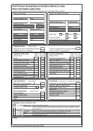
Periphyton – diatoms in watercourses 63<br />
Benthic fauna 66<br />
Fish 71<br />
Presentation of data 83<br />
Appendix 1 List of species with trophic 84<br />
ranking scores for aquatic plants<br />
Appendix 2 Calculation of index <strong>and</strong> other parameters 87<br />
for assessing benthic fauna<br />
Appendix 3 List of Swedish freshwater fish species 100
Reference Group<br />
Mats Bengtsson, Swedish Environmental Protection Agency (Secretary)<br />
Agneta Christensen, Skaraborg/Västra Götal<strong>and</strong> County Administrative Board<br />
Lars Collvin, Kristianstad/Skåne Country Administrative Board<br />
Leif Göthe, Västernorrl<strong>and</strong> County Administrative Board<br />
Mats Jansson, Umeå University<br />
Catarina Johansson, Swedish Environmental Protection Agency<br />
Lennart Lindeström, Swedish Environmental Research Group<br />
Lennart Olsson, Älvsborg/Västra Götal<strong>and</strong> County Administrative Board<br />
Eva Thörnelöf, Swedish Environmental Protection Agency<br />
Anna Ward, Jönköping County Administrative Board<br />
Project Leader: Torgny Wiederholm, Swedish University of Agricultural Sciences<br />
Project responsibility at the Swedish Environmental Protection Agency: Kjell Johansson<br />
English translation: Maxwell Arding, Arding Language Services AB
Foreword<br />
Based on favourable experience with<br />
“Environmental Criteria for <strong>Lakes</strong> <strong>and</strong><br />
<strong>Watercourses</strong>”, the Swedish Environmental<br />
Protection Agency decided in 1994 to<br />
develop a more comprehensive system for<br />
evaluating a variety of ecoystems, under<br />
the heading of “ENVIRONMENTAL QUALITY<br />
CRITERIA”. This development work has<br />
resulted in six separate reports on: the<br />
Forest L<strong>and</strong>scape, the Agricultural l<strong>and</strong>scape,<br />
Groundwater, <strong>Lakes</strong> <strong>and</strong> <strong>Watercourses</strong>,<br />
Coasts <strong>and</strong> Seas, <strong>and</strong> Contaminated<br />
Sites.<br />
ENVIRONMENTAL QUALITY CRITERIA<br />
provide a means of interpreting <strong>and</strong> evaluating<br />
environmental data which is scientifically<br />
based, yet easy to underst<strong>and</strong>. Indicators<br />
<strong>and</strong> criteria are also being developed by<br />
many other countries <strong>and</strong> international<br />
organizations. The Swedish Environmental<br />
Protection Agency has followed those developments,<br />
<strong>and</strong> has attempted to harmonise<br />
its criteria with corresponding international<br />
approaches.<br />
The reports generated thus far are based<br />
on current accumulated knowledge of environmental<br />
effects <strong>and</strong> their causes. But that<br />
knowledge is constantly improving, <strong>and</strong> it<br />
will be necessary to revise the reports from<br />
time to time. Such revisions <strong>and</strong> other developments<br />
may be followed on the Environmental<br />
Protection Agency's Internet web<br />
site, www.environ.se. Concise versions of<br />
the reports are available there as well.<br />
Development of the environmental quality<br />
criteria has been carried out in co-operation<br />
with colleges <strong>and</strong> universities. Various<br />
national <strong>and</strong> regional agencies have been<br />
represented in reference groups. The project<br />
leaders at the Environmental Protection<br />
Agency have been: Rune Andersson, Agricultural<br />
l<strong>and</strong>scapes; Ulf von Brömssen, Groundwater;<br />
Kjell Johansson, <strong>Lakes</strong> <strong>and</strong> <strong>Watercourses</strong>;<br />
Sif Johansson, Coasts <strong>and</strong> Seas;<br />
Marie Larsson <strong>and</strong> Thomas Nilsson, Forest<br />
L<strong>and</strong>scapes; <strong>and</strong> Fredrika Norman, Contaminated<br />
Sites.<br />
Project co-ordinators have been Marie<br />
Larsson (1995-97) <strong>and</strong> Thomas Nilsson<br />
(1998). Important decisions <strong>and</strong> the establishment<br />
of project guidelines have been the<br />
responsibility of a special steering committee<br />
consisting of Erik Fellenius (Chairman),<br />
Gunnar Bergvall, Taina Bäckström, Kjell<br />
Carlsson, Rune Frisén, Kjell Grip, Lars-Åke<br />
Lindahl, Lars Lindau, Anita Linell, Jan Terstad,<br />
Eva Thörnelöf <strong>and</strong> Eva Ölundh.<br />
In April of 1998, public agencies, colleges<br />
<strong>and</strong> universities, relevant organizations<br />
<strong>and</strong> other interested parties were provided<br />
the opportunity to review <strong>and</strong> comment<br />
upon preliminary drafts of the reports. That<br />
process resulted in many valuable suggestions,<br />
which have been incorporated into<br />
the final versions to the fullest extent possible.<br />
The Swedish Environmental Protection<br />
Agency is solely responsible for the<br />
contents of the reports, <strong>and</strong> wishes to<br />
express its sincere gratitude to all who participated<br />
in their production.<br />
Stockholm, Sweden, January 2000<br />
Swedish Environmental Protection Agency<br />
5
Summary<br />
This report on lakes <strong>and</strong> watercourses is one of a six-part series of reports<br />
published by the Swedish Environmental Protection Agency under the<br />
title ENVIRONMENTAL QUALITY CRITERIA. The other titles in the series<br />
are the Forest L<strong>and</strong>scape, the Agricultural L<strong>and</strong>scape, Groundwater,<br />
Coasts <strong>and</strong> Seas <strong>and</strong> Contaminated Sites. The purpose of this report is to<br />
enable local <strong>and</strong> regional authorities <strong>and</strong> others to make accurate assessments<br />
of environmental quality on the basis of available data on the state<br />
of the environment <strong>and</strong> thus obtain a better basis for environmental<br />
planning <strong>and</strong> management by objectives. Each report contains model<br />
criteria for a selection of parameters corresponding to the objectives <strong>and</strong><br />
threats existing in the area dealt with by the report. The assessment involves<br />
two aspects: (i) an appraisal of the state of the environment per se<br />
in terms of the quality of the ecosystem; (ii) an appraisal of the extent to<br />
which the recorded state deviates from a “comparative value”. In most<br />
cases the comparative value represents an estimate of a “natural” state.<br />
The results of both appraisals are expressed on a scale of 1 – 5.<br />
The report on lakes <strong>and</strong> watercourses provides a basis for assessing the<br />
status of aquatic areas in terms of physical <strong>and</strong> chemical factors such as<br />
nutrients/eutrophication, oxygen levels <strong>and</strong> oxygen-consuming substances,<br />
visibility, acidity/acidification <strong>and</strong> metals. The report also contains<br />
data on which to base an assessment of biological conditions in the<br />
form of species balance <strong>and</strong> quantities of planktonic algae, aquatic plants,<br />
diatoms, benthic macroinvertebrates <strong>and</strong> fish. In general, assessments are<br />
assumed to have been based on data gathered in accordance with the instructions<br />
in the Swedish EPA Environmental Monitoring H<strong>and</strong>book.<br />
These environmental quality criteria for lakes <strong>and</strong> watercourses represent<br />
a substantial modification <strong>and</strong> expansion of the previous version (Swedish<br />
EPA General Guidelines 90:4), which they replace.<br />
6
Environmental<br />
Quality Criteria<br />
The vision of an ecologically sustainable society includes protection of<br />
human health, preservation of biodiversity, conservation of valuable natural<br />
<strong>and</strong> historical settings, an ecologically sustainable supply <strong>and</strong> efficient use of<br />
energy <strong>and</strong> other natural resources. In order to determine how well basic<br />
environmental quality objectives <strong>and</strong> more precise objectives are being met,<br />
it is necessary to continuously monitor <strong>and</strong> evaluate the state of the<br />
environment.<br />
Environmental monitoring has been conducted for many years at<br />
both the national <strong>and</strong> regional levels. But, particularly at the regional level,<br />
assessments <strong>and</strong> evaluations of current conditions have been hindered by<br />
a lack of uniform <strong>and</strong> easily accessible data on baseline values, environmental<br />
effects, etc.<br />
This report is one of six in a series which purpose is to fill that information<br />
gap, by enabling counties <strong>and</strong> municipalities to make comparatively<br />
reliable assessments of environmental quality. The reports can thus<br />
be used to provide a basis for environmental planning, <strong>and</strong> for the setting<br />
of local <strong>and</strong> regional environmental objectives.<br />
The series bears the general heading of “ENVIRONMENTAL QUALITY<br />
CRITERIA”, <strong>and</strong> includes the following titles: The Forest L<strong>and</strong>scape, The Agricultural<br />
L<strong>and</strong>scape, Groundwater, <strong>Lakes</strong> <strong>and</strong> <strong>Watercourses</strong>, Coasts <strong>and</strong> Seas, <strong>and</strong><br />
Contaminated Sites. Taken together, the six reports cover most of the natural<br />
ecosystems <strong>and</strong> other types of environment found in Sweden. It should be<br />
noted, however, that coverage of wetl<strong>and</strong>s, mountains <strong>and</strong> urban environments<br />
is incomplete.<br />
Each of the reports includes assessment criteria for a selection of parameters<br />
relating to objectives <strong>and</strong> threats that are associated with the<br />
main subject of the report. The selected parameters are, for the most part,<br />
the same as those used in connection with national <strong>and</strong> regional environmental<br />
monitoring programmes; but there are also some “new” parameters<br />
that are regarded as important in the assessment of environmental<br />
quality.<br />
Most of the parameters included in the series describe current conditions<br />
in natural environments, e.g. levels of pollution, while direct measures<br />
of human impacts, such as the magnitude of emissions, are generally not<br />
7
included. In addition to a large number of chemical parameters, there are<br />
several that provide direct or indirect measures of biodiversity.<br />
In all of the reports, assessments of environmental quality are h<strong>and</strong>led<br />
in the same way for all of the parameters, <strong>and</strong> usually consist of two separate<br />
parts (see also page 11). One part focuses on the effects that observed<br />
conditions can be expected to have on environment <strong>and</strong> human health.<br />
Since knowledge of such effects is often limited, the solution in many cases<br />
has been to present a preliminary classification scale based on general<br />
knowledge about the high <strong>and</strong> low values that are known to occur in Sweden.<br />
The second focuses on the extent to which measured values deviate<br />
from established reference values. In most cases, the reference value represents<br />
an approximation of a “natural” state, i.e. one that has been affected<br />
very little or not at all by human activities. Of course, “natural” is a concept<br />
that is not relevant to the preservation of cultural environments; in such<br />
contexts, reference values have a somewhat different meaning.<br />
The results of both parts are expressed on a scale of 1-5, where Class 1<br />
indicates slight deviations from reference values or no environmental<br />
effects, <strong>and</strong> Class 5 indicates very large deviations or very significant effects.<br />
The report on Contaminated Sites with its discussion of pollutants in<br />
heavily affected areas complements the other five reports. In those cases<br />
where the parameters are dealt with in several of the reports, which is particularly<br />
the cases for metals, the report on Contaminated Sites corresponds<br />
(see further pages 11-12). However, the various parameters cannot<br />
be compared with each other in terms of risks. The following paragraphs<br />
review the extent of agreement with corresponding or similar systems used<br />
by other countries <strong>and</strong> international organizations.<br />
INTERNATIONAL SYSTEMS FOR ENVIRONMENTAL QUALITY ASSESSMENT<br />
Among other countries, the assessment system that most resembles Sweden's<br />
is that of Norway. The Norwegian system includes “Classification of<br />
Environmental Quality in Fjords <strong>and</strong> Coastal Waters” <strong>and</strong> “Environmental<br />
Quality Classification of Fresh Water”. A five-level scale is used to classify<br />
current conditions <strong>and</strong> usability. Classifications are in some cases based on<br />
levels of pollution, in other cases on environmental effects.<br />
The European Union's proposal for a framework directive on water quality<br />
includes an assessment system that in many ways is similar to the Swedish<br />
Environmental Quality Criteria.<br />
If the parameters used in the latter are regarded as forms of environmental<br />
indicators, there are many such systems in use or under development. However,<br />
the concept of environmental indicators is much broader than the<br />
parameters of Environmental Quality Criteria.<br />
10
Internationally, the most widely accepted framework for environmental indicators<br />
is based on PSR-chains (Pressure-State-Response). Indicators are<br />
chosen which reflect the relationship between environmental effects, <strong>and</strong>/or<br />
there causes <strong>and</strong> measures taken. There is also a more sophisticated version,<br />
called DPSIR (Driving forces-Pressure-State-Impact-Response). Variants of<br />
the PSR/DPSIR systems are used by, among others, the OECD, the Nordic<br />
Council of Ministers, the United Nations, the World Bank, the European<br />
Union's Environmental Agency.<br />
ASSESSMENT PROCEDURE<br />
Measurements/data<br />
Assessment of current conditions — indicates<br />
environmental effects associated with<br />
current conditions<br />
Assessments of deviation from reference<br />
values — indicates environmental<br />
impact of human activity<br />
Assessment of current conditions<br />
Wherever possible, the scale used in assessments of current conditions is<br />
correlated with effects on different parts of the ecosystems <strong>and</strong> their biodiversity,<br />
or on human health (”effect-related classification”). In some cases,<br />
the assessment is based only on a statistical distribution of national data<br />
(”statistical classification”).<br />
The scale is usually divided into five classes. Where the assessment is based<br />
on effects, Class 1 indicates conditions at which there are no known negative<br />
effects on the environment <strong>and</strong>/or human health. The remaining classes<br />
indicate effects of increasing magnitude. Class 5 includes conditions leading<br />
to the most serious negative effects on the environment <strong>and</strong>/or human health.<br />
Due to wide natural variations, especially with regard to biological phenomena,<br />
the indicated effects are not always the result of human activities, in<br />
which case they can not be labelled as “negative”(see below).<br />
Where the assessment is based only on a statistical distribution, there is no<br />
well-defined relationship between effects <strong>and</strong> class limits. It should be noted<br />
that parameters that are evaluated on the basis of different criteria cannot be<br />
compared with each other.<br />
Reference values<br />
Ideally, the reference value for a given parameter represents a natural state<br />
that has not been affected by any human activity. In practice, however, reference<br />
values are usually based on observations made in areas that have experienced<br />
some slight human impact. In some cases, historical data or model-<br />
11
ased estimates are used. Given that there are wide natural variations of<br />
several of the parameters, reference values in many cases vary by region or<br />
type of ecoystem.<br />
Deviations from reference values<br />
The extent of human impact can be estimated by calculating deviations from<br />
reference values, which are usually stated as the quotient between a measured<br />
value <strong>and</strong> the corresponding reference value:<br />
Measured value<br />
Deviation = -------------------------------------<br />
Reference value<br />
The extent of deviation is usually classified on a five-level scale. Class 1<br />
includes conditions with little or no deviation from the reference value, which<br />
means that effects of human activity are negligible. The remaining classes<br />
indicate increasing levels of deviation (increasing degree of impact). Class 5<br />
usually indicates very significant impact from local sources.<br />
Organic pollutants <strong>and</strong> metals in heavily polluted areas are dealt with in<br />
greater detail in a separate report, Contaminated Sites, which includes a<br />
further sub-division of Class 5, as follows:<br />
Contaminated Sites<br />
Impact from point sources:<br />
None/ Moderate Substantial Very<br />
slight<br />
great<br />
Class 1 Class 2 Class 3 Class 4 Class 5<br />
Other reports<br />
12
Environmental Quality<br />
Criteria for <strong>Lakes</strong> <strong>and</strong><br />
<strong>Watercourses</strong><br />
Choice of parameters<br />
Environmental Quality Criteria for <strong>Lakes</strong> <strong>and</strong> <strong>Watercourses</strong> should be<br />
used to evaluate the results of environmental monitoring <strong>and</strong> other<br />
studies. The parameters <strong>and</strong> methods to be used for this purpose are<br />
largely determined using the Swedish EPA Environmental Monitoring<br />
H<strong>and</strong>book. Similarly, studies commenced before publication of the<br />
h<strong>and</strong>book are governed by the Agency’s General Guidelines for<br />
Coordinated Monitoring of Receiving Bodies.<br />
The Swedish EPA method instructions contain a large number of<br />
parameters. It is hardly feasible or even desirable to produce model<br />
criteria for all of them. Instead, the parameters selected for this report are<br />
those considered to be the most important indicators of water quality in a<br />
wide sense. Hence, chemical parameters include those indicating threats<br />
to the environment such as eutrophication, acidification <strong>and</strong> the<br />
presence of metals. Among biological parameters are measures of the<br />
state of different parts of food chains <strong>and</strong> which in some cases are<br />
relevant to use of the water. The biological parameters do not usually<br />
reflect specific threats; rather they provide an integrated measure of the<br />
environmental situation as a whole <strong>and</strong> any impact to which an aquatic<br />
area may be exposed. The environmental relevance of each parameter is<br />
explained in detail in the individual chapters <strong>and</strong> in the reasons given for<br />
each type of investigation in the EPA Environmental Monitoring H<strong>and</strong>book.<br />
For various reasons it has not been possible to include some parameters,<br />
which do in fact represent important aspects of water quality.<br />
These include measures of hydrological <strong>and</strong> substrate conditions. Nor<br />
has it been possible to formulate instructions for assessing changes in<br />
water quality over time.<br />
An outline of the parameters included is given in Table 1 on pages 14<br />
<strong>and</strong> 15.<br />
Classification <strong>and</strong> class delimitation<br />
Environmental Quality Criteria use two types of scale: one for assessing<br />
current conditions <strong>and</strong> one for assessing deviation from reference values.<br />
13
TABLE 1.<br />
SUMMARY of parameters included in Environmental Quality Criteria for<br />
<strong>Lakes</strong> <strong>and</strong> <strong>Watercourses</strong> (a minus sign indicates the absence of model<br />
criteria).<br />
Area/parameter <strong>Lakes</strong>/ Current Deviation<br />
water- conditions from<br />
courses<br />
reference<br />
value<br />
Nutrients/eutrophication<br />
Total phosphorus concentration l + +<br />
Total nitrogen concentration l + -<br />
Total nitrogen/total phosphorus ratio (by weight) l + -<br />
Area-specific total nitrogen loss w + +<br />
Area-specific total phosphorus loss w + +<br />
Oxygen status <strong>and</strong> oxygen-consuming substances<br />
Oxygen concentration l/w + -<br />
TOC (total organic carbon) l/w + -<br />
CODMn (chemical oxygen dem<strong>and</strong>) l/w + -<br />
Light conditions<br />
Absorbency l/w + -<br />
Water colour l/w + -<br />
Turbidity l/w + -<br />
Secchi depth l + -<br />
Acidity/acidification<br />
Alkalinity l/w + +<br />
pH l/w + -<br />
Metals<br />
Metals in water, sediment, moss <strong>and</strong> fish l/w* + -<br />
Phytoplankton<br />
Total volume l + +<br />
Chlorophyll concentration l + +<br />
Diatoms l + -<br />
Water-blooming cyanobacteria l + +<br />
Potentially toxin-producing cyanobacteria l + +<br />
Biomass Gonyostomum semen l + +<br />
14
TABLE 1.<br />
Continued<br />
Area/parameter <strong>Lakes</strong>/ Current Deviation<br />
water- conditions from<br />
courses<br />
reference<br />
value<br />
Aquatic plants<br />
Submerged <strong>and</strong> floating-leaved plants,<br />
number of species <strong>and</strong> indicator ratio** l + +<br />
Periphyton – diatoms<br />
IPS index w + -<br />
IDG index w + -<br />
Benthic fauna<br />
Shannon’s diversity index*** l/w + +<br />
Danish fauna index*** l/w + +<br />
ASPT index*** l/w + +<br />
Acidity index l/w + +<br />
BQI index**** l + +<br />
O/C index**** l + +<br />
Fish<br />
Naturally occurring Swedish species l/w + +<br />
Species diversity of native species l + +<br />
Biomass of native species l/w + +<br />
Number of individuals of native l/w + +<br />
species<br />
Proportion of cyprinids l - +<br />
Proportion of Piscivorous fish l + +<br />
Proportion of salmonids w + +<br />
Salmonid reproduction w + +<br />
Species <strong>and</strong> stages sensitive to acidification l/w - +<br />
Species tolerant of low oxygen concentrations l - +<br />
Proportion of biomass comprising l/w - +<br />
alien species<br />
Composite value derived from (part of) the above l/w + +<br />
* lake sediment<br />
** indicator value for assessing deviation from reference value<br />
*** in lakes: the littoral zone<br />
**** the profundal zone<br />
15
16<br />
The current conditions scale in this report is based on the levels occurring<br />
in Sweden for each parameter <strong>and</strong>, to some extent, on the biological<br />
<strong>and</strong> other conditions characterising different levels. Hence, as far as<br />
possible, the boundaries between the classes coincide with clear changes<br />
on the relevant gradient. Where it has not been possible to identify levels<br />
where such changes occur, boundaries have been decided statistically on<br />
the basis of the most representative data possible, or arbitrarily on the<br />
basis of an overall judgement of what can be considered reasonable.<br />
The width of the classes varies, depending on the way each parameter<br />
changes along a gradient from low to high or vice versa. In some cases,<br />
changes in the lower range of the scale are particularly significant. Here<br />
scales have been graduated to give them sufficient resolution in this<br />
respect. In other cases, changes occur gradually along a gradient <strong>and</strong> the<br />
boundaries between classes are more evenly distributed along the scale.<br />
The way scales have been developed for individual parameters may be<br />
seen in each chapter.<br />
It should be emphasised that the assessment scales cannot easily be<br />
interpreted as representing ”good” or ”bad” environmental quality. The<br />
parameters must be evaluated individually in the light of the quality<br />
aspects they are intended to reflect. This applies particularly to the scales<br />
for assessment of current conditions. A number of examples serve to<br />
illustrate this. Chemical parameters such as metals, organic pollutants<br />
<strong>and</strong> alkalinity are fairly closely related to water quality in the sense that<br />
increasing concentrations (decreasing for alkalinity) can generally be said<br />
to reflect a growing risk of negative effects on aquatic organisms or use of<br />
water resources. The scale for total phosphorus reflects conditions for<br />
increasing quantities of phytoplankton in water. From an aesthetic viewpoint,<br />
for bathing, water supply etc, an increase of this kind is generally<br />
considered undesirable, but in production terms, the scale should have<br />
been placed the other way round. This has not been done because the<br />
total phosphorus parameter is primarily intended to indicate conditions<br />
for the presence of phytoplankton <strong>and</strong> associated adverse effects. This<br />
rationale also underlies the form chosen for assessment scales for other<br />
parameters. Thus, classification of the state of fish assemblages is based<br />
on expected fish numbers <strong>and</strong> diversity of fish species. Class 1 (lakes)<br />
indicates a large number of fish, a large number of species with high<br />
diversity <strong>and</strong> a high proportion of piscivorous species, ie, a rich <strong>and</strong><br />
diverse fish community. Class 1 watercourses feature a large number of<br />
salmonids with high breeding success. Class 3 indicates that the fish<br />
assemblages in the lake or watercourse are average for Swedish waters,<br />
whereas class 5 indicates assemblages poor in numbers of species <strong>and</strong><br />
individuals. In the case of parameters where contradictory interpretations<br />
or evaluations are possible, the direction of the scales has been decided
y the environmental quality aspects each parameter is primarily<br />
intended to indicate <strong>and</strong> factors that have been deemed essentially<br />
”good” or ”bad” in this respect.<br />
Assessing deviation from reference values is generally less of a problem<br />
than assessing current conditions. Increasingly pronounced<br />
deviation from the reference value, ie, from a natural state, is usually<br />
regarded as negative. Here too, therefore, class 1 represents the most<br />
favourable conditions <strong>and</strong> class 5 the least favourable. Once again, the<br />
assessment is made in the light of the quality aspects the respective<br />
parameters are primarily intended to reflect. Growing deviations may be<br />
favourable from other perspectives, which should be borne in mind when<br />
using the scales.<br />
The boundaries between classes are such that the classes might be<br />
perceived to overlap. However, when entering recorded values account<br />
should be taken of the way the threshold for the highest or lowest class<br />
has been expressed. Hence, (2.0 for class 1 <strong>and</strong> 2.0 – 5.0 for class 2<br />
(chlorophyll concentration in lakes) means that a readings of 2.0 should<br />
be entered in class 1 <strong>and</strong> a reading of 5.0 in class two, <strong>and</strong> so on.<br />
Reference values<br />
The reference values have been arrived at in different ways for different<br />
parameters, depending on the availability of data. In some cases it has<br />
been possible to use the reference stations in the Swedish National Environmental<br />
Monitoring Programme. In others, collated data from environmental<br />
monitoring or from specific studies has been used, usually<br />
having eliminated stations considered to be affected. As regards fish,<br />
calculations have been made using national or supra-regional data bases<br />
in their entirety. Thus, these reference values represent the mean situation<br />
in Swedish lakes <strong>and</strong> watercourses across the country or for<br />
different types of lakes <strong>and</strong> watercourses. It has not been considered<br />
possible to identify pristine waters. Finally, it has not been possible to set<br />
reference values for some parameters at all. Here, assessments can only<br />
be made using a state scale (current conditions).<br />
In general, it has only been possible to a limited extent to give instructions<br />
on reference values specific to a given lake or watercourse, ie, on the<br />
way in which reference values for a particular lake or watercourse can be<br />
determined in the light of its position <strong>and</strong> other surrounding factors.<br />
Further work on development of calculation models is needed in this<br />
field. In the absence of such methods, reference values have been calculated<br />
statistically for regions (see next chapter) or groups of lakes/watercourses,<br />
eg, different types of lakes. The accuracy of these values varies<br />
<strong>and</strong> the assessment should be made with this in mind <strong>and</strong> in the light of<br />
the factors <strong>and</strong> conditions presented in the relevant background report<br />
17
(in Swedish with English summary). The method of identifying reference<br />
values is explained in each chapter. In general, it may be said that further<br />
systematic studies are needed for most parameters in order to obtain<br />
representative data.<br />
It was proposed in the previous quality criteria for lakes <strong>and</strong> watercourses<br />
(Swedish EPA 1991) that county administrative boards <strong>and</strong><br />
water management associations should compile maps on background<br />
conditions by catchment based on results from earlier surveys <strong>and</strong> studies<br />
of unaffected lakes <strong>and</strong> watercourses or using specified calculation algorithms.<br />
This is still to be recommended <strong>and</strong> would probably allow better<br />
adjustment to local or regional conditions than direct application of the<br />
reference values presented here, which are often regional <strong>and</strong> statistically<br />
based.<br />
Division in type areas<br />
Since available data varies greatly from one parameter to another <strong>and</strong><br />
since various surrounding factors are significant to each parameter, it has<br />
not been possible to classify geographical regions <strong>and</strong> water types on the<br />
basis of principles common to all parameters. The various classifications<br />
are described in each chapter.<br />
References<br />
Swedish Environmental Protection Agency (1991): Bedömningsgrunder<br />
för sjöar och vattendrag (”Quality criteria for lakes <strong>and</strong> watercourses”).<br />
Swedish EPA General Guidelines 90:4.<br />
18
Nutrients /<br />
eutrophication<br />
Introduction<br />
Elevated nutrient levels, known as eutrophication, result from an increased<br />
influx or increased availability of plant nutrients in lakes <strong>and</strong><br />
watercourses. Eutrophication leads to increased production <strong>and</strong> plant<br />
<strong>and</strong> animal biomass, increased turbidity, greater oxygen dem<strong>and</strong> resulting<br />
from the decomposition or organic matter <strong>and</strong> a change in species<br />
composition <strong>and</strong> diversity of plant <strong>and</strong> animal communities. In most<br />
cases the nutrients governing vegetative growth in fresh water are phosphorus<br />
(P) <strong>and</strong>, in a few cases, nitrogen (N).<br />
Total phosphorus, total nitrogen <strong>and</strong> the phosphorus/nitrogen ratio<br />
are parameters used to assess lakes. Total phosphorus has been chosen<br />
even though this includes phosphorus fixed in minerals <strong>and</strong> humus,<br />
which is not directly available to plants. This is due to the need for an<br />
indicator that is analytically straightforward <strong>and</strong> generally used. The<br />
relative importance of phosphorus <strong>and</strong> nitrogen is proportional to the<br />
quantities in which they occur, here described as the weight ratio between<br />
the concentration of total nitrogen <strong>and</strong> that of total phosphorus.<br />
This indicates a deficit or surplus of the two elements <strong>and</strong> shows the<br />
potential for nitrogen fixation <strong>and</strong> for accumulation of nitrogen-fixing<br />
cyanobacteria (”blue-green algae”). The concentration of total phosphorus,<br />
like the N/P ratio, can be clearly linked to biological <strong>and</strong> biochemical<br />
effects. Unlike the N/P ratio, the scale for total nitrogen concentrations,<br />
which is also given, does not measure the effects of nitrogen<br />
on production; it is intended to differentiate between various typical<br />
concentrations in Swedish lakes.<br />
The area-specific loss of nitrogen <strong>and</strong> phosphorus, respectively, is used<br />
when assessing watercourses. Although this indicator, in principle, mainly<br />
belongs to the criteria for the Agricultural L<strong>and</strong>scape <strong>and</strong> the Forest<br />
L<strong>and</strong>scape, it has been included here since monitoring <strong>and</strong> calculation of<br />
these losses are a normal <strong>and</strong> increasingly important part of the environmental<br />
water monitoring programme <strong>and</strong> since area-specific losses <strong>and</strong><br />
discharge of plant nutrients are of importance to the pollution burden on<br />
lakes <strong>and</strong> marine areas.<br />
Area-specific losses are also an indirect predictor of production<br />
19
conditions for watercourse flora <strong>and</strong> fauna. No specific scales are given<br />
for assessing concentrations of nitrogen or phosphorus in watercourses;<br />
it is expected that these will be evaluated having been converted in areaspecific<br />
losses. Instructions for conversion are given with the scales in<br />
question.<br />
High concentrations of nitrate in drinking water can constitute a<br />
health problem <strong>and</strong> the National Food Administration defines drinking<br />
water as ”fully fit for consumption” when nitrate concentrations are<br />
below 10 mg NO3-N/l. Assessment scales for nitrate are not given here,<br />
however.<br />
Ammonium is converted into molecular ammoniac in an equilibrium<br />
reaction at high pH levels. The risk of fish <strong>and</strong> other aquatic organisms<br />
being poisoned rises rapidly at high ammonium concentrations at pH<br />
level exceeding about 8. Calculation methods <strong>and</strong> criteria for toxicity to<br />
fish <strong>and</strong> other aquatic organisms have been published (see references).<br />
Assessment scales for ammoniac are not given here.<br />
Assessment of current conditions<br />
TABLE 2.<br />
CURRENT CONDITIONS: concentration of total phosphorus<br />
in lakes (µg/l)<br />
Class Description Concentration Concentration<br />
May – October August<br />
1 Low concentrations ≤ 12.5 ≤ 12.5<br />
2 Moderately high concentrations 12.5 – 25 12.5 – 23<br />
3 High concentrations 25 – 50 23 – 45<br />
4 Very high concentrations 50 – 100 45 – 96<br />
5 Extremely high concentrations > 100 Not defined<br />
Concentrations are given as seasonal mean (May – October) over one<br />
year based on monthly readings taken in the epilimnion or, if only one<br />
sample is taken, surface water (0.5 m). The concentration of total phosphorus<br />
displays little seasonal variation at lower concentration ranges<br />
<strong>and</strong> an assessment can also be made of concentrations recorded in<br />
August as shown above, although it should then be assessed as a mean<br />
figure over three years. Late summer concentrations vary enormously at<br />
extremely high concentrations <strong>and</strong> seasonal mean figures should be used<br />
to make an assessment. The classes relate to various production levels<br />
long used by limnologists, principally determined by the phosphorus<br />
20
concentrations. Using accepted terminology, the classes correspond to<br />
oligotrophy (1), mesotrophy (2), eutrophy (3 <strong>and</strong> 4) <strong>and</strong> hypertrophy (5).<br />
There is good reason to define a further characteristic sub-group with<br />
concentrations below 6 µg/l within the oligotrophic range. This group<br />
represents ultra-oligotrophy.<br />
Total nitrogen is more variable during the season than total phospho-<br />
TABLE 3.<br />
CURRENT CONDITIONS: concentration of total nitrogen<br />
in lakes (µg/l)<br />
Class Description Concentration May – October<br />
1 Low concentrations ≤ 300<br />
2 Moderately high concentrations 300 – 625<br />
3 High concentrations 625 – 1.250<br />
4 Very high concentrations 1.250 – 5.000<br />
5 Extremely high concentrations > 5.000<br />
rus <strong>and</strong> is therefore unsuitable for assessments based on concentrations in<br />
August. Inorganic nitrogen (nitrate + ammonium) peaks markedly in late<br />
winter <strong>and</strong> organic nitrogen reaches a peak in the summer. It is therefore<br />
difficult to describe a general pattern of variation for total nitrogen.<br />
TABLE 4.<br />
CURRENT CONDITIONS: ratio of total nitrogen/<br />
total phosphorus in lakes<br />
Class Description Ratio June – September<br />
1 Nitrogen surplus ≥ 30<br />
2 Nitrogen – phosphorus balance 15 – 30<br />
3 Moderate nitrogen deficit 10 – 15<br />
4 Large nitrogen deficit 5 – 10<br />
5 Extreme nitrogen deficit < 5<br />
The assessment scale is intended to group concentrations that are<br />
typical of Swedish lakes <strong>and</strong> is not related to biological/microbial effects.<br />
The scale refers to the mean value during June – September over one<br />
year based on monthly readings taken in the epilimnion or, if only one<br />
sample is taken, surface water (0.5 m). The ratios are weight-based <strong>and</strong><br />
21
show the availability of nitrogen in relation to phosphorus in lakes.<br />
In class 1 the availability of phosphorus alone governs production; in<br />
class 2 there is a tendency for accumulation of cyanobacteria (”bluegreen<br />
algae”) in general; in class 3 the occurrence of nitrogen fixation <strong>and</strong><br />
specific nitrogen-fixing cyanobacteria is likely; in class 4 nitrogen fixation<br />
is highly likely but cannot fully compensate for the nitrogen deficit, <strong>and</strong><br />
in class 5 the nitrogen deficit is extreme <strong>and</strong> fixation is unable to<br />
compensate.<br />
TABLE 5.<br />
CURRENT CONDITIONS: area-specific loss of total nitrogen,<br />
watercourses (kg N/ha, year)<br />
Class Description Area-specific loss<br />
1 Very low losses ≤ 1.0<br />
2 Low losses 1.0 – 2.0<br />
3 Moderately high losses 2.0 – 4.0<br />
4 High losses 4.0 – 16.0<br />
5 Very high losses > 16<br />
Area-specific losses refer to the monitoring of concentrations 12 times<br />
a year over three years <strong>and</strong> recorded or modelled water flow per 24-hour<br />
period. It may be necessary to monitor concentrations more frequently in<br />
small watercourses. 24-hour water flow figures are multiplied by the<br />
corresponding concentrations obtained using linear interpolation between<br />
readings. The 24-hour transport figures thus obtained are accumulated<br />
to give annual figures <strong>and</strong> show area-specific losses after division by<br />
the area of the catchment.<br />
Nitrogen loss includes input from all sources upstream of the monitoring<br />
point, which classifies the total area-specific input from the catchment<br />
to lakes <strong>and</strong> seas, for example. The scale is also intended to be used<br />
to assess losses from all types of soil in comparison with normal losses<br />
from different types of l<strong>and</strong> use. Known input from point sources can be<br />
deducted to gain a better picture of diffuse nitrogen losses.<br />
Class 1 represents normal leaching from mountain heaths <strong>and</strong> the<br />
poorest forest soils. Class 2 shows normal leaching from non-nitrogensaturated<br />
forest soils in northern <strong>and</strong> central Sweden. Class 3 contains<br />
losses from unaffected bog/peat l<strong>and</strong> <strong>and</strong> affected forest soils (eg,<br />
leaching from certain clear-cut areas), as well as leaching from arable<br />
soils (unfertilised seeded grassl<strong>and</strong>). Class 4 shows common leaching<br />
22
from fields in lowl<strong>and</strong> areas <strong>and</strong> class 5 represents leaching from cultivated<br />
s<strong>and</strong>y soils, often combined with manure use.<br />
Since nitrogen losses over fairly large agricultural areas exceed 16 kg<br />
N/ha, there is reason to make particular note of areas where nitrogen<br />
losses are extreme (over 32 kg N/ha, year). This is particularly called for<br />
when setting priorities for remedial measures.<br />
The different classes are matched by various flow-weighted annual<br />
mean concentrations, depending on the flow per unit surface area. Figure 1<br />
shows the correlations between area-specific loss <strong>and</strong> concentration at<br />
four different levels of flow per unit surface area.<br />
TABLE 6.<br />
CURRENT CONDITIONS: area-specific loss of total phosphorus,<br />
watercourses (kg P/ha, year)<br />
Class Description Area-specific loss<br />
1 Very low losses ≤ 0.04<br />
2 Low losses 0.04 – 0.08<br />
3 Moderately high losses 0.08 – 0.16<br />
4 High losses 0.16 – 0.32<br />
5 Very high losses > 0.32<br />
Area-specific losses refer to the monitoring of concentrations 12 times<br />
a year over three years <strong>and</strong> recorded or modelled water flow per 24-hour<br />
period. It may be necessary to monitor concentrations more frequently in<br />
small watercourses. 24-hour water flow figures are multiplied by the<br />
corresponding concentrations obtained using linear interpolation<br />
between readings. The 24-hour transport figures thus obtained are<br />
accumulated to give annual figures <strong>and</strong> show area-specific losses after<br />
division by the area of the catchment.<br />
Phosphorus loss includes input from all sources upstream of the<br />
monitoring point, which classifies the total area-specific input from the<br />
catchment to lakes <strong>and</strong> seas, for example. The scale is also intended to be<br />
used to assess losses from all types of soil in comparison with normal<br />
losses from different types of l<strong>and</strong> use. Known input from point sources<br />
can be deducted to gain a better picture of diffuse phosphorus losses.<br />
Class 1 represents the lowest leaching on record from unaffected<br />
forest soils. Class 2 shows normal leaching from normal forest soils in<br />
Sweden. Class 3 contains losses from clear-cut areas, bog/peat l<strong>and</strong>,<br />
23
Mean concentration of total phosphorus (µg P/l)<br />
200<br />
180<br />
160<br />
140<br />
120<br />
100<br />
q = 5 l/s,km 2<br />
q = 10 l/s,km 2 10000<br />
9000<br />
8000<br />
7000<br />
6000<br />
5000<br />
q = 5 l/s,km 2<br />
q = 10 l/s,km 2<br />
80<br />
q = 15 l/s,km 2<br />
4000<br />
q = 15 l/s,km 2<br />
60<br />
40<br />
q = 20 l/s,km 2<br />
3000<br />
2000<br />
q = 20 l/s,km 2<br />
20<br />
1000<br />
0<br />
0 0.04 0.08 0.12 0.16 0.20 0.24 0.28 0.32<br />
0<br />
0 2 4 6 8 10 12 14 16<br />
Area-specific phosphorus loss (kg P/ha, year)<br />
Area-specific nitrogen loss (kg N/ha, year)<br />
Mean concentration of total nitrogen (µg N/l)<br />
Figure 1. Annual mean concentration of phosphorus <strong>and</strong> nitrogen as a function of annual area-specific loss.<br />
arable soils less susceptible to erosion, often with seeded grass cultivation.<br />
Class 4 represents losses from fields under open cultivation <strong>and</strong> class 5<br />
shows leaching from arable soils susceptible to erosion.<br />
Since phosphorus losses over fairly large agricultural areas exceed 0.32<br />
kg P/ha, year, there is reason to make particular note the subgroup of<br />
areas within class 5 where phosphorus losses are extreme (over 0.64 kg<br />
N/ha, year). This is particularly called for when setting priorities for<br />
remedial measures.<br />
The different classes are matched by various flow-weighted annual<br />
mean concentrations, depending on the flow per unit surface area. Figure 1<br />
shows the correlations between area-specific loss <strong>and</strong> concentration at<br />
four different levels of flow per unit surface area.<br />
Assessment of deviation from reference values<br />
TABLE 7.<br />
DEVIATION from reference value, concentration of total<br />
phosphorus in lakes<br />
Class Description Recorded concentration/ reference value<br />
1 No or insignificant deviation ≤ 1.5<br />
2 Significant deviation 1.5 – 2.0<br />
3 Large deviation 2.0 – 3.0<br />
4 Very large deviation 3.0 – 6.0<br />
5 Extreme deviation > 6.0<br />
24
This classification is based on an overall assessment taking account of the<br />
concentrations occurring in Swedish lakes at various degrees of human<br />
impact.<br />
Recorded concentration represents the mean value over three years<br />
for the period May – October. By using 3-year mean values for August<br />
alone, account must be taken of the element of uncertainty introduced.<br />
Reference values can be calculated or estimated in a number of ways.<br />
They can be estimated on the basis of historical studies of the area in<br />
question or studies of similar but unaffected lakes in the vicinity. However,<br />
phosphorus concentrations in some acidified lakes may be lower<br />
than the original level. In the absence of other data, reference values can<br />
be calculated using the correlation between total phosphorus <strong>and</strong><br />
coloured organic matter:<br />
TP ref (µg P/l) = 5 + 48 · abs f 420/5<br />
This function gives minimum observed values at a given absorbency <strong>and</strong>,<br />
generally speaking, a higher degree of deviation. In some cases, the extent<br />
of deviation may be estimated to be up to one class higher than in reality.<br />
Clear mountain waters are a case in point. The function has been derived<br />
from environmental monitoring programme data where series of at least<br />
five years have been available. Taking account of the element of uncertainty<br />
introduced, absorbency (abs f 420/5 ) can be calculated by multiplying<br />
water colour (mg Pt/l) by 0.002.<br />
In some limed or acidified lakes the ratio of recorded concentration to<br />
reference value may be less than 1, which may indicate oligotrophication,<br />
ie, a shift towards a more nutrient-poor state. Conditions of this kind<br />
should be particularly noted so as to allow further study of possible<br />
acidification-related effects.<br />
TABLE 8.<br />
DEVIATION from reference value, area-specific loss of total<br />
phosphorus in watercourses<br />
Class Description Recorded area-specific loss/reference value<br />
1 No or insignificant deviation ≤ 1.5<br />
2 Significant deviation 1.5 – 3<br />
3 Large deviation 3 – 6<br />
4 Very large deviation 6 – 12<br />
5 Extreme deviation > 12<br />
25
TABLE 9.<br />
DEVIATION from reference value, area-specific loss of total<br />
nitrogen in watercourses<br />
Class Description Recorded area-specific loss/reference value<br />
1 No or insignificant deviation ≤ 2.5<br />
2 Significant deviation 2.5 – 5<br />
3 Large deviation 5 – 20<br />
4 Very large deviation 20 – 60<br />
5 Extreme deviation > 60<br />
This classification is based on an overall assessment taking into account<br />
the area-specific losses occurring in Swedish watercourses affected by<br />
man to varying degrees. In some catchments, the ratio between recorded<br />
concentration <strong>and</strong> reference value may be less than 1, which may<br />
indicate a phosphorus deficit. Conditions of this kind should be particularly<br />
noted so as to allow further study of possible acidification-related<br />
effects. In some catchments, the ratio of recorded concentration to<br />
reference value for nitrogen may be less than 1, which may indicate a<br />
nitrogen deficit.<br />
Recorded area-specific loss refers to a mean figure for a 3-year period,<br />
calculated as shown above for classification of current conditions for<br />
area-specific losses.<br />
Reference values can be calculated or estimated in several ways. They<br />
may be estimated on the basis of historical studies of the area in question<br />
or studies of similar but unaffected watercourses in the vicinity. In the<br />
absence of other data, reference values can also be calculated using the<br />
characteristics of the catchment <strong>and</strong> other features of the watercourse.<br />
The equations specified in the previous Quality criteria for lakes <strong>and</strong><br />
watercourses (Swedish EPA 1991) can be used for this purpose, together<br />
with the additional equation shown below. All these relationships are<br />
expected to yield low estimates <strong>and</strong> the highest figure obtained using<br />
equations (1) – (5) <strong>and</strong> (6) – (10) should be used as the reference value.<br />
One exception is where the lake percentage is less than or equal to 2,<br />
where equations (2) <strong>and</strong> (7) should not be used.<br />
26
TP ref (kg P/ha, year) =<br />
0.002 · x 1 + 0.015 (1)<br />
(0.10 · x 2 + 1.2) / (5 · x 2 + 12) (2)<br />
0.91 · x 3 · 10 –3 + 0.02 (3)<br />
2.45 · x 4 · 10 –3 + 0.024 (4)<br />
3.15 · x 1 · 10 –4 · (5 + 60 · x 5 ) (5)<br />
TN ref (kg N/ha, year) =<br />
0.018 · x 1 + 0.85 (6)<br />
–0.023 · x 2 + 1.25 (7)<br />
0.008 · x 3 + 0.85 (8)<br />
0.03 · x 4 + 0. 90 (9)<br />
3.15 · x 1 · 10 –4 · (125 + 500 · x 5 ) (10)<br />
where x 1 = specific flow (l/km 2 , sec)<br />
x 2 = lake percentage in catchment<br />
x 3 = area-specific loss COD Mn (kg/ha, year)<br />
x 4 = area-specific loss silicon (kg/ha, year)<br />
x 5 = flow-weighted mean absorbency 420 nm (abs f 420/5 )<br />
The new function (5, 10) uses the absorbency of the water measured<br />
using filtered water (0.45 µm membrane filter) in a 5 cm cuvette at a<br />
wavelength of 420 nm. Taking account of the element of uncertainty<br />
introduced, absorbency (abs f 420/5 ) can be calculated by multiplying<br />
water colour (mg Pt/l) by 0.002.<br />
COD Mn is derived by dividing the permanganate number by 3.95.<br />
One of these equations may be unsuitable for use in some situations.<br />
Hence, organic matter may raise the concentration of oxygen-consuming<br />
substances, which will render use of COD inappropriate. If the pollutant<br />
is largely uncoloured matter, the absorbency function (5, 10) will be a<br />
better guide. This should in turn be avoided where it is suspected that<br />
water colour is anthropogenically elevated, eg, as a result of discharges<br />
from pulp <strong>and</strong> paper mills, leachate from rubbish tips or because of<br />
increased humus losses caused by forestry practices. Silica (4, 9) may also<br />
be anthropogenically affected, eg, in the form of lower concentrations<br />
due to eutrophication, which will particularly impact on water systems<br />
containing many lakes.<br />
27
Comments<br />
Classifications must be based on samples taken <strong>and</strong> analyses made in<br />
accordance with the Swedish EPA Environmental Monitoring H<strong>and</strong>book.<br />
The scales should be used bearing in mind the wide natural<br />
variation between individual lakes <strong>and</strong> watercourses <strong>and</strong> from year to<br />
year. The number of sampling occasions or the time scale on which the<br />
various assessments are based represents minimum figures. If <strong>and</strong> when<br />
assessments are made on the basis of more limited data, this should be<br />
stated.<br />
The scale for N/P ratios in lakes is intended to be used provisionally<br />
<strong>and</strong> with a degree of feedback as to results obtained. The ratios have been<br />
obtained using older analytical methods for total nitrogen (Kjeldahl-N +<br />
ammonium-N) <strong>and</strong> are affected in calculation terms by the reduction in<br />
the concentrations of total nitrogen obtained using new analytical<br />
methods (total-N using Swedish St<strong>and</strong>ard SSO28131). No correction has<br />
been made to take account of this, however. The effects the class<br />
boundaries are intended to identify may therefore occur at somewhat<br />
lower ratios than those given in the criteria.<br />
References<br />
Alabaster, J.S. & Lloyd, R. (1982): Water quality criteria for freshwater fish. 2nd<br />
ed. – Butterworths, London.<br />
Swedish Environmental Protection Agency (1991): Bedömningsgrunder för sjöar<br />
och vattendrag (”Quality criteria for lakes <strong>and</strong> watercourses”). Swedish EPA<br />
General Guidelines 90:4.<br />
Persson, G. Växtnäringsämnen/eutrofiering (”Nutrients/eutrophication”). – From:<br />
T. Wiederholm (Ed.). Bedömningsgrunder för miljökvalitet - Sjöar och vattendrag.<br />
Bakgrundsrapport 1 – Kemiska och fysikaliska parametrar (”Environmental Quality<br />
Criteria – <strong>Lakes</strong> <strong>and</strong> <strong>Watercourses</strong>. Background report 1 – Chemical <strong>and</strong> physical<br />
parameters”). Swedish EPA Report 4920.<br />
Premazzi, G. & Chiaudani, G. (1992): Ecological quality of surface waters.<br />
Quality assessment for European Community lakes. – ECSC-EEC-EAEC,<br />
Brussels, Luxembourg.<br />
Wiederholm, T., Welch, E., Persson, G., Karlgren, L. & von Brömssen, U. (1983):<br />
Bedömningsgrunder och riktvärden för fosfor i sjöar och vattendrag. Underlag för<br />
försöksverksamhet. (”Quality criteria <strong>and</strong> guide values for phosphorus in lakes <strong>and</strong><br />
watercourses. Background data for experiments”) – Swedish EPA PM 1705.<br />
28
Oxygen status <strong>and</strong><br />
oxygen-consuming<br />
substances<br />
Introduction<br />
Dissolved oxygen is vital for respiration <strong>and</strong> many microbial <strong>and</strong> chemical<br />
processes in the ecosystem. The concentration may thus regulate the<br />
biological structure. Oxygen conditions vary, mainly due to changing<br />
production conditions <strong>and</strong> the organic load, including natural humic<br />
substances leaching from the catchment area. In the bottom water of<br />
stratified lakes (the hypolimnion), the oxygen situation is at its worst at<br />
the end of the stagnation period in summer, at which time conditions<br />
may become critical for many organisms. The end of the period when<br />
lakes <strong>and</strong> rivers are ice-covered is another crucial time. Oxygen conditions<br />
in watercourses may be poorest at times of low flow, particularly in<br />
polluted rivers. Significant variations in oxygen levels <strong>and</strong> oxygen<br />
saturation can occur from one day to the next in the surface waters of<br />
unstratified lakes <strong>and</strong> in rivers <strong>and</strong> streams.<br />
Oxygen concentration is prefered to saturation as a means of characterising<br />
oxygen status because the thresholds of tolerance of various<br />
organisms are usually expressed as concentrations. However, merely<br />
stating the oxygen concentration may give an incomplete picture of<br />
oxygen conditions, particularly in rivers <strong>and</strong> streams. This is due to<br />
variations in oxygen input <strong>and</strong> organic load. The presence of oxygenconsuming<br />
substances should therefore also be taken into account. The<br />
concentration of organic matter provides essential information about the<br />
risk of low oxygen levels occurring between the occasions on which<br />
oxygen concentrations are monitored.<br />
A high oxygen concentration or oxygen saturation is not always a sign<br />
of a ”healthy” environment. Assimilation by plants may result in saturation<br />
figures of over 100 per cent in eutrophic waters.<br />
Scales have only been given for assessing current conditions because<br />
of the difficulties of determining reference values.<br />
Assessment of current conditions<br />
Oxygen status is assessed in the bottom waters of stratified lakes <strong>and</strong> also<br />
in the circulating water column in unstratified lakes. Annual minimum<br />
values based on concentrations monitored during critical periods (late<br />
29
winter/spring, i.e. ice-covered period, late summer/autumn) over three<br />
years are assessed for all lakes.<br />
Annual minimum values for watercourses are also assessed, although<br />
here assessment should be based on samples taken 12 times a year over<br />
three years. It may be necessary to monitor concentrations more<br />
frequently in small watercourses, particularly during the summer.<br />
TABLE 10.<br />
CURRENT CONDITIONS: oxygen concentration (mg O 2 /l)<br />
Class Description Annual minimum concentration<br />
1 Oxygen-rich ≥ 7<br />
2 Moderately oxygen-rich 5 – 7<br />
3 Moderately oxygen-deficient 3 – 5<br />
4 Oxygen-deficient 1 – 3<br />
5 No or almost no oxygen ≤ 1<br />
Note: The presence of hydrogen sulphide (H 2 S) is indicated by ††<br />
Samples from the deepest point in a stratified lake sometimes give a<br />
misleading picture of oxygen state if only a very small proportion of the<br />
total volume of the lake is deep water. To avoid this, a rule of thumb<br />
should be that readings taken from localities or sampling depths representing<br />
at least 10 per cent of the bottom area of the lake should be used<br />
to reflect the oxygen status of stratified lakes.<br />
TABLE 11.<br />
CURRENT CONDITIONS: organic matter<br />
(oxygen-consuming substances)<br />
Class Description Concentration as TOC or COD Mn (mg/l)<br />
1 Very low concentration ≤ 4<br />
2 Low concentration 4 – 8<br />
3 Moderately high concentration 8 – 12<br />
4 High concentration 12 – 16<br />
5 Very high concentration > 16<br />
30
In lakes, seasonal mean values for TOC or COD Mn (May – October)<br />
over one year are used, based on monthly readings taken in the epilimnion<br />
or, if only one sample is taken, in surface water (0.5 m).<br />
Annual mean values are also assessed in watercourses, although here<br />
the assessment should be based on samples taken 12 times a year over<br />
one year.<br />
COD Mn is derived by dividing the permanganate value by 3.95. For<br />
practical reasons, the same scale is given here for TOC <strong>and</strong> for COD Mn .<br />
It should also be noted that the correlation between these variables may<br />
vary, both naturally <strong>and</strong> as a result of admixture of sewage or waste<br />
water, depending on the composition of the organic matter.<br />
Comments<br />
Classifications must be based on samples taken <strong>and</strong> analysed in accordance<br />
with the Swedish EPA Environmental Monitoring H<strong>and</strong>book.<br />
The scales should be used bearing in mind the wide natural variation<br />
between individual lakes <strong>and</strong> watercourses <strong>and</strong> from year to year. The<br />
number of sampling occasions or the time scale on which the various<br />
assessments are based represents minimum figures. If <strong>and</strong> when assessments<br />
are made on the basis of more limited data, this should be stated.<br />
References<br />
Alabaster, J.S. & Lloyd, R. (1982): Water quality criteria for freshwater fish. 2nd<br />
ed. – Butterworths, London.<br />
Doudoroff, P. & Shumway, L. (1970): Dissolved oxygen requirements of<br />
freshwater fishes. - FAO Fisheries Technical paper No. 86.<br />
US EPA (1986): Quality criteria for water. – EPA 440/5-86-001.<br />
Wiederholm, T. (1989): Bedömningsgrunder för sjöar och vattendrag. Bakgrundsrapport<br />
1. Näringsämnen, syre, ljus, försurning. (”Environmental Quality Criteria for<br />
<strong>Lakes</strong> <strong>and</strong> <strong>Watercourses</strong>. Background report 1 – Nutrients, oxygen, light,<br />
acidification”). Swedish EPA Report 3627.<br />
31
Light conditions<br />
Introduction<br />
Light conditions are crucial for the survival of many organisms. Water<br />
quality in this respect is assessed on the basis of absorbency readings<br />
taken from filtered water at a wavelength of 420 nm in a photometer or<br />
equivalent readings taken using a colour comparator, using brownishyellow<br />
platinum chloride as a reference. A high water table, eg, in bogs<br />
<strong>and</strong> marshes, results in run-off with a high humus content <strong>and</strong> hence a<br />
higher colour figure. Various chemical, photochemical <strong>and</strong> biological<br />
processes cause a certain amount of discoloration. This means that lakes<br />
with a long retention time are less discoloured than those with rapid<br />
turnover. From some points of view, a high concentration of humic<br />
matter is advantageous, since it provides scope for complexing, which<br />
reduces the toxicity of metals.<br />
The turbidity of the water is assessed by analysing light dispersion<br />
measured according to the FNU scale. These readings quantify the<br />
particulate content of the water in the form of clayey matter as well as<br />
organic matter such as humus floccules, plankton etc.<br />
Turbidity is determined electronically using a turbidimeter in<br />
accordance with the Swedish st<strong>and</strong>ard. Particles in the water scatter light<br />
<strong>and</strong>, after calibration, the intensity of this light is used as a measure of<br />
turbidity. One complication is that readings are affected by the concentration<br />
as well as the nature of the particles. The turbidity of natural<br />
running water is mainly caused by inorganic particles. The main source<br />
of material like this, which causes turbidity, is probably erosion.<br />
Inorganic matter has a high density <strong>and</strong> therefore sediments fairly<br />
quickly. <strong>Lakes</strong> thus serve as clarification basins, where the predominant<br />
cause of turbidity is usually organic matter.<br />
Measuring the Secchi depth of lakes gives an indication of the optical<br />
characteristics of the water. Secchi depth readings are taken using a<br />
Secchi dish in situ, which indicates the overall effects of water colour <strong>and</strong><br />
turbidity on light penetration. The Secchi depth thus gives a direct,<br />
simple measure of the optical characteristics of the water. It is generally<br />
considered that the Secchi depth represents the depth reached by<br />
approximately 10 per cent of natural light. A Secchi depth figure can be<br />
32
used to estimate the distribution of benthic vegetation, for example, since<br />
double the Secchi depth is regarded as a rough measure of compensation<br />
depth, ie, the depth at which photosynthesis does not occur.<br />
Only current conditions scales are given for the above parameters.<br />
Assessment of deviation from reference values is hindered by the absence<br />
of background data more than is the case with other quality parameters.<br />
Assessment of current conditions<br />
TABLE 12.<br />
CURRENT CONDITIONS: water colour<br />
Class Description Abs f 400/5<br />
Colour figure<br />
(mgPt/l)<br />
1 Clear, or hardly discoloured water ≤ 0.02 ≤ 10<br />
2 Slightly discoloured water 0.02 – 0.05 10 – 25<br />
3 Moderately discoloured water 0.05 – 0.12 25 – 60<br />
4 Substantially discoloured water 0.12 – 0.2 60 – 100<br />
5 Heavily discoloured water > 0.2 > 100<br />
In lakes, classification of water colour is based on seasonal mean values<br />
(May – October) over one year, based on monthly readings taken in<br />
surface water (0.5 m) or in samples taken from several depths.<br />
Assessment of watercourses should be based on samples taken 12 times<br />
over one year. The assessment scale is intended to group water colour<br />
levels typical of Swedish lakes <strong>and</strong> watercourses <strong>and</strong> is not related to<br />
biological or microbial effects.<br />
Photometer readings of the absorbency of filtered water (0.45 µm<br />
membrane filter) in a 5 cm cuvette at a wavelength of 420 nm give<br />
greater accuracy than readings of water colour using a colour comparator,<br />
particular at low colour levels. Photometer readings are therefore<br />
preferable. The table shows a multiplication factor of 500, used to<br />
convert absorbency units (abs f 420/5 ) to a colour value. This factor<br />
involves an element of uncertainty.<br />
33
TABLE 13.<br />
CURRENT CONDITIONS: turbidity<br />
Class Description FNU units<br />
1 No or insignificant turbidity ≤ 0.5<br />
2 Slightly turbid 0.5 – 1.0<br />
3 Moderately turbid 1.0 – 2.5<br />
4 Substantially turbid 2.5 – 7.0<br />
5 Highly turbid > 7.0<br />
In lakes, turbidity is classified using seasonal mean values (May –<br />
October) over one year, based on monthly readings taken in surface<br />
water (0.5 m) or in samples taken at several depths. Assessment of<br />
watercourses should be based on samples taken 12 times over one year.<br />
The assessment scale classifies group concentration levels typical of<br />
Swedish lakes <strong>and</strong> watercourses <strong>and</strong> is not related to biological or<br />
microbial effects.<br />
Turbidity readings using different methods yield somewhat different<br />
results. The previous Swedish st<strong>and</strong>ard expressed turbidity as FTU<br />
(formazine turbidity units). The present Swedish <strong>and</strong> ISO st<strong>and</strong>ard states<br />
readings in the form of FNU (formazine nephelometric units). Other<br />
methods involve readings expressed as NTU (nephelometric turbidity<br />
units) or JTU (Jackson turbidity units). For practical purposes, 1 FTU = 1<br />
FNU = 1 NTU ≈ JTU.<br />
TABLE 14.<br />
CURRENT CONDITIONS: Secchi depth in lakes<br />
Class Description Depth (m)<br />
1 Very great Secchi depth ≥ 8<br />
2 Great Secchi depth 5 – 8<br />
3 Moderate Secchi depth 2.5 – 5<br />
4 Little Secchi depth 1 – 2.5<br />
5 Very little Secchi depth < 1<br />
34
In lakes, Secchi depth is classified using seasonal mean values (May –<br />
October) over one year, based on monthly readings using a Secchi disk in<br />
the offshore area of the lake. Underwater binoculars should be used to<br />
ensure that accurate readings can be taken in different weather conditions.<br />
The assessment scale is intended to group concentration levels<br />
typical of Swedish lakes <strong>and</strong> watercourses <strong>and</strong> is not related to biological<br />
or microbial effects.<br />
Comments<br />
Classifications must be based on samples taken <strong>and</strong> analyses made in<br />
accordance with the Swedish EPA Environmental Monitoring H<strong>and</strong>book.<br />
If assessments are made on the basis of more limited data, this<br />
should be stated.<br />
The variables to be used for classification should be decided from case<br />
to case. As a rule, it is not necessary to use all the given variables.<br />
The scales should be used bearing in mind the wide natural variation<br />
between individual lakes <strong>and</strong> from year to year. All the given variables<br />
vary from season to season, in running water often depending on the<br />
flow rate. Periods of high flow are frequently associated with high colour<br />
<strong>and</strong> turbidity. Sampling should therefore ensure that periods with highest<br />
flow are also represented. Algal production has a very powerful influence<br />
on both turbidity <strong>and</strong> Secchi depth in lakes, particularly eutrophic ones.<br />
References<br />
Anonymous (1989): Vannkvalitetskriterier for ferskvann (”Quality criteria for fresh<br />
water”). Norwegian EPA.<br />
US EPA (1986): Quality criteria for water. – EPA 440/5-86-001.<br />
Wiederholm, T. (1989): Bedömningsgrunder för sjöar och vattendrag.<br />
Bakgrundsrapport 1. Näringsämnen, syre, ljus, försurning. (”Environmental Quality<br />
Criteria for <strong>Lakes</strong> <strong>and</strong> <strong>Watercourses</strong>. Background report 1 – Nutrients, oxygen,<br />
light, acidification”). Swedish EPA Report 3627.<br />
35
Acidity / acidification<br />
Introduction<br />
The acidity of water is significant to aquatic organisms because it affects a<br />
number of important biotic <strong>and</strong> abiotic processes. Indirectly, acidity is also<br />
important to aquatic organisms because it governs the chemical form in<br />
which metals occur. Dissolved aluminium is particularly important, since<br />
this may occur in toxic form at high concentrations under acid conditions.<br />
Most waters have a buffering capacity, ie, they are able to neutralise<br />
the input of acidic substances. Buffering capacity is principally determined<br />
by hydrocarbonate; only when this is nearly exhausted can water<br />
become severely acidified. Alkalinity is used here as a measure of<br />
buffering capacity. The lower the alkalinity, the greater the effect of acidic<br />
input on the acidity.<br />
An alternative measure of buffering capacity is ANC (acid neutralising<br />
capacity), which, in addition to hydrocarbonate, also includes organic<br />
anions. The difference between ANC <strong>and</strong> alkalinity is fairly small in clear<br />
waters, but in brown (humic) waters, ANC may be substantially higher<br />
than alkalinity. ANC has become more widely used internationally for<br />
acidification assessments in recent years, although alkalinity has a simpler<br />
<strong>and</strong> clearer correlation to the acidity of water. When alkalinity approaches<br />
zero pH falls most rapidly, regardless of the ANC level at that point.<br />
The water’s natural content of organic anions may have an appreciable<br />
effect on its acidity <strong>and</strong> sensitivity to acidification. However, the fact<br />
that alkalinity rather than ANC has been chosen as the measure of<br />
buffering capacity does not mean that this natural effect is assumed to be<br />
non-existent, nor that it is confused with anthropogenic impact. The<br />
calculation below showing how present buffering capacity differs from<br />
that during the pre-industrial era, solely refers to the change caused by<br />
the sulphur deposition of recent years, regardless of the original acidity of<br />
the water. In practice, this change in buffering capacity will be equally<br />
great, whether it is measured as the difference in alkalinity or the<br />
difference in ANC. However, the estimated correlation between present<br />
<strong>and</strong> pre-industrial alkalinity is easier to use than the equivalent ANC<br />
correlation as the basis for an assessment of whether the pH of the water<br />
has been affected by acid deposition.<br />
36
Assessment of current conditions<br />
Acidity can be assessed from alkalinity <strong>and</strong> pH value or either. Whereas<br />
alkalinity is primarily a measure of sensitivity to acidification, pH value<br />
reflects actual acidity as such. However, pH usually varies much more<br />
over the year than alkalinity. If the assessment is based on a single<br />
sample, alkalinity is thus preferable to pH as a basis for classification of<br />
current conditions.<br />
TABLE 15.<br />
CURRENT CONDITIONS: alkalinity (meq/l)<br />
Class Description Alkalinity<br />
1 Very good buffering capacity > 0.20<br />
2 Good buffering capacity 0.10 – 0.20<br />
3 Poor buffering capacity 0.05 – 0.10<br />
4 Very poor buffering capacity 0.02 – 0.05<br />
5 No or insignificant buffering capacity ≤ 0.02<br />
The boundaries between the classes are related to impact <strong>and</strong><br />
response. An alkalinity figure of 0.05 meq/l is the upper limit for swedish<br />
government-subsidised liming.<br />
TABLE 16.<br />
CURRENT CONDITIONS: pH<br />
Class Description pH<br />
1 Almost neutral > 6.8<br />
2 Weakly acidic 6.5 – 6.8<br />
3 Moderately acidic 6.2 – 6.5<br />
4 Acidic 5.6 – 6.2<br />
5 Highly acidic ≤ 5.6<br />
Assessment of deviation from reference values<br />
Estimated alkalinity during the pre-industrial era is used as a reference<br />
value. Deviation from this value is expressed as the ratio between present<br />
alkalinity <strong>and</strong> the reference value. This ratio can be fairly accurately<br />
converted into a pH difference (the difference between present <strong>and</strong> pre-<br />
37
industrial pH). The change in acidity since the pre-industrial era –<br />
acidification – should essentially reflect human impact.<br />
TABLE 17.<br />
DEVIATION from reference value, alkalinity<br />
Class Description Present alkalinity/reference value Corresponding<br />
(alk/alk o for alk ≥ 0.01 meq/l)* difference in pH<br />
1 Insignificant deviation > 0.75 ≤ 0.1<br />
2 Moderate deviation 0.50 – 0.75 0.1 – 0.3<br />
3 Large deviation 0.25 – 0.50 0.3 – 0.6<br />
4 Very large deviation 0.10 – 0.25 0.6 – 1.0<br />
5 Extremely large deviation ≤ 0.10 > 1.0<br />
* Classification for alk < 0.01 meq/l, see modified alkalinity ratio below<br />
The reference value (alk o ) is calculated as follows (a simplified <strong>and</strong><br />
modified version of the method described by Bernes, 1991):<br />
alk o = alk + (1 - F) (SO 4 * - SO 4 * o )<br />
SO 4 *<br />
SO 4 * o<br />
BC*<br />
= SO 4 - 0.103 Cl<br />
= 0.005 + 0.05 BC*<br />
= Ca + Mg + Na + K - 1.111 Cl<br />
F = 0.8 arctan (4.3 (alk + 0.2))<br />
where<br />
alk o = reference value<br />
alk = present alkalinity<br />
SO 4 * = present concentration of sulphate ions of nonmarine<br />
origin<br />
SO 4 * o = pre-industrial concentration of sulphate ions of<br />
non-marine origin<br />
BC* = present concentration of base cations of non-marine<br />
origin<br />
F = a measure of the proportion of anthropogenic sulphur<br />
deposition neutralised by ionic exchange reactions in the<br />
soil<br />
All concentrations are expressed in meq/l, whereas F is expressed in<br />
radians. If the water has no detectable alkalinity, acidity should be<br />
measured instead. Acidity is expressed throughout as negative alkalinity.<br />
38
The concentration of base cations in limed lakes must be determined<br />
on the basis of reliable readings taken prior to liming or by calculating the<br />
calcium concentration from the magnesium content of the water <strong>and</strong> the<br />
Ca/Mg ratio in nearby, similar but unlimed waters. The latter alternative<br />
presupposes that limestone containing no magnesium (ie, limestone<br />
containing little dolomite) has been used for liming.<br />
If present alkalinity is less than 0.01 meq/l, the alkalinity ratio derived<br />
above cannot be used as a basis for classifying deviation. Instead, a<br />
modified alkalinity ratio can be estimated as shown below.<br />
alk < –0.01 –0.01< alk < 0.01 alk ≥ 0.01<br />
alk o > 0.01 0.25 (–0.01 /alk) (0.01/alk o ) (0.01/alk o ) 2 –100 (0.01 – alk) alk/alk o<br />
–0,01< alk o < 0.01 (–0.01 /alk) 2 –100 (alk o + 0.01)<br />
2 –100 (alk o – alk)<br />
alk o < –0.01<br />
alk o /alk<br />
The modified alkalinity ratio can be used instead of the normal<br />
alkalinity ratio to determine the deviation class in the deviation table.<br />
Example: Present alkalinity is measured (by acidity analysis) at -0.02<br />
meq/l. Pre-industrial alkalinity is estimated at 0.02 meq/l. The modified<br />
alkalinity ratio (using the expression at top left above) will then be 0.25 (-<br />
0.01/-0.02)(0.01/0.02) = 0.25 · 0.5 · 0.5 = 0.06. It may be seen from the<br />
deviation table that this represents deviation class 5.<br />
0.40<br />
Non-marine sulphate concentration (meq/l)<br />
0.35<br />
0.30<br />
0.25<br />
0.20<br />
0.15<br />
0.10<br />
Extremely severe acidification<br />
Very severe acidification<br />
Severe<br />
Moderate<br />
acidification<br />
acidification<br />
Figure 2. Diagram<br />
showing deviation class<br />
(acidification) based on<br />
recorded alkalinity <strong>and</strong><br />
concentration of nonmarine<br />
sulphate.<br />
0.05<br />
Insignificant<br />
acidification<br />
0<br />
–0.20 –0.15 –0.10 –0.05 0 0.05 0.10 0.15 0.20<br />
Alkalinity (meq/l)<br />
39
The pre-industrial concentration of sulphate (SO 4 * o ) in the majority of<br />
acidified waters or waters sensitive to acidification can safely be set at<br />
zero, in which case the alkalinity ratio <strong>and</strong> deviation classification will<br />
depend solely on present alkalinity <strong>and</strong> sulphate concentration. This<br />
means that the deviation class (acidification class) can be identified<br />
directly from Figure 2.<br />
Comments<br />
Classifications must be based on samples taken <strong>and</strong> analyses made in<br />
accordance with the Swedish EPA Environmental Monitoring H<strong>and</strong>book.<br />
The assessments should be based on data from at least 12 samples<br />
taken either monthly over one year, every other month over two years or<br />
quarterly over three years (see Environmental Monitoring H<strong>and</strong>book –<br />
water chemistry of lakes <strong>and</strong> water chemistry of watercourses). The<br />
calculations <strong>and</strong> classifications described above are intended to refer to<br />
the median values of the relevant parameters during the sampling period.<br />
If assessments are made on the basis of single samples, such as<br />
synoptic studies, this should be stated. If so, samples must have been<br />
taken at a time of year when the acidity of the water is reasonably stable.<br />
The class boundaries given for assessing current conditions take<br />
account of the fact that lakes <strong>and</strong> running waters can be appreciably<br />
more acidic for a short time during the spring flood than during the rest<br />
of the year. However, ”acidic surges” during the spring flood may cause<br />
pronounced biological effects in waters (principally streams), even<br />
though buffering capacity is fairly or even very good at other times of<br />
year. In such cases, relevant assessments of the acidity of such watercourses<br />
require study of both biological parameters <strong>and</strong> water chemistry.<br />
References<br />
Bernes, C. (1991): Acidification <strong>and</strong> liming of Swedish lakes <strong>and</strong> watercourses.<br />
Monitor 12, Swedish EPA.<br />
Wil<strong>and</strong>er, A. (1998): Surhet/försurning (”Acidity/acidification”). – From: T.<br />
Wiederholm (Ed.). Bedömningsgrunder för miljökvalitet – Sjöar och vattendrag.<br />
Bakgrundsrapport 1 – Kemiska och fysikaliska parametrar (”Environmental Quality<br />
Criteria – <strong>Lakes</strong> <strong>and</strong> <strong>Watercourses</strong>. Background report 1 – Chemical <strong>and</strong> physical<br />
parameters”). Swedish EPA Report 4920. In Swedish with English summary.<br />
40
Metals<br />
Introduction<br />
Metals occur naturally in fresh water in low concentrations. Concentrations<br />
in sediment <strong>and</strong> organisms are higher owing to a natural process of<br />
accumulation. Concentrations vary depending on the geology <strong>and</strong> soil<br />
types in the catchment area of the lake or watercourse. The water’s<br />
acidity <strong>and</strong> content of organic matter etc also affect metal concentrations<br />
so that a significant variation occurs even under natural conditions. In<br />
small quantities, many metals perform vital biological functions.<br />
Man has increased the quantities of metals in the environment.<br />
Emissions to air <strong>and</strong> dispersal over large areas have caused concentrations<br />
of some metals to rise generally in Swedish lakes <strong>and</strong> watercourses.<br />
Moreover, emissions directly to water <strong>and</strong> other types of impact have, in<br />
many instances, multiplied metal concentrations in the vicinity of<br />
emission sources. Elevated metal concentrations are serious, since many<br />
metals cause biological damage even at relatively low concentrations. A<br />
deficiency of some metals may also cause adverse effects. Many metals<br />
are essential to plants <strong>and</strong> animals. However, there is unlikely to be a<br />
deficiency of metals in Swedish waters.<br />
Damage caused by metals present in moderately elevated concentrations<br />
occurs primarily in organisms towards the bottom of the food<br />
chain, eg, phytoplankton <strong>and</strong> zooplankton. Fish reproduction is also<br />
susceptible to effects caused by metals, as are fish fry in the early stages of<br />
development. The lowest effect concentrations occur in connection with<br />
long-term exposure (weeks or months). More acute effects occur at concentrations<br />
some 3 – 10 times higher than those causing chronic effects.<br />
Here, an assessment is made using the concentration of metals in<br />
water, sediment, aquatic moss <strong>and</strong>/or fish.<br />
Concentration of metals in water provide the best opportunity to assess<br />
whether there is a risk of biological damage. Analyses of water also allow<br />
calculation of transport of metals in watercourses <strong>and</strong> thus provide data<br />
on which to assess the contributions made by different sources to the<br />
pollution load on an aquatic area. Methods of taking samples <strong>and</strong><br />
analysing metals in water have been substantially improved over the last<br />
decade. Concentrations of metals in water can now be determined with a<br />
41
very high degree of reliability <strong>and</strong> at a much lower cost than previously.<br />
Analyses of metals in aquatic moss (Fontinalis antipyretica <strong>and</strong> F. dalecarlia)<br />
can be used as an indirect measure of concentrations in water. Moss<br />
growing locally as well as planted specimens can be used. Concentrations<br />
in aquatic moss reflect metal concentrations in water over a lengthy<br />
period (weeks) <strong>and</strong> are an effective means of surveying sources <strong>and</strong> the<br />
size of contaminated areas <strong>and</strong> can also be used to gain an idea of the<br />
level of pollution in the aquatic area. However, absorption of metals by<br />
aquatic moss is not dependent merely on the concentration in water;<br />
acidity, for example is another factor. This limits the utility of the<br />
method, particularly in acidified waters.<br />
Concentrations of metals in sediment provide a good picture of the<br />
influx of metals into an aquatic area. Sampling procedures <strong>and</strong> analyses<br />
are fairly simple <strong>and</strong> reliable <strong>and</strong> analyses of sediment are therefore<br />
highly suitable for surveying the impact of metals, for example. By<br />
analysing deeper sediment strata it is possible to extrapolate the time<br />
trend for load backwards in time <strong>and</strong> to determine original metal concentrations<br />
in the aquatic area.<br />
Concentrations of mercury in fish mainly serve to provide a basis for<br />
assessing the risks to humans of eating fish. Metal concentrations in fish<br />
are also a useful means of evaluating the risk of damage to mammals <strong>and</strong><br />
birds whose diet mainly consists of fish.<br />
Assessment of current conditions<br />
TABLE 18.<br />
CURRENT CONDITIONS: metals in water (µg/l)<br />
Class Description Cu 1) Zn Cd Pb Cr Ni As<br />
1 Very low conc. ≤ 0.5 ≤ 5 ≤ 0.01 ≤ 0.2 ≤ 0.3 ≤ 0.7 ≤ 0.4<br />
2 Low conc. 0.5 – 3 5 – 20 0.01 – 0.1 0.2 – 1 0.3 – 5 0.7 – 15 0.4 – 5<br />
3 Mod. high conc. 3 – 9 20 – 60 0.1 – 0.3 1 – 3 5 – 15 15 – 45 5 – 15<br />
4 High conc. 9 – 45 60 – 300 0.3 – 1.5 3 – 15 15 – 75 45 – 225 15 – 75<br />
5 Very high conc. >45 >300 >1.5 >15 >75 >225 >75<br />
1) These values apply particularly to lakes <strong>and</strong> streams. Background concentrations are often higher in<br />
larger watercourses; concentrations of up to 3 µg/l are not uncommon. The boundary between class<br />
1 <strong>and</strong> 2 has been set on the basis of the 75th percentile for northern Swedish streams <strong>and</strong> lakes.<br />
The following may be said of the risk of biological effects caused by<br />
metals in concentrations corresponding to the various classes:<br />
42
Class 1. No or only very slight risk of biological effects. The concentrations<br />
represent an estimate of concentrations in pristine waters, displaying<br />
no signs of anthropogenic impact.<br />
Class 2. Slight risk of biological effects. The majority of waters in this<br />
class have elevated metal concentrations due to emissions from point<br />
sources <strong>and</strong>/or long-distance dispersal. However, the class may include<br />
concentrations that are natural in some areas with different geology, for<br />
example. The rise in concentration is such that it is not generally possible to<br />
detect any effects.<br />
Class 3. Effects may occur. The risk is greatest in bodies of soft, oligotrophic<br />
water, low in humus <strong>and</strong> in waters with low pH. The term ”effects”<br />
here means impact on the reproduction or survival of the young of species or<br />
groups of species, which is often manifested as a reduction in the number of<br />
individuals. This may have repercussions on the communities of organisms<br />
in the water <strong>and</strong> on the structure of the entire ecosystem.<br />
Class 4 <strong>and</strong> 5. A growing risk of biological effects. Metal concentrations<br />
in class 5 affect the survival of aquatic organisms even where exposure is<br />
short-term.<br />
Since the extent of biological effects is largely dependent on water quality<br />
<strong>and</strong> the form in which metals occur, it is recommended that a follow-up biological<br />
examination be made if recorded concentrations reach class 3 or above.<br />
There is reason to exercise particular care when assessing the state in<br />
relation to copper. Copper concentrations are generally higher in rivers<br />
than in streams <strong>and</strong> lakes. Since these concentrations are natural <strong>and</strong> are not<br />
the result of point-source emissions or long-distance dispersal, it is likely<br />
that the ecosystem is adapted to cope with them. The risk of biological<br />
effects in rivers caused by copper concentrations within class 3 is therefore<br />
not as great as it is in lakes <strong>and</strong> streams.<br />
A more detailed assessment of the risk of biological effects will require<br />
that account also be taken of deviation from the reference value. This<br />
applies to copper in particular. The risk of effects is not very great if the<br />
metal concentration in a lake or river comes within class 3 but does not<br />
appreciably deviate from the reference value. The risk is substantially<br />
greater, on the other h<strong>and</strong>, if both current conditions <strong>and</strong> deviation from<br />
reference value are in class 3. A general rule of thumb is that the greater the<br />
deviation from reference value is, the greater the risk of effects.<br />
The classification for metals in sediment (Table 19) is based on the<br />
variation of concentrations in superficial sediment in Swedish lakes. The<br />
classification is designed so that class 1–3 cover approximately 95 per cent<br />
of the levels recorded in the background data. Classes 4 <strong>and</strong> 5 represent<br />
concentrations generally found in areas where there is an exceptional local<br />
load. Only the highest levels recorded in Sweden fall within class 5.<br />
The classification for metals in aquatic moss is based on the breakdown<br />
43
TABLE 19.<br />
CURRENT CONDITIONS: metals in sediment (mg/kg ds)<br />
Class Description Cu Zn Cd Pb Hg<br />
1 Very low concentrations ≤ 15 ≤ 150 ≤ 0.8 ≤ 50 ≤ 0.15<br />
2 Low concentrations 15 – 25 150 – 300 0.8 – 2 50 – 150 0.15 – 0.3<br />
3 Moderate high conc. 25 – 100 300 – 1000 2 – 7 150 – 400 0.3 – 1.0<br />
4 High concentrations 100 – 500 1000 – 5000 7 – 35 400 – 2000 1.0 – 5<br />
5 Very high conc. > 500 > 5000 > 35 > 2000 > 5<br />
Class Description Cr Ni As<br />
1 Very low concentrations ≤ 10 ≤ 5 ≤ 5<br />
2 Low concentrations 10 – 20 5 – 15 5 – 10<br />
3 Moderate high conc. 20 – 100 15 – 50 10 – 30<br />
4 High concentrations 100 – 500 50 – 250 30 – 150<br />
5 Very high conc. > 500 > 250 > 150<br />
TABLE 20.<br />
CURRENT CONDITIONS: metals in aquatic moss (mg/kg ds)<br />
Class Description Cu Zn Cd Pb Hg<br />
1 Very low concentrations ≤ 7 ≤ 60 ≤ 0.3 ≤ 3 ≤ 0.04<br />
2 Low concentrations 7 – 15 60 – 160 0.3 – 1.0 3 – 10 0.04 – 0.1<br />
3 Moderate high conc. 15 – 50 160 – 500 1.0 – 2.5 10 – 30 0.1 – 0.3<br />
4 High concentrations 50 – 250 500 – 2500 2.5 – 15 30 – 150 0.3 – 1.5<br />
5 Very high conc. > 250 > 2500 > 15 > 150 > 1.5<br />
Class Description Cr Ni Co As<br />
1 Very low concentrations ≤ 1.5 ≤ 4 ≤ 2 ≤ 0.5<br />
2 Low concentrations 1.5 – 3.5 4 – 10 2 – 10 0.5 – 3<br />
3 Moderate high conc. 3.5 – 10 10 – 30 10 – 30 3 – 8<br />
4 High concentrations 10 – 50 30 – 150 30 – 150 8 – 40<br />
5 Very high conc. > 50 > 150 > 150 > 40<br />
44
of present concentrations in Sweden. The principles governing class<br />
delineation for metals in sediment have also been used here.<br />
TABLE 21.<br />
CURRENT CONDITIONS: mercury in fish (1-kilo pike, Esox lucius,<br />
muscle) (mg/kg ws)<br />
Class Description Hg<br />
1 Very low concentrations, naturally occurring ≤ 0.20<br />
2 Low concentrations, usually elevated in comparison 0.20 – 0.50<br />
with background 1)<br />
3 Moderately high concentrations, elevated 0.50 – 0.75<br />
in comparison with background<br />
4 High concentrations 0.75 – 1.0<br />
5 Very high concentrations > 1.0<br />
1) Concentrations in this range may be natural in some oligotrophic forest<br />
lakes<br />
Concentrations of mercury in fish are generally greatly elevated these<br />
days. Mean concentrations in one-kilo pike from lakes in various regions<br />
of southern Sweden vary between 0.5 <strong>and</strong> 1.0 mg Hg/kg. Consequently,<br />
the Swedish National Food Administration recommends that pregnant<br />
women <strong>and</strong> those planning to become pregnant should not eat certain<br />
species of fish, eg, perch (perca fluviatilis), pike (Esox lucius), burbot (Lota<br />
lota), z<strong>and</strong>er (pike-perch) (Stizostedion lucioperca) <strong>and</strong> eel (Anguilla<br />
anguilla). Other people are recommended not to eat lake fish more than<br />
once a week on average. Consumption should be further reduced if fish<br />
contain more than 1 mg Hg/kg (National Food Administration 1992).<br />
Variations in mercury levels between lakes in different regions <strong>and</strong> health<br />
considerations have formed the basis for the above class boundaries.<br />
Assessment of deviation from reference values<br />
A somewhat modified classification system has been chosen here as<br />
compared with that proposed in the background report on metals (in<br />
Swedish). This is because the system used here is more consistent with<br />
corresponding model criteria for groundwater, coastal water <strong>and</strong><br />
contaminated sites.<br />
Classification is based on deviation from original, natural concentrations.<br />
Class delineation is not related to biological effects. The following<br />
applies to the respective classes:<br />
45
TABLE 22.<br />
DEVIATION from reference value, water<br />
Class Description Recorded concentration/reference value<br />
Cu Zn Cd Pb Cr<br />
1 No deviation ≤ 1.0 ≤ 1.0 ≤ 1.0 ≤ 1.0 ≤ 1.0<br />
2 Slight deviation 1.0 – 2.0 1.0 – 3.0 1.0 – 8.0 1.0 – 8.0 1.0 – 2.0<br />
3 Significant deviation 2.0 – 4.0 3.0 – 8.0 8.0 – 15 8.0 – 15 2.0 – 6.0<br />
4 Large deviation 4.0 – 7.0 8.0 – 13 15 – 30 15 – 30 6.0 – 11<br />
5 Very large deviation > 7.0 > 13 > 30 > 30 > 11<br />
Class Description Recorded concentration/reference value<br />
Ni Co V As<br />
1 No deviation ≤ 1.0 ≤ 1.0 ≤ 1.0 ≤ 1.0<br />
2 Slight deviation 1.0 – 2.0 1.0 – 8.0 1.0 – 3.0 1.0 – 2.0<br />
3 Significant deviation 2.0 – 4.0 8 – 15 3.0 – 8.0 2.0 – 5.0<br />
4 Large deviation 4.0 – 8.0 15 – 30 8.0 – 13 5.0 – 9.0<br />
5 Very large deviation > 8.0 > 30 > 13 > 9.0<br />
TABLE 23.<br />
DEVIATION from reference value, sediment<br />
Class Description Recorded concentration/reference valuee<br />
Cu Zn Cd Pb Cr<br />
1 No deviation ≤ 1.0 ≤ 1.0 ≤ 1.0 ≤ 1.0 ≤ 1.0<br />
2 Slight deviation 1.0 – 2.0 1.0 – 2.0 1.0 – 5.0 1.0 – 15 1.0 – 2.0<br />
3 Significant deviation 2.0 – 4.0 2.0 – 5.0 5.0 – 13 15 – 45 2.0 – 6.0<br />
4 Large deviation 4.0 – 7.0 5.0 – 10 13 – 23 45 – 80 6.0 – 11<br />
5 Very large deviation > 7.0 > 10 > 23 > 80 > 11<br />
Class Description Recorded concentration/reference value<br />
Ni As Hg<br />
1 No deviation ≤ 1.0 ≤ 1.0 ≤ 1.0<br />
2 Slight deviation 1.0 – 2.0 1.0 – 2.0 1.0 – 3.0<br />
3 Significant deviation 2.0 – 4.0 2.0 – 3.0 3.0 – 8.0<br />
4 Large deviation 4.0 – 8.0 3.0 – 4.0 8.0 – 13<br />
5 Very large deviation > 8.0 > 4.0 > 13<br />
46
Class 1. No or insignificant impact caused by anthropogenic sources.<br />
Class 2 – 4. These include waters that are increasingly becoming<br />
contaminated by local or non-point sources.<br />
Class 5. A clear impact from local sources. The boundary between<br />
classes 4 <strong>and</strong> 5 is based on the 95th percentile for lakes <strong>and</strong> watercourses<br />
not affected by local sources.<br />
Reference values comprise estimates of original, natural concentrations.<br />
Values specific to a given locality should be used as far as possible. If<br />
no such values are available, the st<strong>and</strong>ard values given in Table 24 may be<br />
used. If additional, higher class limits are required, those used in Environmental<br />
Quality Criteria for Contaminated Sites can be used. If so, the<br />
factor in class 5 is multiplied by 5 <strong>and</strong> 25, respectively. These classes are<br />
to be shaded purple <strong>and</strong> black, respectively, on maps, for example.<br />
It should be noted that the dividing lines between the classes for deviation<br />
from the reference value differ between, on the one h<strong>and</strong>, sediment<br />
in lakes <strong>and</strong> watercourses <strong>and</strong>, on the other, coasts <strong>and</strong> seas. The factors<br />
are generally higher in freshwater sediment than in marine environments.<br />
One of the main reasons for this is that freshwater sediment generally<br />
TABLE 24.<br />
Reference values for natural, pristine concentrations in various types of Swedish lakes<br />
<strong>and</strong> watercourses, unaffected by local emissions <strong>and</strong> acidification (pH >6.0). The concentrations<br />
in water have been estimated on the basis of present levels in Northern<br />
Sweden. The table also shows present regional background levels, ie, present ”normal”<br />
concentrations in lakes <strong>and</strong> watercourses not affected by local sources. ”Northern<br />
Sweden” means areas north of the Dalälven river. Minor watercourses are defined as<br />
running waters having a catchment area of up to a few square kilometres.<br />
Cu Zn Cd Pb Cr Ni Co As V Hg<br />
<strong>Watercourses</strong>, major (µg/l)<br />
natural, pristine concentr. 1.0 3.0 0.003 0.05 0.2 0.5 0.05 0.2 0.1 0.001<br />
background, N Sweden 0.9 2.9 0.005 0.12 0.2 0.5 0.05 0.2 0.1 0.002<br />
background, S Sweden 1.3 4.3 0.014 0.32 0.4 1.0 0.13 0.4 0.4 0.004<br />
backg., lowl<strong>and</strong> streams 1.9 5.7 0.016 0.38 0.8 2.7 0.35 0.6 0.8 0.004<br />
<strong>Watercourses</strong>, minor (µg/l)<br />
natural, pristine concentr. 0.3 1.0 0.002 0.02 0.1 0.3 0.03 0.06 0.06 0.001<br />
background, N Sweden 0.3 0.9 0.003 0.04 0.1 0.3 0.03 0.06 0.06 0.002<br />
background, S Sweden* 0.5 2.0 0.016 0.24 0.2 0.4 0.06 0.3 0.2 0.004<br />
47
TABLE 24.<br />
(continued)<br />
Cu Zn Cd Pb Cr Ni Co As V Hg<br />
<strong>Lakes</strong> (µg/l)<br />
natural, pristine concentr. 0.3 1 0.005 0.05 0.05 0.2 0.03 0.2 0.1 0.001<br />
background, N Sweden 0.3 0.9 0.009 0.11 0.05 0.2 0.03 0.2 0.1 0.002<br />
background, S Sweden 0.5 2.0 0.016 0.24 0.2 0.4 0.06 0.3 0.2 0.004<br />
Sediment (mg/kg ds)<br />
natural, pristine concentr. 15 100 0.3 5 15 10 15 8 20 0.08<br />
background, N Sweden 15 150 0.8 50 15 10 10 20 0.13<br />
background, S Sweden 20 240 1.4 80 15 10 10 20 0.16<br />
Aquatic moss (mg/kg ds)<br />
background, all Sweden 10 100 0.5 5 2 5 5 2 0.07<br />
* There is no data on watercourses unaffected by acidification <strong>and</strong> the figures for southern Swedish<br />
lakes are therefore used.<br />
contains far more organic matter <strong>and</strong> that most metals are found in that<br />
fraction of the sediment.<br />
Comments<br />
Classification must be based on samples taken <strong>and</strong> analyses made in<br />
accordance with the Swedish EPA Environmental Monitoring H<strong>and</strong>book<br />
<strong>and</strong> analyses made in accordance with the Swedish st<strong>and</strong>ard. Data<br />
for water <strong>and</strong> aquatic moss should have been obtained over at least three<br />
years, whereas that for sediment <strong>and</strong> fish can derive from single years.<br />
Concentrations in running water should have been monitored once a<br />
month, those in lakes four times a year. It may be necessary to take<br />
samples more frequently in minor watercourses <strong>and</strong> lakes with shorter<br />
retention times. If assessments are made on the basis of more limited<br />
data, this should be stated.<br />
Classification should be based on the arithmetical mean. However,<br />
account should be taken of the fact that biological effects may occur<br />
when the concentrations given under Assessment of current conditions<br />
are exceeded for about a month or more. If individual analyses indicate<br />
that this may have occurred, the water sample programme should be<br />
exp<strong>and</strong>ed <strong>and</strong>/or a biological sampling programme initiated to determine<br />
whether damage is occurring.<br />
48
Assessment of mercury in fish should be based on analysis of pike<br />
weighing 0.4 – 1.6 kg. In lakes with a surface area of up to 10 km 2 , at least<br />
five fish should be used; in larger lakes, at least ten fish.<br />
Concentrations in sediment (present concentrations) refer to the level<br />
0 – 1 cm on accumulation bottoms (loss of ignition >10%, ds < 25%).<br />
Metals in aquatic moss refer to concentrations in annual growth. Moss<br />
growing locally as well as planted specimens can be used. Exposure<br />
should have lasted for at least three weeks in the latter case.<br />
Where possible, it is recommended that local background concentrations<br />
recorded upstream or in a nearby aquatic area be used to determine<br />
present regional background concentrations. This applies particularly to<br />
aquatic moss, about which little is known in relation to regional background<br />
concentrations.<br />
Natural concentrations in sediment should primarily be determined<br />
using local values obtained from deeper strata of sediment, which reflect<br />
pristine concentrations in the area. In the case of most metals, these<br />
concentrations are found in sediments some 15 – 30 cm deep. But in<br />
eutrophied waters (where sedimentation occurs rapidly), the 150-yearold<br />
sediment will be found much deeper down. Much older sedimentary<br />
strata must be analysed for lead, since the environmental load of this<br />
metal has been accumulating for much longer.<br />
When analysing sediment, it is very important that the quantity of<br />
organic matter measured as loss on ignition is approximately as great in<br />
the sediment to be compared. This is particularly important with Pb <strong>and</strong><br />
Hg, since the concentration of these metals in particular is correlated to<br />
the concentration of organic matter in the sediment.<br />
References<br />
Alm, G., Bengtson, M., Borg, H., Göthberg, A., Johansson, K., Lindeström, L. &<br />
Lithner, G. (1998): Metaller (”Metals”). From: T. Wiederholm (Ed.).<br />
Bedömningsgrunder för miljökvalitet – Sjöar och vattendrag. Bakgrundsrapport 1 –<br />
Kemiska och fysikaliska parametrar (”Environmental Quality Criteria – <strong>Lakes</strong> <strong>and</strong><br />
<strong>Watercourses</strong>. Background report 1 – Chemical <strong>and</strong> physical parameters”).<br />
Swedish EPA Report 4920.<br />
Canadian Council of Resource <strong>and</strong> Environmental Ministers (CCME) (1987):<br />
Canadian water quality guidelines. Ottawa, (updated in April 1991 <strong>and</strong> May<br />
1996).<br />
Lithner, G. (1989): Bedömningsgrunder för sjöar och vattendrag. Bakgrundsrapport 2 –<br />
metaller (”Quality criteria for lakes <strong>and</strong> watercourses. Background report 2 –<br />
Metals”). Swedish EPA Report 3628.<br />
National Food Administration (1992): Statens livsmedelsverk kungörelse med<br />
allmänna råd om konsumtion av fisk (”National Food Administration Regulations<br />
on Consumption of Fish”), SLU FS 1991:25. – Vår Föda 44(4):173 – 177.<br />
49
Swedish EPA (1993): Metals <strong>and</strong> the Environment – Status <strong>and</strong> Trends, Swedish<br />
EPA Report 4245.<br />
Norwegian EPA (1997): Klassifisering av miljøkvalitet i ferskvann. – Veiledning<br />
(”Classification of freshwater quality - Guidelines”) 97:04.<br />
50
Phytoplankton in lakes<br />
Introduction<br />
Planktonic algae (phytoplankton) are an essential part of lake food chains<br />
as a producer of organic matter <strong>and</strong> oxygen, as food for grazing animals<br />
(zooplankton, ciliates, benthic fauna, fish) <strong>and</strong> because they excrete<br />
dissolved organic matter, which also serves as a source of energy <strong>and</strong><br />
nutrition for other microbes.<br />
Algae respond rapidly to changes in water quality because of their<br />
rapid reproduction rate. Changes in the physical <strong>and</strong> chemical status of<br />
the water can be identified after only a week or so in the form of changes<br />
in the balance of species <strong>and</strong> species abundance. Lasting water quality<br />
changes can be discerned in the plankton community from one vegetative<br />
period to another.<br />
Some of the parameters used here to assess phytoplankton represent<br />
fundamental characteristics of plankton assemblages <strong>and</strong> reflect impact<br />
resulting from eutrophication. These include total volume of algae <strong>and</strong><br />
spring-developing diatoms. As well as being an indicator of early effects<br />
of eutrophication, these latter organisms are also an important source of<br />
food for the benthic fauna. Other parameters are associated with harmful<br />
algae, which affect water use in various ways. These include waterblooming<br />
<strong>and</strong> potentially toxin-producing cyanobacteria, as well as<br />
Gonyostomum semen, a slime-producing flagellate.<br />
Assessment parameters relate to different times of the year, depending<br />
on the occurrence of algae <strong>and</strong> their impact on water use:<br />
Parameter<br />
Period<br />
Total phytoplankton volume Seasonal mean during May –<br />
October, <strong>and</strong> August<br />
Chlorophyll-a Seasonal mean during May –<br />
October, <strong>and</strong> August<br />
Diatoms<br />
May or April<br />
Water-blooming cyanobacteria August<br />
Potentially toxin-<br />
August<br />
producing cyanobacteria<br />
Gonyostomum semen<br />
August<br />
51
Assessment of current conditions<br />
TABLE 25.<br />
CURRENT CONDITIONS: total phytoplankton volume (mm 3 /l)<br />
Class Description Biomass Biomass<br />
May – October August<br />
1 Very small biomass ≤ 0.5 ≤ 0.5<br />
2 Small biomass 0.5 – 1.5 0.5 – 2.0<br />
3 Moderate biomass 1.5 – 2.5 2.0 – 4.0<br />
4 Large biomass 2.5 – 5.0 4.0 – 8.0<br />
5 Very large biomass > 5.0 > 8.0<br />
The seasonal mean of the phytoplankton biomass has been correlated to<br />
a nutrient gradient where particular account has been taken of changes in<br />
proportions between different groups of algae when deciding the<br />
boundaries between the classes. Class boundaries for August values have<br />
been set on the basis of an average correlation to the seasonal mean.<br />
Class 1 represents oligotrophy, class 2 mesotrophy, class 3 <strong>and</strong> 4<br />
eutrophy <strong>and</strong> class 5 hypertrophy. The algal biomass in ultra-oligotrophic<br />
lakes (eg, large clearwater lakes <strong>and</strong> some mountain lakes) is usually<br />
≤ 0.1 mm 3 /l, both as a seasonal mean <strong>and</strong> as a figure for August. Even a<br />
slight input of nutrients to waters in this class causes marked structural<br />
changes in the plankton community (including a manifold increase in<br />
cyanobacteria).<br />
TABLE 26.<br />
CURRENT CONDITIONS: chlorophyll (µg/l)<br />
Class Description Concentr. May – October Concentr. August<br />
1 Low concentrations ≤ 2 ≤ 2.5<br />
2 Moderate concentrations 2 – 5 2.5 – 10<br />
3 High concentrations 5 – 12 10 – 20<br />
4 Very high concentrations 12 – 25 20 – 40<br />
5 Extremely high concentr. > 25 > 40<br />
52
Chlorophyll-a concentrations refer to seasonal means (May –<br />
October) over three years, based on monthly readings taken in the epilimnion<br />
or, if only one sample is taken, surface water (0.5 m). Alternatively,<br />
August readings taken over three years can be used, although<br />
account must then be taken of the relatively high variation from one year<br />
to another, particularly in eutrophic environments (class 4 <strong>and</strong> 5). The<br />
chlorophyll concentrations represent the intervals on the phytoplankton<br />
scale <strong>and</strong> the corresponding interval on the total phosphorus scale. The<br />
chlorophyll concentration has been assumed to constitute 0.5 per cent of<br />
plankton volume. Discrepancies in relation to the concentration of total<br />
phosphorus depend on lake depth, among other things.<br />
TABLE 27.<br />
CURRENT CONDITIONS: spring-developing diatoms (mm 3 /l)<br />
Class Description Biomass<br />
1 Very small biomass ≤ 0.05<br />
2 Small biomass 0.05 – 0.5<br />
3 Moderate biomass 0.5 – 2.0<br />
4 Large biomass 2.0 – 4.0<br />
5 Very large biomass > 4.0<br />
TABLE 28.<br />
CURRENT CONDITIONS: water-blooming cyanobacteria (mm 3 /l)<br />
Class Description Biomass<br />
1 Very small biomass ≤ 0.5<br />
2 Small biomass 0.5 – 1.0<br />
3 Moderate biomass 1.0 – 2.5<br />
4 Large biomass 2.5 – 5.0<br />
5 Very large biomass > 5.0<br />
The class boundaries have been set on the basis of the greatest<br />
biomass of diatoms occurring in corresponding classes for total volume<br />
of algae.<br />
53
TABLE 29.<br />
CURRENT CONDITIONS: potentially toxin-producing cyanobacteria<br />
Class Description Number of genera, August<br />
1 None or few ≤ 2<br />
3 A moderate number 3 – 4<br />
5 A large to very large number > 4<br />
The boundary between class 1 <strong>and</strong> 2 represents a level below which<br />
nuisance caused by water-blooming cyanobacteria does not usually<br />
occur (biomass 0.5 mm 3 /l). Other class boundaries represent approximately<br />
the 25th, 50th <strong>and</strong> 75th percentiles in that part of the background<br />
material comprising lakes having a biomass exceeding 0.5 mm 3 /l.<br />
The number of genera of potentially toxin-producing cyanobacteria<br />
indicates whether there is a short or a long-term problem in a lake used<br />
for bathing, a reservoir or a lake where fish or shellfish are farmed. The<br />
more genera found on a single sampling occasion, the greater the risk of<br />
persistent problems, since conditions for development vary from one<br />
species to another.<br />
Toxin-producing cyanobacteria are not unique to highly eutrophic<br />
lakes. They may also be found in true oligotrophic waters. As a rule, only<br />
one toxic genus is found in mountain lakes: Anabaena, which develops<br />
during a limited period of the summer season, but in other nutrient-poor<br />
lakes another genus may appear, eg, Aphanizomenon. The boundary for<br />
class 1 has therefore been set at 2 genera.<br />
The following genera <strong>and</strong> species of planktonic cyanobacteria may<br />
produce toxins in Sweden (Willén & Mattsson, 1997).<br />
Anabaena: A. circinalis, A. farciminiformis, A. flos-aquae, A. lemmermannii,<br />
A. solitaria<br />
Aphanizomenon: A. flos-aquae, A. gracile, A. klebahnii, A. yezoense<br />
Microcystis: M. aeruginosa, M. botrys, M. flos-aquae, M. viridis, M. wesenbergii<br />
Planktothrix: P. agardhii (alt. Oscillatoria agardhii)<br />
Woronichinia: W. naegeliana (alt. Gomphosphaeria naegeliana)<br />
Gloeotrichia: G. echinulata<br />
Toxic forms of Woronichinia <strong>and</strong> Gloeotrichia have not yet been<br />
discovered in Sweden, which is probably due to a lack of analysis, since<br />
their ability to produce toxins has been verified in many other countries.<br />
These two genera are more frequently found mass-developing in moder-<br />
54
ately eutrophic lakes. To classify current conditions, it is proposed that a<br />
taxonomic division be made at genus level, since species analysis requires<br />
considerable experience owing to the lack of modern identification keys<br />
<strong>and</strong> uniform flora.<br />
TABLE 30.<br />
CURRENT CONDITIONS: Gonyostomum semen (mm 3 /l)<br />
Class Description Biomass<br />
1 Very small biomass ≤ 0.1<br />
2 Small biomass 0.1 – 1.0<br />
3 Moderate biomass 1.0 – 2.5<br />
4 Large biomass 2.5 – 5.0<br />
5 Very large biomass > 5.0<br />
The class boundaries for Gonyostomum semen have been set to take<br />
account of problems in bathing waters. The biomass in the highest<br />
classes indicates that sensitive individuals may suffer skin reactions. The<br />
boundaries of the various classes coincide roughly with the 25th, 50th,<br />
75th <strong>and</strong> 90th percentiles in the background material.<br />
Assessment of deviation from reference values<br />
TABLE 31.<br />
DEVIATION from reference value, total phytoplankton volume,<br />
spring-developing diatoms, water-blooming cyanobacteria<br />
Class Description Recorded volume/reference value<br />
1 No or insignificant deviation ≤ 1.0<br />
2 Slight deviation 1.0 – 2.0<br />
3 Significant deviation 2.0 – 3.0<br />
4 Large deviation 3.0 – 5.0<br />
5 Very large deviation > 5.0<br />
Reference values for various types of lakes are shown in Table 34. The<br />
figures have been calculated for lowl<strong>and</strong> lakes on the basis of an assumed<br />
pristine mesotrophic state with a typical total phosphorus concentration<br />
55
TABLE 32.<br />
DEVIATION from reference value, potentially toxin-producing cyanobacteria<br />
Class Description No. of potentially toxic genera/<br />
reference value<br />
1 No or insignificant deviation < 1<br />
3 Significant deviation 1 – 1.5<br />
5 Large to very large deviation ≥ 1.5<br />
TABLE 33.<br />
DEVIATION from reference value, Gonyostomum semen<br />
Class Description Recorded volume/reference value<br />
1 No or insignificant deviation ≤ 1.0<br />
2 Slight deviation 1.0 – 10<br />
3 Significant deviation 10 – 25<br />
4 Large deviation 25 – 50<br />
5 Very large deviation > 50<br />
of 15 µg/l. The reference values have then been based on correlations<br />
with the total biomass of planktonic algae. The biomass in August has<br />
been determined by calculating the relationship with the seasonal mean<br />
from the Environmental Monitoring Programme database. The volume<br />
of diatoms in April/May is based on the maximum figure in the database<br />
for mesotrophic lakes having a nutrient status of 15 µg/l (tot-P). Two<br />
reference lakes form the basis for assessment of forest lakes. Maximum<br />
figures from a number of published studies have been used for mountain<br />
lakes, since the Environmental Monitoring Programme database was<br />
inadequate.<br />
Reference values for potentially toxic genera have been set using the<br />
Environmental Monitoring Programme database. Essentially, the<br />
reference value for Gonyostomum semen is considered to be an absence of<br />
viable communities. The reference value has been set using lakes where<br />
there is an influx of humic water capable of carrying limited quantities of<br />
Gonyostomum, which will temporarily survive in a given habitat.<br />
56
TABLE 34.<br />
Reference values for planktonic algae in various lake types<br />
Indicator Lowl<strong>and</strong> lake, Lowl<strong>and</strong> lake, Forest Mountain<br />
shallow* deep* lake* lake*<br />
Total volume, seasonal average, mm 3 /l 1 0.5 0.5 0.5<br />
Total volume, August, mm 3 /l 1.5 0.75 0.5 0.5<br />
Diatom biomass in April/May, mm 3 /l 1 1 0.5 **<br />
Water-blooming cyanobacteria in August, mm 3 /l 0.5 0.5 0.05 **<br />
No. of potentially toxin-producing 4 4 3 2<br />
cyanobacteria (genera) in August<br />
Gonyostomum semen, biomass in August, mm 3 /l 0.1 0.1 0.1 **<br />
* Mountain lake: situated above the tree line<br />
Forest lake: usually, but not always, situated above the reference elevation, referred to in Sweden<br />
as ”the highest coastline”, where surrounding l<strong>and</strong> comprises > 60% forest<br />
Lowl<strong>and</strong> lake: situated on mud sediments, usually below the highest coastline, where surrounding<br />
l<strong>and</strong> comprises > 60% cultivated l<strong>and</strong> (arable l<strong>and</strong>, meadow, fallow, other grazing l<strong>and</strong>).<br />
** No reference values available or the parameter is not relevant to the lake type.<br />
Comments<br />
Classification must be based on samples taken <strong>and</strong> analysed in accordance<br />
with the Swedish EPA Environmental Monitoring H<strong>and</strong>book.<br />
Assessment need not necessarily be made using all parameters for a given<br />
lake. The choice of parameters is governed by the aspects of the presence<br />
of planktonic algae to be highlighted <strong>and</strong> the availability of background<br />
data. Hence, in some cases assessment will be confined to harmful algae.<br />
In others, assessment may focus on biomass quantities in parallel with the<br />
presence of toxic algae.<br />
In oligotrophic lakes, where there is often little difference from one<br />
year to another, results from a single year may be used for assessment. In<br />
moderately eutrophic <strong>and</strong> eutrophic lakes, on the other h<strong>and</strong>, data<br />
should comprise figures from three years of study, so as to obtain mean<br />
values. Variations between years due to weather have a particularly<br />
marked impact on species balance <strong>and</strong> quantities of various algal groups<br />
in such lakes, which in turn affects total biomass. If an assessment is made<br />
using more limited data, this should be stated.<br />
The scales for the respective parameters, as with the choice of parameters<br />
<strong>and</strong> reference values, are intended to be used during a trial period.<br />
57
References<br />
Cronberg, G., Lindmark, G. & Björk, S. (1988): Mass development of the<br />
flagellate Gonyostomum semen (Raphidophyta) in Swedish forest lakes, an effect of<br />
acidification? – Hydrobiologia 161:217–236.<br />
Rosén, G. (1981): Tusen sjöar. Växtplanktons miljökrav (”A thous<strong>and</strong> lakes. The<br />
habitat requirements of phytoplankton”). – Swedish EPA. Liber förlag.<br />
Willén, E. (1998): Planktiska alger i sjöar (”Planktonic algae in lakes”). – From: T.<br />
Wiederholm (Ed.). Bedömningsgrunder för miljökvalitet – Sjöar och vattendrag.<br />
Bakgrundsrapport 2 – Biologiska parametrar (”Environmental Quality Criteria –<br />
<strong>Lakes</strong> <strong>and</strong> <strong>Watercourses</strong>. Background report 1 – Biological parameters”).<br />
Swedish EPA Report 4921.<br />
Willén, E., Willén, T. & Ahlgren, G. (1995): Skadliga cyanobakterier och alger i<br />
svenska sjöar (”Harmful cyanobacteria <strong>and</strong> algae in Swedish lakes”). – From: L.<br />
Edler (Ed.). Skadliga alger i sjöar och hav (”Harmful algae in lakes <strong>and</strong> seas”). –<br />
Swedish EPA Report 4447.<br />
Willén, T. & Mattsson, R. (1997): Water-blooming <strong>and</strong> toxin-producing<br />
cyanobacteria in Swedish fresh <strong>and</strong> brackish waters, 1981 – 1995. –<br />
Hydrobiologia 353:181–192.<br />
58
Aquatic plants in lakes<br />
Introduction<br />
Aquatic plants play an important role in lake metabolism <strong>and</strong> form an<br />
essential part of the habitat of many organisms. The diversity <strong>and</strong><br />
abundance of plants is affected by eutrophication, acidification <strong>and</strong> other<br />
changes in the environment. Both individual species <strong>and</strong> entire types of<br />
plant community can therefore serve as indicators of the state of the<br />
ecosystem.<br />
This assessment system uses mainly floating-leaved <strong>and</strong> submerged<br />
plants. These groups have been chosen because they are well defined <strong>and</strong><br />
contain many species giving a good indication of environmental quality.<br />
The assessment of current conditions is based on the number of species<br />
present. When assessing deviation from reference values, use is also made<br />
of indicator ratios, which reflect the normal occurrence of species in<br />
relation to the nutrient status of the water.<br />
The assessment of aquatic plants is confined to lakes. There is no<br />
background data on which to base model criteria for watercourses.<br />
Assessment of current conditions<br />
TABLE 35.<br />
CURRENT CONDITIONS: number of species of submerged <strong>and</strong><br />
floating-leaved plants<br />
Class Description Total number of species<br />
1 Very high number of species > 18<br />
2 High number of species 14 – 18<br />
3 Moderate number of species 9 – 14<br />
4 Relatively few species 4 – 9<br />
5 Very few species ≤ 4<br />
The classification can be supplemented by specifying the predominant<br />
type of vegetation: A Isoetid type, B Elodeid type, C Floating-leaved type<br />
59
(see Appendix 1). If submerged <strong>and</strong> floating-leaved plants are lacking <strong>and</strong><br />
emergent species are overwhelmingly dominant, this may be expressed<br />
as D Emergent type. The boundaries for classes 1 — 5 comprise the 75th,<br />
50th, 25th <strong>and</strong> 10th percentiles, respectively, in the background data.<br />
Class boundaries are based on a statistical analysis of data on Swedish<br />
lakes, which is as representative as possible.<br />
Assessment of deviation from reference values<br />
TABLE 36.<br />
DEVIATION from reference values, number of species <strong>and</strong> indicator<br />
ratio for submerged <strong>and</strong> floating-leaved plants<br />
Class Description Number of species <strong>and</strong> indicator ratio<br />
1 No or insignificant The number of species <strong>and</strong> indicator ratio<br />
deviation<br />
are equal to the reference value*<br />
2 Slight deviation The number of species or indicator ratio<br />
deviate from the reference value**<br />
3 Significant deviation The number of species <strong>and</strong> indicator ratio<br />
deviate from the reference value**<br />
4 Large deviation The number of species <strong>and</strong> indicator ratio<br />
deviate from the reference value; one of<br />
the measures deviates greatly***<br />
5 Very large deviation Mass presence**** of 1 - 3 species of<br />
elodeids/free-floating or emergent plants<br />
* Reference values as shown in Table 37<br />
** In order to count, the number of species deviation should equal a<br />
current conditions class <strong>and</strong> the indicator ratio deviation should be<br />
0.5 - 1.0 units.<br />
*** The number of species deviation should equal at least two current<br />
conditions classes <strong>and</strong> the indicator ratio deviation should be more<br />
than one unit.<br />
**** The term ”mass presence” means that the surface area available for<br />
vegetation is largely (>75%) covered by individual species foreign to<br />
the lake type or that the surface shows signs of becoming completely<br />
overgrown.<br />
The indicator ratio is calculated as the average of the trophic ranking<br />
scores for species present in the lake as shown in Appendix 1.<br />
Reference values for different regions <strong>and</strong> lake types are given in Table 37.<br />
60
TABLE 37.<br />
Reference values for number of species <strong>and</strong> indicator ratios for submerged<br />
<strong>and</strong> floating-leaved plants in lakes of various sizes <strong>and</strong><br />
location<br />
Northern Sweden*<br />
Southern Sweden<br />
Lake area km 2 No. of species Indicator ratio No. of species Indicator ratio<br />
< 60 m above sea level<br />
< 0.1 3 – 5 5.5 4 – 12 7.4<br />
0.1 – 1 9 – 14 6.5 11 – 16 8.1<br />
1 – 10 10 – 18 6.3 15 – 23 8.0<br />
≥ 10 17 – 21 6.5 17 – 25 8.0<br />
60 – 199 m above sea level<br />
< 0.1 ** ** 5 – 11 6.9<br />
0.1 – 1 5 – 13 6.3 10 – 17 7.0<br />
1 – 10 10 – 16 5.8 17 – 25 6.5<br />
≥ 10 13 – 20 6.3 > 17 6.6<br />
> 200 m above sea level<br />
< 0.1 ** ** ** **<br />
0,1 – 1 4 – 11 6.3 8 – 16 7.2<br />
1 – 10 8 – 15 6.2 15 – 25 6.2<br />
≥ 10 13 – 17 5.9 ** **<br />
* North of the Dalälven River ** Reference values are not provided due to<br />
lack of data.<br />
Comments<br />
A survey to determine the number of species <strong>and</strong> indicator ratio in an<br />
entire lake requires the use of methods providing information on the<br />
vegetation of the whole lake. Studies should be made in high summer or<br />
late summer. The forthcoming description of methods in the Swedish<br />
EPA Environmental Monitoring H<strong>and</strong>book should be used. For the time<br />
being, instructions issued in the form of ”St<strong>and</strong>ards for Biological<br />
Surveys” (in Swedish only, Swedish EPA 1987) can be used.<br />
Available data on the occurrence of aquatic plants in watercourses is<br />
inadequate as a basis for assessment. Systematic surveys are needed<br />
before work can progress.<br />
Studies of contemporary vegetation that cover large or representative<br />
areas of the country are also lacking. Here, too, therefore, the data has<br />
great limitations, although it can be supplemented using regional surveys<br />
to determine reference values. These surveys can also provide data for a<br />
future revision of the Environmental Quality Criteria.<br />
61
References<br />
Andersson, B. (1998): Vattenväxter i sjöar (”Aquatic plants in lakes”). – From: T.<br />
Wiederholm (Ed.). Bedömningsgrunder för miljökvalitet - Sjöar och vattendrag.<br />
Bakgrundsrapport 2 – Biologiska parametrar (”Environmental Quality Criteria –<br />
<strong>Lakes</strong> <strong>and</strong> <strong>Watercourses</strong>. Background report 1 – Biological parameters”).<br />
Swedish EPA Report 4921.<br />
Andersson, B. & Willén, E. (1999): <strong>Lakes</strong>. In Rydin, H., P. Snoeijs & M. Diekmann<br />
(Eds): Swedish plant geography. Acta Phytogeographica Svecica 84, 149 – 168.<br />
Jensén, S. (1995): Makrofyter i skånska sjöar och vattendrag (”Macrophytes in lakes<br />
<strong>and</strong> watercourses in Skåne, southern Sweden”). – Kristianstad County<br />
Administrative Board, 1 December 1995, Kristianstad.<br />
Lohammar, G. (1938): Wasserchemie und höhere Vegetation schwedischer Seen<br />
(”Water chemistry <strong>and</strong> macrophytes in Swedish lakes”). – Symb. Bot. Ups. III:1.<br />
Uppsala.<br />
Lundh, A. (1951): Studies on the vegetation <strong>and</strong> hydrochemistry of Scanian<br />
lakes. III. Distribution of macrophytes <strong>and</strong> some algal groups. Bot. Notiser Suppl.<br />
3(1):138 s.<br />
Palmer, M.A., Bell, S.L. & Butterfield, I. (1992): A botanical classification of<br />
st<strong>and</strong>ing waters in Britain: applications for conservation <strong>and</strong> monitoring. –<br />
Aquatic Conservation: Marine <strong>and</strong> Freshwater Ecosystems 2:125 – 143.<br />
Swedish EPA (1987): BIN Biologiska inventeringsnormer (”St<strong>and</strong>ards for Biological<br />
Surveys”). – Swedish EPA Report 3278.<br />
62
Periphyton – diatoms<br />
in watercourses<br />
Introduction<br />
Periphyton algae play an important part as a primary producer, particularly<br />
in running waters. These algae are also a good indicator of water<br />
quality. Analysis of periphyton algae may therefore serve to supplement<br />
or replace chemical or other biological studies. Periphyton algae may be<br />
the only feasible biological indicator in slow-flowing waters.<br />
The assessment is confined to watercourses <strong>and</strong> is based on two<br />
indices, both designed to reflect the degree of eutrophication <strong>and</strong> general<br />
pollution impact.<br />
Assessment of current conditions<br />
TABLE 38.<br />
CURRENT CONDITIONS: index, diatoms<br />
Class Description IPS index or IDG index<br />
1 Very high index figure ≥ 17.5<br />
2 High index figure 14 – 17.5<br />
3 Moderate index figure 10.5 – 14<br />
4 Low index figure 7 – 10.5<br />
5 Very low index figure < 7<br />
The IPS (Indice de polluo-sensibilité) <strong>and</strong> IDG (Indice diatomique<br />
génerique) indices are calculated as:<br />
∑ A i I i V i /∑ A i V i<br />
where Ai is the relative abundance of taxon i, expressed as a percentage,<br />
V i is the indicator value of taxon i (1 – 3) <strong>and</strong> I i is the sensitivity to<br />
pollution of taxon i (1 – 5). The result obtained using the above formula is<br />
converted into a scale of 1 – 20 as follows:<br />
4.75 · original index value –3.75.<br />
63
The genera in question <strong>and</strong> their trophic ranking scores <strong>and</strong> sensitivity<br />
to pollution are listed in the method description in the EPA Environmental<br />
Monitoring H<strong>and</strong>book; indices can be calculated using the<br />
Omnidia software.<br />
The class boundaries essentially reflect the state of the watercourse as<br />
follows:<br />
Class 1. Highly oligotrophic to oligotrophic state <strong>and</strong> no or insignificant<br />
pollution.<br />
Class 2. Oligotrophic to eutrophic state <strong>and</strong>/or slight pollution.<br />
Class 3. Eutrophic to highly eutrophic state <strong>and</strong>/or obvious pollution.<br />
Class 4. Severe pollution.<br />
Class 5. Very severe pollution.<br />
This classification is based on European studies <strong>and</strong> have been<br />
adapted to Swedish conditions in terms of pollution levels <strong>and</strong> algal<br />
occurrence. It has been tested on limited Swedish data from various<br />
ecotypes.<br />
Assessment of deviation from reference values<br />
There is no background data from which to determine reference values<br />
<strong>and</strong> therefore no proposed assessment of deviation is described here.<br />
Comments<br />
Experience in Sweden of water quality assessment using diatoms is<br />
limited <strong>and</strong> the model criteria in this chapter are therefore largely based<br />
on experience in other countries. Class boundaries <strong>and</strong> other aspects may<br />
be adjusted as more is learnt about Swedish conditions.<br />
The assessment must be based on samples taken <strong>and</strong> analyses made in<br />
accordance with the Swedish EPA Environmental Monitoring H<strong>and</strong>book<br />
<strong>and</strong> analyses made in accordance with the Swedish st<strong>and</strong>ard.<br />
References<br />
Jarlman, A. & Bengtsson, R. (1999): Påväxt – kiselalger (”Periphyton - diatoms”). –<br />
From: T. Wiederholm (Ed.). Bedömningsgrunder för miljökvalitet – Sjöar och vattendrag.<br />
Bakgrundsrapport 2 - Biologiska parametrar (”Environmental Quality Criteria<br />
– <strong>Lakes</strong> <strong>and</strong> <strong>Watercourses</strong>. Background report 2 – Biological parameters”).<br />
Swedish EPA Report 4921.<br />
Lecointe, C., Coste, M. & Prygiel, J. (1993): ”Omnidia”: software for taxonomy,<br />
calculation of diatom indices <strong>and</strong> inventories management. – Hydrobiologia<br />
269/270:509-513.<br />
64
Prygiel, J., Whitton, B.A. & Bukowska, J. (Eds.) (1999): Use of algae for<br />
monitoring rivers III. Proc. Internat. Symp. Douai, France, 29 September – 1<br />
October 1997. Agence de l’Eau Artois-Picardie, Douai.<br />
Whitton, B.A. & Rott, E. (Eds.) (1996): Use of algae for monitoring rivers II. Proc.<br />
Internat. Symp. Innsbruck, Austria, 17 – 19 September 1995. Institut für Botanik,<br />
Univ. Innsbruck.<br />
65
Benthic fauna<br />
Introduction<br />
Benthic fauna is an important element in the biological diversity of lakes<br />
<strong>and</strong> watercourses. These organisms are also an important food resource<br />
for fish <strong>and</strong> play an important part in breaking down organic matter.<br />
Methods of classifying <strong>and</strong> assessing lakes <strong>and</strong> watercourses based on<br />
benthic fauna are in general use.<br />
The model criteria given here cover a selection of parameters for<br />
various types of habitat <strong>and</strong> various quality aspects. Diversity (here<br />
calculated as Shannon-Wiener’s diversity index) is high if there are many<br />
species <strong>and</strong> several of them are dominant, <strong>and</strong> low if there are few<br />
species, one or more being very dominant. The ASPT index is a ”clean<br />
water index”, mainly indicating the presence of sensitive groups (high<br />
values) or tolerant ones (low values). The impact on fauna of eutrophication<br />
<strong>and</strong> organic pollutants is assessed using the Danish fauna index<br />
(watercourses <strong>and</strong> the littoral zone of lakes), the BQI index <strong>and</strong> the O/C<br />
index (profundal zone in lakes). The Danish fauna index is used to<br />
ascertain whether animals belonging to various key groups with varying<br />
tolerance are present in the samples. Depending on the groups occurring,<br />
samples are classified according to a scale from high (sensitive species) to<br />
low values (tolerant species). The BQI index is a quality index based on<br />
chironomid species. High values indicate that species preferring clean<br />
water <strong>and</strong> well-oxygenated water dominate; low values indicate the<br />
presence of tolerant species. The O/C index expresses the relationship<br />
between the number of oligochaete worms <strong>and</strong> chironomid midge larvae<br />
<strong>and</strong> is a further measure of oxygen conditions <strong>and</strong> the degree of organic<br />
load on lake beds. A high index (ratio) shows a predominance of oligochaete<br />
worms, ie, relatively low oxygen levels <strong>and</strong>/or high organic load.<br />
Finally, acidification is reflected by the acidity index, which is based on<br />
the occurrence of species possessing differing degrees of pH tolerance.<br />
High values indicate predominantly species sensitive to acidification. The<br />
methods of calculating the various indices are shown in Appendix 2.<br />
66
Assessment of current conditions<br />
TABLE 39.<br />
CURRENT CONDITIONS: bottom fauna index, watercourses<br />
(riffle areas)<br />
Class Description Shannon’s ASPT- Danish Acidity<br />
diversity index fauna- index<br />
index<br />
index<br />
1 Very high index > 3.71 > 6.9 7 > 10<br />
2 High index 2.97 – 3.71 6.1 – 6.9 6 6 – 10<br />
3 Moderately high index 2.22 – 2.97 5.3 – 6.1 5 4 – 6<br />
4 Low index 1.48 – 2.22 4.5 – 5.3 4 2 – 4<br />
5 Very low index ≤ 1.48 ≤ 4.5 ≤ 3 ≤ 2<br />
TABLE 40.<br />
CURRENT CONDITIONS: bottom fauna index, littoral zone of lakes<br />
(exposed shores)<br />
Class Description Shannon’s ASPT- Danish Acidity<br />
diversity index fauna- index<br />
index<br />
index<br />
1 Very high index > 3.00 > 6.4 > 5 > 8<br />
2 High index 2.33 – 3.00 5.8 – 6.4 5 6 – 8<br />
3 Moderately high index 1.65 – 2.33 5.2 – 5.8 4 3 – 6<br />
4 Low index 0.97 – 1.65 4.5 – 5.2 3 1 – 3<br />
5 Very low index ≤ 0.97 ≤ 4.5 ≤ 2 ≤ 1<br />
Apart from the acidity index, class boundaries are based on statistical<br />
breakdowns, where classes 1 <strong>and</strong> 5 are delimited by the 90th <strong>and</strong> 10th<br />
percentiles (O/C index 10th <strong>and</strong> 90th) <strong>and</strong> where the other class<br />
boundaries are divided evenly between the extremes. The class boundaries<br />
for the acidity index reflect the occurrence of various species along a<br />
pH gradient (see Appendix 2).<br />
67
TABLE 41.<br />
CURRENT CONDITIONS: bottom fauna index, profundal zone<br />
in lakes<br />
Class Description BQI-index O/C-index*<br />
1 Very high/very low index > 4 ≤ 0.5<br />
2 High/low index 3.0 – 4.0 0.5 – 4.7<br />
3 Moderately high/low index 2.0 – 3.0 4.7 – 8.9<br />
4 Low/high index 1.0 – 2.0 8.9 – 13<br />
5 Very low/very high index ≤ 1.0 > 13<br />
* Adjusted for sampling depth (see Appendix 4)<br />
Assessment of deviation from reference values<br />
TABLE 42.<br />
DEVIATION from reference value: bottom fauna index, lakes <strong>and</strong><br />
watercourses<br />
Class Description Recorded value/reference value<br />
O/C index Other index<br />
1 No or slight deviation < 0.3 > 0.9<br />
2 Moderate deviation 0.3 – 0.6 0.8 – 0.9<br />
3 Significant deviation 0.6 – 0.8 0.6 – 0.8<br />
4 Large deviation 0.8 – 0.9 0.3 – 0.6<br />
5 Very large deviation > 0.9 < 0.3<br />
This classification is based on the EC white paper prior to the framework<br />
directive on water (Nixon et al., 1996), which describes each class as<br />
follows (with some modifications).<br />
Class 1. No or insignificant effects of disturbance. No or only<br />
insignificant anthropogenic impact on communities of organisms or their<br />
habitat. The macro invertebrate community resembles that normally<br />
occurring in the type of habitat under undisturbed conditions.<br />
Class 2. Moderate effects of disturbance. The benthic fauna shows<br />
signs of disturbance but only deviates slightly from its undisturbed state.<br />
68
Class 3. Clear effects of disturbance. Substantial impact on assemblages<br />
of organisms <strong>and</strong> their habitat. The bottom fauna deviates moderately<br />
from its normal undisturbed state.<br />
Class 4. Pronounced effects of disturbance. The community deviates<br />
markedly from its undisturbed state.<br />
Class 5. Very great effects of disturbance. Only a few tolerant species<br />
occur.<br />
Reference values specific to a given locality should be used as far as<br />
possible. These may be derived in several ways. They can be estimated<br />
on the basis of historical surveys carried out in the area or they may be<br />
obtained from surveys made in similar but unaffected lakes or watercourses<br />
in the vicinity. If this is not possible, the reference values given in<br />
Table 43 may be used.<br />
TABLE 43.<br />
Reference values for differing habitats <strong>and</strong> natural geography. Reference values comprise<br />
the 25th percentile (75th percentile for O/C index) in data from lakes <strong>and</strong> watercourses<br />
included in the 1995 survey of lakes <strong>and</strong> watercourses, which, as far as possible, are<br />
unaffected. The data used is described in detail in the background report. The boundaries<br />
between the natural geographical regions are shown in Figure 3. The figures given<br />
for the profundal zone of lakes are not specific to regions.<br />
Natural geographical region<br />
Arctic/ Northern Middle Southern Boreo- Nemoral<br />
alpine boreal boreal boreal nemoral<br />
<strong>Watercourses</strong><br />
Shannon-Wiener’s diversity index 1.96 2.56 2.34 2.11 1.97 1.89<br />
ASPT-index 5.8 6.2 6.0 5.5 4.7 4.8<br />
Danish fauna index* 5 5 5 5 5 5<br />
Acidity index 6 6 6 6 6 6<br />
Littoral zone of lakes<br />
Shannon’s-Wiener’s diversity index 1.00 1.06 1.46 1.98 2.15 2.01<br />
ASPT-index 4.6 5.0 5.0 5.0 5.1 4.5<br />
Danish fauna index 3 4 4 4 4 4<br />
Acidity index 6 6 6 6 6 6<br />
Profundal zone in lakes<br />
BQI-index 2<br />
O/C-index 8.5<br />
* Reference values for regions 4, 5 <strong>and</strong> 6 have been adjusted upwards (from 4 to 5) in response to<br />
comments received from consultants, county administrative boards etc working in these regions.<br />
69
Comments<br />
The assessment must be based on samples taken (SS-EN 27828) <strong>and</strong><br />
analyses made in accordance with the Swedish EPA Environmental<br />
Monitoring H<strong>and</strong>book.<br />
References<br />
Friberg, N. & Johnson, R.K. (Eds.) (1995): Biological monitoring of streams. –<br />
Nordic Council of Ministers Report, TemaNord 1995:640, 58 p.<br />
Johnson, R.K. (1998): Bottenfauna (”Benthic macroinvertebrates”). – From: T.<br />
Wiederholm (Ed.). Bedömningsgrunder för miljökvalitet - Sjöar och vattendrag.<br />
Bakgrundsrapport 2 – Biologiska parametrar (”Environmental Quality Criteria –<br />
<strong>Lakes</strong> <strong>and</strong> <strong>Watercourses</strong>. Background report 1 – Biological parameters”).<br />
Swedish EPA Report 4921.<br />
Arctic/alpine<br />
Arktisk/alpin<br />
Northern Nordlig boreal<br />
Middle Mellanboreal<br />
Southern Sydlig boreal<br />
Boreonemoral<br />
Nemoral<br />
Figure 3. Natural<br />
geographical regions<br />
used to calculate<br />
reference values<br />
(from Nordic Council<br />
of Ministers, 1984).<br />
Johnson, R.K., Wiederholm, T. & Rosenberg, D.M. (1993): Freshwater<br />
biomonitoring using individual organisms, populations, <strong>and</strong> species assemblages<br />
of benthic macroinvertebrates. – From: D.M. Rosenberg & V.H. Resh (Eds.).<br />
Freshwater biomonitoring <strong>and</strong> benthic macroinvertebrates. Chapman & Hall,<br />
New York.<br />
Metcalfe, J.L. (1989): Biological water quality assessment of running waters based<br />
on macroinvertebrate communities: history <strong>and</strong> present status in Europe. –<br />
Environmental Pollution 60:101 – 39.<br />
Nixon, S.C., Mainstone, C.P., Milne, I. Iversen, T.M., Kristensen, P., Jeppesen, E.,<br />
Friberg, N., Jensen, A. & Pedersen, F. (1996): The harmonised monitoring <strong>and</strong><br />
classification of ecological quality of surface waters in the European Union. –<br />
Draft Final Report. No. CO., 4096.<br />
Nordic Council of Ministers (1984): Naturgeografisk regionindelning av Norden<br />
(”Division of the Nordic region into natural geographical regions”). – Berlings,<br />
Arlöv 289 p.<br />
SE-EN 27828 Vattenundersökningar – Metoder för biologisk provtagning – Riktlinjer<br />
för provtagning av bottenfauna med h<strong>and</strong>håv (”Analyses of water – Biological<br />
sampling methods – Guidelines for sampling of benthic fauna using a h<strong>and</strong>-held<br />
net”) (ISO 7828:1985).<br />
Wiederholm, T. (1980): Use of benthos in lake monitoring. – Journal of the Water<br />
Pollution Control Federation 52:537 – 547.<br />
70
Fish<br />
Introduction<br />
Fish form an essential part of freshwater ecosystems <strong>and</strong> it is therefore<br />
important to assess the status of fish communities <strong>and</strong> any changes in<br />
them. A considerable amount is known about the life cycles <strong>and</strong> habitat<br />
requirements of individual species, which means that the structure <strong>and</strong><br />
function of fish communities is also a useful tool for assessing whether<br />
any changes have occurred in the habitat.<br />
The assessments in this chapter are based on a large number of<br />
biologically relevant parameters, weighed together to form an overall<br />
index. All parameters indicate various kinds of change in the biota.<br />
Hence, the overall index gives a mean indication of the status of the fish<br />
community, whereas the individual parameters combine to form a profile<br />
indicating the factors of particular importance to the status of the<br />
community.<br />
The system is to some extent founded on a tried <strong>and</strong> tested US system,<br />
used to assess deviation from original status with the help of fish (Index<br />
of Biotic Integrity – IBI). The original IBI <strong>and</strong> most subsequent applications<br />
have classified impact in relation to unaffected references, which<br />
requires good knowledge of the pristine fish fauna in each instance. An<br />
approach of this kind is scarcely possible in Sweden. Although waters<br />
directly affected by acidification, liming <strong>and</strong> point sources, for example,<br />
can indeed be identified, it is not usually possible to distinguish waters<br />
affected in other ways, eg, by changes in l<strong>and</strong> use, introduction of nonnative<br />
species etc. The reference values presented here therefore constitute<br />
”typical” values for each parameter in relation to the two national<br />
fish databases used, rather than values for ”pristine state”. The analyses<br />
performed show that this approach is still well able to distinguish waters<br />
displaying documented impact from evidently pristine waters.<br />
Historical migrations of fish <strong>and</strong> interaction between species determine<br />
their presence in lakes <strong>and</strong> watercourses. Regional adjustments<br />
have therefore been made by describing parameters on the basis of local<br />
conditions such as height above sea level <strong>and</strong> lake size. This approach<br />
71
has yielded better results than did previous attempts at division into<br />
natural geographical regions.<br />
Lake assessment is based on the following parameters, which are<br />
weighed together to give an overall index.<br />
1. Number of native fish species<br />
2. Species diversity of native fish species based on weight<br />
3. Relative biomass of native fish species (weight/effort)<br />
4. Relative number of individuals of native fish species<br />
(number/effort)<br />
5. Proportion of piscivorous (fish-eating) percids out of the total<br />
catch based on weight<br />
6. Proportion of cyprinids out of the total catch based on weight<br />
7. Presence of species <strong>and</strong> stages sensitive to acidification<br />
8. Proportion of biomass of species tolerant of low oxygen concentrations<br />
9. Proportion of biomass of alien species<br />
Parameters 1 – 5 are used to assess current conditions. All nine parameters<br />
are used to assess deviation from reference values.<br />
Watercourse assessment is based on the following parameters, which<br />
are weighed together to give an overall index.<br />
1. Number of native fish species<br />
2. Biomass of native fish species<br />
3. Number of individuals of native fish species<br />
4. Proportion of salmonids based on number<br />
5. Reproduction of native salmonids<br />
6. Presence of species <strong>and</strong> stages sensitive to acidification<br />
7. Proportion of alien species based on number<br />
Parameters 1 – 5 are used to assess current conditions. All seven<br />
parameters are used to assess deviation from reference values.<br />
Assessment of current conditions<br />
The class boundaries of the individual parameters <strong>and</strong> of the overall<br />
assessment (Table 44) are based on statistical distributions of existing<br />
data on fish fauna in Swedish lakes <strong>and</strong> watercourses. With a few isolated<br />
exceptions, the 95th, 75th, 25th <strong>and</strong> 5th percentiles have been used as<br />
72
TABLE 44.<br />
CURRENT CONDITIONS: fish, lakes<br />
Class Description No. of species 1 Species diversity 2 Biomass 3 Number 3<br />
1 Very high number of species, etc ≥ 10 > 0.65 > 4000 > 95<br />
2 High number of species, etc 6 – 9 0.55 – 0.65 1800 – 4000 35 – 95<br />
3 Moderate number of species, etc 3 – 5 0.28 – 0.55 650 – 1800 13 – 35<br />
4 Low number of species, etc 2 0.11 – 0.28 250 – 650 5 – 13<br />
5 Very low number of species, etc ≤ 1 ≤ 0.11 ≤ 250 ≤ 5<br />
Class Description Proportion of piscivorous fish 4<br />
1 Very high proportion of pisc. fish > 0.82<br />
2 High proportion of pisc. fish 0.54 – 0.82<br />
3 Moderately high proportion of pisc. fish 0.24 – 0.54<br />
4 Low proportion of pisc. fish 0.09 – 0.24<br />
5 Very low proportion of pisc. fish ≤ 0.09<br />
Class Description Overall index 5<br />
1 Very low overall index < 2.2<br />
2 Low overall index 2.2 – 2.6<br />
3 Moderately high overall index 2.6 – 3.4<br />
4 High overall index 3.4 – 4.2<br />
5 Very high overall index ≤ 4.2<br />
1 Only fish species native to Sweden are included (see list of species in Appendix 3).<br />
2 Species diversity is calculated as Shannon-Wiener’s H’ = [W tot log 10 (W tot ) – Σ W i log 10 (W i )] / W tot ,<br />
where W tot is the total weight per effort <strong>and</strong> Wi is the weight per effort for each species. An effort<br />
constitutes one night’s fishing with a net using a st<strong>and</strong>ard method.<br />
3 Biomass <strong>and</strong> number are expressed as grams <strong>and</strong> number per effort, respectively.<br />
4 Piscivorous percids includes z<strong>and</strong>er (S<strong>and</strong>er lucioperca) <strong>and</strong> perch (Perca fluviatilis) more than<br />
150 mm in length. The parameter is only calculated for lakes where perch <strong>and</strong>/or z<strong>and</strong>er are<br />
caught.<br />
5 The overall index is calculated as the mean of the class figures for all parameters included.<br />
class boundaries. In most cases, this means that 50 per cent of existing<br />
data will fall within class 3.<br />
Class 1 in the overall index indicates that the fish fauna of the lake<br />
consists of a large number of species with high diversity, many fish with a<br />
high proportion of piscivorous fish, ie, a rich <strong>and</strong> diverse fish community.<br />
73
TABLE 45.<br />
CURRENT CONDITIONS: fish, watercourses<br />
Proportion of<br />
Class Description No. of species 1 Biomass 2 Number 2 salmonids 3<br />
1 Very high number of species, etc ≥ 5 ≥ 2200 ≥ 222 1.00<br />
2 High number of species, etc 3 – 4 640 – 2200 64 – 222 0.90 – 1.00<br />
3 Moderate number of species, etc 2 260 – 640 23 – 64 0.73 – 0.90<br />
4 Low number of species, etc 1 95 – 260 6 – 23 0.16 – 0.73<br />
5 Very low number of species, etc 0 < 95 < 6 < 0.16<br />
Class Description Salmonid reproduction 3<br />
1 Very high salmonid reproduction 1.00<br />
2 High salmonid reproduction 0.67 – 1.00<br />
3 Moderately salmonid reproduction 0.50 – 0.67<br />
4 Low salmonid reproduction 0.33 – 0.50<br />
5 Very low salmonid reproduction < 0.33<br />
Class Description Overall index 4<br />
1 Very low overall index < 2.0<br />
2 Low overall index 2.0 – 2.5<br />
3 Moderately high overall index 2.5 – 3.6<br />
4 High overall index 3.6 – 4.0<br />
5 Very high overall index > 4.0<br />
1 Only fish species native to Sweden are included (see list of species in Appendix 3).<br />
2 Biomass <strong>and</strong> number are expressed per 100 m 2 .<br />
3 At localities where salmonids occur (char, grayling, trout or salmon), a calculation of the number<br />
of these four species having yearlings (recruitment) is ascertained. The number of breeding species<br />
is divided by the number of salmonid species.<br />
4 Calculated as the mean of the class figures for all parameters included.<br />
Class 3 represents average conditions for fish communities in Swedish<br />
lakes (see above).<br />
As with lakes, the class boundaries of the individual parameters <strong>and</strong> of<br />
the overall assessment for watercourses are based on statistical distributions<br />
of existing data on fish fauna in Swedish lakes <strong>and</strong> watercourses.<br />
With a few isolated exceptions, the 95th, 75th, 25th <strong>and</strong> 5th percentiles<br />
have been used as class boundaries. In most cases, this means that 50 per<br />
cent of existing data will fall within class 3.<br />
74
Class 1 in the overall index indicates that the fish fauna of the watercourse<br />
consists of a large number of species with high diversity, many<br />
fishes with a high proportion of salmonids having a high reproduction<br />
level. A classification around class 3 indicates a watercourse close to the<br />
median for Swedish watercourses. Class 5 indicates an ecosystem poor in<br />
species <strong>and</strong> individuals <strong>and</strong> with an absence of salmonids.<br />
Assessment of deviation from reference values<br />
Note that deviation from reference values for lakes (Table 46) is not<br />
calculated for the parameters ”Presence of species <strong>and</strong> stages sensitive to<br />
acidification”, ”Proportion of tolerant fish species” <strong>and</strong> ”Proportion of<br />
alien species”, the deviation can instead be obtained directly by comparing<br />
the recorded value with the classes in table 46. In these cases the<br />
value for class 1 is the result obtained in waters with no or insignificant<br />
impact.<br />
Class boundaries have been adjusted to existing parameters <strong>and</strong> background<br />
data. With a few isolated exceptions, the 50th, 25th, 10th <strong>and</strong> 5th<br />
percentiles have been used for one-sided parameters, which means that<br />
50 per cent of the background data will fall within class 1. The 2nd, 5th,<br />
10th <strong>and</strong> 25th percentiles <strong>and</strong> the 75th, 90th, 95th <strong>and</strong> 98th percentiles,<br />
respectively, have been used for double-sided parameters. Here, too, 50<br />
per cent of the background data falls within class 1.<br />
Note that reference values for watercourses are only calculated for the<br />
”Number of species” parameter. The parameters ”Weight/100 m 2 ” to<br />
”Proportion of alien fish species” are calculated as described in the<br />
footnote. In these cases the value for class 1 is the result obtained in<br />
waters with no or insignificant impact.<br />
Comments<br />
The assessments must be based on fish surveys carried out in accordance<br />
with the instructions given in the Swedish EPA Environmental Monitoring<br />
H<strong>and</strong>book. Hence, lakes having a surface area of less than 10 ha<br />
should not be included. Assessment of current conditions <strong>and</strong> deviations<br />
should also be made with a degree of insight. This is particularly so<br />
where the absence of species <strong>and</strong> stages forms part of the assessment (eg,<br />
proportion of species sensitive to acidification <strong>and</strong> proportion of alien<br />
species). In exceptional cases, natural variations may lead to erroneous<br />
interpretations. Assessment of lakes over 500 m above sea level should be<br />
made with great caution owing to the absence of data on high altitude<br />
lakes <strong>and</strong> lakes with predominantly salmonid assemblages. The background<br />
data on watercourses in lowl<strong>and</strong> areas is similarly limited. Help<br />
with calculations may be obtained from the data host for fish (Institute of<br />
Freshwater Research, National Board of Fisheries).<br />
75
TABLE 46.<br />
DEVIATION from reference value, lakes. For the time being, calculations should only be<br />
made for lakes below 500 m above sea level. Background data on higher altitude lakes is<br />
too limited for reliable assessment. Calculations are only made for lakes that can be<br />
assumed to contain, or have contained, fish.<br />
Class Description Recorded value/reference value<br />
No. of species 1 Species diversity 1 Biomass 1 Number 1<br />
1 No or insignif. deviation > 0.80 > 1.00 0.65 – 1.50 0.60 – 1.40<br />
2 Slight deviation 0.62 – 0.80 0.83 – 1.00 0.45 – 0.65 or 0.37 – 0.60 or<br />
1.50 – 2.15 1.40 – 2.15<br />
3 Significant deviation 0.42 – 0.62 0.60 – 0.83 0.28 – 0.45 or 0.22 – 0.37 or<br />
2.15 – 2.70 2.15 – 2.80<br />
4 Large deviation 0.32 – 0.42 0.38 – 0.60 0.10 – 0.28 or 0.10 – 0.22 or<br />
2.70 – 3.40 2.80 – 3.50<br />
5 Very large deviation ≤ 0.32 ≤ 0.38 < 0.10 or < 0.10 or<br />
> 3.40 > 3.50<br />
Class Description Recorded value/reference value<br />
Proportion pisc. 1 Proportion Proportion Proportion<br />
cyprinids 1 species <strong>and</strong> tolerant<br />
stages sensitive species 3<br />
to acidification 2<br />
1 No or insignificant deviation 1.00 1.00 a) < 0.10<br />
2 Slight deviation 0.65 – 1.00 1.00 – 1.28 0.10 – 0.25<br />
3 Significant deviation 0.40 – 0.65 1.28 – 1.67 b) 0.25 – 0.50<br />
4 Large deviation 0.23 – 0.40 1.67 – 1.89 0.50 – 1.00<br />
5 Very large deviation < 0.23 > 1.89 c) 1.00<br />
Class Description Proportion alien species 4 Overall index 5<br />
1 No or insignificant deviation 0 ≤ 1.7<br />
2 Slight deviation 0 – 0.10 1.7 – 2.1<br />
3 Significant deviation 0.10 – 0.20 2.1 – 2.6<br />
4 Large deviation 0.20 – 0.50 2.6 – 3.0<br />
5 Very large deviation > 0.50 > 3.0<br />
1 The deviation is calculated as the ratio between recorded value <strong>and</strong> the reference value. The reference<br />
value is set with reference to Table 47.<br />
2 a) Presence of spined loach (Cobitis taenia) or crayfish or juvenile roach (Rutilus rutilus), minnow<br />
(Phoxinus phoxinus), burbot (Lota lota), char (Salvelinidae), whitefish (Coregonidae) or vendace<br />
(Coregonus albula).<br />
b) Presence of perch (Perca fluviatilis), trout (Salmo trutta), bullhead (Cottidae), ruffe (Gymnocephalus<br />
cernuus), burbot (Lota lota), grayling (Thymalus thymalus) char, whitefish or vendace (Coregonus albula).<br />
c) Species absent (have disappeared) or only mature/large individual specimens of perch or pike are<br />
present.<br />
3 Calculated as percentage by weight of crucian carp (Carassius carassius) <strong>and</strong>/or tench (Tinca tinca) out<br />
of the total catch. This parameter is only used in lakes where one of these species has been caught.<br />
4 Calculated as percentage by weight of fish species not native to Sweden out of the total catch.<br />
5 The overall assessment of deviation is obtained by calculating the mean class value for all parameters<br />
included (maximum 9 parameters).<br />
76
TABLE 47.<br />
CALCULATION OF REFERENCE VALUES for lakes.<br />
Parameter Height (m) Reference value<br />
Number of fish species 1 0 – 100 J = 2.44 · Lake area 0.233<br />
101 – 300 J = 2.07 · Lake area 0.218<br />
> 300 J = 1.68 · Lake area 0.171<br />
Species diversity 2 all J = –0.0414 + 0.331 · ln (No. of fish species)<br />
Weight per effort 3 0 – 100 J = 3981 · Maximum depth –0.383<br />
101 – 300 J = 2511 · Maximum depth –0.383<br />
> 300 J = 1995 · Maximum depth –0.383<br />
Number per effort 3 0 – 100 J = 77.0 – 35.6 · log 10 (maximum depth)<br />
101 – 300 J = 36.0 – 13.1 · log 10 (maximum depth)<br />
> 300 J = 19.8 – 6.1 · log 10 (maximum depth)<br />
Proportion of piscivorous percids 4 all J = 0.481 – 0.0000615 · (total weight/effort)<br />
Proportion of piscivorous cyprinids 5 all J = 0.283 + 0.0000694 · (total weight/effort)<br />
1 Only fish species native to Sweden are included (see list of species). Lake area is expressed in<br />
hectares.<br />
2 Species diversity is calculated as Shannon-Wiener’s H’ = [W tot log 10 (W tot ) – ΣW i log 10 (W i )] / W tot<br />
where W tot is the total weight per effort <strong>and</strong> W i is the weight per effort for each species.<br />
3 Biomass <strong>and</strong> number are expressed as grams <strong>and</strong> number per effort, respectively. An effort constitutes<br />
one night’s fishing with a net using a st<strong>and</strong>ard method. Depth is expressed in metres.<br />
4 Piscivorous percids includes z<strong>and</strong>er (S<strong>and</strong>er lucioperca) <strong>and</strong> perch (Perca fluviatilis) more than<br />
150 mm in length. The parameter is only calculated for lakes where perch <strong>and</strong>/or z<strong>and</strong>er are<br />
caught.<br />
5 The following species are classified as cyprinids: asp (Aspius aspius), bleak (Alburnus alburnus),<br />
silver bream (Abramis bjoerkna, alt. Blicca bjoerkna), bream (Abramis brama), minnow (Phoxinus<br />
phoxinus), Zope (Abramis ballerus), ide (Leuciscus idus), roach (Rutilus rutilus), crucian carp<br />
(Carassius carassius), rudd (Rutilus erythrophthalmus, alt. Scardinius erythrophthalmus), dace<br />
(Leuciscus leuciscus), tench (Tinca tinca) <strong>and</strong> Baltic vimba (Abramis vimba alt Vimba vimba).<br />
The parameter is only calculated for lakes where cyprinids are caught.<br />
77
TABLE 48.<br />
DEVIATION from reference value, watercourses, used only for watercourses that can be<br />
assumed to contain, or have contained, fish.<br />
Number of species 1<br />
Class Description Recorded value/reference value<br />
1 No or insignificant deviation ≥ 0.85<br />
2 Slight deviation 0.70 – 0.85<br />
3 Significant deviation 0.50 – 0.70<br />
4 Large deviation 0.50 – 0.35<br />
5 Very large deviation < 0.35<br />
Weight 2 /100 m 2<br />
Class Description 0 – 99 m ab. 100 – 299 m ab. 300 – 700 m ab. > 700 m ab.<br />
1 No or insign. deviat. ≥ 525 ≥ 250 ≥ 105 ≥ 65<br />
2 Slight deviation 350 – 525 175 – 250 75 – 105 45 – 65<br />
3 Significant deviation 225 – 350 100 – 175 45 – 75 25 – 45<br />
4 Large deviation 80 – 225 35 – 100 15 – 45 10 – 25<br />
5 Very large deviation < 80 < 35 < 15 < 10<br />
Number 2 /100m 2<br />
Class Description 0 – 99 m ab. 100 – 299 m ab. 300 – 700 m ab. > 700 m ab.<br />
1 No or insign. deviat. ≥ 1.70 ≥ 1.34 ≥ 0.98 ≥ 0.84<br />
2 Slight deviation 1.50 – 1.70 1.05 – 1.34 0.80 – 0.98 0.60 – 0.84<br />
3 Significant deviation 1.24 – 1.50 0.85 – 1.05 0.53 – 0.80 0.40 – 0.60<br />
4 Large deviation 0.67 – 1.24 0.34 – 0.85 0.30 – 0.53 0.30 – 0.40<br />
5 Very large deviation < 0.67 < 0.34 < 0.30 < 0.30<br />
Proportion of salmonids (flow = < 0.2 m/s – Calm)<br />
Class Description 0 – 99 m ab. 100 – 299 m ab. 300 – 700 m ab. > 700 m ab.<br />
1 No or insign. deviat. ≥ 0.77 ≥ 0.31 ≥ 0.86 ≥ 0.95<br />
2 Slight deviation 0.53 – 0.77 0.15 – 0.31 0.54 – 0.86 0.80 – 0.95<br />
3 Significant deviation 0.23 – 0.53 0.10 – 0.15 0.16 – 0.54 0.61 – 0.80<br />
4 Large deviation 0.05 – 0.23 0.05 – 0.10 0.05 – 0.16 0.40 – 0.61<br />
5 Very large deviation < 0.05 < 0.05 < 0.05 < 0.40<br />
Contd. ➤<br />
78
TABLE 48.<br />
(Contd.)<br />
Proportion of salmonids (flow = < 0.2 - 0.7 m/s – Flowing)<br />
Class Description 0 – 99 m ab. 100 – 299 m ab. 300 – 700 m ab. > 700 m ab.<br />
1 No or insign. deviat. ≥ 0.76 ≥ 0.62 ≥ 0.90 ≥ 0.99<br />
2 Slight deviation 0.58 – 0.76 0.34 – 0.62 0.68 – 0.90 0.90 – 0.99<br />
3 Significant deviation 0.38 – 0.58 0.15 – 0.34 0.40 – 0.68 0.88 – 0.90<br />
4 Large deviation 0.17 – 0.38 0.05 – 0.15 0.14 – 0.40 0.54 – 0.88<br />
5 Very large deviation < 0.17 < 0.05 < 0.14 < 0.54<br />
Proportion of salmonids (flow = < 0.7 m/s – Fast-flowing)<br />
Class Description 0 – 99 m ab. 100 – 299 m ab. 300 – 700 m ab. > 700 m ab.<br />
1 No or insign. deviat. ≥ 0.78 ≥ 0.43 ≥ 0.95 ≥ 0.98<br />
2 Slight deviation 0.60 – 0.78 0.25 – 0.43 0.80 – 0.95 0.90 – 0.98<br />
3 Significant deviation 0.37 – 0.60 0.11 – 0.25 0.45 – 0.80 0.50 – 0.90<br />
4 Large deviation 0.19 – 0.37 0.05 – 0.11 0.16 – 0.45 0.25 – 0.50<br />
5 Very large deviation < 0.19 < 0.05 < 0.16 < 0.25<br />
Salmonid reproduction 3<br />
Class Description<br />
1 No or insignificant deviation 1.00<br />
2 Slight deviation 0.67 – 1.00<br />
3 Significant deviation 0.50 – 0.67<br />
4 Large deviation 0.33 – 0.50<br />
5 Very large deviation < 0.33<br />
Presence of species <strong>and</strong> stages sensitive to acidification 4<br />
Class Description<br />
1 No or insignificant deviation a)<br />
2 Slight deviation b)<br />
3 Significant deviation c)<br />
4 Large deviation d)<br />
5 Very large deviation e)<br />
Contd. ➤<br />
79
TABLE 48.<br />
(Contd.)<br />
Proportion of alien species 5<br />
Class<br />
Description<br />
1 No or insignificant deviation 0<br />
2 Slight deviation 0 – 0.01<br />
3 Significant deviation 0.01 – 0.02<br />
4 Large deviation 0.02 – 0.05<br />
5 Very large deviation > 0.05<br />
Overall index 6<br />
Class<br />
Description<br />
1 No or insignificant deviation < 2.8<br />
2 Slight deviation 2.8 – 3.3<br />
3 Significant deviation 3.3 – 4.5<br />
4 Large deviation 4.5 – 4.9<br />
5 Very large deviation ≥ 4.9<br />
1 Only fish species native to Sweden are included. The reference value (J) is calculated as follows:<br />
J = 1.19 + 0.71 · [Log 10 (Width)] + 0.419 · [Catchment] + 0.142 · [Lake percentage]<br />
– 0.0019 · [Height above sea level] using the class values below for the catchment areas <strong>and</strong><br />
percentage of lakes. Width <strong>and</strong> height are expressed in metres.<br />
Class Catchment Percentage of catchment upstream comprising lakes<br />
1 < 10 km 2 10 %<br />
The deviation is then calculated as the ratio between the recorded value <strong>and</strong> the reference value.<br />
2 Biomass <strong>and</strong> number are expressed per 100 m 2 .<br />
3 At localities where salmonids occur (char, grayling, trout or salmon), a calculation of the number<br />
these four species having yearlings (recruitment) is ascertained. The number of breeding species<br />
is divided by the number of species of salmonids.<br />
4 Presence of species <strong>and</strong> stages sensitive to acidification.<br />
a) High density of yearling trout <strong>and</strong>/or presence of yearling salmon, roach or minnow.<br />
b) Presence of cyprinids, gudgeon (Cottus gobio), stone loach (Noemacheilus barbatulus), spined<br />
loach, Wels (Siluris glanis) or crayfish <strong>and</strong>/or occurrence of yearling burbot, grayling or char.<br />
c) Presence of bullhead, ruffe, burbot, grayling, char, whitefish, vendace, salmon or eel (Anguilla<br />
anguilla) <strong>and</strong>/or presence of yearling trout or perch.<br />
d) Only fish present are perch, pike or mature trout (older than yearlings).<br />
e) Absence of species.<br />
5 Calculated as percentage by weight of fish species not native to Sweden out of the total catch.<br />
6 The overall assessment of deviation is obtained by calculating the mean class value for all parameters<br />
included (maximum 7 parameters).<br />
80
Fish species have been transferred from one part of the country to<br />
another since Viking times <strong>and</strong> many transferred species now form a<br />
natural part of the fish fauna. Thus, it is not biologically relevant to<br />
attempt to define transferred Swedish fish species as alien on the basis of<br />
administrative boundaries. For the time being, the term ”alien fish<br />
species” is therefore defined as species introduced into Sweden, eg,<br />
rainbow trout (Onchorhynchus mykiss), lake trout (Salvelinus namaycush)<br />
brook trout (Salvelinus fontinalis), sockeye salmon (Onchorhynchus nerka)<br />
<strong>and</strong> other species (see the list of species in Appendix 3).<br />
References<br />
Appelberg, M. & Bergquist, B. (1994): Undersökningstyper för provfiske i<br />
sötvatten (”Analysis types for fresh water fish surveys”). PM 5:1994, Institute of<br />
Freshwater Research, Drottningholm, 28 p.<br />
Appelberg, M. (Ed). 2000. Swedish st<strong>and</strong>ard methods for sampling freshwater<br />
fish with multi-mesh gillnets. National Board of Fisheries. Information 2000:1. 27 p.<br />
Appelberg, M., Bergquist, B. & Degerman, E (1998): Fisk (”Fish”). – From: T.<br />
Wiederholm (Ed.). Bedömningsgrunder för miljökvalitet - Sjöar och vattendrag.<br />
Bakgrundsrapport 2 – Biologiska parametrar (”Environmental Quality Criteria –<br />
<strong>Lakes</strong> <strong>and</strong> <strong>Watercourses</strong>. Background report 1 – Biological parameters”).<br />
Swedish EPA Report 4921.<br />
Degerman, E. & Lingdell, P-E. (1993): pHisces – fisk som indikator på lågt pH<br />
(”Fish as an indicator of low pH”). – Information from the Institute of Freshwater<br />
Research, Drottningholm (1993) 3:37–54.<br />
Karr, J.R. (1981): Assessment of biotic integrity using fish communities. –<br />
Fisheries 6:21–27.<br />
Minns, C., Cairns, V.W., R<strong>and</strong>all, R.G. & Moore, J.M. (1994): An index of biotic<br />
integrity (IBI) for fish assemblages in the littoral zone of Great <strong>Lakes</strong>’ areas of<br />
concern. – Canadian Journal of Fisheries <strong>and</strong> Aquatic Sciences 51:1804–1822.<br />
Svärdson, G. (1976): Interspecific population dominance in fish communities.<br />
Report, Institute of Freshwater Research, Drottningholm. 55:144–171.<br />
81
Presentation of data<br />
When using these Environmental Quality Criteria, it is essential to<br />
present the data used <strong>and</strong> any adjustments that have been made to<br />
reference values. If the background data does not meet the sampling<br />
frequency <strong>and</strong> other requirements specified in each chapter (eg, the<br />
number of samples differs from the recommended number), this should<br />
be stated.<br />
Colour coding of classes 1 – 5 should use blue, green, yellow, orange<br />
<strong>and</strong> red, as follows.<br />
Class 1 ●<br />
Class 2 ●<br />
Class 3 ●<br />
Class 4 ●<br />
Class 5 ●<br />
83
APPENDIX 1<br />
List of species with trophic ranking<br />
scores for aquatic plants<br />
(cf Palmer et al. 1992). Where no indicator value is given, this is<br />
because none has been set.<br />
Submerged plants<br />
Isoetids<br />
Crassula aquatica 3<br />
Baldellia ranunculoides 4<br />
Isoetes echinospora 4<br />
Subularia aquatica 4<br />
Isoetes lacustris 5<br />
Lobelia dortmanna 5<br />
Limosella aquatica 5.3<br />
Peplis portula 5.3<br />
Ranunculus reptans 5.3<br />
Pilularia globulifera 5.5<br />
Elatine hydropiper 6<br />
Littorella uniflora 6.7<br />
Eleocharis acicularis 8.5<br />
Elodeids<br />
Alisma gramineum<br />
Callitriche brutia (pedunculata)<br />
Callitriche cophocarpa<br />
Callitriche platycarpa<br />
Najas intermedia<br />
Najas minor<br />
Ranunculus fluitans<br />
Ruppia maritima<br />
Ruppia spiralis<br />
Sagittaria natans<br />
Utricularia australis (neglecta)<br />
Utricularia ochroleuca<br />
Potamogeton polygonifolius 3<br />
Sparganium angustifolium 3<br />
Juncus bulbosus 3.7<br />
Scirpus fluitans 4<br />
Sparganium friesii 4<br />
Utricularia intermedia 4<br />
Utricularia minor 4<br />
Callitriche hamulata 5<br />
Callitriche palustris (verna) 5<br />
Myriophyllum alterniflorum 5.5<br />
Nitella spp. 5.5<br />
Potamogeton alpinus 5.5<br />
Utricularia vulgaris 5.5<br />
Potamogeton berchtoldii (pusillus) 7.3<br />
Potamogeton gramineus 7.3<br />
Potamogeton obtusifolius 7.3<br />
Potamogeton perfoliatus 7.3<br />
Potamogeton praelongus 7.3<br />
Callitriche stagnalis 7.7<br />
Hippuris vulgaris 7.7<br />
Potamogeton compressus 7.7<br />
(zosterif.)<br />
Callitriche obtusangula 8.5<br />
Callitriche hermaphroditica 8.5<br />
Chara spp. 8.5<br />
Ceratophyllum submersum 8.5<br />
Elodea canadensis 8.5<br />
Potamogeton crispus 8.5<br />
Ranunculus aquatilis 8.5<br />
Ranunculus peltatus 8.5<br />
Ranunculus trichophyllus 8.5<br />
Hottonia palustris 9.0<br />
Stratiotes aloides 9.0<br />
84
APPENDIX 1<br />
Ceratophyllum demersum 10<br />
Elodea nuttallii 10<br />
Myriophyllum spicatum 10<br />
Myriophyllum verticillatum 10<br />
Najas flexilis 10<br />
Najas marina 10<br />
Oenanthe aquatica 10<br />
Potamogeton acutifolius 10<br />
Potamogeton filiformis 10<br />
Potamogeton friesii (mucron.) 10<br />
Potamogeton lucens 10<br />
Potamogeton pectinatus 10<br />
Potamogeton rutilus 10<br />
Potamogeton trichoides 10<br />
Ranunculus baudotii 10<br />
Ranunculus circinatus 10<br />
Zanichellia palustris 10<br />
Floating-leaved plants<br />
Sparganium angustifolium 3<br />
Sparganium hyperboreum 3<br />
Nuphar pumila 6<br />
Glyceria fluitans 6.3<br />
Nymphaea alba 6.7<br />
Nymphaea c<strong>and</strong>ida 6.7<br />
Potamogeton natans 6.7<br />
Alopecurus aequalis 7.7<br />
Nuphar lutea 8.5<br />
Sparganium gramineum 8.5<br />
Persicaria amphibium 9<br />
Sagittaria sagittifolia 9<br />
Free-floating plants<br />
Lemna minor 8.5<br />
Hydrocharis morsus-ranae 9<br />
Lemna gibba 10<br />
Lemna trisulca 10<br />
Nymphoides peltata 10<br />
Spirodela polyrrhiza 10<br />
Emergent plants<br />
Alisma lanceolatum<br />
Scutellaria galericulata<br />
Eriophorum angustifolium 2.5<br />
Carex limosa 4<br />
Carex rostrata 4.3<br />
Carex nigra 4.7<br />
Menyanthes trifoliata 5.3<br />
Ranunculus flammula 5.3<br />
Carex aquatilis 5.5<br />
Carex lasiocarpa 5.5<br />
Juncus effusus 5.5<br />
Lysimachia thyrsiflora 5.5<br />
Peucedanum palustre 5.5<br />
Potentilla palustris 5.5<br />
Sparganium minimum (natans) 5.5<br />
Agrostis stolonifera 5.7<br />
Veronica scutellata 6.3<br />
Equisetum fluviatile 7<br />
Hydrocotyle vulgaris 7<br />
Calla palustris 7.3<br />
Caltha palustris 7.3<br />
Carex vesicaria 7.3<br />
Eleocharis mammilata 7.3<br />
Eleocharis palustris 7.3<br />
Galium palustre 7.3<br />
Myosotis scorpioides 7.3<br />
Phragmites australis 7.3<br />
Scirpus lacustris 7.3<br />
Myosotis laxa 7.7<br />
Alisma plantago aquatica 8.5<br />
Carex elata 8.5<br />
Cicuta virosa 8.5<br />
Cladium mariscus 8.5<br />
Iris pseudacorus 8.5<br />
Mentha aquatica 8.5<br />
Phalaris arundinacea 8.5<br />
Ranunculus hederaceus 8.5<br />
Sparganium erectum 8.5<br />
(ramosum)<br />
Typha latifolia 8.5<br />
Acorus calamus 9<br />
Ranunculus lingua 9<br />
Sium latifolium 9<br />
Apium inundatum 10<br />
Berula erecta 10<br />
85
APPENDIX 1<br />
Bidens cernua 10<br />
Bidens tripartita 10<br />
Bolboschoenus maritimus 10<br />
Butomus umbellatus 10<br />
Carex acuta 10<br />
Carex acutiformis 10<br />
Carex pseudocyperus 10<br />
Carex riparia 10<br />
Glyceria maxima 10<br />
Nasturtium officinale 10<br />
Polygonum hydropiper 10<br />
Ranunculus sceleratus 10<br />
Rorippa amphibia 10<br />
Rumex hydrolapathum 10<br />
Scirpus tabernaemontani 10<br />
Solanum dulcamara 10<br />
Sparganium emersum (simpl.) 10<br />
Typha angustifolia 10<br />
Veronica anagallis-aquatica 10<br />
Veronica beccabunga 10<br />
86
APPENDIX 2<br />
Calculation of index <strong>and</strong> other<br />
parameters for assessing<br />
benthic fauna<br />
(1) Shannon-Wiener’s diversity index (Shannon, 1948) is calculated as:<br />
s<br />
n i<br />
n i<br />
H’= – Σ — log 2 —<br />
i=1 N N<br />
where N = the total number of individuals, <strong>and</strong> n i = the number of<br />
individuals of the ”i”th species.<br />
(2) The ASPT index (average score per taxon) (Armitage et al., 1983) is<br />
calculated by identifying organisms found in the sample at family (taxon)<br />
level (class for Oligochaeta). Each family is given a point score representing<br />
its tolerance to pollution (see below). The scores are added up <strong>and</strong><br />
the total divided by the total number of families recorded<br />
The following families score 10:<br />
Siphlonuridae, Heptageniidae, Leptophlebiidae, Ephemerellidae,<br />
Potamanthidae, Ephemeridae,Taeniopterygidae, Leuctridae, Capniidae,<br />
Perlodidae, Perlidae, Chloroperlidae, Aphelocheiridae, Phyrganeidae,<br />
Molannidae, Beraeidae, Odontoceridae, Leptoceridae, Goeridae,<br />
Lepidostomatidae, Brachycentridae, Sericostomatidae.<br />
The following families score 8:<br />
Astacidae, Lestidae, Agriidae, Gomphidae, Cordulegasteridae, Aeshnidae,<br />
Corduliidae, Libellulidae, Psychomyiidae, Philopotamidae.<br />
The following families score 7:<br />
Caenidae, Nemouridae, Rhyacophilidae, Polycentropodidae,<br />
Limnephilidae.<br />
The following families score 6:<br />
Neritidae, Viviparidae, Ancylidae, Hydroptilidae, Unionidae, Corophiiidae,<br />
Gammaridae, Platycnemididae, Coenagriidae.<br />
The following families score 5:<br />
Mesoveliidae, Hydrometridae, Gerridae, Nepidae, Naucoridae,<br />
87
APPENDIX 2<br />
Notonectidae, Pleidae, Corixidae, Haliplidae, Hygrobiidae, Dytiscidae,<br />
Gyrinidae, Hydrophilidae, Clambidae, Heledidae, Dryopidae, Elminthidae,<br />
Chrysomelidae, Curculionidae, Hydropsychidae,Tipulidae, Simuliidae,<br />
Planariidae, Dendrocoelidae.<br />
The following families score 4:<br />
Baetidae, Sialidae, Piscicolidae.<br />
The following families score 3:<br />
Valvatidae, Hydrobiidae, Lymnaeidae, Physidae, Planorbidae, Sphaeriidae,<br />
Glossiphoniidae, Hirudidae, Erpobdellidae, Asellidae.<br />
The following families score 2:<br />
Chironomidae.<br />
The following families score 1:<br />
Oligochaeta.<br />
(3) Danish fauna index (Skriver et al., in press) is calculated by<br />
• calculating the number of diversity groups (positive minus negative)<br />
using Table 1a below;<br />
• the fauna index is found using Table 1b below; the table is read from<br />
the top down, the index figure is that for the first group containing a<br />
genus or family found in the sample.<br />
Table 1a. Basis for calculating diversity groups<br />
–––––––––––––––––––––––––––––––––––––––––––––––––––––––––––––––––––––––––––––––––––––<br />
Positive<br />
Negative<br />
–––––––––––––––––––––––––––––––––––––––––––––––––––––––––––––––––––––––––––––––––––––<br />
Tricladida<br />
Oligochaeta ≥ 100 individuals<br />
Gammarus<br />
Helobdella<br />
All Plecoptera genera<br />
Erpobdella<br />
All Ephemeroptera genera<br />
Asellus<br />
Elmis<br />
Sialis<br />
Limnius<br />
Psychodidae<br />
Elodes<br />
Chironomus<br />
Rhyacophilidae<br />
Eristalinae<br />
All cased Trichoptera families Sphaerium<br />
Ancylus<br />
Lymnaea<br />
–––––––––––––––––––––––––––––––––––––––––––––––––––––––––––––––––––––––––––––––––––––<br />
88
APPENDIX 2<br />
Table 1b. Indicator genera for determining the Danish fauna index. The index is<br />
given inversely to the original version (Kirkegaard et al., 1992).<br />
–––––––––––––––––––––––––––––––––––––––––––––––––––––––––––––––––––––––––––––––––––––<br />
No. of diversity groups ≤ –2 –1 – 3 4 – 9 ≥ 10<br />
–––––––––––––––––––––––––––––––––––––––––––––––––––––––––––––––––––––––––––––––––––––<br />
Group 1 ≥ 2 genera - 5 6 7<br />
1 taxon - 4 5 6<br />
Brachyptera<br />
Capnia<br />
Leuctra<br />
Isogenus<br />
Isoperla<br />
Isoptena<br />
Perlodes<br />
Protonemura<br />
Siphonoperla<br />
Ephemeridae<br />
Limnius<br />
Glossomatidae<br />
Sericomatidae<br />
–––––––––––––––––––––––––––––––––––––––––––––––––––––––––––––––––––––––––––––––––––––<br />
Group 2 4 4 5 5<br />
Amphinemura<br />
Taeniopteryx<br />
Ametropodidae<br />
Ephemerellidae<br />
Heptageniidae<br />
Leptophlebiidae<br />
Siphlonuridae<br />
Elmis<br />
Elodes<br />
Rhyacophilidae<br />
Goeridae<br />
Ancylus<br />
If ≥ 5 individuals of Asellus go to group 3<br />
If ≥ 5 individuals of Chironomus, go to group 4<br />
–––––––––––––––––––––––––––––––––––––––––––––––––––––––––––––––––––––––––––––––––––––<br />
Group 3 3 4 4 4<br />
≥ 10 individuals of Gammarus<br />
Caenidae<br />
If ≥ 5 individuals of other Trichoptera than in group 2<br />
Or ≥ 5 individuals of Chironomus, go to group 4<br />
–––––––––––––––––––––––––––––––––––––––––––––––––––––––––––––––––––––––––––––––––––––<br />
89
APPENDIX 2<br />
–––––––––––––––––––––––––––––––––––––––––––––––––––––––––––––––––––––––––––––––––––––<br />
Group 4 ≥ 2 genera 3 3 4 -<br />
1 taxon 2 3 - -<br />
≥ 10 individuals of Gammarus<br />
Asellus<br />
Caenidae<br />
Sialis<br />
Other Trichoptera than in preceding groups<br />
–––––––––––––––––––––––––––––––––––––––––––––––––––––––––––––––––––––––––––––––––––––<br />
Group 5 ≥ 2 genera 2 3 3 -<br />
1 taxon 2 2 3 -<br />
< 10 individuals of Gammarus<br />
Baetidae<br />
≥ 25 individuals of Simuliidae<br />
If ≥ 100 individuals of Oligochaeta, go to group 5, 1 taxon<br />
If ≥ 2 individuals of Eristalinae, go to group 6<br />
–––––––––––––––––––––––––––––––––––––––––––––––––––––––––––––––––––––––––––––––––––––<br />
Group 6 1 1 - -<br />
Tubificidae<br />
Psychodidae<br />
Chironomidae<br />
Eristalinae<br />
–––––––––––––––––––––––––––––––––––––––––––––––––––––––––––––––––––––––––––––––––––––<br />
(4) Acidity index (Henrikson & Medin, 1996) is calculated as the sum of<br />
the highest scores obtained for each of the criteria I – V below.<br />
I. Presence of mayflies (Ephemeroptera), stoneflies (Plecoptera) <strong>and</strong><br />
caddis-flies (Trichoptera) with differing pH tolerance<br />
Genera having an indicator value of 3 (pH ≥ 5.4) score 3 points<br />
Genera having an indicator value of 2 (pH 4.8 – 5.4) score 2 points<br />
Genera having an indicator value of 1 (pH 4.5 – 4.8) score 1 point<br />
Genera having an indicator value of 0 (pH ≤ 4.5) score 0 points<br />
Genus<br />
Indicator value<br />
––––––––––––––––––––––––––––––––––––––––<br />
EPHEMEROPTERA 1<br />
Baetis rhodani 1<br />
Baetis niger 1<br />
Baetis digitatus 3<br />
Baetis muticus 3<br />
Heptagenia sulphurea 1<br />
Genus<br />
Indicator value<br />
––––––––––––––––––––––––––––––––––––––––<br />
Heptagenia fuscogrisea 0<br />
Leptophlebia vespertina 0<br />
Leptophlebia marginata 0<br />
Ephemera danica 3<br />
Ephemera vulgata 2<br />
Ephemera sp. 2<br />
90
Genus<br />
Indicator value<br />
––––––––––––––––––––––––––––––––––––––––<br />
Caenis robusta 3<br />
Caenis rivulorum 3<br />
Caenis horaria 2<br />
Caenis luctuosa 3<br />
Centroptilum luteolum 1<br />
Procloeon bifidum 3<br />
Ephemerella ignita 2<br />
Siphlonurus lacustris 1<br />
PLECOPTERA<br />
Brachyptera risi 0<br />
Taeniopteryx nebulosa 1<br />
Amphinemura sulcicollis 0<br />
Amphinemura borealis 1<br />
Nemurella pictetii 0<br />
Nemoura cinerea 0<br />
Nemoura avicularis 1<br />
Nemoura flexuosa 0<br />
Protonemura meyeri 0<br />
Leuctra hippopus 0<br />
Leuctra nigra 0<br />
Leuctra digitata 0<br />
Diura nanseni 1<br />
Isoperla grammatica 0<br />
Isoperla difformis 0<br />
Perlodes dispar 1<br />
Siphonoperla burmeisteri 1<br />
Dinocras cephalotes 3<br />
TRICHOPTERA<br />
Rhyacophila nubila 0<br />
Rhyacophila fasciata 1<br />
Chimarra marginata 3<br />
Philoptemus montanus 3<br />
Neureclipsis bimaculata 0<br />
APPENDIX 2<br />
Genus<br />
Indicator value<br />
––––––––––––––––––––––––––––––––––––––––<br />
Polycentropus flavomaculatus 0<br />
Polycentropus irroratus 0<br />
Plectrocnemia conspersa 0<br />
Cyrnus trimaculatus 1<br />
Cyrnus flavidus 1<br />
Holocentropus dubius 1<br />
Lype reducta 1<br />
Tinodes waeneri 3<br />
Wormaldia subnigra 3<br />
Cheumatopsyche lepida 3<br />
Hydropsyche siltalai 0<br />
Hydropsyche pellucidula 1<br />
Hydropsyche angustipennis 0<br />
Ceratopsyche silvenii 2<br />
Ithytrichia sp. 2<br />
Hydroptila sp. 2<br />
Oxyethira sp. 1<br />
Agapetus ochripes 2<br />
Oligostomis reticulata 1<br />
Lepidostoma hirtum 1<br />
Molanodes tinctus 2<br />
Sericostoma personatum 1<br />
Silo pallipes 1<br />
Goera pilosa 1<br />
Beraeodes minutus 1<br />
Brachycentrus subnubilus 3<br />
Micrasema sp. 1<br />
Athripsodes cinereus 3<br />
Athripsodes aterrimus 1<br />
Ceraclea annulicornis 3<br />
Oecetis testacea 2<br />
Oecetis sp. 1<br />
Trianodes sp. 2<br />
Mystacides azurea 2<br />
–––––––––––––––––––––––––––––––––––––––––––––––––––––––––––––––––––––––––––––––––––––<br />
II. Presence of amphipods<br />
Amphipods score 3 points.<br />
91
APPENDIX 2<br />
III. Presence of groups sensitive to acidification such as leeches<br />
(Hirudinea), water beetles, (Elmididae) snails (Gastropoda) <strong>and</strong> mussels<br />
(Bivalvia)<br />
1 point per group.<br />
IV. Ratio between number of species of mayflies of the Baetis genus <strong>and</strong><br />
stoneflies (Plecoptera)<br />
Ratio > 1 scores 2 points<br />
Ratio 0.75 – 1 scores 1 point<br />
Ratio < 0.75 scores 0 points<br />
V. Number of genera present from the Table below (the number<br />
according to the original index has been adapted in line with the Swedish<br />
EPA national survey of lakes <strong>and</strong> watercourses in 1995 <strong>and</strong> the genera<br />
included therein)<br />
≥ 32 genera scores 2 points<br />
17 – 31 genera scores 1 point<br />
≤ 16 genera scores 0 points<br />
–––––––––––––––––––––––––––––––––––––––––––––––––––––––––––––––––––––––––––––––––––––<br />
1 Porifera<br />
2 Spongillidae<br />
3 Coelentrata<br />
4 Hydrozoa<br />
5 Plathelminthes<br />
6 Turbellaria<br />
7 Planaridae<br />
8 Dendrocoelidae<br />
9 Nematoda<br />
10 Nemathelminthes<br />
11 Nematomorpha<br />
12 Mollusca<br />
13 Gastropoda<br />
14 Neritidae<br />
15 Theodoxus fluviatilis<br />
16 Viviparidae<br />
17 Viviparus contectus<br />
18 Viviparus viviparus<br />
19 Bithynia leachi<br />
20 Bithynia tentaculata<br />
21 Hydrobiidae<br />
22 Hydrobia/Potamopyrgus<br />
23 Marstoniopsis scholtzi<br />
24 Valvatidae<br />
25 Valvata cristata<br />
26 Valvata macrostoma<br />
27 Valvata piscinalis<br />
28 Valvata sibirica<br />
29 Acroloxus lacustris<br />
30 Lymnaeidae<br />
31 Myxas glutinosa<br />
32 Lymnaea sp.<br />
33 Lymnaea stagnalis<br />
34 Stagnicola sp.<br />
35 Stagnicola palustris-gr.<br />
36 Stagnicola corvus<br />
37 Stagnicola glabra<br />
38 Galba truncatula<br />
39 Radix sp.<br />
40 Radix peregra<br />
41 Radix peregra/ovata<br />
42 Ancylidae<br />
43 Ancylus fluviatilis<br />
44 Planorbidae<br />
92
APPENDIX 2<br />
45 Planorbis sp.<br />
46 Anisus vortex<br />
47 Anisus vorticulus<br />
48 Anisus spirorbis<br />
49 Bathyomphalus contortus<br />
50 Gyraulus sp.<br />
51 Gyraulus acronicus/<br />
albus/laevis<br />
52 Gyraulus riparius<br />
53 Gyraulus crista<br />
54 Hippeutis complanatus<br />
55 Segmentina nitida<br />
56 Planorbarius corneus<br />
57 Physidae<br />
58 Physa fontinalis<br />
59 Physella acuta<br />
60 Aplexa hypnorum<br />
61 Bivalvia<br />
62 Margaritifera margaritifera<br />
63 Unionidae<br />
64 Unio sp.<br />
65 Anodonta/Pseudoanodonta<br />
66 Dreissena polymorpha<br />
67 Sphaeriidae<br />
68 Sphaerium sp.<br />
69 Musculinum lacustre<br />
70 Pisidium sp.<br />
71 Annelida<br />
72 Oligochaeta<br />
73 Hirudinea<br />
74 Piscicolidae<br />
75 Piscicola geometra<br />
76 Glossiphonidae<br />
77 Theromyzon maculosum<br />
78 Theromyzon tessulatum<br />
79 Hemiclepsis marginata<br />
80 Glossiphonia/Batrachobdella<br />
81 Glossiphonia complanata<br />
82 Helobdella stagnalis<br />
83 Hirudinidae<br />
84 Haemopis sanguisuga<br />
85 Hirudo medicinalis<br />
86 Erpobdellidae<br />
87 Erpobdella octoculata<br />
88 Erpobdella testacea<br />
89 Dina lineata<br />
90 Crustacea<br />
91 Branchinecta paludosa<br />
92 Polyartemia forcipata<br />
93 Tanymastix stagnalis<br />
94 Lepidurus arcticus<br />
95 Lepidurus apus<br />
96 Argulus sp.<br />
97 Mysis relicta<br />
98 Asellidae<br />
99 Asellus aquaticus<br />
100 Monoporeia affinis<br />
101 Gammaridae<br />
102 Relictacanthus lacustris<br />
103 Pallasea quadrispinosa<br />
104 Gammarus sp.<br />
105 Gammarus duebeni<br />
106 Gammarus pulex<br />
107 Gammarus lacustris<br />
108 Astacidae<br />
109 Astacus astacus<br />
110 Pacifastacus leniusculus<br />
111 Arachnida<br />
112 Argyroneta aquatica<br />
113 Hydracarina<br />
114 Insecta<br />
115 Ephemeroptera<br />
116 Baetidae<br />
117 Acentrella lapponica<br />
118 Baetis sp.<br />
119 Baetis buceratus<br />
120 Baetis digitatus<br />
121 Baetis niger<br />
122 Baetis liebenauae<br />
123 Baetis muticus<br />
124 Baetis rhodani<br />
125 Baetis vernus-gr.<br />
126 Baetis macani/bundaye<br />
127 Baetis fuscatus-gr.<br />
128 Baetis fuscatus<br />
129 Centroptilum luteolum<br />
93
APPENDIX 2<br />
130 Cloeon dipterum-gr.<br />
131 Cloeon simile-gr.<br />
132 Procloeon bifidum<br />
133 Siphlonuridae<br />
134 Ameletus inopinatus<br />
135 Parameletus sp.<br />
136 Siphlonurus alternatus<br />
137 Siphlonurus armatus<br />
138 Siphlonurus lacustris/aestivalis<br />
139 Metretopus alter<br />
140 Metretopus borealis<br />
141 Heptagenidae<br />
142 Arthroplea congener<br />
143 Ecdyonurus joernensis<br />
144 Heptagenia dalecarlica<br />
145 Heptagenia fuscogrisea<br />
146 Heptagenia orbiticola<br />
147 Heptagenia sulphurea<br />
148 Rhithrogena sp.<br />
149 Leptophlebidae<br />
150 Leptophlebia sp.<br />
151 Paraleptophlebia sp.<br />
152 Ephemeridae<br />
153 Ephemera sp.<br />
154 Ephemera danica<br />
155 Ephemera glaucops<br />
156 Ephemera vulgata<br />
157 Ephemerellidae<br />
158 Ephemerella sp.<br />
159 Ephemerella aurivillii<br />
160 Ephemerella ignita<br />
161 Ephemerella mucronata<br />
162 Caenidae<br />
163 Brachycercus harrisellus<br />
164 Caenis sp.<br />
165 Caenis horaria<br />
166 Caenis lactea<br />
167 Caenis rivulorum<br />
168 Caenis robusta<br />
169 Caenis luctuosa/macrura<br />
170 Prosopistoma foliaceum<br />
171 Plecoptera<br />
172 Perlodidae<br />
173 Arcynopteryx compacta<br />
174 Diura bicaudata<br />
175 Diura nanseni<br />
176 Isogenus sp.<br />
177 Isogenus nubecula<br />
178 Perlodes dispar<br />
179 Isoperla sp.<br />
180 Isoperla difformis<br />
181 Isoperla grammatica<br />
182 Isoperla obscura<br />
183 Dinochras cephalotes<br />
184 Chloroperlidae<br />
185 Isoptena sp.<br />
186 Isoptena serricornis<br />
187 Xanthoperla apicalis<br />
188 Siphlonoperla sp.<br />
189 Siphlonoperla burmeisteri<br />
190 Taeniopterygidae<br />
191 Taeniopteryx sp.<br />
192 Taeniopteryx nebulosa<br />
193 Brachyptera sp.<br />
194 Brachyptera risi<br />
195 Brachyptera braueri<br />
196 Nemouridae<br />
197 Amphinemura sp.<br />
198 Amphinemura borealis<br />
199 Amphinemura st<strong>and</strong>fussi/<br />
sulcicollis<br />
200 Amphinemura sulcicollis<br />
201 Nemoura sp.<br />
202 Nemoura avicularis<br />
203 Nemoura cinerea<br />
204 Nemurella pictetii<br />
205 Protonemura sp.<br />
206 Protonemura meyeri<br />
207 Capniidae<br />
208 Capnia sp.<br />
209 Capnopsis schilleri<br />
210 Leuctridae<br />
211 Leuctra sp.<br />
212 Leuctra fusca/digitata/<br />
hippopus<br />
213 Leuctra fusca<br />
94
APPENDIX 2<br />
214 Leuctra hippopus<br />
215 Leuctra nigra<br />
216 Odonata<br />
217 Calopteryx splendens<br />
218 Calopteryx virgo<br />
219 Lestidae<br />
220 Lestes sp.<br />
221 Sympecma fusca<br />
222 Platycnemis pennipes/<br />
Pyrrhosoma nymphula<br />
223 Platycnemidae<br />
224 Platycnemis pennipes<br />
225 Coenagrionidae<br />
226 Pyrrhosoma nymphula<br />
227 Erythromma najas<br />
228 Coenagrion sp.<br />
229 Enallagma cyathigerum<br />
230 Ischnura sp.<br />
231 Aeshnidae<br />
232 Aeshna sp.<br />
233 Brachytron pratense<br />
234 Gomphidae<br />
235 Gomphus vulgatissimus<br />
236 Ophiogomphus sp.<br />
237 Onychogomphus forcipatus<br />
238 Cordulegasteridae<br />
239 Cordulegaster boltoni<br />
240 Corduliidae<br />
241 Cordulia aenea<br />
242 Somatochlora sp.<br />
243 Libellulidae<br />
244 Leucorrhinia sp.<br />
245 Libellula sp.<br />
246 Orthetrum sp.<br />
247 Sympetrum sp.<br />
248 Coleoptera<br />
249 Gyrinidae<br />
250 Gyrinus sp.<br />
251 Orectochilus villosus<br />
252 Haliplidae<br />
253 Noterus sp.<br />
254 Dytiscidae<br />
255 Copelatus sp.<br />
256 Hydroglyphus sp.<br />
257 Hygrotus sp.<br />
258 Coelambus sp.<br />
259 Hyphydrus sp.<br />
260 Hydroporus sp.<br />
261 Porhydrus sp.<br />
262 Graptodytes sp.<br />
263 Oreodytes sp.<br />
264 Suphrodytes sp.<br />
265 Deronectes sp.<br />
266 Scarodytes sp.<br />
267 Stictotarsus sp.<br />
268 Nebrioporus sp.<br />
269 Platambus sp.<br />
270 Ilybius sp.<br />
271 Agabus sp.<br />
272 Rhantus sp.<br />
273 Colymbetes sp.<br />
274 Laccophilus sp.<br />
275 Hydaticus sp.<br />
276 Graphoderus sp.<br />
277 Acilius sp.<br />
278 Dytiscus sp.<br />
279 Dryopidae<br />
280 Dryops sp.<br />
281 Elmidae<br />
282 Stenelmis sp.<br />
283 Stenelmis canaliculata<br />
284 Elmis sp.<br />
285 Elmis aenea<br />
286 Esolus sp.<br />
287 Esolus angustatus<br />
288 Oulimnius sp.<br />
289 Oulimnius troglodytes/<br />
tuberculatus<br />
290 Oulimnius troglodytes<br />
291 Oulimnius tuberculatus<br />
292 Limnius sp.<br />
293 Limnius volckmari<br />
294 Norm<strong>and</strong>ia sp.<br />
295 Norm<strong>and</strong>ia nitens<br />
296 Riolus sp.<br />
297 Riolus cupreus<br />
95
APPENDIX 2<br />
298 Scirtidae<br />
299 Elodes sp.<br />
300 Microcara sp.<br />
301 Cyphon sp.<br />
302 Trionocyphon sp.<br />
303 Scirtes sp.<br />
304 Chrysomelidae<br />
305 Plateumaris sp.<br />
306 Donacia sp.<br />
307 Hydraenidae<br />
308 Ochtebius sp.<br />
309 Hydraena sp.<br />
310 Limnebius sp.<br />
311 Hydrochidae<br />
312 Hydrochus sp.<br />
313 Spercheidae<br />
314 Spercheus sp.<br />
315 Helophoridae<br />
316 Helophorus sp.<br />
317 Hydrophilidae<br />
318 Berosus sp.<br />
319 Chaetarthria sp.<br />
320 Anacaena sp.<br />
321 Laccobius sp.<br />
322 Helochares sp.<br />
323 Enochrus sp.<br />
324 Hydrobius sp.<br />
325 Cercyon sp.<br />
326 Hygrobiidae<br />
327 Clambidae<br />
328 Helodidae<br />
329 Helodes sp.<br />
330 Curculionidae<br />
331 Hemiptera<br />
332 Mesoveliidae<br />
333 Mesovelia sp.<br />
334 Hydrometridae<br />
335 Hydrometra sp.<br />
336 Velia caprai<br />
337 Velia saulii<br />
338 Microvelia sp.<br />
339 Gerridae<br />
340 Nepidae<br />
341 Nepa cinerea<br />
342 Ranatra linearis<br />
343 Aphelocheiridae<br />
344 Aphelocheirus aestivalis<br />
345 Notonectidae<br />
346 Notonecta sp.<br />
347 Corixidae<br />
348 Neuroptera<br />
349 Sialidae<br />
350 Sialis sp.<br />
351 Sialis fuliginosa/nigripes<br />
352 Sialis lutaria-gr.<br />
353 Sisyra sp.<br />
354 Lepidoptera<br />
355 Trichoptera<br />
356 Rhyacophilidae<br />
357 Rhyacophila sp.<br />
358 Rhyacophila fasciata<br />
359 Rhyacophila obliterata/nubila<br />
360 Rhyacophila nubila<br />
361 Glossosomatidae<br />
362 Glossosoma intermedium<br />
363 Glossosoma sp.<br />
364 Agapetus sp.<br />
365 Hydroptilidae<br />
366 Agraylea sp.<br />
367 Hydroptila sp.<br />
368 Ithytrichia sp.<br />
369 Ithytrichia lamellaris<br />
370 Orthotrichia sp.<br />
371 Oxyethira sp.<br />
372 Tricholeiochiton sp.<br />
373 Tricholeiochiton fagesii<br />
374 Philopotamidae<br />
375 Philopotamus montanus<br />
376 Wormaldia subnigra<br />
377 Wormaldia occipitalis<br />
378 Chimarra marginata<br />
379 Psychomyiidae<br />
380 Lype phaeopa<br />
381 Lype reducta<br />
382 Psychomyia pusilla<br />
383 Tinodes pallidulus<br />
96
APPENDIX 2<br />
384 Tinodes waeneri<br />
385 Ecnomus tenellus<br />
386 Polycentropidae<br />
387 Cyrnus sp.<br />
388 Cyrnus flavidus<br />
389 Cyrnus insolutus<br />
390 Cyrnus trimaculatus<br />
391 Cyrnus crenaticornis<br />
392 Holocentropus sp.<br />
393 Holocentropus dubius<br />
394 Holocentropus insignis<br />
395 Holocentropus picicornis<br />
396 Holocentropus stagnalis<br />
397 Neureclipsis bimaculata<br />
398 Plectrocnemia sp.<br />
399 Plectrocnemia conspersa<br />
400 Polycentropus sp.<br />
401 Polycentropus flavomaculatus<br />
402 Polycentropus irroratus<br />
403 Hydropsychidae<br />
404 Cheumatopsyche lepida<br />
405 Ceratopsyche silfvenii<br />
406 Ceratopsyche nevae<br />
407 Hydropsyche angustipennis<br />
408 Hydropsyche contubernalis<br />
409 Hydropsyche pellucidula<br />
410 Hydropsyche saxonica<br />
411 Hydropsyche siltalai<br />
412 Arctopsyche ladogensis<br />
413 Phryganeidae<br />
414 Agrypnetes crassicornis<br />
415 Agrypnia sp.<br />
416 Oligostomis reticulata<br />
417 Oligotricha sp.<br />
418 Phryganea bipunctata<br />
419 Phryganea gr<strong>and</strong>is<br />
420 Semblis atrata<br />
421 Semblis phalaenoides<br />
422 Trichostegia minor<br />
423 Brachycentridae<br />
424 Brachycentrus subnubilus<br />
425 Micrasema gelidum<br />
426 Micrasema setiferum<br />
427 Lepidostomatidae<br />
428 Crunoecia irrorata<br />
429 Lepidostoma hirtum<br />
430 Limnephilidae<br />
431 Ironoquia dubia<br />
432 Apatania sp.<br />
433 Ecclisopteryx dalecarlica<br />
434 Chaetopteryx/Anitella<br />
435 Limnephilidae<br />
436 Anabolia sp.<br />
437 Glyphotaelius pellucidus<br />
438 Grammotaulius sp.<br />
439 Limnephilus sp.<br />
440 Nemotaulius punctato/<br />
lineatus<br />
441 Phacopteryx brevipennis<br />
442 Halesus sp.<br />
443 Hydatophylax infumatus<br />
444 Micropterna lateralis<br />
445 Micropterna sequax<br />
446 Potamophylax sp.<br />
447 Stenophylax permistus<br />
448 Goeridae<br />
449 Goera pilosa<br />
450 Silo pallipes<br />
451 Beraeidae<br />
452 Beraea maurus<br />
453 Beraea pullata<br />
454 Beraeodes minutus<br />
455 Sericostomatidae<br />
456 Sericostoma personatum<br />
457 Notidobia ciliaris<br />
458 Odontoceridae<br />
459 Odontocerum albicorne<br />
460 Molannidae<br />
461 Molanna albicans<br />
462 Molanna angustata<br />
463 Molanna submarginalis<br />
464 Molanna nigra<br />
465 Molannodes tinctus<br />
466 Leptoceridae<br />
467 Adicella reducta<br />
468 Athripsodes sp.<br />
97
APPENDIX 2<br />
469 Athripsodes albifrons/<br />
commatatus/cinereus<br />
470 Athripsodes aterrimus<br />
471 Ceraclea sp.<br />
472 Ceraclea alboguttata<br />
473 Ceraclea annulicornis<br />
474 Ceraclea dissimilis<br />
475 Ceraclea excisus<br />
476 Ceraclea fulva<br />
477 Ceraclea nigronervosa<br />
478 Ceraclea perplexa<br />
479 Ceraclea senilis<br />
480 Erotesis baltica<br />
481 Leptocerus tineiformis<br />
482 Mystacides sp.<br />
483 Mystacides longicornis/nigra<br />
484 Mystacides azurea<br />
485 Oecetis furva<br />
486 Oecetis lacustris<br />
487 Oecetis notata<br />
488 Oecetis ochracea<br />
489 Oecetis testacea<br />
490 Setodes argentipunctellus<br />
491 Triaenodes sp.<br />
492 Ylodes sp.<br />
493 Diptera<br />
494 Brachysera<br />
495 Psychodidae<br />
496 Pericoma sp.<br />
497 Culicidae<br />
498 Chaoborus sp.<br />
499 Simuliidae<br />
500 Ceratopogonidae<br />
501 Chironomidae<br />
502 Chironomus sp.<br />
503 Tabanidae<br />
504 Atherix ibis<br />
505 Ibisia marginata<br />
506 Dolichopodidae<br />
507 Empididae<br />
508 Eristalis sp.<br />
509 Sciomyzidae<br />
510 Ephydridae<br />
511 Muscidae<br />
512 Tipulidae<br />
513 Limoniidae<br />
514 Ptychoptera sp.<br />
515 Phalacrocera sp.<br />
516 Triogma sp.<br />
517 Dixa sp.<br />
–––––––––––––––––––––––––––––––––––––––––––––––––––––––––––––––––––––––––––––––––––––<br />
(5) BQI index (Benthic Quality Index) (modified after Wiederholm, 1980)<br />
is calculated as:<br />
k i n i<br />
BQI = Σ ——<br />
i=0<br />
N<br />
5<br />
where K i = 5 for Heterotrissocladius subpilosus, 4 for Paracladopelma sp.,<br />
Microspectra sp., Heterotanytarsus apicalis, Heterotrissocladius grimshawi,<br />
Heterotrissocladius marcidus <strong>and</strong> Heterotrissocladius maeaeri, 3 for Sergentia<br />
coracina, Tanytarsus sp. <strong>and</strong> Stictochironomus sp., 2 for Chironomus<br />
anthracinus, 1 for Chironomus plumosus <strong>and</strong> 0 if these indicator species are<br />
absent; ni = number of individuals of each indicator group; N = total<br />
number of individuals of all indicator groups.<br />
98
APPENDIX 2<br />
(6) O/C index (Wiederholm, 1980) is calculated as:<br />
the density of oligochaetes divided by the density of oligochaetes <strong>and</strong><br />
sediment-living chironomids (not including non-sediment-living species<br />
such as Procladius sp.), expressed as a percentage. Values are depthcorrected<br />
by dividing the ratio obtained above by the sampling depth.<br />
References<br />
Armitage, P.D., Moss, D., Wright, J.F. & Furse, M.T. (1983): The performance of a<br />
new biological water quality score system based on macroinvertebrates over a<br />
wide range of unpolluted running-waters. – Water Research 17:333-347.<br />
Henrikson, L. & Medin, M. (1986): Biologisk bedömning av försurningspåverkan på<br />
Lelångens tillflöden och grundområden 1986 (”Biological assessment of the impact<br />
of acidification on tributaries <strong>and</strong> shallow areas of the river Lelången, 1986”). –<br />
Aquaekologerna, Report submitted to Älvsborg County Administrative Board.<br />
Shannon, D.E. (1948): A mathematical theory of communication. Bell System<br />
Technological Journal 37:379–423.<br />
Skriver, J., Friberg, N. & Kirkegaard, J. (to press): Biological assessment of<br />
watercourse quality in Denmark: Introduction of the Danish Stream Fauna Index<br />
(DSFI) as the official biomonitoring method. – Verh<strong>and</strong>lung der Internationalen<br />
Vereinigung für Theoretische und Angew<strong>and</strong>te Limnologie 27.<br />
Wiederholm, T. (1980): Use of benthos in lake monitoring. – Journal of the Water<br />
Pollution Control Federation 52:537-547.<br />
99
APPENDIX 3<br />
List of Swedish freshwater fish species<br />
R = reproduces annually CP = commonly present Ex = previously, annual reproduction,<br />
but not present since 1850 (i) = introduced * = not present year-round in inl<strong>and</strong> waters<br />
––––––––––––––––––––––––––––––––––––––––––––––––––––––––––––––––––––––––––––––––––––––––––––––––––––––––––––––<br />
Family<br />
Scientific name<br />
English name Swedish name<br />
Petromyzontidae Nejonögon<br />
Lampern Flodnejonöga Lampetra fluviatilis (Linnaeus, 1758) R<br />
Brook lamprey Bäcknejonöga Lampetra planeri (Linnaeus, 1758) R<br />
Lamprey Havsnejonöga Petromyzon marinus (Bloch, 1748) R<br />
Acipenseridae Störfiskar<br />
Sturgeon Stör Acipenser sturio (Linnaeus, 1758) Ex<br />
Anguillidae Ålfiskar<br />
Eel Ål Anguilla anguilla (Linnaeus, 1758) CP<br />
Clupeidae Sillfiskar<br />
Allis shad Majsill Alosa alosa (Linnaeus, 1758) R*<br />
Twaite shad Staksill Alosa fallax (La Cépéde, 1800) CP*<br />
Cyprinidae Karpfiskar<br />
Zope Faren Abramis ballerus (Linnaeus, 1758) R<br />
Silver bream Björkna Abramis bjoerkna (Linnaeus, 1758) R<br />
Bream Braxen Abramis brama (Linnaeus, 1758) R<br />
Baltic vimba Vimma Abramis vimba (Linnaeus, 1758) R<br />
Bleak Benlöja Alburnus alburnus (Linnaeus, 1758) R<br />
Asp Asp Aspius aspius (Linnaeus, 1758) R<br />
Crucian carp Ruda Carassius carassius (Linnaeus, 1758) R<br />
Carp Karp Cyprinus carpio (Linnaeus, 1758) R (i)<br />
Gudgeon S<strong>and</strong>krypare Gobio gobio (Linnaeus, 1758) R<br />
Moderlieschen Groplöja Leucaspius delineatus (Heckel, 1758) R<br />
Chub Färna Leuciscus cephalus (Linnaeus, 1758) R<br />
Ide Id Leuciscus idus (Linnaeus, 1758) R<br />
100
APPENDIX 3<br />
Dace Stäm Leuciscus leuciscus (Linnaeus, 1758) R<br />
Ziege Skärkniv Pelecus cultratus (Linnaeus, 1758) CP*<br />
Eurpean minnow Elritsa Phoxinus phoxinus (Linnaeus, 1758) R<br />
Rudd Sarv Rutilus erythrophtalamus (Linnaeus, 1758) R<br />
Roach Mört Rutilus rutilus (Linnaeus, 1758) R<br />
Tench Sutare Tinca tinca (Linnaeus, 1758) R<br />
Cobitidae Nissögefiskar<br />
Spined loach Nissöga Cobitis taenia (Linnaeus, 1758) R<br />
Balitoridae Grönlingfiskar<br />
Stone loach Grönling Barbatula barbatula (Linnaeus, 1758) R<br />
Siluridae Egentliga malar<br />
Wels catfish Mal Silurus glanis (Linnaeus, 1758) R<br />
Esocidae Gäddfiskar<br />
Pike Gädda Esox lucius (Linnaeus, 1758) R<br />
Osmeridae Norsfiskar<br />
Smelt Nors Osmerus eperlanus (Linnaeus, 1758) R<br />
Salmonidae Laxfiskar<br />
Cutthroat trout Strupsnittöring Oncorhynchus clarki (Richardson, 1836) R(i)<br />
Rainbow trout Regnbåge Oncorhynchus mykiss (Walbaum, 1792) R(i)<br />
Sockeye salmon Indianlax Oncorhynchus nerka (Walbaum, 1792) R(i)<br />
Salmon Lax Salmo salar (Linnaeus, 1758) R<br />
Brown trout Öring Salmo trutta (Linnaeus, 1758) R<br />
Arctic char Fjällröding Salvelinus alpinus (Linnaeus, 1758) R<br />
Brook trout Bäckröding Salvelinus fontinalis (Mitchill, 1855) R (i)<br />
Lake trout Kanadaröding Salvelinus namaycush (Walbaum, 1792) R(i)<br />
- Storröding Salvelinus umbla (Linnaeus, 1758) R<br />
Grayling Harr Thymallus thymallus (Linnaeus, 1758) R<br />
Coregonidae Sikfiskar<br />
Vendace Siklöja Coregonus albula (Linnaeus, 1758) R<br />
- Älvsik Coregonus maraena (Bloch, 1779) R<br />
- Storsik Coregonus maxillaris (Günter, 1866) R<br />
Lacustrine fluvial<br />
whitefish Blåsik Coregonus megalops (Widegren, 1863) R<br />
- Planktonsik Coregonus nilssoni (Valenciennes, 1848) R<br />
- Aspsik Coregonus pallasi (Valenciennes, 1848) R<br />
Peled Storskallesik Coregonus peled (Gmelin, 1789) R<br />
101
APPENDIX 3<br />
- Vårsiklöja Coregonus trybomi (Svärdson, 1979) R<br />
Walaam whitefish S<strong>and</strong>sik Coregonus widegreni (Malmgren, 1863) R<br />
Lotidae Lakefiskar<br />
Burbot Lake Lota lota (Linnaeus, 1758) R<br />
Gasterosteidae Spiggfiskar<br />
Three-spined<br />
stickleback Storspigg Gasterosteus aculeatus (Linnaeus, 1758) R<br />
Nine-spined<br />
stickleback Småspigg Pungitius pungitius (Linnaeus, 1758) R<br />
Cottidae Simpor<br />
Bullhead Stensimpa Cottus gobio (Linnaeus, 1758) R<br />
Bullhead Rysk simpa Cottus koshewnikowi (Gratzianow, 1907) R<br />
Alpine bullhead Bergsimpa Cottus poecilopus (Heckel, 1836) R<br />
Fourhorn sculpin Hornsimpa Triglopsis quadricornis (Linnaeus, 1758) R<br />
Percidae Abborrfiskar<br />
Perch Abborre Perca fluviatilis (Linnaeus, 1758) R<br />
Z<strong>and</strong>er Gös S<strong>and</strong>er lucioperca (Linnaeus, 1758) R<br />
Ruffe Gärs Gymnocephalus cernuus (Linnaeus, 1758) R<br />
Pleuronectidae Flundrefiskar<br />
Flounder Skrubbskädda Platichthys flesus (Linnaeus, 1758) *<br />
––––––––––––––––––––––––––––––––––––––––––––––––––––––––––––––––––––––––––––––––––––––––––––––––––––––––––––––<br />
Revised by M. Appelberg on the basis of<br />
– Sven O. Kull<strong>and</strong>er 1999. Swedish Fishes: Check list of Swedish Freshwater Fishes. www electronic publication;<br />
Swedish Museum of Natural History.<br />
– Froese, R., <strong>and</strong> D. Pauly, Eds 1999. FisBase 99. www electronic publication, 28 March, 2000, Fishbase.<br />
102
REPORT 5050<br />
Environmental Quality Criteria<br />
<strong>Lakes</strong> <strong>and</strong> <strong>Watercourses</strong><br />
SWEDEN HAS AN ABUNDANCE OF LAKES AND WATERCOURSES but the<br />
biological diversity in many of them has unfortunately declined.<br />
Many lakes have been hard hit by acidification <strong>and</strong> eutrophication.<br />
Locally, elevated concentrations of metals is a major problem. The<br />
environmental state of lakes <strong>and</strong> watercourses can be interpreted<br />
using the model criteria in this report.<br />
The report is one of a series of six reports published by the<br />
Swedish Environmental Protection Agency under the heading<br />
ENVIRONMENTAL QUALITY CRITERIA. The reports are intended to be<br />
used by local <strong>and</strong> regional authorities, as well as other agencies, but<br />
also contain useful information for anyone with responsibility for,<br />
<strong>and</strong> an interest in, good environmental quality.<br />
Reports available in English are:<br />
Report No.<br />
• Groundwater 5051<br />
• Coasts <strong>and</strong> Seas 5052<br />
• Contaminated Sites 5053<br />
Abridged versions in English of all the six reports are available on<br />
the Agency’s home page: www.environ.se (under the headline<br />
legislation/guidelines).<br />
ISBN 91-620-5050-8<br />
ISSN 0282-7298
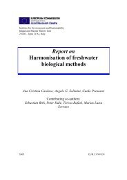

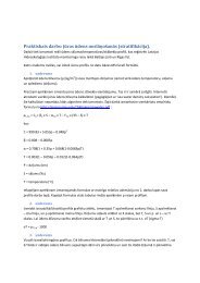

![Accommodation booking form [PDF]](https://img.yumpu.com/39471785/1/184x260/accommodation-booking-form-pdf.jpg?quality=85)