Principles of Polymer Processing

PRINCIPLES OF POLYMER PROCESSING

PRINCIPLES OF
POLYMER
PROCESSING
Second Edition
Z EHEV T ADMOR
The Wolfson Department of Chemical Engineering
Technion-Israel Institute of Technology
Haifa, Israel
C OSTAS G. GOGOS
Otto H. York Department of Chemical Engineering
Polymer Processing Institute
New Jersey Institute of Technology
Newark, New Jersey
An SPE Technical Volume
A John Wiley & Sons, Inc., Publication

Regarding the cover: The five bubbles contain images that represent the five elementary steps of polymer
processing. The bottom image is a picture of the Thomas Hancock masticator, the first documented processing
machine, developed in 1820. This image was originally published in the book Thomas Hancock: Personal
Narrative of the Origin and Progress of the Caoutchouc or India-Rubber Manufacture in England (London:
Longman, Brown, Green, Longmans, & Roberts, 1857).
Copyright # 2006 by John Wiley & Sons, Inc. All rights reserved
Published by John Wiley & Sons, Inc., Hoboken, New Jersey
Published simultaneously in Canada
No part of this publication may be reproduced, stored in a retrieval system, or transmitted in any form or by any
means, electronic, mechanical, photocopying, recording, scanning, or otherwise, except as permitted under
Section 107 or 108 of the 1976 United States Copyright Act, without either the prior written permission of the
Publisher, or authorization through payment of the appropriate per-copy fee to the Copyright Clearance Center,
Inc., 222 Rosewood Drive, Danvers, MA 01923, (978) 750-8400, fax (978) 750-4470, or on the web at
www.copyright.com. Requests to the Publisher for permission should be addressed to the Permissions
Department, John Wiley & Sons, Inc., 111 River Street, Hoboken, NJ 07030, (201) 748-6011, fax (201)
748-6008, or online at http://www.wiley.com/go/permission.
Limit of Liability/Disclaimer of Warranty: While the publisher and author have used their best efforts in
preparing this book, they make no representations or warranties with respect to the accuracy or completeness of
the contents of this book and specifically disclaim any implied warranties of merchantability or fitness for a
particular purpose. No warranty may be created or extended by sales representatives or written sales materials.
The advice and strategies contained herein may not be suitable for you situation. You should consult with a
professional where appropriate. Neither the publisher nor author shall be liable for any loss of profit or any other
commercial damages, including but not limited to special, incidental, consequential, or other damages.
For general information on our other products and services or for technical support, please contact our Customer
Care Department within the United States at (800) 762-2974, outside the United States at (317) 572-3993 or fax
(317) 572-4002.
Wiley also publishes its books in a variety of electronic formats. Some content that appears in print may not be
available in electronic formats. For more information about Wiley products, visit our web site at www.wiley.com.
Library of Congress Cataloging-in-Publication Data:
Tadmor, Zehev, 1937-
Principles of polymer processing / Zehev Tadmor, Costas G. Gogos. – 2nd
ed.
p. cm.
Includes index.
ISBN 0-471-38770-3 (cloth)
1. Polymers. 2. Polymerization. I. Gogos, Costas G. II. Title.
TP1087.T32 2006
668.9–dc22
2006009306
Printed in the United States of America
10987654321

Series Preface
The Society of Plastics Engineers is pleased to sponsor and endorse the second edition of
Principles of Polymer Processing by Zehev Tadmor and Costas Gogos. This volume is an
excellent source and reference guide for practicing engineers and scientists as well as
students involved in plastics processing and engineering. The authors’ writing style and
knowledge of the subject matter have resulted in an enjoyable and thoughtful presentation,
allowing the reader to gain meaningful insights into the subject.
SPE, through its Technical Volumes Committee, has long sponsored books on various
aspects of plastics. Its involvement has ranged from identification of needed volumes and
recruitment of authors to peer review and approval of new books. Technical competence
pervades all SPE activities, from sponsoring new technical volumes to producing technical
conferences and educational seminars. In addition, the Society publishes periodicals,
including Plastics Engineering, Polymer Engineering and Science, and The Journal of
Vinyl and Additive Technology.
The resourcefulness of some 20,000 practicing engineers, scientists, and technologists
has made SPE the largest organization of its type worldwide. Further information is
available from the Society of Plastics Engineers, 14 Fairfield Drive, Brookfield,
Connecticut 06804 or at www.4spe.org.
Susan E. Oderwald
Executive Director
Society of Plastics Engineers
v

Preface to the Second Edition
Tremendous science and engineering progress has been made in polymer processing since
the publication of the First Edition in 1979. Evolution in the field reflects the formidable
contributions of both industrial and academic investigators, and the groundbreaking
developments in rheology, polymer chemistry, polymer physics, life sciences and nanomaterials,
in instrumentation and improved machinery. The emerging disciplines of
computational fluid mechanics and molecular modeling, aided by exponentially
expanding computing power are also part of this evolution.
As discussed in Chapter 1 of this Second Edition, polymer processing is rapidly
evolving into a multidisciplinary field. The aim is not only to analyze the complex thermomechanical
phenomena taking place in polymer processing equipment, per se, but to
quantitatively account for the consequences, on the fabricated polymer products. Thus, the
focus of future polymer processing science will shift away from the machine, and more on
the product, although the intimate material-machine interactions in the former are needed
for the latter.
Consequently, this edition contains not only updated material but also a significant
restructuring of the original treatment of polymer processing. First, we deleted Part I
which discussed polymer structure and properties, since the subject is thoroughly covered
in many classic and other texts. Second, in light of the important technological
developments in polymer blends and reactive processing, new chapters on Devolatilization,
Compounding and Reactive Processing, and Twin Screw and Twin Rotor-based
Processing Equipment are introduced. These processes are widely used because of
their unique abilities to affect rapid and efficient solid deformation melting and chaotic
mixing.
However, the basic philosophy we advocated in the First Edition, which was to analyze
polymer processing operations in terms of elementary and shaping steps, which are
common to all such processing operations, and thereby unifying the field is retained. We
have continued our attempt to answer not only ‘‘how’’ the machines and processes work,
but also ‘‘why’’ they are best carried out using a specific machine or a particular process.
In fact, we believe that this approach has contributed to the fundamental understanding
and development of polymer processing in the last quarter-century, and to the change of
focus from the machine to the quantitative prediction of product properties.
As with the First Edition, this volume is written both as a textbook for graduate and
undergraduate students, as well as resource for practicing engineers and scientists.
Normally, a two-semester course in needed to cover the material in the text. However for
students who are familiar with fluid mechanics, heat transfer and rheology, it is possible to
cover the material in one semester.
vii

viii
PREFACE TO THE SECOND EDITION
To enhance the usefulness of the Second Edition for both students and practitioners of
the field, an extensive Appendix of rheological and thermo-mechanical properties of
commercial polymers, prepared and assembled by Dr. Victor Tan, and for teachers, a
complete problem Solution Manual, prepared by Dr. Dongyun Ren are included. For all it
is hoped that this Second Edition, like the First, proves to be a useful professional
‘‘companion’’.
We would like to acknowledge, with gratitude, the role and help of many: foremost,
the invaluable assistance of Dr. Dongyun Ren, who spent almost three years with us at the
Technion and NJIT/PPI, assisting with many aspects of the text preparation, as well as the
Solution Manual; and Dr. Victor Tan, whose expert and meticulous work in measuring and
gathering rheological and thermo-mechanical polymer properties provides the data needed
to work out real problems. In addition, we wish to thank our colleagures, and students, who
have influenced this book with their advice, criticism, comments, and conversations.
Among them are David Todd, Marino Xanthos, Ica Manas-Zloczower, Donald Sebastian,
Kun Hyun, Han Meijer, Jean-Francois Agassant, Dan Edie, John Vlachopoulos, Musa
Kamal, Phil Coates, Mort Denn, Gerhard Fritz, Chris Macosko, Mike Jaffe, Bob Westover,
Tom McLeish, Greg Rutledge, Brian Qian, Myung-Ho Kim, Subir Dey, Jason Guo, Linjie
Zhu and Ming Wan Young. Special thanks are due to R. Byron Bird for his advice and
whose classic approach to Transport Phenomena, inspired our approach to polymer
processing as manifested in this book.
There are others we wish to mention and recall. While they are no longer with us, their
work, ideas, and scientific legacy resurface on the pages of this book. Among them: Joe
Biesenberger, Luigi Pollara, Peter Hold, Ally Kaufmann, Arthur Lodge, Don Marshall,
Imrich Klein, Bruce Maddock, and Lew Erwin.
We wish to thank our editor, Amy Byers, our production editor, Kristen Parrish, the
copy editor Trumbull Rogers, and the cover designer Mike Rutkowski. We give special
thanks to Abbie Rosner for her excellent editing of our book and to Mariann Pappagallo
and Rebecca Best for their administrative support.
Finally, we thank our families, who in many respects paid the price of our lengthy
preoccupation with this book at the expense of time that justly belonged to them.
ZEHEV TADMOR
COSTAS G. GOGOS
Haifa, Israel
Newark, New Jersey
May 2006

Preface to the First Edition
This book deals with polymer processing, which is the manufacturing activity of converting
raw polymeric materials into finished products of desirable shape and properties.
Our goal is to define and formulate a coherent, comprehensive, and functionally useful
engineering analysis of polymer processing, one that examines the field in an integral, not
a fragmented fashion. Traditionally, polymer processing has been analysed in terms of
specific processing methods such as extrusion, injection molding calendering, and so on.
Our approach is to claim that what is happening to the polymer in a certain type of
machine is not unique: polymers go through similar experiences in other processing
machines, and these experiences can be described by a set of elementary processing steps
that prepare the polymer for any of the shaping methods available to these materials. On
the other hand, we emphasize the unique features of particular polymer processing
methods or machines, which consist of the particular elementary step and shaping
mechanisms and geometrical solutions utilized.
Because with the approach just described we attempt to answer questions not only of
‘‘how’’ a particular machine works but also ‘‘why’’ a particular design solution is the
‘‘best’’ among those conceptually available, we hope that besides being useful for students
and practicing polymer engineers and scientists, this book can also serve as a tool in the
process of creative design.
The introductory chapter highlights the technological aspects of the important polymer
processing methods as well as the essential features of our analysis of the subject. Parts I
and II deal with the fundamentals of polymer science and engineering that are necessary
for the engineering analysis of polymer processing. Special emphasis is given to the
‘‘structuring’’ effects of processing on polymer morphology and properties, which
constitute the ‘‘meeting ground’’ between polymer engineering and polymer science. In all
the chapters of these two parts, the presentation is utilitarian; that is, it is limited to what is
necessary to understand the material that follows.
Part III deals with the elementary processing steps. These ‘‘steps’’ taken together make
up the total thermomechanical experience that a polymer may have in any polymer
processing machine prior to shaping. Examining these steps separately, free from any
particular processing method, enables us to discuss and understand the range of the
mechanisms and geometries (design solutions) that are available. Part III concludes with a
chapter on the modeling of the single-screw extruder, demonstrating the analysis of a
complete processor in terms of the elementary steps. We also deal with a new polymer
processing device to demonstrate that synthesis (invention) is also facilitated by the
elementary-step approach.
We conclude the text with the discussion of the classes of shaping methods available to
polymers. Again, each of these shaping methods is essentially treated independently of
ix

x
PREFACE TO THE FIRST EDITION
any particular processing method. In addition to classifying the shaping methods in a
logical fashion, we discuss the ‘‘structuring’’ effects of processing that arise because the
macromolecular orientation occurring during shaping is fixed by rapid solidification.
The last chapter, a guide to the reader for the analysis of any of the major processing
methods in terms of the elementary steps, is necessary because of the unconventional
approach we adopt in this book.
For engineering and polymer science students, the book should be useful as a text in
either one-semester or two-semester courses in polymer processing. The selection and
sequence of material would of course be very much up to the instructor, but the following
syllabi are suggested: For a one-semester course: Chapter 1; Sections 5.2, 4, and 5;
Chapter 6; Sections 7.1, 2, 7, 9, and 10; Sections 9.1, 2, 3, 7, and 8; Chapter 10; Section
12.1; Sections 13.1, 2, 4, and 5; Section 14.1; Section 15.2; and Chapter 17—students
should be asked to review Chapters 2, 3, and 4, and for polymer science students the course
content would need to be modified by expanding the discussion on transport phenomena,
solving the transport methodology problems, and deleting Sections 7.7, 9, and 10. For a
two-semester course: in the first semester, Chapters 1, 5, and 6; Sections 7.1, 2, and 7 to 13;
Sections 8.1 to 4, and 7 to 13; Chapters 9 and 10; and Sections 11.1 to 4, 6, 8, and 10—
students should be asked to review Chapters 2, 3, and 4; and in the second semester,
Chapters 12 and 13; Section 14.1, and Chapters 15, 16, and 17.
The problems included at the end of Chapters 5 to 16 provide exercises for the material
discussed in the text and demonstrate the applicability of the concepts presented in solving
problems not discussed in the book.
The symbols used follow the recent recommendations of the Society of Rheology; SI
units are used. We follow the stress tensor convention used by Bird et al.,* namely,
p ¼ Pd þ s, where p is the total stress tensor, P is the pressure, and s is that part of the
stress tensor that vanishes when no flow occurs; both P and t ii are positive under
compression.
We acknowledge with pleasure the colleagues who helped us in our efforts. Foremost,
we thank Professor J. L. White of the University of Tennessee, who reviewed the entire
manuscript and provided invaluable help and advice on both the content and the structure
of the book. We further acknowledge the constructive discussions and suggestions offered
by Professors R. B. Bird and A. S. Lodge (University of Wisconsin), J. Vlachopoulos
(McMaster University), A. Rudin (University of Waterloo), W. W. Graessley (Northwestern
University), C. W. Macosko (University of Minnesota), R. Shinnar (CUNY), R. D.
Andrews and J. A. Biesenberger (Stevens Institute), W. Resnick, A. Nir, A. Ram, and M.
Narkis (Technion), Mr. S. J. Jakopin (Werner-Pfleiderer Co.), and Mr. W. L. Krueger (3M
Co.). Special thanks go to Dr. P. Hold (Farrel Co.), for the numerous constructive
discussions and the many valuable comments and suggestions. We also thank Mr. W.
Rahim (Stevens), who measured the rheological and thermophysical properties that appear
in Appendix A, and Dr. K. F. Wissbrun (Celanese Co.), who helped us with the rheological
data and measured Z 0 . Our graduate students of the Technion and Stevens Chemical
Engineering Departments deserve special mention, because their response and comments
affected the form of the book in many ways.
*R. B. Bird, W. E. Stewart, and E. N. Lightfoot, Transport Phenomena, Wiley, New York, 1960; and R. B. Bird,
R. C. Armstrong, and O. Hassager, Dynamics of Polymeric Liquids, Wiley, New York, 1977.

PREFACE TO THE FIRST EDITION
xi
We express our thanks to Ms. D. Higgins and Ms. L. Sasso (Stevens) and Ms. N. Jacobs
(Technion) for typing and retyping the lengthy manuscript, as well as to Ms. R. Prizgintas
who prepared many of the figures. We also thanks Brenda B. Griffing for her thorough
editing of the manuscript, which contributed greatly to the final quality of the book.
This book would not have been possible without the help and support of Professor J. A.
Biesenberger and Provost L. Z. Pollara (Stevens) and Professors W. Resnick, S. Sideman,
and A. Ram (Technion).
Finally, we thank our families, whose understanding, support, and patience helped us
throughout this work.
Haifa, Israel
Hoboken, New Jersey
March 1978
ZEHEV TADMOR
COSTAS G. GOGOS

Contents
1 History, Structural Formulation of the Field Through Elementary Steps,
and Future Perspectives, 1
1.1 Historical Notes, 1
1.2 Current Polymer Processing Practice, 7
1.3 Analysis of Polymer Processing in Terms of Elementary Steps and
Shaping Methods, 14
1.4 Future Perspectives: From Polymer Processing to
Macromolecular Engineering, 18
2 The Balance Equations and Newtonian Fluid Dynamics, 25
2.1 Introduction, 25
2.2 The Balance Equations, 26
2.3 Reynolds Transport Theorem, 26
2.4 The Macroscopic Mass Balance and the Equation of Continuity, 28
2.5 The Macroscopic Linear Momentum Balance and the Equation
of Motion, 32
2.6 The Stress Tensor, 37
2.7 The Rate of Strain Tensor, 40
2.8 Newtonian Fluids, 43
2.9 The Macroscopic Energy Balance and the Bernoulli and Thermal
Energy Equations, 54
2.10 Mass Transport in Binary Mixtures and the Diffusion Equation, 60
2.11 Mathematical Modeling, Common Boundary Conditions, Common
Simplifying Assumptions, and the Lubrication Approximation, 60
3 Polymer Rheology and Non-Newtonian Fluid Mechanics, 79
3.1 Rheological Behavior, Rheometry, and Rheological Material Functions
of Polymer Melts, 80
3.2 Experimental Determination of the Viscosity and Normal Stress
Difference Coefficients, 94
3.3 Polymer Melt Constitutive Equations Based on Continuum Mechanics, 100
3.4 Polymer Melt Constitutive Equations Based on Molecular Theories, 122
xiii

xiv
CONTENTS
4 The Handling and Transporting of Polymer Particulate Solids, 144
4.1 Some Unique Properties of Particulate Solids, 145
4.2 Agglomeration, 150
4.3 Pressure Distribution in Bins and Hoppers, 150
4.4 Flow and Flow Instabilities in Hoppers, 152
4.5 Compaction, 154
4.6 Flow in Closed Conduits, 157
4.7 Mechanical Displacement Flow, 157
4.8 Steady Mechanical Displacement Flow Aided by Drag, 159
4.9 Steady Drag-induced Flow in Straight Channels, 162
4.10 The Discrete Element Method, 165
5 Melting, 178
5.1 Classification and Discussion of Melting Mechanisms, 179
5.2 Geometry, Boundary Conditions, and Physical Properties in Melting, 184
5.3 Conduction Melting without Melt Removal, 186
5.4 Moving Heat Sources, 193
5.5 Sintering, 199
5.6 Conduction Melting with Forced Melt Removal, 201
5.7 Drag-induced Melt Removal, 202
5.8 Pressure-induced Melt Removal, 216
5.9 Deformation Melting, 219
6 Pressurization and Pumping, 235
6.1 Classification of Pressurization Methods, 236
6.2 Synthesis of Pumping Machines from Basic Principles, 237
6.3 The Single Screw Extruder Pump, 247
6.4 Knife and Roll Coating, Calenders, and Roll Mills, 259
6.5 The Normal Stress Pump, 272
6.6 The Co-rotating Disk Pump, 278
6.7 Positive Displacement Pumps, 285
6.8 Twin Screw Extruder Pumps, 298
7 Mixing, 322
7.1 Basic Concepts and Mixing Mechanisms, 322
7.2 Mixing Equipment and Operations of Multicomponent and
Multiphase Systems, 354
7.3 Distribution Functions, 357
7.4 Characterization of Mixtures, 378
7.5 Computational Analysis, 391
8 Devolatilization, 409
8.1 Introduction, 409
8.2 Devolatilization Equipment, 411
8.3 Devolatilization Mechanisms, 413

CONTENTS
xv
8.4 Thermodynamic Considerations of Devolatilization, 416
8.5 Diffusivity of Low Molecular Weight Components in Molten Polymers, 420
8.6 Boiling Phenomena: Nucleation, 422
8.7 Boiling–Foaming Mechanisms of Polymeric Melts, 424
8.8 Ultrasound-enhanced Devolatilization, 427
8.9 Bubble Growth, 428
8.10 Bubble Dynamics and Mass Transfer in Shear Flow, 430
8.11 Scanning Electron Microscopy Studies of Polymer Melt
Devolatilization, 433
9 Single Rotor Machines, 447
9.1 Modeling of Processing Machines Using Elementary Steps, 447
9.2 The Single Screw Melt Extrusion Process, 448
9.3 The Single Screw Plasticating Extrusion Process, 473
9.4 The Co-rotating Disk Plasticating Processor, 506
10 Twin Screw and Twin Rotor Processing Equipment, 523
10.1 Types of Twin Screw and Twin Rotor–based Machines, 525
10.2 Counterrotating Twin Screw and Twin Rotor Machines, 533
10.3 Co-rotating, Fully Intermeshing Twin Screw Extruders, 572
11 Reactive Polymer Processing and Compounding, 603
11.1 Classes of Polymer Chain Modification Reactions, Carried out in
Reactive Polymer Processing Equipment, 604
11.2 Reactor Classification, 611
11.3 Mixing Considerations in Multicomponent Miscible Reactive
Polymer Processing Systems, 623
11.4 Reactive Processing of Multicomponent Immiscible and
Compatibilized Immiscible Polymer Systems, 632
11.5 Polymer Compounding, 635
12 Die Forming, 677
12.1 Capillary Flow, 680
12.2 Elastic Effects in Capillary Flows, 689
12.3 Sheet Forming and Film Casting, 705
12.4 Tube, Blown Film, and Parison Forming, 720
12.5 Wire Coating, 727
12.6 Profile Extrusion, 731
13 Molding, 753
13.1 Injection Molding, 753
13.2 Reactive Injection Molding, 798
13.3 Compression Molding, 811

xvi
CONTENTS
14 Stretch Shaping, 824
14.1 Fiber Spinning, 824
14.2 Film Blowing, 836
14.3 Blow Molding, 841
15 Calendering, 865
15.1 The Calendering Process, 865
15.2 Mathematical Modeling of Calendering, 867
15.3 Analysis of Calendering Using FEM, 873
Appendix A Rheological and Thermophysical Properties of Polymers, 887
Appendix B Conversion Tables to the International System of Units (SI), 914
Appendix C Notation, 918
Author Index, 929
Subject Index, 944

1 History, Structural Formulation
of the Field Through Elementary
Steps, and Future Perspectives
1.1 Historical Notes, 1
1.2 Current Polymer Processing Practice, 7
1.3 Analysis of Polymer Processing in Terms of Elementary
Steps and Shaping Methods, 14
1.4 Future Perspectives: From Polymer Processing to Macromolecular Engineering, 18
Polymer processing is defined as the ‘‘engineering activity concerned with operations
carried out on polymeric materials or systems to increase their utility’’ (1). Primarily, it
deals with the conversion of raw polymeric materials into finished products, involving not
only shaping but also compounding and chemical reactions leading to macromolecular
modifications and morphology stabilization, and thus, ‘‘value-added’’ structures. This
chapter briefly reviews the origins of current polymer processing practices and introduces
the reader to what we believe to be a rational and unifying framework for analyzing
polymer processing methods and processes. The chapter closes with a commentary on the
future of the field, which is currently being shaped by the demands of predicting, a priori,
the final properties of processed polymers or polymer-based materials via simulation,
based on first molecular principles and multiscale examination (2).
1.1 HISTORICAL NOTES
Plastics and Rubber Machinery
Modern polymer processing methods and machines are rooted in the 19th-century rubber
industry and the processing of natural rubber. The earliest documented example of a
rubber-processing machine is a rubber masticator consisting of a toothed rotor turned by a
winch inside a toothed cylindrical cavity. Thomas Hancock developed it in 1820 in
England, to reclaim scraps of processed natural rubber, and called it the ‘‘pickle’’ to
confuse his competitors. A few years later, in 1836, Edwin Chaffee of Roxbury,
Massachusetts, developed the two-roll mill for mixing additives into rubber and the fourroll
calender for the continuous coating of cloth and leather by rubber; his inventions are
still being used in the rubber and plastics industries. Henry Goodyear, brother of Charles
Goodyear, is credited with developing the steam-heated two-roll mill (3). Henry Bewley
and Richard Brooman apparently developed the first ram extruder in 1845 in England (4),
which was used in wire coating. Such a ram extruder produced the first submarine cable,
Principles of Polymer Processing, Second Edition, by Zehev Tadmor and Costas G. Gogos.
Copyright # 2006 John Wiley & Sons, Inc.
1

2 HISTORY, STRUCTURAL FORMULATION OF THE FIELD
laid between Dover and Calais in 1851, as well as the first transatlantic cable, an Anglo-
American venture, in 1860.
The need for continuous extrusion, particularly in the wire and cable field, brought about
the single most important development in the processing field–the single screw extruder
(SSE), which quickly replaced the noncontinuous ram extruders. Circumstantial evidence
indicates that A. G. DeWolfe, in the United States, may have developed the first screw extruder
in the early 1860s (5). The Phoenix Gummiwerke has published a drawing of a screw dated
1873 (6), and William Kiel and John Prior, in the United States, both claimed the development
of such a machine in 1876 (7). But the birth of the extruder, which plays such a dominant role
in polymer processing, is linked to the 1879 patent of Mathew Gray in England (8), which
presents the first clear exposition of this type of machine. The Gray machine also included a
pair of heated feeding rolls. Independent of Gray, Francis Shaw, in England, developed a screw
extruder in 1879, as did John Royle in the United States in 1880.
John Wesley Hyatt invented the thermoplastics injection-molding machine in 1872 (9),
which derives from metal die-casting invented and used earlier. Hyatt was a printer from
Boston, who also invented Celluloid (cellulose nitrate), in response to a challenge award of
$10,000 to find a replacement material for ivory used for making billiard balls. He was a
pioneering figure, who contributed many additional innovations to processing, including
blow molding. His inventions also helped in the quick adoption of phenol-formaldehyde
(Bakelite) thermosetting resins developed by Leo Baekeland in 1906 (10). J. F. Chabot and
R. A. Malloy (11) give a detailed history of the development of injection molding up to the
development and the widespread adoption of the reciprocating injection molding machine
in the late 1950s.
Multiple screw extruders surfaced about the same time. Paul Pfleiderer introduced the
nonintermeshing, counterrotating twin screw extruder (TSE) in 1881, whereas the
intermeshing variety of twin screw extruders came much later, with R. W Eastons corotating
machine in 1916, and A. Olier’s positive displacement counterrotating machine in
1921 (12). The former led to the ZSK-type machines invented by Rudolph Erdmenger at
Bayer and developed jointly with a Werner and Pfleiderer Co. team headed by Gustav Fahr
and Herbert Ocker. This machine, like most other co-rotating, intermeshing TSEs, enjoys a
growing popularity. They all have the advantage that the screws wipe one another, thus
enabling the processing of a wide variety of polymeric materials. In addition, they
incorporate ‘‘kneading blocks’’ for effective intensive and extensive mixing. They also
generally have segmented barrels and screws, which enables the machine design to be
matched to the processing needs. There is a broad variety of twin and multiple screw mixers
and extruders; some of them are also used in the food industry. Hermann (12) and White (7)
give thorough reviews of twin screw and multiple screw extruders and mixers.
The first use of gear pumps for polymeric materials dates from Willoughby Smith, who,
in 1887, patented such a machine fed by a pair of rolls (4). Multistage gear pumps were
patented by C. Pasquetti (13). Unlike single screw extruders and co-rotating twin screw
extruders (Co-TSE), gear pumps are positive-displacement pumps, as are the counterrotating,
fully intermeshing TSEs.
The need for mixing fine carbon black particles and other additives into rubber made
rubber mixing on open roll mills rather unpleasant. A number of enclosed ‘‘internal’’
mixers were developed in the late 19th century, but it was Fernley H. Banbury who in 1916
patented an improved design that is being used to this day. The Birmingham Iron Foundry
in Derby, Connecticut, which later merged with the Farrel Foundry and Machine of
Ansonia, Connecticut, built the machine. This mixer is still the workhorse of rubber

HISTORICAL NOTES 3
processing, and is called the Banbury mixer after its inventor (14). In 1969, at Farrel, Peter
Hold et al. (15) developed a ‘‘continuous version’’ of the Banbury called the Farrel
Continuous Mixer (FCM). A precursor of this machine was the nonintermeshing, twinrotor
mixer called the Knetwolf, invented by Ellerman in Germany in 1941 (12). The FCM
never met rubber-mixing standards, but fortunately, it was developed at the time when
high-density polyethylene and polypropylene, which require postreactor melting, mixing,
compounding, and pelletizing, came on the market. The FCM proved to be a very effective
machine for these postreactor and other compounding operations.
The Ko-Kneader developed by List in 1945 for Buss AG in Germany, is a single-rotor
mixer–compounder that oscillates axially while it rotates. Moreover, the screw-type rotor
has interrupted flights enabling kneading pegs to be fixed in the barrel (12).
The ram injection molding machine, which was used intensively until the late 1950s
and early 1960s, was quite unsuitable to heat-sensitive polymers and a nonhomogeneous
product. The introduction of the ‘‘torpedo’’ into the discharge end of the machine
somewhat improved the situation. Later, screw plasticators were used to prepare a uniform
mix fed to the ram for injection. However, the invention of the in-line or reciprocatingscrew
injection molding machine, attributed to W. H. Willert in the United States (16),
which greatly improved the breadth and quality of injection molding, created the modern
injection molding machine. 1
Most of the modern processing machines, with the exception of roll mills and
calenders, have at their core a screw or screw-type rotor. Several proposals were published
for ‘‘screwless’’ extruders. In 1959, Bryce Maxwell and A. J. Scalora (17) proposed the
normal stress extruder, which consists of two closely spaced disks in relative rotational
motion, with one disk having an opening at the center. The primary normal stress
difference that polymeric materials exhibit generates centripetal forces pumping the
material inward toward the opening. Robert Westover (18) proposed a slider pad extruder,
also consisting of two disks in relative motion, whereby one is equipped with step-type
pads generating pressure by viscous drag, as screw extruders do. Finally, in 1979, one of
the authors (19) patented the co-rotating disk processor, which was commercialized by the
Farrel Corporation under the trade name Diskpack. Table 1.1. summarizes chronologically
the most important inventions and developments since Thomas Hancock’s rubber mixer of
1820. A few selected inventions of key new polymers are included, as well as two major
theoretical efforts in formulating the polymer processing discipline.
A Broader Perspective: The Industrial and Scientific Revolutions
The evolution of rubber and plastics processing machinery, which began in the early 19th
century, was an integral part of the great Industrial Revolution. This revolution, which
transformed the world, was characterized by an abundance of innovations that, as stated by
1. William Willert filed a patent on the ‘‘in-line,’’ now more commonly known as the reciprocating screw
injection molding machine in 1952. In 1953 Reed Prentice Corp. was the first to use Willert’s invention, building a
600-ton machine. The patent was issued in 1956. By the end of the decade almost all the injection molding
machines being built were of the reciprocating screw type.
Albert (Aly) A. Kaufman, one of the early pioneers of extrusion, who established Prodex in New Jersey and
later Kaufman S. A. in France, and introduced many innovations into extrusion practice, told one of the authors
(Z.T.) that in one of the Annual Technical Conference (ANTEC) meetings long before in-line plasticating units
came on board, he told the audience that the only way to get a uniform plasticized product is if the ram is replaced
by a rotating and reciprocating screw. Aly never patented his innovative ideas because he believed that it is better
to stay ahead of competition then to spend money and time on patents.

TABLE 1.1 The Chronological History of Processing Machines, and Some Other Key and Relevant Developments
Machine Process Inventor Date Comments
The ‘Pickle’ Batch mixing T. Hancock 1820 Reclaim rubber
Roll mill Batch mixing E. Chaffe 1836 Steam-heated rolls
Calender Coating and
E. Chaffe 1836 Coating cloth and leather
sheet forming
Vulcanization of Rubber Charles Goodyear 1839
Ram extruder Extrusion H. Bewly and
R. Brooman
Screw extruder Extrusion A. G. DeWolfe
PhoenixGummiwerke
W. Kiel and J. Prior
M. Gray
F. Shaw
J. Royle
1845
1860
1873
1876
1879
1879
1880
Attributed to
Archimedes for
water pumping.
The most important
machine for plastics
and rubber
Injection molding Injection molding J. W. Hyatt 1872 Used first for Celluloid
Extrusion P. Pfleiderer 1881
Counterrotating,
nonintermeshing
twin screw extruder
Gear pump Extrusion W. Smith 1887 Pasqueti invented the
multistage gear pump.
Bakelite Leo Baekeland First purely synthetic plastics
Co-rotating, intermeshing
twin screw extruder
Mixing and
extrusion
R. W. Easton 1916
The Banbury Batch mixing F. H. Banbury 1916 Developed for
rubber mixing.
Counterrotating,
Extrusion A. Olier 1912 Positive displacement
intermeshing twin
screws
pump
4

Nylon W. H. Carothers 1935 At the DuPont Laboratories
Low density polyethylene E. W. Fawcett et al. 1939 At the ICI Laboratories
Knetwolf Twin rotor mixing W. Ellerman 1941
Ko-Kneader Mixing and extrusion H. List 1945 Buss. AG
Triangular
kneading blocks
In-line reciprocating
injection molding
Continuous
mixing
ZSK Continuous mixing
and extrusion
First Systematic
Formulation of
Plastics Processing
Theory
R. Erdmenger 1949 Used in the ZSK
extruders
Injection molding W. H. Wilert 1952 Replaced ram injection
molding
R. Erdmenger, G. Fahr,
and H. Ocker
E. C. Bernhardt,
J. M. McKelvey,
P. H. Squires,
W. H. Darnell, W. D. Mohr
D. I. Marshall,
J. T. Bergen,
R. F. Westover, etc.
1955 Co-rotating intermeshing
twin screw extruder with
mixing elements
1958 Mostly the
DuPont team
Transfermix Continuous mixing N. C. Parshall and P. Geyer 1956 Single screw in a barrel in
which screw-type
channel is cut
Normal stress extruder Extrusion B. Maxwell and A. J. Scalora 1959 Two discks in relative rotation
Continuous ram extruder Extrusion R. F. Westover Reciprocating rams.
Slider-pad extruder Extrusion R. F. Westover 1962 Slider pads rotating on
stationary disk
FCM Continuous mixing P. Hold et al. 1969 Continuous Banbury
Diskpack Extrusion Z. Tadmor 1979 Co-rotating disk processor
5

6 HISTORY, STRUCTURAL FORMULATION OF THE FIELD
Landes (20) ‘‘almost defy compilation and fall under three principles: (a) the substitution of
machines—rapid, regular, precise, tireless—for human skill and effort; (b) the substitution
of inanimate for animate source of power, in particular, the invention of engines for
converting heat into work, thereby opening an almost unlimited supply of energy; and (c) the
use of new and far more abundant raw materials, in particular, the substitution of mineral,
and eventually artificial materials for vegetable or animal sources.’’
Central to this flurry of innovation was James Watt’s invention of the modern steam
engine, in 1774. Watt was the chief instrument designer at the University of Glasgow, and
he made his great invention when a broken-down Thomas Newcomen steam engine,
invented in 1705 and used for research and demonstration, was brought to him. This was a
rather inefficient machine, based on atmospheric pressure acting on a piston in a cylinder
in which steam condensed by water injection created a vacuum, but it was the first manmade
machine that was not wind or falling-water driven. Watt not only fixed the machine,
but also invented the modern and vastly more efficient steam engine, with steam pressure
acting on the system and the separate condenser.
The great Industrial Revolution expanded in waves with the development of steel,
railroads, electricity and electric engines, the internal combustion engine, and the oil and
chemical industries. It was driven by the genius of the great inventors, from James Watt
(1736–1819) to Eli Whitney (1765–1825), who invented the cotton gin, Samuel Morse
(1791–1872), Alexander Graham Bell (1847–1922), Thomas Alva Edison (1847–1931),
Guglielmo Marchese Marconi (1874–1937), Nikola Tesla (1856–1943), and many others.
These also included, of course, J. W. Hyatt, Leo Baekeland, Charles Goodyear, Thomas
Hancock, Edwin Chaffe, Mathew Gray, John Royle, and Paul Pfleiderer who, among many
others, through their inventive genius, created the rubber and plastics industry.
The Industrial Revolution, which was natural resource– and cheap labor–dependent,
was ignited in the midst of an ongoing scientific revolution, which started over two
centuries earlier with Nicolas Copernicus (1473–1543), Galileo Galilei (1564–1642),
Johannes Kepler (1571–1630), René Descartes (1596–1650) and many others, all the way
to Isaac Newton (1642–1727) and his great Principia published in 1687, and beyond—a
revolution that continues unabated to these very days.
The two revolutions rolled along separate tracks, with little interaction between them.
This is not surprising because technology and science have very different historical
origins. Technology derives from the ordinary arts and crafts (both civilian and military).
Indeed most of the great inventors were not scientists but smart artisans, technicians, and
entrepreneurs. Science derives from philosophical, theological, and speculative inquiries
into nature. Technology is as old as mankind and it is best defined 2 as our accumulated
knowledge of making all we know how to make. Science, on the other hand, is defined by
dictionaries as ‘‘a branch of knowledge or study derived from observation, dealing with a
body of facts and truths, systematically arranged and showing the operation of general
laws.’’ But gradually the two revolutions began reinforcing each other, with science
opening new doors for technology, and technology providing increasingly sophisticated
tools for scientific discovery. During the 20th century, the interaction intensified, in
particular during World War II, with the Manhattan Project, the Synthetic Rubber (SBR)
Project, the development of radar, and many other innovations that demonstrated the
2. Contrary to the erroneous definitions in most dictionaries as ‘‘the science of the practical or industrial arts or
applied science.’’

CURRENT POLYMER PROCESSING PRACTICE 7
power of science when applied to technology. In the last quarter of the century, the
interaction between science and technology intensified to such an extent that the two
effectively merged into an almost indistinguishable entity, and in doing so ignited a new
revolution, the current, ongoing scientific–technological revolution. This revolution is the
alma mater of high technology, globalization, the unprecedented growth of wealth in the
developed nations over the past half-century, and the modern science and technology–
based economies that are driving the world.
The polymer industry and modern polymer processing, which emerged in the
second half of the 20th century, are very much the product of the merging of science
and technology and the new science–technology revolution, and are, therefore, by
definition high-tech, as are electronics, microelectronics, laser technologies, and
biotechnology.
1.2 CURRENT POLYMER PROCESSING PRACTICE
The foregoing historical review depicted the most important machines available for
polymer processing at the start of the explosive period of development of polymers and the
plastics industry, which took place after World War II, when, as previously pointed out,
science and technology began to merge catalytically. Thus, the Rubber and Plastics
Technology century of 1850–1950 in Table 1.2 (2a), characterized by inventive praxis
yielding machines and products, which created a new class of materials and a new
industry, came to a close. In the half-century that followed, ‘‘classical’’ polymer
processing, shown again in Table 1.2, introduced and utilized engineering analysis and
process simulation, as well as innovation, and created many improvements and new
developments that have led to today’s diverse arsenal of sophisticated polymer processing
machines and methods of processing polymers and polymer systems of ever-increasing
complexity and variety. As discussed later in this chapter, we are currently in transition
into a new and exciting era for polymer processing.
A snapshot of the current status of the plastics industry in the United States, from the
economic and manufacturing points of view, as reported by the Society of Plastics
Industries (SPI) for 2000 (21), shows that it is positioned in fourth place among
manufacturing industries after motor vehicles and equipment, electronic components and
accessories, and petroleum refining, in terms of shipments. Specifically:
1. The value of polymer-based products produced in the United States by polymer
(resin) manufacturers was $ 90 billion. This industry is characterized by a relatively
small number of very large enterprises, which are either chemical companies, for
which polymer production is a very sizable activity (e.g., The Dow Chemical
Company), or petrochemical companies, for which, in spite of the immense volume
of polymers produced, polymer production is a relatively minor activity and part of
vertically integrated operations (e.g., ExxonMobil Corporation).
2. The value of finished plastics products shipped by U.S. polymer processors was
$ 330 billion. Polymer processing companies are large in number and of small-tomedium
size. They are specialized, have only modest financial and research
resources, but are by-and-large innovative, competitive, entrepreneurial, and seemingly
in constant forward motion, which is characteristic of the first period of
development of the rubber and plastics industry.

TABLE 1.2 The Historical Evolution of Polymer Processing
1850–1950 1950–2000 Transition Future
Time Frame
Rubber and Plastics
Tecnology
“Classical” Polymer
Processing
Polymer Processing
for Structuring
Macromolecular
engineering
Focus Product
Machine invention
Scale Product
Machine
Activity Industry
Entrepreneurial
Process and machine design
(product)
Machine
Product
Corporate labs
Academe
Industry
Discipline Inventive Praxis Transport phenomena
GNF rheology
Computational fluid
mechanics
Profession Technologists
Inventors
Benefits New Class of Materials
New Industry
CHE, ME, CHEM
industry/academe
Ability to process very
diverse polymers
Large resin and processing
industries
4$10 12 worldwide
Process and designed products
Product microstructuring
New products and structures
‘‘Pushing the Limits’’
Product micro (structure) Product molecular microstructure
Academe
Corporate labs
Advanced compounders
Transport phenomena
Full rheology
Melt/solids physics
Interfacial phenomena
Polymer chemistry
In-line characterization
Thermodynamics
CHE, ME, CHEM, PHYS
academe/industry
Customized
structure/properties
Value-added materials
New application fields
Gov/edu/com collaboration
High-tech start-ups
New industry
Macromolecular physics,
chemistry, rheology
Multiscale transport and
computations
Molecular-scale probes
Molecular biology
Macromolecular
engineers/scientists
Truly advanced polymer materials
New generation or
globally applicable polymers
8

CURRENT POLYMER PROCESSING PRACTICE 9
3. The U.S. labor force employed by resin producers is a quarter of million, and by
polymer processors is a million and a half.
A lay-of-the-land presentation, in flowchart form, of the thermomechanical experiences
of polymer systems in processing equipment used for important polymer processing
manufacturing activities, is presented next. The aim is not only to inform but also to illustrate
the inherent commonality of the thermomechanical experiences of polymer systems among
the various types of equipment and operations used, which will help to unify and structure
the understanding and analysis of polymer processing equipment and operations.
Postreactor Polymer Processing (‘‘Finishing’’) Operations
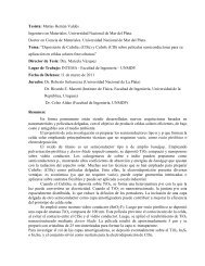
As is depicted in flowchart form in Fig. 1.1, the product of a gas-phase polymerization
reactor produced in a typical polymer (resin) manufacturer’s plant at rates up to 40 t/h, is
exposed to separation and drying steps to obtain pure polymer in particulate (powder) form.
It is then dry mixed with a proprietary package of very low concentration additives—
thermal, ultraviolet (UV), and oxidative stabilizers, as well as processing aids. The drymixed
powder stream is metered into very large (mega) Co-TSEs or continuous melter/
mixers (CMs), where the processes of particulate solids handling (PSH), melting, mixing/
homogenizing, andmelt conveying and pressurization must take place very rapidly, due to
the high production-rate requirements.
This is the first thermomechanical experience of the reactor polymer, and it will not be
the last. The equipment choice of Co-TSE or CM is made on the basis of the unique ability
of these devices to cause very rapid melting and laminar mixing. We refer to the four
processes just discussed as the elementary steps of polymer processing. The melt stream
exiting the Co-TSE or the CM, both of which have poor melt pumping capabilities, is fed
into very large gear pumps (GPs), which are positive displacement, accurate melt
conveying/pumping devices. The melt is pumped into an underwater pelletizer with a
Monomer(s)
Catalyst
initiators
Gas-phase
polymerization
reactor
Separator
Drier
Particulate
polymer
(powder form)
Stabilizing
additives
Polymerization reactor domain
Additives-coated particulates
Shipped to
fabricators
and
compounders
(RR cars, gaylords, bags)
Virgin
plastic
pellets
Form
cut
cool
UW pelletizer
(UWP)
Pump
Mix/homogenize, melt, PSH
Co-TSE
CM
Fig. 1.1
“Finishing” operations line
Postreactor polymer processing (‘‘finishing’’) operations.

10 HISTORY, STRUCTURAL FORMULATION OF THE FIELD
Virgin pellets
(bags, gaylords, RR, cars)
PSH, melt, mix, pres/pump
pump/pres
Shape
cool
cut
Compounded
pellets
To
fabricator
Pigment, fillers
reinforcing agents
TSE (SSE) GP Pelletizer
Fig. 1.2
Polymer compounding operations.
multihole die, where the exiting strands are cut into small pellets and cooled by the coldwater
stream, which takes them to a water–polymer separator. The wet pellets are then
dried and conveyed into silos; they are the ‘‘virgin’’ plastics pellets sold by polymer
manufactures to processing companies, shipped in railroad cars in 1000-lb gaylord
containers or 50-lb bags.
Polymer Compounding Operations
The polymer compounding line is shown schematically in Fig. 1.2. Virgin pellets from
resin manufacturers are compounded (mixed) with pigments (to form color concentrates),
fillers, or reinforcing agents at moderate to high concentrations. The purpose of such
operations is to improve the properties of the virgin base polymer, or to give it specialized
properties, adding value in every case. The production rates are in the range of 1000–
10,000 lb/h. The processing equipment’s critical task is to perform laminar distributive
and dispersive mixing of the additives to the level required to obtain finished product
property requirements. Furthermore, other additives, such as chopped glass fibers, are
often fed after the compounding equipment has melted the pellets, in order to minimize
degrading the attributes of the additives, such as fiber length. Finally, to assist the laminar
mixing process, the additives may be surface-treated.
The processing equipment used by polymer compounders is mainly co-rotating and
counterrotating TSEs, with occasional single-screw extruders (SSEs) in less demanding
compounding lines. As is indicated in Fig. 1.2, the same elementary steps of polymer
processing described previously in postreactor processing are performed by compounding
equipment. The compounded stream is typically fed into a multihole strand die and the
strands are first water cooled and then chopped to form pellets. The compounding
operation exposes the reactor polymer to its second thermomechanical processing
experience. The compounded product is shipped to fabricators of finished plastic products,
commonly known as ‘‘processors.’’
Reactive Polymer Processing Operations
Reactive polymer processing modifies or functionalizes the macromolecular structure of
reactor polymers, via chemical reactions, which take place in polymer processing
equipment after the polymer is brought to its molten state. The processing equipment then
takes on an additional attribute, that of a ‘‘reactor,’’ which is natural since such equipment
is uniquely able to rapidly and efficiently melt and distributively mix reactants into the
very viscous molten polymers. The operation is shown schematically in Fig. 1.3.
The feed stream can be reactor polymer in powder form, which is then chemically
modified (e.g., peroxide molecular weight reduction of polypropylene, known as

CURRENT POLYMER PROCESSING PRACTICE 11
Virgin pellets
(bags, gaylords, RR, cars)
PSH, melt, mix, react,
devol, pres/pump
Pump/pres
Shape
cool
cut
TSE, CM (SSE) GP UWP
Reactant(s)
(e.g., POX, MAH)
Fig. 1.3
Reactive polymer processing operations.
Reactively
modified/
functionalized
pellets
To
fabricator
and blends
compunders
viscracking). Such reactive processing is usually carried out at high rates by resin
manufacturers, and includes, after chemical modification and removal of volatiles, the
incorporation of the proprietary additives package. Alternatively, the polymer feed stream
is very often composed of virgin pellets, which undergo reactive modification such as
functionalization (e.g., the creation of polar groups on polyolefin macromolecules by
maleic anhydride).
As seen in Fig.1.3, here again the reactor-processing equipment used affects the same
elementary steps of polymer processing as previously given, but now a devolatilization
process to remove small reaction by-product molecules has been added. Because of the
need for rapid and uniform melting and efficient distributive mixing (in order to avoid
raising the molten polymer temperature), Co- and counterrotating TSEs as well as CMs are
used, all of which can fulfill the reactive processing requirements for these elementary
steps. Reactive processing, then, can either be the first or second thermomechanical
experience of reactor polymers.
The reactively modified stream is then transformed into pellets, either by underwater or
strand pelletizers. The pellets are again dried and shipped to plastic product fabricators,
who need such specially modified macromolecular structures to fulfill product property
requirements.
Polymer Blending (Compounding) Operations
These polymer processing (compounding) operations are employed for the purpose of
creating melt-processed polymer blends and alloys. After the discovery of the major
commodity and engineering polymers during the second to sixth decades of the 20th
century, and as the cost of bringing a new polymer to market began to rise dramatically,
both the polymer industry and academia focused on developing polymer blends with novel
and valuable properties, in order to enlarge the spectrum of available polymers and to
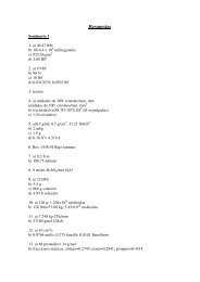
satisfy final plastic product property requirements in cost-effective ways. Thus, as is
shown in Fig. 1.4, since about 1960, the increase in the number of commercially valuable
polymer blends has powerfully driven the growth of the plastics industry and directly led
to the rapid introduction of plastics in new and critical product application areas.
Turning to the polymer blending operations shown in Fig. 1.5, the feed stream consists
of two or more polymers (virgin or reactively modified pellets) and a compatibilizer in
small concentrations, which is necessary to create fine and stable polymer blend
morphologies, since polymers are generally incompatible with each other. The processing
equipment must quickly melt each polymer (concurrently or sequentially), and then
rapidly and efficiently affect distributive and dispersive mixing of the melt components
and the compatibilizer. Co- and counterrotating TSEs can satisfy these elementary steps
that are important to blending operations.

12 HISTORY, STRUCTURAL FORMULATION OF THE FIELD
PEO
PUR
PIB
PET
PA
SBR
LDPE
PMMA
BR
PS
PVC
PPS
POM
PAR
PTFE
EPM
EPOM
PP
HDPE
ABS
PAN
EPOXY
PBT
Silicon
Polymers based on
new monomer units
PEEK
PES
PI
PEI
LCP
1920 1940 1960 1980 2000
Polymers based on
well-known monomer units
and polymer components
SAN/NBR
PS/BR
PVC/NBR
PC/ABS
PC/PBT
PET/EPDM
PA/EPDM
PP/EPDM
PVC/ABS
PVC/EVA
PS/PPO
GRP
COC
EO-Copo
synd. PS
synd. PP
PBT/LCP
PC/ASA
PP/PA
PP/EPDM
HDPE
PVC/CPE
PA/PPO/PS
PA/HDPE
SMA/ABS
POM/PUR
PBT/EPDM
1920 1940 1960 1980 2000
Fig. 1.4 A chronology of the discovery of polymers and their modification. [Courtesy of Prof.
Hans G. Fritz of IKT Stuttgart, Stuttgart, Germany (2b).]
If the compatibilizer is reactive, the rapid and effective melting and mixing will
establish the proper conditions for a uniform molten-phase reaction to take place. Thus, by
employing TSEs, polymer processors (compounders or product fabricators) can create
customized, ‘‘microstructured’’ polymer systems, which we have coined as ‘‘designer
pellets’’ (22), to best serve the special product property needs of their customers; they are
no longer solely dependent on polymer resin manufacturers.
The production rates and, thus, the equipment size, are large for resin manufacturers
and moderate for compounders. We again see, that the polymer blend stream is exposed to
the same elementary steps of processing and that, again, the choice of processing
equipment used is based on which equipment can best perform the critical elementary
steps. Finally, polymer blending operations expose the polymers to their second or perhaps
third thermomechanical experience.
Plastics Product Fabricating Operations
In these operations, polymer processors fabricate finished plastics products starting from
plastic pellets, which are the products of postreactor, compounding, reactive, or blending
polymer processing operations. These pellets are processed alone or, in the case of
producing colored products, together with a minor stream of color concentrates of the
same polymer. As can be seen in Fig. 1.6, the elementary steps in the processing
Polymer 1
Polymer 2
PSH, melt, mix, react,
devol (pump)
Pump/pres
Shape
cool
cut
Polymer
blends
pellets
To
fabricator
Compatibilizer(s)
(reactive/physical),
additives
TSE
Fig. 1.5
GP
Pelletizer
Polymer blend formation operations.

CURRENT POLYMER PROCESSING PRACTICE 13
Virgin pellets
(bags, gaylords, RR cars)
PSH, melt, mix, pres/pump
Shape
structure
cool
Trim
Weld
Thermoform
Finished plastic
products
Minor additive(s)
Single-screw extruders (SSE)
Injection-molding machines(IMM)
Fig. 1.6
SSE dies
molds
Plastic product fabrication operations.
Downstream/
postprocessing
equipment used are again the same as given previously. In product fabrication operations,
though, it is of paramount importance that the pressurization capabilities of the equipment
be very strong, since we need a melt pump to form the shape of a plastic product by forcing
the melt through a die or into a mold. Thus the equipment used by product fabricators are
SSEs and injection molding machines, which have modest particulate solids handling,
melting, and mixing capabilities, but are excellent melt pumps.
The molten stream of polymers flowing through dies or into cold molds is rapidly
cooled to form the solid-product shape. As a consequence of the rapid cooling, some
macromolecular orientations imparted during flow and near the product surfaces, where
cooling first occurs, are retained. The retained orientations in plastic products impart
specific anisotropic properties to the product and, in the case of crystalizable polymers,
special property-affecting morphologies. The ability to affect the above is called
structuring (23), which can be designed to impart extraordinarily different and beneficial
properties to plastic products.
Structuring is also carried out in postshaping operations, mainly by stretching the solid
formed product uni- or biaxially at temperatures appropriate to maximizing the retained
orientations without affecting the mechanical integrity of the product.
In-Line Polymer Processing Operations
The polymer product fabrication operations may be either the second or third thermomechanical
experience of the base polymer. Since polymers are subject to thermal
degradation, and since there is a cost associated with each of the melting/cooling cycles,
significant efforts are currently being made to develop what are called in the polymer
processing industry, in-line processing operations. These operations and equipment
sequentially conduct and functionally control any of the operations discussed earlier with
plastic product fabrication at the end, thus allowing for a smaller degree of macromolecular
and additive-properties degradation, and reducing the processing fabrication cost. The
practice is relatively new, and has required the functional coupling and control of pieces of
processing equipment that have distinctly different elementary step strengths: rapid,
uniform, and efficient melting and mixing versus robust pressurization and accurate
‘‘metering’’ of the product stream. In-line polymer processing operations are shown
schematically in Fig. 1.7.
From a plastics industry point of view, combining the various compounding, reactive
processing and blending operations with the finished product fabrication operation, in a
single line and under one roof, holds the potential for the product fabricator to become the

14 HISTORY, STRUCTURAL FORMULATION OF THE FIELD
Resin(s) +
Fig. 1.7
Reactants
Additives
Compatibilizers
Compounding
microstructuring
reacting
Forming
Finished product
In-line polymer processing operations (in-line compounding).
compounder as well. Furthermore, since fabricators are intimately involved with
the properties needed by the finished product, they would be able to ‘‘fine-tune’’ the
microstructuring of their polymer system to better meet the property needs of the products
they are fabricating. Such capabilities will enable processors to respond to requests for
customized polymer systems, that is, to satisfy ‘‘mass customization’’ needs of users of
plastic products.
Additionally, there is clear evidence that a small number of resin manufacturers ‘‘will
become more of enablers, creating new value-added businesses (of micro-structured
polymer products) ever closer to the ultimate consumer’’ (2c). This translates into the
planning by these companies for commercial expansion into compounding operations,
widening the spectrum of their products, and further contributing to mass customization
needs. Such developments and trends characterize the current ‘‘transition’’ phase of the
polymer industry and of polymer processing, as depicted in Table 1.2. This period, it is
hoped, will mark the gateway to a future where polymer processing will evolve into
macromolecular engineering. We will briefly discuss this possibility in the last section of
this chapter.
1.3 ANALYSIS OF POLYMER PROCESSING IN TERMS
OF ELEMENTARY STEPS AND SHAPING METHODS
The field of polymer processing has been traditionally and consistently analyzed (24) in
terms of the prevailing processing methods, that is, extrusion, injection molding, blow
molding, calendering, mixing and dispersion, rotational molding, and so on. In analogy to
chemical engineering, 3 these processes have been viewed as the ‘‘unit operations’’ of
polymer processing. At the time of the writing of the first edition of this text (24), when
polymer processing was maturing into a well-defined and well-studied engineering
discipline, we found it necessary to reexamine this classic way of analyzing the field,
because the manner in which a field is broken down into its component elements has
profound educational implications. A carefully worked out analysis should evolve into an
abstract structure of the field that accomplishes the following objectives:
1. Focuses attention on underlying engineering and scientific principles, which are
also the basis of the unifying elements to all processes.
2. Helps develop creative engineering thinking, leading to new, improved design.
3. Provides an overall view of the field, facilitating quick and easy assimilation of new
information.
3. Systematic engineering analysis of chemical processes led to the definition of a series of ‘‘unit operations,’’
such as distillation, absorption, and filtration, which are common to different chemical processes (e.g., see W. L.
McCabe and J. C. Smith, Unit Operations in Chemical Engineering, 2nd ed., McGraw-Hill, New York, 1967).

ANALYSIS OF POLYMER PROCESSING IN TERMS OF ELEMENTARY STEPS 15
A quarter of a century later, and in retrospect, the analysis that we presented then, and that we
discuss later, helped fulfill the previously defined objectives, and moved the field forward.
The Shaping Steps
The first step we take in our analysis of polymer processing is to clearly define its
objective(s). In this case, the objective is undoubtedly shaping polymer products. The
shaping operation can be preceded and followed by many manipulations of the polymer to
prepare it for shaping, modify its properties, and improve its appearance. Nevertheless, the
essence of polymer processing remains the shaping operation. The selection of the shaping
method is dictated by product geometries and sometimes, when alternative shaping methods
are available, by economic considerations. Reviewing the various shaping methods practiced
in the industry, we can classify them in the following groups:
1. Calendering and coating
2. Die forming
3. Mold coating
4. Molding and casting
5. Stretch shaping
The first shaping method is a steady continuous process. It is among the oldest methods,
and is used extensively in the rubber and plastics industries. It includes the classic
calendering, as well as various continuous coating operations, such as knife and roll
coating.
Die forming, which is perhaps the most important industrial shaping operation,
includes all possible shaping operations that consist of forcing a melt through a die.
Among these are fiber spinning, film and sheet forming, pipe, tube, and profile forming,
and wire and cable coating. This is also a steady continuous process, in contrast to the last
three shaping methods, which are cyclic.
The term ‘‘mold coating’’ is assigned to shaping methods such as dip coating, slush
molding, powder coating, and rotational molding. All these involve the formation of a
relatively thick coating on either the inner or the outer metal surfaces of the molds.
The next shaping method is molding and casting, which comprises all the different
ways for stuffing molds with thermoplastics or thermosetting polymers. These include the
most widely used shaping operations of injection molding, transfer molding, and
compression molding, as well as the ordinary casting of monomers or low molecular
weight polymers, and in situ polymerization.
Finally, stretch shaping, as implied by the name, involves shaping of preformed polymers
by stretching. Thermoforming, blow molding, stretch blow molding, and cold forming can
be classified as secondary shaping operations. The first three are very widely used.
The complex rheological properties of polymeric melts play a dominant role in the
shaping operations. Thus, the introduction of one of the most striking aspects of non-
Newtonian behavior, that of shear-thinning (pseudoplasticity), has been successfully
incorporated into the analysis of melt flow inside polymer processing equipment.
Similarly, by applying the modern sophisticated tools of numerical methods, the
incorporation of the elastic nature of the polymer is being carried out with increasing
success, particularly in stretch shaping.

16 HISTORY, STRUCTURAL FORMULATION OF THE FIELD
As mentioned earlier, during shaping and postshaping operations, a good deal of
structuring, that is, retained macromolecular orientation and specific morphologies, can
and is being imparted to the final plastic products. Structuring has long been understood to
be of very significant technological importance. The detailed understanding of structuring
requires the ability to quantitatively describe the flow of rheologically complex melts, heat
transfer, nucleation, and crystallization under stress. Work in this area is now underway, as
we discuss in the last section of the chapter.
The Elementary Steps
The polymer is usually supplied to the processors in a particulate form. Shaping of the
polymer takes place only subsequent to a series of preparatory operations. The nature of
these operations determines to a large extent the shape, size, complexity, choice, and cost
of the processing machinery. Hence, the significance of a thorough understanding of these
operations cannot be overemphasized. One or more such operations can be found in all
existing machinery, and we refer to them as elementary steps of polymer processing.
There are five clearly identifiable elementary steps:
1. Handling of particulate solids
2. Melting
3. Pressurization and pumping
4. Mixing
5. Devolatilization and stripping
Defining ‘‘handling of particulate solids’’ as an elementary step is justified, considering
the unique properties exhibited by particulate solids systems. Subjects such as particle
packing, agglomeration, consolidation, gravitational flow, arching, compaction in hoppers,
and mechanically induced flow must be well understood to ensure sound engineering
design of processing machines and processing plants.
Subsequent to an operation involving solids handling, the polymer must be melted or
heat softened prior to shaping. Often this is the slowest, and hence the rate-determining
step in polymer processing. Severe limitations are imposed on attainable melting rates by
the thermal and physical properties of the polymers, in particular, the low thermal
conductivity and thermal degradation. The former limits the rate of heat transfer, and the
latter places rather low upper bounds on the temperature and time the polymer can be
exposed. On the other hand, beneficial to increasing the rate of melting is the very high
polymer melt viscosity, which renders dominant the role of the viscous energy dissipation
(VED) heat-source term. Plastic energy dissipation (PED) (25,26) arising from the
compressive and shear deformation of compacted polymer solid particulates in twin rotor
equipment, such as Co-TSEs, is such a powerful heat source that it may result in nearly
instant melting. All these factors emphasize the need to find the best geometrical
configuration for obtaining the highest possible rates of melting, and for determining the
processing equipment needed for rapid and efficient melting.
The molten polymer must be pumped and pressure must be generated to bring about
shaping—for example, flow through dies or into molds. This elementary step, called
pressurization and pumping, is completely dominated by the rheological properties of
polymeric melts, and profoundly affects the physical design of processing machinery.
Pressurization and melting may be simultaneous, and the two processes do interact with

ANALYSIS OF POLYMER PROCESSING IN TERMS OF ELEMENTARY STEPS 17
each other. Moreover, at the same time, the polymer melt is also mixed by the prevailing
laminar flow. Mixing the melt distributively to obtain uniform melt temperature or uniform
composition (when the feed consists of a mixture rather than a single-component
polymer), ‘‘working’’ the polymer for improving properties, and a broad range of mixing
operations involving dispersive mixing of incompatible polymers, breakup of agglomerates,
and fillers—all these belong to the elementary step of ‘‘mixing.’’
The last elementary step of devolatilization and stripping is of particular importance to
postreactor compounding, blending, and reactive processing operations, although it also
occurs in commonly used processes, for example, devolatilizing in vented two-stage SSEs.
This elementary step involves mass transfer phenomena, the detailed mechanisms of
which have been investigated in some depth since the publication of the first edition of this
book, and therefore, unlike in the first edition, here we devote a full chapter to this step.
Yet, more research is needed to fully elucidate this complex process.
This theoretical analysis of processing in terms of elementary steps, which considers
the basic physical principles and mechanisms involved in each elementary step, has been
helpful since its introduction, in gaining better insight into the currently used processing
methods, encouraging further work on their mathematical formulations, and perhaps also
stimulating creative engineering thinking on improved processing methods. It has helped
provide answers not only to ‘‘how’’ a certain product works, but to ‘‘why’’ a product is
made a certain way and, foremost, ‘‘why’’ a particular machine configuration is the ‘‘best’’
or the appropriate one to use. The latter question is indeed the essence of engineering. For
these reasons we will maintain and add to this approach in this edition.
Structural Breakdown of Polymer Processing
The elementary steps, as well as the shaping operations, are firmly based on the principles
of transport phenomena, fluid mechanics and heat and mass transfer, polymer melt
rheology, solid mechanics, and mixing. These principles provide the basic tools for
quantitatively analyzing polymer processing. Another fundamental input necessary for
understanding polymer processing is the physics and chemistry of polymers. As we noted
earlier, final product properties can be immensely improved by structuring.
Figure 1.8 schematically summarizes our approach to the breakdown of the study of
polymer processing. Raw material is prepared for shaping through the elementary steps. The
elementary steps may precede shaping or they may be simultaneous with it. Structuring
takes place throughout these processes, and subsequent to them. Finally, postshaping
operations for purposes other than structuring (printing, decorating, etc.) may follow.
Clearly, to be able to fully utilize the added degree of freedom for product design
provided by structuring, a full understanding and computational handling of polymer
chemistry, polymer rheology at a macromolecular level, and the physics of phase changes
under stress fields and nonisothermal conditions has to be carried out. With advances in
those fields and the exponential growth of available computing power, significant advances
are already being made toward achieving specific processed product properties, not
through trial and error, but process simulation (2d).
The conceptual breakdown of polymer processing dating back to the first edition of
1979, presented earlier, remains the same. Yet the field and the industry, in the current
transition period, have been focusing on and growing through what used to be called
compounding, and is now expanded from the simple dispersion and distribution of fillers
in polymer melts, to encompass microstructure development and stabilization in

18 HISTORY, STRUCTURAL FORMULATION OF THE FIELD
Raw
material
Finished
product
Handling of
particulate solids
Die forming
Melting
Molding and casting
Elementary steps
Pressurization
and pumping
Mixing
Shaping methods
Stretch shaping
Calendering
and coating
Postshaping
Devolatilization
and stripping
Mold coating
Structuring of polymers in processing
Transport
phenomena
Mixing
principles
Solid
mechanics
Polymer melt
rheology
Polymer
physics
Polymer
chemistry
Engineering principles
Polymer science
Fig. 1.8 Conceptual structural breakdown of polymer processing product fabrication operations (23).
immiscible, compatibilized, and reactive interphase multicomponent polymer systems of
blends and alloys to create ‘‘designer pellets.’’ In this activity, the important elementary
steps are rapid melting, affected mostly by PED and VED (that we refered to as dissipative
mix-melting (23a, 25, 26)), rapid distributive and dispersive mixing created by extentional
time-varying flows, and devolatilization, often occurring in the presence of reactions
involving polymer melts. Co- and counterrotating TSEs, not shear-drag flow melting and
pumping devices (e.g., SSEs), are the processing equipment used in these endeavors.
The conceptual breakdown in Fig. 1.9 (27) simply indicates the fact that in
compounding, blending, and reactive processing, the base polymer(s) undergo two
thermomechanical elementary-step experiences, and that the product of the first are valueadded
and microstructured pellets, while the second is used primarily for fabricating
finished products. The important elementary steps for each experience, and the physical
mechanisms that affect them, are different, because of the different objectives in each.
1.4 FUTURE PERSPECTIVES: FROM POLYMER PROCESSING
TO MACROMOLECULAR ENGINEERING
In May 2002 an International Invited Workshop, attended by leading researchers in
polymer processing and polymer engineering science, was convened in order to take stock
of the historical evolution of the field of polymer processing, analyze current
developments in research, take note of structural changes in the industry, and consider
future trends. The underlying rationale, outlined in Appendix A of the final report (2), was

FUTURE PERSPECTIVES: FROM POLYMER PROCESSING 19
Polymer(s), additives, reactants
pellets
Handling of
particulate solids
Elementary steps
Melting
Pressurization
and pumping
Mixing
Reactions
involving melts
Pelletizing die
Microstructured
“designer” pellets
Second elementary step
thermomechanical experience
Product shaping methods
structuring
Finished product
Devolatilization
and stripping
“Microstructuring” during melting and mixing reactions
Fig. 1.9 Conceptual breakdown of polymer compounding, blending, and reactive polymer
processing (27). Designer pellets are processed in extruders or injection molding machines to form
products, with the possibility of further structuring or ‘destructuring’.
the proposition that this new and still evolving engineering discipline, propelled by the
revolutionary developments in polymer physics, polymer chemistry, computational fluid
mechanics, sophisticated novel instrumentation capabilities, modern catalysis, and
developments in molecular biology, is diverging into a broad-based multidisciplinary
activity, not unlike biotechnology and nanotechnology. Therefore, it is at a turning point.
Needless to say, for both authors working on this second edition, the workshop held the
additional potential of providing a glimpse at the future development of the field. Thus, we
present below some of the major topics of deliberation and conclusions of the workshop,
drawing liberally from the text of the Final Report.
Central to the deliberations was to first outline in broad brush-strokes the knowledge so
far acquired, and identify general areas where future research is needed. The guiding
questions were: What do we know? What do we know that we don’t know? What do we need
to know? What are the ‘‘boundaries’’ of the field? Which are the relevant disciplines needed
for getting ahead in what increasingly appears to be a multidisciplinary field? And how can
polymer processing become a strategic element in the ‘‘chain of knowledge’’?
There was agreement among the participants that much has been accomplished in
the past decades by classic polymer processing (Fig. 1.2). During this period, polymer
processing focused on analyzing the major polymer processing equipment and
processes (SSEs, TSEs, injection molding machines, blow molding machines, vacuum
forming machines, calenders and roll mills, rotational molding machines, batch and
continuous mixers, etc.). In doing so, the field grew and matured with the realization
(as noted in Section 1.3) that there are common phenomena in the thermomechanical
experiences of the material in the diverse polymer processing equipment and processes
described earlier. This realization led to the elucidation and simulation of the detailed
mechanisms and sequence of events that take place in these machines and in the
continuous and cyclic shaping processes: flow of particulate solids; principles of
melting of plastics in SSEs; principles of distributive, dispersive, and chaotic mixing;

20 HISTORY, STRUCTURAL FORMULATION OF THE FIELD
principles and mechanisms of devolatilization; flow of non-Newtonian polymeric
melts in complex conduits with moving surfaces using analytical, finite difference and
finite element techniques; transient developing flows into cavities; wall stress-free
one-, two- and three-dimensional flows as in fiber spinning, bubble formation, and
complex blow molding operations, to name a few; degradation reactions in processing
equipment, and so forth.
Not everything was elucidated to the same level and, as discussed in the following
paragraphs, much remains to be done in classic polymer processing. The knowledge base
developed so far was founded on, and rooted in, several disciplines, such as transport
phenomena—including fluid mechanics, heat transfer and molecular diffusion of chemical
species, non-Newtonian fluid mechanics, rheology (continuum and, to a lesser extent,
molecular), resin thermophysical properties and state equations, classic mathematical
techniques, and computational fluid mechanics, as well as polymer physics and
thermodynamics. The focus of past research, as well as much of the current research, is
on the process and the scale of examination of the machine, with the objective of
developing optimized processes and improved machines.
During this period, relatively little emphasis was placed on the product and its
microscopic and molecular structure, though there was rudimentary and semiquantitative
treatment of what was termed structuring (2b, 23). Today, in some of the larger researchand-development
centers, an important transition is being made, to focus on the product
and its properties on the micro and molecular scale.
Areas on the process side identified as needing further research are:
A better understanding of and advanced mathematical formulation of all the basic
mechanisms under realistic machine conditions with a single polymeric feed or a
mixture of them, with the goal of simulating the process as a whole;
A fundamental and multidisciplinary understanding of melting of compacted
polymer particulates under high deformation rates;
A much deeper understanding of the details on how the process affects the structure
on micro and molecular levels;
Materials/machine interactions, three-dimensional viscoelastic behavior and stability
of polymeric liquids;
Transient flow and nonisothermal rheology;
Nucleation and crystallization under stress;
Molecular orientation phenomena;
Reaction and polymerization under flow and deformation;
Multiphase flows at high rates of strains;
Heat, momentum, mass, entropy balances at ‘‘finite domain structure levels’’ of
solids and liquids, during deformation, melting, and solidification;
Thermodynamics of interfaces;
Phase transition;
Molecular models and modeling;
Quantitative connection of structures and structure formation at the molecular and
micro scale to final properties;
Measurement techniques, including process in-line measurements, at the molecular
and micro-scale levels to verify theories and predictions.

FUTURE PERSPECTIVES: FROM POLYMER PROCESSING 21
However, even the complete understanding of these areas will not suffice to reap the full
benefits embedded in the macromolecular nature of polymeric materials, which are inherent in
the naturally occurring and synthetic polymeric building blocks. For that, a priori quantitative
prediction of product properties, made of yet nonexistent chains or combinations of chains of
different monomeric building blocks from basic principles, requiring information of only the
macromolecular structure and processing conditions, is needed.
Interesting comparisons were made to other fields, such as semiconductors, which
cannot be produced without thorough knowledge at the quantum mechanics level and finetuned
processing; multiscale computing in solids mechanics, in which microscopic
behavior is being predicted from first principles on atomic scales; drug development with
computer simulation screening of new molecules; modern catalysis and biocatalysts; and
molecular biology with potential adaptation of self-assembly properties to other fields,
such as biological microchips.
It was concluded that modern polymer processing, or rather future polymer processing
(see Table 1.2), will focus not on the machine, but on the product. The long-range goal will
be to predict the properties of a product made from a yet nonexistent polymer or polymerbased
material, via simulation based on first molecular principles and multiple-scale
examination. This approach, using increasingly available computing power and highly
sophisticated simulation, might mimic nature by targeting properties via complex
molecular architectural design. However, two important and key challenges have to be met
successfully in order to achieve this goal: first, highly sophisticated simulations require
highly sophisticated molecular models, which do not exist at present; second, a far more
detailed understanding of the full and complex thermomechanical history that transpires in
the polymer processing machine is needed. Then, such analysis will lead not only to new
products, but will also improve existing machines or even lead to radically new machines;
nevertheless, the focus will remain on the product. The goal is to engineer new and truly
advanced materials with yet unknown combinations of properties, which might open up a
new ‘‘golden age’’ for the field, reminiscent of the 1950s, 1960s, and 1970s, when most of
the currently used polymers were developed.
Thus, the terms ‘‘polymer processing,’’ ‘‘polymer engineering,’’ or ‘‘plastics engineering’’
have become too narrow and confining, and a more accurate description of the
emerging new field ought to be macromolecular engineering. As noted earlier, the new
field is inherently multidisciplinary in nature, and if it is to be developed at a world-class
level, requires close collaboration between many disciplines of science and engineering.
Hence, the emphasis must shift from the individual researcher to large team efforts, this
having profound consequences to academic research, as well as academic departmental
boundaries. Real progress will only be possible by pooling substantial resources, and the
allocation of these significant resources should be facilitated by vision, planning, and a
comprehensive alliance between government, academia, and industry.
Macromolecular engineering is part of a broader scene. On the very fundamental level,
its boundaries merge with molecular biology, on the one hand, and the growing field of
complex fluids, that grows out of chemistry, physical chemistry, physics, and chemical
engineering, on the other hand. The preceding, in turn, has profound educational
implications, pointing to the possible creation of an entirely new and unified underlying
discipline, and a basic undergraduate curriculum in molecular, macromolecular
and supramolecular engineering, leading to specialization in chemical molecular
engineering (currently chemical engineering), macromolecular engineering (currently
polymer processing and engineering), and biomacromolecular engineering (currently

22 HISTORY, STRUCTURAL FORMULATION OF THE FIELD
Macromolecular engineering and science
Molecular and supramolecular
engineering and science
Chemical molecular engineering and science
Biomacromolecular engineering and science
Fig. 1.10 A curricular structure discussed during the Touchstones of Modern Polymer Processing
workshop, where a novel discipline called Molecular and Supramolecular Engineering and
Science, becomes the initial, common core of macromolecular, chemical molecular, and
Biomacromolecular engineering.
biochemical engineering or biotechnology). Such a curricular structure is depicted in
Fig. 1.10.
Recently, Jos Put, discussed (28) the very enlightening view of J. L. Atwood et al. (29)
on the nature of molecular biology and synthetic chemistry, shown in Fig. 1.11. Nature has
achieved a tremendous level of complexity and control in living organisms, with a limited
number of building blocks; synthetic (polymer) chemistry has used a much more diverse
number of building blocks and achieved only limited, controlled structural complexity.
Nature is able to do this by supreme control on the molecular level (MW, MWD, sequence,
tacticity, etc.), by ordering on the nanolevel, and by perfect macroscopic design. On the
other hand, macromolecular synthetic chemistry has made great strides by utilizing
chemical species diversity, while achieving very modest controlled structural complexity.
Biotechnology has begun to broaden the chemical diversity of bioapplicable systems, and
synthetic nano chemistry is achieving remarkable controlled complexity at the nano level,
utilizing and offering structurally ordered platforms to macromolecules. Thus, the
merging of the boundaries of macromolecular engineering and molecular biology offers
formidable potential for new materials and products. This is depicted by the 45 vector
direction in Fig. 1.11.
Controlled
complexity
Biology
Biotechnology
Nano chemistry
Synthetic chemistry
Chemical diversity
Fig. 1.11 The diagram used by J. L. Atwood et al. (29), to depict the differences between
synthetic chemistry and biology in terms of the ‘‘building blocks’’ used and the attained structural
controlled complexity.

REFERENCES 23
Macromolecular engineering from the research point of view is clearly a broad-based
multidisciplinary field. Consequently, the research scene and practices, in particular in
academia, require restructuring. The classic ‘‘individual faculty member–graduate
student(s)’’ model is expected to be replaced by the large, multidisciplinary team model,
because, as pointed out earlier, only these larger teams can be expected to conduct
groundbreaking research. Such teams should consist of several senior faculty members in
the needed disciplines, co-advising several graduate students as well as trained
professionals who deal with advanced instrumentation, computing, data analysis, and
literature searches.
It is perhaps worth adding that such large multidisciplinary groups already exist at
leading centers of macromolecular engineering research. In fact, we are witnessing the first
promising examples of a priori quantitative predictions of the solid product properties
requiring information of only the macromolecular structure and processing conditions from
such large multidisciplinary groups. For example, Han E. H. Meijer et al. at the Materials
Technology, Dutch Polymer Institute, Eindhoven University of Technology (30,31)
proposed such an a priori prediction for the yield stress of polycarbonate (PC) specimens
obtained under different molding conditions. Their work is based on defining a novel state
parameter that uniquely determines the current state of amorphous solids and utilizes the
classic constitutive model representation of such solids as presented by Haward and
Thackray (32), who identified two contributions to the total stress: one that accounts for the
rate-dependent plastic flow response attributed to intermolecular interactions on a segmental
scale (33,34) and represented by a nonlinear Maxwell element (35), and the other that
accounts for the strain-hardening contribution that is due to the macromolecular orientation
of the entangled network using a neo-Hookean elastic model (36).
REFERENCES
1. E. C. Bernhardt and J. M. McKelvey, ‘‘Polymer Processing – New Engineering Specialty’’,
Mod. Plast., 35, (July) 154–155, (1958).
2. Final Report of the international invited workshop ‘‘Touchstones of Modern Polymer Processing
– From Classic Polymer Processing to Macromolecular Process Science’’, May 10–12,
2002, The Polymer Processing Institute at NJIT, Newark, NJ (a) Table 1, p. 11, (b) Z. Tadmor,
Appendix A, p. 21, (c) Industrial Considerations p. 13, (d) Z. Tadmor Appendix A, pp. 24 and 25.
3. C. Goodyear, Gum Elastic (private printing), New Haven, CT, 1855.
4. M. Kaufman, ‘‘The Birth of the Plastics Extruder,’’ Polym. Plast., 243–251 (June, 1969).
5. V. M. Hovey, ‘‘History of Extrusion Equipment for Rubber and Plastics,’’ Wire and Wire Prod.,
36, 192 (1961).
6. G. Schenkel, Plastics Extrusion Technology and Theory, Iliffe Books, Ltd., London, 1966.
7. J. L. White, ‘‘Elastomer Rheology and Processing,’’ Rubber Chem. Technol., 42, 256–338
(1969).
8. M. Gray, British Patent 5056 (1879).
9. J. W. Hyatt, Ind. Eng. Chem., 6, 158 (1914).
10. J. H. Dubois, Plastics History USA, Cahners Books, Boston, 1975.
11. J. F. Chabot and R. A. Malloy, ‘‘A History of Thermoplastic Injection Molding. Part I – The
Birth of an Industry’’, J. Inj. Mold. Technol., 1, 1 (1997).
12. H. Herrmann, Scheneken Maschinen Inder Versahrenstechnik, Springer Verlag, Berlin, 1972.

24 HISTORY, STRUCTURAL FORMULATION OF THE FIELD
13. C. Pasquetti, British Patent, 638, 364 (1950).
14. D. H. Killeffer, ‘‘Banbury the Master Mixer’’, Palmerton, NY, 1962.
15. E. H. Ahlenfeld, P. Hold, A. J. Baldwin, W. A. Rapetsky, and H. R. Scharer, U.S. Patent 3, 154,
802 (1969).
16. William H. Willert, ‘‘Injection Molding Apparatus,’’ U.S. Patent 2, 734, 226 (1956).
17. B. Maxwell and A. J. Scalora, Mod. Plast., 37, 107 (1959).
18. R. F. Westover, ‘‘A Hydrodynamic Screwless Extruder,’’ SPE J., 18, 1473 (1962); also U.S.
Patent 3, 123, 861 (1964).
19. Z. Tadmor, U.S. Patent 4, 142, 805 (1979); U.S. Patent 4, 194, 841 (1980).
20. D. Landes, The Wealth and Poverty of Nations, W. W. Norton, New York, 1998; Abacus,
London, 2001. Chapter 13, ‘‘The Nature of Industrial Revolution.’’
21. Information Presented by the Society of Plastics Industries (SPI), 2002. 5plasticsdatasource.
org4
22. C.G. Gogos, ‘‘From Compounding toMicro-structuring toReactive Processing,’’ Keynote Lecture,
Extrusion Division, Proc. 55th Soc. Plastics Eng. Ann. Technical Conf., Toronto, Canada 1997.
23. Z. Tadmor and C. G. Gogos, Principles of Polymer Processing, Wiley-Interscience, New York,
1979, (a) Chapter 9, Section 9.1.
24. E. C. Bernhardt, Processing of Thermoplastic Materials, Reinhold, New York, 1959.
25. C. G. Gogos, Z. Tadmor, and M.-H. Kim, ‘‘Melting Phenomena and Mechanisms in Polymer
Processing Equipment,’’ Adv. Polym. Techn., 17, 286 (1998).
26. B. Qian and C. G. Gogos, ‘‘The Importance of Plastic Energy Dissipation (PED) to the Heating
and Melting of Polymer Particulates in Intermeshing Co-rotating Twin Screw Extruders: An
Experimental Investigation,’’ Adv. Polym. Techn., 19, 287 (2000).
27. C. G. Gogos, ‘‘Elementary Steps and ‘Structuring’ of Polymers—Then and Now,’’ Symposium
13 Honoring Z. Tadmor’s 60th Birthday, paper 13-I, Extended Abstracts in the 13th Meeting of
the Polymer Processing Society, Secaucus, NJ, 1997.
28. J. Put, ‘‘Business in Polymeric Materials,’’ European Polymer Federation in Collaboration with
AIM Magazine, Special Issue, July 2001.
29. J. L. Atwood, J.-M. Lehn, J. E. D. Davies, D. D. Nicol, and F. Vogte, Comprehensive
Supramolecular Chemistry, Pergamon Press, Amsterdam, 1996.
30. L. E. Govaert, T. A. P. Engels, E. T. J. Klompen, G. W. M. Peters, and H. E. H Meijer,
‘‘Processing-induced Properties in Glassy Polymers,’’ Int. Polym. Process., 20, 170 (2005).
31. H. E. H. Meijer and L. E. Govaert, ‘‘Mechanical Performance of Polymer Systems: The Relation
Between Structure and Properties,’’ Prog. Polym. Sci., 30, 915–938 (2005).
32. R. N. Haward and G. Thackray, ‘‘The Use of a Mathematical Model to Describe Isothermal
Stress-Strain Curves in Glassy Thermoplastics,’’ Proc. R. Soc. London, Series A, 302 (1471),
453 (1967).
33. T. A. Tervoort, E. T. J. Klompen, and L. E. Govaert, ‘‘A Multi-mode Approach to Finite, Threedimensional
Nonlinear Viscoelastic Behavior of Polymer Glasses,’’ J. Rheol., 40, 779 (1996).
34. E. T. J. Klompen, Ph.D Thesis, Eindhoven University of Technology, The Netherlands (2005),
Chapter 6.
35. F. P. T. Baaijens, ‘‘Calculation of Residual Stresses in Injection Molded Products,’’ Rheol. Acta,
30, 284 (1991).
36. L. E Govaert, P. H. M. Timmermans, and W. A. M. Brekelmans, ‘‘The Influence of Intrinsic
Strain Softening on Strain Localization in Polycarbonate: Modeling and Experimental Validation,’’
J. Eng. Mater. Tech., 122, 27 (2000).

2 The Balance Equations
and Newtonian Fluid Dynamics
2.1 Introduction, 25
2.2 The Balance Equations, 26
2.3 Reynolds Transport Theorem, 26
2.4 The Macroscopic Mass Balance and the Equation of Continuity, 28
2.5 The Macroscopic Linear Momentum Balance and the Equation of Motion, 32
2.6 The Stress Tensor, 37
2.7 The Rate of Strain Tensor, 40
2.8 Newtonian Fluids, 43
2.9 The Macroscopic Energy Balance and the Bernoulli and Thermal Energy Equations, 54
2.10 Mass Transport in Binary Mixtures and the Diffusion Equation, 60
2.11 Mathematical Modeling, Common Boundary Conditions, Common Simplifying
Assumptions and the Lubrication Approximation, 60
2.1 INTRODUCTION
The engineering science of ‘‘transport phenomena’’ as formulated by Bird, Stewart,
and Lightfoot (1) deals with the transfer of momentum, energy, and mass, and provides
the tools for solving problems involving fluid flow, heat transfer, and diffusion. It is
founded on the great principles of conservation of mass, momentum (Newton’s second
law), and energy (the first law of thermodynamics). 1 These conservation principles
can be expressed in mathematical equations in either macroscopic form or microscopic
form.
In this chapter, we derive these equations in some detail using the generalized,
coordinate-free formulation of the Reynolds Transport Theorem (2). We believe that it
isimportant for every student or reader to work through these derivations at least once. We
then discuss the nature of the stress and rate of deformation tensors, demonstrate the use of
the balance equations for problem solving with Newtonian fluids using analytical and
numerical techniques, discuss the lubrication approximation, which is very useful in
modeling of polymer processing operations, and discuss the broad principles of
mathematical modeling of complex processes.
1. See R. Feynman, The Character of Physical Law, MIT Press, Cambridge, MA, 1967, where the profound nature
of the conservation laws is discussed.
Principles of Polymer Processing, Second Edition, by Zehev Tadmor and Costas G. Gogos.
Copyright # 2006 John Wiley & Sons, Inc.
25

26 THE BALANCE EQUATIONS AND NEWTONIAN FLUID DYNAMICS
2.2 THE BALANCE EQUATIONS
Since in ‘‘transport processes’’ mass, momentum, and energy are transported from one
part of the medium to another, it is essential that proper ‘‘bookkeeping’’ be applied to keep
track of these quantities. This can be done using balance equations, which are the
mathematical statements of the physical laws of conservation. These are very general laws
that always hold, and they apply to all media: solids or fluids, stationary or flowing. These
equations can be formulated over a specified macroscopic volume, such as an extruder, or
a microscopic volume taking the form of a differential (field) equation that holds at every
point of the medium. In the former case, the balance holds over the extensive quantities of
mass, momentum, and energy, whereas in the latter case, it holds over their intensive
counterparts of density, specific momentum, and specific energy, respectively.
In the formulation of the microscopic balance equations, the molecular nature of matter
is ignored and the medium is viewed as a continuum. Specifically, the assumption is made
that the mathematical points over which the balance field-equations hold are big enough to
be characterized by property values that have been averaged over a large number of
molecules, so that from point to point there are no discontinuities. Furthermore, local
equilibrium is assumed. That is, although transport processes may be fast and irreversible
(dissipative), from the thermodynamics point of view, the assumption is made that, locally,
the molecules establish equilibrium very quickly.
2.3 REYNOLDS TRANSPORT THEOREM
The physical laws of conservation of mass, momentum, and energy are commonly
formulated for closed thermodynamic systems, 2 and for our purposes, we need to transfer
these to open control volume 3 formulations. This can be done using the Reynolds
Transport Theorem. 4
Let P represent some extensive property of the system (e.g., mass, momentum, energy,
entropy) and let p represent its intensive counterpart (i.e., per unit mass), such that:
ð
P ¼ rpdV
ð2:3-1Þ
V
where V is the volume of the system, which can be a function of time, t. The Reynolds
Transport Theorem states that the substantial derivative (see Footnote 6) of P is
ð
ð
DP
Dt ¼ @
ðrpÞdV þ rpv n dS
@t
V
S
ð2:3-2Þ
2. A thermodynamic system is an arbitrary volume of matter without any transportation of matter across its surface.
3. The control volume is an arbitrary, fixed volume in space.
4. We assume the reader is familiar with vector notation, which is covered in many texts (e.g., Ref. 1), and except
for brief explanatory comments, no summary of vector operation is presented. However, the tabulated
components of the balance equations in various coordinate systems presented in this chapter should enable the
reader to apply them without any detailed knowledge of vector operations.

REYNOLDS TRANSPORT THEOREM 27
where V is the control volume fixed in space, S is the surface area of the control volume, v
is the velocity field, and n is the unit outward normal vector to the control surface. In
physical terms, Eq. 2.3-2 states that the rate of change of P of the system, at the instant it
coincides with the control volume, is the sum of two terms: the rate of change of P within
the control volume, and the net rate of flow of P out of the control volume.
Proof of Eq. 2.3-2 First we take the substantial derivative of Eq. 2.3-1
DP
Dt ¼ d ð
rp dV
system
dt
V
ðaÞ
Then by defining P s ¼ P system we can express the left-hand side of Eq. (a)
DP s
Dt
¼ lim
t!0
P s;tþt
t
P s;t
ðbÞ
Next we let the arbitrary volume of P s coincide at time t with the control volume. Since the
volume is arbitrary, we can do so without losing generality. But because there is the flow of
matter in the space, at time t þ t the volume of P s will be different, as shown in Fig. 2.1.
Looking at the figure we see that there are three distinct volume regions, A; B; and C.
The control volume equals the sum A þ B, and the system equals B þ C. Therefore P s at
time t þ t can be expressed as
and
P S;tþt ¼ P B;tþt þ P C;tþt ¼ P CV;tþt P A;tþt þ P C;tþt ðcÞ
P S;t ¼ P CV;t
ðdÞ
where the subscript CV stands for control volume. Substituting Eqs. (c) and (d) into Eq. (b)
gives
DP S
Dt
¼ lim
t!0
P CV;tþt
t
P CV;t
P C;tþt
þ lim
t!0 t
P A;tþt
lim
t!0 t
ðeÞ
CS I
A
B
System at
C
t + ∆t
Control volume at t
CS II
Fig. 2.1 The control volume (broken curve) and the thermodynamic system (solid curve) at time
t þ t in a flowing medium. The control volume and the thermodynamic system coincide at time, t.

28 THE BALANCE EQUATIONS AND NEWTONIAN FLUID DYNAMICS
The first expression on the right hand side is the partial differential in time of
P CV ;@P CV =@t. Now,P C;tþt is due to flow through surface CS II of the control volume,
separating volumes B and C, which can be calculated as follows:
The local volumetric rate of flow is v n dS
The local rate of flow of the property is rp v n dS
The differential quantity of P C transported over time t is dP C ¼ tpv n dS
Thus, the total amount of P C transported over surface CS II and time t is given by:
ð
P C;tþt ¼ t rpv n dS
CS II
ðfÞ
and, therefore,
P C;tþt
lim ¼
t!0 t
ð
CS II
rpv n dS
ðgÞ
Similarly we can show that
P A;tþt
lim ¼
t!0 t
ð
CS I
rpv n dS
ðhÞ
The reason for the negative sign is that v n for flow into the system is negative.
Substituting Eqs. g and h into Eq. e yields the following equation:
DP S
Dt
¼ @ ð ð
rpdV þ rpv n dS
@t
V
where S is the total surface ðCS I þ CS II Þ of the control volume and V is its volume, which
is identical to Eq. 2.3-2. This concludes the proof.
S
ðiÞ
2.4 THE MACROSCOPIC MASS BALANCE AND THE EQUATION
OF CONTINUITY
In deriving the balance equations, we use vector notation and the sign convention adopted
by R. B. Bird, W. E. Stewart, and E. N. Lightfoot in their classic book Transport
Phenomena (1).
We begin the derivation of the conservation of mass by simply inserting into Eq. 2.3-2,
P ¼ M and p ¼ 1, yielding directly the macroscopic mass balance equation:
ð ð
@
r dV þ rv n dS ¼ 0
ð2:4-1Þ
@t
V
S

THE MACROSCOPIC MASS BALANCE AND THE EQUATION OF CONTINUITY 29
We can convert the surface integral in Eq. 2.4-1 to a volume integral using the Gauss
Divergence Theorem 5,6 to yield:
ð ð
@
r dV þ ð= rvÞ dV ¼ 0 ð2:4-2Þ
@t
V
V
But by definition, we have selected a fixed control volume, therefore the order of
differentiation by time and integration can be reversed to get:
ð
@r
@t þ = rv dV ¼ 0
V
ð2:4-3Þ
For this equation to hold for any arbitrary volume V, the kernel of the integral must vanish,
resulting in the equation of continuity:
@r
@t þ = rv ¼ 0
ð2:4-4Þ
Equation 2.4-4 can be rewritten in terms of the substantial derivative as:
Dr
Dt ¼
r ð= vÞ
ð2:4-5Þ
Equation 2.4-4 states the mass conservation principle as measured by a stationary
observer. The derivative ð@=@tÞ is evaluated at a fixed position in space (this is referred to
as the Eulerian point of view); whereas, Eq 2.4-5 states the conservation principle, as
5. The Gauss Divergence Theorem states that if V is a volume bounded by a closed surface S, and A is a
continuous vector field, then Ð v ð= AÞ dV ¼ Ð sðn AÞ dS.
6. The recurring vectorial operator =, known as del or nabla, is a differential operator that, in rectangular
coordination is defined as:
= ¼ d 1 þ @ 1
@x 1
þ d 2 þ @ 2
@x 2
þ d 3 þ @ 3
@x 3
where d i are unit vectors in directions x 1 ; x 2 and x 3 . For the derivation of = in curvilinear coordinates, see
Problem 2.1. The ‘‘substantial derivative,’’ namely, the change in time of some property in a fluid element while
being convected (or riding with) the fluid in terms of =, is given by:
D
DT ¼ @ @t þ v =
Recall that the operation of = on a scalar quantity is the gradient, which is a vector. For example, if = is operated
on a scalar pressure field P, then = P is the pressure gradient vector field, which can have different values in the
three spatial directions. The operation of = on a vector field can either be the divergence or the curl of the vector
field. The former is obtained by the dot product (also called the scalar product) as = v or div v ! , where the result
is a scalar; whereas, the latter is obtained by the cross product (also called the vector product) = v, or curl v, and
the result is a vector field.

30 THE BALANCE EQUATIONS AND NEWTONIAN FLUID DYNAMICS
TABLE 2.1
The Equation of Continuity in Several Coordinate Systems
Rectangular Coordinates (x, y, z)
Cylindrical Coordinates (r, , z)
Spherical Coordinates (r, , )
@r
@t þ @ ð
@x rv xÞþ @ @y rv @
y þ ð
@z rv zÞ ¼ 0
@r
@t þ 1 @
ð
r @r rrv rÞþ 1 @
ð
r @y rv yÞþ @ ð
@z rv zÞ ¼ 0
@r
@t þ 1 @ 1 @
r 2 @r rr2 v r þ ð
r sin y @y rv y sin yÞþ 1 @
r sin y @f rv
f ¼ 0
Source: Reprinted with permission from R. B. Bird, W. E. Stewart, and E. N. Lightfoot, Transport Phenomena,
Wiley, New York, 1960.
measured (reported) by an observer who is moving with the fluid (this is referred to as the
Lagrangian point of view). Table 2.1 gives Eq. 2.4-4 in rectangular, cylindrical, and
spherical coordinate systems.
For an incompressible fluid, the density is constant, that is, it does not change in time or
spatial position, and therefore Eq. 2.4-5 simplifies to:
= v ¼ 0 ð2:4-6Þ
In fluid dynamics we frequently invoke the incompressibility assumption, even though
fluid densities change with pressure and temperature, and these may vary in time and
space. If the density change cannot be neglected, then an appropriate equation of state of
the form r ¼ rðT; PÞ must be used in conjunction with the balance equations.
Example 2.1 The Use of the Macroscopic Mass Balance for a Vessel with Salt
Solution A liquid-filled vessel shown in the accompanying figure contains a 1000 kg of
10% by weight salt solution. At time t ¼ 0 we begin feeding a 2% by weight salt solution
at 20 kg/h and extracting 10 kg/h solution. Find the amount of solution M and salt S in the
vessel as a function of time.
S 0
S1
S 2
V a
V 1
h

THE MACROSCOPIC MASS BALANCE AND THE EQUATION OF CONTINUITY 31
Solution Using the macroscopic mass balance Eq. 2.4-1, we first define the control volume
as shown by the dotted line in the figure. Note that we defined the control volume above the
liquid surface. Next, we apply Eq. 2.4-1 to the control volume which, taking into account all
streams entering and leaving the tank, yields:
ð
@
r
@t sol dV þ @ ð
dh
r
@t air dV r sol;2% v 1 S 1 þ r sol v 2 S 2 þ r air
dt S 0 ¼ 0
V l V a
ðchange in M in CVÞ ðmass flow inÞ ðair mass flow outÞ
ðchange in air mass in CVÞ ðmass flow outÞ
Note that n is normal to the surface and points outward from the control volume, hence,
streams entering are negative and leaving are positive. Now the second and last terms cancel
each other so they can be dropped to yield:
dM
dt
20 þ 10 ¼ 0
and integration with the given initial condition gives:
MðkgÞ ¼1000 þ 10tðminÞ
We next apply Eq. 2.4-1 to the salt:
ð
@ S
r
@t M sol dV 20 0:02 þ 10 S
¼ 0
M
V
where the first term is @S=@t and S=M is the instantaneous salt concentration, leading to:
dS
dt þ 10S
1000 þ 10t ¼ 0:4
which results after integration with initial conditions S ¼ 100 at t ¼ 0, in
SðkgÞ ¼
10000 þ 40t þ 0:2t2
100 þ t
where t is in minutes. The ratio of S=M gives the concentration of salt as a function of time.
This will show that, as time goes toward infinity, the concentration approaches inlet
concentration.
Example 2.2 The Radial Velocity in a Steady, Fully Developed Flow Show that in a
steady, fully developed flow of an incompressible liquid in a pipe, the radial velocity component
vanishes.
Solution In a pipe flow we have, in principle, three velocity components v z ; v y , and v r . The
equation of continuity in cylindrical coordinates is given in Table 2.1. For an incompressible
fluid, this equation reduces to
1 @
ð
r @r rv rÞþ 1 @v y
r @y þ @v z
@z ¼ 0

32 THE BALANCE EQUATIONS AND NEWTONIAN FLUID DYNAMICS
However, because of symmetry, v y must vanish and, in a fully developed flow @v z =@z ¼ 0, we
therefore obtain
@
ð
@r rv rÞ ¼ 0
which, upon integration, yields rv r ¼ C,whereC is a constant. However, since there is no flow
across the wall, C ¼ 0, and hence the radial velocity must vanish everywhere.
2.5 THE MACROSCOPIC LINEAR MOMENTUM BALANCE
AND THE EQUATION OF MOTION
Newton’s Second Law is a statement of conservation of linear momentum for a
system:
DP s
Dt
¼ X i
F i
ð2:5-1Þ
where P s is the linear momentum mv of a body of mass m; DP s =Dt is the substantial
derivative of the linear momentum; and P F i are the forces acting on the body.
i
Substituting Eq. 2.5-1 into Eq. 2.3-2 with p ¼ v, we get:
ð ð
@
rv dV þ rvv n dS ¼ F b þ F s
@t
V
S
ð2:5-2Þ
where F b are the body forces (e.g., gravitation), and F s the surface forces (e.g., viscous
forces) that are acting on the control volume. If there are other forces, such as electric or
magnetic forces, acting on the control volume, they should be added to Eq. 2.5-2 and
appropriately accounted for. Within this text, however, the only forces that we will
consider are gravitational and viscous forces.
Now Eq. 2.5-2 is a vectorial equation that has three components, reflecting the fact that
linear momentum is independently conserved in the three spatial directions. For a
rectangular coordinate system, Eq. 2.5-2 becomes:
ð ð
@
rv x dV þ v x rv n dS ¼ F bx þ F sx
@t
V
S
ð ð
@
rv y dV þ v y rv n dS ¼ F by þ F sy
@t
V
S
ð ð
@
rv z dV þ v z rv n dS ¼ F bz þ F sz
@t
V
S
ð2:5-3Þ
ð2:5-4Þ
ð2:5-5Þ
For deriving the equation of motion, which is the microscopic counterpart of the
macroscopic momentum balance, we proceed as in the case of the mass balance and first

THE MACROSCOPIC LINEAR MOMENTUM BALANCE 33
rewrite Eq. 2.5-2 using the Gauss Divergence Theorem to get:
ð
@
ðrvÞþ= vðrvÞ
dV ¼ F b þ F s
@t
V
ð2:5-6Þ
Next, we consider the forces that act on the control volume. The body forces are due to
gravitation and act on all the mass in the control volume:
ð
F b ¼ rg dV
ð2:5-7Þ
V
The surface forces that act on the control volume are due to the stress field in the deforming
fluid defined by the stress tensor p. We discuss the nature of the stress tensor further in the
next section; at this point, it will suffice to state that p is a symmetric second-order tensor,
which has nine components. It is convenient to divide the stress tensor into two parts:
p ¼ Pd þ s
ð2:5-8Þ
where P is a scalar quantity, which is the ‘‘pressure,’’ d is the identity tensor defined as:
0 1
1 0 0
d ¼ @ 0 1 0A
0 0 1
ð2:5-9Þ
and s is the dynamic or deviatoric component of the stress tensor, which accounts for the
viscous stresses created in the fluid as a result of flow.
Thus Eq. 2.5-8 can be written as
0
1 0 1 0
1
p 11 p 12 p 13 1 0 0 t 11 t 12 t 13
@ p 21 p 22 p 23
A ¼ P@
0 1 0A þ @ t 21 t 22 t 23
A
p 31 p 32 p 33 0 0 1 t 31 t 32 t 33
ð2:5-10Þ
which expresses nine separate scalar equations relating the respective components of the
tensors: p ij ¼ Pd ij þ t ij , where d ij ¼ 1 for i ¼ j, and d ij ¼ 0 for i 6¼ j. For convenience, the
tensor p is called the total stress tensor and s is simply the stress tensor. Clearly, p ij ¼ t ij
for i 6¼ j and p ii ¼ P þ t ii for i ¼ j. Thus, the total normal stress incorporates the
contribution of the ‘‘pressure,’’ P, which is isotropic. In the absence of flow, at equilibrium,
the pressure P becomes identical to the thermodynamic pressure, which for pure fluids is
related to density and temperature via a state equation.
Two difficulties are associated with P. First, flow implies nonequilibrium conditions,
and it is not obvious that P appearing during flow is the same pressure as the one defined in
thermodynamics. Second, when the incompressibility assumption is invoked (generally
used in solving polymer processing problems) the meaning of P is not clear, and P is
regarded as an arbitrary variable. No difficulty, however, arises in solving practical
problems, because we only need to know the pressure gradient.

34 THE BALANCE EQUATIONS AND NEWTONIAN FLUID DYNAMICS
Turning back to Eq. 2.5-6, the surface forces F s can now be expressed in terms of the
total stress tensor p as follows:
ð
F s ¼ p n dS
ð2:5-11Þ
S
where the minus sign is introduced to account for the forces the surrounding fluid applies
on the control volume.
Substituting Eqs. 2.5-11 and 2.5-7 into Eq. 2.5-6, using the Gauss Divergence Theorem,
we obtain:
ð
ð ð
@
ðrvÞþ= vðrvÞ
dV ¼ rg dV = p dV ð2:5-12Þ
@t
or
V
ð
@
ðrvÞþ= vðrvÞþrp rg dV ¼ 0
@t
V
V
V
ð2:5-13Þ
Equation 2.5-13 is valid for any arbitrary control volume. The only way this can hold true
is if the kernel of the integral vanishes, that is,
@
ðrvÞþ= vrv þ = p rg ¼ 0 ð2:5-14Þ
@t
which is the equation of motion. But, = vrv ¼ v ð= rvÞþrv =v. Thus Eq. 2.5-14 can
be written as
r @v
@t þ v @r þ vrrv þ rv =v þ = p rg ¼ 0 ð2:5-15Þ
@t
Furthermore, the second and third terms express the product of v with the equation of
continuity. Thus they equal zero, and Eq. 2.5-15 reduces to
or, in terms of the substantial derivative, we get:
r @v þ rv =v ¼ = p þ rg ð2:5-16Þ
@t
r Dv ¼ = p þ rg ð2:5-17Þ
Dt
which we recognize as Newton’s Second Law, which states that the mass (per unit volume)
times acceleration 7 equals the sum of the forces acting on the fluid element.
Next, we substitute Eq. 2.5-8 into Eq. 2.5-16 to yield the common form of the equation
of motion:
r @v þ rv =v ¼ =P = s þ rg ð2:5-18Þ
@t
7. Recall that the substantial derivative implies that we ‘‘ride’’ with the fluid element.

THE MACROSCOPIC LINEAR MOMENTUM BALANCE 35
where the terms on the left-hand side express accumulation of momentum and the
convection of momentum, respectively, and those on the right side express the forces
acting on the fluid element by the pressure gradient, the stresses in the flowing fluid, and
the gravitational forces. The three components of the equation of motion, in rectangular,
cylindrical, and spherical coordinates are given in Table 2.2.
TABLE 2.2
The Equation of Motion in Terms of s in Several Coordinate Systems
Rectangular Coordinates (x, y, z)
r @v x
@t þ v x
r @v y
@t þ v x
r @v z
@t þ v x
@v x
@x þ v @v x
y
@y þ v z
@v y
@x þ v @v y
y
@y þ v z
@v z
@x þ v @v z
y
@y þ v z
@v x
@z
@v y
@z
@v z
@z
¼
¼
¼
@P
@x
@P
@y
@P
@z
@t xx
@x þ @t yx
@y þ @t
zx
þ rg x
@z
@t xy
@x þ @t yy
@y þ @t
zy
þ rg
@z y
@t xz
@x þ @t yz
@y þ @t
zz
þ rg
@z z
Cylindrical Coordinates (r, h, z)
r @v r
@t þ v @v r
r
@r þ v y @v r v 2
y
r @y r þ v @v r
z ¼
@z
r @v y
@t þ v @v y
r
@r þ v y @v y
r @y þ v
rv y @v y
þ v z ¼
r @z
r @v z
@t þ v @v z
r
@r þ v
y @v z
r @y þ v @v z
z ¼
@z
@P
@r
1 @P
r @y
@P
@z
1 @
r @r ðrt rrÞþ 1 @t ry
r @y
1 @
r 2 @r ðr2 t ry Þþ 1 r
1 @
r @r ðrt rzÞþ 1 r
t yy
r þ @t
rz
@z
@t yy
@y þ @t yz
@z
@t yz
@y þ @t zz
@z
þ rg z
þ rg r
þ rg y
Spherical Coordinates (r, h, /)
r
@v r
@t þ v @v r
r
@r þ v y
r
¼
@P
@r
v f
@v r
@y þ @v r
r sin y @f
1 @ 1
r 2 @r r2 t rr þ
v 2 y þ v2 f
r
!
@
ð
r sin y @y t ry sin yÞþ 1
r sin y
@t rf
@f
t yy þ t ff
r
þ rg r
r
@v y
@t þ v @v y
r
@r þ v y @v y
r @y þ v f @v y
r sin y @f þ v rv y
v 2 f cot y
!
r r
¼
1
@P 1 @ 1 @
r @y r 2 @r r2 t ry þ ð
r sin y @y t yy sin yÞþ 1 @t yf
r sin y @f þ t ry
r
cot y
t ff þ rg y
r
r @v f
@t
¼
@v f
þ v r
@r þ v y @v f
r @y þ v f
r sin y
1 @P 1 @ 1
r sin y @f r 2 @r r2 t rf þ
r
@v f
@f þ v fv r
r
þ v yv f
cot y
r
@t yf
@y þ 1 @t ff
r sin y @f þ t rf
r þ 2 cot y
r
t yf
þ rg f
Source: Reprinted with permission from R. B. Bird, W. E. Stewart, and E. N. Lightfoot, Transport Phenomena,
Wiley, New York, 1960.

36 THE BALANCE EQUATIONS AND NEWTONIAN FLUID DYNAMICS
Example 2.3 The Use of the Macroscopic Momentum Balance to Calculate the
Diameter of a Free Jet A free jet of diameter d leaves a horizontal tube of diameter D,
as shown in the accompanying figure. Assuming a laminar, fully developed velocity profile
at the exit of the tube, and neglecting gravitational forces and the drag of the air on the free jet,
prove that d=D ¼ð0:75Þ 0:5 .
r
x
D v x (r) d V e
Solution We first select the control volume as shown by the dotted line in the figure, assuming
that, at the downstream end of the control volume, the velocity profile in the free jet is flat.
Next, we apply the macroscopic momentum balance, Eq. 2.5-3, to the control volume. We
need be concerned only with the x component, because this is the only momentum that crosses
the control volume boundaries. The flow is steady, and therefore the time-dependent term
vanishes, as do the forces, since there are none acting on the control volume. Thus the equation
reduces to:
ð
v x rv n dS ¼ 0
ðE2:3-1Þ
S
h i
The velocity profile in a laminar flow is given by v x ¼ V 0 1 ðr=RÞ 2 , where V 0 is the
maximum velocity. At the exit, the velocity is uniform and given by V e . Substituting these
terms into Eq. E2.3-1 gives:
or
ð h i 2
r V0 2 1 ðr=RÞ2
dS þ rV
2
e pd 2 =4 ¼ 0 ðE2:3-2Þ
S
ð 1
2pV0 2 ðD=2Þ2
x 1 x 2 2
dx þ V
2
e pd 2 =4 ¼ 0 ðE2:3-3Þ
0
where x ¼ r=R, which then yields:
d 2
¼ 1
V 2
0
ðE2:3-4Þ
D 3 V e
Next we apply the macroscopic mass balance, Eq. 2.4-1, which gives a second relationship
between the variables:
ð h i
r V 0 1 ðr=RÞ 2 dS þ rV e pd 2 =4 ¼ 0
S
ðE2:3-5Þ

THE STRESS TENSOR 37
which results in
V 0
¼ 2
d 2
V e D
ðE2:3-6Þ
Combining Eqs. E2.3-4 and E2.3-6 gives the desired result of d=D ¼ 0:75 0:5 .
2.6 THE STRESS TENSOR
Consider a point P in a continuum on an arbitrary surface element S (defined by the
normal n), as in Fig. 2.2. Let f i be the resultant force exerted by the material on the
positive side of the surface on that of the negative side across S.
The average force per unit area is f i =S. This quantity attains a limiting nonzero
value as S approaches zero at point P (Cauchy’s stress principle). This limiting
quantity is called the stress vector, or traction vector T 0 . But T 0 depends on the
orientation of the area element, that is, the direction of the surface defined by normal n.
Thus it would appear that there are an infinite number of unrelated ways of expressing
the state of stress at point P.
It turns out, however, that the state of stress at P can be completely specified
by giving the stress vector components in any three mutually perpendicular planes
passing through the point. That is, only nine components, three for each vector,
are needed to define the stress at point P. Each component can be described by
two indices ij, the first denoting the orientation of the surface and the second, the
direction of the force. Figure 2.3 gives these components for three Cartesian planes.
The nine stress vector components form a second-order Cartesian tensor, the stress
tensor 8 p 0 .
Furthermore, some argumentation based on the principles of mechanics and
experimental observations, as well as molecular theories, leads to the conclusion that
the stress tensor is symmetric, that is,
p 0 ij ¼ p0 ji
ð2:6-1Þ
n
∆ f i
Fig. 2.2 An arbitrary surface element with direction defined by normal n with resultant force f i
acting at point P.
8. Note that we differentiate the stress tensor p 0 discussed in this section from the previously discussed stress
tensor p because they are defined on the basis of different sign conventions, as discussed later in the chapter.

38 THE BALANCE EQUATIONS AND NEWTONIAN FLUID DYNAMICS
x 2
p 11 ′
p 13 ′
p 31 ′
p 32 ′
p 33 ′
p 12 ′
p 21 ′
x 3
p 22 ′
p 23 ′
x 1
Fig. 2.3
point P.
The nine Cartesian components of the stress tensor. In the limit, the cube shrinks to
Hence, only six independent components of the stress tensor are needed to fully define the
state of the stress at point P, where p 0 ii are the normal stress components, and p0 ijði 6¼ jÞare
the shear-stress components.
By considering the forces that the material on the positive side of the surface (i.e.,
material on the side of the surface at which the outward normal vector points) exerts
on the material on the negative side, a stress component is positive when it acts in the
positive direction of the coordinate axes and on a plane whose outer normal points in one of
the positive coordinate directions (or if both of the previously mentioned directions are
negative).
A stress component is negative if any one direction is negative. Hence, by this sign
convention, generally used in mechanics and mechanical engineering, tensile stresses are
positive and compressive stresses are negative. Moreover, according to this sign convention,
all the stresses shown in Fig. 2.3 are positive. Unfortunately, this sign convention is opposite
to that resulting from momentum transport considerations, thus p 0y ¼ p (where y stands
for ‘transpose’). In the latter sign convention, as pointed out by Bird et al. (1), if we consider
the stress vector p n ¼ n p acting on surface dS of orientation n, theforcep n dS is that
exerted by the material on the negative side onto that on the positive side. (According to
Newton’s Third Law, this force is equal and opposite to that exerted by the material of the
positive side to the material of the negative side.) It follows, then, that, in this latter
convention, tensile stresses are negative. In this book we follow this latter sign convention.
As we pointed out in the introductory remarks, polymer processing is the simultaneous
occurrence of momentum, heat, and occasionally, mass transfer in multicomponent
systems. This sign convention, as shown in the following paragraphs, leads to consistency
among the three transport processes. Nevertheless, it is worth emphasizing that the sign
convention used in no way affects the solution of flow problems. Once constitutive
equations are inserted into the equation of motion, and stress components are replaced by
velocity gradients, the two sign conventions lead to identical expressions.

THE STRESS TENSOR 39
Generally, from the tensor p or tensor s, which is related to the former via Eq. 2.5-8, three
independent scalar invariant entities can be formed by taking the trace of s. The three
invariants are:
I s ¼ tr s ¼ X3 1
t ii
ð2:6-2Þ
II s ¼ tr s 2 ¼ X3 1
X 3
1
t ij t ji
ð2:6-3Þ
III s ¼ tr s 3 ¼ X3 1
X 3
1
t ij t jk t ki
ð2:6-4Þ
X 3
1
and the magnitude of the stress tensor s denoted as t is given by:
rffiffiffiffiffiffiffiffiffiffiffiffiffi
rffiffiffiffiffiffiffiffi
1
s ¼jsj ¼
2 ðs:sÞ
1
¼
2 II t
ð2:6-5Þ
Example 2.4 The Similarity Between the Three Transport Phenomena Consider an
infinite slab of solid shown in Fig. E2.4(a) with a constant temperature difference over its
surfaces.
The temperature gradient for Tð0Þ > TðbÞ is negative and given by
and using Fourier’s law, the heat is given by:
dT Tð0Þ TðbÞ
¼
dy b
q y ¼
k dT
dy ¼ k b ½Tð0Þ
TðbÞŠ
where k is the thermal conductivity. Clearly, for the ase shown, the heat flux is in the positive y
direction, and flows from high temperature to low temperature.
Now consider the case of one-dimensional diffusion of component A shown in Fig. E2.4(b).
Similarly, the concentration gradient for C A ð0Þ > C A ðbÞ is negative and given by:
dC A
dy ¼ C Að0Þ C A ðbÞ
b
Fig. E2.4 (a) Temperature, (b) concentration, and (c) velocity profile over infinite slabs of
material. In (c) the fluid is confined between two parallel plates in relative motion.

40 THE BALANCE EQUATIONS AND NEWTONIAN FLUID DYNAMICS
Using Fick’s law (assuming constant density and low concentration of the diffusing
component), the mass flux is positive and is given by
J Ay ¼
dC A
D AB
dy ¼ D AB½C A ð0Þ
C A ðbÞŠ
where D AB is the binary diffusion coefficient. As in the case of heat flux, the flux of the A
component is positive, and it flows from high concentration to low concentration.
Finally, let us examine the flow of viscous fluid between two parallel plates in relative
motion [Fig. E2.4(c)]. Because of intermolecular forces, the fluid layer next to the bottom
plate will start moving. This layer will then transmit, by viscous drag, momentum to the layer
above it, and so on. The velocity gradient for v x ð0Þ > v x ðbÞ is positive and given by
dv x
dy ¼
Vð0Þ
b
Using Newton’s law, which holds for an important class of fluids, we get:
t yx ¼
m dv x
dy ¼ m b Vð0Þ
where m is the viscosity. Clearly, the flux of x momentum is the shear stress, and it is in the y
direction from the lower plate to the upper one; that is, it flows downstream the velocity
profile, from high velocity to low velocity, and there is a positive momentum flux according to
the coordinate system used. This example demonstrates the similarity of the three transport
processes, and the reason for defining the fluxes of heat, mass, and momentum in Fourier’s,
Fick’s, and Newton’s laws with a negative sign.
2.7 THE RATE OF STRAIN TENSOR
We know from everyday experience that applying a given tensile or shear stress to a solid
material results in a given deformation. In the elastic range, Hooke’s law predicts a linear
deformation with the applied stress. The elastic modulus in Hooke’s law specifies the
nature of the particular solid. Yet in viscous fluids, the applied stress is not related to
the deformation of the fluid, but to the rate at which the fluid is being deformed, or to the
rate of strain. As we shall see in this section, in order to define the rate of strain of a fluid at
a given point, we need nine (six independent) numbers. Therefore, just like stress, the rate
of strain is a second-order symmetric tensor. It is the nature of the relationship between the
stress and the rate of strain tensors that the constitution of the particular fluid being
deformed is manifested. The generally empirical equations relating the two, therefore, are
called constitutive equations.
In an important class of materials, called Newtonian, this relationship is linear and one
parameter—the viscosity—specifies the constitution of the material. Water, low-viscosity
fluids, and gases are Newtonian fluids. However, most polymeric melts are non-Newtonian
and require more complex constitutive equations to describe the relationship between the
stress and the rate of strain. These are discussed in Chapter 3.
Geometric Considerations of the Rate of Strain Tensor
We first consider a small rectangular element at time t in shear flow, as shown in Fig. 2. 4.
This element is a vanishingly small differential element, and therefore without loss of
generality we can assume that the local velocity field is linear, as shown in the figure.

THE RATE OF STRAIN TENSOR 41
y
d
t
d
t + ∆ t
Fig. 2.4
The deformation of a fluid element in unidirectional shear flow.
x
At time t þ t the rectangular fluid element is translated in the x direction and deformed
into a parallelogram. We define the rate of shear as –dd=dt, where d is the angle shown in
the figure.
Out of simple geometrical considerations, we express the rate of shear in terms of
velocity gradients as follows:
dd
dt ¼ lim
t!0
¼
lim
t!0
d tþt
d t
t
p=2 arctan v x;yþy v x;y t=y
t
p=2
ð2:7-1Þ
¼ lim
y!0
v x;yþy
y
v x;y
¼ dv x
dy
Thus, we find that the rate of shear (or shear rate, as it is commonly referred to), or the rate
of change of the angle d, simply equals the velocity gradient.
We can extend this analysis to general flow fields vðx; y; z; tÞ by considering the
deformation of the fluid element in the x,y, z,y, and x,z planes. In such a case, for the x,y
plane we get (see Problem 2.6):
dd x;y
dt
¼ @v x
@y þ @v y
@x ¼ _g xy
ð2:7-2Þ
and for the other two planes we get:
dd y;z
dt
dd x;z
dt
¼ @v y
@z þ @v z
@y ¼ _g yz
¼ @v x
@z þ @v z
@x ¼ _g xz
ð2:7-3Þ
ð2:7-4Þ
where we defined the shear components of the rate of deformation tensor _c in Cartesian
(rectangular) coordinates.
Now that we have discussed the geometric interpretation of the rate of strain tensor, we
can proceed with a somewhat more formal mathematical presentation. We noted earlier
that the (deviatoric) stress tensor s related to the flow and deformation of the fluid. The
kinematic quantity that expresses fluid flow is the velocity gradient. Velocity is a vector
and in a general flow field each of its three components can change in any of the three

42 THE BALANCE EQUATIONS AND NEWTONIAN FLUID DYNAMICS
spatial directions, giving rise to nine velocity gradient components. We can therefore
define a velocity gradient tensor =v (i.e., the dyadic product of = with v), which in
Cartesian coordinates can be written as:
0
@v 1 @v 1 @v
1
1
@x 1 @x 2 @x 3
@v 2 @v 2 @v 2
=v ¼
@x 1 @x 2 @x ð2:7-5Þ
B
3 C
@
@v 3 @v 3 @v
A
3
@x 1 @x 2 @x 3
A fluid in motion may simultaneously deform and rotate. Decomposing the velocity
gradient tensor into two parts can separate these motions:
=v ¼ 1 ð
2 _c þ x Þ ð2:7-6Þ
where _c and x are the rate of strain and the vorticity tensors, respectively, defined as:
and
_c ¼ =v þ ð=vÞ y ð2:7-7Þ
x ¼ =v ð=vÞ y ð2:7-8Þ
where ð=vÞ y is the transpose 9 =v: Thus by inserting Eq. 2.7- 5 and its transpose into
Eq. 2.7- 7, we get the following expression for the rate of deformation tensor in Cartesian
coordinates:
0
2 @v 1 @v 2
þ @v 1 @v 3
þ @v 1
1
@x 1 @x 1 @x 2 @x 1 @x 3
@v 1
_c ¼ þ @v 2
2 @v 2 @v 3
þ @v 2
@x 2 @x 1 @x 2 @x 2 @x ð2:7-9Þ
B
3
@v 1
þ @v 3 @v 2
þ @v 3
2 @v C
@
A
3
@x 3 @x 1 @x 3 @x 2 @x 3
For simple shear flow (as between parallel plates in relative motion) Eq. 2.7-9
reduces to:
0 1
0 1 0
_c ¼ @ 1 0 0A_g
ð2:7-10Þ
0 0 0
where _g is the shear rate, which is a scalar quantity related to the second invariant of _c
(see Eqs. 2.6-5 and 2.6-3) as follows:
rffiffiffiffiffiffiffiffiffiffiffiffiffiffiffiffi
1
_g ¼ ð_c : _c Þ
ð2:7-11Þ
2
9. The indices are ‘‘transposed’’—that is, the rows and columns are interchanged (180 flip on the diagonal).

NEWTONIAN FLUIDS 43
For simple shear flow we get:
_g ¼ dv x
dy ¼ d
dx
dy dt
¼ d dt
dx
dy
¼ dg
dt
ð2:7-12Þ
where g is the shear strain.
2.8 NEWTONIAN FLUIDS
In the previous section we discussed the nature and some properties of the stress tensor s
and the rate of strain tensor _c. They are related to each other via a constitutive equation,
namely, a generally empirical relationship between the two entities, which depends on the
nature and constitution of the fluid being deformed. Clearly, imposing a given stress field
on a body of water, on the one hand, and a body of molasses, on the other hand, will yield
different rates of strain. The simplest form that these equations assume, as pointed out
earlier, is a linear relationship representing a very important class of fluids called
Newtonian fluids.
In 1687 Isaac Newton proposed a simple equation relating the shear stress to the
velocity gradient in fluids, and defined viscosity as the ratio between the two:
m ¼
t yx
ð2:8-1Þ
dv x
dy
This equation is known as ‘Newton’s law’. Of course, it is not really a ‘physical law’, but
only an empirical relationship describing a limited, yet very important class of fluids.
Newton’s law is generally valid for ordinary fluids with molecular weights below 1000.
Gases, water, low molecular weight oils, and so on, behave under most normal conditions
according to Newton’s law, namely, they exhibit a linear relationship between the shear
stress and the consequent shear rate.
Equation 2.8-1 holds only for simple shearing flow, namely, when there is one velocity
component changing in one (normal) spatial direction. The most general Newtonian
constitutive equation that we can write for an arbitrary flow field takes the form:
s ¼ m_c þ ð2m=3 kÞ ð= vÞd ð2:8-2Þ
where k is the dilatational viscosity. For an incompressible fluid (and polymers are
generally treated as such), = v ¼ 0 and Eq. 2.8-2 reduces to:
s ¼ m_c ð2:8-3Þ
Equations 2.8-2 and 2.8-3 are coordinate-independent compact tensorial forms of the
Newtonian constitutive equation. In any particular coordinate system these equations
break up into nine (six independent) scalar equations. Table 2.3 lists these equations in
rectangular, cylindrical and spherical coordinate systems.

44 THE BALANCE EQUATIONS AND NEWTONIAN FLUID DYNAMICS
TABLE 2.3 The Components of s ¼ m_c þ ð2m=3 kÞ ð= vÞd in
Several Coordinate Systems
Rectangular Coordinates (x, y, z)
t xx ¼ m 2 @v
x 2
@x 3 ð=
vÞ
t yy ¼ m 2 @v
y 2
@y 3 ð=
vÞ
t zz ¼ m 2 @v
z 2
@z 3 ð=
vÞ
t xy ¼ t yx ¼ m @v x
@y þ @v
y
@x
t yz ¼ t zy ¼ m @v y
@z þ @v
z
@y
t zx ¼ t xz ¼ m @v z
@x þ @v
x
@z
ð= vÞ ¼ @v x
@x þ @v y
@y þ @v z
@z
Cylindrical Coordinates (r, , z)
t rr ¼ m 2 @v
r 2
@r 3 ð=
vÞ
t yy ¼ m 2 1 @v y
r @y þ v
r 2
r 3 ð=
vÞ
t zz ¼ m 2 @v
z 2
@z 3 ð=
vÞ
t ry ¼ t yr ¼ m r @
v
y
þ 1
@v r
@r r r @y
t yz ¼ t zy ¼ m @v y
@z þ 1
@v z
r @y
t zr ¼ t rz ¼ m @v z
@r þ @v
r
@z
ð= vÞ ¼ 1 @
ð
r @r rv yÞþ 1 @v y
r @y þ @v z
@z
Spherical Coordinates (r, , )
t rr ¼ m 2 @v
r 2
@r 3 ð=
vÞ
t yy ¼ m 2 1 @v y
r @y þ v
r 2
r 3 ð=
vÞ
1 @v f
t ff ¼ m 2
r sin y @f þ v r
r þ v y cot y
2
r 3 ð=
vÞ
t ry ¼ t yr ¼ m r @
v
y
þ 1
@v r
@r r r @y
t yf ¼ t fy ¼ m sin y @
v
f
þ 1
@v y
r @y sin y r sin y @f
1 @v r
t fr ¼ t rf ¼ m
r sin y @f þ r @
v
f
@r r
ð= vÞ ¼ 1 @ 1 @
r 2 @r r2 v r þ ð
r sin y @y v y sin yÞþ 1 @v f
r sin y @f
Source: Reprinted with permission from R. B. Bird, W. E. Stewart, and E. N.
Lightfoot, Transport Phenomena, Wiley, New York, 1960.

Inserting Eq. 2.8-3 into the equation of motion, 2.5-18, we get 10 the celebrated Navier–
Stokes 11 equation:
r @v
dt þ rv =v ¼ =P þ mr2 v þ rg ð2:8-4Þ
The symbol defined as = 2 is called the Laplacian. Table 2.4 lists the components of the
Navier–Stokes equation in the various coordinate systems.
We should note that the Navier–Stokes equation holds only for Newtonian fluids and
incompressible flows. Yet this equation, together with the equation of continuity and with
proper initial and boundary conditions, provides all the equations needed to solve (analytically
or numerically) any laminar, isothermal flow problem. Solution of these equations yields the
pressure and velocity fields that, in turn, give the stress and rate of strain fields and the
flow rate. If the flow is nonisothermal, then simultaneously with the foregoing equations,
we must solve the thermal energy equation, which is discussed later in this chapter. In
this case, if the temperature differences are significant, we must also account for the
temperature dependence of the viscosity, density, and thermal conductivity.
Polymer processing flows are always laminar and generally creeping type flows. A
creeping flow is one in which viscous forces predominate over forces of inertia and
acceleration. Classic examples of such flows include those treated by the hydrodynamic
theory of lubrication. For these types of flows, the second term on the left-hand side of
Eq. 2.5-18 vanishes, and the Equation of motion reduces to:
r @v
@t ¼ =P þ m=2 v þ rg ð2:8-5Þ
and the Navier–Stokes equation for creeping flows reduces to:
r @v
@t ¼ =P þ m=2 v þ rg ð2:8-6Þ
On the other extreme of negligible viscosity, which is of little interest to the subject
matter of this book, but is added for the sake of comprehensiveness, the equation of motion
reduces to
r @v þ rv =v ¼ =P þ rg ð2:8-7Þ
@t
which is the well-known Euler equation, after the Swiss mathematician Leonard Euler,
who derived it in 1775.
Finally, for the no-flow situation (v ¼ 0), the equation of motion reduces to
which is the basic equation of hydrostatics.
NEWTONIAN FLUIDS 45
=P ¼ rg ð2:8-8Þ
h i
10. Note that: = s ¼ m= _c ¼ m= =v þð=vÞ y
¼ m = 2
v þ =ð= vÞ ¼ m= 2 v
11. Claude Louis Navier (1785–1836) was a French scientist who, using molecular arguments, derived the
equation in 1882; George Gabriel Stokes (1819–1903) was a British physicist who made many contributions to
the theory of viscous flow in the period 1845–1850.

46 THE BALANCE EQUATIONS AND NEWTONIAN FLUID DYNAMICS
TABLE 2.4
The Navier–Stokes Equation in Several Coordinate Systems
Rectangular Coordinates (x, y, z)
r @v x
@t þ v @v x
x
@x þ v @v x
y
@y þ v @v x
z
@z
r @v y
@t þ v @v y
x
@x þ v @v y
y
@y þ v @v y
z
@z
r @v z
@t þ v @v z
x
@x þ v @v z
y
@y þ v @v z
z
@z
¼
¼
¼
@P
@x þ m @2 v x
@x 2 þ @2 v x
@y 2 þ @2 v x
@z 2 þ rg x
@P
@x þ m @2 v y
@x 2 þ @2 v y
@y 2 þ @2 v y
@z 2 þ rg y
@P
@x þ m @2 v z
@x 2 þ @2 v z
@y 2 þ @2 v z
@z 2 þ rg z
Cylindrical Coordinates (r, , z)
r @v r
@t þ v @v r
r
@r þ v y @v r
r @y
¼
r @v y
@t þ v r
¼
r @v z
@t þ v r
¼
v 2 y
@v r
@z
r þ v z
@P
@r þ m @
1 @
ð
@r r @r rv rÞ
þ 1 @ 2
v r 2 @v y
r 2 @y 2 r 2 @y þ @2 v r
@z 2 þ rg r
@v y
@r þ v y @v y
r @y þ v
rv y @v y
þ v z
r @z
1
@P
r @y þ m @
1 @
ð
@r r @r rv yÞ
þ 1 @ 2 v y
r 2 @y 2 þ 2
@v r
r 2 @y þ @2 v y
@z 2 þ rg y
@v z
@r þ v
y @v z
r @y þ v @v z
z
@z
@P
@z þ m 1
@
r @v
z
þ 1 @ 2
v z
r @r @r r 2 @y 2 þ @2 v z
@z 2 þ rg z
Spherical Coordinates (r, , )
r
r
v f
@v r
@t þ v @v r
r
@r þ v y @v r
r @y þ @v r
r sin y @f
¼
@P
@r þ m 2
r2 v r
r 2 v 2 @v y
r
r 2 @y
@v y
@t þ v @v y
r
@r þ v y
r
¼
r @v f
@t
¼
v 2 y þ v2 f
r
@v y
@y þ v f @v y
r sin y @f þ v rv y
r
1
@P
r @y þ m r2 v y þ 2 @v r
r 2 @y
@v f
þ v r
@r þ v y @v f
r @y þ v f
r sin y
1 @P
r sin y @f þ m r2 v f
v y
r 2 sin 2 y
!
2
r 2 v y cot y
@v f
@f þ v fv r
r
v f
r 2 sin 2 y þ 2
2
r 2 sin y
v 2 f cot y
!
r
2 cos y @v f
r 2 sin 2 y @f
þ v yv f
cot y
r
@v r
r 2 sin y
@v f
@f
þ rg y
@f þ 2 cos y @v y
r 2 sin 2 y @f
þ rg r
þ rg f
Source: Reprinted with permission from R. B. Bird, W. E. Stewart, and E. N. Lightfoot, Transport Phenomena,
Wiley, New York, 1960. In these equations
r 2 ¼ 1 r 2 @
@r
r 2 @ @r þ
1
@
r 2 sin @
sin
@
@ þ
1 @ 2
r 2 sin 2 @ 2

NEWTONIAN FLUIDS 47
Although polymeric melts are generally non-Newtonian, many problems in polymer
processing are initially solved using the Newtonian assumption, because these solutions
(a) provide simple results that help gain insight into the nature of the process; (b) provide
quick, rough, quantitative estimates; and (c) the rigorous non- Newtonian solution may
be too time-consuming for the problem at hand. Yet, for a true appreciation of polymer
processing, the non-Newtonian character of the material must be considered. The study of
non-Newtonian behavior forms an active branch of the science of rheology, and is
discussed in Chapter 3.
In the meantime, we will solve a number of flow problems that are highly relevant to
polymer processing problems, which demonstrate the rather straightforward use of the
equation of motion and continuity.
Example 2.5 Parallel Plate Flow The methodology for formulating and solving flow
problems involves the following well-defined and straightforward steps:
Step 1. Draw a schematic figure of the flow configuration, visualize the flow on physical
grounds, pick the most appropriate coordinate system, and make some sensible assumptions
about the velocity components.
Step 2. Reduce the equation of continuity to the form appropriate for the problem at hand.
Step 3. Reduce the equation of motion or the Navier–Stokes equation to the form appropriate
for the problem at hand. Take advantage of the results of the equation of continuity.
Step 4. State the boundary and initial conditions, if any.
Step 5. Solve the differential equations for the velocity profiles, which then lead to the
volumetric flow rate expression, shear stress, and rate distribution, power consumption,
and so forth.
Step 6. Sketch out the velocity profiles and velocity gradient profiles and see if they are
reasonable for the problem at hand.
In this example, we consider the viscous, isothermal, incompressible flow of a Newtonian
fluid between two infinite parallel plates in relative motion, as shown in Fig. E2.5a. As is
evident from the figure, we have already chosen the most appropriate coordinate system for
the problem at hand, namely, the rectangular coordinate system with spatial variables x, y, z.
We placed the coordinate system at the stationary lower plate, with the coordinate y pointing
across the flow field, and z pointing in the direction of the flow. The upper plate is moving at
constant velocity V 0 and the lower plate is stationary. Derive (a) the velocity profile; (b) the
flow rate; (c) the shear stress and shear rate distributions, and (d) the power consumption.
Solution This flow configuration is of great significance in polymer processing and it is
important to understand in depth. We therefore discuss it in some detail.
y
V 0
H
z
L
Fig. E2.5a Two parallel plates in relative motion. The upper plate moves at a constant
velocity V 0 and the lower plate is stationary.

48 THE BALANCE EQUATIONS AND NEWTONIAN FLUID DYNAMICS
The infinite parallel plates construct may sound theoretical and impractical, but it is not.
The flow in screw extruder channels, between the rotor and the wall of an internal mixer or
between the rolls of calenders and roll-mills, to mention a few, can be considered to first
approximation as taking place locally between parallel plates in relative motion.
We assume a creeping laminar flow because, in all practical cases, the very high viscosities
of polymeric melts preclude turbulent flow. With increasing Reynolds number prior to
reaching turbulence, viscous dissipation heating and degradation will take place. The
following table, which illustrates characteristic values of some typical fluids, gives a sense of
the magnitude of viscosities of polymeric melts:
Characteristic Viscosities of Some Typical Fluids ðNs=m 2 Þ
Fluid Viscosity Character Fluid Viscosity Character
Air 10 5 Gas Polymeric melts 10 2 –10 6 toffee-like
Water 10 3 Liquid Pitch 10 9 stiff
Olive oil 10 1 Liquid Glass 10 21 rigid
Glycerin 1 Thick liquid
We also assume isothermal flow. Of course, no viscous flow can be truly isothermal,
because the friction between the sliding layers of fluid generates heat, called viscous
dissipation. But slow viscous flows in narrow channels can be assumed, at first approximation,
to be isothermal. This assumption greatly simplifies the solution and provides simple, useful
working equations.
We further assume that the flow is steady in time. We make this assumption because most
machines operate continuously, and even in reciprocating machines such as, for example,
injection-molding machines, the flow can be viewed instantaneously as steady state. Finally,
we assume that the fluid is incompressible and Newtonian, that the flow is fully developed, that
is, @v z =@z ¼ 0, and that the gravitational forces are negligible compared to viscous forces.
(a) Now we begin the actual solution of the problem. We start with the equation of continuity
and, turning to Table 2.1, we find that, for an incompressible fluid (constant density), it
reduces to
@v x
@x þ @v y
@y þ @v z
@z ¼ 0
ðE2:5-1Þ
The third term on the left-hand side vanishes because we assumed fully developed flow, as
does the first term because we do not expect any flow in the neutral x direction. Thus we are
left with dv y =dy ¼ 0, which upon integration, yields v y ¼ C, where C is a constant. But v y
must equal zero on the plate surfaces and therefore, v y ¼ 0 everywhere.
Now we turn to the Navier–Stokes equation in Table 2.4. We take each component and
analyze it term by term, dropping those that equal zero. This simple process leads to the
following equations:
@P
@x ¼ 0
@P
@y ¼ 0
m @2 v z
@y 2 ¼ @P
@z
ðE2:5-2Þ
ðE2:5-3Þ
ðE2:5-4Þ

NEWTONIAN FLUIDS 49
Equations E2.5-2 and E2.5-3 tell us that the pressure P is not a function of x or y. Thus P
can only be a function of z. Considering Eq. E2.5-4, with partial derivatives replaced with
ordinary derivatives, we find that the left-hand side of the equation is a function only of y, the
right-hand side of the equation is a function only of z, and the only way this can happen is if
they both equal a constant:
m d2 v z
dy 2 ¼ dP
dz ¼ C
ðE2:5-5Þ
This situation has a number of interesting implications. First, it implies that the pressure
gradient for such flows must be a constant, that is, the pressure changes (drops or rises—we do
not yet know which) linearly with distance. We can further conclude that, in principle, a
moving plate that drags liquid with it, as in this case, may, in principle, generate pressure in
the direction of flow and that this pressure will increase linearly with distance, just as pressure
drops linearly with distance, in pipe flow, for example.
Equation E2.5-5 can be integrated, but first we define the following dimensionless
variables: u z ¼ v z =V and x ¼ y=H. Since the pressure gradient is constant, we can replace it
by the pressure drop:
dP
dz ¼ P L P 0
L
ðE2:5-6Þ
where P L and P 0 are the pressure at z ¼ 0 and z ¼ L, respectively. Clearly, if the pressure at
the exit is higher than at the entrance, we know that pressure rises in the direction of flow and
the pressure gradient is positive, and vice versa. Rewriting Eq. E2.5.6 in dimensionless form
gives:
d 2 u z
dx 2 ¼
H2
ðP L P 0 Þ ðE2:5-7Þ
mVL 0
which can be integrated with the boundary condition u z ð0Þ ¼0 and u z ð1Þ ¼1, to give:
u z ¼ x xð1 xÞ H2 P L P 0
2mV 0 L
ðE2:5-8Þ
Clearly, the first term on the right-hand side expresses a linear velocity profile due to the drag
of the moving plate, and the second term is a parabolic profile due to the pressure gradient. We
will explore the velocity profile after we derive the flow rate.
(b) We obtain the flow rate by integrating the velocity over the cross section:
q ¼
ð H 0
¼ V 0H
2
ð 1
v z dy ¼ V 0 H u z dx
0
H 3
ð
12mL P L P 0 Þ
ðE2:5-9Þ
where q is the net flow rate per unit width, the first term on the right-hand side is the drag
flow q d :
q d ¼ V 0H
2
ðE2:5-10Þ

50 THE BALANCE EQUATIONS AND NEWTONIAN FLUID DYNAMICS
and the second term is the pressure flow q p :
q p ¼ H3
12mL ðP 0 P L Þ ðE2:5-11Þ
For further insight into the flow rate equation, we can now rewrite Eq. E2.5-9 as follows:
dP
dz ¼ P L P 0
L
¼ 12m
H 3 ðq d qÞ ðE2:5-12Þ
This equation now clearly demonstrates that the parallel plate geometry will generate pressure
if q d > q, that is, provided that the moving plate drags more fluid than is actually delivered.
Under these conditions the parallel-plate geometry becomes a pump. This requires a
restriction or die at the discharge end. We can further see that the pressure generation is
proportional to the viscosity. Therefore, the high viscosities encountered with polymeric melts
increase the device pressurization capability (of course, high viscosities also imply large
pressure drops over dies and restrictions). We can further see that, at constant discharge rate q,
increasing plate velocity will increase the pressure generation (by increasing q d ).
Plate velocity in actual machines becomes tantamount to speed of rotation and becomes an
operating variable. Furthermore, we find that pressurization is inversely proportional with the
gap size to the cube, which becomes a sensitive design variable. The maximum pressure that can
be generated is obtained by setting q ¼ 0, to get
dP
¼ 6mV 0
dz
max
H 2
ðE2:5-13Þ
Finally, it can easily be shown (see Problem 2.12) from Eq. E2.5.9 that, for a given net flow
rate q there is an optimum H ¼ 3q=V 0 for a maximum pressure rise of
dP
¼ 6mV 0
3
dz
max;q
27q 2
ðE2:5-14Þ
Equation E2.5-9 further indicates that, in the absence of a pressure drop, the net flow rate
equals the drag flow rate. Note that q p is positive if P 0 > P L and pressure flow is in the
positive z direction and negative when P L > P 0 . The net flow rate is the sum or linear
superposition of the flow induced by the drag exerted by the moving plate and that caused by
the pressure gradient. This is the direct result of the linear Newtonian nature of the fluid, which
yields a linear ordinary differential equation. For a non- Newtonian fluid, as we will see in
Chapter 3, this will not be the case, because viscosity depends on shear rate and varies from
point to point in the flow field.
By dividing Eq. E2.5-11 by Eq. E2.5-10 we get a useful expression for the pressure-to-drag
flow ratio:
q p
¼ q q d
¼ H2
ðP 0 P L Þ ðE2:5-15Þ
q d q d 6mLV 0
Next we substitute Eq. E2.5-15 into Eq. E2.5-8 to yield:
u z ¼ x þ 3 q p
q d
xð1 xÞ ðE2:5-16Þ
We can plot the dimensionless velocity profile with pressure-to-drag flow ratio as a single
parameter. When this ratio is zero we get pure drag flow, when it assumes a value of 1, the

NEWTONIAN FLUIDS 51
v z
u z =
V 0
q p
q p
q
= –1
= 0
d
q d
q p
q d
= 1
Shear stress t yz
.
Shear rate g yz
0
0
0
Fig. E2.5b Schematic representation velocity shear rate and shear stress profiles of a
Newtonian fluid between parallel plates.
net flow rate is zero, and when the value is þ1, the net flow rate is twice the drag flow rate. As
the value of this ratio increases, the velocity profile approaches a parabolic profile of pure
pressure flow between two stationary parallel plates. Figure E2.5b shows the characteristic
velocity profiles.
(c) By taking the derivative of the velocity we obtain the shear rate:
_g yz ¼ dv z
dy ¼ V 0
H
du z
dx ¼ V 0
H
1 þ 31 ð 2x Þq p
q d
ðE2:5-17Þ
This equation shows that, when the pressure to drag flow ratio equals 1=3, the shear rate
at the stationary plate is zero, when it equals þ1=3, the shear rate at the moving plate is
zero, and when it equals zero, the shear is constant and equals V 0 =H. In this range the
velocity profile exhibits no extremum. In terms of the net flow rate, the condition of no
extremum in velocity is:
2q d
3 < q < 4q d
3
ðE2:5-18Þ
With the shear rate at hand, we can calculate the local viscous dissipation per unit volume.
From Table 2.3 we note that the only nonvanishing shear-stress component is t yz ¼ t zy which
is given by
t yz ¼ m_g yz ¼ m V
0
1 þ 31 2x
H ð Þq p
ðE2:5-19Þ
q d
and the stress at the moving plate t yz (1) becomes
t yz ð1Þ ¼ m V
0
H 1 3 q
p
q d
ðE2:5-20Þ
Figure E2.5b depicts the shear rate and shear stress profiles normalized by the pure drag
flow values for a number of pressure-to-drag flow ratios.

52 THE BALANCE EQUATIONS AND NEWTONIAN FLUID DYNAMICS
(d) The power input per unit area needed to drag the moving plate is given by
p w ¼ V 0 t yz ð1Þ ¼m V 0
2
H 1 3 q
p
q d
ðE2:5-21Þ
where the minus sign is introduced because, according to the sign convention adopted in this
book, the shear stress t yz (1) is the stress exerted by the fluid on the plate. The total power
input into a system of length L and width W is
P w ¼ m V 2 0 LW
H
1 3 q
p
q d
ðE2:5-22Þ
For pressure-to-drag flow ratios above 1/3, the P w becomes negative, implying that power
is flowing out of the system via the moving plate. In this case, the pressure drop is negative,
implying that an outside power source pressurized the liquid and some of that is extracted by
the moving (now restraining rather than forward dragging) plate, with the rest of the power
dissipated into heat. The specific power input, defined as the power input into a unit volume of
material leaving the system, is given by
P w
qW ¼ m V2 0 L
Hq 1 3 q
p
¼ 2m V 1 3 q
p
0L q
d
q d H 2 1 þ q ðE2:5-23Þ
p
q d
Clearly, the power input and the specific power input both vanish at a pressure-to-drag flow
ratio of 1/3, when the shear stress at the wall is zero. It is also worth noting that the specific
power input is proportional to viscosity and plate velocity, and inversely proportional to the
distance between the plates squared.
From Eq. E2.5-17 we can calculate the total viscous dissipation between the parallel
plates. The second invariant of the rate of strain tensor multiplied by the viscosity gives the
viscous dissipation per unit volume. From Table 2.3 we find that, for the case at hand, the
second invariant reduces to _g 2 yz; ; therefore, the total viscous energy dissipation (VED) between
the plates will be given by
ð 1
s: _c ¼ m_g 2 ¼ LHW m_g 2 yz
0
dx ¼ mV 2 0 LW
H
"
1 þ 3 q # 2
p
q d
ðE2:5-24Þ
Now the difference between the total power input (Eq. E2.5-22) and the total viscous
dissipation (Eq. E2.5-24) is the power converted into pressure. Indeed, if we subtract the latter
from the former, we get exactly qðP L P 0 Þ, which is the power input required for raising the
pressure. This pressure also will be converted into heat through a die, and therefore the
expression given in Eq. E2.5-23 correctly gives the total power input into the exiting fluid.
Example 2.6 Axial Drag and Pressure Flow between Concentric Cylinders The
accompanying figure provides a schematic representation of a wire-coating die. We wish
to analyze the flow of polymeric melt in the tip region of the die where the flow is confined
in an annular space created by an axially moving wire in a constant-diameter die. This section
determines the thickness of the coating. Polymer melt is forced into the die by an extruder at
high pressure, bringing it in touch with the moving wire. The wire moves at relatively high
speeds of up to 1000–2000 m/min. The wire drags with it the melt and the flow is a combined
pressure and drag flow. Derive expressions for (a) the velocity profile in the tip region, (b) the

shear rate and stress profile, (c) an expression for the flow rate and (d) an expression for the
coating thickness.
In Region A, flow cross-section converges to a constant value in the tip Region A. The wire
moves at a constant speed.
Feed
NEWTONIAN FLUIDS 53
Coated wire
Region A
Region B
Solution
(a) The flow boundaries are best described by a cylindrical coordinate system. We assume
an incompressible, Newtonian fluid flowing at steady state in a fully developed isothermal
flow. We visualize the flow with one nonvanishing velocity component, v z ðrÞ, which is a
function of only r. The y direction is neutral and we do not expect flow in this direction.
Moreover, it is easy to show, along the lines of the previous example, that v r ¼ 0, and,
therefore, the components of the Navier–Stokes equation in cylindrical coordinates listed in
Table 2.4 reduce to:
@P
@r ¼ 0
@P
@y ¼ 0
@P
@z ¼ m 1
@
r @v
z
r @r @r
ðE2:6-1Þ
ðE2:6-2Þ
ðE2:6-3Þ
Thus we find that the pressure is a function of only z and, since the right-hand side of
Eq. E2.6-3 is a function of only r, @P=@z ¼ constant. We can therefore rewrite this equation
as an ordinary differential equation and integrate it with boundary conditions v z ðR i Þ¼V 0
and v z ðR o Þ¼0, where R i and R o are the inner and outer radii, respectively, to give:
lnðr=R o Þ
v z ¼ V 0
ln a
þ R2 o
4m
" #
dP r 2
1
1 a 2 lnðr=R o Þ
dz
ln a
R o
ðE2:6-4Þ
where a ¼ R i =R o . Note that the pressure gradient ðdP=dzÞ ¼ðP 0 P L Þ=L, where P 0 and P L
are the pressures at the beginning of the tip region and at the exit, respectively, and L is the
length of the tip region, is positive because pressure drops in the direction of motion.
(b) Taking the derivative of Eq. E2.6-4 with respect to r gives:
_g rz ¼ @v z
@r ¼ V 0
ln a 1 r
ð
P 0
4mL
P L
Þ
2r
ð1 a 2 Þ
ln a
R2 0
r
ðE2:6-5Þ

54 THE BALANCE EQUATIONS AND NEWTONIAN FLUID DYNAMICS
The shear stress can be obtained with Eq: E2.6-5 as follows:
t rz ¼ m_g rz ¼ P
ð 0 P L Þ
2r
4L
ð1 a 2
Þ
R2 0
ln a r
mV 0
ln a 1 r
ðE2:6-6Þ
(c) The flow rate can be obtained by integrating Eq. E2.6-4 as follows:
Q ¼ pR4 0ð P 0 P L Þð1 a 2
Þ
1 þ a 2 þ 1
a2
8mL
ln a
pR 2 0 V 0 a 2 þ 1
a2
2lna
ðE2:6-7Þ
Note that the flow rate increases with the pressure drop and decreases with increasing wire
speed at constant die geometry.
(d) We define the polymer coating thickness as d. The circular cross-section area of the
coating lay is given as
S ¼ pðR i þ dÞ 2 pR 2 i ¼ pdð2R i þ dÞ ðE2:6-8Þ
In terms of the mass balance in an incompressible fluid, we have
Equation E2.6-9 can be rewritten as
where
Q ¼ V 0 S ¼ pV 0 dð2R i þ dÞ ðE2:6-9Þ
d 2 þ 2R i d K ¼ 0 ðE2:6-10Þ
K ¼ Q
pV 0
Solving Eq. E2.6-10 according to the limit of d > 0 gives
" sffiffiffiffiffiffiffiffiffiffiffiffiffiffiffiffiffiffiffiffiffi
#
d ¼ R i 1 þ K R 2 1
i
ðE2:6-11Þ
ðE2:6-12Þ
If an assumption of K=R 2 i 1 is made, the preceding equation can be rewritten by first taking
two terms of a binomial expansion for it:
d ¼ K
2R i
¼
Q
2pR i V 0
Inserting Eq. E2.6.7 into the preceding equation results in
d ¼ R4 0ð P 0 P L Þð1 a 2
Þ
1 þ a 2 þ 1
a2 R
2
0
a 2 þ 1
a2
16mLR i V 0 ln a 2R i 2lna
ðE2:6-13Þ
ðE2:6-14Þ
Note that the thickness of the coating layer is proportional to the pressure drop and inversely
proportional to wire speed.
2.9 THE MACROSCOPIC ENERGY BALANCE AND THE BERNOULLI
AND THERMAL ENERGY EQUATIONS
Polymer processing operations, by and large, are nonisothermal. Plastics pellets are
compacted and heated to the melting point by interparticle friction, solid deformation

eyond the yield point, and conduction. The molten polymer is heated or cooled by
temperature-controlled processing machine walls, and the deforming viscous polymer
melt constantly undergoes heating by internal viscous dissipation. Therefore, we need to
account for nonisothermal effects via appropriate equations.
The starting point is the first law of thermodynamics, which states mathematically the
great principle of conservation of energy:
dE ¼ dQ þ dW
ð2:9-1Þ
where E is the total energy of a system, dQ is the heat added to the system, and dW is the
work done on the system. The differential d signifies that the changes on the right-hand
side of the equation are path dependent. The rate of change of the energy in the systems is
given by:
dE
dt ¼ _Q þ _W
ð2:9-2Þ
system
where
ð
E system ¼ er dV
v
ð2:9-3Þ
and where e is the specific energy or energy per unit mass. Substituting the energy E and
specific energy e for P and p, respectively, in the Reynolds Transport Theorem, Eq. 2.3-2
we get the macroscopic total energy balance equation:
dE
dt ¼ @ ð ð
redV þ rev n dS ¼ _Q þ _W
ð2:9-4Þ
@t
V
S
The total rate of heat added to the control volume through the control surfaces can be
expressed in terms of the local heat flux q as follows:
ð
_Q ¼ q n dS
ð2:9-5Þ
S
where the negative sign was introduced to be consistent with _Q, which defined heat added
to the system as positive (recall that n is the outward unit normal vector). The rate of work
done on the control volume through the control surfaces and by gravitation is given by
ð
ð
_W ¼ p n v dS þ rg v dV
ð2:9-6Þ
Substituting Eqs. 2.9-5 and 2.9-6 into Eq. 2.9-4 gives
ð ð
ð ð
@
re dVþ re v n dS þ q n dS þ p n v dS
@t
V
S
and using Gauss’ Divergence Theorem, we can rewrite it as
S
S
THE MACROSCOPIC ENERGY BALANCE 55
S
V
ð
rg v dV ¼ 0
V
ð2:9-7Þ
@
ðreÞþ= vre þ = q þ = p v rg v ¼ 0 ð2:9-8Þ
@t

56 THE BALANCE EQUATIONS AND NEWTONIAN FLUID DYNAMICS
Next we break the total specific energy into specific kinetic and internal energies:
e ¼ 1 2 v2 þ u
ð2:9-9Þ
to give
@ 1
@t 2 rv2 þ ru
þ =
1
2 rv2 þ ru v þ = q þ = p v rg v ¼ 0 ð2:9-10Þ
Equation 2.9-10 is the total differential energy balance, and it contains both thermal
and mechanical energies. It is useful to separate the two. We can do this by taking the
dot product of the equation of motion with the velocity vector v to get the mechanical
energy balance equation:
@
@t ðrv2 Þþ=
1
2 rv2
v þ v ð= pÞ rv g ¼ 0 ð2:9-11Þ
Integration of Eq. 2.9-11 leads to the macroscopic mechanical energy balance
equation, the steady-state version of which is the famous Bernoulli equation. Next
we subtract Eq. 2.9-11 from Eq. 2.9-10 to obtain the differential thermal energy-balance
equation:
Substituting p ¼ Pd þ s, we get:
@
ðruÞþ= ðruÞv þ = q þ p : =v ¼ 0 ð2:9-12Þ
@t
@
ðruÞ
@t
rate of increase
in internal energy
per unit volume
¼
= ðruÞv
net rate of
addition of
internal energy
by convective
transport per
unit volume
= q
rate of internal
energy addition
by conduction
per unit volume
P ð= vÞ
reversible rate
of internal
energy increase
per unit volume
s : =v
irreversible
rate of internal
energy increase
per unit volume
by viscous dissipation
ð2:9-13Þ
or
r Du
Dt ¼ = q P ð = v Þ s : =v ð2:9-14Þ
This equation simply states that the increase in internal energy of a fluid element riding
with the stream is due to the heat flux, the reversible increase of internal energy per unit
volume by compression, and viscous dissipation or the irreversible conversion of internal
friction to heat. Should there be another type of heat source (e.g., chemical reaction), it can
be added to the equation.
The heat flux can be expressed in terms of temperature gradient by the Fourier
equation:
q ¼ k=T ð2:9-15Þ

and the internal energy in terms of enthalpy u ¼ h P=r; which in turn is expressed in
terms of specific heat to give 12 the two following expressions for the equation of change of
temperature:
rC v
DT
Dt
@P
¼ = k=T T ð= vÞ s : =v
@T
r
@ ln r DP
s : =v
@ ln T Dt
rC p
DT
Dt ¼ = k=T
P
ð2:9-16Þ
The first equation is listed in rectangular, cylindrical, and spherical coordinates in
Table 2.5. For incompressible Newtonian fluids with constant thermal conductivity, Eq.
2.9-16 reduces to:
DT
rC v
Dt ¼ kr2 T þ 1 m ð_c : _c Þ ð2:9-17Þ
2
which is listed in various coordinate systems in Table 2.6.
Clearly, then, the temperature dependence of viscosity, on the one hand, and the viscous
dissipation term that depends on the magnitude of the local rate of deformation, on the
other hand, couple the energy equation with the equation of motion, and they must be
solved simultaneously.
Example 2.7 Nonisothermal Parallel Plate Drag Flow with Constant Thermophysical
Properties Consider an incompressible Newtonian fluid between two infinite parallel plates
at temperatures Tð0Þ ¼T 1 and TðHÞ ¼T 2 , in relative motion at a steady state, as shown in
Fig. E2.7 The upper plate moves at velocity V 0 . (a) Derive the temperature profile between the
plates, and (b) determine the heat fluxes at the plates.
Solution
(a) By assuming constant thermophysical properties, the equation of motion and energy
are decoupled. The velocity profile between the plates is simple drag flow v z ¼ V 0 ðy=HÞ, and
all other velocity components equal zero. We now turn to the equation of energy in rectangular
coordinates in Table 2.6, which reduces to:
k d2 T
dy 2 þ m dv 2
z
¼ 0 ðE2:7-1Þ
dy
Substituting the linear drag velocity profile ðdv z =dyÞ ¼V 0 =H into Eq. 2.7-1, and defining
x ¼ y=H subsequent to integration, yields:
where Br is the dimensionless Brinkman number defined as
T T 1
¼ x þ Br
T 1 2 xð1 xÞ
ðE2:7-2Þ
T 2
THE MACROSCOPIC ENERGY BALANCE 57
mV 2 0
Br ¼
kT ð 2 T 1 Þ
ðE2:7-3Þ
12. For details see R. Byron Bird, Waren E. Stewart and Edwin N. Lightfoot, Transport Phenomena, 2nd ed.,
Wiley, New York, 2002, pp. 336–340.

58 THE BALANCE EQUATIONS AND NEWTONIAN FLUID DYNAMICS
TABLE 2.5 The Equation of Energy in Terms of Energy and Momentum Fluxes in Several
Coordinate Systems
Rectangular Coordinates (x, y, z)
@T
rC v
@t þ v @T
x
@x þ v @T
y
@y þ v @T
z
@z
@q x
¼
@x þ @q y
@y þ @q
z
T
@P
@z @T
r
@v x
t xx
@x þ t @v y
yy
@y þ t @v z
zz
@z
@v x
t xy
@y þ @v
y
þ t xz
@x
Cylindrical Coordinates (r, y, z)
@T
rC v
@t þ v @T
r
@r þ v
y @T
r @y þ v @T
z
@z
1 @
¼ ð
r @r rq rÞþ 1 @q y
r @y þ @q
z
@z
@v r
t rr
@r þ t 1 @v y
yy
r @y þ v r
t ry r @
v
y
þ 1 @v r
@r r r @y
@v x
@x þ @v y
@y þ @v
z
@z
@v x
@z þ @v z
@x
þ t yz
@v y
@z þ @v z
@y
T
@P
1 @
ð
@T
r
r @r rv r
@v z
þ t zz
@z
þ t rz
@v z
@r þ @v r
@z
Þþ 1 @v y
r @y þ @v z
@z
1 @v z
þ t yz
r @y þ @v y
@z
Spherical Coordinates (r, y, f)
@T
rC v
@t þ v @T
r
@r þ v y @T
r @y þ v
f @T
r sin y @f
1 @ 1 @
¼
r 2 @r r2 q r þ ð
r sin y @y q ysin yÞþ 1
@q f
r sin y @f
T
@P
1 @ 1 @
@T
r
r 2 @r r2 v r þ ð
r sin y @y v ysin yÞþ 1
@v f
r sin y @f
@v r
t rr
@r þ t 1 @v y
yy
r @y þ v 1 @v f
r þ t ff
r sin y @f þ v r
r þ v
y cot y
r
t ry r @
v
y
þ 1
@v r
þ t rf r @
v
f
þ 1
@v r
@r r r @y @r r r sin y @f
sin y @
v
f
þ t yf
þ 1
@v y
r @y sin y r sin y @f
Source: Reprinted with permission from R. B. Bird, W. E. Stewart, and E. N. Lightfoot, Transport Phenomena,
Wiley, New York, 1960.

TABLE 2.6 The Equation of Thermal Energy in Terms of Transport Properties (for
Newtonian fluids at constant q; l and k. Note that constant q implies that C v ¼ C p )
Rectangular Coordinates (x, y, z)
@T
rC v
@t þ v @T
x
@x þ v @T
y
@y þ v @T
z
@z
(
¼ k @2 T
@x 2 þ @2 T
@y 2 þ @2 T @v 2
x
@z 2 þ 2m þ @v 2
y
þ @v ) 2
z
@x @y @z
(
@v x
þ m
@y þ @v 2
y
þ @v x
@x @z þ @v 2
z
þ @v y
@x @z þ @v ) 2
z
@y
Cylindrical Coordinates (r, y, z)
@T
rC v
@t þ v @T
r
@r þ v
y @T
r @y þ v @T
z
@z
¼ k 1
@
r @T
þ 1 @ 2 (
T
r @r @r r 2 @y 2 þ @2 T @v 2
r
@z 2 þ 2m þ 1 @v 2
y
@r r @y þ v r þ @v ) 2
z
@z
(
þ m r @
v
y
þ 1
@v 2
r
þ @v z
@r r r @y @r þ @v 2
r
þ 1 @v z
@z r @y þ @v ) 2
y
@z
Spherical Coordinates (r, y, f)
@T
rC v
@t þ v @T
r
@r þ v y @T
r @y þ v
f @T
r sin y @f
¼ k 1
@
r 2 r 2 @T
þ 1
@ @T
@r @r r 2 sin y þ 1 @ 2
T
siny @y @y r 2 sin 2 y @f 2
(
@v 2
r
þ 2m þ 1 @v y
@r r @y þ v 2
r 1 @v f
þ
r r sin y @f þ v r
r þ v )
y cot y 2
r
(
þ m r @
v
y
þ 1
@v 2
r
þ r @
v
f
þ 1
@v 2
r
@r r r @y @r r r sin y @f
þ sin y @
v
f
þ 1 )
@v 2
y
r @y sin y r sin y @f
THE MACROSCOPIC ENERGY BALANCE 59
Source: Reprinted with permission from R. B. Bird, W. E. Stewart, and E. N. Lightfoot, Transport Phenomena,
Wiley, New York, 1960.
y
y
y
H
T 1
T 2
Conduction
T
Viscous
dissipation
T
T 1
T 2
Combined
T
Fig. E2.7 Schematic temperature profiles between the parallel plates in relative motion at
different temperatures with temperature-independent physical properties.

60 THE BALANCE EQUATIONS AND NEWTONIAN FLUID DYNAMICS
which measures the ratio of the rate of thermal heat generation by viscous dissipation to rate of
heat conduction. Clearly, in the absence of viscous dissipation, the temperature profile between
the plates is linear; whereas, the contribution of viscous dissipation is a parabolic, and the linear
combination of the two yields the desired temperature profile as depicted in Fig. E2.7.
(b) The heat fluxes at the two plates are obtained by differentiating Eq. E2.7-2, and
substituting it at y ¼ 0 and y ¼ H into the Fourier equation to give:
q y ðHÞ ¼ k T 2 T 1
þ mV2 0
H 2H
ðE2:7-4Þ
q y ð0Þ ¼ k T 2 T 1
H
mV 2 0
2H
ðE2:7-5Þ
If T 2 > T 1 ; q y ð0Þ will always be negative. The flux of heat into the lower plate is the sum of
conduction and one half of the rate of heat generated by viscous dissipation. At the upper plate,
on the other hand, the flux may be either negative (into the fluid) or positive (into the plate) or
zero, depending on the relative values of heat flux due to conduction and viscous dissipation.
2.10 MASS TRANSPORT IN BINARY MIXTURES
AND THE DIFFUSION EQUATION
Subsequent to polymer manufacture, it is often necessary to remove dissolved volatiles, such
as solvents, untreated monomer, moisture, and impurities from the product. Moreover,
volatiles, water, and other components often need to be removed prior to the shaping step.
For the dissolved volatiles to be removed, they must diffuse to some melt–vapor interface.
This mass-transport operation, called devolatilization, constitutes an important elementary
step in polymer processing, and is discussed in Chapter 8. For a detailed discussion of
diffusion, the reader is referred to the many texts available on the subject; here we will only
present the equation of continuity for a binary system of constant density, where a low
concentration of a minor component A diffuses through the major component:
DC A
Dt
¼ D AB = 2 c A þ _R A
ð2:10-1Þ
where the diffusivity D AB was assumed constant, c A is the molar concentration of the
species A, and _R A is the molar rate of production of A per unit volume (e.g., by chemical
reaction). The equation, containing the flux and source terms, is identical in form to
Eq. 2.9-17, hence, the components of the equation in the various coordinate systems can be
easily obtained from Table 2.6.
2.11 MATHEMATICAL MODELING, COMMON BOUNDARY
CONDITIONS, COMMON SIMPLIFYING ASSUMPTIONS,
AND THE LUBRICATION APPROXIMATION
Mathematical Modeling
Engineering design, analysis, control, optimization, trouble shooting, and any other
engineering activity related to specific industrial processes, machines, or structures can
best be performed using a quantitative study of effect of the parameters as well as of the

MATHEMATICAL MODELING, COMMON BOUNDARY CONDITIONS 61
design and process variables on the process, machine, or structure. In any of these
contexts, this undertaking calls for mathematical modeling 13 of the specific entity. Hence,
engineering mathematical modeling, as the name implies, refers to the attempt to mimic
(describe) the actual engineering entity through mathematical equations, which will
always contain simplifications about the nature of the substances involved, the relative
magnitudes of the various physical effects, and the geometry of the space in which the
phenomena take place. But ‘‘simplification’’ is not quite the right definition for what is
done in modeling. A better description would be construction of analogs. These may be
physical analogs or mental analogs, which are amenable to mathematical formulation. A
successful modeler is someone with a thorough understanding of the physical mechanisms,
who is imaginative enough to create the analog in such a way that it captures the
essential elements of the process, and is then able to cast it into mathematical equations.
Aris (3) more formally defined a mathematical model thus: ‘‘a system of equations, ,
is said to be a model of prototypical system, S, if it is formulated to express the laws of S
and its solution is intended to represent some aspect of the behavior of S.’’ Seinfeld and
Lapidus (4) gave a more specific definition: ‘‘Mathematical model is taken to mean the
formulation of mathematical relationships, which describe the behavior of actual systems
such that the dependent and independent variables and parameters of the model are
directly related to physical and chemical quantities in the real system.’’
All the mathematical formulations presented in the following chapters are
mathematical models of polymer processing subsystems and systems that generally
consist of a series of intricate, mostly transport-based, physical phenomena occurring in
complex geometrical configurations.
Clearly, then, a mathematical model is always an approximation of the real system. The
better the model, the closer it will approximate the real system.
It is worth noting at this point that the various scientific theories that quantitatively and
mathematically formulate natural phenomena are in fact mathematical models of nature.
Such, for example, are the kinetic theory of gases and rubber elasticity, Bohr’s atomic
model, molecular theories of polymer solutions, and even the equations of transport
phenomena cited earlier in this chapter. Not unlike the engineering mathematical models,
they contain simplifying assumptions. For example, the transport equations involve the
assumption that matter can be viewed as a continuum and that even in fast, irreversible
processes, local equilibrium can be achieved. The paramount difference between a
mathematical model of a natural process and that of an engineering system is the required
level of accuracy and, of course, the generality of the phenomena involved.
An engineering mathematical model may consist of a single algebraic equation, sets of
partial differential equations, or any possible combination of various kinds of equations
and mathematical operations, often in the form of large computer programs. Indeed, the
revolutionary developments in computer technology have immensely increased the
modeling possibilities, their visualization and their interpretation, bringing all engineering
models much closer to the real process. They have also vastly expanded the practical use of
numerical solutions such as finite difference methods and finite elements.
The quantitative study of the process, which as we stressed at the outset, is the reason
for modeling, is called simulation. But modeling and simulation have useful functions
13. The word ‘‘model’’ derives from the Latin word modus which means a ‘‘measure,’’ hinting toward a change in
scale.

62 THE BALANCE EQUATIONS AND NEWTONIAN FLUID DYNAMICS
beyond the quantitative study of the process. An attempt to build a model for a complex
process requires first of all a clear definition of objectives, which is often both useful and
educational. In addition, by repeated simulations, a better understanding of the process is
achieved, greatly improving our insight and developing our engineering intuition. Using a
model, we can study extrapolation or scale-up problems and the effect of individual
variables, and explore sensitivity and stability problems. All of these are often difficult,
costly, or even impossible to carry out in the actual processes.
Model building consists of assembling sets of various mathematical equations, originating
from engineering fundamentals, such as the balance equations which, together with the
appropriately selected boundary conditions, bear the interrelations between variables and
parameters corresponding to those in the actual processes. Modeling a complex process, such
as a polymer processing operation, is done by breaking it down into clearly defined subsystems.
These are then assembled into the complete model. The latter is tested for experimental
verification. A mathematical model, no matter how sophisticated and complicated, is of little
use if it does not reflect reality to a satisfactory degree as proved by experimentation.
There are various ways to classify mathematical models (5). First, according to the
nature of the process, they can be classified as deterministic or stochastic. The former
refers to a process in which each variable or parameter acquires a certain specific value or
sets of values according to the operating conditions. In the latter, an element of uncertainty
enters; we cannot specify a certain value to a variable, but only a most probable one.
Transport-based models are deterministic; residence time distribution models in wellstirred
tanks are stochastic.
Mathematical models can also be classified according to the mathematical foundation
the model is built on. Thus we have transport phenomena–based models (including most
of the models presented in this text), empirical models (based on experimental
correlations), and population–based models, such as the previously mentioned residence
time distribution models. Models can be further classified as steady or unsteady, lumped
parameter or distributed parameter (implying no variation or variation with spatial
coordinates, respectively), and linear or nonlinear.
In polymer processing, the mathematical models are by and large deterministic (as are
the processes), generally transport based, either steady (continuous process, except when
dynamic models for control purposes are needed) or unsteady (cyclic process), linear
generally only to a first approximation, and distributed parameter (although when the
process is broken into small, finite elements, locally lumped-parameter models are used).
Common Simplifying Assumptions
In the examples discussed so far, as well as those to be discussed throughout this book,
several common simplifying assumptions are introduced without proof or discussion. Their
validity for polymeric materials is not always obvious and they merit further discussion.
The No-slip Condition The no-slip condition implies that, at a solid–liquid interface,
the velocity of the liquid equals that of the solid surface. This assumption, based on
extensive experimentation, is widely accepted in fluid mechanics, though its validity is not
necessarily obvious.
The slip of viscoelastic polymeric materials (and flow instabilities) was reviewed in
detail by Denn (6). Apparent slip at the wall was observed with highly entangled linear
polymers, but not with branched polymers or linear polymers with insufficient numbers of

MATHEMATICAL MODELING, COMMON BOUNDARY CONDITIONS 63
entanglements per chain. The slip was observed at stresses below the onset of visible
extrudate distortions. Yet more advanced experimental tools need to be developed to
examine slip and its length scales.
Three theories were proposed to explain wall-slip: (a) adhesive failure at the wall, (b)
cohesive failure within the material as a result of disentanglement of chains in the bulk and
chains absorbed on the wall, and (c) the creation of a lubricating surface layer at the wall
either by a stress-induced transition, or by a lubricating additive. If the polymer contains
low molecular weight components or slip-additives, their diffusion to the wall will create a
thin lubricating layer at the wall, generating apparent slip.
Slip at the wall is closely related to extrudate instabilities, but in normal flow situations
within machines, in virtually all but exceptional cases, the no-slip condition is assumed for
solving flow problems.
Liquid–liquid interface At the interface between two immiscible liquids, the boundary
conditions that must be satisfied are (a) a continuity of both the tangential and the normal
velocities (this implies a no-slip condition at the interface), (b) a continuity of the shear
stress, and (c) the balance of the difference in normal stress across the interface by the
interfacial (surface) force. Thus the normal stresses are not continuous at the interface, but
differ by an amount given in the following expression:
P 1 P 0 ¼ G 1
1
ð2:11-1Þ
R 1 R 2
where P 1 P 0 is the pressure difference, due to the surface tension G, action on a curved
surface of radii of curvature of R 1 and R 2 .
The Steady State Assumption A physical process has reached a steady state when a
stationary observer, located at any point of the space where the process is taking place,
observes no changes in time. Mathematically, this statement reduces to the condition
where, in the field equations describing the process, all the @=@t terms vanish. In reality,
processes are very rarely truly steady. Boundary conditions, forcing functions, system
resistance, and composition or constitution of the substances involved change periodically,
randomly, or monotonically by small amounts. These changes bring about process response
fluctuations. In such cases the process can still be treated as if it were steady using the
pseudo–steady state approximation.
To illustrate this approximation, let us consider a pressure flow in which the drivingforce
pressure drop varies with time. We set @r=@t and @v=@t in the equations of
continuity and motion, respectively, equal to zero and proceed to solve the problem as if it
were a steady-state one, that is, we assume P to be constant and not a function of time.
The solution is of the form v ¼ vðx i ; PðtÞ, geometry, etc:Þ. Because P was taken to be a
constant, v is also a constant with time. The pseudo–steady-state approximation
‘‘pretends’’ that the foregoing solution holds for any level of P and that the functional
dependence of v on time is vðx i ; tÞ ¼vðx i ; PðtÞ, geometry, etc:Þ. The pseudo–steady
state approximation is not valid if the values of ðrvÞ=t (t being the characteristic
time of fluctuation of P) obtained using this approximation contribute to an appreciable
fraction of the mean value of the applied P.
The Constant Thermophysical-Properties Assumption The last commonly used set of
assumptions in liquid flow (isothermal, as well as nonisothermal) and in conductive heat

64 THE BALANCE EQUATIONS AND NEWTONIAN FLUID DYNAMICS
transfer is to treat k, C p ,andr as constant quantities, independent of T and P. In polymer
processing, where both heat transfer and flow take place, typical temperature variations
mayreachupto200 C and pressure variations, 50 MN/m 2 . Under such significant variations,
the density of a typical polymer would change by 10 or 20%, depending on whether it is
amorphous or crystalline, while k and C p would undergo variations of 30 to 40%.
Under normal conditions, when solving momentum and energy equations, we can usually
assume the polymer melt to be incompressible, but the melt density at the prevailing
pressures and temperatures should be carefully evaluated. Assuming constant C p and k
(taken at the average temperature), though it may affect the results of heat transfer or
coupled heat transfer and flow in polymer processing, do give very good approximations.
The Lubrication Approximation
In polymer processing, we frequently encounter creeping viscous flow in slowly tapering,
relatively narrow, gaps as did the ancient Egyptians so depicted in Fig. 2.5. These flows are
usually solved by the well-known lubrication approximation, which originates with the
famous work by Osborne Reynolds, in which he laid the foundations of hydrodynamic
lubrication. 14 The theoretical analysis of lubrication deals with the hydrodynamic behavior
of thin films from a fraction of a mil (10
3 in) to a few mils thick. High pressures of the
Fig. 2.5 Lubrication of a sledge used to transport the statue of Ti in ancient Egypt, about 2400
B.C. [Reprinted by permission from G. Hähner and N. Spencer, ‘‘Rubbing and Scrubbing,’’ Physics
Today, September, 22 (1998).]
14. Osborne Reynolds published his monumental paper on lubrication in 1886 (Phil. Trans. R. Soc., 177,
157–234). The paper was entitled ‘‘On the Theory of Lubrication and Its Application to Mr. Beauchamps Tower’s
Experiments.’’ Mr. Tower was an engineer working for the railroads who was trying to understand the mechanism
of lubrication of railroad cars. He observed experimentally that a very thin layer of lubricating oil appears to be
able to support the huge load of a railroad car. Unable to explain these observations, he turned to Reynolds.
Honoring Reynolds contribution to the field of lubrication, the commonly used engineering unit for viscosity,
lb f s/in 2 , is called a ‘‘reyn’’ (just as the unit ‘‘poise’’ is named after Poiseuille).

MATHEMATICAL MODELING, COMMON BOUNDARY CONDITIONS 65
y
Stationary plate
z
H(x,z)
Vx V z
Flat moving plate
x
V
Fig. 2.6 Flow region formed by two closely spaced plates with variable gap H(x,z). The lower
plate is flat and moves at velocity V. The upper plate is slowly undulating.
order of thousands of psi (millions of newtons per square meter) may develop in these films
as a result of the relative motion of the confining walls. In polymer processing we are
generally dealing with films that are several orders of magnitude thicker, but since the
viscosity of polymeric melts is also several orders of magnitude higher than the viscosity of
lubricating oils, the assumptions leading to the lubrication approximation are valid in
polymer processing as well. Next we review the principles of hydrodynamic lubrication.
Consider a narrow two-dimensional gap with slowly varying thickness in the x,z plane
with the containing wall in relative motion. Specifically, the characteristic length in the x,z
plane is much larger than the characteristic length in the perpendicular direction. Without
loss in generality, we can assume that the flow is confined between a flat surface moving in
the x,z, plane and a slowly undulating fixed surface at distance H(x,z) from the flat plate, as
shown in Fig. 2.6.
According to the lubrication approximation, we can quite accurately assume that
locally the flow takes place between two parallel plates at H(x,z) apart in relative motion.
The assumptions on which the theory of lubrication rests are as follows: (a) the flow is
laminar, (b) the flow is steady in time, (c) the flow is isothermal, (d) the fluid is
incompressible, (e) the fluid is Newtonian, (f) there is no slip at the wall, (g) the inertial
forces due to fluid acceleration are negligible compared to the viscous shear forces, and (h)
any motion of fluid in a direction normal to the surfaces can be neglected in comparison
with motion parallel to them.
According to these assumptions, the only nonvanishing velocity components are v x
and v z , and the equations of continuity and motion in the Cartesian coordinate system
in Tables 2.1 and 2.4 reduce, respectively, to:
@v x
@x þ @v z
@z ¼ 0
@P
@x ¼ m @2 v x
@y 2
@P
@y ¼ 0
@P
@z ¼ m @2 v z
@y 2
ð2:11-2Þ
ð2:11-3Þ
ð2:11-4Þ
ð2:11-5Þ

66 THE BALANCE EQUATIONS AND NEWTONIAN FLUID DYNAMICS
Equation 2.11-4 implies that there is no transverse pressure gradient. The boundary
conditions for solving the equations are v x ðHÞ ¼v z ðHÞ ¼0 and v x ð0Þ ¼V x ; v z ð0Þ ¼V z .
Equations 2.11-3 and 2.11-5 can be directly integrated to give the velocity profiles,
recalling that P is not a function of y:
v x ðyÞ ¼V x 1
v z ðyÞ ¼V z 1
y
þ yH
@P
y
H 2m @x H 1
y
þ yH
@P
y
H 2m @z H 1
ð2:11-6Þ
ð2:11-7Þ
which upon integration gives the volumetric flow rates per unit width, q x and q z:
q x ¼ V
xH
2 þ H3 @P
ð2:11-8Þ
12m @x
q z ¼ V
zH
2 þ H3 @P
ð2:11-9Þ
12m @z
The equation of continuity is next integrated over y:
@v x
@x þ @v
z
dy ¼ 0
@z
ð H 0
ð2:11-10Þ
and substituting Eqs. 2.11-6 and 2.11-7 into Eq. 2.11-10 gives
@
H 3 @P
@x @x
þ @ @z
H 3 @P
@z
¼ 6m @H
@x V x þ 6m @H
@z V z
ð2:11-11Þ
which is known as the Reynolds equation for incompressible fluids. By solving it for any
H(x,z) the two-dimensional pressure distribution P(x,z) is obtained, from which the local
pressure gradients can be computed and, via Eqs. 2.11-6 to 2.11-9, the local velocity
profiles and flow rates obtained.
The lubrication approximation facilitates solutions to flow problems in complex geometries,
where analytical solutions either cannot be obtained or are lengthy and difficult. The utility of
this approximation can well be appreciated by comparing the almost exact solution of pressure
flow in slightly tapered channels to that obtained by the lubrication approximation.
The lubrication approximation as previously derived is valid for purely viscous
Newtonian fluids. But polymer melts are viscoelastic and also exhibit normal stresses in
shearing flows, as is discussed in Chapter 3; nevertheless, for many engineering
calculations in processing machines, the approximation does provide useful models.
Example 2.8 Flow between Two Infinite Nonparallel Plates in Relative Motion
Consider an incompressible Newtonian fluid in isothermal flow between two non-parallel
plates in relative motion, as shown in Fig. E2.8, where the upper plate is moving at constant
velocity V 0 in the z direction. The gap varies linearly from an initial value of H 0 to H 1 over
length L, and the pressure at the entrance is P 0 and at the exit P 1 . Using the lubrication
approximation, derive the pressure profile.

MATHEMATICAL MODELING, COMMON BOUNDARY CONDITIONS 67
Pressure-rise region
Pressure-drop region
H 0
H 1
V 0
L
Drag flow
Fig. E2.8 Two non-parallel plates in relative motion, with schematic velocity profiles
corresponding to a pressure-rise zone followed by a pressure-drop zone when entrance and
exit pressures are equal.
Solution We can gain insight into the nature of the flow if we first consider the special case
where the pressure at the entrance P 0 equals the pressure at the exit P 1 . Figure E2.8 shows the
schematic velocity profiles at different locations. At a steady state, the net volumetric flow rate of
an incompressible fluid must be constant. Since the gap between the plates is wide at the entrance
and narrow at the exit, the drag flow decreases linearly from entrance to exit. Hence, in order to
maintain a uniform net flow rate, pressure must initially rise (with opposing pressure flow reducing
drag flow), and drop toward the exit (with the pressure flow augmenting the drag flow).
Clearly, the pressure profile must reach a maximum, at which point the pressure gradient is
zero and the flow is pure drag flow. Of course, if P 0 6¼ P 1 the pressure may rise continuously,
drop continuously, or go through a maximum, depending on the conditions.
The Reynolds equation (Eq. 2.11-11) for one-dimensional flow, as in the case at hand,
reduces to:
d
dz
H 3 dP
dz
¼ 6mV 0
dH
dz
ðE2:8-1Þ
where z is the flow direction. Equation E2.8-1 can be integrated with respect to z to give
H 3 dP
dz ¼ 6mV 0H þ C 1
ðE2:8-2Þ
where C 1 is an integration constant, which can be conveniently expressed in terms of H *
defined as the separation between the plates where dP=dz ¼ 0. If the pressure exhibits a
maximum within 0 z L, then H * is the separation between the plates at that location; if
the pressure profile exhibits no maximum in this range, the mathematical function describing
the pressure as a function of z will still have a maximum at z 5 0orz 4 L, and H * will be the
‘‘separation’’ between the virtual plates extended to that point. Thus, Eq. E2.8-2 can be
written as
dP
dz ¼ 6mV 0
H
H
H 3
ðE2:8-3Þ
and integrated to give the pressure profile:
ð z H
P ¼ P 0 þ 6mV 0
H 3 dz ðE2:8-4Þ
0
H

68 THE BALANCE EQUATIONS AND NEWTONIAN FLUID DYNAMICS
where Pð0Þ ¼P 0 . For a constant taper, the dimensionless gap size as a function of distance is
given by:
z ¼ z 0 ðz 0 1Þ z L
ðE2:8-5Þ
where z ¼ H=H 1 and z 0 ¼ H 0 =H 1 . Substituting Eq. E2.8-5 into Eq. E2.8-4 and integrating,
the latter gives the desired pressure profile:
P ¼ P 0 þ 6mV
0L z 0 z q z 2 0 z 2
H 0 H 1 zz ð 0 1Þ
V 0 H 0 z 2 ðE2:8-6Þ
ðz 0 1Þ
where q is the net flow rate per unit width:
q ¼ 1 2 V 0H
ðE2:8-7Þ
The pressure distribution therefore depends on a number of variables: geometrical (H 0 , H 1 ,and
L), operational (V 0 and q), and physical properties (m). The maximum pressure that can be
attained is at z ¼ 1 ðz ¼ LÞ, at closed discharge conditions (q ¼ 0):
P max ¼ P 0 þ 6mLV 0
H 0 H 1
ðE2:8-8Þ
If the entrance and discharge pressures are equal, the pressure profile will exhibit a
maximum value at H ¼ 2H 0 = ð1 þ z 0 Þ. This conclusion therefore focuses attention on an
important difference between parallel-plate and non–parallel-plate geometries. In the former,
equal entrance and discharge pressure implies no pressurization and pure drag flow, whereas,
in the latter, it implies the existence of a maximum in the pressure profile. Indeed, this
pressurization mechanism forms the foundation of the lubrication, as is shown in the next
example, and explains the experimental observation of pressure profiles along SSEs as we
discuss in Chapter 6.
Example 2.9 The Journal–Bearing Problem 15 A journal of radius r 1 is rotating in a
bearing of radius r 2 at an angular velocity . The length of the journal and bearing in the z
direction is L. Viscous Newtonian oil fills the narrow gap between the journal and bearing. The
oil lubricates the bearing, that is, it prevents solid-solid frictional contact between the journal
and the bearing. This is accomplished, of course, as a result of the pressure field generated
within the film. We wish to derive a mathematical model that explains this mechanism and
enables us to compute the forces acting on the journal and torque needed to turn the journal.
Solution We assume that the bearing is eccentric to the rotating journal by a displacement of
magnitude, a, as shown in Fig. E2.9a.
The concentric gap is c ¼ r 2 r 1 , and clearly a c. The gap is very small, and locally we
can assume flow between parallel plates. Thus we define a rectangular coordinate system
X,Y,Z located on the surface of the journal such that X is tangential to the journal, as indicated
in Fig. E2.9a. The gap between the journal and bearing is denoted as B(y) and is well
approximated as a function of angle y by the following expression:
r 1 þ BðyÞ ffir 2 þ a cos y
ðE2:9-1Þ
15. We follow the solution presented in R. B. Bird, R. C. Armstrong, and O. Hassager, Dynamics of Polymeric
Liquids, Second Edition Vol. 1, Fluid Mechanics, Wiley, New York, 1987, p. 48.

MATHEMATICAL MODELING, COMMON BOUNDARY CONDITIONS 69
y
Y
X
B
r 1
r 2
F y
F x
a
x
Fig. E2.9a Journal–bearing configuration with centers separated by displacement a. The
force acting by the pressure field on the journal is given by component F y and F x .
or
BðyÞ ¼c þ a cos y
ðE2:9-2Þ
Invoking the lubrication approximation, the local velocity profile (at a given angle y) in
rectangular coordinates X, Y, with boundary conditions v X ð0Þ ¼r 1 and v X ðBÞ ¼0 (see
Example 2.5) is given by
Y B
2
Y
v X ðYÞ ¼r 1 1
1
B 2m B
Integrating Eq. E2.9-3 gives the flow rate:
Y dP
B dX
ðE2:9-3Þ
Q ¼ 1 2 r 1BL
B 3 L dP
12m dX
ðE2:9-4Þ
In this case, we are not interested in the flow rate, but rather the pressure profile around
the journal. Therefore, we express the flow rate, which (at steady state and neglecting
leaks on the sides) is constant, in terms of the gap size B 0 at locations where the pressure
profile attains maximum or minimum, and where the flow rate equals the local drag
flow:
Q ¼ 1 2 r 1B 0 L
ðE2:9-5Þ
There will be two such locations, as schematically indicated in Fig. E2.9b.
Substituting Eq. E2.9-5 into Eq. E2.9-4, gives
dP
dX ¼ 6mr 1 B 0
1
B 2 B 3
ðE2:9-6Þ

70 THE BALANCE EQUATIONS AND NEWTONIAN FLUID DYNAMICS
y
r 2
a
x
P
B 0
B 0
Fig. E2.9b The two broken lines show schematically the locations where the gap size is B 0
and where the pressure profile exhibits a maximum and a minimum.
Next, we obtain an expression for the shear stress by substituting Eq. E2.9-6 into
Eq. E2.9-3 subsequent to taking its derivative and multiplying it by viscosity:
t YX j Y¼0 ¼ m dv
X
dY ¼ mr 4 3B 0
1
B B 2
ðE2:9-7Þ
Next, we substitute Eq. E2.9-2 into Eqs. E2.9-6 and E2.9-7, recalling that dX ¼ r 1 dy; to
get
1 dP
r 1 dy ¼ 6mr 1 B 0
1
B 2 B 3
ðE2:9-8Þ
4
t ry j r¼r1 ¼ mr 1
B
3B 0
B 2
ðE2:9-9Þ
By integrating Eq. E2.9-8 between y ¼ 0andy ¼ 2p, we get an equation that we can solve
for B 0 :
ðP 0
P 0
dP ¼ 6mr 2 1
ð2p
0
1 B 0
B 2 B 3 dy ¼
ð2p
0
1 B 0
B 2 B 3 dy ¼ 0
ðE2:9-10Þ
which yields:
B 0 ¼ J 2
J 3
¼ c
!
c 2 a 2
c 2 þ 1 2 a2
ðE2:9-11Þ

where J n is defined as
J n ¼
and
MATHEMATICAL MODELING, COMMON BOUNDARY CONDITIONS 71
ð2p
J 1 ¼ 2p c 2 a 2 1=2
0
dy
ðc þ a cos y
Þ n
J 2 ¼ dJ 1
dc ¼ 2p c2 a 2 3=2
J 3 ¼ 1
dJ 2
2 dc ¼ 2p c2 þ 1
2 a2
c 2 a 2 5=2
Now we can compute the torque given by
by substituting Eq. E2.9-9 into Eq. E.2.9-12 to give
ð2p
T ¼ L ½ t ry Š r¼r1
r1 2 dy ðE2:9-12Þ
0
T ¼ mLr1 3 ð 4J 1 3B 0 J 2 Þ
¼ 2pmLr3 1 c 2 þ 2a 2
pffiffiffiffiffiffiffiffiffiffiffiffiffiffi
c 2 a 2 c 2 þ a 2 =2
ðE2:9-13Þ
Next, we calculate the net force the fluid exerts on the journal. The components F x and F y
of this force, as shown in Fig. E2.9c, are obtained by integrating around the circumference the
respective contributions of the pressure and shear stress.
The force in the positive y direction is
ð2p
F y ¼ L ð
0
P sin y
8
<
2p ð
¼ L ½Pcos yŠ 2p
0
:
þ
ð2p
¼ L
0
dP
dy
t ry cos yÞ r¼r1
r 1 dy
0
t ry
dP
dy
cos yr 1 dy
t ry
9
=
cos yr 1 dy
;
ðE2:9-14Þ
y
y
x
x
(a)
(b)
Fig. E2.9c (a) The normal force generated by the pressure and its x and y components. (b)
The tangential shear force and its x and y components.

72 THE BALANCE EQUATIONS AND NEWTONIAN FLUID DYNAMICS
We can simplify this equation by neglecting the t ry contribution with respect to the dP=dy
contribution, because the former is of the order r 1 =c; whereas, the latter is of (r 1 =cÞ 2 . Thus
(neglecting higher-order terms from t ry ), we obtain for F y
F y ¼
2p ð
Lr 1 6mr1
2 1 B 0
B 2 B 3 dy
0
¼ 6mLr1 3 ð K 2 B 0 K 3 Þ
ðE2:9-15Þ
where
K n ¼
ð2p
0
cos y dy
ðc þ a cos y
Þ n
and
K 2 ¼
1 ðJ 1 cJ 2 Þ
a
K 3 ¼
1 ðJ 2 cJ 3 Þ
a
or
F y ¼
3mð2pr 1 LÞðr 1 Þr 1
r ffiffiffiffiffiffiffiffiffiffiffiffiffiffiffiffi!
c
ðE2:9-16Þ
2
c
2þ 1
1
a 2
a a 2
The force in the positive x direction, F x ,is
ð2p
F x ¼ L ½ P cos y þ t ry sin yŠ r¼r1
dy ¼ 0 ðE2:9-17Þ
0
Finally, the pressure distribution is obtained by integrating Eq. E2.9-8 to give
P ¼ P 0 þ 6mr2 1a sin y ð c þ 0:5a cos y Þ
ðc 2 þ 0:5a 2 Þðc þ a cos yÞ 2 ðE2:9-18Þ
where P 0 is an arbitrary constant pressure.
Thus we see that the net force acts in the negative y direction, and is proportional to
viscosity, journal surface area, and tangential speed, and inversely proportional and very
sensitive to the displacement a. Indeed, as a approaches zero, the force grows and approaches
infinity, so clearly, this force prevents the journal from contacting the barrel with the tight
clearance circling the bearing.
REFERENCES
1. R. B. Bird, W. E. Stewart, and E. N. Lightfoot, Transport Phenomena, Wiley, New York, 2002.
2. D. Pnueli and H. Gutfinger, Fluid Mechanics, Cambridge University Press, Cambridge 1997.
3. R. Aris, Mathematical Modeling Techniques, Pitman, San Francisco, 1978.

PROBLEMS 73
4. J. H. Seinfeld and L. Lapidus, Mathematical Methods in Chemical Engineering, Vol. 3, Process
Modeling, Estimation and Identification, Prentice Hall, Englewood Cliffs, NJ, 1974.
5. D. M. Himelblau and K. B. Bischoff, Process Analysis and Simulation; Deterministic Systems,
Wiley, New York, 1968.
6. M. M. Denn, ‘‘Extrusion Instabilities and Wall Slip,’’ Ann. Rev. Fluid Mech., 33, 265–287 (2001).
PROBLEMS
2.1 Coordinate Transformation (a) Verify the following relationships for the conversion
of any function in rectangular coordinates fðx; y; zÞ, into a function in
cylindrical coordinates cðr; y; zÞ
x ¼ r cos y; y ¼ r sin y; z ¼ z
p
r ¼
ffiffiffiffiffiffiffiffiffiffiffiffiffiffi
x 2 þ y 2 ; y ¼ arctan y x ; z ¼ z
(b) Show that the derivatives of any scalar function (including components of vectors
and tensors) in rectangular coordinates can be obtained from the derivatives of the
scalar function in cylindrical coordinates
@
@x ¼ cos y @
@r þ sin y @
r @y
@
@y ¼ sin y @
@r þ cos y @
r @y
@
@z ¼ @ @z
(Use the Chain Rule of partial differentiation.)
(c) The unit vectors in rectangular coordinates are d x ; d y ; d z , and those in cylindrical
coordinates are d r ; d y ; and d z . Show that the following relationship between the unit
vectors exists
d r ¼ cos yd x þ sin yd y
d y ¼ sin yd x þ cos yd y
and
d z ¼ d z
d x ¼ cos yd r
sin yd y
(d) From the results of (c), prove that
d y ¼ sin yd r þ cos yd y
@
@r d r ¼ 0;
@
@y d r ¼ d y ;
@
@z d r ¼ 0;
@
@r d y ¼ 0;
@
@y d y ¼ d r ;
@
@z d y ¼ 0;
@
@r d z ¼ 0
@
@y d z ¼ 0
@
@z d z ¼ 0

74 THE BALANCE EQUATIONS AND NEWTONIAN FLUID DYNAMICS
(e) The operator = in rectangular coordinates is
@
= ¼ d x
@x þ d @
y
@y þ d @
z
@z
Using the results of (b) and (d), derive the expression for = in cylindrical coordinates
(f) Evaluate = v in cylindrical coordinates.
2.2 Interpretation of the Equation of Continuity Show that the equation of continuity
can be written as
Dr
Dt ¼
rð= vÞ
where D=Dt is the substantial derivative defined as
D
Dt ¼ @ @t þ v =
2.3 The Equation of Continuity by Differential Mass Balance Derive the equation of
continuity in cylindrical coordinates by making a mass balance over the differential
volume rðryÞz.
2.4 Macroscopic Mass Balance in a Steady Continuous System In the flow system
shown in the accompanying figure, fluid at velocity V 1 and density r 1 enters the
system over the inlet surface S 1 , and it leaves at density r 2 with velocity V 2 over
surface S 2 . The flow is steady state. Derive a mass balance using Eq. 2.4.1.
S 1
S 2
2.5 The Mean Velocity of Laminar Pipe Flow Use the macroscopic mass-balance
equation (Eq. 2.4.1) to calculate the mean velocity in laminar pipe flow of a
Newtonian fluid. The velocity profile is the celebrated Poisseuille equation:
v z ¼ v max 1
r
2
R
2.6 The Rate of Strain Tensor Using geometrical considerations, show that in a
general flow field
_g xy ¼ @v x
@y þ @v y
@x
_g yz ¼ @v y
@z þ @v z
@y
_g xz ¼ @v x
@z þ @v z
@x

2.7 Spatial Variation of Properties Let S(r) beascalarfieldofapropertyofthe
continuum (e.g., pressure, temperature, density) at point P defined by radius
vector r.
(a) Show that for any such scalar field an associated vector field =S can be defined
such that the dot product of which with unit vector e expresses the change of property
S in direction e.
(b) Prove that for a Cartesian coordinate system
@S
=S ¼ d x
@x þ d @S
y
@y þ d @S
z
@z
(c) If S ¼ xy þ z, find the unit vector of maximum gradient at P(2,1,0)
(d) Prove that for a cylindrical coordinate system
=S ¼ d r
@S
@r þ d y
1 @S
r @y þ d z
(e) Prove that for a spherical coordinate system
=S ¼ d r
@S
@r þ d y
@S
@z
1 @S
r @y þ d 1 @S
f
r sin y @f
PROBLEMS 75
2.8 Viscous Stresses Acting in a Surface Element Using the expression p n ds, show
that the forces acting on a unit surface in plane 2, 3 in a rectangular system is
p n ¼ d 1 p 11 þ d 2 p 12 þ d 3 p 13 :
2.9 Sign Convention of the Stress Tensor s 0 Consider a linear shear flow and examine
the stress components t 0 ij
2.10 The Relationship between Shear Rate and Strain Show that ðdv x =dyÞ in a simple
shear flow is identical to ðdg=dtÞ, where g is the angle shown in the accompanying
figure.
y
b
d
x
2.11 The Invariants of the Rate of Strain Tensor in Simple Shear and Simple
Elogational Flows Calculate the invariants of a simple shear flow and elongational
flow.

76 THE BALANCE EQUATIONS AND NEWTONIAN FLUID DYNAMICS
2.12 Optimum Gap Size in Parallel Plate Flow Show that for the flow situation in
Example 2.5, for a given net flow rate the optimum gap size for maximum pressure
rise is
H ¼ 3q=V 0
and the maximum pressure gradient is
dP
dz ¼ 6mV2 0
max
27q 2
2.13 Couette Flow Couette flow is the flow in the annular space between two
long concentric cylinders of radii R o and R i , created by the rotation of one of
them. Consider Couette flow with (a) the outer cylinder rotating with angular
velocity ðs 1 Þ; (b) the inner cylinder is rotating with angular velocity ðs 1 Þ.
(c) Also obtain the result by making a torque balance over a thin fluid shell
formed by two imaginary fluid cylinders of radii r and r þ r and length
LðR i < r < R o Þ.
2.14 Axial Drag Flow between Concentric Cylinders Consider the drag flow created in
the space formed by two concentric nonrotating cylinders of radii R o and R i , with
the inner cylinder moving with an axial velocity V. The system is open to the
atmosphere at both ends. (a) Derive the velocity profile. (b) Also obtain the result by
making a force balance on a thin fluid shell previously discussed.
2.15 Capillary Pressure Flow Solve the problem of flow in a capillary of radius R and
length L, where L R. The fluid is fed from a reservoir under the influence of an
applied pressure P 0 . The exit end of the capillary is at atmospheric pressure.
Consider three physical situations: (a) a horizontal capillary; (b) a downward
vertical capillary flow; and (c) an upward vertical capillary flow.
2.16 Axial Pressure Flow between Concentric Cylinders Solve the problem of flow in
the horizontal concentric annular space formed by two long cylinders of length
L and radii R i and R o ,causedbyanentrancepressureP 0 , which is higher than the
exit (atmospheric) pressure. Consider the limit as ðR 0 R i Þ=ðR 0 þ R i Þ approaches
zero.
2.17 Helical Flow between Concentric Cylinders Consider the helical flow in an
annular space created by a constant pressure drop (P 0 P 1 ) and the rotation of the
inner cylinder with an angular velocity ðs 1 Þ.
2.18 Torsional Drag Flow between Parallel Disks Solve the torsional drag flow
problem between two parallel disks, one of which is stationary while the other is
rotating with an angular velocity (s 1 ). (Note: v y =r ¼ constant.)
2.19 Radial Pressure Flow between Parallel Disks Solve the problem of radial
pressure flow between two parallel disks. The flow is created by a pressure drop
Pj r¼0 Pj r¼R . Disregard the entrance region, where the fluid enters from a small
hole at the center of the top disk.

PROBLEMS 77
2.20 Flow near a Wall Suddenly Set in Motion Set up the parallel-plate drag flow
problem during its start-up period t t tr , when v x ¼ f ðtÞ in the entire flow region,
and show that the presulting ffiffiffiffiffiffiffiffiffiffiffiffi velocity profile, after solving the differential equation
v x =V ¼ 1 erfðy= 4 mt=rÞ, ifH is very large.
2.21 Heat Conduction across a Flat Solid Slab Solve the problem of heat transfer
across an infinitely large flat plate of thickness H, for the following three physical
situations: (a) the two surfaces are kept at T 1 and T 2 , respectively; (b) one surface is
kept at T 1 while the other is exposed to a fluid of temperature T b , which causes a
heat flux q y j y¼H ¼ h 2 ðT 2 T b Þ; h 2 being the heat-transfer coefficient (W/m 2 K); (c)
both surfaces are exposed to two different fluids of temperatures T a and T b with
heat-transfer coefficients h 1 and h 2 , respectively.
2.22 Heat Transfer in Pipes Solve the problem of conductive heat transfer across an
infinitely long tube of inside and outside radii of R i and R o . Consider the
following two physical situations: (a) the surface temperatures at R i and R o are
maintained at T i and T o ; (b) both the inside and outside tube surfaces are exposed
to heat transfer fluids of constant temperatures T a and T b and heat-transfer
coefficients h i and h o .
2.23 Heat Transfer in Insulated Pipes Solve case (b) of Problem 2.22 for a composite
tube made of material of thermal conductivity k i for R i r R m and of material of
thermal conductivity k o for R m r R o .
2.24 Parallel-Plate Flow with Viscous Dissipation Consider the nonisothermal flow
of a Newtonian fluid whose r, C p and k are constant, while its viscosity varies
with temperature as m ¼ Ae E=RT . The flow is between two infinite parallel plates,
one of which is stationary while the other is moving with a velocity V. Thefluid
has a considerably high viscosity, so that the energy dissipated
1 2
mð_c : _cÞ in
Eq: 2:9 17Þ cannot be neglected. State the equations of continuity, momentum,
and energy for the following two physical situations and suggest a solution
scheme: ðaÞ Tð0Þ ¼T 1 ; TðHÞ ¼T 2 ðbÞ q y j y¼0 ¼ q y j y¼H ¼ 0.
2.25 Flow between Tapered Plates 16 Consider the steady isothermal pressure flow of a
Newtonian and incompressible fluid flowing in a channel formed by two slightly
tapered plates of infinite width. Using the cylindrical coordinate system in the
accompanying figure and assuming that v r ðr; yÞ; v y ¼ v z ¼ 0:
y
a
h(x)
r,x
X
L
16. W.E. Langlois, Slow Viscous Flows, Chapter VIII, Mcmillan, London, 1964.

78 THE BALANCE EQUATIONS AND NEWTONIAN FLUID DYNAMICS
(a) show that the continuity and momentum equations reduce to
1 @
ð
r @r rv rÞ ¼ 0 or v r ¼ FðyÞ
r
@P
@r ¼ m
@ 2
v r
r 2 @y 2
@P
@y ¼ 2m
@v r
r @y
Differentiate Eq.(b) with respect to y and Eq.(c) with respect to r and equate. Solve
the resulting equations using the boundary condition
v r ðr; aÞ ¼0;
to obtain the velocity and pressure fields:
where PðX; 0Þ ¼P 0 .
v r ðr; yÞ ¼ Q sin 2 a
r sin a cos a
Q ¼
Z a
a
v r rdy
sin 2 y
a þ 2a sin 2 a
Pðr; yÞ ¼P 0 þ mQ sin 2 a sin 2 y ðX 2 =r 2 1Þ
X 2 sin a cos a a þ 2a sin 2 a
(b) Show that the two nonvanishing pressure gradients in Cartesian coordinates are
@P
@x ¼
@P
@y ¼
ðaÞ
ðbÞ
ðcÞ
ðdÞ
ðeÞ
2mQð1 þ D2 ÞD 3 h h 2 3D 2 y 2
E ðh 2 þ D 2 y 2 Þ 3 ðfÞ
2mQð1 þ D2 ÞD 4 h 3h 2 D 2 y 2
E ðh 2 þ D 2 y 2 Þ 3 ðgÞ
where D ¼ tan a; h ¼ Dðx XÞ and E ¼ D ð1 D 2 Þ arctan D.
(c) From the Reynolds equation (Eq. 2.4-11) show that for the tapered channel
pressure flow,
@P
@x ¼ 3Qm
2h 3
ðhÞ
Plot the ratio of pressure drops obtained by Eqs. (h) and (f) to show that for a 5 10 ,
the error involved using the lubrication approximation is very small.

3 Polymer Rheology
and Non-Newtonian Fluid Mechanics
3.1 Rheological Behavior, Rheometry, and Rheological Material Functions
of Polymer Melts, 80
3.2 Experimental Determination of the Viscosity and Normal Stress
Difference Coefficients, 94
3.3 Polymer Melt Constitutive Equations Based on Continuum Mechanics, 100
3.4 Polymer Melt Constitutive Equations Based on Molecular Theories, 122
In Chapter 2 we discussed the engineering science of transport phenomena and Newtonian
fluid mechanics. Only simple fluids such as gases and small liquid molecules exhibit
Newtonian behavior. High molecular weight polymer melts are structurally complex fluids in
that their macromolecules can assume many conformations, which become more stretched
under flow, while gradually recovering into random conformations upon removal of the flow
stresses. The state of macromolecular conformations profoundly affects intermolecular
interactions during flow and, therefore, the viscosity of polymer melts strongly depends on
the flow velocity gradients, rendering them non-Newtonian and their viscosity a rheological
material function, not just a material parameter, as with Newtonian fluids. Furthermore,
polymer melts also exhibit, in addition to a viscous nature, an elastic response, since
conformations recover from stretched to random. Therefore, melts are viscoelastic materials.
A major portion of all the polymer processing shaping operations and elementary steps
involves either isothermal or, most often, nonisothermal flow of polymer melts in
geometrically complex conduits. Before dealing with the realistic polymer processing flow
problems, it is therefore appropriate to examine separately the rheological (flow) behavior
of polymer melts in simple flow situations and in the absence of temperature gradients.
Our aims are to clarify the physical meaning of terms such as non-Newtonian or
viscoelastic behavior, primary normal stress coefficient, and viscosity functions, to discuss
briefly, from a primarily physical viewpoint, the constitutive equations that either
quantitatively or semiquantitatively describe the observed behavior of polymer melts, and
to examine the experimental methods that yield the rheological information needed to
characterize polymer melt flow behavior in simple flows.
It is important to note that the rheological material functions obtained experimentally,
using rheometers, are evaluated in simple flows, which are often called viscometric or
rheometric. A viscometric flow is defined as one in which only one component of the
velocity changes in only one spatial direction, v x ðyÞ. Yet these material functions are used
to describe the more complex flow situations created by polymer processing equipment.
We assume, therefore, that while evaluated in simple flows, the same rheological
properties also apply to complex ones.
Principles of Polymer Processing, Second Edition, by Zehev Tadmor and Costas G. Gogos.
Copyright # 2006 John Wiley & Sons, Inc.
79

80 POLYMER RHEOLOGY AND NON-NEWTONIAN FLUID MECHANICS
The combined effects of flow, geometric channel complexities, and coupled thermomechanical
phenomena necessitate the use of numerical solutions. In the past 25 years a
large number of increasingly powerful numerical simulation packages have been
developed commercially taking advantage of the exponential growth in available and
affordable computational power to enable solutions of nonisothermal processing flows
of non-Newtonian polymer melts. We will describe some of these in the relevant chapters.
3.1 RHEOLOGICAL BEHAVIOR, RHEOMETRY, AND RHEOLOGICAL
MATERIAL FUNCTIONS OF POLYMER MELTS
Three kinds of viscometric flows are used by rheologists to obtain rheological polymer
melt functions and to study the rheological phenomena that are characteristic of these
materials: steady simple shear flows, dynamic (sinusoidally varying) simple shear flows,
and extensional, elongational, or shear-free flows.
Steady Simple Shear Flows
This type of flow is obtained either by the relative motion of the rheometer surfaces
inducing simple drag flow on the fluid, or by an externally created pressure drop inducing
pressure flow on the fluid as shown in Fig. 3.1, parts 1a, 2a, and 3. These flows have the
following general flow field: v 1 ¼ v 1 ðx 2 Þ, v 2 ¼ v 3 ¼ 0, leading to a single nonzero shear
rate component _g 12 6¼ 0. The coordinates x i for each of the steady shear flows are also
shown on Fig. 3.1. The maximum shear rates that are attainable in the simple shear drag
flows are very low, below _g < 1s 1 , because of secondary flow-induced instabilities
generated at the melt sample periphery edges. On the other hand, the operational shear rate
range for the externally applied pressure-induced capillary flow rheometer is
1 < _g < 10 4 s 1 , covering a range which coincides with most if not all processing flows.
Dynamic (Sinusoidally Varying) Drag Simple Shear Flows
Dynamic (sinusoidally varying) drag simple shear flows are shown in Fig. 3.1, parts 1b and
2b. They are obtained by applying a sinusoidally varying angular displacement
Aðo; tÞ ¼A 0 sin ot in the same rheometers that generate steady simple shear flows.
Since polymer melts are viscoelastic, the resulting time-varying shear stress has both an
in-phase (viscous) and an out-of-phase (elastic) component.
The steady and dynamic drag-induced simple shear-flow rheometers, which are limited
to very small shear rates for the steady flow and to very small strains for the dynamic flow,
enable us to evaluate rheological properties that can be related to the macromolecular
structure of polymer melts. The reason is that very small sinusoidal strains and very low
shear rates do not take macromolecular polymer melt conformations far away from their
equilibrium condition. Thus, whatever is measured is the result of the response of not just a
portion of the macromolecule, but the contribution of the entire macromolecule.
Extensional, Elongational or Shear-free Flows
Extensional, elongational or shear-free flows play a dominant role in the post die-forming
step, such as stretching of melt strands in spinning, uniaxial stretching of molten films

1.
Cone
Flow
and plate
v
γ
1
12
Stationary
cone
R
2.
3.
Parallel
(torsional
Capillary
(Poiseuille
disks
flow)
flow)
flat-plate rotation at
an angular velocity Ω
Stationary
cone
Flat-plate rotation at
an angular velocity Ω
Reservoir
≠
≠
0,
0
v
2
=
v
3
=
0
Liquid held between cone
and plate by surface tension
v f = f(q)
R
v f = f(r,z)
L
w
2R
f
q
Liquid held between cone
and plate by surface tension
Capillary
Piston
y 0
h
Coordinates
x x
φ
1 2
x
θ
z
θ
ψ0 smal l
z
r
r
r
θ
3
Shear
γ
γ
=
=
γ =
s in θ d v
r
Ω
ψ 0
dv
dz
Ωr
h
θ
Rate
Experimental Results
γ 12
Apply Measur e
= C
( φ
/sin θ )
d
θ
( a). Ω P Torqu e
( S tead y )
Normal
γ < 1 s on plate
–1
(b).
γ =
(b) .
γ =
dv z
dr
A = A sin ω
0
A0 : smal l
( D ynami c )
t
n γ ∝
e forc
N Torque ∝ γ
P
Torque
=
N
C
=
ω t
f
1
sin +
Normal
on plate
(
ω
t
)
C
2
cos
force
Torque only
T = T sin 0
ω t
( a). Ω P Torqu e
( S tead y )
Normal
γ < 1 s on plate
–1
sin
A A ω
=
0
A0 : smal l
( D ynami c )
Piston speed
1 / n
P γ = C
1
r
γ =
N
C 2 r
(flow rate: Q)
t
n γ ∝
e forc
N Torque ∝ γ
Torque
=
C¢
sin
=
ω t
Normal
on plate
Pressure
P
f
(
ω
t
+ C¢¢
force
Drop
∆P ∝ Q
n < 1
N ∆P ∝ Q
n
)
cos
ω t
ω t
Rheological
Functions Obtained
2
2
P η ( γ ),Ψ ( γ ),Ψ ( )
N µ (T )
P
G
*
η
(
=
ω
η
N µ (T )
P
η (
γ
)
¢¢
1 2
γ
=
ω ;
η
−
G
i
¢¢
η
=
¢¢;
η
);
2
2
( ψ
1
( γ ) − ψ
2
( γ )
R
N µ (T )
ω
*
P η ( ω ), G ¢( ω ), G¢¢ ( ω )
P η(γ ) ;
Capillary
pressure
extrudate
N µ (T )
entrance
losses,
swell
)
v z = f(z)
Fig. 3.1 Examples of simple, viscometric, shear-flow rheometer geometries. 1a, 2a and 3 are steady while 1b and 2b are dynamic rheological property
rheometers. P denotes polymer melts, while N denotes Newtonian fluids.
,
,
¢
¢
¢
81

82 POLYMER RHEOLOGY AND NON-NEWTONIAN FLUID MECHANICS
exiting a flat film die, or the biaxial stretching of a tubular film exiting a blown film die to
form a ‘‘bubble.’’ However, as with shear rheometers, the extensional rheometer flows are
simpler than the previously mentioned real flows, because they are spatially uniform,
isothermal, and shear-free. The general form of the rate of deformation matrix for
incompressible fluids is
2
3
1 0 0
_c ¼ _e 4 0 m 0 5 ð3:1-1Þ
0 0 ð1 þ mÞ
Three uniform, steady extensional flows, which are related to post–die flows and useful
to study rheological behavior, and the ability of constitutive equations to predict such
behavior, are listed below, and are shown on Fig. 3.2.
Figure 3.2 (Case 1) shows a simple uniaxial extensional flow created by the uniform
stretching of a rectangular or a thin filament in the 1 direction. For this flow, _e 22 ¼ _e 11 =2,
and because of the incompressibility assumption, _e 22 ¼ _e 33 . Thus, in Eq. 3.1-1, m ¼ 0:5,
giving the following rate of deformation matrix
2
3
_e 0 0
_c ¼ 4 0 _e=2 0 5 ð3:1-2Þ
0 0 _e=2
For this simple uniaxial extensional flow to be steady, the instantaneous rate of change of
the 1 direction length (l) must be constant
1 dl
¼ _e ¼ const:
l dt ð3:1-3)
Defining a ¼ l=l 0 , we rewrite the preceding equation:
1 da
a dt ¼ _e
ð3:1-4)
upon integration with l 0 being the length at t ¼ 0
aðtÞ ¼lðtÞ=l 0 ¼ e _et
ð3:1-5)
Thus, in order to create a steady simple uniaxial extensional flow, the rheometer must
cause the thin filament length to increase exponentially in time.
Figure 3.2 shows planar extensional flow generated by the uniform stretching of a thin
wide sheet or film in one direction only, while allowing the thickness in the
perpendicular direction to decrease. Thus, _e 11 ¼ _e 33 and _e 22 ¼ 0. Therefore, m ¼ 0
in Eq. 3.1-1, giving
2 3
1 0 0
_c ¼ _e pl
4 0 0 05 ð3:1-6)
0 0 1
Again, an exponential film length increase is necessary in order to obtain constant _e pl .

Steady
1. Simple uniaxial
extension
2. Planar extension
Uniform Extensional
3. Equibiaxial
extension
x
y
x
z
Flow
l
x r
or
x
Coordinates
x x
1 2
x
x y z
H remains constant
4. Examples of non-uniform die and post–die forming extensional flows
z = 0
z
Uniform
axial
A 0 , v 0
velocity
z
y
Pair
RF
3
Apply
l = l
0
e
1
x y z ( < 1 s )
x
T
y
z
l
(
=
1
pl
l
0
<
e
1
s
pl
1
)
F
F
Obtain
1
( t ), A
1
( t
1
( t ), A
1
( t
)
)
P
Rheological Properties
(
)
F
A
= 1
(steady)
1
( , t ) =
F ( t )
A 1
( t )
N ( T ) = 3 ( T )
(
+
+ 1 (growth)
(
)
F
A
1
p
= (steady)
p
, t ) =
1
F
A
1
1
( t )
( t )
)
)
l
(
1
(
t
bi
)
=
<
l
2
s
(
t
1
=
l
0
e
F ( t ), A ( t )
b
(
+
(
Fully Developed
Upstream Flow
)
F
A
b
= (steady )
,
t
)
b
=
Du
1
1
F
A
Secondary Flow
Vortex
1
1
( t
( t
; (growth)
)
)
; (growth )
Tube Entrance
at z = 0
Fully Developed
Downstream Flow
Vortex
Boundary
L e
Dd
F
v z = D R v 0
Point of
solidification
Fiber spinning
(Nonuniform uniaxial extension)
RD
Film blowing
(Nonuniform biaxial extension)
Stretch blow molding
(Nonuniform biaxial extension)
Vortex Detachment
Plane
z = 0
L v
Re-entrant corner
0 1 2
Die entrance flows
(Uniaxial extension and shear flow)
Fig. 3.2 Cases 1, 2, and 3 show steady, uniform extensional flows. Case 4 shows examples of more complex nonuniform stretching flows encountered in
polymer processing operations.
x
t
t
i t
l
i
l
i
;
;
;
;
r
z
83

84 POLYMER RHEOLOGY AND NON-NEWTONIAN FLUID MECHANICS
In an equibiaxial extensional flow, shown in Fig. 3.2, the film is stretched at a constant
rate _e bi in two directions, allowing the thickness of the incompressible molten film to
decrease. Here _e 11 ¼ _e 22 and _e 33 ¼ 2_e 11 . Thus m ¼ 1 in Eq. 3.1-1 and
2
3
1 0 0
_c ¼ e bi
4 0 1 05 ð3:1-7)
0 0 2
It is quite difficult to experimentally produce the preceding three uniform and
isothermal flows, and extensional rheometers are therefore often limited to low attainable
_e 1s 1 and short duration. Nevertheless, polymer processing engineers have to deal
with nonuniform, nonisothermal extensional flows with polymer melts which, if they are
crystallizable, undergo rapid crystal nucleation and anisotropic growth of the crystalline
phase. As mentioned in Chapter 1, these phenomena in actual post–die forming operations
cause the formation of unique structures and morphologies, called structuring, which
greatly affect product properties. For further reading on experimental rheology, the reader
is referred to the extensive available literature (e.g., Refs. 1–4).
Let us now turn again to Figs. 3.1 and 3.2 to examine the experimental results obtained
with polymer melts in rheometers and the differences between them and those obtained
with Newtonian fluids, thus gaining a specific understanding of what non-Newtonian
behavior means in the response of polymeric melt to deformation.
Rheological Response of Polymer Melts in Steady Simple Shear-Flow Rheometers
Non-Newtonian Viscosity In the cone-and-plate and parallel-disk torsional flow
rheometer shown in Fig. 3.1, parts 1a and 2a, the experimentally obtained torque, and
thus the t 12 component of the shear stress, are related to the shear rate _g ¼ _g 12 as follows:
for Newtonian fluids t 12 / _g, implying a constant viscosity, and in fact we know from
Newton’s law that t 12 ¼ m_g. For polymer melts, however, t 12 / _g n , where n < 1, which
implies a decreasing shear viscosity with increasing shear rate. Such materials are called
pseudoplastic, or more descriptively, shear thinning. 1 Defining a non-Newtonian
viscosity, 2 Z,
t 12 ¼ Zð_gÞ_g
ð3:1-8)
and assuming that the shear rate dependence of Z can be expressed by simple power
dependence, which agrees well with experimental measurements of many polymeric melts
over a broad shear rate range, we get the following relationship
Zð_gÞ ¼m_g n 1 ð3:1-9)
1. The term pseudoplastic is somewhat outdated because there is nothing ‘‘pseudo’’ in the flow behavior of
polymers. In this book we use the term shear thinning, which well describes the phenomenon.
2. Non-Newtonian viscosity is sometimes called apparent viscosity, presumably because it changes with shear
rate. In this book we call it non-Newtonian viscosity.

RHEOLOGICAL BEHAVIOR, RHEOMETRY, AND RHEOLOGICAL MATERIAL FUNCTIONS OF 85
This relationship, as we will see in Section 3.3, is called the Power Law fluid model, and is
used extensively in modeling flows in polymer processing.
In conclusion, we thus find that polymer melts are non-Newtonian in that they have a
viscosity that depends on the shear rate _g 12 , or the shear stress t 12 in steady shear flows. This
is the most important non-Newtonian property that we encounter in polymer processing.
Normal Stresses In the steady cone-and-plate and parallel-disk torsional flow
rheometers, again with polymer melts, we observe experimentally a phenomenon that is
totally unexpected and unpredictable by Newtonian rheological behavior, namely a
normal force, F N , acting on both pairs of plates. For a Newtonian fluid, the only stress
component needed to support the single shear rate components _g ¼ _g 12 is shear stress
component t 12 . This stress component gives rise to the experimentally needed torque, as
noted earlier. How can the normal force F N on the rheometer plates be explained? On the
grounds of physical macromolecular behavior, we can reason that the flow in the direction
that the velocity points, defined as direction 1, tends to orient the macromolecules in that
direction, somewhat like rubber bands stretched around a cylinder. But stretched polymer
melt macromolecules want to revert to their equilibrium coiled conformations. This
creates tensile stresses in the 1 direction, t 11 (which act as ‘‘strangulation’’ forces) as well
as stresses in the normal direction in which the velocity changes, defined as direction 2,
t 22 . These normal stresses would be relieved if the rheometer spacing were increased.
Thus, in order to maintain the plate spacing constant, we have to impose on the sheared
melt a normal force F N . Because of the difficulties associated with the absolute value of
pressure in a flow system (see Chapter 2), we define normal stress differences rather than
individual components, such as the primary normal stress difference t 11 t 22 . In fact, as
we will see later, the measurement of the normal force F N in the cone and plate rheometer
is a direct measure of this normal stress difference.
A graphic example of the consequences of the existence of t 11 stress in simple steady
shear flows is demonstrated by the well-known Weissenberg rod-climbing effect (5). As
shown in Fig. 3.3, it involves another simple shear flow, the Couette (6) torsional
concentric cylinder flow, 3 where x 1 ¼ y, x 2 ¼ r, x 3 ¼ z. The flow creates a shear rate
_g 12 ¼ _g, which in Newtonian fluids generates only one stress component t 12 .
Polyisobutelene molecules in solution used in Fig. 3.3(b) become oriented in the 1
direction, giving rise to the shear stress component in addition to the normal stress
component t 11 .
Furthermore, when the cone-and-plate rheometer is outfitted with pressure taps at
various radial positions, the experimentally obtained pressure distribution is found to be
increasing with decreasing radial distance. This, as we will see later, enables us to compute
the secondary normal stress difference, namely, t 22 t 33 , where direction 3 is the third
neutral spatial direction.
Next we define the two normal stress difference functions that arise in simple shear
flows
t 11 t 22 ¼ 1ð_gÞ_g 2 12 ð3:1-10)
3. The Couette apparatus was developed by Maurice Couette in 1890 as a means for measuring the viscosity of a
fluid at small imposed angular velocities of the cylinders.

86 POLYMER RHEOLOGY AND NON-NEWTONIAN FLUID MECHANICS
Fig. 3.3 A 9.52-mm D aluminum rod rotating at 10 rps in a wide-diameter cylinder containing (a)
Newtonian oil, and (b) polyisobutylene (PIB) solution, which exhibits the rod-climbing
Weissenberg effect [from G. S. Beavers and D. D. Joseph, J. Fluid Mech., 69, 475 (1975)]. (c)
Schematic representation of the flow direction flow-induced t 11 , causing rod climbing. For
Newtonian fluids, t 11 ¼ 0, since the small and simple Newtonian fluid molecules are incapable of
being ‘‘oriented’’ by the flow.
and
t 22
t 33 ¼ 2 ðÞ_g 2 12
ð3:1-11)
The coefficients 1 and 2, like non-Newtonian viscosity, are also found to be shear rate
dependent. The non-Newtonian property of exhibiting normal stresses in shear flows plays
an important role in processing under situations in which shear stresses vanish, as in
extrudate swell, discussed later in this section.
Capillary Flow Rheometry Next we examine the experimentally obtained results with
the capillary flow rheometer shown in Fig. 3.1, which are directly relevant to polymer
processing flows, since the attainable shear rate values are in the range encountered in
polymer processing. The required pressure drop P does not increase linearly with
increases in the volumetric flow rate Q, as is the case with Newtonian fluids. Rather,
increasingly smaller increments of P are needed for the same increases in Q. The
Newtonian Poiseuille equation, relating flow rate to pressure drop in a tube, is linear and
given by
P ¼ 8mL
pR 4 Q
ð3:1-12)
On the other hand, for polymer melts, we obtain experimentally a nonlinear
relationship
P / Q n ðn < 1Þ ð3:1-13)
Again, this dependence may reasonably be attributed to a decreasing viscosity with
increasing shear rate. With decreasing viscosity, resistance to flow at higher flow rates
decreases as well. It is this decreasing viscosity with increasing shear rates that enables

RHEOLOGICAL BEHAVIOR, RHEOMETRY, AND RHEOLOGICAL MATERIAL FUNCTIONS OF 87
processing machinery to operate at high rates of production and avoid excessive heat
generation that may damage the polymer.
Another important ramification of shear-thinning behavior in capillary or tube flow,
relevant to polymer processing, relates to the shape of the velocity profiles. Newtonian and
shear-thinning fluids are very different, and these differences have profound effects on the
processing of polymer melts. The former is parabolic, whereas the latter is flatter and
pluglike. The reason for such differences emerges directly from the equation of motion.
The only nonvanishing component for steady, incompressible, fully developed, isothermal
capillary flow, from Table 2.2, is
1 d
r dr ðrt rzÞ ¼
dP
dz
ð3:1-14)
Integrating with the boundary condition t rz ð0Þ ¼0
t zr ¼ tðrÞ ¼Cr ¼
P
r
2L
ð3:1-15)
Equation 3.1-14 holds for all fluids, since it is a physical law. This is shown in Fig. 3.4(a).
But when a rheological model relating tðrÞ versus _gðrÞ is substituted into Eq. 3.15, two
different shear rate and velocity profiles are obtained. For Newtonian fluids, tðrÞ ¼
m_gðrÞ, the shear rate profile is
_gðrÞ ¼ P
2mL r
ð3:1-16)
indicating that the Newtonian shear rate increases linearly with r, as shown in Fig. 3.4(b),
whereas for shear-thinning melts, using the Power Law model tðrÞ ¼ m_gðrÞ n , we get
_gðrÞ ¼
P 1=n
r 1=n ð3:1-17)
2mL
t (r)
g (r)
P
( 2mL) 1/n
Same
Maximum
velocity
Parabola
t N
= t P
P
2L
P
N
P
2L
N
P
0 r/R 0
1 0 r/R 0
1
(a)
(b)
(c)
Fig. 3.4 The (a) shear stress, (b) shear rate, and (c) velocity profiles of a Newtonian and a shearthinning
fluid flowing in a capillary of dimensions R is under the influence of the same P, that is, tðrÞ.

88 POLYMER RHEOLOGY AND NON-NEWTONIAN FLUID MECHANICS
10 6 Shear rate , g (s –1 )
Viscosity, h (poise)
10 5
10 4
10 3
10 –1 10 0 10 1 10 2 10 3
.
Fig. 3.5 Logarithmic plot of the shear rate-dependent viscosity of a narrow molecular weight
distribution PS ðÞ at 180 C, showing the Newtonian plateau and the Power Law regions and a
broad distribution PSðÞ. [Reprinted with permission from W. W. Graessley et al., Trans. Soc.
Rheol., 14, 519 (1970).]
Thus for shear-thinning melts, that is, n < 1, the shear rate profile, _gðrÞ, dependence is
stronger than the first power, as shown again in Fig. 3.4(b). Consequently, as shown in
Fig. 3.4(c), shear-thinning polymer melts flow in pressure-induced flows with very high
shear rates near the walls, while there is a core of the fluid that is sheared very little.
Because of this, and the high polymer melt viscosity, the melt layers next to the wall heat
up, while the core flows isothermally. Thus, figuratively speaking, at high shear rates
where both shear rate and temperature are high near the capillary wall, the wall polymer
melt layer acts almost as a lubricant, while the core flows almost in plug flow. The shear
viscosity Zð_gÞ of polymer melts typically decreases dramatically with increasing shear
rates in the process range of _g (as shown on Fig. 3.5).
Polymer melts exhibit capillary exit and entrance behavior, which is different than that
of Newtonian fluids. Polymer melt extrudates ‘‘swell,’’ that is, increase in diameter,
following the capillary exit. This is, again, a ramification of the existence of tensile stresses
in the flow direction, encountered earlier. The extrudates in the stress-free boundary region
following the exit relieve this axial tension by contracting, and thus expanding radially.
Just ahead of the capillary entrance, polymer melts undergo a more complex combined
extension and shear flow. The entrance pressure drops generated are much higher for
melts, because their elongational viscosity is higher than the Newtonian, as we will see
later in this section. We will discuss both the preceding phenomena in Chapter 13.
Rheological Response of Polymer Melts to Small, Sinusoidally Varying Shear
Deformations, gðo; tÞ ¼g 0 sin ot
The shear rate field that results from such cyclic deformation is
dg
dt ¼ _gðotÞ ¼g 0 o cos ot ¼ _g 0 cos ot
ð3:1-18)

RHEOLOGICAL BEHAVIOR, RHEOMETRY, AND RHEOLOGICAL MATERIAL FUNCTIONS OF 89
The cyclic stress needed to support the imposed strain and flow field is experimentally
found to be
tðo; tÞ ¼t 0 0 sin ot þ t 0 00 cos ot
ð3:1-19)
The first term of the needed stress is in phase with the applied strain; it is, therefore, an
elastic stress, since elastic materials respond to a stress only by deforming. The second
term of Eq. 3.1-19, which is out of phase with the applied strain, is in phase with the shear
rate, Eq. 3.1-18; it is, therefore, a viscous stress, since viscous fluids respond to a stress by
flow, where flow is a time-increasing strain and its measure is shear rate (see Section 2.7).
The conclusion from the response of polymer melts to small cyclic deformations, then, is
that they are viscoelastic materials. Their viscous nature is due to the ability of polymer
chain segments to drag past one another, while their elastic nature is due to the ability of
stretched chain segments to recoil, thus restoring their coiled configurations, and acting as
elastic springs.
An equivalent representation of Eq. 3.1-19, in terms of rheological functions, is
tðo; tÞ ¼_g 0 Z 00 ðoÞ sin ot þ _g 0 Z 0 ðoÞ cos ot
ð3:1-20)
where Z 0 and Z 00 are components of the complex viscosity
Z ðoÞ ¼Z 0 iZ 00 ð3:1-21)
For Newtonian fluids, tðo; tÞ ¼m cos ot, Z 0 ¼ m, and Z 00 ¼ 0.
The viscoelastic response of polymer melts, that is, Eq. 3.1-19 or 3.1-20, become
nonlinear beyond a level of strain g 0 , specific to their macromolecular structure and
the temperature used. Beyond this strain limit of linear viscoelastic response, Z 0 , Z 00 , and Z
become functions of the applied strain. In other words, although the applied deformations
are cyclic, large amplitudes take the macromolecular, coiled, and entangled structure far
away from equilibrium. In the linear viscoelastic range, on the other hand, the frequency
(and temperature) dependence of Z 0 , Z 00 , and Z is indicative of the specific macromolecular
structure, responding to only small perturbations away from equilibrium. Thus, these
dynamic rheological properties, as well as the commonly used dynamic moduli
G 0 ðoÞ ¼oZ 00 and G 00 ðoÞ ¼oZ 0 ð3:1-22)
are widely used for the characterization of the macromolecular structure by both polymer
scientists and engineers (7,8).
The dependence of Z 0 , Z 00 , G 0 , and G 00 on frequency reflects the ability of
macromolecular systems to flow like Newtonian fluids if the experimental time allowed
them, t exp ¼ 1=o, is very large compared to the time that they require to fully respond
macromolecularly. This temperature-dependent, material-characteristic time is commonly
called the relaxation time, l, although it is actually a relaxation spectrum (7). Conversely,
when t exp is very short, that is, o is very high compared to l, the macromolecular system
can only respond like an elastic solid, able only to undergo deformation and not flow. In

90 POLYMER RHEOLOGY AND NON-NEWTONIAN FLUID MECHANICS
terms of the dimensionless Deborah number, 4
De ¼ l
t exp
¼ lo
ð3:1-23)
Polymer melts act, qualitatively speaking, as elastic solids for De 1, as viscous
liquids for De 1, and viscoelastic materials in the range in-between. Finally, since both
(o) and ð_gÞ represent rates of change of deformation, it is not surprising that both Z ðoÞ
and Zð_gÞ are rate dependent and shear thinning. As a matter of fact, Z ðoÞ, which can be
evaluated experimentally to very low frequency ranges, as low as 10 2 s 1 , often forms an
extension to Zð_gÞ obtained by capillary flow at higher shear rates, as high as 10 4 s 1 ð9Þ.
Thus, the viscosity function can be obtained over six orders of magnitude of frequency/
shear rate, yielding information on both molecular structure and processing. Dynamic
simple shear-flow rheometers yield information on the first normal stress difference N 1
through the out-of-phase component of the complex viscosity Z 00 or its equivalent in-phase
modulus G 0 ¼ Z 00 o. The experimentally determined function 2G 0 ðoÞ tracks N 1 ð_g 2 Þ
determined from steady flow cone-and-plate experiments (10,11). Laun (12) suggested
another empiricism relating G 0 and N 1 that fits the data over wider ranges of shear rate and
frequencies given by
" # 2 0:7
o¼_g
N 1 ¼ t 11 t 22 ¼ 2G 0 Z 00 ðoÞ 1 þ Z00
Z 0
In summary, steady and dynamic simple shear rheometric results are complementary:
at very low ð_gÞ or (o) values they both yield useful macromolecular structure
characterization. Moreover, Z ðoÞ in the range o < 10 s 1 forms an extension of Zð_gÞ
obtained by capillary rheometry at _g > 10 s 1 , a range that is relevant to processing.
Rheological Response of Polymer Melts in Steady, Uniform, Extensional Flows
Turning to Fig. 3.2, Case 1, we see that the tensile force F 1 needed to sustain the applied
constant extensional rate _e, either levels off to a constant F 1 ð_eÞ or exhibits strain hardening
increasing with time, occasionally in an unbounded fashion; the force is then represented
as F þ ð_e; tÞ. For this uniform extensional flow
F 1
A ¼ t 11 þ P
ð3:1-24)
where
P ¼ t 22 ¼ t 33
ð3:1-25)
4. The dimensionless Deborah number was defined and coined by Prof. Marcus Reiner from the Technion–Israel
Institute of Technology, and one of the fathers of rheology, in an after-dinner speech at the 4th International.
Congress on Rheology in Providence, Rhode Island. The Prophetess Deborah, said Marcus, ‘‘knew’’ rheology,
because in her song [Judges 5:5] she says ‘‘The mountains flowed before the Lord’’
,so
not only did she know that mountains, like everything else, flow but she knew that they flowed before the Lord and
not before man for man has a too short lifespan to notice. The ratio of relaxation time to observation time clearly
illuminates this point (Phys. Today, January 1964).

RHEOLOGICAL BEHAVIOR, RHEOMETRY, AND RHEOLOGICAL MATERIAL FUNCTIONS OF 91
We define a material function Z, commonly called the elongational or extensional
viscosity, through the primary normal stress difference t 11 t 22 ; thus, for the case of
F 1 ð_eÞ, it is given by
Zð_eÞ ¼ F
1=A t 11 ð_eÞ t 22
¼
ð3:1-26)
_e
_e
and for F1 þ ð_e; tÞ, the elongational viscosity is given by
Z þ t 11 ð_e; tÞ t 22
ð_e; tÞ ¼
_e
ð3:1-27)
Experimentally, in both cases, we have
Zð_eÞ ¼ F 1ð_eÞ=A 1
_e
ð3:1-28)
or
Z þ ð_e; tÞ ¼ F 1ð_e; tÞ=A 1
_e
ð3:1-29)
thus
For a Newtonian fluid in a simple elongational flow, the constitutive equation becomes
0
1
þ2_e 0 0
s ¼ m_c ¼ m@
0 _e 0 A
ð3:1-30)
0 0 _e
t 11 t 22 ¼ mð2_e þ _e Þ ¼ 3m_e ð3:1-31)
Combining Eqs. 3.1-31 and 3.1-26, we obtain the so-called Trouton relation, which defines
the Trouton viscosity (13).
Z ¼ 3m
ð3:1-32)
For polymer melts where the low shear rate limiting viscosity value is Z 0 , Z ¼ 3Z 0 (14).
Examples of extensional viscosity growth, either to a steady Zð_eÞ value or to a strainhardening–like
mode, are shown in Fig. 3.6 for the linear nonbranched polystyrene (PS), a
high density polyethylene (HDPE) that is only slightly branched with short branches, and a
long chain-branched low density polyethylene (LDPE) (15).
We observe that strain-hardening stress and viscosity growth are associated with long
chain branching. Long chain branching is a chain structural feature that impedes large
macromolecular rearrangements of flow motions because it creates entanglements. With
this in mind, and the fact that in steady uniform extensional flow, the length is increased
exponentially to maintain _e ¼ const, it is not surprising that even at _e ¼ 10 2 s 1 , the
extensional viscosity still exhibits strain hardening. The Deborah number De ¼ l10 2 is
still larger than unity for LDPE, denoting very long relaxation times l > 100 s. Similar

92 POLYMER RHEOLOGY AND NON-NEWTONIAN FLUID MECHANICS
1×10 7 PS
0.01
1×10 6
0.1
0.001
1
100000
10000
ELOGATIONAL VISCOSITY (Pa.s)
100000
10000
1000
HDPE
10
1
0.3
0.1
0.03
0.01
IUPAC A
1×10 6
0.1
0.01
100000
10
1
10000
1000
0.001 0.01 0.1 1 10 100
TIME (s)
Fig. 3.6 Extensional growth viscosity versus time for polystyrene (top), HDPE, and LDPE. [S. A.
Khan, R. K. Prud’homme, and R. G. Larson, Rheol. Acta, 26, 144 (1987).]
results with LDPE are obtained for both the equibiaxial and planar extensional flows, as
shown in Fig. 3.7.
Turning to Fig. 3.2, Case 4, we note that the extensional flows encountered by fibers,
films, and tubes in fiber spinning, film blowing, and stretch blow molding are not uniform;
the strand/film varies in thickness in the stretching direction(s). This extensional flow
rheometry once again involves simpler flow, and the rheological results obtained are used
to analyze or interpret more complicated, nonuniform, post-die forming flows.
Finally, it is worth discussing briefly the flow singularity at the exit corner of pressureflow
dies used for forming fibers and film, which are consequently stretched to orient and
structure them. At that location we have to reconcile the fact that the wall melt flow layer
must, in nearly zero distance, accelerate from a zero to a finite velocity. Irrespective of the
details of this high acceleration, the surface layer undergoes high extensional rate flows,

RHEOLOGICAL BEHAVIOR, RHEOMETRY, AND RHEOLOGICAL MATERIAL FUNCTIONS OF 93
h + (e, t)[Pa·s]
·
10 6 10 -1 10 0 10 1 10 2 10 3
MSF
h 0
10 5
.
0 [1/s]
1.04
10 4
0.312
0.103
0.0305
0.0102
0.0030
10 3
10 -1 10 0 10 1 10 2 10 3
t (s)
(a)
'
MSF
h 0
h + (e bi , t)[Pa·s]
·
10 5
10 4
.
'
0 [1/s]
0.099
0.0304
0.0103
0.0030
10 -1 10 0 10 1 10 2 10 3
t (s)
(b)
10 6
10 5
10 4
10 6 (c)
MSF
h 0
h + (e pl , t)[Pa·s]
·
.
0 [1/s]
0.1
0.0312
0.0096
0.0029
'
t (s)
Fig. 3.7 (a) Uniaxial, (b) equibiaxial, and (c) planar extensional viscosities for a LDPE melt. [Data
from P. Hachmann, Ph.D. Dissertation, ETH, Zurich (1996).] Solid lines are predictions of the molecular
stress function model constitutive equation by Wagner et al, (65,66) to be discussed in Section 3.4.
and consequently, is exposed to potentially very high extensional stresses. Local crack
development can occur at critical stresses equal to those needed to rupture the melt, due to
its inability to disentangle, thus acting as a fracturing solid. Such phenomena may be the
cause of the ‘‘shark-skin’’ (16–19) melt fracture, which is discussed in Chapter 12.

94 POLYMER RHEOLOGY AND NON-NEWTONIAN FLUID MECHANICS
3.2 EXPERIMENTAL DETERMINATION OF THE VISCOSITY
AND NORMAL STRESS DIFFERENCE COEFFICIENTS
This section describes two common experimental methods for evaluating Z, 1, and 2 as
functions of shear rate. The experiments involved are the steady capillary and the coneand-plate
viscometric flows. As noted in the previous section, in the former, only the
steady shear viscosity function can be determined for shear rates greater than unity, while
in the latter, all three viscometric functions can be determined, but only at very low shear
rates. Capillary shear viscosity measurements are much better developed and understood,
and certainly much more widely used for the analysis of polymer processing flows, than
normal stress difference measurements. It must be emphasized that the results obtained by
both viscometric experiments are independent of any constitutive equation. In fact, one
reason to conduct viscometric experiments is to test the validity of any given constitutive
equation, and clearly the same constitutive equation parameters have to fit the
experimental results obtained with all viscometric flows.
Example 3.1 Capillary Flow Rheometry The experimental setup used in capillary
viscometry is shown schematically in Fig. 3.1, Case 3. Care is taken to have a uniform temperature
and to eliminate the piston frictional effects in the reservoir. Either constant pressure
or constant flow rate experiments are conducted, depending on the available instrument. At
very slow flow rates, with shear rates below 1 s
1 , the surface tension of the emerging extrudate,
gravity, and the frictional forces between the piston and the reservoir cannot be
neglected; thus, the viscosity values obtained in this range are usually too high. A capillary
viscometer yields viscosity data up to shear rates, where the phenomenon of melt fracture
occurs (see Chapter 12). At high shear rates, the danger of having a high level of viscous dissipation
of energy, and thus nonisothermal flow, as pointed out earlier, is very real.
The starting point of our analysis is the z-component momentum equation
dP
dz ¼
1 d
r dr ðt rzÞ
ðE3:1-1)
which is valid for all incompressible fluids and is subject to the assumptions of steady and
isothermal flow. Integrating Eq. E 3.1-1, we obtain
r
t rz ¼ t w
R
ðE3:1-2)
where t w is the shear stress at the ‘‘wall’’ (r ¼ R) given by
t w ¼ P
0 P L
R
2L
ðE3:1-3)
The shear stress at the wall t w can be experimentally evaluated by measuring R, L, and
P 0 ¼ P L .
By assuming only that the polymer melt is viscous and time independent, and that the
viscosity is a function of the shear rate, Zð_gÞ, without the need to specify any specific
viscosity function, we can state that for capillary flow at the wall,
where _g w is the shear rate at the wall.
t w ¼ Z_g rz j R ¼ Z_g w ðE3:1-4)

Having the shear stress at the wall from Eq. E3.1-3 as a function of pressure drop, Eq. E3.1-
4 suggests that if in some way the shear rate at the wall, _g w , could be evaluated experimentally
from the flow rate at the corresponding pressure drops, the viscosity function could be
determined. This is indeed possible because of the volumetric flow rate Q, which can be
expressed independently of any constitutive equation as follows
ð R
Q ¼ 2p
0
EXPERIMENTAL DETERMINATION OF THE VISCOSITY 95
2
rv z ðrÞdr ¼ 2p4
r 2 v z ðrÞ
2
R
0
ð R 0
r 2
3
2 dv 5
z
ðE3:1-5)
Assuming no slip at the wall of the capillary, we note that the first term on the right-hand side
of Eq. E3.1-5 is zero and it becomes
Q ¼
ð R
p r 2 dv z
dr
dr
0
ðE3:1-6)
From Eq. E3.1-2, r ¼ t yz R=t w , a relationship that can be utilized to change the integration
variable in Eq. E3.1-6, to obtain the following equation
Q ¼
pR3
t 3 w
ðt w
0
dv z
t 2 rz
dr
dt rz
ðE3:1-7)
Next, Eq. E3.1-7 is differentiated (20) with respect to t w using the Leibnitz formula of
differentiating an integral 5 to give
1
pR 3
t 3 w
dQ
þ 3t 2 w
dt Q ¼
w
t 2 w
dv z
¼ _g
dr
w t 2 w
r¼R
ðE3:1-8)
Equation E3.1-8 indicates that we can obtain the desired shear rate at the wall if we know
the flow rate corresponding to the particular shear stress at the wall and the change in flow rate
(i.e., the slope of the flow-rate function) at that point. Equation E3.1-8 with Eq. E3.1-3 can be
written as
1
_g w ¼
pR 3 3Q þ P dQ
ðE3:1-9)
dðPÞ
Finally, we can rewrite Eq. E3.1-9 as
_g w ¼ 3 w
4 þ t w d w
4 dt w
ðE3:1-10)
where
is the Newtonian shear rate at the wall
w ¼ 4Q
pR 3
ðE3:1-11)
5. The Leibnitz formula:
d
dx
ð a2ðxÞ
a1ðxÞ
f ðs; xÞds ¼
ð a2ðxÞ
a1ðxÞ
@f
@z ds þ f ða 2; xÞ da 2
dx
f ða 1 ; xÞ da
1
dx

96 POLYMER RHEOLOGY AND NON-NEWTONIAN FLUID MECHANICS
Either Eq. E3.1-9 or Eq. E3.1-10, known as the ‘‘Rabinowitsch’’ or ‘‘Weissenberg–Rabinowitsch’’
equations, can be used to determine the shear rate at the wall _g w by measuring Q and P or t w and
w (21). Thus, in Eq. E3.1-4 both t w and _g w can be experimentally measured for any fluid having
a shear rate–dependent viscosity as long as it does not slip at the capillary wall. Therefore, the
viscosity function can be obtained.
Experimentally, it is found that for polymer melts _g w w , with the inequality, as noted in
Section 3.1, becoming more pronounced at higher shear rates.
Finally, because the results obtained in capillary viscometry, especially for capillaries of
small L/R, are influenced by both extensional and shear flow phenomena associated with the
fluid spatial accelerations at the capillary entrance, it is necessary to correct the values of t w
given in Eq. E3.1-3. Chapter 13 covers the nature, magnitude, and significance of these,
commonly known as ‘‘Bagley’’ corrections.
The Rabinowitsch equation has been used in the long capillary viscometry data found in
Appendix A. Figure E3.1 shows long capillary t w vs. w and t w vs. _g w results with and without
the Rabinowitsch correction.
Example 3.2 Cone-and-Plate Flow Rheometry The cone-and-plate flow apparatus is
shown schematically in Fig. E3.2a. The polymer melt flows in the space formed by the rotating
cone and stationary plate.
The experimentally measured quantities are:
1. The cone rotational frequency
2. The resulting torque needed to turn the cone T
3. The total force normal to the fixed plate (thrust) F N .
4. The pressure distribution on the fixed plate as a function of r:
p yy ðÞj r y¼p=2 ¼ P þ t yy rj y¼p=2
ðE3:2-1)
Polypropylene at 193°C
1e + 5
Shear stress [Pa]
1e + 4
.
g w
10
100 1000 10000
Shear rate [1/s]
Fig. E3.1 Shear stress vs. shear rate with and without Rabinowitsch correction. [Courtesy
of V. Tan, Polymer Processing Institute (PPI), Newark, NJ.]

EXPERIMENTAL DETERMINATION OF THE VISCOSITY 97
q
Polymer melt
r
y y 0
Fig. E3.2a
R
Thrust measuring device
Pressure taps on
fixed plate
Schematic representation of the cone and plate viscometer.
We note that with the cone-and-plate rheometers, fracture of the polymer melt is observed
at shear rates exceeding 10 2 or 10 1 s 1 . Fracture is initiated at the melt–air interface at the
perimeter. This has been attributed to the fact that the elastic energy becomes greater than the
energy required to fracture the polymer melt at those shear rates (22). Irrespective of the origin
of the fracture, it limits the operation of the cone-and-plate instrument to below the previously
mentioned shear rates.
The velocity field between the cone and the plate is ‘‘visualized’’ as that of liquid cones
described by y-constant planes, rotating rigidly about the cone axis with an angular velocity
that increases from zero at the stationary plate to at the rotating cone surface (23). The
resulting flow is a unidirectional shear flow. Moreover, because of the very small c 0 (about
1 4 ), locally (at fixed r) the flow can be considered to be like a torsional flow between
parallel plates (i.e., the liquid cones become disks). Thus
v f ¼ r z
ðE3:2-2)
z 0
where z and z 0 can be expressed in terms of the angle c ¼ p=2
y
z ¼ r sin c c
ðE3:2-3)
and
z 0 ¼ r sin c 0 rc 0
ðE3:2-4)
Inserting Eqs. E3.2-3 and E3.2-4 into Eq. E3.2-2, the following velocity profile is obtained
c
v f ¼ r
ðE3:2-5)
Accordingly, the only nonvanishing component of the rate of deformation tensor is
_g yf ¼ _g fy ¼ ð1=rÞ @v f =@y , and from Eq. E3.2-5 we obtain
c 0
_g yf ¼ c 0
¼ constant ðE3:2-6)

98 POLYMER RHEOLOGY AND NON-NEWTONIAN FLUID MECHANICS
t11 t22, (dynes/cm
2 )
h (poise);
10 6
h
160°C
180°C
10 5
200°C
10
.
4 160°C
180°C
. ...
..
...
.. . .. .
...
. .... .
.
. ....
200°C
0.01 0.1
.
1 10
g (s 1 )
Fig. E3.2b The viscosity Z and first (primary) normal stress difference t 11 t 22 of LDPE
evaluated using the Weissenberg rheogoniometer (cone and plate). LDPE is Tenite 800 of
density 0.918 g/cm 3 , and M n ¼ 25; 800. [Reprinted with permission from I. Chen and D. C.
Bogue, Trans. Soc. Rheol., 16, 59 (1972).]
The preceding relationship establishes that the cone-and-plate flow is viscometric, where
f is direction 1, that is, the direction of motion, y is direction 2, that is, the direction in which
the velocity changes, and r is direction 3, that is, the neutral direction. Furthermore, the flow
field is such that shear rate is constant in the entire flow field, as it is in the flow between
parallel plates.
The torque on the shaft of the cone is due to the action of the shear stress t yf on its surface
ð R
T ¼ 2p
0
rt yf
rdr
ðE3:2-7)
where t yf is constant, since _g yf is constant throughout the flow field. Upon integration, we
obtain
t yf ¼
T
ðE3:2-8)
2
3
pR3
This expression suffices to determine experimentally the shear stress. Having evaluated both
t yf and _g yf , we can readily obtain the viscosity function Z _g yf
. Figure E3.2b gives such data
for low-density polyethylene. The data extend beyond the commonly accepted upper limit of
shear rate for polymer melts, probably because of the low average molecular weight of the
polymer.
To obtain experimental information on normal stresses, we employ and mathematically
manipulate the r component of the equation of momentum, which (neglecting centrifugal
forces) is
@P
@r
Introducing p ii ¼ t ii þ P (no sum)
1 @ t yy þ t ff
r 2 @r r2 t rr þ ¼ 0
r
ðE3:2-9)
p yy þ p ff
r
1 @
r 2 @r r2 p rr ¼ 0
ðE3:2-10)

EXPERIMENTAL DETERMINATION OF THE VISCOSITY 99
Upon rearrangement and integration, and taking into account that the negative of the
secondary normal stress difference, p rr p yy , is a constant (since _g yf is constant), and that p y
at y ¼ p=2 (the plate) is a function of the radius, we have
r
½p yy ðrÞ p yy ðRÞŠ y p=2
¼ t ff t yy þ 2 ð tyy t rr Þ ln
R
ðE3:2-11)
The left-hand side of Eq. E3.2-11 can be experimentally evaluated; thus, the quantity in
brackets on the right-hand side can be determined.
The normal force on the stationary plate can be expressed as
ð R
F N ¼ 2p p yy rdr pR 2 P atm ðE3:2-12)
0
With the help of Eq. E3.2-11 and the relation P atm ¼ p rr ðRÞ, we obtain, after integration of Eq.
E3.2-12, the simple relation for the primary normal stress difference function
t 11 t 22 ¼ t ff t yy ¼ 2F N
pR 2
ðE3:2-13)
Figure E3.2b shows experimental data for the primary normal stress difference for LDPE.
In summary, and in terms of the viscometric flow notation, we conclude the following about
the experimental capabilities of the cone-and-plate viscometric flow:
1. The viscosity function Z can be determined with the aid of Eqs. E3.2-6 and E3.2-8.
2. The primary normal stress difference, t 11 t 22 ¼ t ff t yy , can be calculated through
Eq. E3.2-13, and the coefficient 1 can be calculated from Eq. 3.1-10.
3. The secondary normal stress difference, t 22 t 33 ¼ t yy t rr , can be determined
subsequent to the evaluation of t 11 t 22 using Eq. E3.2-11, and the coefficient 2
can be calculated from Eq. 3.1-11.
These conditions are subject to the limitation for polymer melts that the applied shear rate
_g ¼ =c 0 must be below that which gives rise to fracture in the fluid sample. For solutions of
polymers, the upper limit of shear rate (or ), however, is one at which the centrifugal forces
become important.
Figure E3.2b presents the primary normal stress difference data for LDPE, and Fig. E3.2c
presents the primary and secondary normal stress-difference data for a 2.5% polyacrylamide
solution, again using a cone-and-plate rheometer.
We note that the primary normal stress coefficient 1 is positive, whereas the secondary
normal stress coefficient 2 is negative, but with a lot of scatter in the data. It is difficult to
measure ðt 22 t 33 Þ and its value is in doubt, but the ratio ðt 11 t 22 Þ=ðt 22 t 33 Þ appears to
be about 0.1.
Bird et al. (24) pointed out a simple method of estimating the primary normal stress
difference from viscosity data. The method is approximate, originating with the Goddard–
Miller (G–M) (25) constitutive equation (Eq. 3.3-8), and it predicts that
1 ðÞ¼ _g
4K p
ð1
0
Z ðÞ _g Z ð_g 0 Þ
ð_g 0 Þ 2 d_g 0 ð3:2-1)
_g 2
where K is an empirical constant. Good fit to data results are obtained, with K equaling
about 2 for solutions and 3 for melts.

100 POLYMER RHEOLOGY AND NON-NEWTONIAN FLUID MECHANICS
Fig. E3.2c Values for –ðt 11 t 22 Þ, ðt 22 t 33 Þ and the ratio –ðt 11 t 22 Þ=ðt 22 t 33 Þ for
2.5% acrylamide solution measured with a cone-and-plate rheometer. [Reprinted with
permission from E. B. Christiansen and W. R. Leppard, Trans. Soc. Rheol., 18, 65 (1974).]
3.3 POLYMER MELT CONSTITUTIVE EQUATIONS BASED
ON CONTINUUM MECHANICS
There is a multitude of constitutive equations proposed for polymer melts. However, only
a few have been used to solve actual polymer processing problems. Nevertheless, we feel,
as we did in the first edition of this book, that it is instructive to trace their origin and to
indicate the interrelationship among them. We will do this quantitatively, but without
dealing in detail with the mathematical complexities of the subject. The following three
families of empirical equations will be discussed:
1. The generalized Newtonian fluid models (GNF), which are widely used in polymer
processing flow analysis, since they are capable of describing well the very strong
shear rate dependence of melts.
2. The linear viscoelastic models (LVE), which are widely used to describe the
dynamic rheological response of polymer melts below the strain limit of the linear
viscoelastic response of polymers. The results obtained are characteristic of and
depend on the macromolecular structure. These are widely used as rheology-based
structure characterization tools.

POLYMER MELT CONSTITUTIVE EQUATIONS BASED 101
3. The nonlinear viscoelastic models (VE), which utilize continuum mechanics
arguments to cast constitutive equations in coordinate frame-invariant form, thus
enabling them to describe all flows: steady and dynamic shear as well as
extensional. The objective of the polymer scientists researching these nonlinear
VE empirical models is to develop constitutive equations that predict all the
observed rheological phenomena.
Here we follow the systematic and clear classification and description of the constitutive
equations of Bird et al. (14), and we refer the reader who is interested in the
detailed development of the subject to that source. There is general agreement that, by
and large, the constitutive equations for polymer melts and solutions are special cases of
a very general constitutive relation, according to which the stress at any point in a
flowing fluid and at any time depends on the entire flow history of the fluid element
occupying that point. Because it does not depend on the flow history of adjacent
elements, the dependence is ‘‘simple,’’ and the general relation is called the simple fluid
constitutive equation (26).
One physical restriction, translated into a mathematical requirement, must be
satisfied: that is that the simple fluid relation must be ‘‘objective,’’ which means that its
predictions should not depend on whether the fluid rotates as a rigid body or deforms.
This can be achieved by casting the constitutive equation (expressing its terms) in
special frames. One is the co-rotational frame, which follows (translates with)
each particle and rotates with it. The other is the co-deformational frame, which
translates, rotates, and deforms with the flowing particles. In either frame, the observer is
oblivious to rigid-body rotation. Thus, a constitutive equation cast in either frame is
objective or, as it is commonly expressed, ‘‘obeys the principle of material objectivity’’.
Both can be transformed into fixed (laboratory) frame in which the balance equations
appear and where experimental results are obtained. The transformations are similar to,
but more complex than, those from the substantial frame to the fixed (see Chapter 2).
Finally, a co-rotational constitutive equation can be transformed to a co-deformational
one.
Goddard (27) expressed the notion of the simple fluid constitutive equation in a
co-rotational integral series. The integral series expansion had been used in the codeformational
frame by Green and Rivlin (28) and Coleman and Noll (29). The corotational
expansion takes the form:
ð t 1
sðx; tÞ ¼
G 1 ðt t 0 Þ C _ 0 dt 0
1
2
ð t 1
ð t 1
G 11 ðt t 0 ; t t 00
Þ _C 0 _C 00 þ _C 00 _C 0
dt 00 dt 0
ð3:3-1)
where G 1 ; G 11 ; ... are characteristic material functions, _C is the corotating rate of strain
(velocity gradient) tensor, t 0 ; t 00 are integration variables, and t is the present time. Equation
3.3-1 is in an unusable form. There are two alternative routes through which useful
constitutive equations can be obtained:

102 POLYMER RHEOLOGY AND NON-NEWTONIAN FLUID MECHANICS
1. Expand _C in a Taylor series about t 0 ¼ t
_C ðt; t 0 Þ ¼ _c t
ðÞ ðt t 0
Þ D_c
Dt þ
ð3:3-2)
where
D_c
Dt ¼ @ _c
@t þ f v r_c gþ 1 ðfx _c g f_c xgÞ ð3:3-3)
2
is the co-rotational derivative or Jaumann derivative measuring the time rate of change of
_c as measured by an observer who is translating and rotating with the local fluid velocity
and vorticity. Keeping only the first two terms of the Taylor series (which means that the
flow under consideration is almost steady), one can obtain the second-order fluid
constitutive equation
s ¼
a 1 _c þ a 2
D_g
Dt
a 11
f_c _c g ð3:3-4)
where a i are constants related to G 1 ; G 11 ; .Forsteady shear flows, the Criminale–
Ericksen–Filbey (CEF) constitutive equation can be obtained (30):
1
s ¼ Z_c
2 1 þ 2 f_c _c gþ 1 D_c
2 1 ð3:3-5)
Dt
where Z; 1; and 2 are the viscosity, first normal stress-difference coefficient, and
second normal stress difference coefficient functions, prespectively. They are all functions
of the magnitude of the rate of strain tensor _g ¼
ffiffiffiffiffiffiffiffiffiffiffiffiffiffiffiffiffi
ð_g : _g Þ=2. Because many polymer
processing flows are steady shear flows, and because of the physical significance
of the material functions Z; 1, and 2, the CEF equation is considered in detail in
Example 3.3.
If the normal stress coefficient functions 1 and 2 are ignored, the CEF equation
reduces to the GNF equation
s ¼ Z_c ð3:3-6)
This equation reduces for an incompressible Newtonian fluid to Newton’s law, which in
tensorial form is given by
s ¼ m_c ð3:3-7)
2. If, in Eq. 3.3-1 a single integral term is retained, the Goddard-Miller (G–M)
constitutive equation is obtained (17, 25):
ð t 1
s ¼
Gðt t 0 Þ _Cdt 0 ð3:3-8)

POLYMER MELT CONSTITUTIVE EQUATIONS BASED 103
For small deformation flows it is evident from Eqs. 3.3-2 and 3.3-3 that _ equals _g, thus
the G–M equation yields the LVE fluid (14, 28, 29):
ð t 1
s ¼
Gðt t 0 Þ_cðt 0 Þdt 0 ð3:3-8a)
where Gt ð t 0 Þ is the relaxation modulus, which can take specific forms, depending on
the LVE ‘‘mechanical model’’ used to simulate the real LVE behavior. For example, if a
single Maxwell element, consisting of a ‘‘spring’’ G and a ‘‘dashpot’’ m in a series is used,
the Maxwell constitutive equation is obtained
s þ l 0 ds=dt ¼ Z 0 _c ð3:3-9)
where l 0 ¼ Z 0 =G. When l 0 ¼ 0 ðG !1Þ, the Newtonian constitutive equation for an
incompressible fluid, Eq. 3.3-7, is obtained.
Including a velocity gradient in the time derivative, we obtain the Jeffreys model (31)
d
s þ l 1
dt s ¼ Z d
0 _c þ l 2
dt _c
ð3:3-10)
From the G–M equation, while still in the co-rotational frame, we can choose a specific
form of the relaxation modulus. Thus, for a single Maxwell element we can obtain
Ds
s þ l 0
Dt ¼ Z 0 _c ð3:3-11)
This is called the Zaremba-Fromm-DeWitt (ZFD) equation.
As stated earlier, the simple fluid concept can be expressed in a series of codeformational
integrals (14, 28, 29)
ð t 1
s ¼
G 1 ðt t 0 Þ_c ½1Š0 dt 0
1
2
ð t 1
ð t 1
h
i
G 2 ðt t 0 ; t t 00 Þ _c ½1Š0 _c ½1Š00 þ _c ½1Š00 _c ½1Š0 dt 00 dt 0
ð3:3-12)
where G 1 , G 2 , ..., are material functions and _c ½1Š
is the co-deforming rate of strain tensor
using covariant differentiation. If contravariant derivatives are used (14)
ð
s ¼ G 1 ðt t 0 Þ_c 0 ½1Š
dt 0
1
2
ð t 1
ð t 1
h
i
G 2 ðt t 0 ; t t 00 Þ _c 0 ½1Š
_c 00 ½1Š
þ _c 00 0
½1Š
_c ½1Š dt 00 dt 0
ð3:3-13)
where G 1 , G 2 , ...are material functions and _c ½1Š
is the co-deforming rate of strain tensor
using contravariant differentiation.

104 POLYMER RHEOLOGY AND NON-NEWTONIAN FLUID MECHANICS
As was the case with Eq. 3.3-1, Eqs. 3-3.12 and 3.3-13 are also not usable in their
current form. But the same means for making them usable are available (see Ref. 14:
Fig. 9.6-1 and Table 9.4-1). Two specific steps to simplify the equation are as follows:
1. For almost steady flows one can expand _c ½1Š
or _c ½1Š
about t ¼ t 0 and obtain second-order
fluid constitution equations in the co-deforming frame. When steady shear flows are
considered, the CEF equation is obtained, which, in turn, reduces to the GNF equation
for 1 ¼ 2 ¼ 0 and to a Newtonian equation if, additionally, the viscosity is constant.
2. Setting G 1 , G 2 , ...,orG 1 , G 2 , ..., equal to zero, Eqs. 3.3-11 and 3.3-12 reduce to
G–M-type equations. For example,
ð t 1
s ¼
Gt ð t 0 Þ_c 0 ½1Š dt0 ð3:3-14)
is the so-called Oldroyd (32)–Walters (33)–Fredrickson (34) equation. This
equation, when integrated by parts, yields the Lodge rubber-like liquid equation (23)
ð t 1
s ¼
Mt ð t 0 Þc 0 ½0Š dt 0 ð3:3-15)
where Mt ð t 0 Þ ¼ dGðt t 0 Þ=dt 0 and c 0 ½0Š is the strain tensor in a co-deforming
frame using contravariant differentiation.
For small deformations, Eq. 3.3-14 reduces to the LVE Eqs. 3.3-9 and 3.3-10 ðg 0 ½1Š ¼ _gÞ.
On the other hand, for large deformations, while still in the co-deforming frame, one can
use a particular linear viscoelastic model to represent Gt ð t 0 Þin Eq. 3.3-14. If, as before,
a single Maxwell element is used, one can obtain the following analog to Eq. 3.3-11
s þ l 0 s ð1Þ
¼ Z 0 _c ð3:3-16)
where t ð1Þ
is a co-deforming time derivative (14) equal to
s ð1Þ
¼ D n
o
Dt s ðrvÞy
s þ s ðrvÞ
ð3:3-17)
Together with Eq. 3.3-17, Eq. 3.3-16 is the White–Metzner constitutive equation, which
has been used frequently as a nonlinear viscoelastic model. Of course, for small
deformations, s ð1Þ
¼ ds=dt, and the single Maxwell fluid equation (Eq. 3.3-9) is obtained.
Finally, a number of commonly used constitutive equations are derived from Eq. 3.3-13
by specifying G 1 ; G 2 ; ... instead of specifying only G 1 and settingG 2 ; ... equal to zero.
Moreover, in these equations, M i are allowed to be functions of the invariants of the strain
or rate-of-strain tensors, since there is experimental evidence supporting this dependence
(35). Examples of such usable integral co-deformational constitutive equations are:
h
n oi
s ¼þ M 1 t t 0 ;I c 0 ½0Š;II c 0 ½0Š c 0 ½0Š
þ M 2 t t 0 ;I c 0 ½0Š;II c 0 ½0Š c 0 0
½0Š
c ½0Š
dt 0 ð3:3-18)
ð t 1
which is the Bernstein–Kearsley–Zappas (BKZ) (36) constitutive equation, and
s ¼þ Mt t 0 ; II _g ðÞ t
h
1 þ e
0 e
i
c
2 ½0Š
2 c ½0Š0
dt 0 ð3:3-19)
ð t 1

POLYMER MELT CONSTITUTIVE EQUATIONS BASED 105
which is the Bogue or Chen-Bogue (37) and Bird-Carreau (38) constitutive equation,
depending on the representation of the dependence of M on II _g ; e is a constant.
We have tried to give a quick glimpse of the interrelationships among some commonly
used constitutive equations for polymer melts and solutions. None predicts quantitatively
the entire spectrum of the rheological behavior of these materials. Some are better than
others, becoming more powerful by utilizing more detailed and realistic molecular
models. These, however, are more complex to use in connection with the equation of
motion. Table 3.1 summarizes the predictive abilities of some of the foregoing, as well as
other constitutive equations.
In examples 3.3, 3.4 and 3.5 we discuss three of the models listed above: the LVE, some
members of the GNF family and the CEF; the first because it reveals the viscoelastic nature
of polymer melts; the second because, in its various specific forms, it is widely used in
polymer processing; and the third because of its ability to predict normal stress differences
in steady shear flows.
Example 3.3 Small Amplitude Oscillatory Motion of a Linear Viscoelastic Body
We wish to derive the steady state response of a linear viscoelastic body to an externally
applied sinusoidal shear strain (dynamic testing) using the constitutive Eq. 3.3-8, which for
this viscometric flow reduces to
tðÞ¼
t
ð t 1
Gt ð t 0 Þ dg
dt 0 dt
ðE3:3-1)
and
dg
dt 0 ¼ g 0o cos ot 0
ðE3:3-2)
Let the linear viscoelastic body be represented by a continuous spectrum of relaxation times,
that is,
Gt ð t 0 Þ ¼
þ1 ð
1
ð
Hðln lÞe t t0Þ=l
d ln l ðE3:3-3)
Substituting in the constitutive equation and integrating, we have
2
ð1
3
tðÞ¼
t 4 Hðln lÞe e þt0 =l d ln l5 g 0 o cos ot 0 dt 0
ð t 1
1
2
3
1 ð ð t
¼ og 0 Hðln lÞe t=l 4 e t0 =l cos ot 0 dt 0 5 dln l
1 1
1 ð
Hðln lÞ
¼ g 0
1 þ o 2 l 2 ol cos ot þ o2 l 2
sin ot dðln
lÞ
1
2
3
1 ð
Hðln lÞo 2 l 2
¼ g 0
4
1 þ o 2 l 2 dðln lÞ5 sin ot
1
2
3
1 ð
Hðln lÞol
g 0
4
1 þ o 2 l 2 dðln
lÞ
5 cos ot
1
ðE3:3-4)

TABLE 3.1 Selected Constitutive Equations that Have Been Used for Polymer Melts, and Comments on Their Predictive Abilities a
Equation Zð_gÞ 1ð_gÞ; 2ð_gÞ Stress Overshoot VE Response
Newtonian fluid (3.3-7) Constant Zero No No
All GNF fluids (Section 3.3) ð_gÞ fit depends on model Zero No No
LVE fluids (3.3-8a) Constant Zero No Predicts small deformation
linear response
G–M (3.3-8) Good fit can be obtained 2 ¼ 0:5 1; i ¼ f ð_gÞ Yes; followed by spurious Predicts nonlinear response
ð3:2 1Þ oscillations in terms of Gðt t 0 Þ
determined from LVE
ZFD (3.3-11) Abrupt drop for single 2 ¼ 0:5 1; i ¼ f ð_gÞ Yes, followed by spurious Yes. The pairs Zð_gÞ; Z 0 ðoÞ
element; better fit for oscillations and 1 2 1 ð_gÞ; Z 00 ðoÞ are
several l0i; Z 0i identical; semiquantitatively
correct
Second-order fluids (3.3-4) Constant i are constant and related No No
to each other
CEF fluids (3.3-5) Zð_gÞ unspecified ið_gÞ unspecified No No
Lodge rubberlike liquid Constant 1 = constant; 2 ¼ 0 No; predicts elongational Yes
(3.3-15) stress growth Z þ ðt; _eÞ
White–Metzner (3.3-16); Constant 1 = constant; 2 ¼ 0 No Yes
(3.3-17)
BKZ (3.3-18) Predicts Zð_gÞ 1 ¼ f ð_gÞ and related to Yes Yes
Zð_gÞ; this relationship tests
out semiquantitatively
Bogue (Bird–Carreau) Good fit; depends on Good fit; depends on Yes Yes
(3.3-19) model for M model for M
a For more details on the predictive abilities of the constitutive equations listed, see Ref. 14.
106

POLYMER MELT CONSTITUTIVE EQUATIONS BASED 107
Applied strain
Elastic solid stress
Viscous fluid stress
Viscoelastic fluid stress
Amplitude
Time
Fig. E3.3 The schematic stress response of elastic, a viscous, and a viscoelastic body to a
sinusoidally applied strain.
Thus, according to the result just given, the response of a linear viscoelastic body to a
sinusoidal strain (a) lags in time behind the applied strain, and (b) is composed of purely
elastic and purely viscous parts. Figure E3.3 illustrates these features.
Furthermore, it is useful to define the following quantities associated with dynamic
mechanical testing:
(a) The in-phase or elastic dynamic modulus
þ1 ð
G 0 Hðln lÞo 2 l 2
ðoÞ ¼
1 þ o 2 l 2 dðln lÞ ðE3:3-5)
(b) The out-of-phase or loss dynamic modulus
G 00 ðoÞ ¼
1
ð
þ1
1
Hðln lÞol
1 þ o 2 l 2 dðln lÞ
ðE3:3-6)
(c) The loss tangent or dissipation factor; the ratio of the mechanical energy dissipated to
that stored per cycle
tan d ¼ G00
G 0
ðE3:3-7)
Note that since in this case, the Deborah number, De ¼ lo, the moduli and the loss tangent,
G 0 ; G 00 ; tan d, are functions of the Deborah number.
The moduli can be expressed in terms of the discrete spectrum of relaxation times given by
Gt ð t 0 Þ ¼ XN1
G i e
ð t t0 Þ=l i
ðE3:3-8)
i¼1
as
G 0 ¼ XN1
i¼1
G i ðol i Þ 2
1 þ ðol i Þ 2 ðE3:3-9)
and
G 00 ¼ XN1
i¼1
G i ol i
1 þ ðol i Þ 2 ðE3:3-10)

108 POLYMER RHEOLOGY AND NON-NEWTONIAN FLUID MECHANICS
GNF-based Constitutive Equations
As was pointed out before, the GNF is the generic expression for a whole family of
empirical, semiempirical, or molecular model–based equations that were proposed to
account for the non-Newtonian, shear-thinning behavior of polymer melts that take the
form
s ¼ Z_c ð3:3-20)
GNF-based constitutive equations differ in the specific form that the shear rate
dependence of the viscosity, Z ðÞ, _g is expressed, but they all share the requirement that
the non-Newtonian viscosity Z ðÞbe _g a function of only the three scalar invariants of the
rate of strain tensor. Since polymer melts are essentially incompressible, the first invariant,
I _c ¼ 0, and for steady shear flows since v 1 ¼ f ðx 2 Þ; and v 2 ¼ v 3 ¼ 0 the third invariant,
III _c ¼ 0, and therefore the non-Newtonian viscosity can only be a function of the second
invariant Zð_gÞ ¼f II _c . In practice, this functionality is expressed via the
magnitude of _c, and is given by
rffiffiffiffiffiffiffiffi
1
_g ¼
2 II _g
ð3:3-21)
For viscometric flows, II _c ¼ 2_g 2 12 , and thus the magnitude of _c is _g ¼ j _g 12 j, or the absolute
value of the shear rate.
There are numerous fluid models or empirical constitutive equations that comply with
the GNF fluid assumptions that were proposed in the literature. They vary in form and in
the number of parameters that have to be determined by fitting them to experimental
results. Rheological flow curves of non-Newtonian fluids and polymer melts generally
exhibit a Newtonian range in the low shear rate range, followed by a broad range of shearthinning
viscosity, and ending in an upper Newtonian range (though the upper range is
hardly relevant to polymer melts because of excessive heat generation and the possibility
of degradation in this range). These empirical equations have two uses: the primary use is
to insert them into the equation of motion to obtain an analytical solution to real
processing flow problems. The more complex the empirical model is, the more difficult it
is to reach analytical solutions, but even the simplest one converts the equation of motion
into a nonlinear set of differential equations as compared to the linear Newtonian
equivalent. The second use is to record in a simple way (with the minimum number of
required parameters) the experimentally obtained results. This use simply converts a table
of results to an algebraic equation. For numerical solutions, such as finite-element methods
(FEM), having a more complex empirical equation does not add to the mathematical
complexity of the solution. We now review a few of the commonly used empirical
equations with an increasing number of parameters.
The Power Law Model
The Power Law model (excluding temperature dependence) is a two-parameter empirical
model proposed by Ostwald and de Waele (39). It is based on the experimental observation
that by plotting ln Z ðÞvs: _g ln ðÞ, _g a straight line is obtained in the high shear rate region for

POLYMER MELT CONSTITUTIVE EQUATIONS BASED 109
many non-Newtonian fluids, including most polymer melts. This suggests the following
functional relationship between non-Newtonian viscosity and shear rate
Z ðÞ¼m_g n 1 ð3:3-22)
where m(Ns n /m 2 ) and the dimensionless n are parameters, commonly called the
consistency and Power Law index, respectively. Thus a Power Law constitutive equation
can be arrived at:
" rffiffiffiffiffiffiffiffiffiffiffiffiffiffiffiffi# n 1
s ¼ m_g n 1 1
_c ¼ m ð_c : _c Þ _c ð3:3-23)
2
The parameter m is a sensitive function of temperature, obeying an Arrhenius-type
relationship
m ¼ m 0 exp E
1 1
ð3:3-24)
R T
where m 0 is the value of m at T 0 , and E is the flow activation energy. For mathematical
convenience, a simpler relationship is frequently used
T 0
m ¼ m 0 e aðT
T 0Þ
ð3:3-25)
where a is an empirical parameter. Equation 3.3-25 holds well over relatively narrow
temperature ranges.
The following comments can be made about the Power Law equation and the viscosity
or ‘‘flow curve,’’ as, for example, that shown in Fig. 3.5:
The upper limit of the Newtonian plateau is dependent on M w and the melt
temperature. Commonly, it is roughly in the region _g ¼ 10 2 s 1 : Low viscosity
fiber-forming Nylon and polyethylene terephthalate (PET) are important exceptions,
as their Newtonian plateau extends to higher shear rates.
This upper limit decreases with increasing M w , with increasing molecular weight
distribution (MWD) at constant M w , and with decreasing melt temperature. On
physical grounds, it is considered to terminate roughly where the Deborah number
reaches unity.
If the Power Law equation is used in pressure flows, where 0 _g _g max , an error is
introduced in the very low shear rate Newtonian region. In flow rate computation,
however, this is not a very significant (40).
The transition from the Newtonian plateau to the Power Law region is sharp for
monodispersed polymer melts and broad for polydispersed melts (see Fig. 3.5).
The slope of the viscosity curve in the Power Law region is not exactly constant.
The flow index n decreases with increasing shear rate. Thus the Power Law equation
holds exactly only for limited ranges of shear rate, for a given value of n.
In conclusion, despite its limitations, the Power Law model is one of the most widely
used empirical relations in polymer fluid dynamics, and it gives surprisingly good results,
even for nonviscometric and slightly transient flows.

110 POLYMER RHEOLOGY AND NON-NEWTONIAN FLUID MECHANICS
The Ellis Model
The Ellis model (41), is a three-parameter model, in which the non-Newtonian viscosity is
a function of the absolute value of the shear stress tensor, t,
ZðtÞ ¼
yielding the following constitutive equation
Z 0
1 þ t=t 1=2
a 1
ð3:3-26)
s ¼
ZðtÞ_c ¼
" #
Z 0
a 1
_c
1 þ t=t 1=2
ð3:3-27)
where t is related to the second invariant of the stress tensor as follows
rffiffiffiffiffiffiffiffi
1
t ¼
2 II t
ð3:3-28)
The three parameters are a, which is the slope of the curve logðZ=Z 0 1Þ vs. logðt=t 1=2 Þ;
t 1=2 , which is the shear stress value, where Z ¼ Z 0 =2; and Z 0 , which is the zero shear
viscosity. Thus the Ellis model matches the low shear Newtonian plateau and the shearthinning
region.
The Cross Model
The Cross and the temperature-dependent Cross-WLF model (42) is an often used GNFtype
model accounting for, like the Ellis and Carreau fluids for the viscosity at both low
and high shear rates,
Z
Zð_g; T; PÞ ¼ 0 ðT 1 Þ
1 þ Z n 1
ð3:3-29)
0ðTÞ
_g
t
where n denotes the Power Law index; t the critical stress level at which Z transitions
from the Newtonian plateau, Z 0 , to the Power Law regime; and _g is the shear rate. If an
Arrhenius viscosity temperature dependence is assumed, then a shift factor a T is defined as
log a T ¼ E
1 1
ð3:3-30)
R T 1 T 2
Given the value of the activation energy, E, a master curve ZðT; _gÞ can be constructed,
and Eq. 3.3-30 becomes
2
3
Z Z ¼
0
1
6
1 þ Z
4
0 _g 1 n
7
ð3:3-31)
5 a T
t
a T

This relation holds well for semicrystalline polymers; for amorphous polymers, it holds
for T > T g þ 100 C. Below this region free volume effects predominate necessitating the
use of the Arrhenius–WLF equation
log a T ¼ E
R
POLYMER MELT CONSTITUTIVE EQUATIONS BASED 111
1 1
T 1 T 2
T 1 T 2
b 1
b 2 þ T 2 T 1
The parameters b 1 and b 2 have to be experimentally determined.
ð3:3-32)
The Carreau Model
The Carreau model (43) is a four-parameter model that accounts for the both the low shear
rate Newtonian region and the high shear rate upper Newtonian region that is expected
(although polymer melts do not reach this region, because of excessive heating and
degradation at these high shear rate values):
Zð_gÞ Z 1 1
¼ h i
Z 0 Z ð1 nÞ=2
ð3:3-33)
1
1 þ ðl_g
Þ 2
where Z 0 is the zero shear rate viscosity, Z 1 is the infinite shear-rate viscosity, l is a
parameter with units of (relaxation) time, and n is a dimensionless parameter. Note that the
shear-thinning nature of melts is accounted for by the parameter nðn < 1Þ, as was the case
with the Power Law model. The product l_g ¼ De reflects the viscoelastic nature of the
melt, which at low De number values De ! 0 become Newtonian. As De is increased,
melts become less viscous and more elastic.
There are numerous other GNF models, such as the Casson model (used in food
rheology), the Ellis, the Powell–Eyring model, and the Reiner–Pillippoff model. These are
reviewed in the literature. In Appendix A we list the parameters of the Power Law, the
Carreau, and the Cross constitutive equations for common polymers evaluated using
oscillatory and capillary flow viscometry.
The Bingham Fluid
The Bingham fluid is a two-parameter, somewhat different model from the previous
rheological models, in that it has a final yield stress below which there is no flow, whereas
above it, the stress is a linear function of the rate of strain
Z ¼1 t t y
Z ðÞ¼m _g 0 þ
t
y
_g
t > t y
ð3:3-34)
where t y is the yield stress, and m 0 is the Newtonian viscosity for vanishing yield stress. A
typical Bingham plastic fluid is ketchup, but many other fluids have this property, such as
‘‘no drip’’ paints, pastes, and slurries.
Example 3.4 Flow of a Power Law Fluid in Tubes For an isothermal, laminar, fully developed
steady pressure flow of an incompressible Power Law model fluid in a horizontal tube without
slip, we wish to derive (a) the velocity profile and (b) the flow rate.
(a) For a tubular flow we use the cylindrical coordinate system. Since flow is isothermal
and the fluid incompressible, the equation of motion and continuity, together with the

112 POLYMER RHEOLOGY AND NON-NEWTONIAN FLUID MECHANICS
constitutive equation, fully describe the flow. On the basis of symmetry, we assume that there
is no y dependence and that v y ¼ 0. Fully developed flow implies that @v z =dz ¼ 0, and hence
the equation of continuity reduces to
@
@r ðrv rÞ
ðE3:4-1)
which can be integrated to give rv r ¼ C,whereC is a constant. Since v r ¼ 0 at the tube radius, we
conclude that C ¼ 0, and therefore v r ¼ 0. Hence, the only nonvanishing velocity component is
v z , which is a function only of r. Turning to the equation of motion in Table 2.2, the three
components of the equation therefore reduce to
@P
@r ¼ 0
@P
@y ¼ 0
@P
@z ¼ 1 @
ð
r @r rt rzÞ
ðE3:4-2)
Clearly, the left-hand side of the equation is a function only of z, since P 6¼ f ðr, yÞ, whereas
the right-hand side of the last equation is a function only of r; therefore, they both must equal a
constant, indicating that the pressure gradient is constant along the tube and that partial
differentials can be replaced by ordinary differentials. Following integration, we get
t rz ¼
r
dP
2 dz þ C 1
ðE3:4-3)
where C 1 is an integration constant. The constant C 1 is zero, because at r ¼ 0, where the
velocity has a maximum and the gradient is zero, the shear stress must vanish as well. Thus the
shear stress distribution is given by
t rz ¼
r
dP
2 dz
ðE3:4-4)
indicating that the shear stress increases linearly from a value of zero at the center to a
maximum at the wall. The only nonvanishing velocity gradient in this flow is dv z =dr, and
therefore the rate of deformation tensor of Table 2.3 reduces to
0
0 0 dv 1
z
dr
_c ¼
0 0 0
B
C
ðE3:4-5)
@ dv z
A
0 0
dr
and the Power Law constitutive equation reduces to
t rz ¼ m_g n 1 dv z
dr
However, _g in Eq. E3.4-56 is obtained from Eq. E3.4-5 and given by
rffiffiffiffiffiffiffiffiffiffiffiffiffiffiffiffi
s
ffiffiffiffiffiffiffiffiffiffiffiffiffiffiffi
1
dv 2
z
_g ¼ ð_c : _c Þ ¼ ¼ dv z
2 dr dr
ðE3:4-6)
ðE3:4-7)

where the scalar product of the tensor _c is 2ðdv z =drÞ 2 . By substituting Eq. E3.4-7 into
Eq. E3.4-6, we get
t rz ¼ m dv z
n
1 dv z
dr
ðE3:4-8)
dr
Note that shear rate _g is the magnitude of the tensor _c, and therefore it must always be positive.
Thus we maintain the absolute-value sign over the term that reflects the shear dependence of
the viscosity.
Combining Eq. E3.4-8 with Eq. E3.4-4 yields
m dv z
dr
In tubular flow for all r; dv z =dr < 0; therefore
POLYMER MELT CONSTITUTIVE EQUATIONS BASED 113
n
1 dv z
dr ¼ r
dP
2 dz
ðE3:4-9)
dv z
dr ¼
dv z
dr
ðE3:4-10)
and Eq. E3.4-9 can be written as
dv z
dr ¼
r dP s
ðE3:4-11)
2mL dz
where s ¼ 1=n. Note that the pressure gradient in the preceding equation is negative, and
therefore the term in parenthesis is positive. This equation can be integrated with boundary
condition v z ðRÞ ¼0togive
R R dP s
v z ðrÞ ¼
1
s þ 1 2m dz
r
sþ1
R
ðE3:4-12)
For Newtonian fluids with s ¼ 1, this equation reduces to the classic parabolic profile.
(b) The volumetric flow rate is obtained by integrating Eq. E3.4-12.
Q ¼
ð R 0
2prv z dr ¼ pR3
s þ 3
¼ pR3
s þ 3
s
R dP
2m dz
ðE3:4-13)
s
R
2m
where P ¼ P 0 P L ; P 0 is the pressure at z ¼ 0; and P L at z ¼ L. Equation E3.4-13 is the
Power Law equivalent to the celebrated Newtonian Hagen–Poiseuille equation, with s ¼ 1
and m ¼ m
P
L
Q ¼ pR4 ð
8mL P 0 P L Þ ðE3:4-14)
Example 3.5 The CEF Equation in Steady, Fully Developed Flow in Tubes The viscosity
functions in both the Power Law model GNF fluid and the CEF fluid are expected to be

114 POLYMER RHEOLOGY AND NON-NEWTONIAN FLUID MECHANICS
the same. Therefore, assuming that the velocity field of a CEF fluid, in steady viscometric
flow, will be the same as that of a purely viscous fluid, we can calculate the stress field needed
to maintain such a flow. In this Example, we calculate the stress field needed to maintain the
pressure-driven tube flow discussed in Example 3.4.
In Section 3.3 we discussed the origins of the CEF equation
s ¼
Z_c
1
2 1 þ 2 f_c _c gþ 1 D_c
2 1 Dt
ðE3:5-1)
where the material functions Z; 1; and 2 are functions of shear rate, and they hold for steady
shear flow and account for the shear-thinning viscosity and for normal stresses.
Our starting point is the rate-of-deformation tensor given in Eq. E3.4-5
0 1
0 0 _g rz
_c ¼ @ 0 0 0 A
_g rz 0 0
ðE3:5-2)
To calculate the stresses generated by the CEF fluid, we need to calculate the quantities _c _c
and D_c=Dt in Eq. E3.5-1. The first one is a simple matrix multiplication, resulting in
f_c _c g ¼
0
@
1
_g 2 rz 0 0
0 0 0 A
0 0 _g 2 rz
ðE3:5-3)
Next we calculate
D
Dt _c ¼ @ _c þ fv =_c gþ 1 ðfx _c g f_c xgÞ ðE3:5-4)
@t 2
The first term on the right-hand side is zero because the flow is steady. The components of the
second term, v =_c, we obtain from Table 3.2
v y
ðv =_cÞ rz
¼ðv =Þ_g rz
r _g yz
@
¼ v r
@r þ v
y @
r @y þ v @
z
@z
_g rz
v y
r _g yz
ðE3:5-5)
Since v r ¼ 0; v y ¼ 0, and @v z =@z ¼ 0 for a developed flow, the term ðv =_c Þ rz
¼ 0. Similarly,
we evaluate all other components and conclude that v =_c ¼ 0. The vorticity tensor x can be
obtained for this flow from Table 3.3
x ¼ =v ð=vÞ y ¼
Next, with Eqs. E.3.5-2 and E3.5-6 we derive
0
@
0 0 _g rz
0 0 0
_g rz 0 0
1
A
ðE3:5-6)
fx _c g ¼
0
@
0 0 _g rz
0 0 0
_g rz 0 0
10
A 0 0 _g 1 0
rz
@ 0 0 0 A ¼ @
_g rz 0 0
_g 2 rz 0 0
0 0 0
0 0 _g 2 rz
1
A
ðE3:5-7)

POLYMER MELT CONSTITUTIVE EQUATIONS BASED 115
TABLE 3.2
The Components of (v =_c) in Three Coordinate Systems
Rectangular Coordinates a ðx; y; zÞ
ðv =_cÞ xx
¼ðv =Þ_g xx
ðv =_cÞ yy
¼ðv =Þ_g yy
ðv =_cÞ zz
¼ðv =Þ_g zz
ðv =_cÞ xy
¼ðv =_cÞ yx
¼ðv =Þ_g xy
ðv =_cÞ yz
¼ðv =_cÞ zy
¼ðv =Þ_g zy
ðv =_cÞ zx
¼ðv =_cÞ xz
¼ðv =Þ_g xz
Cylindrical Coordinates b ðr; y; zÞ
v y
ðv =_cÞ rr
¼ðv =Þ_g rr
r ð_g ry þ _g yr Þ
ðv =_cÞ yy
¼ðv =Þ_g yy þ v y
r ð_g ry þ _g yr Þ
ðv =_cÞ zz
¼ðv =Þ_g zz
ðv =_cÞ ry
¼ðv =_cÞ yr
¼ðv =Þ_g yr þ v y
r ð_g rr
ðv =_cÞ yz
¼ðv =_cÞ zy
¼ðv =Þ_g yz þ v y
r _g rz
v y
ðv =_cÞ rz
¼ðv =_cÞ zr
¼ðv =Þ_g rz
r _g yz
Spherical Coordinates c ðr; y; fÞ
_g yy Þ
2v y
ðv =_cÞ rr
¼ðv =Þ_g rr
r _g 2v f
ry _g
r rf
ðv =_cÞ yy
¼ðv =Þ_g yy þ 2v y
r _g 2v f
ry _g
r yf cot y
ðv =_cÞ ff
¼ðv =Þ_g ff þ 2v f
r
_g rf þ 2v f
r
_g yf cot y
ðv =_cÞ ry
¼ðv =_cÞ yr
¼ðv =Þ_g ry þ v y
r ð_g v f
rr _g yy Þ
r ð_g fy þ _g rf cot yÞ
v y
ðv =_cÞ rf
¼ðv =_cÞ fr
¼ðv =Þ_g rf
r _g yf þ v f
r ½ð_g rr _g ff Þþ_g ry cot yŠ
ðv =_cÞ yf
¼ðv =_cÞ fy
¼ðv =Þ_g yf þ v y
r _g rf þ v f
r ½_g yr þð_g yy
_g ff Þ cot yŠ
Source: Reprinted by permission from R. B. Bird, R. C. Armstrong, and O. Hassager, Dynamics of
Polymeric Liquids, 2nd Edition, Vol. I, Fluid Dynamics, Wiley, New York, 1987.
a @
ðv =Þ ¼v x
@x þ v @
y
@y þ v @
z
@z
b @
ðv =Þ ¼v r
@r þ v y @
r @y þ v @
z
@z
c @
ðv =Þ ¼v r
@r þ v y @
r @y þ v f @
r sin y @f
and
f_c xg ¼
0
@
_g 2 rz 0 0
0 0 0
0 0 _g 2 rz
1
A
ðE3:5-8)
Thus, Eq. E3.5-4 reduces to
0
1
D
Dt _c ¼ 1 _g 2 rz 0 0
ðfx _c g f_c xgÞ ¼ @ 0 0 0 A
2
0 0 _g 2 rz
ðE3:5-9)

116 POLYMER RHEOLOGY AND NON-NEWTONIAN FLUID MECHANICS
Table 3.3 Components of the Vorticity Tensor x in Three
Coordinate Systems a
Rectangular Coordinates ðx; y; zÞ
o xy ¼
o yz ¼
o zx ¼
o yx ¼ @v y
@x
o zy ¼ @v z
@y
o xz ¼ @v x
@z
@v x
@y
@v y
@z
@v z
@x
Cylindrical Coordinates ðr; y; zÞ
o ry ¼
o yr ¼ 1 @
r @r ðrv yÞ
1 @v r
r @y
o yz ¼
o zr ¼
o zy ¼ 1 @v z
r @y
o rz ¼ @v r
@z
@v z
@r
@v y
@z
Spherical Coordinates ðr; y; fÞ
o ry ¼
o yr ¼ 1 @
r @r ðrv yÞ
1 @v r
r @y
o yf ¼ o fy ¼ 1 @
r sin y @y ðv f sin yÞ
o fr ¼ o rf ¼ 1 @v r
r sin y @f
1 @
r @r ðrv fÞ
1 @v y
r sin y @f
Source: Reprinted with permission from R. B. Bird, R. C. Armstrong,
and O. Hassager, Dynamics of Polymeric Liquids, 2nd Edition, Vol. I,
Fluid Dynamics, Wiley, New York, 1987.
a All diagonal components are zero.
Finally, we substitute Eqs. E3.5-2, E3.5-3, and E3.5-9 into Eq. E3.5-1 to obtain the stress
field
0
t rr t ry
1
t rz
B
@ t yr t yy
C
t yz A ¼
t zr t zy t zz
0
0 0 _g rz
B
Z ðÞ _g @ 0 0 0
_g rz 0 0
1
0 1
_g 2 rz 0 0
B C
@ A
C
A 1 2 1 ð_gÞþ 2ð_gÞ
0 0 0
0 0 _g 2 rz
þ 1 2
0
_g 2 rz 0 0
B
1 ð_gÞ @ 0 0 0
1
C
A
ðE3:5-10)
0 0 _g 2 rz

POLYMER MELT CONSTITUTIVE EQUATIONS BASED 117
From Eq. E3.5-10 we obtain the following nonvanishing stress components:
t rz ¼ t zr ¼ Z_g rz
1
t rr ¼
2 1 þ 2 _g 2 rz þ 1 2 1 _g 2 rz ¼ 2 _g 2 rz
t yy ¼ 0
1
t zz ¼
2 1 þ 2
_g 2 rz
1
2 1 _g 2 rz ¼ ð 1 þ 2
Þ_g 2 rz
ðE3:5-11)
We therefore observe that unlike in the Power Law model solution with a single shear stress
component, t rz , in the case of a CEF model, we obtain, in addition, two nonvanishing normal
stress components. Adopting the sign convention for viscometric flow, where the direction of
flow z is denoted as 1, the direction into which the velocity changes r, is denoted as 2, and the
neutral direction y is denoted as direction 3, we get the expressions for the shear stress in terms
of the shear rate, the primary, and secondary normal stress differences (see Eqs. 3.1-10 and
3.1-11):
t 12 ¼ t 21 ¼ Z_g 21 ðE3:5-12)
t 11 t 22 ¼ t zz t rr ¼ 1 _g 2 21 ðE3:5-13)
t 22 t 33 ¼ t rr t yy ¼ 2 _g 2 21 ðE3:5-14)
with the three material functions of the CEF equation being identified as follows: Z ðÞis _g the
viscosity function; 1 ðÞis _g the first normal stress-difference coefficient; and 2 ðÞis _g
the second normal stress-difference coefficient. Examples of the shear rate dependence of
both the viscosity and the coefficient of the first normal stress-difference functions are shown
in Fig. E3.5.
Viscocity, h (Pa.s)
10 7
10 6
10 6
Y 1
10 5
10 5
h
10 4
10 4
10 3
10 2
10 1
10
T = 150°C
–4 –3 –2 –1
10
10
10 10 0 10 1 10 2 10 3
.
Shear rate, g (s –1 )
Example 3.6 Combined Drag and Pressure Flow between Parallel Plates In this example
we examine the isothermal, laminar, steady, fully developed combined pressure and drag
10 7
10 3
10 2
10 1
10 4
Fig. E3.5 Steady-state shear viscosity Z and first normal stress coefficient 1, obtained from
dynamic measurements versus shear rate for a low-density polyethylene melt, melt I. [H. M.
Laun, Rheol. Acta, 17, 1 (1978).]
Primary normal stress coefficient., 1 (Pa.S 2 )

118 POLYMER RHEOLOGY AND NON-NEWTONIAN FLUID MECHANICS
y
V 0
H
v z ( y)
Fig. E3.6a Two parallel plates at a distance H apart with the upper plate moving at constant
velocity V 0 . The velocity profile is for a particular flow situation where the pressure is ‘‘built
up’’ in the z direction and is sufficiently high to create a ‘‘back flow’’ in the lower part of the
channel.
z
flow of an incompressible Power Law model fluid, between parallel plates in relative motion
as shown schematically in Fig. E3.6a. Superimposed on the drag flow there may be a positive
or negative pressure gradient. In the figure we show a case where the pressure gradient is positive
(i.e., pressure increases in the positive z direction). We present this example for two reasons:
first, it is the type of flow that occurs in many types of processing equipment, most
notably single-screw extruders, and second, it illustrates the relative complexity introduced
in dealing analytically with the absolute sign in the Power Law model.
This problem was solved by Hirshberger (44), whose solution we follow. We will derive
the velocity profile and the flow rate and demonstrate how to deal with a Power Law model
fluid when the flow field where the velocity gradient is negative in one region and positive in
the other.
The flow is viscometric because there is only one velocity component, v z ðyÞ, which is
changing only in one spatial direction, y. Adopting a rectangular coordinate system, we find in
analogy to Example 3.3 that v y ¼ v x ¼ 0, and therefore the equation of motion reduces to
@P
@x ¼ 0
@P
@y ¼ 0
@P
@z ¼
@t yz
@y
ðE3:6-1)
From the preceding equations we conclude that the pressure is a function of coordinate z
only. Consequently, in the last equation the left-hand side is a function of z only, whereas the
right-hand side is a function of y only. This is only possible if both equal a constant. Thus we
conclude that the pressure gradient is constant, that is, pressure rises (or drops) linearly with z,
and that the shear stress, in the presence of a pressure gradient, is a linear function of y, and in
the absence of a pressure gradient it is constant across the gap. These observations follow from
the momentum balance, and, they are therefore, true for all fluids, Newtonian and non-
Newtonian alike.
Following the logic described in Example 3.4, we find that the Power Law model fluid for
this viscometric flow reduces to
t yz ¼
m dv z
dy
n
1 dv z
dy
ðE3:6-2)

POLYMER MELT CONSTITUTIVE EQUATIONS BASED 119
Substituting Eq. E3.6-2 into Eq. E3.6-1 and casting it into dimensionless form, we obtain
d
dx
dv z
dy
n
!
1 dv z
¼ 6G
dy
ðE3:6-3)
where u z ¼ v z =V 0 , and the dimensionless pressure gradient G is defined as
G ¼ Hnþ1 dP
6mV0
n dz
ðE3:6-4)
Equation E3.6-3 can be integrated with respect to x to give
du z
dx
n
1 du z
dx ¼ 6Gðx
lÞ
ðE3:6-5)
where 6Gl is an integration constant. The advantage of writing the integration constant this
way is that l acquires a clear physical meaning; it is the location where the shear rate is zero,
or the location of the extremum in the velocity profile. We need to know this location in order
to rid ourselves of the absolute value in Eq. E3.6-5. Depending on the value of G, there are
four velocity profiles that we must consider (Fig. E3.6b). Cases a and b exhibit an extremum in
the velocity profile within the flow regime. In the former, the pressure gradient is positive
ðdP=dz > 0Þ; in the latter it is negative ðdP=dz < 0Þ. Cases c and d exhibit no extremum in
the velocity profile within the flow regime, thus, in this case, l lacks physical meaning,
although it still is the location of an extremum value of the mathematical function describing
the velocity profile. In Case c, l < 0, and in Case d, it is l > 1. In Cases c and d, _g yz ¼ dv z =dy
is positive through the flow regime, whereas in Cases a and b, it changes sign above and
below l.
We note from Eq. E3.6-4 that G may be positive or negative depending on the sign of the
pressure gradient. It is, therefore, convenient to introduce at this point a variable accounting
for the sign of G
sign G ¼ G jGj
ðE3:6-6)
We can now rewrite Eq. E3.6-5 as
du z
n
1 du z
dx ¼ 6 sign GG
dx j jðx
lÞ
ðE3:6-7)
It can easily be verified that for regions x l for both positive and negative pressure gradients
(i.e., both Cases a and b), Eq. E3.6-5 can be written as follows:
where s ¼ 1=n. Similarly, for x l we get
du z
dx ¼ j6Gjs
ðx lÞ s sign G ðE3:6-8)
du z
dx ¼
j6Gjs
ðl xÞ s sign G ðE3:6-9)

120 POLYMER RHEOLOGY AND NON-NEWTONIAN FLUID MECHANICS
Fig. E3.6b Four regions of the solution of Eq. E3.6-5 corresponding to four types of
velocity profiles. In regions (Cases) a and b, the velocity profile exhibits an extremum. In the
former the pressure gradient is positive ðdP=dz > 0Þ; in the latter, it is negative
ðdP=dz < 0Þ. The location of the extremum is at x ¼ l. In regions c and d, the velocity
profile exhibits no extremum in the flow regime. In the former the pressure gradient is
positive ðdP=dz > 0Þ; in the latter, it is negative ðdP=dz < 0Þ. The curves present solution l
as a function of G from Eq. E3.6-5, for n ¼ 1, n ¼ 0:6, and n ¼ 0:2.
Equations E3.6-8 and E3.6-9 can be integrated subject to boundary conditions u z ð1Þ ¼1
and u z ð0Þ ¼0, respectively, to give
u z ¼ 1
j6Gj s h
ð1 lÞ 1þs ðx l
ð1 þ sÞ
Þ 1þs
i
sign G
ðE3:6-10)
and
u z ¼
j6G
h
i
js
ðx
lÞ 1þs l 1þs sign G
ð1 þ sÞ
ðE3:6-11)
Since the velocity is continuous throughout x, Eqs. E3.6-10 and E3.6-11 are equal at
x ¼ l, resulting in an equation for the unknown l as a function of G and sign G
l 1þs ð1 lÞ 1þs þ 1 þ s
j6Gj s sign G ¼ 0 ðE3:6-12)

Equation E3.6-12 is a nonlinear algebraic equation that must be solved numerically.
However, it provides the limiting values of G for determining a priori whether the flow
corresponds to Case a or b. By setting l ¼ 0 for G > 0, and l ¼ 1 for G < 0, we obtain the
following conditions for the existence of an extremum within the flow region 0 x 1
jGj 1 6 ð1 þ sÞn
ðE3:6-13)
By substituting Eq. E3.6-12 into Eq. E3.6-10, we can rewrite the velocity profile in one
equation
u z ¼
j6G
h
i
js
jx
lj 1þs l 1þs sign G
ðE3:6-14)
ð1 þ sÞ
subject to the inequality in Eq. E3.6-13.
Turning now to Cases c and d, where no extremum occurs and du z =dx > 0, we note that
Eq. E3.6-7 can be written for G > 0 and G < 0, respectively, as
and
POLYMER MELT CONSTITUTIVE EQUATIONS BASED 121
du z
dx ¼ ð6GÞs
ðx lÞ s G > 0 ðE3:6-15)
du z
dx ¼ ð 6GÞs
ðl xÞ s G < 0 ðE3:6-16)
Integration of Eqs. E3.6-15 and E3.6-16 with boundary conditions u z ð0Þ ¼0 and
u z ð1Þ ¼1 results in the following velocity profiles for each of the Cases c and d:
where l is obtained from
u z ¼
ð6G
h
Þs
ðx
lÞ 1þs ð l
ð1 þ sÞ
Þ 1þs
i
G > 0
ðE3:6-17Þ
ð lÞ 1þs ð1 lÞ 1þs þ 1 þ s
ð6GÞ s ¼ 0 G > 0 ðE3:6-18Þ
and
u z ¼
ð 6G h
Þs
ð1 þ sÞ l1þs ðl x
Þ 1þs
i
G < 0
ðE3:6-19Þ
where l is obtained from
ðlÞ 1þs ðl 1Þ 1þs 1 þ s
ð 6GÞ s ¼ 0 G < 0 ðE3:6-20Þ
By setting l ¼ 0 in Eq. E3.6-18 and l ¼ 1 in Eq. E3.6-20, we find the following condition for
the flow without an extremum within the flow regime
jGj 1 6 ð1 þ sÞn
ðE3:6-21Þ
a result that, of course, is predictable from Eq. E3.6-13.

122 POLYMER RHEOLOGY AND NON-NEWTONIAN FLUID MECHANICS
All the velocity profile and the equations for obtaining l can be collapsed, respectively,
into a single equation
u z ¼ j6Gjs
sign G
jx
lj 1þs jlj 1þs ¼ jx
lj1þs
jlj 1þs
ð1 þ sÞ
j1 lj 1þs jlj 1þs
ðE3:6-22Þ
and
jj l
1þs j1 lj 1þs þ 1 þ s
j6Gj s sign G ¼ 0 ðE3:6-23Þ
In solving for l in the last equation, we find multiple solutions, but we must recall the
following inequalities that help select the right solution
if jGj 1 6 ð1 þ sÞn
then 0 l 1
if jGj 1 6 ð1 þ sÞn
and if G > 0 then l 0
if jGj 1 6 ð1 þ sÞn
and if G < 0 then l 1
Figure E3.6b, which plots the solution of Eq. E3.6-23 for three n values, also indicates the
four solution regions.
Finally, we can integrate the velocity profile to obtain the volumetric flow rate per unit
width
q ¼ V 0Hj6Gj s sign G
h
ð1 lÞj1 lj 1þs þ ll
ð1 þ sÞð2 þ sÞ
jj 1þs
i
ð2 þ sÞjlj 1þs
ðE3:6-24Þ
Figure E3.6c plots the dimensionless flow rate q=q d ,whereq d is the drag flow rate,
namely, the flow rate with zero pressure gradient, versus the dimensionless pressure gradient
G. The figure shows that, whereas for Newtonian fluids, as expected, there is a linear
relationship, non-Newtonian fluids deviate from linearity. The more non-Newtonian the
fluid is, the greater is the deviation. Of particular interest is the inflection point indicating,
for example, that in screw extruders, even for the isothermal case, increasing die resistance
brings about somewhat unexpected changes in flow rate.
3.4 POLYMER MELT CONSTITUTIVE EQUATIONS BASED
ON MOLECULAR THEORIES
Molecular theories, utilizing physically reasonable but approximate molecular models,
can be used to specify the stress tensor expressions in nonlinear viscoelastic constitutive
equations for polymer melts. These theories, called kinetic theories of polymers, are, of
course, much more complex than, say, the kinetic theory of gases. Nevertheless, like the
latter, they simplify the complicated physical realities of the substances involved, and we
use approximate ‘‘cartoon’’ representations of macromolecular dynamics to describe the
real response of these substances. Because of the relative simplicity of the models, a
number of response parameters have to be chosen by trial and error to represent the real
response. Unfortunately, such parameters are material specific, and we are unable to
predict or specify from them the specific values of the corresponding parameters of other

POLYMER MELT CONSTITUTIVE EQUATIONS BASED ON MOLECULAR THEORIES 123
2.0
1.9
1.8
1.7
1.6
1.5
1.4
n = 0.6
n = 0.8
n = 1.0
n = 0.2
n = 0.4
1.3
q 1.2
q d 1.1
1.0
0.9
0.8
0.7
0.6
0.5
0.4
0.3
n = 0.2
n = 0.4
n = 0.6
n = 0.8
0.2
n = 1.0
0.1
0
–1.0 –0.8 –0.6 –0.4 –0.2 0 0.2 0.4 0.6 0.8 1.0
G
Fig. E3.6c Dimensionless flow rate versus dimensionless pressure gradient, with the Power
Law exponent n as a parameter, for parallel-plate flow, as given in Eq. E3.6-24.
substances, even of similar macromolecular structures. In other words, the kinetic theory
of polymer melts is not true molecular theory.
With these comments in mind, we list and briefly discuss the two classes of these
theories: the single molecule (14) and entanglement network theories (23).
Single-molecule Theories
Single-molecule theories originated in early polymer physics work (45) to describe the
flow behavior of very dilute polymer solutions, which are free of interpolymer chain
effects. Most commonly, the macromolecular chain, capable of viscoelastic response, is
represented by the well-known bead–spring model or ‘‘cartoon,’’ shown in Fig. 3.8(a),
which consists of a series of small spheres connected to elastic springs.
Upon flow in the solvent environment, the drag that the solvent exerts on the spheres
(representing the viscous nature of the real macromolecule), orients the bead–spring and
stretches the elastic springs between the beads (which represent the elastic nature of the
real macromolecules). The consequent stored energy in the springs is capable of restoring
the equilibrium conformations of the bead–springs, but it is resisted by Stokesian drag on

124 POLYMER RHEOLOGY AND NON-NEWTONIAN FLUID MECHANICS
(a)
Fig. 3.8 Single-molecule bead–spring models for (a) a dilute polymer solution, and (b) an
undiluted polymer (a polymer melt with no solvent). In the dilute solution, the polymer molecule
can move about in all directions through the solvent. In the undiluted polymer, a typical polymer
molecule (black bead) is constrained by the surrounding molecules and tends to execute snakelike
motion (‘‘reptation’’) by sliding back and forth along its backbone direction (46). [Reprinted by
permission from R. B. Bird, W. E. Stewart and E. N. Lightfoot, Transport Phenomena, 2nd Edition,
Wiley New York (2002).]
(b)
the beads, responding with relaxation times that are proportional to the effective solvent
drag viscosity and inversely proportional to the elastic spring constant.
Extension of this theory can also be used for treating concentrated polymer solution
response. In this case, the motion of, and drag on, a single bead is determined by the mean
intermolecular force field. In either the dilute or concentrated solution cases, orientation
distribution functions can be obtained that allow for the specification of the stress tensor
field involved. For the concentrated spring–bead model, Bird et al. (46) point out that
because of the proximity of the surrounding molecules (i.e., spring–beads), it is easier for
the model molecule to move in the direction of the polymer chain backbone rather than
perpendicular to it. In other words, the polymer finds itself executing a sort of a snake-like
motion, called reptation (47), as shown in Fig. 3.8(b).
Entanglement Network Theories
Entanglement network theories are based on the following premise: polymer melts are
much like cross-linked rubber macromolecular networks, except that their cross-links are
due to chain entanglements and are temporary. Such entanglements are continuously
destroyed and formed to establish network entanglement densities characteristic of the
state of motion of the network, being maximum at equilibrium. Green and Tobolsky (48)
extended the rubber elasticity theory (49–52) to liquids with ‘‘temporary junctions’’ with
equal probabilities of breaking and reforming. Following Larson (53), the development of
the constitutive equation for such liquid with temporary entanglement networks is
as follows: Let the probability that a chain breaks loose of a junction point, per unit time,
be 1=l, where l is of the order of the relaxation time. The probability that the strand
does not break free in the time interval t 0 to t (present time), P t0 ;t obeys the differential
equation
d
dt P t 0 ;t ¼ 1 l P t 0 ;t ð3:4-1Þ

POLYMER MELT CONSTITUTIVE EQUATIONS BASED ON MOLECULAR THEORIES 125
with P t 0 ;t 0 ¼ 1. Hence P t 0 ;t ¼ e ðt0 tÞ=l
ð3:4-2Þ
When the material is deformed, each strand is stretched affinely until it breaks free from
its junction. After it breaks free, it relaxes to a configuration typical of equilibrium. As
often as a strand breaks free, another relaxed strand becomes entangled. The probability
that a strand breaks free and becomes reentangled in an interval of time between t 0 and
t 0 þ dt 0 is dt 0 =l. The probability that it survives without breaking from time t 0 to time t is
P t 0 ;t. It obeys the differntial equation
d
dt P t 0 ;t ¼ 1 t P t 0 ;t
ð3:4-3Þ
The contribution dt to the stress from those stretched strands that meet both of these
conditions is, according to Eq. 3.4-1,
ds ¼ dt0
l P t 0 ;tGc ½1Š ðt 0 ; tÞ ¼ G 1 l e ð t0 ;t Þ=l c ½1Š ðt 0 ; tÞ dt 0 ð3:4-3aÞ
with G ¼ð4=5Þvk B T; where v is the entanglement density and c ½1Š is the Finger relative
strain tensor between the states of the fluid at t and t 0 . The total stress produced by strands
that became reentangled at all past times, t 0 , is then
ð t 1
s ¼
mt ð t 0 Þc ½1Š ðt 0 ; tÞ dt 0 ð3:4-4Þ
where mðt t 0 Þ is the so called memory function, which is determined by the linear or the
nonlinear viscoelastic spectra, depending on the level of strain. For the former case,
mt ð t 0 Þ ¼ X i
G i
exp½ðt 0 tÞ=l i Š ð3:4-5Þ
l i
Equations 3.4-3 and 3.4-4 form the molecular theory origins of the Lodge ‘‘rubberlike
liquid’’ constitutive Eq. 3.3-15 (23). For large strains, characteristic of processing flows,
the nonlinear relaxation spectrum is used in the memory function, which is the product of
the linear spectrum and the damping function h(g), obtained from the stress relaxation melt
behavior after a series of strains applied in stepwise fashion (53)
In the preceding treatment, the ‘‘strands’’—entire chains or chain segments—are free to
move through any path, for example, relaxing to an equilibrium configuration. But as
noted in Fig. 3.9, any given polymer chain is able to move only in a constrained path,
because of the surrounding chains and, therefore, tends to move and advance along its
backbone direction by, as pointed out before, in a snakelike, reptation motion.
Pierre-Gilles deGennes (47) utilized this concept and coined the term in his work to
explain why the relaxation times of entangled melts have a l M 3:4 dependence. Earlier,
the lateral confinement of melt chains to a tubelike region had been postulated by Edwards
(54). Since these early days of the reptation theory, a very significant volume of work has
been dedicated to incorporating features that are physically reasonable and warranted in

126 POLYMER RHEOLOGY AND NON-NEWTONIAN FLUID MECHANICS
Fig. 3.9. (a) A polymer melt chain entangled in a mesh of other chains. (b) Individual neighboring
chain entanglement points that result in (c) the confinement of the given chain to a tubelike region.
[(d)(i)–(d)(v)] represents a schematic reptation of the polymer chain out of its (stretched for
visualization) tube, requiring a reptation time t d . [Reprinted by permission from R. G. Larson, The
Structure and Rheology of Complex Fluids, Oxford University Press, New York, 1999.]
order to improve the predictions of the corresponding members of the reptation-based
constitutive equation. But before discussing some of them, it is useful to present a pictorial
representation of reptation according to the work of Graessley (55). He considers the
polymer chain shown on Fig. 3.9(a), entangled in a mesh of other polymers to be confined
by individual chain neighbors in a manner shown in Fig. 3.9(b). As a physical
consequence, the polymer chain is confined in a tubelike region shown in Fig. 3.9(c).
Motion within the tube is achieved by a random walk (‘‘primitive path’’) of unit steps of
the order of the tube diameter, a. When a straight reptation tube is considered, for
simplicity, reptation diffussional motion of the chain out of the tube is represented
schematically in the steps depicted from Fig. 3.9(d)(i) to Fig. 3.9(d)(v).
Perkins and colleagues (56) have provided graphic and direct evidence of reptation,
using a fluorescently stained, very long DNA molecule in an entangled environment of
similar unstained DNA molecules. Figure 3.10 shows time-sequence images of such a
60 mm long molecule, which was attached at one end to a small sphere that was pulled
through the fluid using a laser-optical trap to form a letter ‘‘R.’’ As seen in the picture
sequence, the free end of the DNA undergoes retraction through a tubelike region defined
by the surrounding mesh of the invisible neighboring DNA chains.
The retraction follows the path of ‘‘R’’ containing the stretched, strained DNA
molecule, strikingly demonstrating reptation. Molecular dynamic computational simulations
(a tool of rapidly increasing utility in melt rheology and structuring) also show chain
motion that is highly anisotropic, suggesting that diffusion motions of long chains are
largely confined in a tube (57), as shown in Fig. 3.11.
The constitutive equations benefiting from the specific representations of reptation
theory have the general form of the Lodge rubber-like liquid equation, since they are all

POLYMER MELT CONSTITUTIVE EQUATIONS BASED ON MOLECULAR THEORIES 127
Fig. 3.10. Time sequence of images showing retraction of one end of a fluorescing 60-mm long
DNA molecule entangled in a solution of other, nonfluorescing DNA molecules. The fluorescing
molecule was attached at one end to a small sphere that was pulled through the solution using a laseroptical
trap, to form the letter ‘‘R’’. The free end then retracts through a tubelike region formed by the
surrounding mesh of other, invisible DNA chains. [Reprinted by permission from the cover of
Science, May 6, 1994 (Copyright 1994, American Association for the Advancement of Science).]
entanglement network theories, treating chain motion, deformations, and entanglements
and disentanglements with different degrees of scrutiny and physical assumptions. Thus,
the Doi–Edwards equation (58,59) considers the contributors to the stress tensor of the
stretched and oriented tube segments due to the flow. This results in the integral form
ð t 1
sðÞ¼
t
mt ð t 0 ÞS IA DEð t0 Þdt 0
ð3:4-6Þ
where S IA DE ; the Doi–Edwards strain measure for tube segments independently aligned
* +
S IA DE ¼ 5 u0 u 0
ðu 0 Þ 2 ¼ 5S
ð3:4-7Þ
Fig. 3.11. Each of the two images contains superimposed configurations of a chain at many
different instants in time in a molecular-dynamics simulation of a melt of such chains in a box. Over
the time scale simulated, each chain appears to be confined to a tubelike region of space, except at
the chain ends. [Reprinted by permission from K. Kremer and G. S. Grest, J. Chem. Phys., 92, 5057
(Copyright 1990 American Institute of Physics).

128 POLYMER RHEOLOGY AND NON-NEWTONIAN FLUID MECHANICS
where S is the second-order orientation function and u is the deformation vector. The
memory function mt ð t 0 Þ is expressed as
mt ð t 0 Þ ¼ G0 N
@Ft ð t0Þ=@t 0 ð3:4-8Þ
5
where the plateau modulus is defined from the Treloar theory of rubber elasticity (52):
G 0 n ¼ 3ckTh2
a 2 0
ð3:4-9)
The function Ft ð t 0 Þ is related, as with the temporary network model of Green and
Tobolsky (48) discussed earlier, to the survival probability of a tube segment for a time
interval ðt t 0 Þ of the strain history (58,59). Finally, this Doi–Edwards model (Eq. 3.4-5)
is for monodispersed polymers, and is capable of moderate predictive success in the non
linear viscoelastic range. However, it is not capable of predicting strain hardening in
elongational flows (Figs. 3.6 and 3.7).
The pom-pom polymer reptation model was developed by McLeish and Larson (60) to
represent long chain–branched LDPE chains, which exhibit pronounced strain hardening
in elongational flows. This idealized pom-pom molecule has a single backbone confined in
a reptation tube, with multiple arms and branches protruding from each tube end, as shown
in Fig. 3.12(a). M b is the molecular weight of the backbone and M a , that of the arms.
Corresponding dimensionless entanglement lengths are S b ¼ M b =M e for the backbone
and S a ¼ M a =M e for the arms, where M e is the entanglement molecular weight. The
dominant contribution to the stress tensor is assumed to arise from the backbone/crossbar
segment. Because these branches are entangled with the surrounding molecules, the
backbone can readily be stretched in start-up extensional flows, producing strain
Fig. 3.12 (a) A pom-pom with three arms at each branch point (q ¼ 3). At short times the
polymer chains are confined to the Doi–Edwards tube. S c is the dimensionless length of branch
point retraction into the tube; l is the stretch ratio where L is the curvilinear length of the crossbar
and L 0 is the curvilinear equilibrium length. (b) Relaxation process of a long-chain–branched
molecule such as LDPE. At a given flow rate _e the molecule contains an unrelaxed core of
relaxation times t > _e 1 connected to an outer ‘‘fuzz’’ of relaxed material of relaxation t < _e 1 ,
behaving as solvent. [Reprinted by permission from N. J. Inkson et al., J. Rheol., 43(4), 873 (1999).]

POLYMER MELT CONSTITUTIVE EQUATIONS BASED ON MOLECULAR THEORIES 129
hardening when it gets fully stretched and the poms on each end as they ‘‘cork’’ the tube
ends. The tension that the poms may be able to sustain and impart on the backbone is
qk B =a; where q is the number of poms and a is the reptation tube diameter. Beyond this,
tension in the backbone is sufficient to gradually withdraw the dangling arms into the tube
(S e > 0). When this branch point withdrawal is complete, strain-hardening behavior
disappears. On the other hand, in start-up of shear flows, the backbone tube stretches only
temporarily and eventually goes back to zero as the pom-pom molecule is aligned by the
flow, thus producing shear strain softening.
Inkson et al. (61) and McLeish (62) in a recent review have proposed also a multimode
pom-pom model in an attempt to account for the multiple levels of branching believed to
be present in LDPE molecules. Because the precise structure and degree of branching
of LDPE molecules are unknown, with no experimental techniques to determine them,
the potential exists for these multimode models to ‘‘characterize’’ the LDPE macromolecular
structure through fitting with experimental rheological data.
Figure 3.12(b) indicates how a reptating large molecule with multiple branch points
relaxes after deformation. The free chain arms relax rapidly, much as the pom-pom arms at
the outer branch point. This branch point is able to move one diffusive step after a deep
retraction of the chain arms connected to it. This allows the molecular segment in the next
(inward) branch point to relax. This, in turn, is repeated until the innermost segment relaxes.
The relaxation time of a segment depends hierarchically on the path distance to the nearest
free end that can release it from its tube constraint by retraction. The multimode pom-pom
models, which utilize a small set of trial-and-error picked modes and utilize experimentally
determined discreet relaxation spectra are able to closely account for three rheological
functions: Z ð_g; tÞ; Z þ ð_e; tÞ,andZ þ pl
_e pl ; t , simultaneously over four decades of times and
rates (61), which is rather remarkable. Still, these models lack the ability to predict the
rheological behavior of a structurally slightly different polymer, that is, there is no direct
connection to the specific macromolecular characteristics of the polymer melt
Wagner et al. (63–66) have recently developed another family of reptation-based
molecular theory constitutive equations, named molecular stress function (MSF) models,
which are quite successful in closely accounting for all the start-up rheological functions
in both shear and extensional flows (see Fig. 3.7). It is noteworthy that the latest MSF
model (66) is capable of very good predictions for monodispersed, polydispersed and
branched polymers. In their model, the reptation tube diameter is allowed not only to
stretch, but also to reduce from its original value. The molecular stress function f(t), which
is the ratio of the reduction to the original diameter and the MSF constitutive equation, is
related to the Doi–Edwards reptation model integral-form equation as follows:
ð t 1
ð t 1
sðtÞ ¼
mðt
t 0 Þ S MSF ðt 0 Þdt 0 ¼
mðt t 0 Þ f 2 S IA DE ðt0 Þdt 0 ð3:4-10)
In the MSF theory, the function, f, in addition to simple reptation, is also related to both
the elastic effects of tube diameter reduction, through the Helmholtz free energy, and to
dissipative, convective molecular-constraint mechanisms. Wagner et al. arrive at two
differential equations for the molecular stress function f: one for linear polymers and one
for branched. Both require only two trial-and-error determined parameters.
The constitutive equations discussed previously contain both linear and nonlinear
response parameters. Both have to be evaluated experimentally. The first five to ten terms

130 POLYMER RHEOLOGY AND NON-NEWTONIAN FLUID MECHANICS
Smooth convergent
slit (SCS)
Rheotens extensional
Rheometer
(RER)
Double cavity die
(DCD)
Fig. 3.13 Schematic of three prototype industrial flow (PIF) geometries showing shaded extensional
flow regions for each geometry. [Reprinted by permission from J. F. Agassant et al., Intern.
Polym. Proc., 17, 3 (2002).]
of the discrete LVE spectrum constitute a sufficient number of linear response terms. They
are derived from small-strain (below the limit of linear viscoelastic response), sinusoidally
varying flow experiments, specifically using the experimentally obtained G 0 ; G 00 or Z .
Until recently, the nonlinear response parameters have been obtained from flow
experiments that are relatively simple (rheometric) and that impose large strains as large
step-strain experiments, or extensional flows. Both result in altering the quiescent,
entangled macromolecular network of the melts. This practice has left open the question of
how relevant the evaluation of all the constitutive equation parameters is, using simple
rheometric experiments that do not have the complexity of real processing flows. This
question has been the subject of a large-scale investigation by a multidisciplinary network
of European polymer researchers, which has been in progress for several years, and is
described in by Agassant et al. (67). Two-dimensional, isothermal prototype industrial
flows (PIF), resembling and closely related to polymer processing practice were used.
Three such flows are shown in Fig. 3.13.
The flow birefringence pattern of these flows can be obtained through the use of a pair
of flat glass walls. Using image enhancement and the stress-optical law (68),
¼ Cðt 11 t 22 Þ ð3:4-11)
where is the birefringence and C is the stress-optical constant, the principal normal
stress difference can be obtained experimentally and enhanced and ‘‘skeletized’’ by image
analysis. This is shown in Fig. 3.14 for the smooth convergent die of the PIFs shown in
Fig. 3.13.
Such contours are then compared with numerically derived ones obtained in the
following fashion: a nonlinear response constitutive equation is selected (60, 61, 64, 69) to
be used with the equation of motion for a given PIF. The numerical solution computational

POLYMER MELT CONSTITUTIVE EQUATIONS BASED ON MOLECULAR THEORIES 131
Fig. 3.14 Experimental and matching numerical simulation data for the smooth convergent die
geometry of HDPE, Stamylan HD862 at T ¼ 190 C. [Reprinted by permission from J. F. Agassant
et al., Intern. Polym. Proc., 17, 3 (2002).]
packages required for the solution of the PIFs (as contrasted to the simpler rheometric
flows) have to be powerful and the computational demands on both time and computer are
daunting. Three different finite-element numerical codes were used: the commercial
Fluent Group Polyflow (70), Venus (71), developed at Eindhoven University, and Seve 2
(72), developed at the CEMEF of Ecole des Mines de Paris.
In the example given, the constitutive equation used is a multimode Phan Tien Tanner
(PTT). It requires the evaluation of both linear and nonlinear material-response
parameters. The linear parameters are a sufficient number of the discrete relaxation
spectrum l i and Z i pairs, which are evaluated from small-strain dynamic experiments. The
values of the two nonlinear material-response parameters are evaluated as follows. Three
semiarbitrary initial values of the two nonlinear parameters are chosen and the principal
normal stress difference field is calculated for each of them using the equation of motion
and the multimode PTT. They are compared at each field point (i, j) to the experimentally
obtained normal stress difference and used in the following cost function F
F ¼
" # Xn X n ðG SIM
ij G exp
ij Þ 2 1=2
ð3:4-12Þ
L¼1
j¼1
ðG exp
ij Þ 2
where G SIM
ij is the ‘‘grey level’’ of the normalized simulation pattern and G exp
ij the
corresponding experimental pattern at any (i,j) point. The cost function is then evaluated
for each of the three initial nonlinear parameter pairs (69). The simplex optimization
method is then employed to arrive at the ‘‘optimal’’ values of the nonlinear parameters,
which minimize the value of the cost function. The agreement between the experimentally
and numerically obtained birefringence patterns, using the optimal nonlinear parameter
pair, is shown in Fig. 3.15; it is very good.
Thus, adequate determination of nonlinear rheological parameters can be obtained,
using industrial polymer processing–relevant flows, albeit with very substantial
computational efforts, virtually assuring the relevance of the use of the constitutive
equation for solving other complex processing flows.

132 POLYMER RHEOLOGY AND NON-NEWTONIAN FLUID MECHANICS
Fig. 3.15 (top) Measured and (bottom) calculated isochromatic fringe patterns for the extended
pom-pom model at We ¼ 4:3 of LDPE, DSM Stamylan LD 2008 XC43, T ¼ 150 C. [Reprinted by
permission from J. F. Agassant et al., Intern. Polym. Proc., 17, 3 (2002).]
Finally, as we stated at the beginning of this section, all these recent successful molecular
theory–based constitutive equations are still not capable of answering the question of what
the empirical parameters, chosen by trial and error, will be for a yet-to-be-synthesized
polymer, to accurately describe its rheological properties. One expects an answer to this
question, if the theory would be based on fundamental molecular properties. The inability to
answer this question rests in the fact that molecular theories, such as the previously stated
one, are based on physically reasonable, ingeniously conceived and formulated, molecular
cartoons. Nevertheless, with available computational power growing exponentially, and the
potential synergy between molecular theories and molecular dynamics calculations,
predicting the properties of existing macromolecular systems and those yet to come, from
‘‘first molecular principles’’ will not come in the distant future, but sooner.
REFERENCES
1. K. Walters, Rheometry, Wiley, New York, 1975.
2. R. I. Tanner, Engineering Rheology, Oxford Iniversity Press, London, 1985.
3. J. Dealy and K. F. Wissbrun, Melt Rheology and Its Role in Plastics Processing, Van Nastrand
Reinhold, New York, 1990.
4. C. W. Macosko, Ed., Rheology: Principles, Measurements and Applications, Wiley-
Interscience, New York, 1994.
5. K. Weissenberg, Nature, ‘‘A Continuum Theory of Rheological Phenomena,’’ 159, 310–311
(1947).
6. M. M. Couette, Am. Chem. Phys. Ser. VI, 21, 433 (1890).
7. J. D. Ferry, Viscoelastic Properties of Polymers, Third Edition, Wiley, New York, 1980.
8. H. M. Laun, ‘‘Description of the Non-linear Shear Behaviour of a Low Density Polyethylene
Melt by Means of an Experimentally Determined Strain Dependent Memory Function,’’ Rheol.
Acta, 17, 1–15 (1978).
9. W. P. Cox and E. H. Mertz, ‘‘Correlation of the Complex Viscosity with the Steady Shear
Viscosity,’’ J. Polymer Sci., 28, 619 (1958).
10. E. B. Christiansen and W. R. Leppard, ‘‘Steady-State and Oscillatory Flow Properties of
Polymer Solutions,’’ Trans. Soc. Rheol., 18, 65–86 (1974).
11. D. G. Baird and D. I. Collias, Polymer Processing, Wiley–Interscience, New York, 1998, Chapter 3.

REFERENCES 133
12. H. M. Laun, ‘‘Prediction of Elastic Strains of Polymer Melts in Shear and Elongation,’’ J. Rheol.,
30, 459 (1986).
13. F. T. Trouton, Proc. Roy. Soc., A77, 426 (1906).
14. R. B. Bird, R. C. Armstrong, and O. Hassager, Dynamics of Polymeric Fluids, Second Edition,
Vol. I., Wiley, New York, 1987.
15. S. A. Khan, R. K. Prud’homme, and R. G. Larson, ‘‘Comparison of the Rheology of Polymer
Melts in Shear, and Biaxial and Uniaxial Extensions,’’ Rheol. Acta, 26, 144–151 (1987).
16. F. N. Cogswell, ‘‘Stretching Flow Instablities at the Exits of Extrusion Dies,’’ J. Non-Newt.
Fundam. Mech., 2, 37–47 (1977).
17. J. M. Piau, N. El Kissi, F. Toussaint, and A. Mezghani, ‘‘Distortions of Polymer Melt Extrudates
and their Elimination Using Slippery Surfaces,’’ Rheol. Acta, 34, 40 (1995).
18. C. Venet and B. Vergnes, ‘‘Experimental Characterization of Sharkskin in Polyethylenes,’’ J.
Rheol., 41, 873 (1997).
19. R. P. G. Rutgers and M. R. Mackley, ‘‘The Effect of Channel Geometry and Wall Boundary
Conditions on the Formation of Extrusion Surface Instabilities for LLDPE,’’ J. Non-Newt. Fluid
Mech., 98, 185 (2001).
20. I. S. Sokolnikoff and R. M. Redhefer, Mathematics of Physics and Engineering, McGraw-Hill,
New York, 1958, p. 263.
21. K. Weissenberg as cited by B. Rabinowitsch, Z. Physi-Chem., A145, 1 (1929).
22. J. F. Hutton, ‘‘Fracture of Liquids in Shear,’’ Nature, 200, 646–648 (1963).
23. A. S. Lodge, Elastic Fluids, Academic Press, London, 1964.
24. S. I. Abdel-Khalik, O. Hassager, and R. B. Bird, ‘‘Prediction of Melt Elasticity From Viscosity
Data,’’ Polym. Eng. Sci., 14, 859 (1974).
25. J. D. Goddard and C. Miller, ‘‘An Inverse for the Jaumann Derivative and Some Applications to
the Rheology of Viscoelastic Fluids,’’ Rheol. Acta, 5, 177–184 (1966).
26. W. Noll, Arch. Rat. Mech. Anal., 2, 197 (1958).
27. J. D. Goddard, ‘‘A Modified Functional Expansion for Viscoelastic Fluids,’’ Trans. Soc. Rheol.,
11, 380–399 (1967).
28. A. E. Green and R. S. Rivlin, Arch. Rat. Mech. Anal., 1, 1 (1957).
29. B. D. Coleman and W. Noll, ‘‘Foundations of Linear Viscoelasticity,’’ Rev. Mod. Phys., 33, 239 (1961).
30. W. O. Criminale, Jr., J. L. Ericksen, and G. L. Filbey, Jr., Arch. Rat. Mech. Anal., 1, 410 (1958).
31. H. Jeffreys, The Earth, First Edition, Cambridge University Press, 1924.
32. J. G. Oldroyd, Proc. R. Soc., London, A200, 45 (1950).
33. K. Walters, Q. J. Mech. Appl. Math., 13, 444 (1960).
34. A. G. Fredrickson, ‘‘On Stress-relaxing Solids – I Flow and Normal Stress Effects,’’ Chem. Eng.
Sci., 17, 155 (1963).
35. J. D. Ferry, M. L. Williams, and D. M. Stern, J. Chem. Phys., 22, 987 (1954).
36. B. Bernstein, E. A. Kearsley, and L. J. Zappas, ‘‘A Study of Stress Relaxation with Finite
Strain,’’ Trans. Soc. Rheol., 7, 391 (1963).
37. D. C. Bogue, ‘‘An Explicit Constitutive Equation Based on an Integrated Strain History,’’ Ind.
Eng. Chem. Fundam., 5, 253–259 (1966); also I. Chen and D. C. Bogue, ‘‘Time-Dependent
Stress in Polymer Melts and Review of Viscoelastic Theory,’’ Trans. Soc. Rheol., 16, 59–78 (1972).
38. R. B. Bird and P. J. Carreau, ‘‘A Nonlinear Viscoelastic Model for Polymer Solutions and Melts–
I,’’ Chem. Eng. Sci., 23, 427 (1968).
39. W. Ostwald, Kolloid-Z, 36, 99 (1925); also A. de Waele, Oil and Color Chem. Assoc., 6, 23 (1923).
40. Z. Tadmor, ‘‘Non-Newtonian Tangential Flow in Cylindrical Annuli,’’ Polym. Eng. Sci., 6, 203–
212 (1966).

134 POLYMER RHEOLOGY AND NON-NEWTONIAN FLUID MECHANICS
41. S. B. Ellis, Thesis, Lafayette College, PA., 1927; cited in R. W. Whorlow Rheological
Techniques, Halsted Press, New York, 1980.
42. M. M. Cross, ‘‘Rheology of Non-Newtonian Fluids: a New Flow Equation for Pseudoplastic
Systems,’’ J. Colloids Sci., 20, 417–437 (1965); also M. M. Cross, ‘‘Relation Between Viscoelasiticity
and Shear-thinning Behaviour in Liquids,’’Rheological Acta, 18, 609–614 (1979).
43. P. J. Carreau, Ph.D Thesis, Department. of Chemical.Engineering, University of Wisconsin,
Madison (1968).
44. M. Hirshberger, ‘‘Flow of Non-Newtonian Fluids in Rectangular Channels,’’ M. S. Thesis,
Department of Chemical Engineering, Technion, Israel Institute of Technology, Haifa, 1970.
45. P. E. Rouse, Jr., ‘‘A Theory of the Linear viscoelasitic Properites of Dilute Solution of Coiling
Polymers,’’ J. Chem. Phys., 21, 1272–1280 (1953).
46. R. B. Bird, W. E. Stewart, and E. N. Lightfoot, Transport Phenomena, Second Edition, Wiley,
New York, (2002).
47. P. G. deGennes, ‘‘Reptation of a Polymer Chain in the Presence of Fixed Obstacles,’’ J. Chem.
Phys., 55, 572–579 (1971).
48. M. S. Green and A. V. Tobolsky, ‘‘A New Approach to the Theory of Relaxing Polymeric
Media,’’ J. Chem. Phys., 14, 80–92 (1946).
49. F. T. Wall, ‘‘Statistical Thermodynamics of Rubber. II,’’ J. Chem. Phys., 10, 485–488
(1942).
50. P. J. Flory and J. Rehner, ‘‘Statistical Mechanics of Cross-Linked Polymer Networks I.
Rubberlike Elasticity,’’ J. Chem. Phys., 11, 512–520 (1943).
51. H. M. James and E. Guth, ‘‘Theory of the Elastic Properties of Rubber,’’ J. Chem. Phys, 11, 455–
481 (1943).
52. L. R. G. Treloar, ‘‘The Elasticity of a Network of Long-Chain Molecules–II,’’ Trans. Farady
Soc., 39, 241–246 (1943).
53. R. G. Larson, Structure and Rheology of Complex Fluids, Section 3.4.3, Oxford University
Press, New York 1999.
54. S. F. Edwards, ‘‘The Statistical Mechanics of Polymerized Material,’’ Proc. Phys. Soc., 92, 9–16
(1967).
55. W. W. Graessley, Adv. Polym. Sci., 47, 48 (1982).
56. T. T. Perkins, D. E. Smith, and S. Chu, ‘‘Direct Observation of Tube-Like Motion of a Single
Polymer Chain,’’ Science, 264, 819–822 (1994).
57. K. Kremer and G. S. Grest, ‘‘Dynamics of Entangled Linear Polymer Melts: A Moleculardynamics
Simulation’’, J. Chem. Phys., 92, 5057–5086 (1990).
58. M. Doi and S. F. Edwards, J. Chem. Soc. Faraday Trans. II, 74, 1818 (1978).
59. P. G. deGennes, Scaling Concepts in Polymer Physics, Cornell University Press, Ithaca, NY,
1979.
60. T. C. B. McLeish and R. G. Larson, ‘‘Molecular Constitutive Equations for a Class of Branched
Polymers: The Pom-pom Polymer,’’ J. Rheol., 42, 81 (1998).
61. N. J. Inkson, T. C. B. McLeish, O. G. Harlen, and D. J. Groves, ‘‘Predicting Low Density
Polyethylene Melt Rheology in Elongational and Shear Flows with ‘Pom-pom’ Constitutive
Equations’’, J. Rheol., 43, 873–896 (1999).
62. T. C. B. McLeish, ‘‘The Theory of Entangled Polymer Dynamics,’’ Advances in Physics, 51,
1379–1527 (2002).
63. M. H. Wagner and J. Schaeffer, ‘‘Constitutive Equations from Gaussian Slip-link Network
Theories in Polymer Melt Rheology,’’ Rheol. Acta, 31, 22–31 (1992).
64. M. H. Wagner, H. Bastian, P. Hachmann, J. Meissner, S. Kurtzbeck, H. Münstedt and F.
Langouche, ‘‘The Strain-hardening Behaviour of Linear and Long-chain-branched Polyolefin
Melts in Extensional Flows,’’ Rheol. Acta, 39, 97–109 (2000).

65. M. H. Wagner, P. Ehrecke, P. Hachmann, and J. Meissner, ‘‘A Constitutive Analysis of Uniaxial,
Equibiaxial and Planar Extension of a Commercial Linear High-density Polyethylene Melt,’’ J.
Rheol., 42, 621–638 (1998).
66. M. H. Wagner, P. Rubio, and H. Bastian, ‘‘The Molecular Stress Function Model for
Polydisperse Polymer Melts with Dissipative Convective Constraint Release,’’ J. Rheol., 45,
1387–1412 (2001).
67. J. F. Agassant, F. Baaijens, H. Bastian, A. Bernnat, A. C. B. Bogaerds, T. Coupez, B. Debbaut,
A. L. Gavrus, A. Goublomme, M. van Gurp, R. J. Koopmans, H. M. Laun, K. Lee, O. H.
Nouatin, M. R. Mackley, G.W. M. Peters, G. Rekers, W. M. H. Verbeeten, B. Vergnes, M. H.
Wagner, E. Wassner, and W. F. Zoetelief, ‘‘The Matching of Experimental Polymer Processing
Flows to Viscoelastic Numerical Simulation,’’ Int. Polym. Proc., 17, 3–10 (2002).
68. H. Janeschitz-Kriegl, Polymer Melt Rheology and Flow Birefringence, Springer-Verlag, Berlin
1983.
69. O. H. Nouatin, Ph.D Thesis, Ecole des Mines de Paris, Sophia Antipolis, France (2000).
70. J. A. Nedler and R. Read, ‘‘A Simplex Method for Function Minimization,’’ Comput J., 7, 308–
313 (1965).
71. F. P. T. Baaijens, S. H. A. Selen, H. P. W. Baaijens, G. W. M. Peters, and H. E. H Meijer,
‘‘Viscoelastic Flow Past a Confined Cylinder of a Low Density Polyethylene Melt,’’ J. Non-
Newt. Fluid Mech., 68, 173–203 (1997).
72. C. Braudo, A. Fortin, T. Coupez, Y. Demay, B. Vergnes, and J. F. Agassant, ‘‘A Finite Element
Method for Computing the Flow of Multi-mode Viscoelastic Fluids: Comparison with Experiments,’’
J. Non-Newt. Fluid Mech., 75, 1 (1998)
PROBLEMS
3.1 Pressure Flow between Parallel Plates with Various GNF Fluids Derive expressions
for the pressure flow rate of a fully developed, isothermal, steady flow between
parallel plates for the following constitutive equations: (a) Power Law model: Z ¼ m_g n 1 ,
a 1,
(b) Ellis model: Z 0 =Z ¼ 1 þ t=t 1=2 (c) Bingham Plastic: Z ¼1; t t0 ; Z ¼
m 0 þ t 0 =_g; t t 0 . (d) Calculate the flow rate per unit width for 2 MI LDPE at 170 C
when the pressure gradient is 1.5 MPa/cm and the plate separation is 0.25 cm, using the
Power Law model and the Ellis model.
3.2 Evaluating the Melt Index (MI) from the Flow Curve Develop a methodology and
computer program logic to evaluate the Melt Index (ASTM Standard D) of a material
from its flow curve (non-Newtonian viscosity as a function of shear rate).
3.3 Evaluating the Flow Curve from Experimental Data The flow rate of 3% CMC
solution in water was measured in a long capillary as a function of pressure drop.
Based on the results given in the following table, compute the non-Newtonian
viscosity versus the shear-rate curve.
4Q=pR 3 ðs 1 Þ t w ðN=m 2 Þ 4 Q=pR 3 ðs 1 Þ t w ðN=m 2 Þ
250 220 3500 670
350 255 5000 751
500 298 7000 825
700 341 9000 887
900 382 12500 1000
1250 441 17500 1070
1750 509 25000 1200
2500 584
PROBLEMS 135

136 POLYMER RHEOLOGY AND NON-NEWTONIAN FLUID MECHANICS
3.4 Inherent Errors in Using the Power Law Model in Pressure Flows The shear rate
during pressure flow between parallel plates varies from zero at the center to maximum
shear rate at the wall, _g w . Most polymer melts show Newtonian behavior at low shear rates,
hence using the Power Law model for calculating flow rate introduces a certain error. How
would you estimate the error introduced as a function of x ,wherex is the position below
which the fluid is Newtonian? [See Z. Tadmor, Polym. Eng. Sci., 6, 202 (1966).]
x = 1.0
y
I
x *
II
x = 0
Power Law
Newtonian
x
H
–x *
I
3.5 A Race Between Newtonian and Non-Newtonian Fluids Consider two vertical
tubes, side by side, of diameter R and length L, as shown in the following figure, one
filled with a Newtonian fluid and the other with a Power Law model fluid. The fluids
emerge through a capillary of length l and radius r such that r R. As the fluids
began to emerge, an interesting phenomenon was observed: first, the level of the non-
Newtonian fluids dropped faster than the Newtonian fluid, but then the Newtonian
fluid overcame the former. (a) Derive a mathematical model that can explain the
observed phenomenon. (b) If, after 10s, the height of both fluids is at H=2, what
heights will they reach after 20s if the Power Law exponent is 0.5?
H
R
L
Newtonian
Power law
r
3.6 Stresses Generated by CEF Fluids in Various Viscometric Flows What stresses
are necessary to maintain a CEF fluid flowing in the following flows: (a) parallelplate
drag flow; (b) Couette flow with the inner cylinder rotating; and (c) parallelplate
pressure flow. Assume the same type of velocity fields that would be expected

from a GNF or a Newtonian fluid. The three just-named flows are all viscometric.
You should obtain the results in Eqs. E3.5-12 to E3.5-14.
3.7 Torsional Flow of a CEF Fluid Two parallel disks rotate relative to each other, as
shown in the following figure. (a) Show that the only nonvanishing velocity
component is v y ¼ rðz=HÞ, where is the angular velocity. (b) Derive the stress
and rate of deformation tensor components and the primary and secondary normal
difference functions. (c) Write the full CEF equation and the primary normal stress
difference functions.
z
PROBLEMS 137
r
H
3.8 Special Form of the Rabinowitsch Equation Show that the expression Q ¼
½p R 3 =ðs þ 3ÞŠð RP=2mLÞ s is a special form of the Rabinowitsch equation
(Eq. E3.1-9) for a Power Law fluid.
3.9 The Rabinowitsch Equation for Fluids Exhibiting Slip at the Wall Derive the
Rabinowitsch equation for the case where the fluid has a slip velocity at the wall V w .
[See L. L. Blyler, Jr., and A. C. Hart, Polym: Eng: Sci., 10, 183 (1970).]
3.10 The Flow of Non-Newtonian Fluids in Flows between Almost Parallel Plates
The lubrication approximation was discussed in terms of Newtonian fluids. Considering
a nearly parallel plate pressure flow (H ¼ H 0 Az), where A is the ‘‘taper,’’
what additional considerations would have to be made to consider using the lubrication
approximation for (a) a shear-thinning fluid flow, and (b) a CEF fluid?
3.11 The Flow of a Shear-Thinning Fluid onan Inclined Plate A shear-thinning
a 1
viscous liquid defined by Z 0 =Z ¼ 1 þ t=t 1=2 flows at steady state gravitationally
on a surface inclined by angle b, as shown in the following figure. (a) Derive an
expression for the film thickness d in terms of the volumetric flow rate. (b) Find its
value for a ¼ 1.
r
z
b
d

138 POLYMER RHEOLOGY AND NON-NEWTONIAN FLUID MECHANICS
3.12 Evaluation of GNF Fluid Constants from Viscometric Data Using the flow
curve of Chevron/Philips 1409 MI ¼ 50 LDPE in Appendix A, calculate the parameters
of the Power Law, Cross and Carreau models.
3.13 Helical Annular Flow Consider the helical annular flow between concentric
cylinders with an axial pressure gradient and rotating outer cylinder as shown in the
accompanying figure. Specify the equations of continuity and motion (z and y
components) and show that, if a Newtonian fluid is used, the equations can be
solved independently, whereas if Z ¼ Zð_gÞ, where _g is the magnitude of _g, the
equations are coupled.
r
z
3.14 Dimensional Changes in Planar and Biaxial Extensional Flows Determine the
rate of dimensional changes that have to be applied on a flat film in order to generate
(a) planar extension, and (b) biaxial extension flows.
3.15 Pressure Flow Calculations Using the Equivalent Newtonian Viscosity 6 Consider
fully developed isothermal laminar pressure flow between parallel plates of a
shear-thinning liquid with a flow curve fitted to the following polynomial relationship
above the shear rate _g 0 :
ln Z ¼ a 0 þ a 1 ln _g þ a 11 ðln _gÞ 2 þ a 2 T þ a 22 T 2 þ a 12 T ln _g _g _g 0 ;
and Newtonian behavior below _g 0 :
Z ¼ Z 0 ðTÞ; _g _g 0
The coefficients a ij can be accurately determined from experimental data by
standard linear multiple regression methods.
(a) Show that the flow rate per unit width is given by
q ¼
2h2
t 2 w
ðt w
0
t_g dz
where h is half the thickness and t w is the shear stress at the wall.
6. E. Broyer, C. Gutfinger, and Z. Tadmor, ‘‘Evaluating Flows of Non-Newtonian Fluids,’’ AIChE J., 21, 198
(1975).

(b) Show that, for a Newtonian fluid, the flow rate can be written as
q ¼ 2 h 2 t w
3 m
(c) Show that, by defining an equivalent Newtonian viscosity,
PROBLEMS 139
m ¼
3 Ðt w
0
t 3 w
t_g dt
the flow rate of a non-Newtonian fluid can be calculated with the Newtonian
equation in (b) with m replaced by m.
(d) Show that m can be expressed uniquely in terms of t w and T, for example, by an
equation such as
ln m ¼ b 0 þ b 1 ln t w þ b 11 ðln t w Þ 2 þ b 2 T þ b 22 T 2 þ b 12 T ln t w
and indicate a procedure for evaluating the coefficients of b ij from a ij .
(e) Using the expression in (d), explain how to calculate the flow rate for a given
pressure drop, and the pressure drop for a given flow rate.
3.16 The Secondary Normal Stress Difference as a Stabilizing Force in Wire Coating
Dies Using a CEF equation, it can be shown, 7 that, if the wire in a wire coating die
is off center, a lateral stabilizing force arises proportional to the secondary normal
stress-difference function 2. Use a bipolar coordinate system x; y; (Fig. P3.16),
the components of the equation of continuity, and motion in Table P3.16. Assume
that there is no axial pressure gradient and the only nonvanishing velocity
component is v ðxÞ, with boundary conditions v ðx 1 ; yÞ ¼V 0 and v ðx 2 ; yÞ ¼0.
Further assume the fluid to be incompressible and the flow isothermal.
(a) Show that the velocity profile is given by
v =V 0 ¼ x x 2
x 1 x 2
(b) Show that the equation of motion reduces to
@P
@x þ X @
1
@x X t xx ¼ 0
@P 1
@y X t xx sin y ¼ 0
7. Z. Tadmor and R. B. Bird, ‘‘Rheological Analysis of Stabilizing Forces in Wire-Coating Dies,’’ Polym. Eng.
Sci., 14, 124 (1974).

140 POLYMER RHEOLOGY AND NON-NEWTONIAN FLUID MECHANICS
Fig. P3.16 Bipolar coordinate system. The shaded area denotes the cross section of the fluid, and
the constant a, the distance of the pole from the origin. [Reprinted by permission from R. Bird, R.
Armstrong, and O. Hassager, Dynamics of Polymeric Liquids, Volume 1, Fluid Mechanics, Second
edition, Wiley, New York, 1987.]
where
X ¼ cosh x þ cos y
(c) Show that the lateral force in the wire per unit length f x is
f x ¼
2pV0
2
aðx 1 x 2 Þ 2
where a is the distance of the poles of the bipolar coordinate system from the
origin, which is related to the separation of centers of wire and die d, via
d
R 2
¼
sffiffiffiffiffiffiffiffiffiffiffiffiffiffiffiffiffiffiffiffiffiffi
1 þ a 2
R 2
s
ffiffiffiffiffiffiffiffiffiffiffiffiffiffiffiffiffiffiffiffiffiffiffiffiffiffiffiffiffiffiffi
R 2
1
þ a 2
R 2 R 2
Note that
x 1 ¼ sinh 1 a
R 1
and x 2 ¼ sinh 1 a
R 2
3.17 The Single Maxwell Element LVE Constitutive Equation Consider the single
Maxwell mechanical element shown in the following figure. The element was
at rest for t < 0. A shear strain g 12 ðtÞ is applied at t ¼ 0. By stating that the stress
is the same in the dashpot and spring, while the total strain is the sum of those

PROBLEMS 141
TABLE P3.16 The Equations of Continuity and Motion in Bipolar Coordinates (; ; )
Continuity
@
@t r þ
X @
a @x rv x þ X @
a @y rv y þ @ @ rv
1
a sinh x rv x þ 1
a sin y rv y
¼ 0
Motion
r @v
x
@t þ v X @
x
a @x v x þ 1
a v X @
y siny þ v y
a @y v x þ 1
a v @
y sinhx þ v
@ v x
¼
X
@P X @
a @x a @x t xx þ X @
a @y t yx þ @ @ t x þ 1 ð
a t yy t xx Þsinhx þ 1
ð
a t yx þ t xy Þsiny þ rg x
r @v
y
@t þ v X @
x
a @x v 1
y
a v X @
x siny þ v y
a @y v 1
y
a v @
x sinhx þ v
@ v y
¼
X
@P X @
a @y a @x t xy þ X @
a @y t yy þ @ @ t y þ 1
a t 1
ð yy t xx Þsiny ð
a t yx þ t xy Þsinhx þ rg y
r @v
@t þ v X @
x
a @x v X @
þ v y
a @y v @
þ v
@ v
¼
@P
X @
@ a @x t x þ X @
a @y t y þ @ @ t 1
a t x sinhx þ 1
a t y siny þ rg
n
o
in which, for Newtonian fluids, t ij ¼ m ð=vÞþ ð=vÞ y
Source: Z. Tadmor and R. B. Bird, ‘‘Rheological Analysis of Stabilizing Forces in Wire-Coating Dies,’’ Polym.
Eng. Sci. 14, 124 (1974).
Note: For the definition of X and a, see Problem 3.16.
ij :
of the spring and the dashpot, obtain Eq. 3.3-9 in shear. Solve the differential
equation to obtain t=g 0 ¼ Ge t=l for a stress relaxation experiment, that is,
g 12 ¼ g 0 .

142 POLYMER RHEOLOGY AND NON-NEWTONIAN FLUID MECHANICS
3.18 The Boltzmann Superposition Principle Apply the Boltzmann superposition principle
to obtain the LVE (Eq. 3.3-8) using tðtÞ¼g 0 Ge t=l . Consider the applied strain gðtÞ as
being applied discretely in a series of small steps g, as shown in the following figure:
g
g n
g 2
g 1
g 0
t 0 t 1 t 2 t 3 t n
t
3.19 The Single Voigt Element LVE Constitutive Equation In the Voigt mechanical
element shown in the following figure, the total stress is the sum of the stresses
on the dashpot and spring. On the other hand, the strain in each component
is equal to the total strain. (a) Use these facts to develop the constitutive
equation for a single Voigt element. (b) Solve the differential equation for a
creep experiment ðt ¼ 0; t < 0; t ¼ t 0 ; t 0).
3.20 The Boltzmann Superposition Principle: Alternate form of the LVE Equation
Apply the Boltzmann superposition principle for the case of a continuous stress
application on a linear viscoelastic material to obtain the resulting strain gðtÞ in
terms of Jðt t 0 Þ and dt=dt 0 , the stress history. Consider the applied stress in terms
of small applied t i , as shown on the accompanying figure.
g
g n
g 2
g 1
g 0
t 0 t 1 t 2 t 3 t n
t

PROBLEMS 143
3.21 Creep in Structural Design A pendulum clock manufacturer wants to replace the
metal pendulum arm of the clocks with a polymer rod. Is his idea a good one? Use
the answer to Problem 3.20.
3.22 Prediction of g þ ðtÞ by the Rubberlike Liquid Constitutive Equation Calculate
the extensional viscosity as a function of time after the start-up of a steady
uniaxial extension of a Lodge rubberlike liquid, Eq. 3.4-3, having a single
relaxation time l 0 and modulus G 0 , Eq. 3.4-4. Before the initiation of the steady
extensional flow the sample is and had been at rest, thus the stretch ratio
history is: lðt 0 ; tÞ ¼ exp ½_eðt 0 tÞŠ for t 0 > 0 and lðt 0 ; tÞ ¼exp ð_et 0 Þ for t 0 0
(independent of t 0 )
3.23 Prediction of the Steady-State Viscosity in a Simple Shearing Flow by the K–BKZ
Constitutive Equation The K–BKZ (Kaye–Bernstein, Kearsley, and Zappas)
constitutive equation [A. Kaye, Note No. 134, College of Aeronautics, Cranford
University, U.K. (1962)] has the same integral form as the Green and Tobolsky
Lodge rubberlike liquid, but utilizes a strain-dependent modulus G½ðt
t 0 Þ; gŠ ¼
mðt t 0 ÞhðgÞ ¼hðgÞ P i G i
t i
exp½ðt
t 0 Þ=l i Š. Thus, it has the general form s ¼
Ð t mt ð t 0 Þc ½1Š ðt 0 ; tÞ dt 0 . Consider a fluid with a single relaxation time, l 0 , and
1
modulus, G 0 , and with hðgÞ ¼e g . Calculate the steady-state shear viscosity
function Zð_gÞ.

4 The Handling and Transporting
of Polymer Particulate
Solids
4.1 Some Unique Properties of Particulate Solids, 145
4.2 Agglomeration, 150
4.3 Pressure Distribution in Bins and Hoppers, 150
4.4 Flow and Flow Instabilities in Hoppers, 152
4.5 Compaction, 154
4.6 Flow in Closed Conduits, 157
4.7 Mechanical Displacement Flow, 157
4.8 Steady Mechanical Displacement Flow Aided by Drag, 159
4.9 Steady Drag-induced Flow in Straight Channels, 162
4.10 The Discrete Element Method, 165
In this chapter we deal with the entire ‘‘journey’’ of polymeric particulate solids, from the
polymerization reactor to the shaped and structured finished product. The reader is referred to
Chapter 1, which discusses all the processes and elementary steps involved in this journey.
The products of polymerization reactors are most often in particulate form: gas phase and
slurry reactors produce porous spherical particulates about 300 mm in diameter; emulsion
reactors produce ultrafine 0.1 mm-diameter powder particulates; and suspension reactors
produce beads that are 100–1000 mm in diameter. Except for the gas-phase reactor, the
particulate product stream has to be dried. The particulate reactor products are then
transported in finished form to storage silos. Since they do not contain the necessary
‘‘stabilizer package,’’ and since, fine particulates are in general, more difficult to feed in
compounding and final fabrication processing equipment, the following steps are taken. The
particulates are transported in fluidized form to conical blenders, where stabilizing additives
are spray-mixed onto them. From there, they are metered by weight-in-loss feeders with feed
screws into large, twin-rotor melting extruders where melting and intimate mixing of the
stabilizers are accomplished. Large, multihole, generally underwater strand dies with fast
rotating knife blades in contact with the die-hole ring produce pellets of typical cylindrical
dimension, that is, 0.3 cm diameter and 0.3 cm height. The molten pellets are cooled skindeep
by water in turbulent flow in the water box and transported as slurry for further cooling,
spin-drying, storage, and shipping into 50-lb bags, 1000 lb gaylords or railroad cars. Typical
polymer particulates are shown in Fig. 4.1.
As we pointed out in Chapter 1, the preceding describes the postreactor ‘‘finishing’’
operation. The pellets are then shipped to be compounded, namely, blended with fillers,
colorants, or other polymers, where after melting, mixing, and reacting, they form physical
Principles of Polymer Processing, Second Edition, by Zehev Tadmor and Costas G. Gogos.
Copyright # 2006 John Wiley & Sons, Inc.
144

SOME UNIQUE PROPERTIES OF PARTICULATE SOLIDS 145
Fig. 4.1
Typical polymer particulates.
or reactive blends, as we shall see in Chapter 11. The pellets are meter-fed into twin rotor
compounding equipment and exit again out of multihole dies to be pelletized as hot strands
or underwater; in both cases, they are water-cooled and dried, packaged, and shipped to
final polymer product fabricators. Finally, pellets are fed into single-rotor shaping
processing equipment, such as single screw extruders or injection molding machines. For
water-absorbing polymers, such as PET and polyamide (PA), the pellets are dried by hot
air for 2 to 4 hours before processing, and transported in airtight conduits in fluidized form,
to hoppers sealed from the atmosphere.
All the preceding ‘‘particulate handling steps’’ are affected by the unique properties
of all particulates, including polymeric particulates; while they may behave in a
fluidlike fashion when they are dry, fluidized and above 100 mm, they also exhibit
solidlike behavior, because of the solid–solid interparticle and particle–vessel friction
coefficients. The simplest and most common example of the hermaphroditic solid/
fluidlike nature of particulates is the pouring of particulates out of a container (fluidlike
behavior) onto a flat surface, whereupon they assume a stable-mount, solidlike behavior,
shown in Fig. 4.2. This particulate mount supports shear stresses without flowing and, thus
by definition, it is a solid. The angle of repose, shown below, reflects the static equilibrium
between unconfined loose particulates.
Solidlike behavior abounds when the surface-to-volume ratio is very high, 1 that is, when
the particulates are even mildly compacted, surface-charged, or wet; all contribute to large
frictional forces and to nonuniform, often unstable stress fields in both flowing and
compacted particulate assemblies, as we discuss later in this chapter. We begin by
discussing some of the unique properties of polymer particulates relevant to processing.
Comprehensive reviews can be found in the literature (1–4).
4.1 SOME UNIQUE PROPERTIES OF PARTICULATE SOLIDS
Scientific and engineering investigations into the properties and behavior of particulate
solids date back to the early work of Coulomb, who in 1776 developed a theory on ‘‘soil
pressure and resistance,’’ thus laying sound foundations for important engineering
1. Pellets, compared to fine powders, with low surface-to-volume ratios, are readily flowable, easily fluidized and
meter- or hopper-fed. These attributes justify pelletization.

146 THE HANDLING AND TRANSPORTING OF POLYMER PARTICULATE SOLIDS
Fig. 4.2 The angle of repose. It should be noted that the angle of repose is generally not a measure
of flowability of solids, and as Jenike (22) points out, it is strictly useful only to determine the
contour of a pile. Its popularity stems from the ease with which it can be measured.
practices. Later, in 1852, Hagen analyzed the flow of sand in an hourglass, and shortly
afterward, Reynolds, in 1885, made his observation on the dilatancy of a deforming mass
of sand. 2 The latter, unique property of particulate solids can be observed while walking on
wet sand at the seashore. The sand ‘‘whitens’’ or appears to dry momentarily around the
foot because the pressure of the foot dilates the sand.
The analysis of particulate solids systems in analogy to fluids can be divided into statics
and dynamics: it is interesting to note that, in spite of the early beginnings of scientific
interest in the properties of particulate solids, this field—in particular the dynamics of
particulate solids—has not experienced the same intensive scientific development as fluid
dynamics. In most engineering curricula, relatively little attention is focused on the
analysis of particulate solids. Therefore, as engineers, we are generally ill-equipped to
analyze these complex systems and to design equipment for handling them, and we may
often be surprised by the behavior of solids, such as, for example, the fact that the drag on
the plough is independent of its speed (5).
A closer look at the properties of particulate solids and their response to external forces
reveals, as pointed out earlier, that these are a blend of (a) liquidlike behavior, (b) solidlike
behavior, and (c) particle-interface–dominated behavior, unique to these systems. Like
liquids, particulate systems take the shape of the container they occupy, exert pressure on
the container walls, and flow through openings. Yet like solids, they support shearing
stresses (hence, they form piles), may possess cohesive strength, and exhibit a nonisotropic
stress distribution upon application of a unidirectional load. But unlike liquids, shearing
stress is proportional to normal load rather than to rate of deformation, and unlike solids,
the magnitude of the shearing stress is generally indeterminate, and all that can be said is
that the following inequality holds
t f 0 s
ð4:1-1Þ
where f 0 is the interparticle static coefficient of friction and s represents a range of normal
forces (‘‘pressures’’) that can be applied to the particulate system before a value of shear
stress t is reached that is high enough to start the particles sliding past one another. That is,
before particulate solids flow starts, there is a range of equilibrium states and a range of
bulk densities allowable. Only at the inception of flow are the frictional forces fully
mobilized (4). At this state, the relation takes the form of Amonton’s law, discussed in the
following subsection, which is the defining equation for the coefficient of static friction.
2. O. Reynolds, ‘‘On Dilatancy of Media Composed of Rigid Particles in Contact. With Experimental
Illustrations.’’ Philos. Mag., Ser. 5, 20, 469 (1885).

SOME UNIQUE PROPERTIES OF PARTICULATE SOLIDS 147
Solid–Solid (Dry) Friction
Friction is the tangential resistance offered to the sliding of one solid over another, due to dry
friction. Friction is an apparently simple phenomenon with very complex mechanisms that
takeplaceonavarietyoflengthscales,fromatomictonanoandup.Thestudyoffrictionispart
of the engineering–scientific discipline of tribology, 3 which is the scientific study of friction,
wear, and lubrication (6). It was Leonardo da Vinci (1452–1519) who discovered the first two
laws of friction, namely, that the area of contact has no effect on friction and that friction is
proportional to the load. These two laws were rediscovered later by Guillaume Amontons
(1663–1705), and later Charles-Augustin Coulomb (1736–1806), added the third law:
1. The friction force (F T ) is directly proportional to the applied load (F N ); that is,
F T / F N , where the proportionality constant for any pair of solid surfaces is called
the coefficient of friction, f.
2. The force of friction is independent of the apparent area of contact.
3. Kinetic friction is independent of sliding velocity.
Bowden and Tabor (7) suggested a physical explanation for the observed laws of friction.
They determined that the true area of contact is but a small fraction of the apparent area of
contact, because the surfaces of even the most highly polished material show irregularities
appreciably larger than atomic dimensions called in the literature asperities, as shown in
Fig. 4.3. Thus, with increasing normal load, more asperities come in contact and the
average area of contact grows, as shown in Fig. 4.4
Consequently, Bowden and Tabor (7) specify two factors that are responsible for dry
friction: the first, and usually the more important factor, is the adhesion that occurs at the
Fig. 4.3 A magnified view of a solid surface showing surface roughness of hills, referred to as
asperities, separated by valleys. [Reproduced by permission from I. M. Hutchings, Tribology:
Friction and Wear of Engineering Materials, Edward Arnold, UK, 1992 (co-published by CRC
Press, Boca Raton, FL).]
3. The word ‘‘tribology’’ comes from the Greek word tribo, which means ‘‘to rub.’’

148 THE HANDLING AND TRANSPORTING OF POLYMER PARTICULATE SOLIDS
Fig. 4.4
Two surfaces in contact with (a) without normal load, and (b) with normal load.
regions of real contact: these adhesions, welds, or junctions have to be sheared if sliding is
to occur; the second factor arises from the plowing and grooving of one surface by the
asperities of the other. However, elastic deformation, which precedes the yield point, also
plays a role, as does the presence of surface contaminants, such as organic compounds or
oxides, which tend to decrease adhesion. Disregarding the latter effects, in the case of
static friction, only adhesion at the contact sites is important, whereas in either sliding or
rolling friction, the second factor, plowing, enters the picture. By neglecting the second
factor relative to the first, we can approximately explain the first two laws of friction.
Because the real contact area is so small, we can assume that, even if the normal load is
small, the pressure at the contact points is sufficiently high to reach the value of the yield
stress of the softer material s y . Assuming that this is indeed the case, that is, that plastic
flow occurs, we can argue that the area at a point of contact, A i is
A i ¼ F N i
s y
ð4:1-2Þ
where F Ni is the load supported by the contact point. An adhering contact point forms a
joint that can be broken only when the value of the applied tangential force F Ti reaches the
level
F Ti ¼ t y A i ð4:1-3Þ
where t y is the shear strength of the softer material. If we assume that the total tangential
frictional force is simply the sum of all, F Ti , we obtain that
F T ¼ X F Ti ¼ t X
y FNi ¼ t
y
F N
ð4:1-4Þ
s y s y
Equation 4.1-4 suggests that the static coefficient of friction is a material property
characteristic of the pair of solid surfaces and, specifically, of the softer solid
f 0 ¼ t y
s y
ð4:1-5Þ
By extension, Eqs. 4.1-4 and 4.1-5 are assumed to hold for kinematic friction ( f ), too,
assuming that adhesion predominates. The statement that the kinematic friction coefficient

SOME UNIQUE PROPERTIES OF PARTICULATE SOLIDS 149
f is a material property, independent of the geometric nature of the surface and frictional
process conditions, is only a rough approximation.
Only recent developments in instrumentation of scanning probe microscopy, such as
scanning tunneling microscopy (8) and atomic force microscopy (9), have made it possible
to study friction on the nanometer and higher scales. These experiments show that the
behavior on the single asperity level is different from that on the macroscopic scale.
One of many complications in the experimental studies, and in developing a theoretical
foundation, is the interpretation of the experimental results and the complexity caused
by ambient conditions, because real surfaces are always contaminated with airborne
molecules, water, hydrocarbons, debris, and the formation of liquid bridges. Moreover,
sliding of one solid onto another introduces a new set of circumstances and unknowns. It
may lead to high and unknown local temperatures and pressures, generating fresh and
chemically different surfaces, and mostly altering the topography of the surface as a
result of deformation and wear. For these reasons, the coefficients of static and sliding
friction are different. The static coefficient is larger than the sliding (kinematic)
coefficient. However, recent findings and techniques lend support to Bowden and Tabor’s
assumption that the macroscopic, dry frictional behavior is undoubtedly dominated by
the physics of individual contacts and interactions of contacting asperities (10,11).
In view of these complexities, it is remarkable that Eq. 4.1-4 represents numerous
metal–metal, dry frictional data rather well, for both the static and sliding cases. Polymers,
on the other hand, exhibit an even more complex frictional behavior on metal. This is,
perhaps, not surprising, since the physical situation involves a relatively soft, viscoelastic,
and temperature-dependent material in contact with a hard, elastic, and much less
temperature- and rate-dependent material. Empirical evidence of these complexities is the
nonlinear relationship between the frictional force and the normal load
F T ¼ CF a N
from which a load-dependent coefficient of friction can be deduced
ð4:1-6Þ
f ¼ CF a 1
N
ð4:1-7Þ
where C is a constant and the exponent a is found to vary between the values of 1 and
0.666. It has been suggested by Lodge and Howell (12) that a ¼ 2/3 corresponds to
the case of pure elastic deformation at the contact points, whereas a ¼ 1, according to
Eq. 4.1-4, corresponds to purely plastic (yielding) deformation. Hence, values in
between appear to reflect viscoelastic deformation at the contact points. If this is the
case, the total contact area would be expected to depend on the normal load, the time of
contacts, the temperature, and the speed of sliding. As we shall see later in the chapter, these
effects are generally observed. It is worth noting that the expression for the dry coefficient of
friction (Eq. 4.1-7) has the same form as that of the viscosity (‘‘internal friction’’) of a Power
Law fluid that describes the non-Newtonian behavior of polymer melts.
From the foregoing it follows that, except for a ¼ 1, the coefficient of friction
decreases with increasing load, F N . This observation is a general feature of polymers,
namely, that the effective coefficient of friction reduces at higher loads (13,14).
Thus, before we consider the response of particulate systems to externally applied
stresses, we must know whether the shear and normal stresses at any point and orientation
are above the values specified by the equality of Eq. 4.1-1. Furthermore, since there are
two kinds of particulate solids, the noncohesive (free-flowing) and the cohesive, we

150 THE HANDLING AND TRANSPORTING OF POLYMER PARTICULATE SOLIDS
comment on the phenomenon of agglomeration, which transforms the former to the latter.
Finally, we must remember that, since it is necessary to contain particulate solids, the wall
particulate static coefficient of friction and the wall shear and normal forces must be
specified. The wall is another location at which flow can be initiated.
4.2 AGGLOMERATION
The term agglomeration describes the forming of a cluster of particles from individual
particles. Agglomerates form because of the binding of van der Waals forces between
individual particles, which require intimate contact to exert any significant attraction. For
small particles of sizes up to ultrafine 10 mm, the mass of any one individual particle is so
small that it creates a loose-particle agglomeration, and great difficulties in fluidization
are encountered. Rotating fluidized beds creating 10–20-g centrifugal fields have recently
been used to make the mass of each particulate effectively 10–20 times larger, enabling
gas–solid fluidization (15). Presumably, any surface shear stresses imposed on the system
have the effect of decreasing the size of agglomerates, either by breakup, or by erosion, or
by both (16,17), as is discussed in Chapter 7 in connection with dispersive mixing of solid
additives by shear and extensional polymer processing flows. Additionally, solid–solid
forces are significantly amplified by increases in pressure exerted on loose particulate
assembly regions, leading to ‘‘caking.’’ In the processing of particulate-filled polymers,
when the particulates and polymer (powder or pellets) are fed as a solid mixture into either
single- or twin-rotor processing equipment, compaction takes place in SSEs, and repeated
cycles of compressions in TSEs, often leading to caking before melting. Following
melting, such agglomerated ‘‘cakes’’ may be held strongly enough for the shearing
stresses in the flowing melt to prevent dispersing them. We discuss such a problem in
Chapters 9 and 10.
4.3 PRESSURE DISTRIBUTION IN BINS AND HOPPERS
The static pressure under a liquid column is isotropic and is determined by the height of the
column above the point of measurement, h, and the density of the liquid r
P ¼ rgH
ð4:3-1Þ
In a column of particulate solids contained in a vertical bin, the pressure at the base will
not be proportional to the height of the column because of the friction between the solids
and the wall. Moreover, a complex stress distribution develops in the system, which
depends on the properties of the particulate solids as well as the loading method. The
latter affects the mobilization of friction, both at the wall and within the powder. Finally,
arching or doming may further complicate matters. Hence, an exact solution to the problem
is hard to obtain. In 1895, Janssen (18) derived a simple equation for the pressure at the base
of the bin, which is still frequently quoted and used. The assumptions that he made
are: the vertical compressive stress is constant over any horizontal plane, the ratio of
horizontal and vertical stresses is constant and independent of depth, the bulk density is
constant, and the wall friction is fully mobilized, that is, the powder is in incipient slip
condition at the wall.

PRESSURE DISTRIBUTION IN BINS AND HOPPERS 151
P + dP
H
dh
KP
h
P
Fig. 4.5
A Vertical bin filled with particulate solids.
A force balance over a differential element (Fig. 4.5) simply using pressure P
instead of the compressive stress, with shear stress at the wall t w ¼ s w tan b w þ c w ,
where b w is the angle of internal friction and c w is the coefficient of cohesion at the wall
(14), gives
Ar b gdhþðP þ dPÞA
½Weight of ½Pressure acting
elementŠ downwardŠ
¼ðc w þ f 0 w KPÞCdh
½Frictional forces
suporting elementŠ
þ
PA
½Pressure acting
upwardŠ
ð4:3-2Þ
where r b is bulk density, A is the cross-sectional area, C the ‘‘wetted’’ circumference, and
K is the ratio of compressive stress in the horizontal direction to compressive stress in the
vertical direction. The physical parameter K is discussed by Tadmor and Gogos (19).
Integration of Eq. 4.3-2 results in
f 0 w
P ¼ P CKðh h
1Þ
1
A
þ ðAr
bg=C c w Þ
f 0 w K 1 exp f 0 w CKðh h
1Þ
A
ð4:3-3Þ
where P 1 is the pressure at height h 1 . For the special case of a cylindrical bin, with h ¼ H,
where P 1 ¼ 0 and c w ¼ 0 (no adhesion between solids and the wall), Eq. 4.3-3 reduces to
the more familiar Janssen equation
P ¼ r
bgD
4f 0 w K 1 exp 4f
0
wKðh HÞ
D
Clearly the pressure at the base approaches a limiting value as H goes to infinity
ð4:3-4Þ
P max ¼ r bgD
4f 0 w K
ð4:3-5Þ

152 THE HANDLING AND TRANSPORTING OF POLYMER PARTICULATE SOLIDS
60
2 )
B ase pressure (lb f /f t
50
40
30
20
10
Corresponding
liquid pressure
Pressure of solids
0
0 10 20 30 40 50 60 70 80 90
Height (in)
Fig. 4.6 Base pressure in a 10-in-diameter cylindrical hopper filled with 1/8-in PS cubes with
K ¼ 0:521, f 0 w ¼ 0:523, and r b ¼ 39lb=ft 3 . [Reprinted by permission from W. L. McCabe and J. C.
Smith, Unit Operations of Chemical Engineering, McGraw-Hill, New York, 1956.]
Hence, most of the weight is supported frictionally by the walls of the bin. The maximum
pressure is proportional to bin diameter and inversely proportional to the coefficient of
friction at the wall.
Figure 4.6 plots the pressure measured under a load of PS pellets in a 10-in-diameter
cylindrical bin as a function of solids height. The many attempts to verify the Janssen
equation have met with varying success, and improved models have been offered (20)
(these are discussed in some detail in the first edition of this book), but the shape of the
curve as predicted by the model is usually observed (4). The underlying reason for the
good qualitative agreement is that the particulate assembly in the cylindrical hopper is
stripped of its volume-wise particle-to-particle interactions, which are due to interparticle
friction. The column of particulates is treated as a solid plug with only three properties:
density, r b ; the ratio of the compressive stress in the horizontal direction, K; and the static
friction coefficient between the particulates and the hopper wall, f 0 w . All these may vary
from one location to another, because of neighboring particulate interactions, which
include both Newton’s second law of motion and a force-deformation constitutive
equation for the particulates. The discrete element method (DEM), which we discuss in
Section 4.10, takes this approach in simulating static and flowing particulate assembly
behavior under externally applied and gravity forces.
4.4. FLOW AND FLOW INSTABILITIES IN HOPPERS
In polymer processing practice, we need to ensure that the particulate gravitational mass
flow rate of the hopper exceeds, over the complete operating range, the extruder ‘‘open
discharge’’ rate (i.e., the rate without any die restriction). That is, hoppers must not be the
production-rate limiting factor. Second, and more importantly, it is necessary for stable
extrusion operations and extruded product quality that the flow be steady and free of
instabilities of the particulate flow emerging from the hoppers. Finally, as we will see in
Chapter 9, we need to know the pressure under the hopper in order to determine the
pressure profile in a SSE.
There are generally two types of gravitational flow in bins and hoppers [Fig. 4.7(a),
4.7(c)]: ‘‘mass’’ flow and ‘‘funnel’’ flow. In mass flow, the whole mass of particulate solids

FLOW AND FLOW INSTABILITIES IN HOPPERS 153
(a) (b) (c)
(d)
Fig. 4.7 Schematic representation of (a) ‘‘mass’’ flow in hoppers, (b) ‘‘arching,’’ (c) ‘‘funnel’’
flow, and (d) ‘‘piping.’’
moves toward the exit, and in funnel flow, the particles flow out through a central opening.
In the former, the main cause for flow disturbance is doming or arching, where all the
weight of the solids is supported by the walls [Fig. 4.7(b)], whereas in the latter flow,
disturbances may occur when the solids can sustain the existence of an empty central tube,
called ‘piping’ [Fig. 4.7(d)]. These and other flow disturbances were discussed by
Johanson (21). In both arching and piping, the solids must have consolidated sufficiently to
develop the level of strength necessary to sustain the weight of the retained particulate
solids. Hence, obstruction to flow is acute in cohesive particulate solids and it depends, in
addition to material properties, on hopper geometry, which determines the stress
distribution in the system. Jenike (22) and Richmond and Gardner (23), among others,
developed design methods and criteria for building obstruction-free hoppers and bins.
D
B
A
B
A
C
Fig. 4.8 Regions of different flow behavior in two-dimensional hoppers as observed by radiographic
techniques. [Reprinted by permission from J. Lee et al., Trans. Soc. Rheol., 18, 247 (1974).]

154 THE HANDLING AND TRANSPORTING OF POLYMER PARTICULATE SOLIDS
The flow pattern in two-dimensional hoppers was studied by Lee et al. (24). They used
radiographic techniques to determine simultaneously the flow field and the porosity field.
The marks left by tracer particles during discharge permit the evaluation of the local
velocity vector, and the intensity of the shade, the porosity. On the basis of both velocity
and porosity fields, the authors distinguished between four regions (Fig. 4.8): region D
they identified as a ‘‘plug-flow zone’’; in region B they observed rigid-body behavior;
region A appeared to be a ‘‘rupture zone,’’ where intensive deformation occurs, and region
C is a free-flow zone. A detailed mapping of the flow kinematics in two-dimensional
hoppers using the stereoscopic technique developed by Butterfield et al. (25), was done by
Levinson et al. (26). Other noninvasive techniques such as MRI were applied more
recently to the study of the flow fields in particulate systems (27,28).
Although a great deal of progress has been made in obtaining flow fields of particulate
solids, and design criteria for arch-free flow are available, it is not yet possible to calculate
discharge rates from first principles. Hence, empirical equations are used for this purpose.
It should be noted, perhaps, that in most polymer processing applications, such as in
hopper feeding processing equipment, the maximum, open discharge hopper flow rates are
much higher than present processing rates. This was aptly shown in a recent paper by
Potente and Pohl (29), where it is shown that hoppers can become limiting (because of
flight interference to hopper flows) only at very high screw speeds.
4.5 COMPACTION
The response of particulate solid systems, specifically powders, to forced compaction, is of
great interest in a broad range of processes. Tableting or pelleting of pharmaceutical
products, powder pressing in ceramic industries, powder metallurgy, and briquetting of
coal can serve as examples. In polymer processing, loose particulate solids are compacted
prior to melting inside most processing machinery, and the performance of these machines
is greatly influenced by the compaction behavior of the solids.
In polymer processing, compaction is an important and necessary step in order to
reduce the interparticle, unoccupied spaces and thus eliminate air. It is essential for
melting in both single-screw extruders as well as for twin-rotor processors, as we shall see
in Chapters 5 and 10. In twin-rotor devices, such as Co-TSEs, for example, the large and
repeated deformation of compacted particulates by the ‘‘kneading elements,’’ which
induces large plastic deformation of particulates, is the dominant melting mechanism.
In other applications, the purpose of compaction is to induce agglomeration. The
compaction is obtained by applying an external force. This force is transmitted within the
system through the points of contact between the particles. By a process of small elastic
and plastic deformation (shear deformation and local failure), the points of contact
increase, as do the forces holding the particles together, as discussed in the section dealing
with agglomeration. The externally applied force generates an internal stress field, which,
in turn, determines the compaction behavior.
It was Wollaston (30) who in 1829 recognized the great pressures needed for
compaction of dry powders—an observation that led to his famous toggle press. Since that
time, compaction and deformation of powders and particulate systems have been
extensively studied (31–35). There are many difficulties in analyzing the compaction
process. Troublesome in particular are the facts that the properties of particulate solids
vary greatly with consolidation, and that stress fields can be obtained, in principle, only in

COMPACTION 155
F 0
z = 0
τ rr
τ zz
z = L
Fig. 4.9 Compaction in a cylindrical channel, between frictionless pistons. F 0 is the applied force,
F L is the resultant force on the lower portion.
the limiting cases of steady flow or in a state of incipient flow when the friction is fully
mobilized. In compaction, these conditions are not necessarily fulfilled.
Let us consider an apparently simple situation of compaction of solids in a cylinder
(Fig. 4.9). Assuming a uniform stress field, a normal force F 0 appliedtothetopram
generates within the solids a certain normal stress t zz ,aswellasaradialstresst rr .The
frictional shear force due to the latter acts in the opposite direction to the applied
force. Hence, the transmitted force to the lower ram, F L , will be smaller than the applied
force. By making a force balance similar to that made in deriving the Janssen equation,
and assuming that the wall friction is fully mobilized, that the ratio of axial to radial
stresses is a constant throughout, and that the coefficient of friction at the wall is
constant, we obtain the following simple exponential relationship between the applied
and transmitted force:
F 0
¼ exp 4f 0 w KL
ð4:5-1Þ
F L D
Experimental data seem to conform to this relationship, yet there are serious doubts
about its validity. Both the coefficient of friction and the ratio of normal stresses vary along
the compaction (although it appears that their product stays approximately constant,
explaining the reasonable agreement with experimental data). Experimental measurement
of stresses within the compaction, however, reveal a rather complex stress distribution
(31), which depends very much on conditions at the wall and the geometry of the
compaction, as shown in Fig. 4.10.
Another question of fundamental importance discussed by Long (33) is the nature of
the ratio of axial to radial stresses. Since there is complex stress distribution, the principal
axes may not coincide with the axial and radial directions, respectively. Long (33)
investigated this relationship by carrying out ‘‘radial stress cycles.’’ The cycles are
F L
D

156 THE HANDLING AND TRANSPORTING OF POLYMER PARTICULATE SOLIDS
2000
2000
1600
66
64
89
70
2500
2000
1400
70
68
66
64
(a)
(b)
Fig. 4.10 (a) Stress and (b) density distribution in a cylindrical compaction of magnesium
carbonate at an applied pressure of 2040 kg/cm 2 . [Reprinted by permission from D. Train, Trans.
Inst. Chem. Eng., 35, 262 (1957).]
obtained by first increasing the axial stress, then decreasing it. A residual radial stress
remains after the axial stress has been reduced to zero. This residual stress is responsible
for the necessity of forcing the compacted mass out from the die after removal of the axial
stress. According to Long, at small axial stresses, before any yield takes place in the
powder, the ratio of radial to axial stresses will be given by the Poisson ratio, v, which is the
stress needed to suppress the radial expansion the compact would undergo if it were free to
expand. However, once yield takes place, the ratio is determined by some yield criterion
such as the Coulomb yield function (19), and a more or less linear increase of radial stress
with axial stress is observed.
The response of polymeric particulate solids to compaction was investigated
experimentally by Schneider (36) and Goldacker (37). For polyethylene, for example, a
constant radial-to-axial stress ratio of 0.4 was observed.
The bulk density of particulate solids increases by compaction. Dilation, mentioned
earlier, occurs only in the presence of a free surface, which allows for a loosening of the
packing arrangements of the particles. The increase in density, or decrease in porosity,
seems to follow an exponential relationship with the applied pressure (38,39)
e ¼ e 0 e b0 P
ð4:5-2Þ
where e 0 is the porosity at P ¼ 0, and b 0 is a ‘‘compressibility coefficient,’’ which, in view
of the complex stress distribution in compacts, should depend on properties of the
particulate system, on compact geometry, and possibly on the loading history. Therefore,
Eq. 4.5-2 can be viewed as an approximate empirical relationship reflecting some average
values. The inability to quantitatively describe or predict the internal stresses and
deformations of particulate assemblies under static or dynamic loads, and the velocity
fields of flowing particulates, has led to the rapidly growing development and use of the
numerical method, which is uniquely appropriate for the discreet nature of particulate
assemblies.

MECHANICAL DISPLACEMENT FLOW 157
4.6 FLOW IN CLOSED CONDUITS
In polymer processing, it is usually necessary to force the particulate solids through some
sort of closed conduit or channel. In a ram-type injection molding machine, the solids are
pushed forward by the advancing ram. They move in a channel that becomes an annular
gap upon reaching the torpedo. In a screw extruder, the solids get compacted and dragged
forward in the helical channel formed between the screw and the barrel. These examples
represent the two basic conveying and compaction methods used in polymer processing:
external, mechanical, positive displacement conveying and compaction, and drag-induced
conveying and compaction by a solid boundary in the direction of flow. In the former, the
friction between the solids and the stationary walls reduces the conveying capacity,
whereas in the latter, friction between the solids and the moving wall is the source of the
driving force for conveying. It is perhaps worthwhile to note that the two solids-conveying
mechanisms are identical in concept to external mechanical pressurization and draginduced,
viscous pressurization of liquids, discussed in Chapter 6.
Rigorous analysis of the flow of compacted particulate solids in closed conduits is
difficult, as we discussed earlier. Discreet numerical methods such as DEM, which is
discussed in Section 4.10, offer the promise of more rigorous analysis, but these methods
are also subject to severe limitations related to small elastic deformations and relatively
simple channel geometries. Moreover, the difficulties with using DEM are compounded by
the complexities of polymer processing, such as temperature increases as a result of
friction and external heating, and the viscoelastic response of polymeric particulate
systems under externally applied forces. Thus, despite the very serious doubts as to the
validity of the conventional assumptions that compacted particulate systems can be
analyzed as a continuum, often referred to as a solid plug, which is devoid of internal local
assembly rearrangements and deformations, the ‘solid-plug’ assumption is widely used in
polymer processing modeling. We therefore analyze the following three modes of
particulate flows next: mechanical-displacement flow (Section 4.7), steady mechanicaldisplacement
flow aided by frictional drag (Section 4.8), and steady, drag-induced flow in a
straight channel (Section 4.9). These are really not flows as we refer to them in fluid
mechanics, but rather transport of slightly compressible but otherwise nondeformable plugs.
4.7 MECHANICAL DISPLACEMENT FLOW
We now analyze mechanical-displacement flow in a straight channel of constant crosssectional
area, as shown in Fig. 4.11 (with the upper plate at rest). A column of compacted
solids of length L is compressed between two rams. The one on the left exerts a force F 0 on
the solids and it is opposed by a smaller force F L on the right. Thus, friction on the channel
walls also opposes the applied resultant force.
A differential force balance with the following assumptions: (a) the compacted solids
are either at a steady motion or in a state of incipient slip on the wall (friction at the wall
is fully mobilized); (b) axial and radial stresses vary only with the axial distance x;
(c) the ratio of the radial-to-axial stresses is a constant K, independent of location; (d) the
coefficient of friction is constant and independent of compaction; and (e) temperature
effects in the case of steady motion are negligible, results in
F x ðF x þ dF x Þ C F x
A
Kf i dx ¼ 0
ð4:7-1Þ

158 THE HANDLING AND TRANSPORTING OF POLYMER PARTICULATE SOLIDS
y
dx
V
F 0
F L
x
F x
L
F x + dF x
Fig. 4.11 A column of particulate solids compressed between two pistons in a channel with a
constant cross section. A force F 0 is applied at x ¼ 0, which is balanced by a force F L at x ¼ L. The
column is either moving at constant velocity or is stationary. The upper plate is either stationary or
is moving with constant velocity.
where f i is either the static coefficient of friction for the case of incipient motion, or the
kinematic coefficient of friction for steady motion; C is the circumference, which for
noncircular cross sections is the wetted perimeter; and A is the cross-sectional area.
Integration of Eq. 4.7.1 gives
F x ¼ F 0 e f iKCx=A
ð4:7-2Þ
where F x is the axial force at location x. The axial stress may be obtained by multiplying
the force by the cross-sectional area. The force at the downstream ram F L is obtained by
setting x ¼ L in Eq. 4.7-2.
Hence, in dealing with steady motion of particulate solids, it is evident that the axial
stress or ‘‘pressure’’ drops exponentially, whereas in the case of liquid flow, it drops
linearly with distance. This difference stems, of course, from the fact that frictional forces
on the wall are proportional to the absolute local value of normal stress or pressure. In
liquids, only the pressure gradient and not the absolute value of the pressure affects the
flow. Furthermore, Eq. 4.7.2 indicates that the pushing force increases exponentially with
the coefficient of friction and with the geometric, dimensionless group CL=A, which for a
tubular conduit becomes 4 L=D.
Experimental support on the validity of Eq. 4.7-2 was presented by Spencer et al. (32),
who also proposed a theoretical derivation based on considering a discrete number of
contact points between solids and containing walls. They assumed isotropic stress
distribution (K ¼ 1) and obtained an expression identical to Eq. 4.7-2
F L
F 0
¼ e 4f 0 w L 0=D
ð4:7-3Þ
where L 0 is the initial length of the column. The use of initial length of column, even
though the column shortens upon compression, is justified by Spencer et al. on the basis of
assuming a constant number of contact points. Experiments were carried out with a
stationary column of saran powders and granular polystyrene, and results confirmed the
theoretical derivation within experimental error.
Example 4.1 Force Requirements of Ram Injection Molding Machines We consider a
ram injection-molding machine consisting of a 2-in-diameter barrel in which a well-fitting

STEADY MECHANICAL DISPLACEMENT FLOW AIDED BY DRAG 159
ram reciprocates. We wish to calculate the maximum length of the solid plug the machine can
deliver if the downstream pressure during injection is 10,000 psi and the barrel can sustain a
radial stress of 25,000 psi. The static coefficient of friction is 0.5, and the radial-to-axial stress
ratio is 0.4.
With a 25,000-psi allowed radial stress, the maximum allowable axial stress is
25,000=0.4 ¼ 62,500 psi. Substituting the appropriate values into Eq. 4.7-3, but not setting
K ¼ 1, we get
lnð6:25Þ ¼ð0:5Þð0:4Þð4Þ L 2
The length L is 4.58 in. Thus with an axial force of about 20,000 lb, we can only press a 4.58-
in-long solids column driving the radial stress to its upper limit! Clearly, if it is necessary for
injection molding machines of this type to develop such high downstream pressures,
appropriate means must be provided to reduce the coefficient of friction on the wall. This can
be achieved, for example, by heating the barrel, generating a liquid film on the wall. This will
change the drag mechanism to that of a viscous laminar flow, which is independent of the
absolute local normal stresses.
4.8 STEADY MECHANICAL DISPLACEMENT FLOW AIDED BY DRAG
Drag-aided, particulate solids flow occurs when at least one of the confining solid walls
moves in the direction of flow parallel to its plane. The friction between the moving
wall and the solids exerts a forward dragging force on the solids. Figure 4.11 shows a
rectangular channel with the upper plate, which forms the top of the channel, moving at a
constant velocity in the x direction. Particulate solids are compressed into a column of
length L between two rams. We now can differentiate between four possible states of
equilibrium:
a. The solids are stationary with friction on the stationary walls fully mobilized, and
with F 0 > F L .
b. The same as Case 1, but with F L > F 0 .
c. The solids move at constant velocity (less than the velocity of the upper plate) in the
positive x direction.
d. The same as Case 3, but the solids move in the negative x direction.
Force balances on a differential element for these four cases appear in Fig. 4.12. The
moving plate exerts a force of C 1 f w1 KðF=AÞ in all cases, where C 1 is the portion of the
‘‘wetted’’ perimeter of the moving plate and f w1 is the kinematic coefficient of friction.
The stationary channel walls in Cases (a) and (b) exert a force C 2 f 0 w KðF=AÞ, where f 0 w is the
static coefficient of friction and C 2 is the portion of the wetted perimeter of the lower plate
and side walls that is stationary. This force points in the direction of increasing force. Thus
it points to the left in Case (a) and to the right in Case (b).
Finally in Cases (c) and (d), the stationary walls exert a force C 2 f w2 KðF=AÞ, where f w2
is the kinematic coefficient of friction. This force acts in the direction opposite to the
direction of motion of the plug.

160 THE HANDLING AND TRANSPORTING OF POLYMER PARTICULATE SOLIDS
dx
C 1
f w1
K F A dx
dx
C 1
f w1
K F A dx
F x
F x + dF x
F x
F x + dF x
C 2
f ¢ w
K F A dx
C 2
f w
¢ K F A dx
(a)
(b)
dx
C 1
f w1
K F A dx
dx
C 1
f w1
K F A dx
F x F x + dF x F x + dF x
F x
C 2
f w2
K F A dx
(c)
C 2
f w2
K F A dx
(d)
Fig. 4.12 Force balances on a differential element of solids in Fig. 4.11. (a) Stationary solids
F 0 > F L ; (b) Stationary solids, F 0 < F L ; (c) Solids move at constant velocity in the positive x
direction. (d) Solids move at constant velocity in the negative x direction.
Force balances such as Eq. 4.7.1, with the further assumption that the channel is flat
and the torque induced by couples of forces can be neglected, lead to the following
equations.
Case a F L < F 0 : Stationary plug; friction mobilized:
Case b
Case c
F L
¼ exp ðC 1 f w1
F 0
C 2 f 0 w Þ KL
A
F L > F 0 : Stationary plug; friction mobilized:
F L
¼ exp ðC 1 f w1 þ C 2 f 0 w
F Þ KL
0 A
Plug moves in the direction of the upper plate:
F L
¼ exp ðC 1 f w1
F 0
C 2 f w2 Þ KL
A
ð4:8-1Þ
ð4:8-2Þ
ð4:8-3Þ
Case d Plug moves in the direction opposite to the upper plate ðF L > F 0 Þ:
F L
¼ exp ðC 1 f w1 þ C 2 f w2 Þ KL
F 0 A
ð4:8-4Þ
In the foregoing, we have allowed for different kinematic coefficients of friction on the
moving plate f w1 and the stationary walls f w2 .
Analysis of these equations reveals the role of drag on the force and stress distribution.
First, we consider the case of a stationary column of solids. Assume that the drag force

STEADY MECHANICAL DISPLACEMENT FLOW AIDED BY DRAG 161
F L
F
0
⎛
exp ⎜2Cf
⎝
1 w1
KL ⎞
⎟
A ⎠
FL
F
0
⎡
KL⎤
= exp
⎢
( Cf + C f′
)
1 w1 2 w
⎣
A ⎥
⎦
exp ⎛
⎜Cf
⎝
1 w1
KL ⎞
A
⎟
⎠
F L
F
0
⎡ ⎛ KL⎞⎤
exp ⎢ − ⎜ C f′
2 w
A ⎟⎥
⎣ ⎝ ⎠⎦
Cf = C f ′
1 w1 2 w
FL
⎡
KL⎤
= exp
⎢
( Cf
1 w1−Cf′
2 w)
F ⎣
A ⎥
⎦
0
Cf
1 w 1
Fig. 4.13 The effect of drag on the ratio F L =F 0 for a stationary column of solids. (The ordinate is a
logarithmic scale.)
exerted by the moving plate can be gradually increased by changing f w1 C 1 , by modifying
the surface properties of the plate through coating, roughening, and so on, or increasing
C 1 . This is demonstrated graphically in Fig. 4.13.
If f w1 C 1 is zero, the ratio of the forces is F L =F 0 ¼ exp½ð C 2 f 0 wÞKL=AŠ, as given in
Eq. 4.7-2. A gradual increase in f w1 C 1 increases this ratio, implying that, for a given F L ,
less and less force has to be exerted on the upstream ram, until this ratio reaches a value of
1 (i.e., F L ¼ F 0 ) when C 1 f w1 ¼ C 2 f 0 w . At this point, the forward dragging force exerted by
the upper plate exactly compensates the fully mobilized frictional forces on the stationary
walls. Now we can slightly increase F L , thereby demobilizing the friction on the stationary
walls. This is indicated by the vertical line in Fig. 4.14. We then reach a point where the
frictional forces on the stationary plate are zero and the forward dragging force is fully
compensated by the force F L Under these conditions
F L
KL
¼ exp C 1 f w1 ð4:8-5Þ
F 0 A
F L
F
0
F ⎡
KL⎤
= exp ( Cf + Cf )
A ⎥
⎦
L
1 w1 2 w2
F ⎢
0 ⎣
Solids move opposite to upper plate
⎛
exp⎜2Cf
⎝
1 w1
KL ⎞
⎟
A ⎠
⎛
exp⎜Cf
⎝
⎡
exp
⎛
⎢ − ⎜ Cf
⎣ ⎝
2 w2
2 w2
KL ⎞
⎟
A ⎠
1.0
KL ⎞⎤
⎟
A ⎥
⎠⎦
Cf
= Cf
1 w1 2 w2
FL
⎡
KL⎤
= exp ( Cf
1 w1 Cf
2 w2)
F ⎢ −
⎣
A ⎥
⎦
0
Solids move in direction of upper plate
Cf
1 w 1
Fig. 4.14 The effect of drag on the ratio F L =F 0 for a steadily moving column of solids. (The
ordinate is a logarithmic scale.)

162 THE HANDLING AND TRANSPORTING OF POLYMER PARTICULATE SOLIDS
which is indicated by the heavy dot in Fig. 4.13. The force F L can gradually be further
increased, mobilizing the frictional forces on the stationary walls in the opposite direction
until they are fully mobilized, where the ratio of forces is
F L
KL
¼ exp 2C 1 f w1 ð4:8-6Þ
F 0 A
A further increase in f w1 C 1 will result in an increase in the ratio F L =F 0 according to
Eq. 4.8-2. Analyzing the whole curve, we see that we have a condition indicated by the
vertical line in Fig. 4.13, where the force ratio is indeterminate. The condition indicated by
the heavy dot on the vertical line can also be interpreted as representing a point where the
downstream ram is replaced by a rigid channel block, which responds only to the forces
exerted on it by the solids and prevents mobilizing the friction on the stationary walls. This
is in agreement with the St. Venant principle, which states that, if statically equivalent and
opposing surface tractions are applied on a solid, the differences are negligible at far away
locations, that is, on the surface of the stationary walls; hence, this surface plays no role in
the force balance.
The same kind of analysis for the case of steadily moving solids leads to similar
conclusions, as Fig. 4.14 demonstrates. We should note, though, that in this case, we do not
have a continuous transition between the two directions of motion, because within the
region between the two curves, the solids must come to rest, thus encountering the two
previously discussed cases and leading to possible instabilities.
Both cases, however, vividly demonstrate the profound effect that drag forces, induced
by a moving boundary, may have on the force distribution. In positive displacement flow,
the addition of a drag permits the reduction of the force F 0 needed to maintain a certain
downstream force F L to any desired level. Moreover, results indicate that drag is capable of
generating pressures within the solids above those applied externally. The pressure rise is
exponential with distance. The same holds for a moving plug. Hence drag, as we shall see
in the next section, is a mechanism by which solids can be compacted as well as conveyed.
4.9 STEADY DRAG-INDUCED FLOW IN STRAIGHT CHANNELS
We have concluded that frictional drag, when applied to a steadily moving column of solids,
can generate stresses or pressures above those applied externally. Consider once more the
case of a flat rectangular channel with the upper plate moving and the solids moving in the
same direction at constant velocity. The force ratio is plotted in the lower curve of Fig. 4.14.
Clearly, for any given F 0 (which must be greater than zero, except for the frictionless case),
we can get any F L greater than F 0 , provided C 1 f w1 is large enough. This ratio F L =F 0 seems
to be independent of either the plate velocity or the velocity of the solids. All that is required
is that these velocities be steady. This result was obtained because we have assumed that the
frictional force depends only on normal stress and is independent of velocity, which, as we
have seen in this chapter, is a reasonable assumption. Yet the velocity of the solids multiplied
by the cross-sectional area gives the flow rate. Thus the previous argument implies that, in
this particular setup, flow rate is indeterminate. How, then, can we use the drag-induced flow
concept to obtain a geometrical configuration in which flow rate is not only indeterminate
but is also predictable? Such a situation would arise if the frictional drag could be made
dependent on solids velocity. We can create such a situation by replacing the upper cover

STEADY DRAG-INDUCED FLOW IN STRAIGHT CHANNELS 163
θ
V 0
y
x
z
H
W
A
Fig. 4.15 A rectangular channel filled with solids that move in the positive x direction at constant
velocity u, covered by an infinite plate moving at constant velocity V 0 at an angle y to the downchannel
direction, z.
plate with an infinite plate, moving not in the down-channel direction, but at an angle, y, to
this direction, as in Fig. 4.15.
The frictional force exerted by the moving plate on the solids remains constant, but the
direction of this force will be given by the vectorial difference between the plate velocity
and solids velocity (Fig. 4.16). Hence, the velocity component of this force in the downchannel
direction, which participates in the force balance, becomes a function of both
plate velocity and solids velocity (or flow rate). From the velocity diagram in Fig. 4.16, we
obtain the following expression for the angle f, which is the angle between the direction of
the force exerted by the moving plate on the solids and the direction of motion of the
moving plate (the solids conveying angle) where
tan f ¼
u sin y
ð4:9-1Þ
V 0 u cos y
where V 0 is the velocity of the upper plate, and u is the velocity of the solids. Note that, for
stationary solids, the angle f becomes zero, and it increases with increasing flow rate.
Next we can proceed with the force balance on the differential element shown in
Fig. 4.16. We first concentrate on making a down-channel force balance, neglecting the
cross-channel component of the forces
F x ðF x þ dF x ÞþC 1 f w1 K F
x
A
cosðy þ fÞ dx C 2 f w2 K F x
A
dx ¼ 0
ð4:9-2Þ
u
θ
V 0
W
φ
Fig. 4.16 Top view of a differential element of the column of solids in Fig. 4.15.

164 THE HANDLING AND TRANSPORTING OF POLYMER PARTICULATE SOLIDS
which upon integration with the initial condition Fð0Þ ¼F 0 , gives
P x
¼ F
x
¼ exp ½C 1 f w1 cosðy þ fÞ C 2 f w2 Š Kx
P 0 F 0 A
ð4:9-3Þ
Hence the ratio of forces, which by dividing by the cross-sectional area also equals the
ratio of axial stresses, which we shall refer to as pressures, become a function of the flow
rate via the angle f determined by Eq. 4.9-1. This implies that, for a given inlet pressure
P 0 , a fixed outlet pressure determines the flow rate, or conversely, a given flow rate
determines the magnitude of outlet pressure the device can generate. The lower the flow
rate, the higher the pressure rise.
The previously described solids conveying mechanism represents, in essence, the
conveying of solids in SSEs, although a realistic conveying model for the latter is
somewhat more complicated because, as Chapter 9 explains, the channel is curved.
Drag-induced flow in a rectangular channel, as in Fig. 4.15, neglecting cross-channel
forces, resulted in Eq. 4.9-3. We now consider the effect of these forces on the conveying
mechanism.
At steady flow conditions the moving plate exerts a force on the solids in the ðy þ fÞ
direction. This force is separated into two components: one in the down-channel direction,
which was used in the force balance, and the other in the cross-channel direction, which
was neglected. The latter will have the following effects: it will increase the normal stress
on the side wall, A, in Fig. 4.15, and it will alter the stress distribution within the solids.
Assume for the sake of simplicity that the St. Venant principle holds, that is, the externally
applied force by the plate is completely balanced by the additional force on the side wall A,
and within the solids (which will be considered to be located ‘‘far’’ from the places where
these tractions act), there will be no effect. In other words, we neglect the changes in the
stress distribution within the solids. The cross-channel force component, F ,is
F ¼ f w1 K
F x
HW
ðWdxÞ sinðy þ fÞ ¼ f w1KF x sinðy þ fÞ dx
H
ð4:9-4Þ
where W and H are the width and height of the channels, respectively. Now we can write a
down-channel force balance, including the effect of this additional normal force on side
wall A on the frictional force along this wall
F x ðF x þ dF x Þþf w1 K F
x
HW
f w2 K F
x
Hdxþ F ¼ 0
HW
ðWdxÞ cosðy þ fÞ f w2 K F x
HW
ðW þ HÞ dx
ð4:9-5Þ
which, upon rearrangement and with Eq. 4.9-4, gives
dF x
¼ f
w1K
F x H cosðy þ fÞ f w2
1 þ 2 H
f w1 W
f w2 sinðy þ fÞ dx
ð4:9-6Þ
Integration of this equation gives
P x
¼ F
x
¼ exp f
w1Kx½cosðy þ fÞ f w2 sinðy þ fÞ f w2 =f w1 ð1 þ 2H=WÞŠ
P 0 F 0 H
ð4:9-7Þ

THE DISCRETE ELEMENT METHOD 165
Equation 4.9-7 reduces to Eq. 4.9-3 if the second term on the right-hand side vanishes.
Clearly the cross-channel force induces additional friction on the side wall, A, which in
turn reduces the pressure generation capability for a given flow rate (given angle f), or it
reduces the conveying capacity for a given pressure rise.
4.10 THE DISCRETE ELEMENT METHOD
In Sections 4.4 and 4.5, we dealt briefly with particulate flow instabilities in hoppers and
the nonhomogeneous stress distributions created under uniaxial loading of a particulate
assembly. In this section, we will expand on the discrete nature of such assemblies, and
refer the reader to the computational and experimental tools that have been developed, and
are rapidly advancing, to study such phenomena.
An assembly of particulates is composed of distinct particles that undergo displacements
independently from each other, and interact only via points of contact between the particles.
This discrete character of such assemblies results in complex behavior under loading and
unloading, as well as under flow, which the available, continuum-based constitutive
equations fail to describe. In this section we describe particle dynamics simulations, which
are based on the discreet, rather than the continuum nature of particulates, and which offer a
better chance to describe the behavior of such systems. Experimentally, it is very difficult to
measure internal stresses or flow details in real particulate assemblies. Thus, ‘‘model’’
experimental systems have to be used, which consist of assemblies of geometrically simpler
‘‘particles.’’ For example, DeJosselin de Jong and Verrijt in 1971 (40) used a twodimensional
assembly of photoelastic disks of various sizes under load. Figure 4.17(a), taken
from their work, records the ‘‘force vector’’ plots resulting from the two-dimensional
loading, and Fig. 4.17(b) shows a simulation by Cundall and Strack (41). The complex stress
field is evident where the width of the lines indicates the magnitude of the force.
Relatively simple optical experimental techniques to study noncohesive particulate
flow have also been developed, such as the polarized light probe system by Allersma
(42,43). With this technique, the principal stress distribution and displacement of
photoelastic granular material flowing in two-dimensional hoppers, with and without
obstructions (distribution bars), can be obtained, as shown in Fig. 4.18.
Fig. 4.17 (a) Force vectors obtained in a two-dimensional assembly of photoelastic disks under
horizontal and vertical loads, F H =F V ¼ 0:39. (b) DEM calculations by Cundall and Strack (41) of
the force vectors for F H =F V ¼ 0:41 [Reprinted by permission from P. A Cundall and O. D. L
Strack, ‘‘A Distinct Element Model for Granular Assemblies,’’ Géotechnique, 29, 47–65 (1979).]

166 THE HANDLING AND TRANSPORTING OF POLYMER PARTICULATE SOLIDS
Fig. 4.18 (a) The visualized stress distribution in a hopper with seven distribution bars. (b) The
measured particle displacements in the same hopper indicating uniform flow. [Reprinted by
permission from H. G. B. Allersma ‘‘Optical Analysis of Methods to Influence the Stress
Distribution in Hoppers,’’ in Mechanics of Deformation and Flow of Particulate Materials, C.S.
Chang et al. Eds., ASCE Publication, New York, 1997.]
Altobelli et al., used a more elaborate three-dimensional MRI technique to study the
flow of suspended particles (44) and granular flows (27), also studied by Ng et al. (45) for
pellet-sized pills under load, while being sheared in a nonmagnetic ‘‘shear box,’’ similar to
the Jenicke cell (22). This technique holds great potential for detecting details of
particulate movements and deformations of three-dimensional particulate assemblies, but
is currently limited to very low shearing velocities.
In the last decades, the modeling of both compacted particulates and flowing particle
assemblies under loads and under flow conditions has been advanced by DEM, first
developed by Cundall (46) for two-dimensional compacted-disk assemblies in 1971. The
origins of DEM are in the field of molecular dynamics (MD), where the motions of
individual molecules are tracked under the influence of an external force (e.g., electrostatic)
field (47). Experimental results such as those with model photo-elastic assemblies just
discussed have also assisted the development of the DEM simulation models.
In a dynamic particulate assembly, particle–particle interactions dominate. Thus, it is
essential for DEM to establish methods for identifying contacts and modeling the contact
interactions for all particulates. Most DEM simulations assume that the particles are
spheres, to facilitate the identification of the contact location. There are two categories of
DEM: the hard-(infinitely rigid) sphere model and the soft-sphere model. The hard-sphere
model is appropriate for sparse populations of bodies moving at high speeds, with
instantaneous two-body collisions only, which can be modeled as instantaneous exchanges
of momentum and energy (48). Haff (49) discusses the physical nature of such binary,
collision-dominated systems, resembling gases, but where the collisions are allowed to be
inelastic in the transfer of momentum and energy. He derives, heuristically, the equation of
state and the momentum and energy balances for such systems. This model, however, is
not applicable to dense particulate flows and deformation of packed particulates under
loads, relevant to polymer particulate solids handling.

THE DISCRETE ELEMENT METHOD 167
On the other hand, in Cundall’s soft-sphere model of the DEM, ‘‘soft’’ spheres colliding,
or in contact with several neighboring particles, undergo virtual (overlap) deformations,
which give rise to reaction (e.g., elastic, springlike) forces normal and tangential to the
contact. Thus, each contact can exert both a force and a moment on each particle, the total of
which is the resultant of all the contacts and the body forces of gravity and electrostatic
fields, if any. The new positions and velocities of each particle are determined by Newton’s
second law and solving second order differential equations involving the linear and angular
acceleration of each particle. The simultaneous solution of the entire assembly differential
equations determines the new ‘‘state’’ of the assembly. Figure 4.19 shows the computational
flow diagram of the soft-sphere DEM model. It is important to note that this DEM model is
equally applicable to static, quasi-static, and dynamic flow conditions.
We follow Cundall and Strack (41) in discussing this DEM model in two-dimensional
assemblies of disks under load. The equilibrium contact forces and particle displacements and
deformations of a stressed assembly of disks are predicted through a series of calculations
tracing the dynamic state of each particle, which is the result of the propagation, through the
assembly, of the externally applied wall stresses. Calculations are carried out in sequential,
small time increments over which we can assume that the particle velocities and accelerations
are constant. The time steps are also small enough so that disk-to-disk interactions
(disturbances) have the time to propagate only to immediate ‘‘neighbors’’ and no further. Thus,
at all times during the calculations, the resulting forces on any disk are determined only by its
interactions with the neighbors it is in contact with. This is the essential computational
component that enables DEM to follow nonlinear interactions between very large numbers of
district disks, with moderate computer memory requirements.
Initialize particle position, orientations, and velocities
Update particle link-list
(find new or broken contacts)
Calculate the forces and torques on each particle
Loop
Integrate the equation of motion to calculate the
new positions, velocities, and orientations
Calculate average properties
Time increase: t = t + dt
Fig. 4.19
The computational algorithm of the soft-sphere DEM model.

168 THE HANDLING AND TRANSPORTING OF POLYMER PARTICULATE SOLIDS
The DEM calculation cycle (as noted in Fig. 4.19) involves the use of Newton’s second
law, giving the motion of a particle resulting from the forces acting on it, alternating with
the use of a force-displacement (particle deformation) constitutive relationship to find
contact forces from displacements. The deformations of individual soft particles are
‘‘virtual’’ in the sense that they are used only to calculate reaction forces. The response and
deformation of the entire assembly is calculated by the displacements and the rigid-body
rotation of all particles. This assumption limits the applicability of the soft-sphere DEM to
the description of the dynamic state of packed polymer pellets or powders in processing
equipment, such as twin rotor processing equipment, as we will discuss in Section 5.8 and
Chapter 10. There, the applied deformations are large and the solid polymer particulates
undergo plastic deformations, which cause large temperature increases in the deforming
assembly. The following example serves as a simple illustration of the DEM cycling
through a force-displacement constitutive response, F ¼ k n, and Newton’s second law,
which relates the force to acceleration and, thus, particle motion.
Example 4.2 Soft-Sphere Model DEM Treatment of Two Disks Deformed by Two
Rigid Walls To demonstrate the basic and simple physical model used in DEM, we
turn to a pair of two disks, X and Y, compressed between two rigid walls, as shown in
Fig. E4.2.
Initially, at t ¼ t 0 , the walls and disks touch with no force, F N ¼ 0, Fig. E4.2(a). The walls
move toward each other at a constant velocity, v. At time t ¼ t 0 þ t the walls have each
moved a distance vt. Since the disturbance cannot travel beyond a single disk as assumed by
the model, both disks maintain their initial positions during this time interval. Thus, overlaps
are created at points A and C, Fig. 4.2(b), given by
n ¼ vt
ðE4:2-1Þ
The contact A at time t þ t is defined as the halfway point between A D and A w . The relative
displacement at A is related to the force resulting from the assumed linear constitutive
response of the particle (that of a simple ‘‘spring’’ in LVE terms)
F n ¼ k n ðnÞ t1
ðE4:2-2Þ
At the two disks at t 1 ¼t 0 þ t
F X1 ¼ K n ðnÞ t1
F Y1 ¼ K n ðnÞ t1
ðE4:2-3Þ
Using Newton’s second law of motion to find the accelerations (constant over t) of disks X
and Y
€X 1 ¼ F X 1
m X
€Y ¼ F Y 1
m Y
ðE4:2-4Þ
By integrating _X 1 and €Y 1 over t 1 to t 2 ¼ t 0 þ 2t, the velocities of the two disks at t 2 are
determined by
ð _X 1 Þ t2
¼ F X 1
m x
t ð _Y 1 Þ t2
¼ F
Y 1
t
m y
ðE4:2-5Þ

THE DISCRETE ELEMENT METHOD 169
v v v v
2
1
A x B y C
1
A (D) x B y C
A (w)
2
(∆n A ) t1 = nt
(∆n C ) t2 = nt
(a)
(b)
v
v
2
1
A (D) x B y C
A (w)
(∆n A ) t1
+ (∆n A ) t2
(∆n B ) t2
(∆nC ) t1
+ (∆n C ) t2
Fig. E4.2 Soft-sphere DEM model for two disks being compressed by two confining walls
moving in opposite direction with a velocity v. [Reprinted by permission from P. A. Cundall
and O. D. L. Strack, ‘‘A Distinct Element Model for Granular Assemblies,’’ Géotechnique, 29,
47–65 (1979).]
(c)
Thus the relative displacement at points A, B, and C at t 2 are given by, see Fig. E4.2(a)
F X1
ðn A Þ t2
¼ v t t
ðE4:2-6Þ
m x
ðn B Þ t2
¼ F
X 1
F Y1
t t t
ðE4:2-7Þ
m X m Y
ðn C Þ t2
¼ F
Y 1
t ð vÞ t
ðE4:2-8Þ
m Y
where n i are taken to be positive for compression. This cycle of calculation will be repeated
again and again.
In the general case of an assembly with a very large number of disks the calculation cycle is
as follows: the F i ¼ kn i is applied at each contact point of any disk and the vectorial sum of
the contact forces is calculated to yield the net force acting on the disk. However, for an

170 THE HANDLING AND TRANSPORTING OF POLYMER PARTICULATE SOLIDS
Fig. 4.20 DEM-simulated packing density under gravity for a two-dimensional spherical
particulate assembly 50 mm in diameter, with f 0 ¼ fW 0 ¼ 0:364 and with van der Waals forces,
showing the formation of clusters, which decrease the packing density by more than 10% .
[Reprinted by permission from Y. F. Cheng, S. J. Guo, and H. Y. Li, ‘‘DEM Simulation of Random
Packing of Spherical Particles,’’ Powder Technol., 107, 123–130 (2000).]
assembly of particles there are both normal and tangential forces, the latter giving rise to
moments M Xi and angular acceleration € y Xi ,where
I Xi
€ yXi ¼ X M Xi ðE4:2-9Þ
I Xi are the moments of inertia of disks X i . Interparticle frictional forces are included for both
compacted and flowing particulate assemblies
In 1979, Cundall and Strack (41) used the DEM simulation just outlined to compare it
with the experiment of de Josselin de Jong (40), and their results are shown in Fig. 4. 17(b).
The agreement is excellent, qualitatively, and good, quantitatively. What is important is
the fact that this experimental verification of the power of soft-sphere DEM simulations
established the field and contributed to its rapid growth.
The soft-sphere DEM is also used to model particulate packing under gravity (50),
shown in Fig. 4.20, and particulate flows and fluidization (51,52). DEM simulations
scarcely have been used to simulate the pellet/powder behavior under flow or compaction.
A notable example is the work of Yung, Xu, and Lau (53) in simulating the conveying of
polymer pellets in the solids-conveying region of SSEs. The simulated dependence of the
conveying rate on the screw speed, barrel, and screw wall friction coefficients is consistent
with that observed experimentally.
REFERENCES
1. H. Rumpf, Particle Technology, Dordrecht, The Netherlands, Kluwer, 1990.
2. J. P. K. Seville, U. Tüzün, and R. Clift, Processing of Particulate Solids, Dordrecht, The
Netherland, Kluwer, 1997.

REFERENCES 171
3. C. Orr, Jr., Particulate Technology, Macmillan, New York, 1966.
4. R. L. Brown and J. C. Richards, Principles of Powder Mechanics, Pergamon Press, Oxford, 1966.
5. K. Weinghart, ‘‘Experiments in Granular Flow,’’ Annu. Rev. Fluid Mech., 7, 89–114 (1975).
6. D. Dowson, History of Tribology, Longman, New York, 1979.
7. R. B. Bowden and D. Tabor, Friction and Lubrication of Solids, Oxford Univ. Press, London, 1950.
8. G. Binning, H. Rohrer, Ch. Gerber and E. Weibel, ‘‘Surface Studies by Scanning Tunneling
Microscopy,’’ Phys. Rev. Lett., 49, 57–61 (1982).
9. G. Binning, C. F. Quate and Ch. Gerber, ‘‘Atomic Force Microscope,’’ Phys. Rev. Lett., 56, 930–933 (1986).
10. F. Heslot, T. Baumberger, B. Caroli, and C Caroli, ‘‘Creep, Stick-slip and Dry Friction
Dynamics: Experiments and a Heuristic Model,’’ Phys. Rev., E49, 4973 (1994).
11. A. Tanguy, M. Gounelle and S. Roux, ‘‘From Individual to Collective Pinning: Effect of Longrange
Elastic Interactions,’’ Phys. Rev., E58, 1577 (1998).
12. A. S. Lodge and H. G. Howell, Proc. Phys. Soc. B Band, 67, (1954).
13. K. Schneider, Kunststoffe, 59, 97–102 (1969).
14. B. J. Briskoe, C. M. Pooley, and D. Tabor, in Advances in Polymer Friction and Wear, Vol. 5A,
L. H. Lee, Eds., Plenum Press, New York, 1975.
15. G. H. Qian, I. Bagyi, I. W. Burdick, R. Pfeffer, H. Shaw, and J. Stevens ‘‘Gas-Solid Fluidization
in a Centrifugal Field,’’ AIChE J., 47, 1022–1034 (2001).
16. I. Manas-Zlocwover, A. Nir, and Z. Tadmor, Rubber Chem.Technol., 55, 1250 (1982).
17. K. Allemaskin, I. Manas-Zloczower, and M. Kaufman, ‘‘Simultaneous Characterization of Dispersive
and Distributive Mixing in a SSE,’’ Conference Proc., SPE ANTEC, 61, 268–272 (2003).
18. H. A. Janssen, ‘‘Tests on Grain Pressure Silos,’’ Z. Vereinsch. Dtsch. Ing., 39, 1045–1049 (1895).
19. Z. Tadmor and C. G. Gogos, Principles of Polymer Processing, Section 8.6, Wiley, New York,
1979, Chapter 8.
20. M. Walker ‘‘An Approximate Theory for Pressure and Arching in Hoppers,’’ Chem. Eng. Sci.,
21, 975–997 (1966).
21. J. R. Johanson, ‘‘Feeding,’’ Chem. Eng., 75–82, (October, 1969).
22. A. W. Jenike, Gravity Flow of Bulk Solids, Bulletin #108, Utah Engineering Experimental
Station, University of Utah, Salt Lake City, 1961.
23. O. Richmond and G. C. Gardner ‘‘Limiting Spans of Arching of Bulk Material in Vertical
Channels,’’ Chem. Eng. Sci., 17, 1071–1078 (1962).
24. J. Lee, S. C. Cowin, and J. S. Templeton ‘‘An Experimental Study of the Kinematics of Flow
Through Hoppers,’’ Trans. Soc. Rheol., 18, 247–269 (1974).
25. R. Butterfield, R. M. Harkness, and K. Z. Andrews, ‘‘Stereophotogrammetric Methods for
Measuring Displacement Fields,’’ Goetechnique, 8, 308 (1970).
26. M. Levinson, B. Smutter, and W. Resnick, ‘‘Displacement Velocity Fields in Hoppers,’’ Powder
Technol., 16, 29–43 (1977).
27. M. Nakagawa, S. A. Altobelli, A. Caprihan, E. Fukushima, and E. K. Jeong, ‘‘Non-invasive
Measurements of Granular Flows by MRI,’’ Exp. Fluids, 16, 54–60 (1993).
28. T. T. Ng, C. Wang, and S. A. Altobelli, ‘‘3-D MRI Experiments in Granular Materials,’’ in
Mechanics of Deformation and Flow of Particulate Materials, C. S. Chang, A. Misra, R. Y.
Liang and M. Babic, Eds., ASCE Publication, New York, 1997.
29. H. Potente and T. C. Pohl, ‘‘Polymer Pellet Flow out of the Hopper into the First Section of a
Single Screw,’’ Int. Polym. Proc., 17, 11–29 (2002).
30. W. H. Wollaston, Philos. Trans., 119, 1 (1829).
31. D. Train, ‘‘Transmission of Forces Through a Powder Mass During the Process of Pelletizing,’’
Trans. Inst. Chem. Eng., 35, 262–265 (1957).

172 THE HANDLING AND TRANSPORTING OF POLYMER PARTICULATE SOLIDS
32. R. D. Spencer, G. D. Gilmore and R. M. Wiley, ‘‘Behavior of Granulated Polymers under
Pressure,’’ J. Appl. Phys., 21, 527–531 (1950).
33. M. Long, ‘‘Radial Pressure in Powder Compaction,’’ Powder Met., 6, 73–86 (1960).
34. H. G. B. Allersma, ‘‘Optical Measurements of Stress and Strain in Granular Materials’’, Pro.
2nd Int. Conf. Composite Engineering, New Orleans, LA August 1995, p. 117.
35. C. S. Chang, A. Misra, R. Y. Liang and M. Babic, Eds., Mechanics of Deformation and Flow of
Particulate Materials, ASCE Publication, New York, 1997.
36. K. Schneider, ‘‘Druckausberaitung und Druckverteilung in Schuttgutern,’’ Chem. Ing. Technol.,
49 (1969).
37. E. Goldacker, ‘‘Untersuchungen zur inneren Reibung von Pulvern, insbesondere im Hinblick
auf die Förderung von Extrudern,’’ Dissertation RWTH, Aachen, Germany, 1971.
38. C. Y. Cheng and C. G. Gogos, ‘‘Compressibility of Polymer Pellets and Powders,’’ SPE ANTEC
Tech. Papers, 25, 156 (1979).
39. K. S. Hyun and M. A. Spalding, ‘‘Bulk Density of Solid Polymer Resins as a Function of
Temperature and Pressure,’’ Polym. Eng. Sci., 30, 571 (1990).
40. A. G. de Josselin de Jong and A. Verrijt, Cah. Grpe fr. Etud. Rheol., 2, 73–86 (1971).
41. P. A. Cundall and O. D. L. Strack, ‘‘A Distinct Element Model for Granular Assemblies,’’
Géotechnique, 29, 47–65 (1979).
42. H. G. B. Allersma ‘‘Optical Analysis of Stress and Strain in Photoelastic Particle Assemblies,’’
Ph.D. Thesis, Delft University of Technology, Delft, The Netherlands (1987).
43. H. G. B. Allersma ‘‘Optical Analysis of Methods to Influence the Stress Distribution in
Hoppers’’ in Mechanics of Deformation and Flow of Particulate Materials, C. S. Chang
et al., Eds., ASCE Publication, New. York, 1997.
44. S. A. Altobelli, R. C. Gilver, and E. Fukushima, ‘‘Velocity and Concentration Measurements of
Suspensions by MRI,’’ J. Rheol., 35, 721–734 (1991).
45. T. T. Ng, M. Kelley, and J. Sampson, Proc. 11th Engineering Mechanics Conf., 1, 572 (1996).
46. P. A Cundall ‘‘A Computer Program for Simulating Progressive Large-scale Movements in
Blocky Rock Systems,’’ Proc. Symp. Int. Soc. Rock. Mech., 2, Nancy, France (1971).
47. D. J. Quensel, D. S. Rimai, and L. P. Demejo, ‘‘Molecular Dynamic Modeling of Interfacial
Energy,’’ J. Adhesion Sci. Technol., 9, 1015–1030 (1995).
48. L. Vanel, A. D. Rosato, and R. N. Dave, Phys. Rev. Lett., 17, 1255 (1997).
49. P. K. Haff, ‘‘A Physical Picture of Kinetic Granular Fluids,’’ J. Rheol., 30, 931–948 (1986).
50. Y. F. Cheng, S. J. Guo, and H. Y. Li, ‘‘DEM Simulation of Random Packing of Spherical
Particles,’’ Powder Technol., 107, 123–130 (2000).
51. C. R. Wassgren, C. E. Brennen, and M. L. Hunt, ‘‘Vertical Vibration of a Deep Bed of Granular
Material in a Container,’’ J. Appl. Mech., 63, 712–719 (1996).
52. Y. Tsuji, T. Kawaguchi, and T. Tanaka, ‘‘Discreet Particle Simulation of Two-dimensional
Fluidized Beds,’’ Powder Tech., 77, 79–87 (1993).
53. K. L. Yung, Y. Xu, and K. H. Lau, ‘‘A New Method of Simulating the Conveying of Solid
Pellets,’’ Int. Polym. Proc., 17, 91–94 (2002).
PROBLEMS
4.1. Friction Between Two Surfaces Answer the following questions or discuss statements:
(a) Two clean, highly polished steel surfaces when brought into contact appear
to stick as if having very high coefficient of friction. (b) Would the dynamic coefficient
of friction between steel and a polymer increase or decrease with increasing surface

PROBLEMS 173
roughness. (c) Why would the dynamic coefficient of friction between polymer pellets
and a metal increase with time of rubbing one against the other? How would this affect
start-up of solid pellet-fed machines? (d) Would you expect the dynamic coefficient of
friction to increase or decrease with metal surface temperature? (e) The dynamic
coefficient of friction on a clean surface of LDPE is 0.3 and that of HDPE is 0.08. How
do you explain the difference?
4.2. Effect of Liquids on Friction (a) Why do cars tend to slip on a wet road? Why is
the risk higher with a worn-out tire? (b) Why do certain people lifting something
heavy without gloves spit on their palms? (c) Describe in a short essay how it would
be to live in a frictionless world.
4.3. Solids Height in an Extruder Hopper An LDPE-fed SSE is equipped with a 10-
cm cylindrical hopper. The operation is sensitive to the pressure under the hopper. If
the static coefficient of friction is 0.5 and the ratio of compressive stress in the
horizontal direction to compressive stress in the vertical direction is 0.5, what should
the minimum height of the solids be in the hopper to secure steady operation?
4.4. The Effect of Drag on the Pressure Distribution in Solids Filling a Rectangular
Channel A bed of particulate solids is compressed in a rectangular channel
between two freely moving rams, with the upper plate of the rectangular channel
moving at a constant velocity. The width of the channel is 5 cm and its height is
0.5 cm. The coefficient of friction on the stationary channel walls is 0.5 and the ratio
of axial to perpendicular stresses is 0.4 and can be assumed constant throughout the
bed. The force on the downstream ram is 1000 N. (a) Calculate the force that has to
be applied on the upstream ram at equilibrium conditions as a function of the
coefficient of friction on the moving wall that can be varied in the range of 0 to 1.0.
(b) What effect will the doubling of the velocity of the moving plate have on the
results in part (a)?
4.5. Two-dimensional Pressure Distribution in Solids Filling a Rectangular Channel
Consider the rectangular channel geometry shown in Fig. 4.15. Equation 4.9-7 gives
the pressure distribution, accounting for the cross-channel force, but neglecting
cross-channel pressure distribution. (a) Show that the down-channel pressure
distribution that accounts for cross-channel pressure distribution is given by:
ln PðxÞ
Pð0Þ ¼ðR 1 R 2 Þx ðP4:6-1Þ
where PðxÞ is the mean pressure over the cross-section at location x, the same as
before
PðxÞ ¼ Pðx; 0ÞðeR 1W
R 1 W
where Pðx; 0Þ is the axial pressure at z ¼ 0 (see Fig. 4.15) and
1Þ
R 1 ¼ f w1
sinðy þ fÞ
H

174 THE HANDLING AND TRANSPORTING OF POLYMER PARTICULATE SOLIDS
and
R 2 ¼ f w1 cosðy þ fÞ f w2
H
R 3 ¼ f w3R 1 ðe R1W þ 1Þ
e R 1W
1
where f w1 , f w2 , and f w3 are the coefficients of friction on the moving plate, channel
bottom, and channel sidewalls, respectively. (b) Show that for R 1 W ! 0, Eq. P4.6-1
reduces to Eq. 4.9-7 with K ¼ 1.
4.6. Flow Rate in a Rectangular Channel The pressure profile for drag-induced
solids conveying in a rectangular channel is given by Eq. 4.9-7. The channel
dimensions are W ¼ 2:5 inandH ¼ 0:5 in. The pressure at a certain upstream
positionis10psig,and10indownstreamitis55.7psig.Thecoefficientof
friction on the moving wall is 0.5 and 0.2 on the stationary walls. The upper wall
moves at an angle of 15 to the down-channel direction and at a velocity of 10 in/
s. The bulk density is 30 lb/ft 3 and K ¼ 0:5. Calculate the mass flow rate of
solids.
4.7. Experimental Determination of the Storage Friction Coefficient, 4Kf 0 w Hyun
and Spalding 4 developed a polymer particulate solids compaction cell shown
schematically in Fig. P4.7(a) and used it to obtain temperature and pressuredependent
bulk density data, as shown on Fig. P4.7(b 1 ) and p4.7(b 2 ).
(a) Comment on the compressibility behavior of the semicrystaline LDPE and
amorphous high impact polystyrene (HIPS) (b) the cell was also used to calculate
(estimate) the storage friction coefficient fs 0 ¼ 4f 0 wK in the force balance Eq. 4.5-1.
Measuring the top and bottom plunger pressure, they reported the following:
fs 0 25 C 50 C 75 C 90 C
LDPE 0.28 0.20 0.18
HIPS 0.29 0.25 0.24 0.60
Assuming that P avg ¼ P ¼ P top þ P bot
=2 calculate the ratio of Ptop =P bot for each
temperature. Comment on the physical significance of the results. The inner
diameter of the cell is D ¼ 1:4 cm and H is height of the bulk material in the cell,
D=H ¼ 0:5.
4.8. Calculation of the Particulate Solids Conveying a Screw Feeder The performance
of a feed screw of 1.0-in flight diameter, 0.325-in screw root diameter and
1.2-in lead was experimentally executed for LDPE pellets with a bulk density of
0.45 g/cm 3 by measuring the mass flow rate in the rotational speed range of 10–215
rpm. The results are shown in the table below. Construct a particulates drag-flow
model that calculates with results that are in close agreement with the experimental
results.
4. K. S. Hyun and M. A. Spalding, Polym. Eng. Sci., 30, 571 (1990).

PROBLEMS 175
Screw Speed (rpm)
Throughput (Exp.) (kg/hr)
10 2.94
20 5.88
50 14.04
100 26.4
150 40.44
200 52.2
215 58.08
4.9. The Discreet-Element Method for an Assembly of Two-dimensional Disks Example
4.2 serves as a simple illustration of the DEM cycling through a force-displacement
constitutive response, F i ¼ kn i and the law of motion, which relates the F i with €X i
and, thus, particle motions. In the general case of an assembly with a very large number
of disks the calculation cycle is as follows: the F i ¼ kn i is applied at each contact
point of any disk and the vectorial sum of the contact forces is calculated to yield the net
force acting on the disk. For such an assembly there are both normal and tangential
Linear
transformer
{
Heater
Bottom plug
(a)
Density, kg/M 3
1000
950
900
850
800
750
700
650
Top-load cell
Piston
Cylinder
Thermocouple
Polymer
Density, kg/M 3
Cylinder support
Bottom-load cell
900
850
800
750
700
650
600
75°C
50°C
25°C
550
0 1 2 3 4 5 6 7 8 9
Pressure P, MPa
(b 1 )
600
0 1 2 3 4 5 6 7 8 9
Pressure P, MPa
(b 2 )
90°C
85°C
75°C
50°C
25°C
10
10
Fig. P4.7 (a) Schematic representation of the compaction cell used by Hyun and Spalding. (b)
Experimentally obtained bulk densities of (b 2 ) LDPE pellets (b 2 ) HIPS pellets.

176 THE HANDLING AND TRANSPORTING OF POLYMER PARTICULATE SOLIDS
D
y
θ
( y )
F n
2
R (x)
x
θ
( x )
x 2
x i
e i
α
R (y)
y 2
C
P (x)
P (y)
y
i
x
e i
t i
F s
t i
1
x 1
y 1
(a)
(b)
Fig. P4.9 The soft-sphere DEM method for a two-dimenstional assembly, demonstrated by the
interaction of two disks, x and y. Positive F n and F s are as shown.
forces, the latter giving rise to moments M Xi and angular acceleration € y Xi ,where
I Xi
€ yXi ¼ X M Xi
where I Xi are the moments of inertia of disks X i . After the net forces and moments
are determined on every disk of the assembly, new accelerations are calculated for
Newton’s second law for each disk and, form those, their motions.
The more general force-displacement two-dimensional DEM method is shown in
Fig. P4.9 for a pair of disks x and y in a dynamic state.
The points P ðxÞ and P ðyÞ are defined as the points of intersection of the line
connecting the disk centers with the boundaries of the two disks. Contact takes place
if and only if the center-to-center distance D is smaller than the sum of the two disk
radii. If this condition is met, the relative (virtual) displacement at the contact C is
determined by the integration of the relative velocity, defined as the velocity of point
P ðxÞ with respect to P ðyÞ . The unit vector e i ¼ðcos a; sin aÞ ¼ðy i x i Þ=D. The unit
vector t i is obtained by a clockwise 90 rotation of e i ,thatis,t i ¼ðe 2 e 1 Þ.The
relative velocity of the point P ðxÞ with respect to P ðyÞ can be expressed as _X i
_X i ¼ð_x i _y i Þ ð _ y ðxÞ R ðxÞ þ _ y ðyÞ R ðyÞ Þt i
Calculate (a) the relative normal (_n) and tangential ( _ y) relative velocities and, by
integrating the normal and tangential displacements, (b) the increment of the normal
F n and tangential forces F s using the linear laws F n ¼ k n n and F s ¼ k s s.
(c) Once the normal and shear (tangential) forces are specified for each contact
point, the sums P ðF n Þ ðxÞi
are resolved to the components P ðF n Þ ðx1 Þ
and
P ðFn Þ ðx2 Þ , and the resulting moment on disk x is P M x ¼ P F s R ðxÞ ; the relations
sum the effects of all contacts. From the preceding resultant force and moment on

PROBLEMS 177
disk x and Newton’s second law on disk x
m ðxÞ
€X i ¼ X ðF n Þ ðxÞi
I ðlÞ
€ yðlÞ ¼ X MðxÞ
Calculate the new velocity and updated position and rotation on each disk.
4.10. The Effect of High Single Screw Rotational Speeds in Limiting Operational Mass
Throughput Rates Potente and Pohl 5 point out that as the single screw rotational
speed is increased the actual equipment becomes increasingly smaller than that of the
drag throughput rate of the metering section. This is shown on Fig. P4.10. (a) Give the
physical reasons for this experimental finding. (b) Given the equipment geometric
variables at which rpm value will the throughput rate begin to get affected? D ¼ 50
mm, ¼ 17:4 , W ¼ Lead cos b e ¼ D cos b 0:1 W ¼ 4:4 cmandH ¼
0.5 cm; the polymer is LDPE pellets with b ¼ 0:45 g/cc. (c) Is this limitation of
practical significance?
800
700
Throughput (kg/h)
600
500
400
300
200
100
LDPE
0
0 500 1000 1500 2000 2500
Screw speed (1/min)
Fig. P4.10 The LDPE throughput rate of a 5 cm square-pitched single screw extruder screw with
e ¼ 0.1 W and H ¼ 0.5 cm.
5. H. Potente and T. C. Pohl, Int. Polym. Process., 17, 11 (2002).

5 Melting
5.1 Classification and Discussion of Melting Mechanisms, 179
5.2 Geometry, Boundary Conditions, and Physical Properties in Melting, 184
5.3 Conduction Melting without Melt Removal, 186
5.4 Moving Heat Sources, 193
5.5 Sintering, 199
5.6 Conduction Melting with Forced Melt Removal, 201
5.7 Drag-induced Melt Removal, 202
5.8 Pressure-induced Melt Removal, 216
5.9 Deformation Melting, 219
Most shaping operations consist of the flow and deformation of heat-softened or melted
polymers; hence, the preparation of the polymer for the shaping operation generally
includes a ‘‘heating’’ or ‘‘melting’’ step. In either case, we define the process of bringing
polymers, commonly in particulate form, from the feed temperature to the desired
processing temperature range, appreciably above the glass transition temperature, T g , for
amorphous polymers and above the melting point, T m , for semicrystalline polymers, as the
elementary step of melting.
The thermal energy requirements to achieve melting can be estimated from the specific
enthalpy curves shown in Fig. 5.1. The area under any given curve represents the thermal
energy needed to heat or melt one unit mass of that polymer from room to any higher
temperature.
We note that semicrystalline polymers, where the ‘‘break’’ points are indicative of T m ,
require more energy because they must undergo the phase transition of fusion. For
example, about 700 kJ/kg are needed to heat HDPE to 200 C, while for the same
processing temperature PS requires about 350 kJ/kg, that is, half the energy.
Melting of particulate solids has received relatively little attention in the classic
engineering literature, probably because it is rarely a rate-limiting operation. Nevertheless,
Ross (1) in the 1950s did offer a systematic classification of melting methods of fusible
solids, though none of them is applicable to polymeric solids. However, melting in
polymer processing is a very important elementary step, not only because it is often the
rate-controlling step, which consumes 70–80% of the total processing energy input, but
also because it determines to a large extent the product quality related to homogeneity and
stability (e.g., injection-molding quality and film-thickness variation, respectively).
Additionally, during melting of polymer blends, a major part of the blend morphology is
being established.
In this chapter we elucidate the physical mechanisms of melting, demonstrate some of
the common mathematical tools used in solving them, and demonstrate how these
Principles of Polymer Processing, Second Edition, by Zehev Tadmor and Costas G. Gogos.
Copyright # 2006 John Wiley & Sons, Inc.
178

CLASSIFICATION AND DISCUSSION OF MELTING MECHANISMS 179
800
HDPE
PP
Specific enthalpy [kJ/kg]
600
400
200
PMMA
LDPE
PS, SAN
PC
PVC
Fig. 5.1
0
0 20 100 200 300 400
Temperature [°C]
Specific enthalpy curves for some common polymers.
mechanisms, in conjunction with inherent physical properties of polymers, lead to certain
geometrical configurations of melting.
After the polymer has been shaped into the desired form, we are faced with the
solidification problem (i.e., the inverse of the melting problem). We will find that, some of
the solution methods developed in this chapter with regard to melting, are also valid for
solidification.
5.1 CLASSIFICATION AND DISCUSSION OF MELTING MECHANISMS
The physical mechanisms that can bring about melting or heating of any substance are
included in the terms of the thermal energy balance, Eq. 2.9-14
r Du
Dt ¼ = q P ð= vÞ
ðs:=vÞþ
_S ð5:1-1Þ
In Eq. 5.1-1 we added an additional possible homogeneous energy source _S (e.g.,
dielectric heating). Clearly, the equation indicates four alternative sources by which the
internal energy of a material can be raised, originating from each one of the terms on the
right-hand side of the equation: (a) ( = q), which is the net rate of internal energy
increase per unit volume from an outside source by heat conduction;(b)P ð= vÞ,which
is the (reversible) rate of internal energy increase per unit volume by compression; (c)
[ ðs:=vÞ], which is the (irreversible) rate of internal energy increase by flow and
deformation; and(d)_S, which is a possible external source for homogeneous internal
energy increase such as dielectric heating. We can also include in such a term
exothermic chemical reaction (although this emerges from an appropriately defined
internal energy) and ultrasonic heating (although this can also be accounted for by the
deformation term).
Let us now discuss, in physical terms, how important each of the previously discussed
mechanisms is to the melting of polymers, and the limitations or advantages of each one
due to the physical nature of polymers.

180 MELTING
Fig. 5.2 Schematic representation of melting compacted polymeric solids by an outside heat
source. A melt layer is formed which grows with time.
Conduction Melting
Conduction melting is the most common mode of raising the temperature of a solid and
melting it. The surface temperature of a solid polymer or that of a compacted bed is raised
by contact with a hot, solid surface, as shown in Figure 5.2.
As a result of this contact, a molten layer of polymer is formed, which grows with time.
The mechanism of this kind of melting can be termed conduction melting without melt
removal. The rate-controlling factors are the thermal conductivity, the attainable temperature
gradients, and the available contact area between the heat source and the melting solid,
reflecting material, operational, and configurational constraints, respectively. Thus, the low
thermal conductivity of polymers (polymers are thermal insulators) and their temperature
sensitivity (which makes them subject to thermal degradation and limits the attainable
temperature gradients) place upper limits on the heat fluxes that can be applied.
Example 5.1 Thermal Degradation Characterization Thermal degradation is characterized
by two temperature-dependent parameters, the induction time y (T) for the onset of
degradation, as shown in Fig. E5.1(a) for unplasticized Polyvinyl chloride (PVC), and the rate
of degradation. The latter is shown in Fig. E5.1(b) in terms of the rate of change of the
consistency index of the Power Law parameter, as a function of time and temperature, and can
be expressed by the following equations:
mðtÞ ¼m 0
mðtÞ ¼m 0 exp½Ct exp E=RT Š
t yðTÞ
t > yðTÞ

CLASSIFICATION AND DISCUSSION OF MELTING MECHANISMS 181
10 0
10 2
10 –1
(T ), min
10 1
∂(ln m)
2.303∂t
10 –2
10 0
10 –3
1.94 2.02 2.10 2.18 1.94 2.02 2.10 2.18
1
× 10 3 (K –1 )
1
× 10 3 (K –1 )
T
T
(a)
(b)
Fig. E5.1 Parameter reflecting thermal degradation of unplasticized PVC, Geon 101 EP-F24,
as indicated by the time dependence of the consistency index m of the Power Law fluid model.
[Reprinted by permission from E. A. Collins, B. F. Goodrich Chemical Co., Avon Lake, Ohio.
Paper presented at the 1965 Society of Plastics Engineers Annual National Technical
Conference, March 1966.]
Because of these limitations, and in particular because of the fact that, in such a
mechanism, the temperature gradient at the wall that determines the heat flux to the solids
drops exponentially with time, this melting mechanism is rather inefficient. However, the
latter drawback can be alleviated if some mechanism continuously removes the molten
layer. This, as shown in Fig. 5.3, can be accomplished either by applying a force normal to
the heated surface, forcing out the melt by pressure flow, or by having the contact surface
move parallel to its plane, dragging away the molten layer. These comprise the two
Fig. 5.3 Schematic representation of drag-induced melt removal and pressure-induced melt
removal mechanisms.

182 MELTING
melting mechanisms of conduction melting with pressure-induced melt removal and draginduced
melt removal, respectively.
‘‘Grid melters’’ take advantage of the former mechanism and single screw extruders
(SSEs), of the latter. In the elegant drag-removal melting mechanism that takes place in SSEs,
significant temperature gradients can be maintained over thin films of melt, which not only
quickly removes the freshly molten material from the vicinity of the high temperature zone
and reduces the risk of degradation but also generates heat via viscous dissipation, further
increasing the efficiency of melting. Moreover, in SSEs, the velocity of the moving solid
plane or ‘‘wall’’ is tantamount to screw speed, and it becomes an important operating variable
controlling the melting rate. Later in this chapter, we derive mathematical models for all these
melting mechanisms.
Compressive Melting
Polymer solids and melts are virtually incompressible, and therefore very high pressures are
needed for the term P ð= vÞ to assume reasonable values. Nevertheless, Menges and Elbe (2)
demonstrated the feasibility of an injection molding process based on this mode of melting.
Deformation Melting
For viscous liquids the ½ ðs : =vÞŠ term in Eq. 5.1-1 equals ðs : _cÞ=2 andexpressesthe
viscous energy dissipation (VED) per unit volume due to friction. The expression of the
scalar product of the two tensors is given in the various coordinate systems in Table 2.5. For
Newtonian fluids, this term further simplifies to mð_c : _cÞ=2, and is given in the various
coordinate systems in Table 2.6. Clearly, this term may be quite significant, because the
viscosity of polymeric melts and the shear rates under processing conditions are high. As
this term indicates, most polymeric melt flows are nonisothermal. Yet it also represents an
important source of heat energy in drag-removal conduction melting, because of the very
high shear rates imposed on the thin films in this melting mechanism. In fact, SSEs can be
operated adiabatically with all the heat energy for melting originating in viscous dissipation.
As in viscous liquids, solid deformation also leads to irreversible conversion of
mechanical energy to heat. In solids, however, deformation must exceed the elastic limit,
and the imposed mechanical energy that is not elastically recovered is irreversibly
dissipated into heat energy. In the melting step of polymer processing, we deform not a
single piece of homogeneous solid polymeric body, but rather repeated deformation is
imposed on a compacted bed of particulate solids. This generates significant, though
nonhomogeneous, heat energy throughout the actively deformed bed via two distinct
mechanisms: (a) individual polymeric particles undergo repeated deformations, generating
heat within the particle, which we define as plastic energy dissipation (PED) (3), and
(b) mechanical energy is dissipated into heat via interparticle friction, which we define as
frictional energy dissipation (FED) (3). The compacted bed of solids cannot, of course, be
considered a ‘‘continuum,’’ and neither of these heat sources is uniform and homogeneous
throughout the bed. Yet, as a first approximation for such ‘‘active’’ compacted polymer
particulates and assemblies undergoing plastic deformations, we can add two source terms
to the equation of thermal energy (Eq. 2.9-16), yielding:
r s C s
DT
Dt
¼ = q þ PED þ FED ð5:1-2Þ

CLASSIFICATION AND DISCUSSION OF MELTING MECHANISMS 183
The PED and FED terms are not easy to describe mathematically since, as pointed out
earlier, they are not, strictly speaking, homogeneous sources within the compacted beds or
particulate assemblies, which are made up of discrete bodies. Thus, friction takes place
between macroscopic bodies, and even the deformation field within a single particle is
nonhomogenous. Nevertheless, because of their predominant role in processing equipment,
in particular in co-rotating twin screw extruders (TSEs), these melting sources provide a
very effective deformation mix-melting mechanism. When molten polymer regions are
formed due to PED and FED, and if the deforming stresses persist, then both PED and
VED will act simultaneously as heat sources, resulting in a very effective mechanism of
deformation mix-melting. We discuss this mechanism in more detail, and formulate it
mathematically, in Section 5.8.
Homogeneous Internal Melting
Alternative heating mechanisms to conduction, such as dielectric or ultrasonic energies,
have also been attempted. These mechanisms can be dissipated by polymer solids, creating
volumewide homogeneous heat sources. With these mechanisms, the governing form of
the thermal-energy balance becomes
rC s
@T
@t ¼ = q þ _S ð5:1-3Þ
Although feasible, as shown by Erwin and Suh (4), using dielectric heating as an energy
source is rather limited in polymer processing practice as a primary melting mechanism.
In summary, the melting mechanisms that are effective in melting polymers at
acceptable rates, according to criteria of avoiding thermal degradation and achieving high
processing rates, are summarized in Fig. 5.4a as
1. Conduction melting with forced melt removal, where both conduction and melt
flow–induced VED achieve appreciable melting rates. This is the primary melting
mechanism in single rotor polymer processing equipment. Such equipment, for
example, SSEs and injection molding machines, are primarily forming devices,
with the large pumping capabilities needed for forming; single-rotor devices allow
the compacted polymer particulates to remain passive, without participating in the
melting process.
2. Plastic energy dissipation and frictional energy dissipation, in that order of
importance, where compacted polymer particulates are ‘‘relentlessly’’ deformed
by twin rotor devices, which rapidly raise their temperature and create regions of
melts.
3. Dissipative mix-melting (DMM), which becomes the operative melting mechanism
after PED and FED have created a solids-rich melt suspension. In this early twophase
stage, PED may still be dominant. Soon afterwards, as melt-rich suspensions
are created, VED becomes the dominant mechanism capable of rapidly eliminating
all solids regions. Again twin rotor co- and counterrotating devices can cause the
solid particulate assemblies to deform rapidly and repeatedly, enlisting them in the
melting process. This is the reason that such devices are used when uniform and
very rapid melting is required, as in postreactor polymer ‘‘finishing’’ operations.

184 MELTING
Fig. 5.4 Summary of the main mechanisms of the elementary step of melting. (I) Reprinted from
Z. Tadmor and C. G. Gogos, Principles of Polymer Processing, Wiley, New York, 1979. (II)
Reprinted by permission from C. G. Gogos, Z. Tadmor and M. H. Kim, ‘‘Melting Phenomena and
Mechanisms in Polymer Processing Equipment,’’ Adv. Polym. Technology, 17, 285–305 (1998).
5.2 GEOMETRY, BOUNDARY CONDITIONS, AND PHYSICAL PROPERTIES
IN MELTING
To solve a heat transfer problem in polymer processing, the geometrical boundaries over
which heat transfer takes place must be defined, boundary conditions selected, and the
nature of the physical properties of the polymer specified.
Although melting in polymer processing may take place in geometrically complex
machinery, the rate-determining step can often be modeled in terms of simple geometries,
such as semi-infinite bodies, infinite flat slabs, and thin films. Analytical techniques prove
to be useful in many of these cases. In solidification, on the other hand, the geometry of
the frequently complex finished product coincides with the geometrical boundaries of
the heat transfer problem, necessitating the application of numerical techniques.
The most important boundary condition in heat transfer problems encountered in
polymer processing is the constant surface temperature. This can be generalized to a
prescribed surface temperature condition, that is, the surface temperature may be an
arbitrary function of time Tð0; tÞ. Such a boundary condition can be obtained by direct
contact with an external temperature-controlled surface, or with a fluid having a large heat
transfer coefficient. The former occurs frequently in the heating or melting step in most

GEOMETRY, BOUNDARY CONDITIONS, AND PHYSICAL PROPERTIES IN MELTING 185
processing machinery, whereas the latter may be the case in cooling and solidifying, such
as in the water trough solidification of extruded products.
A prescribed surface convection condition mathematically is stated as
h½T a ðtÞ Tð0; tÞŠ ¼ k @ Tð0; tÞ ð5:2-1Þ
@x
where T a ðtÞ is the ambient fluid temperature, and h is the heat transfer coefficient. The
exposed surface temperature, Tð0; tÞ, is another common boundary condition in heat
transfer; in polymer processing, for example, we find it in air cooling of blown films, in
oven heating of sheets prior to vacuum forming, in cooling of finished injection molding
products, and in many other applications.
Yet another boundary condition encountered in polymer processing is prescribed heat
flux. Surface-heat generation via solid–solid friction, as in frictional welding and
conveying of solids in screw extruders, is an example. Moreover, certain types of intensive
radiation or convective heating that are weak functions of surface temperature can also be
treated as a prescribed surface heat-flux boundary condition. Finally, we occasionally
encounter the highly nonlinear boundary condition of prescribed surface radiation. The
exposure of the surface of an opaque substance to a radiation source at temperature T r
leads to the following heat flux:
sF½Tr 4 T 4 ð0; tÞŠ ¼ k @ Tð0; tÞ ð5:2-2Þ
@x
where s ¼ 5:6697 10 8 W=m 2 K 4 ½1:712 10 9 Btu=hft 2 R 4 ] is the Stefan–Boltzmann
radiation constant, and F is the combined configuration-emissivity factor. As
pointed out earlier, if T r T, the boundary condition Eq. 5.2-2 reduces to a constant-flux
condition.
In the melting process, amorphous polymers undergo a second-order transition and
change from brittle to rubbery solids at the glass transition temperature, T g . Although T g is
reported as a single temperature value, the transition actually takes place over a
temperature range of the order of 5–10 C. The value of T g increases with increasing
heating rate and applied hydrostatic pressure. Amorphous solids gradually become more
deformable as they approach T g , become ‘‘rubberlike’’ at T g < T < T g þ 100 C, known
as the ‘‘rubbery plateau’’ region, and become fluidlike at T > T g þ 100 C, called the flow
(terminal) region. The crystalline portion of semicrystalline polymers, on the other hand,
undergoes a first-order transition from the solid to the liquid state, with a characteristic
heat of fusion l, at the melting point T m . Melting of the crystallites occurs over a 10–30 C
range, depending on the spectrum of their sizes and perfection level, and on the rate of
heating. The reported value of T m is the temperature value at the end of this process; it
depends on the polymer structure and, in the case of random copolymers, on the
copolymer composition. Block copolymers exhibit the melting temperature characteristic
of each of the two homopolymers.
Above T m , the viscosity of the melt has Arrhenius-type dependence, decreasing
(exponentially) with increasing temperature. Therefore a sharp transition is observed in
both mechanical and viscous properties of semicrystalline polymers at T m , resulting in a
physical situation that is closer to the classic melting interface of monomeric crystals
where, on one side, there is a viscous liquid, and on the other side, an elastic solid.

186 MELTING
The physical and thermophysical properties of density, thermal conductivity, and
specific heat are temperature dependent. It is a reasonably good approximation to use
constant values for both the solid and molten states.
5.3 CONDUCTION MELTING WITHOUT MELT REMOVAL
As pointed out in the previous section, melting can often be modeled in terms of simple
geometries. Here we analyze the transient conduction problem in a semi-infinite solid.
We compare the solutions of this problem, assuming first (a) constant thermophysical
properties, then (b) variable thermophysical properties and finally, and (c) a phase
transition with constant thermophysical properties in each phase. These solutions, though
useful by themselves, also help demonstrate the profound effect of the material properties
on the mathematical complexities of the solution.
The equation of thermal energy (Eq. 2.9-16) for transient conduction in solids without
internal heat sources reduces to
rC r
@T
@t ¼ = k=T
ð5:3-1Þ
If the thermal conductivity k and the product rC p are temperature independent, Eq. 5.3-1
reduces for homogeneous and isotropic solids to a linear partial differential equation,
greatly simplifying the mathematics of solving the class of heat transfer problems it
describes. 1
Example 5.2 Semi-infinite Solid with Constant Thermophysical Properties and a Step
Change in Surface Temperature: Exact Solution The semi-infinite solid in Fig. E5.2 is
initially at constant temperature T 0 . At time t ¼ 0 the surface temperature is raised to
T 1 . This is a one-dimensional transient heat-conduction problem. The governing parabolic
differential equation
@T
@t ¼ a @2 T
@x 2
ðE5:2-1Þ
where a is the thermal diffusivity, must be solved to satisfy the following initial and boundary
conditions Tðx; 0Þ ¼Tð1; tÞ ¼T 0 and Tð0; tÞ ¼T 1 . Introducing a new variable 2 Z combines
the two independent variables x and t as follows:
Z ¼ Cxt m
ðE5:2-2Þ
1. For heat conduction in nonisotropic solids, see Ref. 5.
2. This transformation follows from general similarity solution methods, and is a similarity transformation. The
term ‘‘similar’’ implies that profiles of the variable T ¼ Tðx; tÞ (at different coordinates x) differ only by a scale
factor. The profiles can be reduced to the same curve by changing the scale along the axis of ordinates. Problems
that lack a ‘‘characteristic length’’ are generally amenable to this solution method.

CONDUCTION MELTING WITHOUT MELT REMOVAL 187
T
T 1
Solid
t = t 3
t = t 2
t = t 1
T 0
t = 0
x
Fig. E5.2 Temperature profiles in a semi-infinite solid with a step change in temperature at
the boundary.
where C and M are constants to be determined. Inserting Eq. E5.2-2 into Eq. E5.2-1 results in
mZ dT
dZ ¼ aC2 t 2mþ1 d2 T
dZ 2
ðE5:2-3Þ
For Eq. E5.2-3 to be independent of t, the following equality must hold: 2m þ 1 ¼ 0or
m ¼ 1=2. Thus, the following ordinary differential equation is obtained
d 2 T
dZ 2 þ 1
2aC 2 Z dT
dZ ¼ 0
ðE5:2-4Þ
p
Next we let C ¼ 1=
ffiffiffiffiffi
4a , which further simplifies Eq. E5.2-4 to
d 2 T dT
þ 2Z
dZ2 dZ ¼ 0
ðE5:2-5Þ
Equation E5.2-5 can be easily solved by introducing another variable of transformation,
y ¼ dT=dZ. The resulting temperature distribution is
where
pffiffiffi
p
T ¼ C 1
2 erfðZÞþC 2 ðE5:2-6Þ
Z ¼
pffiffiffiffiffiffi
x
4at
ðE5:2-7Þ
and erf (z) is the well-known ‘‘error function’’ defined as
erfðzÞ ¼ 2 ð z
pffiffiffi
e s2 ds
p
0
ðE5:2-8Þ

188 MELTING
The constants C 1 and C 2 are obtained from the boundary conditions. Thus, boundary
condition Tð0; tÞ ¼T 1 is satisfied if C 2 ¼ T 1 whereas both conditions Tðx; 0Þ ¼Tð1; tÞ ¼T 0
imply T ¼ T 0 at Z !1(which is the direct result of the combination of variables). Thus we
get C 1 ¼ 2ðT 0 T 1 Þ=p 1=2 . Substituting these values into Eq. E5.2-6 results in
T T 1
T 0 T 1
¼ erfðZÞ ðE5:2-9Þ
which satisfies both the differential equation and the boundary conditions, and hence is a
solution to the problem.
The heat flux into the solid is obtained by differentiating Eq. E5.2-9 with respect to x, and
using Fourier’s law
q x ¼
k @T
@x
¼ k T p
0 ffiffiffiffiffiffiffi
T 1
x¼0 pat
e Z2
x¼0
¼ pffiffiffiffiffiffiffi
k ðT 1 T 0 Þ ðE5:2-10Þ
pat
The results so far are both interesting and significant. First, we have obtained a particular
dimensionless combination of the key variables: distance, time, and thermal diffusivity in Eq.
E5.2-7, and the temperature profile becomes a unique function of this single dimensionless
variable Z.
We shall see later that this combination of the key variables is also characteristic of
conduction heating with phase transfer. The heat flux is infinite at t ¼ 0, but quickly drops with
the inverse of t 1=2 . Thus after 10 s it is only 30% of the flux at 1 s, and after 60 s, it is only 13% of
the heat flux at 1 s! The obvious conclusion is that conduction melting without melt removal
becomes inefficient for anything but short times.
Example 5.3 The Semi-infinite Solid with Variable Thermophysical Properties and a
Step Change in Surface Temperature: Approximate Analytical Solution We have stated
before that the thermophysical properties (k; r; C p ) of polymers are generally temperature
dependent. Hence, the governing differential equation (Eq. 5.3-1) is nonlinear. Unfortunately,
few analytical solutions for nonlinear heat conduction exist (5); therefore, numerical solutions
(finite difference and finite element) are frequently applied. There are, however, a number
of useful approximate analytical methods available, including the integral method
reported by Goodman (6). We present the results of Goodman’s approximate treatment for
the problem posed in Example 5.2, for comparison purposes.
We begin with Eq. 5.3-1 and introduce a variable of transformation for T
dðx; tÞ ¼rC p dT
ðE5:3-1Þ
or in integrated form:
ð T
ðx; tÞ ¼ rC r dT
T 0
ðE5:3-2Þ
where is the heat added per unit volume at location x and time t. Substituting Eq. E5.3-1 into
Eq. 5.3-1 gives
@
@t ¼ @ @x aðÞ@
@x
ðE5:3-3Þ

Next we integrate Eq. E5.3-3 over x from the outer surface (x ¼ 0) to a certain, yet
unknown depth dðtÞ, which is defined as the thermal penetration depth
ð d 0
CONDUCTION MELTING WITHOUT MELT REMOVAL 189
@
@t dx ¼ ð d 0
@
@x aðÞ@
dx
@x
ðE5:3-4Þ
The penetration depth reflects the time-dependent distance from the surface to a location
where thermal effects become negligible. Using the Leibnitz formula for the left-hand side of
Eq. E5.3-4, we get
ð
d
d dx
dt
0
ðd; tÞ dd
dt
But ðd; tÞ ¼0, because we defined d as the distance at which thermal effects fade away; that is
we assume that TðdÞ ¼T 0 . Thus, the right-hand side of Eq. E5.3-4 simply becomes
aðÞ @
@x
and Eq. 5.3-4 can be rewritten as
x¼0
ð
d
d dx ¼
dt
0
aðÞ @
@x
x¼0
ðE5:3-5Þ
The advantage of the Goodman transformation is now apparent: the temperaturedependent
thermophysical properties in the integrated differential equation have to be
evaluated only at the surface temperature, T 1 . The variation of the properties with the
temperature appear in the boundary condition for ðx; tÞ
ðx; tÞ ¼ 1 ¼
ðT 1
T 0
rC p dT
ðE5:3-6Þ
Boundary conditions Tðx; 0Þ ¼Tð1; tÞ¼ T 0 are both taken care of by assuming a timedependent
thermal penetration depth of finite thickness.
Next we assume a temperature profile that a priori satisfies the boundary condition
ð0; tÞ ¼ 1 ; ðd; 0Þ ¼0 and ð@=@xÞ x¼d
¼ 0, such as
x
3
¼ 1 1
ðE5:3-7Þ
d
By substituting Eq. E5.3-7 into Eq. E5.3-5, the time dependence of d is obtained
p
d ¼
ffiffiffiffiffiffiffiffiffiffiffi
24a 1 t
ðE5:3-8Þ
where a 1 is a evaluated at T 1 . For polymers with typical a values of 1 10 7 m 2 =s, the
penetration depth is 1 mm after 1 s and 1 cm after 60 s.
From Eq. E5.3-7, we obtain
x 3
ðx; tÞ ¼ 1 1 pffiffiffiffiffiffiffiffiffiffiffi
ðE5:3-9Þ
24a 1 t

190 MELTING
The temperature profile at any given time is obtained by calculating for various x values
(0 < x < d) and obtaining from Eq. E5.3-7 the corresponding temperatures. The latter, of
course, requires knowing the temperature dependences of rC p .
For constant thermophysical properties Eq. E5.3-9 reduces to
T T 0
x 3
¼ 1 pffiffiffiffiffiffiffiffiffi
ðE5:3-10Þ
T 1 T 0 24at
The heat flux at x ¼ 0is
k
q x ¼ pffiffiffiffiffiffiffiffiffiffiffi
ðT 1 T 0 Þ ðE5:3-11Þ
8at=3
which can be compared to the exact solution in Eq. E5.2-10, showing a small difference
between the two solution methods. This difference depends on the selection of the trial
function, and in this case it is 8%.
Example 5.4 Melting of a Semi-infinite Solid with Constant Thermophysical
Properties and a Step Change in Surface Temperature: The Stefan–Neumann
Problem The previous example investigated the heat conduction problem in a semi-infinite
solid with constant and variable thermophysical properties. The present Example analyzes
the same conduction problem with a change in phase.
Interest in such problems was first expressed in 1831 in the early work of G. Lamè and B.
P. Clapeyron on the freezing of moist soil, and in 1889 by J. Stefan on the thickness of polar
ice and similar problems. The exact solution of the phase-transition problem in a semi-infinite
medium is due to F. Neumann (who apparently dealt with this kind of problem even before
Stefan), and thus, problems of this kind are called Stefan–Neumann problems. The interest in
these problems has been growing ever since (7,8).
The presence of a moving boundary between the phases introduces nonlinearity into the
boundary conditions. Hence, there are only a few exact solutions, and we must frequently turn
to approximate analytical or numerical solutions.
In this example, we consider the classic Stefan–Neumann solution. The solid is
initially at a constant temperature T 0 .Attimet ¼ 0 the surface temperature is raised to
T 1 , which is above the melting point, T m . The physical properties of each phase are
different, but they are temperature independent, and the change in phase involves a latent
heat of fusion l. After a certain time t, the thickness of the molten layer is X l ðtÞ; ineach
phase there is a temperature distribution and the interface is at the melting temperature T m
(Fig. E5.4).
Heat is conducted from the outer surface through the melt to the free interface, where some
of the heat is absorbed as heat of fusion, melting some more solid, and the rest is conducted
into the solid phase. The densities of melt and solid are usually different. We denote the melt
phase with subscript l and the solid with subscript s. The thickness of the molten layer
increases because of melting, and there is also a slight increase due to a decrease in density as
the solid melts. If there were no decrease in density, the thickness of the molten layer would
remain X s . Thus, the relationship between X l and X s is given by
X l
X s
¼ r s
r l
¼ b
ðE5:4-1Þ

CONDUCTION MELTING WITHOUT MELT REMOVAL 191
Fig. E5.4 Melting in a semi-infinite solid. X l ðtÞ is the thickness of the molten layer at time
t, X s ðtÞ is the distance of the interface from the location of external surface at time t ¼ 0. The
temperature profile in the solid is expressed in coordinate x s , which is stationary, whereas the
temperature profile in the melt is expressed in coordinate x l , which has its original outer
surface of melt, hence, it slowly moves with time if r s 6¼ r l .
The governing differential equation in both phases is Eq. E5.2-1. For the melt phase, it
takes the form
@ 2 T l
@x 2 l
1
a l
@T l
@t ¼ 0
ðE5:4-2Þ
with boundary conditions T l ð0; tÞ ¼T 1 and T l ðx l ; tÞ ¼T m .
It should be noted that the coordinate x l has its origin at the outer surface of the melt which, if
r s 6¼ r l . slowly moves with the melting process. For the solid phase we have
@ 2 T s
@x 2 s
1 @T s
¼ 0
a s @t
ðE5:4-3Þ
with the boundary conditions T s ð1; tÞ ¼T 0 and T s ðx s ; tÞ ¼T m .
The coordinate x s has its origin at the external surface when melting started, and it is
stationary. In addition to the boundary conditions just given, we can write a heat balance for
the interface (this is occasionally referred to as the Stefan condition).
k l
@T l
@x l
x l¼X l
Heat flux into
the interface
k s
@T s
@x s
x s¼X s
¼
Heat flux out
from interface
dX l
lr l
dt
¼ lr s
dX s
dt
Rate of melting
per unit interface
ðE5:4-4Þ
We assume that the temperature profile in each phase has the form of the temperature profile in
a semi-infinite solid with a step change in surface temperature as derived in Example 5.2. Thus
we get the following temperature profiles for melt and solid phases, respectively,
x l
T l ¼ T 1 þ A erf p
2 ffiffiffiffiffi a l t
ðE5:4-5Þ

192 MELTING
which automatically satisfies the boundary condition T l ð0; tÞ ¼T 1 , and
x s
T s ¼ T 0 þ B erfc p
2 ffiffiffiffiffiffi a s t
ðE5:4-6Þ
where erfc ðsÞ ¼1 erfðsÞ, and which satisfies the boundary condition T s ð1; tÞ ¼T 0 . Both
equations must satisfy the boundary condition, stating that the temperature at the interface is
that of the melting point:
X l
T m ¼ T 1 þ A erf p
2 ffiffiffiffiffi a l t
X s
T m ¼ T 0 þ B erfc p
2 ffiffiffiffiffiffi a s t
ðE5:4-7Þ
ðE5:4-8Þ
Now, Eqs. E5.4-7 and E5.4-8 must hold for all times t. This is possible only if both X l and
X s are proportional to the square root of time. We can, therefore, write
p
X s ¼ K
ffiffi t
ðE5:4-9Þ
and with the aid of Eq. E5.4-1 we get
p
X l ¼ bK
ffiffi t
ðE5:4-10Þ
where K is an unknown constant. From Eqs. E5.4-9 and E5.4-10 we conclude, without even
having the complete solution, that the thickness of the molten layer grows at a rate proportional to
the square root of time. It is interesting to note the similarity between the penetration depth, as
obtained in the preceding examples, and the location of the interface. This similarity suggests the
application of approximate solution methods to phase-transition problems.
The constant K can be evaluated by substituting Eqs. E5.4-5 and E5.4-6 into Eq. E5.4-4.
Subsequent to evaluating the constants A and B from the boundary conditions and Eqs. E5.4-9
and E5.4-10
ðT m T 1 Þk l e K2 b 2 =4a l
pffiffiffiffiffiffi
pa p ffiffiffiffi
ðT 0 T m Þk s e K2 =4a s Kb
pffiffiffiffiffiffiffi
pffiffiffiffi
¼ lr
lerfðKb=2
a l Þ pa serfcðK=2
a sÞ
l
2
ðE5:4:11Þ
The root of this transcendental equation is K, and it is a function of the initial and boundary
conditions, as well as the physical properties of the two phases. Tabulated solutions of
Eq. E5.4-11 for b ¼ 1 to four-digit accuracy are given by Churchill and Evans (9). The
temperature profiles in the two phases are obtained from Eqs. E5.4-5 and E5.4-6, with the aid
of Eqs. E5.4-7 and E5.4-8
T l
T m
T 1 T m
¼ 1
pffiffiffiffiffiffiffi
erfðx l =2 a l tÞ
p
erfðKb=2
ffiffiffiffiffiffi
a l Þ
ðE5:4-12Þ
and
T s
T m
T 0 T m
¼ 1
p
erfcðx s =2
ffiffiffiffiffiffiffi
a s tÞ
p
erfcðK=2
ffiffiffiffiffiffi
a s Þ
ðE5:4-13Þ

MOVING HEAT SOURCES 193
Equations E5.4-12 and E5.4-13 satisfy the differential equation and the boundary and
initial conditions. Therefore they form an exact solution to the problem. In the preceding
solution we neglected heat convection as a result of the expansion of the melt phase due to the
density decrease. The rate of melting per unit area as a function of time can be obtained from
Eq. E5.4-10
w A ¼ r l
dX l
dt
¼ r p
sK
2 ffiffi t
ðE5:4-14Þ
Again we note the similarity in the solution of the conduction problem with constant
thermophysical properties, to those with variable properties, and with phase transition.
Clearly, the rate of melting drops with time as the molten layer, which essentially forms a
thermal shield, increases in thickness. This result, once again, directs our attention to the
advantage accruing from forced removal of the molten layer from the melting site. The
average rate of melting is
w A ¼ 1 t
ð t 0
r s K
p
2 ffiffi dt ¼ r p
sK ffiffit
t
ðE5:4-15Þ
The preceding examples discuss the heat-conduction problem without melt removal in
a semi-infinite solid, using different assumptions in each case regarding the
thermophysical properties of the solid. These solutions form useful approximations to
problems encountered in everyday engineering practice. A vast collection of analytical
solutions on such problems can be found in classic texts on heat transfer in solids (10,11).
Table 5.1 lists a few well-known and commonly applied solutions, and Figs. 5.5–5.8
graphically illustrate some of these and other solutions.
Most real cases of polymer melting (and solidification) involve complex geometries
and shapes, temperature-dependent properties, and a phase change. The rigorous treatment
for such problems involve numerical solutions (12-15) using finite difference (FDM) or
FEMs. Figure 5.9 presents calculated temperature profiles using the Crank–Nicolson FDM
(16) for the solidification of a HDPE melt inside a flat-sheet injection-mold cavity. The
HDPE melt that has filled the cavity is considered to be initially isothermal at 300 F, and
the mold wall temperature is 100 F.
5.4 MOVING HEAT SOURCES
Conductive heating with moving heat sources was treated in detail by Rosenthal (17),
particularly in relation to metal processing such as welding, machining, grinding, and
continuous casting. In polymer processing, we also encounter heat conduction problems
with moving heat sources as well as heat sinks. The commonly practiced welding of
polyvinyl chloride, the continuous dielectric sealing of polyolefins, the heating of films
and thin sheets under intense radiation lamps, and in certain cases, the heating or chilling
of continuous films and sheets between rolls are some examples. These processes are
usually steady or quasi–steady state, with heat introduced or removed at a point or along a
line. We now examine one particular case to demonstrate the solution procedure.

TABLE 5.1 Analytical Solutions to Some Common Heat Transfer Problems (Constant Physical Properties)
Geometry Initial and Boundary Conditions Temperature Distribution
T T1
Semi-infinite solid Tðx; 0Þ ¼T0 Tð0; tÞ ¼T1 Tð1; tÞ ¼T0
¼ erf
T0 T1
Semi-infinite solid Tðx; 0Þ ¼T0 Tð1; tÞ ¼T0 k @T
¼ q0 T T0 ¼ q 0
@x
Flat plate Tðx; 0Þ ¼T0 Tðb,tÞ ¼T1
Flat plate
Tðx; 0Þ ¼T0
Cylinder Tðr; 0Þ ¼T0 TðR; tÞ ¼T1
@T
@x
@T
@x
x¼
¼ h ½
b
k T 1 Tð bÞ Š
x¼b
¼ h ½
k TðbÞ T 1 Š
x¼0
T1 T
T1 T0
T1 T
T1 T0
T1 T
k
p
¼ 2 X1
¼ P1
n¼1
T1 T0
¼ 2 R
n¼0
X 1
p
n¼1
ffiffiffiffiffiffi
4at
x ffiffiffiffiffiffi
4at
iecrfc
ð 1Þ n
n þ 1 e
2 p
2 hb
k
x
p ffiffiffiffiffiffi
4at
p x
2 b
ðnþ 1 2Þ 2 p 2 ðat=b 2 Þ 1 cos n þ
x
cos b n
"
b 2 þ hb
þ hb # 2
n þ hb k þ hb k
J0 ðrcn
Þ
ð Þ e ac2 n t J0 ðRcn
Þ ¼ 0
cnJ1 Rcn
b
e b2 n ð at=b2 Þ b n tan b n ¼ hb
k
cos b n
Cylinder Tðr; 0Þ ¼T0 k @T
@r
r¼R
¼ hTðRÞ ½ T1 Š
T1 T
T1 T0
¼ 2 R
X 1
n¼1
k J 0 ðrb n Þ
h
exp ab 2 n t " #
h 2
þb 2 n
k
J0 ðRb n Þ
b n
_J0 ðRb n Þþ h k J 0 ðRb n Þ¼0
Sphere Tðr; 0Þ ¼T0 TðR; tÞ ¼T1
Sphere Tðr; 0Þ ¼T0 k @T
@r
r¼R
¼ hTðRÞ ½ T1 Š
T1 T
T1 T0
T1 T
T1 T0
¼ 2R
pr
¼ 2 h k
r
X 1
n¼1
X 1
n¼1
Rb n cot ðRb n ÞþR h k
ð 1 Þ n
n
sin npr
R e an2 p 2 t=R 2
2
R 2 b 2
exp ab 2 n þ R h
n t k
b 2 n R2 b 2 n þ R h
R h sin ðRb n Þsin ðrb n Þ
1
k k
1 ¼ 0
1
194

MOVING HEAT SOURCES 195
1.0
αt/b 2 =1.0
0.8 α t/b 2 = 0.6
T – T 0
0.6 αt/b 2 = 0.4
T 1 – T 0
0.4
0.2
α t/b 2 = 0.2
αt/b 2 = 0.1
0
0
α
t/b 2 = 0.04 α t/b 2 = 0.01
0.2 0.4 0.6 0.8 1.0
x
b
Fig. 5.5 Temperature profiles for unsteady-state heat conduction in finite flat plates:
Tðx; 0Þ ¼T 0 ; Tðb; tÞ ¼T 1 . [Reprinted by permission from H. S. Carslaw and J. C. Jaeger,
Conduction of Heat in Solids, 2nd ed., Oxford University Press, New York, 1973.]
Example 5.5 Continuous Heating of a Thin Sheet Consider a thin polymer sheet infinite
in the x direction, moving at constant velocity V 0 in the negative x direction (Fig. E5.5).
The sheet exchanges heat with the surroundings, which is at T ¼ T 0 , by convection. At
x ¼ 0, there is a plane source of heat of intensity q per unit cross-sectional area. Thus the
heat source is moving relative to the sheet. It is more convenient, however, to have the coordinate
system located at the source. Our objective is to calculate the axial temperature profile
TðxÞ and the intensity of the heat source to achieve a given maximum temperature. We
assume that the sheet is thin, that temperature at any x is uniform, and that the thermophysical
properties are constant.
Fig. 5.6 Temperature profiles for unsteady-state heat conduction in infinite cylinders:
Tðr; 0Þ ¼T 0 ; TðR; tÞ ¼T 1 . [Reprinted by permission from H. S. Carslaw and J. C. Jaeger,
Conduction of Heat in Solids, 2nd ed., Oxford University Press, New York, 1973.]

1.0
0.8
at/R 2 = 0.4
at/R 2 = 0.2
0.6
T– T 0
T 1 – T 0
0.4
at/R 2 = 0.1
0.2
0
0
at/R 2 = 0.04 at/R 2 = 0.01
0.2 0.4 0.6 0.8 1.0
r
R
Fig. 5.7 Temperature profiles for unsteady-state heat conduction in spheres: Tðr; 0Þ ¼T 0 ;
TðR; tÞ ¼T 1 . [Reprinted by permission from H. S. Carslaw and J. C. Jaeger, Conduction of Heat in
Solids, 2nd ed., Oxford University Press, New York, 1973.]
T1− T
T1 − T0
1.0
0.8
Infinite plate
0.6 Sphere
Square rod
0.4
Cylinder
Infinite
L = D
0.2
cylinder
Cube
0
0 0.1 0.2 0.3 0.4 0.5
αt
X 2
Fig. 5.8 Temperature at the center of different shapes versus time; X is the thickness, side
dimension, or diameter; initial temperature is T 0 , then the temperature of the outside surface is
raised to T 1 . [Reprinted by permission from H. Gröber and S. Erk, Die Grundgesetze der
Wärmeü bertragung, Springer-Verlag, Berlin, 1933, Fig. 28, p. 58.]
1.0
0.8
0.6
Melting temperature
0.4
0.2
0
0 0.2 0.4 0.6 0.8 1.0
x
Fig. 5.9 Dimensionless temperature in a thin injection mold during solidification of HDPE.
[Reprinted by permission from C. Gutfinger, E. Broyer, and Z. Tadmor, Polym. Eng. Sci., 15, 515
(1975).]
196

MOVING HEAT SOURCES 197
T
T max
T 0 T 0
V 0
Fig. E5.5
x
Heating of a moving thin sheet with a plane heat source.
The energy equation for this problem reduces to:
rC p V 0
dT
dx ¼ k d2 T
dx 2 Q v ðE5:5-1Þ
where Q v is the heat exchanged with the surrounding per unit volume:
Q v ¼ hc
A ½TðxÞ T 0Š ðE5:5-2Þ
where c and A are the perimeter and cross-sectional areas, respectively. Substituting Eq. E5.5-
2 into Eq. E5.5-1 and using the ‘‘excess temperature’’ T 0 ðxÞ ¼TðxÞ T 0 instead of TðxÞ; we
obtain
d 2 T 0 V 0 dT 0
dx 2 a dx
m 2 T 0 ¼ 0
ðE5:5-3Þ
where
m ¼
hc 1=2
ðE5:5-4Þ
kA
Equation E5.5-3 is to be solved subject to the boundary conditions T 0 ð1Þ ¼ 0. Equation
E5.5-3 is a linear second-order differential equation that can be conveniently solved by
defining a differential operator D n ¼ d n =dx n , yielding
D 2 V 0
a D
m2
T 0 ¼ 0
ðE5:5-5Þ
in which the differential operator behaves as though it were an algebraic polynomial.
Since T 0 6¼ 0, the expression in parentheses must equal zero, and solving for D, we get as
roots:
sffiffiffiffiffiffiffiffiffiffiffiffiffiffiffiffiffiffiffiffiffiffiffiffiffi
D ¼ V 0
2a
2
m 2 þ V 0
2a
ðE5:5-6Þ

198 MELTING
The temperature profile is then
20
sffiffiffiffiffiffiffiffiffiffiffiffiffiffiffiffiffiffiffiffiffiffiffiffiffi1
3 20
T 0 V 0
ðxÞ ¼A 1 exp
2a þ m 2 þ V 2
4@
0
Ax5 V 0
þ B 1 exp4@
2a
2a
sffiffiffiffiffiffiffiffiffiffiffiffiffiffiffiffiffiffiffiffiffiffiffiffiffi1
3
m 2 þ V 2
0
Ax5
2a
ðE5:5-7Þ
Since we cannot satisfy both boundary conditions except for the trivial case T 0 ¼ 0, we
split our solution into two regions x 0 and x 0, resulting in the following solutions:
2
T 0 ðxÞ ¼B 1 exp4
0sffiffiffiffiffiffiffiffiffiffiffiffiffiffiffiffiffiffiffiffiffiffiffiffiffi
m 2 þ V 2
@
0
2a
1 3
V 0
Ax5 2a
x 0 ðE5:5-8Þ
and
20sffiffiffiffiffiffiffiffiffiffiffiffiffiffiffiffiffiffiffiffiffiffiffiffiffi
1 3
T 0 ðxÞ ¼A 1 exp m 2 þ V 2
4@
0
þ V 0Ax5 x 0 ðE5:5-9Þ
2a 2a
Now at x ¼ 0 both equations should yield the same, yet unknown maximum temperature T 0 max ;
thus, we get
A 1 ¼ B 1 ¼ T 0 max ¼ T0 ð0Þ
ðE5:5-10Þ
The value of Tmax 0 depends on the intensity of the heat source. Heat generated at the plane
source is conducted in both the x and x directions. The fluxes q 1 and q 2 , and in these
respective directions are obtained from Eqs. E5.5-8 and E5.5-9:
0sffiffiffiffiffiffiffiffiffiffiffiffiffiffiffiffiffiffiffiffiffiffiffiffiffi
1
q 1 ¼ kTmax
0 m 2 þ V 2
@
0 V 0
A
2a 2a
0sffiffiffiffiffiffiffiffiffiffiffiffiffiffiffiffiffiffiffiffiffiffiffiffiffi
1
q 2 ¼ kTmax
0 m 2 þ V 2
@
0
þ V 0A
2a 2a
ðE5:5-11Þ
ðE5:5-12Þ
A heat balance at the interface requires
q ¼jq 1 jþjq 2 j ðE5:5-13Þ
Substituting Eqs. E5.5-11 and E5.5-12 into Eq. E5.5-13 and solving for T 0 max gives
Tmax 0 ¼ q
sffiffiffiffiffiffiffiffiffiffiffiffiffiffiffiffiffiffiffiffiffiffiffiffiffi
2k m 2 þ V 2
0
2a
ðE5:5-14Þ
Thus the maximum excess temperature is proportional to the intensity of the source, and it
drops with increasing speed V 0 , and increases in the thermal conductivity and the heat transfer
coefficient. From Eqs. E5.5-8 and E5.5-9 we conclude that the temperature drops quickly in
the positive x direction as a result of the convection (V 0 < 0) of the solid into the plane
source, and slowly in the direction of motion. Again, in this chapter we encounter

SINTERING 199
exponentially dropping temperatures in solids with convection—a frequent situation in
melting configurations.
5.5 SINTERING
When solid particles come in contact with each other at elevated temperatures, they tend to
coalesce, thereby decreasing the total surface area. This process is called sintering (18). It
is usually accompanied by a decrease in the total volume of the particulate bed. A decrease
in surface area brings about a decrease in (surface) free energy; hence, the surface tension
is the driving force for the coalescence process.
The sintering process proceeds in two distinct stages, first by developing interfaces and
bridges between adjacent particles with little change in density, followed by a
densification stage in which the interparticle cavities are eliminated (Fig. 5.10). It should
be noted that sintering is a local phenomenon between adjacent particles involving viscous
flow. The rate of the process is therefore greatly affected by the local temperature. Hence,
along with the sintering process, we usually have to deal with the overall heat transfer
problem within the particulate system, where previously discussed solutions are
applicable, with the thermophysical properties replaced by ‘‘effective’’ values.
Fig. 5.10 A monolayer of 700 mm. diameter Polymethyl methacrylate (PMMA) beads during a
sintering process at 203 C, 50: (a) After 25 min; (b) after 55 min. [Reprinted by permission from
M. Narkis, D. Cohen, and R. Kleinberger, ‘‘Sintering Behavior and Characterization of PMMA
Particles,’’ Department of Chemical Engineering, Technion Israel Institute of Technology, Haifa.]

200 MELTING
The processing of metallic and ceramic powders by sintering is an old and welldeveloped
technological activity. In polymer processing, melting by a sintering process is
practiced in areas such as rotational molding (19,20) and powder coating. Moreover, it
provides the only practical way to process polytetrafluoroethylene, whose very high
molecular weight precludes other common processing methods (21). Finally, a process of
high-pressure compaction, followed by sintering, has been suggested for melting and
shaping high-temperature polymers such as polyimides and aromatic polyesters, as well as
for physical mixtures of preset composition distribution of more common polymers (22,23).
The model of viscous sintering was developed by Frenkel (24), who derived the
following expression for the rate of coalescence of spherical adjacent particles:
x 2
R ¼ 2 G
3 Z t
ð5:5-1Þ
subject to x=R < 0:3, where x is the neck radius (Fig. 5.11), R is the radius of the particles,
G is the surface tension, and Z is the viscosity. This expression was applied successfully to
glass and ceramic materials, but for polymeric materials Kuczynski et al (18), working
with polymethyl metacrylate (PMMA), found the experimental data to follow the
following type of empirical equation:
x 2 p
R 1:02 ¼ FðTÞt ð5:5-2Þ
where t is sintering time, and FðTÞ is a function only of the temperature. For p ¼ 1,
Eq. 5.5-2 reduces to a Frenkel type of equation. Kuczynski et al. derived this equation
theoretically by assuming the melt to be non-Newtonian and to follow the Power Law
constitutive equation. The result is
x 2 1=n
¼ t
8nG 1=n
ð5:5-3Þ
R 2n m
where n and m are the Power Law model constants. Thus the parameter p in Eq. 5.5-2
acquires rheological meaning. For n ¼ 1, Eq. 5.5-3 reduces to the Frenkel equation as
corrected by Eshelby (25). Yet the flow field during the coalescence process is
probably neither homogeneous nor isothermal; therefore, a complete analysis of the
coalescence stage would first require a detailed analysis of the kinematics of the flow field.
Thus, the theoretical analysis should preferably be carried out with a viscoelastic
R
R
2x
Fig. 5.11
Schematic view of the first stage in the sintering process.

SINTERING 201
constitutive equation, because viscoelastic effects, as suggested by Lonz (21), may play an
important role in sintering of polymeric materials, and accounting for nonisothermal
effects.
The coalescence stage is usually considered terminated when x=R reaches a value of
0.5. For the densification stage that follows, Frenkel (24) suggested the following
expression:
r
r 0
¼ 1
G
2Zr 0
t
ð5:5-4Þ
when r 0 is the initial radius of the approximately spherical cavity formed by the first stage,
and r is the radius at time t.
As sintering proceeds and coalescence and densification occur, the overall heat
conduction problem does not remain unaffected. Clearly, the effective thermophysical
properties change, thereby influencing the overall temperature distribution and the local
sintering problem as well.
5.6 CONDUCTION MELTING WITH FORCED MELT REMOVAL
In the preceding sections, we have discussed the physical mechanisms by which thermal
energy can be supplied to a solid polymer, and have outlined some of the mathematical
tools available for solving these problems. We have dealt with various aspects of
‘‘conduction melting without melt removal,’’ which is generally applicable to melting a
semifinished or finished product, as well as to the solidification processes following
shaping. We have noticed in most of the problems analyzed that heat fluxes and rates of
melting diminish rapidly with time as the molten layer increases in thickness. It follows
logically, then, that the rate of melting can be considerably increased by a continuous
removal of the molten layer formed. This process, as Section 5.1 pointed out, not only
leads to high rates of melting, but is the essential element in creating a continuous steady
source of polymer melt, which in turn is the heart of the most important shaping methods of
die forming, molding, calendaring, and coating, as well as for preparing the preshaped
forms for the stretch shaping operations.
Removal of the melt, also discussed in Section 5.1, is made possible, in principle, by
two mechanisms: drag-induced flow and pressure-induced flow (Fig. 5.4). In both cases,
the molten layer must be sheared, leading to viscous dissipation. The latter provides an
additional, important source of thermal energy for melting, the rate of which can be
controlled externally either by the velocity of the moving boundary in drag-induced melt
removal or the external force applied to squeeze the solid onto the hot surface, in pressureinduced
melt removal.
In either of these cases we convert external mechanical energy into heat. This source of
heat is not negligible; it may even be the dominant or sole source in the melting process,
for example, in the case of ‘‘autogenous’’ screw extrusion. 3 Having two alternative sources
of heat energy provides the processing design engineer with a great deal of flexibility.
3. This term is used for an extrusion operation where the barrel is heated for the start-up, but then heating is
discontinued and the only source of heat is viscous dissipation.

202 MELTING
Finally, the continuous removal of melt has the added benefit of not exposing polymer
melts to high temperature surfaces or regions for long residence times.
From a mathematical point of view, problems of conduction melting with forced melt
removal are far more complex than ordinary conduction melting, because they involve the
simultaneous solution of the momentum and energy equations. Moreover, boundary
conditions are often ill defined.
We will now analyze forced drag melt removal in some detail. This is the dominant
melting mechanism in the SSE, and to a very large extent, in the injection molding
machine as well. These, of course, are two very important devices for polymer processing
forming operations. Chapter 6 discusses the flow in the single screw geometry from first
principles, and Chapter 9 analyzes in detail the melting mechanism in single screw-based
machines using the melting model presented in Section 5.7.
5.7 DRAG-INDUCED MELT REMOVAL
We consider an infinite slab of isotropic homogenous solid of width W, pressed against a
moving hot plate (Fig. 5.12). A highly sheared, thin film of melt is formed between the
W
Solid
y
T m
δ ( x )
x
T 0
V 0
Infinite plate
(a)
V sy
T m
T ( y )
δ
y
(b)
x
V 0 T 0
Fig. 5.12 (a) Schematic representation of a slab of polymer melting on a hot moving surface.
(b) Enlarged view of a portion of the melt film.

DRAG-INDUCED MELT REMOVAL 203
solid and the plate, and this film is continuously removed. After a certain time, steady-state
conditions evolve; that is, velocity and temperature profiles become time independent. The
problem is two-dimensional, in that the temperature and velocity fields are functions of x
and y only. No variations occur in the z direction, which is infinite. The thickness of the
melt film is very small at x ¼ 0, and it increases in the positive x direction, the shape of the
melt film dðxÞ being an a priori unknown function.
Heat is conducted from the hot plate, which is at a constant temperature T 0 , to the solid–
melt interface at T ¼ T m , assuming that the polymer is polycrystalline. As discussed in
Section 5.1, amorphous polymers at T g do not change abruptly from brittle solids to
viscous liquids. Thus the choice for T m is not obvious. One can pretend that the transition is
sharp and set an arbitrary level of temperature (larger than T g ) at which flow begins to
occur. Alternatively, as suggested recently by Sundstrom and Lo (26), the glass transition
temperature can be used together with the WLF equation to select an appropriate melting
point.
We are seeking a solution for the rate of melting and the temperature distribution
of the emerging melt. Clearly, these variables will be functions of the
physical properties of the solid, the plate temperature and velocity, and the width of the
solid slab.
The drag-removal melting mechanism was discovered and mathematically modeled by
Tadmor (27) in connection to melting in SSEs (see Section 9.3). It was further refined,
experimentally, verified, and formulated as a self-contained computer package by Tadmor
et al. (28–31). Later Vermeulen et al. (32), and Sundstrom and Lo (26) and Sundstrom and
Young (33) analyzed the problem both experimentally and theoretically; Mount (34)
measured experimental rates of melting, and Pearson (35) analyzed the theoretical
problem mathematically in detail, as shown in Fig. 5.12. In this section we follow
Pearson’s discussion.
In trying to analyze the detailed mechanism of this melting configuration, we must first
consider the nature of the solid. For a perfectly rigid, incompressible body moving toward
the interface without rotation, the rate of melting at the interface must be independent of
the coordinate x, because the bulk velocity of the solid will be uniform across x. Hence,
dðxÞ and PðxÞ, and the velocity and temperature fields in the film must assume values that
will satisfy this requirement, as well as the equations of motion and energy, with the
appropriate boundary conditions. But in highly sheared thin films of very viscous
polymers formed under a relatively soft deformable bed of particulate solids, a constant
pressure assumption in the film is more appropriate. This, in turn, implies that, at steadystate
conditions, the rate of melting may generally be a function of x, although this
variation may be small. A variable melting rate therefore implies, that the solid either
deforms or rotates or does both.
Solid polymers, in particular, in the form of a bed of compressed pellets or powder as
encountered in polymer processing, can be considered deformable. The melt formed at the
interface penetrates some of the voids between the particulate solids forming the bed,
enabling sliding and rearrangement in the neighborhood of the interface. Through such a
mechanism, it is easy to visualize the continuously deforming solid concept. Thus, the
physical situation in this case would be one of a slowly deformable solid pressed against
the moving hot plate.
The solid interface has a small velocity in the negative y direction that may slowly vary
with x. Yet the solid is rigid enough to sustain the shear stresses in the film and to prohibit
the development of an x-direction interface velocity. We are now in a position to state the

204 MELTING
simplifying assumptions to the problem and specify the governing differential equations.
The following assumptions are made:
1. Constant thermophysical properties
2. Incompressible fluid
3. No slip at the wall
4. Power Law (or Newtonian) fluid with temperature-dependent viscosity:
m ¼ m 0 e aT ð
T mÞ
ð5:7-1Þ
5. Steady state conditions
6. Negligible gravitational forces
7. Laminar flow prevails throughout
8. The film thickness is much smaller than its width d=W 1
These, together with the small Reynolds number in the film, justifies the use
of the lubrication approximation. Moreover, the same considerations lead us to
neglect exit effects (at x ¼ W), and precise entrance conditions (at x ¼ 0) need not be
specified.
The equations of continuity and motion, respectively, reduce to
@v x
@x þ @v y
@y ¼ 0
ð5:7-2Þ
and
@P
@x ¼ @t yx
@y
ð5:7-3Þ
Since we assume a pure drag flow in the film, Eq. 5.7-3 further reduces to
@t yx
@y ¼ 0
ð5:7-4Þ
Expressing the shear stress in terms of the local velocity gradient, Eq. 5.7-4 becomes
@
@y e aT
ð T mÞ @v n
x
@y
¼ 0
ð5:7-5Þ
Equation 5.7-5 can be integrated with respect to y to give
@v x
@y
½
¼ C 1 e aT ð
T mÞ=nŠ
ð5:7-6Þ
Thereby, if a ¼ 0 (i.e., temperature-independent viscosity), the velocity profile is linear for
both Newtonian and Power Law fluids. If, however, a 6¼ 0, the local velocity profile

ecomes a function of the temperature. Since temperature varies sharply over y, we expect
significant nonlinearity of the profile in the y direction. Moreover, because of convection,
T is also a (weaker) function of x, introducing a corresponding (weak) x dependence
of the velocity profile. Hence, the equations of motion and energy must be solved
simultaneously. The latter reduces to
r m C m
@T
v x
@x þ v @T
y
@y
¼ k m
@ 2 T
@y 2
t xy
@v x
@y
ð5:7-7Þ
where r m ; C m , and k m are the thermophysical properties of the polymer melt, with heat
conduction in the x direction assumed to be much smaller than conduction in the y
direction, and further assuming that the only significant contribution to viscous dissipation
is that originating from the t yx component of the stress tensor.
Next we specify the boundary conditions in the film. At the solid boundary we have:
and at the solid–melt interface we have:
DRAG-INDUCED MELT REMOVAL 205
Tð0Þ ¼T 0 ; v x ð0Þ ¼V 0 ; v y ð0Þ ¼0 ð5:7-8Þ
TðdÞ ¼T m ; v x ðdÞ ¼0 ð5:7-9Þ
The velocity v y ðdÞ at any position x is determined by the rate of melting at the interface,
to be obtained from the following heat balance:
k m
@T
@y
¼
y¼d
Rate of heat conducted
intothe interface per unit
interface area
r m ½
v y ðdÞŠl þ
Rate of melting at the
interface per unit interface
area timesthe heat of fusion
k s
@T s
@y
y¼d
Rate of heat conducted
out of the interface per
unit interface area
ð5:7-10Þ
where l is the heat of fusion, and k s and T s are the thermal conductivity and temperature,
respectively, of the solid. The term on the left-hand side is the rate of heat conducted from
the hot film into the interface.
For melting to take place, @T=@y < 0. This term is therefore positive and provides the
heat source for melting, which as we see on the right-hand side, is used for two purposes:
to heat the polymer to the melting point at the interface where T ¼ T m (second term) and to
melt the polymer at the interface (first term).
The last term on the right-hand side can be obtained by solving the temperature profile
in the solid bed. Consider a small, x-direction portion of the film and solid [Fig. 5.12(b)].
We assume the solid occupies the region y > d (where d is the local film thickness) and
moves into the interface with constant velocity v sy . The problem thus reduces to a onedimensional
steady heat-conduction problem with convection. In the solid, a steady,
exponentially dropping temperature profile develops. The problem is similar to that in
Section 5.4. The equation of energy reduces to
@T s
r s C s v sy
@y ¼ k @ 2 T s
s
@y 2
ð5:7-11Þ

206 MELTING
where r s ; C s , and k s are the thermophysical properties of the solid polymer. Equation 5.7-
11 can be easily solved with the boundary conditions T s ðdÞ ¼T m and T s ð1Þ ¼ T s0 ,togive
the following temperature profile:
T ¼ T s0 þ ðT m T s0 Þexp v
syðy dÞ
ð5:7-12Þ
The velocity v sy < 0, and hence Eq. 5.7-12, satisfies both boundary conditions. The rate
of heat conduction out of the interface, noting that v sy r s ¼ v y ðdÞ y
r m ,is
@T
k s ¼ ðT m T s0 Þv y ðdÞr
@y
m C s ð5:7-13Þ
y¼d
a s
Thus Eq. 5.7-10 can now be written as
@T
k m ¼ r
@y
m v y ðdÞl
y¼d
ð5:7-14Þ
where
l ¼ l þ C s ðT m T s0 Þ ð5:7-15Þ
Thus l * is the total heat energy required to bring a solid from an initial temperature T s0
to T m and to melt it at that temperature. Sundstrom and Young (33) solved this
set of equations numerically after converting the partial differential equations into
ordinary differential equations by similarity techniques. Pearson (35) used the same
technique to obtain a number of useful solutions to simplified cases. He also used
dimensionless variables, which aid in the physical interpretation of the results, as
shown below:
¼ T T m
ð5:7-16Þ
T 0 T m
x ¼ x and Z ¼ y ð5:7-17Þ
W
d
u x ¼ v x
V 0
and u y ¼
v y
V 0 ðd 0 =WÞ
ð5:7-18Þ
where the meaning of d 0 will be clarified below.
We first rewrite the boundary conditions
ð0Þ ¼1; u x ð0Þ ¼1; u y ð0Þ ¼ 0
ð5:7-19Þ
ð1Þ ¼0; u x ð1Þ ¼0 ð5:7-20Þ
The melting condition at the interface (Eq. 5.7-14) reduces to
k m ðT 0 T m ÞW @
l r m V 0 d 2 ¼ d u y ð1Þ
@Z
0
Z¼1
d 0
ð5:7-21Þ

DRAG-INDUCED MELT REMOVAL 207
This relationship provides us with a reasonable choice of d 0 . Since this boundary condition
determines the physical process, the dimensionless group k m ðT 0 T m ÞW=l r m V 0 d 2 0
should be of the order of 1. Hence, we can choose d 0 as
d 0 ¼ k
mðT 0 T m ÞW 1=2
l ð5:7-22Þ
r m V 0
As we shall see later, d 0 is not merely an arbitrary scaling (normalizing) factor; by the
choice we made it turns out to be of the order of the film thickness, provided viscous
dissipation or convection are not too significant to the process.
We now can rewrite the transport equation in dimensionless form as follows. The
continuity equation is
@u x
@x
d
Z _ @u x
d
@Z þ d 0
d
@u y
@Z ¼ 0
ð5:7-23Þ
where _ d ¼ dd=dx.
Details of the derivation of Eq. 5.7-23 are as follows. Substituting u x and u y from
Eq. 5.7-18 into the equation of continuity results in
@u x
V 0
@x þ V 0d 0
W
@u y
@y ¼ 0
Next we rewrite the partial differentials in terms of the new variables Z and x. We recall
that u x ðx; ZÞ; u y ðZÞ; x ¼ F 1 ðxÞ, and Z ¼ F 2 ðx; yÞ. The x dependence in Z is due to dðxÞ.
Hence, we can write
@u x
@x ¼ @u x @x
@x @x þ @u x @Z
@Z @x ¼ 1 W
¼ 1 @u x Z _d @u x
W @x W d @Z
@u x
@x
y @d @u x
d 2 @x @Z
Similarly, we obtain
@u y
@y ¼ @u y @x
@x @y þ @u y @Z
@Z @y ¼ 1 @u y
d @Z
The dimensionless form of the equation of motion is
@
@Z eb
@u x
@Z
n
¼ 0
ð5:7-24Þ
where
b ¼ aT ð 0 T m Þ ð5:7-25Þ

208 MELTING
Finally the equation of energy using the definition of d 0 becomes
" #
@ d _
u x u x
@x d Z @
@Z þ u d 0 @
y
d @Z
¼ d 2
0 @ 2
d @Z 2 þ Br d nþ1
0
e b @u nþ1
x
ð5:7-26Þ
d
@Z
M 1
where
and
l
M ¼
C m ðT 0
T m
Þ
ð5:7-27Þ
Br ¼ m 0V ð3nþ1Þ=2
ð
ð
0 r ðn 1Þ=2
T 0 T m Þ nþ1Þ=2
km ðnþ1Þ=2
W n 1
m l ðn 1Þ=2
ð Þ=2 ð5:7-28Þ
In these equations, Br is a modified Brinkman number, which is a measure of the extent
to which viscous heating is important, and M measures the ratio of heat energy needed to
melt the polymer, as compared to that needed to heat the melt to T 0 . If the latter is small, M
will be large and the convection terms in the energy equation can be neglected. The
dimensionless parameter b measures the significance of the temperature dependence of the
viscosity over the temperature range considered (flow activation energy).
Achieving a complete solution of the set of equations above is difficult, as pointed out
earlier. In addition to the numerical solution (33), Pearson (35) proposed a heuristic approach.
Insight into the nature of melting with drag-forced removal can be obtained, however, by
considering some special cases that lead to analytical, closed-form solutions. These simplified
cases per se represent very useful solutions to the modeling of processing methods.
Newtonian Fluid with Temperature-Independent Viscosity
and Negligible Convection
For a Newtonian fluid close to isothermal conditions (i.e., n ¼ 1 and b 1), and with
convection neglected (i.e., M 1), the equation of motion becomes
@ 2 u x
@Z 2 ¼ 0
ð5:7-29Þ
which, for the boundary conditions stated in Eqs. 5.7-19 and 5.7-20 has the solution
u x ¼ 1 Z ð5:7-30Þ
The equation of energy, which for this case can be solved independently, reduces to
@ 2
@Z 2 þ Br @u 2
x
¼ 0 ð5:7-31Þ
@Z

DRAG-INDUCED MELT REMOVAL 209
Substituting Eq. 5.7-30 into Eq. 5.7-31, followed by integration, yields the temperature
profile
¼ 1
Z þ Br Zð1 ZÞ ð5:7-32Þ
2
The mean temperature is obtained from Eq. 5.7-32 as follows:
¼
R 1
0 u x dZ
R 1
0 u x dZ ¼ 2 3 þ Br
12
ð5:7-33Þ
Now we can solve Eq. 5.7-21 for u y (1) by substituting from Eq. 5.7-32
ð@=@ZÞ n¼1
¼ ð1 þ Br=2Þ to obtain
u y ðÞ¼ 1
d
0
1 þ Br
ð5:7-34Þ
d 2
Finally, we turn to the equation of continuity and integrate it over Z, after substituting
@u x =@Z ¼ 1 from Eq. 5.7-30 and noting that @u x =@x ¼ 0, to obtain
u y ð1Þ ¼ 1 _d
2
d 0
ð5:7-35Þ
Combining Eqs. 5.7-34 and 5.7-35 subsequent to integration yields the film profile dðxÞ
pffiffiffiffiffiffiffiffiffiffiffiffiffiffiffiffiffiffiffiffiffiffi
d ¼ d 0 ð4 þ 2BrÞx
ð5:7-36Þ
We have obtained the important result that, with convection neglected, the film
thickness is proportional to the square root of the distance. The rate of melting (per unit
width) is now given by
ð 1
w L ðxÞ ¼r m V 0 d u x dZ ¼ V 0d
2 r m ð5:7-37Þ
0
By substituting Eq. 5.7-36 into 5.7-37 with x ¼ 1 and d 0 from Eq. 5.7-22, we obtain
w L ¼ V0 2 d2 0 r2 m 1 þ Br 1=2
¼ V
0r m k m ðT 0 T m Þ
2
l 1 þ Br 1=2
W
2
¼ V
0r m k m ðT 0 T m ÞþmV0 2=2
1=2
W
ð5:7-38Þ
l
The physical meaning of the various terms now becomes evident. The numerator in the
square bracket in the last expression contains the sum of heat conduction and viscous
dissipation terms. The denominator is the heat energy needed to heat the solid from T s0 to
melt at T m . The rate of melting also increases proportionally with the square root of the

210 MELTING
plate velocity and slab width. Yet an increase in plate velocity also increases the viscous
dissipation.
In this expression we have neglected convection in the film. Tadmor et al. (28) and
Tadmor and Klein (29) made an approximate accounting for convection by replacing l*
with an expression that includes the heat needed to bring the melt from T m to the mean
melt temperature
l ¼ l þ C s ðT m T s0 ÞþC m ðT 0 T m Þ ð5:7-39Þ
Furthermore, by carrying out the mental exercise of ‘‘removing’’ the newly melted
material from the interface, ‘‘carrying’’ it to x ¼ 0, and allowing it to flow into the film at
that point, the film thickness will stay p ffifficonstant and the resulting effect will be a reduction
of w L in Eq. 5.7-38 by a factor of 2 .
Power Law Model Fluid with Temperature Dependent Viscosity
Both shear thinning and temperature dependence of viscosity strongly affect the
melting rate. Their effect on the rate of melting can be estimated by considering a
case in which convection is neglected and viscous dissipation is low enough to permit
the assumption that the viscosity variation across the film is determined by a linear
temperature profile:
¼ 1 Z ð5:7-40Þ
The equation of motion (Eq. 5.7-24) reduces to
@
@Z eb ½1
ZŠ
@u n
x
@Z
¼ 0
ð5:7-41Þ
Equation 5.7-41 can be solved for the local velocity profile u x ðZÞ
where
e b0
Z
u x ¼ eb0 ð5:7-42Þ
1 e b0
b 0 ¼ b n ¼ aT ð 0 T m Þ
n
ð5:7-43Þ
Clearly, b 0 is a dimensionless number that takes into account both the temperature and
shear rate viscosity dependence.
The equation of energy (Eq. 5.7-26), reduces in this case to
@ 2
@Z 2 þ Br d n 1
0
e bð1 ZÞ
@u nþ1
x
¼ 0 ð5:7-44Þ
d
@Z

DRAG-INDUCED MELT REMOVAL 211
Substituting Eq. 5.7-42 into Eq. 5.7-44, followed by integration, yields
¼ ð1
d n 1
0 b 0 nþ1
e
h b0
ZÞþBr
d 1 e b0 b 02 1 e b0 Z
Z 1
e b0
i
ð5:7-45Þ
As in the Newtonian case, we solve Eq. 5.7-21 for u y ð1Þ, after obtaining (@=@ZÞ Z¼1
from Eq. 5.7-45
u y ð1Þ ¼
"
d 0 d n 1
0 b 0 nþ1
b 0 #
1 þ e b0
1 þ Br
d
d 1 e b0 b 02
ð5:7-46Þ
Finally, the equation of continuity (Eq. 5.7-23), with @u x =@x ¼ 0 and subsequent to
substituting @u x =@Z from Eq. 5.7-42, results in
which is integrated to give
Z
!
_d
d 0
b 0
e b0 Z
1 e b0
þ @u y
@Z ¼ 0
ð5:7-47Þ
d
u y ðÞ¼ 1
_
1
d 0 b 0 ð1
e b0
h
i
e b0 ðb 0 1Þþ1
Þ
ð5:7-48Þ
Combining Eqs. 5.7-46 and 5.7-48 results in a differential equation for d
"
d dd
d 2 0 1 þ Br d n 1
0 b 0 nþ1
b 0 #
1 þ e b0
dx ¼ d 1 e b0 b 02
e b0 ðb 0 1Þþ1
b 0 ð1
e b0 Þ
ð5:7-49Þ
An approximate solution of Eq. 5.7-49 can be obtained if a mean d value is assumed in
the term (d 0 =dÞ n 1 . This is a weak dependence of the viscous dissipation term on d. The
resulting melt film profile is
8 "
d n 1
0 b 0 nþ1
b 0 # 9
1 þ e b0
><
4 1þ Br
d 1 e b0 b 02 x>=
d ¼ d 0
U 2
>:
>;
1=2
ð5:7-50Þ
where
U 2 ¼ 2 1 b0 e b0
b 0 ðe b0 1Þ
ð5:7-51Þ

212 MELTING
By substituting the expressions of d 0 and Br from Eqs. 5.7-22 and 5.7-28, respectively,
Eq. 5.7-50 can be written as
where
d ¼ 22k
½ mðT 0 T m ÞþU 1 Šx 1=2
U 2 r m V 0 l
ð5:7-52Þ
U 1 ¼ 2m 0V0
nþ1
d n 1
nþ1
b 0
1 þ e b0
b 0
1 e b0
b 02
ð5:7-53Þ
The rate of melting (per unit width) is given by
w L ðÞ¼r x m V 0 d
ð 1 0
u x dZ ¼ V 0dr m
U 2
2
ð5:7-54Þ
And substituting d from Eq. 5.7-52 into Eq. 5.7-54 gives
w L ðxÞ ¼ r
mV 0 U 2 ½k m ðT 0 T m ÞþU 1 =2Šx
1=2
ð5:7-55Þ
Thus the physical significance of U 2 and U 1 becomes evident. The former reflects the
reduction (U 2 < 1) of the rate of melt removal of the film by drag flow as a result of
temperature dependence and shear thinning of the viscosity, whereas U 1 =2 is the rate of
viscous dissipation (per unit width) in the melt film. The relative significance of
conduction and dissipation for melting is obtained by comparing the two terms in the
square Brackets in Eq. 5.7-55.
If convection is to be accounted for by the same approximate method as described in the
previous Newtonian case, then l* in Eq. 5.7-55 is replaced by l**, p ffiffi which is given in
Eq. 5.7-39, and w L ðxÞ given in Eq. 5.7-55 is reduced by a factor of 2 . Finally, the mean
temperature of the film
l
Ð 1 0
u x dZ
u x dZ
Ð 1 0
ð5:7-56Þ
is obtained by substituting Eqs. 5.7-40 and 5.7-42 into Eq. 5.7-56
¼ b0 =2 þ e b0 ð1 þ 1=b 0 Þ 1=b 0
b 0 þ e b0 1
ð5:7-57Þ
This is an approximate expression because, for the sake of simplicity, a linear
temperature profile was used rather than Eq. 5.7-45. The preceding expressions were
applied to the solution of the melting problem in screw extruders (28,29). This is
discussed in Chapter 9.

Melting rate × 10 2 (in 3 /s)
0.6
0.5
0.4
0.3
0.2
0.1
0
0
1.2
1.1
1.0
0.9
0.8
0.7
0.6
0.5
0.4
0.3
0.2
0.1
0
0.2 0.4 0.6 0.8 0 0.2 0.4 0.6 0.8 1.0 1.2 1.4 1.6
Surface velocity (in/s)
(a)
Melting rate × 10 2 (in 3 /s)
DRAG-INDUCED MELT REMOVAL 213
Surface velocity (in/s)
Fig. E5.6 Rate of melting of a 2 2-in block of HDPE on a hot rotating drum. (a) Drum
temperature at 154 C. (b) Drum temperature at 168 C. Rate of melting measured in volume of
displaced solid. [Reprinted by permission from D. H. Sundstrom and C. Young, ‘‘Melting Rates
of Crystalline Polymers under Shear Conditions,’’ Polym. Eng. Sci., 12, 59 (1972).]
(b)
Example 5.6 Drag-induced Melt Removal Melting The rate of melting of a 2 2 in.
block of solid HDPE at room temperature of 25 C on a hot rotating drum was measured
by Sundstrom and Young (33). Their results appear in Fig. E5.6. (a) Analyze the effects
of drum speed and temperature in light of the previously derived theoretical models. (b) Calculate
the rate of melting at a drum speed of 1 in/s on a 168 C drum, using a Newtonian
model and compare it to the experimental value. (c) Repeat step (b) with a Power Law model
with a linear temperature profile in the melt film.
The rheological properties of the HDPE used in the experiments follow a Power Law
model (33)
Z ¼ 4:0334 10 3 e 0:010872ðT 127Þ _g 0:547
where Z is the non-Newtonian viscosity (Ns/m 2 ), T is the temperature ( C), and _g is the shear
rate s
1 . The Power Law exponent is n ¼ 0:453. The melting point (33) is 127 C. The heat of
fusion is 218 kJ/kg. The specific heat of the solid polymer is 2.3 kJ/kg C, and that of the melt
(28) is 2.512 kJ/kg C. The thermal conductivity of HDPE melt is a function of temperature
(36)
k ¼ 0:0573 þ 0:0010467T
where k is in W/m C and T is the temperature ( C). Finally, the density of the solid polymer is
955 kg/m 3 and that of the melt (28) is 776 kg/m 3 .
Solution
(a) The first step is to evaluate the relative significance of heat conduction and viscous
dissipation. This is provided by the Brinkman number in Eq. 5.7-28, which for a Newtonian
liquid, reduces to
mV 2 0
Br ¼
k m ðT 0
T m Þ

214 MELTING
An estimate of the melt viscosity can be obtained from the Power Law expression given
1
earlier, assuming a shear rate of 50 s and taking a mean temperature of
(168 þ 127Þ=2 ¼ 147:5 C. (We will check later whether these assumptions are acceptable.)
This yields
m ¼ð4:0334 10 3 Þe 0:010872ð147:5 127Þ ð50Þ 0:547
¼ 379:8N s=m 2
The tangential velocity of the drum selected is 1 in/s, or V 0 ¼ 0:0254m=s, and the thermal
conductivity at the mean temperature is 0.212 W/m C. Thus
Br ¼
ð379:8Þð0:0254Þ2
ð0:212Þð168 127Þ ¼ 0:0282
Clearly, viscous dissipation is not significant in the experimental range given for the 168 C
drum temperature experiments. Neither is it significant for the lower drum temperature
experiments, which were conducted at lower drum speeds. It follows from the theoretical models
(Eqs. 5.7-38 and 5.7-55) that the rate of melting in this case is proportional to the square root of
drum speed and the temperature difference (T 0 T m )
p
w L /
ffiffiffiffiffiffiffiffiffiffiffiffiffiffiffiffiffiffiffiffiffiffiffiffi
V 0 ðT 0 T m Þ
It is easy to verify that the curves in Fig. E5.6 follow quite well the predicted increase
in rate of melting with drum speed. For example, p the predicted rate of melting at 1.6 in/s
from the corresponding value at 0.2 in/s is 0:4
ffiffiffiffiffiffiffiffiffiffiffiffiffiffiffi
1:6=0:2 ¼ 1:13 in 3 /s, which is very close
to the measured value. Similarly, selecting a fixed drum speed of 0.5 in/s, the measured
ratep
of melting at 154 C is 0.5 in 3 /s. The predicted value at 168 C is
0:5 ffiffiffiffiffiffiffiffiffiffiffiffiffiffiffiffiffiffiffiffiffiffiffiffiffiffiffiffiffiffiffiffiffiffiffiffiffiffiffiffiffiffiffiffiffiffiffiffiffiffi
ð168 127Þ=ð154 127Þ ¼ 0:616 in 3 /s, which once again is very close to the measured
value.
(b) The rate of melting is evaluated from Eq. 5.7-38. First, however, the viscosity
calculation is reexamined. This is done by calculating the film thickness from
Eqs. 5.7-22 and 5.7-36. The former gives d 0 with W ¼ 0:0508 m and with l* calculated
from Eq. 5.7-15
l ¼ 218 10 3 þ 2:3 10 3 ð127
25Þ ¼452:6 10 3 J=kg
Thus
ð
d 0 ¼ 0:212 Þ ð 168 127 Þð0:0508Þ
1=2
ð452:6 10 3
¼ 2:225 10 4 m
Þð776Þð0:0254Þ
and the maximum film thickness at x ¼ 1 from Eq. 5.7-36 is
pffiffiffiffiffiffiffiffiffiffiffiffiffiffiffiffiffiffiffiffiffiffiffiffiffiffiffiffiffiffiffiffiffiffiffi
d max ¼ 2:225 10 4 ð4Þþð2Þð0:0282Þ ¼ 4:481 10 4 m
The mean film thickness is 3:353 10 4 m, and the mean shear rate is 0:0254=3:353
10 4 ¼ 76 s 1 . The mean temperature is obtained from Eq. 5.7-33
¼ 2 3 þ 0:0282 ¼ 0:669
12

Hence, T ¼ 0:669ð168 127Þþ127 ¼ 154:4. Repeating the calculations with the viscosity
evaluated at 76 s
1 and 154 C temperature, and with thermal conductivity of 0.218 W/m C,
results in a viscosity of 281 N s/m 2 , Br ¼ 0:0203; d 0 ¼ 2:256 10 4 m, a mean film
thickness of 3:495 10 4 m, a mean shear rate of 73 s
1 , and a mean temperature of 154 C.
Using these values, the rate of melting is calculated from Eq. 5.7-38
h
w L ¼ ð0:0254Þ 2 2:256 10 4 i
2 1=2
ð776Þ
2 ð1 þ 0:0203=2Þ
¼ 4:469 10 3 kg=m s
The rate of melting for the whole block is ð4:469 10 3 Þð0:0508Þ ¼2:27 10 4 kg=s,
which is equivalent to 0.0145 in 3 /s (note that the volume measured by Sundstrom and Young
(33) is the displaced solid). Comparing this result with the measured value of 0.009 in 3 /s
indicates that the Newtonian model overestimates the rate of melting by about 60%. In the
model used, the effect of convection in the film was neglected. By accounting for convection
as discussed earlier, the rate of melting is given by
"
w L ¼ V
0r m k m ðT 0 T m ÞþmV0 2=2
#
W
2 l þ C m ðT 0 T m Þ
8
h
i 9
< ð0:0154Þð776Þ ð0:218Þð168 127Þþð281Þð0:0254Þ 2 =2 ð0:0508Þ=
¼
: 2½ð452:6 10 3 Þþð2:512 10 3 Þð168 127Þð0:669ÞŠ
;
¼ 2:945 10 3 Kg=m s
which results in a total rate of melting of 0.00956 in 3 /s. This is only 6% above the measured
value.
(c) To calculate the rate of melting from Eq. 5.7-55 we first calculate b 0 ,U 1 , and U 2 as follows:
b 0 ð0:010872Þð168 127Þ
¼ ¼ 0:984
ð0:453Þ
From Eq. 5.7.51, U 2 is obtained
DRAG-INDUCED MELT REMOVAL 215
1=2
ð 0:984Þ ð1Þþe0:984
U 2 ¼ð2Þ
ð 0:984Þð1 e 0:984 ¼ 0:839
Þ
which indicates that the reduction in drag removal due to temperature dependence of viscosity
is 16%. Finally, U 1 is obtained from Eq. 5.7-53 using the previously estimated mean film
thickness
ð2Þð4:0334 103Þð0:0254Þ 1:453 !
0:984 1:453
ð 0:984Þ 1 þ e 0:984
U 1 ¼
ð3:495 10 4 Þ 0:547 e 0:984 1
ð 0:984Þ 2
¼ 0:1644 J=s m
Substituting these values into Eq. 5.7-55, with l* replaced by l ** and a factor of 2 in the
denominator to account for convection, and with from Eq. 5.7-57, gives
w L ¼ ð0:0254Þð776Þð0:839Þ½
ð 0:218 Þð168 127Þþ ð 0:1644 Þ= ð2ÞŠ0:0508
1=2
ð2Þ½ð452:6 10 3 Þþð2:512 10 3 Þð168 127Þð0:695ÞŠ
¼ 2:6885 10 3 kg=m s

216 MELTING
which is equivalent to a total rate of melting of 0.00872 in 3 /s, or only about 3% below the
measured value.
The close agreement between the predictions and the measured rates of melting is to some
degree fortuitous because all the thermophysical properties were selected from the literature
rather than measured on the particular grade of HDPE used in the experiments.
Thermophysical property data can vary for the same polymer over a relatively broad range.
In addition, no doubt, experimental errors were also involved in the measured data, and one
cannot expect perfect agreement. Nevertheless, it is reasonable to conclude that the
theoretical models discussed in this section predict correctly the change in melting rate with
changing experimental conditions, and that they provide reasonable estimates of the rate of
melting.
Incorporating both the effect of convection in the film and the temperature dependence of
the viscosity into the model improves the agreement between predictions and experimental
measurements. It should be noted, however, that experimental conditions were such that
viscous dissipation was insignificant and the temperature drop across the film was relatively
small. Consequently, non-Newtonian effects, and effects due to the temperature dependence
of viscosity, were less significant than were convection effects. This may not be the case in
many practical situations, in particular with polymers, whose viscosity is more temperature
sensitive than that of HDPE.
5.8 PRESSURE-INDUCED MELT REMOVAL
In the pressure-induced process, the melt is removed by the squeezing action of the solid
on the melt; hence, the force by which the solids are pushed against the hot surface
becomes the dominant rate-controlling variable. This melting process is less important in
polymer processing than the drag removal process. Nevertheless, as Stammers and Beek
(37) point out, in manufacturing certain synthetic fibers (e.g., polyester yarns) the polymer
is melted on a melting grid; the melting process on such a melting grid is that of pressure
removal of the melt. Stammers and Beek developed the following approximate theoretical
model for the melting process.
Consider a polymer bar of radius R pressed by force F N against a hot metal bar at
constant temperature T b of the same radius, as in Fig. 5.13. A film of melt is formed that is
being squeezed out by radial flow.
The following simplifying assumptions are made:
1. The solid is rigid and moves with constant velocity toward the hot bar.
2. The film between the polymer and the hot bar has a constant thickness, .
3. Flow in the film is laminar.
4. The fluid is Newtonian.
5. Viscosity is temperature independent.
6. Thermophysical properties are constant.
7. Steady state.
8. Gravitational forces are negligible.
9. Convection and viscous dissipation on the film are negligible.
Some of these assumptions may be questionable, for example, the assumptions that the
solid is rigid and the film thickness constant. In reality, as the preceding section

PRESSURE-INDUCED MELT REMOVAL 217
F
Solid polymer
Melt
v(y)
r
y
δ
v(y)
Heated metal bar
R
Fig. 5.13
Schematic representation of a solid polymer melting on a hot metal bar.
demonstrated, allowing the solid to deform and using an a priori unknown dðrÞ would be
more plausible. Nevertheless the foregoing assumptions do allow the ‘‘construction’’ of a
simple model for the process, providing insight into its nature. Moreover, the model did
show reasonably good agreement with experiments carried out with polyethylene and
polyoxymethylene.
With the rigid polymer assumption, the total rate of melting can immediately be
written as
w T ¼ p v sy
rs R 2 ð5:8-1Þ
where v sy < 0 is the velocity of the solid polymer. Our objective is to find a relationship
between the velocity v sy , the operating conditions (the pushing force F N , the hot plate, and
solid temperatures), and the polymer physical properties.
By pressing the bar against the plate, a radial velocity profile will be induced in the melt
film, thus removing the newly melted polymer from the location of melting, and draining
it. The mean radial velocity at any location r; v r can be expressed in terms of (the yet
unknown) velocity v sy by a simple mass balance
r s pr 2 ð v sy Þ¼2prdv r r m ð5:8-2Þ
where d is the local separation between the interface and plate. Thus from Eq. 5.8-2 the
mean radial velocity with b ¼ r s =r m is
v r ¼ r
v
sy b
¼ 1 ð d v r dy
2d d
0
ð5:8-3Þ

218 MELTING
The radial component of the equation of motion reduces to
dP
dr ¼ m d2 v r
dy 2
ð5:8-4Þ
We have substituted ordinary differentials for the partial differentials in the equation of
motion because the left-hand side is only a function of r, whereas we assume the right-hand
side is only a function of y (lubrication approximation). Therefore, they simply equal a
constant. Equation 5.8-4 can now be integrated over y, with boundary conditions v r ð0Þ ¼0
and v r ðdÞ ¼0, to give
v r ¼ 1 dP
ð
2m dr y d Þy ð5:8-5Þ
An expression for the pressure gradient dP=dr versus r can be obtained by substituting
Eq. 5.8-5 into Eq. 5.8-3
dP
¼ 6m
dr
v
sy rb
d 3
ð5:8-6Þ
Integration of Eq. 5.8-6 with the boundary condition PðRÞ ¼P 0 , where P 0 can be the
atmospheric pressure, leads to the following pressure profile:
PðrÞ P 0 ¼ 3m v
sy b
d 3 R 2 r 2 ð5:8-7Þ
The total force F N can be calculated from the pressure profile:
ð R 0
F N ¼
2prPðrÞ dr ¼ pR 2 P 0 þ 3mp v
sy R 4
b
2d 3
ð5:8-8Þ
Equation 5.8-8 is, in effect, the relationship we are looking for, and by rearranging it we
get a relationship of the velocity v sy in terms of the external total force F N and a number of
other variables
2d 3 ðF N pP 0 R 2 Þ
v sy ¼
3pmR 4 b
ð5:8-9Þ
We cannot, however, calculate the melting rate of this geometrical configuration from
Eq. 5.8-9 because we do not yet know the value of d. This value is determined by the rate
of heat conducted into the solid–melt interface. If we make use of one more of the
simplifying assumptions just given, namely, that viscous dissipation is negligible, the
following simple heat balance can be made on the interface (see Eq. 5.7-14)
T b T m
k m
d
¼ r s ð v sy Þ½l þ C s ðT m T b ÞŠ ð5:8-10Þ

where T 0 is the initial temperature of the solid. Substituting Eq. 5.8-9 into Eq. 5.8-10
results in the final expression, which is the process-design equation
v sy
¼
0:6787
R
DEFORMATION MELTING 219
F N pP 0 R 2 1=4
k m ðT b T m Þ 3=4
ð5:8-11Þ
mb r s ½l þ C s ðT m T 0 ÞŠ
The melting capacity of this geometrical configuration can easily be calculated from
Eqs. 5.8-11 and 5.8-1.
The results are very revealing and instructive. The rate of melting increases with the
total force F N , but only to the one fourth power. The physical explanation for this is that
with increasing force, the film thickness is reduced, thus increasing the rate of melting.
However, the thinner the film, the larger the pressure drops that are needed to squeeze out
the melt. The dependence on the plate temperature is almost linear. The inverse
proportionality with R is perhaps the most important result from a design point of
view. If viscous dissipation were included, some of these results would have to be
modified.
Stammers and Beek (37) have performed a number of experiments to verify the
theoretical model just described, using polyethylene and polyoxymethylene. The linear
relationship between v sy =ðF N Þ 1=4 and ½ðT b T m Þ 3=4 =m 1=4 Š, as predicted by Eq. 5.8-11, was
clearly established, and the slope calculated from this equation agreed well with the
experimental data.
5.9 DEFORMATION MELTING
It is evident from the foregoing discussion that considerable effort has been invested in
elucidating the mechanism of conduction melting, and in particular that of conduction
melting with forced drag flow melt removal, the latter because it is the operative melting
mechanism in single-rotor processing equipment such as SSEs and injection-molding
machines. We will discuss in detail the utilization of this melting mechanism in the
modeling of single-rotor melting in Chapter 9, a task that proves to be rather
straightforward, due to the ordered segregation of the two polymer phases involved: the
flowing molten polymer, and the ‘‘passive,’’gradually melting, compacted particulate
‘‘bed.’’
On the other hand, we discussed and presented in physical terms the very powerful
melting mechanisms resulting from repeated, large deformations, forced on compacted
particulate assemblies by twin co- or counterrotating devices. These mechanisms, which
we refer to in Section 5.1, are frictional energy dissipation (FED), plastic energy
dissipation (PED), and dissipative mix-melting (DMM).
At the time of the writing of the first edition of this text (38), we wrote the following
about mechanical energy dissipation in repeatedly deforming "active" compacted
particulates and the evolution of their melting:
. . . the dominant source of energy for melting (in twin rotor devices) is mechanical energy
introduced through the shafts of the rotors and converted into thermal energy by continuous
gross deformation of the particulate charge of polymer. . . by a number of mechanisms:
individual particle deformations [now known as PED (3)], inter-particle friction [now known as

220 MELTING
FED (3)] and viscous dissipation in the molten regions. As melting progresses the latter
mechanism becomes dominant. Mixing disperses the newly formed melt into the mass [creating
a solids-rich suspension]; the melt that comes in intimate contact with solid particles cools
down and at the same time heats up the surface layer of the particles; the particulate solid charge
is eventually converted into a richer, thermally inhomogeneous suspension and ultimately into a
homogeneous one. . . . Nevertheless, the advantages of this melting method dictate that more
theoretical [and experimental] analysis be devoted to it in the near future.
Indeed, over the last decade, the area of melting of active compacted particulate
assemblies in twin-rotor equipment has received a good deal of experimental attention.
This body of experimental work utilizes both glass windows on sections of the barrel for
on-line observations (39–43) and, more often, extracted solidified ‘‘carcasses’’ of the
processed stream, which are sectioned along the downstream direction in the melting
region (3,44–50). This body of work has confirmed the existence, and elucidated the
natures of PED, FED, and DMM and, most importantly, has confirmed the evolution of
melting in twin-rotor devices mentioned earlier. Such evolution, based on extensive
‘‘carcass’’ analyses for both polypropylene (PP) pellets and powder feeds in Co-TSEs, is
shown in Fig. 5.14 (3,51).
As seen in the figure, the successive downstream states of the PP pellets as they are
conveyed, consolidated, and melted, result from PED, VED, and DMM taking place
throughout the volume of the processed stream. The small size of the 30-mm-diameter
Melt-rich
suspension
Solids-rich
suspension
Melt-bound
solid particulates
Very deformed
solid particles
Slightly deformed
solid particles
Undeformed
solid particles
States of
the stream
Schematic
representation
Fully filled region in
melting configuration
VED
PED
VED
(DMM)
Partially filled region in melting configuration
PED
(FED)
Conduction
Solids conveying
configuration
Co-TSE
screw
configuration
Melting
mechanisms
(pellets)
VED
PED
VED
(DMM)
PED
FED
Conduction
Melting
mechanisms
(powder)
Fig. 5.14 Schematic representation of the evolution of melting of polypropylene (PP) pellets in a
30-mm-diameter co-TSE. The figure represents rendition of the analyses of many experimental
carcasses. Shown are: the physical states of the pellets stream being melted; a schematic of the
carcass ‘‘morphology’’; the screw conveying/kneading element sequence; and the melting
mechanisms responsible for affecting melting of the pellets stream. Shown in the bottom row are
the melting mechanisms responsible for advancing melting of a polypropylene powder feed.
[Reprinted by permission from M. H. Kim, Ph.D Dissertation Department of Chemical
Engineering, Stevens Institute of Technology, Hoboken. NJ., (1999).]

DEFORMATION MELTING 221
Fig. 5.15 Evidence of melting of fine particulates of PP powder melted in a 30-mm Co-TSE,
taking place in the partially filled kneading section. Such molten fines are capable of creating, as
glue points, particulate clusters. [Reprinted by permission from M. Esseghir, D. W. Yu, C. G.
Gogos, and D. B. Todd, SPE ANTEC Tech Papers, 43, 3684 (1997).]
split-barrel extruder with a maximum channel depth of 4 mm causes pellets to be
deformed, that is, undergo PED, even in partially filled sections upstream of the
consolidated particulates melting zone.
Carcasses of PP powder feed (not shown in Fig. 5.14) do show clear evidence of the
melting of single particulates by FED, becoming local ‘‘glue points’’ and creating clusters
of powder particulates, as shown in Fig. 5.15. Further evidence of FED was provided by
Shih et al. (39) working with a glass end-plate Brabender Plasticorder melting powder
charges. Gogos et al. (51) investigated the melting behavior of three PP powder systems
using Shih’s experimental device. The three powder systems differed in concentration of
fine particulates. The fines-rich system exhibited very early and fast evidence of cluster
formation: the power generated by neighboring particulates moving at different speeds
(v) while under a normal force F N is
p w ¼ fF N v
ð5:9-1Þ
where f is the interparticle coefficient of friction. Small particulates wedged between
larger ones in the ‘‘nip’’ compressing region between the rotors will melt first by FED,
because of their large surface-to-volume ratio.
We now turn our attention to PED. As mentioned earlier, individual pellets become
grossly deformed while in compacted assemblies, for example, in kneading sections of the
Co-TSE. These volumewise particulate deformations make the particulate assemblies
active participants in the process of melting through the mechanism of PED. Two
questions must be addressed: (a) how powerful a heat source term is PED? and (b) how can
the complex reality of compacted particulate assemblies undergoing large and repeated
deformations be described and simulated mathematically?
We know from our discussion of deforming particulate ‘‘beds’’ in Chapter 4 that the
answer to the second question, that is, the quantification of PED in deforming assemblies,

222 MELTING
Fig. 5.16 Schematic representation of (a) a compacted pellet assembly undergoing kneading
(squeezing) deformations as the pair of kneading paddles co-rotates, reducing the available volume,
forcing them to move into connecting spaces of neighboring down- and upstream kneading element
pairs; (b) a single molded disk undergoing unconfined compressive deformation, used by Gogos
et. al. (3) to represent the ‘‘complex’’ physical reality shown in (a) and estimate the resulting actual
PED. [Reprinted by permission from M. H. Kim, Ph.D Dissertation, Department of Chemical
Engineering, Stevens Institute of Technology, Hoboken, NJ, (1999).]
is not available to date because of the complexity of the physical phenomena involved. For
this reason, Kim (52) and Gogos et al. (3) decided to probe and elucidate the physical
nature and magnitude of PED by measuring or estimating the adiabatic temperature rise in
single molded-polymer disks undergoing rapid, unconfined compressive deformations.
The complexity of deforming particulate assemblies by kneading Co-TSE elements are
shown side by side with the simplicity of the experiments conducted by Kim and Gogos in
Fig. 5.16 (52).
Typical results obtained during unconfined compressive deformation experiments using
direct thermocouple measurements—a difficult experimental task—are shown in Fig. 5.17.
A number of the results are important: the magnitude of the increases in the observed
specimen temperature is significant; temperature increases are negligible in the initial
elastic deformation region, as expected; and the magnitude of the measured
‘‘adiabatic’’temperature rise T a increases with the strength of the polymer because of
the higher deformation stresses. Thus, for strong amorphous polymers below T g , such as
PS, the observed T a values are almost one order of magnitude larger than those obtained
with semicrystalline polymers at temperatures between T g and T m . It was found
experimentally that the measured T a values can be closely approximated by relating the

DEFORMATION MELTING 223
100
100
80
80
Stress [MPa]
60
40
20
PE 640
PS 685
PP H670
PS 685
PP H670
60
40
20
Temperature [°C]
0
PE 640 0
0.0 0.5 1.0 1.5 2.0 2.5
Hencky strain
Fig. 5.17 Unconfined compression stress–strain curves and experimentally measured temperature
increase T a as a function of strain for PS (Dow 685), LDPE (Dow 640), and PP (LG H670). The
initial test specimen was at 26 C and the crosshead speed of the compressing bar with the load cell
was 25.4 mm/min. The specimen dimensions were: 101 mm diameter and 71 mm height. [Reprinted
by permission from M. H. Kim, Ph.D Thesis, Department of Chemical Engineering, Stevens
Institute of Technology, Hoboken, NJ (1999).]
‘‘area’’ under the stress–strain curve with the adiabatic specific enthalpy increase during
compression
PED ¼
ð e
e e
sde ¼ rC p T a
ð5:9-2Þ
or
T a ¼
Ð e
e e
s de
rC p
ð5:9-3Þ
Note that, since the stress–strain curves are dependent on the applied strain rate and the
specimen temperature, both PED and T a are functions of the strain, strain rate, and
temperature.
Kim (52) conducted a large number of compressive deformation experiments using
specimens at increasingly higher initial temperatures at the highest experimental strain
rate available to the universal testing machine used. With these data he constructed iso-
PED curves in the Hencky strain–initial specimen temperature space, shown in
Fig. 5.18(a). Excellent estimates of the PED generated on PS disks of any initial
temperature above room temperature undergoing deformation to any strain e < 1:6 at 25.4
cm/s can thus be obtained. Furthermore, using Eq. 5.9-2 the iso-PED results can be
transformed to the so T a curves shown in Fig. 5.18(b). Using this figure, one can get a
good estimate of how much the initial temperature of a PS will increase after successive
e Hencky ¼ 1 deformations, as indicated in Fig. 5.19.

224 MELTING
True strain: Hencky strain [–]
1.6
1.4
1.2
1.0
.8
.6
.4
.2
PS 25.4 cm/min, PED [J/m 3 ]
80
10
70
60
50
40
30
80
20 20
10
0.0
20 30 40 50 60 70 80 90 100 110
Initial Temperature [°C]
70
60
50
40
30
70
60
50
40
30
20
10
True strain: Hencky strain [–]
1.6
1.4
1.2
1.0
.8
.6
.4
.2
Crosshead speed; 25.4 cm/min
Temperature [°C]
55
10
5
45
40
35
50
30
25
20
55
0.0
20 30 40 50 60 70 80 90 100 110
Initial Temperature [°C]
45
40
10
5
50
35
30
25
20
15 15
Fig. 5.18 (a) Iso-PED (J/m 2 ) curves obtained from unconfined compressive deformation
experiments of Dow PS 685 cylindrical specimens compressed at 25.4 cm/min. Many experiments
were conducted for a number of initial specimen temperatures (T i ) and with a number of applied
strains at each T i . (b) iso T a ( C) for PS 685 derived from curves in part (a) employing the relation
Tj e0;T i
¼ PED=rC p . [Reprinted by permission from M. H. Kim, Ph.D. Thesis, Department of
Chemical Engineering, Stevens Institute of Technology, Hoboken, NJ (1999).]
45
40
35
30
25
20
15
10
5
T rue strain: Hencky strain [–]
1.6
1.4
1.2
1.0
0.8
0.6
0.4
Crosshead speed; 25.4 cm/min
55
45
55
50
40
50
45
35
45
40
30
40
35
25
35
30
30
20
25
25
15
20
20
1 15 2 15
10 3
0.2
10
5
10
5
5
0.0
20 30 40 50 60 70 80 90 100
Initial Temperature
Fig. 5.19 The effect of consecutive unconfined compressive deformations on the temperature
increase of a PS cylinder initially at 26 C. The first e ¼ 1 deformation increases for sample
temperature by 37 C; the second starting from 26 þ 37 ¼ 63 C, increases it to 97 C, close to T g .
[Reprinted by permission from M.H. Kim, Ph.D. Thesis, Department of Chemical Engineering,
Stevens Institute of Technology, Hoboken, NJ (1999).]

DEFORMATION MELTING 225
True strain: Hencky strain [–]
1.6
1.4
1.2
1.0
0.8
0.6
0.4
0.2
55
55
50
50
45
45
40
40
35
35
30
30
25
25
20
20
15 15
10
10
5
5
45
40
35
30
25
20
15
10
5
True strain: Hencky strain [–]
20 30 40 50 60 70 80 90 100110120130140150160170180
1.0
12
18
10
16
4
0.9
8
14
0.8
0.7
12
0.6
10
8
0.5
0.4
0.3
4
0.2
0.1
6
2
4
6
2
2
0.0
20 30 40 50 60 70 80 90 100 110
Initial temperature [°C]
(a)
0. 0
20 30 40 50 60 70 80 90 100110120130140150160170180
Initial temperature [°C]
Fig. 5.20 The PED for PP is apparently smaller in magnitude than that for PS; it is also more
temperature dependent, decreasing with increasing initial temperature. Semicrystalline plastics are
weaker and their amorphous phase in the region T > T g becomes more mobile, rapidly lowering
the needed deformation stresses. [Reprinted by permission from M.H. Kim, Ph.D. Thesis,
Department of Chemical Engineering, Stevens Institute of Technology, Hoboken, NJ (1999).]
(b)
After the first e ¼ 1 deformation, the initial sample temperature (26 C) will increase by
37 C to (26 þ 37 Þ¼63 C. After the second deformation, the new sample temperature
will be 63 þ 34 ¼ 97 C. It is striking that only two successive compressive e ¼ 1
deformations are capable of raising the PS sample temperature very close to T g .The
conclusion from such experimental findings, which we will discuss further in connection
with twin rotor devices in Chapter 10, is that PED is a very powerful melting mechanism
for PS.
Similar experiments were conducted to evaluate the magnitude of PED in semicrystalline
polymers in the region T room < T < T m . Iso-PED and iso-T a curves for Dow LDPE
640 are shown in Fig. 5.20(a) and 5.20(b). These curves show dramatic differences when
compared to those for PS: not only the magnitude of the PED and, consequently, the T a
values are smaller, for example, for PS at an initial temperature of 26 C after
e ¼ 1; T a ¼ 37 C, while for LDPE it is only 10 C, but the temperature sensitivity of
PED is much stronger for LDPE, so much so that at an initial temperature of 80 C for PS,
it is 27 C, while for LDPE, it is only 4 C.
The physical origin for this difference is indicated in Fig. 5.21: amorphous polymers
below T g exhibit a constant modulus, since they are single-phase, rigid-chain
structures, while semicrystalline, two-phase structures in the range T g < T < T m become
weaker with increasing temperature, due to the increased mobility of the amorphous
chains.
The theoretical models that have been proposed to quantify and simulate the melting
phenomena taking place in ‘‘active’’ compacted particulates are still rudimentary, not for
lack of effort and interest, but because of the physical complexities involved, as noted

226 MELTING
Fig. 5.21 Polymer feed temperatures are at or near T room . For common amorphous plastics,
T room < T g , and for semicrystalline T g < T room < T m . As disussed in the text, PED, through large
solid-state irreversible deformations, makes the solid an ‘‘active participant’’ in the melting process,
rapidly creating a molten state. The modulus of amorphous polymer is higher and less temperature
dependent in the region T > T room . Consequently, the magnitude of amorphous PED is larger and
less temperature dependent when compared to semicrystalline PED.
earlier. Vergnes et al. (53) concur with the foregoing analysis and suggest that ‘‘Gogos
et al. (3) showed the important roles of pellets plastic deformation and interparticle
friction, which modify (i.e., should be included in) the thermal energy balance.’’ These
phenomena, they continue, ‘‘should probably be taken into account in heat generation for
melting. However, it remains difficult to quantify properly these terms, and the lack of
physical data makes it difficult to introduce them in a model.’’
Potente and Melish (49), Vergnes et al. (53), Bawiskar and White (54), and Zhu et al.
(55) have proposed simulation models to describe melting in the Co-TSEs. These models
are all based on the assumption that melting occurs mainly by VED during the flow of
suspensions of solid polymer particulates in melts, with the evolution of melting involving
the decrease in the size of the particulates. In Chapter 10 we will review the model of
Vergnes et al., the PED-based model of Gogos et al. (56) and Kim and Gogos (57), and one
by Jung and White (58), The latter two consider the PED contributions to melting in full
Co-TSE kneading elements.
REFERENCES
1. T. K. Ross, ‘‘Heat Transfer to Fusible Solids,’’ Chem. Eng. Sci., 1, 212–215 (1952).
2. G. Menges and W. Elbe, ‘‘Untersuchungen des Einzugsand Plastifizierverhaltens von Schneckenspritzgiessmachinen,’’
Beitrag zum 5, Kunstofftechnischen Kolloquium des Institut fur
Kunstoffverarbeitung, Aachen, Germany, 1970.
3. C. G. Gogos, Z. Tadmor, and M. H. Kim, ‘‘Melting Phenomena and Mechanisms in Polymer
Processing Equipment,’’ Adv. Polym. Technol., 17, 285–305 (1998).

REFERENCES 227
4. L. Erwin and N. P. Suh, ‘‘A Method for the Rapid Processing of Thermoplastic Articles,’’ Polym.
Eng. Sci., 16, 841–846 (1976).
5. E. R. G. Eckert and R. M. Drake, Jr., Analysis of Heat Transfer, McGraw-Hill, New York, 1972:
(a) p. 219; (b) p. 157; (c) p. 12.
6. T. R. Goodman, ‘‘Application of Integral Methods for Transient Nonlinear Heat Transfer,’’ in
Advances in Heat Transfer, Vol. I, T. F. Irvine, Jr., and J. P. Hartnett, Eds., Academic Press, New
York, 1964, pp. 51–122.
7. S. G. Bankoff, ‘‘Heat Conduction or Diffusion with Change in Phase,’’ in Advances in Chemical
Engineering, Academic Press, New York, 1964, pp. 75–100.
8. L. I. Rubinstein, ‘‘The Stefan Problem,’’ in Translation of Mathematical Monographs, Vol. 27,
American Mathematical Society, Providence, RI, p. 5, 1971.
9. S. W. Churchill and L. B. Evans, ‘‘Coefficients for Calculation of Freezing in a
Semi-infinite Region,’’ Trans. Am. Soc. Mech. Eng., J. Heat Transfer, 93, 234–236
(1971).
10. H. S. Carslaw and J. C. Jaeger, Conduction of Heat in Solids, Second Edition, Oxford University
Press, New York, 1959.
11. W. M. Rosenhow and J. P. Hartnett, Handbook of Heat Transfer, McGraw-Hill, New York,
1973.
12. J. Eisenberg and G. deVahl Davis, ‘‘FDM Methods in Heat Transfer,’’ in Topics in Transport
Phenomena, C. Gutfinger, Ed., Wiley, New York, 1975.
13. G. E. Myers, Analytical Methods in Conduction Heat Transfer, McGraw-Hill, New York, 1971,
Chapter 8.
14. A. M. Clausing, ‘‘Numerical Methods in Heat Transfer,’’ in Advanced Heat Transfer, B. T. Chao,
Ed., University of Illinois Press, Urbana, 1969, pp. 157–216.
15. G. M. Dusinberre, Heat Transfer Calculations by Finite Differences, Second Edition, International
Textbook, Scranton, PA., 1961.
16. J. Crank and P. Nicolson, ‘‘A Practical Method for Numerical Evaluation of Solutions of Partial
Differential Equations of the Heat-conducting Type,’’ Proc. Cambridge. Philos. Soc., 43, 50–67
(1947).
17. D. Rosenthal, ‘‘A Theory of Moving Sources of Heat and its Application to Metal Treatment,’’
Trans. Am. Soc. Mech. Eng., 68, 849–866 (1946).
18. G. C. Kuczynski, B. Neuville, and H. P. Toner, ‘‘Study of Sintering of Poly(Methyl Methacrylate)’’,
J. Appl. Polym. Sci., 14, 2069–2077 (1970).
19. M. A. Rao and J. L. Throne, ‘‘Principles of Rotational Molding,’’ Polym. Eng. Sci., 12, 237–250
(1972).
20. J. L. Throne, ‘‘Rotational Molding Heat Transfer – an Update,’’ Polym. Eng. Sci., 16, 257–264
(1976).
21. J. F. Lonz, ‘‘Sintering of Polymer Materials,’’ in Fundamental Phenomena in the Material
Sciences, Vol. 1, Sintering and Plastic Deformation, L. J. Bonis and H. H. Hausner, Eds.,
Plenum Press, New York, 1964.
22. D. M. Bigg, ‘‘High Pressure Molding of Polymeric Powders,’’ Proc. of the Society of Plastics
Engineers 33rd Annu. Tech. Conf., Atlanta, May 1975, pp. 472–476.
23. G. S. Jayaraman, J. F. Wallace, P. H. Geil, and E. Baer, ‘‘Cold Compaction Molding and
Sintering of Polystyrene,’’ Polym. Eng. Sci., 16, 529–536 (1976).
24. J. Frenkel, J. Phys. (U.S.S.R), 9, 385 (1945).
25. J. D. Eshelby, Trans. Am. Inst. Mech. Eng., 185, 806 (1949).
26. D. H. Sundstrom and J. R. Lo, ‘‘Softening Rates for Polystyrene under Shear Conditions,’’
Polym. Eng. Sci., 18, 422 (1978).

228 MELTING
27. Z. Tadmor, ‘‘Fundamentals of Plasticating Extrusion. I. A Theoretical Model for Melting,’’
Polym. Eng. Sci., 6, 185–190 (1966). First presented at the Society of Plastics Engineers Annual
Technical Conference, Montreal Canada, April 1966.
28. Z. Tadmor, I. J. Duvdevani, and I. Klein, ‘‘Melting in Plasticating Extruders Theory and
Experiments,’’ Polym. Eng. Sci., 7, 198–217 (1967).
29. Z. Tadmor and I. Klein, Engineering Principles of Plasticating Screw Extrusion, Van Nostrand
Reinhold, New York, 1970.
30. Z. Tadmor and I. Klein, ‘‘Melting in Plasticating Extruders’’ in I. Klein and D. I. Marshall, Eds.,
Computer Programs for Plastics Engineers, Reinhold, New York, 1968, Chapter 6.
31. Z. Tadmor, ‘‘Machine Invention, Innovation, and Elementary Steps,’’ Adv. Polym. Technol., 21,
87–97 (2002).
32. J. R. Vermeulen, P. M. Gerson, and W. J. Beek, ‘‘The Melting of a Bed of Polymer Granules on a
Hot Moving Surface,’’ Chem. Eng. Sci., 26, 1455 (1971).
33. D. H. Sundstrom and Chi-Chang Young, ‘‘Melting Rates of Crystalline Polymers under Shear
Conditions,’’ Polym. Eng. Sci., 12, 59–63 (1972).
34. E. M. Mount, III, ‘‘The Melting of High Density Polyethylene on a Heated, Moving Metal
Surface—A Comparison of Experimental and Theoretical Results,’’ M.S. thesis, Rensselaer
Polytechnic Institute, Troy, NY, (1976).
35. J. R. A. Pearson, ‘‘On the Melting of Solids near a Hot Moving Interface, With Particular
Reference to Beds of Granular Polymers,’’ Int. J. Heat Mass Transfer, 19, 405–411 (1976).
36. T. R. Fuller and A. L. Fricke, ‘‘Thermal Conductivity of Polymer Melts,’’ J. Appl. Polym. Sci.,
15, 1729–1736 (1971).
37. E. Stammers and W. J. Beek, ‘‘The Melting of a Polymer on a Hot Surface,’’ Polym. Eng. Sci., 9,
49–55 (1969).
38. Z. Tadmor and C. G. Gogos, Principle of Polymer Processing, Wiley, New York, 1979, Chapter 9.
39. C. K. Shih, D. G. Tynan, and D. A. Denelsbek, ‘‘Rheological Properties of Multicomponent
Polymer Systems Undergoing Melting or Softening during Compounding,’’ Polym. Eng. Sci.,
31, 1670 (1991).
40. N. Hashimoto, J. Kakizaki, JPS Tech. Rev., 16, 48 (1994).
41. T. Sakai, ‘‘The Development of On-line Techniques and Novel Processing Systems for the
Monitoring and Handling of the Evolution of Microstructure in Nonreactive and Reactive
Polymer Systems,’’ Adv. Polym. Techn., 14, 277 (1995).
42. A. C. Y. Wong, F. Zhu, and T. Liu, ‘‘Qualitative Study on Intermeshing Co-rotating Twin
Screw Extrusion Using Novel Visual Technique,’’ Plast. Rubber Comps. Proc. Appl., 26, 271
(1997).
43. L. Zhu and X. Geng, ‘‘Visual Research of Melting Mechanism of Polymer Pellets in
Intermeshing Co-rotating Twin-screw Extrusion,’’ SPE ANTEC Tech. Papers, 55, 3684
(1997).
44. D. B. Todd, ‘‘Melting of Plastics in Kneading Blocks,’’ Int. Polym. Proc. 8, 113 (1993).
45. J. Curry, ‘‘Melting Mechanisms in ZSK Extruders,’’ SPE ANTEC Tech. Papers, 41, 92
(1995).
46. H. T. Chan and D. A. DuFresne, ‘‘Kneading Block Melting Study,’’ SPE ANTEC Tech. Papers,
53, 302 (1995).
47. F. Busby, T. W. McCullough, K. R. Hugues, and R. O. Kirk, ‘‘Melting of Homopolymers in Corotating,
Intermeshing Twin-screw Extruders,’’ SPE ANTEC Tech. Papers, 54, 3571 (1996).
48. M. Esseghir, D. W. Yu, C. G. Gogos, and D. B. Todd, ‘‘Melting Mechanisms of Singlecomponent
Polymers in Co-rotating Twin-Screw Kneading Blocks Through Visual and
Microscopic Analysis,’’ SPE ANTEC Tech. Papers, 43, 3684 (1997).

PROBLEMS 229
49. H. Potente and U. Melish, ‘‘Theoretical and Experimental Investigations of the Melting of
Pellets in Co-rotating Twin-screw Extruders,’’ Int. Polym. Proc., 11, 101 (1996).
50. S. Bawiskar and J. L. White, ‘‘A Composite Model for Solid Conveying, Melting, Pressure and
Fill Factor Profiles in Modular Co-rotating Twin Screw Extruders,’’ Int. Polym. Proc., 12, 1331
(1997).
51. C. G. Gogos, M. Esseghir, D. W. Yu, D. B. Todd and J. Curry, ‘‘The Twin-screw Mixing Element
Evaluator: On-line Performance Evaluation of Modular Twin-screw Mixing Elements,’’ SPE
ANTEC Tech. Papers, 40, 270 (1994).
52. M. H. Kim, Ph.D. Dissertation, Deptartment of Chemical Engineering, Stevens Institute of
Technology, Hoboken, NJ, (1999).
53. B. Vergnes, G. Souveton, M. L. Delacour, and A. Ainser, ‘‘Experimental and Theoretical Study
of Polymer Melting in a Co-rotating Twin Screw Extruder,’’ Int. Polym. Process., 16, 351–362
(2001).
54. S. Bawiskar and J. L. White, ‘‘Melting Model for Modular Self Wiping Co-rotating Twin Screw
Extruders,’’ Polym. Eng. Sci., 38, 727 (1998).
55. L. Zhu, K. A. Narh, and X. Geng, ‘‘Modeling of Particle-dispersed Melting Mechanism and its
Application in Corotating Twin-screw Extrusion,’’ Paper presented at the 17th Polymer
Processing Society Meeting, Montreal, Canada (2001).
56. G. Gogos, B. Qian, D. B. Todd, and M. H. Kim, ‘‘A Predictive Melting Model for Polymer
Particulates in Co-TSE’s,’’ SPE ANTEC Tech. Papers, 47, 134 (2001).
57. M. H. Kim and C. G. Gogos, ‘‘Melting Phenomena and Mechanisms in Co-TSEs,’’ SPE ANTEC
Tech. Papers, 47, 145 (2001).
58. H. Jung and J. L. White, ‘‘Investigations of melting Phenomena in Modular Co-rotating Twin
Screw Extrusion,’’ Int. Polym. Process., 18, 127 (2003).
PROBLEMS
5.1 Feeding a Metal Strip into a Hot Oven A thin metal strip of thickness d and width
W is fed at a constant speed V 0 into a hot furnace at temperature T f , as shown in the
figure. Find the minimum distance L where the feeding roll can be placed, such that
the strip temperature should not exceed T 1 , while the room temperature is T 0 and
T 1 > T 0 . Assume that the strip temperature at x ¼ 0 equals the furnace temperature,
and that heat transfer is uniaxial in the x direction (no heat losses).
y
T f
V 0
L
x
5.2 Here Are the Answers. What Were the Questions? (a) Different operators got
different readings because they immersed the thermometer for different periods of
time. (b) After immersing the bulb for time t ¼ MC p =hA, the dimensionless

230 MELTING
temperature y ¼ðT f TÞ=ðT f T i Þ reached 1=e, and after twice that time 1=e 2 ,
where T f is the fluid temperature, T i the initial temperature, M is the mass of the
bulb, and h is the heat-transfer coefficient.
5.3 Solution of Heat Transfer Problems by Combination of Variables Show that the
partial differential equation
@T
@t ¼ a @2 T
@x 2
is reduced to the ordinary differential equation E5.2-3 by defining a new variable
Z ¼ Cxt m , where C and m are constants. Note that we combine the variables in such a
way that T ¼ f ðZÞ, where Z ¼ Fðx; tÞ. Use the Chain Rule to obtain expressions for
@T=@t, @T=@x, and @ 2 T=@x 2 , then substitute for @Z=@t, @Z=@x, and @ 2 Z=@x 2 .
5.4 Time-dependent Temperature Boundary Conditions (a) Consider the heattransfer
problem involved inside a semi-infinite solid of constant properties with a
varying surface temperature:
Tð0; tÞ ¼T 0 þ A cosðotÞ
(b) Show that, with time,
p
the relative amplitude of temperature A r ¼ AðxÞ=Að0Þ is
given by A r ¼ expð x ffiffiffi
p
p =x0 Þ where x 0 ¼
ffiffiffiffiffiffiffiffiffiffiffiffiffi
2pa=o. If the heat-transfer period
equals the fluctuation period 2p=o, then x 0 is a good estimate of the penetration
thickness.
(c) Find the penetration thickness for a period of 100 s for LDPE, which has thermal
diffusivity of a ¼ 7 10 8m 2 =s.
5.5 Rotational Molding Throne et al. 4 investigated heat-transfer problems in rotational
molding of polymeric powders. One of the simulation models for heat
transfer they have considered is depicted in the accompanying figure. The lower
R
C
4. See M. Anandha Rao and J. L. Throne, ‘‘Principles of Rotational Molding,’’ Polym. Eng. Sci., 12, 237 (1972).

(shaded) area represents a stagnant pool of polymer powder that undergoes
rigid-body rotation with the rotating mold. When it reaches point R, it releases
and falls back to C, where it is again heated by the hot mold wall. For each cycle,
the time of contact is the time it takes for the mold to rotate from C to R. During
the flowing stage, the powder is considered to be mixed thermally.
By following their work, using the Goodman method (6) and a temperature profile
x 3
Tðx; tÞ ¼T s 1
dðtÞ
where T s ¼ Tð0; tÞ ¼T 1 1 e bt þ T , with T 1 the oven setpoint temperature,
b the experimentally determined characteristic time of heating of the mold, and T
the initial offset temperature, show that the penetration thickness dðtÞ is given by
p
2 ffiffiffiffiffiffi
6a s
dðtÞ ¼
T 1 ð1 e bt 2ÞþT
t c T1 2 þ 2T 1T þ T 2
:
þ 2T2 1
b
þ 2T 1T
b
e bt 2
e bt
1
T1
2
2b e 2bt 2
e 2bt 1=2
1
where t c ¼ t 2 t 1 is the time of contact, a s ¼ a at x ¼ 0.
5.6 Dielectric Heating In dielectric heating, the rate of heat generated per unit
volume for a field strength F of frequency f is
G ¼ 13:3 10 14 f F 2 k 0 tan d
where G is in cal/cm 3 s, k 0 is the dielectric constant, and d is the loss tangent. Derive
the one-dimensional temperature profile TðxÞ in a slab of width b and constant
thermophysical properties with dielectric heating of intensity G. The slab is initially
at a uniform temperature T 0 and TðbÞ ¼Tð bÞ ¼T 0 .
Answer:
T
T 0 ¼ G 2k
(
ðb 2
sin
x 2 Þ
ð2n þ 1Þp
2
32b 2
p 3 X 1
1
n¼0 ð2n þ 1Þ 2 exp að2n þ 1Þ2 p 2 t 2
4b 2
1 þ x
b
PROBLEMS 231
5.7 Frictional Welding Two pieces of PMMA are to be welded frictionally. Estimate
the normal pressure that has to be applied in order to raise the interface temperature
from 25 C to 120 C in 1 s. The relative velocity between the sheets is 10 cm/s. The
thermal conductivity of PMMA is 4:8 10 4 cal/cm s, the thermal diffusivity is
9 10 4 cm 2 =s, and the coefficient of friction is 0.5.

232 MELTING
5.8 Fluidized-bed Coating of an Article A rectangular metal article with dimensions
of 0:5 5:0 10:0 cm is to be coated with PVC powder to a uniform coat thickness
of 0.01 cm, using the fluidized-bed coating process. The fluidized-bed temperature
is 20 C and the initial metal temperature is 150 C. (a) Assuming no convective
losses to the fluidized bed, what would the metal temperature decrease need to be to
form the desired coat thickness? (b) Estimate the effect of convective heat losses on
the temperature decrease of the metal.
5.9 Parallel-Plate, Nonisothermal Newtonian Drag Flow with Constant Viscosity (a)
Show that the temperature profile in steady drag flow of an incompressible
Newtonian fluid between parallel plates at distance H apart, in relative motion V 0
and different constant temperatures, T 1 and T 2 , assuming constant thermophysical
properties and temperature independent viscosity, is given by
T T 1
T 2 T 1
¼ x þ Brxð1 Þx
where x ¼ y=H and Br is the Brinkman number defined as
mV 2 0
Br ¼
kT ð 2 T 1 Þ
(b) Calculate the heat fluxes at the two plates.
5.10 Parallel-Plate, Nonisothermal Newtonian Drag Flow with Temperature-dependent
Viscosity (a) Review the approximate linear perturbation solution given in
Example 1.2-2 in R. B. Bird, R. C. Armstrong, and O. Hassager, Dynamics of
Polymeric Fluids, Vol. 1, Wiley, New York, 1977. (b) Review an exact analytical
solution in B. Martin, Int. J. Non-Newtonian Mech., 2, 285–301 (1967).
5.11 Formation of Thick Polymer Sheets Forming thick sheets of unplasticized
amorphous polymers (e.g., PVC) is difficult because of the frequency of void
formation during cooling. For this reason such products are sometimes made by
pressing together a number of thin extruded sheets between hot plates in hydraulic
presses. (a) Using Fig. 5.8 estimate the time required to fuse together twenty sheets
of PVC, each 0.05 cm thick, initially at 20 C, by pressing them between two hot
plates kept at a constant temperature of 150 C. Use the thermo-physical data in
Appendix A. (b) Discuss the problem of thermal degradation.
5.12 Cooling of Extruded PE Wire 5 Consider a copper conductor, 0.16 in in
diameter, coated by extrusion to a 0.62-in insulated wire (first transatlantic cable
core wire). The conductor is preheated to the extrusion temperature 412 F, and
5. R. D. Biggs and R. P. Guenther, Mod. Plast., 1963, 126 (May 1963).

PROBLEMS 233
Thermal conductivity
(Btu/h . ft . °F)
0.20
60 2.0
0.16
C r
56 1.6
0.12
k
52 1.2
r
0.08
48 0.8
0.04
44 0.4
80 160 240 320 400 40 0
Temperature (°F)
Density (Ib/ft 3 )
Specific heat (Btu/lb °F)
.
exits into a water trough maintained at 80 F at 42 ft/min. Assuming a flat
temperature distribution in the copper, since its conductivity is about 2000 times
that of PE, solve the heat transfer problem of cooling the insulated wire in terms of
a heat-transfer coefficient of 500 (Btu/ft 2 hr F) and the thermophysical properties
for PE shown in accompanying figure.
5.13 Adiabatic Compression Heating Melting of polymers by adiabatic compression
has been shown to be feasible for processes such as injection molding (2). Discuss
this method, in principle, in terms of an order-of-magnitude analysis of the terms
of the thermal energy balance for an amorphous (PS) and a semicrystalline
polymer (LDPE). Use the data in Appendix A.
5.14 Melting Efficiency with Melt Removal in Conductive Melting There are four
reasons for melt removal (from the heat-transfer region) in conductive melting.
The first is efficiency of melting; the second is avoidance of thermal degradation
by shortening the residence time of the melt in regions near high-temperature
surfaces; the third is the further generation of heat in the entire volume of the melt
by viscous dissipation of mechanical energy; and the fourth is that melt removal
induces laminar mixing and thermal homogenization. In this Problem, we wish to
compare the melting efficiency and polymer melt stability for the ‘‘melting’’ of
PVC with and without melt removal. A slab of PVC 8 8 2cmat20 Cistobe
melted by a hot metal surface at 200 C. Melt removal is accomplished by moving
the hot surface at a speed of 1 cm/s. Use data in Fig. 5.3 and Appendix A. Assume
an average value for r; k, and C p below and above T g .
5.15 Sintering of PS ‘‘Pearls’’ Calculate the rate of coalescence of PS ‘‘pearls’’ made
from suspension polymerization, which are 0.2 cm in diameter. The temperature of
the sintering process is 180 C. Use the Power Law constants of the unmodified PS
in Appendix A. The surface tension of the melt can be taken to be 32.4 dyne/cm. 6
6. H. Schonhorn, ‘‘Theory of Adhesive Joints,’’ in Adhesion and Bonding, N. M. Bikales, Ed., Wiley, New York,
1971.

234 MELTING
5.16 Flow and Heat Transfer in the Molten Film during Melt Removal Formulate
equations of the coupled heat transfer and flow problems involved during the melt
removal (by a simple shearing flow) in the conductive heating of a polymer sheet.
If x is the direction of the melt removal and y the direction of the main temperature
gradient, allow both v x and v y to be nonzero (because d ¼ dðxÞÞ; also, allow for a
convective heat flux in the x direction. Assume that the polymer is crystalline, with
constant ‘‘average’’ values for r; k, and C p .
5.17 Heat Transfer in Blow Molding Estimate the cooling time of a 15 cm long, 4 cm
in O.D., and 0.3 cm thick HDPE parison at 200 C, which is inflated onto a 10-cmdiameter
and 15-cm-long cylindrical bottle mold at 15 Cby5 C cold air. Solve the
heat-transfer problem involved. Use the r; k, andC p data given in Appendix A.
Assume that the inner surface of the bottle is at 15 C.
5.18 Heat Transfer in Underwater Pelletizing In underwater pelletizing, the melt
strands are extruded directly in a water bath and ‘‘chopped’’ by a rotating, highspeed
knife into short-length cylinders called pellets. Consider an LDPE extrudate
at 200 C, chopped into pellets of L ¼ D ¼ 0:4 cm in a bath kept at 10 C. (a)
Formulate the complete heat-transfer problem. (b) Estimate the time required to
cool the center of the pellet to 70 C by assuming that pellet surface temperature
equals the temperature of the water.

6 Pressurization and Pumping
6.1 Classification of Pressurization Methods, 236
6.2 Synthesis of Pumping Machines from Basic Principles, 237
6.3 The Single Screw Extruder Pump, 247
6.4 Knife and Roll Coating, Calenders, and Roll Mills, 259
6.5 The Normal Stress Pump, 272
6.6 The Co-rotating Disk Pump, 278
6.7 Positive Displacement Pumps, 285
6.8 Twin Screw Extruder Pumps, 298
The polymeric melt generated by the melting step must be conveyed and pressurized or
pumped by the processing machine to force it through dies, or into molds, to assume useful
shapes. This is the subject matter of this chapter.
We shall analyze pressurization, starting with its basic principles. First, by analyzing
the various terms in the equation of motion, we deduce the possible mechanisms for
pumping and pressurizing a fluid. This exercise maps out the theoretical envelope of
pressurization mechanisms. Then, via a set of logical deductions, we uncover the simplest
and most fundamental geometrical elements of all pumps, which through a sequence of
systematic steps will lead us to a rich arsenal of machine configurations, among them, not
surprisingly, most common pumps. In fact, this latter step serves as a formal means to
synthesize or invent novel machine configurations. Finally, we examine in some detail the
mathematical modeling of the most important, common machine configurations, deriving
practical design equations.
Pumping or pressurization is perhaps the most characteristic polymer processing
step, because it shows how dominant an effect the very high viscosity of polymeric
melts has on processing machine configurations. High viscosity mandates very high
pressures to force the melt through restrictions at the desired processing rate.
Extrusion pressures up to 50 MN/m 2 (500 atm) and injection pressures up to 100 MN/m 2
(1000 atm) are not uncommon in practice. We shall see that most machines have narrow
gap configurations, which not only enable the generation of high pressures, but also
provide for good temperature control of the melt and lead to relatively short residence
times. Furthermore, we shall also see that the common, practical processing machines have
not only relatively short residence times but also narrow residence time distributions,
enabling them to process temperature-sensitive polymeric materials.
Principles of Polymer Processing, Second Edition, by Zehev Tadmor and Costas G. Gogos.
Copyright # 2006 John Wiley & Sons, Inc.
235

236 PRESSURIZATION AND PUMPING
6.1 CLASSIFICATION OF PRESSURIZATION METHODS
The response of a fluid to external forces is governed by the equation of motion. Therefore,
by carefully analyzing the various terms of the equation of motion
r Dv ¼ =P = s þ rg ð6:1-1Þ
Dt
we can discover all the possible and fundamentally different pressurization mechanisms.
We first note that the equation of motion provides information only on pressure gradients
in the liquid, and provides no information regarding the absolute value of the pressure. The
latter is determined by external conditions imposed on the system. For example, the pressure
in a liquid contained in a cylinder equipped with a plunger is determined by the force exerted
by the plunger on the liquid, plus the hydrostatic head. We classify this pressurization
method as static pressurization, because the pressure can be maintained without flow and
without motion of the containing walls. The level of pressure that we can generate by this
method is independent of the rheological properties of the fluid. Furthermore, the flow that
results from this pressurization method, if we provide an exit for the liquid, is called positivedisplacement
flow. We already encountered this type of flow in Chapter 4 in solids
conveying. The outstanding characteristic of this type of flow is an external surface moving
normal to its plane and thus displacing part of the fluid. This pressurization method is used
quite extensively in polymer processing, for example, in injection molding, compression
molding, counterrotating fully intermeshing twin screw extrusion, and gear pump extrusion.
An alternative means for generating pressure in a fluid is by inducing an internal
pressure gradient. To achieve this, a positive gradient in the direction of flow is needed for
generating pressure. The equation of motion indicates that a nonzero pressure gradient
can, in principle, be generated if any of the remaining three terms ðrDv=Dt, = s, and rgÞ
has a nonzero value. The first term may acquire a nonzero value only if the fluid is in
motion and there is acceleration (or rather deceleration). The second term will acquire a
nonzero value only if the fluid is under deformation. Hence, these are defined as dynamic
pressurization mechanisms. The third term, which is the gravitational term, creates a
hydrostatic pressure gradient and is utilized, for example, in casting.
Since polymeric melts are characterized by having high viscosity, the dominant
pressurization mechanism stems from = s (which is proportional to viscosity). Clearly,
the higher the viscosity, the larger this term becomes, and potentially larger pressure
gradients can be generated. Thus, the high viscosity of the polymeric melts becomes an
asset in this pressurization mechanism.
The purpose of pressurization is to generate pressure as pumps do (as opposed to lose
pressure, as in pipe flow). This can only be achieved by a moving external surface that
‘‘drags’’ the melt, leading to drag-induced flows. Indeed, the outstanding characteristic
feature of viscous dynamic pressurization is a surface moving parallel to its plane. This,
unlike a surface moving normal to its plane, will not displace the liquid, but drag it along.
The high viscosity implies high momentum transport rates normal to the moving surface.
Single screw extruders (SSEs), co-rotating intermeshing twin screw extruders (TSEs),
calenders and roll mills, and co-rotating disk processors generate the pressure needed to
shape, form, and mix the material by this mechanism.
Viscous dynamic pressurization is not the only pressurization mechanism that stems from
the = s term of the equation of motion. As discussed in Chapter 3, polymeric melts exhibit

SYNTHESIS OF PUMPING MACHINES FROM BASIC PRINCIPLES 237
normal stress differences, and these stresses may also yield a nonzero value to this term.
Indeed, the normal stress extruder utilizes this mechanism of pressurization.
The rDv=Dt term in the equation of motion accounts for acceleration. In polymer
processing this is not a very important source of pressurization. Yet centrifugal casting
takes advantage of angular acceleration as a mechanism for generating pressure, and linear
deceleration to generate ‘‘impact molding.’’
Finally we note that, in principle, a reduction in density can generate pressure in a
closed system. Low-pressure structural molding and certain reaction injection molding
processes involving foaming during the molding operation generate sufficient pressure to
force the melt to fill the mold.
Although the equation of motion provides information on the possible sources of
pressurization, the actual multitude of realistic geometric configurations that can make
efficient use of these mechanisms is a matter of creative engineering design. In the next
section, we propose a methodology for synthesizing or inventing such geometrical
configurations in a rational and systematic way (1,2). This process will also help elucidate
the pressurization mechanism of the machines and the underlying reasons for their
particular shape.
6.2 SYNTHESIS OF PUMPING MACHINES FROM BASIC PRINCIPLES
Machine invention is clearly an act of synthesis, as is engineering design. In synthesis we
construct, assemble, and put together ideas, elements, concepts, or combinations of these
in order to create an artifact that hopefully does something useful. We combine elements
into a whole, into a new entity.
In contrast to invention and engineering design, in science we mostly analyze. We
decompose the whole into its constituent elements. We deconstruct. And, of course, this
process of deconstruction helps us discover the laws of nature. Similarly, when the tools
of analysis and the fundamentals of science are applied to technology, to an engineering
discipline, or an industrial process, they are also decomposed into their fundamental
building blocks and elements. These are then systematically arranged and generalized
in order to create a formal structure. Then by recombining the elements and building
blocks in novel ways into a new whole, inventions and innovations can be made. Thus,
through analysis, the fundamental building blocks and elements of processes and
machines can be uncovered, and after they are uncovered, they can be reassembled in a
rather formal way in a myriad of different ways to create new inventions and
innovations.
The historical origins of this approach, often referred to as the morphological approach,
go back to Frantz Reuleaux (3), who was seeking an ‘‘elementary structure of the machine
simple enough to be general and exhaustive enough to provide designs for special
constructions,’’ and was later generalized by Simon (4), Hubka (5), and others. In this
section, we apply this methodology to polymer processing.
In the previous section, by exploring alternative mechanisms for pressurizing a liquid,
we arrived at two basic geometrical machine elements, namely, a plate moving normal to
its plane and a plate moving parallel to its plane. These are shown in Fig. 6.1.
Next we take these two elements and combine them with a second stationary or moving
plate to create the basic building blocks for machine design. A building block is the
simplest geometrical configuration that captures the most fundamental element of the

238 PRESSURIZATION AND PUMPING
Fig. 6.1 The two basic machine elements: a plane moving normal to its plane and a plane moving
parallel to its plane.
pressurization mechanism. For example, we already demonstrated in Example 2.5 that two
parallel plates in relative motion capture the mechanism of single screw extrusion
pumping, and therefore this is the building block of the SSE.
There are 14 distinguishable building blocks that can be constructed from the two
machine elements and a second plate placed parallel or at an angle to the machine
elements, as shown in Fig. 6.2. Not all of them have the same practical significance, not all
of them may lead to useful design solutions, but they are all clear, distinguishable machine
building blocks.
Next we construct machine configurations using the building blocks. In order to do this
we must first find a practical solution for creating a constantly moving ‘‘infinite’’ plate.
This can, of course, be accomplished by employing rotational motion. In the case of the
plate moving parallel to itself, Fig. 6.3 shows several possible alternatives for achieving
such motion: an infinite moving belt, the outside of a solid cylinder, the inside of hollow
cylinder, and the face of a disk. Many other geometrical shapes can create moving
surfaces, but they will not differ fundamentally from the ones in Fig. 6.3.
In the case of a plate moving normal to itself there are two options: (a) via simple
reciprocating action, as in reciprocating plunger pumps and injection and compression
molding machines, which can also take the form of rolling cylinders, as in intermeshing
counterrotating twin screws; and (b) by placing planes on a rotary element, as is the case
with gear pumps. These are shown schematically in Fig. 6.4.
Now we proceed with the formal invention process by pairing building blocks with the
foregoing design solution to the moving surfaces. A number of the examples that follow
will clarify the process.
1 2 - 4
-
6 7
- 9
10 11 12
13 14
Fig. 6.2 Fourteen different building blocks created from the two machine elements and stationary
plates. Note that motion of the second plane in the opposite direction will not create new building
blocks because only the relative motion between the planes matters.

SYNTHESIS OF PUMPING MACHINES FROM BASIC PRINCIPLES 239
Fig. 6.3
Some design solutions for creating infinite surfaces moving parallel to their plane.
Example 6.1 The Synthesis of the Roll Pump Consider building block 1 in conjunction
with an infinite surface created by a rotating solid cylinder, as shown in Fig. E6.1a(a) and
Fig. E6.1a(b). The curvature of the cylinder does not change the concept and mechanism of
drag flow. Next, the stationary surface must be created. The simplest solution is to place the solid
cylinder inside a stationary barrel, as in Fig. E6.1a(c) and Fig. E6.1a(d), where in addition we
created entrance and exit ports through the barrel separated by a solid obstruction.
Thus, we have invented a new geometrical configuration for a viscous pump. We can now
easily construct a mathematical model and design such a pump for a desired pressure and flow
rates. The pressurization capability of such a pump, at a given frequency of rotation and
geometry, is proportional to the length of the flow channel. In our case, this will be one
circumference. We can relax this constraint by assembling several rolls in sequence, as shown
in Fig. E6.1b. This leads to an apparently infinite number of possible solutions, because in
principle we can add as many rolls as we wish. Of course, most of these will not be practical
solutions. Single roll extruders can be designed not only as pumps, but as complete processors
Fig. 6.4 Some possible design solutions for creating periodic continuous motion of a surface
normal to its plane.

(a)
(b)
(c)
Fig. E6.1a The synthesis of a roll pump from building block 1. (a) The building block; (b) a
rotating solid cylinder forms the moving surface; (c) the inner surface of a hollow cylinder forms
the stationary surface. The two surfaces create a curved shallow pumping channel. Entrance and
exit ports are formed by openings in the outer cylinder, and they are separated by a ‘‘channel
block’’; (d) side view of the roll pump.
(d)
240
Fig. E6.1b Alternative design solution of a roll pump from building block 1. On the top we
see two two-roll pumps: one co-rotating and the other counterrotating. The latter is a toothless
gear pump; where the pumping mechanism is viscous drag rather than positive displacement.
In the middle we have three three-roll configurations, and at the bottom a four-roll pump.

SYNTHESIS OF PUMPING MACHINES FROM BASIC PRINCIPLES 241
(1), and, in fact, such machines have been suggested and built (6,7). However, in practice they
have too many disadvantages as compared to the screw-type processors, and are rarely, if
ever, used.
Example 6.2 The Synthesis of the Inverse Single Screw Pump There is, however,
another, more elegant way to relax the channel-length constraint, as shown in Fig. E6.2. After
one circumference, a flow channel formed by the moving and stationary planes of a given
width can be twisted helically by an amount equal to the width of the channel to create a
much longer helical channel on the same roll or shaft. The channel itself can be simply
machined onto the inner surface of the stationary cylinder or barrel.
By mathematical modeling, it can be shown that the twisting of the channel does not alter
the mechanism of pressurization, but only slightly reduces the pumping efficiency. The
motion of the moving surface, which now is at a certain angle to the direction of flow, reduces
drag or pumping by a factor given by the cosine of this angle. But on the other hand, the
twisting of the channel into a helical one brings about important gains. A cross-channel drag
flow is induced, leading to better mixing and reduced residence time distribution. It
enables the drag-removal melting mechanism to take place, and it also enables the
operation of a partially filled channel for venting, devolatilization, and smooth
(a) (b) (c)
w
(d)
(e)
(f)
Fig. E6.2 The synthesis of an inverse screw extruder from building block 1. (a) The
building block; (b) a rotating solid cylinder forms the moving surface; (c) the inner surface of
a hollow cylinder forms the stationary surface. The result is a single roll processor without
the channel block; (d) the shallow channel is wrapped around the rotating shaft. The
maximum length of the channel is set by the circumference of the shaft; (e) a twisted channel
relaxes the length constraint; (f) cross section of an inverse screw processor.

242 PRESSURIZATION AND PUMPING
conveying of particulate solids. Finally, from a mechanical design point of view, the
helical geometrical configuration makes it easy to feed the machine through an opening
in the stationary barrel and discharge it by terminating the shaft, as shown in Fig. E6.2.
The resulting machine is, in fact, an inverse screw extruder, where the screw channel is
machined into the inside of the barrel and a smooth shaft rotates in it. 1
Example 6.3 The Synthesis of the Hollow Cylinder Pump We take building block 1
and use the inner surface of a hollow cylinder as the moving surface. The procedure follows
the same conceptual lines of design as outlined in the previous examples and it is clearly
demonstrated in Fig. E6.3a. A small variation is to have the entrance and exit ports at different
ends of the shaft, as shown in Fig. E.6.3b.
Example 6.4 The Synthesis of the Single Screw Extruder The SSE is the most common,
important, and extensively used processing machine. It was invented and patented by
Mathew Gray in 1879, although it is generally attributed to Archimedes (it is still called
the ‘‘Archimedes screw’’) and the ancient Egyptians supposedly had the device long before
that (8). Continuing in this distinguished tradition, this important machine configuration can
(a)
(b)
(c)
(d)
Fig. E6.3a The synthesis of a hollow cylinder pump. (a) The building block; (b) a rotating
hollow cylinder forms the moving plane; (c) the stationary plane is formed by the outer surface of
a solid stationary shaft. A channel block separates inlet and outlet. Feeding and discharge are
carried out through slits in the shaft leading to axial holes drilled in the shaft; (d) the two surfaces
that form a shallow curved channel are bounded by a sidewall or ‘‘flight’’ running along the
circumference of the shaft.
1. Using this concept, a helical barrel rheometer (HBR) was developed. It is a single screw pump with a straight
shaft and a helically wound channel mashined into the barrel, with the clearance being the difference between the
barrel and shaft diameters. At closed discharge the pressure drop across one flight can be directly related to the melt
viscosity, given the geometry and frequence of rotation. With this design the pressure trace is steady with time and
not a saw-tooth as in an SSE screw pump, eliminating the need for pressure transducer time responce analysis. It is
pressure generating and can thus be used as an online rheometer, since it can pump the sample stream back to the
processing equipment. Additionally, since it can pressurize the melt during viscosity measurements, it is capable of
measuring the effect of foaming agent diluents on the melt viscosity. [D. B. Todd, C. G. Gogos, and D. N.
Charalambopoulos, U.S. Patent 5,708,197 (1998); D. B. Todd, C. G. Gogos, M. Esseghir, and D. W. Yu,
‘‘Monitoring Process Viscosities with a New On-line Rheometer,’’ Plastics Eng., 53, 107(1997);S.K.Dey,D.B.
Todd, and C. Wan, ‘‘Viscosity of Blowing Agent-laden Polymers,’’ SPE ANTEC Tech. Papers, 50, 3122 (2004).]

SYNTHESIS OF PUMPING MACHINES FROM BASIC PRINCIPLES 243
Fig. E6.3b Side view of a hollow cylinder pump with feed port at one end of the shaft and
discharge at the other end.
easily be ‘‘invented’’ in a systematic way by pairing building block 1 with the inner surface of
a rotating hollow cylinder, as shown in Fig. E6.4.
As in the inverse screw pump, we relax the channel length constraint to one
circumference by twisting it and making it helical [Fig. E6.4(d)]. We create the helical
channel by machining it onto a solid shaft, resulting in a screw. We now have a single
(a) (b) (c)
(d)
(e)
(f)
Fig. E6.4 The synthesis of the SSE for building block 1. (a) The building block; (b) a rotary
hollow cylinder forms the moving plane; (c) the shallow channel of certain width spread over
one circumference of the cylinder; (d) a twisted helical channel relaxes the length constraint;
(e) the channel machined onto a solid shaft, the rotation of the cylinder interchanged with that
of the shaft, and feeding and discharge ports fixed on the cylinder or barrel, resulting in an SSE.

244 PRESSURIZATION AND PUMPING
screw placed inside a rotating hollow barrel. Next, we set the rotation of the barrel and that
of the screw in opposite directions, 2 and then by creating an entry port in the barrel
and terminating the screw for discharge, we obtain the SSE configuration, as shown in
Fig. E6.4(e).
Example 6.5 The Synthesis of the Disk Processor In this example, we once again take
building block 1 and pair it with the flat face of a rotating disk to obtain a disk processor, as
shown in Fig. E6.5a. As was the case in the roll pump, the inlet and outlet ports are cut into the
(a)
(b)
(c)
(d)
(e)
(f)
Fig. E6.5a The synthesis of a disk pump from building block 1. (a) The building block; (b)
a rotating disk forms the moving plane; (c) front view of the pump in a closure with inlet and
outlet ports separated by a channel block; (d) side view of the pump having two pumping
chambers on either side of the rotating disk; (e) multichamber–multistage setup with material
moving from stage to stage via ‘‘transfer channels’’ (not shown) machined in the
closure connecting discharge port of the downstream chamber with the inlet port of the
upstream one; (f) parallel-in series combination of chambers.
2. If centrifugal forces play no role in the mechanisms taking place in the machine, as is the case for viscous polymeric
materials at common screw speeds, then from a fluid mechanics point of view, it makes no difference whatsoever if the
barrel rotates or if the screw rotates in the opposite direction. A fluid particle in the screw channel is oblivious to what
moves. It only senses the relative motion generating the shearing forces. However, it is far more convenient to place the
coordinate system on the screw, because then the boundary conditions become far simpler, with stationary channel walls
and a single surface (that of the barrel), moving relative to them. Moreover, we are interested in the motion of the melt
relative to the stationary screw channel due to drag exerted by the barrel surface, and not relative to a stationary barrel on
which rigid rotation is superimposed. Just consider a slippery barrel surface, which leaves the melt rotating in unison with
the screw with zero output. Clearly, for a fluid particle, the screw will appear stationary. Therefore, in analyzing SSEs
theoretically, we assume that the screw is stationary and that the barrel rotates in the opposite direction.

SYNTHESIS OF PUMPING MACHINES FROM BASIC PRINCIPLES 245
(a) (b) (c)
Fig. E6.5b The synthesis of a flat spiral pump from building block 1. (a) A section of
the curved channel formed by a stationary plane and the rotating disk plane; (b) the extension
of the channel into a flat spiral; (c) outside view of the flat spiral pump, with the spiral
channel machined into the surface of one disk and another closely spaced rotating disk
covering it.
barrel and separated by a ‘‘channel block.’’ Clearly, both surfaces of the disk can be utilized as
shown in Fig. E6.5a(d). Moreover, like the roll pump, we can relax the length restriction by
using a multichamber–multistage arrangement as in Fig. E6.5a(e), or by creating a spiral
channel on the surface of the flat disk, as shown in Fig. E6.5b.
Example 6.6 The Synthesis of the Rotating Cup Pump We now take building block 2
and pair it with both a rotating solid cylinder and a hollow cylinder to create two moving
planes, as shown in Fig. E6.6a. The separation between the axial inlet and outlet ports
machined into the cover plate [Fig. E6.6a] is a bit cumbersome and has to be created by
an axial channel block attached to the cover plate and extending into the cup. Apparently,
no such machine actually exists and it may not be too useful, but the point is that this
(a)
(b)
(c)
(d)
Fig. E6.6a The synthesis of the rotating cup pump from building block 2. (a) The
building block; (b) a rotating solid cylinder and a rotating hollow cylinder for the moving
planes; (c) the rotating elements are separated by a channel block with feeding and discharge
ports shown on either side; (d) side view of the processor where the rotating elements are
combined into a rotating cup and a stationary cover plate closure holds the channel block.

246 PRESSURIZATION AND PUMPING
(a) (b) (c)
Frame placed in annular
space between rotating
cylinders
Increase channel length
by making it helical
The rotaing
spiral extruder
Fig. E6.6b The synthesis of the free rotating flight pump from building block 2. (a) an
annular channel is created between the rotating shaft and hollow cylinder; (b) the channel is
twisted and extended into a helical spiraling channel; (c) the channel is formed by a spiral
that rotates between a stationary shaft and stationary barrel, with a feed port and exit port
machined into the barrel.
novel configuration, which would surely work, emerged systematically from our ‘‘invention’’
procedure.
As in the previous examples, we can relax the channel length limitation either by adding a
second stage using an axially rotating cup pump or alternatively, by creating a spiral channel
between a rotating shaft and hollow cylinder, as shown in Fig. E6.6b. This leads to a rotating
spiral pump which, when optimized, generates eightfold more pressure at the same frequency of
rotation (for a Newtonian fluid) as the single screw pump. Building such a pump for viscous
liquids and high pressure is mechanically rather challenging, but it is a common configuration
for short solids feeders.
Example 6.7 The Synthesis of the Co-rotating Disk Processor The last example in
synthesizing new machine configurations from building blocks is the co-rotating disk processor.
Here we pair building block 2 with the moving planes of two rotating disks, as shown in
Fig. E6.7. The disks are attached to a rotating shaft enclosed within a stationary barrel with
inlet and outlet ports, separated by a channel block. The space thus created forms a processing
chamber.
Processing chambers can be connected in parallel or in series. In the latter case, material
can be conveniently transferred from one chamber to the next via transfer channels machined
into the barrel. Heating and cooling of the disks can be accomplished by temperaturecontrolled
liquids fed through rotary joints into the shaft and the disks. Theoretical analysis
shows that this geometrical configuration is most effective not only for pumping but for all the
other elementary steps as well. This configuration was invented by one of the authors (9) and
the concept was commercialized by the Farrel Company in Ansonia, CT (10–16), which
manufactured and sold a whole series of such machines, trademarked Diskpack (See
Section 9.4).
The preceding examples have shown the potential of the methodology using only two
building blocks. Some additional examples are given in the problems listed in Section 6.5
and at the end of this chapter. The others are left as a challenge to the readers. Uncovering
a novel design solution hidden among the multitude of alternatives offers a worthy
experience in what can be termed ‘‘the joy of design.’’

THE SINGLE SCREW EXTRUDER PUMP 247
(a)
Inlet
(b)
Out
(c)
(d)
Fig. E6.7 The synthesis of the co-rotating-disk pump. (a) The building block; (b) two corotating
disks form the moving planes; (c) front view of the processor showing the inlet and
outlet ports separated by the channel block; (d) side view of the pump.
6.3 THE SINGLE SCREW EXTRUDER PUMP
In this section we derive a simple mathematical model for the single screw pump. In such a
model, we seek relationships between performance and operating variables with the
geometrical variables as parameters.
The single screw configuration has held its ground for over 125 years as the simplest
and most useful geometrical configuration for processing plastics. In fact, the bulk of
plastics are processed using an SSE, shown schematically in Fig. 6.5, at least once in their
journey from raw material to finished product. A detailed treatment of single screw
extrusion is given by Tadmor and Klein (17).
Melt feed
Stationary cylinder (barrel)
Die
W
Rotating
screw
Fig. 6.5 Schematic view of an SSE. Its main components are a rotating screw within a stationary
barrel. Polymer is fed through an inlet port and leaves the machine through a closure equipped with
a die at the discharge end. Not shown in the figure are the electric motor drive and gear reducer for
adjusting the rotational speed.

248 PRESSURIZATION AND PUMPING
Fig. 6.6
A single-flighted square-pitched screw.
Not only is the single screw a very efficient pump but, as we saw in Chapter 4, it also
conveys particulate solids well, and by virtue of its geometry it triggers and maintains
the elegant drag-removal melting mechanism (see Section 5.7). It operates smoothly and
conveniently with partially filled screws for venting (see Problem 6.9) and having a
narrow residence time distribution, it enables processing of temperature-sensitive
materials. It is a good extensive distributive mixer, though of course being close to plug
flow, it lacks back mixing, 3 andcontrarytocommonwisdom,itcanalsobedesignedfor
dispersive mixing (2).
The single screw as shown in Figs. 6.6 and 6.7 is a relatively simple geometrical
configuration that is easy to manufacture, and therefore relatively inexpensive. Thus
multiple screws can be retained with a single machine for different applications.
Geometry
Single screw extruders range in size from as small as 2 cm to as large as 75 cm in diameter,
with axial length L to diameter D (taken at the tip of flight) ratios of 24 to 26, although
occasionally we find extruders with L/Dratios as high as 40 or as low as 8. The latter are
generally either rubber extruders or early 4 thermoplastic extruders. Between the tip of the
q
D s
H - d f
e
W
L s
Fig. 6.7
Geometry of a square-pitched single-flighted screw.
3. Albert Aly Kaufman, one of the pioneers of extrusion, who established the celebrated Prodex Extruder
Manufacturing Company, used to say ‘‘What goes in comes out. Don’t expect the screw to even-out non-uniform
feeding of additives. It can’t.’’
4. The extruders used for rubber do not require the length of those used for plastics, because they do not need as
long a melting section as plastics do. When the plastics industry adopted the rubber machinery, it imitated the
rubber extruder design, but as demands for output and quality mounted, the length-to-diameter ratio of the
extruder grew over time, until it leveled off at current values.

THE SINGLE SCREW EXTRUDER PUMP 249
flight of the screw and the inner surface of the barrel D b , there is a small radial clearance d f
of the order of 0.1–0.3% of D b . Polymer melt fills this gap and acts as a lubricant,
preventing metal-to-metal contact. The diameter of the screw at the tip of the flights is
D s ¼ D b 2d f . The axial distance of one full turn of the flight is called the lead L s .
Most screws of SSEs are single flighted, with L s ¼ D s , referred to as square-pitched
screws. The radial distance between the root of the screw and the barrel surface is the
channel depth, H. The main design variable of screws is the channel depth profile that is
HðzÞ, where z is the helical, down-channel direction, namely, the direction of net flow of
the material. The angle formed between the flight and the plane normal to the axis is called
the helix angle, y, which, as is evident from Fig. 6.8, is related to lead and diameter
tan y ¼ L s
pD
ð6:3-1Þ
The value of the helix angle is therefore a function of the diameter. At the tip of the flight it
is smaller than at the root of the screw. A square-pitched screw, neglecting the flight
clearance, has a helix angle of 17.65 ðtan y ¼ 1=pÞ at the flight tip.
The width of the channel W is the perpendicular distance between the flights, and as
shown in Fig. 6.8, is
W ¼ L s cos y e ð6:3-2Þ
where e is the flight width. Clearly, since y is a function of radial distance, so is W. Finally,
the helical distance along the channel z is related to the axial distance l
z ¼
l
sin y
ð6:3-3Þ
pD
e
q
W
L s
Fig. 6.8 The geometry of an unwound channel. This geometry is obtained by ‘‘painting’’ with ink
the tips of the flights and rolling them one full turn on a sheet of paper. The track left by the flights
is shown in the figure.

250 PRESSURIZATION AND PUMPING
The Isothermal Newtonian ‘‘Standard’’ Mathematical Pumping Model
The mathematical model of isothermal flow of a Newtonian fluid in shallow-screw
channels results in a simple design equation, which gives excellent insight into the flow
mechanism and is very useful for first-order calculations. This model serves as the classic
pumping model for single screw extrusion.
We commence its development by reversing the conceptual synthesis process. The
space between a tightly fitting screw and the barrel is a helical channel. We unwind the
channel from the screw and lay it on a flat surface. The result is a shallow rectangular
straight channel, as in Fig 6.9.
The barrel surface becomes a flat plate covering the channel and moving at constant
velocity of V b at an angle y b to the down channel direction
V b ¼ pND b
ð6:3-4Þ
where N is the frequency of rotation. The surface velocity of the barrel can be decomposed
into down-channel and cross-channel components, given, respectively, by
V bz ¼ V b cos y b
ð6:3-5Þ
and
V bx ¼ V b sin y b
ð6:3-6Þ
The former drags the polymer melt toward the exit, whereas the latter induces crosschannel
mixing.
Comparing the present flow configuration to that in Example 2.5 of flow between two
infinite parallel plates in relative motion, we note two important differences. First, the flow
in the down-channel z direction is two-dimensional due to the stationary side walls created
by the flight [i.e., v z ðx; yÞ], and the barrel surface has a velocity component in the x
direction that results in a circulatory flow in the cross-channel direction.
The simplifying assumptions for solving this flow problem are the same as those used in
Example 2.5 for parallel plate flow, namely, we assume the flow to be an incompressible,
Barrel surface
V b
V bz
f
V bx
q b
H
y
z
Flight
x
W
Flight
Fig. 6.9
Geometry of the unwound rectangular channel.

THE SINGLE SCREW EXTRUDER PUMP 251
steady, isothermal, fully developed flow of a Newtonian fluid. The three components of the
Navier–Stokes equation in rectangular coordinates defined in Fig. 6.9 reduce to
@v x
r v x
@x þ v @v x
y ¼
@P
@y @x þ m @2 v x
@x 2 þ @2 v x
@y 2
ð6:3-7Þ
@v y
r v x
@x þ v @v y
y ¼
@P
@y @y þ m @2 v y
@x 2 þ @2 v y
@y 2
ð6:3-8Þ
@v z
r v x
@x þ v @v z
y ¼
@P
@y @z þ m @2 v z
@x 2 þ @2 v z
@y 2
ð6:3-9Þ
where r is the density of the melt. In these equations the velocity components are not
functions of z, since the flow is fully developed. It is further assumed that the flow in the
cross-channel direction is also fully developed. This is a good approximation for shallow
channels, except in the close neighborhood of the flights. Therefore, @v x =@x, @v y =@x, and
@v z =@x vanish, and with these assumptions we obtain from the equation of continuity that
@v y =@y ¼ 0, and consequently that v y ¼ 0. Equation 6.3-8 thus reduces to @P=@y ¼ 0,
implying that the pressure is a function of only x and z. Therefore, Eq. 6.3-7 reduces to
@P
@x ¼ m @2 v x
@y 2
ð6:3-10Þ
In Eq. 6.3-9 the left-hand side represents acceleration terms, which in the case of slow
motion of a viscous fluid, will be much smaller than the terms representing the viscous
forces on the right-hand side. In a typical flow situation in extruders, the ratio of the inertia
to viscous forces is of the order of 10
5 (17a). Thus Eq. 6.3-9 reduces to
@P
@z ¼ m @2 v z
@x 2 þ @2 v z
@y 2
ð6:3-11Þ
Returning to Eq. 6.3-10, it is clear that the right-hand side is a function of y only, whereas,
the left-hand side is a function only of x and z. Since neither side is dependent on the variable
of the other, both must equal a constant, and Eq. 6.3-10 can be integrated to give
v x ¼ y2
2m
@P
@x
þ C 1 y þ C 2
ð6:3-12Þ
The integration of constants C 1 and C 2 is evaluated from the boundary conditions
v x ð0Þ ¼0 and v x ðHÞ ¼ V bx . Substituting these boundary conditions into Eq. 6.3-12
yields the cross-channel velocity profile
H 2
@P
u x ¼ x þ xðx 1Þ
ð6:3-13Þ
2mV bx @x
where u x ¼ v x =V bx and x ¼ y=H. This equation correctly indicates that the cross-channel
velocity profile depends on the cross-channel pressure gradient. But neglecting leakage
flow, the net cross-channel flow rate is zero
ð 1 0
u x dx ¼ 0
ð6:3-14Þ

252 PRESSURIZATION AND PUMPING
which, subsequent to substituting Eq. 6.3-13 and integration, enables us to express the
pressure gradient in terms of the other variables as follows
@P
@x ¼
6m V bx
H 2 ¼
6m pND b sin y b
H 2
ð6:3-15Þ
Thus we observe that the cross-channel gradient is proportional to screw speed and barrel
diameter, and inversely proportional to the square of the channel depth. By substituting
Eq. 6.3-15 into Eq. 6.3-13, we obtain the cross-channel velocity profile
u x ¼ xð2 3xÞ ð6:3-16Þ
shown in Fig. 6.10.
We note that the melt circulates around a plane located at exactly two-thirds of the channel
height. A fluid particle in the upper one-third of the channel will move in the negative x
direction at the velocity determined by its y position. Then, as the particle approaches the
flight, it turns around and will move in the positive x direction at location y . The relationship
between y and y can be obtained by a simple mass balance. We shall return to this subject
and its implication in Chapter 7 when discussing extensive mixing in screw extruders.
The velocity profile just derived has been repeatedly verified experimentally (17b).
Deviation from it occurs only in the close neighborhood of the flights [at x < H=2 or
x > ðW H=2Þ], where the fluid acquires v y ðx; yÞ components.
A full analytical solution of the cross channel flow v x ðx; yÞ and v y ðx; yÞ, for an
incompressible, isothermal Newtonian fluid, was presented recently by Kaufman (18), in
his study of Renyi entropies (Section 7.4) for characterizing advection and mixing in screw
channels. The velocity profiles are expressed in terms of infinite series similar in form to
Eq. 6.3-17 below. The resulting vector field for a channel with an aspect ratio of 5 is shown
1.0
0.9
0.8
0.7
0.6
0.5
0.4
0.3
0.2
0.1
0
-1.0 -0.6 -0.2 0 0.2 0.6 1.0
Reduced cross channel velocity, u x
Fig. 6.10 Cross-channel velocity profile from Eq. 6.3-16. Note that melt circulates around a plane
located at exactly two-thirds of the height.

THE SINGLE SCREW EXTRUDER PUMP 253
Fig. 6.11 Vector field of the cross-channel flow of an incompressible isothermal Newtonian fluid
in a channel with an aspect ratio of 5. [Reprinted by the permission from M. Kaufman, ‘‘Advection
and Mixing in Single Screw Extruder—An Analytic Model,’’ The AIChE Annu. Tech. Conf. Meeting
Proc., San Francisco (2003).]
in Fig. 6.11. We note the stagnant region in the lower corners and at two-thirds of the
height. The side wall effects are evident up to a distance of about H/2.
In the down-channel direction, the velocity profile is obtained by solving the partial
differential equation (Eq. 6.3-11). It can be shown (17a) that the pressure gradient @P=@z is
constant (although P is a function of both x and z), which makes the solution, where the
boundary conditions are v z ðx; 0Þ ¼0, v z ðx; HÞ ¼V bz , v z ð0; yÞ, and v z ðW; yÞ ¼0, rather
straightforward.
Pure pressure flow was first formulated and solved by Joseph Boussinesq in 1868, and
combined pressure and drag flow in 1922 by Rowell and Finlayson (19) in the first
mathematical model of screw-type viscous pumps. The detailed solution by the method of
separation of variables is given elsewhere (17c), and the resulting velocity profile is given by
u z ¼ 4 X 1
sinhðiphxÞ
p i sinhðiphÞ sinðipwÞþ H 2
@P
2mV
i¼1;3;5
bz @z
" #
x 2 x þ 8 ð6:3-17Þ
X 1 cosh½ipðw 0:5Þ=hŠ
p 3 i 3 sinðipxÞ
coshðip=2hÞ
i¼1;3;5
where u z ¼ v z =V bz , w ¼ x=W, and h ¼ H=W.
Figure 6.12 depicts the velocity distribution of pure drag flow ð@P=@z ¼ 0Þ as constant
velocity curves at different H/W ratios. We note the increasing significance of the
restraining effect of the flight with increasing H/W ratios.
The flow rate through the extruder, the pressure profile along the screw, and the power
consumption are the main quantities of interest for design, and these are calculated
nextfrom the velocity profile. The net volumetric flow rate Q is obtained by integrating
Eq. 6.3-17 across the channel
Q ¼ WHV bz
ð 1 0
ð 1 0
u z dx dw
ð6:3-18Þ

254 PRESSURIZATION AND PUMPING
x
x
1.0
0
1.0
0.5
0
H
W ≈ 0.1
H
≈
W 0.25
0.5
0.4
0.2
0.5
0.4
0.3
0.2
0.1
1.0
0.9
H
≈
W 1.0
Lines of constant velocity
0.8
0.7
0.6
u z
0.5
0.4
0.3
x
0.5
0.4
0.2
0.3
0.1
0.2
0.1
0
0.1 0.2 0.3
0.05
0.4 0.5
0.6 0.7 0.8 0.9 1.0
Fig. 6.12 Down-channel velocity distribution for pure drag flow from Eq. 6.3.17 for various H=W
ratios. [Reprinted by permission from E. C. Bernhardt, Ed., Processing of Thermoplastic Materials,
Reinhold, New York, p. 290 (1959).]
The integration of the infinite series in Eq. 6.3-17 is permissible termwise, because the
series is uniformly converging. The results are given by
Q ¼ V
bzWH
F d þ WH3 @P
F p
ð6:3-19Þ
2 12m @z
where F d and F p are ‘‘shape factors’’ for drag and pressure flow, respectively. They assume
values that are smaller than 1 and represent the restricting effect of the flight on flow
between infinite parallel plates. They are given by
F d ¼ 16W
p 3 H
F p ¼ 1
X 1
i¼1;3;5
X 1
192H
p 5 W
1 ipH
tanh
i3 2W
1
i 5 tanh ipW
H
i¼1;3;5
ð6:3-20Þ
ð6:3-21Þ
Note that the shape factors plotted in Fig. 6.13 are a function of only the H=W ratio. The
effect of the flight on the pressure flow is stronger than that on drag flow. When the ratio
H=W diminishes, both approach unity. In this case, Eq. 6.3-19 reduces to the simplest
possible model for pumping in screw extruders, that is, isothermal flow of a Newtonian
fluid between two parallel plates.

THE SINGLE SCREW EXTRUDER PUMP 255
1.0
0.8
F d
and Fp
0.6
0.4
F p
F d
0.2
0
0 0.2 0.4 0.6 0.8 1.0 1.2 1.4 1.6 1.8 2.0
Channel depth-to-width ratio,
Fig. 6.13 Shape factors for drag and pressure flows from Eqs. 6.3-20 and 6.3-21.
H
W
Equations 6.3-19 is the well-known isothermal Newtonian extrusion theory. Since it
was obtained by the solution of a linear differential equation, it is composed of two
independent terms, the first representing the contribution of drag flow Q d , and the second,
the pressure flow, Q p . The net flow rate is the linear superposition of the two.
Q ¼ Q d þ Q p
ð6:3-22Þ
We note that if the pressure gradient is positive (pressure rises in the direction of flow),
the pressure-flow term is negative and Q < Q d , whereas if pressure drops in the direction
of flow, Q > Q d . The ratio of pressure to drag flow is obtained from Eq. 6.3-19
Q p
Q d
¼
H 2
6mV bz
@P
@z
Fp
F d
ð6:3-23Þ
A negative pressure flow for the positive pressure gradient led to the term back flow,
namely, that the pressure drives the fluid opposite to the direction of the net flow. This term
led to the erroneous concept that actual flow toward the feed end occurs in some part of the
channel. However, it is important to note that under no condition does the melt flow
backward along the screw axis. 5 Fluid particles may move backward along the z direction,
but not along the axial direction, l. Once a fluid particle passes a given axial location, it cannot
cross this plane backward. This is evident from the velocity profile in the axial direction:
v l ¼ v x cos y þ v z sin y
ð6:3-24Þ
Substituting Eqs. 6.3-16 and 6.3-17 (which for very shallow channels simplify to the
velocity profile between infinite parallel plates given in Eq. E2.5-8 with V 0 ¼ V bz , and
ðP L P 0 Þ=L ¼ @P=@z into Eq.6.3-24, using Eq. 6.3-23, and assuming that y b ffi y, we get
u l ¼ 3xð1 xÞ 1 þ Q
p
sin y cos y
ð6:3-25Þ
Q d
5. Except if a head pressure higher than the pressure generated by the screw is imposed at the discharge end
(e.g., by another extruder in head-on configuration).

256 PRESSURIZATION AND PUMPING
1.0
x
0
1.0
Qp
Qd
= 0
x
Qp
Qd
= – 1 3
0
1.0
x
Qp
Qd
= – 2 3
0
1.0
0.8
0.6
x
0.4
0.2
0
–0.4
–0.2
0
vx
Vb
0.2
–0.4
–0.2
0
Qp
Qd
= –1
0.2
0.4
0.6
0.8
1.0
vz
Vb
0
0.2
0.4
Fig. 6.14 Cross-channel, down-channel, and axial velocity profiles for various Q p =Q d values, in
shallow square-pitched screws [Reproduced by permission from J. M. McKelvey, Polymer
Processing, Wiley, New York, 1962.]
vl
Vb
where u l ¼ v l =V b . We observe that this equation implies that for helix angles between 0 and
p=2, u l is always positive. In other words, in the axial direction there cannot be any backflow.
Moreover, the shape of the velocity profile is parabolic with the maximum velocity at
midplane x ¼ 0:5. The value at the maximum is determined by the pressure to drag flow
ratio. For closed discharge ðQ d þ Q p ¼ 0Þ, u l vanishes everywhere. The maximum velocity
increases with reduction in pressure flow until it reaches a maximum value for pure drag flow
u l;max ¼ 3 sin y cos y
4 ð6:3-26Þ
The velocity at any x as indicated by Eq. 6.3-25 is a function of the helix angle y and
attains a maximum value at y ¼ p=4. Hence this is also the optimum helix angle for
maximum flow rate. 6 Figure 6.14 shows cross- and down-channel and axial velocity
profiles for various pressure-to-drag flow ratios. From the velocity profiles, we can deduce
the path of the fluid particles in the channel, as depicted in Fig. 6.15.
6. In spite of this, screws are normally square pitched with a 17.6 helix angle. The reason is that the optimum is
rather flat and the gain in flow rate not that significant. Moreover, a 45 helix will yield a more sensitive screw to
fluctuating head pressure, and finally, the other elementary steps are not necessarily optimal at 45 .

THE SINGLE SCREW EXTRUDER PUMP 257
Q p
Q d
= 0
Q p
Q d
= –0.5
Q p
Q d
= –1.0
Fig. 6.15 The path of a fluid particle in the screw channel for Q p =Q d ¼ 0, Q p =Q d ¼ 0:5,
Q p =Q d ¼ 1:0. Solid lines show the path of the fluid in the upper portion of the channel at a
selected value of x ¼ 0:9, and the broken lines show the path of the same fluid particle in the lower
portion of the channel at the corresponding x ¼ 0:35.
At closed discharge conditions when the net flow rate or throughput is zero
ðQ p =Q d ¼ 1Þ, the fluid particle circulates at a fixed axial plane by advancing and
retreating in the z and x directions. As the particles come close to the flight, they acquire
velocity in the y direction (neglected in this model) and turn around. Under closed
discharge conditions we also note that fluid particles at x ¼ 2=3 are stationary. As the
throughput increases, the loops open and the fluid particles travel along a flattened helical
path. The closer the flow is to pure drag flow, the more open the loops of the helix are. Thus
polymer particles travel in a path that is a flat helix within a helical channel.
So far we have neglected the effect of the flight clearance. As small as the clearance is,
polymer melt is being dragged across the clearance by the barrel surface and the pressure
drop may pump melt across the flight width. This creates a continuous leakage flow from
downstream locations to (one turn back) upstream locations, reducing net flow rate.
It is very difficult to accurately evaluate the effect of leakage flow across the flight in a real
situation with significant non-Newtonian and nonisothermal effects included. At the very high
shear ratesprevailing in the clearance,these might be quite significant,and eventaxsophisticated
finite element methods (FEMs). But for the isothermal Newtonian model, a useful approximate
solution has been derived (17d). The analysis leads to a modified design equation (Eq. 6.3-19):
Q ¼ V
bzW H d f
F d þ WH3 @P
F p ð1 þ f L Þ ð6:3-27Þ
2
12m @z
where d f is the radial flight clearance and f L is given by
f L ¼
d 3 1 þ e
1 þ e=W
f e m W tan
þ
2 y þ 6mV
bz H d f
H 3 ð@P=@zÞ
H W m f
1 þ m m
H 3
e
f d f W
ð6:3-28Þ

258 PRESSURIZATION AND PUMPING
where m f is the viscosity in the flight clearance and m is the viscosity in the channel. This
is an attempt to approximately account for non-Newtonian effects by evaluating the
viscosity at the prevailing shear rates in the clearance. For Newtonian fluids the two are
equal.
Equation 6.3-28 suggests that drag flow is always reduced by the flight clearance by a
factor of 1 d=H. The effect of pressure flow is more complicated. In the special case of
pure drag flow ð@P=@z ¼ 0Þ, the cross-channel pressure gradient creates higher pressure at
the pushing flight than one turn back at the trailing flight, causing pressure leakage backflow
across the flight. This leakage flow increases if pressure rises in the down-channel
direction, and decreases if pressure drops in the down-channel direction over that one turn
segment.
We have seen how the screw extruder pump is synthesized from a simple building block
of two parallel plates in relative motion. We have also seen how the analysis of the screw
extruder leads in first approximation back to the shallow channel parallel plate model. We
carried out the analysis for isothermal flow of a Newtonian fluid, reaching a model
(Eq. 6.3-27) that is satisfactory for gaining a deeper insight into the pressurization and flow
mechanisms in the screw extruder, and also for first-order approximations of the pumping
performance of screw extruders.
The screw extruder is equipped with a die, and the flow rate of the extruder as well as the
pressure rise at a given screw speed are dependent on both, as shown in Fig. 6.16. The screw
characteristic line at a given screw speed is a straight line (for isothermal Newtonian
fluids). This line crosses the abscissa at open discharge (drag flow rate) value and the
ordinate at closed discharge condition. The die characteristic is linearly proportional to the
pressure drop across the die. The operating point, that is, the flow rate and pressure value at
which the system will operate, is the cross-point between the two characteristic lines, when
the pressure rise over the screw equals the pressure drop over the die.
The classic extrusion model gives insight into the screw extrusion mechanism and firstorder
estimates. For more accurate design equations, it is necessary to eliminate a long
series of simplifying assumptions. These, in the order of significance are (a) the shear ratedependent
non-Newtonian viscosity; (b) nonisothermal effects from both conduction and
viscous dissipation; and (c) geometrical factors such as curvature effects. Each of these
Die
Flow rate
N 2
N 3
N 1
Fig. 6.16
Pressure rise
Screw characteristic lines at three screw speeds N 1 < N 2 < N 3 and die characteristic line.

KNIFE AND ROLL COATING, CALENDERS, AND ROLL 259
introduces significant mathematical complications. Thus, whereas it is possible to derive
analytical parallel-plate extrusion models for an isothermal non-Newtonian fluid (e.g.,
using Power Law or Ellis fluid models), it is impossible to have an analytical solution for
channel flows and certainly for nonisothermal flows.
Even the parallel plate non-Newtonian isothermal model is no longer a linear
superposition of drag and pressure flow, but a more complex combination of the
variables. Nonisothermal flows by and large require numerical solutions. The ultimate
model would be a model for nonisothermal flow of a non-Newtonian fluid in the actual
helical channel, including leakage flow and accounting for boundary conditions (e.g.,
barrel temperature and screw temperature profiles, 7 and possible slip on solid surfaces).
Recent advances in computerized fluid mechanics (CFM) using FEMs indeed enable
such solutions. However, they may be time-consuming and expensive and also exhibit
numerical difficulties with real melts that are not only shear thinning but also
viscoelastic fluids, in situations of sudden changes in geometry, such as, for example, at
the entrance and exit to flight clearance, and with circulating flows as those occurring in
the screw channel.
Historically, before CFM or even FEMs were available, two complementary
approaches were used to tackle this problem. On the one hand, there was a continuing
effort to solve increasingly more realistic flow situations analytically or numerically. This
approach was taken by Griffith (20), Colwell and Nicholls (21), Pearson (22) Zamodits
(23), Booy (24), Choo et al. (25), Nebrensky et al. (26), Hami and Pittman (27), Pearson
(28), Pittman and Rashid (29), Bruker et al. (30), and others. On the other hand,
‘‘approximate correction factors’’ were derived using simple models, which could
improve accuracy by accounting at least for the bulk part of the complexity. The ‘‘shape
factors’’ in Eq. 6.3-27 can be viewed as correction factors accounting for the wall effect on
the parallel-plate model. Thus, by comparing Couette and annular pressure flow with
straight corresponding straight-channel flows, a ‘‘curvature correction’’ factor can be
derived separately for drag and pressure flows (17e). Some nonisothermal correction
factors and non-Newtonian correction factors can be similarly evaluated. These lumpedparameter
stepwise models, discussed in Section 9.1, surprisingly agree reasonably well
with experiments using minimal computational effort.
6.4 KNIFE AND ROLL COATING, CALENDERS, AND ROLL MILLS
Knife coating is shown schematically in Fig. 6.17, and roll coating, roll mills, and
calenders are shown schematically in Fig. 6.18. These are devices that generate pressure
on the basis of Building Blocks 3 and 4, namely, two nonparallel plates in relative or joint
motion. The processing function of each device is made possible by the fact that these
geometrical configurations can generate pressure. Thus they are not pumps per se,
although two rolls can act as a continuous pump, as shown in Fig 6.18(d).
7. The correct barrel temperature to be used is the inner surface temperature. This is generally not known and a
heat transfer problem in the barrel must be solved in conjunction with the flow model of the melt in the screw
channel. Screw temperature is generally not controlled and it can be assumed to be roughly equal to the average
melt temperature.

260 PRESSURIZATION AND PUMPING
Fig. 6.17 Schematic representation of knife coating, based on building block 3.
Die
(a) (b) (c) (d)
Fig. 6.18 Schematic representation of pressure generating devices based on building blocks 4:
(a) roll coating; (b) roll mill; (c) calender; (d) twin roll extruder.
Non–parallel Plate Drag Flow
The flow configuration of building block 3, of two non-parallel plates in relative motion,
showninFig.6.19,wasanalyzedindetailinExample2.8usingthelubricationapproximation
and the Reynolds equation. This flow configuration is not only relevant to knife coating and
calendering, but to SSEs as well, because the screw channel normally has constant-tapered
sections. As shown in Fig. 6.19, the gap between the plates of length L is H 0 and H 1 at the
entrance and exit, respectively, and the upper plate moves at constant velocity V 0 .
Pressure rise
Drag
flow
Pressure drop
Moving plate
V 0
v (x)
P
P H *
1 H 1
0
H 0
Stationary
plate
Fig. 6.19 Two non-parallel plates in relative motion, with schematic velocity profiles for a
condition with equal entrance and exit pressure, in which case the pressure profile exhibits a
maximum in the flow range.
L

KNIFE AND ROLL COATING, CALENDERS, AND ROLL 261
As shown in Example 2.8, the pressure profile along the plates is given by
P ¼ P 0 þ 6mLV
0 z 0 z
H 0 H 1 zz ð 0 1Þ
q
z
2
V 0 H 0 z 2 ðz 0
0 z 2
zÞ
ð6:4-1Þ
where P 0 is pressure at the entrance, z 0 ¼ H=H 1 , z ¼ H 0 =H 1 , and q is the volumetric flow
rate per unit width, which can be expressed in terms of the channel gap where pressure
exhibits a maximum value, H q ¼ 1 2 V 0H ð6:4-2Þ
The pressure profile thus depends on a number of variables: geometrical ðH 0 , H 1 , and L),
operational ðq; V 0 Þ, and physical property variables, and the viscosity m. The maximum
pressure that can be attained is z ¼ 1 ðz ¼ LÞ at closed discharge condition ðq ¼ 0Þ
P max ¼ P 0 þ 6mV 0L
H 0 H 1
ð6:4-3Þ
By examining Eq. 6.4-1, as pointed out in Example 2.8, we see that at equal entrance
and discharge pressures, the pressure profile exhibits a maximum at H ¼ 2H 0 =ð1 þ z 0 Þ,
or at z=L ¼ z 0 ð1 þ z 0 Þ, which for z 0 ¼ 2 is two-third of the way down the channel. This
result focuses attention on the important difference between parallel plate and non-parallel
plate geometries. In the former, equal inlet and outlet pressures imply no pressurization and
pure drag flow; in the latter it implies the existence of a maximum in pressure profile. Indeed,
as we saw in Section 2.11, Example 2.9, this pressurization mechanism forms the foundation
of hydrodynamic lubrication.
The gap between the plates does not have to change gradually; it can be an abrupt change,
as shown in Fig. 6.20, with a pressure profile rising linearly and then dropping linearly, with
the maximum value at the step decrease in height. Slider pads are used for hydrodynamic
lubrication because they have good loading capacity. Westover (31) converted this
pressurization method into a continuous rotary slider pad pump, as shown in Fig. 6.21.
P
v (x)
v (x)
Fig. 6.20
Schematic representation of a slider pad.

262 PRESSURIZATION AND PUMPING
Rotor
plate
Feed groove
Stepped
slider plate
Exit
slot
Spider channels
Melt flow
Fig. 6.21 A rotary-sector slider pad extruder. [Reprinted by permission from R. F. Westover,
‘‘A Hydrodynamic Screwless Extruder’’ Soc. Plastics Eng. J., 1473 (1962).]
Finally, as pointed out earlier, extruder screws have tapered channel sections. The
various shaped pressure profiles that can be obtained in simple non–parallel plate
geometry explain the experimentally observed pressure profiles in screw extruders. For
example, in a common metering screw (with a constant channel depth feed section,
followed by a tapered section and a constant channel depth metering section), under
normal conditions the pressure profile exhibits a maximum in the tapered section with the
pressure dropping in the metering section to the die pressure.
From Eq. 6.4-1, with z ¼ 1 we can obtain an expression for the flow rate in terms of the
pressure drop over the tapered section given by
q ¼ V 0H 0
2
2
1 þ z 0
þ H3 0
12m
P 0 P 1
L
2
z 0 ð1 þ z 0 Þ
ð6:4-4Þ
For parallel plates, z 0 ¼ 1, this equation reduces to Eq. 6.3-19 with pressure drop
replacing pressure gradient. Hence, the terms containing z 0 can be viewed as ‘‘correction
factors’’ of the parallel plate model for tapered geometries.
Example 6.8 Knife Coating Consider a knife at angle to a substrate, which moves at velocity
V 0 and being covered by a thin film coating of a viscous Newtonian liquid of thickness d,as
shown schematically in Fig. E6.8. Derive an expression for the film thickness d.

KNIFE AND ROLL COATING, CALENDERS, AND ROLL 263
H 0
H 1
d
V a
0
Fig. E6.8
An infinitely long substrate coated by a knife coater at angle a to it.
Solution
We assume that Eq. 6.4-4 holds with P 0 ¼ P 1 and q ¼ V 0 d, and it reduces to
d ¼ H 0
1 þ z 0
¼ H 1
1 þ 1=z 0
where z 0 ¼ H 0 =H 1 . Clearly, for a knife placed parallel to the substrate, the thickness of the
coating is one half of the gap, and the higher the taper the closer the thickness comes to the gap
size at the exit point, which will be reached with a sharp-edge coating, with the knife
perpendicular to the substrate.
Two Rotating Rolls: Roll Mills and Calenders
The two rotating roll geometry of roll-mills and calenders is an important application of
the non-parallel plate pressurization concept with both plates moving, stemming from
building block 4 in Figure 6.2. There are, however, some differences between the two
cases. In roll mills the operation is generally a batch operation with the polymer forming
a continuous blanket around one of the rolls and the two rolls generally rotating at
different frequencies. In calenders, on the other hand, there is one pass between any set
of two rolls, which occasionally are of different radii, and operate at different speeds.
The purpose of the former is to melt and mix the polymer, whereas the aim of the latter is
to shape a product. Hence, we discuss roll mills in more detail in Chapter 7, which deals
with mixing, and in Chapter 15, which covers calendering. Nevertheless the nip flow in
both cases is based on the same principle of pressurization, and thus it is addressed in
this chapter.
Figure 6.22 depicts schematically the flow configuration. Two identical rolls of radii R
rotate in opposite directions with frequency of rotation N. The minimum gap between the
rolls is 2H 0 . We assume that the polymer is uniformly distributed laterally over the roll
width W. At a certain axial (upstream) location x ¼ X 2 ðX 2 < 0Þ, the rolls come into
contact with the polymeric melt, and start ‘‘biting’’ onto it. At a certain axial (downstream)
location x ¼ X 1 , the polymeric melt detaches itself from one of the rolls. Pressure, which is
assumed to be atmospheric at X 2 , rises with x and reaches a maximum upstream of the
minimum gap location (recall the foregoing discussion on the pressure profile between
non-parallel plates), then drops back to atmospheric pressure at X 1 . The pressure thus
generated between the rolls creates significant separating forces on the rolls. The location
of points X 1 and X 2 depends on roll radius, gap clearance, and the total volume of polymer
on the rolls in roll mills or the volumetric flow rate in calenders.
First we derive the simple Newtonian model following Gaskell’s (32) and McKelvey’s
(33) models. The following assumptions are made: the flow is steady, laminar, and
isothermal; the fluid is incompressible and Newtonian; there is no slip at the walls; the

264 PRESSURIZATION AND PUMPING
R
N
y
2H 2
2H 1
2H 0 2h 2H 1
x
x=X 2
x=0 x=X 1
N
R
Fig. 6.22 The nip region of the two-roll geometry, with radii R. A rectangular coordinate system is
placed at the midplane in the gap between the rolls connecting the two roll centers.
clearance-to-radius ratio is h=R 1 throughout the region; in other words, we assume
narrow gap flow with slowly varying gap separation, which enables us to invoke
the lubrication approximation (which implies that the velocity profile at any location x
with local gap separation 2h equals the velocity profile between two infinite parallel
plates at a distance 2h apart, with pressure gradient and plate velocities equal to the local
values between the rolls); finally, gravity forces are neglected and there is only one
nonvanishing component vðyÞ. Hence, the equation of continuity and motion, respectively,
reduce to
dv x
dx ¼ 0
ð6:4-5Þ
and
dP
dx ¼
@t yx
@y ¼ m @2 v x
@y 2
ð6:4-6Þ
Equation 6.4-6 can be integrated twice without difficulty, because the pressure P is a
function of x only. The boundary conditions are v x ðhÞ ¼U, where U is the tangential
velocity of the roll surface
The resulting velocity profile is
U ¼ 2pNR
v x ¼ U þ y2 h 2
dP
2m dx
ð6:4-7Þ
ð6:4-8Þ

KNIFE AND ROLL COATING, CALENDERS, AND ROLL 265
Note that Eq.6.4-8 indicates that for a positive pressure gradient (i.e., pressure rises in the
positive x direction), v x ð0Þ < U, and for a negative pressure gradient, v x ð0Þ > U.
The flow rate per unit width q is obtained by integrating Eq. 6.4-8 to give
ð h
q ¼ 2 v x dy ¼ 2h U
0
h2 dP
3m dx
ð6:4-9Þ
At steady state, q is constant and dependent on position x. To solve for the pressure profile,
we require that the velocity be uniform at the exit v x ðyÞ ¼U. This requirement implies that
t yx ¼ 0, and from Eq. 6.4-6 we conclude that the pressure gradient also vanishes at this
point. Hence, the flow rate in Eq. 6.4-9 can be expressed in terms H 1 and U as
q ¼ 2H 1 U
ð6:4-10Þ
Substituting Eq. 6.4-10 into Eq. 6.4-9, subsequent to some rearrangement, gives
dP
dx ¼ 3m
H 2
1 H1
H1
2 1
ð6:4-11Þ
h h
Equation 6.4-11 implies that the pressure gradient is zero not only at x ¼ X 1 but also at
x ¼ X 1 , where h also equals H 1 , and where, as we shall see later, the pressure profile
exhibits maximum. The pressure profile is obtained by integrating Eq. 6.4-11 with the
boundary condition PðX 1 Þ¼0. First, however, we must find a functional relationship
between h and x. From plane geometry we get the following relationship
h ¼ H 0 þ R
pffiffiffiffiffiffiffiffiffiffiffiffiffiffiffi
R 2 x 2
ð6:4-12Þ
which can be simplified by expanding the
pffiffiffiffiffiffiffiffiffiffiffiffiffiffiffi
R 2 x 2 using the binomial series and
retaining only the first two terms. This results in
where
h
H 0
¼ 1 þ r 2
ð6:4-13Þ
x2
r 2 ¼
2RH 0
ð6:4-14Þ
Integration of Eq. 6.4-11, subsequent to substituting Eqs. 6.4-13 and 6.4-14, gives the
pressure profile
P ¼ 3mU
rffiffiffiffiffiffiffiffi( " #
)
R r 2 1 5l 2 3l 2 r 2
4H 0 2H 0 ð1 þ r 2 Þ 2 r þ 1 3l 2 tan 1 r þ CðlÞ
where
ð6:4-15Þ
l 2 ¼ X2 1
2RH 0
ð6:4-16Þ

266 PRESSURIZATION AND PUMPING
and the constant of integration CðlÞ is obtained by setting P ¼ 0atr ¼ l
CðlÞ ¼ 1 þ 3l2
1 þ l 2 l ð1 3l2 Þ tan 1 l ð6:4-17Þ
McKelvey suggested the following approximation for CðlÞ
CðlÞ ffi5l 3
The maximum pressure is obtained by substituting r ¼ l into Eq. 6.4-15
P max ¼ 3mU
4H 0
rffiffiffiffiffiffiffiffi
rffiffiffiffiffiffiffiffi
R
½2CðlÞŠ ffi 15mUl3 R
2H 0
2H 0 2H 0
ð6:4-18Þ
ð6:4-19Þ
Note that the maximum pressure is very sensitive to l. Anincreaseinl brings about
both a broadening of the pressure profile as well as an increase in the maximum value.
This is demonstrated in Fig. 6.23 where P=P max;l¼1 is plotted versus r with l as a
parameter.
Results indicate that for any given l, there is a particular upstream position at which the
pressure drops to zero, which is denoted as X 2 . This unique relationship between l
p
and
ffiffiffiffiffiffiffiffiffiffiffi
X 2 ,
obtained by setting P ¼ 0 in Eq. 6.4-15, is plotted in Fig. 6.24 in terms of r 2 ¼ X 2 2RH 0 .
Note that both r 2 and X 2 are negative. Finally, another property of the pressure profile is
that at x ¼ 0, the pressure equals exactly P max =2.
6.4
4.8
l = 0.4
P
P max,l=1
× 10 2
3.2
l = 0.3
1.6
l = 0.2
0
–1.6 –1.2 –0.8 –0.4 0 0.4 0.8
r
Fig. 6.23 Pressure profiles between rolls with l as a parameter. [Reprinted by permission from
J. M. McKelvey, Polymer Processing, Wiley, New York, 1962.]

KNIFE AND ROLL COATING, CALENDERS, AND ROLL 267
–1.6
–1.4
–1.2
–1.0
X 2
r 2 =
2RH 0
–0.8
–0.6
–0.4
–0.2
0
0 0.1 0.2 0.3 0.4 0.5
l
Fig. 6.24 Relationship between r 2 , where the rolls ‘‘bite’’ onto the polymer (equivalent to X 2 ) and
l where the polymer detaches (equivalent to X 1 ). [Curve based on computation from G. Ehrmann
and J. Vlachopoulos, Rheol. Acta, 14, 761 (1975).]
The velocity profile is obtained by substituting Eq. 6.4-11 into Eq. 6.4-8, with the aid of
Eqs. 6.4-13, 6.4-14, and 6.4-16
u x ¼ 1 þ 3 ð1 x 2 Þðl 2 r 2 Þ
2 ð1 þ r 2 Þ
ð6:4-20Þ
where u x ¼ v x =U and x ¼ y=H. Figure 6.25 shows velocity profiles for l 2 ¼ 0:1.
Equation 6.4-20 indicates that at a certain axial location r at x ¼ 0, a stagnation point
may occur ðv x ð0Þ ¼0Þ
pffiffiffiffiffiffiffiffiffiffiffiffiffiffiffi
r ¼ 2 þ 3l 2
ð6:4-21Þ
For l ¼ 0:425, the stagnation point is at the contact point; hence, for l > 0:425a
circulatory flow develops in the entrance region.
The rate of strain and stress distributions can now be obtained from the velocity profile,
which together with Eq. 6.4-13, gives:
and
_g yx ðxÞ ¼ 3Uðr2 l 2 Þ
H 0 ð1 þ r 2 Þ 2 x
ð6:4-22Þ
t yx ðxÞ ¼ 3mUðl2 r 2 Þ
H 0 ð1 þ r 2 Þ 2 x ð6:4-23Þ

268 PRESSURIZATION AND PUMPING
u x
u x ux
u x
x
x
x
x
Point
of contact
r = –l r = 0 r = l
Point of
(a)
detachment
r
U
U
(b)
Fig. 6.25 (a) Velocity profiles between rolls for l 2 ¼ 0:1 from Eq. 6.4-25. At r ¼l velocity
profiles are flat (plug type flow) because pressure gradients vanish at these locations. At
r ¼ 2:46l the melt comes in contact with the rolls and the velocity profile indicates a pressure rise
in the direction of flow. (b) Schematic view of flow patterns obtained by W. Unkrüer using color
tracers. His results indicate circulation patterns not predicted by the Gaskell model. [W. Unkrüer,
‘‘Beitrag zur Ermittlung des Druckverlaufes und der Fliessvorgange im Walzspalt bei der
Kalanderverarbeitung von PVC Hart zu Folien,’’ Doctoral Dissertation, Technische Hochschule
Aachen, Aachen, Germany, 1970. See also, W. Unkrüer, Kunstoffe, 62, 7 (1972).]
An extremum in shear rate _g ¼j_g yx j and stress occur at the roll surface at r ¼ 0, where
the gap is at minimum
_g ext ¼ 3Ul2
H 0
ð6:4-24Þ
and
t ext ¼ 3mUl2
H 0
ð6:4-25Þ
but thepoverall ffiffiffiffiffiffiffiffiffiffiffiffiffiffiffi maximum valuep
of ffiffiffiffiffiffiffiffiffiffiffiffiffiffiffi the shear stressp
and ffiffiffiffiffiffiffiffiffiffiffiffiffiffiffi shear rate occur at r ¼ r 2 if
r 2 > 1 þ 2l 2 , and at r ¼ 1 þ 2l 2 if r 2 < 1 þ 2l 2 . The total power input into
both rolls can now be calculated by integrating the product of roll velocity and the shear
stress at the surface, which is obtained by setting x ¼ 1 in Eq. 6.4-23
p
P w ¼ 2UW
ffiffiffiffiffiffiffiffiffiffiffi
2RH 0
ð l
r 2
t yx ð1Þdr
ð6:4-26Þ

KNIFE AND ROLL COATING, CALENDERS, AND ROLL 269
where W is the width of the rolls, resulting in
rffiffiffiffiffi
P w ¼ 3mWU 2 2R
f ðlÞ
H 0
ð6:4-27Þ
where
f ðlÞ ¼ð1 l 2 Þ½tan 1 l tan 1 r 2 Š
ðl r 2 Þð1
r 2 lÞ
ð1 þ r 2 2 Þ
ð6:4-28Þ
Figure 6.26(a) plots the function f ðlÞ.
Finally, the force separating the two rolls is obtained by integrating the pressure given
in Eq. 6.4-15 over the area of the rolls this pressure acts upon
p
F N ¼ W
ffiffiffiffiffiffiffiffiffiffiffi
2RH 0 Pdr
r 2
ð l
ð6:4-29Þ
resulting in
F N ¼ 3mURW
4H 0
gðlÞ ð6:4-30Þ
0.125
0.100
0.050
1.0
0.025
f (l)
0.010
0.005
g (l)
0.0025
0.001
0.2
0.3
l
(a)
0.4
0.5
0.20 0.25 0.30 0.35 0.40
Fig. 6.26 (a) Relation between f ðlÞ and l from Eq. 6.4-28 [Reprinted by permission from G.
Ehrmann and J. Vlachopoulos, Rheol. Acta., 14, 761–764 (1975).] (b) gðlÞ and l from Eq. 6.4-31.
[Reprinted by permission from J. M. McKelvey, Polymer Processing, Wiley, New York 1962).]
l
(b)

270 PRESSURIZATION AND PUMPING
where
gðlÞ ¼ l r
2
1 þ r 2 2
½ r 2 l 5l 3 ð1 þ r 2 2 ÞŠ þ ð1 3l2 Þ½l tan 1 l r 2 tan 1 r 2 Š
ð6:4-31Þ
The function gðlÞ is given in Fig. 6.26(b). Note that in calculating the separating force, we
have neglected the roll curvature, which is consistent with the simplifying assumption on
which the model is based, namely, that h=R 1. The treatment of non-Newtonian fluids
was outlined by Gaskell (32) in his original publication for Bingham Fluids. Later,
McKelvey (33) reported a detailed solution for Power Law model fluids.
As shown in Fig. 6.25(a) _g yx ðxÞ 0forr < l, and_g yx ðxÞ 0forr > l, where
l is a yet unknown location, and where the pressure profile exhibits a maximum value (or
dP=dx ¼ 0). Moreover, because of symmetry, we have the convenient boundary condition
t yx ¼ _g yx ¼ 0 at y ¼ 0 or x ¼ 0. Making the same simplifying assumptions as the
Newtonian analysis, the following results are obtained for the velocity profile and flow rate:
v x ¼ U þ signð _PÞ
ð1 þ sÞ
signð _ PÞ
m
dP
dx
ðy 1þs h 1þs Þ ð6:4-32Þ
where signð _PÞ is defined as
sign _P ¼ dP=dx
jdp=dxj ¼ þ1 r < l
1 r > l
ð6:4-33Þ
and
h
q ¼ 2h U signð _PÞ signð _PÞ h dP
2 þ s m dx
s
ð6:4-34Þ
By expressing the flow rate in terms of the clearance at the point of detachment, the
following expression is obtained for the pressure gradient:
dP
dx ¼ K ½signð _PÞðr 2 l 2 ÞŠ n
ð1 þ r 2 Þ 2nþ1
ð6:4-35Þ
where
rffiffiffiffiffi
2R ð2 þ sÞ n
K ¼ signð _PÞm
ð6:4-36Þ
H 0 2H 0
The pressure profile is obtained by numerical integration of Eq. 6.4-35, where l is given by
Eq. 6.4-16 and is determined by the flow rate.
Experimental measurements of pressure profiles in calenders were conducted by
Bergen and Scott (34). A strain gauge transducer was embedded in the surface of one of
the 10-in-diameter rolls, and traces were recorded at various conditions corresponding to
both calendering and roll milling.
Figure 6.27 compares the experimental pressure profiles using plasticized thermoplastic
resin (unfortunately, the rheological flow curve was not provided) with

KNIFE AND ROLL COATING, CALENDERS, AND ROLL 271
Dimensionless pressure, P/Pmax
1.00
0.80
0.60
0.40
0.20
Experimental
n = 0.25
n = 1.0
0.00
–1.60 –1.40 –1.20 –1.00 –0.80 –0.60 –0.40 –0.20 0.00 0.20 0.40
Dimensionless distance, r
Fig. 6.27 Comparison between experimental pressure profile for plasticized thermoplastic resin
(34) and theoretical pressure profiles for n ¼ 1 and n ¼ 0:25 calculated by Kiparissides and
Vlachopoulos (35). The theoretical curves were calculated both by finite element method and
analytically by way of Gaskell type models, as discussed in this section, giving virtually identical
results. [Reprinted by permission from C. Kiparissides and J. Vlachopoulos, ‘‘Finite Element
Analysis of Calendering,’’ Polym. Eng. Sci., 16, 712–719 (1976).]
theoretically calculated profiles by Kiparissides and Vlachopoulos (35) using Newtonian
and Power Law model fluid models. The maximum pressure was forced to coincide by
appropriate selection of l. With a Newtonian fluid, a good agreement between experiment
and theory is observed in the region r > l; whereas, in the region r < l, the
theoretical prediction falls well below the experimental measurements. The same
conclusion is reached when the comparison is made by selecting a viscosity that forces the
experimental and theoretical curves to coincide at r ¼ 0, and matching the location of
maximum pressures, as done originally by Bergen and Scott (34). This effective viscosity
was lower by three orders of magnitude than the measured viscosity. The latter, however,
was measured at much lower shear rates than those prevailing in the nip region.
This disagreement between theory and practice must therefore partly be due to the non-
Newtonian shear-thinning viscosity. This conclusion is supported by the work of
Kiparissides and Vlacopoulos (35), who showed that for a Power Law model fluid, lower n
values reduce the disagreement between theory and experiments, as illustrated in Fig. 6.27.
They used the FEM for computing the pressure profile, which eliminates the geometrical
approximations needed in the Gaskell model.
Alternatively the two-roll geometry can be conveniently represented by bipolar
coordinates, as suggested by Finston (36). This approach, as well as the FEM, enables the
analyses of both equal and unequal roll diameters and frequency of rotation, termed
asymmetrical calendering. However, the FEM method provides the most flexibility in
dealing with both Newtonian and non-Newtonian fluids and asymmetrical calendering.
Chapter 15 covers this method in some detail.
In addition to the shear thinning effect, other non-Newtonian properties bring about
additional complexities in the flow pattern, as demonstrated by Unkrüer (37), such as
cross-machine flow superimposed on the main machine-direction flow in the inlet region.

272 PRESSURIZATION AND PUMPING
By using color tracers, he also revealed a much more complex flow and several circulating
regions, as shown in Fig. 6.25. The results indicate that the incoming stream of melt elastic
normal-stress properties and possibly roll deflection may all affect the flow pattern. All these
effects are neglected in the Gaskell model; therefore, it is not surprising that the predication
of the model is at variance with the experimental findings. Yet, the model does explain the
basic elements of the process; it gives an insight into its nature and can serve well for firstorder
approximations. Further discussion on calendering is given in Chapter 15.
6.5 THE NORMAL STRESS PUMP
In Section 6.1 we noted that the term = s in the equation of motion is an important source of
pressurization. We have further pointed out that this source may be related either to viscosity
or to the normal stress difference coefficient. We discuss the latter case in this section.
Consider a two-disk geometry of radii R with one of the disks rotating at frequency
and a non-Newtonian polymeric melt filling the space between them, as shown in Fig. 6.28.
This geometrical arrangement is a schematic representation of a centripetal 8 normal stress
extruder suggested by Maxwell and Scalora (38) and analyzed by a number of
investigators, both theoretically and experimentally (39–41).
When a Newtonian fluid is placed between the disks, the centrifugal forces created by
the rotational motion ‘‘sucks’’ the fluid in through the die and expels it at the
circumference, much as a centrifugal pump would do. If a non-Newtonian fluid exhibiting
normal stresses is placed between the disks, however, an opposite effect is observed,
namely, an inward radial flow into the die. We have seen in Example 3.2, Eq. E3.2-13, that
for the cone-and-plate flow, which is similar to flow between parallel disks, the total thrust
on the plate is given by that product of the plate area and one-half the primary normal
stress difference. Furthermore, we saw that the experimentally measured radial pressure
distribution increases logarithmically with decreasing radius, the relationship containing
both the primary and secondary normal stress differences.
In the normal stress extruder we first want to evaluate the pressure at the center as a
function of disk outer radius, frequency of rotation, and rheological properties. We do this in
the absence of radial flow (i.e., for a closed discharge condition), which will give us the
R
z
r
H
Die
Fig. 6.28 Schematic view of the normal stress extruder. Polymer melt is placed between the disks.
The upper disk is attached to a rotating shaft at frequency of rotation . A pressure profile of
increasing pressure toward the center develops, and the melt is extruded through the die.
8. The first centripetal pump resulting from non-Newtonian properties of liquids was suggested by Marcus Reiner
in the 1950s.

THE NORMAL STRESS PUMP 273
maximum attainable pressure for the set conditions, and we neglect any possible secondary
flows as well ðv r ¼ v z ¼ 0Þ, although such flows (‘‘cigar rolling’’) have been observed (30).
These flows impose practical limits on the pressurization capability of the normal stress
extruder by forcing upper limits on and R. Yet even under these rather severe simplifying
assumptions, unlike the flow in the cone and plate configuration, the flow between the disks is
nonviscometric, because the nonvanishing velocity component v y is a function of both r and z,
v y ðr; zÞ. Nevertheless, we use the Criminale–Ericksen–Filbey (CEF) equation (Eq. 3.3-5),
which, as pointed out in Chapter 3, is applicable to moderately nonviscometric flows with
reasonable accuracy. Finally, steady isothermal flow with no-slip at the walls is assumed.
To determine what stresses are generated in the torsional disk flow of a CEF fluid, we
assume that its flow field is that of a pure viscous fluid; then we calculate the tensor
quantities =v; _c; x; f_c _cg, fx _cg, and fv =_cg that appear in the CEF equation.
Obtaining these quantities, we substitute them in the constitutive equation to find out
which are the nonzero stress components.
Assuming that the flow kinematics of CEF and Newtonian fluids are identical, the
velocity profile in steady torsional disk flow is
v ¼ r z H
ð6:5-1Þ
where H is the separation between the disks. Thus from Table 2.3 and Table 3.3, we obtain
0
1
0 0 0
r
0 0
_c ¼ B
H C
@
A
r
0
0
H
0
0 2 r 1
0
H
x ¼ 2 r
r
0
B
@
H
H C
r A
0
0
H
The following expressions are obtained from Eqs. 6.5-2 and 6.5-3:
0
1
0 0 0
r 2 0
0
f_c _cg ¼ H
B
@
r 2
C
A
0 0
H
0
1
2 2 rz
0 0
H 2
r 2 fx _cg ¼
0
0
H
B
@
r 2 C
A
0 0
H
ð6:5-2Þ
ð6:5-3Þ
ð6:5-4Þ
ð6:5-5Þ

274 PRESSURIZATION AND PUMPING
and
f_c xg ¼
0
B
@
1
0 0 0
r 2 0
0
H
2 2
rz
r 2
C
A
H 2 0
H
ð6:5-6Þ
Finally, using Table 3.2 we obtain
0
fv =_cg ¼
B
@
0 0
0 0 0
2 rz
H 2 0 0
2 rz
H 2
1
C
A
ð6:5-7Þ
Substituting the preceding equation into the CEF equation (Eq. 3.3-5) gives
0
1
0
1
0
1 0 0 0
0 0 0
t rr t ry t rz
r
r 2 B
C
0 0
1
@ t yr t yy t yz A ¼ ZB
H C
@
A 2 ð 0
0
1 þ 2 2Þ
H
B
C
t zr t zy t zz
r
@
r A
0 0
0 0
H
H
0
1
0 0 0
r 2 ð6:5-8Þ
þ 1 0
0
H
2 B
@
r 2
C
A
0 0
H
Thus, the stress components for the assumed flow kinematics and for _g ¼ _g yz ðrÞ ¼ðr=HÞ:
t rr ¼ 0
t yy ¼ ð 1 þ 2Þ r 2
¼ ð 1 þ 2Þ_g 2
H
r 2
t zz ¼ 2
H
t yz ¼ t zy ¼ Z r
¼ Z_g
H
t ry ¼ t yr ¼ t rz ¼ t zr ¼ 0
ð6:5-9Þ
Hence the normal stress difference functions, keeping in mind the direction convention as
discussed in Section 3.1, and noting that in this case y is direction 1, z is direction 2, and r
is direction 3, are
r 2
t 11 t 22 ¼ 1 ¼ 1 _g 2 ð6:5-10Þ
H

and
r 2
t 22 t 33 ¼ 2 ¼ 2 _g 2 ð6:5-11Þ
H
Having all the stress tensor components, we can proceed with the equation of motion,
whose components reduce to (41)
and
r v2 y
r ¼
@P
@y ¼ 0
@P
@z ¼ 0
@P
@r þ t yy
r
ð6:5-12Þ
ð6:5-13Þ
ð6:5-14Þ
Hence, we find that the pressure is a function of only the coordinate r. Substituting t yy from
Eq. 6.5-9 and Eq. 6.5-1 into Eq. 6.5-12, we obtain
dP
dr ¼ z
2 r2 r ð 1 þ 2Þ 2
r ð6:5-15Þ
H
H
The first term on the right-hand side is due to centrifugal forces and contributes to
increasing the pressure with r, as expected; whereas, the second term is due to normal
stress differences and contributes to decreasing pressure with r, because as pointed out in
Chapter 3, experimental evidence for the shear-rate range of interest indicates that 1 is
positive and 2 is negative and smaller by an order of magnitude (namely,
2= 1 0:1). Furthermore, we note a certain inconsistency between the assumptions
and the results. For the assumed velocity profile, we obtained from the equation of motion
that P 6¼ f ðzÞ; yet Eq. 6.5-15 indicates a z dependence. In reality, we should obtain a
circulatory flow due to circulatory motion resulting in nonvanishing @P=@z, v z , and v r
terms. Our solution is, therefore, valid only for negligible circulatory flow. Indeed, we are
interested in the particular case of negligible centrifugal forces as compared to normal
stress forces. Next, we average the pressure over z to obtain
dP
dr ¼ r 2 r
ð 1 þ 2Þ
3
H
Equation 6.5-16 can be integrated to give the pressure at r ¼ 0:
THE NORMAL STRESS PUMP 275
2
r ð6:5-16Þ
Pð0Þ ¼PðRÞþ
2 ð R ð 1 þ 2Þrdr r 2 R 2
H
6
0
¼ PðRÞþ
R=H ð
0
ð 1 þ 2Þ_g d_g r 2 R 2
6
ð6:5-17Þ
Assuming that 1 and 2 are shear rate independent, we obtain the following expression
for the pressure at r ¼ 0:
Pð0Þ ¼PðRÞþ 1
R 2
ð 1 þ 2Þ r 2 R 2
ð6:5-18Þ
2 H
6
which is the design equation for the normal stress pump.

276 PRESSURIZATION AND PUMPING
We find the maximum pressure rise at the center of the disk to be proportional to the
square of R=H, which is the shear rate at r ¼ R. Moreover, by comparing Eq. 6.5-18 to
Eqs. 6.5-10 and 6.5-11, we find that this pressure rise is the sum of the primary and
secondary normal stress-difference functions f ½ðt 11 t 22 Þþðt 22 t 33 ÞŠg at r ¼ R, less
centrifugal forces. Since 2 is probably negative, it opposes pressurization; hence, the
source of the pressurization in the normal stress extruder is the primary normal stress
difference function 1.
Example 6.9 The Maximum Pressure in the Normal-Stress Extruder Calculate the
maximum pressure (at closed discharge) in a normal stress extruder of two 25-cm radius disks
at 0.5 cm apart, shearing Low Density Polyethylene (LDPE) at 60 rpm and 200 C.
Solution We do not have good data on 2, but we know that it is an order of magnitude
smaller than 1, therefore, we shall assume the former to be negligible compared to the latter.
The shear rate ranges from zero at the center to a maximum value at R,
_gðRÞ ¼R=H ¼ 314:2s 1 . Figure 3.26 shows experimental data on 1 for LDPE. At
200 C we can calculate the following shear rate dependence
1ð_gÞ ffi9 10 4 _g 0:92
Furthermore, we assume that this relationship holds for shear rates greater than 10 s 1 . Then,
substituting this relationship into Eq. 6.5-17 followed by integration and taking PðRÞ ¼0 and
melt density 0.75 g/cm 3 , we obtain
Pð0Þ ¼ ð9 104 Þ
ð314:2 1:08 Þ
ð1:08Þ
ð0:75Þð25 2 Þ
ð6Þ
¼ 4:17 10 6 N=m 2 ð605 psiÞ
Two facts are worth noting. First, the normal stress pressurization is indeed much greater
(10 5 times) than that brought about by centrifugal forces. Second, the level of the maximum
pressure generated even at closed discharge is significant but inadequate for most processing
applications. One could suggest increasing the disk speed, but we must remember that
secondary flows (e.g., cigar rolling) will place rather tight upper bounds.
So far we have neglected radial flow, but in a normal stress extruder the objective is to
extrude the polymer melt through a die. Such flow, however, implies a pressure loss in the
inward radial direction, consequently reducing the maximum pressure at the die entrance.
The die resistance determines the ensuing flow rate; at steady flow conditions, the pressure
rise in the radial direction equals the pressure drop across the die.
Rigorous analytical solution of this flow problem is difficult. Good et al. (40) proposed
the following approximate analytical approach, which resulted in good agreement with
their experiments: they assumed that the pressure rise due to normal stresses ðP NS Þ in a
closed discharge condition, the pressure loss between the disks due to radial flow ðP RF Þ,
and entrance losses into the die ðP DE Þ are related to the available pressure drop for
pumping across the die as follows:
P T ¼ P NS P RF P DE ð6:5-19Þ
Figure 6.29 compares predicted pressures with an experimentally measured pressure
using a polyacrylamide solution. There is an optimum separation between the disks for

THE NORMAL STRESS PUMP 277
12
10
Q × 10 2 (cm 3 /s)
8
6
4
2
0
0 0.05 0.10 0.15
H (cm)
Fig. 6.29 Flow rate versus disk gap separation in normal stress pump. The polymer used was
polyacrylamide solution at 28 C. Smooth curves indicate calculated values. The die was 0.482 cm
long and had a diameter of 0.244 cm. [Data replotted from P. A. Good, A. J. Swartz, and C. W.
Macosko, AIChE J., 20, 67(1974).]
0.20
maximum pressurization due to the different H dependence of pressure rise due to normal
stress and pressure drop due to viscous radial flow.
The normal stress extruder can also be used for melting, as shown in Fig. 6.30.
However, because of the limited pressurization capability, various modifications have
Rotating
disk
Hopper
Stationary
disk
Polymer
Heater
Die
Fig. 6.30
Schematic representation of a plasticating normal stress extruder.

278 PRESSURIZATION AND PUMPING
been suggested, one of these being a combination with a screw. Yet in spite of the
modification, it has found only limited use as an extrusion system, although it appears
that a later modification (42) has certain advantages in processing hard-to-mix materials.
6.6 THE CO-ROTATING DISK PUMP
In Example 6.7 we described the synthesis of a co-rotating disk processor (CDP) from
building block 2 consisting of two jointly moving plates. In this section we wish to derive
a mathematical model to relate flow rate and pressure rise with geometrical and
operational variables. We begin by first making a comparison between a jointly moving
plate configuration (JMP) pump and a single moving plate configuration (SMP) pump
(43).
Example 6.10 A Comparison between an SMP- and a JMP-based Pump Figure E6.10
shows the two configurations with plates at distance H apart and constant plate velocities of
V 0 . For steady, fully developed isothermal flow of a Newtonian fluid, we have shown in Example
2.5 that the flow rate is given by
q ¼ V 0H
2
H 3
P
12m L
ðE6:10-1Þ
where H is the separation between the plates, L is the length of the plates, P is the pressure
rise (P discharge P inlet ), and m is the viscosity. This equation can be rearranged as
P ¼ 12m
V 0 H
H 3 q
ðE6:10-2Þ
2
For the JMP configuration, it is easy to show that the corresponding equations are
H 3
P
q ¼ V 0 H
ðE6:10-3Þ
12m L
and
P ¼ 12m
H 3 ðV 0H qÞ ðE6:10-4Þ
H
V 0
H
V 0
Fig. E6.10 Jointly moving plate (JMP) and single moving plate (SMP) configurations with
schematic velocity profiles.
V 0

THE CO-ROTATING DISK PUMP 279
The increase in the drag-flow rate has a profound effect on performance. For a given flow rate
q, the optimum gap size in SMP and JMP configurations can be obtained by differentiating
Eqs. E6.10-2 and E6.10-4, respectively, with respect to H to give H opt ¼ 3q=V 0 and
H opt ¼ 3q=2V 0 . Next we substitute these values in Eqs. E6.10-2 and E6.10-4 and find that the
ratio of pressure rises is
ðP max Þ JMP
ðP max Þ SMP
¼ 8
ðE6:10-5Þ
Similarly, we find that the maximum flow-rate ratio for a given pressure rise is
ðq max Þ JMP
p
¼
ffiffi
8
ðq max Þ SMP
For non-Newtonian Power Law model fluids, these ratios are
ðE6:10-6Þ
ðP max Þ JMP
ðP max Þ SMP
¼ð1 þ sÞ2 ð1þnÞ
ðE6:10-7Þ
and
ðq max Þ JMP
ðq max Þ SMP
¼ 2ð1 þ sÞ 1=ð1þnÞ
ðE6:10-8Þ
where n is the power law exponent, and s ¼ 1=n.
Thus, for Newtonian fluids, the pressurization capability of the optimized JMP is eight times
that of the SMP, and for non-Newtonian fluids, the ratio exhibits a minimum at n ¼ 0:801 and rises
to 11.59 at n ¼ 0:25; whereas, the flow rate at fixed pressure rise for Newtonian fluids is
8 1=2 ¼ 2:83 times in JMP as compared to SMP, and for non-Newtonian fluids with n ¼ 0:25 it
rises to 7.25. Clearly, the JMP configuration is about an order of magnitude more efficient then the
SMP one. Moreover, the specific power input in a JMP configuration for Newtonian fluids is onehalf
that of the SMP, and for n ¼ 0:25, it is one-fifth; the corresponding ratios for specific power
dissipated into heat are, one-quarter and 1/25, respectively.
The geometrical configuration of the CDP is shown in Fig. 6.31. The space between the
disks can be parallel or wedged, with the latter being the optimum configuration. Tadmor
et al (44) derived the mathematical model for the CDP assuming steady, fully developed 9
laminar, isothermal flow of an incompressible non-Newtonian Power Law model liquid.
We begin with the parallel-disk configuration, with disk outer and inner radii R d and R s ,
respectively, at a distance H apart and rotating at frequency N. We select a cylindrical
coordinate system located at the center of the shaft between the disks. As the disks rotate,
they drag the fluid from the inlet to the outlet, and when there is a resistance at the outlet
(i.e., a die), pressure is built up toward the outlet. We assume steady isothermal and
laminar fully developed flow of an incompressible non-Newtonian Power Law model
fluid, and further assume that the effect of the root of the screw and barrel are negligible. 10
9. This assumption is valid only far from the inlet and exit regions, but as we shall see later, the distance between
the disks is relatively small, and therefore this assumption is quite reasonable.
10. This implies that H R d R s , an assumption equivalent to neglecting flight effects in an SSE. Later we will
show how to account for these ‘‘wall’’ effects.

280 PRESSURIZATION AND PUMPING
Inlet
Channel block
Parallel
radial-thickness
profile
Wedge
radial-thickness
profile
Out
Shaft
Shaft
Disk
Disk
Barrel
Barrel
(a)
Process chamber
Fig. 6.31 Schematic view of a co-rotating-disk pump. (a) The disks are attached to a rotating shaft
and placed within a barrel having an inlet and an outlet port, separated by a channel block attached
to the stationary barrel. The space between inlet and outlet ports, the disks, and the channel block
form the processing chamber, (b) parallel arrangements of the disks; (c) wedge-shaped disks.
The only nonvanishing velocity component is v y and it is a function only of the angular
coordinates r and z. The other two velocity components v z and v r vanish, as implied from
the equation of continuity for fully developed flow. The flow kinematics also imply that
t rr ¼ t zz ¼ t yy ¼ t rz ¼ 0 and the only nonvanishing stress components are t yz and t ry .
Consequently the equation of motion reduces to
@P
@r ¼ 0
ð6:6-1Þ
1 @P
r @y ¼ 1 @
r 2 @r ðr2 t ry Þþ @t yz
ð6:6-2Þ
@z
@P
@z ¼ 0
ð6:6-3Þ
Equations 6.6-1 and 6.6-3 indicate that P is only a function of y. Furthermore, since the
right-hand side of Eq. 6.6-2 is not a function of y, we conclude that @P=@y is a constant,
that is, the angular pressure gradient is constant or the pressure rises linearly with y. The
stress components t yz and t ry , consistent to our assumption, reduce to
t ry ¼ Z r @
v
y
ð6:6-4Þ
@r r
t yz ¼ Z @v y
ð6:6-5Þ
@z
The relative significance of these stress components can be estimated by the following
order-of-magnitude calculations
r @
v
y
1 r
jt ry j
jt yz j ¼ @r r r
R @v y
ffi d R s r
ffi H
ð6:6-6Þ
r R d R s
@z
H
(b)
(c)

THE CO-ROTATING DISK PUMP 281
where is the angular velocity. Clearly, in the geometry considered here, H=ðR d R s Þ1
and therefore t ry t yz . The stress component t ry vanishes at the disk surfaces and increases
toward the center. In a wedge-shaped gap (H/r ¼ constant) the angular velocity v y =r is
not a function of r and t ry vanishes everywhere. In either case, Eq. 6.6-2 reduces to
1 @P
r @y ¼ @t yz
@z
ð6:6-7Þ
which can be integrated to give
t yz ¼
1 dP
z þ C
r dy
ð6:6-8Þ
where C is an integration constant. Due to symmetry, t yz ¼ 0atz ¼ 0, and therefore,
C ¼ 0. Expressing this stress component in terms of the velocity gradients using the
Power Law model gives
m @v y
@z
n
1 @v y
@z ¼
1 r
dP
dy
z
ð6:6-9Þ
where m and n are the Power Law parameters. The velocity gradient is positive for z > 0,
and Eq. 6.6-9 can be written as
@v y
@z ¼ 1 dP s
z s ð6:6-10Þ
mr dy
where s ¼ 1=n. The velocity component v y is a function of z and r, but from the previous
conclusion that t ry 0, it follows that @ðv y =rÞ=@r 0, and therefore v y =r ¼ f ðzÞ, where
f ðzÞ is yet an unknown function of z, or
v y ¼ rf ðzÞ
ð6:6-11Þ
Substituting Eq. 6.6-11 into Eq. 6.6-10 gives
which subsequent to integration yields
r_f ðzÞ ¼
1 dP s
z s ð6:6-12Þ
mr dy
f ðzÞ ¼
1
dP s
z sþ1
mr dy s þ 1 þ C 0ðrÞ
ð6:6-13Þ
where C 0 ðrÞ is an integration constant that may be a function of r. Substituting Eq. 6.6-13
into Eq. 6.6-11 gives
v y ¼
1
dP s
z sþ1
mr dy s þ 1 þ C 1ðrÞ
ð6:6-14Þ

282 PRESSURIZATION AND PUMPING
where C 1 ðrÞ ¼rC 0 ðrÞ is evaluated from the boundary conditions v y ¼ðH=2Þ ¼2pNr to
give the required velocity profile:
v y ¼ 2pNr
"
1 1 dP s #
H sþ1
z sþ1
s þ 1 mr dy 2
ð6:6-15Þ
The flow rate is obtained by integrating the velocity profile over the cross section
Q ¼ 2
ðR d
R s
H=2 ð
0
v y dz dr ¼ p NHR 2 d ð1
a2 Þ
H 2þs Rd
1 s ð1 a 1 s
Þ dP s
2 1þs ð2 þ sÞm s ð6:6-16Þ
ð1 sÞ dy
where a ¼ R s =R d . Now the pressure gradient can be expressed in terms of pressure drop
(or rise) as follows:
dP
dy ¼ P out
2pe
P in
¼ P
2pe
ð6:6-17Þ
where P in and P out are the inlet and outlet pressures, respectively, and e < 1 is the fraction
of circumference in which pressurization is taking place.
In Eq. 6.6-16 the first term on the right-hand side is the drag flow and the second term is
the pressure flow. The net flow rate is their linear superposition, as in the case of the
Newtonian model in single screw extrusion. The reason that in this case this is valid for
non-Newtonian flow as well is because the drag flow is simply plug flow.
The shear rate distribution is obtained by differentiating the velocity profile Eq. 6.6-15
to give
_g yz ¼
z
dP s
ð6:6-18Þ
mr dy
The power consumption is obtained by the product of the shear stress at the wall and the
local disk velocity integrated over the disk surface
P w ¼ 2
ðR d
R s
2pe ð
0
2pNrt w rdrdy
ð6:6-19Þ
The shear stress at the wall is
t w ¼
m_g n w ¼ H dP
2r dy
ð6:6-20Þ
Substituting Eq. 6.6-20 into Eq. 6.6-19 subsequent to integration yields
where Q d is the drag flow.
P w ¼ pNHR 2 d ð1 a2 ÞP ¼ Q d P ð6:6-21Þ

It is easy to show that the maximum flow rate for a given pressure rise, or the maximum
pressure rise for a given flow rate, are obtained for such a gap size H that satisfies the
following relationship:
Q
¼ s þ 1
ð6:6-22Þ
Q d s þ 2
For a wedge-shaped gap such that
THE CO-ROTATING DISK PUMP 283
H
r ¼ H d
R d
ð6:6-23Þ
where H d is the gap size at r ¼ R d the velocity profile is
v y
r ¼ 2pN 1 1 dP s " H sþ1 #
d
2z sþ1
1
s þ 1 m dy
H
R d
ð6:6-24Þ
We note that the angular velocity profile v y =r in this geometry is independent of radial
position.
The flow rate is obtained by integrating the velocity profile over the cross section of the
channel to give
Q ¼ 2 3 pNH dR 2 d ð1
a3 Þ
Hd sþ2 Rd 1 s ð1 a 3
Þ dP s
6ðs þ 2Þ2 s m s
ð6:6-25Þ
dy
Example 6.11 Drag Flow Rate in a CDP Pump Consider a 20-cm-diameter disk CDP
with a ¼ 0.5 and H ¼ 1 cm rotating at 240 rpm. Calculate the volumetric flow rate.
Solution
From Eq. 6.6-24 we get
Q d ¼ p 4ðs 1 Þ10 2 ðmÞð10 1 Þ 2 ðm 2 Þð1 0:5 2 Þ¼9:427 10 4 m 3 =s
or 56.52 l/min. By attaching 11 disks to the same shaft we will increase the flow rate tenfold to
565.2 l/min, or 3.39 tons/h if the density is 1 g/cm 3 . This is a very substantial flow rate for
viscous liquids in laminar flow. In the next Example we examine the pressurization capability
of the CDP.
Example 6.12 Flow Rate of LDPE in a CDP with Fixed Head Pressure Calculate the
flow rate of a 2MI LDPE ðm ¼ 4:31 10 3 N s n =m 2 , n ¼ 0:5Þ in a 7.5-in-diameter CDP, with
a ¼ 0.5 and wedged channel with H d ¼ 0:25 in, rotating at 75 rpm with a discharge pressure of
1200 psi. Assume that entrance and exit parts occupy 90 of the circumference.
Solution
First we express the angular pressure gradient in terms of the pressure rise
dP
dy ¼ P
2pe

284 PRESSURIZATION AND PUMPING
where the e ¼ 0.75 is the fraction of the circumference in which pressurization is taking
place. Next, we insert the given data into Eq. 6.6-33 to obtain the flow rate:
Q ¼ 2 3 pð1:25Þð0:635 10 2 Þð9:525 10 2 Þ 2 ð1
0:5 3 Þ
ð0:635 10 2 Þ 2þ2
8:2728 10 6 2
6ð2 þ 2Þð9:525 10 2 Þ 4pð0:75Þð4:31 10 3 ð1 0:5 3 Þ
Þ
¼ 1:3197 10 4 0:2581 10 4 ½m 3 =sŠ
¼ 1:0616 10 4 ½m 3 =sŠ ¼0:382 ½m 3 =hŠ
or using a density of 0.9 g/cm 3 results in 343.8 kg/h.
The barrel surface exerts a retarding effect on flow rate, just as the flights in a screw
extruder do. Edelist and Tadmor (45) derived the shape correction factors for Newtonian
fluids, which are plotted for parallel disks as a function of H=ðR d R s Þ in Fig. 6.32 and for
wedge-shaped disks in Fig. 6.33.
Table 6.1 provides all the design equations including power, specific power,
temperature rise and mean residence time for both types of pumps. This theoretical
model was verified experimentally by Tadmor et al. (43) by pumping molten polystyrene
(PS) in a 7.5-in-diameter single-stage single-chamber experimental Diskpack 11 equipped
with several pressure transducers at various angular positions, as shown in Fig. 6.34. The
pressure profiles are shown in Fig. 6.35.
1
0.9
Fd* or Fp*
0.8
0.7
0.6
0.5
0.4
0.3
1
2
3
4
5
0.2
0.1
Parallel
0
0 0.1 0.2 0.3 0.4 0.5 0.6 0.7 0.8 0.9 1
1
4
a = 1.0
a = 0.3
2
5
H/(R d – R s )
a = 0.7 3 a = 0.5
a = 0.1
F p * for all of a
Fig. 6.32 Shape-correction factors for parallel-shaped chambers. [Reproduced by permission
from Y. Edelist and Z. Tadmor, ‘‘Velocity Profiles in a Co-rotating Disk Processor’’ Polym. Process
Eng., 1,1 (1983).]
11. The CDP was commercially developed into a processing machine by the Farrel Corporation of Ansonia, CT,
USA, under the brand name Diskpack.

POSITIVE DISPLACEMENT PUMPS 285
1
0.9
0.8
Fd′*
0.7
0.6
0.5
4
5
1
3
2
0.4
0.3
0.2
0.1
Wedged
0
0 0.1 0.2 0.3 0.4 0.5 0.6 0.7 0.8 0.9 1
F = H d /R d
1 a = 0.5
4 a = 0.8
2
5
a = 0.6 3 a = 0.7
a = 0.9
Fig. 6.33 Shape-correction factors for wedge-shaped chambers. [Reproduced by permission from
Y. Edelist and Z. Tadmor, ‘‘Velocity Profiles in a Co-rotating Disk Processor’’ Polym. Process Eng., 1,
1 (1983).]
The experiments were conducted at a constant disk speed of 70 rpm and started with
open discharge, after which a discharge valve was gradually closed. Notice that, as the
valve is closed, the chamber begins filling up and the discharge pressure increases. The
profiles are linear as predicated by the model. As closed discharge conditions are
approached, viscous dissipation begins increasing the temperature and reducing the
viscosity, with a consequent drop in discharge pressure.
Figure 6.36 compares theoretical to experimental pressure gradient measured in the
foregoing experimental machine and in a 350-mm-diameter machine for three different
polymeric melts. Results indicate that the experimentally measured pressure gradients are
up to 20% higher than the theoretical ones. Some possible reasons that have been
suggested are either the increased drag due to cooler disks as compared to melt
temperature, or stress overshoot (higher transient viscosities than used in the calculation).
Finally, Edelist and Tadmor (45) used a photogrammetric technique to experimentally
verify the calculated velocity profiles, adding credibility to the theoretical model.
6.7 POSITIVE DISPLACEMENT PUMPS
Positive displacement pumps are based on a surface moving normal to its plane (building
block 5 in Fig. 6.2) pressurizing the melt by an externally imposed (mechanical) force, and
creating a positive displacement–type flow. There are a number of advantages to positivedisplacement
pumps as compared to drag-induced pumps. The latter are sensitive to
the conditions at the moving surface such as, for example, wall temperature and slip at the
wall, whereas, the former are generally insensitive to these problems. Moreover, flow rate

TABLE 6.1 Design Equations for Co-rotating Disk Pumps.
Parallel Chamber Wedge Chamber
Volumetric flow rate Q ¼ Qd Qp Q ¼ Q 0 d Q 0 p
Drag flow rate Qd ¼ pNHR 2 d ð1 a2 ÞFd Q 0 d ¼ 2 3 pNH dR 2 d ð1 a3 ÞF d
0
Pressure flow rate Qp ¼ H2 Rd 1 a 1 s H dP s
Fp Q 0 p
2ðs þ 2Þ 1 s 2mRd d
¼ H2 d R dð1 a 3
Þ Hd dP s
F p
0 6ð2 þ sÞ 2mRd d
Pressure flow for Newtonian fluids QpN ¼ H3 ln a
12m
dP
d
Fp QpN ¼ H3 d ð1 a3 Þ
36m
dP
d
F 0 p
Angular pressure gradient
dP
d ¼ P out Pin
2pe
Pressure rise P ¼ 4pme R1 d
n
H 1þ2n
Pressure to drag flow ratio
Qp
Qd
¼ H
2pNRd
d
¼ P
2pe
" # n
ðQd QÞ n P ¼ 4pme R1 n
2ð2 þ sÞð1 þ sÞ
F p 0 ð1 a1 s Þ
1 a 1 s
ð1 sÞð1 a 2 Þ
H dP s
1
2mRd d ð2 þ sÞ
Fp
Fd
Q 0 p
Q 0 d
¼ H d
4pNRd
d
H 1þ2n
d
" # n
6ð2 þ sÞ
F p 0 ð1 ðQ 0
a3 d QÞ n
Þ
Hd dP s
1
2mRd d ð2 þ sÞ
F p
0
F
d
0
Shaft power Pw ¼ QdP Pw ¼ Q 0 d P
Specific energy Pw ¼ Q
d
Q
P Pw ¼ Q0 d
Q
P
Torque T ¼ HdR 2 d ð1 a2 Þ P
2
T ¼ HdR 2 d ð1 a3 Þ P
3
Total rate of viscous heat dissipation Ev ¼QP P Ev ¼Q 0 p P
286

Adiabatic temperature rise Ta ¼
Mean residence time t ¼ Q de
NQ
1 Q p
rCp Q
P Ta ¼
ðFd ¼ 1Þ t ¼ Q0 d e
NQ
1 Q
0
p
rCp Q
ðF 0 d ¼ 1Þ
P
R d
R s
Geometry
a = R s
/R d
R s
a = R s
/R d
H
Fluid model t ¼ Z_g where Z is the non-Newtonian viscosity, which is a function of _g, the magnitude of the
tensor _c [_g ¼ 1 2 _c : _c 1=2
], Z ¼ m_g n 1 , where m and n are the Power Law model parameters and
s ¼ 1=n. For simple shear flow, _g is the shear rate. For Newtonian fluids, n ¼ 1 and Z ¼ m ¼ m:
H d
287

288 PRESSURIZATION AND PUMPING
Inlet
P5
P1
Outlet
P4
P2
P3
Fig. 6.34
A 7.5-in-diameter co-rotating disk pump. (Courtesy of Farrel Corporation.)
Inlet
Undercut
P5
P4
P3
P2
Outlet
Channel
block
2000
1800
1600
1400
1 118.8 lb/h 70 rpm
2 192 lb/h 70 rpm
3 195 lb/h 70.2 rpm
4 33 lb/h 70.2 rpm
5 234 lb/h 70.2 rpm
6 265 lb/h 70 rpm
Pressure (psi)
1200
1000
800
600
1
2
3
4
5
400
200
6
0
0 20 40 60 80 100 120 140 160 180 200 220 240 260 280 300 320 340 360
Angular position (Degrees)
Fig. 6.35 Characteristic linear pressure profiles for molten PS in a 7.5-in-diameter pump at various
discharge pressures. [Reproduced by permission from Z. Tadmor, P.S. Mehta, L.N. Valsamis and J. Yang
‘‘Co-rotating Disk Pumps for Viscous Liquids,’’. Ind. Eng. Chem. Process. Res. Devel., 24, 311–320 (1985).]
control (metering) is generally better and pressure sensitivity lower in positive
displacement pumps as compared to drag-induced flow.
First we want to gain some insight into the nature and mechanism of positive
displacement flow. In the next two examples we examine the plunger–cylinder

POSITIVE DISPLACEMENT PUMPS 289
1.2
1
(dP/dq) th / (dP/dq) ex
0.8
0.6
0.4
LDPE
0.2
PS
PP
0
100 150 200 250 300 350 400
(dP/dq) ex
Fig. 6.36 Predicted versus measured pressure gradients for LDPE, PS, and PP. [Reproduced by
per mission from Z. Tadmor, P.S. Mehta, L.N. Valsamis and J. Yang ‘‘Co-rotating Disk Pumps for
Viscous Liquids,’’. Ind. Eng. Chem. Process. Res. Devel., 24, 311–320 (1985).]
pump and axially moving disk configurations shown schematically in Fig. 6.37(a) and
Fig. 6.37(b).
(a)
(b)
Inlet port
H
1
2
D f
0
Screw A
D s
Screw B
b B
Discharge port
L s
(c)
(d)
Fig. 6.37 Schematic representation of four geometrical configurations utilizing external mechanical
pressurization giving rise to positive displacement flow. (a) Axially moving plunger in a cylinder. (b)
Squeezing disks. (c) Intermeshing gear pump. (d) Counterrotating intermeshing twin screws.

290 PRESSURIZATION AND PUMPING
Example 6.13 Plunger–Cylinder Pump The first recorded application of the plungercylinder
pump in the field of polymer processing appears to have occurred in 1845 in England,
for the extrusion of guttapercha. The main disadvantage of this pump for extrusion is its noncontinuous
operation. 12 This is, of course, irrelevant to injection molding, where the polymeric
melt is pumped into the die by an axially moving cylinder. Now we discuss the flow
field in front of the cylinder.
It is easier to visualize the flow field in front of the plunger in a coordinate system located
on the moving surface of the plunger (Lagrangian point of view), as shown in Fig. E6.13. In
this coordinate system, if the cylinder moves at a velocity V 0 , the cylinder has a V 0
velocity. By its axial motion, the cylinder drags the adjacent liquid toward the plunger. As a
fluid particle approaches the plunger surface, it must acquire an inward radial velocity
component while gradually decelerating the axial velocity component to zero. Then it
begins to acquire a positive axial velocity component. Hence, the resulting flow pattern is
one that has a ‘‘skin’’ layer of liquid moving toward the plunger, and a core layer moving
axially away from the plunger. Such a flow pattern was termed by Rose (46) 13 as ‘‘a reverse
fountain flow.’’
r
0.5 1.0
1.5
z
Fig. E6.13 Computed streamlines in front of the plunger, assuming isothermal flow,
Newtonian fluid, and a frictionless plunger surface.
12. In an attempt to eliminate this disadvantage, Bob Westover designed a continuous plunger-type extruder
using four sets of plunger cylinders, two for melting and two for pumping. [See R. F. Westover, ‘‘Continuous
Flow Ram Type Extruder,’’ Mod. Plast. (1963).] He also designed a viscometer with two plunger cylinders
connected head-on with a capillary tube between them to evaluate the effect of hydrostatic pressure on
viscosity.
13. Rose examined the flow pattern in a capillary tube where one immiscible liquid displaces another one. In the
front end of the displacing liquid the flow pattern is one he termed ‘‘fountain flow,’’ and in the other ‘‘reverse
fountain flow.’’ In polymer processing the significance of the former was demonstrated in the advancing melt
front in mold filling (see Chapter 13).

Bhattacharji and Savic (47) derived the following approximate velocity profiles:
v z ¼ V 0 1
POSITIVE DISPLACEMENT PUMPS 291
2r 2
pffiffiffiffiffiffi
R 2 1 e z 6=R
ðE6:13-1Þ
and
v r ¼ V pffiffiffi
0 6 r
ffiffi
R 3 ðR 2 r 2 Þe z 6
p
=R
ðE6:13-2Þ
We note that if V 0 is added to v z , the ‘‘laboratory’’ frame of reference is restored (i.e.,
stationary cylinder and moving plunger), and that at large z values the velocity profile
converges to the familiar Poiseuille-type parabolic profile. We also observe that at an axial
distance of one radius from the plunger, 91% of the fully developed velocity profile is
obtained p and at one diameter from the plunger, 99% is obtained. Finally, we note that at
r ¼ R=
ffiffi
p2
the axial velocity component vanishes (equals the velocity of the plunger), at
r > R=
ffiffi
pffiffi
2 the fluid moves toward the plunger, and at r < R= 2 it moves away from the
plunger.
Example 6.14 Squeezing Flow between Two Parallel Disks This flow characterizes
compression molding; it is used in certain hydrodynamic lubricating systems and in rheological
testing of asphalt, rubber, and other very viscous liquids. 14 We solve the flow problem
for a Power Law model fluid as suggested by Scott (48) and presented by Leider and Bird (49).
We assume a quasi-steady-state ‘‘slow’’ flow 15 and invoke the lubrication approximation. We
use a cylindrical coordinate system placed at the center and midway between the plates as
shown in Fig. E6.14a.
F
z
r
R
Fig. E6.14a Schematic representation of squeezing flow with a cylindrical coordinate
system placed midway between the disks.
14. The Williams Plastometer, which is based on this geometry, has been used in the rubber industry for many
years. [I. Williams,’’ Plasticity and its Measurement,’’ Ind. Eng. Chem., 16, 362–364 (1931).] More recently,
Leider and Bird (49) pointed out the advantage of this simple geometry for transient nonviscometric rheological
testing of polymeric melts.
15. For ‘‘fast’’ squeezing flow we would need a constitutive equation that accounts for the stress overshoot
phenomenon.

292 PRESSURIZATION AND PUMPING
In light of these assumptions, the Power Law model reduces to:
dv n
r
t rz ¼ m
ðE6:14-1Þ
dz
and the equation of continuity reduces to
1 @
r @r ðrv rÞþ @v z
@z ¼ 0
ðE6:14-2Þ
which can be integrated to give
ð h
_hpr 2 ¼ 2pr v r dz
0
ðE6:14-3Þ
where _h ¼ dh=dt is the instantaneous disk velocity. The r component of the equation of
motion with inertial terms and normal-stress terms omitted, reduces to
@t rz
@z ¼
@P
@r
ðE6:14-4Þ
The time dependence of v r is introduced through the boundary condition at hðtÞ as given by
Eq. E6.14-3, where
v r ðhÞ ¼0
ðE6:14-5Þ
Furthermore, requirements of symmetry dictate that @v r =@z ¼ 0ort rz ¼ 0atz ¼ 0. It follows
from the simplifying assumptions that the other two components of the equation of motion
reduce to @P=@y ¼ 0 and @P=@z ¼ 0, hence the pressure P is a function of r only, and Eq.
E6.14-3 can be integrated with respect to z, togive:
t rz ¼
@P
@r
z
ðE6:14-6Þ
Substituting Eq. E6.14-6 into Eq. E6.14-1 and integrating over z we obtain the velocity
profile:
v r ¼ h1þs 1 dP
s
1 þ s m dr
1 z
1þs
ðE6:14-7Þ
h
where s ¼ 1=n. Note that this velocity profile is identical to that of a Power Law model fluid in
fully developed flow between parallel plates with the local pressure gradient and
instantaneous disk separation. By substituting the velocity v r from Eq. E6.14-7 into
Eq. E6.14-3, followed by integration, a differential equation for the pressure gradient is
obtained in terms of the instantaneous disk velocity:
dP
dr ¼ m 2 þ s n
2h sþ2 ð _hÞ n r n ðE6:14-8Þ

which can be integrated to obtain the pressure profile
POSITIVE DISPLACEMENT PUMPS 293
P ¼ P a þ m
ð2 þ sÞn
ðn þ 1Þ
ð _hÞ n R 1þn
2 n h 1þ2n 1
r
1þn
R
ðE6:14-9Þ
where P a is the atmospheric pressure. The maximum pressure, as expected, is at the center of
the disk. The total instantaneous force that must be applied to the disk to maintain the velocity
_h is obtained from Eq. E6.14-9 by integrating the product of the pressure and the differential
surface area to give:
F N ¼ mp
ð2 þ sÞn
ð3 þ nÞ
ð _hÞ n R 3þn
2 n h 1þ2n ðE6:14-10Þ
which is the Scott equation. Note that, for a Newtonian fluid, the force is proportional to the
fourth power of the radius, and inversely proportional to the third power of the separation gap.
Normally we would apply a constant force and measure the gap separation profile. This is
obtained from Eq. E6.14-10
"
hðtÞ 2ð1 þ sÞð3 þ nÞs F s #
N h 1þs ð nÞ=ð1þnÞ
0
¼ 1 þ
h 0 2 þ s pmR 2 t
R
ðE:6:14-11Þ
where h 0 ¼ hð0Þ. Finally, the preceding equation yields the value of the ‘‘half time,’’ that is,
the time needed to reduce the gap size to half its initial value:
t 1=2
n ¼ K pmR 2 s
R 1þs
n
ðE6:14-12Þ
F N h 0
where
K N ¼ 21þs 1 2 þ s 1 s
ðE6:14-13Þ
2n 1 þ s 1 þ s
According to the Scott equation, plotting lnðt 1=2 Þ versus lnð1=F N Þ should give a straight line.
This is what Leider (50) observed with a series of fluids in the Scott equation range. However,
Leider and Bird (49) extended the analysis to include stress overshoot phenomena by using a
semiempirical expression for the shear stress:
dv n
r
t rz ¼ m ½1 þðb_gt 1Þe t=an l Š ðE6:14-14Þ
dz
where l is a time constant and _g is the shear rate, which modifies Eq. E6.14-10 to
F N ¼ mp
ð2 þ sÞn
ð3 þ nÞ
ð _hÞ n R 3þn
2 n h 1þ2n 1 þ
ð2 þ sÞ _hh s 0
2 1þs h 2þs
bt 1
e t=an l
ðE6:14-15Þ

294 PRESSURIZATION AND PUMPING
Fig. E6.14b Dimensionless plot of squeezing flow data by Leider (50) representing 181
runs for four fluids: silicone oil, 1% solution of hydroxyethyl cellulose (HEC), 0.5% solution
of Separan (polyacrylamide) in glycerin, and polyisobuthylene solution. [Reprinted by
permission from P. J. Leider, ‘‘Squeezing Flow between Parallel Disks, II, Experimental
Results,’’ Ind. Eng. Chem. Fundam., 13, 342–346 (1974).]
Their experimental results are shown in Fig. E6.14b, which plots dimensionless halftime
versus dimensionless reciprocal force. Clearly, the Scott equations describe the
experimental results given earlier as t 1=2 =nl ¼ 1. They recommend that the choice of the
parameter l be made on the basis of the Power Law parameters m and n and a similar Power
Law relationship of the primary normal stress difference function C 1 ð_gÞ ¼m 1 _g 1=ðn1 nÞ as
follows:
l ¼ m
1 1=ðn1 nÞ
2m
ðE6:14-16Þ
They also recommend the selection of parameters a and b so as to give the best fit for the stress
overshoot data obtained for a constant shear-rate experiment. By following this procedure,
good agreement between experiments and theory was obtained, as demonstrated in
Fig. E6.14b.
Next we examine two important continuous positive-displacement pumps: the gear
pump and the co-rotating fully intermeshing twin-screw pumps. First we show in the
following Example how to convert building block 5 into a continuous intermeshing twinscrew
pump.

POSITIVE DISPLACEMENT PUMPS 295
Example 6.15 Conversion of Building Block 5 in Figure 6.2 Consisting of a Plate Moving
Normal to its Plane into a Fully Intermeshing Counterrotating Twin-screw Pump
The conceptual process is a bit tortuous, but as shown in Fig. E6.15a, it is not unreasonable. In
step one we wish to convert axial motion into rotary motion. This can be achieved by using by
a rolling cylinder over a flat plate. Next we have the rolling cylinder move around a second
solid cylinder. Then the rolling cylinder is sliced into segments and the second cylinder converted
into a screw such that the rolling segments roll in the screw channel. Finally, the rolling
cylinders in the screw channel can be replaced by a second intermeshing screw rotating in the
opposite direction to the first screw, which will push the material forward in the same fashion,
leading to a fully intermeshing twin-screw pump. Note that a 90 angle twin screw converts
(conceptually) into a gear pump.
Fig. E6.15a The synthesis of the intermeshing counterrotating TSE, the gear pumps, and
paddle pump from building block 5.
The gear pump [Fig. 6.37(c)] permits accurate flow-rate metering, coupled with high
discharge pressure for both low and high viscosity liquids. In polymer processing, gear
pumps were applied in pumping low molecular weight (low viscosity) polymers such as
nylons for high-rate pelletizing after reactors of polyolefines, and as ‘‘booster’’ pumps
attached to the discharge end of plasticating extruders for both raising pressure and for
accurately controlling flow rate (e.g., in fiber spinning).
The principle of operation of gear pumps is simple: The melt is fed between the
exposed adjacent gear teeth, and transported by the rotating gears from inlet port to
the discharge port. During this time the liquid is enclosed in a small space created by the
adjacent teeth, the root of the gear and the housing. The latter moves relative to the gear
generating drag-induced rotational flow within the space, similar to the cross-channel
circulatory flow in SSEs. There is also a small leakage flow in the clearance over the teeth.

296 PRESSURIZATION AND PUMPING
Fig. 6.38
Tooth configuration of gear pumps.
The inlet and outlet ports are sealed from each other by meshed gears. The meshing action
squeezes the melt out of the discharge space. The flow is continuous, but every instant that
a new set of gear teeth is exposed to the discharge space, both the pressure and flow rate are
affected, and thus both oscillate slightly at a frequency proportional to gear speed times the
number of teeth.
The shape of the gear is generally of the involute 16 type (Fig. 6.38). With straightteeth
gears, liquid can be trapped between the intermeshing teeth, resulting in
‘‘backlash’’ with its excessive noise and wear. With low-viscosity liquid, this problem
can be relieved by positioning strategically located relief ports. Since this is not possible
for polymeric melts, double helical gears are normally used, as shown in Fig. 6.39. Upon
intermeshing, this geometry of teeth results in a squeezing-out action of the melt, from
the center outward.
Example 6.16 The Flow Rate of a Gear Pump Ideally the displaced volume determines
the flow rate of a gear pump, and it is independent of rheological properties. If the volume of
Fig. 6.39
Double helical gears. [Photograph courtesy of Farrel Corp., Ansonia, CT.]
16. Such a shape is derived from the curve obtained by the end of a string wrapped around the circumference of a
stationary cylinder and being unwrapped under tension.

POSITIVE DISPLACEMENT PUMPS 297
the space between the teeth is given by V n , the number of teeth n, and the speed of rotation N,
the volumetric flow rate Q will be given by
Q ¼ V n nN
ðE6:16-1Þ
The die resistance at the discharge port determines the discharge pressure.
In reality, however, some leakage does occur between the teeth and the housing, and between
the intermeshing gears, somewhat reducing pumping efficiency. The leakage flow is sensitive, of
course, to viscosity. A full hydrodynamic analysis of gear pumps would require the evaluation of
the leakage flows (51), the circulatory flow within the space between the teeth, and the squeezing
flow between the meshing teeth, where the stresses on the gear teeth are affected by both the
viscosity as well as non-Newtonian elastic properties of the liquid such as stress overshoot.
Moreover, nonisothermal conditions should be accounted for. Yet as shown in Fig. E6.16, the
theoretical flow rate is reasonably close to experimental results for very good first-order
estimations.
Gear pumps are characterized by relatively high flow rates at low frequencies of
rotation with low specific power consumption, but they also have a number of
disadvantages. In gravitational feeding, there is an upper limit of viscosity beyond which
the polymer will not fill the gears, resulting in what is called starving. When used
downstream, low pressure-generating processing equipment, such as co-rotating
intermeshing TSEs in postreactor finishing operations, the processing equipment must
operate under conditions that deliver the melt to the gear-pump melt intake at a set minimum
14
12
Frequency of rotation (rpm)
10
8
6
4
LDPE
PS
2
0
100 200 300 400 500 600 700 800 900 1000
Output (lb/hr)
Fig. E6.16 Output versus gear frequency of rotation for a 5.6-in-diameter 4.5 in wide,
double (30 ) helical, 14-teeth 0.67-in-deep gear pump, and with LDPE (circles) and PS
(triangles). Smooth curves are the theoretical ones at the respective densities. [Reprinted with
permission from C. Y. Cheng, Farrel Corp., Ansonia, CT, private communication, 1972.]

298 PRESSURIZATION AND PUMPING
value of the order of 100–200 psi. The other limitation is the large forces that can develop in
the meshing region, which tend to separate the gears and create wear. Finally, gear pumps
may not be used for thermally and shear sensitive polymers because of the numerous dead
spots present.
6.8 TWIN SCREW EXTRUDER PUMPS
By placing two screws side by side to create a TSE (52–54), the number of geometrical
design variables, compared to a SSE, is greatly enriched. Indeed, TSEs come in a large
variety of configurations and arrangements with a wealth of patent literature. The three
principal variants are shown in Fig. 6.40, and they are (a) the direction of rotation, (b) the
level of intermeshing, and (c) the level of engagement. The resulting types of flow
channels are shown in Fig. 6.41.
The screws can co-rotate, in which case the screws have helix angles in the same
direction (either right-handed or left-handed), or counterrotate, in which case, the screws
have opposite helix angles. The screws can be nonintermeshing or intermeshing, that is,
the flight of one screw penetrates into the channel of the other. In the latter case, the screws
can be fully or partially engaged. When fully engaged, the flight of one screw completely
fills the channel of the other and the screws are ‘‘self-wiping.’’ Depending on the geometry
of the screw of a corotating fully intermeshing twin screw, as shown in Fig. 6.41, the
channel may be continuous, with a smooth transition from the channel of one screw to that
Co-rotating
(a)
Counter rotating
Intermeshing
(b)
Nonintermeshing
Fully intermeshing
(c)
Partially intermeshing
Fig. 6.40 Classification of TSEs systems. [Reproduced by permission from J. F. Agassant,
P. Avenas, J.-Ph. Sergent, B. Vergnes, and M. Vincent, La Mise en Forme Des Matières Plastiques,
Technique et Documentation, Third Edition, Technique & Documentation, Paris, 1996].

TWIN SCREW EXTRUDER PUMPS 299
C-shaped separate chamber
Continuous channels
Partially continuous channels
Fig. 6.41 Different types of TSE flow channels. [Reproduced by permission from J. F. Agassant,
P. Avenas, J.-Ph. Sergent, B. Vergnes, and M. Vincent, La Mise en Forme Des Matiéres Plastiques,
Technique et Documentation, Third Edition, Technique & Documentation, Paris, 1996].
of the other, or partially continuous, with the flight width partially blocking the passage
from the channel of one screw to that of the other.
The fully intermeshing Co-TSEs are used extensively in all applications where mild to
intensive compounding must be done. These machines are constructed with multiplesection
screws, 17 each having different geometrical designs, and with self-wiping
kneading blocks. In the case of counterrotating fully intermeshing TSEs, the channel of
one screw is completely blocked by the other, creating isolated channel segments. This
positive displacement type of TSE, which has good plasticating capability at low specific
energy consumption, sometimes uses conical screws to reduce the size of the isolated
chamber space as it moves from entrance to exit. In addition, screws can be single or
multiflighted. Screws do not have to be of equal size (in which case, for intermeshing
screws they rotate at different speeds), though in all practical cases they are. Finally, there
may be more than two screws, but these will be not discussed here. Clearly, the number of
available geometrical design variables greatly exceeds those of most other processing
machines.
This rich variety of design solutions, with their complex geometrical features,
implies the need for a complementary, rich arsenal of theoretical analyses. Such a
resource has never been created and only the most prevalent types of machines have
been analyzed in reasonable detail. Among these are the co-rotating fully intermeshing
TSEs, the counterrotating fully intermeshing TSEs, and the tangential nonintermeshing
TSEs.
Pumping and pressurization in these three configurations are analyzed next.
17. The screw segments (elements) are assembled on keyed shafts.

300 PRESSURIZATION AND PUMPING
The Co-rotating Intermeshing Screw Pump
The pumping mechanism of the co-rotating intermeshing twin screw is drag-induced flow,
much like that of the SSE based on building block 1 in Fig. 6.2. Its main advantage is its selfwiping
surfaces, including the flights and root of the screw, which eliminate dead spots,
while its disadvantages include higher machining costs due to the tight clearances, and
some limitation on power inputs due to the proximity of the axes of the two screws.
First, we discuss the geometry of the co-rotating intermeshing twin screw, which was
studied in detail by Booy (56), who derived the relevant geometrical relationships.
Consider a section perpendicular to the axes of the screws as shown in Fig. 6.42 for single-,
double-, and triple-flighted screws, with the detailed geometrical variables of doubleflighted
screws shown in Fig. 6.43.
The cross section, fulfilling the requirement of self-wiping, has a unique shape
determined by only three variables: the diameter, 2 R s , the centerline distance, C L , and the
number of tips or parallel flights, n. The whole screw can be viewed as the axial assembly
of an infinite number of infinitely thin slices of screws slightly rotated relative to each
other, with each pair fully wiping each other. Hence, for the geometrical definitions of any
screw section, it is sufficient to study the geometry of a single pair.
The angle c bounding the interpenetrating region, as shown in Fig. 6.43, is given by
cos c ¼ C L=2
R s
¼ r c =2 ð6:8-1Þ
n = 1 n = 2
90°
C L = R s 2
C L = R s
2
C L = R s 3 C L =2Rscos (22.5)
n = 3 n = 4
Fig. 6.42 Schematic cross sections of co-rotating fully intermeshing twin screws for single-,
double-, triple-, and quadrupled-flighted screws. [Reprinted by permission from M. L. Booy,
‘‘Geometry of Fully Wiped Twin-Screw Equipment’’ Polym. Eng. Sci., 18, 973 (1978).]

TWIN SCREW EXTRUDER PUMPS 301
Q
D
P
B
C L
a n
A y 0
2y
C
y
X
y
M P
R S
a
Q ′ P′
C L
Fig. 6.43 Geometrical parameters of a co-rotating fully intermeshing double-flighted twin screw.
[Reprinted by permission from M. L. Booy, ‘‘Geometry of Fully Wiped Twin-Screw Equipment’’
Polym. Eng. Sci., 18, 973 (1978).]
where the dimensionless parameter r c is the ratio of centerline distance to the barrel radius.
The angle defining the width of the flight tip a is related to angle c by the following
relationship
a ¼ p n
2c
ð6:8-2Þ
Thus for double-channel screws, n ¼ 2, Eq. p 6.8-2 shows that a c value of p=4 yields a zero
tip angle, a ¼ 0, and from Eq. 6.8-1 r c ¼
ffiffi
p 2 . Similarly, for a triple flighted screw a ¼ 0
and r c ¼
ffiffi
3 at c ¼ p=6. Smaller c angles or larger rc lead to larger tip angles a.
The channel-depth profile is shown in Fig. 6.44. Between points B 1 and B 2 over an
angle equaling the tip of flight a, the channel depth is constant and has a maximum value of
H ¼ 2R s C L ; between points A and P, namely, over the tip of the flight, the channel
depth is zero (i.e., equals the radial clearance that is neglected in this analysis). Between
points B and A the channel depth varies with the angle g as follows:
HðgÞ ¼R s ð1 þ cos gÞ
qffiffiffiffiffiffiffiffiffiffiffiffiffiffiffiffiffiffiffiffiffiffiffiffiffiffiffi
R 2 s sin2 g
C 2 L
ð6:8-3Þ
We note that the channel depth at any angle g remains constant in the down-channel direction.
The area of the barrel cross section A bc and the area of the screw cross section A s , are,
respectively,
A bc ¼ 2ðp cÞR 2 s þ C LR s sin c ð6:8-4Þ

302 PRESSURIZATION AND PUMPING
P 1
A 1
P 1 A 1 C A 2 P 2
a
Z
h
h q
C L
q B 1
B 2
R S
P 2 A 2
B 1 B 2
a a 2a 2a a
C L
t n
(b)
(a)
Fig. 6.44 The channel-depth profile (a) in a cross section normal to the axis, and (b) an axial cross
section. [Reprinted by permission from M. L. Booy, ‘‘Geometry of Fully Wiped Twin Screw
Equipment’’ Polym. Eng. Sci., 18, 973 (1978).]
and
A s ¼ nðcCL 2 C L R s sin cÞ ¼ 1 2 na½R2 s ðC L R s Þ 2 Š ð6:8-5Þ
The free cross-sectional area, A f , between screws and barrel is
A f ¼ A bc A s ð6:8-6Þ
and the free volume between screws and barrel V f is
V f ¼ A f L
ð6:8-7Þ
where L is the axial length of the extruder. The mean residence time is obtained by
dividing free volume by the volumetric flow rate.
As in single screw geometry, the helix y, is given by
tan y ¼ B
2pr
where r is the radial position, and B is the lead. The channel width is given by
W ¼ B cos y
n
e
ð6:8-8Þ
ð6:8-9Þ
where e is the flight width perpendicular to the down-channel direction; it is given by
e ¼ aR s sin y
ð6:8-10Þ
In SSEs the number of parallel channels equals the number of parallel flights. In a TSE
the number of parallel channels is larger than the number of flights. For example, as

TWIN SCREW EXTRUDER PUMPS 303
indicated in Fig. 6.42, for double-flighted screws we obtain three parallel channels. In
general the number of parallel channels, m, is given by
m ¼ 2n
1 þ an
p
ð6:8-11Þ
but since a is small, the number of parallel channels can be well approximated by
m ¼ 2n 1.
Figures 6.45(a) and 6.45(b) show schematically the cross section of a double-flighted
screw configuration with the three parallel channels, and the flattened unwound screws
showing the markings of the flight tips, with corresponding points T and A marked on both.
At the particular cross section shown, Channel 1 is confined to Screw 1, Channel 3 is partly
in Screw 1 and partly in Screw 2, and Channel 2 is confined to Screw 2. Figure 6.45(b) also
shows the passage of the material from the channels of Screw 1 to those of Screw 2 and
back again. Thus, the streakline described by a fluid particle is a spiral within the helical
channel of Screw 1, passing to similar spiral motion in the helical channel of Screw 2. At
closed discharge, at the axial location shown in the figure, in Channels 1 and 2 fluid
particles will be circulating in the C-shaped planes of each screw, and in Channel 3 they
will be circulating between the two screws in the plane shown.
(a)
(b)
Fig. 6.45 (a) Schematic view of a double-flighted screw identifying the three parallel channels; (b)
a section of the flattened unwound screws with the markings of the flight tips. The figure shows a
short section of Screw 1 connecting to Screw 2 and back to Screw 1. [Reproduced by permission from
J. F. Agassant, P. Avenas, J. Ph. Sergent, B. Vergnes, and M. Vincent, La Mise en Forme Des Matières
Plastiques, Technique et Documentation, Third Edition, Technique & Documentation, Paris, 1996.]

304 PRESSURIZATION AND PUMPING
We also notice in Fig. 6.45(b) that for small values, the transition from one screw to the
next is smooth, creating an almost continuous flow; whereas for larger a values, the flight
of the ‘‘other’’ screw creates an obstruction to flow.
Newtonian flow models for fully filled elements were developed by several authors
(57–61). Here we derive the simplest isothermal Newtonian model for calculating the flow
rate in a channel, which is identical to that of SSEs, as discussed in detail in Section 6.3. The
volumetric flow rate in each channel is Q ch ¼ Q=m,whereQ is the total volumetric flow rate.
Thus, considering a channel of length L c , width W, and height H,theflowrateQ ch is given
by
Q ch ¼ 1 2 V bzWH
WH3 P c
ð6:8-12Þ
12m L c
where P c is the pressure rise over length L c , and V bz is the down-channel velocity of the
barrel surface relative to the screw:
V bz ¼ V b cos y ¼ 2pNR s cos y
ð6:8-13Þ
Now it is clear that the drag- and pressure-flow components need to be multiplied by
appropriate shape factors. 18 The total pressure rise, P t , depends on its length L t :
L c
P t ¼ P c 1
ð6:8-14Þ
L c p
where the factor 1 c=p was introduced to account for the fact that, in the transition space
between the screws, drag flow vanishes because of the opposing motion of the other screw.
The Counterrotating Intermeshing Screw Pump
An excellent historical review and applications of this type of extruder were produced by
White (53), and the flow was modeled by Janssen et al. (62) and Wyman (63), whose
derivation we follow. The easiest way to visualize the conveying mechanism of a
counterrotating intermeshing TSE is to place a robot ‘‘viewer’’ into the screw channel at
point 0 in Fig. 6.37(d) and let it report its observations. We first stop the rotation of the
screws and tell our viewer to explore the space around it. It will report that the space is
entirely confined by steel walls: the barrel surface from above, the flights of screw A at
either side, and the intermeshing flight of screw B both up-channel and down-channel. The
space is a helically distorted C-shaped channel that can be shown schematically, as in
Fig. 6.46, or by molding silicone rubber into the space in Fig. 6.47. Clearly, by fully
b
Fig. 6.46 The three-dimensional schematic view of the channel segments formed by two
counterrotating intermeshing twin screws.
18. See Table 10.8.

TWIN SCREW EXTRUDER PUMPS 305
Fig. 6.47 Two intermeshing screws with the channel segments of one of the screws filled with
silicone rubber, reproducing the shape of the channel segments. Two segments are pulled out, one
retaining the original curved shape and the other flattened out into a trapezoidal channel.
meshing two mirror-image screws, both screw channels are subdivided into short helical
segments. We next derive simple mathematical models for the flow rate and velocity
profiles within the chambers.
Unlike in drag-induced flows, where we compute the flow rate from the velocity
profiles, in this case, because of the positive displacement nature of the flow, we could
easily relate flow rate to the axial motion of the closed chambers. But in order to
understand the nature of the flow inside the chamber, for mixing and power consumption
we do need to derive the detailed velocity profiles.
What happens when the screws start to rotate? The robot viewer will report that all the
walls of the confined space began moving, but if it moves axially with velocity:
V l ¼ L s N
ð6:8-15Þ
where L s is the lead shown in Fig. 6.37(d), and N is the frequency of screw rotation, the
walls are moving parallel to their surface and it can maintain a fixed position relative to the
wall. Thus, the whole compartment is transported at constant axial velocity toward the die.
From this Lagrangian point of view, the barrel surface will be moving with velocity V l in
the opposite direction, and the root of the screw in the up-channel helical direction with
velocity,
V s ¼ NZ s
ð6:8-16Þ
where Z s is the helical length of one full turn on the root of the screw, given by
L s
Z s ¼
sin y s
ð6:8-17Þ
where y s is the helix angle on the root of the screw. From these equation we get
V l
V s ¼
sin y s
ð6:8-18Þ
The flights are, of course, also moving in the same direction as the root of the screw.

306 PRESSURIZATION AND PUMPING
p
Barrel
Flight
A
Melt
Flight
B
Melt
D
H
Fig. 6.48
Schematic view of the cross section of an intermeshing counterrotating TSE.
Now that the physical configuration has been clarified, we can consider in detail the
mathematical model for the process. First, we find a relationship between the flow rate and
the geometrical and operational variables. Neglecting leakage flow between the screws, as
well as that between the screws and the barrel, this is simply given by multiplying the
velocity V l with the cross-sectional area of the melt-filled channel, A m , as shown in Fig. 6.48
Q ¼ V l A m
ð6:8-19Þ
For single-flighted screws, A m (indicated in Fig. 6.48 by the dotted area) equals the full
cross-sectional area of the annular space between the root of one screw pðD f HÞH less
the area corresponding to the overlap of the flanks of the flights. Thus neglecting flight
clearance, we get
A m ¼ pðD f HÞH D2 f
2 cos 1 1
H
D f
þ D f
The volumetric flow rate (both screws) is given by
qffiffiffiffiffiffiffiffiffiffiffiffiffiffiffiffiffiffiffiffiffiffiffiffiffi
H
Hð2D f HÞ
2
ð6:8-20Þ
"
1 D f Df
Q ¼ pN DL s H 1
cos 1 H
1 þ 1 rffiffiffiffiffiffiffiffiffiffiffiffiffiffiffiffi#
D f H 2D f
1
1
2p D H
2p D
H
D f
D f
ð6:8-21Þ
where D ¼ D f H is the mean diameter. The actual flow rate is less than the theoretical
value because of leakage flows between chambers. Specifically, there are leakage flows

TWIN SCREW EXTRUDER PUMPS 307
between the screw flights and the barrel, between the tips of flights of one screw and the
root of the second screw, and between the flanks of the flights. These leakage flows were
calculated by Janssen et al. (62,64–67), who also carried out experiments with Newtonian
fluids, confirming their theoretical model, and by Klenk (68–70) and Doboczky (71,72).
Power consumption in twin-screw geometry is given by Schenkel (6), who also analyzes
the various twin screws and compares their action to single-screw pumps.
We now develop a simple model, termed the plate-and-frame model, which
approximates the flow patterns inside the chamber. Since the chambers move at constant
axial velocity given by Eq. 6.8-15, from a Lagrangian point of view, that is, from the point
of view of an observer moving axially at this velocity, the channel walls appear at fixed
position and the velocity profile within the chamber can be assumed as being at steady
state. Assuming relatively shallow channels, we unwind the channel and flatten it out, as
shown in Fig. 6.49. We note the surface of the barrel, which moves at velocity V l in the
direction opposite to the forward axial direction, and the root of the screw, which moves at
velocity V s in the upstream helical direction. The flights, of course, move together with the
root of the screw. The blocking screw rotates with a tangential velocity pND s . The end
result of the simplified model is as follows: The flights and the cylinders (screw B) form a
parallelepiped frame. The ‘‘frame’’ is placed within two infinite plates: the surface of the
barrel and the root of the screw. Figure 6.50 depicts top and side views of this plate-and-frame
model. Each retaining surface moves parallel to its plane, as pointed out earlier and shown
in the figure.
The velocity of the barrel surface can be broken down into two components: downchannel
V l sin y b and cross-channel V l cos y b toward the ‘‘pushing’’ flight. The screw
velocity is the vectorial sum of two components: the tangential velocity of the root of the
screw pND s and the velocity of the barrel or the viewer V l . Finally, Fig. 6.50(b) gives the
first hint of the nature of the flow pattern in the chamber. We note that both the screw and
the barrel drag melt toward the pushing screw. Neglecting end effects and assuming that
the net flow rate is zero (no leakage), the shape of the velocity profile in the down-channel
direction (v z ) must assume a shape as indicated in Fig. 6.50(b). This also implies a pressure
buildup against the pushing screw.
Leading screw B
Pushing screw B
V l
V s
q
Axial direction
Fig. 6.49 The unwound helical channel segment forming a single chamber of the counterrotating
twin screw.

308 PRESSURIZATION AND PUMPING
Vl
Pushing
screw B
Pushing flight
V s
V l cos q b
q b
x
Leading
screw B
q s
V l sinq b
z
ND
Leading flight
(a)
Pushing
screw B
Barrel
V l sin q b
y
Leading
screw B
Root screw A
Vs
z
(b)
Fig. 6.50 (a) Top, and (b) side views of the unwound channel shown in Fig. 6.49.
We next derive the exact velocity profile, assuming steady, laminar, isothermal, and
fully developed flow without slip at the walls, of an incompressible Newtonian fluid. The
equation of continuity reduces to
@v y
@y ¼ 0
ð6:8-22Þ
which upon integration yields v y ¼ constant; but since v y vanishes at either plate, it must
vanish everywhere. Thus, we find that v y ¼ 0. The velocity components that are left in the
equation of motion are v z ðyÞ and v x ðyÞ. The equation of motion reduces to
@P
@x ¼ m @2 v x
@y 2
ð6:8-23Þ
and
@P
@z ¼ @2 v z
@y 2
ð6:8-24Þ
with boundary conditions
v x ð0Þ ¼0
v x ðHÞ ¼V l cos y b
v z ð0Þ ¼V s
v z ðHÞ ¼V l sin y b
ð6:8-25Þ
ð6:8-26Þ
ð6:8-27Þ
ð6:8-28Þ

The y component of the equation of motion indicates that P 6¼ f ðyÞ; thus, Eqs. 6.8-23
and 6.8-24, with the preceding boundary conditions, can be integrated to give the required
velocity profiles
v x ¼ V l cos y b x þ xðx
TWIN SCREW EXTRUDER PUMPS 309
1Þ H2 @P
2m @x
ð6:8-29Þ
and
v z ¼ðV l sin y b V s Þx þ xðx 1Þ H2 @P
2m @z
þ V s
ð6:8-30Þ
where H is the channel depth. By assuming zero net flow rate in both directions (no
leakage), we integrate the velocity profiles to obtain the following expression for the
pressure gradients:
@P
@x ¼ 6mV l cos y b
H 2
ð6:8-31Þ
and
@P
@z ¼ 6mðV l sin y b þ V s Þ
H 2
ð6:8-32Þ
Thus, as in SSEs, the pressure rises linearly in the directions of the pushing flight and
pushing screw, reaching a maximum at the corner between them. However, the absolute
pressure cannot be determined from the model unless the chamber is partially empty,
where the pressure can be assumed atmospheric. Otherwise, the leakage flow must be
considered and the pressure profile along the screw determined.
By substituting Eqs. 6.8-31 and 6.8-32 into Eqs. 6.8-29 and 6.8-30, respectively, we obtain
and
v x
V l cos y b
¼ xð3x 2Þ ð6:8-33Þ
v z
V l sin y b
¼ xð3x 2Þþ V s
V l sin y b
ð1 4x þ x 2 Þ ð6:8-34Þ
Figure 6.51 shows the velocity profiles for square pitched screws (y ¼ 17.65 ), with
V l sin y b ¼ 1. The velocity profiles reveal intense internal circulation, whereby melt is
dragged by the root of the screw toward the pushing screw in the lower portion of the
channel, while it flows in the opposite direction (opposing the motion of the barrel surface)
in the upper portion of the channel. At the same time, there is also circulatory flow in the
channel width direction where in the upper part of the channel, the melt is dragged by the
barrel surface toward the pushing flights and flows back in the lower portion of the channel.
The interaction of the two velocity profiles eliminates the possibility of any stagnant layers.
The paths described by the fluid particles will depend on their initial location and will
be quite complex. In principle, these paths can be calculated from the velocity profiles and

310 PRESSURIZATION AND PUMPING
1.0
0.9
0.8 Barrel
0.7
0.6
0.5
0.4
0.3
Root of
0.2 screw
0.1
0
10 9 8 7 6 5 4 3 2 1 0 –1 –2 –3 –4 4 3 2 1 0 –1
v
v
z
sinq
V l b
(a)
x
sinq
V l b
Fig. 6.51 Velocity profiles in the (a) down-channel and (b) cross-channel directions, assuming a
square pitched screw. Basis: V l sin y b ¼ 1, V s =ðV l sin y b Þ¼1=sin y s sin y b ffi 10, v x ð1Þ=V l sin y b Þ¼
v x ð1Þ=ðV l cos y b Þðcos y b = sin y b Þffiv x ð1Þ=ðV l cos y b Þffi3:13.
(b)
they are expected to have the shape of open-loop helices. The situation is somewhat more
complicated in the neighborhood of the nips (Fig. 6.52). Near the pushing flight, both the
pushing screw and the root of the screw A drag melt toward the nip. This results in
intensive mixing with both high rates and high stresses. The opposite effect occurs at the
trailing screw. We discuss the nip regions in Chapter 10.
Pushing
screw B
Barrel
Leading
screw B
V s
Fig. 6.52
Counterrotating screws
Schematic representation of the streamlines in the neighborhood of the ‘‘nips.’’
The Tangential Nonintermeshing Twin-screw Pump
This TSE consists of two parallel counterrotating screws, as shown in Fig. 6.53. The
distance between the screw centers is L < D b , where D b is the barrel diameter; thus, there
is an open axial slit along the barrel. This type of extruder has advantages for the feeding of
particulate solids (e.g., powder), venting, and devolatilization of the molten polymer.
Kaplan and Tadmor (74) proposed a mathematical model for isothermal pumping in this
extruder for Newtonian fluids, which they termed ‘‘the three plate model.’’ We follow that

TWIN SCREW EXTRUDER PUMPS 311
R
L
Fig. 6.53 Cross-sectional view of the twin-screw extruder. L is the distance between the centers of
the screws and D b ¼ 2R is the barrel diameter.
model and assume that the screws have identical frequencies of rotation and are positioned
such that their respective flights oppose each other. The flow conditions in the channels of
both screws are identical, and therefore, solving for one provides a complete solution.
As in single screw analysis, we assume that one screw is stationary while the barrel
(with the other screw) is rotating in the opposite direction at the same frequency of
rotation. A viewer ‘‘riding’’ on a fluid particle in the stationary screw channel will observe
the root of the screw below and the screw flights on either side or the barrel above. The
barrel surface, however, is not a smooth continuous surface like it is in a single screw
pump, but at every turn of the barrel a slit passes by. Through the slit, the observer will see
the other rotating screw. For shallow channels, we unwind the screw channel and place it
on a rectangular coordinate system with the slitted barrel, as shown in Fig. 6.54.
A cross section perpendicular to the root of the screw and parallel to the flights is shown
in Fig. 6.55, where the other screw across the slit is shown. Clearly, the two screws move at
the same velocity in the same direction; therefore, they will appear to each other as
stationary. Thus, neglecting curvature and flight effects, the model simplifies to a three–
parallel plate model, as shown in Fig. 6.56, with the lower and upper plates representing
V
V cos q
d
q
H
z x
Fig. 6.54 The geometry of the unwound channel with the slitted barrel moving at velocity V b and
V bz in the down-channel direction.

312 PRESSURIZATION AND PUMPING
Barrel
surface
Fig. 6.55
Stationary screw
A down-channel cross-sectional view of the unwound channel.
Screw
Barrel
Screw
Fig. 6.56 The three-parallel plate model. The upper and lower stationary plates represent the
screws, and the slitted midplate is the barrel surface.
the two screws, which are stationary, and the moving central slitted plate representing for
both screws the barrel surface. The velocity of the slitted barrel is V b ¼ pND b at an angle y
(the helix angle) to the down-channel direction, z. The slits in the barrel are perpendicular
to the direction of movement.
Now, for convenience, we assume that the barrel surface is stationary and that the upper
and lower plates representing the screws move in the opposite direction, as shown in
Fig. 6.57, but for flow rate calculations, it is the material retained on the barrel rather than
that dragged by the screw that leaves the extruder. We assume laminar, isothermal, steady,
fully developed flow without slip on the walls of an incompressible Newtonian fluid. We
distinguish two flow regions marked in Fig. 6.57 as Zone I and Zone II. In the former, the
flow is between two parallel plates with one plate moving at constant velocity relative to
Zone I
Zone II
Zone I
H
Fig. 6.57 Schematic representation of the velocity profiles in Zones II and I. Note that in Zone I
pressure is built up due to drag flow between screw and barrel, whereas, in Zone II pressure is lost
due to the pure pressure flow.

the other, and pressure can be generated as in single-screw extrusion. In Zone II, the flow is
pressure-driven between two parallel plates and pressure drops.
The velocity profile in Zone I, with the boundary conditions v z ð0Þ ¼0 and v z ðHÞ ¼
V bz is
v z ¼ 1
2m
@P
@z
y 2 1
2m
TWIN SCREW EXTRUDER PUMPS 313
@P
@z
H þ V bz
H
y
ð6:8-35Þ
where H is the channel depth in Zone I. The velocity profile in this zone relative to a
stationary screw is
v 0 z ¼ v z þ V bz
ð6:8-36Þ
and the flow rate Q delivered by one of the screws is obtained by integrating Eq. 6.8-36,
subsequent to inserting Eq. 6.8-35 into Eq 6.8-36
Q ¼ 1 2 V bzHW
H3 W
12m
@P
@z
ð6:8-37Þ
Equation 6.8-37 expresses the flow rate in Zone I as a function of the pressure gradient in
this zone, and is identical to the single-screw theory.
The pressure rise (or drop) in this Zone P 1 is obtained from Eq. 6.8-37
P 1 ¼ 12m
1
WH 3 2 V bzWH Q z 1
ð6:8-38Þ
where z 1 is the helical length of the channel screw from the end of the slit in the barrel to
the beginning of the next one. Clearly, if the drag flow rate is higher than the net flow rate,
pressure will rise in the down-channel direction.
In Zone II, the velocity profile with boundary conditions v z ðHÞ ¼ V bz and
ð@v z =@yÞ y¼0
¼ 0is
v z ¼ y2 H 2
2m
@P
@z
V bz
ð6:8-39Þ
The velocity profile relative to stationary screws is given by Eq. 6.8-36 and, integrating it
subsequent to substituting Eq. 6.8-39, gives the flow rate per screw as
Q ¼
wH3
3m
@P
@z
ð6:8-40Þ
Clearly, positive flow rate requires a negative pressure gradient, that is, a pressure drop
or pressure loss. The pressure drop is given by
P 2 ¼
3mQ
WH 3 z 2
ð6:8-41Þ
where z 2 is the helical length of the screw channel in the slitted zone.

314 PRESSURIZATION AND PUMPING
The total pressure change along one full turn is the sum of Eqs. 6.8-38 and 6.8-41
P t ¼ 6m
H 2 V bzz 1
3mQ
WH 3 ð4z 1 z 2 Þ ð6:8-42Þ
which can be written in terms of the fraction of the down-channel length without a slit on
the barrel f ¼ z 1 =z t to give
P t
¼ 6mV bz
z t H 2 f
3mQ
ð1 þ 3f Þ
WH3 ð6:8-43Þ
Finally, from Eq. 6.8-44 the flow rate per screw, Q, can be expressed as
Q ¼ 1 2 WHV WH 3
P t
bzF DTW
12m z t
F PTW
ð6:8-44Þ
where
F DTW ¼
4f
1 þ 3f
F PTW ¼ 4
1 þ 3f
ð6:8-45Þ
ð6:8-46Þ
which is the single screw model with appropriate correction factors for the effect of the
slit. Since f < 1, the drag-flow term is reduced because of the loss in drag in the slitted
area, and the pressure-flow term is increased because of the larger gap in the slitted section.
For f ¼ 1, Eq. 6.8-46 converges, as it should to the single-screw parallel-plate model.
Kaplan and Tadmor (73) expanded the model to include leakage flow effects,
considered non-Newtonian fluids, and verified the model experimentally with a
polyisobutylene. We discuss the flow further in a tangential, nonintermeshing TSE in
Chapter 10.
REFERENCES
1. Z. Tadmor, ‘‘The Synthesis of Polymer Processing Machines,’’ Int. Polym. Process., 5, 1–14
(1990).
2. Z. Tadmor, ‘‘Machine Invention, Innovation and Elementary Steps,’’ Adv. Polym. Technol., 21,
87–97 (2002).
3. F. Reuleaux, Cinématique, ‘‘Principales d’une Théorie Générale des Machines,’’ Libraire
F. Savy, Paris, 1877.
4. H. A. Simon, The Science of the Artificial, MIT Press, Cambridge, MA, 1969.
5. V. Hubka, Principles of Engineering Design, Butterworth, Boston, 1982.
6. G. Schenkel, Plastics Extrusion Technology and Theory, Illife Books, London, 1966.
7. G. Schenkel, ‘‘Trends and Highlights in Polymer Processing 1938–1988,’’ Int. Polym. Process.,
3, 3 (1988).

REFERENCES 315
8. I. Asimov, Asimov’s Biographical Encyclopedia of Science and Technology, Avon Books, New
York, 1976.
9. Z. Tadmor, ‘‘Method for Processing Polymeric Materials,’’ U.S. Patent 4,142,805, and ‘‘Method
and Apparatus for Processing Polymeric Materials,’’ U.S. Patent 4,194,841.
10. Z. Tadmor, P. Hold, and L. N. Valsamis, ‘‘A Novel Polymer Processing Machine. Theory and
Experimental Results,’’ Proc. 37th Annu. Techn. Conf. of the Society of Plastics Engineers,New
Orleans, (November 1979), pp. 193–204.
11. P. Hold, Z. Tadmor, and L. V. Valsamis, ‘‘Applications and Design of a Novel Polymer Processing
Machine,’’ Proc. 37th Annu. Tech. Conf. of the Society of Plastics Engineers, New Orleans,
(November 1997), 205–211.
12. Z. Tadmor, L. N. Valsamis, P. S. Mehta, and Y. C. Yang, ‘‘Corotating Disk Pumps for Viscous
Liquids,’’ IEC Process Design Devel., 24, 311–320 (1985).
13. P. S. Mehta, L. N. Valsamis, and Z. Tadmor, ‘‘Foam Devolatilization in Multi-Channel
Corotating Disk Processors,’’ Polym. Process Eng, 2, 103–128 (1984).
14. Z.Tadmor,‘‘CorotatingDiskScrapedSurfaceHeatExchangers,’’Food Techn.,Dec1985pp.66–74.
15. I. Edelist and Z. Tadmor, ‘‘Velocity Profiles in Corotating Disk Processors,’’ Polym. Process
Eng. 1, 1 (1983).
16. B. David and Z. Tadmor, ‘‘Extensive Mixing in Corotating Processors,’’ Int. Polym. Processing,
3, 28–47 (1988).
17. Z. Tadmor and I. Klein, Engineering Principles of Plasticating Extrusion, Van Nostrand-
Reinhold, New York, 1970. (a) p. 190, (b) p. 202, (c) p. 194–199, (d) p. 397, (e) Chapters 6 and 8.
18. M. Kaufman, ‘‘Advection and Mixing in Single Screw Extruder—An Analytic Model,’’ The
AIChE Annual. Techn. Conf. Meeting Proc., San Francisco (2003).
19. R. S. Rowell and D. Finlayson, ‘‘Screw Viscosity Pumps,’’ Engineering, 114, 606 (1922); ibid.,
126, 249 (1928).
20. R. M. Grifith, ‘‘Fully Developed Flow in Screw Extruders,’’ Ind. Eng. Chem. Fundam., 1, 180–
187 (1962).
21. R. E. Colwell and K. R. Nicholls, ‘‘The Screw Extruder,’’ Ind. Eng. Chem., 51, 841–843 (1959).
22. J. R. A. Pearson, Mechanical Principles of Polymer Melt Processing, Oxford Pergamon Press,
Oxford, 1966.
23. H. Zamodits, Extrusion of Thermoplastics, Ph.D. Thesis, University of Cambridge, 1964; also
H. Zamodits and J. R. A. Pearson, ‘‘Flow of Melt in Polymer Extruders, Part 1. The Effect of
Transverse Flow on a Superimposed Temperature Profile,’’ Trans. Soc. Rheol., 13, 357 (1969).
24. M. L. Booy, ‘‘The Influence of Non-Newtonian Flow on Effective Viscosity and Channel
Efficiency in Screw Pumps,’’ Polym. Eng. Sci., 21, 93 (1981).
25. K. P. Choo, M. L. Hami, and J. F. T. Pittman, ‘‘Deep Channel Operating Charcteristics of a
Single Screw Extruder: Finite Element Predictions and Experimental Results for Isothermal
Non-Newtonian Flow,’’ Polym. Eng. Sci., 21, 100 (1981).
26. J. Nebrensky, J. F. T. Pittman, and J. M. Smith, ‘‘Flow and Heat Transfer in Screw Extruder, I. A
Variational Analysis Applied in Helical Coordinates,’’ Polym. Eng. Sci., 13, 209 (1973).
27. M. L. Hami and J. F. T. Pittman, ‘‘Finite Element Solutions for Flow in a Single-Screw Extruder,
Including Curvature Effects’’, Polym. Eng. Sci., 20, 339 (1980).
28. J. R. A. Pearson, Mechanics of Polymer Processing, Elsevier, London, 1985.
29. J. F. T. Pittman and K. Rashid, ‘‘Heat Transfer in Recirculating Extruder Channel
Flow,’’J. Polym. Eng., 5, 1 (1985).
30. I. Bruker, C. Miaw, A. Hasson, and G. Balch, ‘‘Numerical Analysis of the Temperature Profile in
the Melt Converying Section of a Single Screw Extruder: Comparison with Experimental Data,’’
Polym. Eng. Sci., 27, 504 (1987).

316 PRESSURIZATION AND PUMPING
31. R. F. Westover, ‘‘A Hydrodynamic Screwless Extruder’’ Soc Plastics Eng. J., 18, 1473–1480 (1962).
32. R. E. Gaskell, ‘‘The Calendering of Plastics,’’ J. Appl. Mech., 17, 334–336 (1950); also see D. I.
Marshall and E. C. Bernhardt, in ‘‘Calendering,’’ Processing of Thermoplastic Materials,
Krieger, Huntington, New York, 1959, Chapter 6.
33. J. M. McKelvey, Polymer Processing, Wiley, New York, 1962.
34. J. T. Bergen and G. W. Scott, Jr., ‘‘Pressure Distribution in the Calendering of Plastic Materials,’’
J. Appl. Mech., 18, 101–106 (1951).
35. C. Kiparissides and J. Vlachopoulos, ‘‘Finite Element Analysis of Calendering,’’ Polym. Eng.
Sci., 16, 712–719 (1976).
36. M. Finston, ‘‘Thermal Effects in the Calendering of Plastics Materials,’’ J.Appl. Mech., 18, 12
(1951).
37. W. Unkrüer, ‘‘Beitrag zur Ermittlung des Druckverlaufes und der Fliessvorgange im Walzspalt
bei der Kalanderverarbeitung von PVC Hart zu Folien,’’ Doctoral Dissertation, Technische
Hochschule Aachen, Aachen, Germany, 1970; see also W. Unkrüer, Kunstoffe, 62, 7 (1972).
38. B. Maxwell and A. J. Scalora, ‘‘The Elastic Melt Extruder Works Without Screw,’’ Mod. Plast.,
37(2), 107 (1959).
39. V. L. Kocherov, Yu. L. Lukach, E. A. Sporyagin, and G. V. Vinogradov, ‘‘Flow of Melts in Disktype
Extruder,’’ Polym. Eng. Sci., 13, 194–201 (1973).
40. P. A. Good, A. J. Schwartz, and C. W. Macosko, ‘‘Analysis of the Normal Stress Extruder,’’
AIChE. J., 20, 67–73 (1974).
41. R. B. Bird, R. C. Armstrong, and O. Hassager, Dynamics of Polymeric Fluids, Vol. 1, Fluid
Mechanics, JWiley 1977, p.397.
42. B. Maxwell, ‘‘A New Method of Solving the Feeding and Melting Zone Problems in the Normal
Stress Extruder,’’ Presented at the 31 st Annu. Tech. Conf. of the Society Plastics Engineers,
Montreal Canada (1975).
43. Z. Tadmor, P. S. Mehta, L. N. Valsamis and J. Yang, ‘‘Corotating Disk Pumps for Viscous
Liquids,’’ Ind. Eng. Chem. Process Des. Devel., 24, 311–320 (1985).
44. Z. Tadmor, P. Hold, and L. Valsamis, ‘‘A Novel Polymer Processing Machine’’ Proc. 37 th Annu.
Tech. Conf. of the Society of Plastics Engineers, New Orleans, 1979; also A. Tadmor, P. Hold,
and L. Valsamis, Plast. Eng., Part I, 1979, pp. 193–204, Part II, 1979, pp. 34–37.
45. I. Edelist and Z. Tadmor, ‘‘Velocity Profiles in a Corotating Disk Processor,’’ Polym. Process
Eng., 1, 1 (1983).
46. W. Rose, ‘‘Fluid-Fluid Interface in Steady Motion,’’ Nature, 191, 242–243 (1961).
47. S. Bhattacharji and P. Savic, ‘‘Real and Apparent Non Newtonian Behavior in Viscous Pipe flow
of Suspensions Driven by a Fluid Piston,’’ Proc. Heat and Mass Transfer Fluid Mechanics
Institute, 15, 248 (1965).
48. J. R. Scott, IRI Trans., 7, 169 (1931).
49. P. J. Leider and R. B. Bird ‘‘Squeezing Flow Between Parallel Discs I. Theoretical Analysis,’’
Ind. Eng. Chem. Fundam., 13, 336–341 (1974).
50. P. J. Leider, ‘‘Squeezing Flow between Parallel Disks II Experimental Results,’’ Ind. Eng. Chem.
Fundam., 13, 342–346 (1974).
51. A. Ishibashi, ‘‘Studies of Volumetric Efficiency and Theoretical Delivery of Gear Pumps,’’ Bull.
Jp. Soc. Mech. Eng., 13, 688–696 (1970).
52. J. F. Agassant, P. Avenas, J.-Ph. Sergent, B. Vergnes, and M. Vincent, La Mise en Forme des
Matières Plastiques, Technique et Documentation, Paris, 1996.
53. J. L. White, Twin Screw Extrusion Technology and Principles, Hanser, Munich, 1990.
54. J. L. White, A. Y. Coran and A. Moet, Polymer Mixing Technology and Engineeering, Hanser,
Munich, 2001.

PROBLEMS 317
55. H. Herrmann, U. Burkhardt, and S. Jacopin, ‘‘A Comprehensive Analysis of Multiscrew
Extruder Mechanisms,’’ Proc. 35 th Annu. Techn. Conf., Society of Plastics Engineers, Montreal,
Quebec, Canada (1977).
56. M. L. Booy, ‘‘Geometry of Fully Wiped Twin-Screw Equipment,’’ Polym. Eng. Sci., 18, 973
(1978).
57. M. L. Booy, ‘‘A Noniterative Numerical Solutions of Poisson’s and Laplace’s Equations with
Applications to Slow Viscous Flow’’, Trans. ASME Series D, 88, 725–733 (1966); also,
‘‘Isothermal Flow of Viscous Liquids in Corotaing Twin Screw Devices,’’ Polym. Eng. Sci., 20,
1220 (1980).
58. C. D. Denson and B. K. Hwang, ‘‘The Influence of the Axial Pressure Gradient on Flow Rate for
Newtonian Liquids in a Self Wiping, Corotating Twin Screw Extruder,’’ Polym. Eng. Sci., 20,
965 (1980).
59. W. Szydlowski and J. L. White, ‘‘An Improved Theory of Metering in an Intermeshing Corotating
twin-screw extruder,’’ Adv. Polym. Technol., 7, 177 (1987).
60. J. Tayeb, B. Vergnes, and G. J. Della Valle, J. Food Sci., 53, 616 (1988).
61. D. Goffart, D. J. vander Wal, E. M. Klomp, H. W. Hoogstraten, L. P. B. M Janssen, L. Bregsse,
and Y. Trolez, ‘‘Three-dimensional Flow Modeling of a Self-wiping Corotating Twin-screw
Extruder. Part I: The Transporting Section,’’ Polym. Eng. Sci., 36, 901 (1996).
62. L. P. B. M. Janssen, L. P. H. R. M. Mulders, and J. M. Smith, ’’A Model for the Output from the
Pump Zone of the Double-screw Processor or Extruder,’’ Plast. Polym., 43, 93 (1975).
63. C. E. Wyman, ‘‘Theoretical Model for Intermeshing Twin Screw Extruders: Axial Velocity
Profile in Shallow Channels,’’ Polym. Eng. Sci., 15, 606–611 (1975).
64. L. P. B. M. Janssen, Twin Screw Extrusion, Elsevier, Amsterdam, 1978.
65. L. P. B. M. Janssen, J. J. Pelgrom, and J. M. Smith, Kunststoffe, 66, 724 (1976).
66. L. P. B. M. Janssen, and J. M. Smith, Plast. Rubber Process., 44, 90 (1976).
67. J. A. Speur, H. Mavridis, J. Vlachopoulos, and L. P. B. M. Janssen, ‘‘Flow patterns in the
calender gap of a counterrotating twin screw extruder,’’ Adv. Polym. Technol., 7, 39 (1987).
68. K. P. Klenk, ‘‘Property-based technology for processing rigid PVC power on single- and twin
screw extruders, (Beitrag zur werksoffgerechten Verarbeitung von PVC hary-Pulver auf Einund
ZweiSchnecken- Extruder),’’ Plastverarbeiter., 22, 33–38 (1971).
69. K. P. Klenk, ‘‘Processing rigid PVC power on single- screw and twin- screw extruders
in consistency with material properties, (Beitrag zurwerkstoffgerechten Verarbeitung von
PVC hart- Pulver auf Einund Zwei- Schnecken- Extrudern),’’ Plastverarbeiter., 22, 105–109
(1971).
70. K. P. Klenk, Plastverarbeiter, 22, 189 (1971).
71. Z. Doboczky, Plastverarbeiter, 16, 58 (1965).
72. Z. Doboczky, Plastverarbeiter, 16, 395 (1965).
73. A. Kaplan and Z. Tadmor, ‘‘Theoretical Model for Non-Intermeshing Twin Screw Extruders,’’
Polym. Eng. Sci., 14, 58–66 (1974).
PROBLEMS
6.1 Pressurization Methods The equation of motion indicates the possible alternative
sources of pressurization. Indicate the source of the following pressurization
methods: human heart, centrifugal pump, gear pump, blow molding, volcanoes,
single screw extruder, ram extruder, injection molding, compression molding,
centripetal pump, and fully intermeshing co- and counterrotating screw extruder.

318 PRESSURIZATION AND PUMPING
6.2 Novel Pumping Configurations The accompanying figure shows a series of pump
configurations. Identify the building block the pump is based upon and its operation.
(a) (b) (c)
(d)
(e)
(f)
(g)
(h)
(i)
(j)
(k)
(m)
(l)
6.3 The Roll Pump Derive a mathematical model for the roll-pump [depicted in Fig.
E6.1a(c)] having a barrel inner diameter, D b , and a roll diameter, D s , relating the flow
rate, Q, pressure rise, P out P in , and roll speed, N, to the relevant geometrical
variables. Neglect back flow over the channel blade clearance.
6.4 Parallel-Plate Flow of Newtonian Fluids A Newtonian polymeric melt with
viscosity 0.2 lb f s/in 2 and density 48 lb/ft 3 , is pumped in a parallel-plate pump at
steady state and isothermal conditions. The plates are 2 in wide, 20 in long, and 0.2 in
apart. It is required to maintain a flow rate of 50 lb/h. (a) Calculate the velocity of the
moving plate for a total pressure rise of 100 psi. (b) Calculate the optimum gap size
for the maximum pressure rise. (c) Evaluate the power input for the parts (a) and (b).
(d) What can you say about the isothermal assumption?

PROBLEMS 319
6.5 Screw Extruders for Pumping Water It is claimed that the Greek mathematician
Archimedes (born in Sicily about 287 B.C. and died about 212 B.C.) invented the device
called the screw of Archimedes for pumping water, though the Egyptians are supposed
to have had the device long before for pumping water from the Nile. Discuss the use of
extruders for water pumping. What are the limitations and advantages?
6.6 The Freely Rotating Spiral Extruder Pump A free-standing spiral flight, fitted with
a small clearance between a stationary barrel of diameter D b and stationary solid cylinder
of diameter D s rotates at a constant frequency of rotation N. (a) Which building block
among those listed in Fig. 6.2 is this pumping device built on? (b) Assuming a shallowchannel
configuration, derive a mathematical model relating the flow rate, Q, pressure
rise, P out P in ,andN, to the geometrical variable as the parameters.
6.7 Single-screw Pump with Inner Recycle A constant channel-depth single-screw
pump with a linearly rising pressure has a hollow shaft, as shown in the accomapnying
figure, connected to the channel such that part of the flow is recycled. Assuming
isothermal Newtonian flow (a) derive and expression for the flow rate of the extruder,
and (b) for the recycle rate.
6.8 Flat Spiral Pump A spiral flight of height H is welded to a stationary disk
creating a spiral channel of constant width W, as shown in the accompanying
figure. By placing a second disk over the channel, a flat spiral pump is created.
Clockwise rotation of the upper disk pumps liquid from the outer inlet port to the
inner exit port. Derive an expression for the flow rate of an incompressible
Newtonian fluid in isothermal flow.
W
Entrance
or exit
q
R 0
Flight
Stationary
disk

320 PRESSURIZATION AND PUMPING
6.9 Partially Filled Screw Channel The accompanying figure below shows a partially
filled screw channel. Using the single-screw Newtonian parallel plate model show
that the free boundary profile is given by 19
1
X
þ X 0
W
"
W ln 1 #
X 0
W
X
W
X 0
W
¼ z f z
W tan y b
Pushing
flight
Trailing
flight
Z f
dX
P *
P 0
z + dz
x
P 0
Free
Boundary
z
W
z
x
6.10 Blade Coating A schematic view of a blade-coating operation is shown in the
accompanying figure. (a) Show that the coating thickness is H c ¼ H 0 =ð1 þ z 0 Þ
Blade
H 1
H c
V
H 0 y
0
z
Substrate
L
19. A. Berlis, E. Broyer, C. Mund, and Z. Tadmor, ‘‘Flow Patterns in Aprtially Filled Extruder Screw,’’ Plastics
Polym., 41, 145–148 (June 1973).

where z 0 ¼ H 0 =H 1 . (b) Show that the normal force on the blade F N is given by 20
!
F N ¼ 6mL2 WV 0 1 z0 ð1 ln z 0 Þ
H 0 H 1 ðz 0 1Þ 2
PROBLEMS 321
6.11 Nonsymmetric Calendering 21 Derive the pressure distribution of a Newtonian
fluid in a calender (a) with different size rolls but equal peripheral speed; (b) with
different speeds but equal-size rolls. Make the same simplifying assumptions that
were made in the Gaskell model in Section 6.4.
6.12 Non-Newtonian Flow between Jointly Moving Parallel Plates (JMP) Configuration
Derive the velocity profile for isothermal Power Law model fluid in JMP configuration.
6.13 Relative Efficiency of the JMP and Single Moving Plate (SMP) Configurations 22 (a)
Derive and prove Eqs. 6.6-7 and 6.6-8; (b) Show that the specific power input, and the
power dissipated into heat, of the optimized JMP and SMP models are given by
ðp w Þ JMP
=ðp w Þ SMP
¼ 1=ð1 þ sÞ and ðp w Þ JMP =ðp w Þ SMP
¼ 1=ð1 þ sÞ.
6.14 Design of Co-rotating-disk Coal-slurry Pump Moderately viscous suspensions of
50–70% finely pulverized coal in oil and water can be used as a substitute for liquid
fuel. The suspension is a non-Newtonian Power Law model fluid with
m ¼ 16 Ns n =m 2 , n ¼ 0:82 at 60 C, with density 100 lb/ft 3 , and a specific heat of
1 Btu/lb F. Design a 100-gpm co-rotating-disk pump with 10 parallel wedge-shaped
chambers and a ¼ 0.5, generating 100 psi head pressure. The inlet and outlet and
the channel block occupies 25% of the circumference.
20. Y. Greener and S.Middleman, ‘‘Blade Coating of Viscoelastic Fluids,’’ Polym. Eng. Sci., 14, 791–796 (1974).
21. R. E. Gaskell, ‘‘The Calendering of Plastic Materials,’’ J. App. Mech., 17, 334–336 (1950).
22. Z. Tadmor, P. S. Mehta, L. N. Valsamis, and J. C. Yang, ‘‘Corotating Disk Pumps for Viscous Liquids,’’ Ind.
Eng. Chem. Process Des. Devel., 24, 311–320 (1985).

7 Mixing
7.1 Basic Concepts and Mixing Mechanisms, 322
7.2 Mixing Equipment and Operations of Multicomponent and Multiphase Systems, 354
7.3 Distribution Functions, 357
7.4 Characterization of Mixtures, 378
7.5 Computational Analysis, 391
In this chapter we discuss the elementary step of mixing. We will not deal with mixing of
low- or medium-viscosity liquids, but only with mixing of highly viscous polymeric melts.
Mixing is not only a very important step in the processing of polymeric materials for
achieving the required mechanical, physical and chemical properties and the desired
appearance of the product in processing machines. Compounding—that is, mixing
together a variety of components such as different polymeric materials, solid, and liquid
additives, sometimes accompanied by a chemical reaction—is often used to produce a
plastic material with new and improved properties. In fact, compounding actually offers a
far less expensive and more practical route for creating a wide variety of new, improved
products than the development of chemically new polymers.
Mixing principles are relevant to many disciplines: what makes mixing polymeric
materials unique is their exceptionally high viscosity. There are numerous texts (1–5) that
are entirely devoted to the complex problem of mixing of polymers and plastics, and we
refer the reader to them for further reading.
In this chapter we will discuss the mixing operations and machines, present an
overview of the principles of mixing mechanisms, review characterization tools of
mixtures, and outline mathematical tools and models for analyzing mixing processes.
7.1 BASIC CONCEPTS AND MIXING MECHANISMS
Definitions of Mixtures and Mixing Mechanisms
We start our discussion with two fundamental concepts: mixture and mixing. The former
defines the nature of the state of the materials we are concerned with, while the latter,
concerns the mechanism by which we manipulate a property of the former. Mixture is
defined (4) as ‘‘the state formed by a complex of two or more ingredients which do not
bear a fixed proportion to one another and which, however commingled, are conceived as
retaining a separate existence.’’
Mixing is an operation that is intended to reduce the nonuniformity of the mixture. This
can be accomplished only by inducing physical motion of the ingredients. In general, three
Principles of Polymer Processing, Second Edition, by Zehev Tadmor and Costas G. Gogos.
Copyright # 2006 John Wiley & Sons, Inc.
322

BASIC CONCEPTS AND MIXING MECHANISMS 323
basic types of motion are involved in mixing; molecular diffusion, eddy motion, and bulk
flow, or advection (5). Molecular diffusion is driven by a concentration (chemical
potential) gradient and occurs spontaneously. It is the dominant mechanism of mixing in
gases and low-viscosity liquids. In turbulent mixing, molecular diffusion is superimposed
on the gross random eddy motion, which in turn can occur within a larger scale convective
or bulk flow, also known as advection. 1
In polymer processing, because of the very high viscosities of polymeric melts, the flow is
laminar and eddy motion due to turbulence is absent; therefore, it cannot contribute to
mixing. Similarly, molecular diffusion does not contribute much to mixing because it occurs
extremely slowly. We are therefore left with convection as the dominant mixing mechanism. 2
Convection involves movement of fluid particles, blobs of fluid, or clumps of solid in a
system from one spatial location to another. Convection results in mixing either if the
interfacial area, between the minor and the major component, increases (6), or if the minor
component is distributed throughout the major component without necessarily increasing
interfacial area (7). The former criterion is relevant primarily to liquid–liquid mixing, and
the latter to solid–liquid and solid–solid mixing. Convective mixing can be achieved by a
simple bulk rearrangement of the material that involves a plug-type flow and requires no
continuous deformation of the material. Therefore it can be termed bulk-convective mixing,
plug-convective mixing,orsimply,distributive mixing. Spencer and Wiley (6) have referred to
this kind of mixing as repetitive mixing, and McKelvey (8) has used the term simple mixing.
This kind of mixing through repeated rearrangement of the minor component can, in
principle, reduce composition nonuniformity to the molecular level. The repeated
rearrangement in distributive mixing can be either random or ordered. The former is the
process that takes place, for example, in V-blenders and many other solid–solid mixers, as
shown schematically in Fig. 7.1. However, convective mixing in polymer processing is
achieved mainly by imposing laminar shear, elongation (stretching), and squeezing
(kneading) deformation on the mixture, resulting in an increase of the interfacial area (IA)
separating the components. Hence, we term this kind of convective mixing, laminarconvective
mixing. Others refer to it as streamline mixing (6) or simply laminar mixing (8).
We can generally state that if a liquid–liquid system is to be mixed by a laminar mixing
mechanism, permanent deformation or strain must be imposed on the system (6). The term
Fig. 7.1 Schematic representation of random distributive mixing (e.g., a process that takes place
in a V-blender).
1. Advection is derived from the Latin words ad and vehere, meaning ‘‘to carry to.’’ Convection, used in the
chemical engineering literature, derives from the Latin words con and vehere, meaning to ‘‘bring together.’’ In
chaotic mixing, as indicated later in the chapter, the former appears to be the more appropriate term.
2. We should note at this point, however, that if one of the components is a low molecular weight material (e.g.,
certain antioxidants, foaming agents, dyes used for fibers, or slip additives), molecular diffusion may be a
significant factor in the mixing process.

324 MIXING
Stretching, cutting, and stacking
Stretching and folding
Fig. 7.2 The top figure indicates a mixing protocol of mixing by stretching–cutting–stacking,
yielding 2 nþ1 layers after n steps, in this case, n ¼ 1. The bottom figure shows a stretching–folding
bakers’ transformation yielding 1 þ 2 n layers, in this case, n ¼ 2.
‘‘strain’’ in the context of laminar mixing excludes elastic or delayed elastic strains and
certainly not rigid body rotation and translation. Furthermore, for the interfacial surface to
increase, both phases must deform. Hence the rheological properties of both phases may
play an important role.
We can impose strain on a mixture by either stretching or shearing it. Figure 7.2 depicts
two stretching mixing protocols. In the first one we stretch the mixture of rheologically
identical grey and black fluids, cut it, and stack it. The interfacial area increases and the
two components are distributed throughout the volume. A more practical mixing protocol,
which actually takes place in mixers, is the ‘‘bakers’ transformation,’’ consisting of
repeated stretching and folding. Continuing this process will very effectively reduce
nonuniformity to any required level. In fact, this mixing protocol, if repeated in time,
generates exponential rather than linear mixing as in the case of shear flow, and in some 20
repetitions nanodimensions can be reached. Static mixers, such as Kenics, Ross and
Sultzer mixers, are based on this mechanism, as well as mixing protocols conducive to
chaotic advection.
Laminar mixing by shear flow is depicted in Fig. 7.3 in the case of pressure flow in a
tube. The tube is filled with grey viscous liquid with a string of spherical black minor
component. Imposing a pressure drop on the fluid will set it into motion and will induce
shear deformation. The deformation after a given time t 1 is zero at the centerline, where
shear rate vanishes, and maximum at the wall. The black spherical fluid deforms into
spheroids with a consequent increase in interfacial area which, as we will see, is a quantitative
measure of laminar mixing. Clearly, in laminar mixing, be it stretching or shearing,
the decisive variable is strain, whereas the rate of application of strain or stresses play no
role. This is indeed the case for compatible (miscible) viscous systems with negligible
cohesive forces. In these cases, shear stresses are irrelevant to the mixing mechanism.
However, when we have a component that does exhibit cohesive strength, the local
stresses do play a very decisive role in the mixing operation. Examples of such
components are solid agglomerates (e.g., carbon black), viscoelastic polymer blobs or
droplets, and gas bubbles. Moreover, with viscoelastic systems, in particular, the rate of
stress buildup or local stress histories may also be important. This kind of mixing is
referred to as dispersive mixing (8) for solid–liquid mixtures and homogenization for
liquid–liquid mixtures. These are intensive mixing operations in contrast to laminar
mixing discussed earlier, which is also termed extensive mixing.

BASIC CONCEPTS AND MIXING MECHANISMS 325
z
r
t = 0
(a)
z
r
t = t 1
(b)
Fig. 7.3 Laminar mixing in laminar pipe flow. Dark areas are occupied by a tracer consisting of
the bulk liquid and a small amount of a dye.
In summary, there are basically two mixing mechanisms. The first is dispersive or
intensive mixing, which involves the reduction of the size of a component having cohesive
character, within a continuous liquid phase. The component may be solid agglomerate, a
noncompatible liquid phase or a gas bubble. The cohesive character of agglomerates is due
to van der Waals forces between the particles of the agglomerate, to surface tension and
elastic properties of liquid droplets, and to surface tension of gaseous bubbles. The second
is distributive, laminar,orextensive mixing of components, which stretches the interfacial
area elements between the components lacking a cohesive character and distributes them
throughout the volume. This classification is depicted in Fig. 7.4, which indicates that in
distributive mixing, we not only need to stretch the interfacial area, but also, as we will see
Mixing mechanisms
Distributive
mixing
Dispersive
mixing
Laminar flow
IA stretching
IA reorientation
IA randomization
Fig. 7.4
Weak cohesion
Large drops
Soft agglomerates
Classification of mixing mechanisms.
Strong cohesion
Small drops
Hard agglomerates

326 MIXING
Miscible blob
in viscous matrix
Molecular mixing follows
after slow diffusion
(a)
Laminar
flow
(b)
Stresses are irrelevant
Dispersed solids
or dispersed blend
no diffusion
Solid agglomerate
or
immiscible blob
in viscous matrix
High stresses needed
Fig. 7.5 Schematic representation of (a) laminar distributive mixing where the blob is stretched
and deformed and distributed throughout the volume; (b) shows the same process as (a) but with an
immiscible liquid or a soft agglomerate where the stretching leads to a breakup process.
later, to reorient it for effective mixing, as well as to randomize the interfacial elements
throughout the volume.
Chaotic mixing, to be discussed later, may be very effective in stretching, folding, and
randomizing interfacial area elements. In dispersive mixing we distinguish between weak
and strong cohesive forces. In large droplets, the capillary number defined as Ca ¼ ta=G,
where t is the shear stress in the continuous phase, G is the surface tension, and a is the
characteristic size, is large, and therefore shear forces dominate over cohesive forces, and
the droplet deforms in an affine manner into filaments, which at some point break up into
smaller droplets. These smaller droplets deform and in a given shear stress of the continuous
phase reach an equilibrium deformation. With increasing shear stress they break
when the capillary number reaches a certain critical value. Clearly, the smaller the droplet
the higher the shear stress needs to be to break it. In the case of agglomerates, if they are
large and soft, not unlike large liquid droplets, they deform with the liquid phase and the
mechanism is more like extensive mixing. In the case of strong agglomerates, a critical
threshold shear stress is needed to overcome the cohesive forces and break them. As we
will discuss later, unlike liquid droplets, the breakup of strong agglomerates is size
independent.
The mechanisms of mixing of miscible and immiscible liquids and soft agglomerates
are depicted in Fig. 7.5, and that of hard solid agglomerates in Fig. 7.6. In the former,
elongational and shear stretching is the dominant mechanism, whereas, the latter is shear
stress dominated.
Laminar Mixing of Homogeneous Liquids
In the following two examples we show the quantitative relationship between shear strain
and interfacial area and the effect of orientation in laminar mixing.

BASIC CONCEPTS AND MIXING MECHANISMS 327
Dispersive
mixing
Reduces particle
sizes
Not mixed
Distributive
mixing
Well-mixed
dispersively and
distributively
Redistributes
particles uniformly
in space
Fig. 7.6 Dispersive mixing of hard solid agglomerates and immiscible liquid droplets that, after
breakup, are distributed throughout the volume.
Example 7.1 The Relationship between Interfacial Area and Shear Strain When
two viscous liquids are mixed, the interfacial area between them increases. The
use of interfacial area increases, as a quantitative measure for laminar mixing was first
suggested by Brothman et al. (9) and later by Spencer and Wiley (6). This section relates
the change of an interfacial area element to the total strain imposed on the viscous
fluid.
Consider an arbitrarily oriented surface element in a homogeneous simple shear flow field
v x ¼ _g yx y [Fig. 7.1a]. The surface element at time t 0 is confined between two position vectors
q 1 and q 2 . The area of the surface element is
A 0 ¼ 1 2 jj¼ c 1 j
2 q 1 q 2 j ðE7:1-1Þ
The vector c is normal to the surface, and its orientation in space is specified by two of the
three directional cosines; cos a x , cos a y , and cos a z , which satisfy the following equation:
cos 2 a x þ cos 2 a y þ cos 2 a z ¼ 1
ðE7:1-2Þ
The angles a x , a y , and a z [Fig. E7.1a(a)] are expressed in terms of the components of the vector
c as follows:
cos a x ¼ c x
jj c
cos a y ¼ c y
jj c
cos a z ¼ c z
jj c
ðE7:1-3Þ
The position vectors q 1 and q 2 can be expressed in terms of their components as
q 1 ¼ x 1 d x þ y 1 d y þ z 1 d z
ðE7:1-4Þ

328 MIXING
y
y
C
α z
α y
ρ
1
P 1
α x
ρ
2
P
x
C'
ρ'
1
P' 1
ρ'
2
P ' 2
x
z
z
(a)
(b)
Fig. E7.1a Surface element confined between position vectors q 1 and q 2 in a simple shear
flow field v x ¼ _g xy y. (a) At time t 0 . (b) At a later time t 0 .
and
q 2 ¼ x 2 d x þ y 2 d y þ z 2 d z
ðE7:1-5Þ
where x 1 , y 1 and z 1 and x 2 , y 2 , and z 2 are the coordinates of points P 1 and P 2 in Fig. E7.1a(a).
Substituting Eqs. E7.1-4 and E7.1-5 into Eq. E7.1-1, we obtain
c ¼ q 1 q 2
d x d y d z
¼
x 1 y 1 z 1
x 2 y 2 z 2
¼ðy 1 z 2 z 1 y 2 Þd x þðz 1 x 2 x 1 z 2 Þd y ðE7:1-6Þ
¼ðx 1 y 2
x 2 y 1 Þd z
¼ c x d x þ c y d y þ c z d z
Thus the initial area at t 0 is
A 0 ¼ 1 2 jj¼ c 1 1=2
2
c2 x þ c2 y þ c2 z
ðE7:1-7Þ
After a certain elapsed time, t, the new interfacial area is confined between the position
vectors q 0 1 and q 0 2 as shown in Fig. E7.1a(b), such that
q 0 ¼ q þ vt
ðE7:1-8Þ
where the velocity vector v for simple shear flow is
v ¼ _gyd x þð0Þd y þð0Þd z
ðE7:1-9Þ
or
vt ¼ gyd x þð0Þd y þð0Þd z
ðE7:1-10Þ

BASIC CONCEPTS AND MIXING MECHANISMS 329
where g is the total strain. By substituting Eq. E7.1-10 into Eq. E7.1-8, the new position
vectors, in terms of their components, become
q 0 1 ¼ðx 1 þ gy 1 Þd x þ y 1 d y þ z 1 d z
ðE7:1-11Þ
and
q 0 2 ¼ðx 2 þ gy 2 Þd x þ y 2 d y þ z 2 d z
ðE7:1-12Þ
The cross product of the two position vectors becomes
d x d y d z
c 0 ¼ q 0 1 q0 2 ¼ x 1 þ gy 1 y 1 z 1
x 2 þ gy 2 y 2 z 2
¼ c xd x þðc y gc x Þd y þ c z d z ðE7:1-13Þ
where c x , c y , and c z are the components of vector c defined in Eq. E7.1-6. The new interfacial
area A is therefore,
A ¼ 1 j
2 c0 j ¼ 1 1=2
2 c2 x þ c2 y þ c2 z 2c x c y g þ c 2 x g2
ðE7:1-14Þ
The ratio of the two areas at t 0 þ t and t 0 is obtained by dividing Eq. E7.1-14 by Eq. E7.1-7,
and making use of the definition of directional cosines in Eq. E7.1-3
A
A 0
¼ 1 2 cos a x cos a y g þ cos 2 a x g 2 1=2
ðE7:1-15Þ
This expression, derived by Spencer and Wiley (6), indicates that the increase in interfacial
area is a function of initial orientation and total strain. For large deformations, Eq. E7.1-15
reduces to
A
¼ jcos a x jg ðE7:1-16Þ
A 0
We, therefore, obtain the important conclusion that the increase in interfacial area is
directly proportional to total strain. Hence, total strain becomes the critical variable
for the quantitative characterization of the mixing process. We further conclude from Eq. E7.1-
15 that at low strains, depending on the initial orientation, the interfacial area may increase or
decrease with imposed strain. This implies clearly that strain may demix as well as mix two
components. Indeed if the fluid is sheared in one direction a certain number of shear units, an
equal and opposite shear will take the fluid back to its original state (no diffusion).
The role of initial orientation is evident from Eq. E7.1-15. The increase in the interfacial
area attains a maximum when the initial orientation of the interfacial area is the yz plane
ðcos a x ¼ 1; cos a y ¼ 0Þ. The interfacial area remains unchanged if cos a x ¼ 0orc x ¼ 0.
From Eq. E7.1-6 we note that this occurs if y 1 ¼ y 2 ¼ 0 or z 1 ¼ z 2 ¼ 0, implying,

330 MIXING
respectively, that the surface A 0 is either in the xz or the xy plane. In the former case the plane
is translated undeformed, whereas in the latter it is deformed, yet retains the same area. 3
In practice we are dealing with interfacial area elements oriented in all directions, as would
be the case, for example, of a random distribution of minor-component cubical particles in a
major component. Consider a collection of surface area elements of initial size A 0 , randomly
orientated in space. The fraction of area elements, or the probability of a single area element
pointing in that direction, is given by infinitesimal surface area of a sphere pointing in that
direction
f ðy; jÞ dy dj ¼ 1 sin yd ydj
4p ðE7:1-17Þ
where y and j are spherical coordinates, as shown in Fig. E7.1b. Therefore
f ðy; jÞ dy dj is the probability of finding a surface area, with orientation defined by a unit
normal vector, between y and y þ dy and j and j þ dj. The angle y in the
spherical coordinate system is identical to the angle a y , whereas the angle j relates to angles
a x and a y as follows:
cos a x ¼ sin a y sin j
ðE7:1-18Þ
Equation E7.1-16 can now be written as
A
¼ jsin y cos jjg ðE7:1-19Þ
A 0
y
r sinθ dj
θ
r
r dθ
dθ
x
ϕ
dϕ
z
Fig. E7.1b Spherical coordinates r, y, j.
3. Considering the latter case, it would appear that mixing does occur despite the constant surface area. Indeed, if
we consider two dimensional mixing over a plane, mixing would occur, but in such a case the criterion for mixing
would be the perimeter rather than the area.

BASIC CONCEPTS AND MIXING MECHANISMS 331
and the mean change in interfacial areas with random orientation becomes
A
A 0
¼
j¼2p ð
j¼0
y¼p ð
y¼0
jsin y cos jjg 1
4p sin ydydj ¼ g 2
ðE7:1-20Þ
that is, one-half of the total imposed shear strain.
The average striation thickness r, defined in as total volume divided by one-half of the total
interfacial area, can be written as
2
r ¼
ðA=A 0 ÞðA 0 =VÞ
ðE7:1-21Þ
Substituting Eq. E7.1-20 into Eq. E7.1-21 and expressing the ratio of initial surface area
to volume in terms of the volume fraction of the minor component x v and minor cube side
L; ðA 0 =V ¼ 6x v =LÞ results in
r ¼ 2 L
3 x v g ¼ 2r 0
g
ðE7:1-22Þ
where r 0 is the initial striation thickness given by L=3x v .
The foregoing clearly indicates that striation thickness is inversely proportional to total
strain. We also note that the initial striation thickness is proportional to the size of the cube and
inversely proportional to the volume fraction of the minor component. Hence, for any required
final striation thickness, the larger the particles and the smaller the volume fraction of the
minor component the more total strain is required. Therefore it is more difficult to mix a small
amount of minor components into a major, than to make a 50–50 mixture, and the larger the
individual particles of the minor, the more difficult it is to mix. By using Eq. E7.1-22, we can
estimate the strain needed to reduce the striation thickness to a level where molecular
diffusion or Brownian motion will randomize the mixture for a given strain rate and within the
time (residence time) allotted for mixing.
A good rule of thumb for an adequate mixing in processing equipment is a total strain of
the order 10,000–25,000 shear units. This implies a four orders of magnitude reduction in
striation thickness.
An expression for the increase in interfacial area in tensile elongational flow was
derived by Mohr et al. (10). Erwin (11) derived an expression for general homogeneous flow
fields
A
¼ cos2 a 0
A 0 l 2 þ cos2 b 0
x l 2 þ cos2 g 0
y l 2 z
ðE7:1-23Þ
" # 1=2
where cos a 0 ,cosb 0 ,andcosg 0 are directional cosines with respect to the principal axes
of the strain tensor in the initial state, and l x , l y ,andl z are the principal elongational
ratios.
Example 7.2 The Effect of Orientation We want to find the optimal orientation
of an interfacial area element for maximum stretching of the area. By taking the derivative

332 MIXING
of Equation E7.1-15 with respect to g, we get the instantaneous stretching of the
area
" #
dA
dg ¼ A cos a x cos a y þ g cos 2 a x
0
1 2g cos a cos a y þ g 2 cos 2 1=2
a x
ðE7:2-1Þ
which at g ¼ 0, when A ¼ A 0 , becomes
dA
dg ¼ A cos a x cos a y ðE7:2-2Þ
Thus the instantaneous stretching depends only on the orientation of the interfacial area element. It
may increase or decrease, depending on orientation. The maximum stretching is obtained when
a x ¼ 135 o , a y ¼ 45 o ,andcosa z ¼ 0, which maximizes the product cos a x cos a y .Thisimplies
that the interfacial area element, along the z axis, is perpendicular to the direction of shear, and in
the x; y plane is at 45 to it. This gives
dA
dg ¼ A 2
ðE7:2-3Þ
which upon integration yields
A ¼ A 0 e g=2
ðE7:2-4Þ
This important result indicates that if an interfacial area element is maintained at all times at
45 to the direction of the shear, stretching becomes exponential with shear. In fact, this
situation is identical to pure shear or elongational deformation.
Figure E7.2 compares a stepwise increase in interfacial area in simple shear flow with
optimal initial orientation, and simple shear flow where, at the beginning of each step, the
interfacial area element is placed 45 to the direction of shear. The figure shows that, whereas
in the former case the area ratio after four shear units is 4.1, in the latter case the ratio is 6.1,
with a theoretical value of 7.3 when the 45 between the plane and direction of shear is
maintained at all times. We note, however, that it is quite difficult to generate steady
extensional flows for times sufficiently long to attain the required total elongational strain.
This is why a mixing protocol of stepwise stretching and folding (bakers’ transformation) is so
efficient. Not only does it impose elongational stretching, but it also distributes the surface
area elements over the volume.
With unidirectional shear, the efficiency of mixing, as expressed by instantaneous
stretching starts with zero; when the interfacial area element is perpendicular to the direction
of shear, it reaches a maximum value at 45 , and from that point on it begins to diminish,
making the mixing less and less efficient. Frequent reorientation is therefore desirable, as is
the case with random chaotic mixing, which occurs in typical internal mixers and some
continuous mixers.
Chaotic Laminar Mixing of Homogeneous Liquids
Anyone who has looked into a real batch mixer and observed the complexity of the
distribution of, say, a colored blob of liquid in a white matrix must have concluded that the

BASIC CONCEPTS AND MIXING MECHANISMS 333
y
Rotation
Shear
4
α x = 135°
α x = 45°
A 0 , Initial
area
Shear
Shear
Rotation
Shear
2
Rotation
1
3
A, Final area = 6.1A 0
A
e2
7.3
A = =
0
Normal vector
for initial area
element
(a)
x
y
Initial
area
1
Number of shear units
2 3
4
Direction of shear
Final area = 4.1A 0
A
= ( 1+4 ) 1/2
A 2 = 4.1
0
x
Fig. E7.2 Schematic representation of interfacial area increase in simple shear flow. (a)
With initial orientation of 45 to the direction of shear, and after each shear unit, the plane is
rotated back to 45 orientation. (b) With optimal initial orientation and no rotation.
(b)
flow appears not only complex but quite chaotic. In fact, as it turns out, under proper
circumstances it is chaotic. This is a very surprising finding considering that there is no
turbulence and that the flow is deterministic. In other words, in principle, we could
calculate the path of every fluid particle from the velocity fields, which in turn follow from
the basic equations, the rheological properties and the boundary conditions. Mathematically,
in a Lagrangian representation, this takes the form of the following set of
differential equations:
_x ¼ v x ðx; y; z; tÞ
_y ¼ v y ðx; y; z; tÞ
_z ¼ v z ðx; y; z; tÞ
ð7:1-1Þ
By integrating these equations over time, the position of any fluid particle with a given
initial condition can be predicted at any time t. This approach is different from the
common approach in fluid mechanics where flow is described in terms of velocity fields.
However, by following the motion of the fluid we obtain a physically more profound
understanding of mixing.
If the flow is steady in time, we speak about the x,y,z space as the phase space and the
integral curves as trajectories, or in this case, the pathlines. If the fluid is also

334 MIXING
incompressible, pathlines coincide with streamlines, 4 and if the flow is two-dimensional
and steady in time, then
_x ¼
@c
@y
_y ¼ @c
@x
ð7:1-2Þ
where c is the stream function. Equations 7.1-2 are integrable and fully define the
streamlines. Now it is sufficient to let v x and v y be functions of time in such a way that a
discontinuity of the slope of the pathline is introduced. This would make the equation
nonintegrable, which may lead the system to become chaotic, as would be the case, for example,
in time-periodic flows or time-periodic mixing protocols. In such cases, the fluid particle
switches from one pathline to another, and thus can lead to pathline or streamline crossing.
Aref (12, 13) was the first to investigate such systems. He analyzed an idealized system
consisting of an incompressible, inviscid, two-point alternating vortex flow, as shown in
Fig. 7.7. The flow field is assumed to be steady whenever a vortex is activated. The fluid
particle moves along one streamline and when the vortex is switched, it embarks on
another one.
Results demonstrate that when agitators are switched the slope of the pathline becomes
discontinuous. We will see later in this chapter how this mechanism may produce an
essentially stochastic response in the Lagrangian sense. Aref termed this chaotic
advection, which he suggested to be a new intermediate regime between turbulent and
laminar advection. The chaos has a kinematic origin, it is temporal—that is, along
trajectories associated with the motion of individual fluid particles. Chaos is used in the
sense of sensitivity of the motion to the initial position of the particle, and exponential
divergence of adjacent trajectories.
Fig. 7.7 Sample particle trajectories in a twin vortex flow. The agitator location is set by the
amplitude, which is 0.5 (i.e., it is at midpoint between the center and the perimeter) and marked by
the crosses. The dimensionless period for each vortex is 0.5. The mixing protocol is to activate one
agitator for a period of time and then switch to the other agitator. [Reprinted by permission from
H. Aref, ‘‘Stirring Chaotic Advection,’’ J. Fluid Mech., 143, 1–21 (1984).]
4. Pathline is the trajectory a fluid particle describes in the phase space; streamline is a line that is tangent to the
direction of flow at any point; mathematically, streamlines are calculated via dx=dt ¼ @c=@y; dy=dt ¼ @c=@x,
where c is the stream function; streakline is a line that connects all fluid particles that passed a given point in
space; timeline is a line that crosses a given fixed set of fluid particles and follows them in time. For steady flows,
streamlines, streaklines, and pathlines coincide.

BASIC CONCEPTS AND MIXING MECHANISMS 335
A computationally simple and relatively inexpensive diagnostic tool to identify chaotic
flow is the Poincaré section or map. In periodic modulation, where the flow plane coincides
with the phase plane, as is the case with the ‘‘blinking vortex’’ flow, the Poincaré section
consists of a set of stroboscopic images spaced by a period of modulation. It is calculated as
follows: A set of virtual fluid particles is placed in the flow at time t ¼ 0. The positions of the
particles are displayed at t ¼ nT, wheren is an integer and T is the time period, such that
vðx; tÞ ¼vðx; t þ TÞ. This procedure is a point transformation, namely, each particle is
mapped to its new position. The Poincaré section detects integrability by placing stroboscopic
images of a given particle at different times on a smooth curve. It signals nonintegrability or
chaos by smearing the set of stroboscopic images of a given point over a region of finite extent.
Figure 7.8 shows Aref’s computation of the twin vortex flow of given amplitude and
various time periods. Initially nine marker points were placed along the y axis and six
along the x axis. Clearly, for very small periods (the switching between the two vortexes is
very fast), we essentially get steady state flow and the marker particles fall along the
Fig. 7.8 Poincaré sections after 2000 cycles. Initially nine marker points were placed along the y axis
and six along the x axis. The dimensionless amplitude was 0.5, as in Fig. 7.7. The parameter was the
dimensionless period: (a) 0.05; (b) 0.10; (c) 0.125; (d) 0.15; (e) 0.20; (f) 0.35; (g) 0.50; (h) 1.0; (i) 1.5.
For the smallest values of the time period we see that the virtual marker points fall on smooth curves. The
general shape of these curves would be the streamlines of two fixed continuously operating agitators. As
the time period increases the virtual marker particles fall erratically and the regions indicate chaotic flow.
With increasing time periods larger and larger areas become chaotic. [Reprinted by permission from
H. Aref, ‘‘Stirring Chaotic Advection,’’ J. Fluid Mech., 143, 1–21 (1984).]

336 MIXING
Fig. 7.9 Eccentric coaxial cylinders or journal bearing configuration. In the mixing protocol, the
cylinders rotate alternately in the clockwise and counterclockwise directions.
streamlines. But, as the time period increases, we observe increasing areas of smeared
marker points or chaotic regions, until almost all of the area is chaotic. Physically this means
that no matter where the marker’s place was originally, it may end up anywhere over the flow
region. Rather than selecting just a few particles spread over the cross section, we could use
a much larger number to create a small blob or patch, and follow how they are smeared over
the cross section. In this case, of course, the initial location will be important.
Inviscid blinking twin vortex flow is highly idealized and the chaos observed in this
type of flow may not be indicative of realistic viscous flow behavior. Yet, Aref and
Balachandar (14), as well as Chaiken et al. (15,16), who used the term Lagrangian
turbulence, showed that the former results also hold for periodic viscous creeping flows in
a Couette-type flow with on–off, rotating, eccentric coaxial cylinders, as shown in Fig. 7.9
Figure 7.10 shows a typical Poincaré section, which reveals a rich mixture of regular and
chaotic particle motion. Chaiken at al. (15) were the first to verify theoretical predictions
with experimental studies using an eccentric cylinder setup with glycerin, and placing
drops of dye at strategic points on the surface of the fluid and running the experiments for
hundreds of periods. Figure 7.11 shows a comparison after 134 periods, after which time
the dye had spread fairly uniformly over most of the fluid. However, the dye did not
Fig. 7.10 Poincaré sections of viscous Newtonian flow in alternately turning eccentric cylinders.
The inner cylinder turned counterclockwise for a given time, and then the outer cylinder was turned
clockwise for 800 periods. There were 11 initial particles. [Reprinted by permission from J.
Chaiken, R. Chevray, M. Tabor, and Q. M. Tan, ‘‘Experimental Study of Lagrangian Turbulence in
Stokes Flow,’’ Proc. R. Soc. London A, 408, 165–174 (1986).]

BASIC CONCEPTS AND MIXING MECHANISMS 337
Fig. 7.11 Comparison of computed Poincaré section with experimental observation. The
experiment was run for 134 periods, after which time the dye had spread fairly uniformly over
most of the fluid. However, the dye did not penetrate the four small elliptic islands embedded in the
chaotic sea, and their shape is in qualitative agreement with that observed numerically. Note that in
the experimental results, the colors were reversed. [Reprinted by permission from J. Chaiken, R.
Chevray, M. Tabor, and Q. M. Tan, ‘‘Experimental Study of Lagrangian Turbulence in Stokes
Flow,’’ Proc. R. Soc. London A, 408, 165–174 (1986).]
penetrate the four small elliptic islands embedded in the chaotic sea, and their location and
shape is in qualitative agreement with that observed numerically, lending experimental
support to the computational predictions.
At the same time Chien, Rising, and Ottino (17) studied chaotic flow in twodimensional
cavity flows with a periodic moving wall, which is relevant to mixing of
viscous polymeric melts. All two-dimensional flows, as pointed out by Ottino (18), consist
of the same building blocks: hyperbolic points and elliptic points. A fluid particle moves
toward a hyperbolic point in one direction and away from it in another direction, whereas
the fluid circulates around parabolic points, as shown in Fig. 7.12.
Time-dependent, periodic, two-dimensional flows can result in streamlines that in one
flow pattern cross the streamlines in another pattern, and this may lead to the stretchingand-folding
mechanism that we discussed earlier, which results in very efficient mixing. In
such flow situations, the outflow associated with a hyperbolic point can cross the region of
inflow of the same or another hyperbolic point, leading, respectively, to homoclinic or
heteroclinic intersections; these are the fingerprints of chaos.
Such systems can produce horseshoe maps. Figure 7.13 shows the flow patters in a
glycerin-filled rectangular cavity with the top and bottom plate moving in a sinusoidal
fashion. It is instructive to compare the complexity of the pattern arising from timedependent
motion with a steady motion that leads to simple closed streamlines and
therefore to rather poor mixing. Figure 7.14 shows the elliptic and hyperbolic points in
Fig. 7.13. A detailed review of the field of chaotic advection can be found in Ottino (19)
and Wiggins and Ottino (20).
The scale in chaotic laminar mixing goes down from the machine scale to a scale where
the continuum hypothesis breaks down and phenomena are dominated by physical effects,
due to intermolecular forces, such as van der Waals. Danescu and Zumbrunnen (21) and
Zumbrunnen and Chibber (22) took advantage of this and devised an ingenious device to
create ‘‘controlled’’ three-dimensional chaotic flows, with which they were able to tailor
the morphology and properties of blend films and composites.

338 MIXING
Streamline
Elliptic point
Hyperbolic
point
Elliptic point
Fig. 7.12 The flow pattern (bottom) is generated in a cavity filled with glycerin with the walls
moving continuously in opposite directions. The flow pattern (top) has two elliptic and one
hyperbolic point. [Reprinted by permission from J. M. Ottino, ‘‘The Mixing of Fluids,’’ Sci. Am.,
20, 56–67, 1989.]
Fig. 7.13 Evolution of a blob of colored fluid placed at location x ¼ 2:2 cm and y ¼ 3:1 cmina
glycerin-filled, 10.3-cm by 6.2-cm rectangular cavity. The top and bottom move according to
v top ¼ U top sin 2 ðpt=TÞ and v bot ¼ U bot sin 2 ðpt=T þ p=2Þ, where U ¼ 2:69 cm/s. The photographs
correspond to different time periods: (a) T ¼ 15 s; (b) T ¼ 20 s; (c) T ¼ 25 s; (d) T ¼ 30 s; and
displacements (a) 1612 cm ; (b) 752 cm; (c) 951 cm; (d) 1452cm. From a mixing point of view, at
20 s there seems to be an optimum. Beyond that, a large regular region appears to be growing.
[Reprinted by permission from J. M. Ottino, C. W. Leong, H. Rising, and P. D. Swanson,
‘‘Morphological Structures Produced by Mixing in Chaotic Flows,’’ Nature, 333, 419–425 (1988).]

BASIC CONCEPTS AND MIXING MECHANISMS 339
Fig. 7.14 Elliptic and hyperbolic points in Fig. 7.13(d). Circles represent elliptic points, and
squares, hyperbolic points. [Reprinted by permission from J. M. Ottino, C. W. Leong, H. Rising,
and P. D. Swanson, ‘‘Morphological Structures Produced by Mixing in Chaotic Flows,’’ Nature,
333, 419–425 (1988).]
Mixing of Nonhomogeneous Liquids
Laminar mixing frequently involves systems containing components that have significantly
different rheological properties, such as mixing of different grades of the same polymer,
mixing of two components of the same polymer, one of which contains various additives,
mixing different polymers, and thermally nonhomogeneous systems. The main question we
address in this section is the effect of the difference in rheological properties on the mixing
process. Upon initial approximation, this difference is reflected in the viscosity ratio.
It is generally accepted in the field of mixing that it is more difficult to mix a highviscosity
minor component into a low viscosity major component than vice versa.
This is in agreement with the previously mentioned requirement that to achieve
laminar mixing, both components must be deformed and, of course, it is harder to
deform a high viscosity minor component placed in an easily deforming low viscosity
major component than the other way around. This point can be further amplified by
the following example (8a).
Example 7.3 Effect of Viscosity Ratio on Shear Strain in Parallel-Plate Geometry Consider
a two–parallel plate flow in which a minor component of viscosity m 2 is sandwiched
between two layers of major component of viscosities m 1 and m 3 (Fig. E7.3). We assume
that the liquids are incompressible, Newtonian, and immiscible. The equation of motion for
steady state, using the common simplifying assumption of negligible interfacial tension, indicates
a constant shear stress throughout the system. Thus, we have
m 1 _g 1 ¼ m 2 _g 2 ¼ m 1 _g 3
ðE7:3-1Þ
By expressing the shear rates in terms of velocity drop, it is easy to show that
_g 2 ¼ V
1
H ð1 FÞðm 2 =m 1 ÞþF
ðE7:3-2Þ

340 MIXING
V
H 1
V 1
µ
3
H
H 2
H 3
µ
µ
V 2 1
2
Fig. E7.3 Velocity profile for drag flow between parallel plates of layers of immiscible
Newtonian liquids.
where V is the velocity of the upper plate, H is the gap between the plates, and H 2 =H ¼ F is
the fraction of the gap occupied by the minor component. Clearly, the shear rate attainable in
the minor component is a function of the viscosity ratio m 2 =m 1 and F. If F 1,
_g 2 ðV=HÞm 1 =m 2 indicating little deformation for high-viscosity ratios m 2 =m 1 . Furthermore,
the shear rate in the minor component is more sensitive to the viscosity ratio at low F values.
The relevance of these conclusions to mixing, however, must be treated very cautiously, since
the Example reflects an idealized setup. Moreover, in actual mixing, a very low-viscosity
component may tend to migrate to high shear-rate zones, and in other cases one of the phases
may break down into a noncontinuous phase.
However, predictions from simple flows, such as those described in Example 7.3 above,
cannot be generalized to more realistic systems. Bigg and Middleman (23) analyzed a
somewhat more realistic system of flow in a rectangular channel, shown in Fig. 7.15. The
motion of the upper surface induces partial mixing of the fluids, and the interfacial area, which
was calculated as a function of time, is used as a quantitative measure of the laminar mixing.
The ‘‘marker and cell’’ calculation method, developed by Harlow and Welch (24), was used to
solve the flow field and calculate the position of the interface. The evolution of the interface of
two fluids of equal viscosities and densities in a channel with an aspect ratio of 0.52, and a
t = 0
t = 0.5 s
t = 1 s
t = 1.5 s
t = 2 s
t = 2.5 s
H
µ A = µ B
W
Fluid A
Fluid B
(a)
H
µ B
µ A
= 1000
W
Fluid A
Fluid B
Fig. 7.15 The evolution of interface between the two fluids initially stratified. (a) m A ¼ m B ,
H=W ¼ 0:52, Re ¼ 38:7. (b) m B =m A ¼ 1000, H=W ¼ 0:52, Re upper ¼ 1000, Re lower ¼ 1. [Reprinted
by permission from D. M. Bigg and S. Middleman, ‘‘Laminar Mixing of a Pair of Fluids in a
Rectangular Cavity,’’ Ind. Eng. Chem. Fundam., 13, 184 (1974).]
(b)

BASIC CONCEPTS AND MIXING MECHANISMS 341
4
µ
B
µ =
A
1000
µ
B
µ =
A
µ
1
B
µ =
A
2
Interfacial perimeter
Channel width
3
2
µ
B
µ =
A
30
1
0 1
2
3
t (s)
Fig. 7.16 The evolution of interfacial area as a function of time for the rectangular channel
circulatory flow shown in Fig. 7.15, at various viscosity ratios. [Reprinted by permission from D. M.
Bigg and S. Middleman, ‘‘Laminar Mixing of a Pair of Fluids in a Rectangular Cavity,’’ Ind. Eng.
Chem. Fundam., 13, 184 (1974).]
modified Reynolds number defined as V 0 Wr=m, where V 0 is the velocity of the plate, W the
width of the channel, of 38.7 is shown in Fig. 7.15(a). Note that after 2.5 s, distinct striations
between the two fluids have been formed.
Next, the effect of the viscosity ratio was investigated on interface evolution. Figure 7.16
shows that for viscosity ratios up to 30, the evolution of the interfacial area was reduced. In
these simulations the Reynolds number in the upper layer was maintained at the previous
level. If, however, the viscosity ratio was increased to 1000, together with an increase in
Reynolds number of the upper layer, a more complex picture evolved, as indicated in Fig.
7.15(b) and the broken curve in Fig. 7.16. The high Reynolds number in the upper region
with vortex formation may be somewhat misleading, yet it draws attention to the fact that
with variation in viscosity, the Reynolds number also changes and flow conditions may be
altered. Bigg and Middleman (23) have also presented experimental verification to their
theoretical calculations.
One could perhaps then conclude that for good mixing, the viscosities of the
two components should be similar, at least when equal proportions are mixed. This
conclusion seems to be supported by Irving and Saxton (4), who observed a general trend of
reduction in mixing quality with increasing viscosity ratio in a laboratory BR Banbury
mixer. A polyethylene superconcentrate (50% carbon black) was diluted with unfilled
polymer to polyethylene concentrate (25% carbon black). The viscosity of the
superconcentrate was varied by changing the carrier resin. The fraction of black above100
mesh/g was measured as a function of the viscosity ratio. Results plotted in Fig. 7.17
clearly indicate that a high viscosity ratio leads to an increasing number of unmixed black
or poor mixing.

342 MIXING
Unmixed superconcentrate (50%) in
concentrate (25%) (particles (_100 > mesh)/g)
10 0
10 -1
10 -2
10 0 10 1
Viscosity of super concentrate
Viscosity of diluent resion
Fig. 7.17 Unmixed polyethylene superconcentrate (50 % carbon black) in a mixture of
superconcentrate and unfilled polyethylene as a function of viscosity ratio. [Reprinted by
permission from V. W. Uhl and J. B. Gray, Mixing Theory and Practice, Vol. II, Academic Press,
New York, 1967.]
Mixing of Immiscible Liquids, and Filament and Droplet Breakup
Mixing immiscible liquid polymeric components leads to the very important class of
materials that comprises blends and alloys. Figure 7.18 shows some typical morphologies
of polystyrene and high density polyethylene blends. This is an immiscible system, and
we can observe spherical dispersed structures, fibers, co-continuous structures, and
lamellar structures of the minor component. The morphology affects the properties of the
blend, and therefore, for these materials, processing is an effective way to structure the
product with desirable properties. We discuss blends and alloys and their processing in
Chapters 10 and 11. In this section, we review some of the relevant principles and the basic
mechanisms of such a mixing process.
First, we note that miscibility and compatibility mean the same thing. The former
refers generally to liquid systems, whereas, the latter usually designates solid systems.
There are two aspects of the question of miscibility: Will the two liquids mix
(thermodynamics), and how long would this process take (kinetics)? The second aspect is
important in polymer–polymer and polymer–monomer systems, because of the low
diffusivities involved. Thermodynamically, the mixture will be stable if, at temperature T,
G ¼ H TS 0 ð7:1-3Þ
where DG, DH, and DS are the Gibbs free energy, heat, and entropy of mixing. Increasing
temperature tends to favor the thermodynamic conditions for mixing, since DS is almost
always positive. Naturally, the rate of mixing (if DG 5 0) also increases with temperature
because of increased diffusivities. To predict when mixing is possible, one must be able to
calculate DH and DS. The heat of mixing can be estimated using either the solubility

BASIC CONCEPTS AND MIXING MECHANISMS 343
Fig. 7.18 (a) Characteristic morphologies of an incompatible blend of high density polyethylene
and polystyrene; (b) extruded fiberlike structure of the blend; (c) same as (b), but with a larger air
gap between the die and the quench bath giving enough time for the fibers to break into droplets.
[Reprinted by permission from H. E. H. Meijer, ‘‘Processing for Properties,’’ in Material Science
and Technology, R. W. Cahn, P. Haasen, E. J. Kramer, Eds., Wiley-VCH, Weinheim, 1997.]
parameter d (cohesive energy density) of the liquids (25,26) or the parameter w 1 , which
represents the interaction energy per solvent molecule divided by kT
where eH is the heat of mixing per unit volume, and
eH ¼ v 1 v 2 ðd 1 d 2 Þ 2 ð7:1-4Þ
H ¼ w 1 kTN 1 v 2
ð7:1-5Þ
where v 1 and v 2 are the volume fractions of the solvent and solute, N 1 is the number of
solvent moles, and k is the Boltzmann constant. In a polymer–polymer system, it is not
clear which is the solvent and which the solute.
The entropy of mixing can be evaluated approximately from statistical mechanics, by
applying the Flory–Huggins theory (27,28)
S ¼ kN ð 1 ln v 1 þ N 2 ln v 2 Þ ð7:1-6Þ
Using these expressions, which hold for flexible monodispersed, polymer–solvent systems
of normal heat of mixing, we can obtain the critical conditions for phase separation. Such

344 MIXING
predictions indicate that miscibility over the entire composition range occurs between
solvents and polymers when jd 1 d 2 j < 1:7, and between polymer melts when
jd 1 d 2 j < 0:1, for M 10 5 . The more restrictive requirement for polymer–polymer
systems stems from the relatively small entropy increase of such systems upon mixing.
We now consider the deformation of a droplet the size of a pellet, which is a realistic
upper bound of the dispersed phase in practice (29). The order of magnitude of the
capillary number (Ca), assuming a viscosity of 100 Pa/s, a shear rate of 100 s 1 , a surface
tension of a 10 2 N/m, and a drop radius of 10 3 m, is 10 3 , which is much larger than the
Ca crit 1. Thus, shear forces overcome cohesive forces. The drop will not reach an
equilibrium deformation, but will deform affinely with the matrix into elongated filaments
that may break up into small droplets or stay and lead to lamellar-type morphologies. The
small droplets, in turn, depending on the capillary number, may break into yet smaller
entities. Thus, in immiscible systems, mixing commences with a distributive mixing
mechanism and may gradually proceed toward a mechanism of liquid breakdown.
Next we examine the breakup mechanism of immiscible droplets in a continuous phase
and that of liquid filaments (30).
Figures 7.18(b) and 7.18(c) show the breakup into droplets of an extended filament of
high density polyethylene in a polystyrene matrix. In Fig. 7.18(b) the distance between
the extruder die and the quenching bath is short and the fiber freezes before breaking up,
whereas in Fig. 7.18(c) the distance was increased, giving the filaments sufficient time for
breakup. As the filament extends, its diameter is reduced until shear forces no longer
dominate the surface tension cohesive forces and the filaments breaks into droplets, just
like a stream of water from a faucet breaks up into droplets.
Lord Rayleigh (31) was the first to investigate the stability of an infinitely long, liquid
cylinder embedded in an immiscible liquid matrix driven by surface tension, taking into
account inertia. Weber (32) considered stresses in the thread, and Tomotika (33) included
the viscosity of the matrix as well. The analysis follows the evolution in time of small
Rayleigh sinusoidal disturbance in diameter (Fig. 7.19):
RðzÞ ¼R þ a sinð2pz=lÞ
ð7:1-7Þ
where R is the average radius ð

BASIC CONCEPTS AND MIXING MECHANISMS 345
1
0.9
0.8
Ω m
Ω m [ —], X m [— ]
0.7
0.6
0.5
0.4
0.3
0.2
0.1
X m
0
10 –5 10 –4 10 –3 10 –2 10 –1 10 0 10 1 10 2 10 3 10 4 10 5
Fig. 7.20 The dimensionless factor m and the dominant wave number X m ¼ 2pR 0 =l m versus the
viscosity ratio p ¼ m d =m c . [Reprinted by permission from H. H. Meijer and J. M. H. Janssen,
‘‘Mixing of Immiscible Liquids,’’ in Mixing and Compounding of Polymers, I. Manas-Zloczower
and Z. Tadmor, Eds., Hanser, Munich 1994.]
p [ - ]
where b is given by
b ¼ Gðm d=m m Þ
2m d R 0
ð7:1-9Þ
where G is the surface tension, is a dimensionless factor that is a function of the
viscosity ratio of the dispersed to matrix phases given in Fig. 7.20, and a 0 is the initial
amplitude that is estimated from Brownian motion: 5
a 0 ¼
21kT 1=2
ð7:1-10Þ
8p 3=2 G
For a given viscosity ratio there is a predominant wavelength that grows fastest and brings
about the breakdown of the liquid fiber into droplets. The size of the droplets formed is
evaluated from a mass balance
4
3 pR drop ¼ pR 2 0 l m ð7:1-11Þ
5. W. Kuhn, Kolloïd, Z., 132, 84 (1953).

346 MIXING
Fig. 7.21 The photograph shows the breakup of a 0.35-mm-diameter castor oil thread with
viscosity 0.7 Pas, in a quiescent silicone oil of viscosity 0.9 Pas. Both phases are Newtonian, and
the interfacial surface tension is 0.004 N/m. The experiment was carried out at room temperature
and the time between successive photographs was 1 s. [Reprinted by permission from H. H. Meijer
and J. M. H. Janssen, ‘‘Mixing of Immiscible Liquids,’’ in Mixing and Compounding of Polymers,I.
Manas-Zloczower and Z. Tadmor, Eds., Hanser, Munich (1994).]
resulting in
3p 1=3
R drop ¼ R 0
ð7:1-12Þ
2X m
The time to breakup can be calculated from Eq. 7.1-8 as the time needed for the
disturbance amplitude to reach the breakup amplitude a b . This happens when a b reaches
the average radius of the thread R ¼ð2=3Þ 0:5 R 0 . Thus,
t b ¼ 1 b ln ð a b=a 0 Þ ð7:1-13Þ
Figure 7.21 shows the breakup of a 0.35-mm-diameter castor oil thread in quiescent
silicone oil. Both phases are Newtonian. We notice between two main droplets a second
generation of droplets formed from the instability of the extended ‘‘neck,’’ and there is also
a hint of a third generation of droplets as well.
Although the dominant mixing mechanism of an immiscible liquid polymeric system
appears to be stretching the dispersed phase into filament and then form droplets by filament
breakup, individual small droplet may also break up at Ca Ca crit . A detailed review of this
mechanism is given by Janssen (34). The deformation of a spherical liquid droplet in a
homogeneous flow field of another liquid was studied in the classic work of G. I. Taylor (35),
who showed that for simple shear flow, a case in which interfacial tension dominates, the
drop would deform into a spheroid with its major axis at an angle of 45 to the flow, whereas
for the viscosity-dominated case, it would deform into a spheroid with its major axis
approaching the direction of flow (36). Taylor expressed the deformation D as follows
D ¼ L B
L þ B
ð7:1-14Þ

BASIC CONCEPTS AND MIXING MECHANISMS 347
B
L
Fig. 7.22
A single droplet of liquid deformed into a spheroid in a homogeneous shear flow field.
where L and B are the major and minor axes of the spheroid (Fig. 7.22). At equilibrium, a
steady flow field ensues in the droplet, and for small deformations, the deformation D is
given by
D ¼ m 0 _gr
G
19p þ 16
16ðp þ 1Þ
ð7:1-15Þ
where m 0 is the viscosity of the continuous phase, _g the shear rate, r the initial droplet
radius, G the interfacial tension, and p ¼ m d =m m the ratio of viscosities of the dispersed and
continuous phases, respectively. With _g replaced by 2_e, where _e is the rate of elongation,
Eq. 7.1-15 also holds for two-dimensional steady planar elongational flow, v x ¼
_e pl x; V y ¼ _e pl y; v z ¼ 0. Taylor also showed that for high p values, the final deformation
becomes a function of p only
D ¼ 5
p 1
ð7:1-16Þ
4
The problem of droplet breakup was also investigated by Taylor (36), Rumscheidt
and Mason (37), Grace (38), and others. Following the suggestion of Taylor, Rumscheidt
and Mason assumed that a droplet will burst when the pressure drop generated across
the interface exceeds the surface tension force, which tends to hold it together. This
condition can be shown to occur at a critical deformation of D ¼ 1=2 for shear and planar
extension flows. Experimental evidence has revealed a complex bursting behavior, but
the critical deformation at burst agreed reasonably well with the theoretical predictions up
to a viscosity ratio of about 4. Above this value, no droplet bursting was observed. This
is evident from experimental droplet breakup studies done by Grace (38) and shown in
Fig. 7.23 where the Ca crit is plotted versus the viscosity ratio for simple shear and planar
flows of Newtonian fluids.
Above the critical value, the viscous shear stresses overrule the interfacial stresses,
no stable equilibrium exists, and the drop breaks into fragments. For p > 4, it is not
possible to break up the droplet in simple shear flow, due to the rotational character of the
flow. Figure 7.23 also indicates that in shear flow, the easiest breakup takes place when the

348 MIXING
10 3 10 –2
10 2
Breakup
Ca crit
10 1
Simple shear
10 0
2-D elongation
10 –1
10 –6
No breakup
10 –5 10 –4 10 –3 10 –1 10 0 10 1 10 2 10 3
p
Fig. 7.23 Critical capillary number for droplet breakup as a function of viscosity ratio p in simple
shear and planar elongational flow. [Reprinted by permission from H. P. Grace, Chem. Eng.
Commun., 14, 2225 (1971).]
Fig. 7.24 Breakup of a droplet of 1 mm diameter in simple shear flow of Newtonian fluids with
viscosity ratio of 0.14, just above the critical capillary number. [Reprinted by permission from H.
E.H. Meijer and J. M. H. Janssen, ‘‘Mixing of Immiscible Fluids,’’ in Mixing and Compounding of
Polymers, I. Manas-Zloczower and Z. Tadmor, Eds., Hanser, Munich (1994).]
viscosity ratio is in the range 0.1 to 1.0. In Fig. 7.24 a sequence of photographs shows the
deformation of a Newtonian droplet into a spheroid, the appearance of a necking process,
and the breakup of the deformed droplet into two large droplets and a sequence of smaller
ones.
Dispersion of Solid Agglomerates
The dispersion of carbon black into rubber is the classic example of dispersion of solid
agglomerates. The mechanical and physical properties of the rubber (e.g., in tires) depend

BASIC CONCEPTS AND MIXING MECHANISMS 349
to a large extent on the quality of the dispersion of these agglomerates. In the case of
carbon black, the agglomerates, which may range from 10 mm to100mm and above, are
made up of smaller aggregates of the order of 0.1 mm, which in turn are made up of fusedtogether
primary carbon black particles of the order of 0.02 mm. It is the size of the primary
particle that determines the surface area of the black, whereas the ‘‘strength’’ of the
agglomerate is dependent on the size and ‘‘structure’’ of the aggregate, which are held
together by cohesive London–van der Waals forces. A detailed description of carbon black
structure and reinforcement was given by Gessler, Hess, and Medalia in a sequence of
three classic papers (39). Other solid fillers and additives, such as calcium carbonates,
silicates, clays, and organic pigments, form their own particular agglomerates.
In dispersive mixing the clusters of particles held together by cohesive forces
(agglomerates) are successively broken apart by hydrodynamic stresses imposed on the
external surfaces of the deforming liquid matrix, which in turn generate internal stresses
within the cluster (40). A detailed review of dispersive mixing was given by Manas-
Zloczower (41), and in this section we will follow her discussion.
It is generally agreed that, at least for the carbon black–rubber system, the dispersion
process undergoes a number of stages: (a) incorporation of the powder; (b) ‘‘wetting’’ the
powder (i.e., the penetration of the liquid into the agglomerate); (c) deagglomeration (i.e.,
the breaking up the agglomerate into aggregate or the smallest constituent element); and
(d) randomization of the particles throughout the volume. Among these, deagglomeration
is generally the rate-controlling step.
Both elongational and shear flow fields, as shown below, can generate the internal
stretching stresses needed to break up an agglomerate. Elongational flow is more efficient
than shear flow, yet it is more difficult to reach the critical rates of elongation needed for
breakup. Because of power and heat removal constraints, it is not possible to impose on
the whole mass of the mixture the shear stresses needed to bring about breakup, therefore
all mixers are designed with regions of narrow gaps and high shear zones (e.g., the small
clearances between the moving blades and the cool wall in an internal mixer) with the rest
of the mixer designed to bring about randomization of the mixture. This leads to the
concept of the two-zone model, consisting of a recirculating stream between a high shear
zone and a well-mixed zone containing the bulk of the material. Normally, the entrance to
the high shear zone is wedged, creating elongational flow patterns. In this region soft
agglomerates are stretched and separated into smaller entities, and closely spaced hard
agglomerates or fragments of agglomerates are separated from each other. Moreover, the
wedged entrance also builds hydrodynamically the pressure level needed to avoid slip in
the high shear zones.
Agglomerate Structure and Cohesiveness
Most models treat the agglomerate as an assembly of small spheres and relate its tensile
strength to the cohesive forces between spheres. Manas-Zloczower, Nir, and Tadmor (42),
in modeling dispersive mixing in internal mixers, adopted the model proposed by Rumpf
(43) for calculating the strength of the agglomerates. According to the Rumpf model, the
theoretical tensile strength s is given by
s ¼ 9
1 e F
8 e d 2 ð7:1-17Þ

350 MIXING
where e is the volume void fraction, which can be estimated from the mean coordination
number
k c e ’ 3:1 ’ p
ð7:1-18Þ
where d is the diameter of the spherical particles, and F is the force of a single bond given
by
F ¼ Ar
12z 2
ð7:1-19Þ
where A is the Hamaker (44) constant for interaction of two bodies of like materials—of
the order of 5 10 20 5 10 19 J, and z is the physical adsorption separation distance
(for adhering spheres, z is typically 0.4 nm). For carbon black particles in rubber, F (in
Newtons) was estimated to be (42)
F ¼ C 0 d
ð7:1-20Þ
where C 0 is in the range 4:06 10 11 to 4:78 10 11 N/nm, and d is the diameter in
nanometers.
Substituting Eq. 7.1-20 into Eq. 7.1-17 and multiplying it by the cross-sectional area S
of the agglomerate gives the cohesive force of the agglomerate
F c ¼ 9
1 e C0
8 e d S
ð7:1-21Þ
where S is the cross-sectional area at the rupture plane. In a sphere or axisymmetric body
this will be given by pc 2 .
Example 7.4 The Strength of Carbon Black Agglomerates Calculate the tensile
strength of two carbon black agglomerates made, respectively, of 150-nm and 500-nm
spherical aggregates, assuming an ideal coordination of 12.
Solution The force between two aggregates, with an average C 0 value of 4:5
10 11 N/nm, will be 6:75 10 9 N and 22:5 10 9 N, for the aggregates of 150 nm
and 500 nm, respectively. The porosity from Eq. 7.1-18 is 0.258. Next, the tensile
strength is calculated from Eq. 7.1-21 to give 9:7 10 5 N=m 2 (140.7 psi) and
2:91 10 5 N=m 2 (42.2 psi), respectively. Clearly, smaller aggregates form much stronger
agglomerates.
Hydrodynamic Forces in Shear Flow
Consider a single, freely suspended axisymmetric particle in a homogeneous shear flow
field of an incompressible Newtonian liquid. The free suspension condition implies that
the net instantaneous force and torque on the particle vanish. There is, however, a finite net
force along the axis that one half of the particle exerts on the other, as shown schematically
in Fig. 7.25.
Nir and Acrivos (45) showed that this force is given by
F h ¼ wpm_gc 2 sin 2 y sin f cos f
ð7:1-22Þ

BASIC CONCEPTS AND MIXING MECHANISMS 351
F h
F h
Fig. 7.25 An axisymmetric particle freely rotating in a simple shear field. The force F h exerted by
one half of the particle on the other is zero when the main axis is perpendicular to the flow direction;
it reaches a maximum tensile strength at 45 and it drops to zero at 90 . Then at 135 it will reach
maximum compression and return to zero at 180 . If the ellipsoid is at a certain angle to the direction
of shear, the same phenomenon takes place, except that the tensile and compressive forces will be
smaller and the particle will rotate and wobble. If the agglomerate is spherical it will smoothly rotate
and a maximum tensile strength will be generated along an axis at 45 to the direction of shear.
where w is a numerical constant 6 that depends on the shape of the particle, m is the viscosity
of the liquid, _g is the local shear rate, c is a dimension characterizing the size of the particle,
and y and f are instantaneous orientation Euler angles defined in Fig. 7.26.
Equation 7.2-22 indicates that the separating force is proportional to the local shear stress
ðm_gÞ in the liquid, it is a sensitive function of the Euler angles of orientation, and is
proportional to the projection of the cross-sectional are ðS ¼ pc 2 Þ. The angular velocities of
rotation of the freely suspended spheroid particle were given by Zia, Cox, and Mason (46)
dy
¼ b_g sin y cos y sin f cos f
dt
df
dt ¼ _g r ecos 2 f þ sin 2 f
re 2 þ 1
ð7:1-23Þ
z
φ
θ
x
y
Fig. 7.26
Euler angles of orientation.
6. Nir and Acrivos (45) computed the value of w for a doublet of touching equal spheres to be 12.23.

352 MIXING
where r e is the large-to-small axes ratio. Equation 7.2-23 can be integrated to give y(t)andf(t)
in terms of initial orientations, and these indicate that the period of rotation t is given by
t ¼ 2p _g
re 2 þ 1
re
2
ð7:1-24Þ
implying that the hydrodynamic separating force also varies periodically with time within
the same period, and oscillates between tension and compression. The maximum
separating force is obtained from Eq. 7.2-22 with y ¼ 90 o and f ¼ 45 o
F h;max ¼ p w 2 m_gc2
ð7:1-25Þ
Agglomerates will rupture when the hydrodynamic separating forces exceed the cohesive
forces (i.e., F h =F c > 1). The ratio is obtained by dividing Eq. 7.1-22 by Eq. 7.1-21
F h
F c
¼ Z sin 2 y sin f cos f
ð7:1-26Þ
where
Z ¼ 8
9 wm_g e
d
ð7:1-27Þ
1 e C 0
These equations indicate that according to this model: (a) agglomerate rupture is
independent of size (the physical reason is that both the hydrodynamic separating force
and the cohesive forces are proportional to the cross-section area at the rupture plane); (b)
that the ratio F h =F c is proportional to d, thus the smaller the aggregate in the agglomerate,
the higher the shear stress in the liquid must be to reach the breakup condition F h =F c > 1;
and (c) the less optimal the orientation of the main axis of an axisymmetric agglomerate is,
the more difficult it is to break it up. This means that axisymmetric agglomerates in
preferred orientation will break in the high shear region and those that are not will pass the
region unbroken. In other words, only a fraction of the agglomerates will break in one
passage through the high shear zone. For those oriented in the most favorable direction
(y ¼ 90 o and f ¼ 45 o ) or spherical particles, breakup requires Z > 2.
Manas-Zloczower and Feke (47a) extended the model to other linear flows and found
that in the pure elongation and biaxial extension, the breakup criterion is Z > 1, and in
uniaxial extension, Z > 0:5.
Direct experimental observation of the rupture of agglomerates in uncured styrene-cobutadiene
rubber (SBR) in simple shear flow was obtained by Collin and Peuvrel-Disdier
(48), supporting the previously discussed mechanism. It is shown on Fig. 7.27. The shear
rate was 6 s 1 , yielding a shear stress of 130,000 Pas. The agglomerate is broken into two
large, about equal-sized pieces with some debris, and separated.
Scurati et al. also proposed an alternative model (47b), whereby the agglomerate rather
than breaking undergo a process of erosion in shear flow, with the rate proportional to the
difference between the hydrodynamic force acting on the agglomerate and the cohesive
force holding it together
dD
dt ¼ K _gðF h F c Þ ð7:1-28Þ

BASIC CONCEPTS AND MIXING MECHANISMS 353
Fig. 7.27 Rupture time sequence of a carbon black agglomerate (R 0 ¼ 30 mm) in a styrene-cobutadiene
rubber (SBR) in simple shear flow. The shear rate was 13:5s 1 resulting in a shear stress
of 130,000 Pa. [Reprinted by permission from V. Collin, ‘‘Etude Rhéo-optique des Mécanismes de
Dispersion du Noir de Carbone dans des Elastomères,’’ Doctoral Dissertation, Ecole des Mines de
Paris, Sophia, Antipolis, France (2004).]
where D is the agglomerate diameter. In erosion, small fragments from the outer
surface of the agglomerate are detached. When the debonding is significant, this mechanism
is referred to as ‘‘ribbon peeling’’ or ‘‘onion peeling.’’ These two mechanisms, occurring
separately or simultaneously were also experimentally observed by Astruc, as shown on
Figs. 7.28 (a), (b), and (c).
It would be reasonable to assume that all these mechanisms operate in real dispersion.
Hard agglomerates, which are most damaging to the product, would most likely break by
the rupture mechanism, while softer agglomerates may erode.
Fig. 7.28 Erosive dispersion of a carbon black agglomerate in butadiene rubber (BR) in simple shear
flow, showing (a) the ‘‘onion peeling’’ mechanism, (b) a ‘‘ribbon peeling’’ mechanism and (c) both
mechanisms. [Reprinted by permission from M. Astruc, ‘‘Etude Rheo-optique des Mécanismes de
Dispersion de Mélanges sous Cisaillement Simple: 1. Mélanges concentrés de polymères immiscibles,
2. Mélanges polymères-charges poreuses,’’ Doctoral Dissertation, Sophia Antipolis, Ecole des Mines
de Paris, France (2001).]

354 MIXING
Example 7.5 The Shear Stresses Needed to Break 100 mm Diameter Spherical Carbon
Black Agglomerates having Tensile Strengths given in Example 7.4.
Solution The cross-sectional area of the agglomerate is ðp=4Þð10 4 Þ 2 ¼ 0:785
10 8 m 2 . Therefore, the cohesive forces of the agglomerates are 7:62 10 3 N and
2:28 10 3 N, for the smaller and larger aggregates, respectively. The maximum
hydrodynamic separating force from Eq. 7.1-25 is ð0:785 10 8 Þð12:23=2Þðm_gÞ ¼ 4:80
10 8 ðm_gÞ N. The shear stresses needed to break the agglomerate will be ð7:62 10 3 Þ=
4:80 10 8 Þ¼1:5875 10 5 N=m 2 and ð2:28 10 3 Þ=4:8010 8 Þ¼ 0:475 10 5 N=m 2 ,
respectively. These correspond to 23.0 psi and 6.89 psi. The order of magnitude of the mean
shear rate under the blade of an internal mixer is in the range of 200s 1 to 500s 1 .Assuming
a relatively low viscosity of 0.1 lb f s/in 2 , the shear stress range is 20 psi to 50 psi, namely, in the
range needed to break the agglomerate.
7.2 MIXING EQUIPMENT AND OPERATIONS OF MULTICOMPONENT
AND MULTIPHASE SYSTEMS
In the previous section we reviewed the rich variety of mixing mechanisms encounteredinthe
processing of polymers. In this section we review the kind of machinery used for carrying out
these mechanisms. There is a considerable arsenal of machinery; some are specifically
designed for a particular mixing operation, while others are ‘‘ordinary’’ pieces of processing
equipment designed for other elementary steps as well as for mixing. In attempting to classify
mixers, we first distinguish between (a) batch and (b) continuous mixers. We review their
design and analysis or simulation of their functions in Chapters 9 and 10.
Batch Mixers
Batch mixer are the oldest type of mixer developed for rubber processing, and they are still
widely used. Batch mixers are very versatile because operating conditions can be varied
during the cycle, additives can be added at an optimal time sequence, and good
temperature control can be maintained; furthermore, they are available in a very broad
range of sizes and, if need be, can be incorporated in continuous lines.
There are no standard engineering classification methods for mixing equipment, and
often, quite different types of mixers can fulfill the same mixing task. Nevertheless, we can
subdivide mixers used in processing into three broad categories: particulate solids mixers,
laminar distributive mixers, and laminar dispersive mixers. This classification, on the basis
of application, is supported by the nature of the primary mixing mechanism taking place
in them.
Particulate solids mixers, also referred to as blenders, generally involve a random
distributive mixing mechanism. On the basis of their operation, they can be further
subdivided into ‘‘tumbling’’ type, ‘‘agitating ribbon’’ type, and ‘‘fluidized bed’’ type
mixers. The tumbling-type mixers are the simplest and least expensive, but they cannot
handle difficult mixtures. There is a tendency for segregation; stickiness is a problem, and
a considerable electrostatic charge may be created during interparticle and wall-particle
rubbing. The latter property may be advantageous, however, as in the dry blending of
pigments with nonpolar polymers, or during the mixing of two components with opposite
electric charges, when charging can greatly improve the mixing.

MIXING EQUIPMENT AND OPERATIONS OF MULTICOMPONENT AND MULTIPHASE 355
Ribbon blenders consist of some moving elements, such as a spiral element, that induce
convective motion. They are good for cohesive particulate mixtures, but they require more
power than tumbling blenders and are more difficult to clean. In ribbon-type blenders, as
well as some other types, PVC dry blend can be prepared by slowly spraying small
amounts of liquid additives into the mixture. Such additives may sometimes generate the
formation of small, soft balls, which should be avoided if a free-flowing dry blend is
desired. Ribbon blenders generate considerable static electricity.
Finally, fluidized-bed mixers are rapid mixers, but cannot, of course, deal with cohesive
powders or a very wide distribution of particulate sizes; neither are they suitable for
powder mixtures with pronounced size, density, and shape variations because of
segregation problems. They generate small static electric charges.
Liquid mixers can be subdivided on a practical basis of mixture viscosity. On one end we
have the low viscosity mixers, such as the impeller type, and on the other, high-speed
dispersion mixers. In this viscosity range, turbulent mixing may still play a significant role. In
the medium range, we have the various double-blade units such as the sigma blade mixer. This
design consists of a rectangular trough curved at the bottom to form two half-cylinders. The
two blades revolve toward each other at different frequencies of rotation. Usually, a ratio of
2:1 is used. Mixing is induced by imparting both axial and tangential motion. The clearance
between the blades and shell is small, about 1 mm, to eliminate stagnant regions. These mixers
handle liquids in the viscosity range of 0.5–500 Ns/m 2 . Another group of double-blade
mixers consists of the overlapping-blade type, in which the blades rotate at the same
frequency of rotation. Double-blade mixers are widely used in the preparation of reinforced
plastics, as well as for mixing and kneading a large variety of viscous liquids and pastes.
At the high viscosity end of this classification, which is our primary interest, we find,
among others, the high intensity internal mixers such as the Banbury-type mixer 7 and the
roll-mill, both extensively used in the rubber and plastics industries. These mixers, in
addition to imparting laminar distributive mixing, are characterized by forcing the mixture
to pass, repeatedly, through high shear-stress zones where dispersive mixing takes place.
We note here that laminar batch mixers most often require efficient melting capabilities,
since operations start with mixtures with at least one polymer component in the solid state.
We will return to these mixers for a more detailed analysis later.
Continuous Mixers
All single and twin rotor polymer continuous mixers must be capable of efficiently affecting
the elementary steps of particulate solids handling and melting, before carrying out laminar
distributive and dispersive mixing. It is noteworthy, as we discuss in Chapters 10 and 11, that
laminar mixing occurs simultaneously with melting. To enhance the laminar mixing process
leading to both compositional and temperature uniformity, single-rotor continuous mixers
are equipped with special rotors or screws. To enhance dispersive mixing, twin-rotor mixers
have special dispersive mixing elements. These are positioned ‘‘strategically’’ along the
length of the screw(s), always, of course, after most of the feed stream has been melted. The
prime example of a continuous dispersive mixer is the co-rotating intermeshing twin screw
extruder with kneading elements. The screw and the kneading elements are segmented; thus,
by sliding them on a keyed shaft in a certain order, the rotor design can be matched to the
mixing needs. We discuss these mixing elements in Chapters 9 and 10. Another method of
7. See D. H. Killeffer, Banburry, the Master Mixer, Palmerton, NY (1962).

356 MIXING
improving mixing in continuous laminar mixers is with the incorporation of static or
motionless pressure flow mixers placed downstream of the screw(s).
The name ‘‘motionless’’ mixer is derived from the fact that these devices achieve
mixing without any moving parts. Instead, through ingenious construction, they rearrange
the flow field and reshuffle the fluid streams in such a way that the interfacial area increases
appreciably and predictably, in an ordered fashion as the fluid mixture flows through each
one of the repetitive mixing elements making up the motionless mixers. Although the
exact mixing pattern is specific to the particular type of motionless mixer used, it is
generally true that the interfacial area between the major and minor components is
increased in two ways: by shear or extensional flow and by splitting and recombining fluid
streams. Both involve pressure losses. Thus there is a practical limit to the number of
motionless mixer elements that can be used, and hence the quality of mixing that can be
achieved by these devices. In Section 7.5, which deals with computational analysis, we
present computer-simulated flow patterns in a Kenics motionless mixer. Here we briefly
describe the Ross ISG (Interfacial Surface Generator).
Schott et al. (49) have reviewed these motionless mixers commonly used in the polymer
processing industry. The Ross ISG is shown in Fig. 7.29(a). In each element, the four
1
2
3
4
2
First
element
4
1
2
3
4
1
3
2
4
2
4
1
3
First tetrahedral
space between
first and second
elements
1
3
2
4
1
3
(a)
(b)
Fig. 7.29 Schematic representation of (a) the Ross ISG mixing element, and (b) its ordered
distributive mixing action.

circular entrance holes form a line perpendicular to that formed by the exit holes. This is
achieved by drilling the holes obliquely with respect to the axis of the element and in such
a way that an outside entrance has an inside exit, thus achieving radial mixing. This is
shown in Fig. 7.29(b). It is evident that the flow inside each mixing element undergoes
practically no mixing, except for the radial redistribution of the four streams. On the other
hand, by construction, a tetrahedral space is formed between two consecutive elements.
The four streams from the first element join together in this space, creating new interfaces
(striations), as shown in the last part of Fig. 7.29(b). The flow that occurs in the tetrahedral
spaces is divergent–covergent in nature and results in an effective stretching of the
interfacial area-elements. In this stretched state the fluid is divided into four streams by the
holes of the second element where radial redistribution will occur again. The net result of
the fluid stream combination and flow is the fourfold increase of the number of striations,
N s . Following the fluid through consecutive elements, one can easily show that the relation
between N s and the number of elements E is
N s ¼ 4 E
DISTRIBUTION FUNCTIONS 357
ð7:2-1Þ
Other common continuous mixers involve substantial modification of single and twin
screw extruders, aimed at improving distributive mixing capability in particular, and leading
to the development of continuous mixers such as the Transfermix (50) and the Buss Ko-
Kneader (51). Another approach in continuous mixer development is to transform batch
mixers into continuous ones. Thus, the roll-mill can be converted into a continuous mixer by
feeding raw material on one side and continuously stripping product on the other side. In
addition, the Banbury mixer was imaginatively transformed into the Farrel Continuous
Mixer (FCM) by Ahlefeld et al. (52), and, later, two similar continuous mixers were
developed by Okada et al. (53) at Japan Steel Works and by Inoue et al. (54) at Kobe Steel.
Continuous mixing has the advantages of large output, uninterrupted operation, greater
product uniformity, easier quality control, and reduced manpower. It has the disadvantages
of generating lower dispersive mixing quality and smaller possessing flexibility in
switching to new mixtures. The feed must be maintained uniformly with time, and the
mixing ‘‘protocol,’’ the order of introducing the components into the mixture, may be
difficult to change. The design of a continuous mixer is aimed toward a uniform outlet
composition across the exiting stream, as well as composition uniformity in time. The
former is achieved by imparting to all fluid particles leaving the mixer similar total
deformation (i.e., narrow strain-distribution function) as well as exposure to stresses, and
by feeding the mixer with a grossly uniform mixture; ample shuffling and rearrangement
throughout the mixer also must be ensured. Uniformity in time can be obtained by careful
metering of the inlet rate of the ingredients.
7.3 DISTRIBUTION FUNCTIONS
By distribution functions we mean mathematical functions that account for the fact that a
certain variable describing a property or process cannot be fully defined by a single
number, but rather a whole range of numbers is needed.
The most common distribution function that we encounter with polymers is the
molecular weight distribution (MWD). Clearly, most polymerizations do not yield
macromolecules identical in length, but rather a range of lengths or weights. Thus we need
to define MWD functions.

358 MIXING
Similarly, in continuous operations the residence times that exiting fluid elements
experienced in the system are not necessarily uniform, but there is a distribution of
residence times that we must take into account, and we must define residence time
distribution (RTD) functions.
As pointed out above, there are certain process characteristics in mixing that define the
mixing process, such as the total strain imposed on the fluid element. However, strain is
given by the product of time and rate of deformation, and these may assume a range of
values even in a batch mixer, let alone a continuous one. Thus, we need to deal with strain
distribution (SDF) functions. Finally, as discussed in the previous section, dispersion of
solid particles in a viscous polymeric melt depends on stress levels. These levels are
achieved only in specific regions of a batch or continuous mixer, and fluid particles need to
pass repeatedly through these regions to be reduced to acceptable sizes. But different fluid
particles experience a different number of passages, thus, we need to define number of
passage distribution (NPD) functions.
We now briefly define and discuss these various distribution functions. We begin with
MWD functions, which are familiar to most readers, in order to introduce the other
distribution functions.
Molecular Weight Distribution Functions
We begin by defining M x as the concentration (e.g., mole/l ) of molecules having a length
of x repeating units or mers. 8 Clearly, then, P M x , where the summation is over all the
lengths, is the total number of macromolecules in moles per liter; P xM x is the total
number of mers in moles per liter. From these definitions, we obtain the following
expressions for the mole fraction and weight fraction of macromolecules of length x,
respectively:
Y x ¼
M x
P
Mx
ð7:3-1Þ
and
W x ¼
xM x
P xMx
ð7:3-2Þ
Now, we define the moment r of the distribution, m r :
m r ¼ X x r M x
ð7:3-3Þ
8. M x is a distribution function that can be computed if the kinetics of the polymerization mechanism and the type
and condition of polymerization reactor (e.g., batch or continuous, homogeneous or segregated, isothermal or
nonisothermal, etc.) are known. [See, for example, Z. Tadmor and J. A. Biesenberger, ‘‘The Influence of Chain
Initiation Rate on Molecular Weight Dispersion in Free Radical Polymerization,’’ J. Polym. Sci., B3, 753–759
(1965); J. A. Biesenberger and Z. Tadmor, ‘‘Molecular Weight Distribution in Continuous Linear Addition
Polymerization,’’ J. Appl. Polym Sci., 9, 3409–3516 (1965); Z. Tadmor and J. A. Biesenberger, ‘‘Influence of
Segregation on Molecular Weight Distribution in Continuous Linear Polymerization,’’ Ind. Eng. Chem. Fundam.
5, 336–343 (1966); J. A. Biesenberger and Z. Tadmor, ‘‘Residence Time Dependence of Molecular Weight
Distributions in Continuous Polymerizations,’’ Polym. Eng. Sci., 6, 299–305 (1966)]. Otherwise, M x can be
measured experimentally and an empirical function fitted to the measured values. In addition molecular weight
averages can be independently measured.

DISTRIBUTION FUNCTIONS 359
Thus the zero moment m 0 ¼ P M x , the first moment m 1 ¼ P xM x , Y x ¼ M x =m 0 , and
W x ¼ xM x =m 1 .
We can now define the various averages using the moments of the distribution:
x N ¼ m 1
m 0
¼
P xMx
P
Mx
¼ X x M x
P
Mx
¼ X xY x
ð7:3-4Þ
x W ¼ m 2
m 1
¼
P x 2 M x
P xMx
¼ X x xM x
P xMx
¼ X xW x
ð7:3-5Þ
x z ¼ m 3
m 2
x zþ1 ¼ m 4
m 3
; etc: ð7:3-6Þ
where x N is the number average length, x W is the weight average length, and x z and x zþ1 are
the z and the z þ 1 averages. These averages can be measured experimentally by different
techniques (e.g., osmotic pressure, light scattering, and centrifugal separation, respectively).
Of course, higher averages can be defined, but if they cannot be measured experimentally,
they are of little utility.
Using the moments of distribution, we can easily express weight fraction in terms of
mole fraction as follows:
W x ¼
xM x
P xMx
¼ xM x
m 1
¼ xM m 0
m 0
m 1
¼ xY x
x N
ð7:3-7Þ
Next we derive the variance of the distribution:
s 2 N ¼ X ðx
x N Þ 2 Y x
¼ X x 2 Y x 2xx N Y x þ x 2 N Y
x
¼ X x 2 M x
X
2x N xYx þ x 2 N
ð7:3-8Þ
m 0
¼ m 2
2x 2 N
m þ x2 N ¼ m 2 m 1
x 2 N
0 m 1 m 0
¼ ðx W x N Þx N
The variance measures the absolute breadth of the distribution, but properties that
depend on the width of the distribution would depend on the width relative to the average.
For this reason the dispersion index is defined as the ratio of the weight to the number
average molecular weight, which is related to the variance as follows:
D N ¼ x W
x N
¼ 1
s 2 N
x N
ð7:3-9Þ
Further properties of the distribution can be obtained from the averages. One such
measure is g N , which measures the skewness of the distribution. A positive skewness
indicates a tilt toward higher x values and a negative value toward the smaller values
of x:
P x x 3
g N ¼
N
¼ x
N x Z x W 3x W x N þ 2x 2 N
ð7:3-10Þ
s 3 N
s 3 N

360 MIXING
Residence Time Distribution Functions
Polymers are temperature-sensitive materials, and prolonged exposure to high
temperatures may result in thermal degradation. The degree of degradation depends on
the time-temperature history of the polymer. Often polymer systems are processed with
temperature-activated reacting additives (foaming agents, cross-linking agents), or the
system as a whole is reactive, as is the case in reaction injection molding and reactive
extrusion. In these systems, the extent of chemical reaction in the processing equipment
depends, of course, on the time–temperature history. Extrudates of many polymers (e.g.,
nylon 66) contain varying amounts of ‘‘gels,’’ which may be a result of excessive residence
time of a small fraction in processing vessels.
In all the just-mentioned examples, quantitative prediction and design require the
detailed knowledge of the residence time distribution functions. Moreover, in normal
operation, the time needed to purge a system, or to switch materials, is also determined by
the nature of this function. Therefore the calculation and measurement of RTD functions
in processing equipment have an important role in design and operation.
The definition of RTD functions is credited to Danckwerts (55). We first differentiate
between the internal RTD function gðtÞ dt and the external RTD function f ðtÞ dt. The
former is defined as the fraction of fluid volume in the system with a residence time
between t and t þ dt, and the latter is defined as the fraction of exiting flow rate with a
residence time between t and t þ dt. From these definitions we can define the cumulative
functions GðtÞ and FðtÞ, respectively, as follows:
and
GðtÞ ¼
FðtÞ ¼
ð t
t 0
gðtÞ dt
ð t
t 0
f ðtÞ dt
where t 0 is the shortest residence time. It follows from the definition that
The mean residence time is given by
Gð1Þ ¼ Fð1Þ ¼ 1
ð1
ð7:3-11Þ
ð7:3-12Þ
ð7:3-13Þ
t ¼ tf ðtÞ dt
ð7:3-14Þ
t 0
and at steady state it equals the volume of the system divided by the volumetric flow rate.
The Relationships among the RTD Functions
Consider a steady continuous flow system of volume V characterized by a certain external
RTD FðtÞ or f ðtÞ dt, in which a ‘‘white’’ fluid flows at a constant volumetric flow rate of Q.
Q
V
Q

Suppose that at time t ¼ 0, we switch to a ‘‘red’’ fluid having otherwise identical properties,
without altering the flow rate. Following the switch, after any time t we can make, with
the aid of the definitions of the RTD functions, the following material balance of red fluid:
Q QFðtÞ ¼
d
dt ½VGðtÞŠ
Rate of flow of red in Rate of flow of red out Rate of change of red in
the system
Recalling that the mean residence time is given by
DISTRIBUTION FUNCTIONS 361
ð7:3-15Þ
t ¼ V Q
ð7:3-16Þ
Eq. 7.3-15 with Eq. 7.3-11 can be written as
gðtÞ ¼ 1
FðtÞ
t
ð7:3-17Þ
Using Eq. 7.3.16, it is possible to derive all the interrelationships of the RTD functions,
which are listed in Table 7.1. The two extreme flow systems with respect to RTD are the
plug flow system, which exhibits no distribution of residence times, and the continuous
stirred tank (CST), which exhibits perfect back-mixing and has the following RTD
function:
FðtÞ ¼1
e t=t
ð7:3-18Þ
In this case, because perfect back mixing exists, the internal and external RTD functions
are identical. This can be easily verified from Table 7.1, recalling that the minimum
residence time in this case is zero. This is generally not the case in laminar flow systems
where, in principle, the RTD functions can be calculated from the velocity profiles. It
should be noted that in complex systems, a precise description of the path the fluid follows
between subsystems is also needed to calculate the RTD.
TABLE 7.1
Relationships among the Various RTD Functions
Calculate
Given f ðtÞ FðtÞ gðtÞ GðtÞ
f ðtÞ
FðtÞ
gðtÞ
GðtÞ
f ðtÞ
dFðtÞ
dt
t dgðtÞ
dt
ð t
t 0
f ðt 0 Þ dt 0 1
t
FðtÞ
ð
1
t
f ðt
t
0 Þ dt 0 1
t t 0
t
t 0
1 FðtÞ
t
t t 0 1 tgðtÞ t t 0 gðtÞ
t d2 GðtÞ
dt 2 t t 0 1 t dGðtÞ t t 0
dt
dGðtÞ
dt
t t 0
1
t
ð
1
t ð t0
f ðt
t
00 Þ dt 00 dt 0 t t 0
t 0 t 0
1
t
ð t
t 0
Fðt 0 Þdt 0 t t 0
ð t
t 0
gðt 0 Þ dt 0
GðtÞ

362 MIXING
For many cases in which the RTD cannot be calculated theoretically, experimental
techniques have been developed to measure it. Such techniques are used by introducing a
tracer material into the system and recording its concentration at the exit. 9 These methods
are discussed in great detail in the literature. In general, a step change in tracer concentration
results directly in the FðtÞ function, and an impulse type of tracer injection results directly in
the f ðtÞ function.
Example 7.6 Residence Time Distribution in a CST: Kinetic Derivation Consider a
CST of volume V and volumetric flow rate Q (depicted in the figure below). At time t ¼ 0
we increase the inlet concentration, in volume fraction, from zero to X(0). Unlike in the previous
Example, in a CST the concentration of the exiting stream at time t is identical to that in
the tank and equals XðtÞ. A simple mass balance gives
Q
QXðÞ¼ t
d dt ½VXðÞ
t Š ðE:7:6-1Þ
Q
V
Q
The solution of Eq. E7.6-1 with the initial condition XðtÞ ¼0is
Xt ðÞ¼1
e t=t
ðE7:6-2Þ
But, by definition FðtÞ ¼XðtÞ, because XðtÞ is the fraction of volume consisting of the liquid
that entered the tank at t ¼ 0, and therefore it must have a residence time of t or less,
Ft ðÞ¼ 1
e t=t
ðE7:6-3Þ
From Table 7.1
fðÞdt t ¼ gðtÞ dt ¼ 1 t e t=t dt
ðE7:6-4Þ
and GðtÞ ¼FðtÞ. As expected, in a well-stirred tank, external and internal RTD functions are
identical.
Example 7.7 Residence Time Distribution in a CST: Stochastic Derivation 10 A better
insight into the nature of RTD functions can be obtained by deriving the RTD in CST
9. It should be noted, however, that most of these techniques assume a plug-type inlet flow into the system. If this
is not the case, special care must be taken in introducing the tracer material (e.g., in an impulse signal, the amount
of tracer must be proportional to the local velocity, otherwise complex corrections may be required).
10. J. A. Biesenberger, private communication.

DISTRIBUTION FUNCTIONS 363
stochastically. Imagine that we divide the continuous feed into discrete steps, whereby at each
step, we inject into the well-stirred tank an infinitesimally small volume dV ¼ Qdt, and at the
same time we randomly withdraw a sample of the same size. At exactly time t ¼ 0 we inject a
‘‘red’’ sample dV, and we ask what is the probability for it to be withdrawn exactly at time
t. The probability that the first sample withdrawn will not be the marked sample is
ð1 dV=VÞ. The probability that after n withdrawals the marked sample be will not be withdrawn
is ð1 dV=VÞ n . The probability P that the marked sample will be withdrawn on the
n þ 1 drawing is
P ¼ 1
dV
V
n
dV
V
ðE7:7-1Þ
Next we take the log of Eq. E7.7-1 to get
ln P ¼ n ln 1
dV
V
þ ln dV
V
ðE7:7-2Þ
but dV=V is infinitesimally small, and we can rewrite Eq. E7.7-2 as
ln P ¼
n dV V þ ln dV V
ðE7:7-3Þ
or
P ¼ e ndV dV V
ðE7:7-4Þ
But, dV ¼ Qdt ¼ dt=t, and we get
P ¼ fðÞdt t ¼ e t=t dt
ðE7:7-5Þ
Clearly, the probability of a fluid particle that enters at t ¼ 0 leaving at after time t equals
exactly the fraction of flow rate leaving the vessel between time t and t þ dt.
In a similar way we can derive the RTD in a series of CSTs.
Example 7.8 Residence Time Distribution Functions in Fully Developed Laminar
Flow of a Newtonian Fluid in a Pipe The velocity distribution
v z ¼ CðR 2 r 2 Þ ðE7:8-1Þ
where C ¼ P=4Lm. The residence time of a fluid particle depends on its radial position
t ¼ L L
¼
v z CR ð
2 r 2 Þ
ðE7:8-2Þ

364 MIXING
where L is the length of the pipe. The minimum residence time t 0 ¼ L=CR 2 is at the center of
the pipe where the velocity is at maximum. Thus the residence time ranges from t 0 to infinity
at the wall. We can now rewrite Eq. E7.8-2 as
t 1
¼
t 0 1 ðr=RÞ 2 ðE7:8-3Þ
The residence distribution function f ðtÞ dt , which was defined as the fraction of exiting
flow rate with a residence time between t and t þ dt, isexactly the fraction of flow rate
between r and r þ dr. Thus
f ðtÞ dt ¼ dQ Q ¼ 2prv z dr
¼ 2rv zdr
Ð R R 2 L=2t 0
2prv z dr
0
ðE7:8-4Þ
and by using Eqs. E7.8-1 and E7.8-2, we express r and v z in terms of t, to obtain
and the mean residence time
f ðtÞ dt ¼ 2t2 0
t 3 dt t t 0
ðE7:8-5Þ
f ðtÞ dt ¼ 0 t < t 0
t ¼
ð1
t 0
tf ðtÞ dt ¼ 2t 0
ðE7:8-6Þ
The other RTD functions can be easily obtained from the relationships in Table 7.1. These
are
t
2 0
FðtÞ ¼1
t t 0 ; FðtÞ ¼0 t < t 0
t
gðtÞ dt ¼ t 0
2t 2 dt t t 0; gðtÞ dt ¼ 1 dt t < t 0 ðE7:8-7Þ
2t 0
t 0
GðtÞ ¼1
t t 0 ; GðtÞ ¼ 1 t < t 0
2t
2t 0
Strain Distribution Functions
If we accept the premise that the total strain is a key variable in the quality of laminar
mixing, we are immediately faced with the problem that in most industrial mixers, and in
processing equipment in general, different fluid particles experience different strains. This
is true for both batch and continuous mixers. In the former, the different strain histories are
due to the different paths the fluid particles follow in the mixer, whereas in a continuous
mixer, superimposed on the different paths there is also a different residence time for every
fluid particle in the mixer. To quantitatively describe the various strain histories, strain
distribution functions (SDF) were defined (56), which are similar in concept to the
residence time distribution functions discussed earlier.

DISTRIBUTION FUNCTIONS 365
In the following discussion, the meaning of strain is restricted to shear strain,
and specifically to the magnitude of the shear g ¼ Ð t
0 _g yx ðt 0 Þ dt 0
Batch Mixers In a batch mixer the shear rates throughout the volume are not uniform,
and neither are the residence times of various fluid particles in the various shear-rate
regions. Consequently, after a given time of mixing, different fluid particles experience
different strain histories and accumulate different shear strains g. The SDF, gðgÞ dg ,is
defined as the fraction of the fluid in the mixer that has experienced a shear strain from g to
g þ dg. Alternatively, it is the probability of a fluid particle fed to the mixer to
accumulating a shear strain of g in time t. By integrating gðgÞ dg, we get:
ð g 0
GðgÞ ¼
gðgÞ dg
ð7:3-19Þ
where G (g) is the fraction of liquid that experienced a strain of less than g. The mean strain
is
g ¼
g max ð
0
ggðgÞ dg
ð7:3-20Þ
The function SDF depends on mixer geometry operating conditions and the rheological
properties of the fluid. Next, we derive the SDF for some simple idealized mixers.
Example 7.9 Strain Distribution Function in Drag (Couette) Flow between Concentric
Cylinders Consider a Power Law model fluid placed between two long concentric cylinders
of radii R i and R 0 . At a certain time the inner cylinder is set in motion at constant angular
velocity rads/s. Assuming steady isothermal laminar flow without slip at the walls, neglecting
gravitational and centrifugal forces, the velocity profile is
v y
R i r ¼ b2s r 2s
r 2s b 2s 1 ðE7:9-1Þ
where v y is the tangential velocity, r ¼ r=R i , b ¼ R 0 =R i , and s ¼ 1=n, with n being the Power
Law fluid exponent. Taking the derivative of Eq. E7.9-1, we obtain the shear rate
_g ry ¼ r d dr
v y
¼ 2sb2s
R i r r 2s b 2s 1 ðE7:9-2Þ
Clearly, the shear rate is maximum at the inner cylinder and minimum at the outer cylinder.
The difference between their respective values increases with curvature (increasing b) and
with departure from Newtonian behavior (increasing s). The total strain is obtained by simply
multiplying the shear rate by time
g ¼ _g ry t ¼
2sb2s t
r 2s b 2s 1 ðE7:9-3Þ

366 MIXING
Note that t divided by 2p is simply the total number of revolutions. The ratio of maximum
to minimum strain across the gap is
g max
g min
¼ b 2s
ðE7:9-4Þ
The striation thickness is inversely proportional to total strain, and therefore the ratio of the
striation thickness at the outer and inner radii is
r o
r i
¼ g max
g min
¼ b 2s
ðE7:9-5Þ
This effect is evident in the experimental work of Bergen et al. (7), who investigated
the mixing of black-and-white linoleum composition in a concentric cylinder mixer.
Figure E7.9a(a) presents the initial condition and mixing resulting after 1 and 20 revolutions.
Results indicate that after 20 revolutions, a ‘‘band’’ of ‘‘uniform’’ gray mixture is
created at the moving inner cylinder, yet a lack of mixing is very evident at the region close
to the outer cylinder. The authors relate the nonuniformity to a Bingham fluid
response. Although this may partly be the reason, one would expect a mixing nonuniformity
even with a Newtonian fluid, and certainly with a Power Law model fluid, as indicated by
Fig. E7.9b.
In this particular case, the outer and inner radii are 0.75 and 0.5 in, respectively; hence,
the curvature b ¼ 1:5. It follows from Eq. E7.9-5 that the ratio of the striation thickness for a
Newtonian fluid is 2.25; for a power law fluid with n ¼ 0:5, it is 5.06, and for a power law
fluid with n ¼ 0:25, it is 25.6 (!). A better insight into the nature of this problem can be
Fig. E7.9a Mixing of unmatured linoleum compound between concentric cylinder mixers.
(a) Method of loading—initial condition. (b) After one revolution. (c) After 20 revolutions.
Diameter of inner cylinder, 1 in; radial clearance, 0.25 in. [Reprinted by permission from J.
T. Bergen et al., ‘‘Criteria for Mixing and the Mixing Process,’’ paper presented at the 14th
National Technical Conference, Society of Plastics Engineers, Detroit, 1958.]

DISTRIBUTION FUNCTIONS 367
obtained by calculating the SDF G(g). The fraction of material that experiences a total strain
of g or less is equivalent to the fraction of material found between r and b
GðgÞ ¼ p R2 o
p R 2 o
R 2 L
¼ b2 r 2
L b 2 1
R 2 i
ðE7:9-6Þ
where L is the length of the ‘‘mixer.’’ Substituting Eq. E7.9-3 into Eq. E7.9-6, we get
GðgÞ ¼
b2
b 2 1 1 g min
g
n
ðE7:9-7Þ
where g min is the minimum strain (at the outer radius) given by
g min ¼
2st
b 2s 1
ðE7:9-8Þ
The SDF function, gðgÞ dg , is obtained by differentiating Eq. E7.9-7
b 2
g
n
gðgÞ dg ¼ n
min
b 2 1 g nþ1 dg
ðE7:9-9Þ
Finally, the mean strain g is
g max ð
" #
1 b 21 ð sÞ
g ¼ ggðgÞ dg ¼ g max
b 2 1 ðs 1Þ
g min
ðE7:9-10Þ
Figure E7.9b shows the SDFs for the particular case (c) in Fig. E7.9a, with n as a
parameter. We note that even for a Newtonian fluid, 56% of the material experiences a strain
1.0
0.9
0.8
0.7
0.6
n = 0.5
n = 1
n = 0.25
G (γ)
0.5
0.4
0.3
0.2
0.1
0
0
100 200 300 400 500 600 700 800 900100011001200
γ
Fig. E7.9b Strain distribution function in G(g) of a power law model fluid in Couette flow
between concentric cylinders for the case (c) of Fig. E7.9a

368 MIXING
less than the mean, with the distribution spreading over a range of 200–450 shear units. It is
important to note that the 56% falling below the mean is in a narrower strain range (about 100)
than the remaining 44% (which fall in a strain range of about 150 shear units). The
nonuniformity substantially increases with decreasing n. As the mean strain drops, the
distribution broadens, and becomes distorted such that higher fractions of material below the
mean experience strains in relatively narrower ranges than the smaller fractions above the
mean. Thus for n ¼ 0:25, 66% of the material falls below the mean in a strain range of about
200 shear units, whereas the remaining 34% experience strain above the mean in a range of
about 800 shear units.
The rheological properties of the polymer used in the experiment of Bergen et al. (7) were
not reported. If the polymer behaved like a Bingham plastic, one would certainly expect the
nonuniformity as proposed by the authors, but as indicated by the foregoing calculations, one
would expect nonuniform mixing even with Newtonian fluids, because of the mixer curvature.
Furthermore, as seen in Fig. 7.35, the nonuniformity in mixing is considerably amplified by
shear thinning, providing an alternative plausible explanation for the experimental observation
without the need to assume a Bingham plastic type of flow.
Clearly, then, a mixer characterized by a broad SDF, in spite of favorable initial
conditions, leads to a nonuniform mixture. To reduce the nonuniformity to acceptable
levels, part of the material must be overmixed. Hence, a narrow SDF is preferable for good
mixing.
Continuous Mixers In continuous mixers, exiting fluid particles experience both
different shear rate histories and residence times; therefore they have acquired different
strains. Following the considerations outlined previously and parallel to the definition of
residence-time distribution function, the SDF for a continuous mixer f ðgÞ dg is defined as
the fraction of exiting flow rate that experienced a strain between g and g þ dg , or it is the
probability of an entering fluid particle to acquire strain g. The cumulative SDF, FðgÞ,
defined by
FðgÞ ¼
ð g
g 0
f ðgÞ dg
ð7:3-21Þ
is the fraction of exiting flow rate with strain less than or equal to g, where g 0 is the
minimum strain. The mean strain of the exiting stream is
g ¼
ð1
g 0
f ðgÞ dg
ð7:3-22Þ
The SDF, like the RTD functions, can be calculated from the velocity distribution in
the system; that is, a certain flow pattern determines both functions. The reverse,
however, does not necessarily apply. The calculation of the SDF requires a complete
description of the flow pattern, whereas RTD functions often can be calculated from a
less than complete flow pattern. For example, the RTD of axial annular flow between two
rotating concentric cylinders (helical flow) of a Newtonian fluid depends only on the
axial velocity, whereas the SDF depends on both the axial and the tangential velocity

DISTRIBUTION FUNCTIONS 369
distributions. Clearly, SDFs cannot be calculated from experimentally measured RTD
functions.
The following example examines the SDF in drag flow between parallel plates. In this
particular flow geometry, although the shear rate is constant throughout the ‘‘mixer,’’ a
rather broad SDF results because of the existence of a broad residence time distribution.
Consequently, a minor component, even if distributed at the inlet over all the entering
streamlines and placed in an optimal orientation, will not be uniformly mixed in the outlet
stream.
Example 7.10 The Strain Distribution Function in Parallel Plate Drag Flow Two parallel
plates in relative motion with each other can be viewed as an idealized continuous mixer.
A given plane perpendicular to the plates marks the entrance to the ‘‘mixer,’’ and another
plane at a distance L downstream, the exit from the mixer, Fig. E7.10a. We assume that a fluid
entering the gap between the plates had no previous strain history and that a fully developed
pure drag flow exists between the plates. Clearly, although the shear rate is uniform throughout
the system, the closer we get to the upper plate, the shorter the residence time will be;
hence, the fluid particles will experience lower total strains. Moreover, because the velocities
are higher in this region, a larger fraction of the existing flow rate will experience the lower
strains.
The velocity distribution for a fully developed, isothermal drag flow between parallel
plates separated by a distance of H and with the upper plate moving at constant
velocity, V 0 , in a rectangular coordinate system located at the stationary plate, is
v x ¼ yV 0 =H, and the flow rate is q ¼ V 0 H=2. The fraction of exiting flow rate between
y and y þ dy is given by
f ðyÞ dy ¼ dq
q ¼ 2ydy
H 2
ðE7:10-1Þ
We can now compute the fraction of exiting flow rate in the region greater than y (which
equals the fraction of flow rate below time t,wheret corresponds to the time of residence of
the fluid at location y) as
FðyÞ ¼
ð H y
f ðyÞ dy ¼ 1
y 2
H 2
ðE7:10-2Þ
V 0
H
L
Entrance
Exit
Fig. E7.10a Schematic representation of a continuous parallel plate mixer.

370 MIXING
The uniform shear rate is _g ¼ V 0 =H and the residence time at location y is
t ¼ L v x
¼ HL
V 0 y
ðE7:10-3Þ
The shear strain is the product of the shear rate and the residence time
g ¼ _gt ¼ L y
ðE7:10-4Þ
The minimum strain at the moving plate is L=H. By substituting y in terms of g from
Eq. E7.10-4 into Eq. E7.10-2, we get the SDF
FðgÞ ¼1
L 2
ðE7:10-5Þ
Hg
and
f ðgÞ dg ¼ 2L2
H 2 g 3 dg
ðE7:10-6Þ
The mean strain, using Eqs. 7.3-22 and E7.10-6, is
ð1 ð H 0
g ¼ g f ðgÞ dg ¼
g 0
g f ðyÞ dy ¼ 2 L H
ðE7:10-7Þ
Thus Eq. E7.10-5 can be written as
FðgÞ ¼1
g 2
ðE7:10-8Þ
2g
Figure E7.10b shows the SDF and compares it to that of circular tube flow of a Newtonian
fluid. The SDF is broad with about 75% of the flow rate experiencing a strain below the mean
strain. A better insight into the meaning of the SDF is obtained by following simultaneously
the reduction of the striation thickness and the flow rates contributed by the various locations
between the plates (Fig. E7.10c). The distance between the plates is divided into 10 layers. We
assume for the schematic representation of the SDF that the strain is uniform within each
layer. Let us consider in each alternate layer two cubical minor particles separated by a certain
distance, such that the initial striation thickness is r 0 . By following the deformation of the
particles with time, we note that although the shear rate is uniform, since the residence time is
different, the total strain experienced by the particle is minimal at the moving plate
and increases as we approach the stationary plate. But the quality of the ‘‘product’’ of such a
mixer will not be completely determined by the range of strains or striations across the flow
field; the flow rate of the various layers also plays a role, as Fig. E7.10c indicates. A sample
collected at the exit will consist, for example, of 17% of a poorly mixed layer B and only 1%

DISTRIBUTION FUNCTIONS 371
1.0
Circular tube
F ( γ )
0.5
Parallel plate
Fig. E7.10b
0
0 1
γ
2 3
γ
SDFs for drag flow in parallel plate mixer and Newtonian laminar tube flow.
Initial position
Intermediate position
Final position
r 0
r 1
V 0
A
19%
r 2
B
17%
r 0
r 1
r 2
C
15%
D
13%
r 0
r 0
r 0
r 1
r 1
r 2
r 2
r 2
E
F
G
H
I
11%
9%
7%
5%
3%
r 1
J
1%
Fig. E7.10c Schematic representation of the striation thickness at various locations in a
parallel plate mixer with drag flow. The striation thickness at the entrance to the mixer is r 0 ,
somewhere at the middle r 1 , and at the exit it is r 2 . Note that r 2 is large for particles close to
the moving upper plate (because of the short residence time) and small for particles close to
the stationary lower plate. The fraction of flow rate at the exit of layers at different heights is
shown at the right.

372 MIXING
of well-mixed layer J. The SDF reflects the combined effect of accumulated strain and local
flow rate.
Finally, we would expect that existence of axial pressure gradients, which greatly
affect the velocity profile, would also significantly affect the SDF, hence the mixing
performance.
Example 7.11 The Strain Distribution Function in Parallel Plate Combined Pressure
and Drag Flow The parallel plate geometry, as we observed in the preceding chapters, plays
a rather dominant role in polymer processing. It is therefore worthwhile to examine an idealized
continuous ‘‘parallel plate mixer’’ under more realistic flow conditions, where a pressure gradient
is superimposed on the drag flow. The pressure gradient can be considered to be an ‘‘operating
variable’’ that can be manipulated during the process to improve mixing performance. The
SDFs for a combined pressure ðq p Þ and drag flow ðq d Þ between parallel plates and pure pressure
flow were first derived by Lidor and Tadmor (56). Table 7.2 tabulates the results and also lists
the corresponding velocity profiles, minimum strain, and mean strain expressions. In
addition, the SDFs for pressure flow in a circular pipe are listed for comparison. In the case
of combined pressure and drag flow, the SDF cannot be explicitly expressed in terms of g,
but only in terms of the dimensionless height x ¼ y=H, which in turn is uniquely related to
g. The analysis was made for fully developed, isothermal, steady laminar flow of an incompressible
Newtonian fluid. The derivation follows the lines of the derivation presented in Example
7.5 for pure drag flow.
Results reveal a strong effect of the pressure gradient on the SDF, as well as on the mean
strain. A positive pressure gradient (pressure rise in the direction of flow, ðq p =q d < 0Þ will not
only increase the mean strain, it will also reduce the breadth of the distribution, as shown in Fig.
E7.11, whereas a negative pressure gradient has the opposite effect. This conclusion is directly
relevant to single-screw extrusion, because the parallel-plate flow forms a simple model of melt
extrusion, and it lends theoretical support to the experimental observation that an increase in
back pressure (i.e., increase in positive-pressure gradient) in the extruder improves mixing. The
mean strain, as Table 7.2 indicates, is proportional to L=H, which is a design variable. Thus,
long and shallow conduits favor good mixing. But it does not affect the SDF. Finally, pure
pressure flows, as shown in Fig. E7.11, are characterized by broad SDF and a minimum strain of
zero. Obviously, pressure flow devices are poor laminar mixers.
Number of Passage Distribution Functions.
The NPD functions for characterizing dispersive mixing in internal batch mixers were
developed by Manas-Zloczower et al. (57–60) and for SSEs by Manas-Zloczower and
Tadmor (61).They were formalized and generalized by Tadmor (62,63).
Batch and continuous dispersive mixers are designed such that in certain region(s) in
the mixer there are narrow passages, imparting to the fluid high shear stresses. In typical
batch mixers, examples would be the region between the tips of the rotor and the vessel
wall (Fig. 7.30), and in continuous mixers between the screw or rotor flight and the barrel,
as well as between two rotors (Fig. 7.31). In the case of a batch mixer, the fluid in the mixer
of volume V is assumed to be well-mixed, and from it a recirculating stream at a rate q
passes through the high-shear zone. The recirculating flow is mixed with the rest of the
fluid. Thus, at any given time there will be fluid elements in the mixer that never passed
through the high-shear region and others that passed through this region once, twice, or k
times. Therefore, we can characterize the state of the mixer by the number of passage
distribution functions, g k ðtÞ, defined as the fraction of material volume in a circulatingbatch
system that has experienced exactly k passages in a volume region of interest. In our

TABLE 7.2 The Strain Distributions Function for Some Simple Flow Geometries with Newtonian Fluids
Flow between Parallel Plates a
Type of Flow Drag Flow Pressure Flow Combined Pressure and Drag Flow Flow through Tubes
Velocity vz ¼ xV0 vz ¼ 4xð1 xÞVmax vz ¼ x þ 3x q
p
r 2
ð1 xÞ V0 vz ¼ 1
qd
R 2 Vmax
profiles
g 2
C
FðgÞ 1
2g 1 þ ffiffiffiffiffiffiffiffiffiffiffiffiffiffi
1
p 1 þ
1 þ C 2 1 þ ffiffiffiffiffiffiffiffiffiffiffiffiffiffi
x 2
p
FðxÞ ¼1
1 þ q
p
2
ð3 2xÞ
1
p
1 þ C 2
1 þ qp=qd qd
1 þ C 2 =2 þ ffiffiffiffiffiffiffiffiffiffiffiffiffiffi
1 þ C 2
gðxÞ ¼ 1 þ 3 q
p=qd ð1 2xÞ
Mean
strain, g
2L
H
C ¼ 3g
2g
3L
H
2
x 1 þ 3 qp=qd
ð1 xÞ
L
H 1 þ qp=qd
for
1 þ qp=qd
2
1
3 q p
1
qd 3
g C ¼ 8g
3g
8L
3R
Minimum
strain, g 0
L
H
0 Varies with q p
qd
0
a In these equations x ¼ y=H, where H is the separation between the plates, V 0 ¼ vz(1), Vmax is the maximum velocity, and qp=qd ¼ðH 2 =6m 0 V0Þð dP=dzÞ.
373

374 MIXING
F ( γ )
1.0
0.9
0.8
0.7
0.6
0.5
0.4
0.3
0.2
0.1
0
0
q p
1
q
=
d 3
q p
=
q
0
d
q p 1
=−
q d 3
0.4 0.8 1.2 1.6 2.0 2.4
γ
γ
Fig. E7.11 SDFs for fully developed Newtonian, isothermal, steady flows in parallel-plate
(solid curves) and tubular (dashed curve) geometries. The dimensionless constant q p =q d
denotes the pressure gradient. When q p =q d ¼ 1=3, pressure increases in the direction of
flow and shear rate is zero at the stationary plate; q p =q d ¼ 0 is drag flow; when q p =q d ¼ 1=3,
pressure drops in the direction of flow and the shear rate is zero at the moving plate. The SDF
for the latter case is identical to pressure flow between stationary plates. (Note that in this
case the location of the moving plate at x ¼ 1 is at the midplane of a pure pressure flow with
a gap separation of H 0 ¼ 2H:)
2.8
High shear zone
High shear zone
V
q
High shear zone
(a)
(b)
Fig. 7.30 (a) Cross section of batch mixers indicating the high-shear regions between the tip of the
rotors and the wall. (b) Schematic view of a well-mixed mixer of volume Vand a recirculating flow rate q.
Q
∆V
Q
q
V
Q
∆q
(a)
Fig. 7.31 (a) Schematic view of a plug-type flow continuous mixer with a recirculating stream q
from a differential volume V, which moves axially with the bulk of the pluglike axial flow. The
recirculating stream passes through a high-shear zone (e.g., flight tip, or kneading element tip). (b)
Schematic view of a continuous mixer of volume V with back mixing, flow rate Q,andarecirculating
flow (can be inside the vessel or outside, it makes no difference) rate q over a high-shear zone.
(b)

DISTRIBUTION FUNCTIONS 375
case, this is the high-shear region. The function is discrete in k and continuous in t. The
cumulative NPD function, G k ðtÞ, follows from the definition of g k ðtÞ
G k ðtÞ ¼ Xk
j¼0
g j ðtÞ
ð7:3-23Þ
and its physical interpretation is the fraction of material volume in the system that has
experienced no more than k passages in the volume of interest. Clearly, G 1 ðtÞ ¼1. Of
special interest is the mean number of passages kðtÞ, given by
kðtÞ ¼ X1
j¼0
jk j ðtÞ
ð7:3-24Þ
and associated with the fraction of material volume characterized by a passage number less
than or equal to the mean Gk, and that characterized by G k ðk > k 1 Þ, where G k ¼ 1 G k.
The variance of g k ðtÞ is
s 2 ðtÞ ¼ X1
j¼0
The moments of the distribution are defined as
ðj
k Þ 2 g j ðtÞ ð7:3-25Þ
m r ¼ X1
j¼0
jg j ðtÞ
ð7:3-26Þ
and in terms of the moments, we can express the average and variance k ¼ m 1 and
s 2 ¼ m 2 m 2 1 , respectively. Higher moments of the distribution are useful in characterizing
other features of the distribution such as skewness and kurtosis. The former describes
the distortion from a symmetrical distribution and the latter the degree of peakedness of
the distribution.
We can conveniently generate the moments of the distribution by a generating function
defined as
gðZÞ ¼ X1
j¼0
g j Z j
ð7:3-27Þ
where Z is the transform variable, by using the following moment generating equation
m r ¼ limð 1Þ r Z @ r
gZ ð Þ
Z!1 @Z
ð7:3-28Þ
In the case of the continuous mixer shown in Fig. 7.31(a), we can assume that the
differential volume element is, in effect, a small batch mixer similar to the one described

376 MIXING
earlier, that slides from entrance to exit. Thus, at the exit we will find that different fluid
particles have experienced a different number of passages. The same is true with the
schematic, continuous, well-mixed mixer shown in Fig. 7.31(b).
Next, we define a parallel set of NPD function in continuous flow recirculating systems.
We restrict our discussion to steady flow systems. Here, as in the case of RTD, we
distinguish between external and internal NPD functions. We define f k and i k as the
fraction of exiting volumetric flow rate and the fraction of material volume, respectively,
that have experienced exactly k passages in the specified region of the system. The
respective cumulative distribution functions, F k and I k , the means of the distributions, the
variances, and the moments of distributions, parallel the definitions given for the batch
system.
For steady, constant density flow systems, the internal and external NPDs, in a parallel
fashion to RTD, can be shown to be related as follows:
i k ¼ Q ð
q 1 Þ ð7:3-29Þ
F k
where Q and q are the volumetric flow rate of the system and the recirculation rate,
respectively.
Before presenting an example of NPD in model systems, we briefly review the Theory
of Recirculating Systems.
Theory of Recirculating Systems Consider physical systems, such as mixers and reactors,
that contain recirculating fluid streams. Within these systems some physical or chemical
changes takes place in one or a number of well-defined regions of the system. To characterize
such systems, we may wish to know the cycle or passage time, the number of cycles
or passages, and the time spent in these regions by any given fluid element in the system.
Passage times and distribution of passage times in recirculating systems were first
considered by Shinnar et al. (64) in their analysis of RTD in closed-loop systems. The most
important such system is that of blood circulation, but the analysis cited is also relevant to
engineering systems such as fluidized-bed reactors. The main objective of this work was
the analysis of tracer experiments in recirculating systems. The renewal theory discussed
by Cox (65) served as the theoretical framework for their analysis. Both Shinnar et al. (64),
and later Mann and Crosby (66) and Mann et al. (67) have shown that the NPD functions
can be evaluated from the passage time distribution function, which in turn can be obtained
from the renewal theory.
Following Shinnar et al., consider a fluid element at time t ¼ 0, at site A in the
recirculating fluid. The passage time of the fluid element from site A to site B is a
continuous random variable, with probability density function f AB ðtÞ. Site B for our
purpose is the region where the physical or chemical change takes place. This site need not
be a single point, nor a single fixed region, but any fixed fraction of volume of the system.
Next we assign the probability density function f BB ðtÞ for the fluid element at site B to
return to site B. The two passage times are independent, and therefore the probability
density function of moving from site A (at t ¼ 0) to site B in one cycle is the convolution
of the two densities f AB ðtÞf BB ðtÞ. In a similar way we can deduce the density function of k
cycles as f AB ðtÞf BB ðtÞ k . By making the assumption that f AB ðtÞ ¼f BB ðtÞ ¼f ðtÞ, the
density function becomes f ðtÞ ðkþlÞ , that is, the (k þ 1)th-order convolution operator of
f ðtÞ. Next, in terms of probabilities we can state that the probability of a single fluid

particle, of k cycles, going through site B in a time period between t and t þ t is
f ðtÞ ðkþlÞ t. The total volume of fluid particles (with k cycles) to go through site B is
f ðtÞ ðkþlÞ Vt, where V is the material volume in the system. If we let q be the total
volumetric flow rate through site B, then the total volume going through site B in the
period from t to t þ t is qt. We now can define the NPD, g k ðtÞ, as the fraction of volume
in the system that has experienced k passages in time t :
DISTRIBUTION FUNCTIONS 377
kþ1
f ðtÞ Vt
g k ðtÞ ¼ ¼ y f ðtÞ ðkþ1Þ
qt
ð7:3-30Þ
i
ðÞ ð7:3-32Þ
g k ðtÞ ¼ lk
k! e l ð7:3-33Þ
Example 7.12 Number of Passage Distribution Functions in a Batch Mixer with Recirculation
We consider the batch mixer in Fig. 7.30(b). We begin by making a mass balance
on the change in time of the fraction of volume that never passed through the high-shear zone
at time t, g 0 ðtÞ as follows
V dg 0ðtÞ
dt
¼ qg 0 ðtÞ
Rate of change of
volume with zero
Exit flow rate with
zero passages
passages
Integration results in
where y is the mean passage time between successive passages. The NPD function g k ðtÞ is,
of course, also the probability of any fluid particle in the system having k passages. In
terms of the renewal theory, g k ðtÞ is the probability of k renewals of the same fluid element
in time interval t. If all fluid elements are identical, this is also the fraction of material
volume in the system that has experienced k passages.
It is convenient to take the Laplace transformation of Eq. 7.3-30 to give
h i
g k ðtÞ ¼L y f ðtÞ ðkþ1Þ
¼ y fðÞ s
ðkþ1Þ
ð7:3-31Þ
and thus, g k ðtÞ is the inverse of g k ðsÞ
h
g k ðtÞ ¼L 1 y f s
Consider a simple density function f ðtÞ ¼re rt , describing a Poisson process with a
constant age-specific passage rate of 1=r ¼ y. This implies that the probability of an
additional passage is constant, and independent of either location or passage history; that
is, in physical terms, perfect mixing is involved. The Laplace transformation of this
density function is r=ðr þ sÞ, and by Eq. 7.3-32, g k ðtÞ becomes
where l is the dimensionless time t=y.

378 MIXING
TABLE 7.3 NPD Functions, Means, Variances, and Moment of Some Model Batch and Flow
Systems with Recirculation
Well-stirred Plug-flow Well-stirred
Batch Vessel System Flow System
NPD
g k ¼ lk
k! e l f k ¼ lk
k! e l f k ¼ð1 aÞa k
Cumulative NPD G k ¼ ð1 þ k; lÞ=k! F k ¼ ð1 þ k; lÞ=k! F k ¼ að1 a k Þþð1 þ aÞ
Mean number of k ¼ l ¼ t=y k ¼ l ¼ q k ¼
a
Q
1 a ¼ q Q
passages
Generating function gðzÞ ¼e l e l=z z
f ðzÞ ¼ð1 aÞ
z a
First moment m 1 ¼ l m 1 ¼ a=ð1 aÞ
Second moment m 2 ¼ l þ l 2 m 1 ¼ að1 þ aÞ=ð1 aÞ 2
Variance s 2 ¼ m 2 m 2 1 ¼ l s 2 ¼ m 2 m 2 1 ¼ a=ð1 aÞ2
¼ kð1 þ kÞ
Coefficient of
variation
s 2
m 2 1
¼ 1 l
s 2
m 2 1
¼ 1 a ¼ 1 þ 1 k
Note: t ¼ mixing time; Q ¼ volumetric flow rate; V ¼ volume of system; y ¼ V=q mean circulation time;
q ¼ volumetric recirculation rate; ða; bÞ ¼incomplete beta function.
where y ¼ V=q is the mean circulation time. Next we make a balance on g k ðtÞ. In this case, we
must take into account that, as in the case of zero passages, the exiting flow rate takes away
fluid elements with k passages, but the fluid elements with k 1 passages return to the vessel
as fluid elements of k passages:
V dg kðtÞ
¼ qg k ðtÞþqg k 1 ðtÞ k 1
dt
Solving this differential equation iteratively for k ¼ 1; 2, etc., we get the solution given in Eq.
7.3-33.
Table 7.3 lists the various NPD for the well-stirred batch mixer, the plug-flow system
with recirculation, and the well-stirred flow system. Figures E7.12a and E7.12b plot
the distribution in the batch mixer and the continuous batch mixer. Note that in batch
mixers the distribution widens considerably with increasing mean number of passages, and the
distribution is much skewed toward low numbers of passages in the flow batch
system. Therefore, two mixers with the same mean passages may have very different
distributions.
7.4 CHARACTERIZATION OF MIXTURES
A complete characterization of the state of a mixture would require the specification of the
size, shape, orientation, and spatial location of every particle, clump, or blob of the minor
component. A somewhat less than complete characterization could be provided by a threedimensional
concentration distribution function, as suggested by Bergen et al. (7).

CHARACTERIZATION OF MIXTURES 379
g k
0.5
0.4
k = 1
k = 3
k = 5
0.3
k = 10
0.2
0.1
0.0
0
Fig. E7.12a
2 4 6 8 10 12 14 16 18 20
κ
NPD in a batch mixer with the mean number of passages as a parameter.
f k
0.5
k = 1
0.4
k = 2
k = 5
0.3
k = 10
0.2
0.1
0.0
0
Fig. E7.12b
2 4 6 8 10 12 14 16 18 20
κ
NPD in a well-stirred flow mixer with the mean number of passages as a parameter.

380 MIXING
However, for many applications we do not need such a complete characterization of the
state of the mixture; in practice, simple methods often suffice. Commonly used methods,
for example, are color comparison to a standard for qualitative visual homogeneity, or the
measurement of some representative physical property. Between the two extremes of
complete characterization and qualitative or semiqualitative practical evaluation, there is
room for sound quantitative methods of characterization. We must keep in mind, however,
that the ‘‘goodness of mixing’’ is not absolute, but dependent on the required needs.
Generally, in dealing with a mixture, we first examine overall or gross composition
uniformity.Bygross uniformity we mean some quantitative measure that characterizes the
goodness of distribution of the minor component throughout the object or system
analyzed. As an example, consider an extrusion line producing blue shopping bags. We
might take bags from such a roll and examine them for color uniformity. We may find that
they contain virtually the same amount of blue pigment; that is, there is a perfect gross
uniformity throughout the film.
However, looking closely at a single bag, we may find that, although the overall
concentration of pigment is virtually the same in each bag, they display nonuniformity in
the form of patches, stripes, streaks, and so on; that is, the bags exhibit a certain texture.
Alternatively, the analysis may reveal both widely varying pigment concentrations
among bags as well as different textures in each one.
Composition uniformity, however, cannot always be evaluated by visual examination.
For example, if the additive is colorless, or if we want quantitative answers on blue
pigment distribution in the roll of film, we must take testing samples, measure the
concentration of the minor component at various points in the film, and analyze these for
uniformity.
In the preceding discussion we intuitively introduced two concepts that need further
clarification. One is the scale on which we examine for composition nonuniformity; the
second is the size of the testing samples.
In this example we are examining the composition uniformity of a whole roll of film;
this, then, becomes the scale for measuring the composition uniformity. We can, therefore,
define a new concept; the scale of examination, which is the scale or size of the overall
sample we are analyzing for composition uniformity.
We have noted before that by texture, we mean composition nonuniformity reflected in
patches, stripes, and streaks. Thus, by texture, we mean composition nonuniformity that
has some unique pattern that can be recognized by visual perception. Thus, a ‘‘blind’’
random sampling of concentration at various points, though it may reveal the existence of
compositional nonuniformity and may even suggest the intensity of this nonuniformity,
will reveal nothing about the character of the texture.
Texture is important in polymer processing because (a) laminar and even chaotic
distributive mixing inevitably lead to it, (b) many products are visually examined for lack
of texture or for a certain desired texture, and (c) mechanical properties of blends depend
on the texture of the mixture.
The Relationship between Texture and Visual Perception
Since texture has a great deal to do with visual perception, it is interesting to discuss some
work done on texture recognition. The first question we want to focus on is what makes
two samples with identical overall concentration exhibit different textures? Perfect gross
uniformity implies identical concentration in all samples. Julesz (68), in an interesting

CHARACTERIZATION OF MIXTURES 381
Fig. 7.32 The two textures (left field and right field) have the same first-order statistics (the same
number of black dots), but they differ in second-order statistics. In the left field the dots fall at
random, whereas in the right field there are at least 10 dot diameters between dots. [Reprinted by
permission from B. Julesz, ‘‘Experiments in the Visual Perception of Texture’’ Sci. Am., 232, 34
(1975).]
paper on visual perception of texture, refers to two samples with the same concentration of
a minor component as two samples with the same first-order statistics. When dealing with
visual perception, first-order statistics has to do with brightness, or rather, luminance.
Samples taken from a system with the same first-order statistics may exhibit different
granularity. Figure 7.32 gives a simple example of two samples sharing the same firstorder
statistics, but having different granularity or different second-order statistics.
For measuring second-order statistics, Julesz (68) suggests dropping a dipole (e.g., a
needle) on the two textures and observing the frequency with which both ends of the dipole
land on black dots. Identical frequencies imply identical second-order statistics. His
experiments indicate that our visual system can discriminate patterns solely by the
perceptual process only if they differ in second-order statistics. He made a similar
observation with musical ‘‘textures,’’ and found that random melodies could be perceived
as being different only if they possessed different second-order statistics.
Figure 7.33 presents a somewhat more complex texture; black, dark gray, light gray,
and white squares are mixed such that their respective fractions are equal in the left
and right fields. The two textures can be discriminated because there is a difference in
Fig. 7.33 The two textures (left field and right field) made of black, dark gray, light gray, and
white squares have the same first-order statistics, but different second-order statistics, which appear
as a difference in granularity. [Reprinted by permission from B. Julesz, ‘‘Experiments in the Visual
Perception of Texture’’ Sci. Am., 232, 34 (1975).]

382 MIXING
Fig. 7.34 Photographs of extruded LDPE films with carbon black concentrate extruded at various
conditions. The barrel temperature ( C) and screw speed (rpm) are as follows: (a) 160 ,40; (b) 160 ,
60; (c) 160 , 80; (d) 180 ,40; (e) 180 ,60; (f) 180 , 80. [Reprinted by permission from N. Nadav and
Z. Tadmor ‘‘Quantitative Characterization of Extruded Film Texture,’’ Chem. Eng. Sci., 28, 2115
(1973).]
second-order statistics. Third-order differences between the texture could no longer be
discriminated by perception, but require a cognitive process of scrutiny. Neither, of course,
can such differences be detected by a ‘‘dipole throwing process,’’ but would require a
‘‘tripod or triangle throwing process.’’
Figure 7.34 shows a number of film samples extruded under different conditions. They
have approximately the same carbon black concentration and are grossly uniform or have
the same first-order statistics, but clearly exhibit different texture, and thus have different
second-order statistics.
Next, we ask what the scale of examination is when we analyze texture. In dealing with
gross uniformity, the scale of examination was clearly defined, and equaled the system as a
whole. In dealing with texture, the situation is more complex. By perception we can
discriminate textures differing in second-order statistics. These may be due to fine and
coarse granularity. The human eye, through a hierarchy of feature extractors of increasing
complexity, can simultaneously analyze texture on a range of scales of examination. This
range varies according to the distance from which we view the object. Moreover, if in
addition to pure perception we start examining and scrutinizing the texture, we commence
a cognitive process activating ‘‘hypercomplex feature extractors’’ in our visual system,
leading to more detailed and complex texture and pattern recognition (68), which would
require a higher than second-order statistics evaluation process. Similarly, to the human
visual system, in attempting to quantitatively characterize the texture of a sample, the scale
of examination should be varied over a range, determined by the requirements.
Returning to the example of blue shopping bags, we can decide that the upper limit of
the scale on which we shall examine texture is the size of a bag, and the lower limit is the
resolution capability of the naked eye or the minimum size of nonuniform regions. This
range will suffice if the analysis is carried out for evaluating the appearance of a bag. If,
however, we are dealing with a blend of two polymers, the mechanical properties of the
mixture are affected by the uniformity and texture down to a microscopic scale throughout
the volume of the sample.
At the lower limit of the scale of examination, at the level of ultimate particles, we also
must characterize the local structure. When dealing with dispersion of carbon black
particles on this scale of examination, for example, we shall determine whether the

CHARACTERIZATION OF MIXTURES 383
particles are agglomerated in clumps or individually dispersed. This fact may significantly
affect the chemical properties (e.g., resistance to weathering of PE containing carbon
black) and the mechanical properties of polymers.
In conclusion, mixtures are characterized by gross uniformity, texture, and local
structure. Having discussed composition uniformity qualitatively, we now proceed to deal
with the quantitative aspects of characterization of mixtures.
Gross Uniformity
A perfect gross uniformity is obtained when there is a uniform concentration of the minor
component in all testing samples taken from a system. In the example of shopping bags
made from a blown roll of film, this implies the same amount of blue pigment in every bag,
provided we have chosen a bag as a sample. In most practical cases, however, complete
gross uniformity is not achieved. The maximum attainable uniformity is controlled by the
mixing method, and the actual gross uniformity is determined by the conditions and time
of mixing. In random mixing processes, the maximum attainable uniformity is given by
the binomial distribution (69).
Consider a system of a mixture of a minor component of uniform size in a major
component, which can be solid or liquid. In either case, we shall measure the amount of
major component in a withdrawn sample as the number of hypothetical particles, each
having the same volume as a minor-component particle. If the volume fraction of minor
component is p and we withdraw samples containing n particles, the fraction of samples
containing k minor particles is given by
bðk; n; pÞ ¼
n!
k!ðn kÞ! pk ð1 pÞ n k ð7:4-1Þ
Equation 7.4-1 shows that the distribution of the minor component in the samples
depends both on the average concentration of the minor component, p, and on the size of
the sample, n. This point becomes more evident by considering the variance of the
binomial distribution
s 2 ¼ pð1
n
pÞ
ð7:4-2Þ
The more particles the samples contain, the narrower the distribution. In samples taken
from true solutions, where the ultimate particles are molecules, the number of molecules in
the smallest practical withdrawn sample is enormous, the variance will approach a value of
zero, and the distribution will be virtually uniform. Figure 7.35 demonstrates the effect of
the sample size on the shape of the binomial distribution.
To determine experimentally the closeness of a mixture to random distribution, we
must ‘‘sample’’ the mixture, measure the concentration of the minor component in the
withdrawn samples, calculate its volume fractions x i , and compare the resulting
distribution to the appropriate binomial distribution. The average volume fraction of the
minor in the samples, which is given by
x ¼ 1 N
X N
x i
i¼1
ð7:4-3Þ

384 MIXING
50
10
b (k; 0.5, 10)
b (k; 0.5, 100)
%
%
0 1 2 3 4 5 6 7 8 9 10
k
(a)
40 60 50
Fig. 7.35 The binomial distribution with p ¼ 0:5 and two sample sizes. (a) n ¼ 10. (b) n ¼ 100.
(b)
k
where N is the number of withdrawn samples, should not be significantly different from
the fraction of the minor component in the mixture p. A significant deviation of their
values would indicate a faulty testing procedure (70). We can test for the statistical
significance of this difference by a t-test or z-test, for sample numbers below and above 30,
respectively. In either case, the statistic t (or z) is calculated from the following equation:
ð
tðor zÞ ¼ x p Þ
p
S= ffiffiffiffi
N
ð7:4-4Þ
where S 2 is the observed variance (see Eq. 7.4-6) and compared to standard table values. In
addition to comparing the means, we also have statistical tests for determining whether the
experimentally observed distribution differs significantly from the expected (binomial)
distribution, or the difference is only due to chance. The statistic used for this comparison is w 2 .
In practice, simpler though less reliable tests are used for evaluating the state of mixing.
One of these involves calculating certain mixing indices that relate representative
statistical parameters of the samples, such as the variance and mean, to the corresponding
parameters of the binomial distribution. One such index is defined as follows:
M ¼ S2
s 2
ð7:4-5Þ
where s 2 is the variance of the binomial distribution, and S 2 is the variance of the samples
defined as
S 2 ¼ 1 X N
N 1
i¼1
ð x Þ 2 ð7:4-6Þ
where x i is the volume fraction of the minor component in test sample i. Clearly, for a
random mixture M ¼ 1. For an unmixed state that is a completely segregated system
(where samples contain either major or minor components only), the variance from
x i

TABLE 7.4 Mixing Indices Comparing Concentration
Distribution in the Samples to a Perfectly Random
Mixed State
Limiting Values
Mixing Index Perfectly Mixed Perfectly Segregated
S 2
s 2 1 n
s 2 0 S 2
s 2 0
s 2 1 0
ln s 2 0 ln S 2
ln s 2 0
ln s 2 1 0
S 2 s 2
p
CHARACTERIZATION OF MIXTURES 385
0 ð1 pÞ 1
1
n
Eq. 7.4-2 is s 2 0 ¼ pð1 pÞ and M ¼ n. Some other suggested indices reviewed by Bourne
(71) and analyzed by Fan and Wang (72), are listed in Table 7.4
Texture
We now deal with the quantitative characterization of texture. Consider a simple,
geometrically ordered, checkered texture of dark-gray and light-gray squares. This texture
can be easily and fully characterized by measuring the length of a square and the concentrations
of the grays. The former characterizes the scale of the granularity or segregation,
and the latter, the intensity of segregation. These two concepts, developed by Danckwerts
(55,73) for characterizing the state of mixing in chemical reactors, were also suggested by
him for texture characterization (73). Their statistical definition and physical meaning are
discussed later in this section. Clearly, the texture will vanish by either reducing the scale
of segregation or by reducing the intensity of segregation. These processes are depicted
in Fig. 7.36. The goodness of mixing, as far as the texture is concerned, depends on
some combination of both scale of segregation and intensity of segregation. If the scale
of segregation is small, a large intensity of segregation might be tolerated, and vice
versa. Most textures, however, are not as simple as the preceding example. Their
granularity and the intensity of segregation may spread over broad ranges, and some
meaningful statistical averaging would be useful to quantitatively characterize them.
The Scale of Segregation
The coefficient of correlation, R(r), measures the degree of correlation between the
concentrations at two points separated by distance r. It is obtained by randomly
‘‘throwing’’ a dipole of length r, and is defined as follows:
RðrÞ ¼
P N
i¼1
x 0 i
x 00
ðx i x Þ
NS 2
ð7:4-7Þ

386 MIXING
Decreasing intensity of segregation
Decreasing scale of segregation
Fig. 7.36
Schematic representation of scale and intensity of segregation.
where x 0 and x 00 are concentrations at the two points, x is the mean concentration, N is the
total number of couples of concentrations, and S 2 is the variance given by
S 2 ¼
P 2N
i¼1
ð x Þ 2
x i
2N 1
ð7:4-8Þ
The coefficient of correlation ranges from 1 to 1, denoting, respectively, perfect
positive (both points in each couple have the same concentration) and perfect negative
(one point is pure minor, the other is pure major) correlations. Figure 7.37 gives some
typical correlograms.
The scale of segregation is the integral of the coefficient of correlation from distance
zero, where Rð0Þ ¼1, to distance z at which there is no correlation ½RðzÞ ¼0Š
ð z 0
s ¼
RðrÞ dr
ð7:4-9Þ
and it can be calculated along a line, over a surface, or within a volume, depending on how
the concentration points are chosen. In all cases, a linear measure of the scale of
segregation is obtained.

CHARACTERIZATION OF MIXTURES 387
1.0
1.0
R (r)
R (r)
0
0 2 4 6 8 10
r (cm)
(a)
0
0 2 4 6 8 10
r (cm)
(b)
1.0
R (r)
0
0 2 4 6 8 10 12 14
r (cm)
(c)
Fig. 7.37 Typical correlograms. (a) Along a line perpendicular to an equally spaced striped
texture. (b) Over an area of a checkered board texture. (c) Along a line of an extruded film, as
shown in Fig. 7.34, perpendicular to the extrusion direction.
Scale of Segregation Profile
For a complete description of complex texture, the scale of examination must be varied
over a range determined by the uniformity requirements and the texture itself. It is not
surprising, therefore, to find that the scale of segregation may be a function of the scale of
examination, and that by varying the latter over the range of interest and by calculating a
scale of segregation profile, we obtain a better characterization of texture. Figure 7.38
shows the concentration trace of blown film of LDPE with a carbon black concentrate
taken along a line transverse to the ‘‘machine’’ direction (74), and Fig. 7.39 gives the scale
of segregation profile that was calculated by varying the scale of examination or the size of
the representative sample examined. The actual film samples appear in Fig. 7.34.
In this particular example it should be noted that there are two clearly visible
characteristic scales of segregation values, about 6 cm and 0.5 cm. These represent

388 MIXING
10
20
30
%
40
50
60
Fig. 7.38 Concentration trace (in relative units of light transmittance) of a PE film sample shown
in Fig. 7.34(c), taken perpendicular to the extrusion direction. The linear scale is shown in
Fig 7.34(c). [Reprinted by permission from N. Nadav and Z. Tadmor, ‘‘Quantitative Characterization
of Extruded Film Textures’’ Chem. Eng. Sci., 28, 2115 (1973).]
cm
low and medium frequency concentration variations, outstanding in Fig. 7.38, and a less
definite lower value that should reflect the high frequency intense texture visible on the
samples in Fig. 7.34. The accurate evaluation of the latter was not possible with the
experimental method used. Nadav and Tadmor (74) suggested that a relationship may exist
between certain mixing modes in extruders and the characteristic scale of segregation
values.
6
5
Scale of segregation (cm)
4
3
2
1
0 20 40 60 80 100 120
Number of points in block
Fig. 7.39 The scale of segregation profile for the PE film in Fig. 7.32(c). [Reprinted by permission
from N. Nadav and Z. Tadmor, ‘‘Quantitative Characterization of Extruded Film Textures’’ Chem.
Eng. Sci., 28, 2175 (1973).]

CHARACTERIZATION OF MIXTURES 389
The Intensity of Segregation
The intensity of segregation defined as follows
I ¼ S2
s 2 0
ð7:4-10Þ
expresses the ratio of the measured variance divided by the variance of a completely
segregated system. Concentrations are taken as volume fractions of the minor component
in the samples. Hence, for the completely segregated case, the concentration is either 1 or
0. Thus defined, I has a value of 1 when segregation is complete (i.e., the concentration
of any point is either pure minor or pure major) and a value of 0 when the concentration is
uniform ðS 2 ¼ 0Þ. The intensity of segregation therefore reflects the departure of the
concentration in the various regions from the mean, but not the size of the regions.
The intensity of segregation, as defined in Eq. 7.4-10, reflects to some extent ‘‘gross
uniformity’’ on a scale of examination reduced to the scale on which texture is being
examined. Referring to the example of blue shopping bags, if we define one bag as the
‘‘whole system,’’ the intensity of segregation, as measured by Eq. 7.4-10, will be a
measure of the intensity of blue shade variations and also will reflect the gross composition
uniformity of blue pigment within a single bag. Thus, I can be viewed as a particular
mixing index.
The Striation Thickness
Another relatively simple measure for characterizing texture that is suggested in the
polymer processing literature is the striation thickness, which is defined as the total
volume divided by one-half the total interfacial surface (10)
r ¼
V
ðA=2Þ
ð7:4-11Þ
Clearly, the larger the interfacial area is, the smaller the striation thickness. The
striation thickness is meaningful in repetitive patterns where it can be measured, such as
that shown in Figure 7.2, obtained in practice by ‘‘motionless’’ mixers. Here r equals the
linear distance between repetitive units, and completely describes the quality of the
mixture. It is worth recalling that for a simple, uniform striped pattern, the scale of
segregation was shown to equal one-quarter the thickness of one layer, therefore s ¼ r=8.
However, in complex textures where a range of striation thickness values are needed to
define the texture, this measure becomes inefficient because of the lack of a systematic
way to measure it and its imprecise definition. The scale of segregation and the scale of
segregation profile, on the other hand, are precisely defined and do provide a more
systemic measure for texture.
Entropic Characterization of Distributive Mixing
In Section 7.1 we discussed the thermodynamic condition for a stable mixture given
in the Flory–Huggins equation (Eq. 7.1-6), where DS denotes the increase of entropy
due to mixing. This equation is based on Boltzmann’s principle stating that the entropy of a

390 MIXING
system can be defined as
S ¼ k lnðÞ
ð7:4-12Þ
where is the number of microstates that are consistent with given macrostate. Since
is a natural number (1,2,3, ...), the entropy is positive, and it can be viewed as a measure
of the disorder in the system. The greater the disorder, the greater the entropy is. 11 Clearly,
then, when a system moves from lesser disorder to greater disorder the entropy of the
system increases. In distributive mixing, of course, we increase the level of disorder, but
this increase is not necessarily directly related to any thermodynamic property. If we mix
two components, one black and one white, having exactly the same properties,
thermodynamically the system would be stable at any mixing level. However, recently
Wang et al. (75,76) introduced entropy as a direct measure of distributive mixing in
polymer processing, not from a thermodynamic point of view, but from an informational
point of view. In information theory the concept of entropy measures the amount of
randomness of a signal; this concept can be translated to processing where we wish to
measure the amount of randomness in a mixture as a measure of the degree of mixing.
They start with Shannon’s (77) formulation of information entropy, whereby the entropy S
of a particular experimental condition with a set of M possible outcomes is given by
S ¼
XM
j¼1
p j ln p j
ð7:4-13Þ
where p j is the probability (relative frequency) of outcome j. The equation satisfies the
following required and useful conditions: (a) that the lowest entropy is S ¼ 0, and it
corresponds to a condition that one of the probabilities is one and all the rest are zero; (b)
that the largest value corresponds to a condition that all probabilities are equal (total
disorder). In this case, p i ¼ p 0 ¼ const., and
But, since Mp 0 ¼ 1, Eq. 7.4-14 reduces to
S ¼ p 0 M lnðp 0 Þ ð7:4-14Þ
S ¼ lnðMÞ ð7:4-15Þ
(c) That S is additive over partitions. 12
In mixing, where we wish to assess the particle distribution of a minor component into a
major component, M is the number of subdomains or ‘‘bins’’ (which can be twodimensional
for analyzing a cross section of the mixture, or three-dimensional for
11. Consider a set of 10 coins that forms the ‘‘system.’’ The most ordered macroscopic states are 10 heads up or
10 tails up. In either case, there is one possible configuration, and hence the entropy according to Eq. 7.4-13 is
zero. The most disordered state consists of 5 heads up and 5 tails up, which allows for 252 different
configurations. This would be the case if we reflip each coin sequentially for a long time. What we have done is
mix the system.
12. There are relationships between thermodynamic and informational entropy. For example, the well-known
Maxwell’s ‘‘demon,’’ which reverses thermodynamic entropy with information, but getting that information
exactly balances out the thermodynamic gain the demon would otherwise achieve.

COMPUTATIONAL ANALYSIS 391
volumetric study), into which the whole mixing domain is divided. Varying M
implies varying the scale at which we measure the quality of mixing.
Renyi (78) generalized the concept of information entropy to measure different
aspects of system homogeneity, and Alemanskin et al. (79), and Alemanskin and
Manas-Zloczower (80) adopted the Renyi entropy for measuring mixing. Considering
only statistically independent partition, Renyi determined that the information entropy
can be replaced with the following single-variable function
S ¼
ln PM
p b j
j¼1
b 1
ð7:4-16Þ
where b is a positive parameter. In the limit as b ! 1, Eq. 7.4-16 reduces to
the Shanon equation (Eq.7.1-13). For equal probabilities we once again obtain
that the maximum entropy is ln (M), and therefore we can write the following inequality
0 SðbÞ lnðMÞ ð7:4-17Þ
and the ratio of the two can be defined as an index of mixture homogeneity that Shanon
called relative entropy
I en ðbÞ ¼ SðbÞ
lnðMÞ
ð7:4-18Þ
Where I en ð0Þ becomes the ratio of the logarithm of particle-containing bins
(Eq. 7.4-16) to the logarithm of the total number of bins. With increasing b values,
one would increasingly weigh the subdomains (bins) with higher minor concentration.
Figure 7.40 shows the computed I en ð0Þ values with b as a parameter
along the length of a (SSE) melting zone with an initial of ten clusters of 577
tracer particles and 2880 bins equally-divided over the cross section. The analysis
was made over 16 cross sections, one turn apart, downstream of the initial point
where that the tracers were injected. The computed homogeneity indices tend to
quickly level off with apparently little improvement in distributive mixing (over
the whole cross section). The higher b values seem to indicate that with downstream
distance the likelihood of unmixed islands may be more pronounced.
Alemanskin et al. (79) extended the use of the entropic measure of mixing to
both dispersive and distributive mixing using essentially modified Shannon entropy
for systems with multiple species. These authors have also employed entropy to asses
color homogeneity in extruded samples by means of computer image analysis and
using standard direct red–blue–red (RGB) correlations (80,81).
7.5 COMPUTATIONAL ANALYSIS
One of the fastest growing fields of activity in polymer processing, or, in the broader
context discussed in Chapter 1 of macromolecular engineering and science, is numerical

392 MIXING
1
0.9
0.8
0.7
0.6
β)
I e n (
0.5
0.4
0.3
β = 0
β = 1
β = 2
β = 10
0.2
0.1
0
0 2 4 6 8 10 12 14 16
Extruder length
Fig. 7.40 Evolution of I en with b as a parameter along the axial length of a single-screw melt
extruder with 10 clusters of 577 tracer particle each and 2880 equal-sized cross-sectional bins.
[Reprinted by permission from W. Wang, I. Manas-Zloczower, and M. Kaufman ‘‘Entropic
Characterization of Distributive Mixing in Polymer Processing Equipment’’, Am. Chem. Eng. J., 49,
1637 (2003).]
computational analysis of flows in processing equipment and shaping steps. This
development has special significance in mixing, because this is the only method
that can provide quantitative insight into the mixing process. Moreover, it also
provides, in principle, the methodology to follow fluid elements in their journey
through the processing equipment and thus attempt to predict the degree to which
they have changed chemically, if they are reactive, their structuring and final
properties.
We do not review the fast-growing field of computational analysis in this book, but
in the following paragraphs, we only discuss a special example of mixing. There is a
wealth of literature that can be consulted for this purpose. It suffices here to say that there
are two basic elements to the computation: first, the velocity fields must be obtained by
finite difference or finite element methods, and then particles and surfaces must be tracked.
Regarding the former, the mixing process can be viewed as a transformation from one
state to the next. The mixing process then can be broken down into a number of steps,
each analyzed separately and then combined. This mapping method, originally proposed
by Spencer and Wiley (82), is based on tracking of small flow domains, and it follows
an initial subdomain grid from an initial grid to an end grid with results stored in a
mapping matrix. This method may, in principle, convert a complex problem into a tractable
one with reasonable computational effort, and enables alternative mixing protocols to

COMPUTATIONAL ANALYSIS 393
Fig. 7.41 Computation of the velocity pattern in the Kenics mixer. (a) the flow domain; (b) the
finite-element grid; (c) the velocities at the cross section in the middle of an element; (d) the same
just after the transition. The contours in (c) and (d) are isolines of axial velocity, and the arrows
show the lateral velocity. [Reprinted by permission from O. S. Galaktionov, P. D. Anderson, G. W.
M. Peters, and H. E. H. Meijer, ‘‘Analysis and Optimization of Kenics Mixers,’’ Int. Polym.
Process., 18,138–150, (2003).]
be analyzed (83–85). This is a simple method that provides information on the spread of
the particles in the flow space, but it gives no indication of the spatial distribution of the
bulk of the fluid.
An alternative and complementary method is to follow the deformation of the
material by following the boundaries of a fluid domain, by either the front capturing
or front tracking technique. In the former, marker particles are distributed over
the fluid domain volume and tracked over time, with the surface of the domain
being restored by interpolation techniques; in the latter, a separate moving mesh
is used to describe the interface between the subdomain and the rest of the volume
(86–89).
A good example of the foregoing techniques is the computational analysis of the
Kenics mixer, shown in Fig. 7.41(a), carried out by Galaktionov et al. (90,91). The
mixer consists of helically twisted, solid separating plates, each dividing the channel
into two helical semicircular elements. A number of these are stacked, such that the
leading edge of one is perpendicular to the trailing edge of the next one. The pressuredriven
melt generates a three dimensional flow that, by repeated stretching, cutting and
stacking, leads to chaotic mixing. Since there are no moving elements, the Kenics is a
‘‘static mixer.’’ The velocity profile, using a grid containing 1:6 10 5 elements
(400 400 resolutions), was calculated assuming an isothermal flow of a Newtonian
fluid with no slip at the walls and in absence of interfacial surface tension, and is shown
in Fig. 7.41(c) and 7.41(d).
Having the velocity profile, the evolution of mixing can be studied by computing
the concentration distribution of a side-by-side fed black-and-white fluid, with concentrations
ðc ¼ 1Þ and ðc ¼ 0Þ respectively, along the mixer, as shown in Fig. 7.42.

394 MIXING
Fig. 7.42 The concentration distribution of a black ðc ¼ 1Þ and white ðc ¼ 0Þ feed. (a) to (e)
The concentration distribution along the first element; (f) 10 into the subsequent element; (g) at
the end of the second element; and (h) at the end of the third element. The plates are twisted a total
of 180 and with alternate left and right twisting. [Reprinted by permission from O. S. Galaktionov,
P. D. Anderson, G. W. M. Peters, and H. E. H. Meijer, ‘‘Analysis and Optimization of Kenics
Mixers,’’ Int. Polym. Process., 18, 138–150 (2003).]
The first image, (a), in the figure shows the initial concentration distribution and the
leading edge of the first element. The vertical line denotes the direction of the
separating plate. Images (b) to (e) show the evolution of the concentration distribution
along the first element. The dotted line in image (e) shows the orientation of the plate
in the next element. Clearly, the number of layers (striations) is doubled. Image (f)
shows the distribution just 10 into the second, oppositely twisted plate. The striations
are cut and dislocated and at the end of the second element, image (g), the number of
layers is doubled again, as they are after yet another element in image (h), where 16
striations are observed.
Figure 7.43 shows the concentration distribution along 20 elements with alternately
left and right twisting plates at 140 reducing the striation thickness to below
Fig. 7.43 The evolution of concentration distribution after 4, 10, and 20 elements with
alternately left and right twisting plates at 140 . [Reprinted by permission from O. S.
Galaktionov, P. D. Anderson, G. W. M. Peters, and H. E. H. Meijer, ‘‘Morphology Development
in Kenics Static Mixers (Application of the Extended Mapping Method),’’ Can. J. Chem. Eng.,
80, 604–613 (2002).]

REFERENCES 395
Fig. 7.44 Concentration distributional and Poincaré sections after eight elements side
by side. (a) and (b) right–left 180 elements; (c) and (d) right–right 180 elements. [Reprinted
by permission from O. S. Galaktionov, P. D. Anderson, G. W. M. Peters, and H. E. H.
Meijer, ‘‘Analysis and Optimization of Kenics Mixers,’’ Int. Polym. Process., 18, 138–150
(2003).]
naked-eye resolution. By calculating Poincaré sections along the Kenics mixer, as
shown in Fig. 7.44, the chaotic nature of the flow becomes visibly evident. The figure
shows, side by side, the Poincaré section and the concentration distribution after
eight elements with right–left twisting elements [parts (a) and (b)] and with right–right
elements [parts (c) and (d)]. Clearly, the latter provides poor mixing. These
computational techniques provide effective design and optimization tools, and alternate
geometries can be quickly explored and analyzed, though care should be exercised,
because as the particle trajectories are followed, at some point, precision may become a
problem, even with refined mesh.
REFERENCES
1. I. Manas-Zloczower and Z. Tadmor, Eds. Mixing and Compounding of Polymers, Hanser, New
York, 1994.
2. G. Matthews, Polymer Mixing Technology, Applied Science, London, 1982.
3. J. L. White, A. Y. Coran, and A. Moet, Polymer Mixing Hanser, Munich, Germany, 1998.
4. H. F. Irving and R. L. Saxton, ‘‘Mixing in High Viscosity Materials,’’ in Mixing, Vol. 2,
Theory and Practice, V.H.UhlandJ.B.Gray,Eds.,AcademicPress,NewYork,1967,
Chapter 8.
5. R. S. Brodkey, ‘‘Fluid Motion and Mixing,’’ in Mixing, Vol. 1, V. H. Uhl and J. B. Gray, Eds.,
Academic Press, New York, 1966, Chapter 2.
6. R. S. Spencer and R. N. Wiley, ‘‘The Mixing of Very Viscous Liquids,’’ J. Colloid Sci., 6, 133
(1951).
7. J. T. Bergen, G. W. Carrier, and J. A. Krumbansh, ‘‘Criteria for Mixing and Mixing Process,’’
paper presented at the 14th Society of Plastic Engineers National Technical Conference, Detroit,
January 1958.
8. J. M. McKelvey, Polymer Processing, Wiley, New York, 1962; also (a) Chapter 9.
9. G. Brothman, N. Woldan, and S. M. Feldman, Chem. Metal. Eng., 52, 102 (1945).
10. W. D. Mohr, R. L. Saxton, and e. H. Jepson, ‘‘Mixing in Laminar Flow Systems,’’ Ind. Eng.
Chem., 49, 1855–1856 (1957).
11. L. Erwin, ‘‘New Fundamental Considerations on Mixing in Laminar Flow,’’ paper presented at
the Society of Plastics Engineers 36th Annual Technical Conference, Washington, D.C., 1978,
p. 488.

396 MIXING
12. H. Aref, ‘‘Stirring Chaotic Advection,’’ J. Fluid Mech., 143, 1–21 (1984).
13. H. Aref, ‘‘The Development of Chaotic Advection,’’ Phys. Fluids, 14, 1315–1325
(2002).
14. H. Aref and S. Balanchandar, ‘‘Chaotic Advection in Stokes Flow,’’ J. Phys. Fluid, 29, 3516–
3521 (1986).
15. J. Chaiken, R. Chevray, M. Tabor, and Q. M. Tan, ‘‘Experimental study of Lagrangian
Turbulence in Stokes Flow,’’ Proc. Royal Soc. London A 408 165–174 (1986).
16. J. Chaiken, C. K. Chu, M. Tabor, and Q. M. Tan, ‘‘Lagrangian turbulence and Spatial
Complexity in a Stokes Flow,’’ J. Phys. Fluids, 30, 687–99 (1987).
17. W. L. Chien, H. Rising, and J. M. Ottino, ‘‘Laminar Mixing and Chaotic Mixing in Several
Cavity Flows,’’ J. Fluid Mech., 170, 335 (1986)
18. J. M. Ottino, ‘‘The Mixing of Fluids,’’ Sci. Am., 200, 56–67 (1989)
19. J. M. Ottino, The Kinematics of Mixing: Stretching, Chaos and Transport, Cambridge University
Press, Cambridge, 1989.
20. S. Wiggins and J. M. Ottino, ‘‘Foundation of Chaotic Mixing,’’ Philos. Proc. R. Soc. London A,
362, 837–970 (2004).
21. R. I. Danescu and D. A. Zumbrunnen, ‘‘Production of Electrically Conducting Plastics
Composites by Three-Dimensional Chaotic Mixing of Melts and Powder Additives,’’ J. Vinyl
Addit. Technol., 6, 26–33 (2000).
22. D. A. Zumbrunnen and C. Chibber, ‘‘Morphology Development in Polymer Blends
Produced by Chaotic Mixing at Various Compositions,’’ Polymer, 43, 3267–3277
(2002).
23. D. M. Bigg and S. Middleman, ‘‘Laminar Mixing of a Pair of Fluids in a Rectangular Cavity,’’
Ind. Eng. Chem. Fundam., 13, 184 (1974).
24. F. H. Harlow and J. E. Welch, ‘‘Numerical Calculation of Time Dependent Viscous
Incompressible Flow of Fluid with Free Surface,’’ Phys. Fluids, 8, 2182–2189
(1965).
25. J. H. Hildebrand and R. L. Scott, The Solubility of Non-Electrolytes, 3rd ed., Reinhold, New
York, 1950; reprinted by Dover, New York, 1964.
26. H. Burrell and B. Immergut, ‘‘Solubility Parameter Values,’’ IV-341 in Polymer Handbook, J.
Brandrup and E. H. Immergut, Eds., Wiley-Interscience, New York, 1966.
27. P. J. Flory, ‘‘Thermodynamics of High Polymer Solutions,’’ J. Chem. Phys., 10, 51 (1942).
28. M. L. Huggins, ‘‘Theory of Solutions of High Polymers,’’ J. Am. Chem. Soc., 64, 1712
(1942).
29. H. E. H. Meijer, ‘‘Processing for Properties,’’ in Material Science and Technology, R. W. Cahn,
P. Haasen, E. J. Kramer, Eds., Wiley-VCH, Weinheim, Germany, 1997.
30. H. H. Meijer and J. M. H. Janssen, ‘‘Mixing of Immiscible Liquids,’’ in Mixing and
Compounding of Polymers, I. Manas-Zloczower and Z. Tadmor, Eds., Hanser, Munich,
Germany 1994; also J. M. H Janssen, Ph.D. Dissertation, Technical University of Eindhoven,
Eindhoven, The Netherlands, 1993.
31. Lord Rayleigh, ‘‘On the Capillary Phenomena of Jets,’’ Proc.R.Soc., (London), 29, 71–97
(1879).
32. C. Weber, Z. Angew. Math. Mech., 11, 136 (1931).
33. S. Tomotika, ‘‘On the Instability of a Cylindrical Thread of a Viscous Liquid Surrounded by
Another Viscous Fluid,’’ Proc. R. Soc. London, A150, 322–337 (1935).
34. J. M. H. Janssen, ‘‘Emulsions: The Dynamic of Liquid-Liquid Mixing,’’ in Material Science and
Technology, Vol. 18, R. W. Cahn, P. Haasen, E. J. Kramer, Eds., Wiley-VCH, Weinheim,
Germany, 1997.

REFERENCES 397
35. G. I. Taylor, ‘‘The Viscosity of a Fluid Containing Small Drops of Another Fluid,’’ Proc. R. Soc.,
A138, 41 (1932).
36. G. I. Taylor, ‘‘The Formation of Emulsions in Definable Fields of Flow,’’ Proc. R. Soc., A146,
501–523 (1934).
37. F. D. Rumscheidt and S. G. Mason, ‘‘Particle Motion in Sheared Suspensions. XII.
Deformation and Burst of Fluid Drops in Shear and Hyperbolic Flow,’’ J. Colloid Sci.,
16, 238–261 (1961).
38. H. P. Grace, Chem. Eng. Comm. 14, 2225 (1971).
39. A. M. Gessler, W. M. Hess, and A. I. Medalia, ‘‘Reinforcement of Elastomers with Carbon
Black: Part 1. The Nature of the Carbon Black; Part 2. Effect of Incorporating Carbon Black
in Elastomers; and Part 3. The Phenomenon of Reinforcement,’’ Plast. Rubber. Process.,
(1978).
40. W. R. Bolen and R. E. Colwell, ‘‘Intensive Mixing’’, Soc. Plastics Eng. J., 14(8), 24–28 (1958).
41. I. Mans-Zloczower, ‘‘Dispersive Mixing of Solid Additives,’’ in Mixing and Compounding of
Polymers, I. Manas-Zloczower and Z. Tadmor, Eds., Hanser, Munich, Germany, 1994.
42. I. Manas-Zloczower, A. Nir, and Z. Tadmor, ‘‘Dispersive Mixing in Internal Mixers – A
Theoretical Model Based on Agglomerate Rupture,’’ Rubber Chem. Technol., 55, 1250–1285
(1982).
43. H. Rumpf, ‘‘The Strength of Granules and Agglomerates,’’ in Agglomeration, W. A. Knepper,
Ed., Wiley-Interscience, New York 1962.
44. H. C. Hamaker, Physica, 4, 1058 (1937).
45. A. Nir and A. Acrivos, ‘‘On the Creeping Motion of Two Arbitrary-sized Touching Spheres in a
Linear Shear Field,’’ J. Fluid Mech., 59, 209–223 (1973).
46. I. Y. Z. Zia, R. G. Cox, and S. G. Mason, ‘‘Ordered Aggregates of Particles in Shear Flow,’’ Proc.
R. Soc., A300, 421–441 (1967).
47. (a) I. Manas-Zloczower and D. L. Feke, ‘‘Analysis of Agglomerate Rupture in Linear Flow
Fields,’’ Int. Polym. Process., 4, 3–8 (1989); also (b) A. Scurati, I. Manas-Zloczower, and D. L.
Feke, Proc. ACS Rubber Division Meet., Atlanta, GA, 2002.
48. V. Collin and E. Peuvrel-Disdier, ‘‘Disperion Mechanisms of Carbon Black in an Elastomer
Matrix,’’ Elastomery, Vol. 9 (2005) Special Edition JSSN PL 1427-3519; see also V. Collin
and E. Peuvrel-Disdier, presentation at the Conference of European Rubber Research
‘‘Practical Improvements of Mixing Processer,’’ Paterborn, Germany, January 25-26
(2005), pp. 219–241.
49. N. R. Schott, B. Weinstein, and D. LaBombard, ‘‘Motionless Mixers in Plastics Processing,’’
Chem. Eng. Prog., 71, 54–58 (1975).
50. C. M. Marshall and P. Geyer, US Patent 2,744,287.
51. H. List, Kunststoffe, 40, 185 (1950); also, Swiss Patent 247,704 (1947) and U.S. Patent
2,505,125 (1950).
52. E. H Ahlefeld, A. J. Baldwin, P. Hold, W. A. Rapetski, and H. R. Scharer, U.S. Patent 3,154,808
(1964), also, U.S. Patent 3.239,878 (1966).
53. T. Okada, K. Taniguchi and K. Kamimori, US Patent, 3,802,670 (1974).
54. K. Inoue, K. Ogawa, T. Fukui. T. Asai, and S. Hashizume U.S. Patent 4,332,481
(1982).
55. P. V. Danckwerts, ‘‘Theory of Mixtures and Mixing,’’ Research (London), 6, 355–361 (1953);
see also P. V. Danckwerts, ‘‘General Aspects of Mixtures and Mixing,’’ paper presented at the
Symposium on Mixing of Thick Liquids, Pastes, and Slurries, British Society of Rheology,
London, September 1953; cf. N. Wookey, ‘‘Mixing of Thick Liquids, Pastes and Slurries’’,
Nature, 172, 846–847 (1953).

398 MIXING
56. G. Lidor and Z. Tadmor, ‘‘Theoretical Analysis of Residence Time Distribution Functions in
Plasticating Screw Extruders," Polym. Eng. Sci., 16, 450–462, (1976).
57. I. Manas Zloczower, A. Nir and Z. Tadmor, ‘‘Dispersive Mixing in Internal Mixers–A
Theoretical Model Based on Agglomerate Rupture,’’ Rubber Chemistry Technology, 55,
1250–1285 (1982).
58. I. Manas-Zloczower and Z. Tadmor, ‘‘The Dispersive Mixing in Rubber and Plastics–A
Review,’’ Rubber Chem. Technol. Rev., 57, 583–670 (1984).
59. I. Manas-Zloczower and Z. Tadmor, ‘‘Scale-up of Internal Mixers,’’ Rubber Chem. Technoly, 57,
48–54 (1984).
60. I. Manas-Zloczower, A. Nir and Z. Tadmor, ‘‘Dispersive Mixing in Roll-Mills,’’ Polym.
Compos., 6, 222–231 (1984).
61. I. Manas-Zloczower and Z. Tadmor, ‘‘The Distribution of Number of Passes over the Flights in
Single Screw Melt Extruders,’’ Adv. Plast. Technol., 3, 213, (1983).
62. Z. Tadmor, ‘‘Passage Distribution Functions and Their Application to Dispersive Mixing of
Rubber and Plastics,’’ AIChE J., 34, 1943 (1988).
63. Z. Tadmor, ‘‘Number of Passage distribution Functions,’’ in Mixing and Compounding of
Polymers – Theory and Practice, I. Manas-Zloczower and Z. Tadmor, Eds., Hanser, New York,
1994, Chapter 5.
64. R. Shinnar, S. Katz, and P. Naor, Interpretation of Tracer Experiments in Recirculating Systems,
and Application of Renewal Theory, unpublished report, Department of Chemical Engineering,
City College, City University, New York (1970).
65. D. R. Cox, Renewal Theory, Methuen, London; also, Wiley, New York (1962)
66. U. Mann and E. J. Crosby, ‘‘Cycle Time Distribution in Circulating Systems,’’ Chem. Eng. Sci.,
29, 623–627 (1973).
67. U. Mann, E. J. Crosby, and M. Rubinovitch, ‘‘Number of Cycles Distribution in Circulating
Systems,’’ Chem. Eng. Sci., 29, 761–765 (1974).
68. B. Julesz, ‘‘Experiments in the Visual Perception of Texture,’’ Sci. Am., 232, 34–43
(1975).
69. W. Feller, An Introduction to Probability Theory and Its Applications, Vol. 1, Wiley, New York,
1950.
70. W. Clump, ‘‘Mixing of Solids,’’ in Mixing, Vol. II, V. H. Uhl and J. B. Gray, Eds., Academic
Press, New York, 1967, Chapter 10.
71. J. R. Bourne, ‘‘The Mixing of Powders, Pastes, and Non-Newtonian Fluids,’’ Industrial
Research Fellow Report No. 2, The Institute of Chemical Engineers, London, 1969.
72. L. T. Fan and R. H. Wang, ‘‘On Mixing Indices,’’ Powder Technol., 11, 27–32
(1975).
73. P. V. Danckwerts, ‘‘The Definition and Measurement of Some Characteristics of Mixtures,’’
Appl. Sci. Res., A3, 279–296 (1952).
74. N. Nadav and Z. Tadmor, ‘‘Quantitative Characterization of Extruded Film Textures,’’ Chem.
Eng. Sci., 28, 2115–2126 (1973).
75. W. Wang, I. Manas-Zloczower and M. Kaufman, ‘‘Characterization of Distributive Mixing in
Polymer Processing Equipment Using Renyi Entropies,’’ Int. Polym. Process., 16, 315–322
(2001).
76. W. Wang, I. Manas-Zloczower, and M. Kaufman, ‘‘Entropic Characterization of Distributive
Mixing in Polymer Processing Equipment,’’ AIChE J., 49, 1637–1644 (2003).
77. C. E. Shannon, ‘‘A Mathematical Theory of Communication,’’ Bell Syst. Tech. J., 27, 379
(1948).
78. A. Renyi, A Probability Theory, North-Holland, Amsterdam, 1973.

PROBLEMS 399
79. K. Alemanskin, I. Manas-Zloczower, and M. Kaufman, ‘‘Index for Simultaneous Dispersive and
Distributive Mixing Characterization in Processing Equipment,’’ Int. Polym. Process., 19, 327–
333 (2004).
80. K. Alemanskin and I. Manas-Zloczower, ‘‘Color Mixing in the Metering Zone of a Single Screw
Extruder: Numerical Simulation and experimental Validation,’’ Polym. Eng. Sci., 45, 1011–1020
(2005).
81. K. Alemanskin and I. Manas-Zloczower, ‘‘Entropic Analysis of Color Homogeneity,’’ Polym.
Eng. Sci., 45, 1031–1038. (2005).
82. R. Spencer and R. Wiley, ‘‘The Mixing of Very Viscous Liquids,’’ J. Colloid Sci., 6, 133–145
(1951).
83. O.S.Galaktionov,P.D.Anderson,P.G.MKrujit,W.G.M.Peters,andH.E.H.Meijer,‘‘A
Mapping Approach for 3D Distributive Mixing Analysis,’’ Comput. Fluids, 30, 271–289
(2001).
84. G. F. Carey and Y. Shen, ‘‘Simulation of Fluid Mixing Using Least-square Finite Elements and
Particle Tracing,’’ Int. J. Numer. Heat Fluid Flow, 5, 549–573 (1995).
85. B. C. Hutchinson, A. C. Rios, and T. A. Osswald, ‘‘Modeling the Distributive Mixing in Internal
Batch Mixers,’’ Int. Polym. Process. 14, 315–321 (1999).
86. C. V. Hurt and B. D. Nichols, ‘‘Volume of Fluid (VOF) Methods for Dynamic of Free
Boundaries,’’ J. Comput. Phys., 39, 201–225 (1981).
87. O. S. Galaktionov, P. D. Anderson, G. W. M Peters, and F. N. v.d. Vosse, ‘‘An Adaptive Front
Tracking Technique for Three Dimensional Transient Flow,’’ Int. J. Numer. Methods. Fluids, 32,
201–218 (2000).
88. J. M. Hyman, ‘‘Numerical Methods for Tracking Interfaces,’’ Physica, 12, 396–407(1984); also,
M. Rudman, ‘‘Volume Tracking Methods for Interfacial Flow Calculations,’’ Int. J. Numer. Heat
Fluid Flow, 24, 671–691 (1997).
89. S. O. Unverdi and G. Tyggvason, ‘‘Computation of Multi-fluid Flow,’’ Phys. Fluids D, 60, 70–
83 (1992).
90. O. S. Galaktionov, P. D. Anderson, W. G. M. Peters, and H. E. H. Meijer, ‘‘Analysis and
Optimization of Kenics Mixers,’’ Int. Polym. Process., 18, 138–150 (2003).
91. O. S. Galaktionov, P. D. Anderson, W. G. M. Peters, and H. E. H. Meijer, ‘‘Morphology
Development in Kenics static Mixers (Application of the Extended Mapping Method),’’ Can. J.
Chem. Eng., 80, 604–613 (2002).
PROBLEMS
7.1 Mixing Mechanisms Consider a calendering process for manufacturing PVC
floor covering. The line consists of a ribbon-type blender in which the PVC is
dry-blended, and an internal mixer that feeds a SSE equipped with a static mixer,
feeding the first nip of the calender. What types of mixing mechanisms does the
polymer experience? Specify the locations at which each mechanism occurs.
7.2 Chaotic Mixer Designs In discussing chaotic flow, we stressed that for twodimensional
flow, time-periodic variations that lead to nonintegrability of
streamlines or to streamline crossing, are a prerequisite. This is not the case in
three-dimensional flows. The accompanying figures (a–e) show a few imaginative
designs, reviewed by Wiggins and Ottino (20), that have been suggested to
induce chaotic mixing. Describe why and how these mixing devices lead to
chaotic mixing.

A micromixer suggested by Stroock et al., consisting of pressure flow in straight rectangular
channels with ridges on one of the walls [Reprinted by permission from A. D. Stroock,
S. K. W. Dertinger, A. Ajdari, I. Mezić, H. A. Stone, and G. M. Whitesides, ‘‘Chaotic
Mixer for Microchannels,’’ Science, 295, 364–651 (2002).]
Pressure-driven flow in a rotating arc mixer suggested by Metcalfe et al., consisting of two closely
spaced concentric cylinders, with the outer cylinder rotating and strategically located slits in the inner
cylinder. The pressure-driven flow enters axially into the inner cylinder. [Reprinted by permission from
G. Metcalfe, M. Rudman, A. Brydon, and L. Graham, ‘‘Numerical Mixing Experiments in a Rotating
Cylinder Mixer,’’ Proc. 6th World Cong. on Chemical Engineering, Melbourne Australia, 2001.]
Pressure-driven flow in a simplified Kenics-type mixer consisting of a tube with alternating partitions.
400

PROBLEMS 401
Pressure-driven flow in a rectangular channel suggested by Jana et al. consisting of a
rectangular channel with a moving ridged upper wall and alternating axial partitions.
[Reprinted by permission from S. C. Jana, M. Tjahjadi, and J. M. Ottino, ‘‘Chaotic Mixing
of Viscous Fluids by Periodic Changes in Geometry; The Baffled Cavity Flow,’’ AIChE J.,
40, 1769–1781 (1994).]
The micromixer shown in (a) with the wall with ridges replaced by an alternating
cross-sectional area [Reprinted by permission from S. Wiggins and J. M. Ottino,
‘‘Foundations of Chaotic Mixing,’’ Philos. Trans. R. Soc. London, 362, 937–970,
(2004).]

402 MIXING
7.3 Increase in Interfacial Area in Homogeneous Flow The increase in interfacial
area in a general homogeneous flow is given in Eq. E7.1-23. Prove that for simple
shear flow, this equation reduces to Eq. E7.1-15.
(Hint: Recall that the angles formed by the principal axes of the strain spheroid
with direction x (direction of shear), w, w þðp=2Þ are related to the total strain g as
follows
and the principal elongational ratios are
g ¼ 2 cot 2w
l x ¼ cot w; l y ¼ 1 l x
; l z ¼ 1
The angle formed by the principal axes with the x direction in the initial state w 0 is
given by
sin w 0 ¼ cos w
Next, express the angles a 0 and b 0 in terms of angles a x , a y , and w 0 , and substitute in
Eq. E7.1-23.)
7.4 The Distribution of Interfacial Area Elements at High Strains in Simple Shear
Flow Consider randomly distributed and equal-sized interfacial area elements
placed in a rheologically uniform medium in simple shear flow. After a given
strain, the interfacial area elements vary in size; that is, a distribution of interfacial
area elements evolves because of the flow. (a) Show that the variance of the
distribution is
s
2¼ A 2
A ðA
Þ 2 1 ¼ g2 þ 12
3g 3
where A 2 is the mean of the square of the area elements and A is the mean area
A ¼ 1 N
where N is the number of area elements.
X N
A i
i¼1
(b) It has been shown 12 that the mean square of interfacial area elements for any
homogeneous deformation is given by
2
¼ 1 3 l2 1 l2 2 l2 3 l 2
A 0
A 0
1 þ l 2
2 þ l 2
3
12. A. S. Lodge, private communication, 1976.

PROBLEMS 403
where A 0 is the initial surface and l i are the principal elongational ratios. Show that
the preceding equation for simple shear, together with Eq. E7.1-20, reduce to the
results in part (a).
7.5 Deformation of a Sphere in Various Types of Flows A spherical liquid particle of
radius 0.5 in is placed in a liquid medium of identical physical properties. Plot the
shape of the particle (a) after 1 s and 2 s in simple shear flow with _g ¼ 2s 1 ; (b) after
1 s and 2 s in steady elongational flow with _e ¼ 1s 1 . (c) In each case, the ratio of the
surface area of the deformed particle to the initial one can be calculated. What does
this ratio represent?
7.6 Hydrodynamic Analysis of an Idealized Internal Mixer Consider the idealized
mixer shown in the accompanying figure, consisting of two concentric cylinders in
relative motion with a step change in clearance. Calculate the mean shear stress in the
narrow gap.
h
H
P 1 P 2
l
P
P
1
R
P2
y
P 2
y
z
z
V 0
L
L
l
(a)
(b)
7.7 Cohesive Forces in Dispersive Mixing Using the following information, estimate
the cohesive forces holding carbon black particles together. Breakup of the agglomerates
was obtained in an idealized internal mixer, as shown in the figure in Problem
7.6, with V 0 ¼ 25 cm/s. The carrier is LDPE at 150 C. The gap clearance is
h ¼ 0:1 cm, H ¼ 1:0 cm; the clearance length is l ¼ 0:5 cm and L ¼ 10:0 cm.
The particle size is 5 mm in diameter. Assume a constant viscosity 0.05 lb f s/in 2 .
7.8 Roll-mill for Dispersive Mixing A laboratory roll-mill with 5-in diameter rolls and
0.05 in minimum clearance between the rolls is used for dispersive mixing of carbon
black agglomerates in LDPE. Calculate the roll speed needed to break up 5 of the
particles per pass, assuming that the critical shear stress needed for breakup is that
obtained in Problem 7.12 in the narrow clearance, and that the amount of polymer on
the rolls is 50% above the minimum. Assume the same constant viscosity as in
Problem 7.7.
7.9 Relationship between the Mean Strain and the Mean Shear Rate Show
that, for continuous, single-valued viscometric shear flows, the following relationship

404 MIXING
holds:
ð H 0
g ¼ _gt ¼ t 1 H
_g dy
7.10 Purging a Tubular Die A ‘‘red’’ polymer is pumped through a tubular die.
At time t, the inlet stream is switched over to a ‘‘white’’ polymer for purging
the die. Assuming Newtonian fluids, identical viscosities and densities, and
fully developed isothermal laminar flow, calculate the volume fraction of red
polymer left in the die at the time the first traces of white polymer appear at
the exit.
7.11 RTD in Two Systems in a Series The accompanying figure shows two combinations
of a tubular vessel and a well-mixed stirred tank. (a) Assuming plug flow in the
tube, prove that the RTDs in both combinations are identical. (b) Repeat (a),
assuming laminar flow in the tube.
A
B
1 2
1 2
(a)
(b)
7.12 Derivation of RTD in a Continuously Stirred Tank Equation 7.3-18 gives the
RTD function FðtÞ in a CST. (a) Calculate f ðtÞ dt. (b) The function f ðtÞ dt also
expresses the probability that an entering fluid particle will leave at time t. Derive
this function, using probability considerations. (c) Extend the derivation in (b) to N
vessels in series.
7.13 The Two-cylinder Mixer Two concentric cylinders contain a viscous liquid. A
vertical slice of fluid contains black die, which does not affect the rheological
properties. Two experiments are carried out: (a) the outer cylinder rotates clockwise
at 1 rpm for 5 min.; (b) the outer cylinder rotates alternately clockwise and
counterclockwise at 2 rpm, 15 s in each direction, for a total of 2.5 min. Which
mode of motion leads to better mixing?

PROBLEMS 405
7.14 Strain Distribution Function in Poiseuille Flow (a) Derive the SDF F(g)
for fully developed isothermal laminar flow of a Newtonian fluid in a tube.
(b) Calculate the mean strain. (c) If the length of the tube is 1 m and its
radius 0.01 m, what fraction of the exiting stream experiences a total strain of
less than 100?
7.15 Strain Distribution Function in Parallel Plate Flow (a) Derive the SDF F(g) for
the parallel-plate flow with a superimposed pressure gradient in the range
1=3 < q p =q d < 1=3. The velocity profile is given by
v x ¼ x þ 3x q p
ð1
q d
xÞ
V 0
where x ¼ y=H, and q p and q d are pressure and drag flow rates per unit width,
respectively, and their ratio A is
A ¼ q p
¼ 1
dP H
2
q d 6 dx
V 0
(b) Calculate the mean strain. (c) Plot the SDF with q p =q d as a parameter in the
range 1=3 < q p =q d < 1=3.
7.16 The Strain Distribution Function of a Power Law Fluid in Pressure Flow between
Parallel Plates Consider two infinitely wide parallel plates of length L gap H.
Polymer melt is continuously pumped in the x direction. Assuming isothermal
steady, fully developed flow, (a) show that F(x) is given by
FðxÞ ¼ 2 þ s
1
1 þ s
1
2 þ s x1þs x 0 x 1
where x ¼ 2y=H (the coordinate system is placed at the center of the gap).
(b) Show that the total strain is related to x via
gðxÞ ¼2ð1 þ sÞ L H 1 x 1þs 0 x 1
x s
(c) Show that the mean strain g is
g ¼
ð 1 0
gðxÞf ðxÞ dx ¼ 2 2 þ s L
1 þ s H

406 MIXING
(d) Show that the mean strain can also be calculated by using the following
relationship
ð 1
g ¼ t _gðxÞ dx
0
7.17 Random and Ordered Mixtures The accompanying figure shows two samples of
mixtures of black-and-white squares. One is a black-and-white checkered board and
the other was obtained by tossing a coin for each square; if it showed heads, the
square was colored black. (a) If we take a large number of black-and-white particles
of equal numbers and place the mixture in a V-blender, which sample will the
mixture resemble? (b) If we take a large number of small testing samples from
sample 1 and sample 2, and measure the fraction of black particles in each sample,
what type of distribution would be expected in each case? (c) What is the variance
of each distribution?
7.18 Gross Uniformity and Texture Do the two samples in the figure of Problem 7.17
share the same first-order statistics (i.e., are they ‘‘grossly uniform’’)? (b) Do they
have different textures? (c) Outline a computer program for evaluating the scale of
segregation of the sample obtained by tossing a coin.
7.19 The Binomial Distribution Consider a random mixture of minor particles in
major particles of equal size. The fraction of minor particles in the mixture is p.
We withdraw a large number of testing samples from the mixture, each containing
exactly n particles. (a) Show that distribution of minor particles in the
samples is given by Eq. 7.4-1. (b) Calculate the mean and the variance of the
distribution.
7.20 The Coefficient of Correlation of a Two-composition System in Terms of
Probabilities Consider a two-composition texture of concentrations x 1 and x 2
shown in the figure below. Following a (mental) process of ‘‘dipole throwing,’’ we
find that k 11 of them fell with both ends on composition x 1 , k 22 fell with both ends
on composition x 2 , and k 12 fell with one end on composition x 1 and the other on x 2 .

PROBLEMS 407
(a) Show that the mean concentration is given by
x ¼ 2k 11 þ k 12
2N
x 1 þ 2k 22 þ k 12
x 2
2N
where N ¼ k 11 þ k 22 þ k 12
(b) Show that the variance is given by
S 2 ¼ ð2k 11 þ k 12 Þ
2N
ð2k 22 þ k 12 Þ
ðx 1 x 2 Þ 2
2N
(c) Using the results just obtained, show that the coefficient of correlation is
given by
RðrÞ ¼c 11
f 2
f 1
þ c 22
f 1
f 2
c 12
where (for large number of dipoles) c 11 ¼ k 11 =N, c 22 ¼ k 22 =N, c 12 ¼ k 12 =N, and
f 1
f 2
¼ 2k 11 þ k 12
2k 22 þ k 12
x 1
x 2
r
L 2
r
L 1
7.21 The Scale of Segregation of a Striped Texture Using the coefficient of correlation
from the previous problem, show that the linear scale of segregation (perpendicular
to the stripes) of the texture of the figure in Problem 7.21 is given by
ð z 0
s ¼
RðrÞ dr ¼ 1
L 1 L 2
2 L 1 þ L 2
[Hint: The probabilities are evaluated by a (mental) process of ‘‘dipole throwing.’’
Thus the probability that one end of the dipole should fall on region I is
L 1 =ðL 1 þ L 2 Þ. The probability that this point should fall not closer than a distance

408 MIXING
r from either boundary is
L1 2r
L 1
L 1 þ L 2
The probability that the other end should fall on region I is 1. Therefore, the
foregoing equation gives the probability that these dipoles fall with both ends on
region I. (Note: There are additional dipoles that fall on region I.)]
L 1

8 Devolatilization
8.1 Introduction, 409
8.2 Devolatilization Equipment, 411
8.3 Devolatilization Mechanisms, 413
8.4 Thermodynamic Considerations of Devolatilization, 416
8.5 Diffusivity of Low Molecular Weight Components in Molten Polymers, 420
8.6 Boiling Phenomena: Nucleation, 422
8.7 Boiling–Foaming Mechanisms of Polymeric Melts, 424
8.8 Ultrasound-enhanced Devolatilization, 427
8.9 Bubble Growth, 428
8.10 Bubble Dynamics and Mass Transfer in Shear Flow, 430
8.11 Scanning Electron Microscopy Studies of Polymer Melt
Devolatilization, 433
8.1 INTRODUCTION
In the manufacturing process of most polymers, there is a need to separate and
remove undesirable, residual volatile components such as solvents, monomers, and
other low molecular weight components from the polymeric material. These volatiles
are removed in one or more postreactor operations in order to recover the solvent and
monomer, impart the polymer with the desired physical properties, meet environmental
requirements, and eliminate residual odors and taste. In condensation polymerization,
of course, the removal of volatiles is essential to drive the polymerization reaction and
reach high molecular weights. Moreover, removal of volatiles, moisture and entrapped
air is also essential for many types of down-stream compounding and processing
equipment.
The elementary step of devolatilization, discussed in this chapter, refers
to the removal of relatively low concentrations of volatiles of the order of 1%
or less. Much of the research, which elucidated the devolatilization step, took
place over the past two decades. Joseph A. Biesenberger, one of the pioneers of
devolatilization research, published the first review on the subject in 1983 (1),
and more recently, Ramon J. Albalak edited a volume devoted to this subject in
1996 (2).
Devolatilization is a mass transport operation. The molecules of the volatile
components dissolved in the matrix of the polymeric melt must diffuse to liquid–vapor
interfaces, and then be removed and collected. All devolatilization processes, irrespective
of the complexity of the equipment in which they take place, are represented schematically
by Fig. 8.1.
Principles of Polymer Processing, Second Edition, by Zehev Tadmor and Costas G. Gogos.
Copyright # 2006 John Wiley & Sons, Inc.
409

410 DEVOLATILIZATION
m g wg
mw in in
S I
S bi
m out wout
Fig. 8.1 Schematic representation of the devolatilization process. The hatched area represents the
polymer melt being devolatilized, which is almost always subject to laminar flow. The bubbles
shown are created by the boiling mechanism and by entrapped vapors dragged into the flowing/
circulating melt by moving surfaces.
Under steady state operating conditions the macroscopic mass balance of the volatile
component (Eq. 2.4-1) is given by
w in _m in w out _m out w g _m g ¼ 0 ð8:1-1Þ
where _m represents mass flow rate and w represents mass fraction of the volatile
component. It is convenient to express the mass flow rate of the evaporating volatile
component w g _m g in terms of interface transport flux (1), that is, flow rate per unit area of
the volatile component normal to the interfacial
w g _m g ¼ k m S m
ð8:1-2Þ
where k m is a mass transfer coefficient and S m is the total interfacial area given by
S m ¼ S I þ XN
S bi
i¼1
ð8:1-3Þ
where S I is the interfacial area of the melt surface and S bi is the interfacial area of bubble i.
The objective is to reduce volatiles to below 50–100-ppm levels. In most
devolatilization equipment, the solution is exposed to a vacuum, the level of which sets
the thermodynamic upper limit of separation. The vacuum is generally high enough to
superheat the solution and foam it. Foaming is essentially a boiling mechanism. In this
case, the mechanism involves a series of steps: creation of a vapor phase by nucleation,
bubble growth, bubble coalescence and breakup, and bubble rupture. At a very low
concentration of volatiles, foaming may not take place, and removal of volatiles would
proceed via a diffusion-controlled mechanism to a liquid–vapor macroscopic interface
enhanced by laminar flow-induced repeated surface renewals, which can also cause
entrapment of vapor bubbles.

DEVOLATILIZATION EQUIPMENT 411
Alternatively, a third, low boiling-point additive such as water or inert gas can be added to
strip the residual volatiles, which (a) provides more mass transfer area, (b) reduces diffusion
distance for the molecules that we wish to remove, (c) increases the driving force for the
separation because of the lower concentration of the volatile in the bubbles, and (d) the
vaporization of the stripping agent offsets some of the heat generated by viscous dissipation.
Of course, after separation we have to deal with a dilute mixture of the volatile in the
stripping agent, which may need to be separated for recovery and/or environmental reasons.
In this chapter, subsequent to an introduction to devolatilization equipment, we review
the thermodynamics of polymer solution equilibrium, which determines the maximum
amount of volatiles that can be separated under a given set of processing conditions; the
phenomena associated with diffusion and diffusivity of small molecules in polymeric
melts, which affects the rate of mass transfer; the phenomena and mechanisms involving
devolatilization and their modeling and the detailed and complex morphologies within the
growing bubbles created during devolatilization of melts.
8.2 DEVOLATILIZATION EQUIPMENT
As noted earlier, the polymeric melt systems in devolatilization have very low volatile concentration
and therefore very high viscosities. Consequently their handling normally requires
equipment with rotating elements similar or identical to polymer processing machinery such
as single and twin screw extruders (SSEs, TSEs). These extruders are equipped with ‘‘venting
ports,’’ which expose the molten polymer to low absolute pressure levels, superheating the
polymer–volatile mixture, and thus enabling the removal of the volatiles.
In industrial practice, high production postreactor streams, as well as compounding and
reactive processing operations, need to be devolatilized. The devolatilization process
significantly affects the manufacturing cost and is critical to the quality of the product. The
equipment is complex and costly and also involves the recovery of the volatiles. Todd et al.
(3) and Mehta (4) reviewed, in some detail, the commercial equipment used for
devolatilization, which we briefly summarize later in this Section.
Dilute polymer solutions containing relatively large amounts of volatiles are
devolatilized in ordinary, relatively low-cost, single or multiple stage flash tanks. The
flash tank is fed via a preheater that superheats the solution. The vapors of the foaming–
boiling solution are removed at the top of the tank by a vapor takeoff system, and the
concentrated solution is removed at the bottom via a gear pump.
As viscosity increases with decreasing volatile content, the flash tank becomes inefficient
as bubbles are entrapped and redissolved upon discharge. The falling-strand devolatilizer,
shown schematically in Fig. 8.2, was developed to answer this problem, and represents an
improvement over the ordinary flash tank. Here the polymer solution is pumped at high
superheat into thin strands that fall gravitationally into the vacuum tank. Free of hydrostatic
or shear-induced pressure fields, the bubbles nucleate, grow, coalesce, and rupture so that the
volatiles are released before they get trapped in the melt of the cachepot.
As volatile levels drop further, yielding very concentrated polymer solutions, the
viscosity increases to a level that requires rotary equipment for forward pumping of the
solution, which imparts surface renewal and often entraps vapor bubbles, for improved
mass and heat transfer as well. There is a wide variety of rotary equipment available, from
advanced ribbon devolatilizers, vertical-cone devolatilizers, and disk-ring devolatilizers
for moderately viscous solutions, to single and twin screw devolatilizers and thin-film

412 DEVOLATILIZATION
Melt
inlet
Vapor
Baffle
Devolatilizing
melt
Preheater
LC
Reactor
melt
effluent
Melt
pump
Melt
pool
Melt
discharge
Fig. 8.2
Discharge pump
A schematic view of a falling-strand devolatilizer.
devolatilizers for very high-viscosity solutions. Figure 8.3 shows a large, two-shaft reactor
devolatilizer, and Fig. 8.4 shows a wiped thin-film evaporator.
In the case of devolatilization, industrial practice preceded theory, and the rich variety
of equipment used in industry was developed without any thorough understanding of the
molecular mechanisms by which devolatilization takes place. This, of course, is not an
uncharacteristic phenomenon in technology, where practice often anticipates theory by
providing ‘‘satisficing’’ design solutions. 1 These in turn become entrenched and
reproduced in industry, even though there may perhaps be other better or even optimal
and easily scalable design solutions.
1. The term satisficing was coined by the Nobel Prize–winning economist Herbert Simon, who suggested that in
engineering (and management) as a matter of principle one should not look for an optimal solution, but only an
adequate or satisfactory solution, since identifying the former may be a wasteful and time-consuming process with
marginal added gain. Simon conveys a profound point regarding design and practice; however, this should not
discourage us from the pursuit of theoretical understanding. The latter not only enhances our knowledge and may
provide numerous other, possibly better, design solutions which, being theoretically driven, are more adaptable to
industrial scale-up, but also enhances our understanding of current practices.

DEVOLATILIZATION MECHANISMS 413
Fig. 8.3 Schematic representation of the List twin shaft co-rotating continuous mechanical and
thermal processor. [Courtesy of the List Corporation.]
Fig. 8.4 Luwa Corporation Filmtruder (a) Filmtruder HS-1800. (b) Schematic representation of the
Filmtruder. (c) Schematic representation of the falling- and wiped-film in the Filmtruder. [Courtesy Luwa
Corporation.]
8.3 DEVOLATILIZATION MECHANISMS
Devolatilization of concentrated solution may start with an above atmospheric flash
separation. This way the solvent and unreacted monomer can be easily and directly
recycled. However, downstream all devolatilization equipment is operated under reduced

414 DEVOLATILIZATION
pressure or vacuum. This creates the superheat needed for separation and also makes the
collection and condensation of the volatiles rather straightforward. In 1980, Newman and
Simon (5) were the first to model theoretically the foaming mechanism in falling-film
evaporators. They assumed a swarm of bubbles that grow, coalesce, rupture, and vacate
their vapor content into the vapor space.
The pioneering researchers of devolatilization did not recognize, however, that at
low volatile content when rotary equipment is used, in most cases, devolatilization
takes place via a foaming–boiling process, with the vacuum level determining the
supersaturation needed for bubble nucleation and growth. Rather, they initially
conceived a molecular diffusion–controlled mechanism. Thus Latinen (6), who in
1962 was among the first to propose a theoretical mathematical model for devolatilization
in SSEs, suggested that the mass transfer rate is controlled by molecular
diffusion in the thin film deposited by the screw flight on the barrel surface in the
partially filled vented region of the extruder, as shown in Fig. 8.5. The thin film, as it
emerges from under the flight, is uniform in concentration C. As soon as the film surface
is exposed to the vapor phase, its surface concentration drops to C * , which is the volatile
concentration in the solution at equilibrium with the vapor phase. This creates, for a
short time period of one rotation, a high initial concentration gradient in the film, leading
to possibly high mass transfer rates. Then the film is mixed with the rest of the solution
in the rolling pool, and a new film, at a somewhat lower concentration, is deposited on
the barrel. Therefore, by periodic renewal of the film, termed surface renewal, an overall
high rate of mass transfer can be expected. This rate depends on the frequency of screw
rotation, N, because the surface is renewed over a period of time of 1=N, andonthe
Rolling pool of melt
at concentration C
Barrel
Surface concentration C*
at equilibrium with the
partial pressure
in the vapor space
Vapor
space
Molten film deposited
on the barrel surface
Screw
Fig. 8.5 Schematic representation of a screw section in the partially filled vented section of the
extruder, according to Latinen (6).

DEVOLATILIZATION MECHANISMS 415
Fig. 8.6 (a) Schematic representation of the ‘‘rolling pool deposited film’’ mechanism. (b) The
same mechanism, but with bubble formation and entrainment of vapor and noncondensable gas
pockets, which act as nuclei in the boiling–foaming mechanism.
partial pressure of the volatile in the vapor space, which sets the value of C * . According
to this mechanism, the role of the vacuum level is limited only to setting the value of C * .
Of course, if the vapor phase would be swept with an inert gas, C * could be reduced to
practically zero without applying vacuum. The essence of this mechanism is shown in
Fig. 8.6(a) consisting of a rolling pool and a deposited film exposed to low partial vapor
pressure. However, we should note that pockets of vapor can become entrapped in the
rolling pool, and provide the initial nucleation sites in wiped-film devolatilizers and
extruders, as shown in Fig. 8.6(b).
Latinen (6) experimented with the separation of styrene from PS in a vented extruder.
At the time, he did not have experimentally measured values of styrene diffusivity in
molten PS and, therefore, from the experimentally measured separation he backcalculated
the diffusivity. The values he attained were in the range of 10 9 m 2 /s at
200 C. Today we know that these values are at least one order of magnitude too high.
Latinen compared the results he got to diffusivities in low-viscosity systems and they
appeared to him to be too high as well, leading him to suggest possible explanations,
such as melt surface roughness and foaming. He subsequently rejected the latter as being
unlikely for such viscous solutions. Several others tried to improve the Latinen model
(7,8) by accounting for the contribution of the rolling pool to the separation by diffusion,
but they too obtained unreasonably high values for the back-calculated diffusivities,
indicating that this mechanism is unsatisfactory for explaining the devolatilization
mechanism.
The definite proof that, even at such low levels of volatiles, the devolatilization
mechanism in vented SSEs is a foaming–boiling one came from the work of
Biesenberger and Kessidis (9) in 1982, Mehta et al. (10) in 1984, and Tukachinsky
et al. (11) in 1994.
Biesenberger and Kessidis repeated Latinen’s experiment in vented SSEs, but rather
than applying vacuum over the vent, they flushed the vapor space with nitrogen. The
separation they obtained was two orders of magnitude below the one obtained with
vacuum and provided a reasonable match between the Latinen model and the real
diffusivity values. Using the simple geometry of the co-rotating disk (CDP) processor,
which enables accurate modeling as well as visual observation of the deposited film,
Mehta et al. (10) concluded that, contrary to the surface renewal diffusion-controlled
theory, the thinner the film, the poorer the separation efficiency. Moreover, they observed
foaming on the deposited thin films on the disk surfaces. Finally, Tukachinsky et al. (11)

416 DEVOLATILIZATION
videotaped and observed the instantaneous foaming of 6000-ppm polystyrene–styrene
solution in a 50-mm-diameter SSE upon the application of vacuum through an observation
post in the barrel.
Yet in spite of all the evidence just presented, it is not impossible that at very low
volatile levels the Latinen-type model may have some validity, but this likelihood appears
to be small because foaming was observed at volatile concentrations as low as 50 ppm.
Moreover, the likelihood further diminishes due to the fact that, as shown in Section 8.5,
the diffusivity of small molecules in polymeric melts may drop by orders of magnitude,
with dropping concentrations at these levels.
In the rolling pool-film configuration, however, normally nucleation, bubble growth
and rupture take place primarily in the rolling pool. Nucleation is expected to be enhanced
in the regions of stretching (negative pressure) in the rolling melt pool, and by entrainment
of free, noncondensable gases at the pool–film junction where melt ‘‘folding’’ takes place
by the moving solid surface, which creates microbubbles.
Bubble growth is enhanced by bubble deformation in the shear fields, and it was shown
that the alternating pressure field existing in the rolling pool yields continuous bubble
growth and bubble breakup. Bubble breakup in the shear fields increases the bubble
population, and bubble rupture is induced in the bubbles close to the pool surface, where they
release their content into the vacuum space. The total mass transfer surface significantly
increases, because the sum total of bubble surfaces is much larger than that of the
deposited film. For all these reasons, it is not surprising to find an increase in
devolatilization efficiency with increasing speed of rotation.
In view of the foregoing discussion, and in order to better understand devolatilization in
quantitative terms, in the following sections we will revisit elements of polymeric solution
thermodynamics, briefly discuss diffusivity of small molecules in polymeric melts, review
nucleation, bubble growth, bubble breakup, and bubble rupture theories, and elucidate
them if possible in the shear-flow fields that occur in rotating-type devolatilizers. The
chapter concludes with a discussion of experimental microscopic observations designed to
‘‘look’’ into the actual mechanisms taking place in boiling–foaming solutions, which led
to surprising and unexpected results, and some suggestions for their theoretical
formulation.
8.4 THERMODYNAMIC CONSIDERATIONS OF DEVOLATILIZATION
First we consider ideal solutions. An ideal solution is one where the solute and solvent
molecules 1 and 2 have roughly the same size, shape, and force fields. An ideal solution
obeys Raoult’s law:
P 1 ¼ Y 1 P 0 1
ð8:4-1Þ
where Y 1 is the mole fraction of the solute, P 1 is the vapor pressure of the solute in
equilibrium with the solution, and P 0 1 is the vapor pressure of the pure solute at the given
temperature. Very dilute polymer solutions exhibit nearly ideal behavior. More
concentrated solutions, however, exhibit large deviations from Raoult’s law. In one of
the most notable early examples of polymer solution thermodynamics, Flory (12) and
Huggins (13) independently dealt with this nonideal behavior. The result of this work is

the celebrated Flory–Huggins equation:
THERMODYNAMIC CONSIDERATIONS OF DEVOLATILIZATION 417
ln P
1
P 0 ¼ lnð1 f 2 Þþf 2 þ w 12 f 2 2 ð8:4-2Þ
1
where f 1 and f 2 are the volume fractions of the solute and the polymer, respectively, and
w 12 is the Flory–Huggins interaction parameter for a specific polymer–solvent system.
This parameter is indicative of the similarity (affinity) of the two components and can be
related to the solubility parameters d 1 and d 2 of the solute and polymer, respectively, by
the following equation
w 12 ¼ V 1ðd 1 d 2 Þ 2
RT
ð8:4-3Þ
where V 1 is the molar volume of the solvent. Solubility parameters of common
polymer–solvent systems are available in the literature (2,14). Values w 12 < 0:5 denote
mutual solubility, whereas, higher values denote increasing incompatibility. With
Eq. 8.4-2, the interaction parameter can be computed from experimental measurement
of vapor pressure over the solution. We note that, given the interaction parameter, the
limiting solute concentration for phase separation can be obtained by setting P 1 =P 0 1 ¼ 1.
This can be observed in Fig. 8.7, which plots P 1 =P 0 1 vs. f 1 with w 12 as a parameter. We
note that phase separation takes place only at w 12 > 0:5.
At very low solute concentrations (f 2 ! 1), Eq. 8.4-2 reduces to
ln P
1
P 0 ¼ lnð1 f 2 Þþ1 þ w 12 ð8:4-4Þ
1
1
0.1
P 1
/P 1
0
0.01
0.001
0.001 0.01 0.1 1
f 1
0.1 0.3 0.5 1 1.5 2 3
Fig. 8.7
The Flory–Huggins equation with w 12 as a parameter.

418 DEVOLATILIZATION
Equation 8.4-4 can be written with good approximation as
P 1 ¼ r 2
W 1 P 0 1
r e ð 1þw 12
1
Þ
ð8:4-5Þ
where r 1 and r 2 are the solute and polymer densities, respectively, and W 1 is the weight
fraction of the solute in the solution.
Solubility is very frequently expressed in the form of Henry’s law, where P 1 is
proportional to the weight fraction of the solute
P 1 ¼ HW 1
ð8:4-6Þ
and H at low concentrations becomes
H ¼ r 2
r 1
P 0 1 e1þw 12
ð8:4-7Þ
The advantage of expressing H in terms of the Flory–Huggins parameter w 12 is that the
latter is often insensitive to temperature, and may better reflect the dependence on
concentration than H. Its disadvantage is that it does not apply near and above the critical
temperature of the volatile component.
If the pressure over a solution is reduced below the partial pressure of the solvent over
the solution, then the solution is said to be superheated. The degree of superheat is
represented by the difference between the equilibrium partial pressure of the solvent
over the solution and the total pressure (vacuum level) over the solution P 1 P 0 .The
higher the vacuum level, the higher the superheat at a given concentration and
temperature. Increasing the temperature at a fixed pressure level, of course, also
increases the superheat.
Simon (15) suggests that, depending on the degree of superheat, there are three
rate-limiting mechanisms for devolatilization. The first he calls ‘‘free boiling.’’ This
occurs at high degrees of superheat and low viscosities, namely, volatile rich conditions.
Vapor bubbles are initiated at a high rate, grow, and burst. The second mechanism,
he calls ‘‘bubble growth.’’ Here the superheat is lower and the viscosity is higher;
consequently, the rate-determining step is bubble nucleation and growth. The third
mechanism takes place at very low superheat levels where few bubbles are formed and
the rate-determining step is diffusion.
Increasing the temperature of the solution and reducing the pressure above the solution
as much as possible can maximize the superheat. The former is bound by the thermal
sensitivity of the polymers and the latter by technical and economic factors of the vacuum
generating solvent separation and condensation systems.
Example 8.1 The Degree of Superheat and Vapor Volume for a Desired Separation
Level We consider a 10,000 ppm styrene–PS solution at 220 C, which has to be devolatilized
to 1000 ppm. Disregarding the rate of devolatilization, we wish to determine the minimum
superheat necessary in order to achieve the required separation. We assume that

THERMODYNAMIC CONSIDERATIONS OF DEVOLATILIZATION 419
r 1 ¼ r 2 ; w 12 ¼ 0:3, and P 0 1 ¼ 450 kPa. Using Eq. 8.4-5, we first obtain the partial pressure
over the solution at 10,000 ppm:
P 1 ¼ð0:01Þð450 10 3 Þe ð1þ0:3Þ ¼ 16:51 kPa
or 123.8 mmHg. The partial pressure over the desired solution of 1000 ppm is given by:
P 1 ¼ð0:001Þð450 10 3 Þe ð1þ0:3Þ ¼ 1:65 kPa
or 12.4 mmHg. Therefore the minimum degree of superheat that is required is
16:51 1:65 ¼ 14:86 kPa or 111.5 mmHg.
Next we want to calculate the volume of vapors, at 1.65 kPa and 220 C, to be
removed for each kilogram of solution. We will assume that the vapor behaves as an
ideal gas. For each kilogram of solution we remove 9 g of solute. The molecular weight
of styrene is 104.16, and therefore we remove 9=104:16 ¼ 0:0864 mol, which has a
volume of:
V ¼ nRT
P
0:0864ðmoleÞ8:31ðJ=mole KÞð273 þ 220ÞðKÞ
¼ ¼ 0:215 m 3
1650ðPaÞ
Example 8.2 Vacuum Staging If the volatile concentration is relatively high, removal of
all the volatiles at the vacuum level needed to accomplish the desired separation will result in
large vapor volumes, and hence a larger and more expensive vacuum-pumping system. In such
cases, vacuum staging will be advantageous. By staging, we can remove the bulk of the volatiles
at a higher pressure level (low vacuum levels) and remove the leftover volatiles at the low
final pressure (high vacuum). Progressive staging becomes even more important if more than
90% removal is required.
Generally, it can be shown (1,16) that the optimum pressure profile P j over j stage
separation, which minimizes the volume of vapor when the temperature is uniform, is given
by
P j ¼ P 0 a j
1 j N
where
a ¼
P 1=N
N
P 0
where P j is the pressure level in stage j, and P N is the pressure in the last stage that sets the
final separation. For example, in a two-stage separation a ¼ðP 2 =P 0 Þ 1=2 , and the pressure in
stage one will be P 1 ¼ P 0 ðP 2 =P 0 Þ 1=2 . Thus in the previous example, if in order to get the final
separation we need a pressure of 1.65 kPa, than the pressure in the first stage should be
16:51ð1:65=16:51Þ 1=2 ¼ 5:22 kPa. The equilibrium weight fraction in stage one, via Eq. 8.4-5
is W 1 ¼ 5220=ð450 10 3 e ð1þ0:3Þ Þ¼0:0032. Thus, in the first stage we drop the volatile
from 10,000 ppm to 3200 ppm, and in the second stage to the required 1000 ppm. From

420 DEVOLATILIZATION
these we can calculate the volumes to be removed in each stage, as shown in the following
table:
Feed Stage 1 Stage 2
Weight fraction (ppm) 10,000 3200 1000
Partial pressure (kPa) 16.51 5.22 1.65
Removed weight (g/kg) 6.8 2.2
Removed (g mol) 0.06825 0.02112
Removed volume (m 3 /kg) 0.0501 0.0513
Thus, the total vapor volume to be removed in a two-stage operation is 0.1023 m 3 /kg, as
compared to 0.215 m 3 /kg, or about one-half the volume.
8.5 DIFFUSIVITY OF LOW MOLECULAR WEIGHT COMPONENTS
IN MOLTEN POLYMERS
Larry Duda and Jim Vrentas were the first to systematically study the diffusion of small
molecules in molten polymers, formulate a free volume-based theoretical model, and
elucidate the sharp dependence of the diffusion coefficient on temperature and
concentration. 2 Figure 8.8 shows diffusivities of toluene in polystyrene as a function of
concentration and temperature. The values were computed using the Vrentas and Duda
(17) free volume model and, as shown, coincide well with available data.
This model, based on the earlier work of Fujita (18), currently appears to be the
most effective theory to describe diffusion both above and below T g . It adopts the
notion that all transport processes are governed by the availability of free volume in
the system. Free volume isausefulconceptrepresentingaspecificvolume^V fv present
as holes of the order of molecular (monomeric) dimensions or smaller, which together
with the specific volume of the molecules themselves, ^V 0 , gives the total specific
volume, ^V
^V ¼ ^V 0 þ ^V fv
ð8:5-1Þ
As the temperature above T g decreases, the kinetic energy of chain segments
decreases as well and the volume contracts, sharply reducing the relative amount of free
2. This early work was started by Larry Duda and Jim Vrentas in the 1960s at the Dow Chemical Company, in a
study of styrene polymerization reactors and downstream devolatilizers, and was triggered by the lack of any
reliable data on diffusion coefficients of small molecules in molten polymers. Their study continued from the
1970s on at Pennsylvania State University, where the theoretical model based on Fujita’s earlier work (18) was
the subject of detailed experimentation, indicating the sharp temperature and concentration dependence of the
coefficient. Fujita himself became interested in the diffusion problem while working on fish drying for the
Japanese fishery department, at which time he observed a strong concentration dependence of the diffusion
coefficient. (Larry Duda, private communication, 2002.)

DIFFUSIVITY OF LOW MOLECULAR WEIGHT COMPONENTS 421
10 –5 0.1 0.2 0.3 0.4 0.5 0.6 0.7 0.8
178
160
140
10 –6
110°C
Diffusion coefficient (cm 2 /s)
10 –7
10 –8
POLYSTYRENE
178°C
160
140
110
10 –9
0
Weight fraction toluene
Fig. 8.8 Free volume theory prediction of mutual binary diffusion coefficient for the toluene–PS
system based on parameters (19). [Reproduced by permission from J. L. Duda, J. S. Vrentas, S. T.
Ju and H. T. Liu, ‘‘Prediction of Diffusion Coefficients,’’ A.I.Ch.E J., 28, 279 (1982).]
volume between the polymeric chains approaching a constant value at T g . Molecules
diffuse by successive discrete jumps, provided a vacancy of sufficient size appears
adjacent to the molecule and the molecule possesses sufficient energy to break the
nearest-neighbor contacts. Assuming that the vacancy and energy availabilities are
governed by a Boltzmann probability function, and that only that portion of the free
volume is available for diffusion that is continuously redistributed by thermal energy,
Vrentas and Duda derived the following expression for the diffusion coefficient of a
solvent in polymers:
* +
D ¼ð1 f 1 Þ 2 gðw 1 ^V 1 ð1 2f 1 wÞD 0 expð E=RTÞ exp
þ w 2x^V 2 Þ
ð8:5-2Þ
^V fh
where f 1 is the solvent volume fraction; D 0 is a constant preexponential term; E is the
molar energy a molecule needs to overcome the attractive forces between nearest
neighbors; g is an overlap factor (between 0.5 and 1.0) to account for the fact that the
same volume is available to more than one molecule; ^V 1 and ^V 2 are the smallest holes
that need to form before a solvent and polymer segment, respectively, can make a
jump; w 1 and w 2 are the weight fractions of solvent and polymer; x is the ratio of
molar volumes for the solvent and polymer segment involved in a jump; and ^V fh is the
hole free volume, namely, that portion of the free volume that is available for diffusion.
A detailed procedure for computing the diffusivity and evaluating the various
parameters is given by Zielinski and Duda (20).

422 DEVOLATILIZATION
8.6 BOILING PHENOMENA: NUCLEATION
When does a liquid boil? Clearly, boiling at constant pressure—say, atmospheric
pressure—begins when we increase the temperature of a liquid or solution and the
vapor pressure reaches a pressure of one atmosphere. Alternatively, the pressure over
a liquid or solution at constant temperature must be reduced until it reaches the
vapor pressure at that temperature (e.g., vacuum distillation). Yet it is well known
that liquids can be superheated (and vapors supersaturated) without the occurrence
of phase transfer. In fact, liquids must always be superheated to some degree for
nucleation to begin and for boiling to start. That is, the temperature must be raised
above the value at which the equilibrium vapor pressure equals the surrounding
pressure over the liquid, or the pressure must be reduced below the vapor pressure
value. As defined earlier, these differences are called the degree of superheat.Whenthe
liquid is superheated, it is metastable and will reach equilibrium only when it breaks up
into two phases.
There is a thermodynamic upper limit to the degree of superheat of a homogeneous
liquid system, above which the metastable state cannot exist. In fact,
phase separation occurs and homogeneous boiling begins below this limit when
the kinetic limit of superheat is reached. This happens when bubbles begin to
nucleate within the homogeneous liquid at a significant rate. Homogeneous
nucleation theories, developed by Blander and Katz (21), describe a process that
leads to the formation of density fluctuations in the metastable liquid, creating vapor
embryos that may either grow or disappear due to vaporization or condensation,
respectively. According to these theories, which are based on a vast amount of
earlier work reviewed in many available texts, the rate of homogenous nucleation
J takes the form:
J ¼ Ae ð BÞ ð8:6-1Þ
where A and B are groupings of thermodynamic properties as given (21) in the following
expression:
J ¼ 3:73 10 35 r 2 l s 1=2
" #
M 3 exp 1:182 105 s 3
B T 0 ðP e P 0 Þ 2
ð8:6-2Þ
where J (#/cm 3 s) is the rate at which nuclei are created in a unit volume; r l (g/cm 3 )
is the density of the liquid; s (erg/cm 2 ) is the surface tension; M (g/mol) is the molecular
weight of the volatile component; B is a factor equal to 2/3 (and 1 for cavitation); T 0 (K)
is the temperature; P e (at) is the equilibrium vapor pressure at T 0 (K); and P 0 (at) is the
pressure in the liquid. The pressure P e is the actual pressure within the bubble and is not
equal to the equilibrium vapor pressure of the liquid P 0 1 . They are related as follows
P e ¼ ZP 0 1
ð8:6-3Þ

BOILING PHENOMENA: NUCLEATION 423
where
Z ¼ exp v lðP 0 P 0 1 Þ
RT 0
ð8:6-4Þ
where v l is the specific volume of the liquid.
The resulting expression, Eq. 8.6-2, has a weak temperature-dependent preexponential
term, and a temperature sensitive exponential term. The latter contains the surface tension
to the third power and the superheat to the second power. With increasing temperature the
surface tension drops, and superheat increases, giving rise to an increase of orders of
magnitude in J over a very narrow temperature range.
The computed kinetic limit of superheat of n-butane, for example, is 378.3 K and the
experimentally measured 3 value is 376.9 K. With ordinary liquids, the kinetic limit of
superheat approaches the critical temperature (T kls =T crit ¼ 0:89). However, under ordinary
conditions, when the liquid is in contact with solid surfaces, it boils far below the kinetic
limit of superheat. Thus, the boiling point of n-butane, for example, is 272.5 K. Similarly,
the theoretical kinetic superheat of water is 300 C, while the ordinary boiling point of
water is 100 C.
When the vapor phase is generated at a solid interface rather than in the bulk of the liquid,
the process is known as heterogeneous nucleation. Heterogeneous nucleation theories
on smooth surfaces yield similar expression to Eq. 8.6-1 for J, with modified groupings A 0
and B 0 that account for the contribution of geometry and energy of the solid surface (22).
Smooth surfaces in and of themselves do not substantially reduce the kinetic limit of
superheat. However, ordinary surfaces have macroscopic and microscopic scratches—
gouges, grooves, and pits of the order of 1–5 mm—and the preexistence of gas or vapor
phases in these surface imperfections generates the nuclei in heterogeneous boiling. If the
surfaces are not perfectly wetted by the liquid, as the case usually is, it may be expected
that many of these cavities will contain entrapped gas, and hence act as bubble initiators,
thereby reducing the kinetic limit of superheat to negligibly small values. Hence, the
common experience that boiling starts at the solid wall of any kettle (where the superheat
is even higher due to the outside heating sources).
Indeed, it has been proven experimentally that, if prior to heating, the liquid is
pressurized to very high pressures, thereby dissolving the gas in these cavities into the
liquid, the superheat needed for nucleation increases dramatically. Of course, in the
presence of these bubble-generating cavities, the degree of superheat needed for boiling is
significantly reduced. In addition, a liquid saturated at a given temperature (say at room
temperature) with a gas such as air, will activate additional bubbles with increasing
temperature, as a result of decrease in solubility with increasing temperature. The same
happens when the pressure is reduced over a supersaturated and pressurized liquid, as is
the case when a soda bottle is opened.
Finally, it is worth mentioning that the cavitation phenomenon observed in low
viscosity liquids is also caused by (explosive) boiling induced by sudden reduction of
pressure, such as that occurring in regions behind moving surfaces, such as impellers, or as
the result of flow acceleration (Bernoulli effect) (23).
3. A common method to measure the kinetic limit of superheat is by the exploding drop technique. In this
technique a small droplet of the liquid is placed in a column of another immiscible liquid and either the
temperature is raised until homogenous boiling begins or the pressure is reduced.

424 DEVOLATILIZATION
8.7 BOILING–FOAMING MECHANISMS OF POLYMERIC MELTS
The devolatilization process of polymeric melts is generally a boiling–foaming 4
mechanism that takes place within the bulk of the homogenous liquid phase. Thus, one
would expect that homogenous nucleation theories should be applicable to
devolatilization. However, these theories fail to give a satisfactory explanation for
the boiling–foaming process at the temperature and pressures at which it is practiced.
These theories for polystyrene–styrene systems, for example, predict that degrees of
superheat far in excess of processing temperatures are required to attain observed
nucleation rates. In fact, heterogeneous nucleation theories are not useful in predicting
the experimental observation, either. Moreover, bubbles resulting from heterogeneous
nucleation at the solid containing walls would by and large remain close to the wall
and will not move quickly into the bulk because of the very high viscosities of the melt.
The same holds true for bubbles originating from entrapped gasses and vapors in wall
cavities and scratches, which are the major sources of heterogonous nucleation under
ordinary conditions.
What, then, is the nucleation mechanism in the bulk of these viscous molten polymer
solutions?
In a polymeric system, it would be reasonable to examine the possibility that the free
volume concept described earlier, which explains so well phenomena like molecular
diffusion and viscosity, might perhaps also explain nucleation phenomena. The critical
radius r e of a stable bubble can be obtained from a simple mechanical-force balance,
yielding the Laplace equation:
r e ¼
2G
P e P 0
ð8:7-1Þ
where G is the surface tension. Bubbles smaller than r e will shrink and disappear and
larger ones will grow. For a devolatilizing system of, say, 1000–10,000 ppm styrene in
polystyrene (PS), the critical radius can be shown to be of the order of 1–12 mm (24).
However, the free volume theories involve holes of the order of molecular dimensions and,
as shown by Lee and Biesenberger (24) and Lee (25), the probability of finding free
volume of the critical bubble size approaches zero.
Any explanation of nucleation in polymer melts at devolatilization conditions must
also explain the experimental observation of the catalytic effect of shearing on bubble
nucleation, whereby profuse foaming starts with the slightest shearing. Lee and
Biesenberger investigated this phenomenon in some detail. They concluded that a melt
saturated with entrained bubbles in a rolling-pool configuration, shown in Fig. 8.6(b),
foams immediately following the application of vacuum, without being agitated or
experiencing deformation. Otherwise, deformation, however slight, is required in
addition to positive superheat (24). In deformation-induced nucleation, one should
consider the possibility that shearing flow, which normally exists in devolatilizers,
might shift the distribution of free volume toward the large end to give reasonable
4. The term foaming comes from the fact that the melt is very viscous and, when the devolatilization process
begins, the melt fills up with bubbles that appear as foam. Sometimes, as in foaming processes, low boiling-point
additives are added to enhance the process.

BOILING–FOAMING MECHANISMS OF POLYMERIC MELTS 425
(a)
(b)
R < 0
θ
G
θ
G
R
θ
θ a
V
θ r
G
G
(c)
(d)
Fig. 8.9 Schematic representations of metastable cavity models.
probability for the existence of holes of the critical dimensions. However, Lee and
Biesenberger ruled out this possibility as well, on the ground that very low shearing
rates, well within the Newtonian range, sufficed to produce swarms of bubbles in their
experiments.
They suggested explaining bubble nucleation by the preexistence of Harvey-type 5 (26)
heterogeneous germ-nuclei, or free-streaming nuclei, located within the cracks and
crevices of microscopic particulate matter believed to be present in all liquids. It presumes
that within these acute-angle cracks and crevices, pockets of gas or vapor can exist in
equilibrium within the liquid indefinitely, until activated by superheat and shearing.
Figure 8.9 illustrates conical-shaped crevices and various alternative configurations of gas
pockets with negative and positive radii of curvature. In the former case, the surface
tension partly supports the pressure of the liquid, and the pressure within the pocket,
according to Eq. 8.7-1, is less than that in the liquid: P e < P 0 . The deeper the penetration,
the smaller the radius of curvature will be, and the lower the pressure in the gas pocket will
be, until an equilibrium state with the liquid prevails and stable pockets are created.
5. During World War II Harvey et al. investigated the well-known phenomenon of bubbles appearing in the blood
and tissue of divers surfacing too quickly after deep diving.

426 DEVOLATILIZATION
Alternatively, it can be argued, as did Harvey et al., that the contact angle between the
liquid and the hydrophobic surface in this case can reestablish itself as the meniscus
moves, due to absorption or release of vapor, and therefore it is unstable. This could
explain the existence of relatively large, stable pockets of vapor and/or air dispersed within
the melt. Lee and Biesenberger (24) estimated that pockets of the size of 1mm could exist
in the melt, and these fall within the range of critical nuclei for bubble formation. When
superheat is applied, the pressure within the pockets exceeds that in the liquid and the
radius of curvature becomes positive, as in Fig. 8.9(b) and 8.9(c).
Harvey et al. further argued that in order to detach a gas pocket from the solid surface, it
is necessary to reduce the receding angle y r below a critical value. This, claim Lee and
Biesenberger, implies a yield phenomenon that occurs when the pocket is swollen to the
cavity mouth, where contact angles are likely to experience a sharp increase and dislodge
the gas/vapor phase into a bubble [Fig. 8.9(d)]. Possibly, the role of shear in inducing
nucleation may be related to this phenomenon. Indirect support for this proposition comes
from their experimental work with LDPE and CCl 2
F 2
as a volatile foaming agent, which
revealed that the number of bubbles formed per unit volume increased linearly with the
capillary number, expressing the ratio of laminar flow-induced shear forces on the bubbleto-surface
tension forces (27):
Ca ¼ Rm_g
G
ð8:7-2Þ
where m is the melt viscosity, G the surface tension, and _g the shear rate.
As in devolatilization, Harvey-type free-streaming nuclei are also invoked in
explaining cavitation nucleation in water and low viscosity liquids. Brennen (28) points
out that ‘‘many of the observations of the onset of cavitation appear to be the result of free
stream nuclei rather than surface nuclei.’’ Indeed, he points out that cavitation nuclei
number density distributions were measured by holography in water tunnels. This method,
however, does not distinguish between the solid particles and microbubbles that may be
present in the liquid, and the exact character of these free-streaming nuclei still needs to be
elucidated. Moreover, a rather esoteric suggestion was made regarding continuous
production of nuclei by cosmic radiation. Yet, Greenspan and Tschiegg (29) showed that
removal of particles larger than 0.2 mm from water raised its tensile strength to 200 bar,
and Marschall et al. (30) showed that incorporating small spherical hydrophobic particles
into the water significantly reduced the tensile strength of purified water. Furthermore, it
was shown that imposing high pressure on water, which presumably dissolves the
entrained gas pockets and destroys the nuclei, raises the tensile strength and kinetic limit
of superheat of water. All this evidence seems to support the free-streaming nuclei theory,
though no direct experimental observations on their nature have yet been made.
In devolatilization with viscous polymeric melts, it is difficult, of course, to carry out
similar experiments and prove indirectly that free-streaming nuclei may play a similar
role, but microscopic particles originating from the monomers and catalyst systems are
likely to be found in the polymeric product. Moreover, it is well known that the addition of
fine powders and solid particles induces foaming. Therefore, the Biesenberger–Lee
proposition seems plausible.
As mentioned earlier, entrained free air cannot survive indefinitely in a liquid, but it can
still play a role in the devolatilization process in rotary machinery, where the moving
surface can drag free air into the melt, forming small bubbles that can serve as nuclei for

ULTRASOUND-ENHANCED DEVOLATILIZATION 427
further bubble growth. At atmospheric pressures, air entrainment takes place at a critical
modified capillary number of 1.18 (31):
Ca ¼ mV G
ð8:7-3Þ
where V is the velocity of the solid surface. According to this criterion high
viscosity induces gas entrainment, but it is questionable if this criterion holds at low
pressures.
8.8 ULTRASOUND-ENHANCED DEVOLATILIZATION
In devolatilization, the superheat for nucleation and boiling, at a fixed temperature, is set
by the absolute pressure (vacuum) that can be attained. The upper limit of the superheat is
attained by setting absolute pressure to zero. Triaxial stretching of a liquid may reduce the
ambient pressure to negative values. That can be achieved by imposing the liquid to an
ultrasonic source. The acoustic field causes high-frequency stretching–compression
stresses within the liquid which, in ordinary liquids, can result in bubble nucleation and
acoustic cavitations (23). The bubble nucleation rate may be catalyzed by ultrasonic fields,
possibly both as a result of the increased instantaneous superheat and the imposed
deformation, which might overcome the yielding of the Harvey-type activated nuclei, as
was suggested in shear fields. Tukachinsky et al. (32) studied the effect of ultrasonic fields
on polymer strand devolatilization and observed a significant increase in separation, as
shown in Fig. 8.10.
Styrene concentration, ppm
3000
2000
1000
0 10 20 30 40
Time in vaccum, s
Fig. 8.10 Residual styrene concentration in PS extruded at 225 C. The open symbols refer to
experiments without ultrasound, while the filled ones refer to experiments where ultrasound
radiation was applied. The parameter is the absolute pressure in the chamber. Triangles: 150
mmHg; squares: 50 mmHg, and circles: 12 mmHg. [Reprinted by permission from A. Tukachinsky,
Z. Tadmor, and Y. Talmon, ‘‘Ultrasound-enhanced Devolatilization in Polymer Melt,’’ AIChE J., 39,
359 (1993).]

428 DEVOLATILIZATION
8.9 BUBBLE GROWTH
Once a nucleus of a critical size is formed in a superheated solution, the volatile component
in the liquid phase begins diffusing to the interface and vaporizing into the vapor
space. Consequently the pressure in the bubble increases, and it will begin to grow in size.
The rate of bubble growth is a complex and unsteady process affected by diffusion,
heat transfer, and viscous forces. Depending on the system and conditions, one or more of
these transport operations may be the rate-controlling step. Favelukis and Albalak (33)
review a spectrum of solutions proposed in the literature for a single spherical bubble in
a quiescent superheated Newtonian liquid of infinite extent, and discuss their relevance
or rather lack of relevance to devolatilization. The latter is due to the fact that in
devolatilization of polymeric liquids the liquid is non-Newtonian, there are swarms of
bubbles, the liquid is sheared and therefore the bubbles are deformed, and, more
importantly, microscopic studies, discussed below, indicate a far more complex mechanism
than simple diffusion into the surface of a growing bubble.
Nevertheless, in order to get some insight into the mechanism of bubble growth, and
following the classic derivation of Scriven (34), we derive here the particular case for the
rate of growth of a single bubble in a quiescent infinite liquid (Fig. 8.11), with the viscous
forces acting as the rate-controlling step.
The equation of continuity for an incompressible liquid, and with spherical symmetry,
reduces to
@
@r r2 v r
¼ 0
ð8:9-1Þ
Liquid
r
P v
P ∞
R
·R = Velocity of the
bubble surface
Vapor-filled bubble
Bubble
surface
Fig. 8.11 Diffusion of volatiles into a growing bubble of radius R. The pressure inside the bubble
is P v , the pressure in the liquid far from the bubble surface is P 1 , the bubble surface is moving
radially at velocity _R.

BUBBLE GROWTH 429
which can be integrated to give
v r r 2 ¼ f ðtÞ
ð8:9-2Þ
Since v r r 2 is a function of time alone, it must hold everywhere in the liquid,
including at the surface of the bubble. The surface itself moves at velocity _R , while
the liquid adjacent to the surface moves with velocity v r ðRÞ, which is different
from that of the surface because some of the volatile material evaporates, and the
mass flow rate is given by 4pR 2 r L
_R v r ðRÞ , which is the rate of vaporization of
volatile material into the bubble. We now can write a mass balance over the bubble
surface:
d 4
dt 3 pR3 r G ¼ 4pR 2
r L
_R v r ðRÞ
ð8:9-3Þ
where r L and r G are the densities of the gas and liquid phases, respectively. Assuming
constant density of the gas in the bubble Eq. 8.9-3 reduces to
v r ðRÞ ¼ _R ðr L r G Þ=r L ¼ e _R ð8:9-4Þ
Equation 8.9-2 suggests that the product of the radial velocity and the square of the
radius is constant anywhere in the liquid phase, which gives the following continuity
condition:
v r r 2 ¼ e _RR 2
ð8:9-5Þ
Next we turn to the Navier–Stokes equation, which for creeping flow of incompressible
liquids, neglecting inertial and gravitational forces, reduces to
0 ¼ @P
@r þ m 1 @ 2
r 2 @r 2
r2 v r
ð8:9-6Þ
Substituting Eq. 8.9-5 into Eq. 8.9-6 and integrating over the radius from the bubble
surface to infinity results in
@P
@r ¼ 0
ð8:9-7Þ
which after integrating from the surface of the bubble to infinity, gives
P 1 P R ¼ 0 ð8:9-8Þ
where P 1 is the ambient pressure, and P R is the pressure in the liquid phase at the bubble
surface. Next we make a force balance at the bubble surface, much like with the Laplace

430 DEVOLATILIZATION
equation, but for this case involving bubble growth, we must add the viscous forces to the
pressure drop to give
P B P R t rr ¼ 2G=R ð8:9-9Þ
where P B is the uniform pressure in the bubble, G is the surface tension, and t rr is the radial
component of the viscous stress tensor in the liquid, given by
t rr ¼
2m @v r
@t
ð8:9-10Þ
Substituting Eq. 8.9-8 and Eq. 8.9-10 into Eq. 8.9-9 results in:
2G
P B P 1
R ¼ 4m
dR
R dt
ð8:9-11Þ
which is a special case of the Rayleigh equation with the inertial terms neglected. At
constant ambient and bubble pressure, Eq. 8.9-11 may be integrated with the initial
condition of R ¼ R 0 at time zero:
RðtÞ ¼R cr þ ðR 0
R cr
Þ exp P
ð B P 1 Þt
4m
ð8:9-12Þ
where
R cr ¼
2G
P B P 1
ð8:9-13Þ
is the equilibrium critical radius of the bubble in the absence of viscous forces.
We therefore find that in this special case the bubble radius grows exponentially in
time. The pressure drop is a forward-driving force for bubble growth and viscosity is a
retarding force.
8.10 BUBBLE DYNAMICS AND MASS TRANSFER IN SHEAR FLOW
Much of the devolatilization takes place in rotating machines where, by and large,
the bubbles formed are exposed to a shear field. We must therefore consider the
effect of shear fields on bubble shape and mass transfer. It has been shown that
the deformation of a bubble (inviscid droplet) in a Newtonian liquid in simple
shear creeping flow is governed by a single dimensionless parameter, the capillary
number Ca, expressing the ratio of shear to surface tension forces, defined in
Eq. 8.7-2 with the equivalent radius a (radius of a sphere of equal volume) replacing
R. At small deformations (Ca 1) the bubble becomes an ellipsoid, oriented along

BUBBLE DYNAMICS AND MASS TRANSFER IN SHEAR FLOW 431
y
R(0)
a
R(x)
L
x
y = h(x)
Fig. 8.12 Deformation of a bubble in simple shear flow at Ca 1: RðxÞ is the bubble radius as a
function of coordinate x; L is the half-length of the bubble; a is the inclination angle; and y ¼ ZðxÞ is
the position of the bubble centerline.
the principal axis of deformation of the undisturbed flow, with the G.I. Taylor
deformation parameter D, equaling the capillary number Ca
D ¼ l b
l þ b ¼ Ca
ð8:10-1Þ
where l and b are, respectively, the major and minor axes of the ellipse inclined 45 in the
direction of flow.
In devolatilizing systems, however, Ca 1 and the bubbles deform into slender
S-shaped bodies, as shown in Fig. 8.12. Hinch and Acrivos (35) solved the problem
of large droplet deformation in Newtonian fluids. They assumed that the cross
section of the drop is circular, of radius a, and showed that the dimensionless
bubble surface area, A*, defined as the ratio of the surface area of the deformed
bubble A to the surface area of a spherical bubble of the same volume, is approximatedby(36):
A ¼
A ¼ 1:41 Ca1=4
ð8:10-2Þ
4pa2 and the dimensionless half-length of the bubble L*, and the slenderness ratio Rð0Þ=L,
where R*(0) is the dimensionless radius of the cross section at the center,
are given, respectively, by
R ð0Þ ¼ Rð0Þ
a ¼ 0:578 Ca 1=4 ð8:10-3Þ
L ¼ L ¼ 3:45 Ca1=2
ð8:10-4Þ
a
and
R ð0Þ
L
¼ Rð0Þ
L ¼ 00:167 Ca 3=4 ð8:10-5Þ
Canedo et al. (36) confirmed these predictions for bubbles in a Couette flow apparatus.

432 DEVOLATILIZATION
Favelukis et al. (37,38) dealt with the problem of droplet deformation in extensional
flow with both Newtonian and non-Newtonian Power Law model fluids, as
wellas bubble breakup. For the Newtonian case, they find that as an inviscid droplet
(or bubble) deforms, the dimensionless surface area is proportional to the capillary
number
A ¼ 10 3 Ca
ð8:10-6Þ
Thus, extensional flow is more efficient in increasing surface area as compared to shear
flow.
The breakup or bursting of liquid droplets suspended in liquids undergoing shear
flow has been studied and observed by many researchers beginning with the classic work
of G. I. Taylor in the 1930s. For low viscosity drops, two mechanisms of breakup were
identified at critical capillary number values. In the first one, the pointed droplet ends
release a stream of smaller droplets termed ‘‘tip streaming’’; whereas, in the second
mechanism the drop breaks into two main fragments and one or more satellite droplets.
Strictly inviscid droplets such as gas bubbles were found to be stable at all conditions. It
must be recalled, however, that gas bubbles are compressible and soluble, and this may
play a role in the relief of hydrodynamic instabilities. The relative stability of gas bubbles
in shear flow was confirmed experimentally by Canedo et al. (36). They could stretch a
bubble all around the cylinder in a Couette flow apparatus without any signs of breakup. Of
course, in a real devolatilizer, the flow is not a steady simple shear flow and bubble breakup
is more likely to take place.
Bubble deformation in shear flow increases mass transfer because of the increase in
surface area and because of convection. The latter brings volatile-rich liquid to the bubble
surface. Favelukis et al. (39) studied the (identical but experimentally easier) reverse
problem of dissolution of a gas bubble in a sheared liquid, both theoretically and
experimentally, and they confirmed the increase of mass transfer with increasing shear
rate. They also showed that the rate of dissolution, da=dt, where a is the equivalent radius
of the bubble, is given by
da
dt RTðC s C 1 Þ
D 1=2 _g 1=2
P
ð8:10-7Þ
for a nearly spherical bubble (Ca 1), and by:
da
dt RTðC s C 1 Þ
D 1=2 _g 3=8 a 1=8 m
1=8
P
G
ð8:10-8Þ
for a slender bubble (Ca 1), where R is the universal gas constant, T is the absolute
temperature, C s is the concentration of the gas at the interface, and C 1 is the
concentration gas far from the interface, P is the bubble pressure, D is the diffusivity,
_g is the shear rate, m is the viscosity, and G is the surface tension. Clearly, the rate of
dissolution increases significantly at large Ca numbers with 3/8 power of the shear rate.
The same should be expected for bubble growth, and hence one could conclude
that devolatilization efficiency ought to improve with increasing rotational speed.

SCANNING ELECTRON MICROSCOPY STUDIES OF POLYMER 433
Fig. 8.13 Photograph of bubble deformation and bubble dissolution, in simple shear flow at room
temperature, in a Newtonian low molecular-weight polyisobutylene (Chevron PB 24), in a Couette
flow apparatus. Left: shear rate 5.5 s
1 , (a) t ¼ 0 min, a ¼ 1:2 mm; (b) t ¼ 1:5 min, a ¼ 1:14 mm;
(c) t ¼ 5:5 min, a ¼ 0:98 mm; (d) t ¼ 7:5 min, a ¼ 0:92 mm. Right: shear rate 16.6 s
1 ; (e) t ¼ 0
min, a ¼ 1:2 mm; (f) t ¼ 1:1 min, a ¼ 1:15 mm; (g) t ¼ 5:1 min, a ¼ 0:93 mm; (h) t ¼ 8:0 min,
a ¼ 0:80 mm: [Reprinted by permission from M. Favelukis, Z. Tadmor, and Y. Talmon, ‘‘Bubble
Dissolution in Viscous Liquids in Simple Shear Flow,’’ AIChE J., 41, 2637 (1995).]
Figure 8.13 shows the dissolution of bubbles in simple shear flow as a function of time
and shear rate, confirming Eq. 8.10-7.
8.11 SCANNING ELECTRON MICROSCOPY STUDIES OF POLYMER
MELT DEVOLATILIZATION
Albalak et al. (40) were the first to experimentally examine the devolatilization
mechanism on a microscopic scale, and their results revealed a far more complex and
subtle mechanism than what was expected by the straightforward foaming–boiling process
they observed. PS with a known content of styrene was extruded in a modified melt-flow
indexer. The thin melt strand was extruded into a temperature-controlled brass chamber
connected to a vacuum pump, and after a prescribed time, was frozen by a spray of cooling
water. After freezing, scanning electron micrograph (SEM) samples were prepared to
examine the surface and the fractured cross section of the strands. The PS contained
2300 ppm styrene and was extruded in the temperature range of 170–235 C. The partial
pressure of a 2300 pp styrene–PS solution at 170 C is of the order of 4 kPa (30 mmHg),
and at 235 C, is 12 kPa (90 mmHg). Figure 8.14 shows a control sample extruded at 180 C
into atmospheric pressure with no signs of foaming (as would be expected in the absence
of superheat). However, when the strands were extruded into a high vacuum that created
the necessary superheat for boiling, a series of characteristic features were observed. We
discuss these in the following subsections.

434 DEVOLATILIZATION
Fig. 8.14 PS–styrene sample extruded at 180 C into atmospheric pressure. The micrograph shows
the smooth lateral surface and part of the cross section; there is no evidence of bubbles. [Reprinted
by permission from R. J. Albalak, Z. Tadmor, and Y. Talmon, ‘‘Scanning Electron Microscopy
Studies of Polymer Melt Devolatilization,’’ AIChE J., 33, 808–818 (1987).]
Macrobubbles
The first characteristic morphological feature was the appearance of macrobubbles,
relatively large voids, randomly scattered spatially, of the order of 100 mm and above.
These are shown on the lateral surface and cross section of the sample in Fig. 8.15.
Postulating that the macrobubbles have their origins in outside sources, such as entrapped
noncondensable gases or moisture, the authors concluded that they are the final stage of a
growth process of vapor-filled bubbles in the natural course of boiling, as discussed later in
this section.
Blisters
Perhaps the most striking morphological feature discovered were swarms of blisters on the
inner surface of the macrobubbles, located both on the lateral surface and within the core
of the strand, as shown in Figs. 8.16 and 8.17, respectively. These are thin, dome-shaped,
vapor-filled pockets attached to the soft inner surface of the large macrobubbles. There are
two types of blisters: microblisters, ranging in size from 1 to 3 mm diameter, and
miniblisters, ranging in size from 10 to 15 mm diameters. Figure 8.17 shows microblisters
and miniblisters side by side. The researchers hypothesized that this arrangement is not
coincidental and that the miniblisters actually evolve from the microblisters. They
suggested that a first generation of microblisters emerges through the soft surface of a
macrobubble after having been formed as tiny boiling nuclei that grow into microbubbles
under the surface. Being close to the surface in a melt that possesses significant tensile

SCANNING ELECTRON MICROSCOPY STUDIES OF POLYMER 435
Fig. 8.15 PS–styrene sample extruded into 100-Pa pressure. (a) Cross section (170 C); (b) Lateral
surface (180 C). Large macrobubbles are evident over both surfaces. [Reprinted by permission
from R. J. Albalak, Z. Tadmor, and Y. Talmon, ‘‘Scanning Electron Microscopy Studies of Polymer
Melt Devolatilization,’’AIChE J., 33, 808–818 (1987).]
strength, these microbubbles naturally develop into blisters (much like when a stream of
air is blown into a soap solution).
Once the newly formed styrene–vapor-filled microblisters grow to a maximum
diameter of about 3 mm, at which stage the skin containing the vapor is too thin and
weak to withstand the pressure difference, they burst, releasing the contained vapor into
the macrobubble. This behavior is characteristic of microblisters that happen to break to
the surface at relatively large distances (>8mm) from each other. However, microblisters
emerging closer to each other may merge to form a larger ‘‘miniblister’’ with a
slightly thicker skin than that of the original microblister. In this manner, adjacent
microblisters combine to form miniblisters, as clearly evident in Fig. 8.17. At some
later stage, miniblisters also burst and the skin collapses, entraining small vapor-filled
pockets that form nuclei for a new generation of microblisters, as can be clearly seen
in Fig. 8.18.
According to this hypothesized mechanism, the process has an autocatalytic feature in
that the bursting micro- and miniblisters create many new nuclei for new generations of
microblisters. Moreover, the subsequent, quickly expanding macrobubble creates tensile

436 DEVOLATILIZATION
Fig. 8.16 Blisters in a macrobubble on the area of the lateral surface of a PS–styrene sample
extruded at 200 C into 200-Pa pressure. (a) Lowest magnification shows macrobubbles and blistercovered
inner surface. (b) Inner surface of macrobubbles at large magnification. (c) and (d)
Randomly scattered collapsed blisters at increasing magnification, respectively. (e) A single
collapsed blister. [Reprinted by permission from R. J. Albalak, Z. Tadmor and Y. Talmon,
‘‘Scanning Electron Microscopy Studies of Polymer Melt Devolatilization,’’AIChE J., 33, 808–818
(1987).]
stress on the inner surface of the macrobubble, further accelerating the nucleation of new
microbubbles under the soft surface. Thus, perhaps it is no wonder that such a ‘blistering’
devolatilization mechanism would yield relatively few macrobubbles at the expense of the
rest of the core material.
Microblister Remains: Hair-like Fibers, Crusty Nodules, Stringy Fibers,
and Spongy Surfaces
As the volatile content of the polymer is depleted, the blisters undergo a series of
fascinating transformations until they fade away into the featureless soft inner surface of

SCANNING ELECTRON MICROSCOPY STUDIES OF POLYMER 437
Fig. 8.17 Blisters in a macrobubble in the core of the strand of a PS–styrene sample extruded at
235 C into 300-Pa pressure. These magnifications show miniblisters and microblisters on the inner
surface of a macrobubble within the core of the strand. [Reprinted by permission from R. J. Albalak,
Z. Tadmor, and Y. Talmon, ‘‘Scanning Electron Microscopy Studies of Polymer Melt
Devolatilization,’’ AIChE J., 33, 808–818 (1987).]
the macrobubble. Like the blisters, these are transient forms that quickly fade during the
devolatilization process. Among the features observed were hair-like fibers that were 0.1–
0.2 mm thick and about 3–5 mm long; crusty nodule-like structures; stringy fiber-like
structures; spongy surfaces consisting of holes of about 1–3 mm.
The morphology remaining in a blister-inhabited area subsequent to the depletion of
the volatile is shown in Fig. 8.19. The large circular tracks are those of miniblisters,
while the smaller ones are those of the microblisters. Not all macrobubbles show the
presence of blisters. Clearly, in the devolatilization process, after the volatiles are depleted

438 DEVOLATILIZATION
Fig. 8.18 Lateral surface of PS–styrene sample extruded at 170 C into 100-Pa pressure. Two
magnifications of the same area show microblisters growing on the remains of collapsed
miniblisters. [Reprinted by permission from R. J. Albalak, Z. Tadmor, and Y. Talmon,
‘‘Scanning Electron Microscopy Studies of Polymer Melt Devolatilization,’’ AIChE J., 33,
808–818 (1987).]
and before freezing of the samples took place, the surface might have healed itself to
become smooth and featureless.
The preceding observations on the microscopic features of polymer melt devolatilization
are not unique to the PS–styrene system, or to strand devolatilization. Similar, though
somewhat less rich, features of blister-covered macrobubbles were observed with lowdensity
polyethylene (PE), high-density PE and polypropylene (PP) systems (40,41).
Furthermore, Tukachinsky et al. (11) discovered macrobubbles covered with microblisters
in a 50-mm-diameter vented SSE, with PS showing more oblong shapes as a result of
shearing. The onset of foaming with the application of vacuum was quicker with increased
frequency of screw rotation, and the separation was more efficient.
Fig. 8.19 Strand cross section of a PS–styrene sample extruded at 170 C and 100-Pa pressure.
Coarse circular areas are the remains of miniblisters; small circular indentations are those of
microblisters. [Reprinted by permission from R. J. Albalak, Z. Tadmor, and Y. Talmon, ‘‘Scanning
Electron Microscopy Studies of Polymer Melt Devolatilization,’’ AIChE J., 33, 808–818 (1987).]

SCANNING ELECTRON MICROSCOPY STUDIES OF POLYMER 439
The foaming–boiling mechanism described previously may be characteristic not only
to polymeric melts, but it may also be the inherent boiling mechanism of viscoelastic
liquids in general.
Theoretical Formulation
Clearly, this mechanism is more complex than ordinary boiling mechanisms, and any
theoretical formulation of devolatilization must take into account this complexity. An
initial attempt to formulate semiquantitative elements of this mechanism was made by
Albalak et al. (41). They proposed that once a nucleus of a macrobubble is created and the
bubble begins to grow, the stretched inner surface of the bubble enhances the rate of
nucleation just beneath the soft surface, thus generating new blisters, as shown
schematically in Fig. 8.20.
Turning to Eq. 8.6-2, we note that the superheat appears in the denominator of the
exponent term. As pointed out earlier, under ordinary conditions the maximum
superheat of a given system at a fixed temperature can be obtained by reducing P 0 to a
minimum value close to zero. However, further decrease in the local value of P 0 can be
obtained by a cavitation process due to the tensile stresses generated in the moving
boundaries of the macrobubble. Street (42) showed that the bubble surface is stretched
( i.e., the t yy and t ff stress components are negative), and that for a viscoelastic liquid
they are given by
t yy ¼ t ff ¼
2m 0
_R
R þ 4m 0a 2
l
h
1
1 e 1 2al 1
1 2al 1
ð Þðt=l 1 Þ
i
ð8:11-1Þ
(a)
τ θθ
(b)
(c)
Fig. 8.20 Nucleation mechanism on the surface of a macrobubble. (a) A growing macrobubble
generates angular stresses in the surrounding melt; (b) secondary microbubbles nucleate and form
blisters; (c) detail of (b).

440 DEVOLATILIZATION
where m 0 is the zero shear viscosity, l 1 is the first relaxation time, and a ¼ _R=R, where
R is the macrobubble radius. The order of magnitude of these stresses for a
growing bubble was estimated to be (41) 10,000 Pa, as compared to a typical
superheat of about 1000 Pa, suggesting a possibly significant role for these
cavitation-like stresses on the growing bubble surface in enhancing nucleation
rate. Yarin et al. (43) developed a modified nucleation-rate expression accounting
for the surface stretching and possible mechanical degradation of the polymer
and showed a significantly increasing rate of secondary nucleation with bubble
growth.
REFERENCES
1. J. A. Biesenberger, Devolatilization of Polymers, Hanser, Munich; also, Macmillan, New York,
1983.
2. R. J. Albalak, Ed., Polymer Devolatilization, Marcel Decker, New York, 1996.
3. D. B. Todd, R. H. M. Simon, J. Lane, and J. A. Biesenberger, ‘‘Equipment’’ in
Devolatilization of Polymers, Sec. II, J. A. Biesenberger, Hanser, Munich; Macmillan, New
York, 1983.
4. P. S. Mehta, ‘‘An Overview of Devolatilizers,’’ in Polymer Devolatilization, R. J. Albalak, Ed.,
Marcel Decker, New York, 1966.
5. R. E. Newman and R. H. S. Simon,‘‘A Mathematical Model for Devolatilization Promoted by
Bubble Formation,’’ American Institute of Chemical Engineers paper presented at the Annual
Meeting, Chicago, 1980.
6. G. A. Latinen, ‘‘Devolatilization of Viscous Polymeric Systems,’’ Adv. Chem. Ser., 34, 235,
(1962).
7. R. W. Coughlin and G. P. Canevari, ‘‘Drying Polymers during Screw Extrusion,’’ AIChE J., 15,
560 (1969).
8. G. W. Roberts, ‘‘A Surface Renewal Model for Drying of Polymers during Screw Extrusion’’,
AIChE J., 16, 878 (1970).
9. J. A. Biesenberger and G. Kessidis, ‘‘Devolatilization of Polymer Melts in Single Screw
Extruders,’’ Polym. Eng. Sci., 22, 832 (1982).
10. P. S. Mehta, L. N. Valsamis, and Z. Tadmor, ‘‘Foam Devolatilization in a Multi-channel
Corrotating Disk Processor,’’ Polym. Process. Eng., 2, 103 (1984).
11. A. Tukachinsky, Y. Talmon, and Z. Tadmor ‘‘Foam-enhanced Devolatilization of Polystyrene
Melt in a Vented Extruder,’’ AIChE J., 40, 670–675 (1994).
12. P. J. Flory, ‘‘Thermodynamics of High Polymer Solutions,’’ J. Chem. Phys., 10, 51–61
(1942).
13. M. L. Huggins, ‘‘Some Properties of Solutions of Long-chain Compounds,’’ J. Phys. Chem. A.,
46 (1), 151–158 (1942).
14. J. Brandrup and E. H. Immergut, Polymer Handbook, Third Edition, Wiley-Interscience, New
York, 1989.
15. R. H. M. Simon, ‘‘Flash Evaporators and Falling Strand Devolatilizers’’ in Devolatilization of
Polymers, J. A. Biesenberger, Ed., Hanser, Munich, 1983.
16. D. B. Todd, ‘‘Polymer Devolatilization,’’ paper presented at the Society of Plastics Engineers
Annual Technical Conference, San Francisco, 1974.

REFERENCES 441
17. J. S. Vrentas and J. L. Duda, J. Poly. Sci. Part B: Poly. Phys., 15, 403 and 417
(1977).
18. H. Fujita, ‘‘Diffusion in Polymer Diluent Systems,’’ Fortschr. Hochpolym. Forsch., 3, 1–47
(1961).
19. J. L. Duda, J. S. Vrentas, S. T. Ju, and H. T. Liu, ‘‘Prediction of Diffusion Coefficients for
Polymer Solvent Systems,’’ AIChE J., 28, 279 (1982).
20. J. M. Zielinski and J. L. Duda, ‘‘Solvent Diffusion in Polymeric Systems,’’ in Polymer
Devolatilization, R. J. Albalak, Ed., Marcel Decker, New York, 1996.
21. M. Blander and J. L. Katz, ‘‘Bubble Nucleation of Liquids,’’ AIChE J., 21, 833 (1975).
22. R. Cole, ‘‘Homogeneous and Heterogeneous Nucleation’’ in Boiling Phenomena, Vol. 1, S. Van
Stralen, and R. Cole, Eds., McGraw-Hill, New York, 1979, Chapter 3.
23. R. T. Knapp, J. W. Daily, and F. G. Hammitt, Cavitation, McGraw-Hill, New York,
1970.
24. S. T. Lee and J. A. Biesenberger, ‘‘Fundamental Study of Polymer Melt Devolatilization. IV:
Some Theories and Models for Foam-enhanced Devolatilization,’’ Polym. Eng. Sci., 29, 782–
790 (1989).
25. S. T. Lee, Ph.D. Thesis, Chem. Eng. Dept., Stevens Institute of Technology, Hoboken,
NJ.
26. E. N. Harvey, D. K. Barnes, W. D. McElroy, A. H. Whitely, D. C. Pease, and K. W. Cooper,
‘‘Bubble Formation in Animals: I. Physical factors,’’ J. Cellular Comp. Physiol., 24, 1
(1944).
27. S. T. Lee, ‘‘A Fundamental Study of Foam Devolatilization’’ in Polymer Devolatilization, R.J.
Albalak, Ed., Marcel Decker, New York, 1996, Chapter 6.
28. C. E. Brennen, Cavitation and Bubble Dynamics, Oxford University Press, Oxford,
1995.
29. M. Greenspan, and C. E. Tschiegg, J. Res. Natl. Bur. Stand. C. Eng. Instrum., 71C, 299–312
(1967).
30. H. B. Marschall, K. A. Mørch, A. P. Keller, and M. Kjeldsen, ‘‘Cavitation Inception
by Almost Spherical Particles in Water,’’ paper presented at the Fourth International
Symposium on Cavitation, California Institute of Technology, Pasadena, CA, June 20–23,
2001.
31. W. L. Wilkinson, ‘‘Entrainment of Air by a Solid Surface Entering a Liquid/Air Interface,’’
Chem. Eng. Sci., 30, 1227 (1975).
32. A. Tukachinsky, Z. Tadmor, and Y. Talmon, ‘‘Ultrasound-enhanced Devolatilization in Polymer
Melt,’’ AIChE J., 39, 359 (1993).
33. M. Favelukis and R. J. Albalak, ‘‘Fundamentals of Bubble Growth,’’ in Polymer Devolatilization,
R. J. Albalak, Ed., Marcel Decker, New York, 1996.
34. L. E. Scriven, ‘‘On the Dynamics of Phase Growth,’’ Chem. Eng. Sci., 10, 1 (1959).
35. E. J. Hinch and A. Acrivos, ‘‘Long Slender Drops in a Simple Shear Flow,’’ J. Fluid Mech., 98,
305 (1980).
36. E. L. Canedo, M. Favelukis, Z. Tadmor, and Y. Talmon, ‘‘An Experimental Study
of Bubble Deformation in Viscous Liquids in Simple Shear Flow,’’ AIChE J., 39, 553
(1993).
37. M. Favelukis, O. M. Lavrenteva and A. Nir, ‘‘Deformation of a Slender Bubble in a non-
Newtonian Liquid in an Extensional Flow,’’ Chem. Eng. Sci., 56, 4643–4648 (2001).
38. M. Favelukis, O. M. Lavrenteva, and A. Nir, ‘‘Deformation an Breakup of a Non-
Newtonian Slender Drop in an Extensional Flow,’’ J. Non-Newtonian Fluid Mech., 125,
49–59 (2005).

442 DEVOLATILIZATION
39. M. Favelukis, Z. Tadmor, and Y. Talmon, ‘‘Bubble Dissolution in Viscous Liquids in Simple
Shear Flow,’’ J. Non-Newtonian Fluid Mech., 41, 2637–2641 (1995).
40. R. J. Albalak, Z. Tadmor, and Y. Talmon, ‘‘Scanning Electron Microscopy Studies of Polymer
Devolatilization’’ J. Non-Newtonian Fluid Mech., 33, 808–818 (1987).
41. R. J. Albalak, Z. Tadmor, and Y. Talmon, ‘‘Polymer Melt Devolatilization Mechanisms,’’ J. Non-
Newtonian Fluid Mech., 36, 1313–1320 (1990).
42. J. R. Street, ‘‘The Rheology of Phase Growth in Elastic Liquids,’’ Trans. Soc. Rheol., 12, 103
(1968).
43. A. L. Yarin, D. Lastochkin, Y. Talmon, and Z. Tadmor ‘‘Bubble Nucleation during Devolatilization
of Polymer Melts,’’ AIChE J., 45, 2590–2605 (1999).
PROBLEMS
8.1 Equilibrium Concentration of the Solute over the Solution and the Degree of
Superheat Consider a 5000-ppm styrene–(PS) solution at 200 C (w 12 ¼ 0:3
and P 0 1 ¼ 450 kPa) placed in a vacuum of 2 mmHg. Assuming identical
densities, calculate the maximum final separation possible. What is the degree
of superheat?
8.2 Determining the Flory–Huggins Interaction Parameter w 12 Charge a 1-liter
vessel with 250 g polymer (r ¼ 1:37), heat, and evacuate to 1 torr. Add 3.6 mL
nitromethane, agitate at 180 C at final pressure of 560 torr. What is w 12 for the
polymer–nitromethane system?
8.3 Staging and Equilibrium Methylene chloride (CH 2
Cl 2
) is to be removed
from polymer (r ¼ 1:57 g/cm 3 ) containing 8.7% wt CH 2
Cl 2
to a residual
content of 100 ppm, w 12 ¼ 0:56. (a) How many stages should be considered?
(b) At 150 C, what is the theoretical vacuum level required in the last stage?
(c) Above what temperature should the first stage be maintained to obtain
one order of magnitude solvent content reduction, yet keep this stage above
atmospheric pressure, in order to avoid fouling large amounts of the
devolatilized stream? (d) How much energy (kwh/kg polymer) must be put
into the first stage if the feed is at 110 ? Assume C p ¼ 0:4 cal/g C for both
solvent and polymer. (e) Calculate the equilibrium pressure and volume of
vapor (m 3 /kg polymer) removed in each stage when the preceding devolatilizing
process is attempted with n ¼ 1; 2; 3; or 4 stages. Assume equilibrium
in each stage at 150 C. Use the commonly used assumption W j =W jþ1 ¼
ðW 0 =W f Þ 1=n .
8.4 Single Screw Extruder Devolatilization Using Latinen’s Model Review the
paper by Biesenberger and Kessidis * and discuss (a) the experimental method used
* J.A. Biesenberger and G. Kessidis, ‘‘Devolatilization of Polymer Melts in Single Screw Extruders,’’ Polym. Eng.
Sci., 22, 832 (1982).

PROBLEMS 443
by the authors to verify or disprove the Latinen model; (b) why the Latinen model
cannot explain the rate of devolatilization in vacuum-vented screw extruders. (c)
Suggest an alternative technique for choosing between a diffusion-controlled and a
boiling-type devolatilization mechanism.
8.5 The Thermodynamic Pressure–Volume Diagram The accompanying figure
shows a schematic pressure–volume–temperature diagram for a pure liquid.
Trace lines on the diagram showing (a) supersaturation at fixed pressure in terms
of temperature difference, and (b) supersaturation at fixed temperature in
terms of pressure difference. (c) Explain the meaning of the spinodal line.
(d) Explain the difference between the kinetic and thermodynamic limits of
superheat.
A
Critical
point
Liquid saturation
Liquid spinodal
Vapor spinodal
Pressure
P c
Superheated liquid
B
D
E
Vapor saturation
Metastable
F
T = T c
T < T c
Stable
liquid
Metastable
C
Unstable
region
Supersaturated vapor
Stable
vapor
G
Volume
8.6 Homogeneous Nucleation (a) Using Eq. 8.6-2, calculate the rate of homogeneous
nucleation of styrene as a function of temperature at atmospheric pressure
and a temperature range from 145 C to 325 C. In calculating the pressure in the
bubble, assume that it equals the vapor pressure (extrapolate it from lower
temperature values). Use the Eötvös equation s ¼ 2:1ðr=MÞ 2=3 ðT c T 6Þ, where
the surface tension is in erg/cm 3 , temperature is in C, and density in g/cm 3 ,to
evaluate the surface tension as a function of temperature. The critical temperature

444 DEVOLATILIZATION
of styrene is 374 C, and the boiling point at atmospheric pressure is 145 C.
Homogeneous boiling starts when the rate of nucleation is of the order of 10 6 nuclei
per cubic centimeter per second. (b) Explain qualitatively why homogenous
nucleation is unlikely in polymer melt devolatilization.
8.7 Bubble Growth A 1-mm radius bubble with internal pressure of 0.1 atm(g) (above
atmospheric pressure) is placed in a polymeric liquid of viscosity 3:5 10 3 Ns/m 2
and surface tension 2:5 10 2 N/m at ambient pressure. Calculate the bubble
radius as a function of time.
8.8 Bubble Deformation A 5-mm radius bubble is placed in a viscous liquid
of 0.2 lb f s/in 2 and surface tension of 22 dyne/cm. Calculate the shape of the
bubble, the half-length, and slenderness ratio of the bubble at shear rates 1, 10, and
100 s 1 .
8.9 Affine Deformation of a Liquid Droplet in Simple Shear Flow When a drop of
liquid is suspended in another liquid undergoing shear or extensional flow, the drop
will deform. If the strength of the flow exceeds some critical value, as discussed in
the chapter, the drop will break into two or more fragments. In affine deformation
the droplet deforms exactly as the surrounding liquid, which implies that the
suspended droplet does not disturb the original velocity profile. The accompanying
figure shows a two-dimensional drop placed in a simple shear flow
v x ¼ dx=dt ¼ Gy and v y ¼ dy=dt ¼ 0:
y
y
y
y 1
x 1
α
H
α
L
l
t = 0
t = t
(a) Integrate the velocity profile and show that a point at time t ¼ 0 placed at
(x 0 ; y 0 ) is at time t at position (x 0 þ ty; y 0 ), where t ¼ Gt is a dimensionless time.
(b) At time t ¼ 0 a point on the surface of the drop satisfies the equation
x 2 0 =a2 þ y 2 0 =a2 ¼ 1. Show that after time t the shape of the drop is given by
x 2 2txy þð1 þ t 2 Þy 2 ¼ a 2 . (c) Show that the angle of the major axis of the
ellipse with the x-axis is given by tan(2aÞ ¼2=t. (d) Show that the shape of the
ellipse can be expressed in terms of the of the semimajor L and semiminor H axes
as x 2 1 =L2 þ y 2 1 =H2 ¼ 1.
8.10 Affine Deformation of a Liquid Droplet in Extensional Flow The shape of a
droplet in extensional flow defined by v x ¼ dx=dt ¼ Gx and v y ¼ dy=dt ¼ Gy is
shown in the accompanying figure.

PROBLEMS 445
y
y
y
a
H
L
l
t = 0
t = t
(a) Integrate the velocity profile and show that the original point (x 0 ; y 0 ) moves to
the position (x 0 expðtÞ; y 0 expð tÞ) at time t, where t ¼ Gt is a dimensionless
time. (b) Show that the shape of the ellipse is given by expð 2tÞx 2 þ expð2tÞy 2 ¼
a 2 . (c) Show that the semimajor and semiminor axes are given by L=a ¼ expðtÞ
and H=a ¼ expð tÞ.
8.11 Devolatilization of Residual Toluene Residual toluene is continuously removed
from a polymer melt stream of 454 kg/h at 230 C and 0.006 weight fraction of
toluene, at a vacuum of 20 torr. The density of the polymer is 0.98 g/cm 3 , and the
Florry–Huggins interaction parameter is w 12 ¼ 0:43. (a) Calculate the equilibrium
concentration, w e . (b) If equilibrium is reached, that is, w f ¼ w e , where w f is the
final concentration, calculate the separation efficiency F S ¼ðw 0 w f Þ=w 0 . (c) If
the final concentration w f ¼ 2w e , calculate F S . (d) Calculate for (c) the volumetric
flow rate of the vacuum pump removing the volatiles.
8.12 Elastomer Solution Stagewise Devolatilization A stream of 1000 lb/h of an
elastomer solution containing 18% wt hexane at 70 F is to be concentrated by
heating under pressure and flashing, followed by a two-stage devolatilization to a
residual concentration of 0.4% wt. The elastomer must not exceed 320 F to
avoid degradation. The flash should not go below 5 psig to make solvent
recovery easier and to reduce the potential hazard of air incursion under vacuum.
Assume w 12 ¼ 0:4, density 1.0 g/cm 3 , and that the specific heat of the polymer is
the same as for hexane. (a) Estimate the minimum hexane concentration possible
under the flash constraints just given. (b) Estimate the process stream temperature
following the flash. (c) Calculate the percentage of hexane removed in the flash.
(d) Calculate the heat load for the heat exchanger upstream of the flash. (e)
Estimate the surface area required. (f) Estimate the first vacuum-stage pressure if
operated at 300 F. (g) Calculate the last vacuum-stage pressure, also at 300 F,
assuming equilibrium is attained. (h) Calculate the energy loads for the two
vacuum stages.
8.13 Devolatilizing Screw Extruder A 150-mm-diameter, square-pitched, singleflighted
screw extruder, with screw channel depth of 25 mm and 20-mm
flight width is used to devolatilize a 1000-kg/h stream with 0.78-g/cm 3 density at
200 C and 125 torr. (a) At what frequency of screw rotation will the channel be
30% or less full? (b) With water injection, if density is halved by formation of
1-mm bubbles, how much surface area (per meter length) is created? (c) How does

446 DEVOLATILIZATION
this surface compare with the available area before and after foaming? (d)
Assuming a cubical array of the foam bubbles in the melt, what is the minimum
film thickness?
8.14 Silo Volatiles Composition Polymer flake is fed into a silo at 2820 kg/h containing
0.56% residual cyclohexane. (a) What sweep air rate should be employed to
keep the effluent air at less than one-half of the lower explosion limit? (b) Is it
permissible from an environmental point of view to release the effluents into the
atmosphere?

9 Single Rotor Machines
9.1 Modeling of Processing Machines using Elementary Steps, 447
9.2 The Single Screw Melt Extrusion Process, 448
9.3 The Single Screw Plasticating Extrusion Process, 473
9.4 The Co-rotating Plasticating Disk Processor, 506
9.1 MODELING OF PROCESSING MACHINES
USING ELEMENTARY STEPS
By dissecting polymer processing into elementary steps, and analyzing each step in
isolation, we are able to uncover the underlying, basic mechanisms of each individual step,
and its theoretical foundation. As we discussed in Section 2.11, this process is part of a
systematic scientific methodology for modeling any complex system. In our case, the
complex system is the polymer processing discipline as a whole. Along similar lines, we
showed in Section 6.2 that the machines themselves can also be dissected or
‘‘deconstructed’’ into basic elements and building blocks, which capture the basic
underlying mechanism or essence of a particular machine. We further showed in Section
6.2 that we can synthesize new machines by systematically and rationally recombining the
building blocks in imaginative ways.
In this chapter and in Chapter 10, we synthesize or design prototype polymer processing
machines using these elementary steps and building blocks. The uniqueness of each prototype
machine is determined by the building blocks of the machine itself, and the particular
combination of elementary steps and elementary-step mechanisms utilized to create it.
However, once we have conceptually designed the prototype machine, which involves
selecting the elementary steps and the particular mechanisms we wish to use, and
describing them in terms of mathematical subsystem models, we can assemble them into a
comprehensive mathematical model of the whole machine and proceed through simulation
to design-specific machines for given sets of requirements. 1
This chapter focuses on single rotor machines. Specifically, we analyze the single screw
extruder (SSE) and the co-rotating disk processor (CDP). The former, based on two parallel
plates in relative motion (building block 1 in Fig. 6.2) was chosen not only because it enjoys
a dominant role in the processing industry, and therefore ought to be studied by all
processing engineers, but also because of its inherent capability to perform all the
elementary steps of polymer processing. Indeed, the versatility of the SSE, coupled with its
design simplicity, is what makes it so useful. The CDP, based on jointly moving parallel
1. It is worthwhile noting that polymer processing was among the first engineering disciplines in which
comprehensive mathematical modeling was used for the design of machines. This was pioneered by Imrich Klein
and Donald I. Marshall in their book Computer Programs for Plastics Engineers, Reinhold, New York, 1968.
Principles of Polymer Processing, Second Edition, by Zehev Tadmor and Costas G. Gogos.
Copyright # 2006 John Wiley & Sons, Inc.
447

448 SINGLE ROTOR MACHINES
plates (building block 2 in Fig. 6.2), was chosen because it can also perform all the
elementary steps in a radically different geometrical configuration, and the juxtaposition of
these two very different machines helps gain better insight into each of them.
9.2 THE SINGLE SCREW MELT EXTRUSION PROCESS
Melt-fed SSEs are used in post–reactor processing. This involves three stages:
(a) compounding of various additives into the polymer after it exits the reactor;
(b) pressurization of the melt; and (c) pelletizing of the polymeric melt. The compounding
takes place in either a batch mixer (e.g., Banbury-type internal mixer) or a continuous
mixer (CM), feeding an SSE equipped with a pelletizing plate. An alternative solution
calls for using a twin screw extruder (TSE) equipped with kneading elements that
compounds, pressurizes, and pelletizes the polymeric melt.
In this section, we discuss the design of a melt extruder and derive the appropriate
mathematical model. This will also introduce the reader to the plasticating extrusion
process discussed in the following section.
Figure 9.1 shows a schematic view of a metering-type melt extruder, consisting of a
deep channel feed section, a compression section, and a shallow metering section. The
geometrical variables that must be specified to cut a screw are depicted in the figure, and
they include the screw diameter, D s , the total length and the flighted length, L, the length or
number of turns in each geometrical section (feed, tapered, and metering), the lead, L s ,the
feed depth, the metering depth, and the flight width, e. In addition, one must specify the
shank and the bearing diameters, the keyway, the feed pocket, the front and rear radii, and
the nose cone, but these do not affect simulation within the accuracy of the existing models.
The screw is placed within a barrel of diameter D b ¼ D s þ 2d f ; where d f is the radial
flight clearance. This is shown schematically in Fig. 9.2. The figure shows a pelletizing
extruder, but the discussion that follows is valid for any melt extruder equipped with any
kind of die, and for the melt region in a plasticating extruder as well.
The system consists of three subsystems: the feed port, the screw, and the pelletizing plate,
which are connected in series. Therefore, for steady state operation with atmospheric inlet
and outlet conditions, the mass flow rate in each subsystem G i is constant
G i ¼ G 0
ð9:2-1Þ
Shank
Bearing
Pitch
(Lead)
Feed
depth
Rear
radius
Flight
width
Outside
diameter
Nose cone
Metering
depth
Keyway
Shank length
Feed
pocket
Root
diameter
Feed section
Flight
land
Root
diameter
Metering section
Front
radius
Transition
Flight length
Overall length
Fig. 9.1 A metering-type screw indicating the geometrical variables that must be specified for
cutting a screw, and their common names.

Inlet conduit
THE SINGLE SCREW MELT EXTRUSION PROCESS 449
H 1
H 3
Pelletizing die
D b
L 1 L 2 L 3
2R 1 2R 2
Feed section
Tapered section
Metering section
l 1 l 2 l 3
Fig. 9.2 Schematic view of a melt extruder. The extruder is equipped with a feed port and a
pelletizing plate.
where G 0 is the throughput, and the sum of pressure changes over the entire process is
zero
P i ¼ 0
ð9:2-2Þ
which implies that the pressure rise in the extruder equals the pressure drop over the
pelletizing plate. In designing a pelletizing system, therefore, we first of all need to
relate flow rate to pressure change over each subsystem. However, the mass flow rate or
throughput and pressure changes are not the only operational variables of interest.
Linked to the pressurization step are also bulk temperature changes and temperature
distributions, which may affect the uniformity of the pellets, and of course power input
through the shaft of the extruder, which determines the size of the drive system. We
may also be interested in the mean strain, strain, and residence time distribution
functions.
The assembled models of the subsystems provide relationships between the main
process variables mentioned earlier (flow rate, pressure profile, temperature profile, power
requirements, residence time), the relevant geometrical variables (i.e., design variables),
the rheological and thermophysical properties of the melt, and the main operational
variables (i.e., frequency of screw rotation or ‘‘screw speed,’’ barrel temperature profile,
and die temperature settings). These relationships can, therefore, be used both for new
machine design or for the analysis (optimization) of existing ones. In addition to the main
process variables, there are other variables that may be worthwhile studying, such as cross
die variation in temperature (leading to uneven pellets), flow-rate fluctuations, swelling
and shape stability, and parameter sensitivity of the process. Chapter 12, on die forming,
deals with some of these issues.

450 SINGLE ROTOR MACHINES
The Isothermal Newtonian Model for Constant Channel Depth Screw
We now proceed to the main task of subsystem modeling. The inlet flow to the extruder is
simple gravitational flow through (generally) a tubular conduit. In such slow flows, the
shear rate range is very low and the isothermal Newtonian assumption is valid. For a
vertical tubular entrance, the flow rate is given by the Haagen–Poiseuille law (Table 12.2)
Q ¼ p ð P 0 P L ÞR 4
8mL 0
ð9:2-3Þ
where P z ¼ P 0 rgz, z is the downward distance in the inlet conduit of height L 0 .
Therefore, for a melt column of height L 0 , P 0 P L ¼ rgL 0 , and
Q ¼ prgR4
8m
ð9:2-4Þ
Drag-induced pressurization in shallow screw channels was discussed in Section 6.3,
and the flow rate is given in Eqs. 6.3-27 and 6.3-28. The former can be rewritten as
Q s ¼ 1 2 pND WH 3
b cos y b W H d f Fd
12m
P s
L
sin yð1 þ f L ÞF p ð9:2-5Þ
where Q s is the volumetric flow rate in the extruder, L is the axial length of the screw, P s is
the pressure rise over the screw from inlet to exit, and f L is given in Eq. 6.3-28. Note that in
Eq. 9.2-5, we use an average helix angle to convert helical length to axial length; whereas,
for the barrel velocity, we use the helix angle at the barrel inner surface. In developing
Eq. 6.3-27, it was assumed that a congruent velocity distribution exists in the channel, and
therefore, we neglected the end effects. However, in Eq. 9.2-5, we applied it to a finite-length
screw. This introduces an error called the oblique end effect, as shown schematically in
Fig. 9.3. This error is discussed by Tadmor and Klein (1) and was originally suggested by
Booy (2). For low L=D screws, it may be important, and both pressure and drag flows have to
be multiplied by correction factors, which are only functions of L=D and y.
Equation 9.2-5 can be represented by plotting the flow rate Q s versus the pressure rise
P s . Such plots, called screw characteristics, appear in Fig. 9.4. The intersection with the
ordinate gives the drag-flow rate value and that with the abscissa, the maximum pressure at
closed discharge. For isothermal flow of a Newtonian fluid in the absence of leakage flow,
Flight
π D b
θ
L/sin q
Flight
Fig. 9.3 Top view of an ‘‘unwound’’ screw channel indicating the oblique ends of the channel.
The significance of this geometrical end-effect correction factor is of the order p sin y cos y=(L=D).

THE SINGLE SCREW MELT EXTRUSION PROCESS 451
2N, H
Low resistance die
D
High resistance die
Q
N, H
c
C
a
B
N, H/2
A
∆P S , ∆P D
Fig. 9.4 Schematic views of screw characteristic lines for Newtonian fluids and isothermal
flow. The points where the screw and die characteristic lines cross are the operating points of
the extruder. The effect of the screw speed and the channel depth on the operating points is
demonstrated.
the screw characteristics are straight lines with a negative slope of ðWH 3 =12mÞðsin y=L)
F p . Figure 9.4 illustrates the effect of two important variables on screw characteristics:
frequency of screw rotation, or screw speed, as it is commonly referred to, and channel
depth. Changing the former shifts the screw characteristic, whereas the latter affects both
its level and slope.
A general equation for the isothermal pressure flow of an incompressible Newtonian
fluid in a die (without moving parts like, e.g., wire coating dies), can be written as
Q D ¼ K m P D
ð9:2-6Þ
where K is the die constant or ‘‘flow conductance’’ term, determined by the die
geometry, and P D is the pressure drop over the die. For relatively simple dies, K can
be calculated from basic principles (e.g., for the orifice die from Eq. 9.2-1 we find that
K ¼ pR 4 =8L 0 Þ, but for more complex ones, it must be determined experimentally.
Equipping an extruder with a valve is tantamount to a die with a variable K. Figure9.4
shows two die characteristic lines, one at high die resistance and one at low die
resistance. Clearly, the operating point of the former (C, D) is at higher flow rates and
lower pressure drops than the latter (A, B). Note that reducing the channel depth may
have a different effect with high and low resistance dies. In the case shown in Fig. 9.4,
the flow rate increases with the former (operating point C shifts to c) and it drops with
the latter (operating point A shifts to a). We noted in Section 6.3 that there is an
optimum channel depth for maximum output or pressure, and in this schematic
example, the two cases happen to fall on opposite sides of the optimum. Finally, it
should be noted that, for non-Newtonian fluids and/or nonisothermal flow, the general

452 SINGLE ROTOR MACHINES
behavior remains the same, but the extruder and die characteristics, as shown later, will
no longer be straight lines but curved ones.
By combining Eqs. 9.2-5 and 9.2-6, with Q S ¼ Q D ¼ Q and P S ¼ P D ¼ P, the
operating point of the extruder is obtained
Q ¼ 0:5pND
b cos y b W W d f Fd
1 þ WH 3 sin ð9:2-7Þ
yð1 þ f L ÞF p =12LK
P ¼ 0:5mpND
b cos y b W H d f Fd
K þ WH 3 sin ð9:2-8Þ
yð1 þ f L ÞF p =12L
These two equations, together with Eq. 9.2-4, form the complete model for the problem at
hand.
This is the simplest model of a melt extruder–die system, but it qualitatively represents
the behavior of any melt extruder–die combination, and it even provides good order of
magnitude for them.
Example 9.1 Power and Temperature Consideration in Batch and Continuous Systems
Before proceeding with the single screw modeling, we want to make a few general
observations on temperature and power considerations in batch and continuous systems.
The temperature of an incompressible fluid element in a deforming medium is governed by
the equation of thermal energy, Eq. 2.9-14. This excluding the reversible compression term,
and in terms of specific heat, is
rC v
DT
Dt ¼
ð = q Þþ ð s : =v Þ ðE9:1-1Þ
which states that the change of the temperature of a fluid element in a flowing system is the
sum of the heat gain (loss) by conduction and the rate of viscous dissipation in the element.
Since viscosities of polymeric are high and thermal conductivities are low, efficient heat
transfer must be secured to control the system at a desired temperature. The integral of the
second over the volume of the system gives the total rate of conversion of mechanical energy
into heat, E v
ð
E v ¼ ð s : =vÞdV ðE9:1-2Þ
V
In order to evaluate E v we need to know the velocity and temperature fields as well as the
rheology of the fluid.
For a batch system the macroscopic energy balance, 2 in the absence of kinetic and
potential energy changes, reduces to
du
dt ¼ rC VM dT
dt ¼ q h þ P w
ðE9:1-3Þ
2. The macroscopic energy balance is obtained by integrating Eq. 2.9-10.

THE SINGLE SCREW MELT EXTRUSION PROCESS 453
where u is the internal energy, M is the mass in the system, q h is the total heat added (removed)
to the system, and P w is the total power (rate of work) input. Note that for incompressible fluids
C V ¼ C P . Thus, all the input power is dissipated into heat and if isothermal conditions are
desired, all the power input must be removed by conduction.
In a steady, continuous system, the macroscopic energy balance in terms of enthalpy ^h (per
unit mass) reduces to
^h ¼ ^q h þ ^P w
ðE9:1-4Þ
where ^q h ¼ q h =G and ^P w ¼ P w =G, G being the mass flow rate. Now, the enthalpy can be
expressed in terms of temperature and pressure
^h ¼
ð T
T 1
C P dT þ P
r
ðE9:1-5Þ
Thus, from Eqs. E9.1-4 and E9.1-5 we obtain
T ¼ 1
P
^q h þ ^P w
C P r
The macroscopic mechanical energy balance 3 reduces to
^P w ¼ ^E v þ P
r
ðE9:1-6Þ
ðE9:1-7Þ
or
P w ¼ E v þ ðPÞQ ðE9:1-8Þ
where Q is the volumetric flow rate. Thus, the total power input is partly used to increase the
pressure and the rest dissipated into heat (Eq. E9.1-2). In other words, the rate of energy
dissipated into heat in a continuous processor is given by the total shaft power input less the
product of the volumetric flow rate with the pressure rise. By substituting Eq. E9.1-7 into
Eq. E9.1-6) we obtain the temperature change in terms of heat input (loss) and viscous
dissipation
T ¼ 1
^q h þ ^E v ðE9:1-9Þ
C P
Next we calculate the power input of a screw extruder. Equation E9.1-8 indicates that
for calculating the total power we need to know the viscous energy dissipation and the
pressure rise. To calculate the former according to Eq. E9.1-2, we need the complete
velocity and temperature fields inside the machine. However, it is easier to calculate
the total power input by multiplying the shear stress at any point on the barrel surface with
the barrel velocity and integrating over the surface of the barrel. This will be equivalent to
the total shaft power input. In tensor form, accounting for the direction of the shear stress
and velocity, this is given by
ð
P w ¼ ð ½n sŠvÞdS ð9:2-9Þ
s
3. The macroscopic mechanical energy balance is obtained by integrating Eq. 2.9-11.

454 SINGLE ROTOR MACHINES
where S is the surface of the barrel, n is the outward normal unit vector, s is the stress
tensor at the barrel surface, and v is the barrel velocity. Equation 9.2-9 for the simple
model discussed previously reduces to
P w ¼
t yz ðHÞV bz þ t yx ðHÞV bx WZ ð9:2-10Þ
where Z is the total ‘‘unwound’’ channel length. The shear stress component t yz (H) is
obtained from Eq. E2.5-20 by replacing V 0 by V bz and q p =q d with Q p =Q d ¼ Q=Q d 1,
whereas, the t yx (H) is obtained by replacing V 0 by V bx and setting Q ¼ 0, since neglecting
leakage over the flight, there is no net flow in the cross-channel direction. 4 Substituting
these into Eq. 9.2-10 results in
P w ¼ m p2 N 2 D 2 b WL
sin 4 3 cos 2 Q
y b
yH
Q d
ð9:2-11Þ
The total power input is at minimum under open discharge conditions (Q ¼ Q d ) and is at
maximum under closed discharge conditions (Q ¼ 0). However, in addition to the power
consumption in the channel, we must account for the power consumption in the flights, 5
which is by no means negligible (1a).
The rate of power input dissipated into heat can be obtained from Eq. 9.2-11 by
subtracting the term QP, which is the power input for pressurization (Eq. E9.1-8), to give
E v ¼ m p2 N 2 D 2 b WL
sin yH
" #
4 6 cos 2 Q
y b þ 3 cos 2 Q 2
y b
Q d
Q d
ð9:2-12Þ
This expression can also be obtained by integrating the term 0.5m (_c : _c) over the volume
of the channel (Eq. E9.1-2).
Calculating the adiabatic temperature rise can make an approximate test of the validity
of the isothermal assumption is obtained from Eq. E9.1-9
T ¼ 1 C p
E v
rQ
ð9:2-13Þ
If T is significant, we reject the isothermal assumption, but if it is small, local
temperature effects may still be important. 6
Without too much difficulty, we can extend the model to any screw design consisting of
constant depth channels, and moderate tapers by using the taper correction factors of
Eq. 6.4-4 separately for each section, and adding up the pressure drops (rises) according to
Eq. 9.2.2. Thus, for a tapered channel, the drag and pressure flow terms are multiplied by
the expressions 2=ð1 þ z 0 ) and 2=z 0 ð1 þ z 0 ), respectively, where z 0 ¼ H 0 =H 1 , with H 0
4. Note that, for calculating power, we neglect the effect of the leakage flow on the value of t yx ðHÞ, but we account
for leakage flow for flow rate and pressure generation. This is not consistent, but acceptable in mathematical
modeling of an engineering system because the former (depending in flight clearance) is less critical than the latter.
5. If we do this, we must make a minor correction to account for the loss of the barrel surface over the flight.
6. In Section 12.1 we show that in capillary flow average temperature rise may be very misleading, because even
low values may hide large temperature rises at the capillary wall. The same may hold in this case, although the
cross-channel circulatory flow brings about mixing of the melt-reducing cross-channel nonuniformities.

THE SINGLE SCREW MELT EXTRUSION PROCESS 455
being the channel depth at the inlet and H 1 at the outlet, and H in Eq. 9.2-5 being replaced
by H 0 .
Example 9.2 The Design of a HDPE Pelletizing Extruder Design an 18,000-lb/hr
pelletizing extruder for high-density polyethylene (HDPE) melt at 450 F to generate 2500
psi head pressure. Assume a constant channel depth extruder with an axial length of 60
in. The melt density is 54 lb/ft 3 , the viscosity is 0.15 lb f s/in 2 , and the specific heat is
0.717 Btu/lb F.
Solution This is an open-ended problem, which has many possible solutions. We need to
find the diameter of the barrel, the channel depth, and the screw speed needed to generate
the head pressure. We shall assume a square pitched screw, and use British units (in, s,
Btu, lb f ).
First we compute the volumetric flow rate
Q ¼ 18;000ðlb=hÞ1728ðin3 =ft 3 Þ
3600ðs=hÞ54ðlb=ft 3 Þ
¼ 160 in 3 =s
Next we turn to Eq. 9.2-5 and derive the optimum channel depth for the maximum pressure
rise at fixed screw speed and barrel diameter. We rewrite Eq 9.2-5, neglecting the effect of the
flight clearance and the shape factors, as follows
P sin y
¼ 6mpND b cos y b
L
H 2
Q 12m
WH 3
Next, we take the derivative of this equation with respect to channel depth to obtain the
optimum channel depth, H op
d P sin y=L
¼ 6m
dH
2pND b cos y b
H 3
þ 6Q
WH 4
¼ 0
to give
3Q
H op ¼
pNWD b cos y b
It is easy to show that, with the optimum channel depth, Q d ¼ 3 Q=2 and Q p ¼ Q=2.
We now take the drag and pressure flow terms in Eq. 9.2-5 and substitute the relevant
numerical values. We assume a square pitched screw, neglecting the difference between mean
and barrel surface helix angle, and neglecting shape factors and flight clearance. We further
assume that flight width is 10% of the barrel diameter. We can make these simplifying
assumptions because, at this point, we only wish to select the barrel diameter and the screw
speed. The channel width can be expressed in terms of the screw diameter as follows:
W ¼ D b cos y e ¼ 0:953D b 0:1D b ¼ 0:853D b
where we neglected the difference between the helix angle at the barrel surface and at the
midchannel plane. Now, using Eq. 9.2-5, we can write for the drag flow term
Q d ¼ 1:5Q ¼ 0:5pND b ð0:853D b Þ cos y b H op ¼ 1:28D 2 b NH op

456 SINGLE ROTOR MACHINES
and substitute 160 in 3 /s for the net flow rate to get
D 2 b ðin2 ÞH op ðinÞN s 1 ¼ 187:97ðin 3 =sÞ
Next, we write the pressure flow term
Q p ðin 3 =sÞ ¼0:5Q ¼ ð0:853D bÞHop
3 ð2500Þð0:302Þ
¼ 5:963 Hop 3 12ð0:15Þ ð60Þ
D b
and the power input per unit volume is obtained from Eq. 9.2-12 divided by the channel
volume WLH op /sin y, which within the approximation we made, gives
e v ðlb f in=in 3 sÞ¼2:38 ND 2
b
H op
Note that the mean shear rate in the channel is given by
_g_g ¼ pND b
H op
The channel volume divided by the net volumetric flow rate gives the mean residence time
tðsÞ ¼ ð0:853D bÞH op ð60=sin yÞ
¼ 1:0578D b H op
160
Finally, the mean temperature rise is given by
Tð FÞ¼4:7795 10 3 e v ðlb f in=in 3 sÞtðsÞ
From the preceding equations, we can now select a barrel diameter, calculate the optimum
channel depth, then the screw speed, the mean shear rate, and the power per unit volume. In
the following table, the results are shown with barrel diameters from 8 in to 16 in.
D b (in) H op (in) Nðs 1 ) N (rpm) _g_gðs 1 ) e v (lb f in/in 3 s) t (s) T ( F)
8 1.188 2.472 148 52.2 659 10.0 31.7
10 1.103 1.704 102 48.5 568 11.7 31.7
12 1.038 1.258 75 45.7 503 13.2 31.7
14 0.986 0.973 58 43.4 454 14.6 31.7
15 0.964 0.867 52 42.4 434 15.3 31.7
16 0.943 0.779 47 41.5 415 16.0 31.7
At first sight, based on the results we have, any of these extruders would be able to do the job.
The 8-in extruder would need 7.5 turns to build up the required pressure, whereas the 16-in
one will only need 3.75 turns. We note that both mean shear rate and specific power input per

THE SINGLE SCREW MELT EXTRUSION PROCESS 457
unit volume drop significantly with increasing diameter, but the mean residence time
increases, resulting in a constant mean temperature of about 31 F. This is quite a significant
temperature rise, particularly if we take into account that the temperature over the channel
height is not uniform, and may exhibit a significant local maximum that may be as high as
twice the mean value. In actual operation, the barrel at this section may be cooled, somewhat
reducing the mean temperature rise, but this does not eliminate the local maxima. In fact,
overcooling, because of the interplay between convection and creation of a cool viscous melt
layer near the barrel surface, may increase rather than decrease it. This is a rather important
point, because temperature nonuniformities in a pelletizing extruder will yield unequal pellet
sizes. Therefore, a reasonable first choice would be to select an extruder of 14 or 15
in diameters, where the shear rates and specific power inputs are low and the residence
time reasonable. Subsequently, one would go to a more detailed solution without the
simplifying assumptions introduced here, using a nonisothermal and non-Newtonian
computer package.
Non-Newtonian and Nonisothermal Models
Distributed Parameter Models Both non-Newtonian and shear-thinning properties of
polymeric melts in particular, as well as the nonisothermal nature of the flow, significantly
affect the melt extrusion process. Moreover, the non-Newtonian and nonisothermal effects
interact and reinforce each other. We analyzed the non-Newtonian effect in the simple case
of unidirectional parallel plate flow in Example 3.6 where Fig.E 3.6c plots flow rate versus
the pressure gradient, illustrating the effect of the shear-dependent viscosity on flow rate
using a Power Law model fluid. These curves are equivalent to screw characteristic curves
with the cross-channel flow neglected. The Newtonian straight lines are replaced with S-
shaped curves.
Let us next consider the simple isothermal drag flow (dP=dz ¼ 0) of a shear-thinning
fluid in the screw channel. The cross-channel flow, induced by the cross-channel
component of the barrel surface velocity, affects the down-channel velocity profile and
vice versa. In other words, the two velocity profiles become coupled. This is evident by
looking at the components of the equation of motion. Making the common simplifying
assumptions, the equation of motion in this case reduces to
@t yz
@y ¼ 0
ð9:2-14Þ
and
@t yx
@y ¼
@P
@x
ð9:2-15Þ
Expressing the stress components in terms of the velocity gradients, we obtain the
following two coupled differential equations
dv z
dy ¼ C 1
m
"
dv 2
x
þ dv # 2 ð1 nÞ=2
z
dy dy
ð9:2-16Þ

458 SINGLE ROTOR MACHINES
and
" dv x
dy ¼ 1
dv 2
x
þ dv # 2 ð1 nÞ=2
z
dP
ðy
y e Þ ð9:2-17Þ
m dy dy
dx
where C 1 and y e are integration constants to be evaluated from the boundary conditions
v x ð0Þ ¼V z ð0Þ ¼0; v x ðHÞ ¼ V b sin y, and v z ðHÞ ¼V b cos y. The constant C 1 is the
shear stress component in the down-channel direction, and y e is the channel height where
the cross-channel velocity profile exhibits an extremum point. Clearly, the down-channel
velocity profile v z ðyÞ, in spite of the constant shear-stress component value or absence of
down-channel pressure gradient, is no longer linear. In physical terms, the cross-channel
shear-rate distribution affects the non-Newtonian viscosity, which varies with y, hence, in
the down-channel direction, the liquid responds as a rheologically nonhomogeneous
liquid. Consequently, the deviation from linearity becomes a function of the helix angle; as
the helix angle approaches a value of zero, the parallel-plate model is regained.
Next, we explore some nonisothermal effects on of a shear-thinning temperaturedependent
fluid in parallel plate flow and screw channels. The following example explores
simple temperature dependent drag flow.
Example 9.3 Nonisothermal Drag Flow of a Power Law Model Fluid Insight into the
effect of nonisothermal conditions, on the velocity profile and drag flow rate, can be obtained
by analyzing a relatively simple case of parallel-plate nonisothermal drag flow with the two
plates at different temperatures. The nonisothermicity originates from viscous dissipation
and nonuniform plate temperatures. In this example we focus on the latter.
We assume an exponential temperature dependence of the parameter m
m ¼ m 0 e aðT T0Þ ðE9:3-1Þ
If a ¼ 0, the non-Newtonian viscosity is temperature independent and the equations of motion
and energy can be solved independently from each other; if, however, a 6¼ 0, they are coupled.
Next, we assume that viscous dissipation is negligible Br ! 0, and that the moving plate at
velocity V 0 is T 1 and the lower stationary plate is T 0 . The equations of motion and energy
reduce to
d
dx
du z
dx
n
e b
¼ 0
ðE9:3-2Þ
and
d 2
dx 2 ¼ 0
ðE9:3-3Þ
where ¼ðT T 0 Þ=ðT 1 T 0 Þ and b ¼ aðT 1 T 0 Þ. The boundary conditions are
ð0Þ ¼u z ð0Þ ¼0 and ð1Þ ¼u z ð1Þ ¼1. Solving Eqs. E9.3-2 and E9.3-3 yields the velocity
and temperature profiles
e b0 x
u z ¼ 1
ðE9:3-4Þ
1 e b0

THE SINGLE SCREW MELT EXTRUSION PROCESS 459
and
¼ x
ðE9:3-5Þ
where
b 0 ¼ aT ð 1 T 0 Þ
n
ðE9:3-6Þ
Note that the temperature profile is linear, because we neglected viscous dissipation, but
the velocity profile is nonlinear because the temperature dependence of m. Integrating the
velocity profile yields the flow rate per unit width
q ¼ HV 0
2 U 2 ðE9:3-7Þ
where
U 2 ¼ 2 1 b0 e b0
b 0 ðe b0 1Þ
ðE9:3-8Þ
The factor U 2 < 1 for b 0 < 0 ðT 1 > T 0 ); that is, flow rate drops if the temperature of the
dragging surface is higher than the stationary wall, and vice versa. Since the shear stress is
constant across the gap, in the former case, and the viscosity drops as we approach the moving
plate, and, therefore, the shear rate must increase (so that the product is constant), and the
velocity profile becomes convex. This effect, as we will see in the melting model discussed
later, strongly affects the melting rate.
Now let us turn to the case of nonisothermal flow of a shear-thinning temperaturedependent
polymer melts in combined pressure and drag flow. Colwell and Nicholls (3),
explored nonisothermal effects of flow in the screw channels, neglecting the effect of
cross-channel flow in parallel plate geometry. For a Power Law model fluid, their analysis
parallels the nonisothermal effects considered in the preceding example, with pure drag
flow replaced by combined pressure and drag flow. Figure 9.5 summarizes some of their
results, plotting the ‘‘screw’’ characteristic (curve A). We note the typical S-shaped curve,
but at nonisothermal conditions, the mean extrudate temperature varies slightly along the
characteristic curve. There is interaction among heat transfer through the constant
temperature walls, viscous dissipation, and the velocity profile, coupled through the
temperature dependent viscosity. Colwell and Nichols (3) also calculated similar curves
under adiabatic conditions, shown in Fig. 9.5 for high and low inlet temperatures. It is
worth noting that the adiabatic screw characteristic curves exhibit maximum attainable
pressures and a region of double values of flow rate for a given pressure rise.
Griffith (4), Zamodits and Pearson (5) and Yates (6) were the first to account for crosschannel
flow of a temperature-dependent shear-thinning fluid, but they all assumed the
flow to be two-dimensional and fully developed, both hydrodynamically and thermally
½v x ðyÞ; v z ðyÞ, T(y)], by numerical solution using the finite difference method. Figure 9.6
shows some of Griffith’s results of isothermal Power Law model fluids in shallow
channels, exhibiting the typical S-shaped curves, with increasing deviation from
Newtonian behavior ðn < 1), as well as a downward shift of the curves as a result of
the cross-channel–down-channel coupling effect. This downward shift diminishes with
diminishing helix angle. Griffith, who tested these results experimentally with a 1%

u (in/s)
460 SINGLE ROTOR MACHINES
3.0
C Adiabatic,
m i
= 0.236 reyn
376°F
461°
388°F
2.0
474°
473°
1.0
0
0
A 473°
Steady
state
B
Adiabatic,
= 0.0971
m i
1000
188°
503°
528°
472°F
471°
2000
∆P (psi)
403°
416°
472° 428°
490° 453°
473°
476°
3000
Fig. 9.5 Computed average velocities (proportional to volumetric flow rate) as a function of pressure
drop. Length, 50 in; V bz 5.66 in/s. Curve A, steady state; curve B, adiabatic high inlet temperature; curve
C, adiabatic low inlet temperature. Note the double-valued flow rates at a given pressure rise in the
adiabatic operation and the maximum pressure rise at finite flow-rate values. [Reprinted by permission
from R. E. Colwell and K. R. Nicholls, ‘‘The Screw Extroder,’’ Ind. Eng. Chem., 51, 841–843 (1959).]
solution of a carboxyvinyl polymer in water extruded in a 2-in-diameter extruder, reported
good agreement with theoretical predictions. These solutions, however, neglect the rather
significant effect of the down-channel convection on temperature. This was accounted for
in the work of Yates (6), and later that of Fenner (7,8) and Elbirli and Lindt (9).
With the great strides in computational fluid mechanics made over the past decades, the
current trend is toward applying sophisticated finite element methods. These include both
two- and three-dimensional (10–15) methods, which in principle allow the computation of
two- or three-dimensional velocity and temperature fields with a variety of boundary
Q ⎛ WHV ⎞ bz
⎜
2
⎝
⎟
⎠
1.0
0.8
0.6
0.4
0.2
0
–0.2
–0.4
n = 2.0
n = 1.0
n = 2.0 n = 0.8
n = 0.4 n = 0.6
2 3 5 6 7 8
1+
n
H
n
mV cos θ
0 1 4
b
b
n = 1.5
9 10 11 12 13 14 15
⎛dP
⎞
⎜ ⎟
⎝dz
⎠
Fig. 9.6 Computed curves of dimensionless flow rate versus dimensionless pressure gradient for
isothermal flow of a power law model fluid in shallow screw channels with the power law exponent
n as a parameter, for helix angles y f as follows: O, 30 ; , 20 ; , 10 ; solid curves are for a helix
angle 30 . Note that for n < 1, the reduced flow rate is less than 1, with the deviation diminishing
with decreasing of the helix angle. [Reprinted with permission from R. M. Griffith, ‘‘Fully
Developed Flow in Screw Extruders,’’ Ind. Eng. Chem. Fundam., 1, 180–187 (1962).]

THE SINGLE SCREW MELT EXTRUSION PROCESS 461
conditions, while accounting for convection in both directions. Yet, convection terms, in
particular the circulatory flow in the cross-channel direction, may give rise to numericalstability
problems. However, Syrjälä (16) recently computed very efficiently the threedimensional
fluid flow and heat transfer of a shear-thinning temperature-dependent fluid in
a screw channel, accounting for convection in both the recirculation cross-channel flow, as
well as the down-channel flow. He showed that the circulatory flow significantly alters the
temperature, viscosity, and velocity profiles, as compared to two-dimensional solutions
neglecting the cross-channel convection. Specifically, the temperature variation over the
channel height is reduced by the recirculating flow, and the down-channel pressure profile
deviates significantly from the two-dimensional computation. In real extruders, however,
in addition to the recirculating flow, there is a series of additional factors and conditions
that make accurate computation very difficult. For example, the leakage flow over the
flight clearance, which both consumes significant power and may significantly alter the
flow and temperature patterns in the screw channel; the nonprecise boundary conditions on
the barrel surface; the root of the screw and the flights; the possibility of slip on the metal
surfaces; and entrance and exit effects. Moreover, the polymeric material is frequently not
a homogeneous fluid, but rather a filled or multicomponent system, such as a blend and
alloy, or a reactive system with less well-defined rheological properties.
Still, sophisticated, exact, numerical, non-Newtonian and nonisothermal models are
essential in order to reach the goal of accurately predicting final product properties from
the total thermomechanical and deformation history of each fluid element passing through
the extruder. A great deal more research remains to be done in order to accomplish this
goal.
Lumped-parameter Models For engineering design of extruders, much simpler,
lumped-parameter models may generally suffice. The main goal of the engineering design
is to predict the pressure and mean melt temperature profiles along the extruder for a given
screw geometry and output rate as a function of the operational parameters: screw speed,
pressure at the die (or die characteristic), and barrel temperature profiles. In the models
first proposed by Klein and Tadmor (17), the screw channel is divided into short axial
segments, as shown in Fig. 9.7, where the inlet temperature and pressure are known from
the calculation in the previous upstream segment. Within each segment, the temperature is
T in
T out
P in
P out
Fig. 9.7 The shaded area shows an axial slice of the screw with inlet melt temperature and
pressure T in and P in and outlet temperature and pressure T out , P out .

462 SINGLE ROTOR MACHINES
1.32
[ F dc ] q=0
1.24
1.16
1.08
n = 0.33
n = 0.50
n = 0.67
n = 1.00
1.00
0.92
1
2
R0
Ri
3
n = 2.00
n = 3.00
Fig. 9.8 Curvature correction factor for drag flow for a Power Law model fluid. ½F dc Š y¼0
denotes
the ratio of drag flow between parallel plates to drag (Couette) flow between concentric cylinders at
equal gaps and moving surface velocities. The subscript y ¼ 0 indicates that in screw extrusion this
correction factor is rigorously valid only in the limit of a zero helix angle. [Reprinted by permission
from Z. Tadmor and I. Klein, Engineering Principles of Plasticating Extrusion, Van Nostrand
Reinhold, New York, 1970.]
4
assumed to be uniform and is equal to the mean temperature based on inlet and outlet
temperatures: ðT in þ T out Þ=2. Moreover, within each segment mean barrel and screw 7
temperatures are assumed, as well as constant channel depth, which is the mean value
between entrance and exit. Using isothermal non-Newtonian models, the pressure
change across the segment is computed applying rheological properties at the mean
temperature within the segment. Then, via an enthalpy balance including heat fluxes from
the barrel, and screw and viscous dissipation, we calculate the temperature change in the
segment. From these, T out , P out are calculated, and the shaft power input and torque in the
segment. The computation is, of course, iterative within each segment (because the mean
temperature and pressure depend on the exit values) as well as over the whole extruder in
order to converge on the particular output at which the pressure rise in the extruder equals
the pressure drop over the die.
The details of the fluid mechanical computations within each segment can vary in
complexity. One rather useful approach was found to be the previously mentioned general
modeling approach of ‘‘correcting’’ the separately computed drag and pressure flow
terms for Power Law model fluids for shape (18), curvature (Figure 9.8) (19), and viscosity
ratio at barrel and melt temperature 8 (1d), and so on. The pressure-flow term is calculated
using a Power Law model fluid. Of course, for a non-Newtonian fluid, drag and pressure
flow cannot be superimposed as in the case of Newtonian fluids, but by introducing a
‘‘superposition correction factor’’ (1d), this error can be eliminated. These individual
correction factors, in addition to providing some quantitative insight into the magnitude of
the effects considered, were successfully applied to calculations by an appropriate
7. For ‘‘neutral’’ screws, that is, screws that are neither heated nor cooled through the shaft, it was found that the
screw temperature at any given axial location equals that of the melt (1e).
8. The barrel temperature affects not only heat conduction into the barrel but it may strongly affect the drag capacity
of the barrel; for example, if the barrel surface temperature is higher than the melt temperature, drag is reduced.

THE SINGLE SCREW MELT EXTRUSION PROCESS 463
modeling scheme (1d,17). The analytical aspects of the foregoing procedure are given in
great detail by Tadmor and Klein (1), and the computational aspects leading to computer
program packages are given by Klein and Tadmor 9 (17).
The lumped-parameter model approach becomes particularly useful when dealing with
the plasticating extrusion process discussed in the next subsection, where, in addition to
melt flow, we are faced with the elementary steps of solids handling and melting.
Extensive Mixing and Residence Time Distribution in Screw Extruders
The velocity profiles for an isothermal Newtonian fluid in the screw channel were derived
in Section 6.3. We concluded that the fluid particles circulate in the cross-channel direction
while flowing down the channel. Thus, the flow path is a ‘‘helix within a helix.’’ This, as
we will see below, leads to good laminar mixing and to narrow residence time distribution
(RTD). Having narrow RTD which approaches plug-flow conditions, is a useful
characteristic in a polymer processing machine to avoid the risk of thermal degradation
of the long-term ‘‘tail’’ of the RTD. On the other hand, it also implies that inlet time
fluctuations of composition should be avoided because the extruder is ineffective in
‘‘washing’’ out these fluctuations.
We now derive the RTD function f(t) dt and the strain distribution functions f(g) dg for
isothermal Newtonian fluids in shallow screw channels.
The cross- and down-channel velocity profiles are (see Section 6.3):
u x ¼ xð2 3xÞ ð9:2-18Þ
and
u z ¼ x þ 3xð1
xÞ Q p
Q d
ð9:2-19Þ
Thus, the operating conditions affect the down-channel velocity profile, but not the crosschannel
velocity profile. At closed discharge conditions ðQ p =Q d ¼ 1Þ, both the downchannel
and cross-channel velocities vanish at x ¼ 2=3, implying that the whole plane at
this location is stagnant.
The Residence Time Distribution Function A fluid particle at height x > 2=3 will
approach the ‘‘pushing flight’’ turnaround and move toward the trailing flight at height x c .
The relation between the two heights can be obtained by the following mass balance
(neglecting leakage flow over the flights):
ðx c
0
u x dx ¼
Substituting Eq. 9.2-18 into Eq. 9.2-20 yields
ð 1 x
u x dx
ð9:2-20Þ
x 2 c x 3 c ¼ x2 x 3 ð9:2-21Þ
9. Note that in Reference 17, Table 1, which gives the coefficients for the regression analysis of the superposition
correction error, there is a misprint: C 82 ¼ 0:02029 and not 0.2029 as listed.

464 SINGLE ROTOR MACHINES
1.0
t f or x
0.8
0.6
0.4
x vs. x c
t f vs. x c
0.2
0
0
0.2
0.4
0.6
x c
Fig. 9.9 Fluid particle position in the upper part of the channel, x, versus its position in the lower
part of the channel, x c , and the fraction of time t f versus position x c .
where 0 x c 2 3 and 2 3 x 1.
Equation 9.2-21 can be solved to give
x ¼ 1 qffiffiffiffiffiffiffiffiffiffiffiffiffiffiffiffiffiffiffiffiffiffiffiffiffiffiffi
2 1 x c þ 1 þ 2x c 3x 2 c
0 x c 2 3
ð9:2-22Þ
and
x c ¼ 1 qffiffiffiffiffiffiffiffiffiffiffiffiffiffiffiffiffiffiffiffiffiffiffiffiffiffi
2 1 x þ 1 þ 2x 3x 2
2
3 x 1 ð9:2-23Þ
Figure 9.9 plots the relationship between x and x c . In this analysis we disregarded the
complex flow fields in the neighborhood of the flights, which are restricted to regions of
the order of channel height distance from the flight. The exact flow fields can be obtained
by standard numerical methods, which confirm the flow patterns previously described,
though they indicate that in the lower corners small stagnant fluid regions appear where
reverse circulation takes place. 10
The residence time of a fluid particle at a given height in one cycle is obtained by
dividing the channel width with the local cross-channel velocity given in Eq. 9.2-18. The
residence time at x is different, of course, from that at x c . It is easy to show that the
10. These solutions [e.g., O. R. Burggaf, ‘‘Analytical and Numerical Studies of the Structure of Steady Separated
Flows,’’ J. Fluid Mech., 24, 113–151 (1966)] were done with a rectangular channel. Real screws have rounded
corners that most likely eliminate these stagnant pockets. However, we note that residence time and the strain
distribution function are more sensitive to fine local flow structures then design equations relating pressure
gradients and flow rates. Therefore, care should be exercised in using equations based on simple flow models.

THE SINGLE SCREW MELT EXTRUSION PROCESS 465
5
Relative residence time t (x)/t 0
4
3
2
1
0
0
0.2
0.4
0.6
0.8
1.0
Fig. 9.10 The normalized residence time as a function of x.
ξ c
fraction of time the fluid particle spends in the upper portion of the channel, t f ðxÞ, is
given by
1
1
t f ðxÞ ¼
1 þ u ¼
ð9:2-24Þ
j xðxÞj
xð2
3xÞ
1
ju x ðx c Þj
x c ð2
3x c Þ
Figure 9.10 plots t f x as a function of position. Results indicate that the further away the
fluid particle is from x¼ 2=3, the shorter is the fraction of time it spends in the upper
portion of the channel. The fluid particle, while alternating between layers x and x c , also
moves in the down-channel direction, as dictated by Eq. 9.2-19. The residence time of this
fluid particle in an extruder of axial length l is
l
t ¼
ð9:2-25Þ
V b u l ðxÞ
where V b is the barrel velocity relative to the screw and u l ðxÞis the average velocity of the
fluid particle in the axial direction given by
u l ðxÞ ¼ u l ðxÞt f ðxÞþu l ðx c Þ 1 t f ðxÞ
ð9:2-26Þ
The velocity profile in the axial direction is obtained from Eqs. 9.2-18 and 9.2-19 (see
Section 6.3)
u l ðxÞ ¼ 3xð1
xÞ 1 þ Q
p
sin y cos y
ð9:2-27Þ
Substituting Eq. 9.2-26 and 9.2-27 into Eq. 9.2-25, together with Eqs. 9.2-22 and 9.2-23,
gives the residence time of a fluid particle circulating between locations x and x c
" # p
l
3x 1 þ ffiffiffiffiffiffiffiffiffiffiffiffiffiffiffiffiffiffiffiffiffiffiffiffiffiffi
1 þ 2x 3x 2
tðxÞ ¼
h p
3V b 1 þ Q p =Q d sin y cos y x 1 x þ ffiffiffiffiffiffiffiffiffiffiffiffiffiffiffiffiffiffiffiffiffiffiffiffiffiffi i ð9:2-28Þ
1 þ 2x 3x 2
Q d

466 SINGLE ROTOR MACHINES
for 2=3 x 1. The minimum residence time is at x ¼ 2=3
3l
3z
t min ¼
¼
2V b 1 þ Q p =Q d sin y cos y 2V bz 1 þ Q p =Q d
ð9:2-29Þ
where z is the helical distance and V bz the down-channel barrel-velocity component.
Figure 9.10 plots the normalize residence time t/t min as a function of x.
Figure 9.10 indicates that over a broad region of the channel core, the residence time is
close to the minimum, but as we approach the top or bottom of the channel, the residence
time increases significantly. The importance of this, however, cannot be appreciated unless
we derive the RTD function (20), which tells what fraction of the exiting flow rate that
stays a given time t in the channel.
The fraction of flow rate in the upper portion of the channel between x and xþdx,
corresponding to residence time t and t þ dt, is
dQ
Q ¼ V bzWH
Q
u zðÞdx x ¼ V bzWH
Q
x þ 3xð1
and that in the corresponding lower portion of the channel is
dQ c
Q ¼ V bzWH
Q
u zðx c Þjdx c j ¼ V
bzWH
x
Q c þ 3x c ð1
xÞ Q
p
dx
x c
Q d
Þ Q p
Q d
ð9:2-30Þ
jdx c j ð9:2-31Þ
The total fraction of flow rate between time t and t þ dt is the sum of Eqs. 9.2-30 and
9.2-31, which is also the definition of the RTD function f(t) dt
fðÞdt t ¼ dQ þ dQ c
ð9:2-32Þ
Q
By substituting Eqs. 9.2-30 and 9.2-31 into Eq. 9.2-32 and further deriving a relationship
between dx and dx c from Eq. 9.2-23, we get
dx c ¼ 1 3x pffiffiffiffiffiffiffiffiffiffiffiffiffiffiffiffiffiffiffiffiffiffiffiffiffiffi
1 þ 2x 3x 2
pffiffiffiffiffiffiffiffiffiffiffiffiffiffiffiffiffiffiffiffiffiffiffiffiffiffi
dx ð9:2-33Þ
2 1 þ 2x 3x 2
and noting that jdx c j ¼ dx c , we get
pffiffiffiffiffiffiffiffiffiffiffiffiffiffiffiffiffiffiffiffiffi
3x 1 x þ 1 þ 2x 3x 2
fðÞdt t ¼ pffiffiffiffiffiffiffiffiffiffiffiffiffiffiffiffiffiffiffiffiffiffiffiffiffiffi
dx ð9:2-34Þ
1 þ 2x 3x 2
Equation 9.2-28 provides a unique relation between x and t; thus, the RTD function
f(t) dt can be easily evaluated. We note that the RTD functions depend on only one
dimensionless group l=3V b 1 þ Q p =Q d sin y cos y in Eq. 9.2-28, which is a simple
multiplier and does not alter the shape of the RTD.
The mean residence time can be evaluated from Eq. 9.2-32 and Eq. 9.2-28 to give
where t min is given in Eq. 9.2-29.
t ¼
ð1
t min
tf ðtÞ dt ¼ 4 3 t min
ð9:2-35Þ

THE SINGLE SCREW MELT EXTRUSION PROCESS 467
F (t)
1.0
0.8
0.6
CST Plug flow
0.4
Flow in extruder
0.2
Flow in pipe
0
0
1
2
3
4
t
t
Fig. 9.11 The RTD function F(t) versus reduced time t=t for flow in screw extruder compared to
plug flow, isothermal flow of Newtonian fluids in pipes, and a continuously stirred tank vessel (CST).
The cumulative RTD function F(t) is obtained by integrating Eq. 9.2-24 while recalling
that the fraction of flow rate with a residence time less than t is located in the region is
located between x ¼ 2=3 and x:
Ft ðÞ¼FðxÞ ¼ 1
q
2 3x2 1 þ ðx 1Þ
ffiffiffiffiffiffiffiffiffiffiffiffiffiffiffiffiffiffiffiffiffiffiffiffiffiffi
1 þ 2x 3x 2
ð9:2-36Þ
Once again F(t) can be calculated from Eq. 9.2-36 in conjunction with Eq. 9.2-28. Figure
9.11 plots the RTD function F(t) versus reduced time t=t and compares it to the RTD
function of Newtonian laminar flow in a pipe and that in a well-stirred vessel. The RTD
function in the melt extruder is quite narrow, approaching plug-type flow. Only about 5%
of the flow rate stays more than twice the mean residence time in the extruder.
Wolf and White (21) verified the theoretical RTD function experimentally with
radioactive tracer methods. Figure 9.12 gives some of their results, indicating excellent
agreement with theory. RTD functions in extruders using non-Newtonian Power Law
model fluids have also been derived (22,23).
1.0
0.9
0.8
0.7
0.6
0.5
0.4
0.3
0.2
0.1
0
0 0.2 0.4 0.6 0.8 1.0 1.2 1.4 1.6 1.8 2.0 2.2 2.4
t
t
Fig. 9.12 Experimental verification of the RTD function in extruder by radioactive tracer techniques
with a 44.2-mm-diameter, 24:1 L/D extruder, liquid polyester resin, and a radioactive manganese
dioxide tracer: Asterisk, Experiment 1; , Experiment 2; smooth curve indicates theoretical
prediction. [Reprinted by permission from D. Wolf and D. H. White, ‘‘Experimental Study of the
Residence Time Distribution in Plasticating Screw Extruders,’’ AIChE J., 22, 122–131 (1976).]
F (t)

468 SINGLE ROTOR MACHINES
The Strain Distribution Functions In Chapter 7 we established the relation between
interfacial area stretching and the total strain imposed on the fluid. The strain is the product
of rate of strain and time, and therefore strain is a function of location in the channel. The
strain distribution function (SDF) was defined in Chapter 7 as the fraction of exiting flow
rate that experienced a given strain in the extruder. Following similar lines to the derivation
of the RTD functions we now derive the SDF.
The rate of strain components are obtained from Eqs. 6.3-16 and 6.3-17 (simplified for
shallow channels)
_g yx ðxÞ ¼ V bx du x
H dx ¼ 2V b sin y
ð1 3xÞ ð9:2-37Þ
H
and
_g yz ðxÞ ¼ V bz du z
H dx ¼ 2V
b cos y
1 þ 31 ð 2xÞ Q
p
ð9:2-38Þ
H
Q d
According to our model, these are the only components of the rate of strain tensor.
Thus, we can write an expression for the magnitude of the rate of strain tensor (cf. Eq. 2.7-11)
1=2
_gðxÞ ¼ _g 2 yx þ _g2 yz
¼ V b
H
41 ð 3x Þ2 sin 2 y þ 1 þ 31 ð 2xÞ Q 1=2
p
cos 2 y
ð9:2-39Þ
A corresponding expression for _gðx c Þ is obtained by replacing x with x c in Eq. 9.2-39.
The direction of shear of a fluid particle differs at x and at x c . This poses difficulties in
evaluating the total strain experienced by a fluid particle circulating between these two
positions, because depending on the specific position of x and the exact nature of the
turnover at the flight, partial demixing may occur. The exact solution of the problem would
require following the fluid particle in the true three-dimensional flow patterns, with the
prerequisite of relating the increase of interfacial area to the invariants of the strain tensor.
As a first approximation, however, we assume that total strains acquired in the upper and
lower parts of the channel are additive. Thus, the total strain acquired by the fluid particle
after time t is
gx ð Þ ¼ _gðxÞt f ðxÞtðxÞþ _gðx c Þ 1 t f ðxÞ
tðxÞ
ð9:2-40Þ
Q d
Substituting Eqs. 9.2.24, 9.2.28, and 9.2.39 into Eq. 9.2.40 gives
where
gx ð Þ ¼
l
1
E 1 x; y; Q p =Q d þ E2 x; y; Q p =Q d
3H 1 þ Q p =Q d
E 1 x; y; Q p =Q d
¼
2
cos y
t f
"
ðxÞ ð1 3xÞ 2 þ cot2 y
1 þ 3 Q p
6x Q # 2
p
4 Q d Q d
x c ð1
x c Þþ t f ðxÞ
ð x xc Þð1 x x c Þ
1=2
ð9:2-41Þ
ð9:2-42Þ

THE SINGLE SCREW MELT EXTRUSION PROCESS 469
Strain, g × 10 –3
30
28
26
24
22
20
18
16
14
12
10
8
6
3
2
4
2
0
0
0.1 0.2
0.3 0.4 0.5 0.6 0.7
Channel depth, ξ
0.8 0.9 1.0
Fig. 9.13 Total strain as a function of position x in a screw channel. Calculations are based on a
total axial length of 100 in, channel depth of 0.2 in, and 20 helix angle. Curve 1, Q p =Q d ¼ 0;
Curve 2, Q p =Q d ¼ 0:05; and Curve 3, Q p =Q d ¼ 0:075ð20Þ.
and
"
1 t f ðxÞ
41 ð 3xc Þ 2 tan 2 y þ 1 þ 3 Q #
p Q 2
p
6x
1
Q c
d Q d
E 2 x; y; Q p =Q d ¼
sin y x c ð1
x c Þþ t f ðxÞ
ð x xc Þð1 x x c Þ
1
1=2
ð9:2-43Þ
The time fraction t f ðxÞ as a function of x and x c is given in Eq. 9.2-24, and the relationship
between x and x c appears in Eq. 9.2-22. Thus, the total strain as a function of position t can be
evaluated subject to the previously given assumption, without difficulties. Figure 9.13
presents the distribution of total strain as a function of x for various Q p =Q d values.
It is interesting to note that for pure drag flow the minimum strain is obtained (as
expected) at x ¼ 2=3, but when back pressure is applied ðQ p =Q d < 0Þ, the minimum
strain is obtained elsewhere. Yet, like residence time, the total strain is rather uniform over
a significant portion of the channel.
The SDF can be calculated by the same procedure used for the RTD function. For pure
drag flow, where the minimum strain is obtained at x ¼ 2=3, it is given by Eq. 9.2-36, with
x uniquely related to g in Eq. 9.2-40. For the more general case, however, the fraction of
flow rate between x ¼ 2=3 and x is not the fraction of flow rate experiencing a total strain
of g or less, as is evident from Fig. 9.13. First, the location of minimum g must be
established, then Eqs. 9.2-30 and 9.2-31 must be integrated over the appropriate limits. An
alternative approach, which is also applicable to a plasticating extruder, in which the
channel is broken up into small height increments and fluid particles are followed with

470 SINGLE ROTOR MACHINES
1.0
0.8
F (γ )
0.6
rpm
20
40 60 80
100
120
0.4
0.2
0
4000 8000 12,000
γ
16,000 20,000 24,000
Fig. 9.14 Values of F(g) for a 6-in-diameter, 20:1 L/D extruder at constant flow rate (500 lb/h)
with screw speed as a parameter. Simulation was made for a square pitched screw with a constant
channel depth of 0.6 in. [Reprinted by permission from G. Lidor and Z. Tadmor, ‘‘Theoretical
Analysis of Residence Time Distribution Functions and Strain Distribution Functions in Plasticating
Extruders,’’ Polym. Eng. Sci., 16, 450–462 (1976).]
time, was described by Lidor and Tadmor (24). Figure 9.14 gives the results of such
computations for a 6-in-diameter plasticating extruder at 500 lb/h.
Melting is rapid at high screw speeds, and the SDF is essentially that of a melt extruder.
Increasing the screw speed at constant flow rate implies an increase in back pressure, and we
note a consequent shift of the SDF to higher strain ranges. Once again we observe that SDF
in screw extruders is quite narrow. Hence, a good indication of the mixing performance can
be obtained by calculating the mean strain g. The mean strain is proportional to l/H and a
function of Q p =Q d and the helix angle y. Figure 9.15 is a generalized plot of g as a function
of Q p =Q d , with the helix angle as a parameter. That the mean strain is proportional to l/H is
borne out by engineering practice. Similarly, increasing the mean strain with increasing back
pressure is also well supported by experience, and the same holds for the limited effect of the
helix angle within the practical range of y values.
Dispersive Mixing in Screw Extruders
While the common wisdom is that the SSE is a good extensive mixer, at least in the crosschannel
direction, it is a poor dispersive mixer. This is not surprising because, as we
showed in Chapter 7, good dispersion requires repeated passages of all fluid particles over
high shear regions. However, in the single flighted SSE, the only high-shear zone is the
flight clearance. Moreover, much of the material never passes or passes once or a few times
over the flight and only small fractions pass it repeatedly. Finally, even the material that
does pass the flights does not experience the stretching elongational flow, typical to shear
regions in dispersive mixers, nor is it exposed to cool solid boundaries that are needed to
maintain relatively low temperatures, and thus attain high shear stresses.
Next we derive a simple theoretical model to calculate the passage-distribution function
(PDF) in a SSE 11 (25), assuming isothermal Newtonian fluids. We examine a small axial
section of length l, as shown in Fig. 9.16.
11. In Reference 25 down-channel increments were used for the model. Here we use axial increments.

Mean strain, γ
THE SINGLE SCREW MELT EXTRUSION PROCESS 471
30
28
26
24
22
20
18
16
14
12
10
8
6
4
θ = 10°
θ = 17.6°
θ = 30°
2
0
-1.0 -0.8 -0.6 -0.4 -0.2 0 0.2
Q p
Q d
Fig. 9.15 Mean strain as a function Q p =Q d ratio with helix angle as a parameter for l/H ¼ 1.
When Q p =Q d ¼ 1, g goes to infinity; this condition corresponds to a closed discharge operation.
0.4
0.6
0.8
1.0
πΝD b
Fig. 9.16
∆l
An unwound single flighted screw, showing and axial increment of l.

472 SINGLE ROTOR MACHINES
Fig. 9.17 Schematic representation of a well-stirred vessel with a recycling stream over a highshear
zone.
We recall that at closed discharge conditions fluid particles stay at a fixed axial position.
This means that the fluid in the crosshatched incremental volume V ¼ pN DHl does
not leave it. Some fluid is dragged over the flight and recycled to the bulk, and since within
the volume element the fluid circulates due to the drag of the barrel surface, we can model
the system as a well-stirred tank with recycle, as shown in Fig. 9.17.
The PDF for this system, as shown in Chapter 7, is given by
g k
¼ lk
k! e l ð9:2-44Þ
where l ¼ t=t is the ratio of the time elapsed to the mean circulation time in the vessel given
by the ratio of the volume of the vessel to the volumetric flow rate over the flight. If we assume
pure drag flow over the flight and neglect the flight width on the free volume this ratio is
t ¼
p DHz
pND b zd f =2 ¼ 2H D
ND b d f
ð9:2-45Þ
We now extend the model to the positive net flow situation, and assume that the
differential volume moves axially. Although the axial flow is not plug flow, this is not an
unreasonable approximation because as we recall the RTD is rather narrow. In this case,
the elapsed time t becomes the mean residence time in the extruder given by the ratio of
screw channel volume and net flow rate
t ¼ pLH D
Q
ð9:2-46Þ
Substituting Eqs. 9.2.45 and 9.2.46 into the definition of l gives
l ¼ pNLD bd f
2Q
¼ Q f
Q
ð9:2-47Þ
where Q f is defined as the drag flow rate of the flight along the whole extruder. Thus,
neglecting the flight width l is simply the ratio of flow rates over the flight and the net flow
rate over the extruder.

THE SINGLE SCREW PLASTICATING EXTRUSION PROCESS 473
Example 9.4 Passage Distribution in a 60-mm Single Flighted Screw Extruder Calculate
the PDF in a 60-mm diameter 10/1 L/D melt extruder with 0.125-mm flight clearance,
turning at 100 rpm and extruding 100 l/h. Neglect the effect of flight width on the volume
of the channel.
Solution
Using Eq. 9.2-47, we compute the value of l
3
p ð100=60Þð10 0:06Þ0:06 0:125 10
l ¼
2 ð100=3600Þ10 3 ¼ 0:424
Turning to Eq. 9.2-44 and substituting l, yields g 0 ¼ 0:654; g 1 ¼ 0:277; g 2 ¼ 0:059;
g 3 ¼ 0:008, which implies that in this particular case that 65.4% does not pass over the flight,
27.7 passes once, 5.9% twice, and 0.8% three times, and so on. Good dispersion, as mentioned in
Chapter 7, requires 20–30 passages over high-shear zones.
Clearly, the single flighted single screw is a poor dispersive mixer. However, it is
possible to design special multiflighted single screws that can provide multiple passages
over appropriately designed shearing flights (26,27).
9.3 THE SINGLE SCREW PLASTICATING EXTRUSION PROCESS
Most SSEs used in the plastics industry are ‘‘plasticating extruders,’’ that is, they are fed by
solid pellets or powder. The solids are fed gravitationally into the hopper and the screw
channel, where they are conveyed and compressed by a drag-induced mechanism, then
melted, or ‘‘plasticated,’’ by a drag-induced melt removal mechanism. Pressurization and
mixing take place side by side with the melting step. Hence, the plasticating extrusion
process, shown in Fig. 9.18, consists of all four elementary steps: handling of particulate
solids in Regions 1, 2, and 3; and melting, pumping, and mixing in Regions 3 and 4. The
fifth elementary step, devolatilization, may also occur in Regions 3 and 4 through
1 Heated barrel surface
Liquid
cooling
2 3 4
Solid conveying zone Melting, pumping, and mixing zone
Pumping
and mixing
zone
Fig. 9.18 Schematic representation of a plasticating screw extruder. The barrel is cooled in the hopper
region and heated downstream. Typical plasticating SSE have length-to-diameter ratios of 24–26.

474 SINGLE ROTOR MACHINES
appropriate screw design (two-stage screw) and operating conditions, providing for a
partially filled channel.
The Journey of a Polymer Particle in the Plasticating Extruder
It is easy to visualize the mechanisms that take place in the solids conveying zone of a
screw extruder, and to develop appropriate mathematical models describing these
mechanisms. This was done by Darnell and Mol (28) in 1956, and their model is discussed
later in this section.
However, the melting or plasticating process that follows the solids conveying zone is a
relatively complex one, and unlike the melt extrusion and solids conveying processes, the
detailed physical melting mechanisms cannot be easily visualized, predicated, and
modeled from basic principles without experimental investigation.
Indeed, the qualitative elucidation of the melting mechanism and its quantitative
mathematical formulation by Tadmor (29) was done by observing and analyzing
experimental samples obtained by Maddock using an ingenious experimental technique
(30). This technique calls for abruptly stopping an extruder operating at steady state,
chilling both barrel and screw (thereby solidifying the polymer in the screw channel),
pushing out the screw from the barrel, unwinding the solidified helical ribbon of polymer
from the screw (Fig. 9.19), and slicing thin representative sections perpendicular to the
flights. To better visualize the details of the process, a small amount (3–5%) of colored
polymer pellets is added as a tracer. This helps to distinguish between solids filled and
molten regions. It also provides some information on flow patterns.
Figures 9.20–9.25 show the results of such ‘‘cooling’’ experiments obtained by Tadmor
et al. (31) using the Maddock technique. The slices, sectioned every half-turn from the
hopper to the die, are shown for each experiment. Next to each slice, the axial location in
terms of the turn number (starting downstream from the hopper) is given. Figures 9.20–9.24
were obtained from a 2.5-in-diameter extruder with a metering-type screw having a 12.5
turns feed section with a channel depth of 0.370 in; a 10 turns compression section, and
4-turns-long metering section, 0.127-in deep. Results in Fig. 9.25 were obtained from an
8-in extruder with a metering-type screw. The polymers used and the operating conditions
accompany each figure. Figure 9.19 illustrates the relative position of a typical ‘‘slice’’ or
cross section. Thus the pushing flight is on the left and the trailing flight on the right; the
barrel surface is on the top and the root of the screw on the bottom.
Analyzing the experimental results, we note that throughout most of the extruder, the
solid and melt phases coexist side by side, and are clearly segregated from each other, with
Fig. 9.19 Helical ribbon of LDPE, after it was taken off the screw following a cooling experiment.
The numbers indicate turns downstream the hopper and cross sections for examination obtained by
slicing it perpendicular to the flights, as shown by the broken line.

THE SINGLE SCREW PLASTICATING EXTRUSION PROCESS 475
Fig. 9.20 Cross sections obtained from ‘‘cooling’’ experiments of a 2.5-in-diameter 26.5 lengthto-diameter
ratio screw extruder. Material: rigid PVC. Operating conditions are listed in the figure:
T b is the barrel temperature, N the screw speed, P the pressure at the die, and G the mass flow rate.
Numbers denote turns from the beginning (hopper side) of the screw. The screw was of a metering
type with a 12.5 turn feed section 0.37 in deep, a 9.5 turn transition section, and a 4.5 turn metering
section 0.127 in deep. [Reprinted by permission from Z. Tadmor and I. Klein, Engineering
Principles of Plasticating Extrusion, Van Nostrand Reinhold, New York, 1970. The experiments
were carried out at the Western Electric Engineering Research Center, Princeton, NJ.]
the melt phase accumulating the pushing flight in a melt pool and the solids segregated at
the trailing flight as a solid bed. The width of the melt pool gradually increases in the
down-channel direction, whereas that of the solid bed generally decreases. The solid bed,
shaped as a continuous long, helical ribbon of varying width and height, slowly turns in the
channel (much like a nut on a screw) sliding toward the exit, while gradually melting.
Upstream from the point where melting starts, the whole channel cross-section is occupied
by the solid bed, which is composed, as the hopper is approached, of less compacted
solids. The continuity of the solid bed provides an explanation for the capability of the
screw extruder to generate melt that is free of air bubbles: the porous continuous solid bed
provides uninterrupted air-filled passages from deep in the extruder all the way back to the
hopper. Thus, particulate solids forming the solid bed move down-channel while the air is
stationary.

476 SINGLE ROTOR MACHINES
Fig. 9.21 Cross sections obtained from cooling experiments of a 2.5-in-diameter, 26.5 length-todiameter
ratio screw extruder. Material: PP. Operating conditions are listed in the figure ðG ¼ 96:8lb/h).
Symbols and screw descriptions as in Fig. 9.20.
Although the melting behavior in extruders just described appears to be quite general
for amorphous and crystalline polymers, small and large extruders, and diverse operating
conditions, it appears that, with certain PVC compounds, the melt pool accumulates at the
trailing flight (32). Moreover, with large extruders, there was no segregated melt pool at
the channel side, but rather a thickening layer of melt at the barrel surface was observed
(33). Finally, dissipative mix-melting may take place in screw extruders under conditions
that lead to high pressures in the feed zone. In this section, however, we concentrate on the
commonly observed melting mechanism.
It should be noted that melting takes place along most of the extruder. Indeed, the
production capacity of plasticating extruders is frequently determined by their plasticating
capacity. Further visual analysis of the experimental results reveals a tendency of the melt
pool to penetrate ‘‘under’’ the solid bed and, occasionally, to completely surround it; the
continuity of the solid bed is frequently broken and a melt filled gap appears (e.g., turn
15.5, Fig. 9.23). This tendency for solid bed breakup seems to originate in the tapered
sections of the extruder, and it appears to be a source of ‘‘surging’’ (i.e., fluctuation in time
of temperature, pressure, and flow rate) of the extrudate at the die, as well as a source of
entrapping some air bubbles into the melt stream.

THE SINGLE SCREW PLASTICATING EXTRUSION PROCESS 477
Fig. 9.22
Cross sections from ‘‘cooling’’ experiment. For details see Figs. 9.20 and 9.21. Material: nylon.
A close analysis of an individual cross section (Fig. 9.26) suggests further details on the
physical mechanisms taking place in the screw channel. We observe a thin film of melt
between the surface of the barrel and the solid bed. The relative motion of the barrel
surface in the cross-channel direction drags the melt in the film into the melt pool,
generating a cross-channel pressure gradient and a circulatory flow. This hydrodynamically
generated pressure in the melt pool no doubt brings about the segregation of the
solids at the trailing flight, and since melt is continuously removed by drag from the film,
the solid bed must acquire a velocity component toward the barrel surface. But at the same
time it also slides down channel; consequently, the size of the solid bed at a fixed position
in the bed is continuously reduced until, at the end of melting, it completely disappears. At
a fixed position in the screw channel, on the other hand, the size of the solid bed remains
constant in time. Thus, all the elements have emerged for a drag-induced melt removal,
steady state, conduction melting mechanism, discussed in Section 5.7. Moreover, the film
region at the barrel surface is the only place where such a mechanism can develop.
Recalling the significant difference between the rates of melting in conduction melting
with and without melt removal, we can conclude that the melting at the root of the screw
(even when there is melt penetration under the solid bed) as well as at the melt pool–solid
bed interface, are second-order effects in most of the melting region.

478 SINGLE ROTOR MACHINES
Fig. 9.23 Cross sections from the cooling experiments. See Figs. 9.20 and 9.21. Material:
Acrylonitrile-Butadiene-Styrene (ABS).
With this overview on the physical mechanisms of melting in mind, we can proceed to
examine the complete experience of the polymer in the extruder. We shall do this by
launching a pellet and traveling with it throughout the extruder.
In the hopper, where only the elementary step of solids handling occurs, we commence
a slow, somewhat erratic motion downward, repeatedly bumping into neighboring pellets
and occasionally being hung up in a stable arch for short periods, until we reach the throat
area. Here we observe the pellets in helical flight, being swept from underneath and pushed
forward. The moment we are caught up by this flight and start rotating, our coordinate
system changes. We now record our motion relative to the screw; hence, the barrel will
appear to be rotating in the opposite direction. We find ourselves in a shallow channel
confined between the flights, the roots of the screw, and the barrel surface.
We commence in slow motion down the channel, generally maintaining our position
relative to the confining walls. As we move, the neighboring pellets exert an increasing
force on our pellet, and the void between the pellets is gradually reduced. Most pellets are
experiencing the same thing, except for those in contact with the barrel and those in
contact with the screw. The former experience an intense frictional drag by the moving
barrel surface, while the latter experience a frictional drag force in the up-channel
direction by the screw surfaces.

THE SINGLE SCREW PLASTICATING EXTRUSION PROCESS 479
Fig. 9.24 Cross sections from cooling experiments. See Figs. 9.20 and 9.21. Material: Low density
polyethylene (LDPE).
We know from Section 4.9 that this frictional drag at the barrel is the driving force of
the solids conveying mechanism in the screw channel. Both these frictional processes
result in heat generation, raising the polymer temperature, in particular the surface layer at
the barrel surface. At some point, this temperature may exceed the melting point or
softening range of the polymer, converting the frictional drag mechanism into a viscous
drag mechanism. That is, the solids are conveyed forward in the channel by the shear
stresses generated in the melt film.
A more common situation, however, is that before there is any significant frictional
heating, an axial position is reached where the barrel is heated to well above the melting
point, forcing the creation of a film of melt. In either case, this marks the end of that
portion of the process in the extruder called the solids conveying zone, where only solids
are present and the only elementary step that occurs is handling of solids.
By this time, we find our pellet somewhat deformed by the neighboring pellets, which
have come together in a rather sturdy, but deformable, solid bed, which is moving in pluglike
fashion down-channel. The thin film separating the bed from the barrel is sheared
intensely. Heat is generated by this shearing action and conducted from the barrel to the
solid bed. The temperature gradient is large because the barrel temperature drops to the
melting point over a very thin film. As a result of this heat transfer, from this point on our

480 SINGLE ROTOR MACHINES
Fig. 9.25 Cross sections obtained from a ‘‘cooling experiment’’ of an 8-in-diameter extruder. Material
and operating conditions indicated in the figure. [Reprinted by permission from Z. Tadmor and I. Klein,
Engineering Principles of Plasticating Extrusion, Van Nostrand Reinhold, New York, 1970.]
pellet experiences a gradual rise in temperature. Since there is a small radial clearance
between the tip of the flights and the barrel surface, until the melt film is thinner than the
clearance, nothing drastic happens. This condition may continue for a few turns, during
which the film thickens beyond the flight clearance. The flights then start to scrape the melt
off the barrel and the melt starts accumulating at the pushing flight.
The portion of the process taking place from the end of the solids conveying zone to the
point where the melt layer at the barrel surface first appears is called the delay zone (34). In
this zone, the elementary step of melting occurs simultaneously with handling of solids.
The melting mechanism, however, is contact melting without melt removal, but with heat
generation in the molten film. In Fig. 9.20, the solids conveying zone ends at turn 3, where
barrel heating starts, and the delay zone, which starts at this location, ends at turn 7, where
the melt pool begins to form.
Returning to ‘‘our pellet,’’ we note the point where it reaches the end of the delay zone
when the solid bed has acquired a small upward velocity toward the barrel surface. At
some point in the extruder, our pellet will reach the melt film–solid bed interface,
experiencing toward the end of this approach a quick (exponential) rise in temperature up
to the melting point. After being converted into melt, our fluid particle is quickly swept

THE SINGLE SCREW PLASTICATING EXTRUSION PROCESS 481
Fig. 9.26 Idealized cross-section compared to (a) the cross-section from a PVC ‘‘cooling’’
experiment and (b) the cross-section from an LDPE ‘‘cooling’’ experiment. [Reprinted with
permission from Z. Tadmor and I. Klein, Engineering Principles of Plasticating Extrusion, Van
Nostrand Reinhold Book Co., New York, 1970.]
into the melt pool. (For amorphous polymers, as the polymer softens, it moves both toward
the barrel as well as toward the pushing flight.)
Once in the melt pool, the fluid particle settles at some position in the channel and
commences the circulatory flow alternating between two positions. In the upper portion of
the channel, it moves toward the pushing flight and down-channel relatively quickly,
whereas in the lower portion of the channel, it moves toward the solid bed (which also
slides down channel) or trailing flight (if melting is completed) and down channel
relatively slowly. This continues until it leaves the screw channel.
In the melt pool, both the temperature and the pressure change; they generally increase.
The portion of the process where melting takes place is called the melting zone, which lies

482 SINGLE ROTOR MACHINES
side by side with the melt conveying zone. The latter extends to the end of the screw.
Clearly, then, in the melting zone, all elementary steps occur simultaneously; whereas in
the melt conveying zone, as discussed in the preceding section, only pumping and mixing
take place.
Modeling the Plasticating Extrusion Process
In addition to the modeling objectives listed for melt extruders (i.e., velocity, temperature,
and pressure fields), which remain valid for plasticating extrusion, we add the following:
gravitational flow behavior of particulate solids in hoppers, in particular pressure
distribution, arching, and bridging; stress and temperature distribution of the compressed
pellets into a deformable solid body in the solids conveying zone; length of the delay zone
(i.e., the length from the axial location where polymer melts at the barrel surface, to the
point where the melt is segregated into a melt pool at the pushing flight) and the evolution
of the molten film at the barrel surface, as well as temperature and stress fields in the solid
bed; length of the melting zone, rate of melting, mean width profile of the solid bed (solid
bed profile, or SBP), stress and temperature distribution in the solid bed along the melting
zone, mean temperature of the melt film flowing into the melt pool; power consumption in
the solids conveying delay and melting zones; and surging conditions. We could
generalize our modeling objectives to velocity, temperature, and stress fields in both solid
and liquid phases, from which we could calculate all the other variables of interest. But in
plasticating extrusion, more than in melt extrusion, it is very difficult to obtain a complete
solution to this problem.
We now follow the modeling approach outlined for the melt extrusion process. We
assume steady state conditions and a given mass flow rate; then, starting from the hopper,
where initial conditions are known, calculations are made in finite steps, ending up at the
die, with extrudate pressure, mean temperature, and solids content. If the flow rate at these
conditions does not match that of the die, or if the calculations break down for some reason
(e.g., insufficient solids conveying), calculations are repeated at a new mass flow rate.
The Solids Conveying Zone The conveying mechanism in screw extruders is one of
drag-induced flow, as discussed in Section 4.9. Indeed, for shallow channels, we could turn
directly to Eq. 4.9-7, which would form the solids conveying model. The feed section for
screw extruders, however, is generally deep, and curvature effects are not negligible.
Following Darnell and Mol (28), we derive a solids conveying model in a deep screw
channel, subject to simplifying assumptions made in Section 4.9.
At steady state, the solid plug has a constant axial velocity V pl and constant angular
velocity V py , as sown in Fig. 9.27. The former is related to the mass flow rate by the
following equation:
p
G ¼ V pl r b
4 D2 b D 2 eH
s
sin ð9:3-1Þ
y
where D b is the inside diameter of the barrel, D s ¼ D b 2H, H is the channel depth, e is
the flight width, and y is the mean helix angle. The down-channel velocity of the solids is
V pl = sin y, which varies with channel depth. (Note that this velocity is equivalent to
velocity u in Section 4.9.) It is more convenient to express the flow rate G in terms of
the angle f formed between the velocities of the solids and the barrel surface because

THE SINGLE SCREW PLASTICATING EXTRUSION PROCESS 483
Barrel
Section of
polymer plug
e
V p1
Screw
V pz
Flight
V pθ
Fig. 9.27 Axial increment of the solid plug. Velocities given relative to a stationary screw: V pl is
the axial velocity of the plug, which is independent of the radial position; V py and V pz are the
tangential and down-channel components of the plug surface velocity.
force and torque balances provide an expression for this angle. The relationship between
V pl , V b , and the angle f can easily be obtained, as shown in Fig. 9.28:
θ b
tan f tan y b
V pl ¼ V b
tan f þ tan y b
ð9:3-2Þ
where V b ¼ pND b is the tangential velocity of the barrel surface. Clearly, at closed
discharge conditions, f ¼ 0 and V pl ¼ 0. Substituting Eq. 9.3-2 into Eq. 9.3-1, followed
by rearrangements, results in
" #
G ¼ p 2 tan f tan y b
e
NHD b ðD b HÞr b 1
tan f þ tan y b p D b H sin y ð9:3-3Þ
Velocity
difference
between
barrel and
plug
Barrel
velocity,V b
V pl
φ
Velocity of
polymer plug
V pl
θ b
V pl
tanθ b
Tangential
direction
Screw axis
Down-channel
direction
Velocity of polymer
plug in the downchannel
direction,
Fig. 9.28 Velocity vector diagram for calculating the velocity difference between barrel and solid
plug. This is the velocity of the barrel surface observed by a viewer on the plug; the direction of its
velocity relative to the viewer is f.
V pl
sinθ b

484 SINGLE ROTOR MACHINES
F 5
F 4
F 2 F
F 8
3
dZ
F 6
F 7
Fig. 9.29 Forces acting on a down-channel increment of the solid plug: F 1 is the forward dragging
frictional force exerted on the plug by the barrel surface, F 6 F 2 is the net force resulting from the
down-channel pressure gradient, F 3 , F 4 , and F 5 are the frictional retarding forces of the screw, and
F 7 and F 8 are the normal forces by the flights on the plug.
Equation 9.3-3 can be used either to calculate f from G, or vice versa. If bulk density changes
cannot be neglected, the calculations should be performed in small axial increments.
Next we proceed with the force and torque balances. Since pressure builds up in the
down-channel direction, the force and torque balances are made on a differential
increment in the down-channel direction; this is illustrated in Fig. 9.29, where the various
forces acting on the element are also depicted. These forces can be expressed in terms of
the coefficients of friction, local geometry, and the differential pressure increment, which
compensate for the other forces and torques. For an isotropic stress distribution, these are
F 1
φ
θ
F 6
F 1 ¼ f b PW b dz b
F 2 ¼ H WdP
F 8 ¼ PH dz
F 7 ¼ PH dz þ F
F 3 ¼ f s F 7
F 4 ¼ f s F 8
F 5 ¼ f s PW s dz s
ð9:3-4Þ
where the subscripts b and s, respectively, denote the surfaces of the barrel and the root of
the screw, and the overbar denotes the mean value over the channel depth. The motion of
the plug consists of a pure translation in the axial direction and pure rotation in the angular
direction. Hence, by calculating the components of all the forces in the axial and tangential
directions, a force balance can be written in the former direction and a torque balance in
the latter direction. By solving the two equations simultaneously, the force F* is
eliminated and, subsequent to considerable algebraic rearrangements, the following
simple expression is obtained:
or
sin f ¼
cos f ¼ K s sin f þ M
pffiffiffiffiffiffiffiffiffiffiffiffiffiffiffiffiffiffiffiffiffiffiffiffiffiffi
1 þ Ks 2 M 2
1 þ K 2 s
K s M
ð9:3-5Þ
ð9:3-6Þ

THE SINGLE SCREW PLASTICATING EXTRUSION PROCESS 485
where
and
D
K s ¼ sin y þ f s cos y
D b cos y f s sin y
M ¼ 2 H
f s
sin y b K s þ
D
cot
W b f b D y þ W
s f s
sin y b K s þ D
s
cot y s
b W b f b D b
W
þ
H 1
sin
W b Z b f D
y K s þ
cot
b D y ln P 2
b P 1
ð9:3-7Þ
ð9:3-8Þ
where P 1 is the initial pressure at z ¼ 0 and P 2 is the pressure at any down-channel
distance Z b , where solids conveying is the only elementary step taking place. For a given
flow rate, f is obtained from Eq. 9.3-3, M is then calculated from Eq. 9.3-5, and the
pressure rise, from Eq. 9.3-8. If a given pressure rise is needed, the process is reversed,
with the angle f being calculated from Eq. 9.3-6.
Finally, the total power consumption in the solids conveying zone is obtained by taking
the product of the force between the barrel surface and solid plug F 1 and the barrel velocity
in the direction of the force pND b cos f
dP w ¼ pND b cos ff b W b Pdz b
ð9:3-9Þ
Integrating Eq. 9.3-9 after substituting the exponential relationship between P and Z b ,as
expressed in Eq. 9.3-8, results in (35)
P w ¼ pND b W b Z b f b cos f P 2 P 1
lnðP 2 =P 1 Þ
ð9:3-10Þ
Perhaps the most severe assumption in the Darnell and Mol model is the isotropic stress
distribution. Recalling the discussion on compaction in Section 4.5, the stress distribution
in the screw channel is expected to be complex. The first attempt to account for the
nonisotropic nature of the stress distribution was made by Schneider (36). By assuming a
certain ratio between compressive stresses in perpendicular directions and accounting for
the solid plug geometry, he obtained a more realistic stress distribution, where the pressure
exerted by the solids on the flights, the root of the screw, and the barrel surface are all
different and less than the down-channel pressure. The ratio between the former and the
latter is of the order of 0.3–0.4.
Another questionable assumption is that of constant temperature. Frictional forces lead
to surface-heat generation. The total power introduced through the shaft is partly
dissipated into heat at the barrel, flights, and root of the screw surfaces, and is partly used
to generate pressure. However, most of the power is dissipated into heat at the barrel
surface (Fig. 9.30). This quantity is given by the product of the force F 1 and the relative
velocity between barrel surface and solid plug (35)
sin y b P 2 P 1
P wb ¼ pND b W b Z b f b
sinðy b þ fÞlnðP 2 =P 1 Þ
ð9:3-11Þ

486 SINGLE ROTOR MACHINES
Fraction of total power
1.0
0.9
0.8
0.7
0.6
0.5
0.4
0.3
0.2
0.1
P wp
P w
P wb
P w
P wf
P w
P ws
P w
0
0 5 10 15 20 25
Angle f (degrees)
Fig. 9.30 Graphical representation of the various components of the total power consumption in the
solids conveying zone of screw extruders for H=D b ¼ 0:15 and a constant f s =f b ratio as a function of
the angle f: P wb , which is the major component of the power, is the power dissipated into heat at the
barrel plug interface; P ws and P wf are the power dissipated on the root of the screw and flights,
respectively; and P wp is the power consumed for the pressurization of the plug. [Reprinted by
permission from E. Broyer and Z. Tadmor, ‘‘Solids Conveying in Screw Extruders, Part I. A Modified
Isothermal Model,’’ Polym. Eng. Sci., 12, 12–24 (1972).]
This heat generated at the interface is partly conducted through the cooled barrel and
partly conducted into the solid plug. Consequently, a temperature profile develops in the
plug with a maximum temperature at the interface. If we neglect heat generation at
the other surfaces, the problem reduces to a one-dimensional heat conduction problem
soluble by methods discussed in Section 5.3. Since the rate of heat generation varies with
axial location, numerical solution methods are needed. This was achieved by Tadmor and
Broyer (37), with the results indicating that the solids surface temperature at the barrel
increases exponentially. Clearly, once the melting point is reached, the frictional drag
conveying mechanism changes into a viscous drag mechanism (34). This non-isothermal
solids conveying mechanism explains the need for efficient barrel cooling in the solids
conveying zone if high pressure generation is desired.
Finally, all solids conveying models require an estimate of the inlet pressure P 1 . One
approach for evaluating P 1 is to assume that it equals the pressure under the granular
material at the hopper base (35), which can be evaluated from the equations given in
Section 4.3. This approach neglects the complex transition between the gravitational flow
in the hopper and the drag-induced flow of the pluglike solid in the closed screw channel.
However, it does connect the extruder performance to hopper design and loading level.
The need for such a connection follows from experimental observations that, under certain
conditions, small variations in solids height in the hopper bring about significant variation
in extruder performance, such as, for example, pressure variations at the die. In such cases,
keeping the solids height above a certain level eliminates pressure surging at the die. One
possible reason for this behavior is the effect of solids height on the inlet pressure.

THE SINGLE SCREW PLASTICATING EXTRUSION PROCESS 487
Another approach to the problem, proposed by Lovegrove and Williams (38,39), is to
disregard the hopper and assume that the initial pressure in the solids conveying zone is the
result of local gravitational and centrifugal forces. This is a reasonable assumption,
considering the generally low level of pressure values in the inlet region. However, it fails
to account for the effect mentioned previously, relating the hopper design and loading level
to extrusion performance. Clearly, there is a need for additional experimental observation
and a detailed mathematical model encompassing the hopper, the portion of the screw
under the hopper, and the inlet region in the extruder, where the Darnell and Mol model
does not apply.
For an effective solids conveying performance, pressure should rise over this zone.
However the maximum theoretical conveying capacity is obtained by setting P 2 ¼ P 1 .
Analysis of the solids conveying equations indicates that there is an optimum helix angle
as well as an optimum channel depth for maximum conveying capacity or maximum
pressure rise. We pointed out before that P 1 is low; consequently P 2 =P 1 must be very high
to obtain a substantial pressure level P 2 . Increasing P 1 by forced feeding (e.g., with a
feeding screw in the hopper) will increase P 2 . Equation 9.3-8 indicates that the pressure
profile in the solids conveying zone of screw extruders is exponential, as it is in shallow
rectangular channels discussed in Section 4.9. Solids conveying is improved by increased
f b =f s and by increasing the screw speed (f is decreased for a given G), provided that
isothermal conditions are maintained and the coefficients of friction remain constant. An
accurate measurement of the latter, however, involves some experimental difficulties as
discussed in Section 4.1.
Example 9.5 Solids Conveying in Screw Extruders LDPE is extruded in a
6:35 10 2 -m (2.5-in) diameter, 26.5 turns long SSE, with a square pitched ðL ¼ D b Þ metering
type of screw. The feed section is 12.5 turns long and 9:398 10 3 m (0.37 in) deep, the
transition section is 9.5 turns long, and the metering section is 3:22 10 3 m (0.127 in)
deep. Flight width is 6:35 10 3 m (0.25 in), and flight clearance is negligible. Hopper diameter
is 0.381 m (15 in) and K ¼ 0:286, with a converging conical section of 90 and discharge
opening of 0.127 m (5 in), as in Fig. E9.5. The barrel temperature is maintained at
149 C (300 F), and heating starts three turns from the beginning of the flights, with the hopper
opening occupying the first two turns, leaving one turn for solids conveying. At a screw
0.381 m
P 0
P 1
45°
h 0 = 0.190
h 1 = 0.0635
Fig. E9.5
A hopper consisting of cylinder over a truncated cone.

488 SINGLE ROTOR MACHINES
speed of 60 rpm, a mass flow rate of 67.1 kg/hr is obtained with polymer feed at 24 C (screw
design and operating conditions correspond to the experiment reported in Fig. 9.24).
Calculate (a) the base pressure of the hopper, (b) pressure at the end of the solids conveying
zone, and (c) power consumption in the solids conveying zone.
Assume isothermal operation and that the inlet pressure to the solids conveying zone
equals the base pressure of a fully loaded hopper. Bulk density of the feed is 595 kg/m 3 , the
static coefficient of friction in the hopper is 0.3, and the dynamic coefficients of friction on
barrel and screw are 0.45 and 0.25, respectively.
Solution First we compute some geometrical data (needed both in this and the following
example), summarized in the following table:
Variable Feed Section Transition Section Metering Section
Helix angle at
17.65 17.65 17.65
the barrel surface y b
Mean helix angle y 20.48 Varies linearly 18.45
Helix angle at the root 24.33 Varies linearly 19.51
of the screw y s
Channel width at
5:416 10 2 m 5:416 10 2 m 5:416 10 2 m
the barrel surface, W b
Mean channel width, W 5:314 10 2 m Varies linearly 5:358 10 2 m
Channel width at
5:151 10 2 m Varies linearly 5:350 10 2 m
the root of the screw, W s
Axial length 10.5 turns 9.5 turns 4 turns
Axial length 0.666 m 0.603 m 0.2886 m
Mean helical length, z 2.270 m - 0.800 m
(a) We commence calculations in the solids conveying zone. The initial pressure in the
solids conveying zone P 1 is assumed to equal the pressure under the solids in the hopper. We
can calculate it using Eq. 4.3-5. The value P 0 is evaluated assuming that the height of solids
in the vertical part of the hopper is sufficient to result in at least 99% of the maximum
pressure. Thus, from Eq. 4.3-5 we have
P 0 ¼ ð0:99Þð595Þð9:806Þð0:381Þ
¼ 6:412 10 3 N=m 2
ð4Þð0:3Þð0:286Þ
A more accurate calculation of the pressure under the hopper accounting for the conical
section outlined in the first edition of the book results in a lower pressure of
3:776 10 3 N=m 2 ð¼ 0:55 psi).
(b) The axial velocity of the plug V pl from Eq. 9.3-1, neglecting the effect of pressure on
bulk density, is
61:7=3600
V pl ¼
ð595Þ p h
i
ð0:0635Þ 2 ð0:0447Þ 2
4
¼ 0:0187 m=s
ð0:00635Þð0:003226Þ
sinð20:48Þ

THE SINGLE SCREW PLASTICATING EXTRUSION PROCESS 489
The velocity of the barrel surface V b ¼ pND b ¼ 0:1995 m=s. Hence, from Eq. 9.3-2, we
obtain
tan y b
tan f ¼
V b =V pl tan yb 1 ¼ tanð17:65Þ
ð0:1995=0:0187Þtanð17:6Þ 1 ¼ 0:13288
and f is 7.57 . Next K s is evaluated from Eq. 9.3-7
K s ¼ ð0:0541Þ
sinð20:48Þþð0:25Þcosð20:48Þ
ð0:0635Þcosð20:48Þ ð0:25Þsinð20:48Þ ¼ 0:5859
and M is evaluated from Eq. 9.3-5
M ¼ cosð7:57Þ 0:5859 sinð7:57Þ
The pressure rise ratio P 2 =P 1 over one turn of the solids conveying section
ðZ b ¼ 0:0635= sin 17:6 ¼ 0:209 m); from downstream the hopper to the location where
the barrel heating starts, is obtained from Eq. 9.3-8:
0:9141 ¼ ð2Þ ð0:009398Þð0:25Þ
sin 17:6
ð0:05416Þð0:45Þ ð Þ ð 0:5859 0:0541
Þþ ð Þ
ð0:0635Þ þ ð0:05151Þð0:25Þ
sin 17:6
ð0:05416Þð0:45Þ ð Þ ð 0:5859 0:0447
Þþ ð Þ
ð0:0635Þ
ð0:05314Þð0:009398Þsinð20:48Þ
ð0:5859Þþ ð0:0541Þ
ð0:05416Þð0:209Þð0:45Þ
ð0:0635Þ ¼ 0:1676 þ 0:34328 þ 0:09813 ln P 2
P 1
cot ð 20:48 Þ
cot ð 24:33 Þ
cot ð 20:48 Þ
ln P 2
P 1
and this gives P 2 ¼ 60:9P 1 .
Thus, the exit pressure from the solids conveying zone is 3:776 10 3
60:9 ¼ 2:3 10 5 N=m 2 (33 psi). This result indicates that the solids conveying section
functions properly and that higher outputs could be obtained at this screw speed before solids
conveying limitations (e.g., ‘‘starving’’) were encountered. We should note, however, that the
analysis of the solids conveying zone is very sensitive to the values of the coefficient of
friction.
(c) The power consumption is calculated from Eq. 9.3-10
P w ¼ ðpÞð1Þð0:0635Þð0:05416Þð0:209Þð0:45Þcosð7:57Þ
¼ 56:7Wð¼ 0:076 hpÞ
2:3 10 5 ð3:776 10 3 Þ
ln 60:9
The Melting Zone As we pointed out earlier, from the axial location where a melt film is
formed at the barrel surface (either as a result of barrel heating or as a result of heat
generation due to friction), to the axial location where a melt pool appears at the
‘‘pushing’’ flight, lies the delay zone. The conveying mechanism in this zone is one of
viscous drag at the barrel surface, determined by the shear stresses in the melt film and,

Delay in melting (turns)
490 SINGLE ROTOR MACHINES
6
5
4
3
2
1
0
0
50
100
150
200
250 300
1/ψ
Fig. 9.31 Delay in melting expressed in ‘‘turns’’ from the point the barrel temperature exceeds the
melting point (melt-film formed) to the point where a melt pool is segregated at the pushing flight,
as obtained from cooling experiments versus calculated dimensionless group 1=c. Solid curve for
LDPE, ; HDPE, *; PP~; rigid PVC, &; nylon, . [Reprinted by permission from Z. Tadmor and
I. Klein, Engineering Principles of Plasticating Extrusion, Van Nostrand Reinhold, New York, 1970.]
350
400
450
500
550
generally, frictional (retarding) drag on the root of the screw and the flights (34). Thickness
of the melt film increases with down-channel distance and attains a value of several times
that of the flight clearance at the end of the zone. But to predict the exact axial location
where it ends would require information on the strength and stress distribution in the solid
bed. Figure 9.31 gives an approximate empirical correlation based on limited experimental
data, relating the length of the zone expressed in turns and a dimensionless group c related
to melting rate, discussed below.
As mentioned earlier, the melting mechanism in screw extruders was first formulated
by Tadmor (29) on the basis of the previously described visual observations pioneered by
Bruce Maddock. The channel cross section and that of the solid bed are assumed to
be rectangular, as in Fig. 9.26. The prediction of the solid bed width profile (SBP), that is
the width of the solid bed X as a function of down-channel distance z, is the primary
objective of the model, which can be experimentally verified by direct observation via the
‘‘cooling experiment’’ of the kind shown in Figs. 9.20–9.25. As shown by Zhu and Chen
(40), the solid bed can also be measured dynamically during operation by equipping the
extruder with a glass barrel.
The SBP provides a wealth of information: (a) it gives the total length of melting; (b) it
offers a detailed view of the melting process, its efficiency and the interaction with screw
geometry; (c) it gives an indication of likelihood of surging (i.e., time variation in flow rate
and temperature); (d) it provides the width profile of the melt pool needed to compute
pressure and temperature profiles along the screw; and (e) it guides the design engineer in
the selection of the best location for mixing elements and barrier flights.
The model assumes steady state, which implies that the SBP is constant in time, as are
the velocity and temperature profiles in the solid and melt phases. It is further assumed that
melting takes place only at the barrel surface, where a drag-induced melt removal
mechanism exists. The solid bed is assumed to be homogeneous, deformable, and
continuous. Next we assume that the local down-channel velocity of the solid bed is
constant. Slow variations of this velocity (e.g., possible acceleration in the tapered
section), as well as those of physical properties (e.g., density of the solid bed), operating
conditions (e.g., barrel temperature), and geometry, (e.g., channel depth) can easily be
accounted for by a calculation procedure involving small, finite, down-channel
increments. This can be viewed as an ‘‘extended lubrication approximation,’’ whereby
changes in the direction of the main flow are assumed to be small as compared to changes
in the perpendicular direction to this flow, and local changes are functions of local

THE SINGLE SCREW PLASTICATING EXTRUSION PROCESS 491
conditions only. Finally, the fluid is assumed to be Newtonian, the local physical and
thermophysical properties are assumed to be constant, and the solid bed–melt film
interface is assumed to be a sharp interface at the melting point T m .
The change in size of the solid bed over a small down-channel increment will depend
on the rate of melting at the solid bed–melt film interface. Consider a small differential
volume element, perpendicular to the solid–melt interface (Fig. 9.32). The solid bed has a
local down-channel velocity V sz and a local velocity component into the melt film of V sy .
The barrel surface velocity V b is resolved into down-channel and cross-channel
components V bz and V bx .
The relative velocity between barrel surface and solid bed is
V j ¼ V b V sz ð9:3-12Þ
or
V j
¼ Vj V j ¼ V
2
b þ Vsz 2 2V b V sz cos y 1=2
ð9:3-13Þ
which determines the rate of viscous dissipation. For a linear velocity profile, the shear rate
is V j /d, where d is the local film thickness. The melt in the film, however, is removed only
in the cross-channel direction, by the cross-channel velocity component of the barrel
surface V bx , which drags the melt into the melt pool, resulting in a reduction of solid-bed
width. No such effective removal mechanism is possible in the down-channel direction;
indeed, the film thickness variation in the down-channel direction is small.
Inner surface of barrel
V bx
θ
y
V b
V bz
z
d
y
T m
T b
T
x
Solid–melt interface
V sz
∆z
T s
∆x
Solid bed moves with
a velocity V sy into
the interface ∆x∆z
–y
Fig. 9.32 A differential volume element perpendicular to the melt film–solid bed interface.
Schematic view of temperature profile in the film and solid bed shown at right. Schematic views of
velocity profiles (isothermal model) in the x and z directions are also shown.

492 SINGLE ROTOR MACHINES
In view of these assumptions, neglecting small changes in the down-channel direction
over the differential element dz, we deal with a thin slice of solid bed that has a molten
film, whose thickness varies in the x direction, and we regain the basic melting mechanism
discussed in detail in Section 5.7. In particular, we can turn directly to Eq. 5.7-38, with
solid-bed width, X, replacing W, T b replacing T 0 , V bx replacing V 0 in the first term, and V j
replacing V 0 in the second term, to obtain the rate of melting per unit down-channel
distance
8 h
i 9
V bx r m k m ðT b T m Þþðm=2ÞVj
2 1=2
<
X=
w L ðzÞ ¼
ð9:3-14Þ
: l þ C s ðT m T s0 Þ ;
In this equation, the effect of convection on the temperature distribution in the melt film was
neglected. This effect, however, is hardly negligible, and since equations with convection
terms are hard to solve, we wish to include an approximate accounting for the effect.
Consider an imaginary model in which the newly melted polymer at the melt–solid
interface is removed (by a Maxwell-type demon) and then brought to the location x ¼ 0,
heated up to the local melt temperature, and fed to the melt film. Thus, with convection
into the film approximately taken care of in this fashion and the heat needed to heat up the
melt from melt temperature to the cup-average temperature of the film accounted for.
Moreover, with this approximation the film thickness can be assumed to remain constant
with a fully developed velocity and temperature profile. The thermal energy needed to
bring the ‘‘removed’’ melt from the melting point to the local melt-film temperature,
which should be added to the heat of fusion, is given by C mðTb
T m Þ, where is the
mean ‘‘cup’’ average temperature of the melt given in Eq. 5.7-33
¼ 2 3 þ Br
12
ð9:3-15Þ
where Br is the Brinkman number defined in Eq. 5.7-28 which, for a Newtonian fluid,
reduces to
mVj
2 Br ¼
ð9:3-16Þ
k m ðT b T m Þ
Deriving the rate of melting expression expressed in Eq. 9.3-14 under these conditions,
we obtain the following expression
8 h
i 9
V bx r m k m ðT b T m Þþðm=2ÞVj
2 1=2
<
X =
w L ðzÞ ¼
2½l þ C s ðT m T s0 ÞþC m
ð9:3-17Þ
:
ð Tb T m ÞŠ;
Comparing the two equations, we note that, in the denominator, we have the total thermal
energy needed to bring the solid from inlet p ffiffiffi temperature to mean melt temperature,
including heat of fusion, and a factor of 2 . Thus, as expected, neglecting convection
would result in an overestimation of the rate of melting.
Given the rate of melting in Eq. 9.3-17, we make the following differential mass
balance in the down-channel direction
r s V sz ðH
dÞXj z
r s V sz ðH dÞXj zþz
¼ w L ðÞz z
ð9:3-18Þ

THE SINGLE SCREW PLASTICATING EXTRUSION PROCESS 493
which at the limit of z ! 0, neglecting the change in film thickness in the down-channel
direction, results in
dHX ð Þ
dz
¼ w LðzÞ
r s V sz
By substituting Eq. 9.3-17 into Eq. 9.3-19, we get
where
dHX ð Þ
¼
p ffiffiffi
X
dz r s V sz
8 h
i 9
< V bx r m k m ðT b T m Þþðm=2ÞVj
2 =
¼
: 2½l þ C s ðT m T s0 ÞþC m ð Tb T m ÞŠ;
1=2
ð9:3-19Þ
ð9:3-20Þ
ð9:3-21Þ
For a constant channel depth, Eq. 9.3-21 can be integrated to give
X
W ¼ X
1
W 1 cðz Z 1 Þ 2
ð9:3-22Þ
2H
where X 1 is the solid bed width at location z ¼ Z 1 , and c is a dimensionless number that
characterizes the rate of melting given by
c ¼ pffiffiffiffiffi
V sz r s X 1
ð9:3-23Þ
If Z 1 is the location of the beginning of the melting zone, then X 1 ¼ W. The SBP can be
computed from Eq. 9.3-22. If conditions change in the down-channel direction (e.g., the
barrel temperature), computations can be made in small, down-channel increments.
For tapered channels with constant taper
Eq. 9.3-20 can be written as
dH
dz ¼ A
dHX ð Þ
dH ¼ p ffiffiffi
X
Ar s V sz
ð9:3-24Þ
ð9:3-25Þ
which can be integrated to give
X
W ¼ X 1
W
" rffiffiffiffiffi# 2
c c H 1
1
ð9:3-26Þ
A A H
where X 1 is the solid bed width at the down-channel location where the channel depth is
H 1 . The down-channel location is obtained from Eq. 9.3-24.

494 SINGLE ROTOR MACHINES
Equations 9.3-22 and 9.3-26 are the basic equations of the melting model. We note that
the solid-bed profile in both cases is a function of one dimensionless group c, which in
physical
p
terms expresses the ratio of the local rate of melting per unit solid–melt interface
ffiffiffiffiffi X 1=X1
to the local solid mass flux into the interface V sz r s , where r s is the local mean
solid bed density. The solid-bed velocity at the beginning of melting is obtained from the
mass-flow rate
V sz ¼
G
ð9:3-27Þ
r s HW
where H is the channel depth at the beginning of melting. In Eq. 9.3-27 we neglected the
effect of the melt film. The solid bed velocity was measured experimentally (1f) and
proved to remain virtually constant in the feed and moderately tapered sections. In extreme
cases, however, and in particular for large tapers and for low rates of melting, solid bed
acceleration is possible, as discussed earlier.
A better insight into the nature of the melting model can be obtained by first
considering melting in a constant depth channel, with constant c throughout the melting
zone. The latter implies both constant physical properties and constant solid bed velocity.
Equation 9.3-22 with Z l ¼ 0 and X 1 ¼ W reduces to
X
W ¼ 1 c z 2
ð9:3-28Þ
2 H
where c reduces in this case to
c ¼ pffiffiffiffi
¼ p ffiffiffiffiffi
W H
V sz r s W G
ð9:3-29Þ
Equation 9.3-28 indicates that the solid bed profile in a constant-depth channel is
parabolic. The total (down-channel) length, Z T , of melting is obtained from Eq. 9.3-28 by
setting X ¼ 0togive
Z T ¼ 2H c
ð9:3-30Þ
We therefore note that the length of melting is inversely proportional to c; that is, it is
proportional to mass flow rate and inversely proportional to the rate of melting. Clearly,
through in Eq. 9.3-21, the effect of the various operating conditions on the length of
melting can be evaluated. Thus, an increase in screw speed at a constant flow rate brings
about an increase in the rate of melting, both because melt removal is improved
ðV bx increases), and because viscous dissipation increases. An increase in barrel
temperature initially brings about an increase in the rate of melting because the
conduction term k m ðT b T m Þ increases. But because further increases in the barrel
temperature decrease the melt-film viscosity and the amount of viscous dissipation, there
is an optimum barrel temperature for maximum melting rate. (There is, however, an
additional reason for the existence of the optimum, as we shall see later.) Finally, an
increase in solids feed temperature, T s0 , increases the rate of melting and reduces Z T .

THE SINGLE SCREW PLASTICATING EXTRUSION PROCESS 495
Similar conclusions are drawn by considering melting in a tapered section with initial
channel depth H and taper A ¼ dH=dz. In this case, Eq. 9.3-26 reduces to
X
W ¼
" c rffiffiffiffiffiffiffiffiffiffiffiffiffiffi# 2
c H
1
ð9:3-31Þ
A A H Az
and the total down-channel length, Z T , of melting
Z T ¼ H
c 2 A
c
ð9:3-32Þ
Comparing Eq. 9.3-32 to Eq. 9.3-30, we note that the length of melting in a tapered
channel is always shorter than in a channel of constant depth.
Furthermore, the higher the taper, the shorter the melting, Z T . But there is a limit to the
taper that can be allowed, because a high taper may lead to conditions under which the
solid bed width will tend to increase instead of decrease (the cross-sectional area, of
course, always decreases), which may lead to plugging of the screw channel, solid bed
acceleration, and surging conditions in general. It is common practice to characterize the
tapered sections of screws by ‘‘compression ratio,’’ that is, the ratio of the channel depth in
the feed section to that in the metering section, although, from the preceding discussion,
screw taper rather than compression ratio should be the value by which transition sections
are characterized.
Figure 9.33 illustrates the effect of taper on the shape of the calculated SBP. The width
of the solid bed drops if A=c < 1, it stays constant if A=c ¼ 1, and it increases if
A=c > 1. All these cases have been experimentally observed. An increase in solid bed
width means that the reduction in channel depth is faster than the rate of melting. This
condition frequently occurs in a tapered section following a constant depth feed section.
Thus, at the beginning of the taper, X < W, and an increase in X is possible without
generating either surging conditions or a breakdown of the drag removal melting
mechanism. If, however, melting starts in a tapered section and conditions are such that
A=c > 1, a stable drag removal melting mechanism, as described in this section, may not
be attainable. Conceivably, under these conditions, other melting mechanisms may be
triggered into action, such as the previously mentioned dissipative mix-melting discussed
in Chapter 5.
Conditions that result in approximately constant solid bed width in the tapered section
are desirable, and frequently used. Even moderate solid-bed width increases may often be
tolerated. The experimentally measured SBPs of Figs. 9.20, 9.22, and 9.24 are plotted in
Figs. 9.34–9.36. As predicted by the model, in all cases the solid bed drops continuously
in the feed section (up to turn 12), it changes slope upon entering the tapered section, with
plugging type conditions observed with nylon and stable constant width conditions observed
with LDPE. In the metering section, experimental measurements are inaccurate because solidbed
breakup occurs, or because the bed is too narrow. These particular melting conditions are
the combined result of operating conditions, screw design, and polymer properties.
The calculated SBPs in Figs. 9.34–9.36 are based on a model that is no different
in concept from the one discussed previously, except that some of the simplifying
assumptions were eliminated. In particular, a Power Law model fluid, with a temperature
dependent parameter, replaces the Newtonian constant viscosity fluid assumption.

496 SINGLE ROTOR MACHINES
Reduced solid-bed width, X/W
1.0
0.9
0.8
0.7
0.6
0.5
0.4
0.3
0.2
0.1
A
ψ = 0
A
ψ = 0.1
A
ψ = 0.9
A
ψ = 0.7 A
ψ = 0.5
A
ψ = 0.3
0
0 0.1 0.2 0.3 0.4 0.5 0.6 0.7 0.8 0.9 1.0
z
Reduced length in the melting zone,
Fig. 9.33 Calculated SBP versus reduced length of melting in a single-section screw: A=c ¼ 0
denotes a constant channel-depth section. The SBP becomes increasingly concave as A=c increases,
either as a result of an increasing taper (i.e., increasing A) or a decreasing rate of melting (i.e.,
decreasing c). [Reprinted by permission from Z. Tadmor and 1. Klein, Engineering Principles of
Plasticating Extrusion, Van Nostrand Reinhold, New York, 1970.]
Z T
1.0
0.9
0.8
0.7
0.6
0.5
0.4
0.3
0.2
0.1
0.0
5 7 9 11 13 15 17 19 21 23 25 27
Turns
Fig. 9.34 Experimentally measured SBPs by ‘‘cooling’’ experiments as in Fig. 9.20 (PVC) and
theoretically calculated SBP (solid curve). Circles and triangles denote two identical experiments.
Solid circles and triangles denote solid-bed width at the barrel surface (maximum); open circles and
triangles represent the solid-bed width at the root of the screw (minimum). Operating conditions as
follows: T b ¼ 375 ; N ¼ 30 rpm; P ¼ 4300 psi; G ¼ 107:2 lb/h. [Reprinted by permission from
Z. Tadmor and I. Klein, Engineering Principles of Plasticating Extrusion, Van Nostrand Reinhold,
New York, 1970.]
Reduced solid-bed width, X/W

THE SINGLE SCREW PLASTICATING EXTRUSION PROCESS 497
Reduced solid-bed width, X/W
1.0
0.9
0.8
0.7
0.6
0.5
0.4
0.3
0.2
0.1
0.0
5 7 9 11 13 15 17 19 21 23 25 27
Turns
Fig. 9.35 Experimentally measured SBPs, by ‘‘cooling’’ experiments as in Fig. 9.22 (nylon) and
theoretically calculated SBP (solid curve). Circles and triangles as in Fig. 9.34. Note the increasing
solid-bed width in the tapered section. Operating conditions as follows: T b ¼ 575 F; N ¼ 60 rpm;
P ¼ 3000 psi; G ¼ 53:1 lb/h. [Reprinted by permission from Z. Tadmor and I. Klein, Engineering
Principles of Plasticating Extrusion, Van Nostrand Reinhold, New York, 1970.]
Moreover, flight clearance and curvature effects were also accounted for. Figure 9.37
indicates that, in this particular case, the simple Newtonian model provides a reasonable
estimate, although it overestimates the rate of melting. Note that the predicted curve
should approach the closed circles and triangles, which are the measured solid bed width at
the melt film, rather than the open circles and triangles, which are the corresponding values
at the root of the screw. As observed experimentally, the width near the root of the screw is
reduced as a result of melt pool circulation.
Reduced solid-bed width, X/W
1.0
0.9
0.8
0.7
0.6
0.5
0.4
0.3
0.2
0.1
0.0
5 7 9 11 13 15 17 19 21 23 25 27
Turns
Fig. 9.36 Experimentally measured SBPs by ‘‘cooling’’ experiments as in Fig. 9.24 (LDPE) and
theoretically calculated SBP (solid curve). Circles and triangles as in Fig. 9.34. Upper broken curve
is the result of the calculation of the SBP in Example 9.6. Lower broken curve is the result of a
simplified Newtonian model. Operating conditions as follows: T b ¼ 300 F; N ¼ 60 rpm; P ¼ 3000
psi; G ¼ 136:1 Ib/h. [Reprinted by permission from Z. Tadmor and I. Klein, Engineering Principles
of Plasticating Extrusion, Van Nostrand Reinhold, New York, 1970.]

498 SINGLE ROTOR MACHINES
In the melting model already described, the assumption of constant viscosity is
particularly troublesome, since very large variations of viscosity are expected because of
the large temperature variations. The rate of drag removal melting for a Power Law model
fluid with temperature dependent viscosity is given in Eq. 5.7-55. The corresponding value
of , once again accounting for convection (31), is
V bx r
¼
m U 2 ½k m ðT b T m ÞþU 1 Š 1=2
2½C s ðT m T s0 Þþl þ C m
ð9:3-33Þ
ð Tb T m ÞŠ
and the film thickness d is
( ) 1=2
½2k m ðT b T m ÞþU 1 ŠX
d ¼
r m V bx U 2 C s ðT m T s0 Þþl þ C m
ð9:3-34Þ
ð Tb T m Þ
where U 2 is given by Eq. 5.7-51 (see Example 9.3)
U 2 ¼ 2 1
b0 e b0
b 0 ðe b0 1Þ
and b 0 is defined 12 as
b 0 ¼ aT ð b T m Þ
n
ð9:3-35Þ
ð9:3-36Þ
and U 1 is given by in Eq. 5.7-53
U 1 ¼ 2m 0 Vj
nþ1 d 1 n e b0 þ b 0 1
b 0 nþ1
ðb 0 Þ 2 ð9:3-37Þ
1 e b0
Equation 9.3-37 for constant viscosity Newtonian fluid ðn ¼ 1, m ¼ m 0 , and a ¼ 0)
reduces to mV 2 j . Finally, the mean temperature of the film is given by Eq. 5.7-57
¼ b0 =2 þ e b0 ð1 þ 1=b 0 Þ 1=b 0
b 0 þ e b0 1
ð9:3-38Þ
Modifications of this model, including a nonlinear temperature profile in the melt film,
channel curvature effects, and an approximate method to account for the flight clearance
effect, are presented by Tadmor and Klein (1), together with expressions for power
calculations. Numerous other improvements of the melting model have been suggested in the
literature (33,41–46). A detailed discussion of these, however, is beyond the scope of this text.
Example 9.6 Melting in Screw Extruders The screw geometry and operating conditions
for the LDPE extrusion experiment (Figs. 9.24 and 9.36) were given in Example 9.5.
Calculate the SBP, using the Power Law model with temperature-dependent viscosity and
linear temperature profile.
12. Note that for T b > T m ; b 0 < 0 and is identical to A 4 in Reference 1.

THE SINGLE SCREW PLASTICATING EXTRUSION PROCESS 499
We assume that the polymer melt follows the Power Law model in the shear-rate and
temperature ranges of interest
Z ¼ 5:6 10 4 e 0:01ðT 110Þ _g 0:655
where Z(Ns/m 2 ) is the non-Newtonian viscosity, T ( C) is the temperature, and _g (s 1 ) the
shear-rate. The melt density as a function of pressure and temperature follows the empirical
relationship
r m ¼ 852:7 þ 5:018 10 7 P 0:4756T
where r m (kg/m 3 ) is the density, P (N/m 2 ) the pressure, and T ( C) the temperature. The
melting point of the polymer T m is 110 C, its thermal conductivity k m is 0.1817 W/m C, and
heat capacity C m is 2.596 kJ/kg C. The density of the solid polymer is 915.1 kg/m 3 , its heat
capacity C s is 2.763 kJ/kg C, and the bulk density of the feed at atmospheric pressure is 595
kg/m 3 . The heat of fusion is 129.8 kJ/kg.
Solution In this example we know the location of the beginning of the melting zone from
experimental data. As Fig. 9.24 indicates, melting starts at turn number 7. Hence, we can proceed
with the SBP calculation without evaluating the length of the delay zone. The first step is
calculating from Eq. 9.3-33. In the expression for , we have the variables U 2 , U 1 , and y,
which we calculate from Eqs. 9.3-35, 9.3-37, and 9.3-38, respectively, with b 0 evaluated from
Eq. 9.3-36:
b 0 ð
¼ 0:01 Þ ð 149 110 Þ ¼ 1:1304
ð0:345Þ
hence, U 2
U 2 ¼ ð2Þ 1 þ ð1:1304Þ
e1:1304
ð 1:1304Þðe 1:1304 1Þ ¼ 0:814
The physical meaning of this result is that the drag removal action of the barrel is reduced by a
factor of 0.814 as a result of the temperature profile in the film on which the shear thinning
effect is superimposed.
The down-channel velocity of the solid bed is obtained from Eq. 9.3-27
The velocity of the barrel surface is
ð67:1=3600Þ
V sz ¼
¼ 0:0408 m=s
ð915:1Þð0:009398Þð0:05314Þ V b ¼ pð1Þð0:0635Þ ¼ 0:1995 m=s
The absolute value of the velocity difference V b
V sz from Eq. 9.3-13 is
h i 1=2
V j ¼ ð0:1995Þ 2 þð0:0408Þ ð2Þð0:1995Þð0:0408Þcosð17:65Þ
¼ 0:161 m=s

500 SINGLE ROTOR MACHINES
To calculate U 1 from Eq. 9.3-37, we must simultaneously solve Eqs. 9.3-34 and 9.3-37
with the aid of Eq. 9.3-38
U 1 ¼ ð2Þ 5:6 10 4 ð0:161Þ 1:345 d 0:655 e 1:1304
½ ð1:1304Þ ð1ÞŠ
1:1304 1:345
ð1:1304Þ 2 e 1:1304 1
¼ 3163:8d 0:655
The mean dimensionless temperature from Eq. 9.3-38
h
i
e 1:1304 ð1Þ ð1:1304Þ 1 þ ð1:1304Þ 1 ð1:1304Þ=2
¼
e 1:1304 ¼ 0:700
1:1304 1
In Equation 9.3-34, for d we face a difficulty with the density, whose value is a function of
pressure and temperature. The pressure varies with the down-channel location, which couples
the melting with melt conveying. This is a weak coupling, however, and we shall use a
constant density at a mean temperature of T ¼ð0:7Þð149 110Þþ110 137 C and
estimated mean pressure of 6:89 10 6 N=m 2 ð¼ 1000 psi). Thus with r m ¼ 791 kg/m 3 ,Eq.
9.3-34 results in
½ð2Þð0:1817Þð149 110ÞþU 1 ŠX
1=2
d ¼
ð0:1995Þsinð17:65Þð0:814Þð791Þ½ð2763Þð110 24Þþð129:8 10 3 Þþð2596Þð0:638Þð149 110ÞŠ
¼ 2:438 10 4 ½ð14:17 þ U 1 ÞXŠ 1=2
Next, we solve U 1 and d simultaneously for a few X values. Results are given in the
following table:
X (m) U 1 (N/s) d (m)
0.055 16.07 3:144 10 4
0.035 13.46 2:398 10 4
0.025 11.81 1:965 10 4
We note that the value of d is very small compared to the channel depth. Next, from Eq. 9.3-33
we obtain
ð0:1995Þsinð7:65Þð791Þð0:814Þ½ð0:1817Þð149 110Þþ0:5U 1 Š 1=2
¼
ð2Þð2763Þð110 24Þþð129:8 10 3 Þþð2596Þð0:638Þð149 110Þ
¼ 4:7474 10 3 ð14:17 þ U 1 Þ 1:5 kg=s m 1:5
By comparing U 1 values from the table to the value of 14.17, we note that viscous dissipation
and heat conduction are about equal in this case.
Since melting starts in the feed section, we use Eq. 9.3-22 to compute the SBP. Melting starts
at turn 7, and the constant channel feed section ends at turn 12.5. There are, therefore, 5.5 turns
of constant channel depth that are left for melting to take place. Since depends on U 1 ,which
is a function of X, we make the calculation in increments. For this example, we take increments

THE SINGLE SCREW PLASTICATING EXTRUSION PROCESS 501
one turn long and evaluate d, U 2 ,and at conditions prevailing at the entrance of the increment.
A more accurate calculation procedure would involve the evaluation of these variables at
conditions prevailing in the middle of each increment. In this example, this involves the solid
bed width X appearing in the expression for d. Hence, iterative calculation procedures are
needed for this purpose. Such a procedure can easily be carried out on a computer. We calculate
c from Eq. 9.3-23 subsequent to solving for U 1 and by interpolation in the table (for the
interpolation, we use d 1 =d 2 ¼ X 1 =X 2 Þ. Results of the computations are tabulated below. When
the SBP is calculated with Eq. 9.3-22, in the first increment, we use X 1 =W ¼ 1, and then the exit
solid bed width of the upstream increment equals the inlet solid-bed width in the following
increment:
Increment
Inlet Conditions
Start End
(turns) (turns) X 1 (m) U 1 (N/s) (Kg/sm 1:5 ) c
X=W End
of Increment
7 8 5:416 10 2 15.99 0.0261 3:0006 10 3 0.934
8 9 5:060 10 2 15.64 0.0259 3:0862 10 3 0.871
9 10 5:717 10 2 15.28 0.0257 3:1173 10 3 0.810
10 11 4:389 10 2 14.71 0.0255 3:2616 10 3 0.752
11 12 4:074 10 2 14.14 0.0253 3:3521 10 3 0.697
12 12.5 3:774 10 2 13.79 0.0251 3:4617 10 3 0.670
In the tapered section, we follow the same procedure in principle, but use Eq. 9.3-26 to
calculate the SBP. The mean taper is
3
ð9:398 10 Þ ð3:226 10 3 Þ
3
A ¼
ð9:5Þð6:35 10 2
¼ 3:4169 10
Þ= sinð19:51Þ Results are shown in the following table:
Increment Channel Depth 1000 Inlet Conditions
Start
(turns)
End
(turns)
Start
H 1 (m)
End
H 2 (m) H 1 =H 2
X 1 (m)
100
U 1
(N/s)
(Kg/sm 1:5 )
c
1000
X=W End
of Increment
12.5 14.5 9.3980 8.0986 1.1604 3.628 13.61 0.025 3.519 1.030 0.667
14.5 16.5 8.0986 6.7993 1.1911 3.612 13.60 0.025 3.525 1.032 0.663
16.5 18.5 6.7993 5.4999 1.2362 3.592 13.57 0.025 3.534 1.034 0.658
18.5 20.5 5.4999 4.2005 1.3093 3.563 13.54 0.025 3.546 1.038 0.651
20.5 22.0 4.2005 3.2260 1.3020 3.525 13.49 0.025 3.562 1.042 0.643
From turn 22 to turn 26.5, we once again have a constant channel section, which is computed
by the same procedure as in the feed section. The channel depth in Eq. 9.3-22 is that of the
metering section.

502 SINGLE ROTOR MACHINES
Increment
Inlet Conditions
Start
(turns)
End
(turns)
X 1
(m)
U 2
(N/s)
(Kg/sm 1:5 )
c
X=W End
of Increment
22 23 3:482 10 2 13.44 0.0249 3:580 10 3 0.502
23 24 2:720 10 2 21.14 0.0243 3:955 10 3 0.381
24 25 2:065 10 2 11.10 0.0239 4:448 10 3 0.279
25 26.5 1:511 10 2 10.02 0.0233 5:087 10 3 0.158
The fraction of unmelted polymer leaving the screw is obtained from the last X/W value.
The fraction of unmelted polymer in the extrudate is G s =G, where
G s
G ¼ ðX=WÞ
WHV sz r s
G
¼ 0:055
ð
¼ 0:158
2
Þð3:585 10 Þð3:226 10 3 Þð0:0408Þð915:1Þ
67:1=3600
Such a level of unmelted polymer can frequently be tolerated, because the screen pack and the
die itself provide additional opportunities for melting and mixing.
Figure 9.36 plots the calculated SBP as a broken curve compared to experimental data.
We note that the agreement is generally good except in the metering section where, as a
result of the solid bed breakup, experimental data are scattered. The parabolic drop in
constant depth sections, the sharp break in the slope of the SBP upon entering the tapered
section, as well as the approximately constant solid-bed width (which is the combined result
of channel taper and operating conditions) are all clearly evident in the experimental results
and were predicted by the model. The solid curves are the result of computations with a
more accurate model accounting for flight clearance and channel curvature effects
(approximately offsetting each other in this example), as well as nonlinear temperature
distribution in the film of melt and reevaluation of the rheological parameters at the local
conditions. Nevertheless, the example demonstrates that calculations with a relatively
simple model provide useful results.
Melt Conveying In a plasticating extruder, two distinct melt conveying regions can be
found. One is downstream of the melting zone after the completion of melting, where the
models derived in the preceding section can be applied without modifications. In addition,
melt conveying occurs in the melt pool, which extends side by side with the solid bed
profile. Here, the width of the melt pool changes in the flow direction. Moreover, the massflow
rate of melt also changes as a result of the influx from the melt film. Both these
quantities, as well as the mean melt-film temperature, are obtained from the melting
model. Hence, the melt conveying model can be applied approximately to calculate local
pressure gradients and temperature changes over small, finite axial increments using the
mean local flow rate and melt pool size (1,47). The result of these calculations is the
pressure and melt temperature profile over the length of the extruder.
Simulation of the Complete Process Having broken down the extrusion process into a
series of submodels (solids flow in the hopper, solids conveying, melting and melt conveying),
we are now in a position to combine these intimately interconnected submodels into a complete
whole model, capable of simulating the whole plasticating extrusion process. This, however,
requires a great deal of computation, which was made possible and convenient in the 1960s,

THE SINGLE SCREW PLASTICATING EXTRUSION PROCESS 503
0.370
9000
0.127
8000
7000
6000
Channel half filled
with melt
Pressure, psi
5000
4000
3000
2000
Start of
melting
1000
0
3 5 7 9 11 13 15 17 19 21 23 25 27
Axial distance from beginning of thread, turns
Fig. 9.37 Simulated and measured pressure profiles for an LDPE extruded in a 2.5-in-diameter,
26.5 length-to-diameter ratio extruder, with a metering-type screw having 12.5 feed section with
channel depth of 0.37 in and 4.5 turns of metering section of depth of 0.1275. The flow rate is 136
lb/h, the screw speed 60 rpm, and the barrel temperature was set at 300 F. The SBP is shown in
Fig. 9.24. The screw geometry is shown at the top of the figure. Simulation was carried out by the
first computer simulation package for plasticating extrusion developed by the Western Electric
Princeton Engineering Research Center team (17). [Reprinted by permission from Z. Tadmor and I.
Klein, Engineering Principles of Plasticating Extrusion, Van Nostrand Reinhold, New York, 1970.]
when the theoretical model of melting was developed, by the revolutionary advent of digital
computers. Indeed, the simulation of the plasticating extrusion process pioneered by the
Western Electric Engineering Research Center team (17) was among the first computer-aided
design (CAD) engineering software packages. Since that time numerous commercial computer
simulation packages for extrusion have been developed and marketed.
Figure 9.37 presents the pressure profile of the experiment described in Fig. 9.24,
simulated by the first complete extruder computer simulation package for plasticating
extrusion developed by the Western Electric. Princeton Engineering Research Center team
(17). As indicated, the simulated pressure profile agrees well with the measured one. 13 The
program, of course, simulates the whole process, predicting, in addition to the pressure
profile, among others the SBP, the melt temperature profile, residence times and strain,
degree of fill in vented regions, power consumption (and power breakdown for the various
functions), and expected temperature surging at the die.
13. It is worth noting that the simulation of the pressure profile is the most sensitive from all other simulated
variables. Under many operating conditions minor changes in input data as, for example, geometry (e.g., flight
clearance and metering channel depth), or operating conditions (e.g., screw speed) can result in very large
variations in the predicted pressure values. Therefore, a parameter sensitivity study should be carried out to better
judge the accuracy of predictions.

504 SINGLE ROTOR MACHINES
In this class of models, it is assumed that the melting step strongly affects the melt
pumping step, but the possible impact of the latter on the former is neglected. In effect, the
melt in the pool exerts pressure and viscous drag on the solid bed, which, together with the
viscous drag over the melt film, the root of the screw, and the trailing flight, determine the
stress distribution in the solid bed. Such an analysis coupling the two phases has been
attempted (33,46), and in principle, it may provide the means to predict solid deformation,
acceleration, and breakup.
Mixing in plasticating extruders is closely related to melting. In the melt channel,
laminar mixing takes place, as is evident in the uniform color in the previously described
melting experiments. Clearly, however, mixing can only be completed after all solids melt.
In a well-designed ordinary screw extruder this should happen only toward the end of the
screw leading to exit composition fluctuations in time and space as well as temperature
fluctuations. However, both the effectiveness of melting and that of mixing can be
significantly improved by mixing sections and barrier-type screws, as described in the
following subsection.
Finally, we comment on residence distribution in plasticating extruders. Tracer
measurement will indicate a relatively narrow RTD, because the solid moves as a plug and
the RTD of the melt pool is quite narrow as well, as discussed earlier. But what matters for
polymers is the RTD in a molten state. This, as shown by Lidor and Tadmor (24), may be
quite wide, as is the SDF.
Screw Designs
The classic plasticating screw consisted of three sections: a deep-channel feed section, a
tapered melting section, and a shallow metering section. The feed section must be deep
enough to accommodate the low bulk density plastics pellets, to generate the necessary
torque to convey the solids, and to generate sufficient pressure to compact the bed into a
solid bed. The barrel in the feed section is cooled to sustain frictional drag by the barrel
surface. Sometimes axial or helical grooves are machined into the barrel to create an
effective higher coefficient of friction and thus increase the solids conveying efficiency.
Much of the melting takes place in the relatively long tapered section. The decrease in
channel depth is needed not to compensate for the increasing density of the solids, as is
sometimes claimed, but to improve the melting efficiency. This is clearly suggested by the
melting mechanism and the melting model supports it quantitatively. Finally the metering
section, which really does not exclusively meter the flow rate, as this is determined jointly
by the upstream sections and the metering section. Nor does it exclusively generate the
pressures at the die—as often pressure drops in this region—but being shallow it can
homogenize reasonably well the melt that contains partially molten regions left over from
the melting zone, and bring them to a more uniform temperature. This function of the
metering section can be improved by inserting into the channel ‘‘mixing pins,’’ as shown in
Fig. 9.38, or by a variety of mixing heads attached to the screw, as shown in Fig. 9.39.
The elucidation of the melting mechanism has triggered a productive period of
innovation in screw design. Most of these screw designs are barrier-type screws, that is, an
auxiliary flight is added such that it starts at the ‘‘pushing flight’’ and ends at the ‘‘trailing
flight’’; thus, it separates the solids from the melt in the main screw channel. The auxiliary
flight has a larger flight clearance then the primary flight. This way, solids entering the
screw channel cannot generally leave the screw without having to pass over the flight
clearance of the auxiliary flight. Thus, solids are barred from leaving the screw.

THE SINGLE SCREW PLASTICATING EXTRUSION PROCESS 505
Screw root
Flight
Fig. 9.38
Two arrangements of mixing pins in the screw channel.
(a)
Fig. 9.39
(b)
Various mixing heads. (a) Torpedo extension. (b) Dulmage screw.
There are many barrier-type screws that differ from each other by the channel depth
profiles of the melt and solids channels, by the helix angles, profiles, and the number of
flights. We briefly review here just a few if these types of screw. The first barrier-screw
design is due to C. Maillefer 14 and is shown in Fig. 9.40, in which the auxiliary channel
follows roughly the solid-bed profile. Clearly, at certain conditions the auxiliary flight can
restrict flow rate, but at all times it prevents solids from leaving the screw.
The MC-3 screw, shown in Fig. 9.41, developed by the Waldron Hartig Division of the
Midland Ross Corporation, improves upon the Maillefer screw, maintaining from a certain
down-channel point a constant helix angle of the auxiliary flight, with increasing depth in
the melt channel (to accommodate the increasing melt flow rate), and a diminishing solids
conveying channel, until the converge. The Dray and Laurence screw is very similar, but
the helix angle of the primary channel is increased up to a point to create more space for
the melt channel, as is the Kim Screw, in which the helix angle is continuously increased.
The Efficient screw of the Feed Screws Division, New Castle Industries, shown in
Fig. 9.42, has a constant helix angle in the feed section, but at the point the auxiliary flight
begins the helix angle increases, providing space for the new barrier flight and the melt
channel. After the width of the new melt channel is established, the flights remain parallel
through the transition section. Toward the end of the melting zone the open-ended melt
channel merges with the solids channel.
Finally, the Union Carbide Bruce Maddock Fluted Screw Section, shown in Fig. 9.43, is
really a compressed barrier-type screw, whereby the mixture of melt and solids enters a set
Melt
channel
Solids
channel
Greater
barrier
lead
Primary
lead
Rotation
Primary
flight
Fig. 9.40
Barrier
flight
Barrier
clearance
Schematic view of the Maillefer barrier type screw.
14. C. Maillefer, Mod. Plast., 40, 132 (1963).

506 SINGLE ROTOR MACHINES
Melt channel
increases depths
Solids channel
decreases depths
Barrier clearance
Rotation
Primary
flight
Barrier
flight
Lead
Fig. 9.41 Schematic view of the MC-3 of the Waldron Hartig Division of the Midland Ross
Corporation. Smooth gray color indicates melt.
Primary
lead
Solids channel
constant width
Melt channel
constant width
Barrier
clearance
Primary
lead
(modified)
Barrier
lead
Fig. 9.42 Schematic view of the Efficient barrier-type screw by the Feed Screws Division, New
Castle Industries. Smooth gray color indicates melt.
of parallel axial flutes or channel and is dragged by the barrel across barrier flights to a set
of parallel exit flutes. The barrier flights do not separate solids from the melt, but merely
prevent solids from leaving until they are melted. The pressure loss over the Maddock
device, which was analyzed theoretically by Klein and Tadmor (49), is small and in certain
conditions it may generate pressure. The device is frequently located at the end of the
screw like a mixing head, or about two-thirds of the way downstream from the feed port.
A
15 – 25 mil gap
Out
In
Out
Fig. 9.43
A
Section A-A
The Union Carbide Maddock Fluted Mixing Screw Section.
9.4 THE CO-ROTATING DISK PLASTICATING PROCESSOR
Sections 9.2 and 9.3 discussed the elementary steps that make up the important and widely
used screw extrusion process. The common and outstanding feature of all the elementary
steps taking place in the screw channel is that they are induced by drag brought about by a
single moving surface—that of the barrel. Solids are conveyed and compressed by the

THE CO-ROTATING DISK PLASTICATING PROCESSOR 507
Inlet
Channel block
Parallel
radial-thickness
profile
Wedge
radial-thickness
profile
Out
Shaft
Shaft
Disk
Barrel
Disk
Barrel
Process chamber
(a) (b) (c)
Fig. 9.44 (a) Schematic view of a co-rotating disk configuration. The disks are attached to the
rotating shaft and enclosed in a housing. The channel block separates between inlet and outlet. (b)
Parallel disk geometry and (c) wedge-shaped disk geometry.
frictional drag of the barrel surface; they are melted in a drag removal melting step, and the
melt is pressurized and mixed by drag-induced flow. The other main surface of the
channel, the stationary root of the screw, has no useful operational function except as a
geometrical boundary. In fact, the efficiency of the elementary steps is even retarded by it.
In Section 6.2, however, we saw that, at least for pumping, there is a plethora of
alternative geometrical configurations capable of generating pressure by a drag-induced
mechanism. Specifically, in Section 6.6 we examined the co-rotating disk configuration
based on Building Block 2 from Fig. 6.2 of jointly moving parallel plates. Table 6.1
summarized the design equation of such a pump.
In this section we examine the plasticating co-rotating disk configuration functioning
as a complete plastics processor 15 in which all the elementary steps take place (49–51).
This configuration demonstrates that it is possible to process (i.e., to melt, mix,
devolatilize, and pump) polymers in machines other than screw-based ones, whether
single or twin. This, we believe, will help the reader to better understand screw machines
as well. In addition, it provides yet another demonstration of how to mathematically
model processing machines.
In screw extruders, as we have seen, the processing takes place in the helical channel
formed between the screw and the barrel. In a co-rotating disk processor (CDP), on the
other hand, processing takes place in flat doughnut-shaped processing chambers formed
by two neighboring disk surfaces, the inner surface of the barrel, the shaft to which the
disks are attached, and the channel block attached to the barrel, with very small clearance
to the disk surfaces. It thus blocks the channel and separates inlet from outlet, as shown in
Fig. 9.44. Processing chambers can be connected in series, parallel, or any other
15. The CDP was developed by the Farrel Corporation in Ansonia, CT, and sold under the trade name Diskpack.
Although over a dozen machines were manufactured, sold, and used in industry, the line was discontinued. A
retrospective analysis of this development, which is instructive regarding the uphill battle of many engineering
innovations that radically depart from the traditional practices, is given in Z. Tadmor, ‘‘Machine Invention,
Innovation and Elementary Steps,’’ Adv. Polym. Technol., 21, 87–97 (2002).

508 SINGLE ROTOR MACHINES
(a) (b) (c)
Fig. 9.45 Multiple disks attached to the shaft with (a) processing chambers connected in parallel,
(b) processing chambers connected in series, and (c) combined parallel and series connection.
combination, as shown in Fig. 9.45. Generally, each chamber is designed to perform one of
the elementary steps.
Example 9.7 Schematic Design of a Diskpack Co-rotating Disk Compounder Before
discussing the mechanism and modeling of the various elementary steps in the processing
chambers, and in order to gain a better understanding of this machine concept, we discuss
the structure of a co-rotating disk compounder manufactured by the Farrel Corporation under
the trade name Diskpack. This is shown schematically in Figure E9.7a.
This figure shows a schematic but representative design of a Diskpack compounder with
12 processing chambers. In this particular design, solids are fed in parallel into six melting
chambers. The molten material is transferred through an axial transfer channel machined into
the housing upstream of the channel block to a single mixing chamber (7). This mixing
chamber is equipped with three mixing blocks (A, B, and C). Mixing blocks are similar to
channel blocks, but have larger, wedge-shaped clearances to enable molten material to pass,
thereby undergoing high shear stress. The channel block, which is 90 off the prior one forces
the melt into another transfer channel, feeding two additional mixing–venting chambers in
parallel (8 and 9). These chambers have a secondary port, either for adding additives or
venting. In the latter case, a spreading insert (marked A) deposits the melt on the disk surfaces.
Before exiting, the melt is mixed with yet another mixing block (B). Next the melt from the
mixing–venting chambers is fed into a mixing–homogenizing chamber (10), also equipped
with three mixing blocks (A, B, and C). Finally, the melt is transferred to a wedge-shaped
pumping chamber, which normally operates partially filled, because a fraction of the
circumference suffices to generate the pressure needed to extrude the melt through the die.
Outboard of the pumping chamber, there is yet another chamber that collects any leakage through
the viscoseals isolating the pumping chamber, and feeds it back to the pump. The melting
chambers are generally wedge-shaped and wide enough to accept traditional solids feeding. The
mixing chambers are parallel and the mixing blocks may come in a variety of shapes and be easily
removed or replaced. Finally, the pump is wedge-shaped and narrow. The disks are hollow and can
be temperature controlled with hot oil fed through the shaft via a rotary joint.
A 350-mm 12-chamber machine is shown in Fig. E9.7b. Unlike the case in the SSE
described in the previous section, the journey of a polymer particle in a multichannel CDP is
more predictable. Not only do the particles proceed through a sequence of chambers that is
predetermined in the design stage, but in addition, each chamber is dedicated to a specific
elementary step, as indicated in Example 9.7. This, of course, makes modeling and simulation
easier.

THE CO-ROTATING DISK PLASTICATING PROCESSOR 509
Fig. E9.7a A schematic but representative design of a 350-mm-diameter, 12-chamber Diskpack
compounder. The rotor is shown at the top and the cross section of each separate chamber is shown
in the sequence of the processing path. Each cross section shows the housing, the inlet and outlet,
and the various inserts attached to the housing. [Courtesy of Farrel Corporation, Ansonia, CT.]

510 SINGLE ROTOR MACHINES
Fig. E9.7b Photograph of a 350-mm-diameter co-rotating disk Diskpack 16 compounder
manufactured by the Farrel Corporation with a tested production capacity of 3000 lb/h. [Courtesy
of Farrel Corporation, Ansonia, CT.]
Plasticating First we observe that, in a CDP, there is no solids conveying section or
chamber, because the disks are heated and the pellets that come in contact with the rotating
disks quickly melt. The solids are compressed into a solid bed as in the SSE, occupying
2pe of the circumference, as shown in Fig. 9.46.
We invoke the drag removal melting mechanism with thin films of melt created at the
hot disk surfaces. The thickness of the film grows toward the exit, as shown in Fig. 9.47,
2π(1−ε)
r
R o
R i
Fig. 9.46
A co-rotating disk melting chamber with solids filling up much of the channel.
16. This particular Diskpack machine had only four melting chambers.

THE CO-ROTATING DISK PLASTICATING PROCESSOR 511
V r = 2πNr
Melt film
Solid bed
V r = 2πNr
Channel block
Fig. 9.47 Schematic representation of the drag removal melting mechanism along a plane of
constant radius. Pressure builds by the drag exerted by the rotating disks with a maximum value at
the channel block. The melt from the melt pool is discharged radically into a transfer channel to the
next chamber.
which depicts schematically the solid bed along a constant radius. Pressure builds toward
the channel block and, consequently, the melt in the exit region acquires a radial velocity
component toward the exit. This melting model was experimentally observed by Tadmor
et al. (50) for LDPE, HDPE, and Polypropylene (PP) with pelletized feed, using a freezing
technique similar to the one used for elucidating the melting mechanism in SSEs.
We now derive a simple mathematical model for calculating the rate of melting in a
melting chamber. The outer and inner radii of the disk are R o and R i , respectively, and the
gap between them is H; the solid bed occupies 2pe of the circumference; the disk speed N
is constant, the disk temperature is T d ; the molten polymer is Newtonian with constant
viscosity m; the solids and melt have densities and specific heat r s ; c s and r m ; c m ;
respectively; the melting point is T m ; and the heat of fusion is l. We now turn to Eq. 5.7-36,
with W replaced by 2pre, and the velocity V 0 by 2prN, to get the rate of melting per unit
distance in the r direction (kg/(sm))
o r ¼ 2 4ep2 r 2 Nr m ½k m ðT d T m Þþ2p 2 r 2 N 2 1=2
mŠ
l þ C s ðT m T s Þ
sffiffiffiffiffiffiffiffiffiffiffiffiffiffiffiffiffiffiffiffiffiffiffiffiffiffiffiffiffiffiffiffi
eNr
¼ 4pr
m
pffiffiffiffiffiffiffiffiffiffiffiffiffiffiffiffiffiffiffiffiffiffiffiffiffiffiffiffiffiffiffiffiffiffiffiffiffiffiffiffiffiffiffiffiffiffiffiffiffiffiffiffi
½k m ðT d T m Þþ2p
l þ C s ðT m T s Þ
2 r 2 N 2 mŠ
ð9:4-1Þ
The total rate of melting (kg/s) is given by integrating o r :
o T ¼ o r dr
R i
Substituting Eq. 9.4-1 into Eq. 9.4-2 and integration, results in:
sffiffiffiffiffiffiffiffiffiffiffiffiffiffiffiffiffiffiffiffiffiffiffiffiffiffiffiffiffiffiffiffi
o T ¼ 2 er m N
3mpN 2 l þ C s ðT m T s Þ
n 2mp 2 N 2 R 2 0 þ k 3=2 o
mðT d T m Þ 2mp 2 N 2 R 2 3=2
i þ k m ðT d T m Þ
ðR o
ð9:4-2Þ
ð9:4-3Þ

512 SINGLE ROTOR MACHINES
Example 9.8 The Melting Rate in a Co-rotating Disk Chamber In this example we
calculate the rate of melting of LDPE in a parallel chamber of width 0.75 in, outer radius
of 3.75 in, inner radius 2.25 in as a function of disk speed with disk temperature set at 450 F.
The viscosity is 0.035 lb f s/in 2 , the melting point is 231 F, the heat of fusion is 55.8 Btu/lb,
the thermal conductivity of the melt is 0.105 Btu/ft Fh, the specific heat of the melt and
solids are 0.62 and 0.66 Btu/lb F, respectively, and the solids and melt densities are 57
and 48 lb/ft 3 , respectively.
Solution Substituting the given parameters into Eq. 9.4-3 in suitable units and assuming an
inlet temperature of 86 F gives:
2
3
1
2 60 2
0:75 48N
12
o T ¼
3 60
6
7
ð3p 0:036 N 2 Þ4ð55:8 þ 0:66 ð231 86ÞÞ602445
("
2 0:036p 2 3:75 2 N 2 1 2
60
"
2 0:036p 2 2:25 2 N 2 1 2
60
þ 0:105 ð400 231Þ
þ0:105 ð400 231Þ
1=2
60244 1=2
12 3600
)
60244 1=2
12 3600
This can be rewritten as
n 1=2
o T ¼ 0:13088787N 3=2 27:75826 10 4 N 2 þ 24:746059
9:992974 10 4 N 2 o 1=2
þ 24:746059
The rate of melting versus disk speed is shown in Fig. E9.8
However, experimental studies (50), using either powder feed or pelletized feed with
some recycled melt over the channel block into the feed port, have not exhibited drag
removal melting but a dissipative mix–melting mechanism, discussed in Chapter 5. As
Melting rate, lb/h
300
250
200
150
100
50
0
0 50 100 150 200 250 300
Frequency of rotation, N (rpm)
Fig. E9.8 Simulated rates of melting of LDPE in a 7.5-in-diameter co-rotating disk as a function
of disk speed with the disk temperature as a parameter.

x = 2z/H
pointed out there, this melting mechanism is very efficient, although it creates a
nonuniform plasticated melt with some entrapped air bubbles. The entrapped bubbles,
however, can be removed in downstream chambers that also homogenize the melt. The
interesting point is that, unlike in other machines, in this machine the dissipative mix–
melting mechanism can be triggered by enabling melt recycle, at a desired rate, which is
determined by the radial clearance of the channel block.
Mixing The extensive mixing in a co-rotating disk chamber was studied both
theoretically and experimentally. The velocity profiles as predicted by the theoretical
model described in Section 6.6 were verified experimentally (52), and the evolution of the
interfacial area was studied using color tracers (53).
The velocity profile in a parallel channel given in Eq. 6.6-23 can be written in
dimensionless form in terms of the pressure and drag flow rates as follows (52):
½ðs þ 2Þ= ðs þ 1ÞŠðR d =rÞ sþ2
Q p =Q d
u y ¼ 1
2 ða 1 s 1Þ= ðs 1Þð1 a 2 1 x sþ1 ð9:4-4Þ
f ½
ÞŠg
where u y ¼ v y =2pNr is the dimensionless velocity, x ¼ 2z=H, s ¼ 1=n, where n is the
Power Law exponent, a ¼ R s =R d , and Q d and Q p are the drag- and pressure-flow rates
given by
and
Q p ¼
THE CO-ROTATING DISK PLASTICATING PROCESSOR 513
Q d ¼ pNHR 2 d 1 a2 ð9:4-5Þ
H2 R d
2ðs þ 2
a 1 s
ð 1Þ
H @P s
ð9:4-6Þ
Þ ðs 1Þ
2mR d @y
Mixing chambers are relatively wide and, therefore, the pressure and drag flows are
close to each other. A good feel for the mixing condition can be obtained by examining the
velocity profiles at various radial positions, as shown in Fig. 9.48. Clearly, the disks drag
the fluid toward the channel block, where it must turn around and flow backward in the
1
0.8
0.6
0.4
0.2
0
–0.2
–0.4
–0.6
–0.8
–1
65 4 3 2
1
0 2 4 6 8 10
u θ
(x)
1
2
3
4
5
6
r/R d =0.5
0.6
0.7
0.8
0.9
1
Fig. 9.48 Velocity profiles for a Power Law model fluid with s ¼ 2, a ¼ 0:5 at various r=R d
values: 0.5, 0.6, 0.7, 0.8, 0.9, and 1.0, with Q p =Q d ¼ 1.

514 SINGLE ROTOR MACHINES
center region of the channel. This circulatory flow at a fixed radius induces good extensive
mixing. In a wedge-shaped chamber, under closed discharge conditions, fluid particles in a
certain radial position stay at that plane. But in a parallel channel above a certain critical
radius r , there is a net forward flow, whereas, below that value, there is a net backflow.
The critical radius is given by
r 1 2n þ 1 Qp ð1 sÞ
1 a
2 n=ðnþ1Þ
ð Þ
¼ R d
2 ðn þ 1Þ
ð1 a s
ð9:4-7Þ
Þ
Q d
This implies that, superimposed on the circulatory flow at a fixed radius, there is an overall
circulation perpendicular to the constant r plane. This overall circulation helps in
randomizing the composition non-uniformity.
David and Tadmor (54) studied experimentally the evolution of the interfacial area
using Thiokol rubber with a color tracer, and their findings are shown in Fig. 9.49. At one
Fig. 9.49 The evolution of the interfacial area of a viscous Thiokol rubber in a 26.6-cm paralleldisk
mixing chamber with a ¼ 0:5, with the number of turns. The rubber filled up half the chamber
with one-quarter cream color (at the channel block at the left side) and one-quarter black. The
numbers on the figure indicate the number of turns from 1/4 to 10. [Reprinted by permission from
B. David and Z. Tadmor, ‘‘Laminar Mixing in Co-rotating Disk Processors,’’ Int. Polym. Process.,
3, 38–47 (1988).]

THE CO-ROTATING DISK PLASTICATING PROCESSOR 515
quarter of a turn, the disks drag the black material at the disk surfaces all the way to the
channel. At half a turn, the black material turns around and begins to penetrate the cream
material, creating new striations and interfacial area. At one turn, the black material at
the center reaches the feed end. With increasing turns we observe more striations and,
due to the overall circulation, we notice, for example, at five turns, more black in the
lower regions. After only 10 turns, the mixture appears homogeneous to the naked eye.
The smaller the melt pool, the more striations will be created for the same number of
turns.
Dispersive mixing requires high shear stresses. These can be obtained by inserting
shearing pins into the chamber with a prescribed clearance and shape, where the number of
passages over the high shear region (at no recycle) equals the number of pins (55).
Devolatilizing Devolatilization in a co-rotating disk chamber can be achieved by
spreading the melt on the disk surfaces in a chamber under high vacuum, and collecting the
foamed film in a circulating pool at the channel block where bubble rupture takes place.
The partly devolatilized melt can then be fed into another chamber in series, and so on.
Fig. 9.50 shows a setup of three consecutive devolatilizing chambers.
The separation efficiency of a single chamber is given by
e ¼ 1
c out
c e
c in c e
ð9:4-8Þ
where c out and c in are the exit and inlet concentrations, respectively, and c e is the
equilibrium concentration at the imposed vacuum level. In a multiple-chamber setup with
identical conditions in each, it is easy to show that the overall separation efficiency is given
by
E n ¼ 1 ð1 eÞ n ð9:4-9Þ
Transfer grooves
CB
CB
CB
MP MP MP
Exit
Coated
films
Vaccum
port
SB SB SB
V 0 V 0 V 0 V 0
INLET
1 Moving disks
Chamber 1 Chamber 2 Chamber 3
Fig. 9.50 Schematic view of a three-chamber co-rotating disk devolatilizer. The molten inlet feed
is deposited on the disk surface of the first chamber by a spreading block (SB). The film is exposed
to vacuum via the vacuum port. The melt is collected at the channel block (CB) and forced to flow
over the top of the disk to the feed port of the second chamber. Similarly, the melt is fed into the
third chamber from where the devolatilized melt exists.

516 SINGLE ROTOR MACHINES
Separation efficiency, E F
1
0.5
0
Experimental
0 1 2 3
Chamber number
Fig. 9.51 Separation efficiency in consecutive chambers of 450 F PS melt fed at 42 lb/h into 0.54-
in-wide chambers at 50-torr absolute pressure, with disks rotating at 30 rpm. [Reprinted by permission
from P. S. Mehta, L. N. Valsamis, and Z. Tadmor, ‘‘Foam Devolatilization in a Multichannel Corotating
Disk Processor,’’ Polymer Process Eng., 2, 103–128 (1984).]
Devolatilization in a co-rotating disk chamber was studied by Mehta et al. (56). They
used a melt-fed, 7.5-in-diameter co-rotating disk devolatilizer, with three 1-in-wide
chambers connected in series, and with a ¼ 0:566 and e ¼ 93 as shown in Fig. 9.50. The
polymer devolatilized was polystyrene (PS) with 1500–3000 ppm styrene. Figure 9.51
shows the efficiency of separation in the consecutive chambers. The efficiencies measured
were 58%, 88%, and 94%, in one, two, and three chambers, respectively. These results
conform reasonably well with Eq. 9.4-9.
Finally, Fig. 9.52 shows the overall efficiency of separation as a function of disk speed
with flow rate as a parameter. Efficiency increases with flow rate (in spite of decreasing
residence time), just as SSEs and TSEs, indicating that foaming, which was visually
observed to take place, is quick, and the increased separation is most likely due to better
bubble rupture and volatile release in the highly sheared melt pools.
1
20
Separation efficiency, E f
0.5
G (Ib/h)
42
60
100
Calculated residence time
0
0
0 30 60
Frequency of rotation, N (rpm)
Fig. 9.52 Separation efficiency of a three-chamber co-rotating disk devolatilizer of 450 F PS melt
containing 1500–3000 ppm styrene, fed at 42-lb/h into 0.54-in-wide chambers at 50-torr absolute
pressure, as a function of disk speed and with flow rate as a parameter. Broken curves show
calculated residence times. [Reprinted by permission from P. S. Mehta, L. N. Valsamis, and Z.
Tadmor, ‘‘Foam Devolatilization in a Multichannel Co-rotating Disk Processor,’’ Polym. Process.
Eng., 2, 103–128 (1984).]
10
Average residence time, s

REFERENCES 517
REFERENCES
1. Z. Tadmor and I. Klein, Engineering Principles of Plasticating Extrusion, Reinhold, New York,
1970; (a) p. 234; (b) p. 310; (c) p. 328; (d) Chapters 6 and 8; (e) p. 186; (f) p. 90; (g) p. 133.
2. M. L. Booy, ‘‘Influence of Oblique Channel Ends on Screw Pump Performance,’’ Polym. Eng.
Sci., 7, 5–16 (1967).
3. R. E. Colwell and K. R. Nicholls, ‘‘The Screw Extruder,’’ Ind. Eng. Chem., 51, 841–843 (1959).
4. R. M. Griffith, ‘‘Fully Developed Flow in Screw Extruders,’’ Ind. Eng. Chem. Fundam., 1, 180–
187 (1962).
5. H. Zamodits and J. R. A. Pearson, ‘‘Flow of Polymer Melts in Extruders. Part I. The Effect of
Transverse Flow and of Superposed Steady Temperature Profile,’’ Trans. Soc. Rheol, 13, 357–
385 (1969); see also B. Martin, J. R. A. Pearson, and B. Yates, ‘‘On Screw Extrusion. Part I.
Steady Flow Calculations,’’ University of Cambridge, Department of Chemical Engineering,
Polymer Processing Research Center, Report No. 5, 1969.
6. B. Yates, ‘‘Temperature Development in Single Screw Extruders,’’ Ph.D. Thesis, University of
Cambridge, Cambridge, 1968.
7. R. T. Fenner, ‘‘The Design of Large Hot Melt Extruders,’’ Polymer, 16, 298–304 (1975).
8. R. T. Fenner, in Computational Analysis of Polymer Processing, J. R. A. Pearson, and S. M.
Richardson, Eds., Applied Science, London, 1983.
9. B. Elbirli and J. T. Lindt, ‘‘A Note on the Numerical Treatment of the Thermally Developing
Flow in Screw Extruders,’’ Polym. Eng. Sci., 24, 482–487 (1984).
10. K. P. Choo, M. L. Hami, and J. F. T. Pittman, ‘‘Deep Channel Operating Characteristics of Single
Screw Extruder,’’ Polym. Eng. Sci., 21, 100–104 (1981).
11. D. Roylance, ‘‘Use of Penalty Finite Element Analysis of Polymer Melt Processing,’’ Polym.
Eng. Sci., 20, 1029–1034 (1980).
12. R. Y. Chang, C. W. Hsu, W. H. Yang, W. L. Yang, and D. C. Hsu, ‘‘Three Dimensional
Numerical Analysis of the Single Screw Plasticating Extrusion Process,’’ SPE ANTEC Tech.
Papers., 47, 173–175 (2001).
13. E. E. Agur and J. Vlachopoulos, ‘‘Numerical Simulation of a Single Screw Plasticating
Extruder,’’ Polym. Eng. Sci., 22, 1084–1094 (1982).
14. J. F. T. Pittman and K. Rashid, ‘‘Heat Transfer in Recirculating Extruder Channel Flow,’’ J.
Polym. Eng., 5, 1–48 (1985).
15. M. Viriyayuthakorn and B. Kassahun, ‘‘AThree Dimensional Model for a Plasticating Extrusion
Screw Design,’’ SPE ANTEC Tech. Papers, 30, 81 (1984).
16. S. Syrjälä, ‘‘On the Analysis of Fluid Flow and Heat Transfer in the Melt Conveying Section of a
Single Screw Extruder,’’ Num. Heat Trans., Part A, 35, 25–47 (1999).
17. I. Klein and Z. Tadmor, ‘‘Operating Characteristics of a Plasticating Extruder,’’ in Computer
Programs for Plastics Engineers, I. Klein and D. I. Marshall, Eds., Reinhold, New York, 1968,
Chapter 6.
18. S. Middleman, ‘‘Flow of Power Law Fluids in Rectangular Ducts,’’ Trans. Soc. Rheol., 9, 83 (1965).
19. Z. Tadmor, ‘‘Non-Newtonian Tangential Flow in Cylindrical Annuli,’’ Polym. Eng. Sci., 6, 202–
212 (1966).
20. G. Pinto and Z. Tadmor, ‘‘Mixing and Residence Time Distribution in Melt Extruders,’’ Polym.
Eng. Sci., 10, 279–288 (1970).
21. D. Wolf and D. H. White, ‘‘Experimental Study of the Residence Time Distribution in
Plasticating Extruders,’’ AIChE. J., 22, 122–131 (1976).
22. M.Hirshberger, ‘‘Two-Dimensional Non-NewtonianFlow inRectangularChannels,’’ M. S. Thesis,
Department of Chemical Engineering, Technion–Israel Institute of Technology, Haifa, 1972.

518 SINGLE ROTOR MACHINES
23. D. Bigg and S. Middleman, ‘‘Mixing in Screw Extruders: A Model for Residence Time
Distribution and Strain,’’ Ind. Eng. Chem. Fundam., 13, 66 (1974).
24. G. Lidor and Z. Tadmor, ‘‘Theoretical Analysis of Residence Time Distribution Functions in
Plasticating Screw Extruders,’’ Polym. Eng. Sci., 16, 450–462 (1976).
25. I. Manas-Zloczower and Z. Tadmor, ‘‘The Distribution of Number of Passes over the Flights in
Single Screw Melt Extruders,’’ Adv. Plast. Tech., 3, 213 (1983).
26. Z. Tadmor, ‘‘Machine Invention, Innovation and Elementary Steps,’’ Adv. Polym. Technol., 21,
87–97, (2002); also presented at the Fundamental Forums ‘‘Invention and Innovation’’ session at
the 2001 ANTEC at Dallas, TX.
27. Z. Tadmor, ‘‘Screw Elements Having Shearing and Scraping Devices,’’ U.S. Patent 5,356,208,
October 18, 1994; European Patent 0619173; German Patent 69327519.7-08, Great Britain
Patent 133 19134 3.
28. W. H. Darnell and E. A. J. Mol, ‘‘Solids Conveying in Extruders,’’ Soc. Plast. Eng. J., 12, 20–28
(1956).
29. Z. Tadmor, ‘‘Fundamentals of Plasticating Extrusion. I. A. Theoretical Model for Melting,’’
Polym. Eng. Sci., 6, 185–190 (1966).
30. B. H. Maddock, ‘‘AVisual Analysis of Flow and Mixing in Extruder Screws,’’ Tech. Papers, Vol. V,
15th Annu. Tech. Conf., Society of Plastics Engineers, New York, January 1959; also, B. H.
Maddock, ‘‘A Visual Analysis of Flow and Mixing in Extruder Screws,’’ SPE J., 15, 383–389
(1959).
31. Z. Tadmor, I. J. Duvdevani, and I. Klein, ‘‘Melting in Plasticating Extruders—Theory and
Experiments,’’ Polym. Eng. Sci., 7, 198–217 (1967).
32. G. Menges and K. P. Klenk, ‘‘Melting and Plasticating of Unplasticized PVC Powder in the
Screw Extruder,’’ Kunststoffe (German Plastics), 57, 598–603 (1967).
33. J. T. Lindt, ‘‘A Dynamic Melting Model for Single Screw Extruders,’’ Polym. Eng. Sci., 16, 284–
291 (1976).
34. L. Kacir and Z. Tadmor, ‘‘Solids Conveying in Screw Extruders. Part I. The Delay Zone,’’
Polym. Eng. Sci., 12, 387–395 (1972).
35. E. Broyer and Z. Tadmor, ‘‘Solids Conveying in Screw Extruders. Part I. A Modified Isothermal
Model,’’ Polym. Eng. Sci., 12, 12–24 (1972).
36. K. Schneider, ‘‘Technical Report on Plastics Processes in the Feeding Zone of an Extruder’’ (in
German), Institute of Plastics Processing (IKV), Aachen, Germany, 1969.
37. Z. Tadmor and E. Broyer, ‘‘Solids Conveying in Screw Extruders. Part II. Non Isothermal
Model,’’ Polym. Eng. Sci., 12, 378–386 (1972).
38. J. G. A. Lovegrove and J. G. Williams, ‘‘Solids Conveying in a Single Screw Extruders: the Role of
Gravity Forces,’’ J. Mech. Eng. Sci., 15, 114–122 (1973); also, ‘‘Solids Conveying in a Single Screw
Extruder: a Comparison of Theory and Experiments,’’ J. Mech. Eng. Sci., 15, 195–199 (1973).
39. J. G. A. Lovegrove and J. G. Williams, ‘‘Pressure Generation Mechanism in the Feed Section of
Screw Extruders,’’ Polym. Eng. Sci., 14, 589–594 (1974).
40. F. Zhu and L. Chen, ‘‘Studies on the Theory of Single Screw Plasticating Extrusion.
Part I: A New Experimental Method for Extrusion,’’ Polym. Eng. Sci., 31, 1113–1116
(1991).
41. C. I. Chung, ‘‘New Ideas About Solids Conveying in Screw Extruders,’’ Soc. Plast. Eng., 26,32–
44 (1970).
42. C. I. Chung, ‘‘A New Theory for Single Screw Extrusion. Part I and Part II,’’ Mod. Plast., 45, 178
(1968).
43. R. Hinrich and L. U. Lilleleht, ‘‘A Modified Melting Model for Plasticating Extruders,’’ Polym.
Eng. Sci., 10, 268–278 (1970).

PROBLEMS 519
44. R. C. Donovan, ‘‘A Theoretical Melting Model for Plasticating Extruders,’’ Polym. Eng., 11,
247–257 (1971).
45. J. R. Vermeulen, P. G. Scargo, and W. J. Beek, ‘‘The Melting of a Crystalline Polymer in a Screw
Extruder,’’ Chem. Eng. Sci., 26, 1457–1465 (1971).
46. I. R. Edmundson and R. T. Fenner, ‘‘Melting of Thermoplastics in Single Screw Extruders,’’
Polymer., 16, 48–56 (1975).
47. J. Shapiro, A. L. Halmos, and J. R. A. Pearson, ‘‘Melting in Single Screw Extruders,’’ Polymer.,
17, 905–918 (1976).
48. I. Klein and Z. Tadmor, ‘‘Operating Characteristics of a Plasticating Extruder,’’ in Computer
Programs for Plastics Engineers, I. Klein and D. I. Marshall, Eds., Reinhold, New York, 1968,
Chapter 6, Secs. 1 and 2.
49. Z. Tadmor and I. Klein, ‘‘Design of Certain Fluted Mixing Sections of Extruder Screws,’’ Polym.
Eng. Sci., 13, 382–389 (1973).
50. Z. Tadmor, U.S. Patents 4,142,805 and 4,194,841.
51. Z. Tadmor, P. Hold, and L. N. Valsamis, ‘‘A Novel Polymer Processing Machine—Theory and
Experimental Results,’’ SPE ANTEC Tech. Papers., 25, 193–202 (1979).
52. P. Hold, Z. Tadmor, and L. N. Valsamis, ‘‘Applications and Design of a Novel Polymer
Processing Machine’’, SPE ANTEC Tech. Papers., 25, 205–211 (1979).
53. I. Edelist and Z. Tadmor, ‘‘Velocity Profiles in Corotating Disk Processors,’’ Polym. Process.
Eng., 1, 1 (1983).
54. B. David and Z. Tadmor, ‘‘Extensive Mixing in Corotating Processors,’’ Int. Polym. Process., 3,
38–47 (1988).
55. L. N. Valsamis, A. M. Mekkaui, G. S. Donoian, P. S. Mehta, and Z. Tadmor, ‘‘Mixing, Dispersion
and Blending in Corotating Disk Processors,’’ SPE ANTEC Tech. Papers., 30, 987–992 (1984).
56. P. S. Mehta, L. N. Valsamis, and Z. Tadmor, ‘‘Foam Devolatilization in a Multichannel
Corotating Disk Processor,’’ Polym. Process Eng., 2, 103–128 (1984).
PROBLEMS
9.1 Analysis of a Melt Extrusion Process Consider the extrusion process shown in
Fig. 9.2 for pelletizing 8000 kg/h of polymer melt. The 40-cm-diameter and 12 L=D
extruder has a square-pitched metering-type screw. The feed section is three turns
long and 7.5 cm deep, and the metering section is six turns long and 2.5 cm deep. The
flight width is 3 cm and the flight clearance is negligible. Neglecting the breaker plate
and screen pack, the die consists of a 3-cm-thick pelletizing plate with 1000 holes
over its surface of geometry, shown in Fig. 9.2, with l 1 ¼ l 2 ¼ l 3 ¼ 1 cm, R 1 ¼ 0:5
cm, and R 2 ¼ 0:25 cm. The extruded polymer is an incompressible Newtonian fluid
with a viscosity of 10 3 Ns/m 2 and a density of 0.75 g/cm 3 . Calculate (a) the screw
speed needed to obtain the required output and the resulting head pressure; (b) the
power; and (c) the mean strain and residence time in the extruder. In addition, (d)
specify if the isothermal assumption is valid, and (e) estimate the minimum size of a
tubular inlet conduit for gravitational feeding.
9.2 Design of a Melt Extruder Design a 300-lb/h extruder pumping molten nylon at
400 F to generate 1200 psi head pressure. Assume a constant channel depth screw
with axial length of 10 in. The melt density is 62.0 lb/ft 3 , the viscosity is 0.38 lb f s/
in 2 , and the specific heat is 0.35 Btu/lb F.

520 SINGLE ROTOR MACHINES
9.3 The Superposition Correction Factor Combined drag and pressure flow between
parallel plates (or concentric cylinders 17 ) of a Newtonian fluid at isothermal
conditions leads to a flow-rate expression that is the linear sum of two independent
terms, one for drag flow and another for pressure flow:
Q ¼ Q d þ Q p
The former vanishes when the velocity of the moving plate is zero, and the latter
vanishes in the absence of a pressure gradient. (a) Explain on physical and mathematical
grounds why the solution of the same flow problem with a non-Newtonian fluid, for
example, a Power Law model fluid, no longer leads to the same type of expressions.
(b) It is possible to define a superposition correction factor e as follows
Q ¼ e Q d þ Q p
where Q d and Q p are hypothetical drag and pressure flow terms, each calculated with a
Power Law model, assuming the other equals zero. Thus, Q d ¼ Q d as the pure drag
flow term, and Q p is the pure pressure flow term of a Power Law model fluid. Show
that e in parallel-plate flow is a function of only Q=Q d and n. Restrict your analysis to
a positive-pressure gradient and no extremum in the velocity profile. (c) Explain how,
by using a generalized plot of E, one can calculate in a straightforward manner the
pressure gradient for a given geometry, plate velocity, and net flow-rate requirement.
9.4 Viscous Seals Vertical extruders with the feed end of the screw protruding into the
hopper at the top, and the drive attached to the discharge end of the screw at the
bottom, have the advantage of good feeding and high torque input capability. This is
because the drive is on the side where the channel depth is shallow, and consequently
the root of the screw has a higher diameter; however, it has the disadvantage of
leakage at the high pressure end, because the screw at the discharge end becomes a
shaft attached to a drive. The shaft rotates in a slider bearing where substantial
leakage can occur, depending upon the clearance. One way to reduce the leakage or
stop it completely is to cut a reverse flight on the shaft. Thus, the bearing with the
shaft turns into a screw extruder that pumps the leaking polymer melt back into the
high-pressure discharge region. This is called a viscous dynamic seal. This design can
be viewed as two extruders pointing head-on to each other. The main extruder has a
certain throughput and generates a pressure P; the dynamic seal, if no leakage is
allowed, generates the same P at zero flow-rate condition. Design a dynamic seal on
a 2-in shaft to prevent leakage for P ¼ 1000 psi. Assume a Newtonian fluid of
viscosity 0.05 lb f s/in 2 and isothermal conditions.
9.5 Solids Conveying of Nylon in Screw Extruders Consider a 1.991-in-diameter
screw with 2-in lead, 1.375-in root diameter, and 0.2-in flight width, conveying
nylon pellets with bulk density of 0.475 g/cm 3 and a coefficient of friction of 0.25.
Assuming no pressure rise, calculate the solids conveying rate (g/rev) at the
following conditions: (a) no friction between the screw and the solids; (b) no friction
17. Z. Tadmor and I. Klein, Engineering Principles of Plasticating Extrusion, Van Nostrand–Reinhold, New
York, 1970, p. 323.

PROBLEMS 521
on the screw flights; (c) no friction on the trailing flight; and (d) friction on all
contacting surfaces. (e) Compare the experimentally measured value by Darnell and
Mol (28) of 14.9 g/rev with your results.
9.6 Solid Bed Profile in Screw Extruders Determine the solid-bed profile and length of
melting of LDPE extruded in a 2.5-in-diameter, single flighted screw extruder with the
following screw geometry and operating conditions: Feed section, 3.2 turns and 0.5-in
channel depth; compression section, 12 turns with linear taper; and metering section,
12 turns and 0.125-in channel depth. The flight width is 0.25 in and the flight clearance
is negligible. The operating conditions are 82 rpm screw speed, 150 Cconstantbarrel
temperature, and 120-lb/h flow rate. Use the polymer physical property data in
Example 9.6 and assume that melting starts one turn before the end of the feed section.
9.7 The Rotating Flight Extruder The flight on the screw forms a helical spiral.
Consider a processing machine consisting of a detached flight freely rotating on a
smooth shaft in a lightly fitted barrel. The difference between this ‘‘extruder’’ and
the conventional one is that the root of the screw is stationary relative to the flights,
just like the barrel. (a) Derive a theoretical model for pumping (equivalent to the
simple Newtonian melt SSE model). (b) Derive a theoretical model for melting
(equivalent to the simple Newtonian melting model in screw extruders), assuming
that screw temperature in this zone equals the barrel temperature. (c) Derive a
theoretical model for solids conveying. (d) How do the theoretical predictions of
the rotating flight extruder compare to an equivalent size screw extruder? (e)
Discuss the engineering feasibility of the rotating flight extruder.
9.8 Wiped Surface and Heat Transfer Surface The accompanying figure shows the
cross section of an SSE, a co-rotating intermeshing TSE, and a co-rotating disk
processor. (a) Show the surfaces that the polymer comes in contact with. (b) Which
of these surfaces are ‘‘wiped’’. (c) Which of them are temperature controlled? (d)
Based on your findings, analyze the advantages and disadvantages of these machines
regarding the risk of polymer degradation and efficiency of temperature control.
Twin screw Single screw Corotating disk
9.9 Melting in a Jointly Moving, Parallel Plate Configuration Figure 9.47 is also a
schematic representation of a jointly moving, parallel-plate melter. Derive a mathematical
model for this device, assuming that the plates are at constant temperature T b ,the
melting process is steady (i.e., the molten polymer is continuously removed), the plate
velocity is V b , the molten material is Newtonian, and physical and thermophysical
properties are constant and temperature independent.
9.10 Melting in a Co-rotating Disk Chamber Calculate the rate of melting in kg/s of a
polymer fed at room temperature into a co-rotating disk chamber with an outer

522 SINGLE ROTOR MACHINES
diameter of 175 mm and an inner diameter of 100 mm, with e ¼ 0:75 rotating at 100
rpm and disk temperature 230 C. The melting point is 130 C, Newtonian viscosity
of the melt is 400 Ns/m 2 , the heat of fusion is 200 kJ/kg, the thermal conductivity is
0.101 J/ms C, the melt density is 950 kg/m 3 , and the specific heat of the solid is
2.3 kJ/kg C.
9.11 Co-rotating Disk Scraped-surface Heat Exchanger 18 (see accompanying figure) The
heating and cooling of very viscous liquids is carried out in scraped-surface heat
exchanges, in which the viscous liquid is deposited on the heat transfer surfaces and is
repeatedly scraped and replaced by fresh material. A co-rotating disk processor chamber
in which a viscous liquid or polymeric melt is deposited by a spreader on the disk
surfaces and then scraped off by the channel block is, in fact, a scraped-surface heat
exchanger (see photo below). (a) Show that the heat-transfer surface to volume ratio of a
double-pipe heat exchanger is given by A=V ¼ 2=R,whereR is the radius of the heattransfer
surface. (b) Show that, for a multiple-disk co-rotating scraped-surface heat
exchanger, the heat transfer to volume surface is A=V ¼ ½21 ð a 2 Þ=lŠþð1 aÞ=R,
where a is the shaft radius to barrel radius and l is the axial separation between
centerlines. (c) Compare the surface-to-volume ratios of (a) and (b) for a 20-cm-radius
heat exchanger with l ¼ 3cmanda ¼ 0:5. (d) Assuming the molten film deposited on
the disk is a semi-infinite medium, show that the heat-transfer coefficient is given by
h i ¼ 2 krC p N=p 1=2
(e) Plot the heat transfer coefficient for k ¼ 0:10 Btu/hrft F,
C p ¼ 0:46 BTU/lb F, r ¼ 48 lb/ft 3 .
Photograph of a 550-mm-diameter Diskpack scraped-surface heat exchanger designed for
reducing melt temperature from 400 F to 250 F for high Melt Index (MI) PE at 6000 lb/h. All
10 chambers were fed in parallel. The hot melt was spread on the cooled disk walls by selfadjusting
floating spreaders. [Courtesy of the Farrel Corporation, Ansonia, CT.]
18. Z. Tadmor, ‘‘Co-rotating Disk Scraped-Surface Heat Exchanger,’’ Food Technol., 39, 67–74 (1985).

10 Twin Screw and Twin Rotor
Processing Equipment
10.1 Types of Twin Screw and Twin Rotor–based Machines, 525
10.2 Counterrotating Twin Screw and Twin Rotor Machines, 533
10.3 Co-rotating, Fully Intermeshing Twin Screw Extruders, 572
We discussed the principles of melting mechanisms of twin screw extruders (TSEs) in
Sections 5.1 and 5.9, and melt pumping in Section 6.8, where we also discussed basic TSE
configurations and geometry. In this chapter, we discuss, and when possible analyze, the
overall processing performance. We do this in a broader family of polymer processing
equipment, which utilizes two power-transmitting elements such as screws or rotors 1
operating adjacent to each other and rotating in the same or opposite directions in a
common barrel.
Most twin screw-based machines are in fact extruders, and perform the same
elementary polymer processing steps as single screw extruders (SSEs). However, because
of the unique time-varying screw-to-screw interactions that take place in them, which are
absent in single screw-based machines, additional physical mechanisms emerge that
primarily and particularly affect the elementary steps of melting and mixing. Due to these
additional mechanisms, the twin-screw machines offer important advantages over single
screw machines, enabling them to carry out the melting and mixing steps more efficiently
and uniformly. Specifically, melting can take place in a manner involving the entire mass
of the compressed particulates, which results in very rapid and uniform melting over a very
short (1–2 L/D) axial length, and hence narrow residence time distribution (RTD) in the
molten state. 2 Consequently, a large amount of mechanical energy is needed in this axial
rotor section to provide for the enthalpy of heating and melting. Equally important, mixing
in many TSEs benefits from the existence of three-dimensional, time-varying, extensional
melt ‘‘folding’’ chaotic flows, generated by screw-to-screw interactions. The result is very
fine and rapid dispersive mixing that, in the case of immiscible blends, is independent of
the component viscosity ratio and rapid and uniform distributive mixing, requiring less
twin shaft mechanical energy input, since extensional flow kinematics are very efficient for
distributive mixing.
1. Most of these machines are based on two adjacent screws, but some, like the continuous mixers, have a
different geometry, which is better defined as consisting of two rotors.
2. Recall that in the SSE, some of the polymer melts early in the extruder and some at the very end, and hence, the
RTD in the molten state is rather broad.
Principles of Polymer Processing, Second Edition, by Zehev Tadmor and Costas G. Gogos
Copyright # 2006 John Wiley & Sons, Inc.
523

524 TWIN SCREW AND TWIN ROTOR PROCESSING EQUIPMENT
Fig. 10.1 Photograph and schematic representation of the modular screw-element sequences
and barrel sections of an intermeshing, co-rotating TSE. [Courtesy of Coperion Werner and
Pfleiderer Corp.]
Typically, the TSE is custom designed to fit the process and product requirements by
utilizing a wide array of interchangeable screw elements and screw element sequences
‘‘skewered’’ onto polygonal shafts. This capability, together with the wide use of segmented
barrel sections, enables twin screw-based machines to specify or fit the location of any of the
elementary steps, as well as the downstream introduction of additional component feed
streams, or removal of volatiles at the needed locations. The versatility of screw and barrel
design in twin screw–based machines is shown schematically in the exploded view of a
common variant of such equipment, the intermeshing, co-rotating TSE, in Fig. 10.1
Customized and flexible screw-element and barrel segment designs, and fast and
efficient melting and mixing (both dispersive and distributive) in most TSEs make such
equipment very well suited and almost exclusively used for the following polymer
processing operations:
Very high rate postpolymerization reactor product melting and mixing with
stabilizer additives in postpolymerization reactor ‘‘finishing’’ operations.

TYPES OF TWIN SCREW AND TWIN ROTOR–BASED 525
Polymer compounding of multicomponent/two-phase polymer systems.
Reactive polymer processing.
The first operation was briefly discussed in Chapter 5, and we expand on it in this
chapter, while the last two polymer processing operations are discussed in more detail in
Chapter 11.
10.1 TYPES OF TWIN SCREW AND TWIN ROTOR–BASED MACHINES
A wide variety of both co-rotating and counterrotating twin screw and twin rotor-based
extruders are commercially available. White (1) described and discussed the historical
evolution of the design and function of most of them. Herrmann et al. (2) presented the
‘‘classic’’ schematic representation of all the possible variants of co- and counterrotating
extruders. Todd (3) presented a concise schematic representation, shown in Fig. 10.2,
while Agassant et al. presented both a more complete classification, as well as the different
types of flow channels in twin screw-based machines, as shown in Figs. 6.41. As indicated
in this figure, the degree of intermesh in co-rotating devices can be designed to be partial
or full, the latter leading to the self-wiping capability by the screw pair.
Tangential counterrotating machines are available in both matched (shown) and staggered
screw flight configurations. Both designs create screw-to-screw interaction flows and
material exchanges, and result in very good distributive mixers and polymer modification
reactors (4). The intermeshing, counterrotating TSE is essentially a ‘‘positive displacement’’
device, where the material is conveyed downstream in confined, helical, C-shaped channels (5),
Fig. 10.2 Classification of TSEs. [Reprinted by permission from D. B. Todd, ‘‘Introduction to
Compounding,’’ in Plastics Compounding—Equipment and Processing, D. B. Todd, Ed., Hanser,
Munich, 1998.]

526 TWIN SCREW AND TWIN ROTOR PROCESSING EQUIPMENT
Fig. 10.3 Schematic representation of a gear pump. (a) Cross-sectional view [Reprinted by
permission from D. Smith, P. Stoughton, C. Morgan, and G. Hovis, ‘‘Auxiliary Equipment’’ in the
SPE Guide on Extrusion Technology and Troubleshooting, J. Vlachopoulos and J. R. Wagner, Jr.,
Eds., SPE, 2001]; and (b) tooth configuration showing the tooth-to-tooth interlock, creating the
isolated ‘‘pockets’’ conveying the polymer charge in positive displacement.
shown in Figs. 6.46 and 6.47. Because the twin screws are counterrotating, feeding is
facilitated. The volumetric flow rate is proportional to the speed of the counterrotating,
intermeshing screws, as in the widely used gear pumps shown in Fig. 10.3(6).
Both positive displacement pumping devices are rotational speed limited, in that, at
higher speeds, the pressures generated in the calender-like intermesh regions can generate
very high shear and extensional rates and pressures, which may cause the melt films
diametrically opposite to the intermesh to fail and deprive the machine of the lubrication
benefit by the melt. A typical upper rotational speed limit is, for the classic intermeshing
counterrotating extruders (as well as gear pumps), less than 150 rpm. This compares
unfavorably with intermeshing, co-rotating TSEs, which are only torque limited and
capable of very high rotational speeds of over 1000 rpm.
There is another limitation of these machines: the only site generating extensional flow,
beneficial to both distributive and dispersive mixing, is the intermesh region, which affects
only a small fraction of the polymer melt charge. As we will see later, in our introduction
to the intermeshing, co-rotating TSEs, twin screw designs which generate extensional
flows in more than one region of the cross-sectional area available to the polymer
stream are clearly preferable in carrying out the elementary mixing steps. Thus, a new
class of intermeshing, counterrotating TSEs has been developed that have multilobal
screw elements to create multisite, elongational flows (7) similar to those generated by
kneading elements in co-rotating intermeshing extruders. Such machines make wide use
of screw element sequences and barrel sections, which are process and material
appropriate. With segmented screw element pairs, such as the hexalobal, counterrotating
mixing screw elements shown in Fig. 10.4, and using larger intermesh clearances,
counterrotating TSEs can achieve good mixing, and operate at high rotational speeds and
throughput rates.
The continuous mixer (CM) is a counterrotating, nonintermeshing twin-rotor machine.
The Farrel Continuous Mixer (FCM) was the first CM developed (1964) by Ahlefeld et al.
(8). It has rotor designs along the principles of the Banbury 3 high-intensity batch mixer.
3. ‘‘Banbury’’ is a registered trademark of the Farrel Co., Ansonia, CT.

TYPES OF TWIN SCREW AND TWIN ROTOR–BASED 527
Fig. 10.4 Hexalobal, intermeshing, counterrotating twin-screw mixing screw elements. [Reprinted
by permission from W. C. Thiele, ‘‘Counterrotating Intermeshing Twin Screw Extruders,’’ in
Plastics Compounding—Equipment and Processing, D. B. Todd, Ed., Hanser, Munich, 1998.]
The latter, shown in Fig. 10.5, is still used extensively in the rubber compounding industry.
The Banbury mixer consists of a figure-eight, cross-sectional–shaped mixing chamber with
a spiral-lobed rotor in each chamber. The shape of the rotor is such that it induces axial
flow and mixing along the rotors toward the center. The mixture is fed (using a variety of
process-appropriate, ingredient-addition protocols) through a vertical chute in which an
Fig. 10.5 Photograph and cross-sectional schematic representation of a Banbury high-intensity
internal batch mixer. The photograph shows the two elements of the drive: the electrical motor and
the gear reducer. Their large size is due to the very large power requirements of the mixer.
[Photograph courtesy of the Farrel Company, Ansonia, CT.]

528 TWIN SCREW AND TWIN ROTOR PROCESSING EQUIPMENT
air- or hydraulic-driven ram can descend to seal the internal mixing chamber and force the
mixture into the space between the rotors. The lower face of the ram is shaped in such a
way that it becomes part of the chamber. Chamber sealing is critical to keeping the
nanosized carbon black from getting out of the mixer and contaminating the room. 4
Dispersive mixing takes place in the clearances between the rotor and the barrel, and
between the two counterrotating rotors in the trailing apex region. Distributive mixing is
promoted by the axial twists of the rotor flight tips, as previously noted. The mixers
operate about 70% full to enhance distributive mixing. The homogenized charge is
discharged through a slide or ‘‘drop door’’ at the bottom of the chamber.
Soon after its introduction 5 , the CM family of compounders came into widespread use
as a rapid and high production rate machine used in thermoplastic compounding
operations, because if its ability to both melt and mix at the required compounding
production rates of 500–800 kg/h. Larger-size machines (ca. 300 mm D) were also
developed for the thermoplastics ‘‘finishing’’ operations as ‘‘mega’’ melter/mixers,
achieving rates as high as 50 ton/h. For both applications, the rotational speeds are in the
range of 400 to 1200 rpm. The CMs do not generate pressure, and therefore are always
combined downstream with either a discharge extruder or a gear pump.
The top and cross-sectional views of a single stage FCM are shown in Fig. 10.6 (9).
Note that the rotor shafts are supported at both ends. It is worth noting the following CM
design characteristics: first, the high shear rate, tight clearance between the rotor-tip land
area and the barrel is responsible for consuming much of the shaft mechanical energy by
melting compressed polymer particulates, mainly by frictional energy dissipation (FED),
and, further downstream, by viscous energy dissipation (VED), and plastic energy
dissipation (PED) to eliminate the solids in the melt–solids suspension which partially fill
the CM mixing chamber; second, the rotor-to-rotor, partial intermesh available crosssectional
area varies a great deal during each of the rapid rotations, creating considerable
compressing/expanding extensional flows, both responsible for the CM’s capacity to affect
very rapid and efficient mixing; third, the two rotor wings, upstream and downstream of
the apex, create strong axial flows leading to back mixing and three-dimensional chaotic
flows; and finally, CMs have practically no pumping capability, necessitating the use of
single screw melt extruders fed at just above atmospheric pressures for compounding
applications, and gear pumps for the finishing operation applications. The tandem CM/
SSE processing system for compounding applications is shown in Fig. 10.7
The fully intermeshing, co-rotating TSEs shown in Fig. 10.1 are by far the most widely
used twin screw–based processing equipment. They were developed in the 1940s by
4. Fernley Banbury conceived the ‘‘Banbury Mixer’’ to replace the open roll mill mixing of rubber which covered
everything, including the operators, with black dust. In fact, he intended to place the rolls in a closed environment.
But since it was not possible to ‘‘cut-and-turn’’ the rubber in a closed chamber, as is done in two roll mill mixing
to create axial mixing, he had to give the rolls a geometry that would induce axial mixing. He did this quite
successfully and the Banbury mixers are in wide use to the present day. Perhaps, with the burst of other nanosized
additives to the processing scene, the internal mixer may find additional applications.
5. The development of the FCM was undertaken with the intention of replacing the batch Banbury mixing with
continuous operation mixing. However, it did not achieve the quality of batch mixing required by the rubber
industry, and was not adopted by that industry. Yet just at the time when the development was concluded, high
production volume of polypropylene (PP) and high density polyethylene (HDPE) came on board. These polymers
emerge from the reactor in powder form and need immediate postreactor melting and compounding to convert
them into useful pellets. The FCM, with its high melting and adequate mixing capacity, was readily adopted for
this application.

TYPES OF TWIN SCREW AND TWIN ROTOR–BASED 529
Fig. 10.6 The single-stage FCM. (a) Size 15 FCM with chamber opened and rotated hydraulically;
(b) top view of staged apex twin rotors and the axial zones for carrying out the solids feed
handling and the melting and mixing elementary steps; (c) cross-sectional view of two rotor
orientations, tip-to-tip (c 1 ) and tip-to-flat (c 2 ). [Reprinted by permission from E. L. Canedo and L. N.
Valsamis, ‘‘Farrel Continuous Mixer Systems for Plastics Compounding,’’ in Plastics Compounding—Equipment
and Processing, D. B. Todd, Ed., Hanser, Munich, 1998.]
Erdmenger at Bayer A.G., who obtained a German patent in 1951 (10). They were further
developed, under license, by Werner & Pfleiderer in the 1950s (11). The co-rotating,
intermeshing skewered screw elements are self-wiping, which reduces the residence
time of barrel wall melt films, and come in two forms: the screw conveying elements and
the kneading paddle sequences, staggered to approximate conveying screw segments.
Fig. 10.7 Schematic view of the CM/single screw extruder combination used in polymer
compounding operations. The chute, connecting the two processing machines, transfers the molten
and mixed stream at low pressures to the throat of the melt pump SSE, which generates the pressure
needed for pelletization. [Reprinted by permission from E. L. Canedo and L. N. Valsamis, Farrel
Continuous Mixer Systems for Plastics Compounding in Plastics Compounding—Equipment and
Processing, D. B. Todd, Ed., Hanser, Munich, 1998.]

530 TWIN SCREW AND TWIN ROTOR PROCESSING EQUIPMENT
Fig. 10.8 Fully intermeshing, co-rotating elements in configurations matching square-pitch
screws. (a) Forward screw conveying elements with different numbers of lobes; (b) forward
staggered kneading paddles (a.k.a., disk elements) representing ‘‘leaky’’ screw elements, and (c)
neutral configuration. [Reprinted by permission from D. B. Todd, ‘‘APV (Baker Perkins) Systems,’’
in Plastics Compounding—Equipment and Processing, D. B. Todd, Ed., Hanser, Munich, 1998.]
Single, bi-, tri-, and tetralobe screw profiles are shown in Fig. 6.42, and staggered bilobal
kneading paddles are shown in Fig. 10.8(b)(3). The thinner each of the staggered paddles,
the closer the paddle sequence comes to approximate the function of conveying screw
elements, by affording smaller interpaddle spaces for polymer melt to leak backwards in
the presence of a positive pressure gradient. Staggered kneading paddle sequences are
specified by three numbers in the following order: the stagger angle, the number of
paddles, and the total length of the sequence or ‘‘block.’’ 6
Both screw and staggered kneading disk sequences (blocks) can be built to convey
polymer melts in the forward or reverse (backward) directions. They are shown
schematically as forward/reverse (a.k.a., right- and left-handed) pairs in Fig. 10.9 (12).
Both configurations provide a flow barrier at the axial position, joining the forward and
reverse sequences. The physically obvious consequence at this juncture is the following:
the pressure drop required to overcome the flow barrier must be provided by the forward
drag flow of a specific length of filled forward screw or staggered paddle element
sequence. Clearly, screws provide a stronger barrier, one that requires larger drag-induced
pressure buildup by a longer filled section than the ‘‘leaky’’ kneading element forward/
reverse pairs. Even stronger flow barriers, often utilized as ‘‘melt seals’’ before
devolatilization sections in intermeshing, co-rotating TSEs, are the overlapping full-bore
blister rings and a barrel valve (13) used in conjunction with them, as shown in Fig. 10.10.
It is noteworthy that radial or axial barrel valves regulate on-line pressure buildup
independently of any other process, material, or design variables, so they provide an added
6. For example, the Coperion (formerly-Werner & Pfleiderer) designation ‘‘KB 45/5/40’’ denotes a kneading
block (KB) 40 mm long, made of five kneading paddles, staggered 45 part.

TYPES OF TWIN SCREW AND TWIN ROTOR–BASED 531
Fig. 10.9 Forward and reverse screw and kneading element sequences, both of which provide
holdback capability.
variable for regulating the degree of fill and the mechanical energy dissipated in heating up
the melt upstream of the valve (13,14).
We turn now to the most important capability of co-rotating kneading disks when they
are full with the polymer stream, first pointed out by Todd (15). Figure 10.11 consists of
five snapshots of a pair of co-rotating, bilobe kneading disks. The time-sequence of the
snapshots documents the evolution of one of the three cross-sectional area pockets, the one
that is shaded, A s , available to be filled by the polymer charge. Of course, the disks have an
axial thickness, H, and, thus, the volume available to the polymer charge is (A s H). As the
pair of kneading disks co-rotate, A s varies with time: first expanding from the minimum
Fig. 10.10 (a) Top and side views of a pair of full-bore blister rings (orifice plugs), and (b)
schematic of the Todd barrel valve and barrel cross sections in the fully open and closed positions:
there is a bypass channel in the barrel immediately above the intersection of the blister rings and the
barrel valve is rotatable in this bypass channel to vary the restriction of flow. [Reprinted by
permission from D. B. Todd, ‘‘The APV (Baker Perkins) Systems,’’ in Plastics Compounding—
Equipment and Processing, D. B. Todd, Ed., Hanser, Munich, 1998.]

532 TWIN SCREW AND TWIN ROTOR PROCESSING EQUIPMENT
Fig. 10.11 Snapshots of the repetitive expansion/contraction of each of the cross-sectional area
‘‘pockets’’ between a pair of kneading disks and the barrel of fully intermeshing, co-rotating
extruders. The evolution of the expansion/contraction is followed for one of the three ‘‘pockets,’’
the one shaded, A s ðtÞ.
cross section it started to the maximum in the third snapshot, and then contracting to the
minimum, this time in the right lobe of the barrel. If this pair of co-rotating disks is part of
full forwarding or reverse kneading disk sequences, then one can see that as A s expands
from the first to the third snapshot, the material from adjacent upstream and downstream
disk pairs will keep the pair full since, because of the stagger, the communicating crosssectional
areas of the upstream and downstream neighboring pairs will be contracting.
Similarly, when A s is contracting from the third to the fifth snapshot, our pair of disks will
be providing material to the upstream and downstream neighbors. It is important to note
that:
1. The mixing ramifications of this ‘‘repetitive’’ pairwise and axially staggered
expansion/contraction of the cross-sectional area are:
(a) Time-varying axial flow and back mixing.
(b) Time-varying extensional and folding chaotic flows and ‘‘global’’ mixing by
such flows as discussed in Chapter 7.
2. The melting ramifications of the ‘‘relentless’’ compressive deformations on packed
particulates filling the kneading elements are that the rapid and volumewise melting
mechanisms of FED and in particular, PED are introduced, inducing melting in very
short axial distance segments, as discussed in Section 5.8.
It is important to note that similar beneficial mixing flows and solid polymer particulate
charge deformations to those discussed earlier also occur in the multilobal variants of the
counterrotating, ‘‘intermeshing’’ TSEs, as well as in CMs. We used the co-rotating, fully
intermeshing twin screw kneading element pairs, because the relentless expansion/
contraction cycles can best be demonstrated with them.
Finally, before embarking on the discussion and analysis of specific types of screw–
based machines, we must state that not all of the elementary step mechanisms taking place
in twin screw-based machines are completely understood as physical phenomena and,
thus, cannot be adequately modeled and simulated, despite the explosive growth in
accessible computing power and advances in Computational Fluid Mechanics (CFM).
Funatsu et al. (16) correctly pointed out that numerical simulation of some elementary
steps in twin screw-based machines is still difficult to carry out with predictive numerical
treatment, because their understanding is currently under development and incomplete.
This is true for plastic deformation of packed polymer particulates (17,18), melting and
phase transition processes (17–21), and interface deformation and evolution (22,23).
Therefore, three-dimensional numerical studies of twin screw-based machines are now
limited to compositionally homogenized melts in filled mixing and pumping zones.

COUNTERROTATING TWIN SCREW AND TWIN ROTOR MACHINES 533
10.2 COUNTERROTATING TWIN SCREW AND TWIN ROTOR MACHINES
In this section we discuss the following counterrotating, twin rotor-based equipment: the
fully intermeshing TSE, the tangential TSE, the multilobal compounders, the CM FCMs,
and the Banbury-type batch intensive mixer. We will comment on all the elementary steps
taking place in them, and do so quantitatively, when possible.
Flow and Mixing in Counterrotating, Intermeshing Twin Screw Extruders
We mentioned earlier that the classic intermeshing, counterrotating TSEs are essentially
positive displacement continuous pumps, delivering the polymer charge at a constant rate,
which is independent of the die pressure flow restriction. We also mentioned that the
positively displaced material travels in an axial series of confined, helical, C-shaped
pockets. While the term confined is only approximate, as we will see later, the positive
displacement nature of melt pumping is both physically correct and amenable to rather
simple flow analysis, which we presented in Section 6.8 (assuming, for simplicity,
isothermal flow of a Newtonian fluid, Eqs. 6.8-15–6.8-34). Let us now expand this
discussion to include particulate solids transport, melting, partially filled chambers, and
leakage flows in both partially and filled chambers.
Counterrotating, intermeshing TSEs are typically gravity-fed. Provided that the barrel
throat and screw under the hopper are adequately cooled, feeding is facilitated by the
counterrotation of the two screws. The particulates fill C-shaped helical chambers in a
consecutive fashion. Thus, in contrast to the single-screw continuous solid beds, the solid
bed here is divided by the intermeshing flights of the other screw, and is transported
downstream by positive displacement. There is little difference in pressure levels and
particulate bulk-density levels between adjacent C-shaped chambers. Limited frictional
drag-induced pressurization is possible only within individual isolated chambers. Thus,
with constant downstream screw geometry, and taking into consideration that the
particulate bulk density is appreciably smaller than the melt density, the C-shaped
chambers can only be partially filled upon melting, becoming fully filled further
downstream, as we will see later. To obtain better filling, these extruders can be designed
with different screw geometries under the hopper, for example, a greater pitch and more
screw starts, which are aimed at providing for a constant mass flow rate rather than a
constant volumetric flow rate, in the downstream direction.
Melting begins and is completed inside each of the C-shaped chambers. The
downstream melting length is of the order of one diameter, almost an order of magnitude
shorter than that of the typical melting length of SSEs. Janssen (24) conducted screwpulling
experiments similar to those we presented in connection with the SSEs’ melting
mechanism presented in Chapter 9. He extruded PP powder, of 0.65 g/cc bulk density and
0.72 g/cc melt density, in a double-flighted 47-mm extruder. The melting experiments
were carried out at two low rotational speeds of 4.3 and 10.2 rpm, using two dies, one
resulting in a 50-psi and the other in 2700-psi die pressure drop. He observed that melting
lengths inside the more or less isolated C-shaped chambers were smaller than typical SSE
lengths. This is not surprising, since the rotational speeds were very low, resulting in long
exposures to conductive heating aided by the internal C-shaped chamber circulatory flow,
as discussed in Section 6.8. Furthermore, two melting mechanisms were observed and
attributed to the different die pressures used, from the examination of polished C-segment
cross sections along the downstream direction, shown schematically in Fig. 10.12.

534 TWIN SCREW AND TWIN ROTOR PROCESSING EQUIPMENT
Fig. 10.12 Schematic representation of two melting mechanisms observed by Janssen (24) with
PP processed in a double-flighted 47-mm counterrotating TSE operating at low rotational speeds.
(a) Melting when the die pressure was set at the low value of 50 psi, where chamber-to-chamber
leak pressure backflows are negligible. (b) Melting under the high die pressure of 2700 psi, which
enables leak backflows, which result in chamber solid bed compaction and introduce the possibility
of dissipative mix melting. [Reprinted by permission from L. P. B. M. Janssen, Twin Screw
Extrusion, Elsevier Scientific, Amsterdam, 1978.]
The cross-sectional view of melting evolution, starting from the bottom and proceeding
clockwise in Fig.10.12, represents the first and last stages of melting in downstream
successive chambers during the same experiment. In Fig. 10.12(a) the melting mechanism
is indicative of drag-assisted conductive melting provided by the barrel under a low die
pressure of 50 psi. Note that no melt pool is created at the pushing-screw flight. Rather, the
melt created by the mechanism just discussed penetrates into the incompletely packed
particulate bed, creating a well. This ‘well’, in turn, is deformed toward the pulling flight at
later melting stages by the circulatory melt flow to form a melt wedge that grows until the
completion of melting. In Fig.10.12(b), melting conducted under a high die pressure of
2700 psi indicates that during the early stages of melting with this mechanism, melt from
the downstream chamber leaks back into the chamber just upstream, compacting the
particulate bed. That is, in this mechanism, the chambers in the melting zone are not
isolated, but communicate through chamber-to-chamber leak pressure backflows. We will
see later that, at large die pressure drops, these very important leak flows extend to many
C-shaped chambers upstream of the die. The melting process continues by long-exposure–
conductive, barrel–solid, and melt–solid melting, as well as mild dissipative mix melting
(DMM), discussed in Chapter 5. This last melting contributor is small because of the two
very low rotational speeds employed during the experiments. For this reason, melting
under the low die pressure, as in Fig. 10.12(a), started at the fifth chamber from the hopper
and ended at the seventh, often resulting in a chamber partially filled with melt, while, at
the high die pressure, melting started at the fifth and ended in the ninth chamber. It is
expected that at an order-of-magnitude higher screw speed, but still under the operational
limits of counterrotating, intermeshing, TSEs DMM mechanisms, play a more dominant
and beneficial melting role. Indeed, this appears to be so. White and co-workers (25–27)

COUNTERROTATING TWIN SCREW AND TWIN ROTOR MACHINES 535
Fig. 10.13 Melting of low density polyethylene (LDPE) (Equistar NA 204-000) in a starve-fed,
fully intermeshing, counterrotating Leistritz LMS 30.34 at 200 rpm and 10 kg/h. (a) The screw
element sequence used; (b) schematic representation of the melting mechanism involving pellet
compressive deformation in the calender gap; (c) the carcass from screw-pulling experiments.
[Reprinted by permission from S. Lim and J. L. White, ‘‘Flow Mechanisms, Material Distribution
and Phase Morphology Development in Modular Intermeshing counterrotating TSE,’’ Int. Polym.
Process., 9, 33 (1994).]
have experimentally examined the melting behavior in starve-fed, fully intermeshing
(thick-flighted), counterrotating extruders, such as the one shown in Fig. 10.13(a),
operating at 100–200 rpm, and found that melting starts a short distance downstream from
the hopper, far away from the melt-filled C-shaped chambers, and is complete in less than
three diameters. They attribute melting primarily to PED of the pellets in the interscrew
‘‘calender-like’’ gap, where they are dragged by the counterrotation and undergo a
compressive/squeezing plastic deformation, as shown schematically in Fig.10.13(b). This
pellet-dragging process continues until the entire pellet bed is depleted, Fig. 10.13(c), that
is, here PED replaces the mechanism of conductive melting with drag-induced melt
removal, which is responsible for melting in SSEs, discussed in Chapter 5.
Following the completion of melting, under low die pressures the chamber will
typically be partially filled, while melt will occupy the entire chamber under high die
pressures, P die , due to pressure backflows. Assuming that the melt viscosity and screw
geometry are constant, the number of fully filled chambers, n f ,is
n f ¼ P die
P c
ð10:2-1Þ
where the denominator represents each of the equal interchamber pressure drops.
Thus, the transition from the partially to the fully filled zone takes placed within
one pitch, after the die pressure drop has been ‘‘exhausted.’’ Of course, the preceding
equation is approximate, since the viscosity will decrease downstream due to increases
in temperature, themselves intensifying with increasing operating die pressures
(24). Concerning interchamber leak flows, Janssen (24) states that, although the
theoretical volumetric pumping capability of the fully filled metering chambers (see
Section 6.8) is
Q th ¼ 2mNV c
ð10:2-2Þ

536 TWIN SCREW AND TWIN ROTOR PROCESSING EQUIPMENT
Fig. 10.14 The location of four gaps in ‘‘fully’’ intermeshing, counterrotating extruders though
which leak flows can take place. [Reprinted by permission from A. J. van der Goot, O. Poorter, and
L. P. B. M. Janssen, ‘‘Determination of the Degree of Fill in a Counterrotating TSE,’’ Polym. Eng.
Sci., 38, 1193 (1998).]
where m is the number of screw starts, N the rotational speed, and V c the chamber volume,
the real pumping capacity is
Q ¼ Q th Q l ð10:2-3Þ
where Q l represents the sum total of all the leakage flows over a cross section of the
extruder. Four different leakage flows were identified by Janssen et al. (24,28) and van der
Goot et al. (29) in fully intermeshing, counterrotating extruders, as shown in Fig. 10.14:
over the flight gap, Q f ; the tetrahedron gap, Q t ; the calender gap, Q c ; and the side gap, Q s .
They are caused by the drag of the moving surfaces and the interchamber pressure
differences, P ci , which, at first approximation, are taken to be the same in every filled
chamber. Thus, they have the familiar generic form
Q l ¼ AN þ B P c
Z
ð10:2-4Þ
in which A and B are constants of the equipment geometric (design) variables, specific for
each type of leak flow. They can be calculated approximately for isothermal flows, and
using effective viscosities, Z, from equations derived by Janssen (24,28).
The degree of fill in the partially filled zone, a f , is (26)
a f ¼ Q Q th
ð10:2-5Þ
and, since P c in partially filled chambers is zero, the effective leak flow volumetric rate
Q l; pfz is
Q l; pfz ¼ AN
ð10:2-6Þ
and
a f ¼ Q þ Q l; pfz
Q th
ð10:2-7Þ

COUNTERROTATING TWIN SCREW AND TWIN ROTOR MACHINES 537
Fig. 10.15 (a) Velocity profile in the down-channel direction on a helically wound plane in the
middle of the C-shaped chamber; (b) projection of the velocity field on a plane perpendicular to the
helical plane of the C-shaped chamber. [Reprinted by permission from T. Li and I. Manas-
Zloczower, ‘‘A Study of Distributive Mixing in Counterrotating TSEs,’’ Int. Polym. Process., 10,
314 (1995).]
The preceding expressions are approximate and based on the assumption of isothermal
one-dimensional flow of a Newtonian fluid. Speur et al. (30) studied the full calender gap,
two-dimensional flows using finite element methods (FEM), and concluded that the
presence of vortices depends on the magnitude of the calender-gap leak flow.
Li and Manas-Zloczower (31) used the CFM commercial ‘‘FIDAP’’ FEM package to
simulate the three-dimensional isothermal flow patterns and distributive mixing in three
consecutive filled, closed C-shaped chambers of fully intermeshing, counterrotating
extruders, having the dimensions of Leistritz 30.34 (30 denotes the centerline distance and
34 the barrel diameter in mm units). An equal pressure drop per C-shaped chamber was
applied for the calculations. The melt was assumed to be Power Law above _g 0 and
Newtonian below it. The design, process, and material variables are given by the authors.
The velocity in the down-channel direction, Fig. 10.15(a), indicates that most of the
fluid undergoes circulatory flow, as expected. A circulatory flow is also generated in the
plane perpendicular to the helical surface of the C-shaped chambers, Fig. 10.15(b).
Velocity vectors indicating calender-gap leakage flows, Q c , are shown, without using them
to obtain leakage flow rates. The interaction between the two circulatory flows eliminates
the possibility of a stagnant layer at y=H ¼ 2=3.
Li and Manas-Zloczower also studied numerically the dynamics of distributive mixing
by tracking the evolution of particle positions, originally gathered as randomly placed
clusters, as shown in Fig. 10.16. The evolution of particle position distribution just
discussed indicated a fast initial distributive mixing, which levels off but at reasonably
high values. This is also borne out through the computation of distributive mixing
efficiency measures, such as the length stretch, l, used by the authors.
Comparison of Flow and Mixing in Open C-Shaped Channels of Counterrotating and
Co-rotating Twin Screws Katziguara et al. (32) conducted three-dimensional FEM
numerical studies in fully filled, melt conveying, thin-flighted, that is, open C-shaped
channels of both counterrotating and, for comparison, co-rotating TSEs. The two screw
configurations studied are shown in Fig. 10.17. In the first of a series of systematic
numerical studies made by the group, they calculated the velocity field and, from this, the
spatial distribution of tracer particles and the residence time distribution. They also

538 TWIN SCREW AND TWIN ROTOR PROCESSING EQUIPMENT
Fig. 10.16 The evolution of the spatial distribution of 10,000 particles initially clustered in 10
randomly placed clusters in the C-shaped chamber. The fraction or number of pitches denotes the
axial advance of the material in the chamber due to the counterrotation. [Reprinted by permission
from T. Li and Ica Manas-Zloczower, ‘‘A Study of Distributive Mixing in Counterrotating TSEs,’’
Int. Polym. Process., 10, 314 (1995).]
Fig. 10.17 The counter- and co-rotating thin-flight, open C-shaped channels used in the threedimensional
FEM study of Katziguara et al. (32). The two-screw configurations are identical except
for the sense of rotation. [Reprinted by permission from T. Katziguara, Y. Nagashima, Y. Nakano, and
K. Funatsu, ‘‘A Numerical Study of TSEs by 3-D Flow Analysis – Development of Analysis Technique
and Evaluation of Mixing Performance for Full Flight Screws,’’ Polym. Eng. Sci., 36, 2142 (1996).]

COUNTERROTATING TWIN SCREW AND TWIN ROTOR MACHINES 539
obtained the stress field responsible for dispersive mixing. The numerical simulation was
conducted assuming isothermal, steady, incompressible, non-Newtonian, Carreau-type
fluid flow, in fully filled channels, with no slip at the walls, neglecting inertia and
gravitational forces, and assuming fully developed flow far away from the nip region.
The fully filled channel and the isothermal assumptions are not realistic in that, in
practice, channels are partially filled and the flow is nonisothermal. The constitutive
equation and the equations of change used are:
s ¼ 2Z_c
ð10:2-8Þ
h i 2 ðn 1Þ=2
Z ¼ Z 0 1 þ lII _c
ð10:2-9Þ
= v ¼ 0 ð10:2-10Þ
= P þ = s ¼ 0 ð10:2-11Þ
A low density polyethylene was used with Carreau model parameters: Z 0 ¼ 19; 500Pa s;
l ¼ 5:5s; n ¼ 0:52. The screw speed was 100 rpm and the pertinent geometric parameters
appear in Fig. 10.18 with their numerical values are listed in Table 10.1
The numerical analysis domain can be reduced to the one-pitch segment shown in
Fig. 10.19 and further reduced to the midregion containing the intermesh zone, based on
the assumption that the flow is fully developed far from the intermeshing zone. In other
words, the channel flow region, which is far from the nip region, is omitted. The boundary
conditions used were: the flow at cross sections A and B are fully developed and obtained
Fig. 10.18 Definition of the geometric parameters. (a) Screw configuration; (b) a–a 0 (x–y) plane;
(c) b–b 0 (x–z) plane. [Reprinted by permission from T. Katziguara, Y. Nagashima, Y. Nakano, and
K. Funatsu, ‘‘Numerical Study of Twin Screw Extruders by 3-D Flow Analysis – Development of
Analysis Technique and Evaluation of Mixing Performance for Full Flight Screws,’’Polym. Eng.
Sci., 36, 2142 (1996).]

540 TWIN SCREW AND TWIN ROTOR PROCESSING EQUIPMENT
TABLE 10.1 Values of the Geometric Parameters in Fig. 10.18
Pitch L (mm) 40
Flight width B (mm) 10
Barrel radius R b (mm) 20
Screw radius R s (mm) 15
Side gap s (mm) 10
Calender gap C (mm) 0.5
Helix angle (deg) 17.65
the same way as in a SSE; and the flows in the domain boundaries C and D are the same as
that in the central crosssection of the C-shaped channel in the opposite screw, cross section E,
because of the steady periodic condition. The computational scheme used was as follows:
An initial guess was made for cross sections C and D, and the whole domain field was
calculated using this guess. The obtained flow for cross section E wasthenusedforC and D
for a second iterative step, and iterations continued until convergence.
The coordinate system employed moves in the axial direction with the apparent
forward velocity of the screw, that is, 40 mm/s, ensuring that the analysis domain will be
time invariant. In this coordinate system, a given point can be observed to move in the
direction parallel to the flight. It should be noted that in this coordinate system, downchannel
velocity components may appear as having negative values. Velocity fields for the
counterrotating channels were obtained at two planes perpendicular to the screw axes:
plane (I) at the midpoint of the side gap, and plane (II) at the midpoint of the calender gap.
They are shown in Fig. 10.20. The axial velocity contour and velocity vectors at plane (I)
are shown in Fig. 10.21. The corresponding axial velocity contours and vector at the
calender gap, plane (II), are shown in Fig. 10.22. Half of the cross section is shown since
symmetry exists. At the calender gap, plane (II), the tight clearance decreases the axial
velocity field over the entire cross section, as compared to those at plane (I). The contours
at plane (II) are y-axis symmetric (closed C-shaped chambers) with negligible axial
velocities at the gap, while for the side gap, the symmetry axis for the contours is different,
involving both lobes of the barrel. All axial velocities are downstream positive at both
planes of the counterrotating screws.
Turning, for comparison, to the co-rotating screws with identical geometrical
parameters, let us examine once again the axial velocity contours and velocity vectors
Fig. 10.19 The analysis domain and identification of the cross sections used in the discussion on
boundary conditions below. [Reprinted by permission from T. Katziguara, Y. Nagashima, Y.
Nakano, and K. Funatsu, ‘‘Numerical Study of Twin Screw Extruders by 3-D Flow Analysis –
Development of Analysis Technique and Evaluation of Mixing Performance for Full Flight
Screws,’’ Polym. Eng. Sci., 36, 2142 (1996).]

COUNTERROTATING TWIN SCREW AND TWIN ROTOR MACHINES 541
Fig. 10.20 Axial location of the two planes perpendicular to the counterrotating screws, where
velocity fields were calculated. Plane (I) is at the middle of the side, and plane (II) at the middle of
the calender gaps. [Reprinted by permission from T. Katziguara, Y. Nagashima, Y. Nakano, and K.
Funatsu, ‘‘Numerical Study of Twin Screw Extruders by 3-D Flow Analysis – Development of
Analysis Technique and Evaluation of Mixing Performance for Full Flight Screws,’’ Polym. Eng.
Sci., 36, 2142 (1996).]
at plane (I), midway to the co-rotating side gap, and at plane (II), midway to the co-rotating
calender gap. They are shown in Fig. 10.23. We note that negative upstream velocities
exist at both planes, and at plane (I) in the side gap region, a very high axial velocity
gradient contributes to axial mixing. The velocity vectors at plane (I) also indicate that
there is material transfer from lobe to lobe at the side-gap plane (II).
Fig. 10.21 Plane (I): (a) Contours of the axial velocity; (b) velocity vectors at the side gap region,
in (mm/s). [Reprinted by permission from T. Katziguara, Y. Nagashima, Y. Nakano, and K. Funatsu,
‘‘Numerical Study of Twin Screw Extruders by 3-D Flow Analysis – Development of Analysis
Technique and Evaluation of Mixing Performance for Full Flight Screws,’’ Polym. Eng. Sci., 36,
2142 (1996).]

542 TWIN SCREW AND TWIN ROTOR PROCESSING EQUIPMENT
Fig. 10.22 Plane (II) at the calender gap: (a) contours of axial velocity; (b) velocity vectors, in (mm/s).
[Reprinted by permission from T. Katziguara, Y. Nagashima, Y. Nakano, and K. Funatsu, ‘‘Numerical
Study of Twin Screw Extruders by 3-D Flow Analysis – Development of Analysis Technique and
Evaluation of Mixing Performance for Full Flight Screws,’’ Polym. Eng. Sci., 36, 2142 (1996).]
The flow rates, Q, for the counter- and co-rotating screw pumps in Fig. 10.17, the two
leak flow, Q C and Q S , shown in Fig. 10.24, as well as the flow from screw A to screw B,
Q AB . Flows Q, Q AB , Q C , and Q s are listed in Tables 10.2 and 10.3.
The pumping ability of the thin-flighted, filled co-rotating screw is about 1.4 times that of
the counterrotating screw. The side-gap flow with the counterrotating screw is 90% of the
Fig. 10.23 Co-rotating channels. (a) Contours of axial velocity at plane (I); (b) velocity vector at
plane (I); (c) contours of axial velocity at plane (I); (d) velocity vectors at plane (II), in (mm/s).
[Reprinted by permission from T. Katziguara, Y. Nagashima, Y. Nakano, and K. Funatsu,
‘‘Numerical Study of Twin Screw Extruders by 3-D Flow Analysis – Development of Analysis
Technique and Evaluation of Mixing Performance for Full Flight Screws,’’ Polym. Eng. Sci., 36,
2142 (1996).]

COUNTERROTATING TWIN SCREW AND TWIN ROTOR MACHINES 543
Fig. 10.24 Identification of the calender and side-gap cross sections and leak flows Q S and Q C .
[Reprinted by permission from T. Katziguara, Y. Nagashima, Y. Nakano, and K. Funatsu,
‘‘Numerical Study of Twin Screw Extruders by 3-D Flow Analysis – Development of Analysis
Technique and Evaluation of Mixing Performance for Full Flight Screws,’’ Polym. Eng. Sci., 36,
2142 (1996).]
TABLE 10.2
Direction
Flow Rate and Average Velocity in the Transport
Flow Rate (cm 3 /s)
Average Velocity (cm/s)
Counterrotating 10.84 1.408
Co-rotating 15.14 1.670
total flow, the calender gap flow is 5%, and the cross-screw flow around 1%, that is, there is no
material transfer from screw to screw. By contrast and for comparison, with the co-rotating
screws, the calender-gap leak flow is around 1% of the total, and the side-gap leak flow is
20%, both less than in the counterrotating screws, but the cross-screw flow is 83%, denoting
very effective screw-to-screw distributive mixing. The contrast in the magnitude of Q AB is
supported by the numerical determination of the evolution of spatial distribution of tracers
in the rotational direction in both counter- and co-rotating filled channels. Figure 10.25
presents such results for tracer particles aligned in 15 lines along the channel-width
TABLE 10.3
Flow Rates of Various Kinds of Leakage Flows
Q C =Q Q S =Q Q AB =Q
Counterrotating 0.058 0.910 0.016
Co-rotating 0.015 0.194 0.831

544 TWIN SCREW AND TWIN ROTOR PROCESSING EQUIPMENT
Fig. 10.25 Evolution of the spatial distribution of tracer particles initially placed at the location of
the left lobe, as shown for (a) counterrotating, and (b) co-rotating filled channels. [Reprinted by
permission from T. Katziguara, Y. Nagashima, Y. Nakano, and K. Funatsu, ‘‘Numerical Study of
TSEs by 3-D How Analysis-Development of Analysis Technique and Evaluation of Mixing
Performance for Full Flight Screws’’ Polym. Eng. Sci., 36, 2142 (1996).]
direction, as shown, each line having 80 particles in the y direction. All particles are
projected on the cross section perpendicular to the screw axes and are also distributed in
the axial direction. We find that most, if not all, of the particles stay in the initial lobe with
counterrotating screws, while a considerable number of them are transferred to the other
screw. These results suggest that the co-rotating screws can achieve effective distributive
mixing from screw to screw, and from Fig. 10.23, also better axial mixing. This attribute is
important to reactive extrusion, which requires distributive mixing of miscible components.
Finally, Katziguara et al. calculated the isothermal flow stress field, whose strength, locally,
is the driving force of dispersive mixing of agglomerates. The invariant stress measured used is
s ¼
qffiffiffiffiffiffiffiffiffiffiffiffiffiffiffiffiffiffiffiffiffiffiffiffiffiffiffiffiffiffiffiffiffiffiffiffiffiffiffiffiffiffiffiffiffiffiffiffiffiffiffiffiffiffiffiffiffi
ðt max Þ 2 xy þðt maxÞ 2 yz þðt maxÞ 2 zx
ð10:2-12Þ
where ðt max Þ xy
denotes the maximum shear stress in the x-y plane and can be obtained as
ðt max Þ xy
¼
qffiffiffiffiffiffiffiffiffiffiffiffiffiffiffiffiffiffiffiffiffiffiffiffiffiffiffiffiffiffiffiffiffiffiffiffi
4t 2 xy þðt xx t yy Þ 2
ð10:2-13Þ
therefore
s ¼
qffiffiffiffiffiffiffiffiffiffiffiffiffiffiffiffiffiffiffiffiffiffiffiffiffiffiffiffiffiffiffiffiffiffiffiffiffiffiffiffiffiffiffiffiffiffiffiffiffiffiffiffiffiffiffiffiffiffiffiffiffiffiffiffiffiffiffiffiffiffiffiffiffiffiffiffiffiffiffiffiffiffiffiffiffiffiffiffiffiffiffiffiffiffiffiffiffiffiffiffiffiffiffiffiffiffiffiffiffiffiffiffiffiffiffiffiffi
4ðt 2 xy þ t2 yz þ t2 zx Þþðt xx t yy Þ 2 þðt yy t zz Þ 2 þðt zz t xx Þ 2
ð10:2-14Þ

COUNTERROTATING TWIN SCREW AND TWIN ROTOR MACHINES 545
Fig. 10.26 The stress measure, s, contours. ða 1 Þ Counter-, side gap, plane (I). ða 2 Þ Counter
calender gap, plane (II). ðb 1 Þ Co-plane (I) and ðb 2 Þ Co-plane (II). [Reprinted by permission from T.
Katziguara, Y. Nagashima, Y. Nakano, and K. Funatsu, ‘‘Numerical Study of Twin Screw Extruders
by 3-D Flow Analysis – Development of Analysis Technique and Evaluation of Mixing
Performance for Full Flight Screws,’’ Polym. Eng. Sci., 36, 2142 (1996).]
Figure 10.26 shows the contours of the stress measure, s, in Mpa in the two planes used in the
numerical evaluation of the velocity fields: plane (I) in the side gap and plane (II) in the
calender gap in both the counter- and co-rotating filled screw channels. Higher stress contours
are found on the flight in the calender gap region in both counter- and co-rotating screws.
Additionally, the stresses at plane (I) for both counter- and co-rotating channels are very
similar. Thus, from a dispersive stress field point of view, both are the same, while from their
distributive mixing abilities, the co-rotating screws are clearly superior.
Devolatilization in Counterrotating Twin Screw Extruders
Sakai and Hashimoto (33) presented experimental results on devolatilization of a mixture
of octane/hexane in linear low density polyethylene (LLDPE) from 10% to 0.01%, as well
as a rubber slurry of 42% chloroprene and of 58% slurry in carbon tetrachloride in a JSW
TEX 65 counterrotating, intermeshing, TSE. The LLDPE mixture was prepared in SSE
upstream, where the octane/hexane was added to the melt with a plunger pump, which
maintained constant concentration and was fed directly under pressure into the feed throat
of the counterrotating, vented, TSE.
Venting takes place in these devices without the risk of vent-port fouling. The
counterrotation of the screws forces the bubble-rich melt to remain inside the extruder
and away from the vent port. On the other hand, in fully intermeshing extruders, because

546 TWIN SCREW AND TWIN ROTOR PROCESSING EQUIPMENT
Fig. 10.27 Devolatilization of a 42% polychloroprene–58% CCl 4 in a JSW TEX 65 counter
rotating, intermeshing TSE. (a) The effect of increasing the number of vent ports at Q ¼ 30 kg=h
and N ¼ 125 rpm. (b) The effect of decreasing Q=N ratio, at constant Q. [Reprinted by permission
from T. Sakai and N. Hashimoto, ‘‘Application of Novel Counter-rotating Intermeshed Twin
Extruder for a Degasing Operation.’’ SPE ANTEC Tech Papers, 32, 860 (1986).]
the C-shaped chambers are more or less isolated, devolatilization can take place only
below the vent port itself (12). For this reason Sakai used two and three vent ports in the
experiments, in order to increase the number of stages (see Chapter 8), thus decreasing the
final solvent concentration. Figure 10.27(a) shows the beneficial effects of multiple vent
ports for the rubber slurry. Additionally, since the surface of a single C-shaped chamber is
limited, compared to that in a co-rotating, intermeshing vent section between two melt
seals, increasing the screw rotational speed N at constant flow rate Q will be beneficial,
since the rate of melt/solvent rate renewal will be increased. This is shown in Fig. 10.27,
again for the rubber slurry.
Reactive Processing in Counterrotating Twin Screw Extruders
Dey and Biesenberger (34) have reported results of reactive extrusion of methyl
methacrylate in a counterrotating, fully intermeshing, Leistritz 30.34 TSE. Five singleflighted,
6-mm pitch, 120-mm-long screw elements followed by two triple-flighted, 30-
mm pitch, 120-mm-long screw elements were used, with barrel temperature and screw
rotational speed as the processing variables. Benzoyl peroxide was used as the initiator and
the feed was a polymethyl-methacrylate prepolymer, to reduce the quantity of heat to be
removed due to the polymerization exotherm, which is significant. Isothermal differential

scanning calorimetry (DSC) experiments were conducted to obtain the temperaturedependent
polymerization rate constants. The molecular weight was determined by
solution viscometry after obtaining the Mark–Howink constants from Water Associates,
a ¼ 0:69 and k ¼ 1:04 10 4 dl=g. They treated each of the C-shaped chambers as a
batch reactor, which is approximate in that chambers ‘‘communicate’’ through gap
pressure and drag flows, as discussed earlier. Although Dey and Biesenberger obtained
high levels of conversion and high MW reactive extrusion products with some
experiments, there were instances of unplanned and unexpected runaway reactions, as
well as results that indicated that the rate of the heat generated by the polymerization was
appreciably larger than that which can be removed by convective cooling at the barrel
surface (see Section 11.2, where, for thematly stable processes, t G =t r < 10 1 ). The
34-mm extruder used was air cooled, providing a poor heat-transfer coefficient. Larger
extruders would tend to behave more ‘‘adiabatically’’ because of the smaller surface-tovolume
ratio, creating more adverse conditions for thermal uniformity and stability inside
the reactor vessels that are the C-shaped channels.
Gadzenveld and Janssen (35–38) and Gadzenveld et al. (39) have modeled the fully
intermeshing, counterrotating extruder as a reactor, and used it for a number of
polymerizing systems with both free radical and condensation-type reactions. Their model
considers two extruder reactor zones: partially filled C-shaped chambers upstream, and
completely filled chambers downstream, composing the metering zone where pressure is
built up against the die pressure. All four leakage flows through the screw-to-screw and
screw-to-barrel gaps allow for communication between chambers, and contribute to
mixing of reactants. That is, in this zone, the volumetric displacement of the screws is
greater than the actual output volume rate, the difference being the backward leakage
mixing flows, which affect the chamber flow profiles and, thus, mixing and residence time
distribution in each chamber (40). The numerical model of Gadzenveld and Janssen
considers all the C-shaped chambers as a series of perfectly mixed continuous stirred tank
reactors (CSTRs) ‘‘moving on a conveyor belt.’’ The partially filled ones communicate
only through drag-induced gap flows. The mass balance in the j th chamber is
dM j
dt
¼ dðr jeV j Þ
dt
COUNTERROTATING TWIN SCREW AND TWIN ROTOR MACHINES 547
¼ Q t;i r jþ1 þ 2Q f ;i r jþ2 þ 2mðQ t;i þ Q s;i Þr jþ2m
ð10:2-15Þ
Q t;o þ 2Q f ;o þ 2mðQ c;o þ Q s;o Þ rj
where V j is the volume of the j th chamber; e is the filling degree of the chamber; r j is the
density of the material in the j th chamber; and Q t , Q f , Q C , and Q S are the leakage flows,
where subscripts i and o denote inflow or outflow. In the balance, the variation of density
during the polymerization reaction can be incorporated. In the model, however, this
variation is neglected.
This simple model is schematically represented for single flighted screws in Fig. 10.28.
The model is based on the overall balances for enthalpy, mass, and concentration that can
be derived for each individual chamber moving through the extruder. Assuming constant
density, the preceding equation reduces to
dðeV j Þ
dt
¼
Q t;i þ 2Q f ;i þ 2mQ c;i þ 2mQ s;i
Q t;o þ 2Q f ;o þ 2mðQ c;o þ Q s;o Þ
ð10:2-16Þ

548 TWIN SCREW AND TWIN ROTOR PROCESSING EQUIPMENT
j – 3
j – 1 j + 1
Q
Q
j – 2
j
Fig. 10.28 Flow diagram representation of the reaction model of Gadzenveld et al. (39). Each box
represents a C-shaped chamber, and the arrows represent the total leak flows from chamber to
chamber.
Considering a free radical polymerization, the second relevant balance to the model is
that of the monomer concentration over the jth chamber
V j e dc j
dt ¼ eV
j _r þ Q t;i c jþ1 þ 2ðQ f ;i c jþ2 Þþ2mðQ t;i þ Q s;i Þc jþ2m
ð10:2-17Þ
Q t;o þ 2Q f ;o þ 2mðQ c;o þ Q s;o Þ
where _r is the reaction rate and c j is the concentration of monomer in the jth chamber.
The energy balance is coupled to the monomer concentration balance by the reaction
term, as this depends on the monomer concentration and the temperature. The energy
balance equals
dT j
V j erC p
dt ¼ eV
j_rH r þ rC p Q t;i T jþ1 þ 2ðQ f ;i T jþ2 Þþ2mðQ t;i þ Q s;i ÞT jþ2m
Q t;o þ 2Q f ;o þ 2mðQ c;o þ Q s;o Þ Tj þ hAðTw T j Þ
ð10:2-18Þ
where c p is the specific heat, H r the reaction enthalpy, T j the temperature in the chamber
observed, h the heat transfer coefficient, A the heat exchanging surface of the chamber, and
T w the temperature of the wall at the position of the chamber.
The coordinate system is attached to the moving chamber whose velocity, V c , is the
product of the rotational speed, N, and the pitch axial length, L
V c ¼ NLðxÞ
ð10:2-19Þ
Thus, the position of the chamber in the extruder is at any time, t
ð t
xðtÞ ¼N LðxÞ dt
0
ð10:2-20Þ
and for constant pitch
xðtÞ ¼NLt
ð10:2-21Þ
The fully filled length is determined by the die pressure, the viscosity of the reacting
material, and the leakage flows. The die pressure is a model input parameter. Speur (41)
arrived at an empirical model for the heat transfer coefficient, h, based on an energy
balance over a single chamber interacting with its neighbors. Experimental results fitted
well with the following relation,
N 1:65 2:3ar
h ¼ 410
ð10:2-22Þ
0:174

where h is in watt=cm 2 K and a r is the relative throughput, the ratio of the process to the
theoretical volumetric rates.
The rheological model used for the reacting stream is that of Stuber (42), based on
known empirical generic behavior of polymer solutions. The basis of the model is
in which
COUNTERROTATING TWIN SCREW AND TWIN ROTOR MACHINES 549
Z 0 ðc; M w ; TÞ ¼ Fx ð10:2-23Þ
h i
F ¼ K 1 þ a 1 ðc M w Þ 0:5 3:4
þa 2 ðc M w Þ
ð10:2-24Þ
and
x ¼ exp b 0 þ b 1 c þ b 2 c 2 1
T
1
T ref
þ b 3 c 3
ð10:2-25Þ
where c is the polymer concentration in weight percent, M w is the weight average
molecular weight of the polymer in thousands, K, a 1 , a 2 , b 0 , b 1 , b 2 , and b 3 are constants,
and T and T ref are temperatures in degrees kelvin. The parameter T ref adjusts the
concentration dependence of the viscosity model at low concentrations. As T ref decreases,
the concentration dependence for low concentrations decreases.
The preceding model is for the zero shear viscosity, Z 0 . The model does not include the
shear rate dependence of viscosity. This is actually not a limiting assumption, since the
viscosity changes (increases) with increasing polymer concentration are much greater than
those due to shear thinning. The reaction studied was the free radical polymerization of
n-butyl methacrylate. In the early stages, where a dilute polymer solution represents the
reacting material, the polymerization is first order in the monomer concentration. At
higher polymer concentrations, the polymer chain mobility becomes limited and the
termination steps become diffusion controlled, resulting in a reduced combined
termination rate constant, k t . This leads to an increase of free radicals and, thus, loss of
steady state due to the increase of the number of propagating chains, which, due to the
propagation exotherm, increases the propagation rate constants, leading to the ‘‘gel’’ or
Trommsdorff effect (43), where the weight average M w increases to a critical value, M wcr .
Marten and Hamielec (44) developed an empirical kinetic model based on the free volume
theory, leading to the following expression for k t :
k t
k t0
¼
M a
wcr
exp A 1
M w
V F
1
V Fcr
ð10:2-26Þ
where a is a concentration dependent constant, A is a constant, and V F is the free volume,
which can be calculated by the following equation:
V F ¼ 0:025 þ a p ðT
V P
T gp Þ þ 0:025 þ a m ðT
V T
V M
T gm Þ
V T
ð10:2-27Þ
where the subscripts p and m denote polymer and monomer, and a ¼ a l a g ; a l is the
expansion coefficient for the liquid state, a g the expansion coefficient for the

550 TWIN SCREW AND TWIN ROTOR PROCESSING EQUIPMENT
glassy state, T g the glass transition temperature, V the volume, and V r the total
volume.
The critical free volume is determined by
K 3 ¼ M mer1 m exp ð A=V FcrÞ ð10:2-28Þ
where K 3 is a constant that is dependent on temperature and determined empirically, m is
arbitrarily set equal to 0.5, and A is a constant.
The combination of the equations leads, for a bulk polymerization above the glass
transition temperature, to a general rate expression:
dx
dt ¼ k f 0:5
kd ð1 xÞ
M
p
k t0 ð1 exÞ I0:5 0 expð k d t=2Þ a
w
exp A M wcr 2
1 1
V F V Fcr
ð10:2-29Þ
where k d is the reaction constant for the decomposition of the initiator, f is the
efficiency factor of the initiator, k t0 is the initial termination constant, x is the degree of
conversion, e is the volume contraction factor ðd p d m Þ=d p , d p is the density of the
polymer, d m is the density of the monomer, I 0 is the initial initiator concentration, and t is
the time.
The relationship between the molecular weight and conversion for this polymerization
was arrived at empirically, and is approximate, but functional (45)
M w ¼ 781 conversion 6500 ð10:2-30Þ
The previous two equations enable the solution of the reaction kinetics for the
polymerization of n-butyl methacrylate, together with the reaction-specific constants given
by the authors (39). The agreement between experimental data and model predictions of this
rather simplified CSTR-based model is good, as shown in Fig.10.29(a)–10.29(d).
Counterrotating, Tangential, Nonintermeshing Twin Screw Extruders
Counterrotating, tangential, nonintermeshing (CRNI) TSEs were developed by the
Welding Engineers Company (46,47). Their designs were expanded and modified in order
to take advantage of their inherent capabilities in the areas of compounding,
devolatilization, and reactive extrusion (48–50). Common currently used designs, such
as the one shown schematically in Fig. 10.30, exhibit capabilities that have both
similarities and differences when compared to single screw and intermeshing TSEs (12).
Note that one screw is longer than the other, the extra length serving as a single screw melt
pump. Also note that, in Fig. 10.30, the flights of the two counterrotating screws are in a
matched-screw configuration. Figure 10.31 shows the matched-, as well as the staggeredscrew
configuration, also commonly used because it imparts different process capabilities,
as we discuss later. The elementary steps of particulate solids feeding and pressurization,
melting, mixing, and devolatilization are all carried out in the twin screw segment of the
extruder. Those of melt pressurization and pumping, together with additional laminar
shear mixing, are carried out in the downstream, single screw section. The longer screw is
equipped on the drive side with a stronger thrust bearing to support the single screw
pressure generation used to force the melt through the (pelletizing) die.

COUNTERROTATING TWIN SCREW AND TWIN ROTOR MACHINES 551
Conversion (%)
100
88
76
64
52
40
25
(a)
30
35 40 45
Throughput (g/min)
50
Average molecular weight
M w (g/mol) (thousands)
50
47
44
41
38
35
25
(b)
30
35 40 45
Throughput (g/min)
50
Conversion (%)
100
88
76
64
52
40
0.00
(c)
2.40
4.80 7.20 9.60
Die pressure (bar)
12.00
Average molecular weight
M w (g/mol) (thousands)
50
47
44
41
38
35
0.00
(d)
2.40
4.80 7.20 9.60
Die pressure (bar)
Fig. 10.29 Comparison between the experimental data on the reactive extrusion product of
n-butyl methacrylate in a counterrotating, fully intermeshing extruder. (a, b) The dependence of
conversion and M w on throughput; (c, d) the dependence of conversion and M w on die pressure.
( þ , O) experimental point, ( ) model prediction. [Reprinted by permission from K. J. Gadzenveld
et al., ‘‘The Modeling of Counterrotating TSEs as Reactors for Single-component Reactions,’’
Chem. Eng. Sci., 49, 1639 (1994).]
12.00
Since the counterrotating screws do not intermesh, axial screw-to-screw tolerance is not
critical. This allows CRNI TSEs to be built with very long screws (L=D 100), a design
feature particularly useful for reactive processing, since the residence time increases,
without undue viscous dissipation-generated-melt temperature increase, because the screws
are not intermeshing. Relative screw-to-screw timing is also not critical. Thus, the longer
screw, which twists, because of the extra shearing forces on the surface of its single-screw
portion, more at any given axial position than the shorter, is acceptable. From a screw design
Fig. 10.30
Engineers.)
Counterrotating, tangential, nonintermeshing TSE. (Schematic, Courtesy of Welding

552 TWIN SCREW AND TWIN ROTOR PROCESSING EQUIPMENT
Main
Main
Aux
Aux
(a)
(b)
Fig. 10.31 (a) Staggered- and (b) matched-screw flights in a counterrotating, nonintermeshing
TSE. The axial offset of staggered is a design variable.
point of view, screw versatility can be obtained by replacing complete shaft segments,
connected to others with triple-start threaded screws, rather than individual elements, keyed
on polygonal shafts, as in the case with intermeshing, co-rotating TSEs; see Fig. 10.1.
The two apexes, where the two barrel lobes meet, are commonly truncated to promote
axial mixing. The truncation ability eliminates some common fabrication and mechanical
problems in twin-screw equipment. Finally, tight melt sealing is difficult to achieve,
because of the ‘‘open’’ design features of the tangential TSEs.
We now discuss the elementary steps of processing as they occur in the twin screw
segment of the CRNI tangential extruders; melt pumping in the single screw segment was
covered in Chapter 9.
CRNI TSEs are almost always starve-fed to allow for the long lengths needed for
mixing, reactive extrusion, and devolatilization. Starve feeding also decouples the feed
rate from the screw speed. The needs of multiple feed ports are easy to accommodate
because of sufficient equipment length; see Fig. 10.30. The volume available for feeding is
quite large because of the tangential positioning of the screws. It is determined by the
barrel and screw root diameter and the screw pitch, and, as shown in Fig. 10.32, is greater
than that of intermeshing extruders, where it is determined by the centerline-to-diameter
ratio, which is less than unity.
The partially filled counterrotating screws advance the free-flowing particulates
against the region of the pushing flights by metal–particulate frictional forces. The
Apex
Fig. 10.32
Cross-sectional view of the feed throat region of a CRNI TSE.

COUNTERROTATING TWIN SCREW AND TWIN ROTOR MACHINES 553
B
A
A
Fig. 10.33 Cross-sectional view of regions in the melting zone of CRNI TSEs where melting
mechanisms may be different. [Reprinted by permission from R. J. Nichols and F. Kher-adi,
‘‘Melting in CRT Twin Screw Extruders,’’ Mod. Plast., 61(2), 70 (1984).]
barrel–particulate kinematic friction coefficient, as in the feed zone of SSEs, has to be
larger than that between the screw and particulates. There is interchange of particulates
at the tangential interscrew plane, which is larger for the staggered than for the
matched screw arrays. In both cases, the net flux of such particulates interchange is
zero.
The elementary step of melting cannot take place in this partially filled transport zone.
These screw segments, which represent flow restrictors, or ‘‘dams’’—a pair of cylinders
(B), or a pair of reverse screws (D)—are provided in Fig. 10.30. They create a compacted
particulate solid bed that can now undergo melting utilizing mechanisms that depend on
whether the screw arrays are matched or staggered. The similarity between the single and
CRNI TSEs with matched screw arrays in the melting zone is shown schematically in
Fig. 10.33 (51). Away from the tangent plane between the two counterrotating screws
(regions (A) in Fig. 10.33), the dominant or prevailing melting mechanism is conductive
melting with drag-induced melt removal, taking place at a molten thin film in the packedbed
barrel region and forming a melt pool, as in SSEs. This is indicated schematically in
Fig. 10.34, by the ‘‘herring-bone,’’ side-by-side melt pool and packed-bed regions, for the
matched screw array. On the other hand, in the screw-to-screw tangent region (B) in
Fig. 10.33, both the melt and the packed solid beds from the two screws meet, allowing for
the possibility of intermixing between the otherwise segregated solid particulates and
melt, to form a solids-rich or, further downstream, a melt-rich suspension. If this takes
place, then the melting mechanism is dissipative mix-melting.
Fig. 10.34 Schematic representation of the two regions in the melting zone of CRNI TSEs with
matched screw arrays. In the two regions (A), away from the tangent interscrew plane, the melting
mechanism is that of SSEs. In the interscrew plane, a melt–particulates suspension undergoes
dissipative mix-melting. [Reprinted by permission from R J. Nichols and F. Kher-adi, ‘‘Melting in
CRT Twin Screw Extruders,’’ Mod. Plast., 61, 70 (1984).]

554 TWIN SCREW AND TWIN ROTOR PROCESSING EQUIPMENT
Fig. 10.35 Idealized representation of the solid–melt suspension formed in the melting zone of
CRNI twin extruders with staggered screw arrays. The mechanism of melting will be dissipative
mix-melting. [Reprinted by permission from R. J. Nichols and F. Kher-adi, ‘‘Melting in CRT Twin
Screw Extruders,’’ Mod. Plastics, 61(2), 70 (1984).]
Nichols and Kher-adi (51), conducting screw-pushing carcass analysis melting
experiments, observed that the dominant mechanism in a matched-screw array, CRNI
extruders resulted in a segregated melt pool and packed particulate beds, as is the case in
SSEs. They, however, observed shorter melting lengths than in single screws with the same
design and processing conditions. They attributed this to the contributions of the mixmelting
mechanism in region (B). When examining the carcasses obtained from the
melting zone with staggered screw arrays, they found that no coherent and segregated melt
pool was formed. Rather, they observed interspersed regions of melt and particulates,
represented in an idealized fashion in Fig. 10.35. It is reasonable that such a suspension
forms with staggered screw arrays. The mechanism may be as follows: initially, melting of
the compacted particulate beds in both screws occurs by conductive heating with draginduced
melt removal. This results in a molten film and the formation of a small melt pool
in each screw by the scraping of the pushing flights. These pools meet the packed bed of
the opposite screw, setting conditions for the formation of a solids-rich suspension in both
flights, leading to dissipative mix-melting. This mechanism is driven by the viscous energy
dissipation of the molten phase and deformation of solids, as well as conductive heating of
solids. These are all due to the flow in the filled-channel regions (A) and (B), with material
transferred from screw to screw because of the stagger, and leakage flow in the truncated
barrel apex. Satija and Tucker (52) also observed dissipative mix-melting over a range of
processing conditions.
Kaplan and Tadmor (53) (see Section 6.8) were the first to develop a theoretical model
for melt conveying in the tangential, nonintermeshing twin screw pump. Their simplified
‘‘three parallel plate’’ model has two continuous plates representing the two stationary
screws (since the observer is on them), on either side of a series of moving, slitted mid
plates, as shown in Fig. 6.56. The slits represent region (B) and the interrupted plates,
region (A) in Fig. 10.33. Nichols (54) conducted melt-conveying experiments with
matched and staggered screw arrays, in a 2-in CRNI extruder using dimelthylsiloxane, and
found that the three parallel plate model overestimates the throughput rates of both
staggered and matched arrays. He attributed this to the truncated barrel apexes, which
allow back-leakage flows. Figure 10.36 shows the screw characteristic operating lines for
staggered and matched arrays and for two different channel depths and two different
values of f, the fraction of closed barrel, that is, a measure of the degree of apex truncation.
Staggered arrays with open transverse and down-channel, screw-to-screw configuration
have limited pressurization capabilities compared to the matched screw characteristics.

COUNTERROTATING TWIN SCREW AND TWIN ROTOR MACHINES 555
200
150
H Flights
0.100" Matched
0.100" Staggered
0.187" Matched
0.187" Staggered
Rate, lb/h
100
50
60,000 cs fluid
50 rpm
Rate, lb/h
100
50
Viscosity f
10,000 cs 0.867
60,000 cs 0.867
10,000 cs 0.904
60,000 cs 0.904
H = 0.125"
N = 50 rpm
Matched flights
0
50 100 150 200
Pressure , psi
(a)
0 50 100 150 200
Pressure, psi
(b)
Fig. 10.36 Experimental screw-characteristic operating lines for a 2-in CRNI staggered and
matched-screw array at room temperature using polydimethlsiloxane. (a) Comparison of the
pumping capabilities of staggered and matched arrays at two different channel depths, H. (b) The
effect of the fraction of closed barrel, f, on the matched-array screw characteristics for two fluid
viscosities. [Reprinted by permission from R. J. Nichols, ‘‘Pumping Characteristics of Counterrotating
TSEs,’’ SPE ANTEC Tech. Papers, 29, 130 (1983).]
Both staggered and matched screw characteristics show increased sensitivity with
increasing channel depth, as expected. Figure 10.36(b) demonstrates the significance of
the barrel apex truncation in allowing leakage backflows in this region.
Improved fluid mechanical models to better fit the experimental data were proposed by
Nichols (55) and by Nguyen and Lindt (56), the latter being an FEM two- and threedimensional
model, achieving good fit with experimental results. More recently, Bang et al.
(57) and, as previously referred to, Li and Manas-Zloczower (31) as well as Katziguara
et al. (32) have developed three-dimensional FEM solutions of fully filled CRNI flight
channels. As in the fully intermeshing full channels discussed earlier, Li and Manas-
Zloczower tracked the evolution of particles fed continuously and steadily in the hopper of
melt filled, thin-flighted, matched CRNI screw-array channels. They found that distributive
mixing is efficient, resulting in uniform quasi-steady state particle distributions, such as the
one shown in Fig. 10.37 at an axial cross section.
Bang et al. (57) conducted experiments with a 34-mm Leistritz LSM tangential CRNI
extruder using LDPE with Power Law constants m ¼ 3200Pa s n and n ¼ 0:45 at 180 C.
The extruder was outfitted with several pressure transducers. Additionally, screw-pulling
experiments were carried out to determine the filled length upstream of the die, and threedimenasional
FEM isothermal flow simulations were carried out. In general, the
agreement between computational and experimental results was good. The screw melt
conveying segments shown in Fig. 10.38 were studied. The screw characteristic curves for

556 TWIN SCREW AND TWIN ROTOR PROCESSING EQUIPMENT
Fig. 10.37 Cross-sectional view of a quasi-steady state distribution of particles in thin-flighted
tangential CRNI channels. From such distributions, several measures of distributive mixing can be
computed. [Reprinted by permission from T. Li and I. Manas-Zloczower, ‘‘A Study of Distributive
Mixing in Counterrotating TSEs,’’ Int. Polym. Process., 10, 314 (1995).]
these elements were plotted in terms of the dimensionless flow rate, Q , and channel
pressure gradient ðP=LÞ , where
Q Q
¼
ð2pNR b ÞR 2 b
ðP=LÞ ¼ ðP=LÞR b
mð2pNÞ n
ð10:2-31Þ
ð10:2-32Þ
Figure 10.39 depicts the dimensionless screw-characteristic curves for the thin and
thick, forward conveying screw array channels. Included, for comparison, are the
simulated curves, which indicate good predictive agreement with the experimental results.
The pressurization capability of the matched arrays is about three times that of the
staggered arrays for the thin-flighted, and about twice for the ‘‘tighter,’’ thick-flighted
arrays. Furthermore, as expected from the existence of restricted flow paths, the meltconveying
pressure sensitivity of the thick-flighted channels is appreciably smaller than
that in the thin-flighted channels.
As mentioned in Section 10.1, the counterrotating, the fully intermeshing, the thinflighted
intermeshing, and the nonintermeshing TSEs are all low-energy input devices.
The first, because the calendering gap tightness limits the rotational speed to the range of
100–150 rpm, and the second and third because of the existence of open channels, which
(a)
(b)
Fig. 10.38 The examples of Leistritz melt conveying, modular CRNI screw elements studied by
White and associates. (a) Thin flighted forward matched and staggered; (b) thick-flighted, reverse
matched and staggered. [Reprinted by permission from D. S. Bang, M. H. Hong, and J. L. White,
‘‘Modular Tangential Counterrotating TSEs: Determination of Screw Pumping Chararacteristics
and Composite Machine Behaviour,’’ Polym. Eng. Sci., 38 485 (1998).]

COUNTERROTATING TWIN SCREW AND TWIN ROTOR MACHINES 557
Dimensionless throughput Q*
0.5
0.4
0.3
0.2
0.1
0.0
0 50 100 150 200
Dimensionless pressure gradient (∆P/L)*
(a)
Dimensionless throughput Q*
0.5
0.4
0.3
0.2
0.1
0.0
0 50 100 150 200 250
Dimensionless pressure gradient (∆P/L)*
(b)
Fig. 10.39 Dimensionless screw-characteristic curves for forward melt-conveying, tangential
CRNI modular segments in matched and staggered configurations. (a) Thin-flighted
screws; (b) thick-flighted screws; () for staggered; (*) for matched. [Reprinted by permission from
D. S. Bang, M. H. Hong, and J. L. White, ‘‘Modular Tangential Counterrotating TSEs: Determination of
Screw Pumping Chararacteristics and Composite Machine Behaviour,’’ Polym. Eng. Sci., 38, 485
(1998).]
result in weak stress fields, even at high rotational speeds, but strong distributive flow
fields.
Thiele (7) and Martin (58) discuss a new class of counterflight melting and mixing
elements which impart mechanical energy at levels which are comparable to the kneading
elements in co-rotating, intermeshing, self-wiping TSEs. In ‘counterflight’ elements, energy
is dissipated by deforming or forcing squeezing flows in lobes, whose cross-sectional areas
are in constant periodic change because of the counterrotation. Figure 10.40 demonstrates
this point. The bilobal kneading element pair shown in Fig. 10.11 is functional only with
co-rotating shafts. On the other hand, the modified bilobal pair in Fig.10.40 can operate
in both co- and counterrotating modes. If the number of lobes is increased, as shown
schematically by the cross-sectional view of a hexalobal pair of mixing elements, it can
operate only in counterrotation.
To allow for high speeds of 300–500 rpm, open-flighted elements are utilized to drag
polymer melts over their flights. Thus, the number of interlobal mixing events taking place
in hexalobal elements, which is the product of the number of lobes and the rotational
speed, is very large. Indeed, versatile hexalobal designs, such as that shown in Fig. 10.41,
make excellent distributive and dispersive mixing elements. Such counterflight elements
can be used in conjunction with traditional counterrotating segments, but with wider
calender gap clearances to allow for higher rotational speeds (58). There are no reported
FEM simulations in the literature to describe the flow in fully filled counterflight
multilobal element channels.
The Continuous Mixer
The principal characteristics of the CM were discussed briefly in Section 10.1, and
discussed in detail by Valsamis and Canedo (59). The CM is a counterrotating,
nonintermeshing twin rotor device that affects rapid and efficient melting and mixing of
single- or multicomponent polymer systems. The rotors are supported at both ends by
conventional bearings. At the feed end, the bearing is isolated from the particulate charge

558 TWIN SCREW AND TWIN ROTOR PROCESSING EQUIPMENT
Fig. 10.40 A pair of bilobal elements that operate either in co- or counterrotation and impart
mechanical energy in deforming solids or forcing flow in melts filling the available interelement
volume. The shear intensity is depicted by the color code going from white to red with increasing
intensity. [Courtesy of C. Martin, American Leistritz Extrusion Corp.]
Fig. 10.41 Cross-sectional view of a pair of hexalobal mixing elements of counterrotating,
intermeshing TSEs. [Courtesy of C. Martin, American Leistritz Extrusion Corp.]
with a powder (labyrinth) seal, and at the discharge end with a dynamic melt seal. 7 Rotors
are drilled for circulating cooling fluid. Short single-flighted or double-flighted screws,
which extend upstream from the hopper opening, deliver the material in starve–fed,
controlled mass-flow rate fashion to the mixing chamber. The rotors, shown in Fig. 10.6,
are made of two helically twisted wings, approximately 180 apart, with the wings of each
rotor twisted in opposite directions. Each wing has a forward and a backward (reverse)
pumping section, the reverse being shorter and often twisted by a slightly different angle,
in order to provide for forward net pumping. The apex of a wing is offset from the apex of
the complementary wing of the same rotor and from the wings of the other rotor. The
rotors are housed in cylindrical enclosures, the chamber halves, which communicate with
7. The dynamic seal is a reverse extruder created by machining small multiple-screw channels onto the rotor end
rotating in the closed housing. Because of the helix angle, they will pump melt back into the mixing chamber.

COUNTERROTATING TWIN SCREW AND TWIN ROTOR MACHINES 559
each other along the entire mixing chamber. Feed and melt discharge openings are located
at the intersection of the chamber halves.
Solids conveying is carried out by the two counterrotating, short starve–fed screws,
which are double-flighted in large-size melters/mixers to accommodate high feed rates,
often of low bulk density feeds. Particulates are in a moderately fluidized state and are
dragged forward by barrel–particulate frictional forces. Screw cooling is important to
avoid increased frictional (adhesive) forces between the screw walls and particulates. CMs
are effective melters, yet there is only limited published research on the melting
mechanisms in these machines. However, based on their high rates of melting, one can
surmise that they must employ one or more high mechanical energy dissipating
mechanisms of frictional, plastic, and viscous energy dissipation (FED, PED, and VED,
respectively), as discussed in Section 5.8. This conclusion is qualitatively substantiated by
Valsamis and Canedo (59), who presented the only experimental melting investigation in a
full mixing-chamber 2-in-diameter FCM, by carrying out carcass analysis of a 50:50
LDPE/PE immiscible blend.
Example 10.1 Elements of a Plausible Melting Mechanism in Continuous Mixers
The Valsamis–Canedo experiments (60) revealed that extensive melting occurs rather
early in the mixing section. Clearly, the energy dissipated at the entrance region of
the mixing section is large enough to fuse and partly melt the particulates. This can
only be accomplished by the two melting mechanisms that involve polymer particulates,
namely FED and PED. It appears, therefore, that the solids are dragged by the
rotors toward the converging entrance regions of the ‘‘leading faces’’ of the rotors, the
rolling pool regions of Fig. E10.1, where they get compressed and sheared. When they
reach the rotor wing-tip clearance region, these compressed particulates are forced
to undergo shear deformation at a high rate of the order of _ app D max =h, whereh
is the wing tip–barrel clearance and D max is the wing tip rotor diameter.
Next we assume that the particulate solids at the beginning of the mixing chamber
fill the ‘‘rolling pool’’ until the point of the minimum rotor diameter. The maximum
degree of particulate bed densification and compaction, as it is forced through
Fig. E10.1 Cross section of the mixing chamber of an FCM, identifying the regions of
deformation and flow that are responsible for melting and mixing.

560 TWIN SCREW AND TWIN ROTOR PROCESSING EQUIPMENT
the converging region, is h=H 0 ,whereH 0 is the maximum and h is the minimum clearance
between the barrel and the rotors. Typically, h=H 0 10 1 , while the ratio of the
particulate solid bulk density to the density of the monolithic solid polymer, the
densification measure, is r b =r s 0:5. Thus, it is reasonable to assume that a rather
significant compressive, squeezing particulate deformation may occur in this region. It
follows, then, that PED may at least be operative in deforming and softening the contact
regions from particulate to particulate throughout the bed, thus increasing their effective
friction coefficient.
In addition, shear deformation is imposed on the particulate bed in the converging rolling
pool region. Shear deformation of compressed particulates will result in the creation of
velocity differences between adjacent particles. For simplicity, let us consider the shear
deformation at the rotor wing tip clearance region. Each particle is subjected to a normal force
by its neighbors, F N , due to the bed compression. The velocity difference between the moving
rotor wing-tip surface and the stationary barrel is pD max N. Assuming a linear circumferential
velocity profile, the difference in velocity of one circumferential layer of particles to the next
one in the radial direction is
v ¼ pD max N d p =h
ðE10:1-1Þ
where d p is the average particulate diameter, and d p =h 10 2 .
Thus, the power dissipated locally by FED is of the order of
_W FED pD max N d p =h fF N
ðE10:1-2Þ
where f is the interparticle friction coefficient. No investigation has yet been made of
the roles of PED and FED in the initiation of the rapid volumewise melting in CMs.
We believe, based on the physical arguments previously presented, that both PED and FED
contribute to the melting mechanisms operating at the beginning of the mixing chamber;
of the two, FED will most likely be the dominant one. Together, they apparently produce
enough melt to create a solids-rich suspension immediately downstream, which undergoes
vigorous dissipative mix-melting in the ‘‘window of interaction’’ region, where complex
circumferential, radial rotor-to-rotor, and axial flows, due to the opposing wing-tip twists,
take place. In this region, however, not only does dissipative mix-melting take place, but
also effective distributive mixing due to the prevailing chaotic flows.
At this juncture it is important to note the rather profound difference between an
SSE with L=D values of 22–36, and those continuous mixers with L=D values of 5–10.
In the former, which operates at lower frequencies of rotation, the elementary steps of
processing occur in a more sequential fashion, with only partial overlap, while in
continuous mixers, which operate at higher frequencies of rotation, there is significant
overlap and concurrence of elementary steps along most of the axial length. This attribute
enables CMs to be rapid and efficient melting and mixing twin rotor devices, but renders
the development of theoretical models for their functioning more difficult.
Another difference between the extruders and continuous mixers, pointed out by
Valsamis and Canedo, is that, in the former, channel solids and melt flow dominate, and
flow over screw flights is a secondary effect (except for power calculations). In contrast,
the circumferential flow in CMs (and internal mixers) over the wing tips is the major flow
component. Thus, while wing tips and screw flights appear to be equivalent machine
elements, their role and function are quite different. The wing tips provide high shear

COUNTERROTATING TWIN SCREW AND TWIN ROTOR MACHINES 561
Melt pool
Rotor
flat
Mixing
chamber
wall
Leading
face
Rotor
wing
Wing
tip
Trailing
face
Melt film
Tip
clearance
Fig. 10.42 Cross-sectional view of the CM mixing chamber near one of the rotor-wing sections,
identifying relevant flow regions and mixer design parameters.
stress regions for the melt to repeatedly pass over circumferentially and, because of their
helical twists, force axial circulation. On the other hand, continuous mixers, with their
‘‘window of interaction’’ region promoting rotor-to-rotor interaction and material
interchange, are similar to most of the other TSEs, whether co- or counterrotating, as
pointed out in Section 10.1.
Wedge Flow Analysis
Considerable research attention has been focused on circumferential flow simulation in
narrowing gap wedge-type geometries characteristic to batch and continuous mixers, as well
as to mixing regions of TSEs, shown schematically in Fig. 10.42. Bolen and Colwell (61)
and Bergen (62) presented early analyses, and Meissner, et al. (63,64) and Wagenknecht et
al. (65), were the first to use the lubrication approximation for the calender-like wedgedynamic
pressurization flows involved for non-Newtonian melts in nonisothermal flows.
Kim and White used a modified flow-analysis network (FAN) (66) and Cheng and Manas-
Zloczower (67,68) and Wong and Manas-Zloczower (69), a two-dimensional FEM model,
which, for computational necessity, can only describe full mixing chambers.
In this section, we present a simple, one-dimensional lubrication approximation
analysis, assuming isothermal conditions and Newtonian melts, along the lines of Section
6.4, dealing with non-parallel plate dynamic pressurization applications with knife
coating, calendering, and two roll-mill flows (59). Such analysis, in spite of its simplicity,
gives good insight and provides analytical results. Moreover, the lubrication approximation
with common CM rotor-design approach angles of 10–20 results in relatively minor
errors (5–10%), and the effect of shear thinning can be estimated and taken into account.
The cross-sectional view of the CM mixing chamber in the rotor-wing section is shown
schematically in Fig. 10.42. The gap between the rotor and the chamber wall varies from
the minimum gap, h, to the maximum gap, H 0 , given, respectively, by
h ¼ 1 ð
2 D 0 D max Þ ð10:2-33Þ
H 0 ¼ 1 ð
2 D 0 D min Þ ð10:2-34Þ

562 TWIN SCREW AND TWIN ROTOR PROCESSING EQUIPMENT
H 0
Fig. 10.43
Stationary wall
H(x) α
y
x
h
Moving wall
e
Linear wedge model of the mixing chamber near a wing tip.
U 0
where D 0 is the mixer-section barrel diameter, D max the rotor diameter at the wing tip, and
D min the diameter at the rotor flat. In the wing tip vicinity, the flow field geometry can be
approximated by a wedge at an angle a, the leading face wedge angle, and a parallel plate
wing tip clearance, as shown in Fig.10.43. The wedge spacing H, with the stationary
coordinate system placed at the entrance to the wing tip, is given by
H ¼ h x tan a E 0 < x < 0
ð10:2-35Þ
h
0 < x < e
where
jE 0 j ¼ H 0 h
tan a
ð10:2-36Þ
The drag of the moving wall in the wedge section builds up pressure, which is then lost
over the parallel plate section. We now derive expressions for the flow rate in the tip region
and its dependence on wedge geometry and the velocity fields in the wedge region.
For incompressible isothermal flow of a Newtonian fluid, making the lubrication
approximation and the no-slip condition, the equations of continuity and motion become
dv x
dx þ dv y
dy ¼ 0
dP
dx ¼ m @2 v x
@y 2
ð10:2-37Þ
ð10:2-38Þ
with the boundary conditions v x ð0Þ ¼pND 0 ¼ U 0 and y ð0Þ ¼0 for all x, and
v x ðHÞ ¼v y ðHÞ ¼0 for E 0 < x < 0 and v x ðhÞ ¼v y ðhÞ ¼0 for 0 < x < e. Pressure at
planes x E 0 and x e is zero (atmospheric).
In the parallel plate wing tip region, in terms of the pressure and drag flows per unit
width, we obtain (see Example 2.5 and Section 6.3)
ð h 0
q ¼
v x ð0; yÞ dy ¼ðq d þ q p Þ
ð10:2-39Þ
where q d and q p are the drag and pressure flows per unit width, respectively. The drag flow
is given by
q d ¼ 1 2 U 0h
ð10:2-40Þ

COUNTERROTATING TWIN SCREW AND TWIN ROTOR MACHINES 563
and by defining G N ¼ q p =q d , we can write Eq. 10.2-39 as
q ¼ 1 2 U 0hð1 þ G N Þ
ð10:2-41Þ
Solving for the velocity components in the wedge region, we obtain
v x ¼ 1 3 1 ð1 þ G N Þ h y
1
H H
y
H
U 0
ð10:2-42Þ
and by using the equation of continuity, given in Eq. 10.2-37, we can derive the following
expression for the v y component:
v y ¼ tan a 2
31þ ð G N Þ h y
y
2U0
1
ð10:2-43Þ
H H H
By inserting Eq. 10.2-42 into Eq. 10.2-38, we obtain the pressure fields in the wedge
region
PðxÞ ¼ 3mU
0
cot a 2
h
h
ð1 þ G N Þ
HðxÞ þ h
h
H 0 HðxÞ
and, in the tip region (see Example 2.5) we obtain
h
H 0
ð10:2-44Þ
PðxÞ ¼ 6mU 0G N
h 2 ðe xÞ ð10:2-45Þ
Equations 10.2-44 and 10.2-45 are equal at x ¼ 0, where HðxÞ ¼h, which yields
G N ¼
ð1 h=H 0 Þ 2
1 þ 2ðe=hÞ tan a ðh=H 0 Þ 2 ð10:2-46Þ
Thus, we find that, for Newtonian fluid, the pressure-to-drag-flow ratio in the tip region is
dependent only on geometric variables. Valsamis and Canedo (59) point out that, for most
of the practical designs, 0:25 < G N < 0:50, that is, the wedge dynamic pressurization
increases the flow rate over the wing tip by 25–50%.
Turning to the velocity fields, we can find from Eq. 10.2-42 that v x is zero at
y
HðxÞ ¼ 1
ð10:2-47Þ
h
3 1þ ð1 þ G N Þ
Hx ðÞ
From this equation, by setting h ¼ HðxÞ ¼H S we obtain the stagnation point
H s ¼ 3 2 ð1 þ G NÞh
ð10:2-48Þ
shown in Fig. 10.44. Thus, for H < H s , we find that in both Regions I and II, the melt
moves forward in the positive x direction. However, for H > H s , we find Region III near

564 TWIN SCREW AND TWIN ROTOR PROCESSING EQUIPMENT
IV
Rolling pool
Stagnation
streamline
III
Stagnation point, H s
U 0
II
Forward-moving flow
I
Fig. 10.44
High
extension
High shear
Flow regions in the model wedge.
the moving wall, in which the melt also moves forward, and above it we find Region IV
with a rolling, circulating melt pool. Thus, a stagnation streamline exists, as indicated in
Fig. 10.44, y ¼ y S
(x), which can be evaluated by recognizing that the flow rate in Region
III must equal q, the flow rate over the wing tip parallel plate Region I. Thus, the net flow in
the rolling pool is zero, and thus
HðxÞ
ð
v x dy ¼ 0
ð10:2-49Þ
ysðxÞ
Substituting Eq. 10.2-42 into Eq. 10.2-49 yields
1
y s ðxÞ ¼ 2 ð1 þ G NÞh
1 ð1 þ G N Þ½h=HðxÞŠ
ð10:2-50Þ
The v x component of the velocity field along the streamline can be obtained by substituting
Eq. 10.2-50 into 10.2-42, to give
3
1
v s ¼ v x
j s
¼ 2 ð1 þ G NÞðh=HÞ 2
1 ð1 þ G N Þðh=HÞ
ð10:2-51Þ
The v x ðyÞ velocity profiles for Regions III and IV are shown in Fig. 10.45. Using Eq. 10.2-
43, we can compute the whole velocity field and plot the velocity vector field. However, we
must recall that the model assumed the lubrication approximation and neglected all
acceleration and inertia effects.
Turning to the pressure profile PðxÞ given in Eq. 10.2-44, we note that it reaches a
maximum value of
PðxÞj M
¼ 3mU
0
ð1 þ G N Þh cot a 1 ð1 þ G NÞ h 2
ð10:2-52Þ
H 0
at the axial location corresponding to H M , where
H M ¼ð1 þ G N Þh
ð10:2-53Þ

COUNTERROTATING TWIN SCREW AND TWIN ROTOR MACHINES 565
H
n min
y min
Region IV
(rolling pool)
y 0
y s
n s
Stagnation
streamline
h
Region III
(forward flow )
y max
n
max
(a)
U 0
Fig. 10.45 The velocity profiles v x ðyÞ. (a) For Regions III and IV; (b) for Region I.
(b)
U 0
The dimensionless pressure profile is plotted against the dimensionless x direction in
Fig. 10.46. Note that the maximum value is attained upstream of the parallel tip section,
and PðxÞ is the only parameter that can be measured with relative ease in an FCM by
placing a transducer at the mixer section of the barrel wall. Valsamis and Canedo (59),
working with HDPE and a non-Newtonian melt being processed in 4-in-diameter FCM,
reported qualitative agreement with the predictions, and the same order of magnitude of
the maximum pressure given by Eq. 10.2-52.
6
Dimensionless pressure rise (Ph/µU 0 )
5
4
3
2
1
e/h =3
α =15°
0
–15 –12 –9 –6 –3 0 3
Dimensionless position along the wedge (x/h)
Fig. 10.46 The dimensionless pressure profile developed in Regions I–IV by dynamic drag
pressurization.

566 TWIN SCREW AND TWIN ROTOR PROCESSING EQUIPMENT
In addition to the Newtonian fluid, Valsamis and Canedo (70) also used the Carreau
constitutive equation to solve the continuity equation (Eq. 10.2-37) together with the
following form of the equation of motion
0
1
dP B
C
dx ¼ @ @
@y
Z 0
h i1 n
2
1 þ ðl_g Þ 2
A
ð10:2-54Þ
where, for computational simplicity, they used the Newtonian shear rate _g obtained by
differentiating v x with respect to y, Eq. 10.2-42,
_g ¼ 1 3 1 ð1 þ G N Þ h
1
H
2h
U 0
H H
ð10:2-55Þ
obtained the numerical solution and non-Newtonian G ¼ q p =q d values shown in Fig. 10.47.
Valsamis and Canedo found that the non-Newtonian G ¼ q p =q d parameters, when used
with the Newtonian expressions for the pressure, PðxÞ. Equations 10.2-44 and 10.2-45,
give results that agree more closely with experimentally obtained PðxÞ data.
The preceding computational model was extended to allow for nonisothermicities,
through the use of the Carreau–Yasoda model (71)
Z ¼ h
Z 0 e b ð T T RÞ
i ð1 nÞ=2
ð10:2-56Þ
1 þðl_gÞ 2
1.0
Pressurization coefficient, S
0.8
0.6
0.4
H 0/h =20
10
5
e/h = 3
α = 15°
0.2
0.0 0.2 0.4 0.6 0.8 1.0
Power Law index, n
Fig. 10.47 The effect of the Power Law index in the Carreau model, and the melt-pool size for a
characteristic model wedge with e=h ¼ 3 and a ¼ 15 on the non-Newtonian q p =q d parameters.
[Reprinted by permission from L. N. Valsamis and E. L. Canedo, ‘‘Mixing in the Farrel Continuous
Mixer’’ in Mixing and Compounding of Polymers, I. Manas-Zloczower and Z. Tadmor, Eds.,
Hanser, Munich, 1994.]

COUNTERROTATING TWIN SCREW AND TWIN ROTOR MACHINES 567
0.2 m/s
(a)
10,000 s –1
(b)
10 °C
(c)
Fig. 10.48 Numerical simulation results of nonisothermal flow of HDPE, Melt Flow Index
MFI ¼ 0:1 melt obeying the Carreau–Yagoda model for a typical FCM model wedge of e=h ¼ 3
and ¼ 15. (a) Velocity; (b) shear rate; and (c) temperature profiles [Reprinted by permission from E.
L. Canedo and L. N. Valsamis, ‘‘Non Newtonian and Non-isothermal Flow between Non-parallel
Plate – Applications to Mixer Design,’’ SPE ANTEC Tech. Papers, 36, 164 (1990).]
The equations of continuity, motion, and energy, using the constitutive equation
(Eq. 10.2-56), were solved numerically only for Regions I and II, where most heat is
generated, invoking the lubrication approximation, and assuming that conduction takes
place only in the y (radial) direction and that there is no convective heat transfer. The
boundary conditions used were an adiabatic rotor and constant chamber temperature.
Calculated results are shown in Fig. 10.48. The results indicate very large shear rates, but a
moderate temperature rise, due to VED in the melt layer occupying one-third of the tip
clearance closest to the rotors, because of the short residence time. Such results are
important for the estimation of the total shaft energy converted into heat in the axial
section of the mixing chamber, which is partially filled with polymer melt, and not the first
upstream part, where melting occurs.
The original CM was extended by a number of polymer processing equipment
manufacturers to include in-line, axial, two single screw pressurization and melt pumping
elements feeding a gear pump. The advantage of the axial discharge continuous mixer over
CMs is, of course, pressurization capability, while the drawbacks are the loss of the
discharge bearing and the ability to cool the rotors. The loss of the discharge support

568 TWIN SCREW AND TWIN ROTOR PROCESSING EQUIPMENT
bearing can become limiting, especially for large size, high capacity, postreactor finishing
applications.
The two counterrotating rotors in the mixing chambers are under dynamic forces
which are due, on the one hand, to the hydrodynamic separating forces generated in the
region of the window of interaction, which are largest in the transition region from the
feed screws to the mixing chamber, and, on the other hand, the lubrication hydrodynamic
lift forces generated at the wedge and tip clearance regions, which oppose the separating
forces to degrees that depend on the rotor orientation and the wing tip helical twist.
Under these two opposing forces, as well as their own weight, the two rotor shafts
respond in a dynamic deflection mode, which may become the cause of metal-to-metal
contact and wear, especially between the screws and barrels in the dual, single screw
discharge pumps.
The dynamic analysis of the shaft deformation problem requires the simultaneous
solution of the real fluid mechanical problem, that is, a partially filled mixing chamber
with an axially changing solids content, and the solid mechanics problem of deformation
of the variable cross-section, counterrotating shafts. This is not feasible at this time,
because of the inability of FEM CFM schemes to handle these partially filled chamber
flows. Although not examined, this problem can be addressed by combining the full
mixing chamber fluid mechanical simulations, such as by Manas-Zloczower (67–69,72)
and Ishikawa et al. (73), with the solid mechanics shaft deformation CAD packages. On
the other hand, Ishikawa et al., as part of the series of three-dimensional FEM
investigations, obtained numerical results on the velocity, temperature, and pressure fields
of the second stage of the LCM 100G, a 100-mm barrel diameter CM, developed by Kobe
Steel. The LCM 100G and the second-stage rotors are shown schematically in Fig. 10.49.
Since the second stage is usually operated almost filled, the FEM simulation results, which
hold only for filled mixer chambers, are quite relevant. For this reason, they compare them
with experimentally obtained pressure and temperature results on the actual mixing
chamber barrel at positions shown in Fig. 10.50.
Fig. 10.49
The LCM 100G CM. (a) Schematic representation; (b) the second stage LCM rotors.

COUNTERROTATING TWIN SCREW AND TWIN ROTOR MACHINES 569
Fig. 10.50 Location of the pressure gauge (P) and the thermocouples (T) at the five axial barrel
positions. The three cross sections A–A 0 , B–B 0 and C–C 0 are used for contour plots of the
numerical results. [Reprinted by permission from T. Ishikawa, S. Kihara, K. Funatsu, T. Amaiwa,
and K. Yano, ‘‘Numerical Simulation and Experimental Verification of Nonisothermal Flow in
Counterrotating Nonintermeshing Continuous Mixers,’’ Polym. Eng. Sci., 40, 365 (2000).]
The simulation is for a shear thinning fluid and nonisothermal flow. The equations of
change are
= v ¼ 0 ð10:2-57Þ
=P þ = s ¼ 0 ð10:2-58Þ
rC p v rT ¼ kr 2 T þ s : rv
ð10:2-59Þ
The constitutive equation is
s ¼ 2Z_c
ð10:2-60Þ
where
p
Z ¼ HðTÞFð_gHðTÞÞ; II _g ¼ ffiffiffiffiffiffiffiffi
2II _c
ð10:2-61Þ
F ¼ Z 0 1 þ l 2 c ð2II ðn 1Þ=2
_cÞ
ð10:2-62Þ
HðTÞ ¼exp½ bðT T a ÞŠ ð10:2-63Þ
The HDPE melt used has the rheological and thermomechanical parameters listed
in Table 10.4. The boundary conditions employed are listed in Table 10.5. There was no
TABLE 10.4
Material Data of High Density Polyethylene
Carreau model parameter l 1.360
Carreau model parameter n 0.296
Zero shear rate viscosity Z 0 [Pa s] 52,930
Arrhenius’ law parameter b[1/K] 0.01
Reference temperature T a [K] 503.0
Density r[kg/m 3 ] 752.0
Specific heat C p [J/(kg K)] 1,900
Thermal conductivity k[W/(m K)] 0.225

570 TWIN SCREW AND TWIN ROTOR PROCESSING EQUIPMENT
TABLE 10.5
Boundary Conditions
Inlet cross section
Barrel inner surface
Rotor surface
Outlet cross section
Constant flow rate (375, 455, 500 kg/h)
No slip
Tangential velocity by screw rotation
Outflow
mixing-chamber barrel temperature control, the rotational speed was 420 rpm, and the three
flow rates used were 375, 455, and 500 kg/h. The calculated average temperatures
and their measured counterparts at the five axial thermocouple positions are shown in
Fig. 10.51. As expected, decreasing the flow rate at constant rpm increases the temperature
rise. The computed values, although in general agreement with the experimentally
measured ones, are, however, less sensitive to flow rate. Figure 10.52 plots the temperature
contours at cross section B–B 0 for 500 kg/h. The difference between the maximum and
minimum temperatures is 17 C. The temperatures are highest at the adiabatic rotor
surfaces, and lowest at the cooling chamber barrel wall. Figure 10.53 plots the velocity
vectors at plane (B–B 0 ) and the axial velocity contours at cross-sections (B–B 0 ) and
(C–C 0 ) at 500 kg/h.
High velocity vectors are obtained everywhere, and in particular at the window of
interaction region. As expected, positive dP=dy vales are calculated behind each of the
wing tip gap regions. Small axial positive and negative velocities, due to small axial
pressure drops, are calculated at (B–B 0 ) the transition between the forward- and backwardpumping
rotor sections. However, at (C–C 0 ), while axial velocities are only about 5–15%
of the circumferential, negative values are calculated in the large gap areas due to the
backward-pumping mechanism of the helically twisted wings in this section.
The opposite occurs at the forward-pumping section (A–A 0 ). However, axial velocities,
although still beneficial for distributive mixing, are an order of magnitude of the
Fig. 10.51 Comparison between the calculated (average) and experimental temperatures at five
axial positions. The entrance melt temperature was assumed to be 200 C. [Reprinted by permission
from T. Ishikawa, S. Kihara, K. Funatsu, T. Amaiwa, and K. Yano, ‘‘Numerical Simulation and
Experimental Verification of Nonisothermal Flow in Counterrotating Nonintermeshing Continuous
Mixers,’’ Polym. Eng. Sci., 40, 365 (2000).]

COUNTERROTATING TWIN SCREW AND TWIN ROTOR MACHINES 571
254
256
258
260
262
264
254
254
256
258
260
Fig. 10.52 Calculated temperature contours at cross section (B–B 0 ) at 500 kg/h. [Reprinted by
permission from T. Ishikawa, S. Kihara, K. Funatsu, T. Amaiwa, and K. Yano, ‘‘Numerical
Simulation and Experimental Verification of Nonisothermal Flow in Counterrotating Nonintermeshing
Continuous Mixers,’’ Polym. Eng. Sci., 40, 365 (2000).]
circumferential velocities, which are responsible for melting, heating, and dispersive
mixing. Finally, Ishikawa et al. calculated the pressure as a function of the circumferential
angle, and compared it with the experimentally obtained pressure transducer trace at
(B–B 0 ). The results are shown in Fig. 10.54.
Calculated results show a repetitive peak at 0 (120 ), while the pressure transducer
trace registers three peaks. Since the wing tip passes in front of the gauge every 120 , the
Fig. 10.53 Mixing-chamber melt velocities at cross sections (B–B 0 ) and (C–C 0 ). (a) Velocity
vectors at (B–B 0 ); (b) axial velocity contours at (C–C 0 ); (c) axial velocity contours at (C–C 0 ); all at
500 kg/h. [Reprinted by permission from T. Ishikawa, S. Kihara, K. Funatsu, T. Amaiwa, and K.
Yano, ‘‘Numerical Simulation and Experimental Verification of Nonisothermal Flow in Counterrotating
Nonintermeshing Continuous Mixers,’’ Polym. Eng. Sci., 40, 365 (2000).]

572 TWIN SCREW AND TWIN ROTOR PROCESSING EQUIPMENT
1.2E+0
1.0E+0
Experimental
Calculated
8.0E–1
Pressure [Mpa]
6.0E–1
4.0E–1
2.0E–1
0.0E+0
0 20
100
120
40 60 80
Rotational degree [deg]
Fig. 10.54 Comparison between calculated and experimental values of P(y) at(B–B 0 ) and 500
kg/h. [Reprinted by permission from T. Ishikawa, S. Kihara, K. Funatsu, T. Amaiwa, and K. Yano,
‘‘Numerical Simulation and Experimental Verification of Nonisothermal Flow in Counterrotating
Nonintermeshing Continuous Mixers,’’ Polym. Eng. Sci., 40, 365 (2000).]
two extra local maxima are most probably due to small unfilled regions in the chamber.
Other than that, there seems to be good agreement between calculated and measured
pressure values. In summary, simulating an almost fully filled second-stage LCM mixer
chamber with the robust three-dimensional FEM scheme of the Funatsu group, which
assumes full chambers, proves to be useful to engineering practice. Yet for predicting total
energy consumption and for answering scale-up questions, we need a better understanding
of the melting step.
10.3 CO-ROTATING, FULLY INTERMESHING TWIN SCREW EXTRUDERS
We have introduced some of the main design features and attributes of the Co-TSEs in
Section 10.1. We devote this section to the discussion of the elementary steps of processing
as they occur in these devices. We note the following references, chapters in edited texts
that provide detailed information on the design features and capabilities of equipment
provided by the major Co-TSE manufacturers: Andersen of Coperion Werner and
Pfleiderer (74,75), Sakai of Japan Steel Works (76,77), Todd of APV-Baker Perkins
(12,78), and Mack of Berstorff (79). Anderson (75), in an overview of Co-TSE design and
functions, points out that the two most important equipment parameters are (a) the outerto-inner
diameter ratio ðOD=IDÞ, shown for bilobal screws and kneading elements in Fig.
10.55, and (b) the specific torque, defined as the ratio of the torque, M, to the cube of the
screw-to-screw centerline distance, C L . The gap between adjacent screw elements is the
minimum required for mechanical safety. Thus, it is assumed to be zero in evaluating C L .
Since the crest of one screw (kneading disk) traces the root and flank of the mating screw,
one screw wipes its associated mate.

CO-ROTATING, FULLY INTERMESHING TWIN SCREW EXTRUDERS 573
Fig. 10.55
Two extremes of OD=ID ratios for two-lobe machines.
The OD/ID ratio defines the free volume, which can be filled by the polymer, Thus, the
larger the OD/ID, the larger the equipment capacity, but as can be seen in Fig. 10.55, the
smaller the available shaft diameter for torque transmission, the lower the applied average
shear rate. Thus, the design challenge for building a high rate Co-TSE, that is, one with
high OD/ID, is to be able to supply it with high specific torque, which relates to the power
provided to the free volume. If this is achieved, then the Co-TSE can operate at higher
degrees of fill, high rates, and lower rpm, resulting in lower discharge temperatures.
This trend has been developing over the last 30 years or so, as can be seen in Table 10.6,
which lists the evolution of Coperion Werner and Pfleiderer Co-TSEs with both increased
OD/ID and specific torque, MðC L Þ 3 .
The Megacompounder, developed in 1995 by Heidemeyer (80), achieved the highest
specific torque and OD/ID ratio (for the entire spectrum of available machine sizes and
barrel diameter, 32–380 mm) by utilizing 24 shaft splines to transmit the shaft energy to
the screw/kneading elements, instead of the usual one-to-six keys. The 30% increase in
specific torque from the Super- to the Megacompounder required gear box redesign for
delivering greater power and this, together with specific screw configurations, allowed for
rotational speeds of up to 1200 rpm. Finally, it is desirable to have the two important
parameters of OD/ID and M=ðC L Þ 3 constant over the available size range of any given type
TABLE 10.6
Comparison of the Six Generations of ZSK Machines
Z OD/ID M=ðC L Þ 3
1. ZSK–standard 3 1.22 3.7–3.9
2. ZSK–variable 3 1.22 4.7–5.5
1. ZSK–standard 3 1.22 3.7–3.9
3. ZSK–variable 2 1.44 4.7–5.5
4. ZSK–compact 2 or 3 1.22 or 1.44 7.2–8.0
5. ZSK supercompounder 2 1.55 8.7
6. ZSK megacompounder 2 1.55 11.3
7. ZSK mega plus 2 1.55 13.6
Note: OD = screw outer diameter; ID = screw inner diameter; a = centerline
distance; M = torque/shaft; Z = number of flights (75).

574 TWIN SCREW AND TWIN ROTOR PROCESSING EQUIPMENT
OD/ID
1.8
1.6
Megacompounder
Suppercompounder
Mega Plus
1.4
ZSK– 2 lobe
1.2
ZSK– 3 lobe
1
0 100 200 300
Outer diameter [mm]
(a)
400
M/(C L ) 3 400
12
8
4
N ×
cm 3
m
Mega Plus
Megacompounder
Suppercompounder
ZSK– H
ZSK– Std.
0
0 100 200 300
ZSK machine size [mm]
(b)
Fig. 10.56 Different ZSK generations over a range of barrel diameters. (a) Values of OD/ID; (b)
values of the specific torque available. [Reprinted by permission from P. G. Andersen, ‘‘The Werner
and Pfleiderer Twin Screw Co-rotating Extruder System,’’ in Plastics Compounding, D. B. Todd,
Ed., Hanser, Munich (1998); P. G. Andersen, private communication.]
of equipment, for example, supercompounders. The reason being that scale-up become
easier because both the feed intake capabilities and power acquirement do not change.
The latest ZSK Mega Plus generation, developed with further gear box improvements,
achieves a 13.6 specific torque value maintaining OD/ID at 1.55. Currently, the largest size
Mega Plus ZSK is 133 mm. Figure 10.56 provides data on the values of these two
parameters for several generations of Coperion ZSK Co-TSEs.
As mentioned in the introduction to this chapter, Co-TSEs are modular in barrel
components, with individual rotating shaft elements and element sequences associated
with each of the barrel segments in order to achieve a specific primary process goal, such
as affecting melting. Typical types of barrel segments are shown in Fig. 10.57. Each barrel
segment is 4 L/D long, and typical total machine lengths are in the range of 24–40 L/D
for compounding; for large-size postreactor finishing operations, long L/D are necessary.
Co-TSEs are used to carry out reactive processing to provide enough time to the dispersed
and/or mixed reactant so that t react =t res 10 1 (see Section 11.2). One of ‘Todd’s rules’ 8 is
that ‘‘each elementary step in co-rotating, intermeshing TSEs takes 4 L/D (one barrel
section) to be completed.’’ Thus, for solids transport, melting, additives feeding, mixing,
8. D. B. Todd, private communication.

CO-ROTATING, FULLY INTERMESHING TWIN SCREW EXTRUDERS 575
Fig. 10.57 Typical 4 L/D Co-TSE barrel segments. (a) Feed throat; (b) melting; (c) downstream
feed section; (d) mixing; (e) devolatilization; (f) pumping and limited pressurization. [Courtesy of
P. Andersen Coperion Werner and Pfleiderer, Ramsey, NJ.]
devolatilization, and pumping, we need a minimum of 24 L/D length. For large
postreactor extruders, which primarily melt and pelletize powders, L/D 20.
Feeding and Transport of Particulates and Additives in Co-rotating,
Twin Screw Extruders
As is common with twin screw equipment, Co-TSEs are starve-fed by metering feeders,
that is, their solids conveying capacity exceeds that of the downstream requirements,
making feed rate independent of the screw speed. This makes screw speed an independent
variable, and permits the control of residence time, degree of fill, and specific energy input
(kw-h/kg). This, of course, at the expense of having to use feed metering equipment.
Optimal equipment capability utilization is reached when all of the available power is fully
utilized at the feed intake upper limit. Feeders must be capable of adjusting the operating
feed-rate setting to within 1–2% over a 10-s period. This is because the typical residence
time within a process section, where an elementary step takes place, is about 10 s. With
feeders having such capabilities, there is no need for preblending. The feed-throat
diameters are usually 1.5 D, allowing for the accommodation of very low bulk-density
powders. Only with the very large-capacity finishing line extruders can feeding of powders
at rates of 50–100 t/h be troublesome, because the stream of excluded air exiting the feed
throat causes feed fluidization.
Todd (3) notes that (1) in single-stage compounding processes and extruders, all dry
feed components are metered in a single feed throat; liquid additives may be injected
through downstream ports. Non-abrasive additives at low concentrations (e.g., pigments)
can be co-fed with the polymers. (2) In multi-stage compounding processes and extruders,
feed ingredients, such as the preceding, are fed and melted in the first melting section
(zone). Downstream this zone, a section of feed screws, running starved, passes by the
second feed part, where ingredients such as the following are introduced, typically through
a side-entering feeder: long fibers to be mixed with the melted polymer(s), thus
minimizing (not avoiding) fiber length attrition and machine wear; polymers with much
lower viscosities than those fed in the feed stage. If large concentrations of such lowviscosity
polymers are required by the blend application, more than one port can be used
for sequential addition of such low viscosity polymer to avoid ‘‘scalloping,’’ leading to
incomplete mixing or phase inversion (see Section 11.3); and liquid, low-viscosity
additives that would cause first single-stage powder feed to agglomerate. Again, more than
one port may be required for higher concentrations; abrasive solid additives, whereby the

576 TWIN SCREW AND TWIN ROTOR PROCESSING EQUIPMENT
molten first-stage polymer(s) provide lubrication protection to the machine; additional low
density particulate feeds to achieve higher throughput if feed throat feeding capacity is
exceeded; and finally, reactive liquid ingredients in low concentrations, which are
introduced through a barrel tap fitted, small-diameter tube by a liquid-metering pump. The
exit tip may extend into the melt if it is introduced in a rotating disk region (81) so that the
reacting ingredient enters the bulk of the flowing melt to be distributively mixed. High
pitch screw conveying elements (e.g., 2.0 D) are typically used in the feed zone. For low
bulk-density feed, TSE manufacturers have transformed self-wiping feed screw element
profiles into square-channel profiles, allowing for up to 40% increase in free volume and
powder conveying capacity (75).
Melting in Co-rotating Twin Screw Extruders
Melting in Co-TSEs takes place primarily and most commonly in kneading elements that are
full of compacted particulates because of a flow restriction, such as reverse kneading or
screw elements; the restriction creates a certain filled length and generates the needed
pressurization for the melt (or partially molten polymer) to flow through the restriction. The
evolution of melting in such filled kneading-element channels was studied experimentally
by Kim (82) and Gogos et al. (17) utilizing carcass analysis, and is shown schematically in
Fig. 5.14. Their conclusions as to the genesis and evolution of melting appear as comments
in that figure. They found that interparticle FED, defined by Eq. 5.9-1 with evidence of it
shown in Fig. 5.15, takes place early and does not require full compaction. At full
compaction, PED, defined by Eqs. 5.9-2 and 5.9-3, becomes a dominant melting
mechanism. It is caused by the ‘‘mandatory’’ and repetitive compressive/squeezing deformations
brought about by the kneading elements (see Fig. 5.16).
Kim (82) estimated PED from compressive experiments on molded disks of a number
of materials, as shown in Fig. 5.17. High modulus, yielding, amorphous polymers such as
PS dissipate a large amount of mechanical energy, compared to lower modulus,
polycrystalline polymers, as shown again in Fig. 5.17. Iso-PED and corresponding iso-
T adiab contours can be obtained from a number of cylindrical specimens compressed to
various strains at various initial temperatures, as shown in Fig. 5.18(a) and 5.18(b). From
such plots, the expected T adiab from one or more successive e i deformations can be
obtained, as shown in Fig. 5.19, for PS compressed to successive e 0 ¼ 1 deformations.
The experimental work of Kim (82) and later on of Gogos, Qian, Todd, and Kim (83–
86) demonstrated the dominant role of PED, not only in initiating but also appreciably
advancing melting almost to completion for high modulus, yielding under compression
polymers, such as PS. Thus, they created a simplified but physically reasonable model for
predicting the course of melting, by assuming that the compacted particulate assembly can
be reasonably represented as a ‘‘solids continuum’’ undergoing repeated and spatially
uniform deformations and deformation rates determined by geometric and process
variables, and getting heated/melted in the fashion shown in Fig. 5.19. With this approach,
they were able to make good engineering estimates of the actual melting length in full Co-
TSE kneading elements. This simple model is as follows:
1. First, the average ‘‘transit time,’’ t transit , needed by the charge to go over one lobe is
calculated
t transit ¼ V avail
ð10:3-1Þ
_m=r b

CO-ROTATING, FULLY INTERMESHING TWIN SCREW EXTRUDERS 577
where
V avail ¼ 3:08HDL lobe
ð10:3-2Þ
and where D ¼ OD of the bilobal element, _m is the mass flow rate, and H is the
maximum channel depth, that is, the difference between OD and ID of the kneading
element. Thus,
t transit ¼ 3:08H D L lobe r b = _m
ð10:3-3Þ
2. Second, the number of rotations that takes place during the transit time of the
charge over one lobe, N R , is given as
3. N R ¼ t transit RPS ð10:3-4Þ
where RPS is the operating rotational speed (rev/s).
4. With the preceding, the number of compressions experienced by the charge during
its entire transit over one lobe, N C ,is
N C ¼ 4 3 N R
¼ 4 3 t transit RPS
¼ 4 3 3:08HDL lober b RPS= _m
ð10:3-5Þ
¼ 4:1HDL lobe r b RPS= _m
Thus, the number of PED-producing, kneading element pair compressions that the
particulate charge is subjected to during its transit time over one lobe decreases with
increasing mass flow rate and increases with increasing rotational speeds, increasing bulk
density (degree of compaction), increasing diameter and maximum channel depth (related
to (OD/ID)) and finally, it increases with increasing lobe length. There is another effect
caused by increasing the lobe length L lobe , which is shown schematically in Fig. 10.58. As
the axial length (width) of the lobe is increased, the edge effects of reduced pressure
generated become less important and the wide lobe becomes a more effective compressive
‘‘device.’’
The effectiveness of PED to melt PS is shown in Fig. 10.59 as the melting evolution of
the carcass of PS being melted by two forward wide-lobe kneading sequences 2 [45=5=42],
followed by one reverse narrow-lobe sequence 45/5/14 (R) at 180 C, 180 rpm and 6.9 kg/h.
The Co-TSE used was the Twin Screw Mixing Element Evaluator (TSMEE 1 ) developed by
the Polymer Mixing Study of PPI, which has the Coperion Werner and Pfleiderer ZSK 30
design parameters: 30.65-mm barrel diameter, 21.0-mm screw-root diameter, 26.2-mm
centerline distance, and length of one lobe of 8.4 mm. Under these processing conditions, PS
undergoes three compressions during its transit time over one lobe. Experimentally,
practically complete melting is observed in one lobe, Fig. 10.59(a).
Figure 10.59(b) indicates that as few as three e ¼ 1, spatially uniform compressions of
PS are capable of heating it past its T g . Thus, there is good agreement between the

578 TWIN SCREW AND TWIN ROTOR PROCESSING EQUIPMENT
Fig. 10.58 The effect of increasing kneading-lobe length on its compressive and squeezing
capabilities. [Courtesy of C. Martin, American Leistritz Corp.]
experimental and simple PED model results. Kim and Gogos (85) conducted a number of
carcass analysis, PP melting experiments at varying barrel temperature, mass flow rate,
rotational speed, and width of the lobe. The results are shown in Table 10.7. The agreement
between experimental carcass analysis results and those calculated by the PED model is
good. The observed melting lengths are either the same or shorter than the predicted ones.
Fig. 10.59 (a) Picture of the carcass of the compressed PS pellet bed in the melting region of the
TSMEE, indicating that PS reaches T g in one lobe axial distance. (b) Iso-adiabatic temperature
increases during compressive deformation experiments on cylindrical PS samples at various initial
temperatures, indicating that three e ¼ 1 compressions can bring PS to its glass transition
temperature. [Reprinetd by permission from M. H. Kim, Ph.D Dissertation, Department of
Chemical Engineering, Stevens Institute of Technology, Hoboken, NJ, 1999.]

CO-ROTATING, FULLY INTERMESHING TWIN SCREW EXTRUDERS 579
TABLE 10.7 Comparison of the Experimentally Obtained Melting Lengths with those
Calculated by the Simple PED Model of Kim and Gogos (86)
Experimental Melt Holding Predicted Observed
Conditions Temperature Solid-Plug Time Number of Number of
T b = _m=rpm=screw type C Velocity per Lobe Lobes Lobes
150=5=60=s1 163 0.14 5.93 3 3
140=10=60=s1 166 0.28 2.96 6 4
180=10=60=s1 185 0.28 2.96 6 4
140=10=120=s1 187 0.28 2.96 3 2
180=10=120=s1 195 0.28 2.96 3 3
140=40=240=s1 187 1.13 0.74 6 4
180=40=240=s1 190 1.13 0.74 6 5
140=5=60=s2 174 0.14 2.82 6 4
180=5=60=s2 185 0.14 2.82 6 5
140=40=240=s2 197 1.13 0.35 13 10
180=40=240=s2 199 1.13 0.35 13 12
Note: Basel PP 6523 (MFI = 4), L 1 ¼ 8:4 mm, L 2 ¼ 40 mm kneading lobe lengths.
The reason for this discrepancy is that the PED model does not include the melting
mechanism of VED, which, as shown in Fig. 5.14, takes place primarily in the melt-rich
suspension stage of melting. Kim et al. found that their PED model works very well with
polystyrene (PS) which, because of its tough ductile behavior under compression,
generates very high PED values; Fig. 5.17 indicates a bulk temperature increase of around
30 C for a single e ¼ 1 compression. Furthermore, as seen in Fig. 5.1, the specific enthalpy
needed to heat PS to T ¼ T g is about 100 kJ/kg. Under these conditions, with only a few
compressive deformations needed to plasticate (bring to a temperature above T g ) PS, VED
cannot establish itself as a contributing melting mechanism; it does, however, above the
glass transition temperature.
The physical reality is very different for PP: its melting temperature range is around
165 C, and the specific enthalpy needed to melt it is about 500 kJ/kg, five times that
needed for PS to reach T g (Fig. 5.1). Furthermore, as indicated in Fig. 5.17, the adiabatic
temperature increase for a single e ¼ 1 compression of a room temperature cylindrical
sample is only 8–10 C. Thus, a larger number of compressions is needed, at least an order
of magnitude higher, to melt PP. Under these conditions, soon after some initial PED
heating and local melt generation, VED contributes to melting in a significant way,
becoming dominant at the melt-rich stage. Recently Wetzel et al. (87,88), working with a
well-instrument 34-mm Co-TSE, filled with a glass window, attempted to separate the
contributions of FED, PED, and VED during the evolution of melting, by introducing
pulsed increases in the feed rate. Their results are preliminary, but represent a promising
experimental technique to understand the relative roles of these dissipative melting
mechanisms, which will aid in the development of a comprehensive model for melting in
full kneading elements.
Qian et al. (18) have recently studied the evolution of melting of polymer blends
composed of an amorphous high modulus (PS) component and a semicrystalline low
modulus (LLDPE) component in Co-TSE full kneading elements. They observed that over
a concentration range of 10–50%, the weaker modulus LLDPE melts faster than the
higher modulus PS. Furthermore, when the semicrystalline component has a low melt

580 TWIN SCREW AND TWIN ROTOR PROCESSING EQUIPMENT
Fig. 10.60 Compressive stress–strain behavior of PS and LLDPE at 25 C and crosshead speed of
25.4 mm/min. At a compressive stress level of 20 MPa the deformation of the soft LLDPE is large,
in the dissipative region and nearly twenty times the PS deformation, which is of the order of 0.04,
in the elastic nondissipative range. [Reprinted by permission from B. Qian, D. B. Todd, and C. G.
Gogos, ‘‘Plastic Energy Dissipation (PED) and its Role in Heating/Melting of Single Component
Polymers and Multi-component Polymer Blends,’’ Adv. Polym. Techn., 22, 85–95 (2003).]
viscosity, the amorphous component has very good chances of transiting the kneadingelement
melting zone without being completely melted. Of course, as noted earlier, when
melting each of the individual components alone, PS melts faster, over a smaller full
kneading element length than semicrystalline polymers, due to the very strong PED
contribution to melting, as shown on Fig. 10.60, which depicts the individual stress–strain
curves of PS and LLDPE. Examining this figure, we note that, if the two materials were
stacked as two identical disks, one on top of the other, and a compressive deformation
were applied on the stacked pair, then by the time a compressive stress level of 20 MPa
was reached, under the conditions indicated, the deformation of LLDPE would be about
twenty times larger than that of PS. Furthermore, at this stress level, the small PS
deformation is in the ‘‘elastic’’ nondissipative range, while that of the LLDPE is past the
yield point, dissipative, and giving rise to PED heating. Under such stacked-disk
conditions, the LLDPE component will heat up and melt first, before the PS. In kneading
elements full of a mixture of PS and LLDPE pellets we do not have a simple two-disk
stack of the two components. Nevertheless, the forced cross-sectional area reduction
resulting from the kneading element corotation will compress the randomly packed blend
and, as stresses increase, the weaker LLDPE will deform much more than PS, resulting to
the observed earlier melting of LLDPE.
Potente and Melish (89), Bawiskar and White (90,91), Zhu, Narh, and Geng (92) and
Vergnes et al. (93) have developed one-dimensional melting simulation models that are
based on viscous energy dissipation and conduction being responsible for the rapid
melting in Co-TSE’s. The polymer charge being melted is a suspension of pellets, whose
concentration diminishes with the evolution of melting. We deal briefly here with the work

CO-ROTATING, FULLY INTERMESHING TWIN SCREW EXTRUDERS 581
Fig. 10.61 (a) Evolution of the packed solids/melt mixtures obtained by carcass analysis during
melting of PP in the 90 stagger kneading block shown in (b). The Co-TSE used was Clextral 45
mm running at 300 rpm and 100 kg/h. Polypropylene Solvay Eltex HL 001 750 mm beads.
[Reprinted by permission from B. Vergnes, G. Souveton, M. L. Deacour, and A. Ainser,
‘‘Experimental and Theoretical Study of Polymer Melting in a Co-TSE,’’ Int. Polym. Process., 16,
351 (2001).]
of Vergnes et al., which makes good use of experimental carcass analysis results. First,
they discuss and accept, but disregard the ‘‘genesis’’ of the initial heating of pellets and the
initial melt formation brought about by PED. Then they treat the initial, highly
concentrated and inhomogeneous solids/melt mixture, Fig. 10.61(a), as a concentrated
suspension, that is, an idealized ‘‘continuum’’ fluid suspension, shown in Fig. 10.62. The
melting model of Vergnes et al. assumes that this idealized uniform suspension is
characterized simply by a solid, concentration-dependent viscosity, which has the general
form valid for monodispersed size spheres (94–97)
Z susp
Z pol
¼ð1 þ afÞ b
ð10:3-6Þ
where a ¼ 1=f m and f m is the maximum packing, and b is a particle-to-particle
interaction parameter.
The flow on the suspension visualized and simplified in the model just discussed
generates VED and heats the pellets, but does not deform them. Thus, they do not include
the dissipative mix-melting (DMM) melting mechanism, only VED. However, with the
proper parameter adjustments, they are able to make fair predictions of the overall melting
Fig. 10.62 Schematic description of (a) the solid/liquid mixture in the screw channel, and
(b) around a kneading disk (93).

582 TWIN SCREW AND TWIN ROTOR PROCESSING EQUIPMENT
lengths. Their model first computes the number of uniform-sized solid particulate spheres
of radius R 0 , corresponding to the initial volume fraction of particulates, f 0 :
M ¼ 3f 0V
4pR 3 0
ð10:3-7Þ
where V ¼ A f z and A f is the available cross-sectional area between a pair of
kneading elements. The radius of the spheres decreases as they are heated by the flowing
suspension exhibiting VED, via convective heat transfer. The sphere radii become zero at
complete melting. What is needed to complete the model is, first, an evaluation of the
relative viscosity as a function of f; second, the flow field and expressions for the average
shear rate, _g, and VED ¼ Z rel ðfÞ _g_g 2 ¼ WðzÞ; third, the average melt temperature increase
over z; and fourth, the reduction of the pellet radii because of convection heat transfer.
It is worth noting that the method used by Vergnes et al. in experimentally obtaining the
relative viscosity equation parameters, a and b in Eq. 10.3-6. They worked with two
almost identical PP homopolymers, one in 4-mm mean pellet diameter form, and the other
in the form of small, 750-mm-diameter beads (Solvay Eltex HL 101). A 21-mm Co-TSE
was fitted with a rheometric slit of length L ¼ 52 mm, width w ¼ 28 mm, and an
adjustable gap spacing 1:5 h 2:5 mm. The polypropylene in pellet form was fed at the
feed throat and melted. Just before the die, a second feed port introduced the PP in bead
form at various rates, resulting in different effective f values. Two pressure transducers at
the die were used to record the slit pressure drop PðfÞ. The relative viscosity was then
expressed as
Z rel ¼ ZðfÞ
ð10:3-8Þ
Z0
The main assumption made in the preceding relative viscosity evaluation is that no PP
bead size reduction and no shape change took place in the slit. This is reasonable only if
the heating characteristic time R 2 o =a th is small compared to the average residence time in
the slit. Here, a th is the thermal diffusivity, which is in the range of 10
3 cm 2 /s. The
heating time for the 750-mm-diameter beads is then around 1.5 s. Thus, for their
assumption of rigid spheres going through the slit rheometer to hold, the average slit
velocities must be greater than 5 mm/s. Their experimental results yielded values for
the suspension rheological parameters a ¼ 1:11 and b ¼ 0:51. The velocity field in
the kneading elements is approximated by that around one isolated kneading disk in the
manner developed by Werner (98). The results obtained with such a model are shown in
Fig. 10.63, and for the screw and kneading element sequence in Fig. 10.61(b). It is evident
that neither the PED model of Kim and Gogos nor the VED model of Vergnes et al. not
other investigators are physically fully exhaustive in that they are incapable of describing
the evolution of melting in full kneading elements in terms of all the melting mechanisms
taking place alone and in parallel until all particulates melt.
Jung and White (99) expressed PED in the following interesting way: They considered
a bed of compacted pellets with material points inside the pellets. They then applied the
energy equation applicable for this system (100)
@T
rc p
@t þ ðv
= ÞT ¼
= q þ X i
X
j
s ij
@ i
@x j
ð10:3-9Þ

CO-ROTATING, FULLY INTERMESHING TWIN SCREW EXTRUDERS 583
Pressure (bars)
Left-handed KD Right-handed
150
Liquid temperature (°C)
Left-handed KD Right-handed
240
100
50
220
200
180
0
300 200 100 0 –100 –200
Channel and kneading block length (mm)
160
300 200 100 0 –100 –200
Channel and kneading block length (mm)
Solid temperature (°C)
Left-handed KD Right-handed
170
140
110
80
50
Solid fraction (%)
Left-handed KD Right-handed
20
0
300 200 100 0 –100 –200 300 200 100 0 –100 –200
Channel and kneading block length (mm) Channel and kneading block length (mm)
Fig. 10.63 Computation of melting process (screw sequence in Fig. 10.61(b), N ¼
300 min 1 ; Q ¼ 100kg/h); dotted line and black symbols are experimental values. [Reprinted by
permission from B. Vergnes, G. Souveton, M. L. Deacour, and A. Ainser, ‘‘Experimental and
Theoretical study of Polymer Melting in a Co-TSE,’’ Int. Polym. Process., 16, 351 (2001).]
0.8
0.6
0.4
0.2
and integrated it over the pellet, so that it applies to a moving pellet with diameter D,
resulting in
rc p V p
dT p
dt
¼ hA p
T p T s
þ
X
ij
s ij
d i
dx j
V p
ð10:3-10Þ
where V p and A p are the volume and surface area of the pellet, T p is the mean pellet
temperature, h is the heat transfer coefficient, and T s is the surface temperature. The last
term on the right side is PED, or what they call ‘‘bulk interior melting.’’ They then
neglected the convective heat transfer term and assumed that the deformation the pellet
undergoes is uniaxial extension, although in the processing machines pellets undergo
compressive deformation, a difference that is very important if one considers PS, which is
brittle in tension and tough ductile in compression. Under these assumptions
T p ðtÞ
dT p
dt
T p ð0Þ ¼
¼ 1
rc p
ð t 0
1
rc p
!
F 1 dL p
A 0 p L p dt
!
F 1 dL p
dt 0 dt 0
A 0 p
L p
ð10:3-11Þ
ð10:3-12Þ
where ðF/A 0 p Þ is taken to be the tensile yield stress, shown for LLDPE in Fig. 10.64, and A0 p
and L p are the deformed cross-sectional area and length of the pellet.

584 TWIN SCREW AND TWIN ROTOR PROCESSING EQUIPMENT
7.00E+06
Pa
6.39E+06
6.00E+06
Yield stress
5.00E+06
5.58E+06
4.41E+06
4.00E+06
3.52E+06
3.00E+06
2.92E–03 2.83E–03 2.75E–03 2.68E–03K –1
1/Temperature
Fig. 10.64 The temperature dependent tensile yield stress for LLDPE (Dow, Dowlex 2045) obtained
at Instron crosshead speed of 20 in/min. [Reprinted by permission from H. Jung and J. L White,
‘‘Investigation of Melting Phenomena in Modular Co-TSEs,’’ Int. Polym. Process., 18, 127 (2003).]
The temperature increase of a pellet by this rather simplified treatment can be
calculated knowing r, c p , estimating dL p =dt, and thus A 0 p , and evaluating experimentally
ðF=A 0 p Þð T p Þ. This treatment is similar to that of Kim and Gogos in its ability to estimate
pellet heating by PED in a simple fashion, needing only the experimental evaluation of the
large deformation mechanical behavior of polymer solids.
Flow and Pressurization in Co-rotating Twin Screw Extruders
We now turn to flow and pressurization affected by Co-TSE full-screw and kneadingconveying
elements. In Section 6.8 we noted the simple flow rate expressions for isothermal
flow of Newtonian fluids in full Co-TSE conveying screw channels, similar in form to those
in single screw, full-melt pumps, but containing in both the pressure and drag flow terms,
shape factors to account for the channel contour and for the presence of the transition space
between the screws where drag flow vanishes, because of the opposing sense of rotation of
the screws there (see Eqs. 6.8-12 to 6.8-14). Todd (101) presents calculated values for the
drag flow A t and pressure flow B t parameters in the flow rate expression
Q ¼ A t N B t P=ZL ð10:3-13Þ
which are listed in Table 10.8 for both kneading and screw elements. They provide
qualitative engineering estimates.
Considerable work in the three-dimensional simulation of flow in the full conveying
screw and kneading elements has been carried out since 1990, when Gotsis et al. (102)
treated a Newtonian fluid, isothermal flow, and the problem of time dependence of the
geometry of the channels by constructing a three-dimensional mesh covering the entire
space inside the barrel, which could be occupied either by the melt or the kneading disks or
screws, checking at each step for the space occupied by melt. Lawal and Kalyon (103)
extended this work to calculate the intensity of segregation using particle tracers. Wang et al.
(104) used FEM for Power Law fluids flowing isothermally, in a number of Coperion

CO-ROTATING, FULLY INTERMESHING TWIN SCREW EXTRUDERS 585
TABLE 10.8 Drag and Pressure Flow Constants for a 50.8-
mm Twin Screw Extruder (78)
Bilobal Kneading-paddles Configurations
Offset Angle Paddle Width A t (cm 3 ) B t (cm 4 )
30 12.7 51.5 0.53
45 6.3 18.7 0.19
45 12.7 31.1 0.34
45 25.4 36.4 0.60
60 6.3 5.7 0.23
60 12.7 17.9 0.36
60 25.4 22.9 0.49
90 12.7 0.0 0.43
Screw Configurations
HELIX ANGLE A t B t
6.1 12.4 0.021
18 41 0.118
elements. Kiani et al. (105,106) used a spectral-element method for a three-dimensional,
quasi–steady-state solution of the continuity and motion equations, using periodic boundary
conditions. Yang (107) and Cheng and Manas-Zlowczower (108) addressed the transient
nature of the flow by reasonably assuming creeping flow, thus approximating the transient
flow as a sequence of steady flows at intermediate times. Experimental results of the
dynamic pressure profiles by McCullough and Hilton (109) and Christiano and Lindenfelzer
(110) reinforced the importance of the intermeshing region and the three-dimensional
velocity field there, including strong intermeshing, regional axial squeeze flows. They
provided the impetus for intensified investigations by a number of researchers. The first to
address the need to compare three dimensional FEM full kneading-element computational
results with experimentally obtained dynamic pressure profiles was the group of Hrymak,
Bravo et al. (111) and Jaffer et al. (112). The numerical results hold for a quasi–steady-state
solution of isothermal full kneading-channels flow of a Carreau model melt.
McCullough and Hilton equipped the ZSK 30 barrel with five evenly spaced ports every
30 mm along the top and bottom of the center apex region, and three ports along the sides,
spaced every 60 mm. The twin screw assembly was mounted on a movable lathe bed,
allowing the barrel and ports to be moved wherever needed along the screw elements to
obtain the dynamic pressure data. The transducer locations and kneading element block
used are shown in Fig. 10.65. The transducers were capable of responding quickly at 800
MPa/s. Experimentally, it was found that pressure fluctuated as much as 160 MPa/s.
The numerical determination of pressures at the apex and side was as follows: Nine
calculated pressure points (see Fig. 10.66), were interpolated in a cross pattern to cover a
1-mm-diameter circle, which corresponds to the exposed area to the transducer.
Figure 10.67(a) and 10.67(b) depict the experimental and simulation pressure profiles
at the apex region and the side port of kneading element 5 of the 45=5=20 kneading block,
respectively [see Fig. 10.65(b)]. In both cases, of course, it is the motion of the rotors that
generate the pressure profiles. The side port fluctuations are of the same nature as those of
the flight tip in the CMs and calenders, essentially converging/diverging geometry

586 TWIN SCREW AND TWIN ROTOR PROCESSING EQUIPMENT
Fig. 10.65 Experimental apparatus used by McCullough and Hilton (109). (a) Transducer
circumferential locations, (b) kneading block used for the ZSK 30 barrel. [Reprinted by permission
from V. L. Bravo, A. N. Hrymak, and J. D. Wright, ‘‘Numerical Simulation of Pressure and Velocity
Profiles in Kneading Elements of a Co-TSE,’’ Polym. Eng. Sci., 40, 525–541 (2000).]
Z
Apex
X
Y
15
10
Side
5
0
–5
–30
–20
–10
–10
–15
0
+++++
0 –5 –10 10
20
30 15 10 5
1 mm
Fig. 10.66 Schematic representation of the mode of numerical determination of pressure at the
apex and side pressure port. [Reprinted by permission from V. L. Bravo, A. N. Hrymak, and J. D.
Wright, ‘‘Numerical Simulation of Pressure and Velocity Profiles in Kneading Elements of a
Co-TSE,’’ Polym. Eng. Sci., 40, 525–541 (2000).]
+++++
Y
X
Z

CO-ROTATING, FULLY INTERMESHING TWIN SCREW EXTRUDERS 587
5000
4500
Apex, Disk5 (Experimental)
Apex, Disk5 (Simulation)
4000
Pressure (kPa)
3500
3000
2500
2000
1500
0
(a)
62.5
125
Degrees
187.5
250
5000
4500
4000
Apex, Disk 5 (Experimental)
Apex, Disk 5 (Simulation)
Pressure (kPa)
3500
3000
2500
2000
1500
0
(b)
62.5
125
Degrees
Fig. 10.67 Experimental and simulated pressure profiles obtained with kneading disk 5 of the 45/
5/20 element sequence shown in Fig. 10.65(b). (a) Apex region and transducer; (b) wide channel
region and side port. [Reprinted by permission from V. L. Bravo, A. N. Hrymak, and J. D. Wright,
‘‘Numerical Simulation of Pressure and Velocity Profiles in Kneading Elements of a Co-TSE,’’
Polym. Eng. Sci., 40, 525-541 (2000).]
187.5
250
resulting in drag flow pressurization. The experimental extremes are 3 and 2.3 MPa, while
the calculated are 3.7 and 1.8 MPa, clearly overestimated. In the wider gap region, the
agreement is quite good. Turning to the much higher pressure, fluctuations at the apex
region originate from the encounter of the two kneading elements, as shown in Fig. 10.68.
A small chamber is created and then reduced in size until it disappears, another small
chamber appears again and increases in size until it communicates with the wide channels
of both sides of the chamber, creating low pressure, which draws melt into it, since
pressure ‘‘valleys’’ of one pair coincide with pressure peaks in the up- and downstream
neighbors, generating axial backflows. These expansions and contractions, like those

588 TWIN SCREW AND TWIN ROTOR PROCESSING EQUIPMENT
Fig. 10.68 The available expansion–contraction area in the apex region responsible for the
dynamic pressure generated at the apex port. [Reprinted by permission from V. L. Bravo, A. N.
Hrymak and J. D. Wright, ‘‘Numerical Simulation of Pressure and Velocity Profiles in Kneading
Elements of a Co-TSE,’’ Polym. Eng. Sci., 40, 525–541 (2000).]
causing PED in kneading elements full of particulate solids, now cause effective
distributive mixing. As with our PED discussion, the width of the kneading disks is
expected to generate stronger backflows. Although the model predictions by Bravo et al.
(111) are close to those experimentally obtained, the authors attribute these discrepancies
to noninclusion of transient terms in their quasi-steady state three-dimensional FEM, and
nonisothermicities present in the experiments give lower pressure drops. Furthermore, the
neglect of extensional viscosities is also significant in view of the presence of strong
compressive extensional flows.
In 2000 Ishikawa et al. (113) of the Funatsu group conducted three-dimensional FEM
nonisothermal simulations for full Co-TSE kneading-and screw-element blocks, without
making use of the quasi-steady state assumption. Their results were also compared with
those obtained experimentally using a Japan Steel Works TEX 30 (30 mm) machine with
90 stagger angle, bilobal kneading disks. The polymer used was PP, whose rheological
behavior fitted with a nonisothermal Carreau model. The pressure and temperature were
measured at the circumferential and axial locations shown in Fig. 10.69. The pressure
profile 90 away from the apex indicating converging–diverging plate-drag pressurization,
shown in Fig. 10.70, is similar to the one obtained by Bravo et al., Fig. 10.67(b), but with
better agreement between computed and experimental values, as is expected;
nonisothermal and transient flow effects are included in this work. The pressure contours
at the cross-sections A–A 0 , B–B 0 , and C–C 0 , with A–A 0 being the upstream one, are
depicted in Fig. 10.71 and are in line with the results in Fig. 10.70. Furthermore, the dP/dz
axial pressure gradients change at a fixed circumferential position with the axial position.
For example, in the region behind the upper right tip, the ðPj A A 0Pj
B B 0Þ value is
negative, while ðPj B B 0Pj C C 0Þ is positive. On the other hand, in front of the right tip, the

CO-ROTATING, FULLY INTERMESHING TWIN SCREW EXTRUDERS 589
Fig. 10.69 Locations of the thermocouple and pressure transducers used by Ishikawa et al. (113).
Numerical velocity, pressure, and temperature field at cross-sections A–A 0 ,B–B 0 , and C–C 0 .
[Reprinted by permission from T. Ishikawa, S. I. Kihara, and K. Funatsu, ‘‘3-D Numerical
Simulations of Nonisothermal Flow in Co-Rotating Twin Screw Extruders,’’ Polym. Eng. Sci., 40,
357 (2000).]
pressure gradient is positive between A–A 0 and B–B 0 , while it is negative from B–B 0 to C–
C 0 . These pressure gradients attest to the presence at various circumferential locations of
forward and backward axial flows, which are the hallmark of the screw-to-screw interactive
effects, and are of large importance to rapid chaotic mixing. The circumferential velocities
are an order of magnitude larger than the axial velocities. The directions of the calculated
axial velocities correspond to the calculated pressure gradients, since axial flows are pressure
driven. Typical temperature contours are shown in Fig. 10.72 at cross-section B–B 0 obtained
at 200 rpm. The calculated intermesh region values are the highest, higher than those in
flight-gap regions. Nevertheless, the temperature field is rather flat, with a maximum
3.0
Measured
Calculated
2.5
Pressure [Mpa]
2.0
1.5
1.0
0
60
120
Rotational degree α [deg]
Fig. 10.70 Comparison between experimental and computational pressure profile results.
[Reprinted by permission from T. Ishikawa, S. I. Kihara, and K. Funatsu, ‘‘3-D Numerical
Simulations of Nonisothermal Flow in Co-Rotating Twin Screw Extruders,’’ Polym. Eng. Sci., 40,
357 (2000).]
180

590 TWIN SCREW AND TWIN ROTOR PROCESSING EQUIPMENT
Fig. 10.71 Pressure contours computed at the three axial cross sections A–A 0 (upstream), B-B 0 ,
and C-C 0 (downstream). [Reprinted by permission from T. Ishikawa, S. I. Kihara, and K. Funatsu,
‘‘3-D Numerical Simulations of Nonisothermal Flow in Co-Rotating Twin Screw Extruders,’’
Polym. Eng. Sci., 40, 357 (2000).]
temperature difference of 7 C. The total experimentally obtained axial difference, see Fig.
10.69, is only around 8–10 C. Non–isothermicities in the range of 20 C were measured and
calculated for 400 rpm. Since 2000, Funatsu et al. have continued their extensive threedimensional
FEM simulations of nonisothermal flow of shear thinning, Carreau model
polymer melts flowing in the following full channels, with screw geometrical and
operational variables indicated in Table 10.9 (114).
216
217
218
215
216
219
220
221
223
222
222
217
218
219
217
Fig. 10.72 Temperature field at cross section obtained by Ishikawa at 200 rpm. [Reprinted by
permission from T. Ishikawa, S. I. Kihara, and K. Funatsu, ‘‘3-D Numerical Simulations of
Nonisothermal Flow in Co-Rotating Twin Screw Extruders,’’ Polym. Eng. Sci., 40, 357 (2000).]

TABLE 10.9 Twin Rotor, Screw, and Kneading Element Configurations and Typical Dimensions and Operating Conditions Used
for Full Channel Three-dimensional FEM Flow Analysis by Funatsu et al. (114)
Full-Fighted Screw Elements Mixing Elements
Single Flighted Rectangle Self-cleaning Rotors Kneading Blocks
Shielding Disks
Counterrotating Co-rotating Single-flighted Double-flighted Discontinuous Continuous Two-tip Three-tip (Blister rings)
Subjects Geometry
Geometry Number [Unit] I II III IV V VI VII VIII IX X
Barrel radius RB[mm] 20.0 20.0 20.0 20.0 36.5 20.0 15.0 23.5 20.0 30.0 90.0
Flight radius RF[mm] — 19.5 — 19.5 36.0 18.75 19.75 14.6 22.3 19.5 29.0 88.9
Screw root RS [mm] 15.0 15.0 10.0 12.5 23.5 12.5 10.5 23.0 16.0 18.0 55.0
radius
Flight width W[mm] 10.0 2.0 5.3 0.8,2.7 — 4.15 7.8 10.0 10.0 11.0 33.0
(disk width)
Flight (tip) ds[mm] 10.0 0.2 3.5 — — — 0.4 0.7 0.5 1.0 1.7
clearance
Calender gap dc [mm] 0.5 0.5 1.0 1.0 0.5 2.0 0.75 0.7 1.0 1.0 1.2 2.1
Pitch P [mm] 40.0 11.0 10.0 30.0 56.0 — 45.0 50.0 50.0 —
Forward screw LF[mm] — — — — 40.0 — — —
length
Backward screw LB[mm] — — — — 40.0 — — —
length
Intermediate LM [mm] — — — — 0.0 0.8 — — —
length
Disk gap d [mm] — — — — — 0.1 1.5 0.1 1.0—4.5
Stagger angle c [deg] — — — — — 30 90 30 90 —
Rotational N [rpm] 60.0 60.0 60.0 60.0 1300.0 60.0 60.0 1300.00 60.0 86.0 150.0
speed
[Reprinted with permission from K. Funatsu, S.I. Kihara, M. Miyazaki, S. Katsuki and T. Kajiwara, ‘‘3-D Numerical Analysis of the Mixing Performance for Assemblies with Filled-Zone
of Right- and Left-handed Double-Highted Screw and kneading Blocks in TSEs,’’ Polym. Eng. Sci., 42, 707 (2002).]
591

TABLE 10.10 Computational Capabilities () and Possible Simulations (*) of the Full Twin Rotor, Screw, and Kneading Element Channels
of Funatsu et al. (114)
Shear Marker
Twin-screw Velocity Leakage Stress Pressure Residence Tracking Temperature Cited
Element Geometric Configureations Distr. Flows Distr. Drop Time Distr. Animation Distr. Reaction Refs
1 Single-flighted (SF) Rectangular channel * * * (117)
Self-cleaning * * * (118)
2 Double-flighted (DF) Self-cleaning * * (119)
3 Rotor Continuous * * * (73)
Discontinuous * * * *
4 Kneading Two-tip Right-handed (R) stagger angle
blocks (KB)
Neutral (N) stagger angle (113)
Left-handed (L) stagger angle
Three-tip Right-handed (R) stagger angle * *
Neutral (N) stagger angle * * (115)
Left-handed (L) stagger angle * *
5 Disk Shielding disks (Blister rings) * * (120)
3 pitches (EA3-R, N, L)
DF/R þ KB/R þ DF/R
DF/R þ KB/N þ DF/R * In press
DF/R þ KB/L þ DF/R
6 Element 4 pitches (EA4-NL, LL, NR, LR)
assembly (EA)
DF/R þ KB/N þ DF/L þ DF/R
DF/R þ KB/L þ DF/L þ DF/R * * (114)
DF/R þ KB/N þ DF/R þ DF/R
DF/R þ KB/L þ DF/R þ DF/R
10 pitches (EA 10) * * (121)
2DF/R þ 3KB/R þ 2KB/N þ KB/L þ 2DF/R
Source: Reprinted by permission from K. Funatsu, S. I. Kihara, M. Miyazaki, S. Katsuki, and T. Kajiwara, Polym. Eng. Sci., 42, 707 (2002).
592

CO-ROTATING, FULLY INTERMESHING TWIN SCREW EXTRUDERS 593
START
Initial condition
FEM flow analysis
Galerkin method
Velocity field
Viscosity (non-Newtonian)
FEM heat analysis
Streamline-upwind/Petrov–Galerkin
Temperature field
Viscosity
(temperature dependence)
No
Convergence
Yes
END
Fig. 10.73 Schematic of the three-dimensional FEM nonisothermal flow analysis flow
diagram employed by the Ishikawa et al. (113). [Reprinted by permission from T. Ishikawa,
S. I. Kihara and K. Funatsu, ‘‘3-D Numerical Simulations of Nonisothermal Flow in Co-Rotating
Twin Screw Extruders,’’ Polym. Eng. Sci., 40, 365 (2000).]
The computational capabilities of the Funatsu et al. modeling are listed in
Table 10.10 with reference to the publication reporting their computational work.
Some of the following are evident from the Tables 10.9 and 10.10. All common twinrotor
polymer processing equipment and screw-, rotor-, or kneading-element types, as
well as element sequences have been treated:
1. Much computational effort has been devoted to the full-channel Co-TSE kneadingelement
and element sequences.
2. The majority of simulations deal with isothermal flows, though the computational
format of this computational group is shown in Fig. 10.73.
3. There is more attention paid to examining the distributive mixing abilities of each of
the full-channel geometries examined, through marker tracking computational
animation (114–116).
4. Finally, reactive processing in full nonisothermal, twin-rotor channel flows has not
been solved for all but full bilobal kneading-disk sequences and screw-mixing
elements (SME) (116).
It is certain that, in the near future, as is partially true at present, polymer processing
engineers who are involved in the design of twin-rotor processing equipment and process

594 TWIN SCREW AND TWIN ROTOR PROCESSING EQUIPMENT
results analysis will be aided by CFM simulation packages, which will shed light on the
melt mixing and reactive processing capabilities of such equipment
REFERENCES
1. J. L. White, Twin Screw Extrusion, Hanser, Munich, 1990.
2. K. Eise, H. Herrmann, S. Jakopin, U. Burkhardt, and H. Werner, ‘‘An Analysis of Twin Screw
Extruder Mechanisms,’’ Adv. Polym. Tech., 1 (2), 18–39 (1981).
3. D. B. Todd, ‘‘Introduction to Compounding,’’ in Plastics Compounding–Equipment and
Processing, D. B. Todd, Ed., Hanser, Munich, 1998.
4. R. C. Kowalski, ‘‘Case Histories of Industrial Studies of Extruder Reactions,’’ in Reactive
Extrusion, Principles and Practices, M. Xanthos, Ed., Hanser, Munich, 1992.
5. Z. Tadmor and C. G. Gogos, Principles of Polymer Processing, Wiley-Interscience, New York,
1979, Chapter 10.
6. D. Smith, P. Stoughton, C. Morgan, and G. Hovis, in The SPE Guide on Extrusion
Technology and Troubleshooting, J. Vlachopoulos and J. R. Wagner, Jr., SPE, Danbury, CT,
2001, Chapter 5.
7. W. C. Thiele, ‘‘Counter-rotating Intermeshing Twin Screw Extruders,’’ in Plastics Compounding–
Equipment and Processing, D. B. Todd, Ed., Hanser, Munich, 1998.
8. E. H. Ahlefeld, A. J. Baldwin, P. Hold, W. A. Rapetski, and H. R. Scharer, U.S. Patent
3,154,808 (1964); U.S. Patent 3,239,878.
9. E. L. Canedo and L. N. Valsamis, ‘‘Selecting Compounding Equipment Based on Process
Considerations,’’ Int. Polym. Process., 9, 225 (1994); in Plastics Compounding–Equipment
and Processing, D. B. Todd, Ed., Hanser, Munich, 1998.
10. R. Erdmenger, German Patent 813,154 (1951); U. S. Patent 2,670,188 (1954).
11. P. G. Andersen, ‘‘The Werner and Pfleiderer Twin-Screw Corotating Extruder System,’’
in Plastics Compounding—Equipment and Processing, D.B.Todd,Ed.,Hanser,Munich,
1998.
12. D. B. Todd, ‘‘Compounding in Twin Screw Extruders,’’ in Two-phase Polymer Systems,L.A.
Utracki, Ed., Hanser, Munich, 1991.
13. D. B. Todd, U.S. Patent 4,136,968 to Baker Perkins (1979); also, D. B. Todd, ‘‘Energy
Dissipated in Twin Screw Extruders,’’ SPE ANTEC Tech. Papers, 26, 220 (1980).
14. H. Herrmann, H. J. Nettelnbrecker, and A. Dreiblatt, ‘‘Quality Assurance and Improvement in
On-line Controlled Compounding,’’ SPE ANTEC Tech. Papers, 33, 157 (1987).
15. D. B. Todd, ‘‘Drag and Pressure Flow in Twin Screw Extruders,’’ SPE ANTEC Tech. Papers,
35, 168 (1989); also, D. B. Todd, ‘‘Drag and Pressure Flow in Twin Screw Extruders,’’ Int.
Polym. Process., 6, 143 (1991).
16. K. Funatsu, S.-I. Kihara, M. Miyazaki, S. Katsuki, and T. Kajiguara, ‘‘3-D Numerical Analysis
on the Mixing Performance for Assemblies with Filled Zone of Right-handed and Left-handed
Double-flighted Screws and Kneading Blocks in Twin-screw Extruders,’’ Polym. Eng. Sci., 42,
707–723 (2002).
17. C. G. Gogos, Z. Tadmor, and M.-H. Kim, ‘‘Melting Phenomena and Mechanisms in Polymer
Processing Equipment,’’ Adv. Polym. Technol., 17, 285–305 (1998).
18. B. Qian, D. B. Todd, and C. G. Gogos, ‘‘Plastic Energy Dissipation and its Role on Heating/
Melting of Single-component Polymers and Multi-component Polymer Blends,’’ Adv. Polym.
Technol., 22, 85–95 (2003).
19. U. Sundararaj and C. W. Macosko, R. J. Rolando, and H. T. Chan, ‘‘Morphology Development
in Polymer Blends,’’ Polym. Eng. Sci., 32, 1814–1832 (1992).

REFERENCES 595
20. S. Bawiskar and J. L. White, ‘‘Melting Model for Modular Self Wiping Co-rotating Twin
Screw Extruders,’’ Polym. Eng. Sci., 38, 727–740 (1998).
21. B. Vergnes, G. Souveton, M. L. Delacour, and A. Ainser, ‘‘Experimental and Theoretical Study
of Polymer Melting in a Co-rotating Twin Screw Extruder,’’ Int. Polym. Process., 16, 351–362
(2001).
22. D. M. Anderson, G. B. McFadden, and A. A. Wheeler, ‘‘Diffuse-interface Methods in Fluid
Mechanics,’’ Annu. Rev. Fluid Mech., 30, 139 (1998).
23. P. D. Anderson, O. S. Galaktionov, G. W. M. Peters, F. N. Van de Vosse, and H. E. H. Meijer,
‘‘Mixing of Non-Newtonian Fluids in Time-periodic Cavity Flows ,’’ J. Non-Newtonian Fluid
Mech., 93, 265–280 (2000).
24. L. P. B. M. Janssen, Twin Screw Extrusion, Elsevier Scientific, Amsterdam, 1978.
25. S. Lim and J. L. White, ‘‘Flow Mechanisms, Material Distribution and Phase Morphology
Development in a Modular Intermeshing Counterrotating Twin Screw Extruder of Leistritz
Design,’’ Int. Polym. Process., 9, 33–45 (1994).
26. J. W. Cho and J. L. White, ‘‘Melting and Blending in a Modular Corotating/Counter-rotating
Twin Screw Extruder,’’ Int. Polym. Process., 11, 21–28 (1996).
27. K. Wilczynski and J. L. White, ‘‘Experimental Study of Melting in an Intermeshing Counter-
Rotation Twin Screw,’’ Int. Polym. Process., 16, 257–262 (2001).
28. L. P. B. M. Janssen and J. M. Smith, Kunststoffe, 66, 724 (1976).
29. A. J. van der Goot, O. Poorter, and L. P. B. M. Janssen, ‘‘Determination of the Degree of Fill in
a Counterrotating Twin Screw Extruder,’’ Polym. Eng. Sci., 38, 1193–1198 (1998).
30. J. A. Speur, H. Mavridis, J. Vlachopoulos, and L. P. B. M. Janssen, ‘‘Flow Patterns in the Calender
Gap of a Counterrotating Twin Screw Extruder,’’ Adv. Polym. Technol., 7, 39–48 (1987).
31. T. Li and I. Manas-Zloczower, ‘‘A Study of Distributive Mixing in Counter-rotating Twin
Screw Extruders,’’ Int. Polym. Process., 10, 314–320 (1995).
32. T. Katziguara, Y. Nagashima, Y. Nakano, and K. Funatsu, ‘‘Numerical Study of Twin-screw
Extruders by Three-dimensional Flow Analysis–Development of Analysis Technique and
Evaluation of Mixing Performance for Full Flight Screws,’’ Polym. Eng. Sci., 36, 2142–2152
(1996).
33. T. Sakai and N. Hashimoto, ‘‘Application of Novel Counter-rotating Intermeshed Twin
Extruder for Degassing Operation,’’ SPE ANTEC Tech. Papers, 32, 860–863 (1986); also
T. Sakai, N. Hashimoto, and N. Kobayashi, ‘‘Experimental Comparison between Counterrotation
and Co-rotation on the Twin Screw Extrusion Performance,’’ SPE ANTEC Tech.
Papers, 33, 146–151 (1987).
34. S. K. Dey and J. A. Biesenberger, ‘‘Reactive Extrusion of Methyl Methacrylate,’’ SPE ANTEC
Tech. Papers, 33, 133 (1987).
35. K. J. Gadzenveld and L. P. B. M. Janssen, ‘‘Scale-up of Counter-rotating Closely Intermeshing
Twin Screw Extruders without and with Reactions,’’ Polym. Eng. Sci., 30, 1529–1536 (1990).
36. K. J. Gadzenveld and L. P. B. M. Janssen, ‘‘A Mixing Model for Multicomponent Reactions in
Twin Screw Extruders Applied to the Polymerization of Urethanes,’’ Polym. Eng. Sci., 32,
457–466 (1992).
37. K. J. Gadzenveld and L. P. B. M. Janssen, ‘‘The Grafting of Maleic Anhydride on High Density
Polyethylene in an Extruder,’’ Polym. Eng. Sci., 32, 467–474 (1992).
38. K. J. Gadzenveld and L. P. B. M. Janssen, ‘‘Twin Screw Extruders as Polymerization Reactors
for a Free Radical Homo Polymerization,’’ Can. J. Chem. Eng., 71, 411–418 (1993).
39. K. J. Gadzenveld, J. E. Capel, D. J. van der Wal, and L. P. B. M. Janssen, ‘‘The Modeling of
Counterrotating Twin Screw Extruders as Reactors for Single-component Reactions,’’ Chem.
Eng. Sci., 49, 1639–1649 (1994).

596 TWIN SCREW AND TWIN ROTOR PROCESSING EQUIPMENT
40. H. A. Jongbloed, R. K. S. Mulder and L. P. B. M. Janssen, ‘‘The Co-polymerization of
Methacrylates in a Counterrotating Twin Screw Extruder,’’ Polym. Eng. Sci., 35, 588 (1995).
41. J. A. Speur, Ph.D. Thesis, Department of Chemical Engineering, University of Groningen,
Groningen, The Netherlands, 1988.
42. N. P. Stuber, Ph.D. Thesis, Department of Chemical Engineering, University of Minnesota,
Minneapolis 1986.
43. E. Trommsdorff, H. Holle, and P. Lagally, Macromol. Chem., 1, 280 (1947).
44. F. L. Marten and A. E. Hamielec, ‘‘High Conversion Diffusion-controlled Polymerization,’’
ACS SYMP. SER., (10), 34–70 (1979).
45. K. J. Gadzenvelt, Ph.D. Thesis, Department of Chemical Engineering, University of Groningen,
Groningen, The Netherlands, 1992.
46. L. J. Fuller, U.S. Patent 2,441,222 (1948).
47. L. J. Fuller, U.S. Patent 2,615,199 (1952).
48. L. F. Street, U.S. Patent 2,733,051 (1956).
49. L. F. Street, U.S. Patent 3,078,511 (1963).
50. R. H. Skidmore, U.S. Patent 3,985,348 (1976).
51. R. J. Nichols and F. Kher-adi, ‘‘Melting in CRT Twin Screw Extruders,’’ Mod. Plast, 16 (2), 70
(1984).
52. S. Satija and C. S. Tucker, ‘‘Effect of Screw Root Profile on PMMA Melting in Counterrotating
Non-intermeshing Twin Screw Extruder,’’ SPE ANTEC Tech. Papers, 40, 248–255
(1994).
53. A. Kaplan and Z. Tadmor, ‘‘Theoretical Model for Non-intermeshing Twin Screw Extruders,’’
Polym. Eng. Sci., 14, 58–66 (1974).
54. R. J. Nichols, ‘‘Pumping Characteristics of Counterrotating Tangential Twin Screw Extruders,’’
SPE ANTEC Tech. Papers, 29, 130–133 (1983).
55. R. J. Nichols, ‘‘Modeling Performance Characteristics of Counterrotating Tangential Twin
Screw Extruders,’’ SPE ANTEC Tech. Papers, 30, 6–9 (1984).
56. K. Nguyen and J. Lindt, ‘‘Finite Element Modeling of a Counterrotating, Non-intermeshing
Twin Screw Extruder,’’ Polym. Eng. Sci., 29, 709–714 (1989).
57. D. S. Bang, M. H. Hong, and J. L. White, ‘‘Modular Tangential Counterrotating Twin Screw
Extrusion: Determination of Screw Pumping Characteristics of Modules and Composite
Machine Behavior,’’ Polym. Eng. Sci., 38, 485–498 (1998).
58. C. Martin, ‘‘Counterrotating Twin Screw Extruders’’, in Extrusion Toolbox, Society of Plastics
Engineers, Danbury, CT, (2004).
59. L. N. Valsamis and E. L. Canedo, ‘‘Mixing in the Continuous Farrel Mixer,’’ in Mixing and
Compounding of Polymers, I. Manas-Zloczower and Z. Tadmor, Eds., Hanser, Munich
(1994).
60. L. N. Valsamis and E. L. Canedo, ‘‘Effect of Rotor Geometry and Operating Conditions on
Mixing Performance in Continuous Mixers: An Experimental Study,’’ SPE ANTEC Tech.
Papers, 37, 629–632 (1991).
61. W. R. Bolen and R. E. Colwell, SPE J., 14 (3), 24 (1958).
62. J. T. Bergen, ‘‘Mixing and Dispersive Processes,’’ in Processing of Thermoplastic Materials,
E. C. Bernhardt, Ed., Reinhold, New York (1959).
63. K. Meissner and E. O. Reher, Plaste Kautsch., 26, 272 (1979).
64. K. Meissner, J, Bergmann, and E. O. Reher, Plaste Kautsch., 27, 147 (1980).
65. U. Wagenknecht, K. Meissner, E. O. Reher, and B. Polsterdorf, Plaste Kautch., 35, 175
(1988).

REFERENCES 597
66. M. H. Kim and J. L.White, ‘‘Simulation of Flow in a Farrel Continuous Mixer,’’ Int. Polym.
Process., 7, 15–19 (1992).
67. J. J. Cheng and I. Masas-Zloczower, ‘‘Hydrodynamic Analysis of a Banbury Mixer 2-D Flow
Simulations for the Entire Mixing Chamber,’’ Polym. Eng. Sci., 29, 1059–1065 (1989).
68. J. J. Cheng and I. Manas-Zloczower, ‘‘Flow Field Characterization in a Banbury Mixer,’’ Int.
Polym. Process., 5, 178–183 (1990).
69. T. W. Wong and I. Manas-Zloczower, ‘‘Numerical Studies of the Flow Field in Partially Filled
Mixing Equipment,’’ SPE ANTEC Tech. Papers, 38, 1788–1793 (1992).
70. E. L. Canedo and L. N. Valsamis, ‘‘Non-Newtonian, Non-isothermal Flow between Nonparallel
Plates in Relative Motion. Applications to Mixer Design,’’ SPE ANTEC Tech. Papers,
36, 164–167 (1990).
71. R. B. Bird, R. C. Armstrong, and O. Hassager, Dynamics of Polymeric Liquids, Vol. 1, Fluid
Mechanics, Second Edition, Wiley, New York, 1987.
72. C. H. Yao and I. Manas-Zloczower, ‘‘Influence of Design on Dispersive Mixing Performance in
an Axial Discharge Continuous Mixer–LCMAX 40,’’ Polym. Eng. Sci., 38, 936–946 (1998).
73. T. Ishikawa, S. Kihara, K. Funatsu, T. Amaiwa, and K. Yano, ‘‘3-D Numerical Simulations and
Nonisothermal Flow in Co-rotating Twin Screw Extruders,’’ Polym. Eng. Sci., 40, 357–364
(2000).
74. P. G. Andersen, ‘‘Mixing Practices in Co-rotating Twin Screw Extruders,’’ in Mixing and
Compounding of Polymers, I. Manas-Zloczower and Z. Tadmor, Eds., Hanser, Munich (1994).
75. P. G. Andersen, ‘‘The Werner and Pfleiderer Twin Screw Co-rotating Extruder System,’’ in
Plastics Compounding, D. B. Todd, Ed., Hanser, Munich (1998).
76. T. Sakai, ‘‘Intermeshing Twin Screw Extruders,’’ in Mixing and Compounding of Polymers,I.
Manas-Zloczower and Z. Tadmor, Eds., Hanser, Munich (1994).
77. T. Sakai, ‘‘Intermeshed TEX Twin Screw Extruder: JSW Compounding System,’’ in Plastics
Compounding, D. B. Todd, Ed., Hanser, Munich (1998).
78. D. B. Todd, ‘‘APV (Baker Perkins) Systems,’’ in Plastics Compounding, D. B. Todd, Ed.,
Hanser, Munich (1998).
79. M. Mack, ‘‘Co-rotating Intermeshing Twin Screw Extruder: Berstorff’s System,’’ in Plastics
Compounding, D. B. Todd, Ed., Hanser, Munich (1998).
80. P. Heidemeyer, German Patent Application 195,36289.6 (1995).
81. R. Potluri, D. B. Todd, and C. G. Gogos, Proc. 11 th Polymer Mixing Study Semi-annual
Meeting, Polymer Processing Institute, Hoboken, NJ (1995).
82. M. H. Kim, Ph.D. Dissertation, Department of Chemical Engineering, Stevens Institute of
Technology, Hoboken, NJ (1999).
83. B. Qian and C. G. Gogos, ‘‘The Importance of Plastic Energy Dissipation (PED) to the Heating
and Melting of Polymer Particulates in Intermeshing Co-rotating Twin Screw Extruders,’’ Adv.
Polym. Tech., 19, 287–299 (2000).
84. C. G. Gogos, B. Qian, D. B. Todd, and M. H. Kim, ‘‘A Predictive Melting Model for Polymer
Particulates in Co-rotating Twin Screw Extruders,’’ SPE ANTEC Tech. Papers, 47, 134–138
(2001).
85. M. H. Kim and C. G. Gogos, ‘‘Melting Phenomena and Mechanism in Co-rotating Twin Screw
Extruder,’’ SPE ANTEC Tech. Papers, 47, 145–149 (2001).
86. C. G. Gogos and B. Qian, ‘‘Plastic Energy Dissipation during Compressive Deformation of
Individual Polymer Pellets and Polymer Particulate Assemblies,’’ Adv. Polym. Tech., 21, 287–
298 (2002).
87. M. D. Wetzel, C. K. Shih, D. A. Denelsbek, and S. L. Latimer, ‘‘Quantification of Melting
using the Pulse Perturbation Technique, Part I,’’ SPE ANTEC Tech. Papers, 51, 347 (2005).

598 TWIN SCREW AND TWIN ROTOR PROCESSING EQUIPMENT
88. M. D. Wetzel, C. K. Shih, D. A. Denelsbek, and S. L. Latimer, ‘‘Quantification of Melting
using the Pulse Perturbation Technique Part II,’’ SPE ANTEC Tech. Papers, 51, 354 (2005).
89. H. Potente and U. Melish, ‘‘Theoretical and Experimental Investigations of the Melting of
Pellets in Co-rotating Twin Screw Extruders,’’ Int. Polym. Process., 11, 101 (1996).
90. S. Bawiskar and J. L. White, ‘‘A Composite Model for Solid Conveying, Melting, Pressure and
Fill Factor Profiles in Modular Co-rotating Twin Screw Extruders,’’ Int. Polym. Process., 12,
331 (1997).
91. S. Bawiskar and J. L. White, ‘‘Melting Model for Modular Self Wiping Co-rotating Twin
Screw Extruders,’’ Polym. Eng. Sci., 38, 727–740 (1998).
92. L. Zhu, K. A. Nahr, and X. Geng, ‘‘Modeling of Particle-dispersed Melting Mechanism and Its
Application in Corotating Twin Screw Extrusion,’’ J. Polym. Sci. Part B: Polym. Phys., 39,
2461–2468 (2001).
93. B. Vergnes, G. Souveton, M. L. Deacour, and A. Ainser, ‘‘Experimental and Theoretical Study
of Polymer Melting in a Co-rotating Twin Screw Extruder,’’ Int. Polym. Process., 16, 351–362
(2001).
94. J. Mewis and C. W. Macosko, Rheology: Principles, Measurements and Applications, C.W.
Macosko, Ed. Wiley, New York (1994).
95. P. J. Carreau, D. C. R. DeKee, and R. P. Chabra, Rheology of Polymeric Systems: Principles
and Applications, Hanser, Munich (1997).
96. I. M. Krieger and T. J. Dougherty, ‘‘A Mechanism for Non-Newtonian Flow in Suspensions of
Rigid Spheres,’’ Trans. Soc. Rheol., 3, 137–152 (1959).
97. R. Roscoe, in Flow Properties of Dispersed Systems, J. J. Hermans, Ed., Interscience, New
York (1953).
98. H. Werner, Ph.D. Thesis, University of Munich, Munich, Germany (1976).
99. H. Jung and J. L. White, ‘‘Investigation of Melting Phenomena in Modular Co-rotating Twin
Screw Extrusion,’’ Int. Polym. Process., 18, 127–132 (2003).
100. C. Truesdell and R. A. Tupin, ‘‘The Classical Field Theories,’’ in Handuch der Physik,
Springer-Verlag, Berlin (1960).
101. D. B. Todd, ‘‘Drag and Pressure Flow in Twin Screw Extruders,’’ Int. Polym. Process., 6, 143–
147 (1991).
102. A. D. Gotsis, Z. Ji, and D. M. Kalyon, ‘‘3-D Analysis of the Flow in Co-rotating Twin Screw
Extruders,’’ SPE ANTEC Tech. Papers, 36, 139–142 (1990).
103. A. Lawal and D. M. Kalyon, ‘‘Mechanisms of Mixing in Single and Co-rotating Twin Screw
Extruders,’’ Polym. Eng. Sci., 35, 1325–1338 (1995).
104. Y. Wang, J. L. White, and W. Szydlowski, ‘‘Flow in a Modular Intermeshing Co-rotating Twin
Screw Extruder,’’ Int. Polym. Process., 4, 262–269 (1989).
105. A. Kiani and H. J. Samann, ‘‘The Influence of Curvature on the Simulation of Flow in a
Tangential Counter-rotating Twin Screw Extruder,’’ SPE ANTEC Tech. Papers, 39, 2758
(1993).
106. A. Kiani, P. Heidemeyer, and R. Pallas, ‘‘Study of Flow and RTD in a ZSK Twin Screw
Extruder,’’ SPE ANTEC Tech. Papers, 43, 94–99 (1997).
107. H. H. Yang, Ph.D. Thesis, Chemical Engineering Department, Case-Western Reserve University,
Cleveland (1993).
108. J. J. Cheng and I. Manas-Zloczower, ‘‘Hydrodynamic Analysis of a Banbury Mixer 2-D Flow
Simulations for the Entire Mixing Chamber,’’ Polym. Eng. Sci., 29, 1059–1065 (1989).
109. T. W. McCullough and B. T. Hilton, ‘‘The Extrusion Performance of Co-rotating, Intermeshing
Twin Screw Extruder Screw Elements–An Experimental Investigation,’’ SPE ANTEC Tech.
Papers, 39, 3372–3379 (1993).

PROBLEMS 599
110. J. P. Christiano and M. Lindenfelzer, ‘‘Investigation of Mixing Patterns in Co-rotating Fully
Intermeshing Twin Screw Extruders Mixing Elements Using Dynamic Pressure Distributions,’’
SPE ANTEC Tech. Papers, 43, 78–83 (1997).
111. V. L. Bravo, A. N. Hrymak, and J. D. Wright, ‘‘Numerical Simulation of Pressure and Velocity
Profiles in Kneading Elements of a Co-rotating Twin Screw Extruder,’’ Polym. Eng. Sci., 40,
525–541 (2000).
112. S. A. Jaffer, V. L. Bravo, P. E. Wood, A. N. Hrymak, and J. D. Wright, ‘‘Experimental
Validation of Numerical Simulations of the Kneading Disc Section in a Twin Screw Extruder,’’
Polym. Eng. Sci., 40, 892–901 (2000).
113. T. Ishikawa, S. I. Kihara, and K. Funatsu, ‘‘3-D Numerical Simulations of Nonisothermal Flow
in Co-rotating Twin Screw Extruders,’’ Polym. Eng. Sci., 40, 357–364 (2000).
114. K. Funatsu, S. I. Kihara, M. Miyazaki, S. Katsuki, and T. Kajiwara, ‘‘3-D Numerical Analysis
on the Mixing Performance for Assemblies with Filled Zone of Right-handed and Left-handed
Double-flighted Screws and Kneading Blocks in Twin Screw Extruders,’’ Polym. Eng. Sci., 42,
707–723 (2002).
115. M. Yoshinaga, S. Katsuki, M. Miyazaki, L. Liu, S. I. Kihara and K. Funatsu, ‘‘Mixing
Mechanism of Three-tip Kneading Block in Twin Screw Extruders,’’ Polym. Eng. Sci., 40,
168–178 (2000).
116. T. Ishikawa, T. Amano, S. I. Kihara, and K. Funatsu, ‘‘Flow Patterns and Mixing Mechanisms
in the Screw Mixing Element of a Corotating Twin-screw Extruder,’’ Polym. Eng. Sci., 42,
925–939 (2002).
117. T. Kajiwara, Y. Nagashima, Y. Nakano, and K. Funatsu, ‘‘Numerical Study of Twin-screw
Extruders by Three-dimensional Flow Analysis–development of Analysis Technique and
Evaluation of Mixing Performance for Full Flight Screws,’’ Polym. Eng. Sci., 36, 2142–2152
(1996).
118. L. Liu, H. Higashi, Y. Nagashima, T. Kajiwara, and K. Funatsu, Seikei-Kakou, 9, 169 (1997).
119. L. Liu, M. Yoshinaga, S. Kihara, and K. Funatsu, Seikei-Kakou, 11, 250 (1999).
120. M. Miyazaki, M. Yamaura, T. Takayama, S. Kihara, and K. Funatsu, ‘‘3-D Flow Simulation of
Shielding Disk in Twin Screw Extruders,’’ Proc. 16th Ann. Meet. Polym. Process. Soc.,
Shanghai, China, 2000, pp. 268–269.
121. K. Funatsu, S. Katsuki, and S. Kihara, J. Soc. Chem. Eng., 31st Ann. Meet., Vol. II, (in
Japanese) Yonezawa, Japan, 1998, p. 272.
PROBLEMS
10.1 Engineering Estimates of the Drag- and Pressure-Flow Terms of the ‘‘Screw
Characteristic Lines’’ of Co-TSE Conveying Screws and Kneading Elements
Todd * presents the calculated values of the A t and B t geometric parameters for
conveying screw and kneading elements of Co-TSEs needed for engineering
estimates of ‘‘screw characteristic lines,’’ Eq. 10.3-13, also listed on Table 10.8
Q ¼ A t N
B t P=ZL
Examine the assumptions, carry out two sample calculations, one for kneading- and
another for conveying-screw elements, and discuss the range of applicability and
limitations of these engineering estimates.
* D. B. Todd, ‘‘Drag and Pressure Flow in Twin Screw Extruders,’’ Int. Polym. Process., 6, 143 (1991).

600 TWIN SCREW AND TWIN ROTOR PROCESSING EQUIPMENT
10.2 Comparison of Melting Rates of Polypropylene in Single and Twin Screw
Extruders Polypropylene was melted in both a single- and a co-rotating intermeshing
twin-screw extruder. The experimental conditions and the results analysis
of the carcasses by screw pulling to determine the axial lengths in which melting
takes place are as follows:
(a) SSE: 2.5-in D, square pitch, 26.5 L/D with 12.5 turns of feed section 0.37
in deep, a 9.5-turn transition section, and a 4.5-turn metering section 0.127 in
deep. Melting was carried out at 96.8 lb/h at 60 rpm with T barrel ¼ 450 F and a
die pressure of 3000 psi. The melting process starts at turn 7 and ends at turn 24
(see Fig. 9.21).
(b) TSE: 30-mm D, D o D i ¼ 4:7 mm, L lobe ¼ 8:4 mm operating at 10 kg/h, 60 rpm,
and T barrel ¼ 140 C. The observed melting length was approximately
4 L lobe 30 35 mm; second row of Table 10.7.
(1) Calculate the time it takes to melt PP in both the single- and twin-screw
extruders, under the condition, indicated.
(2) Based on the observed total number of lobes needed for melting of PP under the
conditions stated in part (b), what is the total number of compressions needed
for complete melting of PP?
(3) Comment on the difference between the estimated and observed number of
lobes, 6 vs. 4 for Exp 4, Table 10.7, second row of Table 10.7.
10.3 PED-Based Melting Estimates in a ZSK-30 and a ZSK 300 The PED-based
melting model was discussed in Section 10.3. The model was used by Qian and
Gogos to calculate the melting capabilities, under typical operating conditions, of
two Coperion Co-TSEs: the laboratory-scale 30-mm ZSK 30 and the large
production-scale ZSK-300 (Fig. 10.56). Their results appear on the following
table:
Number of Compacted Particulate Compressions Occurring during the Passage over a
1(L=D) Kneading Block
ZSK-30
ZSK-300
Barrel diameter (D, mm) 30 300
Channel depth (H, mm) 4.7 40.75
Mass flow rate (kg/h) 20 35,000
Bulk density (g/cm 3 ) 1 1
Screw speed (rpm) 300 300
Average t transit to go over one (L/D) (s) 2.3 1.2
Number of rotations per one (L/D) transit 11.7 5.8
Number of compressions per one (L/D) transit 15.7 7.7
(a) Verify the results of these calculations using Eqs. 10.3-1 to 10.3-5. (b) In which
of the two Co-TSEs is the assumption that melting arises totally from PED and not
conductive melting from the barrel? (c) Specify the operating conditions at which
the ZSK-30 must be operated, for the melting results to be scalable to the 300
Megacompounder. (d) Does the PED model provide an explanation for the
extraordinary melting capabilities of the 300 Megacompounder for melting such

PROBLEMS 601
high throughput of PE within the 10–20 of residence time? Estimate whether VED
alone can provide enough mechanical energy dissipation to enable this melting rate.
10.4 Throughput Rate Calculations for a Solids Single Screw Feeder Feeding a
Co-TSE A single-screw feeder is used for controlled feed rate of a 30-mm
Co-TSE. The experimentally obtained feed rates with LDPE pellets at different
screw speeds are give in the following table:
Screw Speed (rpm)
Throughput (kg/h)
9.27 3.80
19.44 7.60
48 18.76
96 37.51
144 56.72
192 75.02
207 80.89
Calculate the feeding screw throughput rate capacity assuming plug-flow and LDPE
pellet bulk density of 0.45 g/cc. The geometrical variables of the feeder screw are:
barrel diameter, D 1 ¼ 1:66 in; screw root diameter, D 2 ¼ 0:325 in; and lead,
L ¼ 1:2 in. Examine and discuss the difference between the observed and
calculated throughput rate feeder capabilities, as it relates to the ‘‘plug’’ velocity
assumption.
10.5 Estimation of the Order of Magnitude of the FED Generated during a Single Pass
of a Compacted Particulate Solid Bed over the Rotor Wing-Tip Clearance of a
CM In Example 10.1, the local interparticle mechanical power dissipated into
heat _W FED (watts) by FED during the passage of a compressed polymer particulates
bed over the rotor wing-tip clearance region, is estimated by Eq. E10.1-2
_W FED pD max N d p =h f F N
where D max ¼ 300 mm; h ¼ 7:5 mm; wing-tip width w ¼ 25 mm; particulate size
d p ¼ 300 microns; f ¼ 0:5; and a barrel transducer pressure recording during the
passage of the rotor wing tip of P ¼ 10 7 Pa. Calculate the FED power dissipated per
unit during a single pass over the wing tip just downstream the feed section of the
FCM, Fig. 10.6(b)
10.6 VED-Based Estimate of the Mixing Zone Power Requirements of a CM Engineering
estimates of the power requirement for the mixing section of CMs are
difficult to make, even with 3D FEM fluid mechanical models, because CMs
operate partially full, a physical state with free boundaries, which cannot be handled
by such simulations. Thus, often such estimates are based on the power consumed
during the flow of the polymer melt in the wing-tip region, making a parallel-plate
approximation. The rationale behind this estimate is the realization that this region
creates the highest shear-rate flows, due to the small clearance h between the rotor
lip and the barrel. Calculate (a) the mechanical energy dissipated per pass per unit
wing-tip length for a polyethylene melt with effective Newtonian viscosity

602 TWIN SCREW AND TWIN ROTOR PROCESSING EQUIPMENT
m eff ¼ 300 Pas flowing in isothermal flow in the wing-tip region of h ¼ 7:5 mm,
W ¼ 25 mm, D max ¼ 300 mm at a rotor speed N ¼ 300 rpm.
10.7 Effects of the Co-TSE Kneading-Disk Sequence Stagger Angle and Disk Width on
Melt Distributive and Dispersive Mixing Andersen (75) presents the effects of the
stagger angle in a sequence of forwarding kneading disks, as well as the effect of
their width using the two schematic representations in the accompanying figure.
ELEMENT
DISTRIBUTIVE
MIXING
DISPERSIVE
MIXING
ELEMENT
DISTRIBUTIVE
MIXING
DISPERSIVE
MIXING
Effect of disk width on
distributive mixing
Effect of disk sequence stagger on
distributive and dispersive mixing
Discuss the validity and usefulness of the preceding qualitative figures in terms of
Fig. 10.11 and this chapter’s discussion on melt flow, pressurization and chaotic
mixing in Co-TSEs.
10.8 Vent-Port Staging Analysis of a 42% polychloroprene – 58% CCl 4 Undergoing
Devolatilization in a JSW TEX 65 Counter-TSE Examine the experimental
results obtained by Sakai et al. (33), shown on Fig. 10.27 in terms of equilibrium
stage analysis. The results indicate that the incoming 58% CCl 4 stream concentration
is reduced to just above 7000 ppm after the second vent port downstream of the
feed port. What does vent port equilibrium analysis?
(a) What does equilibrium stage analysis preset for this system?
(b) Are there any problems associated with the fact that the feed stream in a rubber
slurring with a high CCl 4 concentration of 58%, requiring high amounts of
CCl 4 to be removed in the first stage?

11 Reactive Polymer Processing
and Compounding
11.1 Classes of Polymer Chain Modification Reactions, Carried out in Reactive Polymer
Processing Equipment, 604
11.2 Reactor Classification, 611
11.3 Mixing Considerations in Multicomponent Miscible Reactive Polymer Processing
Systems, 623
11.4 Reactive Processing of Multicomponent Immiscible and Compatibilized Immiscible Polymer
Systems, 632
11.5 Polymer Compounding, 635
One can view polymerization as the ‘‘structuring’’ of monomeric molecules into
macromolecular structures and polymer processing as the ‘‘structuring’’ of polymeric
molecules, since it results in products of specific macromolecular orientation and morphology
distributions. These two processes require very different types of process equipment and are
carried out at different manufacturing facilities. Reactive polymer processing, in the broadest
sense, is the execution of both processes simultaneously, in equipment normally associated
with polymer processing. In reactive polymer processing we go either from monomer to
polymer, or more often, from polymer to modified polymer, to shaped and structured finished
products (1). Extruders, both single and twin rotor, have unique advantages in that they are
capable of handling high viscosity reacting systems. On the other hand, extruders also have
limitations, which must be considered when selecting equipment for a given reacting polymer
stream. Following Todd (2), the advantages are easy handling and melting of polymeric
particulates; rapid laminar distributive and dispersive mixing of the reactants; good
temperature and residence-time distribution control; the ability to react in one or more stages
under appreciable pressure levels; and also the ability to remove by the devolatilization
elementary step (3) volatile unreacted species, or reaction by-products. Finally, such devices
are very good drag pressurization devices and affect easy viscous melt discharge and shaping.
The two main limitations are (a) difficulty in handling large heats of reaction, and (b) the high
equipment cost, because of the need that the process provide for long reaction times. It is
because of these two limitations that only few classic polymerization reactions are carried out
in continuous reactive polymer equipment and go from monomer to finished polymer. On the
other hand, single and twin rotor processing equipments are uniquely suited as reactors for
carrying out polymer chain modification reactions. In this chapter, we concentrate on such
reactive polymer systems, which create novel, value-added, or ‘‘designer pellet polymers,’’
needed to meet specific product properties.
The equipment in which reactive polymer processing is carried out, is in fact a chemical
reactor. The performance, design, analysis, and control of such reactors have been dealt
Principles of Polymer Processing, Second Edition, by Zehev Tadmor and Costas G. Gogos
Copyright # 2006 John Wiley & Sons, Inc.
603

604 REACTIVE POLYMER PROCESSING AND COMPOUNDING
with extensively in the chemical engineering literature (4). We follow the standard
chemical engineering reactor design approach, pointing out both the similarities and the
profound differences between classic chemical engineering low viscosity reactor design
and that which is necessary in high viscosity reactors as the ones used in reactive
processing. The main differences between the two are the conditions required for
achieving adequate mixing: in low-viscosity reactors, with their turbulent flow
regimes, mixing times for achieving composition uniformity, although they have to be
addressed, are short compared to the characteristic reaction times. Whereas in high
viscosity reactors, in which only laminar creeping flows are attainable, we have to secure
efficient low-energy–consuming distributive flow kinematics to achieve mixing times
that are commensurate to the reaction times of the reacting components. In this chapter
we make use of the ratios of characteristic times of the competing processes of mixing,
diffusion, reaction, and heat generation/transfer, pioneered by Biesenberger and
Sebastian (5).
11.1 CLASSES OF POLYMER CHAIN MODIFICATION REACTIONS,
CARRIED OUT IN REACTIVE POLYMER PROCESSING EQUIPMENT
There are many polymer chain modification reactions of different types that have been
carried out on polymer melts processed in single and twin rotor extruders. This activity,
(4–6) in the analysis of polymerization reactors, driven by market forces seeking to create
value-added polymers from commodity resins, started in the mid-1960s in industrial
research laboratories (7). Indeed much of the early work is to be found in the patent
literature. 1 Although in recent times more publications, both industrial and academic can
be found in the open literature, there is still a good deal of industrial secrecy, because the
products of reactive polymer processing are of significant commercial value to industry.
Below we will deal briefly with two important examples of such reactions.
Chain Functionalization Reactions
Chain functionalized polymers or graft copolymers are of great technological importance.
They are used as compatibilizing agents for immiscible polymer blends (8) and adhesive
layers between polymer–polymer co-extruded surfaces (8). Currently, of all polymers
sold, about 30% are in the form of compatibilized immiscible blends (9–12). Next we
discuss a few examples of chain functionalization.
Reactive polymer processing has been used extensively in the manufacture of carboxylcontaining
polymers (8). The carboxylation of unsaturated polymers with maleic
anhydride (MAH) proceeds through the ‘‘ene’’ reaction where succinic anhydride is
attached to the polymer with a shift of the double bond to the adjacent site.
1. Kowalski (7), commenting on the early period of work in this area, stated as follows: ‘‘At Exxon Chemical we
measured the level worldwide interest in reactive extrusion via a patent and literature survey for the period 1966–
1983. We found a total of more than 600 different patents granted to 150 companies—many Japanese. In
comparison only 57 papers were found in the open literature, mostly by extruder vendors ...only three papers
were from the above 150 companies!’’

CLASSES OF POLYMER CHAIN MODIFICATION REACTIONS 605
H
C
H
H
C
H
C
H
C
H
H
C
H
C
H
C
H
C
H
The carboxylated ethylene–propylene–diene elastomeric terpolymer (EPDM) with MAH
(13)
EPDM CH 2CH EPDM CH 2 CH
HC
CH 2
CH 3
HC
HC
+
HC
HC
CH 3
is one of the components of producing the impact modified Dupont SuperTough TM
Nylon 6-6 compatibilized polymer blend. The blend components are: EPDM–MAH–
Nylon–EPDM, EPDM and Nylon 6-6 (Zytel TM ST) (14,15). The two amine groups of
Nylon 6-6 (one at each end) are capable of reacting and cross-linking the EPDM, creating
the compatibilizing first blend component in the preceding formula. The dispersed 20%
elastomeric phase is of the order of one micron and is the main toughening agent.
Hydroxylation of saturated polymers can also take place in polymer processing
equipment. As a first example, MAH in the presence of a free-radical initiator will attach
succinic or anhydride groups on the saturated chain (16)
P
R
C
H
+
P
R
C
+
P
R
C
Although this reaction does not involve MAH homopolymerization, the reaction
conditions used are those promoting homoplymerization. Thus, the MAH homopolymerization
mechanism has to be understood in order to properly carry out the MAH
carboxylation of saturated polymers in the presence of a free radical initiator. In other
words, maleation of polyolefins represents a rather complex reaction, involving dimethyl
formmanide (DMF) to inhibit the undesirable MAH homopolimerization (17) and diamyl
peroxide (DCP) to partially cross link the polyolefins being maleated (18). About 0.2% of
the MAH is grafted onto polyolefins using peroxide (POX) concentrations of 100–
500 ppm. We discuss the decomposition rate requirements in Section 11.2 in a process
scheme shown in Fig. 11.1. Higher levels of POX achieve higher bonded MAH
concentrations, but result in chromophoric reactions, which are product-undesirable.
Colorless maleated polyolefins can be produced at concentrations greater than 0.2% in

606 REACTIVE POLYMER PROCESSING AND COMPOUNDING
Rubber
bales
Polymer feed
system
Neutralization
tower
Vent
fan
Vent
fan
Cyclone
Rielz
chopper
Chopped
rubber
Peroxide
Vent
N 2
To pelletizer
MA
injection
E-Reactor
MA
Liq.
Air
compressor
Liquid maleic
anhydride
feed system
Fig. 11.1 Maleic anhydride graft process for baled EP rubber. [Reprinted by permission from
R. C. Kowalski, ‘‘Fit the Reactor to the Chemistry,’’ in Reactive Extrusion, M. Xanthos,
Ed., Hanser, New York, 1992.]
dilute solution; it is obvious, therefore, that maleation, carried out in reactive polymer
processing equipment taking place under evolving degrees of mixedness and in
nonuniform temperature fields that are difficult to control, is a more complex reaction
scheme. We will be discussing the roles and control of the competing phenomena of
laminar mixing, temperature increases, diffusion, and reaction in Sections 11.2 and 11.3.
Saturated polymers are also commonly carboxylated with acrylic acid (AA) monomer,
which is itself polymerizable, since the reaction takes place in the presence of a free-radical
initiator. The result is a graft copolymer, where the polyacrylic acid is the graft, produced
simultaneously with polyacrylic acid. The mechanisms are, for homodymerization (19,20):
R þðAAÞ ! k a
ðAAÞþM ! k p
.
.
ðAAÞ x
þM ! k p
ðAAÞ
ðAAÞ 2
ðAAÞ xþ1
ðAAÞ x
þðAAÞ y
!ðAAÞ xþy
or
!ð AAÞ x
þðAAÞ y

CLASSES OF POLYMER CHAIN MODIFICATION REACTIONS 607
The simultaneous and desired grafting of polyacrylic acid onto the saturated host polymer
proceeds as:
P
R
C. + AA
P
R
C
(AA)
.
xAA
P
R
C
(AA)
x .
followed by the termination step(s).
Common saturated polymers-forming copolymers with AA are HDPE, PP and
ethylene–propylene copolymer (EPR), the last being a grafted elastomer. All are blend
compatibilizers, high density polyethlene (HDPE)–g–AA, PP–g–AA, and EP–g–AA.
Producing these copolymers through reactive processing is the only reaction route
available, because copolymerization between AA and the olefin monomers just given is not
possible since the polar AA reacts and inactivates the metal-based olefin polymerization
catalysts (8).
Polymer Macromolecular Chain Modification Reactions
Soon after the Ziegler–Natta catalyst enabled the commercial production of isotactic
polypropylene (PP), it became apparent that it was a difficult polymer to melt process,
especially in producing thin fibers at acceptable rates. Kowalski (21) carrying out retarded
elastic melt recovery experiments with an instrument developed by Bryce Maxwell
showed that PP has an unusually high melt elasticity that results in both extrudability
problems and extruded products with high levels of retained orientation. Later, Kowalski
and his co-workers at Esso Research and Engineering (22–25) extruded PP using a
‘‘reverse’’ temperature profile by setting high barrel temperatures of 370–425 C at the
single screw extruder (SSE) melting zone. Such high temperatures near the feed zone will
generate oxygen free radicals from the air in the particulates solid bed. Such free radicals
may initiate a b chain scission reaction at the ternary carbon backbone sites of the PP melt.
Since chain scission is more likely to occur with longer PP chains, the product of the
preceding reaction will be of lower weight-average molecular weight ( M W ) and narrower
molecular weight distribution (MWD). In turn, these polymer chain modifications have a
profound effect on both melt viscosity and melt elasticity, as shown in Fig. 11.2, where
melt flow rate (MFR), indicative of viscosity and extrudate swell, indicative of melt
elasticity, are plotted against MW and MWD (21,9). It is evident from this figure that the
entire viscoelastic behavior is affected by the chain ‘‘degradation path,’’ that is, each of the
five cures on Fig. 11.2, where the parameter MFR is indicative of the viscous nature and
the extrudate swell is indicative of the elastic nature of the PP viscracked melts. They are
plotted against M W and MWD. It is evident on this figure that the entire viscoelastic
behavior is affected in every one of the degradation paths, that is, each of the five curves on
Fig. 11.2. It is for this reason that the free radical polymer chain modification of PP carried
out by reactive processing is commonly referred to in practice as ‘‘controlled rheology’’
(CR–PP) or viscracking processes. In practice, the amount and rate of the free radical POX
initiator can be controlled, as can the protocol and mode of addition of the POX stream,
mixed with the feed, or introduced as a diluted or undiluted liquid at an appropriate axial
position, usually after melting is completed. It must be noted, though, that the presence of
oxygen and process stabilizers (free-radical scavengers) may interfere through radical

608 REACTIVE POLYMER PROCESSING AND COMPOUNDING
44
42
40
38
36
34
MWD broadening
.
MFR = 0.17
.
MFR = 0.35
Shear stress at 0.1 s
32
30
28
26
24
22
20
18
16
14
1
.
MFR = 0.89
.
MFR = 3.2
.
MFR = 12.5
Molecular weight increasing
12
10
1
2
3
4
5
6
7
Swell at 0.1 s
Fig. 11.2 The effect of the PP controlled rheology (CR) or ‘‘viscracking’’ process on the
‘‘viscoelastic grid’’; each curve represents a PP macromolecular ‘‘degradation path.’’ [Reprinted by
permission from R. C. Kowalski, ‘‘Fit the Reactor to the Chemistry,’’ in Reactive Extrusion,
M. Xanthos Ed., Hanser, New York, 1992.]
8
9
10
11
12
competing reaction (26). Hence, closed-loop viscracking control schemes, based on the
linear relationship between POX concentrations and MFR, have been developed by
industry (27–29) as well as by academic research (30,31). Of course, in-line or on-line
measurement of MFR is required in these control schemes. Information on the ‘‘process
technology’’ of CR–PP processes can be found in Xanthos (26), and the accepted PP
degradation reaction with peroxides ROOR is given by Dorn (32) and Tzoganakis,
Vlachopoulos, and Hamielec (33).
Since the peroxide decomposition may be the rate-controlling reaction step in the
preceding, it is of paramount importance to choose the peroxide that has the ‘‘required’’
decomposition rate at the real or expected melt processing temperatures. Such rates for
dialkylperoxides are determined from decomposition kinetic data carried out in dilute
decane or dodecane solutions in the form of half-lives, t ½ , which is the time required for
the decomposition of 50% of the POX (34), as shown in Figure 11.3.
High temperature and low reactivity host substances (e.g., polymers) are known to
favor secondary decompositions, leading to other active radicals and nonreactive volatiles

CLASSES OF POLYMER CHAIN MODIFICATION REACTIONS 609
1000
100
B
C
E
t 1/2 (s)
10
200°C
180°C
1
220°C
240°C
0.1
1.90 1.95 2.00 2.05 2.10 2.15 2.20 2.25
1/T × 10 3 (K –1 )
Fig. 11.3 Arrhenius plots of the half-lives of three different POX showing that despite the
difference in half-lives among them, their activation energies are of the same value and equal to
155 KJ/mol.
(32). Thus, is it not surprising that the dilute solution, half-lives shown in Fig. 11.3 are
different from the experimentally obtained effective half-lives in molten flowing
polymers, which may be 2 to 5 times longer than the dilute solutions t ½ (34,35). An
additional reason for this difference is the gradual and, at times, incomplete laminar
mixing of the POX in polymer melts, compared to the ‘‘instantaneous’’ and homogeneous
mixing obtained with very low-viscosity diluents, such as decane. We discuss this further
in Section 11.2. Finally, half-lives, t ½ (T) are important to the semiquantitative
specification of the required residence time of the polymer in molten form, that is, the
‘‘age’’ of the melt from the time of its formation to the die exit at the prevailing processing
temperatures. For 99% POX decomposition, the average residence time of the melt in the
reactive polymer processing equipment must be of the order of six to seven times its halflife
at the process temperature.
Recalling the profound differences in the melting mechanisms in SSEs and in corotating
twin-screw extruders (Co-TSE) (Chapter 5), we see that the latter one creates all
of the melt almost instantaneously, resulting in a very narrow ‘‘melt age distribution,’’
while in SSE the age distribution is very broad. Thus, Co-TSEs and twin rotor melting
devices [e.g., continuous mixers (CMs)] are better suited to be ‘‘reactors’’ of polymer
melts, as is reflected in the current industrial reactive polymer processing practice.
Experiments conducted in laboratory-scale batch-intensive mixers can be suitable for
following the kinetics of CR–PP. PP pellets or powder are introduced and are completely
melted in these hot co-rotating batch devices, under a blanket of nitrogen. Following
melting, the POX is introduced all at once and is mixed into the polymer melt. The ensuing
PP degradation will cause the torque required to drive the mixer shafts at the process speed
to drop, due to the reduction of the melt viscosity of the reacting melt. Figure 11.4 shows
the torque reduction rate, which is very similar to the POX (Lupersol 101) decomposition
in dodecane (36). The result that the kinetics of the controlling POX decomposition in an
isothermal dilute solution environment is the same as the viscracking kinetics in a melt

610 REACTIVE POLYMER PROCESSING AND COMPOUNDING
Peroxide Rmaining, %
100
75
50
25
0
800
1
2
3
Half Lives
4 5 6 7 8
Lupersol 101 in Dodecane
T = 180 o C
(a)
0% Peroxide
Torque, m-g
600
400
PP (MFR = 1.8)
T = 180 o C
30 RPM, Nitrogen
0.1% Peroxide
(b)
200
1% Peroxide
0
0 100 200 300 400 500 600
Time after peroxide injection, s
Fig. 11.4 Comparison of (a) the POX decomposition rate in dodecane at 180 C with (b) the rate
of reduction of the batch mixer torque, that is, reduction of the viscosity of the reacting PP, indicates
that the two are identical; the POX decomposition is rate controlling and the CR-PP reactions are
practically complete after 6–7 POX half-lives. [Reprinted by permission from D. W. Yu,
‘‘Polyolefin Blends Modified through Peroxide Initiated Reactions,’’ Ph.D Dissertation, Department
of Chemical Engineering, Stevens Institute of Technology, Hoboken, NJ, 1991.]
continuously mixed at 180 C and 30 rpm indicates that (a) the mixing rate in the batch
mixer is fast, compared to the Lupersol decomposition rate, and (b) there is little melt
temperature increase during this reactive processing.
Ryu et al. (37) and Xanthos et al. (38) prepared thin films of sintered PP, 200–300
micron diameter, precoated at room temperature with POX ‘‘E’’. The films were allowed
to react in a constant-temperature oven and samples were withdrawn and analyzed to
determine M W and MWD. It was found that the reduction rates of the M W and MWD
became essentially zero after six to seven half-lives of POX ‘‘E’’ as measured in dodecane.
The conclusion is, since there is no mixing during reaction, the diffusion rate of the POX
coating onto the PP particulates is not rate controlling, that is, CR–PP for those coated
200–300-mm PP powder particulates is not diffusion controlled. In reactive processing one
should strive for process conditions and reaction kinetics where the reactive polymer
processing environment is uniform, resulting in uniform product. We discuss this in
Sections 11.2 and 11.3.
Finally it is instructive to present the resulting macromolecular chain modifications
(MWD) and their effect on the rate-dependent viscosity during viscracking, as shown in

.
REACTOR CLASSIFICATION 611
10
8
Lupersol 130, 210°C
Reaction time: 176 s
Pure PP
0.1 wt %
0.3 wt %
0.7 wt %
10 5
10 4
Temperature: 190°C
MFI
0.8
25
100
360
Wn (%)
6
4
h * (Pa s)
10 3
2
10 2
0
3 4 5 6 7
Log M
(a)
10
0.1 1 10 100
w (rad/s)
(b)
Fig. 11.5 (a) the MWD of a 0.8 MFR PP before and ‘‘viscracking’’ using three different POX E
concentrations (b) the corresponding dynamic viscosities and MFR values af the original and three
‘‘viscracked’’ polypropylenes [Reprinted by permission from S. H. Ryu, C. G. Gogos, and M.
Xanthos, ‘‘Kinetic Studies on the Peroxide Initiated Polypropylene Controlled Degradation,’’ SPE
ANTEC Tech. Papers, 35, 879–881 (1989).]
Figure 11.5 (37). At high POX concentrations, Z at low frequencies can be reduced 100-
to 1000-fold, and the polymer melts become essentially Newtonian. Such CR–PP products
are very easily spinnable.
Another example of chain modification reactive processing reactions are those that
induce controlled long chain branching or (light) cross-linking. Such reactions are
carried out in the molten state in order to obtain specific melt rheological properties
needed for specific polymer shaping methods. As an example, long chain branching
incorporation onto (linear) polyethylene terephthalate (PET) chains, imparts sufficient
levels of melt elasticity to the long chain branched PETs and make them suitable for
extruding foamed or blow molded products (39), both of which require appreciable
levels of melt elasticity.
11.2 REACTOR CLASSIFICATION
Chemical reactors are normally classified into batch and continuous reactors. In batch
reactors all the species of the ‘‘batch’’ of compounds placed into the reactor have the same
residence time, since the reactor forms a ‘‘closed system’’ with no material exchange with
the surroundings. If the reactive fluids are agitated and are of monomeric level viscosities,
then the resulting turbulent flow imparts uniform and practically instantaneous mixing.
Turbulent flow is also necessary, but not sufficient, to achieve an efficient heat transfer and
obtain a uniform batch reactor temperature field. For this to happen, first the heat of
reaction has to be relatively small to moderate and second, the rate of heat conducted via
both internal and ‘‘jacketed’’ vessel wall coolers has to be larger or much larger than the
rate of reaction heat generation.

612 REACTIVE POLYMER PROCESSING AND COMPOUNDING
Batch Reactor Analysis
In batch reactors, for thermally simple types of reactions, that is, ones that can be
attributed to a single reaction step, generally applicable to the propagation step of
polymerization reactions, we can write the following thermal energy balance (6)
dT
dt ¼ ð
H rÞ_r
rC p
hA
rC p V ðT T cÞ ð11:2-1Þ
where ð H r Þ is the heat released by the reaction, _r the reaction rate, h the overall heat
transfer coefficient between fluid and coolant, A the heat transfer area, V the batch reactor
volume, and T e the coolant temperature. Equation 11.2-1 can be rewritten in dimensionless
form as
d^T
dt ¼ ð
H rÞ_r ref^_r_r
rC p T ref
hA
rC p V ð^T ^T c Þ ð11:2-2Þ
where the dimensionless temperature is defined as
^T ¼ T
T ref
T ref
ð11:2-3Þ
and the dimensionless reaction rate is defined as
^_r_r ¼
_r
_r ref
ð11:2-4Þ
where T ref is a reference temperature and _r ref is the rate of reaction at the reference
temperature.
The two right-hand terms of Eq. 11.2-2 have units of reciprocal time. Physically, they
are the inverse of the characteristic times for heat released by the reaction, t G , and for heat
removal, t R . These can be written as
and
t G ¼
rC pT ref
ð H r Þ_r ref
ð11:2-5Þ
t R ¼ rC pV
hA
¼ rC pR H
h
ð11:2-6Þ
where R H ¼ V=A is a ‘‘hydraulic radius.’’ The ratio of these characteristic times gives good
estimates on the thermal behavior of the reactor. Thus, Eq. 11.2-2 becomes
d^T
dt ¼ t 1
G ^_r_r t 1
R ð^T ^T c Þ ð11:2-7Þ
If t G =t R < 1, the temperature field is expected to be nonuniform and the average batchreactor
temperature increases with time; whereas, if t G =t R > 1, the temperature field is

REACTOR CLASSIFICATION 613
expected to be uniform and time independent, which, of course, is a desirable reactor
condition to achieve from the point of view of both reaction control and product
uniformity.
A very important characteristic of polymerization reactors is their thermal stability as
discussed by Sebastian (6). Chain addition polymerizations are thermally simple reactions,
in that the polymerization exotherm is attributable almost in its entirety to the chain
propagation step. For chain addition polymerization reactors the rate of reaction _r is
proportional to the product of the square root of initiator concentration, c i , and to monomer
concentration, c m
_r ¼ _r p ¼ k ap c 1=2
i c m ð11:2-8Þ
where _r p is the rate of propagation, and k ap the apparent reaction rate. By assuming that k ap
has an Arrhenius-type dependence on temperature characterized by the activation energy
E, and substituting Eq. 11.2-8 into Eq. 11.2-7, results in
d^T
dt ¼ t 1
G ^_r_r p
1
tR ð^T ^T c Þ ð11:2-9Þ
where
^_r_r p ¼ eð ^E^T=ð1þ^TÞ Þ^c 1=2
i ^c m ð11:2-10Þ
and the dimensionless activation energy and concentration are defined, respectively, as
^E ¼ E=RT ref and ^c k ¼ c k =c k0 ð11:2-11Þ
Next, following Semenov (40) we define another dimensionless temperature , which is
the product of the dimensionless temperature define in Eq. 11.2-3 with the dimensionless
activation energy
¼
and in tems of , Eq. 11.2-9 can be written as
where
d
dt ¼ t 1
AD exp
E
T T ref
¼ ^E^T
RT ref T ref
1 þ e
ð11:2-12Þ
^c 1=2
i ^c m t 1
R ð cÞ ð11:2-13Þ
t AD ¼ ^E 1 t G ¼ et G
ð11:2-14Þ
Semenov noted that when t G =t R

614 REACTIVE POLYMER PROCESSING AND COMPOUNDING
described by
d
dt exp
1 þ e
a
ð11:2-15Þ
where the ignition parameter, a, is the ratio of two characteristic times
a ¼ t AD
t R
¼ e t G h
¼ e
ð11:2-16Þ
t R ð H r Þ_r o R H
The dimensionless heat generation term r G ¼ =ð1 eÞ is plotted as a function of the
dimensionless temperature ¼ ^T=e for various values of the inverse dimensionless
activation energy, e, in Fig. 11.6.
We note two important features on this graph. First, the transition from stable to potentially
‘‘runway’’ conditions increases dramatically with decreasing e, that is, increasing the reaction
constant activation energy; in the limit at e ! 0 we have explosive conditions. Second, the
transition from stable to potentially unstable reactions occurs when the dimensionless at
¼ ^T=e 1. Furthermore, for ¼ 10 1 the reaction is stable with =ð1 þ eÞ ¼1and
for 10 1 there are is a significant increase (of the order of 10 4 to 10 10 ) in the dimensionless
heat-generation term, denoting the potential of unstable, runway reactions.
Chain addition polymerizations have a typical value of e 4 10 2 , and for such
batch reactions r G increase 10 6 times from ¼ 10 1 to ¼ 10, with the plateau region at
values that are 10 10 times higher. It is for this reason that chain addition polymerization
reactions, although experimentally studied, as with methyl methacrylate (41,42), are rarely
carried out in reactive polymer processing equipment.
12
10
e = 0
0.04
8
6
log (r G )
4
0.10
2
0
0.25
–2
–3 0 3 6 9
log (Θ)
Fig. 11.6 Dimensionless heat generation rates for various values of the dimensionless activation
energy. [Reprinted by permission from D. H. Sebastian, ‘‘Non-Isothermal Effects in Polymer
Reaction Engineering,’’ in Temperature Control Principles for Process Engineers, E. P. Dougherty,
Ed., Hanser, Munich, 1993.]

REACTOR CLASSIFICATION 615
2.0
t AD
t R + t H
1.0
0.0
10 –2 10 –1 10 0 10 1 10 2 10 3
Nu
Fig. 11.7 Runaway boundary as a function of Nu number. [Reprinted by permission from D. H.
Sebastian, ‘‘Non-Isothermal Effects in Polymer Reaction Engineering,’’ in Temperature Control
Principles for Process Engineers, E. P. Dougherty, Ed., Hanser, Munich, 1993.]
Sebastian (2,6) following Frank-Kamenetskii (43) arrived at the results depicted on Fig. 11.7,
where the Nusselt (Nu) dimensionless number Nu ¼ hR H =k, k is the thermal conductivity, t H is
the characteristic time for removing the reaction-generated heat by conduction
t H ¼ rC pR 2 H
k
¼ R2 H
a T
ð11:2-17Þ
where a T ¼ k=rC p is the thermal diffusivity. The heat removal in this case is a series
process of the fluid conducting to the vessel followed by convective heat transfer to the
surroundings. For this case a combined heat removal time is defined below
T R ¼ t R þ t H
ð11:2-18Þ
and the Nusselt number is
Nu ¼ t H
T R
ð11:2-19Þ
The ratio of the adiabatic heat generation characteristic time to that of heat removal is
now a ¼ t AD =ðt R þ t H Þ and related to the Nusselt number. For the chain addition
polymerization this relation is shown graphically in Fig. 11.7.
It is noteworthy that the transition from large to small ignition parameter a transition is
practically complete from Nu 10 1 to Nu 10, and that the transition occurs when a is
nearly unity. Both these results, because of their simplicity and because of the fact that
they can be generalized to all competing processes, are very useful in understanding the
results of the effects of competing processes—in this instance, the adiabatic reaction–
generated heat characteristic time to the total heat-removal characteristic time. The

616 REACTIVE POLYMER PROCESSING AND COMPOUNDING
preceding simplified reaction kinetics and reactor behavior models cut to the core of
illustrating competing phenomena in reactors. As suggested by Sebastian, the reader
should not be deceived by this apparent simplicity. These models do not trivialize the
results, but rather capture the essence that distinguishes principal cases of reaction and
reactor behavior without obscuring the principles in intractable mathematics. Thus they
are equally useful in determining dynamic similarity (44) in the process of scale-up as
they are in reactor analysis and design.
The foregoing analysis holds for homogeneous single-phase reactions, but can also be
applied to nonhomogenous, dispersed-phase morphology consisting of spatially welldistributed
small spherical domains. Such systems can be considered, approximately, to be
‘‘pseudocontinua.’’ In the preceding analysis of thermally simple propagation reactions in
batch reactors, t m , the mixing characteristic time was assumed to be essentially zero
because of the prevailing turbulent flow in the early reaction stages. We now address
reactors where mixing is a most important consideration: The polymer processing
equipment–reactor is used primarily to modify polymer chains in the molten state; thus,
the resulting flows are laminar, mixing times can be considerable, and mixing spatial
uniformity can be problematic to product stream quality.
Linear Continuous Flow Reactors
Most reactive polymer processing operations take place in single or twin rotor-type steady
continuous-processing equipment or ‘‘reactors.’’ Following Biesenberger (3), all
continuous flow reactors can be designated as either linear continuous flow reactors
(LCFRs), or back-mixed flow reactors (BMFR). In LCFR, shown schematically in
Fig.11.8, L H and the dominant flow direction axial. The axial distance downstream
the feed inlet, z, corresponds to the time, t, in a batch reactor; that is, the reacting stream
in a LCFR ‘‘ages’’ along the z direction as the batch material does with time.
The plug flow reactor (PFR) is conceptually the simplest example of a LCFR: all
fluid elements have the same axial velocity, and therefore they have the same residence
time or ‘‘age’’ at the exit, which would correspond to the batch reactor time. But, unlike
the batch reactor in the CPFR there is no mixing of the species except by diffusion.
Figure 11.9(a) schematizes a CPFR.
Tubular flow reactors (TFR) deviate from the idealized PFR, since the applied pressure
drop creates with viscous fluids a laminar shear flow field. As discussed in Section 7.1,
shear flow leads to mixing. This is shown schematically in Fig. 11.9(a) and 11.9(b). In the
former, we show laminar distributive mixing whereby a thin disk of a miscible reactive
component is deformed and distributed (somewhat) over the volume; whereas, in the latter
we show laminar dispersive mixing whereby a thin disk of immiscible fluid, subsequent to
being deformed and stretched, breaks up into droplets. In either case, diffusion mixing is
superimposed on convective distributive mixing. Figure 11.9(c) shows schematically the
Q
H
Q
L
Fig. 11.8 Schematic representation of continuous flow reactors of length L, characteristic height
H, and steady flow rate, Q.

REACTOR CLASSIFICATION 617
r
z
v z
dP
dz < 0
(a)
Tubular flow reactor
(b 1) Laminar distributive mixing
D
r
z
v z(r)
dP
dz < 0
(b)
(b 2) Laminar dispersive mixing
z = L
f
v bz
v b
z = 0
(c 1 ) Laminar distributive mixing
v bx
H y
x
z
W
L
z = L
(c)
z = 0
(c 2 ) Laminar dispersive mixing
Fig. 11.9 Types of linear continuous-flow reactors (LCFRs). (a) Continuous plug flow reactor
(CPFR) resembling a batch reactor (BR) with the axial distance z being equivalent to time spent in a
BR. (b) A tabular flow reactor (TFR) with (b 1 ) miscible thin disk of reactive component deformed and
distributed (somewhat) by the shear field over the volume, and (b 2 ) immiscible thin disk is deformed
and stretched and broken up into droplets in a region of sufficiently high shear stresses. (c) SSE
reactor with (c 1 ) showing laminar distributive mixing of a miscible reactive component initially
placed at z ¼ 0 as a thin slab, stretched into a flat coiled strip at z ¼ L, and(c 2 ) showing dispersive
mixing of an immiscible reactive component initially placed at z ¼ 0 as a thin slab, stretched and
broken up into droplets at z ¼ L.

618 REACTIVE POLYMER PROCESSING AND COMPOUNDING
prevailing down-channel and cross-channel velocity profiles in the metering section of an
SSE, with (c 1 ) showing laminar distributive mixing of a miscible reactive component
initially placed at z ¼ 0 as a thin slab, stretched into a flat coiled strip at z ¼ L, and with
(c 2 ) showing dispersive mixing of an immiscible reactive component initially placed at
z ¼ 0 as a thin slab, stretched and broken up into droplets at z ¼ L.
The SSE is an important and practical LCFR. We discussed the flow fields in SSEs in
Section 6.3 and showed that the helical shape of the screw channel induces a cross-channel
velocity profile that leads to a rather narrow residence time distribution (RTD) with crosschannel
mixing such that a small axial increment that moves down-channel can be viewed
as a reasonably mixed differential batch reactor. In addition, this configuration provides
self-wiping between barrel and screw flight surfaces, which reduces material holdback to
an acceptable minimum, thus rendering it an almost ideal TFR.
If the striation thickness, r, becomes smaller than ðrÞ crit
, which satisfies the relation below
t Dcrit
¼ r2 crit
D AB
t res
ð11:2-20Þ
then the ratio of the diffusion and residence characteristic times
t Dcrit
t res
1 ð11:2-21Þ
and the major portion of the LCFR is molecularly mixed. Since the rate of reaction
changes continuously along the reactor as a result of concentration and temperature
changes, some metric is required to represent the typical reactor characteristic, such as the
familiar half-life. Sebastian (6) suggested that based on feed conditions we can devise a
characteristic reaction time without solving any equations as follows:
t r ¼
c 0
_r
ð11:2-22Þ
where c is the reactive species concentration, for example, POX concentration in PP
controlled-rheology reactive processing. For simple nth-order kinetics, _r ¼ kc n
which for first-order kinetics reduces to
t r ¼ 1
kc n 1 j 0
ð11:2-23Þ
t r ¼ 1 k
ð11:2-24Þ
and for second-order kinetics reduces to
t r ¼ 1
kc 0
ð11:2-25Þ
Equation 11.2-25 is the formal definition of half-life, the time the second-order reaction
takes to reduce the initial concentration to half the initial c 0 . Following the methodology of

REACTOR CLASSIFICATION 619
gaining insights for reactive polymer processing systems by examining the ratios of
characteristic times of competing phenomena taking place in such reactors, we define the
Damkohler dimensionless number, Da, as
Da ¼ t
res
¼ V _r 0
ð11:2-26Þ
t r Q c
where V is the reactor volume and Q the volumetric flow rate.
In Fig. 11.10 the ratio of cðtÞ=c 0 is plotted against Da for well-mixed BR and LCFR with
half-, first-, and second-order kinetics systems. Again, we observe that although each case
has different concentration histories and flow conditions, we can have the following simple
rule-of-thumb analysis for complex reactive processing systems: reactions are roughly half
complete at Da ¼ 1; they are practically complete at Da ¼ 10; and the systems are
essentially unreacted at Da ¼ 0:1. The entire dynamic state of the reaction is in the region
10 1 < Da < 10; this is a similar conclusion to that on Fig. 11.7 earlier in this section.
Furthermore, using the conditions for ‘‘complete’’ conversion of Da 10, Sebastian
(6) noted that, one can solve for any parameter in the Da number, given values of others, to
provide a simple linearization of a potentially complicated kinetic analysis. One can
generalize this simple approach and obtain adequate analysis of complex systems with
competing physical phenomena, one ‘‘driving’’ and the other ‘‘resisting’’
0:1 t resisting
t driving
10
ð11:2-27Þ
Examples of the preceding for reactive systems, other than Da, are t D =t mix and t r =t D , both
giving rise to molecularly mixed systems.
1.0
0.8
0.6
c/ c 0
0.4
0.2
1 - BR n = 1/2
2 - 1
3 - 2
4 - MIX n = 1/2
5 - 1
6 - 2
1
2
6
3, 5
0.0
0.01 0.1 1 10
Da
Fig. 11.10 The reduction of the initial reactant concentration as a function of the Da number,
showing the unifying ability of the use of characteristic time ratios. The curves are solutions to the
kinetic expressions for batch and LCFR with half-, first-, and second-order kinetics. [Reprinted by
permission from D. H. Sebastian, ‘‘Non-Isothermal Effects in Polymer Reaction Engineering,’’ in
Temperature Control Principles for Process Engineers, E. P. Dougherty, Ed., Hanser, Munich, 1993.]
4

620 REACTIVE POLYMER PROCESSING AND COMPOUNDING
Back-Mixed Continuous Flow Reactors
Following Biesenberger (3) ‘‘back-mixing’’ in a reactor is defined as mixing of molecules
in advanced stages of the reactor, that is, low reactant and high product content, with those
in early stages, that is, high reactant and low product concentrations. The main
prerequisite for an ideally back-mixed reactor and continuous reacting stream is complete
and instantaneous mixing, as is the case in the classic chemical engineering well-known
continuous stirred tank reactor (CSTR). In such a reactor the exit probability of fluid
particles, independent of its ‘‘age,’’ is constant. Complete and instantaneous mixing can
normally be achieved in low viscosity systems. Since the degree of mixing in CSTRs is
instantaneous and the degree of mixedness is molecular and spatially uniform, the only
requirement of reaction completion is
Da ¼ t
¼ V
_r 0
10
t r Q c
ð11:2-28Þ
In a CSTR, as discussed in Section 7.3, the RTD is exceptionally wide, that is, the age, and
thus the degree of reaction in the existing stream, at any time is very broad: 60% of the
exiting stream has resided in the CSTR for a time less than the mean residence time, t and
10% less than 0.15t. For the reaction completion requirement given in Eq. 11.2-28 to be
satisfied for this 10% young age exit element, Daj 10% ¼ 0:15t=t r > 10. Thus, CSTRs must
have a mean residence time oft > 67t r , and thus, they may not be desirable for all types of
reactions.
It had widely been held by conventional wisdom, and reasonably so, that CSTR
conditions cannot be achieved with high viscosity fluids in laminar flow fields, which as
shown on Fig. 11.11, generally have narrower RTDs. However, in the early 1990s
Biesenberger and Todd, working with Lu (45–47), and later on with Grenci (48),
developed a laminar flow reactor physically resembling a LCFR, but one that achieves
results close to those of a CSTR. For this reason they called it the Back-mixed extruder.
The cumulative RTD function, evaluated experimentally by Lu (45), and shown in
Fig. 11.12, is very close and slightly narrower than the theoretical CSTR.
1.0
0.8
F (t)
0.6
CST
Plug flow
0.4
Flow in extruder
0.2
Flow in pipe
0
0 1 2 3 4
t / t
Fig. 11.11 The cumulative RTD function FðtÞ versus dimensionless time, t=t for the metering
zone of an SSE compared to plug flow, pipe flow (for Newtonian and isothermal conditions), and
the very broad CSTR.

REACTOR CLASSIFICATION 621
1.2
0.8
F (t)
0.4
(a)
(b)
.
CSTR
Back-mixed extruder
0.0
0 2 4 6
t/t
Fig. 11.12 Comparison between the theoretical cumulative RTD function for (a) CSTR and (b)
the back-mixed extruder. [Reprinted by permission from Y. Lu, Ph.D Dissertation, Department of
Chemical Engineering, Stevens Institute of Technology, Hoboken, NJ, 1993.]
The back-mixed extruder is a variant of the conventional nonintermeshing (tangential)
counterrotating TSE represented on Fig. 11.13(a); both counterrotating screws in this
LCFR create a dominant downstream flow with no back mixing and with some mixing
screw-to-screw flow. By contrast, the two counterrotating screws of the back-mixed reactor
(a)
(b)
Fig. 11.13 Schematic representation of the twin-screw flow directions in (a) the conversional
counterrotating nonintermeshing TSE, and (b) its ‘‘back-mixed extruder’’ variant. [Reprinted by
permission from Y. Lu, Ph.D Dissertation, Department of Chemical Engineering, Stevens Institute
of Technology, Hoboken, NJ, 1993.]

622 REACTIVE POLYMER PROCESSING AND COMPOUNDING
convey the material one forward and the other backward, as shown on Fig. 11.13(b).
Such forward–backward flows occurring in parallel and side by side create the CSTRtype
back-mix conditions. But, although this is an important feature of the back-mixed
extruder, there is another feature, equally important, and it concerns the screw-to-screw
material exchange, potentially leading to chaotic flows, and therefore well-mixed
systems, represented by the vertical and reciprocal arrows between the two screws in
Fig. 11.13(b). To understand the origins of these screw-to-screw material-exchange
mixing flows we turn to Fig. 11.14 (45). The pressure ‘‘profiles’’ P b ðzÞ for the backwardand
P f ðzÞ for the forward-pumping flows are created because of the circulatory crossflows
in each of the screws. Their slopes are dP f =dz < 0anddP b =dz > 0. Therefore, the
difference P b P f varies with z and can be negative or positive, and it is a function of the
frequencies of rotation of the screws. When P b P f > 0 melt in the backward-pumping
screw at that z location is pushed into the forward-pumping screw flight. Of course, melt
transfer from the forward- to the backward-pumping screw flight occurs at a z location
when P b P f < 0.
With the preceding arguments we see that the flow is three-dimensional with the
added ‘‘dimension’’ of time periodicity, which as pointed out in Section 7.2, is a required
condition for generating chaotic flows, as is the case in a two-dimensional cavity flow
with periodic boundary conditions (49–51). Although apparently no fluid mechanical
simulation has been done, there is strong experimental evidence of ‘‘instantaneous’’
mixing throughout the back-mixed extruder volume (45), and no composition drift is
observed in copolymerization of two monomers with different reactivities, as expected
only from a reaction occurring in a CSTR (48). Finally, in conventional tangential
counter-rotating, either matched or staggered, TSEs the experimentally obtained FðtÞ
functions, as shown on Fig. 11.15, are very close to each other and very similar to that of
(a)
b
f
P b
P f
Z
(b)
P
0
P b
– P f
(c) 0 Z
Fig. 11.14 Schematic representation of the local pressure and pressure difference at the ‘‘interface’’
between the two screws in the back-mixed extruder. The pressure difference changes periodically with
varying amplitudes and frequencies. [Reprinted by permission from Y. Lu, Ph.D Dissertation,
Department of Chemical Engineering, Stevens Institute of Technology, Hoboken, NJ, 1993.]

MIXING CONSIDERATIONS IN MULTICOMPONENT MISCIBLE REACTIVE POLYMER 623
0.8
0.4
Single
TCTSE matched
TCTSE staggered
Back-mixed
0.0
0 2 4 6
Fig. 11.15 RTD cumulative functions of a single screw; tangential counter-rotating twin-screw
extruder (TCTSE) under matched and staggered conditions, and the back-mixed extruder reactor.
[Reprinted by permission from Y. Lu, Ph.D Dissertation, Department of Chemical Engineering,
Stevens Institute of Technology, Hoboken, NJ, 1993.]
the metering zone of the SSE, denoting parallel pumping along the two forward-pumping
screws with no back mixing. Similarly there is experimental evidence of lack of ‘‘global,’’
CSTR-like back mixing in co-rotating, intermeshing TSEs. There is ‘‘local’’ and limitedrange
back-mixing only in full kneading elements, due to the expansion–contraction
squeezing flow that forces limited flows in the kneading elements of the next kneading
element neighbors to the front and back of that element, as discussed in by Brouwer et al.
(52). Thus both conventional counter- and co-TSEs, as well SSEs, are LCFRs.
11.3 MIXING CONSIDERATIONS IN MULTICOMPONENT MISCIBLE
REACTIVE POLYMER PROCESSING SYSTEMS
Following the preceding discussions on the various types of reactors for reactive
processing, we now discuss the requirements for attaining completed reactions, uniform
reactor environment, and uniform reaction product.
First and foremost, the laminar mixing flow created in the reactive processing
equipment, must reduce the striation thickness to a level where the diffusion characteristic
time, t D ¼ r 2 =D AB , is small compared to the reaction characteristic time. Since the
molecular diffusivities of low molecular weight components in polymeric melts (see
Section 8.3) are very small and of the order of 10
6 cm 2 /s, the striation thickness must be
reduced to the micron level in order to get a characteristic time t D of the order of 1 s. Shear
flow can accomplish this in reasonable mixing times because the striation thickness is
inversely proportional to the total shear (see Section 7.3)
r ¼ r 0
g r 0
_gt mix
ð11:3-1Þ

624 REACTIVE POLYMER PROCESSING AND COMPOUNDING
and therefore the diffusion characteristic time is inversely proportional to the square of the
total shear:
t D ¼ r2
¼ r2 0 1 2
¼ t D 0
D AB D AB g _gt mix
ð11:3-2Þ
This becomes evident from Figure 11.16, which gives the t D ¼ 1 s iso-t D curves in the
_g-t mix space for three initial t D0 values of 10 1 ,10 2 , and 10 3 s. It is evident that for typical
processing shear rates of 50 < _g < 100 s 1 at the t mix needed to achieve t D ¼ 1 s, and thus
molecular mixing, are in the range of 1 s to 20 s. It is important to note that the iso-t D ¼ 1s
curves flatten out with decreasing shear rate. For example, for t D0 ¼ 10 2 , t D ¼ 1s is
reached in about 1 s for _g ¼ 100 s 1 and in about 10 s at _g ¼ 10 s 1 .
Thus, in nonuniform shear rate flows, as in drag- and pressure-induced LCFRs a binary
miscible blend element flowing in regions of very low shear rate, for example,
z ¼ y=H 2=3 in the metering zone of the SSE (see Chapter 6), may exit the linear
reactor with a striation thickness that has hardly changed from its initial t D0 value, and
since with polymer blends 10 3 < t D0 < 10 6 , the reaction and resulting LCFR product will
be quite nonuniform. Furthermore, as shown in Fig. 11.11, in the metering zone of SSEs
the residence time is close to the minimum over a broad region of the channel core, with
75% of the exiting flow rate having experienced a residence time of less than the mean
value, and only 5% of the flow rate stays more than twice the mean value.
The second requirement, for reactions that are not diffusion controlled to reach
completion, is that the Damkohler number be larger than 10. The previous discussion and
Fig. 11.12 strongly indicate that for SSEs, where at t ¼ 0:75t there is an almost vertical
ascent of FðtÞ, we use Da ¼ 0:75t=t r > 10 as the requirement for completion.
1000
100
shear rate (sec –1 )
10
1
t D0 =10 1
t D0 =10 2
t D0 =10 3
0.1
0 5 10 15 20 25 30
t mix (s)
Fig. 11.16 Iso-t D ¼ 1 s curves for various t D0 ¼ s 2 0 =D AB values, indicating that diffusion times of
one second can be reached in short times for typical processing shear flow rates.

MIXING CONSIDERATIONS IN MULTICOMPONENT MISCIBLE REACTIVE POLYMER 625
Example 11.1 Chain Modification (Branching and Partial Cross-linking) of PET with
Triglycidyl Isocyanurate (TGIC) Dhavalkikar (39) conducted the reaction cited in the
Example title on samples placed between the rheometrics mechanical spectrometer (RMS)
parallel disks in the temperature-controlled chamber under nitrogen. He followed the reaction
dynamics chemorheologically by measuring, in-line, the in- and out-of-phase dynamic
moduli G 0 ðtÞ and G 00 ðtÞ; they are indicative of the elastic and viscous nature of the molten
reactive samples.
The reactive PET/TGIC 2.5-cm-diameter and 0.5-cm-thick disks were prepared
by the following two methods: (a) a predried PETand 2000-ppm TGIC were dissolved in a
few drops of hexafluoroisopropanol (HFIP); a thin film was cast and vacuum dried for
48 hours, resulting in a 2.5-cm diameter 0.05-cm thin sheets; ten of these sheets were
stacked between the two parallel disks of the RMS where the reaction took place at 270 C
after 300 s of sample heating in the RMS chamber; (b) the second method involved
making spatially uniform, but microsegregated blends of 0.89-mm dried PET and 0.15
mm TGIC particulates; these blends were compression sintered into 2.5-cm by 0.5-cm
disks, which were allowed to react in the RMS chamber, again under nitrogen.
The results obtained are shown in Fig. E11.1a. The elastic G 0 and loss (viscous) G 00
moduli both increase with increasing branching and high cross-linking chain modification
of PET by TGIC as expected, because the preceding macromolecular changes
increase both the elastic and viscous responses. But there is a notable difference, between
the responses of the homogeneous (solvent) and the initially heterogeneous (powder)
samples. As expected, the homogeneous sample, after the needed time for thermal
equilibrium, shows the expected response of a first-order kinetics of branching dc TGIC =
dt ¼ kC TGIC , through which the reaction kinetic constant at 270 C is found to be
k ¼ 3 10 3 s 1 .
10,000
G ′,G ′′ (Pa)
1,000
G′ - powder G′ - HFIP solution
G′′ - powder
G′′ - solution
100
0 100 200 300 400 500 600 700 800 900
Time (s)
Fig. E11.1a The in-phase G 0 and out-of-phase G 00 moduli of the PET/TGIC
samples, one molecularly mixed (solution) and the other made of compressed and
initially segregated PET. As expected, the homogeneous sample, after the required
time for thermal equilibrium, shows the expected response of first-order kinetics.
[Reprinted by permission from R. Dhavalkikar and M. Xanthos, ‘‘Monitoring
the Evolution of PET Branching Through Chemorheology,’’ Polym. Eng. Sci., 44, 474
(2004).]

626 REACTIVE POLYMER PROCESSING AND COMPOUNDING
On the other hand, the initially heterogeneous ‘‘powder’’ (actually composed of 0.89-mm
average-size particulates) sample response is virtually unchanged for the first 300 s, denoting
the absence of a spatially uniform reaction and, thus, G 0 as well as G 00 are dominated by the
unreacted regions of PET and TGIC. The obvious conclusion is that for this microsegregated
system the reaction will not take place uniformly before the required t D of TGIC diffusing to
the core of the PET particulates, (0.89/2) mm inwards.
For 10 6 -cm 2 =s < D AB < 10 4 cm 2 =s, the characteristic time of diffusion falls in
the range 200 s < t D < 2000 s. Thus, the observed ‘‘delay’’ time for the onset of the
uniform reaction t D 300 s supports the assumption of a diffusion-controlled reaction
for the initially segregated reactive system. Furthermore, the initial slopes of G 0 ðtÞ
and G 00 ðtÞ for the homogeneous samples are larger than those of the segregated counterparts,
300 s later. This is because, for the latter, some nonuniform reaction is taking
place in the mixed-sample regions with, presumably, the same reaction constant. Jeong
and Gogos (53) analyzed these chemorheological results, simulating the following three
cases
1. PET=TGIC reaction only ð‘‘solution’’ sampleÞ
dc
dt ¼ kc TGIC
(E11.1-1)
2. Diffusion of TGIC into PET only ðinitially segregated ‘‘powder’’ sampleÞ
@c
@t ¼ D @ 2 c
AB
@x 2
(E11.1-2)
3. Coupled diffusion and reaction ðactual initially segregatedÞ
@c
@t ¼ D @ 2 c
AB
@x 2 þ kc
(E11.1-3)
From Eq. E11.1-1, as mentioned earlier, the value of k ¼ 300 s fits the ‘‘solution’’ data and
with this k value one determines the time-dependent and spatially uniform drop in TGIC
concentration, as shown on Fig. E11.1b. The reaction is complete in about 500 s, in agreement
with experimental results. To appreciate the effect of the reaction in the coupled diffusionreactions
of the initially segregated ‘‘powder’’ sample, the pure diffusion of TGIC into PET is
examined, Eq. E11.1-2. The results are plotted in Fig. E11.1c. The diffusion process, using
D AB ¼ 10
6 cm 2 /s is effectively complete in 500–900 s, close to the rough t D calculation just
given.
Turning now to the results of Eq. E11.1-3, the coupled diffusion-reaction process
demonstrates the effect of reaction in depleting the TIGC concentrations, especially at longer
t res in the initially segregated sample, as shown in Fig. E11.1d.
Jeong and Gogos proceeded to answer the following question: If, instead of applying
on the initially segregated sample an oscillatory deformation g ¼ g 0 sin ot, a
steady shear flow gðtÞ ¼_g t was applied, by rotating the top RMS disk, the effect of
such a flow, according to Eq. E11.1-3, would be to reduce the initial striation thickness,
r 0 , with time rðtÞ ¼r 0 =ð1 þ _gtÞ and consequently reduce the diffusion time from t D
to t D ðtÞ ¼r 2 ðtÞ=D AB . The results of solving the coupled diffusion-reaction process
(Eq. E11.1-3) in the presence of a steady shear-flow field, which reduces continuously the

MIXING CONSIDERATIONS IN MULTICOMPONENT MISCIBLE REACTIVE POLYMER 627
1.0
Dimensionless TGIC concentration
0.8
0.6
0.4
0.2
0.1 s
0.5 s
1.0 s
5.0 s
10.0 s
20.0 s
30.0 s
40.0 s
50.0 s
100.0 s
500.0 s
0.0
0.0 0.2 0.4 0.6 0.8 1.0
Dimensionless position
Fig. E11.1b Results of Eq. E11.1-1 with k ¼ 300 s. The uniform sample reaction at 270 C
is complete in 500 s.
striation thickness and diffusion time, are shown on Fig. E11.1e for _g ¼ 1s 1 , that
is, g ¼ t.
Comparing the preceding results with those of Fig. E11.1d, where the striation thickness
is constant, demonstrates the dramatic decrease of the reaction time, with a modest
_g ¼ 1s 1 shear flow.
1.0
Dimensionless concentration
0.8
0.6
0.4
0.2
Fig. E11.1c
0 s
24.2 s
72.6 s
121 s
169.4 s
217.8 s
266.2 s
314.6 s
363 s
411.4 s
508.2 s
629.2 s
701.8 s
822.8 s
968 s
0.0
0.0 0.2 0.4 0.6 0.8 1.0
Dimensionless position
Results of Eq. E11.1-2 for the pure diffusional process of TGIC in PET.

628 REACTIVE POLYMER PROCESSING AND COMPOUNDING
1.0
Dimensionless concentration
0.8
0.6
0.4
0.2
0 s
24.2 s
72.6 s
121 s
169.4 s
217.8 s
266.2 s
314.6 s
363 s
411.4 s
508.2 s
629.2 s
701.8 s
822.8 s
968 s
0.0
0.0 0.2 0.4 0.6 0.8 1.0
Dimensionless position
Fig. E11.1d Results of Eq. E11.1-3 for the coupled diffusion-reaction process of the
initially segregated ‘‘powder’’ sample.
Time (s)
0 2 4 6 8 10
1.0
0.00025
Dimensionless concentration
0.8
0.6
0.4
0.2
0.00020
0.00015
0.00010
0.00005
0.0
0.00000
0.0 0.2 0.4 0.6 0.8 1.0
Dimensionless position
Striation thickness (m)
0 s
2.78 s
5.19 s
6.38 s
7.24 s
7.94 s
8.53 s
9.05 s
9.52 s
9.86 s
Striation
thickness
Fig. E11.1e The coupled diffusion-reaction process while applying a steady torsional
parallel-disk flow of _g ¼ 1s 1 to the initially segregated sample.
Example 11.2 Investigation of the Effects of Interfacial Cross-linking, Diffusion, and
Area Generation Rates on Multilayer Miscible (PE-8% GMA)/PE-4% MAH) Films on
the Extensional Rheometry of Such Films. Saito and Macosko (54) prepared multilayer
films of two low density polyethylene (LDPE) miscible copolymers: a random copolymer of

MIXING CONSIDERATIONS IN MULTICOMPONENT MISCIBLE REACTIVE POLYMER 629
ethylene and 8% glycidyl methacrylate (PE-GMA) and an LDPE randomly grafted with 4%
maleic anhydride (MAH) (PE-MAH). The 256-layer films were produced in layer multiplication
dies of Schrenk and Alfrey (55) at 220 C with a die residence time of 180 s and then
cooled to room temperature, T room . Strips were cut whose ends were clamped by the Rheometrics
extension rheometer (RME) grips (56), allowed to come to thermal equilibrium
under a blanket of nitrogen at 140 C, and then forced to undergo constant extensional
strain-rate deformations at 0.01–0.05 s
1 . The length, width, and thickness of the strip
ðlðtÞ; WðtÞ; HðtÞÞ (see Chapter 3) vary with time as follows:
lðtÞ ¼l 0 expð_etÞ
WðtÞ ¼W 0 exp
HðtÞ ¼H 0 exp
1
2 _et
1
2 _et
ðE11:2-1Þ
If, during the extensional multilayer film deformation, the interfacial layers remain
continuous, then the interfacial area per unit film volume, A I , increases exponentially. For
N layers
A I ðtÞ ¼ N 1
exp 1
H 0 2 _et
ðE11:2-2Þ
Because the consecutive stacked film layers are miscible, it is expected that a typical
two-layer sample can be represented morphologically, as shown on Fig. E11.2a. The
thickness of the interface layer, d I , increases with time, provided that the adjacent layers
aremolten,asisthecaseduringtheresidenceinthedie(220 C), as well as during the time
of thermal conditioning and stretching in the RME (140 C). Assuming an Arrhenius-type
temperature dependence of the diffusivity (57),
D AB ðTÞ ¼D AB0 exp
E D
RT
ðE11:2-3Þ
with E D ¼ 24 kJ=mole for PE, they converted the 180-s residence in the die to an equivalent
(longer) time at 140 C and added the 180-s conditioning time in the RME; they
cross-linked layer thickness d I
PE - GMA
d A
PE - MA
d B
Cross-linked point
Fig. E11.2a Schematic representation of an adjacent pair of PE-GMA/PE-MAH
layers. d I , the reacting interphase with cross-linked (branched) LDPE increases with
time because of diffusion, at the expense of both d A and d B ;notethatd A þ d I þ d B ¼
d A0 þ d B0

630 REACTIVE POLYMER PROCESSING AND COMPOUNDING
Reduced interfacial stress (N/m)
0.4
0.3
0.2
0.1
Residence time
740 s
1040 s
1340 s
3140 s
0
0 0.5 1 1.5 2 2.5
Neo-Hookean strain
Fig. E11.2b Interfacial stress versus Neo-Hookean strain for three samples of different
total residence times at 140 C, showing, d I thickening. [Reproduced by permission from
T. Saito and C. W. Macosko, ‘‘Interfacial Cross-linking and Diffusion via Extensional
Rheometry,’’ Polym. Eng. Sci., 42, 1–9 (2002).]
estimated the residence time at 140 C to be 740 s before any extensional deformation in the
RME. Increasing the total residence time increases, d I , and, since the interphase is a crosslinked
PE, the elongational stress–strain measured by the RME increases with total
residence time, as shown on Fig. E11.2b. The measured force (stress) of the deforming
multilayer film is
F multilayer ¼ 1
2 N d a
1
2 d i s a þ 1
2 N
d b
1
2 d i s b þðN
1Þd i s i
WðtÞ
ðE11:2-4Þ
where N is the number of layers, s is the tensile stress, d is the layer thickness, W
is the width, and a, b, andi are the subscripts denoting each polymer and the crosslinked
interlayer, respectively. Since d i < d a;b and s i s a;b , Eq. E11.2-4 can be simplified
to
F multilayer ¼ 1
2 Nðd as a þ d b s b ÞþðN 1Þd i s i WðtÞ
ðE11:2-5Þ
The independent contributions of PE-GMA, A, and PE-MAH, B, depend on their volume
factions f A and f B and therefore:
1
2 Nðd as a þ d b s b ÞWðtÞ ¼f a F a ðtÞþf b F b ðtÞ ðE11:2-6Þ
where F a and F b are measured independently and are shown on Fig. E11.2c together with the
ten times larger force of the multilayer film.

MIXING CONSIDERATIONS IN MULTICOMPONENT MISCIBLE REACTIVE POLYMER 631
100
Multilayer
10
Force (cN)
1
PE-GMA
PE-MAH
0.1
0.01 0.1 1 10
Strain
Fig. E11.2c Extensional stress–strain response of the PE-GMA, PE-MAH, and
256 multilayer films at 140 C and extension rate of 0.1 s
1 . [Reproduced by permission
from T. Saito and C. W. Macosko, ‘‘Interfacial Cross-linking and Diffusion via Extensional
Rheometry,’’ Polym. Eng. Sci., 42, 1–9 (2002).]
The contribution of all the d I cross-linked interlayers is found from the difference between
Eqs. E11.2-5 and E11.2-6
F I ðtÞ ¼ðN 1Þd I s I WðtÞ ¼F multilayer ½f A F A ðtÞþf B F B ðtÞŠ ðE11:2-7Þ
From the first part of the preceding equation the tensile stress per unit width of any
interlayer is
d I s I ðtÞ ¼
ðN
F I ðtÞ
1ÞWðtÞ
ðE11:2-8Þ
Using Eq. E11.2-1 and Eq. E11.2-8 the ‘‘reduced’’ interfacial stress can be calculated and
plotted on Fig. E11.2b for various residence times at 140 o C. There the ‘‘Neo-Hookean’’
strain e NH e NH ¼ expð2_etÞ expð _etÞ ¼ l2 ðtÞ
l 0
l 0
lðtÞ
ðE11:2-9Þ
If a Neo-Hookean constitutive equation is used to describe the tensile behavior of the crosslinked
interlayer
sðtÞ ¼GeðtÞ NH
ðE11:2-10Þ
then d i s i ¼ d i EeðtÞ NH . The modulus E was evaluated from tensile experiments of well crosslinked
PE-MAH and PE-GMA samples and found to be 1:6 10 5 Pa. Using this value with

632 REACTIVE POLYMER PROCESSING AND COMPOUNDING
the 740 s, curve of Fig. E11.2b, which plots the reduced interfacial stress, s i d i , we evaluate the
interfacial thickness to be 0.7 mm. In addition, 740 s is the time in the RME before the start of
the extensional deformation. From the curves, at higher times in the RME, we can obtain the
increase in the interlayer thickness, which was found to grow in a diffusion-controlled manner
with time.
In this example of ‘‘model’’ reactive polymer processing of two immiscible blend
components, as with Example 11.1, we have three characteristic process times: t D , t r , and the
time to increase the interfacial area, all affecting the RME results. This example of stacked
miscible layers is appealing because of the simple and direct connection between the
interfacial layer and the stress required to stretch the multilayer sample. In Example 11.1 the
initially segregated samples do create with time at 270 C an interfacial layer around each PET
particulate, but the torsional dynamic steady deformation torques can not be simply related to
the thickness of the interfacial layer, d I . However, the initially segregated morphology of the
‘‘powder’’ samples of Example 11.1 are more representative of real particulate blend reaction
systems.
11.4 REACTIVE PROCESSING OF MULTICOMPONENT IMMISCIBLE
AND COMPATIBILIZED IMMISCIBLE POLYMER SYSTEMS
As discussed in Chapter 1, the majority of ‘‘new’’ polymers have been blends of
existing commodity or engineering polymers. Blends account for roughly 30% of all
polymer sales (12). Most polymer pairs used in blends are practically immiscible and, as
such, in principle their morphology and properties are unstable. Thus, commercial
blends are made by reactively forming a block copolymer at the interface during
reactive polymer processing operations. The interfacial reactions require that the
homopolymer blend components are functionalized. We have reviewed some of them in
Section 11.1 and there are a number of specific and informative general references
(11,12,58). Block copolymers, synthesized in polymerization reactors, are functioning
much like a ‘‘third’’ surfactant-type component of the blend, since one part of the block
is immiscible to one component, while the other immiscible with the second blend
component (59,60). They therefore, ‘‘compatibilize’’ the two immiscible components.
These compatibilizers improve blend morphology and stability, but because of viscosity
differences, their addition may sometimes lead to the formation of compatibilizer
micelles inside one of the homopolymer, creating the so-called ‘‘salami’’ morphologies
(61,62).
Blends are produced by the intensive mixing that takes place in the processing
equipment. In Chapter 7 we dealt with mixing of both miscible and immiscible blends.
With miscible systems, we discussed both the mechanisms and rates of mixing (rates of
interfacial area increase), which are relatively straightforward, since they depend
primarily on the flow kinematics. In discussing mixing of immiscible blends we
concentrated, not so much on the rates of droplet and filament breakup, but on the physical
mechanisms associated with the breakup process, and with the final morphology in both
shear and extensional flows. In the next section, we discuss the rates of melt droplet and
filament breakup, through ‘‘carcass’’ analysis in compounding equipment, mainly twin
rotor devices, and relate it to both the melting and mixing phenomena, deformations, and
flows in such equipment.
In dealing with the reactive processing (blending) of multicomponent immiscible
systems we must, however, also consider chemical reaction rates. Thus, we have to

REACTIVE PROCESSING OF IMMISCIBLE POLYMER SYSTEMS 633
Fig. 11.17 The melting mechanism of immiscible blends, showing in cartoon form the evolution
of blend morphology during and following melting in twin rotor devices. [Reprinted by permission
from C. E. Scott and C. W. Macosko, ‘‘Morphology Development During the Initial Stages of
Polymer–polymer Blending,’’ Polymer, 36, 461–470, (1995).]
consider three characteristic times: the melt dispersive mixing characteristic time, t mix ,
from the time of melting of the blend components to the time of attainment of a final and
stable morphology; the reaction time, t r ðTÞ, and the time it takes to achieve the very
limited diffusion needed for the reaction, t D , at the interface, creating exceedingly thin,
but beneficial, interphases. Scott and Macosko (63) studied the evolving blend
morphologies in a Co-TSE, with the results shown in ‘‘cartoon’’ form in Fig. 11.17
and in batch-intensive mixers by taking samples at various mixing times and analyzing
them with scanning electron micrography (SEM) (64). Five model blends were used. In
all of them the minor dispersed phase was DuPont Nylon Zytel 330, which is a partially
aromatic amorphous Nylon [polyamide (PA)] capped at both ends with reactive amine
groups. Five matrices were used in the blends of 20% Zytel 330: three are not reactive
and immiscible, and two are reactive and initially immiscible. They are: (a) functionalized
polystyrene (PS) through copolymerization with 1% vinyl oxazoline and reactive with the
amine groups of PA; (DOW RPS X U.S. 4005601) (PS-Ox); (b) styrene-maleic anhydride
copolymer (ARCO Dylark 29), with a reported reactive MAH content of 17% (SMA);
(c) Dow’s PS (Styron 666D), not reactive with Zytel 330; (d) amorphous low MW
copolyester (Eastman Chemical Kodar 6763), nonreactive with the amine end-capped PA
(PETG), and (e) Dow general-purpose polycarbonate, also nonreactive with the end-capped
PA (PC).

634 REACTIVE POLYMER PROCESSING AND COMPOUNDING
It was found (64) that for all five systems, reactive and nonreactive, the melting
mechanism giving rise to the evolution of the blend morphology is identical in the initial
stages of mixing, namely, the formation of molten sheet, lace, filaments, and finally
droplets, as schematically shown in Fig. 11.17. In terms of ratios of characteristic times,
the identical initial morphology of both reactive and nonreactive blends requires that
t mix =t r 10 1 . At longer mixing times, however, after the formation of dispersed PA
droplets it is observed that the mean droplet diameter is 5–10 times smaller and stable for
the reactive blends, because of the compatibilizing products of the chemical reaction at the
interface. One can conclude from these results that, for the two reactive blends just cited,
mixing is not controlling the morphology development down to the droplet level, since the
morphology evolution completion time is very small; at longer times droplets will
decrease in size as the concentration of the interfacial reactions increases, decreasing the
interfacial tension. Furthermore, Marič and Macosko (65) working with aminoterminated
PS and anhydride-terminated polydimethylsiloxane (PDMS) blends, observed that this
reactive immiscible blend gives a fine and stable droplet morphology that is insensitive to
the mixing device used; nonreactive blends, on the other hand, have mixing devicesensitive
morphologies.
We have previously used the term ‘‘interfacial reaction’’ to describe mixing
between two reactive blend components. In reality, as we have seen in the Example
11.2, there is an interphase that is formed on the surface of the dispersed phase where
molecules of both components can be found and react (66,67). If the nonfunctionalized
blend components have high immiscibility, then the thickness, d I , of the interphase
around the droplets, as well as the volume of the interphase, V I , will be small and, thus,
the probability of the functional groups to react forming compatibilizing products will
be low, giving rise to coarse and not very stable morphologies. Helfand (66) defines
d I as
d I ¼ p
2 ffiffiffiffiffiffiffiffiffi
hbi
6w AB
ð11:4-1Þ
where hbi is the mean segment length of the formed block copolymer, and w AB is the
Flory–Huggins interaction parameter between components A and B (68):
w AB ¼ V RT ðd A d B Þ 2 ð11:4-2Þ
where V is the molar volume and d A and d B are the solubility parameters. The mean
length hbi can be calculated from chain dimensions data and estimated as the geometric
mean of the homopolymer segment lengths b A and b B (69,70)
hbi ¼ðb A b B Þ 1=2
ð11:4-3Þ
Macosko and his co-workers have estimated d I for a number of immiscible uncompatibilized
polymer pairs in the Table 11.1.
A blend between two highly immiscible polymers, 20% PDMS in Nylon 6 (PA6) has a
very thin interphase thickness of 2Å, as shown on Table 11.1, and, as a result a coarse
dispersed morphology of about 10mm. Similarly coarse morphology in obtained when
PDMS is blended with PA 6 amine-functionalized at each chain end to form PA 6/diamine.

POLYMER COMPOUNDING 635
TABLE 11.1 Calculated Interphase Thicknesses d I for Four
Pairs of Immiscible Polymers
Blend Component d I (A) T ( C)
PS/PDMS 10 200
PS/PI 23 180
PS/PMMA 68 180
PA6/PDMS 2 235
Apparently, with a very small interphase thickness the two end-cap groups are too few and
not easily accessible to affect compatibilization. On the other hand, when four anhydride
(An) groups are attached, randomly on each PDMS chain, then the blend of 20% PDMS/4-
An and PA 6/di-amine have a very fine and stable morphology (ca 0.5 mm). Thus,
the amount of interfacial reaction product, although diminished by small d I values of the
unmodified polymer components, is promoted by the larger number and more
‘‘accessible’’ functional groups in either or both of the reactive components. Finally,
Macosko and co-workers (62) have estimated that the minimum fraction of the interphase
that has to be covered by reacted compatibilization products to achieve fine and stable
morphologies is about 0.2.
11.5 POLYMER COMPOUNDING
As stated in Chapter 1, polymer processing is the engineering activity concerned with
operations carried out on polymeric materials or material systems to increase their utility.
While the early objective of the field was the shaping (forming) of finished products,
polymer processing has long dealt with and made large technological strides by using the
processing equipment to carry out compounding and chemical reactions in order to
achieve macromolecular modifications, creation of multicomponent and multiphase
structures, and morphology stabilization. All these lead toward technologically and
commercially desired ‘‘value added’’ products. Figure 1.9 depicts schematically the
transformation of feed streams of polymers, additives, and reactants into microstructured
‘‘designer pellets,’’ which are, in turn, used in shaping products with enhanced properties.
Compounding is associated mainly with the dispersive and distributive mixing of
additives into a single polymer matrix, or the creation of stable physical blends of two or
more polymers. Often, before entering the compounding equipment, solid components are
surface modified to improve dispersive mixing during compounding and products with
enhanced mechanical properties. Also in physical blend compounding, interfacial
modifiers and compatibilizers are introduced to achieve stable and finely dispersed
blends. Reactive processing, on the other hand, utilizes chemical reactions that modify the
macromolecular structure of polymers to achieve the same designer pellets as in
compounding. The only difference between compounding and reactive processing is that
interfacial modifications are through reactions that, subject to the associated heats of
reactions, are carried out in situ in the processing equipment. The equipment of choice for
carrying out both reactive processing and compounding are twin rotor devices. The
reasons for this choice, as discussed in Chapter 10, are their ability to achieve rapid
melting and efficient chaotic laminar mixing.

636 REACTIVE POLYMER PROCESSING AND COMPOUNDING
Polymer Additives and Modifiers Used in Compounding
In earlier chapters we mentioned that all commercial plastics are compounds of
polymerization reactor-generated macromolecules and a number of additives and
modifiers that impart chemical stability, facilitation of processing and fabrication, as
well as desired product properties. Although arriving at a specific additives formulation
package may be the result of accumulated practical experience, specific and general
statements can be made concerning their role or functionality in affecting dispersive and
distributive mixing, as well as their effect on processing material variables, such as the
viscoelastic nature of the processed stream, at least after mixing is complete and uniform.
Mascia (71) and Mascia and Xanthos (72) and recently Xanthos (73,74) have suggested
that additives and modifiers be classified according to their function, miscibility, and
concentration. We follow this classification in Tables 11.2, 11.3, and 11.4, as presented by
Xanthos (73).
The additives in the tables below can be either rigid (fillers, reinforcing agents,
inorganic flame retardants, pigments, etc.) or deformable (polymeric impact modifiers,
compatibilizers, dyes, etc.). For rigid particulate additives, as discussed in Chapter 7, the
dominant mixing mechanism determining compounding quality is dispersive mixing,
which depends on many operational and physical property variables, such as the cohesive
strength of the particle, its shape, size, and size distribution, and the volume fraction of the
additive. In addition, the surface area and surface treatment to alter surface tension and
improve wetting and particulate adhesion to the matrix play an important role. For
deformable additives deformation and breakup by the polymer matrix depends on
TABLE 11.2 Examples of Additives that Modify Mechanical Properties,
Electrical Conductivity, and Flame Retardancy
Functions
Examples
Fillers/reinforcements
Inorganics Oxides (glass, MgO, SiO 2 ,Al 2 O 3 )
Hydroxides (Al(OH) 3 )
Salts (CaCO 3 , BaSO 4 , CaSO 4 , phosphates)
Silicates (talc, mica, kaolin, woolastonite)
Metals (boron, steel fibers)
Organics
Carbon-graphite, cellulose, PA, PET, PE, PVA
and aramid fibers, wood starch
Plasticizers
Phthalate esters, trialkyl phosphates, adipates,
chlorinated paraffins, high molecular-weight
polyesters, epoxy derivatives
Impact modifiers EPR, EPDM, NBR, NR, EVA, MBS, CPE,
various elastomers
Cross-linking agents Organic peroxides, rubber curatives
Flame retardants and Sb 2 O 3 , chlorinated paraffins, Al(OH) 3 , Mg(OH) 2 ,
smoke suppressants organophosphate esters, MoO 3 , zinc barate,
brominated organic compounds, molybdate salts
Conductive additives Carbon black, carbon-graphite fibers, metals,
metallized fillers/reinforcements
Source: Reprinted by permission from M. Xanthos, ‘‘The Physical and Chemical Nature
of Plastics Additives,’’ in Mixing and Compounding of Polymers, I. Manas-Zloczower and
Z. Tadmor, Eds. Hanser 1994.]

POLYMER COMPOUNDING 637
TABLE 11.3 Examples of Processing and Antiaging Additives
Functions
Examples
Processing Additive
Stabilizers
Primary antioxidants (sterically hindered phenols,
sec-arylamines) hydroperoxide decomposers
(organophosphites, thioesters), acid absorbers (lead salts,
Ca/Ba-Ba/Cd-Ba/Sn salts, organotins, epoxidized oils)
Lubricants
High molecular weight fatty acids and derivatives,
paraffin waxes, metal soaps, ester and amide waxes,
silicones, polyfluorocarbons
Flow and fusion promoters PMMA and acrylate ester copolymers, MBS
Thixotropic agents
Fumed silica, clays
Antiaging
Antioxidants
Sterically hindered phenols, sec-aromatic amines,
phosphates, thioethers
Metal deactivators
Chelating agents (hydrazones, oxamindes, hydrazides,
phosphates, phosphines)
Light Stabilizers
Pigments (carbon black, iron oxides), UV absorbers
(hydroxyphenones, benzotriazoles), excited-state quenchers
(organic Ni complexes), free-radical scavengers Hindered
amine light stabilizers [piperidines, hindered amine light
stabilizers (HALS)]
Biostabilizers
Copper quinolinolate, phenoxarsines, phthalimides,
thio compounds
Source: Reprinted by permission from M. Xanthos, ‘‘The Physical and Chemical Nature of Plastics Additives,’’
in Mixing and Compounding of Polymers, I. Manas-Zloczower and Z. Tadmor Eds. Hanser, New York, 1994.
TABLE 11.4 Examples of Surface Modifiers, Optical Property Modifiers,
and Blowing Agents
Functions
Examples
Surface modifiers
Antistats
Ethoxylated amines and quatemary ammonium salts,
phosphate esters, glycerides
Antifoggers
Fatty chain glycol and polyether surfactants
Antiblocking agents, slip additives Silica, amide waxes, oleamide
Antiwear additives
Graphite, MoS 2 , polytetrafluoroethylene (PTFE)
Wetting agents
Ionic and nonionic surfactants
Adhesion promoters
Silanes, titanates, block and graft copolymers
Optical property modifiers
Pigments
Inorganic: Ti, Fe, and Cr oxides, Cd, Ba, and Pb sulfides,
sulfates, and chromates
Organic: carbon black, phthalocyanines, quinacridones,
flavanthrones, azo pigments
Dyes
Anthraquinones, azo and bisazo compounds, nigrosines
Nucleating agents
SiO 2 , talc, sodium benzoate, polymers
Blowing agents
Physical Hydrocarbons, halocarbons, CO 2 ,N 2
Chemical
Bicarbonates, azodicarbonamide, benzene
sulfonylhydrazides, tetrazoles
Source: Reprinted by permission from M. Xanthos, ‘‘The Physical and Chemical Nature of Plastics Additives’’
in Mixing and Compounding of Polymers, I. Manas-Zloczower and Z. Tadmor Eds., Hanser, 1994.

638 REACTIVE POLYMER PROCESSING AND COMPOUNDING
interfacial tension—which influences miscibility—volume fraction, and the viscosity and
elasticity ratios of the additives to the matrix at processing conditions. The distributive
mixing aspect of compounding depends primarily, almost exclusively, on the flow field
generated by the compounding equipment in partially and fully filled sections.
Effects of Additives and Modifiers on the Rheology and Processing
of Compounded Systems
The effect of additives and modifiers on product properties will not be discussed here
because it is beyond the scope of this textbook. We must emphasize, however, that the
ultimate objective of compounding additives and modifiers in polymer matrices is to
obtain specific multicomponent and multiphase structures and morphologies needed to
obtain certain desired product properties. We will only discuss their effects on the
compounded systems rheology and, mainly, the shear flow viscosity, and their effects on
compounding equipment and processes.
The Rheology of Solid Particulate-Filled Polymer Matrices
For polymer matrices filled with particulate additives of dimensional aspect ratio near
unity, that is, nearly spherical, the rheological behavior at low volume fraction
concentrations f v < 10% resembles the shear thinning nature of the unfilled polymer
matrix, except that the viscosity is higher and increases with particulate concentration. In
other words, as expected from suspension theory, the suspended particulates do not
interact strongly and do not form a particulate network structure. At higher particulate
volume fractions, on the other hand, such suspended particulate networks are formed and
become stronger, increasingly dominating the rheology of the suspension. The above are
illustrated in Fig. 11.18 for PS–carbon black filled melts (75).
10 7
25% carbon
10 6
10 6
10
20
.
g = 1
h (N . s/m 2 )
10 5
10 4
h (N . s/m 2 )
10 5
10 4
0
5
10 7 10 5 10 6
.
g = 10
.
g = 100
10 3
10 3
10 –2 10 –1 10 0 10 1 10 2 10 2 10 3 10 4
.
g (s –1 )
t (Pa)
(a)
(b)
Fig. 11.18 (a) The steady state shear rate and (b) shear stress-dependent viscosity of carbon black
filled PS melts; M W ¼ 214; 000, carbon black surface are a 124 m 2 /g area. [Reprinted by permission
from V. M. Lobe and J. L. White, ‘‘An Experimental Study of the Influence of Carbon Black on the
Rheological Properties of a Polystyrene Melt,’’ Polym. Eng. Sci., 19, 617 (1979).]

POLYMER COMPOUNDING 639
We observe that at 5% volume concentration carbon black has a very small effect: shear
thinning is preserved and no yield is exhibited. On the other hand, at and above 20% and in
the very low shear rate region 10 2 < _g < 1s 1 network yielding is evident, as well as very
large viscosity increases—two orders of magnitude higher than the polystyrene matrix at
_g ¼ 10 2 s 1 . It is noteworthy that at processing shear rates, which generally are above
10 s 1 , the network structure of the carbon black particulates is destroyed: at the onset of
flow the network is strained until it yields; thus, the rate of network junctions’ destruction
is much larger than the rate of creation. At steady state, normal shear thinning is
established, indicating that now the rheological nature of the matrix dominates. Also
noteworthy is that at the two higher loadings, the viscosity increase with increasing f is
more pronounced.
Figure 11.19(a) and 11.19(b) plot relative viscosities of suspensions of monodispersedsize
spheres in Newtonian liquids. Figure 11.19(a) was constructed by Bigg (76) from data
obtained by Lewis and Nielsen (77), who investigated the viscosity of glass-sphere
suspensions in Aroclor Type 1254, a Monsanto chlorinated bisphenyl liquid with
Newtonian viscosity of 80 poise at 25 C. As we will see later, Lewis and Nielsen
investigated the effect of glass sphere agglomeration on suspension viscosity. Rutgers (78)
has also presented similar results.
Figure 11.19(b) plots the steady state ratio of the viscosities of suspensions of spherical
particles in Newtonian liquids, m s , to the viscosity of the Newtonian fluid, m f . It was
constructed by Thomas (79) using the data of a number of investigators. A variety of
uniform-sized particles having diameters of 1–400 mm were used. They included PS and
100
80
60
40
10 2 8
6
4
20
2
h s / h f
10
8
6
m s / m f
10
8
6
4
4
2
2
1
0 0.2 0.4 0.6 0.8 1.0
f / f m
(a)
1
0 0.16 0.32 0.48 0.64 0.80 0.96 1
f / f m
(b)
Fig. 11.19 Viscosity of suspensions of spherical particles in Newtonian fluids. (a) Curve
constructed by Bigg. [Reprinted by permission from D. M. Bigg, ‘‘Rheological Behavior of Highly
Filled Polymer Melts,’’ Polym. Eng. Sci, 23, 206 (1983).] (b) Curves presented by Thomas (79).

640 REACTIVE POLYMER PROCESSING AND COMPOUNDING
1000
Number of particles /agglomerate
100
10
1
0.1 0.2 0.3 0.4 0.5 0.5 0.6 0.7
f m
Fig. 11.20 Relationship between the number of spherical particulates in an average agglomerate
and f m , plotted by Bigg from data by Lewis and Nielsen (77), on glass spheres in Aroclor with
various degrees of agglomeration. [Reprinted by permission from D. M. Bigg, ‘‘Rheological
Behavior of Highly Filled Polymer Melts,’’ Polym. Eng. Sci, 23, 206 (1983).]
polymethyl methacrylate (PMMA) beads, rubber latex, and glass spheres. To avoid
settling, either the density of the suspending medium was adjusted or a medium of high
viscosity was used. The maximum packing density was determined by extrapolating a plot
of 1=½ðm s =m f Þ 1Š vs. f to zero, giving f m ¼ 0:625, very close to that of randomly packed
spheres of equal size. Frankel and Acrivos (80) have developed and reviewed theories
describing the viscosity behavior of concentrated Newtonian fluid suspensions. Thus f m is
an important parameter in determining the viscosity of filled systems. It depends on the
particle size distribution and shape of the fillers, plus the degree of agglomeration. Small size
fillers, with large surface-to-volume ratios agglomerate under the influence of interparticle
forces. Agglomeration decreases the maximum packing volume fraction, as shown on
Fig. 11.20. Thus, agglomeration increases the viscosity of particulate filled melts.
Surface treatment of fillers normally reduces the interparticle forces, the degree of
agglomeration, which in turn increases the maximum packing density, f m , and decreases
the viscosity at any given level. This is shown on Fig. 11.21 for LDPE filled with uncoated
and stearic acid-coated CaCO 3 (81,82) and for PP filled with uncoated and titanate-coated
CaCO 3 (83,84). The viscosity is reduced by coating CaCO 3 with a physical coupling agent
(stearate) or a reactive coupling agent (titanate), where X is the reactive group. Both
compounds are bifunctional with one end adhering to the matrix and the other to the
particulate filer. In the case of titanate coated CaCO 3 there is an apparent suppression of
the yield stress. It is generally observed that filled polymer melts are ‘‘less elastic’’ than
their matrices, resulting in lower extrudate swell and depressed melt fracture (81). Indeed,
the results in Fig. 11.21(b) indicate that at constant stress the first normal stress coefficient
decreases appreciably with the addition of CaCO 3 , and this is evidence of the decrease in

POLYMER COMPOUNDING 641
Relative melt viscosity
7
6
5
4
3
2
Uncoated
Coated with
stearic acid
monolayer
h (N . s/m 2 )
10 4
10 3
10 5 10 3 10 4 10 5 10 6
10 6
10 5
10 3
t 11 –t 22 (N/m 2 )
1
0 0.05 0.1 0.15 0.2 0.25
Volume fraction of CaCO 3
(a)
10 2 10 3
10 2
t w (N/m 2 )
Fig. 11.21 Increases in viscosity brought about by (a) the deagglomerating effect of coating
CaCO 3 filler particulates with calcium stearate [reprinted by permission from Y. Bomal and P.
Goddard, ‘‘Melt Viscosity of CaCO 3 -filled Low Density Polyethylene: Influence of Matrix-filler
and Particle–particle Interactions,’’ Polym. Eng. Sci., 36, 237–243 (1996)], and (b) a titanate RO-Ti-
(OX) 3 . Viscosity and first normal stress difference vs. shear stress for CaCO 3 -filled polypropylene
with titanate coupling agent TTS (isopropyl triisosotearoyl titanate) at 200 C. (* *) PP; (~ ~)
PP/CaCO 3 ;(& &) PP CaCO3/TTS. Data with open symbols were obtained with a Weissenberg
rheogoniometer, and data with closed symbols were obtained with the Han slit/capillary rheometer.
[Reprinted by permission from C. D. Han et al., ‘‘Effects of Coupling Agents on the Rheological
Properties Processability and Mechanical Properties of Filled PP,’’ Polym. Eng. Sci., 21, 196 (1981).]
(b)
elasticity. The reason behind the smaller decrease in N 1 with the titanate-coated CaCO 3
shown in the figure may be related to better matrix–particulate adhesion.
Next we turn to anisotropic fillers such as glass fibers and explore their effect on the
rheology of polymer matrices. Fibers, like spherical particulates cause an increase in
viscosity and a decrease in elasticity. They are also coated with coupling agents to
decrease agglomeration and increase adhesion between the fibers and the matrix. This is
especially desirable for glass fiber reinforced final products. They decrease solid state
debonding from both thermoplastic polymers, thus becoming true load-bearing
components of such composite structures. But unlike nearly spherical fillers, randomly
suspended rodlike fibers get oriented during flow start-up. In nondilute fiber-filled polymer
matrices fiber orientation is in the direction of flow, with a distribution similar to that of
rodlike fillers in Newtonian fluids (82). Fiber motions in non-Newtonian fluids have been
the main focus of theoretical studies (83–86). Experimental steady state glass fiber
orientation distributions in viscometric pressure flow are shown on Fig. 11.22. Fiber
orientation distribution is narrow and below 5 away from the shear plane at low shear
rates, and it narrows to even smaller angles with increasing shear rate. Thus, there is a
major fiber network destruction that results in lowering the viscous energy dissipation and
allowing the matrix to be the major contributor to the shear thinning behavior of the glassfilled
melt (87–89). This is shown on Fig. 11.23 for a 30% wt glass-filled LDPE melt.
We note that in the entire range of processing shear rates (10 1 –10 3 s
1 ) the viscosity of
the glass-filled melt seems to be dominated by the matrix in its shear-thinning property, but
has an absolute value of about 50% higher than the matrix at this loading level. The filler
aspect ratio (i.e., length to diameter ratio) affects the low shear rate viscosity of glass-filled
melts, as shown on Fig. 11.24 for a series of loadings with a low viscosity Nylon-6. Above

642 REACTIVE POLYMER PROCESSING AND COMPOUNDING
20
15
.
g (s –1 )
0.10
0.06
0.04
Polypropylene+10% GF
% Fibers
10
5
0
–20 –15 –10 –5
0 5 10 15 20
Angle with shear planes
Fig. 11.22 Steady state fiber orientation with respect to shear planes for GF-filled PP. [Reprinted by
permission from A. T. Mutel, Ph.D. Thesis, Department of Chemical Engineering, McGill University,
Montreal, Canada (1989).]
fiber L/D ratio of 10 and shear rates up to about 1 s
1 the effect is more pronounced,
indicating possible network formation. Furthermore, Nylon-6 with longer fibers is more
shear thinning than the Newtonian matrix and matrix filled with shorter fibers. This is an
indication of the destruction of remnants of long-fiber networks, albeit weak.
The flow-induced destruction of networks of both near-spherical and rodlike particulates
suspended in polymer matrices can be reversed with time in quiescent conditions. It is of
limited interest, since it may take hours, which will cause thermal degradation. Larson (90)
Viscosity (kPa-s)
10 3
10 2
10 1
10 0
10 4 0.001 0.010 0.100 1.000 10.000 100.000
Without fibers
Slit
Rheogoniometer
30% glass fibers
Unfilled
Capillary
LDPE
Specific viscosity
10 3
10 2
10 1
10 0
LDPE + 30% glass fibers
10 –1
10 –4 0.001 0.010 0.100 1.000 10.000 100.000
10 –1
10 –4
Shear rate (s –1 ) Shear rate (s –1 )
(a)
(b)
Fig. 11.23 (a) The shear flow viscosity of the matrix and 30% wt glass-filled PP, and (b) the
specific viscosity, equal to the ratio of the glass-filled LDPE to the unfilled LDPE viscosities at the
same shear rate. [Reprinted by permission from H. M. Laun, ‘‘Orientation Effects and Rheology of
Short Glass Fiber-reinforced Thermoplastics,’’ Colloid Polym. Sci., 262, 257 (1984).]

POLYMER COMPOUNDING 643
PA 6
Viscosity (Pa . s)
10 2
10 1
10 3 10 2 10 3
Filler
30% glass fibers
30% glass fibers
30% glass fibers
30% glass fibers
30% glass fibers
None
D (m)
10.0
13.5
10.0
13.5
15-40
L/D
25
25
10
7.3
1
10 –2 10 –1 10 0 10 1
Shear rate (s –1 )
Fig. 11.24 The effects of the fiber aspect ratio, at constant 30% wt loading, on glass-filled
polyamide-6. [Reprinted by permission from H. M. Laun, ‘‘Orientation Effects and Rheology of
Short Glass Fiber-reinforced Thermoplastics,’’ Colloid Polym. Sci., 267, 257 (1984).]
estimates that the diffusion time, t D Zd 3 =k b for a 1-mm-diameter particle in a melt of
viscosity 10 3 Pas is very long, of the order of 10 h! This phenomenon is thixotropy,whichis
shear-thinning with time at constant deformation rate.
Finally, at higher particulate loadings, above 50% vol, the rheological behavior of filled
melts is dominated by particle-to-particle interactions, due to both interparticle forces and
physical flow–caused movement hindrances of the suspended particulates, particularly
during pressure flows. One consequence of this is the creation of a particulate-free wall
film that creates a lubricity slip layer and pluglike flows. Such slip velocities have to be
considered in flow rate versus pressure drop design expressions, as well as the viscometric
rheological characterization (91).
In summary, the following effects of particulates on the viscosity of filled melts are
observed: at very low shear rates and with f v > 0:1–0.2, very large effects are observed,
indicative of the presence of interparticle networks; the destruction of these networks at
the entire processing shear-rate region results in the fact that the matrix shear-thinning
nature is preserved, but with viscosities increasing with increasing f v ; coating particulates
with bifunctional coupling agents decrease agglomerization, increasing f m , and therefore
decreasing the shear viscosity; at higher f v particulate-free wall-slip layers are formed
during flow, resulting in wall-slip velocities; filled melts are less elastic, resulting in low
extrudate swelling and delayed onset of melt fracture; finally, filled melts are thixotropic.
The preceding collection of rheological attributes of particulate-filled polymer melts
renders them to be ‘‘complex’’ fluids.
Compounding of Particulate-Filled Systems
Let us now turn to the question of the consequences of the previously discussed
rheological behavior to polymers compounding operations. In continuous compounding
equipment we have to answer this question for each of the elementary steps involved.

644 REACTIVE POLYMER PROCESSING AND COMPOUNDING
Solids Handling Feeding and solids transport can benefit from coating particulates with
physical and chemical coupling agents, since they reduce agglomeration and make
particulates free flowing, but feeding polymer pellets or stabilized reactive powder with
solid particulates of different size and density may result in feed-constituent segregation.
In general, feeding of dry particulate ingredients requires preblending, which is carried out
in simple ribbon blenders with the blend transferred to a metering feeder in twin rotor
compounders and a gravity or force feeder in a SSE. However, feeding large amounts of
filler may also be carried out by preblending via separately metered joint feeding, or by
sequential addition of the filler through feed ports after melting has taken place (92).
Feeding a mix of a liquid additive with solid particulates is facilitated by preparing a
concentrate in an intensive mixer, for example, a Henschel mixer. The high speed rotors
generate very vigorous flow, coating, and collisions, leading to a rise in temperature and
absorption of the liquid component by the solid particulates, often resulting in a freeflowing
system.
Feeding fibers together with polymer pellets or powder does lead to feeding
complications as well as component segregation. Furthermore, the high fiber aspect ratio
together with their abrasive nature will result in excessive machine wear in those channel
segments that are full of solids (solids transport and early melting sections). For these
reasons continuous glass rovings or ‘‘chopped’’ fibers are fed or ‘‘stuffed’’ at a location
downstream of the melting section, as shown on Fig. 11.25 (93), requiring only
deagglomeration and dispersive mixing by the laminar flow stresses. Within the machine,
downstream from the feeding port, near-spherical particulates may get agglomerated or
Polymer
feeder
Multipurpose twin
screw compounder
Barrel
valve
Fiberglass
feeder
VENT
Side arm
auger
Spin driver
Extruder
(SSE)
...
..
... ....
.
Hot cut
pelletizer
Die
Pellets
Water bath
Fig. 11.25 Schematic of twin-screw compounding system for producing glass-reinforced
polymer pellets. [Reprinted by permission from D. B. Todd and D. K. Baumann, ‘‘Twin Srew
Reinforced Plastics Compounding,’’ Polym. Eng. Sci., 18, 321–325 (1978).]

POLYMER COMPOUNDING 645
‘‘briquetted’’ by compressive forces, thus hindering the tasks of dispersive mixing
following melting. On the other hand, very small and ‘‘fluffy’’ particulate additives, such
as carbon black, are pelletized into moderate density 0.3–0.5-g/cm 3 pellets and transported
in bulk or bags. The process conditions must ‘‘navigate between Scylla and Charybdis’’ 2
(94) in making pellets with enough cohesive strength to endure bulk handling, but weak
enough to be dispersed by laminar flow stresses during compounding. Additives that will
be compounded with water sensitive polymers (e.g., polyamides and polyesters) must be
thoroughly dried, and a nitrogen blanket is required for compounding into polymers
sensitive to oxidative degradation (e.g., LDPE).
The presence of particulate fillers in polymer systems, which are compounded in twin
rotor equipment, does not affect solids transport, since that section of the device is
partially filled and, in the case of co-rotating twin extruders, self-wiping. By contrast, in
single-rotor processing equipment, compressed-particulate solids beds are formed soon
after gravity-fed hoppers. They slide in a pluglike fashion downstream, under the frictional
forces at the barrel–solid bed interface. There, the filler particulates in contact with the
barrel, bring about a higher apparent coefficient of friction, f w;ps above that without the
filler, f w . This results in an increase in frictional forces, which in turn leads to increased
transport capability, to increased torque and power consumption, as well as more machine
wear since most fillers are abrasive. The extra frictional force is
FðzÞ ¼PðzÞA ps ðzÞð f w;ps f w Þ ð11:5-1Þ
where A ps ðzÞ is the area of effective contact between particulates and the barrel. The extra
mechanical power is
_WðzÞ ¼FðzÞðV b V plug Þ ð11:5-2Þ
where V plug is the solids bed plug velocity (see Section 4.9). Higher _W will generate, in a
shorter down-channel distance, the thickness needed for melting to begin, and thus reduce
the length of the ‘‘delay zone,’’ discussed in Chapter 9. The preceding effects increase with
increasing filler loadings.
Melting The effects of particulate fillers on melting are appreciable in both single and
twin rotor compounding equipment. In single rotor devices, melting occurs by conduction
with drag-induced melt removal (see Section 5.7). The two heating contributors are
conduction from the barrel and viscous energy dissipation (VED) generated in the sheared
molten film (see Eq. 5.7-38 for ‘‘Newtonian’’ melts). The VED source term increases
linearly with viscosity. Turning to Fig. 11.18 we observe at a shear-rate value of 10 2 s
1 an
order-of-magnitude increase in the viscosity at 20% by volume of carbon black–filled PS
compared to PS. Since in compounding it is reasonable to assume that VED is the
dominant contributor, the melting rate also may increase by an order of magnitude.
2. Ulysses had been warned by Circe of the two monsters Scylla and Charybdis. Scylla dwelt in a cave high up on
the cliff, from whence she was accustomed to thrust forth her long necks (for she had six heads), and in each of her
mouths to seize one of the crew of every vessel passing within reach. The other terror, Charybdis, was a gulf nearly
on a level with the water. Thrice each day the water rushed into a frightful chasm, and thrice was disgorged. The
Odyssey by Homer.

646 REACTIVE POLYMER PROCESSING AND COMPOUNDING
Similar, but lower increases are observed on Fig. 11.21(a), with 20% loading of uncoated
CaCO 3 giving a fivefold viscosity increase and a twofold increase with the coated filler in
LDPE. The denominator in Eq. 5.7-38 represents the amount of thermal energy needed to
raise the temperature of the feed to the processing melt temperatures. Note that the filler
does not have to undergo melting; thus, the needed thermal energy may be lower, also
contributing to higher melting rates.
In twin rotor compounding equipment melting takes place very rapidly in the melting
section, which is filled by compacted particulate-filled polymers. The initial melting
mechanisms (see Section 5.9) are frictional energy dissipation (FED) and plastic energy
dissipation (PED). After partial melting, the unmelted pellets/powder form ‘‘suspensions’’
in the particulate-filled fresh melt. Thus, VED in the molten regions now becomes an
important melting contributor. The presence of particulates has the following effects: an
appreciable increase of the FED, since frictional forces between deforming filler-coated
assemblies are larger, or much larger, than with only polymer particulate assemblies; thus
FED, which is usually much smaller than PED in unfilled systems becomes a strong
contributor to melting at the polymer–particulate surfaces. This, coupled with PED,
stemming from solid pellet deformations, results in more rapid melting both initially and
during the VED stage. This is shown on Fig. 11.26 for a system of PP powder filled with
only 2% by weight of clay melted in the Twin Screw Melting Element Evaluator 3
(TSMEE) and a Brabender internal mixer (95). The melting length in the TSMEE is
reduced by 17% and the melting peak in the Brabender internal mixer is reduced from 18 s
to 6 s. It is also noteworthy that addition of 5% PE wax lubricant increases the melting
length, for example, for PP powder from 1.6 L/D to 2.2. L/D.
Dispersive Mixing The objective of dispersive mixers is to break down agglomerates.
This is discussed in detail in Section 7.1. Yet, as mentioned earlier in this section,
particulate fillers may undergo agglomeration by the high-frequency pressure generated by
the kneading paddles, and if this happens it will generally be difficult to deagglomerate in
the downstream mixing section. The degree of agglomeration, or rather the lack of
dispersive deagglomeration, at any uniform global concentration will affect the
mechanical properties of the product as well as its visual appearance when analyzed at
small enough scale of examination.
An example of agglomeration in a CaCO 3 -filled PP sample is shown on Fig. 11.27 (96).
The SEM photograph shows that the 8% filled (by volume) sample is packed with
agglomerates of different sizes. The degree of agglomeration can be appreciated by the fact
that an agglomerate of size d 1 15 mm, contains approximately 10 6 primary CaCO 3 particles
of size d 2 0:15 mm.Yet,themainfunctionofmixersistodispersetheagglomerates
into smaller agglomerates, or preferably into the primary particles and distribute them
throughout the volume of a batch mixer, or the discharge of a continuous mixer.
In Section 7.1 we show that the criterion for a spherical agglomerate breakup in viscous
flow depends on parameter Z defined as:
Z ¼ 8
9 wm_g e
d
ð11:5-3Þ
1 e C 0
3. The TSMEE is an experimental device developed to study melting and mixing in twin rotor mixers during the
Polymer Mixing Study conducted at the Polymer Processing Institute (95).

POLYMER COMPOUNDING 647
25
2
L/D ratio
1.5
1
0.5
PP Pellets
PP Powder
0
PP + Lub. Pure PP PP + Clay
(a)
8000
200
Torque (m-g)
7000
6000
5000
4000
3000
98% PP6501 + 2% clay @ 90 rpm
99.5% PP6501 + 0.5% clay @ 90 rpm
Neat PP6501 @ 90 rpm
190
180
170
160
Temperature (°C)
2000
150
1000
140
0
0 25 50 75 100 125 150 175 200
Time (s)
(b)
Fig. 11.26 (a) The length-to-diameter ratio, L/D, required for melting of PP Montell (6523)
pellets and the same powder: PP only, PP with 2% wt clay, and PP with 5% wt PE wax lubricant. (b)
The evolution of torque and temperature in a Brabender internal mixer for neat and clay-filled
powder. [Reprinted by permission from M. Kim and C. G. Gogos, ‘‘The Roles of Clay and PE Wax
Lubricants on the Evolution of Melting in PP Powder and Pellets,’’ Proceedings of the 11 th Polymer
Mixing Study Meeting, Polymer Processing Institute, Hoboken, NJ (1995).]
Agglomerate breakup will occur at Z > 2 in shear flow; in biaxial extensional and uniaxial
extensional flow, it will occur at Z > 1andZ > 0:5, respectively. Breakup does not
depend on agglomerate size, but on the size of the primary particle. Clearly, the smaller the
primary particle is, the higher the shear stresses needed to reach breakup. It is worth noting

648 REACTIVE POLYMER PROCESSING AND COMPOUNDING
Fig. 11.27 Scanning electron micrograph of calcium carbonate–filled polypropylene: the primary
particle size is 0.15 mm; the volume fraction of filler 0.08. [Reprinted by permission from Y.
Suetsugu, ‘‘State of Dispersion-Mechanical Properties Correlation in Small Particle Polymer
Composites,’’ Int. Polym. Process., 5, 184 (1990).]
that the dimensionless number Z is the agglomerate equivalent of the capillary number. Both
are parameters representing the ratio of hydrodynamic surface forces acting to break up the
particle/droplet to the cohesive forces that hold them together. In agglomerates these are van
der Waals forces between the primary particles; whereas, in droplets it is the surface tension.
We have shown in Section 7.1 that hard agglomerate breakup requires fairly high
shear stresses. Yet, because of power and heat transfer limitations, mixers for both
rubbers and plastics, continuous or batch, cannot be designed to impose high stress
levels throughout the mixer volume. All dispersive mixers are therefore designed to have
the following characteristics: (a) high stress regions of relatively small volume with
good heat-removal characteristics; (b) a flow pattern that circulates the fluid repeatedly
through the high shear regions; and (c) an overall geometrical configuration that ensures
very good distributive mixing, frequently stemming from chaotic flow patterns in the
mixers. In classic Banbury-type batch mixers, the high-stress region is the radial
clearance between the tip of the rotating blades and the wall of the mixer. In the
continuous twin screw–type of mixers it is the clearance between the tip of a flight or a
kneading-type element and the barrel surface, or any other geometrical configuration
with narrow clearance.
Clearly, if these conditions are met, different fluid particles experience a different
number of passes (for a given time in a batch mixer, or over a certain length in a
continuous one), and we can only compute the probability of a fluid particle to
experience a given number of passages. This is what the number of passage distribution
(NPD) functions discussed in Section 7.3 accomplish. Now, having the criterion of
breakup, and assuming midplane cleavage when it occurs, and using the NPD
functions, Manas-Zloczower, Nir, and Tadmor (97) derived a complete model for batch
mixers.

POLYMER COMPOUNDING 649
They adopted the well-stirred vessel with recirculation as a model for internal
Banbury-type mixers. They derived the NPD function, combined it with a physical
and hydrodynamic model to describe the rupture of an individual freely suspended
axisymmetric solid particle, and derived the ultimate particle size distribution of
the solid. They tested the model with experimental results on carbon black dispersion
in rubber and showed very good agreement. The good agreement was attributed to
the capture by the NPD function of the key element of the very complex mixing
process. Indeed they suggested (98) as a mixer scale-up criterion the mean number of
passages coupled with securing a given threshold shear stress value in the high shear
region between the tip of the rotor and the chamber wall.
Example 11.3 The Two-Zone Theoretical Model for Agglomerate Dispersion in a
Batch Intensive Mixer In this example we calculate the agglomerate size distributions,
a function of mixing time in a dispersive batch mixer following the two-zone model developed
by Manas-Zloczower et al. (97,98). According to this model the mixer of volume V
is divided into two functional zones: Zone 1 occupies virtually all of the mixer and it is
considered to be a stirred tank, implying uniform composition at all times; whereas, Zone
2 occupies the small narrow gap high shear regions. A constant steady stream q exits
the first zone, passes through the high-shear second zone, and is recirculated to the first
zone. We assume constant shear stress drag flow in the gap. Therefore, since we have
shown in Section 7.1 that for agglomerates with uniform porosity rupture is independent
of size, there are only two outcomes for agglomerates passing in Zone 2: they either rupture
or not. Of course, dispersive mixing occurs only in the former case. We further
assume that the rupture of agglomerates is a repetitive process until the ultimate particle
size is reached, which can no longer rupture. The initial agglomerates are spherical in diameter
size, D 0 , and when they rupture two equal size spherical smaller agglomerates are
formed of size D 1 , and so on. Thus, the size of the agglomerate after k þ 1rupturesis
given by
D kþ1 ¼ D k
2 1=3 ðE11:3-1Þ
and in terms of the initial size
D k ¼ D 0
2 k=3 ðE11:3-2Þ
Initially a fluid particle in the mixer contains a volume fraction v 0 of agglomerates
of size D 0 . After the fluid particle passes Zone 2 once, it will contain the same volume
fraction of particles of size D 1 , and so on. But, as discussed in Section 7.3, at any time, t,we
find fluid particles in Zone 1 that never passed through Zone 2, fluid particles that passed
once, twice, or k times. Therefore, as soon as mixing begins, at any given mixing time, t,we
find a distribution of agglomerate sizes in the mixer. In Section 7.3 we showed that the
volume fraction of fluid that has experienced k passes in a recirculating stirred vessel is
given by
g k ¼ 1
t
k
e
k! t
t=t
ðE11:3-3Þ

650 REACTIVE POLYMER PROCESSING AND COMPOUNDING
wheret is the mean residence time in Zone 1, between passes through Zone 2, and is given by
t ¼ V q
ðE11:3-4Þ
Equation E11.3-3 provides the required size distribution of the agglomerates,
because the direct correspondence between the number of passes in Zone 2 and
the resulting agglomerate size as given in Eq. E11.3-2. Thus, at a given mixing time,
t, the fraction of fluid volume that never passed Zone 2, and, therefore, contains
only agglomerates of size D 0 , according to Eq. E11.3-3 decreases exponentially with
time:
g 0 ¼ e t=t
ðE11:3-5Þ
The volume fraction that contains agglomerates that passed through Zone 2 once and,
therefore contains agglomerates of size of D 1 ,is
g 1 ¼
t
e
t
t=t
ðE11:3-6Þ
We note that the volume fraction of fluid with agglomerates of this size begins with zero and
passes through a maximum at a mixing time t=t ¼ 1 and then drops exponentially. Similarly,
all fractions at k > 1 will exhibit the same type of behavior, but with the maxima at
increasingly longer mixing times.
The quality requirements of dispersive mixing generally require that the fraction of
agglomerate above a critical size be below a certain set value. For carbon black dispersion in
rubber, for example, generally the requirement is that the fraction of agglomerates above
10 mm be less than 1%. In terms of distribution function the mixing time needed to meet such a
criterion is given by
X L
i¼0
g i ¼ XL
i¼0
1
i!
i
e t=t
t
t
< c ðE11:3-7Þ
where L is the minimum number of passes needed to reach the critical size of the
agglomerate, and c is the quality criterion (e.g., 0.01 for carbon black). If, for example,
L ¼ 10, and the mean residence time is 10 s, the mixing time needed to meet a criterion of
c ¼ 0:01 is t ¼ 529 s. That is, 8.8 min are needed to secure that 99% of the agglomerates
experience more than 10 passages.
From the preceding equations, we can also calculate the discreet agglomerate size
distribution at any mixing time. The total initial number of agglomerates is
N 0 ¼
v 0V
4pD 3 0 =3
ðE11:3-8Þ
The number of initial-size agglomerates decreases with time, as given by Eq. E11.3-5:
N 0 ðtÞ ¼N 0 e t=t
ðE11:3-9Þ

POLYMER COMPOUNDING 651
In a fluid particle that passes k times the size of the particle according to Eq. 11.3-2 reduces
to D k , and the number of particles doubles every pass to N k ¼ 2 k N 0 . Thus, the number of
agglomerates of size D k in the mixer at time t is
N k ðtÞ ¼2 k N 0 ð0Þg k
¼ 2 k N 0 ð0Þ 1
t
k
e
k! t
t=t
ðE11:3-10Þ
The fraction of agglomerate of size k is
Y k ¼
N kðtÞ
P L
0 N kðtÞ
ðE11:3-11Þ
There is a series of additional factors that we have not taken into account in this example.
These, however, do not change the concept, but make the model somewhat more
complicated.
The first factor is that the agglomerates are not necessarily spherical in shape. A more
general representation would be to assume that they are spheroids in shape with fore and aft
symmetry. This case was treated in detail by Manas-Zloczower et al. (97). These particles
enter the high shear zone in random orientation, and therefore some may rupture and others
will pass without rupturing. The fraction of particles that rupture in a given set of condition
can be calculated.
The second factor is that the flow field is not pure drag flow, because upstream from
the high shear zone there is a tapered region that generates pressure and affects the
flow field. The pressure is necessary to prevent slip in the narrow gap. Moreover,
elongational flow develops in the tapered section, which by itself helps separate closely
spaced particles and even leads to rupture. Clearly, if the flow field in the narrow-gap is a
combination of drag and pressure flow, the shear stress will no longer be uniform and
consequently not all agglomerates may rupture, because some may pass the narrow gap region
at locations where the shear stress is below the critical value. This factor can be incorporated
into the model, too.
The third factor is the nonuniform temperature field in the gap, because the outside wall is
cooled to secure high enough stresses in the gap, but the rotor is not cooled; moreover, viscous
dissipation generates heat. All these led to a nonuniform stress field, which once again affects
performance.
Finally, the fourth factor in the size-dependent cohesion of agglomerates (99), discussed in
Section 7.1.
Example 11.4 Revisiting the SSE as a Dispersive Mixer In Section 9.2 we discussed
the Manas-Zloczower and Tadmor (100) NPD model for an SSE, which indicates that the
common SSE is an inherently poor dispersive mixer. In this example we examine the
NPD in an SSE with a larger flight clearance providing for more circulation over the flight.
The model is based on a continuous-plug-like flow system with recirculation shown schematically
in Fig. E11.4 where an axial slice of material considered a well-mixed tank, with
recirculation over the flight, moves along the axis of the SSE.
The NPD is given by Eq. 9.2-44 (which is equivalent to Eq. E11.3-3) where l ¼ t=t is
given in Eq. 9.2-47, and it is the ratio of residence time in the extruder (given by the ratio of
free volume of the screw to SSE volumetric flow rate, V=Q) to the mean circulation time over
the flight zone (given by the ratio of the free volume of the screw to the total (drag) flow rate

652 REACTIVE POLYMER PROCESSING AND COMPOUNDING
V plug
Fig. E11.4 A shaded axial slice of the screw extruder of volume v, which is assumed to
move axially in a plug-like mode. The barrel drags melt from the well-mixed annular region
over the flight back to the annular well-mixed region.
over the flight, V=Q f ). If we neglect the effect of the flight width on the free volume of the
screw, l is given by Eq. 9.2-47
l ¼ Q f
Q
ðE11:4-1Þ
As an example consider a single-flighted 60-mm diameter extruder with length-todiameter
ratio of 20 and a relatively large flight clearance of 0.05 cm to allow high rates of
flow over the flight (and thus increase the number of passages) with the screw rotating at 60
rpm and extruding 50 1/h melt.
The flow rate of the flight from Eq. 9.2-47 is
Q f ¼ 1
2 p 60
ð20 0:06Þð0:06Þð0:5 10 3 Þ¼0:565 10 4 m 3 =s
60
And the volumetric flow rate is
Q ¼ 50l=h ¼
50 10
3
3600
Which results in l ¼ 4:068 and the NPD is
¼ 0:13889 10 4 m 3 =s
g 0 1.71%
g 1 6.96%
g 2 14.15%
g 3 19.20%
g 4 19.50%
g 5 15.87%
g 6 10.76%

POLYMER COMPOUNDING 653
Results indicate that although only 1.7% of the exiting flow rate never passes the flight, 61.5%
of the material passes less than five times. Keeping in mind that for good dispersion we need
some 25 passages, clearly the SSE is a poor dispersive mixer. Moreover, the melt in the screw
channel, though mixed by the circulatory flow pattern that ensues in the channel, cannot be
considered well-mixed and chances are that much of the same melt is recirculated; the
velocity profile in the flight clearance is not pure drag flow, but because of temperature effect
it is distorted, reducing the flow rate across the flight; the barrel is hot and the melt is heated
further by viscous dissipation, reducing shear stresses in the flight; and, finally, there is no
tapered entrance into the narrow flight gap, generating pressure to avoid slip in the flight. In
view of all this one cannot expect that the SSE be dispersive mixers. However, using a very
different screw geometry and design, as shown by Tadmor (101), SSEs can be converted into
dispersive mixers.
Finally, along similar lines, Canedo and Valsamis (102) analyzed and modeled the
nonintermeshing twin rotor Farrell Continuous Mixer (FCM) as a continuous plug-flow
system with recirculation. These authors calculate the average number of passages in the
FCM machine to be in the range of 20–50, despite the relative short residence time of the
material. By modeling flow over the clearance they compute the maximum shear stress,
and they propose to quantify mixing performance of continuous mixers in terms of the
maximum shear stress, the mean number of passages, and the mean residence time.
Dispersive mixing requirements with fiber additives are more complex. On the one hand,
we wish to wet and break bunches of fibers into individual fibers and then distribute them
throughout the volume. Yet, the need of dispersion must be carefully balanced with the risk
of fiber length breakdown. Indeed, brittle fiber additives suffer length breakdown mainly
during melting, but also during the subsequent mixing flows, as seen on Fig. 11.28,
tracking the breakdown of glass fibers in an SSE (103). For this reason fibers are fed
(stuffed) at a feed location downstream melting in both single- and twin-rotor continuous
compounders. Figure 11.29 (104) depicts the original fiber length distribution
of magnesium oxysulfate (MOS) whiskers in the extruder when MOS is dry-blended
with PP pellets (feed A) and those when MOS is fed after melting has taken place (feed B).
In the former, fiber breakdown is much larger than in the latter. Nevertheless, fiber feeding
after melting also results in appreciable length breakdown. Turkovich and Erwin
(103) found no significant effect of processing variables and filler concentration (in the
range of 1% to 20%) of 6-mm glass fibers on breakdown of the fiber; this indicates
that for the given initial length and for the equipment size used, fiber–fiber interactions
are not responsible for the breakdown. Gogos et al. (105) studied the effect of preheating
10–15-mm-long pulltruded polyamid pellets containing 50% wt E-glass fibers, during
injection molding. Figure 11.30 shows clearly the benefits of feed preheating by analyzing
‘‘carcass’’ samples taken at the screw tip, which contained almost an order of magnitude
more fibers that were over 6 mm long. This was attributed to melting under lower shearing
stresses. Of course, during the mold filling flow considerable glass-fiber attrition will take
place.
Distributive Mixing Distributive mixing of solid particulate fillers is, to a first
approximation, the same as with homogeneous melts: the flow kinematics, not laminar
stresses dictate it, with chaos-conducive stretching and folding patterns being the most
efficient (see Section 7.1). In the SSE distributive mixing can be greatly improved by a
host of mixing elements. These are being extensively used not only because they improve
distributive mixing, but primarily because they help complete the melting process, which

3000
Average fiber length l n (mm)
2000
1000
0
Compression Melting Mixing
1 2 3 4 5 6
Fig. 11.28 The number average fiber length at various axial positions of an injection molding
screw. DuPont Alathon 2010 pellets preblended with 3.2 mm chopped fibers and extruded in a 0.75
in diameter, 20.1 L/D, with 3:1 compression ratio extruder. [Reprinted by permission from R. von
Turkovich and L. Erwin, ‘‘Fiber Fracture in Reinforced Thermoplastic Processing,’’ Polym. Eng.
Sci., 23, 743 (1983).]
0.3
Feed A
PP/MOS
Frequency n i /N (–)
0.2
0.1
Feed B
Initial
0
10 0 10 1 10 2
Fiber length L (mm)
Fig. 11.29 Fiber-length distribution of MOS and feeding protocol for MOS-filled PP containing
ethylene-propylene copolymer. [Reprinted by permission from Y. Suetsugu, ‘‘The Effect of Mixing
on Some Properties of Compounds and Composites,’’ in Mixing and Compounding of Polymers,
I. Manas-Zloczower and Z. Tadmor, Eds., Hanser, Munich, 1994.]
654

POLYMER COMPOUNDING 655
50
40
Weight fraction (%)
30
20
Long fiber (over 6 mm)
Short fiber (below 6 mm)
10
0
0 25 50 75 100 125 150 175
Pellet temp. (deg°C)
Fig. 11.30 Effect of preheating 50% by weight E-glass fiber–filled polyamide pulltruded pellets
on fiber lengths at the screw tip of a 300-ton 23.86-oz reciprocating injection molding machine.
[Reprinted by permission from C. G. Gogos, C. K. Yoon, and J. Brizzolara, ‘‘Injection Molding
Process Development for Long Fiber Reinforced Thermoplastics,’’ SPE ANTEC Tech. Papers, 40,
384 (1994).]
if uncompleted, is the major source of both composition and thermal nonuniformity. An
extruder having a screw equipped with suitable mixing sections, though it lacks the
dispersive capability of twin-rotor mixers, is a very good compounder. Rauwendaal
(106)reviewedthecommonlyusedmixingelementsinSSEs.Asingle-rotorextruder
with exceptionally good distributive capability is the Ko-kneader-type rotating and
reciprocating machine (107). The barrel in these machines has rows of pins and the
screw flights are slotted to allow the barrel pins to pass through the flight slots. This
results in stretching and folding flows by the relative and reciprocating motions of barrel
pins and screw slots (108). Andersen (109) relates distributive mixing in co-rotating
TSEs to mixing practices and distributive mixing elements, which generate stretching
and folding chaotic flows, as well as splitting and recombination, leading to spatial
redistribution of the compounded stream. As discussed in Chapter 10, simulations of
the stretching and folding flows in full kneading elements in co-rotating TSEs have
been carried out by a number of investigators, notably, Kiani and Samann (110) and
Bravo et al. (111).
Compounding of Polymer Blends
Commercially available important miscible polymer blends are rare, the most notable and
commercially important example being General Electric’s original Noryl TM polyphenylene
oxide (PPO)/PS composition (112). Producing such blends commercially in compounding
equipment is best carried out with chaotic flows following melting of the two components.
With no interfacial forces, the two components flow with shear rates that are inversely
proportional to their viscosities, since t ¼ Z A _g A ¼ Z B _g B . Thus, unless there is a very large

656 REACTIVE POLYMER PROCESSING AND COMPOUNDING
disparity in the viscosities, for example, a ratio greater than 100, chaotic flows will normally
create small and spatially uniform striation thicknesses within short mixing times, t m ,
enabling molecular diffusion to complete mixing on a molecular level. Twin rotor
continuous and, of course, batch equipment are capable of creating rapid and uniform
distributive mixing, and thus they are the preferred equipment for this type of compounding.
However, the majority of commercial blends is immiscible and are either physically or
chemically compatibilized to improve and maintain, or rather to ‘‘lock in’’ the morphology
developed during compounding and forming flows. The two components are
morphologically segregated, coexisting as (a) dispersions at low ‘‘minor’’ component
concentrations; (b) cocontinuous at nearly equal component concentration or phaseinverted
suspensions, where the ‘‘major’’ is dispersed because the minor-to-major
viscosity ratio is very small; and (c) composite-droplet, or ‘‘salami,’’ or droplet-withindroplet
morphologies (113–116). The compatibilizing component(s), being amphiphilic,
is (are) concentrated at the interfaces between the two polymer components.
It is axiomatic that compounding laminar flows are the cause of component domain
breakup, since laminar stresses are the sources for breakup. On the other hand, their
specific effects cannot be easily quantified because the flows are mostly nonviscometric
and most often time-varying, the blend components are viscoelastic, and the stress transfer
across the interfaces is ill-understood as a result of ‘‘dynamic’’ nonequillibrium interfacial
tension. In addition, the domain cohesive strength, resisting laminar stress dispersion, has
in addition to the surfaces stresses due to interfacial tension, as discussed in Section 7.1,
plus a second component due to ‘‘melt strength’’ of the whole bulk of the dispersed
domain. Thus, both the evolution of morphology during compounding and its final state
are difficult to predict. Nevertheless, the mechanisms described in Section 7.1 do provide
insight into the nature of the process. These are sequential liquid droplet breakup at some
critical capillary number and extension of the dispersed phase into filaments and
subsequent breakup of the filament into droplet, as depicted in Fig. 7.23. It is the latter that
is the dominant mechanism in creating polymer blends.
In both batch and continuous mixers the elongational flow, conducive to filament
stretching and breakup, occurs at the tapered entrance regions to narrow gaps between
blades and wall and between kneading elements of the co-rotating intermeshing twin
screw compounders. Past the narrow gap the material is mixed with the bulk. Thus, the
global model for blending compounders is identical conceptually to the ‘‘two-zone’’
model of dispersion of solids previously discussed 4 in which material circulates between a
strong zone, where affine stretching and thread breakup in flow take place, and a weak
zone, where thread breakup at rest continues and drop coalescence may take place. Thus,
the mechanism of liquid breakup is more complex than that of solid breakup. In the latter
case, the criterion for agglomerate breakup is a simple yes/no, depending on the stress
levels in the gap, and there is no size dependence; whereas, in liquid breakup local time
scales in the gap and beyond play a distinctive role and breakup is size dependent. Yet, as
shown by Janssen and Meijer (117), this complex mechanism can be modeled with
reasonable accuracy.
The most commonly used equipment for continuous blending is the co-rotating
intermeshing TSEs. In these machines the kneading flows produce two-dimensional
4. The name ‘‘two-zone model’’ was coined by H. E. H Meijer in his chapter ‘‘Processing for Properties’’ in R. W.
Cahn, P. Haasen, and E. J. Kramer, Eds., Material Science and Technology, Vol. 18, Wiley-VCH, New York, 1997.

POLYMER COMPOUNDING 657
sheets, which progress to become ligaments and then fine droplets. The SSE is more
limited in its capability to process blends for the same reasons it is limited in dispersive
mixing. As pointed out earlier for dispersive mixing, certain screw designs (101) should at
least partially overcome this limitation.
We conclude this chapter by reviewing in some detail an experimental mixing program
entitled ‘‘Polymer Mixing Study,’’ which was led by one of the authors. 5 The study
focused on the central complexities of compounding polymeric blends during melting and
mixing. Two experimental laboratory-size compounders were developed and used to study
the mixing mechanisms in continuous compounders. One was the Single Screw Mixing
Element Evaluator (SSMEE) TM and the other the Co-rotating Twin Screw Mixing Element
Evaluator (TSMEE) TM . Both experimental devices share the following features:
1. They are designed with split barrels, each half having extensive cooling channels;
these two features enable quick quenching of the processed stream and easy
opening of the barrel for morphological examination of the solidified ‘‘carcass’’
to study the evolution of dispersive mixing.
2. They can operate in two mixing modes: the first is the melt–melt mixing (M–M)
mode, where the two blend components are fed into two separate ports as melts,
using two SSE pumps. The two melt streams are mixed at the entrance of the
mixing element to be evaluated for a given component blend. The second is the
dissipative-mix melting (DMM) mode, where the two blend components are fed in
pellet or powder form as a dry blend to be melted and mixed by the melting/mixing
element used. Thus, in the DMM mode, the device can also be used to evaluate
melting performance.
3. Downstream from the mixing element section there are two separate inverse SSEs
(see Section 6.2) that have the helical channel machined into the barrel, thus
needing only rotating shafts to convey the material. Two pressure transducers, one
diameter apart, record the pressure built up at closed discharge, a parameter that can
be used to measure the viscosity of the molten blend at various shear rates. This
‘‘rheometry’’ section is the forerunner of the Helical Barrel Rheometer (HBR) TM of
the Polymer Processing Institute (118).
4. A portion of the exiting stream of the molten blend is diverted into the Flow Cell TM ,
where Nomarsky reflection microscopy is carried out in a thin slit, the bottom plate
of which is reflective polished steel and the top is a quartz window. The microscope,
the rapid image data acquisition device, and analyzer are capable of producing
dispersion data down to sizes of one micrometer. The TSMEE is shown schematically
for both the (M–M) and DMM) modes in Fig. 11.31 (119–121).
These experimental mixers enabled the study of the role of the rheological properties of
the individual blend components on the mechanisms and rates of dispersive mixing. Three
commercial polymers: Dow Chemical Company polystyrene (PS686) and low density
polyethylene (PE 132) and Chevron low density polyethylene (PE 1409) were used in the
study. Figure 11.32 (a) shows the viscosities of the three polymers at 200 C (121). PS 685
5. This industrially cosponsored program was carried out through the 1990s at the Polymer Processing Institute at
New Jersey Institute of Technology, Hoboken, NJ, and directed by one of the authors.

658 REACTIVE POLYMER PROCESSING AND COMPOUNDING
Feed port #1
Additional
feed port
Kneading block
Rheology
section
Drive
Feed port #2
Intermeshing,
co-rotating,
screws
(a)
Die
Flow cell
Feed port #1
Kneading block
Itermesh barrel flights
Drive
Intermeshing,
co-rotating,
screws
Die
Flow cell
(b)
Fig. 11.31 Schematic representation of the Twin Screw Mixing Element Evaluator (TSMEE) in
(a) the melt-melt (M–M) mode, and (b) the dissipative mix-melting (DMM) mode. The last section
of both the M–M and DME modes consists of two separate HBRs. The mixing element sequences
are a ‘‘design’’ variable. [Reprinted with permission from Proceedings of the Sixth Semi-annual
Meeting of the Polymer Mixing Study, Polymer Processing Institute, Hoboken, NJ (1993).]
Viscosity (poise)
10 5
10 4
10 3
LDPE 640
LDPE 132
PS 685
LDPE 1409
PS 623
Elasticvity
3.0
2.5
2.0
1.5
1.0
0.5
10 6 100
LDPE 640
LDPE 132
PS 685
PS 623
10 2
10 –1 10 0 10 1 10 2 10 3
0.0
–1 1 10
Shear rate (1/s)
Frequency (1/s)
(a)
(b)
Fig. 11.32 The rheological properties of the polymer resins used in the polymer mixing study at
200 t11 t22
C. (a) The shear viscosity. (b) The elasticity parameter (
t 12
). [Proceedings of the Sixth Semiannual
Meeting of the Polymer Mixing Study, Polymer Processing Institute, Hoboken, NJ (1993).]

and PE132 are equiviscous. On the other hand, PE 1409 has a much lower viscosity as
compared to PS 685. Furthermore, as shown in Fig. 11.32(b), PS 685 and PE 132 are
elastic, while PE 1409 is almost totally nonelastic. The blends PS 685/PE 132 are
rheologically matched, while those of PS 685/PE1409 are rheologically mismatched, yet
they are both equally immiscible. The following PS/LDPE blends were used to study the
‘‘rheology driven’’ dispersion mechanisms (121):
Blend 1 10% PS 90% PE 1409
Blend 2 10% PS 90% PE132
Blend 3a 90% PS 10% PE 1409
Blend 3b 98% PS 2% PE 1409
Blend 3c 75% PS 25% PE 1409
POLYMER COMPOUNDING 659
The TSMEE in the M–M mixing mode was used with three kneading blocks of 5/45/42
forwarding elements. Experiments were conducted at two melt temperatures, 180 and
140 C, and two rotor speeds, 60 and 120 rpm. The results and conclusions that emerged
from the study are discussed in the following subsections.
Equiviscous Blend 2 Earlier we postulated that the compression/expansion cycles in
fully melt-filled kneading elements of Co-TSEs in fact superpose a periodic axial
stretching flow to the steady flow generated by the shaft rotation (110,111). This results in
time-varying velocity components in both the axial and radial directions, which, in turn,
produce a two-dimensional stretching flow, which is effective for dispersive mixing. We
have observed experimentally the effect of the flow pattern just described at the blend
microstructure level when analyzing blend ‘‘carcasses.’’ Morphology images taken from
samples of equiviscous systems have shown clear evidence of this complex nature of the
flow as evidenced by the affine deformation of the minor phase. The minor, following the
matrix flow field, undergoes stretching and folding before breaking into smaller domains,
as shown in Fig. 11.33. This affine deformation of the dispersed phase was observed only
in the equiviscous Blend 2. The dispersion mechanism for this blend in the stretching/
folding flow field is by the sequential formulation of sheets with holes that reduce the
interfacial area, ligament formation, and stretching of the ligaments, which leads to
breakup formation of fine droplets, as seen on Fig. 11.34. The rate of dispersive mixing in
this equiviscous blend is very rapid, as shown on Fig. 11.35, becoming complete by the
eighth lobe, that is, half way into the middle kneading block.
Also noteworthy is the appreciable coalescence causedbytheshearflowsinthesingle
screws, of the ‘‘rheology’’ section of the TSMEE following the mixing element section. Flow
of dispersed immiscible blends involves continuous breakdown and coalescence of the
dispersed domains (122). Shear flows, where droplet-to-droplet collisions are frequent—in
contrast to extensional flows—favor coalescence over dispersion. The presence of
compatibilizers shifts the balance toward reduced coalescence rate. Macosko et al. (123)
attribute this to the entropic repulsion of the compatibilizer molecules located at the interface
as they balance the van der Waals forces and reduce coalescence, as shown on Fig. 11.36.
The addition of a very small amount of styrene-isoprene-styrene (SIS) triblock
compatibilizer, introduced as a compounded pellet with PS 685, suppresses the shear
flow-induced coalescence appreciably, as seen by comparing Fig. 11.35 with Fig.
11.37. On the other hand, there is no effect of this very small amount of SIS on the
dispersion rate.

660 REACTIVE POLYMER PROCESSING AND COMPOUNDING
Fig. 11.33 Dispersed PS 685 streaks of ligaments and droplets in the equiviscous Blend 2. PS is
flowing/deforming in an affine fashion in the expected stretching and folding pattern. Experiments were
conducted at 180 C and 120 rpm. [Reprinted with permission from Proceedings of the Tenth Semiannual
Meeting of the Polymer Mixing Study, Polymer Processing Institute, Hoboken, NJ (1995).]
When the melt–melt mixing temperature is reduced to 140 C and at 120 rpm, there is
still stretching of PS, but the stretched morphology is different; not smooth, but rather
jagged PS domains stretched into jagged ‘‘finger-like’’ ligaments, followed by shedding
of droplets. This is shown on Fig. 11.38. The fact that at 140 C PS is a rubbery melt, in
Fig. 11.34 The dispersive mixing mechanism of the equiviscous Blend 2 at 180 C and 120 rpm.
Repeated stretching and folding is evident, which result in sheets that have holes, ligaments, and
droplets. [Reprinted with permission from Proceedings of the Eighth Semi-annual Meeting of the
Polymer Mixing Study, Polymer Processing Institute, Hoboken, NJ (1994).]

POLYMER COMPOUNDING 661
Fig. 11.35 Dispersion rate of Blend 2 obtained through carcass analysis: TSMEE at 180 C and
120 rpm. [Reprinted with permission from Proceedings of the Tenth Semi-annual Meeting of the
Polymer Mixing Study, Polymer Processing Institute, Hoboken, NJ (1995).]
the Williams–Landel–Ferry (WLF) regime (124), explains the PS domain’s resistance to
form smooth sheets and ligaments. Figure 11.39 tracks the evolution of dispersion and
140 C. Compared to Blend 2 dispersed at 180 C, shown on Fig. 11.37, the dispersed
morphology is coarser and with a wide size distribution. It was also found that, when
r 0
R
R
R
H
Fig. 11.36 Schematic representation of the effect of compatibilizer chains between two dispersed
droplets. The entropic decrease near the pinch distance H repulses ‘‘the droplets,’’ decreasing
coalescence.

662 REACTIVE POLYMER PROCESSING AND COMPOUNDING
Fig. 11.37 Suppression of shear flow–induced coalescence by incorporating a very low
concentration of SIS triblock compatibilizer into the equiviscous Blend 2. [Reprinted by permission
from the Proceedings of the Tenth Semi-annual Meeting of the Polymer Mixing Study, Polymer
Processing Institute, Hoboken, NJ (1995).]
operating the TSMEE in the dissipative mix-melting mode at 180 C and 120 rpm, the
morphology obtained is closer to that in Fig. 11.39, mix-melting carried out at 140 C.
For the equiviscous Blend 2, M–M mixing results in finer morphologies than those
obtained at the same conditions with dissipative mix-melting. On the other hand,
Fig. 11.38 Blend 2 at 140 C and 120 rpm. Early morphology development reveals rough PS
surfaces and ‘‘fingers’’ indicative of the rubber-like nature of PS at 140 C. [Reprinted by
permission from the Proceedings of the Seventh Semi-annual Meeting of the Polymer Mixing Study,
Polymer Processing Institute, Hoboken, NJ (1993).]

POLYMER COMPOUNDING 663
Fig. 11.39 Melt–melt dispersive mixing Blend 2 in the TSMEE at 140 C and 120 rpm. [Reprinted
by permission from the Proceedings of the Thirteenth Semi-annual Meeting of the Polymer Mixing
Study, Polymer Processing Institute, Hoboken, NJ (1996).]
incorporation of 1–5% SIS compatibilizer into Blend 2 mixed in the dissipative
mix-melting made at 180 C and 120 rpm makes the morphology finer, much like the
one shown on Fig. 11.37. At this level of compatibilizer the transfer of laminar
stresses improves and the interfacial tension decreases, both conducive to finer
dispersions.
Weak Matrix Blend 1 Blend 1 consists of a high viscosity and elasticity rheologically
robust PS resin, in a low-viscosity inelastic rheologically weak LDPE. The viscosity ratio
Z d =Z m 50. The composition of this blend does not favor good dispersion, because the
dispersed PS has both bulk elastic strength and high surface tension that resists breakup,
and the matrix has a weak Newtonian viscosity. Thus, only extensional flows, whose
dispersing ability is only weakly dependent on the viscosity ratio, would achieve
dispersive mixing. Figure 11.40 shows the extrudate emerging from the SSMEE using a
3.5 L/D Maddock mixing element, at 140 C and 90 rpm. A gross unmixed lump of the
rubbery PS, about 100 mm in size, attests to the fact that, even after passing through the
‘‘barrier’’ region of this dispersive mixer with a flow that has some elongational
component, the prevailing shear flow in the mixing element is unable to affect dispersion.
Single rotor devices are not compounding equipment of choice for dispersing systems like
Blend 1. With the TSMEE in the M–M mixing mode, two-dimensional extensional flows
are generated in full kneading disks. The results at the following operating conditions—
140 C and 60 rpm; 140 C and 120 rpm; 180 C and 120 rpm—are shown in Fig. 11.41(a)–
Fig. 11.41(c), respectively. Under all three operating conditions there is strong evidence of

664 REACTIVE POLYMER PROCESSING AND COMPOUNDING
Fig. 11.40 Extrudate of Blend 1 emerging from the SSMEE with a 3.5 L/D Maddock mixer
operating at 140 C and 90 rpm. [Reprinted by permission from the Proceedings of the Fourth Semiannual
Meeting of the Polymer Mixing Study, Polymer Processing Institute, Hoboken, NJ (1992).]
Fig. 11.41 Evolution of the dispersed morphology along the TSMEE mixing element at three
operating conditions of the weak matrix Blend 1: (a) 140 C and 60 rpm; (b) 140 C and 120 rpm; (c)
180 C and 120 rpm. [Reprinted by permission from the Proceedings of the Thirteenth Semi-annual
Meeting of the Polymer Mixing Study, Polymer Processing Institute, Hoboken, NJ (1996).]

POLYMER COMPOUNDING 665
dispersion by ‘‘brittle’’ fracture. Initially in the PS breakup, the domains are being
stretched and form fragments with sharp edges. This is most prevalent at 140 C and
60 rpm; with the brittle features becoming milder and more toward thick stretched sheets
only with increasing melt temperature. That is, brittle fracture becomes less dominant as
the Deborah number, De ¼ l/t exp , becomes smaller, rendering the dispersed domain less
elastic.
For both the 140 C dispersive experiments there is evidence of small–large size
bimodal dispersion with a fair number of ‘‘escapees,’’ that is, large undispersed PS
regions, present in the extrudate. This is, of course, a practically unacceptable dispersion,
albeit common with weak matrix blends. At 180 C, Fig. 11.41(c), bimodal dispersion is
present only in the early lobes where large sheets and droplets coexist. The sheets and
extrudate escapees disappear because PS is now less elastic. It is worth noting in this figure
that the degree of coalescence is smaller than with Blend 2, possibly due to the ease with
which droplets avoid ‘‘collisions’’ in the low viscosity shear flow. On the other hand,
clustering of neighboring droplets, which were not forced to coalesce by strong matrix
laminar shear stresses becomes more prominent, possibly because the low matrix viscosity
allows quiescent diffusional droplet motion. Finally, using the TSMEE in the dissipative
mix melting mode at 180 C and 120 C we obtain both strong brittle fracture features, but
the presence of PS extrudate escapees persists with dispersion bimodal results, as seen on
Fig. 11.42. PED melting, taking place in the dissipative mix-melting mode with the weak
Fig. 11.42 Weak matrix Blend 1. Evolution of dispersed morphology in dissipative mix-melting
mode at 180 C and 120 C. [Reprinted by permission from the Proceedings of the Thirteenth
Semi-annual Meeting of the Polymer Mixing Study, Polymer Processing Institute, Hoboken, NJ
(1996).]

666 REACTIVE POLYMER PROCESSING AND COMPOUNDING
matrix Blend 1 is inefficient, resulting in chunks of cooler PS domains entering the TSMEE
mixing element. This is the reason for being plagued with such escapees in industrial scale
compounding of weak matrix blends compounded in twin rotor equipment.
Let us examine the preceding from the point of view of the PED melting phenomena
taking place in the PS/LDPE pellet blend system. In contrast with the PED melting of the
single component PS, where its high modulus creates high PED heating/melting rates and
complete melting over a short kneading element distance, PS/LDPE blends were found to
melt differently. The stiffer polymer, which normally melts faster (i.e., has a much shorter
melting length in the full kneading element region of the Co-TSE) when melted alone, is
not the faster melting component in blends. This is because in blends, not unlike stacked
cylinders of the blend components undergoing unconfined compressive deformation, the
softer component LDPE is the component that responds first and predominantly to the
forced applied deformations caused by the kneading element corotation. Thus, LDPE
‘‘absorbs’’ most of the plastic deformation energy, melts, and surrounds the mostly
unmolten PS. Melting of the PS particulate suspension in LDPE can now take place
primarily by VED. If the viscosity of the molten LDPE matrix is high (as is the case with
Blend 2), the PS will melt completely; if the viscosity is low (as in Blend 1), PS melting
will be incomplete, resulting in ‘‘escapees.’’ In conclusion, we can state that the relative
rates of the initial heating/melting of the blend components depend inversely on their
individual modulus and mechanical strength at high deformation levels; furthermore,
complete melting of the strong modulus component occurs only when the melt viscosity of
the weak modulus component, which melts first, is high, promoting vigorous VED. This
mechanism is corroborated by the compressive stress–strain behavior of two stacked
molded disks, one PS and one LLDPE, and is depicted in Fig. 11.43 (125). As the stack is
25000
Compression force (N)
20000
15000
10000
Molded PS at 25°C
Stacked PS and PE at 25°C
5000
Molded PE at 25°C
0
0 1 2
3
4
5
Displacement (mm)
Fig. 11.43 The compressive force versus displacement of stacked PS and LLDPE cylinders at 25 C.
Note that initially the stack deformation force tracks that of the more deformable LLDPE, before, at
3 mm, beginning to deform the PS cylinder. [Reprinted by permission from B. Qian, D. B. Todd, and
C. G. Gogos, ‘‘Plastic Energy Dissipation and Its Role on Heating/melting of Single-component
Polymers and Multi-component Polymer Blends,’’ Adv. Polym. Technol., 22, 85 (2003).]

POLYMER COMPOUNDING 667
compressed it is only the weaker modulus LLDPE that deforms and gets heated by PED,
while PS is not affected, and it is only when the LLDPE is almost fully flattened that PS
deformation starts. With the weak matrix Blend 1 in full kneading disks, PS will be
deformed after PE 1409 is melted. But, as previously discussed, the PS pellets now will be
suspended in a low viscosity matrix that will allow for reduced PED and certainly greatly
reduced VED because of the low LDPE 1409 viscosity; the result is incompletely heated
and incompletely melted PS particulates that become ‘‘escapees.’’
Blends 3 (a,b,c) Rheologically Robust Matrix and Weak Dispersed Components Since
PE 1409 is a low viscosity nearly Newtonian polymer melt, its dispersive behavior is
uncomplicated and more Newtonian like. Blend 3a forms a small (3–5-mm) droplet
dispersion morphology, and Blend 3b is even finer (1–2 mm), becoming, only below 2%
concentration, less subject to flow-induced coalescence. The TSMEE-obtained
dispersions are finer than those from the TSMEE, with a variety of kneading elements
(126). What is noteworthy about these blends is the early stages of the dispersion
process, shown on Fig. 11.44, obtained with Blend 3a using the TSMEE at 180 Cand
120 rpm.
The low viscosity PE 1409 breaks up into large ‘‘odd looking’’ domains which, when
theybreakuptosizesaround10mm, become rounder, progressively becoming fine
droplets of size 2–3 mm, by the repeated breakdown mechanisms indicated on Fig. 7.23.
Finally, Blend 3c forms phase-inverted morphology in the SSMEE, as shown on
Fig. 11.45, where the minor low viscosity, dark region PE 1409, engulfs the major PS. In
shear devices sequential addition of low-viscosity blend components is required to
achieve fine dispersions; whereas, TSMEEs do not have this limitation to the same
extent.
Fig. 11.44 Early-stage morphology developed with Blend 3a in the TSMEE at 180 C and
120 rpm. [Reprinted by permission from the Proceedings of the Sixth Semi-annual Meeting of the
Polymer Meeting Study, Polymer Processing Institute, Hoboken, NJ (1993).]

668 REACTIVE POLYMER PROCESSING AND COMPOUNDING
Fig. 11.45 Blend 3a morphology developed in the SSMEE at 180 C and 80 rpm. SEM image of
the carcass. [Reprinted by permission from the Proceedings of the Sixth Semi-annual Meeting,
Polymer Mixing Study, Polymer Processing Institute, Hoboken, NJ (1993).]
REFERENCES
1. J. A. Biesenberger and C. G. Gogos, Guest Eds., Polymer Topics Issue on Reactive Polymer
Processing, Polym. Eng. Sci., 20, 837 (1980).
2. D. B. Todd, ‘‘Features of Extruder Reactors,’’ in Reactive Extrusion, M. Xanthos, Ed., Hanser,
New York, 1992, Chapter 5.
3. J. A. Biesenberger, Ed., Devolatilization of Polymers, Hanser, Munich, 1983.
4. J. A. Biesenberger, ‘‘Principles of Reaction Engineering,’’ in Reactive Extrusion, M. Xanthos,
Ed., Hanser, New York, 1992, Chapter 6.
5. J. A. Biesenberger and D. H. Sebastian, Principles of Polymerization Engineering, Wiley, New
York, 1983.
6. D. H. Sebastian ‘‘Non-Isothermal Effects in Polymer Reaction Engineering,’’ in Temperature
Control Principles for Process Engineers, E. P. Dougherty, Ed., Hanser, Munich, 1993.
7. R. C. Kowalski, ‘‘Fit the Reactor to the Chemistry,’’ in Reactive Extrusion, M. Xanthos, Ed.,
Hanser, New York, 1992.
8. N. G. Gaylord, ‘‘Reactive Extrusion in the Preparation of Carboxyl – containing Polymers and
their Utilization as Compatibilizers,’’ in Reactive Extrusion, M. Xanthos, Ed., Hanser, New
York, 1992, Chapter 3.
9. R. C. Kowalski, ‘‘Fit the Reactor to the Chemistry,’’ in Reactive Extrusion, M. Xanthos, Ed.,
Hanser, New York, 1992.
10. S. Datta and D. J. Lohse, Polymeric Compatibilizers: Uses and Benefits in Polymer Blends,
Hanser, New York, 1996.
11. H. R. Brown, ‘‘Strengthening Polymer-Polymer Interfaces,’’ in Polymer Blends Volume 2:
Performance, D. R. Paul and G. B. Bueknall, Eds., Wiley, New York, 2000, Chapter 23.
12. L. A. Utracki, Polymer Alloys and Blends, Hanser, New York, 1989.
13. N. G. Gaylord, ‘‘Poly(maleic Anhydride), ’’ J. Macromol. Sci.–Rev. Macromol. Chem., C13(2),
235–261 (1975).
14. B. N. Epstein, U.S. Patent 4,174,538, DuPont (1979); U.S. Patent 4,172,859, DuPont (1979).

REFERENCES 669
15. B. N. Epstein and R. U. Pagilagan, U.S. Patent 4,410,661, DuPont (1983).
16. R. A. Steinkamp and T. J. Grail, U.S. Patent 3,862,265, Exxon Res. and Eng. (1975): US
3,953,655, Exxon Res. and Eng. (1976).
17. N. G. Gaylord and J. Y. Koo, ‘‘Participation of Cationic Intermediates in Radical-induced
Homopolymerization of Maleic Anhydride,’’ J. Polym. Sci. Polym Lett. Ed., 19, 107–112 (1981).
18. N. G. Gaylord and R. Mehta, ‘‘Peroxide-catalyzed Grafting of Maleic Anhydride onto Molten
Polyethylene in the Presence of Polar Organic Compounds,’’ J. Polym. Sci.: Part A: Polym.
Chem., 26, 1189–1198 (1988).
19. P. J. Flory, Principles of Polymer Chemistry, Cornell University Press, Ithaca, NY, 1953.
20. G. Odian, Principles of Polymerization, Second Edition, Wiley, New York, 1981.
21. R. C. Kowalski, Ph.D. Dissertation, Department of Chemical Engineering, Polytechnic
Institute of Brooklyn, Brooklyn, NY, 1983.
22. J. C. Statton, J. P. Keller, R. C. Kowalski, and J. Harrison, U.S. Patent 3,551,943, Esso (1971).
23. R. C. Kowalski, U.S. Patent 3,563,972, Esso (1971).
24. J. Beauxis and R. C. Kowalski, U.S. Patent 3,593,011 Esso Res. and Eng. Co. (1971).
25. R. C. Kowalski, J. W. Starrison, J. C. Staton, and J. P. Kener, U.S. Patent 3,608,001, Esso (1971).
26. M. Xanthos, ‘‘Process Analysis from Reaction Fundamentals,’’ in Reactive Extrusion,
M.Xanthos, Ed., Hanser, New York, 1992.
27. A. Dreiblatt, H. Herrmann, and H. J. Nettelnbrecker, ‘‘ON-line Quality Control for Improved
Compounding,’’ Plast. Eng., 43, 31–34 (1987).
28. J. Curry, S. Jackson, B. Stroehrer, and A. VanderVeen, ‘‘Free Radical Degradation of
Polypropylene,’’ Chem. Eng. Prog., 84, 43–46 (1988).
29. J. G. Andersen and M. J. Kenny, SPE RETEC: Polyolefins VI, Tech. Papers, Huston, TX, 1988,
p.186.
30. T. Hertlein and H. G. Fritz, Kunstst. Ger. Plast., 78, 606 (1988).
31. A. Pabedinskas, W. R. Clmett, and S. T. Balke, ‘‘Process Control for Polypropylene
Degradation during Reactive Extrusion,’’ Polym. Eng. Sci., 29, 993–1003 (1989).
32. M. Dorn, ‘‘Modification of Molecular Weight and Flow Properties of Thermoplastics,’’ Adv.
Polym. Tech., 5, 82–98 (1995).
33. C. Tzoganakis, J. Vlachopoulos, and A. E. Hamielec, ‘‘Production of Controlled-rheology
Polypropylene Resins by Peroxide Promoted Degradation during Extrusion,’’ Polym. Eng. Sci.,
28, 170–180 (1988).
34. Atochem, Product Bulletin, ‘‘Half-life: Peroxide Selection Based on Half–life,’’ Buffalo, NY
(1990).
35. Pennwalt Corp., Lucidal Division Product Bulletin ‘‘DialkylPeroxides,’’ Buffalo, NY (1989).
36. D. W. Yu, Ph.D Dissertation, Department of Chemical Engineering, Stevens Institute of
Technology, Hoboken, NJ 1991.
37. S. H. Ryu, C. G. Gogos, and M. Xanthos, ‘‘Kinetic Studies on the Peroxide Initiated
Polypropylene Controlled Degradation,’’ SPE ANTEC Tech. Papers, 35, 879–881 (1989).
38. M. Xanthos, C. G. Gogos, and S. H. Ryu, ‘‘Kinetic Studies on the Peroxide Initiated
Polypropylene Controlled Degradation,’’ Proc. Polym. Process Soc., Meeting, Paper 7F,
Amherst, MA, 879–882 (August 1989).
39. R. Dhavalkikar, Ph.D. Dissertation, Department of Chemical Engineering, New Jersey
Institute of Technology, Newark, NJ 2002; also, R. Dhavalkikar and M. Xanthos, ‘‘Monitoring
the Evolution of PET Branching through Chemorheology,’’ Polym. Eng. Sci., 44, 474 (2004).
40. W. N. Semenov, Some Problems in Chemical Kinetics and Reactivity, Princeton University
Press, Princeton, NJ, 1958, p. 87.

670 REACTIVE POLYMER PROCESSING AND COMPOUNDING
41. S. K. Dey, Ph.D Dissertation, ‘‘Reactive Extrusion of Methyl Methacrylate,’’ Department of
Chemical Engineering, Stevens Institute of Technology, Hoboken, NJ, 1987.
42. S. K. Dey and J. A. Biesenberger, ‘‘Reactive Extrusion of Methyl Methacrylate,’’ SPE, ANTEC
Tech. Papers, 45, 133–135 (1987).
43. D. A. Frank-Kamenetskii, Diffusion and Heat Exchange in Chemical Kinetics, Princeton Univ.
Press, Princeton, NJ, 1955, pp. 202–266.
44. T. Vomkarman, Nachr. Ges. Wiss. Gottingen, Math-physic. K1 (1930).
45. Y. Lu, Ph.D. Dissertation, Department of Chemical Engineering, Stevens Institute of Technology,
Hoboken, NJ, 1993.
46. Y. Lu, J. A. Biesenberger, and D. B. Todd, ‘‘A Backmix Drag-flow Reactor,’’ SPE. ANTEC,
Tech. Papers, 51, 27–29 (1993); also Y. Lu, J. A. Biesenberger, and D. B. Todd, ‘‘Continuous
Polymerization in a back-mixed Drag Flow reactor,’’ SPE. ANTEC Tech. Papers, 52, 113–115
(1994).
47. J. A. Biesenberger and D. B. Todd, U.S. Patent 5, 372,418 (1994).
48. J. Grenci and D. B. Todd, ‘‘Effect of Conversion on Chain Addition Copolymerizations
Performed in a Backmixed Drag Flow Extruder Reactor,’’ Int. Polym. Process., 15, 147–156
(2000).
49. J. M. Ottino, C. W. Leong, H. Rising, and P. D. Swanson, ‘‘Morphological Structures Produced
by Mixing in Chaotic Flows,’’ Nature, 333, 419–425 (1988).
50. J. M. Ottino, The Kinematics of Mixing: Stretching, Chaos and Transport, Cambridge
University Press, London, 1989.
51. F. H. Ling and S. Widagdo, Polymer Mixing Study, Vol. 1, Polymer Processing Institute, 1991.
52. T. Brouwer, D. B. Todd, and L. P. B. M. Janssen, ‘‘Flow Characteristics of Screws and Special
Mixing Enhancers in a Co-rotating Twin Screw Extruder,’’ Int. Polym. Process., 18, 26 (2002).
53. B. Jeong and C. G. Gogos, ‘‘Reactive Extrusion of Initially Segregated Miscible Blends with a
Time Reducing Striation Thickness,’’ Submitted Adv. Polym. Technol. (2005).
54. T. Saito and C. W. Macosko, ‘‘Interfacial Crosslinking and Diffusion via Extensional
Rheometry,’’ Polym. Eng. Sci., 42, 1–9 (2002).
55. W. J. Schrenk and T. Alfrey, ‘‘Some Physical Properties of Multilayered Films,’’ Polym. Eng.
Sci., 9, 393–399 (1969).
56. J. Meissner and J. Hostettler, ‘‘A New Elongational Rheometer for Polymer Melts and Other
Highly Viscoelastic Liquids,’’ Rheol. Acta, 33, 1–21 (1994).
57. J. Klein, D. Fletcher, and L. J. Fetters, ‘‘Dynamics of Entangled Star-branched Polymers,’’
Faraday Symp. Chem., 18, 159–171 (1983).
58. D. R. Paul and C. B. Bucknall, Eds., Polymer Blends Vols. I and II, Wiley, New York, 2000.
59. S. H. Anastasiades, I. Ganattz, and J. T. Koberstein, ‘‘Compatibilizing Effect of Block
Copolymers Added to the Polymer/polymer Interface,’’ Macromolecules, 22, 1449–1453
(1989).
60. W. Hu, J. T. Koberstein, J. P. Lingelser, and Y. Gallot, ‘‘Interfacial Tension Reduction in
Polystyrene/Poly(dimethylsiloxane) Blends by the Addition of Poly(styrene-b-dimethylsiloxane),’’
Macromolecules, 28, 5209–5214 (1995).
61. G. Kim and M. Libera ‘‘Microstructural Analysis of Compatibilizer Distribution in LDPE/PS
Blends with SIS,’’ Proceed. Eleventh Semi-annual Polymer Mixing Study, Polymer Processing
Institute, Hoboken, NJ, 1996.
62. C. W. Macosko, P. Gueram, A. K. Khandpur, A. Nakayama, and P. Marechal, ‘‘Compatibilizers
for Melt Blending: Premade Block Copolymers,’’ Macromolecules, 29, 5590–5598 (1996).
63. C. E. Scott and C. W. Macosko, ‘‘Morphology Development during the Initial Stages of
Polymer-polymer Blending,’’ Polymer, 36, 461–470, (1995).

REFERENCES 671
64. C. E. Scott and C. W. Macosko, ‘‘Model Experiments Concerning Morphology Development
during the Initial Stages of Polymer Blending,’’ Polym. Bull., 26, 341–348 (1991).
65. M. Marič and C. W. Macosko, ‘‘Improving Polymer Blend Dispersion in Mini-mixers,’’ Polym.
Eng. Sci., 41, 118–130 (2001).
66. E. Helfand and Y. Tagami, ‘‘Theory of the Interface between Immiscible Polymers. II,’’ J.
Chem. Phys., 56, 3592 (1972).
67. J. Noolandi and K. M. Hong, ‘‘Interfacial Properties of Immiscible Homopolymer Blends in
the Presence of Block Copolymers,’’ Macromolecules, 15, 482–492 (1982)
68. J. Brandrup and E. H. Immergut, Eds., Polymer Handbook, Third Edition, Wiley, New York,
1985.
69. L. J. Fetters, D. J. Lohse, D. Richter, T. A. Witten, and A. Zirkel, ‘‘Connection between
Polymer Molecular Weight, Density, Chain Dimensions, and Melt Viscoelastic Properties,’’
Macromolecules, 27, 4639–4647 (1994).
70. M. Marič, N. Ashuror, and C. W. Macosko, ‘‘Reactive Blending of Poly- (dimethylsiloxane)
with Nylon 6 and Poly (styrene): Effect of Reactivity on Morphology,’’ Polym. Eng. Sci., 41,
631–642 (2001).
71. L. Mascia, The Role of Additives in Plastics, Edward Arnold, London, 1972.
72. L. Mascia and M. Xanthos, ‘‘An Overview of Additives and Modifiers for Polymer Blends:
Facts, Deductions, and Uncertainties,’’ Adv. Polym. Technol., 11, 237–248 (1992).
73. M. Xanthos, ‘‘The Physical and Chemical Nature of Plastics Additives,’’ in Mixing and
Compounding of Polymers, I. Manas-Zloczower and Z. Tadmor Eds. Hanser, Munich, 1994.
74. M. Xanthos Functional Fillers for Plastics, Wiley-VCH, New York, 2005.
75. V. M. Lobe and J. L. White, ‘‘An Experimental Study of the Influence of Carbon Black on the
Rheological Properties of a Polystyrene Melt,’’ Polym. Eng. Sci., 19, 617–624 (1979).
76. D. M. Bigg, ‘‘Rheological Behavior of Highly Filled Polymer Melts,’’ Polym. Eng. Sci, 23,
206–210 (1983).
77. T. B. Lewis and L. E. Nielsen, ‘‘Viscosity of Dispersed and Aggregated Suspensions of
Spheres,’’ Trans. Soc. Rheol., 12, 421–443 (1968).
78. I. L. Rutgers, Rheol. Acta., 2, 202, (1962); also, I. L. Rutgers, Rheol. Acta., 2, 305, (1962).
79. D. G. Thomas, ‘‘Transport Characteristics of Suspension: VIII. A Note on the Viscosity of
Newtonian Suspensions of Uniform Spherical Particles,’’ J. Colloid Sci., 20, 267–277 (1965).
80. N. A. Frankel and A. Acrivos, ‘‘On the Viscosity of a Concentrated Suspension of Solid
Spheres,’’ Chem. Eng. Sci., 22, 847–853 (1967).
81. Y. Bomal and P. Goddard, ‘‘Melt Viscosity of Calcium–carbonate-filled Low Density Polyethylene:
Influence of Matrix-filler and Particle-particle Interactions,’’ Polym. Eng. Sci., 36,
237–243 (1996).
82. G. Wypych, ‘‘Effects of Fillers on Rheolgoical Properties of Filled Materials,’’ in Handbook of
Fillers, Second Edition, Plastic Design Library, Toronto, Canada, 1999, Chapter 9.
83. C. D. Han, Multiphase Flow in Polymer Processing, Academic Press, New York, 1981.
84. C. D. Han, T. Van-den Weghe, P. Shete, and J. R. Haw, ‘‘Effects of Coupling Agents on the
Rheological Properties, Processability, and Mechanical Properties of Filled Polypropylene,’’
Polym. Eng. Sci., 21, 196–204 (1981).
85. Y. Iso, D. L. Kuch, and C. Cohen, ‘‘Orientation in Simple Shear Flow of Semi-dilute Fiber
Suspensions 1. Weakly Elastic Fluids,’’ J. Non-Newt. Fluid Mech., 62, 115–134 (1996).
86. L. G. Leal, ‘‘The Motion of Small Particles in Non-Newtonian Fluids,’’ J. Non-Newt. Fluid.
Mech., 5, 33–78 (1979).
87. A. T. Mutel, Ph.D. Thesis, Department of Chemical Engineering, McGill University, Montreal,
Canada, 1989.

672 REACTIVE POLYMER PROCESSING AND COMPOUNDING
88. H. M. Laun, ‘‘Orientation Effects and Rheology of Short Glass Fiber-reinforced Thermoplastics,’’
Colloid Polym. Sci., 262, 257–269 (1984).
89. A. T. Mutel and M. R. Kamal ‘‘Rheological Properties of Fiber-reinforced Polymer Melts,’’ in
Two-phase Polymer Systems, L. A. U. Utracki, Ed., Hanser, New York, 1991.
90. R. G. Larson, The Structure and Rheology of Complex Fluids, Oxford University Press,
Oxford, 1999.
91. P. Yaras, U. Yilmazer, and D. M. Kalyon, ‘‘Ustable Flow of Concentrated Suspensions in Tube
Flow,’’ SPE ANTEC Tech. Papers, 39, 2604–2606 (1993); also B. Aral and D. M. Kalyon,
‘‘Time-dependent Development of Wall Slip in Shear Flows of Concentrated Suspensions,’’
SPE ANTEC Tech. Papers, 39, 2607–2610 (1993).
92. D. B. Todd, ‘‘Introduction to Compounding,’’ in Plastics Compounding, D. B. Todd, Ed.,
Hanser, Munich, 1998.
93. D. B. Todd and D. K. Baumann, ‘‘Twin Screw Reinforced Plastics Compounding,’’ Polym.
Eng. Sci., 18, 321–325 (1978).
94. G. Wypych, Handbook of Fillers, Second Edition, Plastics Design Library, 1999.
95. M. Kim and C. G. Gogos, ‘‘The Roles of Clay and PE Wax Lubricants on the Evolution of
Melting in PP Powder and Pellets,’’ Proc..11th Polymer Mixing Study Meeting, Polymer
Processing Institute, Hoboken, NJ (1995).
96. Y. Suetsugu, ‘‘State of Dispersion – Mechanical Properties Correlation in Small Particle Filled
Polymer composites,’’ Int. Polym. Process., 5, 184–190 (1990).
97. I. Manas-Zloczower, A. Nir, and Z. Tadmor, ‘‘Dispersive Mixing in Internal Mixers—A
Theoretical Model Based on Agglomerate Rupture,’’ Rubber Chem. Technol. 55, 1250–1285
(1982); also, I. Manas-Zloczower, I. Nir, and Z. Tadmor, ‘‘Dispersive Mixing in Roll-mills,’’
Polym. Compos., 6, 222 (1985).
98. I. Manas-Zloczower and Z. Tadmor, ‘‘Scale-up of Internal Mixers,’’ Rubber Chem. Technol.,
57, 49–54 (1984).
99. V. Collin and E. Peuvrel-Disdier, ‘‘Disperion Mechanisms of Carbon Black in an Elastomer
Matrix,’’ Elastomery, Vol. 9 (2005) Special Edition JSSN PL 1427-3519; see also V. Collin and
E. Peuvrel-Disdier, presentation at the Conference of European Rubber Research ‘‘Practical
Improvements of Mixing Processer,’’ Paterborn, Germany, January 25-26 (2005), pp. 219–241
100. I. Manas-Zloczower and Z. Tadmor, ‘‘The Distribution of Number of Passes over the Flights in
Single Screw Melt Extruders,’’ Adv. Plasti. Technol., 3, 213–221 (1983).
101. Z. Tadmor, ‘‘Screw Elements Having Shearing and Scraping Devices’’ U.S. Patent 5,356,208,
October 18, 1994; also, Z. Tadmor, ‘‘Machine Invention, Innovation and Elementary Steps,’’
Adv. Polym. Technol., 21, 87–97, 2002.
102. E. L. Canedo and L. N. Valsamis, ‘‘Modeling Mixing in Continuous Mixers,’’ SPE ANTEC
Tech. Papers, 35, 116 (1989).
103. R. Turkovich and L. Erwin, ‘‘Fiber Fracture in Reinforced Thermoplastic Processing,’’ Polym.
Eng. Sci., 23, 743–749 (1983).
104. Y. Suetsugu, ‘‘The Effect of Mixing on Some Properties of Compounds and Composites,’’ in
Mixing and Compounding of Polymers, I. Manas-Zloczower and Z. Tadmor, Eds., Hanser,
Munich, 1994.
105. C. G. Gogos, C. K. Yoon, and J. Brizzolara, ‘‘Injection Molding Process Development for Long
Fiber Reinforced Thermoplastics,’’ SPE ANTEC Tech. Papers, 40, 384 (1994).
106. C. Rauwendaal, ‘‘Mixing in Single Screw Extruders,’’ in Mixing and Compounding of
Polymers, I. Manas-Zloczower and Z. Tadmor, Eds., Hanser, Munich, 1994.
107. C. Rauwendaal, ‘‘Mixing in Reciprocating Extruders,’’ in Mixing and Compounding of
Polymers, I. Manas-Zloczower and Z. Tadmor, Eds., Hanser, Munich, 1994.

PROBLEMS 673
108. R. Brzowski, T. Kumazawa, and J. L. White, ‘‘A Model of Flow in the Mixing Section of the
List KoKneader,’’ Int. Polym. Process., 6, 136 (1991).
109. P. G. Andersen, ‘‘Mixing Practices in Corotating Twin Screw Extruders," in Mixing and
Compounding of Polymers, I. Manas-Zloczower and Z. Tadmor, Eds., Hanser, Munich, 1994.
110. A. Kiani and H. J. Samann, ‘‘Transient Flow Calculation of Co-rorating Twin Screw
Extruders,’’ SPE ANTEC Tech. Papers, 39, 2758–2762 (1993).
111. V. L. Bravo, A. N. Hrymak, and J. D. Wright, ‘‘Numerical Simulation of Pressure and Velocity
Profiles in Kneading Elements of a Co-rotating Twin Screw Extruder,’’ Polym. Eng. Sci., 40,
525–541 (2000).
112. A. F. Yee, ‘‘Mechanical Properties of Mixtures of Two Compatible Polymers,’’ Polym. Eng.
Sci., 17, 213–219 (1977).
113. B. D. Favis, ‘‘Factors Influencing the Morphology of Immiscible Polymer Blends in melt
Processing,’’ in Polymer Blends, Vol. I, D. R. Paul and C. B. Bucknall, Eds., Wiley-
Interscience, New York, 1999.
114. D. R. Paul and J. W. Barlow, ‘‘Polymer Blends (or Alloys),’’ J. Macromol. Sci., Rev. Macromol.
Chem., C18, 109–168 (1980).
115. G. N. Avgeropoulos, F. C. Weissert, P. H. Biddisow, and G. G. A, B€ohm, ‘‘Heterogeneous
Blends of Polymers. Rheology and Morphology,’’ Rubber Chem. Technol., 49, 93–104 (1976).
116. L. A. Utracki, ‘‘On the Viscosity-concentration Dependence of Immiscible Polymer Blends,’’
J. Rheol., 35, 1615–1637 (1991).
117. J. M. H. Janssen and H. E. H. Meijer, ‘‘Dynamics of Liquid-liquid Mixing: A 2-zone Model,’’
Polym. Eng. Sci. 35, 1766–1780 (1995).
118. D. B. Todd, C. G. Gogos, and D. N. Charalambopoulos, U.S. Patent 5,708, 197 (1998).
119. C. G. Gogos, M. Esseghir, B. David, D. B. Todd, and D. H. Sebastian, ‘‘The Mixing Element
Evaluator,’’ SPE ANTEC Tech. Papers, 39, 1542–1545 (1993).
120. C. G. Gogos, M. Esseghir, D.W. Yu, D. B. Todd, and J. E. Curry, ‘‘The Twin-screw Mixing
Element Evaluator: On-line Performance Evaluation of Modular Twin-Screw Mixing Elements,’’
SPE ANTEC Tech. Papers, 40, 270–276 (1994).
121. M. Esseghir, D.W. Yu, and C. G. Gogos ‘‘Rheology-driven Mixing Mechanisms in TSMEE
Kneading Blocks,’’ SPE ANTEC Tech. Papers, 41, 1994 (1995).
122. N. Tokita, ‘‘Analysis of Morphology Formation in Elastomer Blends,’’ Rubber Chem. Technol.,
50, 292–300 (1977).
123. C. W. Macosko, P. Guégan, A. K. Khandpur, A. Nakayama, P. Marechal, and T. Inoue,
‘‘Compatibilizers for Melt Blending: Premade Block Copolymers,’’ Macromolecules, 29,
5590–5598 (1996).
124. M. L. Williams, R. F. Landel, and J. D. Ferry, ‘‘The Temperature Dependence of Relaxation
Mechanisms in Amorphous Polymers and Other Glass-forming Liquids,’’ J. Am. Chem. Soc.,
77, 3701–3707 (1955).
125. B. Qian, D. B. Todd, and C. G. Gogos, ‘‘Plastic Energy Dissipation and Its Role on Heating/
melting of Single-component Polymers and Multi-component Polymer Blends,’’ Adv. Polym.
Technol., 22, 85–95 (2003).
126. M. Esseghir and D. W. Yu, Proc. 4 th Semi-annual Meet. of the Polymer Mixing Study, Polymer
Processing Institute, Hoboken, August 1992.
PROBLEMS
11.1 Complete POX Decomposition Requirements at Various Temperatures If we
define, functionally, complete POX decomposition to be after a reaction time, t f ,at

674 REACTIVE POLYMER PROCESSING AND COMPOUNDING
constant reaction temperature, when the POX concentration Cðt f Þffi4 10 2 ½C 0 Š.
(a) Calculate t f for POXs B and E on Fig. 11.3 at 180 and 240 C. (b) Calculate t f for
POX B in a dilute solution of decane in a reaction vessel, where the temperature is
increased at the following rate: TðtÞ ¼180 þ At, where A ¼ 2 10 1 ½ C s 1 Š.
Use the reported t 1/2 activation energy.
11.2 Rate-Controlling Phenomena in Reactive Processing Figure 11.4 indicates that
the rate of decomposition in dodecane at 180 C of a commonly used POX in PP
viscracking, Lupersol 101 is very close to the rate of decrease of the torque of a PP
melt mixed with this POX in a laboratory scale Brabender internal laminar mixer.
The reduction of the Brabender rotor torque is related to the reduction of the
effective melt viscosity, due to the reduction of M w and narrowing of the MWD,
both consequences of the controlled rheology polypropylene (CR-PP) or viscracking
reaction. (a) The text states that this similarity in the reduction rates of the POX
concentration in dodecane and torque in the Bradender indicates that the POX
decomposition kinetics is rate controlling the CR-PP reaction. What is meant by
this statement? (b) In view of the kinetics of decomposition presented for the three
POXs on Fig. 11.3, and keeping in mind their constant decomposition activation
energy, would you expect POX decomposition to be rate controlling with the
PP-Lupersol 101 reaction carried out at 240 C? If not, what would be the most
probable rate-controlling process? What would be the effect of increasing the
rotor speed? (c) At the POX concentration levels used with the reaction depticled
on Fig. 11.4, what would you expect the order of magnitude of (t G /t R ), Eqs. 11.2-5
and11.2-6tobe?
11.3 Physical Significance and Reactive Processing Consequences of Process Characteristic
Time Ratios A number of reactive processing characteristic times were
presented in Sections 11.2–11.4. Following Biesenberger and Sebastian (5) and
Sebastian (6), our discussion of reactive processing utilizes considerations of the
physical significance of ratios of competing process characteristic times of
processes involved in reactive polymer processing. Discuss the following ratios
of characteristic times; in particular on how and why their order-of-magnitude
values determine the rate-controlling processes in reactive processing, as well as
how they affect process stability: (a) t G =t R or t G =ðt R þ t H Þ (b) Da ¼ t res =t r (c) t D =t r
(d) t D =t res (e) t D =t mix
11.4 Advantages and Limitations of Polymer Processing Equipment as Polymer System
‘‘Reactors’’ Consider the following reacting systems involving polymers. Conduct
the necessary literature 6 searches on the reaction mechanisms, kinetics, and
heats of reaction for each system and discuss it as a candidate to be carried in
polymer processing equipment, considering both batch and continuous processors.
(a) Polymerization of methylmethacrylate monomer into high MW PMMA. (b)
Polymerization of PMMA prepolymer into high MW PMMA. (c) Condensation
polymerization of PET. (d) Halogenation (both chlorination and bromination) of
polyolefins. (e) Grafting of AA onto PE or PP.
6. An excellent source of references on reactions carried out in polymer processing equipment is S. B. Brown,
‘‘Reactive Extrusion: A Survey of Chemical Reaction of Monomers and Polymers, during Extrusion Processing,’’
in Reactive Processing, M. Xanthos, Ed., Hanser, Munich, 1992.

PROBLEMS 675
11.5 Carrying out Controlled Rheology Polypropylene (CR-PP) Viscracking Reactions
in Single Screw and Twin Screw Extruders Historically the early CR-PP
reactions were carried in SSEs with the POX mixed into the feed PP reactor
granules or in a smaller-scale reactive extrusion process by mixing PP-POX
masterbatch pellets with PP pellets. Currently, this process is carried out, almost
exclusively, in TSEs and most often by coating the PP particulates with the required
amount of POX. You are asked to: (a) Discuss the differences in carrying out the
CR-PP reaction in SSEs and Co-TSE, from the points of view of the different
melting and mixing mechanisms in each. (b)Which of the preceding ‘‘reactors’’ will
yield lower M w and narrower MWD viscracked PP product? Why? (c) If the POX
were to be introduced in both extruders as a separate reactant stream after melting,
which of the two will yield a lower M w and narrower MWD? Will the difference
become larger or small at higher melt temperatures? Why?
11.6 Estimation of the Effective Diffusivity of POX in PP Melts Ryu et al. (37), as
discussed in Section 11.1, coated 200–300 mm diameter PP granules with POX,
compressed them to prepare thin films and used the films to carry out CR-PP
reactions by placing them in a constant-temperature oven, withdrawing the samples
after specified reaction times, and obtaining M w and MWD; POX ‘‘E,’’ (see Fig.
11.3) was used. They found no measurable macromolecular structure changes after
reaction times of (6–7) t 1/2 of POX ‘‘E.’’ They concluded that the process of
diffusion of POX ‘‘E’’ into the PP melt was not rate controlling. (a) What is the
basis for this conclusion? (b) Can one obtain an estimate of the effective diffusivity
of POX ‘‘E’’ in the PP melt by specifying the order of magnitude of the ratio of
diffusion to reaction characteristics times (t D /t r )?
11.7 Effect of Compositional Nonuniformities on the ‘‘Unifying’’ Ability of
Characteristic Time Ratios to Analyze the Dynamic State of Reactions Figure
11.10, plotting the dimensionless initial reactant concentration as a function of the
Damkohler number, Da ¼ t res =t r for both batch and continuous reactors. This
analysis assumes a well-mixed reacting system. (a) What will the effects of poor
mixing be and how will they influence this analysis? (b) What is the maximum
allowable striation thickness between the reacting species for the system to be
considered well mixed?
11.8 Physicochemical Mechanisms Responsible for the Beneficial Actions of Polymer
Additives Tables 11.2–11.4 list examples of common polymer additives by their
beneficial action(s) to the polymers during processing and products during their
product life.
1. You are invited to search for and examine the physicochemical mechanisms
responsible for such beneficial actions for the following additives: (a) Sterically
hindered phenol antioxidants; (b) Carbon black, as a light stabilizer (e.g., rubber
tires); (c) Carbon black, as an electrically conductive additive; (d) Silanes, as
glass fiber–coating adhesion promoter with thermosets and thermoplastic reinforced
systems; (e) Quaternary ammonium salts as antistatic agents; (f) Azodicarbonamide
as a chemical blowing agent; (g) CO 2 as a physical blowing agent;
(h) Hydrocarbons as physical blowing agents (e.g., LDPE foams)

676 REACTIVE POLYMER PROCESSING AND COMPOUNDING
2. Are there critical maximum distances between adjacent dispersed additive cites,
above which the additives are not effective? Discuss, with example(s).
11.9 Modeling Melt-Full Kneading Elements by the Two-Zone Theoretical Model The
two-zone model to treat dispersive mixing was developed by Manas-Zloczower et al. 7
for internal batch mixers. An example of this work is presented in this chapter,
Example 11.3 and, as extended to the continuous SSE, viewed as a dispersive mixer,
in Example 11.4. You are invited to consider the melt-full, kneading elements,
Fig.10.11, from a two-zone dispersive mixer point of view. Comment on the gradual
and cyclical reduction/extension of the available cross-sectional area between a pair
of opposing kneading disks and the barrel.
11.10 Fiber Length Attrition during the Single Screw Extrusion of PE Pellets Mixed
with 3.2-mm Chopped Glass Fibers Figure 11.28 presents experimental results
of von Turkovich and Erwin (103) on the fiber number average length attrition
along the single screw in the downstream direction of solids conveying, compression,
melting, and metering/mixing sections. (a) What analytical procedures can be
used to measure the number average fiber length using the SSE carcass along the
screw length? (b) Comment on the observed results, that is, what fiber breaking
phenomena are at play at each section? (c) Would you expect different results in a
larger SSE, say a 4-in-diameter, where the channel dimensions are an order of
magnitude larger than the fiber and pellet dimensions? (d) Will the glass-fiber
attrition rate be different if they were coated with a silane compound?
7. Rubber Chem. Technol., 55, 1250–1285 (1982); Polym. Compos., 6, 222 (1985).

12 Die Forming
12.1 Capillary Flow, 680
12.2 Elastic Effects in Capillary Flows, 689
12.3 Sheet Forming and Film Casting, 705
12.4 Tube, Blown Film and Parison Forming, 720
12.5 Wire Coating, 727
12.6 Profile Extrusion, 731
Dies, as used in polymer processing, are metal flow channels or restrictions that serve the
purpose of imparting a specific cross-sectional shape to a stream of polymer melt that
flows through them. They are primarily used in the extrusion process to continuously
form polymer products such as tubes, films, sheets, fibers, and ‘‘profiles’’ of complex
cross-sectional shapes. Dies are positioned at the exit end of the melt-generating or
-conveying equipment and, generally speaking, consist of three functional and geometrical
regions:
1. The die manifold, which serves to distribute the incoming polymer melt stream over
a cross-sectional area similar to that of the final product but different from that of
the exit of the melt conveying equipment.
2. The approach channel, which streamlines the melt into the final die opening.
3. The die lip, or final die opening area, which is designed to give the proper crosssectional
shape to the product and to allow the melt to ‘‘forget’’ the generally
nonuniform flow experience in regions 1 and 2.
Figure 12.1 shows these regions schematically for a sheet-forming die. The shape of
both the manifold and approach channels may vary in the cross-die x direction, to permit
achievement of the design goals just outlined, that is, melt distribution and delivery to the
die lips area at uniform pressure. Minor adjustments of the die-lip opening are often
required to correct for temperature gradients along the die, as well as bending of the die
under the applied pressure.
The engineering objectives of die design are to achieve the desired shape within set
limits of dimensional uniformity and at the highest possible production rate. This chapter
discusses both objectives, but the question of die-formed product uniformity deserves
immediate amplification. To understand the problem, we must distinguish between two
types of die-formed product nonuniformity: (a) nonuniformity of product in the machine
direction, direction z [Fig. 12.2(a)], and (b) nonuniformity of product in the cross-machine
direction, direction x [Fig. 12.2(b)]. These dimensional nonuniformities generally
originate from entirely different sources. The main source of the former is the variation
Principles of Polymer Processing, Second Edition, by Zehev Tadmor and Costas G. Gogos.
Copyright # 2006 John Wiley & Sons, Inc.
677

678 DIE FORMING
Restrictor
From extruder
Die-lip
adjustors
Die lips
Manifold
Approach
channel
Fig. 12.1 Schematic representation of a sheet die, including manifold, approach channel, and die
lip regions. The restrictor bar is incorporated so that the die can be used with different polymers of
varying viscosities.
over time of the inlet stream temperature, pressure, and composition (when mixtures are
extruded through the die). The latter is generally due to improper die design. From
the discussion on residence time distribution (RTD) in Chapter 7 it is evident that the
capability of eliminating inlet concentration variations depends on the RTD function. A
Sheel or
film
1
z
1
z
x
H (x)
2
H (z)
z
2
z
x
H (x)
Fine and regular variations
3
x
3
Fine, regular variations
∆R(z)
Tube or
blown film
z
∆R(q)
4
z
z
q
H (x)
Weld line
4
z
5
z
(a)
(b)
Fig. 12.2 Die-formed product nonuniformities in (a) the machine direction, and (b) the crossmachine
direction.

DIE FORMING 679
step change in inlet concentration in the plug-flow system will be reflected unchanged at
the exit. Back-mixing will reduce outlet concentration variation. Therefore, narrow RTD
functions, as in pressure-type flow dies, cannot be expected to eliminate concentration or
temperature variation by mixing. Hence, we must ensure adequate inlet uniformity in time,
of both temperature and pressure. These depend on the melt generating and conveying
equipment preceding the die. In terms of the extrusion operation, improper solids
conveying, solid bed breakup, incomplete melting, inefficient mixing due to deep metering
channels (all for set extrusion conditions), or the absence of a mixing or barrier device,
may result in a time variation of the pressure and temperature of the melt being delivered
to the die; this will certainly cause machine direction non-uniformities. Figure 12.3 gives
examples of acceptable and unacceptable temperature and die inlet pressure variations for
a melt stream of low density polyethlene (LDPE). The level of variations that can be
tolerated depends on both the product specifications and the temperature sensitivity of the
viscous and elastic responses of the melt.
It is also worth noting in Fig. 12.3 that the two engineering objectives of die forming—
namely, uniformity of product and maximum throughput rate—are competing ones. That
is, a high throughput rate can be achieved at the expense, in general, of machine direction
product uniformity, at set processing conditions. Additionally, there exists an intrinsic
upper limit in the throughput rate set by the phenomenon of melt fracture, observed with
all polymer melts and discussed in Section 12.2.
Machine direction product nonuniformities always accompany melt fracture, and
this is why the phenomenon marks the throughput upper limit to die forming. These
nonuniformities can be intense or mild, depending on the die streamlining, but they
are always high frequency disturbances in the product thickness. Other causes for machine
Extruder output
(lb/h)
Melt temperature
Die inlet pressure
12
24
34
10° F
10 psi
52
10 s
Fig. 12.3 Types of actual melt temperature and die inlet pressure variations obtained with LDPE.
The last two would result in product nonuniformities in the machine direction. [Reprinted by
permission from H. B. Kessler, R. M. Bonner, P. H. Squires, and C. F. Wolf, Soc. Plast. Eng. J., 16,
267 (1960).]

680 DIE FORMING
direction nonuniformities can be found in the die design that creates stagnation areas
where the melt gets trapped and periodically surges forward, and in the post–die forming,
cooling, and stretching operations, which may vary with time or may be subject to periodic
instabilities.
Product nonuniformities in the cross-machine direction are, as just pointed out, due to
poor die design or are intrinsic to particular types of dies. Any number of die-related
causes can be responsible for the types of nonuniformities in Fig. 12.2(b): inappropriate
design of any one of the three die regions [Fig. 12.2(b) 1–4], inadequate temperature
control of the die walls [Fig. 12.2(b), 1, 2, 4]; bending of the die walls by the flow pressure
[Fig. 12.2(b), 2], and finally the presence of obstacles in the flow channels for die-support
purposes [Fig. 12.2(b), 5].
In principle, all types of cross-machine direction nonuniformities can be remedied
by proper die design, which can be achieved in part through the development of die
design equations, which form the mathematical model of the die flow. This chapter
discusses the origin, form, and limitations of such models as they apply to dies of various
types.
Before getting to that, however, we examine in detail the flow of polymer melts in
capillaries. There are two reasons for revisiting capillary flow, after having discussed it
in Chapter 3. First, capillary flow is characterized by all the essential problems found in
any die forming flow: flow in the entrance, fully developed, and exit regions; therefore,
the conclusions reached from the study of capillary flow can, and will be, generalized for
all pressure flows. Second, capillary flow has been more widely studied by both
rheologists and engineers than any other flow configuration. We pay particular attention
to the problems of entrance pressure drop, viscous heat generation, extrudate swelling,
and extrudate melt fracture.
Finally, in discussing die flow models, we take into account the results presented in
connection with capillary flow, but we also look at the details of the flow in each particular
die. Die flow models should provide quantitative answers to questions of the following
type: (a) if a tube of given dimensions, uniform in the cross-machine direction, is to be
extruded at a given rate and with a specific polymer, what should the die design (or
designs) be, and what would the resulting pressure drop be? (b) How do the design and
pressure drop depend on the processing variables and melt rheology?
12.1 CAPILLARY FLOW
Figure 12.4 depicts schematically the experimental setup used in capillary flow studies.
The primary application of the discussion that follows is in capillary viscometry, which is
useful to die design. The ratio R r =R should be greater than 10, so that the pressure drop due
to the flow in the reservoir can be neglected. 1 The reservoir radius cannot be too large,
though, because the time required for uniform heating of the solid polymer load would be
too long (see Fig. 5.6). Long heating cannot be used for sensitive polymers such as
polyvinyl chloride (PVC), which readily degrade thermally.
It is useful at this point to consider the ‘‘polymer melt experience’’ as it flows from the
reservoir into, through, and out of the capillary tube. In the entrance region shown in
1. In careful viscometric studies, this pressure drop is never neglected; the pressure reading at zero reservoir
height, as found by extrapolation, is used for the value of P 0 .

CAPILLARY FLOW 681
Reservoir
Piston
2R r
Entrance
region
r
Fully developed region
L
z
Capillary
2R = D 0
Exit region
Swollen
extrudate
D
Fig. 12.4 Experimental setup for capillary flow showing reservoir, entrance, fully developed, and
exit regions.
Fig. 12.4, the melt is forced into a converging flow pattern and undergoes a large axial
acceleration, that is, it stretches. As the flow rate is increased, the axial acceleration also
increases, and as a result the polymer melt exhibits stronger elastic response, with the
possibility of rupturing, much like ‘‘silly putty’’ would, when stretched fast. Barring any
such instability phenomena, a fully developed velocity profile is reached a few diameters
after the geometrical entrance to the capillary.
The flow in the capillary, which for pseudoplastic fluids is characterized by a rather
‘‘flat’’ velocity profile, imparts a shear strain on the melt near the capillary walls. The core
of the melt, if the capillary L=R is large and the flow rate is small, can undergo a partial
strain recovery process during its residence in the capillary. At the exit region, the melt
finds itself under the influence of no externally applied stresses. It can thus undergo
delayed strain recovery, which, together with the velocity profile rearrangement to one that
is pluglike in the exit region, results in the phenomenon of extrudate swelling.
The ‘‘polymer melt experience’’ briefly described above is complex and varied; it
involves steady, accelerating, fully developed, and exit flows and strain recovery. It is not
surprising, then, that this apparently simple experiment is used to study not only the
viscous but also the elastic nature of polymer melts.
Entrance and Exit Capillary Pressure Losses; the Bagley Correction
In the fully developed flow region, the assumptions of steady and isothermal flow, constant
fluid density, and independence of the pressure from the radius, resulted in the conclusion

682 DIE FORMING
Fig. 12.5 Schematic representation of the capillary pressure along its axis: Curve a, without P ex ;
Curve b, in the presence of P ex .
that –dP=dz ¼ P=L. This conclusion is obviously not correct near the capillary entrance
where, because of the converging flow, extra velocities (v r ) and velocity gradients
(dv z =dz, dv r =dr, etc.) are present. Although the flow pattern is not known precisely, we
know that a higher pressure drop is needed to support the additional velocity gradients
for any viscous or viscoelastic fluid. Schematically, then, the pressure profile can be
representedasinFig.12.5(Curvea). Thus, –dP=dz ¼ P=L ¼ P=ðL þ ND 0 Þ,where
N > 0 is the entrance loss correction factor that must be evaluated experimentally. The
entrance, or Bagley correction (1), N must be considered in the calculation of the shear
stress at the wall
t w ¼ ðP 0 P L ÞD 0
4L ¼ D 0
4
P
L þ ND 0
ð12:1-1Þ
where t w is the corrected shear stress at the wall for fully developed flow. The stress at the
capillary wall is given by
From the Rabinowitsch equation E3.1-10, _g w is given by
t w ¼ Z_g 12 ðRÞ ¼Z_g w ð12:1-2Þ
_g w ¼ 3 4
þ t w
4
d
dt w
ð12:1-3Þ
where ¼ 32Q=pD 3 0 . Combining the equations for _g w and t w , we see that t w ¼ gð Þ.

CAPILLARY FLOW 683
5
∆P × 10 –6 (N/m 2 )
4
3
2
1
0
0
P ent
Γ = 2000
Γ = 800
Γ = 400
Γ = 200
Γ = 80
Γ = 40
10 20
L
30 40 50
D
Fig. 12.6 Bagley plots for a polystyrene (PS) melt at 200 C, from which N(G) can be evaluated;
P at L=D 0 ! 0 is the entrance pressure drop P. [Reprinted by permission from J. L. White,
Appl. Polym. Symp., No. 20, 155 (1973).]
Equation 12.1-1 can be rearranged as follows:
L
D 0
¼
N þ P
4gð Þ
ð12:1-4Þ
where g(G) is a function of the Newtonian shear rate at the wall. Equation 12.1-4 forms the
basis of the so-called Bagley plots (1) (Fig. 12.6) through which N(G) is evaluated
graphically and the corrected wall shear stresses are determined using Eq. 12.1-1.
Experimental evidence indicates that the P versus L=D 0 curves at constant G are not
straight, but curve upward at high L=D 0 values. This phenomenon has been attributed
in the literature both to the relaxation of normal stresses (2), and probably, to a large
extent, to the effect of the hydrostatic pressure on melt viscosity (3–5), which can be
expressed as
mðPÞ ¼mðP 0 Þ exp½bðP P 0 ÞŠ ð12:1-5Þ
where b is related to polymer melt compressibility and is of the order of 5 10 9
(N/m 2 ) 1 . It should be emphasized that, although the preceding treatment may give better
values for the fully developed region, the same is not true for its entrance region, where
the actual t w values are large. Despite the previously mentioned experimental facts, the
Bagley correction N(G) isfunctionally useful in that it eliminates the effect of L=D 0 from
the capillary flow curves. Problem 12.1(b) indicates the error involved in neglecting P ent
with various L=D 0 capillaries.
Also worth noting in connection with the foregoing discussion is the experimental
observation of a nonzero gauge pressure at the capillary exit P ex (Curve b of Fig. 12.5).
Thus one must take into consideration end corrections, both entrance and exit, and not only
entrance corrections alone, as was done by Bagley. Sakiades (6) was the first to report the
existence of P ex for polymer solutions, and Han and his co-workers have studied it
extensively using polymer melts (7–9). It has been found that P ex =P ent is between 0.15
and 0.20, and that, although P ent does not depend on L=D 0 , P ex decreases up to
L=D 0 ¼ 10, then remains constant (9).

684 DIE FORMING
With these observations in mind (see Curve b, Fig. 12.5), we can rewrite Eq. 12.1-1
t w ¼ PD 0
4L ¼ D 0
4
P
L þ N ent D 0 þ N ex D 0
ð12:1-6Þ
where N ent is the entrance capillary length correction and N ex the exit capillary length
correction. If (P ex =P ent ) 1, then N ¼ N ent ;ifP ex is included, it is found that N ent < N.
Problem 12.2 indicates that, for high density polyetlene (HDPE) the data improvements
obtained with the inclusion of P ex are slight; P e is the sum of P ex and P ent : 2
Viscous Heat Generation
One of the assumptions made in solving the flow in the fully developed region of the
capillary was that of constant fluid temperature throughout the flow region. This is not
a valid assumption for the flow of very viscous fluids at high rates of shear in which a
nonuniform temperature field is created. As we have already mentioned in connection
with the thermal-energy balance (Section 2.2), the rate of viscous heating per unit
volume e v is
e v ¼ ðs : =vÞ ¼ 1 ðs : _c þ s : xÞ ð12:1-7Þ
2
with s : x ¼ 0 as a scalar product of a symmetric and antisymmetric matrix. Thus, for a
Newtonian fluid
e v;N ¼ m 2 _c : _c m v
ð12:1-8Þ
while for a Power Law fluid
"
e v;PL ¼ m rffiffiffiffiffiffiffiffiffiffiffiffiffiffiffi# n 1
1
ð_c : _c Þ ð_c : _c Þ mv
ðnþ1Þ=2
2 2
ð12:1-9Þ
In the fully developed region of the capillary, the flow is described by
0
1
dv z
0 0
dr
_c ¼
0 0 0
B
C
@ dv z
A
0 0
dr
ð12:1-10Þ
2. The Rosand Viscometer [Malvern Instruments Ltd., Enigma Business Park, United Kingdom] consists of two
identical parallel barrels and two equal-length plungers that are driven by the same constant velocity drive. Each
of the plungers has its own pressure transducers. One of the barrels is fitted with a zero-length (knife-edge)
capillary and the other with one of 10 < L=D < 20. When all the melt has been emptied from the barrel, the
pressure registered by the plunger with the knife-edge capillary, represents a direct experimental value of P ent .

CAPILLARY FLOW 685
Thus, Eqs. 12.1-8 and 12.1-9 become, respectively,
where
e v;N ¼ m dv 2
z
ð12:1-11Þ
dr
"
e v;PL ¼ m
dv # 2 ðnþ1Þ=2
z
ð12:1-12Þ
dr
m ¼ m 0 e E=RT
ð12:1-13Þ
and
m ¼ m 0 e E=RT
ð12:1-14Þ
Figure 12.7 gives the velocity gradients of a Newtonian and a Power Law fluid with
m ¼ m; isothermal flow is assumed. It is clear that, for Power Law fluids, viscous heating
may be intense near the capillary wall, whereas the central portion of the fluid is relatively
free of this effect.
The mathematical solution of the nonisothermal flow problem in the fully developed
region of the capillary, even with the simplifying assumption of constant fluid density,
involves the simultaneous solution of the momentum and energy balances, which have the
general forms discussed in Section 2.2, subject to the appropriate boundary conditions.
The two equations must be solved simultaneously, because they are coupled through the
temperature-dependent viscosity (Eq. 12.1-13). Nahme (10) was the first investigator to
look into this coupled-transport problem. Brinkman (11) made the first significant
contributions to the understanding of the problem (the Brinkman number), although his
solution is limited by the assumption of constant viscosity.
The problem of viscous heat generation of a Newtonian fluid with temperaturedependent
transport properties was solved by Turian and Bird (12), and the first numerical
solution is credited to Gerrard, Steidler, and Appeldoorn (13). Using a perturbation
procedure, Turian solved the problem of a Power Law fluid with temperature-dependent
viscosity and conductivity, flowing in Couette and cone and plate flows (14). Morrette and
Gogos (15), using a numerical solution, examined the flow of PVC compounds that are
subject to thermal degradation, and viscosity changes because of it. For this system, the
coupled momentum and energy balances are
"
dP
dz þ 1 d
rm 0 e E=RT dv #
z
n
1 dv z
r dr
dr ¼ 0
dr
dT
rC p v z
dz ¼ 1
@
rk @T
þ m 0 e E=RT dv z
r @r @r
dr
n 1
ð12:1-15Þ
dv 2
z
ð12:1-16Þ
dr
Results obtained by the latter investigators indeed show what is expected from
Eqs. 12.1-15 and 12.1-16: temperature rises are intense and significant for the layer of
the PVC melt near the capillary wall, where e ;PL has high values. As Fig. 12.8 indicates,

686 DIE FORMING
12
10
8
dv z
dr
6
4
n = 0.5
2
n = 1.0
0
0 0.1 0.2 0.3 0.4 0.5 0.6
r
0.7 0.8 0.9 1.0
R
Fig. 12.7 Velocity gradients in a capillary for incompressible Newtonian and Power Law fluids:
m ¼ m ¼ 10 5 N s/m 2 ; P ¼ 5000 psi ¼ 3:45 10 7 N=m 2 ; R ¼ 0:1 cm; L ¼ 5 cm.
about 50 % of the temperature rise occurs in the first tenth of the capillary length when m
has a high value, since the temperature of the entering melt is low. Two cases were
considered, those of isothermal and adiabatic capillary walls, because actual flows lie
between these two extremes.
A good experimental method has yet to be devised to measure the temperature of highly
viscous fluids flowing at high flow rates. Thermocouple measurements (16–18) have not
been successful because they disrupt the flow field and become heated by the viscous fluid
flowing past their surface.
Cox and Macosko (19) have reported experimental results on measurements of the
melt-surface temperature upon exit from the capillary using infrared pyrometry, which
senses the radiation emitted by the hot polymer melt surface. Their work also included the
numerical simulation of viscous heating in a capillary, a slit, and an annular die, using a
method resembling that of Gerrard et al. (13). They used a boundary condition at the die
wall in between the isothermal and adiabatic case, kð@T=@ rÞ ¼hðT T 0 Þ at the wall,
where T 0 is the die temperature ‘‘far’’ from the melt–die interface as well as the inlet melt

CAPILLARY FLOW 687
Fluid-point temperature (°C)
240
235
230
225
Z = z L
Z = 1.0
avg
220
215
Z = 0.5
210
Z = 0.1
205
Z = 0
200
0 0.1 0.2 0.3 0.4 0.5 0.6 0.7 0.8 0.9
r
R
(a)
max
1.0
Fluid-point temperature (°C)
280
270
260
Z = z L
Z = 1.0
250
240
230
Z = 0.1
220
210
Z = 0
Z = 0.5
200
0 0.1 0.2 0.3 0.4 0.5
r
0.6 0.7 0.8 0.9 1.0
R
(b)
Fig. 12.8 Computed temperature profiles for a PVC melt. (a) Isothermal capillary wall. (b)
Adiabatic wall. [Reprinted by permission from R. A. Morrette and C. G. Gogos, ‘‘Viscous
Dissipation in Capillary Fow of Rigid PVC and PVC Degradation,’’ Polym. Eng. Sci., 8, 272 (1968).]
temperature. Some of their results for ABS Cycolac T appear in Figs. 12.9–12.11. The data
and numerical results depicted in these figures suggest the following:
1. Large temperature rises due to viscous heating do indeed occur in melt capillary
flow at moderate and high shear rates. These must be estimated and taken into
account whenever temperature sensitive polymers are extruded and whenever the
extrudate surface quality and extrudate properties are of critical importance.
160
Temperature rise (K)
120
80
40
Adiabatic
wall
Nu = (Gz) 1/3
Nu = 1.75 (Gz) 1/3
0
0
1000 2000 3000 4000 5000 6000
32Q
Γ= (s
−1 )
pD 3
Fig. 12.9 Melt surface temperature rise at the capillary exit, calculated for ABS Cycolac T and
measured () with an infrared pyrometer: T 0 ¼ 505 K, D 0 ¼ 0:319 cm, L=D 0 ¼ 30. The relationships
Nu ¼ CðG z Þ 1=3 are used to estimate h. [Reprinted by permission from H. W. Cox and C. W.
Macosko, ‘‘Viscous Dissipation in Die Flow,’’ AIChE J., 20, 785 (1974).]

688 DIE FORMING
100
Fluid-point temperature (K)
80
60
40
20
∆T bulk,
z
L
= 1.0
z
L
z
L
z
L
= 0.201
= 0.056
= 1.0
0
0 0.2 0.4
r
0.6 0.8 1.0
R
Fig. 12.10 Temperature profiles (calculated) for ABS Cycolac T in tube flow using Nu ¼ 1:75ðGzÞ 1=3
to estimate h; D 0 ¼ 0:319 cm; L=D 0 ¼ 30; T 0 ¼ 505 K; ¼ 5730 s 1 . [Reprinted by permission from
H. W. Cox and C. W. Macosko, ‘‘Viscous Dissipation in Die Flow,’’ AIChE J., 20, 785 (1974).]
2. At least as far as estimating the surface-temperature rise, the simple dimensionless
relationship concerning heat transfer at the wall suffices:
Nu ¼ CðGzÞ 1=3
ð12:1-17Þ
where Nu ¼ hD 0 =k, G z ¼ _mC p =kL, _m is the mass flow rate, and C ¼ 1:75 for
satisfactory fit with the data. The temperature at the capillary wall is never the
w = 4L/D
t ∆P
(N/m
2 )
6 × 10 5
10 5
Isothermal
flow
Adiabatic
wall
Isothermal
wall
Nu = 1.75(Gz) 1/3
10 2 10 3
10 4
32Q
Γ = (s −1)
pD 3
Fig. 12.11 Uncorrected shear stress versus Newtonian wall shear rate for ABS Cycolac T;
measured and calculated using various thermal boundary conditions. D 0 ¼ 0:319 cm; L=D 0 ¼ 30;
T 0 ¼ 505 K. [Reprinted by permission from H. W. Cox and C. W. Macosko, ‘‘Viscous Dissipation
in Die Flow,’’ AIChE J., 20, 785 (1974).]

ELASTIC EFFECTS IN CAPILLARY FLOWS 689
maximum; this occurs at about 9/10 the capillary radius. The temperature field
at the exit, Tðr; LÞ will influence the swelling and drawing behavior of the
extrudate.
3. About 50 % of the temperature rise occurs near the capillary entrance, z 0:2L.
Thus, shortening the capillary length does not decrease the temperature rise due to
viscous heating, proportionally.
4. The bulk temperature rise, T b (Fig.12.10), does not seem to serve any useful
purpose in that it is much smaller than the maximum and is heavily influenced by
the central core of the fluid, which does not significantly heat up; T b is a quantity
often calculated and presented as the reason for not having to worry about viscous
heating. A simple estimate of T b is obtained by assuming that the entire
mechanical energy degenerates to heating the melt. It seems, therefore, that one
must consider and deal with the nonisothermal nature of any type of pressure flow
when the calculated value of T b exceeds 4–5 C.
Galili and Takserman-Krozer (20) have proposed a simple criterion that signifies when
nonisothermal effects must be taken into account. The criterion is based on a perturbation
solution of the coupled heat transfer and pressure flow isothermal wall problem of an
incompressible Newtonian fluid.
The pressure drop calculated assuming the relationship Nu ¼ 1:75ðGzÞ 1=3 for
estimating h is smaller than the calculated P, assuming isothermal flow. For the
conditions depicted in Fig. 12.11, at ¼ 10 3 s 1 the isothermal pressure drop is about
30 % higher than the measured value. This fact must be taken into account in the design
of extrusion dies, so that gross die overdesign can be avoided, as well as in capillary
viscometry.
12.2 ELASTIC EFFECTS IN CAPILLARY FLOWS
So far in this chapter we have looked into the viscous phenomena associated with the flow
of polymer melts in capillaries. We now turn to the phenomena that are related to melt
elasticity, namely: (a) swelling of polymer melt extrudates; (b) large pressure drops at the
capillary entrance, compared to those encountered in the flow of Newtonian fluids; and (c)
capillary flow instabilities accompanied by extrudate defects, commonly referred to as
‘‘melt fracture.’’
These phenomena have been the subject of intensive study during the last 50 years and
still represent major problems in polymer rheology. From a processing point of view they
are very important, since melt fracture represents an upper limit to the rate of extrusion,
and swelling and the large pressure drops must be accounted for in product considerations
and in the design of the die and processing equipment.
Extrudate Swelling
Extrudate swelling refers to the phenomenon observed with polymer melts and solutions
that, when extruded, emerge with cross-sectional dimensions appreciably larger than those
of the flow conduit. The ratio of the final jet diameter to that of the capillary D=D 0 , for
Newtonian fluids varies only from 1.12 at low shear rates to 0.87 at high rates. Polymer

690 DIE FORMING
1.8
D
D 0
1.4
1.0
10 5
10 0 10 1 10 2 10 3 10 4
.
g (s −1 )
h (N.s/m 2 )
Fig. 12.12 Comparison of the viscosity and swelling ratio dependence on shear rate for a
polystyrene melt of M w ¼ 2:2 10 5 and M w = M n ¼ 3:1. [Reprinted by permission from W. W.
Graessley, S. D. Glasscock, and R. L. Crawley, ‘‘Die Swell in Molten Polymers,’’ Trans. Soc.
Rheol., 14, 519 (1970).]
melts exhibit the same low shear rate D=D 0 value in the Newtonian plateau region, but
swell 2–4 times the extrudate diameter at higher shear rates (21,22). Figure 12.12 gives the
shear-rate dependent D=D 0 for melts, together with Zð_gÞ. Extrudate swelling increases
are accompanied by Zð_gÞ decreases.
Experimentally, as indicated in Fig. 12.13, we find that D=D 0 depends on the shear
stress at the wall t w (a flow variable) and the molecular weight distribution (MWD) (a
structural variable) (22). The length-to-diameter ratio of the capillary (a geometric
variable) also influences D=D 0 . The swelling ratio at constant t w decreases exponentially
with increasing L=D 0 and becomes constant for L=D 0 > 30. The reason for this decrease
can be explained qualitatively as follows. Extrudate swelling is related to the ability of
polymer melts and solutions to undergo delayed elastic strain recovery, as discussed in
1.8
D
D 0
1.6
1.4
1.2
1.0
10 4 10 5
t w (N/m 2 )
Fig. 12.13 Extrudate swelling data for polystyrene melts: , broad molecular weight sample; *,
&, ~, narrow distribution sample data at various temperatures. [Reprinted by permission from
W. W. Graessley, S. D. Glasscock, and R. L. Crawley, ‘‘Die Swell in Molten Polymers,’’ Trans. Soc.
Rheol., 14, 519 (1970).]

ELASTIC EFFECTS IN CAPILLARY FLOWS 691
Section 3.1. The more strained and the more entangled the melt is at the capillary exit, the
more it will swell. 3
From this point of view, the decrease of swelling with increasing L=D 0 is due to two
causes. First, along the capillary, the melt recovers from the tensile deformations suffered
at the capillary inlet, which is due to the axial acceleration in that region. Second, the shear
strain imposed on the melt while in the capillary may bring about disentanglements.
Polymer melts and solutions are entangled and, under quiescent conditions, are
characterized by a high entanglement density value. In this sense they possess a
‘‘structure.’’ During shear flow, the entanglement density is reduced, and so is the ability of
the fluid to undergo strain recovery. Thus the value of D=D 0 at very long L=D 0 values
reflects the ability of the viscoelastic liquid to recover from shear strains only. The melt
exiting from a very short capillary is much more entangled and recovers better from both
shear and tensile strains.
In view of the foregoing discussion, it is not surprising that the magnitude of the
first normal stress difference, which measures the extra tension in the flow direction
during the flow in a long capillary, reflects the magnitude of extrudate swelling. Such
a relationship has indeed been suggested by Tanner (23), who applied Lodge’s theory
of free recovery following steady shearing flows (24). For long capillaries, Tanner
obtains
D
D 0
¼ 0:1 þð1 þ S 2 R Þ1=6
ð12:2-1Þ
The constant 0.1 is empirical; S R , the recoverable shear strain, is
S R ¼ t 11 t 22
¼ 1 _g w
2t 12 2Z
ð12:2-2Þ
where the stresses are evaluated at the wall shear rate _g w . The shear stress and normal stress
differences can be measured experimentally or they can be calculated with the aid of
indirect experimental measurements and either continuum or molecular theories. For
example, Tanner used the Bernstein–Kearsler–Zappas (BKZ) theory and Bird et al. (25)
the Goddard–Miller theory. When the Rouse molecular theory is used, the steady-state
shear compliance J R is (26)
J R ¼ 0:4 M w
rRT M z
M zþ1
M 2 w
ð12:2-3aÞ
for PS, Graessley et al. (22) found
J 0 ¼
2:2J R
1 þ 2:1 10 5 r M w
¼ S R
t w
ð12:2-3bÞ
3. Solutions of rigid polymer molecules (e.g., poly-p-phenylene terephthalate) may also exhibit extrudate
swelling because they too are entropy elastic: molecules exit the capillary in a fairly oriented state and become
randomly oriented downstream.

692 DIE FORMING
where r is in g/cm 3 . Thus, for high M w
J 0 ¼
0:4 105
r 2 RT
M z
M zþ1
M 2 w
ð12:2-3cÞ
These relationships indicate that S R and, according to Eq.12.2-1, D=D 0 , depend on the
MWD. We recall that this was also observed by Graessley.
Equation 12.2-1 has been semiquantitatively successful in predicting extrudate
swelling (25). However, White and Roman (27) have shown experimentally with a
number of polymers that D=D 0 is not a function of S R only. Furthermore, they demonstrated
that the success of the Tanner equation depends on the method of measurement of
D=D 0 .
As Fig.12.14 reveals, extrudate swelling values can differ by as much as 30 %,
depending on the measurement method. The Tanner equation compares best with the
results obtained on extrudates frozen in air. The work of White and Roman is important to
processing because, in such operations, extrudate swelling occurs under postextrusion
conditions that are poorly specified and always nonequilibrium. The solution of the
extrudate swelling problem can, in principle, be found by using macroscopic mass and
momentum balances over a control volume bound by the capillary exit plane and another
at a downstream position where the velocity profile is flat (28). This method has been
successfully applied to the solution of extrudate swelling in Newtonian jets (Problem
12.3). The results obtained by such balances in polymers do not agree with experiments.
A detailed analysis of extrudate swell by macroscopic balances was carried out by Bird
et al. (29), who distinguished between two regimes: a low Reynolds number regime and a
high Reynolds number regime. In the latter regime, good analysis can be done using only
macroscopic mass and momentum balances, but in the former regime (which includes
polymer swelling), the macroscopic mechanical energy balance has to be included in the
analysis because of the significant effect of the viscous dissipation term. This renders
2.4
2.0
2
3
D
D 0
1.6
1
4
1.2
10 –1
10 0 10 1 10 2 10 3
Γ (s –1 )
Fig. 12.14 Effect of the method of measurement on the value of D=D 0 for HDPE. Curve 1, frozen
extrudates; Curve 2, extrudates annealed at 160 C in hot silicon oil; Curve 3, photographs of
extrudates emerging from capillary; Curve 4, photographs of extrudates in hot silicon oil.
[Reprinted by permission from J. L. White and J. F. Roman, ‘‘Extrudate Swell During the Melt
Spinning of Fibers-Influence of Rheological Properties and Take-up Force,’’ J. Appl. Polym. Sci.,
20, 1005 (1976).]

ELASTIC EFFECTS IN CAPILLARY FLOWS 693
the analysis more difficult, as it requires detailed knowledge of the jet free-surface shape, the
distance downstream to fully developed flow, the velocity rearrangement in the die, the
Reynolds number, and a new dimensionless group, including the primary normal-stress
difference function 1.
Whipple’s careful experimental study of the velocity profile in the region before
and after the capillary exit is an initial step in answering some of these needs. He found
that polymer melts ‘‘anticipate’’ the swelling phenomenon, in that, just before the exit,
axial decelerations and radial velocity components are observed. Thus the exit velocity
profile is not the same as in the fully developed region and the flow there is not
viscometric. 4
Example 12.1 Recoverable Strain Graessley et al. (22) found that, with polystyrene extrudate
velocities of 1–3 mm/s in the temperature range of 160 –180 C, about 90% of the final
D=D 0 value was reached at an axial distance of 0.1 cm past the capillary exit. The rest of the
swelling was completed in the next three centimeters. We wish to calculate the ‘‘recoverable
strain’’ at 0.1 cm.
Recoverable strain can also be defined as the tensile strain needed to pull a fully swollen
extrudate until its diameter is that of the capillary (22). 5 Assuming constant density
pD 2 L=4 ¼ pD 0 L 0 =4, or L 0 =L ¼ S R ¼ðD=D 0 Þ 2 . At 0.1 cm past the capillary exit S R ¼
0:81ðD=D 0 Þ 2 , and at 3 cm, it is (D=D 0 Þ 2 . Therefore, at 0.1 cm, 19 % of the recoverable tensile
strain that the extrudate is capable of undergoing is still present. In other words, if no further
swelling were allowed, 0.19(D=D 0 Þ 2 would be the value of the average ‘‘frozen-in’’ strain in the
extrudate.
Entrance Flow Patterns
Earlier in this chapter, in discussing the Bagley correction in capillary viscometry, we
pointed out the necessity of eliminating entrance pressure drops to get the correct value of
the wall shear stress t w . As Fig. 12.6 indicates, the level of entrance pressure drops is large
for polymer melts and solutions. Figure 12.15 gives specific evidence of the magnitude of
the ratio of entrance pressure drop to the shear stress at the wall; this is shown for a number
of materials. According to Eq. 12.1-1, we obtain that P en =P cap ¼ðD 0 =4L Þ
ðP ent =t w ). Thus, for LDPE flowing in an L=D 0 ¼ 2:4 capillary, P en =P cap ¼ 1ata
value of ¼ 2s 1 , according to Fig. l2.15. The value of the entrance pressure drop
becomes larger than the total capillary pressure drop at higher shear rates. It follows then
that, in polymer processing, where the length-to-opening ratios are small and shear rates
are high, entrance pressure drops must be included in calculations of the die pressure in
die design equations. Entrance pressure drops are, of course, observed with all fluids in
regions of conduit cross-sectional changes. This is because the conduit shape and the
rheological response of the fluid create extra velocity gradients that, to be sustained, need
to be ‘‘fed’’ by stress terms, which give rise to extra pressure drops (i.e., ½= sŠ ¼ =P in
the equation of motion). Newtonian fluids in laminar flow in contracting regions exhibit
streamlines that radiate in waves in the entire entrance region, as has been shown by
Giesekus (31). This simple flow pattern, together with the simple rheological response of
4. The experimental fact that nonviscometric flow prevails at the capillary exit must be taken into account in
the discussion of P ex (9) mentioned earlier.
5. Here we use the ‘‘engineering strain,’’ e ¼ lðtÞ=l 0 , and not the ‘‘true strain’’ used in Eq. 3.1-3.

694 DIE FORMING
10 2
∆P ent
t w
10 1
10 1 10 2 10 3
Γ (s –1 )
10 4
Fig. 12.15 The ratio of entrance pressure drop to shear stress at the capillary wall versus
Newtonian wall shear rate, G. &, PP; &, PS; *, LDPE; þ , HDPE; , 2.5% polyisobutylene (PIB)
in mineral oil; , 10% PIB in decalin; ~, NBS-OB oil. [Reprinted by permission from J. L. White,
‘‘Critique on Flow Patterns in Polymer Fluids at the Entrance of a Die and Instabilities Leading to
Extrudate Distortion,’’ Appl. Polym. Symp., No. 20, 155 (1973).]
Newtonian fluids, gives rise to relatively small entrance pressure losses that have been
calculated by Weissberg (32) to be
P e;N ¼ 3mQ
2R 3
ð12:2-4Þ
where Q is the volumetric flow rate and R is the capillary radius.
Polymer melts and solutions, on the other hand, are rheologically more complex fluids
and, even under simple radiating flows in the entrance region, would need more stress
components to sustain them; thus there are larger entrance pressure drops. Additionally,
the entrance flow patterns with polymer melts and solutions are typically more complex. 6
Entrance vortices are observed (Fig. 12.16) with the viscoelastic fluid flowing into the
capillary from a ‘‘wine glass’’ region (33). Not all polymers exhibit vortices—HDPE and
isotactic polypropylene (PP) do not—and all polymer melts and solutions behave like
Newtonian fluids at very low shear rates where the viscosity has reached the ‘‘Newtonian
plateau.’’ As the flow rate is increased, vortices are formed, leading to the conclusion that
radiating flow is not compatible with the equation of motion and the constitutive equation
describing these fluids. Furthermore, increasing the flow rate results in increasing the
vortex size (34).
The large entrance pressure losses are a consequence of the large vortices, which
effectively increase the capillary length. Large vortices imply small entrance angles a, as
Fig. 12.16 suggests. 7 In turn, small entrance angles give rise to a small elongational
extension rate in the region of the wine glass stem. This apparently has led Lamb and
Cogswell (35) to relate the entrance angle a to the elongational viscosity Z, arguing that
6. The viscous contribution to the total entrance pressure loss is very small. [C. D. Han, ‘‘Influence of the Die
Entry Angle in the Entrance Pressure Drop, Recoverable Elastic Energy and Onset of Flow Instability in Polymer
Melt Flow,’’ AIChE. J., 17, 1480 (1970).]
7. It follows then that the capillary entrance angle affects the value of P ent . Han (37) has shown that, for HDPE,
P ent decreases with increasing entrance angle, up to 60 , then remains constant from 60 to 180 .

ELASTIC EFFECTS IN CAPILLARY FLOWS 695
Fig. 12.16 Entrance flow patterns in molten polymers. (a) Schematic representation of the ‘‘wine
glass’’ and entrance vortex regions with the entrance angle. [Reprinted by permission from J. L.
White, ‘‘Critique on Flow Patterns in Polymer Fluids at the Entrance of a Die and Instabilities
Leading to Extrudate Distortion,’’Appl. Polym. Symp., No. 20, 155 (1973).] (b) Birefringence
entrance flow pattern for a PS melt. [Reprinted by permission from J. F. Agassant, et al., ‘‘The
Matching of Experimental Polymer Processing Flows to Viscoelastic Numerical Simulation,’’ Int.
Polym. Process., 17, 3 (2002).]
melts with high elongational viscosity would favor small elongational rates, and thus small
entrance angles. The relationship proposed is
a ¼ tan 1 2Z
Z
ð12:2-5Þ
The ratio of shear to elongational viscosities becomes smaller with increasing deformation
rates, giving rise to smaller entrance angles and, consequently, larger entrance vortices, as
observed experimentally.
Ballenger and White (34) relate the entrance angle a in degrees to the ratio of the
entrance pressure loss to the capillary wall-shear stress, P ent =t w
a ¼ 178:5ð0:9644Þ P ent=t w
ð12:2-6Þ

696 DIE FORMING
The relationship is experimental. LaNieve and Bogue (36) have related the entrance
pressure losses of polymer solutions to the viscosity and primary normal stress difference
coefficient. Thus, the works of Ballenger and LaNieve, taken together, seem to imply that
the entrance angle (thus the size of the entrance vortices) depends on both the viscosity
and the first normal stress difference coefficient. White and Kondo (38) have shown
experimentally that, for LDPE and PS
ðt 11 t 22
a ¼ f
ð
t 12 Þ w
Þ w
ð12:2-7Þ
Equations 12.2-6 and 12.2-7 seem to imply that the entrance (or ‘‘ends’’) pressure
losses are simply related to the first normal stress difference function at the capillary wall.
Indeed they find that
P e
ffi 2 ð12:2-8Þ
ðt 11 t 22 Þ w
A better understanding of the exact origins of the entrance pressure loss in polymer melts
requires the experimental determination of the precise flow field in that region. Until such
work and the subsequent analysis have been completed, it suffices to state that entrance
pressure losses with polymer melts are large, since these fluids are viscoelastic and exhibit
large extensional viscosity values. For die design purposes, we must have experimentally
available data, such as those obtained with zero-length capillaries, or with a number of
different L=D 0 capillaries by extrapolations to L=D 0 ¼ 0.
Extrudate Melt Fracture
In the flow of molten polymers through capillaries and other dies, a striking phenomenon
is observed of shear stresses at the wall of the order of 10 5 N/m 2 . As the flow rate is
increased, there is a critical stress level at and above which the emerging polymer stream
exhibits irregular distortion. This distortion contributes evidence for some irregularity or
resistability in flow.
The preceding observations originated with Tordella (39), who not only investigated the
field of unstable polymer melt pressure flow but has written lucidly on it, coining the term
‘‘melt fracture’’ for the just-described phenomena. The phenomenon was first studied by
Spencer and Dillon (40), who found that the critical wall shear stress is independent of the
melt temperature, and inversely proportional to the weight average molecular weight.
These conclusions have remained essentially valid to date. Aside from the review by
Tordella (39), two more review papers should be mentioned: one general article on
polymer processing instabilities by Petrie and Denn (41), and more recently, a thorough
review of the many facets of melt fracture by Denn (42).
Looking at the melt fracture of specific polymers, we see many similarities and a few
differences. Polystyrene extrudates begin to spiral from smooth at t w 105 N/m 2 , and at
higher shear stresses, they are grossly distorted. Visual observations show a wine glass
entrance pattern with vortices that are stable at low stress values and spiral into the
capillary and subsequently break down, as t w is increased. Clearly, melt fracture is an
entrance instability phenomenon for this polymer.

ELASTIC EFFECTS IN CAPILLARY FLOWS 697
Similar observations have been made with polypropylene, with two qualitative
differences. The flow entrance angle is very large, almost 180 , and the observed spiraling
of the extrudate is very regular. LDPE extrudates transit from smooth to dull or matte at
subcritical values of t w . With increasing shear stress, they begin to spiral over a narrow
range of t w , and subsequently become grossly distorted.
Corresponding to smooth and matte extrudates, very small entrance angles but stable
patterns are observed at the capillary entrance. This flow pattern spirals in the capillary at
high stresses, and at the critical shear stress, the wine glass stem flow lines are grossly
disrupted. With the exception of the appearance of the matte extrudate surface, which is an
exit fracture phenomenon as has been demonstrated by Cogswell and Lamb (43) and
Vinogradov (44), and which will be further discussed below, LDPE behaves in the melt
fracture region similarly to PS and PP.
In the three polymers just named, two more observations are worth mentioning. First, at
the melt fracture onset, there is no discontinuity in the flow curve (t w vs: _g w ). Second, as
expected, because the entrance is the site of the instability, increasing L=D 0 decreases the
severity of extrudate distortions.
HDPE exhibits extrudates that are smooth at low t w values, and display ’’sharkskin‘‘ (a
severe form of matte) and regular, helical screw thread surface patterns in the subcritical
stress region (Fig. 12.17), followed by grossly distorted shapes, which are accompanied by
large pressure fluctuations at constant flow rates. That is, in the distorted extrudate region,
there is a discontinuity in the flow curve. At higher stresses (flow rates), the extrudate
surface becomes smooth again, a fact that may be utilized in fast shaping operations such
as wire coating and blow molding of HDPE. The distortions either are not affected or
become amplified with increasing L=D 0 (45).
Fig. 12.17 Scanning electron micrograph of HDPE extruded at a shear rate slightly lower than the
oscillation region, showing ‘‘sharkskin.’’ [Reprinted by permission from N. Bergem, ‘‘Visualization
Studies of Polymer Melt Flow Anomalies in Extruders,’’ Proceedings of the Seventh International
Congress on Rheology, Gothenberg, Sweden, 1976, p. 50.]

698 DIE FORMING
Fig. 12.18 Flow patterns above the oscillating region of HDPE. (a) Microtome cut along the
cylinder axis of HDPE solidified inside a capillary die showing that the flow patterns are formed at
the die entrance. (b) Microtome cut of the HDPE extrudate resulting under the same conditions as
in (a). [Reprinted by permission from N. Bergem, ‘‘Visualization Studies of Polymer Melt Flow
Anomalies in Extruders,’’ Proceedings of the Seventh International Congress on Rheology,
Gothenberg, Sweden, 1976, p. 50.]
The entrance flow pattern at low flow rates corresponding to the matte or smooth
extrudates is stable with a very wide wine glass entrance angle (a 180 ). Bagley and
Birks (33) have observed only high-frequency oscillations into the capillary at the critical
shear stress region, whereas White (34), Oyanagi (46), and Bergem (47) have reported
spiraling flow patterns into the die, well into the distorted extrudate regions.
The site of the sharkskin distortion is again the die exit, and so is the screw thread
pattern. The site of, and the mechanism for the gross extrudate distortion are problems that
have no clear answers. The work of White and Ballenger, Oyanagi, den Otter, and Bergem
clearly demonstrates that some instability in the entrance flow patterns is involved in
HDPE melt fracture. Clear evidence for this can be found in Fig. 12.18. Slip at the
capillary wall, to quote den Otter, ‘‘does not appear to be essential for the instability
region, although it may occasionally accompany it.’’
The idea of slip at the wall was first proposed by Tordella and later gained popularity
because it can be used to explain the discontinuity in the HDPE flow curve (48) and the
fact that, at shear stresses above the discontinuity, the extrudate becomes smooth again
(the melt is continuously slipping at the wall). Den Otter (45) has found evidence of slip in
the flow of linear elastomers. Thus, it is possible that, through molecular disentanglement
at a certain stress level, a low viscosity layer is formed at the die entrance which, if it is at
the periphery, would result in the flow patterns of Fig. 12.18. If disentanglement is
involved for the entrance region, there is no reason to exclude it in the capillary where a
surface layer of low viscosity film would be formed, acting as an effective lubricant (see
section 2.11).
With the discovery and development of metallocene-based LLDPEs with narrow MWD
and high molecular weight, there has been a flurry of investigations with these polymers,
because they exhibit sharkskin melt fracture at quite low and industrially limiting
production rates. The objective of such studies is to increase the rate of production with

ELASTIC EFFECTS IN CAPILLARY FLOWS 699
Fig. 12.19 Cold postextrusion micrographs as a function of the flow rate. The processing conditions
were T ¼ 177 C and no PPA. Each image is actually a composite of two micrographs in which
the side and top are focused. The relative errors in throughputs are 0.05 Q ¼ (a) 1.0, (b) 2.2, (c) 3.8,
(d) 6.3, and (e) 11 g/min. The width of each image corresponds to 3 mm. [Reprinted by permission
from K. B. Migler, ‘‘Extensional Deformation, Cohesive Failure, and Boundary Conditions during
Sharkskin Melt Fracture,’’ J. Rheol., 46, 383–400 (2002).]
sharkskin-free extrudates. The incorporation of two processing additives, fluoroelastomers
(49) and boron nitride (50) achieves this, but at the expense of adulterating the base
polymers. Thus, the studies continue to probe two basic questions relating sharkskin in
LLDPE extrudates: first, where is the location of origin of this flow instability and, second,
what is the cause with LLDPEs.
Migler et al. (49) observe that (a) the fracture phenomena progress with increasing
flow rate from smooth, to sharkskin, to grossly deformed extrudates, as shown in
Fig. 12.19; (b) the onset of sharkskin is not associated with slip at the capillary wall just
upstream of the exit, as shown by the velocity profiles on Fig. 12.20 measured with
Fig. 12.20 Flow velocimetry as a function of the radial position of the polyethylene inside the
capillary die for a series of flow rates. Measurements were taken at x ¼ 0:2 mm (no PPA).
[Reprinted by permission from K. B. Migler, ‘‘Extensional Deformation, Cohesive Failure, and
Boundary Conditions during Sharkskin Melt Fracture,’’ J. Rheol., 46, 383–400 (2002).]

700 DIE FORMING
(a)
Wall
Polymer
(b)
(c)
Surface
Cohesive failure
(d)
Secondary failure
(e,f)
Fig. 12.21 Sketch of the kinetics of the sharkskin instability, side view. [Reprinted by permission
from K. B. Migler, ‘‘Extensional Deformation, Cohesive Failure, and Boundary Conditions during
Sharkskin Melt Fracture,’’ J. Rheol., 46, 383–400 (2002).]
particle-tracking velocimetry through a quartz capillary. Thus, the phenomenon originates
at the capillary exit, as was first presented in clear physical terms by Cogswell (51); (c) the
cause appears to be cohesive failure of the polymer melt at the capillary exit corner, as
shown schematically in Fig. 12.21(b); this splits the extrudate into a core and a surface
layer, as shown in Fig. 12.21(c).
As the extrudate proceeds downstream, there is a secondary failure that creates the
sharkskin ridge [Fig. 12.21(d)]. Following the ridge creation, whose amplitude increases
with flow rate (Fig. 12.19), there is an axial movement of the core downstream, till the
repetition of the cycle [Fig. 12.21(e,f)]; the period of the ridge-core repetition is also flow
rate dependent.
The cohesive failure is brought about by the sudden and large axial acceleration of
the melt layer next to the capillary wall, as shown by Migler et al. (49) in Fig. 12.22(a).
Figure 12.22(b) shows that the addition of a flouroelastomer (PPA) additive allows the
formation of a slip that is larger upstream from the exit, as shown on Fig. 12.23, which
reduces the axial acceleration and the level of extensional deformation and rate.
Recently, Muliawan et al. (52), who have been studying melt fracture, and in
particular sharkskin extrudate instabilities over the last decade, have presented
interesting experimental results relating the extensional stress–Hencky strain behavior
of polymer melts to their sharkskin (exit) and gross (capillary entrance) melt fracture
behavior. For the purposes of this discussion, results obtained with two Nova Chemicals

ELASTIC EFFECTS IN CAPILLARY FLOWS 701
Fig. 12.22 Velocity of the polymer in the vicinity of the wall as it makes the transition from inside
to outside the capillary die. For x < 0 (inside the die), measurements were made of slow-moving
particles, that is, those nearest the wall. For x > 0 (outside the die), the measurements were made at
the air–polymer interface. The flow rate at which the onset of sharkskin is observed is noted. (a)
Without the polymer process additive. For the higher flow rates, we show the velocity of both the
core and the surface regions. (b) With the polymer process additive. [Reprinted by permission from
K. B. Migler, ‘‘Extensional Deformation, Cohesive Failure, and Boundary Conditions during
Sharkskin Melt Fracture,’’ J. Rheol., 46, 383–400 (2002).]

702 DIE FORMING
Fig. 12.23 Flow velocimetry as a function of the radial position of the polyethylene inside the
capillary die for a Q ¼ 2:2 g/min [the same as in Fig. 12.19(b)]. The measurements were taken at
x ¼ 0:05 and 2 mm upstream of the exit. Also shown is the case with PPA. [Reprinted by
permission from K. B. Migler, ‘‘Extensional Deformation, Cohesive Failure, and Boundary
Conditions during Sharkskin Melt Fracture,’’ J. Rheol., 46, 383–400 (2002).]
Corporation film-grade Ziegler-Natta linear low density polyethylenes will be presented.
They are Resin E, Nova FP-015-A, MFI ¼ 0.55, r ¼ 0:9175 g/cc, and Resin C, Nova
PF-120-F, MFI ¼ 1.00, r ¼ 0:9170 g/cc. Their capillary-flow behavior in terms of
apparent shear stress vs. apparent shear rate are shown on Fig. 12.24. The melt fracture
onset is also noted in Figure 12.24 and the data presented in the table below, indicate that
resin E undergoes both sharkskin and gross melt fracture at lower apparent shear rates
and stresses.
Critical Shear Rates and Stresses for All Resins in Capillary
Die Extrusion at 170 C
Critical Shear Rate (s 1 )
and Stress (MPa) for
the Onset of
—————————————
Sample I.D. Sharkskin Gross melt
C (LLDPE FP-120-F) Apparent shear rate 100 1100
Apparent shear stress 0.24 0.42
E (LLDPE FP-015-A) Apparent shear rate 40 700
Apparent shear stress 0.20 0.39
The extensional melt behavior was assessed with the new SER Universal Testing
Platform from X-pansion Instruments, described by Sentmanat (53,54) and shown in
Fig. 12. 25. The obtained tensile stress of the two resins at 170 C and extensional rate
of 20 s 1 are shown on Fig. 12.26. It is evident that Resin E has a higher modulus and
higher tensile stress values, at a given strain below yield, than Resin C. From this, and
the experimental data discussed previously, we see that the values of the critical shear
rate and shear stress for the onset of sharkskin fracture are inversely proportional to the
magnitude of the tensile stress of the resins. This suggests that the rapid increase

ELASTIC EFFECTS IN CAPILLARY FLOWS 703
10 0 10 3 s –1
MPa
Capillary die: D = 1 mm, L/D = 16, 2α = 180°
Apparent shear stress
E
C
Onset of gross melt fracture
10 –1 Onset of sharkskin melt fracture
Resin C
Resin E
E
C
10 –2
10 1
10 2
Apparent shear rate
Fig. 12.24 Flow curves of LLDPE resins E and C, indicating the onset of sharkskin and gross melt
fracture for each resin. T ¼ 170 C, capillary: D ¼ 1 mm, L=D ¼ 16, with entrance angle
2a ¼ 180 . [Reprinted by permission from E. G. Muliawan, S. G. Hatzikiriakos, and M. Sentmanat,
‘‘Melt Fracture of Linear Polyethylene,’’ Int. Polym. Process., 20, 60(2005).]
in extensional stresses leads to an earlier ‘‘rupture’’ of the melt at the capillary exit wall
circumference, where elongational stresses and strains are the highest, with subsequent
rupture propagation toward the center, where they are the lowest. Extensional
rheological data on branched low density polyethylene by Sentmanat and Hatzikirakos
(55) indicate that the presence of long chain branches retards tensile stress growth to much
higher strains, due to the dissipative interaction of the polymer branch entanglements prior to
the main chain stretch. This, they claim, is the reason that sharkskin melt fracture is not
observed with LDPEs.
Torque response
Housing
Windup drums
Sample
Stretching force
exerted by sample
Intermeshing gears
Drive shaft rotation
Fig. 12.25 The Universal testing platform fitted on a rotational Rheometrics RDA II rheometer
host station. The two counterrotating cylinders where the film is mounted cause the application
of the extensional strain. [Reprinted by permission from E. G. Muliawan, S. G. Hatzikiriakos, and
M. Sentmanat, ‘‘Melt Fracture of Linear Polyethylene,’’ Int. Polym. Process., 20, 60 (2005).]

704 DIE FORMING
Pa
1.4e+6
Virgin resin E
1.2e+6
1.0e+6
s E
8.0e+5
6.0e+5
4.0e+5
2.0e+5
Virgin resin C
0.0
0 1 2 3 4 5 6
Fig. 12.26 True tensile stress–Hencky strain curves for resins C and E at Hencky strain rate of
20 s 1 and temperature of 170 C. [Reprinted by permission from E. G. Muliawan, S. G.
Hatzikiriakos, and M. Sentmanat, ‘‘Melt Fracture of Linear Polyethylene,’’ Int. Polym. Process.,
20, 60 (2005).]
Gogos et al. (56) conducted extensive studies on the morphological features of the
surface melt fractured extrudates of metallocene catalyzed LLDPE in pelletizing dies.
They concluded that the morphological evidence, Fig. 12.27, suggested strongly that
surface melt fracture of LLDPE is due to cohesive (‘‘peel’’) strength failure of the melt
layer next to the wall at the die exit of the pelletizing die, under the burden of local high
shear and extensional stresses, as Cogswell (51) suggested in 1977. The objective of their
study was to develop pelletizing dies that extend the shear rate range of surface melt
fracture-free extrudates, without the use of processing aids. They were able to meet this
objective by developing ‘‘integrally heated’’ die plates, which heat the die exit corner
region to unusually high temperatures (up to 200 C higher than the melt bulk temperature)
(57). Thus, while the bulk melt temperature is unaffected, a very low viscosity melt layer
is formed next to the wall of the die exit-corner region, forming a melt slip layer and
rendering the exiting extrudate ‘‘immune’’ to cohesive failure. With such integrally heated
pelletizing dies, they were able to obtain smooth extrudates at nominal calculated shear
stress levels of 0.65 MPa, well above the critical sharkskin surface melt fracture levels
with LLDPE (see Fig. 12.24). Smooth, sharkskin-free extrudates were obtained at flow
rates as high as three times those with conventional conductively heated pelletizing dies,
both in air and under water, as shown on Fig. 12.28. Similarly, beneficial effects were
observed with Ziegler catalyzed LLDPE resins, LLDPE with and without processing aids,
and with dies made of stainless steel and brass. Such integrally heated dies hold the
promise of substantially increasing the current operating rates in postreactor finishing
operations, which are limited by the onset of sharkskin melt fracture.
We now turn to the gross melt fracture behavior. Estimates of the prevailing extensional
rates at the capillary entrance indicate that their value corresponding to the critical gross
melt fracture conditions is larger that the 20 s 1 used in this work. Nevertheless, since
e H

SHEET FORMING AND FILM CASTING 705
Fig. 12.27 Surface morphological features of mLLDPE (ExxonMobil Exceed TM 350D60)
extrudates obtained at 160 C with a tungsten carbide die: D ¼ 0:767 and L ¼ 25:5 mm just above
and in the sharkskin melt fracture flow-rate region. [Reprinted by permission from C. G. Gogos, B.
Qian, D. B. Todd, and T. R. Veariel, ‘‘Melt Flow Instability Studies of Metallocene Catalyzed
LLDPE in Pelletizing Dies,’’ SPE ANTEC Tech. Papers, 48, 112–116 (2002).]
20 s 1 is the highest attainable value with this instrument at present, the tensile stress
versus Hencky strain at this rate is used to explain the inverse relation between the
modulus and the tensile stress values and the critical shear rate for the onset of gross melt
fracture, as previously shown. Resin E has the higher tensile modulus, thus the higher
increase in extensional stress, with this polymer reaching its critical gross melt fracture
stress at an earlier (lower) rate. Thus, for exit and entrance melt fracture phenomena, the
strain dependent, high strain rate, extensional stress behavior appears to be an indicator, if
not a predictor, of the early shear-rate and shear-stress susceptibility of LLDPEs to such
instabilities.
12.3 SHEET FORMING AND FILM CASTING
Polymer flat film sheets are formed continuously by extruding a polymer through a more or
less rectangular sheeting die, which is quite wide with a small opening. Because the
extruder outlet is by necessity circular, and the die rectangular, two fluid particles feeding
Fig. 12.28 Melt-fractured pellets extruded at 8 kg/h per die hole (3.2 mm in diameter) from a
conventional underwater pelletizing die (left) and smooth pellets extruded under the same
conditions at 24 kg/h per die hole from the same underwater pelletizing die when locally heated to
high temperature (right) (57).

706 DIE FORMING
two arbitrarily chosen die positions will have gone through different flow histories, and
this may result in a nonuniform flow rate through the die, dependent on the position along
the die width. As seen in Fig. 12.29(b), the triangular region exists for that purpose,
providing width-dependent flow resistance.
Additionally, the role of the relaxation region is to help erase the width-dependent
upstream flow history. Thus the design and the choice of the flow passages from the
extruder to the die per se are of great importance. A number of sheeting-die designs
representing different practical as well as theoretical solutions are currently in use.
Upon exiting the die, the sheet extrudate will swell to a level determined by the
polymer, the melt temperature, the die length-to-opening ratio, and the shear stress at the
die walls. Additionally, flow instabilities will occur at values of the corrected shear stress
at the wall, of the order of, but higher than 10 5 N/m 2 , as found by Vlachopoulos and Chan
(58), who also concluded that, for PS, HDPE, and LDPE, the critical S R in slits is 1.4 times
higher than in tubes of circular cross section. Aside from these differences, the information
presented in Section 12.1 and 12.2 applies to slit flow.
Polymer sheets are cooled without stretching by convected cold air (or an inert gas), by
immersion into a fluid bath, or by passage over chilled rolls. Flat films are usually stretched
and oriented uniaxially and cooled by either of the methods previously mentioned. Films
are also cast and cooled on rolls for optimal clarity purposes.
Die Design Equations
The most common mechanical sheet die designs are the center-fed ‘‘T’’ and the ‘‘coat
hanger.’’ In both cases, the melt is fed into the center of the manifold, which has a circular
or bead-shaped cross section. The manifold distributes the melt into the approach channel
through a slit opening running along its entire length. The names T and coat hanger refer to
the angle the manifold makes with the flow direction (Fig. 12.29).
Sheet die design equations were first developed by Carley (59) for T-shaped dies using
Newtonian fluids. Pearson (60), whose basic approach we now elucidate, extended the
design equations to Power Law fluids. The proper die design delivers a given polymer melt
under specified conditions through a constant die opening at a constant rate and
temperature (cross-machine direction uniformity). Here, we trace the development of a die
design equation that has this design objective. 8
Figure 12.29 presents the geometrical features of the coat-hanger die, on which the
design equation will be developed. The manifold is a tubular, variable radius channel of
curved axis l. The slit opening H is constant. The only geometric restriction is that the
manifold be of a small curvature, so that the lubrication approximation can be applied in
the manifold region. Also, for the same reason, dRðxÞ=dx 1.
Assuming that the pressure at the manifold entrance is constant and that the problem is
isothermal, we have a constant flow rate entering the die (machine direction uniformity).
Our objective is to ensure cross-machine direction uniformity, that is, constant flow rate at
8. In practice, die design does not concern itself simply with the design of the flow passages to control the flow
and produce a uniform extrudate—the only aspect we deal with—but also with mechanical design to ensure
rigidity of the die under the operating temperatures and pressures, and with chemical and abrasion resistance to
the polymers being formed. It also involves the design of an adequate temperature control system, especially in
sheeting dies where the surface-to-volume ratio is very large.

SHEET FORMING AND FILM CASTING 707
2qW
R(x)
l
a
H
z
0
L(x)
x
y
W
(a)
A
Entry channel
z
x
z
y
Cross section A–A
Distribution channel
Triangular area
Relaxation zone
Die lips
A
Fig. 12.29
(b)
Schematic representations of the coat-hanger die design.
z ¼ 0. But since the slit opening is constant,
dP
dz ¼ a ¼ constant
ð12:3-1Þ
This holds everywhere in the parallel-plate flow region formed by the slit, where z-
constant lines are isobars as a consequence. Integrating Eq.12.3-1 yields
½Lð0Þ LðxÞŠa ¼ P 0 P 0 ðlÞ ð12:3-2Þ
where P 0 ðlÞ is the manifold pressure at position l, and P 0 is the manifold entrance
(delivery) pressure; x and l are related geometrically through the shape of the manifold.

708 DIE FORMING
Differentiating Eq. 12.3-2 with respect to l results in the following relationship between
the pressure gradient in the manifold, its shape, and the pressure gradient in the slit
region:
dP 0
dl ¼ a dL
dl
ð12:3-3Þ
The preceding relation is the general design equation satisfying the objective set in the
beginning of this section. It holds for any fluid. Thus, let us give it a usable form by
considering a Power Law fluid flowing in this die. Turning first to the parallel plate region
formed by the slit, the z-component momentum equation reduces to
dP
dz
dt yz
dy ¼ 0
ð12:3-4Þ
For a Power Law fluid, t yz ¼ mdv j z =dyj n 1 dv z =dy, and using the appropriate
boundary conditions in this assumed fully developed flow, we obtain, after integration
(note that flow is in the negative z direction)
or
v z ðyÞ ¼
n
1 dP 1=n "
H ðnþ1Þ=n #
2jj
y ðnþ1Þ=n
1
n þ 1 m dz 2
H
ð12:3-5Þ
1 1 dP s
H 1þs h i
v z ðyÞ ¼
jxj 1þs 1
1 þ s m dz 2
ð12:3-6Þ
where s ¼ 1=n and x ¼ 2y=H. Integrating over the gap opening, we obtain the following
relationship between the pressure drop and the flow rate per unit width, q, taken to be
positive in the negative z direction:
a ¼ dP
dz ¼ 2nþ1 ð2 þ sÞ n m
qn
H 2nþ1
ð12:3-7Þ
For the flow inside the manifold of a circular cross-section 9 channel, we assume that,
locally, we have fully developed tube (capillary) flow. That is, we disregard the channel
curvature, the channel tapering off, and the effects of the leak flow into the slit region. The
following relationship was derived previously (see Table 12.3):
dP 0
dl
¼
3 þ s n
2m Qn ðlÞ
p RðxÞ 3nþ1
ð12:3-8Þ
9. As Fig. 12.1 indicates, the manifold cross section may be bead shaped and not circular. Thus, pressure flow in
an elliptical cross-section channel may be more appropriate for the solution of the manifold flow. Such a problem,
for Newtonian incompressible fluids, has been solved analytically. (J. G. Knudsen and D. L. Katz, Fluid Dynamics
and Heat Transfer, McGraw-Hill, New York, 1958). See also, Table 12.4 and Fig. 12.51.

From a mass balance point of view, the flow rate in the manifold at any point Q(l)
provides for the melt that flows in the slit region from that point on to the end of the
manifold. Specifically,
Combining Eqs. 12.3-8 and 12.3-9 gives
SHEET FORMING AND FILM CASTING 709
QðlÞ ¼QðxÞ ¼qðW xÞ ð12:3-9Þ
dP 0
dl
¼
3 þ s n
2m ½ qðW xÞ
p
RðxÞ 3nþ1
Šn
ð12:3-10Þ
Inserting Eqs. 12.3-7 and 12.3-10 into the general design equation 12.3-3, we obtain the
specific design equation for Power Law fluids:
2 n ð2 þ sÞ n
dL
H 2nþ1 þ
3 þ s n
2m ½ qðW xÞ Šn
dl p RðxÞ 3nþ1 ¼ 0 ð12:3-11Þ
Given the product width 2W and the rheological parameter n, there are two geometric (die
design) parameters available: for a given manifold axis curvature, dL=dl or dL=dx, there
exists a manifold radial taper profile RðxÞ that results in a uniform pressure at any
z ¼ constant line. In particular, Pð0Þ 6¼ f ðxÞ; this, together with the fact that H 6¼ f ðxÞ,
guarantees the design objectives. Conversely, for a given RðxÞ there exists an LðlÞ or LðxÞ
that ensures the die design objectives. Generally, for simplicity of construction, constant
dL=dl is used. Note that the preceding expression provides the value of the radius at the
center Rð0Þ, which is necessary for designing a die.
It is worth noting that not all RðxÞ and LðlÞ or LðxÞ are acceptable solutions. Any solution
that proposes a steeply curving manifold axis or a steeply tapering manifold radius would
interfere with the lubrication approximation made during the solution. Furthermore, some
solutions may be unacceptable from a machining point of view or because of die-strength
considerations. Finally, some designs may be preferable over others, either because the die
design equation applies to them more rigorously (the design is such that the assumptions
made are reasonable), or because construction is easier. In the first case, more confidence can
be placed in the design, and in the second, the die can be made more economically.
Figure 12.29 shows that the die does not end at the plane z ¼ 0. Because polymer melts
are viscoelastic fluids, it extends to downstream to the end of the die lip region so that a
uniform ‘‘recent’’ flow history can be applied on all fluid elements. In deriving the die
design equation, we disregarded the viscoelasticity of the melts, taking into account only
their shear thinning character.
Example 12.2 Coat Hanger Die Design We specify the coat hanger die manifold radius
along the entire width of the die, if the manifold axis is straight and makes an angle a ¼ 5
with the x coordinate (see Fig. 12.29). The slit opening is set at H ¼ 0:05 cm, the half-width
W ¼ 100 cm, and the Power Law index of the polymer melt n ¼ 0:5.
From Eq. 12.3-11 the following expression for RðxÞ is obtained
RðxÞ 3nþ1 ¼
½ð3 þ sÞ=pŠ n H 2nþ1 ðW xÞ n
2 n ð2 þ sÞ n ðdL=dlÞ

710 DIE FORMING
where dL=dl ¼ sin a ¼ 0:0872. Thus, for n ¼ 0:5 the preceding equation reduces to
RðxÞ ¼0:175ðW
xÞ 0:2
Thus, the manifold radius at the center is Rð0Þ ¼ð0:175Þð2:51Þ ¼0:44 cm, and the value
close to the edge at 90 cm is Rð90Þ ¼ð0:175Þð1:58Þ ¼0:277 cm. The manifold tapered tube
is open to form the slit opening over an angle b such that sin½bðxÞ=2Š ¼ðH=2Þ=RðxÞ. Thus at
x ¼ 0 b(0) ¼ 13 and at x ¼ 90 cm b(90) ¼ 21 . This design results in a very slight taper of
the radius of the manifold, about 2 10 3 . Also worth noting is that the maximum value of
the manifold radius is only about nine times the slit opening. Finally the taper decreases
slightly with decreasing n, while the dependence of the manifold radius on H increases with
decreasing n. The manifold radius becomes infinite at a ¼ 0 and is very sensitive to a when it
has small values. Note that the solution is independent of m.
Other flat film die design equations have been proposed in the literature. The one
advanced by McKelvey and Ito (61) has as a design objective the flow rate uniformity
along the die width. This is achieved by varying the final die lip opening. Thus, although
the resulting flow rate is independent of the width direction, the film or sheet thickness is
not. Additionally, the wall shear rate for a Power Law fluid
_g w ¼
2ðs þ 2Þq
H 2 ðxÞ
ð12:3-12Þ
will be width dependent, allowing extrudate swelling to vary.
The die design equation proposed by Pearson (60) utilizes a constant die lip opening,
but an approach-channel-taper that varies with the die width. Thus, in the region between
the manifold and the die lip opening both the pressure and flow fields are two-dimensional.
This may affect the flow in the die lip region, since the fluid is viscoelastic with memory of
this recent upstream flow experience.
The following criticisms apply to all the die design equations for sheet forming that
have been proposed so far:
1. The manifold and slit flows are treated independently, disregarding the disturbances
in both flow fields as a result of the transition flow from the manifold to the
slit, including ‘‘entrance’’ losses. To reduce the latter, tapered, wedge-shaped
manifolds are used.
2. The flow is assumed to be isothermal. In any real sheet forming operation, some
temperature gradients, both in the melt and along the die, will be present (19).
3. The die lip deflection under the pressure applied by the flow is neglected. This could
be accounted for, at least approximately, by rather straightforward beam calculations
and iterative procedures, as suggested by Pearson (60).
4. The die designs developed or mentioned previously are for a specific polymer and
specific processing conditions. Nonuniform sheets of another polymer would result
if substitutions were made. The same holds true for the same polymer extruded at a
different temperature.
For these reasons, die lip opening adjustor bolts are provided with every sheeting die to make
fine adjustments. Usually these adjustments are made manually. Because the die flows are

SHEET FORMING AND FILM CASTING 711
often quite fast and manual corrections of sheet thickness nonuniformities result in material
waste, feedback systems have been devised to adjust lip openings automatically. Multiple
extruders can be used for very wide dies, or a screw may be placed in the manifold of a T die.
If ‘‘machine direction’’ thickness uniformity is a problem, it can best be remedied with
the use of a gauge detector (beta gauge) that is part of a control system adjusting the speed
of the take-up device, to correct for thickness nonuniformities. Small period variations are
very difficult to remedy in this fashion.
It can generally be said that the approach to developing die design equations, irrespective
of the basic die type, is the following:
1. Simplify the actual flow by assuming that it is a series of well-identified viscometric
flows.
2. By applying one or more mass balances, relate the volumetric flow rates in each of
the viscometric flows.
3. Allowing for one or more die geometric parameters to be variable, state one or more
‘‘extrudate uniformity conditions’’ that, when satisfied (solved for), will determine
the geometric variables given previously as functions of other geometric, process,
material constants.
Obviously, this method of developing die design equations implies that there is no
unique die design to achieve product uniformity in the cross-machine direction. Multiple
alternative designs—and thus die design equations—exist because one has an a priori
choice of what geometric variables will be allowed to ‘‘float.’’ Sun and Gupta (62)
examined computationally the effect of including the extensional viscosity in the coathanger
die flow of Dow LDPE 132i. They used the Sarkar–Gupta model (63), whose four
rheological parameters were evaluated from entrance pressure measurements. They found
that the inclusion of the elongational viscosity has only a minor influence on the velocity
field at the die exit, but that it increased the die lip pressure drop by 10–15%, with
subsequent increases in the viscous energy dissipation and flow nonisothermicities.
Multilayer flat films and sheets can be formed by coextrusion, consisting of two layers
(AB), three (such as ABA), five (such as ABCBA), and up to eleven layers. Each layer and
particular multilayer configuration is selected for its contribution to one or more film/sheet
product properties, such as gas barrier, adhesion, abrasion, and chemical resistance.
There are two basic methods of producing multilayer films and sheets, both using
more than one extruder. The first uses a multimanifold die, where the different layers are
separately distributed along the full width before being merged to form the multilayer
just upstream from the die lips; although expensive, such coextrusion systems can
accommodate polymers with very different rheological behaviors. The second uses a
single manifold being fed by a feed-port system, as shown schematically in Fig. 12.30. The
specific multilayer assembling is created by the feed block.
There are two important multilayer flow instability phenomena. The first is an interface
that changes, migrating spatially and progressively downstream in both the x and y
directions, as shown in Fig. 12.31. It has been established that this instability becomes
more pronounced with increasing viscosity ratios (64). The second manifests itself with
the onset of wavelike irregularities at the interface, which, because of the prevailing
periodicity of below 1 mm, result in loss of see-through optical clarity (65).
Schrenk et al. (66) were among the first to report and study this interfacial instability,
which they attributed to exceeding a critical value of interfacial shear stress. This criterion

712 DIE FORMING
(a)
A
B
C
(b)
Feed port
Groove
Fig. 12.30 Schematic showing the velocity profile in the three-layer coextrusion through a
rectangular channel. [Reprinted by permission from C. D. Han, Multiphase Flow in Polymer
Processing, Academic Press, New York, 1981.]
is akin to the critical wall shear stress at the onset of melt fracture. Mavridis and Shroff
(65) on the other hand have shown that the adjacent layers’ difference of the ‘‘recoverable
shear’’ (67), that is, a difference in their elasticity, is also important and, quite possibly,
controlling. Thus, this instability is a concern in the die lip region of multilayer flow, where
the shear stress and elasticity levels are very high at the prevailing production rates.
We present briefly the two polymer melt coextrusion flow in the die lip region,
following Han (64), without any of the instabilities just discussed. This flow region is
A
B
Fluid
A
Interface
Fluid
B
Cross
section
A
B
A
B
Fig. 12.31 Schematic showing the phase interface, which changes progressively as two polymer
melts flow, side by side, through a rectangular channel. [Reprinted by permission from C. D. Han,
Multiphase Flow in Polymer Processing, Academic Press, New York, 1981.]
A
B

SHEET FORMING AND FILM CASTING 713
W
h
α
A
Flow direction
B
Velocity
profile
Interface
Fig. 12.32 Schematic showing the velocity profile in the two-layer coextrusion through a
rectangular channel. [Reprinted by permission from C. D. Han, Multiphase Flow in Polymer
Processing, Academic Press, New York, [1981.]
x
y
z
shown in Fig. 12.32. For a steady, isothermal flow of two Power Law fluids, A and B,
floating in the die-lip region, where h W, also known as a Hele–Shaw flow, there is only
one velocity component v z ¼ f ðyÞ, thus,
@P=@ z þ @t yz =@y ¼ 0
ð12:3-13Þ
Integrating gives for phase A
and, for phase B
in which z is the pressure gradient defined by
t yz;A ¼ zðy lÞ; 0 y a ð12:3-14Þ
t yz;B ¼ zðy lÞ; a y h ð12:3-15Þ
z ¼ @P A =@z ¼ @P B =@z ¼ const: ð12:3-16Þ
Note that Eq. 12.3-14 implies that the pressure gradients in both phases are the same.
This was verified experimentally by Yu and Han (68). Note further that l is an integration
constant, which corresponds to the position at which the maximum in velocity (and hence,
the minimum in shear stress) occurs.
In order to obtain the velocity profile and then to calculate the volumetric flow rate, we
use
t yz; A ¼ m A _g n A
ð12:3-17Þ
where m A and n A are the Power Law constants for phase A, and _g is the velocity gradient
defined as
_g ¼ dv z;A
dy 0 y a ð12:3-18Þ

714 DIE FORMING
Similarly, for phase B we have
t yz;B ¼ m B _g n B
ð12:3-19Þ
where m B and n B are the Power Law constants for phase B, and _g is the velocity gradient
defined by
_g ¼ dv z;B
dy a y h ð12:3-20Þ
Now, combining Eqs. 12.3-14 and 12.3-17 and integrating the resulting expression, we obtain
v z;A ¼
z sA
1
n
o
l s Aþ1
jl
yj s Aþ1
0 y a ð12:3-21Þ
s A þ 1
m A
Similarly, combining Eqs. 12.3-15 and 12.3-19 and integrating the resulting expression,
we obtain
v z;B ¼
z sB
1
n
o
ðh
lÞ s Bþ1
ðy
lÞ s Bþ1
a y h ð12:3-22Þ
s B þ 1
where
m B
s A ¼ 1=n A s B ¼ 1=n B ð12:3-23Þ
It should be noted that Eqs. 12.3-21 and 12.3-22 contain a constant l, yet to be determined
with the aid of the boundary condition:
at y ¼ a; t yz;A ¼ t yz;B ð12:3-24Þ
That is, the equation
z
sA
1
l s Aþ1
jl
m A s A þ 1
¼
z sB
1
n
ðh
s B þ 1
m B
l
a
js a Aþ1
Þ s Bþ1
ða
l
Þ s Bþ1
o
ð12:3-25Þ
must be solved for l. The solution of Eq. 12.3-25 requires a trial-and-error procedure,
using some kind of successive iteration scheme. Note, however, that in determining the
parameter l from Eq. 12.3-25, the interface position (see Fig. 12.32) has to be specified.
The volumetric flow rates, Q A and Q B , can be obtained from:
Q A ¼ w
z sA
( )
1
l sAþ1 l s Aþ2
ða
lÞ s Aþ2
a
m A s A þ 1
s A þ 2 s A þ 2
Q B ¼ w
z sB
( )
1
ðh
lÞ sBþ1 ðh
lÞ s Bþ2
ðh aÞ
þ ða
lÞs
Bþ2
s B þ 1
s B þ 2 s B þ 2
m B
ð12:3-26Þ
ð12:3-27Þ

SHEET FORMING AND FILM CASTING 715
1.1
1.0
0.9
0.8
(2)
ν z (cm/s)
0.7
0.6
0.5
(1)
0.4
0.3
0.2
0.1
PP
PS
0
0 0.2 0.4 0.6 0.8 1.0
y/h
Fig. 12.33 Theoretically predicted velocity profiles in the two-layer (PP/PS) coextrusion through
a rectangular channel: (1) @P=@z ¼ 2:46 10 7 N/m 3 ; Q ¼ 19:8 cm 3 /min; (2) @P=@z ¼ 2:74
10 7 N/m 3 ; Q ¼ 26:9 cm 3 /min; The Power Law constants used are, for PP: m ¼ 0:724 10 4 Ns n /
m 2 , n ¼ 0:451; and, for PS: m ¼ 2:127 10 4 Ns n /m 2 , n ¼ 0:301. [Reprinted by permission from
C. D. Han, Multiphase Flow in Polymer Processing, Academic Press, New York, 1981.]
Figure 12.33 gives velocity profiles for the PP/PS system, which were obtained with
the aid of Eqs. 12.3-21 and 12.3-22, using volumetric flow rates and pressure gradients
determined experimentally in a rectangular channel. Figure 12.34 gives plots of viscosity
versus shear stress for the PP and PS employed. It is seen that the polymer melts obey a
Power Law model for _g > 10 s 1 .
It should be pointed out that, in computing velocity profiles such as those given
in Fig. 12.30, one needs information about the position of interface a (i.e., the relative
layer thickness) in the die. Yu and Han (68) used computed values of the volumetric
flow ratio, Q A =Q B , as a guide for determining the values of a by comparing them with
the experimentally determined values of Q A =Q B . Note that Eqs. 12.3-26 and 12.3-27
yield.
Q A ð
¼ z=m AÞ s
A
s B þ 1
Q B ðz=m B Þ s B
s A þ 1
8
l sAþ1
a l sAþ2 h
i 9
<
= ðs A þ 2Þ
ða
lÞ sAþ2 = ðs A þ 2Þ
=
h
i h
i
: ðh
lÞ sBþ1 ðh aÞ ðh lÞ sBþ2 = ðs B þ 2Þ
þ ða lÞ sBþ2 = ðs B þ 2Þ
; ð12:3-28Þ

716 DIE FORMING
30
20
h × 10 –2 (N . s/m 2 )
10
7
6
5
4
3
2 3 4 5 6 7 10
t w × 10 –4 (N/m 2 )
Fig. 12.34 Viscosity versus shear stress for the polymers (T ¼ 200 C) used in the computations
that yielded the velocity profiles given in Fig. 12.30: (~) PS; (*) PP. [Reprinted by
permission from C. D. Han, Multiphase Flow in Polymer Processing, AcademicPress,NewYork,
1981.]
It is seen that the volumetric flow ratio Q A =Q B is not equal to the layer thickness
ratio a=ðh aÞ as one might expect. Q A =Q B is a complicated function that depends
on the pressure gradient z, the Power Law constants of each phase (n A , m A , n B ,and
m B ), and the parameters a and l. Therefore, for a given fluid system and flow
conditions, where the pressure gradient z and flow rates (Q A and Q B ) are specified, the
interface position a can be determined from Eq. 12.3-28, when the predicted value of
Q A =Q B agrees with the experimentally determined one, provided Eq. 12.3-25 is
satisfied. In other words, Eqs. 12.3-25 and 12.3-28 can be used for determining values
of a and l.
We now turn to the treatment of the die lip coextrusion analysis of Mavridis and Shroff
(65). Their analysis treats the flow of an arbitrary number of layers of melts that are
viscoelastic, flowing in a one-dimensional nonisothermal flow, shown in Fig. 12.35 and
Layer N
Interface N-1
Interface 2
h
Layer 2
Interface 1
y
x
Layer 1
Fig. 12.35
Schematic of flow geometry in N-layer coextrusion.

SHEET FORMING AND FILM CASTING 717
described as follows:
Q i ¼
ð l 1
v z dy i ¼ 1; ; N ð12:3-29Þ
l i 1
@P
t zy ¼ ðy
y max Þ ð12:3-30Þ
@z
rC p v z
@T
@z ¼ k @2 T
@y 2 þ Z_g2
ð12:3-31Þ
These equations are solved numerically under the assumptions of velocity, shear stress,
and temperature continuity at all interfaces. They use the Sabia 4-parameter viscosity
model (69), because of its ability to include the Newtonian plateau viscosity, which is
important for multilayer extrusion, because of the existence of low shear-rate viscosities
at the interfaces.
ln Z
¼ Z "
A ln 1 þ
_g # B
ð12:3-32Þ
Z 0 Z 0 _g 0
where the parameters Z and Z 0 are both temperature dependent. Furthermore, in order to
explore the role of the melt elasticity of adjacent layers to the wavelike interfacial
disturbances, they evaluated the discreet relaxation spectra, back-calculated from dynamic
measurements. They then used the Leonov Model (70) to obtain the shear stress
t 12 ðÞ¼2 _g
X i
G i
l i _g
ð12:3-33Þ
1 þ X i
and first normal stress difference
where
p X
t 11 t 22 ¼ ffiffiffi
2
i
X i 1
G i ð12:3-34Þ
ð1 þ X i Þ 1=2
X i ¼ 1 þ 4l 2 i _g2 1=2
ð12:3-35Þ
Finally, they calculated the recoverable strain of each of the polymers used, and the
difference between two adjacent layers, S R , that is, the difference in their elasticity
S R ¼ S R;A S R;B ¼ t
11 t 22
2t 12 A
t 11 t 22
2t 12 B
ð12:3-36Þ
Three polymers were used: one grade of polyester and two grades of EVA. Furthermore,
two three-layer systems were investigated: 5% polyester–90% EVA 1 –5% Polyester, and
5% polyester–90% EVA 2 –5% polyester. The viscosity Zð_gÞand first normal stress

718 DIE FORMING
Viscosity (Pa . s)
10 4
Symbols: Capillary data
9
8
7
6
10 2 5
4
Lines: Sabia equation fit
3
2
10 3 8 9
7
6
5
4
3
Polyester, T = 230 °C
2
EVA 1 , T = 150 °C
EVA 2 , T = 150 °C
2 3 4 5 6 7 8 9 2 3 4 5 6 7 8 9 2 3 4 5 6 7 8 9
10 10 2 10 3 2
Shear rate (s –1 )
Fig. 12.36 Capillary viscosity data and Sabia equation fit. [Reprinted by permission from H.
Mavridis and R. N. Shroff, ‘‘Multilayer Extrusion: Experiments and Computer Simulation,’’ Polym.
Eng. Sci., 34, 559 (1994).]
difference ðt 11 t 22 Þð_g 2 Þ of the three polymers are shown in Fig. 12.36 and Fig. 12.37.
The polyester is the least viscous and least elastic of the three polymers used, and EVA 1 is
more viscous and elastic than EVA 2 . Three experiments were conducted with EVA 1 and
three with EVA 2 at conditions that result in different interfacial stresses, with their
4
3
2
( t 11 –t 22 )(Pa)
10 5 2
9
8
7
6
5
4
3
T = 210 °C
Polyester
EVA 1
EVA 2
10 4 9
8 Shear viscometric functions
7
6
from the Leonov model
5
4
10 4 2 3 4 5 6 7 8 9
10 5
Shear stress (Pa)
Fig. 12.37 First normal stress difference vs. shear stress, as predicted by the Leonov model.
[Reprinted by permission from H. Mavridis and R. N. Shroff, ‘‘Multilayer Extrusion: Experiments
and Computer Simulation,’’ Polym. Eng. Sci., 34, 559 (1994).]

SHEET FORMING AND FILM CASTING 719
Shear stress (KPa)
120
120
100
97.3
100
80
69.5
80
60
40
53.9
37.2
27.4
43.4
60
40
20
20
0
Run #1 Run #3 Run #5 Run #6 Run #7 Run #8
0
Polyester/EVA 1 Polyester/EVA 2
Fig. 12.38 Predicted interfacial shear stress at the polyester/EVA interface. [Reprinted by
permission from H. Mavridis and R. N. Shroff, ‘‘Multilayer Extrusion: Experiments and Computer
Simulation,’’ Polym. Eng. Sci., 34, 559 (1994).]
calculated values shown in Fig. 12.38. Also, Fig. 12.39 shows the S R values at the
interface for all experiments.
As mentioned previously, the ‘‘see-through’’ clarity of the coextruded films deteriorates
with the presence and extent of the wavelike interfacial instability. Quantitative
0.5
Polyester/EVA 1
0.4
Polyester/EVA 2
T= 210°C
1
∆S R = (S R,A – S R,B )
0.3
0.2
Run #
5
Run #
2
6
7
8
0.1
Shear viscometric functions
from the Leonov model
0.0
2 3 4 5 6 7 8 9
10 4 10 5
Shear stress (Pa)
Fig. 12.39 Difference in stress ratio vs. interfacial shear stress, for polyester/EVA 1 (solid line) and
polyester/EVA 2 (dashed line). [Reprinted by permission from H. Mavridis and R. N. Shroff,
‘‘Multilayer Extrusion: Experiments and Computer Simulation,’’ Polym. Eng. Sci., 34, 559 (1994).]

720 DIE FORMING
1
NALS (polyester/EVA 1 )
NALS (polyester/EVA 2 )
25
0.8
0.7
21.06
20
0.6
15
0.4
0.2
0.2
0.28
10.28
6.1
10
5
0
Run #1 Run #3 Run #5 Run #6 Run #7 Run #8
0
Polyester/EVA 1
Polyester/EVA 2
Fig. 12.40 Narrow angle scattering measurements of the coextruded films. [Reprinted by
permission from H. Mavridis and R. N. Shroff, ‘‘Multilayer Extrusion: Experiments and Computer
Simulation,’’ Polym. Eng. Sci., 34, 559 (1994).]
measures for see-through clarity are obtained with narrow-angle light-scattering
(NALS) measurements of the transmittance of light through the film (ASTM D-1746).
NALS values for all the experiments are shown in Fig. 12.40, with 100 denoting perfect
clarity.
The NALS ratings of all the EVA 1 films are an order of magnitude lower than those with
EVA 2 . This cannot be explained by the Schrenk (66) criterion of a critical interfacial shear
stress, as we see in Fig. 12.38. On the other hand, the differences of the recoverable strain
values at the interface between polyester/EVA 1 and polyester/EVA 2 shown in Fig. 12.39
correlate better with the obtained NALS results: the higher the S R , that is, the larger the
melt elasticity difference between polyester and EVA, the more severe the interfacial
instability. In other words, the work of Maviridis and Shroff suggests that the instability is
elastic in nature. Such insight would allow for the reduction of the instability through the
in-line reactive extrusion long chain branching modification of the polyester melt, which
will increase its elasticity, S R .
The flat film and sheet coextrusion analyses mentioned earlier can be easily extended to
the treatments of the wire coating and film blowing coextrusion processes.
12.4 TUBE, BLOWN FILM, AND PARISON FORMING
Plastic tube and tubular films are formed continuously by extruding a polymer through
an annular die. The annular flow channel is formed by the outer die body and the die
mandrel. A number of annular die designs are currently employed. In the first, the
mandrel is supported mechanically onto the outer die body by a number of ‘‘fins’’ called
‘‘spider legs’’; Fig. 12.41 illustrates this type of die. The flow is axisymmetric, and the only
serious problem encountered in the cross-machine direction uniformity of the extruded
product is that of ‘‘weld’’ lines and streaks caused by the presence of the spider legs, which
split the flow.

TUBE, BLOWN FILM, AND PARISON FORMING 721
4
Spider leg
3
2
1
Fig. 12.41
Typical spider-type tube or blown film die.
Even though these obstacles are far away from the die lip region, the polymer melt, at
normal extrusion speeds, is unable to ‘‘heal’’ completely. That is, the macromolecules
comprising the two layers that were split by the spider legs do not establish the entanglement
level characteristic of the bulk at the prevailing shear rate and temperature.
This is another ramification of incomplete response of polymers, because the ‘‘experimental
time’’ is smaller than the relaxation time of the system of macromolecules. As
expected, weld lines are mechanically weak and have optical properties that differ from
those of the bulk, making them visible. Furthermore, they result in film or tube gauge
nonuniformities, probably because of the different degree of swelling of the melt in the
neighborhood of the weld line. They also induce cross-machine pressure nonuniformities.
To overcome these problems, basic cross-head die designs (Fig. 12.42) have been devised
in which the mandrel is mechanically attached to the die body in such a way that obstacles
are not presented to the flow in the annular region.
Unlike the coat hanger flat film dies, no simple final film adjustment is possible by
lip flexing. Consequently, the order of magnitude of thickness accuracy in tubular dies
is 10% as compared to 5% in flat sheet and film dies. This larger margin of accuracy in
blown film dies is compensated by die rotation, which permits the distribution of the
thickness variation across the entire width of the product.
For flow simulation in spiral mandrel dies, software simulation packages (e.g.,
SPIRALCAD (TM) by Polydynamics, Inc.) are used. The molten polymer flow is simulated
from the die ports as it moves along and leaks from the spiral channels in the gap between
the body and the mandrel. It predicts the flow, pressure, and temperature distributions
throughout the die and the thickness variation in the final annular extruded film. Regions
of heavy or light gauge film can easily be identified and design modifications made
accordingly.
In the cross-head type of dies, the melt is split at the inlet to the manifold and
recombines 180 from the inlet. Moreover, the flow is not axisymmetric, and fluid
particles flowing around the mandrel have a longer distance to travel than those that do not.

722 DIE FORMING
Die adjustment bolt
(one of 3 or 4)
Adjustable bushing
Heaters
Die mandrel
Die opening
Bleed plug
Heaters
Fig. 12.42
Bleed outlet
Locking nut
(a)
Air inlet
Schematic representation of tubular dies. (a) Side-fed manifold die. (b) Blown-film die.
(b)
Consequently, if the die gap were uniform, the flow rate 180 away from the die entrance
would be smaller, resulting in nonuniform thickness.
There are a number of ways to reduce this nonuniformity. The mandrel can be placed
eccentrically in the die, allowing for a wider gap at the remote end from the lead port.
Such a design can, in principle, provide uniform flow rate, but shear rate and temperature
histories will remain nonuniform. In another solution [Fig. l2.42(b)], an insert directs the
flow at the far end upward, reducing the flow length around the mandrel and eliminating
slow flow (stagnant) regions. In addition, the mandrel is also eccentric.
Finally, Fig. 12.43 shows a spiral mandrel die, currently in common use for film
blowing, which allows greater design flexibility in obtaining a uniform flow rate, uniform
shear rate and temperature histories, and elimination of weld lines. The feed is distributed
into separate flow tubes called feed ports. Each of these ports feeds the polymer in a spiral
groove cut into the mandrel. The spiral decreases in cross-sectional area, whereas the gap
between the mandrel and the die increases toward the exit. The result is a mixing or
‘‘layering’’ of melt originating from the various ports.
Tubes and blown films can be produced as multilayer structures by employing
multiple extruders and coextrusion manifolds and dies. Figure 12.44 is a schematic
representative of a conventional and new spiral coextrusion die. The designs can be used
for both blown-film and blown-molding parison dies. In the extrusion of tubes, such as
rigid PVC or PE pipe, the extrudate passes over a water-cooled mandrel and enters a coldwater
bath whose length depends on the tube thickness; the tube leaves the bath well below
its T m (if it is crystalline) or T g (if it is amorphous) and is sectioned to the desired lengths.
Next we discuss the problem of estimating the total pressure drop in tubular dies, and
we trace the development of the die design equation.
Estimation of Pressure Drop in Tubular Dies
We know that the tubular die flow channel is composed of a series of more or less annular
flow regions, which are straight, tapering, of almost uniform cross section, or interrupted

TUBE, BLOWN FILM, AND PARISON FORMING 723
Outer die body
Spiral mandrel
Fig. 12.43
Schematic representation of a spiral mandrel die.
by obstacles. Thus, although exact solutions of the flow in them may require numerical
methods, we can arrive at a number of useful and simple engineering expressions by
examining the steady isothermal flow between two straight concentric cylinders of
constant radii R o and R i .
Nominal diameter
Nominal diameter
E
D
E
D
Side-fed
inlet
C
B
A
Side-fed
inlet
C
B
A
Traditional
flat plate die
Fig. 12.44
New concept for a
flat plate die
Schematic representation of multilayer extrusion dies.

724 DIE FORMING
Consider the annular flow region R i r R o , 0 z L, and 0 y 2p. An
incompressible Power Law fluid is flowing under steady and isothermal conditions
because of the pressure drop P ¼ P 0 P L . The flow is assumed to be fully developed.
Under these assumptions the z-component momentum equation becomes
dP
dz ¼
1 d
ð
r dr rt rzÞ ð12:4-1Þ
When Eq. 12.4-1 is coupled with the Power Law constitutive equation for this flow
t rz ¼
m dv z
dr
n 1
@v z
@r
ð12:4-2Þ
the following expression is obtained
r
dP
m dz ¼ d dr
r dv z
dr
n
1 dv z
dr
!
ð12:4-3Þ
Let r* be the radial position where the velocity is maximum; that is, dv z =dr ¼ 0. Then
in region I, R i r r , dv I z =dr 0, and Eq. 12.4-3 becomes
r
dP
m dz ¼ d
dr r dvI z
dr
n
ð12:4-4Þ
where v I zðrÞ is the velocity in this region. The accompanying boundary conditions are
v I z ðR iÞ¼0 and dv I z =dr ¼ 0atr ¼ r . Similarly, in region II, r r R O , dv II
z =dr 0, and
Eq. 12.4-3 becomes
r
dP
m dz ¼ d
dr r dv II
z
dr
n
ð12:4-5Þ
having the following boundary conditions: v II
z ðR oÞ¼0 and dv II
z =dr ¼ 0 at r ¼ r*.
Equations 12.4-4 and 12.4-5 can be directly integrated with the foregoing boundary
conditions, and the location r* can be obtained by setting v I zð
r Þ ¼ v II
z ðr Þ. This problem
was solved by Fredrickson and Bird (71), and the resulting flow rate–pressure drop
relationship is
Q ¼
pR3 o Ro P s
b 1 2þs
Fðn; bÞ ð12:4-6Þ
s þ 2 2mL b
where b ¼ R o =R i and Fðn; bÞ is the shear dependency and geometry-dependent function
appearing in Fig. 12.45.
For values of 0:4 R i =R o 1:0, which represent relatively narrow annuli, the
function F becomes independent of the degree of shear thinning of the melt. At the limit
b ! 1:0, Table 12.2 can be used to relate the volumetric flow rate to the axial pressure
drop, since the geometrical situation corresponds to the flow between parallel plates.

TUBE, BLOWN FILM, AND PARISON FORMING 725
1.0
0.9
F (n, b )
0.8
0.7
n = 0.25
n = 0.33
0.6
n = 0.50
n = 1.00
0.5
0.01 0.1 1.0
1
b = k
Fig. 12.45 The function Fðn; bÞ for the flow of Power Law fluids in an annular region. [Reprinted
by permission from A. G. Fredrickson and R. B. Bird, ‘‘Non Newtonian Flow in Annuli,’’ Ind. Eng.
Chem., 50, 347(1958).]
In this case
Q ¼
pR3 o Ro P s
b 1 2þs
1 þ b
s þ 2 2mL b 2b
ð12:4-7Þ
where in Table 12.2 W ¼ pðR i þ R o Þ. Thus, the pressure drop in straight concentric
annular sections of tubular dies can be obtained fairly easily using Eq. 12.4-6 with the help
of Fig. 12.40, or with Eq. 12.4-7 for very narrow annuli.
It should be recalled that, in annular pressure flows, as in all pressure flows, an error
is introduced by using the Power Law model fluid because of inaccuracies in the low
shear rate regions. Moreover, the assumption of isothermicity also introduces errors and
can lead to an overestimation of P 0 P L .
Cox and Macosko (19) have measured increases in melt surface temperature of the
order of 10 –20 C with LDPE flowing in an L ¼ 0:1 m,R i =R o ¼ 0:5 annulus at 190 C,
and Newtonian wall shear rates of about 200 s 1 . Such temperature increases would
reduce the melt viscosity, especially near the exit of the annulus.
For tapering annular flow channels (regions 2 and 4 of the spider-type die in Fig. 12.41),
we can calculate the pressure drop by making the lubrication approximation and using
either Eq. 12.4-6 or Eq. 12.4-7, depending on the width of the annulus. In both cases,
b ¼ bðzÞ and H ¼ HðzÞ. We can use values of b and H that are averaged over the entire
length, or we can solve Eq. 12.4-6 or Eq. 12.4-7 over small axial length increments L i ,
with corresponding b i or H i , then summing up the partial pressure drops. For thin tapered
annuli, which can be represented by two almost parallel plates, one can use the Reynolds
lubrication equation (Eq. 2.11-11).

726 DIE FORMING
In converging or diverging sections of annular dies, the fluid elements are subjected to
axial and radial accelerations. Neglecting the radial special accelerations (for small
tapers), the z-component equation of motion reduces to
rv z
@v z
@z ¼
dP
dz
1 @
ð
r @r rt rzÞþ @t
zz
@z
For very viscous fluids the inertial term rv z ð@v z =@zÞ is negligible, thus
ð12:4-8Þ
dP
dz ¼
1 @
ð
r @r rt rzÞ
@t zz
@z
ð12:4-9Þ
For converging channels the first term on the right-hand side of Eq. 12.4-9 increases with
increasing axial distance, and because of this, dP=dz is not a constant but is z-dependent.
For a viscous fluid, the value of @t zz =@z is given by the relation
t zz ¼
Z @v z
@z
ð12:4-10Þ
A value for @v z =@z averaged over the spacing H can be used for approximate calculations.
This quantity, since q ¼ v z ðzÞHðzÞ, is
@v z
@z ffi @
q
¼ @
q
Aq
¼
@z HðzÞ @z H 0 Az ð AzÞ 2 ð12:4-11Þ
where A is the taper. Considering the result of the preceding equation, as well as
Eq. 12.4-10, we conclude that the contribution of the second term of the right-hand side
of Eq. 12.4-9 is never zero for tapered channels. For more exact calculations, the
dependence of @v z =@z on the thickness direction must be taken into account.
Worth and Parnaby (72) have considered the contribution of the elasticity of the
polymer melt G to the term t zz . Using a Maxwell-type constitutive equation (Eq. 3.3-9),
they find
H 0
t zz
t rr ffi t zz ¼ t2 rz
G
ð12:4-12Þ
Since t zz ¼ f ðzÞ for tapered dies, @t zz =@z is nonzero. For reasonable taper values, they
find these elastic forces to contribute less than 10% of the viscous pressure drop. They
have also calculated the drag and pressure forces on the mandrel.
Turning to the cross-fed tubular dies, we note that, to develop die design expressions,
we must model the two-dimensional flow in the z- and y-directions. This is a task of
considerable difficulty. Pearson (73) was the first to model the flow for narrow dies. The
flow region was ‘‘flattened,’’ and the two-dimensional flow in rectangular coordinates
between two plates was considered. The plate separation was allowed to vary in the
approach channel so that the resulting output is constant. The final die lip opening is
constant, formed by the concentric cylinders.
The resulting design equations are complicated, and their solution is computationally
demanding. Nevertheless, design expressions for both Newtonian and Power Law fluids in

WIRE COATING 727
isothermal flow can be obtained. Gutfinger, Broyer, and Tadmor (74) solved this problem
using the flow analysis network (FAN) method discussed in Chapter 13. This approximate
but relatively simple numerical method is particularly well suited for two-dimensional
slow flow problems in narrow gaps. The results obtained with the FAN method are
identical to those of Pearson, but they can be achieved with much less computational
effort.
As mentioned earlier, there is an additional role that the approach and die lip regions
must play. In these regions, the polymer melt must be given an opportunity to lose all its
‘‘memory’’ of the cross-flow, nonuniform strain history. Worth and Parnaby (72) call these
regions the ‘‘relaxation zone,’’ and by assuming that the melt responds as a simple linear
viscoelastic Voigt fluid model, the authors calculate roughly the minimum length for a
desired level of relaxation of the strains applied at the entrance.
It is worth noting that, although in principle tube and tubular blown film dies are
similar, in practice they are quite different in function, size, and complexity. Blown film
dies are much longer, have a very small die lip opening, and are subject to more stringent
product uniformity criteria because there is no ‘‘sizing’’ equipment downstream.
Furthermore, blown film products are almost exclusively LDPE, and occasionally HDPE
and PP. On the other hand, HDPE and rigid and plasticized PVC are the common polymers
for pipes and tubes.
12.5 WIRE COATING
Wire and cable coating dies are used in the extrusion process for primary insulation of
single conducting wires as well as the jacketing or sheathing of a group of wires already
insulated electrically, for mechanical strength and environmental protection purposes.
The bare wire is unwound, sometimes by a controlled tension device, and is preheated
to a temperature above the T g or T m of the polymer to be extruded; this is done so that the
layer next to the bare wire adheres to it, and to drive moisture or oils off the conductor
surface. The wire is fed in the back of the cross-heat die and into a ‘‘guider tube.’’ Upon
exiting the guider, it meets the molten plastic, which covers it circumferentially. Since the
wire speed, which is controlled by a capstan at the end of the line, is usually higher than
the average melt velocity, a certain amount of ‘‘drawdown’’ is imposed on the melt
anywhere from a value slightly greater than unity to 4.
After exiting the die, the coated wire is exposed to an air or gas flame for the purpose of
surface annealing and melt relaxation, which also improves the coating gloss. It then
enters a cooling trough, where the cooling medium is usually water. The length of the
trough depends on the speed of the wire, the diameter of the wire or cable, and the
insulation thickness; it increases with increasing level of these parameters. As expected,
the cooling trough length is longer for crystalline polymers, since the crystallization
process is exothermic. For undersea cables, cooling troughs not only provide for almost
300 ft of linear travel, but are also divided into several compartments containing water of
successively cooler temperatures (typically of a total range 80 –100 C), to avoid fast
cooling of the jacket surface, which could cause void formation or thermal stresses. 10
10. Cross-linkable LDPE, used in insulating power cables, requires long residence in steam ‘‘curing tubes’’ 100–
300 m long.

728 DIE FORMING
Melt from
extruder
Forming
die
Clearance,
~ 0.002 in
Guider
tip
Coated
wire
Bare
wire
Region A
B 1 B 2
Region B
Fig. 12.46
Detailed schematic representation of the pressure type of wire-coating die.
Upon exiting the cooling trough, the wire passes over the capstan, where its tension is
controlled and further cooling can be provided. It then passes through a capacitancemeasuring
device that detects flaws as well as thickness variations. These variations
provide information for adjusting the pulling device speeds or the extruder screw speeds.
Since defective wire is difficult to reprocess, because the product is a composite, the
process is closely monitored. In addition, great care is taken to design the coating die
properly.
Two types of cross-head dies are used for wire and cable coating. The first type is an
annular flow or tubing die, where a thin-walled tube is extruded and the molten tube drawn
onto the conductor by vacuum after it leaves the die. The vacuum is applied through the
clearance between the conductor and the guide, which is usually of the order of 0.2 mm.
Tubing dies are commonly used for jacketing cables or coating very thin wires with
polymer melts that are very viscous.
The second type of cross-head die used is the ‘‘pressure’’ type, where the polymer melt
contacts the conductor inside the die; Fig. 12.46 gives details of such a die. The clearance
between the guide and the conductor must be quite small, of the order of 0.05 mm, because
at the guide tip, the melt is under some pressure. This type of die is quite commonly used
for wire coating. From a flow analysis point of view, the pressure die can be broken down
into two regions, as in Fig. 12.46. The flow situation in region A is the same as that in the
approach channel of side-fed tubular dies discussed in the previous section. Thus, making
the lubrication approximation, the pressure drop in this region can be estimated using
Eq. 12.4-6.
In region B, one of the containing walls is the conductor wire, which is moving with
a high velocity V. Thus, the flow is both drag and pressure induced. In the streamline
region B, the flow can be treated locally as a combined drag and pressure flow in an
annulus of the local thickness (lubrication approximation). Such a flow truly exists in
region B 2 . Thus, solving the annular drag and pressure flow will help us in the analysis of
the entire region B.

WIRE COATING 729
Example 12.3 The Absence of Melt Fracture in Wire Coating Let us consider the question
of why the wire coating process can operate at very high wire speeds and a shear rate
of 10 4 –10 5 s 1 , given the thin coating thicknesses, without the onset of melt fracture. Referring
to the die lip region of the wire-coating die shown schematically below, consider the following
specific process: L ¼ 10 mm, H ¼ 1mm,R i ¼ 0:5 mm, a polymer with melt viscosity (constant)
m ¼ 100 Pas, melt density r ¼ 750 kg/m 3 , heat capacity of the melt C P ¼ 2:33 10 3
J/(kgK), pressure difference between the exit and the entrance P ¼ P ent P atm ¼ 0:1 MPa,
initial melt temperature T 0 ¼ 200 C, activation energy: E ¼ 6kcal/mol¼ 6 4.1868 kJ/
mol, and the wire being pulled with a velocity V ¼ 1200 m/min.
What will the resulting polymer coat thickness be, assuming that the solid density is
0.95 g/cc?
Solution This flow is z-axisymmetric. We, thus, select a cylindrical coordinate system,
and make the following simplifying assumptions: Newtonian and incompressible
fluid with constant thermophysical properties; no slip at the wall of the orifice die;
steady-state fully developed laminar flow; adiabatic boundaries; and negligible of heat
conduction.
Thus:
q r j r¼Ri
¼ q rr¼Ro j ¼ 0 or
@T
@r ¼ @T
r¼Ri
@r ¼ 0
r¼Ro
ðE12:3-1Þ
The equation of continuity with the preceding assumptions gives @v z =@z ¼ 0.
The equation of motion in the cylindrical coordinates reduces to
@P
@z ¼
1 @
ð
r @r rt rzÞ ðE12:3-2Þ
where
t rz ¼
m @v z
@r
ðE12:3-3Þ
Melt
polymer
P 0
Orifice die
L
P atm
Wire
r
0
z
R o
R i
H h
V
Fig. E12.3
A schematic of the die lip region of a wire coating die.

730 DIE FORMING
Equation E12.3-2 can be rewritten with ð@P=@ zÞ ¼ðP=LÞ as:
P
L ¼ m
@
r @v
z
r @r @r
ðE12:3-4Þ
Integrating Eq. E12.3-4 with respect to r in company with velocity boundary conditions
of v z j r¼Ri ¼ V and v z j r¼Ro ¼ 0gives
v z ðrÞ ¼V þ r 2 1
V V þ a 2 1 ln r
V
ln a
ðE12:3-5Þ
where r ¼ r=R i , a ¼ R o =R i and the dimensionless parameter
The equation of energy reduces to
¼ðR 2 i PÞ=ð4mLVÞ
@T
rC v
@t ¼ m @v 2
z
ðE12:3-6Þ
@r
Making Eq. E12.3-6 dimensionless with new variables, u ¼ v z =V, r ¼ r=R i , and operators
@=@r ¼ð1=R i Þð@=@rÞ results in,
where
@T
@t ¼
m
V 2
@u 2
ðE12:3-7Þ
rC v R i @r
uðrÞ ¼1 þ r 2 1
1 þ a 2 1
ln r
ln a
@u
@r ¼ 2r 1 þ a2 1 1
r ln a
(
@u 2
¼ 4
2 r 2 4 þ 4ða 2
2
1Þ þ 1 þ ð a2 1Þ
) 2 1
@r
ln a
ln a r2
ðE12:3-8Þ
ðE12:3-9Þ
ðE12:3-10Þ
Integrating Eq. E12.3-7 with respect to t can obtain the melt temperature profile of any point in
the die, under the assumptions made
T T 0 ¼ m ( V 2
4
2 r 2 þ 1 þ 2
ð a2 1Þ
1 4 þ 4 a 2 )
2
ð 1Þ rC R i
ln a r 2 t
ln a
ðE12:3-11Þ
The melt residence time of each layer in the die is actually dependent of radius coordinate r,
that is
tðrÞ res
¼
L
uðrÞV
ðE12:3-12Þ

PROFILE EXTRUSION 731
Inserting Eq. E12.3-12 into Eq. E12.3-11 gets the melt temperature increase of each layer of
melt fluid throughout the die.
ðTðrÞ T 0
mL V 2
Þ exit
¼
( rC v VuðrÞ R i
4
2 r 2 þ 1 þ 2
ð a2 1Þ
1 4 þ 4 a 2 )
2
ð 1Þ ln a r 2 ln a
ðE12:3-13Þ
We now discuss the residence times and temperature increases of layers close to the die
wall using the preceding equations: At r ¼ R o 0:1 mm and r ¼ R o 0:01 mm, the
residence time and the temperature increase of the two layers are, respectively, 0.008 s,
77 C and 0.082 s, 704 C. On the other hand, on the core surface (r ¼ R i ), the residence time
is 0.0005 s, and the temperature increase only 38 C. It is obvious that the closer the melt
layer is to the die wall, the residence time is longer and the melt temperature during transit
increases in an exponential fashion. Despite the very high temperature increases, the
residence time of the melt layers near the wall is short and much shorter than the degradation
induction time yðTÞ (see Fig. E5.1(a), which is for unplasticized PVC). Thus, degradation is
not likely to occur, and the wall melt layer has such a small viscosity that it precludes melt
fracture.
If the melt viscosity is considered as a function of temperature, then the momentum
and energy equations will have to be solved simultaneously. Nevertheless, the results
concerning the temperature increase of the melt layers near the wall will be only slightly
different from that just given. The resulting polymer coat thickness can be calculated by
equating the volumetric flow rates inside and outside the die, namely:
Q inside ¼ r melt pR 2 i V ð a2 1Þ
2lna
Q onwire ¼ r solid pV 2R i h þ h 2
ð
1 þ a2 1Þ
a 2 þ 1 ð a 2 1 Þ
ln a
2
ðE12:3-14Þ
ðE12:3-15Þ
Solving for h, the polymer melt-coating thickness, we obtain h ¼ 0:45 mm. Thus, taking
into account the density increase upon solidification, the solid polymer coat thickness is
h s ¼ 0:37 mm.
12.6 PROFILE EXTRUSION
Profiles are all extruded articles having a cross-sectional shape that differs from that of a
circle, an annulus, or a very wide and thin rectangle (flat film or sheet). The crosssectional
shapes are usually complex, which, in terms of solving the flow problem in
profile dies, means complex boundary conditions. Furthermore, profile dies are of
nonuniform thickness, raising the possibility of transverse pressure drops and velocity
components, and making the prediction of extrudate swelling for viscoelastic fluids very
difficult. For these reasons, profile dies are built today on a trial-and-error basis, and final
product shape is achieved with ‘‘sizing’’ devices that act on the extrudate after it leaves
the profile die.

732 DIE FORMING
The problem of steady, isothermal flow in straight axis channels of noncircular
cross section has received considerable theoretical attention. The results of such
studies (usually numerical solutions) indicate that, for Newtonian fluids, flow
involving the axial velocity component alone satisfies the equations of continuity and
motion (75–77).
Thesamestatementcanbemadeaboutinelastic non-Newtonian fluids, such as the
Power Law fluid, from a mathematical solution point of view. In reality, most non-
Newtonian fluids are viscoelastic and exhibit normal stresses. For fluids such as those
(i.e., fluids described by constitutive equations that predict normal stresses for
viscometric flows), theoretical analyses have shown that secondary flows are created
inside channels of nonuniform cross section (78,79). Specifically it can be shown that a
zero second normal stress difference is a necessary (but not sufficient) condition to
ensure the absence of secondary flow (79). Of course, the analyses of flows in
noncircular channels in terms of constitutive equations—which, strictly speaking, hold
only for viscometric flows—are expected to yield qualitative results only. Experimentally
low Reynolds number flows in noncircular channels have not been investigated
extensively. In particular, only a few studies have been conducted with fluids exhibiting
normal stresses (80,81). Secondary flows, such as vortices in rectangular channels, have
been observed using dyes in dilute aqueous solutions of polyacrylamide. Interestingly,
these secondary flow vortices (if they exist) seem to have very little effect on the flow
rate.
Let us examine more closely some of the problems that arise in designing profile
extrusion dies whose origin is to be found in the flow patterns. We consider the squaretube
flow patterns calculated for a Power Law fluid of n ¼ 0:5 (Fig. 12.47). Although
the velocity profiles are symmetric, they are still y-dependent, y being the angle in the
2H
0.7
0.1
0.3
0.5
0.9
R i
q i
2H
Fig. 12.47 Isovelocity contours v=V 0 of a power law fluid flowing in a square channel, n ¼ 0:5.
[Reprinted by permission from F. Röthemeyer, Kunststoffe, 59, 333 (1969).]

PROFILE EXTRUSION 733
Fig. 12.48 (a) Profile die shape used in obtaining the results in (b). (b) Plot of A extr =A die vs. L=R eff
for LDPE, R eff ¼ð2A die /perimeter of die). Curve 1, T ¼ 196 C, eff ¼ 40=pR 3 eff ¼ 79 s 1 ; Curve 2,
T ¼ 189 C, eff ¼ 56 s 1 ; Curve 3, T ¼ 180 C, eff ¼ 30 s 1 . [Reprinted by permission from
F. Röthemeyer, Kunststoffe, 59, 333 (1969).]
cross-sectional plane. Furthermore, it is evident that the velocity gradient d z =dr,wherer
is an ‘‘effective radius’’ coordinate, also depends on the angle y. Therefore, in each
quadrant, for every value of the angle y, there is a different velocity gradient variation
with r. Aty ¼ 0andy p ¼ p=2, the velocity gradients are high, since r ¼ H, while at
y ¼ p=4, where r ¼
ffiffi
2 H, the velocity gradients are small. It follows then that, if a
polymer melt were flowing in a channel of square cross section, the extrudate would
swell more at the vicinity of the center than of its sides, because of the high prevailing
shear rates; the resulting extrudate shape would then show a ‘‘bulge’’ outward at the
sides.
What is important from a die-designing point of view is that the cross-sectional shapes
of the die and the extrudates are different. Simply put, to produce a square cross-section
extrudate, one needs a die that looks like a four-cornered star [Fig. 12.48(a)], whose sides
are concave. The curvature of the walls of the die used depends on the variation of
extrudate swelling with shear stress for the polymer used. The differences in the shapes
and magnitudes of the cross-sectional areas are primarily due to the y-dependence of the
degree of extrudate swelling.
As Fig. 12.48(b) indicates, the degree of swelling and the shape of the extrudate
vary with increasing L=D of the die. First, the ratio of areas of the extrudate and the die
decreases with increasing L=R eff ; this effect was also observed with circular dies. It is again
attributed to the loss of memory by the melt of the entrance deformations.
The second effect is quite interesting and significant. At very short L=R eff values, a
though the degree of swelling is large, the extrudate shape is closer to that of the die
than it is at large L=R eff values. The reason for this phenomenon is the following: at
short capillary lengths, the stress field is probably not fully established, at least as far
as establishing reasonable shear strains that are independent of the axial distance, thus
the effects of the varying velocity gradients and recoverable strains at the various y i
are not fully felt. Furthermore, at short L=R eff values, entrance tensile strains
predominate and mark the effects of the y-dependent flow and recoverable shear
strain fields. From a die design point of view, though, it seems that short profile dies,

734 DIE FORMING
Fig. 12.49 Flow channel of a profile extrusion die: identification of its main zones and geometrical
controllable parameters considered in the definition of the preparallel zone (PPZ).
in addition to resulting in small pressure drops, also form extrudates of shapes closer
to that of the die.
Streamlining of the complex profile dies is as necessary as with any other die shape,
but obviously more difficult. For this reason, plate dies (82) made up of thin plates
inserted in a die housing one behind the other, are common. The channel cross-sections
in the individual plates differ in such a way as to streamline the polymer melt into the
final plate. This construction makes both die modifications and die machining easier. In
such complex dies, even approximate design expressions have not been developed yet;
in practice, the repeated filing off of metal in the approach plates achieves the desired
shape.
The availability of powerful three-dimensional flow computer simulation
packages and personal computers capable of handling them is gradually transforming
profile die design from an empirical trial-and-error process to one where design
optimization benefits from computational results. Sebastian and Rakos (83) were the
first to utilize realistic computational fluid-mechanical results in the design of profile
dies.
Sienz et al. (84,85), and Nóbrega et al. (86,87) divided a given profile die into distinct
axial zones, each having variable and controllable geometric parameters, as shown in
Fig. 12.49. Furthermore, after carrying out the three-dimensional nonisothermal flow
simulation for a given geometry, the ‘‘quality’’ of the result was assesed through the use of
an objective function, in which for Nóbrega et al. (86), combines two criteria: the flow
balance and the segment length to metal thickness ratio ðL=tÞ i
. Two optimization methods
are then utilized to arrive at the optimal profile die geometry: the SIMPLEX method and
one that starts with a trial geometry, suggested by the mold maker, taking advantage of
relevant experience, together with mesh refinement, to arrive at an optimal profile die
geometry. Computational results are shown in Fig. 12.50.
Although such numerical die design optimization techniques significantly improve the
flow uniformity and reduce the level of internal stresses leading to extrudate distortion,

PROFILE EXTRUSION 735
Fig. 12.50 Contours of the ratio V=V obj corresponding to some steps of the optimization procedure
employed by Nóbrega et al. (86,87) [Reprinted by permission from J. M. Nóbrega, O. S. Carneiro, P.
J. Oliveira, F. T. Pinho, ‘‘Flow Balancing in Extrusion Dies for Thermoplastic Profiles, Part III
Experimental Extrusion,’’ Intern. Polym. Process., 19, 225 (2004).]
they still have to be combined with final experimental geometry adjustments. Furthermore,
the viscoelastic profile extrudate swelling is not addressed, requiring further geometry
adjustments, as discussed earlier. Thus, the net gain in using computational die designs is
the elimination of some or many trial-and-error geometries from the initial to the final
versions.
Before closing this chapter, we feel that it is useful to list in tabular form some
isothermal pressure-flow relationships commonly used in die flow simulations. Tables 12.1
and 12.2 deal with flow relationships for the parallel-plate and circular tube channels using
Newtonian (N), Power Law (P), and Ellis (E) model fluids. Table 12.3 covers concentric
annular channels using Newtonian and Power Law model fluids. Table 12.4 contains
volumetric flow rate–pressure drop (die characteristic) relationships only, which are
arrived at by numerical solutions, for Newtonian fluid flow in eccentric annular, elliptical,
equilateral, isosceles triangular, semicircular, and circular sector and conical channels. In
addition, Q versus P relationships for rectangular and square channels for Newtonian
model fluids are given. Finally, Fig. 12.51 presents shape factors for Newtonian fluids
flowing in various common shape channels. The shape factor M 0 is based on parallel-plate
pressure flow, namely,
Q ch ¼ Q PP M 0
ð12:6-1Þ
where
Q pp ¼ PBd3
12mL
ð12:6-2Þ
Q ch is the volumetric flow rate in any of the channels appearing in the figure and B and d
are specified for each channel in the figure.

736 DIE FORMING
TABLE 12.1
*N a t yz ¼ m dv z
dy
Parallel-Plate Pressure Flow:
t yz ðyÞ ¼
P
y
L
H
t w ¼ t yz ¼ HP
2 2L
_g yz ðyÞ ¼
P
y
mL
H
_g w ¼ _g yz ¼ HP
2 2mL
" #
v z ðyÞ ¼ H2 P 2y 2
1
8mL H
v z ð0Þ ¼v max ¼ H2 P
8mL
hv z i ¼ 2 3 v max
Q ¼ WH3 P
12mL
y
z
H
P 1 L
P 2
P = P 1 -P 2
*P a t yz ¼ m dv z
n
1 dv z
dy dy
t yz ðyÞ ¼
P
y
L
H
t w ¼ t yz ¼ HP
2 2L
_g yz ðyÞ ¼
P s mL y y 0
H
_g w ¼ _g yz ¼
HP s
2 2mL
" H HP s #
2y sþ1
v z ðyÞ ¼
1
2ðs þ 1Þ 2mL H
H HP s
v z ð0Þ ¼v max ¼
2ðs þ 1Þ 2mL
hv z i ¼ s þ 1
v max
s þ 2
Q ¼
WH2
2ðs þ 2Þ
HP s
2mL
y 0
*E a t yz ¼ ZðtÞ dv z
dy
Z
ZðtÞ ¼
0
a 1
t ¼ t yz
1 þ t=t 1=2
t yz ðyÞ ¼
P
y
L
H
t w ¼ t yz ¼ HP
2 2L
_g yz ðyÞ ¼
P "
y 1 þ
Py # a 1
Z 0 L t 1=2 L
"
H
_g w ¼ _g yz ¼ HP
2 2Z 0 L 1 þ HP # a 1
2t 1=2 L
(" #
v z ðyÞ ¼ H2 P 2y 2 " 2 HP a 1 # )
2y aþ1
1 þ
1
8Z 0 L H 1 þ a 2Lt 1=2
H
" #
v z ð0Þ ¼v max ¼ H2 P
8Z 0 L 1 þ 2 HP a 1
1 þ a 2Lt 1=2
"
hv z i ¼ 2 #," 3 v 3 HP a 1 #
2 HP a 1
max 1 þ
1 þ
2 þ a 2Lt 1=2
1 þ a 2Lt 1=2
" #
Q ¼ WH3 P 3 HP a 1
1 þ
12Z 0 L 2 þ a
2Lt 1=2
a
*N Newtonian fluid; *P
Power Law model fluid; *E Ellis fluid.

TABLE 12.2
*N t rz ¼ m dv z
dr
t rz ðrÞ ¼
P
r
2L
Circular-Tube Pressure Flow:
t w ¼ t rz ðRÞ ¼ RP
2L
_g rz ðrÞ ¼
P
r
2mL
_g w ¼ _g rz ðRÞ ¼ RP
2mL
v z ðrÞ ¼ R2 P
r
2
1
4mL R
v z ð0Þ ¼v max ¼ R2 P
4mL
hv z i ¼ 1 2 v max
Q ¼ pR4 P
8mL
r
P 1
z
2R
L
∆P = P 1
-P 2
P 2
*P t rz ¼ m dv z
n
1 dv z
dr dr
t rz ðrÞ ¼
P
r
2L
t w ¼ t rz ðRÞ ¼ RP
2L
_g rz ðrÞ ¼
Pr s
2mL
_g w ¼ _g rz ðRÞ ¼
RP
2mL
v z ðrÞ ¼
R
RP s
1
1 þ s 2mL
v z ð0Þ ¼v max ¼
R
1 þ s
hv z i ¼ s þ 1
v max
s þ 3
Q ¼ pR3
s þ 3
RP
2mL
s
RP
2mL
s
PROFILE EXTRUSION 737
r
sþ1
R
s
*E t rz ¼ ZðtÞ dv z
dr
Z 0
ZðtÞ ¼ a 1
t ¼ jt rz j
1 þ t=t 1=2
t rz ðrÞ ¼
P
r
2L
t w ¼ t rz ðRÞ ¼ RP
2L
_g rz ðrÞ ¼
P "
r 1 þ
Pr # a 1
2Z 0 L 2t 1=2 L
"
_g w ¼ _g rz ðRÞ ¼ RP
2Z 0 L 1 þ RP # a 1
2t 1=2 L
v z ðrÞ ¼ R2 P
4Z 0 L
v z ð0Þ ¼v max ¼ R2 P
4Z 0 L 1 þ 2
hv z i ¼ 1 2 v max 1 þ
Q ¼ pR4 P
8Z 0 L
(
r
2 2 RP a 1
r
)
aþ1
1 þ
1
R 1 þ a 2Lt 1=2 R
" #
RP
a 1
1 þ a 2Lt 1=2
" #," 4 RP a 1 #
2 RP a 1
1 þ
3 þ a 2Lt 1=2
1 þ a 2Lt 1=2
" #
4 RP a 1
1 þ
3 þ a
2Lt 1=2

738 DIE FORMING
TABLE 12.3
Concentric Annular Pressure Flow:
r
z
2κR
P 1 L
P 2
∆P = P 1
-P 2
2R
*N a t rz ¼ m dv z
dr
t rz ðrÞ ¼ PR r
1 k 2
R
2L R 2lnð1=kÞ
r
_g rz ðrÞ ¼ PR r
1 k 2
R
2mL R 2lnð1=kÞ
r
t w1 ¼ t rz ðRÞ ¼ PR
1 k 2
1
2L 2lnð1=kÞ
t w2 ¼ t rz ðkRÞ ¼ PR
1 k 2
1
k
2L 2lnð1=kÞ
k
_g w1 ðrÞ ¼ _g rz ðRÞ ¼ PR
2mL 1 1 k 2
2lnð1=kÞ
_g w2 ðrÞ ¼ _g rz ðkRÞ ¼ PR
2mL k 1 k 2
1
2lnð1=kÞ
k
v z ðrÞ ¼ PR2 r
2þ 1 k 2
1
ln r
4mL R 2lnð1=kÞ
R
v z ðlRÞ ¼v max ¼ PR2 1 l 2
1 ln l 2
l 2 ¼ 1 k2
4mL
2lnð1=kÞ
hv z i ¼ PR2 1 þ k 2
1 k 2
8mL
2lnð1=kÞ
" #
Q ¼ pPR4 1 k 4 ð1 k 2 Þ 2
8mL
2lnð1=kÞ
*P b t rz ¼ m dv z
dr
n 1
dv z
dr
r ¼ r R
s ¼ 1 n
t rz ðlRÞ ¼ 0
v I PR s ð r
zðrÞ ¼R
2mL
k
v II PR s ð r
z ðrÞ ¼R
2mL
k
l 2 s r
r
dr k r l
l 2 s
r dr l r 1
r
l is evaluated numerically for the preceding equations using the boundary condition.
v I zðlRÞ ¼vII z ðlRÞ
Q ¼ pR3
s þ 2
RP s
ð1 k
2mL
Þ sþ2 F 1 ðn; kÞ
F 1 ðn; kÞ ¼Fðn; bÞ is given in graphical form in Fig. 12.45, when k ¼ 1=b.
Very thin annuli (k ! 1), F 1 ðn; kÞ !1

PROFILE EXTRUSION 739
TABLE 12.3 (Continued )
*E c t rz ¼ ZðtÞ dv z
dr
Z 0
ZðtÞ ¼ a 1
t ¼ jt rz j
1 þ t=t 1=2
Q ¼ t 1=2pR 3
PR
l 4 ln 1 l 2 1 k 2 þ 1
Z 0 2t 1=2 k
4 1 k4
þ PR ! a X aþ1
e i;i6¼ðaþ3Þ=2 l 2i þ Fl aþ3
2t 1=2
i¼0
e i ¼ a þ 1 ð 1Þ i 1 þð 1Þ a
aþ3 2i
k
i
a þ 3 2i
a þ 1
F ¼
ð 1Þ ða 1Þ=2 ln 1
a odd
ða 1Þ=2
k
F ¼ 2 Xaþ1 a þ 1
ð 1Þ i 1
a even
i 2i a þ 1
i¼0
*E t rz ¼ ZðtÞ dv z
dr
Z 0
ZðtÞ ¼ a 1
t ¼ jt rz j
1 þ t=t 1=2
Approximately d
Q ¼ pR4 Pe 3
6Z 0 L
"
1 þ 3 #
PeR a 1
a þ 2 2t 1=2 L
1
1
2 e þ 1
60 e2 þ
where e ¼ 1 k. This approximate solution is valid for k > 0:6
TABLE 12.4
Flows in Selected Conduits
*N Eccentric annulus pressure flow a
(
Q ¼ pP R 4 ð1 k 4 ðR þ kR þ bÞðR þ kR bÞðR kR þ bÞðR kR bÞ
Þ
8mL
d o
"
#)
4b 2 k 2 R 2 1 þ k2 R 4
k 4 R 8
R 2 b 2þ h
i 2
þ
ðR 2 b 2 Þ 2 k 2 R 2 b 2
R
κR
where
b
o ¼ 1 2 ln F þ M
F M
F ¼ R2 kR 2 þ b 2
2b
d ¼ 1 2 ln F b þ M
F b M
M ¼
p ffiffiffiffiffiffiffiffiffiffiffiffiffiffiffiffi
F 2 R 2
(Continued)

740 DIE FORMING
TABLE 12.4 (Continued )
*N Elliptical channel pressure flow a
v z ðx; yÞ ¼ Pa2 b 2
2mLða 2 þ b 2 1
Þ
Q ¼ pP
4mL
a 3 b 3
a 2 þ b 2
x 2 y 2
b 2 a 2
a
y
b
x
*N Triangular channel pressure flow
1. Equilateral triangle a
v z ðx; yÞ ¼
Q ¼
P
4amL x3 3xy 2 ax 2 þ y 2 þ 4
2
27 a3 þ
Pa4 p
mL
p ¼ pR 2
20 ffiffi
3
Q e:t
Q tube
equal
area
¼ 0:72552
a 2 ffiffi
3
a
3
a
3
y
a
x
2. Isosceles triangle (right) b
y
1
v z ðx; yÞ ¼ 16l2 P
p 4 mL
x
1
"
X X j sinðipx=lÞ sinðjpy=lÞ
ij ð 2 i 2 Þði 2 þ j 2 Þ 2 þ X
#
X i sinðipx=lÞ sinðjpy=lÞ
ji ð 2 j 2 Þði 2 þ j 2 Þ 2
i¼1;3 j¼2;4
i¼2;4 j¼1;3
*N Semicircular channel pressure flow b
v z ðr; bÞ ¼ P
Lm a4
X
i¼1;3;5
4r 2 1
a 4 ipð4 i 2 Þ
4r i
1
a iþ2 ipð4 i 2 sin ib
Þ
a 0
r
β
*N Circular section channel pressure flow c
2
v z ðx; yÞ ¼ P x 2 tan 2 f y 2
2mL 1 tan 2 f þ 16R2 ð2fÞ 2 X
4
1
p 3
i¼1;3...
3
ð 1Þ ðiþ1Þ=2 r
ip=2f cosðipfÞ=2f
h
i5
R ii 2 ð4f=pÞ 2

R 1
R 2
PROFILE EXTRUSION 741
TABLE 12.4 (Continued )
y
R
r
f
x
*N Conical channel pressure flow
L
Q ¼ 3pP
8mL
R 3 1 R3 2
R 2 1 þ R 1R 2 þ R 2 2
*P Conical channel pressure flow d (by the lubrication approximation)
where
Q ¼ npR3 1 R 1 Pa s
13
3n þ 1 2mL
3nðR 1 =R 2 1Þ
a 13 ¼ h
i
R 1 =R 2 ðR 1 =R 2 Þ 3n 1
*N Rectangular channel pressure flow e x
y
H
0
W
v z ðx; yÞ ¼ P
mL
( y 2 yH
2 2 þ 4H2 X 1
cosh½ðip=2HÞð2x WÞŠ
p 3 i 3 sin ipy )
coshðipW=HÞ H
i¼1;3...
"
Q ¼ WH3 P 129H X 1 #
1 ipW
1
12m L p 5 tanh
W i5 2H
i¼1;3...
¼ WH3
12m
P
L
F p
(Continued)

742 DIE FORMING
TABLE 12.4 (Continued )
F p is given graphically as follows:
1.0
F p
0.6
0.2
0.4 0.8 1.2 1.6 2.0
H
W
a J. Happel and H. Brenner, Low Reynolds Number Hydrodynamics, Prentice Hall, Englewood Cliffs, NJ, 1965,
Chapter 2.
b S. M. Marco and L. S. Han, Trans. Am. Soc. Mech. Eng., 56, 625 (1955).
c E. R. G. Eckert and T. F. Irvine, Trans. Am. Soc. Mech. Eng., 57, 709 (1956).
d J. M. Mckelvey, V. Maire, and F. Haupt, Chem. Eng., 95 (September 1976).
e M. J. Boussinesq, J. Math. Pure Appl., Ser. 2, 13, 377 (1868).
1.0
0.9
0.8
Rectangle
B
d
0.7
0.6
B
d
d
B
M 0
0.5
0.4
0.3
B
Ellipse
d
Half
circle
d
B
Square
Circle
0.2
0.1
d
0
0
B
Isosceles triangle
Equilateral
triangle
0.2 0.4 0.6 0.8 1.0
d/B
Fig. 12.51 Graphical representation of shape factor M 0 used in Eq. 12.6-1 [Reprinted by
permission from G. P. Lahti, Soc. Plast. Eng. J., 619 (1963).]

REFERENCES 743
REFERENCES
1. E.B.Bagley,‘‘EndCorrectionsintheCapillaryFlowofPolyethylene,’’J.Appl.Phys.,28,624(1957).
2. C. McLuckie and M. Rogers, ‘‘Influence of Elastic Effects of Capillary Flow of Molten
Polymers,’’ J. Appl. Polym. Sci., 13, 1049 (1969).
3. N. Hirai and H. Eyring, ‘‘Bulk Viscosity of Polymeric Systems,’’ J. Polym. Sci., 37, 51 (1959).
4. I. J. Duvdevani and I. Klein, ‘‘Analysis of Polymer Melt Flow in Capillaries Including Pressure
Effects,’’ Soc. Plast. Eng. J., 23, 41–45 (1967).
5. P. H. Goldblatt and R. S. Porter, ‘‘A Comparison of Equations for the Effect of Pressure on the
Viscosity of Amorphous Polymers,’’ J. Appl. Polym. Sci., 20, 1199 (1976).
6. B. C. Sakiades, ‘‘Equilibrium Flow of a General Fluid through a Cylindrical Tube,’’ AIChE J., 8,
317 (1962).
7. C. D. Han, M. Charles, and W. Philippoff, ‘‘Measurements of the Axial Pressure Distribution of
Molten Polymers in Flow through a Circular Tube,’’ Trans. Soc. Rheol., 13, 453 (1969).
8. C. D. Han, ‘‘On Silt- and Capillary-Die Rheometry,’’ Trans. Soc. Rheol., 18, 163 (1974).
9. C. D. Han, Rheology in Polymer Processing, Academic Press, New York, 1976, Chapter 5.
10. R. Nahme, Ing. Arch., 11, 191 (1940).
11. H. C. Brinkman, ‘‘Heat Effects in Capillary Flow I,’’ Appl. Sci. Res., A2, 120–124 (1951).
12. R. M. Turian and R. B. Bird, ‘‘Viscous Heating in the Cone-and-Plate Viscometer. II.
Temperature Dependent Viscosity and Thermal Conductivity,’’ Chem. Eng. Sci., 18, 689 (1963).
13. J. E. Gerrard, R. E. Steidler, and J. K. Appeldoorn, ‘‘Viscous Heating in Capillaries,’’ Ind. Eng.
Chem. Fundam., 4, 332 (1965).
14. R. M. Turian, ‘‘Viscous Heating in the Cone-and-Plate Viscometer. III,’’ Chem. Eng. Sci., 20,
771 (1965).
15. R. A. Morrette and C. G. Gogos, ‘‘Viscous Dissipation in Capillary Flow of Rigid PVC and PVC
Degradation,’’ Polym. Eng. Sci., 8, 272 (1968).
16. D. E. Marshall, I. Klein, and R. H. Uhl, ‘‘Measurement of Screw and Plastic Temperature
Profiles in Extruders,’’ Soc. Plast. Eng. J., 20, 329 (1964).
17. J. Van Leeuwen, ‘‘Stock Temperature Measurement in Plastifying Equipment,’’ Polym. Eng.
Sci., 7, 98–109 (1967).
18. H. T. Kim and E. A. Collins, ‘‘Temperature Profiles of Polymer Melts in Tube Flow. Conduction
and Shear Heating Corrections,’’ Polym. Eng. Sci., 11, 83 (1971).
19. H. W. Cox and C. W. Macosko, ‘‘Viscous Dissipation in Die Flow,’’ AIChE J., 20, 785 (1974).
20. N. Galili and R. Takserman-Krozer, ‘‘Heat Effect in Viscous Flow through a Pipe,’’ Israeli Tech.,
9, 439 (1971).
21. H. P. Schreiber and E. B. Bagley, ‘‘Melt Elasticity in Fractionated HDPE,’’ Polym. Lett., 1, 365
(1963).
22. W. W. Graessley, S. D. Glasscock, and R. L. Crawley, ‘‘Die Swell in Molten Polymers,’’ Trans.
Soc. Rheol., 14, 519 (1970).
23. R. I. Tanner, ‘‘A Theory of Die Swell,’’ J. Polym. Sci., A-28, 2067 (1970).
24. A. S. Lodge, Elastic Liquids, Academic Press, New York, 1964, p. 131.
25. S. I. Abdel-Khalik, O. Hassager, and R. B. Bird, ‘‘Prediction of Melt Elasticity from Viscosity
Data,’’ Polym. Eng. Sci., 14, 859 (1974).
26. J. D. Ferry, Viscoelastic Properties of Polymers, Wiley, New York, 1971; also, S. Middleman,
Fundamentals of Polymer Processing, McGraw-Hill, New York, 1977, p. 472.
27. J. L. White and J. F. Roman, ‘‘Extrudate Swell During the Melt Spinning of Fibers—Influence
of Rheological Properties and Take-up Force,’’ J. Appl. Polym. Sci., 20, 1005 (1976).

744 DIE FORMING
28. A. B. Metzner, W. T. Houghton, R. A. Sailor, and J. L. White, ‘‘A Method for the Measurement
of Normal Stresses in Simple Shearing Flow,’’ Trans. Soc. Rheol., 5, 133 (1961).
29. R. B. Bird, R. K. Prud’homme, and M. Gottlieb, ‘‘Extrudate Swell as Analyzed by Macroscopic
Balances,’’ The University of Wisconsin, Rheology Research Center Report RRC-35, 1975.
30. B. Whipple, ‘‘Velocity Distributions in Die Swell,’’ Ph.D. Dissertation, Washington University,
St. Louis, MO, 1974.
31. H. Giesekus, ‘‘Verschiedene Phänomene in Strömungen Viskoelastischer Flüssigkeiten durch
Düsen,’’ Rheol. Acta, 8, 411 (1969).
32. H. L. Weissberg, ‘‘End Corrections for Slow Viscous Flow through Long Tubes,’’ Phys. Fluids,
5, 1033 (1962).
33. E. B. Bagley and R. M. Birks, ‘‘Flow of Polyethylene into a Capillary,’’ J. Appl. Phys., 31, 556
(1960).
34. T. F. Ballenger and J. L. White, ‘‘The Development of the Velocity Field in Polymer Melts into a
Reservoir Approaching a Capillary Die,’’ J. Appl. Polym. Sci., 15, 1849 (1971).
35. P. Lamb and F. N. Cogswell, paper presented at the International Plastics Congress on
Processing Polymer Products, Amsterdam, 1966.
36. H. L. LaNieve III, and D. C. Bogue, ‘‘Correlation of Capillary Entrance Pressure Drops with
Normal Stress Data,’’ J. Appl. Polym. Sci., 12, 353 (1968).
37. C. D. Han, ‘‘Influence of the Die Entry Angle in the Entrance Pressure Drop, Recoverable
Elastic Energy and Onset of Flow Instability in Polymer Melt Flow,’’ J. Appl. Polym. Sci., 17,
1403 (1973).
38. J. L. White and A. Kondo, ‘‘Rheological Properties of Polymer Melts and Flow Patterns During
Extrusion through a Die Entry Region,’’ J. Appl. Polym. Sci., in press.
39. J. P. Tordella, in Rheology, Vol. 4, F. R. Eirich, Ed., Academic Press, New York, 1969, Chapter 3.
40. R. S. Spencer and R. D. Dillon, J. Colloid Interface Sci., 3, 163 (1940).
41. C. J. S. Petrie and M. M. Denn, ‘‘Instabilities in Polymer Processing,’’ AIChE J., 22, 209
(1976).
42. M. M. Denn, ‘‘Extrusion Instabilities and Wall Slip,’’ Annu. Rev Fluid Mech., 33, 265–287
(2001).
43. F. N. Cogswell and P. Lamb, Plast. Today, 33 (1969).
44. G. V. Vinogradov A., Ya. Malkin, Yu. G. Yanovskii, E. K. Borisenkova, B. V. Yarlykov, and G. V.
Berezhnaya, ‘‘Viscoelastic Properties and Flow of Narrow Distribution PIB and Polyisoprene,’’
J. Polym. Sci., A2 10, 1061 (1972).
45. J. L. den Otter, ‘‘Mechanisms of Melt Fracture,’’ Plast. Polym., 38, 155 (1970).
46. Y. Oyanagi, ‘‘A Study of Irregular Flow Behavior of HDPE,’’ Appl. Polym. Symp., 20, 123
(1973).
47. N. Bergem, ‘‘Visualization Studies of Polymer Melt Flow Anomalies in Extrusion,’’ Proc 7th
Int. Congr. on Rheology, Gothenburg, Sweden, 1976, p. 50.
48. L. L. Blyler, Jr., and A. C. Hart, Jr., ‘‘Capillary Flow Instability of Ethylene Polymer Melts,’’
Polym. Eng. Sci., 10, 193 (1970).
49. K. B. Migler, Y. Son, F. Qiao, and K. Flynn, ‘‘Extensional Deformation, Cohesive Failure, and
Boundary Conditions during Sharkskin Melt Fracture,’’ J. Rheol, 46, 383–400, (2002).
50. M. Seth, S. G. Hatzikiriakos, and T. Clere, ‘‘Gross Melt Fracture Elimination: The Role of
Surface Energy of Boron Nitride Powders,’’ Polym. Eng. Sci., 42, 743–752 (2002).
51. F. N. Cogswell, ‘‘Stretching Flow Instabilities at the Exits of Extrusion Dies,’’ J. Non-Newt.
Fluid Mech., 2, 37–47 (1977).
52. E. G. Muliawan, S. G. Hatzikiriakos, and M. Sentmanat, ‘‘Melt Fracture of Linear PE,’’ Int.
Polym. Process., 20, 60–67 (2005).

REFERENCES 745
53. M. L. Sentmanat, SER-HV AO1, Universal Testing Platform Instrument Manual, X-Pansion
Instruments 2003.
54. M. L. Sentmanat, ‘‘A Novel Device for Characterizing Polymer Flows in Uniaxial Extension,’’
SPE ANTEC Tech. Papers, 61, 992 (2003).
55. M. Sentmanat and S. G. Hatzikiriakos, ‘‘Mechanism of Gross Melt Fracture Elimination in the
Extrusion of Polyethylenes in the Presence of Boron Nitride,’’ Rheol. Acta, 43, 624–633 (2004).
56. C. G. Gogos, B. Qian, D. B. Todd, and T. R. Veariel, ‘‘Melt Flow Instability Studies of
Metallocene Catalyzed LLDPE in Pelletizing Dies,’’ SPE ANTEC Tech. Papers, 48, 112–116
(2002).
57. T. R. Veariel, B. Qian, C. G. Gogos, and D. B. Todd, Patent Application #2005-0074609,
ExxonMobil Chemical Co, Published April 7, 2005.
58. J. Vlachopoulos and T. W. Chan, ‘‘A Comparison of Melt Fracture Initiation Conditions in
Capillaries and Slits,’’ J. Appl. Polym. Sci.; also, J. Vlachopoulos, M. Horie, and S. Lidorikis,
‘‘An Evaluation of Expressions Predicting Die Swell,’’ Trans. Soc. Rheol., 16, 669 (1972).
59. J. F. Carley, ‘‘Flow of Melts in Crosshead-Slit Dies; Criteria for Die Design,’’ J. Appl. Phys., 25,
1118 (1954).
60. J. R. A. Pearson, ‘‘Non-Newtonian Flow and Die Design. Part IV. Flat Film Die Design,’’ Trans.
J. Plast. Inst., 32, 239 (1964).
61. J. M. McKelvey and K. Ito, ‘‘Uniformity of Flow from Sheeting Dies,’’ Polym. Eng. Sci., 11, 258
(1971).
62. Y. Sun and M. Gupta, ‘‘Elongational Viscosity on the Flow of a Flat Die,’’ Int. Polym. Process.,
18, 353 (2003).
63. D. Sarkar and M. Gupta, ‘‘Further investigation of the effect of elongational viscosity on
entrance flow,’’ J. Reinf. Plast. Comp., 20, 1473–1484 (2001).
64. C. D. Han, Multiphase Flow in Polymer Processing, Academic Press, New York, 1981, Chapter 7.
65. H. Mavridis and R. N. Shroff, ‘‘Multilayer Extrusion: Experiments and Computer Simulation,’’
Polym. Eng. Sci., 34, 559–569 (1994).
66. W. J. Schrenk, N. L. Bradley, T. Alfrey, and H. Maack, ‘‘Interfacial Flow Instability in
Multilayer Coextrusion,’’ Polym. Eng. Sci., 18, 620–623 (1978); also, W. J. Schrenk and
T. Alfrey, ‘‘Co-extruded Multilayer Films and Sheets,’’ in Polymer Blends Vol. 2, D. R. Paul and
N. Seymour, Eds., Academic Press, New York, 1978.
67. J. M. Dealey and K. F. Wissbrun Melt Rheology and Its Role in Plastics Processing, Van
Nostrand Reinhold, New York (1990).
68. T. C. Yu and C. D. Han, ‘‘Stratified Two-phase Flow of Molten Polymers,’’ J. Appl. Polym. Sci.,
17, 1203–1225 (1973).
69. R. Sabia, ‘‘On the Characterization of Non-Newtonian Flow,’’ J. Appl. Polym. Sci., 7, 347–355
(1963).
70. A. I. Leonov, ‘‘On a Class of Constitutive Equations for Viscoelastic Liquids,’’ J. Non-Newt.
Fluid Mech., 25, 1–59 (1987).
71. A. G. Fredrickson and R. B. Bird, ‘‘Non-Newtonian Flow in Annuli,’’ Ind. Eng. Chem., 50, 347
(1958).
72. R. A. Worth and J. Parnaby, ‘‘The Design of Dies for Polymer Processing Machinery,’’ Trans.
Inst. Chem. Eng., 52, 368 (1974).
73. J. R. A. Pearson, ‘‘Non-Newtonian Flow and Die Design. Part I,’’ Trans. J. Plast. Inst., 30, 230
(1962).
74. C. Gutfinger, E. Broyer, and Z. Tadmor, ‘‘Analysis of a Cross Head Film Blowing Die with the
Flow Analysis Network (FAN) Method,’’ Polym. Eng. Sci., 15, 385–386 (1975).
75. O. Yandoff, Acad. Sci., Paris, 223, 192 (1946).

746 DIE FORMING
76. R. S. Schechter, ‘‘On the Steady Flow of a Non-Newtonian Fluid in Cylinder Ducts,’’ AIChE J.,
7, 445 (1961).
77. J. A. Wheeler and E. H. Wissler, ‘‘Steady Flow of Non-Newtonian Fluids in Square Duct,’’
Trans. Soc. Rheol., 10, 353 (1966).
78. A. E. Green and R. S. Rivlin, ‘‘Steady Flow of Non-Newtonian Fluids through Tubes,’’ Quant.
Appl. Math., 14, 299 (1956).
79. J. G. Oldroyd, ‘‘Some Steady Flows of the General Elastic-viscous Liquid,’’ Proc. Roy. Soc.,
A283, 115 (1965).
80. H. Giesekus, ‘‘Sekundärströmungen in viskoelastischen Flüssigkeiten bei stationärer und
periodischer Bewegung,’’ Rheol. Acta, 4, 85-101 (1965).
81. A. G. Dodson, P. Townsend, and K. Walters, ‘‘Non-Newtonian Flow in Pipes of Non-Circular
Cross Section,’’ Comp. Fluids., 2, 317–338 (1974).
82. S. Matsuhisa, Jpn Plast. Age, 12, 25 (1974).
83. D. H. Sebastian and R. Rakos, ‘‘Interactive Software Package for the Design and Analysis of
Extrusion Profile Dies,’’ Adv. Polym. Tech., 5, 333–339 (1985).
84. J. Sienz., S. D. Bullman, and J. F. T. Pittman, paper presented at the 4th ESAFORM Conference,
Liege, Belgium, (2001).
85. I. Szarvasy, J. Sienz, J. F. T. Pittman, and E. Hinton, ‘‘Computer Aided Optimisation of Profile
Assessment,’’ Int. Polym. Process., 18, 235 (2003).
86. J. M. Nóbrega, O. S. Carneiro, P. J. Oliveira, and F. T. Pinho, ‘‘Flow Balancing in Extrusion Dies
for Thermoplastic Profiles, Part I: Automatic Design,’’ Int. Polym. Process., 18, 298 (2003).
87. J. M. Nóbrega, O. S. Carneiro, F. T. Pinho, and P. J. Oliveira, ‘‘Flow Balancing in Extrusion Dies
for Thermoplastic Profiles, Part III: Experimental Extrusion,’’ Int. Polym. Process., 19, 225–235
(2004).
PROBLEMS
12.1 Bagley Corrections (a) Given the ‘‘raw’’ capillary flow data for two capillaries,
plot both [P=ð4L=D o Þ] and P=4½L=D o þ Nð ÞŠ vs. G, showing that the flow
curves of the former depend on L=D o , while the latter is L=D o independent. (b)
Consider the experimental point L=D o ¼ 50 and ¼ 2000 s 1 on Fig. 12.6. What
would the magnitude of the error be in evaluating the shear stress at the wall, if the
Bagley entrance correction is neglected? Repeat the calculation for L=D o ¼ 6,
¼ 2000 s 1 .
Capillary A
Capillary B
—————————————————— ———————————————
L ¼ 0:500 in D 0 ¼ 0:0625 in L ¼ 2:005 in D 0 ¼ 0:0501 in
P(psi) G (s 1 ) P(psi) G(s 1 )
125.7 7.68 578.6 14.87
149.2 15.36 844.5 29.73
227.7 38.40 1353.1 74.34
394.7 76.81 1886.4 148.67
610.3 153.61 2645.8 297.34
972.6 384.03 3943.6 743.35
1298.7 768.07 5103.1 1486.71
1688.2 1536.13 6479.9 2973.41

PROBLEMS 747
12.2 Relative Magnitude of DP ent and P ex In the accompanying figure, Han 11 presents
capillary flow data on HDPE at 180 C with which a Bagley plot can be constructed
for ¼ 327:7 s 1 .(a)AssumingP ex ¼ 0, show that for the shear rate N ¼ 3:3 and
that for L=D 0 ¼ 4 and 8, respectively, t w is 20.21 and 20.46 psi. (b) Taking into
account the measured P ent and P ex values, show that t w ¼ðP P ent
P ex ÞD 0 =4L and that t w values are in this case 21.19 and 21.42 psi for L=D 0 ¼ 4
and 8, respectively. That is, including P ex (which is not readily available experimentally),
increases the value of t w by 5%.
925.0
1000
P (psig)
900
∆P ent
800
700
590.2
600
∆P ent
500
400
300
200
100
P ex
P ex
0
–4 –3 –2 –1 0 1 2 3 4 5 6 7 8 9 10
L/D
12.3 Newtonian and Power Law Fluids Extrudates A Newtonian and a Power Law
model fluid are extruded from a long horizontal pipe of diameter D 0 . Show that in
the absence of gravity, the ratio of the extrudate diameter D to the tube diameter is
given by 0.87 and ½ð2n þ 1Þ=ð3n þ 1ÞŠ 1=2 for the Newtonian and Power Law
model, respectively.
12.4 Estimation Extrudate Swell of a Polymer Tenite 800 LDPE is extruded from a
long horizontal pipe of diameter D 0 . Using Eqs. 12.2-1 and 12.2-2 and the
11. C. D. Han, ‘‘On Silt and Capillary-Die Rheometry,’’ Trans. Soc. Rheol., 18, 163 (1974).

748 DIE FORMING
rheological data on Fig. 3.10, calculate the extrudate swell as a function of shear
rate at the wall at 160 and 200 C.
12.5 Maximum Flow-Rater Production of Flat Sheets Calculate the maximum flow
rate per unit width, q max , for producing a smooth fracture-free sheet with a die of
0.05-cm opening for HDPE – Alathon 7040, LDPE – Alathon 1540 at 473 K; PS –
Dylene 8, ABS and HIPS at 483 K. Use the Power Law model and the rheological
constants below. q max has to be such that t w t crit 10 5 N=m 2 .
Polymers T (K) m (Ns n /m 2 ) n
HDPE–Alathon 7040 473 4.68 10 3 0.59
LDPE–Alathon 1540 473 4.31 10 3 0.47
PS–Dylene 8 483 2.83 10 4 0.25
ABS 483 3.93 10 4 0.25
HIPS 483 3.61 10 4 0.19
12.6 Die for Extruding a Square Extrudate (a) Explain why a die with a square cross
section cannot produce an extruded product with a square cross section. (b) What
cross section should the die have to produce a square-shaped product?
12.7 Design Graphs for Dies of Various Shapes, but the Same Cross-Sectional
Area (a) Use Eqs. 12.6-1 and 12.6-2 and Fig. E5.1(a) to construct Q vs. P
graphs for dies that have the same cross-sectional area and the following shapes:
circle, ellipse, rectangle, and a rectangle with two rounded-off sides in the shape of
half-circles. Use a Newtonian fluid. (b) How can the equivalent Newtonian fluid
concept help you extend these shapes for non-Newtonian fluids?
12.8 Design of Profile Extrusion Dies 12 In designing a die for extruding a product
that has thick and thin sections, we must secure equal extrudate velocities in both the
thin and thick sections. The design in the accompanying figure shows schematically
a die with one thin and one thick section. (a) Show that for such a product design A
is not appropriate. (b) Calculate the lengths L 1 and L 2 (for given H 1 and H 2 )in
design B, which give uniform extrudate velocity at equal entrance pressure. (c)
Descuss design C, and prove that if the mandrel can move axially, this die can
accommodate, in principle, any polymer melt of different rheological properties.
L 1
H 2
L 2
H 1
(a)
(b)
(c)
12.9 Wire Coating Die A wire coating-die, with the wire velocity of V and annular
thickness of H, results in a coating thickness h at a given pressure drop. Develop an
12. F. N. Cogswell, ‘‘The Scientific Design of Fabrication Processes; Blow Molding,’’ Plast. Polym., October,
(1971).

isothermal Newtonian model for calculating the coating thickness for a given
pressure drop.
12.10 Wire-Coating Pressure Dies: The Lubrication Approximation An example of
the wire coating pressure die is shown on Fig. 12.46. Past the guider tip the die
contracts with a small taper. Consider a cross section of this region to be formed by
two nonparallel plates of spacing H(z), that is, disregard the curvature. The bottom
plate is moving with the wire velocity V. (a) Use the lubrication approximation to
obtain an expression for dP=dz. (b) Does this result support, qualitatively, the
velocity field obtained by Tanner shown in the accompanying figure.
38 mm
30°
70 mm
2r 1
PROBLEMS 749
27° 20′
3 mm
Annular region
14.5 mm 14.5 mm
Die region
(a)
Die
R
z
5
7 6 4
2
8
1
5
6
Wire guide
Wire
(b)
12.11 Coextrusion of Flat Sheets 13 A sheet die is fed by two extruders that deliver two
polymer melts at the same temperature, but each having Power Law constants m 1 ,
n 1 and m 2 , n 2 . Fluid 1 is the more viscous of the two. The two streams meet in the
channel approach region of the die. That is, the die has separate manifolds and
restrictors for each of the melts, but a common approach and die-lip region. Let
the more viscous fluid occupy the region 0 y K, where K < H=2, the halfthickness.
Following a solution approach similar to that of Section 12.3 for
evaluating the position of the maximum in the velocity profile, obtain expressions
for the velocity profile if the fluids are HDPE–Alathon 7040 and PP–E612 flowing
at 210 C (see Appendix A).
13. C. D. Han, ‘‘On Silt and Capillary-Die Rheometry,’’ Trans. Soc. Rheol., 18, 163 (1974).

750 DIE FORMING
12.12 Wire-Coating Coextrusion Die Flow In the wire-coating coextrusion process
two different polymer melts are brought together into a cross-head block that
guides the two melts to flow in a concentric annular manner over a fast-moving
wire. Consider the steady and isothermal combined drag and pressure annular flow
of two Power Law melts A and B depicted in the accompanying figure, where the
velocity maximum occurs in melt A. Following the methodology developed by
Han and Rao 14 in Section 12.3, develop the expressions that specify the velocity
profiles in both melts and the radial position of the interface, if the magnitudes of
the respective volumetric flow rates of the two melts are known.
r
z
R o
Die wall
k R o
αR o
λR o
Wire
R o
Die wall
Polymer A
Polymer B
αR o
12.13 Blown-Film Coextrusion Die Flow Consider the stratified concentric steady and
isothermal flow of three Power Law melts A, B, and C in the region 0 Z L in
the accompanying figure. Following Han 15 methodology, formulate the expressions
for obtaining the velocity profiles across all three melts, for known values of the
three flow rates.
k R o
Air ring
Tubular
bubble
Z = L
Z = 0
Feed A
Feed B
Feed C
Air
14. C. D. Han, Multiphase Flow in Polymer Processing, Academic Press, New York, 1981, Chapter 7; also, C. D.
Han and D. A. Rao, ‘‘Studies on Wire coating Extrusion. II. The Rheology of Wire Coating Coextrusion,’’ Polym.
Eng. Sci. 20, 128 (1980).
15. C. D. Han, ‘‘Multiphase Flow in Polymer Processing,’’ Academic Press, New York, 1981, Chapter 7.

PROBLEMS 751
12.14 Effect of the Power Law Index on the Coat-Hanger Die Design Utilizing the
coat-hanger die design equation for Power Law fluids, developed in Section 12.3,
examine whether the design arrived at for the hypothetical n ¼ 0:5 polymer melt in
Example 12.3 will produce a uniform sheet with the following two polymers:
HIPS LX-2400 (ex-Monsanto) m (T ¼ 443 KÞ ¼7:6 10 4 (Ns n /m 2 ) and
n ¼ 0:20, and for Nylon Capron TM 8200 (Ex-Allied Chemical Corp.) m
(T ¼ 503 KÞ ¼ 1:95 10 3 (Ns n /m 2 ) and n ¼ 0:66. If not, what design(s) will
give a uniform sheet from an H ¼ 0:05-cm slit opening?
12.15 Pressure Drop Estimation in Spiral Dies 16 Consider a spiral mandrel die similar
to the one shown on Fig. 12.43. You are asked to develop a mathematical
model for calculating the pressure drop flow rate relationship needed to pump a
polymer melt of known rheological properties (represented, for example, by
Power Law constants m and n). Neglect any ‘‘coupling’’ between the helical
flow inside the grooves and axial flow between the flat cylindrical surfaces.
Also neglect the taper between the cylindrical surfaces. Express your results in
terms of m, n, Q, number and size of the ports and helical grooves, their helical
angle, as well as the cylindrical surface spacing and overall length. Make use
of Fig. E5.1(a).
12.16 Flow in the Parison Die Exit Region The flow in the diverging exit region of a
parison die, shown in the accompanying figure, cannot be easily simulated, both
because of the geometrical complexities involved and because the melt response is
not known for such nonviscometric flow. Consider the die exit flow as the
superposition of annular pressure flow in the z direction and planar extensional
flow with stretching in the y direction. Set up the appropriate equations to hold for
small axial increments z.
r 0i
R 0i
0
α
r
R ii
Θ
r ii
z 1
z i
z
Θ
R p (z)
h p (z)
16. B. Proctor, ‘‘Flow Analysis in Extrusion Dies,’’ Soc. Plast. Eng. J., 28 (1972).

752 DIE FORMING
12.17 Estimation of Entrance Pressure–Pressure Losses from the Entrance Flow
Field 17 Consider the entrance flow pattern observed with polymer melts and
solutions in Fig. 12.16(a). The flow can be modeled, for small values of a, as
follows: for jyj a=2 the fluid is flowing in simple extensional flow and for
a=2 jyj p=2 the flow is that between two coaxial cylinders of which the inner
is moving with axial velocity V. The flow in the outer region is a combined drag–
pressure flow and, since it is circulatory, the net flow rate is equal to 0. The
velocity V can be calculated at any upstream location knowing a and the capillary
flow rate. Use this model for the entrance flow field to get an estimate for the
entrance pressure drop.
17. A. E. Everage, Jr., and R. L. Ballman, ‘‘An Energy Interpretaion of the flow Patterns in Extrusion through a
Die Entry Region,’’ paper presented at the 47th Annual Meeting of the Society of Rheology, New York, 1977.

13 Molding
13.1 Injection Molding, 753
13.2 Reactive Injection Molding, 798
13.3 Compression Molding, 811
The injection molding, compression molding, and casting-shaping operations all entail
forcing the polymer into a cavity and reproducing its shape. In the process of casting, the
cavity is filled by gravitational flow with a low viscosity liquid (reacting monomer or
prepolymer) and, following polymerization the liquid solidifies. In compression molding,
a prepolymer solid mass is heated up or melted and forced to undergo a squeezing flow by
hot mold surfaces that close to form a final shape. The prepolymer usually cross-links and
permanently assumes the shape of the closed cavity. In the injection molding process, a
polymer melt is forced through an orifice (gate) into a closed, cold mold, where it solidifies
under pressure in the shape of the mold cavity.
Two polymers can be used in sequence to fill the mold, forming skin–core sandwich
molded articles. Air can also be introduced in partially melt-filled molds, and pressurized
to form a polymer skin–air core sandwich structure, through the gas-assist injectionmolding
process. In all injection molding processes, the polymer is melted, mixed, and
injected from the injection unit of the machine.
Finally, in the reaction injection-molding (RIM) process, low-viscosity reacting
monomers or prepolymers are intimately mixed just before being injected into a hot cavity,
where they react further and solidify. The RIM process, then, is a variation of the casting
process, where highly reactive liquid systems are injected quickly, rather than being
allowed to flow by gravity, into complex shape cavities, where they quickly react and
solidify.
In this chapter we focus on injection molding, which, along with die forming, is one of
the two most important shaping steps. We also discuss reaction injection molding and
compression molding. From a process analysis point of view, the basic problems this
chapter addresses are (a) nonisothermal and transient flow of polymer melts, followed by
in situ cooling and solidification, and (b) nonisothermal and transient flow of reacting
(polymerizing) liquids followed by in situ polymerization and heat transfer.
13.1 INJECTION MOLDING
Injection molding involves two distinct processes. The first comprises the elementary steps
of solids transport, melt generation, mixing, and pressurization and flow, which are carried
Principles of Polymer Processing, Second Edition, by Zehev Tadmor and Costas G. Gogos.
Copyright # 2006 John Wiley & Sons, Inc.
753

754 MOLDING
Fig. 13.1 (a) Reciprocating-screw machine, injection end. (b) Two-stage screw–plunger machine.
[Courtesy of HPM Division of Koehring Company.]
out in the injection unit of the molding machine; the second is the product shaping and
‘‘structuring,’’ which takes place in the mold cavity. Most injection molding machines are
the in-line, reciprocating-screw type, as illustrated in Fig. 13.1(a). Two-stage injection
molding machines, shown in Fig. 13.1(b) are also used; the polymer melt is produced in an
extruder and exits into a reservoir connected to a hydraulic piston device, which is
cyclically pressurized to deliver the melt into the cold mold cavity.
The theoretical analysis of the injection unit involves all the facets of steady,
continuous, plasticating screw extrusion, with the added complication of a transient

INJECTION MOLDING 755
operation resulting from the intermittent screw rotation, on which axial motion is
superimposed. In the injection unit the melting step is the dominant one regarding design
and operation. Experimental work on melting in injection units (1) revealed a melting
mechanism similar to that in plasticating screw extrusion, which was then used to
formulate a mathematical model for the melting process (2). The product of the injection
unit is the polymer melt accumulating in front of the screw. Melt homogeneity affects the
filling process and final product quality. However, we assume that the same quality of wellmixed
and uniform temperature melt is produced by the injection unit during each cycle,
as well as from one cycle to the next.
To inject the polymer melt into the mold, the melt must be pressurized. This is achieved
by the forward thrust of the screw (a) or the piston (b), both of which act as rams. Hence we
have static mechanical pressurization, as discussed in Section 6.7, which results in positive
displacement flow.
The injection ‘‘molding cycle’’ is shown schematically in Fig. 13.2, indicating the
simultaneous positions and states of the screw, the mold and the process. A typical
injection mold is made of at least two parts, one of which is movable so that it can open
and close during different parts of the molding cycle, as shown in Fig. 13.3(a) and 13.3(b).
The entire mold is kept at a constant temperature below T g or T m . The melt exits the nozzle
of the injection unit and flows through the sprue, runner, and gate into the mold cavity.
Each of these structural elements of the mold performs well-defined functions and
affects the molding operation. Thus the sprue forms the overall entrance into the mold. It
should not generate large resistance to flow, yet at the same time the melt in it should
Increasing time
1
2
5
Part
ejected
Screw
rammed
forward
Mold
filling
3
Mold
closed
Part cooling
Mold
4
Screw
Fig. 13.2 The injection molding cycle. [Reprinted by permission from R. C. Donovan, ‘‘An
Experimental Study of Plasticating in a Reciprocating-Screw Injection Molding Machine,’’ Polym.
Eng. Sci., 11, 353 (1971).]

756 MOLDING
Fig. 13.3 (a) Schematic view of injection molding tooling showing the tip of the injection system
and its connection to the mold. Melt passes from the reservoir through the nozzle, the sprue, and the
runner system, entering the mold cavities through the gate. (b) Two-plate mold. [Courtesy of
Robinson Plastic Corporation.]
quickly solidify upon completion of injection and should be extracted from it
without difficulty. The sprue should also form a streamlined transition between the
nozzle and runner system. All these functions are attainable by a short, diverging conical
shape.
The function of the runner system is to bring the hot melt to the cavities. This should be
done with the minimum of material and pressure-drop ‘‘waste.’’ Therefore the runner
conduit length must be kept to a minimum, and the cross section should be optimally set
for low pressure drop, low material waste, and relatively slow cooling, avoiding premature
solidification and ‘‘short shots.’’ Generally, the runner is about 1.5 times the characteristic
thickness of the molded part, and it is of circular cross section to minimize heat loss as well
as to facilitate easy machining. Polymer saving and faster cycles occasionally can be
achieved by hot-runner systems where the polymer in the runners is prevented from
solidifying through heating units built around them in the mold plate housing them in hotrunner
molds. Alternatively, particularly with large parts, it is sufficient to insulate the
runner system from the mold. In both cases, the sprue can, in effect, be eliminated from the
design.
The gate controls the flow of the polymer melt into the mold. Its size, shape, and
position are affected by a number of considerations. First, a narrow gate is desirable from
the standpoint of ease of separation of the molded part from the runner system, as well as
solidification after the completion of melt injection, to isolate the cavity from the rest of
the system. Of course, early solidification must be prevented. Moreover, narrow gates may
be detrimental to the finished product because they also bring about large shear rates and
stresses (above the melt fracture region), and consequent excessive temperature rise.
When the stress level must be reduced, divergent fan gates are used, spreading the flow.
Generally speaking, the gate length is about half the characteristic thickness of the section

INJECTION MOLDING 757
A
A
Submarine
Parting
line
Plastic
A-A
Flash
Fan
K.O. pin
Top view
Sprue
Diaphragm
Side view
PL
Edge
Ring
Tab
Fig. 13.4 Typical gate designs and locations. [Reprinted by permission from I. Rubin, Injection
Molding—Theory and Practice, Wiley, New York, 1972.]
where the gate is attached (usually the heavy sections). It is positioned such that the
emerging stream impinges on the opposite wall. Figure 13.4 presents typical gate designs
and locations. In multiple-cavity molds, gates (and runners) also serve the function of
balancing flow such that all cavities fill simultaneously. Further discussion of sprue,
runner, and gate design considerations can be found in the literature (3,4). The detailed
mathematical modeling of the flow of polymer melts through these conduits is not easy,
and involves most of the complexities of the cavity filling problems, which we discuss
below.

758 MOLDING
Example 13.1 Flow in an Idealized Runner System We consider a straight tubular runner
of length L. A melt following the Power Law model is injected at constant pressure into
the runner. The melt front progresses along the runner until it reaches the gate located at its
end. We wish to calculate the melt front position and the instantaneous flow rate as a function
of time. We assume an incompressible fluid in isothermal and fully developed flow, and make
use of the pseudo–steady state approximation.
With the preceding assumption, the instantaneous flow rate QðtÞ, at given constant inlet
pressure, P 0 , and instantaneous fill length, ZðtÞ at time, t, is given by (see Example 3.4 or
Table 12.2):
QðtÞ ¼ pR3 RP s
0
ðE13:1-1Þ
s þ 3 2mZðtÞ
The position ZðtÞ is obtained from a mass balance
ZðtÞ ¼ 1 ð t
pR 2 QðtÞdt
0
ðE13:1-2Þ
Differentiating the preceding equation, we obtain
dZðtÞ
¼ QðtÞ
dt pR 2
ðE13:1-3Þ
Finally, substituting the flow rate expression into the preceding equation, followed by
integration, gives
and the flow rate is
ZðtÞ ¼
1 þ n n=ð1þnÞ
R P 1=ð1þnÞ
0
t n=ð1þnÞ ðE13:1-4Þ
1 þ 3n 2m
QðtÞ ¼pR 3 1 þ n n=ð1þnÞ
n
1=ð1þnÞ P0
t
1 þ 3n 1 þ n 2m
1
1=ð1þnÞ
ðE13:1-5Þ
It is interesting to note that the ‘‘penetration depth’’ ZðtÞ is proportional to the radius R.
This implies that the ratio of penetration depths of the same material in two conduits of
different radii is given by Z 1 =Z 2 ¼ R 1 =R 2 , and for constant P 0 is dependent only on geometry
and not the rheological behavior of the fluid. We next consider a polymer melt with
m ¼ 2.18 10 4 N s n =m 2 and n ¼ 0.39, and calculate ZðtÞ and QðtÞ for an applied pressure
P 0 ¼ 20.6 MN=m 2 in a runner of dimensions R ¼ 2.54 mm and L ¼ 25.4 cm.
The expressions for ZðtÞ and QðtÞ for the values just given become
ZðtÞ ¼0:188t 0:281
6
1:07 10
QðtÞ ¼
t 0:719
ðE13:1-6Þ
ðE13:1-7Þ

Values of ZðtÞ and QðtÞ are listed in the following table for various times:
INJECTION MOLDING 759
t (s) Z (m) Q (m 3 /s)
0 0 1
0.5 0.155 1.76 10 6
1 0.188 1.06 10 6
1.5 0.211 0.8 10 6
2 0.228 0.65 10 6
2.88 0.253 0.5 10 6
These results clearly indicate that we should expect a very high flow rate initially, followed by
a rapidly dropping flow rate, QðtÞ as the runner fills up. The first half of the runner is filled in
10% of the total runner fill time. From the equation for QðtÞ given earlier (under the
assumptions made), it is easy to show that, for a constant flow rate, a linear increase in the
applied pressure is required. In practice, the initial part of the mold filling cycle is one of
increasingly applied pressure and almost constant flow rate. If the mold is easy to fill, this
situation will persist until mold filling is completed. On the other hand, if the mold flow
resistance is high (as, for example, in Fig. 13.5), the pressure will reach its maximum available
value and will remain constant for the rest of the filling time, while the flow rate decreases
with time. In the real nonisothermal case, once the flow rate reaches low values, the melt has
time to cool by conduction to the cold walls, its viscosity increases exponentially, and the flow
stops completely, resulting in ‘‘short shots.’’
For comparison purposes, the numerical simulation results of nonisothermal runner filling
are given in the following table (5). For the same conditions, using a flow activation energy
value of 6 kcal/g mole. It is clear from the tabulation, and especially from the nonisothermalto-isothermal
flow ratio, that the polymer is cooling rapidly in the runner and that a ‘‘short
shot’’ will result soon after 1 s. Huang’s (5) simulation indicates that a ‘‘frozen skin’’ was
formed at 0.7 s in the axial region of 2–4 cm from the entrance.
t (s) Z (t) Q (t) ZðtÞ=ZðtÞj T¼const: (%) QðtÞ=QðtÞj T¼const: (%)
0.5109 0.111 1.10 10 6 0.77 0.63
0.9703 0.140 0.51 10 6 0.74 0.48
After the cavity has been filled, the injection pressure is maintained to ‘‘pack’’ a small
additional amount of melt into the cavity and to compensate for the thermal contraction of
the polymer during the cooling and solidification stages. Packing increases the cavity
pressure rapidly and appreciably. When the externally applied pressure is removed (by
retracting the reciprocating screw or piston of the injection-molding machine), backflow
out of the cavity takes place, unless the polymer in the gate has solidified or unless such
flow is prevented by a one-way valve. At the end of the backflow, if there is any, only
cooling of the polymer takes place, together with minute contraction-induced local flows.
When the polymer has solidified sufficiently to withstand the forces of ejection, the mold is
opened and the molded article is removed from the cavity with the aid of the ejection
‘‘knock out’’ (KO) pins.

760 MOLDING
P 1
P 2
P 3
P 4
P 5
10,000
P 1 P P 2 P 3 P 4 5
1,000
P(psi)
100
0.1 1
t (s)
Fig. 13.5 Experimental pressure traces during mold filling of a rectangular cavity shown on the
top with polystyrene at 400 F. P 1 is the pressure at the nozzle, P 2 the pressure at the end of the
runner outside the gate, and P 3 –P 5 are cavity pressures at the locations indicated. Pressure traces P 4
and P 5 are questionable because of an unintentional preloading of the transducers upon mold
closing. [Reprinted by permission from W. L. Krueger and Z. Tadmor, ‘‘Injection Molding into
Rectangular Cavity with Inserts,’’ Proc. Society of Plastics Engineering 36th Annu. Tech. Conf.,
Washington, DC, 1978, pp. 87–91.]
10
A detailed study of mold filling was done by Krueger and Tadmor (6). The various
stages of the injection process was followed by pressure gauges in the mold, as shown in
Fig. 13.5. In this experiment polystyrene (PS) was injected into a shallow rectangular
cavity with inserts as shown in the figure. Pressure transducers were placed in the nozzle,
runner, and mold cavity; their output was scanned every 0.02 s and retrieved by a
computer. The nozzle pressure was set by machine controls to inject at a constant
10,000 psi and, upon mold filling, to hold the pressure at 5500 psi.
Appreciable pressure overshoots and undershoots are noticeable. The pressure trace at
the end of the runner system (P 2 ) at lower levels follows the pattern of the nozzle pressure.

INJECTION MOLDING 761
The two become equal upon cessation of flow when the mold is full. The difference
P 1 P 2 indicates the pressure drop over the sprue and runner system. The pressure drop
across the gate is given approximated by P 2 P 3 . We note that just downstream of the
gate, the pressure P 3 increases with time throughout the filling process (from about 0.4 s to
1.3 s). As Example 13.1 pointed out, such a pressure trace approaches conditions of
constant filling rate. This is supported by ram position measurements, which were also
retrieved at 0.02-s intervals. We further note that, upon mold filling, when P 5 sharply
increases, there is also a steep increase in all the pressures except the nozzle pressure,
which is then reduced to 5500 psi.
During the ‘‘hold’’ time, the three pressure transducers within the cavity record different
pressures in spite of the absence of appreciable pressure drops due to flow. This is probably
the result of skin formation and solidification preventing true core pressure (liquid)
recordings. All cavity pressures drop gradually upon solidification, and this gradual pressure
drop continues after gate solidification. Of particular practical interest is the residual
pressure at the time the mold is opened. If it is near zero, there is the real danger that, with
further cooling to room temperature, the part will either be smaller than the cavity or will
show ‘‘sink marks.’’ On the other hand, if the residual pressure is high, the part cannot be
easily ejected from the mold and will be ‘‘scarred’’ or deformed during the process.
From the short description of the molding cycle, it is clear that flow, viscous heat
generation (filling flow rates are very high), heat transfer, and melt stress relaxation occur
to varying degrees of intensity simultaneously. The transport phenomena involved are
coupled, and since the solidification times can be comparable to the polymer relaxation
times [Deborah number ðDeÞ 1], molded articles solidify under strained conditions, that
is, they contain ‘‘frozen-in’’ strains. Such internal strains greatly affect the properties and
morphology of molded articles. Thus, we can use the injection molding process to
‘‘structure’’ polymers. We will examine the various stages of injection molding separately.
Mold Filling
It is now clear that there is no simple answer to the question of what are the optimal
conditions for the proper molding of a specific polymer in a given mold cavity. Figure 13.6,
however, illustrates an empirical answer, showing an experimentally determined
‘‘molding area’’ processing window on the melt temperature–injection pressure plane.
Within this area the specific polymer is moldable in the specific cavity. The area is
bounded by four curves. Below the bottom curve, the polymer is either a solid or will not
flow. Above the top curve, the polymer degrades thermally. To the left of the ‘‘short shot’’
curve, the mold cannot be completely filled, and to the right of the ‘‘flash’’ curve, the melt
flows in the gaps formed between the various metal pieces that make up the mold, creating
thin webs attached to the molded article at the parting lines.
Another practical approach to the question of moldability, especially in comparing one
polymer with another, is the use of a standard spiral mold cavity and the measurement,
under prescribed molding conditions, of the spiral length filled (7).
Because mold filling is a complex process, flow visualization studies have been
useful and necessary, both for the actual mold design and for the mathematical simulation
of the process. The first important experimental contributions were made by
Gilmore and Spencer (8,9) whose work forms the basis of a review chapter by Beyer
and Spencer (10). Ballman et al. (11–13) conducted mold filling experiments in the
early 1960s. A decade later, a time that marks the beginning of serious efforts to solve

762 MOLDING
T
Thermal
degradation
Flash
Short
shot
Melting
P
Fig. 13.6 Schematic ‘‘molding area’’ or ‘‘molding window’’ diagram that can be determined for a
given polymer and mold cavity.
the injection molding problem, a new wave of mold-filling flow visualization studies
were reported by Aoba and Odaira (14), Kamal and Kenig (15), White and Dee (16),
and Schmidt (17). These studies revealed that the mode of filling at moderate flow
rates is an orderly forward flow, as shown schematically in Fig. 13.7(a) for a constant
Gate
z
y
x
t 1
t 2 t 3
t 4 t 5
(a)
z
y
Gate
region
x
L
Fully developed
region
(b)
Front
region
(fountain flow)
Fig. 13.7 Schematic representation of the flow patterns during the filling of an end-gated
rectangular mold whose width is much greater than its thickness. (a) Width direction flow fronts at
various times. (b) Velocity profiles in the fully developed region, and schematic representation of
the fountain effect in the front region.
H

INJECTION MOLDING 763
depth rectangular cavity. During the early stages of filling, the flow is radial and the
melt ‘‘front’’ circular (in this top view). The flow character changes as the melt front
advances away from the gate, whereby the predominant velocity component is now x
and the front shape is either flat for isothermal filling or curved for filling into cold
molds (16).
In mold cavities with inserts and nonuniform thickness distribution, the flow pattern
is more complicated. This problem was investigated by Krueger and Tadmor (6) using a
thin, rectangular 1.5 6-in cavities like the one shown in Fig. 13.5. Inserts of various
shapes and sizes could be placed in different locations in the mold, creating either
obstacles to the flow or regions of different thickness. PS was injected, and the position
and shape of the advancing front could be traced by a series of short shots, as shown in
Fig. 13.8.
Figure 13.8(a) shows the trace of the advancing front recorded from the experimental
molded pieces in Fig. 13.8(b). The solid lines are the experimentally measure advancing
front lines obtained from the short shots, the simulated results discussed later are marked
by the signs, and the broken curve shows the weld lines clearly visible in the finished
products.
In Fig. 13.8, Sample 1 shows that the outline (shape) of the front is circular in the deep
section and becomes somewhat distorted upon entering the thinner region. The flow is split
by the T insert and reunites past the insert, forming a weld line. The location and the shape
of the weld line are determined by the flow profile around the insert. The insert strongly
affects the direction of the advancing front which, as we see later, determines the direction
of molecular orientation. We would expect, therefore, a highly nonuniform orientation
distribution in such a mold.
In Fig. 13.8, Sample 2, the insert was placed in the thin section close to the gate,
completely changing the weld line location and shape, as well as the advancing melt
profiles (consequently, the orientation distribution). Figure 13.8, Sample 3, shows an
S-shaped deep section connected by a thin web. We note that the penetration lengths in the
deep and shallow sections of the mold, which are being simultaneously filled, qualitatively
follow the predictions of Example 13.1, where for P ¼ constant, ZðtÞ is proportional to the
cross-sectional thickness of the channel, and, to a first approximation, is independent of
the rheological properties of the melt. This is, in fact, what is observed (6). There is also
formation of two weld lines, where the second weld line branches out sideways upon
entering the deep section.
Figure 13.8, Sample 4, shows flow in an S-shaped cavity without weld line formation.
Finally, Fig. 13.8, Sample 5, shows flow around square and circular inserts, with
pronounced weld line formation. These results draw attention to the complex flow patterns
occurring even in relatively simple molds. In particular, it is interesting to note the shape of
weld lines, which are important not only because they sometimes form visual defects in
the product, but also because they generally represent ‘‘weak’’ regions in properties. In
general, we can state that weld lines are formed whenever advancing melt fronts ‘‘meet,’’
that is, whenever their outward normals are opposite or converging. The former case
occurs in double gate filling and immediately past cavity obstacles, whereas the latter
occurs when the front is composed of two segments and there is a discontinuity in the
shape of the advancing front.
As mentioned in Section 12.4, weld line interfaces can be characterized by an
appreciably different (lower) entanglement level as compared to the bulk of the material.
The formation and properties of the weld lines can be explained in view of the detailed

764 MOLDING
Fig. 13.8(a) Experimental (solid lines) and simulated () advancing front profiles in a shallow
rectangular cavity with inserts of various shapes. Experimental profiles were obtained by short
shots (6), as shown in Fig. 13.8(b). Cavity dimensions are 3.8 15.2 cm (1.5 6 in). Sample 1: A
T-shaped insert completely obstructing the flow, and a step reduction in thickness as indicated in the
figure. The deep section was 0.335 cm and the thin section varied from 0.168 to 0.180 cm. (In the
simulations, the actual thickness distribution was determined by measuring the injection molded
samples corrected for contraction, but not for mold distortion.) Sample 2: the reverse of Sample 1,
but the shallow section has a uniform thickness of 0.166 cm. Sample 3 contained two rectangular
web inserts, giving rise to a correspondingly shallow section, 0.35 cm thick. Sample 4 had two
rectangular inserts blocking flow, giving rise to an S-shaped cavity of thickness ranging from
0.165 cm to 0.173 cm. Sample 5 had two rectangular and two circular inserts obstructing the flow
with the rest of the cavity at uniform thickness of 0.323 cm. The broken curves denote visually
observable weld lines. [Reprinted by permission from W. L. Krueger and Z. Tadmor, ‘‘Injection
Molding into Rectangular Cavity with Inserts,’’ Proc. Soc. of Plastics Engineers, 36th Annu. Techn.
Conf., Washington, DC, 1978, pp. 87–91.]

INJECTION MOLDING 765
Fig. 13.8(b) Photographs of superimposed short shots using polarized light. [Reprinted by
permission from W. L. Krueger and Z. Tadmor, ‘‘Injection Molding into Rectangular Cavity with
Inserts,’’ Proc. Society of Plastics Engineers, 36th Annu. Techn. Conf., Washington, DC, 1978, pp.
87–91.]
flow pattern at and near the advancing front, which is different from that in the bulk. In
the front region, the melt at the center of the thickness direction, which moves with
the maximum velocity of the parabolic-like velocity profile, spills out or fountains out to
the mold wall to form the surface of the molded article at that location, as in Fig. 13.7(b).
This is the only way of filling the region near the wall of the mold, where there is no slip.
Thus, in the front region, the central core decelerates from the maximum velocity at the
centerline upstream from the front, to the mean velocity at which the front advances. As it
decelerates in the direction of flow, x, it acquires a velocity component in the thickness
direction, y.
The term fountain effect or fountain flow was coined and discussed by Rose (18),
and it is essentially the reverse of the flow observed near a plunger emptying a
fluid out of a channel of the same cross section. The two-dimensional flow in the

766 MOLDING
front region is important in determining the quality and morphology of the surface of
the molded article as well as the nature of weld lines. We shall return to weld line
morphology following the discussion of the flow pattern in the melt front.
When the gate faces a mold wall that is far away, and when the filling flow rate is very
high, the phenomenon of ‘‘jetting’’ is observed. The melt emerging from the gate forms a
jet that rapidly advances until it is stopped by the mold wall opposite to it. Both melt
fractured and smooth melt jets have been observed. There are two modes of mold filling
under jetting conditions. In the first mode, jetting continues after the jet tip has touched the
opposite wall and the jet folds over many times, starting at the impingement surface and
continuing toward the gate. When the cavity is almost full of the folded melt jet, regular
filling and compression of the folded jet occurs. Thus the filling is in the backward
direction. In the second mode of filling, jetting stops after impingement of the jet tip on the
opposite wall, and regular forward filling commences. In both cases, weld lines may
present problems with respect to the optical and mechanical properties of the molded
article.
It has been experimentally observed that jetting can occur whenever the dimension of
the fluid stream is smaller than the smallest dimension in the plane perpendicular to the
flow (19). It is thus related both to the gate size and to the degree of extrudate swelling of
the melt, rather than to the level of the axial momentum. Filled polymers, which swell less
than unfilled melts, exhibit jetting at lower filling rates. Two ‘‘cures’’ for jetting are
commonly practiced. First, the gate is positioned so that the emerging melt impinges on a
nearby wall; second, ‘‘fan’’ gates are used, which increase one of the dimensions of the
exiting melt stream, thus decreasing its momentum.
Mold Filling Simulations
A complete mold filling simulation would require the calculation of the detailed velocity
and temperature profiles throughout the mold flow region, including the position and shape
of the advancing front. This would suffice, in principle, to determine orientation
distribution affecting the article morphology, which evolves upon cooling and
solidification. Such a complete model, if available, would be instrumental in assisting
the theoretical mold design, as well as in optimizing molding conditions for specified
property requirements.
The complete problem, of course, is extremely complex even for a relatively simple
mold, and is hardly soluble for intricate molds. Fortunately, however, a great deal of
information and insight can be obtained by simulating (i.e., modeling) selected aspects of
the filling problem in isolated ‘‘flow regions.’’ Each of these regions requires a unique
approach and mathematical tools. Considering the mold filling visualizations in
Fig. 13.7(b), we distinguish among the following regions.
1. The ‘‘fully’’ developed region. During the filling process most of the melt flows
in an almost fully developed flow in a narrow-gap configuration between cold
walls. The nature of this flow determines filling time and part core orientation,
as well as the occurrence of short shots. A great deal of insight can be
obtained by analyzing one-dimensional flow (either radial, spreading disk, or
rectilinear) of hot melt between cold walls. The coupling of the momentum and
energy equation eliminates analytical solutions, and finite difference methods
can be used.

INJECTION MOLDING 767
2. The close neighborhood of the front region. As pointed out earlier, this
region determines both surface properties (skin formation) and weld line formations.
Hence, a detailed analysis of the front region is warranted. This region can be
simulated either by approximate analytical or detailed numerical models.
3. The gate region. This region is dominant at the beginning of mold filling. It
contributes less as the melt front advances and, because fresh melt is hot in this
region, melt memory of the flow experience in this region soon decays.
We discuss some of these regions in detail below. In addition, we concern ourselves with
the overall flow pattern during filling. Recall that the manner in which a mold is filled—
that is, the location of the advancing melt front—affects the weld-line location and the
orientation distribution and may be responsible for poor mold filling conditions.
The Fully Developed Region A number of mathematical simulations of the flow and
heat transfer in the fully developed region have been reported (11,15,20–25). Here we
follow the work of Wu et al. (23), who simulated the filling of a center gated disk
(Fig. 13.9). A frozen surface layer (frozen ‘‘skin") can be formed during the filling process,
which forces the fluid to flow through a channel of reduced cross section. Assuming
constant thermophysical properties, quasi-steady-state, @v r =@t ¼ 0, and neglecting t yy
and t rr in the r-momentum equation, as well as the axial conduction in the energy
equation, these balance expressions become
dt zr
dz ¼ dP
dr
ð13:1-1Þ
rC p
@T
@t þ v r
@T
@t
¼ k @2 T
@z 2
t yy
v r
r
t zr
@v r
@z
ð13:1-2Þ
Melt enters at a temperatureT 1
P 0
Isothermal tube flow “runner”
z
R
H
r
Front T 0 , Temperature of
the mold
“Mixing” Frozen surface-layer “skin”
Fig. 13.9 Cross-sectional view of a center-fed, disk-shaped mold cavity. Indicated schematically
are the frozen-skin layer that can form during filling, as well as the ‘‘nipple’’-shaped velocity
profile.

768 MOLDING
The term t yy v r =r is significant only at small values of r. Inserting the Power Law
constitutive equation
t zr ¼
m dv r
dz
n
1 dv r
dz
ð13:1-3Þ
where m ¼ m 0 expðE=RTÞ and n is a constant. The radial pressure drop is given (22) by
the following equation
" # n dP
dr
¼ QðtÞ
4pr Ð ð13:1-4Þ
H=2
0
ðz 1þs =m s Þ dz
The velocity can be obtained by integration of Eq. 13.1-1 and using Eq. 13.1-4
v r ðr; z; tÞ ¼
dP
dr
s ð z
H=2
z
s
dz
m
ð13:1-5Þ
For the numerical calculation of the pressure drop, as well as the velocity field, one
must iterate the pressure at every radial position until the flow rate in the cavity is the same
as that across the tube entrance. In both Eqs. 13.1-4 and 13.1-5, the consistency index m
varies with z, since the temperature varies in the thickness direction. Two boundary
conditions used in the energy equation are of interest. At the advancing front r ¼ r ik ,
the heat transferred to the air in the mold dictates that the term 2r ik hðT ik T a Þ=ðr 2 ik r 2 ik 1 Þ
be included in the right-hand side of Eq. 13.1-2, where h is the heat-transfer coefficient to
the air. At the mold wall
k
@T
¼ h T 0 T r; H
@z
z¼H=2
2 ; t
ð13:1-6Þ
where T 0 is the mold bulk temperature and h is a heat-transfer coefficient that is taken to
be equal to k mold =d,whered is the distance from the mold surface to the depth where the
mold temperature is, T 0 . The energy equation is transformed into a difference equation
using an implicit formula and solved by the Crank–Nicolson (26) or by methods
discussed by O’Brien et al. (27). The grid size used can be logarithmically decreasing
with increasing z, so that the details of the rapidly changing temperature and velocity can
be revealed.
The simulation results indicate that as far as filling time calculations are concerned, the
important variable is the ratio of the rate of heat generated by viscous dissipation to that
lost by heat transfer to the cold walls. As a matter of fact, when the ratio is close to unity,
fair estimates of filling times can be obtained by assuming isothermal flow.
The flow front is found to advance at an ever decreasing rate, when the disk-shaped
cavity is fed at a constant tube-entrance pressure (see Example 13.1). Correspondingly, the
filling pressure builds up at an ever-increasing rate if the front is to advance at a constant
filling rate. As mentioned earlier, a constant filling rate can be assumed if the mold is easy
to fill. Realistically, the flow rate is constant for the early part of filling, and drops during

INJECTION MOLDING 769
12
10
T 1 = 202 °C
Filling time (s)
8
6
4
P 0 = 6000 psi
T 1 = 205 °C
T 1 = 210 °C
2
P 0 = 7500 psi
6
4
P
0
0 = 10,000 psi
200 204 208 212 216 220
T 1 (°C)
14
12
10
8
P 0 × 10 –3 (psi)
Fig. 13.10 Filling time versus entrance melt temperature at three constant injection pressures and
filling time versus injection pressure at three constant entrance melt temperatures. Mold dimensions
are R ¼ 9 cm, H ¼ 0.635 cm. The polymer is unplasticized polyvinyl chloride (PVC) of n ¼ 0.50,
m(202 C) ¼ 4 10 4 (N s n /m 2 ), A ¼ 6.45 10 8 , E ¼ 27.8 (kcal/g mole), r ¼ 1.3 10 3
(kg/m 3 ), C p ¼ 1.88 10 3 (J/kg K), and k ¼ 9.6 10
2 (J/m s K). [Reprinted by permission
from P. C. Wu, C. F. Huang, and C. G. Gogos, ‘‘Simulation of the Mold Filling Process,’’ Polym.
Eng. Sci., 14, 223 (1974).]
the latter part. The filling time versus melt temperature at the mold entrance, as well as
versus injection pressure, is plotted in Fig. 13.10 for an unplasticized polyvinyl chloride
(PVC) resin.
The slope of the filling time versus melt temperature curves depends on the activation
energy for flow, that is, the temperature sensitivity of the consistency index m. Onthe
other hand, the slope of the filling time versus injection pressure curves depends on the
value of the Power Law model index n. The temperature profiles at the instant of
complete fill for the same mold and resin entering the mold at 202 C and 15,000 psi
are shown in Fig. 13.11. A number of features are interesting. First, almost isothermal
conditions prevail in the thickness region from the center of the mold halfway to
the wall. This is because the velocity profile is almost flat and heat transfer is negligible.
Appreciable and rapid conductive cooling occurs only very near the mold cavity
wall.
If 150 C is taken to be a temperature level where PVC has a practically infinite
viscosity, then an effective thin frozen skin is formed for r 4 2.5 cm. At lower injection

770 MOLDING
220
Z* = 0.848
200
0
Z* = 0.902
180
160
T (°C)
Z* = 0.955
140
120
100
Z* = 1
80
0 1 2 3 4 5 6 7 8 9
r (cm)
Fig. 13.11 Temperature distribution at the instant of fill as a function of radial distance and at
various values of Z ¼ z=ðH=2Þ, for PVC at 15,000 psi, H ¼ 0.635 cm, t ¼ 1.45 s; R ¼ 9 cm,
T 1 ¼ 202 C, T 0 ¼ 30 C. [Reprinted by permission from P. C. Wu, C. F. Huang, and C. G. Gogos,
‘‘Simulation of the Mold Filling Process,’’ Polym. Eng. Sci., 14, 223 (1974).]
pressures, thicker frozen skin layers are formed. The dependence of the frozen-skin profile
on molding variables is indicated in Fig. 13.12, where the frozen skin at the moment of fill
is plotted under the conditions specified. Its thickness decreases with increasing pressure,
melt, and mold temperature and mold thickness. The shape of the frozen skin profile is
characterized by a maximum (a ‘‘pinch’’ region). Near the entrance, fresh hot melt keeps
the skin to a minimum, and near the front, the melt near the walls is still hot because it
originates from the center region. It is the pinch region, in which flow would stop first, that
would be responsible for short shots at low injection pressures. It is also worth noting that
the shape of the frozen skin creates both an axial stretching flow and a z-component
velocity. This is particularly true in the gate region. The problem has been discussed by
Barrie (28). In the disk cavity, the stretching flow discussed earlier offsets the assumption
of neglecting the term dv r =dr.
The Front Region The front region was analyzed by Tadmor (29) in an attempt to
model the experimentally observed molecular orientation distribution in molded articles.

INJECTION MOLDING 771
1.0
0.8
5
2
3
Frozen skin
1
4
6
Z
H/2
Z* =
0.6
1
P (psi) T 1 (°C) T 0 (°C)
7,500 202 30
Disk-shaped
mold
a
2
11,600
202
30
a
0.4
3
15,000
202
30
a
4
15,000
202
100
a
0.2
5
6
11,600
11,600
212
202
30
30
a
b
0
1
2
3
r (cm)
Fig. 13.12 Frozen skin profiles in two disk-shaped center-fed molds (a: R ¼ 6 cm, H ¼ 0.5 cm; b:
R ¼ 6cm,H¼ 0.3 cm). Rigid (unplasticized) PVC was considered in the simulation. The frozenskin
region is defined by T 5 150 C (5). [Reprinted by permission from P. C. Wu, C. F. Huang, and
C. G. Gogos, ‘‘Simulation of the Mold Filling Process,’’ Polym. Eng. Sci., 14, 223 (1974).]
4
5
6
Figure 13.13 shows such a distribution measured by Menges and Wübken (30) for
amorphous PS. They measured the shrinkage of microtomed molded samples at elevated
temperatures. Figure 13.13(a) shows the longitudinal (flow direction) orientation distribution
at two injection rates. The characteristic features of the orientation distribution are a
maximum orientation at the wall that vanishes at the center with a local maximum near the
wall. In Fig. 13.13(b), the longitudinal orientation at the wall and secondary maximum
orientation are in close proximity, and the transverse orientation drops continuously from
a maximum value at the surface.
Tadmor (29) suggested that both the orientation in the close neighborhood of the wall
and the transverse orientation originate from the fountain-type flow (18) in the advancing
front region, whereas the source of the orientation in much of the bulk of the material
results by-and-large from the shear flow upstream from the front. Figure 13.14 shows a
numerical simulation by Mavridis et al. (31) of the velocity field in the advancing front
from a coordinate system moving at the average velocity, where the fountain flow is
clearly visible.

772 MOLDING
1.0
Sample
= 3.5 cm/s
Shrinkage
0.5
= 8 cm/s
Gate
0
0 0.5 1.0 1.5
Distance from surface (mm)
Wall
Center
(a)
1.0
Sample
Shrinkage
0.5
Gate
0
0 0.5 1.0 1.5
Distance from surface (mm)
Wall
Center
(b)
Fig. 13.13 Shrinkage distributions of injection molded amorphous PS (a) at two injection rates:
longitudinal direction, (b) solid curves, longitudinal direction; broken curve, transverse direction.
[Reprinted with permission from G. Menges and G. Wübken, ‘‘Influence of Processing Conditions
on Molecular Orientation in Injection Molds,’’ Soc. Plastics Eng., 31st Annual Technical
Conference, Montreal, Canada, 1973.]
Figure 13.15 shows schematically the changing shape of a square-shaped fluid particle
as it approaches the advancing front. It decelerates in the direction of flow and accelerates
in the perpendicular direction. Thus, the fluid particles are stretched perpendicular to the
direction of flow. By assuming a steady extensional flow in the y direction, Tadmor
developed a semiquantitative model for the orientation distribution. The velocity profile in
a coordinate system located on the advancing front and moving with it at the mean velocity
hvi, isv x ¼ _e pl x; v y ¼ _e pl y, and v z ¼ 0, where _e pl is the steady rate of elongation (this
velocity profile also describes incompressible stagnation potential flow). The molecular
orientation is a function of the rate of elongation, which can be estimated by assuming that
the maximum velocity v x;max , upstream of the advancing front, drops to the mean front
velocity hvi within a certain distance. Assuming this distance to be of the order of the gap

INJECTION MOLDING 773
Fig. 13.14 Numerical simulation of the velocity field behind an advancing liquid front, moving at
constant speed inside a two-dimensional channel. Calculations were carried out with a standard,
general purpose FEM program. [Reprinted by permission from H. Mavridis, A. N. Hrymak and
J. Vlachopoulos, ‘‘A Finite Element Simulation of the Fountain Flow,’’ Polym. Eng. Sci., 26, 449
(1986).]
thickness, which is quite reasonable on the basis of Fig. 13.14, we obtain the following
estimated rate of elongation:
_e pl ¼ dv y
dy ¼
dv x
dx ¼ hvi
v max
H
ð13:1-7Þ
x
Direction
of flow
Liquid
Center
line
Advancing
Gas
+y
front
Fig. 13.15 Schematic representation of the flow pattern in the central portion of the advancing
front between two parallel plates. The coordinate system moves in the x direction with the front
velocity. Black rectangles denote the stretching deformation the fluid particles experience.
[Reprinted by permission from Z. Tadmor, ‘‘Molecular Orientation in Injection Molding,’’ J. Appl.
Polym. Sci., 18, 1753 (1974).]

774 MOLDING
Solidifying layer
(y)
dy
Fluid element
x
Cold wall
Advancing front
y
Cold wall
Fig. 13.16 Schematic representation of the flow pattern in the advancing front between two
parallel cold walls. Black rectangles denote the stretching and orientation of a fluid particle
approaching the central region of the front. The curved shape of the front causes fluid particles
initially oriented in the y direction to end up on the wall, oriented in the x direction. The velocity
profile upstream from the front is in the x direction and is viewed from a coordinate system located
on the front. [Reprinted by permission from Z. Tadmor ‘‘Molecular Orientation in Injection
Molding,’’ J. Appl. Polym. Sci., 18, 1753 (1974).]
Note that hvi < 0 and v max < 0, since they are in the negative x direction and hence,
_e pl > 0. If v max is taken from the fully developed flow of a Power Law model fluid between
parallel plates, then
_e pl ¼
n hvi
n þ 1 H
ð13:1-8Þ
Clearly, according to this model the rate of elongation increases with injection rate, with
decreasing gap and increasing n. Because the shape of the front is not flat but, as shown in
Fig. 13.16, bends ‘‘backward’’ and becomes tangent to the walls at y ¼H=2, the fluid
elements that were oriented by the fountain flow in the y direction are deposited on the cold
wall with an x-direction orientation.
Thus, as the result of the fountain type of flow, an oriented polymer layer originating
from the central core of the advancing front and experiencing a steady elongation rate
given in Eq. 13.1-8 is deposited on the cold wall of the mold, where it solidifies upon
contact with the cold wall, retaining its elongational orientation. Molecular relaxation
occurs further away from the surface into the skin layer, reducing this orientation. The

INJECTION MOLDING 775
final orientation distribution in the skin layer will be a function of the cooling rate and the
spectrum of relaxation times. The fountain-type flow mechanism and the orientation
model just described suggest that in narrow-gap flow, skin-layer orientation is
unidirectional in the direction of the front advances. If, however, the cross section of
the flow is deep, the fountain-type flow leads to biaxial orientation, that is, orientation in
the x-longitudinal and z-transverse directions.
Further away from the surface, the fully developed shear flow behind the front is
responsible for any molecular orientation that may be present in the final product. Shear
orientation, is a function of shear rate, which varies over the gap. As discussed earlier, in a
fully developed flow in molds with cold walls, _g is almost zero in the immediate vicinity of
the wall, exhibits a maximum near the wall, and is very low in the central core. Thus the
initial shear orientation distribution at any particular location in the mold is approximately
determined by the local shear-rate distribution at the moment of fill. Shear orientation
therefore is unidirectional in the direction of flow. This initial shear orientation relaxes to
various degrees, depending on the cooling rate and the relaxation spectrum. A complete
orientation distribution can be approximately obtained by superimposing the elongational
and shear orientations. The result, depending on the relative magnitude of the two
orientation sources, may be complex, as is the case in Fig. 13.13(a). Alternatively, if the
shear orientation is dominant, a maximum orientation is exhibited at a short distance from
the wall where the shear rate was maximum. Clearly, the transverse orientation distribution
[broken line in Fig. 13.13(b)] exhibits no secondary maximum, lending support to the
assumption that it originates from the elongational type of flow in the advancing front. We
should note that the relative significance of the orientation sources, as well as the detailed
distribution, depend on polymer properties (ability to orient during and relax upon
cessation of flow), injection conditions (filling rate, melt, and mold temperatures), and
mold geometry.
Finally, by assuming that there is a quantitative relationship between shrinkage due to
orientation and mean molecular end-to-end distance, following the framework of the
previously described model, and assuming a bead-spring molecular model developed by
Warner and Christiansen and Bird (32), Tadmor (29) obtained orientation distributions
that, with a reasonable choice of parameters, agreed semiquantitatively with
experimental measurements (30). The flow pattern and temperature distribution in the
advancing melt, both in the bulk of the liquid and the frontal region, affect not only
molecular orientation distribution, but are also frozen in strains and crystallinity
distributions that have a decisive effect on the properties of the final product. Therefore,
a great deal of work has been done on modeling such flows with Newtonian and non-
Newtonian fluids.
Mavridis et al. (31), as previously pointed out, not only solved the flow pattern using
FEM, but also dealt with the consequences of the deformation history experienced by the
fluid elements on the frozen strains of injection molded parts. Dietz, et al. (33)
demonstrated that birefringence measurements during and after filling can be useful in
obtaining information about the filling flow kinematics. Birefringence measurements are
related to the stress field through the stress optical law, n ¼ Cs, where C is the
‘‘universal’’ stress optical coefficient for amorphous matter. The stress, in turn, is related to
the flow kinematics by assuming the appropriate constitutive relations for flow and stress
relaxation. Conversely, one can check the validity of assumed velocity fields and
constitutive relations by comparing the predicted birefringence to that obtained by
experiments.

776 MOLDING
1.1
1.0
0.9
0.8
0.7
0.6
Newtonian
0.5
0.4
Power Law
0.3
0.2
Semicircle
0.1
0.0
–0.1
–0.2
–0.3
–0.4
–0.5
–0.6
–0.7
–0.8
–0.9
–1.0
–1.1
1.5 1.7 1.9 2.1 2.3 2.5 2.7 2.9 3.1 3.3 3.5
Flow direction
Fig. 13.17 Comparison of advancing front shapes for Newtonian and Power Law fluids (planar
geometry). Power Law parameters: m ¼ 10,000 Pa s n , n ¼ 0.5, _g w ¼ 500 s 1 . [Reprinted by
permission from H. Mavridis, A. N. Hrymak, and J. Vlachopoulos, ‘‘A Finite Element Simulation of
Fountain Flow,’’ Polym. Eng. Sci., 26, 449 (1986).]
Transverse direction
Gogos and Huang (34) and Huang (35) used the ‘‘marker and cell’’ method to
investigate the melt front flow. Assuming isothermal Newtonian and Power Law fluid
behavior, they obtained fountain-type flow patterns. Furthermore, their results are in good
agreement with the experimental work of Schmidt (17) for nonisothermal flows, where
V-shaped streaks of tracer polymer introduced at midplane were observed. Similar results
were obtained by Friedrichs and Guçeri (36) using a hybrid three-dimensional and twodimensional
numerical technique to handle the three-dimensional advancing front flow
and the Hele–Shaw flow behind it. Mavridis et al. (31), as pointed out earlier, used a finiteelement
methods (FEM) scheme developed by Mitsoulis and Vlachopoulos (37) to study
the isothermal fountain flow of Newtonian and Power Law fluids. They followed the
iterative method of Orr and Scriven (38) to find the location and shape of the melt front,
and found that the difference between the calculated Newtonian and Power Law front
shapes is small. As is seen in Fig. 13.17, the front is very close to a semicircle for Power
Law fluids. Recently, Chung and Kwon (39) used a rigorous three-dimensional FEM
analysis, utilizing the pseudoconcentration method at the advancing melt front capturing
technique (40,41).
Figure 13.18 gives an example of the predicted flow field viewed from a reference
frame moving with the velocity of the flow front for a center-gated disk mold. By this
method, using a fiber-filled material, Dinh and Armstrong (42) succeeded in predicting
fiber orientation distributions closer to the experimentally measured ones than those of
assuming a Hele–Shaw flow throughout.

INJECTION MOLDING 777
Fig. 13.18 Predicted velocity field showing fountain flow around the melt front region for non-
Newtonian fiber suspension flow at about half the outer radius of the disk. The reference frame is
moving with the average velocity of melt front, and the length of arrow is proportional to the
magnitude of the velocity. The center corresponds to z=b ¼ 0 and wall is z=b ¼ 1, where z is the
direction along the thickness and b is half-gap thickness. [Reprinted by permission from D. H.
Chung and T. H. Kwon, ‘‘Numerical Studies of Fiber Suspensions in an Axisymmetric Radial
Diverging Flow: The Effects of Modeling and Numerical Assumptions,’’ J. Non-Newt. Fluid Mech.,
107, 67–96 (2002).]
Extensive experimental and simulation investigations (43–45) consistently show that
the rheological melt properties do not affect the shape of the advancing front, as indicated
in Fig. 13.17. The reason for this may be attributed to conservation of mass, and not the
momentum, governing the flow-front kinematics (46). Thus, the following fourth-order
approximate expression (47) for the velocity field of an end-fed wide-slit mold with
respect to an observer moving with the front velocity v x 6¼ðzÞ may be of general use for
obtaining particle tracking information in the flow front domain, which is taken to be of
length equal to the slit spacing H.
v x
¼
v x
ð0:5 6z 2 =H 2 Þ½1 1:45 expð 5x=HÞ sinð0:76 þ 2x=HÞŠ ð13:1-9Þ
0:53ð1 80z 4 =H 4 Þ expð 5x=HÞ sinð2x=HÞ
v z
¼ z=Hð1
v x
4z 2 =H 2 Þ½3:63 expð 5x=HÞ sinð0:76 þ 2x=HÞ
1:45 expð 5x=HÞ cosð0:76 þ 2x=HÞŠ ð13:1-10Þ
2z=Hð1 16z 4 =H 4 Þ½1:32 expð 5x=HÞ sinð2x=HÞ
The dimensionless residence time is
t r ¼ t rv x
H=2
ð13:1-11Þ
with dimensions scaled with H=2, and is shown in Fig. 13.19. The folding point or plane is
the dimensionless z u position where, from the moving observer frame used, the velocity
v x ðzÞ can be considered negative.
Elucidating the flow pattern in the advancing front also helps to better understand the
weld-line formation when two fronts collide. Figure 13.20 depicts the various stages of
flow during weld line formation. When they meet, the two fronts are made of polymer
molecules that are aligned with the front shape. Thus, they will meet tangentially.
Following the first contact, a stagnation-type flow fills the two wedge-shaped regions next
to the two mold walls. This flow further stretches the free boundaries of the two fronts and

778 MOLDING
50
45
40
Normalized residence time
35
30
25
20
15
10
folding plane
5
0
0.5 0.55 0.6 0.65 0.7 0.75 0.8 0.85 0.9 0.95 1
0.58
Normalized z – coordinate
Fig. 13.19 Normalized residence time ðt r ¼ t r x =ðH=2ÞÞ as a function of normalized position
ðz u ¼ z u =ðH=2ÞÞ, where a particle leaves the flow front domain; the dashed line indicates the
position of the folding point. [Reprinted by permission from G. W. M. Peters, P. J. L. van der
Velden, H. E. H. Meijer, and P. Schoone, ‘‘Multilayer Injection Molding,’’ Int. Polym. Process., 9,
258–265 (1994).]
has a tendency to resist the packing flow that is necessary to avoid small sink marks at the
weld line.
Front Instabilities During mold filling flow instabilities, which apparently originate
from the advancing front, may occur. Bogaerds et al. (47) reviewed flow instabilities that
normally occur above a critical filling rate, treating them analytically and experimentally.
The general nature of such instabilities are surface defects, characterized by shiny and dull
bands periodically appearing and alternating from top to bottom surfaces. They are
roughly perpendicular to the flow direction, as shown in Fig. 13.21. The defects are called
tiger stripes, flowmarks, orice lines. Under any name, they limit the use of molded parts
with such defects in unpainted products requiring uniform surface appearance, such as car
bumpers. For homopolymers, such as PP, the dull bands appear in scanning electron
micrographs (SEM) to have a striated topology of hills and valleys (48–50). Hamada and
Tsunasawa (51) showed that in polymer blends such as polycarbonate/acrylonitrilebutadiene-styrene
(PC/ABS), the shiny bands are PC-rich and the dull (cloudy) ones,
ABS-rich. Furthermore, they found that in the shiny bands, the blend morphology
indicated a symmetric flow pattern approaching the free surface. On the other hand, when
the flow front passed through the region where the cloudy band was being formed, the flow
pattern was not symmetric. Other investigators (49,50,52–54) have also concluded that the
surface defects are due to unstable flows in the fountain flow region. The cause of such
unstable fountain flows, shown schematically in Fig. 13.22, is most often thought to be slip
at the wall. This unstable flow mechanism was first demonstrated experimentally by Rielly

INJECTION MOLDING 779
Fig. 13.20 Schematic representation of the impingement and the subsequent flows in the weldline
region: gray areas indicate cold regions of the melt; dashed lines denote regions
undergoing extensional flow. [Reprinted by permission from S. Y. Hobbs, ‘‘Some Observations
on the Morphology and Fracture Characteristics of Knit Lines,’’ Polym. Eng. Sci., 14, 621
(1974).]
and Price (54) at high fill rates: when a small, red, oil/lubricant-based crayon mark was
made on one of the flat mold surfaces, upon mold filling, a red transfer mark would appear
on the opposite wall downstream, with progressively fainter red marks on alternating walls
downstream as the mold was being filled. The wall-slip explanation for this phenomenon is
based on the very low viscosity of the crayon, which causes a melt front slip velocity on
Flow mark
Side view
Top view
Bottom view
Fig. 13.21 Schematic representation of the surface defects that appear periodically and alternate
in location on opposite sides of a flat mold. [Reprinted by permission from A. C. B. Bogaerds, G. W.
M. Peters, and F. P. T. Baaijens, ‘‘Tiger Stripes: Instabilities in Injection Molding,’’ in Polymer
Processing Instabilities, S. G. Hatzikiriakos, and K. B. Migler, Eds., Marcel Dekker, New York,
2005.]

780 MOLDING
Fig. 13.22 Schematic representation of stable (left) and unstable (two right) fountain flows as
causes of surface defects. [Reprinted by permission from A. C. B. Bogaerds, G. W. M. Peters, and
F. P. T. Baaijens, ‘‘Tiger Stripes: Instabilities in Injection Molding,’’ in Polymer Processing
Instabilities, S. G. Hatzikiriakos and K. B. Migler, Eds., Marcel Dekker, New York, 2005.]
one of the walls. Since the other side of the front sticks on the wall, it causes the slipping
side to transfer to the opposite wall, transferring with it part of the crayon mark (55).
Bulters and Schepens (48,49) used a two-color molding technique and high fill rates to
obtain the short-shot flow patterns shown in Fig. 13.23. The black core melt, instead of
becoming the surface layer on both walls, as would be expected in a symmetric fountain
flow, is first swept to the bottom side and then flipped to the top.
Bogaerds et al. (47) developed a linear flow stability analysis ‘‘toolbox’’ in conjunction
with the single-mode extended pom-pom (XPP) constitutive equation (56–58). Their
analysis did not show the periodic nature of the flow-front motion observed experimentally
with instabilities. On the other hand, their simulations do show that the onset of the linear
instability can be postponed by increasing the number of the pom-pom–bearing arms of
the XPP model, which would render in the melt increased, strain-hardening behavior.
Multicomponent Systems The flow kinematics of the multicomponent system is of
considerable interest in molding. Vos et al. (59) used multilayer polymer tracers to study
experimentally and to simulate the fountain and reverse fountain flows occurring in the
driven and driving piston regions of the simple capillary experimental device shown in
Fig. 13.23 Two-color, PP injection, high-rate mold-filling short shots documenting fountain flow
instability. [Reprinted by permission from A. C. B. Bogaerds, G. W. M. Peters, and F. P. T. Baaijens,
‘‘Tiger Stripes: Instabilities in Injection Molding,’’ in Polymer Processing Instabilities, S. G.
Hatzikiriakos and K. B. Migler, Eds., Marcel Dekker, New York, 2005.]

INJECTION MOLDING 781
Fig. 13.24 Schematic representation of the fountain and reverse fountain flows at the driving and
driven pistons.
Fig. 13.24. Solid cylindrical slices of the same polymer, but stacked in two alternating
colors, as shown in Fig. 12.25 are heated and melted to 200 –260 C, causing them to flow
in a circulatory pattern under the force of the driving piston F p F g . The fountain and
reverse fountain flows, with no slip at any of the three melt-containing walls, were studied
for two polymer melts: Dow PS 634 and DMS ABS Ronfalin FX50. PS at 230 C is quasi-
Newtonian for _g < 10 s 1 , while ABS has a Power Law behavior even at _g ¼ 10 s 1 ,as
shown in Fig. 13.26. The ‘‘marker’’ layer deformations are very different for the two
rheologically different polymers, as shown on Figs. 13.27 and 13.28. Furthermore, the
agreement between experimental and simulation results, using the Carreau model for PS
and a Bingham fluid model for ABS, is good. The shear-thinning nature of PS is exhibited
both experimentally and computationally in Fig. 13.27. An FEM, variable mesh-density
method was used with different boundary conditions, to account for leakage at the two
piston corners. The pluglike flow behavior of ABS could be obtained computationally only
F g
2
1
F p
Fig. 13.25 Experimental setup on an apparatus for displacing a multilayered, two-color melt
by the driving piston force (F p F g ). [Reprinted by permission from E. Vos, H. E. H. Meijer, and
G. W. M. Peters, ‘‘Multilayer Injection Molding,’’ Int. Polym. Process., 6, 42–50 (1991).]

782 MOLDING
Log h (Pa .s)
5.0
4.5
4.0
200°C
230°C
260°C
3.5
3.0
2.5
2.0
–2.0
–1.0
0.0
1.0
(a)
2.0
3.0
4.0
.
Log g (1/s)
Log h (Pa.s)
5.0
4.5
200°C
230°C
260°C
4.0
3.5
3.0
2.5
2.0
–2.0
–1.0
0.0
1.0
(b)
2.0
3.0
4.0
.
Log g (1/s)
Fig. 13.26 Experimental flow curves for PS and ABS. Lines represent fits with a Carreau, for PS,
and Power Law, for ABS, constitutive equations. [Reprinted by permission from E. Vos, H. E. H.
Meijer, and G. W. M. Peters, ‘‘Multilayer Injection Molding,’’ Int. Polym. Process., 6, 42 (1991).]
when a Bingham fluid is used, indicating the presence of yield behavior in the circulating
flow inside the chamber. The Bingham fluid model used is
Z ¼ Z b 1 þ t
y
_g 1
Z b
where t y is the yield stress and Z b is the viscosity at high shear rates.
ð13:1-12Þ

INJECTION MOLDING 783
Fig. 13.27 Deformation of PS at different displacements: 0, 22, 33, 44, and 55 mm. (a)
Experimental. (b) Calculated using the Carreau model (T ¼ 230 C). [Reprinted by permission from
E. Vos, H. E. H. Meijer, and G. W. M. Peters, ‘‘Multilayer Injection Molding,’’ Int. Polym. Process.,
6, 42 (1991).]
Peters et al. (46) incorporated particle tracking by means of labels into the FEM
software program developed at Eindhoven University of Technology and used by Vos et al.
(59), whose results were discussed previously. They simulated the coinjection process,
where two different colors of the same polymer DuPont PA (Zytel 101 L N C-10) are
sequentially injected into an end-gated mold with four ribs, shown in Fig. 13.29 (a). Since
particle tracking provides the deformation history of every fluid element that enters the
mold it enables the prediction of the occurrence and the location of the technologically
important problem of ‘‘layer breakthrough,’’ where the second melt breaks through the
first via the fountain flow, and ends up at the outer layer of the coinjection molded product,
which is not acceptable for coinjection. The agreement between the simulated and
experimentally obtained breakthrough regions for the rib mold in Fig. 13.29(a) is good, as
shown in Fig. 13.29(b) and 13.29(c). Once again, the importance of the fountain flow is
demonstrated.
Coinjection Molding
In 1967, Imperial Chemical Industries (ICI) developed the ‘‘sandwich’’ or coinjection
molding process for producing structural foam products. In this process, the first melt is
Fig. 13.28 Deformation of ABS at different piston displacements: 0, 11, 22, 33, 44, and 55 mm.
(a) Experimental. (b) Calculated using a Bingham fluid model (T ¼ 230 C). [Reprinted by
permission from E. Vos, H. E. H. Meijer, and G. W. M. Peters, ‘‘Multilayer Injection Molding,’’ Int.
Polym. Process., 6, 42 (1991).]

784 MOLDING
(a) (b) (c)
Fig. 13.29 (a) The four-ribbed, end-fed rectangular tray mold used by Peters et al. (46) for
coinjection molding experiments and simulations; (b) numerically determined ‘‘breakthrough’’
areas by the second melt; (c) experimentally obtained ‘‘breakthrough’’ areas. [Reprinted by
permission from G. W. M. Peters, P. J. L. van der Velden, H. E. H. Meijer, and P. Schoone
‘‘Multilayer Injection Molding,’’ Int. Polym. Process., 9, 258 (1994).]
injected into the mold until it fills it partway. At this point the second melt, which is the
same polymer as the first, but contains a foaming agent, is injected behind the first, pushing
its core forward and, because of the fountain flow, creating a skin made of the first melt.
When the mold is filled and the polymers undergo cooling, the internal pressure is reduced
and foaming takes place, resulting in the formation of a structural foam product—foamed
core and solid skin. Before the gate freezes, the first polymer is injected again to purge the
sprue of the second melt, in preparation for the next molding cycle. These sequential steps
of the process are shown schematically in Fig. 13.30, where the changeover from one melt
to the other is carried out by shifting a valve. Two melt-generating devices are needed.
This can be achieved either with two injection molding machines or with two extruders
feeding into the reservoir of a ram positive-displacement hydraulic injection unit. When
utilizing hot runner molds, the two melt streams are directed into the mold via separate
channels, which remain hot and separate until they reach the gate area, where they flow in
a concentric nozzle arrangement similar to the common, machine-based coinjection
process in Fig. 13.30. Coinjection molding has found application in ‘‘green’’ products
where the second, foaming agent-containing melt is a recycled grade of the ‘‘virgin’’ melt.
Two different polymers can be used in this process to take advantage of the following
benefits: lower-cost parts, higher strength, reinforcing agent-containing core, sound
absorbing core, and reduced cooling times, especially in thick parts, when the injection
temperature of the core is lower. However, at least one of the two different polymers must
contain a compatibilizing agent with the first in order to achieve interfacial bonding.
Gas-Assisted Injection Molding
The gas-assisted injection molding process involves the high-pressure injection of a gas
into a partially filled mold. Under the gas pressure, the polymer core melt is driven
downstream of the mold and, because of the fountain flow, a continuous melt skin is
formed until the mold is filled. The result of this process is a product with a polymer skin
and a gas core. In this process, the gas pressure is maintained while the polymer skin melt
is cooling, transmitting the required packing pressure to the skin. Having gates that are
not polymer filled, this process is more effective than the application of the packing melt

INJECTION MOLDING 785
(a)
(b)
(c)
Fig. 13.30 Four stages of coinjection molding. (a) Short shot of skin polymer melt (shown in dark
shade) is injected into the mold. (b) Injection of core polymer melt until cavity is nearly filled, as
shown in (c). (d) Skin polymer is injected again, to purge the core polymer away from the sprue.
[Reprinted by permission from Design Center, School of Engineering, Santa Clara University, Santa
Clara, CA.]
(d)
pressure in conventional injection molding, especially for thick product parts, resulting in
the absence of surface sink marks. Once the polymer skin has completely solidified, the
gas pressure is released, the mold opened and the product ejected. The process stages are
shown in Fig. 13.31. In visualizing and understanding the gas-assisted injection molding
process, it is important to note that the viscosity of the gas is immensely lower than that of
the polymer melt it is displacing, and that the gas is compressible. Thus, the pressure
gradient in the gas core is zero, as it advances in the direction of the least resistance, which
involves hot melt-containing thick part regions. As a result, this process yields more
uniform polymer skins compared to those of coinjection-molding products, as shown
schematically in Fig. 13.32. Other consequence of the use of compressed gas include a
more uniform packing pressure distribution, a reduction in injection and packing
pressures, and reduction of the molding cycle due to shorter required cooling times.
Because of these advantageous consequences, gas-assisted injection molding allows for
forming of thick products, which is technologically very significant. On the other hand,
low injection and packing pressures may result in limited reproduction of textured mold
surfaces, in surface marks due to the incompressible melt to compressible gas switchover,
and, finally, uncontrolled gas penetration.
The problem of gas-assisted displacement of Newtonian fluids along capillaries was
first examined by Fairbrother and Stubbs (60). Later, Marchessault and Mason (61)
measured the coating thickness after gas penetration ðR 0 R b Þ as well as the ‘‘fractional

786 MOLDING
Polymer
injection on
Polymer
injection out
Check valve
Gas core
Gas
feed Stage 1
Stage 2
Hydraulic
cylinder
Gas injection
Stage 3
Stage 4
Gas release
Fig. 13.31 Schematic representation of the stages of the gas-assisted injection molding process for
a container handle.
coverage,’’ defined as
m ¼ ðR2 0
R 2 0
R 2 b Þ
ð13:1-13Þ
where R 0 and R b are the capillary wall and the fluid-bubble radii. Their experiments were
expanded by Taylor (62) who examined a large number of Newtonian fluids in the
capillary number region 10
3 5 Ca 5 1.9, where
Ca ¼ U b m=G
ð13:1-14Þ
Second component (core)
(a) Coinjection (sandwich) molding
Skin
Gas (core)
(b) Gas-assist injection molding
Fig. 13.32 Schematic comparison of the skin thickness distributions in co- and gas-assisted
injection molded parts due to the negligible gas viscosity.

INJECTION MOLDING 787
where U b is the constant bubble velocity used in the experiments, m is the Newtonian
viscosity, and G is the gas–liquid interfacial tension. Ca is the ratio of the viscous forces
driving the creation of new interfacial surface to that of the resisting surface tension. In the
absence of gravitational contributions, that is, the Bond number Bo ¼ rgR 2 0 =G 1, the
Ca number is the only controlling dimensionless number. This is what Taylor and later
Cox (63) found experimentally: a single curve of fractional coverage, m, versus Ca was
obtained for a variety of Newtonian fluids and capillary radii, reaching an asymptote of
m ¼ 0:6atCa4 10. Westborg and Hassager (64) used a Galerkin formulation to solve the
problem of a Newtonian fluid by a gas bubble for the region 10 2 5 Ca 5 1 and compared
their results with those of Fairbrother and Stubbs (60) and Taylor (62). The agreement was
quite good.
Turning to the problem of the penetration of long gas bubbles in tubes with non-
Newtonian fluids, a physical situation that is more akin to gas-assisted injection molding,
Poslinski et al. (65,66) concluded both experimentally and through FEM computational
work with shear thinning fluids, that the fractional coverage, m, has asymptotic values
lower than those of Newtonian fluids, and that the asymptote is lower with lower Power
Law index fluids. Finally, Huzyak and Koelling (67), and Gauri and Koelling (68) were the
first to investigate, both through thorough experiments, including particle tracking
velocimetry (PTV), and FEM (POLYFLOW) simulations, the effect of the viscoelasticity
on the coating thickness and fractional coverage, m, during displacement of melts by long
gas bubbles for the wide range of the capillary number 10
2 5 Ca 5 10 2 . For Newtonian
fluids, their experimental and POLYFLOW simulation work predictions coincide with the
experimental results of Taylor (62), as shown in Fig. 13.33.
The simulation results are shown in Fig. 13.34 for the Newtonian, Amoco Polybutene
(PB) H-100 of weight average molecular weight M w ¼ 10 3 and a constant viscosity up
to 10 s 1 of 19 Pa s. The fluid flow in the liquid being displaced by the gas bubble is
viewed from a Lagrangian perpective, where the bubble is stationary and the tube wall is
0.6
Fractional coverage, m
0.5
0.4
0.3
0.2
0.1
0.01 0.1 1 10 100
Capillary number, Ca
Fig. 13.33 Fractional coverage predicted by simulations (solid circles) in comparison
with the experiments of Taylor (62) (open diamond) and Hyzyak and Koelling (67).
[Reprinted by permission from V. Gauri and K. W. Koelling, ‘‘Gas-assisted Displacement of
Viscoelastic Fluids: Flow Dynamics at the Bubble Front,’’ J. Non-Newt. Fluid Mech., 83, 183–203
(1999).]

788 MOLDING
R 0
R b
r (cm)
Ca = 2.0
Ca = 2.0
R 0
(a)
z (cm)
(c)
R b
r (cm)
Ca = 0.1
Ca = 0.1
(b)
z (cm)
Fig. 13.34 Velocity vectors from PTV experiments with the Newtonian PB H-100. (a) Ca ¼ 2.0;
(b) Ca ¼ 0.1; FEM POLYFLOW streamlines for the same fluid; (c) Ca ¼ 2.0; (d) Ca ¼ 0.1.
[Reprinted by permission from V. Gauri and K. W. Koelling, ‘‘Gas-assisted Displacement of
Viscoelastic Fluids: Flow Dynamics at the Bubble Front,’’ J. Non-Newt. Fluid Mech., 83, 183–203
(1999).]
(d)
moving backwards with the bubble advance velocity. At the free surface, the interfacial
tension is 2:95 10 2 Nm 1 for PB H-100 and 2.41 Nm 1 for the Boger fluid, discussed
later. The pressure-related, normal force is an imposed process variable at the free surface.
A reverse fountain-like flow in front of the advancing bubble (the frame of reference) is
observed at low Ca, while a bypass flow is observed with stagnant layers near the bubble
apex at higher Ca values. The shear ratios in front of the bubble are in the range of
0–0.75 s 1 .
Hyzyak and Koelling (67), and Gauri and Koelling (68) used a Boger fluid to study the
effects of viscoelasticity. The fluid is 31 wt % Exxon Vistanex L-120 of M w ¼ 1.2 10 6
in a Newtonian solvent of 95 wt % Amoco PB H-100 and 5 wt % tetradecane. It exhibits a
constant viscosity of 12.5 Pa s and a nonzero, first normal stress coefficient, 1. That is, it
is Newtonian and at the same time elastic and can be modeled with a four-mode Giesekus
constitutive equation (69). The velocity vectors obtained are similar to those of Newtonian
fluids. On the other hand, the fractional coverages, both experimentally and
computationally, are increasing with increasing De, and are 30% higher than the
Newtonian at De ¼ 4, as shown in Fig. 13.35
For the Boger fluid De ¼ l_g w , l ¼ 1(w)=2m, _g is the shear rate and the subscript (w)
denotes the fluid shear rate at the fluid–bubble interface. The increase in the fractional
coverage for Boger fluids at De 4 1 was attributed to their elastic nature, in particular their
extensional flow thickening. Higher De values are obtained at high imposed capillary
numbers, that is, higher U b . Under such conditions, the computed flow, close to the
stagnation point at the centerline, right behind the bubble, is purely extensional, with a

INJECTION MOLDING 789
1.3
1.25
1.2
m/m n
1.15
1.1
1.05
1
0.95
0.01 0.1 1
10
De
Fig. 13.35 Fractional coverage results for the Boger fluids (open circles) compared to experiments
(solid triangles). [Reprinted by permission from V. Gauri and K. W. Koelling, ‘‘Gas-assisted
Displacement of Viscoelastic Fluids: Flow Dynamics at the Bubble Front,’’ J. Non-Newt. Fluid
Mech., 83, 183–203 (1999).]
value of the Giesekus parameter (69) R ¼ 1. This parameter is
R ¼ _g o
_g þ o
ð13:1-15Þ
where _g and o are the scalar local shear rate and vorticity, respectively.
Koelling et al. (70) conducted nonisothermal, pressurized gas-bubble Newtonian fluiddisplacement
experiments. The fluid used was PB H-300. It was injected into a capillary
tube maintained at 60 C. The tube was then transferred in a different temperature bath at
0 C. The penetrating gas was then injected after different delay times, t. The longer the
delay time, the deeper the cooling penetration thickness will be, since it is dependent on
the Fourier number,
F 0 ¼ at
R 2 0
ð13:1-16Þ
where a is the thermal diffusivity of the fluid.
The hydrodynamic fractional coverage for the 60 to 0 C switchover under various F 0
values is shown in Fig. 13.36. It is to be noted that, even at F 0 ¼ 0, the fluid is being
cooled during gas penetration. This explains why m is close to, but higher than, the
isothermal m ¼ 0.6 value. The increase in m with increasing F 0 continues, since the cooler
and the more viscous the fluid layers near the wall are, the more difficult the displacement
would be, so the bubble advances through a narrowed, cylindrical, hotter melt passage. A
maximum is reached as F 0 is further increased and m approaches the isothermal m ¼ 0.6
at F 0 1.0, when an almost uniform 0 C fluid temperature is established. That is, the
experimental conditions revert back to isothermal simulations, and are capable of
predicting the results shown in Fig. 13.36, once the activation energy for flow, which is

790 MOLDING
0.9
0.85
Fractional coverage, m
0.8
0.75
0.7
0.65
0.6
50°C –0°C
Isothermal
0.55
0 0.1 0.2 0.3 0.4 0.5 0.6 0.7 0.8 0.9 1
Fourier number
Fig. 13.36 The fractional coverage during nonisothermal gas-penetration experiments in PB-300,
where the gas was injected after different F 0 ¼ at=R 2 0 , that is, dimensionless delay times, following
the step bath temperature switchover from 60 to 0 C. [Reprinted by permission from K. W.
Koelling, V. Gauri, M. Tendulkar, R. Kaminski, and O. Becker, ‘‘Understanding the Controlling
Mechanisms of Gas-assisted Injection Molding through Visualization,’’ SPE ANTEC Tech Papers,
43, 3697 (1997).]
H=R ¼ 8.525 K 1 for PB H-300, is known. Finally, we note that the nonisothermal
temperature profiles here exist only in the absence of a phase transition, which occurs in
the gas-assisted injection-molding process, at least with semicrystalline polymers.
The Overall Flow Pattern
The most characteristic feature of injection molds is geometrical complexity. In such
molds there is a need to predict overall flow pattern, which provides information on the
sequence in which different portions of the mold fill, as well as on short shots, weld line
location, and orientation distribution. The more complex a mold, the greater this need is.
The irregular complexity of the geometry, which forms the boundary conditions of the
flow problem, leads naturally to FEMs, which are inherently appropriate for handling
complex boundary conditions.
In principle, the pressure, velocity, and temperature distribution can be determined by
such methods. The problem, however, can be greatly simplified by restricting the flow to
the narrow-gap type of configurations in which locally fully developed flow can be
assumed at any instant of time. Many molded articles have a generally thin-walled
structure where such an analysis is relevant. The FEM formulation of the two-dimensional
narrow-gap flow problem would closely follow that of anisotropic seepage problems
analyzed by Zienkiewicz et al. (71). A simple lattice-type FEM formulation called flow
analysis network (FAN) was suggested for this problem by Broyer et al. (72), assuming
isothermal non-Newtonian flow. Krueger and Tadmor (6) simulated with this model the
filling of rectangular molds with inserts (Fig. 13.8). A computational grid of 18 72 was
used. The time-dependent gate pressure used in the simulations were based on the

INJECTION MOLDING 791
experimental pressure traces at location P 3 (Fig. 13.5), neglecting the pressure drop from
the gate outlet to this location. The temperature was also measured at the same location,
and its mean value was used in the simulations. Figure 13.8(a) plots simulation results.
Calculated advancing front profiles are marked by symbols (sudden jumps in values are
the result of the rather coarse grid size) labeled by corresponding filling times.
Experimental front profiles obtained by short shots are denoted by solid lines, and
experimental (visually observable) weld line locations by dotted lines. The agreement
between predicted and measured front profiles is surprisingly good, considering the
restrictive isothermal flow assumption in the model and the possible front distortion in
short shots. The theoretical model does not account for side-wall effects, which clearly
appear to restrict flow in the experimental profile. Reasonable agreement was also
obtained in predicting mold filling times (6). The good prediction of the advancing front
profiles indicates that no large melt temperature drop occurred during filling under the
conditions used, and suggests that theoretical prediction of orientation distribution and
weld-line locations may be possible.
Finally, simulation studies indicate that the overall flow pattern and the front shapes are
only weak functions of the viscous nature of the liquids used; Newtonian liquids exhibit
almost the same front patterns as pseudoplastic melts. Such behavior is implied by the
results of Example 13.1. This finding was supported experimentally by studies that utilized
high-speed movie photography during the injection of low viscosity Newtonian fluids in a
transparent mold (6). The implications of such findings are twofold: from a modeling point
of view we can use at first approximation a simple Newtonian constitutive equation to
predict the position of the advancing front and its shape. Moreover, we can also study
filling patterns of very complex molds with low viscosity Newtonian fluids in transparent
molds experimentally with reasonable accuracy. Of course, filling times and pressures are
highly dependent on the rheological properties of the melt used. For a more reliable and
accurate simulation, there are complete simulation packages for mold filling that can be of
great value in the process of mold design and exploration of operating conditions on the
process. Example 13.2 shows some results with one such package, MoldFlow TM .
Cooling of the Molded Part
Melt cooling takes place from the start of the injection-molding cycle; that is, because,
with the exception of the case of hot runner molding, the entire mold is near room
temperature. We saw earlier that during filling temperature gradients appear in both the
flow and transverse directions, and a ‘‘frozen skin’’ develops whose average thickness
decreases with increasing entering melt temperature and injection rate. At the end of the
filling stage, cooling of the melt is the predominant phenomenon. However, because of the
resulting specific volume decrease, a small amount of melt must be ‘‘packed’’ into the
mold to compensate. Furthermore, if the injection pressure is removed before the gate
freezes (or in the absence of a one-way valve), backflow can occur because of the
prevailing high pressure in the mold cavity. Finally, during cooling, minor secondary flows
occur, which, being at a relatively low temperature, may result in appreciable
macromolecular orientation. These flows are triggered by temperature gradients, causing
the melt to flow from the hot region to the cold to compensate for the volume contraction.
Thus, secondary flows are expected to occur in regions of abrupt decreases in the crosssectional
dimension. Whenever such flows are not possible, usually due to lack of material,
voids are formed in the bulk of the molded article. From an overall point of view, the

792 MOLDING
TABLE 13.1 The Equation of State of Spencer and Gilmore and the Experimental Data
ðP þ pÞð^V oÞ ¼RT
where ^V ¼ ^VðT; PÞ is the specific volume, p ¼ ‘‘internal pressure,’’ o ¼ specific volume at 0 K,
R ¼ material constant.
Polymer R (psi cm 3 /g K) x (cm 3 /g) p (psi)
PS (atactic) 11.60 0.822 27.000
PMMA (Lucite HM 140) 12.05 0.734 * 31.300
PE (du Pont P1000 PM1) 43.00 0.875 * 47.600
* Values uncertain owing to lack of reliable values of equilibrium densities
necessary requirement for avoiding void formation is that the mass of the polymer
injected is greater than or equal to the product of the atmospheric density times the cavity
volume.
In specifying the transport equations that simulate the cooling and solidification of
molded parts, we neglect the packing, back flow, and secondary flows that take place
during that stage of molding and contribute convectively to the heat transfer. Kuo and
Kamal (73) have simulated cavity packing for the following two cases: fast flows that end
in rapid decelerations, and negligible thermal contractions during packing and slow-filling
flows, where deceleration is negligible but thermal contractions are controlling. In both
cases, the equation of state of Spencer and Gilmore (Table 13.1) was used. For an end-fed
rectangular mold cavity of a small thickness compared to the other two dimensions, we
expect temperature gradients in the flow and thickness direction at the end of the filling,
such as those in Fig. 13.10. Thus, for a cavity such as that in Fig. 13.7, the energy equation
describing mold cooling is
@T
rC p
@t ¼ k @2 T
@y 2 þ @2 T
@x 2
ð13:1-17Þ
The temperature field at the end of filling is taken as the initial condition for the preceding
equation. The boundary conditions are (where l is the mold length)
@T
ð0; x; tÞ ¼0
@y
@T H
@y 2 ; x; t ¼ h
k T H
2 ; x; t
@T
ðy; 0; tÞ ¼ h @y
k ½Tðy; 0; tÞ T 0Š
@T
ðy; l; tÞ ¼ h @y
k ½Tðy; l; tÞ T 0Š
T 0
9
>=
>;
ð13:1-18Þ
This problem can be solved numerically for the case of constant thermophysical
properties.

INJECTION MOLDING 793
The next section discusses the solution and its results in covering reactive
molding. As Chapter 5 discussed, the solution of solidification with crystallization can
be treated by stating Eq. 13.1-17 twice, once for the melt and once for the
polycrystalline solid, taking into account the heat released during the first-order
transition by a thermal balance at the interface. Alternatively, Eq.13.1-17 can be used
for both phases if C p , r, andk are allowed to vary continuously over the entire
temperature range. Finally, the conduction in the direction of flow can be neglected,
since the gradients in that direction are, in general, smaller than the transverse
gradients. In this case, the term k@ 2 T=@x 2 is zero, and only the first two boundary
conditions of Eq. 13.1-18 have to be used.
Injection Molding Structuring
There is a broad potential of structuring in injection molding, because the flow field in
filling the mold is rapid and complex and can be varied by varying the process variables.
Furthermore, the heat transfer can be fast and efficient, at least for the molecules near the
surfaces of the mold. In other words, the probability of freezing molecular orientation
brought about by flow is high near the surface layers and low near the core, enabling the
formation of the sandwich type of structure.
From our earlier discussion in this chapter we expect to have the following
macromolecular orientation, starting from the center of the thickness and proceeding
outward: (a) near the center, no orientation at all because the shear velocity gradients are
zero; (b) moving away from the center, an increasing amount of shear flow orientation due
to the shear gradients that pass through a maximum value, and due to the faster cooling as
we approach the wall; (c) near the wall, we expect only some shear flow orientation (shear
gradients are low), in addition to some extensional flow orientation due to the fountain
flow; and (d) in the wall region, only extensional flow orientation, due to the fountain
effect. Although there is no question that shear flow occurs during filling, experimental
evidence must be brought forth in support of the fountain flow, since it is so important to
the resulting morphology.
We cite two experimental investigations, one by Schmidt (17) and the other by
Thamm (74). In Schmidt’s work, colored tracer particles, which entered the mold at
the center of the mold thickness while the mold was partly filled, were found deposited
at the mold walls at a later time, and at an axial distance beyond that of the front at
the time of the tracer entrance (the approximate locations of such particles on the
mold wall were predicted by Huang (35) who simulated the melt front flow region
problem during filling). Thamm, investigating the morphology of injection molded
blends of PP and ethylene-propylene-diene terpolymer (EPDM), found that near the
mold surface, the EPDM profiles are either elongated for flat narrow molds or disk
shaped for more squarelike molds. The EPDM particles in this case act as deformable
tracer particles. Thus, from Schmidt’s work we see that center particles catch up with the
surface and flow to the wall, and from Thamm’s evidence, we can deduce that the flow is
either that of simple extension for narrow flat molds, or biaxial extension for square
molds. Figure 13.37 demonstrates the extensional nature of the front region flow as
the EPDM ‘‘tracer’’ particles are deformed on either side of the weld line. In light of this,
the crystalline morphology reported by Kantz, Newman, and Stigale (75), Clark (76),
and others can be understood fairly clearly. At the surface layer row, nuclei are formed
by chains aligned in the direction of flow (extensional flow) on which lamellae grow in

794 MOLDING
Fig. 13.37 Scanning electron photomicrograph of a weld line formed during the injection molding
of a polypropylene–15% EPDM blend. Surface is hexane-extracted to remove EPDM. [Reprinted
by permission from, R. C. Thamm, Rubber Chem. Technol., 50, 24 (1977).]
the plane perpendicular to the filling direction. At the layer just below, row nucleation
still persists, but there the lamellae are perpendicular to the mold surface, but randomly
oriented with respect to the filling direction. Shear flow orientation in combination
with the prevailing temperature gradients is probably responsible for this morphology.
Recall that both shear and elongational flows are capable of producing chain
orientation that is intense enough to create row nucleation. Spherulitic morphology,
indicative of little or no orientation, is observed in the core region. Figure 13.38 shows
such variation of crystalline morphology with thickness. Similar morphologies have
been reported by Hobbs (77) at and behind weld lines. This is expected in light of our
previous discussion. We note in passing that if nucleating agents were added, the
effect of row nuclei would be masked by profuse nucleation on the surfaces of the
nucleating agents. Furthermore, the spherulitic core morphology would be grainy.
The desirability of adding nucleating agents depends on the mechanical properties that
are sought.
For amorphous polymers, the skin will be oriented, thus ductile, whereas the core
region, being unoriented, will be brittle. Furthermore, the mechanical properties will be
anisotropic, since the orientation is predominant in the filling direction. This anisotropy
can be overcome for cup-shaped injection-molded articles. The male part of the mold can
be rotated during filling, giving rise to additional orientation in the y direction. This double
orientation has been termed helicoidal by Cleereman (78), who suggested the process.
Figure 13.39 illustrates the resulting impact strength.
For decades now, a great deal of work has been conducted in studying injection
molding, both from the mathematical simulation and structuring-morphology points of
view. The stage seems to be set for the next step forward, namely, the complete prediction
of the properties of any given injection molded product, given the macromolecular
specification of the polymer and the design and operating conditions used in molding it.
This is the ultimate goal of polymer processing: to combine the power of computational
continuum mechanics and molecular dynamics packages with powerful, molecular
theory–based constitutive equations, equations of state and crystallization rates, and

INJECTION MOLDING 795
Fig. 13.38 Birefringence microscopy study of a cross section of molded HDPE, depicting various
morphological regions. [Reprinted by permission from V. Tan, paper presented at the International
Conference on Polymer Processing, MIT, Cambridge, MA, August 1977.]
12,000
Tensile strength (psi)
10,000
8,000
6,000
Tensile strength
Hoop impact strength
Axial impact strength
2.0
1.0
Notched Izod impact strength
Increasing degree of biaxial orientation
Fig. 13.39 Mechanical properties of biaxially (helicoidally) oriented PS. [Reprinted by
permission from K. J. Cleereman, ‘‘Injection Molding of Shapes of Rotational Symmetry with
Multiaxial Orientation,’’ Soc. Plast. Eng. J., 23, 43 (1967).]

796 MOLDING
morphology theories, to arrive at an a priori specification of molded product properties.
Once this is achieved, polymer processing will be equally adept both in process and
product scientific design and engineering. For the time being, however, this goal has not
yet been reached. Nevertheless, as discussed in Section 1.4, we can find important progress
being made in this direction in the intense and focused multidisciplinary macromolecular
engineering research, which is being carried out at several leading universities and
research centers.
Computer Simulation Package Analysis
Example 13.2 Simulation of Mold Filling Using the MoldFlow TM Simulation
Package We have previously described the various elements of the mold filling process,
beginning with the hot melt flow through the sprue, runner, and gate into the cold mold. The
details of the flow in an advancing front were discussed, as well as the way this front fills the
mold and determines molecular orientation and the weld lines, and finally the cooling process.
As in the case of plasticating extrusion, where the conveying, melting, mixing, and
pumping of solids take place partly sequentially and partly concurrently, and which requires
a complete computer simulation package to describe the process as a whole (Section 9.3), in
injection molding we also need a complete computer simulation package to describe the
entire process. In this Example, we present simulation with the MoldFlow TM Simulation
Package.
Figure E13.2a shows the geometry of a tray that is to be molded from DuPont Zytel 1 101F
DAM PA66 and injected at 290 C into 90 C mold. The gate is located at the bottom center
of the mold. The computations were carried out with 34 28 elements. Some of the
computed parameters are given in the following table and meshing in Fig. E13.2b:
Fig. E13.2a
A fifteen-compartment flat tray with wall thickness of 2.5 mm.

INJECTION MOLDING 797
Injection time (s) 1.0
Nominal flow rate (cm 3 /s) 12.8
Packing pressure profile (MPa) Duration (s),
0 0.9
10 0.9
Cooling Time (s) 20.0
Total volume of the part and cold runners (cm 3 ) 12.8
Switchover pressure (MPa) 1.2
The results of the simulation are shown in Figs. E13.2c to E13.2m. By using color
coding the designer gets an immediate and in-depth view of the whole process, which
would be very difficult if not impossible to get from a numerical output. Indeed, in modern
computerized fluid mechanics the visual representation plays a key role in studying a
problem and is an inherent part of the solution. The vast amount of detailed data that can
be obtained from the simulation of a complex process cannot be absorbed without
appropriate visual two- or three-dimensional representation.
Figure E13.2c shows the fill time. As expected in this center-gated mold, the center
region fills up first and the outer edges last, by a factor of 2:1.
Figures E13.2d and E13.2e show the melt front and bulk temperature distribution.
Figure E13.2f plots the pressure profile at the injection location.
The next two figures, Figs. E13.2g and E13.2h, show the thickness of the fraction
of frozen layer, and regions of trapped air. Both are important for designing a good
mold.
Figure E13.2i shows the average velocity at the end of fill, which determines, to a large
extent, core orientation [E13.2j], whereas skin orientation, as discussed earlier, is
determined by the normal of the advancing front shown in Fig. E13.2k.
Finally, Fig. E13.2l shows the recommended ram speed, and Fig E13.2m shows the
weld-line locations.
Fig. E13.2b
The FEM cells generated by the program for the simulation.

798 MOLDING
13.2 REACTIVE INJECTION MOLDING
Injection molding has been used to form objects ranging in weight from a fraction of a
gram to several kilograms. As the size of the article to be molded increases, two problems
arise in injection molding: (a) generating enough homogeneous melt in the injection
molding machine, and (b) maintaining sufficient clamping pressure to keep the mold
closed during the filling and packing stages of the injection molding operation. The latter
problem becomes serious when the projected area of the molded part is large and requires
enormous mold presses.
The reaction injection molding (RIM) process was developed to bypass both of
these problems. In this process, two or more low viscosity, 0.1–1.0-Pa s liquid streams,
which react when brought together, are mixed prior to being injected into large cavities
(79). Some of the polymerization reaction (which may result in linear, branched, or crosslinked
polymers) occurs during the filling stage. The bulk of the reaction, however, takes
place after filling and even after removal from the hot mold. Thus, the injection pressures
needed for filling molds in the RIM process are generally small. As the polymerization
proceeds after filling, heat is generated by the reaction, which increases the specific
volume of the polymer system. On the other hand, a specific volume decrease of the order
of 10% accompanies polymerization. Thus, packing flows would be necessary, which would
require high pressures, since the viscosity of the reacting system increases with
increasing molecular weight or degree of cross-linking. To eliminate the necessity of
packing, a small amount of a foaming agent is introduced into one of the streams. The
resulting foaming action ensures that the RIM article will conform to the shape of the
cavity. In this way, very large and complex-shaped cavities can be formed using a rather
small injection pressure, of the order of 1–10 MN/m 2 , and small clamping presses with
inexpensive molds.
Obviously a key to the success of the RIM process has to be economically fast rates
of polymerization. Otherwise the process is not competitive to injection molding, but
comparable to casting. It follows, then, that not all polymer systems are good
candidates for the RIM process. The most commonly used polymer system since the
commercial inception of the process in the early 1970s is that of linear and cross-linked
polyurethanes, where di- or trialcohols and di- or tri-isocyanates are the two main
reacting species. Fiber-filled polyesters also have been used. Other systems used
include polyureas, nylon 6 (ring opening), polyesters, polyacrylamides, and epoxies.
Table 13.2 lists the principal differences between the injection molding and the RIM
processes.
Since RIM involves reaction between miscible reactants, the process equipment must
provide for: (a) fine control of the temperature of both reactant streams, (b) very accurate
stoichiometric metering of the reactants, and (c) nearly instantaneous intimate mixing of
the reactants within a ‘‘mixhead’’ prior to being delivered to the hot mold. Figure 13.40 is
a schematic representation of the polyurethane RIM process. Jacketed and stirred
isocyanate and polyol tanks with gas dispersed in them keep the reactants at process
temperature. Low-pressure pumps recirculate both streams (see right tank) between the
delivery piping and the tanks. Heat exchangers keep the reactants in the pipe channels at
process temperatures so that, when the valves to the two metering cylinders are opened, both
reactants are at process temperature. When the cylinders are filled, the reactants undergo
high-pressure (rate) recirculation until they are directed to the mixhead, where they

REACTIVE INJECTION MOLDING 799
Fig. E13.2c
Fill time.
Fig. E13.2d
Temperature at flow front.
Fig. E13.2e
Bulk temperature.
Fig. E13.2f
Pressure at injection location.

800 MOLDING
Fig. E13.2g
The fraction of frozen layer at the end of injection.
Fig. E13.2h
Air traps locations.
Fig. E13.2i
Average velocity at the end of fill.
Fig. E13.2j
Core orientations.

REACTIVE INJECTION MOLDING 801
Fig. E13.2k
Skin orientation..
Fig. E13.2l
Recommended ram speed..
Fig. E13.2m
Weld line location..
TABLE 13.2
Comparison between Typical RIM and Thermoplastic Injection
Molding (TIM) * RIM TIM
Temperature
reactants 40 C 200 C
mold 70 C 25 C
Material viscosity 1 Pa s 10 2 –10 4 Pa s
Injection pressure 100 bar 1000 bar
Clamping force (for 1 m 2 surface part) 50 ton 3000 ton
* C. W. Macosko, RIM Fundamentals of Reaction Injection Molding, Hanser, Munich, 1989.

802 MOLDING
High pressure
From isocyanate
storage tank
Dry air
silica filter
Feedback
for ratio
control
Dry air
From polyol
blend tank
P
Metering
cylinders
Position P
sensor
Level
control
Gas dispersion
Mixhead
Isocyanate supply
Polyol supply
Jacket temp.
control
Low-pressure
pump
Heat exchanger
Mold
Fig. 13.40 Schematic representation of a typical RIM machine. The machine can be divided
into three basic parts: (1) low-pressure recirculation or conditioning (bounded by the dotted
lines); (2) high-pressure metering; and (3) the impingement mixhead. The mold is usually
considered separately. The figure shows the machine in low-pressure recycle mode. [Reprinted
by permission from C. W. Macosko, RIM Fundamentals of Reaction Injection Molding, Hanser,
Munich, 1989.]
undergo impingement mixing, which is capable of creating very small striation thicknesses.
Consequently, the ratio of the characteristic diffusion times t d ¼ r 2 =D AB is smaller than
the characteristic reaction time of the particular polyurethane reactants used at
process temperature, t r ¼ð½cŠ=_rÞj 0 , where [c] is reactive species concentration, and _r is
the rate of reaction, both at t ¼ 0. The impingement mixing and self-cleaning
features of a mixhead are shown in Fig. 13.41 (80,81)
The success of high velocity jet impingement mixing in reducing the striation
thickness of the impinging reactant streams from 1–3 mm to about 100 mm nearly
instantaneously, and within a very small volume and readily cleanable mixhead, has been
the key to the development of RIM. With a striation thickness of 100 mm, the
reactant diffusivity required for good diffusional mixing in one second, is
D AB ¼ 10 4 cm 2 /s. The mixed reactants flow out of the small mixhead chamber into
the mold through a runner and gate. Impingement mixing with RIM reactants was first
studied by Menges et al. (81) and later by Malguarnera et al. (82,83), by Macosko and Suh
(84), Lee and Macosko (85), and Lee et al. (86). The studies are experimental, with
dimensional analysis of the results. Tucker and Suh (87) took the fine-scale features of the
reactants in the mixhead, l m , to be of the same order as the scale of turbulence given by the
Kolmogoroff microscale, l k
l k ðv 3 P m Þ 1=4 ð13:2-1Þ

REACTIVE INJECTION MOLDING 803
b
c
a
Circulation/cleaning
Mixing
Fig. 13.41 The Keuerleber and Pahl (1970) mixhead. In the closed or recirculation
position, reactants recirculate through grooves (c) along the cylindrical cleanout piston (b). In
the open position, reactants flow at high velocity through circular orifices (a), impinge in the
chamber (d), and flow out to the mold cavity (diagram from G. Oertel, 1985 (80)). [Reprinted by
permission from C. W. Macosko, RIM Fundamentals of Reaction Injection Molding, Hanser,
Munich, 1989.]
d
where v ¼ m=r is the reactant kinematic viscosity and P m is the rate of turbulent energy
dissipation:
P m V 3 =D
ð13:2-2Þ
where V is the average reactant jet velocity in the nozzles leading to the mixhead and D is
the nozzle diameter. Thus, noting l m l k one obtains
l m =D ½v 3 =V 3 D 3 Š 1=4
ð13:2-3Þ
or
l m =D Re 3=4
ð13:2-4Þ
Experimentally it has been found that the Re crit for impingement mixing for onset of
turbulence is around 140. This value seems to be insensitive to the impinging jet angle of
incidence (82). Furthermore, the Re
3/4 dependence seems to hold until the range
140 5 Re 5 250 500 (83).
From a process simulation point of view, in addition to impingement mixing, there are
two main problems: (a) nonisothermal and transient flow with chemical reaction, prevalent
during the filling stage of the process, and (b) conductive heat transfer with heat generation
due to the polymerization reaction. We discuss these two problems next, using the case of

804 MOLDING
linear polyurethane being molded in a long, rectangular, thin mold that is fed by a ‘‘gate’’
occupying the entire feed surface.
Mold Filling by a Reactive Liquid
Domine and Gogos (88–90) considered a very long, very wide, and thin mold being fed by
a constant temperature mixture of AA, BB molecules. Both types are bifunctional and the
feed has a molecular weight M 0 . The polymerization, assumed to be reversible, proceeds
by the reaction of A-ends with B-ends, and follows idealized step polymerization
(condensation) kinetics without the generation of a small molecule (91). Specifically, we
have
AA þ BB Ð k f
k r
AA BB ½ HŠ ð13:2-5Þ
Setting ðAA
BBÞ x
¼ M x , we can write the general reversible condensation reaction
M x þ M y Ð k f
M xþy ½ HŠ ð13:2-6Þ
k r
Equation 13.2-5 is second order in A- or B-ends and first order in A–B links. The rate of
change of the concentrations c A , c B , and c AB are
dc A
¼ k f c A c B þ k r c AB
dt
9> =
dc B
¼ k f c A c B þ k r c AB
ð13:2-7Þ
dt
dc AB
>
¼ k f c A c B k r c AB ;
dt
thus, dc A =dt ¼ dc B =dt ¼ dc AB =dt and for c A ¼ c B , c A0 ¼ c B0 , c AB0 ¼ 0, and
c AB ¼ c A0 c A , and we can write Eq. 13.2-7 as
dc A
dt
Defining the reaction conversion f as
¼ k f c 2 A þ k f ½c A0 c A Š ð13:2-8Þ
c A ¼ c A0 ð1 fÞ ð13:2-9Þ
Eq. 13.2-8 becomes
df
dt ¼ k f c A0 ð1 fÞ 2 k r f ð13:2-10Þ
For a flowing system with a velocity v x ¼ v x ðx; y; tÞ undergoing the chemical reaction
just given, df=dt ¼ Df=Dt. Thus, Eq. 13.2-10 becomes
@f
@t þ v @f
x
@x ¼ k f c A0 ð1 fÞ 2 k r f ð13:2-11Þ

REACTIVE INJECTION MOLDING 805
The boundary and initial conditions are
fð0; y; tÞ ¼0
fðx; y; 0Þ ¼0
ð13:2-12Þ
Both reaction-rate constants are assumed to obey the Arrhenius temperature dependence
9
E fr
k f ¼ k f 0 exp
RT
>=
ð13:2-13Þ
E rr
k r ¼ k r0 exp >;
RT
The forward and reverse reaction activation energies are related to the heat of reaction as
follows (89);
E rr E fr ¼ H ð13:2-14Þ
The reaction also has a characteristic temperature, where k f ¼ k r . For this reacting system
the number and weight average molecular weights are (91)
M n ¼ M 0
1 f
1 þ f
M w ¼ M 0
1 f
ð13:2-15Þ
ð13:2-16Þ
To solve the filling flow and heat-transfer problem with the reacting system just given,
we need to specify the x-direction momentum and energy balances. Following Domine
and Gogos (88–90), the x-momentum equation during filling is
r @v x
@t ¼
@P
@x þ Z @2 v x
@y 2 þ @Z
@y
@v x
@y
ð13:2-17Þ
The boundary conditions for Eq. 13.2-17 are
@v x
ðx; 0; tÞ ¼0
@y
x; H
2 ; t ¼ 0
v x
@Z
ðx; 0; tÞ ¼0
ð13:2-18Þ
@y
@v x
ð0; y; tÞ ¼0
@t
@P
ð0; y; tÞ ¼0
@x

806 MOLDING
The viscosity is given by the Carreau fluid equation, which for melts is
Z
Z ¼
0
ð13:2-19Þ
½1 þðl_gÞ 2 Š ð1 nÞ=2
where
l ¼ l 0Z 0 ðM w Þ 0:75
rT
ð13:2-20Þ
and l 0 is a curve-fitting parameter. The zero shear viscosity is primarily a function of the
weight-average molecular weight
Z 0 ¼ a i ðM w Þ b i
exp E
ð13:2-21Þ
RT
where a i are material parameters, and
e i
E ¼ d i exp
ð13:2-22Þ
and i ¼ 1,2, and denote the two regions of no entanglement and entanglement,
respectively. Specifically, for i ¼ 1, M w < M e (91)
M n
b 1 ¼ 1
d 1 ¼ E 0 exp e
1
M 0
M e þ M 0
e 1 ¼ M 0 ln
E
M e M 0 E 0
ð13:2-23Þ
For i ¼ 2, M w > M e
b 2 ¼ 3:4
d 2 ¼ E
e 2 ¼ 0
ð13:2-24Þ
The energy equation for the filling stage is for constant density and thermal conductivity:
@T
rC p
@t þ v @T
x ¼ k @2 T
@x @y 2 þ Z @v 2
x
þ @f ð HÞ ð13:2-25Þ
@y @t
The boundary conditions for Eq. 13.2-25 are
@T
ðx; 0; tÞ ¼0
@y
@T
x; H
@y 2 ; t ¼ h
k T x; H
2 ; t
ð13:2-26Þ
Tð0; y; tÞ ¼T 0
@T
ð0; y; tÞ ¼0
@t
T w

REACTIVE INJECTION MOLDING 807
where T w is the mold temperature and T 0 is the temperature of the feed, both time
independent.
Section 13.1 indicated that the fountain flow in the front region could be neglected in the
simulation of the mold filling process and calculations of the time-dependent front position
and filling pressure. In RIM, unfortunately, this is no longer true, because the fluid viscosity
depends on the molecular weight, and to know the molecular weight of any fluid element at
any time, we must know where the fluid has been since entering the mold. Domine (88)
tracked fluid particles as they move from the central region of the front toward the front mold
wall in a manner similar to that of the fountain flow.
The species balance relation Eq. 13.2-8 is transformed to a difference equation using
the forward difference on the time derivative and the backward difference on the space
derivative. The finite difference form of the x-momentum equation (Eq. 13.2-25) is
obtained by using the forward difference on all derivatives, and is solved by the Crank–
Nicolson method. The same is true for the energy equation (Eq. 13.2-26).
The results of the simulation show that for reaction rates that are common in the
conventional RIM process, the chemical reaction cannot be ignored during the filling step.
In other words, RIM is not casting. Appreciable conversion and nonisothermicity can be
obtained during filling. Figure 13.42 gives the conversion and temperature fields at the
moment of fill. Both temperature and conversion increase with increasing flow direction
distance; this is simply the result of larger residence times. It is worth noting that the
fountain flow taking the reactive fluid from the center and depositing it on the wall makes
both profiles flatter. As the feed reaction constant and the fill time increase, there is more
chance for chemical reaction during filling.
Figure 13.43 presents the results of such increases, for the case where the product of
(k f t fill ) is four times that of the preceding case. Conversion levels exceeding 90% are
obtained, giving rise to a rather thick ‘‘reacted skin,’’ as Fig.13.43(b) indicates by the
line for velocity of 10 cm/s. Furthermore, there is a pinching effect on the flow midway in
the flow direction, which results in a nipple-like velocity profile with very high velocity
gradients and viscous energy dissipation (VED) levels. As a matter of fact, for the system
studied, there appears to be an upper limit in the feed-condition reaction-rate constant
because of local thermal problems that arise by way of high chemical and viscous heat
generation terms. This problem can be reduced by increasing the thermal conductivity of the
reacting system (by incorporating conductive additives) and by making the system more
shear thinning (perhaps by the addition of dissolved elastomer). At any rate, the effects of
both the material and process variables must be studied in order to understand the filling step
of the RIM process. A study of this kind was carried out by Domine (88).
Peters et al. (46) utilized their fourth-order approximation of the fountain flow
velocity field, Eqs. 13.1-9 and 13.1-10, and the particle tracking numerical technique
they incorporated, to calculate the temperature and conversion fields in that region. They
assumed that the very flow front material particles experience an adiabatic thermal history,
which is reasonable.
At the end of the filling stage, only heat transfer with chemical reaction occurs, which
can be described by the following species and energy balance equations:
df
dt ¼ k f c A0 ð1 fÞ 2 k r f ð13:2-27Þ
@T
rC p
@t ¼ k @2 T
@y 2 þ k @2 T
@x 2 þ @f ð HÞ ð13:2-28Þ
@t

808 MOLDING
Wall
0.16 cm
Thickness direction
0.6 0.678
0.1 0.2 0.3 0.4 0.5
0
0 150 cm
Flow direction
Feed
End
(a)
Wall
0.16 cm
78.8°C
78°C
Thickness direction
69°C
71°C
74°C
76°C
64°C
62°C
0
0 150 cm
Flow direction
Feed
End
(b)
Fig. 13.42 Simulation results of the RIM process involving a linear step polymerization:
T 0 ¼ T w ¼ 60 C, k f ¼ 0.5 L/mole s, t fill ¼ 2.4 s. (a) Conversion contours at the time of fill. (b)
Temperature contours at the time of fill. [Reprinted by permission from J. D. Domine and C. G. Gogos,
‘‘Computer Simulations of Injection Molding of a Reactive Linear Condensation Polymer,’’ paper
presented at the Society of Plastics Engineers, 34th Annu. Tech. Conf., Atlantic City, NJ, 1976. (Also
published in the Polym. Eng. Sci., 20, 847–858 (1980); volume honoring Prof. B. Maxwell).]

REACTIVE INJECTION MOLDING 809
Wall
0.16 cm
0.90
0.92
Thickness direction
0.80
0.90
0.92 0.931
0.50
0.70
0.30
0
0 150 cm
Flow direction
Feed
End
(a)
Wall
0.16 cm
Thickness direction
10
20
70
40
50
0
0 75
150 cm
Flow direction
Feed
End
(b)
Fig. 13.43 Simulation results of the RIM process involving a linear step polymerization:
T 0 ¼ T w ¼ 60 C, k f ¼ 1.0 L/mole s, t fill ¼ 4.8 s. (a) Conversion contours at the time of fill. (b)
Temperature contours at the time of fill. [Reprinted by permission from J. D. Domine and C. G.
Gogos, ‘‘Computer Simulations of Injection Molding of a Reactive Linear Condensation Polymer,’’
paper presented at the Society of Plastics Engineers, 34th Annu. Tech. Conf., Atlantic City, NJ, 1976.
(Also published in the Polym. Eng. Sci., 20, 847–858 (1980); volume honoring Prof. B. Maxwell.)]
30

810 MOLDING
The axial conduction, which was neglected in Eq. 13.2-28 as being smaller than axial
convection, is now included. The two preceding equations hold for t t fill . The temperature
boundary conditions for an adiabatic feed surface are
@T
ð0; y; tÞ ¼0
@x
@T
@x ðl; y; tÞ ¼ h k ½Tðl; y; tÞ T wŠ
@T
x; H
@y 2 ; t ¼ h
k T x; H
ð13:2-29Þ
2 ; t
@T
ðx; 0; tÞ ¼0
@y
T w
Since the energy balance involves second-order derivatives in both the x and y directions, the
alternating direction implicit (ADI) method is used (92). This method requires three time
levels of temperature and involves the solution of the equation twice, once in each direction.
The ‘‘postfill cure’’ and heat transfer continues until the thickness–average tensile
modulus is high enough at every x position for the part to be removed. The tensile modulus
is dependent on the number average molecular weight (89). Through this procedure the demold
time is obtained. The de-mold time for the case corresponding to Fig. 13.42 is 62.4 s,
compared to 12 s for the case corresponding to Fig. 13.43. The low de-mold time in the
latter case is the result of the thick reacted skin formed during the filling process, as
mentioned previously.
Analyses such as the foregoing are necessary to understand the interrelations among the
chemical, process, and rheological variables in RIM.
Thermoplastic Foam Injection Molding
In thermoplastic foam injection molding, which is, in principle, a RIM-like process, a gas
is introduced into the molten polymer in the injection molding machine (93), or a gasproducing
compound (usually in fine powder form) is mixed with the polymer pellets or
powder prior to processing. In either case, upon injection into the mold, the gas can be
released from the solution because of the prevailing low pressures, especially as the
advancing front is approached. The product formed can have a very dense ‘‘skin’’ and a
foamed ‘‘core’’ that has a 20–50% density of the unfoamed polymer. The surface contains
only a few voids because of the phenomenon of skin formation. Nevertheless the surface is
not void-free because of the low pressures during the fountain-flow phenomenon. Typical
density profiles of thermoplastic structural foam articles indicate that the solid surface skin
is usually about one-quarter of the half-thickness. The density decreases rapidly to a
constant low value in the core region.
These facts justify the statement made previously that this process is similar to RIM,
since physicochemical reactions occur concurrently with mold filling. On the other hand,
in contrast to RIM, gas generation can occur well before the melt reaches the mold,
necessitating the consideration of the chemical reaction during the melting, melt storage,
and pumping steps of the process [i.e., inside the injection molding machine (94–96)]. The
principles of bubble nucleation and growth in a polymer melt, which are relevant to this
process as well, were discussed in Chapter 8.

COMPRESSION MOLDING 811
13.3 COMPRESSION MOLDING
In the compression molding process, a thermoplastic or partially polymerized thermosetting
polymer is placed in a heated cavity, usually in a preheated and preformed shape
vaguely corresponding to that of the cavity; the mold begins to close and pressure
is applied to the preform, forcing it to further heat up close to the mold temperature,
and flow to fill the mold cavity. In the process, the polymer undergoes complete polymerization
(cross linking). Then the mold is opened, the part is ejected, and the cycle
starts again. This process wastes very little material (no runners and sprue) and can
produce large parts. However, it is difficult to produce parts with very close tolerances
because the final size of the compression molded article depends on the exact amount of
the preform. Furthermore, the process does not easily lend itself to molding of intricate
parts with deep undercuts.
Figure 13.44 represents the various stages of the compression molding cycle from the
point of view of the plunger force needed to close the mold at a constant rate. In the first
region, t t f , the force increases rapidly as the preform is squeezed and heated. At t f , the
polymer is presumably in the molten state and, as such, is forced to flow into the cavity and
fill it. Filling terminates at t c , when compression of the polymer melt takes place, to
compensate for the volume contraction that results from the polymerization reaction. The
bulk of the chemical reaction occurs after t c . We now comment on each of the steps of the
compression molding process.
During the preform-heating part of the cycle, the main problems to be considered are
heat transfer and flow (or elastic deformation) of the compressed particulate matter.
Referring to Fig. 13.45, the heat transfer problem can be described with the following form
of the energy equation:
@T
rC p
@t ¼ k @2 T
@z 2
ð13:3-1Þ
Compression
Plunger force
Heatup polymer
Flow
“Curing” reaction
t f
t c
Time
Fig. 13.44 Schematic representation of the plunger force applied during compression molding to
move the plunger at a constant speed. The various stages of the process are depicted.

812 MOLDING
F
R o
R i
2h (t)
z
r
R
F
Fig. 13.45 The geometry and coordinate frame used for the simulation of the compressionmolding
process of a cup-shaped cavity.
where the following assumptions have been made: the convective and dissipative effects
associated with r are negligible, as is the radial conductive heat transfer, and the
thermophysical properties are taken to be constant. The temperature of the preform is
constant at the start of the process, and the boundary conditions are
@T
ð0; tÞ ¼0
@z
@T
@z ½hðtÞ; tŠ ¼ U½TðhðtÞ; tÞ T wŠ
ð13:3-2Þ
where U is the ratio of the heat transfer coefficient to the thermal conductivity.
Furthermore, because of the plunger motion,
hðtÞ ¼h 0
_ht ð13:3-3Þ
The heat transfer problem just discussed can be solved in a fashion similar to the one
used in Section 5.3, to yield Tðz; tÞ. In principle, once the temperature field is known in the
preform at any time before t f , the plunger force can be calculated. The preform can be
taken as a solid that slips at the mold surface and has a temperature-dependent
compressive modulus. At any time t < t f , each layer of the preform will deform by an
amount such that (a) the force on every layer of thickness z is the same (and equal to the
unknown quantity), and (b) the sum of the compressive deformations of all the layers
equals the deformation imposed on the preform by the plunger at the given time. The force

can also be estimated by assuming that the preform is a viscous liquid with a temperaturedependent
viscosity undergoing an overall constant rate squeezing flow. The problem can
then be solved in a manner similar to that in Example 6.14. An average temperature value
can be used, or each layer can be considered to flow at a rate such that (a) the force on
every layer is independent of z, and (b) the sum of all the squeezing rates is equal to the one
applied by the plunger _h.
Assuming that T(z, t f ) ¼ T w , we can deal with the flow problem alone for t f 5 t 5 t c .
Referring to Fig. 13.45, as long as the preform radius is less than R 0 , we can treat the
problem as an isothermal radial flow of an incompressible fluid flowing between two disks
that approach each other at a constant rate _h. Recapturing the results for the velocity field,
pressure distribution, and plunger force needed to squeeze an isothermal Power Law fluid
at a constant slow or moderate squeeze rate, we have
v r ðz; r; tÞ ¼ h1þs 1 @P s
1
1 þ s m @r
COMPRESSION MOLDING 813
1þs
z
h
ð13:3-4Þ
where the pressure gradient can be obtained from
P ¼ P a þ
mð2 þ sÞn ð
2 n ðn þ 1Þ
_hÞR nþ1
h 2nþ1 1
r
nþ1
R
ð13:3-5Þ
The plunger force F N can be calculated from the preceding equation to give
F N ¼
pmð2 þ sÞn ð
2 n ðn þ 3Þ
_hÞ n R 3þn
h 2nþ1
ð13:3-6Þ
Since the fluid is incompressible and nonreactive at this stage, its volume is constant,
implying that
hðtÞR 2 ðtÞ ¼C 1
ð13:3-7Þ
Thus, the Scott Equation 13.3-6 becomes
F N ¼
pmð2 þ sÞn ð
2 n ðn þ 3Þ
_hÞ n R 5ðnþ1Þ
C 2nþ1
1
ð13:3-8Þ
When the radius of the flowing preform reaches the value of R o , the fluid is forced to
flow in the annular space R o R i . For a constant squeeze rate, the rate of increase of the
axial annular distance _l occupied by the melt is
pR 2 _ i hðtÞ ¼pðR 2 o R 2 i Þ _l ð13:3-9Þ
For small annular spacing R 1, and Eq. 13.3-9 can be written as
R
_l ¼ _h
2R
ð13:3-10Þ

814 MOLDING
Once annular flow occurs, there is an additional force term acting on the plunger. The
pressure at r ¼ R i is not atmospheric but that which is needed to support the flow in the
annulus. To calculate this pressure, we first turn to the volumetric flow rate in the annular
region, which is
Q ¼ pðR 2 o R 2 i Þ _l ð13:3-11Þ
For a thin annulus, R R, the plunger travel rate _h is very small compared to _l, and
the annular flow can be considered to be a pressure, not a combined pressure and drag flow.
For a thin annulus, Eq. 13.3-11 reduces to
Q ¼ 2pRR_l
ð13:3-12Þ
For isothermal annular pressure flow of an incompressible Power Law fluid,
Fredrickson and Bird (97) have calculated the following relationship between Q
and P
Q ¼ pR3 o R o P s
ð1 kÞ sþ2 Fðn; kÞ ð13:3-13Þ
s þ 2 2ml
where 1=b ¼ k ¼ R i =R o . Figure 12.45 plots Fðn; kÞ. For a thin annulus, Fðn; kÞ !1 and
Eq. 13.3-13 reduces to
Q ¼ pR3 o R o P s
ð1 kÞ sþ2 ð13:3-14Þ
s þ 2 2ml
Therefore, to calculate the added pressure at r ¼ R i , we use Eqs. 13.3-11 and 13.3-13
for a wide annulus, or Eqs. 13.3-12 and 13.3-14 for a thin annulus. For the latter case,
we write
PðRÞ
P atm ¼ 2ml
2ðs þ 2ÞRR _l n
R 3nþ1
o ð1 kÞ þ2n ð13:3-15Þ
When this is multiplied by the plunger area and added to the right-hand side of Eq. 13.3-6,
the plunger force is obtained for the case where annular flow takes place in a cup-shaped
cavity in compression molding. Similar expressions can be obtained for the entire flow
stage t f < t < t c , during the compression molding of other shapes, by making use of the
quasi–steady state and, when needed, the lubrication approximation.
The reaction stage of the compression molding process can be described by Eqs. 13.2-27
and 13.2-28, employed in the simulation of the postfilling reaction stage in the RIM process.
Of course, Eq. 13.2-27 is applicable only to a linear and reversible step polymerization.
Furthermore, we have assumed that the melt is at a uniform temperature at the beginning of
the reaction. Therefore, in Eq. 13.2-28 conduction should occur only in the thickness
direction. Broyer and Macosko (98) have solved the problem of heat transfer numerically
with a cross-linking polymerization reaction that is more representative of the compression
molding process. For a thin rectangular mold of half-thickness h and temperature T w ,aswell

as nth-order kinetics and constant thermophysical properties, the governing equations in
dimensionless form are
dc
A
dx ¼ k c A n exp B Tad 0
T
Tad 0 T þ 1
COMPRESSION MOLDING 815
ð13:3-16Þ
and
dT
dt ¼ @2 T
@y þ k c A n exp B Tad 0
T
Tad 0 T þ 1
ð13:3-17Þ
where c A ¼ c A=c A0 , t ¼ at=h 2 , y ¼ y=h, h is the half-thickness of the polymerizing
slab, k ¼ cA0 n 1h2
Ae B =a, B ¼ E=RT 0 , E is the reaction activation energy, and A is the
frequency factor, T ¼ðT T 0 Þ=ðT ad T 0 Þ, and the adiabatic temperature rise is
T 0 ad ¼ T ad T 0
T 0
¼ Hc A0
rC p T 0
ð13:3-18Þ
where H is the heat of reaction, c A is the concentration of the A functional group in the
trifunctional group-bifunctional group step reaction
A 3 þ B 2 ! cross-linked polymer
The system of Eqs. 13.3-17 and 13.3-18 can be solved for the adiabatic, isothermal, or
constant wall flux cases using the Crank–Nicolson method. The thermomechanical and
reaction data for such systems were evaluated by Lifsitz, Macosko, and Mussatti (99) at
45 C for a polyester triol and a chain extended 1,6-hexamethylene diisocyanate (HDI)
with dibutyltin as a catalyst. Figure 13.46 gives the temperature profiles for the isothermalwall
case. Because of the high heat of polyurethane formation and the low conductivity of
1.0
0.9
1.4
0.8
0.7
y* = 0
1.3
T * 0.6
y* = 0.5
0.5
y* = 0.75
1.2
T′ = T T 0
0.4
0.3
0.2
0.1
0
0
y* = 1
0.2 0.4 0.6 0.8 1.0 1.2 1.4 1.6 1.8 2.0
t*
Fig. 13.46 Temperature distribution in a reacting polyurethane slab; isothermal-wall simulations.
Dotted line denotes the adiabatic temperature rise and ’s indicate gel points. k ¼ 1, n ¼ 1,
Tad 0 ¼ 0:423, and B ¼ 18:7, f gel ¼ 0:707. [Reprinted by permission from E. Broyer and C. W.
Macosko, ‘‘Heat Transfer and Curing in Polymer Reaction Molding,’’ AICHE J. 22, 268 (1976).]
1.1

816 MOLDING
the system, the center of the slab shows nearly an adiabatic temperature rise. The peaks
come also closer to the adiabatic temperature when k is increased.
The extent of the reaction f can be related to the M w for the triol-HDI-polyurethane
system under equal stoichiometry (100) as follows:
2
M w ¼
3 ð1 þ f2 ÞMA 2 3
þð1 þ 2f 2 ÞMB 2 2
þ 4fM A3 M B2
2
3 M A 3
þ M B2 ð1 2f 2 Þ
ð13:3-19Þ
The ‘‘gel point’’ is defined as the condition when M w goes to infinity, which occurs at
f f gel ¼ ð½Þ ½ ¼ 0:707. It follows from Fig. 13.46 that the center of the slab will gel
faster than the skin. A more uniform extent of reaction can be achieved by maintaining the
mold walls at a higher temperature, assuming that this does not result in excessive surface
reaction and interference with the filling and the compression processes. Knowing the
temperature, the conversion, and the MWD as a function of thickness and reaction time is
essential in determining the required compression-mold cycle or the time and temperature
in the postcuring step, if it is necessary.
REFERENCES
1. R. C. Donovan, D. E. Thomas, and L. D. Leversen, ‘‘An Experimental Study of Plasticating in a
Reciprocating-Screw Injection Molding Machine,’’ Polym. Eng. Sci., 11, 353 (1971).
2. S. D. Lipshitz, R. Lavie, and Z. Tadmor, ‘‘A Melting Model for Reciprocating Screw Injection
Molding Machines,’’ Polym. Eng. Sci., 14, 553 (1974).
3. G. B. Thayer, J. W. Mighton, R. B. Dahl, and C. E. Beyer, ‘‘Injection Molding,’’ in Processing
of Thermoplastic Materials, E. C. Bernhardt, Ed., Reinhold, New York, 1959, Chapter 5.
4. I. I. Rubin, Injection Molding-Theory and Practice, Wiley-Interscience, New York, 1972.
5. C. F. Huang, ‘‘Numerical Simulations of the Filling Process with a Cup-shaped Mold,’’ M.S.
Thesis, Department of Chemical Engineering, Stevens Institute of Technology, Hoboken, NJ,
1974.
6. W. L. Krueger and Z. Tadmor, ‘‘Injection Molding into a Rectangular Cavity,’’ Polym. Eng.
Sci., 20, 426–431 (1980).
7. F. C. Caras, ‘‘Spiral Mold for Thermosets,’’ Mod. Plast., 41, 140 (1963).
8. G. D. Gilmore and R. S. Spencer, ‘‘Role of Pressure, Temperature and Time in the
Injection Molding Process,’’ Mod. Plast., 27, 143(April1950);also,R.S.Spencerand
G. D. Gilmore, ‘‘Residual Strains in Injection Molded Polystyrene,’’ Mod. Plast., 28, 97
(December 1950).
9. R. S. Spencer and G. D. Gilmore, ‘‘Some Flow Phenomena in the Injection Molding of PS,’’
J. Colloid Sci., 6, 118 (1951).
10. C. E. Beyer and R. S. Spencer, ‘‘Rheology in Molding,’’ in Rheology, Vol. 3, F. R. Eirich, Ed.,
Academic Press, New York, 1960.
11. R. L. Ballman, T. Shusman, and H. L. Toor, ‘‘Injection Molding-Flow into a Cold Cavity,’’ Ind.
Eng. Chem., 51, 847 (1959).
12. R. L. Ballman and H. L. Toor, ‘‘Injection Molding: A Rheological Interpretation - Part 1,’’
Mod. Plast., 37,105 (September 1959); also R. L. Ballman, T. Shusman, and H. L. Toor,
‘‘Injection Molding: A Rheological Interpretation – Part 2,’’ ibid., 37, 115 (October 1959).

REFERENCES 817
13. G. B. Jackson and R. L. Ballman, ‘‘The Effect of Orientation on the Physical Properties of
Injection Moldings,’’ Soc. Plast. Eng. J., 16, 1147–1152 (1960).
14. T. Aoba and H. Odaira, Flow of Polymer Melt in Injection Mold, Proc. of the 14th Japanese
Congr. on Materials Research, Kyoto, Japan, 1970, p. 124.
15. M. R. Kamal and S. Kenig, ‘‘The Injection Molding of Thermoplastics. Part I. Theoretical
Model,’’ Polym. Eng. Sci., 12, 294 (1972).
16. J. L. White and H. B. Dee, ‘‘Flow Visualization of Injection Molding Polyethylene and
Polystyrene Melts in Sandwich Molding,’’ Polym. Eng. Sci., 14, 212 (1974).
17. L. R. Schmidt, ‘‘A Special Mold and Tracer Technique for Studying Shear and Extensional
Flows in a Mold Cavity during Injection Molding,’’ Polym. Eng. Sci., 14, 797 (1974).
18. W. Rose, ‘‘Fluid-Fluid Interfaces in Steady Motion", Nature, 191, 242–243 (1961).
19. K. Oda, J. L. White, and E. S. Clark, ‘‘Jetting Phenomena in Injection Mold Filling,’’ Polym.
Eng. Sci., 16, 585 (1976).
20. J. R. A. Pearson, Mechanical Principles of Polymer Melt Processing, Pergamon Press, Oxford,
1966, p. 128.
21. D. H. Harry and R. G. Parrott, ‘‘Numerical Simulation of Injection Mold Filling,’’ Polym. Eng.
Sci., 10, 209 (1970).
22. J. L. Berger and C. G. Gogos, ‘‘A Numerical Simulation of the Cavity Filling Process with
PVC,’’ SPE ANTEC Tech. Papers, 17 (1971); also, J. L. Berger and C. G. Gogos, ‘‘A Numerical
Simulation of the Cavity Filling Process with PVC in Injection Molding,’’ Polym. Eng. Sci., 13,
102–112 (1973).
23. P. C. Wu, C. F. Huang, and C. G. Gogos, ‘‘Simulation of the Mold Filling Process,’’ Polym.
Eng. Sci., 14, 223 (1974).
24. B. R. Laurencena and M. C. Williams, ‘‘Radial Flow of Non-Newtonian Fluids between
Parallel Plates,’’ Trans. Soc. Rheol., 18, 331 (1974).
25. G. Williams and H. A. Lord, ‘‘Mold Filling Studies for the Injection Molding of Thermoplastics,’’
Polym. Eng. Sci., 15, 553 (1975).
26. J. Crank and P. Nicolson, ‘‘A Practical Method for Numerical Evaluation of Solutions of Partial
Differential Equations of the Heat-conducting Type," Proc. Cambridge Philos. Soc., 43, 50
(1947).
27. G. G. O’Brien, M. A. Hyman, and S. Kaplan, ‘‘A Study of the Numerical Solution of Partial
Differential Equations," J. Math. Phys., 29, 223–251 (1951).
28. I. T. Barrie, ‘‘Understanding How an Injection Mold Fills,’’ Soc. Plast. Eng. J., 27 (8), 64–69
(1971).
29. Z. Tadmor, ‘‘Molecular Orientation in Injection Molding,’’ J. Appl. Polym. Sci., 18, 1753–
1772 (1974).
30. G. Menges and G. Wübken, ‘‘Influence of Processing Conditions on Molecular Orientation in
Injection Molds,’’ SPE ANTEC Tech. Papers, 19, 519 (1973).
31. H. Mavridis, A. N. Hrymak, and J. Vlachopoulos, ‘‘A Finite Element Simuation of Fountain
Flow," Polym. Eng. Sci., 26, 449–454 (1986).
32. H. R. Warner, Jr., ‘‘Kinetic Theory and Rheology of Dilute Suspensions of Finitely Extendible
Dumbbells,’’ Ind. Eng. Chem. Fundam., 11, 379–387 (1972); also, R. L. Christiansen and R. B.
Bird, ‘‘Dilute Solution Rheology: Experimental Results and Finitely Extensible Nonlinear
Elastic Dumbbell Theory,’’ J. Non-Newt. Fluid Mech., 3, 161–177 (1977/1978).
33. W. Dietz, J. L. White, and E. S. Clark, ‘‘Orientation Development and Relaxation in Molding
of Amorphous Polymers,’’ Polym. Eng. Sci., 18, 273–281 (1978).
34. C. G. Gogos and C. F. Huang, ‘‘The Process of Cavity Filling Including the Fountain Flow in
Injection Molding,’’ Polym. Eng. Sci., 26, 1457–1466 (1986).

818 MOLDING
35. C. F. Huang, Ph.D. Dissertation, Department of Chemical Engineering, Stevens Institute of
Technology, Hoboken, NJ, 1978.
36. B. Friedrichs and S. I. Güçeri, ‘‘A Novel Hybrid Numerical Technique to Model 3-D Fountain
Flow in Injection Molding Processes,’’ J. Non-Newt. Fluid Mech., 49, 141–173 (1993).
37. E. Mitsoulis and J. Vlachopoulos, ‘‘The Finite Element Method for Flow and Heat Transfer
Analysis,’’ Adv. Polym. Technol., 4, 107–121 (1984).
38. F. M. Orr and L. E. Scriven, ‘‘Rimming Flow: Numerical Simulation of Steady, Viscous, Freesurface
Flow with Surface Tension,’’ J. Fluid Mech., 84, 145–165 (1978).
39. D. H. Chung and T. H. Kwon, ‘‘Numerical Studies of Fiber Suspensions in an Axisymmetric
Radial Diverging Flow: the Effects of Modeling and Numerical Assumptions,’’ J. Non-Newt.
Fluid Mech., 107, 67–96 (2002).
40. E. Thompson, ‘‘Use of Pseudo-concentrations to Follow Creeping Viscous Flows during
Transient Analysis,’’ Int. J. Numer. Meth. Fluids, 6, 749–761 (1986).
41. G. A. A. V. Haagh and F. N. V. D. Vosse, ‘‘Simulation of Three-dimensional Polymer Mould
Filling Processes Using a Pseudo-concentration Method,’’ Int. J. Numer. Meth. Fluids, 28,
1355–1369 (1998).
42. S. M. Dinh and R. C. Armstrong, ‘‘A Rheological Equation of State for Semi-concentrated
Fiber Suspensions,’’ J. Rheol., 28 (3), 207–227 (1984).
43. A. C. Garcia, ‘‘Reactive Mold Filling Modeling,’’ Ph.D. Thesis, Chemical Engineering
Department, University of Minnesota, Minneapolis, 1991.
44. S. K. Goyal, E. Chu, and M. R. Kamal, ‘‘Non-isothermal Radial Filling of Center-gated Disc
Cavities with Viscoelastic Polymer Melts,’’ J. Non-Newt. Fluid Mech., 28, 373–406 (1988).
45. D. J. Coyle, J. W. Blake, and C. W. Macosko, ‘‘Kinematics of Fountain Flow in Mold Filling,’’
AIChE J., 33, 1168–1172 (1987).
46. G. W. M. Peters, P. J. L. van der Velden, H. E. H. Meijer, and P. Schoone, ‘‘Multilayer Injection
Moulding,’’ Int. Polym. Process., 9, 258 (1994).
47. A. C. B. Bogaerds, G. W. M. Peters, and F. P. T. Baaijens, ‘‘Tiger Stripes: Instabilities in
Injection Molding’’ in Polymer Processing Instabilities, S. G. Hatzikiriakos and K. B. Migler,
Eds., Marcel Dekker, New York, 2005.
48. M. Bulters and A. Schepens, ‘‘The Origin of the Surface Defect ‘Slip-stick’ on Injection
Moulded Products,’’ Proc. Annu. Meet., American Institute of Chemical Engineering, Los
Angeles, CA, 2000.
49. M. Bulters and A. Schepens, ‘‘The Origin of the Surface Defect ‘Slip-stick’ on Injection Moulded
Products,’’ Proc. 16 th Annu. Meet., Polymer Processing Society, Shanghai, 2000, pp. 144–145.
50. M. C. O. Chang, ‘‘On the Study of Surface Defects in the Injection Molding of Rubbermodified
Thermoplastics,’’ SPE ANTEC Tech. Papers, 40, 360–367 (1994).
51. H. Hamada and H. Tsunasawa, ‘‘Correlation between Flow Mark and Internal Structure of
Thin PC/ABS Blend Injection Moldings,’’ J. Appl. Polym. Sci., 60, 353–362 (1996).
52. S. Y. Hobbs, ‘‘The Development of Flow Instabilities during the Injection Molding of
Multicomponent Resins,’’ Polym. Eng. Sci., 36, 1489–1494 (1996).
53. B. Monasse, L. Mathieu, M. Vincent, J. M. Haudin, J. P. Gazonnet, V. Durand, J. M. Barthez, D.
Roux, and J. Y. Charmeau, ‘‘Flow Marks in Injection Molding of Polypropylene: Influence of
Processing Conditions and Formation in Fountain Flow,’’ Proc. 15 th Annual Meeting, Polymer.
Processing Society, Hertogenbosch, 1999.
54. F. J. Rielly and W. L. Price, ‘‘Plastic Flow in Injection Molds,’’ SPE J., 17, 1097–1101 (1961).
55. M. M. Denn, ‘‘Extrusion Instabilities and Wall Slip,’’ Ann. Rev. Fluid Mech., 33, 265 (2001).
56. R. S. Graham, T. C. B. McLeish, and O. G. Harlen, ‘‘Using the Pom-pom Equations to Analyze
Polymer Melts in Exponential Shear,’’ J. Rheol., 45, 275–290 (2001).

REFERENCES 819
57. N. J. Inkson, T. C. B. McLeish, O. G. Harlen, and D. J. Groves, ‘‘Predicting Low Density
Polyethylene Melt Rheology in Elongational and Shear Flows with ‘Pom-pom’ Constitutive
Equations,’’ J. Rheol., 43, 873–896 (1999).
58. W. M. H. Verbeeten, G. W. M. Peters, and F. P. T. Baaijens, ‘‘Differential Constitutive Equations
for Polymer Melts: The Extended Pom–pom Model,’’ J. Rheol., 45, 823–843 (2001).
59. E. Vos, H. E. H. Meijer, and G. W. M. Peters, ‘‘Multilayer Injection Molding,’’ Int. Polym.
Process., 6, 42–50 (1991).
60. F. Fairbrother and A. E. Stubbs, J. Chem. Soc., 1, 527 (1935).
61. R. N. Marchessault and S. G. Mason, ‘‘Flow of Entrapped Bubbles through a Capillary,’’ Ind.
Eng. Chem., 52, 79–84 (1960).
62. G. I. Taylor, ‘‘Deposition of a Viscous Fluid on the Wall of a Tube,’’ J. Fluid Mech., 10, 161–
165 (1961).
63. B. G. Cox, ‘‘On Driving a Viscous Fluid Out of a Tube,’’ J. Fluid Mech., 14, 81–96 (1962).
64. H. Westborg and O. Hassager, ‘‘Creeping Motion of Long Bubbles and Drops in Capillary
Tubes,’’ J. Colloid Interface Sci., 133, 135–147 (1989).
65. A. J. Poslinski, P. R. Oehler, and V. R. Stokes, ‘‘Isothermal Gas-assisted Displacement of
Viscoplastic Liquids in Tubes,’’ Polym. Eng. Sci., 35, 877–892 (1995).
66. A. J. Poslinski and D. J. Coyle, ‘‘Steady Gas Penetration through Non-Newtonian Liquids in
Tube and Slit Geometries: Isothermal Shear-Thinning Effects,’’ Proc. Polymer Processing
Society, 10 th Annu. Meet., Akron, Ohio (1994), pp. 219–220.
67. P. C. Huzyak and K. W. Koelling, ‘‘The Penetration of a Long Bubble through a Viscoelastic
Fluid in a Tube,’’ J. Non-Newt. Fluid Mech., 71, 73–88 (1997).
68. V. Gauri and K. W. Koelling, ‘‘Gas-assisted Displacement of Viscoelastic Fluids: Flow
Dynamics at the Bubble Front,’’ J. Non-Newt. Fluid Mech., 83, 183–203 (1999).
69. H. Giesekus, Rheol. Acta, 2, 122 (1962).
70. K. W. Koelling, V. Gauri, M. Tendulkar, R. Kaminski, and O. Becker, ‘‘Understanding the
Controlling Mechanisms of Gas-assisted Injection Molding through Visualization,’’ SPE
ANTEC Tech. Papers, 43, 3697–3701 (1997).
71. O. C. Zienkiewicz, P. Mayer, and Y. K. Cheung, ‘‘Solution of Anisotropic Seepage Problems
by Finite Elements,’’ Proc. Am. Soc. Civ. Eng., 92, EM1, 111–120 (1964).
72. E. Broyer, C. Gutfinger, and Z. Tadmor, ‘‘ATheoretical Model for the Cavity Filling Process in
Injection Molding,’’ Trans. Soc. Rheol., 19, 423 (1975).
73. Y. Kuo and M. R. Kamal, ‘‘Flows of Thermoplastics in the Filling and Packing Stages of
Injection Molding,’’ paper presented at the International Conference on Polymer Processing,
MIT, Cambridge, MA. August 16, 1977.
74. R. C. Thamm, ‘‘Phase Morphology of High-Impact-Strength Blends of EPDM and Polypropylene.
Knit-line Behavior,’’ Rubber Chem. Technol., 50, 24–34 (1977).
75. M. R. Kantz, H. H. Newman, Jr., and F. H. Stigale, ‘‘The Skin-Core Morphology and Structure-
Properties Relationships in Injection Molded PP,’’ J. Appl. Polym. Sci., 16. 1249 (1972).
76. E. S. Clark, ‘‘Morphology and Properties of Injection Molded Crystalline Polymers,’’ Appl.
Polym. Symp., 24, 45–53 (1974).
77. S. Y. Hobbs, ‘‘Some Observations in the Morphology and Fracture Characteristics of Knitlines,’’
Polym. Eng. Sci., 14, 621 (1974).
78. K. J. Cleereman, ‘‘Injection Molding of Shapes of Rotational Symmetry with Multiaxial
Orientation,’’ Soc. Plast. Eng. J., 23, 43 (October 1967).
79. R. Keuerleber and F. W. Pahl, U.S. Patent 3,706,518, Kraus Maffei, Germany (1972).
80. G. Oertel, Ed., Polyurethane Handbook, Hansen, Munich, 1985, Chapter 4.
81. G. Menges, K. Schwanitz, J. C. Petersen, and V. Schulte, Kunststoff – Rundschau, 10, 435 (1973).

820 MOLDING
82. S. C. Malguarnera, M.S.Thesis, Deptartment of Mechanical Engineering, MIT, Cambridge,
MA, 1976.
83. S. C. Malguarnera and N. P. Suh, ‘‘Liquid Injection Molding I. An Investigation of Impingement
Mixing,’’ Polym. Eng. Sci. 17, 111–115 (1977).
84. C. W. Macosko, RIM Fundamentals of Reaction Injection Molding, Hansen, Munich, 1989.
85. L. J. Lee and C. W. Macosko, SPE ANTEC Tech. Papers, 24, 151 (1978); also, L. J. Lee, Ph.D.
Thesis, Chemical Engineering Department, University of Minnesota, Minneapolis, 1979.
86. L. J. Lee, J. M. Ottino, W. E. Ranz, and C. W. Macosko, ‘‘Impigment Mixing in Reaction
Injection Molding,’’ Polym. Eng. Sci., 20, 868–874 (1980).
87. C. L. Tucker III and N. P. Suh, ‘‘Mixing for Reaction Injection Molding. I. Impingement
Mixing of Liquids,’’ Polym. Eng. Sci., 20, 875–886 (1980).
88. J. D. Domine, ‘‘Computer Simulation of the Injection Molding of a Liquid Undergoing a
Linear Step Polymerization,’’ Ph.D. Thesis, Department of Chemical Engineering, Stevens
Institute of Technology, Hoboken, NJ, 1976.
89. J. D. Domine and C. G. Gogos, ‘‘Compuiter Simulations of Injection Molding of a Reactive
Linear Condensation Polymer,’’ SPE ANTEC Tech. Papers, 22, (1976).
90. J. D. Domine and C. G. Gogos, ‘‘Simulation of Reactive Injection Molding,’’ Polym. Eng. Sci.,
20, 847–858 (1980).
91. G. Odian, Principles of Polymerization, McGraw-Hill, New York, 1970; also, T. G. Fox and V.
R. Allen, ‘‘Dependence of the Zero Shear Melt Viscosity and the Related Friction Coefficient
and Critical Chain Length on Measurable Characteristics of Chain Polymers,’’ J. Chem. Phys.,
41, 344–352 (1964).
92. D. W. Peaceman and H. H. Rachford, Jr., ‘‘The Numerical Solution of Parabolic and Elliptic
Differential Equations,’’ J. SIAM, 3, 28–41 (1955).
93. R. G. Angell, Jr., U.S. Patent 3,268,636 (to Union Carbide) (1966).
94. J. L. Throne, ‘‘Note on the Mechanical Strength of Self-skinning Foams,’’ J. Cell. Plast., 8,
208–210 (1972).
95. J. L. Throne and R. G. Griskey, ‘‘Structural Thermoplastic Foam – A Low Energy Processed
Material,’’ Polym. Eng. Sci., 15, 747 (1975).
96. P. L. Durrill and R. G. Griskey, ‘‘Diffusion and Solution of Gases in Thermally Softened or
Molten Polymers. Part I,’’ AIChE J., 12, 1147 (1966).
97. A. G. Fredrickson and R. B. Bird, ‘‘Non-Newtonian Flow in Annuli,’’ Ind. Eng. Chem., 50, 347
(1958).
98. E. Broyer and C. W. Macosko, ‘‘Heat Transfer and Curing in Polymer Reaction Molding,’’
AIChE J., 22, 268 (1976).
99. S. D. Lifsitz, C. W. Macosko, and F. G. Mussatti, SPE ANTEC Tech. Papers, 21, 239 (1975).
100. C. W. Macosko and D. R. Miller, ‘‘A New Derivation of Post-gel Properties Network
Polymer,’’ Macromolecules, 9, 206 (1976).
PROBLEMS
13.1 Injection Mold Runner Filling at a Constant Flow Rate Using the viscosity data
and runner dimensions used in Example 14.1 calculate the required injection
pressure to fill the entire runner at a constant rate of 1:2 10 6 m 3 /s.
13.2 Filling of an Injection Mold Runner of Noncircular Cross Section Consider the
filling of a runner, the cross section of which is formed by three rectangle sides and
a semicircle. The filling takes place at a constant applied injection pressure of

PROBLEMS 821
20 MN/m 2 . The dimensions of the runner cross section (see Fig. 12.51) are d/B ¼
0.8 and B ¼ 5.0 mm, while its length is 25 cm. (a) Assuming that the polymer melt
has a viscosity which is shear rate independent and equal to 6 10 3 N s/m 2 , and
making the preudo–steady state assumption, calculate QðtÞ and ZðtÞ.
13.3 Relative Pressure Drops in the Runner and Gate in Injection Molding Consider
the pressure traces on Fig. 13.5, as well as the location of the pressure transducers.
Assuming that the filling process is isothermal, neglecting the ‘‘elbows’’ in the
runner and the distance of P 3 from the gate, calculate P 1 –P 2 (runner pressure drop)
and P 2 –P 3 (gate pressure drop) at 0.7 s. The runner distance from P 1 to P 2 is 8.0 in,
its width is 0.43 in, and the thickness 0.317 in. The gate dimensions are 0.25 in wide,
0.07 in long, and 0.089 in deep. The rheological properties of the PS melt used
are ln Z ¼ A 0 þ A 1 ln _g þ A 11 (ln _g) 2 þ A 2 T þ A 22 T 2 þ A 12 T ln _g, where _g is in s 1 , and
T in F, and Z in lb f s/in. 2 The coefficients are A 0 ¼ 0:14070 10 2 ,
A 1 ¼ 0:80596 10 0 , A 11 ¼ 0:22504 10 1 , A 2 ¼ 0:44972 10 1 , A 22 ¼
0:38399 10 4 , A 12 ¼ 0:99782 10 3 . Compare your answers to the P 1 –P 2 and
P 2 –P 3 transducer values appearing in Fig. 13.5.
13.4 ‘‘Packing’’ Flow during Injection Molding Based on the pressure values recorded
in Fig. 13.5 and assuming that during the period 1.5 s5t53 s no appreciable skin has
been formed at the positions of the transducer P 1 , P 2 ,andP 3 ,obtainanestimateofthe
‘‘packing flow rate’’ both from P 1 –P 2 or P 2 –P 3 . Use the runner and gate dimensions
given in Problem 13.3. The fluid can be assumed to be Newtonian at these slow flow
rates with a viscosity evaluated from the rheological data in Problem 13.3. Check
your answer by calculating the corresponding thermal contraction of the melt in the
mold in the period of 1 s. The thermal expansion coefficient of the PS melt is 6
10 4 K 1 , the entering melt temperature is 400 F and the mold temperature is 75 F.
13.5 Design of a Multiple-Cavity Runner System Multicavity molds need multiple
runners and gates. The accompanying figure shows one half of a center-fed eightcavity
mold, which shows one half of the mold and cavities. The design objective is
to start and end filling the cavities simultaneously to attain uniform properties and to
avoid flash, on the one hand, and partially filled cavities, on the other. Consider the
runner–cavity system shown in the figure. Assuming equal-length branches and
gates, develop design equations for the system that will predict the location of the
penetrating melt and the pressure at the branching points and gates, as a function of
time. Assume that the injection pressure is constant at point A, that flow is
isothermal, and the fluid is incompressible and Newtonian.
3 2
Branch variables R b
,L b
4
Runner
branches
Cavity
1
Gate
A
Gate variables R g
,L g

822 MOLDING
13.6 The ‘ Molding Area’ in Injection Molding (a) Discuss the dependence of each
of the curves making up the molding area in Fig. 13.6 on polymer parameters such
as T g , T m , m(T), n, k, m(P), and T m (P), and thermal degradation. (b) Apply the
preceding ideas to three polymers—PVC, nylon, and HDPE—whose properties
appear in Appendix A.
13.7 The Assumption of Isothermal Cavity Filling As we have seen, good estimates
of filling rates can be obtained by assuming that the cavity filling flow is
isothermal. The success of this assumption is illustrated in Fig. 13.8 (a), where
the predicted positions of the short shots are compared with the experimental
ones. 1 In an attempt to investigate when the isothermicity assumption is good, Wu
et al. 2 compared isothermal and nonisothermal calculated filling times for two
molds (see figure). The material parameters for the PVC used in the simulations
are shown on Fig. 13.10. (a) Discuss the results in terms of the ‘‘balance’’ between
heat generated and heat lost during filling. (b) How do the isothermal and
nonisothermal velocity profiles look and what physical conditions interrelate them?
What can you conclude from this condition about the temperature field? (c) How
would the results be for LDPE?
18
16
14
12
PVC
R = 9 cm
Nonisothermal
T m = 202 o C
T 0 = 202 o C
Isothermal
Tm = T0 = T = 202 o C
Filling time, t (s)
10
8
6
4
2
H = 0.635 cm
H = 0.3175
0
4 6 8 10 12 14 16
P 0
10 –3 (psi)
1. W. L. Krueger and Z. Tadmor, ‘‘Injection Molding into a Rectangular Cavity,’’ Polym. Engin. Sci., 20, 426–431
(1980).
2. P. C. Wu, C. F. Huang, and C. G. Gogos, ‘‘Simulatin of the Mold Filling Process,’’ Polym. Eng. Sci., 14, 223
(1974).

PROBLEMS 823
13.8 Overall Flow-Pattern Simulation (a) Develop a computer model to simulate,
with the FAN 3 method, the filling of a shallow mold, assuming constant gate
pressure, isothermal flow, and incompressible Newtonian fluid. (b) Simulate the
filling of the mold in Fig. 13.8, Case 1, identify the shape of the advancing front at
various times, and the location and shape of the weld lines.
13.9 The Assumption of Constant Frozen-Skin Thickness Barrie, 4 considering the
filling flow of large area articles, suggests that they be treated as isothermal flows
between two plates not of the actual separation h, but ðh 2xÞ, where x is the
frozen-skin thickness. The x is taken to be independent of the flow distance.
Evidence supporting this assumption is brought from structural foam molding,
where the solid skin thickness does not vary much. Empirical estimates of x
indicate that x / t 1/3 , where t ¼ Ah=Q, A is the area covered during filling, and
Q is the filling rate. On the other hand, from heat-transfer calculations, we find that
x / t 1/2 . Prove the second relationship.
13.10 Sandwich Injection Molding In the ICI sandwich molding process, two injection
machines are used to fill a mold. First, a melt fills a fraction of the mold from
10% to 20%, and immediately following, the second injection machine injects a
melt with a foaming agent. It is observed that the first melt forms the surface area
of the entire mold. Explain the flow mechanism—sketching it out at its various
stages—that makes this process possible. (A similar process has been used to
mold articles of ‘‘virgin’’ polymer skin and recycled core. 5 )
13.11 Squeezing Flow A disk-shaped 5-cm-diameter and 1-cm-thick molten polymer
preform with m ¼ 5 104 Ns n =m 2 , n ¼ 0:5 at 200 C is placed between two
plates. A 10 kg weight is placed on the upper plate. Calculate the preform
thickness and diameter as a function of time.
3. E. Broyer, C. Gutfinger, and Z. Tadmor, ‘‘A Theoretical Model for the Cavity Filling Process in Injection
Molding,’’ Trans. Soc. Rheol., 19, 423 (1975).
4. I. T. Barrie, Soc. Plast. Eng. J., 27, 64(1971); also, I. T. Barrie ‘‘An Application of Rheology to the Injection
Molding of Large-Area Articles,’’ Plast. Polym., 47–51 (1970).
5. G. Williams and H. A. Lord, ‘‘Mold Filling Studies for the Injection Molding of Thermoplastics,’’ Polym. Eng.
Sci., 15, 553 (1975).

14 Stretch Shaping
14.1 Fiber Spinning, 824
14.2 Film Blowing, 836
14.3 Blow Molding, 841
In this chapter we discuss three common and important stretch or extensional flow-based
shaping operations: melt fiber spinning, tubular film blowing, and blow molding. These
operations take place downstream from the die. Another stretch-flow–type shaping
method is thermoforming, which involves deformation of previously shaped polymer
sheets or films into a desired shape. Since the principles of thermoforming are very similar
to those of parison inflation discussed later in this chapter, we do not dwell on this shaping
method.
Fiber spinning is a uniaxial extensional deformation process, which is the principal method
of manufacturing synthetic fibers for the textile industry. It also provides a good example of the
enormous significance of ‘‘structuring’’ polymeric chains during shaping for imparting
unique properties to a product. In fact, fiber spinning is the quintessential example of the goal
of modern polymer processing as a multidisciplinary activity, better termed ‘‘macromolecular
engineering,’’ whose objective, as discussed in Chapter 1, is: ‘‘to bridge the gap between
science and technology in material processing using modeling and computation of the full
thermomechanical history during formation to quantitatively predict properties’’ (1).
Film blowing and blow molding are shaping operations that produce most plastics
films, bags, and bottles, respectively. Both processes involve two-dimensional elongational
deformation of the polymer melt. Thermoforming is a versatile, relatively
inexpensive shaping method used extensively for packaging applications, which also
involves two-dimensional extensional deformation. In all these processes, the purpose of a
mathematical analysis is to describe the kinematics and dynamics of the process, to predict
the nature and source of instabilities that are characteristic of these unconfined
deformation processes, and, as just stated, hopefully predict a priori final properties
based on the thermal and deformational history.
14.1 FIBER SPINNING
Until the 20th century mankind was limited to natural fibers such as wool, cotton, linen, and
for the rich, silk. The first man-made fiber was artificial silk rayon (1910), which was based
on cellulose. The big jump came with the invention of nylon by Wallace Carothers, with
commercial production starting in 1939, followed in the 1950s by acrylics (which, when
mixed with cotton, produced the ‘‘wash-and wear’’ textiles), polyesters, and many others.
Principles of Polymer Processing, Second Edition, by Zehev Tadmor and Costas G. Gogos.
Copyright # 2006 John Wiley & Sons, Inc.
824

FIBER SPINNING 825
Fig. 14.1 (a) Schematic representation of the melt fiber spinning process. (b) Photograph of a
spinneret. [Fiber-world Classroom Website.]
The melt spinning of fibers begins with the melting and pumping of solid pellets by a
screw extruder (normally followed by a gear pump for accurate flow-rate control) into a
die with multiple holes called a spinneret. The extruded strands are drawn and the
solidified fibers are wound up and subsequently cold-drawn further, as shown
schematically in Fig. 14.1(a). The design of a commercial spinneret is shown in
Fig.14.1(b). In addition to melt spinning, there are two other spinning methods: wet
spinning, in which the polymer is dissolved in a solvent and extruded through a spinneret
immersed in a chemical solution, and dry spinning, which also extrudes a solution of the
polymer the solvent of which evaporates upon exiting the spinneret. These are used for
polymers that cannot be melt-spun. However, in this chapter we discuss only the
ubiquitous and most commercially important melt spinning.
In analyzing the melt spinning process, we consider a single strand as it emerges from
the spinneret and is drawn by the take-up roll, as shown in Fig. 14.2. There is no clear point
of demarcation where post–die extrudate swelling ends and melt stretching begins. The
two phenomena occur simultaneously, especially near the die exit, where the rapid rate of
swelling ordinarily occurs. Experimental data from actual melt-spinning runs indicate that
the melt strand cross-sectional area decreases hyperbolically from the spinneret exit to the
take-up rolls (2). Figure 14.3 gives typical melt strand area and radius axial profiles. The
melt drawdown region extends to about 200 cm from the spinneret exit. There is no
specific indication of where the melt strand begins to solidify (‘‘frost line’’).
The final properties of the fiber, such as tenacity, 1 modulus, luster, and flex loss, are
determined by the spinning process. This is because, as the molten filament moves from
1. Tenacity equals the breaking strength (grams) divided by denier. Denier is the weight in grams of 9000 meters
of filament.

826 STRETCH SHAPING
Fig. 14.2 A single strand emerging from the spinneret which undergoes die swell, then cooling to
a point of solidification, drawn by the take-up roll.
the spinneret exit to the take-up roll, it is simultaneously stretched and cooled, thus
orienting the polymer chains (Fig. 14.4) and crystallizing the polymer; this is repeated
with the subsequent drawing and orientation in the solid sate. Therefore, the spinning
process is, in fact, not only a fiber forming step, but a ‘‘structuring’’ one as well. Early
0.2
A
A 0
1.0
0.8
0.6
0.4
0.2
0.4
0.6
0.8
1.0
R
R 0
0.0
25 50 75 100 125 150
z (cm)
Fig. 14.3 Melt strand area and radius profiles in the melt drawdown region: nylon 6 at 265 C
and take-up velocity of 300 m/min; , polypropylene (PP) at 262 C and take-up velocity of
350 m/min. [Reprinted with permission from H. F. Mark, in Rheology, Vol. 4, F. R. Eirich, Ed.,
Academic Press. New York, 1969.]

FIBER SPINNING 827
Fig. 14.4
Schematic view of orientation development along the spinline.
work on structuring during fiber spinning was done by Dees and Spruiell (3), who studied
structure development with linear high density polyethylene fiber spinning and modeled it
as shown in Fig. 14.5. They reported that the observed orientation function behavior
during melt spinning can be explained with a morphological model, assuming that at low
Crystallization during melt spinning of linear polyethylene
Melt Melt Melt Melt
b
c
a
b
c
Spherulitic
Row nucleated
twisted lamellae
Row nucleated
lamellae untwisted
(a) (b) (c) (d)
Fig. 14.5 Morphological model of structures developed in as-spun HDPE. Take-up velocities are
(a) very low; (b) low; (c) medium; and (d) high. [Reprinted by permission from J. E. Spruiell and
J. L. White, ‘‘Structure Development during Polymer Processing: Studies of the Melt Spinning of
Polyethylene and Polypropylene Fibers,’’ Polym. Eng. Sci., 15, 660 (1975).]

828 STRETCH SHAPING
Fig. 14.6 Schematic stress–strain curves for a semicrystalline polymer. The shape of tensile
specimens at several stages is indicated. [Reprinted by permission from J. M. Schultz, Polymer
Materials Science, Prentice Hall, Englewood Cliffs, NJ, 1974.]
spinline stresses or take-up velocities, spherulitic structures are obtained. Increasing the
take-up velocity results in row nucleated twisted lamellae, and at even higher speeds, in
row nucleated untwisted lamellae.
As noted in Fig.14.1(a), commercial fibers of semicrystalline polymers are always colddrawn
after spinning to achieve further structuring through further macromolecular
orientation and crystalline morphological changes, many of which are retained because of
the low temperature of the cold-drawing processes. A typical stress–strain curve for a
polycrystalline polymer at a temperature T g < T < T m appears in Fig. 14.6.
The onset of yielding and necking of fibers, as well as films and tensile bar specimens,
is the result of the ability of polycrystalline ‘‘composites’’ to accommodate stress-induced
destruction of the crystalline units. In this process both the amorphous and the crystalline
phases are involved. A ‘‘molecular’’ descriptive model of the morphological changes
initiated with necking, and propagated by cold drawing, indicated in Fig. 14.7, consists of
the following steps:
1. The lamellae slip rigidly past one another. Lamellae parallel to the direction of draw
cannot slip; thus, spherulites become anisotropic. At this stage, at which necking begins,
the strain is accommodated almost entirely by the interlamellar amorphous component.
2. Since the amorphous ‘‘ties’’ are almost completely extended, slip-tilting of the
lamellae is induced.
3. Lamellar breakup occurs through chain pulling and unfolding; the chains pulled still
connect the fragments of the lamellae.
4. The lamellar fragments slip further in the direction of draw and become aligned. They
now form fibrils of alternating crystal blocks and stretched amorphous regions, which
may also contain free chain ends, and some chain folds. Thus, the lamellae break into
fragments that end up stacked in the axial direction. Tie molecules that connect these
fragments in the draw direction provide the strength of the microfibrils in the fiber.
Thus the goal in a fiber structuring operation is to employ the values of the parameters
of spinning and drawing processes, which increase the fraction of tie molecules.

FIBER SPINNING 829
Fig. 14.7 Steps in the deformation of semicrystalline fiber, shown schematically. [Reprinted by
permission from J. M. Schultz, Polymer Materials Science, Prentice Hall, Englewood Cliffs, NJ, 1974.]
It is evident from the preceding that the important cold drawing variables are not only the
rate of extension, determining t exp ¼ 1=_e, and the temperature; determining the relaxation
time, l, but also the initial crystalline morphology, that is, the morphology obtained during
the spinning process (see Fig. 14.5). Capaccio and Ward (4) demonstrated the important role
played by the initial crystalline morphology in obtaining ultrahighly drawn and ultrahigh
stiffness high density polyethylene (HDPE) fibers and films. A HDPE of M n ¼ 13,350 and
M w ¼ 67,800, cooled from 160 C and quenched at 110 C, possessed an initial morphology
such that, when drawn at 75 C at 10 cm/min, it can be extended to a draw ratio of 30. The
cold-drawn sample had a specific Young’s modulus in tension E ¼ 68 10 9 N/m 2 ,anorder
of magnitude higher than of conventionally drawn HDPE. For comparison, ‘‘E’’ glass fibers
have a specific Young’s modulus of 35 (N/m 2 ) and Kevlar fibers, 92 (N/m 2 ). It should be
noted, however, that the theoretical estimates of Young’s modulus for fully extended
HDPE chains range from 240 N/m 2 to 350 N/m 2 (4). Thus, further structuring improvements
are possible, in principle.
The mathematical formulation of the fiber-spinning process is meant to simulate and
predict the hydrodynamics of the process and the relationship between spinning conditions
and fiber structure. It involves rapid extensional deformation, heat transfer to the
surrounding quenching environment, air drag on the filament surface, crystallization under
rapid axial-orientation, and nonisothermal conditions.
Example 14.1 A Semiempirical, Simplified, One-Dimensional, Nonisothermal
Model [C. D. Han, Rheology in Polymer Processing, Academic Press, New York, 1976,
Section 12.3.1.] Assuming steady state and further assuming that there is only one nonvanishing
velocity component v(z), which is a function of only z, and that temperature varies
only in the z direction, the equation of motion reduces to
v z
dv z
dz ¼
v z
d t zz
dz rv z
2 pv
z
F D þ g z
rG
ðE14:1-1Þ

830 STRETCH SHAPING
where G ¼ rpR 2 v z is the mass flow rate and F D is the air drag force per unit area given by:
F D ¼ 0:843
pR 2
ra
r
Gv z
prm a ðL zÞ 0:915
ðE14:1-2Þ
r a G
indicating that extension rate is controlled by tensile stresses, air drag on the fiber, and
gravitational forces. Similarly, the equation of energy reduces to
dT
dz ¼ 2 1=2
p
½hðT T a ÞþseðT 4 Ta 4 ÞŠ ðE14:1-3Þ
C v rGv z
In this equation, h is the heat transfer coefficient given by
hR
¼ 0:21ð1 þ KÞ 2Rr 0:334
av z
ðE14:1-4Þ
k a m a
where K is an adjustable parameter and the subscript a refers to ambient air. According to
Eq. E14.1-3 the temperature drop of the fiber depends on heat transfer to the ambient air and
radiation losses. Han coupled these transport equations with an empirical ‘‘Power Law in
tension’’ constitutive equation containing a temperature-dependent viscosity
" #
t zz ¼ 3ae b=T dv n 1
z dv z
k 1 þ k 2
dz dz
ðE14:1-5Þ
where
a ¼ Z 0 e E=RT0 ¼ Z 0 e b=T0 ðE14:1-6Þ
This system of equations is solved numerically. The results obtained are physically reasonable
up to the axial position where crystallization commences, where the rate of cooling slows
down because of the exothermic solidification phenomenon and the rheological properties
change sharply.
Many of the early models were one-dimensional, in which the field equations were
averaged over the filament cross section. Kase and Matsuo (5,6) were the first to consider
nonisothermal (in the stretching direction) fiber stretching. Matovich and Pearson (7)
studied Newtonian, shear thinning and second order fluids. Denn at al. (8,9) modeled the
process with upper-convected Maxwell constitutive equation. Papanastasiou et al. (10)
studied isothermal viscoelastic spinning. Bell and Edie (11), using a finite element method
(FEM), computed the two-dimensional temperature profile, assuming a one-dimensional
velocity profile and measures of orientation, to obtain the internal stress distribution (12).
The single component models were extended by Kulkarni and Beris (13) and Doufas et al.
(14) to two component models, accounting for stress-induced crystallization.
A detailed two-dimensional numerical analysis of nonisothermal spinning of
viscoelastic liquid with phase transition was carried out recently by Joo et al. (15). They
used a mixed FEM developed for viscoelastic flows (16) with a nonisothermal version of
the Giesekus constitutive equation (17), the Nakamura et al. (18) crystallization kinetics

FIBER SPINNING 831
model, and the dependence of the crystallization rate on temperature and molecular
orientation according to Ziabicki (19). They simulated amorphous polystyrene and fastcrystallizing
nylon-6.6. The results indicate that although the kinematics in the thread line
are approximately one-dimensional, as assumed by most researchers, the significant radial
temperature nonuniformity leads to radially nonuniform viscoelastic stresses, which result
in radially nonuniform molecular orientation and strong radial variation of crystallinity.
The polystyrene simulation followed the experiments of Bell and Edie (12) with good
agreement. Figure 14.8 shows the simulation results for fiber spinning nylon-6.6 with a
draw ratio of 40. The figure demonstrates the wealth of information provided by the model.
It shows the velocity, temperature, axial normal stress, and crystallinity fields along the
threadline. We see the characteristic exponential-like drop in diameter with locally
(radially) constant but accelerating velocity. However, results map out the temperature,
stress, and crystallinity fields, which show marked variation radially and axially.
Recent advances in molecular dynamics simulations enabled Levine et al. (20) to take
modeling one step further, to the molecular level. They succeeded in simulating from first
principles the structure formation of 100 carbon atom polyethylene during uniaxial
extension, under a variety of conditions. Figure 14.9 shows the dynamics of extensional
deformation below the melting point, beautifully indicating the dynamic development of
orientation and order.
Figure 14.10 shows the simulation results of nonisothermal crystallization, during
simultaneous deformation and cooling through the melting point, as is the case in fiber
spinning, indicating the formation of homogeneous, deformation-induced crystallization
nuclei.
The foregoing analyses show, as pointed out earlier, that fiber spinning is perhaps the
first process approaching the goal of modern polymer processing as macromolecular
engineering. That is, developing a multiscale approach to simulate manufacturing
processes using the governing continuum-level equations and operating conditions.
Material-specific parameters for those equations are generated from molecular dynamics
simulations, to ensure consistent, predictive ability. Crystal growth rates are generated
using parameters derived entirely from first principles molecular modeling, over a large
range of temperatures and molecular weight. This is shown schematically in Fig. 14.11.
So far, we assumed that the spinning process is stable. In practice, however, spinning
instabilities may constrain spinning rates and even curb the possibility of spinning a fiber.
Indeed, not all polymers can be melt-spun. Some polymers are easier to spin than others.
The spinnability of a polymer is related to the stability of the process (21,22), particularly
the ability of polymer melts to be drawn without breaking, due to either capillary failure
resulting from surface tension–induced breakup into droplets, ‘‘necking’’ and ductile
failure (23) characteristic to extension-thinning polymers, and/or cohesive fracture (24,25)
exhibited by extension-thickening polymers.
A typical instability is draw resonance. Physically, the occurrence of draw resonance
can be viewed as follows. In the region between the spinneret exit and the take-up rolls
there can be a time variation of the total extrudate mass: although the rate of mass entering
this region is constant, the rate it leaves is not controlled, since only the take-up speed is
regulated, not the fiber diameter. Thus, if the strand thins out near the take-up rolls, the
diameter of the strand above it will increase, creating (from the spinneret exit) a thick–thin
strand. But the thick portion soon reaches the take-up rolls. Mass leaves the region at a
high rate and the strands thin out upstream, creating a thin–thick strand. The process can
repeat itself. This may explain the experimental reports that if solidification occurs before

832 STRETCH SHAPING
Fig. 14.8 Simulation results for velocity, temperature, axial normal stress, and crystallinity fields
for low-speed spinning of nylon-6.6. [Reprinted with permission from Joo et al., ‘‘Two-dimensional
Numerical Analysis of Nonisothermal Melt Spinning with and without Phase Transition,’’ J. Non-
Newt. Fluid Mech., 102, 37–70 (2002).]

FIBER SPINNING 833
Fig. 14.9 Snapshots of a system of twenty 100 carbon atom long polyethylene chains deformed at
300 K. The initial slab at the top rapidly deforms with the applied stress in the x dimension of the
slab, roughly doubling in the first 500 ps to l ¼ 2.64 (second image from the top); then the rate of
deformation is slower and doubles again in 1500 ps to l ¼ 5.15 (third image from the top). Beyond
this point the cell deforms even more slowly to reach a final deformation of l ¼ 6.28 (bottom
image). In absolute values, the initial cell of dimensions 1.88 5.32 5.32 nm deforms to
11.8 2.23 1.96 nm. [Reprinted by permission from M. C. Levine, N. Waheed, and G. C.
Rutledge, ‘‘Molecular Dynamics Simulation of Orientation and Crystallization of Polyethylene
during Uniaxial Extension,’’ Polymer, 44, 1771–1779, (2003).]
the take-up rolls, no resonance is observed (26), as well as the observation of increased
resonance period with increased residence time in the spinline (21).
Isothermal draw resonance is found to be independent of the flow rate. It occurs at a
critical value of draw ratio (i.e., the ratio of the strand speed at the take-up rolls to that at
the spinneret exit). For fluids that are almost Newtonian, such as polyethylene
terephthalate (PET) and polysiloxane, the critical draw ratio is about 20. For polymer
melts such as HDPE, polyethylene low density (LDPE), polystyrene (PS), and PP, which
are all both shear thinning and viscoelastic, the critical draw ratio value can be as low as 3
(27). The maximum-to-minimum diameter ratio decreases with decreasing draw ratio and
decreasing draw-down length.
The experimental and theoretical literature on instabilities in fiber spinning has been
reviewed in detail by Jung and Hyun (28). The theoretical analysis began with the work of
Pearson et al. (29–32), who examined the behavior of inelastic fluids under a variety of
conditions using linear stability analysis for the governing equations. For Newtonian
fluids, they found a critical draw ratio of 20.2. Shear thinning and shear thickening fluids

834 STRETCH SHAPING
Fig. 14.10 Chain configurations from a nonisothermal deformation simulation. From top to
bottom, the images were taken at 374, 368, 364, 360 K, and 290 K, corresponding to 7.6, 8.2, 8.6,
9.0, and 16.0 ns. [Reprinted by permission from M. C. Levine, N. Waheed, and G. C. Rutledge,
‘‘Molecular Dynamics Simulation of Orientation and Crystallization of Polyethylene during
Uniaxial Extension,’’ Polymer, 44, 1771–1779, (2003).]
Fig. 14.11 Schematic representation of fiber spinning process simulation scheme showing the
multiple scale simulation analysis down to the molecular level. This is the goal of the Clemson
University–MIT NSF Engineering Research Center for Advanced Engineering Fibers and Films
(CAEFF) collaboration. CAEFF researchers are addressing fiber and film forming and structuring
by creating a multiscale model that can be used to predict optimal combinations of materials and
manufacturing conditions, for these and other processes.

FIBER SPINNING 835
exhibit critical draw ratios that are smaller or larger, respectively, than 20.2. At the same
time, Denn et al. (8,33–36) systematically carried out both infinitesimal (linearized) and
finite amplitude analyses of the isothermal draw resonance problem. They found that
Newtonian fluids are stable to finite amplitude disturbances for draw ratios of less than
20.2. Linearized stability analysis revealed that for fluids that obey a White–Metzner-type
constitutive equation, the critical draw ratio depends on the Power Law index n and the
viscoelastic dimensionless number N
N ¼ 3 ð1 s=2Þ m
s V 0
ð14:1-1Þ
G L
where s ¼ 1=n, L is the spinline length, G is the tensile modulus, and V 0 is the spinneret
velocity. The results appear in Fig. 14.12. Of interest is the ‘‘nose’’ region of the curves,
which indicates that one could eliminate the draw resonance phenomenon by an increase
in the draw ratio. Also of interest is the work of Han (37), who finds experimentally that as
the temperature level is decreased in isothermal spinning, draw resonance occurs at lower
draw ratios. This seems reasonable from the figure. In the ‘‘nose’’ region, decreasing the
temperature increases G and decreases m, which in turn decreases N, bringing about lower
draw ratio values.
White et al. (38,39) presented experimental and theoretical (isothermal linear stability
analysis) results that indicate the following: first, that polymer melts respond similarly to
uniform elongational flow and to melt spinning; second, that polymers whose elongational
viscosity Z þ ðt; _eÞ increases with time or strain result in a stable spinline, do not exhibit
draw resonance, and undergo cohesive failure at high draw ratios. A prime example of
such behavior is LDPE. On the other hand, polymer melts with a decreasing Z þ ðt; _eÞ
10 3 10 −4
Unstable
Unattainable
10 2 10 −1
D R
n = 1
10
0.9
0.5
n = 0.33
.
1
Stable
10 −3
Fig. 14.12 Results of the linearized stability analysis for a White–Metzner-type fluid, indicating
the dependence of the critical draw ratio on n and N. [Reprinted by permission from R. J. Fisher and
M. M. Denn, ‘‘A Theory of Isothermal Melt Spinning and Draw Resonance,’’ AIChE J., 22, 236
(1976).]
N
10 −2

836 STRETCH SHAPING
exhibit draw resonance at low draw ratios and break in a ductile fashion (after ‘‘necking’’)
at high draw ratios. Typical polymers in this category are HDPE and PP.
The preceding analyses were based on steady state solution of the governing equations,
and examining the response of the system to applied sinusoidal perturbations. However,
for the study of the dynamics of the instability, and for tracing the physical sources of
instability, transient time-dependent solutions are needed. Hyun et al. (40,41) developed
such solutions by tracing and analyzing kinematic traveling waves on the spinline from the
spinneret to the take-up. Their simulation shows good agreement with the experiments (28).
14.2 FILM BLOWING
Most films and bags, in sizes varying from a sandwich bag to large films covering building
sites, are made by the ingenious and deceptively simple process of film blowing. This
process is shown schematically in Fig. 14.13(a), and a photograph of the process is shown in
Fig. 14.13(b). A relatively small diameter tubular film is extruded upwards; upon exit it is
blown up, with air introduced below the die, into a larger tubular film and then picked up by
a pair of nip rolls that seal the bubble. An external stream of chilled air cools and solidifies
the film at a certain upstream location called the freeze line,whereT f ¼ T m .Inthisprocess
the film is stretched biaxially, thereby improving its mechanical properties. The blow up
ratio, R f =R 0 , determined by the pressure level within the bubble, sets the (tangential)
circumferential stretching, and the speed of take-up by the nip rolls sets the axial stretching.
The film thickness produced by film blowing ranges from 10 mm to100mm and the
rates of production are very high. The most common plastic films produced by this method
are branched LDPE, linear low density polyethylene (LLDPE), and linear HDPE films. By
using more than one extruder, multilayer films can also be manufactured. To appreciate the
Fig. 14.13 (a) Schematic representation of the tubular blown film forming operation. (b)
Photograph of a coextruded blown film die followed by blown film with external and internal
cooling. [Courtesy of Windmoeller & Hoelscher (Lincoln RI).]

FILM BLOWING 837
elegant engineering simplicity of this process, we have to compare it to the more
complicated and expensive die forming flat film process, where the melt is extruded
through a slit die onto chilled take-up rolls. The latter process, while more expensive, has
the advantage of producing optically clear films, because of the profuse nucleation
induced by the quenching abilities of the chilled rolls. Yet, as the mathematical analysis
discussed below demonstrates, the film blowing process is not simple at all, particularly
when we consider the multiplicity of steady states and bubble instabilities that may arise
which, in addition to cooling rates, place upper limits on production rates.
The first milestone in modeling the process is credited to Pearson and Petrie (42–44),
who laid the mathematical foundation of the thin-film, steady-state, isothermal Newtonian
analysis presented below. Petrie (45) simulated the process using either a Newtonian fluid
model or an elastic solid model; in the Newtonian case, he inserted the temperature profile
obtained experimentally by Ast (46), who was the first to deal with nonisothermal effects
and solve the energy equation to account for the temperature-dependent viscosity. Petrie
(47) and Pearson (48) provide reviews of these early stages of mathematical foundation for
the analysis of film blowing.
Han and Park (49–51) used a coupled force and thermal energy balances to take care
of the nonisothermal nature of the process and accounted for the non-Newtonian nature
of the viscosity. Gupta (52) presented experimental results that were used by several
investigators. Kanai and White (53,54) carried out detailed experimentation as well as
theoretical analysis of both the kinematics and the dynamics of the process and the effect
of the cooling rate on crystallization. Heat transfer and bubble cooling were studied by
Sidiropoulos and Vlachopoulos (55–58), who used numerical simulation to study air flow
around the bubble, investigated the effect of internal bubble cooling, and studied the
temperature gradient in the blown film. Finally, Campbell et al. (59) carried out a full
aerodynamic analysis of the cooling air around the bubble.
The early attempts to account for the viscoelastic nature of the fluid encountered
mathematical difficulties in the numerical solutions. Yet later, Luo and Tanner (60) expanded
the Petrie model to viscoelastic nonisothermal flow using the convected Maxwell and
Leonov (61) models, and compared results to experiments done by Gupta (52). Cain and
Denn (62) carried out a detailed analysis of both Newtonian and viscoelastic fluids. For the
latter, they used the upper convected Maxwell model and the Marruci (63) model. They
found that multiple solutions of the governing equations are possible even for the Newtonian
fluid, with the existence of more than one steady state bubble profile for a given set of
operating conditions. Furthermore, they found several types of instabilities. A recent,
detailed review of film blowing instabilities is given by Jung and Hyun (28).
Following the principles of the Petrie model, and recalling that the film thickness d is
much smaller than the radius d=R 1, we invoke the ‘‘thin-film approximation,’’ which
implies that field equations are averaged over the thickness and that there are no shear
stresses and moments in the film. The film is regarded, in fact, as a thin shell in tension,
which is supported by the longitudinal force F z in the bubble and by the pressure
difference between the inner and outer surfaces, P. We further assume steady state, a
clearly defined sharp freeze line above which no more deformation takes place and an
axisymmetric bubble. Bubble properties can therefore be expressed in terms of a single
independent spatial variable, the (upward) axial position from the die exit, 2 z. The object
2. To be exact, the origin of variable z is located not at the die exit, but just past the die-exit swell region (21).

838 STRETCH SHAPING
ξ 1
ξ 2
R f
z
R
θ
R 0
Z f
δ
Fig. 14.14 The melt exits the die at z ¼ 0; the radius of the bubble R and the thickness d are a
function of z. The coordinate system x i is embedded into the inner surface of the bubble.
of the analysis is to predict the dependent variables, including the bubble radius, film
thickness, film temperature (in the nonisothermal case), and local values of stresses as a
function of the axial distance, z.
We first derive the kinematics of the deformation. The flow situation is shown in
Fig. 14.14. Coordinate z is the vertical distance in the center of the axisymmetric bubble
with the film emerging from the die at z ¼ 0. The radius of the bubble R and its thickness d
are a function of z. We chose a coordinate system x i embedded in the inner surface of the
bubble. We discussed extensional flows in Section 3.1 where we defined the velocity field
of extensional flows as
v i ¼ a i x i
ð14:2-1Þ
In this case, as pointed out earlier, the extension is planar, but unequal in directions x 1 and
x 3 . In order to derive the rate of deformation tensor components, we need to define the flow
field in terms of the dependent variables d and R. We note that in direction ‘‘2’’ at x 2 ¼ d,
we can write
v 2 ¼ a 2 d ¼ dd
dt
ð14:2-2Þ
Writing a 2 in terms of d, from the kinematics of extensional flow, we have
_g 22 ¼ 2a 2 ¼ 2 dd
d dt
ð14:2-3Þ
We can rewrite Eq. 14.2-3 as follows
_g 22 ¼ 2a 2 ¼ 2 dd dx 1
d dx 1 dt
ð14:2-4Þ
where
dx 1
dt
¼ v 1
ð14:2-5Þ

FILM BLOWING 839
And from geometrical considerations, we find that
dd
¼ dd dz
¼ cos y dd
dx 1 dz dx 1 dz
ð14:2-6Þ
Substituting Eqs, 14.2-6 and 14.2-5 into Eq. 14.2-4, we get
_g 22 ¼ 2 d v 1 cos y dd
dz
ð14:2-7Þ
The volumetric flow rate Q is given by
Q ¼ 2pRdv 1
ð14:2-8Þ
Substituting it into Eq. 14.2-7, we obtain
_g 22 ¼
Q cos y 1 dd
pRd d dz
ð14:2-9Þ
The film circumference at any given z where the bubble radius is R,isl ¼ 2pR, and the
velocity v 3 is given by
v 3 ¼ dl dR dR dx
¼ 2p ¼ 2p 1
dt dt dx 1 dt
ð14:2-10Þ
Substituting Eq. 14.2-5 into Eq.14.2-10 and recalling that dz=dx 1 ¼ cos y, we get
v 3 ¼ 2pv 1 cos y dR
dz
ð14:2-11Þ
Next we substitute Eq. 14.2-8 into Eq.14.2-11 and with Eq. 14.2-1, get
v 3 ¼ Q cos y
d
1
R
dR
dz ¼ 2pRa 3
ð14:2-12Þ
Recalling that _g 33 ¼ 2a 3 , we obtain
_g 33 ¼
Q cos y 1 dR
pRd R dz
ð14:2-13Þ
Finally, we obtain the third component of the rate of deformation tensor _g 11 from the
equation of continuity a i ¼ 0or_g ii ¼ 0togive
_g 11 ¼
Q cos y
pRd
1 dd
d dz þ 1 R
dR
dz
ð14:2-14Þ

840 STRETCH SHAPING
Having the components of the rate of deformation tensor, we can turn to the
components of the stress tensor assuming a Newtonian fluid
p ¼ Pd m_c ð14:2-15Þ
Setting p 22 ¼ 0 because no external forces act in this direction, we can extract P from the
previous equation after substituting Eq. 14.2-9, to obtain
P ¼
mQ cos y dy
pRd 2 dz
ð14:2-16Þ
From the foregoing, the two other normal stress components can be evaluated
Qm cos y 2 dy
p 11 ¼
pRd d dz þ 1
dR
ð14:2-17Þ
R dz
Qm cos y 1 dy 1 dR
p 33 ¼ ð14:2-18Þ
pRd d dz R dz
To solve for d(z) and R(z), one needs to state the force balance equations for the blown
film. The simplest form of these equations, disregarding inertial and gravity forces, are the
classic thin-film equations. The forces per unit length in the film in the x 1 and x 3 directions
are F L =2pR ¼ dp 11 and F H =x 1 ¼ dp 33 , respectively; thus from the thin film equation, we
get
P ¼ d p 11
þ p
33
ð14:2-19Þ
R L R C
pffiffiffiffiffiffiffiffiffiffiffiffiffi
where R C ¼ R 1 þ _R 2 ¼ R=cos y and R L ¼ ð1 þ _R 2 Þ 3=2 =€R ¼ sec 3 y=€R are the radii
of curvature with _R ¼ dR=dz and €R ¼ d _R=dz. Next we make a force balance in the z
direction on a portion of the bubble bound by two planes, one at z and the other at the
freeze line z ¼ Z F , where the radius is R F , and the force F z , acting in the axial direction on
the bubble for z Z F ,is
F z ¼ ð2pR cos yÞdp 11 þ pPðR 2 f R 2 Þ ð14:2-20Þ
By substituting Eq. 14.2-17 and 14.2-18 into Eqs. 14.2-19 and 14.2-21, we obtain two
differential equations, one for the radius and the other for the thickness. In terms of the
dimensionless parameters r ¼ R=R 0 , w ¼ d=R, and z ¼ z=R 0
2r 2 ðA þ r 2 BÞ€r ¼ 6_r þ rð1 þ _r 2 ÞðA 3r 2 BÞ ð14:2-21Þ
where _r ¼ dr=dz and €r ¼ d_r=dz, and is subject to boundary conditions rð0Þ ¼1 and
_r (z f ) ¼ 0, and
_w ¼ w _r
2r þ ð1 þ _r2 ÞðA þ r 2
BÞ
4
ð14:2-22Þ

BLOW MOLDING 841
where _w ¼ dw=dz, and dimensionless groups A and B are
A ¼ R 0F z
mQ
B ¼ pR3 0 P
mQ
B
R 2
f
ð14:2-23Þ
R 0
ð14:2-24Þ
subject to boundary conditions w(0) ¼ d 0 =R 0 .
Note that in order to solve these equations, the position of the freeze line Z f and the
value d 0 at the die exit (post–die exit swelling) must be known. Neither quantity can be
specified a priori. Cain and Denn (62) discuss the numerical solution of these equations for
various rheological models. The two differential equations are decoupled, and after
solving Eq. 14.2-22 for the radius profile, which most investigators solve by using a fourthorder
Runge–Kutta method, the results can be inserted into Eq. 14.2-22 to obtain the
thickness profile. In the former, a final bubble radius at the freeze line is assumed and the
initial bubble radius at the origin is computed. Then the freeze-line radius is adjusted until
the desired initial radius is achieved. Cain and Denn simulations, using the rich
experimental data collected by Gupta (52), show a complex, multiple, steady state
behavior even for the Newtonian isothermal model. Han and Park (50) carried out LDPE
film blowing experiments and, using a modified model described earlier with a Power
Law–type temperature-dependent viscosity and heat transfer calculation, showed good
agreement between simulation and experiments (64).
Bubble instability is one of the complications of this process. Only recently did this
matter receive theoretical attention. As pointed out by Jung and Hyun (28), there are three
characteristic bubble instabilities: axisymmetric draw resonance, helical instability, and
metastability where the bubble alternates between steady states, and the freeze line moves
from one position to another. Using linear stability analysis, Cain and Denn (62) showed
that multiple steady state solutions are possible for the same set of conditions, as pointed
out earlier. However, in order to study the dynamic or time-dependent changes of the
process, transient solutions are needed. This was recently achieved by Hyun et al.
(65), who succeeded in quite accurately simulating the experimentally observed draw
resonance (28).
14.3 BLOW MOLDING
Blow molding is a very important polymer processing method, borrowed from the glass
industry, for manufacturing hollow articles such as small bottles for household products
and personal care, dairy products and beverages, containers for industrial goods or
chemicals, fuel tanks, drums, car dashboards, and so on (66–68). There are three basic
types of blow molding processes: extrusion, injection, and stretch blow molding. Classic
extrusion blow molding involves first the forming of a molten tube, called the parison. The
parison is engaged between two mold halves and, upon their closing, is inflated like a
balloon by compressed air, to conform to the interior shape of the chilled mold, as shown
in Fig. 14.15. The polymer quickly solidifies upon contact with the cold mold, and the
finished hollow article is ejected.

842 STRETCH SHAPING
a
Mold
Blow pin
b
Extruder
c
Blowing
d
Extruded plastic
Fig. 14.15 Schematic representation of the blow molding process. (a) The extruder head with the
blowing pin and open mold; (b) the extrusion of the parison; (c) the mold closed with the parison
pinched in the bottom and sealed at the top; (d) the inflated parison forming a bottle.
The extrusion blow molding process can be continuous or intermittent, as shown in
Fig. 14.16. The former, employed commonly for parts less than 1 gal, has a continuously
rotating screw extruder, extruding parisons through one or more dies. The latter may use
either an accumulator head with a piston-driven extrusion forming of the parison, or a
reciprocating screw, such as the one used in injection molding.
Fig. 14.16 Schematic view of (a) continuous extrusion blow molding; (b) reciprocating screw
blow molding; and (c) ram-accumulator blow molding. [Reprinted by permission from Modern
Plastics Encyclopedia, McGraw-Hill, New York, 1976–1977.)

BLOW MOLDING 843
Fig. 14.17 Example of a parison thickness variation by parson ‘‘programming.’’ [Reprinted by
permission from Modern Plastics Encyclopedia, Vol. 53, McGraw-Hill, New York, 1976–1977.]
The intermittent-parison production methods are more suited to the nature of the blow
molding process; greater flexibility and control are possible in the forming itself, which is
the heart of the process. The inflation step is fast, and little flexibility is allowed in the
control of the ‘‘bubble’’ thickness. Thus, by controlling the rate of extrusion during parison
forming (which results in different degrees of swelling of the extrudate), the thickness of
the parison can be programmed to result in a product of more-or-less uniform thickness.
Figure 14.17 shows a parison of programmed thickness. The same result can be obtained
by varying the annular die gap and extruding the polymer at a constant rate. Parison
forming is very sensitive to both shear and extentional rheological properties, hence to
temperature.
It is possible to blow mold several layers of material by coextrusion blow molding
processes. By appropriate material selection, the various parts of the structure can be
optimized for the best balance between properties and cost.
In the injection blow molding process, the parison is formed by injection molding of the
preshaped parison onto a steel rod, as shown in Fig. 14.18. The rod with the molded thread
already completed is moved to the blowing station, where the article is inflated free of
scrap. The parison thickness distribution is determined in the injection mold without the
need of further control. Some axial orientation is introduced during injection, resulting in
an article with partial biaxial orientation.
A process that greatly improves blow molded product properties is that of injection
stretch blow molding, which introduces biaxial orientation in crystallizable polymers.
There are two variants of this process involving the molding of a preform as the first step.
The thermomechanical paths of the two process variants are shown in Fig. 14.19. In the

844 STRETCH SHAPING
Fig. 14.18 Schematic of the three-position injection blow-molding rotary machine. The third
position is easily accessible for removing the blow-molded article. [Reprinted by permission from
Modern Plastics Encyclopedia, Vol. 53, McGraw-Hill, New York, 1976–1977.]
two-step process, the preform is molded, cooled and transported to the stretch blow
molding station, where it is reheated (thermally conditioned) to a temperature, T s , above
T g , but well below T m , and stretched with an axially moving rod, while simultaneously
being blown in a mold. In the one-step process the preform is cooled to the stretching
temperature T s , and then is stretched and blown in the same molding station to conform in
shape with the mold. Although thermally efficient, the one-step process is not process
efficient, since it ties up the equipment during the parison cooling time period, which
cannot be very small, since a preformwide uniform temperature must be attained before
Molding
of preform
T m
Maximum
crystallization
rate temp.
Rapid
cooling of
preform
One-step
process
(b)
Stretch/blow
molding of preform
and “heat-setting”
T g
T room
Two-step
process
(a)
Rapid
cooling
of bottle
Time
Fig. 14.19 Thermomechanical histories of the two variants of the injection stretch blow molding
process; (a) the two-step, and (b) the less common one-step.

BLOW MOLDING 845
Reciprocating screw
Mold closed
Mold opens–part ejected
(1)
Heating
(2)
Mold closed
Stretch
Fig. 14.20 Schematic representation of the injection stretch blow-molding process. Step (1)
producing preforms may be carried out in different location from the stretch blow molding process.
[Reprinted by permission from Schmidt et al., ‘‘Experimental Study and Numerical Simulation of
the Injection Stretch/Blow Molding Process,’’ Polym. Eng. Sci., 38, 1399 (1998).]
(3)
Blow
Eject
the stretching and blowing step. Thus, the two-step process is the most common and is
typically used to produce PET carbonated beverage bottles, which represent a very large
volume market. The stages of the two-step process are shown in Fig. 14.20. The reason for
thermally conditioning the preform in both process variants to the previously given
temperature range, T g < T s < T m ,istoallow for crystallization during the biaxial stretch
blow molding step, as shown in Fig. 14.21. In this way, deformation-induced
crystallization is promoted both during the stretch blow molding stage and the heatsetting
stage, if a hot mold is used. Following Druin (68), standard PET carbonated
beverage bottles are produced by heating the preform to 95 –105 C and stretch blow
molding it into a cold mold (3 –10 C), producing a deformation-induced crystallinity of
25%. The resulting product T g is 73 C, and the O 2 and CO 2 permeability is reduced to half
that of an nonoriented amorphous PET film.
If the preheated preform is stretched and blown into a hot mold, for example, 100–
110 C and held there for a short period, the resulting T g is in the range of 88 C, allowing
for ‘‘hot fill’’ capabilities of such bottles, increasing the crystallinity to the 28–30% level
and further decreasing the O 2 permeability to one-third that of an nonoriented amorphous

846 STRETCH SHAPING
Polyethylene terephthalate
crystals cannot form here
because molecules are too
sluggish
Crystals form
and grow here
Crystals cannot exist
here because molecules
are too energetic
Existing crystals
are stable
Crystallization
rate curve
Glassy state “Rubbery” state Melt state
65 – 90
Temperature, °C
175
250 – 255
Glasstransition
zone
Max
crystallization
rate
Crystalline
melting
zone
Crystallization
temperature
range
Fig. 14.21 Schematic representation of the crystallization behavior of PET relative to the stretch
blow molding process. [J. S. Schaul, ‘‘Drying and Injection Molding PET for Beverage Bottle
Preform,’’ SPE ANTEC Tech. Papers, 26, 534 (1980).]
PET film. The overall improvement in ‘‘barrier’’ properties of PET upon biaxial
deformation, followed by heat-setting, is the combined result of higher deformationinduced
crystallization and orientation. The role of crystallinity may be more significant
than that of orientation, because it reduces both the diffusion rate (increasing the
permeant’s path ‘‘tortuosity’’) as well as its solubility, while orientation reduces only the
diffusion rate.
Figure 14.22 plots the oxygen permeability of PET nonoriented sheets and biaxially
oriented bottles as a function of the degree of crystallinity. Indeed, the effect of
crystallinity is larger than that of biaxial orientation. But in practical terms, nonoriented
sheets crystallize much more slowly than the biaxially oriented bottle walls, because
deformation-induced orientation proceeds at higher rates at any temperature between T g
and T m . That is, the schematically represented ‘‘crystallization rate’’ curve in Fig. 14.21
extends vertically upwards.
The real ‘‘structuring’’ benefit, then, of the stretch blow molding–induced biaxial
deformation is to create the needed degree of crystallinity during the very short stretch
blowing and heat-setting times, which makes the process commercially viable. Finally,
the deformation-induced nonspherulitic crystalline morphology not only increases the
modulus of elasticity, but also the impact strength of the stretch blow molded bottles.
Thus, the structuring achieved during stretch blow molding for plastic materials has
opened up the vast market for bottling pressurized supersaturated carbonated drinks, at

BLOW MOLDING 847
13
12
11
10
9
8
Nonoriented Sheets
7
6
5
4
Biaxially oriented bottles
3
2
1
0 5 10 15 20 25 30 35 40 45 50
Percent crystallinity
Fig. 14.22 Oxygen permeability of nonoriented PET sheets and biaxially oriented PET bottles as
a function of crystallinity. [M. Salame, paper presented at the Bev-Pak 1992 Conference, Atlanta,
GA March 23–25 (1992).]
O2 Permeability at 23°C
(cc-mil)/(100 in 2 -day-bar)
the expense of both glass and aluminum containers, which have product-appropriate
strength (though glass is brittle and thus breakable) and permeability, but are costlier to
fabricate.
Finally, it is worth mentioning the more recent three-dimensional blow molding in
which a robot arm optimally positions the parison in the mold cavity, to minimize trim-off,
and to produce complex shapes, such as automotive parts.
Parison Formation
If the ratio of the final postinflation diameter to parison diameter is constant along the
parison length (cylindrical shape), then the parison thickness should be uniform along its
length. If, however, it varies, the parison should be thicker at axial locations where the
diameter ratio is larger. Only under such conditions can acceptable product strength levels
be reached with minimum product weight. To accomplish thickness control of the parison,
special dies have been designed. In a typical reciprocating screw blow molding die head
(Fig. 14.23), the choke screw D is adjustable to compensate for batch-to-batch or polymerto-polymer
viscosity variations. The choke ring I is adjustable to eliminate circumferential
melt pressure variations. It also forms an annular channel that is narrow enough to ensure
reduction of the effects of the varying melt flow histories of the incoming melt. The
centering screw J is used for the final adjustments, which ensure that there is no angular
dependence of the parison thickness or diameter.
The final die gap is a conical section, slightly tapering, annular channel. The cone angle
is appreciable (Fig. 14.24) and is an important die design variable in determining the
parison diameter, diameter profile, and thickness. Furthermore, an angle y 4 0 allows
convenient die gap adjustment through slight axial mandrel position changes.
Figure 4.25 shows other possible parison die designs: diverging, converging, and
straight, that also allow for flow rate control. An appreciable value of the diverging or
converging angle renders the flow in the conical die land gap nonviscometric, consisting
of both shear and planar extensional flows. This makes extrudate swell prediction

848 STRETCH SHAPING
A
B
C
D
E
F
G
H A
I
J
K
L
N
Fig. 14.23 Typical blow molding die: A, choke adjusting nut; B, mandrel adjustment; C, feed
throat; D, choke screw; E, die head; F, plastic melt; G, die barrel; H, heater band; I, choke ring;
J, centering screw; K, clamp ring; L, die heater; M, die; N, mandrel. [Reprinted by permission from
J. D. Frankland, ‘‘A High Speed Blow Molding Process,’’ Trans. Soc. Rheol., 19, 371 (1975).]
M
more difficult, in particular since the polymers that are suitable for the blow molding
process are generally strongly elastic with a high extensional viscosity to avoid parison
sagging and to undergo stable parison blowing to form final products. Moreover, in
annular extrudate swell, in addition to the thickness swell (equivalent to radial swell in
capillary flow), we must also deal with the diameter swell, as indicated in Fig. 14.18,
both of which are affected by sagging due to gravitational forces; hence they are timedependent
and also affected by nonuniform temperature due to cooling of the parison. It
is not surprising, therefore, that numerical methods are still somewhat limited, and
semiempirical methods based on experimental measurements need to be used in process
and die design.

BLOW MOLDING 849
0i
R 0i
a
r
R
q ii
ii
0
z 1
z i
z
q
R p (z)
h p (z)
Fig. 14.24 Detailed cross-sectional representation of the die exit and the parison formed in the
blow molding process, with the key design variables and the thickness and outer diameter swell.
Fig. 14.25 Schematic parison die designs: (a) convergent; (b) divergent, and (c) straight.
[Reprinted by permission from A. Gracia-Rejon, R. W. DiRaddo, and M. E. Ryan, ‘‘Effect of Die
Geometry and Flow Characteristics on Viscoelastic Annular Die Swell,’’ J. Non-Newt. Fluid Mech.,
60, 107–128 (1995).]

850 STRETCH SHAPING
A simple and straightforward experimental method to determine parison shape and
thickness distribution was suggested by Sheptak and Beyer (69), who developed a mold
that pinched off the extruded parison in several axial segments, enabling the measurement
of the weight and the lay-flat width of each segment. Kamal et al. (70) derived a timedependent
relationship between diameter and thickness swell based on experimental data.
Kamal and Kalyon (71) correlated between area swell and capillary swell. Gracia-Rejon
et al. (72) explored the effect of the die geometry (e.g., diverging versus converging, die
contraction ratio, inclination angle, and length of tapered section) and flow characteristic
on viscoelastic annular swell of HDPE using the commercial POLYFLOW FEM program
and the Kaye-Bernstein-Kearrsley-Zappas (K-BKZ) constitutive model. They found that
diameter and thickness swell depend on the extent of elongational and shear deformation
history in the die and, of course, the rheological characteristics of the polymer. Orbey and
Dealy (73) also explored the effect of die design on annular swell values for both
converging and diverging dies, and they (74) developed a lumped parameter model to
predict the length and shape of the parison on the basis of experimental swell data and
storage modulus of the resin. Wagner and Kalyon (75) studied parison shape and thickness
distribution experimentally using cinematography and a transparent mold with a range of
polyamide resins. They observe differences in behavior that cannot be easily related to the
rheological properties of the resins. As Fig. 14.26(a), 14.26(b), and 14.26(c) indicates
there are great differences in swell behavior between the resins. The straight nylon
[Fig. 14.26(a)] shows greater nonuniformity along the axis. Diameter swell increases from
1.1 to 1.3, whereas the weight and thickness swell undergo a minimum, due to drawdown
or sag and strain recovery. The addition of 12% glass fiber significantly reduces swell, with
diameter swell slightly above 1 and the weight and thickness swell below 1 due to
drawdown, this, in spite of measuring similar primary normal stress difference and storage
modulus for the two resins. The polyolefin modified resin shows the largest swell ratio and
minimal drawdown, indicating higher melt strength resisting drawdown.
Laroche et al. (76), who developed an integrated numerical model for the blow molding
process, observe that computation of the annular die swell using differential viscoelastic
constitutive models were found to overpredict the measured swell levels. Integral
constitutive models, such as the K-BKZ constitutive equation, have proved to be more
reliable. They deal with parison formation by a numerical Lagrangian scheme, whereby
the parison is subdivided into axial increments and followed from emergence from the die
to the end of the cycle. In each one, deformation due to swell and sagging is obtained using
empirical relations.
Tanue et al. of the Funatsu computational group (77) using an FEM formulation and a
Giesekus constitutive model (17), predicted the parison swell and shape within 20%
accuracy, though it appears that they neglected gravitational effects. A number of
viscoelastic constitutive equations (e.g., K-BKZ, Larson) for computing HDPE annular
extrudate swell in large parisons were explored by Otsuki et al. of the same group (78),
indicating very different responses with the different models, and great sensitivity to
differences in resin properties at relatively small deformation.
The SIMBLOW 3 integrated FEM simulation commercial software for the extrusion
blow molding process also uses the K-BKZ fluid (79), which accounts for shear thinning,
3. The Plamedia Research Corporation (Tokyo, Japan)

BLOW MOLDING 851
Fig. 14.26 Diameter (S D , thickness (S T ), and weight (S W ) swell of a parison extrudate from a
commercial blow-molding machine equipped with CCD camera equipment and parison pinch-off
mold based on the design of Shepak and Beyer (69). (a) A chain extended multibranched
polyamide-6 resin; (b) the former with 12% glass fiber of 10 mm diameter 60:1 L=D; and (c)
polyolefin modified polyamide-6 with some carbon black. [Reprinted by permission from A. H.
Wagner and D. Kalyon, ‘‘Parison Formation and Inflation Behavior pf Polyamide-6 During
Extrusion Blow Molding,’’ Polym. Eng. Sci., 36, 1897–1906 (1996).]
normal stresses in shear flow, and elastic behavior. It is a special case of the Lodge rubberlike
liquid constitutive equations (Eqs. 3.4-4 and 3.4-5)
"
X
t t 0
#
sðtÞ ¼ G i exp hðgÞ½c½1Šðt 0 ; tÞ; IŠ dt 0
ð14:3-1Þ
ð t 1
i
l i
where c[1] is the Finger tensor and H t is the dynamic damping function to account for
nonlinearity in the relaxation spectrum (G i , l i ) (80). The evaluation of the material
rheological parameters needed in Eq.14.3-1 requires the following characterization
experiments: dynamic mechanical, steady shear, and transient uniaxial elongational flow.

852 STRETCH SHAPING
Fig. 14.27 Lagrangian mesh used in the FEM in the post–die extruded parison. [Reprinted by
permission from the Plamedia Research Corporation, Tokyo, Japan.]
The momentum and energy equations are then cast in an Eulerian FEM mesh inside the
conical die and a Lagrangian mesh in the parison being formed, as shown in Fig. 14.27.
Typical results obtained with SIMBLOW are depicted qualitatively in Fig. 14.28. A
conical parison is formed initially, which, under the body force of gravity, turns vertical
downwards. The gradual thickening of the parison is due to the axial programmed parison
core movement.
Fig. 14.28 Parison shape and thickness profile of the parison at different times with programmed
mandrel and a region of partially confined extrudate. [Reprinted by permission from the Plamedia
Research Corporation, Tokyo, Japan.]

BLOW MOLDING 853
Parison Inflation
The parison is inflated fast, within seconds or less, at a predetermined rate such that it does
not burst while expanding. It is a complex process that involves expansion of a nonuniform
membrane-like element. Because the extension ratio is high (above 10), it is difficult to
calculate the final thickness distribution. Naturally, much of the recent theoretical research
on parison stretching and inflation (as in the case with thermoforming) focuses on FEM
methods and the selection of the appropriate rheological constitutive models to predict
parison shape, thickness, and temperature distribution during the inflation.
FEM is the only practical tool to handle the problem. Not surprisingly, this method was
first applied to membranes or thin shells in the field of structural analysis, a field where, in
fact, FEM was pioneered, with a much later penetration to fluid mechanics and polymer
processing. Indeed, Oden and Sato (81) were the first to apply FEM to examine the threedimensional
membrane inflation problem. Two other engineering fields that apply a
similar FEM approach are metal sheet forming and glass bottle blowing (82).
Parison inflation models use a Lagrangian framework with most of them employing
the thin-shell formulation and various solidlike or liquid constitutive equations,
generally assuming no-slip upon the parison contacting the mold. The first attempts to
simulate polymeric parison inflation were made by Denson (83), who analyzed the
implications of elongational flow in various fabrication methods, as discussed in the
following example.
Example 14.2 Inflation of a Cylindrical Uniform Parison Assuming Simple Planar
Extensional Flow Following Denson (83), an approximate description of the inflation of
a cylindrical parison of uniform radius R i and thickness h i to that R 0 and h 0 can be obtained
by assuming that (a) the flow is a planar extension; (b) the flow is isothermal; and (c)
h=r 1, so that the hoop stress t ¼ ½PR(t)=h(t)Š. Experimentally, planar extensional viscosity
at very low strain rates (which clearly is a poor approximation for blow molding processes)
can be expressed as
The tangential elongational stress component t yy is given by
Z pl ¼ Kð_e pl Þ n 1 ðE14:2-1Þ
t yy ¼
PRðÞ
t
ht ðÞ ¼ Kð_e pl Þ n 1 _e pl ðE14:2-2Þ
Since
_e pl ¼ 1 dRðtÞ
RðtÞ dt
ðE14:2-3Þ
and for an incompressible material we have
V ¼ 2pRðtÞhðtÞL ¼ const:
ðE14:2-4Þ
we obtain the expression
dR
dt ¼ CPs R 2sþ1
ðE14:2-5Þ

854 STRETCH SHAPING
where s ¼ 1=n and
C ¼
2pL s
ðE14:2-6Þ
VK
Equation E14.2-5 can be solved for any time-dependent or constant inflation pressure to give
the radial value as a function of time. For example, if P is constant, the parison inflation time
is
" t ¼ 1
1 2s #
1 2s
2sCP s R i R 0
ðE14:2-7Þ
However, since extentional viscous flow behavior is expected to occur only below a certain
critical strain rate given by _e ¼ (2l max) )
1 , and the blow-molding inflation rates are high, the
preceding approximation may only hold at high temperatures, where the maximum relation
time is small.
Petrie and Ito (84) used numerical methods to analyze the dynamic deformation of
axisymmetric cylindrical HDPE parisons and estimate final thickness. One of the early
and important contributions to parison inflation simulation came from DeLorenzi et al.
(85–89), who studied thermoforming and isothermal and nonisothermal parison inflation
with both two- and three-dimensional formulation, using FEM with a hyperelastic,
solidlike constitutive model. Hyperelastic constitutive models (i.e., models that account
for the strains that go beyond the linear elastic into the nonlinear elastic region) were also
used, among others, by Charrier (90) and by Marckmann et al. (91), who developed a
three-dimensional dynamic FEM procedure using a nonlinear hyperelastic Mooney–
Rivlin membrane, and who also used a viscoelastic model (92). However, as was pointed
out by Laroche et al. (93), hyperelastic constitutive equations do not allow for time
dependence and strain-rate dependence. Thus, their assumption of quasi–static equilibrium
during parison inflation, and overpredicts stresses because they cannot account for stress
relaxation; furthermore, the solutions are prone to numerical instabilities. Hyperelastic
models like viscoplastic models do allow for strain hardening, however, which is a very
important element of the actual inflation process.
Vantal et al. (94) and Rodriguez-Villa et al. (95) used viscoplastic models. Wang et al.
(96) also used a viscoplastic model, but assumed the material’s behavior at elevated
temperatures to be strain-rate-dependent, and a non-Newtonian creeping material model to
specify the strain rate–sensitive characteristic of the material, strain hardening, and
temperature dependence. They applied the model to PET stretch blow molding, and
simulated three cases: inflation without stretching, stretching followed by inflation, and
simultaneous stretching and inflation. Their conclusion is that the first case cannot be used
to produce a real product, the second case can lead to wrinkling, and only the third case
resulted in stable and smooth deformation.
With viscoelastic models used by an increasing number of researchers, time and
temperature dependence, as well as strain hardening and nonisotropic properties of the
deformed parison can, in principle, be accounted for. Kouba and Vlachopoulos (97)
used the K-BKZ viscoelastic constitutive equation to model both thermoforming and
parison membrane stretching using two-dimensional plate elements in three-dimensional
space. Debbaut et al. (98,99) performed nonisothermal simulations using the Giesekus
constitutive equation.

REFERENCES 855
Shrivastava and Tang (100) used a viscoelastic constitutive equation with special
reference to thermoforming, whereas Laroche et al. (101) developed an integrated
numerical model for the complete blow molding process, and simulated the blow molding
of a gas tank. The viscoelastic deformations during parison formation and inflation were
modeled by a K-BKZ constitutive equation, and the thermal dependence was accounted
for by the Williams–Landel–Ferry (WLF) equation. Temperature variations during parison
formation that affect the inflation were taken into account. They found good agreement
with commercial size blow molding machine products.
Schmidt et al. (102) carried out a detailed experimental study of PET blow molding
with a well-instrumented machine and compared the results with theoretical predictions
using FEM and an Oldroyd B constitutive equation. They measured and calculated internal
gas pressure, coupled it with the thermomechanical inflation and performed experiments
and computations with free parison inflation.
Parison cooling is an integral part of the process that has been treated by a number of
researchers (103–105). The principles are based on contact solidification without
deformation, as discussed in Chapter 5. A special complication is the frictional heat
generation in injection blow molding between the rod and the parison.
REFERENCES
1. J. F. Agassant, P. Coates, M. Denn, D. Edie, C. G. Gogos, K. S. Hyun, M. Kamal, H. Meijer, W.
Michaeli, D. H. Sebastian, Z. Tadmor, J. Vlachopoulos, J. L. White, and M. Xanthos, (Organizing
Committee), ‘‘Touchstones of Modern Polymer Processing,’’ Workshop Held at the Polymer
Processing Institute at New Jersey Institute of Technology, Newark NJ, May 10–12, 2002. The
quote is due to Han Meijer.
2. H. F. Mark, in Rheology, Vol. 4, F. R. Eirich, Ed., Academic Press, New York, 1969, Chapter 7.
3. J. R. Dees and J. E. Spruiell, ‘‘Structure Development During Melt Spinning of Linear
Polyethylene Fiber,’’ J. Appl. Polym. Sci. 18, 1053 (1974).
4. G. Capaccio and I. M. Ward, ‘‘Ultra-high Modulus Linear Polyethylene through Controlled
Modulus Weight and Drawing,’’ Polym. Eng. Sci., 15, 219–224 (1975).
5. S. Kase and T. Matsuo, ‘‘Studies on Melt Spinning, I. Fundamental Equations on the Dynamics
of Melt Spinning,’’ J. Polym. Sci., Part A, 3, 2541 (1965).
6. S. Kase and T. Matsuo, ‘‘Studies on Melt Spinning, Part II. Steady State and Transient Solutions
of Fundamental Equations Compared with Experimental Results, Fundamental Equations on
the Dynamics of Melt Spinning,’’ J. Appl. Poly. Sci., 11, 251–287 (1967).
7. M. A. Matovich and J. R. A. Pearson, ‘‘Spinning a Molten Threadline,’’ Ind. Eng. Fundam., 8,
512 (1969).
8. M. M. Denn, C. J. S. Petrie, and P. Avenas, ‘‘Mechanics of Steady Spinning of Viscoelastic
Liquids,’’ AIChE J., 21, 791(1975).
9. R. J. Fisher and M. M. Denn, ‘‘A Theory of Isothermal Melt Spinning and Draw Resonance,’’
AIChE J., 22, 236–246 (1976).
10. T. C. Papanastasiou, C. W. Macosko, L. E. Scriven, and Z. Chen, ‘‘Fiber Spinning of
Viscoelastic Liquid,’’ AIChE J., 33, 834–842 (1987).
11. P. W. Bell and D. D. Edie, ‘‘Calculated Internal Stress Distribution in Melt-spun Fibers,’’ J.
Appl. Polym. Sci., 33, 1073–1088 (1987).
12. P. W. Bell and D. D. Edie, ‘‘Measured Orientation and Internal Stress Distribution in Melt-spun
Fibers,’’ J. Appl. Polym. Sci., 33, 1089–1102 (1987).

856 STRETCH SHAPING
13. J. A. Kulkarni and A. N. Beris, ‘‘Lattice-based Simulation of Chain Conformation in Semicrystalline
Polymers with Application to Flow Induced Crystallization,’’ J. Non-Newt. Fluid
Mech., 82, 331–336 (1999).
14. A. K. Doufas, A. J. McHugh, and C. Miller, ‘‘Simulation of Melt Spinning Including Flowinduced
Crystallization. Part I. Model Development and Predictions,’’ J. Non-Newt. Fluid
Mech., 92, 27–66 (2000).
15. Y. L. Joo, M. D. Smith, R. C. Armstrong, R. A. Brown, and R. A. Ross, ‘‘Two-dimensional
Numerical Analysis of Non-isothermal Melt Spinning with and without Phase Transition,’’ J.
Non-Newt. Fluid Mech., 102, 37–70 (2002).
16. R. Guennete and M. Fortin, ‘‘A New Mixed Finite Element Method for Computing Viscoelastic
Flows,’’ J. Non-Newt. Fluid Mech., 77, 153–190 (1998).
17. H. Giesekus, ‘‘A Simple Constitutive Equation for Polymer Fluids Based on the Concept of
Deformation-dependent Tensorial Mobility,’’ J. Non-Newt. Fluid Mech., 11, 60–109 (1982).
18. K. Nakamura, K. Katayama, and T. Amano, ‘‘Some Aspects of Non-isothermal Crystallization
of Polymers. Part II. Consideration of Isokinetic Conditions,’’ J. Appl. Polym. Sci., 17, 1031–
1041 (1982).
19. A. Ziabicki, Fundamentals of Fiber Formation, Wiley, New York, 1976.
20. M. C. Levine, N. Waheed, and G. C. Rutledge, ‘‘Molecular Dynamics Simulation of
Orientation and Crystallization of Polyethylene during Uniaxial Extension,’’ Polymer, 44,
1771–1779 (2003).
21. Y. Ide and J. L. White, ‘‘The Spinnability of Polymer Filaments,’’ J. Appl. Polym. Sci., 20,
2511–2531 (1976).
22. C. J. S Petrie and M. M. Denn, ‘‘Instabilities in Polymer Processing,’’ AIChE J., 22, 209 (1976).
23. Y. Ide and J. L. White, ‘‘Investigation of Failure during Elongational Flow of Polymer Melts,’’
J. Non Newt. Fluid Mech., 2, 281–298 (1977).
24. J. L. White and Y. Ide, ‘‘Instabilities and Failure in Elongational Flow of Melts in Isothermal
Spinning of Fibers,’’ J. Appl. Polym. Sci., 22, 3057–3074 (1978).
25. S. Lee, B. M. Kim, and J. C. Hyun, ‘‘Dichotomous behavior of Polymer Melts in Isothermal
Mel Spinning,’’ Korean J. Chem. Eng., 12, 345–351 (1995).
26. S. Kase, ‘‘Studies in Melt Spinning, IV. On the Stability of Melt Spinning,’’ J. Appl. Polym. Sci.,
18, 3279 (1974).
27. G. F Cruz-Saenz, G. J. Donnelly, and C. B. Weinberger, ‘‘Onset of Draw Resonance during
Isothermal Melt Spinning,’’ AIChE J., 22, 441 (1976).
28. H. W. Jung and J. C. Hyun, ‘‘Fiber Spinning and Film Blowing Instabilities,’’ in Polymer
Processing Instabilities – Control and Understanding, S. G. Hatzikiriakos and K. B. Migler,
Eds., Marcel Dekker, New York, 2004, Chapter 11.
29. J. R. A. Pearson and Y. T. Shaw, ‘‘Stability Analysis of the Fiber Spinning Process,’’ Trans. Soc.
Rheol., 16, 519–533 (1972).
30. Y. T. Shaw and J. R. A. Pearson, ‘‘On the Stability of Non-isothermal Fiber Spinning – General
Case,’’ Ind. Eng. Chem. Fundam., 11, 150–153 (1972).
31. J. R. A. Pearson and Y. T. Shaw, ‘‘On the Stability of Isothermal and Non-isothermal Fiber
Spinning of Power Law Fluids, ‘‘ Ind. Eng. Chem. Fundam., 13, 134–138 (1974).
32. J. R. A. Pearson, Y. T. Shaw, and R. D. Mhaskar, ‘‘On the Stability of Fiber Spinning of
Freezing Fluids, ‘‘ Ind. Eng. Chem. Fundam., 15, 31–37 (1976).
33. R. J. Fisher and M. M. Denn, ‘‘Finite-amplitude Stability and Draw Resonance in Isothermal
Spinning,’’ Chem. Eng. Sci., 30, 1129–1134 (1975).
34. R. J. Fisher and M. M. Denn, ‘‘Mechanics of Nonisothermal Polymer Melt Spinning,’’ AIChE
J., 23, 23–28 (1977).

REFERENCES 857
35. J. C. Chang and M. M. Denn, ‘‘Sensitivity of the Stability of Isothermal Melt Spinning to
Rheological Constitutive Assumptions,’’ in Rheology: Applications, Vol. 3., G. Astarita, G.
Marrucci, and L. Nicolais, Eds., Plenum Publishing, New York 1980, pp.9–13.
36. J. C. Chang, M. M. Denn, and F. T. Geyling, ‘‘Effect of Inertia, Surface Tension and Gravity on
the Stability of Isothermal Drawing of Newtonian Fluids,’’ Ind. Eng. Chem. Fundam., 20, 147–
149 (1981).
37. C. D. Han, Rheology in Polymer Processing, Academic Press, New York, 1976, Section 12.3.1.
38. I. J. Chen, G. E. Hagler, L. E. Abbott, D. C. Bogue, and J. L. White, ‘‘Interpretation of
Tensile and Melt Spinning Experiments in LDPE and HDPE,’’ Trans. Soc. Rheol., 16, 473
(1972).
39. J. L White and Y. Ide, ‘‘Instabilities and Failure in Elongational Flow and Melt Spinning of
Fibers,’’ J. Appl. Polym. Sci. 22, 3057–3074 (1978).
40. B. M. Kim, J. C. Hyun, J. S. Oh, and S. J. Lee, ‘‘Kinematic Waves in the Isothermal Melt
Spinning of Newtonian Fluids,’’ AIChE J., 42, 3134–3169 (1996).
41. H. W. Jung, H.-S. Song, and J. C. Hyun, ‘‘Draw Resonance and Kinematics Waves in
Viscoelastic Isothermal Spinning,’’ AIChE J., 46, 2106–2111 (2000).
42. J. R. A. Pearson and C. J. S Petrie, ‘‘The Flow of a Tubular Film. Part 1. Formal Mathematical
Presentation,’’ J. Fluid Mech., 40, 1–19 (1970).
43. J. R. A. Pearson and C. J. S Petrie, ‘‘The Flow of a Tubular Film. Part 2. Interpretation of the
Model and Discussion of Solutions,’’ J. Fluid Mech., 42, 609–625 (1970).
44. J. R. A. Pearson and C. J. S. Petrie, Plast. Polym., 38, 85 (April 1970).
45. C. J. S. Petrie, ‘‘A Comparison of Theoretical Predications with Published Experimental
Measurements on the Blown Film Process,’’ AIChE J., 21, 275–282 (1975).
46. W. Ast, ‘‘Der Abkälvorgang bein Herstellen von Blasfolien aus Polyäthylen Niedriger Dichte,’’
Kunststoffe, 63, 427 (1973).
47. C. J. S. Petrie, in Computational Analysis of Polymer processing, J. R. A Pearson and S. M.
Richardson, Eds., Applied Science Publishers, New York, 1983, Chapter 7.
48. J. R. A. Pearson, Mechanics of Polymer Processing, Applied Science Publishers, New York,
1985.
49. C. D. Han and J. Y. Park, ‘‘Studies on Blown Film Extrusion, I. Experimental Determination of
Elongational Viscosity,’’ J. Appl. Polym. Sci., 19, 3257 (1975).
50. C. D. Han and J. Y. Park, ‘‘Studies on Blown Film Extrusion, II. Analysis of the Deformation
and Heat Transfer Process,’’ J. Appl. Polym. Sci., 19, 3277 (1975).
51. C. D. Han and J. Y. Park, ‘‘Studies on Blown Film Extrusion, III. Bubble Instability. Analysis of
the Deformation and Heat Transfer Process,’’ J. Appl. Polym. Sci., 19, 3291 (1975).
52. R. K. Gupta, Ph.D. Thesis, Department of Chemical Engineering, University of Delaware,
Newark, NJ 1980.
53. T. Kanai and J. L. White, ‘‘Kinematics, Dynamics and Stability of the Tubular Film Extrusion
of Various Polyethylenes,’’ Polym. Eng. Sci., 24, 1185–1201 (1984).
54. T. Kanai and J. L. White, ‘‘Dynamics, Heat Transfer, and Structure Development in Tubular
Film Extrusion of Polymer Melts: A Mathematical Model and Prediction,’’ J. Polym. Eng., 5,
135 (1985).
55. V. Sidiropoulos and J. Vlachopoulos, ‘‘An Investigation of Venturi and Coanda Effects in
Blown Film Cooling,’’ Int. Polym. Process., 15, 40 (2000).
56. V. Sidiropoulos and J. Vlachopoulos, ‘‘The Effect of Dual-orifice Air-ring Design on Blown
Film Cooling,’’ Polym. Eng. Sci., 40, 1611–1618 (2000).
57. V. Sidiropoulos and J. Vlachopoulos, ‘‘Numerical Study of Internal Bubble Cooling in Film
Blowing,’’ Int. Polym. Process., 16, 48–53, (2001).

858 STRETCH SHAPING
58. V. Sidiropoulos and J. Vlachopoulos, ‘‘Temperature Gradients in Blown Film Bubbles,’’ Adv.
Polym. Technol., 24, 83–90 (2005).
59. G. A. Campbell, N. T. Obot, and B. Cao ‘‘Aerodynamics in the Blown Film Process,’’ Polym.
Eng. Sci., 32, 751 (1992).
60. X.-L. Luo and R. I. Tanner, ‘‘A Computer Study of Film Blowing,’’ Polym. Eng. Sci., 25, 620–
629 (1985).
61. A. I. Leonov, ‘‘Nonequilibrium Thermodynamics and rheology of viscoelastic polymer
media,’’ Rheol. Acta, 15, 85–98 (1976).
62. J. J. Cain and M. M. Denn, ‘‘Multiplicity and Instabilities in Film Blowing,’’ Polym. Eng. Sci.,
28, 1527–1541 (1988).
63. D. Acierno, F. P. La Mantia, G. Marrucci, and G. Titomanlio, ‘‘A Non-linear Viscoelastic
Model with Structure-dependent Relaxation Times: I. Basic Formulation, ’’ J. Non-Newt. Fluid
Mech., 1, 125–146 (1976).
64. C. D. Han, Rheology in Polymer Processing, Academic Press, New York, 1976, fig. 9.14.
65. J. C. Hyun, H. Kim, J. C. Lee, H. S. Song, and H. W. Jung, ‘‘Transient Solutions of the
Dynamics in Film Blowing Processes,’’ J. Non-Newt. Fluid Mech., 121, 157–162 (2004).
66. G. N. Beall and J. L. Throne, Hollow Plastics Parts: Manufacturing and Design, Hanser, New
York, 2004.
67. D. V. Rosato, A. V. Rosato, and D. P. DiMatia, Blow Molding Handbook, Second Edition,
Hanser, Munich, 2003.
68. M. L. Druin, ‘‘PET Properties and Performance Requirements,’’ paper presented at the
Polyester Packaging - The Critical Path Ahead Conference, sponsored by Packaging Strategies,
Inc., Newark, NJ, May 28–30 (1997).
69. N. Sheptak and C. E. Beyer, ‘‘Study of Parison Formation, including the Effects of Swell and
Drawdown,’’ Soc. Plastics Eng. J., 32, 190–196 (1965).
70. M. R. Kamal, V. Tan, and D. Kalyon, ‘‘Measurement and Calculation of Parison Dimensions
and Bottle Thickness Distribution during Blow Molding,’’ Polym. Eng. Sci., 21, 331–338
(1981).
71. M. R. Kamal and D. M. Kalyon, ‘‘An Experimental Investigation of Capillary Extrudate Swell
in Relation to Parison Swell Behavior in Blow Molding,’’ Polym. Eng. Sci., 26, 508–516 (1986).
72. A. Gracia-Rejon, R. W. DiRaddo, and M. E. Ryan, ‘‘Effect of Die Geometry and Flow
Characteristics on Viscoelastic Annular Die Swell,’’ J. Non-Newt. Fluid Mech., 60,107–128
(1995).
73. N. Orbey and J. M. Dealy, ‘‘Isothermal Swell of Extrudate from Annular Dies; Effects of Die
Geometry, Flow Rate, and Resin Characteristics,’’ Polym. Eng. Sci., 24, 511–518 (1984).
74. J. M. Dealy and N. Orbey, ‘‘A Model for Parison Behavior in the Extrusion Blow Molding
Process,’’ AIChE J., 31, 807–811 (1985).
75. A. H. Wagner and D. Kalyon, ‘‘Parison Formation and Inflation Behavior of Polyamide-6
during Extrusion Blow Molding,’’ AIChE J., 36, 1897–1906 (1996).
76. D. Laroche, K. K. Kabanemi, L. Pecora, and R.W. DiRaddo, ‘‘Integrated Numerical Modeling
of the Blow Molding Process,’’ Polym. Eng. Sci., 39, 1223–1233 (1999).
77. S. Tanue, T. Kajiwara, K. Funatsu, K. Terada, and M. Yamabe, ‘‘Numerical Simulation of Blow
Molding – Prediction of Parison Diameter and Thickness Distribution in the Parison Formation
Process,’’ Polym. Eng. Sci., 36, 2008–2017 (1996).
78. Y. Otsuki, T. Kajiwara, and K. Funatsu, ‘‘Numerical Simulations of Annular Extrudate Swell
Using Various Types of Viscoelastic Models,’’ Polym. Eng. Sci., 39, 1969–1981 (1999).
79. B. Bernstein, E. A. Kearsley, and L. J. Zappas, ‘‘A Study of Stress Relaxation with Finite
Strain’’, Trans. Soc. Rheol. 7, 391–410 (1963).

REFERENCES 859
80. M. H. Wagner, T. Raible, and J. Meissner, ‘‘Tensile Overshoot in Uniaxial Extension of LDPE
Melt,’’ Rheol. Acta, 18, 427–428 (1979).
81. J. T. Oden and T. Sato, ‘‘Finite Strains and Displacements of Elastic Membranes by the Finite
Element Method,’’ Int. J. Solids and Struct., 3, 471–488 (1967).
82. J. M. A. Cesar de Sa, ‘‘Numerical Modeling of Glass Forming Processes,’’ Eng. Comput., 3,
266-275 (1986).
83. C. D. Denson, ‘‘Implications of Extentioal Flow in Polymer Fabrication Processes,’’ Polym.
Eng. Sci., 13, 125 (1973).
84. C. J. S. Petrie and K. Ito, ‘‘Prediction of Wall Thickness of Blow Molded Containers,’’ Plast.
Rubber Process., 5, 68-72 (1980).
85. H. G. deLorenzi and H. F. Nied, ‘‘Finite Element Simulation of Thermoforming and Blow
Molding,’’ SPE ANTEC Tech. Papers, 33, 418–420 (1987).
86. H. G. deLorenzi and H. F Nied, ‘‘Blow Molding and Thermoforming of Plastics: Finite
Element Modeling,’’ Compu. Struct. 26, 197–206 (1987).
87. H. G. deLorenzi, H. Nied, and C. A. Taylor, ‘‘Simulation and Analysis of Blow Molding Using
the Finite Element Method,’’ SPE ANTEC Tech. Papers, 34, 797–799 (1988).
88. H. F. Nied, C. A. Taylor, and H. G. deLorenzi, ‘‘Three-dimensional Finite Element Simulation
of Thermoforming,’’ Polym. Eng. Sci., 30, 1314–1322 (1990).
89. H. G. deLorenzi and H. F Nied in Progress in Polymer Processing, A. I. Isayev, Ed., Hanser
Verlag, Munich, 1991.
90. J. M. Charrier, S. Shrivastava, and R. Wu, ‘‘Free and Constrained Inflation of Elastic
Membranes in Relation to Thermoforming - non-axisymmetric Problems,’’ J. Strain Anal.,
24, 55–74 (1989).
91. G. Marckmann, E. Verron, and B. Peseux, ‘‘Finite Element Analysis of Blow Molding and
Thermoforming Using a Dynamic Explicit Procedure,’’ Polym. Eng. Sci., 41, 426–439 (2001).
92. E. Verron, G. Marckmann, and B. Peseux, ‘‘Dynamic Inflation of Non-Linear Elastic and
Viscoelastic Rubber-like Membranes,’’ Int. J. Num. Meth. Eng. 50, 1233–1251 (2001).
93. D. Laroche, K. K. Kabanemi, L. Pecora, and R. W. Diraddo, ‘‘Integrated Numerical Modeling
of the Blow Molding Process,’’ Polym. Eng. Sci., 39, 1223–1233 (1999).
94. M. H. Vantal, B. Monasse, and M. Bellet, Numiform, 95, 1089 (1995).
95. A. Rodriguez-Villa, J. F. Agassant, and M. Bellet, ‘‘Finite Element Simulation of the Extrusion
Blow-Molding Process,’’ Numiform, 95, 1053 (1995).
96. S. Wang , A. Makinouchi, and T. Nakagawa, ‘‘Three-dimensional Viscoplastic FEM Simulation
of a Stretch Blow Molding Process,’’ Adv. Polym. Technol., 17, 189–202 (1998).
97. K. Kouba and J. Valchopoulos, ‘‘Modeling of Thermoforming and Blow Molding,’’ Theoretical
and Applied Rheology, Proc. XIth Cong. Rheology, Brussels, Belgium, August 17–21, 1992.
98. B. Debbaut, B. Hocq, and J. M. Marchal, ‘‘Numerical Simulation of the Blow Molding
Process,’’ SPE ANTEC Tech. Papers, 39, 1870–1872 (1993).
99. B. Debbaut, B. Hocq, J. M. Marchal, Y. Jiang, and V. Legat, ‘‘Blow Molding: a 3D Approach,’’
Proc. III World Congr. on Computational Mechanics, IACM, Chiba, Japan, 1994, pp. 1580–1581.
100. S. Shrivastava and J. Tang, ‘‘Large Deformation Finite Element Analysis of Non-linear
Viscoelastic Membranes With Reference to Thermoforming,’’ J. Strain Anal. 28, 31 (1993).
101. D. Laroche, K. K. Kabanemi, L. Pecora, and R. W. DiRaddo, ‘‘Integrated Numerical Modeling
of the Blow Molding Process,’’ Polym. Eng. Sci., 39, 1223–1233 (1999).
102. F. M. Schmidt, J. F. Aggasant, and M. Bellet, ‘‘Experimental Study and Numerical Simulation
of the Injection Stretch/Blow Molding Process,’’ Polym. Eng, Sci., 38, 1399–1407 (1998).
103. M. F. Edwards, P. K Suvanaphen, and W. L. Wilkinson, ‘‘Heat Transfer in Blow Molding
Operations,’’ Polym. Eng. Sci. 19, 910 (1979).

860 STRETCH SHAPING
104. M. F. Edwards, S. Georghiades, and P. K. Suvanaphen, Plast. Rubber. Compos. Process. Appl.,
1, 161 (1981).
105. M. R. Kamal and D. Kalyon, ‘‘Heat Transfer and Microstructure in Extrusion Blowmolding,’’
Polym. Eng. Sci., 23, 503–509 (1983).
PROBLEMS
14.1 Isothermal Fiber Spinning of a Newtonian Melt 4 In carrying out this analysis,
neglect (i) any heat transfer to the surrounding air, that is, assume that the fiber
drawing is completed over a very short distance downstream from the spinneret and
then quenched in a liquid medium; (ii) the air-drag forces as well as the surfacetension
forces that arise from the rapid generation of new surface during drawing.
The relevant stresses, velocity, surface vectors t and n, and coordinates are shown in
the accompanying figure for a representative section of the fiber being drawn in air.
r
n
f
t
v
z
R(z)
where p il ¼ P þ t li and p ij ¼ t ij (i 6¼ j). Assume that v z ¼ v z (r, z), v r ¼ v r (r, z),
P ¼ P (r, z), and Newtonian constitutive equation p zz ¼ P 2mð@v z =@zÞ
(a) Derive the following expression for the z-component velocity and resulting fiber
radius
1
RðzÞ ¼R 0 exp
2 z ln D
R
L
where D R ¼ V L =V 0 , V 0 and R 0 are values at the spinneret exit, and L is the
length of the drawdown region
(b) If nylon 6–6 is extruded at a volumetric flow rate of 0.1 cm 3 /s, at 285 C and
drawn under isothermal conditions in a chamber of L ¼ 400 cm, D R ¼ 100,
with a take up speed of 1000 m/min, and if the extrudate swell diameter is three
times that of the spinneret diameter, calculate: (1) the maximum stretching rate
of the drawn nylon 6–6 melt, and (2) the maximum tensile stress in the melt and
the force needed to draw the fiber
4. D. G. Baird and D. I. Collias, Polymer Processing, Wiley, New York, 1998, Chapter 9; also, S. Middleman,
Fundamentals of Polymer Processing, McGraw-Hill, New York, 1997, Chapter 9.

14.2 Relative Importance of the Various Terms in the Analysis of the Isothermal Fiber
Spinning of a Newtonian Melt Use the data and result of Problem 14.1(b) to
evaluate the importance in the isothermal fiber spinning of a Newtonian melt analysis
(nylon 6-6 at 285 C) of the inertial terms and gravity relative to the viscous stress
terms. Using Eq. E14.1-2 for F D , evaluate the importance of the air-drag force term.
14.3 Isothermal Fiber Spinning of a Power Law Melt Derive the following expression
for the axial velocity v z (z) resulting from the steady isothermal fiber spinning of a
Power Law melt
h
ðn 1Þ=n z
i n=ðn 1Þ
v z ðzÞ ¼v 0 1 þ DR 1
L
Use the assumption made in Problem 14.1
PROBLEMS 861
14.4 Transport Equations for Nonisothermal Fiber Stretching Starting from the
momentum and thermal energy balances, derive Eqs. E14.1-1 and E14.1-3, which
are used for the description of the nonisothermal stretching of molten polymer
fibers. (a) Discuss in detail the assumptions made, and specifically discuss the
nature of F D and its inclusion in the momentum balance (e.g., ‘‘Where did it come
from?’’); the relative magnitude of gravity (use real Z and _e data); the form of the
entire Eq. 14.1-3 and the absence of radial temperature gradients. (b) What additional
complexities to the solution of the problem would the inclusion of dT=dr bring?
14.5 Estimation of Tðr ¼ 0, tÞ in Melt-Spun Fibers (a) From Tðx 1 ; atÞ values of the
accompanying figure (x 1 ) is the characteristic length equivalent to the radius of
the cylinder) calculate the centerline temperature of a HDPE melt strand exiting the
spinneret at 240 C at a take-up speed of 50 m/min, a mass flow rate of 1.93 g/min,
at distances 50 cm and 10 cm below the spinneret plate. Assume that no change
in phase occurs and that the heat-transfer coefficient is 10 3 cal=cm 2 s K,
k ¼ 8 10 4 cal=cm s K, r ¼ 0:75 g=cm 3 , C p ¼ 0:5cal=g, and the coolingmedium
temperature is 25 C. (b) What can you conclude about the magnitude
of dT=dr relative to dT=dz?

862 STRETCH SHAPING
14.6 Isothermal Film Casting of a Newtonian Melt 5 The film casting process is shown
schematically on the accompanying figure.
For very thin films jrh 1j, both h and w decrease with increasing z. The analysis
of this case for a Newtonian melt being film cast nonisothermally has been treated
by Pearson [J. R. A. Pearson, Mechanics of Polymer Processing, Elsevier, New
York, 1985]. (a) For thicker films the deformation of the melt can be considered as
one where only h ¼ h(z) and w ¼ w 0 . Use the continuity and z-momentum
equations, neglecting inertial terms, gravity, and air-drag forces, to obtain the
following expressions for h(z) and v z (z):
!
zrF
hðzÞ ¼h 0 exp ¼ h 0 D z=L
R
Z pl _m
v z ðzÞ ¼v z0 exp
zrjFj
Z pl _m
!
¼ v z0 D z=L
R
where
D R ¼ exp
!
rFL
Z pl _m
F is the force necessary to draw the film, r is the melt density, and Z pl ¼ 4m, thus,
p zz ¼ 4mðdv z =dzÞ.
(b) Prove that the following relationship holds for isothermal and Newtonian fiber
spinning and film casting:
½ln D R Š spin:
½ln D R Š cast:
¼ 4 3
5. D. G. Baird and D. I. Collias, Polymer Processing, Wiley, New York, 1998, Chapter 9.

PROBLEMS 863
14.7 Free Sheet Blowing Free bubble blowing of heat-softened polymeric sheets is a
good test for thermoformability of polymers. 6 The bubble behaves as a membrane
with rotational symmetry, as shown in the accompanying figure. The shape of the
membrane is specified by a meridian curve r(z) and the thickens distribution d(z).
The two principal radii of curvature of the surface R L and R C , in the meridian
(longitudinal) and circumferential (hoop) directions, respectively, are related to r(z)
as follows:
qffiffiffiffiffiffiffiffiffiffiffiffiffiffiffiffiffiffiffiffiffiffiffiffiffi
R C ¼ r 1 þðdr=dzÞ 2
R L ¼ ½1 þðdr=dzÞ2 3=2
Š
d 2 r=dz 2
By symmetry, the two principal directions of stress (and strain) are in the meridian
direction, p 11 , and the circumferential direction p 33 . The third principal stress is
zero. Show that if body and acceleration forces are neglected, the following
equilibrium equations are obtained for thin membranes:
P ¼ d p 11
þ p
33
R L R C
d
dz ðrdp 11 cos yÞ ¼r
dr
dz P
z
α
R (z)
14.8 Wall Thickness Distribution in a Conical Mold Consider a thermoforming
process of heat-softened polymeric sheet of thickness h 0 into a cold conical mold,
as shown in the accompanying figure. Assuming incompressible polymer, elastic
deformation, uniform spherical bubble thickness at the time of contacting the
conical mold, frictionless contact, and immediate freezing of the plastic upon
contact, show the thickness distribution is given by:
h
¼ 1 þ cos b
z
k
sec b 1
1
h 0 2 H sin b
6. L. R. Schmidt and J. F. Carley, ‘‘Biaxial Stretching of Heat Softened Plastic Sheets: Experiments and Results,’’
Polym. Eng. Sci., 15, 51–62 (1975).

864 STRETCH SHAPING
H
β
r
β
R
z
z k
L
14.9 Wall Thickness–Thermoforming a Cup Consider a cup 6 cm in diameter
throughout its height and 10 cm high, which has to be made out of a 1.5-mmthick
molten high impact polystyrene (HIPS) sheet. Derive an expression for the
thickness distribution assuming that the free bubble is of spherical shape until its
top reaches the mold bottom, once the bubble touches the mold, no further
deformation occurs, and the thickness of the free bubble at any stage of its
deformation is spatially uniform. Once the melt touches the bottom of the mold,
the deformation that fills the corners can be represented by spherical sections of
successively smaller radii and centers that move diametrically to the corners.
14.10 Blown Film Deformation during Folding by the ‘‘Tent’’ and the Nip Rolls 7 In
the film blowing process the solidified round film bubble comes into contact with a
series of guides (slats or rollers) that form the ‘‘tent,’’ and gradually collapses into
a folded configuration between the nip rolls. Folding the bubble and feeding it
into the nip rolls impose a deformation on the film, which is a function of the angle
y in the plane of the cross section of the bubble. The deformation results from the
fact that each ‘‘fiber’’ of the film, that is, at each y, travels a distance L(y) that is
different from the last round cross section to the nip rolls. Derive an expression for
this deformation. What effect does it have on the wrapping step following the
slitting?
7. William Arruda, private communication.

15 Calendering
15.1 The Calendering Process, 865
15.2 Mathematical Modeling of Calendering, 867
15.3 Analysis of Calendering Using FEM, 873
15.1 THE CALENDERING PROCESS
Two-roll mills and calenders belong to the earliest group of equipment used for processing
natural rubber. They were introduced in the 1830s by Edwin Chaffee and Charles Goodyear
in the United States, as described in Section 1.1. The number of rolls of a calender is
determined by the nature of material processed and the product. Rubber can be calendered on
a two-roll calender, with four-roll calenders generally used for double coating of substrates
[Fig. 15.1(a)]. However, the surface quality requirements of calendered thermoplastic
polymer require four-roll calenders [Figs. 15.1(b), 15.1(c)]. Therefore, when calendaring
polymers, the material passes three nip regions. The first pass is the ‘‘feed’’ pass, the second,
the ‘‘metering’’ pass, and the third, the ‘‘sheet formation, gauging, and finishing’’ pass (1).
Calenders with five rolls in various arrangements are also used.
Transfer from one roll to the next is accomplished by some combination of
differentials in roll speed, temperature, and surface finish (2). The width of the sheet
(when the speed of both rolls is equal) changes at each nip in inverse proportion to the
decrease in thickness. The production rate of a calendering line, when not limited by
the mixing and melting capacity upstream, is determined primarily by the size and
surface requirements of the product and the properties of the polymer (1). Thus, heavy
sheets of 0.25 mm and up can be produced at 60 m/min without difficulty. Even higher
speeds are possible if the sheet is posttreated (e.g., embossed, top coated). However,
certain rigid, glossy, roller-polished sheets are produced at much lower rates of 10–35 m/min.
Thin flexible films can be produced at 100 m/min at the roll and 125 m/min at the winder.
The higher speed at the winder is due to a drawdown process that helps in producing
thin films (0.04 mm and below); films of such thickness would be hard to separate from
the roll.
Calender sizes range up to 90 cm (36 in) in diameter and 250 cm (97 in) wide, with
polymer throughputs up to 4000 kg/h. The surface temperature of the rolls is carefully
controlled by using drilled rolls—that is, axially drilled holes all around the periphery—in
which a temperature-controlling liquid is circulated.
The calendering process is commonly used for shaping high melt viscosity thermoplastic
sheets and is particularly suitable for polymers susceptible to thermal degradation or
containing substantial amounts of solid additives. This is because the calender can convey
large rates of melt with a small mechanical energy input (compared to an extruder).
Principles of Polymer Processing, Second Edition, by Zehev Tadmor and Costas G. Gogos
Copyright # 2006 John Wiley & Sons, Inc.
865

866 CALENDERING
Top sheet
Top offset
roll
Rubber
bank
Top stack
roll
Doublecoated
cord
Hydraulic
cylinder
Incoming cord
(a)
Bottom
stack
roll
Bottom sheet
Rubber bank
Bottom
offset
roll
(b)
Fig. 15.1 (a) A four-roll, inclined ‘‘Z’’ calender for double casting of tire cord. (b) A four-roll,
inverted ‘‘L’’ calender. (c) A four-roll ‘‘Z’’ calender.
The thickness of the calendered product must be uniform in both the machine and
cross-machine directions. Any variation in gap size due to roll dimensions, setting, thermal
effects, and roll distortion due to high pressures developing in the gap, will result in
product nonuniformity in the cross-machine direction. Eccentricity of the roll with respect
to the roll shaft, as well as roll vibration and feed uniformity, must be tightly controlled to
avoid nonuniformity in the machine direction. A uniform empty gap size will be distorted
in operation because of hydrodynamic forces, developed in the nip, which deflect the rolls.
The resulting product from such a condition will be thick in the middle and thin at the
edges, as shown in Fig. 15.2.
Three common methods, which are commonly referred to as roll-crown, roll-crossing,
and roll-bending, are employed to compensate for this deformation. Roll-crown indicates
that the roll diameter at the center is slightly greater than at the edges. In principle, by
applying an appropriate roll diameter and profile, roll deflection can be exactly
(c)

MATHEMATICAL MODELING OF CALENDERING 867
Thickness (mm)
140
100
150
110
150
100
140
110
150
100
140
100
Width
Fig. 15.2 Effect of roll-crossing and -bending on web uniformity in a calender 1.8 m wide. (a) No
crossing or bending. (b) Crossing, 4 mm; no bending. (c) Crossing, 8 mm; no bending. (d) Crossing,
12 mm; no bending. (e) No crossing, bending of 10 Mp. (f) No crossing, bending of 16 Mp.
[Reprinted by permission from D. Katz, ‘‘An Inquiry on the Behavior of Bingham Materials in
Calender Processing,’’ M. S. Thesis, Department of Mechanics, Technion—Israel Institute of
Technology, Haifa, 1973.]
(a)
(b)
(c)
(d)
(e)
(f)
compensated for given operating conditions. Roll-crossing and roll-bending provide
means for continuous adjustment of gap size distribution. Roll-crossing results in a wider
gap at the edges and can easily be visualized as giving the same effect as increasing the
roll-crown. In roll-bending, a bending moment is applied on both ends of the roll by two
additional bearings, which can increase or decrease the bending due to hydrodynamic
forces.
Figure 15.2 shows the effect of roll-crossing and roll-bending on product uniformity.
An exact knowledge of the hydrodynamic pressure distribution in the nip is therefore
necessary for predicting by structural analysis the exact gap thickness distribution, as well
as the load on the bearings; we discuss this in Section 15.4. Accurate gap thickness control
and stringent roll temperature uniformity requirements are indicative of the sensitivity of
the product quality to minor variations in conditions. It is not surprising, therefore, that a
calender line takes a long time, sometimes hours, to ‘‘stabilize,’’ that is, to reach steady
state. Consequently calender lines are best utilized in long production runs. The ruggedness
and basic simplicity of the machine elements involved are fully compatible with such long
runs.
15.2 MATHEMATICAL MODELING OF CALENDERING
A comprehensive mathematical model of the calendering process should consist of a
coupled hydrodynamic and roll structural analysis, heat transfer in the deforming polymer

868 CALENDERING
and the rolls, and product response to drawdown. By taking into account the rheological
properties of the material, feed conditions, and operating conditions, such as roll speeds
and temperatures, gap separation, roll-crossing and -bending, the following matters can be
ascertained: the exact nature of the flow in the nip, the width variation from nip to nip, and
the thickness and temperature distribution, as well as the effect of these conditions on the
transfer of the material from roll to roll, and the onset of instabilities. Such a model would
assist the calender designer in selecting roll size, gap separation, roll-crown, -crossing, and
-bending requirements, and operating conditions for given production rates and quality
requirements.
The first step in developing such a model (cf. Section 6.4) is to gain a clear qualitative
picture on the exact nature of the flow mechanism. A viscoelastic melt is fed into the first
nip in strips. The melt accumulates in the center zone of the nip area and simultaneously
undergoes flow into the nip and sideways; the drag-induced flow leads to pressure buildup,
which inevitably produces pressure gradients in the machine and cross-machine
directions, resulting in the flow above. Experimental evidence of such a pressure
distribution is given by Unkrüer (3), who reports on detailed calendering studies of
polyvinyl chloride (PVC) and polystyrene (PS).
Figure 15.3 gives pressure profiles at three cross-machine locations. Thus, a complex
three-dimensional flow field is set up with an a priori, unspecified free boundary. Axial
flow (cross-machine direction) continues throughout the nip zone all the way to the exit,
but the rate varies because of the varying gap size. That is, in the narrow region of the nip,
drag flow in the direction of rotation is predominant as compared to cross-machine
pressure flow.
According to Marshall (2), it can be assumed that the increase in width is virtually
limited to the entrance zone up to where the peak pressure is obtained. The actual
flow in the nip area is further complicated because the gap clearance varies axially as
a result of built-in roll-crowns, hydrodynamic flexing, and bending of the rolls. All
these factors should bring about a flow distribution in the nip area that results in
Pressure
(kp/mm 2 )
1.0
0.8
0.6
0.4
0.2
6 cm
Centerline
5.5 cm
Fig. 15.3 Pressure profiles in the calender gap at various cylinder axial positions, with rigid PVC
(Vestolit Z 1877) at equal roll speeds of 5 cm/s and roll temperature of 185 C: minimum gap,
0.6 mm; roll diameter, 30 cm; width, 50 cm. Note the drop in pressure in the cross-machine
direction with distance from the centerline, which drops to zero at the end of the rolled web.
[Reprinted by permission from W. Unkrüer, Doctoral Thesis, IKV, Technischen Hochschule,
Aachen, 1970.]

MATHEMATICAL MODELING OF CALENDERING 869
uniform flow rate per unit width. Minor variations of pressure profiles in the direction
of rotation will cause variations in detachment locations, and hence, thickness
variations.
In light of the preceding qualitative picture, we can understand recent developments
in a modified calendering process, where an extruder equipped with a simple and short
sheet forming die feeds the nips uniformly throughout the nip width of only one pair of
calender rolls. The sheet forming die therefore performs the functions of the first nip—
namely, spreading out the material and feeding it at a more or less uniform rate to the
second nip.
The functions of the second and third nips are a further reduction of the thickness and of
the flow rate nonuniformities in both the machine and cross-machine directions. The
rolling banks in all nips act as reservoirs that can accommodate and attenuate flow rate
fluctuations. Thus, no sharp qualitative distinction should be made between the functions
of the three nips; it is the relative significance of the various functions that changes from
nip to nip. All nips ‘‘meter’’ flow rate, reduce thickness, and ‘‘wash out’’ variations in
thickness and flow rate to various degrees (just as in plasticating screw extruders, flow rate
is determined by the whole length of the screw, not merely by the ‘‘metering’’ section).
Clearly there is no simple analytical mathematical solution to this three-dimensional flow
in a complex geometry (variable gap thickness in two directions) with rheologically
complex fluids under nonisothermal conditions.
Most models proposed in the literature are based on Gaskell’s (4) model, which was
discussed in detail in Section 6.4. This is a one-dimensional, rather restrictive model.
Recall that to use the model, we must know the location X 1 where the sheet detaches from
one of the rolls (X 1 is uniquely related to X 2 , the upstream location where the rolls come in
contact with the polymer). This is tantamount to an a priori knowledge of the exiting sheet
thickness, 2H 1 . The latter, however, for a given flow rate, Q, depends on the exiting sheet
width W 1
Q ¼ 2H 1 W 1 U ð15:2-1Þ
where U is the velocity of the roll surface. But W 1 cannot be predicted from a onedimensional
model (which implicitly assumes infinitely wide rolls), hence as McKelvey
(5) pointed out, X 1 (or H 1 ) must be considered to be an experimentally determined
parameter of the model. This, of course, restricts the predictive capability of the model. To
overcome this problem, the previously discussed cross-machine flow must be incorporated
into the model.
This, however, is not the only limitation of the Gaskell model. As discussed in Section
6.4, this model fails to predict the experimentally observed flow patterns in the inlet region
because it neglects the effect of the incoming melt stream on the flow in the bank, as well
as the non-Newtonian and viscoelastic effects. Consequently, the model does not
satisfactorily predict the observed pressure profiles, as shown by Bergen and Scott (6),
Unkrüer (3), and others.
Following Gaskell’s work, a great deal of effort was invested by numerous
researchers in the field to improve on his model. Most of this effort, however, basically
concentrated on solving the Gaskell model with more realistic, constitutive equations
and attempts to account for nonisothermal effects. In the original Gaskell model, a
purely viscous (nonelastic and time-independent) fluid model is assumed, with specific

870 CALENDERING
solutions for Newtonian and Bingham Plastic fluids, and a brief treatment of
nonsymmetric calenders. McKelvey (5) and Brazinsky et al. (7) extended the model
to Power Law fluids (as discussed in Section 6.4), and Alston and Astill (8) investigated
fluids whose shear rate dependent viscosity can be represented by a hyperbolic tangent
function.
Flow of viscoelastic fluids in the roll geometry was considered by Paslay (9) and
Tokita and White (10), and by Chong (11); Paslay’s analysis is essentially based on
a three constant Oldroyd model. 1 He analyzes the interrelations of the parameters of
the constitutive equation with flow kinematics, but neglects the normal stresses in the
equation of motion. Tokita and White (10) relate experimental observations on milling of
elastomers to rheological parameters of a second order Rivlin–Ericksen asymptotic
expansion fluid, and point out the significance of the Deborah number
De ¼ _gl ffiðV=LÞl in milling and calendaring, where V and L are characteristic velocity
and gap size. Following their analysis, Example 15.1 briefly explores the significance
of normal stresses in calendering. However velocity and pressure profiles were not
obtained by them.
Chong (11) analyzed a Power Law model fluid, a three-constant Oldroyd fluid and a
modified second order Rivlin–Ericksen fluid. He incorrectly stated that the shear rate and
the shear stress attain maximum values at minimum clearance location, and in
integrating for the velocity profile with the Power Law model fluids, did not properly
account for the sign of the pressure gradient. The velocity profile for the Oldroyd fluid
cannot be obtained analytically. Therefore Chong obtained an approximate pressure
distribution by assuming Newtonian flow kinematics, and he analyzed the flow pattern
with the Rivlin–Ericksen flow equation in terms of dimensionless groups only. He also
measured the separating force at various calendering conditions for cellulose acetate.
Like Tokita and White (10), he found, upon analyzing experimental data of calendering
cellulose acetate, that the Deborah number is an important number in determining the
onset of a nonuniform internal strain pattern, called nerve in calendering. Calendering
defects with PVC were studied in detail by Agassant et al. (12), who also measured
separating force, torque power, and reservoir height-to-gap ratio (H 2 /H 0 ) as a function of
calendering conditions.
With regard to constitutive equations, White (13) notes that, in view of the short
residence time of the polymer in the nip region (of the order of magnitude of seconds), it
would be far more realistic to use a constitutive equation that includes viscoelastic
transient effects such as stress overshoot, a situation comparable to that of squeezing flows
discussed in Section 6.6.
Example 15.1 The Significance of Normal Stresses We consider the calender geometry
of Fig. 6.22 (shown here) and make the same simplifying assumptions as in Section 6.4, but
instead of a Newtonian or Power Law model fluid, we assume a CEF model that exhibits
normal stresses in viscometric flows. By accepting the lubrication approximation, we assume
that locally we have a fully developed viscometric flow because there is only one velocity
component v x , which is a function of only one spatial variable y.
1. The three constant Oldroyd model is a nonlinear constitutive equation of the differential corrotational
type, such as the Zaremba–Fromm–Dewitt (ZFD) fluid (Eq. 3.3-11). [For details, see R. B. Bird, R. C.
Armstrong, and O. Hassager, Dynamics of Polymeric Liquids, Second Edition, Vol. 1, Wiley, New York, 1987,
Table 7.3-2.]

MATHEMATICAL MODELING OF CALENDERING 871
R
N
y
2H 2
2H 1
2H 0 2h 2H 1
x
x=X 2
x=0 x = X 1
N
R
An analysis similar to that carried out in Section 6.5 leads to the following, nonvanishing
stress components
t xx ¼ ð 1 þ 2Þ_g 2 ðE15:1-1Þ
t yy ¼ 2 _g 2 ðE15:1-2Þ
where _g ¼j_g yx j is the shear rate and
_g yx ¼ dv x
dy
ðE15:1-3Þ
which is assumed to be independent of x locally. The three components of the equation of
motion then reduce to
@P
@x ¼ @t yx
@y
@P
@y ¼ @t yy
@y
@P
@z ¼ 0
ðE15:1-4Þ
ðE15:1-5Þ
ðE15:1-6Þ
Comparing with the solution in Section 6.4, we observe that instead of a single differential
equation for the velocity profile, two coupled (through _g) differential equations are obtained.
However, the kinematics can be well approximated by assuming @P=@ y ¼ 0, which then will

872 CALENDERING
lead to the same velocity profile given in Section 6.4. Moreover, we note that the pressure at
the roll surface will differ from that of the simple model by a term 2 _g 2 . Since 2 is found
to be negative, this normal stress contribution adds to the pressure at the roll surface. Hence, it
is the secondary normal difference function that plays a role in calculating the forces on the
calender roll. This can probably be assumed to be small.
The present analysis was based on the lubrication approximation; that is, we neglected
changes in the x direction. If this assumption is lifted, we are faced with a flow field in which
two nonvanishing velocities exist that are functions of two spatial coordinates, v x (x, y), v y
(x, y). This is clearly a nonviscometric flow situation, and the Criminale–Ericksen–Filbey
(CEF) equation is not applicable. White (13) made an order of magnitude evaluation of
normal stress effects for this more realistic flow situation. In this case, the equation of motion
reduces to
@P
@x ¼ @t yx
@y þ @t xx
@x
ðE15:1-7Þ
and
@P
@y ¼ @t yx
@x þ @t yy
@y
ðE15:1-8Þ
which can be combined by respective differentiation into one equation
@ 2 t yx
@y 2
@ 2 t yx
@x 2 þ @2
@x@y t xx t yy
¼ 0 ðE15:1-9Þ
Expressing the various terms in Eq. E15.1-9 at the roll surface as orders of magnitude, we
get
t w
H0
2
;
t w
R 2 ; t xx t yy
H 0 R
ðE15:1-10Þ
where H 0 and R are gap clearance and roll radius, respectively. If R H 0 , the second term is
negligible. The third term, which reflects the primary normal stress difference, is also
negligible, provided
R
H 0
t w t xx t yy ðE15:1-11Þ
The preceding condition is met at low shear rates, but it begins to break down with increasing
shear rate when t xx t yy increases rapidly, as indicated in Fig. E3.2b.
In the Gaskell model, the flow geometry is simplified to facilitate the solution (see Eq.
6.4-13). This geometrical simplification can be avoided either by using bipolar coordinates
or finite element methods (FEMs). Both provide a convenient way to treat calenders of
unequal rolls and unequal speeds. The former approach was taken by Finston (14),
Takserman-Krozer et al. (15), and Bekin et al. (16), whereas the latter was chosen by
Kiparissides and Vlachopoulos (17). Finally, the Gaskell model is isothermal, whereas in
calendaring, significant nonisothermal effects arise because of viscous dissipation and heat
conduction to the temperature-controlled rolls.

ANALYSIS OF CALENDERING USING FEM 873
Temperature
r
–1.0
–0.9
–0.8
–0.7
–0.25
–0.5
–0.75
x
0.25
–0.6
–0.5
–0.4
–0.3
–1.0
–1.25
U
–0.2
–0.1
0
0.1
0.2
0.3
0.4
0.5
0.6
0.7
0.8
0.9
1.0
–1.5
–1.75
Fig. 15.4 Schematic temperature distribution based on data given by Torner (18).
Finston (14) was the first to deal with viscous heating of Newtonian fluids. Torner (18)
reported on an experimental study by Petrusanskii and Stachaev (19) on the calendering of
styrene-butadiene rubber (SBR) on a 12 32-cm calender. Figure 15.4 is a schematic view
of the reported temperature profiles. Characteristic to the temperature profiles is the
existence of two maxima in the vicinity of the rolls. This is the combined effect of a shear
rate profile with a maximum value at the roll surface and heat conduction to the
temperature-controlled roll surface. The temperature profile has a minimum at the center
plane. The temperature profiles change in the machine direction, with a gradual
temperature rise at the center plane and more complex behavior in the vicinity of the rolls.
It should be noted that these temperature profiles do not refer to recirculating regions in the
entry to the calender gap. Temperature effects were also studied by Bekin et al. (16), using
bipolar coordinates and temperature dependent fluid viscosity.
15.3 ANALYSIS OF CALENDERING USING FEM
The FEM, which was originally developed for structural analysis of solids, has been very
successfully applied in the past decades to viscous fluid flow as well. In fact, with the
exponentially growing computer power, it has become a practical and indispensable tool
for solving complex viscous and viscoelastic flows in polymer processing (20) and it
is the core of the quickly developing discipline of computational fluid mechanics (cf.
Section 7.5).
One of the first applications of FEM in polymer processing is a result of the work of
Vlachopoulos and Kiparissides (21,22). Some of the computed results obtained by this

874 CALENDERING
Boundary of
the region
Node
Element
Fig. 15.5
Two-dimensional region represented as an assemblage of triangular elements.
method are discussed later in this chapter. The use of FEM in calendering has the added
advantage that it can, in principle, be combined with a structural FEM analysis of the rolls
accounting for roll deflections.
The principles and applications of FEM are described extensively in the literature (e.g.,
23–26). FEM is a numerical approximation to continuum problems that provides an
approximate, piecewise, continuous representation of the unknown field variables (e.g.,
pressures, velocities).
The continuous region or body is subdivided into a finite number of subregions or
elements (Fig. 15.5). The elements may be of variable size and shape, and they are so
chosen because they closely fit the body. This is in sharp contrast to finite difference
methods, which are characterized by a regular size mesh, describable by the coordinates
that describe the boundaries of the body.
The crossing of two curves bounding adjacent elements form nodes. The values of
the field variables at the nodes form the desired solution. Common shapes of finite
elements are triangular, rectangular, and quadrilateral in two-dimensional problems, and
rectangular, prismatic, and tetrahedral in three-dimensional problems. Within each
element, an interpolation function for the variable is assumed. These assumed functions,
called trial functions or field variable models, are relatively simple functions such as
truncated polynomials. The number of terms (coefficients) in the polynomial selected to
represent the unknown function must at least equal the degrees of freedom associated
with the element. For example, in a simple one-dimensional case [Fig. 15.6(a)], we have
two degrees of freedom, P i and P j , for a field variable P(x) inelemente. Additional
conditions are needed for more terms (e.g., derivatives at nodes i and j or additional
internal nodes).
The chosen function must satisfy certain additional requirements. Not only must it be
continuous throughout the element, but also compatible across element interfaces. In the
simple case [Fig. 15.6(b)], this means P a ¼ P b at the node m is common to elements a and
b. Thus the coefficients of a selected trial function can be expressed in terms of the
(unknown) values of the field variables at the nodes. For a two-dimensional case we can
write for the field variable u,
u ðmÞ ðx; yÞ ¼ Xr
i¼1
N i ðx; yÞu ðmÞ
i
ð15:3-1Þ

ANALYSIS OF CALENDERING USING FEM 875
Pressure
P 1
P 2
P 3
Elements
y
Node 1
(1) (2) (3) (4)
x
P i
(e)
2 3 i j
P j
(E)
P M
M
H m–1
x m–1
P m–1 P m P m+1
(a) (b)
H m
H m+1
Location
x 2 x 3 x 4
Fluid
(a)
L
x m x m+1
(b)
j–1
j
j+1
P i-1, j
i–1 i
i+1
P i, j-1
H(i, j)
P P i, j
i+1, j
P i, j+1
(c)
Fig. 15.6 (a) Side view of two infinite plates with a variable gap in the x direction. The region of
interest 05x5L is broken up into E elements forming M nodes. A schematic pressure profile for
one-dimensional pressure flow is plotted on the top. (b) Details of two neighboring elements a and b with
the common node m. (c) Two-dimensional square elements representing flow analysis network model.
where the superscript denotes that the field is for the mth element, r is the number of nodes
associated with this element, u ðmÞ
i are the nodal values of the variable u, and N i (x,y) is the
shape function. The function N i (x,y) is determined by the shape of the element, the
location of the nodes, and the number of terms in the polynomial. Again, the objective is
the numerical evaluation of u i . The common approach to obtaining this is to set up the
finite element equations either by ‘‘variational’’ methods or by ‘‘residual’’ methods, such
as the Galerkin method. These, together with appropriate boundary conditions, result in a
set of linear or nonlinear algebraic equations with the nodal variables u i as unknowns.
Structural analysis, initially developed on an intuitive basis, later became identified
with variational calculus, in which the Ritz procedure is used to minimize a functional
derived mathematically or arrived at directly from physical principles. By substituting the
final solutions into the variational statement of the problem and minimizing the latter, the
FEM equations are obtained. Example 15.2 gives a very simple demonstration of this
procedure.

876 CALENDERING
However, in many cases (general non-Newtonian flow problems being among them), a
variational principle either does not exist or its existence is not obvious. Nevertheless,
these problems can often be defined by a set of differential equations (e.g., the equations of
continuity and motion with a constitutive equation), together with their boundary
conditions. In such cases, weighted residual methods such as the collocation and the
Galerkin methods produce a simpler and direct formulation of the FEM equations (27). In
the Galerkin method, the approximate interpolation function is substituted into the
governing differential equations, multiplied by the weighting function, which is the
relevant shape function, and integrated over the body. The resulting expressions are set to
zero, leading to a set of algebraic equations.
Inherent in the FEM is the flexibility in dealing with complex geometries as well as
mixed boundary conditions (e.g., stress and velocity boundary conditions as in a die-swell
problem). Moreover, computationally, the FEM is not difficult to carry out. Not only can a
continuous domain of complex boundary be easily broken down into well-fitting finite
elements, but the inherent possibility exists of using elements of various sizes and shapes.
This permits a refined solution in critical regions (corners, sudden changes in geometry,
etc.) without the penalty of excessive computation in the rest of the regions, as would be
the case with the more limited finite difference methods. Finally, it is noted by Oden et al.
(28) that by certain function choices, the standard finite difference processes can be
included in the general finite-elements concept.
Example 15.2 FEM Formulation of Isothermal Steady Pressure Flow in Narrow but
Variable Thickness Gap of a Newtonian Fluid The governing differential equation is the
Reynolds equation given for a two-dimensional flow in Eq. 2.11-11. To demonstrate the FEM
formulation, we consider the one-dimensional flow case, for which Eq. 2.11-11 reduces to
d
dx
!
HðxÞ 3 dP
¼ 0
m dx
ðE15:2-1Þ
We have retained the viscosity because we want to treat approximately the non-Newtonian
fluids case later. If the function H(x) is known, preceding the differential equation can be
solved analytically or numerically for P(x) in a straightforward method without turning to
FEM. Our purpose here, however, is to demonstrate the FEM method and, following Myers
(29), we do so in a step-by-step fashion.
The flow configuration appears in Fig. 15.6(a). The one-dimensional conduit of length L is
broken down into E elements, bounded by M nodes. Our objective is to set up the FEM
equations that will give the pressure values P i .
The first step is to derive the variational statement of the problem. This can be done with
the aid of the Lagrange–Euler equation
@F
@P
d @F
¼ 0
dx @ _P
ðE15:2-2Þ
which must be satisfied for the following functional I
ð L 0
I ¼
Fðx; P; _PÞ dx
ðE15:2-3Þ

ANALYSIS OF CALENDERING USING FEM 877
to be an extremum. Comparison of Eqs. E15.2-1 and E15.2-2 gives the following expressions
for F:
@F
@P ¼ 0
ðE15:2-4Þ
and
@F
@ _P ¼ H3
m _ P
ðE15:2-5Þ
Integration of Eqs. E15.2-4 and E15.2-5, respectively, gives
F ¼ K 0 þ f ð _PÞ
ðE15:2-6Þ
and
F ¼ H3
2m ð _PÞ 2 þ gðPÞ
ðE15:2-7Þ
Comparing Eqs. E15.2-6 and E15.2-7, we note gðPÞ ¼K 0 and f ð _PÞ ¼ðH 3 =2mÞð _PÞ 2 ; thus, F
can be written as
F ¼ K 0 þ 1 H 3
2 m ð _PÞ 2
ðE15:2-8Þ
Hence, the variational statement of this problem reduces to obtaining the extremum of the
functional
I ¼
K 0 þ 1 H 3
2 m ð _PÞ 2 dx
ð L 0
ðE15:2-9Þ
that is, we are searching for the unknown function P(x) that, when substituted into Eq. E15.2-
9, gives an extremum for I. To evaluate I, we break it down into E subintegrals corresponding
to the E elements
I ¼ I ð1Þ þ I ð2Þ þþI ðEÞ ¼ XE
e¼1
IðeÞ
ðE15:2-10Þ
The integral I (e) over a typical finite element is
ð xi
I ðeÞ ¼ K 0 þ 1 H 3
2 m ð _PÞ 2 dx
x i
ðE15:2-11Þ
We now assume a linear trial function for the variation of the pressure within each
element
P ðeÞ ¼ C ðeÞ
1 þ C ðeÞ
2 x ðE15:2-12Þ

878 CALENDERING
We thus have two coefficients, and since we have two degrees of freedom—the (unknown)
nodal values of the pressures—we can express the former in terms of the latter, and Eq. E15.2-
12 can be written as
P ðeÞ ¼ x
j x
x j x i
P i þ x xi
x j x i
P j
ðE15:2-13Þ
Note that Eq. E15.2-13 is of the same form as Eq. 15.3-1. Next we take the derivative of P (e)
given in Eq. E15.2-13 with respect to x
_P ¼ dPðeÞ
dx ¼ P j P i
x j x i
ðE15:2-14Þ
and substitute it into Eq. E15.2-11 which, after integration, gives
I ðeÞ ¼ K 0 ðx j x i Þþ 1 2
H 3
m
ðP j P i Þ 2
ðx j x i Þ
ðE15:2-15Þ
We have assumed in the foregoing integration that m is constant within the element and equal
to the average value in it.
Next we differentiate I (e) with respect to the nodal pressures P i and P j
@I ðeÞ P j
P i
¼ H3
ðE15:2-16Þ
@P i m x j x i
and
@I ðeÞ
@P j
¼ H3
m
P j
P i
x j x i
ðE15:2-17Þ
where I (e) is a function of P i and P j only, whereas I (in Eq. E15.2-10) is a function of P 1 ,
P 2 , ..., P M . To find the extremum of I, we must differentiate I with respect to all P i , and set the
results equal to zero, obtaining M equations. Thus, differentiating Eq. E15.2-10 with respect
to a typical nodal pressure P m , we get
@I
@P m
¼ @Ið1Þ
@P m
þ @Ið2Þ
@P m
þþ @IðEÞ
@P m
¼ 0
ðE15:2-18Þ
But the pressure P m appears only in two neighboring elements, as Fig. 15.6(b) shows. For
element a we set i ¼ m 1 and j ¼ m in Eqs. E15.2-16 and E15.2-17, and for element b we
set i ¼ m and j ¼ m þ 1 in the two previous equations, resulting in
@I ðaÞ ðaÞ
¼
H3 P m P m 1
ðE15:2-19Þ
@P m m x m x m 1

ANALYSIS OF CALENDERING USING FEM 879
and
@I ðbÞ
@P m
¼
H 3 ðbÞ
P mþ1 P m
ðE15:2-20Þ
m x mþ1 x m
where the superscripts a and b on H 3 /m indicate that mean local values are used. Adding
Eqs.E15.2-19 and E15.2-20, and equating the sum to zero, we get
H 3 ðaÞPm
P ðbÞ
m 1
þ H3 P m P mþ1
¼ 0 ðE15:2-21Þ
m x m x m 1 m x mþ1 x m
Since m is any interior nodal point, Eq. E15.2-21 is a set of M 2 algebraic equations, the
solution of which provides the required pressure field (profile).
As a numerical example, consider a linearly decreasing gap broken down into four equal
length elements. The gaps at the entrance and at the exit are 1 and 0.5 cm, respectively. Thus
H 1 ¼ 1, H 2 ¼ 0.875, H 3 ¼ 0.75,H 4 ¼ 0.625, and H 5 ¼ 0.5. The inlet pressure is 1 atm, and
the exit pressure is zero. The resulting equations from Eq. E15.2-21, with constant viscosity,
are
1:53618 þ 2:53618P 2 P 3 ¼ 0
1:6506P 2 þ 2:6506P 3 P 4 ¼ 0
1:8257P 3 þ 2:8257P 4 ¼ 0
which, upon solution, give P 2 ¼ 0.897, P 3 ¼ 0.738, and P 4 ¼ 0.477. The exact analytical
solutions obtained by integrating Eq. E15.2-1 are P 2 ¼ 0.8980, P 3 ¼ 0.7407, and P 4 ¼
0.480, which agree well with the FEM solution using only four elements.
Equation E15.2-21 can also be derived by a ‘‘controlled volume’’ approach. Consider
the a element confining node m in Fig. 15.6(b) (shaded area). For an incompressible
fluid and under the same assumptions as earlier we can make the following flow rate
balance
1 H 3 ðaÞ
P m 1 P m
¼ 1
H 3 ðbÞ
P m P mþ1
12 m x m x
|fflfflfflfflfflfflfflfflfflfflfflfflfflfflfflfflffl{zfflfflfflfflfflfflfflfflfflfflfflfflfflfflfflfflfflffl} m 1 12 m x mþ1 x
|fflfflfflfflfflfflfflfflfflfflfflfflfflfflfflfflffl{zfflfflfflfflfflfflfflfflfflfflfflfflfflfflfflfflfflffl} m
Rate of flow
Rate of flow
into element
out of element
ðE15:2-22Þ
The FEM formulation of two-dimensional problems is not different in principle
from the simple one-dimensional case just described. For two-dimensional problems,
however, the algebra becomes involved and matrix notation is required to keep it
manageable.
Example 15.3 The Flow Analysis Network Method Clearly Eq. E15.2-22 is identical to
Eq. E15.2-21. This is the basis for the flow analysis network (FAN) method developed by
Tadmor et al. (30) to solve two-dimensional steady or quasi-steady state flow problems in
injection molds and extrusion dies. In two-dimensional flows the pressure distribution is
obtained by dividing the flow region into an equal-sized mesh of square elements

880 CALENDERING
[Fig. 15.6(c)]. At the center of each element there is a node. The nodes of adjacent elements
are interconnected by links. Thus, the total flow field is represented by a network of nodes
and links. The fluid flows out of each node through the links and into the adjacent nodes of
the network. The local gap separation determines the ‘‘resistance’’ to flow between nodes.
Making the quasi–steady state approximation, a mass (or volume) flow rate balance can be
made about each node (as done earlier for one-dimensional flow), to give the following set of
algebraic equations
X i; j ðP i; j P iþ1; j ÞþX i 1; j ðP i; j P i 1; j ÞþZ i; j ðP i; j P i; jþ1 ÞþZ i; j 1 ðP i; j P i; j 1 Þ¼0
ðE15:3-1Þ
where X i, j and Z i, j are ‘‘flow conductances’’ in the x and z directions, respectively:
and
X i; j ¼ 1
H i; j þ H 3
iþ1; j
ðE15:3-2Þ
12m 2
Z i; j ¼ 1
H i; j þ H 3
i; jþ1
ðE15:3-3Þ
12m 2
This two-dimensional formulation of the flow problem is identical in concept to the ‘‘discrete
element method’’ or ‘‘lattice models’’ of classic structural analysis. Physically, the FEM
concept differs from the lattice analogy in that the elements themselves are two- or threedimensional
bodies (31). The FAN method, however, is a straightforward, simple method,
which was extended to deal with non-Newtonian fluids by replacing the Newtonian viscosity
with an ‘‘equivalent Newtonian viscosity’’ (32). The latter is uniquely related to the local
shear stress at the wall, which in turn depends on the local pressure gradient. Both can be
converged upon by repeated solutions of the set of algebraic equations for P ij , while in each
iteration, the viscosities are recalculated. This method was applied by Tadmor et al. to crosshead
die flow (33), mold filling (34), and flow in non-intermeshing twin screw extruders (35).
White et al. (36) extended the method and applied it to intermeshing corrotating twin screw
extrusion flow. Both are two-dimensional, the first being steady while the second is assumed
to be quasi–steady.
Mitsoulis, Vlachopoulos, and Mirza (37) were the first to lift the lubrication
approximation in calendering flows and use FEM computational packages to obtain the
flow and temperature fields in the bank and nip regions, with which we can calculate the
pressure distribution, roll-separating force, torques, and power consumption to drive the
rolls, as well as the nip entry and exit locations and the exit sheet thickness. They did the
analysis for a Newtonian and a Power Law model fluid, with rheological constants
representing a rigid PVC melt, which also exhibits slip (38). The FEM results are in fair
agreement with experiments, but give only axysymmetric circulatory flows in the melt
pool upstream from the nip. Park et al. (39) used the viscoelastic integral type Kaye-
Bernstein- Kearsky-Zappas (K-BKZ) fluid model to simulate the converging flow using
an FEM. Luo (40) used a finite volume method (FVM) and the integral K-BKZ to
calculate the converging flow. Both groups of investigators did not integrate their fluidmechanical
results with the resulting roll deformations.

ANALYSIS OF CALENDERING USING FEM 881
Fig. 15.7 Iterative computational scheme used by Mewes et al. [Reprinted by permission from
D. Mewes, S. Luther, and K. Riest, ‘‘Simultaneous Calculation of Roll Deformation and Polymer
Flow in the Calendering Process,’’ Int. Polym. Process., 17, 339–346 (2002).]
Recently, Mewes (41) utilized the FVM CFX4 computational package of Luo (40) and
integrated it with the ANSYS solids structural FEM model to calculate the resulting roll
deformations. The rolls were designed using a computer-aided design (CAD) program.
Their iterative computational scheme is shown in Fig. 15.7.
The calender roll diameter profiles are designed using the CAD Pro/Engineer program
and the isothermal flow field is calculated using the computational fluid mechanics FVM.
With the resulting stress field as boundary conditions, the deformation of the rolls is
calculated using ANSYS. If the resulting gap thickness determined by the initial diameter
axial profile, flow, and axial separation force profile do not yield a uniform gap thickness,
then the CAD design is changed as many times as it takes to obtain a gap spacing for the
calendered material thickness that is uniform, that is, independent of the axial roll
distance.
Conducting iterative flow calculations per se for given initial roll design was not
carried out, since this requires large computational times. Three constitutive equations
were used by Mewes et al: the K-BKZ with a damping function formulation by
Papanastasiou et al. (42) for the polymer melt [a low density polyethylene (LDPE)]; a
three-dimensional Hooke’s law for multiaxial strains (43) and the relation between the
Poison ratio (v), shear (G), and tensile (E) moduli G ¼ E=2ð1 þ vÞ for the steel; and a
Mooney–Rivlin hyperelastic model (44) for the cross-linked elastomer lining of one of
the rolls. All the rheological parameters have to be evaluated. Details of the constitutive
equations, parameters, and the computational details are given in the paper by Mewes
et al. (41).
Computed values of the primary normal stress difference of a low molecular weight
polyisobutelene (PIB) melt we compared with experimentally obtained values, using bire
fringence techniques, as shown on Fig. 15.8; they indicate good agreement.
The effect of changing the longest relaxation time of the K-BKZ and the primary
normal stress difference is shown in Fig. 15.9.
Fig. 15.10(a) represents schematically the roll deformation along the roll axes, z,
caused by the flow of a K-BKZ fluid. Figure 15.10(b) plots the initial roll-diameter profile

882 CALENDERING
Main normal stress difference
1500
Pa
1200
900
600
300
x = –30 mm
calculated
measured
x = –11 mm
d = 0.15 m
h 0 = 5 mm
η = 24 Pa.s
n = 0.133 s –1
0
–1.00
–0.75 –0.50 –0.25 0.00 0.25 0.50 0.75 1.00
Dimensionless position in the gap y* = 2y/h
Fig. 15.8 Calculated and measured differences of the primary normal stresses in the calender gap
for two different planes; y ðx¼0Þ ¼ H 0 =2. [Reprinted by permission from D. Mewes, S. Luther, and K.
Riest, ‘‘Simultaneous Calculation of Roll Deformation and Polymer Flow in the Calendering
Process,’’Int. Polym. Process., 17, 339–346 (2002).]
(‘‘tangential deviation’’), the roll deformation due to flow, and the resulting, almost
constant gap thickness. The desired constant gap thickness is due to the compensating
deformation and initial rolls profiles, as seen in the figure. Finally, for a pair of rolls, one of
which is ‘‘rigid’’ steel and the other coated with a deformable, hyperelastic fluid elastomer,
200
Main normal stress difference
Pa
150
100
50
d = 0.15 m
h 0 = 5 mm
η = 36 Pa⋅s
n = 0.029 s –1
x = 1.8 mm
λ = 1.25 s
λ = 0.5 s
λ = 0.25 s
Newton
0
–1.00
–0.75 –0.50 –0.25 0.00 0.25 0.50 0.75 1.00
Dimensionless position in the gap y* = 2y/h
Fig. 15.9 Primary normal stress differences in the calender gap calculated with the K-BKZ model
for different relaxation times. [Reprinted by permission from D. Mewes, S. Luther, and K. Riest,
‘‘Simultaneous Calculation of Roll Deformation and Polymer Flow in the Calendering Process,’’
Int. Polym. Process., 17, 339–346 (2002).]

ANALYSIS OF CALENDERING USING FEM 883
Fig. 15.10 (a) Representation of the deformation between rolls 3 and 4 of a calender design used
by Mewes at al. (41); not to scale (b) calculated gap uniformity, resulting from the initially imposed
roll diameter and the roll deformation for rolls 3 and 4. [Reprinted by permission from D. Mewes,
S. Luther, and K. Riest, ‘‘Simultaneous Calculation of Roll Deformation and Polymer Flow in the
Calendering Process,’’ Int. Polym. Process., 17, 339–346 (2002).]
the flow stresses in the nip deform the elastomer coats. Figure 15.11 depicts the
calculated von Mises stresses
rffiffiffiffiffiffiffiffiffiffiffiffiffiffiffiffiffiffiffiffiffiffiffiffiffiffiffiffiffiffiffiffiffiffiffiffiffiffiffiffiffiffiffiffiffiffiffiffiffiffiffiffiffiffiffiffiffiffiffiffiffiffiffiffiffiffiffiffiffiffiffiffiffiffiffiffiffiffiffiffi
h i
1
s Mises ¼
2 ðs 1 s 2 Þ 2 þðs 2 s 3 Þ 2 þðs 3 s 1 Þ 2
in the elastomeric coat and the flow pressure buildup, both in the circumferential direction.
Fig. 15.11 Representation of the pressure in the flow field and the deformation of the elastomer
coating. [Reprinted by permission from D. Mewes, S. Luther, and K. Riest, ‘‘Simultaneous
Calculation of Roll Deformation and Polymer Flow in the Calendering Process,’’ Int. Polym.
Process., 17, 339–346 (2002).]

884 CALENDERING
The ANSYS program is used to calculate the deformations and stresses in the elastomeric
coat.
The preceding work demonstrates the benefits of combining CAD design, computational
fluid mechanics (in this case a FVM CFX4), and a solids deformation ANSYS
program to solve the ‘‘complete’’ calendering program and, thus, arrive at a computer roll
design that points to a promising uniform sheet production for a given polymer melt and
operating conditions. Of course, more realistic solutions, such as the simulation of the
nonisothermal flow and roll temperature case, are obtainable with sufficient computing
power.
REFERENCES
1. G. W. Eighmy, Jr., ‘‘Calendering,’’ in Modem Plastics Encyclopedia, McGraw-Hill, New York,
1977, p. 234.
2. D. I. Marshall, ‘‘Calendering,’’ in Processing of Thermoplastics Materials, E. C. Bernhardt, Ed.,
Reinhold, New York, 1959, Chapter 6.
3. W. Unkrüer, ‘‘Beitrag zur Ermittlung des Druckverlaufes und der Fliessvorgange im Walzsplat
bei der Kalanderverarbeitung von PVC Hart zu Folien,’’ Doctoral Thesis, IKV, Technischen
Hochschule, Aachen, Germany, 1970.
4. R. E. Gaskell, ‘‘The Calendering of Plastic Materials,’’ J. Appl. Mech., 17, 334–336 (1950).
5. J. M. McKelvey, Polymer Processing, Wiley, New York, 1962, Chapter 9.
6. J. T. Bergen and G. W. Scott, ‘‘Pressure Distribution in Calendering of Plastic Materials,’’
J. Appl. Mech., 18, 101–106 (1951).
7. I. Brazinsky, H. F. Cosway, C. F. Valle, Jr., R. Jones, R. Clark, and V. Story, ‘‘ATheoretical Study
of Liquid-film Spread Heights in the Calendering of Newtonian and Power Law Fluids,’’ J. Appl.
Polym. Sci., 14, 2771 (1970).
8. W. W. Alston and K. N. Astill, ‘‘An Analysis of the Calendering of Non-Newtonian Fluids,’’ J.
Appl. Polym. Sci., 17, 3157 (1973).
9. P. R. Paslay, ‘‘Calendering of Viscoelastic Materials,’’ J. Appl. Mech., 24, 602 (1957).
10. N. Tokita and J. L. White, ‘‘Milling Behavior of Gum Elastomers,’’ J. Appl. Polym. Sci., 10,
1011 (1966).
11. J. S. Chong, ‘‘Calendering Thermoplastic Materials,’’ J. Appl. Polym. Sci., 12, 191–212 (1968).
12. J. F. Agassant and P. Avenas, ‘‘Calendering of PVC—Forecast of Stresses and Torques,’’ paper
presented at the 2nd Int. Symp. on PVC, Lyon, France, 1976; also, J. L. Bourgeois and J. F.
Agassant, ‘‘Calendering of PVC—Defects in Calendered PVC Films and Sheets,’’ paper
presented at the 2nd Int. Symp. on PVC, Lyon, France, 1976.
13. J. L. White, ‘‘Elastomer Rheology and Processing,’’ Rubber Chem. Technol., 42, 257–338
(1969).
14. M. Finston, ‘‘Thermal Effects in Calendering of Plastic Materials,’’ J. Appl. Mech., 18, 12
(1951).
15. R. Takserman-Krozer, G. Schenkel, and G. Ehrmann, ‘‘Fluid Flow between Rotating Cylinders,’’
Rheol. Acta, 14, 1066–1076 (1975).
16. N. G. Bekin, V. V. Litvinov, and V. Yu. Petrusanskii, ‘‘Method of Calculation of the Energy and
Hydrodynamic Characteristics of the Calendering of Polymeric Materails,’’ Kauch. Rezina, 8,
32 (1975); [English transl., Int. Polym. Sci. Technol., 3, T 55–T 58 (1976)].
17. C. Kiparissides and J. Vlachopoulos, ‘‘Finite Element Analysis of Calendering,’’ Polym. Eng.
Sci., 16, 712 (1976).

REFERENCES 885
18. R. V. Torner, ‘‘Grundprozesse der Verarbeitung von Polymerer,’’ VEB Deutscher Verlag für
Grundstoffindustrie, Leipzig, 1974 (translated from Russian).
19. V. Yu. Petrusanskii and A. I. Stachaev, Uch. Zap. Jaroslavsk. Technol. Inst., t. 23 (1971).
20. R. I. Tanner, ‘‘Some Experiences Using Finite Element Methods in Polymer Processing
and Rheology,’’ Proc. Seventh Int. Congr. on Rheology, Gothenburg, Sweden, 1976,
pp. 140–145.
21. J. Vlachopoulos and C. Kiparissides, ‘‘An Analysis of Thermoplastics in Calendering,’’ paper
presented at the 26th Canadian Chemical Engineering Conf., Toronto, Canada, 1976.
22. C. Kiparissides and J. Vlachopoulos, ‘‘A Study of Viscous Dissipation of Calendering of Power
Law Fluids,’’ Polym. Eng. Sci., 18, 210–213 (1978).
23. O. C. Zienkiewicz, The Finite Element Method in Engineering Science, McGraw-Hill, London,
1971.
24. J. N. Reddy and D. K. Gartling, The Finite Element Method in Heat Transfer and Fluid
Dynamics, CRC Press, London, 2001.
25. K. H. Huebner, H. Dewhirst, D. L. Smith, and D. E. Byron, Finite Element Method, Wiley,
New York, 2001.
26. J. Donea and A. Huerta, Finite Element Methods for Flow Problems, Wiley, Chichester, UK,
2002.
27. O. C. Zienkiewicz and C. Taylor, ‘‘Weighted Residual Processes in Finite Elements with
Particular Reference to Some Transient and Coupled Problems,’’ in Lectures on Finite Element
Methods in Continuum Mechanics, J. T. Oden and E. R. A. Oliveria, Eds., U. A. H. Press,
Huntsville, AL, 1973.
28. J. T. Oden, O. C. Zienkiewicz, R. H. Gallagher, and C. Taylor, Eds., Finite Elements in Flow
Problems, U. A. H. Press, Huntsville, AL, 1974, p. 4.
29. G. E. Myers, ‘‘Finite Elements,’’ in Analytical Methods in Conduction Heat Transfer, McGraw-
Hill, New York, 1971, Chapter 9.
30. Z. Tadmor, E. Broyer, and C. Gutfinger, ‘‘Flow Analysis Network (FAN), A Method for Solving
Flow Problems in Polymer Processing,’’ Polym. Eng. Sci., 14, 660–665 (1974).
31. C. S. Desai and J. F. Abel, Introduction to the Finite Element Method—A Numerical Method for
Engineering Analysis, Van Nostrand Reinhold, New York, 1972, p. 68.
32. E. Broyer, C. Gutfinger, and Z. Tadmor, ‘‘Evaluating Flows of a Non-Newtonian Fluid by the
Method of Equivalent Newtonian Viscosity,’’ AIChE J., 21, 198–200 (1975).
33. C. Gutfinger, E. Broyer, and Z. Tadmor, ‘‘Analysis of a Cross Head Film Blowing Die with the
Flow Analysis Network (FAN) Method,’’ Polym. Eng. Sci., 15, 381–385 (1975).
34. E. Broyer, C. Gutfinger, and Z. Tadmor, ‘‘A Theoretical Model for the Cavity Filling Process in
Injection Molding,’’ Trans. Soc. Rheol., 19, 423–444 (1975).
35. B. David, T. Sapir, A. Nir, and Z. Tadmor, ‘‘Twin Rotor Mixers and Extruders, The Extended
Cartesian Flow Analysis Network Method,’’ Int. Polym. Process., 5, 155 (1990).
36. J. L. White, Twin Screw Extrusion-Technology and Principles, Hanser, Munich, 1990.
37. E. Mitsoulis, J. Vlachopoulos, and F. A. Mirza, ‘‘Finite Element Analysis of Two-dimensional
Polymer Melt Flows,’’ Polym. Process. Eng., 1, 283–308 (1983).
38. J. Vlachopoulos and A. N. Hrymak, ‘‘Calendering of PVC: Theory and Experiments,’’ Polym.
Eng. Sci., 20, 725–731 (1980).
39. H. J. Park, D. Kim, K.-J. Lee, and E. Mitsoulis, ‘‘Numerical Simulation in Converging Channel
Flow of the Fluid M1 Using an Integral Constitutive Equation,’’ J. Non-Newt. Fluid Mech., 52,
69–89 (1994).
40. X. L. Luo, ‘‘A Control Volume Approach for Integral Viscoelastic Models and Its Application to
Contraction Flow of Polymer Melts,’’ J. Non-Newt. Fluid Mech., 64, 173–189 (1996).

886 CALENDERING
41. D. Mewes, S. Luther, and K. Riest, ‘‘Simultaneous Calculation of Roll Deformation and
Polymer Flow in the Calendering Process,’’ Int. Polym. Process., 17, 339–346 (2002).
42. A. C. Papanastasiou, L. E. Scriven, and C. W. Macosco, ‘‘ An Integral Constitutive Equation for
Mixed Flows: Viscoelastic Characterization,’’ J. Rheol., 27, 387–410 (1983).
43. D. Gross, W. Hauger, W. Schnell, and P. Wriggers, Technische mechanic, Band 4. Srpinger-
Verlag, Berlin, 1999.
44. L. R. G. Treloar, The Physics of Rubber Elasticity, Clarendon Press, Oxford, 1975.
PROBLEMS
15.1 Calendering of Polymers: The Newtonian Gaskell Model A 0.2-m-diameter,
1-m-wide, equal-sized-roll calender operates at a speed of 50 cm/s. At a gap
separation of 0.02 cm, it produces a 0.022-cm-thick film. Assuming a Newtonian
viscosity of 10 4 poise, calculate in the last nip (a) the maximum pressure; (b) the
separating force; and (c) estimate the mean temperature rise.
15.2 Separating Force between Rolls in an Experimental Calender A cellulose
acetate–based polymeric compound is calendered on a laboratory inverted, L-
shaped calender with 16-in-wide rolls of 8 in diameter. The minimum gap between
the rolls is 15 mil. The sheet width is 15 in. Calculate the separation force and the
maximum pressure between a pair of rolls as a function of exiting film thickness,
assuming that film thickness equals the gap separation at the point of detachment.
Both rolls turn at 10 rpm. The polymer at the calendered temperature of 90 C
follows a Power Law model with m ¼ 3 10 6 dyne.s n =cm 2 and n ¼ 0:5. [Data
based partly on J. S. Chong, ‘‘Calendering Thermoplastic Materials,’’ J. Appl.
Polym. Sci., 12, 191–212 (1968).]
15.3 Design Considerations of a Calender We would like to manufacture a 2 m wide,
0.1 mm thick PVC film at a rate of 1200 kg/h with an inverted-L calender. Suggest a
design procedure to select roll sizes, gap separations, and operating conditions.
15.4 Dissipated Work in Calendering Calculate the dissipated mechanical work during
the forming of the sheet by calendering, as described in Problem 15.1. How much
work would be dissipated if the sheet were extruded at the same rate through a sheet
die with a 0.02-cm opening and 10-cm-long die lip.
15.5 FEM versus Analytical Solution of Flow in a Tapered Gap Consider isothermal
pressure flow of a constant viscosity Newtonian fluid, between infinite plates, 10 cm
long with a linearly decreasing gap size of 1.5 cm at the entrance and 1 cm at
the exit. The distance between the entrance and the exit is 10 cm. The pressure at
the inlet and outlet are 2 atmospheres and zero, respectively. (a) Calculate the
pressure distribution invoking the lubrication approximation. (b) Calculate the
pressure profile using the FEM formulation with six equal-sized elements, and
compare the results to (a).

APPENDIX A
Rheological and Thermophysical
Properties of Polymers
VICTOR TAN
The Polymer Processing Institute, New Jersey Institute of Technology Newark, NJ
The characterization of polymer in terms of their thermal, rheological, and physical
properties is vital for designing polymer processing equipment, for utilizing computeraided
design (CAD) and computer-aided manufacturing (CAM) software, for optimizing
their operation, and for understanding and troubleshooting problems occurring during
processing.
The thermophysical properties, such as glass transition, specific heat, melting point,
and the crystallization temperature of virgin polymers are by-and-large available in the
literature. However, the thermal conductivity or diffusivity, especially in the molten state,
is not readily available, and values reported may differ due to experimental difficulties.
The density of the polymer, or more generally, the pressure–volume–temperature (PVT)
diagram, is also not readily available and the data are not easily convertible to simple
analytical form. Thus, simplification or approximations have to be made to obtain a
solution to the problem at hand.
The typical CAD software for injection molding may need the following properties to
carry out a simulation:
Rheological properties at three processing temperatures;
Melting points and the heat of fusion;
Crystallization temperature and the heat of crystallization at various cooling rates
(or the ejection temperature of the molded part);
Specific heat of the solid and melt (single value);
Thermal conductivity and/or thermal diffusivity of the solid and melt (single
value);
Density of the solid and melt (single value) or the complete PVT diagram.
For the CAD software of the extrusion processes, in addition to these properties, the
following are required:
Principles of Polymer Processing, Second Edition, by Zehev Tadmor and Costas G. Gogos.
Copyright # 2006 John Wiley & Sons, Inc.
887

888 APPENDIX A
Bulk density as a function of pressure and temperature;
Friction coefficient at the polymer/metallic equipment surface interfaces.
The rheological properties of the polymers reported in Table A.1 were measured
with a capillary die with diameter of 0.030 in or 0.050 in, and with L/D from 33 to 40.
At processing temperatures, the effect of the entrance pressure could be neglected.
The shear-rate dependence of viscosity is obtained by applying the Rabinowitsch
correction.
The thermal properties of the polymers reported in Table A.2 and Table A.3 were
obtained by using a Perkin-Elmer Differential Scanning Calorimeter Model DSC-7 using a
heating rate of 20 C/min. The specific heat was obtained using a heating rate of 10 C/min.
For semicrystalline material, the heat of fusion was obtained from the measured specific
heat curves. The crystallization temperature was obtained at 20 C/min cooling rate.
The density of the polymer at 25 C was obtained by using a molded disk, 0.125 in thick
and 2 in in diameter. The melt density at processing temperature was obtained with an
Instron Capillary Rheometer with plugged exit. The isothermal compaction at meltprocessing
temperature was conducted at a plunger speed of 0.05 in/min with attainable
pressures up to 25,000 psi.
The thermal conductivity was obtained with a miniaturized hot plate device, 1 using
symmetrical heat flow. The apparatus can be heated to above the melt-processing
temperature.
ACKNOWLEDGMENTS
We acknowledge Dr. Dongyun Ren, who, with the help of Mr. B. J. Jeong and Drs. J. Guo
and Linjie Zhu, evaluated, via mathematical regression, the Power Law model, Carreaù
model, and Cross model parameters.
1. M. R. Kamal, V. Tan, and F. Kashani, ‘‘The Thermal Conductivity and Diffusivity of Polyethylene Solids and
Melts,’’ Adv. Polym. Technol., 3, pp. 89–98 (1983).

TABLE A.1 Parameters of the Power Law, Carreau, and Cross Rheological Models a for Commercial Polymers
Power Law Model Carreau Model Cross Model
Polymer,
Commercial Shear rate Shear rate Shear rate
Designation, Temperature range m range l Z0 range t * Z0
Manufacturer (K) (s 1 )
Ns n
m 2
n (s 1 Ns
) n (s)
m 2
(s 1 ) n
N
m 2
Ns
m 2
Acrylonitrile 443 100–5500 1.2 10 5 0.25 100–2000 0.29 0.82 8.0 10 4 – – – –
butadiene styrene 463 100–6000 6.3 10 4 0.25 100–3000 0.26 0.73 4.4 10 4 – – – –
(ABS), AM-1000, 483 100–7000 3.9 10 4 0.25 40–4000 0.25 0.57 2.6 10 4 – – – –
Borg-Warner/GE
Plasics @
ABS, Cycolac KJW, 493 300–14000 4.2 10 4 0.25 10–700 0.44 0.092 3.4 10 3 10–14000 1.77 1.2 10 5 3.6 10 3
GE Plastics 513 300–14000 2.3 10 4 0.30 10–700 0.45 0.1349 2.8 10 3 10–14000 1.73 6.6 10 4 2.9 10 3
533 300–14000 1.4 10 4 0.32 10–700 0.44 0.1252 2.0 10 3 10–14000 1.70 4.3 10 4 2.3 10 3
Ethylene ethyl 443 100–6000 1.2 10 4 0.38 80–6000 0.42 0.40 5.4 10 3 – – – –
acrylate, DPDA-6169, 463 100–4000 6.9 10 3 0.43 10–3000 0.58 1.08 3.5 10 3 – – – –
Union Carbide/DOW @ 483 100–6000 3.8 10 3 0.48 40–1000 0.50 0.51 2.3 10 3 – – – –
Nylon, Capron 8200, 498 100–2500 2.6 10 3 0.63 100–2000 0.63 0.27 1.6 10 3 – – – –
Allied Chemical/ 503 100–2000 2.0 10 3 0.66 100–2000 0.65 0.32 1.3 10 3 – – – –
Honeywell @ 508 100–2300 1.8 10 3 0.66 100–2000 0.68 0.36 1.1 10 3 – – – –
Nylon 6, Nylon 508 700–3000 1.2 10 4 0.46 3–3000 0.49 0.0049 6.2 10 2 3–3000 1.86 5.0 10 5 6.5 10 2
8202, BASF 518 700–3000 7.1 10 3 0.50 3–3000 0.59 0.0093 5.4 10 2 3–3000 1.73 3.3 10 5 5.8 10 2
528 700–3000 7.5 10 3 0.48 3–3000 0.55 0.0053 4.3 10 2 3–3000 1.82 3.9 10 5 4.5 10 2
Nylon 6 503 300–750 8.2 10 4 0.33 3–750 0.46 0.026 5.1 10 3 – – – –
(Amorphous), Zytel 518 300–1500 4.2 10 4 0.39 3–1500 0.44 0.013 2.7 10 3 – – – –
330, DuPont 533 300–3000 2.9 10 4 0.40 3–3000 0.41 0.0085 1.7 10 3 – – – –
(Continued)
889

TABLE A.1 (Continued )
Power Law Model Carreau Model Cross Model
Polymer,
Commercial Shear rate Shear rate Shear rate
Designation, Temperature range m range l Z 0 range t * Z 0
Manufacturer (K) (s 1 )
Ns n
m 2
n (s 1 Ns
) n (s)
m 2
(s 1 ) n
N
m 2
Ns
m 2
Nylon 6 553 100–300 9.6 10 4 0.36 3–300 0.42 0.054 1.3 10 4 – – – –
(Amorphous), 573 300–1500 6.3 10 4 0.34 3–1500 0.36 0.020 4.5 10 3 – – – –
Trogamid T-5000 593 300–3000 7.7 10 3 0.54 3–3000 0.48 0.0071 9.2 10 2 – – – –
Degussa
Nylon 66 þ 33% 553 71–14164 3.5 10 3 0.53 – – – – – – – –
Glass fiber, N 1503–2 563 71–14164 2.8 10 3 0.53 – – – – – – – –
573 71–14164 2.3 10 3 0.52 – – – – – – – –
Polyblutene-1 (PB-1), 423 200–3000 2.4 10 3 0.46 3–3000 0.50 0.0446 3.9 10 2 3–3000 1.62 2.0 10 4 5.0 10 2
DP0800, Shell 443 200–3000 1.1 10 3 0.53 3–3000 0.58 0.0584 2.3 10 2 3–3000 1.55 1.1 10 4 3.0 10 2
463 200–3000 3.4 10 2 0.63 3–3000 0.67 0.0961 1.2 10 2 3–3000 1.44 3.6 10 3 1.8 10 2
Polybutylene 513 700–14000 1.0 10 3 0.69 30–14000 0.71 0.0091 2.2 10 2 30–14000 1.44 1.3 10 5 3.0 10 2
terephthalate (PBT), 598 700–14000 7.9 10 2 0.68 30–14000 0.70 0.0084 1.6 10 2 30–14000 1.46 1.0 10 5 2.1 10 2
2000, Ticona 608 700–14000 4.3 10 2 0.71 30–14000 0.73 0.0152 1.2 10 2 30–14000 1.38 2.5 10 4 1.8 10 2
PBT with 30% GF, 523 10–14000 2.2 10 4 0.43 – – – – – – – –
Vandar 4662 Z, 538 10–14000 1.2 10 4 0.42 – – – – – – – –
Ticona 553 10–14000 6.5 10 3 0.40 – – – – – – – –
Polycarbonate (PC), 553 100–1000 8.4 10 3 0.64 0.01–3000 0.26 0.002 1.5 10 3 – – – –
Allied Chemical/ 573 100–1000 4.3 10 3 0.67 0.01–2000 0.26 0.002 8.0 10 2 – – – –
Honeywell @ 593 100–1000 1.1 10 3 0.80 0.01–2500 0.53 0.002 4.2 10 2 – – – –
890

PC, Lexan 141, 573 1000–3000 2.3 10 4 0.43 3–3000 0.26 0.0009 5.1 10 2 3–3000 2.40 1.4 10 6 5.2 10 2
GE Plastics 593 1000–3000 5.6 10 3 0.56 3–3000 1.39 0.0002 2.6 10 2 3–3000 3.08 1.1 10 6 2.6 10 2
613 1000–3000 9.2 10 2 0.74 3–3000 0.63 0.0007 1.6 10 2 3–3000 2.35 9.9 10 5 1.6 10 2
High density 453 100–1000 6.2 10 3 0.56 100–1200 0.54 0.07 2.1 10 3 – – – –
polyethylene 473 100–1000 4.7 10 3 0.59 100–1200 0.50 0.08 1.5 10 3 – – – –
(HDPE), Alathon 493 100–1000 3.7 10 3 0.61 180–1400 0.58 0.05 1.2 10 3 – – – –
7040, DuPont
HDPE (MI ¼ 0.7), 472 300–14000 4.1 10 4 0.27 10–14000 0.30 0.0259 2.4 10 3 10–14000 1.76 1.3 10 5 3.5 10 3
Marlex, 550 300–14000 2.6 10 4 0.32 10–14000 0.34 0.0292 2.0 10 3 10–14000 1.72 9.7 10 4 3.1 10 3
Philips/Chevron 525 300–14000 1.8 10 4 0.35 10–14000 0.38 0.0361 1.8 10 3 10–14000 1.68 6.7 10 4 2.9 10 3
HDPE (MI ¼ 10), 453 100–1500 7.2 10 3 0.51 2–1500 0.54 0.0688 1.7 10 3 – – – –
Marlex, 463 100–1500 3.3 10 3 0.60 2–1500 0.62 0.0437 8.9 10 2 – – – –
Philips/Chevron 473 100–1500 2.5 10 3 0.63 2–1500 0.63 0.0311 7.0 10 2 2–1500 1.63 1.3 10 5 7.8 10 2
HDPE (MI 4 10), 473 700–14000 8.0 10 3 0.41 10–14000 0.44 0.0061 3.6 10 2 10–14000 1.70 1.4 10 5 4.4 10 2
Alathon H-5618, 507 700–14000 3.4 10 3 0.49 10–14000 0.52 0.0086 2.7 10 2 10–14000 1.61 8.0 10 4 3.5 10 2
DuPont 533 700–14000 2.3 10 3 0.53 10–14000 0.56 0.0078 2.0 10 2 10–14000 1.59 7.7 10 4 2.5 10 2
Low density 433 100–4000 9.4 10 3 0.41 80–1000 0.42 0.59 6.3 10 3 – – – –
polyethylene 453 100–6500 5.2 10 3 0.46 100–7000 0.47 0.47 3.2 10 3 – – – –
(LDPE), Alathon 473 100–6000 4.3 10 3 0.47 100–1000 0.48 0.21 1.7 10 3 – – – –
1540, DuPont @
LDPE (MI ¼ 0.2), 453 3–3000 2.6 10 4 0.34 – – – – – – – –
132, DOW 473 3–3000 1.9 10 4 0.37 – – – – – – – –
493 3–3000 1.5 10 4 0.37 – – – – – – – –
LDPE (MI ¼ 2.0), 453 300–3000 2.1 10 4 0.35 3–3000 0.39 0.1822 5.9 10 3 – – – –
640, DOW 473 300–3000 1.6 10 4 0.37 3–3000 0.42 0.1222 3.3 10 3 – – – –
493 300–3000 9.9 10 3 0.42 3–3000 0.45 0.1026 2.2 10 3 – – – –
(Continued)
891

TABLE A.1 (Continued )
Power Law Model Carreau Model Cross Model
Polymer,
Commercial Shear rate Shear rate Shear rate
Designation, Temperature range m range l Z0 range t * Z0
Manufacturer (K) (s 1 )
Ns n
m 2
n (s 1 Ns
) n (s)
m 2
(s 1 ) n
N
m 2
Ns
m 2
LDPE (MI ¼ 50), 423 300–3000 4.4 10 3 0.48 3–3000 0.51 0.0253 5.6 10 2 3–3000 1.64 6.3 10 4 6.8 10 2
1409, Chevron/Philips 448 300–3000 1.9 10 3 0.55 3–3000 0.57 0.0143 2.6 10 2 3–3000 1.68 8.2 10 4 2.9 10 2
473 300–3000 1.0 10 3 0.59 3–3000 0.61 0.0108 1.5 10 2 3–3000 1.67 8.2 10 4 1.7 10 2
Linear low density 453 400–1500 1.3 10 4 0.44 2–1500 0.53 0.0316 1.3 10 3 – – – –
polyethylene 463 400–1500 6.7 10 4 0.20 – – – – – – – –
(LLDPE) (MI ¼ 6), 473 400–1500 8.4 10 3 0.48 2–1500 0.57 0.0372 1.1 10 3 – – – –
Dowlex 2035, DOW
LLDPE (MI ¼ 50), 423 300–3000 2.7 10 3 0.57 3–3000 0.55 0.0062 3.1 10 2 – – – –
Dowlex 2500, DOW 448 300–3000 1.1 10 3 0.65 3–3000 0.61 0.0045 1.8 10 2 – – – –
473 300–3000 5.7 10 2 0.70 3–3000 0.67 0.0047 1.2 10 2 – – – –
Polymethyl 493 100–6000 8.8 10 4 0.19 100–4000 0.19 0.09 1.3 10 4 – – – –
methacrylate (PMMA), 513 100–6000 4.3 10 4 0.25 100–4000 0.25 0.07 6.0 10 3 – – – –
Lucite 147, DuPont @ 533 100–7000 2.6 10 4 0.27 100–4000 0.36 0.11 2.9 10 3 – – – –
PMMA, V811–100, 473 100–1500 1.7 10 5 0.25 3–1500 0.30 0.199 3.9 10 4 – – – –
Rohm & Haas 493 100–3000 5.8 10 4 0.31 3–3000 0.43 0.4313 1.0 10 4 – – – –
513 100–3000 2.3 10 4 0.37 3–3000 0.42 0.4170 4.8 10 3 – – – –
Polyoxymethylene 473 1000–14000 1.5 10 4 0.37 30–14000 0.38 0.002 2.9 10 2 30–14000 1.84 3.6 10 5 3.2 10 2
(POM) (Acetal), 483 1000–14000 9.7 10 3 0.40 30–14000 0.40 0.002 2.3 10 2 – – – –
Delrin 507, DuPont 493 1000–14000 7.5 10 3 0.42 30–14000 0.40 0.0016 1.9 10 2 30–14000 1.85 3.3 10 5 2.1 10 2
892

POM (Copolymer), 453 3–3000 6.7 10 3 0.57 – – – – – – – –
Celcon U10–01, 468 3–3000 1.1 10 4 0.49 – – – – – – – –
Ticona 483 75–3000 1. 8 10 4 0.42 3–3000 0.45 0.1403 4.9 10 3 – – – –
POM (Copolymer), 453 300–1500 4.4 10 3 0.57 3–1500 0.66 0.0318 7.3 10 2 – – – –
Celcon MM3.5H, 468 300–1500 2.8 10 3 0.60 3–1500 0.68 0.021 4.9 10 2 3–1500 1.62 1.8 10 5 5.4 10 2
Ticona 483 300–1500 1.3 10 3 0.69 3–1500 0.72 0.0197 3.5 10 2 3–1500 1.56 1.7 10 5 4.0 10 2
Polyphenylene 583 1000–14000 2.4 10 3 0.59 140–14000 0.59 0.0016 1.8 10 2 140–14000 1.67 4.6 10 5 2.1 10 2
Sulfide (PPS), 598 1000–14000 1.1 10 3 0.66 140–14000 0.66 0.0017 1.3 10 2 140–14000 1.61 4.3 10 5 1.5 10 2
Fortron 0214B1, 603 1000–14000 5.4 10 2 0.72 140–14000 0.66 0.0007 8.0 10 1 140–14000 1.76 8.1 10 5 8.5 10 1
Ticona
Polypropylene (PP), 453 100–4000 6.8 10 3 0.37 70–4000 0.38 0.49 4.2 10 3 – – – –
CD 460, Exxon Mobil 463 100–3500 4.9 10 3 0.41 70–4000 0.41 0.51 3.2 10 3 – – – –
Chemical @ 473 100–4000 4.4 10 3 0.41 50–3000 0.41 0.40 2.5 10 3 – – – –
PP, E612 ExxonMobil 483 100–3000 3.2 10 4 0.25 100–3500 0.24 1.05 3.5 10 4 – – – –
Chemical @ 513 50–3000 2.2 10 4 0.28 50–3500 0.27 0.81 2.0 10 4 – – – –
PP (MFI ¼ 1.4), -, 463 3–3000 2.1 10 4 0.32 – – – – – – – –
Shell 483 3–3000 1.7 10 4 0.32 – – – – – – – –
503 3–3000 1.4 10 4 0.35 – – – – – – – –
PP (MFI ¼ 7.8) 463 3–3000 6.9 10 3 0.41 – – – – – – – –
Shell 483 3–3000 4.9 10 3 0.44 – – – – – – – –
503 3–3000 3.6 10 3 0.47 – – – – – – – –
PP (MFI ¼ 53) 463 300–3000 1.2 10 3 0.61 3–3000 0.45 0.0305 5.0 10 2 3–3000 1.69 3.7 10 4 6.2 10 2
Shell 483 300–3000 6.7 10 2 0.67 3–3000 0.49 0.0222 3.0 10 2 3–3000 1.68 3.9 10 4 3.6 10 2
503 300–3000 3.6 10 2 0.73 3–3000 0.50 0.0115 1.8 10 2 3–3000 1.75 5.7 10 4 2.0 10 2
PP-PE copolymer, 463 10–1400 1.9 10 4 0.35 – – – – – – – –
7523, Basell 483 10–14000 2.1 10 4 0.31 – – – – – – – –
503 10–14000 1.8 10 4 0.31 – – – – – – – –
Polystyrene (PS), 463 100–4500 4.5 10 4 0.22 30–6000 0.24 0.27 1.4 10 5 – – – –
Dylene 8, ARCO/BP @ 483 100–4000 2.4 10 4 0.25 30–4000 0.27 0.32 9.2 10 3 – – – –
498 100–5000 1. 6 10 4 0.28 30–4000 0.30 0.35 6.6 10 3 – – – –
(Continued)
893

TABLE A.1 (Continued )
Power Law Model Carreau Model Cross Model
Polymer,
Commercial Shear rate Shear rate Shear rate
Designation, Temperature range m range l Z 0 range t * Z 0
Manufacturer (K) (s 1 )
Ns n
m 2
n (s 1 Ns
) n (s)
m 2
(s 1 ) n
N
m 2
Ns
m 2
PS, Styron 615, DOW 453 100–3000 2.9 10 4 0.33 3–3000 0.35 0.2678 1.1 10 4 – – – –
473 100–3000 1.7 10 4 0.33 3–3000 0.35 0.1074 3.5 10 3 – – – –
493 100–3000 7.9 10 3 0.38 3–3000 0.40 0.0614 1.3 10 3 3–3000 1.69 3.6 10 4 1.8 10 3
PS, Styron 685, DOW 453 3–3000 4.8 10 4 0.30 – – – – – – – –
473 3–3000 3.1 10 4 0.28 – – – – – – – –
493 3–3000 1.5 10 4 0.34 – – – – – – – –
High-impact 473 10–16000 1.7 10 4 0.32 – – – – – – – –
polystyrene (HIPS), 498 10–16000 9.6 10 3 0.34 – – – – – – – –
MC6800, 523 10–16000 5.5 10 3 0.38 – – – – – – – –
Chevron/Philips
HIPS, LX2400, 443 100–7000 7.6 10 4 0.20 50–1000 0.26 6.77 2.1 10 5 – – – –
Solutia @ 463 100–7000 4.6 10 4 0.21 50–1000 0.22 5.31 1.5 10 5 – – – –
483 100–7000 3.6 10 4 0.19 100–3000 0.16 2.57 1.1 10 5 – – – –
Polyurethane (PU), 416 100–1400 1.9 10 5 0.21 10–1400 0.21 0.028 1.1 10 4 – – – –
TTFG80A 438 300–7000 1.0 10 5 0.26 10–7000 0.28 0.0148 4.2 10 3 – – – –
466 1000–14000 1.3 10 4 0.41 10–14000 0.40 0.0031 4.6 10 2 10–14000 1.78 3.6 10 5 5.2 10 2
Polyvinyl chloride 438 400–14000 3.5 10 4 0.23 10–14000 0.25 0.0393 2.6 10 3 10–14000 1.79 7.5 10 4 4.4 10 3
(PVC), Polyvin 9774 453 400–14000 1.2 10 4 0.33 10–14000 0.36 0.0377 1.1 10 3 10–14000 1.69 3.7 10 4 1.8 10 3
473 400–14000 3.5 10 3 0.44 10–14000 0.45 0.0149 3.1 10 2 10–14000 1.64 3.8 10 4 4.4 10 2
Styrene acrylonitrile 463 100–9000 9.0 10 4 0.21 100–8000 0.21 0.17 2.2 10 4 – – – –
(SAN), Lustran 493 100–8000 3.2 10 4 0.27 80–8000 0.28 0.18 9.0 10 3 – – – –
31–1000, Solutia @ 523 100–8000 1.1 10 4 0.35 100–5000 0.36 0.25 4.2 10 3 – – – –
894

Styrene-butadiene- 463 400–16000 1.3 10 4 0.29 20–16000 0.30 0.0216 7.8 10 2 20–16000 1.74 4.3 10 4 1.3 10 3
styrene (SBS), 787, 508 400–16000 7.9 10 3 0.32 20–16000 0.32 0.0102 3.3 10 2 20–16000 1.75 4.7 10 4 4.5 10 2
Shell @ 553 400–16000 3.7 10 3 0.38 20–16000 0.36 0.0061 1.6 10 2 20–16000 1.75 4.7 10 4 2.0 10 2
Polyethylene 553 1400–14000 7.4 10 3 0.48 70–14000 0.51 0.0028 3.2 10 2 70–14000 1.69 3.5 10 5 3.9 10 2
terephthalate (PET), 563 1400–14000 4.9 10 3 0.51 70–14000 0.51 0.0018 2.3 10 2 70–14000 1.75 4.4 10 5 2.6 10 2
7352, Amoco/BP, 573 3500–14000 4.1 10 3 0.51 70–14000 0.59 0.0021 1.6 10 2 70–14000 1.66 3.6 10 5 1.9 10 2
Thermoplastic 463 300–14000 1.2 10 4 0.41 10–14000 0.44 0.0185 9.7 10 2 10–14000 1.65 8.9 10 4 1.4 10 3
elastomer (TPE), 473 300–14000 8.7 10 3 0.43 10–14000 0.45 0.0159 7.6 10 2 10–14000 1.65 8.9 10 4 1.0 10 3
Riteflex, Ticona 483 300–14000 5.2 10 3 0.48 10–14000 0.51 0.0237 6.6 10 2 10–14000 1.59 5.3 10 4 9.4 10 2
Thermoplastic 473 100–5000 2.8 10 4 0.27 40–5000 0.28 1.62 3.6 10 4 – – – –
olefin (TPO), 493 100–4000 1.8 10 4 0.30 70–2000 0.31 1.42 2.2 10 4 – – – –
Vistaflex905 B, 513 100–3000 2.0 10 4 0.28 70–2000 0.31 0.72 1.4 10 4 – – – –
ExxonMobil
Chemical @
Polyether sulphone 608 1400–7000 5.6 10 4 0.37 14–7000 0.48 0.0116 2.3 10 3 14–7000 1.66 4.8 10 5 2.9 10 3
(PES), Ultem 1010, 623 1400–14000 4.2 10 4 0.37 14–14000 0.45 0.0062 1.2 10 3 14–14000 1.70 4.9 10 5 1.4 10 3
GE Plastics 643 1400–14000 1.5 10 4 0.45 14–14000 0.51 0.0054 6.7 10 2 14–14000 1.65 3.7 10 5 8.0 10 2
PES, 3600G, ICI 603 7–750 1.5 10 3 0.88 7–750 0.85 0.050 1.1 10 3 – – – –
623 15–3000 1.2 10 3 0.80 15–3000 0.75 0.0218 6.3 10 2 15–3000 1.50 3.6 10 5 7.4 10 2
643 15–3000 7.0 10 2 0.80 15–3000 0.79 0.0793 4.3 10 2 15–3000 1.29 9.5 10 3 8.0 10 2
@ Data appeared in Appendix A of First Edition.
Power Law model: Carreau model: Cross model:
ð _Þ ¼m _ n 1 ð _Þ 1
0 1
¼
1
ð _;T; PÞ ¼
½1 þð _Þ 2 Š ð1 nÞ=2
Parameters given with 1 set to zero
0ðT1Þ
h i n 1
1 þ 0ðTÞ
_
895

10,000
1000
100
10
ABS, Cycolac KJW, GE Plastics
ABS, Cycolac KJW, GE Plastics
10,000
493 K
513 K
533 K
Carreau
1000
493 K
513 K
533 K
Cross
Power Law
10
10 100 1000 10,000 100,000
10 100
[1/s]
[Pa·s]
[Pa·s]
1000
100
EXPERIMENTAL RESULTS AND POWER LAW, CARREAU,
AND CROSS MODELS CURVE FITS
100
1000 10,000 100,000
[1/s]
Nylon 6, Nylon 8202, BASF
508 K
518 K
528 K
Carreau
1000
Nylon 6, Nylon 8202, BASF
508 K
518 K
528 K
Cross
Power Law
100
1
10
100 1000 10,000
1
10
[1/s]
[Pa·s]
[Pa·s]
100 1000 10,000
[1/s]
896

10,000
1000
100
1
Nylon 6 (Amorphous), Zytel 330, Dupont
503 K
518 K
533 K
Carreau
Power Law
10
100 1000
[1/s]
10,000
100,000
10,000
1000
100
Nylon 6 (Amorphous), Trogamid T-5000, Degussa
553 K
573 K
593 K
Carreau
Power Law
1
10
100 1000 10,000
[1/s]
[Pa·s]
[Pa·s]
1000
100
10
10
Nylon 66 +33% Glass fiber, N 1503-2
553 K
563 K
573 K
Power Law
100 1000 10,000
[1/s]
100,000
[Pa·s]
897

1000
100
10
1
10
PB-1, DP0800, Shell
100
[1/s]
423 K
443 K
463 K
Carreau
1000
10,000
1000
100
10
1
10
PB-1, DP0800, Shell
100
[1/s]
423 K
443 K
463 K
Cross
Power Law
1000
10,000
[Pa·s]
[Pa·s]
1000
100
10
10
100
PBT, 2000, Ticona
1000
[1/s]
513 K
523 K
533 K
Carreau
10,000
100,000
1000
100
10
10
100
PBT, 2000, Ticona
1000
[1/s]
513 K
523 K
533 K
Cross
Power Law
10,000
100,000
[Pa·s]
[Pa·s]
898

10,000
1000
100
10
1000
100
10
1
PBT with 30% GF, Vandar 4662Z, Ticona
523 K
538 K
553 K
Power Law
100 1000 10,000 100,000
[1/s]
PC, Lexan 141, GE Plastics
573 K
593 K
613 K
Carreau
10
100 1000 10,000
[1/s]
1000
100
1
PC, Lexan 141, GE Plastics
10
100 1000
[1/s]
573 K
593 K
613 K
Cross
Power Law
10,000
[Pa·s]
[Pa·s]
[Pa·s]
899

10,000
1000
100
10
10
HDPE (MI = 0.7), Marlex, Philips/Chevron
472 K
500 K
525 K
Carreau
100 1000 10,000
[1/s]
100,000
10,000
1000
100
10
10
HDPE (MI = 0.7), Marlex, Philips/Chevron
472 K
500 K
525 K
Cross
Power Law
100 1000 10,000 100,000
[1/s]
[Pa·s]
[Pa·s]
10,000
1000
100
1
HDPE (MI = 10), Marlex, Philips/Chevron
453 K
463 K
473 K
Carreau
Power Law
10
100 1000
[1/s]
10,000
[Pa·s]
900

1000
100
10
10
HDPE (MI > 10), Alathon H-5618, Dupont
473 K
507 K
533 K
Carreau
100 1000 10,000
[1/s]
100,000
1000
100
10
10
HDPE (MI > 10), Alathon H-5618, Dupont
473 K
507 K
533 K
Cross
Power Law
100 1000 10,000 100,000
[1/s]
[Pa·s]
[Pa·s]
100,000
10,000
1000
100
10
1
LDPE (MI = 0.2), 132, DOW
453 K
473 K
493 K
Power Law
10
100 1000
[1/s]
10,000
10,000
1000
100
1
LDPE (MI = 2.0), 640, DOW
453 K
473 K
493 K
Carreau
Power Law
10
100 1000 10,000
[1/s]
[Pa·s]
[Pa·s]
901

1000
100
10
1
LDPE (MI = 50), 1409, Chevron/Philips
423 K
448 K
473 K
Carreau
10
100 1000 10,000
[1/s]
1000
100
10
1
LDPE (MI = 50), 1409, Chevron/Philips
423 K
448 K
473 K
Cross
Power Law
10
100 1000
[1/s]
10,000
[Pa·s]
[Pa·s]
10,000
1000
100
1
LLDPE (MI = 6), Dowlex 2035, DOW
453 K
463 K
473 K
Carreau
Power Law
10
100 1000 10,000
[1/s]
1000
100
10
1
LLDPE (MI = 50), Dowlex 2500, DOW
423 K
448 K
473 K
Carreau
Power Law
10
100 1000
[1/s]
10,000
[Pa·s]
[Pa·s]
902

100,000
10,000
1000
100
1000
100
10
10
1
PMMA, V811-100, Rohm & Haas
473 K
493 K
513 K
Carreau
Power Law
10
100 1000 10,000
[1/s]
POM (Acetal), Delrin 507, Dupont
473 K
483 K
493 K
Carreau
100 1000 10,000 100,000
[1/s]
1000
100
10
10
POM (Acetal), Delrin 507, Dupont
473 K
483 K
493 K
Cross
Power Law
100 1000 10,000 100,000
[1/s]
[Pa·s]
[Pa·s]
[Pa·s]
903

1000
100
1
POM (Copolymer), Celcon MM3.5H, Ticona
453 K
468 K
483 K
Carreau
10
100 1000 10,000
[1/s]
1000
100
1
POM (Copolymer), Celcon MM3.5H, Ticona
453 K
468 K
483 K
Cross
Power Law
10
100 1000 10,000
[1/s]
[Pa·s]
[Pa·s]
[Pa·s]
1000
100
10
100
PPS, Fortron 0214B1, Celanese
583 K
593 K
603 K
[Pa·s]
Carreau
1000
10,000
100,000
[1/s]
1000
100
10
100
PPS, Fortron 0214B1, Celanese
583 K
593 K
603 K
Cross
Power Law
1000
10,000
100,000
[1/s]
904

10,000
1000
100
10
1
PP (MFI = 1.4), Shell
463 K
483 K
503 K
Power Law
10
100 1000 10,000
[1/s]
10,000
1000
100
10
1
10
PP (MFI = 7.8), Shell
100
[1/s]
463 K
483 K
503 K
Power Law
1000
10,000
[Pa·s]
[Pa·s]
10,000
1000
100
10
10
PP-PE copolymer, 7523, Basell
463 K
483 K
503 K
Power Law
100 1000 10,000 100,000
[1/s]
[Pa·s]
905

1000
100
10
10
PP (MFI = 53), Shell
100 1000
[1/s]
473 K
498 K
523 K
Carreau
10,000
1000
100
100,000
PP (MFI = 53), Shell
1000 10,000 100,000
[1/s]
[Pa·s]
[Pa·s]
10,000
1000
100
10
1
PS, Styron 615, DOW
453 K
473 K
493 K
Carreau
Power Law
10 100
[1/s]
1000
10
100,000
10,000
1000
10,000
10
100
473 K
498 K
523 K
Cross
Power Law
PS, Styron 685, DOW
100 1000 10,000
[1/s]
[Pa·s]
[Pa·s]
100
10
1
10
453 K
473 K
493 K
Power Law
906

10,000
1000
100
10
10
HIPS, MC6800, Chevron/Philips
473 K
498 K
523 K
Power Law
100 1000 10,000
[1/s]
100,000
100,000
10,000
1000
100
10
10
100
PU, TTFG80A
1000
[1/s]
416 K
438 K
466 K
Carreau
Power Law
10,000 100,000
[Pa·s]
[Pa·s]
10,000
1000
100
10
10
PVC, Polyvin 9774
438 K
453 K
473 K
Carreau
100 1000 10,000
[1/s]
100,000
10,000
1000
100
10
10
100
PVC, Polyvin 9774
1000
[1/s]
438 K
453 K
473 K
Cross
Power Law
10,000 100,000
[Pa·s]
[Pa·s]
907

1000
100
10
1
10
10 100 1000 10,000
[1/s]
SBS, 787, Shell
463 K
508 K
553 K
Carreau
100 1000 10,000 100,000
[1/s]
1000
100
10
1
10
100
SBS, 787, Shell
1000
[1/s]
10,000
463 K
508 K
553 K
Cross
Power Law
100,000
[Pa·s]
[Pa·s]
[Pa·s]
100,000
10,000
1000
100
10
1
PVC, 58B, TechnorApex
463 K
508 K
553 K
Power Law
908

10,000
1000
100
10
10
100
TPE, Riteflex, Ticona
463 K
473 K
483 K
Carreau
1000 10,000
[1/s]
10,000
1000
100,000
TPE, Riteflex, Ticona
1000 10,000 100,000
[1/s]
[Pa·s]
[Pa·s]
1000
100
10
10
100
PET, 7352, Amoco/BP
553 K
563 K
573 K
Carreau
1000 10,000
[1/s]
1000
100
100,000
100
10
100
PET, 7352, Amoco/BP
553 K
563 K
573 K
Cross
Power Law
1000 10,000 100,000
[1/s]
463 K
473 K
483 K
Cross
Power Law
[Pa·s]
[Pa·s]
10
10
10
100
909

10,000
1000
PES, 3600G, ICI
100
10
100 1000 10,000
[1/s]
[Pa·s]
100
1
PES, Ultem 1010, GE Plastics
10
100 1000 10,000 100,00 10
[1/s]
603 K
623 K
643 K
Carreau
10,000
1000
1
PES, 3600G, ICI
603 K
623 K
643 K
Cross
Power Law
10
100 1000 10,000
[1/s]
[Pa·s]
[Pa·s]
10,000
1000
100
10
10
608 K
623 K
643 K
Carreau
10,000
1000
PES, Ultem 1010, GE Plastics
100 1000 10,000 100,000
[1/s]
[Pa·s]
100
608 K
623 K
643 K
Cross
Power Law
910

PP (MFI1.4) Shell 483 K
PP (MFI7.8) Shell 483 K
PP (MFI53) Shell 483 K
PP E612 ExxonMobil
483 K
[1/s]
[Pa·s]
[Pa·s]
[Pa·s]
10,000
1000
100
10
10,000
1000
100
10
1
1
10
10
100
1000
LLDPE Dowlex 2035 473 K
LLDPE Dowlex 2500 473 K
100 1000 10,000
[1/s]
10,000
100,000
10,000
1000
100
10
1
10
LDPE (MI = 0.2) 132 Dow 473 K
LDPE (MI = 2.0) 132 Dow 473 K
LDPE (MI = 50) 1409 Chevron 473 K
LDPE Alathon 1540 Dupont 453 K
100
1000
10,000
[1/s]
911

TABLE A.2 Thermophysical Properties of Semi-crystalline Thermoplastic Polymers
Specific Heat
[cal/g/ C]
Crystalli- Solid Melt
Heat of Glass Melting zation Density at Density
Melt Density
[g/cm 3 ]
Thermal Conductivity Thermal Diffusivity
[W/m/ K] 10 4 [cm 2 /s]
Solid at Melt Fusion Transition Point Temp. 25 C Temp at 0 at 10 4
25 C (average) [J/g] [ C] [ C] [ C] [g/cm 3 ] [ C] psi psi Solid Melt Solid Melt
LCP (Xydar) 0.221 0.405 0.39 421–432 357–330 1.68 340 1.590 1.680 0.167 0.233 10.8 8.7
LCP (Vectra) 0.252 0.446 0.48 110 276–286 236 1.408 288 1.320 1.378 0.190 0.260 12.8 10.6
Nylon 6 0.649 0.919 11.6 70 220 182 1.130 240 0.958 1.010 0.317 0.341 10.3 9.3
Nylon 66 0.339 0.638 10.6 48 265 231 1.192 280 1.023 1.090 0.215 0.268 12.7 9.8
PBT 0.286 0.489 10 50 224–236 175 1.292 260 1.147 1.218 0.196 0.240 12.7 10.2
PB-1 0.398 0.628 7.5 118–128 79–58 0.915 160 0.813 0.877
HDPE 0.453 0.631 39 120 135 115 0.941–0.968 200 0.767 0.816 0.373 0.324 20.7 16.0
LDPE 0.540 0.600 18.7–23.7 25 112–114 90–88 0.91–0.92 200 0.763 0.830 0.272 0.220 13.1 11.5
LLDPE 0.450 0.479 23.7 135 86 0.922–0.94 150 0.792 0.866 0.368 0.243 20.8 15.3
PEEK 0.241 0.503 8.5 150 350 310 1.453 370 1.228 1.389 0.251 0.197 17.1 7.6
PET 0.284 0.492 13.7 70 243–248 159 1.308 270 1.211 1.298 0.146 0.289 9.4 11.6
PMP 0.432 0.731 11.8 29 240 164 0.835 285 0.710 0.823 0.285 0.310 18.8 14.2
POM 0.337 0.526 32.6 80 168 142 1.385 180 1.195 1.277 0.308 0.291 15.7 11.0
copolymer
PP 0.421 0.669 21.6 10 167 101 0.910 210 0.764 0.833 0.298 0.234 18.6 10.9
PPS (40% 0.227 0.420 10.8 91 285 232 1.653 300 1.550 1.627 0.215 0.289 13.7 10.6
Filled
912

TABLE A.3 Thermophysical Properties of Amorphous Thermoplastic Polymers
Specific Heat Solid Melt Melt Density
[cal/g/ C]
Glass Density Density [g/cm 3 ]
Thermal Conductivity Thermal Diffusivity
[W/m/ K] 10 4 [cm 2 /s]
Solid at Melt Transition at 25 C Temp at 0 at 10 4
25 C (average) [ C] [g/cm 3 ] [ C] psi psi Solid Melt Solid Melt
ABS 0.284 0.445 100 1.226 200 1.154 1.216 0.155 0.205 10.6 9.5
Polyamide-imide 0.247 0.505 272 1.36 360 1.260 1.320 0.218 0.243 15.5 9.1
Polyamide, 0.314 0.538 155 1.19 260 1.052 1.112
amorphous
Polyarylsulfone 0.261 0.480 220 1.29 360 1.192 1.277 0.195 0.238 13.9 10.0
Polyaryester 0.260 0.412 185 0.233 0.243
Polyetherimide 0.261 0.481 218 1.275 280 1.220 1.287 0.162 0.218 11.6 8.9
Polycarbonate 0.258 0.432 145 1.2 230 1.132 1.207 0.175 0.255 13.5 12.5
Polymethyl- 0.307 0.508 105 1.183 200 1.130 1.179 0.172 0.202 11.3 8.4
methacrylate
Polystyrene 0.296 0.499 100 1.067 200 0.970 1.040 0.153 0.185 11.6 9.1
Polyurethane 0.659 0.776 1.26 165 1.073 1.130 0.230 0.247 6.6 7.1
Polyvinylchloride 0.317 0.400 65 1.353 165 1.241 1.307 0.169 0.185 9.4 8.9
Note: For engineering estimates of the dependence of polymer melt density on pressure and temperature use:
Compressibility 10 9 (N/m 2 ) 1 7 10 6 (psi) 1 and Thermal Expansion Coefficient 5 10 4 (K) 1
913

APPENDIX B
Conversion Tables to the
International System of Units (SI)
The International System of Units (SI) and Conversion Tables *
Quantity Unit SI Symbol
Basic units
Length meter m
Mass kilogram kg
Time second s
Electric current ampere A
Thermodynamic temperature kelvin K
Luminous intensity candela cd
Supplementary units
Plane angle radian rad
Solid angle steradian sr
Derived units
Acceleration meter per second squared — m=s 2
Activity (of a radioactive source) disintegration per second — (disintegration/s)
Angular acceleration radian per second squared — rad=s 2
Angular velocity radian per second — rad=s
Area square meter — m 2
Density kilogram per cubic meter — kg=m 3
Electric capacitance farad F A s=V
Electric field strength volt per meter — V=m
Electric inductance henry H V s=A
Electric potential difference volt V W=A
Electric resistance ohm V=A
Electromotive force volt V W=A
Energy joule J N m
Entropy joule per kelvin — J=K
Force newton N kg m=s 2
Frequency hertz Hz —
Magnetomotive force ampere A —
Power watt W J=s
* E. A. Mechtly ‘‘The International System of Units,’’ NASA SP-7012, Washington, D.C. 1969; also, AIChE J.,
17, 511 (1971).
Principles of Polymer Processing, Second Edition, by Zehev Tadmor and Costas G. Gogos
Copyright # 2006 John Wiley & Sons, Inc.
914

APPENDIX B 915
Quantity Unit SI Symbol
Pressure newton per square meter — N=m 2
Quantity of electricity coulomb C A s
Quantity of heat joule J N m
Radiant intensity watt per steradian — W=sr
Specific heat joule per kilogram-kelvin — J=kg K
Stress newton per square meter — N=m 2
Thermal conductivity watt per meter-kelvin — W=m K
Velocity meter per second — m=s
Viscosity, dynamic Newton-second per square meter — N s=m 2
Viscosity, kinematic square meter per second — m 2 =s
Voltage volt V W=A
Volume cubic meter — m 3
Wavenumber reciprocal meter — (wave)=m
Work joule J N m
SI Prefixes
Factor Prefix Symbol Factor Prefix Symbol
10 12 tera T 10 1 deci d
10 9 giga G 10 2 centi c
10 6 mega M 10 3 milli m
10 3 kilo k 10 6 micro
10 2 hecto h 10 9 nano n
10 1 deka da 10 12 pico p
Physical Constants
Unit
Value
Avogadro constant k mole 1 6.0222 E þ 26 *
Gas law constant J=kmole K 8.3143 E þ 3
Boltzmann constant J=K 1.3806 E 23
Stefan–Boltzmann constant W=m 2 K 4 5.66916 E 8
Planck constant J s 6.6262 E 34
Gravitational acceleration m=s 2 9.80665 E þ 00
* E þ 26 denotes 10 26 .
Conversion Table to SI Units
To Convert from To Multiply by
angstrom meter (m) 1.000 000 * E 10
atmosphere (normal) newton=meter 2 (N=m 2 ) 1.013 250 * E þ 05
barrel (for petroleum, 42 gal) meter 3 (m 3 ) 1.589 873 E 01
Bar newton=meter 2 (N=m 2 ) 1.000 000 * E þ 05
British thermal unit joule (J) 1.055 04 E þ 03
(International Table)
Btu=Ibm- F (heat capacity) joule=kilogram-kelvin (J=kg K) 4.186 800 * E þ 03
Btu=second watt (W) 1.054 350 E þ 03

916 APPENDIX B
Conversion Table to SI Units—(Continued)
To Convert from To Multiply by
Btu/ft 2 -hr- F (heat transfer joule=meter 2 -second-kelvin (J=m 2 s K) 5.678 264 E þ 00
coefficient)
Btu=ft 2 -hr (heat flux) joule=meter 2 -second (J=m 2 s) 3.154 591 E þ 00
Btu=ft-hr-deg F (thermal joule=meter-second-kelvin (J=m s K) 1.730 735 E þ 00
conductivity)
Calorie (International Table) joule (J) 4.186 800 * E þ 00
cal=g- C joule=kilogram kelvin (J=kg K) 4.186 800 * E þ 03
cal=sec-cm-K joule=meter-second-kelvin (J=m s K) 4.186 800 * E þ 02
centimeter meter(m) 1.000 000 * E 02
centimeter 2 =second meter 2 =second (m 2 =s) 1.000 000 * E 04
centimeter of mercury (0 C) newton=meter 2 (N=m 2 ) 1.333 22 E þ 03
centimeter of water (4 C) newton=meter 2 (N=m 2 ) 9.806 38 E þ 01
centipoise newton-second=meter 2 (N s=m 2 ) 1.000 000 * E 03
centistokes meter 2 =second (m 2 =s) 1.000 000 * E 06
degree Celsius kelvin (K) t K ¼ t C þ 273.15
degree Fahrenheit kelvin (K) t K ¼ (t F þ 459.67)=1.8
degree Rankine kelvin (K) t K ¼ t R =1.8
dyne newton (N) 1.000 000 * E 05
dynes=centimeter 2 newton=meter 2 (N=m 2 ) 1.000 000 * E 01
erg joule (J) 1.000 000 * E 07
fluid ounce (U.S.) meter 3 (m 3 ) 2.957 353 E 05
foot meter (m) 3.048 000 * E 01
foot (U.S. survey) meter (m) 3.048 006 E 01
foot of water (39.2 F) newton=meter 2 (N=m 2 ) 2.988 98 E þ 03
foot 2 meter 2 (m 2 ) 9.290 304 * E 02
foot=second 2 meter=second 2 (m=s 2 ) 3.048 000 * E 01
foot 2 =hour meter 2 =second (m 2 =s) 2.580 640 * E 05
foot-pound-force joule (J) 1.355 818 E þ 00
foot 2 =second meter 2 =second (m 2 =s) 9.290 304 * E 02
foot 3 meter 3 (m 3 ) 2.831 685 E 02
gallon (U.S. liquid) meter 3 (m 3 ) 3.785 412 E 03
gram kilogram (kg) 1.000 000 * E 03
gram=centimeter 3 kilogram=meter 3 (kg=m 3 ) 1.000 000 * E þ 03
horsepower (550 ft Ib f =s) watt (W) 7.456 999 E þ 02
horsepower-hour joule (J) 2.6845 E þ 06
hour (mean solar) second (s) 3.600 000 E þ 03
inch meter (m) 2.540 000 * E 02
inch of mercury (60 F) newton=meter 2 (N=m 2 ) 3.376 85 E þ 03
inch of water (60 F) newton=meter 2 (N=m 2 ) 2.488 4 E þ 02
inch 2 meter 2 (m 2 ) 6.451 600 * E 04
inch 3 meter 3 (m 3 ) 1.638 706 * E 05
kilocalorie joule (J) 4.186 800 * E þ 03
kilogram-force (kgf) newton (N) 9.806 650 * E þ 00
kilowatt-hour joules (J) 3.600 000 E þ 06
liter meter 3 (m 3 ) 1.000 000 * E 03
micron meter (m) 1.000 000 * E 06
mil meter(m) 2.540 000 * E 05
mile (U.S. statute) meter (m) 1.609 344 * E þ 03

Conversion Table to SI Units—(Continued)
APPENDIX B 917
To Convert from To Multiply by
mile=hour meter=second (m=s) 4.470 400 * E 01
millimeter mercury newton=meter 2 (N=m 2 ) 1.333 224 E þ 02
(0 C) (torr)
minute (angle) radian (rad) 2.908 882 E 04
minute (mean solar) second (s) 6.000 000 * E þ 01
ohm (international of 1948) ohm () 1.000 495 E þ 00
ounce-mass (avoirdupois) kilogram (kg) 2.834 952 E 02
ounce (U.S. fluid) meter 3 (m 3 ) 2.957 353 E 05
pint (U.S. liquid) meter 3 (m 3 ) 4.731 765 E 04
poise (absolute viscosity) newton-second=meter 2 (N s=m 2 ) 1.000 000 * E 01
poundal newton (N) 1.382 550 E 01
pound-force (Ibf avoirdupois) newton (N) 4.448 222 E þ 00
pound-force-second=foot 2 newton-second=meter 2 (N s=m 2 ) 4.788 025 E 01
pound-force-second=inch 2 newton-second=meter 2 (N s=m 2 ) 6.894 757 E þ 03
pound-mass (lbm avoirdupois) kilogram (kg) 4.535 924 E 01
pound-mass=foot 3 kilogram=meter 3 (kg=m 3 ) 1.601 846 E þ 01
pound-mass=foot-second newton-second=meter 2 (N s=m 2 ) 1.488 164 E þ 00
pound-mass=foot 2 -second kilogram=meter 2 -second (kg=m 2 s) 4.88243 E þ 00
(mass transfer coefficient)
psi (pounds per inch 2 ) newton=meter 2 (N=m 2 ) 6.894 757 E þ 03
quart (U.S. liquid) meter 3 (m 3 ) 9.463 529 E 04
second (angle) radian (rad) 4.848 137 E 06
slug kilogram (kg) 1.459 390 E 01
stoke (kinematic viscosity) meter 2 =second (m 2 =s) 1.000 000 * E 04
ton (long, 2240 lbm) kilogram (kg) 1.016 047 E þ 03
ton (short, 2000 lbm) kilogram (kg) 9.071 847 E þ 02
torr (mm Hg, 0 C) newton=meter 2 (N=m 2 ) 1.333 22 E þ 02
volt (international of 1948) volt (absolute) (V) 1.000 330 E þ 00
watt (international of 1948) watt (W) 1.000 165 E þ 00
watt-hour joule (J) 3.600 000 * E þ 03
watt=centimeter 2 - K joule=meter 2 -second-K (J=m 2 s K) 1.000 000 * E þ 04
* An asterisk after the sixth decimal place indicates the conversion factor is exact and all subsequent digits are
zero.

APPENDIX C
Notation
Only symbols used repeatedly in the text are included here. Reference is made to the
equation, section, or example where the symbol is first used.
a Temperature dependence coefficient of viscosity parameter m of a Power Law
model fluid (3.3-25)
a T Time-temperature superposition shift factor (3.3-30)
A Interfacial area element (E7.1-14)
A ¼ dH=dz taper of a screw channel in the down channel direction (9.3-31)
A f Free area between screws and barrel in an intermeshing twin screw
extruder(6.8-6)
A Dimensionless surface area of a deformed bubble (8.10-2)
b ¼ aðT 1 T 0 Þ (5.7-25)
b 0 ¼ b=n (5.7-43)
Br Brinkman number Newtonian (E2.7-3); Power Law model (5.7-28)
c i Molar concentration of species i. (2.10-1)
c e Equilibrium molar concentration (9.4-8)
C v Specific heat at constant volume (2.9-16)
C p Specific heat at constant pressure (2.9-16)
C s ; C m Specific heat of solid and molten polymer (Section 5.1)
C L Centerline distance between intermeshing screws (6.8-1)
Ca Capillary number (Section 7.1; 8.7-2)
d Diameter
D Diameter
D Deformation of a droplet (7.1-14)
D b Inside diameter of an extruder barrel (6.3-4)
D s ¼ D b 2H diameter of the root of the screw
D f ¼ D b 2d f diameter of the screw at the tip of the flight
De Deborah number (3.1-23)
D N Dispersion index of molecular weight distribution (7.3-9)
Da Damkohler number (11.2-26)
D Diffusion coefficient of solvent in molten polymer (8.5-2)
D AB Binary mass diffusion coefficient in Fick’s law (Example 2.4)
Principles of Polymer Processing, Second Edition, by Zehev Tadmor and Costas G. Gogos
Copyright # 2006 John Wiley & Sons, Inc.
918

e Total specific energy of a system (2.9-9)
e Flight width (6.3-2)
e v Rate of viscous heating per unit volume (12.1-7)
E Total energy of a system (2.9-1)
E Activation energy
^E Dimensionless activation energy (11.2-11)
E n Separation efficency of n stages (9.4-9)
E v Rate of conversion of mechanical energy into heat (E9.1-2)
^E v Rate of conversion of mechanical energy into heat per unit mass flow rate
(E9.1-7)
erf(z) error function (E5.2-8)
f Kinematic coefficient of friction (4.1-7)
f 0 Static coefficient of friction (4.1-1)
f L
Leakage flow correction factor for the pressure flow rate in screw extruders
(6.3-28)
f ðtÞdt External residence time distribution function (Section 7.3)
f k Exit passage distribution function (Section 7.3)
f ðgÞdg Exit strain distribution function (Section 7.3)
f ðgÞdg external strain distribution function (Section 7.3)
F Force
F(t) Cumulative exit residence time distribution function (7.3-12)
FðgÞ Cumulative exit strain distribution function (7.3-21)
F c Cohesive force of the agglomerate (7.1-21)
F d Drag flow shape factor in a screw extruder (6.3-20)
Fd Drag-flow shape factor for co-rotating disk processor (Example 6.12)
F D Air drag-force on fiber in fiber-spinning (E14.1-2)
F h Hydrodynamic forces acting on a particle in a sheared liquid (7.1-22)
F k Cumulative exit passage distribution function (Section 7.3; 7.3-29)
F N Normal force (E3.2-12)
F p Pressure-flow shape factor in a screw extruder (6.3-21)
Fp Pressure-flow shape factor for co-rotating disk processor (Example 6.12)
F DTW Volumetric drag-flow correction factor for nonintermeshing twin-screw
extruder (6.8-45)
F PTW Volumetric pressure-flow correction factor for nonintermeshing twin-screw
extruder (6.8-46)
F 0 Fourier number (13.1-16)
g Gravitational acceleration (2.5-7)
g N Skewness measure of a molecular weight distribution (7.3-10)
gðtÞdt Internal residence time distribution function (Section 7.3)
gðgÞdg Internal strain distribution function (Section 7.3)
g k (t) Passage distribution function in batch systems (Section 7.3)
g(Z) Generating function (7.3-27)
G Mass flow rate (9.2-1)
G Dimensionless pressure gradient (E3.6-4)
G(t) Cumulative internal residence time distribution function (7.3-11)
G(g) Cumulative internal strain distribution function (7.3-19)
APPENDIX C 919

920 APPENDIX C
G k (t) Cumulative passage distribution function (7.3-23)
G 0 ðoÞ In-phase dynamic modulus (3.1-22)
G 00 ðoÞ Out-of-phase dynamic modulus (3.1-22)
Gz Graetz number (12.1-17)
h Heat transfer coefficient (5.2-1)
h Enthalpy (Section 2.9)
^h Enthalpy per unit mass (E9.1-4)
h Half-separation between two rolls (Section 6.4)
H separation between parallel plates (Example 2.5); channel depth of a screw
H 0 Half-minimum gap between rolls (Section 6.4 and Fig.6.22)
H 1 Half thickness of sheet leaving the roll; also half separation between rolls at
point of detachment at axial location X 1 (Section 6.4 and Fig.6.22)
H 2 Half-separation between the rolls at axial location X 2 (Section 6.4 and
Fig.6.22)
i k Internal-passage distribution function (Section 7.3; 7.3-29)
I Intensity of segregation (7.4-10)
I en (b) Shanon’s relative entropy (7.4-18)
I k Cumulative internal passage distribution function (Section 7.3)
I t First scalar invariant of the stress tensor (2.6-2)
II t Second scalar invariant of the stress tensor (2.6-3)
III t Third scalar invariant of the stress tensor (2.6-4)
J Rate of homogeneous nucleation (8.6-1)
J Ai Mass flux of component A in the i direction relative to the mass average
velocity (Example 2.4)
J n n th -order Bessel function (Example 2.9)
J R Steady state shear compliance (12.2-3a)
k Boltzmann constant
k Thermal conductivity in Fourier’s law (Example 2.4)
k Mean number of passages (7.3-24)
k c Mean packing coordination number (7.1-18)
k s ; k m Thermal conductivity of solid and molten polymer
K Ratio of compressive stress in the horizontal direction to compressive stress in
the vertical direction in bins and hoppers (4.3-2)
l Axial direction in single screw extruders (9.2-25)
L Characteristic length of flow channels
L s Lead of a screw (6.3-1)
L Effective capillary length to account for end effect (Section 12.1)
m Power Law model parameter (3.1-9)
m 0 m(T 0 ) (3.3-24)
M Mass
M x Concentration of molecules of x-mers (Section 7.3)
M n Number average molecular weight

APPENDIX C 921
M w
M z
Mean weight average molecular weight
Mean z-average molecular weight
n Unit outward normal vector
n Power Law model parameter (3.1-9)
n f Number of fully filled chambers in counterrotating intermeshing twin screw
extruders (10.2-1)
N Screw speed (frequency of screw rotation) (6.3-4)
N C Number of compressions during transit time in co-rotating twin screw
extruders (10.3-5)
N R Number of screw rotations during transit time in co-rotating twin screw
extruders (10.3-4)
Nu Nusselt number (11.2-19)
p w
Power input per unit area in parallel plate flow (E2.5-21)
p w Power generated by interparticle friction (5.9-1)
P Pressure (2.5-8)
P a Atmospheric pressure
P w Total power input; in parallel plate flow (E2.5-22)
^P w Power per unit mass flow rate (E9.1-4)
P 1 Vapor pressure of the solute over an ideal solution (8.4-1)
P 0 1 Vapor pressure of the pure solute (8.4-1)
q Heat flux (2.9-5)
q Volumetric flow rate in parallel plate flow per unit width (E2.5-9)
q d Volumetric drag flow rate in parallel plate flow per unit width (E2.5-10)
q p Volumetric pressure flow rate in parallel plate flow per unit width (E2.5-11)
^q h Heat added to per unit mass flow rate (E9.1-4)
Q Volumetric flow rate
Q d Volumetric drag flow rate in a screw extruder (6.3-22)
Q l Leakage flow rate in a counter rotating intermeshing twin screw extruder
(10.2-3)
Q p Volumetric pressure-flow rate in a screw extruder (6.3-22)
Q ch Volumetric flow rate per channel in a co-rotating intermeshing twin screw
extruder (6.8-12)
Q th Theoretical volumetric flow rate in a counterrotating intermeshing twin screw
extruder (10.2-2)
Q D Volumetric flow rate through an extruder die (9.2-6)
r Radial coordinate in cylindrical and spherical coordinates
r Striation thickness (E7.1-21; 7.4-11)
r e Critical radius of a bubble (8.7-1)
R Radius
R(r) Coefficient of correlation (7.4-7)
R C , R L Circumferential and longitudinal radii of curvature (14.2-19)
R cr Equilibrium critical radius of a bubble (8.9-13)
s
S
¼ 1=n; n is the Power Law model parameter
Surface area

922 APPENDIX C
S Entropy of a system (7.4-12)
S IA
ED Doi-Edwards chain orientation tensor (3.4-7)
S MSF Molecular Stress Function theory orientation tensor (3.4-10)
S R Recoverable strain (12.2-2)
S 2 Variance of samples taken from mixture (7.4-6)
s Scale of segregation (7.4-9)
sign function with either plus or minus values
t Time
t 0 Minimum residence time
t 1/2 Half life time (Section 11.1)
t f (x) Fraction of time a fluid particle spends in the upper part of a screw channel
(9.2-24)
t D diffusion characteristic time (11.3-2)
t G Characteristic time for heat release in batch reactor (11.2-5)
t R Characteristic time for heat removal in batch reactors (11-2-6)
t transit Transit time of a charge through one lobe of a co-rotating intermeshing twinscrew
extruder (10.3-1)
t Mean residence time
T 0 Traction vector (Section 2.6)
T Temperature
^T Dimensionless temperature (11.2-3)
T g Glass transition temperature
T m Melting point
T s Temperature of the solid polymer
T m Temperature of the molten polymer
T Torque (E2.9-12)
u Internal energy (2.9-9)
u 0 Chain deformation vector (3.4-7)
u i Dimensionless velocity component
U Tangential velocity of calender rolls (Section 6.4)
U 1 Viscous-dissipation dimensionless term in polymer melting (5.7-53)
U 2 Dimensionless factor for temperature dependence of drag flow (5.7-51)
v Velocity vector
v i Velocity components
v l Velocity component in a screw extruder in axial direction (6.3-24)
V Volume
V 0 Plate velocity in parallel plate flow (Example 2.5)
V b Velocity of the extruder barrel relative to screw (6.3-4)
V f Free volume between screws and barrel in an intermeshing twin-screw
extruder (6.8-7)
V j Relative velocity vector between barrel surface and solid bed (9.3-1)
V pl Axial velocity of the solids in the solids conveying zone of a single-screw
extruder (9.3-2)
V sz Down-channel velocity of the solid bed in a screw extruder (9.3-27)
w a
Rate of melting per unit area (E5.4-14)

w L Rate of melting per unit length in drag-removal melting (5.7-38); in single
screw extruders (9.3-14)
w T Total rate of melting in pressure-induced melting (5.8-1)
W Width of flow channel; screw channel width (6.3-2)
W x Weight fraction of x-mers (7.3-2)
x; y; z Cartesian coordinates
x N Number-average molecular chain length (7.3-4)
x W Weight-average molecular chain length (7.3-5)
x z , x zþ1 z-average molecular chain lengths (7.3-6)
X Width of the solid bed (Sections 5.7 and 9.3)
Y x Mole fraction of x-mers (7.3-1)
z Helical length of a screw channel (6.3-3)
Z Ratio of hydrodynamic to cohesive forces (7.1-27)
Z T Down-channel length of melting in single screw extruders (9.3-30)
Greek Letters
a Thermal diffusivity (E5.2-1)
a Parameter in the Ellis model (3.3-26)
a Angle defining the width of the flight tip in intermeshing twin screws (6.8-2
and Fig. 6.43)
a Angle formed by polymer melts in the entrance region or capillary flow
(12.2-5)
b Parameter for the pressure dependence of viscosity (12.1-5)
g Total shear strain (E7.1-9)
g Mean shear strain (7.3-20 and 7.3-22)
_c Rate of deformation tensor (2.7-7)
_g Shear rate (2.7-11); magnitude of _g (3.3-21)
_g_g Mean shear rate (Example 9.2)
_g w Shear rate at the wall (E3.1-9)
_g w Corrected shear at the wall of a capillary (12.1-3)
_g xy Components of the shear stress tensor (2.7-2)
Surface tension (2.11-1)
Newtonian shear rate at the wall in capillary flow (E3.1-11)
w
APPENDIX C 923
d Thermal penetration depth (E5.3-8)
d Melt film thickness (Section 5.7; in singles screw extruders 9.3-34)
d Solubility parameter (8.4-3)
d f Radial flight clearance between flight tip and barrel (6.3-27)
d Unit tensor (2.5-9)
d i Unit vectors
H r Heat released by chemical reaction in a batch reactor ( H r ) (11.2-1)
E Flow activation energy (3.3-24)
P Pressure difference over a finite channel length or flow region

924 APPENDIX C
P D Pressure drop through a die (9.2-6)
T a Adiabatic temperature rise in PED (5.9-3)
e Porosity of particulate solids (4.5-2)
e Separation efficiency of one stage (9.4-8)
_e Uniaxial elongational strain rate (3.1-1)
_e pl Planar elongational strain rate (3.1-6)
e bi Biaxial elongational strain rate (3.1-7)
z ¼ H=H 1 dimensionless height between nonparallel plates (Example 2.8)
Z Non-Newtonian shear rate-dependent viscosity (3.1-8)
Z 0 Zero shear viscosity; Ellis Model (3.3-26); Cross model (3.3-29); Carreau
model (3.3-33)
Z 1 Infinite shear rate viscosity; parameter in the Carreau model (3.3-33)
Z 0 , Z 00 Components of complex viscosity Z ¼ Z 0 iZ 00 (3.1-21)
Z Elongational viscosity (3.1-26)
Z þ Elongational stress-growth viscosity (3.1-27)
y Angle in cylindrical and spherical coordinates
y Helix angle of an extruder screw (6.3-1)
y Spherical and cylindrical coordinate
y b , y s Helix angle of an extruder screw at the barrel surface ðD ¼ D b Þ and root of the
screw ðD ¼ D s Þ (6.3-1)
Dimensionless temperature (E5.3-1)
l Relaxation time (3.1-23)
l Heat of fusion (5.7-10)
l * Modified heat of fusion (5.7-15)
l ** Modified heat of fusion (5.7-39)
m Viscosity of a Newtonian fluid (2.8-1)
m f Viscosity in the flight clearance of a screw extruder (6.3-28)
m r r th moment of a molecular-weight distribution (7.3-3); moment generating
function (7.3-28)
x
Dimensionless coordinate
p ¼ Pd þ s the total stress tensor (2.5-8)
p 0 ¼ p y
p ij Stress tensor components (2.5-10)
r Density
r s , r m Density of solid and molten polymer (Section 5.1)
q i Position vector (E7.1-1)
s Normal stress in particulate solids (4.1-1)
s Tensile strength of an agglomerate (7.1-17)
s Stefan-Boltzmann radiation constant (5.2-2)
s y Yield stress (4.1-2)

APPENDIX C 925
s 2 Variance of binomial distribution (7.4-2)
s 2 N Molecular weight distribution variance (7.3-8)
t Shear stress; magnitude of the stress tensor (2.6-5)
t w Shear stress at wall (E3.1-4)
t y Yield stress (3.3-34)
t ij Dynamic stress tensor components (2.5-10)
t Parameter in the Cross model (3.3-29)
t w Corrected shear stress at the wall of a capillary (12.1-1)
s Dynamic or deviatoric stress tensor (2.5-8)
f Spherical coordinate
f Solids conveying angle (4.9-1; 9.3-2)
r Newtonian rate of viscous heating per unit volume
w 12 Flory-Huggins interaction parameter (8.4-3)
C Half the angle bounding the interpenetrating region between intermeshing
screws (6.8-1 and Fig. 6.43)
C Dimensionless number measuring melting rate in singles-screw extruders
(9.3-23)
C 1 Primary normal stress coefficient (3.1-10)
C 2 Secondary normal stress coefficient (3.1-11)
x Vorticity tensor (2.7-8)
Angular velocity
Number of microstates (7.4-12)
Mathematical symbols
D/Dt Substantial derivative (2.3-2)
D=Dt Corotational or Jauman derivative (3.3-3)
r Vector operator ‘‘del’’ or ‘‘nabla’’ (Footnote 6, Chapter 2)
Abbreviations
ASA acrylonitrile styrene acrylate
BR butyl rubber
CAD computer aided design
CFM computerized fluid mechanics
CM continuous mixer
COC cyclic olefin copolymers
Co-TSE co-rotating twin screw extruders
CPFR continuous plug flow reactor
CR-PP controlled rheology polypropylene
CSTR continuous stirred tank reactor
CV control volume
DMF dimethyl formamide

926 APPENDIX C
DMM
EPDM
EPM
EPOM
FAN
FED
FEM
GMA
GRP
HBR
HFIP
LCFR
LCP
L/D
LDPE
LLDPE
MAH
MFR
MOS
MW
MWD
NPD
OD/ID
PA
PBT
PC
PDMS
PED
PEEK
PEI
PEO
PES
PET
PETG
PFR
PI
PMMA
PMP
POM
POX
PP
PPA
PPO
PPS
PTFE
PS
PUR
PVC
dissipative mix-melting
ethylene-propylene-diene
ethylene-propylene monomer
engineering polymers oil modified
flow analysis network
frictional energy dissipation
finite element method
glycidyl methacrylate
glass reinforced polymers
helical barrel rheometer
hexafluoroisopropanol
linear continuous flow reactor
liquid crystal polymers
length-to-diameter ratio
low density polyethylene
linear low density polyethylene
maleic anhydride
melt flow rate
magnesium oxysulfate
molecular weight
molecular weight distribution
number of passage distribution
outer-to-inner diameter ratio
polyamide
polybytylene terephthalate
polycarbonate
polydimethylsiloxane
plastic energy dissipation
polyetherether ketone
polyetherimide
polyethylene oxide
polyethersulfone
polyethylene terephtalate
glassy PET modified with cyclohexanemethanol
plug flow reactor
polyimide
polymethyl methacrylate
polymethylpentene
polyoximethylene
peroxide
polypropylene
polymer processing additive
polyphenylene oxide
polyphenylene sulfide
polytetrafluorehtylene
polystyrene
polyurethane
polyvinyl chloride

APPENDIX C 927
RIM
RMS
RTD
SDF
SIS
SMA
SME
SSE
SSMEE
TIM
TFR
TGIC
TSE
TSMEE
VED
reaction injection molding
rheometrics mechanical spectrometer
residence time distribution
strain distribution function
styrene-isoprene-styrene block copolymer
styrene maleic anhydride
screw mixing elements
single screw extruder
single screw mixing element evaluator
thermoplastic injection molding
tubular flow reactor
triglycidyl isocyanurate
twin screw extruder
twin screw mixing element evaluator
viscous energy dissipation

AUTHOR INDEX
Abbott, L. E., 857
Abdel-Khalik, S. I., 133, 743
Abel, J. F., 885
Acierno, D., 858
Acrivos, A., 350, 351, 397, 431, 441, 640, 671
Agassant, J. F., 130, 131, 132, 135, 298, 299,
303, 316, 695, 855, 859, 870, 884
Agur, E. E., 517
Ahlefeld, E. H., 24, 357, 397, 526, 594
Ainser, A., 229, 581, 583, 595, 598
Ajdari, A., 400
Albalak, R. J., 409, 428, 433, 434, 435, 436,
437, 438, 440, 441, 442
Alemanskin, K., 391, 399
Alfrey, T., 629, 670, 745
Allemaskin, K., 171
Allen, V. R., 820
Allersma, H. G. B., 165, 166, 172
Alston, W. W., 870, 884
Altobelli, S. A., 166, 171, 172
Amaiwa, T., 569, 570, 571, 572, 597
Amano, T., 599, 856
Amontons, G., 147
Anastasiades, S. H., 670
Andersen, J. G., 669
Andersen, P. G., 572, 574, 575, 576, 594, 597,
602, 655, 673
Anderson, D. M., 595
Anderson, P. D., 393, 394, 395, 399, 595
Andrews, K. Z., 171
Angell, R. G., Jr., 820
Aoba, T., 762, 817
Appeldoorn, J K., 685, 743
Aral, B., 672
Archimedes, 319
Aref, H., 334, 335, 336, 396
Aris, R., 61, 72
Armstrong, R. C., 68, 106, 115, 116, 133, 140,
232, 316, 597, 776, 818, 856, 870
Arnold, E., 147
Arruda, W., 864
Asai, T., 397
Ashuror, N., 671
Asimov, I., 315
Ast, W., 837, 857
Astill, K. N., 870, 884
Astruc, M., 353
Atochem Corporation, 669
Atwood, J. L., 22, 24
Avenas, P., 298, 299, 303, 316, 855, 884
Avgeropoulos, G. N., 673
Baaijens, F. P. T., 24, 135, 779, 780, 818, 819
Beaijens, H. P. W., 131
Babic, M., 172
Baer, E., 227
Bagley, E. B., 683, 743, 744
Bagyi, I., 171
Baird, D. G., 132, 860, 862
Balanchandar, S., 336, 396
Balch, G., 315
Baldwin, A. J., 24, 397, 594
Balke, S. T., 669
Ballenger, T. F., 695, 744
Ballman, R. L., 752, 761, 816
Banbury, F., 528
Bang, D. S., 555, 556, 557, 596
Bankoff, S. G., 227
Barlow, J. W., 673
Barnes, D. K., 441
Barrie, I. T., 770, 817, 823
Barthez, J. M., 818
Bastian, H., 93, 131, 134, 135
Baumann, D. K., 644, 672
Baumberger, T., 171
Bawiskar, S., 226, 229, 580, 595, 598
Beall, G. N., 858
Beauxis, J., 669
Principles of Polymer Processing, Second Edition, by Zehev Tadmor and Costas G. Gogos.
Copyright # 2006 John Wiley & Sons, Inc.
929

930 AUTHOR INDEX
Beavers, G. S., 86
Becker, O., 790, 819
Beek, W. J., 216, 219, 228, 519
Bekin, N. G., 872, 873, 884
Bell, P. W., 830, 831, 855
Bellet, M., 859
Berezhnaya, G. V., 744
Bergem, N., 697, 698, 744
Bergen, J. T., 270, 271, 316, 366, 368, 378, 395,
561, 596, 869, 884
Berger, J. L., 817
Bergmann, J., 596
Beris, A. N., 830, 856
Berlis, A., 320
Bernhardt, E. C., 23, 24, 254, 316
Bernnat, A., 135
Bernstein, B., 104, 133, 143, 850, 858
Beyer, C. E., 761, 816, 850, 858
Bhattacharji, S., 291, 316
Biddisow, P. H., 673
Biesenberger, J. A., 358, 362, 409, 415, 424,
425, 426, 440, 441, 442, 546, 547, 595, 604,
616, 620, 668, 670, 674
Bigg, D. M., 227, 340, 341, 396, 518, 639, 640,
671
Biggs, R. D., 232
Binning, G., 171
Bird, R. B., 25, 28, 30, 35, 38, 44, 46, 57, 58,
59, 68, 72, 99, 101, 105, 106, 115, 116, 123,
124, 133, 134, 139, 140, 141, 232, 291,
293, 316, 597, 685, 691, 692, 724, 725, 743,
744, 745, 775, 814, 817, 820, 870
Birks, R. M., 698, 744
Bischoff, K. B., 73
Blake, J. W., 818
Blander, M., 422, 441
Blyler, L. L., Jr., 137, 744
Bogaerds, A. C. B., 135, 778, 779, 780, 818
Bogue, D. C., 98, 105, 106, 133, 696, 744, 857
Böhm, G. G. A., 673
Bolen, W. R., 397, 561, 596
Bomal, Y., 641, 671
Bonner, R. M., 679
Booy, M. L., 259, 300, 301, 302, 315, 317, 450,
517
Borisenkova, E. K., 744
Bourgeois, J. L., 884
Bourne, J. R., 385, 398
Boussinesq, M. J., 253, 742
Bowden, F. P., 147, 149, 171
Bradley, N. L., 745
Brandrup, J., 396, 440, 671
Braudo, C., 135
Bravo, V. L., 585, 586, 587, 588, 599, 673
Brazinsky, I., 870, 884
Bregsse, L., 317
Brekelmans, W. A. M., 24
Brennen, C. E., 172, 426, 441
Brenner, H., 742
Brinkman, H. C., 685, 743
Briskoe, B. J., 171
Brizzolara, J., 655, 672
Brodkey, R. S., 395
Brothman, G., 327, 395
Brouwer, T., 623
Brown, H. R., 668
Brown, R. L., 171, 856
Brown, S. B., 674
Broyer, E., 138, 196, 320, 486, 518, 727, 745,
790, 814, 815, 819, 820, 823, 885
Bruker, I., 259, 315
Brydon, A., 400
Brzowski, R., 673
Bucknall, C. B., 670
Bullman, S. D., 746
Bulters, M., 780, 818
Burdick, I. W., 171
Burggaf, O. R., 464
Burkhardt, U., 317, 594
Burrell, H., 396
Busby, F., 228
Butterfield, R., 154, 171
Byron, D. E., 885
Cahn, R. W., 343, 396, 656
Cain, J. J., 837, 841, 858
Campbell, G. A., 837, 858
Canedo, E. L., 431, 432, 441, 529, 558, 559,
563, 565, 566, 567, 594, 596, 597, 653, 672
Canevari, G. P., 440
Cao, B., 858
Capaccio, G., 829, 855
Capel, J. E., 595
Caprihan, A., 171
Caras, F. C., 816
Carey, G. F., 399
Carley, J. F., 706, 745, 863
Carneiro, O. S., 735, 746
Caroli, B., 171
Caroli, C, 171
Carreau, P. J., 105, 106, 110, 111, 133, 134,
598
Carrier, G. W., 395
Carslaw, H. S., 195, 196, 227

AUTHOR INDEX 931
Cesar de Sa, J. M. A., 859
Chabot, J. F., 2, 23
Chabra, R. P., 598
Chaiken, J., 336, 337, 396
Chan, H. T., 228, 594
Chan, T. W., 706, 745
Chang, C. S., 166, 172
Chang, J. C., 857
Chang, M. C. O., 818
Chang, R. Y., 517
Charalambopoulos, D. N., 242, 673
Charles, M., 743
Charmeau, J. Y., 818
Charrier, J. M., 854, 859
Chen, I., 98
Chen, I. J., 857
Chen, J., 98, 105
Chen, L., 490, 518
Chen, Z., 855
Cheng, C. Y., 172, 297
Cheng, J. J., 561, 585, 597, 598
Cheng, Y. F., 170, 172
Cheung, Y. K., 819
Chevray, R., 336, 337, 396
Chibber, C., 337, 396
Chien, W. L., 337, 396
Cho, J. W., 595
Chong, J. S., 870, 884, 886
Choo, K. P., 259, 315, 517
Christiano, J. P., 585, 599
Christiansen, R. L., 817
Christiansen, E. B., 100, 132, 775
Chu, C. K., 396
Chu, E., 818
Chu, S., 134
Chung, C. I., 518
Chung, D. H., 776, 777, 818
Churchill, S. W., 192, 227
Clapeyron, B. P., 190
Clark, E. S., 793, 817, 819
Clark, R., 884
Clausing, A. M., 227
Cleereman, K. J., 794, 795, 819
Clere, T., 744
Clift, R., 170
Clmett, W. R., 669
Clump, W., 398
Coates, P., 855
Cogswell, F. N., 133, 694, 697, 700, 704, 744,
748
Cohen, C., 671
Cohen, D., 199
Cole, R., 441
Coleman, B. D., 101, 133
Collias, D. I., 132, 860, 862
Collin, V., 352, 353, 397, 672
Collins, E. A., 181, 743
Colwell, R. E., 259, 315, 397, 459, 460, 517,
561, 596
Cooper, K. W., 441
Coperion Werner and Pfleiderer Corporation,
524, 530
Coran, A. Y., 316, 395
Cosway, H. F., 884
Couette, M. M., 85, 132
Coughlin, R. W., 440
Coulomb, C.-A., 147
Coupez, T., 135
Cowin, S. C., 153, 171
Cox, B. G., 787, 819
Cox, D. R., 376, 398
Cox, H. W., 686, 687, 688, 725, 743
Cox, R. G., 351, 397
Cox, W. P., 132
Coyle, D. J., 818, 819
Crank, J., 193, 227, 768, 817
Crawley, R. L., 690, 743
Criminale, W. O., Jr., 102, 133
Crosby, E. J., 376, 398
Cross, M. M., 110, 134
Cruz-Saenz, G. F, 856
Cundall, P. A., 165, 166, 167, 169, 170, 172
Curry, J. E., 228, 229, 669, 673
Dahl, R. B., 816
Daily, J. W., 441
Danckwerts, P. V., 360, 385, 397, 398
Danescu, R. I., 337, 396
Darnell, W. H., 474, 482, 485, 518
Datta, S., 668
Dave, R. N., 172
David, B., 315, 514, 519, 673, 885
Davies, J. E. D., 24
Davis, G. deV., 227
Deacour, M. L., 581, 583, 598
Dealy, J. M., 132, 745, 858, 850, 858
Debbaut, B., 135, 854, 859
Dee, H. B., 762, 817
Dees, J. R., 827, 855
deGennes, P. G., 125, 127, 128, 134
de Josselin de Jong, A. G., 165, 170, 172
DeKee, D. C. R., 598
Delacour, M. L., 229, 595
Della Valle, G. J., 317

932 AUTHOR INDEX
DeLorenzi, H. G., 854, 859
Demay, Y., 135
Demejo, L. P., 172
Denelsbek, D. A., 228, 597, 598
Denn, M. M., 62, 73, 696, 744, 818, 830, 835,
837, 841, 855, 856, 857, 858
den Otter, J. L., 698, 744
Denson, C. D., 317, 853, 859
Dertinger, S. K. W., 400
Desai, C. S., 885
de Waele, A., 108, 133
Dewhirst, H., 885
Dey, S. K., 242, 546, 547, 595, 670
Dhavalkikar, R., 625, 669
Dietz, W., 775, 817
Dillon, R. D., 696, 744
DiMatia, D. P., 858
Dinh, S. M., 776, 818
DiRaddo, R. W., 849, 858, 859
Doboczky, Z., 307, 317
Dodson, A. G., 746
Doi, M., 127, 128, 129, 134
Domine, J. D., 804, 805, 807, 808, 809, 820
Donea, J., 885
Donnelly, G. J., 856
Donoian, G. S., 519
Donovan, R. C., 519, 755, 816
Dorn, M., 608, 669
Doufas, A. K., 830, 856
Dougherty, T. J., 598
Dowson, D., 171
Drake, R. M., Jr., 227
Dreiblatt, A., 594, 669
Druin, M. L., 858, 845, 858
Dubois, J. H., 23
Duda, J. L., 420, 421, 441
DuFresne, D. A., 228
Durand, V., 818
Durrill, P. L., 820
Dusinberre, G. M., 227
Duvdevani, I. J., 228, 518, 743
Eckert, E. R. G., 227, 742
Edelist, I., 284, 285, 315, 316, 519.
Edie, D. D., 830, 831, 855
Edmundson, I. R., 519
Edwards, M. F., 859, 860
Edwards, S. F., 127, 128, 129, 134
Ehrecke, P., 93, 135
Ehrmann, G., 267, 269, 884
Eighmy, G. W., Jr., 884
Eirich, F. R., 826
Eise, K., 594
Eisenberg, J., 227
Elbe, W., 182, 226
Elbirli, B., 460, 517
El Kissi, N., 102, 133
Ellis, S. B., 110, 134
Engels, T. A. P., 24
Epstein, B. N., 668, 669
Erdmenger, R., 529, 594
Ericksen, J. L., 102, 133
Erk, S., 196
Erwin, L., 183, 227, 395, 653, 654, 672, 676
Eshelby, J. D., 200, 227
Esseghir, M., 221, 228, 229, 242, 673
Evans, L. B., 192, 227
Everage, A. E., Jr., 752
Eyring, H., 743
Fairbrother, F., 785, 787, 819
Fan, L. T., 385, 398
Farrel Corporation, 508, 509, 510, 522, 527
Favelukis, M., 428, 432, 433, 441, 442
Favis, B. D., 673
Feke, D. L., 352, 397
Feldman, S. M., 395
Feller, W., 398
Fenner, R. T., 460, 517, 519
Ferry, J. D., 104, 132, 133, 661, 673, 743
Fetters, L. J., 670, 671
Feynman, R., 25
Fiber-world Classroom Website, 825
Filbey, G. L., Jr., 102, 133
Finlayson, D., 253, 315
Finston, M., 316, 872, 873, 884
Fisher, R. J., 835, 855, 856
Fletcher, D., 670
Flory, P. J., 134, 343, 396, 416, 417, 418, 440,
669
Flynn, K., 744
Fortin, A., 135
Fortin, M., 856
Fox, T. G., 820
Frank-Kamenetskii, D. A., 615, 670
Frankel, N. A., 640, 671
Frankland, J. D., 848
Fredrickson, A. G., 104, 133, 724, 725, 745,
814, 820
Frenkel, J., 200, 201, 227
Fricke, A. L., 228
Friedrichs, B., 776, 818
Fritz, H. G., 12, 669
Fujita, H., 420, 441

AUTHOR INDEX 933
Fukui, T., 397
Fukushima, E., 171, 172
Fuller, L. J., 596
Fuller, T. R., 228
Funatsu, K., 532, 538, 539, 540, 541, 542, 543,
544, 545, 569, 570, 571, 572, 589, 590, 591,
592, 593, 594, 595, 597, 599, 858
Gadzenveld, K. J., 547, 548, 551, 595, 596
Galaktionov, O. S., 393, 394, 395, 399, 595
Galili, N., 689, 743
Gallagher, R. H., 885
Gallot, Y., 670
Ganattz, I., 670
Garcia, A. C., 818
Gardner, G. C., 153, 171
Gartling, D. K., 885
Gaskell, R. E., 263, 270, 271, 316, 321, 869,
884
Gauri, V., 787, 788, 789, 790, 819
Gavrus, A. L., 135
Gaylord, N. G., 668, 669
Gazonnet, J. P., 818
Geil, P. H., 227
Geng, X., 228, 229, 580, 598
Georghiades, S., 860
Gerber, Ch., 171
Gerrard, J. E., 685, 686, 743
Gerson, P. M., 228
Gessler, A. M., 349, 397
Geyer, P., 397
Geyling, F. T., 857
Giesekus, H., 693, 744, 746, 788, 789, 819, 830,
850, 856
Gilmore, G. D., 172, 761, 792, 816
Gilver, R. C., 172
Glasscock, S. D., 690, 743
Goddard, J. D., 99, 101, 102, 133
Goddard, P., 641, 671
Goffart, D., 317
Gogos, C. G., 24, 151, 171, 172, 184, 221, 222,
226, 228, 229, 242, 576, 578, 579, 580,
582, 584, 594, 597, 611, 626, 647, 653, 655,
666, 668, 669, 670, 672, 673, 685, 687,
704, 705, 743, 745, 769, 770, 771, 776, 804,
805, 808, 809, 817, 820, 822, 855
Goldacker, E., 156
Goldblatt, P. H., 743
Good, P. A., 276, 277, 316
Goodman, T. R., 188, 227, 231
Goodyear, C., 1, 23
Gotsis, A. D., 584, 598
Gottlieb, M., 744
Goublomme, A., 135
Gounelle, M., 171
Govaert, L. E., 24
Goyal, S. K., 818
Grace, H. P., 347, 348, 397
Gracia-Rejon, A., 849, 850, 858
Graessley, W. W., 88, 126, 134, 690, 691, 692,
693, 743
Graham, L., 400
Graham, R. S., 818
Grail, T. J., 669
Gray, J. B., 342
Gray, M., 2, 4, 23, 242
Green, A. E., 101, 133, 746
Green, M. S., 124, 128, 134, 143
Greener, Y., 321
Greenspan, M., 426, 441
Grenci, J., 620, 670
Grest, G. S., 127, 134
Griffith, R. M., 259, 315, 459, 460, 517
Griskey, R. G., 820
Gröber, H., 196
Gross, D., 886
Groves, D. J., 128, 129, 134, 819
Güçeri, S. I., 776, 818
Guégan, P., 673
Guennete, R., 856
Guenther, R. P., 232
Gueram, P., 670
Guo, S. J., 170, 172
Gupta, M., 711, 745
Gupta, R. K., 837, 841, 857
Gutfinger, H., 72, 138, 196, 727, 745, 819, 823,
885
Guth, E., 134
Haagh, G. A. A. V., 818
Haasen, P., 343, 396, 656
Hachmann, P., 93, 134, 135
Haff, P. K., 166, 172
Hagler, G. E., 857
Hähner, G., 64
Halmos, A. L., 519
Hamada, H., 778, 818
Hamaker, H. C., 350, 397
Hami, M. L., 259, 315, 517
Hamielec, A. E., 549, 596, 608, 669
Hammitt, F. G., 441
Han, C. D., 641, 671, 694, 712, 713, 715, 716,
743, 744, 745, 747, 749, 750, 829, 835, 837,
841, 857, 858

934 AUTHOR INDEX
Han, L. S., 742
Happel, J., 742
Harkness, R. M., 171
Harlen, O. G., 128, 129, 134, 818, 819
Harlow, F. H., 340, 396
Harry, D. H., 817
Hart, A. C., Jr., 137, 744
Hartnett, J. P., 227
Harvey, E. N., 425, 426, 441
Hashimoto, N., 228, 545, 546, 595
Hashizume, S., 397
Hassager, O., 68, 106, 115, 116, 133, 140, 232,
316, 597, 743, 787, 819, 870
Hasson, A., 315
Hatzikiriakos, S. G., 703, 704, 744, 745, 856
Haudin, J. M., 818
Hauger, W., 886
Haupt, F., 742
Haw, J. R., 671
Haward, R. N., 23, 24
Heidemeyer, P., 573, 597, 598
Helfand, E., 634, 671
Herrmann, H., 2, 23, 317, 525, 594, 669
Hertlein, T., 669
Heslot, F., 171
Hess, W. M., 349, 397
Higashi, H., 599
Hildebrand, J. H., 396
Hilton, B. T., 585, 586, 598
Himelblau, D. M., 73
Hinch, E. J., 431, 441
Hinrich, R., 518
Hinton, E., 746
Hirai, N., 743
Hirshberger, M., 118, 134, 517
Hobbs, S. Y., 779, 794, 818, 819
Hocq, B., 859
Hold, P., 3, 5, 24, 315, 316, 397, 519, 594
Holle, H., 596
Homer, 645
Hong, K. M., 671
Hong, M. H., 556, 557, 596
Hoogstraten, H. W., 317
Horie, M., 745
Hostettler, J., 670
Houghton, W. T., 744
Hovey, V. M., 23
Hovis, G., 526, 594
Howell, H. G., 149, 171
Hrymak, A. N., 586, 587, 588, 599, 673, 773,
776, 817, 885
Hsu, C. W., 517
Hsu, D. C., 517
Hu, W., 670
Huang, C. F., 759, 769, 770, 771, 776, 793, 816,
817, 818, 822
Hubka, V., 237, 314
Huebner, K. H., 885
Huerta, A., 885
Huggins, M. L., 343, 396, 416, 417, 418, 440
Hugues, K. R., 228
Hunt, M. L., 172
Hurt, C. V., 399
Hutchings, I. M., 147
Hutchinson, B.C., 399
Hutton, J. F., 133
Huzyak, P. C., 787, 788, 819
Hwang, B. K., 317
Hyatt, J. W., 2, 4, 23
Hyman, J. M., 399
Hyman, M. A., 817
Hyun, J. C., 833, 836, 837, 841, 858, 857, 856
Hyun, K. S., 172, 174, 175, 855
Ide, Y., 856, 857
Immergut, B., 396
Immergut, E. H., 396, 440, 671
Inkson, N. J., 128, 129, 134, 819
Inoue, K., 357, 397, 673
Irvine, T. F., 742
Irving, H. F., 341, 395
Ishibashi, A., 316
Ishikawa, T., 568, 569, 570, 571, 572, 588, 589,
590, 593, 597, 599
Iso, Y., 671
Ito, K., 854, 859, 710, 745
Jackson, G. B., 817
Jackson, S., 669
Jaeger, J. C., 195, 196, 227
Jaffer, S. A., 585, 599
Jakopin, S., 317, 594
James, H. M., 134
Jana, S. C., 401
Janeschitz-Kriegl, H., 135
Janssen, H. A., 150, 151, 171
Janssen, J. M. H., 345, 346, 348, 396, 656,
673
Janssen, L. P. B. M., 304, 307, 317, 533, 534,
535, 536, 547, 595, 596, 670
Jayaraman, G. S., 227
Jeffreys, H., 103, 133
Jenike, A. W., 146, 153, 166, 171
Jeong, B., 626, 670

AUTHOR INDEX 935
Jeong, E. K., 171
Jepson, E. H., 395
Ji, Z., 598
Johanson, J. R., 153, 171
Jones, R., 884
Jongbloed, H. A., 596
Joo, Y. L., 830, 832, 856
Joseph, D. D., 86
Ju, S. T., 421
Julesz, B., 380, 381, 398
Jung, H. W., 226, 229, 582, 598, 833, 837, 841,
856, 857
Kabanemi, K. K., 858, 859
Kacir, L., 518
Kajiwara, T., 537, 538, 539, 540, 541, 542,
543, 544, 545, 555, 591, 592, 594, 595,
599, 858
Kakizaki, J., 228
Kalyon, D. M., 584, 598, 672, 850, 851, 858,
860
Kamal, M. R., 672, 762, 792, 817, 818, 819,
850, 855, 858, 860, 888
Kamimori, K., 397
Kaminski, R., 790, 819
Kanai, T., 837, 857
Kantz, M. R., 793, 819
Kaplan, A., 310, 314, 317, 554, 596
Kaplan, S., 817
Kase, S., 830, 855, 856
Kashani, F., 888
Kassahun, B., 517
Katayama, K., 856
Katsuki, S., 591, 592, 594, 599
Katz, D. L., 708, 867
Katz, J. L., 422, 441
Katz, S., 398
Kaufman, A. A., 248
Kaufman, M., 23, 171, 252, 253, 315, 392, 398,
399
Kawaguchi, T., 172
Kaye, A., 143, 850
Kearsley, E. A., 104, 133, 143, 850, 858
Keller, A. P., 441
Keller, J. P., 669
Kelley, M., 172
Kenig, S., 762, 817
Kenny, M.J., 669
Kessidis, G., 415, 440, 442
Kessler, H. B., 679
Keuerleber, R., 803, 819
Khan, S. A., 92, 133
Khandpur, A. K., 670, 673
Kher-adi, F., 553, 554, 596
Kiani, A., 585, 598, 655, 673
Kihara, S. I., 569, 570, 571, 572, 589, 590, 591,
592, 593, 594, 597, 599.
Killeffer, D. H., 24, 355
Kim, B. M., 856, 857
Kim, D., 885
Kim, G., 670
Kim, H., 858
Kim, H. T., 743
Kim, M., 647, 672
Kim, M.-H., 24, 184, 220, 222, 223, 224, 225,
226, 229, 561, 576, 578, 579, 582, 584,
597
Kiparissides, C., 271, 316, 872, 873, 884, 885
Kirk, R. O., 228
Kjeldsen, M., 441
Klein, I., 210, 228, 247, 315, 447, 450, 461,
462, 463, 475, 480, 481, 490, 496, 497, 498,
503, 506, 517, 518, 519, 520, 743, 670
Kleinberger, R., 199
Klenk, K. P., 307, 317
Klenk, P., 518
Klomp, E. M., 317
Klompen, E. T. J., 24
Knapp, R. T., 441
Knudsen, J. G., 708
Kobayashi, N., 595
Koberstein, J. T., 670
Kocherov, V. L., 316
Koehring Company, 754
Koelling, K. W., 787, 788, 789, 790, 819
Kondo, A., 696, 744
Koo, J. Y., 669
Koopmans, R. J., 135
Kouba, K., 854, 859
Kowalski, R. C., 594, 604, 606, 607, 668,
669
Kramer, E. J., 343, 396, 656
Kremer, K., 127, 134
Krieger, I. M., 598
Krueger, W. L., 760, 763, 764, 765, 790, 816,
822
Krujit, P. G. M, 399
Krumbansh, J. A., 395
Kuch, D. L., 671
Kuczynski, G. C., 200, 227
Kuhn, W., 345
Kulkarni, J. A., 830, 856
Kumazawa, T., 673
Kuo, Y., 792, 819

936 AUTHOR INDEX
Kurtzbeck, S., 134
Kwon, T. H., 776, 777, 818
LaBombard, D., 397
Lagally, P., 596
Lahti, G. P., 742
La Mantia, F. P., 858
Lamb, P., 694, 697, 744
Lamé, G., 190
Landel, R. F., 661, 673
Landes, D., 6, 24
Lane, J., 440
Langlois, W. E., 77
Langouche, F., 134
LaNieve, H. L., III, 696, 744
Lapidus, L., 61, 73
Laroche, D., 850, 854, 855, 858, 859
Larson, R. G., 92, 124, 126, 128, 133, 134,
642, 672
Lastochkin, D., 442
Latimer, S. L., 597, 598
Latinen, G. A., 414, 415, 440, 442-443
Lau, K. H., 170, 172
Laun, H. M., 90, 117, 132, 133, 135, 642,
643, 672
Laurencena, B. R., 817
Lavie, R., 816
Lavrenteva, O. M., 441
Lawal, A., 584, 598
Leal, L. G., 671
Lee, J., 153, 154, 171
Lee, J. C., 858
Lee, K., 135
Lee, K.-J., 885
Lee, L. J., 802, 820
Lee, S., 856
Lee, S. J., 857
Lee, S. T., 424, 425, 426, 441
Lehn, J.-M., 24
Leider, P. J., 291, 293, 294, 316
Leong, C. W., 338, 339, 670
Leonov, A. I., 717, 745, 837, 858
Leppard, W. R., 100, 132
Leversen, L. D., 816
Levine, M. C., 831, 833, 834, 856
Levinson, M., 154, 171
Lewis, T. B., 639, 640, 671
Li, H. Y., 170, 172
Li, T., 537, 538, 555, 556, 595
Liang, R. Y., 172
Libera, M., 670
Lidor, G., 372, 398, 470, 504, 518
Lidorikis, S., 745
Lifsitz, S. D., 815, 820
Lightfoot, E. N., 25, 28, 30, 35, 38, 44, 46, 57,
58, 59, 72, 124, 134
Lilleleht, L. U., 518
Lim, S., 535, 595
Lindenfelzer, M., 585, 599
Lindt, J. T., 460, 517, 518, 555, 596
Ling, F. H., 670
Lingelser, J. P., 670
Lipshitz, S. D., 816
List, H., 397
List Corporation, 413
Litvinov, V. V., 884
Liu, H. T., 421
Liu, L., 599
Liu, T., 228
Lo, J. R., 203, 227
Lobe, V. M., 638, 671
Lodge, A. S., 104, 106, 125, 126, 133, 143, 149,
171, 402, 691, 743
Lohse, D. J., 668, 671
Long, M., 155, 156, 172
Lonz, J. F., 227
Lord, H. A., 817, 823
Lovegrove, J. G. A., 487, 518
Lu, Y., 620, 621, 622, 623, 670
Lukach, Yu. L., 316
Luo, X. -L., 837, 858, 880, 881, 885
Luther, S., 881, 882, 883, 886
Luwa Corporation, 413
Maack, H., 745
Mack, M., 572, 597
Mackley, M. R., 133, 135
Macosko, C. W., 132, 277, 316, 594, 598,
628, 630, 631, 633, 634, 635, 659, 670,
671, 673, 686, 687, 688, 725, 743, 801,
802, 803, 814, 815, 816, 818, 820, 855,
886
Maddock, B. H., 474, 506, 518
Madock, B., 490
Maillefer, C., 505
Maire, V., 742
Makinouchi, A., 859
Malguarnera, S. C., 802, 820
Malkin, Ya., 744
Malloy, R. A., 2, 23
Manas-Zloczower, I., 171, 345, 348, 349, 352,
372, 391, 392, 395, 396, 397, 398, 399, 518,
537, 538, 555, 556, 561, 566, 568, 585, 595,
597, 598, 637, 648, 649, 651, 654, 672, 676

AUTHOR INDEX 937
Mann, U., 376, 398
Marchal, J. M., 859
Marchessault, R. N., 785, 819
Marckmann, G., 854, 859
Marco, S. M., 742
Marechal, P., 670, 673
Marič, M., 634, 671
Mark, H. F., 826, 855
Marrucci, G., 858
Marschall, H. B., 426, 441
Marshall, C. M., 397
Marshall, D. E., 743
Marshall, D. I., 316, 447, 868, 884
Marten, F. L., 549, 596
Martin, B., 232
Martin, C., 557, 558, 596
Mascia, L., 636, 671
Mason, S. G., 347, 351, 397, 785, 819
Mathieu, L., 818
Matovich, M. A., 830, 855
Matsuhisa, S., 746
Matsuo, T., 830, 855
Matthews, G., 395
Mavridis, H., 317, 595, 712, 716, 718, 719, 720,
745, 771, 773, 775, 776, 817
Maxwell, B., 3, 5, 24, 272, 316, 607
Mayer, P., 819
McCabe, W. L., 14, 152
McCullough, T. W., 228, 585, 586, 598
McElroy, W. D., 441
McFadden, G. B., 595
McHugh, A. J., 856
McKelvey, J. M., 23, 256, 263, 266, 270, 316,
323, 395, 710, 742, 745, 869, 870, 884
McLeish, T. C. B., 128, 129, 130, 134, 818,
819
McLuckie, C., 743
Mechtly, E. A., 914
Medalia, A. I., 349, 397
Mehta, P. S., 288, 289, 315, 316, 321, 411, 415,
440, 516, 519, 669
Meijer, H. E. H, 23, 24, 135, 343, 345, 346, 348,
393, 394, 395, 396, 399, 595, 656, 673, 778,
781, 782, 783, 784, 818, 819, 855
Meissner, J., 93, 134, 135, 670, 859
Meissner, K., 561, 596
Mekkaui, A. M., 519
Melish, U., 226, 229, 580, 598
Menges, G., 182, 226, 518, 771, 772, 802, 817,
819
Mertz, E. H., 132
Metcalfe, G., 400
Metzner, A. B., 744
Mewes, D., 881, 882, 883, 886
Mewis, J., 598
Mezghani, A., 102, 133
Marič, I., 400
Mhaskar, R. D., 856
Miaw, C., 315
Michaeli, W., 855
Middleman, S., 321, 340, 341, 396, 517, 518,
860
Mighton, J. W., 816
Migler, K. B., 699, 700, 701, 702, 744, 856
Miller, C., 99, 102, 133, 856
Miller, D. R., 816, 820
Mirza, F. A., 880, 885
Misra, A., 172
Mitsoulis, E., 776, 818, 880, 885
Miyazaki, M., 591, 592, 594, 599
Modern Plastics Encyclopedia, 842, 843, 844
Moet, A., 316, 395
Mohr, W. D., 395
Mol, E. A. J., 474, 482, 485, 518
Monasse, B., 818, 859
Mørch, K. A., 441
Morgan, C., 526, 594
Morrette, R. A., 685, 687, 743
Mount, E. M., III, 203, 228
Mulder, R. K. S., 596
Mulders, L. P. H. R. M., 317
Muliawan, E. G., 700, 703, 704, 744
Mund, C., 320
Münstedt, H., 134
Mussatti, F. G., 815, 820
Mutel, A. T., 642, 671, 672
Myers, G. E., 227, 876, 885
Nadav, N., 382, 388, 398
Nagashima, Y., 538, 539, 540, 541, 542, 543,
544, 545, 595, 599
Nahme, R., 685, 743
Nahr, K. A., 580, 598
Nakagawa, M., 171
Nakagawa, T., 859
Nakamura, K., 830, 856
Nakano, Y., 538, 539, 540, 541, 542, 543, 544,
545, 595, 599
Nakayama, A., 673, 670
Naor, P., 398
Narh, A., 229
Narkis, M., 199
Navier, C. L., 45
Nebrensky, J., 259, 315

938 AUTHOR INDEX
Nedler, J. A., 135
Nettelnbrecker, H. J., 594, 669
Neumann, F., 190
Neuville, B., 227
Newman, H. H., Jr., 793, 819
Newman, R. E., 414, 440
Ng, T. T., 166, 171, 172
Nguyen, K., 555, 596
Nicholls, K. R., 259, 315, 459, 460, 517
Nichols, B. D., 399
Nichols, R. J., 553, 554, 555, 596
Nicol, D. D., 24
Nicolson, P., 193, 227, 768, 817
Nied, H. F., 859
Nielsen, L. E., 639, 640, 671
Nir, A., 171, 349, 350, 351, 397, 398, 441, 648,
672, 885
Nóbrega, J. M., 734, 735, 746
Noll, W., 101, 133
Noolandi, J., 671
Nouatin, O.H., 135
Obot, N. T., 858
O’Brien, G. G., 768, 817
Oda, K., 817
Odaira, H., 762, 817
Oden, J. T., 853, 859, 876, 885
Odian, G., 669, 820
Oehler, P. R., 819
Oertel, G., 803, 819
Ogawa, K., 397
Oh, J. S., 857
Okada, T., 357, 397
Oldroyd, J. G., 104, 133, 746
Oliveira, P. J., 735, 746
Orbey, N., 850, 858
Orr, C., Jr., 171
Orr, F. M., 776, 818
Osswald, T. A., 399
Ostwald, W., 108, 133
Otsuki, Y., 850, 858
Ottino, J. M., 337, 338, 339, 396, 399, 401, 670,
820
Oyanagi, Y., 698, 744
Pabedinskas, A., 669
Pagilagan, R. U., 669
Pahl, F. W., 803, 819
Pallas, R., 598
Papanastasiou, T. C., 830, 855
Papanastasiou, A. C., 881, 886
Park, H. J., 880, 885
Park, J. Y., 837, 841, 857
Parnaby, J., 726, 727, 745
Parrott, R. G., 817
Paslay, P. R., 870, 884
Pasquetti, C., 2, 24
Paul, D. R., 670, 673, 745
Peaceman, D. W., 820
Pearson, J. R. A., 203, 206, 208, 228, 259, 315,
459, 517, 519, 706, 710, 726, 745, 817,
830, 833, 837, 855, 856, 857, 862
Pease, D. C., 441
Pecora, L., 858, 859
Pelgrom, J. J., 317
Pennwalt Corporation, 669
Perkins, T. T., 126, 134
Peseux, B., 859
Peters, G. W. M., 24, 135, 393, 394, 395, 399,
595, 778, 779, 780, 781, 782, 783, 784, 807,
818, 819
Petrie, C. J. S., 696, 744, 837, 854, 855, 856,
857, 859
Petrusanskii, V. Yu., 873, 884, 885
Peuvrel-Disdier, E., 352, 397, 672
Pfeffer, R., 171
Philippoff, W., 743
Piau, J. M., 102, 133
Pinho, F. T., 735, 746
Pinto, G., 517
Pittman, J. F. T., 259, 315, 517, 746
Plamedia Research Corporation, 850, 852
Pnueli, D., 72
Pohl, T. C., 154, 171, 177
Polsterdorf, B., 596
Polymer Processing Institute, 657, 658, 660,
661, 662, 663, 664, 665, 667, 668
Pooley, C. M., 171
Poorter, O., 536, 595
Porter, R. S., 743
Poslinski, A. J., 787, 819
Potente, H., 154, 171, 177, 226, 229, 580, 598
Potluri, R., 597
Price, W. L., 779, 818
Proctor, B., 751
Prud’homme, R. K., 92, 133, 744
Put, J., 22, 24
Qian, B., 24, 229, 576, 579, 580, 594, 597, 666,
673, 705, 745
Qian, G. H., 171
Qiao, F., 744
Quate, C. F., 171
Quensel, D. J., 172

AUTHOR INDEX 939
Rachford, H. H., Jr., 820
Raible, T., 859
Rakos, R., 746
Ranz, W. E., 820
Rao, D. A., 750
Rao, M. A., 227, 230
Rapetski, W. A., 24, 397, 594
Rashid, K., 259, 315, 517
Rauwendaal, C., 655, 672
Rayleigh, Lord, 344, 396
Read, R., 135
Reddy, J. N., 885
Redhefer, R. M., 133
Reher, E. O., 596
Rehner, J., 134
Reiner, M., 90, 272
Rekers, G., 135
Renyi, A., 391, 398
Resnick, W., 171
Reuleaux, P., 237, 314
Reynolds, O., 64, 146
Richards, J. C., 171
Richmond, O., 153, 171
Richter, D., 671
Rielly, F. J., 778, 818
Riest, K., 881, 882, 883, 886
Rimai, D. S., 172
Rios, A. C., 399
Rising, H., 337, 338, 339, 396, 670
Rivlin, R. S., 101, 133, 746
Roberts, G. W., 440
Robinson Plastic Corporation, 756
Rodriguez-Villa, A., 854, 859
Rogers, M., 743
Rohrer, H., 171
Rolando, R. J., 594
Roman, J. F., 692, 743
Rosato, A. D., 172
Rosato, A. V., 858
Rosato, D. V., 858
Roscoe, R., 598
Rose, W., 290, 316, 765, 817
Rosenhow, W. M., 227
Rosenthal, D., 193, 227
Ross, R. A., 856
Ross, T. K., 178, 226
Röthemeyer, F., 732, 733
Rouse, P. E., Jr., 123, 134
Roux, D., 818
Roux, S., 171
Rowell, R. S., 253, 315
Roylance, D., 517
Rubin, I. I., 757, 816
Rubinovitch, M., 398
Rubinstein, L. I., 227
Rubio, P., 93, 135
Rudman, M., 399, 400
Rumpf, H., 170, 349, 397
Rumscheidt, F. D., 347, 397
Rutgers, I. L., 639, 671
Rutgers, R. P. G., 133
Rutledge, G. C., 833, 834, 856
Ryan, M. E., 849, 858
Ryu, S. H., 610, 611, 669
Sabia, R., 717, 745
Sailor, R. A., 744
Saito, T., 628, 630, 631, 670
Sakai, T., 228, 545, 546, 572, 595, 597, 602
Sakiades, B. C., 683, 743
Salame, M., 847
Samann, H. J., 598, 655, 673
Sampson, J., 172
Santa Clara University School of Engineering
Design Center, 785
Sapir, T., 885
Sarkar, D., 711, 745
Satija, S., 554, 596
Sato, T., 853, 859
Savic, P., 291, 316
Saxton, R. L., 341, 395
Scalora, A. J., 3, 5, 24, 272, 316
Scargo, P. G., 519
Schaeffer, J., 134
Scharer, H. R., 24, 397, 594
Schaul, J. S., 846
Schechter, R. S., 746
Schenkel, G., 23, 307, 314, 317, 884
Schepens, A., 780, 818
Schmidt, F. M., 845, 855, 859
Schmidt, L. R., 762, 776, 793, 817, 863
Schneider, K., 156, 171, 172, 485, 518
Schnell, W., 886
Schonhorn, H., 233
Schoone, P., 778, 784, 818
Schott, N. R., 356, 397
Schreiber, H. R., 743
Schrenk, W. J., 629, 670, 745
Schultz, J. M., 828, 829
Schwanitz, K., 819
Schwartz, A. J., 316
Scott, C. E., 633, 670, 671
Scott, G. W. Jr., 270, 271, 316, 869, 884
Scott, J. R., 291, 293, 316

940 AUTHOR INDEX
Scott, R. L., 396
Scriven, L. E., 428, 441, 776, 818, 855, 886
Scurati, A., 397
Sebastian, D. H., 604, 613, 614, 615, 618, 619,
668, 673, 674, 746, 855
Seinfeld, J. H., 61, 73
Selen, S. H. A., 135
Semenov, W. N., 613, 669
Sentmanat, M. L., 702, 703, 704, 744, 745
Sergent, J.-Ph., 298, 299, 303, 316
Seth, M., 744
Seville, J. P. K., 170
Seymour, N., 745
Shannon, C. E., 390, 398
Shapiro, J., 519
Shaw, H., 171
Shaw, Y. T., 856
Shen, Y., 399
Sheptak, N., 850, 858
Shete, P., 671
Shih, C. K., 221, 228, 597, 598
Shinnar, R., 376, 398
Shrivastava, S., 855, 859
Shroff, R. N., 712, 716, 718, 719, 720, 745
Shusman, T., 816
Sidiropoulos, V., 837, 857, 858
Sienz, J., 734, 746
Simon, H., 412
Simon, H. A., 237, 314
Simon, R. H. M., 418, 440
Simon, R. H. S., 414, 440
Skidmore, R. H., 596
Smith, D., 526, 594
Smith, D. E., 134
Smith, D. L., 885
Smith, J. C., 14, 152
Smith, J. M., 315, 317, 595
Smith, M. D., 856
Smutter, B., 171
Society of Plastics Industries (SPI), 7, 24
Sokolnikoff, I. S., 95, 133
Son, Y., 744
Song, H.-S., 857, 858
Souveton, G., 229, 581, 583, 595, 598
Spalding, M. A., 172, 174, 175
Spencer, N., 64
Spencer, R., 392, 399
Spencer, R. D., 158, 172
Spencer, R. S., 323, 327, 329, 395, 696, 744,
761, 792, 816
Speur, J. A., 317, 537, 548, 595, 596
Sporyagin, E. A., 316
Spruiell, J. E., 827, 855
Squires, P. H., 679
Stachaev, A. I., 873, 885
Stammers, E., 216, 219, 228
Starrison, J. W., 669
Staton, J. C., 669
Stefan, J., 190
Steidler, R. E., 685, 743
Steinkamp, R. A., 669
Stern, D. M., 104
Stern, D. M., 133
Stevens, J., 171
Stewart, W. E., 25, 28, 30, 35, 38, 44, 46, 57, 58,
59, 72, 124, 134
Stigale, F. H., 793, 819
Stokes, G. G., 45
Stokes, V. R., 819
Stone, H. A., 400
Story, V., 884
Stoughton, P., 526, 594
Strack, O. D. L., 165, 167, 169, 170, 172
Street, J. R., 439, 442
Street, L. F., 596
Stroehrer, B., 669
Stroock, A, D., 400
Stubbs, A. E., 785, 787, 819
Stuber, N. P., 549, 596
Suetzugu, Y., 648, 654, 672
Suh, N. P., 183, 227, 802, 820
Sun, Y., 711
Sundararaj, U., 594
Sundstrom, D. W., 203, 206, 213, 215, 227, 228
Suvanaphen, P. K., 859, 860
Swanson, P. D., 338, 339, 670
Swartz, A. J., 277
Syrjälä, S., 461, 517
Szarvasy, I., 746
Szydlowski, W., 317, 598
Tabor, D., 147, 149, 171
Tabor, M., 336, 337, 396
Tadmor, Z., 5, 24, 133, 136, 138, 139, 141,
151, 171, 184, 196, 203, 210, 226, 228, 247,
284, 285, 288, 289, 310, 314, 315, 316, 317,
320, 321, 345, 348, 349, 358, 372, 382, 388,
395, 396, 397, 398, 427, 433, 434, 435, 436,
437, 438, 440, 440, 441, 442, 450, 461,
462, 463, 470, 474, 475, 480, 481, 486, 490,
496, 497, 498, 503, 504, 506, 507, 514, 516,
517, 518, 519, 520, 522, 554, 566, 594, 596,
597, 637, 648, 651, 653, 654, 672, 727, 745,
760, 763, 764, 765, 770, 773, 774, 775,

AUTHOR INDEX 941
790, 816, 817, 819, 822, 823, 855, 879,
880, 885
Tagami, Y., 671
Takayama, T., 599
Takserman-Krozer, R., 689, 743, 872, 884
Talmon, Y., 427, 433, 434, 435, 436, 437, 438,
440, 441, 442
Tan, Q. M., 336, 337, 396
Tan, V., 96, 795, 858, 888
Tanaka, T., 172
Tang, J., 855, 859
Tanguy, A., 171
Taniguchi, K., 397
Tanner, R. I., 132, 691, 743, 837, 858, 885
Tanue, S., 850, 858
Tayeb, J., 317
Taylor, C., 885
Taylor, C. A., 859
Taylor, G. I., 346, 347, 397, 431, 432, 786, 787,
819
Templeton, J. S., 153, 171
Tendulkar, M., 790, 819
Terada, K., 858
Tervoort, T. A., 24
Thackray, G., 23, 24
Thamm, R. C., 793, 794, 819
Thayer, G. B., 816
Thiele, W. C., 527, 557, 594
Thomas, D. E., 816
Thomas, D. G., 639, 671
Thompson, E., 818
Throne, J. L., 227, 230, 820, 858
Timmermans, P. H. M., 24
Titomanlio, G., 858
Tjahjadi, M., 401
Tobolsky, A. V., 124, 128, 134, 143
Todd, D. B., 221, 228, 229, 242, 411, 440, 525,
527, 599, 530, 531, 572, 574, 575, 580, 584,
594, 597, 598, 599, 603, 620, 644, 666, 668,
670, 672, 673, 705, 745
Tokita, N., 673, 870, 884
Tomotika, S., 344, 396
Toner, H. P., 227
Toor, H. L., 816
Tordella, J. P., 696, 744
Torner, R. V., 873, 885
‘‘Touchstones of Modern Polymer
Processing—From Classic Polymer
Processing to Macromolecular
Process Science’’ Report, 23
Toussaint, F., 102, 133
Townsend, P., 746
Train, D., 156, 171
Treloar, L. R. G., 128, 134, 886
Trolez, Y., 317
Trommsdorff, E., 549, 596
Trouton, F. T., 91, 133
Truesdell, C., 598
Tschiegg, C. E., 426, 441
Tsuji, Y., 172
Tsunasawa, H., 778, 818
Tucker, C. L., III, 802, 820
Tucker, C. S., 554, 596
Tukachinsky, A., 415, 427, 438, 440, 441
Tupin, R. A., 598
Turian, R. M., 685, 743
Turkovich, R., 654
Tüzün, U., 170
Tyggvason, G., 399
Tynan, D. G., 228
Tzoganakis, C., 608, 669
Uhl, R. H., 743
Uhl, V. W., 342
Unkrüer, W., 268, 271, 316, 868, 869, 884
Unverdi, S. O., 399
Utracki, L. A., 668, 673
Valle, C. F., Jr., 884
Valsamis, L. N., 288, 289, 315, 316, 321, 440,
516, 519, 529, 558, 559, 563, 565, 566, 567,
594, 596, 597, 653, 672
Van-den Weghe, T., 671
van der Goot, A. J., 536, 595
VanderVeen, A., 669
van der Velden, P. J. L., 778, 784, 818
van der Wal, D. J., 317, 595
Van de Vosse, F. N., 399, 595 , 818
Vanel, L., 172
van Gurp, M., 135
Van Leeuwen, J., 743
Van Straelen, S., 441
Vantal, M. H., 854, 859
Veariel, T. R., 705, 745
Venet, C., 133
Verbeeten, W. M. H., 135, 819
Vergnes, B., 133, 135, 226, 229, 298, 299,
303, 316, 317, 580, 581, 582, 583,
595, 598
Vermeulen, J. R., 203, 228, 519
Verrijt, A., 165, 172
Verron, E., 859
Vincent, M., 298, 299, 303, 316, 818
Vinogradov, G. V., 316, 697, 744

942 AUTHOR INDEX
Viriyayuthakorn, M., 517
Vlachopoulos, J., 267, 269, 271, 316, 317, 517,
526, 595, 608, 669, 706, 745, 773, 776,
817, 818, 837, 854, 855, 857, 858, 859, 872,
873, 880, 884, 885
Vogte, F., 24
Vomkarman, T., 670
von Turkovich, R., 653, 672, 676
Vos, E., 780, 781, 782, 783, 819
Vrentas, J. S., 420, 421, 441
Wagenknecht, U., 561, 596
Wagner, A. H., 850, 851, 858, 859
Wagner, J. R., Jr., 526
Wagner, M. H., 93, 129, 134, 135
Waheed, N., 833, 834, 856
Walker, M., 171
Wall, F. T., 134
Wallace, J. F., 227
Walters, C., 746
Walters, K., 104, 132, 133
Wan, C., 242
Wang, C., 171
Wang, R. H., 385, 398
Wang, S., 854, 859
Wang, W., 390, 392, 398
Wang, Y., 584, 598
Ward, I. M., 829, 855
Warner, H. R., Jr., 775, 817
Wassgren, C. R., 172
Wassner, E., 135
Weber, C., 344, 396
Weibel, E., 171
Weinberger, C. B., 856
Weinghart, K., 171
Weinstein, B., 397
Weissberg, H. L., 694, 744
Weissenberg, K., 85, 96, 132, 133
Weissert, F. C., 673
Welch, J. E., 340, 396
Werner, H., 582, 594, 598
Westborg, H., 787, 819
Westover, R. F., 3, 5, 24, 261, 262, 290, 316
Wetzel, M. D., 597, 598
Wheeler, A. A., 595
Wheeler, J. A., 746
Whipple, B., 744
White, D. H., 467, 517
White, J. L., 395
White, J. L., 2, 23, 226, 229, 304, 316, 317,
525, 534, 535, 556, 557, 561, 580, 582, 594,
595, 596, 597, 598, 638, 671, 673, 683, 692,
694, 695, 696, 698, 743, 744, 762, 817, 827,
835, 837, 855, 856, 857, 870, 872, 880,
884, 885
Whitely, A. H., 441
Whitesides, G. M., 400
Whorlow, R. W., 134
Widagdo, S., 670
Wiggins, S., 337, 396, 399, 401
Wilczynski, K., 595
Wiley, R., 392, 399
Wiley, R. M., 172
Wiley, R. N., 323, 327, 329, 395
Wilkinson, W. L., 441, 859
Willert, W. H., 3, 5, 24
Williams, G., 817, 823
Williams, I., 291
Williams, J. G., 487, 518
Williams, M. C., 817
Williams, M. L., 104, 133, 661, 673
Windmoeller & Hoelscher, 836
Wissbrun, K. F., 132, 745
Wissler, E. H., 746
Witten, T. A., 671
Woldan, N., 395
Wolf, C. F., 679
Wolf, D., 467, 517
Wollaston, W. H., 154, 171
Wong, A. C. Y., 228
Wong, T. W., 561, 597
Wood, P. E., 599
Wookey, N., 397
Worth, R. A., 726, 727, 745
Wriggers, P., 886
Wright, J. D., 586, 587, 588, 599, 673
Wu, P. C., 767, 769, 770, 771, 817, 822
Wu, R., 859
Wübken, G., 771, 772, 817
Wyman, C. E., 304, 317
Wypych, G., 671, 672
Xanthos, M., 606, 608, 610, 611, 625, 636, 637,
669, 671, 674, 855
Xu, Y., 170, 172
Yamabe, M., 858
Yamaura, M., 599
Yandoff, O., 745
Yang, H. H., 585, 598
Yang, J., 288, 289, 316
Yang, J. C., 321
Yang, W. H., 517
Yang, W. L., 517

AUTHOR INDEX 943
Yang, Y. C., 315
Yano, K., 569, 570, 571, 572, 597
Yanovskii, Yu. G., 744
Yao, C. H., 597
Yaras, P., 672
Yarin, A. L., 440, 442
Yarlykov, B. V., 744
Yates, B., 459, 460, 517
Yee, A. F., 673
Yilmazer, U., 672
Yoon, C. K., 655, 672
Yoshinaga, M., 599
Young, C.-C, 203, 206, 213, 215, 228
Yu, D. W., 221, 228, 229, 242, 610, 669, 673
Yu, T. C., 713, 715, 745
Yung, K. L., 170, 172
Zamodits, H., 259, 315, 459, 517
Zappas, L. J., 104, 133, 143, 850, 858
Zhu, F., 228, 490, 518
Zhu, L., 226, 228, 229, 580, 598
Zia, I. Y. Z., 351, 397
Ziabicki, A., 831, 856
Zielinski, J. M., 421, 441
Zienkiewicz, O. C., 790, 819, 885
Zirkel, A., 671
Zoetelief, W. F., 135
Zumbrunnen, D. A., 337, 396

SUBJECT INDEX
ABS
melting in single screw extruder, 478
surface temperature in capillary flow, 687
Advection, 323
chaotic, 334
Agglomerates,
breakup in dispersive mixing, 348–354
criterion for breakup, 352
hydrodynamic forces in shear flow on,
350–352
strength of, 350
structure and cohesiveness, 349–350
Agglomeration of powders, 150
in compaction, 154–156
Amonton’s law, 146–147
Angle of internal friction, 151
Angle of repose, 145
Annular axial flow,
combined pressure and drag flow, 729–731
Ellis model, pressure flow, 739
Newtonian, pressure flow, 738
Power law model, pressure flow, 738
eccentric, Newtonian, pressure flow, 739
eccentric CEF model, drag flow, 139–140
Annular tangential flow
concentric, 365–366
Apparent viscosity, see Non-Newtonian
viscosity
Arching, see Hoppers
Asperites, 147–148
Batch mixers, 354–355
invention of, 2, 3
power and temperature considerations in,
452–453
two-zone model for dispersive mixing in,
649–651
Back-mixed continuous flow reactor, see
Reactors, back-mixed
Bagley end correction, see Capillary flow
Bakelite, 2, 4
Bakers’ transformation, 324
Balance equations, see Equation of continuity;
Equation of energy; and Equation of motion
Banbury mixers, see Mixers, 2, 355
Barrier screws, 505–506
Batch reactors, see Reactors
Bernoulli equation, 56
Biaxial extensional flow, 83, 93
kinematics of, 81–83 see also Planar
extensional flow
in film blowing, 837–841
in parison inflation, 853–855
Bins, see Hoppers
Bingham model, 111
Binomial distribution, 383
Bipolar coordinates, 139–140
equations of continuity and motion in, 141
Bird-Carreau model, 105, 106
Birefringence, 130
application in mold filling, 772
measurement of, 130–132
Bipolar coordinates, 140
BKZ model, 104–105, 106
Blade coating, 320
Blenders, see Mixers
Blending operations, 11 see also Mixing
Blends, see Compounding
Blow molding, 15, 824, 841–855
description of, 841–847
dies, 847–849
extrusion blow molding, 842
injection blow molding, 843
parison formation, 847–855
stretch blow molding, 843–847
Bogue-Chen model, 100, 105, 106
Boiling in devolatilization, see
Devolatilization
Principles of Polymer Processing, Second Edition, by Zehev Tadmor and Costas G. Gogos.
Copyright # 2006 John Wiley & Sons, Inc.
944

SUBJECT INDEX 945
Boiling phenomena see also Devolatilization,
mechanisms
bubble deformation in shear flow, 430–433
bubble growth, 416, 428–430
bubble rupture, 416
in polymeric melts, 424–427
nucleation, 416, 422–423
Boundary conditions:
for heat transfer problems, 184–186
at liquid-liquid interface, 63
at liquid-solid interface, 62–63
in polymer processing, common, 62–66
Bubble dynamics
in shear flow, 430
of dissolution, 432–433
Building blocks for machine synthesis, see
Machine synthesis
Brinkman number, 492
Bulk convective mixing, see Distributive
mixing
Caking, see Agglomeration of powders
Calendering, 865–884
analysis by FEM, 873–884
Newtonian isothermal model, 263–270
Non-Newtonian isothermal model, 270–272
normal stresses in, 870–872
power input, 268–269
pressurization in, 259–260
process of, 865–867
product nonuniformity and defects, 870
rolls separating force, 269
shaping method classification of, 15
temperature distribution in, 873
Calenders:
invention of, 1
inverted ‘‘L’’ type, 866
pressurization in, 259–260, 263–272
roll crossing, bending, and crown, 866–867
‘‘Z’’ type, 866
Capillary flow, 680–705, 737 see also Tubular
flow
Bagley correction, 96, 682–683
rheometry, 86–88, 94–96
elastic effects, 689–693
entrance and exit effect, 681–684
entrance flow patters and pressure losses,
693–696
extrudate swelling, 689–691
melt fracture, 696–706
recoverable strain, 691–693
rheometry, 86–88
slip at the wall, 62–63
viscous heat generation in, 684–689
Capillary number, 326, 426,
criterion for droplet breakup, 344, 346–347
effect on rate of nucleation, 426–427
Carbon black,
strength of agglomerate, 350, 352–254
Carreau model, 111
parameters of commercial polymers,
Appendix A
Carboxylation of unsaturated polymers,
see Reactive processing, chain
functionalization
Cavitation, see Boiling phenomena
Cauchy’s equation, see Equation of motion
CEF equation, 102, 106, 113–117
Celluloid, 2, 4
Centripetal pumping, see Normal stress
extrusion
Chaotic mixing, 326, 332–339
elliptic points in, 337
in cavity flow, 337–339
two point vortex flow, 334–335
eccentric cylinder flow, 336–337
hyperbolic points in, 337
Poincaré section in, 335
Characterization of mixing,
striation thickness, 331, 389
Characterization of mixtures, 378–391
entropic, 389–391
gross uniformity, 380, 383–385
intensity of segregation, 389
local structure of, 382
scale of examination, 380
scale of segregation, 385–387
scale of segregation profile, 387–389
striation thickness, 389
testing samples of, 380
texture, 380–383, 385
Circular section channel flow, 740
Coat hanger die, see Dies
Coating: knife and roll, 259–260, 262–263
Codeformational constitutive equations, 101,
103–105
See also Constitutive equations
Codeformational reference frame, 102
Coefficient of correlation, 385
Coefficient of friction, 146–150
definition, 146
static, 146, 148
kinematic, 148
interparticle, 146

946 SUBJECT INDEX
Cohesive energy density, 343
Compatibility of polymers, see Miscibility of
polymers
Complex viscosity, 89
Compounding, 10, 11, 635–668
additives and modifiers used in, 636–638
dispersive mixing in, 646–653
distributive mixing in, 653–655
handling of solids in, 644–645
melting in, 645–646
of blends, 655–668
of particulate filled systems, 643–655
rheology of particulate filled polymer
matrices, 638–643
Compressive melting, 182. See also Melting
Compression molding, 811–816
description of, 811
reactive, 814–816
squeezing flow in, 291–294
Computer aided design (CAD)
blow molding, 850–852
calendaring, 881–884
molding, 796–800
single screw extruders, 503
Compression melting, 182
Compression ratio, of extruder screws,
495
Computational analysis of mixing, see Mixing,
computational analysis
Concentric annular pressure flow, 738
Conduction melting with forced melt removal,
181–182, 183–184, 201–219
drag induced, 202–216
Newtonian fluids, 208–210
power-law model fluids, 202–208
pressure induced, 216–218
Conduction melting (heating) without melt
removal, 180, 186–193
boundary conditions in, 184–185
by sintering, 199–201
constant thermophysical properties,
186–188
finite differences, 193
moving heat sources, 193–199
phase transition (Stefan-Neumann problem),
190–193
semi-infinite solid, 186–193
variable physical properties, 188–190
Cone-and-plate viscometer, 96–100
Configurational emissivity factor, 185
Consistency index of power law model, 109
temperature dependence, 109
Constitutive equations,
Based on continuum mechanics, 100–111
Based on molecular theories, 122–132
Bingham model, 111
BKZ model, 104–105, 106
Bogue, Chen-Boge, Bird-Carreau, 105, 106
Carreau model, 111
comparison, 106
CEF, 102, 106, 113–117, 139
Cross model, 110
definition of, 40
Ellis model, 110
generalized Newtonian fluid (GNF), 100, 106
Goddard-Miller model, 102–103, 106
Lodge rubberlike liquid, 104, 106
LVE model, 100
Molecular models, 122–132
Doi-Edwards model, 127, 129
entanglement network theories, 124–132
McLeash-Larson pom-pom models,
128–129
reptation models, 125–129
single-molecule theories, 123–124
Maxwell model, 103
Newtonian model, 43
Oldroyd-Walters-Fredrickson, 104
Power-Law model, 108–109
Second order fluid, 102, 106
White-Metzner model, 104, 106
ZFD model, 103, 106
Contact melting, see Conduction melting
Continuity, equation of, see Equation of
continuity
Continuous mixers, 558–572, see also Twin
screw machines
Buss Ko-Kneader, 357
FCM, 3, 357, 526–529
invention of, 3, 4
melting in, 559–561
Newtonian wedge flow analysis in, 561–567
non-Newtonian wedge flow analysis in,
567–571
power and temperature considerations in,
453–454
Transfermix, 357
Continuous stirred tank
in twin non-intermeshing screw extruders,
547
NPD in, 372–378
RTD in, 362
Control volume, 26
Convected coordinates, 29

SUBJECT INDEX 947
Convective mixing see Distributive mixing;
Laminar mixing; and Mixing
Coordinate transformation, 73
Corotational constitutive equations, 102–103.
See also Constitutive equations
Corotational reference frame, 102
Co-rotating disk processor, 506–516
design of, 508–510
devolatilization in, 415, 515–516
invention of, 3, 5
mixing in, 513–515
plasticating model, 510–513
non Newtonian isothermal pumping model,
278–289
synthesis of, see Synthesis of pumping
machines
Correlograms, 386
Couette flow, 76
for power law fluid, 365–368
strain distribution function in, 365–368
Crank-Nicolson method, 768
Creeping flows, definition of, 45
Criminale-Ericksen-Filbey (CEF) equation,
102, 106, 113–117
eccentric, annular axial drag flow,
139–140
torsional flow between parallel disks,
272–278
tube flow, 113–117
Critical stress for melt fracture, 696
Cross head die, 722
Cross model, 110 see Constitutive equations
parameters of commercial polymers see
Appendix A
Crystallization temperature, of generic
commercial polymers, see Appendix A
Curl, 29. see also Del operations
Curvilinear coordinates, see Bipolar
coordinates; Cylindrical coordinates
Cylindrical coordinates:
del operations in, table, 115
equation of continuity, table, 30
equation of energy, table, 58,59
equation of motion, table, 35, 46
stress components, table, 44
unit vectors, 73
vorticity tensor, table, 116
Damkohler number, 619
Deborah number, 90
Del operation,
definition of, 29
Deformation melting, 182–183, 219–226
Delay zone, in single screw extrusion,
489–490
Density of generic commercial polymers, see
Appendix A
of particulate solids, effect of pressure,
156
Devolatilization, 409–446
boiling and foaming mechanism of,
414, 422–430, see also Boiling
phenomena
coefficient of diffusion, 420–421
degree of superheat in, 418–419
diffusion controlled, 414–415
elementary step of, definition, 11
equipment, 411–413
in co-rotating disk processor, 515–516
in single screw extruders, 415–416
in counterrotating twin screw extruders,
545–546
mechanisms, 413–416
scanning electron microscopy in, 433–440
superheat in, 418–419
ultrasonically enhanced, 427
vacuum staging in, 419–420
Die characteristics curves, 451
Die forming, 15, 677–746 see also Capillary
flow
definition of, 15, 16
design equation, 680, 706–720
extrudate melt fracture, see capillary flow
fiber spinning, 825–836
multilayer sheet forming, 711–719
non-uniformities in, 677–680
parisons, 722
profiles, 731–735
tubes, pipes, and tubular (blown) films,
720–727
sheets and film casting, 705–720
weld lines, 720–721
wire coating, 727–731
Dielectric heating, 179 See also Melting of
polymers
Die swell, see Extrudate swell
Dies, 677–680, see also Blow molding dies
blown film, 722
coat hanger, 706–711
cross head, 722
parison forming, 731–735
profile, 731–735
spiral mandrel, 723
wire coating, 727–728

948 SUBJECT INDEX
Diffusion in mixing, bulk, ‘‘eddy’’, molecular,
323
Diffusivity,
in polymeric systems, 420–421
Dilatancy of powders, see Particulate solids
Dilatational viscosity, 43
Discrete element method, (DEM)
in particulate solids, 152, 165–170
Disk processor, see Synthesis of pumping
machines
Diskpack 3, 5 see co-rotating disk processor
Dispersive mixing,
definition, 324
of solid agglomerates, 348–354
in compounding 646–653
two-zone model in batch mixers,
649–651
Dispersion of agglomerates, see Dispersive
mixing, Agglomerates
Dissipative-mix-melting, 18, 183
Distribution functions, 357–378 see Molecular
weight distribution; Passage
distribution functions, Residence
time distribution, and Strain
distribution functions
Distributive mixing, 323 see also mixing
in motionless mixers, 324,356–357,
393–395
ordered, 323
random, 323
striation thickness in, 331, 389
Drag flow rate, 49
between parallel plate flow, 49
in rectangular channel, 255
in screw extruders, 255, 450
Drag induced flow 236
between concentric cylinders, 52–54
of particulate solids, 159–165
of viscous liquids, 239–247
Drag-induced melt-removal, see Conduction
melting with drag removal
Droplet and filament breakup, 342–348
deformation in shear flow, 346–347
Rayleigh instability, 344–346
Dynamic pressurization: See pressurization
and pumping
Eccentric annular flow, see Annular flow
Elastic liquid, see Non-Newtonian fluids
Elementary steps:
analysis of polymer processing in terms of,
14–19
analysis of single screw extrusion in terms of,
448–506
definition of, 16
devolatilization, 409–446
handling of particulate solids, 144–177
in non-intermeshing counterrotating screw
extruders, 553–557
melting, 178–234
mixing, 322–408
modeling processing machines with, 447
pressurization and pumping, 235–321
Ellis model, 110
circular tube flow, 737
concentric annular flow, 738–739
parallel plate flow, 736
Elliptical channel flow, 740
Elongational flows, 90–93
breakup of agglomerates in, 352
in advancing melt fronts, 771–777
in blow molding, 853–855
in fiber spinning, 829–830
film blowing, 838–841
in mixing, 324, 332, 344–348, 352
kinematics of, 80–84
Elongational strain, 80–84
Elongational stress growth, 90–93
Elongational viscosity, 83, 90–93
in capillary entrance flow, 694–695
in melt spinning, 835–836
End effects, in capillary (tube) flow,
681–684
Enthalpy, balance in continuous systems, 453
of mixing, 342
Entrance pressure loss, see Capillary flow
Entropy,
of mixing, 342
Equation of continuity,
derivation of, 28–30
for binary mixtures, 60
in bipolar coordinates, table, 141
in various coordinate systems, table, 30
incompressible fluids, 30
Equation of energy,
derivation of, 54–57
in several coordinate systems, tables,
58, 59
macroscopic, 54–55
with a homogeneous energy source, 179
Equation of motion, derivation of, 32–35
in bipolar coordinates, 141
Navier-Stokes equation, table, 46
in various coordinate systems, table, 35

SUBJECT INDEX 949
Equations of change see Equation of continuity;
Equation of energy; and Equation of
motion
Equivalent Newtonian viscosity, 138–139
Error function, 187
Euler equation, 45
Extensional flows, see Elongational flows
Extensional viscosity, see Elongational
viscosity
Extensive mixing, see Distributive mixing;
Laminar mixing
Extrudate roughness, see Capillary flow,
Melt fracture
Extrudate swell, see also Capillary flow
macroscopic momentum balance for, 36
in profile extrusion, 733–735
Extruders, see Ram extruders; Single
screw extruders; and Twin screw
extruders
Extrusion: see Single screw extrusion;
Twin screw extrusion, and Die
forming;
Extrusion blow molding, see Stretch forming
FAN, see Flow analysis network
FCM, see Continuous mixers
FEM, see Finite elements
Fiber spinning, 824–836, See also Die
forming
critical draw ratio, 833
draw resonance, 831–836
dry spinning, 825
melt spinning, 825–836
simulation of, 829–836
spinnability, 831
structuring in, 825–836
wet spinning, 825
Fibers, 824–825
tenacity of, 825
Fick’s law for diffusion, 40
Fillers, see Compounding additives and
modifiers
Film blowing, 824, 836–841, See also Die
forming
simulation of, 837–841
Film forming, see Film blowing; Sheet and flat
film forming
Filmtruder (Luwa) see Devolatilization,
equipment
Finishing operations see postreactor finishing
operations
Finite Differences 193
Finite elements, 873–879
analysis of calendering with, 873–884
flow in narrow gap with variable thickness,
876–879
First normal stress difference, see Primary
normal stress difference
First order statistics, 381, see also Gross
uniformity; Texture of mixtures
Flory-Huggins interaction parameter, 343,
416–417, 634
Flow analysis network, 879–880
in injection molding, 790–791
relationship to FEM, 879–880
Flow curve, see Non-Newtonian viscosity
Foaming devolatilization, see Devolatilization
Foam injection molding, see Reaction injection
molding
Fountain flow, 765
in mold filling, 765–766
in reaction injection molding, 807
Fourier’s law for heat conduction, 188
Free energy of mixing, 342
Free volume in polymers, 420
Friction, 147–150
Frictional energy dissipation (FED), 182–183,
219–226
Friction coefficient, see Coefficient of friction
Gate, in injection molds, 755–757
Gauss divergence theorem, 29
Gear pumps, 2, 289, 296–298, 526
Generalized linear viscoelastic, fluid (GNF), see
Constitutive equations
Generalized Newtonian fluid, definition of,
100. See also Constitutive
equations;
Generating functions, 375
Glass transition temperature: definition of,
185
for generic commercial polymers, see
Appendix A
Goddard expansion, see Corotational reference
frame
Goddard-Miller model, see Constitutive
equations
Goodness of mixing, see Characterization of
mixing
Graetz number, 688
Gradient, 29. See also Del operations
Grid melters, 182, 216–219
Gross (composition) uniformity, see
Characterization of mixtures

950 SUBJECT INDEX
Hagen-Poiseuille law, 113
Handling and transporting of polymer
particulate solids: 144–177 see also
Solids conveying
definition, elementary step of, 16
Heat conduction,
boundary conditions in, 184–185
approximate solutions, 188–190
in slabs, spheres and cylinders,
194–196
moving heat sources, 193–199
semi-infinite solid, 186–193
sintering, 199–201
with phase transition (Stefan-Neumann),
190–193
with uniform heat source, 231
Heat of fusion, of generic commercial polymers
see Appendix A
Heat transfer, see Heat conduction
Heating of polymers, see Heat conduction;
Helix angle, 249
Henry’s law, 418
Hollow cylinder pump, see Synthesis of
pumping machines
Homogenization, 324
Hoppers:
arching or doming in, 153
flow instabilities in, 152–154
funnel flow in, 152
gravitational flow in, 152–154
mass flow in, 152
piping in, 153
pressure distribution in, 150–152
Hot runners, in injection molds, 756
Hydroxilation of saturated polymers, see
Reactive processing, chain
functionalization
Identity tensor, 33
Impact molding, 237
Incompressible fluid, assumption of, 30
definition of pressure in, 33
Infinite shear rate viscosity, see Constitutive
equation Carreau model
Information entropy, see Characterization of
mixtures, entropic.
Injection blow’ molding, see a Blow
molding
Injection molding, 2, 15, 753–800 see also
Mold filling
computer simulation, 796–800
cooling of molded parts in, 791–793
cycle, 755
flow in runner system, 758–759
fountain flow in, 765–766
gas assisted, 784–790
jetting in, 766
molecular orientation in, 770–778
mold filling, 761–766
moldability, 761–762
of reacting systems, 800–811
packing in, 759
pressure profiles in, 760–761
reactive (RIM), see Reactive injection
molding
short shots, 756. 766, 770, 780, 790
simulation of mold filling, 766–800
sink marks, 761
skin formation, 761, 767, 810
structuring in, 754, 793–796
weld lines in, 763, 764, 794, 796, 800
Injection molding cycle, 755
Injection molding machines:
description of, 753–755
invention of, 2, 4, 5
reciprocating, 2
reciprocating screw, invention of, 3
Injection molds, 755–757
gate, 755–757
runner, 755–757
sprue, 755–757
Intensity of segregation, see Characterization of
mixtures
Intensive mixing, see Dispersive mixing
Interfacial area in mixing, 326–331
distribution in shear flow, 402
for homogeneous flows, 331
orientation of, 331–332
of randomly distributed elements, 330–331
relation to strain in simple shear flow,
326–330
in motionless mixers, 357
with random initial orientation of,
330–333
Internal energy, 56
Internal mixers, see Batch mixers
Invariants, of rate of strain tensor, 42
Invention of machines, see Synthesis of
pumping machines
Inverse screw extruder, see Synthesis of
pumping machines
Janssen equation, 150
Jaumann derivative, 102

SUBJECT INDEX 951
Jet swell, see Extrudate swell
Journal-bearing problem, 68–72
Kenics static mixer, see Motionless mixers
Kinematics, of viscometric shear flows,
80–81
of elongational flows, 80–84
Kinetics of polymerization in reaction injector
molding, 606–607, 626
Knetwolf, 3
Knife coating, see Coating
Ko-Kneader, 3
Lagrange-Euler equation, 876
Lagrangian frame, 30
Lagrangian turbulence, see Chaotic mixing
Laminar mixing, 323, 326–332
chaotic, see Chaotic mixing
characterization of, see Characterization of
mixing, Striation thickness
effect of viscosity ratio, 339–341
interfacial area, as a criterion for
327–332
mean strain in, 365, 368
in Couette flow, 365–368
in homogeneous liquids, 326–332
in motionless (static) mixers, 393–395
in non-homogeneous liquids, 339–341
role of shearing strain in, 326–332
in single screw extruders, 463–470
strain distribution functions in, 364–372
strain in, 324
Laplacian, 45, See also Del operations
Leakage flow, in screw extruders,
257–258
Leibnitz formula for differentiating an integral,
95
Linear viscoelastic flow:
elongational, 91–93
relaxation time, 89
small amplitude oscillatory, 105–107
Linear viscoelasticity, 100
Boltzman superposition principle, 142
time-temperature superposition in, 111
WLF equation, 111
Lodge rubber like liquids, 104, 106
Lubrication, 64
Lubrication approximation, 25, 64–66
in journal-bearing, 68–72
in melting with drag removal, 204
in non-parallel plate flow, 66–68
Lubricants, 637
Macromolecular engineering, 18–23
Macromolecules, see Polymers
Macroscopic balances
energy, 54–57
linear momentum, 32–35
mass, 28–30
Maddock fluted screw section, 506
Molecular and supramolecular engineering,
22
Magnitude:
of rate of strain tensor, 42
of stress tensor, 39
Maillefer screw, 505
Manifold in sheeting dies, see Dies, coat hanger
Mathematical modeling,
principles of, 60–62
of processing machines with elementary steps,
447
Mathematical operators,
del or nabla, definition, 29
Laplacian, 45
Maxwell model, see constitutive equations
Mean strain, 365
in batch mixers, 365
in concentric cylinder mixer, 367
in continuous mixers, 368
in parallel plate drag flow, 370, 373
in parallel plate pressure flow, 405
relationship to mean shear rate, 403–404
in single screw extruders, 471
in tubular flow, 373
Melt conveying,
in single screw extruders, 450–461, 502–504
in co- and counterotatring intermeshing twin
screw extruders, 533–545
in counterrotating non-intermeshing twin
screw extruders, 554–558
in twin screw extruders, 304–310
in the wedge of a CM, 561–567
Melt extrusion, see Die forming; Single screw
extrusion; and Twin screw extrusion
Melt fracture, 696–706
gross distortion, 698
sharkskin, 697
of HDPE, 697–698
of LDPE, 697
of LLDPE, 698–705
Melt pool, in screw extrusion, 475
Melting, 178–234
classification of methods of, 179, 183–184
conduction with forced melt removal,
181–182, 201–219

952 SUBJECT INDEX
Melting (continued)
conduction without melt removal, 180
compression, 182
deformation, 182–183, 219–226
dielectric heating, 179
dissipative-mix-melting (DMM) 18, 183,
219–226
elementary step of, 16, 178–234
in co-rotating disk processor, 510–513
in co-rotating tintermeshing twin screw
extruders, 576–584
in co- and counterrotating intermeshing twin
screw extruders, 533–545
in non-intermeshing counterrotating twin
screw extruders, 553–554
in single screw extruders, 473–482, 489–502
of particulate filled systems in compounding,
645–646
mechanism in screw extruders, 477
sintering, 199–201
thermal energy requirements of, 178–179
with moving heat source, 193–199
Melting point,
of generic commercial polymers, see
Appendix A
Melting zone, in single screw extruders, 481,
489–502
Metering screw, 504
Milling, see Roll-mills
Miscibility of polymers, 342–344
Mixers:
Banbury, 2, 355, 526–528
batch, see Batch mixers
SDF in, 364–372
classification of, 354–355
concentric cylinder, 365–368
continuous, see Continuous mixers
internal, high intensity, 2, 355
motionless, see Motionless mixers
power and temperature consideration in
batch and continuous systems,
452–454
single screw extruders as, see Single screw
extruders
static see Motionless mixers
Mixing, 322–408
advection in, 323
basic concepts and mixing mechanisms, 322
bulk convective, 323
chaotic, see Chaotic Mixing
characterization of see Characterization of
mixing
computational analysis, 391–395
convection and convective flow in, 323
definition of, 322
dispersive, see Dispersive Mixing
distributive, 323, 653–655
eddy motion in, 323
effect of the viscosity ratio on, 339–342
elementary step of, definition, 16
homogeneous liquids, see Laminar mixing
kneading paddles, 529–532
immiscible liquids, see Droplet and filament
breakup
in reactive processing, 623–632
intensive, see Dispersive mixing
interfacial area in, 323
laminar, see Laminar mixing
mechanisms of, 322–326
molecular diffusion in, 323
protocol of, 324
residence time distribution (RTD), 360–364
static, see Motionless mixing
in co-rotating disk processor, 513–515
in intermeshing twin screw extruders,
533–545
in non-intermeshing twin screw extruders, 555
in single screw extruders, 463–473
scraped surface heat exchanger, 522
strain distribution functions (SDF), 364–372
thermodynamics of, 342–344
temperature effects and power considerations
in, 452–455
Mixing indices, 384–385
Mixtures,
characterization see Characterization of
mixtures
definition of, 322
Modeling, see Mathematical modeling
Mold coating, 15
Mold filling, 761–800
computer simulation, 796–800
cooling of molded parts in, 791–793
chemical reaction in, 800–810
cycle, 755
flow in runner system, 758–759
front instabilities, 778–780
front region, 770–778
fully developed region, 766–770
fountain flow, 765–766
gas assisted, 784–790
jetting in, 766
molecular orientation in, 770–778
multicomponent systems, 780–783

SUBJECT INDEX 953
overall flow pattern, 790–791
packing in, 759
pressure profiles in, 760–761
short shots, 756, 766, 770, 780, 790
skin formation in, 761, 767, 810
simulation of, 766–800
sink marks, 761
structuring in, 754, 793–796
weld lines, 763, 764, 794, 796, 800
Molding, see Injection molding;
coinjection, 783–784
Molds, injection, 755–757
Molecular orientation:
in injection molding, 770–775, 790
in spun fibers, 827–829
of parisons, 843
Molecular weight distribution (MWD),
357–359
averages, 359
control by viscracking of PP,
607–611
controlled long chain branching, 611
dispersion index, 359
effect on die swell, 690
mole fraction and weight fraction
distribution, 358
moments of, 359
skewness, 359
standard deviation, 359
Molecular weight averages, 359
Molecular weight distribution, 357–359
by viscracking, 607–611
dispersion index for, 359
Motion, equation of, see Equation of
motion
Motionless mixers, 324, 356–357
Kenics static, 324, 356, 393–395
Ross ISG, 324, 356–357
Sultzer, 324
Navier-Stokes equation, 45
in various coordinate systems, table, 46
see also Equation of motion
Newton’s law of viscosity, see Constitutive
equations; Newtonian fluids
Newtonian flow problems:
axial annular flow, 738
axial annular drag flow, 52–54
axial annular combined pressure an drag
flow, 729–731
calenders and roll-mill, 263–272
circular section channel, 740
circular tube, 113, 737
conical channel, 741
elliptical channel, 740
eccentric annular, 739
film blowing, 837–841
journal-bearing flow, 68–72
non-parallel plate flow, 66–68,
561–565
non-parallel plate flow with variable gap,
876–879
parallel plate flow, 47–52
non-isothermal, 57–60
positive displacement flow, plunger-cylinder,
290–291
rectangular channel pressure flow,
250–259, 741
rectangular channel combined drag and
pressure flow, 250–259
semi circular channel, 740
single screw pump, extruder, 250–259,
450–457
triangular channel, 742
twin screw extruder, intermeshing
counterrotating, 304–310
wire and cable coating die, 729–731
Newtonian fluids: of commercial polymers
see Appendix A
constitutive equation for, 43
in various coordinate systems, table, 44
viscosity of, 43, 48,
Non-Newtonian flow problems in:
axial annular flow, 738–739
blow molding, 847–855
calenders and roll-mills, 270–272,
870–873
circular tube flow, Power Law model,
111–113,
CEF fluid, 113–117
cone and plate viscometer, 96–100
Couette flow, 365–368
fiber spinning, 829–830
non-parallel plate wedge flow of Carreau
model, 566–568
parallel disks, torsional flow of CEF fluid,
272–278
parallel plate flow Power law model,
117–122
single screw extruders, 457–461
squeezing flow in, 291–294
Wire coating die, 139–140
Non-Newtonian fluids see also Constitutive
equations

954 SUBJECT INDEX
Non-Newtonian flow (continued)
definition of, 79
empirical models for, see Constitutive
equations
normal stresses in shear flow of, 85–86
shear rate dependence of, 84
stress overshoot 106
stress relaxation, 125, 141
stress overshoot of, 106
Non-Newtonian viscosity, 84–86
empirical models for, 108–111
flow curves of commercial polymers, see
Appendix A
measurement of, 84–85, 94–99
Non-parallel plate flow, 66–68, 260–262
Normal stress differences,
convention for indices, 85
measurement of,
in calendaring, 870–872
in cone-and-plate, 96–100
in shear flow, 85–86
see also Primary normal stress coefficient;
Secondary normal stress coefficient
Normal stress extruder (pump),
272–278
invention of, 3, 5
Numerical methods:
finite differences, 193
finite elements (FEM), 873–879
flow analysis network (FAN), 879–880
Number of passage distribution (NPD), see
Passage distribution functions
Nylon:
melting in screw extruders, 477
pre-processing drying, 145
temperature distribution in spun fibers, 832
Oldroyd-Walters-Fredrickson model, see
constitutive equations
Operating point of screw extruders, 451
Orientation, see Molecular orientation
Osdwald-de Waele model, see Power law model
Packing, in injection molding, 759
Parallel disks, radial flow, 767–770
squeezing flow, 291–294
torsional flow, 272–278
Parallel disk plastometer, 291
Parallel plate flow:
both plates moving, 278–279
dynamic viscous pressurization by, 236–247
Ellis model, 736
multilayer, 711–720
Newtonian fluids, isothermal, 47–52, 736
nonisothermal, 57–60
optimum plate separation, 50
of particulate solids, 159–162
Power Law model, isothermal, 117–122, 736
nonisothermal, 57–60
strain distribution functions in, 369–372, 373
Parison formation, see Blow molding
cooling, 844, 855
die design for, 847–849
inflation, 853–855
programming, 843
sagging, 848
simulation, 850–855
Particulate solids:
agglomeration of, 150
angle of internal friction, 151
coefficient of cohesion at the wall, 151
compaction of, 154–156
conveying of, in screw extruders, 482–489
dilatancy of, 146
discrete element method in, 152, 165–170
effect on melting in compounding, 645–646
handling of, 144–173, in compounding,
644–645
flow in closed conduits, 157–165, in straight
channel, 162–165
gravitational flow in bins and hoppers,
152–154
mechanical displacement flow, 157–159,
aided by drag, 159–165
pelleting, tableting 154
porosity of, 156
pressure distribution in bins and hoppers,
150–152
properties of, 145–146
size distribution in batch dispersive mixer,
649–651
Passage distribution function (NPD),
372–378
batch mixer, 375, 377–378
continuous mixers, 375
generating function, 375
in single screw extruders, 470–473
moments of, 375
relationship between internal and external
functions, 376
theory of recirculation systems, 376–377
Z-transform, 375
Pathlines, 334
Pelleting, see Particulate solids, compaction of

SUBJECT INDEX 955
Pelletizing,
melt fracture in, 705
Pickle, 1
Pipe extrusion, see Die forming, tubes
Pipe flow, see Tubular flow
Planar elongational flow:
kinematics of, 81–83
Plastic energy dissipation (PED), 16, 182–183,
219–226
Plasticating single screw extrusion, 473–506
delay zone, 489–490
melt conveying, 502–504
melting, 489
polymer journey in, 474–482
solids conveying, 482–489
Plasticizers, see Compounding additives and
modifiers Plug convective mixing, see
Distributive mixing
Plug flow reactor, see Reactors, linear
continuous flow reactors
Plunger-cylinder flow, 290–291
Poisseuille flow, see Tube, flow
Poisson ratio, in particulate solids, 156
Polyethylene,
cohesive failure at capillary exit, 700
entrance and exit pressure losses in
capillaries, 694
entrance flow in capillaries, 693–694
fiber spinning of HDPE, 827
extrudate melt fracture (HDPE, LDPE,
LLDPE) 697–705
extrudate swell of (HDPE), 692
fiber spinning of, (HDPE), 827
melt fracture of, 697–705
in screw extruders (LDPE), 479, 480
mixing in Banbury of (LDPE), 342
rheological properties see Appendix A
thermophysical properties of, see Appendix A
swelling, 692
Polymer melts: constitutive equations for, see
Constitutive equations
Polymer,
additives and modifiers in compounding, see
Compounding additives and modifiers
Polymer processing:
analysis in terms of elementary steps, 9, 14–18
as part of the industrial revolution, 3
current practices, 7–14
definition of, 1
historical notes on, 1–5
in-line, 13–14
post-reactor, 9–10, 144
reactive, 10–11
structural breakdown, 17–18
Polymer manufacturing in USA, 7
Polymerization reactors
particulate products of, 144
Polymers:
additives for, see Compounding additives and
modifiers
chronology of discovery, 12
compatibility of, 342–344
miscibility see Polymers compatibility of
structuring, 13
viscracking, 11
Polypropylene (PP)
entrance flow in capillaries, 697
entrance and exit pressure losses in
capillaries, 694
fiber spinning, 826
melt fracture, 697
melting in screw extruders, 476
Polystyrene (PS),
coefficient of diffusion in, 421
devolatilization in vented extruder, 415–416
entrance and exit pressure losses in
capillaries, 694
entrance flow in capillaries, 695
extrudate swell, 690
injection molding of, 760–761
melt fracture, 697
orientation in injection molding, 771–775
recoverable strain, 693
swelling, 690
Polyvinyl chloride,
melting in single screw extruders, 475,
481
calendering of, 868
flow in capillary, 687
thermal degradation of, 181
viscosity, temperature dependence, 180–181
Poincaré section, see Chaotic mixing
Positive displacement flow
in gear pumps, 296–298
of particulate solids, 157–159
plunger-cylinder, 290–291
pressurization (pumping) by, 236
squeezing, 291–294
in twin screw extruders, 298–314
Postreactor polymer processing operations, 9–10
Powders, see Particulate solids
Power
in batch and continuous systems, 452–454
in single screw extrusion, 454, 485–486

956 SUBJECT INDEX
Power law model, 108–109 see also Constitutive
equations
axial annular flow, 738–739
calenders and roll mills, 270–272
circular tube, 111–114
coat hanger die, 706–710
concentric annular flow, 738
conical channel, 741
Couette flow (SDF), 365–368
error in pressure flows, 136
parallel disk flow, radial, 767–770
parameters, 109
parameters of commercial polymers see
Appendix A
parallel plate flow, 117–122, 736 single screw
melt extrusion, 457–461
squeezing flow in, 291–294
temperature dependence of parameters, 109
tubular dies, 724–726
Pressure, 33
in incompressible fluid, 33
Pressured-induced melt removals see
Conduction melting with forced melt
removal
Pressure flow rate in screw extruders, 255
Pressurization and pumping, 235–321
classification of methods of, 236–237
drag-induced, 236
dynamic normal stress, 272–278
dynamic viscous, 236
elementary step of, 16
of particulate solids, 157–165
positive displacement, 285–298
static mechanical, 236
Primary normal stress coefficient:
definition of, 85
described by CEF equation, 106, 113–117,
139
from viscosity data, 99
measurement of, 96–100
prediction by various constitutive equations,
98–99
shear rate dependence of, 85
Primary normal stress difference
as pressurization source, 272–277
in capillary flow, 696
definition of, 85–86
in torsional flow, 272–277
in tubular flow, 113–117
measurement of, 96–100
see also Normal stress difference; Primary
normal stress coefficient
Principal elongational ratios, 331
Product fabrication, 13
Profile extrusion, 731–735, see also Die forming
Pseudoplastic fluids, see non-Newtonian fluids,
shear thinning
Pseudo-steady state approximation, 63
Pumping see Pressurization and pumping
Pure shear flow, see Planar elongational flow
Purging:
purging of a tubular die, 404
role of RTD in, 360
Rabinowitsch equation, 96
with slip at the wall, 137
Radial flow between parallel disks, 767–769
Radiation boundary condition, 185
Radius of curvature, 840
Ram extruders, 1
flow in front of ram in, 290–291
force requirements for solids, 158–159
Raoult’s law, 416
Rate-of-deformation tensor, see Rate-of-strain
tensor
Rate of strain tensor, 40–43
invariants of, 104, 108
magnitude of, 42, 43, 108,
Reactive injection molding (RIM), 753,
800–810
description of, 800–804
mold filling in, 804–810
thermoplastic (foam) injection molding
(TIM), 801, 810
Reactive processing, 546–550, 603–673
batch reactors, 612–616
chain functionalization, 604–607
chain modification, 607–611
chain modification reactions, 603–611,
625–628
compression molding, 814–816
controlled long chain branching, 611
interfacial cross-linking in, 628–631
mixing consideration in, 623–632
modeling in counterrotating twin screw
extruders, 546–550
multicomponent immiscible and
compatibilized systems, 632–635
viscracking of PP with peroxides, 607–611
Reactors,
back-mixed continuous flow reactors,
620–623
batch reactor analysis, 612–616
linear continuous flow reactors, 619

SUBJECT INDEX 957
post reactor processing, 144
classification of, 611–623
Reciprocating screw injection molding
machines, see Injection molding
Recirculating systems, see Passage distribution
functions
Rectangular channel flow, 250–259
see also Single screw extrusion
Reinforcing agents, see additives and modifiers
used in, 636–638
Relaxation modulus, 103
Repetitive mixing, see Distributive mixing
Residence time distribution (RTD) functions,
360–364
cumulative, 360
in single melt extruders, 463–467
external, 360
in continuous stirred tank, 362–363
in single screw extruders, 463–467
internal, 360
mean residence time, 360
relationship among RTD functions,
360–362
in pipe flow, 363–364
Reynolds equation, see Lubrication
approximation
Reynolds Transport Theorem, 26
Rheological equations of state, see Constitutive
equations
Rheological flows,
capillary, 94–96
cone-and-plate, 96–100
dynamic sinusoidally varying, 80
elongational, extensional, 80–84, 90–93
simple shear flow, 80
viscometric, 81
Rheological Material Functions, see
Constitutive equations
Rheological properties of commercial polymers
see Appendix A
Rheometry, see also viscometry, 86
capillary flow, 86–88
cone-and-plate flow, 96–100
Sinusoidally varying shear flow, 86–90
RIM, see Reaction injection molding
Roll-mills, see Calendering
invention of, 1, 4
Roll pump, see Synthesis of pumping
machines
Ross mixer see Motionless mixers
Rotating flight extruder, see Synthesis of
pumping machines
Rubber and plastics century, 7
Runners, see Injection molds
flow in, see Injection molding
Scale of examination, 380
profile of, 387–389
Scale of segregation, see Characterization of
mixtures
Scale-up by mathematical modeling, 60–62
Scott equation, 294, 813
Screw characteristics, 258–259
Screw
barrier type, 505–506
geometry of, 248–249
channel width, 249
helix angle, 249
designs, 504–506
metering, 504
mixing sections, 505
Screw pumps see also Single screw extruders;
Single screw extrusion
flow path in, 255–257
flow rate of, 253–254
geometry of, 248–249
leakage flow in, 257–258
modeling of, 250–259
Newtonian isothermal model in, 250–259
Non-Newtonina models, 259
optimum channel depth, 50
power input in, 453–454
shape factors in, 254–255
synthesis of, 242–244
velocity profiles, 250–253
Screwless extruder, 262
Second normal stress difference, see Secondary
normal stress difference
Secondary normal stress coefficient:
in CEF equation, 102, 113–117
definition of, 85–86
measurement of, 96–100
prediction by various constitutive equations,
106
shear rate dependence, 86
Secondary normal stress difference:
definition of, 85–86
measurement of, 96–100
in tubular flow, 113–117
in wire coating, 139
see also Normal stress difference; Secondary
normal stress coefficient
Second-order statistics, 381–382. See also
Scale of segregation; Texture of mixtures

958 SUBJECT INDEX
Semicircular channel flow, 740
Shape factors (in screw extrusion), 254–255
Shaping methods (steps), 15,16
calendering, 1, 865–884
compression molding, 811–816
definition of, 15–16
die forming, 677–746
molding, 753–816
stretch shaping, 824–855, see also Fiber
spinning and Blow molding
Sharkskin see Melt fracture
Shear free flow, see Elongational flows
Shear rate, definition of, 42, See also Rate of
strain tensor, magnitude of
Shear strain:
recoverable, 691
role in mixing, 327–332
in simple shear flow, 43
in single screw extruders, 468–470
Shear thinning, 84. See also Non-Newtonian
fluids; Pseudoplastic fluids
Sheet (free) blowing, 863
Sheet and flat film forming, 15, 705–720, see
also Die forming
coextrusion of, 711–720
Short shots in injection molding, 763–765
Shrinkage:
measurement of orientation in injection
molding by, 771–772
Similarity transformation, 186
Simple elongational flow, 90
breakup of agglomerates in, 352
response of nonlinear constitutive equations
in, 91–93
Simple fluid, See constitutive equations
Simple mixing, see Distributive mixing
Simple shear flow, 43, 80
breakup of agglomerates in, 350–354
dynamic sinusoidal varying, 80
invariants in,
normal stresses in, 85, 90
rheological response in, 84
Simplifying assumptions:
common in polymer processing, 62–64
constant thermophysical properties,
63–64
incompressibility, 63–64
lubrication approximation, 64–66
no-slip at the wall, 62–63
steady state approximation, 63
Simulation, mathematical modeling, 60–62
Single rotor machines, 447–522
Single screw extruders: see also Screw pumps;
Single screw melt-extrusion and Single
screw plasticating extrusion
development from parallel plate geometry,
247–259
design of HDPE pelletizing extruder, 455–457
geometry of, 248–249
invention of, 2, 4
mixing element evaluator, (SSMEE), 657
surging in, 476
vented two stage, 17
synthesis of, 242–244
Single screw melt extrusion, 448–473
characteristic curves of, 258
devolatilization in, 415–416
dispersive mixing in, 470–473, 651–653
flow path in, 255–257
leakage flow in, 257–258
lumped-parameter model, 461–463
melt conveying (pumping), 250–259
isothermal Newtonian model of, 250–259,
450–457
isothermal non-Newtonian model, 259
mixing in, 463–473, 653–655
non Newtonian non-isothermal model,
457–461
optimum channel depth, 50,451
power consumption, 453–454
residence time distribution in, 463–467
screw characteristic curves, 450–451
shape factors, 254–255
strain distribution in, 468–470
velocity profiles, 250–253
Single screw plasticating extrusion, 473–506
cooling experiments, 474–482
delay zone in, 480, 489–490
journey of polymer particle, 474–482
melt conveying zone, 482, 502–504
melt pool, 475
melting, 489–502
melting zone, 481
modeling, 482–498
pushing flight and trailing flight, 474
solid bed, 475
solids conveying zone, 479, 482–489
screw designs, 504–506
surging in, 476
Sintering, 199–201
Slider pad extruder, 261–262
invention of, 3, 5
Slip agents, see Compounding additives and
modifiers

SUBJECT INDEX 959
Slip at the wall, see Simplifying assumptions,
common in polymer processing
Slip-stick, 62–63
role in flow instabilities, 698–699
Solid bed, in single screw extrusion, 478
profile, 482, 495–502
Solids conveying, see also Particulate solids;
Single screw plasticating extrusion
in co-rotating twin screw extruders, 575–576
in rectangular channels, 162–165
in screw extruders, 482–489
Solubility parameter, 342–343
Specific heat,
of generic commercial polymers see
Appendix A
Spinnability, 831
Spinnerette, 825
Spiral pump, 319
Spiral mandrel die, 723
Sprue, 755, 756
Square pitched screw, 249
Squeezing flow:
in compression molding, 811–813
between parallel disks, 291–294
Stabilizers, see Compounding additives and
modifiers
Static mechanical pressurization, 236
Static mixers, see Motionless mixers
Stefan-Boltzman radiation constant, 185
Stefan condition, 191
Stefan-Neumann problem, 190–193
Strain in laminar mixing see Laminar mixing
Strain distribution function (SDF), 364–372
in batch mixers, 365
in concentric cylinder mixer, 365–368
in continuous mixers, 368–372
in single screw melt extruders, 468–470
mean strain, 365, 368
in parallel plate mixer, 369–372
relation to RTD in continuous mixers, 373
in single screw extruders, 468–470
Strain recovery,
In capillary flow, 691–693
Strain tensor
principal axes of, 331
Streaklines, 334
Streamlines, 334
Streamline mixing, see Laminar mixing
Stream function, 334
Stress growth:
in elongational flow, 90–91
Stress optical coefficient, 130
Stress overshoot, 106
In co-rotating disk pumps, 285
in squeezing flow, 293
Stress relaxation, 125
Stress tensor, 33, 37–39
deviatoric, dynamic, 33
invariants of, 39
magnitude of, 39
sign convention, 38
total, 33
Stretch blow molding, see Blow molding
Stretch shaping, 824–855
blow molding, 841–855
fiber spinning, 824–836
film blowing, 836–841
Striation thickness, 331, 389
definition, 331
in concentric cylinder mixer, 366
in laminar mixing, 331
in parallel plate mixer, 370
relation to total strain, 331
Stripping, see Devolatilization
Structuring,
definition of, 13
in fiber spinning, 825–836
in injection molding, 793–796
Substantial derivative, 29
Superconcentrate, 342
Superheat, see devolatilization
Superposition of drag and pressure flows, 255,
520
error for non-Newtonian fluids, 520
Sultzer mixer, see Motionless mixers
Surface renewal, see Devolatilization,
mechanisms
Surface tension,
boundary condition between two liquids,
63
role in mixing, 326, 344–345, 347
Surging in screw extruders, 476
Synthesis of pumping machines, 237–247
building blocks for, 237–238
co-rotating disc processor, 246–247
disk processors, 244–245
hollow cylinder, 242
inverse screw pump, 241–242
machine elements for, 238
roll pumps, 239–241
rotating cup, 245
rotating flight, 246
screw extruder, 242–244
systematic invention, 239–247

960 SUBJECT INDEX
T die, 706
Tapered channel flow, 66–68, 260–263 see also
Lubrication approximation
Testing samples for mixtures, 380
Texture of mixtures, see Characterization of
mixtures
granularity of, 381
recognition by visual perception, 380
Thermal conductivity: of generic commercial
polymers, see Appendix A
Thermal degradation,
rate as function of temperature, 180–181
role of residence time distribution in,
360
Thermal diffusivity, of generic commercial
polymers, see Appendix A
Thermal energy equation, 57
with homogeneous energy source, 179, 183
with PED and FED, 182
Thermal penetration depth, 189, 231
Thermodynamics,
in devolatilization, 416–418
of mixing, 342–344
Thermodynamic system, 26
Thermoforming, 824
Thermophysical properties of commercial
polymers, See Appendix A
Thin film evaporator, see Devolatilization
equipment
Torsional flow between parallel disks,
372–376
Total strain in mixing, see Laminar mixing
Transfermix,
invention of, 5
Transport phenomena, 25
Triangular channel pressure flow, 740, 742
Tribology, 147
Trouton viscosity, 91
Tube and pipe forming, 720–727
Tubular flow, see also Capillary flow
CEF equation, 113–117
Ellis model, 737
Newtonian, 113, 737
reactors, see Reactors, linear continuous flow
reactors
RTD in, 363–364
SDF in, 373
power law model, 11–113, 684–689, 737
Twin rotor machines
continuous mixers (CM), 526–529
internal Banbury type mixer, 526–528
types of, 525–532
Twin shaft machines, see Twin rotor
machines
Twin screw extruders, 523–594, 572–594
co-rotating fully intermeshing, 572–594
co-rotating twin screw mixing elements
(TSMEE), 657
flow in co- and counterrotating, 533–545
kneading paddles, 529–532
intermeshing co-rotating, 300–304,
525–533
intermeshing counterrotating, 295–296,
304–310, 525–533
invention of, 2, 4, 5
kneading blocks in, 2
melting in co-rotating, 576–584
mixing in co- and counterrotating,
533–545
pumps, 298–314
reactive processing in, 546–550
self-wiping, 525
tangential non-intermeshing, 550–558
tangential non-intermeshing as back-mixed
flow reactors, 620–623
types of, 525–532
ZSK in, 572–575
Twin screw extrusion,
devolatilization in counterrotating, 545–546
feeding and transport of particulates in
co-rotating, 575–576
flow in intermeshing co- and counterrotating,
533–545
intermeshing co-rotating, 300–304, 584–594
flow and pressurization in co-rotating
intermeshing, 584–594
geometry in, 300–303
intermeshing counterrotating, 295–296
mixing in co- and counterrotating, 533–545,
653–655
Newtonian isothermal model, 304–310
non-intermeshing tangential, 310–314,
550–558
Newtonian isothermal plate-and-frame model
for, 311–314
of blends, 655–668
reactive, 546–550
Ultimate particle in mixing, 382
Ultrasonic heating, 183, see also Melting
Unit tensor, identity tensor, 33
Unit vectors, 29
Units, SI, 914–915
conversion table, 915–917

SUBJECT INDEX 961
Vacuum forming, see Thermoforming
Vacuum staging in devolatilization, see
Devolatilization
Variance of,
binomial distribution, 384
molecular weight disributions, 359
completely segregated mixtures,
385
Variational method:
in FEM, 876–879
Lagrange-Euler equation, 876
Vectors:
unit, 29
unit normal, 26, 27
Velocity gradient tensor, 42
Viscoelasticity, see Linear
viscoelasticity
Viscometry
capillary, 86–88, 94–96
cone-and-plate, 96–100
parallel disks, torsional flow, 372–376
squeezing flow, 291–294
Viscometric flow,
configurations, 81
definition of, 79
Viscosity:
elongational, 91–94
measurement of, 94–99
non-Newtonian, 84–86
pressure dependence of, 683
temperature dependence of, 109
of various polymers, Appendix A
Viscous dynamic seal, 508, 520
Viscous energy dissipation (VED) 16, 182–183,
219–226
in capillary flow, 684–689
Vorticity tensor, 42
in various coordinate systems, table, 116
Wear, 147
Weld lines, 763–764, 793, 800
Weight average molecular weight, 359
Weissenberg
effect, 85–86
rheogoniometer, 98
Weissenberg-Rabinowitsch equation, see
Rabinowitsch equation
White-Metzner model, 104, 106
Williams-Landel-Ferry (WLF) equation, 111
Wine glass effect, 694. See also Capillary
viscometer entrance region
Wire coating, 727–731
coating thickness in, 52–54
melt fracture in, 729–731
secondary normal stress difference in,
139–140
stabilizing forces in, 139–140
Yield stress, in Bingham fluid, 111
Z-transform, 375
Zero shear rate viscosity, 110
ZFD model, 103, 106
ZSK, see also Twin screw extruders
invention of, 2, 5
geometrical classification, 573–575

Raw
material
Finished
product
Handling of
particulate solids
Die forming
Melting
Molding and casting
Elementary steps
Pressurization
and pumping
Mixing
Shaping methods
Stretch shaping
Calendering
and coating
Postshaping
Devolatilization
and stripping
Mold coating
Structuring of polymers in processing
Transport
phenomena
Mixing
principles
Solid
mechanics
Polymer melt
rheology
Polymer
physics
Polymer
chemistry
Engineering principles
Polymer science