Seismic Noise Correlations

Seismic Noise Correlations
- RL Weaver, U Illinois, Physics
Karinworkshop
May 2011

Over the last several years, Seismology
has focused growing attention on
Ambient Seismic Noise
and its Correlations.
Citation count on one of the seminal papers:
High-resolution surface-wave tomography from ambient seismic noise
NM Shapiro et al SCIENCE 307 1615-1618 MAR 2005

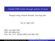
The reason is (in part) due to the striking maps of seismic
velocity that noise reveals . . .
A map of Surface-Wave
Velocity in California
Obtained from correlating
seismic noise
earthquake
1 year of
correlations
4 one-month
correlations
Frequencies ~0.02 < f < 1 Hz; 3km < !

Lin and Ritzwoller and Snieder (2009) Geophys J Int
3 years of data on a bigger array

Tomographically generated maps of wave speed
Hot spot in Yellowstone
24 sec 12 sec
Different properties at different frequencies
i.e, different depths

They even resolve ~ 1% anisotropies in wave speed

Main Assertion of Theory:
G( x, y;! ) ~ "
"! < # ( x,t)# ( y,t + ! ) > ?
! ( x,t)
Correlation of a diffuse field
gives the Green's function
( + sundry fine print and qualifications)
Where did this assertion come from?
Why should we believe it?
How much should we believe it?

History of the approach . . .
Conversations with a seismologist, at a 1999 workshop,
about the seismic coda - which appeared to be equipartitioned
S arrival
coda
An earthquake record
P arrival
Ray arrivals are
followed by
low amplitude
noise, or "coda"
time(sec)
The coda appears to
achieve a steady state
ratio of its energy contents
For example, its shear-todilational
energies: S/P
Equipartition
Phys Rev Lett 86 3447-50 (2001)

History of the approach continued. . .
I then pointed out
"if a wave field (e.g. seismic coda) is
multiply scattered to the point of
being equipartitioned, the field's
correlations should be Green's function,
And we could recover lots of information
without using a controlled source"
Geophysicist: "useful, if true"
Physicist: "Nonsense, can't possibly be true"

Hand-waving plausibility argument . . .
that there could well be a signature, an "arrival,"
at the correct travel time
- due to those few rays that happen to be going the right way
But G exactly?
And where's the proof?
And won't other ray directions obscure the effect?

Standard Proofs . .
•For a thermally diffuse field
modal picture
fluctuation-dissipation theorem
•For a conventional acoustic diffuse field
modal picture ( sensible only for closed systems )
plane wave picture (sensible only for homogeneous systems)
•Systems with uniformly distributed incoherent sources everywhere
•Heterogenous loss-free region without sources,
but insonified by an external diffuse field
But what about imperfectly diffuse fields?
• There is an asymptotic ~validity to assertion

The simplest proof involves a common definition of a fully diffuse field,
from room acoustics or physics of thermal phonons:
in terms of the normal mode expansion for the field in a finite body
!(x,t) = U " ∞ n =1 a n u n (x) exp{i# n t}
"equipartition"
n.b: this follows from maximum entropy
where F ~ energy per mode ( k B T )
C "
< ! (x, t) ! (y, t + ") > = 1 2 U # ∞ n =1F($ n ) u n (x) u n (y) exp{ % i$ n "}
/$ n
2
Compare with G . . .
G xy (!) = " ∞ n=1u n (x) u n (y) sin # n!
# n
[ for ! > 0 , 0 otherwise ]
So, ∂C/∂# = G - G time reversed , i.e, G - G* or Im G if F is constant

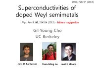
Verification?
e.g. . . .
1.00
0.75
0.50
!

Comparison of a
Direct Pulse-Echo
Signal,
(conventional ultrasonics)
and
Thermal Noise
Correlation

Phys Rev Lett 87 134301 (2001)
Correlation
Of
Thermal noise
rms u ~ 3 fm/√MHz
15
10
5
0
-5
-10
100000
After
Capturing
320 seconds
Of data
(and taking 2.5
hours to do so)
Direct
Pulse-Echo
Signal
.
-15
0.20
0.15
0.10
0.05
0.00
-0.05
50 100 150 200
time (microsecondds)
-0.10
-0.15
50 100 150 200
time (microseconds)

But proofs that require full diffusivity
and/or finite bodies and closed acoustic systems,
May not be relevant for practice.
Ambient seismic noise(*), for example, is
NOT fully diffuse
It has preferred directions (sources in ocean storms)
Nevertheless, these
maps are impressive
Why does it work?
*Late coda appears
fully diffuse, but
there isn't enough of it.

What if an incident field does not have isotropic intensity?
What it it is not equipartitioned?
Consider a homogeneous medium with
incoherent sources at infinity
Intensity distribution
B(&)

The field in the vicinity of the origin is a superposition of plane waves
! ( r,t) =
% A(")exp(#ik ˆ"i r + i$t) d"
( 2-d)
with < A >= 0; < A(!)A * (! ') >= B(!)"(! # ! ')
i.e, an incident plane wave intensity B(&)
Which implies that the field-field correlation is
< ! ( r,t)! ( r ',t ') >= % B(")exp(#i$ ˆ"i( r # r ') / c + i$(t # t ')) d"
exact

C =< ! ( r,t)! ( r ',t ') >=
% B(")exp(#i$ ˆ"i( r # r ') / c + i$(t # t ')) d"
= !1
4"
wavelet S(t) related to power spectrum of noise
2"
$ +%
# x 0
d#i exp(i#(t ! x / c)) S(# ! # o
) &
{B(0)e i" /4 + B"(0) 1
2# x e3i" /4 ! B(0) i
8# x e5i" /4 ..)+ c.c.
Leading term
first correction
Permits us to show that the apparent arrival time is delayed
relative to |r-r'|/c by a fractional amount B"(0)/2k 2 |r-r'| 2 B(0)
'The effect of non-isotropic B or arrival time is small in practice
'Hence the high quality of the maps of seismic velocity
even though the ambient seismic noise is not equipartitioned

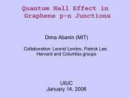
Comparison of Correlation waveform (solid line)
and time-symmetrized G ( dashed line)
For case of non-trivial ponderosity B(&) = 1 - 0.8 cos &
Froment et al
2009
Note: a) assertion fails, G≠dC/d#
b) large differences in positive and negative time amplitudes
c) there are tiny shifts of apparent arrival time, as predicted

In sum, the method works well for arrival times, hence the good maps
The method is well suited to seismology because
Controlled sources are highly inconvenient,
(earthquakes and nuclear explosions)
Recent advent of large arrays of long-period seismic stations
and world-side access to their time records
For many years seismologists would record seismic time-records,
ignore the noise, and examine the earthquakes
Now they throw out the earthquakes and keep the noise.

Other consequences of imperfectly partitioned ambient noise:
Spurious features in the correlations due to scatterers
Amplitude information is hard to interpret

Spurious arrivals..
Intensity distribution
B(&)
Correlations in the presence of a scatterer will show
and
a direct arrival at # = |r-r'|/c
an indirect arrival at # = |r-s|/c + |r'-s|/c
a spurious arrival at # = |r-s|/c - |r'-s|/c
} parts of G
Disappears if field is
equipartitioned

Amplitude information?
The technique has been used very successfully in seismology to
recover seismic velocities, with high spatial resolution. But . . .
Arrival time is evident
Arrival amplitude?
Is this meaningful?
If we really had G, we'd be able to infer attenuation also.
Issues include the unknown field intensity in the direction
between the detectors

Ray amplitudes X depend on
attenuation %
"on-strike" intensity B
X i! j
= B i
( ˆn i! j
) 2" / # o
| r i
$ r j
| exp($ & %( r )d)
rj
r i
If field is not equipartitioned, then B varies. But how?
Noise intensity B varies in space like an RTE?
ˆn ! "B( r , ˆn) + 2#( r )B( r , ˆn) = P( r , ˆn) +
$ B( r , ˆn') p( r , ˆn, ˆn')d ˆn'
sources
Scattering into direction n

Another application
Detecting changes in a medium . . .
Brenguier et al Science: 321. 1478 - 1481(2008)
correlated ocean-generated seismic noise on a daily basis
from an array of seismometers in Parkfield Ca.
Typical Daily Correlation between two of the stations:
15000
10000
C ij (#)
Very hard to interpret.
5000
0
The correlations
are about 80% converged.
-5000
-10000
-15000
No clear "arrivals."
This is G??
-100 -80 -60 -40 -20 0 20 40 60 80 100
lapse time (seconds)

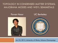
They then constructed dilation correlation coefficients
X(() (a measure of relative stretch)
( This is a 4th order statistic on the seismic field )
Between the C ij on different dates and the (year-long) average C ij
0.0010
0.0005
Parkfield earthquake
of 2004
0.0000
-0.0005
-0.0010
200 400 600 800 1000 1200 1400
day, starting 19 July 2003
Method has been used to predict
volcano eruptions

In Sum . .
It has been about 12 years now, and the topic is still growing, still hot,
especially in seismology
Applications in
High resolution seismic velocity maps
Maps of attenuation too?
Monitor changes in a medium
Maps of scattering ?
We still need better understanding
of the effects of imperfectly diffuse fields.